Sharp weighted estimates for multilinear commutators

C. Perez∗ and R. Trujillo-Gonzalez†

Journal of the London mathematical society 65 (2002), 672–692.

Abstract

We consider multilinear commutators with vector symbol ~b = (b1, ··, bm) defined by

T~b(f)(x) =

∫Rn

m∏j=1

(bj(x)− bj(y))

K(x, y)f(y)dy,

where K is a Calderon-Zygmund kernel. We prove the following a priori estimates for w ∈ A∞.For 0 < p < ∞ there exists a constant C such that

‖T~b(f)‖

Lp(w)≤ C‖~b‖ ‖M

L(logL)1/r(f)‖Lp(w)

and

supt>0

1Φ(1

t )w({y ∈ Rn : |T~b

f(y)| > t}) ≤ C supt>0

1Φ(1

t )w({y ∈ Rn : M

L(logL)1/r(||~b||f)(y) > t})

where ||~b|| =∏m

j=1 ‖bj‖oscexpL

rj, Φ(t) = t log1/r(e+t), 1

r = 1r1

+··+ 1rm

, and ML(logL)α is an Orlicz

type maximal operator. This extends, with a different approach, classical results by Coifman[5] (see also [6] [24]).

As a corollary we deduce that the operators T~bare bounded on Lp(w) when w ∈ Ap and

that they satisfy corresponding weighted L(logL)1/r type estimates with w ∈ A1.

∗Partially supported by DGESIC Grant PB980106.†Partially supported by Gobierno de Canarias PI1999/105.

1991 Mathematics Subject Classification: 42B20, 42B25.Keywords: Calderon-Zygmund singular integral operators, commutators, Ap weights, maximal functions

1

1 Introduction

The main purpose of this article is to prove sharp estimates for multilinear commutators involv-ing nonstandard symbols. This will be established by means of appropriate maximal operatorswhich somehow control the commutators. This illustrates the classical Calderon–Zygmund prin-ciple which roughly states that any singular integral operator is controlled by a suitable maximaloperator.

BackgroundMotivated by the work of Calderon on commutators, Coifman, Rochberg and Weiss intro-

duced in [7] the operator

Tbf(x) =∫

Rn

(b(x)− b(y))K(x, y)f(y) dy, (1.1)

where K is a kernel satisfying the standard Calderon-Zygmund estimates (see section 3.1) andwhere b, the “symbol” of the operator, is any locally integrable function. The operator is calledcommutator since Tb = [b, T ] = bT − T (b ·) where T is the Calderon-Zygmund singular integraloperator associated to K. The main result from [7] states that [b, T ] is a bounded operator onLp(Rn), 1 < p < ∞, when the symbol b is a BMO function.

These commutators have proved to be of interest in many situations. We shall only men-tion the recent results in the theory of non divergence elliptic equations with discontinuouscoefficients [2] [3] [9]. There is also an interesting connection, as pointed out in [21], with thenonlinear commutator considered by R. Rochberg and G. Weiss in [23] and defined by

f → Nf = T (f log |f |)− Tf log |Tf |.

This is in turn is related to the Jacobian mapping of vector function and with nonlinear P.D.E.as shown in [13] [14].

A natural generalization of the commutator [b, T ] is given by

Tmb f(x) =

∫Rn

(b(x)− b(y))mK(x, y)f(y) dy, (1.2)

where m ∈ N. The case m = 0 recaptures the Calderon-Zygmund singular integral operator.

Observing that Tmb =

(m times)︷ ︸︸ ︷[b, ··, [b, T ]] we have that for m ∈ N, Tm

b is also a bounded operator onLp(Rn), 1 < p < ∞, when b is a BMO function.

It was shown in [21] that there is an intimate connection between the commutator Tmb and

iterations of the maximal operators. Indeed, the main theorem from [7] was sharpened in [21]as follows: for any 0 < p < ∞ and any w ∈ A∞ there is a constant C such that∫

Rn

|Tmb f(x)|p w(x)dx ≤ C ‖b‖mp

BMO

∫Rn

(Mm+1f(x))p w(x)dx, (1.3)

2

where Mm+1 denotes the m + 1 iterations of the Hardy-Littlewood maximal operator, namely

Mm =

(m times)︷ ︸︸ ︷M ◦ · · ◦M . Furthermore, this inequality is sharp since, by the Lebesgue differentiation

theorem, Mm+1 can not be replaced by the smaller operator Mm.Estimate (1.3) can also be seen as a generalization of a by now classical result of Coifman

for Calderon-Zygmund singular integral operators. See [5] and also [6].There is a weak version of inequality (1.3) obtained in [20]. Indeed, if we let Φm(t) =

t logm(e + t), for any w ∈ A∞ and b ∈ BMO there is a constant C such that

supt>0

1Φm(1

t )w({y ∈ Rn : |Tm

b f(y)| > t}) ≤ C supt>0

1Φm(1

t )w({y ∈ Rn : Mm+1f(y) > t}). (1.4)

A priori inequalities of the form (1.3) (or (1.4)) encode a good amount of information aboutthe behavior of the operator. The first observation is that in any case they reflect the higherdegree of singularity of Tm

b , as compared with T , since a larger operator than M , namely Mm+1,is needed to balance the inequality. As a second instance, if p > 1 we can apply m + 1 timesMuckenhoupt’s theorem to conclude from (1.3) the well known fact that high order commutatorsare bounded on Lp(w) whenever w ∈ Ap. It should be mentioned that this Ap estimate follows,as it is well known, from an estimate due to Stromberg (see [15, p. 268], [25, p. 417]). Thismethod is powerful and can be applied to different situations. As a sample we remit to [10]for a very nice application to commutators with strongly singular integral operators. However,this estimate of Stromberg is not sharp enough neither to derive (1.3) nor (1.4). In fact it canbe shown from (1.4) the following (L log L type) endpoint estimate first deduced in [20]: letw ∈ A1 and b ∈ BMO, then there exists a constant C such that for all λ > 0

w({y ∈ Rn : |Tmb f(y)| > λ}) ≤ C

∫Rn

|f(y)|λ

(1 + log+(|f(y)|

λ))m w(y)dy. (1.5)

As a third instance, it was shown in [21] that estimate (1.3) implies a sharp two weightedinequalities for the commutator of the form∫

Rn

|Tmb f(x)|p w(x)dx ≤ C ‖b‖mp

BMO

∫Rn

|f(x)|p M [(m+1)p]+1w(x)dx,

where no condition on the weight w is assumed. This result is an extension of the case m = 0proved in [18] generalizing some previous partial results by M. Wilson [26]. The approachconsidered in [18] is different from that in [26] and it combines (1.3) with certain sharp twoweighted estimates for the Hardy–Littlewood maximal function derived in [19].

Finally, there is a relationship between (1.4) and the endpoint behavior of the operator.Indeed, an interesting observation that occurs in the development of the theory of commutatorsis that the Lp theory, p > 1, was developed without appealing to any endpoint estimate. On theother hand, it is well known that in the classical Calderon-Zygmund Lp theory, p > 1, a crucialstep is to show that the operators are of weak type (1, 1). However, this is not the case of thecommutator [b, T ] when b ∈ BMO as shown in [20] and estimate (1.5) is the right replacement.

3

This can be seen as another way of expressing the fact that commutators have a higher degreeof singularity as compared with the Calderon-Zygmund singular integral operators.

Results of this paperIn this paper we obtain similar estimates for a wider class of commutators. Given a Calderon-

Zygmund singular integral operator T with kernel K in Rn ×Rn and a vector ~b = (b1, .., bm) oflocally integrable functions, we define the multilinear operator

T~bf(x) =

∫Rn

m∏j=1

(bj(x)− bj(y))

K(x, y)f(y)dy, (1.6)

generalizing the commutator (1.2). We remit the reader to [6] for an extensive study of multi-linear operators.

We will be considering the following class of symbols: for r ≥ 1 and for any locally integrablefunction f , we define

‖f‖oscexpLr

= supQ‖f − fQ‖expLr,Q

being the supremum taken over all the cubes Q with sides parallels to the axes. Here ‖g‖expLr,Q

is the mean value of g on the cube Q with respect to the Young function Φ(t) = etr − 1. SeeSection 2.2 for the precise definition. As usual, fQ denotes the average of f on Q. For r ≥ 1 wedefine the space Osc

expLr by

OscexpLr = {f ∈ L1

loc(Rn) : ‖f‖oscexpLr

< ∞}.

In the particular case of r = 1, OscexpL1 coincides with the BMO space by John-Niremberg’s

theorem. Also we have OscexpLr BMO for any r > 1. Other examples are provided by

Trudinger’s inequality for Riesz potentials. To be more precise, for any 0 < α < n and anyf ∈ Ln/α(Rn), the Riesz potential Iαf of order α belongs to Osc

expL(n/α)′ (cf. [12, 27])

For the statement of our results we introduce some notation that will simplify the presen-tation. Along this paper m will always be the number of symbols of the operator T~b

where~b = (b1, .., bm) is a family of m locally integrable functions. If r1, .., rm are m positive realnumbers, we denote

1r

=1r1

+ · ·+ 1rm

and

||~b|| =m∏

j=1

‖bj‖oscexpL

rj.

Our main results are the following.

Theorem 1.1 Let 0 < p < ∞, w ∈ A∞. Suppose that T~bf is the commutator (1.6) where b is

as above such that bi ∈ OscexpLri

, ri ≥ 1, 1 ≤ i ≤ m. Then there exists a constant C > 0 suchthat ∫

Rn

|T~b(f)(x)|pw(x)dx ≤ C ||~b||p

∫Rn

(ML(logL)1/r(f)(x))pw(x)dx (1.7)

4

for all bounded functions f with compact support.

For the precise definition of the operator ML(logL)α see Section 2.2.Inequality (1.7) shows that the maximal operator ML(logL)1/r is the one that controls the

multilinear commutators Tb. Since ri ≥ 1 for each i, it follows that ML(logL)1/r is pointwisesmaller than ML(logL)m and this in turn is known to be equivalent to m + 1 iterations of theHardy–Littlewood maximal operator Mm+1. Hence we can use again Muckenhoupt’s theoremand deduce the boundedness of Tb on Lp(w) for p > 1 and any w ∈ Ap:

Corollary 1.2 Let 1 < p < ∞ and w ∈ Ap. Suppose that T~bf is the commutator (1.6) where

b is as above such that bi ∈ OscexpLri

, ri ≥ 1, 1 ≤ i ≤ m. Then there exists a constant C > 0such that ∫

Rn

|T~b(f)(x)|pw(x)dx ≤ C ||~b||p

∫Rn

|f(x)|pw(x)dx (1.8)

for all bounded functions f with compact support.

As we mentioned above this estimate is a generalized version of Coifman’s result in [5].However, our approach is different and will be based on a pointwise inequality that roughly canbe expressed as

M#δ (T~b

f)(x) ≤ C ||~b||ML(logL)1/rf(x) + R(f)(x) (1.9)

for an appropriate positive but small enough number δ. R denotes certain “remainder” operatorwhich is smoother, less singular, than ML(logL)1/r in some suitable sense. See Lemma 3.1 for acomplete and precise statement of this estimate.

Moreover, reasoning as in [21], Theorem 2, from this theorem we deduce the followingestimate for general weights. As usual [α] will denote the integer part of α.

Theorem 1.3 Let 1 < p < ∞ and let T~bbe as in Theorem 1.1. Then there exists a constant C

such that for any weight w∫Rn

|T~b(f)(x)|pw(x) dx ≤ C||~b||p

∫Rn

|f(x)|pM [( 1r+1)p]+1(w)(x) dx

for all bounded functions f with compact support.

Remark 1.4 We remark that the number of iterations of the maximal function needed in theTheorem is optimal as can be seen in [21], Section 5. In fact it follows from the proof of Theorem1.3 that there is a sharper estimate:∫

Rn

|T~b(f)(x)|p w(x)dx ≤ C ||~b||p

∫Rn

|f(x)|p ML(log L)(

1r +1)p−1+ε(w)(x)dx

where ε > 0, being the result false for ε = 0.

5

The key pointwise estimate (1.9) is also used to derive the next endpoint result. Recall thatcommutators with BMO functions are not of weak type (1, 1).

Recall that we denote ||~b|| =∏m

j=1 ‖bj‖oscexpL

rjand Φ(t) = t log1/r(e + t), where 1

r =1r1

+ · ·+ 1rm

.

Theorem 1.5 Let w ∈ A1 . There exists a constant C > 0 such that for all λ > 0

w({y ∈ Rn : |Tbf(y)| > λ}) ≤ C

∫Rn

Φ(||~b|| |f(y)|

λ) w(y)dy, (1.10)

for all bounded functions f with compact support and for all ~b.

The proof is based on the following result which generalizes inequality (1.4).

Theorem 1.6 Let w ∈ A∞. Then, there exists a positive constant C such that

supt>0

1Φ(1

t )w({y ∈ Rn : |Tbf(y)| > t}) ≤ C sup

t>0

1Φ(1

t )w({y ∈ Rn : MΦ(||~b||f)(y) > t}) (1.11)

for all bounded functions f with compact support.

In any of the above results, if we choose b1 = ·· = bm and r1 = ·· = rm = 1, we recovercompletely the corresponding results from [20] and [21].

As usual C will denote a positive constant that can change its value on each statement. Ifthe constant depends on precise parameters it will be pointed out.

2 Preliminaries

In this section we introduce the basic tools needed for the proof of the main results.

2.1 The Fefferman-Stein inequality for A∞ weights

A weight will always mean a positive function which is locally integrable. We say that a weightw belongs to the class Ap, 1 < p < ∞, if there is a constant C such that(

1|Q|

∫Q

w(y) dy

)(1|Q|

∫Q

w(y)1−p′ dy

)p−1

≤ C

for each cube Q and where as usual 1p + 1

p′ = 1. A weight w belongs to the class A1 if there isa constant C such that

1|Q|

∫Q

w(y) dy ≤ C infQ

w.

We will denote the infimum of the constants C by [w]Ap

. Observe that [w]Ap

≥ 1 by Jensen’sinequality.

6

Since the Ap classes are increasing with respect to p, the A∞ class of weights is defined in anatural way by A∞ = ∪p>1Ap. However, the following characterization it is more interesting:there are positive constants c and ρ such that for any cube Q and any measurable set E containedin Q then

w(E)w(Q)

≤ c

(|E||Q|

)ρ

.

A simple fact that will be useful is that, for any w ∈ Ap and any m > 0, wm = min{w,m} ∈Ap with [wm]

Ap≤ Cp[w]

Ap. For more information on Ap weights we remit the reader to the

references [11] and [25].We recall now the definitions of classical maximal operators. If, as usual, M denotes the

Hardy–Littlewood maximal operator, we consider for δ > 0

Mδf(x) = M(|f |δ)1/δ(x) =

(supQ3x

1|Q|

∫Q|f(y)|δ dy

)1/δ

,

M#(f)(x) = supQ3x

infc

1|Q|

∫Q|f(y)− c| dy ≈ sup

Q3x

1|Q|

∫Q|f(y)− fQ| dy

and a variant of this sharp maximal operator that will become the main tool in our scheme

M#δ f(x) = M#(|f |δ)(x)1/δ.

The main inequality between these operators to be used is a version of the classical one dueto C. Fefferman and E. Stein (see [24], [16]).

Lemma 2.1 Let w be an A∞ weight, then there exists a constant c depending upon the A∞

condition of w such that for all λ, ε > 0

w({y ∈ Rn : Mf(y) > λ,M#f(y) ≤ λε}) ≤ c ερw({y ∈ Rn : Mf(y) >λ

2}).

As a consequence we have the following estimates for δ > 0.a) Let ϕ : (0,∞) → (0,∞) doubling. Then, there exists a constant c depending upon the A∞

condition of w and the doubling condition of ϕ such that

supλ>0

ϕ(λ)w({y ∈ Rn : Mδf(y) > λ}) ≤ c supλ>0

ϕ(λ)w({y ∈ Rn : M#δ f(y) > λ}) (2.1)

for every function such that the left hand side is finite.b) Let 0 < p < ∞ there exists a positive constant C upon the A∞ condition of w and p suchthat ∫

Rn

(Mδf(x))p w(x)dx ≤ C

∫Rn

(M#δ f(x))p w(x)dx, (2.2)

for every function f such that the left hand side is finite.

7

2.2 Orlicz maximal functions

By a Young function Φ we shall mean a continuous, nonnegative, strictly increasing and convexfunction on [0,∞) with

limt→0+

Φ(t)t

= limt→∞

t

Φ(t)= 0.

We define the Φ-averages of a function f over a cube Q by

‖f‖Φ,Q = ‖f‖Φ(L),Q = inf{λ > 0 :1|Q|

∫Q

Φ(|f(x)|

λ

)dx ≤ 1}.

For Orlicz norms we are usually only concerned about the behavior of Young functions forlarge values of t’s. Given two functions B and C, we write B(t) ≈ C(t) if B(t)/C(t) is boundedand bounded below for t ≥ c > 0. We also recall that if B(t) ≤ C(t) for t ≥ c > 0, then

‖f‖B,Q ≤ C ‖f‖C,Q

with C an absolute constant. For more information on the subject see the reference [22].Associate to this average we can define a maximal operator MΦ given by

MΦf(x) = MΦ(L)f(x) = supQ3x

‖f‖Φ,Q,

where the supremum is taken over all the cubes containing x.For example, if Φ(x) = exr − 1, then ‖ · ‖

expLr,Qand M

expLr , denote respectively theΦ-average and the maximal operator associated to Φ. Similarly we have for Φ(x) = x logr(e+x)‖ · ‖L(logL)r,Q and ML(logL)r . Observe that by the above remarks, Mf ≤ CML(logL)rf for anyr > 0. These examples will be relevant in our work.

Finally, we will be using the following known pointwise inequality: if m ∈ N then

ML(logL)m ∼ Mm+1 =

(m+1 times)︷ ︸︸ ︷M ◦ · · ◦M,

the m + 1 iterations of the Hardy-Littlewood maximal operator. A generalization of this equiv-alence can be found in [8].

We begin with some technical lemmas on convex functions whose proofs are standard.

Lemma 2.2 ([17], Lema 2.1) If Φ0,Φ1, ...,Φm are real-valued, non-negative, nondecreasing, leftcontinuous functions defined on [0,∞) such that, with the definition

Φ−1i (x) = inf{y : Φi(y) > x},

it verify

Φ−11 (x)Φ−1

2 (x) · ·Φ−1m (x) ≤ Φ−1

0 (x), (2.3)

8

then for all 0 ≤ x1, x2, .., xm < ∞

Φ0(x1x2 · ·xm) ≤ Φ1(x1) + Φ2(x2) + · ·+Φm(xm)

Lemma 2.3 Let Φ0 be a convex function such that Φ0(0) = 0 and let Φ1, ..,Φm as in theprevious lemma all verifying (2.3). If f1, f2, .., fm are functions satisfying that ‖fi‖Φi,Q < ∞for all 1 ≤ i ≤ m and for a given cube Q, then

‖f1 · · · fm‖Φ0,Q ≤ m‖f1‖Φ1,Q · · · ‖fm‖Φm,Q. (2.4)

PROOF: Taking ε > 0 small enough, by Lemma 2.2 and convexity

1|Q|

∫Q

Φ0

(f1(x)f2(x) · ·fm(x)

m(‖f1‖Φ1,Q + ε)(‖f2‖Φ2,Q + ε) · ·(‖fm‖Φm,Q + ε)

)dx ≤

1m

1|Q|

∫Q

Φ0

(f1(x)f2(x) · ·fm(x)

(‖f1‖Φ1,Q + ε)(‖f2‖Φ2,Q + ε) · ·(‖fm‖Φm,Q + ε)

)dx ≤

1m

1|Q|

∫Q

[Φ1

(f1(x)

‖f1‖Φ1,Q + ε

)+ · ·+Φm

(f1(x)

‖fm‖Φm,Q + ε

)]dx ≤ 1

which implies that

‖f1f2 · ·fm‖Φ0,Q ≤ m(‖f1‖Φ1,Q + ε) · ·(‖fm‖Φm,Q + ε).

Now, taking letting ε → 0 we get (2.4).

The main example that we will be using is the following:

1|Q|

∫Q|f1 · · · fm g| ≤ C‖f1‖expLr1 ,Q

· · · ‖fm‖expLrm ,Q‖g‖L(logL)1/r,Q, (2.5)

where r1, .., rm ≥ 1 and1r

=1r1

+ · ·+ 1rm

.

Indeed, in this case we can write for any x ≥ 0 that

log1r1 (1 + x) · · · log

1rm (1 + x)

x

log1r1

+··+ 1rm (e + x)

≤ x.

Then (2.3) holds forΦ0(x) = x,

Φ−1i (x) = log

1ri (1 + x),

i = 1, ..,m andΦ−1

m+1(x) =x

log1r1

+··+ 1rm (e + x)

.

The inverse functions are given by Φi(x) = exri−1, i = 1, ..,m, and Φm+1(x) ≈ x log1r1

+··+ 1rm (e+

x).

9

2.3 The oscillation of a function

We define the oscillation oscΦ(f,Q) of a function f with respect to any Young function Φ as

oscΦ(f,Q) = ‖f − fQ‖Φ,Q.

We list the following properties that are very easy to check.

Lemma 2.4 For any cube Q and any locally integrable functions f and g, we have

i) oscΦ(f ± g,Q) ≤ oscΦ(f,Q) + oscΦ(g,Q)

ii) oscΦ(λf,Q) = |λ|oscΦ(f,Q) for all λ ∈ R.

iii) oscΦ(|f |, Q) ≤ 2oscΦ(f,Q).

iv) oscΦ(min{f, g}, Q) ≤ 32(oscΦ(f,Q) + oscΦ(g,Q)).

v) oscΦ(max{f, g}, Q) ≤ 32(oscΦ(f,Q) + oscΦ(g,Q)).

Given a function g, we define for any N ∈ N,

gN (x) =

N, g(x) > N

g(x), |g(x)| ≤ N

−N, g(x) < −N

(2.6)

Now, from Lemma 2.4 and taking into account that gN = max{min{g,N},−N}, we inferthat for any locally integrable function oscΦ(gN , Q) ≤ C oscΦ(g,Q) and consequently

‖gN‖oscΦ

≤ C ‖g‖oscΦ

(2.7)

for all N ∈ N and where C > 0 is an absolute constant.

3 Proofs of the main results

3.1 Proof of Theorem 1.1

By a kernel K in Rn×Rn we mean a locally integrable function defined away from the diagonal.We say that K satisfies the standard estimates if there exist positive and finite constants γ andC such that, for all distinct x, y ∈ Rn and all z with 2|x− z| < |x− y|, it verifies

i) |K(x, y)| ≤ C|x− y|−n,

ii) |K(x, y)−K(z, y)| ≤ C∣∣∣x−zx−y

∣∣∣γ |x− y|−n,

iii) |K(y, x)−K(y, z)| ≤ C∣∣∣x−zx−y

∣∣∣γ |x− y|−n.

10

We define a linear and continuous operator T : C∞0 (Rn) → D′(Rn) associated to the kernel

K by

Tf(x) =∫

Rn

K(x, y)f(y)dy

where f ∈ C∞0 (Rn) and x is not in the support of f . T is called a Calderon-Zygmund operator

if K satisfies the standard estimates and if it extends to a bounded linear operator on L2(Rn).These conditions imply that T is also bounded on Lp(Rn), 1 < p < ∞ and is of weak type–(1,1).For more information on this subject see [4],[6] or [16].

Given any positive integer m, for all 1 ≤ j ≤ m, we denote by Cmj the family of all finite

subset σ = {σ(1), .., σ(j)} of {1, ..,m} of j different elements. For any σ ∈ Cmj we associate the

complementary sequence σ′ given by σ′ = {1, 2, ..,m} \ σ.Let ~b = (b1, b2, ..., bm) be a finite family of integrable functions. For all 1 ≤ j ≤ m and any

σ = {σ(1), .., σ(j)} ∈ Cmj , we will denote ~bσ = (bσ(1), ···, bσ(j)) and the product bσ = bσ(1) ···bσ(j).

So, with this notation, we write for any m-tuple r = (r1, .., rm) of positive numbers

‖~bσ‖oscexpLrσ= ‖bσ(1)‖osc

expLrσ(1)

· · · ‖bσ(j)‖oscexpL

rσ(j).

For the product of all the functions we simply write

‖~b‖oscexpLr

= ‖b1‖oscexpLr1· · · ‖bm‖oscexpLrm

.

For any σ ∈ Cmj , we denote

T ~bσf(x) =

∫Rn

(bσ(1)(x)− bσ(1)(y)) · · · (bσ(j)(x)− bσ(j)(y))K(x, y)f(y)dy.

In the particular case of σ = {1, ..,m} we understand T ~bσas simply T~b

.Finally observe that T~b

(f) satisfies the following homogeneity on the symbol T~b( f

||~b||) = T~

b(f)

where b = (b1/‖b1‖oscexpL

rj, · · · , bm/‖bm‖oscexpLrm

) such that ||b|| = 1.

The following lemma gives a pointwise estimate of M#δ (T~b

f) in terms of other maximalfunctions of operators of lower order. This result can be understood as the extension of Lemma7.1 in [20] to high order commutators and for the classes of symbols considered in this paper.

Lemma 3.1 Let T~bbe as in Theorem 1.1 and 0 < δ < ε < 1. Then there exists a constant

C > 0, depending only on δ and ε such that

M#δ (T~b

f)(x) ≤ C

||~b||ML(logL)1/rf(x) +m∑

j=1

∑σ∈Cm

j

‖bσ‖oscexpLrσMε(T ~bσ′

f)(x)

(3.1)

for any bounded function f with compact support.

11

Recall that ||~b|| =∏m

j=1 ‖bj‖oscexpL

rj.

Proof:

Recall that the operator T~b= Tb1,..,bm is defined by

T~bf(x) =

∫Rn

m∏j=1

(bj(x)− bj(y))

K(x, y)f(y)dy.

By homogeneity we may assume that ||~b|| = 1.We first consider the case m = 1. Hence, we only have one symbol b ∈ osc

expLr , r ≥ 1 and(3.1) becomes

M#δ (Tbf)(x) ≤ C‖b‖

oscexpLr

[ML(logL)1/rf(x) + Mε(Tf)(x)

]. (3.2)

For any λ ∈ R we have

Tbf(x) =∫

Rn

(b(x)− b(y))K(x, y)f(y)dy

= (b(x)− λ)Tf(x)− T ((b− λ)f)(x).

Now, fixed x ∈ Rn, for any number c and any ball B centered at x and radius R > 0, since0 < δ < 1 implies ||α|δ − |β|δ| ≤ |α− β|δ for any α, β ∈ R, we can estimate(

1|B|

∫B

∣∣∣|Tbf(y)|δ − |c|δ∣∣∣ dy

)1/δ

≤(

1|B|

∫B|Tbf(y)− c|δ dy

)1/δ

≤ C

[(1|B|

∫B|(b(y)− λ)Tf(y)|δ dy

)1/δ

+(

1|B|

∫B|T ((b− λ)f)(y)− c|δ dy

)1/δ]

= I + II.

We analyze each term separately taking along all the proof λ = (b)2B, the average of b onthe ball concentric with B but with double radius. For any 1 < q < ε/δ we have by Holder andJensen’s inequality,

I ≤ C

(1

|2B|

∫2B|b(y)− λ|δq′ dy

)1/δq′ ( 1|B|

∫B|Tf(y)|δq dy

)1/δq

≤ C‖b‖oscexpLr

Mδq(Tf)(x)

≤ CMε(Tf)(x). (3.3)

To deal with II we split f as usual by f = f1 + f2 where f1 = fχ2B and f2 = f − f1. Thisyields

12

II ≤ C

[(1|B|

∫B|T ((b− λ)f1)(y)|δ dy

)1/δ

+(

1|B|

∫B|T ((b− λ)f2)(y)− c|δ dy

)1/δ]

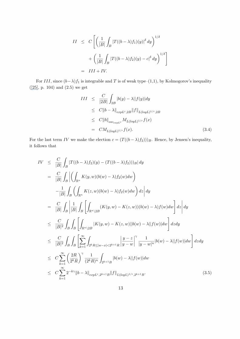
= III + IV.

For III, since (b−λ)f1 is integrable and T is of weak type–(1,1), by Kolmogorov’s inequality([25], p. 104) and (2.5) we get

III ≤ C

|2B|

∫2B|b(y)− λ||f(y)|dy

≤ C‖b− λ‖expLr,2B

‖f‖L(logL)1/r,2B

≤ C‖b‖oscexpLr

ML(logL)1/rf(x)

= CML(logL)1/rf(x). (3.4)

For the last term IV we make the election c = (T ((b− λ)f2)))B. Hence, by Jensen’s inequality,it follows that

IV ≤ C

|B|

∫B|T ((b− λ)f2)(y)− (T ((b− λ)f2)))B| dy

=C

|B|

∫B

∣∣∣∣(∫Rn

K(y, w)(b(w)− λ)f2(w)dw

)

− 1|B|

∫B

(∫Rn

K(z, w)(b(w)− λ)f2(w)dw

)dz

∣∣∣∣ dy

=C

|B|

∫B

∣∣∣∣∣ 1|B|

∫B

[∫Rn\2B

(K(y, w)−K(z, w))(b(w)− λ)f(w)dw

]dz

∣∣∣∣∣ dy

≤ C

|B|2

∫B

∫B

[∫Rn\2B

|K(y, w)−K(z, w)||b(w)− λ||f(w)|dw

]dzdy

≤ C

|B|2

∫B

∫B

[ ∞∑k=1

∫2kR≤|w−x|<2k+1R

∣∣∣∣ y − z

y − w

∣∣∣∣γ 1|y − w|n

|b(w)− λ||f(w)|dw

]dzdy

≤ C∞∑

k=1

(2R

2kR

)γ 1(2kR)n

∫2k+1B

|b(w)− λ||f(w)|dw

≤ C∞∑

k=1

2−kγ‖b− λ‖expLr,2k+1B

‖f‖L(logL)1/r,2k+1B

. (3.5)

13

The fifth inequality follows because y, z ∈ B and w ∈ Rn \B and therefore 2|y − w| < |z − w|,the sixth does since |y − z| ≤ 2R and |y − w|−1 ≤ ((2k − 1)R)−1 ≤ C(2kR)−1, and the last oneis an application of the generalized Holder inequality (2.5).

Now, we claim that‖b− λ‖

expLr,2k+1B≤ Ck‖b‖

oscexpLr. (3.6)

Indeed,

‖b− λ‖expLr,2k+1B

≤ ‖b− (b)2k+1B‖expLr,2k+1B+ ‖(b)2k+1B − λ‖

expLr,2k+1B

≤ ‖b− (b)2k+1B‖expLr,2k+1B+ |(b)2k+1B − λ|

≤ Ck‖b‖oscexpLr

where the last estimate follows by the standard inequality |(b)2B − bB| ≤ 2‖b‖oscexpLr

(cf. [16],p. 31), and then we take supremum over the balls.

Thus, IV is estimated by

IV ≤ C∞∑

k=1

(2−k)γk‖b‖oscexpLr

ML(logL)1/rf(x)

≤ CML(logL)1/rf(x). (3.7)

¿From (3.4) and (3.7) we conclude

II ≤ CML(logL)1/rf(x)

which, together with (3.3), gives (3.2) and proves the lemma for m = 1.Consider now the case m ≥ 2. Then, for any ~λ = (λ1, .., λm) ∈ Rn we have

T~bf(x) =

∫Rn

(b1(x)− b1(y)) · · · (bm(x)− bm(y))K(x, y)f(y)dy

=∫

Rn

((b1(x)− λ1)− (b1(y)− λ1)) · · · ((bm(x)− λm)− (bm(y)− λm))K(x, y)f(y)dy

=m∑

j=0

∑σ∈Cm

j

(−1)m−j(b(x)− ~λ)σ

∫Rn

(b(y)− ~λ)σ′K(x, y)f(y)dy

= (b1(x)− λ1) · · · (bm(x)− λm)Tf(x)

+(−1)mT ((b1 − λ1) · · · (bm − λm)f)(x)

+m−1∑j=1

∑σ∈Cm

j

(−1)m−j(b(x)− ~λ)σ

∫Rn

(b(y)− b(x))σ′K(x, y)f(y)dy

14

Now, expanding (b(y)− ~λ)σ′ = [(b(y)− b(x)) + (b(x)− ~λ)]σ′ as above it is easy to see that

T~bf(x) = (b1(x)− λ1) · · · (bm(x)− λm)Tf(x)

+(−1)mT ((b1 − λ1) · · · (bm − λm)f)(x)

+m−1∑j=1

∑σ∈Cm

j

cm,j(b(x)− ~λ)σT ~bσ′f(x)

where cm,j are absolute constants depending only on m and j.Now, fixed x ∈ Rn, for any number c and any ball B centered at x and radius R > 0 it

follows since 0 < δ < 1

(1|B|

∫B

∣∣∣|T~bf(y)|δ − |c|δ

∣∣∣ dy

)1/δ

≤(

1|B|

∫B

∣∣T~bf(y)− c

∣∣δ dy

)1/δ

≤ C

[(1|B|

∫B|(b1(y)− λ1) · · · (bm(y)− λm)Tf(y)|δ dy

)1/δ

+m−1∑j=1

∑σ∈Cm

j

(1|B|

∫B

∣∣∣((b− ~λ)σT ~bσ′f(y)

∣∣∣δ dy

)1/δ

+(

1|B|

∫B|T ((b1 − λ1) · · · (bm − λm)f)(y)− c|δ dy

)1/δ]

= I + II + III.

Reasoning as in (3.3) with λi = (bi)2B, i = 1, ..,m, using this time the standard Holderinequality for finitely many functions with 1 < q < ε/δ, we have

I ≤ CMε(Tf)(x) (3.8)

and

II ≤ Cm−1∑j=1

∑σ∈Cm

j

Mε(T ~bσ′f)(x) (3.9)

with C > 0 depending only on m.For III we split f = f1 + f2 with f1 = fχ2B and f2 = f − f1. So

III ≤ C

[(1|B|

∫B|T ((b1 − λ1) · · · (bm − λm)f1)(y)|δ dy

)1/δ

+(

1|B|

∫B|T ((b1 − λ1) · · · (bm − λm)f2)(y)− c|δ dy

)1/δ]

= IV+V.

15

Now, as in (3.4) and making use again of Kolmogorov’s inequality and (2.5), we can estimateIV by

IV ≤ C

|2B|

∫2B|b1(y)− λ1| · · · |bm(y)− λm||f(y)|dy

≤ C‖b1 − λ1‖expLr1 ,2B· · · ‖bm − λm‖expLrm ,2B

‖f‖L(logL)1/r,2B

≤ CML(logL)1/rf(x), (3.10)

where recall that1r

=1r1

+ · ·+ 1rm

.

Finally, for V , choosing c = (T ((b1−λ1) · ·(bm−λm)f2)))B and repeating the argument usedto get (3.5), it follows from (2.5) and (3.6) that

V ≤ C

∞∑k=1

2−kγ 1(2k+1R)n

∫2k+1B

m∏j=1

|bj(w)− λj |

|f(w)|dw

≤ C∞∑

k=1

2−kγ

m∏j=1

‖bj − λj‖expLrj ,2k+1B

‖f‖L(logL)1/r,2k+1B

≤ C

[ ∞∑k=1

2−kγkm

] m∏j=1

‖bj‖oscexpL

rj

ML(logL)1/rf(x). (3.11)

Finally, from (3.10) and (3.11) we conclude

III ≤ CML(logL)1/rf(x),

which together with (3.8) and (3.9) gives (3.1) and the proof of the lemma is finished.

We are now in a position to prove Theorem 1.1Proof of Theorem 1.1: We may assume that∫

Rn

(ML(logL)1/rf(x))pw(x)dx < ∞, (3.12)

since otherwise there is nothing to be proved.To apply the Fefferman-Stein inequality (2.2) we first take for granted that ‖Mδ(T~b

f)‖Lp(w)

is finite. We will check this to the end of the proof.

16

We proceed by induction on m. For m = 1, by (2.2) and Lemma 3.1 we can estimate

‖Tb1f‖Lp(w) ≤ ‖Mδ(Tb1f)‖Lp(w)

≤ C ‖M#δ (Tb1f)‖Lp(w)

≤ C ‖b1‖oscexpLr1

[‖Mε(Tf)‖Lp(w) + ‖ML(logL)1/r1f‖Lp(w))

]≤ C ‖b1‖oscexpLr1

[‖Tf‖Lp(w) + ‖ML(logL)1/r1f‖Lp(w)

]≤ C ‖b1‖oscexpLr1

[‖Mf‖Lp(w) + ‖ML(logL)1/r1f‖Lp(w)

]≤ C ‖b1‖oscexpLr1

‖ML(logL)1/r1f‖Lp(w)

where the fourth inequality follows since w ∈ A∞ and therefore there exists q > 1 such thatw ∈ Aq, then we can choose ε such that 0 < ε < p/q (we may take q > p if necessary). Thefifth holds by the classical estimate (1.3) for m = 0 (see [6], Chapter 1).

Suppose now that for m − 1 the theorem is true and let’s prove it for m. So, the sameargument used above and by the induction hypothesis gives

‖T~bf‖Lp(w) ≤ ‖Mδ(T~b

f)‖Lp(w)

≤ C ‖M#δ (T~b

f)‖Lp(w)

≤ C[‖b1‖oscexpLr1

· ·‖bm‖oscexpLrm‖ML(logL)1/rf‖Lp(w)

+m−1∑j=1

∑σ∈Cm

j

‖bσ‖oscexpLσ

‖Mε(T ~bσ′)‖Lp(w)

≤ C

[‖b1‖oscexpLr1

· ·‖bm‖oscexpLrm‖ML(logL)1/rf‖Lp(w)

+m−1∑j=1

∑σ∈Cm

j

‖bσ‖oscexpLσ‖bσ′‖osc

expLσ′‖M

L(logL)1/rσ′ f‖Lp(w)

≤ C ‖b1‖oscexpLr1

· ·‖bm‖oscexpLrm‖ML(logL)1/rf‖Lp(w),

since ML(logL)1/rσ′ ≤ C ML(logL)1/r

Let us check now that for appropriate δ we have ‖Mδ(T~bf)‖Lp(w) < ∞. Indeed, as above

since w ∈ A∞, there exists q > 1 such that w ∈ Aq and we can choose δ small enough so thatp/δ > q. Then by Muckehoupt’s theorem all is reduced to checking that ‖Tbf‖Lp(w) < ∞.

Suppose that the symbols bk’s and the weight w are all bounded functions. Since f hascompact support we may assume that the support of f is contained in the ball BR = B(0, R).Then we can split the integral as∫

Rn

|T~bf(x)|pw(x)dx =

∫|x|≤2R

|T~bf(x)|pw(x)dx +

∫|x|>2R

|T~bf(x)|pw(x)dx.

17

The first integral can be easily estimated making use of the L∞–boundedness of the bk’s andw and the Lq–boundedness for q > 1 of the Calderon–Zygmund operator T .

For the second term, by the properties of the kernel K and the boundedness of the symbolsbk’s, since |x| > 2R, we have the following pointwise estimate

|T~bf(x)| ≤ C

∫BR

|b1(x)− b1(y)| · · · |bm(x)− bm(y)||f(y)||x− y|n

dy

≤ C

|x|n

∫B(0,|x|)

|f(y)|dy

≤ CMf(x)

≤ CML(logL)

1rf(x). (3.13)

Thus, ∫|x|>2R

|T~bf(x)|pw(x)dx ≤ C

∫|x|>2R

(ML(logL)

1rf(x))pw(x)dx

which is finite by the assumption (3.12).For the general case, we will truncate the symbols bk’s and the weight w as follows (cf [6],

p. 40). We denote by ~bN the vector of truncated elements by N , i.e., ~bN = (bN1 , .., bN

m) whereeach bN

k is the truncation of bk as it is defined in (2.6). Observe that in our case (2.7) becomes

‖bNk ‖oscexpLrk

≤ C‖bk‖oscexpLrk(3.14)

with C > 0 a constant independent of N . Analogously we consider the truncations of the weightw by wN = inf{w,N} that satisfy

[wN ]A∞

≤ C [w]A∞

. (3.15)

Then (1.7) holds for the operator T ~bN and the weight wN . Combining (3.14) and (3.15), thisestimate gives∫

Rn

|T ~bN f(x)|pwN (x)dx ≤ C

m∏j=1

‖bj‖p

oscexpL

rj

∫Rn

(ML(logL)1/rf(x))pw(x)dx.

Next, taking into account that f has compact support, we deduce that any product bNi1· ·bN

ikf

converges in any Lq for q > 1 to bi1 · ·bikf as N → ∞. Hence, the classical Lq–boundednessof the operator T gives, at least for a subsequence, that |T ~bN f(x)|pwN (x) converges pointwisealmost everywhere to |T~b

f(x)|pw(x) and by Fatou’s lemma we conclude the theorem for thisgeneral case. The theorem is proved.

3.2 Proof of Theorem 1.5

We adapt here some of the arguments from [20]. Since the proof of Theorem 1.5 is based onTheorem 1.6 we prove this first, namely we must show that

supt>0

1Φ(1

t )w({y ∈ Rn : |T~b

f(y)| > t}) ≤ C supt>0

1Φ(1

t )w({y ∈ Rn : MΦ(||~b||f)(y) > t}) (3.16)

18

for all bounded functions f with compact support. Recall that Φ(t) = Φ~b(t) = t log1/r(e + t).

In fact we are going to prove something stronger than (3.16) namely:

For every ~b, ϕ : (0,∞) → (0,∞) doubling with ϕ(t) ≤ C t, t > 0, and for every0 < δ < 1 there exists a constant C such that

supt>0

ϕ(t) w({y ∈ Rn : Mδ(T~bf)(y) > t}) ≤ C sup

t>0ϕ(t) w({y ∈ Rn : MΦ(||~b||f)(y) > t})

(3.17)for all bounded functions f with compact support.

By the Lebesgue differentiation theorem and taking ϕ(t) = Φ(1t )−1 = t

log1/r(e+ 1t)

it is clear

that (3.17) implies (3.16).By making use of the weighted version of the Fefferman-Stein lemma 2.1, more precisely

estimate (2.1), we have that

supt>0

ϕ(t) w({y ∈ Rn : Mδ(T~bf)(y) > t}) ≤ C sup

t>0ϕ(t) w({y ∈ Rn : M#

δ (T~bf)(y) > t}) (3.18)

whenever the left hand side is finite. Therefore (3.17) will follow from

supt>0

ϕ(t) w({y ∈ Rn : M#δ (T~b

f)(y) > t}) ≤ C supt>0

ϕ(t) w({y ∈ Rn : MΦ(||~b||f)(y) > t}). (3.19)

We first check that the left hand side of (3.18) is finite for all bounded function f withcompact support. By proceeding as in the proof of Theorem 1.1, we may assume that b and w

are bounded. For the general case of unbounded symbols and unbounded weight we reproducethe argument used in the proof of Theorem 1.1 taking into account this time the weak–(1,1)boundedness of the operator T which gives the convergence in measure.

Suppose that supp f ⊂ BR = B(0, R). Hence, since 0 < δ < 1, it follows

ϕ(t) w({y ∈ Rn : Mδ(T~bf)(y) > t}) ≤ C ϕ(t) |{y ∈ Rn : Mδ(χB2R

T~bf)(y) > t/2}|

+C ϕ(t) |{y ∈ Rn : Mδ(χRn\B2RT~b

f)(y) > t/2}|= I + II.

For I we use that M is of weak type–(1,1) and the fact that ϕ(t) ≤ C t, then

I ≤ Ct |{y ∈ Rn : M(χB2RT~b

f)(y) > t/2}|

≤ C

∫B2R

|T~bf(y)|dy

≤ CRn/2

(∫Rn

|Tf(y)|2dy

)1/2

,

which is finite since T is a Calderon–Zygmund operator and using that the symbols bk’s arebounded.

19

For II we take into account the pointwise estimate (3.13) and the well known fact that(Mf)δ ∈ A1, then we have

II ≤ C t |{y ∈ Rn : Mδ(Mf)(y) > Ct}|≤ Ct |{y ∈ Rn : Mf(y) > Ct}|

≤ C

∫Rn

|f(y)| dy < ∞.

Combining the homogeneity and the linearity of T~b, it is easy to see that we may assume

that ||~b|| = 1 in both (1.10) and (3.16).To prove (3.19) we proceed by induction on m.

3.3 The case m = 1

This case is essentially taken from [20] and we repeat it, with minor modifications, for the sakeof completeness. In this case the operator Tb is simply defined by one single function b

Tbf = [b, T ]f = b T (f)− T (bf),

where T is any Calderon–Zygmund operator. Recall that by homogeneity we may assume that||b|| = ‖b‖

oscexpLr= 1 and therefore what we must prove is

supt>0

ϕ(t) w({y ∈ Rn : M#δ ([b, T ]f)(y) > t}) ≤ C sup

t>0ϕ(t) w({y ∈ Rn : ML(log L)1/r(f)(y) > t})

(3.20)for all bounded functions f with compact support. Now applying Lemma 3.1 with any α suchthat δ < α < 1 we have that the left hand side of (3.20) is estimated by

C supt>0

ϕ(t) w({y ∈ Rn : C[ML(log L)1/r(f)(y) + Mα(Tf)(y)

]> t})

≤ C supt>0

ϕ(t) w({y ∈ Rn : ML(log L)1/r(f)(y) > t}) + C supt>0

ϕ(t) w({y ∈ Rn : Mα(Tf)(y) > t})

where we also have used the doubling condition of ϕ.Next, considering the estimate

M#α (Tf)(y) ≤ Cα Mf(y), (3.21)

which holds for all 0 < α < 1 (see [1], Theorem 2.1), if we further select α such that 0 < δ <

α < 1, the Fefferman-Stein’s lemma yields

supt>0

ϕ(t) w({y ∈ Rn : M#δ ([b, T ]f)(y) > t}) ≤

≤ C supt>0

ϕ(t) w({y ∈ Rn : ML(log L)1/r(f)(y) > t}) + C supt>0

ϕ(t) w({y ∈ Rn : M#α (Tf)(y) > t})

≤ C supt>0

ϕ(t) w({y ∈ Rn : ML(log L)1/r(f)(y) > t}) + C supt>0

ϕ(t) w({y ∈ Rn : M(f)(y) > t})

≤ C supt>0

C ϕ(t) w({y ∈ Rn : ML(log L)1/r(f)(y) > t}),

since trivially M(f) = ML(f) ≤ ML(log L)1/r(f). This finishes the proof of (3.20).

20

3.4 The general case

Suppose now that (3.19) holds for m − 1 and let’s prove it for m. Recall that Φ(t) = Φb(t) =t log1/r(e + t) with 1

r = 1r1

+ · ·+ 1rm

.Then, by Lemma 3.1,

supt>0

ϕ(t) w({y ∈ Rn : M#δ (T~b

f)(y) > t})

≤ supt>0

ϕ(t) w({y ∈ Rn : C

MΦ(f)(y) +m∑

j=1

∑σ∈Cm

j

‖bσ‖oscexpLrσMε′(T ~bσ′

f)(y)

> t})

≤ Cm supt>0

ϕ(t) w({y ∈ Rn : MΦ(f)(y) > t})

+Cm

m∑j=1

∑σ∈Cm

j

supt>0

ϕ(t) w({y ∈ Rn : Mε′

(T ~bσ′

(‖bσ‖oscexpLrσ

f))

(y) > t})

Since ε′ < 1 and we already checked that the distribution set on the left hand side is finite,combining the Fefferman–Stein’s lemma together with the induction hypothesis on (3.19) toT ~bσ′

we can estimate the last expression by

Cm

m∑j=1

∑σ∈Cm

j

supt>0

ϕ(t) w({y ∈ Rn : M#ε′

(T ~bσ′

(‖bσ‖oscexpLrσ

f))

(y) > t})

≤ Cm

m∑j=1

∑σ∈Cm

j

supt>0

ϕ(t) w({y ∈ Rn : MΦ ~bσ′(‖bσ′‖osc

expLrσ′‖bσ‖oscexpLrσ

f)(y) > t})

≤ Cm

m∑j=1

∑σ∈Cm

j

supt>0

ϕ(t) w({y ∈ Rn : MΦ ~bσ′(f)(y) > t})

since ‖ ~bσ′‖oscexpL

rσ′‖~bσ‖oscexpLrσ

= ||~b|| = 1. Finally, using the trivial observation that MΦ ~bσ′(f) ≤

MΦ ~bσ(f) = MΦ(f) we have

supt>0

ϕ(t) w({y ∈ Rn : M#δ (T~b

f)(y) > t}) ≤ Cm supt>0

ϕ(t) w({y ∈ Rn : MΦ(f)(y) > t})

and the claim (3.19) is proved.

We need the following lemma concerning estimates of the maximal operator MΦ, which is amore general version than the one given in Lemma 8.3 [20]. The proof is standard and we shallomit it.

Lemma 3.2 Let w ∈ A1, then there exists a positive constant C such that for any t > 0 andany locally integrable function f

w({y ∈ Rn : MΦf(y) > t}) ≤ C

∫Rn

Φ(|f(y)|

t)w(y)dy.

21

We are now in position to prove Theorem 1.5

Proof of the Theorem 1.5: By homogeneity it is enough to assume t = ||b|| = 1 and hencewe must prove

w({y ∈ Rn : |Tbf(y)| > 1}) ≤ C

∫Rn

Φ(|f(y)|)w(y)dy.

Now, since Φ is submultiplicative, namely Φ(ab) ≤ 2Φ(a) Φ(b), a, b ≥ 0 we have by Theorem1.6 and Lemma 3.2

w({y ∈ Rn : |Tbf(y)| > 1}) ≤ C supt>0

1Φ(1

t )w({y ∈ Rn : |Tbf(y)| > t})

≤ C supt>0

1Φ(1

t )w({y ∈ Rn : MΦf(y) > t})

≤ C supt>0

1Φ(1

t )

∫Rn

Φ(|f(y)|

t)w(y)dy

≤ C supt>0

1Φ(1

t )

∫Rn

Φ(|f(y)|)Φ(1t)w(y)dy

≤ C

∫Rn

Φ(|f(y)|)w(y)dy

and the proof is concluded.

References

[1] Alvarez, J., and Perez, C., Estimates with A∞ weights for various singular integraloperators, Boll. Un. Mat. Ital. A (7) 8 (1994), no. 1, 123–133.

[2] Chiarenza, F., Frasca, M., and Longo, P., Interior W 2,p estimates for non diver-gence elliptic equations with discontinuous coefficients, Richerche Mat. 40 (1991), 149–168.

[3] Chiarenza, F., Frasca, M., and Longo, P., W 2,p–solvability of the Dirichlet problemfor nondivergence elliptic equations with VMO coefficients, Trans. Amer. Math. Soc. 334(1993), 841–853.

[4] Christ, M., Lectures on Singular Integral Operators, Reg. Conferences Series in Math.77. Amer. Math. Soc., Providence, 1990.

[5] Coifman, R., Distribution function inequalities for singular integrals, Proc. Acad. Sci.U.S.A. 69, 2838–2839.

[6] Coifman, R., and Meyer, Y., Wavelets. Calderon-Zygmund and multilinear operators.Cambridge Studies in Advanced Mathematics, 48. Cambridge University Press, Cam-bridge, 1997.

[7] Coifman, R., Rochberg, R., and Weiss, G., Factorization theorems for Hardy spacesin several variables, Ann. of Math. 103 (1976), 611–635.

22

[8] Carozza, M., and Passarelli, A., Composition of maximal operators, Pub. Mat. 40(1996), 397–409.

[9] Di Fazio, G., and Ragusa, M. A., Interior estimates in Morrey spaces for strongsolutions to nondivergence form equations with discontinuous coefficients, J. of FunctionalAnalysis 112 (1993), 241–256.

[10] Garcıa-Cuerva, J., Harboure, E., Segovia, C., and Torrea, J. L., Weightednorm inequalities for commutators of strongly singular integrals, Indiana Univ. Math. J.40 (1991), 1397–1420.

[11] Garcıa-Cuerva, J. and Rubio de Francia, J. L., Weighted Norm Inequalities andRelated Topics, North Holland Math. Studies 116, North Holland, Amsterdam, 1985.

[12] Gatto, A. E., and Vagi, S., On the exponential integrability of fractional integrals onspaces of homogeneous type, Colloq. Math. 64 (1993), 121–127.

[13] Greco, L., and Iwaniec, T., New inequalities for the Jacobian, Ann. Inst. HenriPoincare, 11 (1994), 17–35.

[14] Iwaniec. T., and Sbordone, C., Weak minima of variational integrals, J. Reine Angew.Math. 454, 143–161.

[15] Janson, S., Mean oscillation and commutators of singular integral operators, Ark. Mat.16 (1978), 263–270.

[16] Journe, J. L., Calderon-Zygmund Operators, Pseudo-Differential Operator, and theCauchy Integral of Calderon, Lecture Notes in Math., Vol. 994, Springer-Verlag, NewYork, 1983.

[17] O’Neil, R., Fractional integration in Orlicz spaces, Trans. Amer. Math. Soc. 115 (1963),300–328.

[18] Perez, C., Weighted norm inequalities for singular integral operators, J. London Math.Soc. 49 (1994), 296–308.

[19] Perez, C., On sufficient conditions for the boundedness of the Hardy–Littlewood maximaloperator between weighted Lp–spaces with different weights, Proc. of the London Math.Soc. (3) 71 (1995), 135–157.

[20] Perez, C., Endpoint estmates for commutators of singular integral operators, J. Funct.Anal. 128 (1995), 163–185.

[21] Perez, C., Sharp estimates for commutators of singular integrals via iterations of theHardy-Littlewood maximal function, J. Fourier Anal. Appl. 3 (6) (1997), 743–756.

[22] Rao, M.M., and Ren,Z.D., Theory of Orlicz Spaces,Marcel Dekker, New York, 1991.

[23] Rochberg, R. and Weiss, G., Derivatives of analytic families of Banach spaces, Ann.of Math. 118 (1983), 315–347.

23

[24] Stein, E. M., Harmonic analysis: real-variable methods, orthogonality, and oscillatoryintegrals, Princeton Mathematical Series, 43, Princeton University Press, Princeton , NJ,(1993).

[25] Torchinsky, A., Real Variable Methods in Harmonic Analysis, Academic Press, NewYork, 1988.

[26] Wilson, J. M., Weighted norm inequalities for the continuos square functions, Trans.Amer. Math. Soc. 314 (1989), 661–692.

[27] Ziemer, W. P., Weakly Differentiable Functions, Graduate Texts in Mathematics, Vol.120, Springer-Verlag, New York/Berlin, 1989.

Carlos Perez

Departmento de Analisis Matematico

Facultad de Matematicas

Universidad de Sevilla

41080 Sevilla

Spain

E-mail address: carlosperez@us.es

Rodrigo Trujillo-Gonzalez

Departmento de Analisis Matematico

Universidad de La Laguna

38271 La Laguna - S/C de Tenerife

Spain

E-mail address: rotrujil@ull.es

24