Sharp weighted estimates for vector-valued singular

integral operators and commutators

Carlos Perez and Rodrigo Trujillo-Gonzalez

Tohoku mathematics journal, 55 (2003), 109-129.

Abstract

We prove sharp weighted norm inequalities for vector-valued singular integraloperators and commutators. We first consider the strong (p, p) case with p >

1 and then the weak-type (1, 1) estimate. Our results do not assume any kindof condition on the weight function and involve iterations of the classical Hardy-Littlewood maximal function.

1 Introduction and Main Results

The purpose of this paper is to sharpen the results obtained in [5] for vector valued

singular integral operators. Indeed, the method considered in that paper is based on

extrapolation ideas. This method is very general and the results hold for any kind of

operators. Furthermore, it is not possible to derive better results with such a generality.

However, we are going to show that for vector valued singular integral operators we can

improve those results.

To be more precise, we let T be a classical Calderon-Zygmund operator with kernel

K (see Section 2.2), and let Tq, q > 0, be the vector-valued singular integral operator

associated to T by

Tqf(x) = |Tf(x)|q =

(∞∑

j=1

|Tfj(x)|q)1/q

,

where, by abuse of notation, we also denote by T the vector valued extension of the scalar

operator T . For any Calderon-Zygmund singular integral operator T the first author

2000 Mathematics Subject Classification. Primary 42B20; Secondary 42B25.Key words and phrases: singular integral operators, maximal functions, weights.Partially supported by DGESIC Grant PB980106 and DGESIC Grant PB98044.

1

proved in [11] that whenever p > 1 and ε > 0,∫Rn

|Tf(y)|pw(y) dy ≤ C

∫Rn

|f(y)|p ML(log L)p−1+ε(w)(y) dy.

See Section 2.3 for the definition and main properties of the maximal operator of ML(log L)α ,

α > 0. On the other hand, it is not hard to see that if we apply the extrapolation method

from [5, Theorem 1.4] to the vector-valued singular operator Tq, we obtain, for p > q > 1

and ε > 0,

(1.1)

∫Rn

|Tqf(y)|p w(y) dy ≤ C

∫Rn

|f(y)|pq ML(log L)

p2q −1+ε

(w)(y) dy,

where |f(x)|q =(∑∞

j=1 |fj(x)|q)1/q

.

We show in this paper that this estimate can be improved by using different techniques.

Our result on (p, p)-type weighted estimates is the following.

Theorem 1.1 Let 1 < p, q < ∞, w(x) be a weight and Tq be a vector-valued singular

integral operator. Suppose that A(t) is a Young function satisfying the condition

(1.2)

∫ ∞

c

(t

A(t)

)p′−1dt

t< ∞

for some c > 0. Then there exists a constant C > 0 such that

(1.3)

∫Rn

(Tqf(x))p w(x) dx ≤ C

∫Rn

|f(x)|pq MA(w)(x) dx.

Observe that (1.2) is independent of q and this is not the case of (1.1).

As a corollary we have the following result.

Corollary 1.2 Let 1 < p, q < ∞, w(x) be a weight and Tq be a vector-valued singular

integral operator.

a) Let ε > 0. Then there exists a constant C > 0 such that

(1.4)

∫Rn

(Tqf(x))p w(x) dx ≤ C

∫Rn

|f(x)|pq ML(log L)p−1+ε(w)(x) dx.

b) As a consequence, we have that there exists a constant C > 0 such that

(1.5)

∫Rn

(Tqf(x))p w(x) dx ≤ C

∫Rn

|f(x)|pq M [p]+1(w)(x) dx.

Estimates (1.5) and (1.4) are sharp because they coincide with the corresponding

scalar results, where the results are already optimal [11].

2

We remark that the first author obtained in [15] an estimate similar to (1.5) (also to

(1.4)) for the vector-valued maximal operator

Mqf(x) =

(∞∑

j=1

(Mfj(x))q

)1/q

.

The main result from [15] is∫Rn

(Mqf(x))p w(x) dx ≤ C

∫Rn

|f(x)|pq M [p/q]+1(w)(x) dx.

Observe that the operator M [p]+1 is replaced by the pointwise smaller operator M [p/q]+1.

This result is also sharp, but is different from the corresponding scalar result, namely the

celebrated Fefferman and Stein weighted estimate∫Rn

(Mf(x))p w(x)dx ≤ c

∫Rn

|f(x)|p Mw(x)dx.

As in the scalar situation, the proof of Theorem 1.1 is based on the Calderon-Zygmund

classical principle which establishes the control of the singular integral operator by the

Hardy-Littlewood maximal operator (see Theorem 1.3 below). Also our approach makes

use of a pointwise estimate between the maximal operators M#δ and M :

(1.6) M#δ (Tqf)(x) ≤ CM(|f |q)(x),

where 0 < δ < 1 (see Lemma 3.1 for details). When δ = 1, estimate (1.6) is false and the

right hand side should be replaced by M(|f |rq)(x)1/r, r > 1. In this case we believe that

this estimate was known, but it is not sharp enough to derive our results.

As a consequence of (1.6), we deduce the following vector-valued version of the classical

estimate of Coifman [2] which is used in the proof of Theorem 1.1.

Theorem 1.3 Let 1 < q < ∞ and 0 < p < ∞. Let w(x) be a weight satisfying the

A∞ condition. Then the following a priori estimate holds: there exists a positive constant

C = C[w]A∞

such that

(1.7)

∫Rn

(Tqf(x))p w(x) dx ≤ C

∫Rn

(M(|f |q)(x))p w(x) dx

for any smooth function f for which the left hand side is finite. Similarly, we have that

there exists a constant C > 0 such that

(1.8) ‖Tqf‖Lp,∞(w) ≤ C ‖M(|f |q)‖Lp,∞(w)

for any smooth vector function f for which the left hand side is finite.

3

We remark that it is not clear how to prove (1.7) adapting the good-λ inequality

derived in [2].

The weighted weak-type (1, 1) estimate version of (1.3) is the following.

Theorem 1.4 Let 1 < q < ∞ and ε > 0. Then there exists a constant C > 0 such that

for any weight w and λ > 0

w(y ∈ Rn : |Tqf(y)| > λ) ≤ C

λ

∫Rn

|f(x)|q ML(log L)ε(w)(x) dx,

where f is an arbitrary smooth vector function.

Remark 1.5 As above this result is a vector valued extension of the corresponding scalar

result [11]. When T is replaced by M , the weight on the right hand side is the best possible,

namely Mw ([15]). The result can be sharpened by replacing the maximal operator

ML(log L)ε by the maximal operator M

A, where A is any Young function satisfying (1.2)

for all p > 1.

We also consider in this paper vector-valued extensions of the by now classical com-

mutator of Coifman-Rochberg-Weiss [h, T ] defined by the formula

[h, T ]f(x) = h(x)Tf(x)− T (hf)(x) =

∫Rn

(h(x)− h(y))K(x, y)f(y) dy.

Here h is a locally integrable function and is usually called the symbol of the operator. T

is any Calderon-Zygmund operator with kernel K. The main result from [3] establishes

that, whenever the symbol h is a B.M.O. function, the commutator is bounded on Lp(Rn),

p > 1. Later on this result was extended to the case Lp(w), w ∈ Ap. The first author

has shown in [14] that there is a version of Coifman’s estimate [2] where the role played

by the maximal function M is replaced by M2 = M M . This is also the point of view

of [12], where it is shown that commutators with B.M.O. functions are not of weak type

(1, 1) but that they satisfy a L(log L) type estimate. These results show that somehow

commutators with B.M.O. functions carry a higher degree of singularity. We will extend

these estimates to the vector-valued context.

As above, for a sequence f(x) = fj(x)∞j=1 of functions, the vector–valued version of

the commutator [h, T ] is given by the expression

[h, T ]qf(x) = |[h, T ]f(x)|q =

(∞∑

j=1

|[h, T ]fj(x)|q)1/q

.

As in the case of singular integrals, we first need an appropriate version of the

Calderon-Zygmund principle. The precise estimate is given as follows.

4

Theorem 1.6 Let 1 < q < ∞, 0 < p < ∞, w ∈ A∞ and h ∈ BMO. Then there exists a

constant C = C[w]A∞

such that

(1.9)

∫Rn

([h, T ]qf(x))p w(x) dx ≤ C ‖h‖p

BMO

∫Rn

(ML log L

(|f |q)(x))pw(x) dx

for any smooth vector function f such that the left hand side is finite.

The proof of this theorem is also based on a pointwise estimate very much in the spirit

of the pointwise estimate (1.6) required for the proof of Theorem 1.3, namely

(1.10) M#δ ([h, T ]qf)(x) ≤ C‖h‖

BMO

(Mε(Tqf)(x) + M

L log L(|f |q)(x)

),

where 0 < δ < ε (see Lemma 3.2). This time there is an extra term involving the maximal

operator ML log L

, which is pointwise comparable to M2. This is optimal and explains why

commutators have a higher degree of singularity.

By arguing as in [14, Theorem 2], we obtain the sharp two-weight estimates where no

assumption is assumed on the weight w.

Theorem 1.7 Let 1 < p, q < ∞, δ > 0 and h ∈ BMO. Then there exists a constant

C > 0 such that for each weight w

(1.11)

∫Rn

([h, T ]qf(x))pw(x) dx ≤ C‖h‖p

BMO

∫Rn

|f(x)|pqML(log L)2p−1+δ(w)(x) dx,

where f = fi∞i=1 is any sequence of bounded functions with compact support.

As in the singular integral operator case, (1.11) improves the result obtained for [h, T ]q

as an application of the general extrapolation theorem from [5] derived from the scalar

estimate given in [14, Theorem 2].

The weighted weak-type (1, 1) estimate version of (1.11) is the following.

Theorem 1.8 Let 1 < q < ∞, ε > 0 and h ∈ BMO. Then there exists a constant C > 0

such that for any weight w and λ > 0

w(x ∈ Rn : |[h, T ]qf(x)| > λ) ≤ C

∫Rn

Φ(‖h‖BMO|f(x)|q

λ) M

L(log L)1+ε(w)(x)dx,

where Φ(t) = t log(e + t). The constant C is independent of the weight w, f and λ > 0.

This result is a vector valued version of the main result proved in [16].

2 Preliminaries

In this section we introduce the basic tools needed for the proof of the main results.

5

2.1 Ap weights and maximal operators

By a weight we mean a positive and locally integrable function. We say that a weight w

belongs to the class Ap, 1 < p < ∞, if there is a constant C such that(1

|Q|

∫Q

w(y) dy

)(1

|Q|

∫Q

w(y)1−p′ dy

)p−1

≤ C

for each cube Q and where as usual 1/p + 1/p′ = 1. A weight w belongs to the class A1

if there is a constant C such that

1

|Q|

∫Q

w(y) dy ≤ C infQ

w.

We will denote the infimum of the constants C by [w]Ap

. Observe that [w]Ap

≥ 1 by

Holder’s inequality.

Since the Ap classes are increasing with respect to p, the A∞ class of weights is defined

in a natural way by A∞ =⋃

p>1 Ap. However, the following characterization is more

interesting in applications: there are positive constants c and ρ such that for any cube Q

and any measurable set E contained in Q

w(E)

w(Q)≤ c

(|E||Q|

)ρ

.

We recall now the definitions of classical maximal operators. If, as usual, M denotes

the Hardy–Littlewood maximal operator, we consider for δ > 0

Mδf(x) = M(|f |δ)(x)1/δ =

(supQ3x

1

|Q|

∫Q

|f(y)|δ dy

)1/δ

,

M#(f)(x) = supQ3x

infc

1

|Q|

∫Q

|f(y)− c| dy ≈ supQ3x

1

|Q|

∫Q

|f(y)− (f)Q| dy,

where as usual (f)Q denotes the average of f on Q, and a variant of this sharp maximal

operator, which will become the main tool in our scheme, M#δ f(x) = M#(|f |δ)(x)1/δ.

The main inequality between these operators to be used is a version of the classical

one due to Fefferman and Stein (see [6], [9]).

Theorem 2.1 Let 0 < p, δ < ∞ and w ∈ A∞. There exists a positive constant C such

that

(2.1)

∫Rn

Mδf(x)p w(x)dx ≤ C[w]pA∞

∫Rn

M#δ f(x)p w(x)dx

for every function f such that the left hand side is finite.

6

2.2 Calderon-Zygmund operators

By a kernel K in Rn × Rn we mean a locally integrable function defined away from the

diagonal. We say that K satisfies the standard estimates if there exist positive and finite

constants γ and C such that, for all distinct x, y ∈ Rn and all z with 2|x − z| < |x − y|,it verifies

i) |K(x, y)| ≤ C|x− y|−n,

ii) |K(x, y)−K(z, y)| ≤ C∣∣∣x−zx−y

∣∣∣γ |x− y|−n,

iii) |K(y, x)−K(y, z)| ≤ C∣∣∣x−zx−y

∣∣∣γ |x− y|−n.

We define a linear and continuous operator T : C∞0 (Rn) → D′(Rn) associated to the

kernel K by

Tf(x) =

∫Rn

K(x, y)f(y)dy,

where f ∈ C∞0 (Rn) and x is not in the support of f . T is called a Calderon-Zygmund

operator if K satisfies the standard estimates and if it extends to a bounded linear operator

on L2(Rn). It is well known that under these conditions T can be extended to a bounded

operator on Lp(Rn), 1 < p < ∞ and is of weak type–(1,1). For more information on this

subject see [1],[4],[6] or [9].

We next define the vector-valued singular operator Tq associated to the operator T by

Tqf(x) = |Tf(x)|q =

(∞∑

j=1

|Tfj(x)|q)1/q

.

It is well-known that, for 1 < q < ∞, Tq is of type-(p, p), 1 < p < ∞, and weak type-

(1,1). Moreover, the Ap condition also implies the corresponding weighted estimate. For

a complete study on these results see [8, Chapter V].

2.3 Orlicz maximal functions

By a Young function A(t) we shall mean a continuous, nonnegative, strictly increasing

and convex function on [0,∞) with A(0) = 0 and A(t) →∞ as t →∞. In this paper any

Young function A will be doubling, namely A(2t) ≤ C A(t) for t > 0.

We define the A-averages of a function f over a cube Q by

‖f‖A,Q

= inf

λ > 0 :

1

|Q|

∫Q

A

(|f(x)|

λ

)dx ≤ 1

.

7

An equivalent norm, which is often useful in calculations, is (see [10, p. 92] or [17, p.

69]):

(2.2) ‖f‖A,Q ≤ infµ>0

µ +

µ

|Q|

∫Q

A

(|f |µ

)dx

≤ 2‖f‖A,Q.

If A, B and C are Young functions such that

A−1(t)B−1(t) ≤ C−1(t),

then

‖fg‖C,R

≤ 2‖f‖A,R

‖g‖B,R

.

The examples to be considered in our study will be A−1(t) = log(1+t), B−1(t) = t/ log(e+

t) and C−1(t) = t. Then A(t) ≈ et and B(t) ≈ t log(e+t) which gives the Holder inequality

(2.3)1

|Q|

∫Q

|fg|dx ≤ C‖f‖expL,Q

‖g‖L log L,Q

.

For these examples we recall that, if h ∈ BMO and (h)Q

denotes its average on the

cube Q, then

(2.4) ‖h− (h)Q‖

expL,Q≤ C‖h‖

BMO

by the classical John-Nirenberg inequality.

Associate to this average, for any Young function A(t) we can define a maximal oper-

ator MA

given by

MAf(x) = sup

Q3x‖f‖

A,Q,

where the supremum is taken over all the cubes containing x.

The following result from [13] will be very useful.

Theorem 2.2 Let 1 < p < ∞. Suppose that A is a Young function. Then the following

are equivalent:

i) There exists a positive constant c such that

(2.5)

∫ ∞

c

(t

A(t)

)p−1dt

t< ∞.

ii) There exists a constant C such that

(2.6)

∫Rn

Mf(x)p w(x)

[MA(u)(x)]p−1

dx ≤ C

∫Rn

f(x)p Mw(x)

u(x)p−1dx

for all non-negative, locally integrable functions f and all weights w and u.

8

3 Pointwise estimates

In this section we prove the basic pointwise estimates for the vector-valued singular inte-

gral operator and commutator.

Lemma 3.1 Let 1 < q < ∞ and 0 < δ < 1. Then there exists a constant C > 0 such

that

(3.7) M#δ (Tqf)(x) ≤ CM(|f |q)(x)

for any smooth vector function f = fj∞j=1 and for every x ∈ Rn.

Proof. Let f = fj be any smooth vector function. Fix x ∈ Rn and let B be a ball

centered at x of radius r. Decompose f = f 1 + f 2, where f 1 = fχ2B

= fjχ2B. As

usual, 2B denotes the ball concentric with B and radius two times the radius of B. Set

c = |(Tf 2)B|q =

(∞∑

j=1

|(Tf 2j )B|q

)1/q

.

Since for any 0 < r < ∞ it follows

(3.8) |αr − βr| ≤ Cr|α− β|r

for any α, β ∈ C with Cr = max1, 2r−1, we can estimate(1

|B|

∫B

∣∣|Tqf(y)|δ − cδ∣∣ dy

)1/δ

≤(

1

|B|

∫B

∣∣|Tf(y)|q − |(Tf 2)B|q∣∣δ dy

)1/δ

≤(

1

|B|

∫B

∣∣Tf(y)− (Tf 2)B

∣∣δqdy

)1/δ

≤ C

[(1

|B|

∫B

∣∣Tf 1(y)∣∣δqdy

)1/δ

+

(1

|B|

∫B

∣∣Tf 2(y)− (Tf 2)B

∣∣δqdy

)1/δ]

= I + II.

For I we recall that Tq is weak type-(1,1). Then by Kolmogorov’s inequality ([18, p. 104]),

I ≤ C1

|B|‖Tqf

1‖L1,∞

≤ C

|2B|

∫2B

|f(y)|q dy

≤ CM(|f |q)(x).(3.9)

9

To estimate II we will use Jensen’s inequality, the definition of T , the basic estimates

of the kernel K and Minkowski’s inequality to obtain the following:

II ≤ C

|B|

∫B

∣∣Tf 2(y)− (Tf 2)B

∣∣qdy

=C

|B|

∫B

(∞∑

j=1

∣∣Tf 2j (y)− (Tf 2

j )B

∣∣q)1/q

dy

=C

|B|

∫B

(∞∑

j=1

∣∣∣∣ 1

|B|

∫B

(Tf 2j (y)− Tf 2

j (z))dz

∣∣∣∣q)1/q

dy

=C

|B|

∫B

(∞∑

j=1

∣∣∣∣ 1

|B|

∫B

∫Rn\2B

(K(y, w)−K(z, w))fj(w) dwdz

∣∣∣∣q)1/q

dy

≤ C

|B|1

|B|

∫B

∫B

∫Rn\2B

(∞∑

j=1

|K(y, w)−K(z, w)|q|fj(w)|q)1/q

dwdzdy

≤ C

|B|1

|B|

∫B

∫B

∫Rn\2B

(∞∑

j=1

∣∣∣∣ y − z

y − w

∣∣∣∣γq1

|y − w|nq|fj(w)|q

)1/q

dwdzdy

≤ C∞∑

k=1

∫2kr≤|w−x|<2k+1r

(∞∑

j=1

(2r

2kr

)γq1

(2kr)nq|fj(w)|q

)1/q

dw

≤ C∞∑

k=1

1

2kγ

1

(2k+1r)n

∫2k+1B

(∞∑

j=1

|fj(w)|q)1/q

dw

≤ CM(|f |q)(x)(3.10)

Finally, (3.7) follows from (3.9) and (3.10) and the proof of the lemma is concluded.

2

As mentioned in the introduction we need a similar estimate for the commutator.

Lemma 3.2 Let h ∈ BMO and let 0 < δ < ε. Then there exists a constant C > 0 such

that

(3.11) M#δ ([h, T ]qf)(x) ≤ C‖h‖

BMO

(Mε(Tqf)(x) + M

L log L(|f |q)(x)

)for any smooth vector function f = fj∞j=1 and for every x ∈ Rn.

10

Proof. Observe that for any constant λ

[h, T ]f(x) = (h(x)− λ)Tf(x)− T ((h− λ)f)(x).

As above we fix x ∈ Rn and let B be a ball centered at x of radius r > 0. We split

f = f 1 + f 2, where f 1 = fχ2B

= fjχ2B. Let λ be a constant and c = cj∞j=1 a

sequence of constants to be fixed along the proof.

By (3.8) we have(1

|B|

∫B

∣∣|[h, T ]qf(y)|δ − |c|δq∣∣ dy

)1/δ

≤ Cδ

(1

|B|

∫B

||[h, T ]f(y)|q − |c|q|δ dy

)1/δ

≤ Cδ

(1

|B|

∫B

|[h, T ]f(y)− c|δq dy

)1/δ

= Cδ

(1

|B|

∫B

|(h(y)− λ)Tf(y)− T ((h− λ)f)(y)− c|δq dy

)1/δ

≤ Cδ

[(1

|B|

∫B

|(h(y)− λ)Tf(y)|δq dy

)1/δ

+

(1

|B|

∫B

∣∣T ((h− λ)f 1)(y)∣∣δqdy

)1/δ

+

(1

|B|

∫B

∣∣T ((h− λ)f 2)(y)− c∣∣δqdy

)1/δ]

= I + II + III.

To deal with I, we first fix λ = (h)2B

, the average of h on 2B. Then, for any

1 < p < ε/δ, we have

I = Cδ

(1

|B|

∫B

|h(y)− (h)2B|δ|Tf(y)|δqdy

)1/δ

≤ Cδ

(1

|2B|

∫2B

|h(y)− (h)2B|p′δdy

)1/p′δ (1

|B|

∫B

(Tqf(y))pδdy

)1/pδ

≤ C‖h‖BMO

Mδp(Tqf)(x)

≤ C‖h‖BMO

Mε(Tqf)(x).(3.12)

11

For II we make use of Kolmogorov’s inequality again. Then

II ≤ C1

|B|

∫B

|h(y)− (h)2B||f 1(y)|q dy

≤ C1

|2B|

∫2B

|h(y)− (h)2B||f(y)|q dy

≤ C‖h− (h)2B‖expL,2B‖|f |q‖L log L,2B

≤ C‖h‖BMO

ML log L

(|f |q)(x),(3.13)

where we have used (2.3) and (2.4).

Finally, for III we first fix the value of c by taking c = (T ((h− (h)2B)f 2j ))B∞j=1, the

average of each T ((h − (h)2B)f 2j ) on B. Then, by Jensen and Minkowski’s inequalities,

respectively, and the basic estimates of the kernel K, we have

12

III ≤ Cδ1

|B|

∫B

∣∣T ((h− λ)f 2)(y)− c∣∣qdy

= Cδ1

|B|

∫B

(∞∑

j=1

∣∣T (h− (h)2B)f 2j )(y)− (T (h− (h)2B)f 2

j )B

∣∣q)1/q

dy

= Cδ1

|B|

∫B

(∞∑

j=1

∣∣∣∣ 1

|B|

∫B

T (h− (h)2B)f 2j )(y)− T (h− (h)2B)f 2

j (z) dz

∣∣∣∣q)1/q

dy

=C

|B|

∫B

(∞∑

j=1

∣∣∣∣ 1

|B|

∫B

∫Rn\2B

(K(y, w)−K(z, w))(h(w)− (h)2B)fj(w) dwdz

∣∣∣∣q)1/q

dy

≤ C

|B|1

|B|

∫B

∫B

∫Rn\2B

(∞∑

j=1

∣∣∣∣ y − z

y − w

∣∣∣∣γq1

|y − w|nq|(h(w)− (h)2B)fj(w)|q

)1/q

dwdzdy

= C∞∑

k=1

∫2kr≤|w−x|<2k+1r

(2r

2kr

)γ1

(2kr)n|h(w)− (h)2B||f(w)|q dw

≤ C∞∑

k=1

1

2kγ

1

(2k+1r)n

∫2k+1B

|h(w)− (h)2B||f(w)|q dw

≤ C∞∑

k=1

1

2kγ

1

(2k+1r)n

∫2k+1B

|h(w)− (h)2k+1B||f(w)|q dw

+C∞∑

k=1

1

2kγ|(h)2k+1B − (h)2B|

1

(2k+1r)n

∫2k+1B

|f(w)|q dw

≤ C∞∑

k=1

1

2kγ‖h− (h)2k+1B‖expL,2k+1B

‖|f |q‖L log L,2k+1B

+C‖h‖BMO

M(|f |q)(x)

(∞∑

k=1

k

2kγ

)≤ C‖h‖

BMOM

L log L(|f |q)(x),

(3.14)

where in the last inequality we have used that |(h)2k+1B − (h)2B| ≤ 2k‖h‖BMO

.

From (3.12), (3.13) and (3.14) we get (3.11) and the proof is finished. 2

13

4 Proof of the theorems

4.1 Proof of Theorem 1.3

In order to prove

(4.15)

∫Rn

(Tqf(x))p w(x) dx ≤ C

∫Rn

(M(|f |q)(x))p w(x) dx,

we make some reductions. First, we assume that the right hand side of (4.15) is finite,

since otherwise there is nothing to prove. Next we restrict to a finite number of elements

fm = (f1, f2, · · · , fm, 0, · · · ) and prove (4.15) with a constant independent of m. Then we

let m go to ∞. To apply Theorem 2.1, take it for granted that

(4.16)

∫Rn

(Mδ(Tq(fm))(x))p w(x) dx < ∞.

Then, since w ∈ A∞, we can combine Theorem 2.1 together with Lemma 3.1 with 0 <

δ < 1 to get ∫Rn

(Tqfm(x))p w(x) dx ≤∫

Rn

(Mδ(Tqfm)(x))p w(x) dx

≤ C

∫Rn

(M#

δ (Tqfm)(x))p

w(x) dx

≤ C

∫Rn

(M(|fm|q)(x))p w(x) dx.

It only remains to show (4.16). Indeed, since w ∈ A∞, there exists r > 1 such that w ∈ Ar

and we can choose δ small enough so that p/δ > r. Then, by Muckenhoupt’s theorem, all

is reduced to checking that ‖Tqfm‖Lp(w) < ∞. Now, by the classical Coifman [2] estimate

we have ∫Rn

(m∑

j=1

|Tfj(x)|q)p/q

w(x) dx ≤ Cm

m∑j=1

∫Rn

|Tfj(x)|p w(x) dx

≤ Cm

m∑j=1

∫Rn

(M(fj)(x))p w(x) dx

≤ Cm

∫Rn

(M(|f |q)(x))p w(x) dx.

The proof of the theorem is complete. 2

4.2 Proof of Theorem 1.1

We want to show that the vector valued extension of T is a bounded operator from

Lplq(MA

w(x)) into Lplq(w) (the definition of Lp

lq(µ) is standard, see [8, Chapter V]). A

14

simple duality argument shows that this is equivalent to see that the adjoint operator T ∗

is bounded from Lp′

lq′(w1−p′) into Lp′

lq′((M

Aw(x))1−p′).

So, the estimate to be established is

(4.17)

∫Rn

(T ∗

q′f(x))p′

(MAw(x))1−p′ dx ≤ C

∫Rn

|f(x)|p′

q′ w(x)1−p′ dx.

As above we may restrict to a finite number of elements fm = (f1, f2, · · · , fm, 0, · · · ) and

show the estimate with a constant independent of m. First we note that (MAw(x))1−p′ ∈

A∞ (see [11, p. 300]). Thus, since T ∗ is also a Calderon-Zygmund operator, we can apply

Theorem 1.3 combined with Theorem 2.2 to deduce∫Rn

(T ∗

q′f(x))p′

(MAw(x))1−p′ dx ≤ C

∫Rn

(M(|f |q′)(x))p′ (MAw(x))1−p′ dx

≤ C

∫Rn

|f(x)|p′

q′ w(x)1−p′ dx,

whenever ∫Rn

(T ∗

q′f(x))p′

(MAw(x))1−p′ dx < ∞.

To show this we use an argument similar to the proof of Theorem 1.3, where now we make

use of the scalar version of (1.3) derived in [11], since we are assuming that∫ ∞

c

(t

A(t)

)p′−1dt

t< ∞.

2

4.3 Proof of Theorem 1.4

Fix λ > 0 and let Qj be the standard family of nonoverlapping dyadic cubes satisfying

(4.18) λ <1

|Qj|

∫Qj

|f(x)|qdx ≤ 2nλ,

maximal with respect to left hand side inequality. Denote by zj and rj the center and

side-length of each Qj, respectively. As usual, if we denote Ω =⋃

j Qj, then |f(x)|q ≤ λ

a.e. x ∈ Rn \ Ω.

Now we proceed to construct an slightly different version of the classical Calderon-

Zygmund decomposition. Split f as f = g + b, where g = gi∞i=1 is given by

gi(x) =

fi(x) for x ∈ Rn \ Ω,

(fi)Qjfor x ∈ Qj,

15

being, as usual, (fi)Qjthe average of fi on the cube Qj, and

b(x) = bi(x)∞i=1 =

∑Qj

bij(x)

∞

i=1

with bij(x) = (fi(x)− (fi)Qj)χ

Qj(x). Let Ω = ∪j2Qj. We then have

w(y ∈ Rn : |Tqf(y)| > λ) ≤ w(y ∈ Rn \ Ω : |Tqg(y)| > λ/2)+w(Ω)

+w(y ∈ Rn \ Ω : |Tqb(y)| > λ/2).(4.19)

For the first term we invoke Theorem 1.1. Let ε > 0. By choosing 1 < p < 1 + ε, we

have that Aε(t) = t logε(1 + t) satisfies (1.2). Thus,

w(y ∈ Rn \ Ω : |Tqg(y)| > λ/2) ≤ C

λp

∫Rn\eΩ (Tqg(y))p w(y) dy

≤ C

λp

∫Rn

|g(y)|pq ML(log L)ε(χRn\eΩw)(y) dy

≤ C

λp

∫Rn\Ω

|f(y)|pq ML(log L)ε(w)(y) dy

+C

λp

∫Ω

|g(y)|pq ML(log L)ε(χRn\eΩw)(y) dy

= I + II

The estimate of I is immediate; since |f(x)|q ≤ λ a.e. x ∈ Rn \ Ω,

I ≤ C

λ

∫Rn

|f(y)|q ML(log L)ε(w)(y) dy.

For II, taking into account that for any j

ML(log L)ε(χRn\2Qj

w)(y) ≈ ML(log L)ε(χRn\2Qj

w)(z)

for all y, z ∈ Qj (see [11, p. 303]), we have by Minkowski’s inequality

16

II =C

λp

∑Qj

∫Qj

|g(y)|pq ML(logL)ε(χRn\eΩw)(y) dy

=C

λp

∑Qj

∫Qj

(∞∑i=1

∣∣(fi)Qj

∣∣q)p/q

ML(log L)ε(χRn\eΩw)(y) dy

≤ C

λp

∑Qj

(∞∑i=1

∣∣∣∣∣ 1

|Qj|

∫Qj

fi(z) dz

∣∣∣∣∣q)p/q

|Qj| infy∈Qj

ML(log L)ε(χRn\2Qj

w)(y)

≤ C

λp

∑Qj

(1

|Qj|

∫Qj

|f(z)|q dz

)p

|Qj| infy∈Qj

ML(log L)ε(w)(y)

≤ C

λ

∑Qj

(1

|Qj|

∫Qj

|f(z)|qdz

)|Qj| inf

y∈Qj

ML(log L)ε(w)(y)

≤ C

λ

∑Qj

∫Qj

|f(z)|qML(log L)ε(w)(z)dz

≤ C

λ

∫Rn

|f(z)|qML(log L)ε(w)(z)dz.(4.20)

where the fifth inequality follows by (4.18).

For the second term of (4.19) we proceed as follows. Again by (4.18)

w(Ω) ≤ C∑Qj

w(2Qj)

|2Qj||2Qj|

≤ C

λ

∑Qj

w(2Qj)

|2Qj|

∫Qj

|f(y)|qdy

≤ C

λ

∑Qj

∫Qj

|f(y)|qMw(y)dy

≤ C

λ

∫Rn

|f(y)|qML(log L)εw(y)dy(4.21)

since Mw(y) ≤ ML(log L)εw(y).

Finally, for the third term of (4.19) we recall that each bij has zero average on Qj.

Hence, if zj denotes the center of Qj, we have

w(y ∈ Rn \ Ω : |Tqb(y)| > λ/2) ≤

17

≤ C

λ

∫Rn\eΩ Tqb(y)w(y) dy

=C

λ

∫Rn\eΩ

[∞∑i=1

|Tbi(y)|q]1/q

w(y) dy

=C

λ

∫Rn\eΩ

∞∑i=1

∣∣∣∣∣∣∑Qj

∫Qj

K(y, z)bij(z) dz

∣∣∣∣∣∣q 1/q

w(y) dy

=C

λ

∫Rn\eΩ

∞∑i=1

∣∣∣∣∣∣∑Qj

∫Qj

(K(y, z)−K(y, zj))bij(z) dz

∣∣∣∣∣∣q1/q

w(y) dy

≤ C

λ

∫Rn\eΩ

∑Qj

∫Qj

[∞∑i=1

|K(y, z)−K(y, zj)|q|bij(z)|q]1/q

dz

w(y) dy

≤ C

λ

∑Qj

∫Qj

∫Rn\2Qj

[∞∑i=1

|K(y, z)−K(y, zj)|q|bij(z)|q]1/q

w(y) dy

dz

≤ C

λ

∑Qj

∫Qj

(∫Rn\2Qj

∣∣∣∣z − zj

z − y

∣∣∣∣γ 1

|x− y|nw(y) dy

)[∞∑i=1

|bij(z)|q]1/q

dz

≤ C

λ

∑Qj

∫Qj

(∞∑

k=1

∫2krj≤|y−zj |<2k+1rj

(2rj

2krj

)γ1

(2krj)nw(y) dy

)[∞∑i=1

|bij(z)|q]1/q

dz

≤ C

λ

∑Qj

∫Qj

[∞∑i=1

|bij(z)|q]1/q

M(χRn\2Qjw)(z)dz(4.22)

≤ C

λ

∑Qj

[∫Qj

|f(z)|qM(χRn\2Qjw)(z)dz +

∫Qj

|g(z)|qM(χRn\2Qjw)(z)dz

]= III + IV.

Trivially,

III ≤ C

λ

∫Rn

|f(z)|qML(log L)εw(z)dz.

18

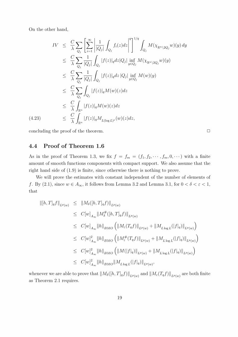
On the other hand,

IV ≤ C

λ

∑Qj

[∞∑i=1

∣∣∣∣∣ 1

|Qj|

∫Qj

fi(z)dz

∣∣∣∣∣q]1/q ∫

Qj

M(χRn\2Qjw)(y) dy

≤ C

λ

∑Qj

1

|Qj|

∫Qj

|f(z)|qdz|Qj| infy∈Qj

M(χRn\2Qjw)(y)

≤ C

λ

∑Qj

1

|Qj|

∫Qj

|f(z)|qdz |Qj| infy∈Qj

M(w)(y)

≤ C

λ

∑Qj

∫Qj

|f(z)|qM(w)(z)dz

≤ C

λ

∫Rn

|f(z)|qM(w)(z)dz

≤ C

λ

∫Rn

|f(z)|qML(log L)ε(w)(z)dz,(4.23)

concluding the proof of the theorem. 2

4.4 Proof of Theorem 1.6

As in the proof of Theorem 1.3, we fix f = fm = (f1, f2, · · · , fm, 0, · · · ) with a finite

amount of smooth functions components with compact support. We also assume that the

right hand side of (1.9) is finite, since otherwise there is nothing to prove.

We will prove the estimates with constant independent of the number of elements of

f . By (2.1), since w ∈ A∞, it follows from Lemma 3.2 and Lemma 3.1, for 0 < δ < ε < 1,

that

‖[h, T ]qf‖Lp(w)≤ ‖Mδ([h, T ]qf)‖

Lp(w)

≤ C[w]A∞‖M#

δ ([h, T ]qf)‖Lp(w)

≤ C[w]A∞‖h‖

BMO

(‖Mε(Tqf)‖

Lp(w)+ ‖M

L log L(|f |q)‖Lp(w)

)≤ C[w]2

A∞‖h‖

BMO

(‖M#

ε (Tqf)‖Lp(w)

+ ‖ML log L

(|f |q)‖Lp(w)

)≤ C[w]2

A∞‖h‖

BMO

(‖M(|f |q)‖Lp(w)

+ ‖ML log L

(|f |q)‖Lp(w)

)≤ C[w]2

A∞‖h‖

BMO‖M

L log L(|f |q)‖Lp(w)

,

whenever we are able to prove that ‖Mδ([h, T ]qf)‖Lp(w)

and ‖Mε(Tqf)‖Lp(w)

are both finite

as Theorem 2.1 requires.

19

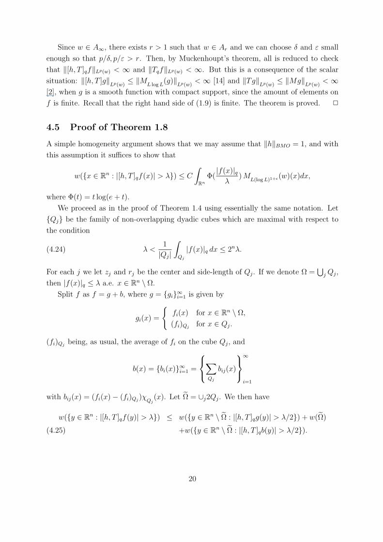
Since w ∈ A∞, there exists r > 1 such that w ∈ Ar and we can choose δ and ε small

enough so that p/δ, p/ε > r. Then, by Muckenhoupt’s theorem, all is reduced to check

that ‖[h, T ]qf‖Lp(w) < ∞ and ‖Tqf‖Lp(w) < ∞. But this is a consequence of the scalar

situation: ‖[h, T ]g‖Lp(w)

≤ ‖ML log L

(g)‖Lp(w)

< ∞ [14] and ‖Tg‖Lp(w)

≤ ‖Mg‖Lp(w)

< ∞[2], when g is a smooth function with compact support, since the amount of elements on

f is finite. Recall that the right hand side of (1.9) is finite. The theorem is proved. 2

4.5 Proof of Theorem 1.8

A simple homogeneity argument shows that we may assume that ‖h‖BMO = 1, and with

this assumption it suffices to show that

w(x ∈ Rn : |[h, T ]qf(x)| > λ) ≤ C

∫Rn

Φ(|f(x)|q

λ) M

L(log L)1+ε(w)(x)dx,

where Φ(t) = t log(e + t).

We proceed as in the proof of Theorem 1.4 using essentially the same notation. Let

Qj be the family of non-overlapping dyadic cubes which are maximal with respect to

the condition

(4.24) λ <1

|Qj|

∫Qj

|f(x)|q dx ≤ 2nλ.

For each j we let zj and rj be the center and side-length of Qj. If we denote Ω =⋃

j Qj,

then |f(x)|q ≤ λ a.e. x ∈ Rn \ Ω.

Split f as f = g + b, where g = gi∞i=1 is given by

gi(x) =

fi(x) for x ∈ Rn \ Ω,

(fi)Qjfor x ∈ Qj.

(fi)Qjbeing, as usual, the average of fi on the cube Qj, and

b(x) = bi(x)∞i=1 =

∑Qj

bij(x)

∞

i=1

with bij(x) = (fi(x)− (fi)Qj)χ

Qj(x). Let Ω = ∪j2Qj. We then have

w(y ∈ Rn : |[h, T ]qf(y)| > λ) ≤ w(y ∈ Rn \ Ω : |[h, T ]qg(y)| > λ/2) + w(Ω)

+w(y ∈ Rn \ Ω : |[h, T ]qb(y)| > λ/2).(4.25)

20

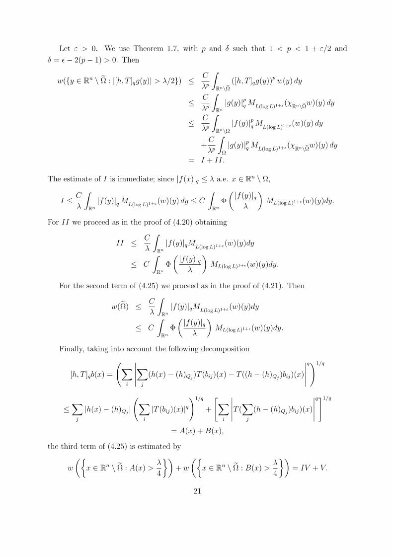
Let ε > 0. We use Theorem 1.7, with p and δ such that 1 < p < 1 + ε/2 and

δ = ε− 2(p− 1) > 0. Then

w(y ∈ Rn \ Ω : |[h, T ]qg(y)| > λ/2) ≤ C

λp

∫Rn\eΩ ([h, T ]qg(y))p w(y) dy

≤ C

λp

∫Rn

|g(y)|pq ML(log L)1+ε(χRn\eΩw)(y) dy

≤ C

λp

∫Rn\Ω

|f(y)|pq ML(log L)1+ε(w)(y) dy

+C

λp

∫Ω

|g(y)|pq ML(log L)1+ε(χRn\eΩw)(y) dy

= I + II.

The estimate of I is immediate; since |f(x)|q ≤ λ a.e. x ∈ Rn \ Ω,

I ≤ C

λ

∫Rn

|f(y)|q ML(log L)1+ε(w)(y) dy ≤ C

∫Rn

Φ

(|f(y)|q

λ

)ML(log L)1+ε(w)(y)dy.

For II we proceed as in the proof of (4.20) obtaining

II ≤ C

λ

∫Rn

|f(y)|qML(log L)1+ε(w)(y)dy

≤ C

∫Rn

Φ

(|f(y)|q

λ

)ML(log L)1+ε(w)(y)dy.

For the second term of (4.25) we proceed as in the proof of (4.21). Then

w(Ω) ≤ C

λ

∫Rn

|f(y)|qML(log L)1+ε(w)(y)dy

≤ C

∫Rn

Φ

(|f(y)|q

λ

)ML(log L)1+ε(w)(y)dy.

Finally, taking into account the following decomposition

[h, T ]qb(x) =

(∑i

∣∣∣∣∣∑j

(h(x)− (h)Qj)T (bij)(x)− T ((h− (h)Qj

)bij)(x)

∣∣∣∣∣q)1/q

≤∑

j

|h(x)− (h)Qj|

(∑i

|T (bij)(x)|q)1/q

+

[∑i

∣∣∣∣∣T (∑

j

(h− (h)Qj)bij)(x)

∣∣∣∣∣q]1/q

= A(x) + B(x),

the third term of (4.25) is estimated by

w

(x ∈ Rn \ Ω : A(x) >

λ

4

)+ w

(x ∈ Rn \ Ω : B(x) >

λ

4

)= IV + V.

21

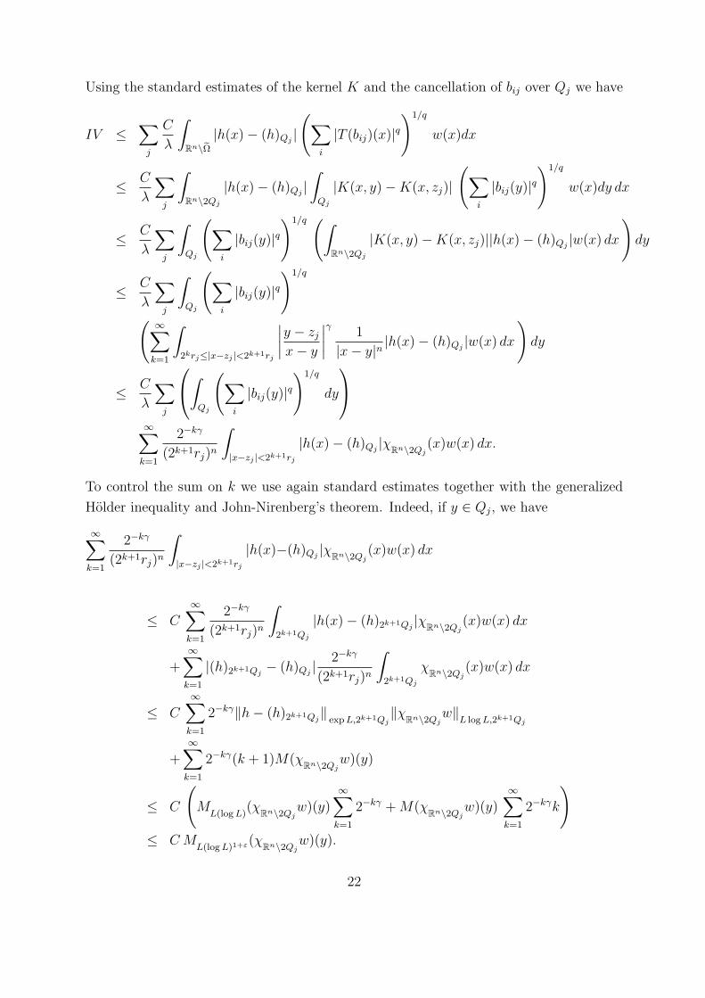
Using the standard estimates of the kernel K and the cancellation of bij over Qj we have

IV ≤∑

j

C

λ

∫Rn\eΩ |h(x)− (h)Qj

|

(∑i

|T (bij)(x)|q)1/q

w(x)dx

≤ C

λ

∑j

∫Rn\2Qj

|h(x)− (h)Qj|∫

Qj

|K(x, y)−K(x, zj)|

(∑i

|bij(y)|q)1/q

w(x)dy dx

≤ C

λ

∑j

∫Qj

(∑i

|bij(y)|q)1/q (∫

Rn\2Qj

|K(x, y)−K(x, zj)||h(x)− (h)Qj|w(x) dx

)dy

≤ C

λ

∑j

∫Qj

(∑i

|bij(y)|q)1/q

(∞∑

k=1

∫2krj≤|x−zj |<2k+1rj

∣∣∣∣y − zj

x− y

∣∣∣∣γ 1

|x− y|n|h(x)− (h)Qj

|w(x) dx

)dy

≤ C

λ

∑j

∫Qj

(∑i

|bij(y)|q)1/q

dy

∞∑

k=1

2−kγ

(2k+1rj)n

∫|x−zj |<2k+1rj

|h(x)− (h)Qj|χRn\2Qj

(x)w(x) dx.

To control the sum on k we use again standard estimates together with the generalized

Holder inequality and John-Nirenberg’s theorem. Indeed, if y ∈ Qj, we have

∞∑k=1

2−kγ

(2k+1rj)n

∫|x−zj |<2k+1rj

|h(x)−(h)Qj|χRn\2Qj

(x)w(x) dx

≤ C∞∑

k=1

2−kγ

(2k+1rj)n

∫2k+1Qj

|h(x)− (h)2k+1Qj|χRn\2Qj

(x)w(x) dx

+∞∑

k=1

|(h)2k+1Qj− (h)Qj

| 2−kγ

(2k+1rj)n

∫2k+1Qj

χRn\2Qj(x)w(x) dx

≤ C

∞∑k=1

2−kγ‖h− (h)2k+1Qj‖

exp L,2k+1Qj‖χRn\2Qj

w‖L log L,2k+1Qj

+∞∑

k=1

2−kγ(k + 1)M(χRn\2Qjw)(y)

≤ C

(M

L(log L)(χRn\2Qj

w)(y)∞∑

k=1

2−kγ + M(χRn\2Qjw)(y)

∞∑k=1

2−kγk

)≤ C M

L(log L)1+ε(χRn\2Qjw)(y).

22

Thus we have

IV ≤ C

λ

∑j

∫Qj

(∑i

|bij(y)|q)1/q

ML(log L)1+ε(χRn\2Qj

w)(y)dy,

and we can continue the estimate of IV in the same way as in the proof of (4.22) with M

replaced by ML(log L)1+ε . We conclude that

IV ≤ C

λ

∫Rn

|f(y)|qML(log L)1+ε(w)(y)dy

≤ C

∫Rn

Φ

(|f(x)|q

λ

)ML(log L)1+ε(w)(x)dx.

To estimate V we will use Theorem 1.4 for singular integrals:

V = w

(x ∈ Rn \ Ω : B(x) >

λ

4

)

≤ C

λ

∫Rn

[∑i

∣∣∣∣∣∑j

(h(x)− (h)Qj)bij(x)

∣∣∣∣∣q]1/q

ML(log L)ε(χRn\eΩw)(x)dx

≤ C

λ

∑j

∫Qj

|h(x)− (h)Qj|

(∑i

|bij(x)|q)1/q

ML(log L)ε(χRn\2Qjw)(x)dx

≤ C

λ

∑j

infQj

ML(log L)ε(χRn\2Qjw)(x)(∫

Qj

|h(x)− (h)Qj||f(x)|q dx +

∫Qj

|h(x)− (h)Qj||g(x)|q dx

)= V1 + V2.

To estimate V2 we combine the argument to prove (4.23), replacing M by ML log L

,

together with the definition of BMO:

V2 ≤ C

∫Rn

|f(x)|qML(log L)ε(w)(x)dx.

For V1 we have by the generalized Holder inequality (2.3)

V1 =C

λ

∑j

infQj

ML(log L)ε(χRn\2Qj

w)(x)

∫Qj

|h(x)− (h)Qj||f(x)|q dx

≤ C

λ

∑j

infQj

ML(log L)ε(χRn\2Qj

w)(x)|Qj|‖|f |q‖L log L,Qj.

23

Now, combining formula (2.2) with (4.24) and recalling that Φ(t) = t log(e + t), we have

1

λ|Qj|‖fq‖L log L,Qj

≤ 1

λ|Qj| inf

µ>0µ +

µ

|Qj|

∫Qj

Φ

(|f(x)|q

µ

)dx

≤ |Qj|+∫

Qj

Φ

(|f(x)|q

λ

)dx

≤ 1

λ

∫Qj

|f(x)|q dx +

∫Qj

Φ

(|f(x)|q

λ

)dx

≤ 2

∫Qj

Φ

(|f(x)|q

λ

)dx.

Then

V1 ≤ C

∫Qj

Φ

(|f(x)|q

λ

)M

L(log L)ε(χRn\2Qjw)(x)dx

≤ C

∫Rn

Φ

(|f(x)|q

λ

)ML(log L)1+ε(w)(x)dx.

The proof of the theorem is finished. 2

References

[1] M. Christ, Lectures on Singular Integral Operators, CBMS Reg. Conf. Ser. Math.

77, Amer. Math. Soc., Providence, RI, 1990.

[2] R. Coifman, Distribution function inequalities for singular integrals, Proc. Acad.

Sci. U.S.A. 69 (1972), 2838–2839.

[3] R. Coifman, R. Rochberg and G. Weiss, Factorization theorems for Hardy

spaces in several variables, Ann. of Math. 103 (1976), 611–635.

[4] R. Coifman and Y. Meyer, Wavelets. Calderon-Zygmund and Multilinear Op-

erators. Cambridge Studies in Advanced Mathematics, 48. Cambridge University

Press, Cambridge, 1997.

[5] D. Cruz-Uribe and C. Perez, Two weight extrapolation via the maximal oper-

ator, J. Funct. Anal. 174 (2000), 1–17.

[6] J. Duoandikoetxea, Fourier Analysis, American Math. Soc., Grad. Stud. Math.,

29, Providence, RI, 2000.

[7] C. Fefferman and E. M. Stein, Some maximal inequalities, Amer. J. Math.

93 (1971), 107–115.

24

[8] J. Garcıa-Cuerva and J. L. Rubio de Francia, Weighted Norm Inequalities

and Related Topics, North Holland Math. Studies 116, North Holland, Amsterdam,

1985.

[9] J. L. Journe, Calderon-Zygmund Operators, Pseudo-Differential Operators and

the Cauchy Integral of Calderon, Lecture Notes in Math., 994, Springer-Verlag,

New York, 1983.

[10] M. A. Krasnosel’skiı and Ya. B. Rutickiı, Convex Functions and Orlicz

Spaces, P. Noordhoff, Groningen, 1961.

[11] C. Perez, Weighted norm inequalities for singular integral operators, J. London

Math. Soc. 49 (1994), 296–308.

[12] C. Perez, Endpoint estmates for commutators of singular integral operators, J.

Funct. Anal. 128 (1995), 163–185.

[13] C. Perez, On sufficient conditions for the boundedness of the Hardy–Littlewood

maximal operator between weighted Lp–spaces with different weights, Proc. London

Math. Soc. (3) 71 (1995), 135–157.

[14] C. Perez, Sharp estimates for commutators of singular integrals via iterations

of the Hardy-Littlewood maximal function, J. Fourier Anal. Appl. 3 (6) (1997),

743–756.

[15] C. Perez, Weighted norm inequalities for the vector-valued maximal function,

Trans. Amer. Math. Soc. 352 (2000), 3265–3288.

[16] G. Pradolini and C. Perez, Sharp weighted endpoint estimates for commuta-

tors of singular integral operators, Michigan Math. J. 49 (2001).

[17] M. M. Rao, and Z.D. Ren, Theory of Orlicz Spaces, Monogr. Textbooks Pure

and Appl. Math. 146, Marcel Dekker, New York, 1991.

[18] A. Torchinsky, Real Variable Methods in Harmonic Analysis, Academic Press,

New York, 1988.

Carlos Perez

Departmento de Analisis Matematico

Facultad de Matematicas

Universidad de Sevilla

41080 Sevilla

25

Spain

E-mail address: carlosperez@us.es

Rodrigo Trujillo-Gonzalez

Departmento de Analisis Matematico

Universidad de La Laguna

38271 La Laguna - S/C de Tenerife

Spain

E-mail address: rotrujil@ull.es

26