Single-layered Complex-Valued Neural Network for Real-Valued Classification Problems

Faijul Amin1 and Kazuyuki Murase1, 2

1Department of Human and Artificial Intelligence Systems, Graduate School of Engineering, and 2Research and Education Program for Life Science, University of Fukui, 3-9-1 Bunkyo, Fukui 910-8507, Japan

Acknowledgement: Supported by grants of K.M. from Japanese Society for promotion of Sciences, and Technology, and the University of Fukui.

Correspondence: Dr. Kazuyuki MuraseProfessor Department of Human and Artificial Intelligence Systems, University of Fukui3-9-1 Bunkyo, Fukui 910-8507, JapanTel: +81(0)776 27 8774Fax: +81(0)776 27 8420E-mail: murase@synaspe.his.fukui-u.ac.jp

The total number of pages 35, figures 6, tables 9.The total number of words in the whole manuscript 5281, abstract 242, introduction 605

* Manuscript

Single-layered Complex-Valued Neural Network for Real-Valued Classification Problems

Abstract

This paper presents two models of complex-valued neurons (CVNs) for real-valued classification problems, incorporating two newly-proposed activation functions, and presents their abilities as well as differences between them on benchmark problems. In both models, each real-valued input is encoded into a phase between 0 and of a complex number of unity magnitude, and multiplied by a complex-valued weight. The weighted sum of inputs is fed to an activation function. Activation functions of both models map complex values into real values, and their role is to divide the net-input (weighted sum) space into multiple regionsrepresenting the classes of input patterns. The gradient-based learning rule is derived for each of the activation functions. Ability of such CVNs are discussed and tested with two-classproblems, such as two and three input Boolean problems, and symmetry detection in binary sequences. We exhibit here that both the models can form proper boundaries for these linear and nonlinear problems. For solving n-class problems, a complex-valued neural network (CVNN) consisting of n CVNs is also considered in this paper. We tested such single-layered CVNNs on several real world benchmark problems. The results show that the classification and generalization abilities of single-layered CVNNs are comparable to the conventional real-valued neural networks (RVNNs) having one hidden layer. Moreover, convergence of CVNNs is much faster than that of RVNNs in most of the cases.

Keywords: activation function, classification, complex-valued neural networks, generalization, phase-encoding.

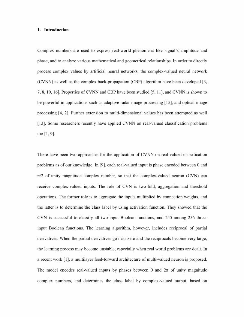
1. Introduction

Complex numbers are used to express real-world phenomena like signal’s amplitude and

phase, and to analyze various mathematical and geometrical relationships. In order to directly

process complex values by artificial neural networks, the complex-valued neural network

(CVNN) as well as the complex back-propagation (CBP) algorithm have been developed [3,

7, 8, 10, 16]. Properties of CVNN and CBP have been studied [5, 11], and CVNN is shown to

be powerful in applications such as adaptive radar image processing [15], and optical image

processing [4, 2]. Further extension to multi-dimensional values has been attempted as well

[13]. Some researchers recently have applied CVNN on real-valued classification problems

too [1, 9].

There have been two approaches for the application of CVNN on real-valued classification

problems as of our knowledge. In [9], each real-valued input is phase encoded between 0 and

/2 of unity magnitude complex number, so that the complex-valued neuron (CVN) can

receive complex-valued inputs. The role of CVN is two-fold, aggregation and threshold

operations. The former role is to aggregate the inputs multiplied by connection weights, and

the latter is to determine the class label by using activation function. They showed that the

CVN is successful to classify all two-input Boolean functions, and 245 among 256 three-

input Boolean functions. The learning algorithm, however, includes reciprocal of partial

derivatives. When the partial derivatives go near zero and the reciprocals become very large,

the learning process may become unstable, especially when real world problems are dealt. In

a recent work [1], a multilayer feed-forward architecture of multi-valued neuron is proposed.

The model encodes real-valued inputs by phases between 0 and 2 of unity magnitude

complex numbers, and determines the class label by complex-valued output, based on

output’s vicinity to the roots of unity. It has been shown that the model was able to solve the

parity n and two spirals problems, and could perform better in “sonar” benchmark and the

Mackey–Glass time series prediction problems.

In this paper, we propose two activation functions that map complex values to real-valued

outputs. The role of the activation functions is to divide the net-input (sum of weighted

inputs) space into multiple regions representing the classes. Both the proposed activation

functions are differentiable with respect to real and imaginary parts of the net-input. As a

result, gradient-based learning rule can be derived. To present complex-valued inputs to CVN,

real-valued inputs are phase encoded between 0 and . We will show in the following

sections that such a CVN is able to solve linear and nonlinear classification problems such as

two-input Boolean functions, 253 among 256 three-input Boolean functions, and symmetry

detection in binary sequences.

To solve n-class problems, we considered a single-layered CVNN (without hidden layer)

consisting of n CVNs described above, and formulated the learning and classification scheme.

The single-layered CVNN has been applied and tested on various real world benchmark

problems. Experimental results showed that generalization ability of the single-layered

CVNN is comparable to the conventional two-layered (with one hidden layer in addition to

input and output layer) real-valued neural network (RVNN). It is noteworthy that in the

proposed single-layered CVNN, the architecture selection problem does not exist. In the

multilayered RVNNs which are considered as universal approximators [6], in contrast, the

architecture selection is crucial to achieve better generalization and faster learning abilities.

The remaining of the paper is organized as follows. In section 2, we discuss about the model

of CVN along with the proposed activation functions. In section 3, we develop gradient-

based learning rules for training the CVNs. Section 4 discusses the ability of the single CVN

on some binary-valued classification problems. In section 5, performances of the single-

layered CVNN consisting of multiple CVNs are compared to those of the conventional two-

layered RVNN on some real world benchmark problems. Finally, section 6 gives the

discussion and concluding remarks.

2. Complex-valued neuron (CVN) model

Since the complex-valued neuron (CVN) processes complex-valued information, it is

necessary to map real input values to complex values for solving real-valued classification

problems. After such mapping, the neuron processes information in a way similar to the

conventional neuron model except that all the parameters and variables are complex-valued,

and computations are performed according to the complex algebra. As illustrated in Fig. 1,

the neuron, therefore, first sums up the weighted complex-valued inputs and the threshold

value to represent its internal state for the given input pattern, and then the weighted sum is

fed to an activation function which maps the internal state (complex-valued weighted sum) to

a real value. Here, the activation function combines the real and imaginary parts of the

weighted sum.

2.1. Phase encoding of the inputs

This section explains how the real-valued information is presented to a CVN. Consider

),( cX be an input example, where mRX represents the vector for m attributes of the

example, and 1,0c denotes the class of the input pattern. We need a mapping mm CR to

process the information by CVN. One such mapping for each element of the vector X can be

done by the following transformation.

Rbabax , where,,Let , then

)/()( abax , and (1)

sincos iez i (2)

Here 1i . Eq. (1) is a linear transformation which maps ],[ bax to ],0[ . Then by the

Euler’s formula, as given by Eq. (2), a complex value z is obtained. When a real variable

moves in the interval of [a, b], the above transformation will move the complex variable z

over the upper half of a unit circle. As shown in Fig. 2, the variation on a real line is thus now

in the variation of phase over the unit circle.

Some facts about the transformation are mentionable. Firstly, the transformation retains

relational property. For example, when two real values x1 and x2 hold a relation 21 xx , the

corresponding complex values have the same property in their phases as such,

)()( 21 zphasezphase . Secondly, the spatial relationship between real values is also

retained. For example, two real values x1 and x2 are farthest from each other

when ax 1 and bx 2 . The transformed complex values 1z and 2z are also farthest from

each other as shown in Fig. 2. Thirdly, the interval [0, ] is better than the interval [0, 2] as

we loose the spatial relationship among the variables in the latter. For example,

ax 1 and bx 2 will be mapped to same complex value, since 20 ii ee . It is mentionable

that interval [0, /2] can also be used for phase encoding. However, experiments presented in

the section 5 and Table 9 exhibit that learning convergence is faster in case of the interval [0,

]. Finally, the transformation can be regarded as a preprocessing step. The preprocessing is

commonly used even in real-valued neural networks in order for mapping input values into a

specified range, and so on. The transformation in the proposed CVN, therefore, does not

increase any additional stage for the process with neural networks. In fact, the above

transformation does not loose any information from the real values, rather lets a CVN to

process the information in a more powerful way.

2.2. Activation function

When a CVN sums up inputs multiplied by the synaptic weights, the weighted sum is fed to

an activation function to make the output bounded. In the real-valued case, activation

functions are generally differentiable and bounded in the entire real domain, which makes it

possible to derive gradient-based backpropagation (BP) algorithm. But from Liouville’s

theorem, there is no complex-valued function except constant which is differentiable and

bounded at the same time. However, this is not as frustrating as it seems. For solving real-

valued classification problems, we can combine real and imaginary parts of the weighted sum

in some useful ways.

In this paper we propose two activation functions that map complex values to real values for

classification problems. Their role is to divide the neuron’s net-input (sum of weighted

inputs) space into multiple regions for identifying the classes, as is the role of the real-valued

neuron in classification problems.

Let the net-input of a complex neuron be ivuz , then we define two activation functions

1 and 2 by the following Eq. (3) and Eq. (4), respectively.

22 ))(())(()( vfufzf RRRC (3)

2)()()( vfufzf RRRC (4)

where ))exp(1/(1)( xxfR and Rvux ,, . Both the activation functions combine the real and

imaginary parts, but in different ways. The real and imaginary parts are first passed through

the same sigmoid function individually. Thus each part becomes bounded within the interval

(0, 1). The activation function 1 in Eq. (3) gives the magnitude of the resulted complex value,

while the activation function 2 in Eq. (4) gives the square of the difference between real and

imaginary parts. Fig. 3 illustrates the output value y of both the activation functions in the

domain of real and imaginary parts of net-input, u and v, respectively. It is noteworthy that

defining activation functions as above, makes it possible to compute the partial

derivativesu

f

andv

f

, which in turn makes it possible to derive gradient-based learning

rules.

As seen in Fig. 3, both the CVNs with the proposed activation functions saturate in four

regions. On the contrary, the real-valued sigmoid function saturates only in two regions. Thus

a real valued neuron can solve only linearly separable problem. We show in the later sections

that saturation in four regions of the proposed CVNs significantly improves their

classification ability.

3. Learning rule

Here we derive a gradient-descent learning rule for a CVNN consisted of multiple CVNs

described in the previous section. We deal with the CVNN without any hidden units.

Consider an m-n CVNN, where m and n are the numbers of inputs and outputs, respectively.

Let TmxxX ][ 1 be an m dimensional complex-valued input vector, T

kmkk wwW ][ 1 the

complex-valued weight vector of neuron k, and θk the complex-valued bias for the kth neuron.

To express the real and imaginary parts, let Ij

Rjj ixxx , I

kjRkjkj iwww , I

kRkk i . Then

the net-input zk, and the output yk of the kth neuron are given by

k

m

jjkjk xwz

1

(5)

Ik

m

j

Ij

Rkj

Rj

Ikj

Rk

m

j

Ij

Ikj

Rj

Rkj xwxwixwxw )()(

11

(6)

Ik

Rk izz (7)

and

)( kRCk zfy (8)

If the desired output of the kth neuron is dk, then the error function to be minimized during

the training is given by

n

kk

n

kkk eydE

1

2

1

2 )2/1()()2/1( (9)

During the training, the biases and the weights are updated according to the following

equations.

Ik

RkI

kRk

k iE

iE

(10)

kjIkj

RkjI

kjRkj

kj xwiww

Ei

w

Ew

(11)

where is the learning rate and jx is the complex conjugate of the complex number jx .

If the activation function is given by Eq. (3), then

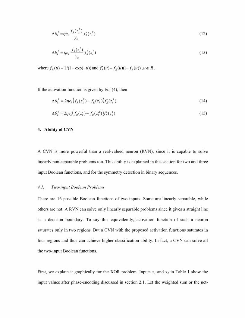
)()( R

kRk

RkR

kRk zf

y

zfe (12)

)()( I

kRk

IkR

kIk zf

y

zfe (13)

where ))exp(1/(1)( uuf R and ))(1)(()( ufufuf RRR , Ru .

If the activation function is given by Eq. (4), then

)()()(2 RkR

IkR

RkRk

Rk zfzfzfe (14)

)()()(2 IkR

RkR

IkRk

Ik zfzfzfe (15)

4. Ability of CVN

A CVN is more powerful than a real-valued neuron (RVN), since it is capable to solve

linearly non-separable problems too. This ability is explained in this section for two and three

input Boolean functions, and for the symmetry detection in binary sequences.

4.1. Two-input Boolean Problems

There are 16 possible Boolean functions of two inputs. Some are linearly separable, while

others are not. A RVN can solve only linearly separable problems since it gives a straight line

as a decision boundary. To say this equivalently, activation function of such a neuron

saturates only in two regions. But a CVN with the proposed activation functions saturates in

four regions and thus can achieve higher classification ability. In fact, a CVN can solve all

the two-input Boolean functions.

First, we explain it graphically for the XOR problem. Inputs x1 and x2 in Table 1 show the

input values after phase-encoding discussed in section 2.1. Let the weighted sum or the net-

input of the neuron be ivuxwxwz 2211 , where θ is the bias. After training the

neuron, the net-input for each input pattern should produce the output near the desired output

value shown in Table 1 by the mapping of )(zfy RC .

The net-inputs for the four input patterns in XOR problem and the contour diagram of output

y are shown in Fig. 4. Among the four regions of saturation in the activation function 1 (Fig.

4(a)), the net-inputs after training were located at three regions; upper left, lower left, and

lower right regions, since the desired outputs were either zero or one. In case of the activation

function 2 (Fig. 4(b)), all four regions were used. As apparent in Fig. 4, both CVNs with the

proposed activation functions were able to solve the XOR problem, while a single RVN

cannot solve such a linearly non-separable problem.

Parameters obtained after training, for all possible two-input Boolean functions, are given in

Table 2. Each sequence 4321 yyyyY denotes a Boolean function,

where )0,0(1 fy , )1,0(2 fy , )0,1(3 fy and )1,1(4 fy . For example, the

sequence 0110 is the XOR problem, 0001is the AND problem, 0111is the OR problem, and

so on.

4.2. Three-input Boolean Problems

For three inputs, the number of different Boolean functions is 256. Michel et al. [9] have

reported that their CVN model solves 245 among the 256 functions. Our proposed model of

CVN with the activation function 2 could solve 253 functions, and 250 functions with the

activation function 1. These impressive results are suggestive to examine the CVN, with the

new activation functions, on more complex problems.

4.3. Symmetry detection Problem

The symmetry detection problem is to detect whether or not binary activity levels of a one-

dimensional input array is symmetrical about the center point. An example of input-output

mapping, for the input length of three bits is shown in Table 3. It is a linearly non-separable

problem and hence can not be solved by a single RVN.

4.3.1. Solving with one CVN

We tested CVN on symmetry detection problems of various input lengths ranging from 2 bits

to 10 bits. A single CVN with the proposed activation functions could solve all of the

problems. For training the CVN, we set the target values as follows. With the activation

function 1, the target was set to 0 if the input pattern was symmetric, and 1 if asymmetric.

With the activation function 2, target was 1 if symmetric, and 0 if asymmetric.

Solutions for four-input problem obtained with the activation function 1 and 2 are shown in

the contour graphs (a) and (b) in Fig. 5, respectively. Though the activation function 1

saturates in four regions, we can expect that three regions will be used because the target

output values are set to 0 and 1. The other region for which output is near 2 will not be used.

As expected, experimental results presented in Fig. 5(a) showed that the net-inputs for sixteen

different input patterns were distributed in the three regions, according to symmetry and

asymmetry, after the training. For the activation function 2, on the other hand, all four regions

of saturation can be used, and the experimental results in Fig. 5(b) shows that the input

patterns were distributed in four regions according to symmetry and asymmetry.

We then reversed the target output setting for both the activation functions. That is, with the

activation function 1, the target was set to 1 if the input pattern was symmetric, and 0 if

asymmetric, while with the activation function 2, target was set to 0 if symmetric, and 1 if

asymmetric. The CVN with the activation function 1 could solve the symmetry detection

problem up to the length of 3 bits, and with the activation function 2 up to 5 bits. This

degraded result can be explained by the imbalance in numbers of input patterns assigned to

each output value. That is, as the length of inputs increases, the percentage of symmetric

inputs among all possible input patterns decreases. For example, there are 50% symmetric

patterns for the symmetry detection problem of 3 bits, while only 6.25% and 3.125% for that

of 9 and 10 bits, respectively. The detailed explanation is given below.

Nonlinearity comes from the fact that input patterns having numerically far different values,

and being spatially far different in location belong to the same class. When the same weight

vector is multiplied with different input vectors of the same class, the weighted sum is

different. The activation function 1 has two regions of saturation for the target value of 1 and

only one region for the target value of 0 (Fig. 3(a)). Since most of the input patterns are

asymmetric for higher dimensional problems having the target output 0, in case of reverse

target setting, only one region is not enough to accommodate all asymmetric input patterns

having numerically far different values. With the other target setting, 0 for symmetry and 1

for asymmetry, activation function 1 could solve higher dimensional problems as there are

two well spread regions for output values near the value of 1, and most of the input patterns

are asymmetric having the target value of 1. The same argument can be applied to the CVN

with the activation function 2. That is, in case of reverse target output settings (0 for

symmetric and 1 for asymmetric), though there are two regions of saturation for target output

of 1, the regions are not as spread as the regions for 0, while most of the input patterns are

asymmetric.

4.3.2. Solving with two CVNs

To solve the output encoding problem described above, one solution is to use two CVNs,

each with opposite target output settings. If the target value for one CVN is 1, then that of the

other CVN is 0. Output class of a given input pattern is decided according to the CVN with

the larger output. Results of using two CVNs for the symmetry detection problems are

summarized in Table 4. Here the average of 10 independent runs is shown. Two CVNs with

activation function 1 could solve the symmetry detection problem up to seven bits, and

activation function 2 up to six bits. The reason for these degraded results in comparison to

using a single CVN is that although response from one of the CVN is near its target value, the

output of the other neuron degrades the result more strongly. This can be seen from table 5,

where a result of a single run for the seven-bit symmetry detection problem with the

activation function 2 is given. Underlined outputs denote the misclassification. Response of

one of the neuron (neuron 2) degraded the result strongly even though the other neuron

(neuron 1) gave the correct output.

Nevertheless, though limitations exist, a single CVN is at least more powerful than a single

RVN as it can solve linear as well as nonlinear problems to some considerable extents. Its

applicability will be justified in the next section where we applied multiple CVNs on real

world benchmark problems.

5. Single-layered complex-valued neural network (CVNN) on real world classification

problems

Discussion in the previous sections is suggestive to explore the ability of multiple CVNs,

which we call the single-layered complex-valued neural network (CVNN), on real world

classification problems. To compare CVNN’s performance with the conventional two-layered

RVNN, both the neural networks are tested on some real world benchmark problems. We

used PROBEN1 [14] datasets for the experiments. In this section, first we give a short

description of the datasets, and then compare learning convergence and generalization ability

of CVNN and RVNN.

5.1. Description of the datasets

PROBEN1 is a collection of learning problems well suited for supervised learning. Most of the

problems are classification problems regarding diagnosis. Here we use five of them. Each of

the problems is available in three datasets, which vary in the ordering of examples. For

example, cancer problem consists of cancer1, cancer2 and cancer3 datasets. Short

descriptions of these five problems are given below.

5.1.1. Cancer

This is a problem on diagnosis of breast cancer. The task is to classify a tumor as either

benign or malignant based on cell descriptions gathered by microscopic examination. Input

attributes are for instance the clump thickness, the uniformity of cell size and cell shape, the

amount of marginal adhesion, and the frequency of bare nuclei. The data comprise of 9 inputs,

2 outputs, 699 examples, of which 65.5% are benign example. This data is originally obtained

from University of Wisconsin Hospitals, Madison, from Dr. William H. Wolberg [17].

5.1.2. Card

The task is to predict the approval or non-approval of a credit card to a customer. Each

example represents a card application and the output describes whether the bank (or similar

institution) granted the card or not. There are 51 inputs, 2 outputs, and 690 examples.

5.1.3. Diabetes

This is on diagnosis of diabetes of Pima Indians. The task is to decide whether a Pima Indian

individual is diabetes positive or not, based on personal data (age, number of times pregnant)

and the results of medical examination (e.g. blood pressure body mass index, result of

glucose tolerance test, etc.). It has 8 inputs, 2 outputs, and 768 examples.

5.1.4. Glass

Here the task is to classify glass types. The results of a chemical analysis of glass splinters

(percent content of 8 different elements) plus the refractive index are used to classify the

samples to be either float processed or non float processed building windows, vehicle

windows, containers, tableware, or head lamps. This task is motivated by forensic needs in

criminal investigation. The data have 9 inputs, 6 outputs, and 214 examples.

5.1.5. Soybean

The task is to recognize 19 different diseases of soybeans. The discrimination is done based

on a description of bean (e.g. whether its size and color are normal), the plants (e.g. the size

of spots on the leafs, whether these spots have a halo, whether plant growth is normal,

whether roots are rotted), and information about the history of the plant’s life (whether

changes in crop occurred in the last year or last two years, whether seeds were treated, how

the environment temperature is). There are 35 inputs, 19 outputs, and 683 examples in the

data.

5.2. Experimental setup

All the datasets discussed above contain real-valued data. The inputs were phase encoded as

discussed in section 2.1. Class labels were encoded by 1-of-n encoding for n-class problem

using output values 0 and 1. To determine the class winner-takes-all method was used, i.e. for

a given input pattern, the output neuron with the highest activation designated the class.

Regarding the architecture of neural networks, the single-layered CVNN consisted of n

CVNs, while two-layer RVNN architecture was selected in such a way that the number of

parameters for both the CVNN and RVNN were nearly equal. For CVNNs, each complex-

valued weight was counted as two parameters since it has real and imaginary part. Table 6

shows the number parameters for CVNNs and RVNNs used in the experiments.

The backpropagation algorithm was used to train the RVNN, while the learning rules

discussed in section 3 were used to train the CVNN. During the training, we kept the learning

rate at 0.1 for both the networks. Weights and biases (in case of CVNN, real and imaginary

parts) were initialized with random numbers from uniform distribution in the range of [-0.5,

0.5].

We used the partitioning of the dataset into training, validation, and test sets as given in

PROBEN1 [14]. The partitioning is shown in Table 7. We trained both the networks over the

training set for 1000 epochs, except for the Glass and Soybean problems. During these 1000

epochs, the weight parameters with the minimum mean squared error (MSE) over validation

set, was stored and applied on test set. We calculated this validation error by using the same

formulation as Eq. (16) below, except with the validation set instead of training set.

Validation error was measured after every five epochs during the training process. For Glass

problem we trained RVNN up to 5000 epochs, and for Soybean 4000 epochs. CVNN was

trained up to 1000 epochs for all the datasets.

5.3. Learning convergence

When a neural network is trained with input patterns, the error on the training set decreases

gradually with the epochs. We used the following formula to measure the mean squared

training error over an epoch.

P

p

n

ipipi yd

PE

1 1

2)(2

1 (16)

where, p is the pattern number, P the total number of training patterns, and n is the number

of output neurons.

Fig. 6 shows how the mean squared training error changed over the epochs for two-layered

RVNN, and single-layered CVNN with both the proposed activation functions on diabetes

dataset. For both the activation functions, CVNN converged much faster then the RVNN.

Especially, CVNN with the activation function 2 converged faster than with the activation

function 1. In the following section we show it quantitatively for all the datasets used in the

experiments.

5.4. Results

Here we compare the generalization ability of the single-layered CVNN and two-layered

RVNN on the basis of misclassification on test dataset. We also compare the number of

epochs during training to reach the minimum MSE over validation set as discussed in section

5.3. Table 8 summarizes the results. Results were taken over 20 independent runs for each of

the datasets.

As shown in Table 8, the test set errors obtained with the activation function 1 tended to be

more or less similar to those with the activation function 2. For six datasets, Cancer3,

Diabetes2, Glass1, Glass2, Glass3 and Soybean1, the average classification errors of CVNN

were a little bit less than those of the RVNN, while for the others little a bit more than those

of the RVNN. Single-layered CVNNs, with both the activation functions, thus exhibit

comparable generalization ability to that of RVNNs.

Regarding the learning convergence, single-layered CVNNs required far less training cycles

(epochs), in almost all the cases, to reach the minimum validation error than the RVNN

counterpart as can be seen in Table 8. In other words, learning convergence of CVNNs is

faster than that of the RVNN. CVNNs with the activation function 2 seem to have even faster

convergence than that of the activation function 1 in most of the cases.

In section 2.1, we mentioned that both the interval [0, ] and [0, /2] may be used for the

phase encoding of real-valued inputs. Table 9 shows the number epochs to reach the

minimum validation error in both the encoding schemes, with each of the activation functions.

As apparent from the table, the learning convergence is faster for the interval [0, ] in most of

the cases. The difference in generalization ability (test set error) was insignificant and thus

the results are not shown.

6. Discussion

Two new activation functions for CVNs have been proposed in this study. These are suitable

for applying single-layered CVNN to real-valued classification problems. It is shown that

encoding real-valued inputs into phases, and processing information in complex domain,

improves classification ability of a neuron. Capability of the proposed CVNs is illustrated by

solving two-input Boolean functions, three-input Boolean functions, and symmetry detection

in binary sequences of various lengths. A single-layered CVNN consisted of multiple CVNs

with decision making in a winner-takes-all fashion is proposed and tested with real world

benchmark problems.

We explained graphically the nature of the proposed activation functions. Both the activation

functions have four regions of saturation. We exploited three regions for activation function 1,

and all four regions for activation function 2, since target outputs were given either 0 or 1.

Such saturation regions improve the classification ability of a CVN. Michel et al. [8] have

reported that their model is able to solve 245 out of 256 three-input Boolean functions, while

the proposed CVNs could solve 253 functions. Solving symmetry detection problem in

binary sequences by a CVN up to six bits has been reported by Nitta [12]. We here showed

that the proposed CVN can solve up to 10 bits. However, there is a limitation of output

encoding for high dimensional symmetry detection problems. Using two CVNs, this problem

can be solved to a considerable extent.

The single-layered CVNN is much faster in learning than the RVNN in terms of number of

epochs for reaching minimum validation error. Generalization ability of the single-layered

CVNN is comparable to two-layer RVNN on real world benchmark problems. One

advantage of using such a single-layered CVNN instead of RVNN for classification problems

is that the architecture selection problem does not exist in case of the single-layered CVNN.

Though there is no complex-valued activation function having differentiability and

boundness at the same time in the entire complex domain, one can treat real and imaginary

parts of net-input of a CVN individually, and then can combine them meaningfully. Also

making dimensionality high (for example, quaternions) may be a new direction for enhancing

the ability of neural networks. We think solving real-valued problems by CVNN more

efficiently deserves further research.

References

[1] I. Aizenberg, C. Moraga, Multilayer feedforward neural network based on multi-valued

neurons and a backpropagation learning algorithm, Soft Computing, 11 (2) (2007) 169–

183.

[2] H. Aoki, Application of complex-valued neural networks for image processing, in: A.

Hirose, ed., Complex-Valued Neural Networks: Theories and Applications, Vol. 5

(World Scientific Publishing, Singapore, 2003) 181–204.

[3] G. Georgiou, C. Koutsougeras, Complex backpropagation, IEEE Transactions on

Circuits and Systems II, 39 (5) (1992) 330–334.

[4] A. Hirose, Applications of complex-valued neural networks to coherent optical

computing using phase-sensitive detection scheme, Information Sciences – Applications,

2 (2) (1994) 103–117.

[5] A. Hirose, Complex-Valued Neural Networks (Springer-Verlag, Berlin, 2006).

[6] K. Hornik, M. Stinchombe, H. White, Multilayer Feedforward networks are universal

approximators, Neural Networks, 2 (1989) 359–366.

[7] T. Kim, T. Adali, Fully complex multilayer perceptron for nonlinear signal processing,

Journal of VLSI Signal Processing Systems for Signal, Image, and Video Technology,

Special Issue: Neural Networks for Signal Processing, 32 (2002) 29–43.

[8] H. Leung, S. Haykin, The complex backpropagation algorithm, IEEE Transactions on

Signal Processing, 39 (9) (1991) 2101–2104.

[9] H. E. Michel, A. A. S. Awwal, Enhanced artificial neural networks using complex-

numbers, in: Proc. IJCNN’99 International Joint Conference on Neural Networks, Vol. 1

(1999) 456–461.

[10] T. Nitta, An extension of the backpropagation algorithm to complex numbers, Neural

Networks, 10 (8) (1997) 1391–1415.

[11] T. Nitta, On the inherent property of the decision boundary in complex-valued neural

networks. Neurocomputing, 50 (C) (2003) 291–303.

[12] T. Nitta, Solving the XOR problem and the detection of symmetry using a single

complex-valued neuron, Neural Networks, 16 (8) (2003) 1101–1105.

[13] T. Nitta, Three-dimensional vector valued neural network and its generalization ability.

Neural Information Processing – Letters and Reviews, 10 (10) (2006) 237–242.

[14] L. Prechelt, PROBEN1 – A set of benchmarks and benchmarking rules for neural

network training algorithms, University of Karlsruhe, Germany, Available FTP:

(ftp.ira.uka.de/pub/neuron/proben1.tar.gz).

[15] A. B. Suksmono, A. Hirose, Adaptive interferometric radar image processing by

complex-valued neural networks, in: A. Hirose, ed., Complex-Valued Neural Networks:

Theories and Applications, Vol. 5 (World Scientific Publishing, Singapore, 2003) 277–

301.

[16] B. Widrow, J. McCool, M. Ball, The complex LMS algorithm, Proceedings of IEEE, 63

(4) (1975) 719–720.

[17] W. H. Wolberg, O. L. Mangasarian, Multisurface method of pattern separation for

medical diagnosis applied to breast cytology, Proceedings of the National Academy of

Sciences, 87 (1990) 9193–9196.

Table 1

Inputs

1x 2x

Outputy

01 i 01 i 0

01 i 01 i 1

01 i 01 i 1

01 i 01 i 0

Table 2

Activation 1 Activation 2Function

4321 yyyy θ w1 w2 θ w1 w2

0000 -3.61-3.61i 0.00+0.00i 0.00+0.00i -0.15+0.33i -0.19-0.28i -0.33-0.34i

0001 -2.97-2.98i -1.83-1.99i -1.83-1.99i -2.53+0.17i -0.96-2.68i 2.26-1.13i

0010 -2.97-2.98i -1.79-2.03i 1.79+2.03i 1.58-2.03i -2.69-0.74i -0.29-2.64i

0011 -1.68-1.02i -1.93-2.59i 0.00+0.00i -2.27+2.32i 2.41-2.34i 0.05+0.07i

0100 -2.97-2.97i 1.86+1.96i -1.86-1.96i -2.36+1.05i 1.03+2.74i 2.57-0.25i

0101 -1.25-1.47i 0.03-0.03i -2.36-2.14i -2.27+2.32i -0.03-0.03i 2.40-2.35i

0110 -2.83-2.81i -2.83+2.82i 2.83-2.82i -0.08-0.06i 1.72-2.24i -2.38+1.19i

0111 -1.64+0.39i -2.70-0.39i 1.61-2.90i -1.74+1.98i -1.74+1.98i 4.05-4.02i

1000 -2.95-2.96i 2.46+1.37i 2.46+1.37i -2.31+0.96i -2.48+0.33i 0.98+2.67i

1001 -2.83-2.83i -2.83+2.83i -2.83+2.83i -0.06-0.07i -2.13+2.64i -2.54+2.03i

1010 -1.66-1.05i -0.01+0.01i 1.95+2.56i 2.36-2.20i -0.08-0.08i 2.31-2.46i

1011 1.58-1.89i -1.58-2.17i 2.88-1.15i 1.50-2.17i -4.10+3.98i -1.50+2.17i

1100 -1.31-1.42i 2.30+2.19i 0.00+0.00i 2.22-2.50i 2.45-2.17i -0.07-0.03i

1101 1.81-1.91i 2.91-0.93i -1.81-1.95i -4.01+4.07i -1.99+1.74i 1.99-1.74i

1110 -1.05-0.84i 2.82-0.84i -1.05+2.83i -2.25+1.38i 2.25-1.38i -3.95+4.13i

1111 1.11+0.57i 0.08-0.09i -0.19+0.21i -4.66+4.67i 0.02+0.01i -0.01+0.00i

Table 3

Inputsx1 x2 x3

Outputy

0 0 0 10 0 1 00 1 0 10 1 1 01 0 0 01 0 1 11 1 0 01 1 1 1

Table 4

Misclassified. 3 / Total patternsLength Sym. 1 + Asym. 2

Activation 1 Activation 22 2 + 2 0/4 0/43 4 + 4 0/8 0/84 4 + 12 0/16 0/165 8 + 24 0/32 0/326 8 + 56 0/64 0/647 16 + 112 0/128 0.8/1288 16 + 240 16/256 6.6/2569 32 + 480 32/512 8.8/51210 32 + 992 32/1024 32/1024

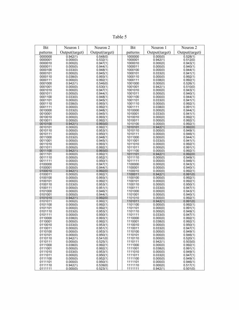
Table 5

Bit patterns

Neuron 1 Output(target)

Neuron 2 Output(target)

Bit patterns

Neuron 1 Output(target)

Neuron 2 Output(target)

0000000 0.942(1) 0.548(0) 1000000 0.000(0) 0.528(1)0000001 0.000(0) 0.532(1) 1000001 0.942(1) 0.512(0)0000010 0.000(0) 0.947(1) 1000010 0.000(0) 0.943(1)0000011 0.000(0) 0.944(1) 1000011 0.000(0) 0.940(1)0000100 0.033(0) 0.948(1) 1000100 0.000(0) 0.944(1)0000101 0.000(0) 0.945(1) 1000101 0.033(0) 0.941(1)0000110 0.038(0) 0.993(1) 1000110 0.000(0) 0.992(1)0000111 0.000(0) 0.992(1) 1000111 0.038(0) 0.992(1)0001000 0.942(1) 0.546(0) 1001000 0.000(0) 0.526(1)0001001 0.000(0) 0.530(1) 1001001 0.942(1) 0.510(0)0001010 0.000(0) 0.947(1) 1001010 0.000(0) 0.943(1)0001011 0.000(0) 0.944(1) 1001011 0.000(0) 0.940(1)0001100 0.033(0) 0.948(1) 1001100 0.000(0) 0.944(1)0001101 0.000(0) 0.945(1) 1001101 0.033(0) 0.941(1)0001110 0.038(0) 0.993(1) 1001110 0.000(0) 0.992(1)0001111 0.000(0) 0.992(1) 1001111 0.038(0) 0.991(1)0010000 0.033(0) 0.948(1) 1010000 0.000(0) 0.944(1)0010001 0.000(0) 0.945(1) 1010001 0.033(0) 0.941(1)0010010 0.000(0) 0.993(1) 1010010 0.000(0) 0.992(1)0010011 0.000(0) 0.992(1) 1010011 0.000(0) 0.992(1)0010100 0.942(1) 0.993(0) 1010100 0.000(0) 0.992(1)0010101 0.000(0) 0.992(1) 1010101 0.942(1) 0.992(0)0010110 0.000(0) 0.953(1) 1010110 0.000(0) 0.949(1)0010111 0.000(0) 0.950(1) 1010111 0.000(0) 0.946(1)0011000 0.033(0) 0.948(1) 1011000 0.000(0) 0.944(1)0011001 0.000(0) 0.945(1) 1011001 0.033(0) 0.941(1)0011010 0.000(0) 0.993(1) 1011010 0.000(0) 0.992(1)0011011 0.000(0) 0.992(1) 1011011 0.000(0) 0.991(1)0011100 0.942(1) 0.993(0) 1011100 0.000(0) 0.992(1)0011101 0.000(0) 0.992(1) 1011101 0.942(1) 0.992(0)0011110 0.000(0) 0.952(1) 1011110 0.000(0) 0.949(1)0011111 0.000(0) 0.950(1) 1011111 0.000(0) 0.946(1)0100000 0.000(0) 0.947(1) 1100000 0.000(0) 0.943(1)0100001 0.000(0) 0.944(1) 1100001 0.000(0) 0.940(1)0100010 0.942(1) 0.992(0) 1100010 0.000(0) 0.992(1)0100011 0.000(0) 0.992(1) 1100011 0.942(1) 0.991(0)0100100 0.000(0) 0.993(1) 1100100 0.000(0) 0.992(1)0100101 0.000(0) 0.992(1) 1100101 0.000(0) 0.992(1)0100110 0.033(0) 0.953(1) 1100110 0.000(0) 0.950(1)0100111 0.000(0) 0.951(1) 1100111 0.033(0) 0.947(1)0101000 0.000(0) 0.946(1) 1101000 0.000(0) 0.943(1)0101001 0.000(0) 0.944(1) 1101001 0.000(0) 0.940(1)0101010 0.942(1) 0.992(0) 1101010 0.000(0) 0.992(1)0101011 0.000(0) 0.992(1) 1101011 0.942(1) 0.991(0)0101100 0.000(0) 0.992(1) 1101100 0.000(0) 0.992(1)0101101 0.000(0) 0.992(1) 1101101 0.000(0) 0.991(1)0101110 0.033(0) 0.953(1) 1101110 0.000(0) 0.949(1)0101111 0.000(0) 0.950(1) 1101111 0.033(0) 0.947(1)0110000 0.038(0) 0.993(1) 1110000 0.000(0) 0.992(1)0110001 0.000(0) 0.992(1) 1110001 0.038(0) 0.992(1)0110010 0.033(0) 0.953(1) 1110010 0.000(0) 0.950(1)0110011 0.000(0) 0.951(1) 1110011 0.033(0) 0.947(1)0110100 0.000(0) 0.953(1) 1110100 0.000(0) 0.949(1)0110101 0.000(0) 0.950(1) 1110101 0.000(0) 0.946(1)0110110 0.942(1) 0.541(0) 1110110 0.000(0) 0.520(1)0110111 0.000(0) 0.525(1) 1110111 0.942(1) 0.503(0)0111000 0.038(0) 0.992(1) 1111000 0.000(0) 0.992(1)0111001 0.000(0) 0.992(1) 1111001 0.038(0) 0.991(1)0111010 0.033(0) 0.953(1) 1111010 0.000(0) 0.949(1)0111011 0.000(0) 0.950(1) 1111011 0.033(0) 0.947(1)0111100 0.000(0) 0.952(1) 1111100 0.000(0) 0.949(1)0111101 0.000(0) 0.950(1) 1111101 0.000(0) 0.946(1)0111110 0.942(1) 0.539(0) 1111110 0.000(0) 0.517(1)0111111 0.000(0) 0.523(1) 1111111 0.942(1) 0.501(0)

Table 6Dataset CVNN RVNN

Name Input Output Parameters Hidden units Parameterscancer 9 2 40 3 38card 51 2 208 4 218

diabetes 8 2 36 3 35glass 9 6 120 7 118

soybean 82 19 3154 31 3181

Table 7

DatasetTotal

patternsTraining

setValidation

setTest set

cancer 699 350 175 174card 690 345 173 172

diabetes 768 384 192 192glass 214 107 54 53

soybean 683 342 171 170

Table 8

Test set error ± S.D. Epoch at min validation errorCVNN CVNNDataset

RVNNAct. 1 Act. 2

RVNNAct. 1 Act. 2

cancer1 1.440.29 2.560.29 2.500.28 133.25 30.00 23.25cancer2 3.710.35 4.370.29 4.480.30 69.00 21.25 16.25cancer3 4.480.35 4.020.00 4.020.00 69.25 27.25 20.25card1 14.480.75 14.940.80 14.800.61 30.75 7.25 6.00card2 17.940.76 17.821.07 17.791.17 16.25 4.50 6.25card3 19.130.96 18.981.20 19.161.58 33.75 10.25 10.00

diabetes1 23.720.60 25.600.39 25.570.50 630.25 83.75 40.00diabetes2 26.170.84 23.780.80 24.710.85 313.75 94.50 45.50diabetes3 21.900.64 21.280.76 21.020.59 416.25 7.00 6.00

glass1 35.285.38 32.641.95 29.723.67 4590.50 194.00 131.25glass2 53.871.67 46.796.05 44.725.61 217.50 388.75 110.25glass3 50.387.62 39.065.71 40.755.21 4195.25 311.00 131.50

soybean1 10.621.23 8.290.44 9.321.62 3545.50 220.75 209.75

soybean2 7.441.52 6.880.57 8.472.55 3452.50 299.75 155.00soybean3 8.651.54 9.681.22 10.182.50 3122.25 140.00 116.25

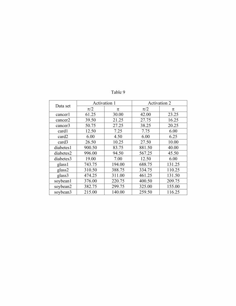
Table 9

Activation 1 Activation 2Data set

/2 /2 cancer1 61.25 30.00 42.00 23.25cancer2 39.50 21.25 27.75 16.25cancer3 50.75 27.25 38.25 20.25card1 12.50 7.25 7.75 6.00card2 6.00 4.50 6.00 6.25card3 26.50 10.25 27.50 10.00

diabetes1 900.50 83.75 881.50 40.00diabetes2 996.00 94.50 567.25 45.50diabetes3 19.00 7.00 12.50 6.00

glass1 743.75 194.00 688.75 131.25glass2 310.50 388.75 334.75 110.25glass3 474.25 311.00 461.25 131.50

soybean1 376.00 220.75 400.50 209.75soybean2 382.75 299.75 325.00 155.00soybean3 215.00 140.00 259.50 116.25

Table Caption

Table 1. Input-output mapping for XOR problem after phase encoding of inputs.

Table 2. Learned weights and bias of CVN for two-input Boolean functions.

Table 3. Input-output mapping of a symmetry detection problem with three inputs. Output 1

means corresponding input pattern is symmetric, and 0 means asymmetric.

Table 4. Average number of misclassifications by two CVNs for symmetry detection problems.

Averages are taken over 10 independent runs. 1, 2, and 3 refer to the number of symmetric

patterns, number of asymmetric patterns, and average number of misclassification, respectively.

Table 5. Examples of outputs of two CVNs with the activation function 2 for the seven-input

symmetry detection problem in a single run.

Table 6. Number of parameters for single-layered CVNNs and two-layered RVNNs. Parameters

include the connection weights and the biases of the neurons. For CVNN, each weight and bias

are counted as two parameters, since they have real and imaginary parts.

Table 7. Total number of examples, and partitioning of the datasets into training, validation and

test sets.

Table 8. Average classification error on the test set, and the average number of epochs required

to reach the minimum validation error. Averages are taken over 20 independent runs. Act. 1 and

2 refer to the activation function 1 and activation function 2, respectively.

Table 9. Average number of epochs required to reach the minimum validation error for the phase

encoding [0, /2] and [0, ]. Averages are taken over 20 independent runs.

Figure Captions

Fig. 1. Model of a complex neuron. The sign sums up the weighted inputs )1( mjxw jj

and the bias . RCf is an activation function that maps the complex-valued internal state to a

real-valued output y.

Fig. 2. Phase encoded inputs. When a real value x moves in the interval [a, b], corresponding

complex value moves over the upper half of unit circle. x = a, and x = b are mapped by 0ie ,

and ie respectively.

Fig. 3. The proposed activation functions 1 and 2 that map complex-value ivu to real-value y.

(a) Activation function 1 is the magnitude )()( vfiuf RR of sigmoided real and imaginary parts,

(b) Activation function 2 is the square of differences 2))()(( vfuf RR between sigmoided real

and imaginary parts.

Fig. 4. Net-inputs of a CVN for XOR problem and contour diagram for the activation function 1

and 2 in (a) and (b), respectively. Curved lines indicate the points taking the same output values

as indicated by the numbers. Horizontal and vertical lines are the real and imaginary axes,

respectively. Cross mark [×] denotes the net-input for the input pattern belonging to class 1

(target output 1), and circle [O] denotes the net-input belonging to class 0 (target output 0).

Fig. 5. Net-inputs of a single CVN for sixteen possible input patterns in the four-input symmetry

detection problem on the contour diagrams of (a) the activation function 1, and (b) the activation

function 2.

Fig. 6. Learning processes of the two-layered RVNN, and single-layered CVNNs with the

activation function 1 (CVNN Act1) and activation function 2 (CVNN Act2).

å yRCf

®

1

mxmw

q

M

1w

2w

1x

2x

Figure1

p20 ii ee =

jie

pie j

ax=

bx =

Figure2

(a)

0.0

0.4

0.8

1.2

1.6

2.0

y

−10−6

−22

610

u−10

−6

−2

2

6

10

v

(b)

0.0

0.4

0.8

1.2

1.6

2.0

y

−10−6

−22

610

u−10−6

−22

610

v

Figure3

0.08

0.7 0.97

1.3

1.4

−10 −8 −6 −4 −2 0 2 4 6 8 10−10

−8

−6

−4

−2

0

2

4

6

8

10

(a)

u

v

class 1

class 2

0.05

0.05

0.2

0.2

0.5

0.5

0.92

0.92

−5 −4 −3 −2 −1 0 1 2 3 4 5−5

−4

−3

−2

−1

0

1

2

3

4

5

(b)

u

v

class 1

class 2

Figure4

0.02

0.5

0.99

1.3

1.4

−15 −10 −5 0 5 10 15−15

−10

−5

0

5

10

15

(a)

u

v

symmetric

asymmetric

0.05 0.05

0.5

0.5

0.91

0.91

0.99

0.99

−15 −10 −5 0 5 10 15−15

−10

−5

0

5

10

15

(b)

u

v

symmetric

asymmetric

Figure5

0 100 200 300 400 500 600 700 800 900 1000

0.13

0.14

0.15

0.16

0.17

0.18

0.19

0.20

0.21

0.22

0.23

Iteration

Err

or

RVNN

CVNN Act1

CVNN Act2

Figure6