Searching for the dimension ofvalued preference relations

J. Gonz�aalez-Pach�oon a, D. G�oomez b, J. Montero b,*,J. Y�aa~nnez b

a Department of Artificial Intelligence, Universidad Polit�eecnica de Madrid,

E-28660 Boadilla del Monte, Spainb Faculty of Mathematics, Universidad Complutense, E-28040 Madrid, Spain

Received 1 July 2002; accepted 1 November 2002

Abstract

The more information a preference structure gives, the more sophisticated repre-

sentation techniques are necessary, so decision makers can have a global view of data

and therefore a comprehensive understanding of the problem they are faced with. In this

paper we propose to explore valued preference relations by means of a search for the

number of underlying criteria allowing its representation in real space. A general rep-

resentation theorem for arbitrary crisp binary relations is obtained, showing the

difference in representation between incomparability––related to the intersection oper-

ator––and other inconsistencies––related to the union operator. A new concept of di-

mension is therefore proposed, taking into account inconsistencies in source of

information. Such a result is then applied to each a-cut of valued preference relations.� 2002 Elsevier Science Inc. All rights reserved.

Keywords: Multicriteria decision analysis; Valued relations; Dimension theory

1. Introduction

Easy decision making problems are those that allow a direct and clearanswer, most probably without taking into consideration any formal abstract

www.elsevier.com/locate/ijar

International Journal of Approximate Reasoning 33 (2003) 133–157

*Corresponding author. Tel.: +34-91-394-4522; fax: +34-91-394-4607.

E-mail address: javier_montero@mat.ucm.es (J. Montero).

0888-613X/02/$ - see front matter � 2002 Elsevier Science Inc. All rights reserved.

doi:10.1016/S0888-613X(02)00150-0

model, or just a simple one. The difficulty of a decision making problem is of

course relative to each particular decision maker. In fact, a frequent strategy isa search for a specialist, i.e., a person we can trust who declares such a problem

as easy according to his/her knowledge or experience (decision makers, or even

specialists, may be wrong, and the problem is not the way they see it, but that is

another problem). Difficult decision making problems usually require a formal

abstract model.

In some cases, a problem cannot be understood as easy because of the

amount of data or information we should keep in mind: then we need a

mathematical model showing how simple the solution is. The decision maker isoverwhelmed by the amount of information, but the problem requires only an

organizing data procedure.

In some other cases, the formal model has a deeper role in the decision

making problem, showing its internal structure. A solution will follow after

some calculation. Of course we may require a second specialist in order to find

a solution for the model proposed by the first specialist (although models are

usually established taking into account his/her own knowledge, in such a way

that the model is at least understood by the first specialist proposing such amodel and therefore the existence of a solution is expected). Classical multi-

criteria American School and many optimization approaches can be allocated

here (see [19]): finding out the right formal model may take some time, but once

such a model is accepted, we have a complete understanding of the problem

and the problem itself becomes simple, even when we cannot reach a solution.

We may of course be surprised by the fact that our model cannot be imple-

mented, due perhaps to some practical restriction, and it may be even the case

that we are dealing with a yet unsolved mathematical problem. Anyway, assoon as we can propose a mathematical model fitting information and our

decision problem is reduced to a formal optimization problem, we can declare

that our problem has been understood (until some conflicting new information

reaches us).

But too often in practice we find out that our decision making problem is

complex in nature: we do not expect to get a model fully explaining such a

problem. We only expect to increase our knowledge about the problem, i.e., to

get a better insight into the problem structure.Simple decision making problems are those where a complete representation

model has been possible. The inner structure of the problem has been fully

understood, and the problem can be analyzed by means of an appropriate

software playing a decision maker role. That is not the situation when the

problem is complex: in real life, most people avoid those ‘‘black boxes’’ telling

them what to do, partially because they know how complex in nature their

problem is. Users want to be the only decision makers. It is not only a claim for

an interactive procedure, which indeed will help, but the advance acknowl-

134 J. Gonz�aalez-Pach�oon et al. / Internat. J. Approx. Reason. 33 (2003) 133–157

edgement that there is no such complete representation of the problem. Those

decision makers are then looking for a better understanding of the problem, sothey can be sure they are not forgetting essential facts or possibilities (some-

times they know the solution by heart, but they still need a formal model ex-

plaining why). Such a better knowledge of the problem will hopefully open the

decision maker�s mind to new alternatives or approaches (see [16,18]). In thissense, classical French School and disaggregation–aggregation approaches are

closer to a position for exploiting information and improve knowledge of de-

cision makers rather than the classical American School and the multiobjective

optimization approach (see [19]).Real complex decision making problems do need methodologies for a better

understanding rather than choice proposals, i.e., aid for knowledge rather than

aid for decisions. Each particular multicriteria approach can in principle be

considered, in as far as each model can be showing a particular view of the

problem. In this context, geometrical representation will always play a key role,

as a natural way of showing elaborated information to decision makers. And it

is a fact that modern multicriteria procedures give an increasing role to rep-

resentation software (see, e.g., [10]).This paper deals with such a geometrical representation. Indeed, one of the

key issues in order to understand a problem is the knowledge of possible

underlying criteria. Classical dimension theory [5] seems to be a natural

possibility when basic information is given in terms of crisp preference rela-

tions: the number of underlying criteria may be a hint in the search of un-

derlying criteria (to be defined later in a formal way in order to be useful).

Such an approach presents well known algorithmic problems (see [23]), par-

tially solved in [24].When dealing with valued preference relations, searching for a representa-

tion that is comprehensible to the decision maker (or at least a Belton–

Hodgkins facilitator [2]) is an absolute need. A first proposal can be found in

[12] (see also [13]), by exploiting information from the dimension function as-

sociated with every a-cut of a given preference relation, once some assumptionshave been imposed to our valued preference relation. We now generalize such

an approach, taking into account a general representation for arbitrary crisp

preference relations.This paper is organized as follows: basics about classical (crisp) dimension

theory are reviewed, being this dimension restricted to partial order sets (Sec-

tion 2); such an approach is applied to max–min transitive valued preference

relations, developing a dimension value for certain a-cuts (Section 3); a rep-resentation of arbitrary crisp preferences is then shown (Section 4), and this

general result allows the definition of a dimension value for every a-cut ofarbitrary valued preference relations (Section 5). Several examples are ana-

lyzed, and some particular informative indexes are proposed (Section 6).

J. Gonz�aalez-Pach�oon et al. / Internat. J. Approx. Reason. 33 (2003) 133–157 135

2. Crisp dimension theory

Dimension concept has been widely developed in the context of crisp binary

relations R � X � X , i.e., mappings

lR : X � X ! f0; 1g

where X ¼ fx1; x2; . . . ; xng represents a finite set of alternatives and

lRðxi; xjÞ ¼ 1 whenever xiRxj and lRðxi; xjÞ ¼ 0 otherwise. Dimension theorywas initially developed by Dushnik–Miller [5], and subsequently applied to

partial orders, i.e., crisp binary relations such that the following conditions

hold:

• Non-reflexivity (lRðxi; xiÞ ¼ 0 8xi 2 X ).• Asymmetry (lRðxi; xjÞ ¼ 1) lRðxj; xiÞ ¼ 0).• Transitivity (lRðxi; xjÞ ¼ lRðxj; xkÞ ¼ 1) lRðxi; xkÞ ¼ 1).Szpilrajn [20] proved that every partial order may be represented as intersec-

tions of linear orders. The dimension of a crisp partial order R, dimðRÞ, is thendefined by Dushnik–Miller [5] as the minimum number of linear orders

(complete orders) whose intersection is R. Being R a partial order set (poset)with dimension dimðRÞ ¼ d, each element xi 2 X can be represented in real

space ðx1i ; . . . ; xdi Þ 2 Rd in such a way that

xiRxj () xki > xkj 8k 2 f1; . . . ; dg 8xi; xj 2 X

(see also Trotter [21]).

Within preference modeling, xiRxj means that ‘‘alternative xi is strictlybetter than alternative xj’’, and it can be also denoted as xi > xj (by ½xi; xj; xk�we shall denote here the linear order with xi > xj; xj > xk; xi > xk). Hence, theabove intersection of linear orders will be associated with the existence of

incomparabilities in decision theory. The dimension dimðRÞ ¼ d of a crispposet R suggests the existence of d underlying criteria, and the coordinates ofeach element xi 2 X represent the valuation of xi with respect to all criteria.From this hint, the decision maker can then search for those underlying

criteria.

From an algorithmic point of view, dimension theory presents well known

difficulties. In particular, Yannakakis [23] proved that it is a NP -completeproblem to determine if a poset has dimension n, whenever nP 3. However, the

algorithm proposed by Y�aa~nnez–Montero [24] allows the evaluation of dimen-sion for medium size posets.

In the following section we extend the dimension concept to a particular

valued context: when preference relation is max–min transitive.

136 J. Gonz�aalez-Pach�oon et al. / Internat. J. Approx. Reason. 33 (2003) 133–157

3. Dimension function of max–min transitive valued preference relations

Given X , a finite set of alternatives, a valued preference relation in X is (see[25]) a fuzzy subset of the cartesian product X � X , being characterized by itsmembership function

l : X � X ! ½0; 1�

in such a way that lðxi; xjÞ represents the degree to which alternative xi ispreferred to alternative xj. We shall assume by definition that such a preferenceintensity is referred to as strict preference, in such a way that lðxi; xjÞ is un-derstood as the degree to which the assertion xi > xj is true. Hence, by defi-nition,

lðxi; xiÞ ¼ 0 8xi 2 X

Once a 2 ð0; 1� has been fixed, the a-cut of a valued preference relation l isdefined as a crisp binary relation Ra in X such that

xiRaxj () lðxi; xjÞP a

Then, as far as Ra is a poset, its dimension dimðRaÞ is defined. A dimension

mapping has been in this way defined,

d : ½0; 1� ! N

with dðaÞ ¼ dimðRaÞ whenever such a dimension is well defined. Such a di-mension mapping is translating the dimension approach into a valued prefer-ence context.

Some alternative approaches to the dimension concept of valued preference

relations can be found in the literature, taking a quite different point of view.

Adnadjevic [1], for example, has proposed an alternative definition of dimen-

sion for valued preference relations based upon the notion of multichain, but

assuming strong consistency properties to the decision makers. On the con-

trary, Ovchinnikov [14] proposes a different dimension concept in terms of an

underlying representation which appears to be too difficult to be managedby decision makers. Analogous criticism applies to Fodor–Roubens [6] and

Doignon–Mitas [4] (both based upon a previous result of Valverde [22], valued

preference relations are represented by means of valued preference relations).

But managing the whole preference structure is sometimes the key difficulty for

decision makers.

As pointed out in the first section, representation techniques should allow a

better understanding of our valued preferences, perhaps taking advantage of

informative graphics. Within these possible graphics, representation of a-cutsin real space seems to be a first proposal, to be followed of course by any other

more sophisticated tool that decision makers can really deal with. Crisp di-

mension approach applied to all a-cuts of a valued preference relation, as

J. Gonz�aalez-Pach�oon et al. / Internat. J. Approx. Reason. 33 (2003) 133–157 137

proposed in [12,13], seems an useful hint for decision makers in practice, and

they are in fact taken into account in [4] in order to obtain operative bounds.However, the approach proposed in [12] requires asymmetry and transitivity

for every a-cut.In case our valued strict preference relation is max–min transitive, i.e.,

lðxi; xjÞP minflðxi; xkÞ; lðxk; xjÞg 8xi; xj; xk 2 X

then Ra is a poset whenever asymmetry holds, i.e., meanwhile those a-cuts donot show second-order cycles. In particular (see [12]), Ra is asymmetric for all

a > a2, being

a2 ¼ maxxi 6¼xj

minflðxi; xjÞ;lðxj; xiÞg

Therefore, since l is max–min transitive, if and only if, every a-cut Ra is

transitive (see [12] but also [4]), if l is max–min transitive, then we can considerthe dimension of Ra for every a > a2.One problem partially addressed in [12] is how to exploit information from

the dimension values

fdðaÞ; a 2 ða2; 1�gwhich seems to summarize all the information about the number of underlying

criteria. A graphic representation of dðaÞ versus a indeed allows a better insightinto the problem, perhaps taking advantage of some appropriate location or

dispersion indexes (see [12]). However, this approach shows a strong basic

assumption: the valued preference relation must be max–min transitive. This is

a strong restriction in practice, totally unrealistic when X is large.So, some kind of general representation for any arbitrary a-cut is desirable,

even if it is non-symmetric or non-transitive. A useful representation should

allow a dimension function being defined in the whole unit interval, but in

some way showing every inconsistency. Hence, we should be searching for

explanatory representations of arbitrary crisp preference relations. As pointed

out in [9], there is an absolute need to understand and explain decision maker

inconsistencies: accepted inconsistencies are some times extremely informative.

These considerations suggest a generalization of Szpilrajn [20] representationtheorem, as shown in the next section.

4. Representation of a general crisp preference

Let us consider first two different situations in order to clarify our approach:

Example 4.1. Let X ¼ fx1; x2g and the empty relation R1 on X :

lR1ðx1; x2Þ ¼ lR1ðx2; x1Þ ¼ 0

138 J. Gonz�aalez-Pach�oon et al. / Internat. J. Approx. Reason. 33 (2003) 133–157

Example 4.2. Let X ¼ fx1; x2g and the complete non-reflexive preference rela-tion R2 on X :

lR2ðx1; x2Þ ¼ lR2ðx2; x1Þ ¼ 1

First preference relation R1 shows two incomparable alternatives, allowingthe standard representation with dimension 2, by means of the two possiblelinear orders

C ¼ fL1; L2gbeing L1 ¼ ½x1; x2� and L2 ¼ ½x2; x1�. In fact,

R1 ¼ L1 \ L2

Second preference relation R2 shows a cycle of two alternatives, thereforenot allowing a standard representation by means of intersections of linear

orders. However, linear orders, L1 or L2 could explain relation R2, by using theunion operator:

R2 ¼ L1 [ L2

In both examples it can be suggested that there are two underlying simul-taneous arguments, so a general concept of dimension should assign dimension

2 to both cases. But those two underlying criteria show a deeper conflict in the

second case. Whenever neither x1 > x2 or x2 > x1 hold, crisp dimension theorywill assure that each one appears in at least one of those underlying criteria

(both preferences are added in classical representation model and intersection

show this). But when both preferences x1 > x2 and x2 > x1 are simultaneouslyaccepted by the decision maker, there is a truly deep conflict and decomposi-

tion is being done in a different way: there are cycles, but a representation isstill possible by means of the union operator.

The following result shows that any strict preference relation can be rep-

resented in terms of unions and intersections of linear orders (see [8,9] but also

[6]): meanwhile incomparability can be explained by means of the intersection

operator, inconsistencies (i.e., symmetry and non-transitivity) require the union

operator.

Theorem 4.1. Let X ¼ fx1; . . . ; xng be a finite set of alternatives, and let usconsider

C ¼ fL=L linear order on Xg

Then for every non-reflexive crisp binary relation R on X there exists a family oflinear orders fLstgs;t � C such that

R ¼[s

\t

Lst

J. Gonz�aalez-Pach�oon et al. / Internat. J. Approx. Reason. 33 (2003) 133–157 139

Proof. On one hand, if R is an empty binary relation (i.e., lRðxi; xjÞ ¼ 08ðxi; xjÞ), R may be represented by the intersection of two linear orders

½x1; x2; . . . ; xn�1; xn� \ ½xn; xn�1; . . . ; x2; x1�

On the other hand, let R be a non-empty binary relation and let ðxi; xjÞ be a pairsuch that lRðxi; xjÞ ¼ 1. We then define the poset Rij such that lRijðxi; xjÞ ¼ 1and lRijðxk; xlÞ ¼ 0; 8ðxk; xlÞ 6¼ ðxi; xjÞ. Obviously,

R ¼[

fði;jÞ=xiRxjgRij

Since every poset, due to Dushnik–Miller result, can be expressed as inter-

section of linear orders, Rij ¼ \kLijk , then,

R ¼[ij

\k

Lijk �

Now we can generalize the classical concept of dimension, initially conceived

only for posets.

Definition 4.1. Let us consider X a finite set of alternatives. The generalizeddimension, DimðRÞ, of a crisp non-reflexive binary relation R, is the minimumnumber of different linear orders, Lst, such that

R ¼[s

\t

Lst

Notice that our generalized representation is minimal in the sense that wesearch for the minimum number of different linear orders Lst we need (no

matter if the same linear order is taken into account several times in the par-ticular representation of some of those posets \tLst, such a linear order counts

only once). Therefore, the following theorem holds.

Theorem 4.2. Let X ¼ fx1; . . . ; xng be a finite set of alternatives, and let R be aposet on X . Then

DimðRÞ6 dimðRÞ6 n=2

Proof. First inequality is direct from main definition of generalized dimen-

sion. �

Moreover, we know (see, e.g., Trotter [21]) that dimðRÞ6 n=2 for any posetdefined on a set X with nP 4 alternatives.As pointed out in proof of the above Theorem 4.1, the minimal represen-

tation for the extreme case R ¼ ; is obtained by means of the intersection oftwo linear orders, in such a way that

140 J. Gonz�aalez-Pach�oon et al. / Internat. J. Approx. Reason. 33 (2003) 133–157

Dimð;Þ ¼ dimð;Þ ¼ 2For general posets, however, the procedure outlined in proof of Theorem 4.1

will not necessarily produce the minimal representation covering the binary

relation R. In fact, what we obtain is an upper bound: in any case we can assurethat

DimðRÞ6 2nðn� 1Þfor any non-reflexive crisp binary relation R on a finite X .Let us introduce three illustrative examples.

Example 4.3. Let us consider X ¼ fx1; x2; x3; x4g and the following poset on X :

R3 ¼ fx1 > x2; x3 > x4gFollowing proof of Theorem 4.1,

R3 ¼ fx1 > x2g [ fx3 > x4gin such a way that such a binary relation R3 can be covered with three differentlinear orders:

R3 ¼ ½x1; x2; x3; x4� \ ½x4; x3; x1; x2�f g [ ½x3; x4; x2; x1� \ ½x1; x2; x3; x4�f gHowever, the relation R3 defines a poset

R ¼ ½x1; x2; x3; x4� \ ½x3; x4; x1; x2�f gwhose dimension is equal to 2:

DimðR3Þ ¼ dimðR3Þ ¼ 2

Example 4.4. Let us consider X ¼ fx1; . . . ; xng and the relation R4 such thatlR4ðxi; xjÞ ¼ 1, 8i 6¼ j. Then

fx1 > x2g ¼ ½x1; x2; x3; . . . ; xn�1; xn� \ ½xn; xn�1; . . . ; x3; x1; x2�and in general,

fxi > xjg ¼ ½xi; xj; x1; . . . ; xn�1; xn� \ ½xn; xn�1 . . . ; x1; xi; xj� 8i 6¼ j

We can then conclude that R4 can be covered by means of

4n2

� �¼ 2nðn� 1Þ

linear orders, in such a way that we can directly assure that DimðR4Þ6 nðn� 1Þ(if n ¼ 3 such a representation implies the use of every linear order on X ). But

DimðR4Þ ¼ 2since

R4 ¼ ½x1; x2; x3; . . . ; xn�1; xn� [ ½xn; xn�1; . . . ; x3; x2; x1�

J. Gonz�aalez-Pach�oon et al. / Internat. J. Approx. Reason. 33 (2003) 133–157 141

Example 4.5. Let X ¼ fx1; x2; x3; x4g and let R5 be a crisp binary relation definedby the following matrix

lR5 ¼

0 1 0 1

0 0 1 0

1 0 0 0

0 1 1 0

0BB@

1CCA

where, as usual, lR5ij ¼ lR5ðxi; xjÞ. Its graph is shown in Fig. 1.

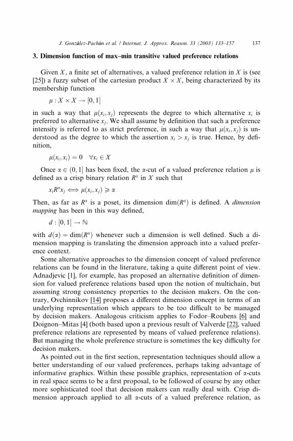
This binary relation R5 can be represented by the union of the followingthree posets P1, P2, P3 given respectively by the following matrices (see Fig. 2):

lP1 ¼

0 1 0 0

0 0 0 0

0 0 0 0

0 1 1 0

0BB@

1CCA lP2 ¼

0 0 0 1

0 0 1 0

0 0 0 0

0 0 0 0

0BB@

1CCA lP3 ¼

0 0 0 0

0 0 0 0

1 0 0 0

0 0 0 0

0BB@

1CCA

On the other hand, each one of those three posets can be decomposed as in-

tersection of the following linear orders:

P1 ¼ ½x1; x4; x2; x3� \ ½x4; x3; x1; x2�P2 ¼ ½x2; x3; x1; x4� \ ½x1; x4; x2; x3�P3 ¼ ½x4; x3; x1; x2� \ ½x2; x3; x1; x4�

This representation is based upon the algorithm proposed in [9], so we get a

representation in terms of three disjoint posets.

Of course, as in classical dimension theory, such a representation is not

unique. The following representation, for example, takes into account three

maximal posets (maximal with respect to the natural inclusion, see Fig. 3):

Fig. 1. Binary relation in Example 4.5.

142 J. Gonz�aalez-Pach�oon et al. / Internat. J. Approx. Reason. 33 (2003) 133–157

Fig. 2. Binary relation in Example 4.5 decomposed in disjoint partial orders.

Fig. 3. Binary relation in Example 4.5 decomposed in maximal posets.

J. Gonz�aalez-Pach�oon et al. / Internat. J. Approx. Reason. 33 (2003) 133–157 143

lP 01 ¼

0 1 0 1

0 0 0 0

0 0 0 0

0 1 0 0

0BB@

1CCA lP 0

2 ¼

0 0 0 0

0 0 1 0

0 0 0 0

0 1 1 0

0BB@

1CCA lP 0

3 ¼

0 0 0 0

0 0 0 0

1 0 0 0

0 1 0 0

0BB@

1CCA

in such a way that R5 can be also represented by the union of these three posetsP 01, P

02, P

03 and

P 01 ¼ ½x1; x4; x2; x3� \ ½x3; x1; x4; x2�

P 02 ¼ ½x4; x2; x3; x1� \ ½x1; x4; x2; x3�

P 03 ¼ ½x4; x2; x3; x1� \ ½x3; x1; x4; x2�

In any case, its generalized dimension is 3:

DimðR5Þ ¼ 3

It is very interesting to point out that this new concept of generalized di-mension is not an extension of classical dimension: if restricted to posets, theminimal generalized representation may need less linear orders than classical

representation, as shown in the next example.

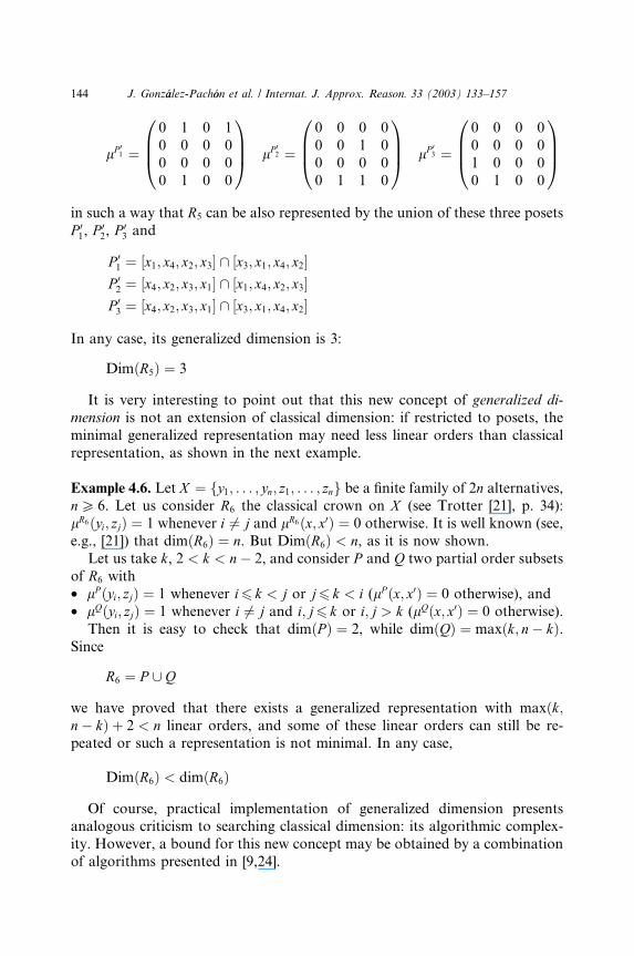
Example 4.6. Let X ¼ fy1; . . . ; yn; z1; . . . ; zng be a finite family of 2n alternatives,nP 6. Let us consider R6 the classical crown on X (see Trotter [21], p. 34):lR6ðyi; zjÞ ¼ 1 whenever i 6¼ j and lR6ðx; x0Þ ¼ 0 otherwise. It is well known (see,e.g., [21]) that dimðR6Þ ¼ n. But DimðR6Þ < n, as it is now shown.Let us take k, 2 < k < n� 2, and consider P and Q two partial order subsets

of R6 with• lP ðyi; zjÞ ¼ 1 whenever i6 k < j or j6 k < i (lP ðx; x0Þ ¼ 0 otherwise), and• lQðyi; zjÞ ¼ 1 whenever i 6¼ j and i; j6 k or i; j > k (lQðx; x0Þ ¼ 0 otherwise).Then it is easy to check that dimðP Þ ¼ 2, while dimðQÞ ¼ maxðk; n� kÞ.

Since

R6 ¼ P [ Q

we have proved that there exists a generalized representation with maxðk;n� kÞ þ 2 < n linear orders, and some of these linear orders can still be re-peated or such a representation is not minimal. In any case,

DimðR6Þ < dimðR6Þ

Of course, practical implementation of generalized dimension presentsanalogous criticism to searching classical dimension: its algorithmic complex-

ity. However, a bound for this new concept may be obtained by a combination

of algorithms presented in [9,24].

144 J. Gonz�aalez-Pach�oon et al. / Internat. J. Approx. Reason. 33 (2003) 133–157

5. Generalized dimension function

Once we have fully generalized and overcome all key restrictions of classical

dimension theory, the above general representation result for crisp strict re-

lations can be therefore translated to relax the normative approach given in

[12] and evaluate the generalized dimension DimðRaÞ for each a-cut, witha 2 ð0; 1�. We no longer need to impose that every a-cut defines a poset.This approach will then lead to a generalized dimension function showing the

generalized dimension for every a-cut, no matter our valued preference relationl is max–min transitive or not.

Definition 5.1. Let X be a finite set of alternatives, and let l : X � X ! ½0; 1� bea valued preference relation such that lðx; xÞ ¼ 0; 8x 2 X . Then its generalizeddimension function is a mapping

D : ½0; 1� ! N

where DðaÞ ¼ DimðRaÞ.

The following example considers a max–min transitive valued relation lwhere there exists a threshold a2 such that there is no inconsistency in any Ra,

for all a > a2, and incomparability is present.

Example 5.1. Let us consider X ¼ fx1; x2g and let us denote by L1 ¼ ½x1; x2� andL2 ¼ ½x2; x1� the two possible linear orders on X . Let R7 be a strict valued binaryrelation such that lR7ðx1; x2Þ ¼ 0:3 and lR7ðx2; x1Þ ¼ 0:4. This relation is de-picted in Fig. 4. In this case,

1. If a > 0:3, Ra7 is a poset, although two cases can be distinguished:

(a) a > 0:4,

lRa7 ¼ 0 0

0 0

� �

in such a way that

DimðRa7Þ ¼ dimðRa

7Þ ¼ 2

with Ra7 ¼ L1 \ L2.

Fig. 4. Binary valued relation in Example 5.1.

J. Gonz�aalez-Pach�oon et al. / Internat. J. Approx. Reason. 33 (2003) 133–157 145

(b) 0:3 < a6 0:4,

lRa7 ¼ 0 0

1 0

� �

and

DimðRa7Þ ¼ dimðRa

7Þ ¼ 1

with Ra7 ¼ L1.

2. If a6 0:3, Ra7 is not a poset and

lRa7 ¼ 0 1

1 0

� �

in such a way that

DimðRa7Þ ¼ 2

with Ra7 ¼ L1 [ L2.

The generalized dimension function of this example is shown in Fig. 5.It is important to note in the above example that we have found different

representations, showing different decision maker attitudes. In fact, a decision

maker defining a valued preference relation l, if forced to be crisp, can facedifferent crisp problems depending on their exigency level: if the decision maker

does not take into account low intensities (high a in the above example),

Fig. 5. Generalized dimension function in Example 5.1.

146 J. Gonz�aalez-Pach�oon et al. / Internat. J. Approx. Reason. 33 (2003) 133–157

alternatives are easily incomparable (no alternative is sufficiently better than

the other according to any underlying criteria); but if the decision maker issensible to low intensities (low a in the above example), formal cycles will befrequent. Note that formal cycles will most probably introduce a special kind

of stress, different from the one with incomparability (see, e.g., [15,17]). In any

case, the sequence of a-cuts shows how decision makers, if forced to definecrisp preferences when they are valued, may give different answers depending

on the a-level they choose.A simple case of a non-max–min transitive valued preference relation is

analyzed in the following example.

Example 5.2. Let us consider X ¼ fx1; x2; x3g and the valued preference relationR8 such that

lR8 ¼0 0:4 0

0 0 0:60:7 0 0

0@

1A

depicted in Fig. 6. Four cases can be considered:• When a6 0:4, there is a three-cycle in the associated a-cut, and such an a-cutcan be represented in terms of the following three crisp linear orders:

Ra8 ¼ f½x1; x2; x3� \ ½x3; x1; x2�g [ f½x2; x3; x1� \ ½x1; x2; x3�g

[ f½x3; x1; x2� \ ½x2; x3; x1�g

Hence, we have

DimðRa8Þ ¼ 3

• When 0:4 < a6 0:6, no cycle is present, but since x2 > x3 and x3 > x1 are pre-sent, it is missing x2 > x1 (Ra

8 is not a poset):

Ra8 ¼ f½x2; x3; x1� \ ½x1; x2; x3�g [ f½x3; x1; x2� \ ½x2; x3; x1�g

So, we also needed three linear orders:

Fig. 6. Binary valued relation in Example 5.2.

J. Gonz�aalez-Pach�oon et al. / Internat. J. Approx. Reason. 33 (2003) 133–157 147

DimðRa8Þ ¼ 3

• When 0:6 < a6 0:7, we have a crisp partial ordered set with only one arc(x3 > x1):

Ra8 ¼ ½x3; x1; x2� \ ½x2; x3; x1�

This poset has dimension 2:

DimðRa8Þ ¼ dimðRa

8Þ ¼ 2

• When a > 0:7, we have the poset with incomparability between every pair:

Ra8 ¼ ½x1; x2; x3� \ ½x3; x2; x1�

and, consequently, two linear orders are again needed:

DimðRa8Þ ¼ dimðRa

8Þ ¼ 2

The generalized dimension function of valued binary relation of this example is

depicted in Fig. 7.

Example 5.3. Let us consider X ¼ fx1; x2; x3g and let R9 be the strict valuedpreference relation depicted in Fig. 8,

lR9 ¼0 0:2 0:30:4 0 0:60:7 0:1 0

0@

1A

Seven different a-cuts intervals can be considered:

Fig. 7. Generalized dimension function in Example 5.2.

148 J. Gonz�aalez-Pach�oon et al. / Internat. J. Approx. Reason. 33 (2003) 133–157

1. When a6 0:1, we have

lRa9 ¼

0 1 1

1 0 11 1 0

0@

1A

This relation shows cycles (e.g., x1 > x3, x3 > x1) but it can be obtained as

Ra9 ¼ L1 [ L2

where

lL1 ¼0 1 10 0 1

0 0 0

0@

1A lL2 ¼

0 0 01 0 0

1 1 0

0@

1A

That is,

Ra9 ¼ ð½x1; x2; x3�Þ [ ð½x3; x2; x1�Þ

and DimðRa9Þ ¼ 2.

2. When 0:1 < a6 0:2, Ra9 also shows cycles

lRa9 ¼

0 1 1

1 0 1

1 0 0

0@

1A

In this case, Ra9 can be obtained as the union of three linear orders

Ra9 ¼ L1 [ P1

where

lP1 ¼0 0 0

1 0 0

1 0 0

0@

1A

in such a way that

Ra9 ¼ ð½x1; x2; x3�Þ [ ð½x3; x2; x1� \ ½x2; x3; x1�Þ

and DimðRa9Þ ¼ 3.

Fig. 8. Binary valued relation in Example 5.3.

J. Gonz�aalez-Pach�oon et al. / Internat. J. Approx. Reason. 33 (2003) 133–157 149

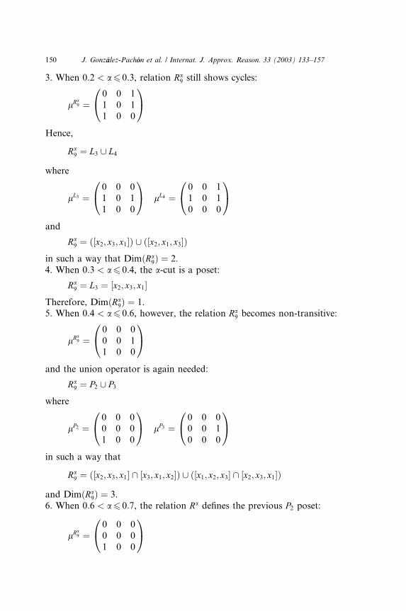
3. When 0:2 < a6 0:3, relation Ra9 still shows cycles:

lRa9 ¼

0 0 1

1 0 1

1 0 0

0@

1A

Hence,

Ra9 ¼ L3 [ L4

where

lL3 ¼0 0 0

1 0 1

1 0 0

0@

1A lL4 ¼

0 0 1

1 0 1

0 0 0

0@

1A

and

Ra9 ¼ ð½x2; x3; x1�Þ [ ð½x2; x1; x3�Þ

in such a way that DimðRa9Þ ¼ 2.

4. When 0:3 < a6 0:4, the a-cut is a poset:

Ra9 ¼ L3 ¼ ½x2; x3; x1�

Therefore, DimðRa9Þ ¼ 1.

5. When 0:4 < a6 0:6, however, the relation Ra9 becomes non-transitive:

lRa9 ¼

0 0 0

0 0 1

1 0 0

0@

1A

and the union operator is again needed:

Ra9 ¼ P2 [ P3

where

lP2 ¼0 0 00 0 0

1 0 0

0@

1A lP3 ¼

0 0 00 0 1

0 0 0

0@

1A

in such a way that

Ra9 ¼ ð½x2; x3; x1� \ ½x3; x1; x2�Þ [ ð½x1; x2; x3� \ ½x2; x3; x1�Þ

and DimðRa9Þ ¼ 3.

6. When 0:6 < a6 0:7, the relation Ra defines the previous P2 poset:

lRa9 ¼

0 0 0

0 0 0

1 0 0

0@

1A

150 J. Gonz�aalez-Pach�oon et al. / Internat. J. Approx. Reason. 33 (2003) 133–157

and

Ra9 ¼ ½x2; x3; x1� \ ½x3; x1; x2�

in such a way that DimðRa9Þ ¼ 2.

7. When 0:7 < a, the relation Ra9 is the empty relation.

lRa9 ¼

0 0 00 0 0

0 0 0

0@

1A

with DimðRa9Þ ¼ 2 and

Ra9 ¼ ½x1; x2; x3� \ ½x3; x2; x1�

The generalized dimension function of this Example 5.3 is depicted in Fig. 9.

An interesting result shown in [7] is that our generalized dimension functionwill not show big jumps in case arcs are being deleted or added one by one:

Theorem 5.1. Let us assume that

lðxi; xjÞ ¼ lðxk; xlÞ ) lðxi; xjÞ ¼ lðxk; xlÞ ¼ 0

holds for any xi; xj; xk; xl 2 X , and let us denote

Ra� ¼ limak"a

Rak

Fig. 9. Generalized dimension function in Example 5.3.

J. Gonz�aalez-Pach�oon et al. / Internat. J. Approx. Reason. 33 (2003) 133–157 151

Then

(a) DimðRa�Þ �DimðRaÞ6 2; 8a > 0

(b) DimðRaÞ �DimðRa�Þ6 2; 8a > 0

Proof. Since the difference between Ra and Ra� is in this case one pair at most,

and this isolated pair can be represented as the intersection of two linear or-

ders, it can be added by means of the union of this intersection. In case such an

arc has to be deleted, we only need to note that the complementary of that arc

can be represented as the union of two linear orders. �

6. Critical levels of a generalized dimension function

Generalized dimension function D is therefore well defined for every valuedstrict binary preference relation R, DðaÞ ¼ DimðRaÞ for all a 2 ð0; 1�.Indeed, dimension function does not capture all the information contained

in the associated representation. It is obvious from previous examples that

different representations may arise with the same dimension. Depending on the

value of a, each a-cut of a valued preference relation can be either:• a complete order, i.e., Ra is a linear order; or

• a partial order, i.e., asymmetry and transitivity hold, but some incompara-

bility appears; or

• a non-transitive relation without cycles (i.e., some arcs implied by transitiv-ity are missing); or

• a conflictive relation because of cycles, i.e., sequences x1; . . . ; xk such thatxi > xiþ1, 8i ¼ 1; . . . ; k � 1 and xk > x1 (notice that this definition includessymmetry, i.e., second-order cycles where both arcs xi > xj and xj > xi simul-taneously hold).

The last two cases will require the union operator in order to get a gener-

alized representation, although the union operator may also be present in the

minimal representation of some posets.Hence, we wish to evaluate meaningful critical levels in order to verify if a-

cuts are still posets, or the degree of the shortest cycle, if it exists. On one hand,

it has already been pointed out that transitivity may fail either because some

arcs are missing (weak non-transitivity) or because a cycle appears (strong non-transitivity). Hence, non-transitivity region can be again divided into two parts,depending on whether there are cycles or not. Strong non-transitivity region canalso be divided into different regions, depending on the length of its shortest

cycle (following [11], the shorter the cycle is, the larger the conflict should beconsidered in practice). This fact leads us to introduce a family of critical values

that generalizes the above a2 critical level for second-order cycles, as defined inSection 2. The following levels can therefore be introduced:

152 J. Gonz�aalez-Pach�oon et al. / Internat. J. Approx. Reason. 33 (2003) 133–157

1. The transitivity level a0, representing the minimal value such that Ra is tran-

sitive for all a > a0. As an exercise, we can check transitivity of a-cuts in Ex-ample 5.3:

• a 2 ð0:0; 0:1�: Ra9 is transitive.

• a 2 ð0:1; 0:2�: Ra9 is non-transitive, since

lR9ðx3; x2Þ ¼ 0:1 < minflR9ðx3; x1Þ ¼ 0:7; lR9ðx1; x2Þ ¼ 0:2g

• a 2 ð0:2; 0:4�: Ra9 is transitive.

• a 2 ð0:4; 0:6�: Ra9 is non-transitive, since

lR9ðx2; x1Þ ¼ 0:4 < minflR9ðx2; x3Þ ¼ 0:6; lR9ðx3; x1Þ ¼ 0:7g

• a 2 ð0:6; 1:0�: Ra9 is again transitive.

Hence, a0 ¼ 0:6 for this relation R9 (see Fig. 10).2. The k-acyclicity level ak, representing the minimal value such that Ra has no k-order cycles (nor has the lower order). Of course, a1 ¼ 0 since we have as-sumed by definition that lðx; xÞ ¼ 0, 8x 2 X , and a2 has been already defined.It is obvious that ðakÞ1k¼1 is a non-decreasing sequence whose maximum is acritical acyclicity level a1 being the minimum value such that there is no cycle

in Ra, 8a > a1. Obviously, a1 ¼ an, n being the number of elements in X .

Indeed, our generalized dimension function together with the sequence of

critical values

a0; a2; . . . ; an

gives a quite complete approach to the underlying representation and its as-

sociated inconsistencies. In particular, we can assure that a-cuts are posetswhenever

a > maxfa0; a2g

The transitivity level a0 can be easily obtained by means of the followingalgorithm, with complexity Oðn3Þ:

Fig. 10. Transitivity intervals in Example 5.3.

J. Gonz�aalez-Pach�oon et al. / Internat. J. Approx. Reason. 33 (2003) 133–157 153

Transitivity level computationa0 ¼ 0do i ¼ 1; n

do j ¼ 1; n (j 6¼ i)do k ¼ 1; n (k 6¼ i, k 6¼ j)

b ¼ minflik; lkjgif (lij < b) then

a0 ¼ maxfa0; bgendif

enddoenddo

enddo

In order to compute the critical acyclicity level, we require to enumerate all

possible cycles defined in X . Taking into account that there are

nk

� �ðk � 1Þ!

cycles of k elements in X , the total number of cycles in X are

Xn

k¼2

nk

� �ðk � 1Þ!

and the critical acyclicity level can be computed as

an ¼ maxCðxi1;...;xik Þ

fminflðxi1 ; xi2Þ; . . . ; lðxik ; xi1Þgg

This computation has exponential complexity.

Example 6.1. In previous Example 5.3, we find three second-order cycles and

two third-order cycles in R9 (n ¼ 3):1. Cðx1; x2Þ : minflR9ðx1; x2Þ ¼ 0:2; lR9ðx2; x1Þ ¼ 0:4g ¼ 0:2.2. Cðx1; x3Þ : minflR9ðx1; x3Þ ¼ 0:3; lR9ðx3; x1Þ ¼ 0:7g ¼ 0:3.3. Cðx2; x3Þ : minflR9ðx2; x3Þ ¼ 0:6; lR9ðx3; x2Þ ¼ 0:1g ¼ 0:1.4. Cðx1; x2; x3Þ : minflR9ðx1; x2Þ ¼ 0:2; lR9ðx2; x3Þ ¼ 0:6; lR9ðx3; x1Þ ¼ 0:7g ¼ 0:2.5. Cðx3; x2; x1Þ : minflR9ðx3; x2Þ ¼ 0:1; lR9ðx2; x1Þ ¼ 0:4; lR9ðx1; x3Þ ¼ 0:3g ¼ 0:1.Hence,

a3 ¼ maxf0:2; 0:3; 0:1; 0:2; 0:1g ¼ 0:3 ¼ a2

The acyclicity interval ð0:3; 1� is depicted in Fig. 11, meanwhile a cycle appearsin Ra

9 for a 2 ð0:0; 0:3� (notice that interval ð0:4; 0:6� does not show cycles, buttransitivity does not hold).

Poset region (i.e., the values of a for which the binary relation Ra9 is a poset)

in Example 5.3 is depicted in Fig. 12: ð0:3; 0:4� [ ð0:6; 1:0�. Classical dimension

154 J. Gonz�aalez-Pach�oon et al. / Internat. J. Approx. Reason. 33 (2003) 133–157

theory does apply to these two intervals, meanwhile our extended dimension

theory also applies to ð0:0; 0:3� [ ð0:4; 0:6�.

7. Final comments

Once a general representation theorem for crisp preference relations have

been proved, it has been possible to develop a more general dimension concept,

not being restricted now to partial ordered sets. The fact that this new gen-

eralized dimension is not an extension of classical dimension should not be

disturbing: as we pointed out in the first section of this paper, a key issue for

any multicriteria methodology, if we wish it to be a useful knowledge aidtool, should focus on the representation issue. It could have been expected

that allowing representations by means of the union operator together withthe intersection operator will give more accurate representations than repre-

sentations obtained taking into account only intersections. Our main objec-

tive should not be a number (DimðRÞ), but an informative representation

Fig. 11. Acyclicity intervals in Example 5.3.

Fig. 12. Poset intervals in Example 5.3.

J. Gonz�aalez-Pach�oon et al. / Internat. J. Approx. Reason. 33 (2003) 133–157 155

(R ¼ [s \t Lst). Dimension, no matter how we define it, is only a hint for a

attractive representation. Perhaps generalized dimension deserves as muchtheoretical attention as classical dimension theory has deserved in the past.

In any case, our generalized dimension is associated with the minimal

number of underlying linear orders explaining preference relations in the

presence of incomparability and inconsistency (other rational backgrounds,

according to [3] will be considered in the future, see [7]). Such a result has been

translated to every a-cut of an arbitrary valued preference relation, allowing ageneralized dimension function which should in turn give a better insight into

the structure of underlying criteria explaining our preferences. In this way,decision makers can take some advantage of the standard representation in the

real spaces they are used to.

Acknowledgements

This research has been partially supported by the Government of Spain anda Del Amo bilateral programme between Complutense University and the

University of California at Berkeley. We also deeply appreciate all comments

and suggestions from an anonymous colleague, who provided us with a key

example which has been finally included in this paper.

References

[1] D. Adnadjevic, Dimension of fuzzy ordered sets, Fuzzy Sets and Systems 67 (1994) 349–357.

[2] V. Belton, J. Hodgkin, Facilitators, decision makers, DIY users: Is intelligent multicriteria

decision support for all feasible or desirable? European Journal of Operational Research 113

(1999) 247–260.

[3] V. Cutello, J. Montero, Fuzzy rationality measures, Fuzzy Sets and Systems 62 (1994) 39–54.

[4] J.P. Doignon, J. Mitasm, Dimension of valued relations, European Journal of Operational

Research 125 (2000) 571–587.

[5] B. Dushnik, E.W. Miller, Partially ordered sets, American Journal of Mathematics 63 (1941)

600–610.

[6] J.C. Fodor, M. Roubens, Structure of valued binary relations, Mathematical Social Sciences

30 (1995) 71–94.

[7] J. Gonz�aalez-Pach�oon, D. G�oomez, J. Montero, J. Y�aa~nnez, Soft dimension theory, Fuzzy Sets andSystems, in press [doi:10.1016/S0165-0114(02)00437-2].

[8] J. Gonz�aalez-Pach�oon, S. R�ııos-Insua, A method for searching rationality in pairwise choices, in:

G. Fandel, T. Gal (Eds.), Multiple Criteria Decision Making, Lecture Notes in Economics and

Mathematical Systems, vol. 448, Springer, 1997, pp. 374–382.

[9] J. Gonz�aalez-Pach�oon, S. R�ııos-Insua, Mixture of maximal quasi orders: a new approach to

preference modelling, Theory and Decisions 47 (1999) 73–88.

[10] C. Macharis, J.P. Brans, The GDSS promethee procedure, Journal of Decision Systems 7

(1998) 283–307.

[11] J. Montero, Arrow�s theorem under fuzzy rationality, Behavioral Science 32 (1987) 267–273.

156 J. Gonz�aalez-Pach�oon et al. / Internat. J. Approx. Reason. 33 (2003) 133–157

[12] J. Montero, J. Y�aa~nnez, V. Cutello, On the dimension of fuzzy preference relations, in:Proceedings International ICSC Symposium on Engineering of Intelligent Systems, La

Laguna, vol. 3, 1998, pp. 38–33.

[13] J. Montero, J. Y�aa~nnez, D. G�oomez, J. Gonz�aalez-Pach�oon, Consistency in dimension theory, in:

Proceedings of the Workshop on Preference Modelling and Applications, Granada, 2001, pp.

93–98.

[14] S.V. Ovchinnikov, Representation of transitive fuzzy relations, in: H.J. Skala, S. Termini, E.

Trillas (Eds.), Aspects of Vagueness, Reidel, Amsterdam, 1984, pp. 105–118.

[15] P.K. Pattanaik, Voting and Collective Choice, Cambridge University Press, London, 1971.

[16] B. Roy, Decision aid and decision making, European Journal of Operational Research 45

(1990) 324–331.

[17] A.K. Sen, Collective Choice and Social Welfare, Holden-Day, San Francisco, 1970.

[18] G. Shafer, Savage revisited (with discussion), Statistical Science 1 (1986) 435–462.

[19] Y. Siskos, A. Spyridakos, Intelligent multicriteria decision support: overview and perspectives,

European Journal of Operational Research 113 (1999) 236–246.

[20] E. Szpilrajn, Sur l�extension de l�ordre partiel, Fundamenta Mathematicae 16 (1930) 386–389.[21] W.T. Trotter, Combinatorics and Partially Ordered Sets. Dimension Theory, The Johns

Hopkins University Press, Baltimore, 1992.

[22] L. Valverde, On the structure of F-indistinguishability operators, Fuzzy Sets and Systems 17

(1985) 313–328.

[23] M. Yannakakis, On the complexity of the partial order dimension problem, SIAM Journal of

Algebra and Discrete Mathematics 3 (1982) 351–358.

[24] J. Y�aa~nnez, J. Montero, A poset dimension algorithm, Journal of Algorithms 30 (1999) 185–208.

[25] L.A. Zadeh, Similarity relations and fuzzy orderings, Informations Sciences 3 (1971) 177–200.

J. Gonz�aalez-Pach�oon et al. / Internat. J. Approx. Reason. 33 (2003) 133–157 157