Preference Reversals for Ambiguity Aversion

Preference Reversals For Ambiguity Aversion

Stefan T. Trautmanna, Ferdinand M. Vieiderb, and Peter P. Wakkerc*

a: Tiber, CentER, Department of Economics, Tilburg University, P.O. Box 90153,

Tilburg, 5000 LE, the Netherlands; [email protected]

b: Faculty of Economics, Ludwig-Maximilians University Munich, Geschwister

Scholl Platz 1, 80802 Munich, Germany; [email protected]

c: Econometric Institute, Erasmus University, P.O. Box 1738, Rotterdam, 3000 DR,

the Netherlands; [email protected]; 31-10.408.12.65 (O); 31-10.408.91.62 (F)

November, 2010

Astract. This paper finds preference reversals in measurements of ambiguity

aversion, even if psychological and informational circumstances are kept constant.

The reversals are of a fundamentally different nature than the reversals found before

because they cannot be explained by context-dependent weightings of attributes. We

offer an explanation based on Sugden’s random-reference theory, with different

elicitation methods generating different random reference points. Then measurements

of ambiguity aversion that use willingness to pay are confounded by loss aversion

and, hence, overestimate ambiguity aversion.

Key words: ambiguity aversion, preference reversal, loss aversion, choice vs.

valuation

JEL CLASSIFICATION: D81, D03, C91

* We thank Gideon Keren for detailed discussions, and three reviewers and an associate editor for useful comments. Trautmann acknowledges financial support by a VENI grant of the Netherlands Organization of Scientific Research (NWO).

2

1. Introduction

One of the greatest challenges to the classical paradigm of rational choice was put

forward by preference reversals, first found by Lichtenstein & Slovic (1971):

strategically irrelevant details of framing can lead to a reversal of preference. Grether

& Plott (1979) confirmed this phenomenon while using real incentives and controlling

for several potential biases. These findings raise the question what true preferences

are, if they exist at all. Preference reversals have triggered the development of many

new insights into preference measurements, the biases that distort them, and ways to

avoid these biases or to correct for them (Arkes 1991; Plott 1996). This paper shows

that preference reversals also occur for one of the most important topics in decision

theory today: the measurement of ambiguity attitudes. Ambiguity attitudes concern

the difference between decisions under uncertainty (unknown probabilities) and risk

(known probabilities). We will use the preference reversals found to obtain new

insights into the measurement of ambiguity attitudes, explained in more detail later.

Our preference reversals are of a fundamentally different nature than the

traditional ones (Berg, Dickhaut, & Rietz 2010; Seidl 2002). Traditional preference

reversals can be explained by different weightings of attributes in different evaluation

modes. For example, the preference reversals of Lichtenstein & Slovic (1971)

concerned risky decisions where outcomes (i.e., the outcome attribute) are

overweighted in certainty-equivalent evaluations but the probabilities (i.e., the

likelihood attribute) are overweighted in binary-choice evaluations. Our preference

reversals entail a complete reversal of preference within one attribute (the likelihood

attribute). Furthermore, they are obtained while informational circumstances and

context are kept constant, so that they must concern an intrinsic aspect of evaluation.

Section 7 gives details. Maafi (2010) and Pogrebna (2010) investigated traditional

preference reversals under ambiguity, and found that they are stronger than under risk.

Closely related is also Choi et al.’s (2007) study into violations of basic revealed-

preference principles under ambiguity.

We investigate two commonly used formats for measuring ambiguity attitudes.

The first is to offer subjects a direct choice between ambiguous and risky prospects,

and the second is to elicit subjects’ willingness to pay (WTP) for each of the

prospects. The latter format is popular because it provides a quantitative index of

ambiguity aversion at the individual level. We compare the two approaches in simple

3

Ellsberg two-color problems. In three experiments, WTP for the risky prospect

(gambling on an urn with known composition) strongly exceeds that for the

ambiguous prospect (gambling on an urn with unknown composition). Almost no

subject expressed higher WTP for the ambiguous prospect than for the risky prospect.

Remarkably, however, this finding also holds for the group of subjects who prefer the

ambiguous prospect in direct choice. Hence, in the latter group the majority assigns a

higher WTP to the not-chosen risky prospect, entailing a preference reversal. There

are virtually no opposite preference reversals, and explanations based on more noise

under choice than under WTP can also be ruled out (end of Section 4 and of Section

5). Hence the reversals found are systematic and are not due to noise.

The contradictory findings of WTP versus choice raise a question of general

interest: which of these findings reflects true underlying ambiguity attitudes? To

distinguish between WTP and choice, where at least one does not reflect true

ambiguity attitude, we add qualifiers. The finding of higher WTP for the risky than

for the ambiguous prospect is called WTP-ambiguity aversion, and a direct choice of

the risky prospect rather than the ambiguous one is called choice-ambiguity aversion.

A fourth experiment with certainty equivalent measurements instead of WTP shows

that WTP-ambiguity aversion, if taken as ambiguity aversion, entails a uniform

overestimation of the latter, also for subjects who did not exhibit preference reversals.

It shows that the preference reversals, observed only for ambiguity-seeking subjects,

serve as a smoking gun identifying a more general problem of WTP measurements of

ambiguity attitudes. A fifth experiment with willingness to accept (WTA), another

commonly used format for measuring ambiguity attitudes, further confirms the

overestimation in WTP. Consistent with the literature (Halevy 2007; Smith et al.

2002), we do find clear evidence of ambiguity aversion in the Ellsberg problem for all

measurement methods considered.

Because of the effects of ambiguity aversion on market outcomes proposed in the

theoretical literature and the consequential potential for regulation (Easley & O’Hara

2009; Rigotti & Shannon 2005), quantitative measurements of ambiguity attitudes are

becoming an important policy variable. Given the biases of WTP measurements of

ambiguity aversion, we recommend avoiding or adjusting these measurements as

policy inputs. Further problems of WTP measurements are discussed by

Blumenschein et al. (2008), Hahnemann (1991), Völckner (2006), and others.

4

Using Sugden’s (2003) and Schmidt, Starmer, & Sugden’s (2008) generalization

of prospect theory with a random reference point, we develop a quantitative model

that explains the pattern of ambiguity attitudes and preference reversals in our

experiments. Different elicitation methods promote the perception of different

random reference points. Preferences under direct choice depend on the attitudes

toward unknown probabilities, as is warranted for measurements of ambiguity

attitudes. WTP evaluations are, however, determined primarily by loss aversion,

which distorts WTP-ambiguity measurements. Recent studies supporting the

importance of loss aversion in risky and in riskless choice include Abdellaoui,

Bleichrodt, & Paraschiv (2007), Baucells & Heukamp (2006), Fehr & Götte (2007),

Gächter, Johnson, & Hermann (2007), Langer & Weber (2001), Pennings & Smidts

(2003), and Rizzo & Zeckhauser (2004). The current paper demonstrates the

importance of loss aversion in ambiguous choice. Our theoretical explanation assumes

that WTP for ambiguity is determined in the presence of WTP for risk (joint

evaluation), as in most measurements today and as also in ours. Section 7 explains

that our finding has general implications, also if no risky option is available. The

problems we find support the interest of comparative ignorance effects in

measurements of ambiguity attitudes, as studied by Chow & Sarin (2001), Du &

Budescu (2005 Table 5), Fox & Tversky (1995), and Fox & Weber (2002).

The paper proceeds as follows. Section 2 presents our basic experiment, and our

preference reversals. All other experiments are variations of the basic experiment.

Whereas WTP was not incentivized in our basic experiment so as to avoid income

effects, it was incentivized in two ways in Sections 3 and 4. We then found the same

preference reversals, showing that absence of incentives or income effects did not

generate our findings. In Section 4, we report the results of interviews with our

subjects, verifying that the preference reversals found are not due to elementary

misunderstandings. Section 5 presents an experiment where reference effects that can

generate loss aversion are ruled out. Then the preference reversals disappear,

suggesting that loss aversion is indeed the cause of the preference reversals. Section 6

presents a theoretical model for our findings, showing how loss aversion can explain

the preference reversals found. The derivations are presented there informally.

Appendix A presents formal derivations. Implications for the measurement of

ambiguity aversion and its applications are in Section 7. Section 8 contains a general

discussion, and Section 9 concludes.

5

2. Experiment 1; Basic Experiment

Our basic experiment, reported in this section, concerns Ellsberg two-color urns.

Subjects. N = 59 econometrics students from Erasmus University Rotterdam in the

Netherlands participated in this experiment, carried out in a classroom.

Stimuli. At the beginning of the experiment, two urns were presented to the subjects,

so that when evaluating one urn they knew about the existence of the other. The

known urn1 contained 20 red and 20 black balls, and the ambiguous urn contained 40

red and black balls in an unknown proportion. Subjects had to select a color at their

discretion (red or black) and then make a simple Ellsberg choice. This choice was

between gambling on the color selected for the (ball to be drawn from the) known urn,

or gambling on the color selected from the ambiguous urn. Next they themselves

randomly drew a ball from the urn chosen. If the drawn color matched the announced

color, they won �50; otherwise, they won nothing. It was made clear to the subjects

that they would draw only once, that is, that the game was one-shot.

Before drawing the ball, subjects were also asked to specify their maximum WTP

for both urns (Appendix B). In this basic experiment, the WTP questions were

hypothetical. One reason we included this hypothetical treatment besides incentivized

treatments is that it avoids possible house money effects (Thaler & Johnson 1990).

Those could arise from the significant endowment necessary to enable subjects to pay

for prospects with a prize of �50. A second reason is that, with prior endowment,

even if the majority of subjects will not integrate the payments, a minority will do,

leading to noise.

All choices and questions were on the same sheet of paper, were all read and

explained before any was answered, and could be answered in the order that the

subject preferred. We also recorded the subjects’ age and gender.

1 This term is used in this paper. In the experiment, we did not use this term. We used bags instead of urns, and the ambiguous bag was designated through its darker color without using terms ambiguous or unknown. We did not use balls but chips, and the colors used were red and green instead of red and black. For consistency of terminology in the field, we use the same terms and colors in our paper as in the original Ellsberg (1961).

6

Incentives. Two subjects were randomly selected to play for real money. These

subjects were paid according to their choices and could win �50 in cash.

Analysis. In this experiment, as in the other experiments in this paper, a clear direction

of effects can usually be expected. Therefore, unless stated otherwise, one-sided tests

were employed. Tests are t-tests unless stated otherwise. The abbreviation ns

designates not significant. The WTP difference is the WTP for the risky prospect

minus the WTP for the ambiguous prospect. It is often used as a quantitative index of

the degree of WTP-ambiguity aversion. WTP-ambiguity aversion holds if the index is

positive.

Results. In direct choice, 22 of 59 subjects chose ambiguous (37%; p < 0.05,

binomial). Thus, we find a majority of choice-ambiguity aversion. Table 1 shows the

average WTP separately for choice-ambiguity seekers and choice-ambiguity averters.

TABLE 1. Willingness to Pay in �

WTP risky

WTP ambiguous

WTP difference

t-test

Choice-ambiguity seeking 12.25 9.50 2.75 t21=2.72, p < 0.01

Choice-ambiguity averse 11.64 6.27 5.37 t36=6.7, p < 0.01

Two-sided t-test t57 = 0.33, ns

t57 = 2.14, p < 0.05

t57 = 2.01, p < 0.05

We find no significant difference in WTP values for risky between choice-

ambiguity seekers and choice-ambiguity averters.2 The WTP for the ambiguous

prospects is, obviously, much higher for the choice-ambiguity seekers than for the

choice-ambiguity averters. The latter group values the risky prospect on average by

�5.37 higher than the ambiguous prospect (p < 0.01). Surprisingly, choice-ambiguity

seekers also value the risky prospect �2.75 higher than the ambiguous one (p < 0.01),

2 This holds under the null of equality. A more plausible null would be, however, that the WTP of the choice-ambiguity seekers for risky would be lower than for choice-ambiguity averters rather than the same. The former group is not aselect, having preferred something else (ambiguity) to risk. The

7

which entails a preference reversal. They exhibit choice-ambiguity seeking but WTP-

ambiguity aversion. Table 2 gives frequencies of WTP-ambiguity attitudes and

choice-ambiguity attitudes.

TABLE 2. Frequencies of WTP- versus Choice-Ambiguity Attitudes

WTP-ambiguity seeking

WTP-indifferent

WTP-ambiguity averse

Binomial test

Choice-ambiguity seeking 2 9 11 p = 0.01

Choice-ambiguity averse 0 6 31 p < 0.01

Almost no WTP-ambiguity seeking is found, not only among the choice-ambiguity

averters but also among the choice-ambiguity seekers. Thus, for 11 of 59 subjects the

WTP- and choice attitudes are inconsistent. All these subjects combine WTP-

ambiguity aversion with choice-ambiguity seeking, with the result that 50% of choice-

ambiguity seekers reverse their preference under WTP. No reversed inconsistency

was found. The number of the reversals found is large enough to depress the positive

correlation between choice- and WTP-ambiguity aversion to 0.34 (Spearman’s ρ, p <

0.05 two-sided), excluding indifferences. We find significant WTP-ambiguity

aversion for the choice-ambiguity seekers (p=0.01, binomial). Obviously this is also

found for choice-ambiguity averters (p < 0.01, binomial).

Discussion. We find prevailing choice-ambiguity aversion, but still 22 out of 59

subjects exhibit choice-ambiguity seeking. For WTP there is considerably more,

almost universal, ambiguity aversion, leading to preference reversals for 11 subjects.

Only 2 choice-ambiguity seekers are WTP-ambiguity seeking. This result is

particularly striking because direct choice and WTP had to be indicated together on

the same sheet. No preference reversal occurs for the choice-ambiguity averters.

Asymmetric error theories will be discussed in Sections 4 and 5.

The preference reversals in Experiment 1 were observed without incentivizing

WTP. WTP with real incentives may differ from hypothetical WTP (Cummins,

Harrison, & Rutström 1995; Hogarth & Einhorn 1990). In addition, the options

finding of equal WTPs accordingly confirms that the choice-ambiguity seekers in general, both for risk

8

considered for WTP can generate losses (if the WTP exceeds the outcome obtained

from the prospect) whereas those for choice cannot, so that the options are of a

different nature in terms of final wealth. Losses can generate different decision

attitudes, as discussed in detail in Section 6. These problems can be avoided by

giving a prior endowment to the subjects, from which they pay back the WTP

(Bateman et al. 1997, Section I). Then, in terms of final wealth, WTP no longer

involves losses. Further, real incentives can then be implemented. We present this

treatment in the next section.

We let subjects choose the winning color so as to avoid suspicion, as discussed by

Pulford (2009) and Zeckhauser (1986, p. S445). A drawback is that such a choice can

generate an illusion of control (Langer 1975), but this effect is weaker than suspicion

and avoiding the latter is more important. This explains our choice of design.

3. Experiment 2; Real Incentives for WTP

Subjects. N = 74 subjects participated similarly as in Experiment 1. Everything was

identical to Experiment 1, except the incentives.

Incentives. At the end of the experiment, four subjects were randomly selected for

real play. They were endowed with �30. Then a die was thrown to determine

whether a subject played his or her direct choice to win �50, or would play the

Becker-DeGroot-Marschak (1963) (BDM) mechanism (both events had equal

probability). In the latter case, the die was thrown again to determine which prospect

was sold (both prospects had an equal chance to be sold). Then, following the BDM

mechanism, we randomly chose a prize between �0 and �50. If the random prize was

below the expressed WTP, the subject paid the random prize to receive the prospect

considered and played this prospect for real. If the random prize exceeded the

expressed WTP, no further transaction was carried out and the subject kept the

endowment (Appendix C). The BDM is often used in the literature. Under some

common assumptions, it is in the subjects’ best interest to report preferences truthfully

under the BDM mechanism.

and ambiguity, are more optimistic.

9

Results. In direct choice, 15 out of 74 subjects chose ambiguous (20%; p < 0.01,

binomial), implying a majority of choice-ambiguity aversion. The following table

gives average WTP.

TABLE 3. Willingness to Pay (BDM) in �

WTP risky WTP ambiguous

WTP difference

t-test

Choice-ambiguity seeking 13.44 11.21 2.23 t14=2.58, p=0.01

Choice-ambiguity averse 13.46 7.14 6.31 t58=6.21, p<0.01


t72 = 1.99, p = 0.05

t72 = 1.97, p = 0.05

The WTPs for both groups and both prospects are slightly (but not significantly)

higher than the WTPs in experiment 1 (p>0.5, two-sided). Also the WTP differences

are not significantly different from Experiment 1 (p>0.5, two-sided). All patterns of

Experiment 1 are confirmed. In particular, the choice-ambiguity seekers exhibit

WTP-ambiguity aversion. The following table compares WTP- with choice-

ambiguity attitudes.

TABLE 4. Frequencies of WTP- (through BDM) versus Choice-Ambiguity Attitudes


WTP-indifferent


Binomial test

Choice-ambiguity seeking 0 9 6 p < 0.05


Here 6 out of 15 choice-ambiguity seekers, or 40% of choice-ambiguity seekers, were

inconsistent in exhibiting WTP-ambiguity aversion. The hypothesis that preference

reversals were as pronounced as in experiment 1 thus could not be rejected (p > 0.5,

Mann-Whitney, two-sided). All other choice-ambiguity seekers exhibited WTP-

indifference, and not even one of them exhibited WTP-ambiguity seeking. Of 59

choice-ambiguity averters 1 was inconsistent and exhibited WTP-ambiguity seeking.

Clearly, there is no positive correlation between choice-ambiguity aversion and WTP-

10

ambiguity aversion (Spearman’s ρ = −0.051, ns two-sided) excluding indifferences.

We find significant WTP-ambiguity aversion for the choice-ambiguity seekers (p <

0.05, binomial). The same holds for the choice-ambiguity averters (p < 0.01,

binomial).

The distribution of bids in experiment 2 is very similar to that in experiment 1.

There is no systematic over- or underbidding (WTP > 25 or WTP = 0) that would

suggest that subjects misunderstood the BDM mechanism. The subjects who reversed

their preference did so over a large range of buying prices.3

Discussion. With all parts of the experiment, including WTP, incentivized, this

experiment confirms the findings of Experiment 1. The reversals are therefore not

caused by absence of prior endowment, incentive effects, or low motivation for the

WTP task. Although now, in terms of final wealth, there are no more losses in WTP if

subjects, rationally, integrate the prior endowment with WTP, they seem to disregard

this fact and to still perceive a possibility of losses in WTP. The subjects seem to

perceive WTP as in Experiment 1, confirming the isolation effect of Starmer & Sugden

(1991). They incorporate the prior endowment into their reference point, isolated from

WTP, and the latter is still perceived as potentially inducing losses. The experiment of

the next section shows that the preference reversals found cannot be ascribed to low

motivation of the subjects or to elementary misunderstandings.

4. Experiment 3; Real Incentives for Each Subject in the Laboratory

This experiment was identical to Experiment 1 except for the following aspects.

Subjects. N = 63 students participated in the laboratory. Now about 25% were from

other fields than economics.

Incentives. The experiment was part of a larger session with an unrelated task. Every

subject received �10 from the other task and up to �15 from the Ellsberg task. Each

3 The subjects who reversed their preference from ambiguous in choice to risky in valuation had the following pairs of WTPs (WTP risky/WTP ambiguous): (25/20), (20/15), (20/10), (12.5/5), (10/5), and (3/2).

11

subject played his or her choice for real. Subjects were paid in cash. Now the

nonzero prize was �15 instead of �50.

Results. In direct choice, 17 out of 63 subjects chose ambiguous, implying a majority

of choice-ambiguity aversion (27%; p < 0.01, binomial). The following table gives

average WTP values. Note that the prize of the prospects was �15 now.

TABLE 5. Willingness to Pay in � when the Nonzero Prize is �15

WTP risky WTP ambiguous WTP difference t-test

Choice-ambiguity seeking 5.63 4.65 0.99 t16=1.56, p=0.07



t61 = 2.90, p < 0.01

t61 = 2.49, p = 0.01

The pattern is identical to the one observed in the previous experiments. The

following table compares WTP-ambiguity aversion with choice-ambiguity aversion.

TABLE 6. Frequencies of WTP- versus Choice-Ambiguity Attitudes (Lab)


WTP-indifferent


Binomial test

Choice-ambiguity seeking 2 6 9 p < 0.05


The positive correlation between choice- and WTP-ambiguity aversion is 0.39

(Spearman’s ρ, p < 0.01 two-sided), excluding indifferences. Of the choice-ambiguity

seekers, 9 out of 17 are WTP-ambiguity averse, a proportion that at 53% is very

similar to the ones observed in experiments 1 and 2. The hypothesis of WTP-

ambiguity seeking can be rejected for the choice-ambiguity seekers (p < 0.05,

binomial). The same holds for the choice-ambiguity averters (p < 0.01, binomial).

Exit-Interviews. The 9 subjects who exhibited inconsistencies were approached at the

end of the experiment. We pointed out the inconsistency and asked them if they

wanted to change any part of their decision. None of them wanted to change a choice

12

(we did not insist and only asked once). They confirmed that they were ready to take

their chance and try the ambiguous prospect in a direct choice. These interviews

suggested that in the WTP evaluation the subjects commonly started from the easier to

assess risky prospect (hence taken as reference point in our theory presented later) and

then adjusted the WTP of the ambiguous prospect downward for the higher

uncertainty. Although they chose ambiguous in direct choice (choice-ambiguity

seeking), they were not willing to pay as much for this prospect as for the risky one

(WTP-ambiguity aversion). This evidence, while of an informal nature, did

encourage us to develop the theory presented later. The inconsistency is apparently

based on a natural way of thinking.

Discussion. This experiment replicates the findings of experiment 1 in the laboratory

and with real incentives for every subject. It shows that the preference reversal is not

due to low motivation in the classroom.

The exit-interviews suggested to us that an alternative explanation for the

preference reversals, based on error theories for individual choice does not apply. In

particular, the alternative explanation concerns an asymmetric-error conjecture (cf.

Bardsley et al. 2010 p. 299; Blavatskyy 2009). It entails that WTP best measures true

preferences, which supposedly are almost unanimously ambiguity averse, and that

direct choice is simply subject to more errors than WTP. This explanation is not

supported by the interviews.

Another argument against the asymmetric-error conjecture is that direct choice

constitutes the simplest value-elicitation conceivable, and that the literature gives no

reason to suppose that direct choice is more prone to error than WTP. This holds the

more so as we always carried out direct choices with real incentives. Further

arguments against the asymmetric-error conjecture are provided in Experiment 4.

Some authors have argued that indifferences (such as in WTP) are better derived

from observed choices, such as through the choice list method, than from direct

matching as done in the WTP measurements in Experiments 1-3. As explained in more

detail in Section 6, the latter procedure may have generated a reference point effect and

loss aversion. In the next section we present a treatment that avoids these effects.

5. Experiment 4; Certainty Equivalents from Choices to Control for Loss

Aversion

13

Subjects. N = 79 subjects participated as in Experiment 1.

Stimuli. All stimuli were the same as in Experiment 1, starting with a simple Ellsberg

choice, with one modification. Instead of making a WTP judgment, subjects were

asked to make 9 choices between playing the risky prospect and receiving a sure

amount, and 9 choices between playing the ambiguous prospect and receiving a sure

amount (Appendix B). Thus, there was no direct comparison between the values of

the risky and ambiguous prospects. The choices served to elicit the subjects’ certainty

equivalents (CEs, being the sure amount equally preferred as the prospect), as

explained later.

Incentives. The prizes were as in Experiment 1. Subjects first made all 19 decisions.

Then two subjects were selected randomly. For both, one of their choices was

randomly selected to be played for real by throwing a 20-sided die, where the direct

choice had probability 2/20 and each of the 18 CE choices had probability 1/20.

Analysis. For each prospect, the CE was the midpoint of the two sure amounts for

which the subject switched preference. All subjects were consistent in the sense of

specifying a unique switching point. The CE difference is the CE of the risky

prospect minus the CE of the ambiguous prospect. CE-ambiguity aversion refers to a

positive CE-difference.

Results. In direct choice, 26 subjects out of 79 chose ambiguous (33%; p < 0.01,

binomial). Thus, we have a majority of choice-ambiguity averters. The following

table gives average CE values.

TABLE 7. CEs in �

CE risky CE ambiguous CE difference t-test

Choice-ambiguity seeking 16.73 17.60 −0.86 t25=1.61, p=0.06



t77 = 4.75, p < 0.01

t77 = 4.02, p < 0.01

14

The choice-ambiguity seekers are again more risk seeking with higher CE values,

as in Experiment 1. Their CE for the risky prospect is not significantly higher than for

the choice-ambiguity averters, but is very significantly higher for the ambiguous

prospect. Now, however, the choice-ambiguity seekers evaluate the ambiguous

prospect higher, reaching marginal significance and entailing choice consistency. The

following table compares the CE-ambiguity attitudes with choice-ambiguity attitudes.

TABLE 8. Frequencies of CE- versus Choice-Ambiguity Attitudes

CE-ambiguity seeking

CE-indifferent

CE-ambiguity averse

Binomial test



There is considerable consistency between CE- and choice-ambiguity attitudes, with

only few and insignificant inconsistencies. Hence, we do not find preference

reversals here. There is a strong positive correlation of 0.64 between choice- and CE-

ambiguity attitudes (Spearman’s ρ, p < 0.01 two-sided), excluding indifferences. We

reject the hypothesis of CE-ambiguity seeking for choice-ambiguity averters (p <

0.01, binomial), and we reject the hypothesis of CE-ambiguity aversion for the

choice-ambiguity seekers (p = 0.05, binomial). Indeed, only 8% of choice-ambiguity

seekers commit a preference reversal, a percentage that is significantly different from

the one found in experiment 1 (p = 0.001, Mann-Whitney, two-sided) as well as from

the one in experiment 2 (p = 0.01, Mann-Whitney, two-sided). Subjects who are

indifferent in the CE task distribute evenly between choice-ambiguity seeking and

aversion.

Table 9 gives frequencies per group and urn. It illustrates once more that the

results of CEs and choices are equivalent, again underscoring that the ambiguity

seeking found for CE is not merely noise. It shows that not only for group averages

(Table 8), but also at the individual level there are no systematic preference reversals.

15

TABLE 9: Distribution of CEs by Choice Groups and Urn

All subjects Choice-ambiguity seekers

Choice-ambiguity averters

CE Risky Ambiguous Risky Ambiguous Risky Ambiguous 0 - 5 1 5 0 0 1 5 5.5 - 10 11 16 1 1 10 15 10.5 - 15 24 24 9 5 15 19 15.5 -20 28 24 10 14 18 10 20.5- 25 15 10 6 6 9 4

Results Comparing Experiments 1 and 4. For both prospects, CE values in Experiment

4 are significantly higher than the WTP values in Experiment 1 (p < 0.01). The CE

differences in Experiment 4 are smaller than the WTP differences in Experiment 1 for

both choice-ambiguity seekers and choice-ambiguity averters (p < 0.01), suggesting

smaller ambiguity aversion in Experiment 4.

Discussion. In Experiment 4 the CE differences are negative for choice-ambiguity

seekers. Hence, no preference reversals are found here. This confirms that the joint

matching used in Experiments 1-3 for WTP, and the reference point effect and the loss

aversion that it generates, are the cause of the preference reversals found.

The experiment has also shown that WTP increases the valuation difference

between risky and ambiguous prospects for all subjects, that is, also for those for whom

no preference reversal is observed because they always prefer risky. The preference

reversals that we found in the basic experiment, while concerning only a subgroup,

served as a signal showing that something is wrong. The comparison between the basic

experiment and the follow-up experiments provides more insights. WTP measurements

affect ambiguity attitude for all subjects, and not just for the subgroup where the

preference reversals were found.

The asymmetric-error conjecture, which suggests that choice-ambiguity seeking

be due to error, is rejected by Experiment 4 because there is significant CE-ambiguity

seeking. CE values are generally higher than the WTP values in Experiment 1 whereas

the differences between risky and ambiguous are smaller. They are so both for the

choice-ambiguity seekers, who exhibit preference reversals under WTP, and for choice-

ambiguity averters, who exhibit no preference reversals. The consistency of CE-

ambiguity aversion with choice-ambiguity aversion suggests, indeed, that joint WTP-

16

measurements entail an overestimation of ambiguity aversion. That we find as much

choice-ambiguity seeking as aversion under CE indifference further suggests that errors

are not asymmetric.

6. An Explanation through Prospect Theory with Random Reference Points

This section presents a theoretical deterministic model that we developed to

explain our data. The presentation will be informal. A formal presentation is in

Appendix A. Point of departure is the most popular theory for risk and uncertainty

today: prospect theory (Tversky & Kahneman 1992). We need one generalization.

The reference point in our analysis of WTP will be the risky prospect, which is not

constant as assumed in prospect theory, but is random. We, therefore, use Sugden's

(2003) generalization of prospect theory, which does allow for random reference

points. Sugden (2003) introduced random reference points for the special case of

additive weighting functions, as in expected utility. The generalization to nonadditive

weighting functions was presented by Schmidt, Starmer, & Sugden (2008). They,

however, only considered decision under risk where probabilities are transformed.

We will use an extension of their theory to general uncertainty.

Let ρ denote the risky prospect of gambling on a color, say black, drawn from the

known urn; α denotes the ambiguous prospect of gambling on a black ball randomly

drawn from the ambiguous urn. We consider four (single) events (also called states of

nature in the literature) that combine results of (potential) drawings from urns—

extracting a black ball from both the known and the ambiguous urn (BB); extracting a

black ball from the known urn and a red one from the ambiguous urn (BR); extracting

a red ball from the known urn and a black ball from the ambiguous urn (RB);

extracting a red ball from both the known and the ambiguous urn (RR). Thus the first

letter always refers to the known urn. Let x be the prize to be won in case the color

gambled on matches the color of the ball extracted from the chosen urn.

Table 10 displays the payoffs that result for each prospect under the four events.

17

TABLE 10. Payoffs for the Risky and the Ambiguous Prospect under Direct Choice

(BB) (BR) (RB) (RR)

α x 0 x 0

ρ x x 0 0

We first consider direct choice. Here we assume that the reference point is the

status quo, denoted 0. Any traditional constant reference point other than 0 would

give the same conclusions in what follows. Prospect α gives the best prize under the

ambiguous composite event BB ∪ RB, whereas prospect ρ gives it under the

unambiguous composite event BB ∪ BR. Common ambiguity aversion implies a

preference for ρ.

We next turn to the WTP evaluation task. As suggested by the exit-interviews,

we assume that the risky prospect serves as a reference point for the evaluation of the

ambiguous prospect. It is easier to produce a quantitative evaluation for the risky

prospect because of the known probabilities it provides. This way of thinking for

WTP is thus natural irrespective of the actual direct choice made between the

prospects. The WTP for the ambiguous prospect α is then determined relative to the

outcomes offered by the risky prospect ρ. Under the events BB and RR, the outcomes

of α are neutral. Under the single event RB a gain (better than the reference point)

results, and under the single event BR an equally large loss results. Loss aversion

implies that the latter is weighed considerably more in the decision.

For the moderate amounts considered here, (differences in) utility curvature

(beyond loss aversion) will be weak, and will not have much effect. Event weighting

will also be approximately the same for the two singular events RB and BR. By

symmetry, they are equally ambiguous, and weighting for loss events (beyond loss

aversion) does not differ much from weighting for gain events (Abdellaoui,

Vossmann, & Weber 2005; Tversky & Kahneman 1992). Hence, primarily because

of loss aversion, α is evaluated as worse than ρ, and α’s WTP accordingly is less than

that of ρ. In general, loss aversion implies that the reference prospect is favored

relative to its alternatives, by overweighting all drawbacks of those alternatives and

underweighting their advantages. We conclude that WTP-ambiguity aversion is

primarily driven by loss aversion, irrespective of the attitude towards ambiguity.

18

A case similar to our WTP analysis can be found in Roca, Hogarth, & Maule

(2006). Traditional analyses of their experiment, which do not reckon with reference

dependence, would predict a particular choice due to ambiguity aversion. Similarly as

in our paper, reference dependence suggests that ambiguity plays no role in their

experiment (cf. Wakker 2010 p. 350 l. 4). Instead, loss aversion will be effective,

leading to an opposite prediction. The latter prediction is confirmed by the data. This

finding confirms the importance of reference dependence and loss aversion.

The scenario analyzed above is, of course, only one of several possible ones. In

general, many choices of reference points are conceivable in reference-dependent

theories. Although subjects may resort to many heuristics for their evaluation, the

phenomena described in our theoretical analysis will play a significant role for many

subjects. This in turn will lead to an overestimation of ambiguity aversion when

measured trough WTP.

7. Implications of Our Findings

Implications for preference reversals.—The preference reversals observed here are

fundamentally different from preference reversals found before. They cannot be

ascribed to different weightings of attributes in different situations. Instead, they

entail a reversal of preference within one dimension, being the likelihood dimension.

Stalmeier, Wakker, & Bezembinder (1997) also found a preference reversal within

one attribute, being life duration for health states that may be worse than death.

It is well known that changes in psychological and informational circumstances can

affect behavior under ambiguity. Examples of such circumstances are relative

competence (whether or not there are others knowing more; Tversky & Fox 1995;

Heath & Tversky 1991; Fox & Weber 2002), gain-loss framings (Du & Budescu 2005),

and order effects (Fox & Weber 2002). Closest to the preference reversals reported in

our paper is a discovery by Fox & Tversky (1995): ambiguity aversion is reduced when

measured by separate rather than joint evaluations (Chow & Sarin 2001; Du &

Budescu 2005, Table 5; Fox & Weber 2002). From this finding, preference reversals

can be generated. The preference reversals in our paper are more fundamental than

those just mentioned. We compared two evaluation methods while keeping

psychological and informational circumstances constant. For example, all evaluations

were joint and not separate. Thus, the preference reversals cannot be ascribed to

changes in information. They must concern an intrinsic aspect of evaluation.

19

Our aim to have identical informational circumstances for all choices and all

subjects, with everyone seeing the same stimuli, excludes between-subject designs. Our

finding is driven by comparative factors. It does not speak to WTP of single ambiguous

options without the presence of risky (or less ambiguous) options. Our design also

implies that subjects, in WTP, were aware of the presence of choice questions, a

factor that will reduce inconsistencies. We find WTP differences between prospects

that are similar to previous findings (Chow and Sarin 2001; Fox and Tversky 1995),

suggesting that the awareness of choice in our experiment did not generate the

ambiguity aversion in WTP. The only study that, to our best knowledge, reports

implied WTP preferences as in our tables 2, 4 and 6 is Keren and Gerritsen (1999,

Study 4). Aimed at other questions, this study reports only 2.6% ambiguity seeking in

WTP. These results support the external validity of our prediction of increased (and

virtually universal) ambiguity aversion in comparative WTP measurements.

Implications for measuring ambiguity attitudes.—Our findings suggest that joint WTP

evaluations using matching procedures lead to overestimations of ambiguity aversion

because they are distorted by loss aversion. Direct choice, choice-list based CEs, and

WTA (see next Section), seem to provide better measurements. If WTP

measurements are used, then adjustments are desirable.

Implications for applications.—Our experiment found an effect of WTP only when an

ambiguous option is compared to an unambiguous option. The same effect can be

expected to occur if there is no unambiguous option, but options of varying degrees of

ambiguity are priced, some more ambiguous and others less so. This situation is

common in practice. Then it is also plausible that people first evaluate the least

ambiguous option and, next, take this as reference point for evaluating the more

ambiguous options. Then loss aversion will, again, work against the latter options.

In choice situations, ambiguity aversion leads to a widespread but not uniform

preference for unambiguous options. Consider for example the ambiguous risks

surrounding genetically modified food. We would expect a significant minority of

consumers to choose genetically modified alternatives of some product if they are

more attractive in terms of price or other attributes. In situations more similar to

WTP, however, for instance when evaluating various financial investments

simultaneously, our study predicts a stronger preference for unambiguous options and

20

a large discount in the valuation of ambiguous options for virtually all market subjects

(Easley & O’Hara, 2009; Zeckhauser, 2006). Our findings suggest, for instance, that

in contingent valuation studies the willingness to pay for reductions in ambiguous

security or health risks may be distorted because of loss aversion (Carlsson,

Johansson-Stenman, & Martinsson, 2004; The Economist, 2008). Similar

observations apply to the evaluation of new treatments in the health domain, the

evaluation of public programs, and investment decisions in a firm.

8. General Discussion

We have used the random incentive system, where one task is randomly selected

to be played for real. Some papers explicitly tested whether it matters if for each

subject one choice is played for real as in Experiment 3, or if only for some randomly

selected subjects one choice is played for real, as in our other experiments (Armantier

2006; Harrison, Lau, & Rutström 2007). They found no difference. The consistency

of our results between experiments 1-3 confirms this finding. Baltussen et al. (2009)

did find differences, but their stimuli were complex and concerned dynamic choices.

Our experiment only concerned simple static choices.

Systematic preference reversals as modeled in the preceding section cannot be

expected to occur for CE valuations. There the subjects are involved in comparing the

ambiguous prospect to a sure outcome for the purpose of choosing, which will not

encourage them to search for other anchors. The CE tasks are similar to direct choice

and can be expected to generate similar weightings and perceptions of reference

points. That the differences between ambiguous and risky CE evaluations are smaller

than the corresponding WTP differences for both choice-ambiguity averters and

choice-ambiguity seekers further supports the theory of the preceding section. It also

underscores that the bias for WTP that we discovered at first through the observed

preference reversals does not apply only to the minority of subjects for whom this

preference reversal arises. Rather, it is a general phenomenon that concerns all

subjects.

Many studies have used willingness to accept (WTA) to measure ambiguity

attitudes. Here subjects are first endowed with a prospect and are then asked for how

much money they are willing to sell it, leading to the usual bid-ask spread (Coursey,

Hovis, & Schulze 1987; Eisenberger & Weber 1995 for ambiguity). As in the study

21

of Roca, Hogarth, & Maule (2006), the WTA procedure will encourage some

subjects, especially after having chosen ambiguous in the direct choice, to take the

ambiguous prospect as reference point when determining its WTA. Our model

therefore predicts a reduction in the observed preference reversals compared to WTP.

To test this prediction we conducted an experiment that was identical to Experiment

1, except that we asked subjects for their WTA instead of WTP. The results are shown

in Table 11.

TABLE 11. Frequencies of WTA- versus Choice-Ambiguity Attitudes

WTA-ambiguity seeking

WTA-indifferent

WTA-ambiguity averse

Binomial test



As predicted, we observe that only a minority of the choice-ambiguity seekers

commits a preference reversal under WTA. At 19% the observed inconsistencies are

indeed less frequent than in experiment 1 (p < 0.05, Mann-Whitney, two-sided). Still,

reversals occur more often for choice-ambiguity seekers than for choice-ambiguity

averters (p < 0.01, Mann-Whitney, two-sided). This is consistent with the assumption

that, similar to WTP, the WTA of the risky prospect is easier to determine, and

therefore more likely to serve as a reference point in the WTA task.

An interesting question is what happens if the reference point is changed

extraneously. Roca, Hogarth, & Maule (2006) found that when subjects are endowed

with the ambiguous prospect they become reluctant to switch to the risky prospect if

offered such an opportunity. The authors explain such reluctance by loss aversion

where the ambiguous prospect constitutes the reference prospect. This finding

supports our theory. Our theory is also consistent with the reduced aversion to

ambiguous prospects if evaluated separately from risky options (Du & Budescu 2005;

Fox & Tversky 1995), or if preceding the risky prospects (Fox & Weber 2002). If the

risky (or less ambiguous) prospect is not yet present when the ambiguous prospect is

evaluated, it obviously will not serve as a reference point. Then the increase in

aversion to the ambiguous prospect derived in the preceding section cannot arise.

22

An interesting test of our findings, suggested by a reviewer, results if we consider

ambiguous events of low likelihood. If ambiguity attitudes drive our findings for WTP,

then for such events we should find WTP-ambiguity seeking rather than aversion,

because the former is the prevailing ambiguity attitude for unlikely events (Wakker

2010 p. 292). If, however, as we claim, loss aversion drives our findings, then we

should continue to find WTP-ambiguity aversion.

9. Conclusion

Preference reversals have affected many domains in decision theory and have led

to many new insights. We found that they also affect choice under ambiguity, even if

psychological and informational circumstances are kept fixed, and can be used to

obtain new insights into ambiguity attitudes. The preference reversals found in our

study are of a different nature than preference reversals found before, requiring a

reversal of preference within one attribute. The results are stable under real incentives

and different experimental conditions. They concern deliberate choices that were not

made by simple mistakes of misunderstanding stimuli. Our results support recent

theories on reference dependence by Sugden (2003) and Schmidt, Starmer, & Sugden

(2008). These theories suggest that it is primarily loss aversion that generates a strong

aversion to ambiguous options under willingness to pay. This implies that the often-

used willingness to pay measurements lead to a general overestimation of ambiguity

aversion.

Extrapolation of ambiguity preferences elicited from choices without concern for

other factors that play a role will not correctly predict ambiguity preferences in

situations more similar to WTP, and vice versa. For applications it will be valuable to

develop a taxonomy of factors that affect choices under ambiguity in different

situations.

Appendix A. A Formal Derivation Using Random Reference Points

Definitions. Let f and g denote uncertain prospects over monetary outcomes x,

and let a constant prospect be denoted by its outcome. V(f|g) denotes the value of

prospect f with prospect g as the reference point. Sugden’s (2003) random-reference

generalization entails that g can be a prospect rather than a riskless outcome as it was

in original prospect theory. The value V(f|g) will be based on: (a) an event-weighting

23

function W+ for gains; (b) an event-weighting function W− for losses; (c) a (basic)

utility function u(x|r) of outcome x if the reference outcome on the outcome-relevant

event is r, where u is scaled such that u(r|r) = 0 for all r; and (d) a loss aversion

parameter λ. Note that the (basic) utility function u does not comprise the loss

aversion parameter. The overall utility of a loss α is λu(α). Because our experiment

concerns only prospects with no more than one gain outcome and one loss outcome,

we present the theory only for this case, briefly indicating its extension to general

prospects in a footnote.

Assume that: (a) under event E+, prospect g yields an outcome g+ and f yields an

outcome f+ with f+ > g+; (b) under event E−, prospect g yields an outcome g− and f

yields an outcome f− with f− < g−; (c) under all other events, f yields the same

outcome as g. Then the value of f with reference prospect g is:

W+(E+)u(f+|g+) + λW−(E

−)u(f−|g−). (A1)

This model extends Sugden's (2003) model for uncertainty by allowing nonadditive

event weighting, which further is sign-dependent, through W+ and W−. It extends

Schmidt, Starmer, & Sugden's (2008) model from risk to uncertainty. It thus

combines these two models on our domain.4 Sugden (2003) provided conditions

implying that u(x|r) is of the form

u(x|r) = ϕ(u*(x) − u*(r)) (A2)

for some functions ϕ, u*. Let the risky ρ, the ambiguous α, and the singular events be

as in §6.

Direct Choice. Table 10 in §6 displays the relevant payoffs. Because the probability

of BB ∪ BR is 0.5, the event BB ∪ BR is unambiguous and ρ is risky. The probability

of BB ∪ RB is unknown so that event BB ∪ RB, and the prospect α, are ambiguous.

We assume that the reference point at the time of making the choice is zero (previous

wealth). Then

4 The model can be extended to more than one gain and more than one loss, with rank-dependent weighting involved, by replacing transformed probabilities w+(p) and w−(p) in Eq. 3 of Schmidt, Starmer, & Sugden (2008) by our weighting functions W+(E) and W−(E). Then we need no more assume probabilities p = P(E) of events to be available, so that we can handle general uncertainty and ambiguity.

24

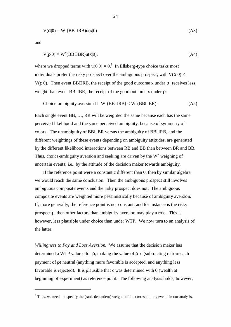
V(α|0) = W+(BB∪ RB)u(x|0) (A3)

and

V(ρ|0) = W+(BB∪ BR)u(x|0), (A4)

where we dropped terms with u(0|0) = 0.5 In Ellsberg-type choice tasks most

individuals prefer the risky prospect over the ambiguous prospect, with V(α|0) <

V(ρ|0). Then event BB∪ RB, the receipt of the good outcome x under α, receives less

weight than event BB∪ BR, the receipt of the good outcome x under ρ:

Choice-ambiguity aversion ⇔ W+(BB∪ RB) < W+(BB∪ BR). (A5)

Each single event BB, …, RR will be weighted the same because each has the same

perceived likelihood and the same perceived ambiguity, because of symmetry of

colors. The unambiguity of BB∪ BR versus the ambiguity of BB∪ RB, and the

different weightings of these events depending on ambiguity attitudes, are generated

by the different likelihood interactions between RB and BB than between BR and BB.

Thus, choice-ambiguity aversion and seeking are driven by the W+ weighing of

uncertain events; i.e., by the attitude of the decision maker towards ambiguity.

If the reference point were a constant c different than 0, then by similar algebra

we would reach the same conclusion. Then the ambiguous prospect still involves

ambiguous composite events and the risky prospect does not. The ambiguous

composite events are weighted more pessimistically because of ambiguity aversion.

If, more generally, the reference point is not constant, and for instance is the risky

prospect ρ, then other factors than ambiguity aversion may play a role. This is,

however, less plausible under choice than under WTP. We now turn to an analysis of

the latter.

Willingness to Pay and Loss Aversion. We assume that the decision maker has

determined a WTP value c for ρ, making the value of ρ–c (subtracting c from each

payment of ρ) neutral (anything more favorable is accepted, and anything less

favorable is rejected). It is plausible that c was determined with 0 (wealth at

beginning of experiment) as reference point. The following analysis holds, however,

5 Thus, we need not specify the (rank-dependent) weights of the corresponding events in our analysis.

25

for any value of c, irrespective of the reference point chosen when determining c.

Hence, we do not analyze the determination of c further. The main text took c = 0 for

simplicity of presentation, but here we analyze the more general case.

We assume that the risky prospect serves as a reference point for the evaluation

of the ambiguous prospect. More precisely, we assume in what follows that the

decision maker takes ρ–c as neutral and as reference point, so that WTP(α) is the

amount such that α – WTP(α) is equivalent to the neutral ρ–c. That is,

V(α–WTP(α)|ρ–c) = 0.

We analyze, for the sake of comparison, the auxiliary prospect α–c and its evaluation

V(α–c|ρ–c) . Table A1 displays outcomes for various events.

TABLE A1. Payoffs for the Risky and the Ambiguous Prospect under Direct Choice

(BB) (BR) (RB) (RR)

α–c x–c –c x–c –c

ρ–c x–c x–c –c –c

For the evaluation of α–c, the events BB and RR are now taken as neutral (utility

0) according to (our version of) the theory of Schmidt, Starmer, & Sugden (2008).

These events do not contribute to the evaluation, which is why they do not appear in

the following Eq. A6. In particular, we need not specify their rank-dependent

weights. BR is now a loss event and RB is a gain event for prospect α–c.

WTP-ambiguity aversion (WTP(α) < c) results if α–c is evaluated lower than ρ–

c. Given that ρ–c is the reference point with V(ρ–c|ρ–c) scaled to be 0, this is

equivalent to negativity of the following evaluation.

WTP-ambiguity aversion ⇔

V(α–c|ρ–c) = W+(RB)u(x–c|–c) + λW−(BR)u(–c|x–c) < 0. (A6)

Here λ is the loss aversion parameter as in Eq. A1, which usually exceeds 1 indicating

an overweighting of losses. We discuss utility u in some detail, arguing that

u(x–c|–c) = −u(–c|x–c) (A7)

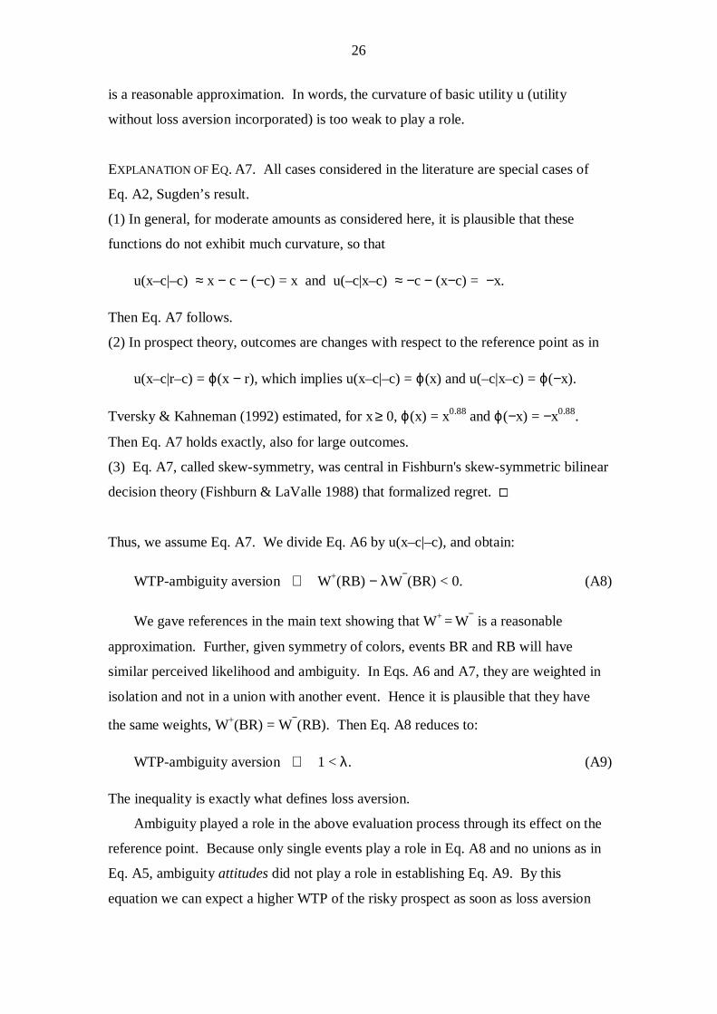
26

is a reasonable approximation. In words, the curvature of basic utility u (utility

without loss aversion incorporated) is too weak to play a role.

EXPLANATION OF EQ. A7. All cases considered in the literature are special cases of

Eq. A2, Sugden’s result.

(1) In general, for moderate amounts as considered here, it is plausible that these

functions do not exhibit much curvature, so that

u(x–c|–c) ≈ x − c − (−c) = x and u(–c|x–c) ≈ −c − (x−c) = −x.

Then Eq. A7 follows.

(2) In prospect theory, outcomes are changes with respect to the reference point as in

u(x–c|r–c) = ϕ(x − r), which implies u(x–c|–c) = ϕ(x) and u(–c|x–c) = ϕ(−x).

Tversky & Kahneman (1992) estimated, for x ≥ 0, ϕ(x) = x0.88 and ϕ(−x) = −x0.88.

Then Eq. A7 holds exactly, also for large outcomes.

(3) Eq. A7, called skew-symmetry, was central in Fishburn's skew-symmetric bilinear

decision theory (Fishburn & LaValle 1988) that formalized regret. ·

Thus, we assume Eq. A7. We divide Eq. A6 by u(x–c|–c), and obtain:

WTP-ambiguity aversion ⇔ W+(RB) − λW−(BR) < 0. (A8)

We gave references in the main text showing that W+ = W

− is a reasonable

approximation. Further, given symmetry of colors, events BR and RB will have

similar perceived likelihood and ambiguity. In Eqs. A6 and A7, they are weighted in

isolation and not in a union with another event. Hence it is plausible that they have

the same weights, W+(BR) = W−(RB). Then Eq. A8 reduces to:

WTP-ambiguity aversion ⇔ 1 < λ. (A9)

The inequality is exactly what defines loss aversion.

Ambiguity played a role in the above evaluation process through its effect on the

reference point. Because only single events play a role in Eq. A8 and no unions as in

Eq. A5, ambiguity attitudes did not play a role in establishing Eq. A9. By this

equation we can expect a higher WTP of the risky prospect as soon as loss aversion

27

holds (λ > 1), irrespective of ambiguity attitude, if the decision maker takes the risky

process as the reference point. A decision maker who is ambiguity neutral or seeking

but loss averse will reveal WTP-ambiguity aversion. Empirical studies have

suggested that loss aversion is widespread and strong. This is the reason that virtually

all subjects will exhibit WTP-ambiguity aversion, in agreement with our data.

Appendix B. Instructions Experiment 1 and 4

Both experiments’ instructions started with the following description of prospects:

Consider the following two lottery options:

Option A gives you a draw from a bag that contains exactly 20 red and 20 green poker chips. Before you draw, you choose a color and announce it. Then you draw. If the color you announced matches the color you draw you

win �50. If the colors do not match, you get nothing. (white bag)

Option B gives you a draw from a bag that contains exactly 40 poker chips. They are either red or green, in an unknown proportion. Before you draw, you choose a color and announce it. Then you draw. If the color you announced

matches the color you draw you win �50. If the colors do not match, you get nothing. (beige bag)

In experiment 1 the subjects were then asked to make a direct choice and give their

WTP for both options:

You have to choose between the two prospect options. Which one do you

choose?

O Option A (bet on a color to win �50 from bag with 20 red and 20

green chips)

O Option B (bet on a color to win �50 from bag with unknown

proportion of colors)

Additional hypothetical question:

Imagine you had to pay for the right to participate in the above described

options with the possibility to win �50. How much would you maximally pay

for the right to participate in the prospects? Please indicate your valuations:

28

I would pay �_________ to participate in Option A (bet on a color to win �50

from bag with 20 red and 20 green chips).

I would pay �_________ to participate in Option B (bet on a color to win �50

from bag with unknown proportion of colors).

In experiment 4 the subjects were asked to make a direct choice and 18 choices

between sure amounts and the prospects:

Below you are asked to choose between the above two options and also to

compare both options with sure amounts of money. Two people will be

selected for real play in class. For each person one decision will be randomly

selected for real payment as explained by the teacher.

[1, 2] You have to choose between the two prospect options. Which one do

you choose?

O Option A (bet on a color to win �50 from bag with 20 red and 20

green chips)

O Option B (bet on a color to win �50 from bag with unknown

proportion of colors)

Valuation of prospects.

Now determine your monetary valuation of the two prospect options. Please

compare the prospect options to the sure amounts of money. Indicate for both

options and each different sure amount of money whether you would rather

choose the sure cash or try a bet on a color from the bag to win �50!

Option A (bet on color from bag with 20 red and 20 green chips to win �50)

or sure amount of �:

[3] Play Option A ΟΟΟΟ or ΟΟΟΟ get �25 for sure







29



Option B (bet on color from bag with unknown proportion of colors to win

�50) or sure amount of �:

[12] Play Option B ΟΟΟΟ or ΟΟΟΟ get �25 for sure









Make sure that you filled out all 18 choices on this page!

In both experiments we asked the following question at the end:

Please give your age and gender here:

Age:_________________ Gender: male ΟΟΟΟ female ΟΟΟΟ

30

Appendix C. Instructions Experiment 2

In experiment 2 the hypothetical WTP questions have been replaced by the following

real payoff WTP decision using the BDM mechanism:

You have to buy the right to make a draw from the above described bags with

the possibility to win 50�. The procedure we use guarantees that a truthful

indication of your valuation is optimal for you, see details below at (*). How

much do you maximally want to pay for the right to participate in the prospect

options? Please indicate your offers:

I will pay �_________ to participate in Option A (bet on a color to win �50

from bag with 20 red and 20 green chips).

I will pay �_________ to participate in Option B (bet on a color to win �50

from bag with unknown proportion of colors).

*

The procedure is as follows: The experimenter throws a die to determine

which option he wants to sell. If a 1,2, or 3 shows up, Option A will be

offered; if a 4,5, or 6 shows up, Option B will be offered. After the option for

sale has been selected, the experimenter draws a lot from a bag that contains

50 lots, numbered 1, 2, 3, …, 48, 49, 50. The number indicates the

experimenter’s reservation price (in Euro) for the selected option: if your offer

is larger than the reservation price, you pay the reservation price only and play

the option. If your offer is smaller than the reservation price, the experimenter

will not sell the option. You keep your money and the game ends.

References

Abdellaoui, Mohammed, Han Bleichrodt, & Corina Paraschiv (2007) “Loss Aversion

under Prospect Theory: A Parameter-Free Measurement,” Management Science

53, 1659–1674.

Abdellaoui, Mohammed, Frank Vossmann, & Martin Weber (2005) “Choice-Based

Elicitation and Decomposition of Decision Weights for Gains and Losses under

Uncertainty,” Management Science 51, 1384–1399.

31

Arkes, Hal R. (1991) “Costs and Benefits of Judgments Errors: Implications for

Debiasing,” Psychological Bulletin 110, 486–498.

Armantier, Olivier (2006) “Do Wealth Differences Affect Fairness Considerations,”

International Economic Review 47, 391–429.

Baltussen, Guido, Thierry Post, Martijn J. van den Assem, & Peter P. Wakker (2009)

“Random Incentive Systems in a Dynamic Choice Experiment,” Department of

Economics, Erasmus University, Rotterdam, the Netherlands.

Bardsley, Nick, Robin P., Cubitt, Graham Loomes, Peter Moffat, Chris Starmer, &

Robert Sugden (2010) “Experimental Economics; Rethinking the Rules.”

Princeton University Press, Princeton, NJ.

Bateman, Ian J., Alistair Munro, Bruce Rhodes, Chris Starmer, & Robert Sugden

(1997) “A Test of the Theory of Reference-Dependent Preferences,” Quarterly

Journal of Economics 112, 479–505.

Baucells, Manel & Franz H. Heukamp (2006) “Stochastic Dominance and Cumulative

Prospect Theory,” Management Science 52, 1409–1423.

Becker, Gordon M., Morris H. de Groot, & Jacob Marschak (1963) “Stochastic

Models of Choice Behavior,” Behavioral Science 8, 41–55.

Berg, Joyce E., John W. Dickhaut, & Thomas A. Rietz (2010) “Preference Reversals:

The Impact of Truth-Revealing Monetary Incentives,” Games and Economic

Behavior 68, 443–468.

Blavatskyy, Pavlo R. (2009) “Preference Reversals and Probabilistic Decisions,”

Journal of Risk and Uncertainty 39, 237–250.

Blumenschein, Karen , Glenn C. Blomquist, Magnus Johannesson, Nancy Horn, &

Patricia Freeman (2008) “Eliciting Willingness to Pay Without Bias: Evidence

from a Field Experiment,” The Economic Journal 118, 114–137.

Carlsson, Fredrik, Olof Johansson-Stenman, & Peter Martinsson (2004) “Is Transport

Safety More Valuable in the Air?,” Journal of Risk and Uncertainty 28, 147–163.

Choi, Syngjoo, Raymond Fishman, Douglas Gale, & Shachar Kariv (2007)

“Consistency and Heterogeneity of Individual Behavior under Uncertainty,”

American Economic Review 97, 1921–1938.

Chow, Clare C. & Rakesh K. Sarin (2001) “Comparative Ignorance and the Ellsberg

Paradox,” Journal of Risk and Uncertainty 22, 129–139.

32

Coursey, Don L., John L. Hovis, & William D. Schulze (1987) “The Disparity

between Willingness to Accept and Willingness to Pay Measures of Value,”

Quarterly Journal of Economics 102, 679–690.

Cummins, Robert G., Glenn W. Harrison, & E. Elisabet Rutström (1995)

“Homegrown Values and Hypothetical Surveys: Is the Dichotomous Choice

Approach Incentive-Compatible?” American Economic Review 85, 260–266.

Du, Ning & David Budescu (2005) “The Effects of Imprecise Probabilities and

Outcomes in Evaluating Investment Options,” Management Science 51, 1791–

1803.

Easley, David & Maureen O’Hara (2009) “Ambiguity and Nonparticipation: The Role

of Regulation,” Review of Financial Studies 22, 1817–1843.

Eisenberger, Roselies & Martin Weber (1995) “Willingness-to-Pay and Willingness-

to-Accept for Risky and Ambiguous Lotteries,” Journal of Risk and Uncertainty

10, 223–233.

Ellsberg, Daniel (1961) “Risk, Ambiguity and the Savage Axioms,” Quarterly

Journal of Economics 75, 643–669.

Fehr, Ernst & Lorenz Götte (2007) “Do Workers Work More if Wager Are high?

Evidence from a Randomized Field Experiment,” American Economic Review 91,

298–317.

Fishburn, Peter C. & Irving H. LaValle (1988) “Context-Dependent Choice with

Nonlinear and Nontransitive Preferences,” Econometrica 56, 1221–1239.

Fox, Craig R. & Amos Tversky (1995) “Ambiguity Aversion and Comparative

Ignorance,” Quarterly Journal of Economics 110, 585–603.

Fox, Craig R. & Martin Weber (2002) “Ambiguity Aversion, Comparative Ignorance,

and Decision Context,” Organizational Behavior and Human Decision Processes

88, 476–498.

Gächter, Simon, Andreas Herrmann, & Eric J. Johnson (2007) “Individual-Level Loss

Aversion in Riskless and Risky Choice.” Working Paper, University of

Nottingham.

Grether, David M. & Charles R. Plott (1979) “Economic Theory of Choice and the

Preference Reversal Phenomenon,” American Economic Review 69, 623–638.

Hahnemann, W. Michael (1991) “Willingness to Pay and Willingness to Accept: How

Much Can They Differ?,” American Economic Review 81, 635–647.

33

Halevy, Yoram (2007) “Ellsberg Revisited: An Experimental Study,” Econometrica

75, 503–536.

Harrison, Glenn W., Morten I. Lau, & E. Elisabet Rutström (2007) “Estimating Risk

Attitudes in Denmark: A Field Experiment,” Scandinavian Journal of Economics

109, 341–368.

Heath, Chip & Amos Tversky (1991) “Preference and Belief: Ambiguity and

Competence in Choice under Uncertainty,” Journal of Risk and Uncertainty 4, 5–

28.

Hogarth, Robin M. & Hillel J. Einhorn (1990) “Venture Theory: A Model of Decision

Weights,” Management Science 36, 780–803.

Keren, Gideon B. & Léonie E.M. Gerritsen (1999) “On the Robustness and Possible

Accounts of Ambiguity Aversion,” Acta Psychologica 103, 149–172.

Langer, Ellen J. (1975) “The Illusion of Control,” Journal of Personality and Social

Psychology 32, 311–328.

Langer, Thomas & Martin Weber (2001) “Prospect Theory, Mental Accounting, and

Differences in Aggregated and Segregated Evaluation of Lottery Portfolios,”

Management Science 47, 716–733.

Lichtenstein, Sarah & Paul Slovic (1971) “Reversals of Preference between Bids and

Choices in Gambling Decisions,” Journal of Experimental Psychology 89, 46–55.

Maafi, Hela (2010) “Preference Reversals under Ambiguity, ” Sciences Economiques,

Université de Paris I (Panthéon-Sorbonne), France.

Pennings, Joost M.E. & Ale Smidts (2003) “The Shape of Utility Functions and

Organizational Behavior,” Management Science 49, 1251–1263.

Plott, Charles R. (1996) “Rational Individual Behaviour in Markets and Social Choice

Processes: The Discovered Preference Hypothesis.” In Kenneth J. Arrow, Enrico

Colombatto, Mark Perlman, & Christian Schmidt (eds.) The Rational

Foundations of Economic Behavior: Proceedings of the IEA Conference Held in

Turin, Italy, 225–250, St. Martins Press, New York.

Pogrebna, Ganna (2010) “Ambiguity Preference Reversals,” Department of

Economics, University of Warwick, UK.

Pulford, Briony D. (2009) “Is Luck on My Side? Optimism, Pessimism, and

Ambiguity Aversion,” Quarterly Journal of Experimental Psychology 62, 1079–

1087.

34

Rigotti, Luca & Chris Shannon (2005) “Uncertainty and Risk Aversion in Financial

Markets,” Econometrica 73, 203–243.

Rizzo, John A. & Richard J. Zeckhauser (2004) “Reference Incomes, Loss Aversion,

and Physician Behavior,” The Review of Economics and Statistics 85, 909–922.

Roca, Mercè, Robin M. Hogarth, & A. John Maule (2006) “Ambiguity Seeking as a

Result of the Status Quo Bias,” Journal of Risk and Uncertainty 32, 175–194.

Schmidt, Ulrich, Chris Starmer, & Robert F. Sugden (2008) “Third-Generation

Prospect Theory,” Journal of Risk and Uncertainty 36, 203–223.

Seidl, Christian (2002) “Preference Reversal,” Journal of Economic Surveys 16, 621–

655.

Smith, Kip, John W. Dickhaut, Kevin McCabe, & José V. Pardo (2002) “Neuronal

Substrates for Choice under Ambiguity, Risk Certainty, Gains and Losses,”


Stalmeier, Peep F.M., Peter P. Wakker, & Thom G.G. Bezembinder (1997)

“Preference Reversals: Violations of Unidimensional Procedure Invariance,”

Journal of Experimental Psychology, Human Perception and Performance 23,

1196–1205.

Starmer, Chris & Robert Sugden (1991) “Does the Random-Lottery Incentive System

Elicit True Preferences? An Experimental Investigation,” American Economic

Review 81, 971–978.

Sugden, Robert (2003) “Reference-Dependent Subjective Expected Utility,” Journal

of Economic Theory 111, 172–191.

Thaler, Richard H. & Eric J. Johnson (1990) “Gambling with the House Money and

Trying to Break Even: The Effects of Prior Outcomes on Risky Choice,”


The Economist (2008) “Anti-Terrorist Spending. Feel Safer now?,” March 8. p. 64.

Tversky, Amos & Craig R. Fox (1995) “Weighing Risk and Uncertainty,”

Psychological Review 102, 269–283.

Tversky, Amos & Daniel Kahneman (1992) “Advances in Prospect Theory:

Cumulative Representation of Uncertainty,” Journal of Risk and Uncertainty 5,

297–323.

Völckner, Franziska (2006) “An Empirical Comparison of Methods for Measuring

Consumers' Willingness to Pay,” Marketing Letters 17, 137–149.

35

Wakker, Peter P. (2010) “Prospect Theory: for Risk and Ambiguity.” Cambridge

University Press.

Zeckhauser, Richard J. (1986) “Comments: Behavioral versus Rational Economics:

What You See Is What You Conquer,” Journal of Business 59, S435–S449.

Zeckhauser, Richard J. (2006) “Investing in the Unknown and Unknowable,”

Capitalism and Society 1, Article 5, 1–39.

Preference Reversals for Ambiguity Aversion

Documents

Transcript of Preference Reversals for Ambiguity Aversion