Risk Aversion with Production
15
Four Examples Risk and Information We present a few examples to illustrate the possibility that trading of risk/hedging might lead to lower aggregate welfare. The argument relies on our hunch that hedging is a substitute for collecting information and that, in the aggregate, society would be better off if agents collected information to reduce their variance instead of hedging. Example 1—The Allocation Problem (Chapter 7 Problem 12): Consider an economy with three agents, A, B and C, two goods—good 1 and good 2, and two time periods ! and ! . At time ! two mutually exclusive states of the world— ! and ! —could occur. The utilities for Agents A and B throughout are: = 1 2 ∗ log ! ! + 1 2 ∗ log ( ! ! ) = 1 2 ∗ log ! ! + 1 2 ∗ log ( ! ! ) where ! ! is the amount of good 1 consumed by Agent A; ! ! is the amount of good 2 consumed. Similarly for ! ! , ! ! The endowments for Agents A and B are the same in both states: 1 ! = 2,0 ! = 0,2 1 Here the amount of the good 1 is represented by the number before the comma and amount of good 2 is represented by the number in after the comma
Transcript of Risk Aversion with Production

Four Examples
Risk and Information We present a few examples to illustrate the possibility that trading of risk/hedging might lead to lower aggregate welfare. The argument relies on our hunch that hedging is a substitute for collecting information and that, in the aggregate, society would be better off if agents collected information to reduce their variance instead of hedging.
Example 1—The Allocation Problem (Chapter 7 Problem 12): Consider an economy with three agents, A, B and C, two goods—good 1 and good 2, and two time periods-‐-‐ 𝑡! and 𝑡!. At time 𝑡! two mutually exclusive states of the world— 𝑠! and 𝑠!—could occur. The utilities for Agents A and B throughout are:
𝑢 𝐴 =12 ∗ log 𝑥!
! +12 ∗ log (𝑥!
!)
𝑢 𝐵 =12 ∗ log 𝑥!
! +12 ∗ log (𝑥!
!) where 𝑥! ! is the amount of good 1 consumed by Agent A; 𝑥!! is the amount of good 2 consumed. Similarly for 𝑥!! , 𝑥!! The endowments for Agents A and B are the same in both states:1
𝑒! = 2,0
𝑒! = 0,2
1 Here the amount of the good 1 is represented by the number before the comma and amount of good 2 is represented by the number in after the comma
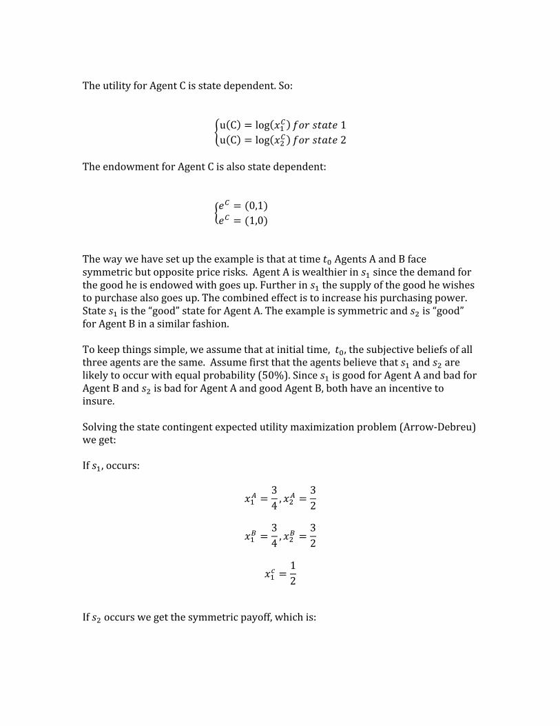
The utility for Agent C is state dependent. So:
u C = log 𝑥!! 𝑓𝑜𝑟 𝑠𝑡𝑎𝑡𝑒 1u C = log 𝑥!! 𝑓𝑜𝑟 𝑠𝑡𝑎𝑡𝑒 2
The endowment for Agent C is also state dependent:
𝑒! = (0,1)𝑒! = (1,0)
The way we have set up the example is that at time 𝑡! Agents A and B face symmetric but opposite price risks. Agent A is wealthier in 𝑠! since the demand for the good he is endowed with goes up. Further in 𝑠! the supply of the good he wishes to purchase also goes up. The combined effect is to increase his purchasing power. State 𝑠! is the “good” state for Agent A. The example is symmetric and 𝑠! is “good” for Agent B in a similar fashion. To keep things simple, we assume that at initial time, 𝑡!, the subjective beliefs of all three agents are the same. Assume first that the agents believe that 𝑠! and 𝑠! are likely to occur with equal probability (50%). Since 𝑠! is good for Agent A and bad for Agent B and 𝑠! is bad for Agent A and good Agent B, both have an incentive to insure. Solving the state contingent expected utility maximization problem (Arrow-‐Debreu) we get: If 𝑠!, occurs:
𝑥!! =34 , 𝑥!
! =32
𝑥!! =34 , 𝑥!
! =32
𝑥!! =12
If 𝑠! occurs we get the symmetric payoff, which is:

𝑥!! =32 , 𝑥!
! =34
𝑥!! =32 , 𝑥!
! =34
𝑥!! =12
We now consider a case where information about which state is going to occur is exogenously revealed. Without loss of generality, assume that it is revealed that state 𝑠! is going to occur. The availability of this information kills the insurance market since Agent A has no incentive to insure Agent B. The allocation when 𝑠! is going to occur with 100% probability is:
𝑥!! = 1, 𝑥!! = 2
𝑥!! =12 , 𝑥!
! = 1
𝑥!! =12
The allocation when 𝑠! is going to occur for sure is analogously symmetric and we omit further discussion for narrative clarity. We wish to highlight here that revelation of information doesn’t make the society of this example better off in the aggregate. Agent A is indeed better off when 𝑠! is known to occur and Agent B is worse off. But Agent A cannot sufficiently compensate Agent B to make them both better off. Information is not a public good. In other words, the two allocations in state 𝑠!—the allocation when the probability of occurrence of 𝑠! was 50% and when probability of occurrence of 𝑠! was 100%—are both along the same pareto frontier. While there is nothing wrong with this example and it may well describe some economic circumstances, it is certainly not generally true. Clarity about what is going to happen in the future should make society better off in the aggregate since it gives everyone a chance to adjust, adapt, prepare and innovate for the future. Perfect foresight should move the pareto frontier outwards. Intuitively we expect the allocation when information was known to be pareto superior to the one when it wasn’t.

The reason that the revelation of information doesn’t lead to a pareto-‐superior allocation in this example is that the three agents have no opportunity to react to information. Endowments are final consumption goods handed down to the agents like manna from heaven. This is an unreasonable description of most economic circumstances. Example 2—The Decision Problem (Chapter 7 Problem 11): In order for information to play a more familiar role in the economy we change some of the assumptions of Example 1. In Example 2 we introduce production to the economy. As we shall see, information will help co-‐ordinate production decisions with consumption desires. The utilities of Agents A and Agent B remain unchanged, as does the state dependent utility and endowment of Agent C. However, we change the endowments of Agents A and B. Instead of being allocated consumption goods, the agents now receive an endowment of 2 units each of a general-‐purpose resource like labor or capital. This resource can be employed in the manner most beneficial to the agent. He could use the resource to produce any combination of good 1 or good 2 as long as the total production does not exceed 2 units. The best way to think of such an endowment is to imagine that the 2 units of the resource can be employed to sow the seeds of good 1 or good 2 at time 𝑡!. These seeds will grow into the two goods in the proportion in which they were planted. As in the real economy, Agents A and B can’t make state contingent production decisions. They have to decide at time 𝑡! based on the information available at that time. The output will be the same regardless of which state occurs at time 𝑡!. Agent A and Agent B now face a decision problem. What proportion of good 1 and good 2 should they each plant at time 𝑡! such that it maximizes their consumption utility at time 𝑡!? From the perspective of the society in Example 2 the decision problem can be thought of the decision to build the optimal “Edgeworth Box”.2
2 We abuse the term Edgeworth Box somewhat which technically has only two agents and two commodities. Again it is just to make our narrative easier to comprehend.

So what “Edgeworth Box” should Agents A and B build? Together they have 4 units of a resource. The possible integer production possibilities are (4,0), (3,1), (2,2), (1,3), (0,4)3 and can be visualized as the boxes below:
As in the previous example demand for good 1 increases in 𝑠! and demand for good 2 increases in 𝑠!. It stands to reason that Agent A and Agent B must, on balance, produce more of good 1 if they know that 𝑠! is going to occur. 4 CASE 1: Assuming the probability of 𝑠! is 100% , we then know that Agent C has a fixed endowment of (0,1). Agents A and B will choose to produce a combination of good 1 and good 2 to maximize their consumption utilities. The problem is to pick the best “Edgeworth Box”. The possible integer production possibilities are:
3 The use of integer combinations is only for expository purposes. We place no restrictions on Agents A and B 4 The set up of this example is also symmetric. We again omit discussion on 𝑠! for narrative clarity

1. (4,1)
2. (3,2)
3. (2,3)

4. (1,4)
5. (0,5) It is easy to see that a benevolent social planner who has the interest of the three agents at heart will choose to produce (3,2). No other combination can yield a higher aggregate welfare. Agents A and B are similar in every respect, so they will produce the same quantities. Note here that more of good 1 than good 2 is indeed produced.
𝑦!! =32 ,𝑦!
! =125
𝑦!! =32 ,𝑦!
! =12
The competitive equilibrium when (3,2) is produced is:
5 𝑦! ! is the amount of good 1 produced by Agent A; 𝑦!! is the amount of good 2 produced. Similarly for 𝑦!! , 𝑦!!

𝑥!! = 1, 𝑥!! = 1
𝑥!! = 1, 𝑥!! = 1
𝑥!! = 1 CASE 2: Assume that the probability of state 𝑠! occurring is 50% at time 𝑡!. The production decisions will now be different from the earlier case. It should be easy to see that Agent A and Agent B will produce:
𝑦!! = 1,𝑦!! = 1
𝑦!! = 1,𝑦!! = 1 There is no reason for them to produce more of one good than the other. In the absence of any information both agents will hedge their production bets by diversifying. Without loss of generality we solve for the competitive equilibrium if state 𝑠! occurs at time 𝑡!:
𝑥!! =34 , 𝑥!
! =32
𝑥!! =34 , 𝑥!
! =32
𝑥!! =12
The competitive equilibrium of Case 1 is pareto superior (with transfers) to the competitive equilibrium on Case 2. Rearranging the allocation in Case 1 we get: 𝑥!! =
!!, 𝑥!! = 1 is pareto superior to 𝑥!! =
!!, 𝑥!! =
!!
𝑥!! =!!, 𝑥!! = 1 𝑥!! =
!!, 𝑥!! =
!!
𝑥!! =!! 𝑥!! =
!!

It might be helpful to visualize the decision with the Edgeworth Boxes of the previous examples. In the best of all worlds, i.e. with perfect foresight, this society will produce (3,2) when 𝑠! is going to occur and (2,3) when 𝑠! is going to occur. To see this, consider that Agents A and B produce (3,1) in 𝑠!. Add one unit of good 2 that Agent C is endowed with in 𝑠!and we get (3,2). A parallel argument works for 𝑠!. The good that is more is demand is produced in greater quantity. When agents have no information about which state of the world is going to occur, which is just another way of saying that 𝑠! is going to occur with probability 50%, they both produce (1,1) each. We get production of (2,2) for each state. To get the relevant Edgeworth Boxes we add the state dependent endowment of Agent C. In terms of the visualization :
State 1 State 2
Perfect Foresight
State 1 State 2
No information

We wish to highlight the following points:
• The allocation under Case 2 is exactly the same under the expected utility maximization in Example 1.
• The allocation when full information is available (Case 1) is pareto superior to the allocation when no information was available (Case 2). This agrees with our intuition of the economy. The availability of information allows agents to improve their lot. There is no reason to believe in the contingent destiny embodied by the “states of the world”. If we know ahead of time that there is some trouble for us in the future, we can take action today to change that eventuality. It is such actions that push the pareto-‐frontier outwards. Specifically in this example the availability of information allows us to align our resources to produce what we want.
• Taken together, the two points highlighted above indicate that it might be
possible to attain a utility possibility frontier better than the Arrow Debreu frontier. Of course Example 1 and Example 2 are not strictly comparable. We have changed the assumptions and therefore the problem.
• Still it is possible for the economy to achieve a higher utility possibility
frontier by relaxing the assumptions of the standard Arrow-‐Debreu framework. The idea that agents receive consumption goods as endowments is a stronger assumption than the one we made in Example 2 about agents being endowed with a general purpose resource and faced with a decision on how best to use the resource.
• The role played by information in Example 2 is also worth noting. This
economy is a co-‐ordination game and as with every other co-‐ordination game more information is pareto-‐superior. Information helps the agents co-‐ordinate the production decisions with consumption preferences.
• A related last point is about the cost of information. So far in this discussion,
information has been exogenously specified. But in the real economy resources are spent on collecting information. The takeaway from this example is that as the cost of information goes up, the pareto frontier moves back. Again this is intuitive given what we know about the economy. Uncertainty lowers the welfare of society and can sink the economy into a recession.

Example 3—The Recession6: In this example the set up remains as it was in Example 2. The utilities and endowments of agents A, B and C are as they were before. However, the probability of occurrence of 𝑠! is now 75%. The agent’s problem too remains the same. What combination of good 1 and good 2 should Agents A and B decide to produce? Our purpose here is to compare to different allocations in terms of their expected utility. As we have seen previously, perfect foresight yields a higher pareto-‐frontier and therefore a higher aggregate welfare. The task before this society is to get as close to the ideal of perfect foresight. In terms of the Edgeworth Box visualization the task is to get as close to the ideal shape of (3,2) for 𝑠! and (2,3) for 𝑠! as possible. We compare three different production combinations in terms of the expected utility of their outcomes. The decision choice for Agents A and B is how much of more of good 1 should they produce compared to good 2. If they produce (3,1) and 𝑠! does occur the decision works out very well—they have achieved the highest possible pareto-‐frontier. But there is 25% probability that 𝑠! will occur, in which case they would produced too much of good 1 relative to its demand. On the other hand by producing (2,2) they may be playing it too safe. We compare the following production combinations at time 𝑡!:
1. 𝑦!! = 1.5 ,𝑦!! = 0.5, 𝑦!! = 1.5,𝑦!! = 0.5 Total (3,1)
2. 𝑦!! = 1.125 ,𝑦!! = 0.875, 𝑦!! = 1.125,𝑦!! = 0.875 Total (2.25,1.75) 7
3. 𝑦!! = 1 ,𝑦!! = 1, 𝑦!! = 1,𝑦!! = 1 Total (2,2)
6 Again the term recession is used loosely to describe features of what we observe in a recession. 7 The (2.25,1.75) production combination is not rigorously derived. We arrived at it by hit and trial

State 1 State 2
Comparison
Boom
Recession
3,1
2.25,175
2,2
Ideal

The allocations of the different combinations are as follows.
𝑥!! =!!, 𝑥!! = 1 𝑥!! = 2, 𝑥!! =
!!
𝑥!! =!!, 𝑥!! = 1 𝑥!! = 2, 𝑥!! =
!!
𝑥!! =!! 𝑥!! =
!!
𝑥!! =!!, 𝑥!! =
!!! 𝑥!! =
!"!, 𝑥!! =
!!
𝑥!! =!!, 𝑥!! =
!!! 𝑥!! =
!"!, 𝑥!! =
!!
𝑥!! =!! 𝑥!! =
!!
𝑥!! =!!, 𝑥!! =
!! 𝑥!! =
!!, 𝑥!! =
!!
𝑥!! =!!, 𝑥!! =
!! 𝑥!! =
!!, 𝑥!! =
!!
𝑥!! =!! 𝑥!! =
!!
A few points of note are:
• It is easy to check that the combination (2.25, 1.75) yields the highest expected utility
• Some resources move to produce more of good 1 as we expect but because of risk aversion of the agents, they are reluctant to move too many.
• The 75% of the times when 𝑠! occurs this economy will experience a boom. The other 25% of the time the economy experiences a recession because too much of good 1 relative to its demand has been produced.
2.25, 1.75 and 𝒔𝟏 2.25, 1.75 and 𝒔𝟐
(3,1) and 𝒔𝟏 (3,1) and 𝒔𝟐
(2,2) and 𝒔𝟏 (2,2) and 𝒔𝟐

• The key message is that the boom and bust cycle is rational. More information gives us the opportunity to direct our production optimally to produce what we want. Ofcourse we suffer the occasional bust/recession when we get our forecast wrong. Still it is a calculated risk worth taking
• As in Example 2, more information pushes out the pareto-‐frontier.
Example 4—The Capital Market: We keep the basic structure of Example 2. But now we introduce comparative (competitive?) advantage. Agents A and B are still endowed with the general-‐purpose resource. But in this example Agent A can use this resource to produce 2 units of good 1 but only 1 unit of good 2. Agent A spends twice as much of the resource to produce good 2 compared to good 1. A useful way to think about this might be that the fertility of the soil at the disposal of the two agents is different. Good 1 grows better in Agent A’s soil. This example is symmetric too. So Agent B can produce good 2 at lower cost than good 1. If no information is available (probability of 𝑠! is 50% ) it is easy to see that by comparative advantage, Agent A will produce (2,0) and Agent B will produce (0,2) and both will hedge at time 𝑡!. We are familiar with the allocation that will result. The more interesting case, however, when it is known that 𝑠! will occur with 100% probability. We know from the previous examples that the best possible solution is for Agents A and B to produce (3,1). However, Agent A is limited by the 2 units of endowed resource. And Agent B is not competitive in producing good 1. We think the optimal allocation can still be produced if Agent B transfers 1 unit of his resource to Agent A as a loan or as equity. Now Agent A produces (3,0), Agent B produces (0,1) and with Agent C’s endowment (0,1) we get the desired allocation (3,2). As long as (3,1) is produced, this society will find a way of making everyone better off. This is a capital market, where agents who don’t believe that there is sufficient demand for the goods they have a comparative advantage in producing loan out the surplus capital to those agents who are producing goods which are in demand. The informational aspect of this example is extremely interesting. We can do away with the idea of the “states of the world”. All we need from both agents is to estimate the demand for the goods they have a comparative advantage in. By correctly estimating just that much they help in the aggregate price discovery and thereby

push the pareto frontier outwards. It is finding information rather than hedging that helps the society to direct resources optimally.