The emerging aversion toinequalityEvidence from subjective data1

Irena Grosfeld* and Claudia Senik***Paris School of Economics and CNRS, Paris, France. E-mail: grosfeld@pse.ens.fr

**Paris School of Economics and University Paris-Sorbonne, Paris, France.

E-mail: senik@pse.ens.fr

Abstract

This paper provides evidence of the changing attitudes to inequality duringtransition to the market in Poland. Using repeated cross-sections of the popula-tion, it identifies a structural break in the relationship between income inequal-ity and satisfaction. Whereas in the first stage of the transition process, anincrease in income inequality was interpreted by the population as a positivesignal of wider opportunities, later in the transition period increased inequalitybecame a factor in dissatisfaction with the country’s economic situation. Thiswas accompanied by increasing public sentiment that the process of incomedistribution is flawed and corrupt.

JEL classifications: C25, D31, D63, I30, P20, P26.Keywords: Inequality, subjective well-being, growth, breakpoint, transition.

Received: January 20, 2009; Acceptance: July 22, 2009

1 We thank Malgorzata Kalbarczyk for outstanding research assistance and Jolanta Sommer for help withthe data. We are grateful to Katia Zhuravskaya for insightful comments and to Marc Gurgand, AndrewClark and seminar participants in London, Bonn, Warsaw and Paris for discussions. The support of CEPRE-MAP is gratefully acknowledged.

Economics of TransitionVolume 18(1) 2010, 1–26

� 2010 The AuthorsJournal compilation � 2010 The European Bank for Reconstruction and Development.Published by Blackwell Publishing Ltd, 9600 Garsington Road, Oxford OX4 2DQ, UK and 350 Main St, Malden, MA 02148, USA

1. Introduction

Reform fatigue and disenchantment seem to have appeared in the transition coun-tries of Central and Eastern Europe. The rise in populist parties relying on populardiscontent with reforms was observed in a number of countries at the end of thelast century despite the significant achievements in establishing democratic andmarket institutions, continuous economic growth, and accession to NATO and theEuropean Union (Denisova et al., 2008; Desai and Olofsgard, 2006; Krastev, 2007).This contrasts with the remarkable popular support for reform and high expecta-tions that were found at the outset of transition. In Poland, for example, an initialstrong consensus for reforms faded away in the middle of the 1990s, giving way todisappointment. Criticism of some of transition outcomes, such as corruption,growing inequality and a high price paid by part of the population, progressivelybecame the dominant theme of public discourse. Popular discontent was associatedwith increasing distrust of political elites, accused of being corrupt and self-interested. We argue that in Poland, as in many other transition countries, thebacklash of reforms is partly due to the rise in income inequality and theperception that the process of income distribution and mobility is flawed andcorrupt (Brainerd, 1998; Kornai, 2006; Milanovic, 1999).

As one of the central features of former socialist regimes – income equality –was replaced by sharp income differentiation, it is no surprise that the subjectiveperception of inequality is one of the key elements of the attitudes towards reforms.In theory, income inequality may affect subjective welfare in several ways, eitherdirectly, for instance in the case of pure preferences for equal outcomes, or indi-rectly, through more sophisticated mechanisms involving the externalities of cor-ruption and criminality (Alesina and Perotti, 1996; Alesina et al., 2004; Fong, 2001).In practice, the relationship between income inequality and satisfaction has beenshown to be predominantly negative, especially in Europe (Alesina et al., 2004). Yetinequality can also improve subjective welfare in certain contexts, as suggested byHirschman and Rothschild (1973). The authors argue that societies experiencingrapid development may initially show tolerance for higher inequality, because theyinterpret it in terms of greater opportunities. This is also the idea of Alesina et al.(2004): ‘…in the US, the poor see inequality as a ladder that, although steep, may beclimbed…’ This tolerance for inequality may, however, wither away over time: ifexpectations are not met, supporters of the development process may become itsenemies. After such a ‘turning point’, some side-effects of development, and inparticular, an increase in inequality, may swamp the subjective benefits of growth.

The dynamic scenario sketched by Hirschman and Rothschild, including thedownturn in public satisfaction and adhesion to reforms, might actually be takingplace in the former socialist bloc. While the beginning of transition was perceivedas a big reshuffling of cards with high uncertainty, after more than 15 years, citi-zens of transition countries have acquired a more precise idea of the new economic

2 Grosfeld and Senik

� 2010 The AuthorsJournal compilation � 2010 The European Bank for Reconstruction and Development

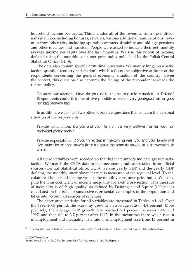
regime and of their own prospects in the new society. Depending on how fair theprocess of social change and the resulting income distribution appears to citizens,some transition countries may find themselves in the second part of the roadmapsketched by Hirschman and Rothschild.

The objective of this paper is to test Hirschman and Rothschild’s conjecture,using a series of repeated cross-sections of exceptional frequency and length thatcover the entire transition experience in Poland. We mainly focus on self-declaredsatisfaction with the state of the Polish economy (henceforth ‘country satisfaction’),which is both a satisfaction domain and a political attitude. We explore the relation-ship between income inequality and country satisfaction over time between 1992and 2005, when Poland experienced sustained economic growth. We identify abreak in the relationship between country satisfaction and income inequality at theend of 1996. In the first period (1992–1996), we observe a positive associationbetween these variables, whereas in the second period (1997–2005), this relationshipbecomes negative. In order to interpret this break, we also examine other satisfac-tion variables available in the survey. In the first period, inequality is associatedwith higher expectations, which is no longer true in the second period, suggestingthat it has lost its informational value in the eyes of the population. In addition,people’s self-declared satisfaction with their personal situation is negatively andsignificantly associated with income inequality after 1996, whereas there was nostatistically significant relationship in the earlier period. Additional evidence on theevolution of public opinion suggests that the changing tolerance for inequality coin-cided with the growing perception that high incomes are unmerited and oftenreflect corruption.

This paper is related to different strands of economic literature. First, the subjec-tive perception of the country’s situation touches upon the political economy ofdevelopment. Several papers have underlined the sociopolitical instability thatresults from income inequality (Alesina and Perotti, 1996; Perotti, 1996). Incomedistribution concerns have also been shown to discourage individuals’ adhesion tothe deepening of market reforms or development policies, leading to calls for fiscalpolicies that hamper economic growth (Alesina and Rodrik, 1994; Persson andTabellini, 1994). Acemoglu and Robinson (2000, 2002) have argued that in 19th cen-tury Europe, the extension of voting rights that led to unprecedented redistributiveprogrammes can be viewed as a strategy by the elite to avoid political discontentand revolution, which was in turn fed by the inequalities rising from economicdevelopment and industrialization. Analysing country satisfaction is a means toaddress these issues with the tools of the happiness literature using subjective vari-ables.

This paper also contributes to the literature on the relationship between incomedistribution and happiness and on the subjective foundations of the demand forredistribution. Most studies in this field find that individuals’ attitude towardsincome inequality depends on their beliefs and preferences regarding the factors ofeconomic success and failure. Prospects of upward mobility make people more

The Emerging Aversion to Inequality 3

� 2010 The AuthorsJournal compilation � 2010 The European Bank for Reconstruction and Development

tolerant of inequality (Alesina and la Ferrara, 2005; Alesina et al., 2004), but the per-ceived fairness of the mobility process itself also plays an important role (Alesinaand Angeletos, 2005; Fong, 2001). In sum, people dislike inequality and suffer fromit, when they view income differences as unmerited (for recent surveys, see Alesinaand Giuliano, 2009; Senik, 2009).

The subjective welfare effect of inequality during the process of transition hasbeen studied extensively. For instance, Sanfey and Teksoz (2007) find that incomeinequality has a positive effect on life satisfaction in transition countries, whereasthe impact is negative in other countries covered by the World Values Survey.Guriev and Zhuravskaya (2009) investigate a weaker relationship, ceteris paribus,between GDP and life satisfaction in transition countries as compared with non-transition countries. They identify inequality as one of the culprits of lower satisfac-tion in transition countries. Several papers treat the experience of transition as a‘natural experiment’ in order to assess the negative welfare effects of inequality(Ravallion and Lokshin, 2000) and income comparisons (Ferrer-i-Carbonell, 2005;Senik, 2004, 2008). Alesina and Fuchs-Schundeln (2007) document the slow conver-gence of preferences for state intervention in East Germany after the shock of theGerman reunification. We follow this usage of transition as a country-wide experi-ment. Starting from a situation of relatively egalitarian distribution of income(notwithstanding other forms of inequality), transition to a market economy makesit possible to trace the relationship between unfolding inequality and subjectivesatisfaction, as we assume that most changes are perceived as exogenous shocks bycitizens of the former socialist bloc.

The following section presents the data, Section 3 discusses the empirical strat-egy, and Section 4 presents the results. Last, Section 5 draws conclusions.

2. Data

The data are constructed from individual-level surveys carried out by CBOS inPoland.2 We exploit 84 surveys of representative samples of the Polish adult popu-lation, with samples of 1,000–1,300 individuals per survey, covering the period1992–2005 (six surveys per year). Even though some variables are available in ear-lier years, we choose 1992 as our starting date, the year that GDP growth resumedafter 2 years of a significant decline. We focus on the period of sustained economicgrowth, during which the fall in satisfaction with the country’s economic perfor-mance is most puzzling. In addition, our main variable of interest is missing formany dates before 1992.

A standard set of questions was asked in each survey: gender, age, education,residential location, labour market status, and occupation. In terms of income,the best documented and most complete measure available is net total monthly

2 The sample design is explained at http://www.cbos.pl/EN/About_us/design.shtml.

4 Grosfeld and Senik

� 2010 The AuthorsJournal compilation � 2010 The European Bank for Reconstruction and Development

household income per capita. This includes all of the revenues from the individ-ual’s main job, including bonuses, rewards, various additional remunerations, reve-nues from other jobs, including sporadic contracts, disability and old-age pensionsand other revenues and transfers. People were asked to indicate their net monthlyaverage income per capita over the last 3 months. We use this notion of income,deflated using the monthly consumer price index published by the Polish CentralStatistical Office (GUS).

The data also contain specific attitudinal questions. We mainly hinge on a satis-faction question (country satisfaction), which reflects the subjective attitude of therespondents concerning the general economic situation of the country. Giventhe context, this question also captures the feeling of the respondent towards thereform policy.

Country satisfaction: How do you evaluate the economic situation in Poland?Respondents could tick one of five possible answers: very good/good/neither goodnor bad/bad/very bad.

In addition, we also use two other subjective questions that concern the personalsituation of the respondents:

Private satisfaction: Do you and your family live: very well/well/neither well norbadly/badly/very badly.3

Private expectations: Do you think that in the coming year, you and your family willlive: much better than now/a little bit better/the same as now/a little bit worse/muchworse.

All these variables were recoded so that higher numbers indicate greater satis-faction. We match the CBOS data to macroeconomic indicators taken from officialsources (Central Statistical office, GUS): we use yearly GDP and the yearly GDPdeflator; the monthly unemployment rate is measured at the regional level. To cal-culate real household income we use the monthly consumer price index. We com-pute the Gini coefficient of income inequality for each cross-section. This measureof inequality is of ‘high quality’ as defined by Deininger and Squire (1996): it iscalculated on the basis of successive representative samples of the population andtakes into account all sources of revenues.

The descriptive statistics for all variables are presented in Tables A1–A3. Overthe 1992–2005 period, the economy grew at an average rate of 4.4 percent. Moreprecisely, the average GDP growth rate reached 5.3 percent between 1992 and1997, and then fell to 3.7 percent after 1997. In the meantime, there was a rise inunemployment and inequality. The rate of unemployment rose from 13 percent in

3 This question in Polish is understood both in terms of material situation and overall life satisfaction.

The Emerging Aversion to Inequality 5

� 2010 The AuthorsJournal compilation � 2010 The European Bank for Reconstruction and Development

1992 to 18 percent in 2005 (Table A3). Income inequality as measured by the Ginicoefficient was 0.32 at the beginning of 1992 but reached 0.38 by the end of 2005(Table A1). This is quite high by international standards. For instance, Grun andKlasen (2008) estimated adjusted Gini indices of gross income per capita, using theWorld Inequality Database (WIID, 2000), and showed that the world average withincountry Gini coefficient was of 0.33 in the 1980s and 0.34 in the 1990s.

This deformation in the distribution of income was accompanied by a generalincrease in real incomes at all levels of the income scale. In 2005, the median realincome per head was one-third higher than that in 1992. However, the enrichmenthas been more important for those at the top of the distribution. The average realincome per head in the second decile (D2) has increased by about 11 percent against43 percent in the ninth decile (D9). Accordingly, the ratio D2/D9 has fallen from 14percent to 11 percent during the period.

Figure 1 displays yearly averages of the main variables of interest: country sat-isfaction, private expectations, private satisfaction, real GDP and the Gini coeffi-cient. Although real GDP has been rising since 1992, satisfaction with the country’seconomic situation improved only up to 1997, and then declined substantially until2002, with a slight improvement after this date. The patterns of private satisfactionand expectations exhibit similar movements, albeit with a smaller amplitude. Even-tually, the final level of all satisfaction variables remains higher in 2005 than it wasin 1992.

1

1.5

2

2.5

3

3.5

1992 1993 1994 1995 1996 1997 1998 1999 2000 2001 2002 2003 2004 20050.3

0.32

0.34

0.36

0.38

0.4

Left axis Country satisfaction level Left axis Private satisfaction level

Left axis Private expectations levelLeft axis GDP real, index, 1992=1

Right axis Gini

Figure 1. Satisfaction levels, real GDP and Gini coefficient, 1992–2005(yearly averages)

6 Grosfeld and Senik

� 2010 The AuthorsJournal compilation � 2010 The European Bank for Reconstruction and Development

3. Empirical strategy

We consider the relationship between country satisfaction and income inequality,as in Alesina et al. (2004), who study the effect of income inequality in Europe andin the USA. We adopt the same specification in terms of statistical model and con-trol variables. In contrast to Alesina et al. (2004), who perform a cross-country anal-ysis of the relationship between income inequality and satisfaction in differentenvironments, we are interested in the dynamic evolution of this relationship inone country.

More precisely, we test for the presence of a structural break in this relationship,without imposing any specific date for the discontinuity, treating the breakpoint asendogenous. As Wald tests constructed with breaks treated as parameters do notpossess standard large-sample asymptotic distributions, we use the sup-Wald testbased on the maximum of a sequence of Wald statistics, with critical values fromAndrews (1993). The basic regression we estimate is:

Sit ¼ aT �Ginit þ b1Xit þ b2cT þ b3hj þ b4 � inflationt þ b5 � unemploymentvt þ eit

ð1Þ

where Sit is the country satisfaction of individual i at date t, Ginit is an inequal-ity measure calculated for each representative cross-section4; Xit represents thesocio-economic characteristics of individual i at date t consisting of age, age-squared, gender, education, occupation, labour market status, household incomeper capita and residential location; cT are year dummies capturing the generalmacroeconomic and other circumstances that affect all individuals in a givenyear; hj are region dummies for seven regions (north, west, centre-west, centre,east, south-east and south-west) and eit is the error term. We also control forthe monthly inflation rate and the monthly unemployment rate at the voıvode-ship level,5 in order to separate the influence of income inequality from othermacroeconomic determinants of country satisfaction. These variables are com-monly used as macroeconomic determinants of satisfaction (see, for example, DiTella et al., 2003).

As the satisfaction variables are ordinal, we estimate Equation 1 using theordered logit model. We pool individual observations from different surveys overtime. We adjust standard errors to allow for clusters by cross-section (or wave, thatis, by t).6 We also estimated the regression with clusters by voıvodeship and theresults turned out to be robust to such alternative assumptions about the variance–covariance matrix.

4 Below we also consider cross-sectional variations in Gini coefficient.5 Voivodeship (wojewodztwo, in Polish) is an administrative unit.6 Clustering is important because inflation and unemployment are aggregated at a higher level than thedependent variable and standard errors would otherwise be too high (Moulton, 1990).

The Emerging Aversion to Inequality 7

� 2010 The AuthorsJournal compilation � 2010 The European Bank for Reconstruction and Development

We test the hypothesis that the coefficient on the Gini index (at) is the same overthe entire period. Consequently, we use a partial structural change model, con-straining the coefficients of the other explanatory variables to remain the same overall of the periods. Specifically:

H0 : aT ¼ a� for all T

H1 : aT ¼ a1 for T ¼ 1992; . . . ;TB

aT ¼ a2 for T ¼ TB þ 1; . . . ; 2005

We consider different potential break points TB occurring at the first observationof each year between 1993 and 2004. We choose to leave one year of observations atthe beginning and at the end of each tested sample, which implies leaving about 15percent of the sample either before or after the break (trimming at 15 percent). Wecompute the Wald statistic for each value of TB in order to test whether the regres-sion coefficient on the Gini estimated over the sub-period [1992, TB] is equal to thatestimated over the sub-period [TB + 1, 2005]. We calculate the Wald statistic overall possible breakpoints and compare the maximal value with the relevant criticalvalue (taken from Andrews, 1993). If the sup-Wald statistic exceeds the criticalvalue, the test rejects the null hypothesis of equal coefficients. We then divide thesample into two parts at the estimated breakpoint and carry out a parameter con-stancy test for each sub-sample. If the hypothesis of no break in the sub-samples isnot rejected, we estimate Equation 1 separately for each sub-sample.

In order to understand which groups drive the average result, we exploit cross-sectional variations. We also run a series of robustness tests in order to excludealternative explanations of the downturn in country satisfaction and to check thatour results are robust to the use of alternative indices of income inequality. In orderto enrich the picture of the changing perception of income inequality, we alsoexplore the relationship between income inequality and other indicators of satisfac-tion available in the surveys. Finally, we use several public opinion polls that illus-trate the changing attitudes of the population towards income differentiation.

4. Results

We first pool the data and estimate country satisfaction controlling for all variablesas in Equation 1. The results are shown in Table A4. The difference between col-umns 1 and 2 is that the latter includes two macroeconomic variables: the regionalrate of unemployment and the monthly rate of inflation. We observe that men,richer and more educated people, students, and those in higher occupations (fordefinitions, see Table A2, panel B) are more satisfied with the country’s situation.Country satisfaction is U shaped in age. Pensioners, farmers, unqualified workers

8 Grosfeld and Senik

� 2010 The AuthorsJournal compilation � 2010 The European Bank for Reconstruction and Development

and those who live in rural areas are less satisfied than employees (the referencegroup defined as in Table A2, panel B). Comparison of the two columns shows thatthe coefficients on the individual characteristics are robust to the inclusion of mac-roeconomic indicators. Unemployment is negatively associated with country satis-faction, whereas the coefficient of inflation is statistically insignificant. Thecoefficient of income inequality remains insignificant. We then try to identify a dis-continuity in the relationship between income inequality and country satisfaction.

4.1 A structural break in the relationship between countrysatisfaction and income inequality

As explained in Section 3, we test the hypothesis of no break in the pooled sample.The results are displayed in Table 1. In column 1 the numbers are the values of v2

corresponding to the Wald statistics for all possible breakpoints. In columns 2 and 3we show the coefficients of the Gini index obtained for the periods before and aftereach potential break. Each row of the table corresponds to the year, which dividesthe sample into two parts. Country satisfaction is then estimated separately for each

Table 1. Test of a break in the relationship between income inequality and country

satisfaction

Wald test Gini index before the break Gini index after the break

(1) (2) (3)

1993 7.09 5.685*** [1.668] )1.394 [2.056]

1994 3.98 4.418** [2.034] )1.586 [2.223]

1995 6.31 4.358*** [1.644] )3.299 [2.592]

1996 18.44 5.828*** [1.732] )6.116*** [2.177]

1997 8.10 3.583* [1.891] )6.040** [2.821]

1998 7.00 3.202* [1.833] )6.155** [3.035]

1999 5.54 2.804 [1.802] )5.828* [3.203]

2000 14.12 3.312* [1.700] )8.910*** [2.810]

2001 3.42 1.231 [1.928] )7.861* [4.526]

2002 0.83 0.631 [1.869] )6.053 [7.075]

2003 1.96 0.791 [1.845] )10.747 [8.033]

2004 0.53 0.074 [1.855] 4.600 [5.943]

Notes: The numbers in column 1 are values of v2 corresponding to Wald statistics for all possible break-points. We test the existence of a break, trimming at 15%. The critical value from Andrews (1993) for oneparameter and trimming at 15% is 8.85 at the 5% level. In columns 2 and 3 we show the coefficients of theGini index obtained for the periods before and after each break. Values are significant at the *10%, **5% and***1% levels.

The Emerging Aversion to Inequality 9

� 2010 The AuthorsJournal compilation � 2010 The European Bank for Reconstruction and Development

sub-sample. When the break point is situated in 1996, the two coefficients on theGini index, before and after the break, are significant at 1 percent and have oppositesigns. This does not happen for any other year-break.

The critical value from Andrews (1993) for one parameter and trimming at 15percent is 8.85 at the 5 percent level. Hence, as the sup-Wald equals 18.44, we iden-tify the break at the end of 1996. However, as in 2000 the value of the v2 is alsogreater than the critical value, we check for the possible existence of a second breakin the period 1997–2005. This time with trimming at 25 percent, the critical value is7.93. The test is unable to reject the hypothesis of no break in the second sub-period.In order to make sure that the second break, although statistically insignificant,does not affect our results, we test the persistence of the break in 1996 keeping onlythe observations before 2000. The sup-Wald test in 1996 is now 16.71 (with trim-ming at 20%, the critical value is 8.45).

Consequently, we divide the whole sample into two sub-periods: 1992–1996 and1997–2005. Table 2 shows the estimation results for Equation 1 over the two sub-samples. In panel A, we observe that when the sample is divided into two periods,the coefficient on income inequality is statistically significantly positive before 1997(column 2) and then significantly negative after that date (column 3). If one admitsthe interpretation of the coefficient on the Gini index as the causal effect of incomeinequality on satisfaction, as do Alesina et al. (2004), then Table 2 suggests that theperception of inequality changes around the year 1997. After that date individualsare less inclined to consider themselves satisfied with reforms and, more generallywith the economic situation of their country, when inequality is high, even aftercontrolling for individual income, a number of personal characteristics, inflation,unemployment, year and region. However, before that date, inequality interpretedas a measure of higher opportunities is positively correlated with the subjectiveevaluation of reforms. More specifically, before the break, a one percentage pointincrease in the Gini index leads to a 0.9 percentage point decrease in the probabilityof considering the country’s economic situation as bad; after the break the sameincrease in the Gini index leads to a one percentage point increase in the probabilityof such an answer.

In panels B and C, we verify that the results are robust to the use of alterna-tive measures of inequality. One could argue that people have more local viewsof the income distribution and that the Gini coefficient calculated at the countrylevel is a less precise measure of the level of inequality than the one peopleperceive in their closer environment. Thus, in panel B we report results basedon a measure of income inequality calculated for different residential locations:large cities (over 50,000 inhabitants), smaller cities and rural areas. In panel Cwe measure income inequality based on our data as the standard deviation oflog household income for each cross-section. The results in panels B and C con-firm the pattern observed in panel A: inequality measures are positively associ-ated with the satisfaction variable in the first period, and turn out to besignificantly negative in the second period.

10 Grosfeld and Senik

� 2010 The AuthorsJournal compilation � 2010 The European Bank for Reconstruction and Development

We must emphasize that we are not trying to test whether the setback in atti-tudes is due to an external exogenous shock. Rather, the implicit model that wehave in mind is a cumulative process of disappointment, which at a certain pointgoes beyond a critical threshold (exhaustion of patience). Quoting Hirschman andRothschild (1973, p. 552). ‘The turning point in attitudes is not caused by a suddenshock. It comes about ‘‘purely as a result of the passage of time – no particular out-ward event sets off this dramatic turnaround’’. [In] ‘‘the easy early stage […] every-body seems to be enjoying the very process that will later be vehementlydenounced and damned as one consisting essentially in ‘‘the rich becomingricher’’’. However, if we wanted to indicate some specific events that could havecontributed to the turning point in the relationship between income inequality andcountry satisfaction, we could refer to the fact that 1997 coincides with theannouncement by the newly appointed government of a wave of second-generation

Table 2. Country satisfaction and income inequality before and after the break

(ordered logit)

1992–1996 1997–2005

Panel A

Gini 5.906*** [1.815] )6.443*** [2.183]

Log household income 0.330*** [0.024] 0.330*** [0.021]

Inflation 0.022 [0.023] 0.082** [0.037]

Unemployment )0.008*** [0.003] )0.017*** [0.004]

Observations 30,520 43,061

v2 52,297 9,210

Pseudo R2 0.06 0.06

Panel B

Gini by residential location 2.052*** (0.571] )2.382*** [0.881]

v2 48,193 6,756

Pseudo R2 0.055 0.057

Panel C

Standard deviation of household income 0.001*** [0.000] )0.001*** [0.000]

v2 12,338 8,309

Pseudo R2 0.056 0.057

Notes: The dependent variable, country satisfaction, scores the answers to the following question: ‘How doyou assess current economic situation in Poland?’ Answers from 1 = very bad to 5 = very good (Countrysatisfaction). Controls in panel A include female, age, age-squared, education, residential location (except inpanel B), labour market status, occupation, region dummies and year dummies. In panels B and C, loghousehold income, inflation and unemployment are also included. Gini coefficients and standard deviationof household income are calculated for each successive representative cross-section. All standard errors (inbrackets) are clustered by cross-section. Values are significant at the *10%, **5% and ***1% levels.

The Emerging Aversion to Inequality 11

� 2010 The AuthorsJournal compilation � 2010 The European Bank for Reconstruction and Development

welfare state reforms (concerning health, pensions and education), which was metwith little enthusiasm from the population. It is likely that this has contributed tothe ‘reform fatigue’ of the population, by reinforcing the perception of the costsimposed by reforms.

4.2 Who is most affected by inequality?

Different segments of the population may differ in their perception of incomeinequality. In this section, we investigate which particular groups drive the averageresult (established above). First, as income inequality is initially interpreted interms of increased opportunities, the effect should be more pronounced for thoseindividuals who had a longer experience of the socialist regime and who haveexperienced the transition process from the start. Hence, we expect ‘older’ peopleto have higher expectations at the beginning of the transition and to be more disap-pointed afterwards. Table 3 reports the results separately for the two cohorts, thosewho were born before 1970 and therefore were at least 23 years old in 1992, andthose who were born in 1970 or after. It shows that it is older cohorts who are ini-tially more likely to see income differentiation in terms of opportunities. Indeed,the coefficient on the Gini index is statistically significantly positive (column 1)in the regression on the sub-sample of ‘older’ people, whereas it is not significant inthe regression on the sub-sample of younger people (column 3). In the second per-iod, however, the coefficient on the Gini index is negative and statistically signifi-cant for both groups. The initial positive attitude of older cohorts towards incomeinequality has vanished, giving way to a general aversion for inequality.

Table 3. Country satisfaction and income inequality: cohort effects (ordered logit)

Born before 1970 Born after 1969

1992–1996 1997–2005 1992–1996 1997–2005

(1) (2) (3) (4)

Gini 6.351*** [1.802] )6.386*** [2.265] 1.237 [2.834] )6.791*** [2.410]

Log household income 0.335*** [0.028] 0.365*** [0.022] 0.295*** [0.065] 0.232*** [0.035]

Regional unemployment )0.009*** [0.003] )0.018*** [0.004] )0.005 [0.009] )0.011* [0.006]

Inflation rate 0.021 [0.023] 0.088** [0.040] 0.034 [0.032] 0.049 [0.039]

Observations 27,851 34,818 2,669 8,243

v2 644,537 11,502 5,378,140 1,761

Pseudo R2 0.05 0.06 0.06 0.05

Log likelihood )31,910 )40,627 )2,955 )9,488

Notes: Controls include female, age, age-squared, education, residential location, labour market status, occu-pation, region dummies and year dummies. All standard errors (in brackets) are clustered by cross-section.Values are significant at the *10%, **5% and ***1% levels.

12 Grosfeld and Senik

� 2010 The AuthorsJournal compilation � 2010 The European Bank for Reconstruction and Development

Second, we expect to see a difference in the perception of inequality dependingon the ideological self-identification of individuals. Alesina et al. (2004) observedthat left-wing Europeans were more affected by income inequality, compared withright-wingers. The notions of left and right are not completely clear in countriesthat have experienced communism for 45 years, but we rely on the self-definitionof individuals who answered the following question: ‘Please describe your politicalopinions using the scale from 1 (left) to 7 (right)’. We classified as left-wingers therespondents who chose ‘1’ and as right-wingers those who chose ‘7’ (left and righteach represent about 5 percent before 1997 and 10 percent after 1997). Table 4shows that in Poland, the initial positive association between income inequalityand satisfaction is statistically significant for right-wingers (who probably seeincome differentiation as a source of incentives and efficiency) but not for left-win-gers (who are less likely to share this view). After 1996, a statistically significantnegative association between income inequality and country satisfaction isobserved in both groups.

Overall, these results suggest that the initial perception of income differentiationwas more positive in groups which had a longer experience of socialism or definedthemselves as right-wingers, who were more likely to interpret the process ofincome differentiation as the corollary of increased opportunities and efficiency.

4.3 Possible alternative explanations

Due to the limitation of the data, we are unable to establish the direction of causal-ity in the relationship between income inequality and country satisfaction.

Table 4. Country satisfaction and income inequality: left and right (ordered logit)

Left Right

1992–1996 1997–2005 1992–1996 1997–2005

(1) (2) (3) (4)

Gini 0.871 [4.117] )6.063** [2.944] 12.341** [4.820] )8.523** [4.336]

Log household income 0.598*** [0.114] 0.210*** [0.072] 0.241** [0.111] 0.374*** [0.073]

Inflation 0.106*** [0.041] 0.039 [0.062] 0.028 [0.043] 0.113** [0.054]

Unemployment )0.011 [0.015] )0.006 [0.011] 0.002 [0.011] )0.006 [0.010]

Observations 1,081 3,035 1,564 3,168

v2 18,803 1,106 17,005 1,681

Pseudo R2 0.10 0.07 0.02 0.08

Log likelihood )1,293.81 )3,580 )1,946 )3,797

Notes: Controls include female, age, age-squared, education, residential location, labour market status, occu-pation, region dummies and year dummies. All standard errors (in brackets) are clustered by cross-section.Values are significant at the *10%, **5% and ***1% levels.

The Emerging Aversion to Inequality 13

� 2010 The AuthorsJournal compilation � 2010 The European Bank for Reconstruction and Development

However, our objective is to assess the association between income inequality andsatisfaction and to establish the existence of a break in this relationship over time.Hence, we need to rule out alternative potential explanations of the change in coun-try satisfaction. The first natural suspect is a time trend. As income inequality isrising along the whole considered period, the coefficient on the Gini index could behiding the pure effect of time. This could happen if, the level of inequality notwith-standing, with the passage of time, people who initially had high expectationsbecame disappointed. The inclusion of year dummies partly takes care of this issue.Alternatively, we have included a time trend in the estimation of Eqn 1. The resultsconcerning the changing impact of income inequality were not altered [the coeffi-cient on the Gini index was 5.569 (SD 2.100) in the first period and )13.725(SD 4.342) in the second period].

We also considered the possibility that the results are driven by seasonal varia-tions of country satisfaction. Including monthly dummies in the basic regressiondoes not affect the results. Third, the changing tolerance for inequality could bedue to the reduced importance of the welfare state. The public attitude towardsinequality certainly depends on the extent of redistribution and social protection.Keane and Prasad (2002), following Garner and Terrell (1998), argued that inPoland, at the beginning of transition, substantial social transfers compensated forincreasing wage inequality. The mechanisms of social transfers were thus criticalin ensuring political support for reform. Their period of observation stops in 1997,but official statistics show that the share of social expenditure in GDP hasremained stable at around 23 percent since 1997. Hence, the changing tolerancefor inequality does not seem to be associated with the withering away of thewelfare state.

Finally, we asked whether a similar break is observable in the relationshipbetween country satisfaction and other macroeconomic variables. We thus carriedthe same test for the presence of a structural break in the relationships between (1)unemployment rate and country satisfaction and (2) inflation rate and country sat-isfaction. We find that the coefficient on unemployment remains negative in allsub-periods defined by consecutive breaks, whereas the coefficient on inflationremains statistically insignificant. Therefore, our main result does not seem to bedriven by a change in public opinion regarding other major macroeconomic indica-tors. To sum up, our results prove to be immune to several potential alternativeexplanations.

4.4 Other indicators of satisfaction

In order to complete the picture and provide more evidence on personal satisfac-tion during the transition process, we now turn to the relationship between twoother subjective variables and income inequality over time. As shown in Figure 1,private satisfaction and private expectations follow a similar pattern as country sat-isfaction but of smaller amplitude. Although more flat than country satisfaction,

14 Grosfeld and Senik

� 2010 The AuthorsJournal compilation � 2010 The European Bank for Reconstruction and Development

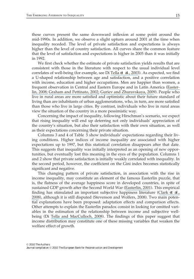
these curves present the same downward inflexion at some point around themid-1990s. In addition, we observe a slight upturn around 2001 at the time wheninequality receded. The level of private satisfaction and expectations is alwayshigher than the level of country satisfaction. All curves share the common featurethat the level of satisfaction and expectations is higher in 2005 than it was initiallyin 1992.

We first check whether the estimate of private satisfaction yields results that areconsistent with those in the literature with respect to the usual individual levelcorrelates of well-being (for example, see Di Tella et al., 2003). As expected, we finda U-shaped relationship between age and satisfaction, and a positive correlationwith income, education and higher occupations. Men are happier than women, afrequent observation in Central and Eastern Europe and in Latin America (Easter-lin, 2008; Graham and Pettinato, 2002; Guriev and Zhuravskaya, 2009). People wholive in rural areas are more satisfied and optimistic about their future standard ofliving than are inhabitants of urban agglomerations, who, in turn, are more satisfiedthan those who live in large cities. By contrast, individuals who live in rural areasview the situation of the country in a more pessimistic way.

Concerning the impact of inequality, following Hirschman’s scenario, we expectthat rising inequality will end up deterring not only individuals’ appreciation ofthe country’s situation, but also their satisfaction with their own situation, as wellas their expectations concerning their private situation.

Columns 3 and 4 of Table 5 show individuals’ expectations regarding their liv-ing conditions. Higher indices of income inequality are associated with higherexpectations up to 1997, but this statistical correlation disappears after that date.This suggests that inequality was initially interpreted as an opening of new oppor-tunities, but eventually lost this meaning in the eyes of the population. Columns 1and 2 show that private satisfaction is initially weakly correlated with inequality. Inthe second period, however, the coefficient on the Gini index becomes statisticallysignificant and negative.

This changing pattern of private satisfaction, in association with the rise inincome inequality, may constitute an element of the famous Easterlin puzzle, thatis, the flatness of the average happiness score in developed countries, in spite ofsustained GDP growth after the Second World War (Easterlin, 2001). This empiricalfinding has stimulated an important subjective happiness literature (Clark et al.,2008), although it is still disputed (Stevenson and Wolfers, 2008). Two main poten-tial explanations have been proposed: adaptation effects and comparison effects.Other attempts to explain the Easterlin paradox consist in looking for omitted vari-ables in the estimation of the relationship between income and subjective well-being (Di Tella and MacCulloch, 2008). The findings of this paper suggest thatincome distribution may constitute one of these missing variables that weaken thewelfare effect of growth.

The Emerging Aversion to Inequality 15

� 2010 The AuthorsJournal compilation � 2010 The European Bank for Reconstruction and Development

successful should be paid more’ rose from 24 percent in 1992 to 32 percent in 1998and 54 percent in 2004. Figure 3 uses another survey (CBOS, 2004) to illustrate theshare of the population who considers corruption as an important problem. Thissentiment increased sharply, from 32 percent in 1991 to 75 percent in 2004. Overall,

0

10

20

30

40

50%

60

70

80

90

1991 1992 2000 2001 2003 2004

Very important

Rather importantNot important

Perc

enta

geof

peop

lew

hoan

swer

posi

tivel

yth

efo

llow

ing

ques

tion:

‘In

your

opin

ion,

how

impo

rtan

tis

the

corr

uptio

npr

oble

min

Pola

nd:

very

impo

rtan

t/rat

her

impo

rtan

t/not

very

impo

rtan

t/not

impo

rtan

t’

Figure 3. ‘In your opinion, how important is the corruption problem in Poland?’

Source: CBOS (2004).

0

10

20

30

40

50

60

%

70

80

90

100

1994 1997 1998 1999 2003

Energetic entrepreneurs should be remunerated well to ensure the growth of the Polish economyLarge inequalities of income are necessary to guarantee future well-beingInequalities of income are too large in Poland

Perc

enta

ge o

f peo

ple

who

agr

eew

ith th

e ab

ove

stat

emen

ts

Figure 2. Opinions concerning income inequality, Poland, 1994–2003

Source: CBOS (2003).

The Emerging Aversion to Inequality 17

� 2010 The AuthorsJournal compilation � 2010 The European Bank for Reconstruction and Development

it appears that the perception of the Polish population concerning the fairness andefficiency of income distribution has deteriorated during the period under observa-tion, with a visible turning point around 1997.

These results suggest that the parallel processes of income growth and inequal-ity were initially well accepted by Poles, who might have seen them as a promise offuture shared gains. However, by the late 1990s, high expectations seem to havegiven way to more negative attitudes, fed by the rising intolerance for incomeinequality, the continued growth in GDP notwithstanding.

5. Conclusion

This paper provides evidence of a change in the relationship between incomeinequality and individuals’ views of the economic situation of their country, whichcan partly be interpreted as a measure of support for reforms. Our results suggestthat income inequality was initially perceived as a positive signal of increasedopportunities. However, after several years, unfulfilled expectations and diminish-ing patience brought about a change in attitudes, and growing inequality startedto undermine satisfaction. Individuals seem to have become disappointed with thecountry’s transformation and skeptical about the legitimacy of the enrichment ofreform winners. Various public opinion surveys confirm the changing popularsentiment about the degree of corruption in the country and the desirability ofhigh pay-offs in certain professions. Hence, the turning point in the tolerance forincome inequality seems to come with the increasingly wide perception that theprocess that generates income distribution is itself unfair.

The findings of this paper constitute a link between the literature on subjectivewell-being and the political economy literature focusing on inequality and growth.It provides evidence in support of a hypothesis put forth by Acemoglu and Robin-son (2000, 2002) and Perotti (1996) that growth accompanied by inequality gener-ates dissatisfaction and, as such, carries the menace of social instability.

The results obtained in this paper offer a number of lessons for developing andtransition countries: if it is important for governments to rapidly exploit the initial‘window of opportunity’ for reforms, it is also crucial that they pay attention toincome distribution in order to enjoy durable popular support for reforms. This lessoncan also be extended to developed countries, as it stresses the importance of ensuringthe fairness and transparency of the market and of the process of income distribution.

References

Acemoglu, D. and Robinson, J. A. (2000). ‘Why did the West extend the franchise? Democ-racy, inequality, and growth in historical perspective’, Quarterly Journal of Economics, 115,pp. 1167–1199.

18 Grosfeld and Senik

� 2010 The AuthorsJournal compilation � 2010 The European Bank for Reconstruction and Development

Acemoglu, D. and Robinson, J. A. (2002). ‘The political economy of the Kuznets curve’,Review of Development Economics, 6, pp. 183–203.

Alesina, A. and Angeletos, G.-M. (2005). ‘Fairness and redistribution: US versus Europe’,American Economic Review, 95, pp. 913–935.

Alesina, A. and Fuchs-Schundeln, N. (2007). ‘Good bye Lenin (or not?) – The effect of com-munism on people’s preferences’, American Economic Review, 97, pp. 1507–1528.

Alesina, A. and Giuliano, P. (2009). ‘Preferences for redistribution’, IZA DP 4056, Bonn: IZA.Alesina, A. and la Ferrara, E. (2005). ‘Preferences for redistribution in the land of opportuni-

ties’, Journal of Public Economics, 89, pp. 897–931.Alesina, A. and Perotti, R. (1996). ‘Income distribution, political instability, and investment’,

European Economic Review, 40, pp. 1203–1228.Alesina, A. and Rodrik, D. (1994). ‘Distributive politics and economic growth’, Quarterly Jour-

nal of Economics, 109, pp. 465–490.Alesina, A., Di Tella, R. and MacCulloch, R. (2004). ‘Inequality and happiness: Are Europe-

ans and Americans different?’ Journal of Public Economics, 88, pp. 2009–2042.Andrews, D. W. K. (1993). ‘Test for parameter instability and structural change with

unknown change point’, Econometrica, 61, pp. 821–856.Brainerd, E. (1998). ‘Winners and losers in Russia’s economic transition’, American Economic

Review, 88, pp. 1094–1116.CBOS (2003). Attitudes Towards Income Inequality, Warsaw: CBOS, June.CBOS (2004). The Perception of Corruption in Poland, Warsaw: CBOS, January.Clark, A., Frijters, E. P. and Shields, M. (2008). ‘Relative income, happiness and utility: An

explanation for the Easterlin paradox and other puzzles’, Journal of Economic Literature,46, pp. 95–144.

Deininger, K. and Squire, L. (1996). ‘A new data set measuring income inequality’, WorldBank Economic Review, 10, pp. 565–591.

Denisova, I., Markus, E. and Zhuravskaya, E. (2008). ‘What Russians think about transition:Evidence from RLMS survey’, CEFIR and NES working paper no. 113, Moscow: CEFIR.

Desai, R. M. and Olofsgard, A. (2006). ‘Political constraints and public support for marketreform’, IMF Staff Papers, 53, Washington, DC: IMF.

Di Tella, R. and MacCulloch, R. (2008). ‘Gross national happiness as an answer to the Easter-lin Paradox?’ Journal of Development Economics, 86, pp. 22–42.

Di Tella, R., MacCulloch, R. and Oswald, A. (2003). ‘The macroeconomics of happiness’,Review of Economics and Statistics, 85, pp. 809–827.

Easterlin, R. (2001). ‘Income and happiness: a unified theory’, Economic Journal, 111, pp. 1–20.Easterlin, R. (2008). ‘Lost in transition: Life satisfaction on the road to capitalism’, IZA DP

3409, Bonn: IZA.Ferrer-i-Carbonell, A. (2005). ‘Income and well-being: An empirical analysis of the compari-

son income effect’, Journal of Public Economics, 89, pp. 997–1019.Fong, Ch. (2001). ‘Social preferences, self-interest, and the demand for redistribution’, Journal

of Public Economics, 82, pp. 225–246.Garner, T. and Terrell, K. (1998). ‘A Gini decomposition of inequality in the Czech and

Slovak Republics during the transition’, Economics of Transition, 6, pp. 23–46.Graham, C. and Pettinato, S. (2002). ‘Frustrated achievers: Winners, losers, and subjec-

tive well being in new market economies’, Journal of Development Studies, 38,pp. 100–140.

The Emerging Aversion to Inequality 19

� 2010 The AuthorsJournal compilation � 2010 The European Bank for Reconstruction and Development

Grun, C. and Klasen, S. (2008). ‘Growth, inequality, and welfare: Comparisons across spaceand time’, Oxford Economic Papers, 60, pp. 212–236.

Guriev, S. M. and Zhuravskaya, E. V. (2009). ‘(Un)happiness in transition’, Journal ofEconomic Perspectives, 23, pp. 143–168.

Hirschman, A. and Rothschild, M. (1973). ‘The changing tolerance for income inequality inthe course of economic development’, Quarterly Journal of Economics, 87, pp. 544–566.

Keane, M. and Prasad, E. (2002). ‘Inequality, transfers and growth: New evidence from theeconomic transition in Poland’, Review of Economics and Statistics, 84, pp. 324–341.

Kornai, J. (2006). ‘The great transformation of Central Eastern Europe’, Economics of Transi-tion, 14, pp. 207–244.

Krastev, I. (2007). ‘The strange death of the liberal consensus’, Journal of Democracy, 18,pp. 56–63.

Milanovic, B. (1999). ‘Explaining the increase in inequality during the transition’, Economicsof Transition, 7, pp. 299–341.

Moulton, B. (1990). ‘An illustration of a pitfall in estimating the effects of aggregate variableson micro units’, Review of Economics and Statistics, 72, pp. 334–338.

Perotti, E. (1996). ‘Growth, income distribution, and democracy: What the data say’, Journalof Economic Growth, 1, pp. 149–187.

Persson, T. and Tabellini, G. (1994). ‘Is inequality harmful for growth?’ American EconomicReview, 8, pp. 600–621.

Ravallion, M. and Lokshin, M. (2000). ‘Who wants to redistribute? The tunnel effect in 1990sRussia’, Journal of Public Economics, 76, pp. 81–104.

Sanfey, P. and Teksoz, U. (2007). ‘Does transition make you happw41 TN4–81.4(9Me‘.p83 hN8.2203 TDrT.6the)-493((2008ition’,)]TJ/F61552.5(Statistics)]TJ7/F3731,)-489.8(18,)]TJ-3Russia’, Journal of Public88253.3(Economics)]TJ20/F3213(,)-489.2343914]TJ-3

Appendix

Table A1. Subjective variables, household income and the Gini coefficient: mean

values of variables for each cross-section

Dates

(year_month)

Country

satisfaction

Private

expectations

Private

satisfaction

Household

income

Gini

coefficient

1992_01 2.002 2.679 2.753

1992_05 1.944 2.531 2.613 5.454 0.323

1992_07 2.036 2.849 2.640 5.528 0.331

1992_09 2.060 2.742 2.635 5.569 0.312

1992_10 2.147 2.707 2.652 5.515 0.339

1992_12 2.108 2.453 2.610 5.467 0.320

1993_01 2.124 2.637 2.659 5.516 0.353

1993_03 2.126 2.641 2.677 5.528 0.355

1993_05 2.085 2.741 2.713 5.527 0.324

1993_07 2.124 2.700 2.628 5.490 0.325

1993_09 2.272 3.046 2.663 5.486 0.379

1993_11 2.347 3.169 2.720 5.532 0.347

1994_01 2.343 2.924 2.788 5.488 0.351

1994_03 2.235 2.704 2.703 5.407 0.345

1994_06 2.437 2.886 2.738 5.471 0.357

1994_07 2.462 2.861 2.769 5.514 0.347

1994_09 2.379 2.733 2.818 5.510 0.337

1994_11 2.426 2.859 2.749 5.542 0.323

1995_01 2.521 2.928 2.832 5.546 0.339

1995_03 2.430 2.952 2.809 5.519 0.336

1995_05 2.526 2.904 2.851 5.573 0.306

1995_07 2.599 2.963 2.847 5.569 0.353

1995_09 2.574 2.931 2.841 5.566 0.339

1995_11 2.606 3.117 2.868 5.683 0.358

1996_01 2.943 3.137 2.975 5.650 0.364

1996_03 2.786 3.041 2.911 5.574 0.348

1996_05 2.702 2.988 2.938 5.614 0.329

1996_07 2.699 2.953 2.923 5.668 0.336

1996_09 2.724 2.941 2.959 5.675 0.329

1996_11 2.771 3.006 2.925 5.691 0.342

1997_01 2.745 3.072 2.906 5.726 0.371

1997_03 2.687 3.028 2.987 5.728 0.344

The Emerging Aversion to Inequality 21

� 2010 The AuthorsJournal compilation � 2010 The European Bank for Reconstruction and Development

Table A1. (cont) Subjective variables, household income and the Gini coefficient:

mean values of variables for each cross-section

Dates

(year_month)

Country

satisfaction

Private

expectations

Private

satisfaction

Household

income

Gini

coefficient

1997_05 2.840 3.048 3.023 5.807 0.332

1997_07 2.895 3.029 3.074 5.749 0.324

1997_09 2.939 3.141 3.005 5.794 0.352

1997_11 2.866 3.052 2.985 5.801 0.328

1998_01 2.771 2.929 3.000 5.720 0.337

1998_03 2.769 2.965 2.942 5.706 0.354

1998_05 2.774 2.988 2.967 5.797 0.337

1998_07 2.721 2.957 2.991 5.822 0.339

1998_09 2.746 2.878 2.943 5.834 0.352

1998_11 2.699 2.923 2.997 5.823 0.353

1999_01 2.706 2.889 2.945 5.805 0.347

1999_03 2.457 2.830 2.879 5.735 0.363

1999_05 2.471 2.828 2.912 5.818 0.342

1999_07 2.396 2.749 2.875 5.823 0.345

1999_09 2.330 2.814 2.882 5.879 0.353

1999_11 2.431 2.840 2.941 5.856 0.350

2000_01 2.490 2.848 2.874 5.800 0.372

2000_02 2.427 2.781 2.889 5.755 0.365

2000_05 2.320 2.792 2.904 5.827 0.365

2000_07 2.339 2.751 2.826 5.775 0.337

2000_09 2.375 2.854 2.882 5.814 0.359

2000_11 2.348 2.834 2.830 5.779 0.354

2001_01 2.383 2.844 2.896 5.787 0.328

2001_03 2.201 2.770 2.809 5.791 0.368

2001_05 2.198 2.781 2.842 5.783 0.351

2001_07 2.098 2.841 2.864 5.840 0.377

2001_09 2.147 2.879 2.846 5.811 0.340

2001_11 2.077 2.899 2.870 5.811 0.378

2002_01 2.071 2.834 2.881 5.831 0.361

2002_03 2.056 2.791 2.849 5.779 0.375

2002_05 2.071 2.788 2.835 5.824 0.379

2002_07 2.035 2.839 2.864 5.885 0.389

2002_09 2.160 2.876 2.910 5.820 0.366

2002_11 2.247 2.885 2.906 5.852 0.357

22 Grosfeld and Senik

� 2010 The AuthorsJournal compilation � 2010 The European Bank for Reconstruction and Development

Table A1. (cont) Subjective variables, household income and the Gini coefficient:

mean values of variables for each cross-section

Dates

(year_month)

Country

satisfaction

Private

expectations

Private

satisfaction

Household

income

Gini

coefficient

2003_01 2.249 2.867 2.914 5.832 0.373

2003_03 2.111 2.836 2.880 5.822 0.355

2003_05 2.060 2.873 2.900 5.864 0.363

2003_07 2.134 2.804 2.882 5.806 0.356

2003_09 2.188 2.887 2.997 5.819 0.360

2003_11 2.120 2.683 2.917 5.778 0.369

2004_01 2.257 2.864 2.920 5.822 0.372

2004_03 2.121 2.772 2.934 5.802 0.381

2004_05 2.370 2.924 2.982 5.882 0.367

2004_07 2.323 2.891 2.942 5.786 0.351

2004_09 2.451 2.939 3.007 5.811 0.369

2004_11 2.445 2.902 2.961 5.773 0.355

2005_01 2.541 2.981 2.980 5.737 0.363

2005_03 2.415 2.966 2.926 5.747 0.351

2005_05 2.525 3.073 2.965 5.809 0.362

2005_07 2.371 2.903 2.989 5.782 0.369

2005_09 2.471 2.974 2.971 5.776 0.365

2005_11 2.588 3.123 3.037 5.778 0.377

Notes: Country satisfaction: How do you assess the current economic situation in Poland? Answers from1 = very bad to 5 = very good; Private expectations: Do you think that in a year your life and the life of yourfamily will be: Answers from 1 = much worse to 5 = much better than now; Private satisfaction: How doyou and your family live? Answers from 1 = very bad to 5 = very good. Household income is the logarithmof net total monthly household income per capita, deflated by the monthly CPI. Gini coefficients are calcu-lated for each successive representative cross-section.

The Emerging Aversion to Inequality 23

� 2010 The AuthorsJournal compilation � 2010 The European Bank for Reconstruction and Development

Table A2. The socio-demographic structure of the sample, yearly averages

Panel A

Year Female Age Secondary education Rural areas Urban areas Large cities

1992 0.55 46.77 0.34 0.42 0.30 0.281993 0.55 47.93 0.35 0.42 0.30 0.281994 0.48 47.89 0.37 0.40 0.32 0.281995 0.55 48.24 0.37 0.40 0.31 0.291996 0.55 47.61 0.39 0.37 0.35 0.281997 0.57 47.53 0.41 0.37 0.32 0.311998 0.56 47.74 0.41 0.37 0.33 0.301999 0.56 48.17 0.43 0.37 0.33 0.302000 0.55 48.13 0.45 0.37 0.32 0.322001 0.56 47.86 0.44 0.36 0.31 0.322002 0.55 48.46 0.46 0.35 0.30 0.352003 0.55 47.82 0.46 0.37 0.30 0.332004 0.52 46.89 0.46 0.41 0.30 0.292005 0.53 46.73 0.44 0.37 0.32 0.30

Notes: Rural areas are those which, according to administrative rules, do not have the status of cities ortowns. Among non-rural areas, urban areas are cities with no more than 50,000 inhabitants, and large citiesare defined as having over 50,000 inhabitants. Secondary education is a dummy equal to one if the personhas at least a secondary education.

Panel B

Year Unemployed Pensioners Farm Not

working

Unqualified

workers

Qualified

workers

Higher

occupations

Self-

employed

Employees

1992 0.08 0.34 0.11 0.07 0.06 0.14 0.06 0.03 0.151993 0.05 0.44 0.09 0.03 0.04 0.10 0.06 0.04 0.131994 0.04 0.45 0.09 0.02 0.04 0.10 0.06 0.04 0.131995 0.06 0.43 0.08 0.04 0.04 0.10 0.06 0.04 0.121996 0.08 0.37 0.07 0.06 0.04 0.10 0.07 0.04 0.151997 0.08 0.35 0.06 0.06 0.04 0.10 0.08 0.04 0.161998 0.07 0.37 0.06 0.05 0.04 0.09 0.07 0.04 0.161999 0.08 0.37 0.06 0.05 0.04 0.09 0.07 0.04 0.162000 0.09 0.37 0.06 0.05 0.03 0.08 0.07 0.04 0.162001 0.12 0.37 0.05 0.05 0.03 0.08 0.06 0.04 0.162002 0.13 0.37 0.05 0.04 0.03 0.07 0.07 0.04 0.162003 0.12 0.35 0.05 0.05 0.03 0.07 0.07 0.04 0.162004 0.12 0.34 0.06 0.05 0.03 0.07 0.07 0.04 0.162005 0.11 0.33 0.05 0.05 0.04 0.08 0.05 0.03 0.17

Notes: Higher occupations include directors, presidents and managerial staff in public administration, lib-eral professions with higher education, engineers, school directors, physicians and lawyers. Employeesinclude those working in administration, technicians, nurses and medium-level employees: directors ofshops, mailmen, train conductors, etc.

24 Grosfeld and Senik

� 2010 The AuthorsJournal compilation � 2010 The European Bank for Reconstruction and Development

Table A3. Macroeconomic variables: yearly averages

Year Nominal

GDP

Real

GDP growth

Unemployment

rate

Gini coefficient

(our data)

Gini coefficient

UNICEF data

1992 114,243 2.6 13.1 0.325 0.274

1993 155,780 3.8 14.9 0.348 0.317

1994 210,377 5.2 16.5 0.343 0.323

1995 306,318 7.0 15.2 0.339 0.321

1996 385,448 6.2 14.4 0.342 0.328

1997 469,372 7.1 11.6 0.342 0.334

1998 549,467 5.0 10.0 0.345 0.326

1999 665,688 4.5 11.9 0.350 0.334

2000 744,378 4.3 13.9 0.359 0.345

2001 779,564 1.2 16.1 0.356 0.341

2002 808,578 1.4 17.7 0.371 0.353

2003 843,156 3.9 18.0 0.363 0.356

2004 924,538 5.3 19.6 0.366 –

2005 982,565 3.6 18.2 0.353 –

Notes: Gini coefficients calculated using yearly average household income in our data. The estimates of theGini coefficient from the UNICEF Database (IRC TransMONEE 2005) are based on interpolated distributionsfrom grouped data from household budget surveys reported to the MONEE project.Source: Polish Central Statistical Office (GUS).

The Emerging Aversion to Inequality 25

� 2010 The AuthorsJournal compilation � 2010 The European Bank for Reconstruction and Development

Table A4. Country satisfaction, ordered logit

(1) (2)

Female )0.061*** [0.021] )0.062*** [0.021]

Age )0.031*** [0.003] )0.032*** [0.003]

Age-squared 0.026*** [0.003] 0.026*** [0.003]

Log household income 0.334*** [0.016] 0.329*** [0.016]

Education 0.117*** [0.024] 0.115*** [0.024]

Unemployed )0.032 [0.028] )0.030 [0.027]

Pensioners )0.110*** [0.023] )0.107*** [0.023]

Farm )0.173*** [0.034] )0.170*** [0.034]

Unqualified workers )0.086** [0.034] )0.086*** [0.033]

Qualified workers )0.019 [0.031] )0.021 [0.031]

Not working 0.133*** [0.039] 0.129*** [0.038]

Higher occupations 0.189*** [0.038] 0.189*** [0.038]

Self-employed 0.040 [0.047] 0.039 [0.047]

Students 0.211*** [0.041] 0.209*** [0.041]

Rural areas )0.152*** [0.022] )0.154*** [0.023]

Large cities )0.022 [0.025] )0.037 [0.025]

West )0.076** [0.031] )0.087*** [0.031]

Centre-west )0.017 [0.030] )0.064** [0.031]

Centre )0.132*** [0.029] )0.202*** [0.030]

East )0.204*** [0.039] )0.247*** [0.039]

South-east )0.083*** [0.030] )0.150*** [0.032]

South-west 0.149*** [0.031] 0.058* [0.034]

cut1:Constant )0.405 [0.614] 2.616 [2.450]

cut2:Constant 2.066*** [0.612] 5.088** [2.449]

cut3:Constant 4.077*** [0.614] 7.101*** [2.449]

cut4:Constant 8.618*** [0.625] 11.643*** [2.467]

Gini 0.074 [1.865] 0.087 [1.834]

Unemployment )0.012*** [0.002]

Inflation 0.032 [0.023]

Observations 73,581 73,581

v2 4,633.67 4,531.66

Pseudo R2 0.05 0.05

Log likelihood )85,275.60 )85,242.27

Notes: Country satisfaction answers the following question: How do you assess the current economic situa-tion in Poland? Answers range from 1 = very bad to 5 = very good; Gini coefficients are calculated for eachsuccessive representative cross-section. Yearly dummies included. Omitted variables: men, less than second-ary education, urban areas (with less than 100,000 inhabitants), employees and north region. Age-squarewas divided by 100. All standard errors (in brackets) are clustered by cross-section. Values are significant atthe *10%, **5% and ***1% levels.

26 Grosfeld and Senik

� 2010 The AuthorsJournal compilation � 2010 The European Bank for Reconstruction and Development