The relationship between income inequality and inequality of opportunities in a high-inequality...

Serie Documentos de TrabajoN 292

The relationship between Inequality of Outcomes and Inequality of Opportunities in a high-inequality country:

The case of Chile*

Javier Núñez Andrea Tartakowsky

Abstract

Based on the methodology developed by Bourguignon, Melendez and Ferreira (2005) we explore the extent to which income inequality in Chile is associated with inequality of observed exogenous circumstances of origin, which shape individuals “opportunities” to pursue their chosen life plans. We find that equalizing a diverse set of observed circumstances of origin across individuals such as parents’ schooling and employment, household size and composition, ethnic background and features of the municipality of origin reduces the Gini coefficient in about 7-8 percentage points. About half of this effect is transmitted directly on earnings, while the remaining part through its indirect effect on the accumulation of schooling. Further results suggest that the influence of unobserved circumstances on income distribution may be limited, and hence aspects such as preferences, effort, luck, income shocks and income measurement errors may also be important factors behind income inequality, issue that awaits further research.

JEL classification:

D31, D63

Keywords:

Income Inequality, Equality of Opportunities.

* We are grateful to Jeremy Behrman and Esteban Puentes for all their very valuable and helpful comments. As usual, the authors are responsible for all errors.

1

The relationship between Inequality of Outcomes and Inequality of Opportunities in a

high-inequality country: The case of Chile1

Javier NúñezDepartment of Economics

Universidad de Chile

Andrea TartakowskyMideplan, Chile

JEL: D31, D63

Keywords: Income Inequality, Equality of Opportunities.

Abstract

Based on the methodology developed by Bourguignon, Melendez and Ferreira (2005) we

explore the extent to which income inequality in Chile is associated with inequality of

observed exogenous circumstances of origin, which shape individuals “opportunities” to

pursue their chosen life plans. We find that equalizing a diverse set of observed

circumstances of origin across individuals such as parents’ schooling and employment,

household size and composition, ethnic background and features of the municipality of

origin reduces the Gini coefficient in about 7-8 percentage points. About half of this

effect is transmitted directly on earnings, while the remaining part through its indirect

effect on the accumulation of schooling. Further results suggest that the influence of

unobserved circumstances on income distribution may be limited, and hence aspects such

as preferences, effort, luck, income shocks and income measurement errors may also be

important factors behind income inequality, issue that awaits further research.

1 We are grateful to Jeremy Behrman and Esteban Puentes for all their very valuable and helpful comments. As usual, the authors are responsible for all errors.

2

I. Introduction

An old normative debate has existed around the question of what kind of economic

inequality should public policies aim to reduce. While many authors have leaned towards

dealing with the inequality of “outcomes” (i.e. income inequality), other traditions have

instead proposed that public policies should promote “equality of opportunities” across

individuals.2 This debate has benefited from various conceptual and philosophical

contributions, yet limited insights have been gained from empirical perspectives.

Building upon the methodology developed by Bourguignon, Melendez and Ferreira

(2005), this paper aims to contribute to this debate by empirically examining the extent to

which observed income inequality is associated with the inequality of circumstances of

origin that shape individuals´ opportunities.

The idea of equality of opportunities rests on the notion that individuals should be

entitled to similar opportunities to pursue their desired life plans, which in turn requires

that those opportunities not be determined by circumstances of origin that individuals

inherit without their consent, such as, for example, parental and family background.

Equal opportunities advocates have argued that differences in economic outcomes (i.e.

income inequality) partly reflect differences in dimensions controlled by individuals,

such as effort, responsibility, choices and so on. Accordingly, public policies should aim

to equalize the exogenous circumstances that shape individuals’ opportunities that

constrain their choices, and then accept the resulting level of income inequality that

would emerge from individuals’ choices and preferences. With variations, this has

somewhat become the dominant view of the notion of equity that deserves legitimate

public action, as suggested, for example, by The World Banks’ 2005 Report on Equity

and Development:

2 See for example Roemer (1996), (1998) and (2000) and Dworking (1981) for descriptions of the notions of equality of opportunities and of outcomes. Also, Amartya Sen’s Capability approach has a resemblance with the notion of equality of opportunities, as described for example in Sen (1999) and Nussbaum and Sen (2000). See Roemer (1996) for a discussion of the main theories of distributive justice. See also Alessina, Di Tella and MacCulloch (2004) for a discussion on different attitudes between Europeans and Americans towards different notions of equality.

3

"By equity we mean that individuals should have equal opportunities to pursue a life of

their choosing and be spared from extreme deprivation in outcomes", (p. 2)3

Yet, little is known about the extent to which income inequality reflects individual

choices and preferences vs. the exogenous circumstances that individuals inherit.

Empirical investigation of the relationship between “opportunities” and “outcomes” is

relevant for various reasons. First, the practical implications of the philosophical

distinction between “opportunities” and “outcomes” would be less significant if both

were empirically associated. This would reinforce the interpretation of income

distribution indicators as good measures of both equality of outcomes and equality of

opportunities. This scenario would also suggest a more significant role for the individual

circumstances of origin versus individual choices and preferences, as a means of jointly

promoting equality of outcomes and of opportunities in the long run. If, on the contrary,

exogenous circumstances empirically played a limited role in shaping income inequality,

then this would have different implications depending on the chosen normative

standpoint: advocates of equality of opportunities should expect and accept that a

significant amount of income inequality would remain upon equalizing opportunities.

Advocates of equality of outcomes, in turn, should realize that achieving this aim would

require more than policies intended to equalize opportunities and circumstances, and that

some additional, purely redistributive policies would be needed.

For this task we follow Bourguignon et al (2005) pioneering work, which attempts to

establish the effect of circumstances of origin vs. individual “effort” in the determination

of income inequality in Brazil.4 In their work, a double role is played by circumstances:

3 On page 3 of the overview this view is reinforced in these passages: "Three considerations are important at the outset. First, while more even playing fields are likely to lead to lower observed inequalities in educational attainment, health status and incomes, the policy aim is not equality in outcomes"….” Second a concern with equality of opportunities implies that public action should focus on the distributions of assets, economic opportunities, and political voice, rather than directly on inequality in incomes. “

4 Behrman (2006) and Ruiz Tagle (2007) also examine the role of schooling on income inequality, although employing a framework different to that developed by Bourguignon et. al., which allows establishing and separating the direct and indirect effects of observed circumstances on income inequality. However, their

4

they have a direct impact on earnings, and an indirect effect on “effort”, that they take to

be the schooling level. They define the former effect as the “partial effect” of observed

circumstances on earnings, and the “total effect” to be the joint effect of the direct and

indirect effects of observed circumstances on earnings. Our work differs from theirs in

three respects. First, we employ a larger and diverse set of circumstances of origin, which

includes parental education and employment characteristics, ethnic background,

household size and composition, and features of the municipality of origin, among others.

Second, our aim is more modest in the sense that we do not address the (more complex)

issue of the effects of “effort on income distribution, but simply attempt to establish the

effects of observed circumstances on earnings. Accordingly, we refer to the indirect

effect simply as the effect of observed circumstances on the level of schooling (not

effort), and also interpret the unexplained part of the income distribution simply as an

unknown combination of unobserved circumstances, individual effort, sheer luck and

possibly income measurement errors. Finally, we provide some circumstance-equalizing

benchmarks in addition to the “partial” and “total” effects outlined above, in order to

shed some light on the possible effects of unobserved circumstances on the income

distribution. One benchmark consists of an extreme situation where everyone’s schooling

levels only reflect individuals circumstances- either observed or unobserved-, such that

individual “merit” and “effort” play no role in the determination of schooling, which

amounts to simply computing the income distribution after equalizing schooling levels

across individuals. The second equalizing benchmark consists of guaranteeing everyone a

minimum of 10 years of schooling (completed at about age 16) and employ the simulated

level of schooling otherwise, to reflect the idea that a simulated value of schooling lower

than 10 would almost certainly reflect unobserved circumstances. In addition, we perform

other exercises to examine further the role of unobserved circumstances.

The paper is structured as follows: The next section presents the basic model and the

empirical identification strategy of the four observed circumstances-equalizing

benchmarks. The third section describes the data and the set of circumstances employed.

results are similar to the results found in this work, in the sense that both studies suggest a limited role of schooling in reducing income inequality.

5

The fourth section presents and discusses the results in comparative perspective, and

discusses the role of unobserved circumstances, and finally section five concludes.

II. The model

Following Bourguignon et al (2005) and the adaptations in Núñez and Tartakowsky

(2007), it is possible to distinguish two different kinds of determinants of individual

earnings: those that result from actions that people take along their lives, which allow

them to expand their productivity, and those that obey to circumstances out of people’s

control. Bourguignon et al (2005) refer to the first set of determinants as “effort

variables” and the second as “circumstances”. The relationship between incomes, efforts

and circumstances is described as ),( iii ECfW � , where circumstances C typically

includes a series of variables of the individuals’ socioeconomic origin and effort E

reflects human capital variables.

In order to estimate the model empirically, this relationship can be expressed as a

linearized model, as follows:

iiii UECWLn �� )( (1)

where a and ß are coefficient vectors and Ui, is the residual that includes the unobserved

circumstance and effort variables, measurement error and variations of the individuals’

measured income from their corresponding permanent income level. All these factors are

supposed to be independent from the included variables in Ci and Ei, to have zero mean

and to be identically and independently distributed across individuals.

However, this formulation is restrictive and debatable, as it assumes additive separability

between circumstances and efforts. For example, it seems reasonable to expect that an

individual’s circumstances during his childhood and the characteristics of his household

and his parents’ human capital must have had an influence on his own human capital

6

accumulation and “effort”. Accordingly, Bourguignon et al (2005) propose “effort” to be

partly a function of circumstances:

iii VCBE �� (2)

where B is a coefficient matrix and Vi represents a non-observable effort determinant

vector. As usual, Vi it is supposed to have mean zero and to be i.i.d. across individuals.

Introducing equation (2) in (1) yields,

iiii UVCBWLn �� )()( (3)

The formulation in (3) is more general than model (1) since it allows the circumstance

variables to affect people’s incomes directly, as well as indirectly through its effects on

the effort variables. In particular, in model (1) the marginal effect of circumstances on

earnings amounts only to a. Bourguignon et al (2005) call this effect the “Partial Effect”

of observed circumstances on earnings. On the other hand, in model (3) the effect of

observed circumstances on earnings is B�� . This corresponds to the “Total Effect”

of observed circumstances on earnings. Note that this effect includes the partial effect of

circumstances on earnings, a, but also de indirect effect of circumstances on earnings

through “effort”, ßB. The total effect of observed circumstances on earnings is larger than

the partial effect if ßB>0, as expected.

In practice, Bourguignon et al (2005) employ schooling as their measure of “effort” Ei.

However, as discussed in the introduction we believe it is both controversial and

misleading to refer to schooling as an “effort” variable, at least in countries with known

inequality of educational opportunities. Accordingly, we have preferred to replace effort

Ei simply by individual schooling level Si. Given this new interpretation, equation (1)

would simply indicate that wages are a function of human capital (i.e. schooling),

circumstances of origin, as well as term Ui, which captures unobserved circumstances,

sheer luck, “effort” at work, deviations from permanent income, and possibly income

7

measurement errors. In addition, parameter ß would be more directly interpreted simply

as the return to schooling, while parameter B would reflect the effect of observed

circumstances of origin on the accumulation of schooling. For example, parameter B can

capture parents’ resources to invest in their son’s tertiary education, the role of cognitive

and non-cognitive abilities acquired during infancy and adolescence on the chances of

gaining access to tertiary education. In addition, parameter a would reflect the direct

effect of circumstances on earnings, for a given schooling level, or alternatively, as the

effect of circumstances on the return of a given amount of schooling. For example,

parameter a can capture the effect of the quality of education (likely to be associated with

circumstances), the role of abilities acquired in the household of origin on labor

productivity and earnings, access to social networks and even the possibility of “class

discrimination” in the labor market.5 In conclusion, this modified interpretation openly

treats “effort” as a non observable variable, which would be captured in term Vi in

equation (2).

a. Partial and Total effects of observed circumstances on income inequality

The estimation of parameters a, ß and B through an OLS estimation of equations (1) and

(2) allows performing two types of simulations of the distribution of income after

equalizing exogenous observed circumstances C. Let WP denote the simulated income

distribution associated with the “Partial Effect” described above, obtained after

equalizing all the circumstance variables across individuals in equation (1). Accordingly,

the resulting income distribution would reflect individual differences in schooling and in

the residue Ui. More formally, the hypothetical distribution WP would be derived from

the simulation of the individual incomes PiW using the following equation, and after

estimating equation (1) by OLS:

iiP

i USCWLn��

�� )( (4)

where C is the vector of population means of the circumstance variables.

5 See for example Núñez and Gutiérrez (2004).

8

An alternative hypothetical wage distribution WT associated with the “Total effect” of

observed circumstances on earnings can be obtained by equalizing all the observed

circumstance variables across individuals in equation (3), after estimating equation (1)

and (2) by OLS. The income distribution WT would thus be obtained from:

iiT

i UVCBWLn��

�� )()( (5)

where again C stands for the population means of the circumstance variables and the

coefficients are obtained from OLS estimations of equations (1) and (2) .

The comparison between the actual (observed) distribution W and distribution WP

reflects the partial effect of observed circumstances on the distribution of income, while

the comparison between W and WT provides the effect of the total effect of observed

circumstances on earnings, i.e. including the effect of observed circumstances on the

accumulation of schooling. Both measures of income inequality allows distinguishing the

part of income inequality associated with the direct influence of observed circumstances

on earnings, from the part that comes from the indirect effect of the observed

circumstances on the accumulation of schooling.

b. Two additional circumstance-equalizing benchmarks

However, a limitation of the methodology described above is that part of the income

inequality obtained after equalizing observed circumstances may still be caused by

differences in unobserved circumstances. In particular, it can be argued that unobserved

circumstances can explain part of the diversity in schooling that is not associated with

observed circumstances, �Vi. In this context, in addition to the circumstance-equalizing

propositions of Bourguignon et. al. (2005) described above, namely the partial and total

effects, we perform two additional equalizing benchmarks of the effect of circumstances

on income distribution to explore the possible role of unobserved circumstances.

Following Núñez and Tartakowsky (2009), assume an extreme hypothetical situation

9

where all schooling acquired by an individual were fully determined by his circumstances

of origin, either observed or unobserved. Or to phrase it more simply, assume that there is

no role for “effort” or “merit” in the accumulation of schooling. This situation would be

equivalent to setting the term Vi = 0 (which includes unobserved effort) for all

individuals. In this context, schooling would vary across individuals only due to the

effect of circumstances, not effort. This is equivalent to simulating individuals’ income

by replacing Ci by the population mean circumstancesC and Vi = 0 in equation (3), or

equivalently, replacing Ci and Si by C and the population mean schooling S in equation

(1), respectively.6 More formally, the simulated income distribution after equalizing

observed circumstances and schooling, WES, would be derived from the simulated

individual earnings from:

iES

i UCBWLn��

�� )()( ��

Hence, in this case the only source of variation in the simulated income distribution

would arise from term Ui in equation (1).7 8

The second additional exploratory equalizing benchmark that we carry out arises from the

observation that individuals cannot be made responsible for their human capital

accumulation in the early years of the life cycle, but they can arguably be made partly

responsible for it later in their life cycle, after some age threshold. Let ii VCBS��

��'

denote the simulated schooling of individual I after equalizing observed circumstances in

equation (2). In this context, a low level of simulated schooling level 'iS , say dropping

out of school at an early age, can be interpreted not as lack of “effort”, but as the result of

unobserved circumstances contained in iV�

. However, after some age threshold, the value

of simulated schooling 'iS will presumably reflect a combination of effort and

6 Note that estimating equation (2) by OLS yields K = BC .7 Note however, that term Ui can include the direct effect of unobserved circumstances on earnings. 8 However, in the earnings regressions we include potential experience as an independent variable, which adds another source of variation in the simulated incomes.

10

unobserved circumstances. Although it may seem absurd to fix a specific age threshold

after which individuals can be made partly responsible for their accumulation of

schooling, it must be remembered that this happens de facto in other spheres such as

penal responsibility, and in the gain of rights such as voting and driving, during the teen

years. For simulation purposes, we implement this benchmark by guaranteeing everyone

10 years of schooling (achieved at about age 16), and employ the simulated value of

schooling 'iS whenever it is greater than 10. More formally, the simulated income

distribution after guaranteeing 10 years of schooling, GSiW , is derived from:

iiGS

i USCWLn��

�� '')( ��

where,

10'' �iS if 10' ��

ii VCBS , and iii VCBSS��

�� ''' if 10' ��

ii VCBS .

Although this threshold is admittedly arbitrary, we claim that it partly addresses the

shortcoming implicit in the indirect effect, namely that infants and young teenagers are

assumed to be partly responsible for their schooling achievement.9

Finally, let � denote an operator that computes an income inequality coefficient from a

given income distribution W, such as the Gini and Theil coefficients, and top-bottom

ratios. Given the differences in the sources of variation in the observed and in the

simulated individual incomes under each of the four circumstance-equalizing

benchmarks, it can be expected that �(W) > �(WP) > �(WT) > �(WGS) > �(WES).

III. Data

This work employs data from the 2006 National Socio-Economic Characterization

Survey (CASEN) in Chile. In this survey, various questions were added to the traditional

questionnaire in order to obtain measures of the individuals’ circumstances of origin, in

addition to the standard core of socio-economic and labor market questions. These

9 Using alternative age thresholds in the range of 14 to 18 years of age yielded only marginally different results than those reported below for age threshold 16.

11

include household characteristics during infancy such as household size, if the respondent

was raised in a single vs. a bi-parental household, father’s and mother’s schooling,

ethnicity, existence of a birth handicap, municipality of origin, father and mother’s

participation in the labor market, frequency of father’s and mother’s employment, as

reported by their offspring. Besides, income and urban/rural composition of the

respondent’s municipality of origin were computed.10

The sample of sons and daughters was delimited to ages in the range from 24 to 65 years

both in the schooling regressions and earnings regressions in order to avoid possible

selectivity problems, as individuals younger than 23 may be in tertiary education and not

fully inserted in the labor market, and may not have achieved their long-run level of

schooling. Unemployed individuals or those who did not report positive incomes were

eliminated, as well as those who did not report sufficient information about the

characteristics of their parents. Finally, we considered individuals working between 30

and 72 hours per week.

IV. Results

a. Schooling and earnings regressions

Tables 1 and 2 provide the results of OLS regressions of schooling determinants for men

and women, respectively, as in equation (2) of the model.11 Tables 1 and 2 indicate that

various observed circumstances of origin have a significant effect on the accumulation of

schooling in both men and women. In particular, parental education has a strong effect on

the offspring schooling, up to approximately 6 to 7 extra years for the offspring of

university-educated parents vs. parents with incomplete primary schooling. Tables 1 and

2 also indicate that household size, being raised in a single parent household, or in poorer

and rural Municipalities decrease schooling. In conclusion, Tables 1 and 2 indicate that a

10 These variables were obtained from the 1994 CASEN Survey, which is the oldest with an important number of municipalities having a representative sample.11 We performed regressions with robust standard errors for both the schooling and earnings regressions, but yielded similar result to the ones reported here.

12

diverse set of observed circumstances of origin have a significant effect in reproducing

inequality through their impacts on the accumulation of human capital in Chile. We

employ specification 2 of Tables 1 and 2 to carry out the income simulations associated

with the circumstance-equalizing benchmarks described above.

[Insert Tables 1 and 2 about here]

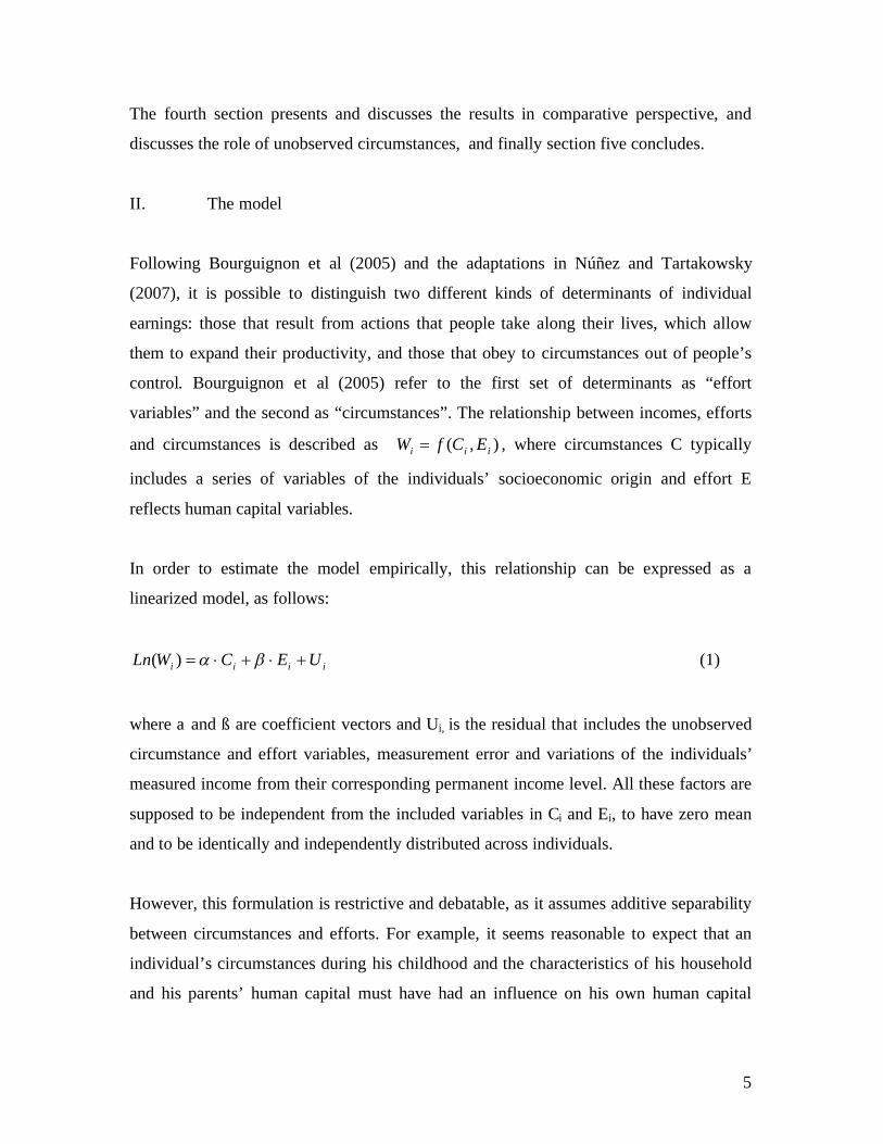
Tables 3 and 4 show the results of OLS wage equations for men and women, including

the labor market participation equation for women to address the standard selection bias.

All specifications show the standard effects of schooling and potential experience on

earnings. In addition, Tables 3 and 4 indicate that parental schooling has a significant

effect on earnings, of about 50 to 60 per cent for offspring of university-educated parents,

relative to offspring of parents with incomplete primary schooling.12 In addition, Tables 3

and 4 show that Amerindian ancestry is associated with about 10 to 15 per cent lower

wages. Municipality characteristics do not have a robust effect once other circumstance

variables are included. We employ specification 3 of Tables 3 and 4 for the simulation of

individual incomes based on the four circumstance-equalizing benchmarks described

above.


b. Simulated income distribution coefficients

Using the results of specifications 2 in Tables 1 and 2 and of specifications 3 in Tables 3

and 4, we performed the four circumstance-equalizing benchmarks described above in

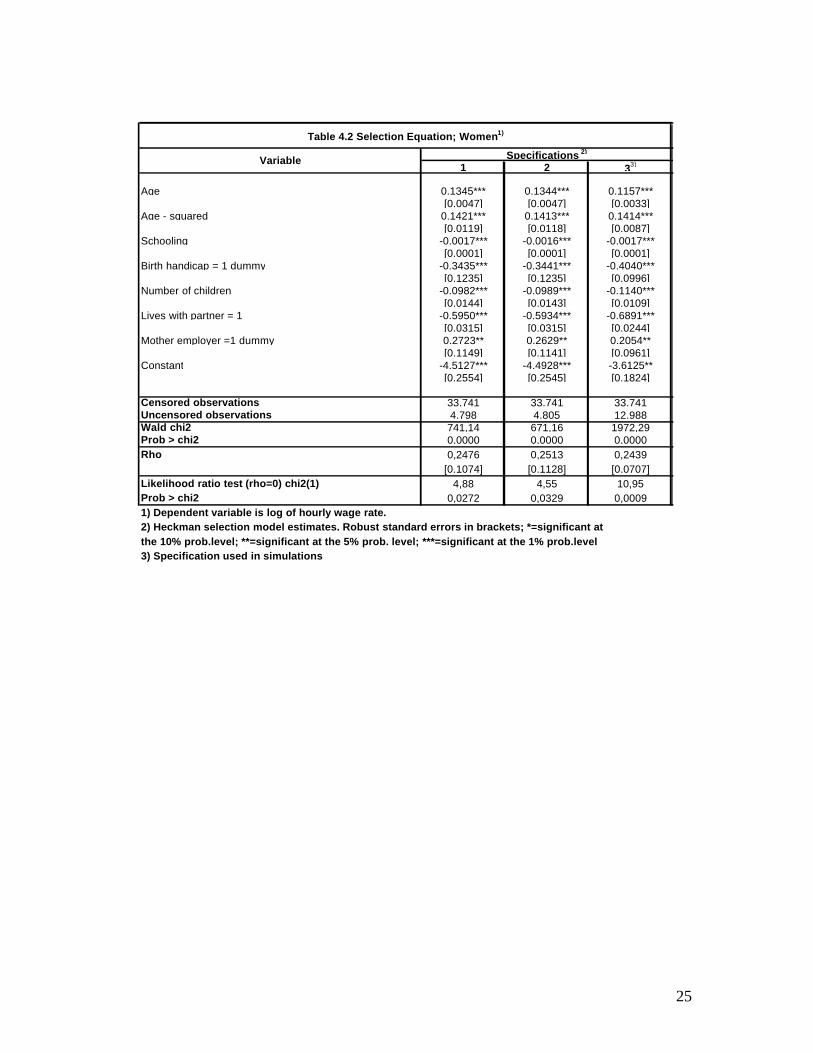
order to compute the simulated income distribution coefficients. Tables 5 to 7 report the

12 This is consistent with the finding reported by Bravo, Contreras and Medrano (1999), who report statistically significant coefficients of about 0.02 and 0.01 for the father’s and the mother’s schooling on their sons’ earnings, respectively.

13

results for the Gini coefficient and the top/bottom quintiles ratios, including bootstrap-

generated 95 per cent confidence intervals for each inequality measure.13

Tables 5-7 report Gini coefficients for the actual (observed) inequality of 0.54, 0.5 for

women and 0.53 for men, women and total population, respectively, consistent with the

known values for Chile.14 They also indicates that the Gini coefficient for the younger

cohorts is lower, which may be a consequence of earnings profiles being less

heterogeneous early in the life cycle.

[Insert Tables 5, 6 and 7 about here]

Tables 5-7 indicate that the Partial Effect associated with a wide and diverse set of

observed circumstances explain about 4 and 5 points of the Gini coefficients for men and

women, respectively, which represent drops of about 8 to 10 per cent. The Total Effect,

in turn, yields a drop of about 7-8 points of the Gini coefficient, about 14-16 percent drop

for men and women. These results indicate that part of the observed income inequality in

Chile is associated with inequalities in the set of circumstances of origin employed in this

work. However, these results also suggest that, after equalizing this wide and diverse set

of observed circumstances, a significant amount of income inequality remains, in fact

about 85 per cent of it. Another significant feature of the results in Table 1 is that the

Partial and the Total effects of observed circumstances yield rather similar changes in

income inequality, suggesting that the direct effect of circumstances on earnings and the

indirect effect of them on schooling are of a similar order of magnitude in their effect on

the income distribution.

Regarding the two additional circumstance-equalizing benchmarks described above,

Tables 5 to 7 indicate that guaranteeing 10 years of schooling would yield similar income

inequality to the Total effect, a fall of about 7-9 points in the Gini coefficient. Finally, the

13 Confidence intervals were computed using a bootstrap method. We generated 200 estimates for each inequality coefficient. The reported value of the inequality coefficient is the average of the sampling distribution, and the confidence intervals were built from the values between percentile 2.5 and 97.5 of the distribution.14 See for example Ferranti, Perry, Ferreira and Walton (2003).

14

rather extreme situation of equalizing schooling at complete secondary education for

everyone (close to Chile’s average schooling of 10.5 years for adults in 23-65 age range)

reduces the Gini coefficient in about 11-13 points that is, about a 22-25 per cent fall.

Even though this equalizing exercise may seem extreme, it reinforces the idea that still a

significant amount of income inequality would persist even under these circumstances.

We report the results also for the Theil coefficient for men and women in Table 8. In this

case the Partial and Total Effects explain about 9 and 15 points of the Theil coefficient,

respectively, representing falls of about 16 and 26 per cent. Table 8 also report that 10

years of schooling guaranteed yields a drop of about 6 points of the Theil coefficient,

equivalent to a 28 per cent fall. Equalizing schooling at complete secondary education

reduces the Theil coefficient in about 23 points, implying almost a 40 per cent fall.

Hence, as noted in other studies, the influence of observed circumstances seems to have a

larger relative effect on the Theil coefficient than on the Gini coefficient.

[Insert Tables 8 about here]

It is interesting to note that the results reported in Tables 5-8 are similar to the results

obtained by Bourguignon et. al. (2005) for Brazil, who employ parental schooling and

race as circumstances of origin. In their study, the Partial and Total effects for adult men

and women are approximately 5 and 10 points of the Gini coefficient, which amount to

falls of about 9 and 18 per cent. In addition, the results of Table 5 (for men) are also

similar to the results in Núñez and Tartakowsky (2007) study conducted only on adult

men in Greater Santiago, Chile’s capital city. In that study, which also employs parental

schooling and household size and composition as circumstances of origin, the Partial and

Total effects are 7 and 8 points of the Gini coefficient, respectively. These comparisons

suggest that the larger set of circumstance variables employed here do not seem to yield

higher orders of magnitude of the Partial and Total effects.

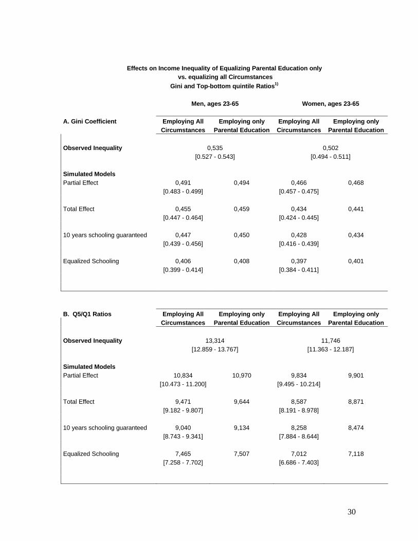
In order to explore this issue further, Table 9 presents the effects on income inequality of

equalizing parental education only vs. equalizing all observed circumstances, including

15

ethnicity, income and urban-rural composition of the respondents’ municipality of origin,

size and composition (mono-parental vs. bi-parental) of the household of origin, parental

employment features, all in addition to parental education. The purpose of this exercise is

to compare the effects of equalizing a larger and more diverse set of circumstances of

origin with those of equalizing parental education only, as if all the circumstances other

that parental education remained “unobserved”. This exercise informs us about the

marginal effect on income distribution of equalizing all the circumstances other than

parental education, once this latter dimension has been already equalized.

Columns 2 and 4 of Table 9 presents the effects on income inequality of equalizing all

circumstances for men and women, respectively, as in column 5 of Tables 5 and 6.

Columns 3 and 5 of Table 9, in turn, report the results of equalizing parental education

only for men and women, respectively.

[Insert Table 9 about here]

Table 9 shows that, as expected, the simulated inequality derived from equalizing

parental education only is indeed higher that equalizing all the circumstance variables

(including parental education) for all four circumstance-equalizing benchmarks. This

indicates that all circumstances other than parental education contribute to income

inequality, in addition to the effect associated with parental education, pattern that is

observed for both men and women. Yet, the additional effect on the simulated income

inequality associated with the circumstances other than parental schooling is small, about

half a point of the Gini coefficient for the total effect, which represents a small fraction of

what equalizing parental education achieves on its own. Moreover, note that the values

of the simulated inequality indicators derived from equalizing parental education only

always falls within the confidence interval of the inequality coefficients obtained from

equalizing all observed circumstances. This indicates that the differences of the simulated

inequality values for all four equalizing benchmarks are low and statistically similar.

16

These results reinforce the idea that the effect of unobserved circumstances on inequality

may be limited. Indeed, the evidence in Table 9 suggests that, adding to parental

education a larger and more diverse set of circumstances such as the ones considered here

(“as if” they were initially unobserved), adds little in explaining income inequality. Of

course, it is certainly possible that other key circumstances may not be included in this set

of circumstances, but considering the relevance and diversity of these circumstances,

these results are nevertheless suggestive.15

The idea that unobserved circumstances have a limited role in shaping income inequality

is coherent with evidence in the related literature. For example, Behrman and

Rosenzweig (2004) suggest that the influence of unobserved circumstances (fixed family

background) on the offspring’s performance is indeed important, indicating that a part of

the income inequality obtained after equalizing observed circumstances may indeed be

associated with unobserved circumstances. However, in an earlier related study, Behrman

and Rosenzweig (2002) also suggest that maternal schooling seems to proxy some

important unobserved factors associated with family background. This evidence,

consistent with the evidence in Table 9, would suggest that the observed circumstances

employed in this work are likely to capture the effect of important unobserved

circumstances associated with family background. In fact, Núñez and Tartakowsky

(2007) employ data for Greater Santiago to show that parental schooling is highly

associated with other circumstances of origin, namely parents’ involvement in their

offspring´s progress at school, attendance to a private vs. a public school, access to

sanitation during infancy, parent’s reading and writing skills, growing in an urban vs. a

rural environment, parents’ ethnicity (amerindian vs. non-amerindian), and access to pre-

school education during infancy. This reinforces the idea that parental schooling and

possibly the other circumstances of origin employed in this work are likely to capture the

effects of a variety of relevant unobserved circumstances of origin than may have an

15 This result also suggests a promising perspective for studying “equality of opportunities” and the influence of circumstances of origin on observed inequality from a comparative perspective employing a restricted set of common circumstances that includes parental education as an essential single one.

17

impact on income distribution, at least many of those that can be affected by public

action.

V. Conclusions

This paper has examined the extent to which income inequality is associated to

inequalities in a large and diverse set of observed circumstances of origin, including

parental schooling, ethnic background, household size and composition (single vs. a bi-

parental), parental occupations, income and urban/rural composition of the Municipality

of origin. We find that after equalizing individual circumstances to the mean values of the

population, the resulting standard income distribution indicators become more

egalitarian, indicating that a part of income inequality does indeed reflect inequalities of

circumstances of origin. Yet, a large amount of income inequality is not associated with

inequality in these observed circumstances. In particular, after equalizing observed

circumstances, the Gini coefficient decreases in about 7-8 percentage points, representing

approximately a fall of 15 per cent. About half of this variation is associated with the

direct effect of observed circumstances of origin on earnings, while the remaining part is

associated with its indirect effect on earnings through the accumulation of schooling.

These results are similar to those obtained by Bourguignon et al (2005) for Brazil and

Núñez and Tartakowsky (2007) in Chile, despite the wider the set of observed

circumstances employed here.

This paper also finds that a significant amount of income inequality persists even after

equalizing individuals’ schooling to the population mean, to reflect an hypothetical

extreme situation where all schooling is tacitly assumed to depend on circumstances-

either observed or unobserved. Likewise, guaranteeing all individuals 10 years of

schooling to account for adverse unobserved circumstances of those who achieve less

than 10 years of schooling, yield similar results to the total effect. Further on the

influence of unobserved circumstances on inequality, we find that adding a large set of

circumstances to parental schooling adds little to the effect on income inequality that

18

parental schooling achieves on its own. These results jointly suggest a limited influence

of unobserved circumstances on income distribution.

These results suggest that, as long as the exercise of equalizing observed circumstances is

an accepted approximation of the notion of “equality of opportunities”, then income

inequality indicators may not necessarily reflect adequately a country’s degree of equality

of opportunities, as income inequality may be also reflecting aspects such as individual

“effort”, preferences, choices, sheer luck and possibly transitory shocks in income and

income measurement errors. This, in turn, suggests implications for public policy,

depending on the preferred moral standpoint in the equality-of-outcomes vs. equality-of-

opportunities debate: Promoting equality of outcomes would require more than trying to

equalize circumstances and “opportunities” across individuals, and in consequence

additional redistributive policies are likely to be needed. On the other hand, advocates of

equality of opportunities must be ready to accept that promoting equal opportunities is

likely to yield a significant amount of income inequality. However, a challenging agenda

remains ahead to distinguish more precisely the roles of unobserved circumstances and

the consequences of individual choices and preferences, as well as other sources of

variation in measured incomes.

VI. References

Alesina, Alberto, Di Tella, Rafael and Robert MacCulloch (2004), “Inequality and Happiness: Are Europeans and Americans Different?” Journal of Public Economics88(9-10), pp. 2009-42.

Behrman, J. and M. Rosenzweig (2002) “Does increasing women’s schooling raise the schooling of the next generation?”, American Economic Review 92:1, pp. 323-334.

Behrman, J. and M. Rosenzweig (2004) “Returns to Birthweight”, Review of Economics and Statistics, 86:2, pp. 586-601.

Behrman, J. (2006), “How Much Might Human Capital Policies Affect Earnings Inequalities and Poverty?”, IDB-University of Chile Workshop on Income Inequality, December 2006.

19

Bourguignon, François, Ferreira, Francisco and Marta Menendez (2005), “Inequality of Opportunity in Brazil?” World Bank. Washington, D.C.

Bravo, D., Contreras, D. y P. Medrano (1999), "Measurement error, unobservables and skill bias in estimating the return to education in Chile", Department of EconomicsUniversidad de Chile.

De Ferranti, D., Perry, G., Ferreira F., and M. Walton (2003), Inequality in Latin America and the Caribbean. Breaking with History?. The International Bank for Reconstruction and Development/The World Bank, Washington DC.

Dworkin, R. (1981), “What is Equality? Part 2: Equality of Resources”, Philosophy and Public Affairs, 10(3): 283-345.Núñez, J. and R. Gutiérrez (2004) “Class discrimination and meritocracy in the labor market: evidence from Chile” Estudios de Economía, 31:2, pp. 113-132.

Núñez, J. and A. Tartakowsky (2007) “Inequality of Outcomes vs. Inequality of Opportunities in a Developing Country. An exploratory analysis for Chile”, Estudios de Economía, Vol. 34, Nº 2, pp.185-202.

Núñez, J. and L. Miranda (2007), “Recent findings in intergenerational income and educational mobility in Chile”. IDB-University of Chile Workshop on Income Inequality, December 2006, and Documento de Trabajo N 244, Department of Economics, Universidad de Chile.

Nussbaum, M. and A. Sen (2000), La Calidad de Vida, Fondo de Cultura Económica, Ciudad de Mexico.

Rawls, John (1971), A Theory of Justice. Cambridge, MA: Harvard University Press.

Ruiz Tagle, J. (2007), “Forecasting Income Inequality”, forthcoming in Estudios de Economia.

Roemer, John E. (1996), Theories of Distributive Justice. Cambridge, MA: Harvard University Press.

Roemer, John E. (1998), Equality of Opportunity, Cambridge, MA: Harvard University Press.

Roemer, John E. (2000), “Equality of Opportunity”, in Meritocracy and Economic Inequality, Keneth Arrow, Samuel Bowles and Steven Durlauf, editors, Princeton University Press, New Jersey.

Sen, A. (1999), Development as Freedom, Knopf, New York.

20

World Bank (2005), Equity and Development, World Development Report 2006, The World Bank and Oxford University Press, New York.

21

1 23)

Personal characteristicsAge -0.0551*** -0.0544***

[0.0030] [0.0030]Birth handicap = 1 dummy -1.0665*** -1.2412***

[0.3639] [0.3496]Amerindian ethnic group=1 dummy -0.6554*** -0.6337***

[0.1706] [0.1696]Parental schoolingfather's primary education = 1 dummy 1.1927*** 1.1560***

[0.1260] [0.1249]father's secondary schooling =1 dummy 2.5465*** 2.5443***

[0.1408] [0.1397]father's technical education=1 dummy 4.1030*** 4.0781***

[0.1884] [0.1874]father's university education=1 dummy 4.8102*** 4.8245***

[0.1801] [0.1788]mother's primary education=1 dummy 0.8596*** 0.8778***

[0.1212] [0.1203]mother's secondary education = 1 dummy 1.9119*** 1.9330*

[0.1382] [0.1374]mother's technical education = 1 dummy 1.8882*** 1.9410***

[0.2154] [0.2135]mother's university education = 1 dummy 2.0429*** 2.0634***

[0.1855] [0.1839]Childhood household attributesHousehold size -0.1244*** -0.1218***

[0.0108] [0.0107]Biparental household = 1 dummy 0.6122*** 0.6333***

[0.0899] [0.0860]Father employer dummy 0.1219

[0.1483]Mother employer = 1 dummy 1.1680*** 1.2447***

[0.2572] [0.2365]Childhood household location characteristicsIncome of municipality of origin 0.0000***

[0.0000]Rural population in municipality of origin -1.6350*** -1.6118***

[0.1642] [0.1619]

Constant 11.4796*** 11.4108***[0.1851] [0.1814]

Sample size 10.737 10.988R-squared 0,3743 0,3746Adjusted R-squared 0,3733 0,3737

3) Specification used in simulations

2) OLS estimates standard errors in brackets; *=significant at the 10% prob.level; **=significant at the 5% prob. level; ***=significant at the 1% prob.level

Table 1. Schooling Determinants; Men1)

Variable Specifications 2)

1) Dependent variable is years of schooling.

22

1 23)

Personal charasteristicsAge -0.0782*** -0.0780***


[0.2268] [0.2204]Amerindian ethnic group=1 dummy -0.3775*** -0.3547**






[0.0966] [0.0946]mother's secondary education = 1 dummy 2.3641*** 2.3450***





[0.0766] [0.0731]Father employer dummy -0.0652




[0.1375] [0.1351]

Constant 11.7688*** 11.7163***[0.1549] [0.1509]




Table 2. Schooling Determinants; Women1)



23

1 2 33)

Schooling returnPrimary education 0.0391*** 0.0396*** 0.0422***

[0.0080] [0.0080] [0.0039]Secondary education 0.0390*** 0.0403*** 0.0486***

[0.0120] [0.0120] [0.0060]Tertiary education 0.1148*** 0.1166*** 0.1001***

[0.0087] [0.0087] [0.0048]Experience variablesPotential experience 0.0339*** 0.0344*** 0.0311***

[0.0028] [0.0028] [0.0015]Potential experience - squared -0.0004*** -0.0004*** -0.0003***

[0.0001] [0.0001] [0.0000]Personal charasteristicsBirth handicap = 1 dummy -0.1633* -0.1694* -0.2468***

[0.0935] [0.0937] [0.0477]Amerindian ethnic group=1 dummy -0.1005** -0.1066*** -0.1441***

[0.0403] [0.0403] [0.0186]Parental schoolingfather's primary education = 1 dummy 0.0122 0.0341**

[0.0305] [0.0159]father's secondary schooling = 1 dummy 0.0052 0.0901***

[0.0341] [0.0188]father's technical education=1 dummy 0.073 0.1549***

[0.0459] [0.0275]father's university education=1 dummy 0.2792*** 0.2778*** 0.3711***

[0.0445] [0.0323] [0.0262]mother's primary education=1 dummy -0.01 0.0479***

[0.0291] [0.0153]mother's secondary education = 1 dummy 0.1896*** 0.2059*** 0.1916***

[0.0331] [0.0187] [0.0187]mother's technical education = 1 dummy 0.2010*** 0.2362*** 0.2417***

[0.0509] [0.0418] [0.0309]mother's university education = 1 dummy 0.1506*** 0.1808*** 0.2236***

[0.0442] [0.0362] [0.0265]Childhood household attributesHousehold size -0.004 -0.0060***

[0.0027] [0.0015]Biparental household = 1 dummy 0.0779*** 0.0724*** 0.0484***

[0.0218] [0.0211] [0.0127]Father employer dummy 0.1113*** 0.1194*** 0.0989***

[0.0354] [0.0355] [0.0203]Mother employer = 1 dummy 0.2092*** 0.2101*** 0.2533***

[0.0618] [0.0618] [0.0363]

Childhood household location characteristicsIncome of municipality of origin 0.0000***

[0.0000]Rural population in municipality of origin -0.0891** -0.1724***

[0.0398] [0.0381]

Constant 5.8547*** 5.8885*** 5.779***[0.0666] [0.0650] [0.0339]

Sample size 8452 8452 24.891R-squared 0.4293 0.4255 0,4312Adjusted R-squared 0.4279 0.4245 0,4308

2) OLS estimates standard errors in brackets; *=significant at the 10% prob.level; **=significant at the 5% prob. level; ***=significant at the 1% prob.level3) Specification used in simulations

Table 3. Wage Equations; Men1)


1) Dependent variable is log of hourly wage rate.

24

1 2 33)


[0.0277] [0.0272] [0.0128]Secondary education -0.0156 -0.0047 0.0261



[0.0062] [0.0061] [0.0037]Potential experience - squared -0.0003** -0.0003** -0.0003***

[0.0001] [0.0001] [0.0001]Personal charasteristicsBirth handicap = 1 dummy -0.2073** -0.1883** -0.1789***

[0.0848] [0.0827] [0.0591]Amerindian ethnic group=1 dummy -0.1561*** -0.1799*** -0.1222***





[0.0811] [0.0568] [0.0534]mother's primary education=1 dummy 0.02

[0.0542]mother's secondary education = 1 dummy 0.1354*** 0.1353***

[0.0697] [0.0316]mother's technical education = 1 dummy 0.0616 0.0746

[0.0904] [0.0533]mother's university education = 1 dummy 0.275 0.1940*** 0.2895***

[0.0961] [0.0736] [0.0603]Childhood household attributesHousehold size 0.0005

[0.0053]Biparental household = 1 dummy -0.0101

[0.0446]Father employer dummy 0.2060*** 0.2353*** 0.1975***

[0.0661] [0.0656] [0.0439]Mother employer = 1 dummy 0.0889

[0.1221]Childhood household location characteristicsIncome of municipality of origin 0.0000***

[0.0000]Rural population in municipality of origin -0.1333* -0.1769***

[0.0688] [0.0664]

Constant 5.1827*** 5.2504 5.3409***[0.2541] [0.2639] [0.1187]

Table 4.1 Wage Equations; Women1)


1) Dependent variable is log of hourly wage rate. 2) Heckman selection model estimates. Robust standard errors in brackets; *=significant at the 10% prob.level; **=significant at the 5% prob. level; ***=significant at the 1% prob.level3) Specification used in simulations

25

1 2 33)

Age 0.1345*** 0.1344*** 0.1157***[0.0047] [0.0047] [0.0033]

Age - squared 0.1421*** 0.1413*** 0.1414***[0.0119] [0.0118] [0.0087]

Schooling -0.0017*** -0.0016*** -0.0017***[0.0001] [0.0001] [0.0001]

Birth handicap = 1 dummy -0.3435*** -0.3441*** -0.4040***[0.1235] [0.1235] [0.0996]

Number of children -0.0982*** -0.0989*** -0.1140***[0.0144] [0.0143] [0.0109]

Lives with partner = 1 -0.5950*** -0.5934*** -0.6891***[0.0315] [0.0315] [0.0244]

Mother employer =1 dummy 0.2723** 0.2629** 0.2054**[0.1149] [0.1141] [0.0961]

Constant -4.5127*** -4.4928*** -3.6125**[0.2554] [0.2545] [0.1824]

Censored observations 33.741 33.741 33.741Uncensored observations 4.798 4.805 12.988Wald chi2 741,14 671,16 1972,29Prob > chi2 0,0000 0,0000 0,0000Rho 0,2476 0,2513 0,2439

[0.1074] [0.1128] [0.0707]Likelihood ratio test (rho=0) chi2(1) 4,88 4,55 10,95Prob > chi2 0,0272 0,0329 0,0009




2) Heckman selection model estimates. Robust standard errors in brackets; *=significant at the 10% prob.level; **=significant at the 5% prob. level; ***=significant at the 1% prob.level

Table 4.2 Selection Equation; Women1)

26

Gini Coefficient Age= 23-36 Age=37-50 Age=51-65 Age=23-65

Total Inequality (W) 0.481 0.511 0.608 0.535[0.474 - 0.488] [0.503 - 0.518] [0.601 - 0.615] [0.527 - 0.543]

Simulated Models Partial Effect (W P ) 0.436 0.47 0.557 0.491

[0.429 - 0.442] [0.463 - 0.477] [0.550 - 0.563] [0.483 - 0.499]

Total Effect (W T ) 0.395 0.441 0.503 0.455[0.389 - 0.401] [0.433 - 0.451] [0.496 - 0.511] [0.447 - 0.464]

10 Years of Schooling Guaranteed (W SG ) 0.389 0.434 0.487 0.447[0.384 - 0.395] [0.426 - 0.443] [0.479 - 0.495] [0.439 - 0.456]

Equalized Schooling (W ES ) 0.353 0.396 0.436 0.406[0.347 - 0.358] [0.388 - 0.403] [0.429 - 0.442] [0.399 - 0.414]

Q5/Q1 Quintile Ratio Age= 23-36 Age=37-50 Age=51-65 Age=23-65



[7.955 - 8.421] [9.825 - 10.437] [14.665 - 15.668] [10.473 - 11.200]

Total Effect (W T ) 7.267 8.933 11.909 9.471[7.085 - 7.435] [8.637 - 9.280] [11.543 - 12.329] [9.182 - 9.807]



1) 95 per cent confidence Intervals in brackets, obtained by bootstrapping.

Table 5. Effects of Equalizing Circumstances on Labor Income Inequality, MenGini and Top-Bottom Quintile Ratio1)

27




[0.389 - 0.400] [0.477 - 0.495] [0.507 - 0.529] [0.457 - 0.475]

Total Effect (W T ) 0.362 0.442 0.488 0.434[0.355 - 0.369] [0.433 - 0.453] [0.475 - 0.503] [0.424 - 0.445]






[6.932 - 7.325] [10.187 - 11.070] [13.213 - 14.601] [9.495 - 10.214]

Total Effect (W T ) 6.133 8.959 12.086 8.587[5.934 - 6.342] [8.564 - 9.327] [11.421 - 12.901] [8.191 - 8.978]




Table 6. Effects of Equalizing Circumstances on Labor Income Inequality, WomenGini and Top-Bottom Quintile Ratio1)

28




[0.420 - 0.430] [0.478 - 0.488] [0.547 - 0.559] [0.483 - 0.496]

Total Effect (W T ) 0.391 0.451 0.505 0.457[0.387 - 0.395] [0.445 - 0.458] [0.498 - 0.512] [0.450 - 0.464]






[7.762 - 8.138] [10.540 - 11.061] [15.087 - 15.935] [10.634 - 11.190]

Total Effect (W T ) 7.042 9.422 12.411 9.576[6.903 - 7.180] [9.187 - 9.704] [12.042 - 12.798] [9.324 - 9.880]

10 Years of Schooling Guaranteed (W SG ) 6.846 8.964 11.248 9.176[6.716 - 6.976] [8.740 - 9.238] [10.890 - 11-617] [8.920 - 9.470]


1) 95 per cent confidence Intervals in brackets, obtained by bootstrapping

Table 7. Effects of Equalizing Circumstances on Labor Income Inequality, Men and Women Gini and Top-Bottom Quintile Ratio1)

29

Theil Coefficient Age= 23-36 Age=37-50 Age=51-65 Age=23-65



[0.330 - 0.357] [0.437 - 0.478] [0.597 - 0.639] [0.460 - 0.503]

Total Effect (W T ) 0.287 0.397 0.531 0.423[0.278 - 0.296] [0.375 - 0.426] [0.507 - 0.558] [0.400 - 0.449]

10 Years of Schooling Guaranteed (W SG ) 0.280 0.388 0.504 0.414[0.271 - 0.289] [0.366 - 0.416] [0.478 -0.534] [0.390 - 0.440]


D10/D1 Decile Ratio Age= 23-36 Age=37-50 Age=51-65 Age=23-65



[13.041 - 13.902] [18.470 - 19.580] [29.490 - 31.811] [19.104 - 20.431]

Total Effect (W T ) 12.163 16.885 24.702 17.657[11.782 - 12.565] [16.227 - 17.350] [23.699 - 25.708] [17.059 - 18.440]




Table 8. Effects of Equalizing Circumstances on Labor Income Inequality, Men and Women Theil Index, and Top-Bottom Decile Ratio1)

30

Effects on Income Inequality of Equalizing Parental Education only vs. equalizing all Circumstances

Gini and Top-bottom quintile Ratios1)

Men, ages 23-65 Women, ages 23-65

A. Gini Coefficient Employing All Employing only Employing All Employing onlyCircumstances Parental Education Circumstances Parental Education

Observed Inequality 0,535 0,502[0.527 - 0.543] [0.494 - 0.511]

Simulated Models Partial Effect 0,491 0,494 0,466 0,468

[0.483 - 0.499] [0.457 - 0.475]

Total Effect 0,455 0,459 0,434 0,441[0.447 - 0.464] [0.424 - 0.445]

10 years schooling guaranteed 0,447 0,450 0,428 0,434[0.439 - 0.456] [0.416 - 0.439]

Equalized Schooling 0,406 0,408 0,397 0,401[0.399 - 0.414] [0.384 - 0.411]

B. Q5/Q1 Ratios Employing All Employing only Employing All Employing onlyCircumstances Parental Education Circumstances Parental Education



[10.473 - 11.200] [9.495 - 10.214]

Total Effect 9,471 9,644 8,587 8,871[9.182 - 9.807] [8.191 - 8.978]



THE RELATIONSHIP BETWEEN INEQUALITY OF OUTCOMES AND INEQUALITY OF OPPORTUNITIES IN A HIGH-INEQUALITY COUNTRY: THE CASE OF CHILE

Autores: Javier Núñez y Andrea Tartakowsky

Santiago, Enero 2009

SDT 292

Serie Documentos de TrabajoN 292

The relationship between Inequality of Outcomes and Inequality of Opportunities in a high-inequality country:

The case of Chile1

Javier Núñez Andrea Tartakowsky

Abstract

Based on the methodology developed by Bourguignon, Melendez and Ferreira (2005) we explore the extent to which income inequality in Chile is associated with inequality of observed exogenous circumstances of origin, which shape individuals “opportunities” to pursue their chosen life plans. We find that equalizing a diverse set of observed circumstances of origin across individuals such as parents’ schooling and employment, household size and composition, ethnic background and features of the municipality of origin reduces the Gini coefficient in about 7-8 percentage points. About half of this effect is transmitted directly on earnings, while the remaining part through its indirect effect on the accumulation of schooling. Further results suggest that the influence of unobserved circumstances on income distribution may be limited, and hence aspects such as preferences, effort, luck, income shocks and income measurement errors may also be important factors behind income inequality, issue that awaits further research.

JEL classification:

D31, D63

Keywords:

Income Inequality, Equality of Opportunities.

1 We are grateful to Jeremy Behrman and Esteban Puentes for all their very valuable and helpful comments. As usual, the authors are responsible for all errors.

3

I. Introduction

An old normative debate has existed around the question of what kind of economic

inequality should public policies aim to reduce. While many authors have leaned towards

dealing with the inequality of “outcomes” (i.e. income inequality), other traditions have

instead proposed that public policies should promote “equality of opportunities” across

individuals.2 This debate has benefited from various conceptual and philosophical

contributions, yet limited insights have been gained from empirical perspectives.

Building upon the methodology developed by Bourguignon, Melendez and Ferreira

(2005), this paper aims to contribute to this debate by empirically examining the extent to

which observed income inequality is associated with the inequality of circumstances of

origin that shape individuals´ opportunities.

The idea of equality of opportunities rests on the notion that individuals should be

entitled to similar opportunities to pursue their desired life plans, which in turn requires

that those opportunities not be determined by circumstances of origin that individuals

inherit without their consent, such as, for example, parental and family background.

Equal opportunities advocates have argued that differences in economic outcomes (i.e.

income inequality) partly reflect differences in dimensions controlled by individuals,

such as effort, responsibility, choices and so on. Accordingly, public policies should aim

to equalize the exogenous circumstances that shape individuals’ opportunities that

constrain their choices, and then accept the resulting level of income inequality that

would emerge from individuals’ choices and preferences. With variations, this has

somewhat become the dominant view of the notion of equity that deserves legitimate

public action, as suggested, for example, by The World Banks’ 2005 Report on Equity

and Development:

2 See for example Roemer (1996), (1998) and (2000) and Dworking (1981) for descriptions of the notions of equality of opportunities and of outcomes. Also, Amartya Sen’s Capability approach has a resemblance with the notion of equality of opportunities, as described for example in Sen (1999) and Nussbaum and Sen (2000). See Roemer (1996) for a discussion of the main theories of distributive justice. See also Alessina, Di Tella and MacCulloch (2004) for a discussion on different attitudes between Europeans and Americans towards different notions of equality.

4

"By equity we mean that individuals should have equal opportunities to pursue a life of

their choosing and be spared from extreme deprivation in outcomes", (p. 2)3

Yet, little is known about the extent to which income inequality reflects individual

choices and preferences vs. the exogenous circumstances that individuals inherit.

Empirical investigation of the relationship between “opportunities” and “outcomes” is

relevant for various reasons. First, the practical implications of the philosophical

distinction between “opportunities” and “outcomes” would be less significant if both

were empirically associated. This would reinforce the interpretation of income

distribution indicators as good measures of both equality of outcomes and equality of

opportunities. This scenario would also suggest a more significant role for the individual

circumstances of origin versus individual choices and preferences, as a means of jointly

promoting equality of outcomes and of opportunities in the long run. If, on the contrary,

exogenous circumstances empirically played a limited role in shaping income inequality,

then this would have different implications depending on the chosen normative

standpoint: advocates of equality of opportunities should expect and accept that a

significant amount of income inequality would remain upon equalizing opportunities.

Advocates of equality of outcomes, in turn, should realize that achieving this aim would

require more than policies intended to equalize opportunities and circumstances, and that

some additional, purely redistributive policies would be needed.

For this task we follow Bourguignon et al (2005) pioneering work, which attempts to

establish the effect of circumstances of origin vs. individual “effort” in the determination

of income inequality in Brazil.4 In their work, a double role is played by circumstances:

3 On page 3 of the overview this view is reinforced in these passages: "Three considerations are important at the outset. First, while more even playing fields are likely to lead to lower observed inequalities in educational attainment, health status and incomes, the policy aim is not equality in outcomes"….” Second a concern with equality of opportunities implies that public action should focus on the distributions of assets, economic opportunities, and political voice, rather than directly on inequality in incomes. “

4 Behrman (2006) and Ruiz Tagle (2007) also examine the role of schooling on income inequality, although employing a framework different to that developed by Bourguignon et. al., which allows establishing and separating the direct and indirect effects of observed circumstances on income inequality. However, their results are similar to the results found in this work, in the sense that both studies suggest a limited role of schooling in reducing income inequality.

5

they have a direct impact on earnings, and an indirect effect on “effort”, that they take to

be the schooling level. They define the former effect as the “partial effect” of observed

circumstances on earnings, and the “total effect” to be the joint effect of the direct and

indirect effects of observed circumstances on earnings. Our work differs from theirs in

three respects. First, we employ a larger and diverse set of circumstances of origin, which

includes parental education and employment characteristics, ethnic background,

household size and composition, and features of the municipality of origin, among others.

Second, our aim is more modest in the sense that we do not address the (more complex)

issue of the effects of “effort on income distribution, but simply attempt to establish the

effects of observed circumstances on earnings. Accordingly, we refer to the indirect

effect simply as the effect of observed circumstances on the level of schooling (not

effort), and also interpret the unexplained part of the income distribution simply as an

unknown combination of unobserved circumstances, individual effort, sheer luck and

possibly income measurement errors. Finally, we provide some circumstance-equalizing

benchmarks in addition to the “partial” and “total” effects outlined above, in order to

shed some light on the possible effects of unobserved circumstances on the income

distribution. One benchmark consists of an extreme situation where everyone’s schooling

levels only reflect individuals circumstances- either observed or unobserved-, such that

individual “merit” and “effort” play no role in the determination of schooling, which

amounts to simply computing the income distribution after equalizing schooling levels

across individuals. The second equalizing benchmark consists of guaranteeing everyone a

minimum of 10 years of schooling (completed at about age 16) and employ the simulated

level of schooling otherwise, to reflect the idea that a simulated value of schooling lower

than 10 would almost certainly reflect unobserved circumstances. In addition, we perform

other exercises to examine further the role of unobserved circumstances.

The paper is structured as follows: The next section presents the basic model and the

empirical identification strategy of the four observed circumstances-equalizing

benchmarks. The third section describes the data and the set of circumstances employed.

The fourth section presents and discusses the results in comparative perspective, and

discusses the role of unobserved circumstances, and finally section five concludes.

6

II. The model

Following Bourguignon et al (2005) and the adaptations in Núñez and Tartakowsky

(2007), it is possible to distinguish two different kinds of determinants of individual

earnings: those that result from actions that people take along their lives, which allow

them to expand their productivity, and those that obey to circumstances out of people’s

control. Bourguignon et al (2005) refer to the first set of determinants as “effort

variables” and the second as “circumstances”. The relationship between incomes, efforts

and circumstances is described as ),( iii ECfW � , where circumstances C typically

includes a series of variables of the individuals’ socioeconomic origin and effort E

reflects human capital variables.

In order to estimate the model empirically, this relationship can be expressed as a

linearized model, as follows:

iiii UECWLn �� )( (1)

where a and ß are coefficient vectors and Ui, is the residual that includes the unobserved

circumstance and effort variables, measurement error and variations of the individuals’

measured income from their corresponding permanent income level. All these factors are

supposed to be independent from the included variables in Ci and Ei, to have zero mean

and to be identically and independently distributed across individuals.

However, this formulation is restrictive and debatable, as it assumes additive separability

between circumstances and efforts. For example, it seems reasonable to expect that an

individual’s circumstances during his childhood and the characteristics of his household

and his parents’ human capital must have had an influence on his own human capital

accumulation and “effort”. Accordingly, Bourguignon et al (2005) propose “effort” to be

partly a function of circumstances:

7

iii VCBE �� (2)

where B is a coefficient matrix and Vi represents a non-observable effort determinant

vector. As usual, Vi it is supposed to have mean zero and to be i.i.d. across individuals.

Introducing equation (2) in (1) yields,

iiii UVCBWLn �� )()( (3)

The formulation in (3) is more general than model (1) since it allows the circumstance

variables to affect people’s incomes directly, as well as indirectly through its effects on

the effort variables. In particular, in model (1) the marginal effect of circumstances on

earnings amounts only to a. Bourguignon et al (2005) call this effect the “Partial Effect”

of observed circumstances on earnings. On the other hand, in model (3) the effect of

observed circumstances on earnings is B�� . This corresponds to the “Total Effect”

of observed circumstances on earnings. Note that this effect includes the partial effect of

circumstances on earnings, a, but also de indirect effect of circumstances on earnings

through “effort”, ßB. The total effect of observed circumstances on earnings is larger than

the partial effect if ßB>0, as expected.

In practice, Bourguignon et al (2005) employ schooling as their measure of “effort” Ei.

However, as discussed in the introduction we believe it is both controversial and

misleading to refer to schooling as an “effort” variable, at least in countries with known

inequality of educational opportunities. Accordingly, we have preferred to replace effort

Ei simply by individual schooling level Si. Given this new interpretation, equation (1)

would simply indicate that wages are a function of human capital (i.e. schooling),

circumstances of origin, as well as term Ui, which captures unobserved circumstances,

sheer luck, “effort” at work, deviations from permanent income, and possibly income

measurement errors. In addition, parameter ß would be more directly interpreted simply

as the return to schooling, while parameter B would reflect the effect of observed

circumstances of origin on the accumulation of schooling. For example, parameter B can

8

capture parents’ resources to invest in their son’s tertiary education, the role of cognitive

and non-cognitive abilities acquired during infancy and adolescence on the chances of

gaining access to tertiary education. In addition, parameter a would reflect the direct

effect of circumstances on earnings, for a given schooling level, or alternatively, as the

effect of circumstances on the return of a given amount of schooling. For example,

parameter a can capture the effect of the quality of education (likely to be associated with

circumstances), the role of abilities acquired in the household of origin on labor

productivity and earnings, access to social networks and even the possibility of “class

discrimination” in the labor market.5 In conclusion, this modified interpretation openly

treats “effort” as a non observable variable, which would be captured in term Vi in

equation (2).

a. Partial and Total effects of observed circumstances on income inequality

The estimation of parameters a, ß and B through an OLS estimation of equations (1) and

(2) allows performing two types of simulations of the distribution of income after

equalizing exogenous observed circumstances C. Let WP denote the simulated income

distribution associated with the “Partial Effect” described above, obtained after

equalizing all the circumstance variables across individuals in equation (1). Accordingly,

the resulting income distribution would reflect individual differences in schooling and in

the residue Ui. More formally, the hypothetical distribution WP would be derived from

the simulation of the individual incomes PiW using the following equation, and after

estimating equation (1) by OLS:

iiP

i USCWLn��

�� )( (4)

where C is the vector of population means of the circumstance variables.

An alternative hypothetical wage distribution WT associated with the “Total effect” of

observed circumstances on earnings can be obtained by equalizing all the observed

5 See for example Núñez and Gutiérrez (2004).

9

circumstance variables across individuals in equation (3), after estimating equation (1)

and (2) by OLS. The income distribution WT would thus be obtained from:

iiT

i UVCBWLn��

�� )()( (5)

where again C stands for the population means of the circumstance variables and the

coefficients are obtained from OLS estimations of equations (1) and (2) .

The comparison between the actual (observed) distribution W and distribution WP

reflects the partial effect of observed circumstances on the distribution of income, while

the comparison between W and WT provides the effect of the total effect of observed

circumstances on earnings, i.e. including the effect of observed circumstances on the

accumulation of schooling. Both measures of income inequality allows distinguishing the

part of income inequality associated with the direct influence of observed circumstances

on earnings, from the part that comes from the indirect effect of the observed

circumstances on the accumulation of schooling.

b. Two additional circumstance-equalizing benchmarks

However, a limitation of the methodology described above is that part of the income

inequality obtained after equalizing observed circumstances may still be caused by

differences in unobserved circumstances. In particular, it can be argued that unobserved

circumstances can explain part of the diversity in schooling that is not associated with

observed circumstances, �Vi. In this context, in addition to the circumstance-equalizing

propositions of Bourguignon et. al. (2005) described above, namely the partial and total

effects, we perform two additional equalizing benchmarks of the effect of circumstances

on income distribution to explore the possible role of unobserved circumstances.

Following Núñez and Tartakowsky (2009), assume an extreme hypothetical situation

where all schooling acquired by an individual were fully determined by his circumstances

of origin, either observed or unobserved. Or to phrase it more simply, assume that there is

10

no role for “effort” or “merit” in the accumulation of schooling. This situation would be

equivalent to setting the term Vi = 0 (which includes unobserved effort) for all

individuals. In this context, schooling would vary across individuals only due to the

effect of circumstances, not effort. This is equivalent to simulating individuals’ income

by replacing Ci by the population mean circumstancesC and Vi = 0 in equation (3), or

equivalently, replacing Ci and Si by C and the population mean schooling S in equation

(1), respectively.6 More formally, the simulated income distribution after equalizing

observed circumstances and schooling, WES, would be derived from the simulated

individual earnings from:

iES

i UCBWLn��

�� )()( ��

Hence, in this case the only source of variation in the simulated income distribution

would arise from term Ui in equation (1).7 8

The second additional exploratory equalizing benchmark that we carry out arises from the

observation that individuals cannot be made responsible for their human capital

accumulation in the early years of the life cycle, but they can arguably be made partly

responsible for it later in their life cycle, after some age threshold. Let ii VCBS��

��'

denote the simulated schooling of individual I after equalizing observed circumstances in

equation (2). In this context, a low level of simulated schooling level 'iS , say dropping

out of school at an early age, can be interpreted not as lack of “effort”, but as the result of

unobserved circumstances contained in iV�

. However, after some age threshold, the value

of simulated schooling 'iS will presumably reflect a combination of effort and

unobserved circumstances. Although it may seem absurd to fix a specific age threshold

after which individuals can be made partly responsible for their accumulation of

6 Note that estimating equation (2) by OLS yields K = BC .7 Note however, that term Ui can include the direct effect of unobserved circumstances on earnings. 8 However, in the earnings regressions we include potential experience as an independent variable, which adds another source of variation in the simulated incomes.

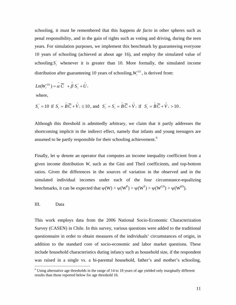
11

schooling, it must be remembered that this happens de facto in other spheres such as

penal responsibility, and in the gain of rights such as voting and driving, during the teen

years. For simulation purposes, we implement this benchmark by guaranteeing everyone

10 years of schooling (achieved at about age 16), and employ the simulated value of

schooling 'iS whenever it is greater than 10. More formally, the simulated income

distribution after guaranteeing 10 years of schooling, GSiW , is derived from:

iiGS

i USCWLn��

�� '')( ��

where,

10'' �iS if 10' ��

ii VCBS , and iii VCBSS��

�� ''' if 10' ��

ii VCBS .

Although this threshold is admittedly arbitrary, we claim that it partly addresses the

shortcoming implicit in the indirect effect, namely that infants and young teenagers are

assumed to be partly responsible for their schooling achievement.9

Finally, let � denote an operator that computes an income inequality coefficient from a

given income distribution W, such as the Gini and Theil coefficients, and top-bottom

ratios. Given the differences in the sources of variation in the observed and in the

simulated individual incomes under each of the four circumstance-equalizing

benchmarks, it can be expected that �(W) > �(WP) > �(WT) > �(WGS) > �(WES).

III. Data

This work employs data from the 2006 National Socio-Economic Characterization

Survey (CASEN) in Chile. In this survey, various questions were added to the traditional

questionnaire in order to obtain measures of the individuals’ circumstances of origin, in

addition to the standard core of socio-economic and labor market questions. These

include household characteristics during infancy such as household size, if the respondent

was raised in a single vs. a bi-parental household, father’s and mother’s schooling,

9 Using alternative age thresholds in the range of 14 to 18 years of age yielded only marginally different results than those reported below for age threshold 16.

12

ethnicity, existence of a birth handicap, municipality of origin, father and mother’s

participation in the labor market, frequency of father’s and mother’s employment, as

reported by their offspring. Besides, income and urban/rural composition of the

respondent’s municipality of origin were computed.10

The sample of sons and daughters was delimited to ages in the range from 24 to 65 years

both in the schooling regressions and earnings regressions in order to avoid possible

selectivity problems, as individuals younger than 23 may be in tertiary education and not

fully inserted in the labor market, and may not have achieved their long-run level of

schooling. Unemployed individuals or those who did not report positive incomes were

eliminated, as well as those who did not report sufficient information about the

characteristics of their parents. Finally, we considered individuals working between 30

and 72 hours per week.

IV. Results

a. Schooling and earnings regressions

Tables 1 and 2 provide the results of OLS regressions of schooling determinants for men

and women, respectively, as in equation (2) of the model.11 Tables 1 and 2 indicate that

various observed circumstances of origin have a significant effect on the accumulation of

schooling in both men and women. In particular, parental education has a strong effect on

the offspring schooling, up to approximately 6 to 7 extra years for the offspring of

university-educated parents vs. parents with incomplete primary schooling. Tables 1 and

2 also indicate that household size, being raised in a single parent household, or in poorer

and rural Municipalities decrease schooling. In conclusion, Tables 1 and 2 indicate that a

diverse set of observed circumstances of origin have a significant effect in reproducing

inequality through their impacts on the accumulation of human capital in Chile. We

10 These variables were obtained from the 1994 CASEN Survey, which is the oldest with an important number of municipalities having a representative sample.11 We performed regressions with robust standard errors for both the schooling and earnings regressions, but yielded similar result to the ones reported here.

13

employ specification 2 of Tables 1 and 2 to carry out the income simulations associated

with the circumstance-equalizing benchmarks described above.


Tables 3 and 4 show the results of OLS wage equations for men and women, including

the labor market participation equation for women to address the standard selection bias.

All specifications show the standard effects of schooling and potential experience on

earnings. In addition, Tables 3 and 4 indicate that parental schooling has a significant

effect on earnings, of about 50 to 60 per cent for offspring of university-educated parents,

relative to offspring of parents with incomplete primary schooling.12 In addition, Tables 3

and 4 show that Amerindian ancestry is associated with about 10 to 15 per cent lower

wages. Municipality characteristics do not have a robust effect once other circumstance

variables are included. We employ specification 3 of Tables 3 and 4 for the simulation of

individual incomes based on the four circumstance-equalizing benchmarks described

above.


b. Simulated income distribution coefficients

Using the results of specifications 2 in Tables 1 and 2 and of specifications 3 in Tables 3

and 4, we performed the four circumstance-equalizing benchmarks described above in

order to compute the simulated income distribution coefficients. Tables 5 to 7 report the

results for the Gini coefficient and the top/bottom quintiles ratios, including bootstrap-

generated 95 per cent confidence intervals for each inequality measure.13

12 This is consistent with the finding reported by Bravo, Contreras and Medrano (1999), who report statistically significant coefficients of about 0.02 and 0.01 for the father’s and the mother’s schooling on their sons’ earnings, respectively.13 Confidence intervals were computed using a bootstrap method. We generated 200 estimates for each inequality coefficient. The reported value of the inequality coefficient is the average of the sampling distribution, and the confidence intervals were built from the values between percentile 2.5 and 97.5 of the distribution.

14

Tables 5-7 report Gini coefficients for the actual (observed) inequality of 0.54, 0.5 for

women and 0.53 for men, women and total population, respectively, consistent with the

known values for Chile.14 They also indicates that the Gini coefficient for the younger

cohorts is lower, which may be a consequence of earnings profiles being less

heterogeneous early in the life cycle.

[Insert Tables 5, 6 and 7 about here]

Tables 5-7 indicate that the Partial Effect associated with a wide and diverse set of

observed circumstances explain about 4 and 5 points of the Gini coefficients for men and

women, respectively, which represent drops of about 8 to 10 per cent. The Total Effect,

in turn, yields a drop of about 7-8 points of the Gini coefficient, about 14-16 percent drop

for men and women. These results indicate that part of the observed income inequality in

Chile is associated with inequalities in the set of circumstances of origin employed in this

work. However, these results also suggest that, after equalizing this wide and diverse set

of observed circumstances, a significant amount of income inequality remains, in fact

about 85 per cent of it. Another significant feature of the results in Table 1 is that the

Partial and the Total effects of observed circumstances yield rather similar changes in

income inequality, suggesting that the direct effect of circumstances on earnings and the

indirect effect of them on schooling are of a similar order of magnitude in their effect on

the income distribution.

Regarding the two additional circumstance-equalizing benchmarks described above,

Tables 5 to 7 indicate that guaranteeing 10 years of schooling would yield similar income

inequality to the Total effect, a fall of about 7-9 points in the Gini coefficient. Finally, the

rather extreme situation of equalizing schooling at complete secondary education for

everyone (close to Chile’s average schooling of 10.5 years for adults in 23-65 age range)

reduces the Gini coefficient in about 11-13 points that is, about a 22-25 per cent fall.

Even though this equalizing exercise may seem extreme, it reinforces the idea that still a

significant amount of income inequality would persist even under these circumstances.

14 See for example Ferranti, Perry, Ferreira and Walton (2003).

15

We report the results also for the Theil coefficient for men and women in Table 8. In this

case the Partial and Total Effects explain about 9 and 15 points of the Theil coefficient,

respectively, representing falls of about 16 and 26 per cent. Table 8 also report that 10

years of schooling guaranteed yields a drop of about 6 points of the Theil coefficient,

equivalent to a 28 per cent fall. Equalizing schooling at complete secondary education

reduces the Theil coefficient in about 23 points, implying almost a 40 per cent fall.

Hence, as noted in other studies, the influence of observed circumstances seems to have a

larger relative effect on the Theil coefficient than on the Gini coefficient.

[Insert Tables 8 about here]

It is interesting to note that the results reported in Tables 5-8 are similar to the results

obtained by Bourguignon et. al. (2005) for Brazil, who employ parental schooling and

race as circumstances of origin. In their study, the Partial and Total effects for adult men

and women are approximately 5 and 10 points of the Gini coefficient, which amount to

falls of about 9 and 18 per cent. In addition, the results of Table 5 (for men) are also

similar to the results in Núñez and Tartakowsky (2007) study conducted only on adult

men in Greater Santiago, Chile’s capital city. In that study, which also employs parental

schooling and household size and composition as circumstances of origin, the Partial and

Total effects are 7 and 8 points of the Gini coefficient, respectively. These comparisons

suggest that the larger set of circumstance variables employed here do not seem to yield

higher orders of magnitude of the Partial and Total effects.

In order to explore this issue further, Table 9 presents the effects on income inequality of

equalizing parental education only vs. equalizing all observed circumstances, including

ethnicity, income and urban-rural composition of the respondents’ municipality of origin,

size and composition (mono-parental vs. bi-parental) of the household of origin, parental

employment features, all in addition to parental education. The purpose of this exercise is

to compare the effects of equalizing a larger and more diverse set of circumstances of

origin with those of equalizing parental education only, as if all the circumstances other

16

that parental education remained “unobserved”. This exercise informs us about the

marginal effect on income distribution of equalizing all the circumstances other than

parental education, once this latter dimension has been already equalized.

Columns 2 and 4 of Table 9 presents the effects on income inequality of equalizing all

circumstances for men and women, respectively, as in column 5 of Tables 5 and 6.

Columns 3 and 5 of Table 9, in turn, report the results of equalizing parental education

only for men and women, respectively.

[Insert Table 9 about here]

Table 9 shows that, as expected, the simulated inequality derived from equalizing

parental education only is indeed higher that equalizing all the circumstance variables

(including parental education) for all four circumstance-equalizing benchmarks. This

indicates that all circumstances other than parental education contribute to income

inequality, in addition to the effect associated with parental education, pattern that is

observed for both men and women. Yet, the additional effect on the simulated income

inequality associated with the circumstances other than parental schooling is small, about

half a point of the Gini coefficient for the total effect, which represents a small fraction of

what equalizing parental education achieves on its own. Moreover, note that the values

of the simulated inequality indicators derived from equalizing parental education only

always falls within the confidence interval of the inequality coefficients obtained from

equalizing all observed circumstances. This indicates that the differences of the simulated

inequality values for all four equalizing benchmarks are low and statistically similar.

These results reinforce the idea that the effect of unobserved circumstances on inequality

may be limited. Indeed, the evidence in Table 9 suggests that, adding to parental

education a larger and more diverse set of circumstances such as the ones considered here

(“as if” they were initially unobserved), adds little in explaining income inequality. Of

course, it is certainly possible that other key circumstances may not be included in this set

17

of circumstances, but considering the relevance and diversity of these circumstances,

these results are nevertheless suggestive.15

The idea that unobserved circumstances have a limited role in shaping income inequality

is coherent with evidence in the related literature. For example, Behrman and

Rosenzweig (2004) suggest that the influence of unobserved circumstances (fixed family

background) on the offspring’s performance is indeed important, indicating that a part of

the income inequality obtained after equalizing observed circumstances may indeed be

associated with unobserved circumstances. However, in an earlier related study, Behrman

and Rosenzweig (2002) also suggest that maternal schooling seems to proxy some

important unobserved factors associated with family background. This evidence,

consistent with the evidence in Table 9, would suggest that the observed circumstances

employed in this work are likely to capture the effect of important unobserved

circumstances associated with family background. In fact, Núñez and Tartakowsky

(2007) employ data for Greater Santiago to show that parental schooling is highly

associated with other circumstances of origin, namely parents’ involvement in their

offspring´s progress at school, attendance to a private vs. a public school, access to

sanitation during infancy, parent’s reading and writing skills, growing in an urban vs. a

rural environment, parents’ ethnicity (amerindian vs. non-amerindian), and access to pre-

school education during infancy. This reinforces the idea that parental schooling and

possibly the other circumstances of origin employed in this work are likely to capture the

effects of a variety of relevant unobserved circumstances of origin than may have an

impact on income distribution, at least many of those that can be affected by public

action.

V. Conclusions

15 This result also suggests a promising perspective for studying “equality of opportunities” and the influence of circumstances of origin on observed inequality from a comparative perspective employing a restricted set of common circumstances that includes parental education as an essential single one.

18

This paper has examined the extent to which income inequality is associated to

inequalities in a large and diverse set of observed circumstances of origin, including

parental schooling, ethnic background, household size and composition (single vs. a bi-

parental), parental occupations, income and urban/rural composition of the Municipality

of origin. We find that after equalizing individual circumstances to the mean values of the

population, the resulting standard income distribution indicators become more

egalitarian, indicating that a part of income inequality does indeed reflect inequalities of

circumstances of origin. Yet, a large amount of income inequality is not associated with

inequality in these observed circumstances. In particular, after equalizing observed

circumstances, the Gini coefficient decreases in about 7-8 percentage points, representing

approximately a fall of 15 per cent. About half of this variation is associated with the

direct effect of observed circumstances of origin on earnings, while the remaining part is

associated with its indirect effect on earnings through the accumulation of schooling.

These results are similar to those obtained by Bourguignon et al (2005) for Brazil and

Núñez and Tartakowsky (2007) in Chile, despite the wider the set of observed

circumstances employed here.

This paper also finds that a significant amount of income inequality persists even after

equalizing individuals’ schooling to the population mean, to reflect an hypothetical

extreme situation where all schooling is tacitly assumed to depend on circumstances-

either observed or unobserved. Likewise, guaranteeing all individuals 10 years of

schooling to account for adverse unobserved circumstances of those who achieve less

than 10 years of schooling, yield similar results to the total effect. Further on the

influence of unobserved circumstances on inequality, we find that adding a large set of

circumstances to parental schooling adds little to the effect on income inequality that

parental schooling achieves on its own. These results jointly suggest a limited influence

of unobserved circumstances on income distribution.

These results suggest that, as long as the exercise of equalizing observed circumstances is

an accepted approximation of the notion of “equality of opportunities”, then income

inequality indicators may not necessarily reflect adequately a country’s degree of equality

19

of opportunities, as income inequality may be also reflecting aspects such as individual

“effort”, preferences, choices, sheer luck and possibly transitory shocks in income and

income measurement errors. This, in turn, suggests implications for public policy,

depending on the preferred moral standpoint in the equality-of-outcomes vs. equality-of-

opportunities debate: Promoting equality of outcomes would require more than trying to

equalize circumstances and “opportunities” across individuals, and in consequence

additional redistributive policies are likely to be needed. On the other hand, advocates of

equality of opportunities must be ready to accept that promoting equal opportunities is

likely to yield a significant amount of income inequality. However, a challenging agenda

remains ahead to distinguish more precisely the roles of unobserved circumstances and

the consequences of individual choices and preferences, as well as other sources of

variation in measured incomes.

VI. References

Alesina, Alberto, Di Tella, Rafael and Robert MacCulloch (2004), “Inequality and Happiness: Are Europeans and Americans Different?” Journal of Public Economics88(9-10), pp. 2009-42.

Behrman, J. and M. Rosenzweig (2002) “Does increasing women’s schooling raise the schooling of the next generation?”, American Economic Review 92:1, pp. 323-334.

Behrman, J. and M. Rosenzweig (2004) “Returns to Birthweight”, Review of Economics and Statistics, 86:2, pp. 586-601.

Behrman, J. (2006), “How Much Might Human Capital Policies Affect Earnings Inequalities and Poverty?”, IDB-University of Chile Workshop on Income Inequality, December 2006.

Bourguignon, François, Ferreira, Francisco and Marta Menendez (2005), “Inequality of Opportunity in Brazil?” World Bank. Washington, D.C.

Bravo, D., Contreras, D. y P. Medrano (1999), "Measurement error, unobservables and skill bias in estimating the return to education in Chile", Department of EconomicsUniversidad de Chile.

De Ferranti, D., Perry, G., Ferreira F., and M. Walton (2003), Inequality in Latin America and the Caribbean. Breaking with History?. The International Bank for Reconstruction and Development/The World Bank, Washington DC.

20

Dworkin, R. (1981), “What is Equality? Part 2: Equality of Resources”, Philosophy and Public Affairs, 10(3): 283-345.Núñez, J. and R. Gutiérrez (2004) “Class discrimination and meritocracy in the labor market: evidence from Chile” Estudios de Economía, 31:2, pp. 113-132.

Núñez, J. and A. Tartakowsky (2007) “Inequality of Outcomes vs. Inequality of Opportunities in a Developing Country. An exploratory analysis for Chile”, Estudios de Economía, Vol. 34, Nº 2, pp.185-202.

Núñez, J. and L. Miranda (2007), “Recent findings in intergenerational income and educational mobility in Chile”. IDB-University of Chile Workshop on Income Inequality, December 2006, and Documento de Trabajo N 244, Department of Economics, Universidad de Chile.

Nussbaum, M. and A. Sen (2000), La Calidad de Vida, Fondo de Cultura Económica, Ciudad de Mexico.

Rawls, John (1971), A Theory of Justice. Cambridge, MA: Harvard University Press.

Ruiz Tagle, J. (2007), “Forecasting Income Inequality”, forthcoming in Estudios de Economia.

Roemer, John E. (1996), Theories of Distributive Justice. Cambridge, MA: Harvard University Press.

Roemer, John E. (1998), Equality of Opportunity, Cambridge, MA: Harvard University Press.

Roemer, John E. (2000), “Equality of Opportunity”, in Meritocracy and Economic Inequality, Keneth Arrow, Samuel Bowles and Steven Durlauf, editors, Princeton University Press, New Jersey.

Sen, A. (1999), Development as Freedom, Knopf, New York.

World Bank (2005), Equity and Development, World Development Report 2006, The World Bank and Oxford University Press, New York.

21

1 23)

Personal characteristicsAge -0.0551*** -0.0544***


[0.3639] [0.3496]Amerindian ethnic group=1 dummy -0.6554*** -0.6337***






[0.1212] [0.1203]mother's secondary education = 1 dummy 1.9119*** 1.9330*





[0.0899] [0.0860]Father employer dummy 0.1219




[0.1642] [0.1619]

Constant 11.4796*** 11.4108***[0.1851] [0.1814]




Table 1. Schooling Determinants; Men1)



22

1 23)

Personal charasteristicsAge -0.0782*** -0.0780***


[0.2268] [0.2204]Amerindian ethnic group=1 dummy -0.3775*** -0.3547**






[0.0966] [0.0946]mother's secondary education = 1 dummy 2.3641*** 2.3450***





[0.0766] [0.0731]Father employer dummy -0.0652




[0.1375] [0.1351]

Constant 11.7688*** 11.7163***[0.1549] [0.1509]




Table 2. Schooling Determinants; Women1)



23

1 2 33)


[0.0080] [0.0080] [0.0039]Secondary education 0.0390*** 0.0403*** 0.0486***



[0.0028] [0.0028] [0.0015]Potential experience - squared -0.0004*** -0.0004*** -0.0003***

[0.0001] [0.0001] [0.0000]Personal charasteristicsBirth handicap = 1 dummy -0.1633* -0.1694* -0.2468***

[0.0935] [0.0937] [0.0477]Amerindian ethnic group=1 dummy -0.1005** -0.1066*** -0.1441***





[0.0445] [0.0323] [0.0262]mother's primary education=1 dummy -0.01 0.0479***

[0.0291] [0.0153]mother's secondary education = 1 dummy 0.1896*** 0.2059*** 0.1916***

[0.0331] [0.0187] [0.0187]mother's technical education = 1 dummy 0.2010*** 0.2362*** 0.2417***

[0.0509] [0.0418] [0.0309]mother's university education = 1 dummy 0.1506*** 0.1808*** 0.2236***

[0.0442] [0.0362] [0.0265]Childhood household attributesHousehold size -0.004 -0.0060***

[0.0027] [0.0015]Biparental household = 1 dummy 0.0779*** 0.0724*** 0.0484***

[0.0218] [0.0211] [0.0127]Father employer dummy 0.1113*** 0.1194*** 0.0989***

[0.0354] [0.0355] [0.0203]Mother employer = 1 dummy 0.2092*** 0.2101*** 0.2533***

[0.0618] [0.0618] [0.0363]

Childhood household location characteristicsIncome of municipality of origin 0.0000***

[0.0000]Rural population in municipality of origin -0.0891** -0.1724***

[0.0398] [0.0381]

Constant 5.8547*** 5.8885*** 5.779***[0.0666] [0.0650] [0.0339]

Sample size 8452 8452 24.891R-squared 0.4293 0.4255 0,4312Adjusted R-squared 0.4279 0.4245 0,4308

2) OLS estimates standard errors in brackets; *=significant at the 10% prob.level; **=significant at the 5% prob. level; ***=significant at the 1% prob.level3) Specification used in simulations

Table 3. Wage Equations; Men1)



24

1 2 33)


[0.0277] [0.0272] [0.0128]Secondary education -0.0156 -0.0047 0.0261



[0.0062] [0.0061] [0.0037]Potential experience - squared -0.0003** -0.0003** -0.0003***

[0.0001] [0.0001] [0.0001]Personal charasteristicsBirth handicap = 1 dummy -0.2073** -0.1883** -0.1789***

[0.0848] [0.0827] [0.0591]Amerindian ethnic group=1 dummy -0.1561*** -0.1799*** -0.1222***





[0.0811] [0.0568] [0.0534]mother's primary education=1 dummy 0.02

[0.0542]mother's secondary education = 1 dummy 0.1354*** 0.1353***

[0.0697] [0.0316]mother's technical education = 1 dummy 0.0616 0.0746

[0.0904] [0.0533]mother's university education = 1 dummy 0.275 0.1940*** 0.2895***

[0.0961] [0.0736] [0.0603]Childhood household attributesHousehold size 0.0005

[0.0053]Biparental household = 1 dummy -0.0101

[0.0446]Father employer dummy 0.2060*** 0.2353*** 0.1975***

[0.0661] [0.0656] [0.0439]Mother employer = 1 dummy 0.0889

[0.1221]Childhood household location characteristicsIncome of municipality of origin 0.0000***

[0.0000]Rural population in municipality of origin -0.1333* -0.1769***

[0.0688] [0.0664]

Constant 5.1827*** 5.2504 5.3409***[0.2541] [0.2639] [0.1187]

Table 4.1 Wage Equations; Women1)


1) Dependent variable is log of hourly wage rate. 2) Heckman selection model estimates. Robust standard errors in brackets; *=significant at the 10% prob.level; **=significant at the 5% prob. level; ***=significant at the 1% prob.level3) Specification used in simulations

25

1 2 33)

Age 0.1345*** 0.1344*** 0.1157***[0.0047] [0.0047] [0.0033]

Age - squared 0.1421*** 0.1413*** 0.1414***[0.0119] [0.0118] [0.0087]

Schooling -0.0017*** -0.0016*** -0.0017***[0.0001] [0.0001] [0.0001]

Birth handicap = 1 dummy -0.3435*** -0.3441*** -0.4040***[0.1235] [0.1235] [0.0996]

Number of children -0.0982*** -0.0989*** -0.1140***[0.0144] [0.0143] [0.0109]

Lives with partner = 1 -0.5950*** -0.5934*** -0.6891***[0.0315] [0.0315] [0.0244]

Mother employer =1 dummy 0.2723** 0.2629** 0.2054**[0.1149] [0.1141] [0.0961]

Constant -4.5127*** -4.4928*** -3.6125**[0.2554] [0.2545] [0.1824]

Censored observations 33.741 33.741 33.741Uncensored observations 4.798 4.805 12.988Wald chi2 741,14 671,16 1972,29Prob > chi2 0,0000 0,0000 0,0000Rho 0,2476 0,2513 0,2439

[0.1074] [0.1128] [0.0707]Likelihood ratio test (rho=0) chi2(1) 4,88 4,55 10,95Prob > chi2 0,0272 0,0329 0,0009




2) Heckman selection model estimates. Robust standard errors in brackets; *=significant at the 10% prob.level; **=significant at the 5% prob. level; ***=significant at the 1% prob.level

Table 4.2 Selection Equation; Women1)

26




[0.429 - 0.442] [0.463 - 0.477] [0.550 - 0.563] [0.483 - 0.499]

Total Effect (W T ) 0.395 0.441 0.503 0.455[0.389 - 0.401] [0.433 - 0.451] [0.496 - 0.511] [0.447 - 0.464]






[7.955 - 8.421] [9.825 - 10.437] [14.665 - 15.668] [10.473 - 11.200]

Total Effect (W T ) 7.267 8.933 11.909 9.471[7.085 - 7.435] [8.637 - 9.280] [11.543 - 12.329] [9.182 - 9.807]




Table 5. Effects of Equalizing Circumstances on Labor Income Inequality, MenGini and Top-Bottom Quintile Ratio1)

27




[0.389 - 0.400] [0.477 - 0.495] [0.507 - 0.529] [0.457 - 0.475]

Total Effect (W T ) 0.362 0.442 0.488 0.434[0.355 - 0.369] [0.433 - 0.453] [0.475 - 0.503] [0.424 - 0.445]






[6.932 - 7.325] [10.187 - 11.070] [13.213 - 14.601] [9.495 - 10.214]

Total Effect (W T ) 6.133 8.959 12.086 8.587[5.934 - 6.342] [8.564 - 9.327] [11.421 - 12.901] [8.191 - 8.978]




Table 6. Effects of Equalizing Circumstances on Labor Income Inequality, WomenGini and Top-Bottom Quintile Ratio1)

28




[0.420 - 0.430] [0.478 - 0.488] [0.547 - 0.559] [0.483 - 0.496]

Total Effect (W T ) 0.391 0.451 0.505 0.457[0.387 - 0.395] [0.445 - 0.458] [0.498 - 0.512] [0.450 - 0.464]






[7.762 - 8.138] [10.540 - 11.061] [15.087 - 15.935] [10.634 - 11.190]

Total Effect (W T ) 7.042 9.422 12.411 9.576[6.903 - 7.180] [9.187 - 9.704] [12.042 - 12.798] [9.324 - 9.880]

10 Years of Schooling Guaranteed (W SG ) 6.846 8.964 11.248 9.176[6.716 - 6.976] [8.740 - 9.238] [10.890 - 11-617] [8.920 - 9.470]



Table 7. Effects of Equalizing Circumstances on Labor Income Inequality, Men and Women Gini and Top-Bottom Quintile Ratio1)

29

Theil Coefficient Age= 23-36 Age=37-50 Age=51-65 Age=23-65



[0.330 - 0.357] [0.437 - 0.478] [0.597 - 0.639] [0.460 - 0.503]

Total Effect (W T ) 0.287 0.397 0.531 0.423[0.278 - 0.296] [0.375 - 0.426] [0.507 - 0.558] [0.400 - 0.449]

10 Years of Schooling Guaranteed (W SG ) 0.280 0.388 0.504 0.414[0.271 - 0.289] [0.366 - 0.416] [0.478 -0.534] [0.390 - 0.440]


D10/D1 Decile Ratio Age= 23-36 Age=37-50 Age=51-65 Age=23-65



[13.041 - 13.902] [18.470 - 19.580] [29.490 - 31.811] [19.104 - 20.431]

Total Effect (W T ) 12.163 16.885 24.702 17.657[11.782 - 12.565] [16.227 - 17.350] [23.699 - 25.708] [17.059 - 18.440]




Table 8. Effects of Equalizing Circumstances on Labor Income Inequality, Men and Women Theil Index, and Top-Bottom Decile Ratio1)

30

Effects on Income Inequality of Equalizing Parental Education only vs. equalizing all Circumstances

Gini and Top-bottom quintile Ratios1)

Men, ages 23-65 Women, ages 23-65

A. Gini Coefficient Employing All Employing only Employing All Employing onlyCircumstances Parental Education Circumstances Parental Education



[0.483 - 0.499] [0.457 - 0.475]

Total Effect 0,455 0,459 0,434 0,441[0.447 - 0.464] [0.424 - 0.445]



B. Q5/Q1 Ratios Employing All Employing only Employing All Employing onlyCircumstances Parental Education Circumstances Parental Education



[10.473 - 11.200] [9.495 - 10.214]

Total Effect 9,471 9,644 8,587 8,871[9.182 - 9.807] [8.191 - 8.978]



The relationship between income inequality and inequality of opportunities in a high-inequality...

Documents

Transcript of The relationship between income inequality and inequality of opportunities in a high-inequality...