Explaining The Changes of Income Inequality in Chinese ...

CEMA Working Paper No. 473

1

Explaining the Changes of Income Distribution in China

by

Lixin Colin Xu

Development Research Group, the World Bank, USA

Heng-fu Zou1

Guanghua School of Management, Peking University, China

Institute for Advanced Study, Wuhan University, China

Development Research Group, the World Bank, USA

Revised, May 2000

ABSTRACT

China has experienced one of the most remarkable increase in inequality over the last

decade: the Gini coefficient increasing from 25.7 in 1984 to 37.8 in 1992. Using the recent

developments in the theory of income distribution (Benerjee and Newman, 1993; Galor and

Zeira, 1993) and a new panel data set about Chinese provincial-urban-level income inequality,

this paper finds that inequality increased with the reduction of the share of state-owned

enterprises in GDP, high inflation, growth, and (less significantly) the increasing exposure to

foreign trade. We also find some evidence for the Director’s Law: income redistribution tends to

1 Mailing address: Dr. Heng-fu Zou, The World Bank, MC2-611, 1818 H St. NW, Washington, DC 20433,

USA; Tel. (202) 473-7939; Fax (202) 522-1154; Email: [email protected]. For data, comments, and help, the

authors are grateful to Tamar Manuelyan, Xiaoqing Yu, Tao Zhang, and Shaohua Chen.


2

shift resources from the rich and the poor to the middle class. We do not find schooling and

urbanization to be a significant explanatory factor.

I. Introduction

Among many developed countries, Atkinson (1997) has noticed the unparalleled rise in

United Kingdom income inequality in the 1980s:

“In the United States, the Gini coefficient of inequality for household income rose

between 1968 and 1992 by three and a half percentage points.... This is a significant increase, but

if you want to see a big increase then it is to the United Kingdom that one has to look. Between

1977 and 1991, the United Kingdom Gini coefficient rose by 10 percentage points.”

Among developing countries, China shows a similar trend in rising income inequality.

Starting from a relatively low Gini coefficient of household income of 25.7 on a scale of 100 in

1984, China reached a relatively high Gini coefficient of income of 37.8 in 1992. Over a short

period of 8 years, the Gini coefficient in China increased 12 percentage points, and the rising

trend has been continuing to the present. To illustrate the significance and uniqueness of the

Chinese case, note that the Gini coefficient in India remained almost constant for forty years

(1951-92) with a mean of 32.6 and a standard deviation of 2.0 (see Li, Squire and Zou, 1998, for

more details on the evidence of intertemporal stability in the Gini coefficients for over forty

countries).

The Chinese case is even more interesting when we consider its spectacular output

growth since the economic reforms initiated in 1978. Over a period of 16 years (1978-1994), the

average growth rate in terms of real GDP was 9.86 percent. This positive correlation between


3

income growth and inequality immediately throws doubt on the significant negative association

between income growth and inequality found in Alesina and Rodrik (1994) and Persson and

Tabellini (1994) based on both theory and a cross section of international data. This positive

correlation between growth and inequality also contradicts an influential World Bank study The

East Asian Miracle (World Bank, 1993), which found economic growth to be associated with

low and declining levels of inequality for the eight East Asian countries excluding mainland

China. On the other hand, this positive correlation seems to support the age-old Kuznets (1955)

inverted U-curve and the more complicated theoretical relationship between economic growth

and income inequality in Greenwood and Jovanovic (1990), Banerjee and Newman (1993),

Galor and Zeira (1993), Perotti (1993), and Benabou (1996), among many others (see Benabou,

1996, or Atkinson, 1997, for a survey and further developments).

What accounts for the rapid rise in income inequality in China? Recent advances in

income distribution theory mentioned above provides plenty of channels. While many of these

theoretical models have confronted cross-country data, very few examine individual countries. In

this paper, we follow Banerjee and Newman (1993), Galor and Zeira (1993), and Atkinson

(1997), and apply their theoretical insights to the case of China. Since 1978 China’s experience

provides a fertile field for testing the determinants of changes in income inequality explored in

many recent theoretical contributions. We broaden the Benerjee-Newman and Galor-Zeira

framework, and look at the role played by output growth, increasing exposure to international

trade, urbanization, taxation and government spending, inflation, human capital formation,

geography, and especially the sectoral structure of the economy (the share of state enterprises) in

determining the changes of income inequality. Theoretical considerations of all these factors will

be presented in section II.


4

Section III provides a brief description of our provincial panel data on urban income

distribution and all explanatory variables in our empirical study. We provide detailed regression

analysis on the determinants of income inequality in Chinese provinces in sections IV and V. In

section VI, we summarize our findings and offer concluding remarks on the direction for further

work.

II. Some Analytical Considerations

II.1 The Occupational Choice between the State Sector and Private Sector

In China and other transition economies the obvious choice facing individuals is whether

to continue to work in the state sector or find new employment and set up a money-making

business in the private sector. Since the reform starting in 1978, the share of state-owned

industrial output has continued to decline. The reduction is most dramatic in coastal provinces

like Hainan and Guangdong, where state-owned enterprise (SOE) share of industrial output had

declined as much as 30 to 40 percentage points. To model this choice and its effect on income

distribution, we follow the ideas in Banerjee and Newman (1991, 1993), and Galor and Zeira

(1993). In general, the state sector continues to provide a stable and meager income plus various

fringe benefits including free or cheap health care, schooling, and housing. These benefits are

denoted ws . All agents live for two periods as in Galor and Zeira (1993). In the first period, they

can either work in the state sector or invest in the private sector. All agents in our model

maximize their life-time earning. If agents work in the state sector, they earn ws for both periods.

During the first period, since they do not consume, their savings generate a capital income at a

safe rate r. Therefore, their life-time income, ys is

y r x w ws s s ( )( )1 , (1)


5

where x is the initial endowment for agents. As in Banerjee and Newman (1993), we assume that

all agents are risk neutral. The risk-neutral assumption allows us to exclude the role of risk

aversion in risk-taking and occupational choices. Therefore agents in the state sector maximize

their expected life-time income or expected second-period consumption:

MaxEU y E ys s( ) ( ) = y r x w ws s s ( )( )1 , (2)

where E is the expectation operator.

For agents undertaking investment in the private sector, the investment project is

indivisible and requires an initial investment of I units of capital2. Here we can take I to be a

combination of investment in both physical and human capital. If the project succeeds, it

generates a random return I where is h or l with probabilities q and 1-q, respectively,

with h > l > 0. Since all agents are assumed to be risk neutral, the agents in the private sector

maximize their life-time expected income yp:

EU E y x I r I q qp h l ( ) ( )( ) [ ( ) ] ( )1 1 3

if the initial endowment x is larger than I: x > I.

As in Banerjee-Newman and Galor-Zeira models, the credit market is assumed to be

imperfect. In fact, in China only the powerful and the well-connected agents have access to

credit markets at reasonable borrowing costs. If agents intend to invest in the private sector by

credit financing, the cost is given by:

2 See the similar indivisibilities of investment in Galor and Zeira (1993) for human capital investment and

Banerjee and Newman (1993) for physical capital investment. Indivisibilities are very essential for history

dependence and multiple equilibria in the model. Otherwise, with decreasing returns to scale, it is possible for

income distribution across individuals to become more equilized over time, see Stiglitz (1969), Chatterjee (1994),

Caselli and Ventura (1996), and Li, Xie, and Zou (1996).


6

h b R b b( ) ( ) 12

2 , (4)

where b denotes the amount borrowed, R( > r ) is the official borrowing rate, which is never

available to the public, is the power index, and is a positive parameter reflecting convex

borrowing costs. For the initial poor with no political power or connections, they have no access

to the credit market at the official rate R. Actual lending rates in the credit markets depend on the

official rate, the power index and a rising marginal cost of borrowing. Those agents choosing to

borrow will maximize their expected income:

EU E y r x b I I q q R b bb h l ( ) ( )( ) [ ( ) ] ( )1 1 12

2 (5)

The optimal choice of b is a function of the official lending rate R, the power or connection

index , the deposit rate r, and the rising-cost parameter :

b b R r ( , , , ) . (6)

Agents with an initial endowment x larger than I or initially rich agents choose not to

work in the state sector if and only if

[ ( ) ( )] ( )q q r I w rh l s 1 1 2 . (7)

In inequality (7), the left-hand side is the expected excess return on the indivisible investment in

the private sector, and the right-hand side is the life-time earning in the state sector. Therefore, if

(7) holds, initially rich agents with investment in the private sector will become even richer in

the second period compared to the employees in the state sector. In a province with a larger

private sector, income distribution is likely to be more unequal compared to a province with a

large share of state ownership.


7

In this paper, we will call agents with power and connection, and access to credit finance

as “powerful”. The powerful will invest in the private sector instead of working in the state

sector if and only if

I q q r b R r r h b R r w rh l s[ ( ) ( )] ( , , , )( ) ( ( , , , )) ( ) 1 1 1 2 (8)

The left-hand side is the net gain from investment through borrowing in the credit market, and

again the right-hand side is the life-time earning in the state sector. Therefore, agents even with

poor initial resources but politically powerful are likely to become the new rich in the second

period if credit costs are not exceedingly high. Agents with an initial endowment x smaller than I

and without access to credit or cannot afford the credit will continue to work in the state sector.

All things given, these poor agents in both economic and political terms will likely remain poor

in the second period because they are excluded from the credit markets. The driving force for

this result is the indivisibility of investment projects, as in Banerjee and Newman (1993) and

Galor and Zeira (1993).

The model thus yields a few implications. The initial rich in the urban sector will become

richer through their investment in the private sector; the initial poor will remain poor as the

employees of the state sector if they lack political clout and access to credit markets; and the

powerful, even without sufficient initial resources, may gain as a result of their access to credit

and profitable, money-making opportunities.

II.2 The Role of Other Factors in Determining Income Inequality

Our simple model allows us to consider the effects of various other factors on income

distribution. First, aggregate growth can influence both the state sector and the private sector. An

increase in the demand for the products manufactured in the state sector can lead to a higher


8

wage ws in equation (1) for the employees in the state sector, which may improve income

distribution ceteris paribus. Meanwhile, the rising aggregate demand for products in the non-

state sector can lead to a higher probability of success in the private investment project q or a

higher average return on the private investment. With rising expected profits from investment as

a result of the rise in market demand, the powerful can afford to borrow more and improve their

economic lot in life. Thus the initial rich and the powerful may benefit from the increase in

market demand disproportionally than the initial poor. If this is the case, income distribution can

become even more unequal. For our empirical analysis, we take provincial GDP growth as an

approximation for the aggregate change in market demand.

Second, foreign trade and foreign direct investment have played a special role in both the

product market and the credit market in China. During the reform period, the government has

granted export subsidies and foreign exchange retention to various special economic zones and

open cities in different regions in order to promote exports. Their effects on wages and

profitability can be favorable to both the state sector and the non-state sector. Trade licenses and

quotas seem to benefit the rich and the powerful much more than the poor. The powerful have a

direct access to trade licenses and quotas, and the rich can obtain these trade privileges through

bribery and numerous other measures. Foreign direct investment and joint ventures can create or

reduce the imperfection of the credit or capital market in China. The powerful and the rich are in

a better position to collude with foreign investors in granting licenses for foreign direct

investment and joint ventures. In this way, the powerful and the rich can benefit

disproportionally from the rents generated by foreign direct investment. On the other hand, the

flow of foreign capital into China naturally reduces the high borrowing cost in the credit market,

and that may increase the possibility even for the poor to set up private businesses as a result of


9

lower borrowing cost parameters R and in equations (4) and (5). Therefore, the net effect of

foreign trade and foreign direct investment on income distribution is not clear.

Third, geographical location is relevant for income distribution across provinces. Coastal

provinces like Guangdong and Fujian have a natural advantage in serving domestic and foreign

demand through the sea ports and expanding their product markets to Hong Kong, Taiwan, the

Pacific Rim, and Northern America. This partly explains why foreign direct investment and joint

ventures have concentrated in coastal provinces in China. Since this concentration can

significantly improve the access to the credit market not only for the rich and the powerful, but

also for the poor in coastal provinces, geographical advantage may reduce income inequality in

coastal provinces relative to inland provinces.

Fourth, large increases in the share of urban population are observed across provinces

since 1978. Our model shed light on the effect on urban income distribution of urbanization and

migration from the rural sector to the urban sector. If migrants have accumulated a certain

amount initial capital through their individual efforts or through the contributions from their

rural communities or extended families, and if these funds are sufficient for them to set up

private businesses in the urban sector, their migration to cities and towns can increase the

number of the middle class or they may even become the new rich. That may even improve

urban income distribution. But if migrants are very poor peasants and go to cities and towns to

find employment opportunities, they may earn a lower wage in the informal sector than

employees in the state sector. As a result, they become the new poor of the urban sector, and

urban income distribution can become more unequal. Thus it is not clear how urbanization

affects urban inequality.


10

Fifth, the importance of income policy in the distribution of personal income has been

emphasized by Atkinson (1997). If taxation and public spending intend to remedy income

inequality, the government can tax investment income in the private sector and subsidize the

workers and the poor in the state sector. Accordingly, income distribution is expected to improve.

But if tax revenues are channeled to subsidize credit for the politically powerful, income for the

powerful may rise and income inequality may even increase. Furthermore, government spending

may worsen income distribution if redistribution and public spending are tilted toward the

middle class, the rich, and the powerful instead of the poor in education, health, and social

welfare. Thus the net effects of income policy on inequality is ambiguous.

Sixth, inflation can affect the poor more than the rich and the powerful. In reality, the

assets of the rich and the powerful are more diversified (stocks, equities, land ownership, private

housing, and business ventures), whereas the urban poor and the state-sector employees depend

mainly on salary and pension income, which are usually fixed at a nominal term and adjusted

only slowly to the inflation rate. Thus, we expect that inflation raises income inequality and

reduces the income share of the poor.

III. Data and the Changes of Income Distribution in China, 1985-95

Current descriptive studies on inequality in China have mainly relied on per capita

income and per capita consumption comparisons across provinces because systemic data on

regional income distribution is lacking. Many studies report alarming, ever-growing disparities

across provinces in terms of per capita income and consumption (Lyons 1991; Tsui 1991, 1996).

Yet there is no provincial-level data on income inequality. We try to fill this gap by employing

the published results of average incomes of different percentiles for urban residents in each


11

province (World Bank, 1996). This new data set allows us to examine more closely how the poor

are doing in each province, how the incomes of the poor and the rich income are determined, and

how the income of the poor and economic growth are linked.

It is useful to get to know the data before proceeding to examine the income distribution

of Chinese provinces. Based on the urban household surveys, the data we use covers the period

of 1985 to 1995 (except 1987 and 1988) on the income distribution of urban residents of each

province. For the 1989-95 period, there are 20 average incomes for each 5 percentiles (5

percentile, 10 percentile, and so on). For 1985 and 1986 the data are less perfect: we have the

average incomes of the bottom 10 percentile, the next 10 percentile, the next three quintiles, then

the top two 10 percentiles.3 Based on these data we computed the Gini coefficients, the

percentage of income of top quintile in total income (Q5), that of bottom quintile (Q1), and that

of the third and fourth quintiles (Q34), and the ratio of the percentage of Q5 over that of Q1

(Q5/Q1).

While the computation of the rest of the measures is straightforward, the computation of

the Gini coefficient is more complex. To compute this measure we used an approximation

method, which has the virtue of being simple and without imposing parametric assumptions

about the Lorenz curve. In general, however, it underestimates the Gini with the assumption of a

relative smooth Lorenz curve, and the downward bias decreases with the number of percentile

points. When twenty 5-percentiles are used, for instance, the upper bound of underestimation of

the Gini is 0.025. When 7 percentiles (as in 1985 and 1986) are used, however, the

underestimation bias should be larger. In all our future regressions we correct for this problem by

including a dummy variable whose value is 1 for the years of 1985 and 1986. This dummy

3. In 1985, we also have the average income of the bottom 5 percentile.


12

variable should capture the underestimation of the Gini, and other systematic biases for quintiles

in 1985 and 1986. Since we cannot determine exactly the size of the bias here our descriptive

discussion of income distribution shall focus on the 1989 to 1995 period. In later regressions we

include 1985 and 1986 dummies to filter out the bias.

Since 1978 urban residents in most provinces have witnessed a worsening income

distribution. Between 1989 and 1995 the Gini coefficient increased by 2.4 points (from 21.0 to

23.4). The ratio of Q5 over Q1 rose from 2.0 to 2.6. Underlying these figures is an increasing

disparity between the rich and the poor: Q5’s claim to total income went up from 27 percent to

31.7 percent, and Q1’s share dropped from 14.6 percent to 12.5 percent. The middle class (Q34)

also slightly suffered with the lapse of time: its share dropped by almost 1 percent from 41.

Worsening income distribution was by no means evenly shared among the provinces

(table 1). Some provinces, such as Guangdong, Guangxi, Hunan, Qinghai, did not change much;

Xinjiang, located in the northwest corner of China, even improved its Gini by 1.3 point. Other

provinces, in contrast, dramatically raised their Gini: Tianjin (one of the three municipalities)

increased its Gini by more than 9.3 points, (inland) Henan by 9.5, (inland) Heilongjiang by 9.2,

and (inland) Sichuan by 9 points. To summarize the changes in income distribution by provinces,

table 2 presents the trend of the Gini coefficient by province. We found that 19 of the 29

provinces had a positive and statistically significant trend. No province experienced a negative

and significant trend in the Gini. More strikingly, Q5 increased significantly in 27 provinces, and

Q1 decreased significantly in 24 provinces. The share of the middle class, Q34, dropped

significantly in 7 provinces, and increased significantly in 3 provinces. Thus the more

fundamental trend behind the worsening of the Gini is the increasing claim of wealth by the rich

and the opposite for the poor in almost all provinces.


13

While the income distribution worsened, the total pie for the Chinese grew. The average

per capita GDP growth rate was 8.8 percent (table 3). The provinces exhibited a large difference

in their growth. While the average growth rate was 4.8 percent for (inland) Qinghai, 5 percent

for (inland) Heilongjiang, 6.3 percent for (inland) Guizhou, it was 14.2 for (coastal) Guangdong,

13.9 for (coastal) Zhejiang, 12.7 for (coastal) Fujian, and 11.7 for (coastal) Jiangsu. The

coefficient of variation for growth rate was also non-trivial: from 0.09 to 0.19. The correlation

between the growth rate and the Gini coefficient is 0.27.

Accompanying the growth, the share of the volume of import and export to GDP

increased dramatically. The highest trade shares, not surprisingly, were seen in Beijing, Fujian,

Guangdong, Shanghai, and Tianjin, which are located near the seashore. The largest change in

trade share over time also belonged to these trade giants. The dwarfs of trade were mostly inland

provinces (the smallest being Guizhou, which saw a moderate increase in trade; Henan, which

also had the second worst increase in trade share; Qinghai, which also had quite slow growth in

trade share). The correlation between trade share and the Gini coefficient is 0.22.

Table 4 presents the correlation matrix for the variables we shall use. Note a high positive

correlation between the Gini and inflation rate. The correlation between the Gini and schooling

(as measured by the percentage of population having above secondary schooling) is -0.02, small

in magnitude. Government expenditure (as measured by the share of budgetary expenditure of

total GDP) also had negligible correlation with the Gini. In addition, note the strong correlation

of GDP growth with both the trade share and urbanization growth, and its negative correlation

with the SOE share and that province’s distance to the coast by railroad.

IV. The Empirical Specifications and Issues


14

Based on discussions in section II, our examination of income inequality involves these

variables: (a) the occupational structure, specifically, the share of state-owned enterprises

(SOES); (b) macro economic policies, in particular, as an implicit transfer (from the poor to the

rich), the inflation rate (INFL), and as an explicit transfer, the share of government budgetary

expenditure as a share of GDP (GEXPS); (c) geography as measured by the distance of a

province’s capital to the nearest port by railroad (DISTA); (d) the share of residents with more

than secondary schooling (SCH); (e) GDP growth rates; (f) the involvement of the provinces in

foreign trade, as measured by the ratio of the value of the volume of import and export to GDP

(TRADE), and finally, (g) the change of urbanization level of a province, as measured by the

growth rate of the share of non-agricultural population in the province (URBANGR).4

Note that the variables we use are province-level (not just the urban sector) measures.

Ideally one wants to use the urban measures, but unfortunately it is not feasible given the data we

have and all the sources we have checked. On the other hand, some variables have less problems.

SOE, for instance, does not present a major problem because all SOEs are located in the urban

domain. In addition, INFL in urban areas should be quite closely related to provincial inflation

rates. Lastly, URBANGR is the ideal measure, because we want to see how urbanization growth

itself affected the income distribution within the urban sector. This said, now we estimate the

following equation5:

4. We chose not to use the growth of urban population because urban population, by official statistics,

consisted of both true urban residents and farmers. Urbanization should therefore be measured as the share of non-

agricultural population.

5 . This specification is very close to Edwards (1997) and Li, Squire and Zou (1998) for cross-country

study on the determinants of income inequality. The SOE share and geographic location are the added, special

features for China.


15

y SOE INFL DISTA SCH GDPGR

TRADE GEXPS URBGRit it it i it

b it it it i it

0 1 2 3 4 5

7 8

(9)

where yit could be GINI, Q5/Q1, Q5, Q1, and Q34. We wish to examine how the explanatory

variables affected the inequality (GINI, Q5/Q1), the rich (Q5), the poor (Q1), and the middle

class (Q34). i is unobserved province-specific factors that may affect yit. The inclusion of i

is justified by the finding that inequality tends to persist over time (Li, Squire and Zou 1997).

When i is correlated with the included explanatory variables (Xit), the fixed effects (FE) (or the

least square dummy variables, LSDV) model is appropriate. When i is not correlated with Xit,

a random effects model is more efficient than a FE model. We can test the correlation by the

Hausman-Wu test, whose basic idea is that, if i is correlated with Xit, then FE estimates should

differ significantly from RE estimates; consequently, if the difference of the two vectors of

estimates is large, FE is preferred. In order to see whether the results are robust--since the theory

does not tell us what conditioning information set is appropriate for the effects of variables of

interests (Levine and Renelt 1992)--we experimented with many different sets of regressors. In

particular, we consider SOES, INFL, DISTA, SCH, and GDPGR as the base set of regressors

about whose impacts on outcomes we are most concerned. Then we add accumulatively one

variables at a time, and all results are reported.

While FE estimates should filter out the time-invariant province-specific factors, we still

have to consider the potential correlation of some elements of Xit with it . Among Xit we

consider DISTA, INFL, and SCH exogenous: (a) DISTA is a purely natural endowment; (b)

SCH measures the percentage of population with more than secondary schooling, surveyed once

every five years. This stock of human capital was largely a consequence of past history, unlikely

to be correlated with it . (c) INFL is seen as exogenous because the monetary policy was set by


16

the central banks, and unlikely to be correlated with the province-specific time-variant it . It is

still possible that it follows an AR(1) process, and that it1 affected INFLit; however, we have

experimented with allowing it to be distributed as AR(1), and the results remained largely

similar to FE estimates. Since our main concern is the correlation of endogenous variables

with it -- and we control for provincial dummies--the lagged value of the endogenous variables

should be considered predetermined, likely to be uncorrelated with it , and therefore, qualify as

instruments. In addition, the share of rural industrial output in total rural output is strongly

correlated with GDPGR and TRADE; yet it should not affect it , which measures the

contemporaneous shock affecting the province’s urban sector. Thus, it is also a natural

instrument.

V. Results

Table 5 to table 9 report the empirical results. For each measure of income distribution

(GINI, Q5/Q1, Q5, Q1, and Q34), we run OLS, FE, RE, and FE+2SLS model (in which we

control for provincial dummies and also use the aforementioned instruments for two-staged least

square estimation). The OLS results are not reported because all tests show them to be

statistically inferior. In addition, we have experimented with a FE model (by controlling

provincial dummies) with the AR(1) error term. The results are very similar to FE estimates; thus,

we do not bother the reader with more numbers.

The Gini Coefficient (Table 5)

For model (1) and model (2) the Hausman-Wu test favors FE and for models (3) and (4) it favors

the RE model. The R2 reported for FE and RE models are R2 within, computed using FE model


17

formulae--it measures the extent the deviation of the Gini from its provincial mean can be

explained by by using the explanatory variables. The R2 between (measuring the ability of the

model to explain the difference between provincial means) tended to be very small, suggesting

that our FE estimates fails to explain the level of the Gini coefficient. Yet, the R2’s within are

quite high, all above 0.69. Thus the changes of the provincial Gini’s can largely be explained by

our measures.

The results for SOES, INFL, and SCH are robust. Provinces with higher SOE share had

smaller Gini coefficients. The estimates suggest that an increase of a standard deviation of SOES

would be associated with an increase of the Gini by 1.2 to 2.8. Provinces with higher inflation

rates had higher Gini’s: a standard deviation of INFL was associated with an increase of the Gini

by 0.7 to 1.0. The finding supports our earlier discussion. By the preferred FE or 2SLS models, a

higher education probably increased the Gini. Before rushing into any judgment, note that SCH

did not show large variations across time in our data set, and that it was fixed in every five years;

so, for the purpose of accounting for the change of income inequality, SCH is not capable of

contributing much. In fact, when we look into a similar measure of the Gini, Q5/Q1, this result

no longer holds.

Growth (GDPGR) increased the Gini and is quite significant in all specifications except

in the 2SLS model that controls for provincial dummies; in the latter model the sign remains

positive, but becomes insignificant and smaller when we do not control for URBANGR. When

URBANGR is controlled for in model (4), however, GDPGR become marginally significant.6

Similarly, the share of foreign trade in GDP (TRADE) was significant in FE and RE

6 This finding is consistent with the positive association between inequality and growth in a cross-country

study by Edwards (1997).


18

specifications for all models. The use of 2SLS does not alter its sign, but it becomes insignificant.

Whereas government expenditure is supposed to reduce income inequality, the opposite is found:

models (3) and (4) consistently suggest that it increased inequality; a standard deviation increase

of GEXPS was associated with an increase of the Gini by 0.9 point (RE) to 1.2 point (2SLS).

Finally, increasing urbanization (URBANGR) might have reduced income inequality; the large

standard errors for estimates, however, urge caution.

In examining Q5/Q1 (table 6), we find similar results compared to the case of the Gini.

This is hardly surprising. After all, they are both good summary statistics of inequality. A

comforting discovery, though, is that GDPGR remains quite significant in the models of 2SLS

with FE. Later, we shall add more support for this finding by examining how GDPGR improved

Q5 and reduced Q1. Another finding is that the coefficient of schooling no longer approaches

significance; and when we use 2SLS, the sign reverses. Lastly, GEXPS now has larger standard

deviations, although the qualitative results remain intact.

Q5 (Table 7)

From model (1) to model (4), FE specification won the statistical contests convincingly, as

witnessed by the small P-values of the Hausman-Wu test. Moreover, the use of instruments in

general does not fundamentally change any result. The R2’s within for FE are not as high as in

the case of the Gini.

The market from 1985 to 1995 certainly benefited the rich. Q5, for instance, increased

significantly with INFL, whose increase of one standard deviation was associated with about 0.5

point increase of Q5. Furthermore, Q5 moved shoulder to shoulder with GDPGR, whose

increase by one standard deviation increased Q5 by 0.6 to 0.7 according to point estimates.


19

TRADE has ambiguous signs when we compare FE (and RE) with 2SLS and with provincial

dummies. When we increase the conditioning information set from model (2) to model (4), it

becomes increasingly less significant. The use of instruments made it flip signs, but the large

standard error precludes any strong assertion here.

The restraining force for the increase of Q5 seems to come mainly from the state. First, a

large SOES was associated with lower Q5, a finding consistent with our assumption in the model.

Moreover, a standard deviation increase of GEXPS was associated with 0.8 point decrease of Q5.

Unrelated to the state, the direction of the effects of URBANGR on Q5 is not clear: the large

standard deviations for FE and 2SLS estimates warrants caution.

Provinces that are far away from the coast have a larger Q5; this is consistent with our

conjecture that inland capital markets are more imperfect. Another finding is that, in FE models,

SCH seems to raise Q5; yet once instruments are used, its sign flipped. This finding suggests that

higher Q5 for provinces with higher SCH reflected probably just the positive correlation of SCH

with the error term in FE estimation.

Q1 (Table 8)

FE specifications still dominate RE ones, except in model (3). But the inclusion of instruments

seems to matter. The R2 within are similar to Q1: whereas a bit less than half of the variance of

the changes of Q1 can be explained by our variables, still more cannot be explained by our

model.

The most noticeable finding is that the forces that increased Q5 also reduced Q1, thus the

poor came out of this period as the loser. INFL certainly had reduced the income share of the

poor. When INFL increased by one standard deviation, Q1 would decline by around 0.4


20

percentage point. GDPGR, another force that helped the rich, harmed the poor in terms of

relative share of income. When GDPGR increased by one standard deviation, Q1 dropped by 0.4

point (FE), and 2SLS implies an even larger figure, especially when the conditioning

information set is larger. TRADE, while helped the rich, again hurt the poor. The sign flip with

the use of instruments does not suggest a strong effects of TRADE on the poor. Finally, the poor

farther from the seashore claimed a smaller share of total income, an observation consistent with

the role of imperfect capital markets in reducing the poor’s income in inland areas.

The state did not help the poor. The reduction of SOES reduced Q1. One standard

deviation decrease of SOES would at least reduce Q1 by a whopping 7 points, even by more than

10 points when a larger conditioning information set is used. In addition, GEXPS did not

significantly help the poor. The consistently negative signs with large standard errors may even

suggest the opposite. Finally, URBANGR did not give a consistent message: it was insignificant

in FE and RE estimation, and approached significance in 2SLS.

Q34 (Table 9)

Although our variables are least useful in predicting the fortune of middle class, the within R2

are the largest when compared to Q1 and Q5. This is hardly surprising. Q34 hardly changed on

average over the period (at least for 1989-95). For most models, the Hausman-Wu tests do not

favor FE or RE consistently. Not a single variable significantly affected Q34 consistently. We

have some weak evidence that GDPGR reduced Q34, but the standard errors of estimates are

large.

VI. Conclusion


21

Examining the experiences of 29 provinces over 11 years, we have focused on how the change

of income distribution (and the income share of the rich, the poor, and the middle class) had been

affected by the changing structure of economy (higher growth rates, increasing exposure to

foreign trade), the role of the state (the reduction of SOE sector, and more decentralized fiscal

expenditure), and increasing urbanization. We have found that inequality and Q5 increased with,

and Q1 decreased with, the reduction of SOE share, higher inflation and growth rates, and (less

significantly) the increasing extent of foreign trade. We have also found some evidence for

Director’s Law (Stigler 1970): income redistribution tends to shift resources from the rich and

the poor to the middle class, as witnessed by the positive sign on Q34, but generally negative

signs of Q5 and Q1. Intriguingly, provinces farther from the coast had larger inequality, an

observation probably reflecting the consequences of greater imperfection of capital market.

Schooling and increasing urbanization did not play a significant role in the increasing income

inequality during this period.

The findings of this paper answer some questions, but elicits more questions. Is it

inevitable that growth and openness will increase income inequality? Will the poor necessarily

be the loser of the growth gains? Under what circumstances do the above scenarios arise? If the

scenario is true, what can governments do to reduce the suffering of the poor during growth and

global economic integration processes? In addition, given the nature of this data, and the short

time-span we have, some questions evade answer. What determines, for instance, the level

differences across different provinces? Further research is needed to answer these questions.


22

Data Appendix

Our empirical estimations are based on annual data for 29 provinces. Data sources are all

official publications in China. Although over 100 volumes of statistical publications are involved,

major data sources include China Statistical Yearbook and provincial statistical yearbooks for

various years. Variables used for estimations are listed below with their data sources. Names of

provincial areas included in our estimations are also listed.

GDPGR = the real growth rate of provincial GDP, measured at constant price level.

Source: For 1985-1995: China Statistical Yearbook (Zhongguo Tongji Nianjian)

various issues.

TRADE = the degree of openness of a provincial economy, measured by the share of

total volume of foreign trade (exports and imports) in provincial income.

Source: Almanac of China's Foreign Economic Relations and Trade (Zhongguo

Duiwai Jingji Maoyi Nianjian), various issues in 1984-1994/95.

INFL = the inflation rate, measured by the overall social retail price index in each

province.

Source: China Statistical Yearbook (Zhongguo Tongji Nianjian), various issues.

GEXPS = total provincial public spending over provincial GDP.

Source: For provincial population and government spending: various volumes of

provincial statistical yearbooks.

URBANGR= the growth rate of the share of urban population of total provincial

population:

Source: Various volumes of provincial statistical yearbooks.

SCH = share of population with more than secondary schooling in each province.


23


SOE = share of SOEs output in provincial GDP.


List of provincial areas:

Beijing, Tianjin, Hebei, Shanxi, Neimenggu (Inner Mongolia), Liaoning, Jilin,

Heilongjiang, Shanghai, Jiangsu, Zhejiang, Anhui, Fujian, Jiangxi, Shandong, Henan, Hubei,

Hunan, Guangdong, Guangxi, Sichuan, Guizhou, Yunnan, Shaanxi, Gansu, Qinghai, Ningxia,

and Xinjiang.


24

REFERENCES

Alesina, A. and D. Rodrik (1994). Distributive politics and economic growth. Quarterly Journal

of Economics, 109, 465-490.

Atkinson, T. (1997). Bring income distribution in from the cold. Economic Journal, 107, 297-

321.

Banerjee, A. and A. Newman (1993). Occupational choice and the process of development.

Journal of Political Economy, 101, 274-298.

Benabou, R. (1996). Inequality and growth. In NBER Macroeconomics Annual 1996. MIT Press.

Caselli, F. and J. Ventura (1996). A representative consumer theory of distribution. Working

paper, Harvard University and MIT .

Chatterjee, S. (1994). Transitional dynamics and the distribution of wealth in a neoclassical

growth model. Journal of Public Economics, 54, 97-119.

Edwards, S. (1997). Trade policy, growth, and income distribution. American Economic Review,

82, 205-210.

Galor, O. and J. Zeira (1993). Income distribution and macroeconomics. Review of Economic

Studies, 60, 35-52.

Greenwood, J. and B. Jovanovic (1990). Financial development, growth, and the distribution of

income. Journal of Political Economy, 98, 1076-1107.

Kuznets, S. (1955). Economic growth and income inequality. American Economic Review, 45, 1-

28.

Levine, R. and D. Renelt (1992). A sensitivity analysis of cross-country growth regressions.

American Economic Review, 82, 942-963.


25

Li, H., L. Squire and H. Zou (1998). Explaining international and intertemporal variations in

income inequality. Economic Journal, 108, 26-43.

Li, H., D. Xie, and H. Zou (1996). Dynamic of Income Distribution. Forthcoming in Canadian

Journal of Economics.

Li, H., and H. Zou (1998). Income inequality is not harmful for growth: Theory and evidence.

Review of Development Economics, 2, 318-334.

Lyons, T. (1991). Interprovincial disparities in China: Output and consumption. Economic

Development and Cultural Change, 39, 471-506.

Perotti, R. (1993). Political equilibrium, income distribution, and growth. Review of Economic

Studies, 60, 755-776.

Persson, T. and G. Tabellini (1994). Is inequality harmful for growth? Theory and evidence.

American Economic Review, 84, 600-621.

Tsui, K. (1991). China’s regional inequality, 1952-1985. Journal of Comparative Economics, 15,

1-21.

Tsui, K. (1996). Economic reform and interprovincial inequalities in China. Journal of

Development Economics, 50, 353-368.

Stigler, George (1970). Director’s Law of Public Income Redistribution, Journal of Law and

Economics, 13, 1-10.

Stiglitz, J. (1968). Distribution of income and wealth among individuals. Econometrica 37, 382-

397.

World Bank, (1993). The East Asian Miracle. New York: Oxford University Press.

World Bank, (1996). A Survey on Urban Household Income in China.


26

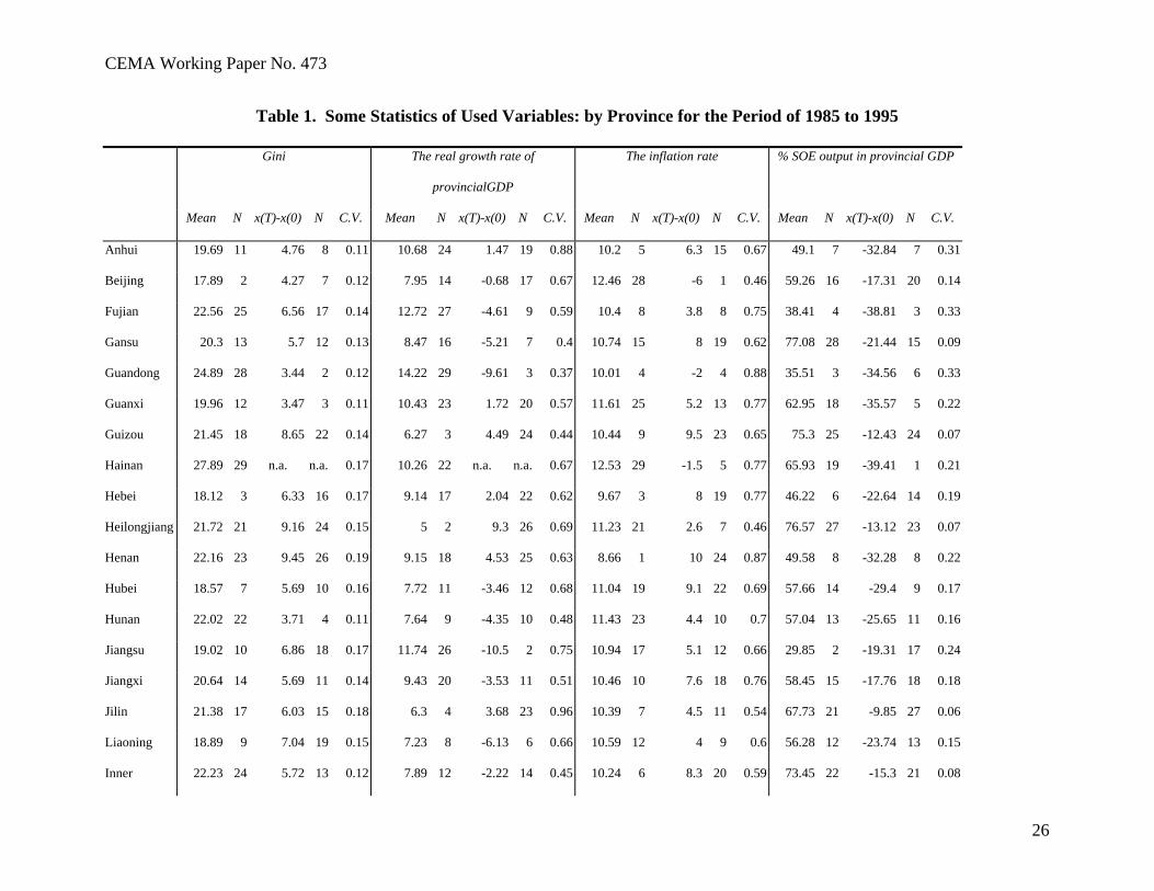
Table 1. Some Statistics of Used Variables: by Province for the Period of 1985 to 1995

Gini The real growth rate of

provincialGDP

The inflation rate % SOE output in provincial GDP

Mean N x(T)-x(0) N C.V. Mean N x(T)-x(0) N C.V. Mean N x(T)-x(0) N C.V. Mean N x(T)-x(0) N C.V.

Anhui 19.69 11 4.76 8 0.11 10.68 24 1.47 19 0.88 10.2 5 6.3 15 0.67 49.1 7 -32.84 7 0.31

Beijing 17.89 2 4.27 7 0.12 7.95 14 -0.68 17 0.67 12.46 28 -6 1 0.46 59.26 16 -17.31 20 0.14

Fujian 22.56 25 6.56 17 0.14 12.72 27 -4.61 9 0.59 10.4 8 3.8 8 0.75 38.41 4 -38.81 3 0.33

Gansu 20.3 13 5.7 12 0.13 8.47 16 -5.21 7 0.4 10.74 15 8 19 0.62 77.08 28 -21.44 15 0.09

Guandong 24.89 28 3.44 2 0.12 14.22 29 -9.61 3 0.37 10.01 4 -2 4 0.88 35.51 3 -34.56 6 0.33

Guanxi 19.96 12 3.47 3 0.11 10.43 23 1.72 20 0.57 11.61 25 5.2 13 0.77 62.95 18 -35.57 5 0.22

Guizou 21.45 18 8.65 22 0.14 6.27 3 4.49 24 0.44 10.44 9 9.5 23 0.65 75.3 25 -12.43 24 0.07

Hainan 27.89 29 n.a. n.a. 0.17 10.26 22 n.a. n.a. 0.67 12.53 29 -1.5 5 0.77 65.93 19 -39.41 1 0.21

Hebei 18.12 3 6.33 16 0.17 9.14 17 2.04 22 0.62 9.67 3 8 19 0.77 46.22 6 -22.64 14 0.19

Heilongjiang 21.72 21 9.16 24 0.15 5 2 9.3 26 0.69 11.23 21 2.6 7 0.46 76.57 27 -13.12 23 0.07

Henan 22.16 23 9.45 26 0.19 9.15 18 4.53 25 0.63 8.66 1 10 24 0.87 49.58 8 -32.28 8 0.22

Hubei 18.57 7 5.69 10 0.16 7.72 11 -3.46 12 0.68 11.04 19 9.1 22 0.69 57.66 14 -29.4 9 0.17

Hunan 22.02 22 3.71 4 0.11 7.64 9 -4.35 10 0.48 11.43 23 4.4 10 0.7 57.04 13 -25.65 11 0.16

Jiangsu 19.02 10 6.86 18 0.17 11.74 26 -10.5 2 0.75 10.94 17 5.1 12 0.66 29.85 2 -19.31 17 0.24

Jiangxi 20.64 14 5.69 11 0.14 9.43 20 -3.53 11 0.51 10.46 10 7.6 18 0.76 58.45 15 -17.76 18 0.18

Jilin 21.38 17 6.03 15 0.18 6.3 4 3.68 23 0.96 10.39 7 4.5 11 0.54 67.73 21 -9.85 27 0.06

Liaoning 18.89 9 7.04 19 0.15 7.23 8 -6.13 6 0.66 10.59 12 4 9 0.6 56.28 12 -23.74 13 0.15

Inner 22.23 24 5.72 13 0.12 7.89 12 -2.22 14 0.45 10.24 6 8.3 20 0.59 73.45 22 -15.3 21 0.08


27

Mongolia

Ningxia 21.59 19 3.93 5 0.2 7.93 13 -0.86 16 0.61 10.67 14 7.5 17 0.56 76 26 -10.64 25 0.05

Qinghai 21.19 16 4.09 6 0.09 4.82 1 n.a. n.a. 0.72 11.52 24 5.6 14 0.56 82.51 30 4.44 29 0.03

Shaanxi 21.72 20 n.a. n.a. 0.17 6.92 7 -12.57 1 0.66 11.34 22 10.5 27 0.69 66.43 20 -14.45 22 0.08

Shandong 18.5 5 5.91 14 0.14 11.51 25 1.84 21 0.6 9.56 2 7.1 16 0.67 39.87 5 -23.86 12 0.32

Shanghai 17.31 1 8.26 21 0.19 8.39 15 -2.85 13 0.59 12.42 27 -3.4 2 0.4 60.08 17 -37.98 4 0.23

Shanxi 23.15 26 n.a. n.a. 0.16 6.73 6 11.28 27 0.69 10.51 11 8 19 0.67 55.24 10 -17.44 19 0.13

Sichuan 20.92 15 8.95 23 0.18 9.31 19 -4.89 8 0.64 10.62 13 10.2 26 0.74 56.11 11 -29.29 10 0.21

Tianjin 18.82 8 9.33 25 0.18 6.63 5 0.56 18 0.7 10.76 16 -3.3 3 0.4 53.05 9 -39.04 2 0.26

Xinjiang 23.45 27 -1.28 1 0.12 9.59 21 -7.48 5 0.42 11.86 26 8.6 21 0.57 78.76 29 -10.32 26 0.04

Yunnan 18.52 6 5.49 9 0.13 7.69 10 -1.63 15 0.41 10.98 18 10.1 25 0.64 74.61 23 -8.5 28 0.04

Zhejiang 18.44 4 7.93 20 0.16 13.89 28 -8.31 4 0.61 11.21 20 -0.5 6 0.63 25.53 1 -21.43 16 0.29


28

Table 1. Some Statistics of Used Variables: by Province for the Period of 1985 to 1995 (Continue)

SCH TRADE GEXPS URBANGR

mean rank x(T)-x(0) rank C.V. mean rank x(T)-x(0) rank C.V. mean rank C.V. mean rank x(T)-x(0) rank cv

Anhui 30.14 8 9.74 19 0.13 6.68 6 4.3 6 0.28 9.99 5 0.24 0.48 12 -0.63 6 0.8

Beijing 64.57 30 10.17 21 0.09 62.73 29 210.47 30 1.49 11.88 13 0.18 0.77 25 0.01 23 0.84

Fujian 26.00 5 7.4 10 0.11 39.41 27 38.45 25 0.46 13.64 17 0.22 0.48 11 -0.21 17 1.57

Gansu 28.12 6 6.95 5 0.12 5.88 4 6.64 14 0.46 18.87 24 0.09 0.41 6 -0.12 18 0.9

Guandong 34.52 13 10.27 22 0.12 83.03 30 132.27 29 0.7 10.62 9 0.1 0.89 29 -0.95 4 0.78

Guanxi 30.18 9 8.41 14 0.14 12.96 18 7.49 18 0.34 15.4 20 0.2 0.49 14 -0.03 20 0.86

Guizou 19.98 3 7.39 9 0.12 4.79 1 7.17 17 0.49 18.55 23 0.12 0.39 4 0.06 24 1.64

Hainan 40.28 22 n.a. n.a. 0.01 34.09 25 48.32 27 0.69 15.04 19 0.26 0.75 24 -0.47 8 0.92

Hebei 38.44 18 7.03 6 0.12 11.31 17 0.88 2 0.28 10.48 8 0.23 0.34 3 0.17 28 1.04

Heilong 45.54 25 9.59 17 0.1 10.92 16 5.34 10 0.35 13.25 16 0.18 0.64 22 -0.03 21 0.82

Henan 39.63 20 10.37 23 0.15 5.51 2 3.24 3 0.28 10.39 6 0.17 0.47 10 -0.24 16 0.72

Hubei 37.23 17 6.08 1 0.11 8.85 12 6.72 16 0.3 10.47 7 0.17 0.68 23 -1.87 1 1.16

Hunan 35.05 14 8.5 15 0.13 8.12 11 3.29 4 0.37 11.27 10 0.11 0.48 13 -0.32 14 1.03

Jiangsu 41.17 23 9.41 16 0.09 16.12 19 17.97 23 0.4 7.18 1 0.13 1 30 -0.07 19 1.09

Jiangxi 29.92 7 9.69 18 0.18 7.71 8 4.61 7 0.27 12.7 14 0.16 0.6 20 -0.29 15 1.55

Jilin 46.50 26 12.04 28 0.12 16.5 20 10.87 20 0.39 17.23 21 0.2 0.78 26 -0.65 5 0.93

Liaoning 48.62 27 6.4 2 0.07 30.68 23 6.68 15 0.18 11.8 12 0.15 0.55 16 -0.53 7 1.05

Neimeng 39.97 21 7.69 11 0.07 9.21 14 6.15 13 0.4 21 25 0.21 0.56 18 -0.41 10 0.86

Ningxia 33.72 11 11.89 27 0.16 8.07 9 5.22 9 0.26 24.92 27 0.29 0.58 19 -0.37 13 0.69


29

Qinghai 25.76 4 11.27 26 0.19 5.86 3 4.71 8 0.35 25.13 28 0.18 0.63 21 -1.23 2 1.79

Shaanxi 39.34 19 7.32 8 0.1 9.12 13 11.5 22 0.52 n.a. n.a. n.a. 0.52 15 -0.39 11 1.22

Shandong 35.53 15 10.77 24 0.1 16.5 21 8.54 19 0.22 8.12 2 0.18 0.8 27 -0.39 12 0.9

Shanghai 61.36 29 9.84 20 0.06 51.99 28 49.69 28 0.33 9.84 4 0.13 0.83 28 0.15 27 0.81

Shanxi 43.47 24 11.09 25 0.11 7.08 7 5.94 12 0.26 13.99 18 0.19 0.55 17 0.13 26 1.12

Sichuan 30.77 10 8.14 13 0.13 6.5 5 5.58 11 0.37 11.62 11 0.15 0.4 5 -0.43 9 1.09

Tianjin 52.63 28 7.88 12 0.06 38.92 26 47.89 26 0.45 13.09 15 0.21 0.45 8 0.26 29 1.49

Xinjiang 33.97 12 6.75 4 0.08 9.40 15 3.94 5 0.18 18.49 22 0.33 0.41 7 0.00 22 1.35

Yunnan 19.73 2 6.68 3 0.13 8.08 10 11.09 21 0.48 24.79 26 0.12 0.46 9 0.06 25 1.39

Zhejiang 36.64 16 7.31 7 0.1 17.77 22 19.18 24 0.42 8.53 3 0.18 0.32 2 -1.03 3 1.64

Note. Source of data: various volumes of provincial statistical yearbooks.


30

Table 2. Trend of Inequality Measures over Time (1985-95)

GINI

Q5/Q1

Q5

Q1

Q34

year Mean S.D. Mean S.D. Mean S.D. Mean S.D. Mean S.D.

85 17.13 2.58 2.45 0.39 30.05 1.76 12.39 0.98 35.17 0.98

86 16.43 2.11 2.38 0.36 29.57 1.21 12.59 1.06 35.54 0.55

89 21.02 3.80 1.99 0.86 27.08 2.25 14.59 2.55 40.96 1.33

90 20.25 2.60 1.84 0.27 27.01 1.94 14.85 1.25 40.74 0.98

91 19.93 2.12 1.89 0.30 27.71 1.94 14.91 1.58 40.42 1.02

92 20.81 2.57 2.10 0.33 28.80 2.02 13.89 1.32 40.55 0.80

93 22.69 2.90 2.41 0.42 30.73 2.30 13.02 1.82 40.30 1.19

94 24.63 2.88 2.75 0.55 32.05 2.69 11.93 1.53 40.63 1.20

95 23.42 2.57 2.60 0.50 31.73 2.62 12.46 1.46 40.14 1.30

Note. These income inequality measures are based on the authors’ calculation based on the published accounts of the

average incomes of urban residents for various percentiles. No data are provided for 1987 and 1988 because we do

not have sources for these two years.

Table 3. Descriptive Statistics of Used Variables

Variable Obs Mean Std.

Dev.

Min Max Variable Obs Mean Std.

Dev.

Min Max

GINI 252 20.73 3.69 12.98 34.17 INFL 261 10.84 6.72 -4.40 26.8

Q1 247 13.41 1.90 5.05 19.49 SCH 259 36.62 12.10 1.53a 68.21

Q5 247 29.41 2.77 21.4 40.36 DISTA 261 0.79 0.77 0.00 3.65

Q5/Q1 247 2.27 0.56 1.10 5.94 TRADE 261 19.10 28.17 1.63 232.70

Q34 247 39.41 2.40 32.25 45.57 GEXPS 224 14.22 5.77 5.65 35.77


31

GDPGR 259 8.83 5.76 -5.72 26.16 URBAN

GR

261 0.58 0.64 -0.60 3.50

SOES 261 58.78 17.46 14.06 87.82

a. This low figure is attributed to Tibet. These income inequality measures are based on the authors’ calculation

based on the published accounts of the average incomes of urban residents for various percentiles.

Table 4. The Correlation Matrix of Used Variables

GINI Q1 Q5 Q5/Q1 Q34 GDPGR SOES INFL SCH DISTA TRADE GEXPS

GINI 1

Q1 -0.43 1

Q5 0.58 -0.81 1

Q5/Q1 0.57 a -0.94 0.84 1

Q34 0.46 0.18 -0.25 -0.15 1

GDPGR 0.27 -0.36 0.43 0.36 -0.06 1

SOES -0.18 0.14 -0.15 -0.12 -0.31 -0.43 1.00

INFL 0.40 -0.23 0.31 0.30 0.19 0.25 -0.27 1

SCH -0.00 0.22 -0.23 -.10 0.35 -0.07 -0.21 0.11 1

DISTA 0.17 -0.04 0.05 0.08 -0.06 -0.14 0.54 -0.01 -0.37 1

TRADE 0.22 -0.05 0.10 0.08 0.17 0.28 -0.36 0.15 0.40 -0.35 1.00

GEXPS -0.03 0.03 -0.06 0.02 -0.29 -0.30 0.75 -0.22 -0.42 0.50 -0.26 1.00

URBANG

R

0.15 -0.19 0.28 0.21 -0.05 0.39 -0.20 0.31 0.11 -0.14 0.12 -0.17

Note. See the data appendix for definition of varables.

a. This correlation is low because we pooled 1985-86 with the data in 1989-95. Recall that we had different number of

observations for these two periods, and because of that, GINI is underestimated more in the first period than the second. Not

surprisingly, this correlation becomes 0.82 when we only used 1989-95, and it turns to 0.98 when we use only 1985-86.


32

Table 5. Determinants of the Gini coefficients (Dependent Variable=Gini Coefficient)

Model (1) Model (2) Model (3) Model (4)

Model FEa RE 2SLS

LSDV

FE RE 2SLS

LSDV

FE RE 2SLS

LSDV

FE RE 2SLS

LSDV

No. Obs. 251 251 250 247 247 246 239 239 238 239 239 238

R2 0.696 0.687 0.799 0.701 0.690 0.800 0.704 0.695 0.803 0.704 0.696 0.690

Constant 21.328 23.066 28.501 18.344 21.229 26.064 17.328 19.839 25.725 17.461 19.819 11.950

(6.080) (12.115) (4.710) (5.035) (11.241) (3.950) (4.705) (9.977) (3.929) (4.728) (9.833) (1.332)

SOES -0.115 -0.078 -0.153 -0.091 -0.052 -0.136 -0.094 -0.069 -0.152 -0.095 -0.070 -0.132

(-6.115) (-4.577) (-5.337) (-4.207) (-2.867) (-3.753) (-4.368) (-3.642) (-4.131) (-4.391) (-3.689) (-2.818)

INFL 0.106 0.123 0.094 0.121 0.136 0.104 0.127 0.142 0.108 0.130 0.144 0.162

(5.178) (5.943) (4.192) (5.712) (6.599) (4.036) (5.707) (6.712) (4.006) (5.725) (6.658) (3.764)

DISTA 1.534 1.695 1.484 1.496

(2.725) (3.155) (2.696) (2.671)

SCH 0.131 -0.002 0.176 0.149 -0.025 0.198 0.143 -0.011 0.159 0.140 -0.009 0.483

(1.608) (-0.068) (0.969) (1.829) (-0.733) (1.094) (1.762) (-0.305) (0.869) (1.724) (-0.247) (2.081)

GDPGR 0.053 0.069 0.010 0.037 0.050 0.002 0.050 0.066 0.037 0.055 0.070 0.154

(2.281) (2.846) (0.207) (1.563) (2.042) (0.041) (1.993) (2.602) (0.703) (2.097) (2.648) (1.389)

TRADE 0.050 0.060 0.029 0.049 0.056 0.020 0.049 0.056 0.053


33

(2.640) (3.730) (0.844) (2.619) (3.513) (0.598) (2.599) (3.485) (1.337)

GEXPS 0.096 0.135 0.158 0.097 0.136 0.111

(1.792) (2.703) (2.109) (1.813) (2.707) (1.217)

URBANGR -0.136 -0.126 -2.149

(-0.661) (-0.595) (-1.682)

2 5( )

29.47 b

2 6( )

24.60

2 7( )

42.52

2 8( )

28.86

P: 0.000 P: 0.000 P: 0.000 P: 0.000

Note. In the parentheses are the t-statistics. See the data appendix for the definitions of the variables.

a. In all these tables, the R2 reported for FE and RE specifications are R2 within. This is appropriate because we focus on the change of the dependent variables.

b. The Hausman’s (Chi-Square) test statistics: a large value favors the FE model (instead of RE model); P is the associated P-value.


34

Table 6. Determinants of Q5/Q1 (Dependent Variable=Q5/Q1)


FE RE 2SLS

LSDV

FE RE 2SLS+FE FE RE 2SLS

LSDV

FE RE 2SLS

LSDV

No. Obs. 246 246 245 242 242 241 234 234 233 234 234 233

R2 within 0.412 0.388 0.548 0.416 0.393 0.535 0.412 0.394 0.519 0.412 0.395 0.108

Constant 2.040 2.332 4.758 1.677 2.154 4.933 1.565 2.012 4.835 1.570 2.016 0.588

(2.569) (7.833) (3.454) (2.003) (7.130) (3.189) (1.842) (6.226) (3.084) (1.842) (6.130) (0.234)

SOES -0.021 -0.010 -0.023 -0.018 -0.008 -0.024 -0.019 -0.011 -0.027 -0.019 -0.011 -0.021

(-5.024) (-3.193) (-3.497) (-3.726) (-2.366) (-2.879) (-3.784) (-2.908) (-3.108) (-3.778) (-2.940) (-1.703)

INFL 0.019 0.023 0.014 0.020 0.024 0.013 0.020 0.024 0.013 0.021 0.024 0.029

(4.000) (5.141) (2.670) (4.200) (5.351) (2.182) (3.998) (5.156) (2.046) (3.947) (4.982) (2.539)

DISTA 0.160 0.181 0.163 0.167

(1.949) (2.214) (1.939) (1.940)

SCH 0.025 -0.003 -0.026 0.028 -0.005 -0.027 0.027 -0.002 -0.034 0.026 -0.002 0.059

(1.376) (-0.527) (-0.623) (1.482) (-0.934) (-0.644) (1.425) (-0.425) (-0.792) (1.415) (-0.400) (0.961)

GDPGR 0.017 0.021 0.026 0.016 0.019 0.026 0.018 0.021 0.034 0.018 0.021 0.071

(3.230) (3.748) (2.269) (2.845) (3.285) (2.203) (3.061) (3.575) (2.629) (2.943) (3.365) (2.258)

TRADE 0.006 0.006 -0.002 0.006 0.005 -0.004 0.006 0.005 0.006


35

(1.375) (1.998) (-0.258) (1.294) (1.685) (-0.493) (1.287) (1.683) (0.587)

GEXPS 0.013 0.018 0.031 0.013 0.018 0.021

(1.022) (1.690) (1.705) (1.027) (1.685) (0.890)

URBANGR -0.008 0.003 -0.641

(-0.159) (0.057) (-1.778)

2 5( ):

20.31

2 6( ):

18.88

2 7( ):

17.63

2 6( ):

16.84

P: 0.001 P: 0.004 P: 0.014 P: 0.032



36

Table 7. Determinants of Q5 (Dependent Variable=Q5)


FE RE 2SLS

LSDV


LSDV

FE RE 2SLS

LSDV

No. Obs. 246 246 245 242 242 241 234 234 233 234 234 233

R2 within 0.530 0.508 0.618 0.538 0.515 0.596 0.548 0.519 0.626 0.550 0.523 0.442

Constant 27.492 30.552 45.699 25.785 29.489 48.047 27.436 30.054 47.971 27.301 30.158 33.600

(8.295) (19.437) (7.275) (7.416) (18.336) (6.729) (7.896) (17.521) (6.995) (7.856) (17.367) (3.400)

SOES -0.110 -0.068 -0.091 -0.095 -0.054 -0.101 -0.089 -0.049 -0.093 -0.088 -0.049 -0.071

(-6.224) (-4.443) (-3.040) (-4.644) (-3.326) (-2.589) (-4.390) (-2.788) (-2.422) (-4.326) (-2.813) (-1.483)

INFL 0.087 0.105 0.061 0.096 0.112 0.055 0.077 0.102 0.039 0.073 0.096 0.093

(4.490) (5.387) (2.600) (4.783) (5.709) (1.962) (3.678) (5.056) (1.379) (3.410) (4.656) (2.042)

DISTA 0.985 1.080 1.140 1.175

(2.182) (2.407) (2.457) (2.495)

SCH 0.148 -0.016 -0.303 0.156 -0.026 -0.342 0.152 -0.030 -0.286 0.155 -0.031 0.032

(1.923) (-0.552) (-1.608) (2.004) (-0.912) (-1.768) (1.997) (-1.003) (-1.522) (2.034) (-1.007) (0.132)

GDPGR 0.123 0.136 0.220 0.117 0.130 0.228 0.107 0.128 0.207 0.099 0.118 0.325

(5.518) (5.857) (4.172) (5.080) (5.391) (4.139) (4.541) (5.182) (3.643) (3.954) (4.559) (2.632)

TRADE 0.031 0.032 -0.018 0.026 0.032 -0.021 0.026 0.032 0.014


37

(1.736) (2.199) (-0.492) (1.453) (2.141) (-0.583) (1.476) (2.136) (0.359)

GEXPS -0.113 -0.048 -0.122 -0.116 -0.052 -0.156

(-2.249) (-1.009) (-1.542) (-2.310) (-1.098) (-1.668)

URBANGR 0.211 0.228 -2.105

(1.087) (1.112) (-1.486)

2 5( ):

32.06

2 5( ):

31.87

2 5( ):

22.90

2 5( ):

21.81

P: 0.000 P: 0.000 P: 0.002 P: 0.005



38



FE RE 2SLS

LSDV


LSDV

FE RE 2SLS

LSDV

No. Obs. 246 246 245 242 242 241 234 234 233 234 234 233

R2 within 0.469 0.456 0.600 0.475 0.463 0.589 0.470 0.459 0.571 0.471 0.460 0.192

Constant 13.474 12.651 4.630 15.001 13.117 4.115 15.032 13.319 4.424 14.989 13.333 18.507

(5.470) (12.341) (1.055) (5.804) (12.268) (0.833) (5.745) (11.697) (0.880) (5.713) (11.510) (2.275)

SOES 0.068 0.043 0.070 0.056 0.036 0.079 0.056 0.040 0.087 0.056 0.041 0.065

(5.208) (4.027) (3.365) (3.674) (3.217) (2.919) (3.646) (3.248) (3.075) (3.659) (3.278) (1.648)

INFL -0.053 -0.063 -0.031 -0.060 -0.067 -0.028 -0.059 -0.065 -0.027 -0.060 -0.066 -0.081

(-3.650) (-4.494) (-1.916) (-4.021) (-4.698) (-1.457) (-3.720) (-4.483) (-1.322) (-3.734) (-4.413) (-2.160)

DISTA -0.540 -0.614 -0.569 -0.576

(-1.871) (-2.085) (-1.879) (-1.867)

SCH -0.061 0.011 0.132 -0.071 0.018 0.124 -0.068 0.015 0.137 -0.067 0.014 -0.173

(-1.071) (0.592) (1.003) (-1.232) (0.958) (0.924) (-1.182) (0.751) (0.995) (-1.163) (0.699) (-0.867)

GDPGR -0.067 -0.074 -0.126 -0.059 -0.067 -0.127 -0.061 -0.069 -0.146 -0.064 -0.071 -0.267

(-4.054) (-4.328) (-3.421) (-3.478) (-3.788) (-3.330) (-3.432) (-3.831) (-3.507) (-3.392) (-3.718) (-2.625)

TRADE -0.024 -0.018 0.015 -0.022 -0.017 0.021 -0.022 -0.017 -0.012


39

(-1.792) (-1.820) (0.598) (-1.658) (-1.647) (0.811) (-1.645) (-1.653) (-0.372)

GEXPS -0.013 -0.026 -0.075 -0.014 -0.027 -0.043

(-0.338) (-0.775) (-1.300) (-0.363) (-0.790) (-0.560)

URBANGR 0.068 0.043 2.113

(0.461) (0.283) (1.812)

2 5( ):

14.14

2 6( ):

14.36

2 7( ):

15.81

2 8( ):

14.90

P: 0.015 P: 0.026 P: 0.027 P: 0.061



40



FE RE 2SLS

LSDV


LSDV

FE RE 2SLS

LSDV

No. Obs. 246 246 245 242 242 241 234 234 233 234 234 233

R2 within 0.855 0.852 0.851 0.858 0.853 0.849 0.854 0.849 0.844 0.856 0.850 0.837

Constant 42.999 41.053 37.306 42.165 41.299 36.719 41.921 41.400 36.526 42.024 41.319 34.382

(22.501) (66.907) (11.070) (21.094) (64.872) (9.717) (20.387) (59.703) (9.538) (20.476) (58.605) (7.442)

SOES 0.003 -0.012 -0.016 0.009 -0.014 -0.019 0.007 -0.012 -0.025 0.007 -0.012 -0.022

(0.294) (-1.742) (-0.969) (0.741) (-1.995) (-0.912) (0.625) (-1.414) (-1.169) (0.548) (-1.388) (-0.974)

INFL 0.000 -0.007 -0.003 0.003 -0.008 -0.004 0.007 -0.007 -0.001 0.010 -0.004 0.008

(0.025) (-0.652) (-0.273) (0.273) (-0.772) (-0.294) (0.552) (-0.665) (-0.040) (0.810) (-0.321) (0.358)

DISTA -0.013 -0.032 -0.033 -0.046

(-0.079) (-0.189) (-0.183) (-0.250)

SCH -0.063 0.011 0.105 -0.055 0.012 0.131 -0.056 0.009 0.118 -0.059 0.010 0.165

(-1.429) (1.083) (1.040) (-1.241) (1.073) (1.278) (-1.251) (0.773) (1.123) (-1.302) (0.840) (1.456)

GDPGR -0.014 -0.022 -0.022 -0.020 -0.023 -0.024 -0.018 -0.026 -0.013 -0.012 -0.020 0.006

(-1.058) (-1.774) (-0.762) (-1.476) (-1.793) (-0.824) (-1.321) (-1.925) (-0.410) (-0.800) (-1.410) (0.109)

TRADE 0.011 -0.005 -0.005 0.011 -0.005 -0.007 0.010 -0.004 -0.002


41

(1.041) (-0.815) (-0.256) (1.029) (-0.665) (-0.351) (1.003) (-0.626) (-0.110)

GEXPS 0.022 -0.011 0.057 0.025 -0.009 0.053

(0.742) (-0.461) (1.301) (0.825) (-0.373) (1.206)

URBANGR -0.163 -0.146 -0.330

(-1.415) (-1.287) (-0.499)

2 5( ):

13.74

2 6( ):

11.83

2 7( ):

10.42

2 8( ):

11.69

P: 0.017 P: 0.066 P: 0.166 P: 0.165


Explaining The Changes of Income Inequality in Chinese ...

Documents

Transcript of Explaining The Changes of Income Inequality in Chinese ...