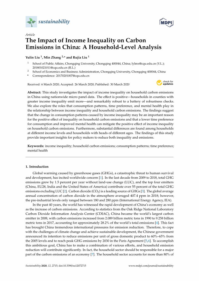
sustainability

Article

The Impact of Income Inequality on CarbonEmissions in China: A Household-Level Analysis

Yulin Liu 1, Min Zhang 2,* and Rujia Liu 1

1 School of Public Affairs, Chongqing University, Chongqing 400044, China; lylmx@cqu.edu.cn (Y.L.);201801021011@cqu.edu.cn (R.L.)

2 School of Economics and Business Administration, Chongqing University, Chongqing 400044, China* Correspondence: 20170201007@cqu.edu.cn

Received: 6 March 2020; Accepted: 26 March 2020; Published: 30 March 2020�����������������

Abstract: This study investigates the impact of income inequality on household carbon emissionsin China using nationwide micro panel data. The effect is positive—households in counties withgreater income inequality emit more—and remarkably robust to a battery of robustness checks.We also explore the roles that consumption patterns, time preference, and mental health play inthe relationship between income inequality and household carbon emissions. The findings suggestthat the change in consumption patterns caused by income inequality may be an important reasonfor the positive effect of inequality on household carbon emissions and that a lower time preferencefor consumption and improved mental health can mitigate the positive effect of income inequalityon household carbon emissions. Furthermore, substantial differences are found among householdsat different income levels and households with heads of different ages. The findings of this studyprovide important insights for policy makers to reduce both inequality and emissions.

Keywords: income inequality; household carbon emissions; consumption patterns; time preference;mental health

1. Introduction

Global warming caused by greenhouse gases (GHGs), a catastrophic threat to human survivaland development, has incited worldwide concern [1]. In the last decade from 2009 to 2018, total GHGemissions grew by 1.5 percent per year without land-use change (LUC), and the top four emitters(China, EU28, India and the United States of America) contribute over 55 percent of the total GHGemissions excluding LUC [2]. Carbon dioxide (CO2) is a leading source of GHGs [3]. The global averageannual concentration of carbon dioxide in the atmosphere averaged 407.4 ppm in 2018; however,the pre-industrial levels only ranged between 180 and 280 ppm (International Energy Agency, IEA).

In the past 40 years, the world has witnessed the rapid development of China’s economy as wellas the increase of carbon emissions. According to statistics from the Oak Ridge National LaboratoryCarbon Dioxide Information Analysis Center (CDIAC), China became the world’s largest carbonemitter in 2008, with carbon emissions increased from 2.089 billion metric tons in 1990 to 9.258 billionmetric tons in 2017, accounting for approximately 28.2% of the world’s total emissions [4]. This facthas brought China tremendous international pressures for emission reduction. Therefore, to copewith the challenges of climate change and achieve sustainable development, the Chinese governmentannounced its intention to reduce emissions per unit of gross domestic product to 60%–65% fromthe 2005 levels and to reach peak GHG emissions by 2030 in the Paris Agreement [5,6]. To accomplishthis ambitious goal, China has to make a combination of various efforts, and household emissionreduction will contribute significantly. In fact, the household sector should be responsible for a majorpart of the carbon emissions of an economy [7]. The household sector accounts for more than 80% of

Sustainability 2020, 12, 2715; doi:10.3390/su12072715 www.mdpi.com/journal/sustainability

Sustainability 2020, 12, 2715 2 of 22

carbon emissions in the United States [8] and exceeds 70% in the United Kingdom and India [9,10]. Liuet al. (2011) found that in China, the share of emissions from household sector was approximately 40%of the total [11], and Fan et al. (2013) found that the annual growth rate of household carbon emissionsin China was 8.7% [12]. Although the industrial sector remains the key source of carbon emissions, asa demander of industrial products, the household sector indirectly promotes CO2 emissions [13,14],and in China, the residential sector has become the second largest CO2 emissions source [15]. This factemphasizes the importance of placing greater attention on household carbon emissions.

In addition to environmental degradation, the increasing income inequality, as a by-productof economic growth, is also an important socio-economic issue [16,17]. Income inequality maycause substantial social and economic problems, such as poorer mental health [18,19], higher statusanxiety [20], and a higher level of general violence [21]. Furthermore, income inequality will createhighly indebted, low-income households, which eventually results in a fragile economy [22]. China’seconomy has made remarkable achievements since its reform and opening up, but the fruits of economicgrowth are not shared equally among the population [23]. The Gini coefficient of income distributionin China increased by 55% between 1974 and 2010 [24], and in 2017, it reached 0.467 (China Yearbookof Household Survey), exceeding the warning level of 0.40 set by the United Nations. A series of fiscaland tax policies have been adopted to regulate income distribution. One question deserving attentionis whether under the dual pressures of environment and inequality, the policy goal of narrowingthe income gap consistent with the carbon reduction target. In particular, does income inequality itselflead to the increase of carbon emissions [25]?

Different from previous studies, this paper focuses on the effect of income inequality on carbonemissions of households at similar income levels; that is to say, we explore whether households at similarincome levels emit differently when facing different levels of income inequality. More specifically, we usethree waves of data at the household level, from the China Family Panel Survey (CFPS, downloadable athttp://www.isss.pku.edu.cn/cfps/), to estimate the influence of income inequality on household carbonemissions and to examine consumption patterns, mental health and time preference for consumptionas important channels through which income inequality influences household emissions.

The present paper may contribute to the literature in three ways. First, we test the relationshipbetween income inequality and household carbon emissions in China; here, we diverge from a largebody of the existing literature on the differences of emissions among households at different incomelevels to focus on the emissions of households at similar income levels when facing different levels ofincome inequality. Although there is a general perception that households at different income levelsemit differently, it is unclear how households with similar income act when facing different incomeinequality levels. Second, we explore the mechanisms by which income inequality affects householdCO2 emissions. Subjective factors such as mental health and time preference for consumption, inaddition to consumption patterns, allow us to offer some new insights into this topic. Third, ourfindings suggest that with the increase of the age of household heads and the increase of households’per capita income, the positive effect of income inequality on household carbon emissions graduallydecreases. This result suggests a new approach for the government to formulate more precise incomedistribution and emission reduction policies.

The rest of the paper is structured as follows. Section 2 briefly reviews the related literature.Section 3 describes the data and methodology. Section 4 presents the empirical estimation results andthe corresponding analysis. Section 5 concludes the paper.

2. Literature Review

Boyce (1994) performed the pioneering work of incorporating inequality into environmentaldegradation and argued that greater inequalities in power and wealth led to worse environmentalquality [26]. Boyce presented a political-economic explanation that, on the one hand, the wealthypreferred weaker environmental protection policies because they reaped disproportionate gains frompollution, while on the other hand, inequality increased the preference for current resource consumption

Sustainability 2020, 12, 2715 3 of 22

of both the poor and the rich. However, this argument holds only in the assumption that the rich prefermore pollution than the poor [27,28]. Ravallion et al. (2000), Heil and Selden (2001), and Borghesi (2006)explained the relationship between income inequality and carbon emissions from the perspective of“marginal propensity to emit” (MPE) [29–31]; however, they did not obtain accordant conclusions. Inline with Boyce’s point of view, studies relying on individual economic behavior suggest that increasinginequality in income will increase CO2 emissions. Not only the wealthy but also the poor will engagein expensive and conspicuous consumption to maintain or obtain a higher social status, which Schor(1998) and Veblen (2009) described as the “Veblen effect” [32,33].

There are also many empirical studies, but unfortunately, no consensus on the relationshipbetween income inequality and carbon emissions has been reached. Golley and Meng (2012), Baekand Gweisah (2013), Jorgenson (2015), Kasuga and Takaya (2017), Liu et al. (2019), and Uzar andEyuboglu (2019) came to the conclusion that higher CO2 emissions were positively associated withincreasing income inequality [34–39]. In contrast, Heerink et al. (2001), Coondoo and Dinda (2008),Baloch et al. (2017), Hübler (2017), and Sager (2019) held that inequality affected carbon emissions inthe opposite direction [28,40–43]. Using an unbalanced panel data set from 158 countries, Grunewaldet al. (2017) found that the impact of income inequality on carbon emissions varied with economicdevelopment levels [44]. For low- and middle-income economies, higher levels of income inequalityhelped reduce emissions, while in upper middle-income and high-income economies, higher levelsof income inequality increased emissions. Jorgenson et al. (2017) studied the influence of incomeinequality, measured with the income share of the top 10% and the Gini coefficient, on state-levelCO2 emissions of the United States [25]. They found a positive relationship between inequality andcarbon emissions, but the relationship was only significant when income inequality was measuredwith the income share of the top 10%. Liu et al. (2019), for the first time, took the short- and long-termimpacts of income inequality on CO2 into consideration [38]. They suggested that higher incomeinequality increased carbon emissions in the short term, but in the long term, it promoted carbonreduction. There are even studies finding no linkage between income inequality and environmentalquality [45,46].

Some studies found that income anticipations could affect mental health and that income inequalitygenerally damaged subjective well-being and led to psychological problems [18,47–51]. Further,Velek and Steg (2007) proposed that psychological factors were important in promoting sustainableconsumption of natural resources [52]. Kaida and Kaida (2016) found that pro-environmentalbehavior was positively associated with present subjective well-being [53]. Koenig-Lewis et al.(2014) tested 312 Norwegian consumers on their evaluation of a beverage container incorporatingorganic material [54]. They suggested that emotions and rationality drove pro-environmentalpurchasing behavior, and positive emotion was a significant predictor of green product purchases.Bissing-Olson et al. (2016) examined the dynamic interplay between everyday emotions andpro-environmental behavior over time, and their findings showed that whether individuals feltpride or guilt had an impact on the related pro-environmental behaviors during the course of theirday [55]. Ibanez et al. (2017) reported that awe fostered solemnity and heightened analytical ability,which in turn affected individuals’ pro-environmental behavior [56]. A recent study by Li et al. (2019)using the China Household Finance Survey (CHFS) also found that feeling happy caused a decrease inenergy consumption and thus reduced household carbon emissions [57].

Based on these discussions, it is clear that most of the existing literature investigates the effect ofincome inequality on carbon emissions focused on the national level, state level, or city level; however,few studies concern about the micro behavior body: the households. Based on the United StatesConsumer Expenditure Survey (CEX) from 1996 to 2009, Sager (2019) estimated the EnvironmentalEngel curves (EECs) and examined the effects of different factors on the evolution of carbon emissionsover time [43]. He found that income, age structure, education, family size, race, and region wererelevant, and among these factors, income played a major role. Using the data from China’s UrbanHousehold Income and Expenditure Survey (UHIES) in 2005, Golley and Meng (2012) investigated

Sustainability 2020, 12, 2715 4 of 22

variations in household CO2 emissions among households at different income levels [34]. Theydemonstrated that rich households emitted more than poor households and that marginal propensity toemit (MPE) slightly increased with income over the relevant income range. Therefore, they concludedthat the redistribution of income from the rich to the poor could reduce aggregate household emissions.More importantly, studies rarely consider the differences in carbon emissions among householdsat similar income levels, and few studies focus on the relationship between income inequality andhousehold carbon emissions from the perspective of psychology.

3. Data Source and Empirical Methodology

Using the consumption lifestyle approach (CLA), we first calculate household carbon emissionsby consumption category, which is the dependent variable of this paper but cannot be obtained directlyfrom the CFPS. Then we estimate the Gini coefficient of each county as the proxy variable of incomeinequality. In the empirical section, we employ fixed-effects estimation to reveal the causal relationshipbetween income inequality and household carbon emissions.

3.1. Data Source

This study adopts panel data from China Family Panel Survey (CFPS) administered by Instituteof Social Science Survey, Peking University. The CFPS is a nationally representative survey of Chinesecommunities, families, and individuals. This dataset provides a high-quality comprehensive survey ofhousehold income, expenditure, subjective attitudes, and other demographic characteristics. The CFPSwas launched in 2010, commenced with a total of 14,960 households from 635 communities, including33,600 adults and 8990 youths, located in 25 provinces (excluding Tibet, Xinjiang, Inner Mongolia,Hainan, Ningxia, Qing Hai, Hong Kong, Macao, and Taiwan). Because there are lots of defaults insubjective attitude, which is important for mechanism analysis, in the fourth round of the CFPS in2016, we use the first three rounds of the survey, conducted in 2010, 2012, and 2014, respectively.

3.1.1. Household Carbon Emissions

According to Wei et al. (2007), household carbon emissions include indirect emissions anddirect emissions [58]. The indirect carbon emissions are from the following seven consumptioncategories: (1) food, (2) clothing, (3) household facilities, articles, and services, (4) medicine and medicalservices, (5) transportation and communication services, (6) education, cultural and recreation services,and (7) miscellaneous commodities and services. The direct carbon emissions are from residentialuse of electricity, fuel, and other utilities. Following the approach of Li et al. (2019), we calculatehousehold carbon emissions by multiplying the monetary expenditure in each expenditure categoryby the respective emissions conversion coefficient [57]:

emissioni,j = fi(I−A)−1× expensei,j (1)

emissionj =∑

iemissioni,j (2)

where emissioni, j is carbon emissions of the jth household caused by ith category, fi is the vector ofdirect emissions intensity in each production sector, and (I −A)−1 is the domestic Leontief inversematrix, expensei, j is the spending in the ith category by the jth household, emission j is total carbonemissions of the jth household. Because China reports the input-output table every five yearsand the most recent report that is available to us is from 2012, we calculate the carbon intensitycoefficients for each consumption category based on the China Input-Output Table in 2012 andsectoral carbon emissions data from the China Emission Accounts and Datasets (downloadableat: http://www.stats.gov.cn/ztjc/tjzdgg/trccxh/zlxz/trccb/201701/t201701131453448.html) in 2012 overthe three years. The expenditures and income values for 2012 and 2014 are adjusted to constant 2010prices according to the CPI indices published by the National Bureau of Statistics (NBS). Following Su

Sustainability 2020, 12, 2715 5 of 22

and Ang (2015) and Li et al. (2019), we use the non-competitive imports assumption to account forthe embodied emissions from domestic production [57,59].

Because expenditure on miscellaneous commodities and services is generally very small in numberand there is no detailed expenditure information on miscellaneous commodities and services in the CFPS,this paper does not consider the emissions of this category. Figure 1 plots a histogram of the averagehousehold carbon emissions by consumption category in 2010, 2012, and 2014, respectively. We findthat the residential use, food, education, culture and recreation services are the first three categoriesin inducing carbon emissions, and the residential use produces most of the total emissions witha proportion of 53.88% in 2010, 53.93% in 2012, and 77.68% in 2014. A great deal of literature documentsthat different consumption patterns of households in different income levels cause a positive/negativeimpact of income equality on household carbon emissions [60]. Therefore, we further aggregatethe households in the CFPS into five groups according to the principle of classification of the NBS andcalculate the carbon emissions of different income groups by category. As shown in Figure 2, carbonemissions generated by household facilities, articles and services, transportation and communicationservices, and residential use are more in richer households, especially in 2010 and 2012, and these threecategories are considered to be high carbon-intensive mix [61]. In 2014, the carbon emissions generatedby residential use increased a lot in all income groups, compared with the previous two years. We canalso clearly see that poorer households spend more on medicine and medical services. Taking year2010 as an example, the proportion of carbon emissions caused by medicine and medical services ofthe income groups from the 1st to the 5th are about 16.20%, 12.79%, 8.07%, 8.07%, 5.29%, respectively.

Figure 1. Household carbon emissions by consumption category in China: Y-axis is the averagehousehold carbon emissions of each consumption category. X-axis is consumption categories, where“food” refers to expenditure on food, “dress” refers to expenditure on clothing, “daily” refers toexpenditure on household facilities, articles, and services, “eec” refers to expenditure on education,cultural and recreation services, “trco” refers to expenditure on transportation and communicationservices, “med” refers to expenditure on medicine and medical services, “house” refers to expenditureon residential use.

Sustainability 2020, 12, 2715 6 of 22

Figure 2. Carbon emissions of different income groups by consumption category: Y-axis is the proportionof average household carbon emissions of each consumption category. X-axis is households in differentincome groups.

3.1.2. Income Inequality

Following Liu et al. (2019), we apply the Gini coefficient to proxy the income inequality withina given county [62]. The specific formula is as follows:

Gini =1

2n2µ

n∑h1=1

n∑h1=1

∣∣∣Ch1 −Ch2

∣∣∣ (3)

where Gini denotes the county-level Gini coefficient; n is the number of households; µ refers tothe average per capita income of all households. Ch1 and Ch2 represent the per capita income ofhousehold h1 and household h2, respectively. The values of estimated Gini coefficients can range fromzero (perfect equality) to 1 (perfect inequality).

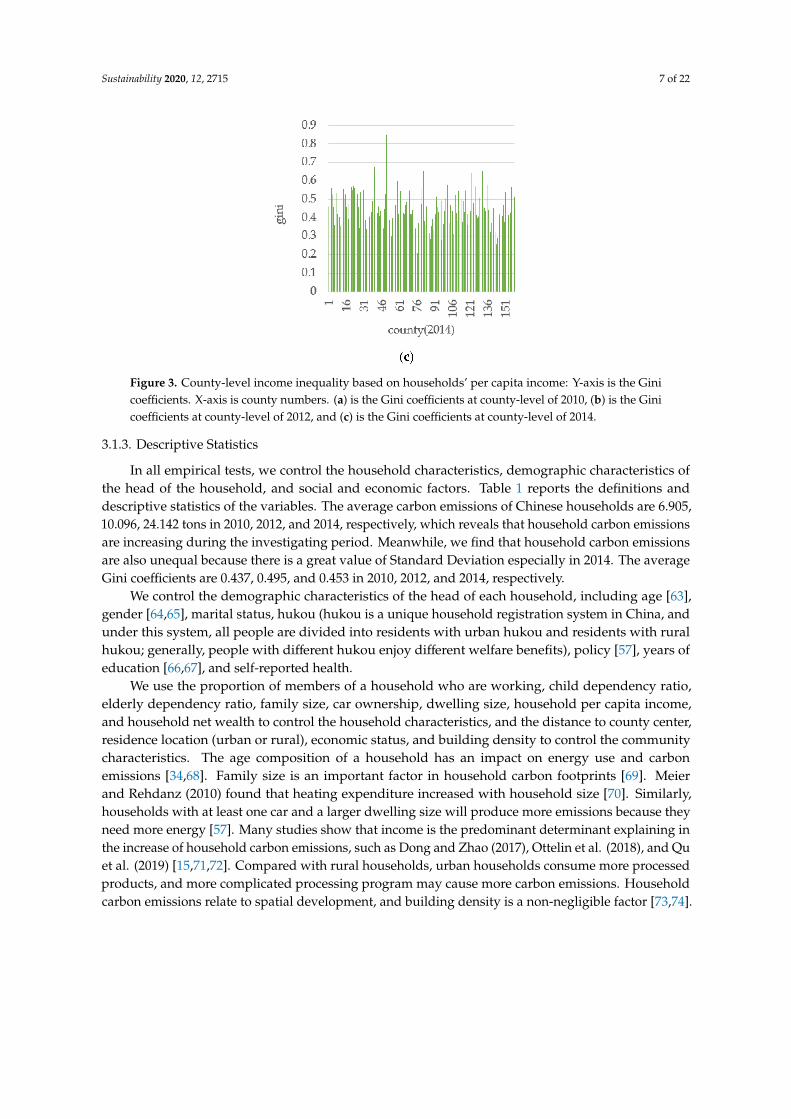
Figure 3 shows the income inequality distribution of China based on the estimated sample ofCFPS in 2010, 2012, and 2014. There are many counties with the Gini coefficient exceeding the warningvalue of 0.4 (73.5% in 2010, 76.1% in 2012, 71.6% in 2014), which indicates that the income inequality isat a high level in China. This is consistent with the results published by the NBS: the national Ginicoefficients in 2010, 2012, and 2014 are 0.481, 0.474, and 0.469, respectively.

Figure 3. Cont.

Sustainability 2020, 12, 2715 7 of 22

Figure 3. County-level income inequality based on households’ per capita income: Y-axis is the Ginicoefficients. X-axis is county numbers. (a) is the Gini coefficients at county-level of 2010, (b) is the Ginicoefficients at county-level of 2012, and (c) is the Gini coefficients at county-level of 2014.

3.1.3. Descriptive Statistics

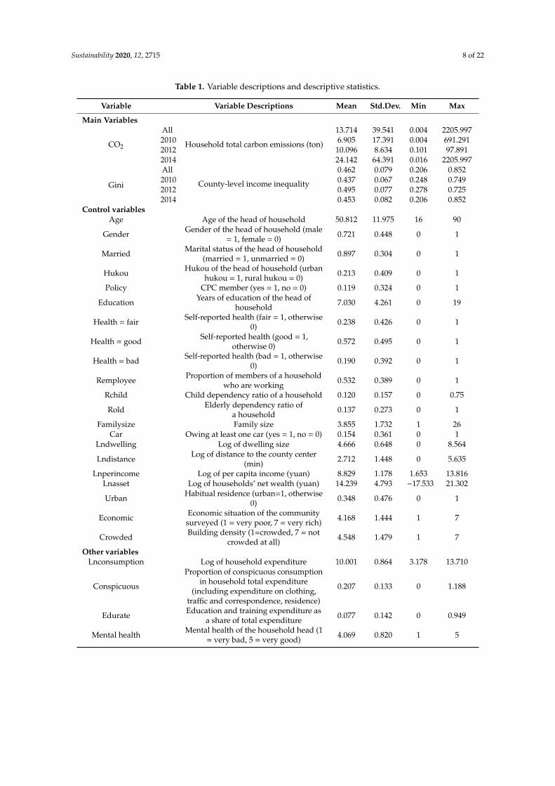
In all empirical tests, we control the household characteristics, demographic characteristics ofthe head of the household, and social and economic factors. Table 1 reports the definitions anddescriptive statistics of the variables. The average carbon emissions of Chinese households are 6.905,10.096, 24.142 tons in 2010, 2012, and 2014, respectively, which reveals that household carbon emissionsare increasing during the investigating period. Meanwhile, we find that household carbon emissionsare also unequal because there is a great value of Standard Deviation especially in 2014. The averageGini coefficients are 0.437, 0.495, and 0.453 in 2010, 2012, and 2014, respectively.

We control the demographic characteristics of the head of each household, including age [63],gender [64,65], marital status, hukou (hukou is a unique household registration system in China, andunder this system, all people are divided into residents with urban hukou and residents with ruralhukou; generally, people with different hukou enjoy different welfare benefits), policy [57], years ofeducation [66,67], and self-reported health.

We use the proportion of members of a household who are working, child dependency ratio,elderly dependency ratio, family size, car ownership, dwelling size, household per capita income,and household net wealth to control the household characteristics, and the distance to county center,residence location (urban or rural), economic status, and building density to control the communitycharacteristics. The age composition of a household has an impact on energy use and carbonemissions [34,68]. Family size is an important factor in household carbon footprints [69]. Meierand Rehdanz (2010) found that heating expenditure increased with household size [70]. Similarly,households with at least one car and a larger dwelling size will produce more emissions because theyneed more energy [57]. Many studies show that income is the predominant determinant explaining inthe increase of household carbon emissions, such as Dong and Zhao (2017), Ottelin et al. (2018), and Quet al. (2019) [15,71,72]. Compared with rural households, urban households consume more processedproducts, and more complicated processing program may cause more carbon emissions. Householdcarbon emissions relate to spatial development, and building density is a non-negligible factor [73,74].

Sustainability 2020, 12, 2715 8 of 22

Table 1. Variable descriptions and descriptive statistics.

Variable Variable Descriptions Mean Std.Dev. Min Max

Main Variables

CO2

All

Household total carbon emissions (ton)

13.714 39.541 0.004 2205.9972010 6.905 17.391 0.004 691.2912012 10.096 8.634 0.101 97.8912014 24.142 64.391 0.016 2205.997

Gini

All

County-level income inequality

0.462 0.079 0.206 0.8522010 0.437 0.067 0.248 0.7492012 0.495 0.077 0.278 0.7252014 0.453 0.082 0.206 0.852

Control variablesAge Age of the head of household 50.812 11.975 16 90

Gender Gender of the head of household (male= 1, female = 0) 0.721 0.448 0 1

Married Marital status of the head of household(married = 1, unmarried = 0) 0.897 0.304 0 1

Hukou Hukou of the head of household (urbanhukou = 1, rural hukou = 0) 0.213 0.409 0 1

Policy CPC member (yes = 1, no = 0) 0.119 0.324 0 1

Education Years of education of the head ofhousehold 7.030 4.261 0 19

Health = fair Self-reported health (fair = 1, otherwise0) 0.238 0.426 0 1

Health = good Self-reported health (good = 1,otherwise 0) 0.572 0.495 0 1

Health = bad Self-reported health (bad = 1, otherwise0) 0.190 0.392 0 1

Remployee Proportion of members of a householdwho are working 0.532 0.389 0 1

Rchild Child dependency ratio of a household 0.120 0.157 0 0.75

Rold Elderly dependency ratio ofa household 0.137 0.273 0 1

Familysize Family size 3.855 1.732 1 26Car Owing at least one car (yes = 1, no = 0) 0.154 0.361 0 1

Lndwelling Log of dwelling size 4.666 0.648 0 8.564

Lndistance Log of distance to the county center(min) 2.712 1.448 0 5.635

Lnperincome Log of per capita income (yuan) 8.829 1.178 1.653 13.816Lnasset Log of households’ net wealth (yuan) 14.239 4.793 −17.533 21.302

Urban Habitual residence (urban=1, otherwise0) 0.348 0.476 0 1

Economic Economic situation of the communitysurveyed (1 = very poor, 7 = very rich) 4.168 1.444 1 7

Crowded Building density (1=crowded, 7 = notcrowded at all) 4.548 1.479 1 7

Other variablesLnconsumption Log of household expenditure 10.001 0.864 3.178 13.710

Conspicuous

Proportion of conspicuous consumptionin household total expenditure

(including expenditure on clothing,traffic and correspondence, residence)

0.207 0.133 0 1.188

Edurate Education and training expenditure asa share of total expenditure 0.077 0.142 0 0.949

Mental health Mental health of the household head (1= very bad, 5 = very good) 4.069 0.820 1 5

Sustainability 2020, 12, 2715 9 of 22

3.2. The Econometric Model

This study relies on a panel regression model, which we used to analyze the relationship betweenincome inequality and household CO2 emissions. We construct a model of household CO2 emissionsas follows:

ln emission j = β0 + β1ginimt + β2Xt + ε (4)

where j, m and t denote the household, county, and year, respectively; emission j represents CO2

emissions of the jth household; gini is the income inequality measured by Gini coefficient at the countylevel; X is a vector of control variables that includes the demographic characteristics of the heads ofhouseholds, household characteristics, and community characteristics.

4. Empirical Results

This section presents the regression results. We first report the baseline results to show how incomeinequality on the county-level affects household carbon emissions. We use a fixed-effects methodto test Model (4), and use Lewbel (2012) two-stage least squares method to solve the endogenousproblem [75]. We make a series of robustness tests. Then, the interaction terms are introduced intothe basic model to reveal the underlying mechanisms. Finally, we examine the heterogeneity of incomeinequality affecting household carbon emissions.

4.1. Baseline Results

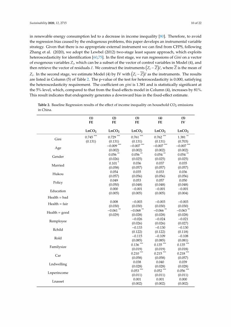
Columns (1), (2), (3) and (4) of Table 2 reports the estimation results with respect to different controlvariables according to Model (4). There is only the core explanatory variable, the Gini coefficient,in Column (1). Column (2) includes the controlling variables of the demographic characteristics ofthe household head, and in Column (3), we further add the household characteristics. In Column (4),the Gini coefficient is included along with all of the controlling variables.

As seen, the results paint a consistent picture. The coefficients on income inequality are significantand positive in all of the columns, (1), (2), (3) and (4), implying that household carbon emissionsincrease with income inequality at the county level, which is in accordance with Liu et al. (2019) andUzar and Eyuboglu (2019) [39,62]. Specifically, a one-standard-deviation increase in the Gini coefficientwill increase household carbon emissions by 6%. This result demonstrates that income inequality ina region have a strong negative impact on pro-environmental behavior. Indeed, improving incomeinequality improves the social stability, and this additional value is crucial for general sustainabledevelopment in China.

The results of other control variables are generally consistent with our expectations. For example,women are more environmentally friendly than men [76,77]. A larger household emits more becauseit consumes more energy [70], and households with at least one car produce more emissions thanhouseholds without a car, as the former consume more fuel for driving [57]. Households at a higherincome level have a stronger purchasing power, which leads to an increase in demand for homecomforts and, in turn, induces more CO2 emissions [78,79]. Households located in urban areas producemore carbon emissions [57].

A common view is that older people tend to generate more CO2 emissions [34,68]; however, wefind otherwise. The older generations have experienced difficult times, and this experience forms inthem a frugal consumption habit. Few studies have investigated the role of health in carbon emissions.Given that health care contributes abundant total emissions, this paper takes the health status ofthe heads of households into consideration. We find that a household with a healthy head emits lessthan one with an unhealthy head.

Although we use a fixed-effects model to control for missing variables that do not change withtime at the household level, there are still some unobservable factors affecting both households’consumption style and income inequality. There also may be reverse causality between householdcarbon emissions and income inequality. For instance, Topcu and Tugcu (2020) found that an increase

Sustainability 2020, 12, 2715 10 of 22

in renewable energy consumption led to a decrease in income inequality [80]. Therefore, to avoidthe regression bias caused by the endogenous problems, this paper develops an instrumental variablestrategy. Given that there is no appropriate external instrument we can find from CFPS, followingZhang et al. (2020), we adopt the Lewbel (2012) two-stage least square approach, which exploitsheteroscedasticity for identification [60,75]. In the first stage, we run regressions of Gini on a vectorof exogenous variables Zi, which can be a subset of the vector of control variables in Model (4), andthen retrieve the vector of residuals ε̂. We construct the instruments

(Zi −Z

)ε̂, where Z is the mean of

Zi. In the second stage, we estimate Model (4) by IV with(Zi −Z

)ε̂ as the instruments. The results

are listed in Column (5) of Table 2. The p-value of the test for heteroscedasticity is 0.000, satisfyingthe heteroscedasticity requirement. The coefficient on gini is 1.381 and is statistically significant atthe 5% level, which, compared to that from the fixed-effects model in Column (4), increases by 81%.This result indicates that endogeneity generates a downward bias in the fixed-effect estimate.

Table 2. Baseline Regression results of the effect of income inequality on household CO2 emissionsin China.

(1)FE

(2)FE

(3)FE

(4)FE

(5)IV

LnCO2 LnCO2 LnCO2 LnCO2 LnCO2

Gini 0.745 ***

(0.131)0.729 ***

(0.131)0.761 ***

(0.131)0.762 ***

(0.131)1.381 **

(0.703)

Age −0.009 ***

(0.002)−0.007 ***

(0.002)−0.007 ***

(0.002)−0.007 ***

(0.002)

Gender 0.056 **

(0.026)0.056 **

(0.025)0.054 **

(0.025)0.054 **

(0.025)

Married 0.101 *

(0.058)0.036

(0.057)0.037

(0.057)0.035

(0.057)

Hukou 0.054(0.057)

0.035(0.056)

0.033(0.056)

0.036(0.056)

Policy 0.049(0.050)

0.053(0.048)

0.057(0.048)

0.050(0.048)

Education 0.000(0.005)

−0.001(0.005)

−0.001(0.005)

−0.001(0.004)

Health = bad

Health = fair 0.008(0.030)

−0.003(0.030)

−0.003(0.030)

−0.003(0.030)

Health = good −0.061 **

(0.029)−0.068 **

(0.028)−0.066 **

(0.028)−0.063 **

(0.028)

Remployee −0.026(0.026)

−0.024(0.026)

−0.021(0.027)

Rchild −0.133(0.122)

−0.130(0.122)

−0.130(0.118)

Rold −0.115(0.085)

−0.109(0.085)

−0.108(0.081)

Familysize 0.136 ***

(0.019)0.135 ***

(0.019)0.135 ***

(0.018)

Car 0.210 ***

(0.058)0.215 ***

(0.058)0.218 ***

(0.057)

Lndwelling 0.038(0.028)

0.040(0.028)

0.039(0.028)

Lnperincome 0.053 ***

(0.011)0.052 ***

(0.011)0.056 ***

(0.011)

Lnasset 0.001(0.002)

0.001(0.002)

0.000(0.002)

Sustainability 2020, 12, 2715 11 of 22

Table 2. Cont.

(1)FE

(2)FE

(3)FE

(4)FE

(5)IV

LnCO2 LnCO2 LnCO2 LnCO2 LnCO2

Lndistance −0.029(0.028)

−0.034(0.028)

Urban 0.176 **

(0.072)0.169 **

(0.071)

Economic 0.011(0.010)

0.012(0.010)

Crowded −0.009(0.009)

−0.009(0.008)

Constant 7.938 ***

(0.059)8.877 ***

(0.134)8.188 ***

(0.226)8.198 ***

(0.247)Year dummies Yes Yes Yes Yes Yes

Family FEs Yes Yes Yes Yes YesModified Wald test(heteroskedasticity) 0.000

Under-id. test 0.000F-stat 69.37

Over-id. test 0.000Obs 11388 11388 11388 11388 11388

R-squared 0.353 0.357 0.374 0.375

Note: Robust standard errors are in parentheses; *** p < 0.01, ** p < 0.05, * p < 0.1; “Health = bad” is a controlgroup of “Health = fair” and “Health = good”; “IV” refers to the Lewbel (2012) approach. Under-id. Test reportsthe p-value of the Kleibergen and Paap (2006) rk statistic [81]; F-stat. reports the Kleibergen–Paap Wald rk F statistic;Over-id. Test reports the p-value of Hansen J statistic.

However, we caution that the Gini coefficient is argued to have certain weaknesses [82]. Cobhamet al. (2013) point out that the Gini coefficient is not very sensitive to the change in high or low income,thus, it cannot clearly explain the reason for inequality [83]. We use the income share of the top 10%(P10) and Palma ratio (Palma) as the proxy of income inequality to test its impact on household carbonemissions again. Liu et al. (2019) used the income share of the top 10% to study whether inequalityfacilitates carbon reduction in the United States [38]. Palma (2011) found that the income ratio ofthe richest 10% and the poorest 40% highly determined the inequality degree, thus, in this paper Palmaratio refers to the ratio of income of the top 10% to income of the bottom 40% [84]. Columns (1) and (2)of Table 3 present the results with the income share of the top 10% and Palma ratio, respectively. Wefind that there is still significantly positive effect of income inequality on household carbon emissions.

Another potential concern is that the outlier of per capita income may affect our calculation ofthe Gini coefficient, in which case our Gini coefficient cannot accurately reflect the degree of regionalinequality. To control for this possibility, we recalculate the Gini coefficient based on per capita incometreated by Winsor method. The results are listed in Column (3) of Table 3. We confirm the baselineregression results by finding a very significantly positive effect of income inequality on householdcarbon emissions.

We also examine the impact of income inequality on household per capita carbon emissions.As Column (4) in Table 3 shows, there is still positive and significant effect of income inequality onhousehold carbon emissions. What is different from the basic regression results is that the coefficienton family size is significantly negative, which implies that per capita carbon emissions decrease withthe expansion of household size [85].

Sustainability 2020, 12, 2715 12 of 22

Table 3. Robustness Checks.

(1)FE

(2)FE

(3)FE

(4)FE

LnCO2 LnCO2 LnCO2 LnperCO2

Gini 0.818 ***

(0.185)0.800 ***

(0.131)

P10 0.651 ***

(0.122)

Palma 0.026 ***

(0.005)

Age −0.007 ***

(0.002)−0.007 ***

(0.002)−0.007 ***

(0.002)−0.007 ***

(0.002)

Gender 0.055 **

(0.025)0.054 **

(0.025)0.053 **

(0.025)0.053 **

(0.025)

Married 0.039(0.057)

0.040(0.057)

0.037(0.057)

−0.062(0.056)

Hukou 0.034(0.056)

0.032(0.057)

0.034(0.056)

0.034(0.056)

Policy 0.057(0.048)

0.061(0.048)

0.059(0.048)

0.059(0.048)

Education −0.002(0.005)

−0.002(0.005)

−0.001(0.005)

−0.001(0.005)

Health=bad

Health=fair −0.002(0.030)

−0.002(0.030)

−0.005(0.030)

−0.003(0.029)

Health=good −0.066 **

(0.028)−0.064 **

(0.028)−0.068 **

(0.028)−0.066 **

(0.028)

Remployee −0.025(0.026)

−0.027(0.026)

−0.023(0.026)

−0.009(0.026)

Rchild −0.131(0.122)

−0.122(0.122)

−0.131(0.123)

−0.183(0.118)

Rold −0.109(0.085)

−0.109(0.085)

−0.106(0.085)

−0.074(0.084)

Familysize 0.135 ***

(0.018)0.136 ***

(0.018)0.136 ***

(0.019)−0.101 ***

(0.013)

Car 0.215 ***

(0.058)0.211 ***

(0.058)0.216 ***

(0.058)0.211 ***

(0.058)

Lndwelling 0.041(0.028)

0.042(0.028)

0.038(0.028)

0.037(0.028)

Lnperincome 0.049 ***

(0.011)0.051 ***

(0.011)0.053 ***

(0.011)0.054 ***

(0.011)

Lnasset 0.001(0.002)

0.001(0.002)

0.001(0.002)

0.001(0.002)

Lndistance −0.025(0.028)

−0.024(0.028)

−0.033(0.028)

−0.024(0.028)

Urban 0.181 **

(0.072)0.181 **

(0.072)0.173 **

(0.072)0.172 **

(0.072)

Economic 0.012(0.010)

0.011(0.010)

0.011(0.010)

0.012(0.010)

Crowded −0.009(0.009)

−0.007(0.009)

−0.008(0.009)

−0.009(0.009)

Constant 8.348 ***

(0.242)7.964 ***

(0.233)8.187 ***

(0.255)7.903 ***

(0.244)Year dummies Yes Yes Yes Yes

Family FEs Yes Yes Yes YesObs. 11388 11388 11388 11388

R-squared 0.374 0.375 0.374 0.387

Note: Robust standard errors are in parentheses; *** p < 0.01, ** p < 0.05, * p < 0.1; “Health = bad” is a control groupof “Health = fair” and “Health = good”.

Sustainability 2020, 12, 2715 13 of 22

4.2. Roles of Consumption Patterns, Time Preference for Consumption, and Mental Health

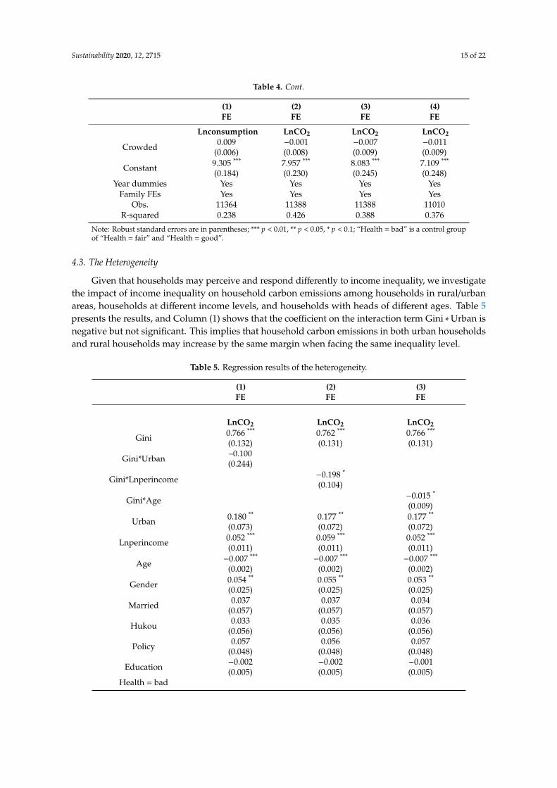
The differences in the scale and patterns of consumption lead to an unequal distribution ofhouseholds’ carbon footprints among the rich and the poor in China [86]. Will income inequalityincrease household carbon emissions by stimulating household consumption? Column (1) of Table 4shows that there is no significant effect of income inequality on household consumption scale. Then,we test the role of consumption patterns. According to Charles et al. (2009), Kaus (2013) and Zhou etal. (2018), we define consumption on clothing, transportation and communication, and residence asconspicuous consumption [87–89]. We use the proportion of conspicuous consumption expenditureof total expenditure to measure a household’s consumption patterns, and a larger proportion meansan extravagant consumption pattern. From Column (2) of Table 4, we find that the coefficient onconspicuous is positive, while that on the interaction term Gini ∗Conspicuous is negative, and bothare significant at the 1% level. This result indicates that household CO2 emissions increase withconspicuous consumption, but higher levels of conspicuous consumption may reduce households’perception of income inequality, and thus reduce carbon emissions caused by inequality. This effectmay occur because there is little room for households at a high level of conspicuous consumptionto change to a more extravagant consumption pattern, whereas those at a low level of conspicuousconsumption will engage more in conspicuous consumption to maintain or obtain a higher socialstatus when facing higher levels of income inequality. This result confirms the “Veblen effect” [32,33].

We also investigate whether time preference for consumption and mental health can affectthe relationship between income inequality and household carbon emissions. We use the share ofeducation and training expenditure in household total expenditure (Edurate) as the proxy variable oftime preference, and a larger share indicates a lower degree of time preference. For mental health,there were six questions on the state of an individual’s mental health in the CFPS of 2010 and 2014.In 2012, there were twenty questions; thus, we extract six questions to match the data to those from2010 and 2014. These questions comprise the K6 scale developed by Kessler et al. (2002) [90]. The sixquestions in the K6 instrument ask the following: During the past month, about how often did you feel(1) so depressed that nothing could cheer you up? (2) nervous? (3) restless or fidgety, or you could notkeep calm? (4) hopeless? (5) that everything was difficult? (6) life is worthless? There are five optionsfor respondents to choose from: Never (five points), once a month (four points), two or three timesa month (three points), two or three times a week (two points), and almost every day (one point). Weuse the mean score of the six questions as a proxy for mental health of the head of the household.

Column (3) of Table 4 shows that the coefficient on edurate is positive and that on the interactionterm Gini ∗ Edurate is negative, and both are significant at the 1% level. This result implies thatmore household emissions are associated with a greater proportion of expenditure on education andtraining. Investing more in education and training (future) may increase the households’ tolerancedegree to current income inequality because they pay more attention to future gains, thus alleviatingthe effect of income inequality on household carbon emissions. Column (4) of Table 4 shows thatthe coefficients on both mentalhealth and the interaction term Gini ∗Mentalhealth are negative, butonly the interaction term is significant. This result indicates that income inequality may damage mentalhealth, and thus cause more carbon emissions. A mentally healthier household head is not susceptibleto income inequality.

Sustainability 2020, 12, 2715 14 of 22

Table 4. Regression results with interaction terms.

(1)FE

(2)FE

(3)FE

(4)FE

Lnconsumption LnCO2 LnCO2 LnCO2

Gini 0.104(0.107)

0.566 ***

(0.123)0.717 ***

(0.129)0.750 ***

(0.134)

Gini*Conspicuous −2.784 ***

(1.055)

Gini*Edurate −2.211 ***

(0.688)

Gini*Mental health −0.308 **

(0.126)

Conspicuous 1.716 ***

(0.093)

Edurate 0.991 ***

(0.078)

Mental health −0.008(0.018)

Age −0.007 ***

(0.001)−0.007 ***

(0.002)−0.007 ***

(0.002)−0.007 ***

(0.002)

Gender 0.052 ***

(0.020)0.055 **

(0.024)0.051 **

(0.025)0.051 **

(0.026)

Married 0.060(0.047)

0.031(0.055)

0.047(0.057)

0.022(0.057)

Hukou 0.026(0.042)

0.047(0.052)

0.034(0.057)

0.026(0.055)

Policy 0.061(0.037)

0.062(0.045)

0.061(0.047)

0.058(0.049)

Education 0.001(0.004)

0.000(0.004)

−0.001(0.004)

−0.001(0.005)

Health=bad

Health=fair −0.023(0.024)

−0.020(0.029)

−0.005(0.029)

−0.009(0.030)

Health=good −0.058 ***

(0.022)−0.085 ***

(0.027)−0.071 **

(0.028)−0.066 **

(0.029)

Remployee −0.041 *

(0.022)−0.042 *

(0.025)−0.005(0.026)

−0.020(0.026)

Rchild −0.227 **

(0.092)−0.203 *

(0.116)−0.014(0.122)

−0.153(0.122)

Rold −0.163 **

(0.063)−0.088(0.081)

−0.111(0.084)

−0.100(0.084)

Familysize 0.124 ***

(0.013)0.129 ***

(0.017)0.124 ***

(0.018)0.153 ***

(0.014)

Car 0.507 ***

(0.044)0.267 ***

(0.055)0.240 ***

(0.058)0.204 ***

(0.058)

Lndwelling 0.038 *

(0.020)0.035

(0.026)0.044

(0.028)0.034

(0.029)

Lnperincome 0.070 ***

(0.009)0.051 ***

(0.010)0.058 ***

(0.011)0.053 ***

(0.011)

Lnasset −0.000(0.002)

−0.000(0.002)

0.001(0.002)

0.001(0.002)

Lndistance −0.062 ***

(0.020)−0.040(0.025)

−0.036(0.028)

−0.032(0.028)

Urban 0.035(0.050)

0.141 **

(0.068)0.174 **

(0.071)0.175 **

(0.073)

Economic −0.003(0.007)

0.005(0.009)

0.010(0.010)

0.013(0.010)

Sustainability 2020, 12, 2715 15 of 22

Table 4. Cont.

(1)FE

(2)FE

(3)FE

(4)FE

Lnconsumption LnCO2 LnCO2 LnCO2

Crowded 0.009(0.006)

−0.001(0.008)

−0.007(0.009)

−0.011(0.009)

Constant 9.305 ***

(0.184)7.957 ***

(0.230)8.083 ***

(0.245)7.109 ***

(0.248)Year dummies Yes Yes Yes Yes

Family FEs Yes Yes Yes YesObs. 11364 11388 11388 11010

R-squared 0.238 0.426 0.388 0.376

Note: Robust standard errors are in parentheses; *** p < 0.01, ** p < 0.05, * p < 0.1; “Health = bad” is a control groupof “Health = fair” and “Health = good”.

4.3. The Heterogeneity

Given that households may perceive and respond differently to income inequality, we investigatethe impact of income inequality on household carbon emissions among households in rural/urbanareas, households at different income levels, and households with heads of different ages. Table 5presents the results, and Column (1) shows that the coefficient on the interaction term Gini ∗Urban isnegative but not significant. This implies that household carbon emissions in both urban householdsand rural households may increase by the same margin when facing the same inequality level.

Table 5. Regression results of the heterogeneity.

(1)FE

(2)FE

(3)FE

LnCO2 LnCO2 LnCO2

Gini 0.766 ***

(0.132)0.762 ***

(0.131)0.766 ***

(0.131)

Gini*Urban –0.100(0.244)

Gini*Lnperincome −0.198 *

(0.104)

Gini*Age −0.015 *

(0.009)

Urban 0.180 **

(0.073)0.177 **

(0.072)0.177 **

(0.072)

Lnperincome 0.052 ***

(0.011)0.059 ***

(0.011)0.052 ***

(0.011)

Age −0.007 ***

(0.002)−0.007 ***

(0.002)−0.007 ***

(0.002)

Gender 0.054 **

(0.025)0.055 **

(0.025)0.053 **

(0.025)

Married 0.037(0.057)

0.037(0.057)

0.034(0.057)

Hukou 0.033(0.056)

0.035(0.056)

0.036(0.056)

Policy 0.057(0.048)

0.056(0.048)

0.057(0.048)

Education −0.002(0.005)

−0.002(0.005)

−0.001(0.005)

Health = bad

Sustainability 2020, 12, 2715 16 of 22

Table 5. Cont.

(1)FE

(2)FE

(3)FE

LnCO2 LnCO2 LnCO2

Health = fair −0.003(0.030)

−0.003(0.030)

−0.003(0.030)

Health = good −0.066 **

(0.028)−0.065 **

(0.028)−0.066 **

(0.028)

Remployee −0.024(0.026)

−0.023(0.026)

−0.027(0.026)

Rchild −0.130(0.122)

−0.125(0.122)

−0.128(0.122)

Rold −0.108(0.085)

−0.105(0.085)

−0.107(0.085)

Familysize 0.135 ***

(0.019)0.136 ***

(0.019)0.136 ***

(0.018)

Car 0.215 ***

(0.058)0.214 ***

(0.058)0.215 ***

(0.058)

Lndwelling 0.040(0.028)

0.039(0.028)

0.039(0.028)

Lnasset 0.001(0.002)

0.001(0.011)

0.001(0.002)

Lndistance −0.029(0.028)

−0.028(0.028)

−0.028(0.028)

Economic 0.011(0.010)

0.011(0.07)

0.011(0.010)

Crowded −0.008(0.009)

−0.008(0.009)

−0.008(0.009)

Constant 8.191 ***

(0.248)8.129 ***

(0.252)8.192 ***

(0.247)Year dummies Yes Yes Yes

Family FEs Yes Yes YesObs. 11388 11388 11388

R-squard 0.375 0.375 0.375

Note: Robust standard errors are in parentheses; *** p < 0.01, ** p < 0.05, * p < 0.1; “Health = bad” is a control groupof “Health = fair” and “Health = good”.

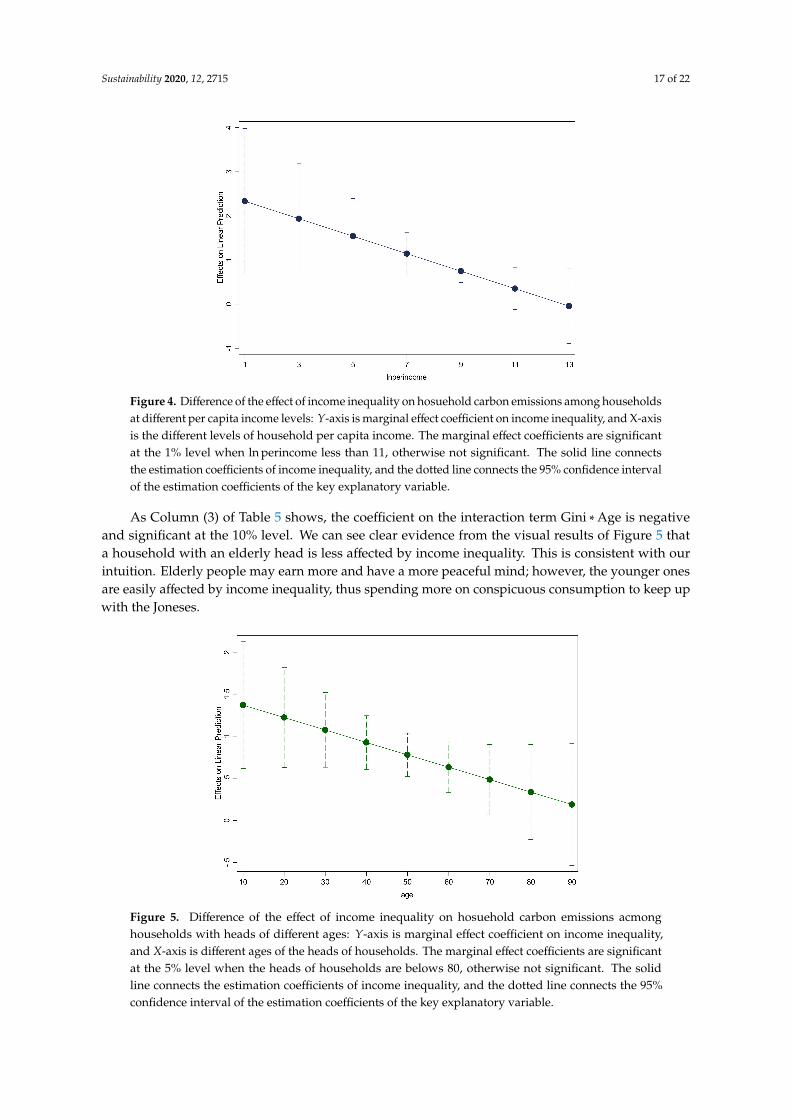
As illustrated in Column (2) of Table 5, the coefficient on the interaction term Gini ∗ Lnperincomeis negative and significant at the 10% level. Figure 4 shows the visual results. We find that as incomeincreases, the positive impact of inequality on household carbon emissions decreases, while this onlyworks if the log of per capita income is less than 11. This result means that households at a relativelylower income level are more affected by inequality, while the highest income class may be not evenaffected by inequality at all.

Sustainability 2020, 12, 2715 17 of 22

Figure 4. Difference of the effect of income inequality on hosuehold carbon emissions among householdsat different per capita income levels: Y-axis is marginal effect coefficient on income inequality, and X-axisis the different levels of household per capita income. The marginal effect coefficients are significantat the 1% level when ln perincome less than 11, otherwise not significant. The solid line connectsthe estimation coefficients of income inequality, and the dotted line connects the 95% confidence intervalof the estimation coefficients of the key explanatory variable.

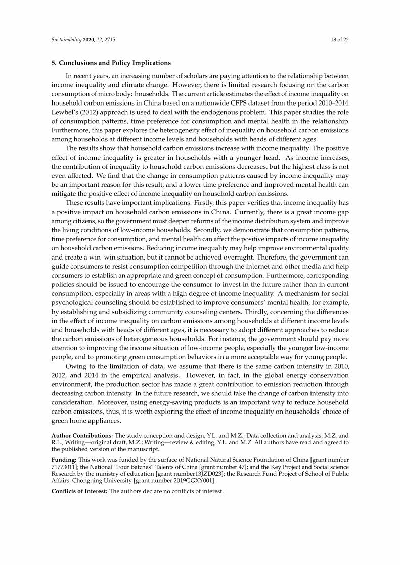
As Column (3) of Table 5 shows, the coefficient on the interaction term Gini ∗Age is negativeand significant at the 10% level. We can see clear evidence from the visual results of Figure 5 thata household with an elderly head is less affected by income inequality. This is consistent with ourintuition. Elderly people may earn more and have a more peaceful mind; however, the younger onesare easily affected by income inequality, thus spending more on conspicuous consumption to keep upwith the Joneses.

Figure 5. Difference of the effect of income inequality on hosuehold carbon emissions acmonghouseholds with heads of different ages: Y-axis is marginal effect coefficient on income inequality,and X-axis is different ages of the heads of households. The marginal effect coefficients are significantat the 5% level when the heads of households are belows 80, otherwise not significant. The solidline connects the estimation coefficients of income inequality, and the dotted line connects the 95%confidence interval of the estimation coefficients of the key explanatory variable.

Sustainability 2020, 12, 2715 18 of 22

5. Conclusions and Policy Implications

In recent years, an increasing number of scholars are paying attention to the relationship betweenincome inequality and climate change. However, there is limited research focusing on the carbonconsumption of micro body: households. The current article estimates the effect of income inequality onhousehold carbon emissions in China based on a nationwide CFPS dataset from the period 2010–2014.Lewbel’s (2012) approach is used to deal with the endogenous problem. This paper studies the roleof consumption patterns, time preference for consumption and mental health in the relationship.Furthermore, this paper explores the heterogeneity effect of inequality on household carbon emissionsamong households at different income levels and households with heads of different ages.

The results show that household carbon emissions increase with income inequality. The positiveeffect of income inequality is greater in households with a younger head. As income increases,the contribution of inequality to household carbon emissions decreases, but the highest class is noteven affected. We find that the change in consumption patterns caused by income inequality maybe an important reason for this result, and a lower time preference and improved mental health canmitigate the positive effect of income inequality on household carbon emissions.

These results have important implications. Firstly, this paper verifies that income inequality hasa positive impact on household carbon emissions in China. Currently, there is a great income gapamong citizens, so the government must deepen reforms of the income distribution system and improvethe living conditions of low-income households. Secondly, we demonstrate that consumption patterns,time preference for consumption, and mental health can affect the positive impacts of income inequalityon household carbon emissions. Reducing income inequality may help improve environmental qualityand create a win–win situation, but it cannot be achieved overnight. Therefore, the government canguide consumers to resist consumption competition through the Internet and other media and helpconsumers to establish an appropriate and green concept of consumption. Furthermore, correspondingpolicies should be issued to encourage the consumer to invest in the future rather than in currentconsumption, especially in areas with a high degree of income inequality. A mechanism for socialpsychological counseling should be established to improve consumers’ mental health, for example,by establishing and subsidizing community counseling centers. Thirdly, concerning the differencesin the effect of income inequality on carbon emissions among households at different income levelsand households with heads of different ages, it is necessary to adopt different approaches to reducethe carbon emissions of heterogeneous households. For instance, the government should pay moreattention to improving the income situation of low-income people, especially the younger low-incomepeople, and to promoting green consumption behaviors in a more acceptable way for young people.

Owing to the limitation of data, we assume that there is the same carbon intensity in 2010,2012, and 2014 in the empirical analysis. However, in fact, in the global energy conservationenvironment, the production sector has made a great contribution to emission reduction throughdecreasing carbon intensity. In the future research, we should take the change of carbon intensity intoconsideration. Moreover, using energy-saving products is an important way to reduce householdcarbon emissions, thus, it is worth exploring the effect of income inequality on households’ choice ofgreen home appliances.

Author Contributions: The study conception and design, Y.L. and M.Z.; Data collection and analysis, M.Z. andR.L.; Writing—original draft, M.Z.; Writing—review & editing, Y.L. and M.Z. All authors have read and agreed tothe published version of the manuscript.

Funding: This work was funded by the surface of National Natural Science Foundation of China [grant number71773011]; the National “Four Batches” Talents of China [grant number 47]; and the Key Project and Social scienceResearch by the ministry of education [grant number13JZD023]; the Research Fund Project of School of PublicAffairs, Chongqing University [grant number 2019GGXY001].

Conflicts of Interest: The authors declare no conflicts of interest.

Sustainability 2020, 12, 2715 19 of 22

References

1. IPCC. Global Warming of 1.5 ◦C. An IPCC Special Report on the Impacts of Global Warming of 1.5 ◦C abovePre-Industrial Levels and Related Global Greenhouse Gas Emission Pathways. In The Context of Strengtheningthe Global Response to the Threat of Climate Change, Sustainable Development, and Efforts to Eradicate Poverty;IPCC: Geneva, Switzerland, 2018; in press.

2. UNEP (United Nations Environment Program). The Emissions Gap Report 2019; United Nations EnvironmentProgramme (UNEP): Nairobi, Kenya, 2019.

3. World Bank. Growth and CO2 Emissions: How Do Different Countries Fare; Environment Department:Washington, DC, USA, 2007.

4. Hao, Y.; Chen, H.; Zhang, Q. Will income inequality affect environmental quality? Analysis based on China’sprovincial panel data. Ecol. Indic. 2016, 67, 533–542. [CrossRef]

5. Guo, D.; Chen, H.; Long, R.; Ni, Y. An integrated measurement of household carbon emissions froma trading-oriented perspective: A case study of urban families in Xuzhou, China. J. Clean. Prod. 2018, 188,613–624. [CrossRef]

6. Ji, Q.; Zhang, D. China’s crude oil futures: Introduction and some stylized facts. Financ. Res. Lett. 2019, 28,376–380. [CrossRef]

7. Xu, K.; Han, Y.; Lv, F. Household carbon inequality in urban China, its sources and determinants. Ecol. Econ.2016, 128, 77–86. [CrossRef]

8. Bin, S.; Dowlatabadi, H. Consumer lifestyle approach to US energy use and the related CO2 emissions.Energy Policy 2005, 33, 197–208. [CrossRef]

9. Baiocchi, G.; Minx, J.; Hubacek, K. The impact of social factors and consumer behavior on carbon dioxideemissions in the United Kindom. J. Ind. Ecol. 2010, 14, 50–72. [CrossRef]

10. Pachauri, S.; Spreng, D. Direct and indirect energy requirements of households in India. Energy Policy 2002,30, 511–523. [CrossRef]

11. Liu, L.; Wu, G.; Wang, J.; Wei, Y. China’s carbon emissions from urban and rural households during 1992–2007.J. Clean. Prod. 2011, 19, 1754–1762. [CrossRef]

12. Fan, J.; Liao, H.; Liang, Q.; Tatano, H.; Liu, C.; Wei, Y. Residential carbon emission evolutions in urban-ruraldivided China: An end-use and behavior analysis. Appl. Energy 2013, 101, 323–332. [CrossRef]

13. Hertwich, E.G.; Peters, G.P. Carbon footprint of nations: A global, trade-linked analysis. Environ. Sci. Technol.2009, 43, 6414–6420. [CrossRef]

14. Wu, S.; Lei, Y.; Li, S. CO2 emissions from household consumption at the provincial level and interprovincialtransfer in China. J. Clean. Prod. 2019, 210, 93–104. [CrossRef]

15. Dong, Y.; Zhao, T. Difference analysis of the relationship between household per capita income, per capitaexpenditure and per capita CO2 emissions in China: 1997–2014. Atmos. Pollut. Res. 2017, 8, 310–319.[CrossRef]

16. Stiglitz, J.T. The Price of Inequality: How Today’s Divided Society Endangers Our Future; WW Norton & Company:New York, NY, USA, 2012.

17. Piketty, T. Capital in the Twenty-First Century; Harvard University Press: Cambridge, MA, USA, 2014.18. Ribeiro, W.S.; Bauer, A.; Andrade, M.C.; York-Smith, M.; Pan, P.M.; Pingani, L.; Knapp, M.; Coutinho, E.S.;

Evans-Lacko, S. Income inequality and mental illness-related morbidity and resilience: A systematic reviewand meta-analysis. Lancet Psychiatry 2017, 4, 554–562. [CrossRef]

19. Burns, J.K.; Tomita, A.; Kapadia, A.S. Income inequality and schizophrenia: Increased schizophreniaincidence in countries with high levels of income inequality. Int. J. Soc. Psychiatry 2014, 60, 185–196.[CrossRef]

20. Layte, R.; Whelan, C. GINI DP 78: Who Feels Inferior? A Test of the Status Anxiety Hypothesis of Social Inequalitiesin Health; AIAS, Amsterdam Institute for Advanced Labour Studies: Amsterdam, The Netherlands, 2013.

21. Vanderende, K.E.; Young, I.K.M.; Dynes, M.M.; Sibley, L.M. Community-level correlates of intimate partnerviolence against women globally: A systematic review. Soc. Sci. Med. 2012, 75, 1143–1155. [CrossRef]

22. Kumhof, M.; Rancière, R.; Winant, P. Inequality, Leverage, and Crises. Am. Econ. Rev. 2015, 105, 1217–1245.[CrossRef]

23. Wolde-Rufael, Y.; Idowu, S. Income distribution and CO2 emission: A comparative analysis for China andIndia. Renew Sustain Energy Rev. 2017, 4, 1336–1345. [CrossRef]

Sustainability 2020, 12, 2715 20 of 22

24. Solt, F. Standardizing the world income inequality database. Soc. Sci. Q. 2009, 90, 231–242. [CrossRef]25. Jorgenson, A.; Schor, J.; Huang, X.R. Income inequality and carbon emissions in the United States: A State-level

Analysis, 1997–2012. Ecol. Econ. 2017, 134, 40–48. [CrossRef]26. Boyce, J.K. Inequality as a cause of environmental degradation. Ecol. Econ. 1994, 3, 169–178. [CrossRef]27. Scruggs, L.A. Political and economic inequality and the environment. Ecol. Econ. 1998, 26, 259–275.

[CrossRef]28. Heerink, N.; Mulatu, A.; Bulte, E. Income inequality and the environment: Aggregation bias in environmental

Kuznets curves. Ecol. Econ. 2001, 3, 359–367. [CrossRef]29. Ravallion, M.; Heil, M.; Jalan, J. CO2 emissions and income inequality. Oxf. Econ. Pap. 2000, 4, 651–669.

[CrossRef]30. Heil, M.; Selden, T. CO2 emissions and economic development: Future trajectories based on historical

experience. Environ. Dev. Econ. 2001, 1, 63–83. [CrossRef]31. Borghesi, S. Income inequality and the environmental Kuznets curve. In Environment, Inequality Collective

Action; Routledge: London, UK, 2006.32. Schor, J. The Overspent American: When Buying Becomes You; Basic books: New York, NY, USA, 1998.33. Veblen, T. The Theory of the Leisure Class; Oxford University Press: Oxford, UK, 2009.34. Golley, J.; Meng, X. Income inequality and carbon dioxide emissions: The case of Chinese urban households.

Energy Econ. 2012, 34, 1864–1872. [CrossRef]35. Baek, J.; Gweisah, G. Does income inequality harm the environment? Empirical evidence from the United

States. Energy Policy 2013, 62, 1434–1437. [CrossRef]36. Jorgenson, A. Inequality and the carbon intensity of human well-being. J. Environ. Stud. Sci. 2015, 3, 277–282.

[CrossRef]37. Kasuga, H.; Takaya, M. Does inequality affect environmental quality? Evidence from major Japanese cities.

J. Clean. Prod. 2017, 142, 3689–3701. [CrossRef]38. Liu, C.; Jiang, Y.; Xie, R. Does income inequality facilitate carbon emission reduction in the US? J. Clean. Prod.

2019, 217, 380–387. [CrossRef]39. Uzar, U.; Eyuboglu, K. The nexus between income inequality and CO2 emissions in Turkey. J. Clean. Prod.

2019, 227, 149–157. [CrossRef]40. Coondoo, D.; Dinda, S. Carbon dioxide emission and income: A temporal analysis of cross-country

distributional patterns. Ecol. Econ. 2008, 65, 375–385. [CrossRef]41. Baloch, A.; Shah, S.Z.; Noor, Z.M.; Magsi, H.B. The nexus between income inequality, economic growth and

environmental degradation in Pakistan. Geo J. 2018, 83, 207–222. [CrossRef]42. Hübler, M. The inequality-emissions nexus in the context of trade and development: A quantile regression

approach. Ecol. Econ. 2017, 134, 174–185. [CrossRef]43. Sager, L. Income inequality and carbon consumption: Evidence from environmental Engel curves. Energy Econ.

2019, 84, 104507. [CrossRef]44. Grunewald, N.; Klasen, S.; Martínez-Zarzoso, I.; Muris, C. The Trade-off between income inequality and

carbon dioxide emissions. Ecol. Econ. 2017, 142, 249–256. [CrossRef]45. Clément, M.; Meunié, A. Inégalités, développement et qualité de l’environnement: Mécanismes et application

empirique. Mondes En Développement 2010, 151, 67–82. [CrossRef]46. Policardo, L. Is democracy good for the environment? Quasi-experimental evidence from regime transitions.

Environ. Resour. Econ. 2016, 2, 275–300. [CrossRef]47. Waston, B.; Osberg, L. Can positive income anticipations reverse the mental health impacts of negative

income anxieties. Econ. Hum. Biol. 2019, 35, 107–122.48. Vilhjalmsdottir, A.; Gardarsdottir, R.B.; Bernburg, J.G.; Sigfusdottir, I.D. Neighborhood income inequality,

social capital and emotional distress among adolescents: A population-based study. J. Adolesc. 2016, 51,92–102. [CrossRef]

49. Layte, R. The association between income inequality and mental health: Testing status anxiety, social capital,and neo-materialist explanations. Eur. Sociol. Rev. 2011, 28, 498–511. [CrossRef]

50. Chiavegatto Filho, A.D.; Kawachi, I.; Wang, Y.P.; Viana, M.C.; Andrade, L.H. Does income inequality getunder the skin? A multilevel analysis of depression, anxiety and mental disorders in Sao Paulo, Brazil.J. Epidemiol. Community Health 2013, 67, 966–972. [CrossRef]

Sustainability 2020, 12, 2715 21 of 22

51. Oishi, S.; Kesebir, S. Income inequality explains shy economic growth does not always translate to an increasein happiness. Psychol. Couns. 2015, 26, 1630–1638.

52. Velek, C.; Steg, L. Human behavior and environmental sustainability: Problems, driving forces, and researchtopics. J. Soc. Issues 2007, 63, 1–19. [CrossRef]

53. Kaida, N.; Kaida, K. Pro-environmental behavior correlates with present and future subjective well-being.Environ. Dev. Sustain. 2016, 18, 111–127. [CrossRef]

54. Koenig-Lewis, N.; Palmer, A.; Dermody, J.; Urbye, A. Consumers’ evaluations of ecological packaging-rationaland emotional approaches. J. Environ. Psychol. 2014, 37, 94–105. [CrossRef]

55. Bissing-Olson, M.J.; Iyer, A.; Fielding, K.S.; Zacher, H. Relationships between daily affect andpro-environmental behavior at work: The moderating role of pro-environmental attitude. J. Organ.Behav. 2013, 34, 151–171. [CrossRef]

56. Ibanez, L.; Moureau, N.; Roussel, S. How do incidental emotions impact pro-environmental behavior?Evidence from the dictator game. J. Behav. Exp. Econ. 2017, 66, 150–155. [CrossRef]

57. Li, J.; Zhang, D.; Su, B. The impact of social awareness and lifestyles on household carbon emissions in China.Ecol. Econ. 2019, 160, 145–155. [CrossRef]

58. Wei, Y.; Liu, L.; Fan, Y.; Wu, G. The impact of lifestyle on energy use and CO2 emission: An empirical analysisof China’s residents. Energy Policy 2007, 35, 247–257. [CrossRef]

59. Su, B.; Ang, B.W. Multiplicative decomposition of aggregate carbon intensity change using input-outputanalysis. Appl. Energy 2015, 154, 13–20. [CrossRef]

60. Zhang, Q.; Churchill, S.A. Income inequality and subjective wellbeing: Panel data evidence from China.China Econ. Rev. 2020, 60, 101392. [CrossRef]

61. Zhang, W.; Shi, P.; Wang, K.; Xue, J.; Song, G.; Sun, P. Intertemporal lifestyle changes and carbon emissions:Evidence from a China household survey. Energy Econ. 2020, 86, 104655. [CrossRef]

62. Liu, Q.; Wang, S.; Zhang, W.; Li, J.; Kong, Y. Examining the effects of income inequality on CO2 emissions:Evidence from non-spatial and spatial perspectives. Appl. Energy 2019, 236, 163–171. [CrossRef]

63. Andersson, D.; Nässén, J.; Larsson, J.; Holmber, J. Greenhouse gas emissions and subjective well-being:An analysis of Swedish households. Ecol. Econ. 2014, 102, 75–82. [CrossRef]

64. Streimikiene, D.; Volochovic, A. The impact of household behavioral changes on GHG emission reduction inLithuania. Renew. Sustain. Energy Rev. 2011, 15, 4118–4124. [CrossRef]

65. Büchs, M.; Schnepf, S.V. Who emits most? Associations between socio-economic facts and UK households’home energy, transport, indirect and total CO2 emissions. Ecol. Econ. 2013, 90, 114–123. [CrossRef]

66. Dai, H.; Masui, T.; Matsuoka, Y.; Fujimori, S. The impacts of China’s household consumption expenditurepatterns on energy demand and carbon emissions towards 2050. Energy Policy 2012, 50, 736–750. [CrossRef]

67. Lee, S.; Lee, B. The influence of urban form on GHG emissions in the US household sector. Energy Policy2014, 68, 534–549. [CrossRef]

68. Chancel, L. Are younger generations higher carbon emitters than their elders? Inequalities, generations andCO2 emissions in France and in the USA. Ecol. Econ. 2014, 100, 195–207. [CrossRef]

69. Jones, C.; Kammen, D.M. Spatial distribution of U.S. Household carbon footprints reveals suburbanizationundermines greenhouse gas benefits of urban population density. Environ. Sci. Technol. 2014, 48, 895–902.[CrossRef]

70. Meier, H.; Rehdanz, K. Determinants of residential space heating expenditures in Great Britain. Energy Econ.2010, 32, 949–959. [CrossRef]

71. Ottelin, J.; Heinonen, J.; Junnila, S. Carbon footprint trends of metropolitan residents in Finland: How strongmitigation policies affect different urban zones. J. Clean. Prod. 2018, 170, 1523–1535. [CrossRef]

72. Qu, J.; Liu, L.; Zeng, J.; Zhang, Z.; Wang, J.; Pei, H.; Dong, L.; Liao, Q.; Maraseni, T. The impact of income onhousehold CO2 emissions in China based on a large sample survey. Sci. Bull. 2019, 64, 351–353. [CrossRef]

73. Ewing, R.; Rong, F. The impact of urban form on us residential energy use. Hous. Policy Debate 2008, 19, 1–30.[CrossRef]

74. Qin, B.; Han, S. Planning parameters and household carbon emission: Evidence from high-and low-carbonneighborhoods in Beijing. Habitat Int. 2013, 37, 52–60. [CrossRef]

75. Lewbel, A. Using heteroscedasticity to identify and estimate mismeasured and endogenous regressor models.J. Bus. Econ. Stat. 2012, 30, 67–80. [CrossRef]

Sustainability 2020, 12, 2715 22 of 22

76. Casaló, L.V.; Escario, J.J. Heterogeneity in the association between environmental attitudes andpro-environmental behavior: A multilevel regression approach. J. Clean. Prod. 2018, 175, 155–163.[CrossRef]

77. Li, J.; Zhang, J.; Zhang, D.; Ji, Q. Does gender inequality affect household green consumption behavior inChina? Energy Policy. 2019, 135, 111071. [CrossRef]

78. Miao, L. Examining the impact factors of urban residential energy consumption and CO2 emissions inChina-Evidence from city-level data. Ecol. Indic. 2017, 73, 29–37. [CrossRef]

79. Bai, Y.; Deng, X.; Gibson, J.; Zhao, Z.; Hu, H. How does urbanization affect residential CO2 emissions?An analysis on urban agglomerations of China. J. Clean. Prod. 2019, 209, 876–885. [CrossRef]

80. Topcu, M.; Tugcu, C.T. The impact of renewable energy consumption on income inequality: Evidence fromdeveloped countries. Renew. Energy 2020, 151, 1134–1140. [CrossRef]

81. Kleibergen, G.; Paap, R. Generalized reduced rank tests using the singular value decomposition. J. Econom.2006, 133, 97–126. [CrossRef]

82. De Maio, F.G. Income inequality measures. J. Epidemiol. Community Health 2007, 61, 849–852. [CrossRef][PubMed]

83. Cobham, A.; Sumner, A.; Cornia, A.; Dercon, S.; Engberg-pedersen, L.; Evans, M.; Lea, N.; Lustig, N.;Manning, R.; Milanovic, B.; et al. Putting the Gini Back in the Bottle? ‘The Palma’ As a Policy-Relevant Measure ofInequality; King’s College WP-5: London, UK, 2013.

84. Palma, J.G. Homogeneous middles vs. Heterogeneous tails, and the end of the ‘inverted-U’: it’s all aboutthe share of the rich. Dev. Chang. 2011, 42, 87–153. [CrossRef]

85. Lyons, S.; Pentecost, A.; Tol, R.S.J. Socioeconomic distribution of emissions and resource use in Ireland.J. Environ. Manag. 2012, 112, 186–198. [CrossRef] [PubMed]

86. Wiedenhofer, D.; Guan, D.; Liu, Z.; Meng, J.; Zhang, N.; Wei, Y.M. Unequal household carbon footprints inChina. Nat. Clim. Chang. 2016, 7, 75–80. [CrossRef]

87. Charles, K.K.; Hurst, E.; Roussanov, N. Conspicuous consumption and race. Q. J. Econ. 2009, 124, 425–467.[CrossRef]

88. Kaus, W. Conspicuous consumption and “race”: Evidence from South Africa. J. Dev. Econ. 2013, 100, 63–73.[CrossRef]

89. Zhou, G.; Fan, G.; Ma, G. The impact of income inequality on the visible expenditure of China’s households.Financ. Trade Econ. 2018, 39, 21–35.

90. Kessler, R.C.; Andrews, G.; Colpe, L.J.; Hiripi, E.; Mroczek, D.K.; Normand, S.L.; Walters, E.E.; Zaslavsky, A.M.Short screening scales to monitor population prevalences and trends in non-specific psychological distress.Psychol. Med. 2002, 6, 959–976.

© 2020 by the authors. Licensee MDPI, Basel, Switzerland. This article is an open accessarticle distributed under the terms and conditions of the Creative Commons Attribution(CC BY) license (http://creativecommons.org/licenses/by/4.0/).