Urban Socio-Economic Segregation and Income Inequality
520
The Urban Book Series Maarten van Ham Tiit Tammaru Rūta Ubarevičienė Heleen Janssen Editors Urban Socio-Economic Segregation and Income Inequality A Global Perspective
-
Upload
khangminh22 -
Category
Documents
-
view
0 -
download
0
Transcript of Urban Socio-Economic Segregation and Income Inequality
The Urban Book Series
Maarten van HamTiit TammaruRūta UbarevičienėHeleen Janssen Editors
Urban Socio-Economic Segregation and Income InequalityA Global Perspective
The Urban Book Series
Editorial Board
Fatemeh Farnaz Arefian, University of Newcastle, Singapore, Singapore, Silk Cities& Bartlett Development Planning Unit, UCL, London, UK
Michael Batty, Centre for Advanced Spatial Analysis, UCL, London, UK
Simin Davoudi, Planning & Landscape Department GURU, Newcastle University,Newcastle, UK
Geoffrey DeVerteuil, School of Planning and Geography, Cardiff University,Cardiff, UK
Andrew Kirby, New College, Arizona State University, Phoenix, AZ, USA
Karl Kropf, Department of Planning, Headington Campus, Oxford BrookesUniversity, Oxford, UK
Karen Lucas, Institute for Transport Studies, University of Leeds, Leeds, UK
Marco Maretto, DICATeA, Department of Civil and Environmental Engineering,University of Parma, Parma, Italy
Fabian Neuhaus, Faculty of Environmental Design, University of Calgary, Calgary,AB, Canada
Steffen Nijhuis, Architecture and the Built Environment, Delft University ofTechnology, Delft, The Netherlands
Vitor Manuel Aráujo de Oliveira , Porto University, Porto, Portugal
Christopher Silver, College of Design, University of Florida, Gainesville, FL, USA
Giuseppe Strappa, Facoltà di Architettura, Sapienza University of Rome, Rome,Roma, Italy
Igor Vojnovic, Department of Geography, Michigan State University, East Lansing,MI, USA
Jeremy W. R. Whitehand, Earth & Environmental Sciences, University ofBirmingham, Birmingham, UK
Claudia Yamu, Department of Spatial Planning and Environment, University ofGroningen, Groningen, Groningen, The Netherlands

The Urban Book Series is a resource for urban studies and geography researchworldwide. It provides a unique and innovative resource for the latest developmentsin the field, nurturing a comprehensive and encompassing publication venue forurban studies, urban geography, planning and regional development.
The series publishes peer-reviewed volumes related to urbanization, sustainabil-ity, urban environments, sustainable urbanism, governance, globalization, urbanand sustainable development, spatial and area studies, urban management, transportsystems, urban infrastructure, urban dynamics, green cities and urban landscapes. Italso invites research which documents urbanization processes and urban dynamicson a national, regional and local level, welcoming case studies, as well ascomparative and applied research.
The series will appeal to urbanists, geographers, planners, engineers, architects,policy makers, and to all of those interested in a wide-ranging overview ofcontemporary urban studies and innovations in the field. It accepts monographs,edited volumes and textbooks.
Now Indexed by Scopus!
More information about this series at http://www.springer.com/series/14773
Maarten van Ham • Tiit Tammaru •
Rūta Ubarevičienė • Heleen JanssenEditors
Urban Socio-EconomicSegregation and IncomeInequalityA Global Perspective
123
EditorsMaarten van HamFaculty of Architecture and the BuiltEnvironment, Department of UrbanismDelft University of TechnologyDelft, Zuid-Holland, The Netherlands
School of Geography and SustainableDevelopmentUniversity of St AndrewsSt Andrews, UK
Rūta UbarevičienėFaculty of Architecture and the BuiltEnvironment, Department of UrbanismDelft University of TechnologyDelft, Zuid-Holland, The Netherlands
Institute of Sociology, Departmentof Regional and Urban StudiesLithuanian Centre for Social SciencesVilnius, Lithuania
Tiit TammaruDepartment of GeographyUniversity of TartuTartu, Estonia
Faculty of Architecture and the BuiltEnvironment, Department of UrbanismDelft University of TechnologyDelft, Zuid-Holland, The Netherlands
Heleen JanssenFaculty of Architecture and the BuiltEnvironment, Department of UrbanismDelft University of TechnologyDelft, Zuid-Holland, The Netherlands
ISSN 2365-757X ISSN 2365-7588 (electronic)The Urban Book SeriesISBN 978-3-030-64568-7 ISBN 978-3-030-64569-4 (eBook)https://doi.org/10.1007/978-3-030-64569-4
© The Editor(s) (if applicable) and The Author(s) 2021, corrected publication 2021. This book is an openaccess publication.Open Access This book is licensed under the terms of the Creative Commons Attribution 4.0International License (http://creativecommons.org/licenses/by/4.0/), which permits use, sharing, adap-tation, distribution and reproduction in any medium or format, as long as you give appropriate credit tothe original author(s) and the source, provide a link to the Creative Commons license and indicate ifchanges were made.The images or other third party material in this book are included in the book’s Creative Commonslicense, unless indicated otherwise in a credit line to the material. If material is not included in the book’sCreative Commons license and your intended use is not permitted by statutory regulation or exceeds thepermitted use, you will need to obtain permission directly from the copyright holder.The use of general descriptive names, registered names, trademarks, service marks, etc. in this publi-cation does not imply, even in the absence of a specific statement, that such names are exempt from therelevant protective laws and regulations and therefore free for general use.The publisher, the authors and the editors are safe to assume that the advice and information in thisbook are believed to be true and accurate at the date of publication. Neither the publisher nor theauthors or the editors give a warranty, expressed or implied, with respect to the material containedherein or for any errors or omissions that may have been made. The publisher remains neutral with regardto jurisdictional claims in published maps and institutional affiliations.
This Springer imprint is published by the registered company Springer Nature Switzerland AGThe registered company address is: Gewerbestrasse 11, 6330 Cham, Switzerland
Preface
This book attempts to get a true global overview of trends in urban inequality andresidential socio-economic segregation in a large number of cities all over theworld. It investigates the link between income inequality and socio-economicresidential segregation in 24 large urban regions in Africa, Asia, Australia, Europe,North America and South America. In many ways the book is a sequel to the earlierbook “Socio-Economic Segregation in European Capital Cities” which focussedsolely on trends in Europe. Although that book was very well received, readers alsoasked whether trends in Europe were representative for what is happening in therest of the world. This new book is a direct response to that question and aims to bemore globally representative.
The main outcome of this book is the proposal of a Global Segregation Thesis,which combines ideas of rising levels of inequality, rising levels of socio-economicsegregation, and important changes in the social geography of cities. At the time ofwriting this preface, the world is still grappling with the global outbreak ofCOVID-19. Now the spread of the virus is slowing down in the Global North, theGlobal South is hit very hard. In response to the spread of the virus, unprecedentedmeasures were taken, having a huge impact on the world economy. It is widelyexpected that these measures will lead to a deep economic crisis, which will hitthose who are the most vulnerable hardest. Some of the chapters in this bookmention the COVID-19 crisis, and it is expected that this crisis will speed up theincrease in inequality, both globally and locally, leading to an accelerated growth insocio-economic segregation in cities.
This book would not have been possible without the generous contributionsfrom author teams from all over the world. We are very grateful for their generosityand their contributions. Much of the editorial time invested in this book wascovered by funding from the European Research Council under the European
v

Union’s Seventh Framework Program (FP/2007-2013)/ERC Grant Agreement n.615159 (ERC Consolidator Grant DEPRIVEDHOODS, Socio-spatial inequality,deprived neighbourhoods and neighbourhood effects); from the Estonian ResearchCouncil (PUT PRG306, Infotechnological Mobility Laboratory, RITA-Ränne), andfrom TU Delft where Tiit Tammaru was a visiting professor in 2018.
Delft, The Netherlands Maarten van HamTartu, Estonia
March 2021
Tiit TammaruDelft, The Netherlands Rūta UbarevičienėDelft, The Netherlands Heleen Janssen
vi Preface
Contents
Part I Introduction
1 Rising Inequalities and a Changing Social Geography of Cities.An Introduction to the Global Segregation Book . . . . . . . . . . . . . . 3Maarten van Ham, Tiit Tammaru, Rūta Ubarevičienė,and Heleen Janssen
2 Residential Segregation Between Income Groups in InternationalPerspective . . . . . . . . . . . . . . . . . . . . . . . . . . . . . . . . . . . . . . . . . . . 27Andre Comandon and Paolo Veneri
Part II Africa
3 Income Inequality, Socio-Economic Status, and ResidentialSegregation in Greater Cairo: 1986–2006 . . . . . . . . . . . . . . . . . . . . 49Abdelbaseer A. Mohamed and David Stanek
4 Social Inequality and Spatial Segregation in Cape Town . . . . . . . . 71Ivan Turok, Justin Visagie, and Andreas Scheba
5 Income Inequality and Socio-economic Segregation in the Cityof Johannesburg . . . . . . . . . . . . . . . . . . . . . . . . . . . . . . . . . . . . . . . 91Richard Ballard and Christian Hamann
Part III Asia
6 Dual Land Regime, Income Inequalities and MultifacetedSocio-Economic and Spatial Segregation in Hong Kong . . . . . . . . . 113Mee Kam Ng, Yuk Tai Lau, Huiwei Chen, and Sylvia He
7 Income Inequality and Socioeconomic Segregationin Jakarta . . . . . . . . . . . . . . . . . . . . . . . . . . . . . . . . . . . . . . . . . . . . 135Deden Rukmana and Dinar Ramadhani
vii
8 Socio-spatial Segregation and Exclusion in Mumbai . . . . . . . . . . . . 153Abdul Shaban and Zinat Aboli
9 Social Polarization and Socioeconomic Segregation in Shanghai,China: Evidence from 2000 and 2010 Censuses . . . . . . . . . . . . . . . 171Zhuolin Pan, Ye Liu, Yang Xiao, and Zhigang Li
10 Increasing Inequality and the Changing Spatial Distributionof Income in Tel-Aviv . . . . . . . . . . . . . . . . . . . . . . . . . . . . . . . . . . . 191Tal Modai-Snir
11 Changes in Occupational Structure and Residential Segregationin Tokyo . . . . . . . . . . . . . . . . . . . . . . . . . . . . . . . . . . . . . . . . . . . . . 209Masaya Uesugi
Part IV Australia
12 The Land of the ‘Fair Go’? Mapping Income Inequalityand Socioeconomic Segregation Across MelbourneNeighbourhoods . . . . . . . . . . . . . . . . . . . . . . . . . . . . . . . . . . . . . . . 229Michelle Sydes and Rebecca Wickes
Part V Europe
13 Making Sense of Segregation in a Well-Connected City:The Case of Berlin . . . . . . . . . . . . . . . . . . . . . . . . . . . . . . . . . . . . . 249Talja Blokland and Robert Vief
14 Socio-spatial Disparities in Brussels and its Hinterland . . . . . . . . . . 271Rafael Costa and Helga A. G. de Valk
15 Residential Segregation in a Highly Unequal Society:Istanbul in the 2000s . . . . . . . . . . . . . . . . . . . . . . . . . . . . . . . . . . . . 293Oğuz Işık
16 Segregation in London: A City of Choices or Structures? . . . . . . . 311David Manley
17 Income Inequality and Segregation in the Paris Metro Area(1990–2015) . . . . . . . . . . . . . . . . . . . . . . . . . . . . . . . . . . . . . . . . . . . 329Haley McAvay and Gregory Verdugo
Part VI North America
18 Growing Income Inequality and Socioeconomic Segregationin the Chicago Region . . . . . . . . . . . . . . . . . . . . . . . . . . . . . . . . . . . 349Janet L. Smith, Zafer Sonmez, and Nicholas Zettel
viii Contents
19 Income Inequality and Economic Segregation in Los Angelesfrom 1980 to 2010 . . . . . . . . . . . . . . . . . . . . . . . . . . . . . . . . . . . . . . 371John R. Hipp and Jae Hong Kim
20 Socioeconomic Segregation in Mexico City: Scale, Social Classes,and the Primate City . . . . . . . . . . . . . . . . . . . . . . . . . . . . . . . . . . . . 389Paavo Monkkonen, M. Paloma Giottonini, and Andre Comandon
21 Reordering Occupation, Race, and Place in MetropolitanNew York . . . . . . . . . . . . . . . . . . . . . . . . . . . . . . . . . . . . . . . . . . . . 407Kasey Zapatka, John Mollenkopf, and Steven Romalewski
Part VII South America
22 Socioeconomic Residential Segregation and Income Inequalityin Bogotá: An Analysis Based on Census Data of 2005 . . . . . . . . . . 433Alexandra López Martínez and Owen Eli Ceballos Mina
23 Socio-Economic Residential Segregation in Greater Buenos Aires:Evidence of Persistent Territorial Fragmentation Processes . . . . . . 451Florencia Molinatti
24 Changes in Spatial Inequality and Residential Segregationin Metropolitan Lima . . . . . . . . . . . . . . . . . . . . . . . . . . . . . . . . . . . 471Graciela Fernández-de-Córdova, Paola Moschella,and Ana María Fernández-Maldonado
25 Socio-economic and Ethnic Segregation in the GreaterParamaribo Region, Suriname . . . . . . . . . . . . . . . . . . . . . . . . . . . . 491Kimberley Fung-Loy and Anton Van Rompaey
26 Measuring Changes in Residential Segregation in São Pauloin the 2000s . . . . . . . . . . . . . . . . . . . . . . . . . . . . . . . . . . . . . . . . . . . 507Flávia Feitosa, Joana Barros, Eduardo Marques,and Mariana Giannotti
Correction to: Income Inequality, Socio-Economic Status,and Residential Segregation in Greater Cairo: 1986–2006 . . . . . . . . . . . C1Abdelbaseer A. Mohamed and David Stanek
Contents ix
Editors and Contributors
About the Editors
Maarten van Ham is Professor of Urban Geography at Delft University ofTechnology in the Netherlands, and Professor of Geography at the University of StAndrews in the UK. In Delft, he leads the Urban Studies group and is head of theUrbanism Department, at the Faculty of Architecture and the Built Environment.Van Ham studied economic geography at Utrecht University, where he obtained hisPh.D. with honours in 2002. In 2011, he was appointed full Professor in both St.Andrews and Delft. Van Ham has published over 100 academic papers and 10edited books. He is a highly cited academic with research projects in the UK, TheNetherlands, Germany, Sweden, Finland, Lithuania, Estonia, Spain and China.Maarten has expertise in the fields of urban poverty and inequality, segregation,residential mobility and migration; neighbourhood effects; urban and neighbour-hood change; housing market behaviour and housing choice; geography of labourmarkets; spatial mismatch of workers and employment opportunities. In 2014, vanHam was awarded a 2 million Euro ERC Consolidator Grant for a 5-year researchproject on neighbourhood effects (DEPRIVEDHOODS).
Tiit Tammaru is Professor of Urban and Population Geography and Head of theChair of Human Geography at the Department of Geography, University of Tartu.He is the member of the Estonian Academy of Sciences. Tammaru leads thedevelopment of longitudinal linked censuses and registers data for urban andpopulation geographic studies in Estonia. He was trained in human geography andreceived a doctoral degree from the University of Tartu in 2001. In 2018 he was aVisiting Professor at the Neighbourhood Change and Housing research group at theDepartment OTB—Research for the Built Environment, Faculty of Architectureand the Built Environment, Delft University of Technology. He has also worked aguest researcher at the Department of Geography, University of Utah andDepartment of Geography, Umeå University. He is the Editorial Board member ofSocial Inclusion. Tammaru is theorizing the paradigmatic shift in segregation
xi
studies from residential neighbourhood approach to activity space-based approach.Together with colleagues from Delft and Tartu he is developing the concept ofvicious circle of segregation that focuses on how social and ethnic inequality andsegregation are produced and reproduced across multiple life domains: homes,workplaces, schools, leisure time activity sites.
Rūta Ubarevičienė is a researcher with a background in urban and regionalgeography as well as sociology. Rūta has successfully defended two Ph.D. thesis inthese fields. In 2017 she obtained Ph.D. degree from Delft University ofTechnology, and in 2018 from Lithuanian Social Research Centre. Currently Rūtais a postdoctoral researcher in the Urban Studies research group at the Departmentof Urbanism, Delft University of Technology and in the Department of Regionaland Urban Studies at the Lithuanian Centre for Social Sciences. Using spatialanalysis and statistical techniques, she analyses global and local spatial processesof the social and economic systems. Her research interests include socio-spatialinequalities, social segregation, depopulation, internal migration and post-socialistchange.
Heleen Janssen is an Assistant Professor in the Urban Studies research group atthe Department of Urbanism of Delft University of Technology. She is a socialscientist with a background in sociology and criminology and received her doctoraldegree from Utrecht University in 2016. Her main research interests include urbansociology, crime and delinquency, spatial inequality, segregation, ethnic diversity,social cohesion and neighbourhood effects. Heleen is affiliated to the independentresearch group Space, Contexts and Crime at the Max Planck Institute for the Studyof Crime, Security and Law (Freiburg, Germany). She is also an Associate Editorof the Journal of Housing and the Built Environment. Heleen has previouslyworked at the Max Planck Institute for Foreign and International Criminal Law(Freiburg, Germany) and the Netherlands Institute for the Study of Crime and LawEnforcement (NSCR; Amsterdam, the Netherlands).
Contributors
Zinat Aboli Department of Mass Media, Mithibai College, Mumbai, India
Richard Ballard Gauteng City-Region Observatory (GCRO), a Partnership of theUniversity of Johannesburg, the University of the Witwatersrand, Johannesburg, theGauteng Provincial Government and Organised Local Government in Gauteng(SALGA), Johannesburg, South Africa
Joana Barros Geography Department, Birkbeck, University of London, London,UK
xii Editors and Contributors
Talja Blokland Department for Urban and Regional Sociology, Institute of SocialSciences, Humboldt-Universität Zu Berlin, Berlin, Germany
Owen Eli Ceballos Mina Autonomous Metropolitan University, Mexico City,Mexico
Huiwei Chen Guangdong University of Technology, Guangdong, China
Andre Comandon Department of Urban Planning, UCLA Luskin School ofPublic Affairs, Los Angeles, CA, USA
Rafael Costa Vrije Universiteit Brussel & Netherlands InterdisciplinaryDemographic Institute/KNAW/University of Groningen, Brussels, Belgium
Helga A. G. de Valk Netherlands Interdisciplinary Demographic Institute/KNAW/University of Groningen, The Hague, Netherlands
Flávia Feitosa Center for Engineering, Modeling and Applied Social Sciences,Federal University of ABC, Santo André, Brazil
Graciela Fernández-de-Córdova Academic Department of Architecture,Pontifical Catholic University of Peru, Lima, Peru
Ana María Fernández-Maldonado Department of Urbanism, Delft University ofTechnology, Delft, The Netherlands
Kimberley Fung-Loy Department of Infrastructure, Anton de Kom University ofSuriname, Paramaribo, Suriname;Geography and Tourism Research Group, Department Earth and EnvironmentalSciences, KU Leuven, Leuven, Belgium
Mariana Giannotti Center for Metropolitan Studies, Polytechnic School,University of São Paulo, São Paulo, Brazil
Christian Hamann Gauteng City-Region Observatory (GCRO), a Partnershipof the University of Johannesburg, the University of the Witwatersrand,Johannesburg, the Gauteng Provincial Government and Organised LocalGovernment in Gauteng (SALGA), Johannesburg, South Africa
Sylvia He Department of Geography and Resource Management, The ChineseUniversity of Hong Kong, Hong Kong, China
John R. Hipp Department of Criminology, Law and Society, Social Ecology II,University of California, Irvine, CA, USA;Department of Sociology, University of California, Irvine, USA
Oğuz Işık Ankara, Turkey
Heleen Janssen Delft University of Technology, Faculty of Architecture and theBuilt Environment, Department of Urbanism, Delft, The Netherlands
Editors and Contributors xiii
Jae Hong Kim Department of Urban Planning and Public Policy, University ofCalifornia, Irvine, USA
Yuk Tai Lau Department of Geography and Resource Management, The ChineseUniversity of Hong Kong, Hong Kong, China
Zhigang Li School of Urban Design, Wuhan University, Wuhan, China
Ye Liu School of Geography and Planning, Sun Yat-Sen University, Guangzhou,China
Alexandra López Martínez Technological of Antioquia University Institution,Medellín, Colombia
David Manley University of Bristol, Bristol, UK
Eduardo Marques Center for Metropolitan Studies, Department of PoliticalScience, University of São Paulo, São Paulo, Brazil
Haley McAvay Department of Sociology, University of York, York, UK
Tal Modai-Snir Delft University of Technology, Delft, Netherlands
Abdelbaseer A. Mohamed Urban Planning Department, Al-Azhar University,Cairo, Egypt
Florencia Molinatti Center for Research and Studies on Culture and Society(CIECS), National Scientific and Technical Research Council (CONICET),National University of Cordoba, Cordoba, Argentina
John Mollenkopf Department of Political Science and Sociology, City Universityof New York, New York, NY, USA
Paavo Monkkonen UCLA, Los Angeles, USA
Paola Moschella Department of Humanities, Pontifical Catholic University ofPeru, Lima, Peru
Mee Kam Ng Department of Geography and Resource Management, The ChineseUniversity of Hong Kong, Hong Kong, China
M. Paloma Giottonini UCLA, Los Angeles, USA
Zhuolin Pan School of Geography and Planning, Sun Yat-Sen University,Guangzhou, China
Dinar Ramadhani Bandung Institute of Technology, Bandung, Indonesia
Steven Romalewski CUNY Mapping Service, City University of New York, NewYork, NY, USA
Deden Rukmana Alabama A&M University, Huntsvill, USA
xiv Editors and Contributors
Andreas Scheba Human Sciences Research Council, Pretoria, South Africa
Abdul Shaban School of Development Studies, Tata Institute of Social Sciences,Deonar, Mumbai, India
Janet L. Smith Urban Planning and Policy, Nathalie P Voorhees Center forNeighborhood and Community Improvement, University of Illinois, Chicago, USA
Zafer Sonmez Innovation and Technology, The Conference Board of Canada,Ottawa, Canada
David Stanek Department of City and Regional Planning, University ofPennsylvania, Philadelphia, USA
Michelle Sydes School of Social Science, ARC Centre of Excellence in Childrenand Families Over the Life Course, The University of Queensland, Brisbane,Australia
Tiit Tammaru University of Tartu, Department of Geography, Tartu, Estonia;Faculty of Architecture and the Built Environment, Department of Urbanism, DelftUniversity of Technology, Delft, The Netherlands
Ivan Turok Human Sciences Research Council, Pretoria, South Africa;SARCHI Chair in Urban Economies, University of the Free State, Bloemfontein,South Africa
Rūta Ubarevičienė Faculty of Architecture and the Built Environment,Department of Urbanism, Delft University of Technology, Delft, The Netherlands;Institute of Sociology, Department of Regional and Urban Studies, LithuanianCentre for Social Sciences, Vilnius, Lithuania
Masaya Uesugi Fukuoka Institute of Technology, Fukuoka, Japan
Maarten van Ham Faculty of Architecture and the Built Environment,Department of Urbanism, Delft University of Technology, Delft, The Netherlands;School of Geography and Sustainable Development, University of St Andrews, StAndrews, UK
Anton Van Rompaey Geography and Tourism Research Group, DepartmentEarth and Environmental Sciences, KU Leuven, Leuven, Belgium
Paolo Veneri SMEs, Regions and Cities, OECD Centre for Entrepreneurship,Paris, France
Gregory Verdugo Université Paris-Saclay, Univ Evry, EPEE and OFCE, Evry,France
Robert Vief Department for Urban and Regional Sociology, Institute of SocialSciences, Humboldt-Universität Zu Berlin, Berlin, Germany
Justin Visagie Human Sciences Research Council, Pretoria, South Africa
Editors and Contributors xv

Rebecca Wickes School of Social Sciences, Monash University, Melbourne,Australia
Yang Xiao Department of Urban Planning, Tongji University, Shanghai, China
Kasey Zapatka Department of Sociology, City University of New York, NewYork, NY, USA
Nicholas Zettel Chicago 1st Ward Office (Alderman Daniel La Spata), Chicago,USA
xvi Editors and Contributors

Part IIntroduction
Chapter 1Rising Inequalities and a Changing SocialGeography of Cities. An Introductionto the Global Segregation Book
Maarten van Ham, Tiit Tammaru, Ruta Ubareviciene, and Heleen Janssen
Abstract The book “Urban Socio-Economic Segregation and Income Inequality: aGlobal Perspective” investigates the link between income inequality and residentialsegregation between socio-economic groups in 24 large cities and their urban regionsin Africa, Asia, Australia, Europe, North America, and SouthAmerica. Author teamswith in-depth local knowledge provide an extensive analysis of each case studycity. Based on their findings, the main results of the book can be summarised asfollows.Rising inequalities lead to rising levels of socio-economic segregation almosteverywhere in the world. Levels of inequality and segregation are higher in citiesin lower income countries, but the growth in inequality and segregation is faster incities in high-income countries, which leads to a convergence of global trends. Inmany cities the workforce is professionalising, with an increasing share of the topsocio-economic groups. In most cities the high-income workers are moving to thecentre or to attractive coastal areas, and low-income workers are moving to the edgesof the urban region. In some cities, mainly in lower income countries, high-incomeworkers are also concentrating in out-of-centre enclaves or gated communities. Theurban geography of inequality changes faster and is more pronounced than city-wide single-number segregation indices reveal. Taken together, these findings haveresulted in the formulation of a Global Segregation Thesis.
M. van Ham (B) · T. Tammaru · R. Ubareviciene · H. JanssenDelft University of Technology, Faculty of Architecture and the Built Environment, Departmentof Urbanism, P.O. Box 5043, 2600 GA Delft, The Netherlandse-mail: [email protected]
H. Janssene-mail: [email protected]
T. TammaruUniversity of Tartu, Department of Geography, Vanemuise 46, 5104 Tartu, Estoniae-mail: [email protected]
R. UbarevicieneLithuanian Centre for Social Sciences, Institute of Sociology, Department of Regional and UrbanStudies, Vilnius, Lithuaniae-mail: [email protected]
M. van HamSchool of Geography and Sustainable Development, University of St Andrews, St Andrews, UK
© The Author(s) 2021M. van Ham et al. (eds.), Urban Socio-Economic Segregation and Income Inequality,The Urban Book Series, https://doi.org/10.1007/978-3-030-64569-4_1
3

4 M. van Ham et al.
Keywords Socio-economic segregation · Income inequality · Residentialsegregation · Global segregation thesis
1.1 Introduction
Since the 1980s, globalisation, restructuring of labour markets, and liberalisation ofthe economy, have led to rising income andwealth inequality across the globe (Piketty2014; Alvaredo et al. 2018). These rising levels of inequality have consequences forthe social and spatial organisation of cities as inequality also has a spatial footprintin the form of socio-economic segregation. When referring to socio-economic segre-gation we mean an uneven distribution of different occupational or income groupsacross residential neighbourhoods of a city or an urban region. Research has shownthat residential segregation between high-income and low-income groups in Euro-pean cities has increased in recent decades (Kazepov 2005; Musterd and Ostendorf1998; Fujita andMaloutas 2016; Tammaru et al. 2016;Musterd et al. 2017; Tammaruet al. 2020). Thismeans that peoplewith high and low incomes are increasingly livingseparated in different neighbourhoods. Segregation by income is largely driven bythe residential choices of higher income households as they have the financial meansto realise their housing and neighbourhood preferences (Harvey 1985; Hulchansky2010; Tammaru et al. 2020). At the same time, lower income households are livingin those neighbourhoods where housing is cheap, often in the least desirable parts ofa city. Rising levels of segregation cause concern regarding the social sustainabilityof cities and reduce the status of cities as places of opportunity with equal opportu-nities for all. As a result, there is increasing attention for understanding intra-urbaninequalities and divided cities (see van Ham, Tammaru and Janssen 2018; EU/UNHabitat 2016).
The relationship between income inequality and socio-economic segregation iscomplex, as it partly depends on the local political, economic, and planning contextin cities (see also Tammaru et al. 2016; Musterd et al. 2017). However, there areincreasing indications that there is a causal relationship, and that it takes some timebefore a rise in income inequality leads to higher levels of socio-economic segrega-tion.With otherwords, there is a time lag between a change in income inequality and achange in levels of segregation (Marcinczak et al. 2015;Musterd et al. 2017;Tammaruet al. 2020; Wessel 2016). This time lag can be explained by the fact that the rela-tionship between income inequality and segregation is a process. As inequality rises,in situ processes will downgrade some neighbourhoods and upgrade others, and overtime this will translate into selective residential mobility flows between neighbour-hoods, ultimately leading to changes in the level of segregation. However, because ofselectivemobility, levels of segregation can also drop after a rise in inequality, becausehigh-income groups move into low-income neighbourhoods as is characteristic togentrification. This drop in levels of segregation at times of growing inequality isreferred to as the segregation paradox (Sýkora 2009; Tammaru et al. 2020). As higher
1 Rising Inequalities and a Changing Social Geography of Cities … 5
income groups move into centrally located and attractive lower income neighbour-hoods, these neighbourhoods temporarily become more socio-economically mixedand levels of segregation can drop. But as these gentrifying neighbourhoods becomeunaffordable for lower income households, lower income households move out, andlevels of segregation go up. The fact that levels of income inequality have risen glob-ally leads to the expectation that also levels of socio-economic segregation in citieswill go up globally.
Another important process in global cities, which is related to segregation, is thechanging occupational structure of theworkforce. In the 1990s, Sassen (1991) arguedthat the occupational structure was polarising, with increasing shares of high-incomeand low-incomeworkers, at the expense of themiddle-incomegroup.Hamnett (1994)argued that the concept of social polarisation is ambiguous, and in hisworkonLondonhe found evidence of processes of professionalisation and socio-economic upgrading(Butler et al. 2008). More recent work has also found evidence of other forms ofoccupational changes since 2000 (Davidson and Wyly 2015; Manley and Johnston2014). A very recent paper by van Ham and colleagues (2020) found clear trends ofprofessionalisation in New York, Tokyo, and London, evidenced by a rising shareof high-income occupations in all three cities. Professionalisation of the workforcecan lead to a dramatically changing social geography of cities without changes inthe levels of city-wide single-number measures of segregation. Over the last fewdecades, high-income workers are increasingly revaluing city life, leading to a highdemand for inner city living. Van Ham and colleagues (2020) showed that over the1981–2011 period levels of segregation in London remained relatively stable, but atthe same time the social geography of London turned inside out. Where in the 1980sthe rich lived on the edges of London and the poor in the centre, by 2011 this patternwas reversed. A similar process can be seen for the city of Toronto (Hulchansky2010).
Despite a wealth of knowledge on socio-economic segregation and the changinggeography of inequality, there is little internationally comparative research, andmanyregions of the world are still under researched. This book aims to fill this gap andprovides a comprehensive picture of socio-economic segregation in a large numberof large cities from all continents. Including cities from all over the globe enablesus to study segregation in a truly international context, where many previous studiesfocussed on a much more limited set of case studies, including mainly Westerncountries with a good data infrastructure. The main question of this book is: Arethere global trends in changes in inequality and segregation, or do cities in differentparts of the world show very distinctive patterns of socio-economic segregation?Ultimately, the question is whether there is such a thing as a Global SegregationThesis?
6 M. van Ham et al.
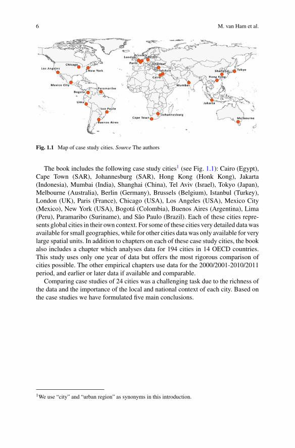
Fig. 1.1 Map of case study cities. Source The authors
The book includes the following case study cities1 (see Fig. 1.1): Cairo (Egypt),Cape Town (SAR), Johannesburg (SAR), Hong Kong (Honk Kong), Jakarta(Indonesia), Mumbai (India), Shanghai (China), Tel Aviv (Israel), Tokyo (Japan),Melbourne (Australia), Berlin (Germany), Brussels (Belgium), Istanbul (Turkey),London (UK), Paris (France), Chicago (USA), Los Angeles (USA), Mexico City(Mexico), New York (USA), Bogotá (Colombia), Buenos Aires (Argentina), Lima(Peru), Paramaribo (Suriname), and São Paulo (Brazil). Each of these cities repre-sents global cities in their own context. For some of these cities very detailed data wasavailable for small geographies, while for other cities data was only available for verylarge spatial units. In addition to chapters on each of these case study cities, the bookalso includes a chapter which analyses data for 194 cities in 14 OECD countries.This study uses only one year of data but offers the most rigorous comparison ofcities possible. The other empirical chapters use data for the 2000/2001-2010/2011period, and earlier or later data if available and comparable.
Comparing case studies of 24 cities was a challenging task due to the richness ofthe data and the importance of the local and national context of each city. Based onthe case studies we have formulated five main conclusions.
1We use “city” and “urban region” as synonyms in this introduction.

1 Rising Inequalities and a Changing Social Geography of Cities … 7
(1) There is general trend of professionalisation of the occupational structure ofcities, with an increase in the share of high-income occupations, and a decreasein the share of low-income occupations. As many high-income workers have apreference for living in central cities, this explains the changing social geographyof urban inequality.
(2) Segregation asmeasured city-wide by theDissimilarity Index (DI) has increasedfor most cities (except Cape Town, Johannesburg, Mexico, and Buenos Aires,and excluding some citieswith problematic data). Based on our resultswe expectlevels of segregation to increase further in the future, as inequality is increasing,and because in the last decade processes of gentrification have temporarilycaused central areas of cities to become more mixed in terms of income.
(3) The higher the level of inequality, the higher the level of segregation. This rela-tionship becomes stronger when lagged inequality data is used. This is becausewhen inequality levels increase, it takes time for this to be reflected in thegeography of inequality.
(4) Generally speaking, middle-income countries combine high levels of inequalitywith high levels of segregation, while high-income countries combine lowerlevels of inequality with lower levels of segregation. Over time we see thatthere is convergence between the higher and lower income countries; levels ofinequality and segregation in the higher income countries are going up and thegap between the higher and lower income countries is decreasing.
(5) The geography of social inequality is changing faster than levels of segregationmeasured by the Dissimilarity Index. In most cities the rich are moving to thecentre and attractive coastal regions, and the poor are being pushed to the edgesof the urban region. Where this does not happen, or sometimes in combinationwith this trend, the rich also concentrate in enclaves and gated communities.
The remainder of this introduction is organised as follows. First, we present theoverall approach of the book; this section deals with the measures, geographies,and definitions used, and it discusses some of the challenges of doing internationalcomparative work. Second, we present how income inequality leads to residentialsegregation. Next, we discuss the main findings of the book in detail, includingsummary tables and figures. Finally, this introductory chapter presents a discussionand overall conclusions, with an outlook to the future. After the introduction, eachcase study city is presented in a separate chapter, authored by expert local teams.The only deviation is Chap. 2, which compares data for one year for a large numberof cities in selected OECD countries.
8 M. van Ham et al.
1.2 Approach and Justification
This book provides a systematic comparison of changes in income inequality, occu-pational change, and socio-economic segregation in large cities around the worldover the last decades. As previous studies focussed on either a small number of casestudies, or only on European cities, this study will provide a global coverage of citiesfrom all continents, and it includes 24 case study cities in Africa, Asia, Australia,Europe, North America, and South America. Although we aimed for the largestcities, and an even geographical coverage in each of the continents, the final set ofcase studies was influenced by the availability of research teams and data.
A large-scale internationally comparative project raises many challenges. Notsurprisingly, these challenges mostly concern data availability and comparability ofcase study cities. In the selection of case study cities, we complemented compara-bility with an inclusive approach, which means that some chapters are not strictlycomparable to others. To maximise comparability of cases, the analysis of cities isbased on fairly basic and harmonised guidelines (see Appendix 1). The authors wereasked to use Functional Urban Areas as defined by the OECD (2013) or equiva-lent; to create socio-economic groups by categorising occupations into Top, Middle,and Bottom occupational status groups; to provide a city-level Gini index; and theywere asked to use the Dissimilarity Index to measure residential segregation betweenoccupations. To analyse the geography of segregation we asked authors to constructa series of maps based on the smallest possible spatial units of analysis (preferablycensus tracts of around 5000 inhabitants), and data from around 2000 and 2010.Although for some cities more recent data is available (and also presented in theirchapters), for most cities 2011 is the year of the most recent census, and hence alsothe most recent data point.
For only a few case study cities it was possible to closely follow the guidelines.Most of the chapters had to deviate from the guidelines to a certain extent (seeAppendix 2 for a detailed overview of the data used per chapter). For example, mostchapters use data on occupational categories, but in cases where such data was notavailable, data was used on education, income, or unemployment. The spatial unitsof analysis ranged from as small as 800 inhabitants in Buenos Aires to as large as750,000 inhabitants in Jakarta. The size of urban areas analysed also varies greatly:from 0.4 million inhabitants in Paramaribo to 35.7 million in Tokyo.
The analyses for the cities Berlin, Bogotá, Jakarta, and Mumbai deviate the mostfrom the guidelines because of the lack of comparable data. For that reason, they arenot included in our comparative analysis in this introductory chapter. These citiesare still included in the book since they do provide very valuable insights on socio-economic segregation on their own. Jakarta and Mumbai could not be included dueto the very large spatial units available for the analysis. Berlin could not be includedbecause of a different indicator available to measure the level of segregation. Bogotácould not be included because only data for 2005 is available that does not allow tostudy changes in socio-economic segregation.
1 Rising Inequalities and a Changing Social Geography of Cities … 9
Central to this book is the link between income inequality and socio-economicsegregation. Ideally, the relationship between inequality (measured using the Giniindex) and segregation (measured using the Dissimilarity Index) would be measuredat the city-level. However, the Gini index is not available on the city-level for mostcities and, as a result, most chapters report inequality data at the country-level. Forconsistency, country-level Gini data as provided by the World Bank is used in thisIntroductory chapter. As a consequence, the relationship between inequality andsegregation is somewhat weaker compared to using city-level Gini Index. As shownin previous studies, income inequality is almost always higher in large cities ascompared to the rest of the country.
All chapters (except Berlin) have used the Dissimilarity Index (DI) to measurecity-wide segregation. Although the Dissimilarity Index has certain disadvantagesover other measures, it is important to use a simple measure to increase the compara-bility of cases. See Appendix 1 for more detail on the DI used. The index can rangefrom 0 to 100, and levels of segregation are often categorised as being low whenunder 30, moderate when between 30 and 60, and high when above 60 (Massey andDenton 1993). This categorisation was initially developed to characterise ethnic andracial segregation in the US. However, this book focusses on socio-economic segre-gation in an international context, and there are large differences between countries,regions, and cities in the world with regard to what is considered a low or a high levelof segregation. While 50 would be very high in Europe (e.g., chapter on Brussels),in Latin America (e.g., chapters on Paramaribo and Buenos Aires) it is consideredmoderate. Therefore, we find that a strict classification in high and low is not veryuseful in the context of this book.
Finally, in analysing the results from all the case study cities, it is useful to cate-gorise cities. For this purpose, we have relied on a country classification by incomeas provided by theWorld Bank (2020). According to this classification, countries aredivided into four income groups: low, lower middle, upper middle, and high. Incomeis measured using gross national income (GNI) per capita. In 2020, low-incomecountries are defined as those with a GNI per capita of $1,025 or less in 2018; lowermiddle-income countries are thosewith aGNI per capita between $1,026 and $3,995;upper middle-income countries are those with a GNI per capita between $3,996 and$12,375; high-income countries are those with a GNI per capita of $12,376 or more.The countries included in this book fall into the last three categories (see Appendix2). No low-income country was included in this book due to a lack of data andresearchers available to contribute. However, for simplicity, in this introduction weoften refer to high-income countries and middle-income countries (pooling togetherupper middle and lower middle-income countries).
10 M. van Ham et al.
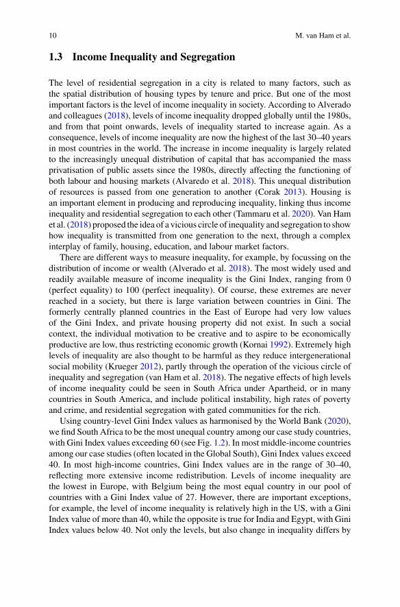
1.3 Income Inequality and Segregation
The level of residential segregation in a city is related to many factors, such asthe spatial distribution of housing types by tenure and price. But one of the mostimportant factors is the level of income inequality in society. According to Alveradoand colleagues (2018), levels of income inequality dropped globally until the 1980s,and from that point onwards, levels of inequality started to increase again. As aconsequence, levels of income inequality are now the highest of the last 30–40 yearsin most countries in the world. The increase in income inequality is largely relatedto the increasingly unequal distribution of capital that has accompanied the massprivatisation of public assets since the 1980s, directly affecting the functioning ofboth labour and housing markets (Alvaredo et al. 2018). This unequal distributionof resources is passed from one generation to another (Corak 2013). Housing isan important element in producing and reproducing inequality, linking thus incomeinequality and residential segregation to each other (Tammaru et al. 2020). Van Hamet al. (2018) proposed the idea of a vicious circle of inequality and segregation to showhow inequality is transmitted from one generation to the next, through a complexinterplay of family, housing, education, and labour market factors.
There are different ways to measure inequality, for example, by focussing on thedistribution of income or wealth (Alverado et al. 2018). The most widely used andreadily available measure of income inequality is the Gini Index, ranging from 0(perfect equality) to 100 (perfect inequality). Of course, these extremes are neverreached in a society, but there is large variation between countries in Gini. Theformerly centrally planned countries in the East of Europe had very low valuesof the Gini Index, and private housing property did not exist. In such a socialcontext, the individual motivation to be creative and to aspire to be economicallyproductive are low, thus restricting economic growth (Kornai 1992). Extremely highlevels of inequality are also thought to be harmful as they reduce intergenerationalsocial mobility (Krueger 2012), partly through the operation of the vicious circle ofinequality and segregation (van Ham et al. 2018). The negative effects of high levelsof income inequality could be seen in South Africa under Apartheid, or in manycountries in South America, and include political instability, high rates of povertyand crime, and residential segregation with gated communities for the rich.
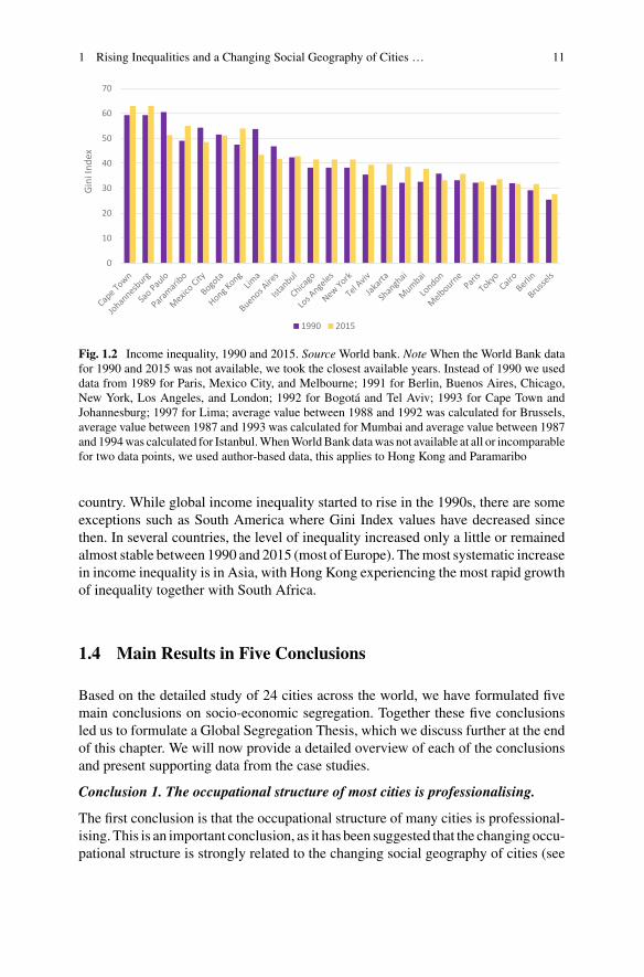
Using country-level Gini Index values as harmonised by the World Bank (2020),we find South Africa to be the most unequal country among our case study countries,with Gini Index values exceeding 60 (see Fig. 1.2). In most middle-income countriesamong our case studies (often located in the Global South), Gini Index values exceed40. In most high-income countries, Gini Index values are in the range of 30–40,reflecting more extensive income redistribution. Levels of income inequality arethe lowest in Europe, with Belgium being the most equal country in our pool ofcountries with a Gini Index value of 27. However, there are important exceptions,for example, the level of income inequality is relatively high in the US, with a GiniIndex value of more than 40, while the opposite is true for India and Egypt, with GiniIndex values below 40. Not only the levels, but also change in inequality differs by
1 Rising Inequalities and a Changing Social Geography of Cities … 11
0
10
20
30
40
50
60
70Gi
ni In
dex
1990 2015
Fig. 1.2 Income inequality, 1990 and 2015. Source World bank. Note When the World Bank datafor 1990 and 2015 was not available, we took the closest available years. Instead of 1990 we useddata from 1989 for Paris, Mexico City, and Melbourne; 1991 for Berlin, Buenos Aires, Chicago,New York, Los Angeles, and London; 1992 for Bogotá and Tel Aviv; 1993 for Cape Town andJohannesburg; 1997 for Lima; average value between 1988 and 1992 was calculated for Brussels,average value between 1987 and 1993 was calculated for Mumbai and average value between 1987and 1994was calculated for Istanbul.WhenWorldBank datawas not available at all or incomparablefor two data points, we used author-based data, this applies to Hong Kong and Paramaribo
country. While global income inequality started to rise in the 1990s, there are someexceptions such as South America where Gini Index values have decreased sincethen. In several countries, the level of inequality increased only a little or remainedalmost stable between 1990 and 2015 (most of Europe). Themost systematic increasein income inequality is in Asia, with Hong Kong experiencing the most rapid growthof inequality together with South Africa.
1.4 Main Results in Five Conclusions
Based on the detailed study of 24 cities across the world, we have formulated fivemain conclusions on socio-economic segregation. Together these five conclusionsled us to formulate a Global Segregation Thesis, which we discuss further at the endof this chapter. We will now provide a detailed overview of each of the conclusionsand present supporting data from the case studies.
Conclusion 1. The occupational structure of most cities is professionalising.
The first conclusion is that the occupational structure of many cities is professional-ising. This is an important conclusion, as it has been suggested that the changing occu-pational structure is strongly related to the changing social geography of cities (see
12 M. van Ham et al.
van Ham et al. 2020). The book “The Global City” by Sasia Sassen (1991) provokeda decades-long debate on whether the occupational structure of global cities is polar-ising or professionalising (see also Hamnett 1994; van Ham et al. 2020). Althoughthere are some exceptions, generally speaking we observe an increase in the share ofthe Top socio-economic groups, and a decrease (or stabilisation) in the share of theBottom socio-economic groups. This implies a general trend of professionalisationof the occupational structures also in most of our case studies. The professionalisa-tion of the occupational structure leads to increasing shares of high-income workers,and many of these high-income workers have developed a preference for living incentral cities (cf. Hamnett 2009).
Although there are some similar trends, the case study cities vary greatly in theiroccupational structure and are almost perfectly split into two groups coinciding withthe country classification by income (see Appendix 3). In high-income countries, theTop socio-economic groupsmake up a significantly higher proportion of occupations,compared to the middle-income countries. While the Top socio-economic groupsaccount for about 40% in Brussels, New York, and Melbourne, they do not exceed15% in Jakarta, São Paulo, and Lima. Accordingly, the Bottom socio-economicgroups account for at least 40% in Shanghai, Cairo, São Paulo, and Jakarta, andthese groups form less than 15% in Los Angeles, Melbourne, and Paris. The highestshare of the middle socio-economic groups is found in Paramaribo, Paris, and TelAviv (around 60%), while the lowest in Shanghai (14%). It has to be noted that thedefinitions of the three groups differ between case study cities, so care should betaken when comparing results. The definition of the Top socio-economic groups ismore consistent than the definition of the two other groups. All cities experienced anincrease in the share of Top occupations, except for Johannesburg, where the shareremained stable, and Brussels, where it dropped slightly, but remained to be one ofthe highest among the case studies.
Conclusion 2. Segregation measured by the Dissimilarity Index has increased formost cities.
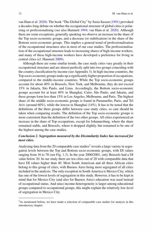
Analysing data from the 20 comparable case studies2 reveals a large variety in segre-gation levels between the Top and Bottom socio-economic groups, with DI valuesranging from 16 to 78 (see Fig. 1.3). In the year 2000/2001, only Brussels had a DIvalue below 20. In our study there are ten cities out of 20 with comparable data thathave DI values higher than 40. Most South American and all three African citiesbelong to this group of cities, with Buenos Aires being most segregated of all citiesincluded in the analysis. The only exception in South America is Mexico City, whichhas one of the lowest levels of segregation in this study. However, it has to be kept inmind that for Mexico City (and also for Buenos Aires) education was used insteadof occupational status. And since income-heterogeneity is larger among educationalgroups compared to occupational groups, this might explain the relatively low-levelof segregation in Mexico City.
2As mentioned before, we have made a selection of comparable case studies for analysis in thisintroductory chapter.
1 Rising Inequalities and a Changing Social Geography of Cities … 13
0
10
20
30
40
50
60
70
80Di
ssim
ilarit
y In
dex
2000/2001 2010/2011
Fig. 1.3 Residential segregation between top and bottom socio-economic groups, 2000/2001 and2010/2011. Source Individual chapters in this book, see Appendix 4 for more details). Notes *Topand bottom groups based on income; **Top and bottom groups based on educational attainment.Data for Paramaribo 2004 and 2012, Paris 1999 and 2015, Cairo 1996 and 2016, Lima 1993 and2007, New York 2000 and 2013-2017, Mexico City 1990 and 2010, Tel Aviv 1995 and 2008
Figure 1.3 clearly shows that European cities do not necessarily have low levelsof segregation as one might expect from their low levels of income inequality andthe high levels of income redistribution in Europe. In fact, Paris is one of the mostsegregated cities in our study, with a level of segregation which is much higher thanthe Anglo-American cities, and comparable to Johannesburg in South Africa. Thefive cities with the lowest levels of segregation in this study are Tokyo, Tel Aviv,Brussels, Mexico City, and Chicago, which is a regionally very mixed group ofcities. Interestingly, Hong Kong is one of the most segregated cities in this study, butthis city is a-typical for Asia with its recent colonial past. All Anglo-American citiesincluded into our study are modestly segregated.
While comparisons of levels of segregation between cities should be treated withsome caution due to limitations in the comparability of data, the comparison ofsegregation levels over time within each city is more straightforward. Our resultsshow that levels of segregation between the Top and Bottom socio-economic groupshave increased (or remained stable in two cases) in most cities. However, theseincreases have been small for most cities, with the exception of Brussels. Segrega-tion levels have dropped somewhat in four cities: Buenos Aires, Cape Town, Johan-nesburg, and Mexico City. Again, we should recall that the cases of Buenos Airesand Mexico City differ from the other cities because education is used as a measureof socio-economic status instead of occupation. Interestingly, in almost all cities inhigh-income countries levels of segregation have increased, while the situation inmiddle-income countries is a little more mixed.
14 M. van Ham et al.
The low level of segregation in Tokyo is striking, especially because it is somuch lower than in many European cities. In many European cities there is a strongoverlap between ethnic and socio-economic segregation due to the on average lowincomes of migrants compared to natives (Andersson and Kährik 2016). The share ofinternational migrants in Tokyo is very small compared to other global cities, and atthe same time Tokyo is characterised by a low level of income inequality, and strongpublic sector involvement in the economy, the housing market, and urban planning.Tokyo is also a very densely populated compact city, providing few opportunitiesfor residential separation. In this context vertical segregation may be more importantthan the sorting of different socio-economic groups into different neighbourhoods(Hirayama 2017).
In addition to the case studies, Chap. 2 analyses income data from 194 cities in14 OECD countries to provide an overview of residential segregation in a compara-tive perspective. Not surprisingly, segregation levels between the Top and Bottom-income groupswere found to bemuch higher compared to segregation levels betweenMiddle- andBottom-incomegroups. Themain contributionof this chapter to the bookis the comparison of segregation levels of multiple cities within the same country.The results show that there is a lot of variation in levels of segregation betweencities within some countries. With other words, studying only one case study cityper country does not do justice to the variety of segregation levels within countries.Although generally speaking the analyses ofOECDdata show a relationship betweenlevels of inequality and levels of income segregation, the results also suggest thatlocal circumstances can greatly affect how levels of inequality are translated into thesocial geography of cities within a country. This needs to be taken into account whencomparing single city case studies between countries as these case studies are notnecessarily representative for the rest of the country.
Conclusion 3. The higher the level of inequality, the higher the level of segregation.
Previous studies have suggested that it takes time before a rise in income inequalityleads to higher levels of socio-economic segregation. Therefore, it is important totake into account a time lag when studying the relationship (Marcinczak et al. 2015;Musterd et al. 2017; Wessel 2016; Tammaru et al. 2020). The time needed for trans-mitting changes in income inequality to changes in residential segregation variesfrom city to city, because of other factors shaping segregation. For example, inmarketdominated housing systems with little public interventions in housing, changes inincome inequality may translate quickly (within ten years’ time) into income-basedresidential sorting. However, in a housing system with a high share of social orpublic housing, andwith strong policy interventions, the time lag between a change inincome inequality and a change in residential segregation becomes longer, extendingwell beyond ten years (Wessel 2016). It is also important to note that the relation-ship tends to hold in both ways; an increase in income inequality is followed by anincrease in residential segregation later in time, and a decrease in income inequality isfollowed by a decrease in residential segregation later in time (Tammaru et al. 2020).Our analysis of the relationship between income inequality (measured by Gini andlagged 10 years) and the level of socio-economic segregation has been summarised
1 Rising Inequalities and a Changing Social Geography of Cities … 15
Brussels
Chicago
Hong Kong
London Los AngelesMelbourne New York
Paris
Tel AvivTokyo
Buenos Aires
Cairo
Cape Town
Istanbul
JohannesburgLima
Mexico City
ParamariboSão Paulo
Shanghai
15
25
35
45
55
65
75
15 25 35 45 55 65 75
1002/0002xednIytirali
missiD
Gini Index 1990High income country Middle income country
BrusselsChicago
Hong Kong
London Los AngelesMelbourne
New …
Paris
Tel AvivTokyo
Buenos Aires
Cairo
Cape TownIstanbul
JohannesburgLima
Mexico City
Paramaribo
São Paulo
Shanghai
15
25
35
45
55
65
75
15 25 35 45 55 65 75
Diss
imila
rity I
ndex
201
0/20
11
Gini Index 2000High income country Middle income country
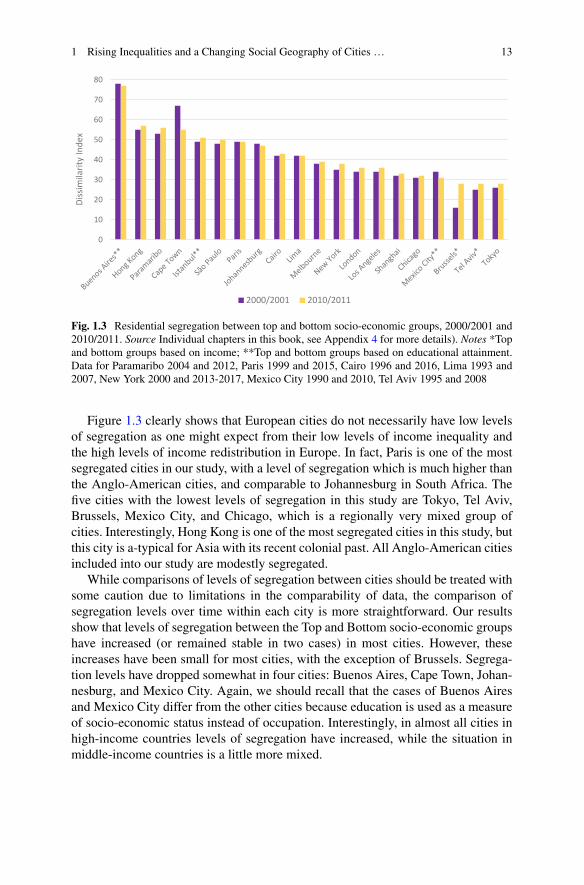
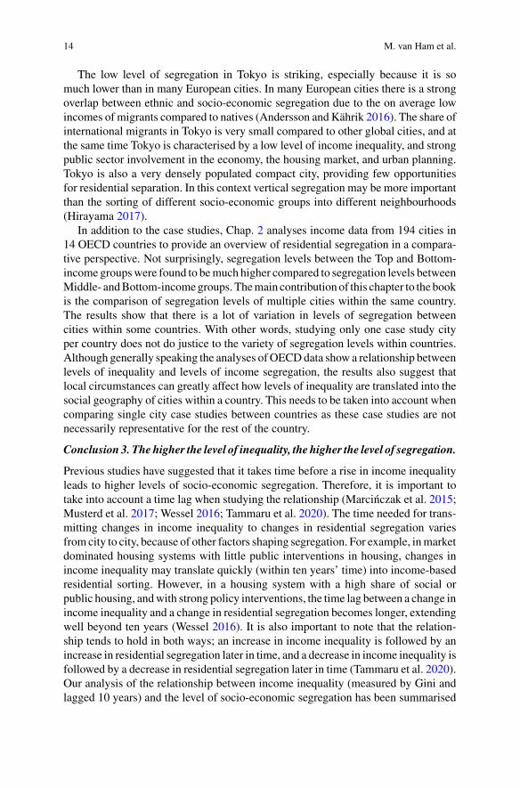
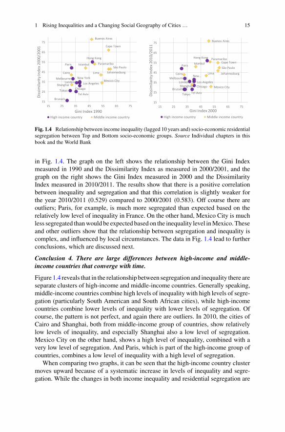
Fig. 1.4 Relationship between income inequality (lagged 10 years and) socio-economic residentialsegregation between Top and Bottom socio-economic groups. Source Individual chapters in thisbook and the World Bank
in Fig. 1.4. The graph on the left shows the relationship between the Gini Indexmeasured in 1990 and the Dissimilarity Index as measured in 2000/2001, and thegraph on the right shows the Gini Index measured in 2000 and the DissimilarityIndex measured in 2010/2011. The results show that there is a positive correlationbetween inequality and segregation and that this correlation is slightly weaker forthe year 2010/2011 (0.529) compared to 2000/2001 (0.583). Off course there areoutliers; Paris, for example, is much more segregated than expected based on therelatively low level of inequality in France. On the other hand, Mexico City is muchless segregated thanwould be expected based on the inequality level inMexico. Theseand other outliers show that the relationship between segregation and inequality iscomplex, and influenced by local circumstances. The data in Fig. 1.4 lead to furtherconclusions, which are discussed next.
Conclusion 4. There are large differences between high-income and middle-income countries that converge with time.
Figure 1.4 reveals that in the relationship between segregation and inequality there areseparate clusters of high-income and middle-income countries. Generally speaking,middle-income countries combine high levels of inequality with high levels of segre-gation (particularly South American and South African cities), while high-incomecountries combine lower levels of inequality with lower levels of segregation. Ofcourse, the pattern is not perfect, and again there are outliers. In 2010, the cities ofCairo and Shanghai, both from middle-income group of countries, show relativelylow levels of inequality, and especially Shanghai also a low level of segregation.Mexico City on the other hand, shows a high level of inequality, combined with avery low level of segregation. And Paris, which is part of the high-income group ofcountries, combines a low level of inequality with a high level of segregation.
When comparing two graphs, it can be seen that the high-income country clustermoves upward because of a systematic increase in levels of inequality and segre-gation. While the changes in both income inequality and residential segregation are
16 M. van Ham et al.
more diverse for themiddle-income countries, this suggests convergence between thehigh-income and middle-income countries. The trend towards convergence betweenhigher income and middle and low-income countries warrants some more attention.Further increases in both income inequality and residential segregation are not verylikely in cities that are already highly unequal and highly segregated. The overallmodernisation of societies and professionalisation of the labour force tends to reducedifferences in incomes and residential sorting. However, the main reason for conver-gence relates to changes taking place in cities located in high-income countries. Itis notable that increases in residential segregation in high-income countries tendto be larger than predicted by their levels of income inequality. Paris is the mostoutstanding case in this regard, where a very high level of residential segregationbetween the Top and Bottom socio-economic groups is combined with a low level ofincome inequality. InParis, a possible explanation is related tomigration,where lowerincome migrant households tend to cluster in modernist housing estates (Lelévrierand Melic 2018). In Paris, but also in other high-income cities, it may also be thecase that an increased emphasis on market forces in the housing market increas-ingly sorts households with different financial means into different neighbourhoods,despite overall low levels of income inequality.
Conclusion 5. The social geography of cities changes faster than levels ofsegregation measured city-wide.
The data from this book shows an overall picture of increasing levels of socio-economic segregation between 2000/2001 and 2010/2011, although segregationlevels remained stable in some cities, and even dropped in others. Segregation wasmeasured by using the Dissimilarity Index, and like many indices of segregation, itdoes not take into account the social geography of cities. In theory it is possible thatover time the poor move to rich areas, and the rich to poor, while the overall measureof segregation remains stable.
Based on the case studies we can conclude that social geography of inequality ischanging faster thanmeasures of city-wide socio-economic segregation, asmeasuredby the Dissimilarity Index. In many of the case study cities the Top socio-economicgroups are concentrating in the centre and attractive coastal regions, and the Bottomsocio-economic groups are concentrating on the edges of the urban region. In somecases, they are also concentrating in enclaves and gated communities outside theurban core. In all cases, the residential choices of the Top socio-economic groupsare driving changes in the geography of segregation.
Beyond those general trends there are also many differences between the citiesdue to local circumstances, including historical, economic, and political factors, butalso the physical geography of cities. There are some examples of cities in which theTop socio-economic groups concentrate in the central areas, and the Bottom socio-economic groups in the periphery. In Shanghai, for example, the Top socio-economicgroups concentrate into the centre as well as into certain suburbs. Also in Tel Aviv,London, Chicago, Buenos Aires, Melbourne, Paris, Mexico City, and New Yorkthe Top socio-economic groups are concentrating in the central area of the urbanregion. In all these cities they are more residentially concentrated than the Bottom

1 Rising Inequalities and a Changing Social Geography of Cities … 17
socio-economic groups. We also observed in all these cities that the Bottom socio-economic groups increasingly live in the urban periphery. For example, in Berlin itwas observed that child poverty is increasingly moving to the urban periphery, whichis likely to increase inequality due to a lack of opportunity for these children as theygrow up.
In Chicago, the city seems to be polarising geographically with an increasing resi-dential division between the Top and Bottom socio-economic groups. In many othercities there is an increase of socio-economically mixed areas due to gentrification.This is the case in, for example, New York, Paris, and Mexico City. Los Angeleshas a more geographically dispersed pattern of residential inequality than the citiesmentioned above. This is due to the polycentric nature of the urban region, withconcentrations of Top socio-economic groups in various parts of the city, gentrifica-tion in adjacent areas of rich enclaves, and a rise in the number of gated communities.Cities like São Paulo, Istanbul, Lima, and Hong Kong are also characterised by aconcentration of the Top socio-economic groups in the central area of the city. Atthe same time, also gated communities for the high-income groups can be found inthese urban regions.
Somecities, like Johannesburg,CapeTown, Paramaribo, andCairo, showanoppo-site geography of residential inequality. In these cities the Bottom socio-economicgroups are concentrating into the city centre and the periphery, and the Top socio-economic groups are concentrating in suburbs and gated communities. In Brusselsthe central area of the city is quite deprived and the outskirts are more prosperous; theTop socio-economic groups mainly concentrate in the peripheral areas (but also insome pockets in the central area), and the Bottom socio-economic groups concentratein and around the centre in densely populated neighbourhoods. The cities of Tokyo,Mumbai, and Bogotá all show very distinct patterns of segregation. In Tokyo, the Topsocio-economic groups live in the elevated areas in theWest, and in the harbour area,and the Bottom socio-economic groups live in the lowlands in the East. In Mumbaithere is a clear North-South division, with the Top socio-economic groups living inthe South, and the Bottom socio-economic groups living in the North. And in Bogotáthe Top socio-economic groups live in the North, and the Bottom socio-economicgroups live in the South. For Jakarta, the spatial units were too large for an in-depthanalysis of the geographical patterns of inequality.
Many cases reveal that residential areas in the city centres are getting more socio-economically mixed due to gentrification and expansion of the urban core. This isthe case in, for example, Hong Kong, Mumbai, London, Berlin, and Paris. Thefact that urban cores in these cities become more mixed might be a temporaryphenomenon as in the course of the process of gentrification these areas becomeunaffordable for Bottom socio-economic groups, and become over-represented bymore andmore affluent households. Although this book predominantly studies socio-economic segregation, many case studies also mention the link between ethnic segre-gation and socio-economic segregation. The clear South-North division in Mumbaiis strongly related to ethnic and religious segregation in the city. Segregation in TelAviv is also related to both ethnicity and religion. In London, Chicago, New York,
18 M. van Ham et al.
and Paris, socio-economic segregation is also strongly related to patterns of racialand ethnic segregation.
1.5 A Global Segregation Thesis
The central research question of this book was whether there is any evidence fora Global Segregation Thesis, or whether cities in different parts of the world showvery distinctive patterns of socio-economic segregation? Taken together, the fivemain conclusions of this book provide support for what we call the Global Segrega-tion Thesis, which is characterised by a global trend of rising levels of segregation,combined with a changing social geography of cities. Rising levels of segregation arecaused by rising levels of income inequality, and although the link between the twois complex, it seems almost universal and globally applicable. At the same time thesocial geography of cities is changing, where high-income households increasinglylive in city centres and other attractive areas, while lower income households moveto the fringes of the city. This changing social geography is related to the profession-alisation of the urban workforce, which leads to more higher income households,which have developed a preference for living in central parts of large cities. Levelsof segregation have not gone up as much as could be expected based on rising levelsof inequality, and this is possibly due to gentrification and the temporally socio-economic mixing of central city neighbourhoods. Over time, processes of gentrifica-tion will lead to further increases in levels of segregation. The combination of risinglevels of inequality and professionalisation of the workforce is expected to lead to afurther increase in segregation and more uneven landscapes of opportunity.
For most cities in this book, the most recent census data used was from 2010 or2011, and data from the next (2020 or 2021) census will not be available for another5 years. This means that the 2010/2011 census only started to capture the effectsof the 2008 Global Financial Crisis. At the time of writing this introduction, theworld is facing a new economic crisis related to the COVID-19 pandemic. Althoughit is impossible to know how long and deep this crisis will be, there are signs thatthe weakest in society will be hit the hardest. This is likely to lead to rising levelsof inequality, and ultimately more segregation in cities. At the same time there arediscussions on the future of cities and on the residential preferences of higher incomehouseholds. These households might decide to leave their relatively small dwellingsin densely populated areas and live in more spacious dwellings in suburban environ-ments. Such a change might have dramatic effects on the social geography of citiesand spaces of opportunity. Densely populated areas might increasingly become thedomain low-income groups, while higher income groups once again suburbanise asthey did decades ago. In the short run it can be expected that levels of socio-economicsegregation continue to rise and that the social geography of cities continues to showa pattern of rich centres, with poor suburbs. In the long run cities are in constant flux,and the future of cities depends on many factors yet still unknown.
1 Rising Inequalities and a Changing Social Geography of Cities … 19
Future research on inequality and socio-economic segregation should focus onbetter understanding local variation in the relationships between the two. Andmost importantly, how different urban policies—area-based, people-based, andconnectivity-based—can make a difference? It is also important to improve ourunderstanding on how residential inequalities are produced and reproduced overdifferent life domains (home, family, education,work) and across generations.Under-standing the vicious cycle of segregation and inequality can lead to more effectivepolicies aimed at improving access to opportunity. The professionalisation of theurban workforce and increasing educational levels leads to a higher share of high-income earners in cities, which initially leads to more social mix in many urbanneighbourhoods. But in the longer run these trends might lead to higher levels ofsegregation as cities become more and more unaffordable for many people. It istherefore crucial to take a multi-scale perspective on cities (Petrovic et al. 2018),studying large urban regions instead of cities. Finally, as global cities are increas-ingly multi-ethnic, the overlap between income inequality and ethnicity and race inmany cities needs further attention. Themost severe and persistent inequalities appearwhere different variables intersect, and these intersections require most attention.
Appendix 1: Guidelines for Authors, Data, and Methods
Each chapter should contain two parts: a compulsory part including an analysis ofchanges in the occupational structure, income inequality, and residential segregation;and a free part, which discusses the local context and other important factors relatedto segregation in the specific country or city. To define urban regions, all authorsshould use functional urban areas as defined by the OECD. Socio-economic groupsare preferably distinguished based on occupational status, and classified into Top,Middle, and Bottom (or High, Middle, and Low for educational or income levels).The main measure of segregation to be used is the Dissimilarity Index. Chaptersshould preferably provide the city-level Gini index, and otherwise the national-levelGini index. To analyse the geography of segregation authors were asked to constructsome standard maps using guidelines provided by the editors. For calculations of theDissimilarity Index and the construction of maps, authors were asked to use smallspatial units, preferably census tracts of around 5000 inhabitants. And authors wereasked to analyse data from at least the year 2000/2011 and 2010/2011, but a longerperiod of analysis was welcome if data allowed.
A functional urban area consists of a city and its commuting zone (OECD 2013).In this bookoccupational categories are used as a proxy for socio-economic status.
Occupational categories are derived from the International Standard Classificationof Occupations (ISCO) (ILO 2012) and they are directly comparable and availablein all countries conducting censuses. People with different occupations do not onlyperform different tasks, but occupational attainment is also closely related to personalwork income. A typical example of this classification, which applies to many cities,
20 M. van Ham et al.
is TOP: managers + professionals; MIDDLE: everything in between; BOTTOM:elementary occupations + plant and machine operators and assemblers.
The Gini index is the most commonly used measurement of inequality. It is theratio of income distribution within a country or city, where 0 represents perfectequality with no income differences between individuals and 100 represents perfectinequality with one person earning all income.
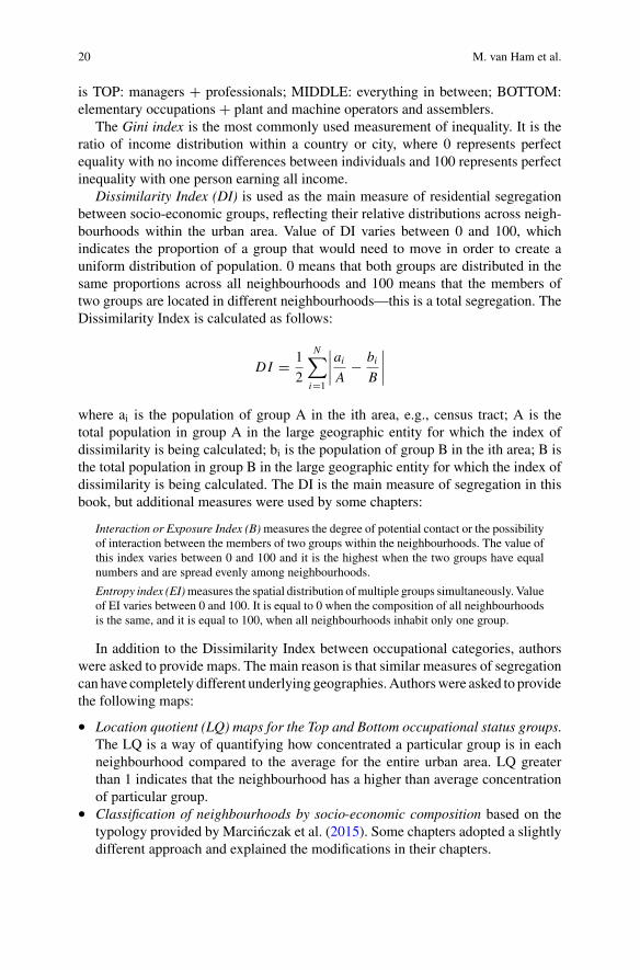
Dissimilarity Index (DI) is used as the main measure of residential segregationbetween socio-economic groups, reflecting their relative distributions across neigh-bourhoods within the urban area. Value of DI varies between 0 and 100, whichindicates the proportion of a group that would need to move in order to create auniform distribution of population. 0 means that both groups are distributed in thesame proportions across all neighbourhoods and 100 means that the members oftwo groups are located in different neighbourhoods—this is a total segregation. TheDissimilarity Index is calculated as follows:
DI = 1
2
N∑
i=1
∣∣∣∣aiA
− biB
∣∣∣∣
where ai is the population of group A in the ith area, e.g., census tract; A is thetotal population in group A in the large geographic entity for which the index ofdissimilarity is being calculated; bi is the population of group B in the ith area; B isthe total population in group B in the large geographic entity for which the index ofdissimilarity is being calculated. The DI is the main measure of segregation in thisbook, but additional measures were used by some chapters:
Interaction or Exposure Index (B)measures the degree of potential contact or the possibilityof interaction between the members of two groups within the neighbourhoods. The value ofthis index varies between 0 and 100 and it is the highest when the two groups have equalnumbers and are spread evenly among neighbourhoods.
Entropy index (EI)measures the spatial distribution ofmultiple groups simultaneously. Valueof EI varies between 0 and 100. It is equal to 0 when the composition of all neighbourhoodsis the same, and it is equal to 100, when all neighbourhoods inhabit only one group.
In addition to the Dissimilarity Index between occupational categories, authorswere asked to provide maps. The main reason is that similar measures of segregationcan have completely different underlying geographies.Authorswere asked to providethe following maps:
• Location quotient (LQ) maps for the Top and Bottom occupational status groups.The LQ is a way of quantifying how concentrated a particular group is in eachneighbourhood compared to the average for the entire urban area. LQ greaterthan 1 indicates that the neighbourhood has a higher than average concentrationof particular group.
• Classification of neighbourhoods by socio-economic composition based on thetypology provided by Marcinczak et al. (2015). Some chapters adopted a slightlydifferent approach and explained the modifications in their chapters.
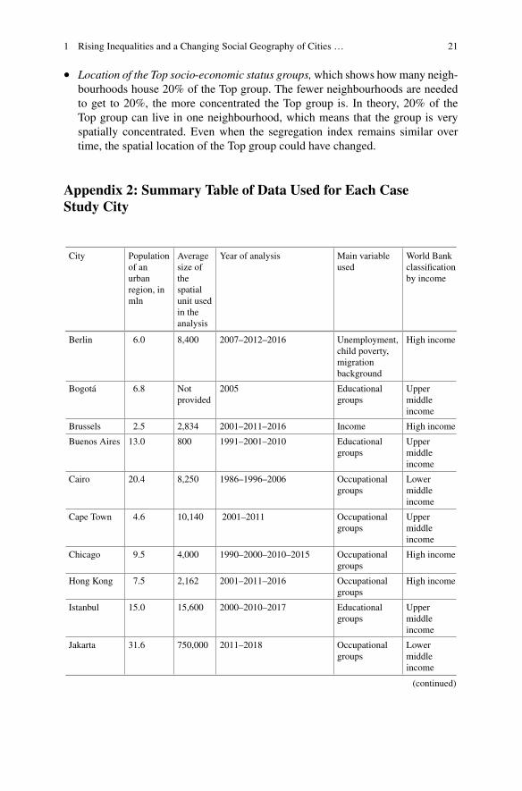
1 Rising Inequalities and a Changing Social Geography of Cities … 21
• Location of the Top socio-economic status groups,which shows howmany neigh-bourhoods house 20% of the Top group. The fewer neighbourhoods are neededto get to 20%, the more concentrated the Top group is. In theory, 20% of theTop group can live in one neighbourhood, which means that the group is veryspatially concentrated. Even when the segregation index remains similar overtime, the spatial location of the Top group could have changed.
Appendix 2: Summary Table of Data Used for Each CaseStudy City
City Populationof anurbanregion, inmln
Averagesize ofthespatialunit usedin theanalysis
Year of analysis Main variableused
World Bankclassificationby income
Berlin 6.0 8,400 2007–2012–2016 Unemployment,child poverty,migrationbackground
High income
Bogotá 6.8 Notprovided
2005 Educationalgroups
Uppermiddleincome
Brussels 2.5 2,834 2001–2011–2016 Income High income
Buenos Aires 13.0 800 1991–2001–2010 Educationalgroups
Uppermiddleincome
Cairo 20.4 8,250 1986–1996–2006 Occupationalgroups
Lowermiddleincome
Cape Town 4.6 10,140 2001–2011 Occupationalgroups
Uppermiddleincome
Chicago 9.5 4,000 1990–2000–2010–2015 Occupationalgroups
High income
Hong Kong 7.5 2,162 2001–2011–2016 Occupationalgroups
High income
Istanbul 15.0 15,600 2000–2010–2017 Educationalgroups
Uppermiddleincome
Jakarta 31.6 750,000 2011–2018 Occupationalgroups
Lowermiddleincome
(continued)
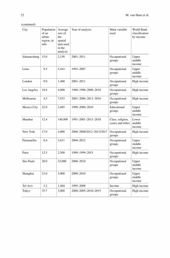
22 M. van Ham et al.
(continued)
City Populationof anurbanregion, inmln
Averagesize ofthespatialunit usedin theanalysis
Year of analysis Main variableused
World Bankclassificationby income
Johannesburg 15.0 2,158 2001–2011 Occupationalgroups
Uppermiddleincome
Lima 9.5 5,443 1993–2007 Occupationalgroups
Uppermiddleincome
London 9.0 1,400 2001–2011 Occupationalgroups
High income
Los Angeles 18.8 4,000 1980–1990–2000–2010 Occupationalgroups
High income
Melbourne 4.5 7,933 2001–2006–2011–2016 Occupationalgroups
High income
Mexico City 22.0 3,485 1990–2000–2010 Educationalgroups
Uppermiddleincome
Mumbai 12.4 140,909 1991–2001–2011–2018 Class, religion,castes and tribes
Lowermiddleincome
New York 17.0 4,000 2000–2008/2012–2013/2017 Occupationalgroups
High income
Paramaribo 0.4 3,611 2004–2012 Occupationalgroups
Uppermiddleincome
Paris 12.5 2,500 1990–1999–2015 Occupationalgroups
High income
São Paulo 20.0 32,000 2000–2010 Occupationalgroups
Uppermiddleincome
Shanghai 23.0 3,000 2000–2010 Occupationalgroups
Uppermiddleincome
Tel Aviv 3.2 1,484 1995–2008 Income High income
Tokyo 35.7 3,000 2000–2005–2010–2015 Occupationalgroups
High income
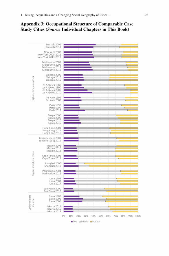
1 Rising Inequalities and a Changing Social Geography of Cities … 23
Appendix 3: Occupational Structure of Comparable CaseStudy Cities (Source Individual Chapters in This Book)
0% 10% 20% 30% 40% 50% 60% 70% 80% 90% 100%
Jakarta 2018Jakarta 2015Jakarta 2011
Cairo 2006Cairo 1996Cairo 1986
Sao Paulo 2010Sao Paulo 2000
Lima 2017Lima 2007Lima 1993
Parimaribo 2012Parimaribo 2004
Shanghai 2010Shanghai 2000
Cape Town 2011Cape Town 2001
Mexico 2015Mexico 2010Mexico 2005
Johannesburg 2011Johannesburg 2001
Hong Kong 2016Hong Kong 2011Hong Kong 2001
Tokyo 2015Tokyo 2010Tokyo 2005Tokyo 2000
Paris 2015Paris 1999Paris 1990
Tel Aviv 2008Tel Aviv 1995
Los Angeles 2010Los Angeles 2000Los Angeles 1990Los Angeles 1980
Chicago 2015Chicago 2010Chicago 2000
Melbourne 2016Melbourne 2011Melbourne 2006Melbourne 2001
New York 2013-2017New York 2008-2012
New York 2000
Brussels 2011Brussels 2001
Low
er m
iddl
ein
com
eU
pper
mid
dle
inco
me
High
inco
me
coun
trie
s
Top Middle Bo�om
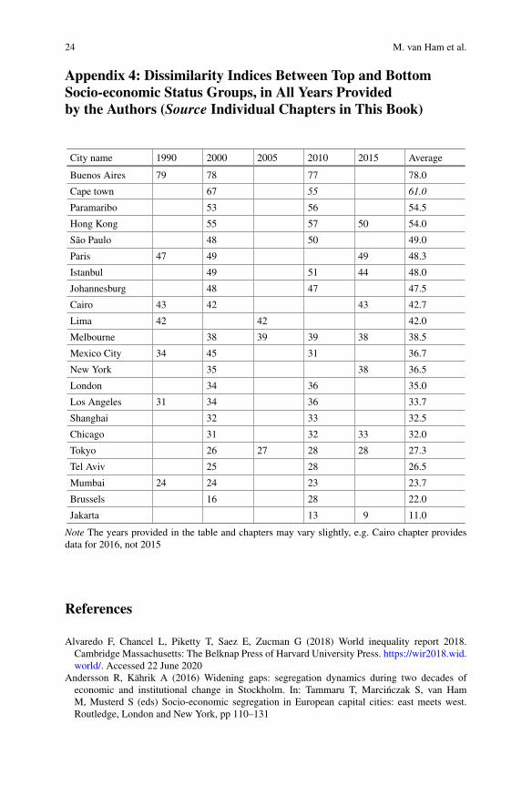
24 M. van Ham et al.
Appendix 4: Dissimilarity Indices Between Top and BottomSocio-economic Status Groups, in All Years Providedby the Authors (Source Individual Chapters in This Book)
City name 1990 2000 2005 2010 2015 Average
Buenos Aires 79 78 77 78.0
Cape town 67 55 61.0
Paramaribo 53 56 54.5
Hong Kong 55 57 50 54.0
São Paulo 48 50 49.0
Paris 47 49 49 48.3
Istanbul 49 51 44 48.0
Johannesburg 48 47 47.5
Cairo 43 42 43 42.7
Lima 42 42 42.0
Melbourne 38 39 39 38 38.5
Mexico City 34 45 31 36.7
New York 35 38 36.5
London 34 36 35.0
Los Angeles 31 34 36 33.7
Shanghai 32 33 32.5
Chicago 31 32 33 32.0
Tokyo 26 27 28 28 27.3
Tel Aviv 25 28 26.5
Mumbai 24 24 23 23.7
Brussels 16 28 22.0
Jakarta 13 9 11.0
Note The years provided in the table and chapters may vary slightly, e.g. Cairo chapter providesdata for 2016, not 2015
References
Alvaredo F, Chancel L, Piketty T, Saez E, Zucman G (2018) World inequality report 2018.Cambridge Massachusetts: The Belknap Press of Harvard University Press. https://wir2018.wid.world/. Accessed 22 June 2020
Andersson R, Kährik A (2016) Widening gaps: segregation dynamics during two decades ofeconomic and institutional change in Stockholm. In: Tammaru T, Marcinczak S, van HamM, Musterd S (eds) Socio-economic segregation in European capital cities: east meets west.Routledge, London and New York, pp 110–131
1 Rising Inequalities and a Changing Social Geography of Cities … 25
Butler T, Hamnett C, Ramsden M (2008) Inward and upward: marking out social class change inLondon, 1981–2001. Urban Stud 45(2):67–88
Corak M (2013) Income inequality, equality of opportunity, and intergenerational mobility. J EconPerspect 27(3):79–102
Davidson M, Wyly E (2015) Same, but different: within London’s ‘static’ class structure and themissing antagonism. City 19(2–3):247–257
Commission European, Habitat UN (2016) The state of European cities 2016: cities leading theway to a better future. European commission, directorate-general for regional and urban policy,Brussels
Fujita K,Maloutas T (eds) (2016) Residential segregation in comparative perspective: making senseof contextual diversity. Routledge, London
Hamnett C (1994) Social polarisation in global cities: theory and evidence. Urban Stud 31(3):401–424
Hamnett C (2009) The newmikado? tom slater, gentrification and displacement. City 13(4):476–482Harvey D (1985) The urbanisation of capital. Johns Hopkins University Press, BaltimoreHirayama Y (2017) Selling the Tokyo sky: urban regeneration and luxury housing. In Cities andthe super-rich, pp 189–208, Palgrave Macmillan, New York
Hulchansky D (2010) The three cities in Toronto: Income polarization among Toronto’s neighbour-hoods, 1970–2005. University of Toronto, Toronto
International Labour Organization (2012) International standard classification of occupations:structure, group definitions and correspondence tables. https://www.ilo.org/wcmsp5/groups/public/—dgreports/—dcomm/—publ/documents/publication/wcms_172572.pdf. Accessed 22 June2020
Kazepov Y (ed) (2005) Cities of Europe, changing contexts, local arrangement and the challengeto urban cohesion. Wiley-Blackwell, London
Kornai J (1992) The socialist system: the political economy of communism. Princeton UniversityPress, Princeton, NJ
Krueger A (2012) The rise and consequences of inequality in the United States, presentation at thecenter for American progress in Washington, DC January 12, 2012. https://pages.wustl.edu/files/pages/imce/fazz/ad_10_1_krueger.pdf. Accessed 1 Jan 2018
Lelévrier C, Melic T (2018) Impoverishment and social fragmentation in housing estates of theParis region, France. In Housing estates in Europe, pp 313–338, Springer, Cham
Manley D, Johnston R (2014) London: a dividing city, 2001–11? City 18(6):633–643Marcinczak S, Tammaru T, Novák J, Gentile M, Kovács Z, Temelová J, Valatka V, Kährik A,Szabó B (2015) Patterns of socioeconomic segregation in the capital cities of fast-track reformingpostsocialist countries. Ann Assoc Am Geogr 105(1):183–202
Massey DS, Denton NA (1993) American apartheid: Segregation and the making of the underclass.Harvard University Press, Cambridge, Massachusetts, London
Musterd S,Marcinczak S, vanHamM, Tammaru T (2017) Socio-economic segregation in Europeancapital cities. Increasing separation between poor and rich. Urban Geogr 38(7):1062–1083
Musterd S, Ostendorf W (1998) Urban segregation and the welfare state: inequality and exclusionin western cities. Routledge, London
OECD (2013) Definition of functional Urban areas (FUA) for the OECD metropolitandatabase. http://www.oecd.org/regional/. Accessed 10 Sep 2018
Petrovic A, van HamM,Manley D (2018)Multiscale measures of population:Within-and between-city variation in exposure to the sociospatial context. Ann Am Assoc Geogr 108(4):1057–1074
Piketty T (2014) Capital in the twenty-first century. The Belknap Press of Harvard University Press,Cambridge Massachusetts
Sassen S (1991) The global city: New York, London, Tokyo. Princeton University Press, PrincetonSýkora L (2009) New socio-spatial formations: places of residential segregation and separation inCzechia. Tijdschrift voor Economische en Sociale Geografie 100:417–435
26 M. van Ham et al.
Tammaru T,Marcinczak S, Aunap R, van HamM, Janssen H (2020) Understanding the relationshipbetween income inequality and residential segregation between socioeconomic groups. Reg Stud54(4):450–461
Tammaru T,Marcinczak S, vanHamM,Musterd S (2016) Socio-economic segregation in Europeancapital cities: east meets west. Routledge, London and New York
van Ham M, Uesugi M, Tammaru T, Manley D, Janssen H (forthcoming) Changing occupationalstructures and residential segregation in New York, London and Tokyo. Nature human behaviour
van Ham M, Tammaru T, Janssen H (2018) A multilevel model of vicious circles of socio-economic segregation. In Divided cities: understanding intra-urban inequalities, pp 135–153,OECD Publishing, Paris
Wessel T (2016) Economic segregation in Oslo: polarisation as a contingent outcome. In: TammaruT, Marcinczak S, van Ham M, Musterd S (eds) Socio-economic segregation in European capitalcities: east meets west. Routledge, London and New York, pp 132–155
World Bank (2020) World bank country and lending groups. https://datahelpdesk.worldbank.org/knowledgebase/articles/906519. Accessed 10 Feb 2020
Open Access This chapter is licensed under the terms of the Creative Commons Attribution 4.0International License (http://creativecommons.org/licenses/by/4.0/), which permits use, sharing,adaptation, distribution and reproduction in any medium or format, as long as you give appropriatecredit to the original author(s) and the source, provide a link to the Creative Commons license andindicate if changes were made.
The images or other third party material in this chapter are included in the chapter’s CreativeCommons license, unless indicated otherwise in a credit line to the material. If material is notincluded in the chapter’s Creative Commons license and your intended use is not permitted bystatutory regulation or exceeds the permitted use, you will need to obtain permission directly fromthe copyright holder.
Chapter 2Residential Segregation Between IncomeGroups in International Perspective
Andre Comandon and Paolo Veneri
Abstract This chapter analyzes income data from 194 cities in 14 countries toprovide an overview of residential segregation patterns in a comparative perspective.We use the dissimilarity index to measure segregation between lower income house-holds and middle-income and higher income households. The results expand resultsconsistent with existing research to a larger number of countries. Higher incomehouseholds segregation from lower incomehouseholds is significantly higher than formiddle-income households. High-inequality cities are more segregated, on average,than low-inequality ones. It is in the deviation from these patterns, however, thatthe analysis contributes to a comparative research agenda. It highlights cities andcountries that do not fit general trends and raises questions about the relative roleof national and local factors in influencing levels of segregation, questions the casestudies delve into in the rest of the volume.
Keywords Income inequality · Segregation · International comparison
2.1 Introduction
How do we make sense of income inequality and residential segregation in citiesas different as Houston, Hong Kong, and Johannesburg? Finding common groundbetween cities in disparate national context has the potential to illuminate overlookedfactors that influence segregation and suggest new directions for study. For example,Melbourne in Australia and Boston in the United States have much in common: near
The views expressed herein are those of the authors and do not necessarily reflect the views of theOECD and/or those of its member countries.
A. Comandon (B)Department of Urban Planning, UCLA Luskin School of Public Affairs, 3250 Public AffairsBuilding, Box 951656, Los Angeles, CA 90095-1656, USAe-mail: [email protected]
P. VeneriSMEs, Regions and Cities, OECD Centre for Entrepreneurship, Paris, Francee-mail: [email protected]
© The Author(s) 2021M. van Ham et al. (eds.), Urban Socio-Economic Segregation and Income Inequality,The Urban Book Series, https://doi.org/10.1007/978-3-030-64569-4_2
27
28 A. Comandon and P. Veneri
identical population size, large immigrant populations in primarily white regions,sprawling suburbs, and similar levels of income inequality before redistribution. Yet,our data show that Melbourne is less segregated than not only Boston, but also nearlyall American cities. Is Melbourne less segregated only because it is in Australia orare there characteristics unique to Melbourne and other Australian cities that setthem apart? This chapter introduces the most comprehensive international databaseon segregation by income to date as a tool that can help elucidate such questions.
We use a sample of 194 cities in 14 countries to show the extent of variation inresidential segregation by income (income segregation from hereafter) within andbetween countries. We focus on this difference because it provides crucial insightsinto the process of comparison. International comparisons compound the number ofrelevant explanatory factors: the role of government in the housing sector, historyof discrimination, and economic structure are all likely to have significant influenceon the degree of segregation in cities. Case studies, like the ones in the followingchapters of this book, are ideal for analyzing how these factors intersect to shapethe socio-spatial structures of a city. However, case studies tend to focus on primatecities and can never zoom out to measure systematic variation across borders. Tounderstand the role and magnitude of these factors, and identify useful comparativecases, requires consistent data across countries. We take the first steps towards thiskind of analysis.
The chapter consists of two main parts. First, we provide an overview of thetheoretical and empirical literature on comparative segregation studies. The reviewhighlights trends in international research and the potential (and limitations) of thiskind of work. It also provides a foundation and scope for interpreting our empiricalresults. The second part is a descriptive analysis of income segregation data. Wehave been working on expanding the international coverage of comparable data to adiverse set of countries so that thework of adding layers of analysis and understandingcan build upon it (Comandon et al. 2018). Figure 2.1 shows the location of citiesand countries included in the sample. In nine of these countries, we have spatiallysmall-scale data on income (or some close equivalent) for all large urban areas. In theother five, there is either only one large urban area in the country or we had access todata for a single city. We are still in the early stages of developing the internationaldatabase, which limits the scope of the analysis to income. However, the results showthe potential of these data and of expanding the database.
For each city, we calculate the dissimilarity index to summarize the metropolitanlevel of segregation in an intuitive and easily comparable measure. We measureresidential segregation between the bottom and top income quintiles and betweenthe bottom and middle-income quintiles. We include both measures to emphasizethe dynamics of income inequality. Existing research shows that segregation of thehighest income residents tends to drive overall segregation, leading to the implicationthat greater inequality will translate to greater segregation (Reardon and Bischoff2011).
Consistentwith this trend,we find that segregation between themiddle and bottomof the income distribution is lower for all cities within a country and, on average,across countries. The national average segregation between the top and bottom is
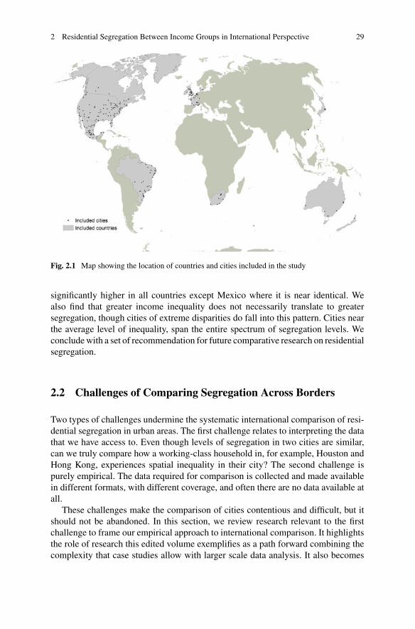
2 Residential Segregation Between Income Groups in International Perspective 29
Fig. 2.1 Map showing the location of countries and cities included in the study
significantly higher in all countries except Mexico where it is near identical. Wealso find that greater income inequality does not necessarily translate to greatersegregation, though cities of extreme disparities do fall into this pattern. Cities nearthe average level of inequality, span the entire spectrum of segregation levels. Weconcludewith a set of recommendation for future comparative research on residentialsegregation.
2.2 Challenges of Comparing Segregation Across Borders
Two types of challenges undermine the systematic international comparison of resi-dential segregation in urban areas. The first challenge relates to interpreting the datathat we have access to. Even though levels of segregation in two cities are similar,can we truly compare how a working-class household in, for example, Houston andHong Kong, experiences spatial inequality in their city? The second challenge ispurely empirical. The data required for comparison is collected and made availablein different formats, with different coverage, and often there are no data available atall.
These challenges make the comparison of cities contentious and difficult, but itshould not be abandoned. In this section, we review research relevant to the firstchallenge to frame our empirical approach to international comparison. It highlightsthe role of research this edited volume exemplifies as a path forward combining thecomplexity that case studies allow with larger scale data analysis. It also becomes
30 A. Comandon and P. Veneri
clear that large-scale data analyses lag in coverage and scope, issues relevant to thesecond challenge. The rest of the chapter will focus on the state-of-the-art concerningthis challenge.
There is an astounding number of factors that make cities more distinct than,for example, countries. Countries, with few exceptions, fit within a system of nationstates, have defined, stable borders and central governments. Cities, on the other hand,often have no clear-cut borders. They includemunicipalities, which have boundaries,and urbanized areas outside those boundaries. Municipal boundaries not only fluc-tuate, they also matter little for many urban infrastructure and processes (e.g., workcommutes).1 Furthermore, cities are embedded within distinct polities (sometimes atseveral governmental levels, as is the case in federal systems) that have authority overthem, multiply the number of historical paths to urbanization, and tend to changemore rapidly than other units of analysis.
This distinction of urban areas has spurred a flourishing theoretical debate aboutthe nature of cities and their comparison. Key questions at the core of this debatesinclude how we understand the relationship and ties between and within cities(Jessop et al. 2008), how to balance individual, experience and generalizable anal-ysis (Robinson 2011; Storper and Scott 2016), and how do we choose and developthe methods for comparison (Abu-Lughod 2007; Dear 2005; Gough 2012; Robinson2016). These strands have all grappled with the challenges of using the city as a unitof analysis. Answers range from the poetic nomadism of Simone (2010) who suggestbringing pieces of cities together to form a new, cohesive unit, to the data-driven useof machine learning to map every urban settlement down to the last house (Esch et al.2017).
These debates have seeped into the study of segregation. Greater emphasis onthe significance of spatial scale has given rise to re-assessment of the mechanismsof segregation (Fowler 2016; Schafran 2018; Trounstine 2018) and methodolog-ical innovation (Lloyd et al. 2014; Reardon et al. 2006; Petrovic et al. 2018). Thegrowing diversity of cities has displaced dominant binary narratives to be replacedwith multifaceted analysis and greater scrutiny of the role of residential integration(e.g., Clark et al. 2015; de la Roca et al. 2014; Goetz 2018; Musterd 2003). Thepersistence of segregation and combination of forms of inequality has widened thelens to include multiple domains (van Ham and Tammaru 2016), including schools(e.g., Bischoff and Tach 2018), housing (e.g. Owens 2019), and infrastructure (e.g.,Trounstine 2018). Here, too, answers tend towards the multiplication of methodsrather than a coherent framework to study spatial inequality.
This expansion of the study of segregation does not translate easily to an interna-tional context. Ethnicity and race, for example, are critical dimensions of segregationthat cross borders. They have, however, different meanings and influences dependingon a country’s history of racial oppression (Abu-Lughod 1980; Massey and Denton
1The US Census Boundary and Annexation Survey, for example, reported over 96,000 municipalboundary changes between 2001 and 2010, an average of three changes per municipality. Most ofthe changes are small but can change the configuration of a city as they accumulate.
2 Residential Segregation Between Income Groups in International Perspective 31
1993; Telles 2006) and its colonial history (Nightingale 2012). As such, the interac-tion of race and class will have different undertones in Canada, the United States,and South Africa (e.g., Fong 1996; Johnston et al. 2007). In the multi-racial contextthat defines many large metropolises today, interactions between groups, their statuswithin a nation (e.g., recent migrants), and the prevalent socioeconomic stratifica-tion can further complicate the picture. Quillian (2012), for example, showed that theinteractions between three types of segregation—ethno-racial segregation, povertysegregation within ethno-racial groups, and segregation of higher income groups—contributed to the process of spatial concentration of poverty. Reproducing studiesof this complexity and scope in multiple countries not only requires much data, italso requires an intimate understanding of how these factors interact in the localcontext. This edited volume takes a significant step in that direction by balancinglocal knowledge, geographical scope, and complexity.
Trounstine (2018) highlighted another dimension that needs systematic engage-ment. While researchers often summarize segregation as a single index, segregationoperates within jurisdictionally defined units that have greater relevance for resi-dents’ well-being. She showed that levels of neighborhood racial segregation aregoing down in many regions of the United States, but is being reinforced at themunicipal level with far reaching implications for access to critical services (see alsoBischoff 2008; Fennell 2009). The chapters in Lloyd et al’s (2014) edited volumemake a similar point, though they emphasize how single-index summaries obscuremuch of the variation that gives segregation meaning. As Hwang’s (2014) chapterdemonstrates, and in a reversal of our initial question, two cities can be very similarin many respects, and yet have entirely different outcomes in terms of segregation.
Recent innovations in the field of segregation studies have advanced our under-standing of spatial inequality in a small set of cities and countries. However, thereis a long way to go for large scale comparative work to catch up to these refine-ments. Existing comparative studies tend to be regionally defined (e,g, Musterd et al.2017; Tammaru et al. 2020 for Europe) or a wide-ranging selection of individualcase studies that emphasize the distinct features of each (Maloutas and Fujita 2012).Some comparative approaches have focused on specific aspects, such as race (Fong1996) or the role of different types of welfare states (Arbaci 2007). What is missing,including from this review, is the systematic integration of knowledge that does notderive from the hegemonic Anglo-Saxon framework of understanding. As accessto data expands to include countries from outside the Global North, more needsto be done to interrogate the assumptions that decades of dominance by Americanscholarship embedded in the methods and in the analytical lenses that we use.
2.3 Method and Data
What we generally understand as cities are more accurately described as urbanregions. Regions are the sum of urban areas that make up a relatively unified laborand housing market (Storper et al. 2015). They are the appropriate scale of study
32 A. Comandon and P. Veneri
for segregation because urban regions often represent regional housing markets. Forexample, when someone gets a new job in the Sydney central business district, theyare not constrained to living in the city proper. They may elect or, in fact, only beable to afford to live in a distant suburb. Residential segregation is the sum of thisprocess of sorting across administrative boundaries and should, therefore, be studiedat the scale that matches the process.
The first step in comparing cities, then, is to establish their boundaries. However,even this step proves challenging. The norm is to use commuting patterns to estimatethe extent of the regional market (OECD 2012). Basically, a functional urban area isthe sum of all urban clusters where a substantial share (15%) of residents commuteto the largest cities in the region. The lack of such data in many countries has ledresearchers to look for alternatives to achieve the consistency that is essential torobust results (Bosker et al. 2018).
For this study, we use the OECD harmonized database of Functional Urban Areas(FUA). The OECD database covers Australia, Canada, Denmark, France, Ireland,Mexico, the Netherlands, the United Kingdom, and the United States. For SouthAfrica, New Zealand, and Brazil, which are not in the database, we use an alternativedefinition (based on administrative definition) closest to the scale of the region. Welimit the sample to FUA and regions with a population over 500,000 people to ensureeach city in the sample has sufficient data coverage in every country.2 This gives usa sample of 194 urban regions in a total of 14 countries. In five countries, however,the data include only one city either due to data availability (Japan) or because thecountry has only one large FUA (Denmark, Hong Kong, Ireland, New Zealand).
For each of these countries, a further obstacle is the differences in data type,spatial scale, and data collection methodology. Some differences are easily, althoughnot perfectly, remedied. For example, France collects income data as decile thresholdvalues. Each tract is assigned Euro denominated values that correspond to each 10%of the population of the tract. For example, if the 10% of the population with thelowest incomes have income below e8500, that is the value reported in the data.The problem is that the values are not comparable across tract because the incomeis not relative to a fixed point. In contrast, all other countries define a set of incomecategories based on fixed ranges and report the number of households that fall withinthat range. In Canada, for example, the first of 15 income categories ranges from$0 to $5000. We address these differences through a mathematical transformationthat uses the information about decile values to estimate how many households fallwithin income categories we defined.
More troublesome are the differences in the spatial scale of small spatial areas,and their coverage. Ideally, we would have data reported at a consistent scale, withfull geographic coverage of the region, and based on the full census of the popula-tion. Much of our work has been devoted to identifying the differences in data andcorrecting themwhere possible. Throughout, we refer to the baseline geographic unitas the tract. This is the neighborhood-scale unit the United States Census Bureau uses
2Some countries, such as France and Canada have restrictions on the minimum population withina unit for it to be included in the publicly available database.
2 Residential Segregation Between Income Groups in International Perspective 33
and has an equivalent in most countries in our sample.We summarize the data formatin Table 2.1.
Some countries have rules about the minimum number of households that mustbe in a tract before the data can be released (due to privacy concerns). This oftenmakes the coverage sparser outside the urban core of a region. In these cases (France,Canada, and the Netherlands), we complement the tract data with the next smallestadministrative unit, which ends up being about the same size in terms of popula-tion, though not geographically. Differences between countries are more difficult tobypass. In some cases, a full range of spatial scales are available, and we can pick theone most consistent with the average size of the tract in other countries. However,we are sometimes stuck with a spatial unit that is either larger or smaller than thetract. For example, the two smallest administrative units in Australia, SA1 and SA2,straddle the tract size. SA1 is smaller, the equivalents of a few square blocks. SA2works in some dense areas but is too large for the lower-density suburbs.
Differences in the spatial scale used to calculate segregation indexes will havean impact on the calculated values. The difference in unit of analysis areas in oursample is not so large that it would lead to the reinterpretation of the broad patternsthat we describe (Wong 2004; Manley et al. 2019). The countries for which the scaleof the geographic unit is of greatest concern are Brazil and South Africa. The twocountries have the highest levels of segregation and the small scale of their units maybias the estimates upward. However, the results are consistent not only with othermethods that minimize the effect of scale (Comandon et al. 2018), the two countriesalso have some of the highest levels of income inequality and, in the case of SouthAfrica, a history of violent segregation that substantiates the high observed levels.
Differences in the timing of the census add another concern. In cross-sectionalstudies like this one, time is an issue only to the extent that levels of segregation havelikely changed in the intervening years (i.e., we do not integrate comparison betweenyears), thus undermining the comparison.Mexico, Japan, and the Netherlands are theonly country with data pre-dating 2010.Mexico, in particular, is problematic becausethe country and cities have changed more rapidly than most other countries in oursample. Results from countries where longitudinal data are available (e.g., UnitedStates) confirm that even in countries with more stable urbanization rates, largechanges occur (Comandon et al. 2018). Cases like Mexico illustrate the limitationof relying on census data which tends to evolve substantially over 10-year periods.However, changes, on average, tend to not change overall interpretation, especiallyfor national trends (Monkkonen et al. 2018).
As part of the data summary, we include the income definition and the methodof data collection. Differences in income definition are relatively benign. The maindifferences relate to whether total income is reported or after-tax income, and tothe composition of income. Generous income redistribution programs and highertax rates will alter the income distribution from pre-tax to after-tax. However, redis-tributive programs should not shift the income distribution so much that the relativeposition of households changes drastically (i.e., a household in the bottom quintileof the pre-tax distribution is unlikely to end up in the middle quintile of post-taxdistribution). We therefore assume this difference is negligible for our purposes. As

34 A. Comandon and P. Veneri
Table2.1
Summaryof
source
andkeymeasures
Country
(year)
Censusauthority
Neighborhood
averagenumberof
households
average
neighborhood
area
Incometype
Num
berof
incomebins
Low
estand
highestincom
ecatego
ries
Samplingrate
Australia**
(2015)
AustralianBureau
ofStatistic
134
1.57
weeklyhousehold
incomeexpressed
inbins
15negativ
eto
14000
andup
100%
Brazil(2010)
Institu
toBrasileiro
deGeografiae
Estatístic
a
206
5.18
Household
minim
umwage
multip
lier
(mw)—
converted
toReal
100to
1/4
minim
umwage
(mw)
20mwandup
Variable(from
50to
5%)basedon
mun
icipality
size
Canada(2016)
Statistic
sCanada—
National
Household
Survey
2007
4.25
Yearlytotal
Household
income
190to
4999
250,000andup
25%
Denmark(2013)
Dansk
Dem
ografisk
Database
1674
18.79
Household
income
50to
149,999
800,000andup
100%
triangulated
with
taxrecords
France
(2014)
Institu
tNationald
elaStatistiq
ueetdes
etudes
econom
ique
1318
5.62
Incomein
euros
foreach
decile—
converted
tobins
110to
10,000
100,000andup
40%
over
5-year
period
HongKong
(2011)
Censusand
Statistic
sDepartm
ent
1455
0.18
Totalm
onthly
householdincome
110to
4,000
40,000
andup
99%
basedon
mon
thly
rotatio
nal
design
Ireland(2011)
CentralStatistic
sOffice
980.77
Socioecono
mic
classes
9Unskille
dmanagerial
100%
(contin
ued)
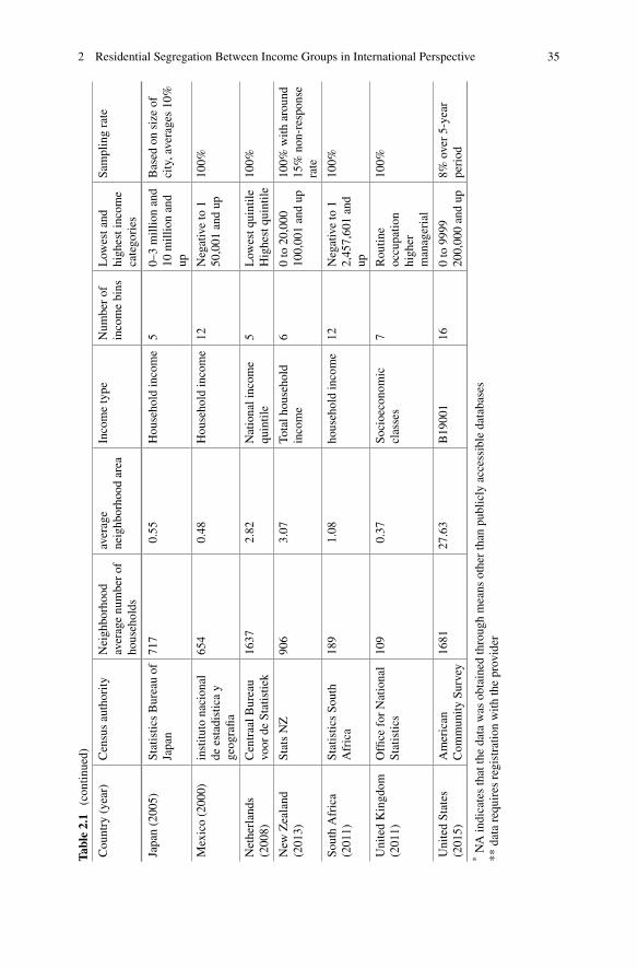
2 Residential Segregation Between Income Groups in International Perspective 35
Table2.1
(contin
ued)
Country
(year)
Censusauthority
Neighborhood
averagenumberof
households
average
neighborhood
area
Incometype
Num
berof
incomebins
Low
estand
highestincom
ecatego
ries
Samplingrate
Japan(2005)
Statistic
sBureauof
Japan
717
0.55
Household
income
50–3millionand
10millionand
up
Based
onsize
ofcity,averages10
%
Mexico(2000)
institu
tonacion
alde
estadisticay
geografia
654
0.48
Household
income
12Negativeto
150,001
andup
100%
Netherlands
(2008)
CentraalB
ureau
voor
deStatistie
k1637
2.82
Nationalincom
equ
intile
5Low
estq
uintile
Highestqu
intile
100%
New
Zealand
(2013)
StatsNZ
906
3.07
Totalh
ousehold
income
60to
20,000
100,001andup
100%
with
around
15%
non-response
rate
SouthAfrica
(2011)
Statistic
sSo
uth
Africa
189
1.08
householdincome
12Negativeto
12,457,601and
up
100%
UnitedKingdom
(2011)
Office
forNational
Statistic
s109
0.37
Socioecono
mic
classes
7Rou
tine
occupatio
nhigher
managerial
100%
UnitedStates
(2015)
American
Com
munity
Survey
1681
27.63
B19001
160to
9999
200,000andup
8%over
5-year
period
*NAindicatesthatthedatawas
obtained
throug
hmeans
otherthan
publicly
accessibledatabases
**datarequ
ires
registratio
nwith
theprovider
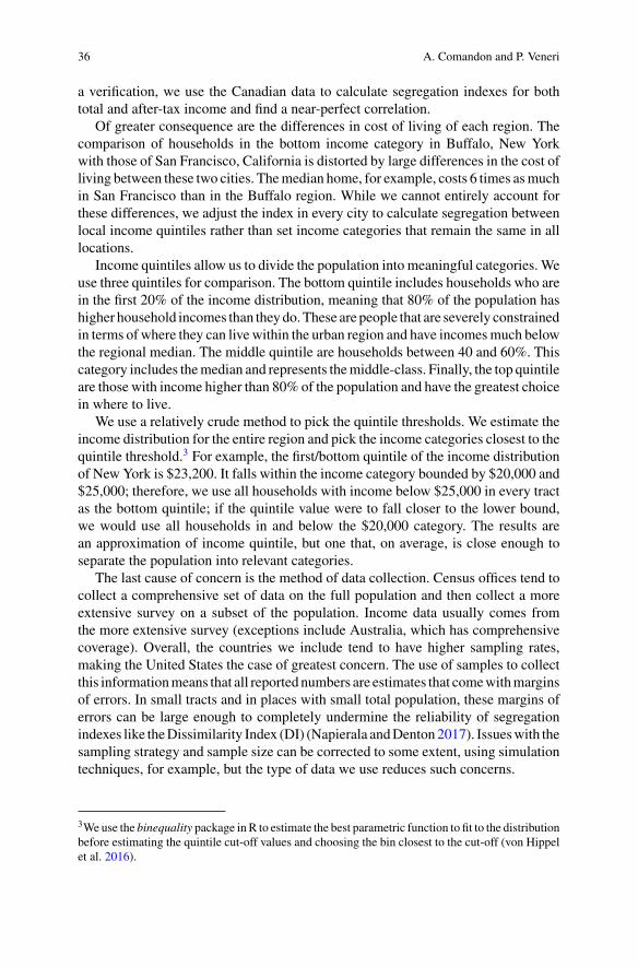
36 A. Comandon and P. Veneri
a verification, we use the Canadian data to calculate segregation indexes for bothtotal and after-tax income and find a near-perfect correlation.
Of greater consequence are the differences in cost of living of each region. Thecomparison of households in the bottom income category in Buffalo, New Yorkwith those of San Francisco, California is distorted by large differences in the cost ofliving between these two cities. Themedian home, for example, costs 6 times asmuchin San Francisco than in the Buffalo region. While we cannot entirely account forthese differences, we adjust the index in every city to calculate segregation betweenlocal income quintiles rather than set income categories that remain the same in alllocations.
Income quintiles allow us to divide the population into meaningful categories. Weuse three quintiles for comparison. The bottom quintile includes households who arein the first 20% of the income distribution, meaning that 80% of the population hashigher household incomes than theydo.These are people that are severely constrainedin terms of where they can live within the urban region and have incomesmuch belowthe regional median. The middle quintile are households between 40 and 60%. Thiscategory includes themedian and represents themiddle-class. Finally, the top quintileare those with income higher than 80% of the population and have the greatest choicein where to live.
We use a relatively crude method to pick the quintile thresholds. We estimate theincome distribution for the entire region and pick the income categories closest to thequintile threshold.3 For example, the first/bottom quintile of the income distributionof New York is $23,200. It falls within the income category bounded by $20,000 and$25,000; therefore, we use all households with income below $25,000 in every tractas the bottom quintile; if the quintile value were to fall closer to the lower bound,we would use all households in and below the $20,000 category. The results arean approximation of income quintile, but one that, on average, is close enough toseparate the population into relevant categories.
The last cause of concern is the method of data collection. Census offices tend tocollect a comprehensive set of data on the full population and then collect a moreextensive survey on a subset of the population. Income data usually comes fromthe more extensive survey (exceptions include Australia, which has comprehensivecoverage). Overall, the countries we include tend to have higher sampling rates,making the United States the case of greatest concern. The use of samples to collectthis informationmeans that all reportednumbers are estimates that comewithmarginsof errors. In small tracts and in places with small total population, these margins oferrors can be large enough to completely undermine the reliability of segregationindexes like theDissimilarity Index (DI) (Napierala andDenton2017). Issueswith thesampling strategy and sample size can be corrected to some extent, using simulationtechniques, for example, but the type of data we use reduces such concerns.
3We use the binequality package in R to estimate the best parametric function to fit to the distributionbefore estimating the quintile cut-off values and choosing the bin closest to the cut-off (von Hippelet al. 2016).

2 Residential Segregation Between Income Groups in International Perspective 37
The concerns about margins of error tend to stem from the underrepresentationof a group of interest. However, since we are interested in income classes, we canexpect a relatively even distribution throughout the region. Furthermore, our strategyaggregates income groups to obtain quintiles, which further reduces the incidenceof tracts with little to no representation. As an additional attempt to put to rest someof these concerns, we use a method Reardon et al (2018) developed to correct forthe bias in ordinal segregation indexes that comes from the sampling method. Thisis not the same index, but the magnitude of the correction should parallel what wewould find for the DI. The correction for income data in the United States is up to10% of the estimated value, but much smaller in Canada, which has a sampling rateof 25% (in contrast to around 8% in the United States, see Table 2.1 for an overviewof sampling rates).
Like the rest of the book, we used the Dissimilarity Index (DI) as our measure ofsegregation. We used the dissim function in the “seg” package in R to calculate theindex for every city in the sample (Hong et al. 2019). We ran the operation for thebottom andmiddle quintile, and the bottom and top quintiles. The dissimilarity indexhas many shortcomings (e.g., Napierala and Denton 2017; Reardon et al. 2006), butremains useful as an intuitive indicator of a city’s spatial structure. In interpretingthe index, however, it is important to keep in mind that there is no such thing as nosegregation, nor is the absence of segregation desirable (Ellickson 2006). There is alevel of segregation that would always be present purely by virtue of the distributionof the housing stock and the impossibility of restricting people’s residential choice(Sander and Kucheva 2016). Massey and Denton (1993) have therefore proposeda generally agreed upon rule of thumb for what constitutes low (0.2–0.3), medium(0.3–0.5), and high levels (>0.5) of segregation. In our interpretation, however, werely more on relative levels than on the values themselves.
2.4 Results
The sets of DI values show that residential segregation between the top and bottomincome groups is much higher than between the bottom and the middle-incomegroup (henceforth, we compare other income groups with the bottom category as thereference point, i.e., we refer only to top DI andmiddle DI to indicate how segregatedthey are from the bottom group). The average middle DI is 0.26 compared to 0.48 forthe top. Figure 2.2 shows these differences in magnitude across and within countries.Variation in top DI (excluding single city countries) across countries is also largerthan it is within any country. The difference between the highest and lowest nationalmedian top DI is 0.42 which is much more than the countries with the largest rangeof about 0.25. In contrast, variation between country medians for middle DI is 0.09and the widest national range in Brazil at about 0.25, six countries with ranges above0.09.
Individual cities highlight these differences. The lowest top DI is Tokyo at 0.2compared to the high of 0.73 in Tshwane. The same comparison for middle DI
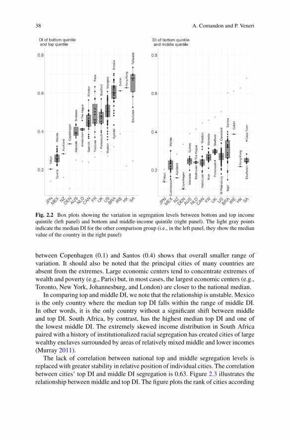
38 A. Comandon and P. Veneri
Fig. 2.2 Box plots showing the variation in segregation levels between bottom and top incomequintile (left panel) and bottom and middle-income quintile (right panel). The light gray pointsindicate the median DI for the other comparison group (i.e., in the left panel, they show the medianvalue of the country in the right panel)
between Copenhagen (0.1) and Santos (0.4) shows that overall smaller range ofvariation. It should also be noted that the principal cities of many countries areabsent from the extremes. Large economic centers tend to concentrate extremes ofwealth and poverty (e.g., Paris) but, in most cases, the largest economic centers (e.g.,Toronto, New York, Johannesburg, and London) are closer to the national median.
In comparing top and middle DI, we note that the relationship is unstable. Mexicois the only country where the median top DI falls within the range of middle DI.In other words, it is the only country without a significant shift between middleand top DI. South Africa, by contrast, has the highest median top DI and one ofthe lowest middle DI. The extremely skewed income distribution in South Africapaired with a history of institutionalized racial segregation has created cities of largewealthy enclaves surrounded by areas of relatively mixed middle and lower incomes(Murray 2011).
The lack of correlation between national top and middle segregation levels isreplaced with greater stability in relative position of individual cities. The correlationbetween cities’ top DI and middle DI segregation is 0.63. Figure 2.3 illustrates therelationship between middle and top DI. The figure plots the rank of cities according
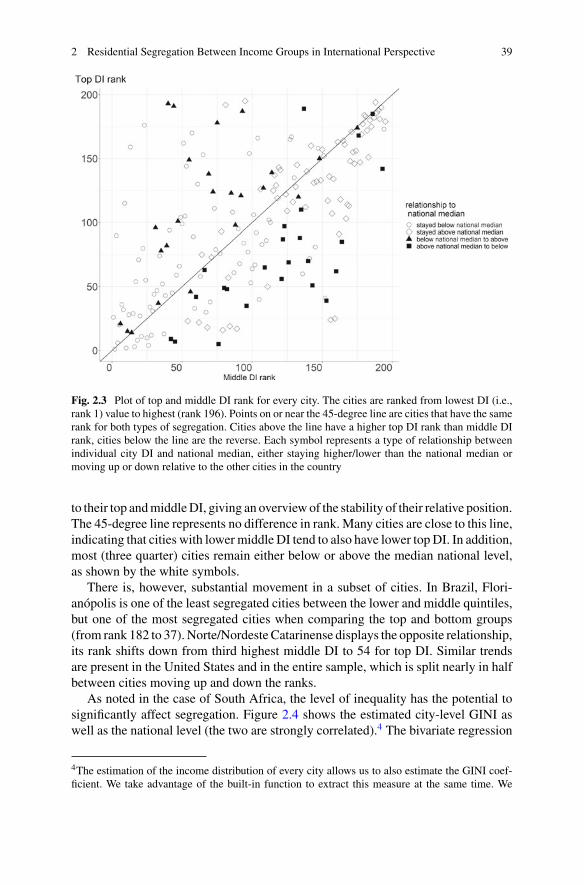
2 Residential Segregation Between Income Groups in International Perspective 39
Fig. 2.3 Plot of top and middle DI rank for every city. The cities are ranked from lowest DI (i.e.,rank 1) value to highest (rank 196). Points on or near the 45-degree line are cities that have the samerank for both types of segregation. Cities above the line have a higher top DI rank than middle DIrank, cities below the line are the reverse. Each symbol represents a type of relationship betweenindividual city DI and national median, either staying higher/lower than the national median ormoving up or down relative to the other cities in the country
to their top andmiddleDI, giving an overviewof the stability of their relative position.The 45-degree line represents no difference in rank. Many cities are close to this line,indicating that cities with lowermiddle DI tend to also have lower topDI. In addition,most (three quarter) cities remain either below or above the median national level,as shown by the white symbols.
There is, however, substantial movement in a subset of cities. In Brazil, Flori-anópolis is one of the least segregated cities between the lower and middle quintiles,but one of the most segregated cities when comparing the top and bottom groups(from rank 182 to 37). Norte/Nordeste Catarinense displays the opposite relationship,its rank shifts down from third highest middle DI to 54 for top DI. Similar trendsare present in the United States and in the entire sample, which is split nearly in halfbetween cities moving up and down the ranks.
As noted in the case of South Africa, the level of inequality has the potential tosignificantly affect segregation. Figure 2.4 shows the estimated city-level GINI aswell as the national level (the two are strongly correlated).4 The bivariate regression
4The estimation of the income distribution of every city allows us to also estimate the GINI coef-ficient. We take advantage of the built-in function to extract this measure at the same time. We
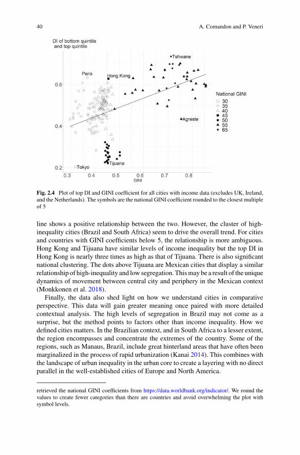
40 A. Comandon and P. Veneri
Fig. 2.4 Plot of top DI and GINI coefficient for all cities with income data (excludes UK, Ireland,and the Netherlands). The symbols are the national GINI coefficient rounded to the closest multipleof 5
line shows a positive relationship between the two. However, the cluster of high-inequality cities (Brazil and South Africa) seem to drive the overall trend. For citiesand countries with GINI coefficients below 5, the relationship is more ambiguous.Hong Kong and Tijuana have similar levels of income inequality but the top DI inHong Kong is nearly three times as high as that of Tijuana. There is also significantnational clustering. The dots above Tijuana are Mexican cities that display a similarrelationship of high-inequality and low segregation. Thismay be a result of the uniquedynamics of movement between central city and periphery in the Mexican context(Monkkonen et al. 2018).
Finally, the data also shed light on how we understand cities in comparativeperspective. This data will gain greater meaning once paired with more detailedcontextual analysis. The high levels of segregation in Brazil may not come as asurprise, but the method points to factors other than income inequality. How wedefined cities matters. In the Brazilian context, and in South Africa to a lesser extent,the region encompasses and concentrate the extremes of the country. Some of theregions, such as Manaus, Brazil, include great hinterland areas that have often beenmarginalized in the process of rapid urbanization (Kanai 2014). This combines withthe landscape of urban inequality in the urban core to create a layering with no directparallel in the well-established cities of Europe and North America.
retrieved the national GINI coefficients from https://data.worldbank.org/indicator/. We round thevalues to create fewer categories than there are countries and avoid overwhelming the plot withsymbol levels.
2 Residential Segregation Between Income Groups in International Perspective 41
2.5 Discussion and Conclusion
Now that we examined the data, we can come back to the questions we openedwith. Despite the lack of contextual data about individual cities and countries, thereis much we can infer from the observed patterns. We learn that income inequality,certainly high-inequality, correlates with residential segregation between incomegroups but leaves much variation unexplained. Many cities with similar levels ofincome inequality, even within the same country, have segregation levels at theopposite ends of the spectrum. While differences in segregation are not as largewithin countries as they are between countries, our data suggest that both need tobe studied in conjunction. Therefore, it is not just a matter of understanding thedifference between Melbourne and Boston as cities within countries with differentpolitical economy, it also matters that segregation levels in all Australian cities aresimilar while in the United States they vary from Australian to Brazilian levels. Thisrelationship between inequality and segregation raises important substantive andmethodological questions for between-country and within-country comparisons.
The case of Mexico, for example, stands out on its own because of the prevalentlow levels of segregation by income but raises additional questions in comparisonto other middle-income, high-inequality countries such as South Africa and Brazil.South Africa shares more with Mexico when limiting the comparison to middle-income segregation when both countries have lower levels of segregation. It may bethat Mexico’s data limitation fails to capture the translation of high inequality intospatial patterns of separation or that Mexican cities developed in such a way that theisolation of wealthy households that defines South African cities has not taken holdto the same extent.
Elucidating these questions has implications for policies aiming to reduce segrega-tion. There is too little evidence to speculate as to the importance of national welfaresystems on explaining the differences in within-country variation. Some countries,like France, have a more centralized system of urban governance and comprehen-sive redistributive systems, yet, the range of income segregation levels resemblesmore closely that of the Unites States than the Netherlands. This can be interpretedas evidence that differences between cities are more important than national-leveldifferences. The lower average level of segregation in higher income equality coun-triesmay point in the other direction. Here too, however, important deviations preventstraightforward inference.
A key aspect of explaining deviations from general relationships is history. Singlecountry studies have revealed important processes that persistently shaped segrega-tion. In the United States, for example, scholars have showed how the migration ofblack people out of the South led to the creation of modern residential racial segre-gation. Where the social hierarchy was institutionalized in the South under slaveryand Jim Crow laws, the rest of the country lacked such rules to establish white domi-nance and relied instead on the systematic spatial separation of blackmigrants (Logan2017). To this day, southern cities have lower levels of segregation than the rest ofthe country. Nightingale (2012) showed that a similar process operated in South
42 A. Comandon and P. Veneri
Africa where residential segregation was unnecessary until a large black labor forcedeveloped in urban centers. The data we presented can serve to conceptualize histor-ical processes more broadly to include the implications of different starting point ofurbanization, colonial relations, and changing economic relations (e.g., centered onlabor and property).
One promising area of study is the integration of economic geography into thestudy of segregation. As cities take on different roles in relation to their internationalpeers and national competitors, the pressures on urban structures will be different. Alarge-scale data analysis would allow for the modeling of urban system to considersub-national labor market trends and the accompanying migration patterns. It wouldalso open the possibility of studying the role of different historical trajectories ofcities. The period in which urbanization takes place, and the set of events that shapesthe life of a city matter, but studying such phenomena as cases studies can lead toself-fulfilling analysis if one chooses cases based on the outcome one wishes to study(Abu-Lughod 2007). The trends in urban research and segregation studies point tofruitful complementarities between case studies and large-scale data analyses.
Many questions we have suggested point to the importance of data spanningseveral time periods for future research. The only country for which we have accessto reliable data over time for the entire country is the United States. Even in that case,issues of comparison over time are non-negligible (Reardon et al. 2018). Countriesare improving their data collection methods with every census and we hope that astime passes, the scope of comparison will only increase.
References
Abu-Lughod JL (2007) The challenge of comparative case studies. City 11(3):399–404. https://doi.org/10.1080/13604810701669140
Abu-Lughod JL (1980) Rabat: urban apartheid in Morocco. Princeton University Press, Princeton,NJ
Arbaci S (2007) Ethnic segregation, housing systems and welfare regimes in Europe. Eur J HousingPolicy 7(4):401–433. https://doi.org/10.1080/14616710701650443
Bischoff K (2008) School district fragmentation and racial residential segregation: how doboundaries matter? Urban Affairs Rev 44(2):182–217. https://doi.org/10.1177/1078087408320651
Bischoff K, Tach L (2018) The racial composition of neighborhoods and local schools: the roleof diversity, inequality, and school choice. City Community 17(3):675–701. https://doi.org/10.1111/cico.12323
Bosker M, Park J, Roberts M (2018) Definition matters: metropolitan areas and agglomerationeconomies in a large developing country. Policy ResearchWorking Papers. https://doi.org/https://doi.org/10.1596/1813-9450-8641
Clark WAV, Anderson E, Östh J, Malmberg B (2015) A multiscalar analysis of neighborhoodcomposition in Los Angeles, 2000–2010: a location-based approach to segregation and diversity.Ann Assoc Am Geogr 105(6):1260–1284. https://doi.org/10.1080/00045608.2015.1072790
ComandonA, DaamsM, Garcia-LópezM-À, Veneri P (2018) Divided cities: understanding incomesegregation in OECD metropolitan areas. Divided cities: understanding intra-urban inequalities.OECD, Paris, France, pp 19–51
2 Residential Segregation Between Income Groups in International Perspective 43
De la Roca J, Ellen IG, O’Regan KM (2014) Race and neighborhoods in the 21st century: whatdoes segregation mean today? Reg Sci Urban Econ 47:138–151. https://doi.org/10.1016/j.regsciurbeco.2013.09.006
Dear M (2005) Comparative urbanism. Urban Geogr 26(3):247–251. https://doi.org/10.2747/0272-3638.26.3.247
Esch T, Heldens W, Hirner A, Keil M, Marconcini M, Roth A, Zeidler J, Dech S, Strano E (2017)Breaking new ground in mapping human settlements from space – The Global Urban Footprint.ISPRS J Photogramm. Remote Sens 134:30–42. https://doi.org/10.1016/j.isprsjprs.2017.10.012
Ellickson RC (2006) The puzzle of the optimal social composition of neighborhoods. In: FischelWA, Oates WE (Eds) The Tiebout model at fifty: essays in public economics in honor of wallaceoates. Lincoln Institute of Land Policy, Cambridge, MA
Fennell LA (2009) The unbounded home: property values beyond property lines. Yale UniversityPress, New Haven, CT. https://doi.org/https://doi.org/10.12987/yale/9780300122442.001.0001
Fong E (1996) A comparative perspective on racial residential segregation. Sociol Quart 37(2):199–226
Fowler C (2016) Segregation as a multiscalar phenomenon and its implications for neighborhood-scale research: the case of South Seattle 1990–2010. Urban Geogr 37(1):1–25. https://doi.org/10.1080/02723638.2015.1043775
Goetz EG (2018) The one-way street of integration: fair housing and the pursuit of racial justice inAmerican Cities. Cornell University Press, Ithaca, NY
Gough KV (2012) Reflections on conducting urban comparison. Urban Geogr 33(6):866–878.https://doi.org/10.2747/0272-3638.33.6.866
Hong S-Y, O’Sullivan D, Jarvis, Choi C (2019) Seg: measuring spatial segregation. Retrieved fromhttps://CRAN.R-project.org/package=seg
Hwang S (2014) A tale of two cities: residential segregation in St. Louis and Cincinnati. In: LloydC, Shuttleworth I, Wong D (eds) Social-spatial segregation. Policy Press, Bristol
Jessop B, Brenner N, JonesM (2008) Theorizing sociospatial relations. Environ PlannD: Soc Space26(3):389–401. https://doi.org/10.1068/d9107
JohnstonR, PoulsenM, Forrest J (2007) The geography of ethnic residential segregation: a compara-tive study of five countries. AnnAssocAmGeogr 97(4):713–738. https://doi.org/10.1111/j.1467-8306.2007.00579.x
Kanai JM (2014)On the peripheries of planetary urbanization: globalizingmanaus and its expandingimpact. Environ Plann D: Soc Space 32(6):1071–1087. https://doi.org/10.1068/d13128p
Lloyd C, Shuttleworth I, Wong D (eds) (2014) Social-spatial segregation. Policy Press, BristolLogan J (2017) Racial segregation in postbellum southern cities: the case of Washington, D.C.Demogr Res 36:1759–1784. https://doi.org/10.4054/DemRes.2017.36.57
Maloutas T, Fujita K (2012) Residential segregation in comparative perspective: making sense ofcontextual diversity. In: Maloutas T, Fujita K (eds) Cities and society. Ashgate, Burlington, VT
Manley D, Jones K, Johnston R (2019) Multiscale segregation: multilevel modeling of dissim-ilarity—challenging the stylized fact that segregation is greater the finer the spatial scale.Professional Geographer 71(3):566–578. https://doi.org/10.1080/00330124.2019.1578977
Massey DS, Denton NA (1993) American apartheid: segregation and the making of the underclass.Harvard University Press, Cambridge, MA
Monkkonen P, Comandon A, Montejano Escamilla JA, Guerra E (2018) Urban sprawl and thegrowing geographic scale of segregation in Mexico, 1990–2010. Habitat Int 73:89–95. https://doi.org/10.1016/j.habitatint.2017.12.003
Murray MJ (2011) City of extremes: the spatial politics of Johannesburg. Duke University Press,Durham, NC
Musterd S (2003) Segregation and integration: a contested relationship. J Ethnic Migration Stud29(4):623–641. https://doi.org/10.1080/1369183032000123422
Musterd S, Marcinczak S, van HamM, Tammaru T (2017) Socioeconomic segregation in Europeancapital cities. Increasing separationbetweenpoor and rich.UrbanGeogr 38(7):1062–1083. https://doi.org/10.1080/02723638.2016.1228371
44 A. Comandon and P. Veneri
Napierala J, Denton N (2017) Measuring residential segregation with the acs: how the marginof error affects the dissimilarity index. Demography 54(1):285–309. https://doi.org/10.1007/s13524-016-0545-z
Nightingale CH (2012) Segregation: a global history of divided cities. The University of ChicagoPress, Chicago, IL
OECD (2012) Redefining “Urban”: a new way to measure metropolitan areas. https://doi.org/10.1787/9789264174108-en
Owens A (2019) Building inequality: housing segregation and income segregation. Sociol Sci6:497–525. https://doi.org/10.15195/v6.a19
Petrovic A, van HamM,Manley D (2018)Multiscale measures of population: within- and between-city variation in exposure to the sociospatial context. Ann Am Assoc Geograph 108(4):1057–1074. https://doi.org/10.1080/24694452.2017.1411245
Quillian L (2012) Segregation and poverty concentration: The role of three segregations. Am SociolRev 77(3):354–79. https://doi.org/10.1177/0003122412447793
Reardon SF, Bischoff K (2011) Income inequality and income segregation. Am J Sociol116(4):1092–1153. https://doi.org/10.1086/657114
Reardon SF, Bischoff K, Owens A, Townsend JB (2018) Has income segregation really increased?bias and bias correction in sample-based segregation estimates. Demography 55(6):2129–2160
Reardon SF, Firebaugh G, O’Sullivan D, Matthews S (2006) A new approach to measuring socio-spatial economic segregation. Measurement of segregation: new directions and results. Presentedat the general conference of the international association for research in income and wealth,Joensuu, Finland. Retrieved from https://www.iariw.org/papers/2006/reardon.pdf
Robinson J (2011) Cities in a world of cities: the comparative gesture: cities in a world of citiescompared. Int J Urban Reg Res 35(1):1–23. https://doi.org/10.1111/j.1468-2427.2010.00982.x
Robinson J (2016) Thinking cities through elsewhere: Comparative tactics for a more global urbanstudies. Prog Hum Geogr 40(1):3–29. https://doi.org/10.1177/0309132515598025
Sander R, Kucheva Y (2016) Structural versus ethnic dimensions of housing segregation. Retrievedfrom ftp://ftp2.census.gov/ces/wp/2016/CES-WP-16-22.pdf
Schafran A (2018) The road to resegregation: Northern California and the failure of politics.University of California Press, Oakland, CA
Simone A (2010) City Life from Jakarta to Dakar: Movements at the Crossroads. Routledge, NewYork, NY
Storper M, Kemeny T, Makarem NP, Osman T (2015) The rise and fall of urban economies: lessonsfrom San Francisco and Los Angeles. Stanford Business Books, Stanford, CA
Storper M, Scott AJ (2016) Current debates in urban theory: A critical assessment. Urban Studies53(6):1114–1136. https://doi.org/10.1177/0042098016634002
Tammaru T, Marcinczak S, Aunap R, van HamM, Janssen H (2020) Relationship between incomeinequality and residential segregation of socioeconomic groups. Reg Stud 54(4):450–461. https://doi.org/10.1080/00343404.2018.1540035
Telles EE (2006) Race in another America: the significance of skin color in Brazil. PrincetonUniversity Press, Princeton, N.J.
Trounstine J (2018) Segregation by design: local politics and inequality in American Cities.Cambridge University Press, Cambridge. https://doi.org/10.1017/9781108555722
van Ham M, Tammaru T (2016) New perspectives on ethnic segregation over time and space. aDomains Approach. Urban Geography 37(7):953–962. https://doi.org/10.1080/02723638.2016.1142152
von Hippel PT, Scarpino SV, Holas I (2016) Robust estimation of inequality from binned incomes.Sociol Methodol 46(1):212–251. https://doi.org/10.1177/0081175015599807
Wong DWS (2004) Comparing traditional and spatial segregation measures: a spatial scaleperspective. Urban Geogr 25(1):66–82. https://doi.org/10.2747/0272-3638.25.1.66

2 Residential Segregation Between Income Groups in International Perspective 45
Open Access This chapter is licensed under the terms of the Creative Commons Attribution 4.0International License (http://creativecommons.org/licenses/by/4.0/), which permits use, sharing,adaptation, distribution and reproduction in any medium or format, as long as you give appropriatecredit to the original author(s) and the source, provide a link to the Creative Commons license andindicate if changes were made.
The images or other third party material in this chapter are included in the chapter’s CreativeCommons license, unless indicated otherwise in a credit line to the material. If material is notincluded in the chapter’s Creative Commons license and your intended use is not permitted bystatutory regulation or exceeds the permitted use, you will need to obtain permission directly fromthe copyright holder.

Part IIAfrica
Chapter 3Income Inequality, Socio-EconomicStatus, and Residential Segregationin Greater Cairo: 1986–2006
Abdelbaseer A. Mohamed and David Stanek
Abstract Greater Cairo is a primate, monocentric metropolis with significantsocio-economic disparities among its population and neighborhoods. This chapterexamines the relationship between income inequality, the welfare regime, central-ized governance, settlement type, housing policies, occupational status, and socio-economic segregation. Using data from the 1986, 1996, and 2006 censuses, wereport the dissimilarity index to demonstrate the distribution of residents in theGreater Cairo Region by occupational status, we show patterns of socio-economicsegregation based on the distribution of the population by categories of occupationsacross census tracts and employ the location quotient to compare the concentra-tion of the top/bottom groups in each census tract relative to the city average. Theresults show that growing economic inequality does not necessarily result in greatersocio-economic segregation. The results also suggest that social class contributesto residential clustering. While the poorer strata of the Greater Cairo Region werepushed to the periphery and the older urban core, affluent inhabitants were morelikely to settle voluntarily in segregated enclaves to isolate themselves from thegeneral population.
Keywords Greater Cairo · Socio-economic status · Residential segregation ·Housing policies · Income inequality
The original version of this chapter was revised: In the figure 3.3 missed out correction have beenincorporated. The correction to this chapter is available at https://doi.org/10.1007/978-3-030-64569-4_27
A. A. Mohamed (B)Urban Planning Department, Al-Azhar University, Cairo, Egypte-mail: [email protected]
D. StanekDepartment of City and Regional Planning, University of Pennsylvania, Philadelphia, USAe-mail: [email protected]
© The Author(s) 2021, corrected publication 2021M. van Ham et al. (eds.), Urban Socio-Economic Segregation and Income Inequality,The Urban Book Series, https://doi.org/10.1007/978-3-030-64569-4_3
49
50 A. A. Mohamed and D. Stanek
3.1 Introduction
Urbanization and social inequality have been on the rise in Egypt since themid-1970swhen President Anwar Sadat (1970–1981) initiated a series of reforms beginningwith the 1974 infitah (open-door) policy to reduce state welfare spending and expandthe private sector through state support and foreign direct investment (Ben Nefissa2011: 180). In 1991, under President Hosni Mubarak (1981–2011), Egypt adoptedthe Economic Reform and Structural Adjustment Program with the support of theWorld Bank, European Union, and African Development Bank (ADB 2000). Theseneoliberal policies contributed to the urbanization of theGreater CairoRegion (GCR)and increased social inequality in several ways. Reduced state welfare funding andagricultural mechanization encouraged economic migrants to seek work in the GCR.Some Egyptians emigrated to neighboring Gulf countries to work in the boomingoil sector. They sent remittances to their families who, in turn, invested in land andconstruction to satisfy an increased housing demand (Sims 2010; El Kadi 2009). Atthe same time, the state withdrew from social housing construction and engaged inland speculation of its own, leaving a largely unregulated private market to providehousing for the growing population of theGCR.Housing demand pushed speculatorsto build on the urban periphery, turning large tracts of productive (and scarce) agri-cultural land into densely built, informal housing settlements, which are now hometo poor and middle-income Cairenes alike (UNCHS 1993; Sims 2010). Internationalreal estate investment concentrated in the GCR’s central business district and alongthe Nile’s “Gold Coast”, as well as in a series of new satellite cities that catered tomobile, urban elites.
In 1979, the government adopted a deliberate urban decentralization strategy torelieve some of the congestion and pollution brought about by the urbanization ofGCR (Tadamun 2018). By 2008, the development of new urban communities, such asthe 6th of October City and Sheikh Zayed City, set apart from the urban fabric on thedesert plains, had transformed the GCR from a compact, monocentric metropolitanregion into a discontinuous, polycentric, dispersed urban structure (Taubenböck et al.2009). This rapid expansion has provided opportunities for higher income Egyptiansto leave central Cairo. At the same time, poorer communities have concentrated inundesirable, underserved, and often unsafe areas, also known as “poverty pockets,”where chances of upward mobility and opportunities are limited (Tadamun 2018).This chapter explores the factors that have influenced the socio-economic spatial divi-sions in GCR. A city’s socio-spatial division is a function of many factors includingcontext, institutional power, welfare regimes (Arbaci 2007), ethnicity, commodifi-cation of housing, and people’s residential preferences (Marcinczak et al. 2015).Research from the United States and Western Europe has shown that economicinequality can result in (socio)economic segregation, the uneven spatial distributionof households based on income, occupation and/or educational attainment (Burgess1925; Massey 1979b; Schteingart 2001). Singerman and Amar (2006) show that, inaddition to economic inequalities, social inequalities reinforce socio-spatial segre-gation. Several authors including Gilbert (1992) have suggested that social class is
3 Income Inequality, Socio-Economic Status, andResidential Segregation… 51
replacing ethnicity as the basis for the social urban geography. While many studieshave looked at poverty in Egypt (e.g., World Bank 1990; Korayem 1994; El-Laithy1996; Sabry 2010), poverty in relation to spatial justice and unemployment in theGCR (Shawkat 2013; Nassar and Biltagy 2016; Tadamun 2018), and the patterns oflow-income housing inGCR (Harris andWahba 2002), no rigorous research has beenconducted on the intersection of economic inequality and residential segregation ofsocio-professional groups in the GCR.
This work focuses on post-socialist Greater Cairo (1986–2006) as a monocentriccity and uses occupation as an indicator of social status to study the distribution ofsocio-economic groups across the region. UsingMarcinczak’s et al. (2015) approachwith publicly available data, we answer the following questions: To what extent isthere residential segregation of occupational groups in theGCR?Can socio-economicinequality explain residential segregation? Towhat extent can the welfare regime andthe characteristics of housing provision explain segregation trends in the GCR?
3.2 The Social Geography of GCR
With the exception of its recent history, the GCR had a compact, monocentric urbanstructure that followed Burgess’s (1925) concentric zone model that theorizes howeconomic and political forces influence the distribution of social groups within thecity. The model suggests that cities evolve in successive rings around the centralbusiness district (CBD). The first ring, widely visible in the developing world, ismade up by deteriorating housing formerly occupied by higher income familiesand is called the “zone of transition”, or what Stokes (1962) refers to as “slumsof despair.” This zone is followed by three successive rings of housing rangingfrom high-density poor-quality working class housing, to lower density high-qualityhousing for the elite. Change occurs in this model through the invasion-successionprocess in which a group of people or type of land use arrives and comes to dominatean area previously occupied by another group (Kendall 2013).
An important criticism of Burgess’s model is that many settlements on theperiphery of contemporary megacities are not higher class neighborhoods, but whatStokes calls “slums of hope”1 which are problematic, but not as dire as the inner-city“slums of despair”. While the differentiation between slums in the urban core andthose in fringe areas looks outdated and prejudiced, authors like Harris and Wahba(2002) confirm its usefulness and validity for the GCR.
Rural–urban migration has been a dominant force in shaping the socio-spatialstructure of the GCR. The limited availability of publicly subsidized housing andthe high cost of formal market-rate housing forces lower income residents to live ineither older, affordable neighborhoods often with substandard housing or in informal
1In this instance, we apply Stokes’s use of the word “slum” to the informal settlements, orashwaiyaat, of Cairo although they are technically dissimilar. See footnote 2 below.
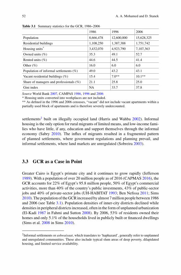
52 A. A. Mohamed and D. Stanek
Table 3.1 Summary statistics for the GCR, 1986–2006
1986 1996 2006
Population 8,666,478 12,600,000 15,628,325
Residential buildings 1,108,250 1,387,388 1,751,742
Housing units* 3,432,070 4,923,790 7,107,363
Owned units (%) 35.3 49.1 52.7
Rented units (%) 44.6 44.5 41.4
Other (%) 16.0 6.0 6.0
Population of informal settlements (%) 49.0 43.2 43.1
Vacant residential buildings (%) 15.4 7.0** 10.1**
Share of managers and professionals (%) 21.1 25.8 25.0
Gini index NA 33.7 37.8
Source World Bank 2007, CAMPAS 1986, 1996 and 2006* Housing units converted into workplaces are not included.** As defined in the 1996 and 2006 censuses, “vacant” did not include vacant apartments within apartially used block of apartments and is therefore severely undercounted.
settlements2 built on illegally occupied land (Harris and Wahba 2002). Informalhousing is the only option for rural migrants of limited means, and low-income fami-lies who have little, if any, education and support themselves through the informaleconomy (Sabry 2010). The influx of migrants resulted in a fragmented patternof planned settlements, where government regulations and planning prevail, andinformal settlements, where land markets are unregulated (Sobreira 2003).
3.3 GCR as a Case in Point
Greater Cairo is Egypt’s primate city and it continues to grow rapidly (Jefferson1989). With a population of over 20 million people as of 2016 (CAPMAS 2016), theGCR accounts for 22% of Egypt’s 95.8 million people, 50% of Egypt’s commercialactivities, more than 40% of the country’s public investments, 43% of public-sectorjobs and 40% of private-sector jobs (UH-HABITAT 1993; Ben Nefissa 2011; Sims2010). The population of theGCR increased by almost 7million people between 1986and 2006 (see Table 3.1). Population densities of inner-city districts declined whiledensities in peripheral districts increased, often in the formof unplanned urbanization(El-Kadi 1987 in Fahmi and Sutton 2008). By 2006, 53% of residents owned theirhomes and only 5.1% of the households lived in publicly built or financed dwellings(Sims et al. 2008 in Sims 2010).
2Informal settlements or ashwaiyaat, which translates to ‘haphazard’, generally refer to unplannedand unregulated communities. These also include typical slum areas of deep poverty, dilapidatedhousing, and limited service availability.
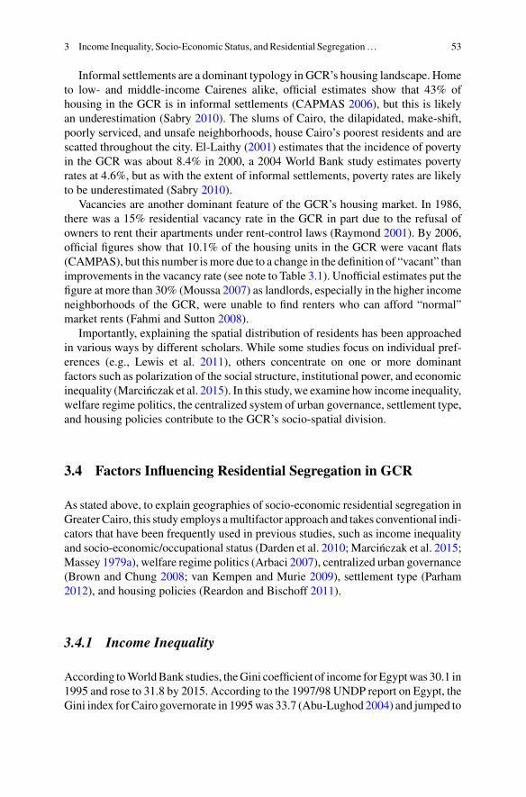
3 Income Inequality, Socio-Economic Status, andResidential Segregation… 53
Informal settlements are a dominant typology in GCR’s housing landscape. Hometo low- and middle-income Cairenes alike, official estimates show that 43% ofhousing in the GCR is in informal settlements (CAPMAS 2006), but this is likelyan underestimation (Sabry 2010). The slums of Cairo, the dilapidated, make-shift,poorly serviced, and unsafe neighborhoods, house Cairo’s poorest residents and arescatted throughout the city. El-Laithy (2001) estimates that the incidence of povertyin the GCR was about 8.4% in 2000, a 2004 World Bank study estimates povertyrates at 4.6%, but as with the extent of informal settlements, poverty rates are likelyto be underestimated (Sabry 2010).
Vacancies are another dominant feature of the GCR’s housing market. In 1986,there was a 15% residential vacancy rate in the GCR in part due to the refusal ofowners to rent their apartments under rent-control laws (Raymond 2001). By 2006,official figures show that 10.1% of the housing units in the GCR were vacant flats(CAMPAS), but this number ismore due to a change in the definition of “vacant” thanimprovements in the vacancy rate (see note to Table 3.1). Unofficial estimates put thefigure at more than 30% (Moussa 2007) as landlords, especially in the higher incomeneighborhoods of the GCR, were unable to find renters who can afford “normal”market rents (Fahmi and Sutton 2008).
Importantly, explaining the spatial distribution of residents has been approachedin various ways by different scholars. While some studies focus on individual pref-erences (e.g., Lewis et al. 2011), others concentrate on one or more dominantfactors such as polarization of the social structure, institutional power, and economicinequality (Marcinczak et al. 2015). In this study, we examine how income inequality,welfare regime politics, the centralized system of urban governance, settlement type,and housing policies contribute to the GCR’s socio-spatial division.
3.4 Factors Influencing Residential Segregation in GCR
As stated above, to explain geographies of socio-economic residential segregation inGreater Cairo, this study employs amultifactor approach and takes conventional indi-cators that have been frequently used in previous studies, such as income inequalityand socio-economic/occupational status (Darden et al. 2010; Marcinczak et al. 2015;Massey 1979a), welfare regime politics (Arbaci 2007), centralized urban governance(Brown and Chung 2008; van Kempen and Murie 2009), settlement type (Parham2012), and housing policies (Reardon and Bischoff 2011).
3.4.1 Income Inequality
According toWorldBank studies, theGini coefficient of income forEgyptwas 30.1 in1995 and rose to 31.8 by 2015. According to the 1997/98 UNDP report on Egypt, theGini index forCairo governorate in 1995was 33.7 (Abu-Lughod 2004) and jumped to
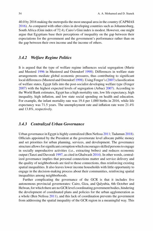
54 A. A. Mohamed and D. Stanek
40.0 by 2016 making the metropolis the most unequal area in the country (CAPMAS2016). As compared with other cities in developing countries such as Johannesburg,South Africa (Gini index of 72.4), Cairo’s Gini index is modest. However, one mightargue that Egyptians base their perceptions of inequality on the gap between theirexpectations for the government and the government’s performance rather than onthe gap between their own income and the income of others.
3.4.2 Welfare Regime Politics
It is argued that the type of welfare regime influences social segregation (Murieand Musterd 1996 in Mustered and Ostendorf 1998). Differences in welfare statearrangements mediate global economic pressures, thus contributing to significantlocal differences (Musterd andOstendorf 1998). Using Fenger’s (2007) classificationof welfare states, Egypt falls into the post-socialist developing welfare type (Fenger2007) with the highest expected levels of segregation (Arbaci 2007). According tothe World Bank estimates, Egypt has a high mortality rate, low life expectancy, highinequality, high inflation, and low state social spending on health and education.For example, the infant mortality rate was 19.4 per 1,000 births in 2016, while lifeexpectancy was 71.5 years. The unemployment rate and inflation rate were 21.4%and 13.8%, respectively.
3.4.3 Centralized Urban Governance
Urban governance in Egypt is highly centralized (BenNefissa 2011; Tadamun 2018).Officials appointed by the President at the governorate level allocate public moneyand set priorities for urban planning, services, and development. The governancestructure allows for significant corruptionwhich encourages skilled persons to engagein socially unproductive activities (i.e., extracting bribes) and reduces economicoutput (Tanzi and Davoodi 1997, as cited in Ghalwash 2014). In other words, central-ized governance implies that personal connections matter and service delivery andthe quality of neighborhoods are tied to those connections, thus reinforcing existingspatial inequalities. It also leaves lower income households with little opportunity toengage in the decision-making process about their communities, reinforcing spatialinequalities among neighborhoods.
Further complicating the governance of the GCR is that it includes fiveautonomous provincial governorates: Cairo, Giza, and Qalyubia, 6th October andHelwan, forwhich there are noGCR level coordinating government bodies, hinderingthe development of coordinated plans and policies for the urban agglomeration asa whole (Ben Nefissa 2011), and this lack of coordination prevents the governmentfrom addressing the spatial inequality of the GCR region in a meaningful way. This
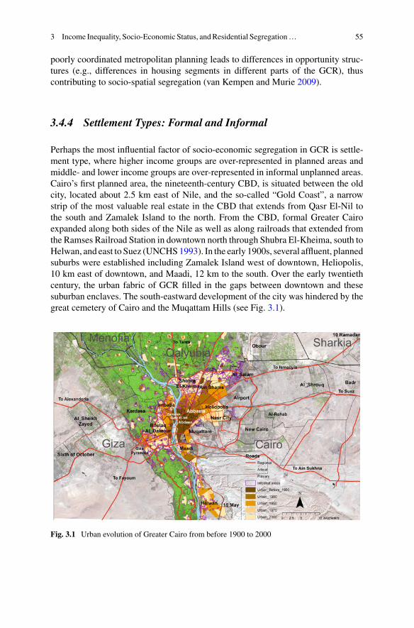
3 Income Inequality, Socio-Economic Status, andResidential Segregation… 55
poorly coordinated metropolitan planning leads to differences in opportunity struc-tures (e.g., differences in housing segments in different parts of the GCR), thuscontributing to socio-spatial segregation (van Kempen and Murie 2009).
3.4.4 Settlement Types: Formal and Informal
Perhaps the most influential factor of socio-economic segregation in GCR is settle-ment type, where higher income groups are over-represented in planned areas andmiddle- and lower income groups are over-represented in informal unplanned areas.Cairo’s first planned area, the nineteenth-century CBD, is situated between the oldcity, located about 2.5 km east of Nile, and the so-called “Gold Coast”, a narrowstrip of the most valuable real estate in the CBD that extends from Qasr El-Nil tothe south and Zamalek Island to the north. From the CBD, formal Greater Cairoexpanded along both sides of the Nile as well as along railroads that extended fromthe Ramses Railroad Station in downtown north through Shubra El-Kheima, south toHelwan, and east to Suez (UNCHS1993). In the early 1900s, several affluent, plannedsuburbs were established including Zamalek Island west of downtown, Heliopolis,10 km east of downtown, and Maadi, 12 km to the south. Over the early twentiethcentury, the urban fabric of GCR filled in the gaps between downtown and thesesuburban enclaves. The south-eastward development of the city was hindered by thegreat cemetery of Cairo and the Muqattam Hills (see Fig. 3.1).
Fig. 3.1 Urban evolution of Greater Cairo from before 1900 to 2000
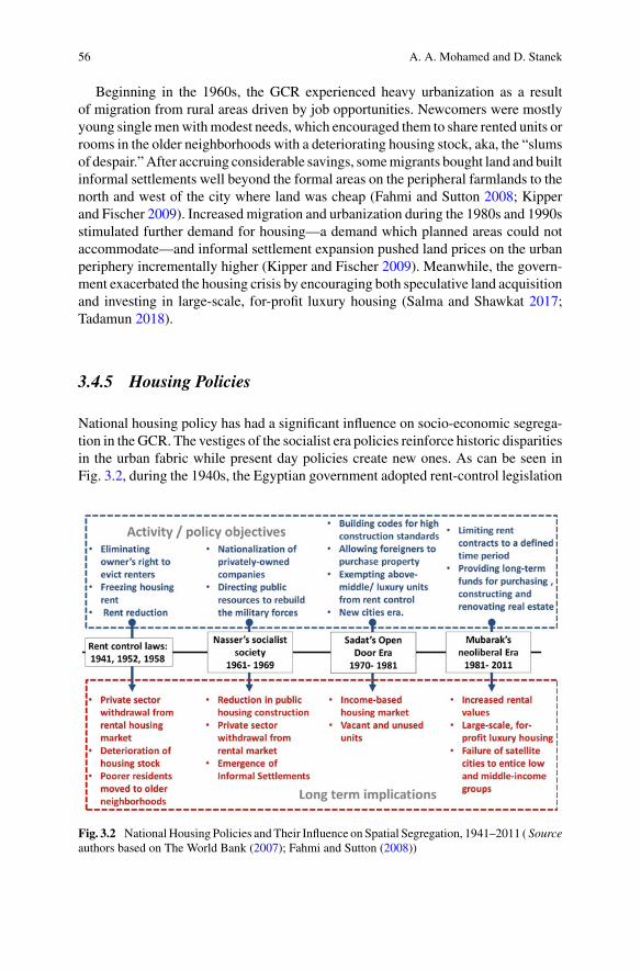
56 A. A. Mohamed and D. Stanek
Beginning in the 1960s, the GCR experienced heavy urbanization as a resultof migration from rural areas driven by job opportunities. Newcomers were mostlyyoung singlemenwithmodest needs, which encouraged them to share rented units orrooms in the older neighborhoods with a deteriorating housing stock, aka, the “slumsof despair.”After accruing considerable savings, somemigrants bought land and builtinformal settlements well beyond the formal areas on the peripheral farmlands to thenorth and west of the city where land was cheap (Fahmi and Sutton 2008; Kipperand Fischer 2009). Increased migration and urbanization during the 1980s and 1990sstimulated further demand for housing—a demand which planned areas could notaccommodate—and informal settlement expansion pushed land prices on the urbanperiphery incrementally higher (Kipper and Fischer 2009). Meanwhile, the govern-ment exacerbated the housing crisis by encouraging both speculative land acquisitionand investing in large-scale, for-profit luxury housing (Salma and Shawkat 2017;Tadamun 2018).
3.4.5 Housing Policies
National housing policy has had a significant influence on socio-economic segrega-tion in the GCR. The vestiges of the socialist era policies reinforce historic disparitiesin the urban fabric while present day policies create new ones. As can be seen inFig. 3.2, during the 1940s, the Egyptian government adopted rent-control legislation
Fig. 3.2 NationalHousing Policies andTheir Influence on Spatial Segregation, 1941–2011 ( Sourceauthors based on The World Bank (2007); Fahmi and Sutton (2008))
3 Income Inequality, Socio-Economic Status, andResidential Segregation… 57
to reduce rents for lower income families. Freezing rent prices discouraged privateinvestors to supply formal housing for rent. Furthermore, insufficient rent revenuesdiscouraged private owners to maintain existing housing units and this, in turn, ledto a deterioration of the housing stock. With the industrialization policy under thestate-sponsored socialism of the Nasser era, specifically in the 1950s, the govern-ment reduced rents gave renters the right to complain aboutmaintenance and partiallyprovided subsidized housing to the poor. During the 1960s, the state vastly reducedthe construction of public housing and infrastructure gave tenants the right to inheritrental units, and directed most of the national income to military purposes. Thispolicy widened the gap between supply and demand, further encouraged informaldevelopment, and contributed to the deterioration of rental stock (World Bank 2007;Fahmi and Sutton 2008).
In 1979, the government adopted a strategy to relieve central Cairo of congestionand pollution by supporting the construction of car-dependent, planned “new urbancommunities” in the desert, a policy that continues today (Hegazy and Moustafa2013). In these formal areas, the government prohibited microeconomic activitiessuch as retail shops, workshops, and street kiosks which generate employment andinvestment opportunities for lower income residents (Sims 2014). Low- and middle-class families could neither afford the cost of housing nor the cost of commuting suchlong distances, thereby ensuring that the satellite cities would be elite spaces withinthe expanding region (Sims 2014; Salma and Shawka 2017; Tadamun 2018). Thegovernment has tried to support subsidized social housing projects (Iskan Igtema’ey)in the newurban communities for low- andmiddle-incomehouseholds, but because ofbureaucratic opacity (Sims 2014), and income requirements that exceed the averageincomes of even upper middle-class households (Salma and Shawkat 2017), thisprogram has contributed to further socio-economic segregation in the city (Tadamun2018).
Given the high costs of subsidized housing and the exclusionary nature of thenew urban communities, low- and middle-income residents relied on the informalprivate sector for housing and the only available land on which they could buildwas the agricultural land that surrounds the city. Unfortunately, the informal privatesector was unable to satisfy the increasing housing demands of the population due torising construction costs, the incessant inflation of land prices (UN-HABITAT 1993),and the large devaluation of the Egyptian pound over the period from 1989 to 1991(Mohieldin and Kouchouk 2003). Ultimately, the informal private sector withdrewfrom its key role as the main supplier of affordable housing for lower income groupsand focused on higher end housing (Salma and Shawkat 2017). As of 2016, GCRhad about 4.7 million vacant housing units, which is roughly equivalent to the totalnumber of housing units in 1996 (CAPMAS 1996, 2016).
58 A. A. Mohamed and D. Stanek
3.5 Landscape of Residential Segregation in GCR,1986–2006
This study relies on publicly available data from the General Office of PhysicalPlanning (GOPP) and the Central Agency for Public Mobilization and Statistics(CAPMAS). As information aggregated to the tract level, we use census tracts todefine the shiyakha, or neighborhoods. Tract boundaries for the selected study periodsare nearly unchanged and do not require data harmonization for pre-2006 censustracts.
The urban agglomeration of the GCR is comprised of the whole governorate ofCairo and, except for some scattered towns, urban Giza, and urban Qalyubia (HarrisandWahba 2002). In 1986 there were 486 tracts, with an average population of about5,500 each. In 1996, the number of tracts increased to 509with an average populationof about 7,000, and in 2006, there were 553 tracts with a mean population of 8,250.In order to control for differences in tract sizes and populations, we standardize thedata by transforming counts into rates/ratios. Z-scores are also used for normalizingscores on the same scale.
We use occupational data from the 1986, 1996, and 2006 censuses to study socio-economic segregation in the GCR. The 1996 and 2006 data include the nine occupa-tional categories as defined by the International Standard Classification of Occupa-tions (ISCO) and the 1986 census includes seven, where the lowest three elementaryoccupations are merged into one category. To mirror socio-economic disparities at amicro-scale, we adopt the aggregation method of Marcinczak et al. (2015) in whichthe original ISCO classifications are grouped into three socio-spatial categories: top,middle, and bottom. Managers (1) and professionals (2) comprise the top socio-economic category. Associate professionals (3), clerks (4), and service and salesworkers (5) form the middle socio-economic category. Skilled agricultural, forestry,and fishery workers (6); craft and related trades workers (7); plant and machineoperators and assemblers (8), and elementary occupations (9) fall into the bottomsocio-economic group (see also Azhdari et al. 2018). FollowingMarcinczak’s (2015)method, we then find the percentage of employed residents in each tract that fall intothe high, middle and low group to classify the census tracts of GCR into six cate-gories: high, middle-to-high, mixed, low-to-middle, low, and polarized (see Table3.2).
While occupational status is a major indicator of income, prestige, educationalattainment, and health-related behaviors, it is an insufficient and sometimes unreli-able indicator of socio-economic status (SES) on its own. A disadvantage is that jobstatus as well as skill and education requirements for certain types of employmentchange over time. For example, a teacher may have had a higher social status in 1986than in 2006.Moreover, income and lifestyle, as indicators of occupational status, arecontext-sensitive and subject to cultural preferences (Berkman and Macintyre 1997;Marcinczak et al. 2015). Finally, SES indicators often exclude individuals engagedexclusively in the informal economy as their activity is not captured in governmentdata sets (Krieger et al. 1997). This is particularly problematic in the GCR where
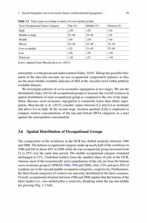
3 Income Inequality, Socio-Economic Status, andResidential Segregation… 59
Table 3.2 Tracts types according to shares of socio-spatial groups
Tract Occupational Status Category Top (%) Middle (%) Bottom (%)
High ≥50 <30 <30
Middle-to-high 25–49 25–49 <25
Middle <30 ≥50 <30
Mixed 25–49 25–49 25–49
Low-to-middle <25 25–49 25–49
Low <30 <30 ≥50
Polarized ≥30 <25 ≥30
Source adapted from Marcinczak et al. (2015)
informality is widespread and undercounted (Sabry 2010). Taking this possible limi-tation of the data into account, we use occupational composition statistics as theyare the most reliable available indicator of SES at the shiyakha level within publiclyavailable datasets.
We investigate patterns of socio-economic segregation at two stages. We use thedissimilarity index (D) for all occupational groups to measure the overall evenness inspatial distribution of each occupational group as compared to the rest of the popu-lation. Because socio-economic segregation is commonly lower than ethnic segre-gation, Marcinczak et al. (2015) consider values between 0.2 and 0.4 as moderateand above 0.4 as high. In the second stage, location quotient (LQ) is employed tocompare relative concentrations of the top and bottom ISCO categories in a tractagainst the metropolitan concentration.
3.6 Spatial Distribution of Occupational Groups
The composition of the workforce in the GCR has shifted modestly between 1986and 2006. The bottom occupational category made up nearly half of the workforce in1986 and fell to about 44% in 2006 while the top occupational group increased from21 to 25% over the same time period. The middle occupational category remainedunchanged at 31%. Unskilled workers form the smallest share of jobs in the GCR,whereas most of the economically active populations of the city are from the bottomsocio-economic group (CAPMAS1986, 1996 and 2006).Also, 25%and up to 30%ofresidents are in the top and middle occupation categories, respectively. Furthermore,the three broad categories of workers are unevenly distributed in the three censuses.Overall, occupational structure between 1986 and 2006 implies that the bottom of thelabor market (i.e., low-skilled jobs) is relatively shrinking while the top and middleare growing (Fig. 3.3 left).
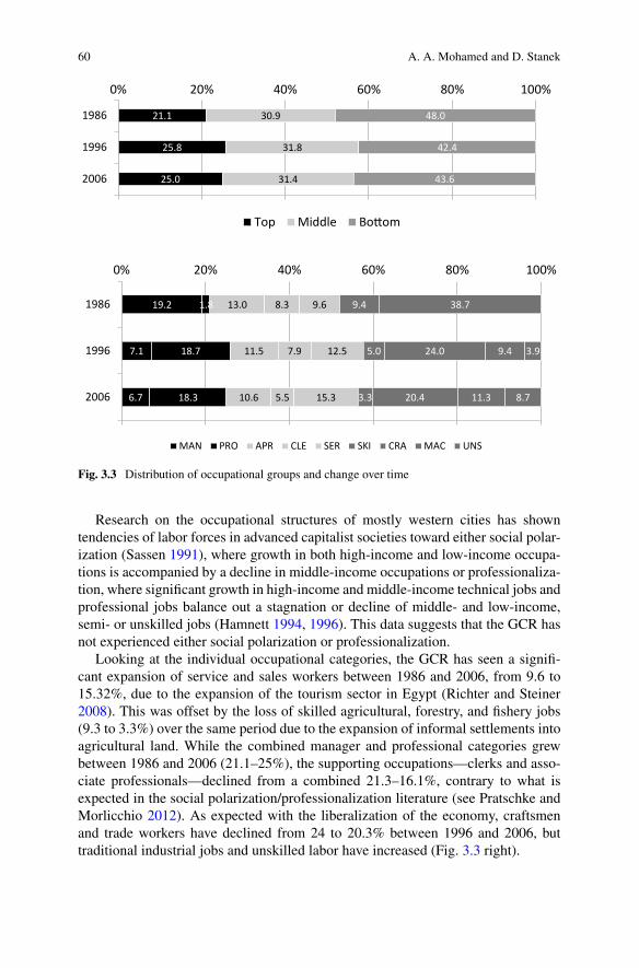
60 A. A. Mohamed and D. Stanek
25.0
25.8
21.1
31.4
31.8
30.9
43.6
42.4
48.0
0% 20% 40% 60% 80% 100%
2006
1996
1986
Top Middle Bo om
6.7
7.1
19.2
18.3
18.7
1.8
10.6
11.5
13.0
5.5
7.9
8.3
15.3
12.5
9.6
3.3
5.0
9.4
20.4
24.0
38.7
11.3
9.4
8.7
3.9
0% 20% 40% 60% 80% 100%
2006
1996
1986
MAN PRO APR CLE SER SKI CRA MAC UNS
Fig. 3.3 Distribution of occupational groups and change over time
Research on the occupational structures of mostly western cities has showntendencies of labor forces in advanced capitalist societies toward either social polar-ization (Sassen 1991), where growth in both high-income and low-income occupa-tions is accompanied by a decline in middle-income occupations or professionaliza-tion, where significant growth in high-income and middle-income technical jobs andprofessional jobs balance out a stagnation or decline of middle- and low-income,semi- or unskilled jobs (Hamnett 1994, 1996). This data suggests that the GCR hasnot experienced either social polarization or professionalization.
Looking at the individual occupational categories, the GCR has seen a signifi-cant expansion of service and sales workers between 1986 and 2006, from 9.6 to15.32%, due to the expansion of the tourism sector in Egypt (Richter and Steiner2008). This was offset by the loss of skilled agricultural, forestry, and fishery jobs(9.3 to 3.3%) over the same period due to the expansion of informal settlements intoagricultural land. While the combined manager and professional categories grewbetween 1986 and 2006 (21.1–25%), the supporting occupations—clerks and asso-ciate professionals—declined from a combined 21.3–16.1%, contrary to what isexpected in the social polarization/professionalization literature (see Pratschke andMorlicchio 2012). As expected with the liberalization of the economy, craftsmenand trade workers have declined from 24 to 20.3% between 1996 and 2006, buttraditional industrial jobs and unskilled labor have increased (Fig. 3.3 right).
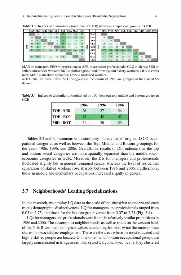
3 Income Inequality, Socio-Economic Status, andResidential Segregation… 61
Table 3.3 Indices of dissimilarity (multiplied by 100) between occupational groups in GCRMAN PRO APR CLE SER SKI CRA MAC UNS
14 21 22 26 73 35 35 33 MAN24 26 28 35 75 43 43 41 PRO20 42 9 16 70 23 22 30 APR31 48 19 14 69 22 21 30 CLE29 48 19 17 65 14 16 22 SER56 69 52 49 45 66 61 63 SKI
15 24 CRA40 59 24 21 18 45 27 MAC
UNS
1986
1996
MAN PRO APR CLE SER SKI CRA MAC UNS
1023 2420 21 828 31 18 1877 78 74 76 7442 45 28 31 25 6541 44 25 29 25 62 1234 36 23 24 20 65 18 18
2006
MAN = managers; PRO = professionals; APR = associate professionals; CLE = clerks; SER =sellers and service workers; SKI = skilled agricultural, forestry, and fishery workers; CRA = craftsmen; MAC = machine operators; UNS = unskilled workersNOTE The last three lower ISCO categories in the census of 1986 are grouped in the CAPMASdataset
Table 3.4 Indices of dissimilarity (multiplied by 100) between top, middle and bottom groups inGCR
1986 1996 2006TOP - MID 26 27 24TOP - BOT 43 42 43MID - BOT 21 20 25
Tables 3.3 and 3.4 summarize dissimilarity indices for all original ISCO occu-pational categories as well as between the Top, Middle, and Bottom groupings forthe years 1986, 1996, and 2006. Overall, the results of DIs indicate that the topand bottom social categories are more spatially separated than the middle socio-economic categories in GCR. Moreover, the DIs for managers and professionalsfluctuated slightly but in general remained steady, whereas the level of residentialseparation of skilled workers rose sharply between 1996 and 2006. Furthermore,those in middle and elementary occupations increased slightly in general.
3.7 Neighborhoods’ Leading Specializations
In this research, we employ LQ data at the scale of the shiyakhat to understand eachtract’s demographic distinctiveness. LQ for managers and professionals ranged from0.03 to 3.75, and those for the bottom group varied from 0.07 to 2.21 (Fig. 3.4).
LQs formanagers and professionalswere found in relatively similar proportions in1986 and 2006. The easternmost neighborhoods, as well as tracts on thewestern bankof the Nile River, had the highest values accounting for over twice the metropolitanshare of top social class employment. These are the areaswhere themost educated andhighly skilled people are located. On the other hand, bottom occupational groups arelargely concentrated in fringe areas in Giza andQalyubia. Specifically, they clustered
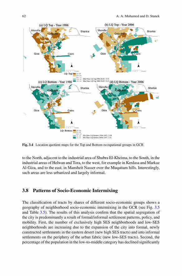
62 A. A. Mohamed and D. Stanek
Fig. 3.4 Location quotient maps for the Top and Bottom occupational groups in GCR
to the North, adjacent to the industrial area of Shubra El-Kheima, to the South, in theindustrial areas of Helwan and Tora, to the west, for example in Kerdasa and MarkazAl-Giza, and to the east, in Mansheit Nasser over the Muqattam hills. Interestingly,such areas are less urbanized and largely informal.
3.8 Patterns of Socio-Economic Intermixing
The classification of tracts by shares of different socio-economic groups shows ageography of neighborhood socio-economic intermixing in the GCR (see Fig. 3.5and Table 3.5). The results of this analysis confirm that the spatial segregation ofthe city is predominantly a result of formal/informal settlement patterns, policy, andmobility. First, the number of exclusively high SES neighborhoods and low-SESneighborhoods are increasing due to the expansion of the city into formal, newlyconstructed settlements in the eastern desert (new high SES tracts) and into informalsettlements on the periphery of the urban fabric (new low-SES tracts). Second, thepercentage of the population in the low-to-middle category has declined significantly
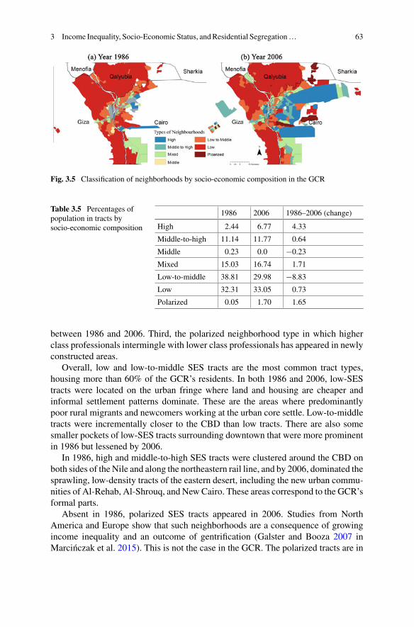
3 Income Inequality, Socio-Economic Status, andResidential Segregation… 63
Fig. 3.5 Classification of neighborhoods by socio-economic composition in the GCR
Table 3.5 Percentages ofpopulation in tracts bysocio-economic composition
1986 2006 1986–2006 (change)
High 2.44 6.77 4.33
Middle-to-high 11.14 11.77 0.64
Middle 0.23 0.0 −0.23
Mixed 15.03 16.74 1.71
Low-to-middle 38.81 29.98 −8.83
Low 32.31 33.05 0.73
Polarized 0.05 1.70 1.65
between 1986 and 2006. Third, the polarized neighborhood type in which higherclass professionals intermingle with lower class professionals has appeared in newlyconstructed areas.
Overall, low and low-to-middle SES tracts are the most common tract types,housing more than 60% of the GCR’s residents. In both 1986 and 2006, low-SEStracts were located on the urban fringe where land and housing are cheaper andinformal settlement patterns dominate. These are the areas where predominantlypoor rural migrants and newcomers working at the urban core settle. Low-to-middletracts were incrementally closer to the CBD than low tracts. There are also somesmaller pockets of low-SES tracts surrounding downtown that were more prominentin 1986 but lessened by 2006.
In 1986, high and middle-to-high SES tracts were clustered around the CBD onboth sides of the Nile and along the northeastern rail line, and by 2006, dominated thesprawling, low-density tracts of the eastern desert, including the new urban commu-nities of Al-Rehab, Al-Shrouq, and NewCairo. These areas correspond to the GCR’sformal parts.
Absent in 1986, polarized SES tracts appeared in 2006. Studies from NorthAmerica and Europe show that such neighborhoods are a consequence of growingincome inequality and an outcome of gentrification (Galster and Booza 2007 inMarcinczak et al. 2015). This is not the case in the GCR. The polarized tracts are in
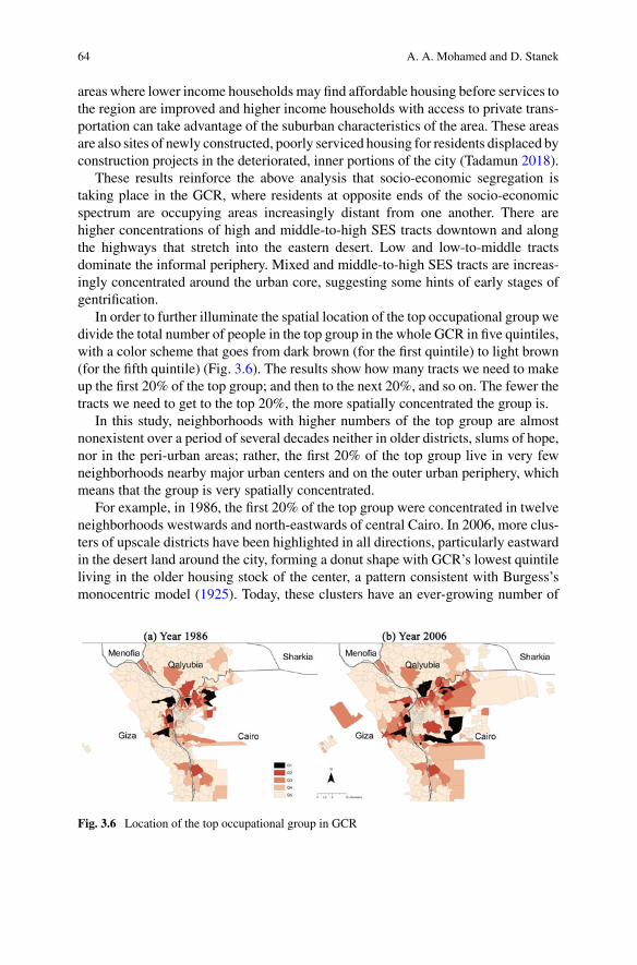
64 A. A. Mohamed and D. Stanek
areas where lower income households may find affordable housing before services tothe region are improved and higher income households with access to private trans-portation can take advantage of the suburban characteristics of the area. These areasare also sites of newly constructed, poorly serviced housing for residents displaced byconstruction projects in the deteriorated, inner portions of the city (Tadamun 2018).
These results reinforce the above analysis that socio-economic segregation istaking place in the GCR, where residents at opposite ends of the socio-economicspectrum are occupying areas increasingly distant from one another. There arehigher concentrations of high and middle-to-high SES tracts downtown and alongthe highways that stretch into the eastern desert. Low and low-to-middle tractsdominate the informal periphery. Mixed and middle-to-high SES tracts are increas-ingly concentrated around the urban core, suggesting some hints of early stages ofgentrification.
In order to further illuminate the spatial location of the top occupational group wedivide the total number of people in the top group in the whole GCR in five quintiles,with a color scheme that goes from dark brown (for the first quintile) to light brown(for the fifth quintile) (Fig. 3.6). The results show how many tracts we need to makeup the first 20% of the top group; and then to the next 20%, and so on. The fewer thetracts we need to get to the top 20%, the more spatially concentrated the group is.
In this study, neighborhoods with higher numbers of the top group are almostnonexistent over a period of several decades neither in older districts, slums of hope,nor in the peri-urban areas; rather, the first 20% of the top group live in very fewneighborhoods nearby major urban centers and on the outer urban periphery, whichmeans that the group is very spatially concentrated.
For example, in 1986, the first 20% of the top group were concentrated in twelveneighborhoods westwards and north-eastwards of central Cairo. In 2006, more clus-ters of upscale districts have been highlighted in all directions, particularly eastwardin the desert land around the city, forming a donut shape with GCR’s lowest quintileliving in the older housing stock of the center, a pattern consistent with Burgess’smonocentric model (1925). Today, these clusters have an ever-growing number of
Fig. 3.6 Location of the top occupational group in GCR

3 Income Inequality, Socio-Economic Status, andResidential Segregation… 65
upscale venues such as expensive shopping malls and supermarkets that target onlyindividuals with higher purchasing power.
3.9 Conclusions
This chapter examined the role of income inequality in explaining socio-economicresidential segregation in the GCR. Using occupational data from 1986, 1996, and2006 censuses, we measured metropolitan and neighborhood segregation indexesbasedon shares ofSES.To study the dominant occupations in specificneighborhoods,we computed LQs to top and low social classes. Results from our study lead toseveral conclusions that are discussed in the light of the three questions that guidedthe analysis.
The first question asked: to what extent is there residential segregation of occu-pational groups in the GCR? While the overall scale of segregation under neolib-eralization is on the low side, the profile of socio-economic intermixing revealsthat the poorest groups were more segregated from the wealthy minority than fromthe middle-income residents. Specifically, the Dissimilarity Index between top andbottom groups was 0.43 in 2006. This level is much higher than those found in NorthAmerican and Western European cities (mostly range between 0.1 and 0.35) (see,e.g., White 1987; Marcinczak et al. 2015).
In addition, the local patterns of socio-economic intermixing also demonstratethat GCR is highly segregated. The dominance of large clusters of low and high SEStracts reveals a sharp socio-spatial division. Likewise, LQ values show that specificoccupational groups are strongly represented in some tracts than others. Overall, itmay be true, as Sims (2010: 3) has argued, that ostentatious wealth coexists “side byside with extreme poverty”.
The answer to the second question—“Can socio-economic inequality explainresidential segregation?”—is that while socio-economic inequality is a prerequisitefor socio-economic segregation, the link between the two variables ismodest. In otherwords, greater economic inequality does not necessarily result in clear-cut socio-spatial divisions. Although this is in line with the results seen in Eastern Europeancities, we acknowledge inherent limitations in our dataset in terms of selected studyperiods and focusing exclusively on one single case.
Third, we asked: To what extent can the welfare regime and the characteristicsof housing provision determine segregation trends in the GCR? The answer is thatboth the welfare regime and housing policies contribute in residential settlementpatterns. There is much evidence that the Egyptian government reduced expenditureson education and social protection andonbuildingpublic housing.Neoliberal policiesaimed to optimize government revenues but steered residential segregation as well.The chronic lack of adequate and affordable housing in many parts of the city hasresulted in the concentration of low-incomehouseholds in undesirable and sometimesdangerous locations where land is cheap and jobs are scarce.
66 A. A. Mohamed and D. Stanek
In spite of their bad conditions, the inner city housing stock, as well as informalsettlements at the urban fringe, contains about 40% of GCR population (CAPMAS2006). Low-income households were in favor of these areas because of two reasons:the advantages of affordability and geographic location nearby jobs. Put differently,searching for a decent affordable price for all residents resulted in some intriguingtrends in patterns of socio-economic segregation. However, we acknowledge thecontextual factor which makes GCR atypical of other cities in the global south.Continued socio-economic polarization may threaten social cohesion, stability, andsecurity.
Finally, we acknowledge that occupational status may be insufficient and some-times unreliable indicator of socio-economic status (SES) on its own. Additionalindicators such as educational level may well be added to explore the relationshipbetween social class and residential segregation further. We also hope to replicatethe analysis using the final 2016 census findings when CAPMAS releases them.
References
Abu-Lughod J (2004) Cairo: too many people, not enough land, too few resources. In: Gugler J (ed)World cities beyond the west: globalization, development and inequality. Cambridge UniversityPress, New York
African Development Bank (ADB) (2000) Egypt: economic reform and structural adjustmentprogramme project performance evaluation report
Arbaci S (2007) Ethnic segregation, housing systems and welfare regimes in Europe. Int J HousingPolicy 7(4):401–433
Azhdari A, Sasani M, Soltani A (2018) Exploring the relationship between spatial driving forcesof urban expansion and socioeconomic segregation: the case of Shiraz. Habitat Int 81:33–44
Ben Nefissa S (2011) Cairo’s city government: the crisis of local administration and the refusal ofurban citizenship. In: Singerman D (ed) Cairo contested: governance, urban space, and globalmodernity. The American University in Cairo Press, Cairo, pp 177–198
Berkman LF, Macintyre S (1997) The measurement of social class in health studies: old measuresand new formulations. In: Kogevinas M, Pearce N, Susser M, Boffetta P (eds) Social inequalitiesand cancer. IARC Scientific Publications No. 138, Lyon, pp 51–64
Brown LA, Chung SY (2008) Market-led pluralism: Rethinking our understanding of racial/ethnicspatial patterning in U.S. cities. Ann Assoc Am Geograph 98(1):180–212
Burgess E (1925) The growth of the city: an introduction to a research project. In: The trend ofpopulation. American Sociological Society, pp 85–97
Central Agency for PublicMobilization and Statistics (CAPMAS) (1986) Cairo, Egypt, 1986. [Finalresults of the census of population, housing conditions, buildings and establishments: volumesfor the governorates of Cairo, Qalyubia, and Giza.]
Central Agency for Public Mobilization and Statistics (CAPMAS) (1996) Census of Egypt. Cairo,Egypt, 1996. [Final results of the census of population, housing conditions, buildings andestablishments: volumes for the governorates of Cairo, Qalyubia, and Giza.]
Central Agency for Public Mobilization and Statistics (CAPMAS) (2006) Census of Egypt. Cairo,Egypt, 2006. [Final results of the census of population, housing conditions, buildings andestablishments: volumes for the governorates of Cairo, Qalyubia, Helwan, 6 October, and Giza.]
Central Agency for Public Mobilization and Statistics (CAPMAS) (2016) Census of Egypt, 2016.Cairo, Egypt, 2016. [Preliminary results of the census of population, housing conditions, buildingsand establishments: volumes for the governorates of Cairo, Qalyubia, and Giza.]
3 Income Inequality, Socio-Economic Status, andResidential Segregation… 67
Darden J, Rabhar M, Jezierski L, Li M, Velie E (2010) The measurement of neighbourhood socioe-conomic characteristics and black and white residential segregation in metropolitan Detroit:implications for the study of social disparities in health. Ann Assoc Am Geogr 100(1):137–158
El-Kadi G (1987) L’urbanisation spontanée au Caire. URBAMA, ToursEl Kadi G (2009) Al-Tahaddur al-ashwa’i. Translated from El Kadi G (1987), L’urbanisationspontanée de Caire (Tours: Urbama, Orstom) by Minha al-Bitrawi (Cairo: al-Markaz al-Qawmili-l-Targama)
El Laithy H (1996) Structural adjustment and poverty. International Conference on StructuralAdjustment, UCLA
El-Laithy H (2001) The gender dimensions of poverty in Egypt. Economic Research Forum for theArab Countries, Iran & Turkey, Cairo, Egypt
El Shakry O (2006) Cairo as capital of socialist revolution? In: Singerman D, Amar P (eds) Cairocosmopolitan: politics, culture, and urban space in the new globalizedMiddle East. TheAmericanUniversity in Cairo Press, Cairo
Fahmi W, Sutton K (2008) Greater Cairo’s housing crisis: contested spaces from inner city areas tonew communities. Cities 25:277–297
Fenger H (2007) Welfare regimes in central and Eastern Europe: Incorporating post-communistcountries in a welfare regime typology. Contemp Issues Ideas Soc Sci 3(2):1–30
Ghalwash T (2014) Corruption and economic growth: evidence from Egypt. Modern Econ5(10):1001
Gilbert A (1992) The housing of the urban poor. In: Gilbert A, Gugler J (eds) Cities, poverty anddevelopment. Urbanisation in the third world. Oxford University Press, London
Harris R, Wahba M (2002) The urban geography of low-income housing: Cairo (1947–96)exemplifies a model. Int J Urban Reg Res 12(1):58–79
Hamnett, C. (1994). Social polarisation in global cities: theory and evidence. Urban Stud31(3):401–424. Retrieved from JSTOR.
Hamnett. (1996) Social polarisation, economic restructuring and welfare state regimes. Urban Stud33(8):1407–1430
Hegazy IR, Moustafa WS (2013) Toward revitalization of new towns in Egypt case study: Sixth ofOctober. Int J Sustain Built Environ 2(1):10–18
Jefferson M (1989) Why geography? The law of the primate city. Geogr Rev 79(2):226–232Johnston R, Poulsen M, Forrest J (2007) The geography of ethnic residential segregation: acomparative study of five countries. Ann Assoc Am Geogr 97(4):713–738
Kendall D (2013) Sociology in our times: the essentials, 9th edn. Cengage Learning, BostonKipper R, Fischer M (Eds) (2009) Cairo’s informal areas between urban challenges and hiddenpotentials. GTZ, Cairo
Korayem K (1994) Poverty and income distribution in Egypt. The Third World Forum, CairoKrieger N, Williams DR, Moss NE (1997) Measuring social class in U.S. public health research:concepts, methodologies, and guidelines. Annu Rev Public Health 18:341–378
Lewis VA, Emerson MO, Klineberg SL (2011) Who we’ll live with: neighborhood racialcomposition preferences of whites, blacks and Latinos. Soc Forces 89(4):1385–1407
Marcinczak S, Tammaru T, Novak J, Gentile M, Kovacs Z, Temelova J, Valatka V, Kahrik A, SzaboB (2015) Patterns of socioeconomic segregation in the capital cities of fast-tracking reformingpostsocialist countries. Ann Assoc Am Geogr 105(1):183–202
Massey D (1979a) Effects of socioeconomic factors on the residential segregation of blacks andSpanish Americans in U.S. urbanized areas. Am Sociol Rev 44:1015–1022
Massey D (1979b) In what sense a regional problem? Reg Stud 13(2):233–243MoussaA (2007)Housing experts: Egyptian housingmarket serves interests of only the rich.MiddleEast News Economic Weekly, Middle East News Agency & Anba al-Sharq al-Awsat 45:45–52
Murie A, Musterd S (1996) Social segregation, housing tenure and social change in Dutch cities inthe late 1980s. Urban Stud 33:495–516. https://doi.org/10.1080%2F00420989650011889
Musterd S, Ostendorf W (eds) (1998) Urban segregation and the welfare state: inequality andexclusing in western cities. Routledge, London and New York
68 A. A. Mohamed and D. Stanek
Nassar H, BiltagyM (2016) The nexus of regional poverty and education in Egypt: a micro analysis.Int J Econ Financial Issues 6(4):1446–1453
Parham E (2012) The segregated classes: spatial and social relationships in slums. In: Greene M,Reyes J, Castro A (eds) Proceedings of the eighth international space syntax symposium. PUC,Satiago de Chile , 8150, pp 1–19
Pratschke J, Morlicchio E (2012) Social polarisation, the labour market and economic restructuringin Europe: an urban perspective. Urban Stud 49(9):1891–1907
Raymond A (2001) Cairo: city of history. The American University in Cairo Press, CairoReardon SF, Bischoff K (2011) Income inequality and income segregation. Am J Sociol116(4):1092–1153
Richter T, Steiner C (2008) Politics, economics and tourism development in Egypt: insights intothe sectoral transformations of a neo-patrimonial rentier state. Third World Quart 29(5):939–959
Sabry S (2010) How poverty is underestimated in Greater Cairo. Egypt. Environ Urban 22(2):523–541
Salma S, Shawkat Y (2017) Analysis: government policy commodifies housing. The Built Environ-ment Observatory https://marsadomran.info/en/policy_analysis/2017/11/1218/. Last accessed 4March 2019
Sassen S (1991) The global city: New York, London, Tokyo. Princeton University Press, Princeton,NJ
Schteingart M (2001) La división social del espacio en las ciudades. Perfiles latinoamericanos:revista de la Facultad Latinoamericana de Ciencias Sociales, Sede México 9:13–31
Shawkat Y (2013) Social justice and the built environment: a map of Egypt. The Shadow Ministryof Housing, Cairo, Egypt [In Arabic]
Sims D (2010) Understanding Cairo: the logic of a city out of control. The American University inCairo Press, Cairo
Sims D (2014) Egypt’s desert dreams: development or disaster? The American University in CairoPress, Cairo
Sims D, Kamal H, Solomon D (2008) Housing study for urban Egypt. USAID/EGYPT Policy andPrivate Sector Office, Technical Assistance for Policy Reform TAPRII
Singerman D, Amar P (eds) (2006) Cosmopolitan Cairo: politics, culture and urban space in thenew globalized Middle East. The American University in Cairo Press, Cairo
Sobreira F (2003) Squatter settlements consolidation: spatial analysis in an agent-based envi-ronment. In: Proceedings of the 4th international space syntax symposium, London, UK, pp16.1–16.12
Stokes C (1962) A theory of slums. Land Economics 38:187–197Tadamun (2018) Planning [in]justice: spatial analysis for urban Cairo. Tadamun (The CairoUrban Solidarity Initiative) https://www.tadamun.co/2018/08/23/planning-justice-report/?lang=en#.W8bvEBMzYdX. Last accessed 4 March 2019
Tanzi V, Davoodi H (1997) Corruption, public investment, and growth, in: the welfare state, publicinvestment, and growth. Springer pp 41–60
Taubenböck H,WegmannM, Roth A,Mehl H, Dech S (2009) Analysis of urban sprawl at mega cityCairo, Egypt using multisensoral remote sensing data, landscape metrics and gradient analysis.In: International symposium on remote sensing of environment (ISRSE), Stresa, Italy
UN HABITAT (1993) Metropolitan planning and management in the developing world: Spatialdecentralization policy in Bombay and Cairo, Nairobi: UNCHS (Habitat)
White M (1987) American neighborhoods and residential differentiation. Russell Sage, New Yorkvan Kempen R, Murie A (2009) The new divided city: Changing patterns in European cities.Tijdschrift Voor Economische En Sociale Geografie 100(4):377–398
World Bank (1990) World development report: poverty. Washington, D.CWorld Bank (2015) World Bank estimate, Egypt. https://data.worldbank.org/indicator/SI.POV.GINI?locations=EG. Last accessed 4 March 2019
World Bank and Ministry of Economic Development (2007) Arab republic of Egypt: a povertyassessment update, Report 39885—EGT, World Ban
3 Income Inequality, Socio-Economic Status, andResidential Segregation… 69
Mohieldin and Kouchouk 2003MohieldinM, Kouchouk A (2003) On exchange rate policy: the caseof Egypt 1970–2001. Economic Research Forum (ERF), WP No. 0312
Open Access This chapter is licensed under the terms of the Creative Commons Attribution 4.0International License (http://creativecommons.org/licenses/by/4.0/), which permits use, sharing,adaptation, distribution and reproduction in any medium or format, as long as you give appropriatecredit to the original author(s) and the source, provide a link to the Creative Commons license andindicate if changes were made.
The images or other third party material in this chapter are included in the chapter’s CreativeCommons license, unless indicated otherwise in a credit line to the material. If material is notincluded in the chapter’s Creative Commons license and your intended use is not permitted bystatutory regulation or exceeds the permitted use, you will need to obtain permission directly fromthe copyright holder.
Chapter 4Social Inequality and Spatial Segregationin Cape Town
Ivan Turok, Justin Visagie, and Andreas Scheba
Abstract Cape Town is widely considered to be South Africa’s most segregatedcity. The chapter outlines the history of social stratification and spatial segregation,including the coercion of colonial and apartheid governments to divide the popula-tion by race. Since 1994, the democratic government has lacked the same resolve andcapacity to reverse this legacy and integrate the city. The chapter also analyses thechanging socio-economic and residential patterns between 2001 and 2011 in moredetail. It shows that the extent of segregation diminished between 2001 and 2011,contrary to expectations. It appears that affluent neighbourhoods became slightlymore mixed and people in high-status occupations spread into surrounding areas.Some low-income neighbourhoods also became slightly more mixed by accommo-dating middle class residents. Further research is required to verify and explain thesefindings.
Keywords Socio-economic segregation · Labour market inequalities · Socialmobility · Apartheid city · Residential desegregation
4.1 Introduction
Cape Town is South Africa’s (SA) oldest and second largest city. The municipalarea covers an extensive territory of 2,461 km2 with a population of 4.6 million in2020. The population grew by 2.6% per annum between 2001 and 2011. This isslower than Johannesburg, but faster than other cities in SA. The city’s population
I. Turok (B) · J. Visagie · A. SchebaHuman Sciences Research Council, Pretoria, South Africae-mail: [email protected]
J. Visagiee-mail: [email protected]
A. Schebae-mail: [email protected]
I. TurokSARCHI Chair in Urban Economies, University of the Free State, Bloemfontein, South Africa
© The Author(s) 2021M. van Ham et al. (eds.), Urban Socio-Economic Segregation and Income Inequality,The Urban Book Series, https://doi.org/10.1007/978-3-030-64569-4_4
71
72 I. Turok et al.
growth has been influenced by its economy. Between 2001 and 2011 jobs increasedmore slowly than in Johannesburg, but faster than elsewhere, making Cape Town arelatively attractive destination for migration (Turok and Borel-Saladin 2014). CapeTown also has a different demographic make-up from the rest of the country, withcoloureds outnumbering black Africans.1 The population is slightly better educatedon average than the rest of SA.
Cape Town’s social composition and fractured spatial form bear the strong imprintof its colonial and apartheid history. For three centuries the city was managed tofavour a privileged minority at the expense of the indigenous majority, based on thecolour of their skin. Between 1948–1994, racial discrimination was taken to extremeas the apartheid regime forced different ethnic groups to live in separate places,with different institutions and infrastructure. This was supposed to prevent inter-racial contact under the pretext of ‘separate development’. National laws governingthe economy, society and built environment systematically favoured white house-holds and disadvantaged blacks. The result was that race became synonymouswith socio-economic status (or ‘class’). Whites became increasingly better-off thanIndians/Asians, followed by coloureds and then black Africans (Statistics SA 2019).
These odious policies were abolished in 1994, but many scars remain. Gapingurban inequalities continue to impact people’s well-being and life chances. Thesubjugation of blacks was so far-reaching that efforts to undo the damage have hadmuted effects (WorldBank 2018a). Economic growth and state-sponsored affirmativeaction have done little to erase the social and spatial divides. Social class continuesto be intertwined with race, even if the relationship is less direct than it used to be.Wide social and spatial gaps inhibit mutual understanding and trust, and underminepolicies to draw people together behind a common purpose, such as tackling thecoronavirus crisis. SA’s Gini coefficient is the world’s highest at 0.65, essentiallyunchanged since 1994 (Statistics SA 2019).
This chapter analyses segregation between different socio-economic groups. Itdiffers from earlier studies focused on racial segregation (Christopher 2000; Parryand van Eeden 2015). Socio-economic status offers a different lens on spatial differ-entiation. Although the legal basis of racial segregation has been removed, manytangible effects remain and are slow to change precisely because social stratifi-cation is still bound up with race. Deep inequalities across both dimensions arecompounded by spatial divides to undermine economic inclusion, social progressand racial integration.
Socio-economic status is intimately related to people’s occupation, income andwealth (i.e. their labour market position). This drives residential outcomes today, ashouseholds are distributed across the city according to their market power, or abilityto buy into neighbourhoodswith different attributes, infrastructure and housing types.
1We use the racial terminology common in SA in this chapter: blackAfrican, coloured, Indian/Asianand white. The term black is used to refer to everyone excluded from the white group privilegedunder apartheid. These terms, like any racial classifications, are problematic social constructs froma particular era. They continue to be used to monitor progress since democracy. According to the2011 census, the largest population group in Cape Town was coloured (42.4%), followed by blackAfricans (38.6%), whites (15.7%) and Indians/Asians (1.4%).
4 Social Inequality and Spatial Segregation in Cape Town 73
A steep property price gradient inhibitsmost people’s ability tomove intomore desir-able areas. Residential patterns are also influenced by the activities of the state, bothin providing low-income housing and in selling public land. Individual lifestyle pref-erences are relevant too, and affected by stage in the life cycle, family characteristicsand cultural backgrounds.
4.2 Determinants of Residential Patterns
The analysis begins with the powerful historic role of the apartheid state in shapingthe city’s structure. We then consider contemporary economic forces through theproperty market, followed by the recent tendency of state-subsidised housing toreproduce segregation.
4.2.1 Racial Segregation: 1950s–1980s
Cape Town is a famously divided city, with affluent, leafy suburbs offering excep-tional amenities and picturesque mountain and coastal settings, juxtaposed againstaustere and inhospitable dormitory settlements on the treeless sand-plains of theCape Flats. At the heart of the city is the vibrant City Bowl, a natural amphithe-atre that concentrates enormous wealth, surrounded by the stunning slopes of TableMountain. A patchwork of intensely crowded informal settlements is barely toleratedin various parts of the city. These unauthorised shanty-towns reflect poor people’sefforts to access city opportunities without paying for formal accommodation.
Cape Town’s unusual topography and status as a biodiversity hotspot have otherconsequences for access to housing and segregation. Special nature reserves intendedto restrict house-building cover more than 40% of the municipal area. The mountainalso shapes the road and rail networks, which have historically guided propertyinvestment and acted as barriers between race-based neighbourhoods. The AtlanticSeaboard attracts super-rich international homebuyers and tourists, which inflateshouse prices throughout the market.
The city’s physical footprint expanded most in the second half of the twentiethcentury, when the economy was booming and the southern and northern suburbsbecame the preferred residential areas for the white middle and upper classes. Popu-lation density declined by about 50% between the 1950s and the 1980s (City ofCape Town 2018). This was when racial ideology was most pernicious and the statedirectly shaped the city’s form. Previous growth was slower and segregation by racewas not all-pervasive. During the colonial era, the community was highly stratifiedand unequal, and white settlers exploited indigenous groups and slaves brought infromAsia and elsewhere in Africa (van Rooyen and Lemanski 2020). Discriminationand subjugation were widespread, but the city was not rigidly demarcated by race.In the early twentieth century, public health concerns (infectious diseases) provided
74 I. Turok et al.
the pretext for dispossessing most black Africans of their prime land and housing inthe urban core and relocating them beyond the urban fringe. This laid the legal andpolitical foundations for intensified segregation policies after the second world war.
The National Party won the 1948 general election and launched a spate of laws toentrench white supremacy using explicit spatial instruments, such as urban planning.Peoplewere rigidly classified by race and physically separated through a combinationof controls and distinct institutions. The notorious Group Areas Act assigned peopleto particular places kept apart by buffer strips. The racial hierarchywas entrenched byallocating large central areas towhites, peripheral sites to blackAfricans and spaces inbetween to coloureds. Implementation destroyed well-established coloured commu-nities and forced the removal of approximately 150,000 people to townships on theCape Flats by the end of the 1960s. District Six in the City Bowl was most affected,with 55,000 residents forcefully displaced (van Rooyen and Lemanski 2020).
The impact was compounded by separate local authorities created for differentareas, and separate schools, healthcare and public transport systems. This redis-tributed resources from working-class communities to the well-endowed whitesuburbs, and deepened the regressive effects of racial segregation (Mabin 2005).For example, the education system for whites was vastly superior to that for blacks,with better-equipped teachers, smaller classes and a more advanced curriculum. It ishard to overestimate the lasting impact on contemporary society.
The Cape was declared a ‘coloured labour preference area’, which inhibited in-migration by black Africans and explains the distinctive demographics today. Popu-lation movements were strictly controlled by pass laws. By the early 1990s, CapeTown was the most segregated city in the country, and less than 6% of the popu-lation lived outside the areas designated for their race, such as domestic workers(Christopher 2000).
Two immense districts on the Cape Flats—Mitchells Plain and Khayelitsha—demonstrate the force of the apartheid state. Mitchells Plain was created in the 1970sas a coloured township for middle- and low-income families, 25–30 km from theCBD. Many residents were victims of forced removals. It was laid out with neigh-bourhood precincts, basic public facilities and wide arterial roads. There was noeffort to develop local industrial estates, employment centres or small business units,let alone to restore the social fabric of dislocated communities. Many precincts soondeteriorated with rising unemployment, gangsterism, drug abuse, physical decay andshack housing. The current township population is around 300,000.
Khayelitsha was created during the 1980s for black Africans and envisaged as the‘solution’ to two problems facing Cape Town: the rapid increase in rural migrantsfrom the Eastern Cape and overcrowding in other townships. Thousands of peoplewere forcefully relocated to inferior housing and open land, 30–35 km from theCBD.There was even less effort to create local jobs, a commercial centre or public ameni-ties, ensuring that this would become a major poverty trap. The current population iswell over 400,000, with high levels of food insecurity, hardship, crime and informalhousing. High transport costs and arduous journeys add to the burden people face inaccessing jobs elsewhere in the city.
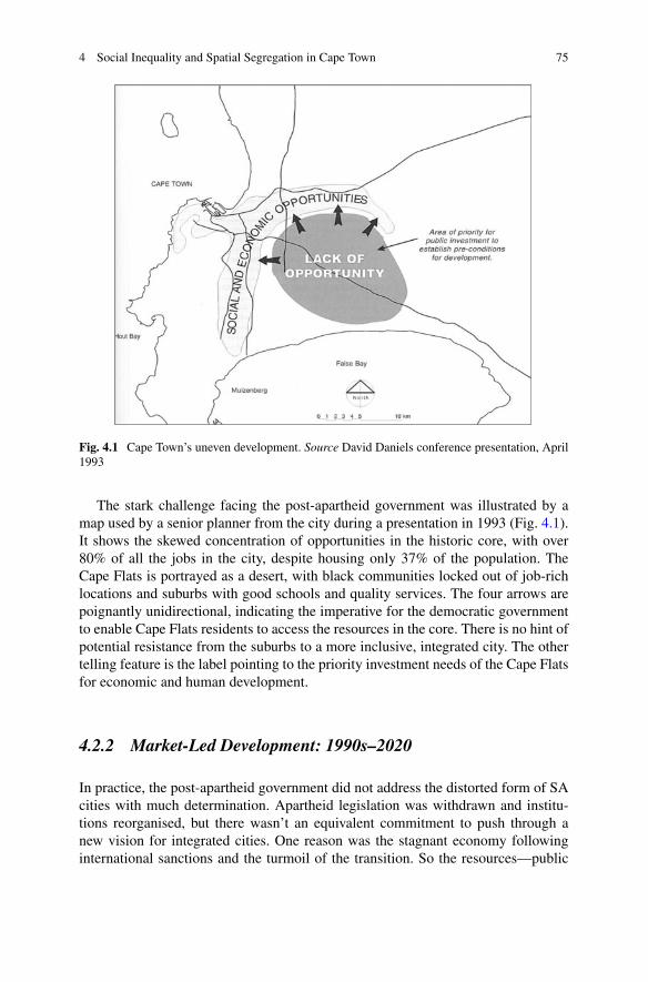
4 Social Inequality and Spatial Segregation in Cape Town 75
Fig. 4.1 Cape Town’s uneven development. Source David Daniels conference presentation, April1993
The stark challenge facing the post-apartheid government was illustrated by amap used by a senior planner from the city during a presentation in 1993 (Fig. 4.1).It shows the skewed concentration of opportunities in the historic core, with over80% of all the jobs in the city, despite housing only 37% of the population. TheCape Flats is portrayed as a desert, with black communities locked out of job-richlocations and suburbs with good schools and quality services. The four arrows arepoignantly unidirectional, indicating the imperative for the democratic governmentto enable Cape Flats residents to access the resources in the core. There is no hint ofpotential resistance from the suburbs to a more inclusive, integrated city. The othertelling feature is the label pointing to the priority investment needs of the Cape Flatsfor economic and human development.
4.2.2 Market-Led Development: 1990s–2020
In practice, the post-apartheid government did not address the distorted form of SAcities with much determination. Apartheid legislation was withdrawn and institu-tions reorganised, but there wasn’t an equivalent commitment to push through anew vision for integrated cities. One reason was the stagnant economy followinginternational sanctions and the turmoil of the transition. So the resources—public
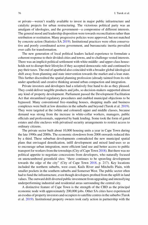
76 I. Turok et al.
or private—weren’t readily available to invest in major public infrastructure andcatalytic projects for urban restructuring. The victorious political party was anamalgam of ideologies, and the government—a compromise of different interests.The general mood and leadership disposition were towards reconciliation rather thanretribution or restitution. Many progressive policies were approved, but not matchedby concrete action (Statistics SA 2019). Institutional practices were often conserva-tive and poorly coordinated across government, and bureaucratic inertia prevailedover calls for transformation.
The new generation of local political leaders lacked experience to formulate acoherent response to their divided cities and towns, and to challenge vested interests.There was an implicit political settlement with white middle- and upper-class house-holds not to disrupt their lifestyles if they accepted democratic rule and continued topay their taxes. The end of apartheid also coincided with a broader global ideologicalshift away from planning and state intervention towards the market and a lean state.This further discredited the spatial planning profession (already tainted from its roleunder apartheid) and creative thinking around urban compaction and integration.
Private investors and developers had a relatively free hand to do as they pleased.They could deliver tangible products and jobs, so decision-makers supported almostany kind of property development. Parliament passed the Development FacilitationAct that streamlined regulatory procedures and enabled municipal objections to bebypassed. Many conventional free-standing houses, shopping malls and businesscomplexes were built at low densities in the suburbs and beyond (Turok et al. 2019).They were targeted at the (white and coloured) upper and middle classes, becausedemand was strong from the increase in white-collar workers, managers, publicofficials and professionals, supported by bank lending. Some took the form of gatedestates and elite enclaves with privatised security arrangements to restrict access toordinary citizens.
The private sector built about 10,000 housing units a year in Cape Town duringthe late 1990s and 2000s. The economic slowdown from 2008 onwards reduced thisby a third. These suburban developments contradicted the new municipal spatialplans that envisaged densification, infill development and mixed land-uses so asto encourage urban integration, more efficient land use and better access to publictransport for workers from the townships (City of Cape Town 2018). But there was nopolitical appetite to negotiate concessions from developers, who naturally focusedon unencumbered greenfield sites: “there continues to be sprawling developmenttowards the edge of the city” (City of Cape Town 2018, p. 217). Key locationsincluded the northern suburbs, west coast, Kuils River and Mitchells Plain, withsmaller pockets in the southern suburbs and Somerset West. The public sector oftenhad to fund the infrastructure, even though developers profited from the uplift in landvalues. The outward drift diverted public investment from upgrading and intensifyingunderperforming industrial and residential areas surrounding the central city.
A distinctive feature of Cape Town is the strength of the CBD as the principaleconomic node with approximately 200,000 jobs. Other SA cities have experiencedan exodus of property investors and occupiers to satellite centres in the suburbs (Turoket al. 2019). Institutional property owners took early action in partnership with the
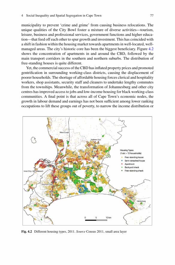
4 Social Inequality and Spatial Segregation in Cape Town 77
municipality to prevent ‘crime and grime’ from causing business relocations. Theunique qualities of the City Bowl foster a mixture of diverse activities—tourism,leisure, business and professional services, government functions and higher educa-tion—that feed off each other to spur growth and investment. This has coincided witha shift in fashionwithin the housingmarket towards apartments in well-located, well-managed areas. The city’s historic core has been the biggest beneficiary. Figure 4.2shows the concentration of apartments in and around the CBD, followed by themain transport corridors in the southern and northern suburbs. The distribution offree-standing houses is quite different.
Yet, the commercial success of the CBDhas inflated property prices and promotedgentrification in surrounding working-class districts, causing the displacement ofpoorer households. The shortage of affordable housing forces clerical and hospitalityworkers, shop assistants, security staff and cleaners to undertake lengthy commutesfrom the townships. Meanwhile, the transformation of Johannesburg and other citycentres has improved access to jobs and low-income housing for black working-classcommunities. A final point is that across all of Cape Town’s economic nodes, thegrowth in labour demand and earnings has not been sufficient among lower rankingoccupations to lift these groups out of poverty, to narrow the income distribution or
Fig. 4.2 Different housing types, 2011. Source Census 2011, small area layer
78 I. Turok et al.
to encourage private housing developers to broaden their product range to meet themajority’s needs for affordable accommodation.
4.2.3 State-Led Housing: 1990s–2020
The government has acted with unusual resolve to provide housing directly, usingfully subsidised contractors. Apartheid denied blacks the right to own property inthe cities and stopped building them houses to discourage urbanisation. This causedserious overcrowding and gave rise to many squatter settlements. The 1994 govern-ment saw decent housing as the key to reducing squalor and restoring dignity andrespect. Housing was treated as part of a ‘social wage’, along with welfare grantsand free basic services. Households below a certain income were promised a freehousing unit on its own small plot.
Direct state provision gave the government control over the quantity of housingit could deliver, without relying on the vagaries of private developers. Ambitioustargets were set and broadly met. About 5,000 government houses have been built inCape Town every year since the early 2000s, amounting to a quarter of all housingsupplied, and almost half of the formal supply (City of Cape Town 2018). This couldhave changed the city’s physical growth pattern if it was carefully targeted.
There have been undoubted benefits for households moving out of shacks orovercrowded family homes through improved privacy, protection from the weather,internal services, children’s safety and an asset for security. However, the state hasborne the full cost, letting the banks and private developers off the hook.Most houseshave been built on the outskirts to economise on the land. Large greenfield sites haveenabled mass construction of standardised units. A separate production process forprivate sector housing has kept the occupiers far apart. This has avoided NIMBYresistance, but contradicts the goal of racial diversity and integration.
Most government housing in Cape Town has been built around the periphery, inDelft, Khayelitsha,Mitchells Plain, Kraaifontein and SomersetWest. This is far fromjobs, good schools, training colleges and other opportunities for advancement. Themunicipality estimates that poor households spend up to 40% of their disposableincome travelling to work, which “inhibits upward socio-economic mobility anddeepens household dependency. These features are common to many SA cities buttend to be more acute in Cape Town” (City of Cape Town 2018, p. 215). Manyhouseholds are trapped in marginal locations because they are not allowed to selltheir homes for eight years and have not received their title deeds (Turok 2016).Many build shacks in their backyards to generate rental income (Scheba and Turok2020). Their concentration on the Cape Flats is shown in green in Fig. 4.2.
A National Treasury review concluded that housing policy: “reinforces the legacyof apartheid and relegates the poor to areas that are far from economic opportu-nity” (GTAC 2016, p. 1). There is public land available within Cape Town’s historiccore that could be developed for affordable housing. Some are large parcels that
4 Social Inequality and Spatial Segregation in Cape Town 79
could accommodate tens of thousands of dwellings, including Culemborg, Yster-plaat, Wingfield, Youngsfield and Denel. There has been insufficient determinationto release these strategic assets in the public interest (Turok 2016). Civic activistshave begun to target empty buildings, golf courses and undeveloped land to protestat the inertia (Turok et al. 2019).
4.3 Inequality in the Labour Market
4.3.1 Data and Methods
The labour market has a major influence on housing patterns. Employment andoccupation data were drawn from the 2001 and 2011 Censuses—the most accurateand most recent source of neighbourhood information. Occupations were codedaccording to the SA Standard Classification of Occupations (SASCO).2
The municipal boundary is used to define the extent of Cape Town. This approx-imates to the functional labour market area because it includes settlements beyondthe continuous built-up area. This reflects the political imperative post-apartheidto incorporate outlying suburbs, commuter belts and dormitory townships with thecore city in order to permit effective strategic planning and resource redistribution(‘one city, one tax base’). A minor technical issue is that some enumeration areasshifted between years, so the internal configuration of maps between 2001 and 2011is slightly different if one looks at specific sub-places very closely. This doesn’taffect broad spatial trends. A few sparsely populated sub-places were excluded fromthe analysis, taking the number of sub-places to 858 in 2011.3 Sub-places range ingeographical size with larger, more sparsely populated sub-places generally locatedon the periphery. The median population in 2011 was 10,140 persons and the medianarea was 0.542 km2.
4.3.2 Occupational Structure
The growth rate and structure of a city’s economy determine the demand for labour,and therefore the occupations of the local workforce. This includes the distribution
2Detailed occupation data for Census 2011 was released in late 2017, thoroughly cleaned with noincomplete information. The occupation data for 2001 included 7% of all responses as ‘undeter-mined’. The effect of such differences in data management between the Censuses is unclear. Theproblem is fairly common in analysing cross-sectional household data which spans lengthy periods.We omit undetermined responses for greater consistency between years when estimating the resultsin the figures and tables that follow.3Sub-places with less than 10 economically active persons are arguably too small for a sensibleclassification by occupation and hence were omitted.
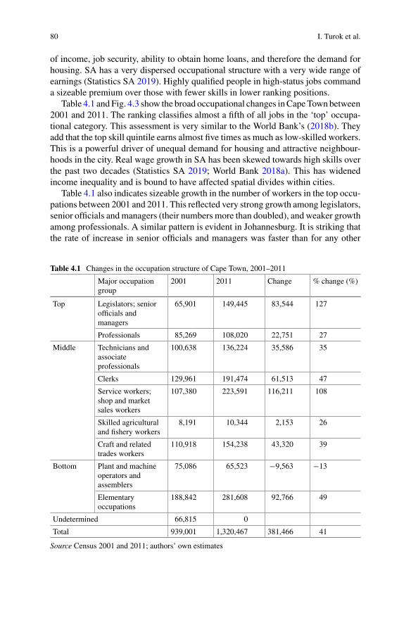
80 I. Turok et al.
of income, job security, ability to obtain home loans, and therefore the demand forhousing. SA has a very dispersed occupational structure with a very wide range ofearnings (Statistics SA 2019). Highly qualified people in high-status jobs commanda sizeable premium over those with fewer skills in lower ranking positions.
Table 4.1 and Fig. 4.3 show the broad occupational changes inCapeTownbetween2001 and 2011. The ranking classifies almost a fifth of all jobs in the ‘top’ occupa-tional category. This assessment is very similar to the World Bank’s (2018b). Theyadd that the top skill quintile earns almost five times as much as low-skilled workers.This is a powerful driver of unequal demand for housing and attractive neighbour-hoods in the city. Real wage growth in SA has been skewed towards high skills overthe past two decades (Statistics SA 2019; World Bank 2018a). This has widenedincome inequality and is bound to have affected spatial divides within cities.
Table 4.1 also indicates sizeable growth in the number of workers in the top occu-pations between 2001 and 2011. This reflected very strong growth among legislators,senior officials andmanagers (their numbers more than doubled), and weaker growthamong professionals. A similar pattern is evident in Johannesburg. It is striking thatthe rate of increase in senior officials and managers was faster than for any other
Table 4.1 Changes in the occupation structure of Cape Town, 2001–2011
Major occupationgroup
2001 2011 Change % change (%)
Top Legislators; seniorofficials andmanagers
65,901 149,445 83,544 127
Professionals 85,269 108,020 22,751 27
Middle Technicians andassociateprofessionals
100,638 136,224 35,586 35
Clerks 129,961 191,474 61,513 47
Service workers;shop and marketsales workers
107,380 223,591 116,211 108
Skilled agriculturaland fishery workers
8,191 10,344 2,153 26
Craft and relatedtrades workers
110,918 154,238 43,320 39
Bottom Plant and machineoperators andassemblers
75,086 65,523 −9,563 −13
Elementaryoccupations
188,842 281,608 92,766 49
Undetermined 66,815 0
Total 939,001 1,320,467 381,466 41
Source Census 2001 and 2011; authors’ own estimates
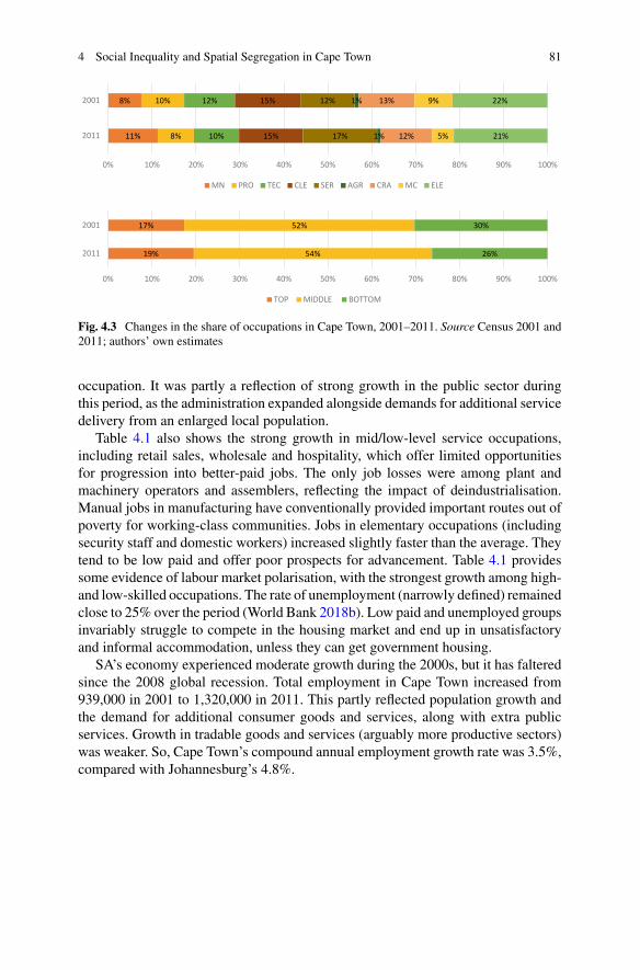
4 Social Inequality and Spatial Segregation in Cape Town 81
11%
8%
8%
10%
10%
12%
15%
15%
17%
12%
1%
1%
12%
13%
5%
9%
21%
22%
0% 10% 20% 30% 40% 50% 60% 70% 80% 90% 100%
2011
2001
MN PRO TEC CLE SER AGR CRA MC ELE
19%
17%
54%
52%
26%
30%
0% 10% 20% 30% 40% 50% 60% 70% 80% 90% 100%
2011
2001
TOP MIDDLE BOTTOM
Fig. 4.3 Changes in the share of occupations in Cape Town, 2001–2011. Source Census 2001 and2011; authors’ own estimates
occupation. It was partly a reflection of strong growth in the public sector duringthis period, as the administration expanded alongside demands for additional servicedelivery from an enlarged local population.
Table 4.1 also shows the strong growth in mid/low-level service occupations,including retail sales, wholesale and hospitality, which offer limited opportunitiesfor progression into better-paid jobs. The only job losses were among plant andmachinery operators and assemblers, reflecting the impact of deindustrialisation.Manual jobs in manufacturing have conventionally provided important routes out ofpoverty for working-class communities. Jobs in elementary occupations (includingsecurity staff and domestic workers) increased slightly faster than the average. Theytend to be low paid and offer poor prospects for advancement. Table 4.1 providessome evidence of labour market polarisation, with the strongest growth among high-and low-skilled occupations. The rate of unemployment (narrowly defined) remainedclose to 25% over the period (World Bank 2018b). Low paid and unemployed groupsinvariably struggle to compete in the housing market and end up in unsatisfactoryand informal accommodation, unless they can get government housing.
SA’s economy experienced moderate growth during the 2000s, but it has falteredsince the 2008 global recession. Total employment in Cape Town increased from939,000 in 2001 to 1,320,000 in 2011. This partly reflected population growth andthe demand for additional consumer goods and services, along with extra publicservices. Growth in tradable goods and services (arguably more productive sectors)was weaker. So, Cape Town’s compound annual employment growth rate was 3.5%,compared with Johannesburg’s 4.8%.
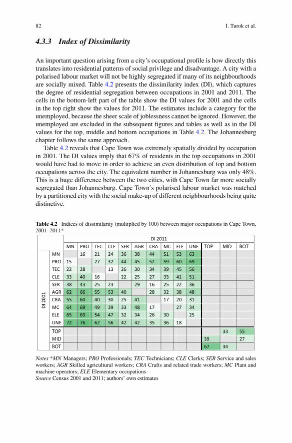
82 I. Turok et al.
4.3.3 Index of Dissimilarity
An important question arising from a city’s occupational profile is how directly thistranslates into residential patterns of social privilege and disadvantage. A city with apolarised labour market will not be highly segregated if many of its neighbourhoodsare socially mixed. Table 4.2 presents the dissimilarity index (DI), which capturesthe degree of residential segregation between occupations in 2001 and 2011. Thecells in the bottom-left part of the table show the DI values for 2001 and the cellsin the top right show the values for 2011. The estimates include a category for theunemployed, because the sheer scale of joblessness cannot be ignored. However, theunemployed are excluded in the subsequent figures and tables as well as in the DIvalues for the top, middle and bottom occupations in Table 4.2. The Johannesburgchapter follows the same approach.
Table 4.2 reveals that Cape Town was extremely spatially divided by occupationin 2001. The DI values imply that 67% of residents in the top occupations in 2001would have had to move in order to achieve an even distribution of top and bottomoccupations across the city. The equivalent number in Johannesburg was only 48%.This is a huge difference between the two cities, with Cape Town far more sociallysegregated than Johannesburg. Cape Town’s polarised labour market was matchedby a partitioned city with the social make-up of different neighbourhoods being quitedistinctive.
Table 4.2 Indices of dissimilarity (multiplied by 100) between major occupations in Cape Town,2001–2011*
DI 2011MN PRO TEC CLE SER AGR CRA MC ELE UNE TOP MID BOT
DI 2
001
MN 16 21 24 36 38 44 51 53 63PRO 15 27 32 44 45 52 59 60 69TEC 22 28 13 26 30 34 39 45 56CLE 33 40 16 22 25 27 33 41 51SER 38 43 25 23 29 16 25 22 36AGR 62 66 55 53 40 28 32 38 48CRA 55 60 40 30 25 41 17 20 31MC 64 69 49 39 33 48 17 27 34ELE 65 69 54 47 32 34 26 30 25UNE 72 76 62 56 42 42 35 36 18
TOP 33 55MID 39 27BOT 67 34
Notes *MN Managers; PRO Professionals; TEC Technicians; CLE Clerks; SER Service and salesworkers; AGR Skilled agricultural workers; CRA Crafts and related trade workers; MC Plant andmachine operators; ELE Elementary occupationsSource Census 2001 and 2011; authors’ own estimates
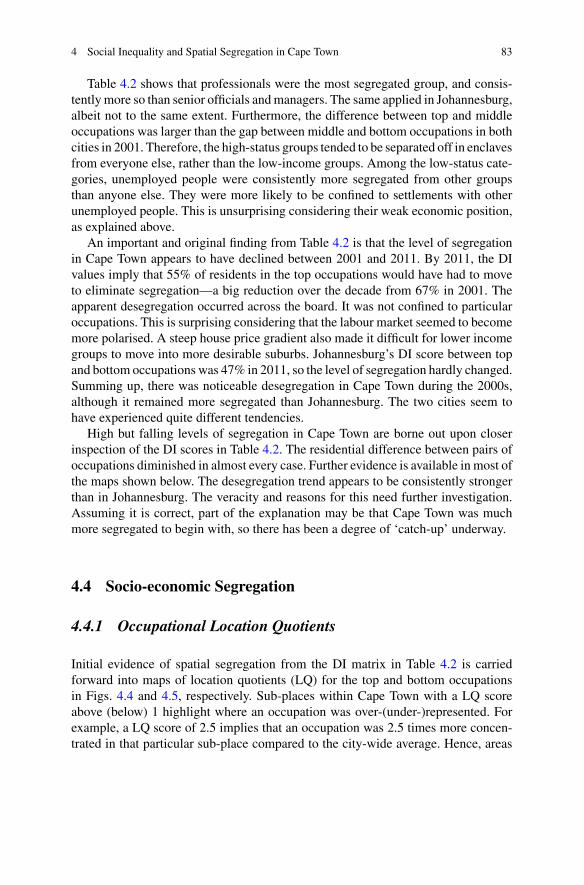
4 Social Inequality and Spatial Segregation in Cape Town 83
Table 4.2 shows that professionals were the most segregated group, and consis-tentlymore so than senior officials andmanagers. The same applied in Johannesburg,albeit not to the same extent. Furthermore, the difference between top and middleoccupations was larger than the gap between middle and bottom occupations in bothcities in 2001. Therefore, the high-status groups tended to be separated off in enclavesfrom everyone else, rather than the low-income groups. Among the low-status cate-gories, unemployed people were consistently more segregated from other groupsthan anyone else. They were more likely to be confined to settlements with otherunemployed people. This is unsurprising considering their weak economic position,as explained above.
An important and original finding from Table 4.2 is that the level of segregationin Cape Town appears to have declined between 2001 and 2011. By 2011, the DIvalues imply that 55% of residents in the top occupations would have had to moveto eliminate segregation—a big reduction over the decade from 67% in 2001. Theapparent desegregation occurred across the board. It was not confined to particularoccupations. This is surprising considering that the labour market seemed to becomemore polarised. A steep house price gradient also made it difficult for lower incomegroups to move into more desirable suburbs. Johannesburg’s DI score between topand bottom occupations was 47% in 2011, so the level of segregation hardly changed.Summing up, there was noticeable desegregation in Cape Town during the 2000s,although it remained more segregated than Johannesburg. The two cities seem tohave experienced quite different tendencies.
High but falling levels of segregation in Cape Town are borne out upon closerinspection of the DI scores in Table 4.2. The residential difference between pairs ofoccupations diminished in almost every case. Further evidence is available in most ofthe maps shown below. The desegregation trend appears to be consistently strongerthan in Johannesburg. The veracity and reasons for this need further investigation.Assuming it is correct, part of the explanation may be that Cape Town was muchmore segregated to begin with, so there has been a degree of ‘catch-up’ underway.
4.4 Socio-economic Segregation
4.4.1 Occupational Location Quotients
Initial evidence of spatial segregation from the DI matrix in Table 4.2 is carriedforward into maps of location quotients (LQ) for the top and bottom occupationsin Figs. 4.4 and 4.5, respectively. Sub-places within Cape Town with a LQ scoreabove (below) 1 highlight where an occupation was over-(under-)represented. Forexample, a LQ score of 2.5 implies that an occupation was 2.5 times more concen-trated in that particular sub-place compared to the city-wide average. Hence, areas
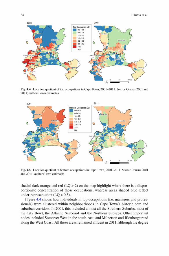
84 I. Turok et al.
Fig. 4.4 Location quotient of top occupations in Cape Town, 2001–2011. Source Census 2001 and2011; authors’ own estimates
Fig. 4.5 Location quotient of bottom occupations in Cape Town, 2001–2011. Source Census 2001and 2011; authors’ own estimates
shaded dark orange and red (LQ > 2) on the map highlight where there is a dispro-portionate concentration of those occupations, whereas areas shaded blue reflectunder-representation (LQ < 0.5).
Figure 4.4 shows how individuals in top occupations (i.e. managers and profes-sionals) were clustered within neighbourhoods in Cape Town’s historic core andsuburban corridors. In 2001, this included almost all the Southern Suburbs, most ofthe City Bowl, the Atlantic Seaboard and the Northern Suburbs. Other importantnodes included Somerset West in the south-east, and Milnerton and Bloubergstrandalong the West Coast. All these areas remained affluent in 2011, although the degree
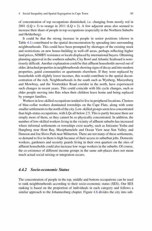
4 Social Inequality and Spatial Segregation in Cape Town 85
of concentration of top occupations diminished, i.e. changing from mostly red in2001 (LQ > 3) to orange in 2011 (LQ > 2). A few adjacent areas also seemed toincrease their share of people in top occupations (especially in the Northern Suburbsand Helderberg).
It could be that the strong increase in people in senior positions (shown inTable 4.1) contributed to the spatial deconcentration by spreading into surroundingneighbourhoods. This could have been prompted by shortages of the existing stockand restrictions on new house-building in well-off areas, perhaps reflecting higherland prices, NIMBY resistance or locals displaced by international buyers. Obtainingplanning approval in the southern suburbs, City Bowl and Atlantic Seaboard is noto-riously difficult. Another explanation could be that affluent households moved out ofolder, detachedproperties in neighbourhoods showing signs of decay and intomodernproperties, gated communities or apartments elsewhere. If they were replaced byhouseholds with slightly lower incomes, this would contribute to the spatial decon-centration of the rich. Neighbourhoods in the south such as Wynberg, Muizenbergand Mowbray, and the Voortrekker Road corridor in the north, have experiencedsuch changes in recent years. This could coincide with life cycle changes, such asolder people moving into flats when their children leave home and being replacedby younger families.
Workers in less-skilled occupations tended to live in peripheral locations. Clustersof blue-collar workers dominated townships on the Cape Flats, along with somesmaller settlements to the north of the city. Low-skilled groups seem less concentratedthan high-status occupations, with LQs all below 2.5. This is partly because there aresimply more of them, so they cannot be so physically concentrated. In addition, thenumber of low-skilled workers living in the vicinity of affluent suburbs has increasedwhere informal settlements or townships exist nearby, such as Imizamo Yethu andHangberg near Hout Bay, Masiphumelele and Ocean View near Sun Valley, andDunoon and Joe Slovo Park near Milnerton. There are not many of these settlements,so demand to live in them is high because of their access to suburban jobs. Domesticworkers, gardeners and security guards living in their own quarters on the sites ofaffluent households could also increase low-wage workers in the suburbs. Of course,the co-existence of different income groups in the same sub-places does not meanmuch actual social mixing or integration occurs.
4.4.2 Socio-economic Status
The concentration of people in the top, middle and bottom occupations can be usedto rank neighbourhoods according to their socio-economic status (SES). Our SESranking is based on the proportion of individuals in each category and follows asimilar approach to the Johannesburg chapter. Figure 4.6 divides the city into sub-
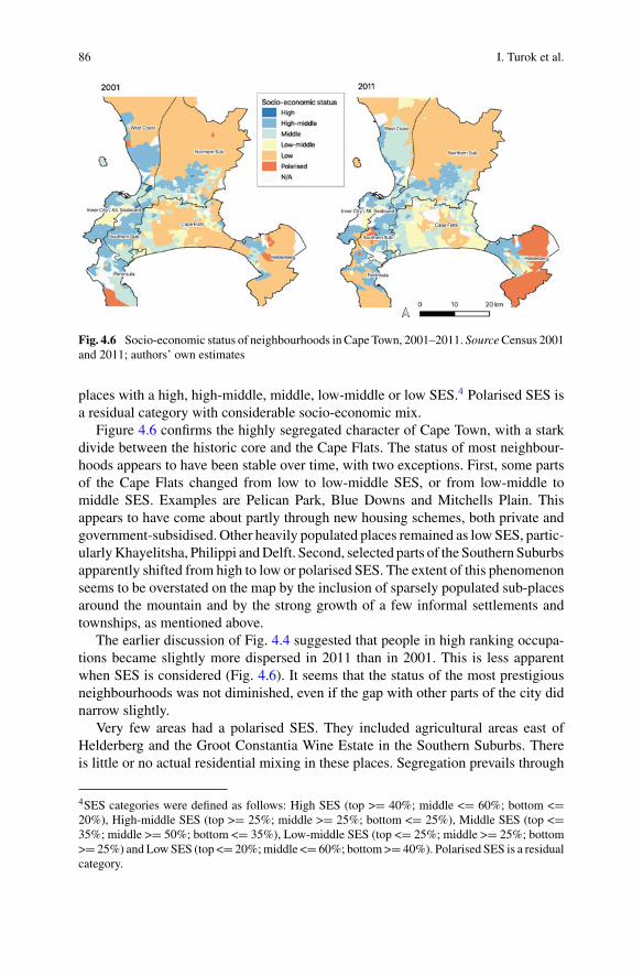
86 I. Turok et al.
Fig. 4.6 Socio-economic status of neighbourhoods in Cape Town, 2001–2011. SourceCensus 2001and 2011; authors’ own estimates
places with a high, high-middle, middle, low-middle or low SES.4 Polarised SES isa residual category with considerable socio-economic mix.
Figure 4.6 confirms the highly segregated character of Cape Town, with a starkdivide between the historic core and the Cape Flats. The status of most neighbour-hoods appears to have been stable over time, with two exceptions. First, some partsof the Cape Flats changed from low to low-middle SES, or from low-middle tomiddle SES. Examples are Pelican Park, Blue Downs and Mitchells Plain. Thisappears to have come about partly through new housing schemes, both private andgovernment-subsidised. Other heavily populated places remained as low SES, partic-ularlyKhayelitsha, Philippi andDelft. Second, selected parts of the Southern Suburbsapparently shifted from high to low or polarised SES. The extent of this phenomenonseems to be overstated on the map by the inclusion of sparsely populated sub-placesaround the mountain and by the strong growth of a few informal settlements andtownships, as mentioned above.
The earlier discussion of Fig. 4.4 suggested that people in high ranking occupa-tions became slightly more dispersed in 2011 than in 2001. This is less apparentwhen SES is considered (Fig. 4.6). It seems that the status of the most prestigiousneighbourhoods was not diminished, even if the gap with other parts of the city didnarrow slightly.
Very few areas had a polarised SES. They included agricultural areas east ofHelderberg and the Groot Constantia Wine Estate in the Southern Suburbs. Thereis little or no actual residential mixing in these places. Segregation prevails through
4SES categories were defined as follows: High SES (top >= 40%; middle <= 60%; bottom <=20%), High-middle SES (top >= 25%; middle >= 25%; bottom <= 25%), Middle SES (top <=35%; middle >= 50%; bottom <= 35%), Low-middle SES (top <= 25%; middle >= 25%; bottom>= 25%) and LowSES (top <= 20%;middle <= 60%; bottom>= 40%). Polarised SES is a residualcategory.
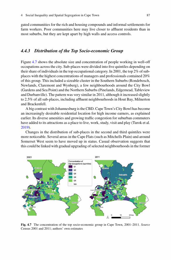
4 Social Inequality and Spatial Segregation in Cape Town 87
gated communities for the rich and housing compounds and informal settlements forfarm workers. Poor communities here may live closer to affluent residents than inmost suburbs, but they are kept apart by high walls and access controls.
4.4.3 Distribution of the Top Socio-economic Group
Figure 4.7 shows the absolute size and concentration of people working in well-offoccupations across the city. Sub-places were divided into five quintiles depending ontheir share of individuals in the top occupational category. In 2001, the top 2% of sub-places with the highest concentrations of managers and professionals contained 20%of this group. This included a sizeable cluster in the Southern Suburbs (Rondebosch,Newlands, Claremont and Wynberg), a few neighbourhoods around the City Bowl(Gardens and Sea Point) and theNorthern Suburbs (Pinelands, Edgemead, Tableviewand Durbanville). The pattern was very similar in 2011, although it increased slightlyto 2.5% of all sub-places, including affluent neighbourhoods in Hout Bay, Milnertonand Brackenfell.
A big contrast with Johannesburg is the CBD. Cape Town’s City Bowl has becomean increasingly desirable residential location for high income earners, as explainedearlier. Its diverse amenities and growing traffic congestion for suburban commutershave added to its attractions as a place to live, work, study, visit and play (Turok et al.2019).
Changes in the distribution of sub-places in the second and third quintiles weremore noticeable. Several areas in the Cape Flats (such asMitchells Plain) and aroundSomerset West seem to have moved up in status. Casual observation suggests thatthis could be linkedwith gradual upgrading of selected neighbourhoods in the former
Fig. 4.7 The concentration of the top socio-economic group in Cape Town, 2001–2011. SourceCensus 2001 and 2011; authors’ own estimates
88 I. Turok et al.
and new private housing in the latter. A few large sub-places on the city’s northernperiphery also raised their status. This has a visible effect on the maps, but the realimpact is quite limited because most areas were very sparsely populated in 2001and a few middle income housing projects and wine farms that opened during thefollowing decade could have had this effect.
4.5 Conclusion
Cape Town remains sharply divided by socio-economic status. Social inequalitiescontinue to be aligned with race, although the causes have shifted from apartheidcontrols to the economy and labour market. The scale and nature of employmentgrowth have not been sufficient to lift many people out of poverty and into better-offsocial strata. Geography reinforces social divides through the gulf in opportunitiesavailable to residents of different neighbourhoods. Townships on the Cape Flats areliterally worlds’ apart from the southern and northern suburbs, where the contoursof affluence remain the same.
Despite the economic, social and spatial barriers to change, there appears to havebeen a noticeable reduction in the degree of segregation between 2001 and 2011. Thisis more substantial than in Johannesburg. The index of dissimilarity and locationquotients both indicate that the extent of socio-economic segregation diminished.On the one hand, it appears that the concentration of top occupational groups wassomewhat diluted as some of them spread out into surrounding neighbourhoods. Onthe other hand, a number of lower income neighbourhoods seemed to move up instatus.
It is important to validate this analysis with further investigation. Other economicand social trends suggest increasingpolarisation and a steeper social gradient betweenthe suburbs and townships, yet the statistical analysis presented here indicates anarrowing of the gap. It is unclear whether the decline in segregation is a realphenomenon, or more of a construct arising from the indicators and spatial unitsused to measure it. The apparent desegregation needs additional analysis, includingthe application of different socio-economic indicators and the use of different sizedspatial units. Drilling deeper should help to identifywhich neighbourhoods and socialgroups have been most affected, and by how much conditions have changed.
In addition, it is vital to improve understanding of the reasons for these shifts andthe detailedmechanisms involved. Research and policy concerned with spatial segre-gation tend to focus on changes in land-use and the built environment, particularlythe housing stock. This is highly visible and relatively easily measured. The assump-tion is that new housing developments are the main driver of change. Sometimesthis is extended to include the conversion, upgrading, extension or redevelopment ofexisting buildings, in recognition that the social make-up and number of householdsin a neighbourhood are affected by in situ property dynamics and not simply newgreenfield investments.
4 Social Inequality and Spatial Segregation in Cape Town 89
This analysis is important and needs to be extended to investigate the lessvisible social processes underway within and between neighbourhoods, includingdetailed forms of householdmovement, household formation and in situ occupationalmobility, upwards and downwards. Unfortunately, the information available on thesetrends is limited. Changing patterns of segregation are bound to be the outcome ofa complex interplay between alterations to the built environment and intricate socialshifts. For example, new house-building may set in train long filtering chains thataffect multiple households and neighbourhoods in unexpected ways. A better graspof these dynamics is essential for more effective policies to tackle spatial divides.There are few more important research agendas in SA today.
Acknowledgements The research was partly funded by the UK Government’s Global ChallengesResearch Fund via UK Research and Innovation and the ESRC through the GCRF Centre forSustainable, Healthy and Learning Cities and Neighbourhoods. Thanks to David Maclennan foruseful feedback.
References
Christopher AJ (2000) The Atlas of changing South Africa. Routledge, LondonCity of Cape Town (2018) Metropolitan spatial development frameworkGovernment Technical Advisory Centre (GTAC) (2016) Programmatic and costing comparison ofthe housing programmes. Pretoria, National Treasury. http://www.gtac.gov.za/
Mabin A (2005) Suburbanisation, segregation, and government of territorial transformations.Transformation 57(1):41–63
Parry K, van Eeden A (2015) Measuring racial residential segregation at different geographic scalesin Cape Town and Johannesburg. S Afr Geogr J 97(1):31–49
Scheba A, Turok I (2020) Informal rental housing in the South: dynamic but neglected. EnvironUrban 32(1):109–132
Statistics South Africa (2019) Inequality trends in South Africa: a multidimensional diagnostic ofinequality. Report No. 03-10-19. Statistics SA, Pretoria, 232 pp
Turok I (2016) South Africa’s new urban agenda: transformation of compensation? Local Econ31(1):9–27
Turok I, Borel-Saladin J (2014) Is urbanization in South Africa on a sustainable trajectory? DevSouth Afr 31(5):675–691
Turok I, Seeliger L, Visagie J (2019) Restoring the core? Central city decline and transformationin the South. Prog Plan 100434. https://doi.org/10.1016/j.progress.2019.100434
van Rooyen J, Lemanski C (2020) Urban segregation in South Africa: the evolution of exclusion inCape Town. In: Musterd S (ed) Handbook of urban segregation
World Bank (2018a) An incomplete transition: overcoming the legacy of exclusion in South Africa.World Bank, Washington DC. https://doi.org/10.1596/29793
World Bank (2018b) Overcoming poverty and inequality in South Africa: an assessment of drivers,constraints and oppportunities. The World Bank, Washington DC

90 I. Turok et al.
Open Access This chapter is licensed under the terms of the Creative Commons Attribution 4.0International License (http://creativecommons.org/licenses/by/4.0/), which permits use, sharing,adaptation, distribution and reproduction in any medium or format, as long as you give appropriatecredit to the original author(s) and the source, provide a link to the Creative Commons license andindicate if changes were made.
The images or other third party material in this chapter are included in the chapter’s CreativeCommons license, unless indicated otherwise in a credit line to the material. If material is notincluded in the chapter’s Creative Commons license and your intended use is not permitted bystatutory regulation or exceeds the permitted use, you will need to obtain permission directly fromthe copyright holder.
Chapter 5Income Inequality and Socio-economicSegregation in the City of Johannesburg
Richard Ballard and Christian Hamann
Abstract This chapter analyses income inequality and socio-economic segregationin South Africa’s most populous city, Johannesburg. The end of apartheid’s segre-gation in 1991 has been followed by both continuity and change of urban spatialpatterns. There is a considerable literature on the transformation of inner-city areasfrom white to black, and of the steady diffusion of black middle-class residentsinto once ‘white’ suburbs. There has been less analysis on the nature and pace ofsocio-economic mixing. Four key findings from this chapter are as follows. First,dissimilarity indices show that bottom occupation categories and the unemployedare highly segregated from top occupation categories, but that the degree of segre-gation has decreased slightly between the censuses of 2001 and 2011. Second, thedata quantifies the way in which Johannesburg’s large population of unemployedpeople are more segregated from top occupations than any of the other employmentcategories, although unemployed people are less segregated from bottom occupa-tions. Third, over the same period, residents employed in bottom occupations are lesslikely to be represented in affluent former white suburbs. This seemingly paradoxicalfinding is likely to have resulted from fewer affluent households accommodating theirdomestic workers on their properties. Fourth, although most post-apartheid publichousing projects have not disrupted patterns of socio-economic segregation, someimportant exceptions do show the enormous capacity of public housing to transformthe spatial structure of the city.
Keywords Johannesburg · Apartheid · Socio-economic segregation · Townships ·Suburbs
R. Ballard (B) · C. HamannGauteng City-Region Observatory (GCRO), a Partnership of the University of Johannesburg, theUniversity of the Witwatersrand, Johannesburg, the Gauteng Provincial Government andOrganised Local Government in Gauteng (SALGA), Johannesburg, South Africae-mail: [email protected]
© The Author(s) 2021M. van Ham et al. (eds.), Urban Socio-Economic Segregation and Income Inequality,The Urban Book Series, https://doi.org/10.1007/978-3-030-64569-4_5
91
92 R. Ballard and C. Hamann
5.1 Introduction
The City of Johannesburg is the largest of eight metropolitan municipalities in SouthAfrica with respect to population size and economy. It sits within a broader city-region of 15 million people in the province of Gauteng, including the metropolitanmunicipalities of Tshwane to the north and Ekurhuleni to the east. The municipaljurisdiction of Johannesburg measures 1,648 km2 and includes urban, peri-urban andagricultural land uses. The population of Johannesburg grew by about 3% per annumbetween the 2001 and 2011 national census counts (from 3.2 to 4.4 million people).In line with national population composition, the majority of Johannesburg’s popula-tion is black1 (78%). The second-largest population group, whites, constituted 12%of Johannesburg in 2011. Indians and Coloureds2 make up 6% and 4% of popula-tion, respectively. Education outcomes are improving; for example, the proportion ofadults who have not been to school has fallen between 2001 and 2011 and the propor-tion of adults with tertiary education has increased. The average annual householdincome in Johannesburg (adjusted for inflation) increased by 2% per annum between2001 and 2011 (Statistics South Africa (Stats SA) 2012a), but increases are highlyuneven between population groups and across space.
Johannesburg was subject to intensive social and spatial engineering since itsorigins as a gold mining town in 1886. Given the emphasis that apartheid (1948–1994) placed on racial segregation, many analyses of spatial transformation in Johan-nesburg have focused on the endurance or breakdown of racial segregation (Beavon2004; Christopher 1994; Crankshaw 2008). This chapter examines residential segre-gation between socio-economic groups rather than the more familiar focus on racialsegregation. In doing so, we do not seek to claim any primacy of socio-economicsegregation, but rather to consider the relationship between various kinds of socialand spatial stratifications and the drivers of dominant residential patterns. In fact, it isnot possible to separate social and spatial inequalities from each other or from racialsegregation in the South African context. In the post-apartheid era, legal drivers ofracial segregation have been abolished, but actual patterns of racial segregation areslow to change precisely because of various forms of socio-economic segregationand stratification. Furthermore, even where racial desegregation does occur, theseprocesses do not necessarily disrupt socio-economic segregation.
1Statistics SouthAfrica records data against fourmain population groups. Respondents self-identifyas black, coloured, Indian/Asian or white.2Whereas the term coloured in North America is a dated synonym for African Americans, inSouthern Africa the meaning is quite different. It came to refer to mixed ancestry populations whowere (in Apartheid’s convoluted racial classifications) neither European (white) nor bantu (black),although they could have a heritage of both.
5 Income Inequality and Socio-economic Segregation … 93
5.2 Drivers of Dominant Residential Patterns
5.2.1 Racial Segregation
Johannesburg is a city of extremes, with densely populated working class townships3
(such as Diepsloot, Alexandra, Soweto and Orange Farm) juxtaposed against someof the richest neighbourhoods in Africa (Sandton and surrounding areas). Althoughapartheid formally ended in 1994, a century of white minority rule continues toaffect many urban patterns. Apartheid’s policies of racial segregation resulted in thedivision of residential areas between four different race groups: black, white, Indianand coloured. This shaped where new migrants to cities could settle and whetherpeople could migrate to cities at all (many black people were forced to stay in rural‘homelands’). These policies also caused the relocation of large numbers of estab-lished urban residents. In the 1950s, for example, about 72,000 black people weremoved from established areas of Johannesburg to the new settlement of Soweto onthe south-western periphery of the city (Christopher 1994). Notwithstanding deseg-regation inmany Johannesburg suburbs since the fall of apartheid, the overall popula-tion distribution and associated socio-economic patterns are tenacious (Fig. 5.1). By2019, Soweto contained about 1.8 million people or a third of the city’s population(Quantec 2018). Soweto, along with other townships, remains almost entirely blackand poor relative to northern suburbs.
During the apartheid era, the white minority government tried to create a strongoverlap between race, socio-economic status and space. Until 1980, better paying jobcategories were mostly reserved for whites, resulting in an income ceiling for blackemployees. Much more was spent on the education of white children than of othercity dwellers (Seekings andNastrass 2005). Until the 1980s, most black people couldnot own property in urban areas, including the homes they lived in. These and manyother policies ensured that spaces intended for black residents were also working-class spaces, with their residents having less capacity to earn and acquire assets thanwhite residents of white-designated areas. As a result, there has been considerableinertia to these patterns beyond the repeal of discriminatory policies in the 1980sand early 1990s. Nowadays, black residents are no longer prohibited by law fromliving in former white suburbs. However, poorer residents of the city are financiallyexcluded frommore expensive areas. Since low-income earners are overwhelminglyblack, and since expensive areas are often those that were historically designated forwhite use, some of apartheid’s patterns continue.
Since the end of apartheid, some kinds of urban growth have produced entirelynew black working-class settlements or have extended or intensified longer estab-lished townships. With racialized restrictions of urbanisation being lifted in 1986,a period of catch-up urbanisation saw many people migrate from rural areas and
3The common name for settlements established under apartheid for black residents, althoughDiepsloot and Orange Farm began much later than the others and are largely post-apartheidsettlements.
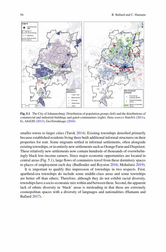
94 R. Ballard and C. Hamann
Fig. 5.1 The City of Johannesburg: Distribution of population groups (left) and the distributions ofcommercial and industrial buildings and gated communities (right). Data sources StatsSA (2011a,b), AfriGIS (2013), GeoTerraImage (2016)
smaller towns to larger cities (Turok 2014). Existing townships densified primarilybecause established residents living there built additional informal structures on theirproperties for rent. Some migrants settled in informal settlements, often alongsideexisting townships, or in entirely new settlements such asOrangeFarmandDiepsloot.These relatively new settlements now contain hundreds of thousands of overwhelm-ingly black low-income earners. Since major economic opportunities are located incentral areas (Fig. 5.1), large flows of commuters travel from these dormitory spacesto places of employment each day (Budlender and Royston 2016; Mohulatsi 2019).
It is important to qualify this impression of townships in two respects. First,apartheid-era townships do include some middle-class areas and some townshipsare better off than others. Therefore, although they do not exhibit racial diversity,townships have a socio-economicmixwithin and between them. Second, the apparentlack of ethnic diversity in ‘black’ areas is misleading in that these are extremelycosmopolitan spaces with a diversity of languages and nationalities (Hamann andBallard 2017).
5 Income Inequality and Socio-economic Segregation … 95
5.2.2 Housing
Since the end of apartheid, the state has built new settlements as a way of addressingthe housing demand. Households earning below R3,500 per month ($241 in March2019 prices) qualify for government housing. This often takes the form of a detachedtwo-room ‘low-cost house’. In the first two decades of democracy, the state deliveredabout 3.7million of these houses nationally4 (The Presidency 2014).With an ongoingflowof newmigrants to cities, and the division of households into smaller sizes, manypeople who qualify to be given government houses have yet to receive them. Othersdo not qualify because they earn above the threshold or are migrants from othercountries. As a result, 18% of dwellings in the province are informal dwellings, anda further 24% are unplanned-for backyard structures (Hamann 2018).
Although there have been instances of urban infill projects that break up apartheidpatterns, both in terms of race and class, most government-provided housing hasnot done this (Charlton 2014). In 2013, the Johannesburg municipal governmentlaunched a programme called Corridors of Freedom which intends to densify anddiversify residential neighbourhoods along Bus Rapid Transit routes, although thishas yet to have a major impact (Ballard et al. 2017). Other housing projects involveupgrading settlements by clearing existing informal settlements and rehousing someof the residents in formal accommodation on the same site or elsewhere. However,the most common form of government-funded housing has been the developmentof new greenfield settlements with hundreds or thousands of units. Concerns thatthis approach will produce homogenous low-cost settlements, and therefore perpet-uate segregation, resulted in a policy change in 2004 that promoted settlementswith a higher mix of housing types, including fully subsidised, partially subsidised,and private (mortgage funded) homes (Department of Human Settlements 2004).A prominent example of this new generation of ‘human settlements’ is a 12,500-unit settlement called Cosmo City on the north-western boundary of Johannesburg(Haferburg 2013).
While such settlements focus on social mixing, they do not achieve racial diversityas they are almost entirely black, given the nature of the housing backlog produced byapartheid. Such settlements do achieve some income mixing to a certain level, albeitwith small-scale segregation between different kinds of housing within a settlement.However, the upper range of income in such settlements does not overlap substantiallywith the income ranges of more affluent suburbs. In 2014, the state announced plansto fund many more large-scale settlements of this kind, and given the shortage ofland in established urban areas, they would likely occur on peripheral greenfield sites(Ballard and Rubin 2017). Private developers are also building low-density suburbson cheap peripheral land for entry-level black home buyers (Butcher 2016).
Some apartheid spaces were comprehensively transformed, such as inner-citytower blocks and many low-rise central neighbourhoods. These areas were oncereserved for white residents but became racially mixed in the 1980s and then became
4Housing delivery figures were not available at the city level.
96 R. Ballard and C. Hamann
primarily black by the 1990s. The white residents that had once lived in inner-city areas left because they were following work and lifestyle opportunities in theNorth, and also because of what they regarded as undesirable changes to inner-cityneighbourhoods (Beavon 2004). Some buildings were abandoned by owners andoccupied by economicallymarginal residents.As a result, conditions deteriorated, notleast because electricity, water and sewerage were cut off when municipal accountswere no longer being paid (Murray 2008). Since the 2000s, developers began refittingsome inner-city buildings for highly controlled working-class rental accommodation(Mosselson 2017). These spaces are diverse in terms of language, ethnicity andnationality if not race (almost all residents are black). In terms of class, inner-cityareas are a mix of lower- and middle-class residents.
5.2.3 Suburbs
As noted above, suburbs with more affordable housing stock, like those close tothe inner-city, experienced complete transitions from majority white to majorityblack populations. The activity of slumlords in some parts of such suburbs hassuppressed their average income by allowing overcrowding of units and by underin-vesting in general maintenance. Meanwhile, affluent northern suburbs once reservedfor white residents have largely retained their expensive positions in the propertyhierarchy. Newer suburban housing stock for the middle- and upper-market tends tobe ‘gated’, ranging from high-end golf estates to more modest ‘townhouse’ clustereddevelopment. This new housing stock is generally built on land adjacent to formerwhite suburbs, for example, on smallholdings on the northern and western suburbanfringe, but is also inserted into the suburban footprint when large suburban plots areredeveloped into denser clustered housing (Todes et al. 2017).
Many areas with expensive properties are dominated by white people, given theirstronger buying capacity. However, since the white population only constitutes 12%of the city, it offers limited demand and there are many black, Indian and colouredresidents with equally significant purchasing power.5 The removal of job reservationpolicies and the training of black nurses and teachers created a nascent black middleclass in the 1980s (Crankshaw1997).After the political transition in 1994, the upwardmobility of some of the black population significantly reshaped social and spatialhierarchies (Seekings and Nastrass 2005; Crankshaw 2008). Those who did not stayin middle-class parts of townships moved to middle-class areas elsewhere in the city.As a result, suburbs once designated for white occupation are now some of the mostracially integrated parts of the city. Many new cluster housing developments are alsoracially integrated (Chipkin 2012).
5According to the census the white population is ageing. There is also evidence of affluent whitepeople migrating to Cape Town or even emigrating. Therefore as new professional jobs emerge theyare taken up by individuals from other race groups who can then afford to live in more expensivesuburbs.
5 Income Inequality and Socio-economic Segregation … 97
However, these processes of racial diversification within former white suburbsmay be reinforcing broader patterns of socio-economic segregation (Kracker SelzerandHeller 2010).One analysis shows that the average household income in townshipsare not growing as fast as the provincial average, while many affluent areas aregrowing at a faster rate (Hamann and Cheruiyot 2017). The transfer of more affluentresidents out of townships and into suburbs may account, in part, for this spatialdivergence of average incomes. Former white suburbs also attract the overwhelmingmajority of private commercial and retail investment (Fig. 5.1).
Ironically, former white suburbs have lost a kind of race and class diversity thatwas integral to apartheid. Before democracy, many low-income black workers livedin ‘white’ suburbs as domestic workers on their employers’ properties. Much of thisaccommodation has now been converted to rental accommodation (Falkof 2016), andmany new cluster housing developments do not build ‘servants’ quarters’ as wouldhave once been standard in suburban housing. Domestic workers now aremore likelyto commute from townships. In 2019, the municipality of Johannesburg introducedan inclusionary housing policy to oblige developers of gated communities, clusterhousing and apartments to incorporate more affordable options in their plans. Thisdoes not apply to the vast number of developments already built or that have alreadybeen given approval, so is yet to have a diversifying effect on the city.
While race and class are being, to some extent, untethered from one another inpatterns of segregation in Johannesburg, it would be too simplistic to say that class isreplacing race, since the historical processes of class formation were so comprehen-sively racialized. Even to the extent that racial integration is taking place through theupward mobility of some of the black population, the high levels of socio-economicinequality raise the important consideration of socio-economic segregation. In thischapter, we examine inequality and segregation of occupations following the broadermethodologies of this volume in order to generate comparable findings.
5.3 Inequality in Johannesburg
5.3.1 Data Sources
In this chapter, occupation data is presented per sub-place in the City of Johannesburgfor 2001 and 2011, the two most recent census dates. There are 804 sub-places inJohannesburg. Sub-places with zero population in either 2001 or 2011were excludedfrom the analysis along with one other sub-place that is not a contiguous polygonand is geographically very large. The remaining sub-places vary somewhat in termsof geographic size but constitute loosely defined functional neighbourhoods. Sub-places had an average economically active population (i.e. all those aged between15 and 65 years) of 2,158 people in 2011, ranging from one to 35,949 people. Themajor occupation categories, captured in the census by Statistics South Africa (StatsSA), are shown in Table 5.1. All employed, economically active respondents were
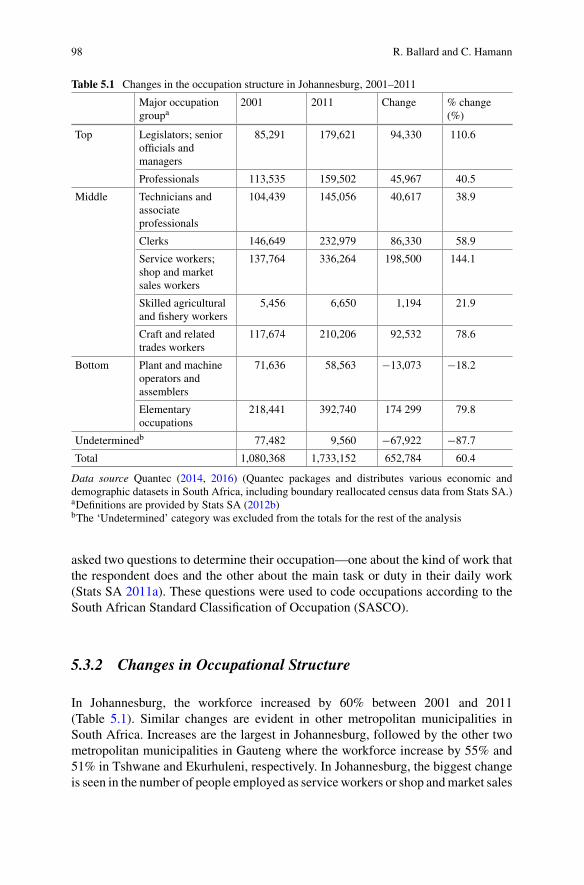
98 R. Ballard and C. Hamann
Table 5.1 Changes in the occupation structure in Johannesburg, 2001–2011
Major occupationgroupa
2001 2011 Change % change(%)
Top Legislators; seniorofficials andmanagers
85,291 179,621 94,330 110.6
Professionals 113,535 159,502 45,967 40.5
Middle Technicians andassociateprofessionals
104,439 145,056 40,617 38.9
Clerks 146,649 232,979 86,330 58.9
Service workers;shop and marketsales workers
137,764 336,264 198,500 144.1
Skilled agriculturaland fishery workers
5,456 6,650 1,194 21.9
Craft and relatedtrades workers
117,674 210,206 92,532 78.6
Bottom Plant and machineoperators andassemblers
71,636 58,563 −13,073 −18.2
Elementaryoccupations
218,441 392,740 174 299 79.8
Undeterminedb 77,482 9,560 −67,922 −87.7
Total 1,080,368 1,733,152 652,784 60.4
Data source Quantec (2014, 2016) (Quantec packages and distributes various economic anddemographic datasets in South Africa, including boundary reallocated census data from Stats SA.)aDefinitions are provided by Stats SA (2012b)bThe ‘Undetermined’ category was excluded from the totals for the rest of the analysis
asked two questions to determine their occupation—one about the kind of work thatthe respondent does and the other about the main task or duty in their daily work(Stats SA 2011a). These questions were used to code occupations according to theSouth African Standard Classification of Occupation (SASCO).
5.3.2 Changes in Occupational Structure
In Johannesburg, the workforce increased by 60% between 2001 and 2011(Table 5.1). Similar changes are evident in other metropolitan municipalities inSouth Africa. Increases are the largest in Johannesburg, followed by the other twometropolitan municipalities in Gauteng where the workforce increase by 55% and51% in Tshwane and Ekurhuleni, respectively. In Johannesburg, the biggest changeis seen in the number of people employed as service workers or shop andmarket sales
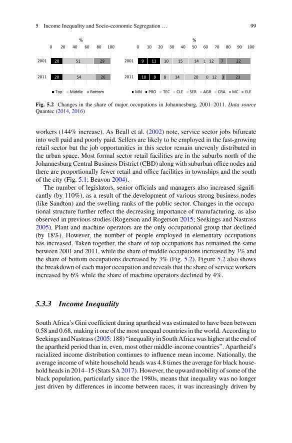
5 Income Inequality and Socio-economic Segregation … 99
20
20
51
54
29
26
0 20 40 60 80 100
2001
2011
%
Top Middle Bo om
9
10
11
9
10
8
15
14
14
20
1
0
12
12
7
3
22
23
0 10 20 30 40 50 60 70 80 90 100
2001
2011
%
MN PRO TEC CLE SER AGR CRA MC ELE
Fig. 5.2 Changes in the share of major occupations in Johannesburg, 2001–2011. Data sourceQuantec (2014, 2016)
workers (144% increase). As Beall et al. (2002) note, service sector jobs bifurcateinto well paid and poorly paid. Sellers are likely to be employed in the fast-growingretail sector but the job opportunities in this sector remain unevenly distributed inthe urban space. Most formal sector retail facilities are in the suburbs north of theJohannesburg Central Business District (CBD) along with suburban office nodes andthere are proportionally fewer retail and office facilities in townships and the southof the city (Fig. 5.1; Beavon 2004).
The number of legislators, senior officials and managers also increased signifi-cantly (by 110%), as a result of the development of various strong business nodes(like Sandton) and the swelling ranks of the public sector. Changes in the occupa-tional structure further reflect the decreasing importance of manufacturing, as alsoobserved in previous studies (Rogerson and Rogerson 2015; Seekings and Nastrass2005). Plant and machine operators are the only occupational group that declined(by 18%). However, the number of people employed in elementary occupationshas increased. Taken together, the share of top occupations has remained the samebetween 2001 and 2011, while the share of middle occupations increased by 3% andthe share of bottom occupations decreased by 3% (Fig. 5.2). Figure 5.2 also showsthe breakdown of eachmajor occupation and reveals that the share of service workersincreased by 6% while the share of machine operators declined by 4%.
5.3.3 Income Inequality
South Africa’s Gini coefficient during apartheid was estimated to have been between0.58 and 0.68, making it one of themost unequal countries in the world. According toSeekings andNastrass (2005: 188) “inequality inSouthAfricawashigher at the endofthe apartheid period than in, even, most other middle-income countries”. Apartheid’sracialized income distribution continues to influence mean income. Nationally, theaverage income of white household heads was 4.8 times the average for black house-hold heads in 2014–15 (Stats SA 2017). However, the upwardmobility of some of theblack population, particularly since the 1980s, means that inequality was no longerjust driven by differences in income between races, it was increasingly driven by
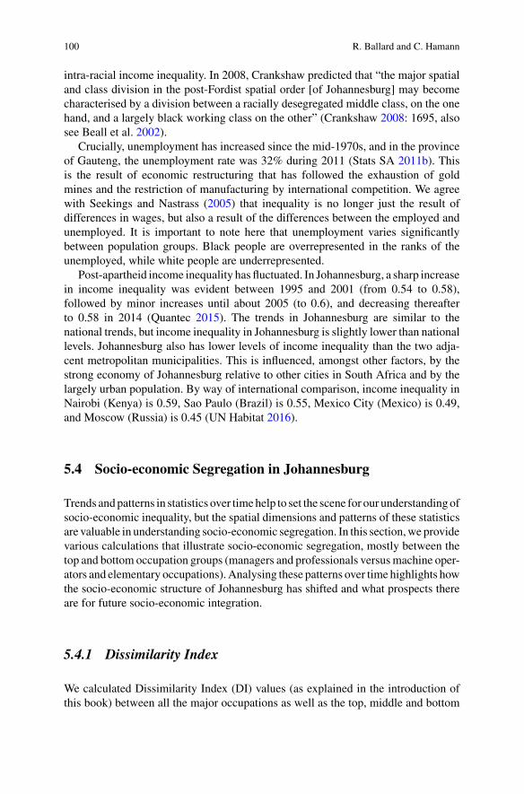
100 R. Ballard and C. Hamann
intra-racial income inequality. In 2008, Crankshaw predicted that “the major spatialand class division in the post-Fordist spatial order [of Johannesburg] may becomecharacterised by a division between a racially desegregated middle class, on the onehand, and a largely black working class on the other” (Crankshaw 2008: 1695, alsosee Beall et al. 2002).
Crucially, unemployment has increased since the mid-1970s, and in the provinceof Gauteng, the unemployment rate was 32% during 2011 (Stats SA 2011b). Thisis the result of economic restructuring that has followed the exhaustion of goldmines and the restriction of manufacturing by international competition. We agreewith Seekings and Nastrass (2005) that inequality is no longer just the result ofdifferences in wages, but also a result of the differences between the employed andunemployed. It is important to note here that unemployment varies significantlybetween population groups. Black people are overrepresented in the ranks of theunemployed, while white people are underrepresented.
Post-apartheid income inequality has fluctuated. In Johannesburg, a sharp increasein income inequality was evident between 1995 and 2001 (from 0.54 to 0.58),followed by minor increases until about 2005 (to 0.6), and decreasing thereafterto 0.58 in 2014 (Quantec 2015). The trends in Johannesburg are similar to thenational trends, but income inequality in Johannesburg is slightly lower than nationallevels. Johannesburg also has lower levels of income inequality than the two adja-cent metropolitan municipalities. This is influenced, amongst other factors, by thestrong economy of Johannesburg relative to other cities in South Africa and by thelargely urban population. By way of international comparison, income inequality inNairobi (Kenya) is 0.59, Sao Paulo (Brazil) is 0.55, Mexico City (Mexico) is 0.49,and Moscow (Russia) is 0.45 (UN Habitat 2016).
5.4 Socio-economic Segregation in Johannesburg
Trends andpatterns in statistics over timehelp to set the scene for our understandingofsocio-economic inequality, but the spatial dimensions and patterns of these statisticsare valuable in understanding socio-economic segregation. In this section,we providevarious calculations that illustrate socio-economic segregation, mostly between thetop and bottom occupation groups (managers and professionals versusmachine oper-ators and elementary occupations).Analysing these patterns over time highlights howthe socio-economic structure of Johannesburg has shifted and what prospects thereare for future socio-economic integration.
5.4.1 Dissimilarity Index
We calculated Dissimilarity Index (DI) values (as explained in the introduction ofthis book) between all the major occupations as well as the top, middle and bottom
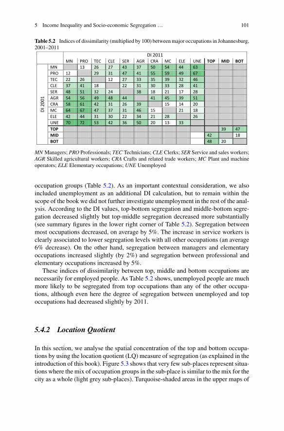
5 Income Inequality and Socio-economic Segregation … 101
Table 5.2 Indices of dissimilarity (multiplied by 100) betweenmajor occupations in Johannesburg,2001–2011
DI 2011 MN PRO TEC CLE SER AGR CRA MC ELE UNE TOP MID BOT
DI 2
001
MN 13 26 27 43 37 50 54 44 63 PRO 12 29 31 47 41 55 59 49 67 TEC 22 26 12 27 33 35 39 32 46 CLE 37 41 18 22 31 30 33 28 41 SER 48 51 32 24 38 18 21 17 28 AGR 54 56 49 48 44 41 45 39 51 CRA 58 61 42 31 26 39 15 14 20 MC 64 67 47 37 31 46 15 21 18 ELE 42 44 31 30 22 34 21 28 26 UNE 70 72 53 42 36 50 20 13 33 TOP 39 47 MID 42 18 BOT 48 20
MN Managers; PRO Professionals; TEC Technicians; CLE Clerks; SER Service and sales workers;AGR Skilled agricultural workers; CRA Crafts and related trade workers; MC Plant and machineoperators; ELE Elementary occupations; UNE Unemployed
occupation groups (Table 5.2). As an important contextual consideration, we alsoincluded unemployment as an additional DI calculation, but to remain within thescope of the book we did not further investigate unemployment in the rest of the anal-ysis. According to the DI values, top-bottom segregation and middle-bottom segre-gation decreased slightly but top-middle segregation decreased more substantially(see summary figures in the lower right corner of Table 5.2). Segregation betweenmost occupations decreased, on average by 5%. The increase in service workers isclearly associated to lower segregation levels with all other occupations (an average6% decrease). On the other hand, segregation between managers and elementaryoccupations increased slightly (by 2%) and segregation between professional andelementary occupations increased by 5%.
These indices of dissimilarity between top, middle and bottom occupations arenecessarily for employed people. As Table 5.2 shows, unemployed people are muchmore likely to be segregated from top occupations than any of the other occupa-tions, although even here the degree of segregation between unemployed and topoccupations had decreased slightly by 2011.
5.4.2 Location Quotient
In this section, we analyse the spatial concentration of the top and bottom occupa-tions by using the location quotient (LQ) measure of segregation (as explained in theintroduction of this book). Figure 5.3 shows that very few sub-places represent situa-tions where the mix of occupation groups in the sub-place is similar to the mix for thecity as a whole (light grey sub-places). Turquoise-shaded areas in the upper maps of
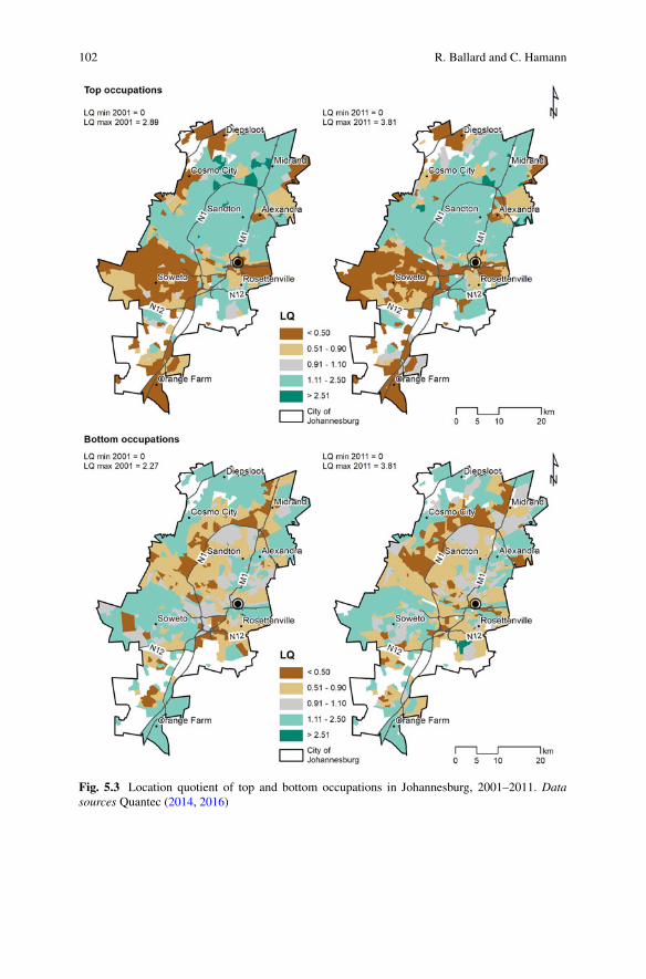
102 R. Ballard and C. Hamann
Fig. 5.3 Location quotient of top and bottom occupations in Johannesburg, 2001–2011. Datasources Quantec (2014, 2016)
5 Income Inequality and Socio-economic Segregation … 103
Fig. 5.3 are those in which top occupations are overrepresented while areas shadedbrown in the upper figures are those in which top occupations are underrepresented.The highly clustered overrepresentation of top occupations (LQ higher than 1.10)in 2001 and 2011 is apparent in much of northern Johannesburg, and some isolatedparts of southern Johannesburg. By contrast, the Johannesburg CBD and townships,such as Diepsloot, Soweto and Orange Farm show an underrepresentation of topoccupations in 2001 and 2011. By 2011, the underrepresentation of top occupationsdecreased slightly in some areas, particularly in Soweto, Cosmo City and north ofOrange Farm. Their significant underrepresentation directly east of Sandton is due tothe presence of the working-class township of Alexandra. From 1912, black peoplewere able to own land in the ‘freehold’ settlement of Alexandra, and as the city grewnorth, Alexandra became an unusual case of a centrally-located township.
In the lower two maps, turquoise-shaded areas are those in which bottom occu-pations are overrepresented, while brown is where they are underrepresented. Thoseemployed in bottom occupations are less spatially clustered than those employed intop occupations, but they are overrepresented on the fringes of the city and in town-ships like Soweto and Diepsloot (Fig. 5.3). The residential population of the Johan-nesburg CBD shows a slight underrepresentation of bottom occupations in 2001,increasing in 2011. Given that the CBD population is also highly underrepresentedby top occupations, it is likely that the CBD provides affordable homes and easyaccess to middle occupations such as technicians, clerks, service workers and tradesworkers. In 2001, bottom occupations were slightly overrepresented (LQ between1.11 and 2.5) in some suburbs surrounding Sandton. These concentrations aroundSandton would include domestic workers that lived on the properties of middle- andupper-class employers. As anticipated above, we see evidence for the reduction ofthis employment category in these suburbs by 2011 as such workers now commutefrom townships and other settlements. The increasing underrepresentation of bottomoccupations is evenmore striking in the arc of suburbs west of the N1 highway. Thesesuburbs contain many new cluster housing developments for middle- and upper-classhome buyers but provide limited accommodation for domestic workers.
5.4.3 Classification of Neighbourhoods by Socio-economicComposition
The socio-economic status (SES) of neighbourhoods can be determined by theproportion of occupations that are considered top, middle or bottom occupations. Forthe neighbourhood classification in Fig. 5.4, the classification used by Marcinczaket al. (2015) was altered slightly and two categories were added afterwards to allowfor the unambiguous classification of all sub-places in Johannesburg. The neighbour-hood types that were slightly adapted include High SES (top >= 50; middle <= 35;bottom <= 35),Middle SES (top <= 35; middle >= 50; bottom <= 35) and LowSES(top <= 35; middle <= 35; bottom >= 50). Thereafter, the remaining uncategorised
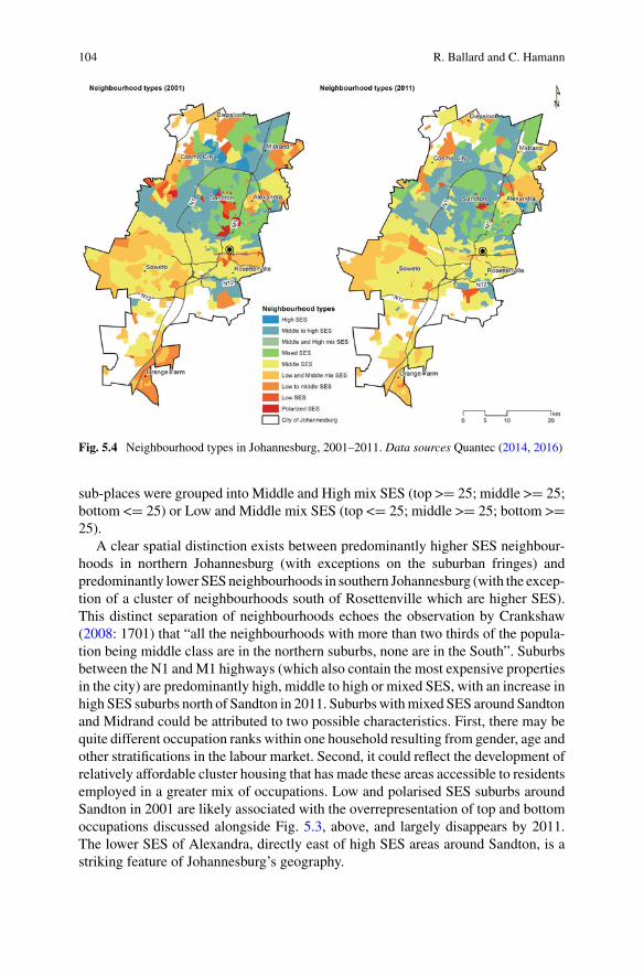
104 R. Ballard and C. Hamann
Fig. 5.4 Neighbourhood types in Johannesburg, 2001–2011. Data sources Quantec (2014, 2016)
sub-places were grouped into Middle and High mix SES (top >= 25; middle >= 25;bottom <= 25) or Low and Middle mix SES (top <= 25; middle >= 25; bottom >=25).
A clear spatial distinction exists between predominantly higher SES neighbour-hoods in northern Johannesburg (with exceptions on the suburban fringes) andpredominantly lower SESneighbourhoods in southern Johannesburg (with the excep-tion of a cluster of neighbourhoods south of Rosettenville which are higher SES).This distinct separation of neighbourhoods echoes the observation by Crankshaw(2008: 1701) that “all the neighbourhoods with more than two thirds of the popula-tion being middle class are in the northern suburbs, none are in the South”. Suburbsbetween the N1 andM1 highways (which also contain the most expensive propertiesin the city) are predominantly high, middle to high or mixed SES, with an increase inhigh SES suburbs north of Sandton in 2011. Suburbswithmixed SES around Sandtonand Midrand could be attributed to two possible characteristics. First, there may bequite different occupation ranks within one household resulting from gender, age andother stratifications in the labour market. Second, it could reflect the development ofrelatively affordable cluster housing that has made these areas accessible to residentsemployed in a greater mix of occupations. Low and polarised SES suburbs aroundSandton in 2001 are likely associated with the overrepresentation of top and bottomoccupations discussed alongside Fig. 5.3, above, and largely disappears by 2011.The lower SES of Alexandra, directly east of high SES areas around Sandton, is astriking feature of Johannesburg’s geography.
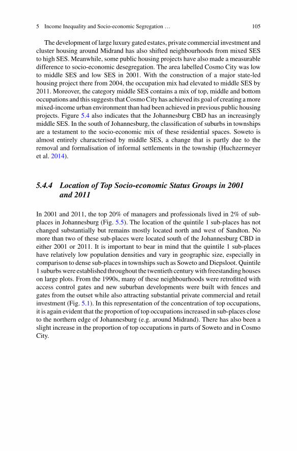
5 Income Inequality and Socio-economic Segregation … 105
The development of large luxury gated estates, private commercial investment andcluster housing around Midrand has also shifted neighbourhoods from mixed SESto high SES. Meanwhile, some public housing projects have also made a measurabledifference to socio-economic desegregation. The area labelled Cosmo City was lowto middle SES and low SES in 2001. With the construction of a major state-ledhousing project there from 2004, the occupation mix had elevated to middle SES by2011. Moreover, the category middle SES contains a mix of top, middle and bottomoccupations and this suggests thatCosmoCity has achieved its goal of creating amoremixed-income urban environment than had been achieved in previous public housingprojects. Figure 5.4 also indicates that the Johannesburg CBD has an increasinglymiddle SES. In the south of Johannesburg, the classification of suburbs in townshipsare a testament to the socio-economic mix of these residential spaces. Soweto isalmost entirely characterised by middle SES, a change that is partly due to theremoval and formalisation of informal settlements in the township (Huchzermeyeret al. 2014).
5.4.4 Location of Top Socio-economic Status Groups in 2001and 2011
In 2001 and 2011, the top 20% of managers and professionals lived in 2% of sub-places in Johannesburg (Fig. 5.5). The location of the quintile 1 sub-places has notchanged substantially but remains mostly located north and west of Sandton. Nomore than two of these sub-places were located south of the Johannesburg CBD ineither 2001 or 2011. It is important to bear in mind that the quintile 1 sub-placeshave relatively low population densities and vary in geographic size, especially incomparison to dense sub-places in townships such as Soweto and Diepsloot. Quintile1 suburbswere established throughout the twentieth centurywith freestanding houseson large plots. From the 1990s, many of these neighbourhoods were retrofitted withaccess control gates and new suburban developments were built with fences andgates from the outset while also attracting substantial private commercial and retailinvestment (Fig. 5.1). In this representation of the concentration of top occupations,it is again evident that the proportion of top occupations increased in sub-places closeto the northern edge of Johannesburg (e.g. around Midrand). There has also been aslight increase in the proportion of top occupations in parts of Soweto and in CosmoCity.
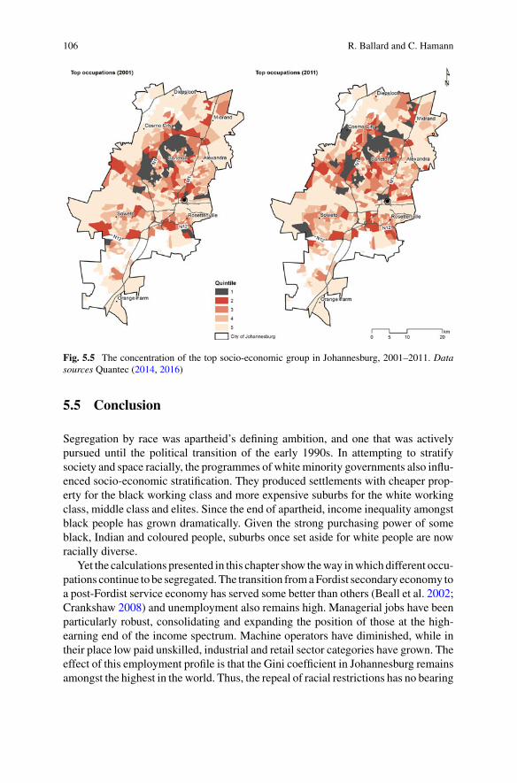
106 R. Ballard and C. Hamann
Fig. 5.5 The concentration of the top socio-economic group in Johannesburg, 2001–2011. Datasources Quantec (2014, 2016)
5.5 Conclusion
Segregation by race was apartheid’s defining ambition, and one that was activelypursued until the political transition of the early 1990s. In attempting to stratifysociety and space racially, the programmes of white minority governments also influ-enced socio-economic stratification. They produced settlements with cheaper prop-erty for the black working class and more expensive suburbs for the white workingclass, middle class and elites. Since the end of apartheid, income inequality amongstblack people has grown dramatically. Given the strong purchasing power of someblack, Indian and coloured people, suburbs once set aside for white people are nowracially diverse.
Yet the calculations presented in this chapter show theway inwhich different occu-pations continue to be segregated.The transition fromaFordist secondary economy toa post-Fordist service economy has served some better than others (Beall et al. 2002;Crankshaw 2008) and unemployment also remains high. Managerial jobs have beenparticularly robust, consolidating and expanding the position of those at the high-earning end of the income spectrum. Machine operators have diminished, while intheir place low paid unskilled, industrial and retail sector categories have grown. Theeffect of this employment profile is that the Gini coefficient in Johannesburg remainsamongst the highest in the world. Thus, the repeal of racial restrictions has no bearing
5 Income Inequality and Socio-economic Segregation … 107
on the inability of the low-earning black majority to afford housing in more expen-sive suburbs once reserved for white occupation. The dissimilarity index betweentop and bottom occupation groups decreased slightly between the 2001 and 2011censuses but increased between other occupation groups. The concentrations of topand bottom occupations illustrate the polarised structure of Johannesburg describedby Crankshaw (2008) as being divided into northern suburbs (mostly middle class)and the southern suburbs or townships (mostly working class).
Residential development and job markets have both reproduced the spatial natureof socio-economic inequality and facilitated key changes. Although state-providedhousing might have acted somewhat independently of the market to break upthese patterns, it has largely failed to do so. Essentially, long-term and deeplyentrenched inequalities have not changed substantially notwithstanding the scrappingof apartheid segregation. The 2016 Johannesburg Spatial Development Frameworkrecognises these enduring patterns of socio-economic segregation and the city hassubsequently proposed more proactive responses to the situation, including densifi-cation along transit corridors and inclusionary housing. Our analysis does suggestthat state housing developments such as Cosmo City has enabled a greater mix ofoccupations than what was previously possible. Whether these proactive measurescan offset market-led production of residential space is an important issue for thecoming decades.
References
AfriGIS (2013) Gated communities in Gauteng. AfriGIS. https://www.afrigis.co.za/Ballard R, Rubin M (2017) A “Marshall Plan” for human settlements: how megaprojects becameSouth Africa’s housing policy. Transform Crit Perspect South Afr 95:1–31. https://doi.org/10.1353/trn.2017.0020
Ballard R, Dittgen R, Harrison P, Todes A (2017) Megaprojects and urban visions: Johannesburg’sCorridors of FreedomandModderfontein. TransformCrit Perspect SouthAfr 95:111–139. https://doi.org/10.1353/trn.2017.0024
Beall J, Crankshaw O, Parnell S (2002) Uniting a divided city: governance and social exclusion inJohannesburg. Earthscan, London
Beavon K (2004) Johannesburg: the making and shaping of the city. University of South AfricaPress, Pretoria
Budlender J, Royston L (2016) Edged out: spatial mismatch and spatial justice in South Africa’smain urban areas. Socio-economic Right Institute of South Africa. http://www.seri-sa.org/images/SERI_Edged_out_report_Final_high_res.pdf. Accessed 10 Feb 2017
Butcher S (2016) Infrastructures of property and debt: making affordable housing, race and placein Johannesburg. PhD, University of Minnesota
Charlton S (2014) Public housing in Johannesburg. In: Harrison P, Gotz G, Todes A, Wray C (eds)Changing space, changing city: Johannesburg after apartheid. University of the WitwartersrandPress, Johannesburg, pp 176–193
Chipkin I (2012) Middle classing in Roodepoort capitalism and social change in South Africa.Public Affairs Research Institute, Johannesburg
Christopher AJ (1994) The atlas of apartheid. Routledge, LondonCrankshaw O (1997) Race, class, and the changing division of labour under apartheid. Routledge,London
108 R. Ballard and C. Hamann
Crankshaw O (2008) Race, space and the post-fordist spatial order of Johannesburg. Urban Stud45(8):1692–1711. https://doi.org/10.1177/0042098008091497
Department of Human Settlements (2004) “Breaking new ground” a comprehensive plan for thedevelopment of sustainable human settlements. http://www.dhs.gov.za/sites/default/files/documents/BREAKING%20NEW%20GROUND%202004_web.pdf. Accessed 28 Aug 2019
Falkof N (2016) Out the back: race and reinvention in Johannesburg’s garden cottages. Int J CultStud 19:627–642. https://doi.org/10.1177/1367877915581856
GeoTerraImage (2016) Building-based land use layer. GeoTerraImage. http://www.geoterraimage.com/products-landuse.php
Haferburg C (2013) Townships of To-Morrow? Cosmo City and inclusive visions for post-apartheidurban futures. Habitat Int 39:261–268. https://doi.org/10.1016/j.habitatint.2012.10.014
Hamann C (2018) Change in residential buildings. Gauteng City-Region Observatory, Johannes-burg, Map of the Month, 31 October. https://www.gcro.ac.za/outputs/map-of-the-month/detail/change-in-residential-buildings/. Accessed 26 Sept 2019
Hamann C, Ballard R (2017) Dimensions of diversity in Gauteng. Gauteng City-Region Obser-vatory, Johannesburg, Map of the Month, 29 September. http://www.gcro.ac.za/outputs/map-of-the-month/detail/dimensions-of-diversity-in-gauteng/. Accessed 13 Mar 2019
Hamann C, Cheruiyot K (2017) Differentiating household income growth in Gauteng2001–2011. Gauteng City-Region Observatory, Johannebsurg, Map of the Month, 31October. http://www.gcro.ac.za/outputs/map-of-the-month/detail/differentiating-household-income-growth-in-gauteng-2001-2011/. Accessed 13 Mar 2019
Huchzermeyer M, Karam A, Maina M (2014) Informal settlements. In: Harrison P, Götz G, TodesA, Wray C (eds) Changing space, changing city: Johannesburg after apartheid. Wits UniversityPress, Johannesburg, pp 154–175
Kracker Selzer A, Heller P (2010) The spatial dynamics of middle-class formation in postapartheidSouth Africa: enclavization and fragmentation in Johannesburg. In: Go J (ed) Political power andsocial theory, vol 21. Emerald Group Publishing Limited, Bingley, pp 171–208
Marcinczak S, Tammaru T, Novák J, Gentile M, Kovács Z, Temelová J, Valatka V, Kährik A, SzabóB (2015) Patterns of socio-economic segregation in the capital cities of fast-track reforming post-socialist countries. Ann Assoc Am Geogr 105(1):183–202. https://doi.org/10.1080/00045608.2014.968977
Mohulatsi B (2019) Population concentrations: night vs day. http://www.gcro.ac.za/outputs/map-of-the-month/detail/population-concentrations-night-vs-day/. Accessed 13 Mar 2019
Mosselson A (2017) ‘Joburg has its own momentum’: towards a vernacular theorisation of urbanchange. Urban Stud 54:1280–1296. https://doi.org/10.1177/0042098016634609
Murray M (2008) Taming the disorderly city: the spatial landscape of Johannesburg after apartheid.Cornell University Press, Icatha
Quantec (2014) 2001 sub-place community profiles. https://www.easydata.co.za/. Accessed 20 Feb2019
Quantec (2015) Gini coefficient at 2011municipal level (ward-based region for metros) 1995–2014.https://www.easydata.co.za/. Accessed 13 Dec 2018
Quantec (2016) 2011 sub-place community profiles. https://www.easydata.co.za/. Accessed 20 Feb2019
Quantec (2018) Population group at 2011 local municipal/ward-based metro region level 1993–2017. https://www.easydata.co.za/. Accessed 14 Sep 2018
Rogerson CM, Rogerson JM (2015) Johannesburg 2030: the economic contours of a “Linkingglobal city”. Am Behav Sci 59(3):347–368. https://doi.org/10.1177%2F0002764214550303
Seekings J, Nastrass N (2005) Class, race, and inequality in South Africa. Yale University Press,London
Statistics South Africa (2011a) Census 2011 metadata. http://www.statssa.gov.za/?page_id=3955.Accessed 11 Dec 2018
Statistics South Africa (2011b) Quarterly labour force survey. Quarter 3, 2011. https://www.statssa.gov.za/publications/P0211/P02113rdQuarter2011.pdf. Accessed 6 Mar 2019
5 Income Inequality and Socio-economic Segregation … 109
Statistics South Africa (2012a) Census 2011 Municipal report: Gauteng. http://www.statssa.gov.za/?page_id=3955. Accessed 6 Mar 2019
Statistics South Africa (2012b) South African Standard Classification of Occupation (SASCO).http://www.statssa.gov.za/classifications/codelists/SASCO_2012.pdf. Accessed 26 Feb 2019
Statistics South Africa (2017) Living conditions of households in South Africa: An analysis ofhousehold expenditure and income data using the LCS 2014/2015. Pretoria. http://www.statssa.gov.za/publications/P0310/P03102014.pdf. Accessed 18 Mar 2019
The Presidency (2014) Twenty year review, South Africa, 1994–2014. Republic of South Africa,Pretoria. https://www.dpme.gov.za/news/Documents/20%20Year%20Review.pdf. Accessed 22Aug 2019
Todes A, Harrison P, Weakley D (eds) (2017) Resilient densification: four studies from Johannes-burg. South African Research Chair in Spatial Analysis and City Planning, Johannesburg
Turok I (2014) South Africa’s tortured urbanisation and the complications of reconstruction. In:McGranahan G, Martine G (eds) Urban growth in emerging economies: lessons from the BRICS.Routledge, Abingdon, pp 143–190
UN Habitat (2016) World cities report 2016: urbanization and development, emerging futures.United Nations Human Settlements Programme, Nairobi. http://wcr.unhabitat.org/wp-content/uploads/2017/02/WCR-2016-Full-Report.pdf
Open Access This chapter is licensed under the terms of the Creative Commons Attribution 4.0International License (http://creativecommons.org/licenses/by/4.0/), which permits use, sharing,adaptation, distribution and reproduction in any medium or format, as long as you give appropriatecredit to the original author(s) and the source, provide a link to the Creative Commons license andindicate if changes were made.
The images or other third party material in this chapter are included in the chapter’s CreativeCommons license, unless indicated otherwise in a credit line to the material. If material is notincluded in the chapter’s Creative Commons license and your intended use is not permitted bystatutory regulation or exceeds the permitted use, you will need to obtain permission directly fromthe copyright holder.

Part IIIAsia
Chapter 6Dual Land Regime, Income Inequalitiesand Multifaceted Socio-Economicand Spatial Segregation in Hong Kong
Mee Kam Ng, Yuk Tai Lau, Huiwei Chen, and Sylvia He
Abstract Hong Kong has a dual land regime in the urban and rural territories. Theurban areas on both sides ofVictoriaHarbour (8.8%of land, excludingCountry Parkson Hong Kong Island) and new towns (about 15.3% of land) house over 90% of thecity’s population (about 7.5 million) with an extremely high population density ofabout 26,000 per km2. After deducting Country Parks and Special Areas (about 40%of land), the rest of the rural New Territories (traditional settlements leased by theBritish Government in 1898 for 99 years) constitutes about 35% of land, but houses5.5% of all residents with a substantially lower population density of about 1,000per km2. China’s Open Door Policy since 1978 has led to economic restructuringin Hong Kong, changing its occupational structure, intensifying income inequality,and leading to socio-economic and spatial segregation. Whilst the affluent classescontinue to concentrate in traditionally central locations in urban areas, or in luxuriousresidential enclaves in rural New Territories, the less well-off tend to be marginalisedand live in remote new towns or rural New Territories. The latter is also a resultof a skewed power relationship between the government and the property sectorin directing spatial development that breeds a hegemonic (dis)course and regimeof urban-biased and property-dominant development, sustaining the government’scoffer through a high land price policy.
Keywords Dual land regime · Income inequalities ·Multifaceted socio-economicsegregation · Spatial segregation · Hong kong
M. K. Ng (B) · Y. T. Lau · S. HeDepartment of Geography and Resource Management, The Chinese University of Hong Kong,Hong Kong, Chinae-mail: [email protected]
Y. T. Laue-mail: [email protected]
S. Hee-mail: [email protected]
H. ChenGuangdong University of Technology, Guangdong, Chinae-mail: [email protected]
© The Author(s) 2021M. van Ham et al. (eds.), Urban Socio-Economic Segregation and Income Inequality,The Urban Book Series, https://doi.org/10.1007/978-3-030-64569-4_6
113
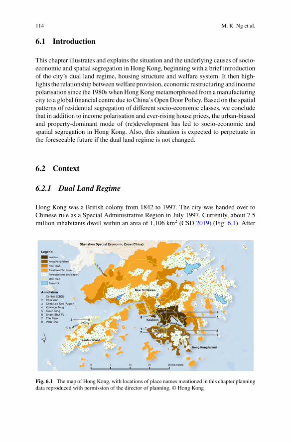
114 M. K. Ng et al.
6.1 Introduction
This chapter illustrates and explains the situation and the underlying causes of socio-economic and spatial segregation in Hong Kong, beginning with a brief introductionof the city’s dual land regime, housing structure and welfare system. It then high-lights the relationship betweenwelfare provision, economic restructuring and incomepolarisation since the 1980s whenHongKongmetamorphosed from amanufacturingcity to a global financial centre due to China’s OpenDoor Policy. Based on the spatialpatterns of residential segregation of different socio-economic classes, we concludethat in addition to income polarisation and ever-rising house prices, the urban-biasedand property-dominant mode of (re)development has led to socio-economic andspatial segregation in Hong Kong. Also, this situation is expected to perpetuate inthe foreseeable future if the dual land regime is not changed.
6.2 Context
6.2.1 Dual Land Regime
Hong Kong was a British colony from 1842 to 1997. The city was handed over toChinese rule as a Special Administrative Region in July 1997. Currently, about 7.5million inhabitants dwell within an area of 1,106 km2 (CSD 2019) (Fig. 6.1). After
Fig. 6.1 The map of Hong Kong, with locations of place names mentioned in this chapter planningdata reproduced with permission of the director of planning. © Hong Kong
6 Dual Land Regime, Income Inequalities and Multifaceted Socio-Economic … 115
excluding Country Parks and Special Areas (as ‘Protected areas’ that occupy 443km2 or 40% of Hong Kong’s total land area) within which urban development isstrictly prohibited, the actual territorial population density is about 11,000 per km2.
However, there is a dual land regime in Hong Kong as reflected in differentpopulation densities between the urbanised areas (Hong Kong Island, Kowloon andnew towns, that is, about 24.1% of land area) with an average population density ofabout 26,000 per km2, and the rural New Territories (with village-type settlements,brownfield sites, agricultural land and green belts, etc.) occupying 35% of the landwith a population density of about 1,000 per km2. Such a striking difference inpopulation density has to do with the city’s colonial history. Colonial Hong Kongstarted with the ceded territories of Hong Kong Island and Kowloon Peninsula in themid-nineteenth century, forming the existing densely populated urban areas. UnlikeHong Kong Island and Kowloon Peninsula, the New Territories where the existenceof indigenous villagers predated the colonists, were only leased to Britain in 1898for 99 years.
Urban development activities in the New Territories were minimal before theurban riots in 1966 and 1967. After the riots, in order to pacify the restless population,the colonial government started to build public housing through developing newtowns in the 1970s (Glaser et al. 1991). Developed from market towns or alongthe coast by land reclamation, the nine new towns now form pockets of denselypopulated urbanised zones in the New Territories. The vast ‘rural’ area in the rest(about 35%) of the New Territories accommodate only around 5.5% or 412,500 ofHong Kong’s 7.5 million population (CSD 2017a). Contrary to the urban areas andnew towns, urban planning was not extended to the rural New Territories until 1991,seven years after a court case that allowed farmland to be converted into storagesites (Lai and Ho 2002). Consequently, massive brownfield sites with a diversity ofland uses emerged, including most notably open storage. They serve the opening andrapid industrialising economy across the border in mainland China (Chau and Lai2004).
To accommodate population growth and economic development, the Hong Konggovernment has relied on massive land reclamation within and beyond VictoriaHarbour and incessant redevelopment of old and low-rise tenement buildings tomakeway for high-rise residential apartments (Ng 1998; Adams and Hastings 2001). Thisurban-biased (re)development strategy has boosted land values and the emergenceof gated private housing estates (Wong et al. 2011) that are unaffordable for mostHong Kong residents. As house prices in Hong Kong rank the top among other worldcities (Gurran and Bramley 2017), many less well-off residents have to rely on publichousing (mostly located in Kowloon and new towns) or move to smaller dwellingsor remote locations.
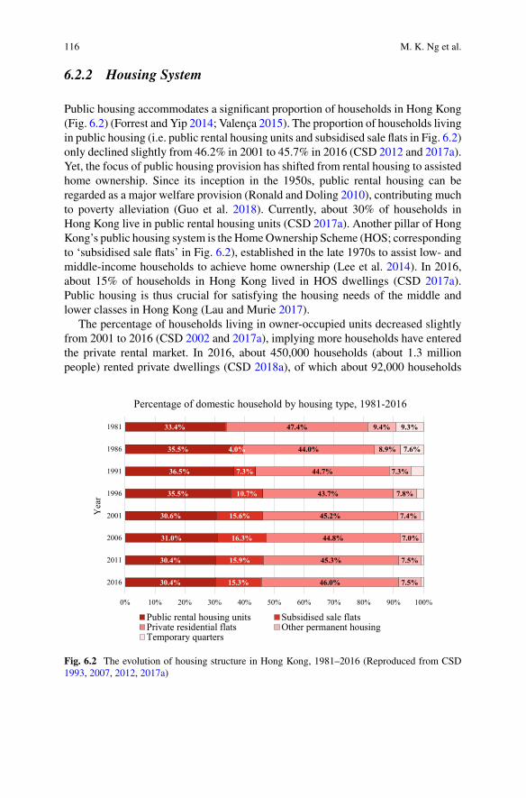
116 M. K. Ng et al.
6.2.2 Housing System
Public housing accommodates a significant proportion of households in Hong Kong(Fig. 6.2) (Forrest and Yip 2014; Valença 2015). The proportion of households livingin public housing (i.e. public rental housing units and subsidised sale flats in Fig. 6.2)only declined slightly from 46.2% in 2001 to 45.7% in 2016 (CSD 2012 and 2017a).Yet, the focus of public housing provision has shifted from rental housing to assistedhome ownership. Since its inception in the 1950s, public rental housing can beregarded as a major welfare provision (Ronald and Doling 2010), contributing muchto poverty alleviation (Guo et al. 2018). Currently, about 30% of households inHong Kong live in public rental housing units (CSD 2017a). Another pillar of HongKong’s public housing system is the HomeOwnership Scheme (HOS; correspondingto ‘subsidised sale flats’ in Fig. 6.2), established in the late 1970s to assist low- andmiddle-income households to achieve home ownership (Lee et al. 2014). In 2016,about 15% of households in Hong Kong lived in HOS dwellings (CSD 2017a).Public housing is thus crucial for satisfying the housing needs of the middle andlower classes in Hong Kong (Lau and Murie 2017).
The percentage of households living in owner-occupied units decreased slightlyfrom 2001 to 2016 (CSD 2002 and 2017a), implying more households have enteredthe private rental market. In 2016, about 450,000 households (about 1.3 millionpeople) rented private dwellings (CSD 2018a), of which about 92,000 households
30.4%
30.4%
31.0%
30.6%
35.5%
36.5%
35.5%
33.4%
15.3%
15.9%
16.3%
15.6%
10.7%
7.3%
4.0%
46.0%
45.3%
44.8%
45.2%
43.7%
44.7%
44.0%
47.4%
7.5%
7.5%
7.0%
7.4%
7.8%
7.3%
8.9%
9.4%
7.6%
9.3%
0% 10% 20% 30% 40% 50% 60% 70% 80% 90% 100%
2016
2011
2006
2001
1996
1991
1986
1981
Yea
r
Percentage of domestic household by housing type, 1981-2016
Public rental housing units Subsidised sale flatsPrivate residential flats Other permanent housingTemporary quarters
Fig. 6.2 The evolution of housing structure in Hong Kong, 1981–2016 (Reproduced from CSD1993, 2007, 2012, 2017a)
6 Dual Land Regime, Income Inequalities and Multifaceted Socio-Economic … 117
(around 210,000 people) lived in subdivided units (CSD 2018b). Given popula-tion growth due to immigration from China, stagnant income levels and skyrock-eting house prices, the population living in subdivided units with harsh conditionsis expected to increase. Meanwhile, the city’s house price to income ratio of 20.9 isone of the highest in the developed world (compared with Singapore: 4.6; New YorkCity: 5.5 and Greater London: 8.3) (Bertaud 2018; Ng 2018). As house prices keepincreasing, property ownership leads to a wideningwealth gap inHongKong. For theindigenous population in rural New Territories, the colonial government introducedthe ‘Small House Policy’ in 1972 to satisfy their housing needs in the course of newtown development. Under this policy, adult male indigenous inhabitants are entitledwith rights to build a village house of 700 ft2 (approx. 65 m2) up to three stories inapproved villages in the New Territories (Hayes 2007).
6.2.3 Welfare System and Inequality
Despite the extensive provision of public housing, Hong Kong has never been awelfare state. The government spending in Hong Kong has been capped to around18%ofGDP,much lower than in theUSA (37.8%), Britain (41.6%) or Japan (38.7%)(Miller et al. 2019). Education is the largest component of recurrent governmentexpenditure, amounting to about 17.3% of total government spending in the 2016/17fiscal year (HKSAR Government 2017a). In September 2009, the 9-year free educa-tion systemwas extended to 12 years, allowing school-age children to receive, respec-tively, 6 years of free primary and secondary education (HKSARGovernment 2008).In addition, subsidised tertiary education is provided by eight universities financedby public funds (HKSAR Government 2018b). Health care also constitutes 17% ofthe government’s total spending. The public sector provides around 74% of inpatientand specialist medical services expenditure. In late 2016, there were around 28,000beds in all public hospitals and institutions under the management of the statutoryHospital Authority (HKSARGovernment 2017a). The bed-population ratio in publichospitals is about 3.8 per 1,000, which is comparable to the aggregate ratio of publicand private hospital beds in Britain (2.8 in 2013), USA (2.9 in 2012), Japan (13.3 in2013) and Singapore (3.2 in 2014) (HKSAR Government 2016).
As of 2019, Hong Kong has no public pension system. Retirement security provi-sion has been delegated to the private sector via theMandatory Provident Fund (MPF)scheme, in operation since 2000. The MPF scheme requires the working populationand employers to contribute an aggregate sum of 10% of individuals’ total monthlysalary to pension schemes offered by the private sector (Sawada 2004; Lee et al.2014). Since the MPF contributions are tied to salaries, the non-working populationis not covered by the MPF scheme. Nevertheless, several cash transfer policies fromthe public sector exist in the city.
An important cash transfer is the Comprehensive Social Security Assistance(CSSA), which is means-tested for the economically vulnerable to support theirbasic needs (SWD 2018a). Between 2001 and 2016, more than half of all CSSA
118 M. K. Ng et al.
recipients were elderly people. There are also two cash benefits for the elderly: OldAge Allowance (OAA) and Old Age Living Allowance (OALA). The former is anon-means-tested allowance given to the elderly aged 70 or above (Lee et al. 2014).The latter, introduced in 2013, is means-tested for poor elderly people aged 65 orabove with monthly income and assets lower than a defined level (SWD 2018b).
Cash transfers and subsidies are also available in transport. To facilitate commu-nity participation and social inclusion of the elderly and the disabled population, aschemewas launched in June 2012 to covermajor transport modes, and the beneficia-ries only need to spend HK$2.0 (US$0.25) for each trip whilst the fare differentialsare subsidised by the government (TD 2018). In January 2019, the government intro-duced the Public Transport Fare Subsidy Scheme. If the monthly transport-relatedexpenditures of commuters exceed HK$400 (US$51.3), the exceeded expenses areentitled to a cash rebate equivalent to 25% of travelling expenditure with a monthlymaximum of HK$300 (US$38.5). This scheme aims particularly at lessening thetransport burden of long-haul commuters in new towns and rural New Territories(HKSAR Government 2018a).
The Gini Index offers a clear indication of income inequality in Hong Kong.Notwithstanding the enhancement ofwelfare provision over recent decades, the indexsoared from 0.451 in 1981, surpassed the 0.5 mark in 1996 and then graduallyclimbed to 0.539 in 2016 (HKSARGovernment 2017b), the largest inequality amongall developed economies (Central Intelligence Agency 2019). Such upward trendsuggests that occupational polarisation due to economic restructuring has broughtabout income polarisation in Hong Kong.
6.3 Census Data and Spatial Units
In this chapter, data obtained from the 2001 and 2011 Population Census and the2016 By-census are used for the segregation analysis. Each dataset consists of datawith nine occupational groups, categorised according to the International StandardClassification of Occupation (ISCO) published by International Labour Organisation(ILO). The ISCO-08 version is applied in the 2011 Census and the 2016 By-census,whilst ISCO-88 is applied in the 2001 Census (CSD 2017b). The nine occupationalgroups are further classified into three large socio-economic status (SES) groupsbased on their income:
Top SES (income) group (TOP)
– Managers and Administrators (MAN)– Professionals (PRO)
Middle SES (income) group (MID)
– Associate Professionals (APR)– Clerical Support Workers (CLE)– Craft and Related Workers (CRA)
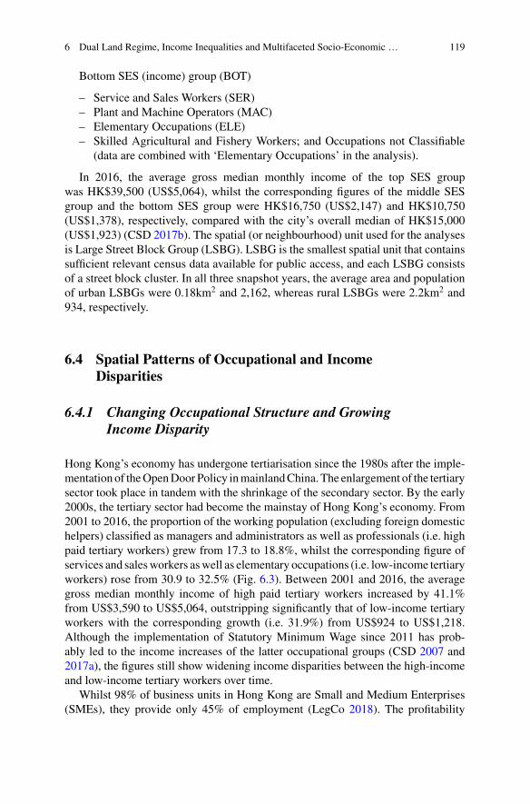
6 Dual Land Regime, Income Inequalities and Multifaceted Socio-Economic … 119
Bottom SES (income) group (BOT)
– Service and Sales Workers (SER)– Plant and Machine Operators (MAC)– Elementary Occupations (ELE)– Skilled Agricultural and Fishery Workers; and Occupations not Classifiable
(data are combined with ‘Elementary Occupations’ in the analysis).
In 2016, the average gross median monthly income of the top SES groupwas HK$39,500 (US$5,064), whilst the corresponding figures of the middle SESgroup and the bottom SES group were HK$16,750 (US$2,147) and HK$10,750(US$1,378), respectively, compared with the city’s overall median of HK$15,000(US$1,923) (CSD 2017b). The spatial (or neighbourhood) unit used for the analysesis Large Street Block Group (LSBG). LSBG is the smallest spatial unit that containssufficient relevant census data available for public access, and each LSBG consistsof a street block cluster. In all three snapshot years, the average area and populationof urban LSBGs were 0.18km2 and 2,162, whereas rural LSBGs were 2.2km2 and934, respectively.
6.4 Spatial Patterns of Occupational and IncomeDisparities
6.4.1 Changing Occupational Structure and GrowingIncome Disparity
Hong Kong’s economy has undergone tertiarisation since the 1980s after the imple-mentation of theOpenDoorPolicy inmainlandChina. The enlargement of the tertiarysector took place in tandem with the shrinkage of the secondary sector. By the early2000s, the tertiary sector had become the mainstay of Hong Kong’s economy. From2001 to 2016, the proportion of the working population (excluding foreign domestichelpers) classified as managers and administrators as well as professionals (i.e. highpaid tertiary workers) grew from 17.3 to 18.8%, whilst the corresponding figure ofservices and salesworkers aswell as elementary occupations (i.e. low-income tertiaryworkers) rose from 30.9 to 32.5% (Fig. 6.3). Between 2001 and 2016, the averagegross median monthly income of high paid tertiary workers increased by 41.1%from US$3,590 to US$5,064, outstripping significantly that of low-income tertiaryworkers with the corresponding growth (i.e. 31.9%) from US$924 to US$1,218.Although the implementation of Statutory Minimum Wage since 2011 has prob-ably led to the income increases of the latter occupational groups (CSD 2007 and2017a), the figures still show widening income disparities between the high-incomeand low-income tertiary workers over time.
Whilst 98% of business units in Hong Kong are Small and Medium Enterprises(SMEs), they provide only 45% of employment (LegCo 2018). The profitability
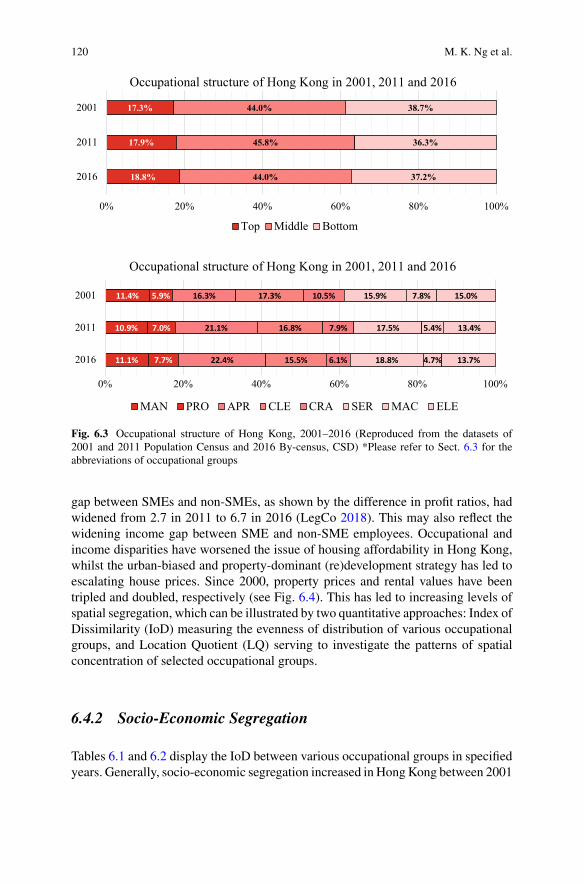
120 M. K. Ng et al.
18.8%
17.9%
17.3%
44.0%
45.8%
44.0%
37.2%
36.3%
38.7%
0% 20% 40% 60% 80% 100%
2016
2011
2001
Occupational structure of Hong Kong in 2001, 2011 and 2016
Top Middle Bottom
11.1%
10.9%
11.4%
7.7%
7.0%
5.9%
22.4%
21.1%
16.3%
15.5%
16.8%
17.3%
6.1%
7.9%
10.5%
18.8%
17.5%
15.9%
4.7%
5.4%
7.8%
13.7%
13.4%
15.0%
0% 20% 40% 60% 80% 100%
2016
2011
2001
Occupational structure of Hong Kong in 2001, 2011 and 2016
MAN PRO APR CLE CRA SER MAC ELE
Fig. 6.3 Occupational structure of Hong Kong, 2001–2016 (Reproduced from the datasets of2001 and 2011 Population Census and 2016 By-census, CSD) *Please refer to Sect. 6.3 for theabbreviations of occupational groups
gap between SMEs and non-SMEs, as shown by the difference in profit ratios, hadwidened from 2.7 in 2011 to 6.7 in 2016 (LegCo 2018). This may also reflect thewidening income gap between SME and non-SME employees. Occupational andincome disparities have worsened the issue of housing affordability in Hong Kong,whilst the urban-biased and property-dominant (re)development strategy has led toescalating house prices. Since 2000, property prices and rental values have beentripled and doubled, respectively (see Fig. 6.4). This has led to increasing levels ofspatial segregation, which can be illustrated by two quantitative approaches: Index ofDissimilarity (IoD) measuring the evenness of distribution of various occupationalgroups, and Location Quotient (LQ) serving to investigate the patterns of spatialconcentration of selected occupational groups.
6.4.2 Socio-Economic Segregation
Tables 6.1 and 6.2 display the IoD between various occupational groups in specifiedyears. Generally, socio-economic segregation increased in HongKong between 2001
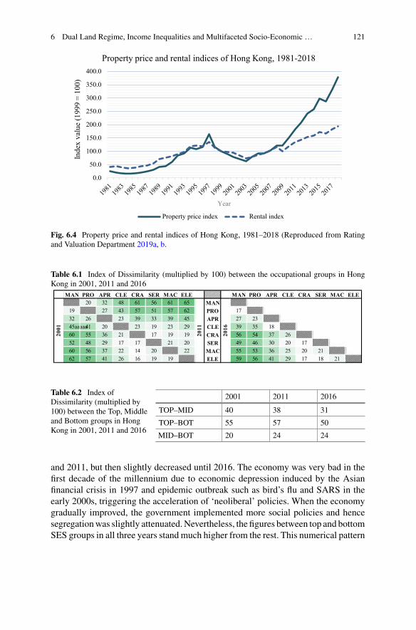
6 Dual Land Regime, Income Inequalities and Multifaceted Socio-Economic … 121
0.0
50.0
100.0
150.0
200.0
250.0
300.0
350.0
400.0In
dex
valu
e (1
999
= 10
0)
Year
Property price and rental indices of Hong Kong, 1981-2018
Property price index Rental index
Fig. 6.4 Property price and rental indices of Hong Kong, 1981–2018 (Reproduced from Ratingand Valuation Department 2019a, b.
Table 6.1 Index of Dissimilarity (multiplied by 100) between the occupational groups in HongKong in 2001, 2011 and 2016
MAN PRO APR CLE CRA SER MAC ELE MAN PRO APR CLE CRA SER MAC ELE20 32 48 61 56 61 65 MAN
19 27 43 57 51 57 62 PRO 1732 26 23 39 33 39 45 APR 27 2345aaaaa41 20 23 19 23 29 CLE 39 35 1860 55 36 21 17 19 19 CRA 56 54 37 2652 48 29 17 17 21 20 SER 49 46 30 20 1760 56 37 22 14 20 22 MAC 55 53 36 25 20 2162 57 41 26 16 19 19 ELE 59 56 41 29 17 18 21
2001
2011
2016
Table 6.2 Index ofDissimilarity (multiplied by100) between the Top, Middleand Bottom groups in HongKong in 2001, 2011 and 2016
2001 2011 2016
TOP–MID 40 38 31
TOP–BOT 55 57 50
MID–BOT 20 24 24
and 2011, but then slightly decreased until 2016. The economy was very bad in thefirst decade of the millennium due to economic depression induced by the Asianfinancial crisis in 1997 and epidemic outbreak such as bird’s flu and SARS in theearly 2000s, triggering the acceleration of ‘neoliberal’ policies. When the economygradually improved, the government implemented more social policies and hencesegregationwas slightly attenuated.Nevertheless, the figures between top and bottomSES groups in all three years stand much higher from the rest. This numerical pattern
122 M. K. Ng et al.
reveals apparent segregation between top and bottomSESworking population aswellas the persistence of self-segregation of the top SES workforce.
6.4.3 Residential Locations of Top and Bottom SESWorkforce
Figure 6.5 shows the distribution of neighbourhoods with top SES working popu-lation in 2001 and 2016. In this figure, all neighbourhoods are categorised into fivequintiles (Q1–Q5), each ofwhich accommodates about 20%ofHongKong’s top SESworking population. Seemingly, quite a number of neighbourhoods with large topSES working populations (Q1–Q3) were initially concentrated in the formally cededterritories of Hong Kong Island and Kowloon. As time passed, more neighbourhoodsin new towns had a large top SES working population. This may contribute to a slimdrop in the extent of segregation. Owing to the compact urban environment of HongKong, neighbourhoods with the largest top SES working population (categorised asQ1) are usually located in high-density residential areas, some of which are coastalareas with beautiful sea views or recently redeveloped districts. Additionally, theseneighbourhoods often consist of middle-class private housing estates and gated resi-dential areas with detached houses. It should, however, be noted that traditionallywealthy residential areas such as southern Hong Kong Island and Kowloon Tong arenot featured in the maps because these districts are of much lower density and hencethey accommodate a smaller number of top SES workers.
There is a huge wealth gap even within the top SES working population, and theprohibitively high house prices in wealthy residential areas in Hong Kong mean thatthese areas are only accessible to a very small percentage of the top SES group. Therest of the topSESworkforce thusmostly live inmore densely populatedmiddle-classresidential areas in which Q1 neighbourhoods are located.
The LQ analysis offers us another perspective to examine residential locations ofvarious SES groups. An LQ value greater and smaller than 1.0 indicates a higher andlower share of an occupational group within a neighbourhood than the city’s overallshare, respectively, whilst a value of 1.0 implies an equal share of an occupationalgroup compared to the city as a whole. Figures 6.6 and 6.7 depict the spatial distri-bution of residence of top SES and bottom SES working population, respectively.According to Fig. 6.6, the residential distribution of top SES working populationin 2001 is clustered around The Peak, southern coast of Hong Kong Island andKowloon Tong. These are areas where luxurious residences and detached housesdominate. Meanwhile, fewer neighbourhoods in the New Territories had their LQexceeding 1.0. The distribution of the top group became more even in 2016 as someneighbourhoods in the New Territories experienced LQ increases due to large-scalelow-density gated residential developments, whilst the LQ decreased in conventionalwealthy residential areas as a result of the reduction of top SES workers who mightmove to the newly completed gated communities in the New Territories. Whilst still
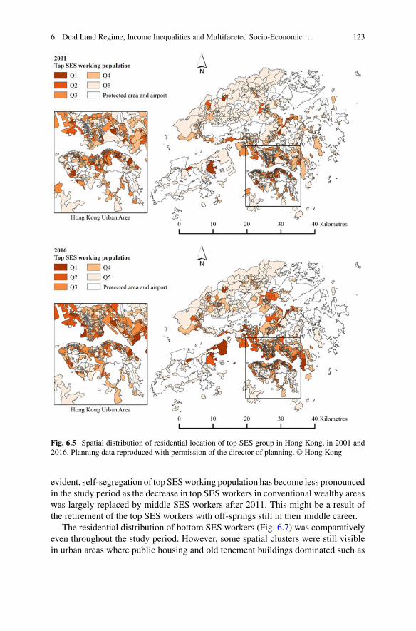
6 Dual Land Regime, Income Inequalities and Multifaceted Socio-Economic … 123
Fig. 6.5 Spatial distribution of residential location of top SES group in Hong Kong, in 2001 and2016. Planning data reproduced with permission of the director of planning. © Hong Kong
evident, self-segregation of top SESworking population has become less pronouncedin the study period as the decrease in top SES workers in conventional wealthy areaswas largely replaced by middle SES workers after 2011. This might be a result ofthe retirement of the top SES workers with off-springs still in their middle career.
The residential distribution of bottom SES workers (Fig. 6.7) was comparativelyeven throughout the study period. However, some spatial clusters were still visiblein urban areas where public housing and old tenement buildings dominated such as
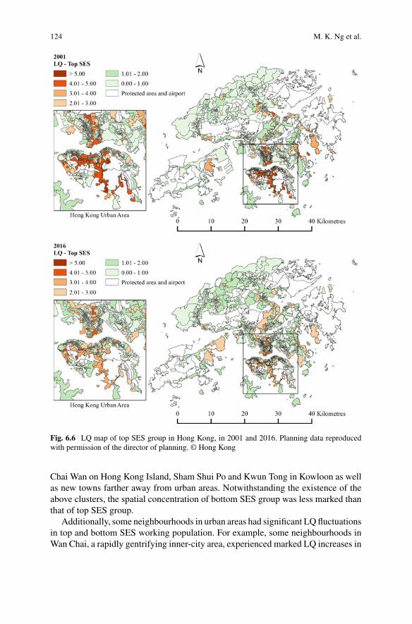
124 M. K. Ng et al.
Fig. 6.6 LQ map of top SES group in Hong Kong, in 2001 and 2016. Planning data reproducedwith permission of the director of planning. © Hong Kong
Chai Wan on Hong Kong Island, Sham Shui Po and Kwun Tong in Kowloon as wellas new towns farther away from urban areas. Notwithstanding the existence of theabove clusters, the spatial concentration of bottom SES group was less marked thanthat of top SES group.
Additionally, some neighbourhoods in urban areas had significant LQ fluctuationsin top and bottom SES working population. For example, some neighbourhoods inWan Chai, a rapidly gentrifying inner-city area, experienced marked LQ increases in
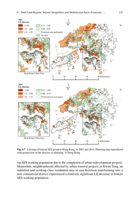
6 Dual Land Regime, Income Inequalities and Multifaceted Socio-Economic … 125
Fig. 6.7 LQmap of bottom SES group in Hong Kong, in 2001 and 2016. Planning data reproducedwith permission of the director of planning. © Hong Kong
top SES working population due to the completion of urban redevelopment projects.Meanwhile, neighbourhoods affected by urban renewal projects in Kwun Tong, anindustrial and working-class residential area in east Kowloon transforming into anew commercial district, experienced a relatively significant LQ decrease in bottomSES working population.
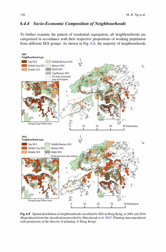
126 M. K. Ng et al.
6.4.4 Socio-Economic Composition of Neighbourhoods
To further examine the pattern of residential segregation, all neighbourhoods arecategorised in accordance with their respective proportions of working populationfrom different SES groups. As shown in Fig. 6.8, the majority of neighbourhoods
Fig. 6.8 Spatial distribution of neighbourhoods classified by SES in Hong Kong, in 2001 and 2016(Reproduced from the classification provided by Marcinczak et al. 2015. Planning data reproducedwith permission of the director of planning. © Hong Kong)
6 Dual Land Regime, Income Inequalities and Multifaceted Socio-Economic … 127
in Hong Kong can be categorised as mixed (Middle/Top or Middle/Bottom) SESneighbourhoods during the study period, meaning that most neighbourhoods aresocio-economically heterogeneous. This situation is probably due to a compact anddense urban living environment where populations with diverse SES have to beaccommodated within small areas. Yet, the distribution of ‘Middle/Top SES’ and‘Middle/Bottom SES’ neighbourhoods is rather distinctive, echoing the distributionof the top and bottom SES workforce.
In urban areas, ‘Middle/Top SES’ neighbourhoods can be found in middle-classand wealthy residential areas, such as the northern coast of Hong Kong Island andcoastal areas of Kowloon Peninsula (where gated private high-rise residential towerswere built), as well as central Kowloon, a low-density residential area. On the otherhand, ‘Middle/Bottom SES’ neighbourhoods are located in inner cities and publichousing areas such as Chai Wan on Hong Kong Island as well as Sham Shui Po andKwun Tong in Kowloon, all of which had low LQs of the top SES working popu-lation. The neighbourhood classification reveals clear socio-economic and spatialsegregation in the urban areas of Hong Kong.
Meanwhile, a minority of neighbourhoods labelled as ‘Middle SES’ and ‘Multi-SES’ neighbourhoods were evenly distributed throughout the urban areas and newtowns without apparent spatial clustering. In new towns, the widespread presence of‘Middle/Bottom SES’ neighbourhoods is probably associated with the prevalenceof public housing, often considered as neighbourhoods for low-income households.There is sporadic existence of ‘Middle/Top SES’ neighbourhoods amidst primarily‘Middle/Bottom SES’ ones. Hence, new towns in Hong Kong could be regarded asresidential areas mainly for the middle and bottom SES population.
Notwithstanding the prevalence of mixed SES neighbourhoods, spatial clusteringof top SES neighbourhoods within luxurious residential areas in urban areas (e.g.The Peak and southern HongKong Island) was clearly observable. However, some ofthese neighbourhoods were no longer dominated by top SES population and became‘Middle/Top SES’ neighbourhoods by the end of the study period. This was probablydue to the departure of top SES population to gentrified urban areas or newly builtgated communities in the New Territories, whilst the population there was replacedbymiddle SES population. Self-segregation of the top SESworkforce takes place notonly in urban, but also in rural areas. In Fig. 6.8, ‘Middle/Top SES’ neighbourhoodsare confined within gated low-density residential areas with detached houses. In themeantime, rural New Territories house the majority of agricultural workers, who areclassified as part of the bottom SES group. Together with other bottom SES workers,they spread evenly in various typical rural settlements, thus giving rise to an extensive‘Middle/Bottom SES’ residential area throughout rural New Territories, particularlyin northwest and northeast New Territories adjacent to the Hong Kong-Shenzhenborder.
128 M. K. Ng et al.
6.5 Underlying Causes for Socio-Spatial Segregation
Socio-spatial segregation in Hong Kong has been attributed to income polarisationdue to economic restructuring together with rising house prices since the 1980s.After the implementation of China’s Open Door Policy in the late 1970s, economicrestructuring in Hong Kong transformed the city into a financial and service hub andChina’s strategic gateway to the global economy. As a consequence, the occupationalstructure of Hong Kong changed, with a shrinking manufacturing sector and anexpanding tertiary sector (see Sect. 4.1). The tertiary sector is subdivided into high-income tertiary sector workers (e.g. managers and administrators, professionals)and low-income tertiary sector workers (e.g. services and sales workers, elementaryoccupations). Although Hong Kong had experienced rapid and continuous economicgrowth until the Asian financial crisis in late 1997 (the year Hong Kong returned toChinese rule), most economic benefits were skewed towards the high-income tertiarysector including the financial and professional sectors. Therefore, top SES workerswho were engaged in related occupations experienced rapid income increases. Onthe contrary, bottom SES workers, many of whom were originally employed in themanufacturing sector that moved out of Hong Kong to mainland China since theearly 1980s, had to enter the low pay tertiary sector, sharing little, if any, benefitfrom economic growth.
Concurrently, soaring house prices over recent decades have made home owner-ship a very remote dream for those in the bottom SES workforce (see Fig. 6.4).Even though bottom SES workers have experienced income increases, these wereseverely outpaced by a massive rise of property and rental values. Therefore, bottomSES workers mostly could not afford to buy private units and have to either apply forpublic rental housing or rent low-cost private units including subdivided flats. Thesetypes of dwellings are mostly located in new towns and in inner-city areas such asSham Shui Po, with relatively high proportions of the impoverished bottom SESworking population (see Fig. 6.7). Given the relatively large population size, segre-gation of the bottom SES workforce was less pronounced than the self-segregationof the top SES workforce over the study period.
Secondly, the urban-biased and property-dominant mode of (re)development ledby the government and property developers have sustained or even intensified socio-spatial segregation in Hong Kong. For many decades, the Hong Kong governmenthas relied on massive reclamation projects to create new land along coastal areasto accommodate urban growth and new town development, whilst the vast ruralland resources in the heart of the New Territories have been largely left untouched.Urban development has thus long been confined to urban areas and new towns.The Hong Kong government, as the city’s dominant landowner under the leaseholdland tenure system, has relied on high land prices and related income as majorsources (at least 20%) of revenue (Wong 2015). As a thriving property sector isindispensable to sustain high land prices, an ‘alliance’ between the government andbig property development tycoons is perceived to have developed in the course ofurban development. To maximise profit from developing valuable land plots, the
6 Dual Land Regime, Income Inequalities and Multifaceted Socio-Economic … 129
planning and building mechanisms have allowed property developers to build high-rise residential blocks, especially in coastal areas with great sea views that often giverise to ‘wall-like buildings’, ‘overshadowing’ old urban areas (Ng et al. 2011; Ng2014;Wong et al. 2011). The exorbitant prices for these housing units mean that onlythe top SES workforce can afford to live there. Hence, coastal areas in both urbanareas and new towns have become primarily top SES neighbourhoods (see Figs. 6.5and 6.6).
Redevelopment is an alternativemeans of recycling scarce land resources in urbanHong Kong. Usually, redevelopment projects are carried out by public–private part-nership between property developers and the Urban Renewal Authority, a statutorybody responsible for facilitating urban redevelopment (Ng 2002; Ye et al. 2015).Therefore, redevelopment projects in the city are directed towards the maximisationof exchange value (Tang 2017) and often result in gentrification of neighbourhoods.As residents affected by redevelopment often cannot afford soaring house priceswithin their original communities of residence, they are often displaced to otherareas with lower rents such as other inner-city areas, new towns (Ye et al. 2015)or even the rural New Territories. Meanwhile, the regenerated built environmentin redeveloped areas can only be afforded by the top SES population. As a result,socio-economic segregation in urban HongKong is also characterised by the infillingof the top SES population into gentrified inner cities and the exodus of the bottomSES population to other inner cities and remote areas. This process is expected toaccentuate in years to come.
Interestingly, it seems that colonial legacies continue to influence the currentsocio-spatial distribution of Hong Kong’s population. In urban areas, the designationof The Peak on Hong Kong Island as a European-exclusive residential zone in thefirst half of the twentieth century (Lai and Yu 2001) and the establishment of a low-density Garden City in Kowloon Tong before World War II had attracted the eliteand affluent population for residence (Forrest et al. 2004; Lo 2005). These residentialareas are still mainly for the top SES population today. In the massive territory of therural New Territories where the colonial government had avoided major investments,except for coastal areas reclaimed for new development, most neighbourhoods areclassified as ‘Middle/Bottom SES’ neighbourhoods.
6.6 Conclusion
The legacies of Hong Kong’s colonial urban development history can still be seen inthe new millennium. Dictated by historical events, a dual land regime can be seen inHong Kong: dense urban development had once been concentrated on Hong KongIsland and Kowloon until the development of new towns in the 1970s; the imple-mentation of a ‘Small House Policy’ since 1972, and the designation of conservationareas, green belts and Sites of Special Scientific Interest in rural New Territories,have led to low population density. Such spatial patterns of urban development andpopulation distribution have sustained a property-dominant mode of urban-biased
130 M. K. Ng et al.
development, a cornerstone of the government’s high land price policy to sustain itscoffer.
Meanwhile, the restructuring (or tertiarisation) of Hong Kong’s economy as aresult of the Open Door Policy in China since the 1980s has led to occupational andincome polarisation among the city’s working population. As depicted by the risingtrend of theGini Index, the income gapwidened constantly despite the improvementsin welfare provision over recent decades. The widening income gap coupled withthe astronomical rise of housing costs also intensified residential segregation in thecity, especially in urban areas and new towns.
As indicated in Tables 6.1, 6.2 and Fig. 6.8, self-segregation of the top SESworking population is arguably one of the key features of socio-spatial segregationin Hong Kong as the IoD levels between top and bottom SES occupational groupsmostly stood at 0.5 or above throughout the study period. Spatial clustering of topSES neighbourhoods is clearly identifiable. In the meantime, the IoD levels betweenmiddle and bottom SES groups as well as between top and middle SES groupsgenerally stayed at 0.4 or below, showing no apparent residential segregation betweenthese occupational groups.
Contrary to other major cities where segregation is characterised by monotonousneighbourhoodswith a dominant SES and/or racial group, segregation inHongKong,due to its dual land regime, is marked by the clustering of two types of socio-economically mixed neighbourhoods: ‘Middle/Top SES’ neighbourhoods in high-and middle-class residential areas and ‘Middle/Bottom SES’ neighbourhoods whereold tenement buildings and public housing dominate. This is especially obvioustowards the end of the study period. Such a dichotomy of socio-economically hetero-geneous neighbourhoods, a consequence of a compact urban environment in the city’sdual urban–rural land and density regimes, demonstrates Hong Kong’s distinctivefeature of residential and socio-economic spatial segregation.
Acknowledgements This research was funded by the Research Grants Council of the Hong KongSpecial Administrative Region, China (grant numbers CUHK14652516 and CUHK14604218).
References
Adams D, Hastings EM (2001) Urban renewal in Hong Kong: transition from development corpo-ration to renewal authority. Land Use Policy 18(3):245–258. https://doi.org/10.1016/S0264-8377(01)00019-9
BertaudA (2018) 15thAnnual demographia international housing affordability survey: 2019,Ratingmiddle-income housing affordability. https://demographia.com/dhi.pdf. 12 Mar 2019
Census and Statistics Department, HKSARGovernment (CSD) (1993) HongKong 1991 populationcensus main report. CSD, Hong Kong
Census and Statistics Department, HKSARGovernment (CSD) (2002) HongKong 2001 populationcensus key statistics. CSD, Hong Kong
Census and Statistics Department, HKSAR Government (CSD) (2007) 2006 population by-censusmain report:, vol I. CSD, Hong Kong
6 Dual Land Regime, Income Inequalities and Multifaceted Socio-Economic … 131
Census and Statistics Department, HKSAR Government (CSD) (2012) 2011 population censusmain report:, vol I. CSD, Hong Kong
Census and Statistics Department, HKSAR Government (CSD) (2017) 2016 population by-census:main results. CSD, Hong Kong
Census and Statistics Department, HKSAR Government (CSD) (2017) 2016 population by-censusthematic report: household income distribution in Hong Kong. CSD, Hong Kong
Census andStatisticsDepartment,HKSARGovernment (CSD) (2018a)TableE213domestic house-holds by district council district,monthly domestic household rent (hk$), year and type of quarters.https://www.bycensus2016.gov.hk/en/bc-mt.html?search=E213.18 Mar 2019
Census and Statistics Department, HKSARGovernment (CSD) (2018b) 2016 population by-censusthematic report: persons living in subdivided units. CSD, Hong Kong
Census and Statistics Department, HKSARGovernment (CSD) (2019) HongKong in figures–2019.CSD, Hong Kong
Central Intelligence Agency (2019) The world factbook 2018. Central intelligence agency. https://www.cia.gov/library/publications/download/download-2018/factbook.zip. 11 Mar 2019
Chau KW, Lai LWC (2004) Planned conversion of rural land: a case study of planning applicationsfor housing and open storage uses in agriculture zones. Environ Plan B: Plan Des 31(6):863–878.https://doi.org/10.1068/b3122
Forrest R, La Grange A, Yip NM et al (2004) Hong Kong as a global city? social distance and spatialdifferentiation. Urban Stud 41(1):207–227. https://doi.org/10.1080/0042098032000155759
Forrest R, Yip NM (2014) The future for reluctant intervention: the prospects for Hong Kong’spublic rental sector. Hous Stud 29(4):551–565. https://doi.org/10.1080/02673037.2013.878020
Glaser R, Haberzettl P, Walsh RPD et al (1991) Land reclamation in Singapore, Hong Kong andMacau. Geo J 24(4):365–373
Guo Y, Chang SS, Sha F, Yip PSF et al (2018) Poverty concentration in an affluent city: geographicvariation and correlates of neighborhood poverty rates in Hong Kong. PLoS ONE. https://doi.org/10.1371/journal.pone.0190566
Gurran N, Bramley G (2017) Urban planning and the housing market—international perspectivesfor policy and practice. Palgrave Macmillan, London
Hayes J (2007) The great difference: hong kong’s new territories and its people 1898–2004. HongKong University Press, Hong Kong
HKSAR Government (2008) 2007–08 policy address. https://www.policyaddress.gov.hk/07-08/eng/policy.html. 15 Jan 2019
HKSAR Government (2016) Public health. In: Hong Kong: the facts.HKSAR government. https://www.gov.hk/en/about/abouthk/factsheets/docs/public_health.pdf. 11Mar 2019
HKSAR Government (2017) Hong Kong yearbook 2016. HKSAR Government, Hong KongHKSAR Government (2017b) Half-yearly economic report 2017. HKSAR government.https://www.hkeconomy.gov.hk/en/pdf/er_17q2.pdf. 13 Dec 2018
HKSARGovernment (2018a)TDannounced implementation details of public transport fare subsidyscheme. (Press release) https://www.info.gov.hk/gia/general/201811/01/P2018110100588.htm.15 Jan 2019
HKSAR Government (2018b) Education. In: Hong Kong: the facts. HKSAR government. https://www.edb.gov.hk/attachment/en/about-edb/publications-stat/hk_thefacts_education/HK_TheFacts_Education_EN.pdf. 11Mar 2019
Lai LW, Yu MK (2001) The rise and fall of discriminatory zoning in Hong Kong. Environ Plan B:Plan Des 28(2):295–314. https://doi.org/10.1068/b2720
Lai LW, Ho WK (2002) Planning for open storage of containers in a major international containertrade centre: an analysis of Hong Kong development control statistics using probit modelling.Environ Plan B: Plan Des 29(4):571–587. https://doi.org/10.1068/b12819
Lau KY, Murie A (2017) Residualisation and resilience: public housing in Hong Kong. Hous Stud32(3):271–295. https://doi.org/10.1080/02673037.2016.1194376
Lee KM, To BHP, Yu KM et al (2014) The new paradox of thrift: financialisation, retirementprotection, and income polarisation in Hong Kong. China Perspect 1:15–24
132 M. K. Ng et al.
Legislative Council, HKSAR Government (LegCo) (2018) Small and medium enterprises. In:Statistical highlights–commerce and industry. LegCo. https://www.legco.gov.hk/research-publications/english/1718issh28-small-and-medium-enterprises-20180608-e.pdf. 11Mar 2019
Lo CP (2005) Decentralization and polarization: contradictory trends in Hong Kong’s postcolonialsocial landscape. Urban Geogr 26(1):36–60. https://doi.org/10.2747/0272-3638.26.1.36
Marcinczak S, TammaruT,Novák J,GentileM,Kovács Z, Temelová J,ValatkaV,KährikA, SzabóBet al (2015) Patterns of socioeconomic segregation in the capital cities of fast-track reforming post-socialist countries. Ann Assoc Am Geogr 105(1):183–202. https://doi.org/10.1080/00045608.2014.968977
Miller T, Kim AB, Roberts JM, et al (2019) 2019 Index of economic freedom: 25th anniversaryedition. The heritage foundation. https://www.heritage.org/index/pdf/2019/book/index_2019.pdf. 11 Mar 2019
Ng E, Yuan C, Chen L, Ren C, Fung JC et al (2011) Improving the wind environment in high-densitycities by understanding urban morphology and surface roughness: a study in Hong Kong. LandscUrban Plan 101(1):59–74. https://doi.org/10.1016/j.landurbplan.2011.01.004
Ng I (1998) Urban redevelopment in Hong Kong: the partnership experience. Int J Public SectManag 11(5):414–420. https://doi.org/10.1108/09513559810226879
Ng MK (2002) Property-led urban renewal in Hong Kong: any place for the community? SustainDev 10(3):140–146. https://doi.org/10.1002/sd.189
Ng MK (2014) The state of planning rights in Hong Kong: a case study of ‘wall-like building.’Town Plan Rev 85(4):489–511. https://doi.org/10.3828/tpr.2014.28
Ng MK (2018) Transformative urbanism and reproblematising land scarcity in Hong Kong. UrbanStud. https://doi.org/10.1177/0042098018800399
Rating and Valuation Department, HKSAR Government (2019a) Price indices by class (Territory-wide) (from1979). https://www.rvd.gov.hk/en/property_market_statistics/index.html. 5 Jun 2019
Rating and Valuation Department, HKSARGovernment (2019b) Rental indices by class (Territory-wide) (from1979). https://www.rvd.gov.hk/en/property_market_statistics/index.html. 5 Jun 2019
Ronald R, Doling J (2010) Shifting East Asian approaches to home ownership and the housingwelfare pillar. Int J Hous Policy 10(3):233–254. https://doi.org/10.1080/14616718.2010.506740
Sawada Y (2004) The social security system in Hong Kong: establishment and readjustment of theliberal welfare model. Dev Econ 42(2):198–216. https://doi.org/10.1111/j.1746-1049.2004.tb01063.x
Social Welfare Department, HKSAR Government (SWD) (2018a) Comprehensive social secu-rity allowance (CSSA) scheme.https://www.swd.gov.hk/en/index/site_pubsvc/page_socsecu/sub_comprehens/index.html. 15 Jan 2019
SocialWelfare Department, HKSARGovernment (SWD) (2018b) Old age living allowance. https://www.swd.gov.hk/oala/index_e.html. 15 Jan 2019
Tang WS (2017) Beyond gentrification: hegemonic redevelopment in Hong Kong. Int J Urban RegRes 41(3):487–499. https://doi.org/10.1111/1468-2427.12496
Transport Department, HKSARGovernment (TD) (2018) Government public transport fare conces-sion scheme for the elderly and eligible persons with disabilities.https://www.td.gov.hk/en/gov_public_transport_fare_concession/index.html. 15 Jan 2019
Valença MM (2015) Social rental housing in HK and the UK: Neoliberal policy divergence orthe market in the making? Habitat International 49:107–114. https://doi.org/10.1016/j.habitatint.2015.05.017
Wong MS, Nichol J, Ng E et al (2011) A study of the ‘wall effect’ caused by proliferation ofhigh-rise buildings using GIS techniques. Landsc Urban Plan 102(4):245–253. https://doi.org/10.1016/j.landurbplan.2011.05.003
Wong SHW (2015) Real estate elite, economic development, and political conflicts in postcolonialHong Kong. China Rev 15(1):1–38
Ye M, Vojnovic I, Chen G et al (2015) The landscape of gentrification: exploring the diversity of‘upgrading’ processes in Hong Kong, 1986–2006. Urban Geogr 36(4):471–503. https://doi.org/10.1080/02723638.2015.1010795

6 Dual Land Regime, Income Inequalities and Multifaceted Socio-Economic … 133
Open Access This chapter is licensed under the terms of the Creative Commons Attribution 4.0International License (http://creativecommons.org/licenses/by/4.0/), which permits use, sharing,adaptation, distribution and reproduction in any medium or format, as long as you give appropriatecredit to the original author(s) and the source, provide a link to the Creative Commons license andindicate if changes were made.
The images or other third party material in this chapter are included in the chapter’s CreativeCommons license, unless indicated otherwise in a credit line to the material. If material is notincluded in the chapter’s Creative Commons license and your intended use is not permitted bystatutory regulation or exceeds the permitted use, you will need to obtain permission directly fromthe copyright holder.
Chapter 7Income Inequality and SocioeconomicSegregation in Jakarta
Deden Rukmana and Dinar Ramadhani
Abstract Socioeconomic segregation has become a common phenomenon, both inthe Global North and Global South, and highly relates to income inequality. Themerging of these two notions affects the geography of residential areas which arebased on the socio-occupational composition. This chapter focuses on the JakartaMetropolitan Area (JMA). Not only is Jakarta the largest metropolitan area in South-east Asia, it is also one of the most dynamic. Batavia, the colonial capital of theformer Dutch East Indies in the first half of the twentieth century, was a smallurban area of approximately 150,000 residents. In the second half of the century,Batavia became Jakarta, a megacity of 31 million people and the capital of inde-pendent Indonesia was beset with most of the same urban problems experiencedin twenty-first-century Southeast Asia, including poverty, income inequality, andsocioeconomic segregation. This study aims to identify the correlation among incomeinequality, socioeconomic segregation, and other institutional and contextual factorswhich caused residential segregation in JMA. The analysis consists of two stages.First, we examine income inequality measured by the Gini Index as well as the occu-pational structure based on the International Standard Classification of Occupations(ISCO). Second, we investigate residential segregation by using the DissimilarityIndex as a result of socioeconomic intermixing in residential areas. The data in thisstudy comes from multiple sources including Indonesia’s Central Bureau of Statis-tics, Indonesia’s National Socio-economic Survey (Susenas), Indonesia’s EconomicCensus, Jakarta’s Regional Bureau of Statistics, and policies related to the housingsystem and investment in the JMA. This study also produces maps of socioeconomicsegregation patterns from several sources including Jakarta’s Geospatial InformationCentre, Jakarta’s Spatial Plan Information System, and the Indonesian Poverty Mapby the SMERU Research Institute.
D. Rukmana (B)Alabama A&M University, Huntsvill, USAe-mail: [email protected]
D. RamadhaniBandung Institute of Technology, Bandung, Indonesiae-mail: [email protected]
© The Author(s) 2021M. van Ham et al. (eds.), Urban Socio-Economic Segregation and Income Inequality,The Urban Book Series, https://doi.org/10.1007/978-3-030-64569-4_7
135
136 D. Rukmana and D. Ramadhani
Keywords Income inequality · Residential segregation · Rapid urbanization ·Jakarta
7.1 Introduction
Socioeconomic segregation has become a common phenomenon, both in the GlobalNorth and theGlobal South, and is strongly related to income inequality. The residen-tial geography of income inequality represents where different income groups live,but also affects an individual’s spatial opportunity structures. This study will focuson residential segregation in the metropolitan region of Jakarta. Not only is Jakartathe largest metropolitan area in Southeast Asia, it is also one of the most dynamic.Batavia, which used to be the colonial capital of the Dutch East Indies in the first halfof the twentieth century was a small urban area of approximately 150,000 residents.In the second half of the twentieth century, Batavia became Jakarta, a megacity of31 million people and the capital of independent Indonesia was beset with most ofthe same urban problems experienced in twenty-first-century Southeast Asia.
The modern city of Jakarta was envisioned by President Soekarno in the early1960s. He used the 1962 Asian Games to modernize Jakarta by building the nationalmonument of Monas, government and parliament buildings, shopping plazas, thenational stadium, and hotels. The New Order regime continued such developmentwhile Indonesia enjoyed steady economic growth during the 1980s and 1990s. Theboom of the property sector through foreign and domestic investments transformedJakarta as it gained the status as a global city. Jakarta has been the powerhouse ofIndonesia’s economy since the colonial era due to its high concentration of skilledlabor and entrepreneurs and Jakarta’s dominance in the financial and business sector(Firman 2008; Salim andKombaitan 2009). Jakarta is also themost attractive area fordomestic and foreign investment in Indonesia. Jakarta’s contribution to Indonesia’sGDP increased from 14.9% in 2000 to 16.7% in 2010 and 17.5% in 2016.
Despite robust development and economic growth, Jakarta remains a place ofpoverty. The contrast between rich and poor is highly pronounced in many partsof the city (Prasetyanti 2015; Salim et al. 2019). Many modern towers in Jakartaare surrounded by kampungs, which are unplanned, incrementally developed areaswith small plots of land and low-quality building structures and materials and areoften associated with slums (Winarso 2010). Most of the inhabitants of kampungsare low-income residents.
This chapter explores income inequality and residential segregation betweensocioeconomic groups in Jakarta, and the institutional and contextual factors thatcause residential segregation in the metropolitan region of Jakarta. The analysisconsists of two stages. First, we examine income inequality measured by the GiniIndex as well as the occupational structure based on the International Standard Clas-sification of Occupations (ISCO). Second, we investigate residential segregationby using the Location Quotients (LQs) and the Dissimilarity Index as a result ofsocioeconomic intermixing in residential areas.
7 Income Inequality and Socioeconomic Segregation in Jakarta 137
This chapter uses data frommultiple sources including Indonesia’sCentral Bureauof Statistics, the National Socio-Economic Survey (Susenas), the National LaborForce Survey (Sakernas), and the Jakarta’s Regional Bureau of Statistics, as wellas policies related to the housing system and investment in the metropolitan regionof Jakarta. The study will also create maps representing socioeconomic segrega-tion patterns and the data will be obtained from several sources including Jakarta’sGeospatial Information Centre, Jakarta’s Spatial Plan Information System, and theIndonesian Poverty Map by the SMERU Research Institute.
7.2 Jakarta: The Core, Inner Peripheries and OuterPeripheries
Jakarta is the capital of Indonesia and the largest city inSoutheastAsia. The core of themetropolitan region of Jakarta is calledDaerah Khusus Ibukota (DKI) or the SpecialCapital Region of Jakarta. DKI Jakarta has provincial government level status andcovers a total area of 664 square kilometers. DKI Jakarta consists of five municipali-ties (West Jakarta City, East Jakarta City, Central Jakarta City, North Jakarta City, andSouth Jakarta City) and 42 districts (kecamatan). The metropolitan region of Jakartais popularly known as Jabodetabek, taken from the initial letters of the administra-tive units of Jakarta, Bogor, Depok, Tangerang, and Bekasi. Jabodetabek consistsof the core, inner peripheries, and outer peripheries. The inner peripheries of themetropolitan region of Jakarta include four municipalities (City of Tangerang, Cityof South Tangerang, City of Depok, City of Bekasi), whereas the outer peripheriesof Jabodetabek include the City of Bogor, Tangerang Regency, and Bekasi Regency.The peripheries of Jabodetabek are within the jurisdiction of two provinces. The Cityof Bogor, City of Depok, City of Bekasi, and Bekasi Regency are within the juris-diction of West Java Province, whereas Tangerang City, City of South Tangerang,and Tangerang Regency are within the jurisdiction of Banten Province as shownin Fig. 7.1. The metropolitan region of Jakarta covers a total area of 6,392 squarekilometers. The four municipalities within the inner peripheries of Jabodetabek arefounded in the 1990s and 2000s. Tangerang City, City of Bekasi, City of Depok,and City of South Tangerang were founded in 1993, 1996, 1999, and 2008, respec-tively. Depok City seceded from Bogor Regency and Bekasi City was part of BekasiRegency. Meanwhile, Tangerang City and City of South Tangerang seceded fromTangerang Regency.
The population of Jakarta was about 115,000 in 1900, and increased to 544,823in 1940. After Independence, Jakarta’s population increased by nearly three timesto 1.43 million in 1950. It increased to 2.91 million in 1960 and 4.47 million in1970. Table 7.1 shows the population of the metropolitan region of Jakarta includingJakarta, the inner and outer peripheries of Jakarta, from 1990 to 2010 and 2015. Alldata come from the population censuses, except the population data of 2015 fromthe intercensal survey of Indonesia (SUPAS). The population of the metropolitan
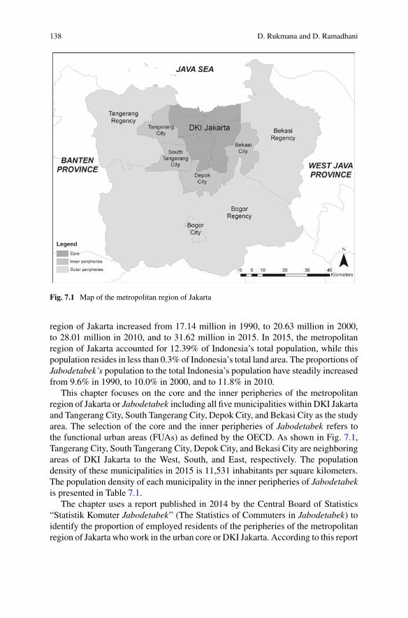
138 D. Rukmana and D. Ramadhani
Fig. 7.1 Map of the metropolitan region of Jakarta
region of Jakarta increased from 17.14 million in 1990, to 20.63 million in 2000,to 28.01 million in 2010, and to 31.62 million in 2015. In 2015, the metropolitanregion of Jakarta accounted for 12.39% of Indonesia’s total population, while thispopulation resides in less than 0.3% of Indonesia’s total land area. The proportions ofJabodetabek’s population to the total Indonesia’s population have steadily increasedfrom 9.6% in 1990, to 10.0% in 2000, and to 11.8% in 2010.
This chapter focuses on the core and the inner peripheries of the metropolitanregion of Jakarta or Jabodetabek including all five municipalities within DKI Jakartaand Tangerang City, South Tangerang City, Depok City, and Bekasi City as the studyarea. The selection of the core and the inner peripheries of Jabodetabek refers tothe functional urban areas (FUAs) as defined by the OECD. As shown in Fig. 7.1,Tangerang City, South Tangerang City, Depok City, and Bekasi City are neighboringareas of DKI Jakarta to the West, South, and East, respectively. The populationdensity of these municipalities in 2015 is 11,531 inhabitants per square kilometers.The population density of each municipality in the inner peripheries of Jabodetabekis presented in Table 7.1.
The chapter uses a report published in 2014 by the Central Board of Statistics“Statistik Komuter Jabodetabek” (The Statistics of Commuters in Jabodetabek) toidentify the proportion of employed residents of the peripheries of the metropolitanregion of Jakarta who work in the urban core or DKI Jakarta. According to this report
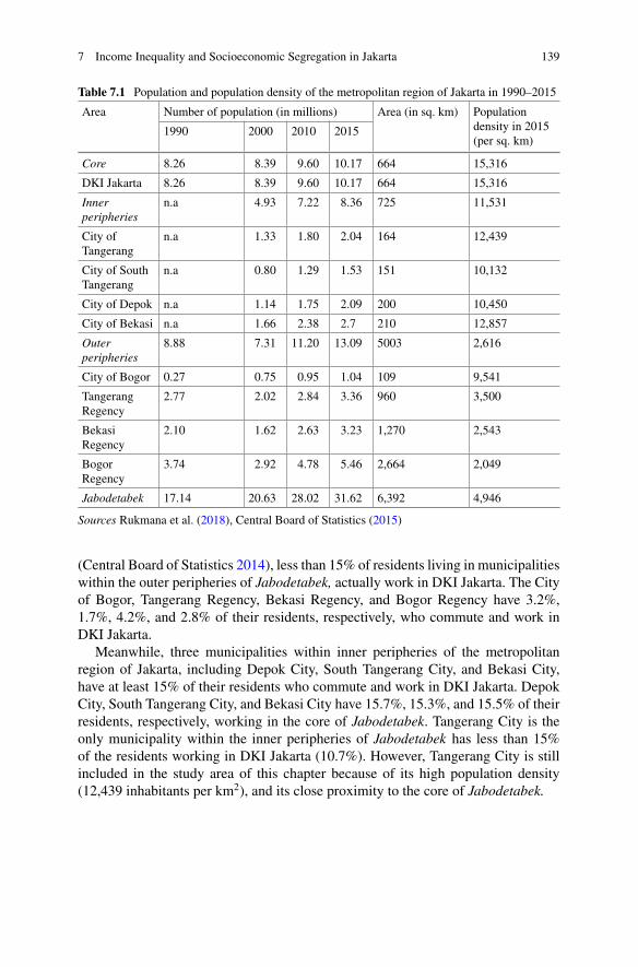
7 Income Inequality and Socioeconomic Segregation in Jakarta 139
Table 7.1 Population and population density of the metropolitan region of Jakarta in 1990–2015
Area Number of population (in millions) Area (in sq. km) Populationdensity in 2015(per sq. km)
1990 2000 2010 2015
Core 8.26 8.39 9.60 10.17 664 15,316
DKI Jakarta 8.26 8.39 9.60 10.17 664 15,316
Innerperipheries
n.a 4.93 7.22 8.36 725 11,531
City ofTangerang
n.a 1.33 1.80 2.04 164 12,439
City of SouthTangerang
n.a 0.80 1.29 1.53 151 10,132
City of Depok n.a 1.14 1.75 2.09 200 10,450
City of Bekasi n.a 1.66 2.38 2.7 210 12,857
Outerperipheries
8.88 7.31 11.20 13.09 5003 2,616
City of Bogor 0.27 0.75 0.95 1.04 109 9,541
TangerangRegency
2.77 2.02 2.84 3.36 960 3,500
BekasiRegency
2.10 1.62 2.63 3.23 1,270 2,543
BogorRegency
3.74 2.92 4.78 5.46 2,664 2,049
Jabodetabek 17.14 20.63 28.02 31.62 6,392 4,946
Sources Rukmana et al. (2018), Central Board of Statistics (2015)
(Central Board of Statistics 2014), less than 15% of residents living in municipalitieswithin the outer peripheries of Jabodetabek, actually work in DKI Jakarta. The Cityof Bogor, Tangerang Regency, Bekasi Regency, and Bogor Regency have 3.2%,1.7%, 4.2%, and 2.8% of their residents, respectively, who commute and work inDKI Jakarta.
Meanwhile, three municipalities within inner peripheries of the metropolitanregion of Jakarta, including Depok City, South Tangerang City, and Bekasi City,have at least 15% of their residents who commute and work in DKI Jakarta. DepokCity, South Tangerang City, and Bekasi City have 15.7%, 15.3%, and 15.5% of theirresidents, respectively, working in the core of Jabodetabek. Tangerang City is theonly municipality within the inner peripheries of Jabodetabek has less than 15%of the residents working in DKI Jakarta (10.7%). However, Tangerang City is stillincluded in the study area of this chapter because of its high population density(12,439 inhabitants per km2), and its close proximity to the core of Jabodetabek.
140 D. Rukmana and D. Ramadhani
7.3 Rapid Urbanization and Income Inequality
Jakarta experienced rapid urbanization in the 1980s and 1990s. The population ofthe core area of Jabodetabek or DKI Jakarta increased from 6.50 million in 1980to 8.26 million in 1990. The population of the peripheries of Jabodetabek increasedfrom 5.41 million to 8.88 million in the same period (Rukmana et al. 2018). Inthe 1990s, Jakarta sustained the rapid growth of population, but the growth occurredmostly in the peripheries. The core area of Jabodetabek experienced a slow growth ofpopulation of 0.15% per year, but the peripheries of Jabodetabek experienced a veryhigh growth of population of 3.78% per year. In addition to a high population growthand rural-to-urban migration, this rapid suburbanization was a result of Indonesia’ssteady economic growth and Indonesia’s growing linkages to the world economy(Herlambang et al. 2019; Indraprahasta and Derudder 2019; Leaf 1994; Winarsoet al. 2015). In the early 1980s, agricultural areas and forests in the outskirts ofJakarta were transformed into large-scale subdivisions and new towns (Silver 2008).Jakarta’s suburbanization followed the development of a network of freeways fromJakarta to the peripheries including the Jagorawi toll road, the Jakarta-Merak tollroad, and the Jakarta-Cikampek toll road (Henderson and Kuncoro 1996).
The urban development in the peripheries of Jabodetabek is a planned or regu-lated process (Leaf 1994). It contrasts the unregulated urban growth in the Jakarta’skampungs. Suburban development in Jakarta is made up of large-scale housingprojects and new town developments by private developers. These housing projectsand new towns are sold to mostly middle and upper-income residents (Firman 2004;Leaf 1994). Some of the new towns have excellent infrastructure and facilities,including shopping malls, hospitals, and golf courses. Many middle and upper-income residents moved from the core of the urban region to new towns in theperipheries. The poor and lower middle-income residents of the metropolitan regionof Jakarta still live in unplanned and unregulated settlements of kampungs locatedin both the core area and in the peripheries. Most residents in kampungs own theirhousing units, built with low-quality building materials on small plots of land. Mostof the dwellings are constructed gradually by the residents from permanent and non-permanent materials, depending largely on what the residents can afford (Tunas andPeresthu 2010). Many poor kampung residents in the metropolitan region of Jakartaare marginalized urban residents who illegally construct their dwellings on state landsuch as riverbanks, disposal sites, and railway tracks, or on private unoccupied land(Rukmana 2018; Winayanti and Lang 2004).
Jakarta is a city of dualistic contrasts (Leaf 1994). The new suburban settlementsor the ‘modern’ city are associated with wealth, formality, and globalized standardsof urban development. Meanwhile, the kampung city is associated with poverty,informality, and traditional standards of living. The existence of new suburbancommunities and kampungs in Jakarta reflects the socioeconomic dualism whichpervades Indonesia’s urban society (Leaf 1994; Winarso 2010). The dualism ofJakarta’s society also reflects the widening socioeconomic disparities and residen-tial segregation based on income level and lifestyle. Firman (2004) argues that the
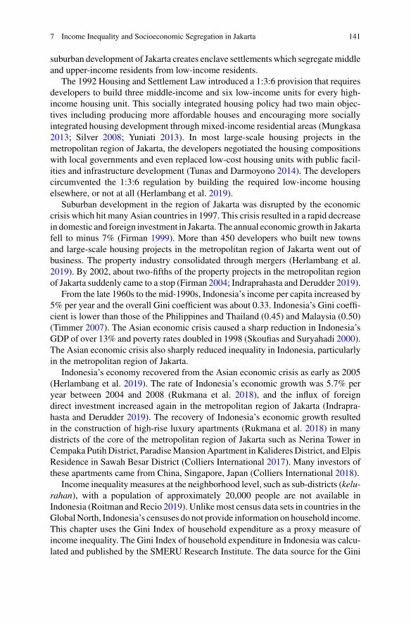
7 Income Inequality and Socioeconomic Segregation in Jakarta 141
suburban development of Jakarta creates enclave settlements which segregate middleand upper-income residents from low-income residents.
The 1992 Housing and Settlement Law introduced a 1:3:6 provision that requiresdevelopers to build three middle-income and six low-income units for every high-income housing unit. This socially integrated housing policy had two main objec-tives including producing more affordable houses and encouraging more sociallyintegrated housing development through mixed-income residential areas (Mungkasa2013; Silver 2008; Yuniati 2013). In most large-scale housing projects in themetropolitan region of Jakarta, the developers negotiated the housing compositionswith local governments and even replaced low-cost housing units with public facil-ities and infrastructure development (Tunas and Darmoyono 2014). The developerscircumvented the 1:3:6 regulation by building the required low-income housingelsewhere, or not at all (Herlambang et al. 2019).
Suburban development in the region of Jakarta was disrupted by the economiccrisis which hit many Asian countries in 1997. This crisis resulted in a rapid decreasein domestic and foreign investment in Jakarta. The annual economic growth in Jakartafell to minus 7% (Firman 1999). More than 450 developers who built new townsand large-scale housing projects in the metropolitan region of Jakarta went out ofbusiness. The property industry consolidated through mergers (Herlambang et al.2019). By 2002, about two-fifths of the property projects in the metropolitan regionof Jakarta suddenly came to a stop (Firman 2004; Indraprahasta and Derudder 2019).
From the late 1960s to the mid-1990s, Indonesia’s income per capita increased by5% per year and the overall Gini coefficient was about 0.33. Indonesia’s Gini coeffi-cient is lower than those of the Philippines and Thailand (0.45) and Malaysia (0.50)(Timmer 2007). The Asian economic crisis caused a sharp reduction in Indonesia’sGDP of over 13% and poverty rates doubled in 1998 (Skoufias and Suryahadi 2000).The Asian economic crisis also sharply reduced inequality in Indonesia, particularlyin the metropolitan region of Jakarta.
Indonesia’s economy recovered from the Asian economic crisis as early as 2005(Herlambang et al. 2019). The rate of Indonesia’s economic growth was 5.7% peryear between 2004 and 2008 (Rukmana et al. 2018), and the influx of foreigndirect investment increased again in the metropolitan region of Jakarta (Indrapra-hasta and Derudder 2019). The recovery of Indonesia’s economic growth resultedin the construction of high-rise luxury apartments (Rukmana et al. 2018) in manydistricts of the core of the metropolitan region of Jakarta such as Nerina Tower inCempaka PutihDistrict, ParadiseMansionApartment inKalideresDistrict, and ElpisResidence in Sawah Besar District (Colliers International 2017). Many investors ofthese apartments came from China, Singapore, Japan (Colliers International 2018).
Income inequality measures at the neighborhood level, such as sub-districts (kelu-rahan), with a population of approximately 20,000 people are not available inIndonesia (Roitman and Recio 2019). Unlikemost census data sets in countries in theGlobalNorth, Indonesia’s censuses do not provide information on household income.This chapter uses the Gini Index of household expenditure as a proxy measure ofincome inequality. The Gini Index of household expenditure in Indonesia was calcu-lated and published by the SMERU Research Institute. The data source for the Gini
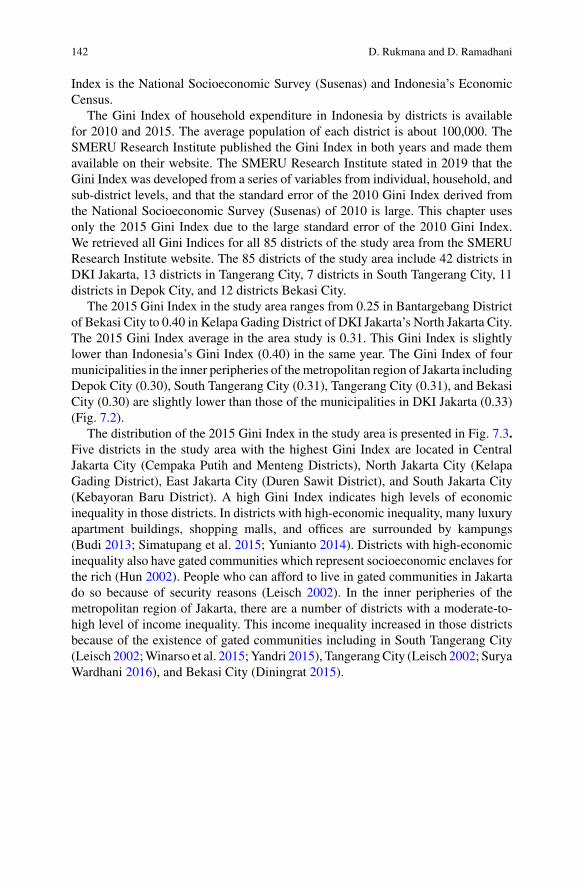
142 D. Rukmana and D. Ramadhani
Index is the National Socioeconomic Survey (Susenas) and Indonesia’s EconomicCensus.
The Gini Index of household expenditure in Indonesia by districts is availablefor 2010 and 2015. The average population of each district is about 100,000. TheSMERU Research Institute published the Gini Index in both years and made themavailable on their website. The SMERU Research Institute stated in 2019 that theGini Index was developed from a series of variables from individual, household, andsub-district levels, and that the standard error of the 2010 Gini Index derived fromthe National Socioeconomic Survey (Susenas) of 2010 is large. This chapter usesonly the 2015 Gini Index due to the large standard error of the 2010 Gini Index.We retrieved all Gini Indices for all 85 districts of the study area from the SMERUResearch Institute website. The 85 districts of the study area include 42 districts inDKI Jakarta, 13 districts in Tangerang City, 7 districts in South Tangerang City, 11districts in Depok City, and 12 districts Bekasi City.
The 2015 Gini Index in the study area ranges from 0.25 in Bantargebang Districtof Bekasi City to 0.40 in Kelapa Gading District of DKI Jakarta’s North Jakarta City.The 2015 Gini Index average in the area study is 0.31. This Gini Index is slightlylower than Indonesia’s Gini Index (0.40) in the same year. The Gini Index of fourmunicipalities in the inner peripheries of themetropolitan region of Jakarta includingDepok City (0.30), South Tangerang City (0.31), Tangerang City (0.31), and BekasiCity (0.30) are slightly lower than those of the municipalities in DKI Jakarta (0.33)(Fig. 7.2).
The distribution of the 2015 Gini Index in the study area is presented in Fig. 7.3.Five districts in the study area with the highest Gini Index are located in CentralJakarta City (Cempaka Putih and Menteng Districts), North Jakarta City (KelapaGading District), East Jakarta City (Duren Sawit District), and South Jakarta City(Kebayoran Baru District). A high Gini Index indicates high levels of economicinequality in those districts. In districts with high-economic inequality, many luxuryapartment buildings, shopping malls, and offices are surrounded by kampungs(Budi 2013; Simatupang et al. 2015; Yunianto 2014). Districts with high-economicinequality also have gated communities which represent socioeconomic enclaves forthe rich (Hun 2002). People who can afford to live in gated communities in Jakartado so because of security reasons (Leisch 2002). In the inner peripheries of themetropolitan region of Jakarta, there are a number of districts with a moderate-to-high level of income inequality. This income inequality increased in those districtsbecause of the existence of gated communities including in South Tangerang City(Leisch 2002;Winarso et al. 2015;Yandri 2015), TangerangCity (Leisch 2002; SuryaWardhani 2016), and Bekasi City (Diningrat 2015).
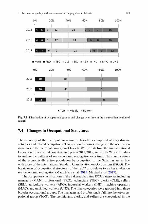
7 Income Inequality and Socioeconomic Segregation in Jakarta 143
4
4
4
7
6
6
6
5
5
9
12
12
29
24
23
1
1
1
6
6
7
9
8
9
12
16
16
0% 20% 40% 60% 80% 100%
2018
2015
2011
MAN PRO TEC CLE SEL AGR IND MAC UNS
11
10
10
44
41
40
28
31
33
0% 20% 40% 60% 80% 100%
2018
2015
2011
Top Middle Bo om
Fig. 7.2 Distribution of occupational groups and change over time in the metropolitan region ofJakarta
7.4 Changes in Occupational Structures
The economy of the metropolitan region of Jakarta is composed of very diverseactivities and related occupations. This section discusses changes in the occupationstructures in themetropolitan region of Jakarta.We use data from the annual NationalLabor ForceSurvey (Sakernas) in three years (2011, 2015, and 2018).Weuse this datato analyze the patterns of socioeconomic segregation over time. The classificationsof the economically active population by occupation in the Sakernas are in linewith those of the International Standard Classification on Occupations (ISCO). Thebreakdown of occupational structures of the ISCO also relates to earlier studies onsocioeconomic segregation (Marcinczak et al. 2015; Musterd et al. 2017).
The occupation classifications of the Sakernas has nine ISCO categories includingmanagers (MAN), professional (PRO), technicians (TEC), clerks (CLE), sellers(SEL), agriculture workers (ARG), industrial workers (IND), machine operators(MAC), and unskilled workers (UNS). The nine categories were grouped into threebroader occupational groups. The managers and professionals fall into the top occu-pational group (TOG). The technicians, clerks, and sellers are categorized in the
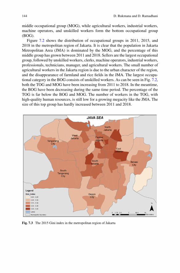
144 D. Rukmana and D. Ramadhani
middle occupational group (MOG), while agricultural workers, industrial workers,machine operators, and unskilled workers form the bottom occupational group(BOG).
Figure 7.2 shows the distribution of occupational groups in 2011, 2015, and2018 in the metropolitan region of Jakarta. It is clear that the population in JakartaMetropolitan Area (JMA) is dominated by the MOG, and the percentage of thismiddle group has grown between 2011 and 2018. Sellers are the largest occupationalgroup, followed by unskilled workers, clerks, machine operators, industrial workers,professionals, technicians, manager, and agricultural workers. The small number ofagricultural workers in the Jakarta region is due to the urban character of the region,and the disappearance of farmland and rice fields in the JMA. The largest occupa-tional category in the BOG consists of unskilled workers. As can be seen in Fig. 7.2,both the TOG and MOG have been increasing from 2011 to 2018. In the meantime,the BOG have been decreasing during the same time period. The percentage of theTOG is far below the BOG and MOG. The number of workers in the TOG, withhigh-quality human resources, is still low for a growing megacity like the JMA. Thesize of this top group has hardly increased between 2011 and 2018.
Fig. 7.3 The 2015 Gini index in the metropolitan region of Jakarta
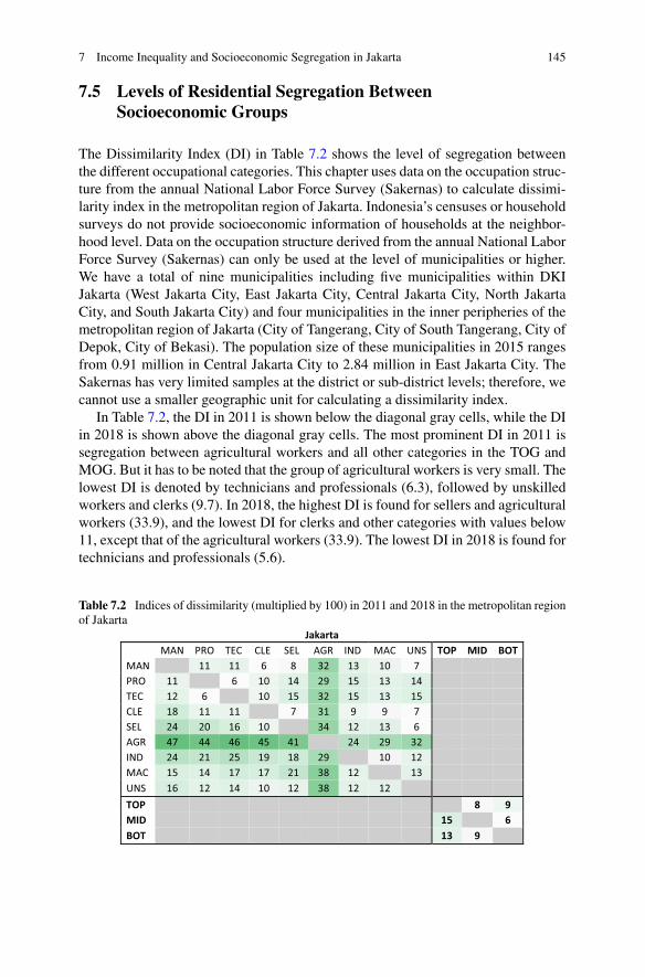
7 Income Inequality and Socioeconomic Segregation in Jakarta 145
7.5 Levels of Residential Segregation BetweenSocioeconomic Groups
The Dissimilarity Index (DI) in Table 7.2 shows the level of segregation betweenthe different occupational categories. This chapter uses data on the occupation struc-ture from the annual National Labor Force Survey (Sakernas) to calculate dissimi-larity index in the metropolitan region of Jakarta. Indonesia’s censuses or householdsurveys do not provide socioeconomic information of households at the neighbor-hood level. Data on the occupation structure derived from the annual National LaborForce Survey (Sakernas) can only be used at the level of municipalities or higher.We have a total of nine municipalities including five municipalities within DKIJakarta (West Jakarta City, East Jakarta City, Central Jakarta City, North JakartaCity, and South Jakarta City) and four municipalities in the inner peripheries of themetropolitan region of Jakarta (City of Tangerang, City of South Tangerang, City ofDepok, City of Bekasi). The population size of these municipalities in 2015 rangesfrom 0.91 million in Central Jakarta City to 2.84 million in East Jakarta City. TheSakernas has very limited samples at the district or sub-district levels; therefore, wecannot use a smaller geographic unit for calculating a dissimilarity index.
In Table 7.2, the DI in 2011 is shown below the diagonal gray cells, while the DIin 2018 is shown above the diagonal gray cells. The most prominent DI in 2011 issegregation between agricultural workers and all other categories in the TOG andMOG. But it has to be noted that the group of agricultural workers is very small. Thelowest DI is denoted by technicians and professionals (6.3), followed by unskilledworkers and clerks (9.7). In 2018, the highest DI is found for sellers and agriculturalworkers (33.9), and the lowest DI for clerks and other categories with values below11, except that of the agricultural workers (33.9). The lowest DI in 2018 is found fortechnicians and professionals (5.6).
Table 7.2 Indices of dissimilarity (multiplied by 100) in 2011 and 2018 in the metropolitan regionof Jakarta
Jakarta MAN PRO TEC CLE SEL AGR IND MAC UNS TOP MID BOT
MAN 11 11 6 8 32 13 10 7PRO 11 6 10 14 29 15 13 14TEC 12 6 10 15 32 15 13 15CLE 18 11 11 7 31 9 9 7SEL 24 20 16 10 34 12 13 6AGR 47 44 46 45 41 24 29 32IND 24 21 25 19 18 29 10 12MAC 15 14 17 17 21 38 12 13UNS 16 12 14 10 12 38 12 12TOP 8 9MID 15 6BOT 13 9
146 D. Rukmana and D. Ramadhani
For the broader occupational group, it can be seen that the DIs for all combi-nations of groups are decreasing. It means that the spatial enclaves of these socio-occupational groups are getting smaller. In other words, the segregation level amongoccupational groups is decreasing and the municipalities in Jakarta are more mixedin 2018 than in 2011. It is especially apparent in the spatial proximity between thekampongs and neighboring luxury apartment buildings in the inner city, such as inMega Kuningan (Budi 2013), Menteng, and Rasuna (Simatupang et al. 2015), andKemayoran (Yunianto 2014).
The biggest decline is related to the DI between the TOG and MOG category,which halves from 15 in 2011 to 7.7 in 2018. It is then followed by the 3.9 pointsdecrease of the TOP and BOG from 13 in 2011 to 9.1 in 2018. The smallest reductionis found for the DI of the MOG and the BOG category from 8.6 in 2011 to 5.9 in2018. It can also be seen that the order of the highest to smallest DI is shifting. Theorder in 2011 is TOG-MOG (15), TOG-BOG (13), and MOG-BOG (8.6), while theorder in 2018 is TOG-BOG (9.1), TOG-MOG (7.7), and MOG-BOG (5.9). From theorder of the DI, it can be concluded that TOG is still the most segregated group whencompared with the others, though the gap is getting smaller.
7.6 Geography of Residential Segregation BetweenSocioeconomic Groups
This section analyzes the geography of residential segregation between the top andthe bottom socioeconomic groups. We use location quotient maps for the top andbottomoccupation groups at the level ofmunicipalities as a proxymeasure of changesin residential segregation between socioeconomic groups. Location quotients of theoccupational structure by municipalities in the study area were calculated from the2011 and 2018 Sakernas surveys. The location quotients of the TOG in 2011 rangefrom 0.58 in North Jakarta City to 1.72 in Central Jakarta City. Central JakartaCity remained as the municipality with the highest location quotient (1.45) and EastJakartaCity became themunicipalitywith the lowest location quotient (0.88) in 2018.The location quotients for the BOG in 2011 ranged from 0.72 (East Jakarta City) to1.42 (Tangerang City). In 2018, East Jakarta City remained as the municipality withthe lowest location quotient (0.71) and Central Jakarta City was the municipalitywith the highest location quotient for the BOG (1.75).
Figure 7.4 shows the location quotient maps for the top and bottom occupationalgroups in 2011 and 2018. Thesemaps cannot showchanges in residential segregation,but they do give an indication of changes in the geographical concentrations ofthe top and bottom occupational groups at the municipal level. The TOG remainshighly concentrated in Central Jakarta City and South Tangerang City. Some luxuryapartments such asKeraton andLe Parc inCentral Jakarta City reached toUS$10,700and US$5,350 per m2, respectively (Alexander 2019). This price is far higher thanthe rest of the city. In contrast, the lowest land price in the inner city of Jakarta
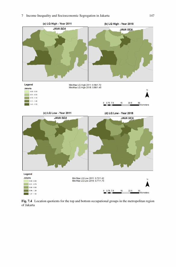
7 Income Inequality and Socioeconomic Segregation in Jakarta 147
Fig. 7.4 Location quotients for the top and bottom occupational groups in the metropolitan regionof Jakarta
148 D. Rukmana and D. Ramadhani
can be found at Kamal Muara, North Jakarta, which is worth merely US$34 perm2 (Elmanisa et al. 2016). Meanwhile, South Tangerang City has a couple of largeluxury residential areas including Bintaro Jaya and BSD City.
Central Jakarta City became a concentration area for both the TOG and BOG.According to an interview with staff from the Housing Department of JakartaProvince, such a concentration is the result of the fact that luxury houses and apart-ments are increasingly found in Central Jakarta City. It is also the location of manyshopping malls, the central business district, government buildings, embassies, andofficial government houses which makes the land and housing prices expensive. Thehigh concentration of the TOG in South Tangerang City is caused by the develop-ment of a new central business district, and middle-upper class housing, especiallyin Bumi Serpong Damai (BSD). In addition, both Central Jakarta City and SouthTangerang City have good accessibility and are connected with highways and trainroutes.
In reference to Fig. 7.4a, b, many households of the top occupational groupmovedfrom Tangerang City to the core of the metropolitan region of Jakarta. It relates to thefact that a large industrial area is located inTangerang. The laborerswhich fall into theBOGmostly reside in Tangerang. Meanwhile, the BOG remains highly concentratedin Central Jakarta City and Tangerang City. Behind the high-rise buildings in CentralJakarta City, there can be found many informal housing areas in the form of urbankampongs. Based on an interviewwith a staff member from the Housing Departmentof Jakarta Province, urban kampongs in Jakarta are the residential locations forthe BOG or informal sector workers such as street vendors, cleaning workers, andsecurity guards.
The changes of location quotients indicate that four municipalities have anincreased concentration of the TOG in 2018 includingWest Jakarta City, East JakartaCity, North Jakarta City, and Depok City. It is marked by several concentrationsof luxury apartments found in those municipalities, such as Veranda Residence,Wang Residence, St Moritz (West Jakarta City), The H Residence, Patria Park (EastJakarta City), Regatta London Tower, The Summit, Sherwood Residence (NorthJakarta City), De Vonte Apartments, Grand Depok City, Permata Green Sentosa, andVictoria Hills Residence (Depok City).
In the meantime, three municipalities experienced an increased concentration ofthe BOG in 2018 including Central Jakarta City, South Jakarta City, and Bekasi City.Tangerang City is the only municipality in the study area experiencing a decreasedconcentration of both top and bottom occupational groups from 2011 to 2018. Afurther analysis shows that Tangerang City has an increased concentration of themiddle occupational group during the same period.
7 Income Inequality and Socioeconomic Segregation in Jakarta 149
7.7 Conclusion
This chapter describes changes in inequality and socioeconomic segregation in thecore and the inner peripheries of the Jakarta metropolitan region. Under the transfor-mative government of Indonesia, Jakarta has experienced various kinds of develop-ment, the most important of which is openness to private and foreign investment. Thesuburban area of Jakarta has grown rapidly and transformed rural areas and agricul-tural land into a vast area of housing which were targeted mostly to the middle-upperclass community. This has led to rather homogenous socioeconomic areas in theoutskirts of themetropolitan area.As the result, theGini Indices in the inner peripheryof Jakarta are lower than those in the municipalities of DKI Jakarta. It means that thehousehold expenditure inequality in the inner periphery is narrower than that in themunicipalities of DKI Jakarta. The high Gini Indices in the municipalities of DKIJakarta are caused by the existence of urban kampongs among the high-rise buildingwith luxury apartments, offices, and shopping center. Meanwhile, segregation in theperiphery of Jakarta occurred because of gated communities developed by the privatesector.
In 2030, vertical housing for the low, middle, and upper class will dominate thecity. A lecturer from the University of Tarumanegara, Suryono Herlambang, arguedthat the existence of vertical housing will worsen residential segregation (Mariani2019). Vertical residential buildings tend to be more socioeconomically segregated.The luxury apartments and penthouse for the upper class are built separately fromlow-cost apartments for the middle-low class will (Mariani 2019). This chapter useddata by municipalities for calculating the segregation indices. If data would havebeen available at a smaller geographical unit, the levels of residential segregationwould be possibly higher.
The occupational profile breakdown shows that the Jakarta Metropolitan Arearesidents are dominated by the MOG, and then followed by the BOG and TOG. Thelargest groups are the sellers (MOG) and unskilled workers (BOG), and the sizeof the TOG group is relatively small. As the LQ maps showed, it is obvious thatthe high proportion of LOG occupied more municipalities than the TOG. However,housing provision by the private sector does not meet the demand for the middle-and low-class population of society who reside outside gated communities and createsegregated residential areas.
The socioeconomic segregation in JMA is fostered by the government’s policy onland use. The privatization of land in the core and the inner peripheries of Jakarta byprivate developers affected the housing market and the affordability of the commu-nity. Addressing segregation in this context should not only rely on controllingthe housing market, but also on developing community capacity and creating moreemployment opportunities in JMA.
In August 2019, Indonesia’s President Joko Widodo announced Indonesia’scapital relocation plan. The government of Indonesia selected two regencies (NorthPenajam Paser and Kutai Kartanegara) in East Kalimantan as the new site forIndonesia’s capital. The governmental function and buildings will be moved to the
150 D. Rukmana and D. Ramadhani
new site and will be ready for occupation in 2024. However, Jakarta will remainthe country’s economic hub. It means that the housing market in Jakarta will remaintense. Furthermore, the 2030 Jakarta Spatial Plan also mentions the phrase ‘estatemanagement’ which means land management in Jakarta will be bestowed to privatedevelopers. The relocation of Indonesia’s capital out of Jakarta will not ease themyriad of problems Jakarta will face, especially as it is projected that 1.5 millionpeople will migrate from Jakarta (Walton 2019). Jakarta’s problems will remain inplace unless serious attention is paid to them including socioeconomic segregationand income inequality.
References
Alexander HB (2019) Para pengembang apartemen mewah untuk kalangan super ksaya(The developers of luxury apartments for ultra-rich buyers). Kompas Property, 19July 2019. https://properti.kompas.com/read/2019/07/19/070000821/para-pengembang-apartemen-mewah-untuk-kalangan-super-kaya?page=all. Accessed 4 Aug 2019
Budi AP (2013) The survival phenomenon of Kampong Kuningan amidst the development of MegaKuningan business-area in Jakarta. Int J Sci Eng Res 4(1)
Central Board of Statistics (2014) Statistik komuter Jabodetabek (The statistics of commuters inJabodetabek). Central Board of Statistics, Jakarta
Central Board of Statistics (2015) Indonesian intercensal population survey. Jakarta: BPS.Colliers International (2017) Jakarta apartment Colliers quarterly, 25 Apr 2017Colliers International (2018) Jakarta property market report Q3 2018, 3 Oct 2018Diningrat R (2015) Segregasi spasial perumahan skala besar: studi kasus kota baru Kota HarapanIndah (KHI) Bekasi. Jurnal Perencanaan Wilayah Dan Kota 26(2):111–129
Elmanisa A, Kartiva A, Fernando A, Arianto R, Winarso H, Zulkaidi D (2016) Land price mappingof Jabodetabek, Indonesia. Geoplanning J Geomat Plan 4(1):53
Firman T (1999) From “global city” to “city of crisis”: Jakarta metropolitan region under economicturmoil. Habitat Int 23(4):447–466
Firman T (2004) New town development in Jakarta metropolitan region: a perspective of spatialsegregation. Habit Int 28(3):349–368
Firman T (2008) In search of a governance institution model for Jakarta metropolitan area (JMA)under Indonesia’s new decentralisation policy: old problems, new challenges. Public Adm Dev28(4):280–290
Henderson JV, Kuncoro A (1996) The dynamics of Jabotabek development. Bull Indones EconStud 32(1):71–95
Herlambang S, Leitner H, Tjung LJ, Sheppard E, Anguelov D (2019) Jakarta’s great landtransformation: hybrid neoliberalisation and informality. Urban Stud 56(4):627–648
Hun K (2002) Research notes on the making of a “Gated Community”: a study of an inner cityneighbourhood, Jakarta, Indonesia. Asian J Soc Sci 30(1):97–108
Indraprahasta GS, Derudder B (2019) World city-ness in a historical perspective: probing the long-term evolution of the Jakarta metropolitan area. Habitat Int89
Leaf M (1994) The suburbanization of Jakarta: a concurrence of economics and ideology. ThirdWorld Plan Rev 16(4):341–356
Leisch H (2002) Gated communities in Indonesia. Cities 19(5):341–350Marcinczak S, Tammaru T, Novák J, Gentile M, Kovács Z, Temelová J, Valatka V, Kahrik A,Szabo B (2015) Patterns of socioeconomic segregation in the capital cities of fast-track reformingpostsocialist countries. Ann Assoc Am Geogr 105(1):183–202
7 Income Inequality and Socioeconomic Segregation in Jakarta 151
Mariani E (2019) Jakarta 2030?Draft plan not looking good [online]. The Jakarta Post. https://www.thejakartapost.com/news/2010/01/08/jakarta-2030-draft-plan-not-looking-good.html. Accessed28 Oct 2019
Musterd S,Marcinczak S, Van HamM, Tammaru T (2017) Socioeconomic segregation in Europeancapital cities. Increasing separation between poor and rich. Urban Geogr 38(7):1062–1083
Mungkasa O (2013) Catatan Kritis tentang Hunian Berimbang. HUD Mag 4:18–21Prasetyanti R (2015) Slum Kampong tourism “Jakarta Hidden Tour”: designing eco-cultural basedpro-poor tourism. Eur J Interdiscip Stud 1(3):111–121
Roitman S, Recio RB (2019) Understanding Indonesia’s gated communities and their relationshipwith inequality. Housing Stud 1–25
Rukmana D (2018) Upgrading housing settlement for the urban poor in Indonesia: an analysis ofthe Kampung Deret program. In: Grant B, Liu CY, Ye L (eds) Metropolitan governance in Asiaand the Pacific Rim. Springer, Singapore, pp 75–94
Rukmana D, Fahmi FZ, Firman T (2018) Suburbanization in Asia: a focus on Jakarta. In: Hanlon B,Vicino TJ (eds) The Routledge companion to the suburbs. Routledge, NewYork, NY, pp 110–120
SalimW, Bettinger K, Fisher M (2019) Maladaptation on the waterfront: Jakarta’s growth coalitionand the Great Garuda. Environ Urban ASIA 10(1):63–80
Salim W, Kombaitan B (2009) Jakarta: the rise and challenge of a capital. City 13(1):120–128Silver C (2008) Planning the megacity: Jakarta in the twentieth century. Routledge, London andNew York
SimatupangW, Irawati M, Mardona R (2015) Symbiosis of Kampong and large scale development:the case of Kampung Menteng Atas and Rasuna Epincentrum development. In: Proceedings of8th conference of the international forum on urbanism (IFoU). https://doi.org/10.3390/ifou-a009
Skoufias E, Suryahadi A (2000) Changes in household welfare, poverty and inequality during thecrisis. Bull Indones Econ Stud 36(2):97–114
SuryaWardhani I (2016)The implications of gated society in Jakartametropolitan region: amultiple-case study in Tangerang District, Banten Indonesia. J Gov Polit 7(1):128
Timmer MP (2007) The structural transformation and the changing role of agriculture in economicdevelopment: empirics and implications Wendt Lecture, 30 Oct 2007. American EnterpriseInstitute Washington, DC
TunasD, Darmoyono L (2014) Indonesian housing development amidst socioeconomic transforma-tion. In:Doling J, RonaldR (eds)HousingEastAsia: socioeconomic and demographic challenges.Palgrave Macmillan, Hampshire, pp 91–115
Tunas D, Peresthu A (2010) The self-help housing in Indonesia: the only option for the poor? HabitInt 34:315–322
Walton K (2019) How Jokowi can get Indonesia’s new capital right—Southeast Asia globe [online].Southeast Asia Globe. https://southeastasiaglobe.com/how-jokowi-can-get-indonesias-new-capital-right/. Accessed 29 Oct 2019
Winarso H (2010) Urban dualism in the Jakarta metropolitan area. In: Sorensen A, Okata J (eds)Megacities: urban form, governance, and sustainability. Springer, pp 163–191
Winarso H, Hudalah D, Firman T (2015) Peri-urban transformation in the Jakarta metropolitan area.Habit Int 49:221–229
Winayanti L, Lang H (2004) Provision of urban services in an informal settlement: a case study ofKampung Penas Tanggul Jakarta. Habit Int 28:41–65
Yandri P (2015) Conflicts and segregation of housing cluster communities and its surrounding.Jurnal Kependudukan Indonesia 10(2):75
Yuniati V (2013) Inclusionary housing in Indonesia: the role of balanced residential ratio 1:3:6 inMakassar. Unpublished master’s thesis. Erasmus University, Rotterdam
Yunianto T (2014) On the verge of displacement. Thesis Eleven 121(1):101–121

152 D. Rukmana and D. Ramadhani
Open Access This chapter is licensed under the terms of the Creative Commons Attribution 4.0International License (http://creativecommons.org/licenses/by/4.0/), which permits use, sharing,adaptation, distribution and reproduction in any medium or format, as long as you give appropriatecredit to the original author(s) and the source, provide a link to the Creative Commons license andindicate if changes were made.
The images or other third party material in this chapter are included in the chapter’s CreativeCommons license, unless indicated otherwise in a credit line to the material. If material is notincluded in the chapter’s Creative Commons license and your intended use is not permitted bystatutory regulation or exceeds the permitted use, you will need to obtain permission directly fromthe copyright holder.
Chapter 8Socio-spatial Segregation and Exclusionin Mumbai
Abdul Shaban and Zinat Aboli
Abstract Indian society is characterised by significant horizontal (religious,regional, linguistic) and vertical (income, occupation, caste) divisions. These socio-economic fragmentations significantly shape the production of space in cities. Infact, all major cities in the country are pervaded by socio-spatial divides, whichoften become sources of conflict, violence, exclusion and, also, solidarity. Mumbaiis the industrial, commercial and financial capital of the country. Bollywood has, overthe years, helped in carving out a distinct (pan) Indian identity for itself and the city,both within and outside India, and is a major rallying and unifying aspect for India.Among all its glitter, the city is also infamous for its underworld (originating from itsexcluded and marginalised neighbourhoods), slums and poor residential areas. Thecity is pervaded by socio-spatial fragmentation and is a divided city. This chaptershows that the highest level of segregation in Mumbai is based on religion (Muslimsand Non-Muslims), followed by class, caste and tribe.
Keywords Socio-spatial segregation · Real estate prices · Slums · Communalviolence ·Marginalisation
8.1 Introduction
India is socio-culturally a very diverse country. Historically, it has been home to allthe major races, castes, languages and religions. Hundreds of minor groups havealso existed side by side. Indian civilisation has evolved through the processes ofimmigration, assimilation and adaptation. Although large-scale inter-group wars and
A. Shaban (B)School of Development Studies, Tata Institute of Social Sciences, Deonar 400088, Mumbai, Indiae-mail: [email protected]
Z. AboliDepartment of Mass Media, Mithibai College, Vile Parle (West), 400056 Mumbai, Indiae-mail: [email protected]
© The Author(s) 2021M. van Ham et al. (eds.), Urban Socio-Economic Segregation and Income Inequality,The Urban Book Series, https://doi.org/10.1007/978-3-030-64569-4_8
153
154 A. Shaban and Z. Aboli
violence have been absent in Indian history, as experienced by European civilisa-tion, the processes of devalourisation, de-assimilation, discrimination and peacefulhostility against marginalised and minorities have existed in one form or another.
About 80% of the Indian population follows Hinduism. Caste, especially inHinduism, has been one of the major defining social features, based on the concep-tion of purity and pollution, endogamy and commensality. Hindus are divided intofour varnas1 (major caste groups) where the lowest caste group is Shudras (theuntouchables), now termed as Scheduled Castes2 (SCs). The Shudras, historically,have faced socio-spatial exclusion. Another defining feature of Indian society is thedivision based on tribes. Tribal groups in India belong to different ethnic groups andare often treated as outcaste population. Although the Government of India has madeseveral provisions and anti-discrimination laws, socio-spatial exclusion, discrimina-tion and segregation continue to be practised both in urban and rural areas. Thesesocio-spatial practices largely shape the morphologies of Indian villages and cities.
The early twentieth century saw the emergence of religion-based politics in India.Hinduism became a major rallying point for certain political parties [Jana Sangh,now Bhartiya Janata Party (BJP) and cultural groups like Rashtriya SwayamsevakSangh (RSS)]. Muslims, as a religious minority group, have been under constantthreat from hostility, violence and discrimination by right-wing Hindus. Thousandsof lives from both communities have been lost in these hostilities. The open and tacitdiscrimination against Muslims in the housing market, jobs and education have alsoexisted since then. Succumbing to theHindu right-wing groups, the State has not beenable to bring any separate provisions to deal with the violence and discriminationagainst Muslims [as has been done in the case of SC and Scheduled Tribes (STs)3].As a result, today, a very polarised communal (religious) concentration exists inIndian cities.
These socially discriminatory practices have also shaped the morphology anddistribution of populations in Indian cities. All the major cities in the country,including Mumbai, are pervaded by socio-spatial divides, which in turn becomesources of conflict, violence, exclusion and, also, of solidarity. Mumbai is the indus-trial, commercial and financial capital of the country. Among all its glitter, the cityis also infamous for its underworld (originating from its excluded and marginalisedsocial groups and neighbourhoods), slums and poor residential areas. The city ispervaded by socio-spatial fragmentation and the divides run deep along religious,class and caste lines. We do not have city-level data for income inequalities, but theWorld Bank (2020) estimates show that income inequalities at the country level in
1There are four varnas among Hindus, namely Brahmins (priestly castes), Kshatriyas (warriorcastes), Vaishyas (cultivators and merchant castes) the Shudras (the lowest castes in the hierarchy,the untouchables).2Scheduled Caste is an officially designated group of historically disadvantaged people in India.The British in India created a list of castes belonging to Shudra group which was adopted in 1935under the Government of India Act (see Dushkin 1967: 626).3Scheduled Tribes are the tribal groups of India scheduled under the Government of IndiaConstitutional Order of 1950 or the Act as amended thereafter (Government of India 1950).
8 Socio-spatial Segregation and Exclusion in Mumbai 155
India measured through the Gini index have risen from 32.1 in 1982, to 34.4 in 2004and 35.7 in 2011.
The present paper attempts to examine exclusionary development and socio-spatial divides in Mumbai on class (population with formal housing versus thoseliving in informal neighbourhoods, called slums), religion (between Non-Muslimsand Muslims), castes (non-SCs and SCs) and tribes (non-STs and STs) bases. Thepaper is divided into six sections. Section 8.2 outlines the data and methods used toexamine the socio-spatial segregations. Section 8.3 deals with real estate prices andslums in Mumbai. Section 8.4 examines the religious conflicts and segregation ofMuslims in the city. Section 8.5 discusses the spatial concentrations and exclusionsof SCs and STs. The last section concludes the paper.
8.2 Data and Methods
Mumbai city (Greater Mumbai) has seen a steady increase in population over theyears. The population of the city has risen from 0.9 million in 1901 to 12.4 millionin 2011. The population density of the city is currently about 28,472 persons/sq. km.This population growth has been fuelled by migration from different states of thecountry including from within Maharashtra state (in which Mumbai is located). Thecity is home to all major religious communities in the world. Muslims constituted20.7% of the total population ofMumbai city in 2011 and formed the largest religiousminority group (Census of India 2011). The share of Hindus in the same year was66%. Other religious groups like Buddhists (4.9%), Jains (4.1%), Christians (3.3%),and Sikhs (0.5%) individually constituted less than 5% each of the total populationof the city.
For this study, data has been collected from various sources to examine place-based segregation and interaction between dominant and marginalised ethnic groupsin Mumbai city. The decennial population census of India is a major source for dataon religion, caste and tribes. It provides data at ward and sub-ward (section) levelsfor SC and ST populations for cities. There are 88 sections in Mumbai and they havean average population of around 141,000. Data on the religious groups are avail-able only at city and district levels, which are meso units. Therefore, an attempt wasmade to find out the data from alternative sources. The Election Commission of Indiaprovides the eligible voter’s name.An attemptwasmade to sort the names ofMuslimsfrom the voter lists of 2018 [(as has been done by Susewind (2017) for 11 cities ofIndia)]. The adults over 18 years old are registered in these voter lists. The distinctly‘Muslim sounding’ names were sorted out from the lists. However, there remains apossibility of errors of 5–10% due to non-recognisable names and non-registration ofMuslims in voter lists (see Shariff and Shaifullah 2018 on Muslim missing voters).There are in total 36 assembly constituencies in Mumbai and Mumbai Suburbandistricts. Together these districts are known as Greater Mumbai or Mumbai City(see Fig. 8.1). The data was compiled for 7289 polling booths (with an averagenumber of voters about 930, and a population of about 1250, respectively, per booth)
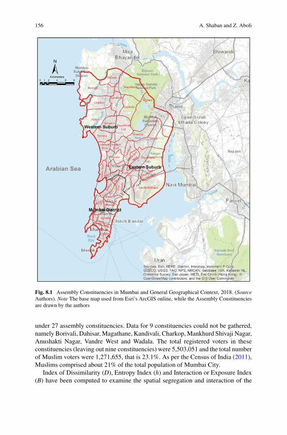
156 A. Shaban and Z. Aboli
Fig. 8.1 Assembly Constituencies in Mumbai and General Geographical Context, 2018. (SourceAuthors). Note The base map used from Esri’s ArcGIS online, while the Assembly Constituenciesare drawn by the authors
under 27 assembly constituencies. Data for 9 constituencies could not be gathered,namely Borivali, Dahisar,Magathane, Kandivali, Charkop,Mankhurd Shivaji Nagar,Anushakti Nagar, Vandre West and Wadala. The total registered voters in theseconstituencies (leaving out nine constituencies) were 5,503,051 and the total numberof Muslim voters were 1,271,655, that is 23.1%. As per the Census of India (2011),Muslims comprised about 21% of the total population of Mumbai City.
Index of Dissimilarity (D), Entropy Index (h) and Interaction or Exposure Index(B) have been computed to examine the spatial segregation and interaction of the
8 Socio-spatial Segregation and Exclusion in Mumbai 157
above-mentioned ethnic groups. For discussion on D, h and B indices, see alsoChap. 1 of this book.
The data for slums by census tracts or sections are available only for the year2001. The 2011 Census provides data for slum population only at the city level.Therefore, only the 2001 Census data, for its 88 sections are used for understandingthe distribution and concentration of slum populations in the city. The data on realestate (residential/flat) prices are taken from supplements published by the popularbroadsheet daily, The Times of India and adjusted to property tax wards.
8.3 Real Estate and Increase of Slums in the City
Residentially,Mumbai is a divided city. On the one hand, there are upper andmiddle-class high rises and colonies, on the other, there are vast areas of slums inhabitedby lower and underclasses. The high rises and middle- and upper class colonies arealso interspersed by slums. It is a city where thousands also live on the pavementin rudimentary structures, which may have not be classified as slums by the Censusof India.4 In fact, an increasing population, a lack of land supply, and lackadaisicalgovernment policy response have created considerable housing and shelter issues inthe city. The prices of the houses in the city have grown enormously over the yearsand have gone beyond the reach of the lower class population. The ratio between theindex number of the income of factory workers (this index is used for the workingclass related inflation and as most of the population in the city are workers, it is themost appropriate index) in Maharashtra and the price of residential flats in Mumbaiprovides further insight into this issue (Table 8.1). The ratio has considerably risenover the years. Notwithstanding the rise in income of factory workers, the compara-tively higher rise in real estate prices have dashed the hopes of lower classes to owna house. Between 2003 and 2012, the price of real estate in the city increased by 3.5times relative to the wages of the factory workers. Only in the Eastern Suburb of thecity, the increase in real estate priceswas slightly lower,while the highest increasewasin Mumbai District. During 2003–2012, the average flat prices in Mumbai District[from INR 6,872 (US $147.5) to INR 36,056 (US $773.7)], and Western Suburb[from INR 3,726 (US $80.0) to INR 18,211 (US $390.8)] have risen more than five
4Census of India (2011: 4) defines a slum as residential areas where dwellings are unfit for humanhabitation by reasons of dilapidation, overcrowding, faulty arrangements and design of such build-ings, narrowness or faulty arrangement of street, lack of ventilation, light or sanitation facilitiesor any combination of these factors which are detrimental to the safety and health. Three types ofslums have been identified for the purpose of Census. There are: (i) notified slums (All notifiedareas in a town or city notified as ‘slum’ by State, UT Administration or Local Government underany Act including a ‘Slum Act’), (ii) recognised slums (All areas recognised as ‘Slum’ by State,UT Administration or Local Government, Housing and Slum Boards, which may have not beenformally notified as slum under any act) and (iii) identified slums (A compact area of at least 300population or about 60–70 households of poorly built congested tenements, in unhygienic envi-ronment usually with inadequate infrastructure and lacking in proper sanitary and drinking waterfacilities).
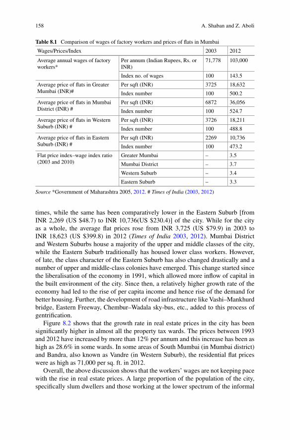
158 A. Shaban and Z. Aboli
Table 8.1 Comparison of wages of factory workers and prices of flats in Mumbai
Wages/Prices/Index 2003 2012
Average annual wages of factoryworkers*
Per annum (Indian Rupees, Rs. orINR)
71,778 103,000
Index no. of wages 100 143.5
Average price of flats in GreaterMumbai (INR)#
Per sqft (INR) 3725 18,632
Index number 100 500.2
Average price of flats in MumbaiDistrict (INR) #
Per sqft (INR) 6872 36,056
Index number 100 524.7
Average price of flats in WesternSuburb (INR) #
Per sqft (INR) 3726 18,211
Index number 100 488.8
Average price of flats in EasternSuburb (INR) #
Per sqft (INR) 2269 10,736
Index number 100 473.2
Flat price index–wage index ratio(2003 and 2010)
Greater Mumbai – 3.5
Mumbai District – 3.7
Western Suburb – 3.4
Eastern Suburb – 3.3
Source *Government of Maharashtra 2005, 2012. # Times of India (2003, 2012)
times, while the same has been comparatively lower in the Eastern Suburb [fromINR 2,269 (US $48.7) to INR 10,736(US $230.4)] of the city. While for the cityas a whole, the average flat prices rose from INR 3,725 (US $79.9) in 2003 toINR 18,623 (US $399.8) in 2012 (Times of India 2003, 2012). Mumbai Districtand Western Suburbs house a majority of the upper and middle classes of the city,while the Eastern Suburb traditionally has housed lower class workers. However,of late, the class character of the Eastern Suburb has also changed drastically and anumber of upper and middle-class colonies have emerged. This change started sincethe liberalisation of the economy in 1991, which allowed more inflow of capital inthe built environment of the city. Since then, a relatively higher growth rate of theeconomy had led to the rise of per capita income and hence rise of the demand forbetter housing. Further, the development of road infrastructure like Vashi–Mankhurdbridge, Eastern Freeway, Chembur–Wadala sky-bus, etc., added to this process ofgentrification.
Figure 8.2 shows that the growth rate in real estate prices in the city has beensignificantly higher in almost all the property tax wards. The prices between 1993and 2012 have increased by more than 12% per annum and this increase has been ashigh as 28.6% in some wards. In some areas of South Mumbai (in Mumbai district)and Bandra, also known as Vandre (in Western Suburb), the residential flat priceswere as high as 71,000 per sq. ft. in 2012.
Overall, the above discussion shows that the workers’ wages are not keeping pacewith the rise in real estate prices. A large proportion of the population of the city,specifically slum dwellers and those working at the lower spectrum of the informal
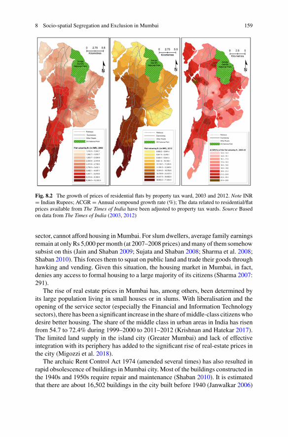
8 Socio-spatial Segregation and Exclusion in Mumbai 159
Fig. 8.2 The growth of prices of residential flats by property tax ward, 2003 and 2012. Note INR= Indian Rupees; ACGR = Annual compound growth rate (%); The data related to residential/flatprices available from The Times of India have been adjusted to property tax wards. Source Basedon data from The Times of India (2003, 2012)
sector, cannot afford housing inMumbai. For slum dwellers, average family earningsremain at onlyRs 5,000 permonth (at 2007–2008 prices) andmany of them somehowsubsist on this (Jain and Shaban 2009; Sujata and Shaban 2008; Sharma et al. 2008;Shaban 2010). This forces them to squat on public land and trade their goods throughhawking and vending. Given this situation, the housing market in Mumbai, in fact,denies any access to formal housing to a large majority of its citizens (Sharma 2007:291).
The rise of real estate prices in Mumbai has, among others, been determined byits large population living in small houses or in slums. With liberalisation and theopening of the service sector (especially the Financial and Information Technologysectors), there has been a significant increase in the share ofmiddle-class citizenswhodesire better housing. The share of the middle class in urban areas in India has risenfrom 54.7 to 72.4% during 1999–2000 to 2011–2012 (Krishnan and Hatekar 2017).The limited land supply in the island city (Greater Mumbai) and lack of effectiveintegration with its periphery has added to the significant rise of real-estate prices inthe city (Migozzi et al. 2018).
The archaic Rent Control Act 1974 (amended several times) has also resulted inrapid obsolescence of buildings in Mumbai city. Most of the buildings constructed inthe 1940s and 1950s require repair and maintenance (Shaban 2010). It is estimatedthat there are about 16,502 buildings in the city built before 1940 (Janwalkar 2006)
160 A. Shaban and Z. Aboli
which are in a dilapidated condition; some of them have collapsed in recent years,killing several. A judgment passed by the Supreme Court on September 4, 2008, haspaved the way for the redevelopment of these buildings by providing an extra FloorSpace Index (FSI)5 to the builders. They now can profitably build the structures andmake a 225 sq. ft. flat available to every resident family of the buildings, free of cost(Mahapatra 2008). The decision by the court ushers hopes for the redevelopment ofdilapidated buildings in south and central Mumbai (in Mumbai District).
The government’s inadequate response and skewed policies are responsible for thehousing crisis in the city. Mumbai was expecting a massive respite from congestiondue to the availability of about one-third of some 600 acres of land from 60 textilemills for open space. Mumbai has an open space ratio of about only 0.03 acres per1000 persons. Recommended open space at the international level is often 4 acres per1000 persons. The availability of mill land was expected to somewhat correct this.However, much of the land went to builders and only 133 acres have been providedfor open spaces and public housing (Katakam 2006).
The controversy over the sale of mill land dates back to 1991 when the govern-ment, in response to appease mill owners, introduced Sect. 58 in the DCR. Betterknown as the ‘one-third formula’, DCR 58 allowedmill owners to divide the area intothree parts. They could then sell one-third, give the second part to Greater MumbaiMunicipal Corporation to create open spaces and the other third to the MaharashtraHousing and Area Development Authority to provide affordable housing to the fami-lies of mill workers who lost their livelihoods with the closure of the mills. In 2001,however, the state government used a loophole in the Maharashtra Regional andTown Planning Act, 1966, and amended DCR 58–DCR 53 (I), according to whichthe only land that is vacant—that is, with no built-up structure—shall be dividedunder the one-third formula. Thus, the mill owners managed to keep the bulk of theland and the area to be given to the municipal corporation and to the workers wassubstantially reduced (Katakam 2005, 2006).
The political bargaining and competition within the city have assured somehousing schemes for the poor in an otherwise neoliberal regime. In the 1990s, popularcity leader Bal Thackeray initiated the Slum Rehabilitation Scheme (SRA). SRAattempted to provide houses for slum dwellers through cross-subsidy. The transferof development rights was granted to the builders who came forward to developslums and provide flats of 225 sq. ft., free of cost to the dwellers. The scheme hasbeen hugely successful as poorer sections of the population have been able to acquireconstructed homes free of cost in place of their hutments. This has also resulted inthe decline of the slum population, as is evident from the data of the 2001 and 2011Indian censuses, mentioned below.
In sum, the lack of adequate provisions for affordable formal housing has createda huge number of slums in Mumbai. High real estate prices, government apathy andlower wages have undermined the city’s development. This has resulted in amassingof the lower class population in slums. In fact, in 2001 and 2011, 54.0% and 41.1%,
5Floor Space Index (FSI) is the ratio of built or constructed area and actual land area. For instance,if a land is 100 sq. ft. and construction on the same land is of 300 sq. ft. area, FSI is 3.
8 Socio-spatial Segregation and Exclusion in Mumbai 161
respectively, of Mumbai’s population was living in slums (Census of India 2014a, b).In 2011, 15.85% of Mumbai district (489,068 of total population of 3,085,411) and49.38% in Mumbai suburban district (4,620,654 of total population of 9,356,962)lived in slums (Census of India 2014a, b). One of the reasons for this has been thesuccess of the SRA. However, many claim that the Census of India undercounts theslum population and does not reflect the actual situation in the city. Going by thisclaim, the proportion of population living in slums in Mumbai is estimated to beabout 60% of the total population (Shaban 2008).
The lack of development of social and physical infrastructure, poverty, large sizefamilies and a dense population do increase the probability of social deviance. Itis found that slum areas of the city are also prone to a higher crime rate (Shaban2010). A large family with limited resources often results in family disruption anddecreasing formal and informal social controls. Communities with a higher level ofsocial disruption tend to be characterised by a lower rate of participation in voluntaryorganisations and local efforts, which have an important role to play in controllingcrime. Overcrowding in houses means that personal matters are difficult to keepprivate in domestic life (Shaban 2010).
The slumpopulation is not evenly distributed in the city. The highest concentrationof the slum population is found in the Eastern Suburb, which is the least developedpart of the city (Shaban 2010). As shown in Fig. 8.3, Mankhurd, Trombay, Govandi,Deonar, Vikhroli, Bhandup, Bazar Church-Hall and Chembur, have a large share oftheir total population living in slums.
The computed Dissimilarity Index (D) between non-slum and slum population forthe year 2001 inMumbai city is 0.460, which shows high levels of spatial segregationbetween non-slum and slum population (Table 8.2) (Jahn et al 1947). Further, thecomputed value of Interaction or Isolation Index (B) for slum and non-slum popu-lations for the year 2001 is 0.321, showing that the probability of a slum dwellerinteracting with a non-slum dweller is about 32.1%.
8.4 Inter-religious Conflicts and the Segregation of Muslims
Hindu–Muslim rivalry in India arose during the colonial period in the latter half ofthe nineteenth century. It gave rise to religious nationalism and an ethno-nationalistphilosophy, which resulted in the division of India in 1947 into India and Pakistan.After independence, the Hindu right-wing with their political formations haveattempted to communalise Indian democracy. This has resulted in the marginali-sation of Muslims. As Sen (2013) writes “India’s Muslims are … victims of untoldindignities in a country still fighting the ghosts of a blood-soaked partition in 1947that turned vast swathes of it into Muslim-majority Pakistan. The baggage of historyand the cynical calculus of caste, class, community and religion still dictate the fateofmost things in India: fromwhowins elections andwields power towho has a betterchance of getting jobs, healthcare or justice” (p. 127). The religious politics of the
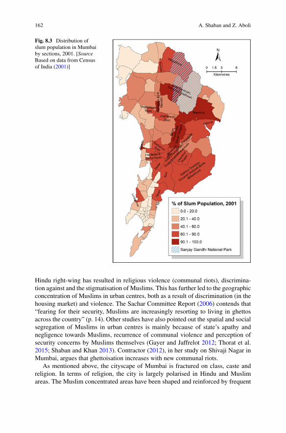
162 A. Shaban and Z. Aboli
Fig. 8.3 Distribution ofslum population in Mumbaiby sections, 2001. [SourceBased on data from Censusof India (2001)]
Hindu right-wing has resulted in religious violence (communal riots), discrimina-tion against and the stigmatisation of Muslims. This has further led to the geographicconcentration of Muslims in urban centres, both as a result of discrimination (in thehousing market) and violence. The Sachar Committee Report (2006) contends that“fearing for their security, Muslims are increasingly resorting to living in ghettosacross the country” (p. 14). Other studies have also pointed out the spatial and socialsegregation of Muslims in urban centres is mainly because of state’s apathy andnegligence towards Muslims, recurrence of communal violence and perception ofsecurity concerns by Muslims themselves (Gayer and Jaffrelot 2012; Thorat et al.2015; Shaban and Khan 2013). Contractor (2012), in her study on Shivaji Nagar inMumbai, argues that ghettoisation increases with new communal riots.
As mentioned above, the cityscape of Mumbai is fractured on class, caste andreligion. In terms of religion, the city is largely polarised in Hindu and Muslimareas. The Muslim concentrated areas have been shaped and reinforced by frequent
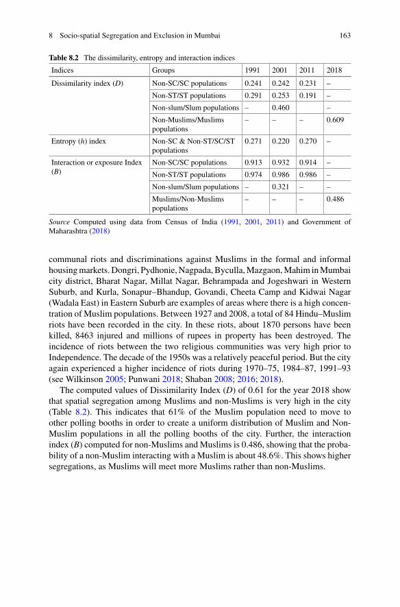
8 Socio-spatial Segregation and Exclusion in Mumbai 163
Table 8.2 The dissimilarity, entropy and interaction indices
Indices Groups 1991 2001 2011 2018
Dissimilarity index (D) Non-SC/SC populations 0.241 0.242 0.231 –
Non-ST/ST populations 0.291 0.253 0.191 –
Non-slum/Slum populations – 0.460 –
Non-Muslims/Muslimspopulations
– – – 0.609
Entropy (h) index Non-SC & Non-ST/SC/STpopulations
0.271 0.220 0.270 –
Interaction or exposure Index(B)
Non-SC/SC populations 0.913 0.932 0.914 –
Non-ST/ST populations 0.974 0.986 0.986 –
Non-slum/Slum populations – 0.321 – –
Muslims/Non-Muslimspopulations
– – – 0.486
Source Computed using data from Census of India (1991, 2001, 2011) and Government ofMaharashtra (2018)
communal riots and discriminations against Muslims in the formal and informalhousingmarkets. Dongri, Pydhonie,Nagpada, Byculla,Mazgaon,Mahim inMumbaicity district, Bharat Nagar, Millat Nagar, Behrampada and Jogeshwari in WesternSuburb, and Kurla, Sonapur–Bhandup, Govandi, Cheeta Camp and Kidwai Nagar(Wadala East) in Eastern Suburb are examples of areas where there is a high concen-tration of Muslim populations. Between 1927 and 2008, a total of 84 Hindu–Muslimriots have been recorded in the city. In these riots, about 1870 persons have beenkilled, 8463 injured and millions of rupees in property has been destroyed. Theincidence of riots between the two religious communities was very high prior toIndependence. The decade of the 1950s was a relatively peaceful period. But the cityagain experienced a higher incidence of riots during 1970–75, 1984–87, 1991–93(see Wilkinson 2005; Punwani 2018; Shaban 2008; 2016; 2018).
The computed values of Dissimilarity Index (D) of 0.61 for the year 2018 showthat spatial segregation among Muslims and non-Muslims is very high in the city(Table 8.2). This indicates that 61% of the Muslim population need to move toother polling booths in order to create a uniform distribution of Muslim and Non-Muslim populations in all the polling booths of the city. Further, the interactionindex (B) computed for non-Muslims and Muslims is 0.486, showing that the proba-bility of a non-Muslim interacting with a Muslim is about 48.6%. This shows highersegregations, as Muslims will meet more Muslims rather than non-Muslims.
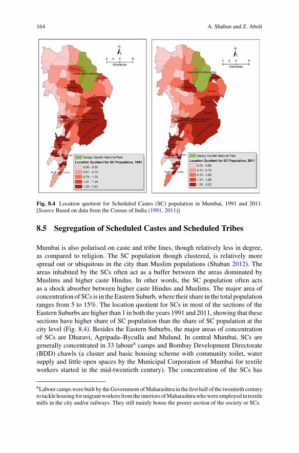
164 A. Shaban and Z. Aboli
Fig. 8.4 Location quotient for Scheduled Castes (SC) population in Mumbai, 1991 and 2011.[Source Based on data from the Census of India (1991, 2011)]
8.5 Segregation of Scheduled Castes and Scheduled Tribes
Mumbai is also polarised on caste and tribe lines, though relatively less in degree,as compared to religion. The SC population though clustered, is relatively morespread out or ubiquitous in the city than Muslim populations (Shaban 2012). Theareas inhabited by the SCs often act as a buffer between the areas dominated byMuslims and higher caste Hindus. In other words, the SC population often actsas a shock absorber between higher caste Hindus and Muslims. The major area ofconcentration of SCs is in theEastern Suburb,where their share in the total populationranges from 5 to 15%. The location quotient for SCs in most of the sections of theEastern Suburbs are higher than 1 in both the years 1991 and 2011, showing that thesesections have higher share of SC population than the share of SC population at thecity level (Fig. 8.4). Besides the Eastern Suburbs, the major areas of concentrationof SCs are Dharavi, Agripada–Byculla and Mulund. In central Mumbai, SCs aregenerally concentrated in 33 labour6 camps and Bombay Development Directorate(BDD) chawls (a cluster and basic housing scheme with community toilet, watersupply and little open spaces by the Municipal Corporation of Mumbai for textileworkers started in the mid-twentieth century). The concentration of the SCs has
6Labour campswere built by theGovernment ofMaharashtra in the first half of the twentieth centuryto tackle housing formigrantworkers from the interiors ofMaharashtrawhowere employed in textilemills in the city and/or railways. They still mainly house the poorer section of the society or SCs.
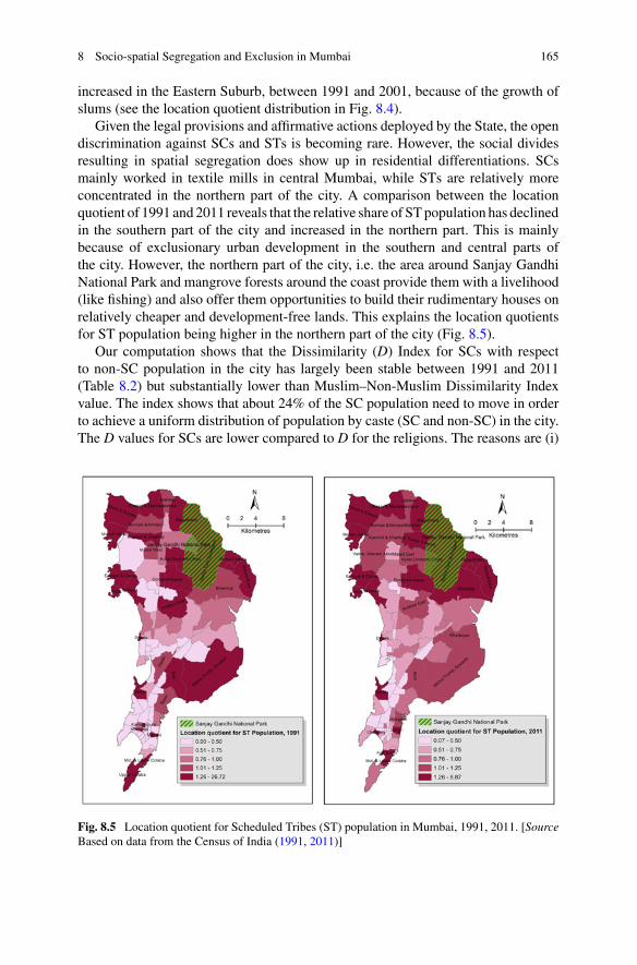
8 Socio-spatial Segregation and Exclusion in Mumbai 165
increased in the Eastern Suburb, between 1991 and 2001, because of the growth ofslums (see the location quotient distribution in Fig. 8.4).
Given the legal provisions and affirmative actions deployed by the State, the opendiscrimination against SCs and STs is becoming rare. However, the social dividesresulting in spatial segregation does show up in residential differentiations. SCsmainly worked in textile mills in central Mumbai, while STs are relatively moreconcentrated in the northern part of the city. A comparison between the locationquotient of 1991 and 2011 reveals that the relative share of STpopulation has declinedin the southern part of the city and increased in the northern part. This is mainlybecause of exclusionary urban development in the southern and central parts ofthe city. However, the northern part of the city, i.e. the area around Sanjay GandhiNational Park and mangrove forests around the coast provide them with a livelihood(like fishing) and also offer them opportunities to build their rudimentary houses onrelatively cheaper and development-free lands. This explains the location quotientsfor ST population being higher in the northern part of the city (Fig. 8.5).
Our computation shows that the Dissimilarity (D) Index for SCs with respectto non-SC population in the city has largely been stable between 1991 and 2011(Table 8.2) but substantially lower than Muslim–Non-Muslim Dissimilarity Indexvalue. The index shows that about 24% of the SC population need to move in orderto achieve a uniform distribution of population by caste (SC and non-SC) in the city.The D values for SCs are lower compared to D for the religions. The reasons are (i)
Fig. 8.5 Location quotient for Scheduled Tribes (ST) population in Mumbai, 1991, 2011. [SourceBased on data from the Census of India (1991, 2011)]
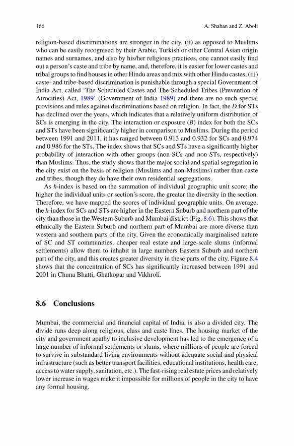
166 A. Shaban and Z. Aboli
religion-based discriminations are stronger in the city, (ii) as opposed to Muslimswho can be easily recognised by their Arabic, Turkish or other Central Asian originnames and surnames, and also by his/her religious practices, one cannot easily findout a person’s caste and tribe by name, and, therefore, it is easier for lower castes andtribal groups to find houses in other Hindu areas andmixwith other Hindu castes, (iii)caste- and tribe-based discrimination is punishable through a special Government ofIndia Act, called ‘The Scheduled Castes and The Scheduled Tribes (Prevention ofAtrocities) Act, 1989’ (Government of India 1989) and there are no such specialprovisions and rules against discriminations based on religion. In fact, the D for STshas declined over the years, which indicates that a relatively uniform distribution ofSCs is emerging in the city. The interaction or exposure (B) index for both the SCsand STs have been significantly higher in comparison to Muslims. During the periodbetween 1991 and 2011, it has ranged between 0.913 and 0.932 for SCs and 0.974and 0.986 for the STs. The index shows that SCs and STs have a significantly higherprobability of interaction with other groups (non-SCs and non-STs, respectively)than Muslims. Thus, the study shows that the major social and spatial segregation inthe city exist on the basis of religion (Muslims and non-Muslims) rather than casteand tribes, though they do have their own residential segregations.
As h-index is based on the summation of individual geographic unit score; thehigher the individual units or section’s score, the greater the diversity in the section.Therefore, we have mapped the scores of individual geographic units. On average,the h-index for SCs and STs are higher in the Eastern Suburb and northern part of thecity than those in theWestern Suburb andMumbai district (Fig. 8.6). This shows thatethnically the Eastern Suburb and northern part of Mumbai are more diverse thanwestern and southern parts of the city. Given the economically marginalised natureof SC and ST communities, cheaper real estate and large-scale slums (informalsettlements) allow them to inhabit in large numbers Eastern Suburb and northernpart of the city, and this creates greater diversity in these parts of the city. Figure 8.4shows that the concentration of SCs has significantly increased between 1991 and2001 in Chuna Bhatti, Ghatkopar and Vikhroli.
8.6 Conclusions
Mumbai, the commercial and financial capital of India, is also a divided city. Thedivide runs deep along religious, class and caste lines. The housing market of thecity and government apathy to inclusive development has led to the emergence of alarge number of informal settlements or slums, where millions of people are forcedto survive in substandard living environments without adequate social and physicalinfrastructure (such as better transport facilities, educational institutions, health care,access towater supply, sanitation, etc.). The fast-rising real estate prices and relativelylower increase in wages make it impossible for millions of people in the city to haveany formal housing.
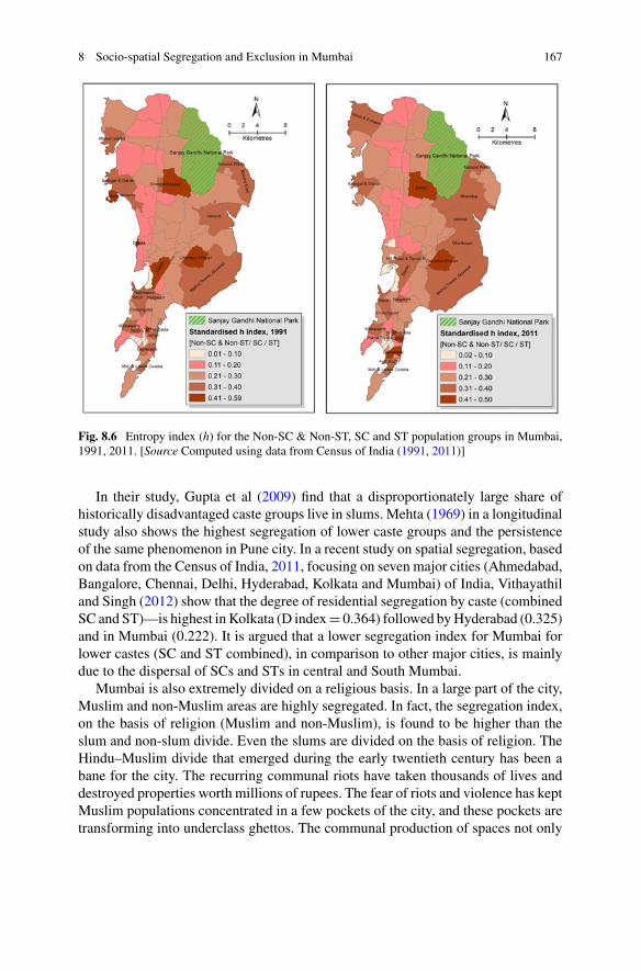
8 Socio-spatial Segregation and Exclusion in Mumbai 167
Fig. 8.6 Entropy index (h) for the Non-SC & Non-ST, SC and ST population groups in Mumbai,1991, 2011. [Source Computed using data from Census of India (1991, 2011)]
In their study, Gupta et al (2009) find that a disproportionately large share ofhistorically disadvantaged caste groups live in slums. Mehta (1969) in a longitudinalstudy also shows the highest segregation of lower caste groups and the persistenceof the same phenomenon in Pune city. In a recent study on spatial segregation, basedon data from the Census of India, 2011, focusing on seven major cities (Ahmedabad,Bangalore, Chennai, Delhi, Hyderabad, Kolkata and Mumbai) of India, Vithayathiland Singh (2012) show that the degree of residential segregation by caste (combinedSC and ST)—is highest in Kolkata (D index= 0.364) followed byHyderabad (0.325)and in Mumbai (0.222). It is argued that a lower segregation index for Mumbai forlower castes (SC and ST combined), in comparison to other major cities, is mainlydue to the dispersal of SCs and STs in central and South Mumbai.
Mumbai is also extremely divided on a religious basis. In a large part of the city,Muslim and non-Muslim areas are highly segregated. In fact, the segregation index,on the basis of religion (Muslim and non-Muslim), is found to be higher than theslum and non-slum divide. Even the slums are divided on the basis of religion. TheHindu–Muslim divide that emerged during the early twentieth century has been abane for the city. The recurring communal riots have taken thousands of lives anddestroyed properties worth millions of rupees. The fear of riots and violence has keptMuslim populations concentrated in a few pockets of the city, and these pockets aretransforming into underclass ghettos. The communal production of spaces not only
168 A. Shaban and Z. Aboli
manifest various forms of injustices but actually produces and reproduces them, andthereby maintains established social relations based on domination and oppression.
To bridge these social and spatial divides, the city needs new emancipatory poli-tics. The emancipation from suppression, domination, repression and exclusion. Thisemancipatory approach should be able to free and liberate those trapped and incarcer-ated in space, chained to a place or disabled by socially produced spaces. This politicsneeds to end the social devalourisation of communities and avert social exclusionand spatial segregation.
Acknowledgements We are grateful to Mr. Khalid Saifullah for technical help in segregating thedata from electoral lists for Muslims and non-Muslims.
References
Census of India (1991) Primary census abstract for slums. Office of the Registrar General & CensusCommissioner, India, New Delhi
Census of India (2001) Primary census abstract for slums. Office of the Registrar General & CensusCommissioner, India, New Delhi
Census of India (2011) Primary census abstract. https://www.censusindia.gov.in/pca/pca.aspx 8April 2019
Census of India (2014) District census handbook: Mumbai suburban, 2011. Directorate of CensusOperation, Government of Maharashtra, Mumbai
Census of India (2014) District census handbook: Mumbai, 2011. Directorate of Census Operation,Government of Maharashtra, Mumbai
Centre for the Studies in Society and Secularism (Various Years). Data on Hindu and Muslim Riotsin India. Mumbai
Contractor Q (2012) Unwanted in my city: the making of a ‘“Muslim slum”’ in Mumbai. In: GayerL, Jaffrelot C (eds) Muslims in Indian cities: trajectories of marginalisation. Hurst, London, pp23–42
DushkinL (1967)Scheduled caste policy in india: history, problems. ProspectsAsianSurv7(9):626–636. https://doi.org/10.2307/2642619
Government of India (1950). The Constitution (Scheduled Tribes) Order (1950) The gazette ofIndia, extraordinary, Part-III, Sect. 3, 6th September. Ministry of Law, New Delhi
Government of India (1989) The scheduled castes and the scheduled tribes (Prevention ofAtrocities)Act, 1989, 6th September, New Delhi
Government of India (n.d.). GOI (SC) ORDER 1936 dated 06.06.1936. Ministry of Social Justice,New Delhi. https://socialjustice.nic.in/writereaddata/UploadFile/GOI-SC-ORDER-1936.pdf 7April 2019
Government of Maharashtra (2004) Economic survey of Maharashtra 2003–4. Directorate ofEconomics and Statistics, Bandra, Mumbai
Government of Maharashtra (2012) Economic survey of Maharashtra 2011–12. Directorate ofEconomics and Statistics, Bandra, Mumbai
Government ofMaharashtra (2018). Electoral roll. Office of the chief electoral officer, Maharashtra.https://ceo.maharashtra.gov.in 5 Oct 2018
Gupta K, Arnold F, Lhungdim H (2009) Health and living conditions in eight Indian cities, nationalfamily health survey (NFHS-3), India, 2005–06 (Mumbai: International Institute for PopulationSciences; Calverton, Maryland: ICF Macro)
8 Socio-spatial Segregation and Exclusion in Mumbai 169
Jaffrelot C, Gayer L (2012) Muslims in Indian cities: trajectories of marginalisation. ColumbiaUniversity Press
Jahn JA, Schmid CF, Schrag C (1947) The measurement of ecological segregation. Am Sociol Rev103:293–303
Jain R, Shaban A (2009) Socio-economic and educational status of muslims in Mumbai. A reportsubmitted to Maharashtra State Minorities Commission, Government of Maharashtra, Mumbai
Janwalkar M (2006) Not all buildings are beyond repair, says high court. DNAIndia.com,December 12. https://www.dnaindia.com/mumbai/report_not-all-old-buildings-are-beyond-repair-says-high-court_1068816 10 Aug 2009
Katakam A (2005) Vanishing mill lands. Frontline, SeptemberKatakam A (2006) All for the builder. Frontline, March–AprilKrishnan S, HatekarN (2017) Rise of the newmiddle class in India and its changing structure. EconPolit Wkly 52(22):40–48
Migozzi J, Shaban A, Gonçalves RS (2018) Urban national parks and the making of the housingmarket in emerging cities: places of exclusiveness, land of opportunities. In: Landy F (ed) Fromurban national parks to natured cities in the global south: the quest for naturbanity. Springer,Singapore, pp 131–155
Mahapatra D (2008) The city skyline set to change as SC okays cluster of towers. Times of India,September 5, Mumbai
Mehta S (1969) Patterns of residence in Poona, India, by caste and religion: 1822–1965.Demography 6(4):473–491
Punwani J (2018) Police conduct during communal riots: evidence from 1992–93Mumbai riots andits implications. In: Shaban A (ed) Lives of muslims in India: politics, exclusion and violence.Routledge, New Delhi/London, pp 187–207
Sachar, Committee Report (2006) The social, economic and education of the muslim communityof India. Prime Minister’s Office, Government of India, New Delhi
Susewind R (2017) Muslims in Indian cities: degrees of segregation and the elusive ghetto. EnvironPlan A: Econ Space 49(6):1286–1307
Sen A (2013) Muslims in Indian cities: trajectories of marginalisation. Asian Aff 44(1):127–128.https://doi.org/10.1080/03068374.2012.760803
Shaban A (2008) Ghettoisation, crime and punishment in Mumbai. Econ Polit Wkly 43(33):68–73Shaban A (2012) ‘Ethnic politics, muslims and space in contemporary Mumbai’. In: Shaban A (ed)Lives of muslims in India: politics, exclusion and violence, pp 208–225. New Delhi/London,Routledge
Shaban A (2016) Muslim Citizenship, Identity and Violence in India. In: In Kannabiran K (ed)Violence Studies. Oxford University Press, New Delhi, pp 142–169
Shaban A (2010) Mumbai: political economy of crime and space. Orient Blackswan, HyderabadShaban A, Khan S (eds) (2013) Muslims in urban India: development and exclusion. ConceptPublishing, New Delhi
Shaban A (2018) Lives of Muslims in India: politics, exclusion and violence. Second Edition.Routledge, New Delhi/London
Shariff A, Khalid S (2018) Electoral exclusion of muslims continues to plague Indian democracy.Econ PolitWkly 53(20). https://www.epw.in/engage/article/electoral-exclusion-muslims-continues-plague-indian-democracy 9 April 2019
Sharma RN (2007) The housing market in Mumbai metropolis and its irrelevance to the averagecitizen. In: Shaw A (ed) Indian cities in transition. Orient Longman, Chennai, pp 283–313
Sharma RN, Sita K, Vyas M, Jha M, Shaban A (2008) Impact assessment of resettlementimplementations under MUTP-II. Report submitted to MMRDA, Mumbai
Sujata S, Shaban A (2008) Human-technology interface in the banking sector: a study of micro-deposit machines in Mumbai. Report submitted to NCR Financial Solution Group Ltd., Dundee,U.K.
Thorat S et al (2015) Urban rental housing market: caste & religion matters in access. Econ PolitWkly 50(26 & 27):47–53
170 A. Shaban and Z. Aboli
Times of India (2003) Property times, 6 September. MumbaiTimes of India (2009) Property times, 5 September. MumbaiTimes of India (2010) Property times, 15 September. MumbaiTimes of India (2012). Property times, 8 September. MumbaiVithayathil T, Singh G (2012) Spaces of discrimination: residential segregation in Indian cities.Econ Polit Wkly 47(37):60–66
Wilkinson SI (2005) Religious politics and communal violence. Oxford University Press, NewDelhi
World Bank (2020) GINI index (World Bank Estimate).https://data.worldbank.org/indicator/SI.POV.GINI 19 March 2020
Open Access This chapter is licensed under the terms of the Creative Commons Attribution 4.0International License (http://creativecommons.org/licenses/by/4.0/), which permits use, sharing,adaptation, distribution and reproduction in any medium or format, as long as you give appropriatecredit to the original author(s) and the source, provide a link to the Creative Commons license andindicate if changes were made.
The images or other third party material in this chapter are included in the chapter’s CreativeCommons license, unless indicated otherwise in a credit line to the material. If material is notincluded in the chapter’s Creative Commons license and your intended use is not permitted bystatutory regulation or exceeds the permitted use, you will need to obtain permission directly fromthe copyright holder.
Chapter 9Social Polarization and SocioeconomicSegregation in Shanghai, China:Evidence from 2000 and 2010 Censuses
Zhuolin Pan, Ye Liu, Yang Xiao, and Zhigang Li
Abstract China’s rapid economic growth since the early 1980s has been accom-panied by a substantial increase in economic inequality. Economic restructuring,rural–urban migration, globalization and marketization have jointly led to a trans-formation of the socio-spatial structure of large Chinese cities. Although a handfulof studies have examined the level and pattern of socioeconomic segregation in aparticular Chinese city using neighbourhood-level census data from the year 2000,little research has been done to investigate in-depth changes in the level and patternof segregation using more up to date and more geographically detailed data. Thischapter aims to examine the levels, patterns and drivers of socioeconomic segrega-tion in Shanghai, China, using neighbourhood-level and subdistrict-level data fromthe 2000 and 2010 decennial population census. This chapter uses the dissimilarityindex to measure the overall level of socioeconomic segregation by occupation andhousehold registration (hukou) status. Based on a location quotient and neighbour-hood composition, it also illustrates the change in the spatial pattern of segregation.The chapter ends with a discussion on the possible drivers of segregation and policysuggestions to combat segregation in large Chinese cities.
Keywords Socioeconomic segregation · Occupation · Hukou status · Shanghai ·China
Z. Pan · Y. Liu (B)School of Geography and Planning, Sun Yat-Sen University, Guangzhou, Chinae-mail: [email protected]
Z. Pane-mail: [email protected]
Y. XiaoDepartment of Urban Planning, Tongji University, Shanghai, Chinae-mail: [email protected]
Z. LiSchool of Urban Design, Wuhan University, Wuhan, Chinae-mail: [email protected]
© The Author(s) 2021M. van Ham et al. (eds.), Urban Socio-Economic Segregation and Income Inequality,The Urban Book Series, https://doi.org/10.1007/978-3-030-64569-4_9
171
172 Z. Pan et al.
9.1 Introduction
Over the past four decades, rapid economic growth has been interwovenwith internaland international migration during a process of globalization, which has led to anunprecedented socioeconomic transition around theworld (Marcinczak 2012). Rapidgrowth in the economy is inevitably accompanied by a substantial increase in socioe-conomic inequality (Marcinczak et al. 2015), and China is no exception. Accordingto the National Bureau of Statistics of China, the Gini Index of the country increasedfrom 0.317 in 1978 to 0.465 in 2016, which indicates a widening income gap. Inthe largest Chinese cities, such as Beijing, Shanghai and Guangzhou, rising incomeinequality has resulted in socioeconomic segregation. Evidence from the 2000 and2010 censuses showed that many large cities in China have experienced a rise in resi-dential segregation by class, household registration (hukou) status and housing tenure(Li and Wu 2006, 2008; Chen and Li 2014). The increase in residential segregationhas resulted in a number of detrimental consequences, such as the reproduction ofmarginality, the prolonged and rising rate of unemployment in deteriorated towns, thewidening of social inequality and the weakening of social solidarity (Wilson 1987;Bolt et al. 2010). Understanding the pattern and drivers of residential segregationin large cities in China will help policymakers to achieve the goal of building aninclusive and harmonious society.
A growing body of literature has explored patterns of residential segregationin large Chinese cities since the beginning of the reforms in 1978. Earlier studieshave focused mainly on the delineation of socio-spatial differentiation in Chinesecities (Gu and Kesteloot 1997). More recently, growing attention has been paidto the drivers and mechanism of residential segregation (Gu et al. 2006; Li andWu 2006). Nevertheless, most earlier studies on residential segregation were basedon the fourth and fifth waves of the national population census carried out in theyears 1990 and 2000, respectively (Gu and Kesteloot 1997; Feng and Zhou 2003).Recently, a few studies have examined the residential segregation of a particular city,such as Shanghai and Nanjing, using data from the sixth round of population censusconducted in 2010 (Wu et al. 2014, 2018; Shen and Xiao 2020), but surprisingly,little attention has been paid to neighbourhood segregation with regard to hukoustatus, occupation and socioeconomic status (Liao and Wong 2015; Wu et al. 2018).Moreover, little research has been done to investigate the changes in the spatial patternof residential segregation over time in globalized Chinese cities, and the process ofurban socio-spatial reconfiguration remains under-researched.
This chapter aims to examine and compare the level and pattern of socioeconomicsegregation between 2000 and 2010 by occupation and hukou status in Shanghaiusing neighbourhood-level and subdistrict-level data from the decennial populationcensus. As a polarizing global city with a dramatically rising number of both super-rich and extremely disadvantaged and poor citizens, Shanghai provides an ideal labo-ratory to investigate the patterns, drivers and consequences of residential segregationagainst the backdrop of globalization and marketization in China.
9 Social Polarization and Socioeconomic Segregation in Shanghai, China … 173
9.2 Residential Segregation in Large Cities in China
Residential segregation has always existed in the history of urbanization (Nightngale2012). InEurope andNorthAmerica, racial segregation is regarded as themost persis-tent form of segregation, and a large number of empirical studies have been devotedto this form of segregation (Massey 1985; Wilson 1987). Although some globalizingChinese cities attract a large number of international migrants, they account for onlya very small proportion of the total population of these cities (for example, 0.71% ofShanghai’s total population in 2000), exerting an insignificant effect on the spatialpattern of residential segregation. Socioeconomic status has become a major dimen-sion of residential segregation in the newmillennium in the transition from a plannedeconomy to a market-oriented economy (Li and Wu 2008). Socioeconomic segre-gation was not severe in the period of the planned economy when the state exerteda monopoly over a wide range of resources, and state-owned work units played animportant role in arranging resource allocation (Wu and Li 2005). The work unitdetermined workers’ wage levels and the allocation of means of subsistence, such ashousing and health care. Meanwhile, the hukou system imposed stringent constraintson internalmigration and excluded outsiders fromurban public services (Chan 2009).Chinese cities experienced a low degree of socioeconomic differentiation before theearly 1980s as a result of the state-dominated housing system and the stringent hukousystem.
The advent of the reform and the opening up has provided more freedom andincentives for the growth of the private sector and thereby generated a new-rich class,but the reform of the state-owned work units has also led to millions of workers beingmade redundant, and housing is now no longer allocated by work units (Wu 2004; LiandWu 2008). Although the government still owns the land after the housing reform,real estate developers can obtain the land use right through the land conveyancesystem. Supported by bank loans, real estate developers have gradually become theprincipal participants in the housing development (Fu 2013). Housing reform haspromoted the formation of housing marketization in China and increased levels ofhousing consumption. From 1984 to 2010, the rate of homeownership increasedfrom 9.4 to 89.3% in China. However, the market mechanism has led to the riseof house prices in large cities, and housing has become a commodity which can bepurchased on the market rather than a welfare benefit allocated by the state and workunits (Wu and Li 2005; Logan et al. 2010). The market-oriented housing reform hasaggravated the segregation among socioeconomic status groups, thus restructuringthe socio-spatial structure of Chinese cities (Walder and He 2014; Song et al. 2017).In addition, internal migration has also contributed to the socio-spatial restructuringof urban China (Liao and Wong 2015). The loosening of the hukou system andthe growth of low-end urban job opportunities have caused the influx of migrantsinto urban areas since the mid-1980s (Fan 2008). However, the long-established dualsystembetweenmigrants and urban residents excludesmigrants from themainstreamsocialwelfare system (Chan andZhang1999;Chan andBuckingham2008).Migrantssuffer from only limited accessibility to the urban formal housing system, and they
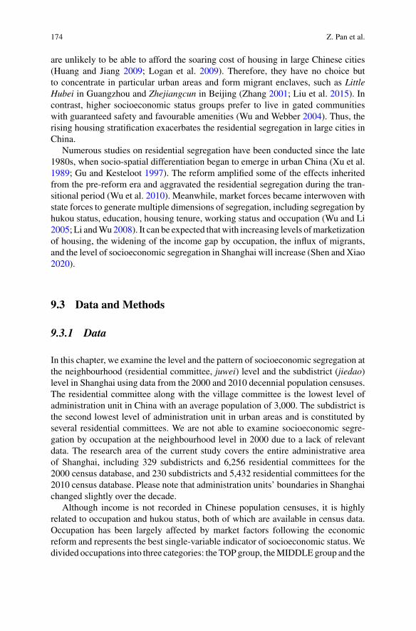
174 Z. Pan et al.
are unlikely to be able to afford the soaring cost of housing in large Chinese cities(Huang and Jiang 2009; Logan et al. 2009). Therefore, they have no choice butto concentrate in particular urban areas and form migrant enclaves, such as LittleHubei in Guangzhou and Zhejiangcun in Beijing (Zhang 2001; Liu et al. 2015). Incontrast, higher socioeconomic status groups prefer to live in gated communitieswith guaranteed safety and favourable amenities (Wu and Webber 2004). Thus, therising housing stratification exacerbates the residential segregation in large cities inChina.
Numerous studies on residential segregation have been conducted since the late1980s, when socio-spatial differentiation began to emerge in urban China (Xu et al.1989; Gu and Kesteloot 1997). The reform amplified some of the effects inheritedfrom the pre-reform era and aggravated the residential segregation during the tran-sitional period (Wu et al. 2010). Meanwhile, market forces became interwoven withstate forces to generate multiple dimensions of segregation, including segregation byhukou status, education, housing tenure, working status and occupation (Wu and Li2005; Li andWu2008). It can be expected thatwith increasing levels ofmarketizationof housing, the widening of the income gap by occupation, the influx of migrants,and the level of socioeconomic segregation in Shanghai will increase (Shen and Xiao2020).
9.3 Data and Methods
9.3.1 Data
In this chapter, we examine the level and the pattern of socioeconomic segregation atthe neighbourhood (residential committee, juwei) level and the subdistrict (jiedao)level in Shanghai using data from the 2000 and 2010 decennial population censuses.The residential committee along with the village committee is the lowest level ofadministration unit in China with an average population of 3,000. The subdistrict isthe second lowest level of administration unit in urban areas and is constituted byseveral residential committees. We are not able to examine socioeconomic segre-gation by occupation at the neighbourhood level in 2000 due to a lack of relevantdata. The research area of the current study covers the entire administrative areaof Shanghai, including 329 subdistricts and 6,256 residential committees for the2000 census database, and 230 subdistricts and 5,432 residential committees for the2010 census database. Please note that administration units’ boundaries in Shanghaichanged slightly over the decade.
Although income is not recorded in Chinese population censuses, it is highlyrelated to occupation and hukou status, both of which are available in census data.Occupation has been largely affected by market factors following the economicreform and represents the best single-variable indicator of socioeconomic status. Wedivided occupations into three categories: the TOPgroup, theMIDDLEgroup and the
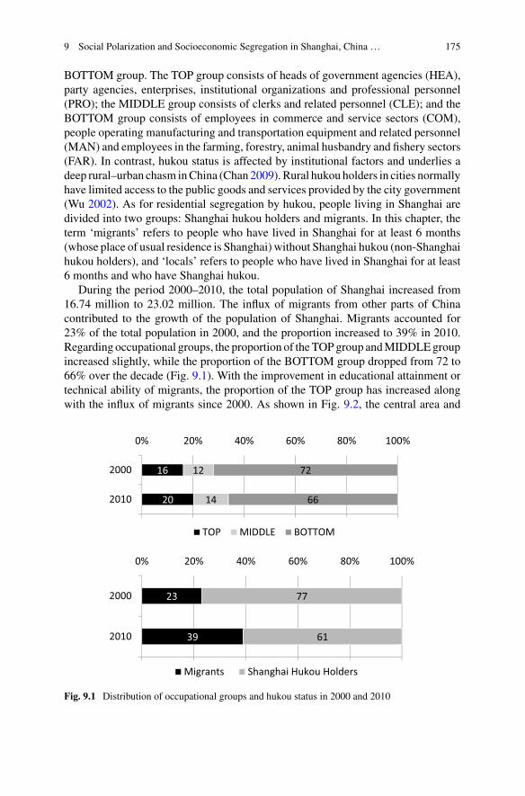
9 Social Polarization and Socioeconomic Segregation in Shanghai, China … 175
BOTTOM group. The TOP group consists of heads of government agencies (HEA),party agencies, enterprises, institutional organizations and professional personnel(PRO); the MIDDLE group consists of clerks and related personnel (CLE); and theBOTTOM group consists of employees in commerce and service sectors (COM),people operating manufacturing and transportation equipment and related personnel(MAN) and employees in the farming, forestry, animal husbandry and fishery sectors(FAR). In contrast, hukou status is affected by institutional factors and underlies adeep rural–urban chasm inChina (Chan 2009). Rural hukou holders in cities normallyhave limited access to the public goods and services provided by the city government(Wu 2002). As for residential segregation by hukou, people living in Shanghai aredivided into two groups: Shanghai hukou holders and migrants. In this chapter, theterm ‘migrants’ refers to people who have lived in Shanghai for at least 6 months(whose place of usual residence is Shanghai) without Shanghai hukou (non-Shanghaihukou holders), and ‘locals’ refers to people who have lived in Shanghai for at least6 months and who have Shanghai hukou.
During the period 2000–2010, the total population of Shanghai increased from16.74 million to 23.02 million. The influx of migrants from other parts of Chinacontributed to the growth of the population of Shanghai. Migrants accounted for23% of the total population in 2000, and the proportion increased to 39% in 2010.Regarding occupational groups, the proportion of theTOPgroup andMIDDLEgroupincreased slightly, while the proportion of the BOTTOM group dropped from 72 to66% over the decade (Fig. 9.1). With the improvement in educational attainment ortechnical ability of migrants, the proportion of the TOP group has increased alongwith the influx of migrants since 2000. As shown in Fig. 9.2, the central area and
20
16
14
12
66
72
0% 20% 40% 60% 80% 100%
2010
2000
TOP MIDDLE BOTTOM
39
23
61
77
0% 20% 40% 60% 80% 100%
2010
2000
Migrants Shanghai Hukou Holders
Fig. 9.1 Distribution of occupational groups and hukou status in 2000 and 2010
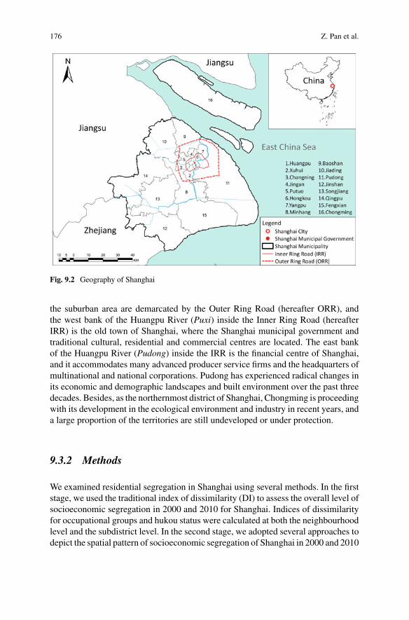
176 Z. Pan et al.
Fig. 9.2 Geography of Shanghai
the suburban area are demarcated by the Outer Ring Road (hereafter ORR), andthe west bank of the Huangpu River (Puxi) inside the Inner Ring Road (hereafterIRR) is the old town of Shanghai, where the Shanghai municipal government andtraditional cultural, residential and commercial centres are located. The east bankof the Huangpu River (Pudong) inside the IRR is the financial centre of Shanghai,and it accommodates many advanced producer service firms and the headquarters ofmultinational and national corporations. Pudong has experienced radical changes inits economic and demographic landscapes and built environment over the past threedecades. Besides, as the northernmost district of Shanghai, Chongming is proceedingwith its development in the ecological environment and industry in recent years, anda large proportion of the territories are still undeveloped or under protection.
9.3.2 Methods
We examined residential segregation in Shanghai using several methods. In the firststage, we used the traditional index of dissimilarity (DI) to assess the overall level ofsocioeconomic segregation in 2000 and 2010 for Shanghai. Indices of dissimilarityfor occupational groups and hukou status were calculated at both the neighbourhoodlevel and the subdistrict level. In the second stage, we adopted several approaches todepict the spatial pattern of socioeconomic segregation of Shanghai in 2000 and 2010
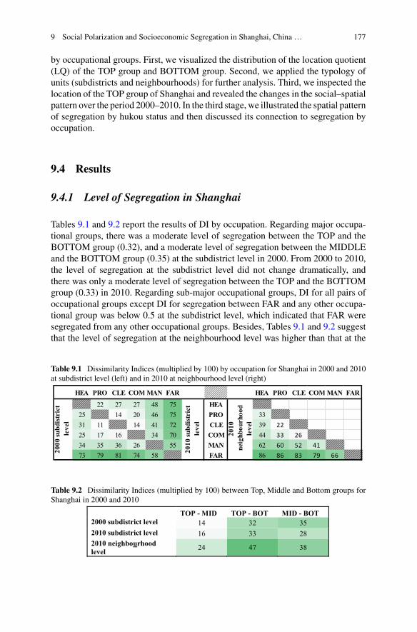
9 Social Polarization and Socioeconomic Segregation in Shanghai, China … 177
by occupational groups. First, we visualized the distribution of the location quotient(LQ) of the TOP group and BOTTOM group. Second, we applied the typology ofunits (subdistricts and neighbourhoods) for further analysis. Third, we inspected thelocation of the TOP group of Shanghai and revealed the changes in the social–spatialpattern over the period 2000–2010. In the third stage, we illustrated the spatial patternof segregation by hukou status and then discussed its connection to segregation byoccupation.
9.4 Results
9.4.1 Level of Segregation in Shanghai
Tables 9.1 and 9.2 report the results of DI by occupation. Regarding major occupa-tional groups, there was a moderate level of segregation between the TOP and theBOTTOM group (0.32), and a moderate level of segregation between the MIDDLEand the BOTTOM group (0.35) at the subdistrict level in 2000. From 2000 to 2010,the level of segregation at the subdistrict level did not change dramatically, andthere was only a moderate level of segregation between the TOP and the BOTTOMgroup (0.33) in 2010. Regarding sub-major occupational groups, DI for all pairs ofoccupational groups except DI for segregation between FAR and any other occupa-tional group was below 0.5 at the subdistrict level, which indicated that FAR weresegregated from any other occupational groups. Besides, Tables 9.1 and 9.2 suggestthat the level of segregation at the neighbourhood level was higher than that at the
Table 9.1 Dissimilarity Indices (multiplied by 100) by occupation for Shanghai in 2000 and 2010at subdistrict level (left) and in 2010 at neighbourhood level (right)
HEA PRO CLE COM MAN FAR HEA PRO CLE COM MAN FAR
22 27 27 48 75 HEA25 14 20 46 75 PRO 3331 11 14 41 72 CLE 39 2225 17 16 34 70 COM 44 33 2634 35 36 26 55 MAN 62 60 52 4173 79 81 74 58 FAR 86 86 83 79 6620
00 su
bdis
tric
t le
vel
2010
subd
istr
ict
leve
l
2010
neig
hbou
rhoo
d le
vel
Table 9.2 Dissimilarity Indices (multiplied by 100) between Top, Middle and Bottom groups forShanghai in 2000 and 2010
TOP - MID TOP - BOT MID - BOT2000 subdistrict level 14 32 352010 subdistrict level 16 33 282010 neighbourhood level 24 47 38
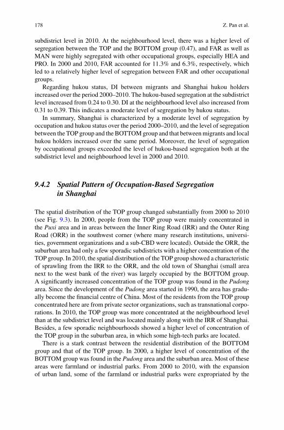
178 Z. Pan et al.
subdistrict level in 2010. At the neighbourhood level, there was a higher level ofsegregation between the TOP and the BOTTOM group (0.47), and FAR as well asMAN were highly segregated with other occupational groups, especially HEA andPRO. In 2000 and 2010, FAR accounted for 11.3% and 6.3%, respectively, whichled to a relatively higher level of segregation between FAR and other occupationalgroups.
Regarding hukou status, DI between migrants and Shanghai hukou holdersincreased over the period 2000–2010. The hukou-based segregation at the subdistrictlevel increased from 0.24 to 0.30. DI at the neighbourhood level also increased from0.31 to 0.39. This indicates a moderate level of segregation by hukou status.
In summary, Shanghai is characterized by a moderate level of segregation byoccupation and hukou status over the period 2000–2010, and the level of segregationbetween the TOP group and the BOTTOMgroup and that betweenmigrants and localhukou holders increased over the same period. Moreover, the level of segregationby occupational groups exceeded the level of hukou-based segregation both at thesubdistrict level and neighbourhood level in 2000 and 2010.
9.4.2 Spatial Pattern of Occupation-Based Segregationin Shanghai
The spatial distribution of the TOP group changed substantially from 2000 to 2010(see Fig. 9.3). In 2000, people from the TOP group were mainly concentrated inthe Puxi area and in areas between the Inner Ring Road (IRR) and the Outer RingRoad (ORR) in the southwest corner (where many research institutions, universi-ties, government organizations and a sub-CBD were located). Outside the ORR, thesuburban area had only a few sporadic subdistricts with a higher concentration of theTOP group. In 2010, the spatial distribution of the TOP group showed a characteristicof sprawling from the IRR to the ORR, and the old town of Shanghai (small areanext to the west bank of the river) was largely occupied by the BOTTOM group.A significantly increased concentration of the TOP group was found in the Pudongarea. Since the development of the Pudong area started in 1990, the area has gradu-ally become the financial centre of China. Most of the residents from the TOP groupconcentrated here are from private sector organizations, such as transnational corpo-rations. In 2010, the TOP group was more concentrated at the neighbourhood levelthan at the subdistrict level and was located mainly along with the IRR of Shanghai.Besides, a few sporadic neighbourhoods showed a higher level of concentration ofthe TOP group in the suburban area, in which some high-tech parks are located.
There is a stark contrast between the residential distribution of the BOTTOMgroup and that of the TOP group. In 2000, a higher level of concentration of theBOTTOM group was found in the Pudong area and the suburban area. Most of theseareas were farmland or industrial parks. From 2000 to 2010, with the expansionof urban land, some of the farmland or industrial parks were expropriated by the
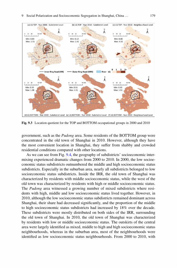
9 Social Polarization and Socioeconomic Segregation in Shanghai, China … 179
Fig. 9.3 Location quotient for the TOP and BOTTOM occupational groups in 2000 and 2010
government, such as the Pudong area. Some residents of the BOTTOM group wereconcentrated in the old town of Shanghai in 2010. However, although they havethe most convenient location in Shanghai, they suffer from shabby and crowdedresidential conditions compared with other locations.
As we can see from Fig. 9.4, the geography of subdistricts’ socioeconomic inter-mixing experienced dramatic changes from 2000 to 2010. In 2000, the low socioe-conomic status subdistricts outnumbered the middle and high socioeconomic statussubdistricts. Especially in the suburban area, nearly all subdistricts belonged to lowsocioeconomic status subdistricts. Inside the IRR, the old town of Shanghai wascharacterized by residents with middle socioeconomic status, while the west of theold town was characterized by residents with high or middle socioeconomic status.The Pudong area witnessed a growing number of mixed subdistricts where resi-dents with high, middle and low socioeconomic status lived together. However, in2010, although the low socioeconomic status subdistricts remained dominant acrossShanghai, their share had decreased significantly, and the proportion of the middleto high socioeconomic status subdistricts had increased by 18% over the decade.These subdistricts were mostly distributed on both sides of the IRR, surroundingthe old town of Shanghai. In 2010, the old town of Shanghai was characterizedby residents with low or middle socioeconomic status. The outskirts of the centralarea were largely identified as mixed, middle to high and high socioeconomic statusneighbourhoods, whereas in the suburban area, most of the neighbourhoods wereidentified as low socioeconomic status neighbourhoods. From 2000 to 2010, with
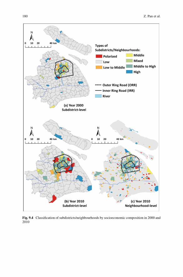
180 Z. Pan et al.
Fig. 9.4 Classification of subdistricts/neighbourhoods by socioeconomic composition in 2000 and2010
9 Social Polarization and Socioeconomic Segregation in Shanghai, China … 181
the expansion of urban land and the improvement in the average socioeconomic statusof the population in Shanghai, the districts with residents with high socioeconomicstatus sprawled from the west of the old town to other areas inside the ORR. Thepattern at the neighbourhood level was much more fragmentized due to smaller scalegeographic units. Neighbourhoods in the old town largely belonged to low, low tomiddle or middle socioeconomic status neighbourhoods, surrounded by middle tohigh and high socioeconomic status neighbourhoods.
Figure 9.5 depicts the residential landscape of theTOPgroup in Shanghai. In 2000,subdistricts of Q1 were mainly located in and dispersed across the central area andlargely situated near the universities, government organizations and the sub-CBDs.In 2010, Q1 was situated mainly between the area of the ORR and the IRR, andespecially concentrated in the Pudong area, which has become the financial centreof Shanghai, attracting an increasing number of experts from all over the world.Although the proportion of each type of subdistrict remained fairly stable over theperiod 2000–2010, the spatial distribution changed significantly.
9.4.3 Spatial Pattern of Hukou-Based Segregationin Shanghai
In 2000,most Shanghai hukou holders lived in the old townof Shanghai, andmigrantsweremainly concentrated along both sides of the ORR. In 2010, the location quotientof migrants was found at a low level inside the IRR. Migrants’ agglomerations hadbeen moved away from the IRR, and neighbourhoods on both sides of the IRR weremainly inhabited by local hukou holders in 2010 (Fig. 9.6).
Above all, it was found that segregation by occupation is interwoven with segre-gation by hukou status. Over the period 2000–2010, the spatial distribution of theBOTTOM group was similar to that of migrants, while the spatial distribution of theTOP group was contrary to that of migrants. This indicates that, in Shanghai, mostmigrants occupy the lowest position in the socioeconomic hierarchy. Shanghai localhukou is highly associated with higher socioeconomic status, while those withoutShanghai hukou may suffer from lower socioeconomic status and so be segregatedfrom residents with high socioeconomic status.
9.5 Drivers of Changing Patterns of ResidentialSegregation in Shanghai
Our findings reveal that the level of segregation by occupational groups has surpassedthe level of hukou-based segregation, and occupation has become an increasinglysignificant factor in the reconstruction of the social space. In the post-reform era,educational attainment, occupation and income are interrelated and reinforce each
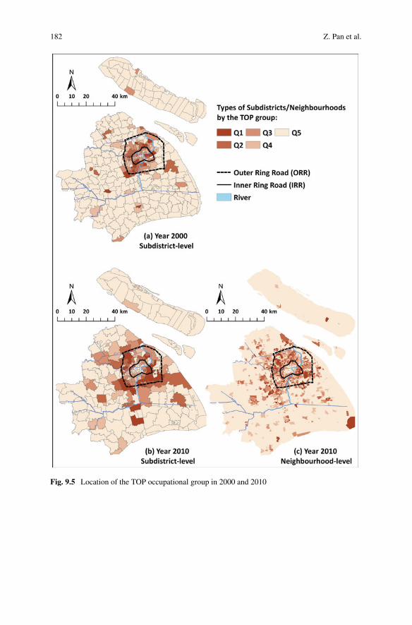
182 Z. Pan et al.
Fig. 9.5 Location of the TOP occupational group in 2000 and 2010
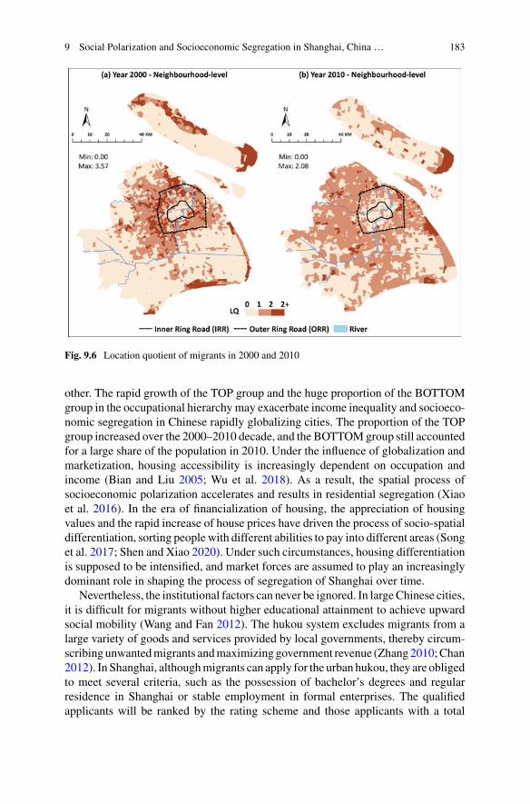
9 Social Polarization and Socioeconomic Segregation in Shanghai, China … 183
Fig. 9.6 Location quotient of migrants in 2000 and 2010
other. The rapid growth of the TOP group and the huge proportion of the BOTTOMgroup in the occupational hierarchy may exacerbate income inequality and socioeco-nomic segregation in Chinese rapidly globalizing cities. The proportion of the TOPgroup increased over the 2000–2010 decade, and the BOTTOMgroup still accountedfor a large share of the population in 2010. Under the influence of globalization andmarketization, housing accessibility is increasingly dependent on occupation andincome (Bian and Liu 2005; Wu et al. 2018). As a result, the spatial process ofsocioeconomic polarization accelerates and results in residential segregation (Xiaoet al. 2016). In the era of financialization of housing, the appreciation of housingvalues and the rapid increase of house prices have driven the process of socio-spatialdifferentiation, sorting people with different abilities to pay into different areas (Songet al. 2017; Shen and Xiao 2020). Under such circumstances, housing differentiationis supposed to be intensified, and market forces are assumed to play an increasinglydominant role in shaping the process of segregation of Shanghai over time.
Nevertheless, the institutional factors can never be ignored. In largeChinese cities,it is difficult for migrants without higher educational attainment to achieve upwardsocial mobility (Wang and Fan 2012). The hukou system excludes migrants from alarge variety of goods and services provided by local governments, thereby circum-scribing unwantedmigrants andmaximizing government revenue (Zhang2010;Chan2012). In Shanghai, althoughmigrants can apply for the urban hukou, they are obligedto meet several criteria, such as the possession of bachelor’s degrees and regularresidence in Shanghai or stable employment in formal enterprises. The qualifiedapplicants will be ranked by the rating scheme and those applicants with a total
184 Z. Pan et al.
score higher than the qualification mark set by the Shanghai government can attainurban hukou. These criteria are intentionally skewed in favour of those with highereducational attainment or technical credentials (Zhang 2010; Zhang andWang 2010).Even though the hukou system has been relaxed and migrants can attain urban hukoueasily in small- and medium-sized cities, in large cities, hukou remains as an insur-mountable barrier for most of the migrants to obtain public goods and services suchas education and medical insurance, owing to the high threshold and limited quotaof urban hukou attainment in large Chinese cities. Nevertheless, as the Lewis turningpoint is reached, surplus rural labour has been absorbed by the manufacturing sectorand labour supply has become limited in urban China. The labour-intensive growthmodel in China has gradually lost its competitiveness (Cai 2010; Zhang et al. 2011).Therefore, the reform will be deepened, and an increasing number of migrants willbe encouraged to integrate into urban China to spur economic growth. The marketmechanism will play a significant role in mobility and resource allocation, and thelevel of hukou-based segregation will decrease at the expense of the increasing levelof segregation by socioeconomic status.
Additionally, social factors play an important role in shaping the process of segre-gation in large Chinese cities. Chain migration is one of the most important formsof migration, and migrants tend to congregate in a particular location with the aidof kinship ties and native place ties (Liu et al. 2015). These social ties are vital formigrant communities to survive and thrive in large cities, as newly arrived migrantstend to seek jobs and accommodation with the aid of their family, relatives andfellow townsmen (lao xiang) (Liu et al. 2012; Huang et al. 2017). Besides, poorsocioeconomic status and lower educational attainment reinforce the disadvantagedposition of migrants in urban China, who suffer from persistent discrimination by thelocal residents (e.g. exclusion from community activities, difficulty in constructing asocial network with local residents) (Chen andWang 2015). As a result, migrants areisolated by the local residents, and they subsequently prefer to congregate in migrantenclaves for both instrumental and emotional support (Liu et al. 2012). Both theinternal cement within each migrant group and the external discrimination againstmigrant groups contribute to the residential segregation between migrants and localhukou holders in Chinese cities.
Besides, the historical legacy of urban inequality laid a foundation for the structureof urban space (Wu and Li 2005; Li and Wu 2006). In the pre-reform era, rurallabourers were forced to stay in rural areas, and urban residents who were affiliatedwith state-owned work units lived in city centres (Wu 2002; Chan 2009). The processof the marketization of housing affected the acquisition of housing property rights(Wu 2017). In the early period after the reform in 1988, as the sitting tenants of publichousing inShanghai, local hukouholders could affordhousing and acquire property athighly subsidized prices (Logan et al. 2009). They benefitted from the housing reformand thus owned housing properties at the centre of Shanghai. The offspring of thebeneficiaries of the housing reform inherited these properties, and some of them stilllived in the centre of Shanghai. Thus, the housing reform and the commodification ofhousing have led to the problem of housing unaffordability and housing inequality,and therefore familial financial support and intergenerational transmission of housing
9 Social Polarization and Socioeconomic Segregation in Shanghai, China … 185
are increasingly important for young people to achieve homeownership (Cui et al.2019). The drastic increase in house prices after the housing reform in Shanghai andthe intergenerational transmission of housing reinforce the historical pattern of urbansocial space and aggravate the hukou-based segregation in Shanghai.
Moreover, urban planning by the local government also plays an active role inreshaping the socio-spatial configuration in Shanghai (Feng and Zhou 2003). Therenewal projects in the rundown neighbourhoods have improved the living conditionsand residential environment of the old town in Shanghai, attracting residents witha higher socioeconomic status and resulting in the gentrification of the city centre(He 2010). Besides, the development of the metro network and the construction ofthe new high-tech development zone have promoted the development of suburbanareas and new towns. With the improvement of public transportation, residents whowere employed in high-tech industries located in suburban areas tended to move tothe periphery of the central area for a better job-housing balance and better livingconditions (Liu andHou 2014). Thus, Shanghai experienced the processes of gentrifi-cation and suburbanization (Yang 2005). Additionally, the construction of the metronetwork exerts a direct effect on house prices. Houses around the metro stationsare more expensive than those away from metro stations, which are unaffordablefor people from the BOTTOM group, aggravating segregation between the TOPand the BOTTOM groups. Through planning intervention, the Shanghai municipalgovernment also contributed to the exacerbation of residential segregation.
Apart from the driving forces mentioned above, demographic factors, such asthe family structure and household life cycle, play an important role in shapingthe socio-spatial configuration in urban China (Feng and Zhou 2008). For example,the elderly may prefer inner-city areas with good access to public services, such aspublic-funded hospitals, over suburban areas, while families with children wouldrather live in gated communities in the periphery for more a spacious environmentand better living conditions (Feng and Zhong 2018). The demographic processesresult in socio-spatial differentiation in housing demands and thus shape the spatialpattern of residential segregation.
9.6 Conclusion and Discussion
China’s economic reform has brought about a widening gap between the rich andthe poor and thereby has led to a rise in socioeconomic segregation in large cities.This chapter provides an overview of the change in the level and spatial patternof residential segregation in Shanghai over the period 2000–2010. Our findingsreveal that socioeconomic status based on occupation has become a dominant axisof segregation in large Chinese cities, as the level of segregation by occupationhas surpassed the level of hukou-based segregation. The evolving socioeconomicresidential segregation patterns in Shanghai have emerged from the combination ofmarket and institutional forces both of which favour higher socioeconomic groupsover lower socioeconomic groups.
186 Z. Pan et al.
An increasing level of segregation in Shanghai is affected by various driving forcesat the macro, meso and micro levels. Market factors (e.g. globalization and marketi-zation), institutional factors (e.g. the hukou system), social factors (e.g. social bondswithinmigrant groups and discrimination from themainstream society), the historicallegacy of urban inequality, urban planning practices and demographic processes (e.g.family structure and household life cycle) have been interwoven to reshape the socio-spatial structure of Shanghai. The confluence of these forces has led to the change inthe level and pattern of residential segregation. Inconsistent with findings from citiesof transitional Central and Eastern European countries, where increasing economicinequality has promoted the formation of mixed neighbourhoods rather than segre-gated neighbourhoods (Marcinczak et al. 2015), our findings from Shanghai suggestthat thewidening of the incomegap and the influxof internalmigrants fromelsewherehave led to an increasing level of socioeconomic segregation.
It would be difficult to reverse the trend of increased segregation in Chinese citiesin the near future, as the market mechanism plays a dominant role in shaping theurban landscape (Xiao et al. 2016). However, it is advisable for Chinese policy-makers to adopt the following measures to counter segregation. Most importantly,the government is advised to lower the threshold of attaining urban citizenship (urbanhukou) and gradually remove institutional barriers against migrants. Current qual-ifications of urban hukou in large Chinese cities strongly favour those with highereducational attainment or desirable skills (Zhang 2010). In addition, strict rules andlimited quotas exclude most of the migrants from urban hukou and the affiliatedpublic goods and services such as pension and medical insurance. A comprehensiveurban citizenship can improve migrants’ integration and lower the level of residen-tial segregation. Second, the government is advised to provide education and skilltraining for the low-end labourers and migrants since the accumulation of humancapital is effective for migrants to integrate into the host society and achieve upwardsocial mobility (Bian and Logan 1996).
Additionally, there is a need to provide more affordable housing in locationsaccessible to the disadvantaged. Recent years have witnessed large-scale redevelop-ment schemes carried out in many large cities. These redevelopment schemes arecriticized because they fail to satisfy migrants’ basic demand for accommodationand do not address the negative consequences of poverty concentration (Wu et al.2012). Besides, policymakers are advised to promote the development of mixedcommunities by providing public rental housing1 in middle-class neighbourhoods orproviding a rental allowance to avoid an excessive concentration of the vulnerable.Moreover, the disadvantaged are forced to congregate in enclaves with poor livingenvironments. Providing open green spaces and improving the traffic conditions canincrease the value of these areas and therefore attract residents with a higher socioe-conomic status. Last but not least, the pursuit of land revenue by the local government
1Public rental housing is a government sponsored economic assistance aimed towards alleviatinghousing expenses for low-income families or individuals, retired elderly, disabled or migrants withstable employment in urban areas. The public rental housing is owned by the local government, andthe rental price is slightly lower than the market rental price.
9 Social Polarization and Socioeconomic Segregation in Shanghai, China … 187
has led to a rapid increase in the price of housing and increased resident segregationin urban China. Therefore, the local government should implement stiffer regula-tions on real estate investment. By implementing these strategies, governments canprevent the marginalization of the disadvantaged and ease the level of segregation inChinese large cities.
References
Bian Y, Liu Y (2005) Social Stratification, home ownership, and quality of living: evidence fromChina’s fifth census. Sociol Stud 82–98:243
Bian Y, Logan JR (1996) Market transition and the persistence of power: the changing stratificationsystem in urban China. Am Sociol Rev 61(5):739–758
Bolt G, Özüekren AS, Phillips D (2010) Linking integration and residential segregation. J Ethn &Migr Stud 36(2):169–186
Cai F (2010) Demographic transition, demographic dividend, and Lewis turning point in China.China Econ J 3(2):107–119
Chan KW (2009) The Chinese hukou system at 50. Eurasian Geogr Econ 50(2):197–221Chan KW (2012) Migration and development in China: trends, geography and current issues. MigrDev 1(2):187–205
Chan KW, Buckingham W (2008) Is China abolishing the hukou system? China Q 195:582–606Chan KW, Zhang L (1999) The hukou system and rural-urban migration in China: processes andchanges. China Q 160:818–855
Chen H, Li Z (2014) Tenure-based housing segregation under rapid urbanization in post-reformurban China: a case study of Guangzhou. Acta Geogr Sin 69(12):1821–1832
Chen Y, Wang J (2015) Social integration of new-generation migrants in Shanghai China. HabitatInt 49:419–425
Cui C, Deng W, Lu T (2019) Pathways to homeownership in urban China: transitions andgenerational fractures. J Housing Built Environ. https://doi.org/10.1007/s10901-019-09664-0
Fan C (2008) China on the move: migration, the state, and the household. New York, Routledge,London
Feng J, Zhong Y (2018) Restructuring of social space in Beijing from 2000 to 2010. Acta GeogrSin 73(4):711–737
Feng J, Zhou Y (2003) The social spatial structure of Beijing metropolitan area and its evolution:1982–2000. Geogr Res 22(4):465–483
Feng J, Zhou Y (2008) Restructuring of socio-spatial differentiation in Beijing in the transitionperiod. Acta Geogr Sin 63(8):829–844
Fu Q (2013) Local state marketism: an institutional analysis of China’s urban housing and landmarket. Chin Sociol Rev 46(1):3–24
Gu C, Chan R, Liu J et al (2006) Beijing’s socio-spatial restructuring: immigration and socialtransformation in the epoch of national economic reformation. Prog Plan 66(4):249–310
Gu C, Kesteloot C (1997) Social polarisation and segregation phenomenon in Beijing. Acta GeogrSin 52(5):384–393
He SJ (2010) New-build gentrification in central Shanghai: demographic changes and socioeco-nomic implications. Popul Space Place 16(5):345–361
Huang X, Dijst M, Van Weesep J (2017) Social networks of rural–urban migrants after residentialrelocation: evidence from Yangzhou, a medium-sized Chinese city. Hous Stud 32(6):816–840
Huang YQ, Jiang LW (2009) Housing inequality in transitional Beijing. Int J Urban Reg Res33(4):936–956
Li ZG, Wu FL (2006) Socioeconomic transformations in Shanghai (1990–2000): policy impacts inglobal-national-local contexts. Cities 23(4):250–268
188 Z. Pan et al.
Li ZG, Wu FL (2008) Tenure-based residential segregation in post-reform Chinese cities: a casestudy of Shanghai. Trans Inst Br Geogr 33(3):404–419
Liao B, Wong DW (2015) Changing urban residential patterns of Chinese migrants: Shanghai,2000–2010. Urban Geogr 36(1):109–126
Liu W, Hou C (2014) Urban residents’ home-work space and commuting behavior in Guangzhou.Sci Geogr Sin 34(3):272–279
LiuY,LiZ,BreitungW(2012)The social networks of new-generationmigrants inChina’s urbanizedvillages: a case study of Guangzhou. Habitat Int 36(1):192–200
Liu Y, Li Z, Liu Y et al (2015) Growth of rural migrant enclaves in Guangzhou, China: agency,everyday practice and social mobility. Urban Stud 52(16):3086–3105
Logan JR, Bian Y, Bian F (2010) Housing inequality in urban China in the 1990s. Int J Urban RegRes 23(1):7–25
Logan JR, FangY,ZhangZ (2009)Access to housing in urbanChina. Int JUrbanRegRes 33(4):914–935
Marcinczak S (2012) The evolution of spatial patterns of residential segregation in central Europeancities: the Łódz functional urban region from mature socialism to mature post-socialism. Cities29(5):300–309
Marcinczak S, Tammaru T, Novák J et al (2015) Patterns of socioeconomic segregation in the capitalcities of fast-track reforming postsocialist countries. Ann Assoc Am Geogr 105(1):183–202
Massey DS (1985) Ethnic residential segregation: a theoretical synthesis and empirical review.Sociol Soc Res 69:315–350
Nightngale CH (2012) Segregation: a global history of divided city. University of Chicago Press,Chicago
Shen J, Xiao Y (2020) Emerging divided cities in China: socioeconomic segregation in Shanghai,2000–2010. Urban Stud 57(6):1338–1356
SongW,MaoN,Chen P et al (2017)Couplingmechanism and spatial-temporal pattern of residentialdifferentiation from the perspective of housing prices: a case study of Nanjing. Acta Geogr Sin72(4):589–602
Walder AG, He X (2014) Public housing into private assets: wealth creation in urban China. SocSci Res 46(3):85–99
Wang WW, Fan CC (2012) Migrant workers’ integration in urban China: experiences inemployment, social adaptation, and self-identity. Eurasian Geogr Econ 53(6):731–749
Wilson WJ (1987) The truly disadvantaged: the inner city, the underclass, and public policy.University of Chicago Press, Chicago
Wu F (2004) Urban poverty and marginalization under market transition: the case of Chinese cities.Int J Urban Reg Res 28(2):401–423
Wu F, He S, Webster C (2010) Path dependency and the neighbourhood effect: urban poverty inimpoverished neighbourhoods in Chinese cities. Environ Plan A 42(1):134–152
Wu F, Zhang F,Webster C (2012) Informality and the development and demolition of urban villagesin the Chinese peri-urban area. Urban Stud 50(10):1919–1934
Wu FL, Li ZG (2005) Sociospatial differentiation: processes and spaces in subdistricts of Shanghai.Urban Geogr 26(2):137–166
Wu FL, Webber K (2004) The rise of “foreign gated communities” in Beijing: between economicglobalization and local institutions. Cities 21(3):203–213
Wu K (2017) Housing reform, life course and urban housing acquisition (1980–2010). Sociol Stud32(5):64–89
Wu M, Li Z, Xiao Y (2018) Study on spatial-temporal evolution of residential differentiation inShanghai from an employee perspective. China City Plan Rev 27(3):6–15
Wu QY, Cheng JQ, Chen G et al (2014) Socio-spatial differentiation and residential segregation inthe Chinese city based on the 2000 community-level census data: a case study of the inner cityof Nanjing. Cities 39:109–119
Wu W (2002) Migrant housing in urban China choices and constraints. Urban Aff Rev 38:90–119
9 Social Polarization and Socioeconomic Segregation in Shanghai, China … 189
Xiao Y, Chen S, Wang X et al (2016) Study on segregation of residential space of new migrants inShanghai from the perspective of global city. City Plan Rev 40(3):25–33
Xu X, Hu H, Yeh C-O (1989) A factoral ecological study of social spatial structure in Guangzhou.Acta Geogr Sin 44(4):385–399
Yang S (2005) Study on the social structure evolvement of megapolis: a case study of Shanghai.Urban Plan Forum 5:17–22
Zhang L (2001) Migration and privatization of space and power in late socialist China. Am Ethnol28(1):179–205
Zhang L (2010) The right to the entrepreneurial city in reform-era China. China Rev 10(1):129–156Zhang L, Wang G (2010) Urban citizenship of rural migrants in reform-era China. Citizsh Stud14(2):145–166
Zhang X, Yang J, Wang S (2011) China has reached the Lewis turning point. China Econ Rev22(4):542–554
Open Access This chapter is licensed under the terms of the Creative Commons Attribution 4.0International License (http://creativecommons.org/licenses/by/4.0/), which permits use, sharing,adaptation, distribution and reproduction in any medium or format, as long as you give appropriatecredit to the original author(s) and the source, provide a link to the Creative Commons license andindicate if changes were made.
The images or other third party material in this chapter are included in the chapter’s CreativeCommons license, unless indicated otherwise in a credit line to the material. If material is notincluded in the chapter’s Creative Commons license and your intended use is not permitted bystatutory regulation or exceeds the permitted use, you will need to obtain permission directly fromthe copyright holder.
Chapter 10Increasing Inequality and the ChangingSpatial Distribution of Income in Tel-Aviv
Tal Modai-Snir
Abstract Despite its egalitarian past, in recent decades Israel followed the foot-steps of the United States in terms of growing inequality levels and reducedwelfare arrangements. It is assumed, therefore, to have followed similar trends ofincreasing residential segregation between income groups. This study focuses on themetropolitan area of Tel-Aviv, Israel’s financial and cultural centre and examines thechange in the spatial distribution of income groups between the years 1995–2008. Itidentifies trends in segregation between top and bottom income earners, as well asthose between other income groups, given corresponding trends in income inequality.In addition, it examines spatial patterns of affluence and poverty concentration andassesses the influence of concentrated disadvantage among specific income andreligious groups on overall segregation trends.
Keywords Spatial inequality · Income segregation · Tel-aviv · Inequality trends
10.1 Introduction
The level of residential segregation by income (income segregation from hereafter)is affected by the level of income inequality. This association has been investigatedin several studies during the past decade (Watson 2009; Reardon and Bischoff 2011;Tammaru et al. 2015, 2019; Quillian and Lagrange 2016), and there is growinginsight about several aspects of this relationship. First, it is understood that differentcharacteristics of the income distribution affect the segregation of different incomestrata. Second, it is known that the residential distribution of income groups canfollow diverse spatial patterns. Finally, it is acknowledged that given income dispar-ities among ethnic or social sub-groups, increasing inequality affects the segregationbetween such groups.
This chapter focuses on the metropolitan area of Tel-Aviv, Israel’s financial andcultural centre. It examines the change in income segregation between the years 1995
T. Modai-Snir (B)Delft University of Technology, Delft, Netherlandse-mail: [email protected]
© The Author(s) 2021M. van Ham et al. (eds.), Urban Socio-Economic Segregation and Income Inequality,The Urban Book Series, https://doi.org/10.1007/978-3-030-64569-4_10
191
192 T. Modai-Snir
and 2008. Those were the years when population censuses were conducted, but alsoa period in which inequality substantially increased. The study follows segregationtrends of various income-group combinations, relating them to trends in inequality atdifferent parts of the income distribution. A popular belief in Israel attributes a largeextent of inequality to the effect of two extremely disadvantaged groups in society,Arabs and ultra-orthodox Jews. This study, therefore, also examines the effects ofthose groups on total income segregation in the metropolitan area.
The objective of this chapter is to explore patterns of change in the spatial distri-bution of income classes in the Tel-Aviv metropolitan area. The chapter will addressseveral questions that arise given the background of Israel’s inequality trends, itsunique socio-demographic context and the patterns of urban development in the Tel-Aviv MA: How did the segregation of different income classes evolve and how didsegregation patterns correspond to inequality trends? Did the increasing relativedisadvantage of Arabs and ultra-orthodox Jews play a role in increasing incomesegregation? How are the different income classes spatially distributed? Is thisdistribution indicative of spatial patterns of poverty/affluence concentration?
10.2 Increasing Income Inequality in Israeland Socio-spatial Implications
Israel was born as a socialist state in 1948 and through its first decades was char-acterized by a progressive welfare policy. The days of socialism came to an endwithin three decades. A political upheaval in 1977 marked a shift to a neo-liberalregime, when the labour party, which led all governments until then, handed over thereins to a right-wing coalition. This political shift is believed to have transformedIsraeli society. Another event, however, has also been considered a turning pointin Israel’s economy. A dramatic stabilization programme, which was conceived in1985 following a severe economic crisis, reflected a final transition from socialismto capitalism.
Following these developments, and as part of Israel’s integration in the globaleconomy, income inequality levels have increased substantially since the 1980s. TheGini coefficient for disposable incomes1 increased from 0.33 in 1985 to 0.38 in 2010.Inequality in market incomes also increased substantially due to structural processesin the labour market, with Gini coefficients mounting from a low of 0.47 in 1985 to ahigh 0.51 in 2005. The significant reductions in direct taxes and transfers resulted inincreased participation in the labour market and decreased unemployment, which ledto a substantial decrease in inequality, based onmarket incomes, from 2005 onwards.Inequality in disposable incomes, however, remained very high given the reducedtransfers (Cornfeld and Danieli 2015), and as of 2015, Israel stands out together withthe US as the most unequal among developed countries (OECD 2015).
1OECD data, extracted from OECD.Stat.
10 Increasing Inequality and the Changing Spatial Distribution of Income in Tel-Aviv 193
Israel also stood out (as of 2005) as having extreme upper and lower tail inequality(Ben-David and Bleikh 2013). Trends in wage decile ratios over the past decadesindicate substantial increases in upper tail inequality (P90/P50) and decreases inlower tail inequality (P50/P10) during about a decade since the mid 1990s, whichoffset increases in that inequality during the previous decade (Cornfeld and Danieli2015). The concentration of income among the top decile and top percentile is lessextreme in Israel than in several OECD countries (Ben-David and Bleich 2013, asof 2005).
Increasing residential segregation appears from increasing income disparitiesamong classes that affect the differential spending on housing. The increase ininequality levels involves diverse changes in the distribution of income and corre-spondingly, there may be diverse patterns of change in income segregation. Underconditions of increasing inequality, income disparities between the top and bottomclasses inevitably increase and so does the segregation of top and bottom incomegroups. A study of income inequality and segregation among 13 European citiesrevealed that, in all of them, segregation between top and bottom classes increasedwith the increase in income inequality (Marcinczak et al. 2015). Increasing inequalitymay also manifest in changing disparities within different parts of the distributionwhich can affect income segregation, respectively. Lesser disparities in the lowerpart of the distribution and greater disparities in the upper part of the distribution areassociated with greater segregation of affluence which is a most common aspect ofsegregation in contemporary cities of the developed world (Reardon and Bischoff2011; Marcinczak et al. 2015; Quillian and Lagrange 2016).
The degree to which the income differential is translated into increasing resi-dential segregation depends, to a great extent, on housing policies. The declineof the Israeli welfare state manifested also in the evolution of housing policies.During the first decades after Israel’s establishment, housing policies were directedto achieve collective goals such as immigrant absorption and population dispersal inthe country’s periphery (Carmon 2001). The public housing sector peaked at a shareof around 23% by the end of the 1950s, a share that remained stable for anotherdecade (Werczberger and Reshef 1993). In contrast with many countries where theprivatization of public housing reflected a reversal of housing policies, in Israel priva-tization was an ongoing policy long before the political shift, reflecting a preferentialstatus of homeownership (Werczberger and Reshef 1993; Werczberger 1995). Priva-tization through the sale of public housing units to occupying renters intensified overthe years and by 2015, the public housing sector constituted only 3% of the housingstock in Israel (Hananel et al. 2018). Despite the important decline of this sector,it is not assumed to have had an important role in changing residential segregationwithin the Tel-Aviv MA, as most public housing were located in peripheral areas.However, it may have played a role in the positioning of Israel’s central urban areaas increasingly wealthier.
194 T. Modai-Snir
10.3 Inequality Among Socio-demographic Groupsin Israel
In many cities, income disparities among ethnic groups generate complex patterns ofsegregation that involve both the socioeconomic dimension and the ethnic dimension.The effect of increasing income inequality on the segregation of disadvantaged socialgroups depends on whether disparities are growing between or within sub-groups. Inaddition, there is also a question of whether groups compete in the same housing sub-markets. The less the groups are constrained to separate sub-markets, the stronger thelink between income inequality and segregation within each sub-market (Reardonand Bischoff 2011).
The Israeli population is very heterogeneous in terms of ethnic origin and religiousidentity. Income inequalities are related, to some extent, to disparities among popula-tion sub-groups. The two most disadvantaged groups are Arabs2 and ultra-orthodoxJews,3 which together account for approximately 30% of the total population, and areboth characterized by low education levels, low participation in the labourmarket andhigh fertility rates. Poverty rates among these groups (based on disposable incomes)significantly increased during the period 1992–2011 and reached a high of 50% and57%, respectively (Ben-David and Bleikh 2013). The popular belief is that the highoverall poverty rates in Israel (among the highest in OECD countries4) and the highinequality levels can be attributed to the effect of those disadvantaged sub-groups.A simulation of poverty rates excluding those sub-groups revealed that in such casepoverty rates would not show important increases since the late 1990s and that therate as of 2011 would be 8.5% points lower (ibid.). Similar simulations (excludingArabs and ultra-orthodox Jews) with respect to inequality levels show a relativelymodest reduction in the Gini index which would, nevertheless, still be very highcompared to OECD countries (Ben-David and Bleikh 2013; Cornfeld and Danieli2015).
Arabs and ultra-orthodox Jews are extremely segregated spatially. Of the totalArab population, at least 65% live in separate towns and villages5 (in which thepopulation is almost 100% Arab). The rest who live in a few mixed cities are alsohighly segregated, mostly in separate neighbourhoods (Falah 1996). Of the ultra-orthodox Jews population, it has been estimated that during the period 2002–2009around 75% lived in cities or neighbourhoods identified as relatively homogeneous
2The Arab ethnic category composes approximately 20% of the Israeli population. It consists ofMuslims, Christians, Druze and more, of which the former is the largest (82% of total populationwith Arab ethnicity, according to 2008 census) and the most disadvantaged.3Ultra-orthodox Jews accounted for approximately 10% of the population in 2008. Identifying thegroup of ultra-orthodox in statistics is very complex. These figures are estimated by Friedman et al.(2011).4Around 18% in 2011, according to OECD data, retrieved from OECD.Stat.5Estimated by the author based on published census data from 2008.
10 Increasing Inequality and the Changing Spatial Distribution of Income in Tel-Aviv 195
ultra-orthodox.6 Economic inequalities are not themain driver of segregation of eitherof these groups. The segregation of Arabs has been shaped by historical settlementpatterns and by the ongoing political tension between the Arab minority and Jewishmajority. The segregation of ultra-orthodox Jews is voluntary and is based on theirrejection of secular western values, culture and lifestyles and as a means of limitingexternal influence on the community (Shilhav 1993). Even though segregation inthese two cases is not driven by economic factors, the groups may contribute signif-icantly to indices measuring economic segregation given their spatial isolation anddistinct socioeconomic disadvantage. Since these groups do not compete in the samehousing sub-markets as the majority group, their increasing relative disadvantagemay manifest as increasing income segregation, whereas the sorting processes itselfwould not necessarily be highly affected by increasing income disparities.
Being an immigrant society, Israel’s Jewish population is also very diverse interms of ethnic origin. The main ethnic division is between Jews that originatedfrom Europe and America and those that originated from countries in Africa and theMiddle East. Those originated from Europe and America consistently held a highersocioeconomic status than those from Africa and the Middle East and income gapsare persistent (Haberfeld andCohen 2007). The socioeconomic gap plays a role in theresidential segregation of the two ethnic groups (Kraus and Koresh 2012). In contrastwith Arab and ultra-orthodox Jews, those ethnic groups take part in the same housingmarket. Socioeconomic disparities are assumed to take the lead in residential sortingprocesses between those sub-groups, but prejudice and discrimination are not likelyto be substantial in the housing market within Israel’s central region compared to thecontext of non-Western immigrants in other developed countries and compared tothe context of racial divisions in North America.
10.4 The Tel-Aviv MA: Development and Transition
The Tel-AvivMA is Israel’s financial and cultural centre. Its core city was establishedin 1909 as a Jewish suburb of the historical Arab city of Jaffa. The urban area devel-oped along the Mediterranean seashore to the north and south. According to currentdelineations, the MA stretches between the ‘Hefer Valley’ regional council in thenorth (bordering the city of Netanya) and the city of Ashdod in the south (Fig. 10.1).Themetropolitan area unites 30 cities and towns, and 183 rural settlements. The popu-lation of theTel-AvivMA increased from2.45million in 1995 to 3.23million in 2008,constituting 44% of the Israeli population in both years. As of 2008, 90.4% wereJewish, 5.4% Arabs and 4.3% ‘others’ (a category which commonly refers to non-Arab Christians).More than 60% ofArabs live in six Arab towns/villages and the restlive in three mixed cities: Tel-Aviv, Lod and Ramla, where they constitute 4%, 30%
6These figures are based on estimates by Gurovich and Cohen-Kastro (2004) who used votingpatterns to identify ultra-orthodox geographic concentrations in 1996 and updated estimates for theperiod 2002–2009 (Friedman et al. 2011).
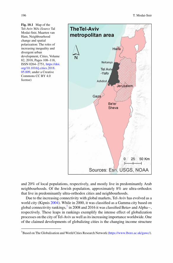
196 T. Modai-Snir
Fig. 10.1 Map of theTel-Aviv MA (Source TalModai-Snir, Maarten vanHam, Neighbourhoodchange and spatialpolarization: The roles ofincreasing inequality anddivergent urbandevelopment, Cities, Volume82, 2018, Pages 108–118,ISSN 0264–2751, https://doi.org/10.1016/j.cities.2018.05.009, under a CreativeCommons CC BY 4.0license)
and 20% of local populations, respectively, and mostly live in predominantly Arabneighbourhoods. Of the Jewish population, approximately 8% are ultra-orthodoxthat live in predominantly ultra-orthodox cities and neighbourhoods.
Due to the increasing connectivity with global markets, Tel-Aviv has evolved as aworld city (Kipnis 2004). While in 2000, it was classified as a Gamma city based onglobal connectivity rankings,7 in 2008 and 2016 it was classified Beta+ and Alpha−,respectively. These leaps in rankings exemplify the intense effect of globalizationprocesses on the city of Tel-Aviv as well as its increasing importance worldwide. Oneof the claimed developments of globalizing cities is the changing income structure
7Based on The Globalisation andWorld Cities Research Network (https://www.lboro.ac.uk/gawc/).
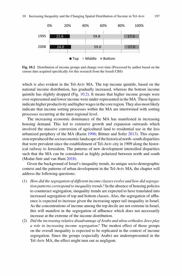
10 Increasing Inequality and the Changing Spatial Distribution of Income in Tel-Aviv 197
24.0
22.6
59.0
59.8
17.0
17.6
0% 20% 40% 60% 80% 100%
2008
1995
Top Middle Bo�om
Fig. 10.2 Distribution of income groups and change over time (Processed by author based on thecensus data acquired specifically for this research from the Israeli CBS)
which is also evident in the Tel-Aviv MA. The top income quintile, based on thenational income distribution, has gradually increased, whereas the bottom incomequintile has slightly dropped (Fig. 10.2). It means that higher income groups wereover-represented and lower incomewere under-represented in theMA. These figuresindicate higher productivity andhigherwages in the core region.They alsomost likelyindicate that income sorting processes within the MA are intertwined with sortingprocesses occurring at the inter-regional level.
The increasing economic dominance of the MA has manifested in increasinghousing demand. This led to extensive growth and expansion outwards whichinvolved the massive conversion of agricultural land to residential use in the lessurbanized periphery of the MA (Razin 1996; Bittner and Sofer 2013). This expan-sion reproduced the socioeconomic landscapeof the historical north–south disparitiesthat were prevalent since the establishment of Tel-Aviv city in 1909 along the histor-ical railway to Jerusalem. The patterns of new development intensified disparitiessuch that the MA can be considered as highly polarized between north and south(Modai-Snir and van Ham 2018).
Given the background of Israel’s inequality trends, its unique socio-demographiccontext and the patterns of urban development in the Tel-Aviv MA, the chapter willaddress the following questions:
(1) How did the segregation of different income classes evolve and how did segrega-tion patterns correspond to inequality trends? In the absence of housing policiesto counteract segregation, inequality trends are expected to have translated intoincreased segregation of top and bottom classes. Also, the segregation of afflu-ence is expected to increase given the increasing upper tail inequality in Israel.As the concentrations of income among the top decile are not extreme in Israel,this will manifest in the segregation of affluence which does not necessarilyincrease at the extreme of the income distribution.
(2) Did the increasing relative disadvantage of Arabs and ultra-orthodox Jews playa role in increasing income segregation? The modest effect of those groupson the overall inequality is expected to be replicated in the context of incomesegregation. Since the groups (especially Arabs) are underrepresented in theTel-Aviv MA, the effect might turn out as negligent.
198 T. Modai-Snir
(3) How are the different income classes spatially distributed? Is this distribu-tion indicative of spatial patterns of poverty/affluence concentration? Thereis already evidence that the socio-spatial structure of the Tel-Aviv MA hasdeveloped in a spatially polarized manner. Addressing this question, additionalspatial aspects of the clustering of income classes are examined, which cannotbe explored using dissimilarity indices alone.
10.5 Data and Methods
This study is based on data from the two recent censuses, 1995 and 2008, whichwere processed by the Israeli Central Bureau of Statistics (CBS). Compared to othercountries, therefore, census data is less updated, and the 13-year time gap betweencensuses is longer than the 10-year standard gap in most countries. The research areais the Tel-Aviv MA as delineated by the Israeli CBS. Its boundaries are based onfunctional relationships among localities that surround the city of Tel-Aviv and areidentical in 1995 and 2008. The basic spatial unit used is the census tract, which is aclose approximation of a neighbourhood. The division to census tracts is only avail-able in localities with more than 10,000 residents. Smaller localities are consideredone census tract.
In this study, income data was used to analyse residential segregation. The datasetcomprises of counts of individuals pertaining to each income decile, of those whowere employed andwhosemonthly income exceeded 100ILS,8 including all employ-ment statuses. Income data from the 1995 census were collected from a 20% sample.The 2008 census data were collected for the whole population from administra-tive sources. Income decile cut-offs are based on the national income distributionof each year, respectively. Census tracts with less than 30 employed individualswere excluded from the analysis. Also, illegal workers and asylum seekers are notincluded in census data, and so their effect on segregation is not accounted for. Thenumber of census tracts, as well as the number of employees, have substantiallygrown between the two censuses. This reflects extensive metropolitan developmentduring that period. The final dataset includes 900 census tracts in 1995, in which theaverage number of employees was 949, and 1027 census tracts in 2008, in which theaverage number of employees was 1484.
Income quintile counts are used for mapping location quotients and neighbour-hood income compositions. Segregation is measured using dissimilarity indices fordifferent pairs of income classes, using various aggregations of the data.
8ILS—Israeli new shekel. 100 ILS was equivalent to 20 EUR in 2008 (around 25 Euros as of 2019).
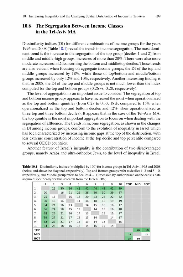
10 Increasing Inequality and the Changing Spatial Distribution of Income in Tel-Aviv 199
10.6 The Segregation Between Income Classesin the Tel-Aviv MA
Dissimilarity indices (DI) for different combinations of income groups for the years1995 and 2008 (Table 10.1) reveal the trends in income segregation. The most domi-nant trend is the increase in the segregation of the top group (deciles 1 and 2) frommiddle and middle-high groups, increases of more than 20%. There were also moremoderate increases inDI concerning the bottom andmiddle/top deciles. Those trendsare also evident when focusing on aggregate income groups; the DI of the top andmiddle groups increased by 18%, while those of top/bottom and middle/bottomgroups increased by only 12% and 10%, respectively. Another interesting finding isthat, in 2008, the DI of the top and middle groups is not much lower than the indexcomputed for the top and bottom groups (0.26 vs. 0.28, respectively).
The level of aggregation is an important issue to consider. The segregation of topand bottom income groups appears to have increased the most when operationalizedas the top and bottom quintiles (from 0.28 to 0.33, 18%, compared to 15% whenoperationalized as the top and bottom deciles and 12% when operationalized asthree top and three bottom deciles). It appears that in the case of the Tel-Aviv MA,the top quintile is the most important aggregation to focus on when dealing with thesegregation of affluence. The trends in income segregation, as shown in the changesin DI among income groups, conform to the evolution of inequality in Israel whichhas been characterized by increasing income gaps at the top of the distribution, withless extreme concentration of income at the top decile and top percentile comparedto several OECD countries.
Another feature of Israel’s inequality is the contribution of two disadvantagedgroups, namely Arabs and ultra-orthodox Jews, to the level of inequality in Israel.
Table 10.1 Dissimilarity indices (multiplied by 100) for income groups in Tel-Aviv, 1995 and 2008(below and above the diagonal, respectively). Top and Bottom groups refer to deciles 1–3 and 8–10,respectively, and Middle group refers to deciles 4–7. (Processed by author based on the census dataacquired specifically for this research from the Israeli CBS)
1 2 3 4 5 6 7 8 9 10 TOP MID BOT 1 22 30 36 41 42 44 43 42 39 2 20 16 21 26 28 30 30 29 27 3 25 13 15 18 20 23 22 22 22 4 30 18 14 14 16 18 18 19 19 5 34 21 16 13 14 15 16 16 17 6 36 24 18 15 13 14 15 16 18 7 38 26 21 16 14 13 15 15 17 8 39 27 21 17 15 13 14 14 17 9 38 27 21 17 16 13 14 13 15 10 34 23 18 16 16 15 16 15 15 TOP 26 28 MID 22 11 BOT 25 10
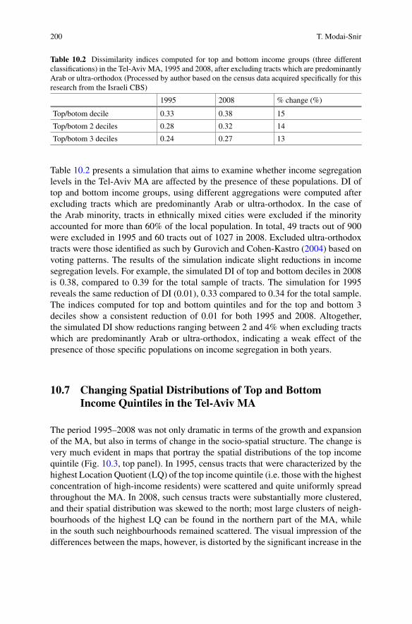
200 T. Modai-Snir
Table 10.2 Dissimilarity indices computed for top and bottom income groups (three differentclassifications) in the Tel-Aviv MA, 1995 and 2008, after excluding tracts which are predominantlyArab or ultra-orthodox (Processed by author based on the census data acquired specifically for thisresearch from the Israeli CBS)
1995 2008 % change (%)
Top/botom decile 0.33 0.38 15
Top/botom 2 deciles 0.28 0.32 14
Top/botom 3 deciles 0.24 0.27 13
Table 10.2 presents a simulation that aims to examine whether income segregationlevels in the Tel-Aviv MA are affected by the presence of these populations. DI oftop and bottom income groups, using different aggregations were computed afterexcluding tracts which are predominantly Arab or ultra-orthodox. In the case ofthe Arab minority, tracts in ethnically mixed cities were excluded if the minorityaccounted for more than 60% of the local population. In total, 49 tracts out of 900were excluded in 1995 and 60 tracts out of 1027 in 2008. Excluded ultra-orthodoxtracts were those identified as such by Gurovich and Cohen-Kastro (2004) based onvoting patterns. The results of the simulation indicate slight reductions in incomesegregation levels. For example, the simulated DI of top and bottom deciles in 2008is 0.38, compared to 0.39 for the total sample of tracts. The simulation for 1995reveals the same reduction of DI (0.01), 0.33 compared to 0.34 for the total sample.The indices computed for top and bottom quintiles and for the top and bottom 3deciles show a consistent reduction of 0.01 for both 1995 and 2008. Altogether,the simulated DI show reductions ranging between 2 and 4% when excluding tractswhich are predominantly Arab or ultra-orthodox, indicating a weak effect of thepresence of those specific populations on income segregation in both years.
10.7 Changing Spatial Distributions of Top and BottomIncome Quintiles in the Tel-Aviv MA
The period 1995–2008 was not only dramatic in terms of the growth and expansionof the MA, but also in terms of change in the socio-spatial structure. The change isvery much evident in maps that portray the spatial distributions of the top incomequintile (Fig. 10.3, top panel). In 1995, census tracts that were characterized by thehighest Location Quotient (LQ) of the top income quintile (i.e. those with the highestconcentration of high-income residents) were scattered and quite uniformly spreadthroughout the MA. In 2008, such census tracts were substantially more clustered,and their spatial distribution was skewed to the north; most large clusters of neigh-bourhoods of the highest LQ can be found in the northern part of the MA, whilein the south such neighbourhoods remained scattered. The visual impression of thedifferences between the maps, however, is distorted by the significant increase in the
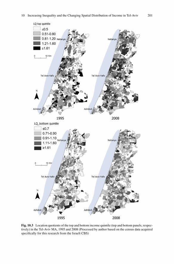
10 Increasing Inequality and the Changing Spatial Distribution of Income in Tel-Aviv 201
Fig. 10.3 Location quotients of the top and bottom income quintile (top and bottom panels, respec-tively) in the Tel-Aviv MA, 1995 and 2008 (Processed by author based on the census data acquiredspecifically for this research from the Israeli CBS)
202 T. Modai-Snir
number of neighbourhoods during that period. Both the numbers of neighbourhoodscharacterized by the highest and lowest LQ increased. However, in percentage terms,the former increased from 12 to 17%, whereas the latter stayed stable. Further exam-ination reveals that neighbourhoods with very high concentrations of high-incomeresidents increased at the expense of more mixed neighbourhoods with moderateconcentrations, as will also be confirmed in subsequent analysis. As for the spatialdistribution of the bottom income quintile, (Fig. 10.3, bottom panel), there is nosubstantial change over the study period in clustering patterns and locations ofneighbourhoods with different relative shares of low-income residents. Moreover,the shares of each LQ categories were similar in 1995 and 2008.
10.8 Changing Socioeconomic Compositions in Tel-AvivNeighbourhoods
The changing spatial distribution of income groups is also reflected in how theymix within neighbourhoods. Based on a typology of neighbourhood socioeconomiccompositions fromMarcinczak et al. (2015), which is based on occupational groups,in this chapter, the neighbourhoods are classified according to the composition ofincome classes. Each neighbourhood type is characterized by a distinctive mix ofincome classes which is defined by the shares of individuals pertaining to eachclass. Income classes to which individuals pertain were defined based on incomedeciles: Those pertaining to the three top and three bottom deciles were consideredas pertaining to ‘high’ and ‘low’ income classes, respectively. Those pertaining tothe four middle deciles (4–7) were considered as pertaining to the ‘middle’ incomeclass.
During the study period, the share of neighbourhoods that were classified as‘mixed’ decreased significantly (from 33.6 to 22.7%). This decrease was accompa-nied by a substantial increase in the proportion of neighbourhoods with high andmiddle-high statuses (from 36.3 to 45.9%) and a lesser increase in the proportionof middle-low neighbourhoods. Interestingly, the proportion of low-income neigh-bourhoods slightly decreased, but it was very small in the first place (2.4% in 1995and 1.6% in 2008).
The changing distribution of metropolitan neighbourhoods among types involveddistinctive spatial patterns (Fig. 10.4). While the decrease in the proportion ofmixed neighbourhoods seems to be uniformly spread, the increase in high and high-middle neighbourhoods is not even. The emergence of high-income neighbourhoodswas mainly in the north part of the MA, closer to the core. Middle-high-incomeneighbourhoods emerged in the southern part of the metropolitan area and in itsnorthern outskirts. Middle-low-income neighbourhoods continued to cluster in themost urbanized areas (visually they can be identified as the smaller tracts). Polarizedneighbourhoods changed locations completely between1995 and2008, implying thatpolarization characterizes neighbourhoods in transition. A close inspection reveals
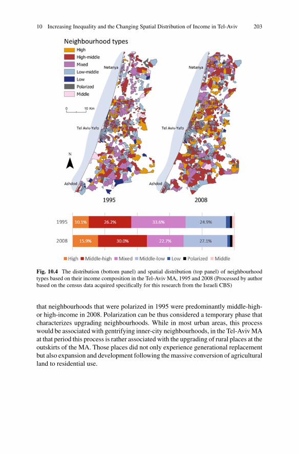
10 Increasing Inequality and the Changing Spatial Distribution of Income in Tel-Aviv 203
Fig. 10.4 The distribution (bottom panel) and spatial distribution (top panel) of neighbourhoodtypes based on their income composition in the Tel-Aviv MA, 1995 and 2008 (Processed by authorbased on the census data acquired specifically for this research from the Israeli CBS)
that neighbourhoods that were polarized in 1995 were predominantly middle-high-or high-income in 2008. Polarization can be thus considered a temporary phase thatcharacterizes upgrading neighbourhoods. While in most urban areas, this processwould be associated with gentrifying inner-city neighbourhoods, in the Tel-AvivMAat that period this process is rather associated with the upgrading of rural places at theoutskirts of the MA. Those places did not only experience generational replacementbut also expansion and development following themassive conversion of agriculturalland to residential use.
204 T. Modai-Snir
10.9 Conclusions
This study explores the changing spatial distribution of incomes in the metropolitanarea of Tel-Aviv, Israel. It is focused on the period between 1995 and 2008 duringwhich inequality increased substantially. The study addresses a series of questionsof which the first deals with the segregation of different classes and the connection toinequality trends. Predictions regarding this question were quite correct. Segregationof top and bottom income groups significantly increased between 1995 and 2008,for all group definitions (narrower and wider), as reflected in dissimilarity indices.The segregation of top and bottom quintiles was larger than the segregation of topand bottom deciles, which corresponds to the fact that Israel does not stand outin income shares held by the top decile or centile. The segregation of affluence wasmuch higher than the segregation of poverty in both years, and its rate of increase wasthe highest. This corresponds to the trends in upper tail inequality. Trends in incomesegregation also correspond to the changes in the distribution of neighbourhoodsamong neighbourhood types according to their income composition. A decline ofaround 50% in the proportion of neighbourhoods which were ‘mixed’ is quite adramatic change in the socio-spatial structure which inevitably means an increase insegregation.
The second question was whether the increasing relative disadvantage of Arabsand ultra-orthodox Jews played a role in increasing income segregation. The simula-tion of dissimilarity indices after excluding predominantly Arab and ultra-orthodoxtracts revealed that the two distinct populations seem to not have a significant effecton income segregation inmetropolitan Tel-Aviv; the exclusion of those tracts reducedbetween 2% and 4% of segregation measures. The effect of the presence of thosedisadvantaged groups on residential segregation is much weaker than we wouldexpect, given the substantially higher poverty rates among those groups and thesignificant increase in poverty rates during the period 1992–2011 (Ben-David andBleikh 2013). Thismay be related to the under-representation of the groups in the Tel-Aviv MA (especially the Arab group which makes up around 5% of the metropolitanpopulation compared to 20% in the total Israeli population). Another possible expla-nation is that disparities between those groups and the majority population withinthe MA are lesser than at the national level. This possibility should be addressed infurther research provided that sufficient individual-level data of these groups can becollected, which is especially challenging in the case of ultra-orthodox Jews.
The last question deals with how income classes were spatially distributed acrossthe MA over time, and whether there are indications of changing spatial patterns ofaffluence/poverty concentration. Themaps provide preliminary indications regardingthe changing socio-spatial structure of the MA and the changing concentration ofaffluence andpoverty over the research period.Location quotientmaps show that low-income classeswere quite evenly spread both in 1995 and 2008,whereas high-incomeclasses became very spatially clustered in 2008. The clusters of affluent groups aremuch larger in 2008 than in 1995 and indicate that they no longer concentrate inspecific neighbourhoods but in entire districts or cities. This change may have a
10 Increasing Inequality and the Changing Spatial Distribution of Income in Tel-Aviv 205
negative impact on the potential interaction among classes and on the distribution ofeconomic and political resources featured at the municipality level.
The numbers of high- and middle-high-income neighbourhoods increased signif-icantly over time and so did their shares of total metropolitan neighbourhoods. Thechanging distribution of neighbourhoods among types involved particular spatialpatterns. Themap of neighbourhood types highlights a distinction between the spatialdistributions of high- and middle-high-income neighbourhoods. In 1995, both wereevenly spread across theMA, apart froma slight under-representation of high-incomeneighbourhoods in the far north of themetropolitan area. In 2008, high-incomeneigh-bourhoods were clustered across the entire northern part of the metropolitan area,and especially close to the core; middle-high-income neighbourhoods emerged inthe southern part of the metropolitan area and in the northern outskirts. This findingadds insight into the patterns of north–south polarization.
Poverty rates in Israel are among the highest in the OECD, but both the locationquotient map and the neighbourhood types map indicate that there was hardly anyconcentration of poverty in theMA in either year. There were very few scattered poorneighbourhoods. The lowest prevalent neighbourhood statuswas low-middle-incomeneighbourhoods. In that respect, it can be said that the socioeconomic landscape ofthe Tel-Aviv MA, despite the high inequality and poverty rates in Israel, is differentthan urban areas in the United States where concentrated poverty is an issue of greatconcern. There is, however, some difference between the classification of ‘concen-trated poverty’ in the United States and ‘low-income’ neighbourhoods in the contextof this study, which should be considered. Neighbourhoods of concentrated povertyin the United States are usually characterized as those with at least 40% poor (e.g.Jargowsky 2013). In this study, low-income neighbourhoods are those in which atleast 50% of the residents are low income. However, low-income residents in thisclassification are those pertaining to the three bottom deciles, which is a much widergroup than those defined as strictly poor. With poverty rates in Israel of around 18%,the poor can be defined approximately as those pertaining to the two bottom deciles.The inclusion of low-income people who are not considered strictly ‘poor’ shouldcompensate for the reductionist 50% definition of neighbourhoods with concentratedpoverty.
Altogether, this study reveals trends of increasing income segregation in Tel-AvivMA, which conforms to other cities in the developed world. However, the fine-grained picture of segregation reflects particular inequality trends in Israel, as wellas the interaction with its particular socioeconomic landscape and patterns of urbandevelopment.
References
Ben-David D, Bleikh H (2013) Poverty and inequality over time in israel and in the OECD. In: Stateof the nation report: society, economy and policy in Israel 2013. Taub Centre for Social PolicyStudies in Israel.
206 T. Modai-Snir
Bittner C, Sofer M (2013) Land use changes in the rural-urban fringe: an Israeli case study. LandUse Policy 33:11–19. https://doi.org/10.1016/j.landusepol.2012.11.013
Carmon N (2001) Housing policy in Israel: review, evaluation and lessons. Isr Aff 7:181–2008.https://doi.org/10.1080/13537120108719620
Central Bureau of Statistics (Israel), Population censuses. https://www.cbs.gov.il/en/Surveys/Pages/Population-Census.aspx
Cornfeld O, Danieli O (2015) The origins of income inequlaity in Israel—trends and policy. IsrEcon Rev 12:51–95
Falah G (1996) Living together apart: residential segregation in mixed Arab-Jewish Cities in Israel.Urban Stud 33:823–857
Friedman I, Shaul-Mena N, Fogel N et al (2011) Measurement and estimates of the population ofultra-orthodox Jews
Gurovich N, Cohen-Kastro E (2004) Ultra-orthodox Jews—geographic distribution and demo-graphic, social and economic characteristics of the ultra-orthodox jewish population in Israel1996–2001
Haberfeld Y, Cohen Y (2007) Gender, ethnic, and national earnings gaps in Israel: the role of risinginequality. Soc Sci Res 36:654–672. https://doi.org/10.1016/J.SSRESEARCH.2006.02.001
Hananel R, Perlman S, Vatury A, Krefetz SP (2018) Housing matters: public housing policy inSweden, the United States, and Israel. J Plan Educ Res. https://doi.org/10.1177/0739456X18793702
Jargowsky PA (2013) Concentration of poverty in the new millennium: changes in prevalence,composition, and locationof highpoverty neighborhoods.CenturyFoundation andRutgersCenterfor Urban Research and Education.
Kipnis BA (2004) Tel Aviv, Israel—a world city in evolution: urban development at a deadend ofthe global economy. Dela 21:183–193
Kraus V, Koresh Y (2012) The course of residential segregation: ethnicity, socioeconomic status,and suburbanization in Israel. Sociol Q 33:303–319
Marcinczak S, Musterd S, van Ham M, Tammaru T (2015) Inequality and rising levels of socio-economic segregation: lessons from a pan-E. In: Tammaru T, van HamM,Marcinczak S,MusterdS (eds) Socio-economic segregation in european capital cities: east meets west. Routledge,London
Marcinczak S, Tammaru T, Novák J et al (2015) Patterns of socioeconomic segregation in the capitalcities of fast-track reforming postsocialist countries. Ann Assoc Am Geogr. https://doi.org/10.1080/00045608.2014.968977
Modai-Snir T, van Ham M (2018) Neighbourhood change and spatial polarization: the roles ofincreasing inequality and divergent urban development. Cities 82:108–118. https://doi.org/10.1016/J.CITIES.2018.05.009
OECD (2015) In it together: why less inequality benefits all. OECD Publishing, Paris. https://doi.org/10.1787/9789264235120-en
Quillian L, Lagrange H (2016) Socioeconomic segregation in large cities in France and the UnitedStates. Demography 53:1051–1084. https://doi.org/10.1007/s13524-016-0491-9
Razin E (1996) Trends in the urban-rural fringe of the Tel-Aviv metropolis and their implicationsfor the organization of local government. Floresheimer Inst Policy Stud, Jerusalem
Reardon SF, Bischoff K (2011) Income inequality and income segregation. Am J Sociol 116:1092–1153. https://doi.org/10.1086/657114
Shilhav Y (1993) The emergence of ultra-orthodox neighbourhoods in Israeli urban centres. In: BenE (ed) Local communities and the Israeli polity: conflict of values and interests. State Universityof New-York Press, Albany, NY, pp 157–187
Tammaru T, Marcinczak S, Aunap R et al (2019) Relationship between income inequality andresidential segregation of socioeconomic groups. Reg Stud 1–12. https://doi.org/10.1080/00343404.2018.1540035
Tammaru T,Marcinczak S, VanHamM,Musterd S (2015) Socio-economic segregation in Europeancapital cities: east meets west. Routledge, London
10 Increasing Inequality and the Changing Spatial Distribution of Income in Tel-Aviv 207
Watson T (2009) Inequality and the measurement of residential segregation by income in Americanneighbourhoods. Rev IncomeWealth 55:820–844. https://doi.org/10.1111/j.1475-4991.2009.00346.x
Werczberger E (1995) The role of public housing in Israel: Effects of privatization. Scand HousPlan Res 12:93–108. https://doi.org/10.1080/02815739508730378
Werczberger E, Reshef N (1993) Privatisation of public housing in Israel: inconsistency orcomplementarity? Hous Stud 8:195–206. https://doi.org/10.1080/02673039308720761
Open Access This chapter is licensed under the terms of the Creative Commons Attribution 4.0International License (http://creativecommons.org/licenses/by/4.0/), which permits use, sharing,adaptation, distribution and reproduction in any medium or format, as long as you give appropriatecredit to the original author(s) and the source, provide a link to the Creative Commons license andindicate if changes were made.
The images or other third party material in this chapter are included in the chapter’s CreativeCommons license, unless indicated otherwise in a credit line to the material. If material is notincluded in the chapter’s Creative Commons license and your intended use is not permitted bystatutory regulation or exceeds the permitted use, you will need to obtain permission directly fromthe copyright holder.
Chapter 11Changes in Occupational Structureand Residential Segregation in Tokyo
Masaya Uesugi
Abstract Similar to other industrialized countries, Japan has experienced a growthin income inequality since the 1980s. Furthermore, in the past few decades, Tokyohas come to adopt a more liberalist position for not only welfare and housing policyof the state but also to urban policy. This chapter examines the changes in socio-spatial inequality in Tokyo from2000 to 2015.During this period, segregation indicesconfirm some level of residential separation between the top and bottom occupationalgroups, and segregation is fairly stable over time. This suggests that certain factorscounteract the increase of residential segregation. A comparison between the TokyoMetropolitan Region and the core city reveals that the core city amplifies spatialinequality. In contrast to the limited change in the city-wide levels of segregation,the changes in the residential patterns show that people with high occupational statustend to concentrate around the main railway station in suburban areas in the regionand inside the core city, especially adjacent to the central neighborhoods.
Keywords Occupational structure · Residential segregation · Neighborhood ·Tokyo
11.1 Introduction
Since the 1960s, a robust middle class has developed along with the growth ofthe economy in Japan. Around 1970, Japan belonged to the group of the lowesteconomic inequality among the OECD countries, along with the Nordic countries(Sawyer 1976). However, the Gini coefficient and the relative poverty rate increasedand became higher than the OECD average in the 2000s, which evoked public andpolitical discourse on various forms of inequality (Chiavacci and Hommerich 2017).
An important manifestation of inequality from a geographical perspective is resi-dential segregation. Recent international comparative studies suggest that levels ofresidential segregation depend not only on levels of economic inequality but also
M. Uesugi (B)Fukuoka Institute of Technology, Fukuoka, Japane-mail: [email protected]
© The Author(s) 2021M. van Ham et al. (eds.), Urban Socio-Economic Segregation and Income Inequality,The Urban Book Series, https://doi.org/10.1007/978-3-030-64569-4_11
209
210 M. Uesugi
on contextual factors such as welfare, housing regimes, and political and institu-tional environments (Tammaru et al. 2016). Tokyo is not only Japan’s center ofeconomy, politics, and culture but also one of the most global cities with NewYork and London, as highlighted by Sassen (1991), whose examination of socialpolarization and its impact on social geography has attracted abundant interest fromscholars. In the central part of Tokyo (Tokyo City area consists of 23 special wards;hereinafter, referred to as City), a distinct pattern of socio-economic segregationhas been identified for several decades: white-collar workers are concentrated in theupland area (Yamanote) and spread from the center to the west of the city, and theblue-collar workers live principally in the lowland downtown area (Shitamachi) inthe east (Kurasawa and Asakawa 2004). In the early 2000s in particular, managerialworkers tended to concentrate in the city center (Wakabayashi and Koizumi 2018).On the other hand, although acknowledging such a contrast in general, Fujita andHill (2012) and Wissink and Hazelzet (2012), who investigated the proportion ofdifferent social classes at the neighborhood level, suggested that neighborhoods inTokyo are socially mixed.
Another definition of the Tokyo area is the Tokyo Metropolitan Region (here-inafter, referred to as Region), which includes suburban areas of neighboringmunicipalities. Studies at the level of municipalities found that the distribution ofhigh-income residents shifted from the suburbs to the city from the 1980s to the2000s (Jacobs 2012; Toyoda 2007). They also stress that residential segregation hasincreased with elevated income levels in Yamanote and the city center, and decreasedincome levels in Shitamachi and the peripheral area.
We must ask ourselves if the level of residential segregation in Tokyo is greaterthan in cities of other countries. Fielding (2004) demonstrated that although thereis a certain degree of socio-economic segregation at neighborhood level in Japan,it is lower than that of a British city. As reasons for this, he refers to the smallerincome disparity in Japan compared to Great Britain. In addition, Fujita and Hill(2012) argued that several factors, including a centralized tax system and publichousing policy, prevent income inequality from leading to class-based segregationin Tokyo. Jacobs (2005, 2012) confirmed that residential segregation in Tokyo wasless than in the larger US metropolitan areas, despite the fact that income disparitybetween municipalities expanded in the Tokyo metropolitan area after the 1980s.He emphasizes the significance of severe restrictions on immigration (the numberof migrant workers is very low in Tokyo) and the government policy to preventsocio-economic fragmentation of municipalities in Japan.
Previous studies on segregation in Tokyo covered its changes until the mid-2000s,but since the late 2000s, Tokyo has experienced somemajor socio-economic changes,such as the global financial crisis triggered by the bankruptcy of Lehman Brothers in2008, the M9.0 Great East Japan earthquake1 of 2011, and unprecedented monetaryeasing by the central bank of Japan from2013. Income inequality, thewelfare system,and the housing system are also changing. In this chapter, based on these contextualchanges, we elucidate the process of social–spatial change in Tokyo from 2000 to
11 Changes in Occupational Structure and Residential … 211
2015. In addition, this studywill contribute to the field of socio-economic segregationby emphasizing the relationship between city and suburb based on two differentdefinitions of Tokyo (Region and City).2
11.2 Context
11.2.1 Income Inequality
Since the 1980s, income inequality has been increasing in many countries (OECD2015). During this time, income inequality has also been on the rise in Japan,albeit slightly, as indicated by the Gini coefficients of equivalent disposable income.However, the size of the coefficient varies somewhat depending on which data areused. OECD data indicate the coefficient increased from 0.30 in 1985 to 0.34 in2000 and decreased slightly to 0.32 in 2003. After that, the coefficient rose to 0.34again in 2009. Nevertheless, the Gini coefficient of 0.33 in 2013 remained higherthan the OECD average of 0.32 (OECD 2015). Japan’s Gini coefficient, based onthe National Survey of Family Income and Expenditure provided by the Ministry ofInternal Affairs and Communications, is smaller in size, but indicates a similar trend:it increased from 0.25 in 1984 to 0.28 in 2009 and remained flat in 2014.
The publication of statistics indicating growing income inequality in Japan fromthe 1980s until the 1990s provoked strong reactions; for example, Tachibanaki’s(2005) assertion that Japan is no longer a middle-class society. However, the reasonsfor these changes are not universally agreed upon, with some also pointing a fingerat the aging population and the shrinking size of households (Ohtake 2008). Never-theless, Shikata (2013) argued that income inequality began to increase within agegroups after 2000 and that this was due to factors such as the increase in irregularemployment in all age groups, rather than demographic causes. In fact, since 2007,over one-third of all workers have been irregular workers, and their number hasdoubled since the 1990s (MHLW 2013).
11.2.2 Welfare System
There is no consensus regarding which of the three main types of welfare regimes ofEsping-Andersen (1990) corresponds to that of current Japan. As described below,the characteristics of the Japanese welfare state can be aligned with multiple welfareregimes (MHLW 2012). First, policy in Japan has emphasized employment security,protecting employment through measures such as minimizing layoffs by companiesand public work projects. Japan also guarantees a pension, health insurance, andservices to all its citizens.As a result, the country hasmaintained a lowunemploymentrate on par with that of countries with social democratic welfare regimes. Conversely,
212 M. Uesugi
Japan’s system includes characteristics of a conservativewelfare regime; for example,the generous social security benefits for the elderly and its strong emphasis on thefamily. However, the system also contains elements peculiar to a liberal welfareregime. Social security expenditure, as a whole, is relatively limited and medicalbenefits (universal health care) in Japan are comparable to those in the US and theUK as a share of GDP.
Since the 1990s, however, increasing globalization of the economy and intensifiedinternational competition among companies as a result of the government’s liberalpolicies, have fostered an increase in the number of irregular workers, who can beutilized flexibly and cheaply. Widespread layoffs of temporary workers became asocial problem during the 2008 economic crisis, highlighting the limited institu-tional support available to those who have left the labor market. As social secu-rity expenditure balloons to keep pace with the aging population, calls for fiscalreform have increased and benefits, such as medical benefits and pensions, are beingreduced. Consequently, for example, individual pensions have become smaller fornearly 20 years.
11.2.3 Housing System
Japan’s post-WWII housing policy was drawn up with the aim of improving defi-cient housing and ameliorating housing shortages. Under the principle that everyfamily should have its own home, the core of the housing policy was that suchhousing systems should ultimately allow individuals to acquire their own housingvia the market, principally by providing support in the form of mortgage loans. Thegovernment provided themiddle-income householdswith long-term and low-interestloans to buy their own home through the Government Housing Loan Corporation. Inaddition to that, the government encouraged housing ownership with a tax reduction.
The population living in urban areas increased rapidly in Japan during the period ofhigh economic growth from the 1950s to the 1960s. As the economy grew, residentialdevelopments in the suburbs, featuring mainly detached single-family homes, servedto house the rapidly expanding middle class. During the 1980s economic bubble,soaring land prices further accelerated the move to the suburbs. An overview ofthe Tokyo metropolitan area suggests that homeownership developed chiefly in thesuburbs. In the city center and adjacent areas, where land prices were high, affordableland and housing were in short supply. Consequently, homeownership rates limpedbehind those observed in the suburbs (Takagi 2012).
Therefore, Tokyo, to this day, has a relatively small stock of public housing,including housing aimed at the middle-income bracket, and the percentage of peoplewho own their houses is almost the same as the percentage of people using theprivate rental market. In spite of the weak support for the private rental market andthe absence of rent regulation, the proportion of private rental housing tends to behigh in urban areas. On the contrary, public housing provided by local governmentshas an income ceiling for tenants and the rents are regulated. The census revealed
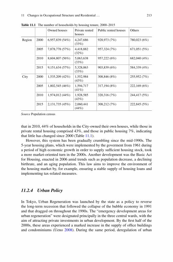
11 Changes in Occupational Structure and Residential … 213
Table 11.1 The number of households by housing tenure, 2000–2015
Owned houses Private rentedhouses
Public rented houses Others
Region 2000 6,957,839 (54%) 4,247,686(33%)
928,973 (7%) 780,023 (6%)
2005 7,878,778 (57%) 4,418,882(32%)
957,324 (7%) 671,051 (5%)
2010 8,604,807 (56%) 5,063,638(33%)
957,222 (6%) 682,040 (4%)
2015 9,151,634 (57%) 5,328,063(33%)
903,839 (6%) 584,339 (4%)
City 2000 1,535,209 (42%) 1,552,984(43%)
308,846 (8%) 255,952 (7%)
2005 1,802,545 (46%) 1,594,717(41%)
317,194 (8%) 222,169 (6%)
2010 1,974,012 (44%) 1,928,585(43%)
320,316 (7%) 244,417 (5%)
2015 2,131,735 (45%) 2,060,441(44%)
308,212 (7%) 222,845 (5%)
Source Population census
that in 2010, 44% of households in the City-owned their own houses, while those inprivate rental housing comprised 43%, and those in public housing 7%, indicatingthat little has changed since 2000 (Table 11.1).
However, this system has been gradually crumbling since the mid-1990s. The5-year housing plans, which were implemented by the goverment from 1961 duringa period of high economic growth in order to supply sufficient housing stock, tooka more market-oriented turn in the 2000s. Another development was the Basic Actfor Housing, enacted in 2006 amid trends such as population decrease, a decliningbirthrate, and an aging population. This law aims to improve the environment ofthe housing market by, for example, ensuring a stable supply of housing loans andimplementing tax-related measures.
11.2.4 Urban Policy
In Tokyo, Urban Regeneration was launched by the state as a policy to reversethe long-term recession that followed the collapse of the bubble economy in 1991and that dragged on throughout the 1990s. The “emergency development areas forurban regeneration” were designated principally in the three central wards, with theaim of attracting private investments in urban development. By the first half of the2000s, these areas experienced a marked increase in the supply of office buildingsand condominiums (Ueno 2008). During the same period, deregulation of urban
214 M. Uesugi
planning encouraged private investments in urban redevelopment. Deregulation, aspart of urban policy, is commonly considered to be an important factor behind socialand spatial changes (vanKempen 2007). In fact, although some urban redevelopmentprojects are implemented jointly by private developers and public sectors in Tokyo,most are undertaken by the private sector, mainly by large Japanese corporations,backed by the TokyoMetropolitan Government. This has played a large role in urbanrestructuring in Tokyo (Waley 2007), mainly taking place in the center of the cityand by Tokyo bay.
The above-mentioned developments changed the urban landscape and the spatialstructure of Tokyo (Waley 2013). Lützeler (2008) suggested that this kind of middleclass-oriented development of a city center risks triggering class-selective migrationand increases the overall level of residential segregation. Hirayama (2005) high-lighted urban renewal policy implemented from the late 1990s to the early 2000sstimulated the housing market, which resulted in the simultaneous emergence of“hot spots” in the city center and “cold spots” in the surrounding areas as a notice-able example of residential inequality. The “hot spots” were characterized as clustersof condominium skyscrapers, such as Roppongi, Shinagawa, and Toyosu districts(see Fig. 11.2). As one of those urban development projects—Roppongi Hills thatconsists of a mix of office, commercial, and residential functions with 720 thousandm2 of floor space implemented by a private developer—became a symbol of thosehigh-end neighborhoods of Tokyo. In Shinagawa District near Tokyo bay, severalprivate developers built high-rise buildings for offices and residences, using the siteof Japan National Railway. The Japanese National Railway, a former government-owned company, has been privatized in 1987 and disposed of some railway yardsthat were no longer used in order to reduce the debt. High-rise condominiums havealso been on the rise in the waterfront area around Toyosu. Conversely, the marketwas stagnant in the “cold spots.” In the early 2000s, some cities located in thesuburban area, such as Sayama City and Konan Ward in Yokohama City, had losttheir population despite their advantage of access to the city center.
11.3 Data and Methods
In this research, we used census data from 2000, 2005, 2010, and 2015. Tokyois defined in two ways: Region and City. The Region is the functional urban area(FUA) and comprises Tokyo and certain areas in Kanagawa, Chiba, Saitama, Ibaraki,Yamanashi, and Tochigi prefectures, as defined by the OECD (2013). The City isthe central area of the Region and consists of 23 special wards. As of 2015, thepopulation of the City is 9.3 million and the population of the Region is 35.7 million,accounting for approximately one-quarter of the entire Japanese population. In thecensus, the number of employed persons by occupation is available at cho districtlevel (hereinafter, referred to as neighborhood level), which is the smallest censustract. The average number of residents of this unit is approximately 1,700 for theRegion and approximately 3,000 for the City.
11 Changes in Occupational Structure and Residential … 215
However, there are two problemswith this data. First, since the boundaries of someneighborhoodswere changed between 2000 and 2015, in this study, we re-aggregatedthe census data from 2010 and before according to the latest 2015 census boundaries.Second, the Japan Standard Occupational Classification, which does not necessarilycorrespond to the International Standard Occupational Classification (ISCO), wasrevised in 2009 (Ministry of Internal Affairs and Communications 2009). Somemajor groups of blue-collar workers were abolished and restructured to new groups.Moreover, classifications of some sub-major groups were revised, although the labeldid not necessarily change. In this study, major occupational groups are assignedto three socio-economic groups as follows: the top group consists of administrativeand managerial workers and professional and technical workers; the middle groupof clerical workers, sales workers, security workers, and service workers; and thebottom group of transport and communication workers and production process andrelated workers (manufacturing process workers, construction and mining workers,and carrying, cleaning, packaging, and related workers in 2010 and 2015).
We first examined the polarization thesis of Sassen (1991), starting from the2000s, based on the changes in occupational structure. Subsequently, we measuredresidential segregation between the top and bottom occupational categories using thedissimilarity index (DI) (Duncan and Duncan 1955), which is a traditional indicatorof residential segregation between two specific groups. Next, from a geographicalpoint of view, we used three kinds of maps to verify the spatial patterns of residentialsegregation: concentration of the top occupational group, location quotient (LQ)for the top and bottom occupational groups, and classification of neighborhoods bysocio-economic composition. First, the areas where the top group are concentratedare identified and sorted in a descending order based on the number of people in thetop group. Neighborhoods including a cumulative population of one-fifth of the topgroup are labeled Q1, neighborhoods that contain the next one-fifth population inthe top group are labeled Q2, and so on. If the number of Q1 neighborhoods is small,it means that top occupational groups are residentially concentrated only into a fewneighborhoods.
Second, the spatial distribution of the LQ at both ends of the occupational hier-archy or top and bottom occupational groups is explored. LQ or the ratio of a certainoccupation group in each neighborhood divided by the ratio of the same occupa-tion group occupying the whole area is a well-known method for representing thespatial distribution of socio-economic segregation (Tammaru et al. 2016). When theLQ ratio for a certain group is greater than one, the group is over-represented in theneighborhood.
Finally, we investigated the within-neighborhood socio-economic intermixingfrom the spatial distribution of neighborhood classifications by socio-economiccomposition. According to the classification based on the proportion of the threesocio-economic groups ofMarcinczak et al. (2015), all neighborhoods fall into seventypes: high socio-economic status (SES) neighborhoods, middle to high SES neigh-borhoods, mixed neighborhoods, middle SES neighborhoods, low to middle SESneighborhoods, low SES neighborhoods, and polarized neighborhoods.
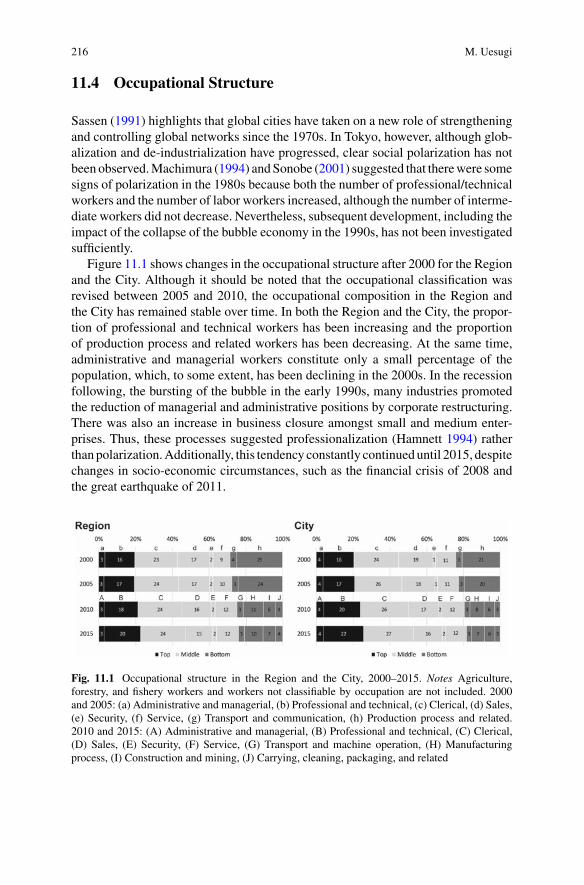
216 M. Uesugi
11.4 Occupational Structure
Sassen (1991) highlights that global cities have taken on a new role of strengtheningand controlling global networks since the 1970s. In Tokyo, however, although glob-alization and de-industrialization have progressed, clear social polarization has notbeen observed.Machimura (1994) andSonobe (2001) suggested that therewere somesigns of polarization in the 1980s because both the number of professional/technicalworkers and the number of labor workers increased, although the number of interme-diate workers did not decrease. Nevertheless, subsequent development, including theimpact of the collapse of the bubble economy in the 1990s, has not been investigatedsufficiently.
Figure 11.1 shows changes in the occupational structure after 2000 for the Regionand the City. Although it should be noted that the occupational classification wasrevised between 2005 and 2010, the occupational composition in the Region andthe City has remained stable over time. In both the Region and the City, the propor-tion of professional and technical workers has been increasing and the proportionof production process and related workers has been decreasing. At the same time,administrative and managerial workers constitute only a small percentage of thepopulation, which, to some extent, has been declining in the 2000s. In the recessionfollowing, the bursting of the bubble in the early 1990s, many industries promotedthe reduction of managerial and administrative positions by corporate restructuring.There was also an increase in business closure amongst small and medium enter-prises. Thus, these processes suggested professionalization (Hamnett 1994) ratherthanpolarization.Additionally, this tendency constantly continueduntil 2015, despitechanges in socio-economic circumstances, such as the financial crisis of 2008 andthe great earthquake of 2011.
Fig. 11.1 Occupational structure in the Region and the City, 2000–2015. Notes Agriculture,forestry, and fishery workers and workers not classifiable by occupation are not included. 2000and 2005: (a) Administrative and managerial, (b) Professional and technical, (c) Clerical, (d) Sales,(e) Security, (f) Service, (g) Transport and communication, (h) Production process and related.2010 and 2015: (A) Administrative and managerial, (B) Professional and technical, (C) Clerical,(D) Sales, (E) Security, (F) Service, (G) Transport and machine operation, (H) Manufacturingprocess, (I) Construction and mining, (J) Carrying, cleaning, packaging, and related
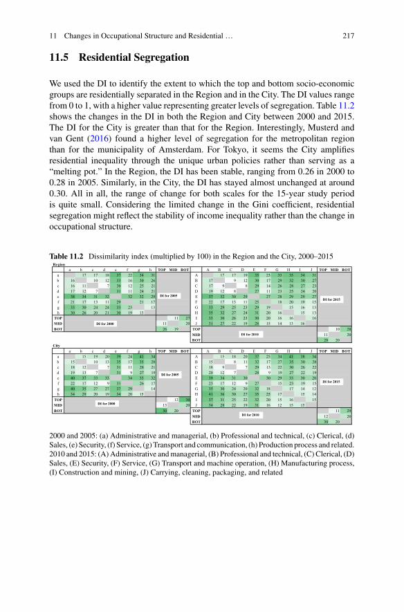
11 Changes in Occupational Structure and Residential … 217
11.5 Residential Segregation
We used the DI to identify the extent to which the top and bottom socio-economicgroups are residentially separated in the Region and in the City. The DI values rangefrom 0 to 1, with a higher value representing greater levels of segregation. Table 11.2shows the changes in the DI in both the Region and City between 2000 and 2015.The DI for the City is greater than that for the Region. Interestingly, Musterd andvan Gent (2016) found a higher level of segregation for the metropolitan regionthan for the municipality of Amsterdam. For Tokyo, it seems the City amplifiesresidential inequality through the unique urban policies rather than serving as a“melting pot.” In the Region, the DI has been stable, ranging from 0.26 in 2000 to0.28 in 2005. Similarly, in the City, the DI has stayed almost unchanged at around0.30. All in all, the range of change for both scales for the 15-year study periodis quite small. Considering the limited change in the Gini coefficient, residentialsegregation might reflect the stability of income inequality rather than the change inoccupational structure.
Table 11.2 Dissimilarity index (multiplied by 100) in the Region and the City, 2000–2015Region
a b c d e f g h TOP MID BOT A B C D E F G H I J TOP MID BOTa 17 17 18 37 22 34 31 A 17 17 19 35 23 33 35 34 31b 16 10 12 33 16 30 26 B 17 9 12 30 17 29 32 30 27c 16 11 7 30 12 25 21 C 17 9 8 29 14 26 28 27 23d 17 12 7 31 11 24 21 D 19 12 8 27 11 23 25 24 20e 38 34 31 32 32 32 29 E 37 32 30 29 27 28 29 29 27f 21 17 13 11 29 21 17 F 22 17 13 11 25 18 20 19 15g 33 30 24 24 33 23 13 G 33 29 25 23 29 19 15 16 13h 30 26 20 21 30 19 13 H 35 32 27 24 31 20 16 15 13
TOP 11 27 I 33 30 26 23 30 20 16 16 16MID 11 20 J 31 27 22 19 28 15 14 13 16BOT 26 19 TOP 10 28
MID 11 20BOT 28 20
Citya b c d e f g h TOP MID BOT A B C D E F G H I J TOP MID BOT
a 15 19 20 39 24 41 34 A 15 18 20 37 25 34 41 38 34b 15 10 13 35 17 35 28 B 15 8 11 32 17 27 35 30 28c 18 12 7 31 11 28 21 C 18 9 7 29 13 22 30 26 22d 19 13 7 31 9 27 19 D 20 12 7 28 9 19 27 22 19e 40 37 33 33 34 35 32 E 39 34 31 30 30 29 33 30 28f 22 17 12 9 31 26 17 F 23 17 12 9 27 15 23 19 15g 40 35 27 27 37 29 14 G 35 30 24 20 32 18 17 14 12h 34 29 20 19 34 20 15 H 41 36 30 27 35 25 17 15 14
TOP 12 30 I 37 31 25 22 32 20 15 16 15MID 13 20 J 34 28 22 19 31 16 12 15 15BOT 30 20 TOP 11 29
MID 12 20BOT 30 20
DI for 2000
DI for 2005
DI for 2005
DI for 2000
DI for 2010
DI for 2015
DI for 2015
DI for 2010
2000 and 2005: (a) Administrative and managerial, (b) Professional and technical, (c) Clerical, (d)Sales, (e) Security, (f) Service, (g) Transport and communication, (h) Production process and related.2010 and 2015: (A)Administrative andmanagerial, (B) Professional and technical, (C) Clerical, (D)Sales, (E) Security, (F) Service, (G) Transport and machine operation, (H) Manufacturing process,(I) Construction and mining, (J) Carrying, cleaning, packaging, and related
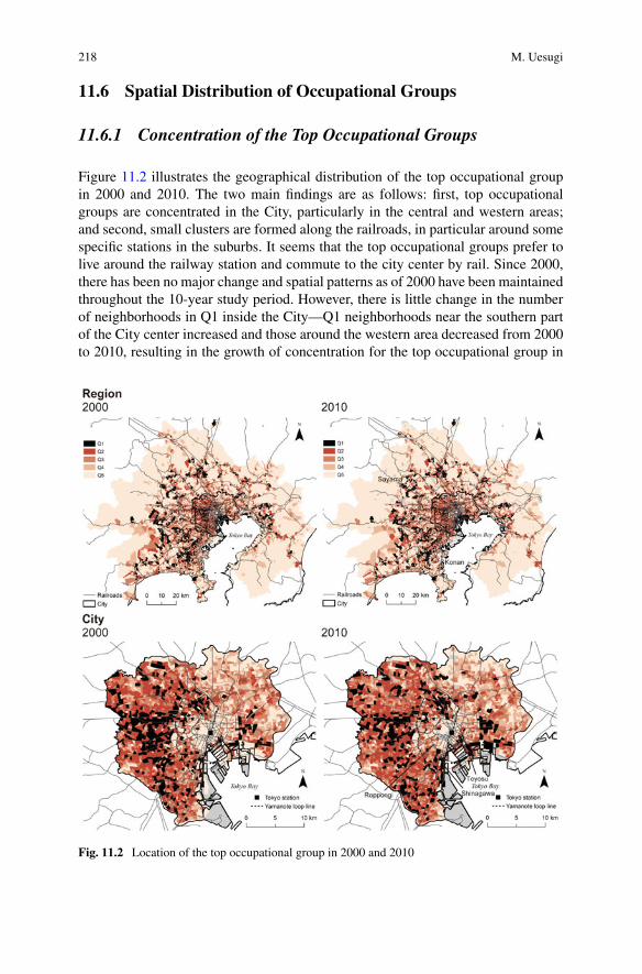
218 M. Uesugi
11.6 Spatial Distribution of Occupational Groups
11.6.1 Concentration of the Top Occupational Groups
Figure 11.2 illustrates the geographical distribution of the top occupational groupin 2000 and 2010. The two main findings are as follows: first, top occupationalgroups are concentrated in the City, particularly in the central and western areas;and second, small clusters are formed along the railroads, in particular around somespecific stations in the suburbs. It seems that the top occupational groups prefer tolive around the railway station and commute to the city center by rail. Since 2000,there has been no major change and spatial patterns as of 2000 have been maintainedthroughout the 10-year study period. However, there is little change in the numberof neighborhoods in Q1 inside the City—Q1 neighborhoods near the southern partof the City center increased and those around the western area decreased from 2000to 2010, resulting in the growth of concentration for the top occupational group in
Fig. 11.2 Location of the top occupational group in 2000 and 2010
11 Changes in Occupational Structure and Residential … 219
the central districts of Tokyo. This demographic change is partly associated withgentrification that accompanied the upward shift in the socio-economic structureof residents. For instance, more and more wholesale shops and factories have beenreplaced by condominiums in such districts as Nihonbashi, Tsukishima, and Minato(Fujitsuka 2017). These districts are locatedwithin 2 or 3 km southeast of the businessdistrict surrounding Tokyo station.
11.6.2 Location Quotient for the Top and BottomOccupational Groups
Figure 11.3 shows the LQ for the top and bottom occupational groups in 2000 and2010.3 In terms of the residential location of the top occupational group, in linewith the findings of the previous section, there were several clusters in the Region,including in the center of the City. The residential patterns based on the concentricstructure around the city center and railroad network have remained robust over time.Within theCity aswell, the top occupational groupwas concentrated in the city center.Neighborhoods with a high LQ prevailed in the center and became geographicallyagglomerated, especially inside the southern half of the Yamanote loop line. On theother hand, neighborhoods with a high LQ for the bottom occupational group spreadto the suburbs, to the periphery of the Region, avoiding areas along the railroad lines.These sorts of low socio-economic neighborhoods are growing where the proportionof the bottom occupational group was already above average and the concentrationcontinues to increase.
11.6.3 Classification of Neighborhoods by Socio-economicComposition
Figure 11.4 presents the geographical distribution of seven neighborhood types basedon socio-economic composition. As confirmed in the previous section, high SES andhigh-middle SES neighborhoods are spreading from the center of the City to thewest side and are scattered along the railroad toward the suburbs. Low SES and low-middle SES neighborhoods are distributed to the peripheral area. In the Region as awhole, there has been a remarkable growth of high-middle SES neighborhoods since2000. Thus, while the absolute number of people in the bottom occupational group isdecreasing, they are being pushed to peripheral areas of the Tokyo metropolitan area.In the City, the high SES and high-middle SES neighborhoods filled the inside ofthe Yamanote loop line to the west part of the City, including Roppongi, Shinagawa,and Toyosu districts. Additionally, as mentioned above, gentrification is generallyconsidered to have occurred from the southern part of the city center to the eastside. Although it is not shown on this map, the spatial patterns of 2010 are almostmaintained in 2015.
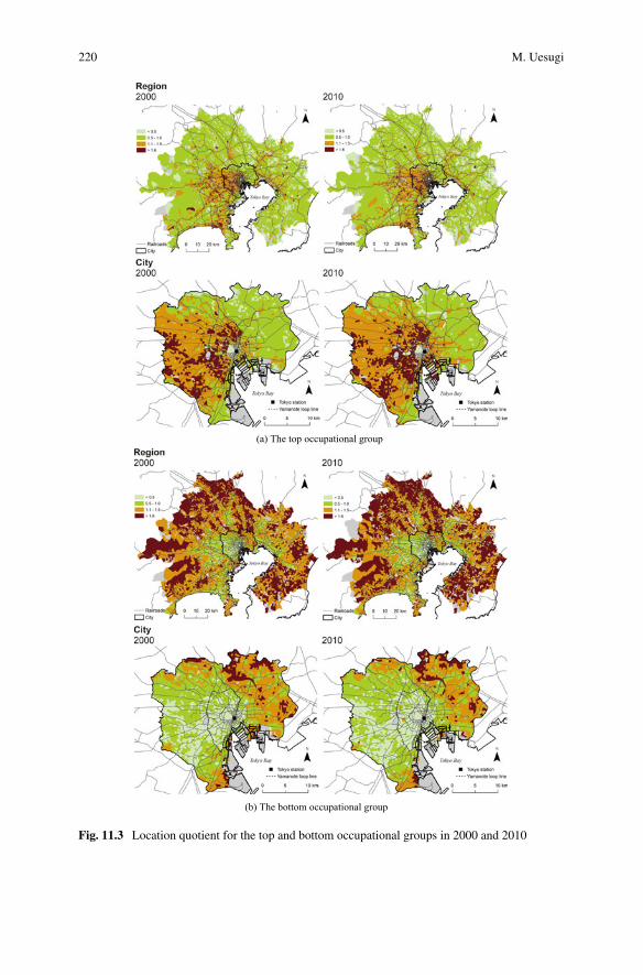
220 M. Uesugi
(a) The top occupational group
(b) The bottom occupational group
Fig. 11.3 Location quotient for the top and bottom occupational groups in 2000 and 2010
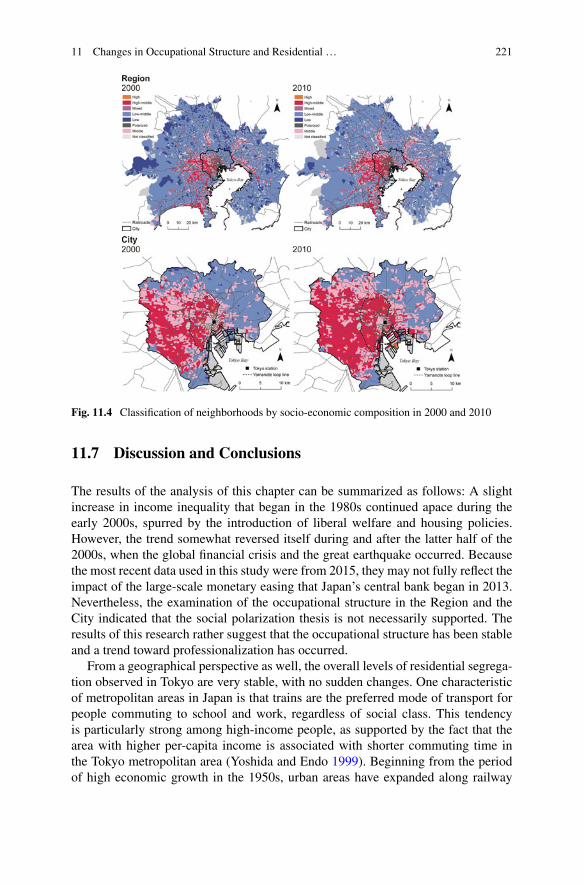
11 Changes in Occupational Structure and Residential … 221
Fig. 11.4 Classification of neighborhoods by socio-economic composition in 2000 and 2010
11.7 Discussion and Conclusions
The results of the analysis of this chapter can be summarized as follows: A slightincrease in income inequality that began in the 1980s continued apace during theearly 2000s, spurred by the introduction of liberal welfare and housing policies.However, the trend somewhat reversed itself during and after the latter half of the2000s, when the global financial crisis and the great earthquake occurred. Becausethe most recent data used in this study were from 2015, they may not fully reflect theimpact of the large-scale monetary easing that Japan’s central bank began in 2013.Nevertheless, the examination of the occupational structure in the Region and theCity indicated that the social polarization thesis is not necessarily supported. Theresults of this research rather suggest that the occupational structure has been stableand a trend toward professionalization has occurred.
From a geographical perspective as well, the overall levels of residential segrega-tion observed in Tokyo are very stable, with no sudden changes. One characteristicof metropolitan areas in Japan is that trains are the preferred mode of transport forpeople commuting to school and work, regardless of social class. This tendencyis particularly strong among high-income people, as supported by the fact that thearea with higher per-capita income is associated with shorter commuting time inthe Tokyo metropolitan area (Yoshida and Endo 1999). Beginning from the periodof high economic growth in the 1950s, urban areas have expanded along railway
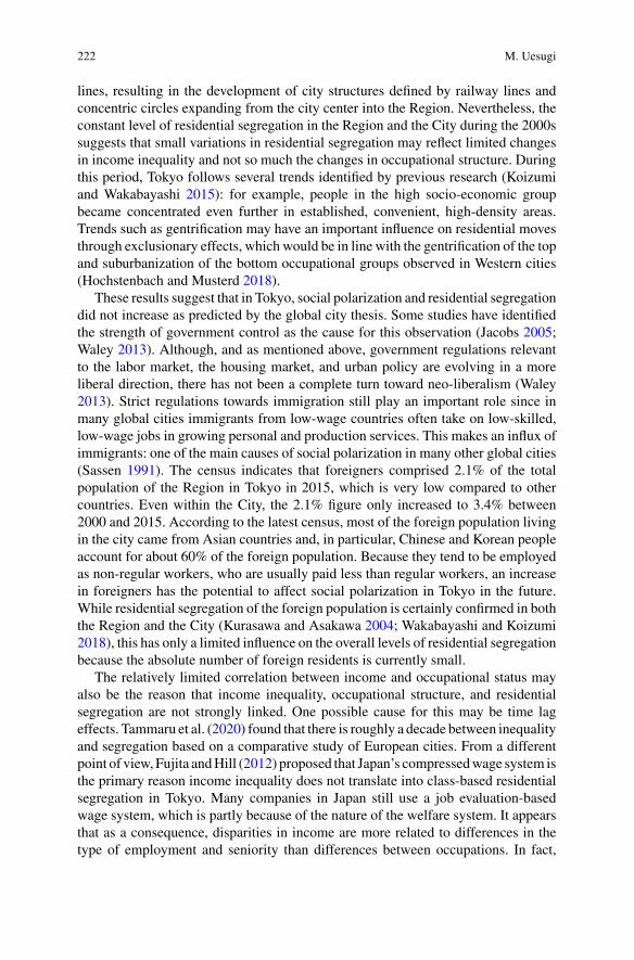
222 M. Uesugi
lines, resulting in the development of city structures defined by railway lines andconcentric circles expanding from the city center into the Region. Nevertheless, theconstant level of residential segregation in the Region and the City during the 2000ssuggests that small variations in residential segregation may reflect limited changesin income inequality and not so much the changes in occupational structure. Duringthis period, Tokyo follows several trends identified by previous research (Koizumiand Wakabayashi 2015): for example, people in the high socio-economic groupbecame concentrated even further in established, convenient, high-density areas.Trends such as gentrification may have an important influence on residential movesthrough exclusionary effects, which would be in line with the gentrification of the topand suburbanization of the bottom occupational groups observed in Western cities(Hochstenbach and Musterd 2018).
These results suggest that in Tokyo, social polarization and residential segregationdid not increase as predicted by the global city thesis. Some studies have identifiedthe strength of government control as the cause for this observation (Jacobs 2005;Waley 2013). Although, and as mentioned above, government regulations relevantto the labor market, the housing market, and urban policy are evolving in a moreliberal direction, there has not been a complete turn toward neo-liberalism (Waley2013). Strict regulations towards immigration still play an important role since inmany global cities immigrants from low-wage countries often take on low-skilled,low-wage jobs in growing personal and production services. This makes an influx ofimmigrants: one of the main causes of social polarization in many other global cities(Sassen 1991). The census indicates that foreigners comprised 2.1% of the totalpopulation of the Region in Tokyo in 2015, which is very low compared to othercountries. Even within the City, the 2.1% figure only increased to 3.4% between2000 and 2015. According to the latest census, most of the foreign population livingin the city came from Asian countries and, in particular, Chinese and Korean peopleaccount for about 60% of the foreign population. Because they tend to be employedas non-regular workers, who are usually paid less than regular workers, an increasein foreigners has the potential to affect social polarization in Tokyo in the future.While residential segregation of the foreign population is certainly confirmed in boththe Region and the City (Kurasawa and Asakawa 2004; Wakabayashi and Koizumi2018), this has only a limited influence on the overall levels of residential segregationbecause the absolute number of foreign residents is currently small.
The relatively limited correlation between income and occupational status mayalso be the reason that income inequality, occupational structure, and residentialsegregation are not strongly linked. One possible cause for this may be time lageffects. Tammaru et al. (2020) found that there is roughly a decade between inequalityand segregation based on a comparative study of European cities. From a differentpoint of view, Fujita andHill (2012) proposed that Japan’s compressedwage system isthe primary reason income inequality does not translate into class-based residentialsegregation in Tokyo. Many companies in Japan still use a job evaluation-basedwage system, which is partly because of the nature of the welfare system. It appearsthat as a consequence, disparities in income are more related to differences in thetype of employment and seniority than differences between occupations. In fact,
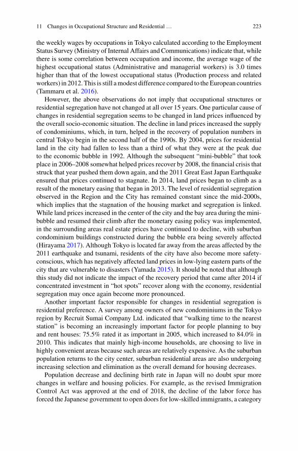
11 Changes in Occupational Structure and Residential … 223
the weekly wages by occupations in Tokyo calculated according to the EmploymentStatus Survey (Ministry of Internal Affairs and Communications) indicate that, whilethere is some correlation between occupation and income, the average wage of thehighest occupational status (Administrative and managerial workers) is 3.0 timeshigher than that of the lowest occupational status (Production process and relatedworkers) in 2012. This is still amodest difference compared to theEuropean countries(Tammaru et al. 2016).
However, the above observations do not imply that occupational structures orresidential segregation have not changed at all over 15 years. One particular cause ofchanges in residential segregation seems to be changed in land prices influenced bythe overall socio-economic situation. The decline in land prices increased the supplyof condominiums, which, in turn, helped in the recovery of population numbers incentral Tokyo begin in the second half of the 1990s. By 2004, prices for residentialland in the city had fallen to less than a third of what they were at the peak dueto the economic bubble in 1992. Although the subsequent “mini-bubble” that tookplace in 2006–2008 somewhat helped prices recover by 2008, the financial crisis thatstruck that year pushed them down again, and the 2011 Great East Japan Earthquakeensured that prices continued to stagnate. In 2014, land prices began to climb as aresult of the monetary easing that began in 2013. The level of residential segregationobserved in the Region and the City has remained constant since the mid-2000s,which implies that the stagnation of the housing market and segregation is linked.While land prices increased in the center of the city and the bay area during the mini-bubble and resumed their climb after the monetary easing policy was implemented,in the surrounding areas real estate prices have continued to decline, with suburbancondominium buildings constructed during the bubble era being severely affected(Hirayama 2017). Although Tokyo is located far away from the areas affected by the2011 earthquake and tsunami, residents of the city have also become more safety-conscious, which has negatively affected land prices in low-lying eastern parts of thecity that are vulnerable to disasters (Yamada 2015). It should be noted that althoughthis study did not indicate the impact of the recovery period that came after 2014 ifconcentrated investment in “hot spots” recover along with the economy, residentialsegregation may once again become more pronounced.
Another important factor responsible for changes in residential segregation isresidential preference. A survey among owners of new condominiums in the Tokyoregion by Recruit Sumai Company Ltd. indicated that “walking time to the neareststation” is becoming an increasingly important factor for people planning to buyand rent houses: 75.5% rated it as important in 2005, which increased to 84.0% in2010. This indicates that mainly high-income households, are choosing to live inhighly convenient areas because such areas are relatively expensive. As the suburbanpopulation returns to the city center, suburban residential areas are also undergoingincreasing selection and elimination as the overall demand for housing decreases.
Population decrease and declining birth rate in Japan will no doubt spur morechanges in welfare and housing policies. For example, as the revised ImmigrationControl Act was approved at the end of 2018, the decline of the labor force hasforced the Japanese government to open doors for low-skilled immigrants, a category
224 M. Uesugi
that had hitherto not been admitted. Insufficient development of housing policiestoward them remains another issue. As for urban policy, in 2014, the governmentrevised the Act on Special Measures concerning Urban Reconstruction to realizecompact cities suitable for the declining population. The Act gave each municipalitythe ability to designate specific areas where city functions and residential housingcould be consolidated to encourage residents to move there. Such policies stimulatethe selection and concentration of population in city centers, meaning they couldaccelerate residential segregation. In short, future trends in economic inequality andresidential segregation in Tokyo will be an important topic of study.
Notes
1. Tokyo was not a direct disaster area, but the earthquake influenced the energypolicy and real estate market nationwide.
2. This corresponds to the relationship between New York City and New YorkMetropolitan Area in the US as an example.
3. Neighborhoods with fewer than 50 workers are not reported.
Acknowledgements This research was supported by JSPS KAKENHI Grant NumberJP17K13584.
References
Chiavacci D, Hommerich C (eds) (2017) Social inequality in post-growth Japan: transformationduring economic and demographic stagnation. Routledge, New York
Duncan O, Duncan B (1955) Residential distribution and occupational stratification. Am J Sociol60(5):493–503
Esping-Andersen G (1990) The three worlds of welfare capitalism. Polity Press, CambridgeFielding AJ (2004) Class and space: social segregation in Japanese cities. Trans Inst Br Geogr29:64–84
Fujita K, Hill RC (2012) Residential income inequality in Tokyo and why it does not translate intoclass-based segregation. In: Maloutas T, Fujita K (eds) Residential segregation in comparativeperspective: making sense of contextual diversity. Ashgate, Farnham, pp 54–86
Fujitsuka Y (2017) Jentorifikeshon [Gentrification]. Kokon Shoin, TokyoHamnett C (1994) Social polarisation in global cities: theory and evidence. Urban Stud 31(3):401–424
Hirayama Y (2005) Running hot and cold in the urban home-ownership market: the experience ofJapan’s major cities. J Hous Built Environ 20:1–20
Hirayama Y (2017) Selling the Tokyo sky: urban regeneration and luxury housing. In: Forrest R,Koh SY, Wissink B (eds) Cities and the super-rich: real estate, elite practices, and urban politicaleconomies. Palgrave MacMillan, London, pp 189–208
Hochstenbach C, Musterd S (2018) Gentrification and the suburbanization of poverty: changingurban geographies through boom and bust periods. Urban Geogr 39(1):26–53
Jacobs AJ (2005) Has central Tokyo experienced uneven development? an examination of Tokyo’s23 ku relative to America’s largest urban centers. J Urban Aff 27(5):521–555
Jacobs AJ (2012) The nested global city-region: intermunicipal income stratification in the Tokyometropolitan region, 1980–2007. Urban Geogr 33(1):120–146
11 Changes in Occupational Structure and Residential … 225
Koizumi R, Wakabayashi Y (2015) Changes in the spatial patterns of occupational structure inthe Tokyo metropolitan area after the bubble economy. In: Singh R (ed) Urban developmentchallenges, risks and resilience in Asian mega cities. Springer, Tokyo, pp 351–366
Kurasawa S, Asakawa T (eds) (2004) Shinpen Tokyoken no shakai chizu, 1975–90 [New socialatlas of metropolitan Tokyo, 1975–90]. University of Tokyo Press, Tokyo
Lützeler R (2008) Population increase and “new-build gentrification” in central Tokyo. Erdkunde62:287–299
Marcinczak S, Tammaru T, Novak J, Gentile M, Kovács Z, Temelova J, Valatka V, Kährik A,Szabo B (2015) Patterns of socioeconomic segregation in the capital cities of fast-track reformingpostsocialist countries. Ann Am Assoc Geogr 105:183–202
Machimura T (1994) Sekai toshi Tokyo no kouzou tenkan [The structural change of a global city:urban restructuring in Tokyo]. University of Tokyo Press, Tokyo
MHLW (2012) Annual health, labour and welfare report 2012. Ministry of Health, Labour andWelfare, Tokyo
MHLW (2013) Analysis of the labour economy 2013 (White paper on the labour economy 2013).Ministry of Health, Labour and Welfare, Tokyo
Ministry of Internal Affairs and Communications (2009) The history of the Japan standardoccupational classification. http://www.soumu.go.jp/english/dgpp_ss/seido/shokgyou/co09-1.htm. Accessed 1 Mar 2019
Musterd S, van Gent W (2016) Changing welfare context and income segregation in Amsterdamand its metropolitan area, 2004–2011. In: Tammaru T, van Ham M, Marcinczak S, Musterd S(eds) Socio-economic segregation in European capital cities: east meets west. Routledge, Londonand New York, pp 55–79
OECD (2013) Definition of functional urban areas (FUA) for the OECD metropolitandatabase. https://www.oecd.org/cfe/regional-policy/Definition-of-Functional-Urban-Areas-for-the-OECD-metropolitan-database.pdf. Accessed 1 Mar 2019
OECD (2015) In it together: why less inequality benefits all. OECD Publishing, ParisOhtake F (2008) Inequality in Japan. Asian Econ Policy Rev 3:87–109Sassen S (1991) The global city: New York, London. Princeton University Press, Princeton, TokyoSawyer M (1976) Income distribution in OECD countries, OECD economic outlook. OECD, ParisShikata M (2013) Family structure, employment and income equality in Japan: decompositionanalysis of age-specific income inequality. Q Soc Secur Res 49(3):326–338 (In Japanese)
SonobeM (2001) Gendai daitoshi shakai ron: bunkyokuka suru toshi? [Contemporary metropolitansociety: dual city?]. Toshindo Publishing, Tokyo
Tachibanaki T (2005) Confronting income inequality in Japan: a comparative analysis of causes,consequences and reform. MIT Press, Cambridge
Takagi K (2012) Toshi jutaku seisaku to shakai-kuukan kouzou [Urban housing policy and socio-spatial structure: a case study of the Tokyo metropolitan area]. Yuhikaku, Tokyo
Tammaru T, van Ham M, Marcinczak S, Musterd S (eds) (2016) Socio-economic segregation inEuropean capital cities: east meets west. Routledge, London and New York
Tammaru T, Marcinczak S, Aunap R, van HamM, Janssen H (2020) Relationship between incomeinequality and residential segregation of socioeconomic groups. Reg Stud 54(4):450–461
ToyodaT (2007)Social polarization and socio-spatial structure ofmetropolitan areas:Acomparativeanalysis of income inequality in Tokyo, Osaka andNagoya. Ann JpnAssoc Urban Sociol 25:5–21(In Japanese)
Ueno J (2008) The impact of deregulation and urban development: socio-spatial polarization inTokyo. Ann Jpn Assoc Urban Sociol 26:101–115 (In Japanese)
vanKempenR (2007)Divided cities in the 21st century: challenging the importance of globalization.J Hous Built Environ 22(1):13–31
Wakabayashi Y, Koizumi R (2018) Spatial patterns of population change in central Tokyo sincethe period of the bubble economy. In: Kikuchi T, Sugai T (eds) Tokyo as a global city: newgeographical perspectives. Springer, Singapore, pp 155–176
226 M. Uesugi
Waley P (2007) Tokyo-as-world-city: reassessing the role of capital and the state in urbanrestructuring. Urban Stud 44(8):1465–1490
Waley P (2013) Pencilling Tokyo into the map of neoliberal urbanism. Cities 32:43–50WissinkB,Hazelzet A (2012) Social networks in “NeighbourhoodTokyo”. Urban Stud 49(7):1527–1549
Yamada H (2015) Spatial characteristics of land evaluation in the Tokyo metropolitan area afterthe Great East Japan Earthquake. In: Hino M, Tsutsumi J (eds) Urban geography of post-growthsociety. Tohoku University Press, Sendai, pp 159–178
Yoshida A, Endo H (1999) Spatial distribution of per-capita income and occupations in the Tokyometropolitan area. J Appl Reg Sci 4:15–25 (In Japanese)
Open Access This chapter is licensed under the terms of the Creative Commons Attribution 4.0International License (http://creativecommons.org/licenses/by/4.0/), which permits use, sharing,adaptation, distribution and reproduction in any medium or format, as long as you give appropriatecredit to the original author(s) and the source, provide a link to the Creative Commons license andindicate if changes were made.
The images or other third party material in this chapter are included in the chapter’s CreativeCommons license, unless indicated otherwise in a credit line to the material. If material is notincluded in the chapter’s Creative Commons license and your intended use is not permitted bystatutory regulation or exceeds the permitted use, you will need to obtain permission directly fromthe copyright holder.

Part IVAustralia
Chapter 12The Land of the ‘Fair Go’? MappingIncome Inequality and SocioeconomicSegregation Across MelbourneNeighbourhoods
Michelle Sydes and Rebecca Wickes
Abstract Despite enduring political rhetoric that promotes Australia as ‘the luckycountry’ and ‘the land of the fair go’, recent decades have seen a noticeable increase inlevels of income inequality. This growing economic divide has driven housing pricesup and left lower-income families unable to access the housing market in inner-city locations. In contrast to other countries, Australia’s socioeconomic segregationdoes not overlap with ethnic segregation. Australia’s highly regulated immigrationprogram has resulted in a relatively well-educated and employable foreign-bornpopulation who largely reside in middle-income neighbourhoods. These particu-larities make Australia an interesting context to explore patterns of socioeconomicsegregation over time. In this chapter, we will utilise both traditional measures ofsegregation (such as the dissimilarity index) as well more spatialised measures (suchas location quotients and Local Morans I) to assess socioeconomic segregation atthe local level. Drawing on four waves of census data (2001, 2006, 2011 and 2016),we explore how socioeconomic segregation has changed over time across nearly 500neighbourhoods in Melbourne. We further examine the degree to which socioeco-nomic segregation aligns with ethnic segregation patterns and levels in this city. Wefind patterns of socioeconomic segregation remain relatively unchanging over timein Melbourne. Additionally, our findings highlight important differences in patternsand levels of socioeconomic and ethnic segregation in the Australian context.
Keywords Melbourne · Socioeconomic segregation · Inequality · Geocodedcensus data
M. Sydes (B)School of Social Science, ARC Centre of Excellence in Children and Families Over the LifeCourse, The University of Queensland, Brisbane, Australiae-mail: [email protected]
R. WickesSchool of Social Sciences, Monash University, Melbourne, Australiae-mail: [email protected]
© The Author(s) 2021M. van Ham et al. (eds.), Urban Socio-Economic Segregation and Income Inequality,The Urban Book Series, https://doi.org/10.1007/978-3-030-64569-4_12
229
230 M. Sydes and R. Wickes
12.1 Introduction
In the 2019 federal election campaign, opposition leader Bill Shorten promisedAustralian voters a ‘fair go’ government if elected. While campaigning, Shortenassured voters, ‘if we win this election, our priority is not making the very richeven richer… it is getting wages moving again for working people’ (Benson 2019).Shorten went on to accuse current PrimeMinister Scott Morrison of only ‘defendingthe top end of town’, positioning himself and the Australian Labour Party as the keyto a fairer, more egalitarian society (Bagshaw 2019). This campaign strategy is notunprecedented. Australian politicians from both sides of the political spectrum havelong capitalised on the general public’s attachment to the ‘fair go’ sentiment. In fact,polling data shows that over 90% of Australians perceive the ‘fair go’ to be a coreAustralian value (Gough 2006).
Given the importance of the ‘fair go’ to Australians, many have voiced concernsabout growing levels of income inequality. In fact, 78% of Australians believe thecurrent gap between the rich and the poor is too large (Douglas 2018). Public percep-tions of growing inequality are reflected in the data. Income inequality, as measuredby the Gini coefficient, has increased from 0.313 in 1981 to 0.358 in 2014 (WorldBank 2019). At the same time, house prices in Australia’s capital cities have skyrock-eted—growing by 250% since the 1990s (OECD 2017). Growth in house priceshas outpaced growth in incomes, leaving many lower-income households strug-gling to access the housing market, especially in inner-city locations where jobsand services are concentrated (Spiller 2014). Consequently, lower-income house-holds and younger generations are increasingly forced to live on the outskirts of thecity in neighbourhoods that offer fewer employment opportunities, particularly inhigh skilled jobs (Randolph and Tice 2014). This trend reflects a growing spatialdivide between the haves and the have nots—a process described by Randolph andTice (2014: 385) as the ‘suburbanisation of disadvantage’.
Set against this backdrop of growing inequality and increasing house prices, thischapter examines trends in socioeconomic segregation over time acrossMelbourne—Australia’s second-largest city. Using occupational categories as a proxy for socioe-conomic status, we draw on both traditional measures of segregation (such as thedissimilarity index) as well as more spatialised measures (such as location quotientsand Local Morans I) to assess socioeconomic segregation across nearly 500 neigh-bourhoods over time. We further consider whether trends in socioeconomic segre-gation align with ethnic segregation patterns in the Australian context. The find-ings demonstrate relatively stable, albeit slightly increasing trends in socioeco-nomic segregation over time in Melbourne and highlight differences in patterns ofsocioeconomic segregation and ethnic segregation.
12 The Land of the ‘Fair Go’? Mapping Income Inequality … 231
12.2 Welfare in Australia
There are two primary objectives that underpin tax-transfer systems globally. Thefirst is referred to by Barr (2001: 1) as the ‘piggy bank objective’ whereby the systemis designed to provide insurance against unemployment, disability or sickness—thatis, periods during an individual’s life cycle when they have greater needs or lower-income (Barr 2001). The second is described as the ‘Robin Hood objective’ (Barr2001: 1) whereby taxation is used to redistribute wealth amongst residents by takingfrom the rich to give to the poor. To achieve this, high-income earners are taxed ata much higher rate than low-income earners and lower-income households receive agreater proportion of social benefits.
According to Whiteford (2010), Australia’s welfare system strongly emphasisesthe latter objective, offering a safety net to those unable to support themselves.Those eligible for welfare payments in Australia include the elderly, persons with adisability, carers, families with children, veterans, and unemployed persons (AIHW2017). Income support payments are fully funded by government revenue generatedthrough the tax system (AIHW 2017). As such, Australians are not required to makeindividualised social security contributions and income support payments are set ata flat rate rather than linked to past earnings (Whiteford 2015).
Expenditure on welfare in real terms has risen over the past decade. In 2016,the Australian government spent $6,566 AUD per resident, up from $5,663 AUD in2006 (AIHW 2017). Yet compared to other OECD countries, Australia is a relativelylow social spender (Whiteford 2017), with social spending as a proportion of GDPwell below the OECD average (17.8% compared to 20%) (OECD 2019). Whiteford(2017) attributes this low social spending to Australia’s relatively efficient welfaresystem, which utilises means-testing to determine eligibility. While means-testing isnot unique to the Australian context, it is more widely used in Australia comparedto any other OECD country, with approximately 80% of cash benefits means-tested(AIHW 2017). In 2011, the most disadvantaged households in Australia (the lowestquintile) received 42% of social benefits, while the most advantaged households (thehighest quintile) received only 3.8% of social benefits (Whiteford 2017). In otherwords, the poorest 20% received 11 times more in social benefits than the richest20% (Whiteford 2015). Given Australia’s social spending is largely directed towardsthe poorest quintile, Whiteford (2017: 1) argues that ‘an across-the-board reductionin social security spending in Australia would increase income inequality more thanin any other OECD country’.
12.3 Income Inequality in Australia
Since the 1980s,Australia’s incomedistribution has gradually grownmore unequal—rising from 0.313 in 1981 to 0.358 in 2014 (World Bank 2019). Globally this placesAustralia behind France (0.323), the United Kingdom (0.34) and Canada (0.34) but
232 M. Sydes and R. Wickes
ahead of theUnited States (0.411) (World Bank 2019). Although household incomes2
experienced growth between 1993–94 and 2013–14, the degree of growth was notuniform across all quintiles. The highest quintile experienced the greatest amount ofgrowth, with incomes rising by 80% (AIHW 2017), doubling the gap between thehighest quintile and the lowest quintile over this time period (AIHW 2017). WhileAustralians wish to see the gap close (Douglas 2018), there is limited support forthe tax increases necessary to allow for greater social spending. In fact, 50% ofAustralians believe they pay too much tax and an additional 34% believe they payenough (Herscovitch 2013).
12.4 The Australian Housing System
This growing inequality directly threatens the ‘great Australian dream’ of home-ownership—a widely held aspiration amongst Australians dating back to the mid-twentieth century (Gurran and Phibbs 2016). Colic-Peisker and Johnson (2010: 352)suggest that ‘the importance of homeownership inAustralia is closely associatedwitha perception of an egalitarian society where everyone can become a homeowner’.Unfortunately, this dream has become increasingly unattainable in recent years. Thelast twodecades have seen astronomical increases in house prices—growing by 250%since the 1990s (OECD 2017). Even after adjusting for growth in income between1980 and 2015, a 78% increase in Australian house prices remains (AIHW 2017).As rising house prices have outpaced household incomes, homeowners have becomeincreasingly reliant on mortgages to finance housing. In 2016, 32.8% of householdsowned their home outright, 35.7% owned their home with a mortgage and 31.5%were renting (ABS 2016).
Overall rates of homeownership have moderately declined over the last twentyyears in Australia (Burke et al. 2014). Indeed, 71% of Australians owned their homeeither with or without a mortgage in 1994–95 compared to 67% in 2013–14 (AIHW2017). Sharper decreases in homeownership are evident amongst young people.While 60% of persons between 25 and 34 years owned their own home in 1988–89, this number fell to just 39% in 2013–14 (AIHW 2017). This downward trendsuggests housing affordability issues have created a barrier to accessing the housingmarket for younger generations, giving rise to intergenerational inequities (Saunders2017).
For the averageAustralian household, housing costs (either rent payments ormort-gage repayments) account for approximately 18%of total household expenditure andrepresent the largest household expense (ABS 2011; Saunders 2017). Homeownersthat spend over 30% of their gross income on housing costs are deemed to be expe-riencing mortgage stress. In 2017, one in four households with mortgages were
12013 World Bank estimate.2Measure of equivalised household weekly income which is the total household income afteradjusting for differing household size and composition (ABS 2006).
12 The Land of the ‘Fair Go’? Mapping Income Inequality … 233
considered in financial distress (Hughes 2017). Low-income renters are also strug-gling. In 2013–14, 50% of lower-income rental households reported spending morethan 30% of their gross income on housing compared to 42% in 2005–06 (AIHW2017). There are no national-level rent control systems for the private rental marketin Australia, with the rental market overseen at the state level.
For those unable to afford housing through the private market, public housing isprovided by the state and federal government (Morris 2018). Low-incomehouseholdsare prioritised for public housing, particularly those who also have special needssuch as Indigenous Australians, young people, old people, persons with disabilities,victims of domestic and family violence and the homeless (AIHW 2017). Rentsare monitored to ensure that eligible tenants pay no more than 30% of their grossincome (AIHW2017).Yet demand for public housing far exceeds supply,with almost200,000 households onwaiting lists in 2015. Further, wait times are long, with almost50% of households waiting for more than two years (AIHW 2017).
12.5 Greater Melbourne
Melbourne is the capital of the state of Victoria and is the second most populated cityin Australia. Melbourne has been ranked as one of the world’s most liveable cities bythe Economist Intelligence Unit (EIU) (The Economist 2018). Indeed, Melbourneheld the number one ranking across 140 cities for seven years. Greater Melbournespans nearly 10,000 km2 and is home to a residential population of approximately4.5 million persons (ABS 2016) (see Fig. 12.1). Similar to other Australian cities,Melbourne is a low-density city—with the average household comprising 2.7 personsand the majority of residents (66%) living in detached houses on suburban blocks(ABS 2016).
Between 2001 and 2011, the median house price in Melbourne increased by163% (Department of Transport, Planning and Local Infrastructure (DTPLI) 2012).At the same time, wages increased by just 57% (DTPLI 2012). As a consequence ofsoaring house prices, inner-city neighbourhood housing is largely inaccessible forhomebuyers on low to moderate household incomes (Goodman 2018). While thoseon an average household income could afford to buy a residence within 10 kms fromMelbourne’s central business district (CBD) in 1994, by 2009 this distance increasedto 40 kms (DTPLI 2014). Low-income renters are similarly struggling to find housingclose to the city centre. According to Hulse, Reynolds and Yates (2014), the shortageof affordable and available rental dwellings exceeds 20,000 in the middle suburbs ofMelbourne. Given the majority of jobs and services inMelbourne are concentrated inand around the CBD, lower-income households are left at a significant disadvantage(Spiller 2014).
The Residential Tenancies Act (1997) provides the legislative framework whichguides the rental market inMelbourne. In 2017, these rental laws were reviewed witha series of reforms set for implementation by July 2020 (Victoria State Government2019). Most notable of these reforms was a reduction in how often landlords can

234 M. Sydes and R. Wickes
Fig. 12.1 Greater Melbourne
increase rent (previously every six months, now every 12 months). Further, severalreforms focused on improving the long term suitability of rental properties for house-holds by introducing long term leases, permitting minor modifications and allowingpets (Victoria State Government 2019).
As a longstanding gateway city for new immigrants arriving in Australia,Melbourne is renowned for being a progressive city with a strong history of ethnicdiversity and inclusion (ABS 2014). In many countries, socioeconomic and ethnicsegregation patterns are largely indistinguishable with certain ethnic groups livingin the more disadvantaged areas (Iceland and Wilkes 2006). However, Australia’shighly controlled immigration program has resulted in a relatively well-educated andemployable foreign-born populationwho largely reside inmiddle-incomeneighbour-hoods (Sydes 2018). Between 2006 and 2016, the proportion of Melbourne’s popu-lation born overseas increased from 28.9% up to 33.9% (ABS 2016). In Australia,immigrants who arrive through the skilled stream are required to speak English profi-ciently, and thus the number of linguistically isolated immigrants is relatively small.While 38% of Melbourne’s population spoke a language other than English in 2016,just 5.6% reported not speaking English well or not at all (ABS 2016). In 2016,the top five countries of birth residing in Melbourne included India (3.6%), China(3.5%), England (3%), Vietnam (1.8%) and New Zealand (1.8%) (ABS 2016). Incontrast to the immigrant population, Indigenous Australians experience high levelsof disadvantage (Altman, Biddle, and Hunter 2018). In 2016, Indigenous Australianscomprised just 0.5% of the total population inMelbourne—amuch lower percentage
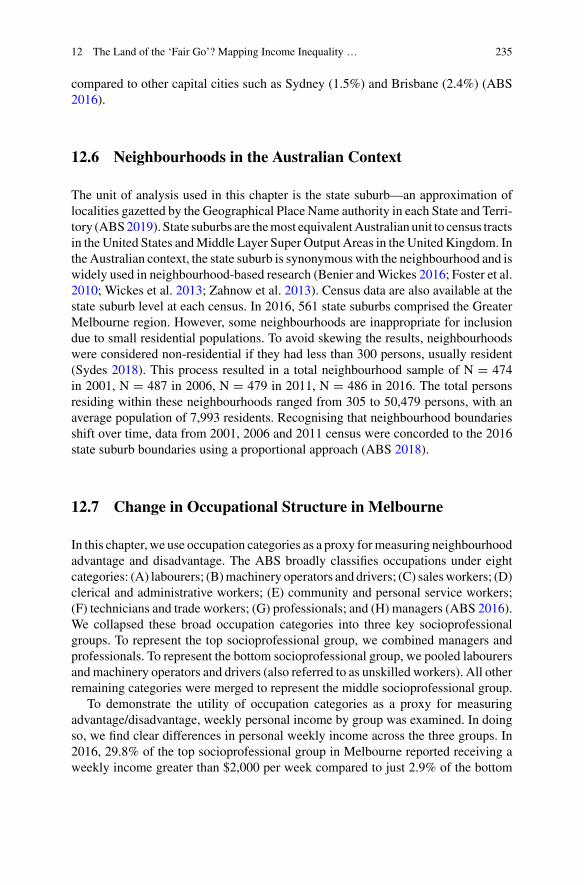
12 The Land of the ‘Fair Go’? Mapping Income Inequality … 235
compared to other capital cities such as Sydney (1.5%) and Brisbane (2.4%) (ABS2016).
12.6 Neighbourhoods in the Australian Context
The unit of analysis used in this chapter is the state suburb—an approximation oflocalities gazetted by the Geographical Place Name authority in each State and Terri-tory (ABS2019). State suburbs are themost equivalentAustralian unit to census tractsin the United States andMiddle Layer Super Output Areas in the United Kingdom. Inthe Australian context, the state suburb is synonymouswith the neighbourhood and iswidely used in neighbourhood-based research (Benier andWickes 2016; Foster et al.2010; Wickes et al. 2013; Zahnow et al. 2013). Census data are also available at thestate suburb level at each census. In 2016, 561 state suburbs comprised the GreaterMelbourne region. However, some neighbourhoods are inappropriate for inclusiondue to small residential populations. To avoid skewing the results, neighbourhoodswere considered non-residential if they had less than 300 persons, usually resident(Sydes 2018). This process resulted in a total neighbourhood sample of N = 474in 2001, N = 487 in 2006, N = 479 in 2011, N = 486 in 2016. The total personsresiding within these neighbourhoods ranged from 305 to 50,479 persons, with anaverage population of 7,993 residents. Recognising that neighbourhood boundariesshift over time, data from 2001, 2006 and 2011 census were concorded to the 2016state suburb boundaries using a proportional approach (ABS 2018).
12.7 Change in Occupational Structure in Melbourne
In this chapter, we use occupation categories as a proxy formeasuring neighbourhoodadvantage and disadvantage. The ABS broadly classifies occupations under eightcategories: (A) labourers; (B)machinery operators and drivers; (C) salesworkers; (D)clerical and administrative workers; (E) community and personal service workers;(F) technicians and trade workers; (G) professionals; and (H) managers (ABS 2016).We collapsed these broad occupation categories into three key socioprofessionalgroups. To represent the top socioprofessional group, we combined managers andprofessionals. To represent the bottom socioprofessional group, we pooled labourersandmachinery operators and drivers (also referred to as unskilled workers). All otherremaining categories were merged to represent the middle socioprofessional group.
To demonstrate the utility of occupation categories as a proxy for measuringadvantage/disadvantage, weekly personal income by group was examined. In doingso, we find clear differences in personal weekly income across the three groups. In2016, 29.8% of the top socioprofessional group in Melbourne reported receiving aweekly income greater than $2,000 per week compared to just 2.9% of the bottom
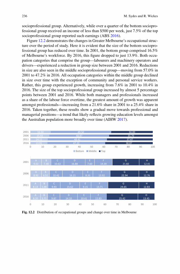
236 M. Sydes and R. Wickes
socioprofessional group. Alternatively, while over a quarter of the bottom sociopro-fessional group received an income of less than $500 per week, just 7.5% of the topsocioprofessional group reported such earnings (ABS 2016).
Figure 12.2 demonstrates the changes in Greater Melbourne’s occupational struc-ture over the period of study. Here it is evident that the size of the bottom sociopro-fessional group has reduced over time. In 2001, the bottom group comprised 16.5%of Melbourne’s workforce. By 2016, this figure dropped to just 13.9%. Both occu-pation categories that comprise the group—labourers and machinery operators anddrivers—experienced a reduction in group size between 2001 and 2016. Reductionsin size are also seen in the middle socioprofessional group—moving from 57.0% in2001 to 47.2% in 2016. All occupation categories within the middle group declinedin size over time with the exception of community and personal service workers.Rather, this group experienced growth, increasing from 7.6% in 2001 to 10.4% in2016. The size of the top socioprofessional group increased by almost 5 percentagepoints between 2001 and 2016. While both managers and professionals increasedas a share of the labour force overtime, the greatest amount of growth was apparentamongst professionals—increasing from a 21.6% share in 2001 to a 25.4% share in2016. Taken together, these results show a gradual move towards professional andmanagerial positions—a trend that likely reflects growing education levels amongstthe Australian population more broadly over time (AIHW 2017).
13.91 14.11 15.43 16.50
47.22 48.41
48.87 49.50
38.87 37.47 35.70 34.00
0 10 20 30 40 50 60 70 80 90 1002016201120062001
Bo om Middle Top
A 8.20
A 8.13
A 8.92
A 9.02
B 5.71
B 5.98
B 6.51
B 7.48
C 9.87
C 9.93
C 10.42
C 10.63
D 14.10
D 15.62
D 16.21
D 16.88
E 10.41
E 9.15
E 8.33
E 7.60
F 12.83
F 13.71
F 13.92
F 14.39
G 25.42
G 24.65
G 22.94
G 21.60
H 13.45
H 12.83
H 12.76
H 12.41
0 10 20 30 40 50 60 70 80 90 100
2016
2011
2006
2001
Fig. 12.2 Distribution of occupational groups and change over time in Melbourne
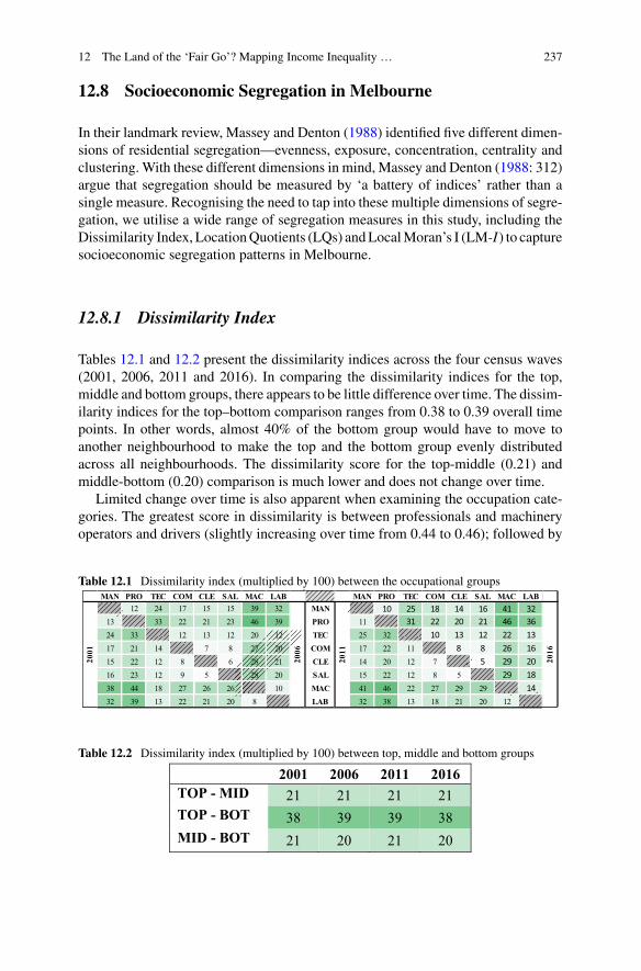
12 The Land of the ‘Fair Go’? Mapping Income Inequality … 237
12.8 Socioeconomic Segregation in Melbourne
In their landmark review, Massey and Denton (1988) identified five different dimen-sions of residential segregation—evenness, exposure, concentration, centrality andclustering. With these different dimensions in mind, Massey and Denton (1988: 312)argue that segregation should be measured by ‘a battery of indices’ rather than asingle measure. Recognising the need to tap into these multiple dimensions of segre-gation, we utilise a wide range of segregation measures in this study, including theDissimilarity Index, LocationQuotients (LQs) andLocalMoran’s I (LM-I) to capturesocioeconomic segregation patterns in Melbourne.
12.8.1 Dissimilarity Index
Tables 12.1 and 12.2 present the dissimilarity indices across the four census waves(2001, 2006, 2011 and 2016). In comparing the dissimilarity indices for the top,middle and bottom groups, there appears to be little difference over time. The dissim-ilarity indices for the top–bottom comparison ranges from 0.38 to 0.39 overall timepoints. In other words, almost 40% of the bottom group would have to move toanother neighbourhood to make the top and the bottom group evenly distributedacross all neighbourhoods. The dissimilarity score for the top-middle (0.21) andmiddle-bottom (0.20) comparison is much lower and does not change over time.
Limited change over time is also apparent when examining the occupation cate-gories. The greatest score in dissimilarity is between professionals and machineryoperators and drivers (slightly increasing over time from 0.44 to 0.46); followed by
Table 12.1 Dissimilarity index (multiplied by 100) between the occupational groupsMAN PRO TEC COM CLE SAL MAC LAB MAN PRO TEC COM CLE SAL MAC LAB
12 24 17 15 15 39 32 MAN 10 25 18 14 16 41 3213 33 22 21 23 46 39 PRO 11 31 22 20 21 46 3624 33 12 13 12 20 12 TEC 25 32 10 13 12 22 1317 21 14 7 8 27 20 COM 17 22 11 8 8 26 1615 22 12 8 6 28 21 CLE 14 20 12 7 5 29 2016 23 12 9 5 28 20 SAL 15 22 12 8 5 29 1838 44 18 27 26 26 10 MAC 41 46 22 27 29 29 1432 39 13 22 21 20 8 LAB 32 38 13 18 21 20 12
2016
2001
2006
2011
Table 12.2 Dissimilarity index (multiplied by 100) between top, middle and bottom groups
2001 2006 2011 2016TOP - MID 21 21 21 21TOP - BOT 38 39 39 38MID - BOT 21 20 21 20
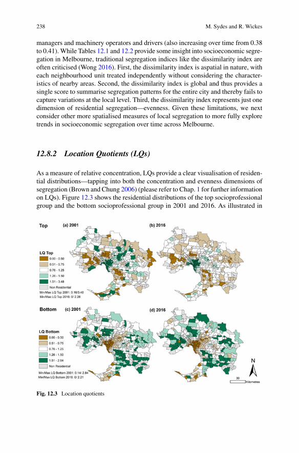
238 M. Sydes and R. Wickes
managers and machinery operators and drivers (also increasing over time from 0.38to 0.41). While Tables 12.1 and 12.2 provide some insight into socioeconomic segre-gation in Melbourne, traditional segregation indices like the dissimilarity index areoften criticised (Wong 2016). First, the dissimilarity index is aspatial in nature, witheach neighbourhood unit treated independently without considering the character-istics of nearby areas. Second, the dissimilarity index is global and thus provides asingle score to summarise segregation patterns for the entire city and thereby fails tocapture variations at the local level. Third, the dissimilarity index represents just onedimension of residential segregation—evenness. Given these limitations, we nextconsider other more spatialised measures of local segregation to more fully exploretrends in socioeconomic segregation over time across Melbourne.
12.8.2 Location Quotients (LQs)
As a measure of relative concentration, LQs provide a clear visualisation of residen-tial distributions—tapping into both the concentration and evenness dimensions ofsegregation (Brown and Chung 2006) (please refer to Chap. 1 for further informationon LQs). Figure 12.3 shows the residential distributions of the top socioprofessionalgroup and the bottom socioprofessional group in 2001 and 2016. As illustrated in
Fig. 12.3 Location quotients
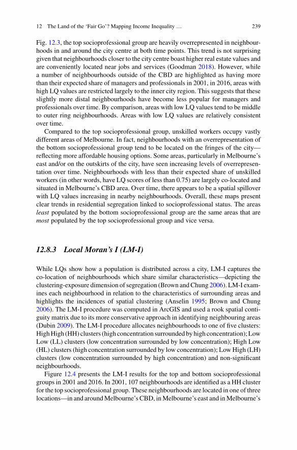
12 The Land of the ‘Fair Go’? Mapping Income Inequality … 239
Fig. 12.3, the top socioprofessional group are heavily overrepresented in neighbour-hoods in and around the city centre at both time points. This trend is not surprisinggiven that neighbourhoods closer to the city centre boast higher real estate values andare conveniently located near jobs and services (Goodman 2018). However, whilea number of neighbourhoods outside of the CBD are highlighted as having morethan their expected share of managers and professionals in 2001, in 2016, areas withhigh LQ values are restricted largely to the inner city region. This suggests that theseslightly more distal neighbourhoods have become less popular for managers andprofessionals over time. By comparison, areas with low LQ values tend to be middleto outer ring neighbourhoods. Areas with low LQ values are relatively consistentover time.
Compared to the top socioprofessional group, unskilled workers occupy vastlydifferent areas of Melbourne. In fact, neighbourhoods with an overrepresentation ofthe bottom socioprofessional group tend to be located on the fringes of the city—reflecting more affordable housing options. Some areas, particularly in Melbourne’seast and/or on the outskirts of the city, have seen increasing levels of overrepresen-tation over time. Neighbourhoods with less than their expected share of unskilledworkers (in other words, have LQ scores of less than 0.75) are largely co-located andsituated in Melbourne’s CBD area. Over time, there appears to be a spatial spilloverwith LQ values increasing in nearby neighbourhoods. Overall, these maps presentclear trends in residential segregation linked to socioprofessional status. The areasleast populated by the bottom socioprofessional group are the same areas that aremost populated by the top socioprofessional group and vice versa.
12.8.3 Local Moran’s I (LM-I)
While LQs show how a population is distributed across a city, LM-I captures theco-location of neighbourhoods which share similar characteristics—depicting theclustering-exposure dimension of segregation (Brown andChung 2006). LM-I exam-ines each neighbourhood in relation to the characteristics of surrounding areas andhighlights the incidences of spatial clustering (Anselin 1995; Brown and Chung2006). The LM-I procedure was computed in ArcGIS and used a rook spatial conti-guity matrix due to its more conservative approach in identifying neighbouring areas(Dubin 2009). The LM-I procedure allocates neighbourhoods to one of five clusters:HighHigh (HH) clusters (high concentration surroundedbyhigh concentration); LowLow (LL) clusters (low concentration surrounded by low concentration); High Low(HL) clusters (high concentration surrounded by low concentration); LowHigh (LH)clusters (low concentration surrounded by high concentration) and non-significantneighbourhoods.
Figure 12.4 presents the LM-I results for the top and bottom socioprofessionalgroups in 2001 and 2016. In 2001, 107 neighbourhoods are identified as a HH clusterfor the top socioprofessional group. These neighbourhoods are located in one of threelocations—in and aroundMelbourne’s CBD, inMelbourne’s east and inMelbourne’s
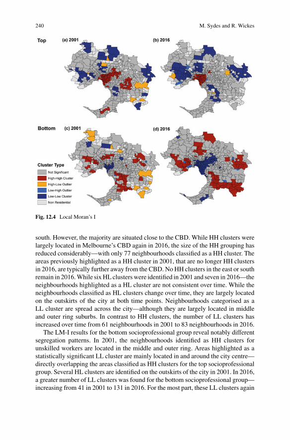
240 M. Sydes and R. Wickes
Fig. 12.4 Local Moran’s I
south. However, the majority are situated close to the CBD. While HH clusters werelargely located in Melbourne’s CBD again in 2016, the size of the HH grouping hasreduced considerably—with only 77 neighbourhoods classified as a HH cluster. Theareas previously highlighted as a HH cluster in 2001, that are no longer HH clustersin 2016, are typically further away from the CBD. NoHH clusters in the east or southremain in 2016.While sixHL clusterswere identified in 2001 and seven in 2016—theneighbourhoods highlighted as a HL cluster are not consistent over time. While theneighbourhoods classified as HL clusters change over time, they are largely locatedon the outskirts of the city at both time points. Neighbourhoods categorised as aLL cluster are spread across the city—although they are largely located in middleand outer ring suburbs. In contrast to HH clusters, the number of LL clusters hasincreased over time from 61 neighbourhoods in 2001 to 83 neighbourhoods in 2016.
The LM-I results for the bottom socioprofessional group reveal notably differentsegregation patterns. In 2001, the neighbourhoods identified as HH clusters forunskilled workers are located in the middle and outer ring. Areas highlighted as astatistically significant LL cluster are mainly located in and around the city centre—directly overlapping the areas classified as HH clusters for the top socioprofessionalgroup. Several HL clusters are identified on the outskirts of the city in 2001. In 2016,a greater number of LL clusters was found for the bottom socioprofessional group—increasing from 41 in 2001 to 131 in 2016. For the most part, these LL clusters again
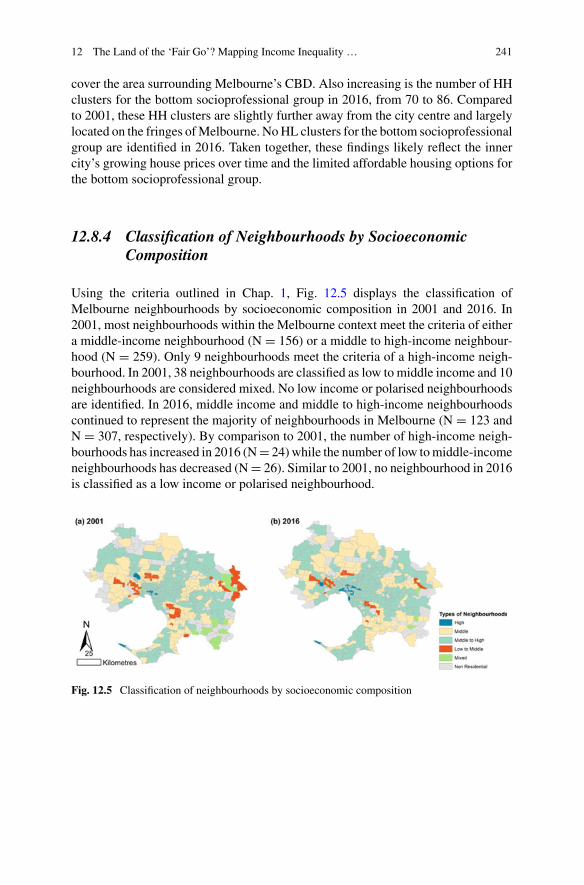
12 The Land of the ‘Fair Go’? Mapping Income Inequality … 241
cover the area surrounding Melbourne’s CBD. Also increasing is the number of HHclusters for the bottom socioprofessional group in 2016, from 70 to 86. Comparedto 2001, these HH clusters are slightly further away from the city centre and largelylocated on the fringes ofMelbourne. NoHL clusters for the bottom socioprofessionalgroup are identified in 2016. Taken together, these findings likely reflect the innercity’s growing house prices over time and the limited affordable housing options forthe bottom socioprofessional group.
12.8.4 Classification of Neighbourhoods by SocioeconomicComposition
Using the criteria outlined in Chap. 1, Fig. 12.5 displays the classification ofMelbourne neighbourhoods by socioeconomic composition in 2001 and 2016. In2001, most neighbourhoods within the Melbourne context meet the criteria of eithera middle-income neighbourhood (N = 156) or a middle to high-income neighbour-hood (N = 259). Only 9 neighbourhoods meet the criteria of a high-income neigh-bourhood. In 2001, 38 neighbourhoods are classified as low to middle income and 10neighbourhoods are considered mixed. No low income or polarised neighbourhoodsare identified. In 2016, middle income and middle to high-income neighbourhoodscontinued to represent the majority of neighbourhoods in Melbourne (N = 123 andN = 307, respectively). By comparison to 2001, the number of high-income neigh-bourhoods has increased in 2016 (N= 24) while the number of low tomiddle-incomeneighbourhoods has decreased (N= 26). Similar to 2001, no neighbourhood in 2016is classified as a low income or polarised neighbourhood.
Fig. 12.5 Classification of neighbourhoods by socioeconomic composition
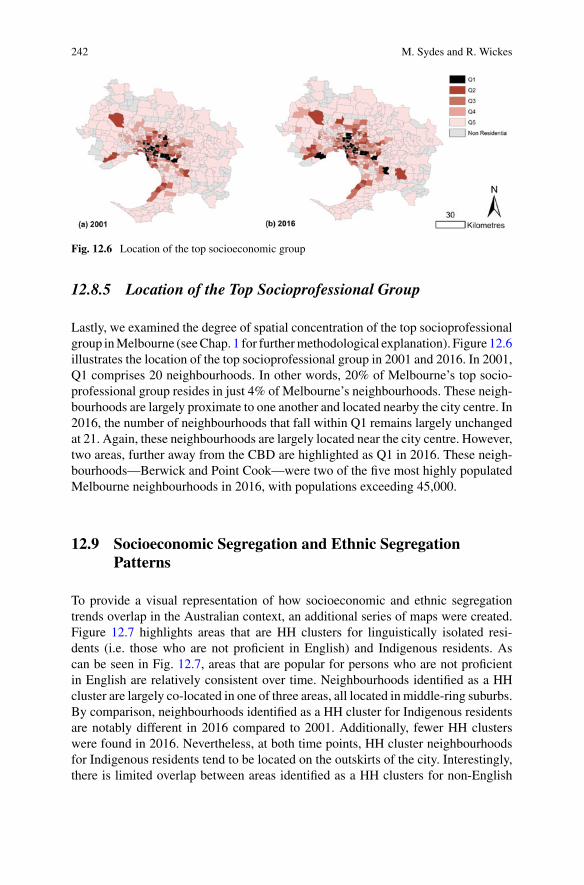
242 M. Sydes and R. Wickes
Fig. 12.6 Location of the top socioeconomic group
12.8.5 Location of the Top Socioprofessional Group
Lastly, we examined the degree of spatial concentration of the top socioprofessionalgroup inMelbourne (seeChap. 1 for furthermethodological explanation). Figure 12.6illustrates the location of the top socioprofessional group in 2001 and 2016. In 2001,Q1 comprises 20 neighbourhoods. In other words, 20% of Melbourne’s top socio-professional group resides in just 4% of Melbourne’s neighbourhoods. These neigh-bourhoods are largely proximate to one another and located nearby the city centre. In2016, the number of neighbourhoods that fall within Q1 remains largely unchangedat 21. Again, these neighbourhoods are largely located near the city centre. However,two areas, further away from the CBD are highlighted as Q1 in 2016. These neigh-bourhoods—Berwick and Point Cook—were two of the five most highly populatedMelbourne neighbourhoods in 2016, with populations exceeding 45,000.
12.9 Socioeconomic Segregation and Ethnic SegregationPatterns
To provide a visual representation of how socioeconomic and ethnic segregationtrends overlap in the Australian context, an additional series of maps were created.Figure 12.7 highlights areas that are HH clusters for linguistically isolated resi-dents (i.e. those who are not proficient in English) and Indigenous residents. Ascan be seen in Fig. 12.7, areas that are popular for persons who are not proficientin English are relatively consistent over time. Neighbourhoods identified as a HHcluster are largely co-located in one of three areas, all located in middle-ring suburbs.By comparison, neighbourhoods identified as a HH cluster for Indigenous residentsare notably different in 2016 compared to 2001. Additionally, fewer HH clusterswere found in 2016. Nevertheless, at both time points, HH cluster neighbourhoodsfor Indigenous residents tend to be located on the outskirts of the city. Interestingly,there is limited overlap between areas identified as a HH clusters for non-English
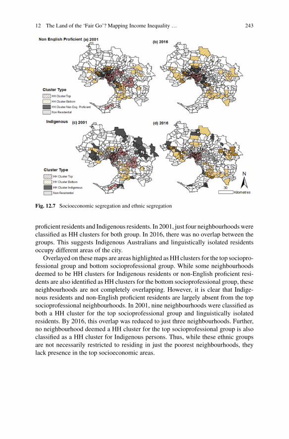
12 The Land of the ‘Fair Go’? Mapping Income Inequality … 243
Fig. 12.7 Socioeconomic segregation and ethnic segregation
proficient residents and Indigenous residents. In 2001, just four neighbourhoodswereclassified as HH clusters for both group. In 2016, there was no overlap between thegroups. This suggests Indigenous Australians and linguistically isolated residentsoccupy different areas of the city.
Overlayed on thesemaps are areas highlighted asHH clusters for the top sociopro-fessional group and bottom socioprofessional group. While some neighbourhoodsdeemed to be HH clusters for Indigenous residents or non-English proficient resi-dents are also identified as HH clusters for the bottom socioprofessional group, theseneighbourhoods are not completely overlapping. However, it is clear that Indige-nous residents and non-English proficient residents are largely absent from the topsocioprofessional neighbourhoods. In 2001, nine neighbourhoods were classified asboth a HH cluster for the top socioprofessional group and linguistically isolatedresidents. By 2016, this overlap was reduced to just three neighbourhoods. Further,no neighbourhood deemed a HH cluster for the top socioprofessional group is alsoclassified as a HH cluster for Indigenous persons. Thus, while these ethnic groupsare not necessarily restricted to residing in just the poorest neighbourhoods, theylack presence in the top socioeconomic areas.
244 M. Sydes and R. Wickes
12.10 Conclusions
While the overwhelming majority of Australians perceive the ‘fair go’ to be a coreAustralian value, the growing levels of income inequality, issueswith housing afford-ability and increasing socioeconomic segregation outlined in this chapter present athreat to its longevity. Melbourne is expected to be the largest city in Australia inthe coming decades and is predicted to grow to a population of 8 million people by2051 (Victoria State Government 2016). Therefore a key priority for governmentand urban planning is to maintain liveability and ensure that access to housing andemployment does not fall outside of the reach of ‘ordinary’ Australians.
The results of the analyses undertaken for this chapter highlight clear trends insocioeconomic segregation in Melbourne. Traditional measures of segregation likethe dissimilarity index indicate that almost 40% of the bottom socioprofessionalgroup would need to move to another neighbourhood in order to make the top and thebottom group evenly distributed. However, the dissimilarity indices show a limitedchange in socioeconomic segregation over time.
By comparison, the more spatialised measures reveal a growing spatial dividebetween the top and bottom socioprofessional groups. Looking first to locationquotients, the top socioprofessional group are overrepresented in neighbourhoodsclosest to the centre of the city. Results also show that top socioprofessional groupand unskilled workers inhabit different parts of city, with the bottom socioprofes-sional group residing in the city’s outer suburbs. Put simply, those areas least popularfor the top socioprofessional group are the areas where unskilled workers are mostlikely to live. Similar patterns are found when looking at the LM-I results. Takentogether this demonstrates a growing geographical distance between the ‘haves’ andthe ‘have-nots’. This increasing segregation is likely to be further compounded bythe expected population growth of Melbourne.
References
ABS (2006) Household income—equivalised (HED). https://www.abs.gov.au/ausstats/[email protected]/0/A390E2529EC00DFECA25720A0076F6C6?opendocument. Accessed 30 May 2019
ABS (2011) 2011 census data via Tablebuilder. https://www.abs.gov.au/websitedbs/censushome.nsf/home/tablebuilder. Accessed 15 May 2019
ABS (2014) Where do migrants live? https://www.abs.gov.au/ausstats/[email protected]/Lookup/4102.0main+features102014. Accessed 15 May 2019
ABS (2016) 2016 census data via Tablebuilder. https://www.abs.gov.au/websitedbs/censushome.nsf/home/tablebuilder. Accessed 20 May 2019
ABS (2018) Australian Statistical Geography Standard (ASGS) correspondences. https://www.abs.gov.au/websitedbs/D3310114.nsf/home/Correspondences. Accessed 22 May 2019
ABS (2019) Census geography basics. https://www.abs.gov.au/websitedbs/D3310114.nsf/home/2016%20Census%20Geography%20Basics. Accessed 22 May 2019
AIHW (2017) Australia’s welfare 2017. Canberra, AIHW
12 The Land of the ‘Fair Go’? Mapping Income Inequality … 245
Altman J, Biddle N, Hunter B (2018) How realistic are the prospects for ‘closing the gaps’ insocioeconomic outcomes for Indigenous Australians. Centre for Aboriginal Economic PolicyResearch, Canberra
Anselin L (1995) Local indicators of spatial association—LISA. Geographical Anal 27(2):93–115Bagshaw E (2019) Labor’s $32 billion plan to tax the ‘top end of town’ will hit 10% of taxpayers,May 10. The Sydney Morning Herald. https://www.smh.com.au/federal-election-2019/labor-s-32-billion-plan-to-tax-the-top-end-of-town-will-hit-10-per-cent-of-taxpayers-20190508-p51lf9.html. Accessed 22 May 2019
Barr NA (2001) The welfare state as piggy bank: information, risk, uncertainty, and the role of thestate. Oxford University Press, New York
Benier K,Wickes R (2016) The effect of ethnic diversity on collective efficacy in Australia. J Sociol52(4):856–873
Benson S (2019) Bill Shorten’s ‘fair go’ wealth transfer, May 6. The Australian. https://www.theaustralian.com.au/nation/politics/bills-fair-go-wealth-transfer/news-story/fca0ea2a0c8ed4609d3642a19413c26d. Accessed 22 May 2019
Brown LA, Chung SY (2006) Spatial segregation, segregation indices and the geographicalperspective. Populat Space Place 12(2):125–143
Burke T, Stone W, Ralston L (2014) Generational change in home purchase opportunityin Australia. https://apo.org.au/sites/default/files/resource-files/2014/11/apo-nid420821198866.pdf. Accessed 22 May 2019
Colic-Peisker V, Johnson G (2010) Security and anxiety of homeownership: perceptions of middle-class Australians at different stages of their housing careers. Hous Theory Soc 27(4):351–371
Douglas B (2018) A fair go for all Australians. https://www.tai.org.au/sites/default/files/A%20Fair%20Go%20For%20All%20Australians.pdf. Accessed 22 May 2019
DTPLI (2012) Metropolitan planning strategy—housing fact sheet. Department of transport, plan-ning and local infrastructure, Melbourne. https://www.planmelbourne.vic.gov.au/_data/assets/pdf_file/0011/130322/330_60_2-NEWfact-sheets-Housing-11052012. Accessed 30 May 2019
DTPLI (2014) Plan Melbourne metropolitan planning strategy. Department of Transport, Planningand Local Infrastructure, Melbourne
Dubin R (2009) Spatial weights. In: Fotheringham S, Rogerson PA (eds) The SAGE handbook ofspatial analysis. SAGE Publications, California, pp 125–159
The Economist (2018) The global liveability index. https://www.eiu.com/public/topical_report.aspx?campaignid=liveability2018. Accessed 15 May 2019
Foster S, Giles-Corti B, Knuiman M (2010) Neighbourhood design and fear of crime: a social-ecological examination of the correlates of residents’ fear in new suburban housing developments.Health Place 16(6):1156–1165
Goodman R (2018) Melbourne-growth challenges for a liveable city. Plan Rev 54(1):6–17Gough D (2006) Australians value a ‘fair go’ highest. https://www.theage.com.au/national/australians-value-a-fair-go-highest-20061112-ge3juk.html. Accessed 27 May 2019
GurranN, Phibbs P (2016) Boulevard of broken dreams’: planning, housing supply and affordabilityin urban Australia. Built Environ 42(1):55–71
Herscovitch B (2013) A fair go: fact or fiction? https://apo.org.au/node/34061. Accessed 27 May2019
Hughes D (2017) Record numbers under mortgage stress, May 1. https://www.afr.com/wealth/record-numbers-under-mortgage-stress-20170501-gvw2vt. Accessed 23 May 2019
HulseK,ReynoldsM,Yates J (2014)Changes in the supply of affordable housing in the private rentalsector for lower income households, 2006–11. AHURI final report no. 235. AHURI, Melbourne
Iceland J, Wilkes R (2006) Does socioeconomic status matter? Race, class, and residentialsegregation. Soc Probl 53(2):248–273
Massey DS, Denton NA (1988) Suburbanization and segregation in US metropolitan areas. Am JSociol 94(3):592–626
Morris A (2018) The financialisation of housing and the housing affordability crisis in Sydney.Hous Finance 32(4):63–69
246 M. Sydes and R. Wickes
OECD (2017) Affordability housing database. https://www.oecd.org/social/affordable-housing-database.htm. Accessed 27 May 2019
OECD(2019)Social expenditure database. https://www.oecd.org/social/expenditure.htm.Accessed10 May 2019
Randolph B, Tice A (2014) Suburbanizing disadvantage in Australian cities: sociospatial change inan era of neoliberalism. J Urban Affa 36(1):384–399
Saunders P (2017) Housing costs, poverty and inequality in Australia. Hous Stud 32(6):742–757Spiller M (2014) Social justice and the centralisation of governance in the Australian metropolis: acase study of Melbourne. Urban Policy Res 32(3):361–380
Sydes M (2018) Where immigrants live: capturing ethnic segregation at the local level in twoAustralian cities. Austral Geograph 1–21
Victoria State Government (2016) Victoria in future 2016 population and household projec-tion. https://www.planning.vic.gov.au/data/assets/pdf_file/0014/14036/Victoria-in-Future-2016-FINAL-web.pdf. Accessed 10 June 2019
Victoria State Government (2019) Rent fair-rental reforms for Victorians. https://www.vic.gov.au/rentfair-rental-reforms-victorians. Accessed 15 May 2019
Whiteford P (2010) The Australian tax-transfer system: architecture and outcomes. EconomicRecord 86(275):528–544
Whiteford P (2015) The tax-transfer system, progressivity and redistribution: how progressive isthe Australian transfer system. Tax and Transfer Policy Institute, Canberra
Whiteford P (2017) Social security and welfare spending in Australia: assessing long-term trends.Tax and Transfer Policy Institute, Canberra
Wickes R, Hipp JR, Zahnow R, Mazerolle L (2013) “Seeing” minorities and perceptions ofdisorder: explicating the mediating and moderating mechanisms of social cohesion. Criminology51(3):519–560
Wong DW (2016) From aspatial to spatial, from global to local and individual: are we on the righttrack to spatialize segregation measures?. In Howell F, Porter J, Matthews A (eds) Recapturingspace: new middle-range theory in spatial demography (pp 77–98). Springer, Cham
World Bank (2019) GINI index (World Bank estimate). https://data.worldbank.org/indicator/SI.POV.GINI?end=2017&start=1979&view=chart. Accessed 22 May 2019
Zahnow R, Wickes R, Haynes M, Mazerolle L (2013) Change and stability in ethnic diversityacross urban communities: explicating the influence of social cohesion on perceptions of disorder.Austral New Zealand J Criminol 46(3):335–356
Open Access This chapter is licensed under the terms of the Creative Commons Attribution 4.0International License (http://creativecommons.org/licenses/by/4.0/), which permits use, sharing,adaptation, distribution and reproduction in any medium or format, as long as you give appropriatecredit to the original author(s) and the source, provide a link to the Creative Commons license andindicate if changes were made.
The images or other third party material in this chapter are included in the chapter’s CreativeCommons license, unless indicated otherwise in a credit line to the material. If material is notincluded in the chapter’s Creative Commons license and your intended use is not permitted bystatutory regulation or exceeds the permitted use, you will need to obtain permission directly fromthe copyright holder.

Part VEurope
Chapter 13Making Sense of Segregationin a Well-Connected City: The Caseof Berlin
Talja Blokland and Robert Vief
Abstract This chapter analyses socioeconomic segregation and segregation bymigration background for Berlin, Germany. Berlin’s history of division and reunifi-cation affected suburbanization patterns and the unequal economic restructuring ofthe city over time. Within this historical context, we present our empirical results onsegregation, and we reflect on the implications of segregation for the daily use ofthe city. Arguments that segregation affects access to amenities (as in the literatureon ‘food deserts’) or reduces access to jobs (as in spatial mismatch theories) arenot so useful for Berlin with its strong public transport infrastructure. We find thatsocioeconomic segregation was moderate and stable for the working-age populationbetween 2007 and 2016, whereas segregation of poor children increased. At the sametime, segregation of foreigners and segregation by migration background stronglydeclined. And yet, even though segregation levels are low and public services arepresent everywhere, the social use of the city, we argue, may be more segregatedthan statistical indicators suggest. Drawing on various case studies, we suggest thatthe use of the overall city reflects segregation patterns of the use of space for otherreasons than commonly suggested.
Keywords Residential segregation · Social segregation · Berlin · Child poverty ·Resource access
T. Blokland · R. Vief (B)Department for Urban and Regional Sociology, Institute of Social Sciences, Humboldt-UniversitätZu Berlin, Berlin, Germanye-mail: [email protected]
T. Bloklande-mail: [email protected]
© The Author(s) 2021M. van Ham et al. (eds.), Urban Socio-Economic Segregation and Income Inequality,The Urban Book Series, https://doi.org/10.1007/978-3-030-64569-4_13
249
250 T. Blokland and R. Vief
13.1 Introduction
Residential segregationmeans that people put in a box of statistical similarity (socioe-conomic or racially/ethnically constructed categories) live closer to people in thatsame box than to others. Living is measured in most segregation studies by whereone is registered. In most cases, that is where we sleep.
Policymakers and politicians see segregation as problematic for roughly threesets of reasons. First, segregation can reinforce inequalities if it constitutes differ-ential access to urban amenities, as discussions of, for example, ‘food deserts’ andspatial mismatch in the labour market suggest (Holzer 1991; Wrigley 2002). Espe-cially in non-European cities, the presence and quality of formal amenities connectdirectly to segregation patterns (Marques 2012). Second, whether from a perspectiveof containment and punishment of the poor in the hyper-ghetto (Wacquant 2008), orconservative versions of the culture of poverty thesis (Herrnstein and Murray 1996),segregation discussion may include cultural worries (Sampson 2012; Gould 1999):isolation reduces connection to mainstream values, with various ascribed negativeconsequences. Third, worries about segregation premise that negative consequencesoccur as neighbourhood effects. Living among others with similar limitations, sothe argument goes, would further limit chances to get ahead (Souza Briggs 1997),or hamper collective efficacy (Sampson et al. 1997). In European cities especially,segregation of income groups correlates with segregation of people without and with(recent) migration histories or ‘ethnic minorities’, which is a result of specific racial-ized logics of capitalism and colonialism and thus of global inequalities. Many Euro-pean public discussions thus express worries about segregation not simply because ofpoor people’s isolation. Instead, these discussions at times disguise a cultural-racistdebate when labels of disadvantaged neighbourhoods or concentration areas point towhere the poor live in higher densities but primarily draw attention to ethnic minorityconcentration.
All these approaches share the assumption that where we sleep has high relevancefor our lives. This seems obvious in a favela where the bus may only come twice aday (or not at all). It may even apply to Chicago (but not NewYork; Small 2009). Butwhat does residential segregation mean in a well-connected and not-so-huge city?Do residential segregation patterns matter? What for?
Berlin, as amedium-sized citywith awell-functioning public transport system andinfrastructure, serves as a case to reflect on these questions. Its history as a divided citymakes it an exceptional case, provoking questioning of some standard segregationarguments. This chapter aims to explore whether Berlin has segregation patterns atall, how these patterns may have developed over time, and how to interpret them.We first discuss the German and Berlin historical context. After describing Berlin’sdata-shortage and our analytic choices, we analyse indicators for socioeconomic andmigrant segregation. Finally, we connect statistical findings to city use as a dailyroutine, pleading for more focus on social rather than residential segregation.
13 Making Sense of Segregation in a Well-Connected City … 251
13.2 From Divided to Gentrified City
Germany’s socioeconomic inequality, measured by the GINI index (G), decreasedfrom 1990 to 1998 and increased from 1998 to 2005 (28.3 in 1998 to 32.3 in 2005).1
Scholars using different data acquire different results, but sketch a similar trend ofstrongly increasing inequality from the 1990s to 2005. Since then, World Bank datasuggest a drop in income inequality from 2005 to 2010 (32.3 to 30.2) and an increaseuntil 2015 (31.7).Although theGINI coefficient cannot be reported for all years of ouranalysis for lack of data (2007, 2012, 2016—see methods section below), the trendlagged by one year shows a slight U-shape (2006: 31.3; 2011: 30.5; 2015: 31.7).Moststatistical offices also computed aminor drop after 2005 but underline amostly stablesituation from 2005 to 2016, around a GINI coefficient of 0.29 (Grabka et al. 2019).In contrast, some researchers emphasize that affluent households profited most fromwage increases over the last twenty years, while in the lowest deciles of the incomedistribution, hardship remained. Income inequality since 2010 sharpened, especiallyin major cities in Germany, where low-income households have become dispropor-tionally numerous (ibid.). Berlin’s statistical office highlights an increase of the GINIcoefficient until 2003 and stability since then (Amt für Statistik Berlin-Brandenburg2017a: 48), showing a very similar stable pattern for our period of interest as forGermany overall (G = 30.0 for 2006, 2011 and 2015). Berlin’s Bezirke (12 districtsof around 300.000 inhabitants) have higher income inequality in theWest than in theEast. EastBerlin’s Lichtenberg (G=23) orMarzahn-Hellersdorf (G=25) havemuchlower levels of income inequality than for example Charlottenburg-Wilmersdorf (G= 35) in the West (ibid.: 49). This inequality, and forms of segregation connected toit, must be understood in Berlin’s peculiar context.
After the Second World War, Soviet Union, France, UK and USA dividedGermany into two: German Democratic Republic (GDR) and Federal Republicof Germany (FRG). Berlin, as capital, was divided into four sectors, one in East(under Soviet control) and three in West Berlin (under control of France, UK andUSA). Soon, the tension between the USSR communist project in East Berlin and thepredominantly USA project of market capitalism in West Berlin created a peculiarsituation for residents. The breaking up of Germany (and Berlin) was an imposedpolitical project against its unity, not a fortification of a boundary that in any sensewaslived—ideologically, religiously, or else—by people or their movements. Notwith-standing regional differences, nation-state building since the late nineteenth centuryhad worked effectively towards the creation of German unity. Berlin’s division thusresulted not, as former divided cities like Belfast or Mostar, from activation ofsymbolic boundaries of ethnicity, religion or both. Figure 13.1 shows Berlin’s currentBezirke and the Wall’s location.
Of all Germans, Berliners experienced the artificiality of the divided life mostextremely. With the construction of the Berlin Wall in 1961, places and people in thedaily lives of Berlin residents were suddenly separated. To understand contemporaryBerlin, this division matters in various ways. First, the building and then the removal
1https://data.worldbank.org/indicator/SI.POV.GINI?locations=DE.
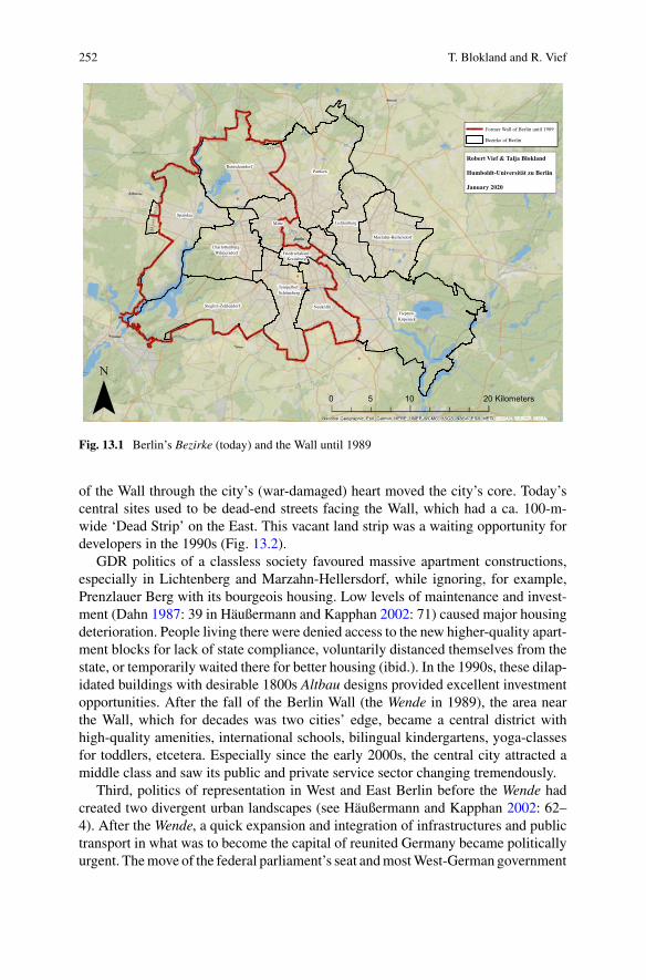
252 T. Blokland and R. Vief
Fig. 13.1 Berlin’s Bezirke (today) and the Wall until 1989
of the Wall through the city’s (war-damaged) heart moved the city’s core. Today’scentral sites used to be dead-end streets facing the Wall, which had a ca. 100-m-wide ‘Dead Strip’ on the East. This vacant land strip was a waiting opportunity fordevelopers in the 1990s (Fig. 13.2).
GDR politics of a classless society favoured massive apartment constructions,especially in Lichtenberg and Marzahn-Hellersdorf, while ignoring, for example,Prenzlauer Berg with its bourgeois housing. Low levels of maintenance and invest-ment (Dahn 1987: 39 in Häußermann and Kapphan 2002: 71) caused major housingdeterioration. People living there were denied access to the new higher-quality apart-ment blocks for lack of state compliance, voluntarily distanced themselves from thestate, or temporarily waited there for better housing (ibid.). In the 1990s, these dilap-idated buildings with desirable 1800s Altbau designs provided excellent investmentopportunities. After the fall of the Berlin Wall (the Wende in 1989), the area nearthe Wall, which for decades was two cities’ edge, became a central district withhigh-quality amenities, international schools, bilingual kindergartens, yoga-classesfor toddlers, etcetera. Especially since the early 2000s, the central city attracted amiddle class and saw its public and private service sector changing tremendously.
Third, politics of representation in West and East Berlin before the Wende hadcreated two divergent urban landscapes (see Häußermann and Kapphan 2002: 62–4). After the Wende, a quick expansion and integration of infrastructures and publictransport in what was to become the capital of reunited Germany became politicallyurgent. Themove of the federal parliament’s seat andmostWest-German government
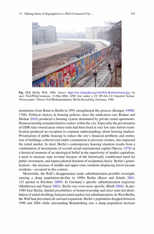
13 Making Sense of Segregation in a Well-Connected City … 253
Fig. 13.2 Berlin Wall, 1986. Source https://en.wikipedia.org/wiki/File:Berlinermauer.jpg, byuser: Noir/WikiCommons, 22-Mar-2004, GNU free under a CC BY-SA-3.0 Unported license.Photographer Thierry Noir/Bethaniendamm, Berlin-Kreuzberg, Germany, 1986
institutions from Bonn to Berlin in 1991 strengthened this process (Kemper 1998b:1766). Political choices in housing policies since the unification (see Bodnar andMolnar 2010) produced a housing system dominated by private rental apartments.Homeownership remained hard to realize within the city. Especially the privatisationof GDR state-owned areas where rents had been fixed at very low rates before reuni-fication produced an exception to common understandings about housing markets.Privatisation of public housing to reduce the city’s financial problems and restitu-tion of buildings collectivized under communism to previous owners, also impactedthe rental market. In short, Berlin’s contemporary housing situation results from acombination of investments of second circuit international capital (Harvey 1978) ata historical moment of an ideological belief in the superiority of market capitalism,a need to increase state revenue because of the historically conditioned need forpublic investment, and unprecedented freedom of residential choice. Berlin’s gentri-fication—the increase of middle and upper-class residents displacing lower-incomeresidents—occurred in this context.
Meanwhile, the Wall’s disappearance made suburbanization possible overnight,causing a sharp population-decline in 1990s Berlin (Beyer and Schulz 2001:123 quoted in Kirchner 2009). In Germany’s specific suburbanization trajectory(Matthiesen and Nuissl 2002), Berlin was even more specific (Bluth 2004). In pre-1989 East Berlin, limited possibilities of homeownership and strict state-led distri-bution of rental dwellings had prevented market-led suburbanization. InWest Berlin,the Wall had prevented all outward expansion. Berlin’s population dropped between1990 and 2004 while surrounding Brandenburg saw a sharp population increase

254 T. Blokland and R. Vief
(Beran et al. 2015). For example, Falkensee, bordering directly at West Berlin’sSpandau, grew in a decade from 22,087 to 40,511 residents, causing challenges tocohesion, identity and infrastructure (Kirchner 2009: 41f). Since 2004, more peoplemove fromBerlin to Brandenburg than in the other direction (Beran et al. 2015). Andyet, the influx from other German states and abroad made Berlin grow from 3.3 to3.75 million between 2004 and 2018 (Amt für Statistik Berlin-Brandenburg 2019).
Both in the East and the West before the Wende, industries received politicallymotivated state-support. As this disappeared after the Wende, deindustrialisationfollowed, especially but not exclusively in the East, causing high unemploymentrates and the lowest GDP of all European metropoles compared to their nationwideaverages (Bernt et al. 2013: 16; Gornig et al. 2013: 8f). In the early 2000s, sociolo-gists predicted growing economic marginalization (Kronauer 1997 in Häußermannand Kapphan 2002: 18). Instead, in the last decade, Berlin grew economically, landvalues increased, and unemployment rates declined. This decrease in unemploymentpartly results from growth in flexible service-jobs with little income security. InEast Berlin, pre-1989 full employment with absolute job security and low incomeand little consumer goods availability has now turned into low unemployment buthigh job insecurity, continuous low or moderate incomes, rent increase and endlessconsumer goods—unaffordable for many. Additionally, younger and new Berlinersface precarity in self-employment in the creative sector.2
Berlin has moved from a politically divided city to a city with new divisions. Itundergoeswell-documented gentrification (Holm 2013), towhich political initiativesseek answers, including housing development in selected surrounding Brandenburgareas, which will further affect its demography. But Berlin also moved from a cityinitially divided only by political decision to a city of distinctive social lives. Weexplorewhat segregationmaymean in this context after presentingBerlin’s statisticaldevelopment of segregation.
13.3 Methods
German scholars and journalists vigorously debate segregation but lack precise,small-scale data to demonstrate the existenceof poverty pockets before 1998 (Kemper1998a: 22) and have limited data since then. Some described a stable rate of socioeco-nomic segregation between 1990 and 2005 for Berlin (Friedrichs and Triemer 2009:120), but only based on analysis of large spatial units (ibid.: 20) or argued that in the1990s, poverty increasingly concentrated in specific neighbourhoods (Häußermannand Kapphan 2004) and produced social problems, but again drawing on limited
2Figures suggest weak correlations between education and income for residents without migrationbackground or European Union backgrounds (especially Italy, Spain, Greece since 2008s crisis)(Gathmann et al. 2014).
13 Making Sense of Segregation in a Well-Connected City … 255
data. Others found that social segregation by Sozialgesetzbuch II3 slightly increasedbetween 2005 and 2014 (Helbig and Jähnen 2018: 139).
Germany has poor statistics. Before 1989, the FRG and the GDR had their ownways of collecting census data. After reunification, Germany delayed the census to2011, leaving a 24 year gap (Statistische Ämter des Bundes und der Länder 2015:9). Berlin does not have a useful panel of census data since 1989. Germany does notcollect census data on income. It does not publish data on occupational status for cities(which it collects; Eisenmenger et al. 2014; Heckel and Heyde 2015). On the locallevel, census data regulations are stricter than in other countries. The Mikrozensus,Germany’s largest household survey, allows predictions of income distributions butdoes not publish data for spatial units smaller than Berlin’s 12 Bezirke. The spatialsampling of the Mikrozensus is on the same scale, so we cannot infer to smallerlevels.
Berlin answered in 2006 to the lack of data with the Monitoring Soziale Stad-tentwicklung, an initiative of academics and city planners to join available datasources on a low spatial scale to assess neighbourhoods’ relative positions. TheLORs (Lebensweltlich-Orientierte Räume) in the Monitoring provide 447 spatialunits (Planungsräume) with 7,500–10,000 inhabitants (Bömermann et al. 2006).4
The data do not include income. Fortunately, income is only one indicator suggestingwhere the rich, the poor and others live. As proxies for economic status, theMonitorcontains information on unemployment, state family subsidies and child poverty.
We analyse data for three time points (2007, 2012, 2016) with four indicators ofsocioeconomic segregation: unemployed persons among people aged 15–65; long-term5 unemployed persons among those aged 15–65; non-unemployed recipients ofstate subsidies in all age groups (for example when people work but make too littleto reach the minimum state-guaranteed standard, receive very low pensions, or havechildren living in a poor household); and poverty among children aged 0–15. Theseindicators allow an estimation of the lower part of the income distribution. Theycannot show polarization of the rich within neighbourhoods and throughout Berlin.
Scholars have also investigated ‘ethnic’ segregation of legally defined foreignersin neighbourhoods. Kemper (1998a, b) found ethnic segregation to be stable duringthe 1990s in West Berlin and to decline in East Berlin until 1996. Overall, ethnicsegregation rates were higher in East Berlin, where residential mobility was verylow. Friedrichs and Triemer (2009: 120f) observed an increasing level of segregationuntil the mid-2010s. Helbig and Jähnen (2018) observed a decrease since 2002.Again, both used data on a high spatial scale. Häußermann and Kapphan (2002: 212)underlined the increasing concentration of foreign-born residents since the 1970s(with only 20,000 foreigners in entire East Berlin), then stability since the 1990s,but on Bezirke scale. Existing studies thus do not report consistent results and usedifferent spatial scales—we aim to clarify the recent development on a small spatialscale.
3Sozialgesetzbuch II only covers a part of the unemployed population.4We exclude 14 LOR-Planungsräume with fewer than 300 inhabitants in our analyses.5Unemployed over one year without interruption, Sozialgesetzbuch II and III (Nagel 2018: 16f).
256 T. Blokland and R. Vief
Germany collects no data of racialized categories, but we can compute segregationof foreigners and Germans with a migration background, also clustered by country-of -origin groups. We analyse such segregation using proportions of foreigners andpersons with a migration background,6 and by country groups (European Union andTurkey/Muslim States).7 We are aware of the ways in which statistics construct cate-gories: as our last section will show, for Berlin’s social landscape, or how the city islived and used, these social constructions and their imaginations matter: stereotypingpeople with certain passports as ‘Muslim’ is an act of othering.
We calculated residential segregation using the segregation index (IS)8 and thelocation quotient (LQ) with the Geo-Segregation Analyzer (Apparicio et al. 2013).We cannot report indices of dissimilarity between groups of our analysis, because thegroups partly overlap (long-term unemployed residents count also as unemployed;poor children may also be residents receiving subsidies, etc.).
13.4 Socioeconomic Segregation
Figure 13.3 shows the IS for 3 years of data for socioeconomic and ethnic indi-cators: Berlin’s moderate unemployment and long-term unemployment segregationwas stable between 2007 and 2016, with a tiny drop between 2007 and 2012. Poorchildren and state support recipients became slightly more segregated over time,especially between 2007 and 2012. Poor children lived overall much more segre-gated than other categories (IS .43/42 in 2012/2016). As school-aged children typi-cally have high neighbourhood use (Blokland 2003; Karsten 2002), this may affectsocial segregation (see Table 13.1).
Figures 13.3, 13.4, 13.5, 13.6 and 13.7 map the distribution of the LQs of ourindicators in both 2007 and 2016. In Fig. 13.3, LQs of unemployment for 2007 and2016 reveal a very slight decrease in poverty concentration areas. The index went upin areas at the city borders far from the new centre such as the South-West, where wenowobserve less concentration of employedpeoplewithout benefits andwithout poorchildren than in 2007. Other outskirts (as theNorth ofMarzahn-Hellersdorf) desegre-gated somewhat. Formerly deprived inner-city neighbourhoods (parts of Kreuzbergand Neukölln) now have intermediate values, but pockets of high concentrations ofunemployment remained. Land values and rents increased disproportionally here
6Foreigners and Germans born outside of Germany with second nationality, naturalized citizens,children of two foreign parents born in Germany since 2000. Changes in data-collection after 2014ask for cautious interpretation of 2016 numbers (Nagel 2018: 59f).7Egypt, Algeria, Bahrain, Djibouti, Iraq, Yemen, Jordan, Qatar, Comoros, Kuwait, Lebanon, Libya,Morocco, Mauritania, Oman, Saudi Arabia, Somalia, Sudan, Syria, Tunisia, United Arab Emirates.8The IS (Apparicio et al. 2008: 1;Duncan andDuncan 1955) is defined by I S = 1
2
∑ni=1
∣∣∣ xiX − ti−xi
T−X
∣∣∣
and the most common one-group segregation measure. In this formula, n is the number of spatialunits in the overall city (in our case: Berlin), xi is the total population of group X in spatial unit i,ti the total population in spatial unit i, X is the total population of X within the overall city. T is thetotal overall city population.
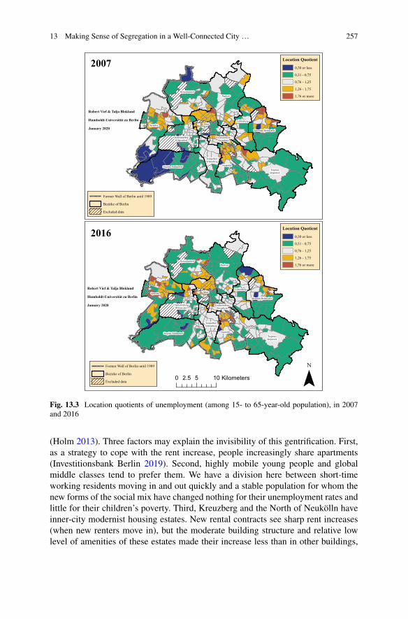
13 Making Sense of Segregation in a Well-Connected City … 257
Pankow
Spandau
Treptow-Köpenick
Reinickendorf
Mitte
Steglitz-Zehlendorf Neukölln
Lichtenberg
Marzahn-Hellersdorf
Tempelhof-Schöneberg
Charlottenburg-Wilmersdorf
Friedrichshain-Kreuzberg
0 5 102.5 Kilometers
Former Wall of Berlin until 1989
Bezirke of Berlin
Excluded data
2007
Robert Vief & Talja Blokland
Humboldt-Universität zu Berlin
January 2020
Pankow
Spandau
Treptow-Köpenick
Reinickendorf
Mitte
Steglitz-Zehlendorf Neukölln
Lichtenberg
Marzahn-Hellersdorf
Tempelhof-Schöneberg
Charlottenburg-Wilmersdorf
Friedrichshain-Kreuzberg
Robert Vief & Talja Blokland
Humboldt-Universität zu Berlin
January 2020
Former Wall of Berlin until 1989
Bezirke of Berlin
Excluded data
2016
Location Quotient
0,30 or less
0,31 - 0,75
0,76 - 1,25
1,26 - 1,75
1,76 or more
Location Quotient
0,30 or less
0,31 - 0,75
0,76 - 1,25
1,26 - 1,75
1,76 or more
Fig. 13.3 Location quotients of unemployment (among 15- to 65-year-old population), in 2007and 2016
(Holm 2013). Three factors may explain the invisibility of this gentrification. First,as a strategy to cope with the rent increase, people increasingly share apartments(Investitionsbank Berlin 2019). Second, highly mobile young people and globalmiddle classes tend to prefer them. We have a division here between short-timeworking residents moving in and out quickly and a stable population for whom thenew forms of the social mix have changed nothing for their unemployment rates andlittle for their children’s poverty. Third, Kreuzberg and the North of Neukölln haveinner-city modernist housing estates. New rental contracts see sharp rent increases(when new renters move in), but the moderate building structure and relative lowlevel of amenities of these estates made their increase less than in other buildings,
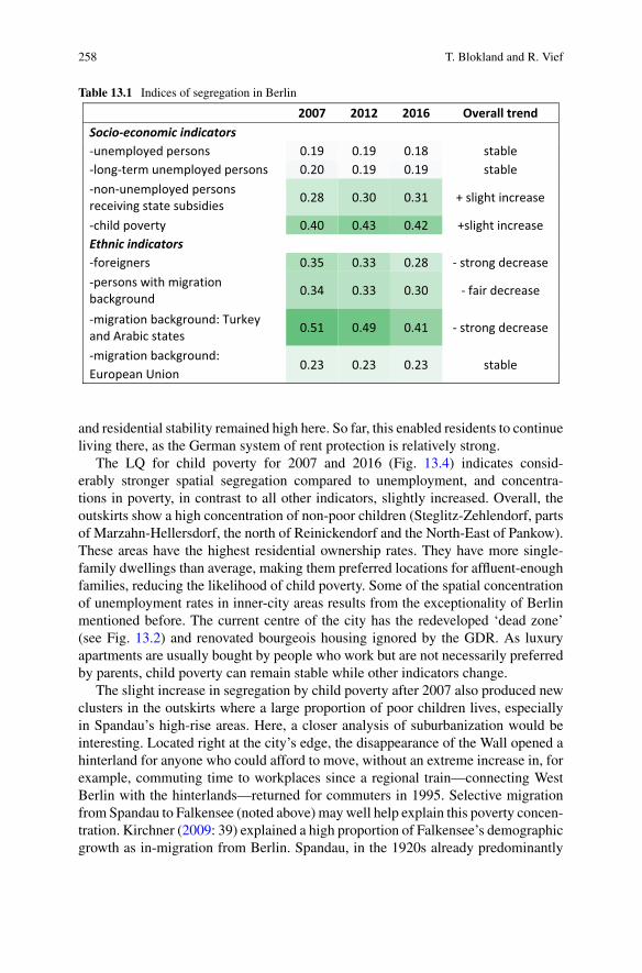
258 T. Blokland and R. Vief
Table 13.1 Indices of segregation in Berlin
2007 2012 2016 Overall trendSocio-economic indicators-unemployed persons 0.19 0.19 0.18 stable-long-term unemployed persons 0.20 0.19 0.19 stable-non-unemployed persons receiving state subsidies 0.28 0.30 0.31 + slight increase
-child poverty 0.40 0.43 0.42 +slight increaseEthnic indicators-foreigners 0.35 0.33 0.28 - strong decrease-persons with migration background 0.34 0.33 0.30 - fair decrease
-migration background: Turkey and Arabic states 0.51 0.49 0.41 - strong decrease
-migration background:0.23 0.23 0.23 stable
European Union
and residential stability remained high here. So far, this enabled residents to continueliving there, as the German system of rent protection is relatively strong.
The LQ for child poverty for 2007 and 2016 (Fig. 13.4) indicates consid-erably stronger spatial segregation compared to unemployment, and concentra-tions in poverty, in contrast to all other indicators, slightly increased. Overall, theoutskirts show a high concentration of non-poor children (Steglitz-Zehlendorf, partsof Marzahn-Hellersdorf, the north of Reinickendorf and the North-East of Pankow).These areas have the highest residential ownership rates. They have more single-family dwellings than average, making them preferred locations for affluent-enoughfamilies, reducing the likelihood of child poverty. Some of the spatial concentrationof unemployment rates in inner-city areas results from the exceptionality of Berlinmentioned before. The current centre of the city has the redeveloped ‘dead zone’(see Fig. 13.2) and renovated bourgeois housing ignored by the GDR. As luxuryapartments are usually bought by people who work but are not necessarily preferredby parents, child poverty can remain stable while other indicators change.
The slight increase in segregation by child poverty after 2007 also produced newclusters in the outskirts where a large proportion of poor children lives, especiallyin Spandau’s high-rise areas. Here, a closer analysis of suburbanization would beinteresting. Located right at the city’s edge, the disappearance of the Wall opened ahinterland for anyone who could afford to move, without an extreme increase in, forexample, commuting time to workplaces since a regional train—connecting WestBerlin with the hinterlands—returned for commuters in 1995. Selective migrationfrom Spandau to Falkensee (noted above) maywell help explain this poverty concen-tration. Kirchner (2009: 39) explained a high proportion of Falkensee’s demographicgrowth as in-migration from Berlin. Spandau, in the 1920s already predominantly
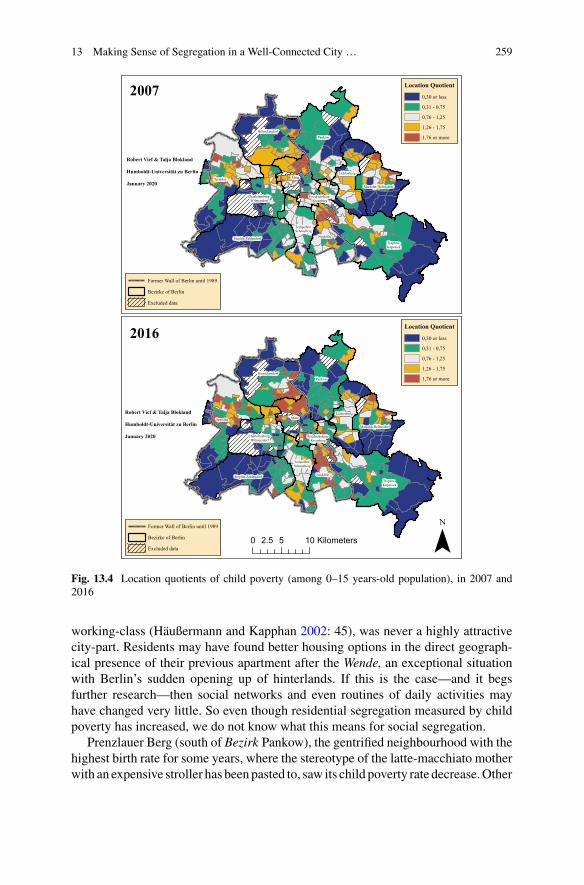
13 Making Sense of Segregation in a Well-Connected City … 259
Pankow
Spandau
Treptow-Köpenick
Reinickendorf
Mitte
Steglitz-Zehlendorf Neukölln
Lichtenberg
Marzahn-Hellersdorf
Tempelhof-Schöneberg
Charlottenburg-Wilmersdorf
Friedrichshain-Kreuzberg
0 5 102.5 Kilometers
Former Wall of Berlin until 1989
Bezirke of Berlin
Excluded data
2007
Robert Vief & Talja Blokland
Humboldt-Universität zu Berlin
January 2020
Pankow
Spandau
Treptow-Köpenick
Reinickendorf
Mitte
Steglitz-Zehlendorf Neukölln
Lichtenberg
Marzahn-Hellersdorf
Tempelhof-Schöneberg
Charlottenburg-Wilmersdorf
Friedrichshain-Kreuzberg
Robert Vief & Talja Blokland
Humboldt-Universität zu Berlin
January 2020
Former Wall of Berlin until 1989
Bezirke of Berlin
Excluded data
2016
Location Quotient
0,30 or less
0,31 - 0,75
0,76 - 1,25
1,26 - 1,75
1,76 or more
Location Quotient
0,30 or less
0,31 - 0,75
0,76 - 1,25
1,26 - 1,75
1,76 or more
Fig. 13.4 Location quotients of child poverty (among 0–15 years-old population), in 2007 and2016
working-class (Häußermann and Kapphan 2002: 45), was never a highly attractivecity-part. Residents may have found better housing options in the direct geograph-ical presence of their previous apartment after the Wende, an exceptional situationwith Berlin’s sudden opening up of hinterlands. If this is the case—and it begsfurther research—then social networks and even routines of daily activities mayhave changed very little. So even though residential segregation measured by childpoverty has increased, we do not know what this means for social segregation.
Prenzlauer Berg (south of Bezirk Pankow), the gentrified neighbourhood with thehighest birth rate for some years, where the stereotype of the latte-macchiato motherwith an expensive stroller has beenpasted to, saw its child poverty rate decrease.Other
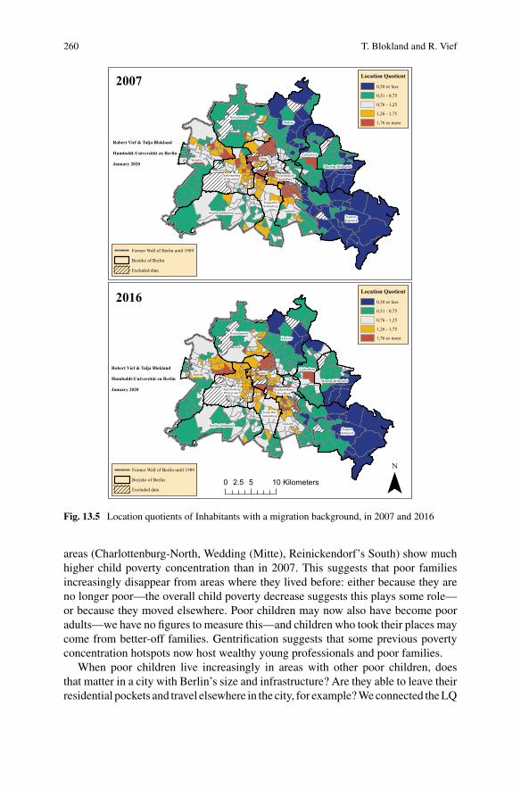
260 T. Blokland and R. Vief
Pankow
Spandau
Treptow-Köpenick
Reinickendorf
Mitte
Steglitz-Zehlendorf Neukölln
Lichtenberg
Marzahn-Hellersdorf
Tempelhof-Schöneberg
Charlottenburg-Wilmersdorf
Friedrichshain-Kreuzberg
0 5 102.5 Kilometers
Former Wall of Berlin until 1989
Bezirke of Berlin
Excluded data
2007
Robert Vief & Talja Blokland
Humboldt-Universität zu Berlin
January 2020
Pankow
Spandau
Treptow-Köpenick
Reinickendorf
Mitte
Steglitz-Zehlendorf Neukölln
Lichtenberg
Marzahn-Hellersdorf
Tempelhof-Schöneberg
Charlottenburg-Wilmersdorf
Friedrichshain-Kreuzberg
Robert Vief & Talja Blokland
Humboldt-Universität zu Berlin
January 2020
Former Wall of Berlin until 1989
Bezirke of Berlin
Excluded data
2016
Location Quotient
0,30 or less
0,31 - 0,75
0,76 - 1,25
1,26 - 1,75
1,76 or more
Location Quotient
0,30 or less
0,31 - 0,75
0,76 - 1,25
1,26 - 1,75
1,76 or more
Fig. 13.5 Location quotients of Inhabitants with a migration background, in 2007 and 2016
areas (Charlottenburg-North, Wedding (Mitte), Reinickendorf’s South) show muchhigher child poverty concentration than in 2007. This suggests that poor familiesincreasingly disappear from areas where they lived before: either because they areno longer poor—the overall child poverty decrease suggests this plays some role—or because they moved elsewhere. Poor children may now also have become pooradults—we have no figures to measure this—and children who took their places maycome from better-off families. Gentrification suggests that some previous povertyconcentration hotspots now host wealthy young professionals and poor families.
When poor children live increasingly in areas with other poor children, doesthat matter in a city with Berlin’s size and infrastructure? Are they able to leave theirresidential pockets and travel elsewhere in the city, for example?Weconnected theLQ
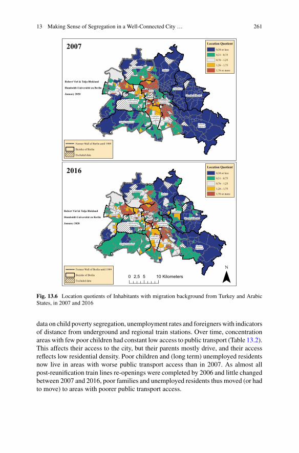
13 Making Sense of Segregation in a Well-Connected City … 261
Pankow
Spandau
Treptow-Köpenick
Reinickendorf
Mitte
Steglitz-Zehlendorf Neukölln
Lichtenberg
Marzahn-Hellersdorf
Tempelhof-Schöneberg
Charlottenburg-Wilmersdorf
Friedrichshain-Kreuzberg
0 5 102,5 Kilometers
Former Wall of Berlin until 1989
Bezirke of Berlin
Excluded data
2007
Robert Vief & Talja Blokland
Humboldt-Universität zu Berlin
January 2020
Pankow
Spandau
Treptow-Köpenick
Reinickendorf
Mitte
Steglitz-Zehlendorf Neukölln
Lichtenberg
Marzahn-Hellersdorf
Tempelhof-Schöneberg
Charlottenburg-Wilmersdorf
Friedrichshain-Kreuzberg
Robert Vief & Talja Blokland
Humboldt-Universität zu Berlin
January 2020
Former Wall of Berlin until 1989
Bezirke of Berlin
Excluded data
2016
Location Quotient
0,30 or less
0,31 - 0,75
0,76 - 1,25
1,26 - 1,75
1,76 or more
Location Quotient
0,30 or less
0,31 - 0,75
0,76 - 1,25
1,26 - 1,75
1,76 or more
Fig. 13.6 Location quotients of Inhabitants with migration background from Turkey and ArabicStates, in 2007 and 2016
data on child poverty segregation, unemployment rates and foreigners with indicatorsof distance from underground and regional train stations. Over time, concentrationareas with few poor children had constant low access to public transport (Table 13.2).This affects their access to the city, but their parents mostly drive, and their accessreflects low residential density. Poor children and (long term) unemployed residentsnow live in areas with worse public transport access than in 2007. As almost allpost-reunification train lines re-openings were completed by 2006 and little changedbetween 2007 and 2016, poor families and unemployed residents thus moved (or hadto move) to areas with poorer public transport access.
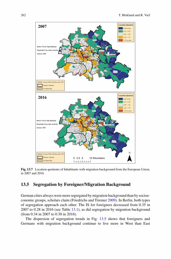
262 T. Blokland and R. Vief
Pankow
Spandau
Treptow-Köpenick
Reinickendorf
Mitte
Steglitz-Zehlendorf Neukölln
Lichtenberg
Marzahn-Hellersdorf
Tempelhof-Schöneberg
Charlottenburg-Wilmersdorf
Friedrichshain-Kreuzberg
0 5 102.5 Kilometers
Former Wall of Berlin until 1989
Bezirke of Berlin
Excluded data
2007
Robert Vief & Talja Blokland
Humboldt-Universität zu Berlin
January 2020
Pankow
Spandau
Treptow-Köpenick
Reinickendorf
Mitte
Steglitz-Zehlendorf Neukölln
Lichtenberg
Marzahn-Hellersdorf
Tempelhof-Schöneberg
Charlottenburg-Wilmersdorf
Friedrichshain-Kreuzberg
Robert Vief & Talja Blokland
Humboldt-Universität zu Berlin
January 2020
Former Wall of Berlin until 1989
Bezirke of Berlin
Excluded data
2016
Location Quotient
0,30 or less
0,31 - 0,75
0,76 - 1,25
1,26 - 1,75
1,76 or more
Location Quotient
0,30 or less
0,31 - 0,75
0,76 - 1,25
1,26 - 1,75
1,76 or more
Fig. 13.7 Location quotients of Inhabitants with migration background from the European Union,in 2007 and 2016
13.5 Segregation by Foreigner/Migration Background
German cities alwaysweremore segregated bymigration background than by socioe-conomic groups, scholars claim (Friedrichs and Triemer 2009). In Berlin, both typesof segregation approach each other. The IS for foreigners decreased from 0.35 in2007 to 0.28 in 2016 (see Table 13.1), as did segregation by migration background(from 0.34 in 2007 to 0.30 in 2016).
The dispersion of segregation trends in Fig. 13.5 shows that foreigners andGermans with migration background continue to live more in West than East
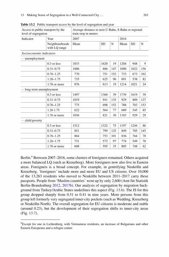
13 Making Sense of Segregation in a Well-Connected City … 263
Table 13.2 Public transport access by the level of segregation and year
Access to public transport by thelevel of segregation
Average distance to next U-Bahn, S-Bahn or regionaltrain stop in meters
Indicator Year 2007 2016
Neighbourhoodswith LQ range
Mean SD N Mean SD N
Socioeconomic indicators
– unemployment
0.3 or less 1833 1620 19 1204 948 9
0.31–0.75 1006 886 147 1090 1022 156
0.76–1.25 770 751 152 733 673 162
1.26–1.75 735 625 96 691 538 82
1.76 or more 876 613 19 1214 1021 24
– long-term unemployment
0.3 or less 1497 1360 39 1739 1619 39
0.31–0.75 1019 941 135 929 809 127
0.76–1.25 775 698 152 788 703 153
1.26 1.75 622 564 77 689 545 85
1.76 or more 1036 821 30 1183 929 29
– child poverty
0.3 or less 1512 1322 75 1197 1244 86
0.31–0.75 851 799 125 849 705 145
0.76–1.25 864 753 101 836 764 70
1.26–1.75 731 572 97 774 549 70
1.76 or more 608 595 35 805 748 62
Berlin.9 Between 2007–2016, some clusters of foreigners remained. Others acquireda more balanced LQ (such as Kreuzberg). More foreigners now also live in Easternareas. Foreigners is a broad concept. For example, in gentrifying Neukölln andKreuzberg, ‘foreigners’ include more and more EU and US citizens. Over 10,000of the 13,263 residents who moved to Neukölln between 2011–2017 carry thesepassports. People from ‘Muslim countries’ went up by only 2,600 (Amt für StatistikBerlin-Brandenburg 2012, 2017b). Our analysis of segregation by migration back-ground from Turkey/Arabic States underlines this aspect (Fig. 13.6). The IS for thisgroup dropped sharply from 0.51 to 0.41 in nine years. More persons from thisgroup left formerly very segregated inner-city pockets (such as Wedding, Kreuzbergor Neukölln-North). The overall segregation for EU-citizens is moderate and stable(around 0.23), but the development of their segregation shifts to inner-city areas(Fig. 13.7).
9Except for one in Lichtenberg, with Vietnamese residents, an increase of Bulgarians and otherEastern Europeans and a refugee center.
264 T. Blokland and R. Vief
13.6 How Does Segregation Matter?
As Marcuse (1993: 357 in Hamnett 2003: 167) argued 25 years ago, divided citiesare nothing new. From ancient Athens and Rome onwards, the poor have lived awayfrom the rich: ‘at least from the outset of the industrial revolution, cities have beendivided in ways that are quite familiar to us’ (ibid.). So how does segregation matter?
Statistics of where people sleep matters when we assume that people do not leavetheir concentration areas and residents have access to amenities, networks or otherresources only through their residential location. This assumption is questionable(Blokland and van Eijk 2010). A mixed environment can be social wallpaper for thebetter-off (Butler 2003) without them ever building network ties with people in lowersocial, economic or cultural positions. Curley (2008) showed that people whomovedfrompoverty pockets tomixed areas benefitted because their resourceswere no longerdrained, not because new social capital emerged. Kronauer (2002) suggested thatmuch depends on life conditions: single mothers found best support infrastructuresin apartment blocks on the outskirts, single unemployed persons benefitted mostfrom inner-city resources. So, segregation effects on life chances are multi-facetedand dynamic, even within one life-trajectory.
Besides networks, social capital and cultural interpretations, scholars may want tofocus much more on urban infrastructure, including its precise workings for accessto resources. Social segregation, the degree to which people conduct their role reper-tories (Blokland 2003; Hannerz 1980) in relative isolation or interaction with peoplewith a different class or racial/ethnic position than theirs, emerges through theseworkings.
Berlin is a well-connected city; public transport is affordable and even free forschool children. However, segregated poverty, as we saw before, coincides now withless easy transport access. When moving around the city becomes more difficultfor those who are most disadvantaged, it starts to matter where things are located.Resource access is central to how segregation matters, especially for resourcesthrough which social positions are reproduced: resources for raising kids. Fourexamples, drawing on students’ work at Humboldt, support this claim.
First, this work suggests a congruence of socioeconomic segregation and distribu-tion of certain child-oriented resources.Wemapped elementary schools, kindergartenand praxis for speech- and ergo-therapy. The choice of kindergarten types is smallerin high unemployment areas (Fritz 2013). Elementary school access is equal, buthigh unemployment areas have fewer schools with special profiles. Other indica-tors (teacher absence, computers in school, teacher/student ratio) show no system-atic pattern (Zwirner 2013). People living in affluent areas have a higher chance ofhaving therapists nearby. As high child poverty shifted to locations with worse publictransport, this can point to a difference in life chances.
Second, school segregation does not require residential segregation. Berlin’selementary school zoning laws should create schools with the same compositionas their catchment zone. Parents cannot simply send children elsewhere. In practice,parents differ in their possibilities to do so (Blokland and Große Löscher 2016).
13 Making Sense of Segregation in a Well-Connected City … 265
Especially in not segregated neighbourhoods, schools are more segregated thanthey should be for the residential composition (Vief 2018). As strongest school-neighbourhood segregation gaps occur in mixed settings, residential mix does notnecessarily create a social mix in important institutions.
Third, as children’s actual neighbourhood use tends to be high (Blokland 2003),the interplay of family and neighbourhood works differently in areas different inpoverty concentration. In amiddle-class pocket in Lichterfelde (Steglitz-Zehlendorf)and an owner-occupied development in Kreuzberg, qualitative interviews withparents taught us that both lived with people with similar orientations on domi-nant parenting ideas. Interviewees showed little awareness of the rest of the cityand a localness in their use of facilities and non-family networks. The neighbour-hood worked as village—or exclusive island. The interviewees did not intentionallyavoid mixing with people unlike themselves. But even in a middle-class enclave in ahyper-diverse district, the parents were so oriented on organizing the best resourcesfor their children that it never occurred to them that their practices of secluding(Giustozzi et al. 2016) excluded others (Blokland and Große Löscher 2016: 81–82).Giustozzi concluded (2016: 100): ‘Effectively (…) these mothers avoided routesthrough the city—also shown in their preference for cars over public transport—forfluid encounters (…) with residents unlike themselves. (…) Segregation, then, wasactively enhanced and reified by residential choices and everyday practices of thesemothers.
Fourthly, social processes affect the relative absence of migrants and foreignersin East Berlin. The long length of residence in some of these areas suggest thatfew places became vacant, and residential mobility is low there. Häußermann andKapphan (2002) claimed that foreigners chose not to move to the East because ofNeonazis. That certain Eastern parts were ‘spaces of fear’ for migrants had sincebecome a claim frequently used geographically to address the right-wing extremismand related fears of their potential victims, non-White Germans and immigrants(Lewek 2016: 37), producing imaginaries accordingly. The reproduction of theimagery of racism is a problem of ‘the East’ locates it away from the core of thecity and its proper ‘Western’ democratic qualities, but the evidence is weak. Whenwe asked people with a Sub-Saharan migration background to draw on a Berlin mapwhere they went or did not go, they excluded Eastern Berlin areas. In the early 2000s,racist violence tended to be stronger in the East of the city. Some nationalist, racistmeeting venues moved from Eastern areas to the region around Berlin (Shoshan2016), but the extreme right-wing political party AFD holds office in Köpenickand focusses electoral propaganda on Treptow-Köpenick and Marzahn-Hellersdorf,making racism visible.
That segregation occurs from migrant choices not to move to East Berlin outof a fear of racism (Häußermann and Kapphan 2002) is tentative but a commonnarrative. This narrative, Lewek (2016) argued, helped the city marketing itself asdiverse, hip and tolerant. By effectively spatializing racism in areas with low touristattractivity anyway, where it was constructed as a problem of the particular back-wardness of a particular part of Berlins population, the rest of the city could bemarketed as welcoming cosmopolitan. The imagery may have worked: in the last
266 T. Blokland and R. Vief
20 years, migration background only increased slowly and slightly in these areas,although collective performances of right-wing extremists today are less spatiallyconcentrated in the Eastern part of Berlin (ibid.: 248). Most reported racist incidentsnow happen in Neukölln and the new Mitte, in contrast to the early 2000s.10
In another study, lower-classmigrant youth reported avoidance of areaswhere theyfelt unwelcome (Blokland and Šerbedžija 2018). Young men with Arab and Turkishroots in two Kreuzberg estates curbed their city use to avoid racist encounters. Diegoexpressed fear in Marzahn: ‘five or six Germans who will stand next to you willthink: Come on, there is a foreigner, he is going to get beaten’. Another youth hadbeen ‘stupidly talked to’ by a ‘Granny’ who scolded that ‘you foreigners’ made herBezirk, Hellersdorf, kaputt. Their local comfort zone (Blokland and Nast 2014) wasa response to experiences of discomfort elsewhere, interviewee Serdar suggested:
[…] [what causes that] you don’t like to go much into other Bezirke?
‘You can’t really put that to words, because I had a job training once (…) in Spandau (…) Ifelt not at all, zero well there, for real. Because you notice like, they look at you differently.(…) we, apparently, the foreigners have something against the Germans, they treat thembadly and so on (.) But really (…) the ones that label us that way, these are mostly thepeople, that live according to the old (…) mentalities, like so GDR, like some of them stillhave that in their heads. And you see it very well, one recognizes it clearly (…) Even thoughyou’re born here, you have no difference form them, only that in your roots you happen tobe Turkish (..) they say (…) you aren’t a German and so on (…) they want to be the onlyGermans. (Blokland and Šerbedžija 2018: 35)
Serdar interpreted his Spandau experience through the common lens of East Berlinas a container of racists. Spandau, however, was always West-Berlin. These expe-riences were not at all located in the East only. Two young migrant women feltdiscomfort in all Bezirke with few people with migration background: exactly thelocations where mothers quoted above felt so comfortable as they did not ‘have toprotect’ their children, living in a ‘village’. Here these women felt ‘uncomfortable’and ‘as exclusion, to be honest’:
When one gets to places where there are few migrants (…) it is always quite glaring (krass).In Zehlendorf (…), I was there (…) because my brother-in-law was in the hospital (…) Iwalked around with my nephew (…) and two minutes down the street, there is a lamppost,and it has sticker on it, ‘Islamist out’, ‘Migrants out’, ‘Nafros go home’ - so really krass.And then I walked around there thinking, shit, when I would be wearing a headscarf here,what would happen to me? (…) You get a look, I don’t know, it is always this krasse feeling,then I think, I belong here too, what are you looking at me like that for?’.
The closure of the city goes further than that when migrant youth experience that‘normal’ behaviour is demonized. Emre reportedly travelled to his internship but waslate, so ran from his train over the platform at a main railway station. He was stoppedby police or security. They asked his ID, then to open his bag, then questioned himif he had stolen something—all taking 10 min of Emre’s time, making him arrivelate at his workplace: ‘they did not believe me at first because I was out of breath,because I ran, they thought I must be fleeing’. Not everyone running at a station is
10See for example: Register Berlin (2019); Senatsverwaltung für Inneres und Sport (2007).
13 Making Sense of Segregation in a Well-Connected City … 267
stopped. Emre sensed that. For these youngsters, the everyday experience of beingundesired and put under general suspicion and policing was even stronger outsidetheir neighbourhood. They limited their use of the city for stories told and experiencesmade with subtle and direct racism. To these experiences, East/West divisions do notapply—but discursively impact imaginaries.
13.7 Conclusion
Berlin’s residential segregation is moderate to low, and not univocally increasing,especially not for people with migration background. Socioeconomic inequalityby income was stable between 2007 and 2016 but could only be measured at theBezirke level. On a smaller spatial scale, segregation for the working-age populationwas stable, but slightly increased for poor children. Contrary to public perception,segregation by foreigners/migration backgrounddecreased, especially for inhabitantswith roots from Turkey and ‘Muslim’ states. Some pockets of poverty concentrationshifted from (well-connected) inner-city areas to (worse-connected) outskirts.
Residential segregation does not necessarily mean social segregation, no morethan that, residential mix means social mix. Statistical segregation in terms ofwhere people fitting certain categories spend the nights may have little connectionto their actual city use, although neighbourhood use may correlate with our rolerepertoires, and role repertories change over time (Blokland 2003). We suggestedthat social segregation, more than residential segregation, is what divides a city. Astrong role in how Berliners use the city play, firstly, subtle forms of racism—a signon a wall, a remark made loudly, a seat changed on the bus to not come near ‘amigrant’. Secondly, the middle class, especially German and European, may engagein secluding practices when organizing their daily lives, securing the best resourcesfor their own—excluding others as a consequence.
So social and residential segregation must be analytically separated, especiallyfor understanding (the reproduction of) urban inequalities. We suggest that socialsegregation in Berlin is a more important theme than the statistical question of whosleeps where. Social segregation of the use of urban places and institutions in thecity may influence the reproduction of disadvantage across groups and possiblygenerations.
References
Amt für Statistik Berlin-Brandenburg (2012) Statistischer Bericht A I 5 – hj 2/11, Berlin. https://www.statistik-berlin-brandenburg.de/Publikationen/Stat_Berichte/2012/SB_A01-05-00_2011h02_BE.pdf. Accessed 15 Feb 2020
Amt für Statistik Berlin-Brandenburg (2017a) Regionaler Sozialbericht Berlin und Brandenburg2017, Potsdam. https://www.statistik-berlin-brandenburg.de/produkte/pdf/SP_Sozialbericht-000-000_DE_2017_BBB.pdf. Accessed 15 Feb 2020

268 T. Blokland and R. Vief
Amt für Statistik Berlin-Brandenburg (2017b) Statistischer Bericht A I 5 – hj 1/17, Berlin.https://www.statistik-berlin-brandenburg.de/publikationen/stat_berichte/2017/SB_A01-05-00_2017h01_BE.pdf. Accessed 15 Feb 2020
Amt für Statistik Berlin-Brandenburg (2019) Statistischer Bericht: Einwohnerinnen und Einwohnerim Land Berlin am 31. Dezember 2018, Potsdam. https://www.statistik-berlin-brandenburg.de/publikationen/stat_berichte/2019/SB_A01-05-00_2018h02_BE.pdf. Accessed 15 Feb 2020
Apparicio P, Martori JC, Pearson AL, Fournier É, Apparicio D (2013) An open-source softwarefor calculating indices of urban residential segregation. Soc Sc Comput Rev 32:117–128
Apparicio P, Petkevitch V, Charron M (2008) Segregation analyzer: a C#. Net application forcalculating residential segregation indices. Cybergeo 414:1–27
Beran F, Czarnetzki F, Nuissl H (2015) Von der Suburbanisierung zur Reurbanisierung in Berlin?Standort 39:62–68
Bernt M, Grell B, Holm A (2013) Introduction. In: Bernt M, Grell B, Holm A (eds) The Berlinreader. Transcript, Bielefeld, pp 11–24
Beyer W, Schulz M (2001) Berlin—Suburbanisierung auf Sparflamme!? In: Brake K, DangschatJS, Herfert G (eds) Suburbanisierung in Deutschland: Aktuelle Tendenzen. Leske & Budrich,Opladen, pp 123–150
Blokland T (2003) Urban bonds. Polity Press, CambridgeBlokland T, Große Löscher G (2016) Cheating the system to get the best for one’s kids: middleclass practices and racist marginalization. In: Blokland T, Giustozzi C, Krüger D, Schilling H(eds) Creating the unequal city. Ashgate, Farnam, pp 71–83
Blokland T, Nast J (2014) From public familiarity to comfort zone. IJURR 38:1142–1159Blokland T, Šerbedžija V (2018) Gewohnt ist nicht normal: Jugendalltag in zwei KreuzbergerKiezen. Logos-Verlag, Berlin
Blokland T, van Eijk G (2010) Do people who like diversity practice diversity in neighbourhoodlife? JEMS 36:313–332
Bluth F (2004) Stadt -Umland -Wanderung imRaumBerlin. Berliner Statistik.Monatsschrift 94–99Bodnar J, Molnar V (2010) Reconfiguring private and public. Urban Stud 47:789–812Bömermann H, Jahn S, Nelius K (2006) Lebensweltlich orientierte Räume im RegionalenBezugssystem. https://www.stadtentwicklung.berlin.de/planen/basisdaten_stadtentwicklung/lor/download/BerlinerStatistik0608.pdf. Accessed 15 Feb 2020
Butler T (2003) Living in the bubble: gentrification and its ‘others’ in North London. Urban Stud40:2469–2486
Curley AM (2008) A new place, a new network?: social capital effects of residential relocation forpoor women. In: Blokland T, Savage M (eds) Networked urbanism. Ashgate, Farnam, pp 85–104
Dahn D (1987) Prenzlauer Berg-Tour. Mitteldeutscher Verlag, HalleDuncan OD, Duncan B (1955) A Methodological analysis of segregation indexes. ASR 20:210Eisenmenger M, Loos C, Sedmihradsky D (2014) Erwerbstätigkeit in Deutschland - Ergebnissedes Zensus 2011. Wirtschaft und Statistik 544–560
Friedrichs J, Triemer S (2009) Gespaltene Städte?: Soziale und ethnische Segregation in deutschenGroßstädten. VS Verlag für Sozialwissenschaften, Wiesbaden
Fritz D (2013) Kindertagesbetreuung als Nachbarschaftsressource und die Reproduktion vonUngleichheit. Unpublished paper, HU Berlin
Gathmann C, Keller N, Monscheuer O, Straubhaar T, Schäfer H, Zimmermann KF, BrückerH (2014) Zuwanderung nach Deutschland—Problem und Chance für den Arbeitsmarkt.Wirtschaftsdienst 94:159–179
Giustozzi C (2016) In the interest of the child: gendered practices of middle class mothers. In:Blokland T, Giustozzi C, Krüger D, Schilling H (eds) Creating the unequal city. Ashgate,Farnam, pp 85–106
Giustozzi C et al (2016) Secluding: middle class segregation in schools and neighborhoods. In:Blokland T, Giustozzi C, Krüger D, Schilling H (eds) Creating the unequal city. Ashgate,Farnam, pp 53–70
Gornig M et al (2013) Wirtschaftsentwicklung in Berlin: Szenario 2030. DIW Berlin, vol 77

13 Making Sense of Segregation in a Well-Connected City … 269
Gould M (1999) Race and theory: culture, poverty, and adaptation to discrimination in Wilson andOgbu. Sociol Theory 17:171–200
Grabka MM, Goebel J, Liebig S (2019) Wiederanstieg der Einkommensungleichheit – aber auchdeutlich steigende Realeinkommen. DIW Wochenbericht 344–353
Hamnett C (2003) Unequal city: London in the global arena. Routledge, LondonHannerz U (1980) Exploring the city. Columbia UP, New YorkHarvey D (1978) The urban process under capitalism: a framework for analysis. IJURR 2:101–131Häußermann H, Kapphan A (2002) Berlin. Von der geteilten zur gespaltenen Stadt? VS Verlag fürSozialwissenschaften, Wiesbaden
Häußermann H, Kapphan A (2004) Berlin: Ausgrenzungsprozesse in einer europäischen Stadt.In: Häußermann H, Kronauer M, Siebel W (eds) An den Rändern der Städte: Armut undAusgrenzung. Suhrkamp, Frankfurt/Main, pp 203–234
Heckel C, von der Heyde C (2015) Anmerkungen zum Zensus 2011 aus Sicht der Markt- undSozialforschung. AStA Wirtschafts- Und Sozialstatistisches Archiv 9:251–268
Helbig M, Jähnen S (2018) Wie brüchig ist die soziale Architektur unserer Städte? Trends undAnalysen der Segregation in 74 deutschen Städten. WZB discussion paper, Berlin. https://www.econstor.eu/bitstream/10419/179001/1/p18-001.pdf. Accessed 15 Feb 2020
Herrnstein RJ, Murray C (1996) The bell curve: intelligence and class structure in American life.Simon & Schuster, New York
Holm A (2013) Berlin’s gentrification mainstream. In: Bernt M, Grell B, Holm A (eds) The Berlinreader. Transcript, Bielefeld, pp 171–189
Holzer H (1991) The spatial mismatch hypothesis: what has the evidence shown? Urban Stud28:105–122
Investitionsbank Berlin (2019) IBB Wohnungsmarktbericht 2018. https://www.ibb.de/media/dokumente/publikationen/berliner-wohnungsmarkt/wohnungsmarktbericht/ibb_wohnungsmarktbericht_2018.pdf. Accessed 15 Feb 2020
Karsten L (2002) Mapping childhood in Amsterdam: the spatial and social construction ofchildren’s domains in the city. TESG 93:231–241
Kemper F-J (1998a) Residential segregation and housing in Berlin: changes since unification.GeoJournal 46:17–28
Kemper F-J (1998b) Restructuring of housing and ethnic segregation: recent developments inBerlin. Urban Stud 35:1765–1789
Kirchner F (2009) Soziale Integration in Gemeinden rund um Berlin - Netzwerke Alteingesessenerund Zugezogener in der Stadt Falkensee. Master’s thesis, HU Berlin
Kronauer M (2002) Exklusion: Die Gefährdung des Sozialen im hoch entwickelten Kapitalismus.Campus, Frankfurt/Main
Lewek M (2016) Spaces of fear and their exclusionary consequences. In: Blokland T, Giustozzi C,Krüger D, Schilling H (eds) Creating the unequal city. Ashgate, Farnam, pp 31–52
Marcuse P (1993) What’s so new about divided cities? IJURR 17:355–365Marques E (2012) Opportunities and deprivation in the urban South. Ashgate, FarnhamMatthiesen U, Nuissl H (2002) Phasen der Suburbanisierung seit 1989. In: Matthiesen U (ed) Anden Rändern der Deutschen Hauptstadt. Leske + Budrich, Opladen, pp 79–92
Nagel H (2018) Monitoring Soziale Stadtentwicklung Berlin: Erläuterungen zu den Indikatorenund Indizes zum MSS 2017 – “Indikatorenblätter”, Berlin. https://www.stadtentwicklung.berlin.de/planen/basisdaten_stadtentwicklung/monitoring/download/indikatoren/MSS2017Indikatorenblaetter_Fortschreibung.pdf. Accessed 15 Feb 2020
Register Berlin (2019) Auswertung 2018 der Berliner Register zur Erfassung rechter, rassistischer,antisemitischer, LGBTIQ*-feindlicher und anderer diskriminierender Vorfälle, Berlin. https://www.berliner-register.de/sites/default/files/Registerauswertung_Berlin_2018.pdf
Sampson RJ (2012) Great American city: Chicago and the enduring neighborhood effect. TheUniversity of Chicago Press, Chicago, London
Sampson RJ, Raudenbush SW, Earls F (1997) Neighborhoods and violent crime. Science277:918–924
270 T. Blokland and R. Vief
Senatsverwaltung für Inneres und Sport (2007) Rechte Gewalt in Berlin: 2003 bis 2006. im Fokus,Berlin. https://www.verfassungsschutz.de/de/oeffentlichkeitsarbeit/publikationen/pb-rechtsextremismus/publikationen-landesbehoerden-rechtsextremismus/broschuere-be-2007-11-rechte-gewalt-in-berlin-2003-2006. Accessed 15 Feb 2020
Shoshan N (2016) The management of hate. Princeton, Princeton UPSmall ML (2009) Unanticipated gains: origins of network inequality in everyday life. Oxford UP,New York
de Souza Briggs X (1997) Moving up versus moving out: neighbourhood effects in housingmobility programs. Hous Policy Debate 8:195–234
StatistischeÄmter des Bundes und der Länder (2015) Zensus 2011.Methoden undVerfahren,Wies-baden. https://www.zensus2011.de/SharedDocs/Downloads/DE/Publikationen/Aufsaetze_Archiv/2015_06_MethodenUndVerfahren.pdf?__blob=publicationFile&v=6. Accessed 15 Feb 2020
Vief R (2018) ‘Stacking the odds’: the intersection between neighborhood and school segregation.A comparison between New York and Berlin. Master’s thesis, HU Berlin
Wacquant LJD (2008) Urban outcasts: a comparative sociology of advanced marginality. PolityPress, Cambridge
Wrigley N (2002) Food Deserts’ in British cities. Urban Stud 39:2029–2040Zwirner L (2013) Inwiefern besteht eine Korrelation zwischen Wohngebiet und Schulqualität?Unpublished paper, HU Berlin
Open Access This chapter is licensed under the terms of the Creative Commons Attribution 4.0International License (http://creativecommons.org/licenses/by/4.0/), which permits use, sharing,adaptation, distribution and reproduction in any medium or format, as long as you give appropriatecredit to the original author(s) and the source, provide a link to the Creative Commons license andindicate if changes were made.
The images or other third party material in this chapter are included in the chapter’s CreativeCommons license, unless indicated otherwise in a credit line to the material. If material is notincluded in the chapter’s Creative Commons license and your intended use is not permitted bystatutory regulation or exceeds the permitted use, you will need to obtain permission directly fromthe copyright holder.
Chapter 14Socio-spatial Disparities in Brusselsand its Hinterland
Rafael Costa and Helga A. G. de Valk
Abstract Brussels’ urban and suburban landscape has changed considerably sincethe 1980s. The consolidation of socioeconomic fractures inside the city, a reinforce-ment of long-lasting disparities between the city and its prosperous hinterland, aswellas the increasing diversification of migration flows—both high- and low-skilled—contributed to these disparities. Recent evolutions of these patterns, however, havenot been investigated yet and therefore remain unknown. Besides, the extent to whichsegregation is primarily related to economic inequalities and to migration flows—ora combination/interaction between the two—so far has not been studied. This chapteroffers a detailed overview of the socio-spatial disparities in the Brussels FunctionalUrban Area. Our analyses relied on fine-grained spatial data, at the level of statis-tical sections and of individualised neighbourhoods built around 100 m x 100 mgrids. We analysed socioeconomic segregation measures and patterns, as well astheir evolution between 2001 and 2011. Socioeconomic groups were defined basedon individuals’ position with respect to national income deciles. In line with previousresearch, our results show very marked patterns of socioeconomic segregation in andaround Brussels operating both at a larger regional scale and at the local level.
Keywords Brussels · Socioeconomic segregation · Inequality · Geocoded censusdata
R. Costa (B)Vrije Universiteit Brussel & Netherlands Interdisciplinary DemographicInstitute/KNAW/University of Groningen, Brussels, Belgiume-mail: [email protected]
H. A. G. de ValkNetherlands Interdisciplinary Demographic Institute/KNAW/University of Groningen,The Hague, Netherlandse-mail: [email protected]
© The Author(s) 2021M. van Ham et al. (eds.), Urban Socio-Economic Segregation and Income Inequality,The Urban Book Series, https://doi.org/10.1007/978-3-030-64569-4_14
271
272 R. Costa and H. A. G. de Valk
14.1 Introduction
Socioeconomic segregation, its origins and its consequences have attracted the atten-tion of public policy and scientists alike. This also holds for Brussels, where the urbanand suburban landscape has changed considerably since the 1980s with the consol-idation of socioeconomic fractures inside the city, a reinforcement of long-lastingdisparities between the city and its prosperous hinterland, as well as the increasingdiversification of migration flows in terms of origin, occupations and socioeconomicposition. Recent evolutions in these patterns, however, have not been investigated bythe latest research and remain unknown. Besides, the extent to which segregation inBrussels is primarily related to economic inequalities and to migration flows—or acombination/interaction between them—so far remains unclear.
In this chapter, we provide a detailed overview of segregation patterns in Brus-sels and the hinterland and discuss whether and how these patterns can be linked toeconomic inequality and migration. We focus on the local level at Brussels’ munic-ipalities and the city’s outskirts. This level of detail is needed as overall incomeinequality has remained relatively stable in Belgium over the past decades. Goingbeyond the national level and looking at processes of spatial inequality at a smaller,local-level scale can help us understand what is driving change or stability.
Our analyses are based on fine administrative units aswell as individualised neigh-bourhoods. We first investigate socio-spatial inequalities in and around Brussels, inparticular the residential segregation of high- and low-income groups. For this end,we rely on income data based on tax returns for 2001 and 2011 at the level of thestatistical sections in theBrussels FunctionalUrbanArea (FUA).We then concentrateon the deprived and affluent spots that have experienced the fastest improvementsor deterioration of socioeconomic composition over the study period. This can helpunderstand what is steering local-level disparities. The use of individualised neigh-bourhoods based on gridded data from the 2001 to 2011 Censuses allows us to takea closer look at these areas. Looking at socioeconomic segregation at a very detailedspatial level may shed new light on issues that remain unnoticed when taking a higherlevel of analyses.
14.2 Background
Brussels, such as other Belgian cities, is characterised by relatively high levels ofsocioeconomic segregation compared to other European cities (Musterd 2005). Thisis the result of both the specific migration history to the country and the housing poli-cies in which homeownership is key. Housing policies in Belgium are characterisedby a deregulated rental market, limited public housing and public policies focusedon homeownership (De Decker 2008; Kesteloot and Cortie 1998). Social housing inBelgium in general and Brussels alike is limited and the public rental sector is notwell developed. In fact, public housing accounts for only 8% of the housing stock in
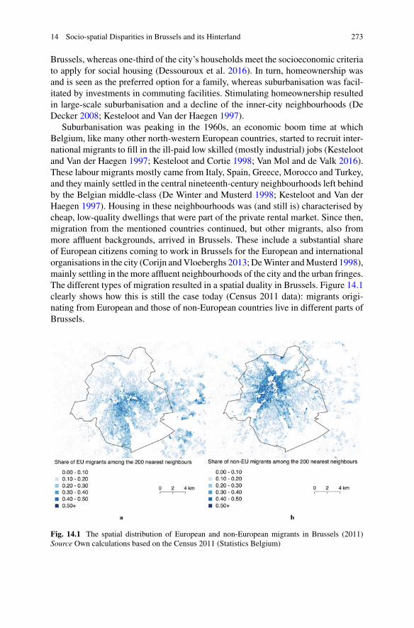
14 Socio-spatial Disparities in Brussels and its Hinterland 273
Brussels, whereas one-third of the city’s households meet the socioeconomic criteriato apply for social housing (Dessouroux et al. 2016). In turn, homeownership wasand is seen as the preferred option for a family, whereas suburbanisation was facil-itated by investments in commuting facilities. Stimulating homeownership resultedin large-scale suburbanisation and a decline of the inner-city neighbourhoods (DeDecker 2008; Kesteloot and Van der Haegen 1997).
Suburbanisation was peaking in the 1960s, an economic boom time at whichBelgium, like many other north-western European countries, started to recruit inter-national migrants to fill in the ill-paid low skilled (mostly industrial) jobs (Kestelootand Van der Haegen 1997; Kesteloot and Cortie 1998; Van Mol and de Valk 2016).These labour migrants mostly came from Italy, Spain, Greece, Morocco and Turkey,and they mainly settled in the central nineteenth-century neighbourhoods left behindby the Belgian middle-class (De Winter and Musterd 1998; Kesteloot and Van derHaegen 1997). Housing in these neighbourhoods was (and still is) characterised bycheap, low-quality dwellings that were part of the private rental market. Since then,migration from the mentioned countries continued, but other migrants, also frommore affluent backgrounds, arrived in Brussels. These include a substantial shareof European citizens coming to work in Brussels for the European and internationalorganisations in the city (Corijn andVloeberghs 2013; DeWinter andMusterd 1998),mainly settling in the more affluent neighbourhoods of the city and the urban fringes.The different types of migration resulted in a spatial duality in Brussels. Figure 14.1clearly shows how this is still the case today (Census 2011 data): migrants origi-nating from European and those of non-European countries live in different parts ofBrussels.
Fig. 14.1 The spatial distribution of European and non-European migrants in Brussels (2011)Source Own calculations based on the Census 2011 (Statistics Belgium)
274 R. Costa and H. A. G. de Valk
The reported duality was reinforced during the economic transition to a post-industrial economy after the 1970s, which led to a polarisation in terms of settlementand labour market into those with high- and low-skilled jobs. Similar to many Euro-pean cities, new urban jobs in the post-industrial economy were mainly taken up byhigh-skilled workers, while the low-skilled urban populations had less opportunitiesin the labour market. In the case of Brussels, high-skilled jobs were filled espe-cially by suburban commuters and international workers (De Winter and Musterd1998; Corijn and Vloeberghs 2013). On the other hand, migrants of Turkish andMoroccan origin living in the city were among the groups that suffered most fromthe urban economic changes. Upward mobility was most difficult for these groupsnot only due to their low education level but also because they are more likely toface discrimination in the labour market (Rea 2013) as well as in the housing market(Verstraete and Verhaeghe 2019). As such, they were forced to stay in the neighbour-hoods where they had initially settled (Kesteloot and Cortie 1998). Research hasshown that also to date, newly arrived migrants from non-European countries tend tosettle in the same central deprived neighbourhoods, where the housing stock is olderand cheaper, where socioeconomic conditions are worse, and where a strong ethnicconcentration prevails (Van Hamme et al. 2016; Costa and de Valk 2018). Moreover,due to the lack of public housing in Brussels (and the resulting long waiting lists),thesemigrantsmainly have to rely on the private rentalmarketwith the lowest-qualityhousing stock, often located in inner-city neighbourhoods previously occupied bythe industrial workers and earlier migrants.
More recently, Brussels’ central neighbourhoods have experienced gentrificationprocesses. Since the end of the twentieth century, Brussels has increasingly attractedyoung, well-off households composed of childless couples or isolated individuals,mainly highly educated and coming from other parts of Belgium andWestern Europe(Van Criekingen 2010). Typically, these households only spend part of their earlyadulthood in Brussels before relocating to more prosperous areas: the city is thusa stage in their professional and family trajectories (Van Criekingen 2010). Thesehouseholds tend to establish themselves in inner neighbourhoods originally inhab-ited by low-income households (many from foreign origin), attracted by their centrallocation and cheap rental prices (Van Hamme et al. 2016). The intense comingand going of such households has led to the reinvestment of certain inner neigh-bourhoods, with a housing offer increasingly targeted at higher-income earners andescalating rental prices—which is facilitated by the deregulated housingmarket (VanCriekingen 2010). There is, therefore, strong demographic pressure and increasingcompetition in the rental market in central areas that concentrate deprived householdsand ethnic minorities. Whereas long-distance displacement of these groups is stilllimited (Van Criekingen 2009), some low-income households have been pushed toadjacent poor neighbourhoods (Van Criekingen 2008; Van Hamme et al. 2016). Butother households find themselves trapped in their neighbourhoods and experience adeterioration of their housing conditions, ending up in lower-quality or overcrowdeddwellings (Van Criekingen 2010). At the city level, these gentrification processes inBrussels’ inner neighbourhoods may appear as a rise in the social mix since young
14 Socio-spatial Disparities in Brussels and its Hinterland 275
professionals share the space with low-income households, but at the local level, theycertainly contribute to socio-spatial disparities.
In sum, segregation patterns in Brussels were shaped by urban economic tran-sitions—similar to many other Western cities—combined with specific housingpolicies and migration background in Belgium. As a result, Brussels is markedby important socio-spatial inequalities inside the city as well as in respect to thehinterland.
In the more recent period, the persistent levels of socioeconomic segregationin European cities have been ascribed to the rise in income inequality produced byeconomic liberalisation since the 1980s and subsequent economic crises (Marcinczaket al. 2015). However, it is unclear to what extent this also holds for Brussels, asincome distribution seems to have remained rather stable in Belgium over the lastdecades.
Belgium is among the countries with a relatively low level of income inequalityworldwide, close to (or even lower than) the Scandinavian countries. The Gini coef-ficient for disposable income remained stable over time and varied between 30 and26 in the time period 1995–2017, with even a recent downward trend between 2000and 2017 (EU-SILC data via Eurostat 2019). In addition, Belgium was the onlycountry in Europe in which the share of the national income captured by the top 10%earners did not increase since the 1980s (Blanchet et al. 2019; Decoster et al. 2017).The few existing studies suggest that, contrary to many other countries, economicliberalisation over the last decades and the economic crises of 1998 and 2008 did notincrease overall income inequality in Belgium. This is believed to be due to institu-tional factors, namely a rigid system that regulates salaries and labour, as well as theimportance of the trade unions (Valenduc 2017).
Compared to the national level, income inequality is higher in Brussels, as isthe case for most large cities. For comparison, Brussels had a Gini coefficient of36 in 2013, at a similar level as Paris, and slightly higher than the Scandinaviancapitals (OECD 2019). It is unclear, however, how the income distribution evolvedover the last decades. On the one hand, the protective systems regulating salariesand labour also hold for Brussels, and they would have prevented inequalities fromrising in Brussels as well. On the other hand, it has been shown that the Brusselspopulation in the lowest income decile has been losing purchasing power since the1980s at a higher rate than the other income deciles (Kesteloot and Loopmans 2009).Furthermore, it is unclear to what extent changes observed in segregation are linkedto changes in income distribution.
In the remainder of this chapter, we aim to produce a detailed update of the recenttrends in segregation in Brussels and its hinterland. In addition, we look into howthese trends are related to income inequalities and what other factors may be at play.
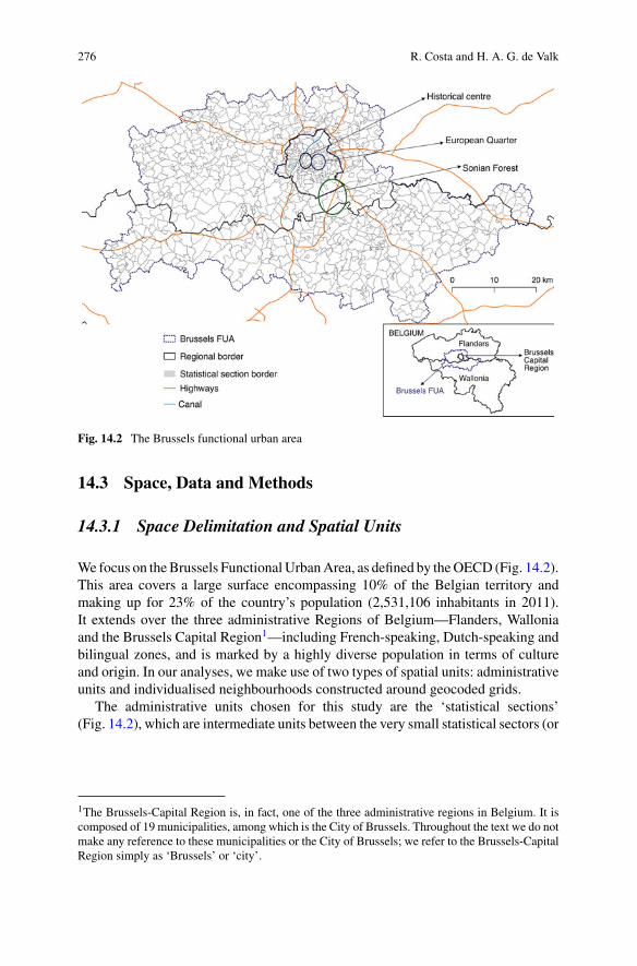
276 R. Costa and H. A. G. de Valk
Fig. 14.2 The Brussels functional urban area
14.3 Space, Data and Methods
14.3.1 Space Delimitation and Spatial Units
We focus on theBrussels FunctionalUrbanArea, as defined by theOECD (Fig. 14.2).This area covers a large surface encompassing 10% of the Belgian territory andmaking up for 23% of the country’s population (2,531,106 inhabitants in 2011).It extends over the three administrative Regions of Belgium—Flanders, Walloniaand the Brussels Capital Region1—including French-speaking, Dutch-speaking andbilingual zones, and is marked by a highly diverse population in terms of cultureand origin. In our analyses, we make use of two types of spatial units: administrativeunits and individualised neighbourhoods constructed around geocoded grids.
The administrative units chosen for this study are the ‘statistical sections’(Fig. 14.2), which are intermediate units between the very small statistical sectors (or
1The Brussels-Capital Region is, in fact, one of the three administrative regions in Belgium. It iscomposed of 19 municipalities, among which is the City of Brussels. Throughout the text we do notmake any reference to these municipalities or the City of Brussels; we refer to the Brussels-CapitalRegion simply as ‘Brussels’ or ‘city’.
14 Socio-spatial Disparities in Brussels and its Hinterland 277
wards)2 and the broader municipalities. The Brussels FUA contains 1,069 sections;from these, 180 were dropped due to the small number of inhabitants (<200 in 2001)in order to avoid random fluctuations. In the remaining 874 sections, the number ofresidents in 2011 ranged from 222 to 27,217 (average = 2,879; median = 1,546). Inaddition to sections, we use a nearest-neighbours approach in order to zoom in on theBrussels FUA. This approach implies that we start from geocoded individual datainstead of areal units and use these data to construct individualised neighbourhoodswith 200 nearest neighbours. These are fine-scale units that are independent of admin-istrative borders (Fig. 14.1). The individualised neighbourhoods were constructed bydividing the territory into grids of 100 m by100 m (resulting in a total number of79,588 grid cells in the FUA). We then used geocoded individual data to identifythe population aged 25–64 inside each grid by their x–y coordinates. Individualisedneighbourhoods were constructed for each grid with the EquiPop software (see Östhet al. 2015). This software adds up adjacent grid cells until it reaches the 200 nearestneighbours. If a given grid cell has more than 200 individuals (due, for instance,to the presence of apartment blocks), the software does not add up adjacent cells.Most of the resulting individualised neighbourhoods have around 200 working-ageindividuals, except for a few outliers.3
14.3.2 Data and Definitions
In Belgium, there are no complete data on the professional occupation. Such dataare available from surveys but are not representative at a fine spatial level and arethus not suitable for our spatial analyses. Therefore, we use income data as analternative measure of socioeconomic position. We start from an individual-leveldataset containing individuals’ position in national income deciles (obtained fromtax returns). This dataset, based on the administrative census, contains all individualsresiding in Belgium in 2011. Null incomes were excluded from our analyses as theycomprise many international employees who do not pay income taxes in Belgium oraccompanying spouses with no own income. Excluding them is necessary as other-wise, they would falsely appear in the statistics as being poor. After the exclusionof null incomes, we computed the proportion of sections’ population aged 25–64 ineach income decile in 2011. Note that the dataset contains individual income andnot household income. This is a limitation because high- and low-income earners inthe same household are counted separately, as if they were neighbours of differentincome levels.
2We chose not to work with the statistical sectors—which are the smallest spatial units available—because they are often too small: the median population of sectors in 2011 was only 429, whereasone-third of sectors had less than 200 inhabitants.3The active population in individualised neighbourhoods range from 200 to 1,094, with a medianof 205; 99% of these neighbourhoods have less than 315 inhabitants. Of note, in the computation ofindividualised neighbourhoods together with Statistics Belgium, we did not keep the original grids’population (prior to the aggregation of adjacent grids) for privacy reasons.
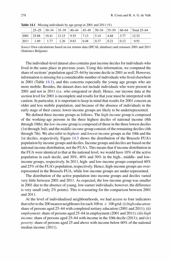
278 R. Costa and H. A. G. de Valk
Table 14.1 Missing individuals by age group in 2001 and 2011 (%)
25–29 30–34 35–39 40–44 45–49 50–54 55–59 60–64 Total 25–64
2001 25.88 19.41 13.15 9.55 7.13 5.14 4.68 3.77 12.52
2011 1.89 1.77 1.26 0.83 0.48 0.37 0.21 0.12 0.91
Source Own calculations based on tax returns data (IPCAL database) and censuses 2001 and 2011(Statistics Belgium)
The individual-level dataset also contains past income deciles for individuals wholived in the same place in previous years. Using this information, we computed theshare of sections’ population aged 25–64 by income decile in 2001 as well. However,information is missing for a considerable number of individuals who lived elsewherein 2001 (Table 14.1), and this concerns especially the young age groups who aremore mobile. Besides, the dataset does not include individuals who were present in2001 and not in 2011 (i.e. who emigrated or died). Hence, our income data at thesection level for 2001 is incomplete and results for that year must be interpreted withcaution. In particular, it is important to keep in mind that results for 2001 concern anolder and less mobile population, and because of the absence of individuals in theearly stage of their career, lower-income groups are likely to be underrepresented.
We defined three income groups as follows. The high-income group is composedof the working-age persons in the three highest deciles of national income (8ththrough 10th); the low-income group is composed of those in the three lowest deciles(1st through 3rd); and themiddle-income group consists of the remaining deciles (4ththrough 7th). We also refer to highest- and lowest-income groups as the 10th and the1st deciles, respectively. Figure 14.3 shows the distribution of the Brussels FUA’spopulation by income groups and deciles. Income groups and deciles are based on thenational income distribution, not the FUA’s. This means that if income distribution inthe FUA were identical to that at the national level, we would have 10% of the activepopulation in each decile, and 30%, 40% and 30% in the high-, middle- and low-income groups, respectively. In 2011, high- and low-income groups comprised 40%and 25% of the FUA’s population, respectively. Hence, high-income groups are over-represented in the Brussels FUA, while low-income groups are under-represented.
The distribution of the active population into income groups and deciles variedvery little between 2001 and 2011. As expected, the low-income group was smallerin 2001 due to the absence of young, low-earner individuals; however, the differenceis very small (only 2% points). This is reassuring for the comparison between 2001and 2011.
At the level of individualised neighbourhoods, we had access to four indicatorsthat refer to the 200 nearest neighbours for each 100m × 100 grid: (i) high education:share of persons aged 25–64 with completed tertiary education (2001 and 2011); (ii)employment: share of persons aged 25–64 in employment (2001 and 2011); (iii) highincome: share of persons aged 25–64 with income in the 10th decile (2011); and (iv)poverty: share of persons aged 25 and above with income below 60% of the nationalmedian income (2011).
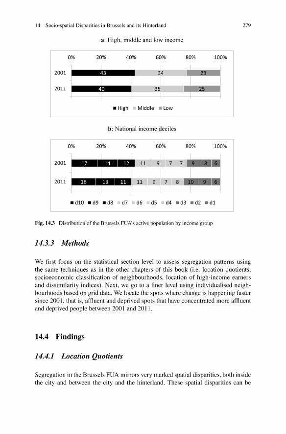
14 Socio-spatial Disparities in Brussels and its Hinterland 279
a: High, middle and low income
b: National income deciles
40
43
35
34
25
23
0% 20% 40% 60% 80% 100%
2011
2001
High Middle Low
16
17
13
14
11
12
11
11
9
9
7
7
8
7
10
9
9
8
6
6
0% 20% 40% 60% 80% 100%
2011
2001
d10 d9 d8 d7 d6 d5 d4 d3 d2 d1
Fig. 14.3 Distribution of the Brussels FUA’s active population by income group
14.3.3 Methods
We first focus on the statistical section level to assess segregation patterns usingthe same techniques as in the other chapters of this book (i.e. location quotients,socioeconomic classification of neighbourhoods, location of high-income earnersand dissimilarity indices). Next, we go to a finer level using individualised neigh-bourhoods based on grid data. We locate the spots where change is happening fastersince 2001, that is, affluent and deprived spots that have concentrated more affluentand deprived people between 2001 and 2011.
14.4 Findings
14.4.1 Location Quotients
Segregation in the Brussels FUA mirrors very marked spatial disparities, both insidethe city and between the city and the hinterland. These spatial disparities can be
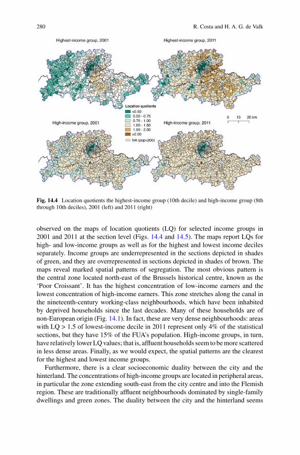
280 R. Costa and H. A. G. de Valk
Fig. 14.4 Location quotients the highest-income group (10th decile) and high-income group (8ththrough 10th deciles), 2001 (left) and 2011 (right)
observed on the maps of location quotients (LQ) for selected income groups in2001 and 2011 at the section level (Figs. 14.4 and 14.5). The maps report LQs forhigh- and low-income groups as well as for the highest and lowest income decilesseparately. Income groups are underrepresented in the sections depicted in shadesof green, and they are overrepresented in sections depicted in shades of brown. Themaps reveal marked spatial patterns of segregation. The most obvious pattern isthe central zone located north-east of the Brussels historical centre, known as the‘Poor Croissant’. It has the highest concentration of low-income earners and thelowest concentration of high-income earners. This zone stretches along the canal inthe nineteenth-century working-class neighbourhoods, which have been inhabitedby deprived households since the last decades. Many of these households are ofnon-European origin (Fig. 14.1). In fact, these are very dense neighbourhoods: areaswith LQ > 1.5 of lowest-income decile in 2011 represent only 4% of the statisticalsections, but they have 15% of the FUA’s population. High-income groups, in turn,have relatively lowerLQvalues; that is, affluent households seem to bemore scatteredin less dense areas. Finally, as we would expect, the spatial patterns are the clearestfor the highest and lowest income groups.
Furthermore, there is a clear socioeconomic duality between the city and thehinterland. The concentrations of high-income groups are located in peripheral areas,in particular the zone extending south-east from the city centre and into the Flemishregion. These are traditionally affluent neighbourhoods dominated by single-familydwellings and green zones. The duality between the city and the hinterland seems
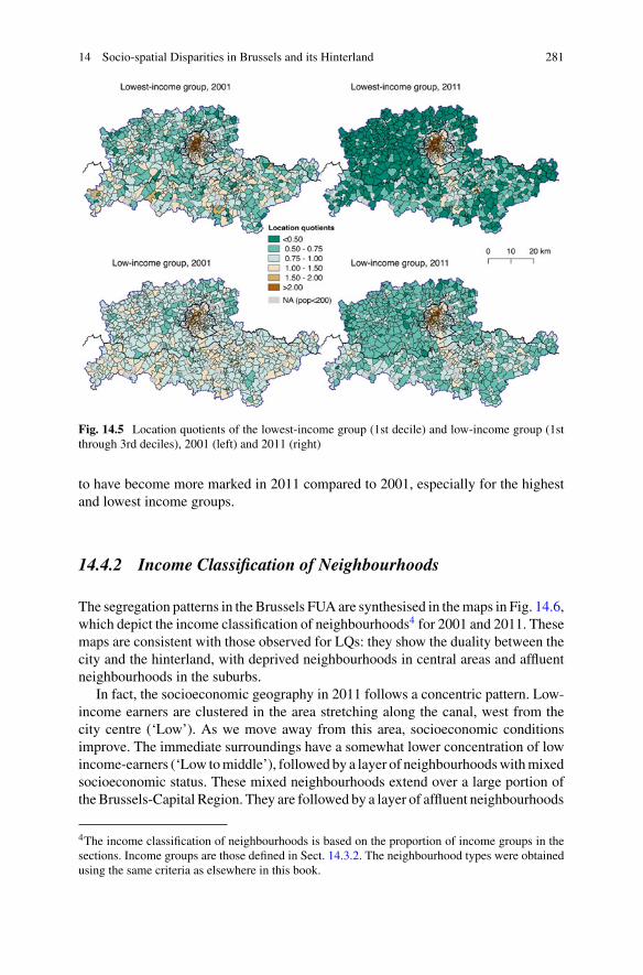
14 Socio-spatial Disparities in Brussels and its Hinterland 281
Fig. 14.5 Location quotients of the lowest-income group (1st decile) and low-income group (1stthrough 3rd deciles), 2001 (left) and 2011 (right)
to have become more marked in 2011 compared to 2001, especially for the highestand lowest income groups.
14.4.2 Income Classification of Neighbourhoods
The segregation patterns in the Brussels FUA are synthesised in themaps in Fig. 14.6,which depict the income classification of neighbourhoods4 for 2001 and 2011. Thesemaps are consistent with those observed for LQs: they show the duality between thecity and the hinterland, with deprived neighbourhoods in central areas and affluentneighbourhoods in the suburbs.
In fact, the socioeconomic geography in 2011 follows a concentric pattern. Low-income earners are clustered in the area stretching along the canal, west from thecity centre (‘Low’). As we move away from this area, socioeconomic conditionsimprove. The immediate surroundings have a somewhat lower concentration of lowincome-earners (‘Low tomiddle’), followed by a layer of neighbourhoodswithmixedsocioeconomic status. These mixed neighbourhoods extend over a large portion oftheBrussels-Capital Region. They are followed by a layer of affluent neighbourhoods
4The income classification of neighbourhoods is based on the proportion of income groups in thesections. Income groups are those defined in Sect. 14.3.2. The neighbourhood types were obtainedusing the same criteria as elsewhere in this book.
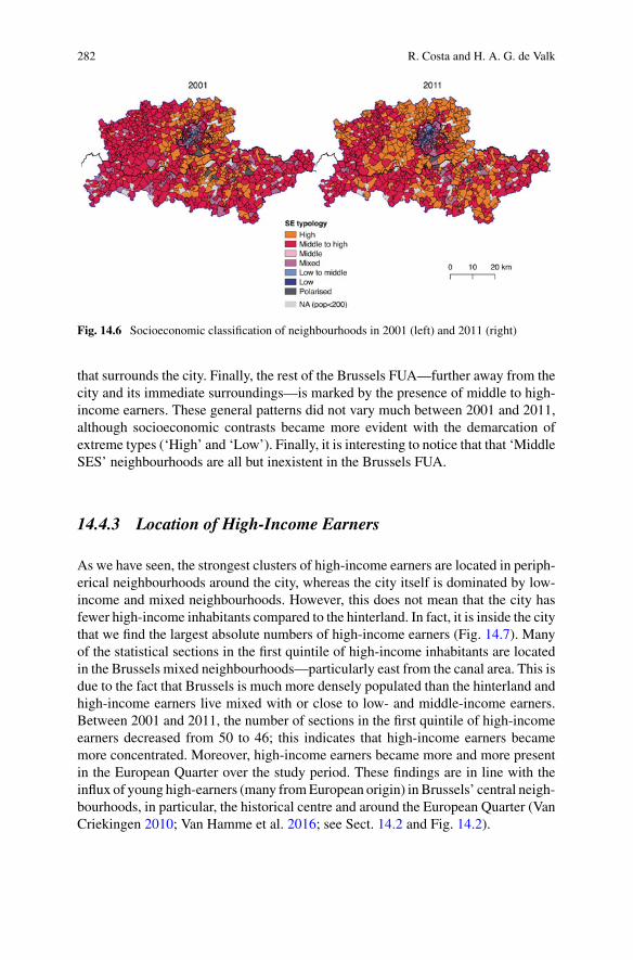
282 R. Costa and H. A. G. de Valk
Fig. 14.6 Socioeconomic classification of neighbourhoods in 2001 (left) and 2011 (right)
that surrounds the city. Finally, the rest of the Brussels FUA—further away from thecity and its immediate surroundings—is marked by the presence of middle to high-income earners. These general patterns did not vary much between 2001 and 2011,although socioeconomic contrasts became more evident with the demarcation ofextreme types (‘High’ and ‘Low’). Finally, it is interesting to notice that that ‘MiddleSES’ neighbourhoods are all but inexistent in the Brussels FUA.
14.4.3 Location of High-Income Earners
As we have seen, the strongest clusters of high-income earners are located in periph-erical neighbourhoods around the city, whereas the city itself is dominated by low-income and mixed neighbourhoods. However, this does not mean that the city hasfewer high-income inhabitants compared to the hinterland. In fact, it is inside the citythat we find the largest absolute numbers of high-income earners (Fig. 14.7). Manyof the statistical sections in the first quintile of high-income inhabitants are locatedin the Brussels mixed neighbourhoods—particularly east from the canal area. This isdue to the fact that Brussels is much more densely populated than the hinterland andhigh-income earners live mixed with or close to low- and middle-income earners.Between 2001 and 2011, the number of sections in the first quintile of high-incomeearners decreased from 50 to 46; this indicates that high-income earners becamemore concentrated. Moreover, high-income earners became more and more presentin the European Quarter over the study period. These findings are in line with theinflux of young high-earners (many fromEuropean origin) in Brussels’ central neigh-bourhoods, in particular, the historical centre and around the European Quarter (VanCriekingen 2010; Van Hamme et al. 2016; see Sect. 14.2 and Fig. 14.2).
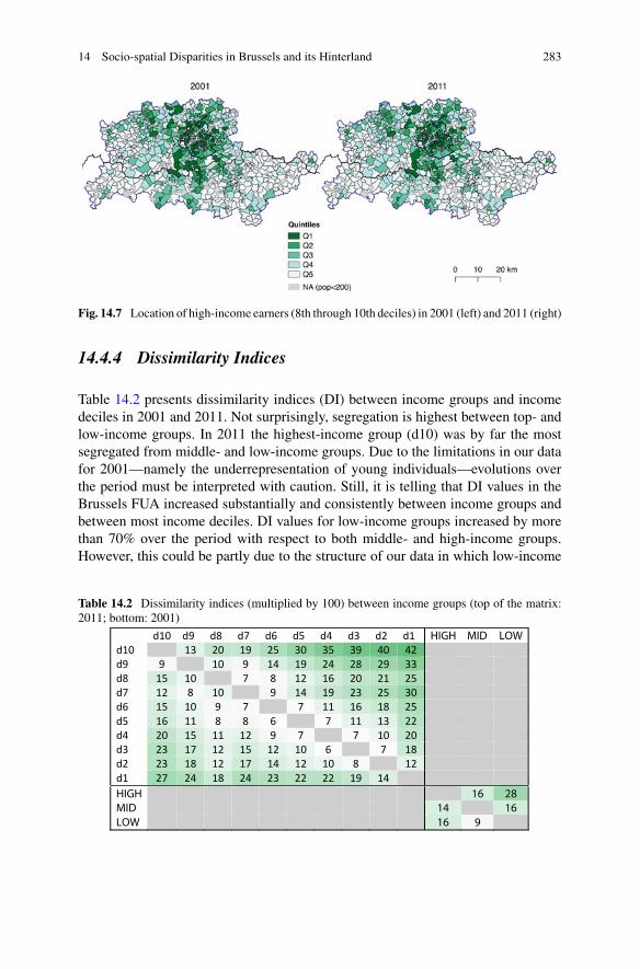
14 Socio-spatial Disparities in Brussels and its Hinterland 283
Fig. 14.7 Location of high-income earners (8th through 10th deciles) in 2001 (left) and 2011 (right)
14.4.4 Dissimilarity Indices
Table 14.2 presents dissimilarity indices (DI) between income groups and incomedeciles in 2001 and 2011. Not surprisingly, segregation is highest between top- andlow-income groups. In 2011 the highest-income group (d10) was by far the mostsegregated from middle- and low-income groups. Due to the limitations in our datafor 2001—namely the underrepresentation of young individuals—evolutions overthe period must be interpreted with caution. Still, it is telling that DI values in theBrussels FUA increased substantially and consistently between income groups andbetween most income deciles. DI values for low-income groups increased by morethan 70% over the period with respect to both middle- and high-income groups.However, this could be partly due to the structure of our data in which low-income
Table 14.2 Dissimilarity indices (multiplied by 100) between income groups (top of the matrix:2011; bottom: 2001)
d10 d9 d8 d7 d6 d5 d4 d3 d2 d1 HIGH MID LOW d10 13 20 19 25 30 35 39 40 42 d9 9 10 9 14 19 24 28 29 33 d8 15 10 7 8 12 16 20 21 25 d7 12 8 10 9 14 19 23 25 30 d6 15 10 9 7 7 11 16 18 25 d5 16 11 8 8 6 7 11 13 22 d4 20 15 11 12 9 7 7 10 20 d3 23 17 12 15 12 10 6 7 18 d2 23 18 12 17 14 12 10 8 12 d1 27 24 18 24 23 22 22 19 14 HIGH 16 28 MID 14 16 LOW 16 9
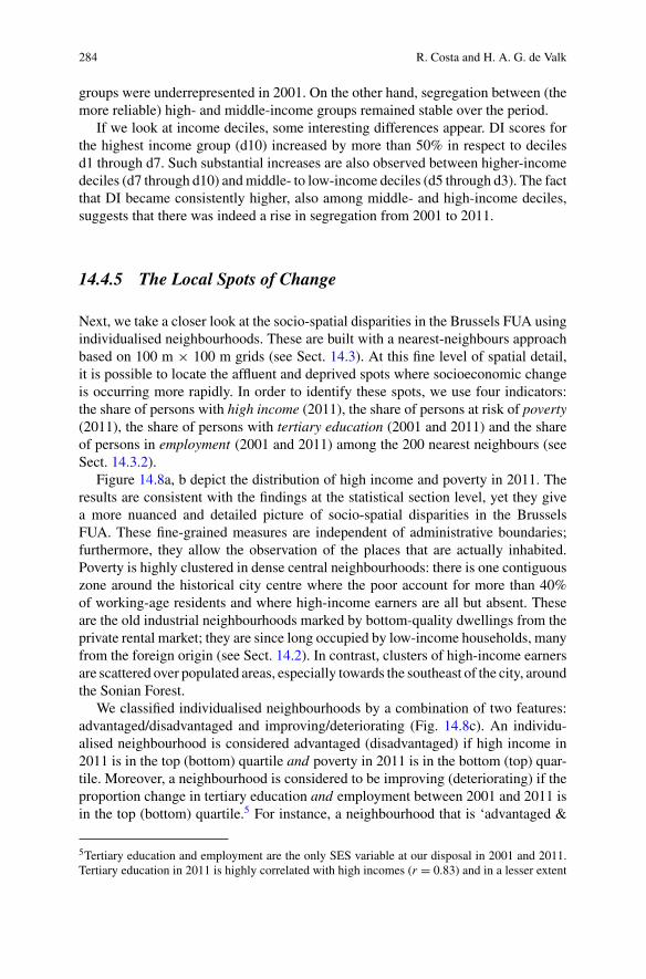
284 R. Costa and H. A. G. de Valk
groups were underrepresented in 2001. On the other hand, segregation between (themore reliable) high- and middle-income groups remained stable over the period.
If we look at income deciles, some interesting differences appear. DI scores forthe highest income group (d10) increased by more than 50% in respect to decilesd1 through d7. Such substantial increases are also observed between higher-incomedeciles (d7 through d10) andmiddle- to low-income deciles (d5 through d3). The factthat DI became consistently higher, also among middle- and high-income deciles,suggests that there was indeed a rise in segregation from 2001 to 2011.
14.4.5 The Local Spots of Change
Next, we take a closer look at the socio-spatial disparities in the Brussels FUA usingindividualised neighbourhoods. These are built with a nearest-neighbours approachbased on 100 m × 100 m grids (see Sect. 14.3). At this fine level of spatial detail,it is possible to locate the affluent and deprived spots where socioeconomic changeis occurring more rapidly. In order to identify these spots, we use four indicators:the share of persons with high income (2011), the share of persons at risk of poverty(2011), the share of persons with tertiary education (2001 and 2011) and the shareof persons in employment (2001 and 2011) among the 200 nearest neighbours (seeSect. 14.3.2).
Figure 14.8a, b depict the distribution of high income and poverty in 2011. Theresults are consistent with the findings at the statistical section level, yet they givea more nuanced and detailed picture of socio-spatial disparities in the BrusselsFUA. These fine-grained measures are independent of administrative boundaries;furthermore, they allow the observation of the places that are actually inhabited.Poverty is highly clustered in dense central neighbourhoods: there is one contiguouszone around the historical city centre where the poor account for more than 40%of working-age residents and where high-income earners are all but absent. Theseare the old industrial neighbourhoods marked by bottom-quality dwellings from theprivate rental market; they are since long occupied by low-income households, manyfrom the foreign origin (see Sect. 14.2). In contrast, clusters of high-income earnersare scattered over populated areas, especially towards the southeast of the city, aroundthe Sonian Forest.
We classified individualised neighbourhoods by a combination of two features:advantaged/disadvantaged and improving/deteriorating (Fig. 14.8c). An individu-alised neighbourhood is considered advantaged (disadvantaged) if high income in2011 is in the top (bottom) quartile and poverty in 2011 is in the bottom (top) quar-tile. Moreover, a neighbourhood is considered to be improving (deteriorating) if theproportion change in tertiary education and employment between 2001 and 2011 isin the top (bottom) quartile.5 For instance, a neighbourhood that is ‘advantaged &
5Tertiary education and employment are the only SES variable at our disposal in 2001 and 2011.Tertiary education in 2011 is highly correlated with high incomes (r = 0.83) and in a lesser extent

14 Socio-spatial Disparities in Brussels and its Hinterland 285
a: High income
b: Poverty
c: Local spots of change
Fig. 14.8 Income distribution by the grid (individualised neighbourhoods)
286 R. Costa and H. A. G. de Valk
improving’ is at the same time among the highest shares of high incomes, the lowestshares of poverty, and the highest improvement in tertiary education and employ-ment. All the individualised neighbourhoods that fall out of the four combinationsof advantaged/disadvantaged and improving/deteriorating are considered ‘stable’.
The resulting map (Fig. 14.8c) reveals interesting patterns. Disadvantaged spots(both improving and deteriorating) are much more frequent than advantaged onesand the vast majority of them are located within the city. Disadvantaged and deteri-orating spots are by far the most frequent type and extend over contiguous zones inand around the city centre, but not in the most deprived neighbourhoods identifiedearlier. Instead, the most deprived neighbourhoods (‘Poor Croissant’) are markedby disadvantaged and improving spots. Although these neighbourhoods continue toconcentrate the highest proportions of poor households, there seems to be a changein composition locally with an increase in highly educated inhabitants in employ-ment. It is likely that gentrification contributes to these processes of improvementand deterioration of central areas. On the one hand, improvements in socioeconomiccomposition in the most deprived neighbourhoods may be stirred by new real estateprojects in the canal area targeted at young, socially advantaged households; on theother hand, socioeconomic deterioration in adjacent poor neighbourhoods could bepartially due to the arrival of low-income households pushed away from gentrifiedspots in the city centre, thus relocating to less-gentrified affordable neighbourhoods(Van Criekingen 2008; Van Hamme et al. 2016). In contrast to disadvantaged spots,advantaged spots are much less numerous and are scattered outside the city borders:these are isolated spots, each encompassing nomore than (portions of) specific streetsin wealthy neighbourhoods. In sum, there is a certain stability in wealthy neighbour-hoods, whereas change—both improvement and deterioration—is happening fasterinside the city among the already deprived neighbourhoods.
Between 2001 and 2011, there was a substantial change in the migration back-ground in deteriorating spots. The average proportion of non-European migrantshalved over the period in ‘disadvantaged and improving’ spots (from 14.2 to 7%),while it doubled in ‘disadvantaged and deteriorating spots (from 13.4 to 24.5%). Thiscould indicate that improving spots have attracted Belgian and European households,whereas low-income households of non-European origin have been moving awayfrom gentrified spots towards other deprived neighbourhoods. Of note, the propor-tion of migrants is very small in the spots that are ‘advantaged and improving’ (lessthan 3%).
with poverty (r = –0.33). Employment is fairly correlated both with poverty (r = –0.59) and tertiaryeducation (r = 0.53).
14 Socio-spatial Disparities in Brussels and its Hinterland 287
14.5 Discussion
This chapter offers an overview of the socio-spatial disparities in the Brussels Func-tional Urban Area. Our analyses relied on fine-grained data, at the level of statisticalsections and of individualised neighbourhoods built around 100 m × 100 m grids.We analysed socioeconomic segregation patterns and levels in 2001 and 2011 withdifferent methods and using data on income, education and employment. The anal-yses carried out here provide an update on the situation based on the latest availabledata and go beyond that of previous studies by using individualised neighbourhoodsbased on grid data. In line with previous research, our results show very marked andpersistent patterns of socioeconomic segregation in and around Brussels, operatingboth at a larger geographic scale and at the local level.
At the large-scale level, there is a clear divide between deprived central neighbour-hoods and prosperous outskirts. Low-income groups are highly clustered in denseneighbourhoods in and around the city centre. In fact, around 15% of the Brus-sels FUA total population lives in central neighbourhoods where the low-incomegroup is overrepresented (LQ ≥ 1.5). In turn, high-income groups are more sparselydistributed in the south-east neighbourhoods of Brussels and across most of thehinterland. These large-scale patterns of segregation, with a poorer centre and pros-perous suburbs, are typical in Belgium, also for other cities; they are due to specificlong-term territorial processes and housing policies (see also Costa and de Valk2018).
Below these large-scale disparities, segregation processes operate at the locallevel, especially inside the city. Low-income groups are highly clustered in the neigh-bourhoods around the historical centre—the so-called ‘Poor Croissant’. These are theold industrial neighbourhoods, with low-quality dwellings and which also concen-trate a large share of migrants from non-European countries. Apart from these poorneighbourhoods, the largest portion of the city is composed ofmixed neighbourhoods(with 25–50% of each low-, middle- and high-income group). Interestingly, thesemixed neighbourhoods are home to the highest absolute numbers of high-incomeearners of the Brussels FUA. In contrast with their suburban counterparts, this urbanelite share their space with the middle class. Finally, we also find clustering of high-income earners in the green south-east part of the city, where single-family dwellingsare most frequent.
Due to limitations with regard to the data on income we have at hand, it is a bridgetoo far to decisively conclude that segregation levels increased between 2001 and2011, although our analyses point in that direction. In all cases, our findings showthe tenacity of the same patterns of segregation in Brussels over time. Moreover,below these persistent patterns, change seems to take place at the local level in thealready deprived areas inside the city. Most of these areas have been deterioratingover time in terms of socioeconomic composition; but interestingly, themost deprivedneighbourhoods from the Poor Croissant have improved over the study period.
Although we know that inequalities measured by the Gini coefficient at thenational level remained stable, it is yet unclear whether income inequalities have
288 R. Costa and H. A. G. de Valk
increased in the Brussels FUA over the last decades. Either way, it is unlikely thatvariations in income inequalities are the primary cause of the observed segrega-tion patterns. Rather, the persistence of these patterns in Brussels may be driven bymigration patterns influencing socio-spatial inequalities, as well as specific housingpolicies.
First, international migration may fuel the existing segregation patterns (VanHamme et al. 2016). On the one hand, it is likely that many non-European migrantswith a low socioeconomic position establish themselves in the most deprived neigh-bourhoods. Not only do these neighbourhoods offer affordable housing (albeit of lowquality), they can also be an easier gateway to the city because of the existing ethnicnetworks as well as language (and commercial) facilities. In addition, discriminationin the housing market may limit the residential choices of non-European migrantsand thus their access to other neighbourhoods (Verstraete and Verhaeghe 2019).Our results have shown, indeed, that the most deprived neighbourhoods are alsothose which concentrate the highest proportions of non-European migrants. On theother hand, newly arrived international professionals are likely to choose neighbour-hoods with a high proportion of expats, especially those in the European Quarter.These neighbourhoods are close to many international institutions and also to thecity centre. In addition, real estate agencies operating in expats networks often attractnewcomers to these areas. This explanation is supported by our finding that there wasan increase in the top-income group settling in the European Quarter since 2001. Insum, if newcomers establish themselves in the typical concentration neighbourhoodsaccording to their socioeconomic position and transnational networks, their residen-tial choices (or lack thereof) are likely to maintain and even reinforce the existingsegregation patterns.
Second, internal migration can also contribute to the observed segregationpatterns. Whereas low-income groups are often forced into deprived neighbour-hoods, higher-income groups have the choice to live in well-off neighbourhoods.As our results suggest, the richest 10% are by far the most segregated group andare highly clustered in specific spots. In addition, Brussels’ central neighbourhoodshave increasingly attracted highly educated youngsterswho spend a part of their earlyadulthood in the city, before moving to outer neighbourhoods (Van Criekingen 2010;Van Hamme et al. 2016). The constant renewal of these transient residents has led toreinvestment in central neighbourhoods and consequently to gentrification processes(Van Criekingen 2008, 2009). The increasing competition in the housing market andthe resulting rise in rental prices have forced low-income households that stayed inthese neighbourhoods intomore precarious conditions, whilemany relocated to othercentral neighbourhoods with more affordable rentals. These processes are supportedby our analysis of local spots of change: some spots in the most deprived neighbour-hoods have improved their socioeconomic composition over time—likely due to thearrival of better-off young households—whereas many other central areas have dete-riorated their socioeconomic composition—probably aided by the residential moveof low-income households coming from gentrified neighbourhoods. All in all, these
14 Socio-spatial Disparities in Brussels and its Hinterland 289
selective residential moves might be contributing, at a large scale, to a greater socioe-conomic mix in Brussels as a whole, but at the same time, at the local level, theymight be fuelling socio-spatial fractures in central neighbourhoods.
Third, the housing market and housing policies do not seem to be effective inreducing socio-spatial disparities, and may even reinforce them. Belgium is char-acterised by liberal housing policies with a deregulated rental market and a focuson homeownership (De Decker 2008). Deprived neighbourhoods are dominated bybottom-quality dwellings in the private rental market, whereas the affluent neigh-bourhoods are dominated by owner-occupied dwellings. At the same time, socialand public housing remain marginal in Brussels and is way below the populationneeds, which results in long waiting lists (Dessouroux et al. 2016). More recently,it is likely that regional (neoliberal inspired) housing policies in Brussels havefavoured the emergence of large real estate projects targeted to the young middle-and upper class (Decroly and Van Criekingen 2009). These projects are especiallysituated in the remaining available spaces in the canal area. This could explain ourfinding that in some deprived local spots in this area, socioeconomic compositionhas improved since 2001. Such local-level processes driven by liberal policies andprivate investments may increase and fuel local inequalities.
It is difficult to determine what ultimately drives socio-spatial inequalities at thelocal level. Local concentrations of socioeconomic groups can be easily altered bysmall changes, for example, in the housing stock and in population composition dueto in- and out-migration or social mobility processes. Future research should makeuse of longitudinal micro-data linked with fine-grained spatial information in orderto understand how individual mobility and migration background interact with theexisting segregation patterns as well as how they act to reinforce or attenuate themover time. This type of detailed analyses is much needed and could help clarify theunderlying causes of socioeconomic fractures and point to policy interventions thatmay counteract high socio-spatial disparities and its determinants in Brussels.
Acknowledgements The authors thank Johan Surkyn and Patrick Deboosere for their insightson the possibilities and limitations of the Belgian administrative data and on the interpretationof our findings. This work is part of the JPI Urban Europe project ‘Residential segregation infive European countries: a comparative study using individualised scalable neighbourhoods’ (grantagreement No. 2014-1676; more information is available at www.residentialsegregation.org). Thework of the second author was part of and funded by the European Research Council (ERC) underthe European Union’s Horizon 2020 research and innovation programme (grant agreement No.819298) CoGrant awarded to De Valk.
References
Blanchet T, Chancel L, Gethin A (2019) How unequal is Europe? Evidence from distributionalnational accounts, 1980–2017. WID.world working paper N° 2019/06
290 R. Costa and H. A. G. de Valk
Corijn E, Vloeberghs E (2013) Brussels, a small world city. In: Corijn E, Van de Ven J (eds) TheBrussels reader. A small world city to become the capital of Europe. Urban Notebooks. VUBPress, Brussels
Costa R, de Valk HAG (2018) Ethnic and socioeconomic segregation in Belgium: a multiscalarapproach using individualised neighbourhoods. Eur J Popul 34(2):225–250
De Decker P (2008) Facets of housing and housing policies in Belgium. J Hous Built Environ23:155–171
De Winter M, Musterd S (1998) Towards undivided cities in Western Europe: New challenges forurban policy: Part 4 Brussels. Delft University Press
Decoster A, Dedobbeleer K,Maes S (2017) Using fiscal data to estimate the evolution of top incomeshares in Belgium from 1990 to 2013. WID world working paper N° 2019/04
Decroly JM, Van Criekingen M (2009) The Brussels International Development Plan (IDP). Realestate development promises and growing inequalities? Brussels Stud 25
Dessouroux C, Benslimanx R, Bernard N, Laet De S, Demonty F, Marissal P, Surkyn J (2016)Housing in Brussels: diagnosis and challenges BSI synopsis. Brussels Stud 99
Eurostat (2019) Gini coefficient of equivalised disposable income—EU-SILC survey. https://appsso.eurostat.ec.europa.eu/nui/submitViewTableAction.do. Accessed 01 November 2019
Kesteloot C, Cortie C (1998) Housing turks and moroccans in Brussels and Amsterdam: thedifference between private and public markets. Urban Stud 35(10):1835–1853
Kesteloot C, Loopmans M (2009) Social inequalities. Brussels Stud, Synop N° 15Kesteloot C, Van der Haegen H (1997) Foreigners in Brussels 1981–1991: spatial continuity andsocial change. Tijd Voor Econ En Soc Geogr 88(2):105–119
Marcinczak S, Musterd S, van Ham M, Tammaru T (2015) Inequality and rising levels ofsocio-economic segregation. Lessons from a pan-European comparative study. In: Tammaru T,Marcinczak S, van Ham M, Musterd S (eds) Socio-economic segregation in European capitalcities: east meets west, pp 358–382. Routledge
Musterd S (2005) Social and ethnic segregation in Europe: levels, causes and effects. J Urban Aff27(3):331–348
OECD (2019) OECD statistics. https://stats.oecd.org. Accessed 01 November 2019.Östh J,WilliamAV,MalmbergB (2015)Measuring the scale of segregation using k-nearest neighboraggregates. Geograph Anal 47(1):1–16
Rea A (2013) Immigration and diversity. In Corijn E, Van de Ven J (eds) The Brussels reader. Asmall world city to become the capital of Europe, pp 244–266. VUB Press, Brussels
Valenduc C (2017) Distribution et redistribution des revenus : évolution des inégalités en Belgique.Courr Hebd Du CRISP 21:5–78
Van Criekingen M (2008) Towards a geography of displacement. Moving out of Brussels’ gentri-fying neighbourhoods. J Housing Built Environ 23:199–213. https://doi.org/10.1007/s10901-008-9112-2
Van Criekingen M (2009) Moving in/out of brussels’ historical core in the early 2000s: migrationand the effects of gentrification. Urban Stud 46(4):825–848
Van Criekingen M (2010) ‘Gentrifying the re-urbanisation debate’, not vice versa: the unevensocio-spatial implications of changing transitions to adulthood in Brussels. Popul Space Place16:381–394
Van Hamme G, Grippa T, Van Criekingen M (2016) Migratory movements and dynamics of neigh-bourhoods in Brussels. Brussels Stud General Collection, no 97. https://doi.org/10.4000/brussels.1338
VanMol C, de Valk HAG (2016)Migration and immigrants in Europe: a historical and demographicperspective. In: Garcés-Mascareñas B, Penninx R (eds) Integration processes and policies inEurope. Springer, Cham, pp 31–55
Verstraete J, Verhaeghe PP (2019) Ethnic discrimination upon request? Real estate agents’ strategiesfor discriminatory questions of clients J Hous Built Environ. https://doi.org/10.1007/s10901-019-09721-8

14 Socio-spatial Disparities in Brussels and its Hinterland 291
Open Access This chapter is licensed under the terms of the Creative Commons Attribution 4.0International License (http://creativecommons.org/licenses/by/4.0/), which permits use, sharing,adaptation, distribution and reproduction in any medium or format, as long as you give appropriatecredit to the original author(s) and the source, provide a link to the Creative Commons license andindicate if changes were made.
The images or other third party material in this chapter are included in the chapter’s CreativeCommons license, unless indicated otherwise in a credit line to the material. If material is notincluded in the chapter’s Creative Commons license and your intended use is not permitted bystatutory regulation or exceeds the permitted use, you will need to obtain permission directly fromthe copyright holder.
Chapter 15Residential Segregation in a HighlyUnequal Society: Istanbul in the 2000s
Oguz Isık
Abstract Contrary to trends in many European countries, income inequality inTurkey, measured by the Gini coefficient, has declined between 1994 and 2014,with a small but consistent increase since then. Turkish income inequality is amongthe highest in OECD countries, with levels not lower than 0.4. This chapter willexamine residential socio-economic segregation in Istanbul against the backdrop ofthis relatively stable and high-income inequality. The chapter shows signs that resi-dential segregation is on the rise. Istanbul has undergone a radical change in the2000s thanks to active intervention by the state in the real estate market by openingup large pieces of land in the outskirts and gentrifying inner-city areas once occupiedby unauthorized settlements that once were home to the poor. Dynamics of urbandevelopment, fueled by rapid urban sprawl in peri-urban areas and ceaseless gentri-fication of inner-city areas, gave way to diverse patterns of segregation dependingon the already existing divisions and physical geography of cities. Given the lackof neighbourhood level data on either occupations or income, this chapter analysessegregation through indices based on fertility and educational level, which we knowfrom detailed household microdata are closely correlated with income. On the basisof 2000 and 2017 neighbourhood data, we show that in Istanbul, there is a clearlyvisible pattern where the poor are progressively pushed further to the city limits,while some parts of built-up areas once home to middle classes, were recapturedby the poor. The result in some parts of the city is a juxtaposition of seeminglyconflicting patterns: parts of the inner city were reclaimed by the poor while someparts were gentrified led by the nascent urban elite. The urban periphery was partlyoccupied by the bourgeoning middle classes and was also home to the urban poorwho were displaced by urban transformation projects.
Keywords Istanbul · Residential segregation · Urban renewal · Neoliberalurbanisation
O. Isık (B)Ankara, Turkeye-mail: [email protected]
© The Author(s) 2021M. van Ham et al. (eds.), Urban Socio-Economic Segregation and Income Inequality,The Urban Book Series, https://doi.org/10.1007/978-3-030-64569-4_15
293
294 O. Isık
15.1 Introduction
Turkey is a land of vast and enduring inequalities. Ever since the first reliable studieswere made on income inequality in the late 1960s, the Gini coefficient has not fallenbelow 0.4 except a few years in the early 2000s, making Turkey one of the mostunequal countries in the OECD, and placing it somewhere between European coun-tries with relatively low levels of inequality and Latin American countries whereincome inequality has been notoriously high. In the face of a state unwilling to takeactive measures to reduce inequality, the society devisedmany ingenious ways, espe-cially in the urban labour and property markets, to cope with high levels of inequalityand to keep at bay the tensions that may arise therefrom. Things went well till the2000s and the poor were able to find a place to live for themselves in the rapidlybourgeoning urban propertymarket thanks to networks of solidarity they set up, span-ning in most cases the boundaries between the formal and informal and authorisedand unauthorised. Thanks to the innovative survival strategies of the urban poor, theproblems that are often associated with high inequality and residential segregationwent unnoticed for most of society.
The 2000s have been frantic years in terms of urban development in all largecities in Turkey, a period when the mechanisms devised by the urban poor provedinefficient, and the state that had been a silent partner became an active agent inthe housing and urban property market. Given the voracious desire on the part ofthe state to appropriate ever-increasing land values in many gargantuan projects, thepoor found it increasingly difficult to maintain their positions in the city and weredriven to the city limits where they had to compete with many other agents for landand shelter, finding themselves unable to use space as means of power as they haddone in previous periods.
This chapter is an attempt to assess how already high levels of residential segre-gation have changed in line with the massive urban restructuring of the 2000s. Theobjective is to understand how the construction frenzy and urban sprawl of the 2000swere articulated with the existing pattern of residential segregation inherited fromearlier periods of urban development. Starting with a summary of the basic contoursof urban development in Turkey, the chapter discusses the problems of studyingsegregation with limited available data in Istanbul, where the physical geographyhas a strong impact on almost every urban process, including residential segregation.
15.2 Background: Frantic years of 2000s
Compared to the 2000s, urban development in Turkey in the pre-2000 period wascertainly a calm process, which ensured that some of the big problems encounteredby similar countries undergoing a rapid process of urbanisation were solved withoutcausing large-scale unrest. The basic characteristics of this period can be describedsuccinctly in a few statements: An informal job and urban property market which
15 Residential Segregation in a Highly Unequal Society: Istanbul in the 2000s 295
guaranteed that the ceaseless flux of newcomers would easily find a job and a shelterthanks to the networks of solidarity they set up, though the jobs they found were asshaky as the squatters they built up for themselves on vast state land, mostly at theperiphery of cities; a populist-clientelist state apparatus, incapable of responding tothe needs of these newcomers, that happily turned a blind eye, in exchange for theirvotes, to people who squat illegally on state land or who run informal businesses(Isık and Pınarcıoglu 2009). Things did really go well both for the urban poor andthe state till the late 1990s; by exploiting the opportunities of the informal labourand real estate markets, the urban poor were able to transfer part of their povertyconditions to newcomers and thus to climb up the social ladder into the ranks ofthe rapidly growing middle class. This undeclared alliance between the state and theurban poor secured a decent place for the latter while the politicians were able tomaintain their position, thus laying the foundations for amore repressive and populistpolitical climate in the 2000s.
This tacit alliance, whereby the urban poor made use of the informal labour andproperty markets as leverage to cope with the prevailing levels of inequality, cameto an end in the late 1990s due to several intertwined processes. The reasons behindthe collapse of this alliance and the ensuing changes that Turkish society has gonethrough in the 2000s are too large to be summarised in a few words. The 2000s canbe best described by rising to the power of the Justice and Development Party (JDP),an Islamist-leaning party, and their desire to mould the society in their vision, in away described by some rightfully as the marriage of Islamism and neo-liberalism(Gürcan and Peker 2015; Karaman 2013a; Atasoy 2009) with strong populist over-tones. The JDP and local governments launched an ambitious ‘urban transformationprogramme’ through public–private partnership schemes inmost large Turkish cities,under the strong support of the state-runhousing administration (TOKI).TOKIunder-took huge housing projects at the outskirts of cities and played a leading role in theclearance of formerly unauthorised housing areas in inner cities where land priceshad soared (Türkün 2011; Karaman 2013b). TOKI became the most powerful agentin the real estatemarket, by acquiring the right to transfer public land to private devel-opers for the construction of housing estates on the outskirts through public–privatepartnership scheme with titles delivered to prospective buyers. In a country whereowner-occupation is the rule (nearly 2/3 of the existing stock is owner-occupied)and public housing ownership is an exception, projects undertaken through public–private partnership programmes such as those by TOKI fuelled the fragmentation ofthe housing market. It is estimated that some 66 million square meters of state landwere transferred to TOKI between 2002 and 2008. In inner-city areas, TOKI helpedclear former squatter areas and residents’ property rights were transferred to housingprojects far from the city centre. When considered in combination with the privatisa-tion frenzy of the JDP and their obsession with grandiose urban projects (includingrenovation of former shipyards, ports and railway stations and large-scale urbanrenewal projects, shopping malls, colossal luxury hotels and gated communities),this heralded the end of a long period in Turkish history of urbanisation where themigrating masses had used their networks of solidarity as a survival strategy underthe harsh conditions of persistent inequality. Devoid of any chance and means to
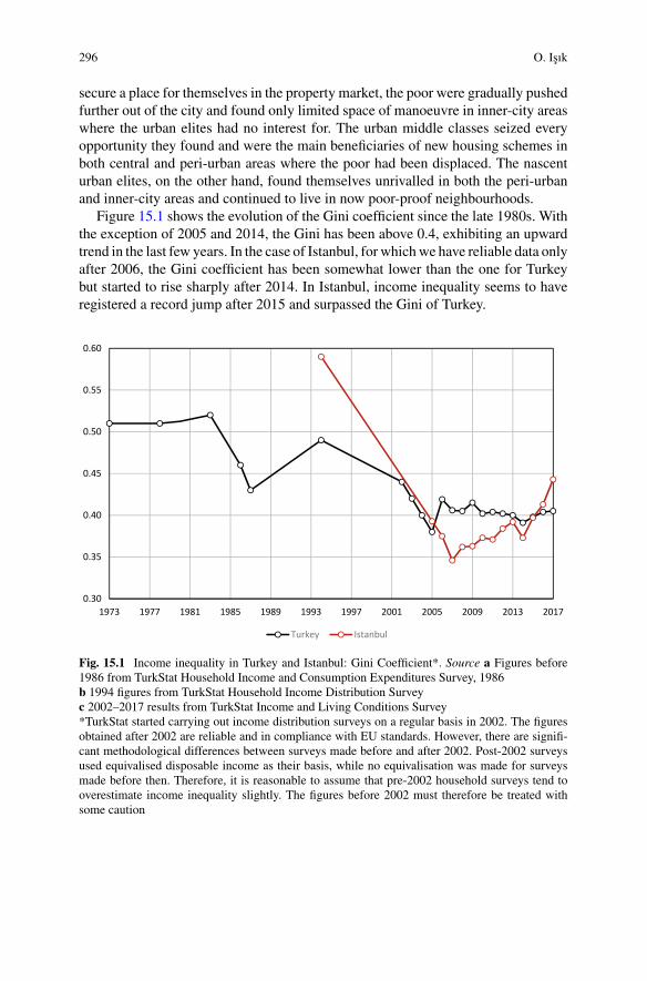
296 O. Isık
secure a place for themselves in the property market, the poor were gradually pushedfurther out of the city and found only limited space of manoeuvre in inner-city areaswhere the urban elites had no interest for. The urban middle classes seized everyopportunity they found and were the main beneficiaries of new housing schemes inboth central and peri-urban areas where the poor had been displaced. The nascenturban elites, on the other hand, found themselves unrivalled in both the peri-urbanand inner-city areas and continued to live in now poor-proof neighbourhoods.
Figure 15.1 shows the evolution of the Gini coefficient since the late 1980s. Withthe exception of 2005 and 2014, the Gini has been above 0.4, exhibiting an upwardtrend in the last few years. In the case of Istanbul, for whichwe have reliable data onlyafter 2006, the Gini coefficient has been somewhat lower than the one for Turkeybut started to rise sharply after 2014. In Istanbul, income inequality seems to haveregistered a record jump after 2015 and surpassed the Gini of Turkey.
0.30
0.35
0.40
0.45
0.50
0.55
0.60
1973 1977 1981 1985 1989 1993 1997 2001 2005 2009 2013 2017
Turkey Istanbul
Fig. 15.1 Income inequality in Turkey and Istanbul: Gini Coefficient*. Source a Figures before1986 from TurkStat Household Income and Consumption Expenditures Survey, 1986b 1994 figures from TurkStat Household Income Distribution Surveyc 2002–2017 results from TurkStat Income and Living Conditions Survey*TurkStat started carrying out income distribution surveys on a regular basis in 2002. The figuresobtained after 2002 are reliable and in compliance with EU standards. However, there are signifi-cant methodological differences between surveys made before and after 2002. Post-2002 surveysused equivalised disposable income as their basis, while no equivalisation was made for surveysmade before then. Therefore, it is reasonable to assume that pre-2002 household surveys tend tooverestimate income inequality slightly. The figures before 2002 must therefore be treated withsome caution
15 Residential Segregation in a Highly Unequal Society: Istanbul in the 2000s 297
15.3 Studying Segregation in Istanbul
The study of segregation in Istanbul is beset by a number of difficulties. The firstset of problems originates from the fact that Istanbul is literally a city in flux, asite of a never-ending process of creation and destruction. Its population rose from7.2 million in 1990 to 11 million in 2000 and finally to 15 million in 2017. Thisrefers to an annual growth rate of no less than 2% on most occasions, a rate whichis difficult to imagine for many cities of the West. In a similar fashion, the numberof neighbourhoods increased from 550 in 2000 to some 780 in 2017, making themeasurement of segregation and comparisons over time an arduous task.
The second set of difficulties arises from the unique geographical setting of thecity. Built on two continents (Europe and Asia), with an extremely busy seaway(Bosporus) in between connecting Balkan countries and Russia to the rest of theworld, Istanbul is divided into two distinct geographical units. For the study ofsettlement and segregation patterns, this means that Istanbul is destined to be apolycentric city, with each geographical unit having its core and peripheral areas(Dökmeci and Berköz 1994). The uneven distribution of population between thesetwo parts (nearly two-thirds living on the European side and one-thirds on the Asianside) generates an immense volume of traffic and development pressure for the wholecity. Fifteenmillion people squeezed on a piece of land slightly larger than 5,000 km2
and the existence of numerous naturally and historically important sites in and aroundthe city make land the most precious commodity for Istanbul. Fierce competition forland contributes to the emergence of a segregation pattern resembling a patchwork,especially at the periphery.
Though not peculiar to Istanbul but common to all cities of Turkey, the mainchallenges arise to those interested in the study of segregation, mostly due to thelimited availability of geocoded data. Given the absence of appropriate spatial dataand the fact that most cities are in a constant process of building and destruction, onehas to find some innovative and particularly indirect ways to decipher the pattern ofsegregation observed in Turkish cities. It is to this problem of data and methodologythat I turn briefly in the following section.
15.4 Data and Method
Although Turkey has gone a long way in the 2000s in assuring the quality of statis-tical data, there is still a long way to go in what may be called small area statistics.Designation of functional urban areas and NUTS areas has yet to be completed. Theonly spatial unit where data is available for cities is the ambiguous level of neigh-bourhoods (mahalle).Mahalle does not have a clear definition in the administrativesystem, nor are there any known limits to its population and size. In the case ofIstanbul, the population of neighbourhoods in 2017 varied between 50 and 93,000,
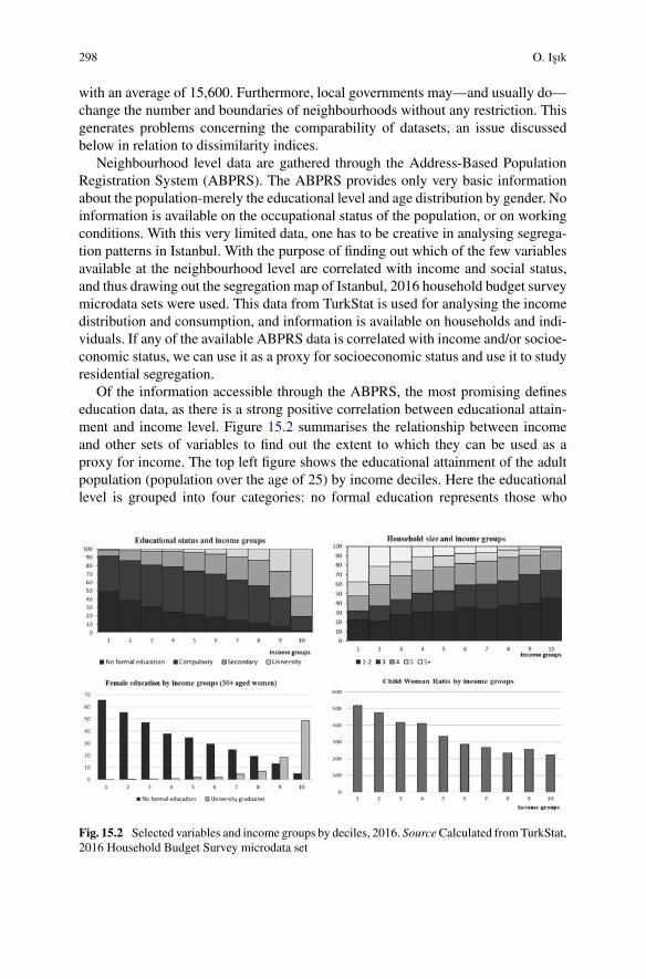
298 O. Isık
with an average of 15,600. Furthermore, local governments may—and usually do—change the number and boundaries of neighbourhoods without any restriction. Thisgenerates problems concerning the comparability of datasets, an issue discussedbelow in relation to dissimilarity indices.
Neighbourhood level data are gathered through the Address-Based PopulationRegistration System (ABPRS). The ABPRS provides only very basic informationabout the population-merely the educational level and age distribution by gender. Noinformation is available on the occupational status of the population, or on workingconditions. With this very limited data, one has to be creative in analysing segrega-tion patterns in Istanbul. With the purpose of finding out which of the few variablesavailable at the neighbourhood level are correlated with income and social status,and thus drawing out the segregation map of Istanbul, 2016 household budget surveymicrodata sets were used. This data from TurkStat is used for analysing the incomedistribution and consumption, and information is available on households and indi-viduals. If any of the available ABPRS data is correlated with income and/or socioe-conomic status, we can use it as a proxy for socioeconomic status and use it to studyresidential segregation.
Of the information accessible through the ABPRS, the most promising defineseducation data, as there is a strong positive correlation between educational attain-ment and income level. Figure 15.2 summarises the relationship between incomeand other sets of variables to find out the extent to which they can be used as aproxy for income. The top left figure shows the educational attainment of the adultpopulation (population over the age of 25) by income deciles. Here the educationallevel is grouped into four categories: no formal education represents those who
Fig. 15.2 Selected variables and income groups by deciles, 2016. SourceCalculated fromTurkStat,2016 Household Budget Survey microdata set
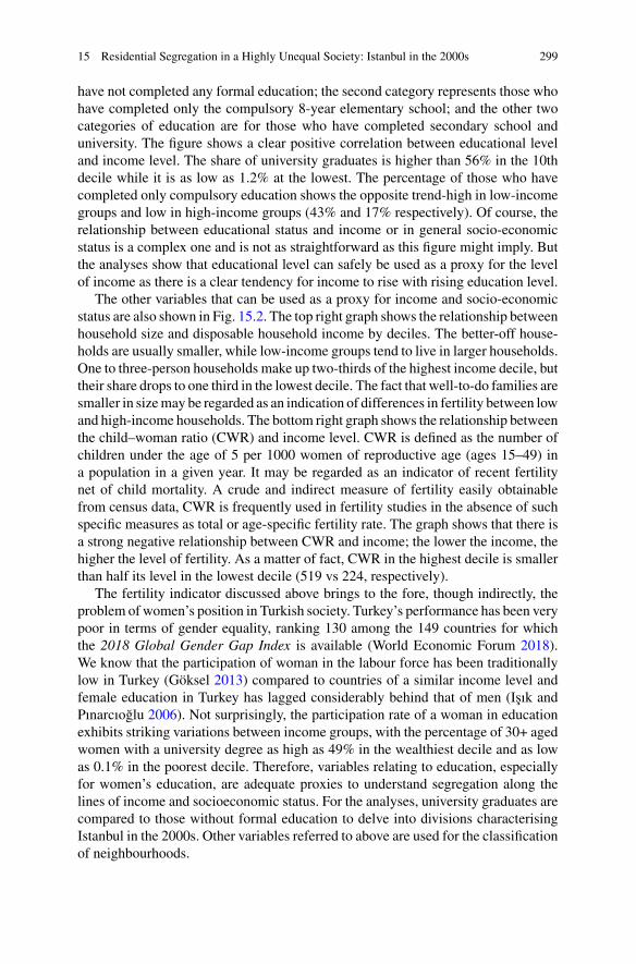
15 Residential Segregation in a Highly Unequal Society: Istanbul in the 2000s 299
have not completed any formal education; the second category represents those whohave completed only the compulsory 8-year elementary school; and the other twocategories of education are for those who have completed secondary school anduniversity. The figure shows a clear positive correlation between educational leveland income level. The share of university graduates is higher than 56% in the 10thdecile while it is as low as 1.2% at the lowest. The percentage of those who havecompleted only compulsory education shows the opposite trend-high in low-incomegroups and low in high-income groups (43% and 17% respectively). Of course, therelationship between educational status and income or in general socio-economicstatus is a complex one and is not as straightforward as this figure might imply. Butthe analyses show that educational level can safely be used as a proxy for the levelof income as there is a clear tendency for income to rise with rising education level.
The other variables that can be used as a proxy for income and socio-economicstatus are also shown in Fig. 15.2. The top right graph shows the relationship betweenhousehold size and disposable household income by deciles. The better-off house-holds are usually smaller, while low-income groups tend to live in larger households.One to three-person households make up two-thirds of the highest income decile, buttheir share drops to one third in the lowest decile. The fact that well-to-do families aresmaller in sizemay be regarded as an indication of differences in fertility between lowand high-income households. The bottom right graph shows the relationship betweenthe child–woman ratio (CWR) and income level. CWR is defined as the number ofchildren under the age of 5 per 1000 women of reproductive age (ages 15–49) ina population in a given year. It may be regarded as an indicator of recent fertilitynet of child mortality. A crude and indirect measure of fertility easily obtainablefrom census data, CWR is frequently used in fertility studies in the absence of suchspecific measures as total or age-specific fertility rate. The graph shows that there isa strong negative relationship between CWR and income; the lower the income, thehigher the level of fertility. As a matter of fact, CWR in the highest decile is smallerthan half its level in the lowest decile (519 vs 224, respectively).
The fertility indicator discussed above brings to the fore, though indirectly, theproblem of women’s position in Turkish society. Turkey’s performance has been verypoor in terms of gender equality, ranking 130 among the 149 countries for whichthe 2018 Global Gender Gap Index is available (World Economic Forum 2018).We know that the participation of woman in the labour force has been traditionallylow in Turkey (Göksel 2013) compared to countries of a similar income level andfemale education in Turkey has lagged considerably behind that of men (Isık andPınarcıoglu 2006). Not surprisingly, the participation rate of a woman in educationexhibits striking variations between income groups, with the percentage of 30+ agedwomen with a university degree as high as 49% in the wealthiest decile and as lowas 0.1% in the poorest decile. Therefore, variables relating to education, especiallyfor women’s education, are adequate proxies to understand segregation along thelines of income and socioeconomic status. For the analyses, university graduates arecompared to those without formal education to delve into divisions characterisingIstanbul in the 2000s. Other variables referred to above are used for the classificationof neighbourhoods.
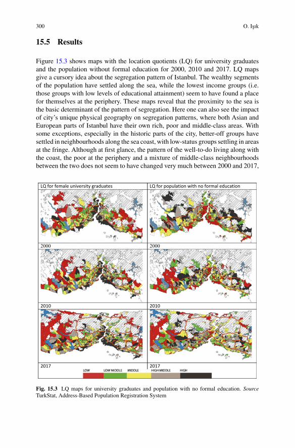
300 O. Isık
15.5 Results
Figure 15.3 shows maps with the location quotients (LQ) for university graduatesand the population without formal education for 2000, 2010 and 2017. LQ mapsgive a cursory idea about the segregation pattern of Istanbul. The wealthy segmentsof the population have settled along the sea, while the lowest income groups (i.e.those groups with low levels of educational attainment) seem to have found a placefor themselves at the periphery. These maps reveal that the proximity to the sea isthe basic determinant of the pattern of segregation. Here one can also see the impactof city’s unique physical geography on segregation patterns, where both Asian andEuropean parts of Istanbul have their own rich, poor and middle-class areas. Withsome exceptions, especially in the historic parts of the city, better-off groups havesettled in neighbourhoods along the sea coast, with low-status groups settling in areasat the fringe. Although at first glance, the pattern of the well-to-do living along withthe coast, the poor at the periphery and a mixture of middle-class neighbourhoodsbetween the two does not seem to have changed very much between 2000 and 2017,
LQ for female university graduates LQ for population with no formal education
20002000
20102010
20172017
Fig. 15.3 LQ maps for university graduates and population with no formal education. SourceTurkStat, Address-Based Population Registration System
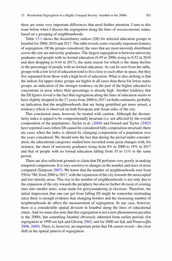
15 Residential Segregation in a Highly Unequal Society: Istanbul in the 2000s 301
there are some very important differences that need further attention. I turn to thisissue below when I discuss the segregation along the lines of socioeconomic status,based on a grouping of neighbourhoods.
Table 15.1 shows the dissimilarity indices (DI) for selected education groups inIstanbul for 2000, 2010 and 2017. The table reveals some crucially important featuresof segregation. Of the groups considered, the ones that are most unevenly distributedacross the city are university graduates. The largest segregation is between universitygraduates and people with no formal education (0.49 in 2000, rising to 0.52 in 2010and then dropping to 0.44 in 2017), the main reason for which is the sharp declinein the percentage of people with no formal education. As can be seen from the table,groups with a low level of education tend to live close to each other in space, but theylive separated from those with a high level of education. What is also striking is thatthe indices for upper-status groups are higher in all cases than those for lower statusgroups, an indication of the stronger tendency on the part of the higher educated toconcentrate in areas where their percentage is already high. Another tendency thatthe DI figures reveal is the fact that segregation along the lines of education seems tohave slightly dropped in the 17 years from 2000 to 2017 on both continents, probablyan indication that the neighbourhoods that are being gentrified get more mixed, atendency which is observed on both European and Asian sides of the city.
This conclusion must, however, be treated with caution. Although the dissimi-larity index is argued to be compositionally invariant (i.e. not affected by the overallcomposition of the population), Taylor et al. (2000) and Gorard and Taylor (2002)have reported cases where DI cannot be considered fully composition invariant; thereare cases when the index is altered by changing composition of a population overthe years considered. We should note the fact that during the period under consider-ation, the educational categories studied here recorded some great changes with, forinstance, the share of university graduates rising from 8% in 2000 to 19% in 2017and that of people with no formal education falling from 35 to 11% in the sameperiod.
There are also sufficient grounds to claim that DI performs very poorly in makingtemporal comparisons. It is very sensitive to changes in the number and sizes of areascompared (Simpson 2007). We know that the number of neighbourhoods rose from550 to 780, from 2000 to 2017, with the expansion of the city towards the unoccupiedand low-density areas. This rise in the number of neighbourhoods is not only due tothe expansion of the city towards the periphery but also to further division of existingones into smaller units; some made for gerrymandering in elections. Therefore, theinitial impression that one can get from falling DI might be somewhat misleadingsince there is enough evidence that changing borders and the increasing number ofneighbourhoods do affect the measurement of segregation. In any case, however,there is a considerable spatial division in Istanbul along the lines of educationalstatus. And wemust also note that this segregation is not a new phenomenon peculiarto the 2000s, but something Istanbul obviously inherited from earlier periods (forsegregation in 1990 see Isık and Güvenç 2002; and for 2000 see Isık and Pınarcıoglu2008, 2009). There is, however, an important point that DI cannot reveal—the clearshift in the spatial pattern of segregation.
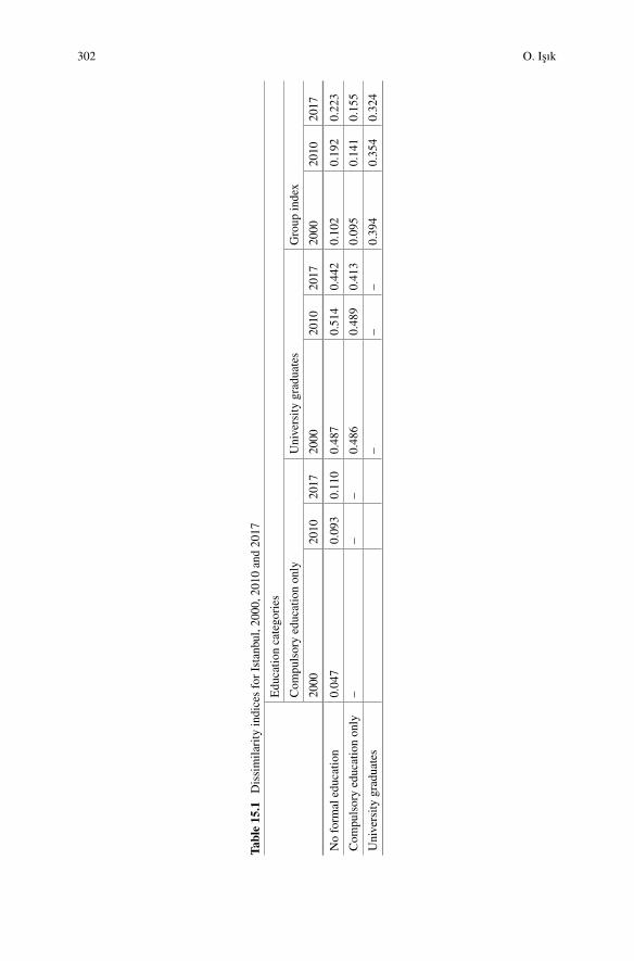
302 O. Isık
Table15.1
Dissimilarity
indicesforIstanbul,2
000,
2010
and2017
Edu
catio
ncatego
ries
Com
pulsoryeducationonly
University
graduates
Group
index
2000
2010
2017
2000
2010
2017
2000
2010
2017
Noform
aleducation
0.047
0.093
0.110
0.487
0.514
0.442
0.102
0.192
0.223
Com
pulsoryeducationonly
––
–0.486
0.489
0.413
0.095
0.141
0.155
University
graduates
––
–0.394
0.354
0.324
15 Residential Segregation in a Highly Unequal Society: Istanbul in the 2000s 303
15.5.1 Classification and Mapping of Neighbourhoods
Given that neighbourhood level data is scarce for Istanbul, three variables are usedto classify neighbourhoods to gain a better understanding of how spatial segregationpatterns have changed between 2000 and 2017. (1) The percentage of those with auniversity degree in the total adult population (population older than 25 years of age)of each neighbourhood; (2) child–woman ratio (CWR) calculated as the numberof children under age 5 per 1000 women of ages between 15 and 49; and (3) thepercentage of women with a university degree in the female population of 30 yearsand over in each neighbourhood.
Using these three variables, neighbourhoods were sorted for each variable fromthe lowest to the highest value and then divided into quintiles. Each quintile wasthen assigned a score from 1 to 5, depending on its ranking. In the case of universitygraduates (both total and female), the lowest quintile was given a score of 1 and thehighest quintile a score of 5, since both are positively correlated with income. In thecase of CWR, the scoring was reversed (1 to the highest quintile and 5 to the lowestquintile) as CWR is negatively correlated with income. Finally, the individual scoreswere added up without assigning any weight to reach an overall score between 3and 15, representing the socioeconomic status of each neighbourhood. Dependingon their scores, neighbourhoods were then divided into 5 categories named low, low-middle, middle, middle-high and high-status neighbourhoods. The results are shownin Fig. 15.4 for 2000, 2010 and 2017.
15.5.2 From 2000 to 2017: Exodus of the Poor
The segregation map for 2000 represents a typical pattern of segregation that couldbe found not only in Istanbul but also in most other Turkish cities. The basic charac-teristics of this segregation pattern can be summarised in a few words: concentrationof affluence in and around the prestigious areas of the city (in the case of Istanbul,along the sea coast) and clustering of the poor at the fringe that is of no interest to thebetter-off classes. It must be noted that in the case of Istanbul, these areas are mostlyunauthorised squatter housing areas built in the 1960s and 1970s. Another importantaspect of this segregation pattern is the existence of middle-income groups actingas a buffer between low- and high-income groups. The lower and upper ends of thesocial ladder do not seem to touch each other in residential neighbourhoods. In fewinstances where they seem to have a direct contact, there is almost always a physicalbarrier: D-100 highway on both the Asian and European side is a clear separatorbetween the rich and the poor (Isık and Güvenç 2002). There are very few examplesof the rich and the poor living in neighbouring areas. Poor areas next to rich areascan be found on both sides of the Bosporus, but they are more visible on the Asianside of Istanbul. They are the remnants of squatters built at times when these areas
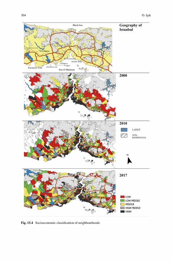
304 O. Isık
Geography of Istanbul
2000
2010 LAKES
NON-RESIDENTIAL
2017
Fig. 15.4 Socioeconomic classification of neighbourhoods
15 Residential Segregation in a Highly Unequal Society: Istanbul in the 2000s 305
were of little value to the wealthy, but their relative position in the city has changedover time due to transformation in the late 1990s.
The 2000 segregation map shows the first signs of what we may call the flight ofthe upper classes from their traditional residential neighbourhoods at the coastline.This flight of the upper classes started in the 1990s but was until then of sporadic andlimited nature. The growing tendency on the part of high-income groups to settle atthe urban fringe, particularly in areas known as ‘gated communities’ (Genis 2007;Tanülkü 2012, 2013) is still invisible in the 2000map because neighbourhoods on thefringe are too large for the impact of such scattered communities to be observable.Such flight of high-income groups is only visible if it is large enough to make up asignificant portion of a neighbourhood.Themost notable example of suchmovementsis a new settlement known as Bahçesehir (Garden City) on the far European edge ofthe city (see the westernmost part of 2000 map). As a harbinger of what was to comein the 2000s, this settlement was built in the late 1980s with generous credit supportfrom now-abolished state-owned real estate banks and became a symbolic exampleof the flight of the middle and upper classes from the built-up areas of the city.
A pattern where the wealthy appropriated the privileged parts of the city, the poorlived exclusively in clusters at the outskirts and the middle classes acted as a bufferbetween the twowas almost a trademark of most Turkish cities in the 1990s and early2000s (cf. Ataç 2017). But this pattern was subject to a brutal and abrupt change atan unforeseen speed in the 2000s, with some disastrous results for the urban poorand ruining everything we thought we knew about Turkish cities. A glimpse of thechanges that took place in the 2000s can be caught even with a cursory comparisonof the maps for 2000 and 2010. Although the basic pattern of the rich along the seacoast and the poor at the outskirts still remains, there are important trends that shedlight to the defeat of the poor, the zeitgeist of the period. Here we can see the first andundeniable traces of what we may refer to as the (a) displacement of the urban poorfrom most of their previous locations and their exodus to even more remote parts ofthe city; (b) consolidation of the urban elites in, around and along with the privilegedareas by cleansing the remnants of the poor that had settled there in earlier periods;(c) large-scale gentrification of some inner-city areas with some conflicting results;and (d) occupation by the poor or lower classes of some inner-city areas abandonedby the wealthy, the so-called degradation of some parts of the city.
It is not surprising to see that some of the largest transformation projects took placeunder the generous support of the state in areas with high accessibility between theTEM and D-100 highways on both sides of the metropolis. Parts of these areashad been subject to unauthorised housing development in the 1970s and 1980s.They were the typical examples of pre-2000 type of unauthorised urban develop-ment—built on occupied state land through ad hoc networks working along thelines of ethnicity, religious affiliation and fellow-townsmanship, meaning that theyhad some degree of heterogeneity within themselves before the onset of large-scaleprojects of 2002. Though they had lost their initial characteristics and turned intomore heterogeneous settlements by time in terms of their inhabitants, they werewithout exception on pieces of land that were far more valuable than their initial
306 O. Isık
value. This ‘non-correspondence’ between their relative position within the city—hence their soaring land values—and the characteristics of their inhabitants pavedthe way for a large-scale and devastating intervention on the part of the state andlocal authorities. Ayazma transformation project for about 20.000 inhabitants on theEuropean side (see Lovering and Türkmen 2011) and Maltepe-Basıbüyük projectsfor about 15.000 inhabitants on the Asian side (Kuyucu and Ünsal 2010; Karaman2013b) are among the best documented and best-known examples of such projects.In all these projects, former residents were offered housing units at the outskirts andthus forced to live in newly built residential areas on the far edges of the city. Thesewere, with no doubt, cleansing projects whereby the poor were pushed further awayfrom the city.
A similar process of sterilisation is also visible in areas close to the prestigiousareas inhabited by the upper classes, particularly on sites overlooking the Bosporuson both continents. A comparison of 2000 and 2010 maps shows how the upperclasses expanded geographically and how pockets of the poor were eradicated alongwith the areas between the two Bosporus bridges. These areas, too, had been subjectto extensive squatter development in earlier periods. The transformation projects inthe Beykoz district on the Asian side and the infamous Armutlu project are amongthe many examples of such projects (Ergun 2004). It must be noted that the cleansingof hills overlooking the Bosporus served more to the upper classes as opposed tothe ones described above, such as Ayazma, where middle and upper-middle-incomegroups made the most use of.
In the historic parts of the city, several renewal projects took place and twoprocesses were at work there; large-scale projects launched by the state and projectsof a minor scale initiated by the nascent urban elite. As an example of the latter, wecan refer to the Cihangir area (Lovering and Türkmen 2011), a once degraded site,opposite to the historic peninsula in an area known as Pera occupied in the nineteenthand early twentieth century by non-Muslim minorities. This area became the focusof culture-led regeneration (Günay and Dökmeci 2012). The gentrification of theCihangir area was a slow and self-paced process, while the ones instigated by thestate were brutal and devoid of any room for the residents to get their share of risingvalues. Of these renewal projects, that in Sulukule, famous for being the first neigh-bourhood in the world to be permanently settled by the Romani people, became thestage of a widespread protest and was even mentioned in EU’s 2006 annual progressreport as an example of the displacement of Roma population (CEC 2006). All theseprotests were in vain, and the neighbourhood was evacuated by police force, andSulukule residents found themselves exiled to a distant part of the metropolis wherethey had not seen before (Uysal 2012; Schoon 2014).
Amidst this chaos, parts of the historic peninsula, once the home of middle andupper-income groups, were reclaimed by low-income groups (Dinçer 2011). The partplayed by Syrian refugees fleeing from the civil war must be stressed in this context.According to official figures, Turkey is home to 3.6 million Syrian refugees livingmostly in big cities with many unsettling impacts not just for Istanbul but for manyother cities. Of these refugees, more than 15% (560,000) live in Istanbul, usually inareas where rents and living costs are low and accessibility is high (Kılıç et al. 2019).
15 Residential Segregation in a Highly Unequal Society: Istanbul in the 2000s 307
Those parts of the historic peninsula for which the upper classes had no interest forwere thus appropriated by a mixture of low-income groups coalescing with Syrianrefugees.
All these huge projects of transformation at the periphery and gentrificationprojects of various scales left behind a patchwork metropolis in some parts of thecity. Especially in the peri-urban areas where land is scarce and competition is high,the transformation of the fringe was sporadic and remained incomplete, producinga patchy pattern in some parts of the metropolis resembling the one emphasised byFlorida (2017) as an important component of the new urban crisis. An examinationof the 2017 segregation map in Fig. 15.4 would reveal that the tendencies that startedin the early years of the first decade of the 2000s produced a significantly differentpattern. Although the parts of the city close to the most valuable asset—namely, tothe sea coast—are still colonised by the wealthy, the new Istanbul at the end of thesecond decade of the 2000s can be best described by the almost total absence ofthe poor in inner-city areas close to or easily accessible from the city centre. Thepoor have now been driven away to the edges of the city, with little contact to therest of Istanbulites. The heavy-handed attitude of the state and local governments inmost of the transformation projects and their determination to break any resistanceusing even police force when they felt necessary must be regarded as an indicationof insatiable desire to redistribute urban rents, which in previous periods had beena lifesaver for newcomers and the urban poor. It is to this issue of redistribution ofurban rents and consequences flowing out of it that I turn in the concluding remarks.
15.6 Concluding Remarks
Turkey was and still is a country of high inequality. Although the level of inequalitydid not change significantly on the surface in the last few decades, the underlyingclass equations and the mechanisms whereby society coped with these inequalitiesdid. Up until the 2000s, the urban poor found the means to appropriate soaringproperty values in prospering metropoles and make use of these opportunities asleverage for social climbing. It is this informal redistribution mechanism in bothurban labour and property markets that guaranteed that all social tensions related tohigh levels of inequality were kept at bay and masses joining the ranks of the urbanpoor maintained their hopes for reaching the upper echelons of social divisions. Inthis game of inequality, the state acted as an accomplice, turning a blind eye tothe existence of markets in the undefined shady zone between the legal and illegal,the formal and informal. The geography of inequality changed as well, with therich concentrating along the sea coast as they did in previous periods, plus air-tightpockets in gated communities on the edges and creating spaces for themselves inparts of the centre. The final pattern is a patchwork metropolis as opposed to theprevious one characterised by clear lines of demarcation in space between socialgroups.
308 O. Isık
The resulting pattern of segregation that we see for the year 2017 is the outcomeof several intertwined processes that had their origin in the late 1990s and culminatedin the 2000s:
(a) State-led eradication of former squatter areas especially in peripheral parts ofthe city where accessibility and thus property values are high;
(b) Selective gentrification of inner-city areas, some under the auspices of the state,others self-initiated and infiltration of the nascent urban elite into formermiddle-class areas; and,
(c) In any case, apathy and even brutality on the part of the state toward the losers,that is the former residents of project areas; and thus, the cleansing parts of theperiphery and the inner city from the urban poor, a process I referred to as theexodus of the urban poor to the remote parts of the metropolis where they canhave little contact with the city.
The extent to which this change in segregation pattern can be attributed to incomeinequality is a question for which I have no ready-made answer as high inequalityhas been an integral aspect of Turkish society for a long time. It is, however, certainthat a metropolis where the poor have been driven out of sight, a process by whichthe ability of the poor to use space as means of power has been castrated, is a newphenomenon even for Turkey. This is something we all have to think about.
References
Ataç E (2017) Turkish-style segregation: socio-economic divisions in seven metropolitan areas.Asian J Soc Sci 45(3):235–270
Atasoy Y (2009) Islam’s marriage with neoliberalism: state transformation in Turkey. PalgraveMacmillan, New York
Commission of the European Communities—CEC (2006) Turkey 2006 progress report, Brus-sels, SEC (2006) 1390. https://www.avrupa.info.tr/sites/default/files/2016-11/Turkey_progress_report%202006.pdf
Dinçer I (2011) The impact of neoliberal policies on historic urban space: areas of urban renewalin Istanbul. Int Plan Stud 16(1):43–60
Dökmeci V, Berköz L (1994) Transformation of Istanbul from a monocentric to a polycentric city.Eur Plan Stud 2:193–205
Ergun N (2004) Gentrification in Istanbul. Cities 21(5):391–405Florida R (2017) The new urban crisis. Basic Books, New YorkGenis S (2007) Producing elite localities: the rise of gated communities in Istanbul. Urban Stud44(4):771–798
Gorard S, Taylor C (2002) What is segregation?: a comparison of measures in terms of ‘strong’ and‘weak’ compositional invariance. Sociol Br Sociol Assoc 36(4):875–895
Göksel I (2013) Female labor force participation in Turkey: the role of conservatism.Women’s StudInt Forum 41:45–54
Günay Z, Dökmeci V (2012) Culture-led regeneration of Istanbul waterfront: golden horn culturalvalley project. Cities 29:213–222
Gürcan EC, Peker E (2015) Neoliberalism with Islamic characteristics’: political, economic, andcultural conjuncture of the GPPs. In: Challenging neoliberalism at Turkey’s Gezi Park. Socialmovements and transformation. Palgrave Macmillan, New York.
15 Residential Segregation in a Highly Unequal Society: Istanbul in the 2000s 309
Isık O, Güvenç M (2002) A metropolis at the crossroads: the changing social geography of Istanbulunder the impact of globalisation. In: Marcuse P, Van Kempen R (eds) Of states and cities: thepartitioning of urban space. Oxford University Press, Oxford, pp 203–220
Isık O, Pınarcıoglu M (2009) Segregation in Istanbul: patterns and processes. Tijdschrift VoorEconomische En Sociale Geografie 100(4):469–484
Isık O, PınarcıogluM (2008) Not only helpless, but also hopeless now: changing dynamics of urbanpoverty in Turkey. Eur Plan Stud 16(10):1353–1371
IsıkO,PınarcıogluM(2006)Geographies of a silent transition: a geographicallyweighted regressionapproach to regional fertility differences in Turkey. Eur J Popul 22(4):399–421
Karaman O (2013a) Urban neoliberalism with Islamic characteristics. Urban Stud 50(16):3412–3427
Karaman O (2013b) Urban renewal in Istanbul: reconfigured spaces, robotic lives. Int J Urban RegRes 37(2):715–733
Kılıç ÖO et al. (2019) The use of big mobile data to gain multi-layered insights for Syrian refugeecrisis. In: Salah AA, Pentland A, Lepri B, Letouzé E (eds) Guide to mobile data analytics inrefugee scenarios. Springer
Kuyucu T, Ünsal Ö (2010) ‘Urban transformation’ as state-led property transfer: an analysis of twocases of urban renewal in Istanbul. Urban Stud 47(7):1479–1499
Lovering J, Türkmen H (2011) Bulldozer neo-liberalism in Istanbul: the state-led construction ofproperty markets, and the displacement of the urban poor. Int Plan Stud 16(1):73–96
Schoon D (2014) Sulukule is the gun and we are its bullets. City 18(6):655–666Simpson L (2007) Ghettos of the mind: the empirical behaviour of indices of segregation anddiversity. J Roy Stat Soc A 170:405–424
Taylor C, Gorard S, Fitz J (2000) (2000) A re-examination of segregation indices in terms ofcompositional invariance. Soc Res Update, Autumn
Tanülkü B (2012) Gated communities: from ‘self-sufficient towns’ to ‘active urban agents.’Geofroum 43:518–528
Tanülkü B (2013) Gated communities: ideal packages or processual spaces of conflict. Hous Stud28(7):937–959
TürkünA (2011) Urban regeneration and hegemonic power relationships. Int Plan Stud 16(1):61–72Uysal ÜU (2012) An urban social movement challenging urban regeneration: the case of Sulukule,Istanbul. Cities 29:12–22
World Economic Forum (2018) The global gender gap report, Geneva. The Report available atwef.ch/gggr18.
Open Access This chapter is licensed under the terms of the Creative Commons Attribution 4.0International License (http://creativecommons.org/licenses/by/4.0/), which permits use, sharing,adaptation, distribution and reproduction in any medium or format, as long as you give appropriatecredit to the original author(s) and the source, provide a link to the Creative Commons license andindicate if changes were made.
The images or other third party material in this chapter are included in the chapter’s CreativeCommons license, unless indicated otherwise in a credit line to the material. If material is notincluded in the chapter’s Creative Commons license and your intended use is not permitted bystatutory regulation or exceeds the permitted use, you will need to obtain permission directly fromthe copyright holder.
Chapter 16Segregation in London: A City of Choicesor Structures?
David Manley
Abstract This chapter provides a comprehensive overview of the socio-economicsegregation in London. The cosmopolitan nature of the city means there is an inter-woven complexity that prevents the separation of social, cultural and economic resi-dential trajectories of the population.As a result, the chapter explores socio-economicsegregation within the context of the changing nature of the (sub)urban contexts. Inparticular, the chapter documents not only the occupational segregation but alsointroduces the often-used dimension of ethnicity and pairs it with the less commonlyexplored age and tenure dimensions through which the social structure of the city isinscribed. This enables a broader understanding of the rapid changes that have beenwrought on the micro-scale can be understood in the context of a city that has, interms of the overall composition, changed little.
Keywords Segregation · London · Housing · Ethnicity · Occupation
16.1 Introduction
Originally founded by the Romans as Londinium, the city has prospered over almosttwo millennia growing from its initial roots as a trading port on the River Thamesto national capital and international finance hub. In terms of global reach, Londonis on par with New York (GaWC 2020). Over this period, the functions of the city,the relative population composition and the social, economic and ethnic populationdistributions have changed, but London remains a city of contrasts. With almost 9million people living in the Urban Core, it is the most populous of any EuropeanCapital, a population that grows substantially when including the wider commuterbelt areas of over 14 million people (Eurostat 2018). It is also one of the most impor-tant cities globally in terms of finance, business and industry as well as amajor touristdestination on the international stage, and exerts considerable influence nationallyas the seat of Government for the United Kingdom. As one of the original Global
D. Manley (B)University of Bristol, Bristol, UKe-mail: [email protected]
© The Author(s) 2021M. van Ham et al. (eds.), Urban Socio-Economic Segregation and Income Inequality,The Urban Book Series, https://doi.org/10.1007/978-3-030-64569-4_16
311
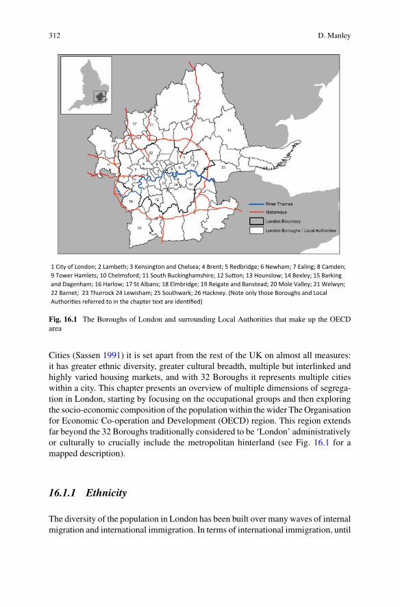
312 D. Manley
1 City of London; 2 Lambeth; 3 Kensington and Chelsea; 4 Brent; 5 Redbridge; 6 Newham; 7 Ealing; 8 Camden; 9 Tower Hamlets; 10 Chelmsford; 11 South Buckinghamshire; 12 Su on; 13 Hounslow; 14 Bexley; 15 Barking and Dagenham; 16 Harlow; 17 St Albans; 18 Elmbridge; 19 Reigate and Banstead; 20 Mole Valley; 21 Welwyn; 22 Barnet; 23 Thurrock 24 Lewisham; 25 Southwark; 26 Hackney. (Note only those Boroughs and Local Authori es referred to in the chapter text are iden fied)
Fig. 16.1 The Boroughs of London and surrounding Local Authorities that make up the OECDarea
Cities (Sassen 1991) it is set apart from the rest of the UK on almost all measures:it has greater ethnic diversity, greater cultural breadth, multiple but interlinked andhighly varied housing markets, and with 32 Boroughs it represents multiple citieswithin a city. This chapter presents an overview of multiple dimensions of segrega-tion in London, starting by focusing on the occupational groups and then exploringthe socio-economic composition of the populationwithin thewider TheOrganisationfor Economic Co-operation and Development (OECD) region. This region extendsfar beyond the 32 Boroughs traditionally considered to be ‘London’ administrativelyor culturally to crucially include the metropolitan hinterland (see Fig. 16.1 for amapped description).
16.1.1 Ethnicity
The diversity of the population in London has been built over many waves of internalmigration and international immigration. In terms of international immigration, until
16 Segregation in London: A City of Choices or Structures? 313
the end of the Second World War, entry into the UK was largely dominated by resi-dents from countries in what became the Commonwealth. After the British Nation-alityAct in 1948, the right to enter andwork in theUKwas granted to over 800millionresidents in the former countries included in the British Empire. The resulting flowswere, of course, much smaller than this, but there was still a substantial number ofeconomically motivated migrants entering the UK, and especially London, to take uppositions in occupations with a deficit of labour supply—such as transportation andthe newly formed national health service. Within the Boroughs of London, the expe-rience of migration has been highly varied. For instance, Lambeth and Kensingtonand Chelsea were Boroughs where the Black Caribbean population first settled in thecity, and Brixton is still regarded as the Caribbean Capital of Britain. Other Boroughssuch as Hackney, Brent, Lewisham and Southwark also played important roles inthe initial years for these groups. By contrast, people belonging to the Bangladeshicommunities in London have tended to concentrate in theBorough of TowerHamlets.Within the vast diversity of groups, the other two largest are the Pakistani (aroundRedbridge and Newham) and the Indians (Ealing and Brent). There is, then, there isthe potential for substantial ethnic segregation at the macro (Borough) scale.
16.1.2 Economic
Economically, the residential history of London is just as varied as it is for ethnicity.Meen and colleagues (2012) highlighted the potential for the social and economicprofile of neighbourhoods to steadfastly remain static within the wider urban system,even in the presence of some substantial (e.g. regeneration or gentrification) shocksin the longer term. London’s social mosaic was initially mapped out by Booth (1903)using street by street observation to give classifications across the whole of the city.It is notable in his classification that areas such as the present-day Kensington andChelsea were already identified as belonging to the ‘upper-middle and upper classes,wealthy’ group, just as any modern-day classification would conclude. Similarly, theneighbourhoods in the Belsize Park1 area (Camden) were similarly identified andcontinue today to be areas of wealth and affluence. By contrast, neighbourhoodslocated in the Borough of Tower Hamlets, especially those located in was known as‘Stepney’ were classified in the ‘lowest class’, ‘very poor’ and ‘poor’, neighbour-hoods. Tellingly, these correspond closely with those neighbourhoods identified asbeing the poorest in London using modern deprivation measures such as the Indexof Multiple Deprivation (Smith et al. 2015). Although these are only a couple ofbrief exemplars, they allude to the wider trend which despite London being a seatof substantial gentrification (from the initial work by Ruth Glass (1964) to the morerecent Super Gentrification literature of Bulter and Lees 2006; Butler et al. 2013) thestructure of many neighbourhoods within London has been locked into the long term
1The name Bellsize is derived from the French ‘bel assis’ which translates into English as ‘wellsituated’.
314 D. Manley
reproduction of spatial inequality. Investigating the change in spatial characteristicsof occupation and focusing particularly on the places of residence of the workingclass and middle-class, Manley and Johnston (2014) revealed that substantial changewas a rare phenomenon over a relatively long (10 year) period.
16.1.3 Housing
In recent years London has attracted substantial investment from globally wealthyinvestors and has become an international site of investment for the superrich majorhousing developments, especially in interventions in the central areas (see Atkinson2016). This process has fuelled the continuation of much longer-term trends withinthe city where the residential infrastructure of the city is often highly sought after.Many current property developments are targeted at the private market, often forowner occupation or private rent. Where mixed tenure has been explored, the imple-mentations have been sometimes controversial (see the development of gated playspaces, Guardian 2019a) or highly exclusionary, such as the poor door2 access tomixed tenure developments (see for instance Osborne 2014).
However, the British housing system was not always like this. The UK is tradi-tionally viewed as a LiberalWelfare State with early moves into state provision in thefirst part of the 1900s under the Liberal Government of Asquith. This state provisionof housing was substantially bolstered in the post-war period (1942 onwards) withthe introduction of the National Health Service. In terms of the development of thecity, the welfare state was critical in the organisation, access to and redevelopment ofslum areas across the UK. In particular, London was the setting for many of the early‘council houses’ (herein referred to as social housing) under the instruction of theEstates Department of the then London County Council (LCC). The creation overmuch of the 1900s of large estates across the city provided the backdrop for a largelymixed population at the city scale where all Boroughs provided some form of socialhousing. Since inception, it has been possible for tenants to purchase the propertythey rent from the council provider, but until the late 1970s, it was rare for tenantsto exercise their Right to buy (RTB). However, in 1980 the Housing Act passed bythe then Conservative government of Margret Thatcher formalised the policy andin the decades that followed, over 4 million properties were sold across the UK,leading to a substantial reduction in the availability of rental stock. Within London,where to date, almost of 290,000 properties have been sold (DCLG 2019), the conse-quences of RTB played out differentially in each borough. In some parts of the city,former social housing stock is in private ownership and worth well over £1 millionwhile equivalent houses elsewhere are still valued at a 10th of that price. Regardless
2The term ‘poor door’ refers to the practice of putting separate entrances on multi-dwelling devel-opments so that those residents in the cheaper (often denoted as affordable or rented) properties aredistanced from residents in the more expensive apartments by literally entering the building throughdifferent entrances.
16 Segregation in London: A City of Choices or Structures? 315
of location, the RTB was a major element in the residualisation of social housing,resulting in a reduced stock available to a smaller section of society. It was then alsoa process that leads to social housing being increasingly viewed as a tenue of lastresort. The ultimate expression of this residualisation was seen in the early hoursof 14 June 2017 when the Grenfell Tower caught fire, and 72 lives were lost in theensuing blaze. Grenfell Tower, owned by Kensington and Chelsea London BoroughCouncil with the Kensington and Chelsea Tenant Management Organisation actingas Landlord disaster, highlights the complexity of the two-tier housing system thatthe RTB reinforced. Those tenants living in the apartments which remained owned bythe council would be managed as traditional social housing tenants with inspectionsand the ultimate housing responsibility falling to the local authority, or the repre-sentatives they appointed. By contrast, those flats bought under RTB but existing inthe same tower block would not be under scrutiny to the same degree. While theleaseholder remains the same, the RTB either as a dwelling for the owners or as aprivate market rental, the upkeep and maintenance is a private issue.
16.1.4 Chapter Outline
In the sections that follow, an in-depth assessment of segregation by occupation ispresented usingmultiplemeasures. This is followedby adiscussion about segregationfocusing on the characteristics of the city explored above—ethnicity, and housingtype—along with age as a further important demographic characteristic. Data aredrawn from the 2001 and 2011 UK Census, the largest source of data for the UKpopulation. UK Census data is not available at an individual level, so in order toexplore segregation, it is necessary to use aggregated areal units: in this chapter, theLower Super Output Area (LSOA) is used, representing ‘neighbourhoods’ whichhave on average around 1400 people. By considering multiple characteristics, wecan explore the extent of different types of segregation in the metropolitan area anddevelop a wider understanding of the social geography of the city.
16.2 Inequality and Occupational Segregation
The Gini Index for the United Kingdom since 1961 demonstrates a clear increase ininequality. In 1961 the UK had a Gini coefficient of 0.25, which increased slightlythrough the1970s and1980s.After 1980 theGini increased to0.35by1991 increasingagain in the middle of the 2000s to about 0.36. By 2011 the figure had begun tofall and there is evidence, post-2008, that the trend is in decline; however, whilstthis might be regarded positively and suggest a decline in inequality, the reductionshould be interpreted with the Global Financial Crisis in mind. Gini reduction canoccur through a number of processes that result in the gap between the richest andpoorest declining. It might be that the real incomes of the poorest increase, thus
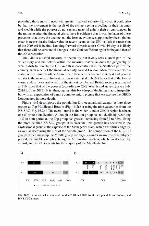
316 D. Manley
providing those most in need with greater financial security. However, it could alsobe that the movement is the result of the richest seeing a decline in their incomesand wealth while the poorest do not see any material gain in their circumstances. Inthe moments after the financial crisis, there is evidence that it was the latter of theseprocesses that drove the decline, not the former, evidence supported by the slight butclear increases in the Index value in recent years as the UK has left the recessionof the 2008 crisis behind. Looking forward towards a post-Covid-19 city, it is likelythat there will be substantial changes in the Gini coefficient again far beyond that ofthe 2008 recession.
The Gini is a useful measure of inequality, but it only tells a small part of thewider story and the details within the measure matter, as does the geography ofwealth distribution. In the UK, wealth is concentrated in the Southern part of thecountry, with much of the financial activity around London. Moreover, even with astable or declining headline figure, the differences between the richest and poorestare stark: the income of highest earners is estimated to be 6.8 times that of the lowestearners while the overall wealth of the richest members of British society is estimatedat 316 times that of the poorest (according to ONS Wealth and Assets Survey July2014 to June 2016). It is, then, against this backdrop of declining macro inequalitybut with an expectation of a more complex micro picture that we explore the OECDLondon area in more depth.
Figure 16.2 decomposes the population into occupational categories into threegroups as Top Middle and Bottom (Fig. 16.2a) or using the nine categories from theNS-SEC (Fig. 16.2b). The overall trend in the wider London OECD region has beenone of professionalization. Although the Bottom group has not declined (recording14% in both periods), the Top group has grown, increasing from 32 to 38%. Usingthe more detailed NS-SEC groups, it is clear that this growth has occurred in theProfessional group at the expense of the Managerial class, which has shrunk slightly,as well as decreasing the size of the Middle group. The composition of the NS-SECgroups which make up the Middle group are largely similar in size over the 10-yearperiod, the notable exception being the Administrative class, which has declined bya third, and which accounts for the majority of the Middle decline.
a) b)
38
32
48
54
14
14
0% 20% 40% 60% 80% 100%
2011
2001
Top Middle Bo om
15
18
23
14
16
17
10
15
10
9
6
6
5
7
6
5
8
9
0% 50% 100%
2011
2001
Ele Plant Sales Caring Skilled Adm
in Assoc Prof M
an
Fig. 16.2 Occupational structure of London 2001 and 2011 for the a top middle and bottom, andb NS-SEC groups
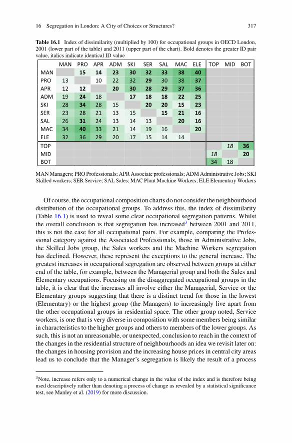
16 Segregation in London: A City of Choices or Structures? 317
Table 16.1 Index of dissimilarity (multiplied by 100) for occupational groups in OECD London,2001 (lower part of the table) and 2011 (upper part of the chart). Bold denotes the greater ID pairvalue, italics indicate identical ID value
MAN PRO APR ADM SKI SER SAL MAC ELE TOP MID BOT MAN 15 14 23 30 32 33 38 40 PRO 13 10 22 32 29 30 38 37 APR 12 12 20 30 28 29 37 36 ADM 19 24 18 17 18 18 22 25 SKI 28 34 28 15 20 20 15 23 SER 23 28 21 13 15 15 21 16 SAL 26 31 24 13 14 13 20 16 MAC 34 40 33 21 14 19 16 20 ELE 32 36 29 20 17 15 14 14 TOP 18 36 MID 18 20 BOT 34 18
MANManagers; PROProfessionals; APRAssociate professionals; ADMAdministrative Jobs; SKISkilled workers; SER Service; SAL Sales; MAC PlantMachineWorkers; ELE ElementaryWorkers
Of course, the occupational composition charts do not consider the neighbourhooddistribution of the occupational groups. To address this, the index of dissimilarity(Table 16.1) is used to reveal some clear occupational segregation patterns. Whilstthe overall conclusion is that segregation has increased3 between 2001 and 2011,this is not the case for all occupational pairs. For example, comparing the Profes-sional category against the Associated Professionals, those in Administrative Jobs,the Skilled Jobs group, the Sales workers and the Machine Workers segregationhas declined. However, these represent the exceptions to the general increase. Thegreatest increases in occupational segregation are observed between groups at eitherend of the table, for example, between the Managerial group and both the Sales andElementary occupations. Focusing on the disaggregated occupational groups in thetable, it is clear that the increases all involve either the Managerial, Service or theElementary groups suggesting that there is a distinct trend for those in the lowest(Elementary) or the highest group (the Managers) to increasingly live apart fromthe other occupational groups in residential space. The other group noted, Serviceworkers, is one that is very diverse in composition with some members being similarin characteristics to the higher groups and others to members of the lower groups. Assuch, this is not an unreasonable, or unexpected, conclusion to reach in the context ofthe changes in the residential structure of neighbourhoods an idea we revisit later on:the changes in housing provision and the increasing house prices in central city areaslead us to conclude that the Manager’s segregation is likely the result of a process
3Note, increase refers only to a numerical change in the value of the index and is therefore beingused descriptively rather than denoting a process of change as revealed by a statistical significancetest, see Manley et al. (2019) for more discussion.
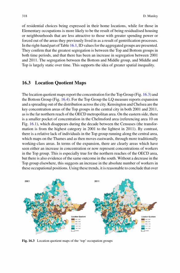
318 D. Manley
of residential choices being expressed in their home locations, while for those inElementary occupations is more likely to be the result of being residualised housingor neighbourhoods that are less attractive to those with greater spending power orforced out of the areas they previously lived in as a result of gentrification processes.In the right-hand part of Table 16.1, IDvalues for the aggregated groups are presented.They confirm that the greatest segregation is between the Top and Bottom groups inboth time periods, and that there has been an increase in segregation between 2001and 2011. The segregation between the Bottom and Middle group, and Middle andTop is largely static over time. This supports the idea of greater spatial inequality.
16.3 Location Quotient Maps
The location quotientmaps report the concentration for the TopGroup (Fig. 16.3) andthe Bottom Group (Fig. 16.4). For the Top Group the LQ measure reports expansionand a spreading out of the distribution across the city. Kensington and Chelsea are thekey concentration areas of the Top groups in the central city in both 2001 and 2011,as is the far northern reach of the OECDmetropolitan area. On the eastern side, thereis a smaller pocket of concentration in the Chelmsford area (referencing area 10 onFig. 16.1), which disappears during the decade between the Censuses (the transfor-mation is from the highest category in 2001 to the lightest in 2011). By contrast,there is a relative lack of individuals in the Top group running along the central area,which maps on the Thames and as then moves eastwards, through more traditionallyworking-class areas. In terms of the expansion, there are clearly areas which haveseen either an increase in concentration or now represent concentrations of workersin the Top group. This is especially true for the northern reaches of the OECD area,but there is also evidence of the same outcome in the south. Without a decrease in theTop group elsewhere, this suggests an increase in the absolute number of workers inthese occupational positions. Using these trends, it is reasonable to conclude that over
Fig. 16.3 Location quotient maps of the ‘top’ occupation groups
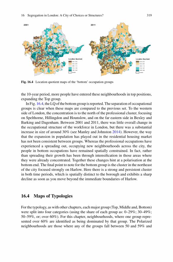
16 Segregation in London: A City of Choices or Structures? 319
Fig. 16.4 Location quotient maps of the ‘bottom’ occupation groups
the 10-year period, more people have entered these neighbourhoods in top positions,expanding the Top group.
InFig. 16.4, theLQof the bottomgroup is reported. The separation of occupationalgroups is clear when these maps are compared to the previous set. To the westernside of London, the concentration is to the north of the professional cluster, focusingon Spelthorne, Hillingdon and Hounslow, and on the far eastern side in Bexley andBarking and Dagenham. Between 2001 and 2011, there was little overall change inthe occupational structure of the workforce in London, but there was a substantialincrease in size of around 30% (see Manley and Johnston 2014). However, the waythat the expansion in population has played out in the residential housing markethas not been consistent between groups. Whereas the professional occupations haveexperienced a spreading out, occupying new neighbourhoods across the city, thepeople in bottom occupations have remained spatially constrained. In fact, ratherthan spreading their growth has been through intensification in those areas wherethey were already concentrated. Together these changes hint at a polarisation at thebottom end. The final point to note for the bottom group is the cluster in the northeastof the city focused strongly on Harlow. Here there is a strong and persistent clusterin both time periods, which is spatially distinct to the borough and exhibits a sharpdecline as soon as you move beyond the immediate boundaries of Harlow.
16.4 Maps of Typologies
For the typology, as with other chapters, eachmajor group (Top,Middle and, Bottom)were split into four categories (using the share of each group as: 0–29%; 30–49%;50–59%, or; over 60%). For this chapter, neighbourhoods, where one group repre-sented over 60% are identified as being dominated by that group. The Polarizedneighbourhoods are those where any of the groups fall between 50 and 59% and
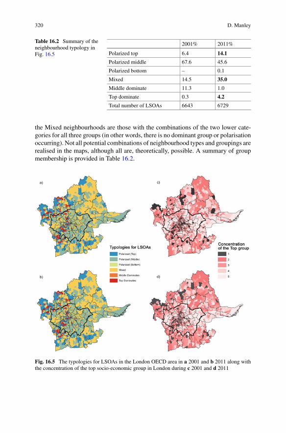
320 D. Manley
Table 16.2 Summary of theneighbourhood typology inFig. 16.5
2001% 2011%
Polarized top 6.4 14.1
Polarized middle 67.6 45.6
Polarized bottom – 0.1
Mixed 14.5 35.0
Middle dominate 11.3 1.0
Top dominate 0.3 4.2
Total number of LSOAs 6643 6729
the Mixed neighbourhoods are those with the combinations of the two lower cate-gories for all three groups (in other words, there is no dominant group or polarisationoccurring). Not all potential combinations of neighbourhood types and groupings arerealised in the maps, although all are, theoretically, possible. A summary of groupmembership is provided in Table 16.2.
Fig. 16.5 The typologies for LSOAs in the London OECD area in a 2001 and b 2011 along withthe concentration of the top socio-economic group in London during c 2001 and d 2011
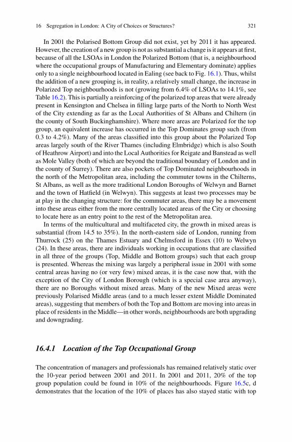
16 Segregation in London: A City of Choices or Structures? 321
In 2001 the Polarised Bottom Group did not exist, yet by 2011 it has appeared.However, the creation of a newgroup is not as substantial a change is it appears at first,because of all the LSOAs in London the Polarized Bottom (that is, a neighbourhoodwhere the occupational groups of Manufacturing and Elementary dominate) appliesonly to a single neighbourhood located in Ealing (see back to Fig. 16.1). Thus, whilstthe addition of a new grouping is, in reality, a relatively small change, the increase inPolarized Top neighbourhoods is not (growing from 6.4% of LSOAs to 14.1%, seeTable 16.2). This is partially a reinforcing of the polarized top areas that were alreadypresent in Kensington and Chelsea in filling large parts of the North to North Westof the City extending as far as the Local Authorities of St Albans and Chiltern (inthe county of South Buckinghamshire). Where more areas are Polarized for the topgroup, an equivalent increase has occurred in the Top Dominates group such (from0.3 to 4.2%). Many of the areas classified into this group about the Polarized Topareas largely south of the River Thames (including Elmbridge) which is also Southof HeathrowAirport) and into the Local Authorities for Reigate and Banstead as wellas Mole Valley (both of which are beyond the traditional boundary of London and inthe county of Surrey). There are also pockets of Top Dominated neighbourhoods inthe north of the Metropolitan area, including the commuter towns in the Chilterns,St Albans, as well as the more traditional London Boroughs of Welwyn and Barnetand the town of Hatfield (in Welwyn). This suggests at least two processes may beat play in the changing structure: for the commuter areas, there may be a movementinto these areas either from the more centrally located areas of the City or choosingto locate here as an entry point to the rest of the Metropolitan area.
In terms of the multicultural and multifaceted city, the growth in mixed areas issubstantial (from 14.5 to 35%). In the north-eastern side of London, running fromThurrock (25) on the Thames Estuary and Chelmsford in Essex (10) to Welwyn(24). In these areas, there are individuals working in occupations that are classifiedin all three of the groups (Top, Middle and Bottom groups) such that each groupis presented. Whereas the mixing was largely a peripheral issue in 2001 with somecentral areas having no (or very few) mixed areas, it is the case now that, with theexception of the City of London Borough (which is a special case area anyway),there are no Boroughs without mixed areas. Many of the new Mixed areas werepreviously Polarised Middle areas (and to a much lesser extent Middle Dominatedareas), suggesting that members of both the Top and Bottom are moving into areas inplace of residents in theMiddle—in other words, neighbourhoods are both upgradingand downgrading.
16.4.1 Location of the Top Occupational Group
The concentration of managers and professionals has remained relatively static overthe 10-year period between 2001 and 2011. In 2001 and 2011, 20% of the topgroup population could be found in 10% of the neighbourhoods. Figure 16.5c, ddemonstrates that the location of the 10% of places has also stayed static with top
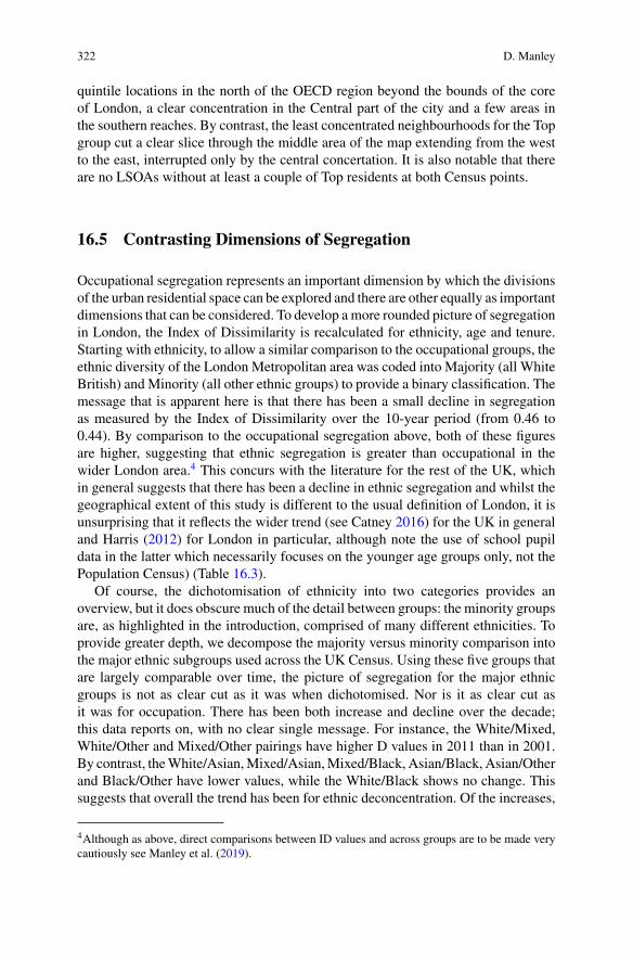
322 D. Manley
quintile locations in the north of the OECD region beyond the bounds of the coreof London, a clear concentration in the Central part of the city and a few areas inthe southern reaches. By contrast, the least concentrated neighbourhoods for the Topgroup cut a clear slice through the middle area of the map extending from the westto the east, interrupted only by the central concertation. It is also notable that thereare no LSOAs without at least a couple of Top residents at both Census points.
16.5 Contrasting Dimensions of Segregation
Occupational segregation represents an important dimension by which the divisionsof the urban residential space can be explored and there are other equally as importantdimensions that can be considered. To develop amore rounded picture of segregationin London, the Index of Dissimilarity is recalculated for ethnicity, age and tenure.Starting with ethnicity, to allow a similar comparison to the occupational groups, theethnic diversity of the London Metropolitan area was coded into Majority (all WhiteBritish) and Minority (all other ethnic groups) to provide a binary classification. Themessage that is apparent here is that there has been a small decline in segregationas measured by the Index of Dissimilarity over the 10-year period (from 0.46 to0.44). By comparison to the occupational segregation above, both of these figuresare higher, suggesting that ethnic segregation is greater than occupational in thewider London area.4 This concurs with the literature for the rest of the UK, whichin general suggests that there has been a decline in ethnic segregation and whilst thegeographical extent of this study is different to the usual definition of London, it isunsurprising that it reflects the wider trend (see Catney 2016) for the UK in generaland Harris (2012) for London in particular, although note the use of school pupildata in the latter which necessarily focuses on the younger age groups only, not thePopulation Census) (Table 16.3).
Of course, the dichotomisation of ethnicity into two categories provides anoverview, but it does obscure much of the detail between groups: the minority groupsare, as highlighted in the introduction, comprised of many different ethnicities. Toprovide greater depth, we decompose the majority versus minority comparison intothe major ethnic subgroups used across the UK Census. Using these five groups thatare largely comparable over time, the picture of segregation for the major ethnicgroups is not as clear cut as it was when dichotomised. Nor is it as clear cut asit was for occupation. There has been both increase and decline over the decade;this data reports on, with no clear single message. For instance, the White/Mixed,White/Other and Mixed/Other pairings have higher D values in 2011 than in 2001.By contrast, theWhite/Asian,Mixed/Asian,Mixed/Black, Asian/Black, Asian/Otherand Black/Other have lower values, while the White/Black shows no change. Thissuggests that overall the trend has been for ethnic deconcentration. Of the increases,
4Although as above, direct comparisons between ID values and across groups are to be made verycautiously see Manley et al. (2019).
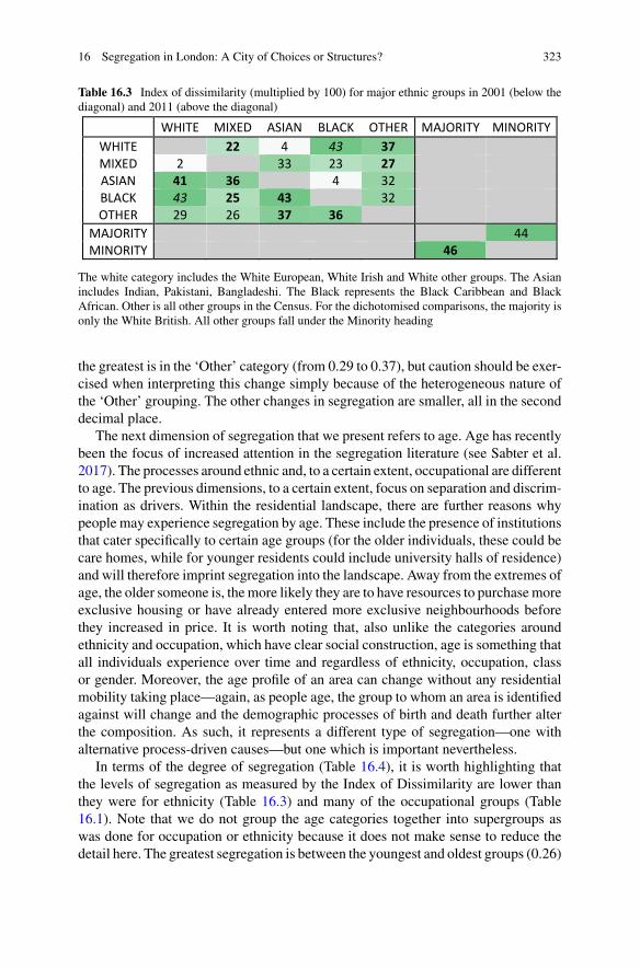
16 Segregation in London: A City of Choices or Structures? 323
Table 16.3 Index of dissimilarity (multiplied by 100) for major ethnic groups in 2001 (below thediagonal) and 2011 (above the diagonal)
WHITE MIXED ASIAN BLACK OTHER MAJORITY MINORITY WHITE 22 4 43 37 MIXED 2 33 23 27 ASIAN 41 36 4 32 BLACK 43 25 43 32 OTHER 29 26 37 36
MAJORITY 44 MINORITY 46
The white category includes the White European, White Irish and White other groups. The Asianincludes Indian, Pakistani, Bangladeshi. The Black represents the Black Caribbean and BlackAfrican. Other is all other groups in the Census. For the dichotomised comparisons, the majority isonly the White British. All other groups fall under the Minority heading
the greatest is in the ‘Other’ category (from 0.29 to 0.37), but caution should be exer-cised when interpreting this change simply because of the heterogeneous nature ofthe ‘Other’ grouping. The other changes in segregation are smaller, all in the seconddecimal place.
The next dimension of segregation that we present refers to age. Age has recentlybeen the focus of increased attention in the segregation literature (see Sabter et al.2017). The processes around ethnic and, to a certain extent, occupational are differentto age. The previous dimensions, to a certain extent, focus on separation and discrim-ination as drivers. Within the residential landscape, there are further reasons whypeople may experience segregation by age. These include the presence of institutionsthat cater specifically to certain age groups (for the older individuals, these could becare homes, while for younger residents could include university halls of residence)and will therefore imprint segregation into the landscape. Away from the extremes ofage, the older someone is, themore likely they are to have resources to purchasemoreexclusive housing or have already entered more exclusive neighbourhoods beforethey increased in price. It is worth noting that, also unlike the categories aroundethnicity and occupation, which have clear social construction, age is something thatall individuals experience over time and regardless of ethnicity, occupation, classor gender. Moreover, the age profile of an area can change without any residentialmobility taking place—again, as people age, the group to whom an area is identifiedagainst will change and the demographic processes of birth and death further alterthe composition. As such, it represents a different type of segregation—one withalternative process-driven causes—but one which is important nevertheless.
In terms of the degree of segregation (Table 16.4), it is worth highlighting thatthe levels of segregation as measured by the Index of Dissimilarity are lower thanthey were for ethnicity (Table 16.3) and many of the occupational groups (Table16.1). Note that we do not group the age categories together into supergroups aswas done for occupation or ethnicity because it does not make sense to reduce thedetail here. The greatest segregation is between the youngest and oldest groups (0.26)
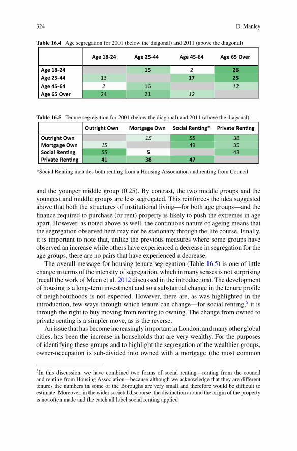
324 D. Manley
Table 16.4 Age segregation for 2001 (below the diagonal) and 2011 (above the diagonal)
Age 18-24 Age 25-44 Age 45-64 Age 65 Over
Age 18-24 15 2 26 Age 25-44 13 17 25 Age 45-64 2 16 12 Age 65 Over 24 21 12
Table 16.5 Tenure segregation for 2001 (below the diagonal) and 2011 (above the diagonal)
Outright Own Mortgage Own Social Ren ng* Private Ren ng
Outright Own 15 55 38 Mortgage Own 15 49 35 Social Ren ng 55 5 43 Private Ren ng 41 38 47
*Social Renting includes both renting from a Housing Association and renting from Council
and the younger middle group (0.25). By contrast, the two middle groups and theyoungest and middle groups are less segregated. This reinforces the idea suggestedabove that both the structures of institutional living—for both age groups—and thefinance required to purchase (or rent) property is likely to push the extremes in ageapart. However, as noted above as well, the continuous nature of ageing means thatthe segregation observed here may not be stationary through the life course. Finally,it is important to note that, unlike the previous measures where some groups haveobserved an increase while others have experienced a decrease in segregation for theage groups, there are no pairs that have experienced a decrease.
The overall message for housing tenure segregation (Table 16.5) is one of littlechange in terms of the intensity of segregation, which inmany senses is not surprising(recall the work of Meen et al. 2012 discussed in the introduction). The developmentof housing is a long-term investment and so a substantial change in the tenure profileof neighbourhoods is not expected. However, there are, as was highlighted in theintroduction, few ways through which tenure can change—for social renting,5 it isthrough the right to buy moving from renting to owning. The change from owned toprivate renting is a simpler move, as is the reverse.
An issue that has become increasingly important inLondon, andmanyother globalcities, has been the increase in households that are very wealthy. For the purposesof identifying these groups and to highlight the segregation of the wealthier groups,owner-occupation is sub-divided into owned with a mortgage (the most common
5In this discussion, we have combined two forms of social renting—renting from the counciland renting from Housing Association—because although we acknowledge that they are differenttenures the numbers in some of the Boroughs are very small and therefore would be difficult toestimate. Moreover, in the wider societal discourse, the distinction around the origin of the propertyis not often made and the catch all label social renting applied.

16 Segregation in London: A City of Choices or Structures? 325
route to house purchase where the money is borrowed from a lender such as a bankor building society) and owned outright which in the context of much of the Londonmarket is an expression of high wealth. The segregation between the owning (mort-gage) and the owning (outright) and social renting have remained static. There hasbeen a slight fall in segregation between social renting and owning with a mortgage(the right to buy is likely to be an explanation here, with the right to buy tenantsaccessing their purchase via a mortgage, although some redevelopment and inclu-sion of mixed tenure developments may also provide an insight). The main featureof interest here, however, is the magnitude of the Index of Dissimilarity. Comparedwith the other dimensions of segregation we have considered (age, ethnicity andoccupation), the pairwise comparison between social renting and other tenure formsare the highest of all the comparisons (up to 0.55).6 What this suggests is that segre-gation in London is very much driven by the location of the housing that a householdaccesses: housing is built in clusters and those smaller clusters of tenure types oftenare co-located in broader neighbourhoods with similar housing. Although there hasbeen a push towards creating a greater mixing of tenures (see, for instance, Bridgeet al. 2011), the fixity of housing—it takes large financial investments and time—spread over substantially large areas of the city to fundamentally alter the urbanspatial structure. As a result, the underlying housing stock does not change verymuch from year to year, or even over a ten-year period, and so the neighbourhoodsreproduce themselves. In terms of the changes in segregation, the biggest has beenfor private renters. Here there has been a decrease for all pairwise combinations. Asthe period 2001 to 2011 saw an increase in the prevalence of private renting, this isnot a surprising outcome.
16.6 Conclusions
Segregation is and always has been a complex and multi-faceted issue, and withincreasing diversity and concern around the mixing of populations (on many dimen-sions), it is not an issue that is going to be solved anytime soon. What is clearfrom this chapter is that there are many dimensions along which segregation can bemeasured. Some, such as ethnicity, refer to (historical) discriminatory practices andhave exclusionary outcomes which have been linked to further societal problems
6Although tenure is the largest it is important to note that the measures of segregation are not net ofeach other. Therefore, the tenure segregation outcomes do not take into account the distribution ofage, ethnicity or occupational all ofwhich are likely to be conflatedwith access to and the distributionof individuals in the tenures (seeManley et al. 2019) for a discussion about the issue of conflation andnet measures of segregation). Regardless of this critique, however, this is an instructive explorationof the multiple dimensions and as housing tenure is the one issue that is considered in this chapterthat has a spatial fixity to it—you can only living in social renting housing if there is a sociallyrented property available in the neighbourhood, with similar restrictions for the private renters andowners as well—it is reasonable to consider that tenure distribution is the greatest determinant ofsegregation in the city.
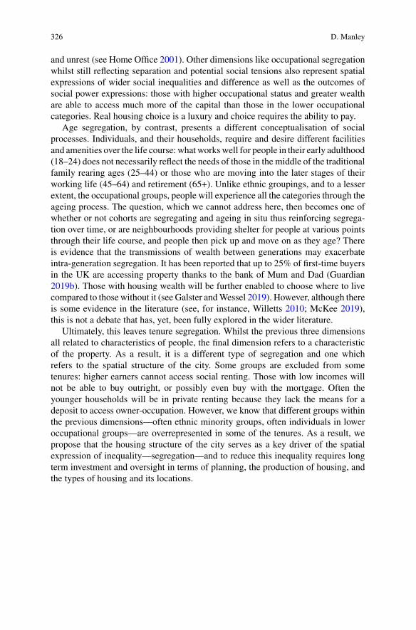
326 D. Manley
and unrest (see Home Office 2001). Other dimensions like occupational segregationwhilst still reflecting separation and potential social tensions also represent spatialexpressions of wider social inequalities and difference as well as the outcomes ofsocial power expressions: those with higher occupational status and greater wealthare able to access much more of the capital than those in the lower occupationalcategories. Real housing choice is a luxury and choice requires the ability to pay.
Age segregation, by contrast, presents a different conceptualisation of socialprocesses. Individuals, and their households, require and desire different facilitiesand amenities over the life course: whatworkswell for people in their early adulthood(18–24) does not necessarily reflect the needs of those in the middle of the traditionalfamily rearing ages (25–44) or those who are moving into the later stages of theirworking life (45–64) and retirement (65+). Unlike ethnic groupings, and to a lesserextent, the occupational groups, people will experience all the categories through theageing process. The question, which we cannot address here, then becomes one ofwhether or not cohorts are segregating and ageing in situ thus reinforcing segrega-tion over time, or are neighbourhoods providing shelter for people at various pointsthrough their life course, and people then pick up and move on as they age? Thereis evidence that the transmissions of wealth between generations may exacerbateintra-generation segregation. It has been reported that up to 25% of first-time buyersin the UK are accessing property thanks to the bank of Mum and Dad (Guardian2019b). Those with housing wealth will be further enabled to choose where to livecompared to those without it (see Galster andWessel 2019). However, although thereis some evidence in the literature (see, for instance, Willetts 2010; McKee 2019),this is not a debate that has, yet, been fully explored in the wider literature.
Ultimately, this leaves tenure segregation. Whilst the previous three dimensionsall related to characteristics of people, the final dimension refers to a characteristicof the property. As a result, it is a different type of segregation and one whichrefers to the spatial structure of the city. Some groups are excluded from sometenures: higher earners cannot access social renting. Those with low incomes willnot be able to buy outright, or possibly even buy with the mortgage. Often theyounger households will be in private renting because they lack the means for adeposit to access owner-occupation. However, we know that different groups withinthe previous dimensions—often ethnic minority groups, often individuals in loweroccupational groups—are overrepresented in some of the tenures. As a result, wepropose that the housing structure of the city serves as a key driver of the spatialexpression of inequality—segregation—and to reduce this inequality requires longterm investment and oversight in terms of planning, the production of housing, andthe types of housing and its locations.
16 Segregation in London: A City of Choices or Structures? 327
References
Atkinson R (2016) Limited exposure: social concealment, mobility and engagement with publicspace by the super-rich in London. Environ Plan A Econ Space 48(7):1302–1317
Booth C (1903) Life and labour of the people in London, vol 1. MacmillanBridge G, Lees L, Butler T (eds) (2011) Mixed communities: gentrification by stealth? Policy PressButler T, Hamnett C, Ramsden MJ (2013) Gentrification, education and exclusionary displacementin East London. Int J Urban Reg Res 37(2):556–575
Butler T, Lees L (2006) Super-gentrification in Barnsbury, London: globalization and gentrifyingglobal elites at the neighbourhood level. Trans Inst British Geograp 31(4):467–487
Catney G (2016) Exploring a decade of small area ethnic (de-) segregation in England and Wales.Urban Stud 53(8):1691–1709
DCLG (2019) Table 685: annual Right to Buy sales by local authority (final version). https://www.gov.uk/government/statistical-data-sets/live-tables-on-social-housing-sales#right-to-buy-sales.Site accessed 16 Dec 2019
Eurostat (2018) Metropolitan area populations. Eurostat, 19 July 2018. https://appsso.eurostat.ec.europa.eu/nui/show.do?dataset=met_pjanaggr3&lang=en. Accessed 7 May 2019
Galster G,Wessel T (2019) Reproduction of social inequality through housing: a three-generationalstudy from Norway. Soc Sci Res 78:119–136
GaWC (2020)GaWC city link classification 2018. https://www.lboro.ac.uk/gawc/world2018link.html. Accessed 19 March 2020
Glass RL (1964) London: aspects of change, vol 3. MacGibbon & KeeGuardian (2019a)Why can’t they come and play?: housing segregation in London, 26March 2019. https://www.theguardian.com/society/2019/mar/26/why-cant-they-come-and-play-housing-segregation-in-london. Accessed 22 July 2019
Guardian (2019b) What first home buyers should know about the bank of Mum andDad. https://www.theguardian.com/australia-news/2019/jul/01/what-first-home-buyers-should-know-about-bank-of-mum-and-dad
Harris R (2012) Local indices of segregation with application to social segregation betweenLondon’s secondary schools, 2003–08/09. Environ Plan A 44(3):669–687
Home Office (2001) Community cohesion: a report of the independent review team (Cantle report)Manley D, Johnston R (2014) London: a dividing city, 2001–11? City 18(6):633–643Manley D, Jones K, Johnston R (2019) Multiscale segregation: multilevel modeling of dissimi-larity—challenging the stylized fact that segregation is greater the finer the spatial scale. ProfessGeograph 1–13. OnlineFirst
McKee K (2019) Generation rent is a myth—housing prospects for millennials are determined byclass. The Conversation, 03.01.2019. https://theconversation.com/generation-rent-is-a-myth-housing-prospects-for-millennials-are-determined-by-class-108996
Meen G, Nygaard C, Meen J (2012) The causes of long-term neighbourhood change. In:Understanding neighbourhood dynamics. Springer, Dordrecht, pp 43–62
Osborne H (2014) Poor doors: the segregation of London’s inner-city flat dwellers’. Guardian25:2014
Sabater A, Graham E, Finney N (2017) The spatialities of ageing: evidencing increasing spatialpolarisation between older and younger adults inEngland andWales.DemographRes 36:731–744
Sassen S (1991) The global city: New York, London, Tokyo. Princeton paperbacks, New YorkSmith T, Noble M, Noble S, Wright G, McLennan D, Plunkett E (2015) The English indices ofdeprivation 2015. Department for Communities and Local Government, London
Willetts D (2010) The Pinch: how the baby boomers took their children’s future-and why theyshould give it back. Atlantic Books Ltd

328 D. Manley
Open Access This chapter is licensed under the terms of the Creative Commons Attribution 4.0International License (http://creativecommons.org/licenses/by/4.0/), which permits use, sharing,adaptation, distribution and reproduction in any medium or format, as long as you give appropriatecredit to the original author(s) and the source, provide a link to the Creative Commons license andindicate if changes were made.
The images or other third party material in this chapter are included in the chapter’s CreativeCommons license, unless indicated otherwise in a credit line to the material. If material is notincluded in the chapter’s Creative Commons license and your intended use is not permitted bystatutory regulation or exceeds the permitted use, you will need to obtain permission directly fromthe copyright holder.
Chapter 17Income Inequality and Segregationin the Paris Metro Area (1990–2015)
Haley McAvay and Gregory Verdugo
Abstract In the last decades, the Paris metro area has experienced important struc-tural changes linked to rising income inequality and a rapidly growing immigrantpopulation. Using census data from 1990, 1999 to 2015, this chapter explores thesetransformations and how they have shaped trends in residential segregation. We findthat the occupational structure of the area shifted upwards in the recent decade with asubstantial increase in the share of the top occupational groups. This trend, however,did not primarily concern the immigrant population, which nonetheless experienceda growth in the middle class. These trends were further accompanied by an increasein income inequality driven by rising wages among the top 1% earners. Despite thesechanges, dissimilarity indexes between socioeconomic groups and between nativesand immigrants have remained quite stable over the period. However, interactionindexes suggest that neighbourhoods are becoming more homogenous over time,both in terms of socioeconomic and ethnic diversity. Finally, the findings shed light onthe correlation between socioeconomic and immigrant segregation. Socioeconomicdisadvantage and the presence of immigrants within neighbourhoods, especially ofnon-European origin, are tightly correlated, and that correlation became strongerover time.
The authors accessed the data via the Centre d’accès sécurisé distant, (CASD), dedicated to theuse of authorized researchers, following the approval of the Comité français du secret statis-tique. This research was supported by a French state grant (grant no. ANR-10-EQPX-17) (Centred’accès sécurisé aux données, CASD) and the ‘Flash Asile’ program of the Agence Nationalede la Recherche (ANR-16-FASI-0001 and ANR-11-IDEX-0003-02). We would also like to thankThe Paris Region Development and Urban Planning Agency (IAU Ile-de-France) for providingshapefiles.
H. McAvay (B)Department of Sociology, University of York, 292 Wentworth Way, Heslington, YorkYO10 5NG, UKe-mail: [email protected]
G. VerdugoUniversité Paris-Saclay, Univ Evry, EPEE and OFCE, 23 Boulevard Francois Mitterrand, 91000Evry, Francee-mail: [email protected]
© The Author(s) 2021M. van Ham et al. (eds.), Urban Socio-Economic Segregation and Income Inequality,The Urban Book Series, https://doi.org/10.1007/978-3-030-64569-4_17
329
330 H. McAvay and G. Verdugo
Keywords Paris metro area · Spatial segregation · Socioeconomic segregation ·Immigrant segregation
17.1 Introduction
In the last decade, the population of the Paris metro area grew rapidly, and withmore than 12 million inhabitants in 2015, it is one of the largest urban centres inEurope. As a major economic and political capital, the composition of its populationis more polarised than the French or European average, with a smaller proportionof the middle classes and strong income inequality (Labrador 2013). Moreover, likeother major cities in Western Europe, the Paris area has seen a rise in immigrationin recent decades, particularly from non-European countries.
Despite these broad structural changes, relatively little evidence is available onhow these transformations affected residential segregation in the Paris metro area.Since the 1980s, substantial urban renewal and social mix policies have been imple-mented in Francewith the aim of combating segregation. Policymaking has primarilytargeted the poor peripheral urban areas known as the banlieues, where many immi-grants from France’s former colonies settled in public housing projects. Hit bydeindustrialisation and economic hardship, these areas have become synonymouswith high unemployment, poor-quality schools, crime and are even symbolic of thefailure of immigrant integration. Recent assessments of French urban policy docu-ment that urban renewal and social mix initiatives have been largely unsuccessful andhave even had the unintended consequence of reinforcing segregation (Epstein 2011;Fol 2013). Meanwhile, an increasing number of studies suggest negative effects ofliving in disadvantaged and segregated neighbourhoods on employment (Gobillonet al. 2011; Petit et al. 2016).
This chapter uses French census data from 1990, 1999 and 2015 to investigatechanges in occupational structure, inequality and residential segregation in the Parismetro area. We add to prior literature on segregation in Paris by using the mostrecent available data on the entire metropolitan area, comparing three census datesusing small spatial scales comparable to census tracts (IRIS),1 and by articulatingsocioeconomic and immigrant segregation. The chapter has three broad objectives:(1) to document structural changes in the urban population linked to occupation,income inequality and immigration; (2) to analyse the residential distribution ofsocioeconomic groups and (3) to describe trends in socioeconomic and immigrantsegregation over time and the ways in which they are correlated.
1We use the entire Ile de France region and census tracts of about 2,500 inhabitants, whereas themajor prior study on socioeconomic segregation focused on the city of Paris only using larger tracts(Préteceille 2006) due to data availability constraints.
17 Income Inequality and Segregation in the Paris Metro Area (1990–2015) 331
17.2 Background
Since the 1980s, residential segregation has been a predominant target of policy-making and has received pervasive media attention in France (Lelévrier and Melic2018). Yet, it is only recently that systematic empirical research based on represen-tative data has shed light on spatial inequalities. Unlike the U.S. or other Europeancontexts, which have long been concerned with the unequal spatial distribution ofminorities, in France, the earliest studies tackled segregation from the angle of socialclass using occupational groups (Tabard 1993;Maurin 2004; Préceteille 2006). Préte-ceille (2006) offers one of the first studies of socioeconomic segregation in the Parisregion, measuring changes in dissimilarity indexes between occupational groups inneighbourhoods between 1990 and 1999. He finds that the strongest indices areobserved for upper-status occupations and are increasing over time, whereas inter-mediary groups are becoming less segregated. He further points out that residentsof Paris still predominately live in middle-class and mixed neighbourhoods. Morerecent studies have weighed in on this debate using tax and administrative employeedata, allowing analysis by income groups rather than occupational categories. Gode-chot (2013) focuses on the spatial concentration of the wealthiest households (top1% and 0.1% of earners) and documents that the level of segregation for top earnersis the strongest in Paris compared to other French cities and is on the rise. Mostrecently, using tax data at the communal level, Ribardière (2019) also points to anincrease in residential segregation by income in the Paris area between 1999 and2015.
Overall, despite methodological differences between these studies, the evidenceindicates increasing socioeconomic segregation, owing to the strong spatial isola-tion of upper-status groups in particular. Below we discuss three potential mecha-nisms underpinning socioeconomic segregation in the Paris area: the segregation ofimmigrants, urban policy and public housing, and rising income inequality.
17.2.1 The Role of Immigrant Residential Segregation
While residential segregation in France is primarily viewed as an issue of class, that is,relating to the unequal distribution of socioeconomic groups, urban disadvantage andimmigration have been historically tightly intertwined in the French context.2 Duringthe 1980s, post-colonial immigrants found accommodation primarily in the largepublic housing projects embedded in the suburbs of large urban areas (banlieues)
2This framing of segregation as predominately a problem of class can be at least partly understoodin light of the Republican colorblind model and the Marxist tradition in the French social sciences.France considers distinctions on the basis of race/ethnicity to be illegitimate and therefore does notcollect ethnic/racial statistics, creating significant barriers tomeasuring racial residential segregationor other inequalities. At the same time, the predominance of Marxism within French sociologyhindered enquiry into the ethnoracial dimensions of stratification beyond social class mechanisms(Safi 2013).
332 H. McAvay and G. Verdugo
near industrial sites where jobs were available. In the wake of deindustrialisation andrising unemployment, the banlieues became explicitly synonymous with socioeco-nomic disadvantage and implicitly associated with racial minorities. These neigh-bourhoods drew public attention following the highly mediatised urban riots duringthe 1980s and early 2000s involving minorities and contributed to the constructionof segregation as a social problem.
It is not until the mid-2000s that research began to quantify the extent of residen-tial segregation between immigrants and French natives (Préteceille 2009; Safi 2009;Verdugo 2011; Pan Ké Shon and Verdugo 2015). These studies analyse segregationat the municipality level from consecutive censuses. Their results show high segre-gation in Paris between natives and immigrants from North Africa, Sub-SaharanAfrica and Turkey, which increased moderately between 1968 and 1999. Verdugo(2011) was the first to study the long-term evolution of immigrant segregation atthe level of the census tract. He documented higher levels of segregation for non-European immigrants, which were rising largely due to the increased concentrationof immigrants living in public housing. Although less is known about segregationbeyond the first generation, due to restrictions in census data, a few studies indicatethat spatial inequalities are largely transmitted to the second generation, particularlyamong non-Europeans (McAvay 2018a, b;McAvay and Safi 2018). Immigrant segre-gation appears to be in part maintained by discrimination on the Parisian housingmarket (Bonnet et al. 2016; Bunel et al. 2017) as well as native flight dynamics outof immigrant areas (Rathelot and Safi 2014; McAvay 2018a, b), particularly in areasnear large public housing projects (Verdugo and Toma 2018).
These findings from France align with lessons from the U.S. about racial resi-dential segregation. Massey and Denton (1993) emphasise how discrimination andrace-based residential preferences create a segmented housing market that channelminorities into poor areas. They further make the argument that racial segregationand racial inequalities may more broadly operate as a mechanism of socioeconomicsegregation and the concentration of poverty. If racial minorities have lower incomeon average, the spatial separation of racial groups would automatically result insegregation along class lines, separating high-income racial groups from low-incomeracial groups (Massey and Denton 1993; Reardon and Bischoff 2011). Quillian andLagrange (2016) show that racial segregation and income segregation are correlatedto a similar degree in France and the U.S., while McAvay and Safi (2018) showan overlap between ethnoracial and socioeconomic segregation at the individuallevel. Hence, it is possible that the rise in non-European immigrants and their spatialseparation from natives may contribute to socioeconomic segregation in the Frenchcontext.
17.2.2 The Role of Urban Policy and Public Housing
French urban policy emerges formally in the 1980s with the aim of reducing socialinequalities, targeting specifically the so-called quartiers sensibles with large shares
17 Income Inequality and Segregation in the Paris Metro Area (1990–2015) 333
of public housing. The main locus of state intervention in urban areas is the publichousing sector, which provides low-rent government-owned or -subsidised units(habitation à loyer modéré, or HLM). Built in the post-war period to improve livingconditions and resettle slum residents, public housing projects are now associatedwith socioeconomic disadvantage and the concentration ofminorities in thebanlieues(Lelévrier 2010). With the creation of ‘priority zones,3’ France implemented its firstspatial affirmative action (Epstein 2011; Fol 2013). The most ambitious national-level urban policy plan was introduced in 2003, the Loi Borloo, with the aim ofcreating a social mix in priority zones through urban renewal and redistributive poli-cies. The policies aimed to achieve a social mix by first demolishing public housingto create new real estate opportunities on the private market in these areas, with theaim of attracting the middle class; and second, by building new public housing unitsin areas where it is under-represented, in order to relocate poor households to moremixed spaces. While these policies are explicitly about class, many argue that theyare implicitly concerned with the concentration of minorities (Epstein 2011).
More than a decade later, the social mix sought by the 2003 reform is largelyconsidered a failure. Research even suggests that urban renewal and social mixpolicies had unintended consequences that contributed to reinforcing segregation.Studying these effects in the Paris area, Lelévrier (2010) shows that these policiestriggered upper-class mobility out of the targeted areas, while poor households wererelocated in disadvantaged areas, primarily in other sensitive urban zones. Thus, incontradiction with their stated aim, these policies actually resulted in a reconcen-tration of poverty by channelling similar SES households to similar areas. Further,despite the substantial resources invested in the targeted areas, Epstein (2011) empha-sises the failure of spatial affirmative action as unemployment is still two times higherin sensitive urban zones compared to the national average.
Other unintended consequences of urban policy have unfolded in the publichousing sector, revealing its ambiguous role in maintaining segregation. The urbanpolicy has used public housing as a tool for maintaining social mix. The 2000 UrbanSolidarity andRenewal law (SRU)made itmandatory for all cities to have at least 20%social housing. This would allow poor populations to live in more affluent munic-ipalities and prevent them from being forced out of gentrifying areas with risinghousing prices (Ribardière 2019). Yet evidence shows that the sector is stronglysegregated along class lines. As income eligibility requirements are broad enoughto include middle-class households, the public housing sector is not reserved for thepoor (Whitehead and Scanlon 2007). However, the poorest residents tend to live inlow-quality housing in poor areas, while high and middle-income households haveaccess to higher-quality buildings in more attractive, central locations (WhiteheadandScanlon 2007; Lelévrier andMelic 2018). Public housing has also had ambiguouseffects on the segregation of immigrants. A number of French urban studies haveshown that social mix policies used in attributing public housing have resulted ininformal racial profiling, by which the housing demand of non-European origin
3Specifically, the creation of priority educational zones (‘ZEP’) in 1981, followed by sensitive urbanzones (‘ZUS’) in 1996.
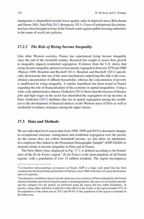
334 H. McAvay and G. Verdugo
immigrants is channelled towards lower quality units in deprived areas (Kirszbaumand Simon 2001; Sala Pala 2013; Bourgeois 2013). Cases of institutional discrimina-tion have been brought in front of the French courts against public housing authoritiesin the name of social mix policies.
17.2.3 The Role of Rising Income Inequality
Like other Western societies, France has experienced rising income inequalitysince the end of the twentieth century. Research has sought to assess how growthin inequality impacts residential segregation. Evidence from the U.S. shows thatrising income inequality spurred socioeconomic segregation between 1970 and 2000(Watson 2009; Reardon and Bischoff 2011). Reardon and Bischoff (2011) specifi-cally demonstrate that one of the main mechanisms underlying this link is the exac-erbated concentration of affluent households, whereas the concentration of povertyis unaffected by rising inequality. A similar hypothesis has been tested in Franceregarding the role of financialisation of the economy in spatial inequalities. Using awide-scale administrative dataset, Godechot (2013) shows that the increase of financejobs and high wages in the sector has intensified the segregation of top incomes inParis. Godechot (2013) attributes this rise in spatial segregation among the wealth-iest to the development of financial districts in the Western areas of Paris as well asresidential avoidance strategies among the upper classes.
17.3 Data and Methods
We use individual-level census data from 1990, 1999 and 2015 to document changesin occupational structure, immigration and residential segregation over the period.As the census does not collect household income, we also draw on administra-tive employee files linked to the Permanent Demographic Sample4 (EDP-DADS) tomeasure trends in income inequality in Paris and in France.
The Paris Metro Area, displayed in Fig. 17.1, is defined according to the bound-aries of the Ile-de-France region.5 Ile-de-France is the most populous of all Frenchregions, with a population of over 12 million residents. The region encompasses
4L’échantillon démographique permanent in French. EDP is a large scale panel that has beenconducted by the FrenchNational Institute of Statistics since 1968 on the basis of census declarationsand civil registries.5An alternativewould have been to use the urban area (aire urbaine) of Paris estimated by the Frenchstatistical institute andwhich is based on daily commuting patterns. Because it is revised periodicallyand has changed over the period, we preferred using the region that has stable boundaries. Inpractice, using either definition would have little effect on the results as the region includes 97% ofthe population of the urban area in 2013 and 99.9% of the population of the region is included inthe urban area.
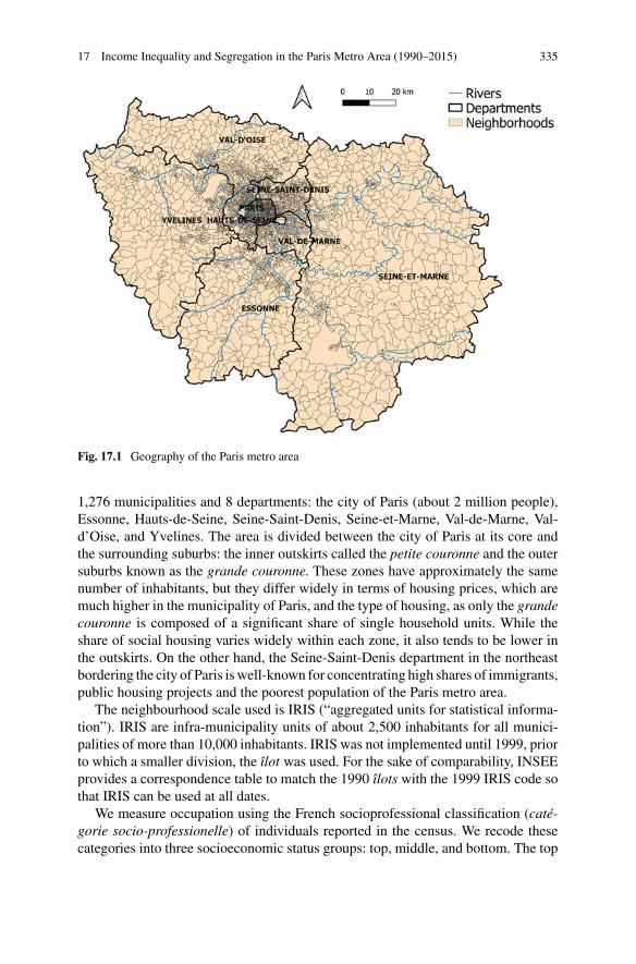
17 Income Inequality and Segregation in the Paris Metro Area (1990–2015) 335
Fig. 17.1 Geography of the Paris metro area
1,276 municipalities and 8 departments: the city of Paris (about 2 million people),Essonne, Hauts-de-Seine, Seine-Saint-Denis, Seine-et-Marne, Val-de-Marne, Val-d’Oise, and Yvelines. The area is divided between the city of Paris at its core andthe surrounding suburbs: the inner outskirts called the petite couronne and the outersuburbs known as the grande couronne. These zones have approximately the samenumber of inhabitants, but they differ widely in terms of housing prices, which aremuch higher in the municipality of Paris, and the type of housing, as only the grandecouronne is composed of a significant share of single household units. While theshare of social housing varies widely within each zone, it also tends to be lower inthe outskirts. On the other hand, the Seine-Saint-Denis department in the northeastbordering the city of Paris iswell-known for concentrating high shares of immigrants,public housing projects and the poorest population of the Paris metro area.
The neighbourhood scale used is IRIS (“aggregated units for statistical informa-tion”). IRIS are infra-municipality units of about 2,500 inhabitants for all munici-palities of more than 10,000 inhabitants. IRIS was not implemented until 1999, priorto which a smaller division, the îlot was used. For the sake of comparability, INSEEprovides a correspondence table to match the 1990 îlots with the 1999 IRIS code sothat IRIS can be used at all dates.
We measure occupation using the French socioprofessional classification (caté-gorie socio-professionelle) of individuals reported in the census. We recode thesecategories into three socioeconomic status groups: top, middle, and bottom. The top
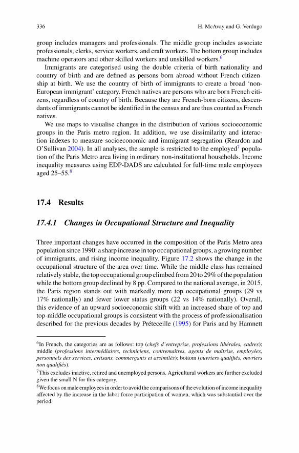
336 H. McAvay and G. Verdugo
group includes managers and professionals. The middle group includes associateprofessionals, clerks, service workers, and craft workers. The bottom group includesmachine operators and other skilled workers and unskilled workers.6
Immigrants are categorised using the double criteria of birth nationality andcountry of birth and are defined as persons born abroad without French citizen-ship at birth. We use the country of birth of immigrants to create a broad ‘non-European immigrant’ category. French natives are persons who are born French citi-zens, regardless of country of birth. Because they are French-born citizens, descen-dants of immigrants cannot be identified in the census and are thus counted as Frenchnatives.
We use maps to visualise changes in the distribution of various socioeconomicgroups in the Paris metro region. In addition, we use dissimilarity and interac-tion indexes to measure socioeconomic and immigrant segregation (Reardon andO’Sullivan 2004). In all analyses, the sample is restricted to the employed7 popula-tion of the Paris Metro area living in ordinary non-institutional households. Incomeinequality measures using EDP-DADS are calculated for full-time male employeesaged 25–55.8
17.4 Results
17.4.1 Changes in Occupational Structure and Inequality
Three important changes have occurred in the composition of the Paris Metro areapopulation since 1990: a sharp increase in top occupational groups, a growing numberof immigrants, and rising income inequality. Figure 17.2 shows the change in theoccupational structure of the area over time. While the middle class has remainedrelatively stable, the top occupational group climbed from20 to 29%of the populationwhile the bottom group declined by 8 pp. Compared to the national average, in 2015,the Paris region stands out with markedly more top occupational groups (29 vs17% nationally) and fewer lower status groups (22 vs 14% nationally). Overall,this evidence of an upward socioeconomic shift with an increased share of top andtop-middle occupational groups is consistent with the process of professionalisationdescribed for the previous decades by Préteceille (1995) for Paris and by Hamnett
6In French, the categories are as follows: top (chefs d’entreprise, professions libérales, cadres);middle (professions intermédiaires, techniciens, contremaîtres, agents de maîtrise, employées,personnels des services, artisans, commerçants et assimilés); bottom (ouvriers qualifiés, ouvriersnon qualifiés).7This excludes inactive, retired and unemployed persons. Agricultural workers are further excludedgiven the small N for this category.8We focus onmale employees in order to avoid the comparisons of the evolution of income inequalityaffected by the increase in the labor force participation of women, which was substantial over theperiod.
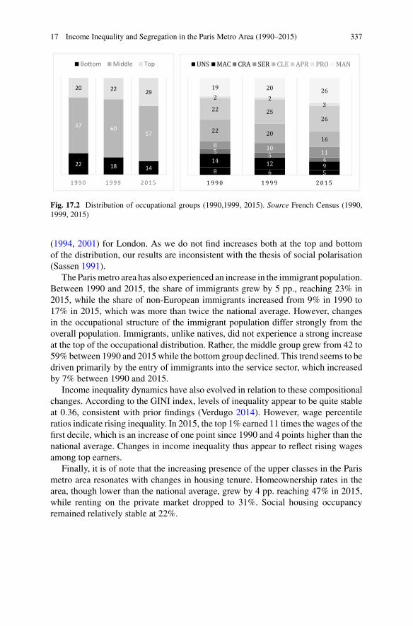
17 Income Inequality and Segregation in the Paris Metro Area (1990–2015) 337
22 18 14
57 6057
20 22 29
1990 1999 2015
Bo om Middle Top
Fig. 17.2 Distribution of occupational groups (1990,1999, 2015). Source French Census (1990,1999, 2015)
(1994, 2001) for London. As we do not find increases both at the top and bottomof the distribution, our results are inconsistent with the thesis of social polarisation(Sassen 1991).
The Parismetro area has also experienced an increase in the immigrant population.Between 1990 and 2015, the share of immigrants grew by 5 pp., reaching 23% in2015, while the share of non-European immigrants increased from 9% in 1990 to17% in 2015, which was more than twice the national average. However, changesin the occupational structure of the immigrant population differ strongly from theoverall population. Immigrants, unlike natives, did not experience a strong increaseat the top of the occupational distribution. Rather, the middle group grew from 42 to59% between 1990 and 2015while the bottom group declined. This trend seems to bedriven primarily by the entry of immigrants into the service sector, which increasedby 7% between 1990 and 2015.
Income inequality dynamics have also evolved in relation to these compositionalchanges. According to the GINI index, levels of inequality appear to be quite stableat 0.36, consistent with prior findings (Verdugo 2014). However, wage percentileratios indicate rising inequality. In 2015, the top 1% earned 11 times the wages of thefirst decile, which is an increase of one point since 1990 and 4 points higher than thenational average. Changes in income inequality thus appear to reflect rising wagesamong top earners.
Finally, it is of note that the increasing presence of the upper classes in the Parismetro area resonates with changes in housing tenure. Homeownership rates in thearea, though lower than the national average, grew by 4 pp. reaching 47% in 2015,while renting on the private market dropped to 31%. Social housing occupancyremained relatively stable at 22%.
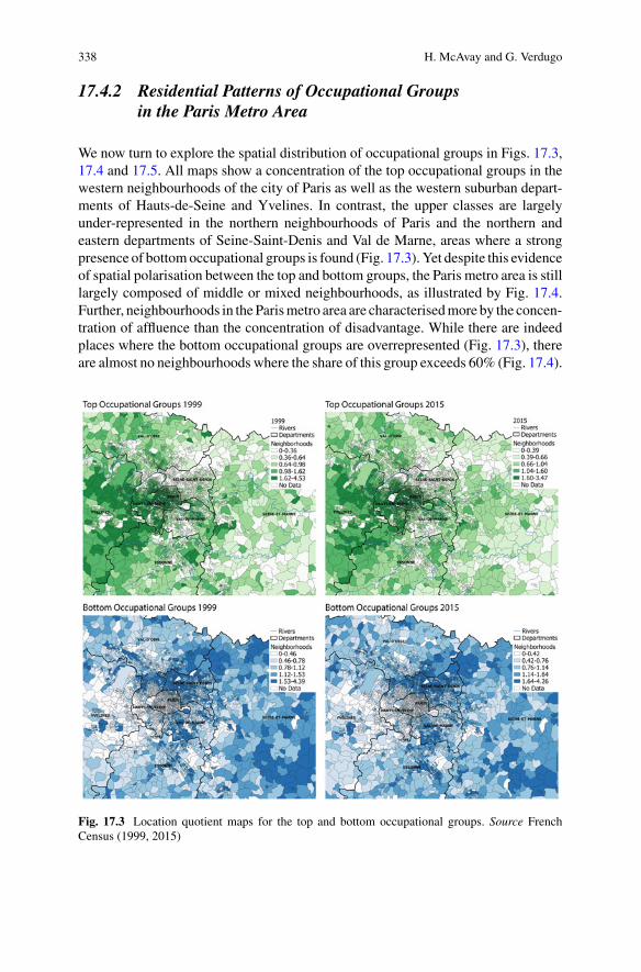
338 H. McAvay and G. Verdugo
17.4.2 Residential Patterns of Occupational Groupsin the Paris Metro Area
We now turn to explore the spatial distribution of occupational groups in Figs. 17.3,17.4 and 17.5. All maps show a concentration of the top occupational groups in thewestern neighbourhoods of the city of Paris as well as the western suburban depart-ments of Hauts-de-Seine and Yvelines. In contrast, the upper classes are largelyunder-represented in the northern neighbourhoods of Paris and the northern andeastern departments of Seine-Saint-Denis and Val de Marne, areas where a strongpresence of bottomoccupational groups is found (Fig. 17.3). Yet despite this evidenceof spatial polarisation between the top and bottom groups, the Paris metro area is stilllargely composed of middle or mixed neighbourhoods, as illustrated by Fig. 17.4.Further, neighbourhoods in theParismetro area are characterisedmore by the concen-tration of affluence than the concentration of disadvantage. While there are indeedplaces where the bottom occupational groups are overrepresented (Fig. 17.3), thereare almost no neighbourhoods where the share of this group exceeds 60% (Fig. 17.4).
Fig. 17.3 Location quotient maps for the top and bottom occupational groups. Source FrenchCensus (1999, 2015)
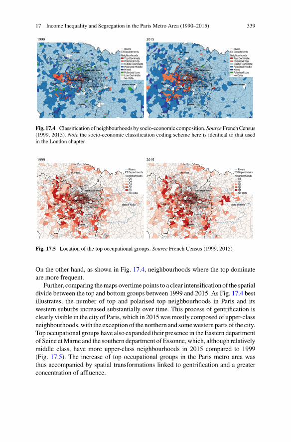
17 Income Inequality and Segregation in the Paris Metro Area (1990–2015) 339
Fig. 17.4 Classification of neighbourhoods by socio-economic composition. SourceFrenchCensus(1999, 2015). Note the socio-economic classification coding scheme here is identical to that usedin the London chapter
Fig. 17.5 Location of the top occupational groups. Source French Census (1999, 2015)
On the other hand, as shown in Fig. 17.4, neighbourhoods where the top dominateare more frequent.
Further, comparing themaps overtime points to a clear intensification of the spatialdivide between the top and bottom groups between 1999 and 2015. As Fig. 17.4 bestillustrates, the number of top and polarised top neighbourhoods in Paris and itswestern suburbs increased substantially over time. This process of gentrification isclearly visible in the city of Paris, which in 2015wasmostly composed of upper-classneighbourhoods,with the exception of the northern and somewestern parts of the city.Top occupational groups have also expanded their presence in the Eastern departmentof Seine etMarne and the southern department of Essonne, which, although relativelymiddle class, have more upper-class neighbourhoods in 2015 compared to 1999(Fig. 17.5). The increase of top occupational groups in the Paris metro area wasthus accompanied by spatial transformations linked to gentrification and a greaterconcentration of affluence.
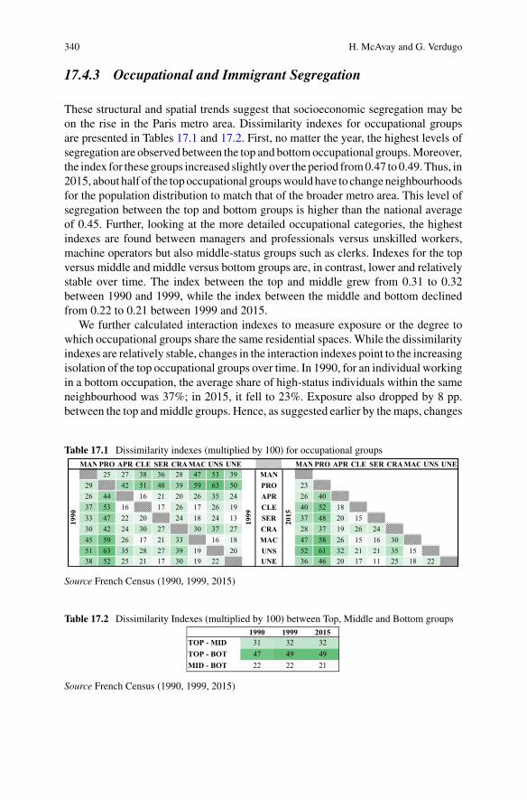
340 H. McAvay and G. Verdugo
17.4.3 Occupational and Immigrant Segregation
These structural and spatial trends suggest that socioeconomic segregation may beon the rise in the Paris metro area. Dissimilarity indexes for occupational groupsare presented in Tables 17.1 and 17.2. First, no matter the year, the highest levels ofsegregation are observed between the top and bottomoccupational groups.Moreover,the index for these groups increased slightly over the period from0.47 to0.49.Thus, in2015, about half of the topoccupational groupswouldhave to changeneighbourhoodsfor the population distribution to match that of the broader metro area. This level ofsegregation between the top and bottom groups is higher than the national averageof 0.45. Further, looking at the more detailed occupational categories, the highestindexes are found between managers and professionals versus unskilled workers,machine operators but also middle-status groups such as clerks. Indexes for the topversus middle and middle versus bottom groups are, in contrast, lower and relativelystable over time. The index between the top and middle grew from 0.31 to 0.32between 1990 and 1999, while the index between the middle and bottom declinedfrom 0.22 to 0.21 between 1999 and 2015.
We further calculated interaction indexes to measure exposure or the degree towhich occupational groups share the same residential spaces. While the dissimilarityindexes are relatively stable, changes in the interaction indexes point to the increasingisolation of the top occupational groups over time. In 1990, for an individual workingin a bottom occupation, the average share of high-status individuals within the sameneighbourhood was 37%; in 2015, it fell to 23%. Exposure also dropped by 8 pp.between the top andmiddle groups. Hence, as suggested earlier by themaps, changes
Table 17.1 Dissimilarity indexes (multiplied by 100) for occupational groupsMAN PRO APR CLE SER CRA MAC UNS UNE MAN PRO APR CLE SER CRA MAC UNS UNE
25 27 38 36 28 47 53 39 MAN29 42 51 48 39 59 63 50 PRO 2326 44 16 21 20 26 35 24 APR 26 4037 53 16 17 26 17 26 19 CLE 40 52 1833 47 22 20 24 18 24 13 SER 37 48 20 1530 42 24 30 27 30 37 27 CRA 28 37 19 26 2445 59 26 17 21 33 16 18 MAC 47 58 26 15 16 3051 63 35 28 27 39 19 20 UNS 52 61 32 21 21 35 1538 52 25 21 17 30 19 22 UNE 36 46 20 17 11 25 18 22
1999
2015
1990
Source French Census (1990, 1999, 2015)
Table 17.2 Dissimilarity Indexes (multiplied by 100) between Top, Middle and Bottom groups1990 1999 2015
TOP - MID 31 32 32TOP - BOT 47 49 49MID - BOT 22 22 21
Source French Census (1990, 1999, 2015)
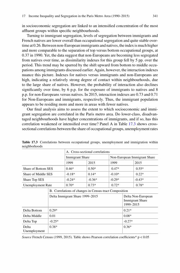
17 Income Inequality and Segregation in the Paris Metro Area (1990–2015) 341
in socioeconomic segregation are linked to an intensified concentration of the mostaffluent groups within specific neighbourhoods.
Turning to immigrant segregation, levels of segregation between immigrants andFrench natives are lower overall than occupational segregation and quite stable over-time at 0.26.Betweennon-European immigrants andnatives, the index ismuchhigherand more comparable to the separation of top versus bottom occupational groups, at0.37 in 1990. Yet, the data suggest that non-Europeans are becoming less segregatedfrom natives over time, as dissimilarity indexes for this group fell by 5 pp. over theperiod. This trend may be spurred by the shift upward from bottom to middle occu-pations among immigrants discussed earlier. Again, however, the interaction indexesnuance this picture. Indexes for natives versus immigrants and non-Europeans arehigh, indicating a relatively strong degree of contact within neighbourhoods, dueto the large share of natives. However, the probability of interaction also declinessignificantly over time, by 6 p.p. for the exposure of immigrants to natives and 8p.p. for non-Europeans versus natives. In 2015, interaction indexes are 0.73 and 0.71for Non-Europeans and immigrants, respectively. Thus, the immigrant populationappears to be residing more and more in areas with fewer natives.
Our final analysis aims to assess the extent to which socioeconomic and immi-grant segregation are correlated in the Paris metro area. Do lower-class, disadvan-taged neighbourhoods have higher concentrations of immigrants, and if so, has thiscorrelation weakened or intensified over time? Panel A in Table 17.3 shows cross-sectional correlations between the share of occupational groups, unemployment rates
Table 17.3 Correlations between occupational groups, unemployment and immigration withinneighborhoods
A. Cross-sectional correlations
Immigrant Share Non-European Immigrant Share
1999 2015 1999 2015
Share of Bottom SES 0.46* 0.50* 0.47* 0.55*
Share of Middle SES -0.18* 0.14* -0.10* 0.22*
Share Top SES -0.24* -0.36* -0.29* -0.43*
Unemployment Rate 0.70* 0.73* 0.72* 0.78*
B. Correlations of changes in Census-tract Composition
Delta Immigrant Share 1999–2015 Delta Non-EuropeanImmigrant Share1999–2015
Delta Bottom 0.29* 0.21*
Delta Middle 0.01 0.08*
Delta Top -0.25* -0.27*
DeltaUnemployment
0.38* 0.36*
Source French Census (1999, 2015). Table shows Pearson correlation coefficients* p < 0.05
342 H. McAvay and G. Verdugo
and immigrant shares of neighbourhoods in the area. In both 1999 and 2015, greatershares of immigrants are strongly positively correlated with the share of bottomoccupational groups and high unemployment rates in neighbourhoods. On the otherhand, the presence of immigrants—especially of non-European origin—is negativelylinked with the share of top occupational groups. Interestingly, however, while theshare of immigrants in neighbourhoods was negatively correlated with the presenceof middle groups in 1999, this correlation turned positive—if still weak—in 2015.
All in all, the correlation between immigrant-dense and low-SES neighbourhoodsbecome markedly stronger between 1999 and 2015. This is confirmed in panel B inwhich we report the correlations between the changes in shares of immigrants, lowand high-status groups and unemployment rates in neighbourhoods between 1999and 2015. Clearly, neighbourhoods that experienced an influx of immigrants or non-European immigrants saw a significant reduction in the shares of high-status groups,an increase in unemployment and a rise in the share of low-status occupations. Whilenot causal, these patterns suggest that immigrant neighbourhoods tend to increasinglyconcentrate disadvantage alongwith a “flight” of the upper classes from these spaces.
17.5 Conclusion
This chapter explored changes in occupational structure, income inequality andimmigration in the Paris metro area between 1990 and 2015 and ways in whichthese changes shaped the spatial divide between socioeconomic groups and immi-grants and natives. We find that a shift to the top of the occupational distributionoccurred in recent decades with a substantial increase in the share of top occupationsand a drop in low-status groups. Income inequality also grew over the period, drivenby rising wages among the top 1% earners.
At first glance, residential segregation between occupational groups appeared tochange only marginally in conjunction with these evolutions. Dissimilarity indexesremained quite stable, with only a small increase observed between the bottom andtop occupational groups. Segregation further appeared to decrease slightly betweenmiddle and bottom occupations. However, the dissimilarity indexes mask increasingspatial homogeneity over the period, as interaction indexes reveal that the upperclasses have become substantially less likely to share the same neighbourhoods withother groups. In line with this lower degree of contact between SES groups, the mapsshowed an expansion of high-status neighbourhoods in the Western suburbs of Parisand the city centre. These trends alignwith evidence of gentrification and the growingspatial isolation of the upper classes highlighted in previous studies (Préteceille 2006;Godechot 2013; Ribardière 2019), and lend support to the hypothesis that incomeinequality, likely related to the expanding financial sector (Godechot 2013), hascontributed to the intensification of socioeconomic residential segregation in theParis area.
We further investigated changes in the residential segregation of immigrants andits relation to socioeconomic segregation. The findings show that segregation is
17 Income Inequality and Segregation in the Paris Metro Area (1990–2015) 343
highest between Non-Europeans and natives, much stronger than levels of segre-gation for immigrants overall and for most occupational groups. Further, althoughdissimilarity indexes remained stable or dropped somewhat between immigrantsand natives, interaction indexes again revealed decreasing contact between thesegroups within neighbourhoods over time. Moreover, while immigrants have enteredthe middle occupational groups over the period, the correlation in neighbourhoodsbetween low socioeconomic status, high unemployment and the presence of immi-grants is strong and growing. These trends may reflect the effects of discriminationor native flight processes—especially among the upper classes—which consolidatedisadvantage within neighbourhoods that have high shares of immigrants. Overall,socioeconomic and immigrant segregation are tightly correlated, and increasingly soover time.
A limitation of our analysis is that we do not observe second-generation immi-grants.Descendants of immigrantswho are not livingwith their parents are not identi-fied as such in the census and are thus counted as French natives. It is possible that thestability and even decline in the dissimilarity indexes between Non-European immi-grants and natives masks an increase in the share of second-generation immigrants inthe neighbourhood. This would coincide with prior research that shows similar levelsof residential segregation and disadvantage for second generations compared to theirparents (McAvay 2018a, b; McAvay and Safi 2018). While plausible, this claimshould be nuanced by the fact that second generations of non-European origin livingindependently from their parents accounted for about 3% of the French populationin 2015 (Brutel 2017).
All in all, it is notable that, as prior research has highlighted, the intensification ofspatial inequalities documented here is at oddswith recent French urban policy initia-tives that have explicitly sought to curtail socioeconomic segregation, particularlyby renewing disadvantaged urban areas to attract middle and upper-class house-holds (Lelévrier 2010; Epstein 2011; Fol 2013). As the Paris area becomes moregentrified and wages are rising among the wealthiest households, the upper classesare better able to implement strategies to avoid poor or ethnoracially diverse areas,while prohibitive housing prices and discrimination keep poor households and immi-grants out of upper-class neighbourhoods. It also seems likely that the conjunctionof socioeconomic disadvantage and the presence of immigrants within neighbour-hoods will reinforce white flight and avoidance processes as these areas becomestigmatised both due to their class and ethnic composition. At the same time, thereduced social and residential mobility prospects of people living in poor areas,particularly minorities, compounds socio-spatial inequalities. Rather than investingin costly transformations of targeted urban neighbourhoods, more effective redis-tributive policymaking might aim at favouring social mobility opportunities amongminorities and disadvantaged groups.
344 H. McAvay and G. Verdugo
References
Bonnet F,LaléE,SafiM,WasmerE (2016)Better residential than ethnic discrimination!Reconcilingaudit and interview findings in the Parisian housing market. Urban Stud 53(13):2815–2833
Bourgeois M (2013) Choisir les locataires du parc social? Une approche ethnographique de lagestion des HLM. Sociol Du Travail 55(1):56–75
Bunel M, l’Horty Y, Du Parquet L, Petit P (2017) Les discriminations dans l’accès au logement àParis: une expérience contrôlée 〈halshs-01521995〉
Brutel, C. (2017). Etre né en France d’un parent immigré: Une population diverse reflétant l’histoiredes flux migratoires (Insee Première No. 1634). L’Institut National de la Statistique et desÉtudesÉconomiques, Paris, France
Epstein R (2011) Politiques de la ville: bilan et (absence de) perspectives. Regards Croisés Surl’économie 1:203–211
FolS (2013)Lapolitiquede la ville, unoutil pour lutter contre la ségrégation?L’infGéogr 77(3):6–28Gobillon L, Magnac T, Selod H (2011) The effect of location on finding a job in the Paris region. JAppl Econ 26:1079–1112
Godechot O (2013) Financiarisation Et Fractures Socio-Spatiales. L’année Sociol 63(1):17–50Hamnett, C. (1994). Socio-economic change in London: professionalization not polarization. BuiltEnviron 192–203.
Hamnett C (2001) Social segregation and social polarization. Handbook of urban studies, pp 162–176
Kirszbaum T, Simon P (2001) Les discriminations raciales et ethniques dans l’accès au logementsocial
Labrador J (2013) Une forte hétérogénéité des revenues en Ile-de-France. Ile-de-France à la page.N. 414. INSEE
Lelévrier C (2010) La mixité dans la rénovation urbaine: dispersion ou re-concentration? EspacesEt Sociétés 1:59–74
Lelévrier C, Melic T (2018) Impoverishment and social fragmentation in housing estates of theParis region, France. In: Hess DB, Tammaru T, van Ham M (eds) Housing estates in Europe:poverty, ethnic segregation and policy challenges. Springer.
Massey DS, Denton NA (1993) American apartheid: segregation and the making of the underclass.Harvard University Press.
Maurin E (2004) Le ghetto français. Enquête sur le séparatisme social, Paris, Le SeuilMcAvay H (2018a) How durable are ethnoracial segregation and spatial disadvantage? Intergener-ational Contextual Mobility in France. Demography 55(4):1507–1545
McAvay H (2018b) The ethnoracial context of residential mobility in France: Neighbourhoodout-migration and relocation. Population, Space and Place 24(6):e2138
McAvay H, Safi M (2018) Is there really such thing as immigrant spatial assimilation in France?Desegregation trends and inequality along ethnoracial lines. Soc Sci Res 73:45–62
Pan Ké Shon JL, Verdugo G (2015) Forty years of immigrant segregation in France, 1968–2007.How different is the new immigration?. Urban Stud 52(5):823–840
Petit P, Bunel M, Ene E, L’Horty Y (2016) Effets de quartier, effet de département: discriminationliée au lieu de résidence et accès à l’emploi. Revue Économique 67(3):525–550
Preteceille E (1995) Division sociale de l’espace et globalisation: le cas de la métropole parisienne.Sociétés Contemp. 22(23):33–67
Préteceille E (2006) La ségrégation sociale a-t-elle augmenté : la métropole parisienne entrepolarisation et mixité. Sociétés Contemp, no 62:69–93
Préteceille E (2009) La ségrégation ethno-raciale a-t-elle augmenté dans la métropole parisienne?Revue Française De Sociol 50(3):489–519
Quillian L, Lagrange H (2016) Socioeconomic segregation in large cities in France and the UnitedStates. Demography 53(4):1051–1084
Rathelot R, Safi M (2014) Local ethnic composition and natives’ and immigrants’ geographicmobility in France, 1982–1999. Am Sociol Rev 79(1):43–64
17 Income Inequality and Segregation in the Paris Metro Area (1990–2015) 345
Reardon SF, O’Sullivan D (2004) Measures of spatial segregation. Sociol Methodol 34(1):121–162Reardon SF, Bischoff K (2011) Income inequality and income segregation. Am J Sociol116(4):1092–1153
Ribardière A (2019) Les territoires populaires du Grand Paris : entre paupérisation, gentrificationet moyennisation. Métropolitiques, 18 février 2019. https://www.metropolitiques.eu/Les-territoires-populaires-du-Grand-Paris-entre-pauperisation-gentrification-et.html.
Sala Pala V (2013) Discriminations ethniques. Rennes (Presses universitaires de), Les politiquesdu logement social en France et au Royaume-Uni
Safi M (2009) La dimension spatiale de l’intégration: évolution de la ségrégation des populationsimmigrées en France entre 1968 et 1999. Revue Française De Sociologie 50(3):521–552
Safi M (2013) Les inégalités ethno-raciales. Découverte (La).Sassen S (1991) The global city: New York, London, Tokyo. Princeton University Press, PrincetonTabard N (1993) Des quartiers pauvres aux banlieues aisées: une représentation sociale du territoire.Economie Et Statistique 270(1):5–22
Verdugo G (2011) Public housing and residential segregation of immigrants in France, 1968–1999.Population 66(1):169–193
Verdugo G (2014) The great compression of the French wage structure, 1969–2008. Labour Econ28:131–144
Verdugo G, Toma S (2018) Can public housing decrease segregation? Lessons and challenges fromnon-european immigration in France. Demography 55(5):1803–1828
Watson T (2009) Inequality and the measurement of residential segregation by income in Americanneighborhoods. Rev Income Wealth 55(3):820–844
Whitehead CM, Scanlon K (2007) Social housing in Europe. London School of Economics andPolitical Sciences
Open Access This chapter is licensed under the terms of the Creative Commons Attribution 4.0International License (http://creativecommons.org/licenses/by/4.0/), which permits use, sharing,adaptation, distribution and reproduction in any medium or format, as long as you give appropriatecredit to the original author(s) and the source, provide a link to the Creative Commons license andindicate if changes were made.
The images or other third party material in this chapter are included in the chapter’s CreativeCommons license, unless indicated otherwise in a credit line to the material. If material is notincluded in the chapter’s Creative Commons license and your intended use is not permitted bystatutory regulation or exceeds the permitted use, you will need to obtain permission directly fromthe copyright holder.

Part VINorth America
Chapter 18Growing Income Inequalityand Socioeconomic Segregationin the Chicago Region
Janet L. Smith, Zafer Sonmez, and Nicholas Zettel
Abstract Income inequality in the United States has been growing since the 1980sand is particularly noticeable in large urban areas like the Chicago metro region.While not as high as New York or Los Angeles, the Gini Coefficient for the Chicagometro area (.48) was the same as the United States in 2015 but rising at a fasterrate, suggesting it will surpass the US national level in 2020. This chapter examinesthe Chicago region’s growing income inequality since 1980 using US Census datacollected in 1990, 2000, 2010, and 2015, focusing on where people live based onoccupation aswell as income.Whenmapped out, the data shows a city and region thatis becomingmore segregated by occupation and income as it becomes both richer andpoorer. A result is a shrinking number of middle-class and mixed neighbourhoods.The resulting patterns of socioeconomic spatial segregation also align with patternsof racial/ethnic segregation attributed to historical housing development and marketsegmentation, as well as recent efforts to advance Chicago as a global city throughtourism and real estate development.
Keywords Chicago region · Socio-economic segregation · Spatial segregation ·Occupational structure
J. L. Smith (B)Urban Planning and Policy, Nathalie P Voorhees Center for Neighborhood and CommunityImprovement, University of Illinois, Chicago, USAe-mail: [email protected]
Z. SonmezInnovation and Technology, The Conference Board of Canada, Ottawa, Canadae-mail: [email protected]
N. ZettelChicago 1st Ward Office (Alderman Daniel La Spata), Chicago, USAe-mail: [email protected]
© The Author(s) 2021M. van Ham et al. (eds.), Urban Socio-Economic Segregation and Income Inequality,The Urban Book Series, https://doi.org/10.1007/978-3-030-64569-4_18
349
350 J. L. Smith et al.
18.1 Introduction
In the United States, changes in the relative size and wages of different occupa-tional groups (i.e., occupational structure) are central to understanding socioeco-nomic segregation (Mouw and Kalleberg 2010). By socioeconomic segregation,we mean ‘residential segregation of population groups based on occupation andincome’ (Tammaru et al. 2016). It is empirically shown that there is a strong relation-ship between occupations, socioeconomic status, and resulting income distributionin American cities. Mouw and Kalleberg note that ‘Between-occupation changesexplain 66% of the increase in inequality from 1992/1994 to 2007/2008, and theexplanatory power of occupations (the proportion of inequality explained by occu-pation codes) has risen from 0.382 in 1983 to 0.433 in 2008 (2010: 427). Similarly,Glaeser et al. (2009) show that occupations are a better indicator than conventionalmeasures of human capital (i.e., the share of adults with college degrees and the shareof adults who are high school graduates) in explaining income inequality. The samestudy also notes that ‘not only do contemporaneous skill levels predict inequality,but inequality of skills in 1980 predicts an increase in income inequality since then’(2009: 630). This research supports using occupations as a proxy for determiningresidents’ socioeconomic status.
In this chapter, we examine socioeconomic segregation in the Chicago regionthrough the lens of occupations as well as income. The region is an interestingcase given Chicago’s industrial history and its evolution to become a post-industrialglobal city, growing as a ‘command and control’ centre for finance and bankingas well as the commodities market (Abu-Lughod 2000). However, it has not beena straight path to social polarization as Sassen (1991) would predict, and likelybecause, as Hamnett (1994) might suggest: Chicago’s economic trendlines did notalign with Los Angeles and NewYork in the 1970s and 1980s. In contrast, the regionexperienced a more prolonged decline in manufacturing, primarily because of thediversity within the industry. Further, while it is consistently in the top ten in theUnited States for receiving immigrants, the net gain in population has not offset out-migration and shrinking family size (Pletz 2019). Finally, a relatively large AfricanAmerican population in the City is often competing with immigrants for lower-paidjobs.
Still, Chicago has worked hard to make itself a global city by building uponits assets. This includes its location, which is a major crossroad for the move-ment of goods to and from national and international destinations through differentmodes of freight transportation (rail, truck, air and water). Large scale public workshelped transform Chicago’s downtown, its river and lakefront, and its public housing(Bennett 2012). At the same time, the city ‘incentivized’ private investment throughtax-increment financing and other tax breaks. This includes the addition of more than40,000 new units of higher-end housing since 2010 (about 3% of the total housingstock), with more than half in the city centre and nearby neighbourhoods (Real-page.com 2018). While these efforts have attracted higher-income people to live inthe region, tourism has attracted nearly 58 million visitors in 2018 (Rackl 2019). To
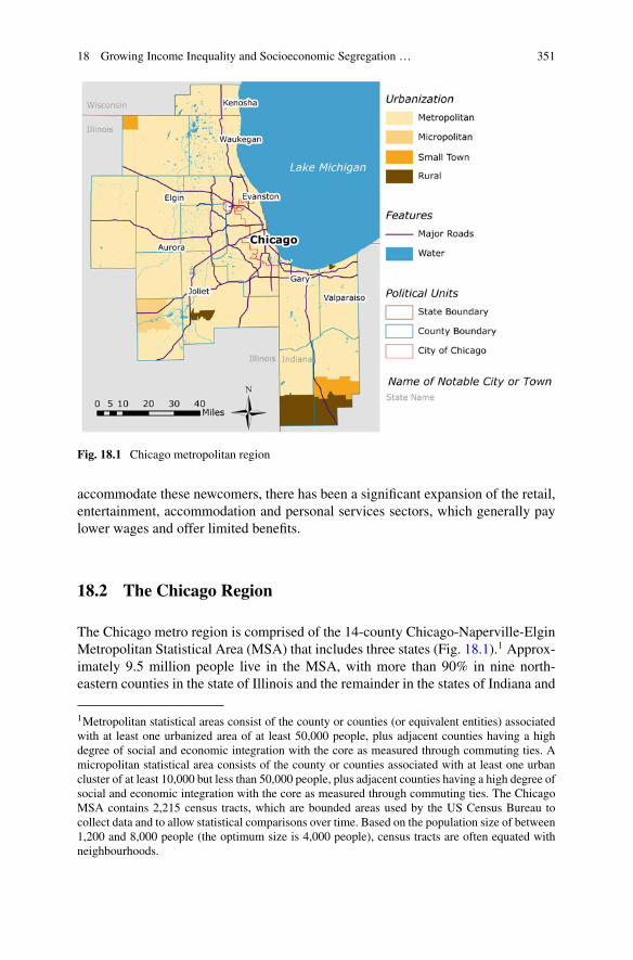
18 Growing Income Inequality and Socioeconomic Segregation … 351
Fig. 18.1 Chicago metropolitan region
accommodate these newcomers, there has been a significant expansion of the retail,entertainment, accommodation and personal services sectors, which generally paylower wages and offer limited benefits.
18.2 The Chicago Region
The Chicago metro region is comprised of the 14-county Chicago-Naperville-ElginMetropolitan Statistical Area (MSA) that includes three states (Fig. 18.1).1 Approx-imately 9.5 million people live in the MSA, with more than 90% in nine north-eastern counties in the state of Illinois and the remainder in the states of Indiana and
1Metropolitan statistical areas consist of the county or counties (or equivalent entities) associatedwith at least one urbanized area of at least 50,000 people, plus adjacent counties having a highdegree of social and economic integration with the core as measured through commuting ties. Amicropolitan statistical area consists of the county or counties associated with at least one urbancluster of at least 10,000 but less than 50,000 people, plus adjacent counties having a high degree ofsocial and economic integration with the core as measured through commuting ties. The ChicagoMSA contains 2,215 census tracts, which are bounded areas used by the US Census Bureau tocollect data and to allow statistical comparisons over time. Based on the population size of between1,200 and 8,000 people (the optimum size is 4,000 people), census tracts are often equated withneighbourhoods.
352 J. L. Smith et al.
Wisconsin; four counties in northwestern Indiana and one county in southeasternWisconsin.2 The Chicago region is the third most populous MSA in the UnitedStates after Los Angeles and New York, and it is the tenth-largest among the OECDmetro-regions. It is approximately 7,196 square miles (18,638 km2) with a popula-tion density of about 1,325 people per square mile. While now considered one nearlycontinuous urbanized area, the region began as a collection of settlements, whichat the time were mostly farm centres or industrial towns (Keating 2005). Today, theregion has very little land that is classified as rural and most of the industrial townsare now suburbs of the City of Chicago, which is the largest settlement in the regionwith 2.7 million people. The next largest is the suburb of Aurora, which has about200,000 people.
18.2.1 The Economy
The Chicago region is a major employment centre with about 4.7 million peopleemployed in the region in 2015, which was a 9.3% increase from 2000. As withmany older urban areas, there has been a shift in the location of work as new employ-ment centres have formed outside the city centre in suburban locations. However,the City of Chicago remains the home to many corporate headquarters and hasbeen aggressively recruiting new firms with attention to technology. The region’stop 10 employment clusters based on employment size are: Business Services(383,000), Distribution and Electronic Commerce (250,000), Education and Knowl-edge Creation (135,000), Financial Services (90,000), Transportation and Logis-tics (85,000), Hospitality and Tourism (79,000), Marketing, Design and Publishing(78,000), Insurance Services (53,000), Food Processing andManufacturing (36,000),and Production Technology and Heavy Machinery (35,000).3
About 63% of the population is of working age (18–64 years old; the median ageis 37.4 years). A significant concern for the region and generally in the United Statesis that the average age of workers in manufacturing is much higher (around 55 yearsold). While employment in this segment is declining, there still is a demand forworkers, but fewer younger people are filling job openings in this industry.Workforcedevelopment efforts are focused on closing the growing skills gap needed to fillmanufacturing jobs and other tech-related sectors. While unemployment is relativelylow at around 5% for the region, it varies by race/ethnicity, with unemploymentamong working-age African Americans about three times higher than Whites andtwo times higher than Latinos (CMAP 2018). In addition, about 20% of working-agepeople do not participate in the labour force at all. This includes people who have
2The source of socio-economic data in this section, unless noted otherwise, is the USCensus Bureau(2017) American Community Survey 1-year estimates for the Chicago-Naperville-Elgin, IL-IN-WIMetro Area.3These data are from The U.S. Cluster Mapping Project https://www.clustermapping.us/.
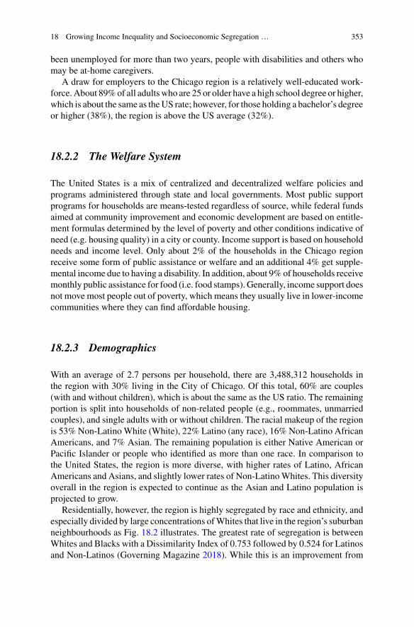
18 Growing Income Inequality and Socioeconomic Segregation … 353
been unemployed for more than two years, people with disabilities and others whomay be at-home caregivers.
A draw for employers to the Chicago region is a relatively well-educated work-force.About 89%of all adultswho are 25 or older have a high school degree or higher,which is about the same as theUS rate; however, for those holding a bachelor’s degreeor higher (38%), the region is above the US average (32%).
18.2.2 The Welfare System
The United States is a mix of centralized and decentralized welfare policies andprograms administered through state and local governments. Most public supportprograms for households are means-tested regardless of source, while federal fundsaimed at community improvement and economic development are based on entitle-ment formulas determined by the level of poverty and other conditions indicative ofneed (e.g. housing quality) in a city or county. Income support is based on householdneeds and income level. Only about 2% of the households in the Chicago regionreceive some form of public assistance or welfare and an additional 4% get supple-mental income due to having a disability. In addition, about 9% of households receivemonthly public assistance for food (i.e. food stamps). Generally, income support doesnot move most people out of poverty, which means they usually live in lower-incomecommunities where they can find affordable housing.
18.2.3 Demographics
With an average of 2.7 persons per household, there are 3,488,312 households inthe region with 30% living in the City of Chicago. Of this total, 60% are couples(with and without children), which is about the same as the US ratio. The remainingportion is split into households of non-related people (e.g., roommates, unmarriedcouples), and single adults with or without children. The racial makeup of the regionis 53% Non-Latino White (White), 22% Latino (any race), 16% Non-Latino AfricanAmericans, and 7% Asian. The remaining population is either Native American orPacific Islander or people who identified as more than one race. In comparison tothe United States, the region is more diverse, with higher rates of Latino, AfricanAmericans and Asians, and slightly lower rates of Non-LatinoWhites. This diversityoverall in the region is expected to continue as the Asian and Latino population isprojected to grow.
Residentially, however, the region is highly segregated by race and ethnicity, andespecially divided by large concentrations ofWhites that live in the region’s suburbanneighbourhoods as Fig. 18.2 illustrates. The greatest rate of segregation is betweenWhites and Blacks with a Dissimilarity Index of 0.753 followed by 0.524 for Latinosand Non-Latinos (Governing Magazine 2018). While this is an improvement from
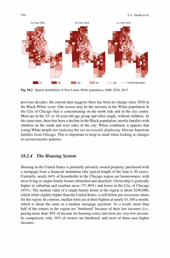
354 J. L. Smith et al.
Fig. 18.2 Spatial distribution of Non-Latino White population, 2000, 2010, 2015
previous decades, the current data suggests there has been no change since 2010 inthe Black-White score. One reason may be the increase in the White population inthe City of Chicago that is concentrating on the north side and in the city centre.Most are in the 25- to 34-year-old age group and often single, without children. Atthe same time, there has been a decline in the Black population, mostly families withchildren on the south and west sides of the city. When combined, it appears thatyoung White people are replacing but not necessarily displacing African Americanfamilies from Chicago. This is important to keep in mind when looking at changesin socioeconomic patterns.
18.2.4 The Housing System
Housing in the United States is primarily privately owned property, purchased witha mortgage from a financial institution (the typical length of the loan is 30 years).Currently, nearly 64% of households in the Chicago region are homeowners, withmost living in single-family homes (detached and attached). Ownership is generallyhigher in suburban and exurban areas (75–80%) and lower in the City of Chicago(45%). The median value of a single-family home in the region is about $240,000,which while slightly higher than the United States, is still below pre-recession valuesfor the region. In contrast, median rents are at their highest at nearly $1,100 a month,which is about the same as a median mortgage payment. As a result, more thanhalf of the renters in the region are ‘burdened’ because of their low incomes (i.e.,paying more than 30% of income for housing costs) and most are very low income.In comparison, only 34% of owners are burdened, and most of them earn higherincomes.
18 Growing Income Inequality and Socioeconomic Segregation … 355
The region does have public housing and other forms of subsidized housing viarental assistance programs and funding for development; however, it only benefitsabout 17% of renters. Public housing has also contributed to economic and racialsegregation sincemost of it was built in the City of Chicago in the 1950s and 1960s inpredominantly AfricanAmerican communities.While housing choice vouchers havegiven families the opportunity to use their rental assistance anywhere in the region,most voucher holders live in lower-income areas where there is more affordablerental housing available.
As the following analysis illustrates, there are clear patterns of socioeconomicconcentration and segregation. While tied historically to uneven development, mostis attributed to long-standing lending and real estate practices coupled with discrim-ination based on race and ethnicity (MPC 2017). Despite it being illegal since the1960s in the United States to discriminate based on race or ethnicity in both thehousing and labour market, changing the racial, spatial patterns has been slow, espe-cially in suburban areas where Whites have historically had higher income levels,better access to capital and more personal wealth than non-Whites. This divide isevident in the rates of ownership and home values by the three major populationgroups in the region: Blacks are at 41% ownership with a median housing value of$140,000, Latinos have a 53% ownership rate and median home value of $160,000,andWhites have a 76% ownership rate andmedian home value of $225,000 (Institutefor Research on Race and Public Policy 2018).4
18.3 Analysis and Results
18.3.1 Income Inequality
Income inequality has increased considerably in theChicago region since 1980 and ata faster rate than in the United States (see Table 18.1).5 The region’s Gini coefficientincreased nearly 36% from 0.35 in 1980 to 0.48 in 2015, while it increased only19% in the country. This trend is important considering that in 1980, Chicago’s Ginicoefficient was well below the United States, and how it has grown at a much fasterrate in the last 15 years (13.3% compared to 3.7%).
This pattern is consistent with the global city literature, which posits that citiessuch as Chicago, which serve as command and control centres in the world economyand help sustain a polarized labour force in terms of skill and wage levels (Sassen1991; Zhong et al. 2007). Faster growing inequality in Chicago also suggests that
4This report used data from the US Census, American Community Survey, 2010–2014.5TheGini indexwas constructedwith data from the Integrated Public-UseMicro-Samples (IPUMS)for the 1980, 1990, and 2000 US Censuses and 2013–2017 American Community Survey. We usehousehold income, which means that single households and households with children are evaluatedthe same. Using household income instead of per capita income is consistent with most studiesconducted in the US (Glaeser et al. 2009; Florida and Mellander 2016).
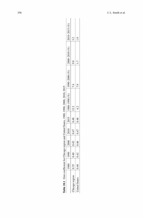
356 J. L. Smith et al.
Table18.1
Ginicoefficientfor
Chicago
region
andUnitedStates,1980,
1990,2
000,
2010,2
015
1980
1990
2000
2010
2015
1980–1990(%
)1990–2000(%
)2000–2010(%
)2010–2015(%
)
Chicago
region
0.35
0.40
0.42
0.47
0.48
12.2
7.4
9.8
3.2
UnitedStates
0.40
0.42
0.46
0.47
0.48
6.2
7.9
1.7
1.9
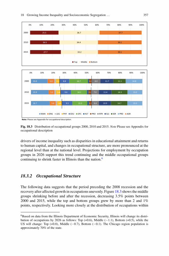
18 Growing Income Inequality and Socioeconomic Segregation … 357
Note: Please see Appendix for occupa onal descrip on.
25.5
26.5
27.7
36.7
34.4
33.2
37.7
39.1
39.1
0% 10% 20% 30% 40% 50% 60% 70% 80% 90% 100%
2000
2010
2015
Top Middle Bo om
15.0
15.9
16.7
5.9
5.2
5.6
3.3
3.8
4.0
8.8
9.6
9.5
16.7
14.1
13.3
2.0
2.2
2.2
8.0
7.0
6.6
11.7
11.4
10.9
11.1
14.3
14.7
14.8
13.2
13.3
0% 10% 20% 30% 40% 50% 60% 70% 80% 90% 100%
2000
2010
2015
MAN ENG LEG PHY EDU OFC HLT PRO NTR SLS SER PRD AGR
Fig. 18.3 Distribution of occupational groups 2000, 2010 and 2015. Note Please see Appendix foroccupational description
drivers of income inequality such as disparities in educational attainment and returnsto human capital, and changes in occupational structure, are more pronounced at theregional level than at the national level. Projections for employment by occupationgroups in 2026 support this trend continuing and the middle occupational groupscontinuing to shrink faster in Illinois than the nation.6
18.3.2 Occupational Structure
The following data suggests that the period preceding the 2008 recession and therecovery after affected growth in occupations unevenly. Figure 18.3 shows themiddlegroups shrinking before and after the recession, decreasing 3.5% points between2000 and 2015, while the top and bottom groups grew by more than 2 and 1%points, respectively. Looking more closely at the distribution of occupations within
6Based on data from the Illinois Department of Economic Security, Illinois will change its distri-bution of occupations by 2026 as follows: Top (+0.6), Middle (−1.1), Bottom (+0.5), while theUS will change: Top (+0.8), Middle (−0.7), Bottom (−0.1). The Chicago region population isapproximately 70% of the state.
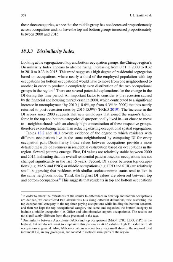
358 J. L. Smith et al.
these three categories, we see that themiddle group has not decreased proportionatelyacross occupations and nor have the top and bottom groups increased proportionatelybetween 2000 and 2015.
18.3.3 Dissimilarity Index
Looking at the segregation of top and bottomoccupation groups, theChicago region’sDissimilarity Index appears to also be rising, increasing from 0.31 in 2000 to 0.32in 2010 to 0.33 in 2015. This trend suggests a high degree of residential segregationbased on occupations, where nearly a third of the employed population with topoccupations (or bottom occupations) would have to move from one neighborhood toanother in order to produce a completely even distribution of the two occupationalgroups in the region.7 There are several potential explanations for the change in theDI during this time period. An important factor to consider is the recession causedby the financial and housing market crash in 2008, which contributed to a significantincrease in unemployment by 2010 (10.6%, up from 4.3% in 2000) that has nearlyreturned to post-recession rates by 2015 (5.9%) (FRED 2019). The increase in theDI scores since 2000 suggests that new employees that joined the region’s labourforce in the top and bottom categories disproportionally lived in—or chose to moveto—neighbourhoods with an already high concentration of these respective groups,therefore exacerbating rather than reducing existing occupational spatial segregation.
Tables 18.2 and 18.3 provide evidence of the degree to which residents withdifferent occupations live in the same neighborhood by computing DI for everyoccupation pair. Dissimilarity Index values between occupations provide a moredetailed measure of evenness in residential distribution based on occupations in theregion. Several patterns emerge. First, DI values are relatively stable between 2000and 2015, indicating that the overall residential pattern based on occupations has notchanged significantly in the last 15 years. Second, DI values between top occupa-tions (e.g. MAN and ENG) or middle occupations (e.g. PRD and SER) are relativelysmall, suggesting that residents with similar socioeconomic status tend to live inthe same neighbourhoods. Third, the highest DI values are observed between topand bottom occupations.8 This suggests that residents in top and bottom occupations
7In order to check the robustness of the results to differences in how top and bottom occupationsare defined, we constructed two alternatives DIs using different definitions, first restricting thetop occupational category to the top three paying occupations while holding the bottom constant,and then we kept the top occupational category the same and expanded the bottom category toinclude a middle occupation (i.e. Office and administrative support occupations). The results arenot significantly different from those presented in the text.8Dissimilarity between Agriculture (AGR) and top occupations (MAN, ENG, LEG, PHY) is thehighest, but we do not want to emphasize this pattern as AGR exhibits high DI value with alloccupations in general. Also, AGR occupations account for a very small share of the regional total(around 0.1%) in any given year, and located in isolated, rural parts of the region.
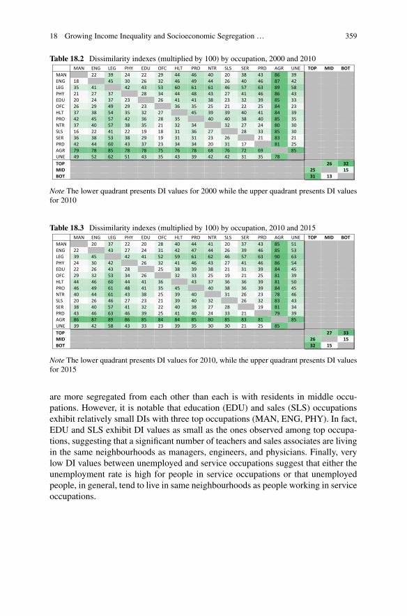
18 Growing Income Inequality and Socioeconomic Segregation … 359
Table 18.2 Dissimilarity indexes (multiplied by 100) by occupation, 2000 and 2010MAN ENG LEG PHY EDU OFC HLT PRO NTR SLS SER PRD AGR UNE TOP MID BOT
MAN 22 39 24 22 29 44 46 40 20 38 43 86 39ENG 18 45 30 26 32 46 49 44 26 40 46 87 42LEG 35 41 42 43 53 60 61 61 46 57 63 89 58PHY 21 27 37 28 34 44 48 43 27 41 46 86 43EDU 20 24 37 23 26 41 41 38 23 32 39 85 33OFC 26 29 49 29 23 36 35 25 21 22 25 84 23HLT 37 38 54 35 32 27 45 39 39 40 41 84 39PRO 42 45 57 42 36 28 35 40 40 38 40 85 35NTR 37 40 57 38 35 21 32 34 32 27 24 80 30SLS 16 22 41 22 19 18 31 36 27 28 33 85 30SER 36 38 53 38 29 19 31 31 23 26 21 83 21PRD 42 44 60 43 37 23 34 34 20 31 17 81 25AGR 79 78 85 78 78 75 76 78 68 76 72 69 85UNE 49 52 62 51 43 35 43 39 42 42 31 35 78TOP 26 32MID 25 15BOT 31 13
Note The lower quadrant presents DI values for 2000 while the upper quadrant presents DI valuesfor 2010
Table 18.3 Dissimilarity indexes (multiplied by 100) by occupation, 2010 and 2015MAN ENG LEG PHY EDU OFC HLT PRO NTR SLS SER PRD AGR UNE TOP MID BOT
MAN 20 37 22 20 28 40 44 41 20 37 43 85 51ENG 22 43 27 24 31 42 47 44 26 39 46 85 53LEG 39 45 42 41 52 59 61 62 46 57 63 90 63PHY 24 30 42 26 32 41 46 43 27 41 46 86 54EDU 22 26 43 28 25 38 39 38 21 31 39 84 45OFC 29 32 53 34 26 32 33 25 19 21 25 81 39HLT 44 46 60 44 41 36 43 37 36 36 39 81 50PRO 46 49 61 48 41 35 45 40 38 36 39 84 45NTR 40 44 61 43 38 25 39 40 31 26 23 78 46SLS 20 26 46 27 23 21 39 40 32 26 32 83 43SER 38 40 57 41 32 22 40 38 27 28 19 81 34PRD 43 46 63 46 39 25 41 40 24 33 21 79 39AGR 86 87 89 86 85 84 84 85 80 85 83 81 85UNE 39 42 58 43 33 23 39 35 30 30 21 25 85TOP 27 33MID 26 15BOT 32 15
Note The lower quadrant presents DI values for 2010, while the upper quadrant presents DI valuesfor 2015
are more segregated from each other than each is with residents in middle occu-pations. However, it is notable that education (EDU) and sales (SLS) occupationsexhibit relatively small DIs with three top occupations (MAN, ENG, PHY). In fact,EDU and SLS exhibit DI values as small as the ones observed among top occupa-tions, suggesting that a significant number of teachers and sales associates are livingin the same neighbourhoods as managers, engineers, and physicians. Finally, verylow DI values between unemployed and service occupations suggest that either theunemployment rate is high for people in service occupations or that unemployedpeople, in general, tend to live in same neighbourhoods as people working in serviceoccupations.
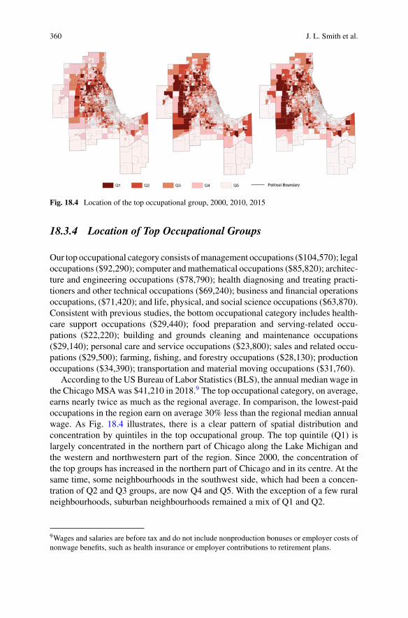
360 J. L. Smith et al.
Fig. 18.4 Location of the top occupational group, 2000, 2010, 2015
18.3.4 Location of Top Occupational Groups
Our top occupational category consists ofmanagement occupations ($104,570); legaloccupations ($92,290); computer andmathematical occupations ($85,820); architec-ture and engineering occupations ($78,790); health diagnosing and treating practi-tioners and other technical occupations ($69,240); business and financial operationsoccupations, ($71,420); and life, physical, and social science occupations ($63,870).Consistent with previous studies, the bottom occupational category includes health-care support occupations ($29,440); food preparation and serving-related occu-pations ($22,220); building and grounds cleaning and maintenance occupations($29,140); personal care and service occupations ($23,800); sales and related occu-pations ($29,500); farming, fishing, and forestry occupations ($28,130); productionoccupations ($34,390); transportation and material moving occupations ($31,760).
According to the US Bureau of Labor Statistics (BLS), the annual median wage inthe Chicago MSAwas $41,210 in 2018.9 The top occupational category, on average,earns nearly twice as much as the regional average. In comparison, the lowest-paidoccupations in the region earn on average 30% less than the regional median annualwage. As Fig. 18.4 illustrates, there is a clear pattern of spatial distribution andconcentration by quintiles in the top occupational group. The top quintile (Q1) islargely concentrated in the northern part of Chicago along the Lake Michigan andthe western and northwestern part of the region. Since 2000, the concentration ofthe top groups has increased in the northern part of Chicago and in its centre. At thesame time, some neighbourhoods in the southwest side, which had been a concen-tration of Q2 and Q3 groups, are now Q4 and Q5. With the exception of a few ruralneighbourhoods, suburban neighbourhoods remained a mix of Q1 and Q2.
9Wages and salaries are before tax and do not include nonproduction bonuses or employer costs ofnonwage benefits, such as health insurance or employer contributions to retirement plans.
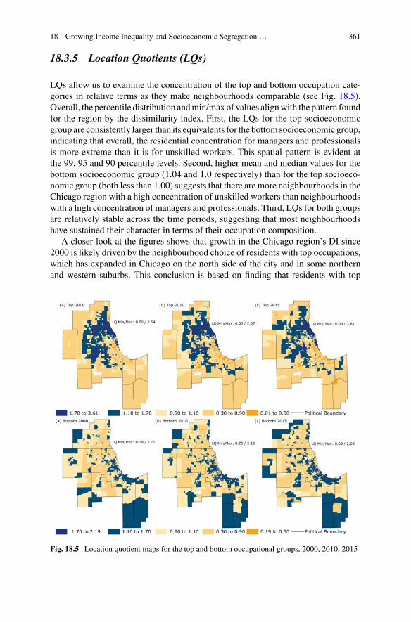
18 Growing Income Inequality and Socioeconomic Segregation … 361
18.3.5 Location Quotients (LQs)
LQs allow us to examine the concentration of the top and bottom occupation cate-gories in relative terms as they make neighbourhoods comparable (see Fig. 18.5).Overall, the percentile distribution andmin/max of values alignwith the pattern foundfor the region by the dissimilarity index. First, the LQs for the top socioeconomicgroup are consistently larger than its equivalents for the bottom socioeconomic group,indicating that overall, the residential concentration for managers and professionalsis more extreme than it is for unskilled workers. This spatial pattern is evident atthe 99, 95 and 90 percentile levels. Second, higher mean and median values for thebottom socioeconomic group (1.04 and 1.0 respectively) than for the top socioeco-nomic group (both less than 1.00) suggests that there are more neighbourhoods in theChicago region with a high concentration of unskilled workers than neighbourhoodswith a high concentration of managers and professionals. Third, LQs for both groupsare relatively stable across the time periods, suggesting that most neighbourhoodshave sustained their character in terms of their occupation composition.
A closer look at the figures shows that growth in the Chicago region’s DI since2000 is likely driven by the neighbourhood choice of residents with top occupations,which has expanded in Chicago on the north side of the city and in some northernand western suburbs. This conclusion is based on finding that residents with top
Fig. 18.5 Location quotient maps for the top and bottom occupational groups, 2000, 2010, 2015
362 J. L. Smith et al.
occupations disproportionally added to those neighbourhoods with an already highconcentration of top occupations (LQ > 1 for top occupations). Neighbourhoods withLQs larger than 1.00 in both 2000 and 2010 for the top occupational group gained adisproportionate share of the net increase in the top occupations (80% of total). Atthe same time, neighbourhoods with LQs less than 1.00 in both 2000 and 2010 fortop occupations gained only 3% of the net increase in the top occupations. Thesenumbers confirmour hypothesis that neighbourhoodswith a high concentration of thetop occupational group gained disproportionally more people in the top occupationsthan neighbourhoods with a low concentration of this group, thereby pushing the DIup.
Since the change inDI is driven by two components (residential changes of top andbottomoccupational groups), we alsomust examinewhat happened to those residentsin the bottom occupations during the same period. The large increase in bottom occu-pations (relative to the regional average) could be indicative of the regional economy,creating more low-paid/skilled jobs during the recession period. It is also possiblethat some of the existing residents in 2000 working in middle occupations lost theirjobs during this period and transitioned to low-paid jobs, thus being re-classified inthe bottom occupational group. For this type of change to push up the DI, at leastone of two processes must have happened. First, residents working in low occupa-tions would have to be disproportionally added to those neighbourhoods with analready high concentration of bottom occupations (LQ > 1.00 for bottom occupa-tions). Second, residents with bottom occupations in low concentration neighbour-hoods (LQ < 1.00 for bottom occupations) would have to lose their jobs at a fasterrate than the regional average or relocate to high concentration neighbourhoods orleave the region.
While data limitations prevent us from providing a definitive answer to the latterprocess, it is possible to determine the net gains of neighbourhoods in the bottomoccupational group (the former process). A closer look at the change in the locationof residents with bottom occupations from 2000 to 2010 shows that 59,384 people,or 41% of the total net new people employed in the bottom occupations, were addedto those neighbourhoods that have LQs larger than 1.00 in both 2000 and 2010. Asthe maps illustrate, these neighbourhoods are both in the City of Chicago and in thesuburbs.NeighbourhoodswithLQs less than 1.00 in both years gained approximatelythe same number of bottom occupations from 2000 to 2010 (61,422 or 42% ofthe total). These figures suggest that the location choice of residents with bottomoccupations played a relatively small role in pushing DI in upward direction.
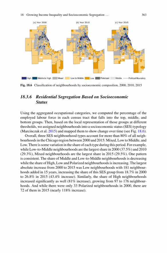
18 Growing Income Inequality and Socioeconomic Segregation … 363
Fig. 18.6 Classification of neighbourhoods by socioeconomic composition, 2000, 2010, 2015
18.3.6 Residential Segregation Based on SocioeconomicStatus
Using the aggregated occupational categories, we computed the percentage of theemployed labour force in each census tract that falls into the top, middle, andbottom groups. Then, based on the local representation of those groups at differentthresholds, we assigned neighbourhoods into a socioeconomic status (SES) typology(Marcinczak et al. 2015) and mapped them to show change over time (see Fig. 18.6).
Overall, three SES neighbourhood types account for more than 80% of all neigh-bourhoods in theChicago region between 2000 and 2015:Mixed, Low toMiddle, andLow.There is somevariation in the share of each type during this period. For example,while Low-to-Middle neighbourhoods are the largest share in 2000 (37.5%) and 2010(29.3%), Mixed neighbourhoods are the largest share in 2015 (29.5%). One patternis consistent. The share of Middle and Low-to-Middle neighbourhoods is decreasingwhile the share ofHigh, Low and Polarized neighbourhoods is increasing. The largestabsolute increase from 2000 to 2015 was Low neighbourhoods with 181 neighbour-hoods added in 15 years, increasing the share of this SES group from 18.7% in 2000to 26.8% in 2015 (43.4% increase). Similarly, the share of High neighbourhoodsincreased significantly as well (81% increase), growing from 97 to 176 neighbour-hoods. And while there were only 33 Polarized neighbourhoods in 2000, there are72 of them in 2015 (nearly 118% increase).
364 J. L. Smith et al.
18.4 Conclusion
These results suggest two trends in the Chicago region. First, an occupational shiftis ‘shrinking the middle’ while also increasing the number of people in the bottomand top occupational groups. This is consistent with the global city literature onthe social polarization of the workforce. Second, holding the occupation structureconstant, residents with similar occupations at the top and bottom appear to be sortingthemselves into neighbourhoods with people in similar occupations; for example, asdiscussed in the LQ section, residents with top occupations overwhelmingly chooseto live in neighbourhoods with already high LQs for the top occupational group. Theclassification of neighbourhoods by socioeconomic composition reflects these trends,showing that the share of middle neighbourhoods is decreasing while the share of topand bottom neighbourhoods is increasing. This implies that social polarization hasled to residential polarization between the top and bottomoccupational groups.Whilewe did not include race and ethnicity in the DI analysis, the spatial patterns suggestthat the long history of racial segregation may be contributing to those residentialpatterns as well.
Looking ahead, given the large increase in the region’s Gini score since 2000, theChicago region appears to be on a trajectory toward greater income inequality in 2020than the United States on average. We also expect that factors that have sustainedracial and ethnic segregation (e.g. housing discrimination, unequal access to capital)will continue to contribute to this trend, but also that inequality will reinforce racialand ethnic segregation since most of the White population are currently in the topoccupations while most African American and Latino people are in bottom occu-pations. Still, there are many variables that can affect these patterns of segregationand inequality in the future. This includes investment and development decisionsin the region by both the private and public sector, which are somewhat hard topredict under current national economic policies (i.e. fluctuating tariffs and globaltrade wars, especially between United States and China). Furthermore, local policiescan also shape the future, including efforts by the Chicago Metropolitan Agency forPlanning to address segregation (CMAP 2018) and Chicago’s new mayor elected inSpring of 2019, who ran on a platform of inclusion and equity, which may changewhere development occurs and who benefits in decades to come.
Appendix
See Tables 18.4, 18.5, 18.6, 18.7 and 18.8.
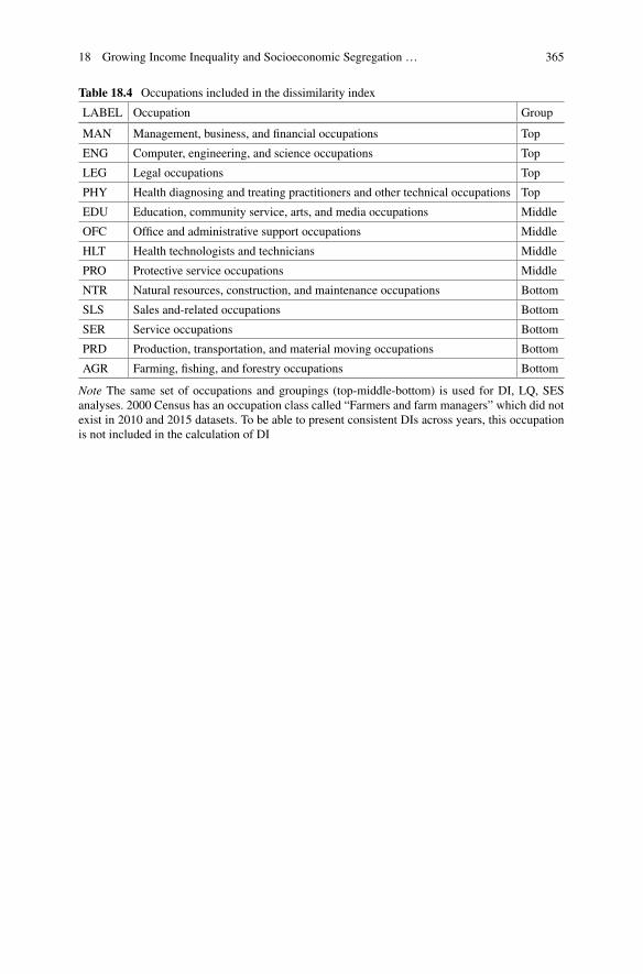
18 Growing Income Inequality and Socioeconomic Segregation … 365
Table 18.4 Occupations included in the dissimilarity index
LABEL Occupation Group
MAN Management, business, and financial occupations Top
ENG Computer, engineering, and science occupations Top
LEG Legal occupations Top
PHY Health diagnosing and treating practitioners and other technical occupations Top
EDU Education, community service, arts, and media occupations Middle
OFC Office and administrative support occupations Middle
HLT Health technologists and technicians Middle
PRO Protective service occupations Middle
NTR Natural resources, construction, and maintenance occupations Bottom
SLS Sales and-related occupations Bottom
SER Service occupations Bottom
PRD Production, transportation, and material moving occupations Bottom
AGR Farming, fishing, and forestry occupations Bottom
Note The same set of occupations and groupings (top-middle-bottom) is used for DI, LQ, SESanalyses. 2000 Census has an occupation class called “Farmers and farm managers” which did notexist in 2010 and 2015 datasets. To be able to present consistent DIs across years, this occupationis not included in the calculation of DI
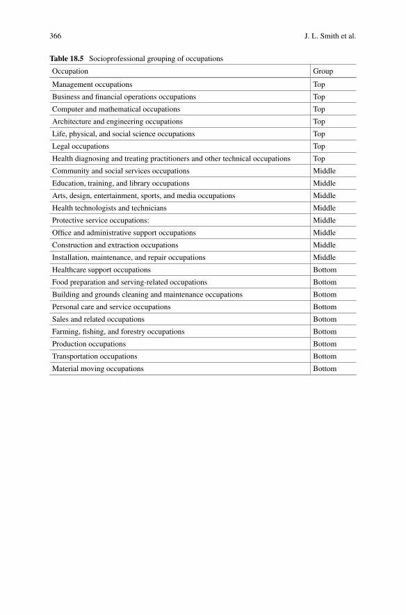
366 J. L. Smith et al.
Table 18.5 Socioprofessional grouping of occupations
Occupation Group
Management occupations Top
Business and financial operations occupations Top
Computer and mathematical occupations Top
Architecture and engineering occupations Top
Life, physical, and social science occupations Top
Legal occupations Top
Health diagnosing and treating practitioners and other technical occupations Top
Community and social services occupations Middle
Education, training, and library occupations Middle
Arts, design, entertainment, sports, and media occupations Middle
Health technologists and technicians Middle
Protective service occupations: Middle
Office and administrative support occupations Middle
Construction and extraction occupations Middle
Installation, maintenance, and repair occupations Middle
Healthcare support occupations Bottom
Food preparation and serving-related occupations Bottom
Building and grounds cleaning and maintenance occupations Bottom
Personal care and service occupations Bottom
Sales and related occupations Bottom
Farming, fishing, and forestry occupations Bottom
Production occupations Bottom
Transportation occupations Bottom
Material moving occupations Bottom
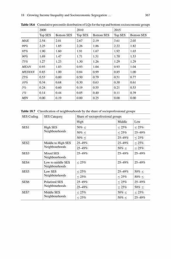
18 Growing Income Inequality and Socioeconomic Segregation … 367
Table 18.6 Cumulative percentile distribution of LQs for the top and bottom socioeconomic groups
2000 2010 2015
Top SES Bottom SES Top SES Bottom SES Top SES Bottom SES
MAX 2.54 2.01 2.67 2.19 3.61 2.05
99% 2.25 1.85 2.26 1.86 2.22 1.82
95% 1.90 1.60 1.91 1.67 1.92 1.65
90% 1.69 1.47 1.71 1.51 1.70 1.53
75% 1.27 1.23 1.30 1.26 1.29 1.29
MEAN 0.93 1.03 0.93 1.04 0.93 1.04
MEDIAN 0.85 1.00 0.84 0.99 0.85 1.00
25% 0.53 0.80 0.50 0.79 0.51 0.77
10% 0.34 0.68 0.30 0.63 0.30 0.61
5% 0.24 0.60 0.19 0.55 0.21 0.53
1% 0.14 0.44 0.05 0.40 0.11 0.39
MIN 0.00 0.19 0.00 0.25 0.00 0.00
Table 18.7 Classification of neighbourhoods by the share of socioprofessional groups
SES Coding SES Category Share of socioprofessional groups
High Middle Low
SES1 High SESNeighbourhoods
50% ≤ ≤ 25% ≤ 25%
50% ≤ ≤ 25% 25–49%
50% ≤ 25–49% ≤ 25%
SES2 Middle to High SESNeighbourhoods
25–49% 25–49% ≤ 25%
25–49% 50% ≤ ≤ 25%
SES3 Mixed SESNeighbourhoods
25–49% 25–49% 25–49%
SES4 Low to middle SESNeighbourhoods
≤ 25% 25–49% 25–49%
SES5 Low SESNeighbourhoods
≤ 25% 25–49% 50% ≤≤ 25% ≤ 25% 50% ≤
SES6 Polarized SESNeighbourhoods
25–49% ≤ 25% 25–49%
25–49% ≤ 25% 50% ≤SES7 Middle SES
Neighbourhoods≤ 25% 50% ≤ ≤ 25%
≤ 25% 50% ≤ 25–49%
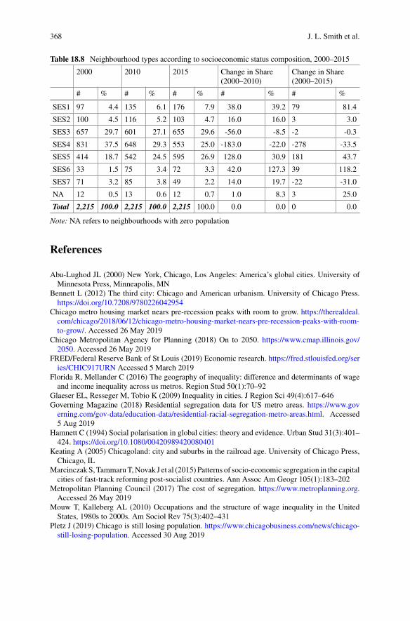
368 J. L. Smith et al.
Table 18.8 Neighbourhood types according to socioeconomic status composition, 2000–2015
2000 2010 2015 Change in Share(2000–2010)
Change in Share(2000–2015)
# % # % # % # % # %
SES1 97 4.4 135 6.1 176 7.9 38.0 39.2 79 81.4
SES2 100 4.5 116 5.2 103 4.7 16.0 16.0 3 3.0
SES3 657 29.7 601 27.1 655 29.6 -56.0 -8.5 -2 -0.3
SES4 831 37.5 648 29.3 553 25.0 -183.0 -22.0 -278 -33.5
SES5 414 18.7 542 24.5 595 26.9 128.0 30.9 181 43.7
SES6 33 1.5 75 3.4 72 3.3 42.0 127.3 39 118.2
SES7 71 3.2 85 3.8 49 2.2 14.0 19.7 -22 -31.0
NA 12 0.5 13 0.6 12 0.7 1.0 8.3 3 25.0
Total 2,215 100.0 2,215 100.0 2,215 100.0 0.0 0.0 0 0.0
Note: NA refers to neighbourhoods with zero population
References
Abu-Lughod JL (2000) New York, Chicago, Los Angeles: America’s global cities. University ofMinnesota Press, Minneapolis, MN
Bennett L (2012) The third city: Chicago and American urbanism. University of Chicago Press.https://doi.org/10.7208/9780226042954
Chicago metro housing market nears pre-recession peaks with room to grow. https://therealdeal.com/chicago/2018/06/12/chicago-metro-housing-market-nears-pre-recession-peaks-with-room-to-grow/. Accessed 26 May 2019
Chicago Metropolitan Agency for Planning (2018) On to 2050. https://www.cmap.illinois.gov/2050. Accessed 26 May 2019
FRED/Federal Reserve Bank of St Louis (2019) Economic research. https://fred.stlouisfed.org/series/CHIC917URN Accessed 5 March 2019
Florida R, Mellander C (2016) The geography of inequality: difference and determinants of wageand income inequality across us metros. Region Stud 50(1):70–92
Glaeser EL, Resseger M, Tobio K (2009) Inequality in cities. J Region Sci 49(4):617–646Governing Magazine (2018) Residential segregation data for US metro areas. https://www.governing.com/gov-data/education-data/residential-racial-segregation-metro-areas.html. Accessed5 Aug 2019
Hamnett C (1994) Social polarisation in global cities: theory and evidence. Urban Stud 31(3):401–424. https://doi.org/10.1080/00420989420080401
Keating A (2005) Chicagoland: city and suburbs in the railroad age. University of Chicago Press,Chicago, IL
MarcinczakS, TammaruT,Novak J et al (2015) Patterns of socio-economic segregation in the capitalcities of fast-track reforming post-socialist countries. Ann Assoc Am Geogr 105(1):183–202
Metropolitan Planning Council (2017) The cost of segregation. https://www.metroplanning.org.Accessed 26 May 2019
Mouw T, Kalleberg AL (2010) Occupations and the structure of wage inequality in the UnitedStates, 1980s to 2000s. Am Sociol Rev 75(3):402–431
Pletz J (2019) Chicago is still losing population. https://www.chicagobusiness.com/news/chicago-still-losing-population. Accessed 30 Aug 2019
18 Growing Income Inequality and Socioeconomic Segregation … 369
Rackl L (2019) Chicago sets new tourism record with nearly 58 million visitors in 2018—and themayor is thrilled. Chicago Tribune. https://www.chicagotribune.com/travel/ct-trav-chicago-tourism-record-numbers-2018-0111-story.html. Accessed 26 May 2019
Realpage.com (2018) Apartment completion volumes spike in Chicago. https://www.realpage.com/analytics/apartment-completion-volumes-spike-chicago/. Accessed 1 Aug 2019
Sassen, S (1991) The global city: NewYork, London, Tokyo. Princeton University Press, Princeton,NJ
Tammaru T,Musterd S, vanHamM,Marcinczak S (2016) Amulti-factor approach to understandingsocio-economic segregation in European capital cities. In: Tammaru et al (ed) Socio-economicsegregation in European capital cities. Taylor & Francis, Abingdon, p 1
US Census Bureau (2017) American community survey 1-year estimates for Chicago-Naperville-Elgin, IL-IN-WI Metro Area. https://censusreporter.org/profiles/31000us16980-chicago-naperville-elgin-il-in-wi-metro-area/. Accessed 5 May 2019
Zhong X, Clark TN, Sassen S (2007) Globalization, producer services and income inequality acrossUS metro areas. Int Rev Sociol 17(3):385–391
Open Access This chapter is licensed under the terms of the Creative Commons Attribution 4.0International License (http://creativecommons.org/licenses/by/4.0/), which permits use, sharing,adaptation, distribution and reproduction in any medium or format, as long as you give appropriatecredit to the original author(s) and the source, provide a link to the Creative Commons license andindicate if changes were made.
The images or other third party material in this chapter are included in the chapter’s CreativeCommons license, unless indicated otherwise in a credit line to the material. If material is notincluded in the chapter’s Creative Commons license and your intended use is not permitted bystatutory regulation or exceeds the permitted use, you will need to obtain permission directly fromthe copyright holder.
Chapter 19Income Inequality and EconomicSegregation in Los Angeles from 1980to 2010
John R. Hipp and Jae Hong Kim
Abstract Rising income inequality is a critical problem in both the global Northand South. In the United States, the Gini coefficient measuring nationwide incomeinequality rose from 0.403 in 1980 to 0.480 in 2014 (US Census), and residentialsegregation by income has increasingly occurred in many metropolitan regions andis particularly reflected in the spatial separation of the wealthiest households. Thischapter focuses on the change in the level of income inequality in the Los Angelesregion since 1980 and how it is related to changes in residential segregation betweeneconomic groups over that same time period. We use data from the US Censuscollected in 1980, 1990, 2000, and 2010.Wemeasure residential segregation betweeneconomic groups based on occupational structure, and measure ‘neighbourhoods’using Census tracts: these are units defined by the US Census and typically averageabout 4,000 residents. The overall level of inequality in the region is measured ateach decade point using theGini coefficient for household income.Maps demonstratewhere different socioeconomic status groups have tended to locate and howeconomicsegregation has changed in Los Angeles over this time period. We also assess theextent to which changes in inequality are related to changes in economic segregationover the last four and a half decades.
Keywords Neighbourhoods · Economic segregation · Long-term trends
Electronic supplementary material The online version of this chapter(https://doi.org/10.1007/978-3-030-64569-4_19) contains supplementary material, which isavailable to authorized users.
J. R. Hipp (B)Department of Criminology, Law and Society, Social Ecology II, University of California, Irvine,CA 3311, USAe-mail: [email protected]
Department of Sociology, University of California, Irvine, USA
J. H. KimDepartment of Urban Planning and Public Policy, University of California, Irvine, USA
© The Author(s) 2021M. van Ham et al. (eds.), Urban Socio-Economic Segregation and Income Inequality,The Urban Book Series, https://doi.org/10.1007/978-3-030-64569-4_19
371
372 J. R. Hipp and J. H. Kim
19.1 Introduction
An upward trajectory of economic inequality has been quite apparent around theworld, although what has caused this trend would vary widely across countries,and so does the response chosen to address it. In the United States, the Gini coef-ficient measuring income inequality had begun to rise rapidly since the 1980s andincreased every decade, despite yearly ups and downs.1 Nationwide, this (uncom-fortable) reality has received extensive media coverage, often highlighting whatpercentage of the aggregated income growth has been taken by the top 1% and howthe income (or wealth) concentration has been accelerated in recent decades. Muchattention has also been paid in academic and policy circles to ways to curb this trendof ‘the fading American Dream’ (Chetty et al. 2017) and promote intergenerationaleconomic mobility.
The rising economic inequality is not an aspatial phenomenon. There is substan-tial variation across regions, and it has been reported that ‘[t]he rise in inequalityexperienced in the United States over the past four-plus decades is not just a storyof those on Wall Street, in Hollywood, or in the Silicon Valley reaping outsizedrewards, … [and that] rising inequality and increases in top 1 percent incomes affectevery part of the U.S.’ (Sommeiller and Price 2018: p. 16). Furthermore, some recentstudies have suggested that the rising inequality can take the form of a higher levelof residential segregation between economic groups (economic segregation fromhereafter) within a region, especially the separation of wealthier household groupsfrom the remainder, which would further reinforce the increasing trend of inequality(see, e.g., Reardon and Bischoff 2011; Scarpa 2016). Such a reciprocal interactionbetween inequality and segregationwould be particularly problematic when resourceallocation and land-use decisions are not made in favour of disadvantaged groupsor communities. In such circumstances, the vicious cycle can persist and create asignificant disparity in access to jobs or other essential amenities/opportunities.
Yet, our understanding of these critical mechanisms is far from complete. Asmentioned above, increasing inequality is an indisputable reality in the United States(or even worldwide). However, a question is whether this apparent macro change hasplayed out differently across various metropolitan areas in the US. Little is knownabout the various ways in which economic groups are residentially segregated incontemporary cities or larger metropolitan areas along with rising inequality. More-over, there has been a dearth of comparative work that would enable us to identifycommonalities or capture (subtle) differences between cities or regions around theworld.
This chapter, combined with other contributions in the book, attempts to fill thisgap. More specifically, here consideration is given to Los Angeles (and its vicinity),which is unique inmanyways but presents some important representative qualities ofpost-industrial large metropolises. Materials presented in this chapter were produced
1For more detailed information, see US Census Historical Income Tables: Income Inequality, avail-able at https://www.census.gov/data/tables/time-series/demo/income-poverty/historical-income-inequality.html.
19 Income Inequality and Economic Segregation… 373
using an occupational classification scheme to make the analysis comparable toother case studies in the volume. The present occupation-oriented analysis was alsoexpected to provide some fresh insights into the complex process that underlies thestudy region’s segregation dynamics that would not be fully captured by traditionalincome-oriented approaches.
19.2 Background
The Los Angeles region provides an interesting case to study the spatial dynamics ofinequality and segregation, given that studies have frequently pointed to its spatiallayout as differing from the traditional monocentric development. Instead, it hasbeen described as a polycentric region where an increasing number of employmentsubcenters have emerged (Kane et al. 2018). This region is the quintessential exampleof what is referred to as a member of the Sunbelt part of the country, and as such,exemplifies much of the post-World War II development in the United States in thatit is a car culture built around roadways and highways, along with a relative lack ofpublic transportation.
These characteristics of the Los Angeles region have been constructed throughmultiple waves of population and employment decentralisation over the history ofits growth. While the City of Los Angeles grew most rapidly in the late nineteenthcentury through the 1930s, the entire metropolitan region has continued to expanddramatically. An early form of the suburban expansion occurred partly in the formof upper and middle-class flight from the core city, as observed in many other USmetropolises, resulting in massive development in Orange County during the mid-twentieth century (Note: Orange County’s population increased more than ten timesfrom 130 thousand to 1.42 million between 1940 and 1970. Currently, it is thesixth-most populous county in the nation with a population of over 3 million). Inthe late-twentieth century, the growth was headed toward inland areas, specificallyRiverside and San Bernardino counties, where new housing units were provided atmuch more affordable rates, although job opportunities were relatively scarce there.More recently, there has been increasing evidence of inner-city gentrification andassociated poverty suburbanisation (Tong and Kim 2019), but new development inremote locations has continued (Hipp et al. 2014). We display key features of theregion in Fig. 19.1.
Much of the new development has taken place in the form of single-familyhousing construction. While the housing stock has diversified in the region, low-density residential development remains common, particularly in remote locations.The percentage of owner-occupied housing units, however, has not increased substan-tially over the last three decades. Despite the growing decentralisation of households,the overall percentage has remained around 54%, while the level of homeownershipvaries across counties, ranging from 47% (Los Angeles County) to 68% (RiversideCounty) in 2010.
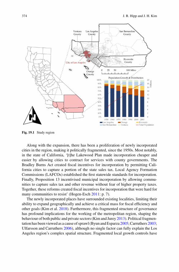
374 J. R. Hipp and J. H. Kim
Fig. 19.1 Study region
Along with the expansion, there has been a proliferation of newly incorporatedcities in the region, making it politically fragmented, since the 1950s. Most notably,in the state of California, ‘[t]he Lakewood Plan made incorporation cheaper andeasier by allowing cities to contract for services with county governments. TheBradley Burns Act created fiscal incentives for incorporation by permitting Cali-fornia cities to capture a portion of the state sales tax. Local Agency FormationCommissions (LAFCOs) established the first statewide standards for incorporation.Finally, Proposition 13 incentivised municipal incorporation by allowing commu-nities to capture sales tax and other revenue without fear of higher property taxes.Together, these reforms created fiscal incentives for incorporation that were hard formany communities to resist’ (Hogen-Esch 2011: p. 7).
The newly incorporated places have surrounded existing localities, limiting theirability to expand geographically and achieve a critical mass for fiscal efficiency andother goals (Kim et al. 2018). Furthermore, this fragmented structure of governancehas profound implications for the working of the metropolitan region, shaping thebehaviour of both public and private sectors (Kim and Jurey 2013). Political fragmen-tation has been viewed as a cause of sprawl (Byun andEsparza 2005;Carruthers 2003;Ulfarsson and Carruthers 2006), although no single factor can fully explain the LosAngeles region’s complex spatial structure. Fragmented local growth controls have

19 Income Inequality and Economic Segregation… 375
pushed development out and made it particularly difficult to construct higher-densityaffordable housing units where the demand has arisen (Levine 1999).
In this light, it is not surprising that common interest developments (CIDs),including gated communities and condominiums, are prevalent in the Los Angelesmetropolitan region. According to Sanchez et al. (2005), providing useful estimatesbased on the 2001 American Housing Survey data, a considerable percentage ofhouseholds in the region reported that they lived in walled (18.2%) or access-controlled (11.7%) communities. Such types of housing developments are evenmorepopular in new development projects, producing increased social segregation (LeGoix 2005). Fragmented local governments have been in favour of CIDs, whichwould allow them to ‘acquire new property tax payers without having to extendto them the full panoply of municipal services, … [and] some municipal govern-ments have begun to virtually require that new housing construction consist of CIDs’(McKenzie 2003: p. 207).
These structural characteristics have also created various forms of isolation, eventhough there have been growing efforts to promote mixing in multiple dimensions(Hipp et al. 2017b). While the conventional spatial mismatch hypothesis does notfit well in the case of Los Angeles (Blumenberg and Manville 2004), a recent studyhas shown that job accessibility of inner-city residents has declined significantly inthe region (Hu 2015). Other forms of barriers have also existed, making it difficultto connect job opportunities to welfare recipients who are supposed to move fromwelfare to work in the post-1996 welfare reform era in the United States (Ong andBlumenberg 1998). It is not uncommon that workers commute across city or countyborders in this large metropolitan area. The following empirical analysis shows howdifferent groups of workers were spatially distributed and in what ways the spatialdistributions have changed over time, based on their place of residence, as opposedto where their jobs were located.
Thus, although this is a single region, there are differences across the five coun-ties in the region in various ways. These counties have different spatial patterns ofamenities and jobs. The density of LosAngeles County can be seen in that its housingunits have many more amenities within one mile of them (measuring various typesof amenities such as retail, restaurants, parks, etc.) than the other counties; housingunits in Orange County have the next most amenities nearby, with the other threecounties having far fewer (Kane et al. 2017: 25). There is also more job density inLos Angeles county compared to the others: the downtown of Los Angeles city haslong been a business hub (Kane et al. 2016), and the west side of Los Angeles alsohas a high jobs/housing relationship (Hipp et al. 2017a). In Orange County, the Irvinearea serves as a high jobs/housing location, whereas the Inland Empire counties haveless evidence of such jobs/housing locations (Hipp et al. 2017a).
376 J. R. Hipp and J. H. Kim
19.3 Data and Methods
19.3.1 Data
Our study area is the Los Angeles area, which is defined as the five-county SouthernCalifornia metropolitan region, including Los Angeles, Orange, Riverside, SanBernardino and Ventura counties. For this large metropolitan region, we used censustracts as the unit of analysis to construct a temporally comparable neighbourhood-level dataset. We harmonised the tracts to 2010 boundaries based on population-weighted apportioning as defined by the US Census Master Area Reference Files.We used US Census data for the earlier waves, and used the American CommunitySurvey 5-year estimates for the most recent decade (we used the 2008–12 data giventhat it is centred on 2010) to construct our dataset of 3,892 tracts with at least 100population in 2010.
To assess the socioeconomic status of the neighbourhoods in the region, in additionto the occupation measures, we created two other measures. One is a measure of theaverage household income of residents in the tract. The second is a measure ofeducation level in the tract, and is captured by the percent of residents with at leasta bachelor’s degree.
19.3.2 Methods
A challenge is to define consistent categories of occupations over time. We used theISO definitions for defining categories. We, therefore, classified nine categories ofoccupations, one of which—agriculture, forestry, and fishery workers—we excludedfrom analyses given the small proportion constituted by this group in this urban area.The categories are: (1) managers; (2) professionals; (3) technicians and associatedprofessionals; (4) clerical support workers; (5) service and sales workers; (6) agricul-ture, forestry, and fishery workers; (7) craft and related trades workers; (8) plant andmachine operators and assemblers; (9) elementary occupations. We describe howweclassified the occupation codes defined by the US Census for each decade into eachof these categories in Appendix Table A1 (available online).
We also constructed a measure of the degree of occupation mixing in neighbour-hoods with a Herfindahl Index of the nine occupation codes just described. Themeasure is a sum of squares of the proportion of residents in a tract in each ofthe occupation categories, and then is subtracted from 1 to make it a measure ofheterogeneity. The theoretical range is from 0 to 0.8742.
19 Income Inequality and Economic Segregation… 377
19.4 Results
19.4.1 General Trends in Occupation Groups Over Time
We begin by describing the socioeconomic status of the five counties in this region.Orange and Ventura Counties are the two wealthiest counties in the region with thehighest average income and education levels, whereas Riverside and San BernardinoCounties are the two counties from the Inland Empire (IE)—which tends to beblue-collar—and consistently show the lowest average income and lowest levels ofeducation. Los Angeles County, the largest county in the region, is between thesetwo extremes based on socioeconomic status. Although Ventura County is closer toLos Angeles County for average education level, they are close to Orange Countyfor average household income.
We next describe the change in household income inequality in the region overall,as well as across the five counties in the region, for our study period.2 The generalupward trend in the level of inequality in the region has closely tracked the trendfor Los Angeles County, the largest county in the region. The Gini coefficient forhousehold income in the region has gone from 0.415 in 1980 to 0.43 in 1990 to 0.455in 2000 before slightly falling to 0.449 by 2010. Los Angeles County has paralleledthis with systematically higher Gini values, and peaked at 0.474 in 2000. The twoInland Empire (IE) Counties of Riverside and San Bernardino have very similarincome inequality levels in 2010, but took very different paths to that point. WhereasRiverside County had the second-highest level of income inequality in the regionin 1980, inequality has only slightly increased over the time period in this County.In contrast, San Bernardino County has gone from relatively low-income inequalityin 1980 (0.382) to steadily increasing such that they have nearly caught RiversideCounty by 2010 (0.421). Finally, the two more wealthy counties are Orange andVentura, and although they started with the lowest levels of inequality in the regionin 1980 (0.37 and 0.38), they have both experienced quite steady increases over theentire study period such that Orange County has slightly higher income inequalitythan the two IE counties by 2010.
Turning to the occupation structure of the region, Fig. 19.2 provides this informa-tion for the tracts in the region. We see that the percentage of professional employeesin the region has increased dramatically since 1990. Whereas 12% of employeeswere in professional occupations in 1980, this increased slightly to 13% in 1990,and then jumped to 22% in 2000 and 28% in 2010. This trend is clearly reflected inFig. 19.3, which shows seven distinct types of neighbourhoods using a classification
2We computed the Gini coefficient for the region, as well as for each of the five counties, based onbinned income data. Thus, we summed up the number of persons in each of the income bins for aparticular decade, and then used the RPME ado package for Stata created by Paul T. von Hippeland Daniel A. Powers. It adjusts for the binned nature of the data, and uses an assumed Paretodistribution to handle the top-coded bin. There were 17 income bins in 1980, 25 bins in 1990, and16 bins in 2000 and 2010.
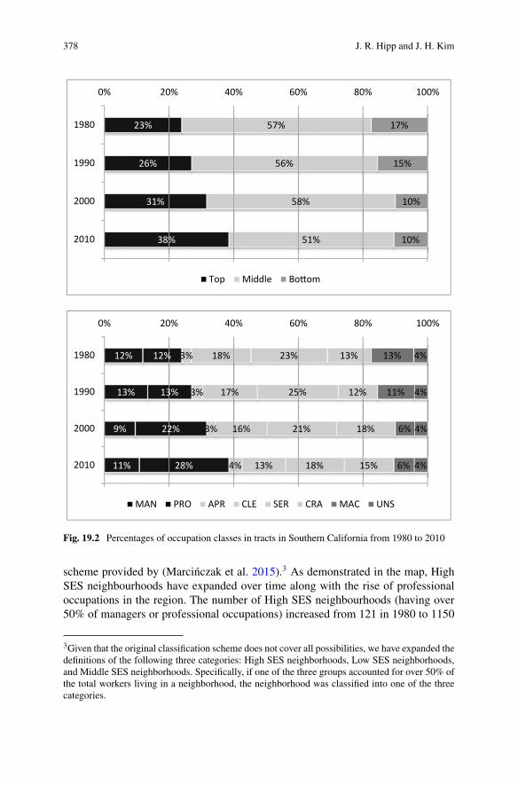
378 J. R. Hipp and J. H. Kim
38%
31%
26%
23%
51%
58%
56%
57%
10%
10%
15%
17%
0% 20% 40% 60% 80% 100%
2010
2000
1990
1980
Top Middle Bo om
11%
9%
13%
12%
28%
22%
13%
12%
4%
3%
3%
3%
13%
16%
17%
18%
18%
21%
25%
23%
15%
18%
12%
13%
6%
6%
11%
13%
4%
4%
4%
4%
0% 20% 40% 60% 80% 100%
2010
2000
1990
1980
MAN PRO APR CLE SER CRA MAC UNS
Fig. 19.2 Percentages of occupation classes in tracts in Southern California from 1980 to 2010
scheme provided by (Marcinczak et al. 2015).3 As demonstrated in the map, HighSES neighbourhoods have expanded over time along with the rise of professionaloccupations in the region. The number of High SES neighbourhoods (having over50% of managers or professional occupations) increased from 121 in 1980 to 1150
3Given that the original classification scheme does not cover all possibilities, we have expanded thedefinitions of the following three categories: High SES neighborhoods, Low SES neighborhoods,and Middle SES neighborhoods. Specifically, if one of the three groups accounted for over 50% ofthe total workers living in a neighborhood, the neighborhood was classified into one of the threecategories.
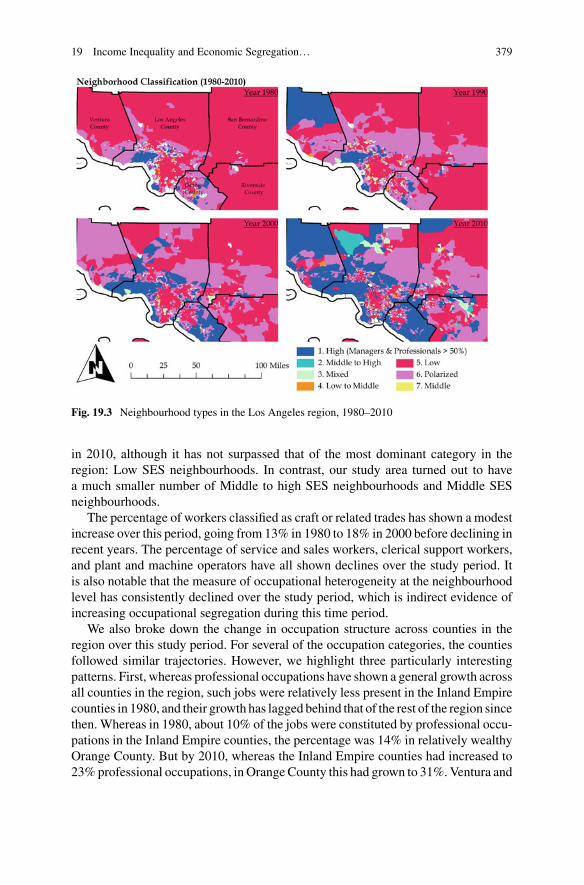
19 Income Inequality and Economic Segregation… 379
Fig. 19.3 Neighbourhood types in the Los Angeles region, 1980–2010
in 2010, although it has not surpassed that of the most dominant category in theregion: Low SES neighbourhoods. In contrast, our study area turned out to havea much smaller number of Middle to high SES neighbourhoods and Middle SESneighbourhoods.
The percentage of workers classified as craft or related trades has shown a modestincrease over this period, going from 13% in 1980 to 18% in 2000 before declining inrecent years. The percentage of service and sales workers, clerical support workers,and plant and machine operators have all shown declines over the study period. Itis also notable that the measure of occupational heterogeneity at the neighbourhoodlevel has consistently declined over the study period, which is indirect evidence ofincreasing occupational segregation during this time period.
We also broke down the change in occupation structure across counties in theregion over this study period. For several of the occupation categories, the countiesfollowed similar trajectories. However, we highlight three particularly interestingpatterns. First, whereas professional occupations have shown a general growth acrossall counties in the region, such jobs were relatively less present in the Inland Empirecounties in 1980, and their growth has lagged behind that of the rest of the region sincethen. Whereas in 1980, about 10% of the jobs were constituted by professional occu-pations in the Inland Empire counties, the percentage was 14% in relatively wealthyOrange County. But by 2010, whereas the Inland Empire counties had increased to23%professional occupations, in Orange County this had grown to 31%.Ventura and
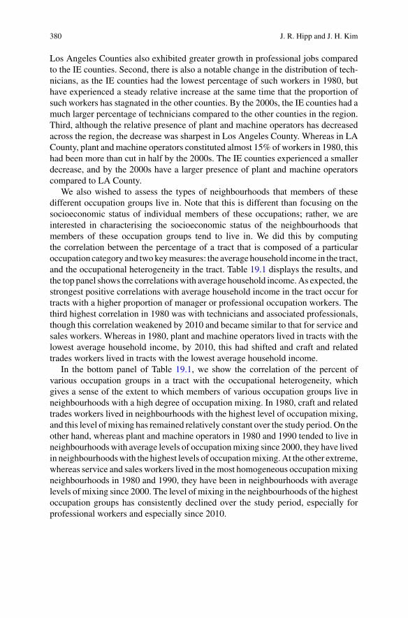
380 J. R. Hipp and J. H. Kim
Los Angeles Counties also exhibited greater growth in professional jobs comparedto the IE counties. Second, there is also a notable change in the distribution of tech-nicians, as the IE counties had the lowest percentage of such workers in 1980, buthave experienced a steady relative increase at the same time that the proportion ofsuch workers has stagnated in the other counties. By the 2000s, the IE counties had amuch larger percentage of technicians compared to the other counties in the region.Third, although the relative presence of plant and machine operators has decreasedacross the region, the decrease was sharpest in Los Angeles County. Whereas in LACounty, plant andmachine operators constituted almost 15% of workers in 1980, thishad been more than cut in half by the 2000s. The IE counties experienced a smallerdecrease, and by the 2000s have a larger presence of plant and machine operatorscompared to LA County.
We also wished to assess the types of neighbourhoods that members of thesedifferent occupation groups live in. Note that this is different than focusing on thesocioeconomic status of individual members of these occupations; rather, we areinterested in characterising the socioeconomic status of the neighbourhoods thatmembers of these occupation groups tend to live in. We did this by computingthe correlation between the percentage of a tract that is composed of a particularoccupation category and twokeymeasures: the average household income in the tract,and the occupational heterogeneity in the tract. Table 19.1 displays the results, andthe top panel shows the correlationswith average household income.As expected, thestrongest positive correlations with average household income in the tract occur fortracts with a higher proportion of manager or professional occupation workers. Thethird highest correlation in 1980 was with technicians and associated professionals,though this correlation weakened by 2010 and became similar to that for service andsales workers. Whereas in 1980, plant and machine operators lived in tracts with thelowest average household income, by 2010, this had shifted and craft and relatedtrades workers lived in tracts with the lowest average household income.
In the bottom panel of Table 19.1, we show the correlation of the percent ofvarious occupation groups in a tract with the occupational heterogeneity, whichgives a sense of the extent to which members of various occupation groups live inneighbourhoods with a high degree of occupation mixing. In 1980, craft and relatedtrades workers lived in neighbourhoods with the highest level of occupation mixing,and this level ofmixing has remained relatively constant over the study period. On theother hand, whereas plant and machine operators in 1980 and 1990 tended to live inneighbourhoodswith average levels of occupationmixing since 2000, they have livedin neighbourhoodswith the highest levels of occupationmixing.At the other extreme,whereas service and sales workers lived in themost homogeneous occupationmixingneighbourhoods in 1980 and 1990, they have been in neighbourhoods with averagelevels of mixing since 2000. The level of mixing in the neighbourhoods of the highestoccupation groups has consistently declined over the study period, especially forprofessional workers and especially since 2010.
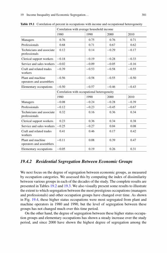
19 Income Inequality and Economic Segregation… 381
Table 19.1 Correlation of percent in occupations with income and occupational heterogeneity
Correlation with average household income
1980 1990 2000 2010
Managers 0.76 0.75 0.76 0.71
Professionals 0.68 0.71 0.67 0.62
Technicians and associateprofessionals
0.12 0.14 −0.29 −0.17
Clerical support workers −0.18 −0.19 −0.28 −0.33
Service and sales workers −0.02 −0.09 −0.05 −0.16
Craft and related tradesworkers
−0.39 −0.53 −0.58 −0.55
Plant and machineoperators and assemblers
−0.56 −0.58 −0.55 −0.50
Elementary occupations −0.50 −0.57 −0.46 −0.43
Correlation with occupational heterogeneity
1980 1990 2000 2010
Managers −0.08 −0.24 −0.28 −0.39
Professionals −0.12 −0.23 −0.45 −0.67
Technicians and associateprofessionals
0.32 0.16 0.36 0.34
Clerical support workers 0.23 0.36 0.34 0.38
Service and sales workers −0.25 −0.27 0.04 0.08
Craft and related tradesworkers
0.41 0.46 0.17 0.42
Plant and machineoperators and assemblers
−0.11 0.08 0.39 0.47
Elementary occupations −0.05 0.19 0.26 0.31
19.4.2 Residential Segregation Between Economic Groups
We next focus on the degree of segregation between economic groups, as measuredby occupation categories. We assessed this by computing the index of dissimilaritybetween various groups in each of the decades of the study. The complete results arepresented in Tables 19.2 and 19.3. We also visually present some results to illustratethe extent to which segregation between the most prestigious occupations (managersand professionals) and other occupation groups have changed over time. As shownin Fig. 19.4, these higher status occupations were most segregated from plant andmachine operators in 1980 and 1990, but the level of segregation between thesegroups has not changed much over this time period.
On the other hand, the degree of segregation between these higher status occupa-tion groups and elementary occupations has shown a steady increase over the studyperiod, and since 2000 have shown the highest degree of segregation among the
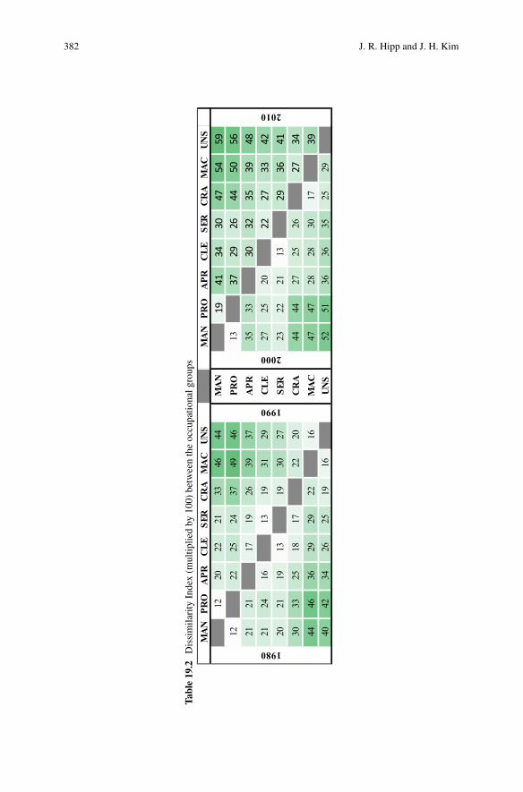
382 J. R. Hipp and J. H. Kim
Table19.2
Dissimila
rity
Index(m
ultip
liedby
100)
betw
eentheoccupatio
nalg
roup
s
MA
NPR
OA
PRC
LESE
RC
RA
MA
CUN
SM
AN
PRO
APR
CLE
SER
CR
AM
AC
UNS
1220
2221
3346
44M
AN
1941
3430
4754
5912
2225
2437
4946
PRO
1337
2926
4450
5621
2117
1926
3937
APR
3533
3032
3539
4821
2416
1319
3129
CLE
2725
2022
2733
4220
2119
1319
3027
SER
2322
2113
2936
4130
3325
1817
2220
CR
A44
4427
2526
2734
4446
3629
2922
16M
AC
4747
2828
3017
3940
4234
2625
1916
UNS
5251
3636
3525
29
1980
1990
2000
2010
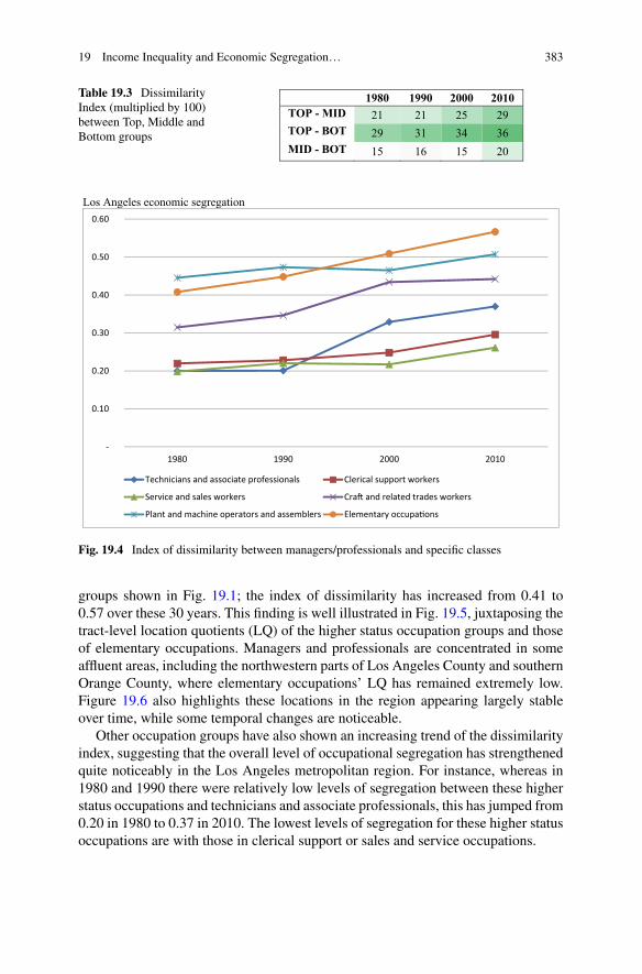
19 Income Inequality and Economic Segregation… 383
Table 19.3 DissimilarityIndex (multiplied by 100)between Top, Middle andBottom groups
1980 1990 2000 2010 TOP - MID 21 21 25 29 TOP - BOT 29 31 34 36 MID - BOT 15 16 15 20
Los Angeles economic segregation
-
0.10
0.20
0.30
0.40
0.50
0.60
1980 1990 2000 2010
Technicians and associate professionals Clerical support workers
Service and sales workers Cra and related trades workers
Plant and machine operators and assemblers Elementary occupa ons
Fig. 19.4 Index of dissimilarity between managers/professionals and specific classes
groups shown in Fig. 19.1; the index of dissimilarity has increased from 0.41 to0.57 over these 30 years. This finding is well illustrated in Fig. 19.5, juxtaposing thetract-level location quotients (LQ) of the higher status occupation groups and thoseof elementary occupations. Managers and professionals are concentrated in someaffluent areas, including the northwestern parts of Los Angeles County and southernOrange County, where elementary occupations’ LQ has remained extremely low.Figure 19.6 also highlights these locations in the region appearing largely stableover time, while some temporal changes are noticeable.
Other occupation groups have also shown an increasing trend of the dissimilarityindex, suggesting that the overall level of occupational segregation has strengthenedquite noticeably in the Los Angeles metropolitan region. For instance, whereas in1980 and 1990 there were relatively low levels of segregation between these higherstatus occupations and technicians and associate professionals, this has jumped from0.20 in 1980 to 0.37 in 2010. The lowest levels of segregation for these higher statusoccupations are with those in clerical support or sales and service occupations.
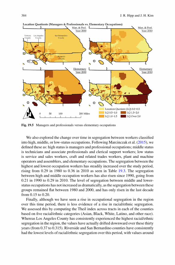
384 J. R. Hipp and J. H. Kim
Fig. 19.5 Managers and professionals versus elementary occupations
We also explored the change over time in segregation between workers classifiedinto high, middle, or low-status occupations. FollowingMarcinczak et al. (2015), wedefined these as: high status is managers and professional occupations; middle statusis technicians and associate professionals and clerical support workers; low statusis service and sales workers, craft and related trades workers, plant and machineoperators and assemblers, and elementary occupations. The segregation between thehighest and lowest occupation workers has steadily increased over the study period,rising from 0.29 in 1980 to 0.36 in 2010 as seen in Table 19.3. The segregationbetween high and middle occupation workers has also risen since 1990, going from0.21 in 1990 to 0.29 in 2010. The level of segregation between middle and lower-status occupations has not increased as dramatically, as the segregation between thesegroups remained flat between 1980 and 2000, and has only risen in the last decadefrom 0.15 to 0.20.
Finally, although we have seen a rise in occupational segregation in the regionover this time period, there is less evidence of a rise in racial/ethnic segregation.We assessed this by computing the Theil index across tracts in each of the countiesbased on five racial/ethnic categories (Asian, Black, White, Latino, and other race).Whereas Los Angeles County has consistently experienced the highest racial/ethnicsegregation in the region, the values have actually drifted downward over these thirtyyears (from 0.37 to 0.315). Riverside and San Bernardino counties have consistentlyhad the lowest levels of racial/ethnic segregation over this period, with values around

19 Income Inequality and Economic Segregation… 385
Fig. 19.6 Distribution of managers and professionals, 1980–2010
0.16. Ventura is slightly higher (0.22), although it has remained stable. Only OrangeCounty has experienced a modest increase over the study period from 0.16 to 0.23.Thus, the increasing occupational segregation in the region appears to not be relatedto racial/ethnic segregation processes.
19.5 Conclusion
This study has focused on how levels of inequality in the Los Angeles area havechanged from 1980 to 2010. Whereas we observed notable increases in inequalityover the time period, as measured by the Gini coefficient based on household incomelevels, we also observed substantial changes in the region’s occupation structure. Theregion has experienced a large increase in the proportion of professional workers overthe study period. At the same time, there has been a large drop in the relative propor-tion of plant and machine operators. This pattern is consistent with the restructuringof jobs from blue collar towards white collar work, especially in this region.
Importantly,we also detected evidence of increasing residential segregation acrossthe economic groups over time. Among others, we found that the highest status occu-pations (managers and professional workers) are becomingmore spatially segregatedfrom other occupations over the study period, while the rates of segregation increase
386 J. R. Hipp and J. H. Kim
varied by group and decade. There was also evidence that these highest status occu-pation workers tend to live in areas with the most economical resources to whichother groups have limited access.
Admittedly, the traditional dissimilarity index and other metrics employed in thisstudy would not allow us to capture the full extent and details of the segregationdynamics underway in the Los Angeles metropolitan region. It is also known thatthe census tracts used here, as done in numerous other studies, have a limited abilityto represent the true neighbourhood boundaries in reality. There is also concern thatthe lower sampling rate of the ACS in 2010 can bias segregation estimates; indeed,studies have shown such an effect when measuring economic segregation based onbinned income data (Reardon et al. 2018). However, the fact that our occupationcategories are less extensive than the income bins (and therefore not as subject tosmall counts) suggests that our results may be less impacted by this issue. Also,other limitations would not invalidate the strong evidence of increasing occupationalsegregation patterns and should not undermine the implications of the evidence thatdeserves further attention.
How these patterns might change as Los Angeles County—the central county inthe region—continues to build out its light rail public transportation system, remainsto be seen. In the short-term, these new light rail lines seem to engender gentrifica-tion processes in the adjacent neighbourhoods. In the long-term, the question ariseswhether this public investment can change some of the current patterns observedin this more sprawling, car-centric, development. One can be optimistic about thefuture, given that there have been numerous state-level efforts to promote affordablehousing provision in various locations, including transit-rich areas, but we shouldnot underestimate the obstacles that will have to be overcome in order to make ameaningful difference in the next decades.
References
Blumenberg E, Manville M (2004) Beyond the spatial mismatch: welfare recipients and transporta-tion policy. J Plann Lit 19:182–205
Byun P, Esparza AX (2005) A revisionist model of suburbanization and sprawl: The role of politicalfragmentation, growth control, and spillovers. J Plann Educ Res 24:252–264
Carruthers JI (2003) Growth at the fringe: the influence of political fragmentation in United Statesmetropolitan areas. Papers Reg Sci 82:475–499
Chetty R, Grusky D, HellM, Hendren N,Manduca R, Narang J (2017) The fading American dream:trends in absolute income mobility since 1940. Science 356:398–406
Hipp JR, Kane K, Kim JH (2017a) Jobs-housing balance in Egohoods in Southern California.Metropolitan Futures Initiative (MFI), Irvine, CA
Hipp JR, Kane K, Kim JH (2017b) Recipes for neighborhood development: a machine learningapproach toward understanding the impact of mixing in neighborhoods. Landscape Urban Plann164:1–12
Hipp JR,Kim JH,BasoloV (2014) SouthernCalifornia regional progress report: 2014.MetropolitanFutures Initiative (MFI), Irvine, CA
Hogen-Esch T (2011) Fragmentation, fiscal federalism, and the ghost of Dillon’s rule: municipalincorporation in Southern California, 1950–2010. Calif J Polit Policy 3:1–22
19 Income Inequality and Economic Segregation… 387
Hu L (2015) Job accessibility of the poor in Los Angeles: has suburbanization affected spatialmismatch? J Am Plann Assoc 81:30–45
KaneK,Hipp JR,Kim JH (2018) LosAngeles employment concentration in the twenty-first century.Urban Stud 55:844–869
Kane K, Kim JH, Hipp JR (2016) Detecting job density over time. Metropolitan Futures Initiative(MFI), Irvine, CA
Kane K, Kim JH, Hipp JR (2017) What makes housing accessible to everyday destinations inSouthern California. Metropolitan Futures Initiative (MFI), Irvine, CA
Kim JH, Hipp JR, Basolo V, Dillon HS (2018) Land use change dynamics in southern California:does geographic elasticity matter? J Plann Educ Res 38:39–53
Kim JH, Jurey N (2013) Local and regional governance structures: Fiscal, economic, equity, andenvironmental outcomes. J Plann Lit 28:111–123
Le Goix R (2005) Gated communities: Sprawl and social segregation in Southern California. HousStud 20:323–343
Levine N (1999) The effects of local growth controls on regional housing production and populationredistribution in California. Urban Stud 36:2047–2068
Marcinczak S, Tammaru T, Novák J, Gentile M, Kovács Z, Temelová J, Valatka V, Kährik A,Szabó B (2015) Patterns of socioeconomic segregation in the capital cities of fast-track reformingpostsocialist countries. Ann Assoc Am Geogr 105:183–202
McKenzie E (2003) Common-interest housing in the communities of tomorrow.Hous PolicyDebate14:203–234
Ong P, Blumenberg E (1998) Job access, commute and travel burden among welfare recipients.Urban Stud 35:77–93
Reardon SF, Bischoff K (2011) Income inequality and income segregation. Am J Sociol 116:1092–1153
Reardon SF, Bischoff K, Owens A, Townsend JB (2018) Has income segregation really increased?Bias and bias correction in sample-based segregation estimates. Demography 55:2129–2160
Sanchez TW, Lang RE, Dhavale DM (2005) Security versus status? A first look at the census’sgated community data. J Plann Educ Res 24:281–291
Scarpa S (2016) Looking beyond the neighbourhood: income inequality and residential segregationin Swedish metropolitan areas, 1991–2010. Urban Geogr 37:963–984
Sommeiller E, Price M (2018) The new gilded age: Income inequality in the U.S. by state,metropolitan area, and county. Economic Policy Institute, Washington DC
Tong X, Kim JH (2019) Concentration or diffusion? Exploring the emerging spatial dynamics ofpoverty distribution in Southern California. Cities 85:15–24
Ulfarsson GF, Carruthers JI (2006) The cycle of fragmentation and sprawl: a conceptual frameworkand empirical model. Environ Plann B: Plann Des 33:767–788
Open Access This chapter is licensed under the terms of the Creative Commons Attribution 4.0International License (http://creativecommons.org/licenses/by/4.0/), which permits use, sharing,adaptation, distribution and reproduction in any medium or format, as long as you give appropriatecredit to the original author(s) and the source, provide a link to the Creative Commons license andindicate if changes were made.
The images or other third party material in this chapter are included in the chapter’s CreativeCommons license, unless indicated otherwise in a credit line to the material. If material is notincluded in the chapter’s Creative Commons license and your intended use is not permitted bystatutory regulation or exceeds the permitted use, you will need to obtain permission directly fromthe copyright holder.
Chapter 20Socioeconomic Segregation in MexicoCity: Scale, Social Classes,and the Primate City
Paavo Monkkonen, M. Paloma Giottonini, and Andre Comandon
Abstract Mexico City is known as one of the largest cities in the world and thoughtbymany to be one of themost unequal.Not surprisingly, it has receivedmore attentionthan other Mexican urban areas. However, the city’s internal social organization isoften misunderstood. Mexico City stands out as a city where segregation is relativelylow, and levels of inequality are actually lower than perceptions. Moreover, between1990 and 2010, both segregation and inequality have declined. This chapter exam-ines these changes. We report on changes in occupational structure and patterns ofsegregation by educational level. Educational level is different from income or occu-pation, but these three dimensions of socioeconomic conditions are closely linked.While the overall level of segregation between educational groups in the city hasslightly decreased, residential patterns of educational groups have changed signifi-cantly. The number of neighborhoods with high concentrations of highly educatedpeople increased significantly and expanded geographically. At the same time, theprevalence of neighborhoods with residents with low and middle educational attain-ment has diminished and neighborhoods that house people of all educational cate-gories or high and middle categories are more numerous. This chapter illustrates thecomplexity of segregation patterns in such a large metropolitan area, as well as thechallenges of determining why patterns have changed.
Keywords Segregation · Inequality · Education · Neighborhood ·Mexico City
“Juntos pero no revueltos” [Together but not mixed]
Mexican proverb
Electronic supplementary material The online version of this chapter(https://doi.org/10.1007/978-3-030-64569-4_20) contains supplementary material, which isavailable to authorized users.
P. Monkkonen (B) · M. Paloma Giottonini · A. ComandonUCLA, Los Angeles, USAe-mail: [email protected]
© The Author(s) 2021M. van Ham et al. (eds.), Urban Socio-Economic Segregation and Income Inequality,The Urban Book Series, https://doi.org/10.1007/978-3-030-64569-4_20
389
390 P. Monkkonen et al.
20.1 Introduction
Mexico City is one of the largest cities in the world and by far the largest in Mexico.One in six Mexicans live in the Mexico City Metropolitan Area (MCMA). It also hasone of the longest histories of large-scale urbanization in the Americas, giving thesprawling metropolis multiple personalities. The patchwork of neighborhoods thathave developed over centuries form the economic hub of the country, the center ofthe federal government, and a concentrated cultural repository. Cities that dominatetheir national urban system—primate cities like Mexico City—tend to be richer butalso more unequal. Yet, the MCMA is not as unequal as one might expect. Moresurprisingly, given the popular understanding of the city, levels of social segregationare relatively low in the MCMA when measured using available data.
The perception of Mexico as an extremely unequal country is widespread. It doeshave a high rate of inequality compared to OECD countries, with a Gini coefficient1
in 2016 of 0.43 being 25% higher than the OECD average. Yet it is less unequalthan most other Latin American and many middle-income countries. For example,its Gini coefficient was lower than Brazil, Colombia, and South Africa, which all hadGINI coefficients over 0.5 (OECD 2019b; World Bank 2019). Income inequality inMexico increased in the 1990s before declining after 2000 to levels below those of1990 (Cortés 2013). Though income inequalitymay be lower than expected, there aremultiple aspects of social inequality in Mexican society, with dramatic differencesin access to education, health services, housing, safety, and overall quality of life.
In this chapter, we assess income inequality and the levels and patterns of residen-tial segregation in the MCMA.We focus on segregation by educational achievementbecause it is the only variable for which data are available. Education is also a proxyfor socioeconomic status and a critical aspect of social inequality. One distinction isthat unlike income, educational attainment of a person cannot go down. In Mexico,educational achievement has increased over time, while incomes have remained rela-tively stagnant. Nonetheless, they are strongly linked. Our central research questionfits within the questions of socioeconomic segregation this book deals with. We askhow and to what extent levels of segregation by education and the residential patternsof educational groups have changed In the MCMA during the last two decades.
The answer to that question addresses a debate over the relationship betweeninequality and spatial segregation. Researchers in high-income countries have founda correlation between socioeconomic inequality and residential segregation (Reardonand Bischoff 2011), but evidence for this relationship in Mexico is mixed. Thischapter details this connection by first describing the complex spatial and economicstructures of the region. The next section provides an overview of inequality and itsconnection to segregation in the context of Mexico City. The fourth section presentsthe empirical results and illustrates the main patterns visually. The final two sectionsprovide a discussion of the results and possible futures for the city.
1All GINI estimates presented in this chapter are calculated using after tax income.
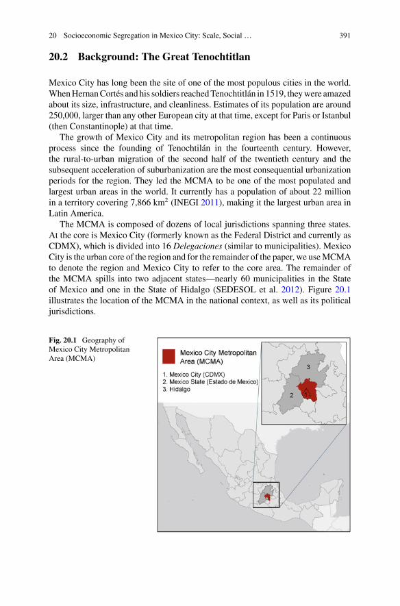
20 Socioeconomic Segregation in Mexico City: Scale, Social … 391
20.2 Background: The Great Tenochtitlan
Mexico City has long been the site of one of the most populous cities in the world.WhenHernanCortés and his soldiers reachedTenochtitlán in 1519, theywere amazedabout its size, infrastructure, and cleanliness. Estimates of its population are around250,000, larger than any other European city at that time, except for Paris or Istanbul(then Constantinople) at that time.
The growth of Mexico City and its metropolitan region has been a continuousprocess since the founding of Tenochtilán in the fourteenth century. However,the rural-to-urban migration of the second half of the twentieth century and thesubsequent acceleration of suburbanization are the most consequential urbanizationperiods for the region. They led the MCMA to be one of the most populated andlargest urban areas in the world. It currently has a population of about 22 millionin a territory covering 7,866 km2 (INEGI 2011), making it the largest urban area inLatin America.
The MCMA is composed of dozens of local jurisdictions spanning three states.At the core is Mexico City (formerly known as the Federal District and currently asCDMX), which is divided into 16 Delegaciones (similar to municipalities). MexicoCity is the urban core of the region and for the remainder of the paper, we useMCMAto denote the region and Mexico City to refer to the core area. The remainder ofthe MCMA spills into two adjacent states—nearly 60 municipalities in the Stateof Mexico and one in the State of Hidalgo (SEDESOL et al. 2012). Figure 20.1illustrates the location of the MCMA in the national context, as well as its politicaljurisdictions.
Fig. 20.1 Geography ofMexico City MetropolitanArea (MCMA)
392 P. Monkkonen et al.
The population of the metropolitan area used to be more concentrated in MexicoCity itself, but after it urbanized most available land, Mexico City has had a lowergrowth rate than the adjacent municipalities of State ofMexico andHidalgo. In 1990,over 50% of the population of the MCMA was in Mexico City (about eight millionpeople), whereas in 2015 Mexico City’s nine million residents are only 40% ofthe larger metropolitan region (INEGI 2015a, b). The government officially definedthe current MCMA (also known as Zona Metropolitana del Valle de Mexico) in2004 (SEDESOL et al. 2012). At this time, 36 additional municipalities were added,practically doubling the metropolitan region’s territory.
Most of the population growth of the metropolitan area is the result of thisterritorial annexation and of the high population growth rates in the municipali-ties belonging to State of Mexico, rather than population growth within MexicoCity. Nonetheless, the MCMA stands out for its slower rate of population growth ascompared to the national average. Between 2000 and 2010, the MCMA had one ofthe slowest urban growth rates (0.9%) in the country. The national average was 1.4%and other metropolitan areas grew at 2.0%. However, given the size of the region,this lower rate still means large population changes in absolute numbers. MexicoCity is also the densest urban area in the country with about 6,000 inhabitants persquare kilometer (INEGI 2015a, b).Many peripheral areas have also become denselypopulated (see Figure in supplementary material online).
The urban primacy of the MCMA is unquestionable: it is the most populated andeconomically competitive city in Mexico. In 2009, the MCMA housed about 19% ofthe country’s population, 25% of national gross domestic product (GDP), and 23% ofjobs (Trejo Nieto 2016). Mexico City is not only an important global financial center,it is also widely recognized as the cultural capital of Latin America. Mexico City hasthe oldest university in the continent, two world heritage sites, and more museumsthan any other city in the world. This status, combined with the continued internalmigration of people moving from rural-to-urban areas in search of better economicopportunity, has privileged low-skilled manufacturing and (informal) service jobsin the city’s occupational makeup (García et al. 1978; Zenteno and Solís 2006).Thus, despite its slowing growth rate, the city continues to attract people fromwithinMexico and the rest of the world.
20.2.1 Occupational Characteristics of the Metropolitan Area
Compared to the other large metropolitan areas in Mexico, the MCMA has a morespecialized occupational profile. It has a large share of jobs in the service sector—45% compared to 30% in the average city (Montejano et al. 2019). Its populationhas among the highest educational attainment and a high level of productivity percapita, though perhaps not as high as one might expect. The MCMA is home tothe country’s largest corporate headquarters but has such a large labor force that theaverage statistics overwhelm these high-level jobs.
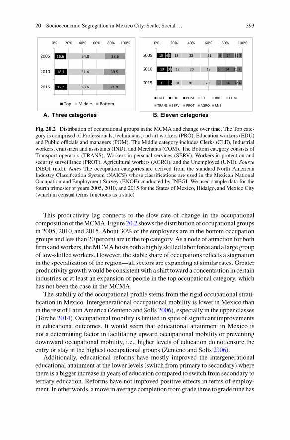
20 Socioeconomic Segregation in Mexico City: Scale, Social … 393
A. Three categories B. Eleven categories
18.4
18.1
16.6
50.6
51.4
54.8
31.0
30.5
28.6
0% 20% 40% 60% 80% 100%
2015
2010
2005
Top Middle Bo om
13
13
10
3
3
4
2
2
3
10
12
13
20
20
22
20
19
21
6
6
6
16
14
14
1
3
3
2
1
2
6
7
5
0% 20% 40% 60% 80% 100%
2015
2010
2005
PRO EDU POM CLE IND COM
TRANS SERV PROT AGRO UNE
Fig. 20.2 Distribution of occupational groups in the MCMA and change over time. The Top cate-gory is comprised of Professionals, technicians, and art workers (PRO), Education workers (EDU)and Public officials and managers (POM). The Middle category includes Clerks (CLE), Industrialworkers, craftsmen and assistants (IND), and Merchants (COM). The Bottom category consists ofTransport operators (TRANS), Workers in personal services (SERV), Workers in protection andsecurity surveillance (PROT), Agricultural workers (AGRO), and the Unemployed (UNE). SourceINEGI (n.d.). Notes The occupation categories are derived from the standard North AmericanIndustry Classification System (NAICS) whose classifications are used in the Mexican NationalOccupation and Employment Survey (ENOE) conducted by INEGI. We used sample data for thefourth trimester of years 2005, 2010, and 2015 for the States of Mexico, Hidalgo, and Mexico City(which in censual terms functions as a state)
This productivity lag connects to the slow rate of change in the occupationalcompositionof theMCMA.Figure 20.2 shows thedistributionof occupational groupsin 2005, 2010, and 2015. About 30% of the employees are in the bottom occupationgroups and less than 20 percent are in the top category. As a node of attraction for bothfirms andworkers, theMCMAhosts both a highly skilled labor force and a large groupof low-skilled workers. However, the stable share of occupations reflects a stagnationin the specialization of the region—all sectors are expanding at similar rates. Greaterproductivity growthwould be consistent with a shift toward a concentration in certainindustries or at least an expansion of people in the top occupational category, whichhas not been the case in the MCMA.
The stability of the occupational profile stems from the rigid occupational strati-fication in Mexico. Intergenerational occupational mobility is lower in Mexico thanin the rest of Latin America (Zenteno and Solís 2006), especially in the upper classes(Torche 2014). Occupational mobility is limited in spite of significant improvementsin educational outcomes. It would seem that educational attainment in Mexico isnot a determining factor in facilitating upward occupational mobility or preventingdownward occupational mobility, i.e., higher levels of education do not ensure theentry or stay in the highest occupational groups (Zenteno and Solís 2006).
Additionally, educational reforms have mostly improved the intergenerationaleducational attainment at the lower levels (switch from primary to secondary) wherethere is a bigger increase in years of education compared to switch from secondary totertiary education. Reforms have not improved positive effects in terms of employ-ment. In otherwords, amove in average completion fromgrade three to grade nine has
394 P. Monkkonen et al.
a greater numerical impact when it comes to years-in-education than a move fromgrade nine to grade 12, but the latter has stronger positive effects on individuals’labor market outcomes. This greatly limits the impact of reforms when high-wagejobs require a college degree or graduate diploma.
The link between education and occupation is also visible across neighborhoods.Residents of Mexico City have higher education and are more likely to be in thetop occupational category (23%) than residents of the States of Mexico and Hidalgo(only 13%). This concentration also translates to local clustering. The clusteringof high-skilled jobs in and around the central business district of Mexico City ismismatched with the location of workers (Trejo Nieto 2016). Spatial mismatch ofhigh-status jobs results partly because people with greater resources also have greaterability to commute longer distances.
20.2.2 The Mexican Housing System and Segregation
Housing occupies an uneasy position in relation to the welfare system (Malpass2008). The state tends to intervene systematically in the housing sector, espe-cially in middle-income countries. Like other Latin American countries, Mexicohas embarked on an ambitious policy agenda to increase access to formal housing.TheMexican program has shaped cities perhaps evenmore than in its southern neigh-bors. Until recently, Mexican cities have had a spatial structure similar to that of therest of Latin America. This structure has three elements: (1) low-income householdsmostly clustered to low-density peripheral areas, usually with limited or no urbanservices; (2) high-income households concentrated in certain areas of the city, usuallystarting near the historic center and move outward in one direction; and (3) a greatersocioeconomic homogeneity in low-income neighborhoods (Griffin and Ford 1980;Sabatini 2003).
During recent decades, however, the peripheral areas of cities inMexico, includingthe MCMA, have changed dramatically. Numerous large, homogeneous housingdevelopments for the working class were built in cities across the country, drivenby the reform and expansion of a federal housing fund (named INFONAVIT for itsinitials in Spanish) beginning in the early 1990s. The boom in financing transformedtheway housing is produced and acquired (Monkkonen 2011). Prior to the year 2000,individuals built the majority of housing in an incremental, self-help manner on plotsof land they purchased. Since then, federal mortgages enabled private developers tobuild large tracts of formal housing for purchase and now a majority of housing isbuilt by developers and purchased with a mortgage. The federal mortgage fund isgenerated through a 5% payroll tax and has greater resources than other welfaresectors in Mexico. The share of public expenditure is still relatively low, at around1% of GDP.
Housing provision through this fund has some significant shortcomings. First,workers in the informal sector, whose housing need is often most severe (OECD2006), cannot access this government program which is available only to salaried
20 Socioeconomic Segregation in Mexico City: Scale, Social … 395
employees. Second, the housing offered is of a very small size, low quality and gener-ally has a peripheral location often far from jobs. The changes to the government’shousing fund without concurrent changes in municipal planning practice meant thatdevelopers also became de facto urban planners, with certain freedoms in decidingwhere, what, and how to build (Libertun de Duren 2018). New housing develop-ments are homogenous, whichmeans potential buyers are of a similar socioeconomicstatus. This has exacerbated residential segregation between socioeconomic groups(Monkkonen 2012a) and is connected to problems of housing vacancy (Monkkonen2019).
20.3 Socioeconomic Segregation and Income Inequalityin Mexico City
Recent work on segregation in Mexico shows that larger and higher cost cities aremore segregated, though there are some regional differences across the country(Monkkonen 2012b, 2018). Cities in the northern region of Mexico have a largerpresence of formal workers and high-income households, while the cities in thesouth have a much higher proportion of lower-income households and indigenouspopulation. These two findings align with the general regional development trendsin Mexico, i.e. the industrialization of northern cities and the persistent poverty inthe south (Garza 1999; Trejo Nieto 2019). Nonetheless, the median city in the southis roughly 10% less segregated than the median city in the north.
The MCMA, located in the central region of Mexico, has the highest proportionof workers in the informal sector (54%) in the country. At the same time that ithouses the most affluent households in the country, the federal government, and thenation’s most prominent cultural institutions, the MCMA also has a high proportionof low-income households (38%), a share only surpassed by the Southern region(Monkkonen 2012b). The MCMA also has a disproportionate share of high-incomehouseholds—using a separate dataset from 2015 (INEGI 2015a, b), we find roughly18% of the households in Mexico City fall into the top decile of earners nationwide.This number is only 15% for the entire MCMA.
The MCMA is relatively unequal but not socially segregated. In 2014, comparedto the country’s states, Mexico City had the fifth highest GINI coefficient (0.48),and the states of Hidalgo and Mexico State had GINI coefficients of 0.48 and 0.44,respectively (OECD 2019a). Apart from income inequality and occupational profile,city size and urban growth are fundamental drivers of socioeconomic segregation(Monkkonen 2012a; Rubalcava and Schteingart 2000; Ariza and Solis 2009). Ascities expand their territories, commuting distances and disparities in land valuesincrease, which leads to more differentiated neighborhoods (Mills and Hamilton1994).
396 P. Monkkonen et al.
The rapid population growth of the MCMA took place in the form of densifi-cation of the existing urban area as well as expansion into neighboring municipal-ities by both migrants moving from other states as well as from Mexico City tothe metropolitan periphery. The horizontal expansion is consistent with patterns ofspatial differentiation as new neighborhoods are developed.
20.4 Measuring the Relationship Between Incomeand Socioeconomic Composition
The decennial census of Mexico does not inquire about occupation. Data on occupa-tion is, therefore, only partially available through the Mexican National Occupationand Employment Survey (ENOE). The statistical design of the ENOE producesprecise estimates at the national level and by state, but not for municipalities andthe smaller geographical units required for analyzing segregation. Therefore, we useeducational groupings as a proxy for socioeconomic status. Education correlateswithincome and socioeconomic status (Caragliu et al. 2012), and residential segregationby income correlates with residential segregation by education (Monkkonen et al.2018). We are, therefore, confident that our measures capture the main underlyingspatial patterns of inequality. However, education differs from income or occupationin that education is not asmuch a product of market forces and does not determine theresidential choice of people directly. Therefore, it does have a different relationshipto spatial residential patterns.
Using education as the main variable changes the comparison of segregationpatterns over time. For example, the education reform of 1993 established compul-sory secondary education.2 As such, children in school in the 1990s will automat-ically have on average higher educational achievement than people who finishedschool before the reform. Additionally, educational achievement is more permanentthan income. Most people do not go back to school later in life, but their incomecan change every year, increasing or decreasing. This has different implications forchanges in social mix.
Throughout this analysis, we use education attainment at the level of the basicgeo-statistical area (known as AGEB for its initials in Spanish), which is equivalentto a census tract. We use data from the census of 1990, 2000 and 2010 carried outby the National Institute of Geography, Informatics and Statistics (INEGI). We useall urban AGEBs in the 76 municipalities of the MCMA in the year 2010.3 That is,we apply the 2004 MCMA boundaries to the years 2000 and 1990. A large share oftracts outside Mexico city itself do not have data in 1990 because they had not beenurbanized yet.
2In Mexico, secondary education refers to secundaria, which is equivalent to years 7, 8 and 9 ofschooling.3The MCMA has 5,605 AGEBs. They have mean and median population of 3,485 and 3,171.
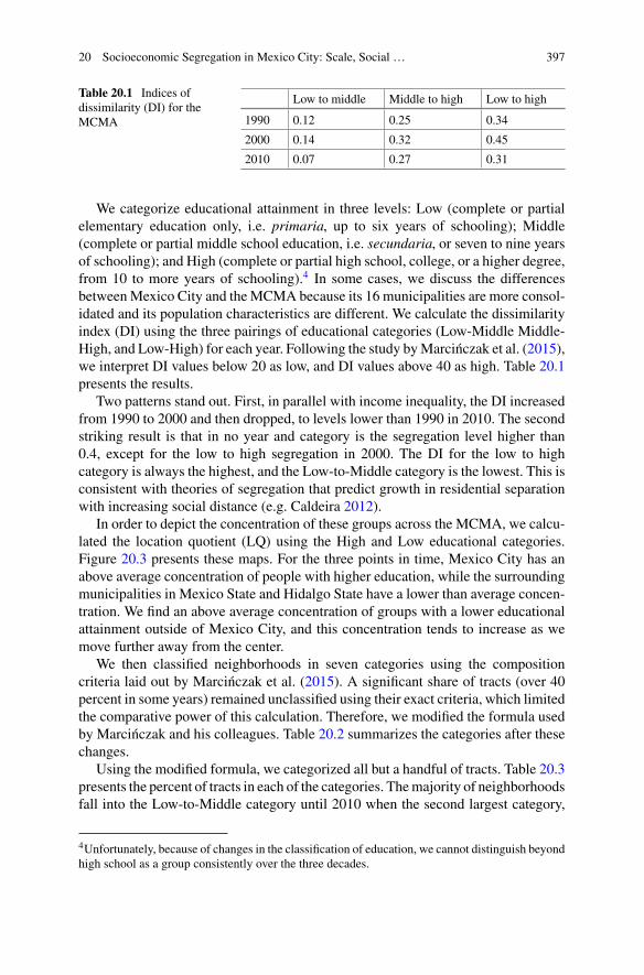
20 Socioeconomic Segregation in Mexico City: Scale, Social … 397
Table 20.1 Indices ofdissimilarity (DI) for theMCMA
Low to middle Middle to high Low to high
1990 0.12 0.25 0.34
2000 0.14 0.32 0.45
2010 0.07 0.27 0.31
We categorize educational attainment in three levels: Low (complete or partialelementary education only, i.e. primaria, up to six years of schooling); Middle(complete or partial middle school education, i.e. secundaria, or seven to nine yearsof schooling); and High (complete or partial high school, college, or a higher degree,from 10 to more years of schooling).4 In some cases, we discuss the differencesbetweenMexico City and theMCMA because its 16 municipalities are more consol-idated and its population characteristics are different. We calculate the dissimilarityindex (DI) using the three pairings of educational categories (Low-Middle Middle-High, and Low-High) for each year. Following the study byMarcinczak et al. (2015),we interpret DI values below 20 as low, and DI values above 40 as high. Table 20.1presents the results.
Two patterns stand out. First, in parallel with income inequality, the DI increasedfrom 1990 to 2000 and then dropped, to levels lower than 1990 in 2010. The secondstriking result is that in no year and category is the segregation level higher than0.4, except for the low to high segregation in 2000. The DI for the low to highcategory is always the highest, and the Low-to-Middle category is the lowest. This isconsistent with theories of segregation that predict growth in residential separationwith increasing social distance (e.g. Caldeira 2012).
In order to depict the concentration of these groups across the MCMA, we calcu-lated the location quotient (LQ) using the High and Low educational categories.Figure 20.3 presents these maps. For the three points in time, Mexico City has anabove average concentration of people with higher education, while the surroundingmunicipalities in Mexico State and Hidalgo State have a lower than average concen-tration. We find an above average concentration of groups with a lower educationalattainment outside of Mexico City, and this concentration tends to increase as wemove further away from the center.
We then classified neighborhoods in seven categories using the compositioncriteria laid out by Marcinczak et al. (2015). A significant share of tracts (over 40percent in some years) remained unclassified using their exact criteria, which limitedthe comparative power of this calculation. Therefore, we modified the formula usedby Marcinczak and his colleagues. Table 20.2 summarizes the categories after thesechanges.
Using the modified formula, we categorized all but a handful of tracts. Table 20.3presents the percent of tracts in each of the categories. Themajority of neighborhoodsfall into the Low-to-Middle category until 2010 when the second largest category,
4Unfortunately, because of changes in the classification of education, we cannot distinguish beyondhigh school as a group consistently over the three decades.
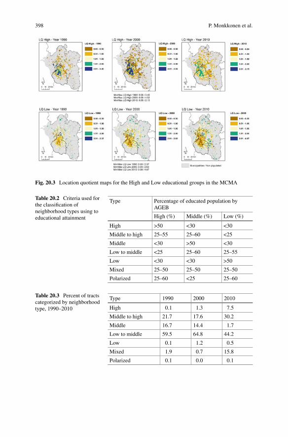
398 P. Monkkonen et al.
Fig. 20.3 Location quotient maps for the High and Low educational groups in the MCMA
Table 20.2 Criteria used forthe classification ofneighborhood types using toeducational attainment
Type Percentage of educated population byAGEB
High (%) Middle (%) Low (%)
High >50 <30 <30
Middle to high 25–55 25–60 <25
Middle <30 >50 <30
Low to middle <25 25–60 25–55
Low <30 <30 >50
Mixed 25–50 25–50 25–50
Polarized 25–60 <25 25–60
Table 20.3 Percent of tractscategorized by neighborhoodtype, 1990–2010
Type 1990 2000 2010
High 0.1 1.3 7.5
Middle to high 21.7 17.6 30.2
Middle 16.7 14.4 1.7
Low to middle 59.5 64.8 44.2
Low 0.1 1.2 0.5
Mixed 1.9 0.7 15.8
Polarized 0.1 0.0 0.1
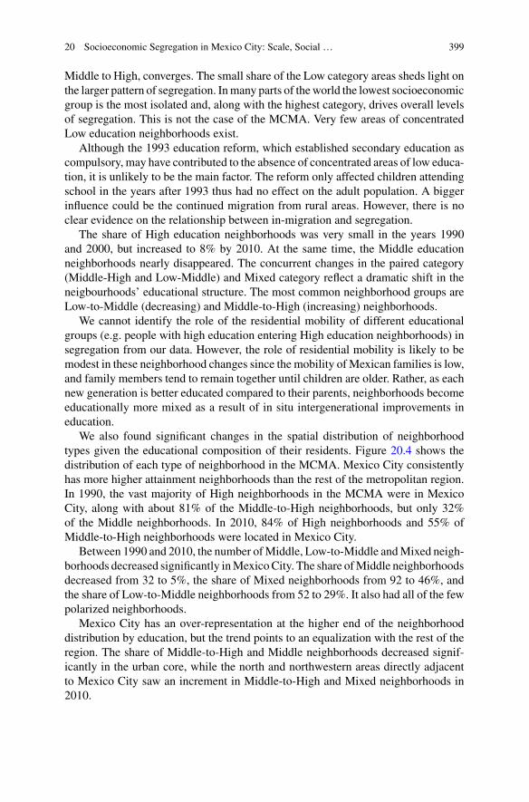
20 Socioeconomic Segregation in Mexico City: Scale, Social … 399
Middle to High, converges. The small share of the Low category areas sheds light onthe larger pattern of segregation. Inmany parts of theworld the lowest socioeconomicgroup is the most isolated and, along with the highest category, drives overall levelsof segregation. This is not the case of the MCMA. Very few areas of concentratedLow education neighborhoods exist.
Although the 1993 education reform, which established secondary education ascompulsory, may have contributed to the absence of concentrated areas of low educa-tion, it is unlikely to be the main factor. The reform only affected children attendingschool in the years after 1993 thus had no effect on the adult population. A biggerinfluence could be the continued migration from rural areas. However, there is noclear evidence on the relationship between in-migration and segregation.
The share of High education neighborhoods was very small in the years 1990and 2000, but increased to 8% by 2010. At the same time, the Middle educationneighborhoods nearly disappeared. The concurrent changes in the paired category(Middle-High and Low-Middle) and Mixed category reflect a dramatic shift in theneigbourhoods’ educational structure. The most common neighborhood groups areLow-to-Middle (decreasing) and Middle-to-High (increasing) neighborhoods.
We cannot identify the role of the residential mobility of different educationalgroups (e.g. people with high education entering High education neighborhoods) insegregation from our data. However, the role of residential mobility is likely to bemodest in these neighborhood changes since the mobility ofMexican families is low,and family members tend to remain together until children are older. Rather, as eachnew generation is better educated compared to their parents, neighborhoods becomeeducationally more mixed as a result of in situ intergenerational improvements ineducation.
We also found significant changes in the spatial distribution of neighborhoodtypes given the educational composition of their residents. Figure 20.4 shows thedistribution of each type of neighborhood in the MCMA. Mexico City consistentlyhas more higher attainment neighborhoods than the rest of the metropolitan region.In 1990, the vast majority of High neighborhoods in the MCMA were in MexicoCity, along with about 81% of the Middle-to-High neighborhoods, but only 32%of the Middle neighborhoods. In 2010, 84% of High neighborhoods and 55% ofMiddle-to-High neighborhoods were located in Mexico City.
Between 1990 and 2010, the number ofMiddle, Low-to-Middle andMixed neigh-borhoods decreased significantly inMexicoCity. The share ofMiddle neighborhoodsdecreased from 32 to 5%, the share of Mixed neighborhoods from 92 to 46%, andthe share of Low-to-Middle neighborhoods from 52 to 29%. It also had all of the fewpolarized neighborhoods.
Mexico City has an over-representation at the higher end of the neighborhooddistribution by education, but the trend points to an equalization with the rest of theregion. The share of Middle-to-High and Middle neighborhoods decreased signif-icantly in the urban core, while the north and northwestern areas directly adjacentto Mexico City saw an increment in Middle-to-High and Mixed neighborhoods in2010.
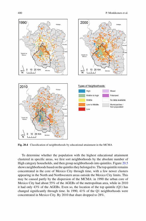
400 P. Monkkonen et al.
Fig. 20.4 Classification of neighborhoods by educational attainment in the MCMA
To determine whether the population with the highest educational attainmentclustered in specific areas, we first sort neighborhoods by the absolute number ofHigh category households, and then group neighborhoods into quintiles. Figure 20.5showsneighborhoods basedon the quintles they belonged to. The topquintile remainsconcentrated in the core of Mexico City through time, with a few newer clustersappearing in the North and Northwestern areas outside the Mexico City limits. Thismay be caused partly by the dispersion of the MCMA: in 1990 the urban core ofMexico City had about 55% of the AGEBs of the metropolitan area, while in 2010it had only 43% of the AGEBs. Even so, the location of the top quintile (Q1) haschanged significantly through time. In 1990, 41% of the Q1 neighborhoods wereconcentrated in Mexico City. By 2010 that share dropped to 28%.
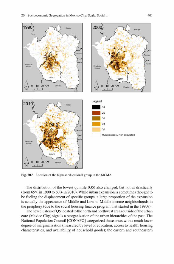
20 Socioeconomic Segregation in Mexico City: Scale, Social … 401
Fig. 20.5 Location of the highest educational group in the MCMA
The distribution of the lowest quintile (Q5) also changed, but not as drastically(from 65% in 1990 to 60% in 2010). While urban expansion is sometimes thought tobe fueling the displacement of specific groups, a large proportion of the expansionis actually the appearance of Middle and Low-to-Middle income neighborhoods inthe periphery (due to the social housing finance program that started in the 1990s).
Thenewclusters ofQ5 located to the north andnorthwest areas outside of the urbancore (Mexico City) signals a reorganization of the urban hierarchies of the past. TheNational Population Council [CONAPO] categorized these areas with a much lowerdegree of marginalization (measured by level of education, access to health, housingcharacteristics, and availability of household goods); the eastern and southeastern
402 P. Monkkonen et al.
areaswhere older incremental housing developments ofNeza andChalco are located,remain poor and with a higher degree of marginalization (CONAPO 2012).
20.5 An Uncertain Trajectory
Inequality is a necessary condition for socioeconomic segregation, but decreases ininequality do not always lead to lower levels of residential segregation, i.e., to higherlevels of residential integration. When assessing social segregation using educationlevels, it is important to consider that a more systematic link between educationalimprovements andwage improvementswould have likely led to greater segregationistpressures at the same time that it reduced inequality in the short term. According totheMexican National Evaluation Council [CONEVAL], all municipalities within theMCMA experienced a reduction in inequality between 1990 and 2010—the averageGINI coefficient dropped from 0.44 in 1990 to 0.40 in 2010. Mexico City had a Ginicoefficient of 0.49 in 1990, 0.48 in 2000, and 0.42 in 2010. At the metropolitan level,inequality increased slightly between 1990 and 2000 for the municipalities outsideof Mexico City (GINI coefficients of 0.41–0.44 for Mexico State and of 0.42–0.45for Hidalgo5), but then dropped to below 0.40 in 2010 (CONEVAL 2017).
The decrease in segregation between 2000 and 2010 points to other factors influ-encing the spatial structure of the MCMA. The economic structure of the MCMAis stable and incomes have gone up. The number (though not the share) of peoplein high-wage occupations has increased. The large-scale provision of housing haslikely contributed to the sorting of people and a selection process that affects segre-gation. Many of the people moving to the peripheries are doing so because of thegovernment’s housing fund, available only to formally employed, salaried workers.This leaves different types of people in the core city, including those with informalemployment (and likely lower levels of educational achievement), as well as highincome but non-salaried workers, and salaried workers who do not want to commuteto jobs in the core city.
MexicoCity is changing. LargerMiddle andHigh-income enclaves and secondarybusiness districts have emerged in the peripheries, especially at the edge of theurban core of Mexico City. The city’s development is more fragmented and there
5These GINI coefficients are only for those municipalities that are part of the MCMA, not for theState of Mexico and Hidalgo.
20 Socioeconomic Segregation in Mexico City: Scale, Social … 403
are more differentiated spaces: gated communities of different income levels andinternationally oriented districts. This is likely to accelerate the process of residentialsegregation yet it has not, at least in the way we can measure it.
20.6 Conclusion
The spatial complexity of the Mexico City Metropolitan Area, the vast amalgam ofneighborhoods that make up its dozens of municipalities, does not translate to highlevels of segregation. This fact contrasts with Mexico’s rigid economic and socialstructures and underlying inequalities, which are likely why many observers—andexperts—assume the city and the country are highly segregated. In this analysis, wefind that the spatial distribution of people of different educational levels is relativelyeven across the city. Most neighborhoods have at least two groups (usually Lowand Middle or Middle and High educational attainment), with an increasing numberhaving representation of all educational groups.
There is an increase in the number of neighborhoods where one group dominates,most notably in neighborhoods where people with high education are clearly over-represented. This suggests distinct processes shaping economic returns to educationand residence. Despite localized changes, citywide changes in education outcomeshave not translated to increased segregation as measured by the dissimilarity index.The improved education of people living in Mexico City has not improved labormarket outcomes, however. This, we hypothesize, has led to a city where people stayin place (including children with improved education still staying in parental home)to maintain access to family members, community, and jobs.
With the improvement of education but modest residential mobility, in situ educa-tion change in neighborhoods has been important, andwe assume drive the decease ofcity-wide levels of segregation between 1990 and 2010. Separation ismost systematicbetween those with the highest level of education and those with low educationalattainment. This separation has translated into a rapid increase in the number ofneighborhoods dominated by highly educated individuals. At the same time, mixedneighborhoods and areas where people withmiddle and high levels of education havebecome the norm, replacing the long dominant mix of low and middle educationalattainment.
These shifts, while not increasing segregation, are reshaping the spatial structureof the MCMA. Newly built neighborhoods in the peripheries are receiving largenumbers of residents, who risk being locked in places that lack access to qualityeducation and jobs. People with high educational attainment are moving into newerdevelopments that might afford them greater opportunities to isolate themselves fromthe rest of population compared to the traditional core areas that used to be the homeof most highly educated residents. These changes were clearly visible in 2010.
404 P. Monkkonen et al.
Mexico City’s new administration has already proposed new approaches tohousing, including the idea of inclusionary housing6 that may allow it to countertendencies of social segregation in the core of the metropolitan area. Concurrentimprovements in social services and educational opportunities in the State ofMexicoand Hidalgo will reduce the disadvantage of the metropolitan periphery, but thetendency of employment centralization will be more difficult to change. The 2020census will shed important light on which trajectory the city is following.
References
Ariza M, Solís P (2009) Dinámica socioeconómica y segregación espacial en tres áreas metropoli-tanas de México, 1990 y 2000. Estudios sociológicos 171–209
Caldeira TP (2012) Fortified enclaves: the new urban segregation. The urban sociology reader.Routledge, London, pp 419–427
Caragliu A, Del Bo C, Nijkamp P (2012) Smart cities in Europe. J Urban Technol 18:65–82Consejo Nacional de Población [CONAPO] (2012) Indice de marginación urbana, 2010. [PDFdocument]. http://www.conapo.gob.mx/work/models/CONAPO/indices_margina/marginacion_urbana/AnexoA/Mapas/01_Zona_Metropolitana_del_Valle_de_Mexico.pdf
ConsejoNacional de Evaluación [CONEVAL] (2017) Indicadores de pobreza, pobreza por ingresos,rezago social y gini 2010 (municipal). [Data file]. https://datos.gob.mx/busca/dataset/indicadores-de-pobreza-pobreza-por-ingresos-rezago-social-y-gini-2010-municipal
Cortés F (2013)Medio siglo de desigualdad en el ingreso enMéxico. Seminario “Las desigualdadesy el progreso enMéxico: enfoques, dimensiones ymedición” COLMEX/INEGIMéxicoD.F. 20 y21 de marzo de 2013. [PDF document]. https://www.inegi.org.mx/eventos/2013/Desigualdades/doc/P-FernandoCortes.pdf
García B,MuñozH,DeOliveira O (1978)Migraciones internas y grupos populares urbanos: Ciudadde México (1950–1970). Revista Mexicana de Sociología 107–129
Garza G (1999) Global economy, metropolitan dynamics, and urban policies in Mexico. Cities16(3):149–170. https://doi.org/10.1016/S0264-2751(99)00013-X
Griffin E, Ford L (1980) A model of Latin American city structure. Geogr Rev 70(4):397–422Instituto Nacional de Estadística y Geografía [INEGI] (n.d.) Encuesta Nacional de Ocupación yEmpleo (ENOE). [Data file]. https://www.inegi.org.mx/programas/enoe/15ymas/default.html#Microdatos
Instituto Nacional de Estadística y Geografía [INEGI] (2011) Censo de Población y Vivienda 2010.https://www.inegi.org.mx/programas/ccpv/2010/
Instituto Nacional de Estadística y Geografía [INEGI] (2015a) Encuesta Intercensal 2015. [Datafile]. https://www.inegi.org.mx/programas/intercensal/2015/default.html#Tabulados
Instituto Nacional de Estadística y Geografía [INEGI] (2015b) Encuesta Nacional de Ingresosy Gastos de Hogares 2015. [Data file]. https://www.inegi.org.mx/programas/mcs/2015/default.html#Microdatos
Libertun de Duren N (2018) Why there? Developers’ rationale for building social housing inthe urban periphery in Latin America. Cities 72:411–420. https://doi.org/10.1016/j.cities.2017.10.006
Malpass P (2008) Housing and the new welfare state: wobbly pillar or cornerstone? Hous Stud23(1):1–19. https://doi.org/10.1080/02673030701731100
6Formore, see the program announcement https://www.cdmx.gob.mx/portal/articulo/programa-especial-de-regeneracion-urbana-y-vivienda-incluyente (last accessed 12/19/2019).
20 Socioeconomic Segregation in Mexico City: Scale, Social … 405
Marcinczak S, Tammaru T, Novák J, Gentile M, Kovács Z, Temelová J, Valatka V, Kährik A, SzabóB (2015) Patterns of socioeconomic segregation in the capital cities of fast-track reforming post-socialist countries. Ann Assoc Am Geogr 105(1):183–202. https://doi.org/10.1080/00045608.2014.968977
Mills ES, Hamilton BW (1989) Urban economics, Glenview, IL: Scott, Foresman and CoMonkkonen P (2011) The housing transition inMexico: expanding access to housing finance. UrbanAffairs Rev 47(5):672–695
Monkkonen P (2012a) Housing finance reform and increasing socioeconomic segregation inMexico. Int J Urban Reg Res 36(4):757–772
Monkkonen P (2012b) La segregación residencial en el México urbano [Residential Segregation inUrban Mexico]. EURE - Revista Latinoamericana de Estudios Urbano Regionales 38(114):124–146
Monkkonen P, Comandon A, Montejano Escamilla JA, Guerra E (2018) Urban sprawl and thegrowing geographic scale of segregation in Mexico, 1990–2010. Habitat Int 73:89–95. https://doi.org/10.1016/j.habitatint.2017.12.003
Monkkonen P (2019) Empty houses across North America: housing finance and Mexico’s vacancycrisis. Urban Stud 56(10):2075–2091
Montejano J,Monkkonen P, Guerra E, Caudillo C (2019) The costs and benefits of urban expansion:evidence from Mexico, 1990–2010. [PDF document]. https://www.lincolninst.edu/sites/default/files/pubfiles/montejano_wp19jm1.pdf
Organisation for Economic Co-Operation and Development [OECD] (2006) Policy note: povertyalleviation. [PDF document]. http://www.oecd.org/social/soc/38120467.pdf
Organisation for Economic Co-Operation and Development [OECD] (2019a) Regional well-being:regional income distribution and poverty. Mexico. [Data file]. https://stats.oecd.org
Organisation for Economic Co-Operation and Development [OECD] (2019b) Society at a glance—2019: OECD social indicators. OECD Publishing, Paris [PDF document]. http://www.oecd.org/mexico/sag2019-mexico-en.pdf
Reardon SF, Bischoff K (2011) Income inequality and income segregation. Am J Sociol116(4):1092–1153
Rubalcava RM, Schteingart M (2000) Segregacion socio-espacial en el Area Metropolitana de laCiudad de Mexico en G. Garza (Ed) La Ciudad de Mexico en el fin del segundo milenio. Mexico,El Colegio de Mexico-Gobierno del Distrito Federal
Sabatini F (2003) The social spatial segregation in the cities of Latin America. Documento deEstrategia para el Desarrollo Social. Banco Interamericano de Desarrollo, Washington, DC
Secretaría de Desarrollo Social [SEDESOL], Consejo Nacional de Población [CONAPO] and Insti-tutoNacional deEstadística yGeografía [INEGI] (2012)Delimitación de las zonasmetropolitanasde México 2010. [PDF document]. http://www.conapo.gob.mx/ES/CONAPO/Zonas_metropolitanas_2010
Torche F (2014) Intergenerational mobility and inequality: the Latin American Case. Ann RevSociol 40:619–642
Trejo Nieto A (2016) A spatial analysis of urban labour markets and submarkets in the metropolitanarea of Mexico City. In: Paper presented at the 56th congress of the European regional scienceassociation, 23–26 August, Vienna, Austria
Trejo Nieto A (2019) Metropolitan economic development: the political economy of urbanisationin Mexico. Routledge, New York, NY
TheWorld Bank (2019)World development indicators. [Data file]. http://datatopics.worldbank.org/world-development-indicators/
Zenteno R, Solís P (2006) Continuidades y discontinuidades de la movilidad ocupacional enMéxico. Estudios demográficos y urbanos 515–546

406 P. Monkkonen et al.
Open Access This chapter is licensed under the terms of the Creative Commons Attribution 4.0International License (http://creativecommons.org/licenses/by/4.0/), which permits use, sharing,adaptation, distribution and reproduction in any medium or format, as long as you give appropriatecredit to the original author(s) and the source, provide a link to the Creative Commons license andindicate if changes were made.
The images or other third party material in this chapter are included in the chapter’s CreativeCommons license, unless indicated otherwise in a credit line to the material. If material is notincluded in the chapter’s Creative Commons license and your intended use is not permitted bystatutory regulation or exceeds the permitted use, you will need to obtain permission directly fromthe copyright holder.
Chapter 21Reordering Occupation, Race, and Placein Metropolitan New York
Kasey Zapatka, John Mollenkopf, and Steven Romalewski
Abstract The New York metropolitan area is one of the oldest, largest, and perhapsmost complex urban region in the United States (U.S.). Its 23.7 million residentslive across four states, produce a GDP of more than $1.7 trillion, are governed by afragmented political system, and experience persistently high degrees of geographicand racial/ethnic inequality and segregation. This chapter investigates the evolvingspatial organization of occupation and race across themetropolitan area.While whiteprofessionals have traditionally lived in an outer ring of suburbs and blue-collarimmigrant and minority groups have lived closer to the city center, our researchshows that the forces of gentrification and minority and immigrant suburbaniza-tion have been turning the metropolitan area inside out. Specifically, young, usuallywhite, professionals are increasingly located in and around the central city whereasmany working-class minorities have shifted away from it. At the heart of this spatialreordering lie the diminishingplurality of native-bornwhiteswithin the region and theincreasing share of immigrantminority groups, especially for foreign-bornHispanicsand Asians. This trend has lessened the share of white males in better occupationseven as the region’s occupational structure slowly but inexorably tilts towardmanage-rial and professional occupations. Technology is transforming white-collar work asblue-collar work continues to disappear. Dramatic shifts are thus afoot, yet inequality
Electronic supplementary material The online version of this chapter(https://doi.org/10.1007/978-3-030-64569-4_21) contains supplementary material, which isavailable to authorized users.
K. Zapatka (B)Department of Sociology, City University of New York, The Graduate Center, New York, NY10016, USAe-mail: [email protected]
J. MollenkopfDepartment of Political Science and Sociology, City University of New York, The GraduateCenter, New York, NY 10016, USAe-mail: [email protected]
S. RomalewskiCUNY Mapping Service, City University of New York, The Graduate Center, New York, NY10016, USAe-mail: [email protected]
© The Author(s) 2021M. van Ham et al. (eds.), Urban Socio-Economic Segregation and Income Inequality,The Urban Book Series, https://doi.org/10.1007/978-3-030-64569-4_21
407
408 K. Zapatka et al.
and segregation remain high. We argue that these changes in the spatial organizationof the metropolitan area challenge us to see these inequalities from a new vantagepoint. As elites are now more likely to live among less advantaged groups, this mayprovide the social basis for new thinking.
Keywords New York metropolitan area · Demographic change · Spatialinequality · Immigrant suburbanization · Segregation
21.1 Introduction
The New York metropolitan region is old, large, and complex. Settlers sent by theDutch West India Company founded the colony on Lenape Native American land in1624 at the southernmost tip of present-day Manhattan. The great protected harborat the confluence of the Hudson River and the East River provided water access notonly along the East Coast of the U.S., but also north and west to the Great Lakesand the inland U.S. (especially after the Erie Canal was completed in 1825). NewYork City firms made the most of these advantages, achieving dominance over theU.S. and the trans-Atlantic trading systems in the mid-nineteenth century. Buildingon these initial advantages, a vast regional system of work, residence, and recreationgrew up around the city over time.
Today, the broadest official definition of the metropolitan region is the U.S.Census-defined Combined Statistical Area (CSA). The border of the New York CSAstretches from Atlantic City on the southern New Jersey coast northwest to Allen-town, Pennsylvania, eastward across the Hudson River valley to Connecticut, andthen southeast across the Long Island Sound to include the length of Long Island.This broad definition encompasses 23.7 million residents and more than 10 millionworkers producing a $1.7 trillion GDP—ten percent of the U.S. total. More than athird of these residents live in or just outside New York City at high-density levels(656 people per square kilometer or more). Narrower definitions of the metropolitanarea include the U.S. Census-defined Core-Based Statistical Area (CBSA) and theOECD Functional Urban Area (FUA). The CBSA contains almost 20 million peopleand 9.8 million workers but excludes Connecticut and distant subordinate metroareas. This chapter analyzes patterns in the even smaller FUA delineation, picturedin Fig. 21.1. It consists of 16 New York and New Jersey counties accounting for 17million people and 8.3 million workers. The denser, inner FUA thus contains almostthree-quarters of the broader CSA population and four-fifths of its labor force.
The FUA’s metropolitan hierarchy centers on one large, dense city (New York)surrounded by other smaller but still substantial cities (New Brunswick, Newark,JerseyCity,Yonkers,White Plains, and themajorLong Island towns) and an extensivenetwork of suburbs.At present,NewYorkCity contains half of the FUApopulation—8.6 million residents, 4.1 million workers, and 4.6 million jobs, four-fifths of whichare held by city residents. The FUA’s satellite cities and suburbs contain the other halfof the FUA’s residents, with 8.4million dwellers, 4.2millionworkers, and 3.6million
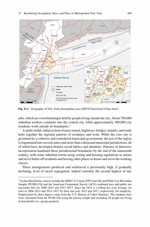
21 Reordering Occupation, Race, and Place in Metropolitan New York 409
Fig. 21.1 Geography of New York metropolitan area (OECD Functional Urban Area)
jobs, which are overwhelmingly held by people living outside the city. About 790,000suburban workers commute into the central city, while approximately 300,000 cityresidents work outside its boundaries.1
Amulti-nodal, radial system ofmass transit, highways, bridges, tunnels, and roadsknits together the regional patterns of residence and work. While the core city isgoverned by a cohesive and centralized municipal government, the rest of the regionis fragmented into several states andmore than a thousandmunicipal jurisdictions, allof which have developed distinct social fabrics and identities. Patterns of defensiveincorporation hardened these jurisdictional boundaries by the end of the nineteenthcentury, with some suburban towns using zoning and housing regulations to attractand serve better-off residents and leaving other places to house and serve the workingclasses.
These arrangements produced and reinforced a persistently high, if graduallydeclining, level of racial segregation, indeed currently the second highest of any
1As described below, sources include the 2000U.S. Census STF3 tract file and PublicUseMicrodataSample (PUMS) File and the American Community Survey (ACS) combined tract and public usemicrodata files for 2008–2012 and 2013–2017. Since the ACS is a rolling five-year average, werefer to 2008–2012 and 2013–2017 by their end year, 2012 and 2017, respectively, for simplicity.Employment by place figures come from the U.S. Bureau of Labor Statistics. The numbers herewere calculated from the PUMs File using the person weight and excluding all people not livingin households (i.e., group quarters).
410 K. Zapatka et al.
U.S. metro area (Frey 2018). As it does elsewhere in the United States, class hasa color in New York, since racial and ethnic groups cluster in specific occupationsand industries. Whites are strongly represented in top occupations in the highervalue-added industries while minority groups cluster in less rewarding occupationsand industries (Waldinger 1996).2 The residential segregation of different racial andethnic groups is thus intimately intertwined with patterns of socioeconomic segre-gation and inequality. As the remainder of this analysis specifically discusses theregional occupational and socioeconomic patterns of FUA, readers should keep thepatterns of the larger metropolitan region in mind.
21.2 Background: Changing Occupational Structuresand Patterns of Inequality and Segregation
New York exemplifies the post-World War II American metropolis. From the 1950sthrough the 1980s, the decline of population and employment in inner cities withgrowing minority populations was a key feature of this regional mosaic. By contrast,growing suburbs attracted the white middle-class residents and workers with newhousing, shoppingmalls, and corporate office parks. Since then, however, three potentforces have gradually begun to erode and alter this pattern. The first is demographic(declining native and rising immigrant-origin populations), the second involves occu-pational restructuring (the shift from production to services with a new ethno-racialand gender division of labor), and the third concerns the shifting geography ofpopulation concentrations (a shift in residential locations).
21.2.1 The Decline of the Native-Born and the Riseof Immigrant-Origin Populations
The twin patterns of declining native-born and rising immigrant-origin populationsare reshaping the metropolitan region. The number and share of people living inhouseholds headed by native-born non-Hispanic whites have declined relatively andabsolutely not just in the older central cities like New York City or Newark, but alsoin the whole region, falling from 6.4 to 5.9 million between 2000 and 2017 and from52.1 to 47.9% of the FUA total. This story of the native white population decline
2The U.S. Census collects information separately on race and Hispanic origin. In analyzing censusdata, social scientists almost always group all Hispanics together as a distinct group, leaving non-Hispanic whites, blacks, Asians, and other races as the other categories. When we use the termswhite, black, and Asian, we mean the non-Hispanic portions of those populations. Since “Hispanic”is the official Census term, we use it here, although sometimes preferred alternatives are “Latino/a”or “Latinx”. The census PUMS also ask respondents about their ethnic ancestries, places of birth,and citizenship status, allowing researchers to identify specific ethnic groups (e.g.‚ Irish‚ Italian‚Jamaican‚ or Dominican).
21 Reordering Occupation, Race, and Place in Metropolitan New York 411
is relatively old, but the pattern now also extends to native African American andPuerto Rican households (For most of the period between 1950 and 1980, PuertoRicans contributed to the vast majority of Hispanic households). Membership inAfrican American households declined by 129,000 and Puerto Rican households by59,000. If this had been the only trend, the region would have shrunk greatly, just asit did on other rustbelt areas, but native out-migration was not the only force at work.The number of people living in immigrant-origin households grew within all theracial categories, more than offsetting the native declines.3 The immigrant-headedhousehold population surged by 1.34 million to 43.5% of the FUA total. As a result,the FUA’s total population rose 6.5% between 2000 and 2017.
Ever since AfricanAmericans and Puerto Ricans became substantial groups in theregion, high levels of white-black segregation and lower but still high levels of white-Hispanic segregation have characterized metropolitan residential patterns. Occupa-tional segregation was lower, yet still considerable. Over time, however, deindustri-alization and the shift to services have altered the types of industries and occupationsin the regional economy. As new immigrant-origin racial and ethnic groups enteredthe metropolitan labor market, they tended to cluster in specific industry-occupationniches thatwere open to thembecause native groupswere departing them, these occu-pations were less desirable to native workers, job growth outstripped the supply ofnative-born workers, or immigrant entrepreneurs found ways to enter them. Enteringgroups competed with each other to access the available niches that offered higherwages and more opportunity and achieve ethnic closure within them (Waldinger1996). While workers from every ethnic or racial group span every occupation andindustry, they do so unevenly, achieving significant clustering in some niches andremaining relatively sparse in others. To give one example, native-born whites makeup 41.6% of the workers in the FUA, yet they hold 65% of the chief executive andonly 6.9% of the dishwasher positions. Conversely, foreign-born Hispanics (12.6%of all workers) hold only 2.7% of chief executive positions but are 61.4% of the dish-washers. Racial and occupational segregation thus intertwine to create distinctivepatterns in the geography of the labor force.
21.2.2 New Ethno-Racial and Gender Divisions of Labor
The interaction between economic and demographic change between 2000 and 2017has gradually reshaped the ethno-racial and gender division of labor in the region.The dominance of suburban white males in the top occupations has diminished andinner-city minorities have slowly shifted away from low-paid service jobs. Women,minorities, and immigrants now hold increasing shares of higher-paying jobs.4 Of
3We group people by the characteristics of the household head because this identifies the immigrantorigin of native-born children with foreign born parents.4Gender and family patterns are a critical part of this story, as more women enter the labor force andmore families rely on two earners. Ideally, our analyses would not only take race and nativity into
412 K. Zapatka et al.
course, dominant groups may still try to ensure that members of their own or otherfavored groups will succeed them by maintaining barriers to immigrant and minorityupward occupational mobility. However, the declining number and share of workersfrom native-born groups, especially whites, and the rising shares of workers fromminority immigrant households make it impossible for them to do so fully. Whitemales are aging out of the Top occupations and younger cohorts do not containenough white males to replace them. This has opened paths for what Richard Alba(2009, p. 15) has called “non-zero sum upward mobility.”
21.2.3 A Shift in Residential Locations
Another important force reshaping the metropolitan area has been the shift in theresidential preferences of younger native-born, non-Hispanic white managers andprofessionals away from their former distant suburban strongholds toward raciallydiverse neighborhoods in and around the central city (see Ley 1996; Smith 1996for competing theories as to why and how this occurs). This has been paired withthe outward movement of minority and immigrant workers. The period from 2000to 2017 has been one of changing places: native white professionals and managersshifting into increasingly white, inner-city neighborhoods and minority and immi-grant workers in the middle and lower occupations shifting into decreasingly white,inner suburban areas.
“Given the strong correlation between income and race in the United States”(Reardon and Bischoff 2011, p. 1093), it is hardly surprising that racial successionhas resulted in declining real median household incomes in many inner suburbs.For example, between 2000 and 2017, the blue-collar city of Bayonne, New Jersey,suffered a net loss of 20,000 people living in white native-born households and5,000 living in black native-born households, yet it gained 6,000 people livingin black immigrant households, 11,000 in native Hispanic households, 15,000 inimmigrant Hispanic households, 1,800 in native Asian households, and 11,000 inimmigrant Asian households, thus more than offsetting native-born losses. At thesame time, Bayonne’s real median household income per capita declined by 5.5%.Reciprocally, the increasing movement of white, middle-class residents into manylow-income inner-city neighborhoods has raised their median incomes. The gentri-fying Brooklyn neighborhoods of Greenpoint,Williamsburg, EastWilliamsburg, andBushwick collectively attracted 85,700 more people living in native white house-holds while losing 19,300 members of native black households and 12,200 membersof native Hispanic households. Real median household income per capita rose to68%, erasing many of the previous effects of deindustrialization, disinvestment, anddepopulation on these neighborhoods.
account, but gender as well in terms of how groups are sorted across industry-occupation niches.We refrain from exploring that here because adding gender to the analysis would increase the eightmajor racial-nativity categories to sixteen.
21 Reordering Occupation, Race, and Place in Metropolitan New York 413
More broadly, people with good jobs and high incomes have been recentralizingin recent years after diffusing away from their central cities in previous decades(Shearer et al. 2019). Although white managers and professionals and their familiesstill live mainly in affluent suburbs located 30 to 40 miles away fromManhattan, thecenter of gravity of the net shift in this population has moved strongly toward neigh-borhoods surrounding the Manhattan central business district, including Harlem,the East River communities in Queens and Brooklyn, and Hoboken and Jersey Cityacross the Hudson River. Simultaneously, the poor, minorities, and immigrants previ-ously concentrated in central cities are shifting toward the inner suburbs beyond thisgentrifying ring. While the overall spatial patterns of economic and social differencestill bear many marks of the post-World War II period, they are clearly changing. Ifsuburbanization of the white middle class and the growth of the central city minoritypoor defined the metropolitan form between 1950 and 1980, the recentralization ofyoung professional households (primarily but not exclusively white) and the gradualdispersal of native and immigrant minority group members mark the period between1980 and the present. A complicatedmix of factors is shaping this dynamic, includingchanging preferences among those who have a choice of where to live, rising centralcity housing costs that directly or indirectly displace some former residents, and thefading of a post-World War II generation of suburban housing and family formationchoices.
Economic restructuring has changed themix of occupations; demographic changehas altered themake-up of theirworkers; and altered location patterns have shifted themosaic of jobs, residences, and commutes in the metropolitan area. This is particu-larly evident between the Manhattan central business district and the distant affluent,white suburbs. The predominantly black and Hispanic inner-city communities thatexperienced the largest gains in white residents were all in Brooklyn areas withgood transit connections to Manhattan (Bed-Stuy, Crown Heights, Fort Greene, EastWilliamsburg, andBushwick), or inNorthernManhattan (Harlem,WestHarlem, EastHarlem, and Washington Heights). Collectively, these communities gained 248,000employed workers, doubled their number of managers and professionals, and lostoffice and factory workers. The overall drop in the FUA’s white population reducedtheir standing in many communities, especially the inner suburbs on Long Island andin New Jersey. Arriving minorities (especially immigrant Asian and Hispanic house-holds) more than offset the white population’s departure. While these communitiesslowly gained employed workers, managers, and professionals, these communities’biggest gains were in health support occupations, food preparation, home, child andhealthcare aides, and other service jobs.
WhileNewYork remains one of the country’smost racially segregatedmetro areas(Logan and Stults 2011, p. 6), its core white and black neighborhoods are not as whiteor black today as they were in 2000. Hispanic and Asian immigrant households havesettled in and between them, blurring their boundaries; new kinds of “global neigh-borhoods” have emerged in the process (Zhang and Logan 2016). The subsequentanalysis investigates how the spatial redistribution and repositioning of racial andoccupational groups have created new occupational mixtures and juxtapositions.
414 K. Zapatka et al.
21.2.4 The Influence of the Welfare System
The U.S. has a comparatively fragmented welfare state that relies heavily on privateprovision (e.g., employer-sponsored healthcare and retirement systems) (Lynch2014). The welfare system is largely funded by the federal government, but somestates minimize or maximize the variety and quantity of services provided. In thatcontext, New York and New Jersey have relatively extensive welfare systems, withNew York City being one of the most social-democratic jurisdictions in the U.S. Itscurrent Fiscal Year 2020 budget is $92.8 billion, spending large amounts on housing,social services, and other redistributive programs. The Department of HomelessServices alone will spend $2.1 billion. The City finances this high level of spendingwith the highest level of municipal taxation in the U.S. (Independent Budget Office2007). While government spending levels are somewhat lower elsewhere in theregion, the entire FUA is a relatively high tax, high public spending environment.Public employment is thus an important part of the labor market, with governmentcontracts also sustaining high levels of employment in nonprofit organizations. NewYork City may be the business capital of the United States, but it also has the largestmunicipal hospital system; a huge municipal elementary, high school and univer-sity educational system; and a vast array of nonprofit organizations. Together, thesesystems help to sustain a substantial set of middle-income occupations held by Cityresidents.
21.2.5 The Influence of Housing and Land Tenure
Before World War II, the vast majority of American households rented their homes;after the war, U.S. housing policy dramatically shifted in favor of homeownership(Schwartz 2015). As the Federal Housing Administration (FHA) instituted 30-yearself-amortizing mortgages, insured mortgages issued by qualified lenders, institutedconstruction standards, and required housing inspections before sale, the FederalHousing National Mortgage Association (Fannie Mae) also purchased and securi-tized FHA-issued mortgages to provide capital so banks could issue more loans.Additionally, homeowners began deducting mortgage interest from their federaltaxes, significantly subsidizing homeownership and making it more affordable thanrenting. As a result, the national homeownership rate grew from 44% in the 1940sto 62% in the 1960s. (Schwartz 2015). As of April 2019, it hovers at 64.2% (U.S.Census Bureau 2019).
Although these policies benefited many homeowners, systematic racial discrimi-nation in lending and home sales preventedmanyminority groups from sharing in thegains. Restrictive covenants—private agreements preventing owners from selling tonon-whites—were legal until 1948. FHAguidelines initially enshrined banking prac-tices of refusing to lend in certain neighborhoods and did little to alter these practiceseven after Congress passed the Fair Housing Act in 1968 (Schwartz 2015). Failure
21 Reordering Occupation, Race, and Place in Metropolitan New York 415
to aggressively enforce the Fair Housing Act has left informal but systematic racialdiscrimination in place,maintaining segregation and limitingminority groups’ abilityto leverage homeownership to generate wealth and transfer it between generations.
While homeownership predominates in the suburban areas of metropolitan NewYork, approximately 65% of City residents rent their homes, since high housing costslimit access to homeownership. Compared to other cities, New York City has strongrent regulation laws and a substantial stock of public housing. While 43% of NewYork City renters live in market-rate housing, 45% are protected by rent regulationand another 12% live in other types of regulated units, which is largely public housing(New York City Rent Guidelines Board 2018, p. 4).5 Recently strengthened, theselaws provide a degree of affordability and stability to renters in New York City(Paybarah 2019). As a result, median gross rent for all New York City renters wasreported to be $1,830 in 2017, but $1,375 for rent-stabilized units (Gaumer 2018).It is against this backdrop that our analysis examines shifting patterns of residentialsegregation, growing income inequality, and a changing occupational structure overtime.
21.3 Data and Methods
We created two datasets for our analysis: one spatial and the other individual. Thefirst uses tract-level data from three time periods: the 2000 Decennial Census andthe 2008–2012 and 2013–2017 American Community Survey (ACS) 5-year Esti-mates.6 The second dataset is an individual-level dataset drawn from University ofMinnesota’s Integrated Public Use Microdata Series (IPUMS).7 These data includetwo time periods that mirror the start and end of the spatial dataset; we used the5% public use microdata sample from the 2000 Census as well as the public usemicrodata sample from the 2013–2017 ACS 5-year estimates (hereafter referred toas 2017). The census tract dataset provides a spatial analysis of small neighborhoodareas called census tracts, which are small geographic areas that contain on averageabout 4,000 people. The second dataset provides a repeated cross-sectional analysisof individual and household data for geographic areas called Public Use MicrodataAreas (PUMAs) that hold at least 100,000 people. The first dataset allows us to
5“Other types of regulatedunits” largely consists of public housing, but also inclduesMitchell-Lama,In Rem, HUD-regulated, Article 4, and Loft Board units.6U.S. Census data can be found at https://www.census.gov/programs-surveys/acs. We used the2008–2012 ACS 5-Year Estimates instead of the 2010 Decennial Census since the ACS 5-YearEstimates are meant to give a better sense of what is happening over five-year periods than thesnapshot the Decennial Census offers. Additionally, the ACS 5-Year Estimates provides muchgreater demographic and economic detail than does the Decennial Census, which counts populationonly by age, sex, race, and housing tenure. Since the ACS is a rolling five-year average, we refer to2008–2012 and 2013–2017 by their end year, 2012 and 2017, respectively.7IPUMS has received several federal grants to harmonize and integrate U.S. Census microdata,which can be accessed on their website: https://usa.ipums.org/usa/.
416 K. Zapatka et al.
analyze occupational trends by a neighborhood of residence within the FUA whilethe second allows us to analyze any combination of factors (including race, age, sex,education, and detailed occupation) for individuals and households within the largerPUMA areas.8 (The FUA contains 4,652 census tracts nested within 151 PUMAs.)We use the terms census tract and neighborhood interchangeably and refer to PUMAsas communities.
Since census tract boundaries change over time, we used the Longitudinal TractDatabase (Logan et al. 2014) to harmonize data from 2000 into 2010 boundaries,the same boundaries used in the subsequent ACS data panels. All monetary valuesin both databases were inflation adjusted to 2018 dollars using the Consumer PriceIndex (CPI) for New York-Newark-Jersey City, NY-NJ-PA (U.S. Bureau of LaborStatistics 2019a).We inflation-adjusted housing-related variables using the all-items-less-shelter CPI so as to not control away variation in housing costs across years (U.S.Bureau of Labor Statistics 2019b).9
21.3.1 Measures of Inequality
The most widely used measure of income inequality is the Gini coefficient (HoqueandClarke 2015; Peñaloza 2016).Although these coefficients are typically calculatedfor individual or household incomes, we use them to examine the spatial patterns ofinequality over time in the metropolitan area. The U.S. Census Bureau calculatedtract-level Gini coefficients of income inequality for the two panels of tract data inour analysis but not for the 2000 Decennial Census. To create consistent measuresacross our data, we therefore used the von Hippel and colleagues’ (2017) methodof the cumulative distribution function and mean matching to approximate Ginicoefficients with ordinal categorical data on household income from each of thethree Census periods (see Peñaloza 2016; Reardon and Bischoff 2011; von Hippelet al. 2016, 2017). When we compare our results with the Census estimates fromthe two ACS tract data panels, they slightly underestimate the Gini’s reported by theCensus Bureau. This gives a slight conservative bias to our analysis of the changingspatial patterns of inequality compared to what we would find if we had CensusBureau-calculated Gini coefficients for all three periods.
8While both datasets are repeated cross-sectional, we refer to the first dataset that uses census tractsas the spatial dataset and the second that uses individual data as the cross-sectional dataset.9The all-items-less-shelter CPI is similar to the all-items CPI; however, it does not include housingin its calculations of the overall CPI.
21 Reordering Occupation, Race, and Place in Metropolitan New York 417
21.3.2 Measures of Residential and SocioeconomicSegregation
Weused theU.S.Department of Labor’s Bureau of Labor StatisticsO*NETResourceCenter to condense census occupational categories into their appropriate ISCO cate-gories (O*NET 2019 and Bureau of Labor Statistics 2019c). Similarly, we calculatedlocation quotients and dissimilarity indices according to the methodology describedin Chap. 1. However, we slightly departed from these methods in two ways. Sincethe socioeconomic distribution in the NewYork City metropolitan area skews towardthe high end, we altered the socioeconomic classification of neighborhoods used inFig. 21.4 to be exhaustive of all neighborhoods (Appendix reports our alternativeclassification scheme.) Second, we used the SEG package in Stata developed byReardon and Townsend (1999) to calculate dissimilarity indices.
21.4 Spatial Analysis
21.4.1 Changes in Income Inequality
According to theWorldBank, between 1979 and 2016 theGini coefficient for incomeinequality in the U.S. increased by one-fifth, from 34.6 to 41.5 (World Bank 2019).The largest increases happened between 1979 and 1986, rising from 34.6 to 37.5,rising again to 38.8 between 1991 and 1994 and then increasingmore slowly, by 2.7%points, from 2000 to 2016. In short, income inequality grew dramatically across theUnited States in the early 1980s and early 1990s, but then grewmore slowly between2000 and the present, in part because of major recessions.
Metropolitan New York has a slightly different story. We calculated Gini coeffi-cients separately for each neighborhood and the entire FUA. The average Gini acrossall FUA neighborhoods started at 42.6 in 2000, dropped slightly to 41.6 in 2012 (asthe regional economy experienced recession), and then rebounded to 42.6 in 2017 (asthe region recovered). The index fell primarily because the financial crisis reducedthe highest incomes. While this level of inequality is high by international standards,this average neighborhood inequality rests just above U.S. levels as reported by theWorld Bank. In contrast, the Gini index for the overall FUA is higher, beginning at47.8 in 2000, rising to 48.0 in 2012, and rising again to 48.8 in the 2017 period.The inequality of the overall metropolitan area is thus higher than that of the averageneighborhood—as much as 6.2 points higher in 2017.
21.4.2 Changes in Occupational Structure
Figure 21.2 reports how the Top, Middle, and Bottom occupational shares have
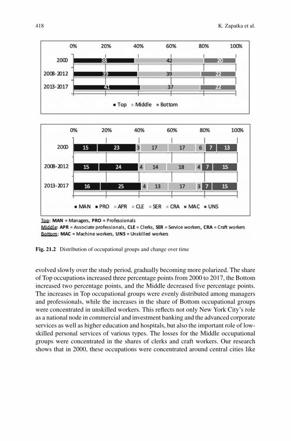
418 K. Zapatka et al.
Fig. 21.2 Distribution of occupational groups and change over time
evolved slowly over the study period, gradually becoming more polarized. The shareof Top occupations increased three percentage points from 2000 to 2017, the Bottomincreased two percentage points, and the Middle decreased five percentage points.The increases in Top occupational groups were evenly distributed among managersand professionals, while the increases in the share of Bottom occupational groupswere concentrated in unskilled workers. This reflects not only New York City’s roleas a national node in commercial and investment banking and the advanced corporateservices as well as higher education and hospitals, but also the important role of low-skilled personal services of various types. The losses for the Middle occupationalgroups were concentrated in the shares of clerks and craft workers. Our researchshows that in 2000, these occupations were concentrated around central cities like
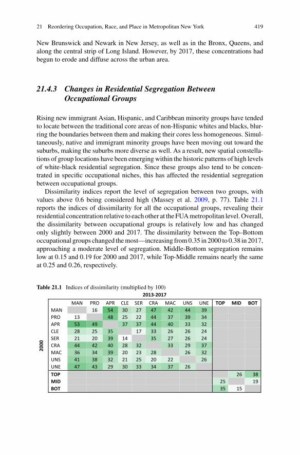
21 Reordering Occupation, Race, and Place in Metropolitan New York 419
New Brunswick and Newark in New Jersey, as well as in the Bronx, Queens, andalong the central strip of Long Island. However, by 2017, these concentrations hadbegun to erode and diffuse across the urban area.
21.4.3 Changes in Residential Segregation BetweenOccupational Groups
Rising new immigrant Asian, Hispanic, and Caribbean minority groups have tendedto locate between the traditional core areas of non-Hispanic whites and blacks, blur-ring the boundaries between them and making their cores less homogeneous. Simul-taneously, native and immigrant minority groups have been moving out toward thesuburbs, making the suburbs more diverse as well. As a result, new spatial constella-tions of group locations have been emergingwithin the historic patterns of high levelsof white-black residential segregation. Since these groups also tend to be concen-trated in specific occupational niches, this has affected the residential segregationbetween occupational groups.
Dissimilarity indices report the level of segregation between two groups, withvalues above 0.6 being considered high (Massey et al. 2009, p. 77). Table 21.1reports the indices of dissimilarity for all the occupational groups, revealing theirresidential concentration relative to each other at the FUAmetropolitan level.Overall,the dissimilarity between occupational groups is relatively low and has changedonly slightly between 2000 and 2017. The dissimilarity between the Top–Bottomoccupational groups changed themost—increasing from0.35 in 2000 to 0.38 in 2017,approaching a moderate level of segregation. Middle-Bottom segregation remainslow at 0.15 and 0.19 for 2000 and 2017, while Top-Middle remains nearly the sameat 0.25 and 0.26, respectively.
Table 21.1 Indices of dissimilarity (multiplied by 100)2013-2017
2000
MAN PRO APR CLE SER CRA MAC UNS UNE TOP MID BOT MAN 16 54 30 27 47 42 44 39 PRO 13 48 25 22 44 37 39 34 APR 53 49 37 37 44 40 33 32 CLE 28 25 35 17 33 26 26 24 SER 21 20 39 14 35 27 26 24 CRA 44 42 40 28 32 33 29 37 MAC 36 34 39 20 23 28 26 32 UNS 41 38 32 21 25 20 22 26 UNE 47 43 29 30 33 34 37 26 TOP 26 38MID 25 19BOT 35 15
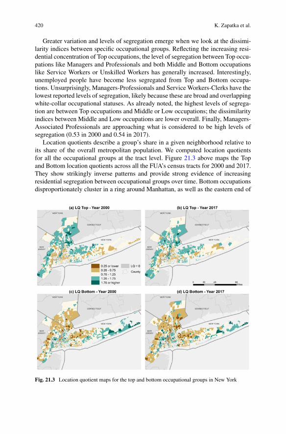
420 K. Zapatka et al.
Greater variation and levels of segregation emerge when we look at the dissimi-larity indices between specific occupational groups. Reflecting the increasing resi-dential concentration of Top occupations, the level of segregation between Top occu-pations like Managers and Professionals and both Middle and Bottom occupationslike Service Workers or Unskilled Workers has generally increased. Interestingly,unemployed people have become less segregated from Top and Bottom occupa-tions. Unsurprisingly, Managers-Professionals and Service Workers-Clerks have thelowest reported levels of segregation, likely because these are broad and overlappingwhite-collar occupational statuses. As already noted, the highest levels of segrega-tion are between Top occupations and Middle or Low occupations; the dissimilarityindices between Middle and Low occupations are lower overall. Finally, Managers-Associated Professionals are approaching what is considered to be high levels ofsegregation (0.53 in 2000 and 0.54 in 2017).
Location quotients describe a group’s share in a given neighborhood relative toits share of the overall metropolitan population. We computed location quotientsfor all the occupational groups at the tract level. Figure 21.3 above maps the Topand Bottom location quotients across all the FUA’s census tracts for 2000 and 2017.They show strikingly inverse patterns and provide strong evidence of increasingresidential segregation between occupational groups over time. Bottom occupationsdisproportionately cluster in a ring around Manhattan, as well as the eastern end of
Fig. 21.3 Location quotient maps for the top and bottom occupational groups in New York
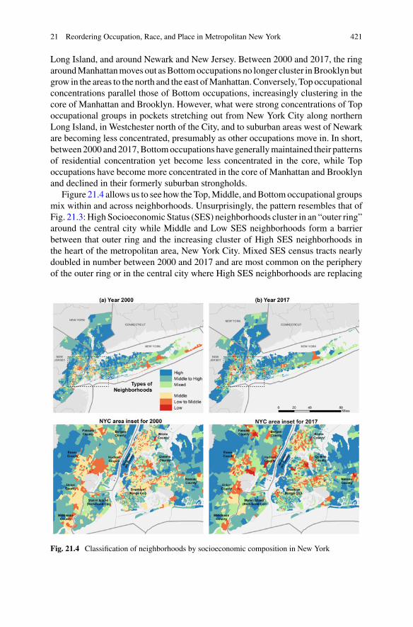
21 Reordering Occupation, Race, and Place in Metropolitan New York 421
Long Island, and around Newark and New Jersey. Between 2000 and 2017, the ringaroundManhattanmoves out asBottomoccupations no longer cluster inBrooklynbutgrow in the areas to the north and the east ofManhattan. Conversely, Top occupationalconcentrations parallel those of Bottom occupations, increasingly clustering in thecore of Manhattan and Brooklyn. However, what were strong concentrations of Topoccupational groups in pockets stretching out from New York City along northernLong Island, in Westchester north of the City, and to suburban areas west of Newarkare becoming less concentrated, presumably as other occupations move in. In short,between2000 and2017,Bottomoccupations have generallymaintained their patternsof residential concentration yet become less concentrated in the core, while Topoccupations have become more concentrated in the core of Manhattan and Brooklynand declined in their formerly suburban strongholds.
Figure 21.4 allows us to see how theTop,Middle, andBottomoccupational groupsmix within and across neighborhoods. Unsurprisingly, the pattern resembles that ofFig. 21.3: High Socioeconomic Status (SES) neighborhoods cluster in an “outer ring”around the central city while Middle and Low SES neighborhoods form a barrierbetween that outer ring and the increasing cluster of High SES neighborhoods inthe heart of the metropolitan area, New York City. Mixed SES census tracts nearlydoubled in number between 2000 and 2017 and are most common on the peripheryof the outer ring or in the central city where High SES neighborhoods are replacing
Fig. 21.4 Classification of neighborhoods by socioeconomic composition in New York
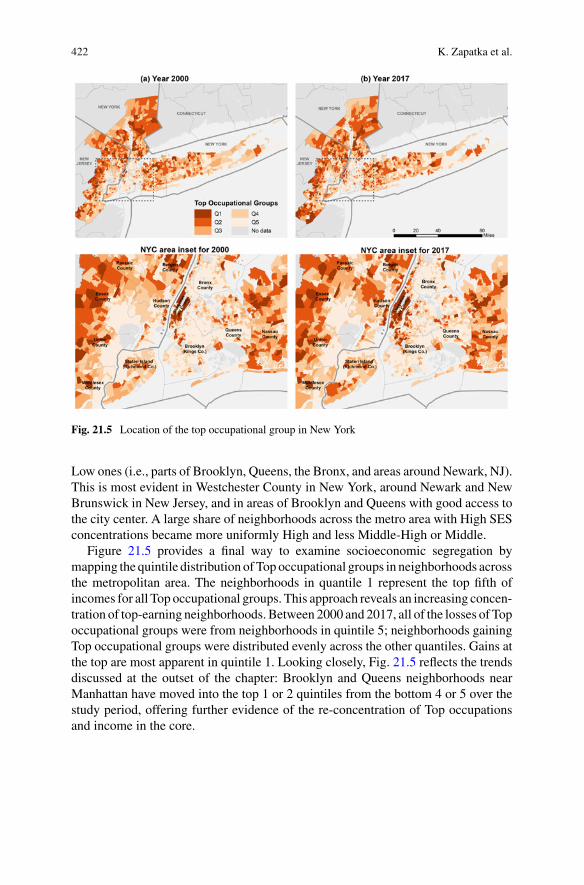
422 K. Zapatka et al.
Fig. 21.5 Location of the top occupational group in New York
Low ones (i.e., parts of Brooklyn, Queens, the Bronx, and areas around Newark, NJ).This is most evident in Westchester County in New York, around Newark and NewBrunswick in New Jersey, and in areas of Brooklyn and Queens with good access tothe city center. A large share of neighborhoods across the metro area with High SESconcentrations became more uniformly High and less Middle-High or Middle.
Figure 21.5 provides a final way to examine socioeconomic segregation bymapping the quintile distribution ofTopoccupational groups in neighborhoods acrossthe metropolitan area. The neighborhoods in quantile 1 represent the top fifth ofincomes for all Top occupational groups. This approach reveals an increasing concen-tration of top-earning neighborhoods. Between 2000 and 2017, all of the losses of Topoccupational groups were from neighborhoods in quintile 5; neighborhoods gainingTop occupational groups were distributed evenly across the other quantiles. Gains atthe top are most apparent in quintile 1. Looking closely, Fig. 21.5 reflects the trendsdiscussed at the outset of the chapter: Brooklyn and Queens neighborhoods nearManhattan have moved into the top 1 or 2 quintiles from the bottom 4 or 5 over thestudy period, offering further evidence of the re-concentration of Top occupationsand income in the core.
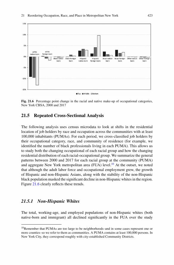
21 Reordering Occupation, Race, and Place in Metropolitan New York 423
Fig. 21.6 Percentage point change in the racial and native make-up of occupational categories,New York CBSA, 2000 and 2017
21.5 Repeated Cross-Sectional Analysis
The following analysis uses census microdata to look at shifts in the residentiallocation of job holders by race and occupation across the communities with at least100,000 inhabitants (PUMAs). For each period, we cross-classified job holders bytheir occupational category, race, and community of residence (for example, weidentified the number of black professionals living in each PUMA). This allows usto study both the changing occupational of each racial group and how the changingresidential distribution of each racial-occupational group.We summarize the generalpatterns between 2000 and 2017 for each racial group at the community (PUMA)and aggregate New York metropolitan area (FUA) level.10 At the outset, we notedthat although the adult labor force and occupational employment grew, the growthof Hispanic and non-Hispanic Asians, along with the stability of the non-Hispanicblack populationmasked the significant decline in non-Hispanic whites in the region.Figure 21.6 clearly reflects these trends.
21.5.1 Non-Hispanic Whites
The total, working-age, and employed populations of non-Hispanic whites (bothnative-born and immigrant) all declined significantly in the FUA over the study
10Remember that PUMAs are too large to be neighborhoods–and in some cases represent one ormore counties–so we refer to them as communities. A PUMA contains at least 100,000 persons. InNew York City, they correspond roughly with city-established Community Districts.
424 K. Zapatka et al.
period. This reflects net outflows of native-born groups to other parts of theU.S., theircomparatively low fertility, and their aging populations. While the overall growth inemployment drew more whites into the workforce, the non-Hispanic white sharestill declined across all occupational groups in a way that left non-Hispanic whitesslightly redistributed toward Top occupations.11 According to our analysis, the dropin the white share of Top occupations was as large as 9% points, and even largerin Bottom occupations like services and sales (13% points) or plant and machineoperators (14% points).
Interestingly, the net loss of non-Hispanic whites in Top occupations was concen-trated in the distant upper-middle-class suburbs. As discussed in the introduction,the number of whites in Top occupations actually rose in gentrifying areas close tothe Manhattan central business districts. White managerial losses were particularlylarge (above 20% points) in the New Jersey suburbs of Elizabeth, Englewood-FortLee, and New Brunswick, as well as the Bayside-Little Neck area of Queens andBensonhurst in Brooklyn. By contrast, older and more centrally located neighbor-hoods like Prospect Lefferts Gardens, CrownHeights, EastWilliamsburg-Bushwick,and Bedford Stuyvesant in Brooklyn and Central Harlem in Manhattan had substan-tial gains (20% points or more) in white managers. In short, non-Hispanic whites inTop occupations decreased their share in their long-term suburban strongholds butgained in gentrifying neighborhoods close to the urban core.
21.5.2 Non-Hispanic Blacks
Non-Hispanic black managers and professionals presented a mirror image of thewhite pattern.While the occupational distribution among blackswas relatively stable,the number and share of non-Hispanic black managers and professionals decreasedin the central city neighborhoods where non-Hispanic whites saw large increases,including central city black strongholds like Bedford-Stuyvesant, Central Harlem,East Harlem, East Williamsburg-Bushwick, Crown Heights, and Prospect LeffertsGardens. On a net basis, black managers and professionals moved away from thesecentral city areas and deeper into Long Island or New Jersey suburbs. Despite sharingan occupation, black managers and professionals earned substantially less than theirwhite counterparts, which further limited their residential choices.
11Small occupational categories of Agriculture, Forestry, Fishery as well as Military were excludedfrom all cross-sectional analyses.
21 Reordering Occupation, Race, and Place in Metropolitan New York 425
21.5.3 Hispanics
In direct contrast to non-Hispanic whites, Hispanics gained numbers and shares in allISCO occupations. They made the smallest gains in Top occupations like managersand professionals and the largest in Bottom ocupations like machine operators andelementary occupations. Since just under 60% of Hispanic workers are immigrants,this positioning in the labor market reflects both their low levels of educationalattainment upon arrival as well as constraints on achieving further education ingreater New York. It appears that the growth of the Hispanic working class hasalso supplanted the loss of non-Hispanic whites in Middle and Bottom occupationsin certain communities. For example, the non-Hispanic white share of machine oper-ators in the northern New York suburb of Ossining-Peekskill, where this occupationwas relatively common, dropped from 64% to just under 39%, while the Hispanicshare in this occupation grew from30 to 54%. This is a continuation of a phenomenonnoted byWaldinger (1996) in which immigrant groups find a place even in decliningindustries and occupations if whites were exiting them even faster than they declined.This was also true of other suburban areas like North Fork-Hamptons, White Plains,and West Milford-Wayne as well as satellite city areas like Bayonne-Kearny andNewark. As Top occupations and non-Hispanic whites shifted toward the centralcity area, minorities and Bottom occupations moved from the central city areas andinto the inner suburbs—a literal turning inside out of the urban socioeconomic fabricof the New York metropolitan area.
21.5.4 Non-Hispanic Asians
The Asian story differs from that of the other groups. Like whites, they have becomemore concentrated in Top occupations (specifically managerial and professionaloccupations), but their immigrant origins initially clustered them in Middle andBottom occupations. This represents great progress; the share of Asian workers whoare managers rose from 14 to 19%, while the Asian share of all managers rose from9 to 15%. In general, Asians are now more likely than other minority groups to holdTop and Middle occupations, with managerial, professional, technical, and clericalpositions accounting for over 60% of all Asian employment in the New York FUA.Since almost 90% of Asians in the labor force are foreign born, this reflects bothsignificant upwardmobility for them aswell as the higher levels of educational attain-ment among Asian immigrant groups compared to other immigrant groups (Kasinitzet al. 2009).
The rate of occupational change was relatively stable across communities, withlarger shifts among Top occupations and smaller ones for Bottom occupations.In 2000, Asian managers and professionals were concentrated either in centralManhattan, Brownstone Brooklyn, Northeast Queens, or the ring of upper-incomesuburbs 30–40miles distant fromManhattan. The single largest number of managers
426 K. Zapatka et al.
lived in and around Saddle River, New Jersey, while the Upper East Side inManhattan had the highest share of managers. Because employment in the manage-rial and professional occupations grew substantially over the period, their numbersincreased in almost every community, with only the Upper East and Upper WestSides and Kingsbridge losing numbers and share. Some large gains in the numbersof managers and professionals occurred as expected in well-established upper-middle-class communities, but they also took place in the neighborhoods closelyringing Manhattan, such as Jersey City (sometimes called New York City’s sixthborough), and Brooklyn Heights, Fort Greene, Bedford-Stuyvesant, Williamsburg,and Greenpoint, just across the East River from Manhattan.
A few communities that gained managers and professionals also attracted thosewith craft and trade occupations (Englewood-Fort Lee andBayside-LittleNeck). Thisout-migration ofmanagers and professionals is consistentwith the generalmovementof minority groups that have achieved higher socioeconomic levels out of central cityareas, while Bottom occupations like craft and trade production saw a reshufflingwithin the city core, with neighboring areas often seeing some of the greatest gainsand losses. As Asian managers and professionals moved out and away from thecentral city and toward more suburban and wealthier areas, Bottom occupationsreshuffled within the urban core.
21.6 Conclusion
For many years, European scholars worried that the cities of Western Europe mightbe moving toward an American model, with the middle class moving to suburbanjurisdictions in a way that would undermine the high levels of social provision inthe big cities. The continued commitment of the professional and managerial occu-pations to dense central city locations often sustained these high levels of socialprovision (Häussermann 2005; LeGales 2002; Tammaru et al. 2015). Ironically, asEuropean metropolitan areas get less dense and more spread out, the New Yorkmetropolitan area may be moving in a more (traditional) European direction, whereTop occupations are becoming more concentrated in and around the center and thepost-industrial working classes are being repositioned in the inner suburbs (Ehrenhalt2013).
At the same time, the New York region has undergone a racial, ethnic, nativity,and gender transition that is just beginning to be widely felt in West European cities.Not only do native-born, non-Hispanic whites make up a fairly small minority of thecentral city population (with less than afifth of the city’s residents living in householdsheaded by native-born, non-Hispanicwhites), but this group accounts for only 35%ofthe total FUApopulation.While they remain the single largest race andnativity group,they are a diminishing plurality. No other single group has risen to supplant them.The region’s next largest groups live in foreign-born Hispanic households (16.2%),foreign-born non-Hispanic Asian households (10.9%), native-born black households
21 Reordering Occupation, Race, and Place in Metropolitan New York 427
(10.1%), native-born Hispanic households (9.5%), and foreign-born non-Hispanicwhite households (8.3%).
Given that the occupational structure of the regional labor market is slowly tiltingtoward managerial and professional occupations that require higher levels of educa-tion, that whitemales hold a diminishing share of those occupations, and that youngercohorts of white males are too small to replace aging white males, new patterns ofopportunity and constraint are opening up in the regional labor market. The educa-tional attainment of many minority and immigrant groups is rising across genera-tions. Whether and how the growing racial-ethnic-gender-nativity groups get accessto opportunities for career advancementwill be the key towhether the region becomesless or more equitable. Many informal and formal factors shape which groups canaccess what employment opportunities. As recent work by Chetty and colleagues(2018) shows, New York City and its surrounding region have done a slightly betterjob in promoting upward mobility from the lowest income quintile than might beexpected, given their finding that high levels of segregation and poverty generallyhinder upwardmobility. Thismay reflect how institutions of higher education, partic-ularly the City University of New York, can play a critical role in opening pathwaysof career advancement. In our view, however, the public and private elites of thecity as well as the region have not put nearly enough effort into making sure thesepathways are open to disadvantaged groups.We hope that the increase of elites livingamong less advantaged groups in central neighborhoods will provide a social basisfor new thinking in this regard, even as it raises inequality within them.
References
Alba RD (2009) Blurring the color line: the new chance for a more integrated America. HarvardUniversity Press, Cambridge, MA
Chetty R, Friedman J, Hendren N, Jones M, Porter S (2018) The opportunity atlas: mapping thechildhood roots of social mobility. NBER working paper series, 25147
Ehrenhalt A (2013) The great inversion and the future of the American City. Vintage Books, NewYork City, NY
Frey W (2018) Black-white segregation edges down since 2000, Census data show. https://www.brookings.edu/blog/the-avenue/2018/12/17/black-white-segregation-edges-downward-since-2000-census-shows/. Accessed 30 Sept 2019
Gaumer E (2018) Selected initial findings of the 2017 New York City housing and vacancy survey,vol 2017. New York City, NY. https://www1.nyc.gov/assets/hpd/downloads/pdfs/about/2017-hvs-initial-findings.pdf
Häussermann H (2005) The end of the European City? Eur Rev 13(2):237–249Hoque AA, Clarke JA (2015) On variance estimation for a gini coefficient estimator obtained fromcomplex survey data. Commun Stat Case Stud Data Anal and Appl 1(1), 39–58. https://doi.org/10.1080/23737484.2015.1044050
Kasinitz P, Mollenkopf JH, Waters MC, Holdaway J (2009) Inheriting the city: the children ofimmigrants come of age. Russell Sage Foundation, New York, NY
LeGales P (2002) European cities. Oxford University Press, OxfordLey D (1996) The new middle class and the remaking of the central city. Oxford University Press,New York
428 K. Zapatka et al.
Logan JR, Stults BJ (2011) The persistence of segregation in the metropolis: new findings from the2010 census. Providence, RI. https://s4.ad.brown.edu/Projects/Diversity/Data/Report/report2.pdf
Logan JR, Xu Z, Stults B (2014) Interpolating U.S. decennial census tract data from as early as1970 to 2010: a longitudinal tract database. Prof Geogr J Assoc Am Geogr 66(3):412
Lynch JA (2014) Cross-national perspective on the American welfare State. In: Béland D, MorganKJ, and Howard C (eds) Oxford Handbook of U.S. Social Policy. Oxford University Press, NewYork City, NY. https://doi.org/10.1093/oxfordhb/9780199838509.013.023
Massey DS, Rothwell J, Domina T (2009) The changing bases of segregation in the United States.Ann Am Acad Polit Soc Sci 626(1):74–90
New York City Rent Guidelines Board (2018) 2018 housing supply report. New York City,NY. https://rentguidelinesboard.cityofnewyork.us/wp-content/uploads/2019/08/18HSR.pdf
O*NET (2019) O*NET Resource Center. https://www.onetcenter.org/overview.htmlPaybarah A (2019) 6 ways new rent laws will affect New Yorkers. New York Times. https://www.nytimes.com/2019/06/17/nyregion/newyorktoday/nyc-news-rent-laws-ny.html
Peñaloza R (2016) Gini coefficient for ordinal categorical data (Working Paper). https://www.researchgate.net/profile/Rodrigo_Penaloza3/publication/308150405_Gini_coefficient_for_ordinal_categorical_data/links/57db535508ae5292a376a612/Gini-coefficient-for-ordinal-categorical-data.pdf
Reardon SF, Bischoff K (2011) Income inequality and income segregation. Am J Sociol116(4):1092–1153
Reardon S, Townsend J (1999) SEG: stata module to compute multiple-group diversity andsegregation indices. https://ideas.repec.org/c/boc/bocode/s375001.html
Schwartz AF (2015) Housing policy in the United States (Third). Taylor & Francis Group, NewYork City, NY
Shearer C, Vey JS, Kim J (2019) Where jobs are concentrating and why it matters to citiesand regions. https://www.brookings.edu/research/where-jobs-are-concentrating-why-it-matters-to-cities-and-regions/
Smith N (1996) The new urban frontier: gentrification and the revanchist city. Routledge, NewYorkCity, NY
Tammaru T, HamMvan,Marcinczak S,Musterd S (2015) Socio-economic segregation in Europeancapital cities: east meets west. Routledge. https://doi.org/10.4324/9781315758879
TheWorld Bank (2019) United State country profile. https://data.worldbank.org/country/united-states?view=chart
U.S. Bureau of Labor Statistics (2019a) Consumer price index: all items in New York-Newark-Jersey City, NY-NJ-PA, All Urban Consumers [CUURA101SA0]. https://fred.stlouisfed.org/series/CUUSA101SA0. Accessed 5 Oct 2019
U.S. Bureau of Labor Statistics (2019b) Consumer price index: all items less shelter in New York-Newark-Jersey City, NY-NJ-PA (CBSA) [CUURA101SA0L2]. https://fred.stlouisfed.org/series/CUURA101SA0L2. Accessed 17 Jan 2019
U.S. Bureau of Labor Statistics (2019c) Standard occupational classification. https://www.bls.gov/soc/
U.S. Census Bureau (2019) Quarterly residential vacancies and homeownership. First quarter 2019.https://www.census.gov/housing/hvs/files/currenthvspress.pdf
von Hippel P, Hunter D, Drown M (2017) Better estimates from binned income data: interpolatedCDFs and mean-matching. Sociol Sci 4(26):641–655
von Hippel P, Scarpino SV, Holas I (2016) Robust estimation of inequality from binned incomes.Sociol Methodol 46(1):212–251
Waldinger RD (1996) Still the promised city? African-Americans and new immigrants inpostindustrial New York. Harvard University Press, Cambridge, MA
Zhang W, Logan J (2016) Global neighborhoods: beyond the multiethnic metropolis. Demography53(6):1933–1953

21 Reordering Occupation, Race, and Place in Metropolitan New York 429
Open Access This chapter is licensed under the terms of the Creative Commons Attribution 4.0International License (http://creativecommons.org/licenses/by/4.0/), which permits use, sharing,adaptation, distribution and reproduction in any medium or format, as long as you give appropriatecredit to the original author(s) and the source, provide a link to the Creative Commons license andindicate if changes were made.
The images or other third party material in this chapter are included in the chapter’s CreativeCommons license, unless indicated otherwise in a credit line to the material. If material is notincluded in the chapter’s Creative Commons license and your intended use is not permitted bystatutory regulation or exceeds the permitted use, you will need to obtain permission directly fromthe copyright holder.

Part VIISouth America
Chapter 22Socioeconomic Residential Segregationand Income Inequality in Bogotá:An Analysis Based on Census Dataof 2005
Alexandra López Martínez and Owen Eli Ceballos Mina
Abstract Residential segregation is both a cause and consequence of socioeco-nomic inequalities. Since the 1990s, segregation patterns in Latin American citieshave changed significantly. This is related to major urban transformations causedby privatization policies related to urban development, commercialization, and realestate activity. Themain purpose of this chapter is to study residential socioeconomicsegregation in the city of Bogotá, Colombia in 2005, using educational attainmentas an indicator of socioeconomic status while considering the drivers of segregationduring the 1990s. We also introduce a brief analysis of the relationship betweenresidential segregation and inequality based on a model that allows replicating theincome distribution of the population using census variables. This chapter shows thatresidential segregation in Bogotá is related to per capita income inequality, however,segregation may be caused by the dynamics of land and housing markets rather thaninequality.
Keywords Socioeconomic residential segregation · Income inequality · Bogotá
22.1 Introduction
Residential segregation has become relevant in recent decades due to the economic,social, and cultural effects of urban development which depend on the capitalistaccumulation model (De Mattos 2002, 2012). Territories are not homogeneous intheir material or symbolic components and Latin American cities are no exception.
Electronic supplementary material The online version of this chapter(https://doi.org/10.1007/978-3-030-64569-4_22) contains supplementary material, which isavailable to authorized users.
A. López Martínez (B)Technological of Antioquia University Institution, Medellín, Colombiae-mail: [email protected]
O. E. Ceballos MinaAutonomous Metropolitan University, Unit Azcapotzalco, Mexico City, Mexicoe-mail: [email protected]
© The Author(s) 2021M. van Ham et al. (eds.), Urban Socio-Economic Segregation and Income Inequality,The Urban Book Series, https://doi.org/10.1007/978-3-030-64569-4_22
433
434 A. López Martínez and O. E. Ceballos Mina
Segregation patterns may change according to the characteristics of each city which,while adjusting under a neoliberalism logic, reveal the differential distribution ofpopulation groups, both at a macro- and micro-scale (Sabatini 2003). Distribution ofpopulation groups is determined by government, market, and population interactionsin the social production of space, the actions of these actors that territorializes,sectorizes, and segregates people as a result of the social and economic relationshipsdeveloped in their territories.
This chapter focuses on residential segregation of educational groups, and howit is related to income inequality. Addressing this relation is supported by literaturethat indicates that inequalities and segregation tend to reproduce each other (Elorza2013). This happens because economic inequality is attributed to the labor market,which creates varied living conditions for different demographic groups, includingdifferences in access to land and housing, which causes diverse residential locationpatters, i.e., segregation between groups with different economic resources. Also,belonging to a certain social group allows or constrains access to opportunities toimprove one’s welfare (Kaztman 2003) which occurs depending on the role differentgroups play in the social division of labor.
In this chapter, two dimensions of residential segregation between educationalgroups are considered. First, at the urban scale, characterized through the analysis oflocation quotients of themain demographic groups with high educational attainment;second, block scale level analysis is used for obtaining the socio-spatial distributionof population groups. The proceeding two sections address the theoretical back-ground and changes in socio-spatial segregation patterns in the city of Bogotá. Themethodology is presented in the third section, including data sources and variablesused formeasuring segregation and inequality. The fourth section presents the results.Finally, conclusions are drawn from the main findings.
22.2 Changes in Socio-spatial Segregation Patterns
When communities are socially segregated or intentionally separated from othersocial groups, we are referring to the phenomenon of socio-spatial segregation(Kaztman 2003). This phenomenon is often produced and reproduced through theinstitutional control of resources which allow barriers that restrict the physical andsocial contact of internally homogeneous groups with other groups which havedifferent characteristics based on income, education, or any other characteristic (DeQueiroz 2003).
Segregation as a concept has been approached from differences in residentiallocation and unequal access to land and housing. In the first case, within the frame-work of classic social ecology theory from the Chicago School in the early twentiethcentury, the concept of segregation was developed by Robert Ezra Park and ErnestBurgess as a means to analyze the “natural concentration” of certain groups in anurban population. Thereafter, segregation was considered as a neutral topic of urban
22 Socioeconomic Residential Segregation and Income Inequality … 435
ecology for characterizing spatial differentiation of population groups in the cities(Salas 2008).
With the arrival of Modern Social Ecology in the 1950s, quantitative studiesof the urban social structure and socio-spatial segregation were carried out. Theprecursors were Shevky and Williams (1949) and Shevky and Bell (1955) who,under a deductive analysis of homogeneous social areas in the urban environment,categorized demographic groups by their social rank, that is, by their socioeconomicsituation, by variable urbanizationwhich is related to the family situation, and by theirethnic characteristics (Buzai 2003, p. 43). Thus, it was possible to analyze the socialdifferentiation and stratification of a specific group, by means of several variabletechniques. Since the 1970s, segregation has been analyzedwithin the unequal accessframework by the classic urban theorists—Lefebvre, Lojkine, and Castells—1whoagree that residential segregation is revealed by the organizational form of space incapitalist societies.
However, segregation is a phenomenon that has been present since the time whencities emerged and is not only present in capitalist societies. Urban segregation isexpressed differently depending on the age in which it is studied. Until the 1980s, thetraditional pattern of socio-spatial segregation in Latin America was characterizedby the residential localization of high-income population groups near the historicaldowntown in a concentrated way, while low-income populations were concentratedin suburbs and dangerous areas of the city (Sabatini 2003; Sabatini and Cáceres2005). There are additional layers that make segregation patterns more complex,including (a) the demographic diversity of middle-income populations in the histor-ical downtown, (b) a duality of the city with stigmatized areas related to povertyconditions, and (c) other zones that have emerged in the modern city.
On its own, patterns of segregation are expressed in the urban structure where(a) high-income population groups are becoming increasingly scattered throughoutthe city and not concentrated in a high rent area in the city center, (b) constructionof new commercial and service sub-centers are located outside the traditional centerwith the aim of gaining new markets, (c) a rise in land prices that isolate low-incomegroups into suburban zones with low-cost housing, and (d) urban renovation in thedeteriorated downtown areas in the form of gentrification (Sabatini 2003).
This new spatial expression emerged in the 1990s, at the beginning of the neolib-eral era when land started to be treated like merchandise since. It was at this pointwhen the government downgraded its role to that of a regulator by means of lawsand norms, and real estate and other market actors obtained a stronger role in thehousing market, especially when it came to the supply of new housing (Janoschkaand Glasze 2003; Moura 2003; Sabatini and Cáceres 2005; Torres et al. 2009). Suchdynamics have allowed the extension of existing affluent neighborhoods and the
1Lefebvre (1976, 1978a, b) pointed out that segregation was an implicit analytical category inthe space’s production and appropriation, while the sociologist Lojkine (1979) considered thatthe concept guided an investigative work and Castells (2008) established a definition of urbansegregation based upon dimensions, intra homogeneous status and different from others, and as aprocess because such inequalities tend to perpetuate through time.
436 A. López Martínez and O. E. Ceballos Mina
dispersion of the concentrated elites to the suburbs due to capital concentration andthe liberalization of land markets (Sabatini and Cáceres 2005).
In this context, it can be said that housing access in Bogotá is determined by thelaws of: “(…) housing distribution and therefore, produces re-grouping in functionof the social capability of people in the capitalist system” (cf. Castells 2008, p. 203),in which a user-client-consumer relationship develops (Aprile and Mosquera 1984).Then, it is possible to state that socio-spatial segregation appears when there is acontradiction between the production of space in the city and private appropriation(Alessandri 2013), where land and housing become a trade value rather than a usageasset.
To be more specific, three main agents intervene in the segregation process, thegovernment, the real estate market, and the population (Ábramo 2003). These agentsare related to the three relevant causes that produce such process: the economicinequality between people generated in the labor market, land valorization throughthe real estate market, and the urban legislation regulated by the state (Torres et al.2003).
The living conditions of different social groups are attributable to the labor marketsince it is partly responsible for economic inequality, which leads to unequal accessto land and housing and, therefore, residential segregation between different demo-graphic groups. Members of different social groups may or may not have access toopportunities for improving their welfare (Kaztman 2003) and, as a consequence,are differentially positioned across urban socio-spatial dividing lines.
On its part, the geography of opportunity theory suggests that the physical prox-imity between varied population groups (based on their socioeconomic level, race,religion, etc.) could overcome social problems by means of opportunity structuresand positive socialization (Howell-Moroney 2005). However, this approach presentsa neoliberal bias since it indicates that the proximity between poor and rich areasencourages social mixing, which is needed in order to improve the standard of livingof the poor (Ruiz-Tagle and López 2014). This approach ignores the fact that behindsuch an “opportunity” is an implicit market-oriented assumption (Ruiz-Tagle 2016),which does not take into account the role that institutions must carry on to securea just redistribution of resources and opportunities that mitigate the formation ofenclaves. In this way, the activities of the three main urban agents and the conse-quent spatial order of cities also contribute to the reproduction of urban socio-spatialinequalities.
22.3 Residential Segregation in Bogotá
The phenomenon of residential segregation in Bogotá is not new, and some studieshave corroborated that from the colonial model to the fragmentarymodel that charac-terizes the city today (Bäbr and Borsdorf 2005), the city has shifted from amacro to amicro-scale of segregation (SecretaríaDistrital de Planeación 2011). Since the 1950s,
22 Socioeconomic Residential Segregation and Income Inequality … 437
Bogotá has been characterized by urban expansion driven by population displace-ment due to the search for better opportunities and by migration caused by politicalviolence in rural areas (Aliaga and Álvarez 2010).
In the colonial era, the city (until 1920), maintained its spatial configurationaround themain square, whichmatches a concentric residential differentiationmodel(Cardeño 2007) characterized by the fact that high-income population resided nearthe administrative, commercial, and political zone. It can be said that segregation atthat time was low. Later, technological advancements in transport, road networks,and the increase of cars in the city paved the way to the growth of industry in the city.In the late 1930s, Bogotá shifted from an economy based on commercial capitalismto an industrial one, with its spatial model characterized by sectoral differentiationfocused on growth around and along main roads and to areas with sufficient work-force, following a north–south expansion and leading to a mixed commercial andresidential land use (Salas 2008). In other words, industrial activities were locatedalong the main roads and to areas with a sufficient workforce, leading to a mixedcommercial and residential land use. It is important to stress that the city’s expan-sion in this era was not continuous since working-class neighborhoods were built ina scattered way over the Bogotá savanna. High-income residential neighborhoodsconsolidated to the north of the city with the aim of ratifying its economic andsocial power, while neighborhoods in the southern zone provided shelter to lowersocioeconomic groups (Cardeño 2007).
Around the mid-twentieth century, due to the rural in-migration to the city causedby the civil war,2 population growth intensified, shaping the segregation at a macro-scale because the newly arrived people did not have sufficient income to buy ahouse. The construction of houses for those displaced from violence took place inperipheral areas and at the same time, the high-income population was more worriedabout its social status—from the center to the northeast—as it happened in otherLatin American countries (Aliaga and Álvarez 2010). The high-income populationhad low a population density, residing near green areas such as the Oriental Hills,and in neighborhoods with quality infrastructure, aspects that commonly determinehigher land and housing values (Salas 2008). So, low-income populations clusteredin the formal and informal settlements in the peripheral zone, generating irregularurbanization patterns in the form of neighborhoods that lacked basic public services(Aliaga and Álvarez 2010). In this manner, a dual city was developed, with a richnorth and a poor south.
As a consequence of this duality, some zones grew in value and other urbanzones lost value, and the functioning of a private market for the production andconstruction of new housing sorted people into those neighborhoods according tothe buyer’s payment capacity. However, since the 1980s, due to the promotion ofgated housing complexes for the upper middle class, fitted with private securityand high-end equipment to, the center welcomed again such a population. As aresult, a mixture of rich and poor people with different characteristics and population
2The population of the city of Bogotá increased from 330,000 to 1,130,000, between 1938 and1958, the urbanized area went from 2,514 to 8,084 m2 in the said years (Salas 2008).
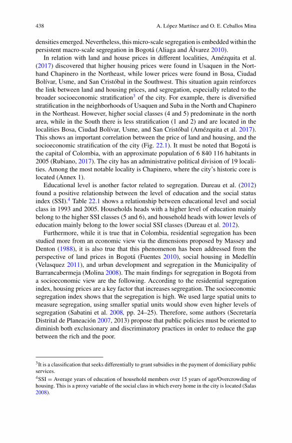
438 A. López Martínez and O. E. Ceballos Mina
densities emerged. Nevertheless, thismicro-scale segregation is embeddedwithin thepersistent macro-scale segregation in Bogotá (Aliaga and Álvarez 2010).
In relation with land and house prices in different localities, Amézquita et al.(2017) discovered that higher housing prices were found in Usaquen in the Nort-hand Chapinero in the Northeast, while lower prices were found in Bosa, CiudadBolívar, Usme, and San Cristóbal in the Southwest. This situation again reinforcesthe link between land and housing prices, and segregation, especially related to thebroader socioeconomic stratification3 of the city. For example, there is diversifiedstratification in the neighborhoods of Usaquen and Suba in the North and Chapineroin the Northeast. However, higher social classes (4 and 5) predominate in the northarea, while in the South there is less stratification (1 and 2) and are located in thelocalities Bosa, Ciudad Bolívar, Usme, and San Cristóbal (Amézquita et al. 2017).This shows an important correlation between the price of land and housing, and thesocioeconomic stratification of the city (Fig. 22.1). It must be noted that Bogotá isthe capital of Colombia, with an approximate population of 6 840 116 habitants in2005 (Rubiano, 2017). The city has an administrative political division of 19 locali-ties. Among the most notable locality is Chapinero, where the city’s historic core islocated (Annex 1).
Educational level is another factor related to segregation. Dureau et al. (2012)found a positive relationship between the level of education and the social statusindex (SSI).4 Table 22.1 shows a relationship between educational level and socialclass in 1993 and 2005. Households heads with a higher level of education mainlybelong to the higher SSI classes (5 and 6), and household heads with lower levels ofeducation mainly belong to the lower social SSI classes (Dureau et al. 2012).
Furthermore, while it is true that in Colombia, residential segregation has beenstudied more from an economic view via the dimensions proposed by Massey andDenton (1988), it is also true that this phenomenon has been addressed from theperspective of land prices in Bogotá (Fuentes 2010), social housing in Medellín(Velasquez 2011), and urban development and segregation in the Municipality ofBarrancabermeja (Molina 2008). The main findings for segregation in Bogotá froma socioeconomic view are the following. According to the residential segregationindex, housing prices are a key factor that increases segregation. The socioeconomicsegregation index shows that the segregation is high. We used large spatial units tomeasure segregation, using smaller spatial units would show even higher levels ofsegregation (Sabatini et al. 2008, pp. 24–25). Therefore, some authors (SecretaríaDistrital de Planeación 2007, 2013) propose that public policies must be oriented todiminish both exclusionary and discriminatory practices in order to reduce the gapbetween the rich and the poor.
3It is a classification that seeks differentially to grant subsidies in the payment of domiciliary publicservices.4SSI = Average years of education of household members over 15 years of age/Overcrowding ofhousing. This is a proxy variable of the social class in which every home in the city is located (Salas2008).
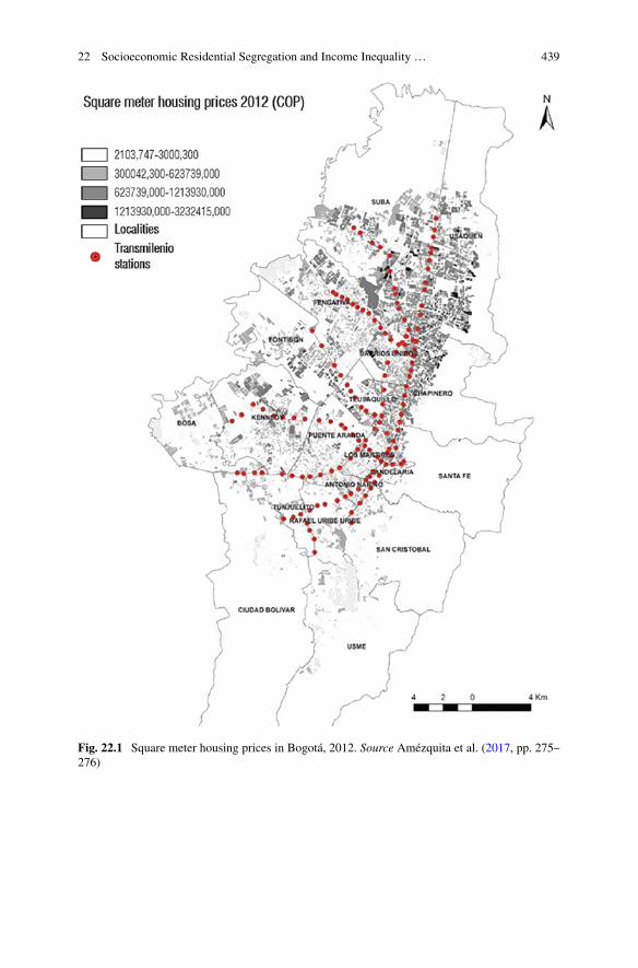
22 Socioeconomic Residential Segregation and Income Inequality … 439
Fig. 22.1 Square meter housing prices in Bogotá, 2012. Source Amézquita et al. (2017, pp. 275–276)
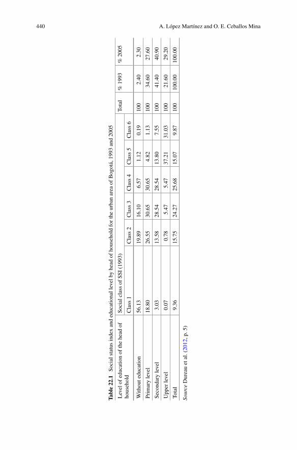
440 A. López Martínez and O. E. Ceballos Mina
Table22.1
Socialstatus
indexandeducationallevelby
head
ofhouseholdfortheurbanarea
ofBogotá,1993
and2005
Levelof
educationof
thehead
ofhousehold
Socialclassof
SSI(1993)
Total
%1993
%2005
Class
1Class
2Class
3Class
4Class
5Class
6
With
outeducatio
n56.13
19.89
16.10
6.57
1.12
0.19
100
2.40
2.30
Prim
arylevel
18.80
26.55
30.65
30.65
4.82
1.13
100
34.60
27.60
Secondarylevel
3.03
13.58
28.54
28.54
13.80
7.55
100
41.40
40.90
Upper
level
0.07
0.78
5.47
5.47
37.21
31.03
100
21.60
29.20
Total
9.36
15.75
24.27
25.68
15.07
9.87
100
100.00
100.00
Source
Dureauetal.(2012,p
.5)
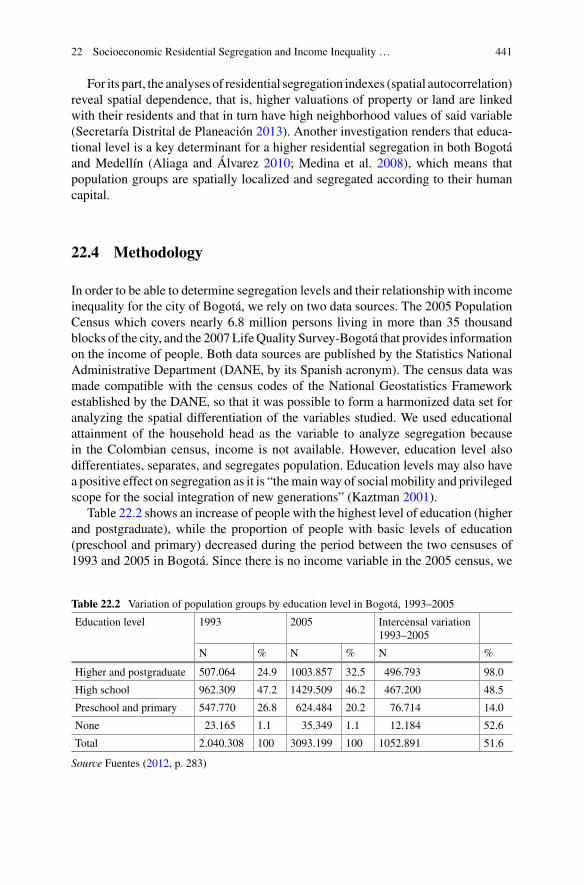
22 Socioeconomic Residential Segregation and Income Inequality … 441
For its part, the analyses of residential segregation indexes (spatial autocorrelation)reveal spatial dependence, that is, higher valuations of property or land are linkedwith their residents and that in turn have high neighborhood values of said variable(Secretaría Distrital de Planeación 2013). Another investigation renders that educa-tional level is a key determinant for a higher residential segregation in both Bogotáand Medellín (Aliaga and Álvarez 2010; Medina et al. 2008), which means thatpopulation groups are spatially localized and segregated according to their humancapital.
22.4 Methodology
In order to be able to determine segregation levels and their relationship with incomeinequality for the city of Bogotá, we rely on two data sources. The 2005 PopulationCensus which covers nearly 6.8 million persons living in more than 35 thousandblocks of the city, and the 2007LifeQuality Survey-Bogotá that provides informationon the income of people. Both data sources are published by the Statistics NationalAdministrative Department (DANE, by its Spanish acronym). The census data wasmade compatible with the census codes of the National Geostatistics Frameworkestablished by the DANE, so that it was possible to form a harmonized data set foranalyzing the spatial differentiation of the variables studied. We used educationalattainment of the household head as the variable to analyze segregation becausein the Colombian census, income is not available. However, education level alsodifferentiates, separates, and segregates population. Education levels may also havea positive effect on segregation as it is “themainway of socialmobility and privilegedscope for the social integration of new generations” (Kaztman 2001).
Table 22.2 shows an increase of people with the highest level of education (higherand postgraduate), while the proportion of people with basic levels of education(preschool and primary) decreased during the period between the two censuses of1993 and 2005 in Bogotá. Since there is no income variable in the 2005 census, we
Table 22.2 Variation of population groups by education level in Bogotá, 1993–2005
Education level 1993 2005 Intercensal variation1993–2005
N % N % N %
Higher and postgraduate 507.064 24.9 1003.857 32.5 496.793 98.0
High school 962.309 47.2 1429.509 46.2 467.200 48.5
Preschool and primary 547.770 26.8 624.484 20.2 76.714 14.0
None 23.165 1.1 35.349 1.1 12.184 52.6
Total 2.040.308 100 3093.199 100 1052.891 51.6
Source Fuentes (2012, p. 283)
442 A. López Martínez and O. E. Ceballos Mina
constructed a representative variable for average income distribution at the block-level based on the 2007LifeQuality Survey-Bogotá. It is harmonizedwith theColom-bian population and housing census and it provides and an additional perspective foranalyzing the relationship between residential segregation and inequality.
Dissimilarity index (DI) was used5 to determine city-wide levels of segregation.TheDI compares levels of segregation between specific groups (Massey and Denton1988), and we express it in an unitary interval where values near zero imply lowsegregation and one indicates high segregation. Its interpretation suggests that thegroup’s proportion in focus must change its spatial unit with respect to the restof the population in the same area, in order to accomplish an equal distribution(Martori et al. 2006). However, spatial indexes such as the DI don’t reveal statisticalsignificance (Garrocho andCampos-Alanís 2013). For this reason,weused the spatialautocorrelation index in order to determine the existence of a random distributionbetween adjacent units for the samevariable, aswell as theMoránGlobal Index (IGM,by its Spanish acronym)6 (Reardon and O’Sullivan 2004) which allows researchersto determine the existence of clustered population groups in a given geographicalspace.
In order to measure inequality in light of the non-available information regardingincome and employment structure, we built a representative variable of averageincome distribution at the block scale using microdata from the 2007 Bogotá Qualityof Life Survey and the exercise was replicated with the 2005 census. We estimated alinear regression model with the 2007 Bogotá Quality of Life Survey data to identifythe weight or factors of population and housing characteristics regarding the averageincome distribution at the block level. Then the obtained weights were applied to thecensus variables in order to estimate a measure for average income distribution forthe 2005 census.7
This exercise was initiated with an estimation, adjustment, and aggregation atthe block level (geographical scale) for the variable of the 2007 Bogotá Quality
5D = 12
∑ni=1 | xiX − yi
Y
where: xi= group’s population in the spatial unit i;
X= group’s population in the whole city;
yi= reference group’s population in the spatial unit i; and.
Y = reference group’s population in the whole city.6 I = n
∑ni=1
∑ni=1wi j (yi−y)(y j−y )
(∑n
i=1(yi−y)2)(∑
i �=1∑
wi j )
where: yi = variable or attribute value en each spatial unit i;
y j = variable or attribute value in each adjacent spatial unit i;
wi j = proximity between spatial units i and j; and
n= number of spatial units.7This exercise has its empiric background in the estimation of socio-economic levels (NSE, by itsSpanish acronym) carried on by theMexicanAssociation ofMarket Intelligence and Public OpinionAgencies (AMAI, by its Spanish acronym) in order to classify households by socio-economic groupshighly correlated with income levels (AMAI 2018).
22 Socioeconomic Residential Segregation and Income Inequality … 443
of Life Survey in order to make them equivalent with those in the 2005 census.8
The response variable selected in the model was the per capita income logarithmper block. A correlation analysis was made between the available variables and theresponse variable in order to identify those variables with higher explanatory power.Themodel considered 17 variables grouped in three analytical dimensions in order toexplain the income: (i) human capital and employment, (ii) demographic structure,and (iii) housing and services. Table 22.3 presents an estimation of all variables.Withthis set of determinants, the least weighted squares regression model was estimatedfor the average per capita current income, in order to consider the expansion factorassociated with each household in the 2007 Bogotá Quality of Life Survey (seeAnnexes 2 and 3). The weights estimated by the model are used in the estimation ofper capita income with the 2005 census data in order to map the spatial distributionof income in the neighborhoods of Bogotá (Fig. 22.4) and compares the income mapwith the educational attainment map (Fig. 22.3).9
22.5 Inequality and Socio-spatial Segregation in Bogotá
Before establishing the relationship between income inequality and residential segre-gation inBogotá, a brief review ismade of the evolution of theGini Index at a nationallevel and forBogotá in the last twenty years. Figure 22.2 shows that income inequalityhas decreased both in Bogotá and in the country, but to different degrees. The indexhas changed in a range between 59 points in the second half of 2000s (Colombia’shighest Gini level was in 2008) and 49 towards the end of the analysis period (lowestlevel in 2017 both for country and Bogotá). Bogotá shows less inequality than thewhole country except in the period between 2002 and 2006. However, Sanchez-Torres (2017) and Hoyos (2016) state that Bogotá always was in the top 5 of themost unequal cities in Colombia. Bogotá shows a remarkable decrease in inequalitybetween 2006 and 2012, and since then the Gini Index value indicated no significantvariations. By 2017, the city’s index value was almost equal to the national average.Nevertheless, in 2018 the level of national inequality showed a rebound in contrastwith a decreasing tendency between 2008 and 2017.
When considering the location quotient (see Fig. 22.3), household heads with ahigh education level are concentrated in the Northeast of the city, where there isa medium to high socioeconomic stratification (Secretaría Distrital de Planeación2007). It is very unlikely to find households heads with low education level in this
8Even though income information is asked and recollected in tables at individual level, ECV-B2007is a representative survey with micro data available at household level. On other hand, the accessto census’ information has block as maximum disaggregation level given the confidentiality andinformation protection parameters.9In Bogotá, the population density in 2005 was 175.4 people per hectare and the population densityof household head was 50 per hectare (AlcaldiaMayor de Bogotá; Secretaria Distrital de Planeación2010). However, the population density of the head of household may change depending on hisgeographical location.
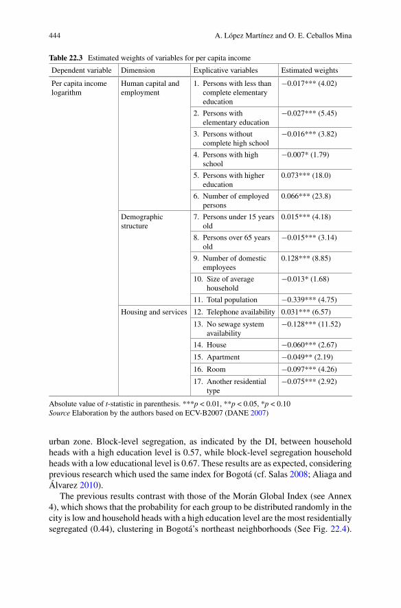
444 A. López Martínez and O. E. Ceballos Mina
Table 22.3 Estimated weights of variables for per capita income
Dependent variable Dimension Explicative variables Estimated weights
Per capita incomelogarithm
Human capital andemployment
1. Persons with less thancomplete elementaryeducation
−0.017*** (4.02)
2. Persons withelementary education
−0.027*** (5.45)
3. Persons withoutcomplete high school
−0.016*** (3.82)
4. Persons with highschool
−0.007* (1.79)
5. Persons with highereducation
0.073*** (18.0)
6. Number of employedpersons
0.066*** (23.8)
Demographicstructure
7. Persons under 15 yearsold
0.015*** (4.18)
8. Persons over 65 yearsold
−0.015*** (3.14)
9. Number of domesticemployees
0.128*** (8.85)
10. Size of averagehousehold
−0.013* (1.68)
11. Total population −0.339*** (4.75)
Housing and services 12. Telephone availability 0.031*** (6.57)
13. No sewage systemavailability
−0.128*** (11.52)
14. House −0.060*** (2.67)
15. Apartment −0.049** (2.19)
16. Room −0.097*** (4.26)
17. Another residentialtype
−0.075*** (2.92)
Absolute value of t-statistic in parenthesis. ***p < 0.01, **p < 0.05, *p < 0.10Source Elaboration by the authors based on ECV-B2007 (DANE 2007)
urban zone. Block-level segregation, as indicated by the DI, between householdheads with a high education level is 0.57, while block-level segregation householdheads with a low educational level is 0.67. These results are as expected, consideringprevious research which used the same index for Bogotá (cf. Salas 2008; Aliaga andÁlvarez 2010).
The previous results contrast with those of the Morán Global Index (see Annex4), which shows that the probability for each group to be distributed randomly in thecity is low and household heads with a high education level are the most residentiallysegregated (0.44), clustering in Bogotá’s northeast neighborhoods (See Fig. 22.4).
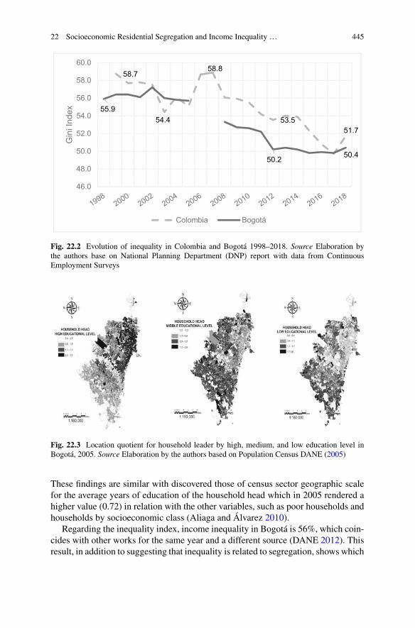
22 Socioeconomic Residential Segregation and Income Inequality … 445
58.7
54.4
58.8
53.551.7
55.9
50.2 50.4
46.0
48.0
50.0
52.0
54.0
56.0
58.0
60.0G
ini I
ndex
Colombia Bogotá
Fig. 22.2 Evolution of inequality in Colombia and Bogotá 1998–2018. Source Elaboration bythe authors base on National Planning Department (DNP) report with data from ContinuousEmployment Surveys
Fig. 22.3 Location quotient for household leader by high, medium, and low education level inBogotá, 2005. Source Elaboration by the authors based on Population Census DANE (2005)
These findings are similar with discovered those of census sector geographic scalefor the average years of education of the household head which in 2005 rendered ahigher value (0.72) in relation with the other variables, such as poor households andhouseholds by socioeconomic class (Aliaga and Álvarez 2010).
Regarding the inequality index, income inequality in Bogotá is 56%, which coin-cides with other works for the same year and a different source (DANE 2012). Thisresult, in addition to suggesting that inequality is related to segregation, shows which
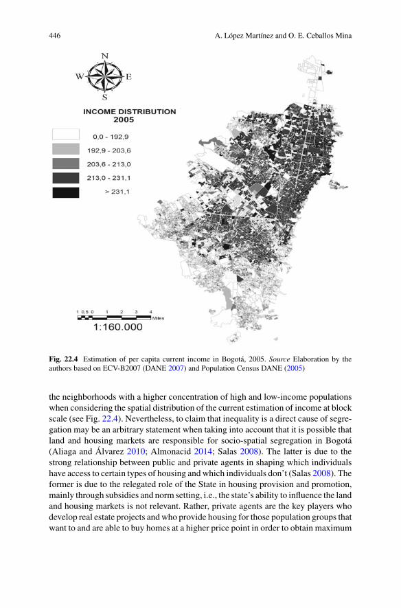
446 A. López Martínez and O. E. Ceballos Mina
Fig. 22.4 Estimation of per capita current income in Bogotá, 2005. Source Elaboration by theauthors based on ECV-B2007 (DANE 2007) and Population Census DANE (2005)
the neighborhoods with a higher concentration of high and low-income populationswhen considering the spatial distribution of the current estimation of income at blockscale (see Fig. 22.4). Nevertheless, to claim that inequality is a direct cause of segre-gation may be an arbitrary statement when taking into account that it is possible thatland and housing markets are responsible for socio-spatial segregation in Bogotá(Aliaga and Álvarez 2010; Almonacid 2014; Salas 2008). The latter is due to thestrong relationship between public and private agents in shaping which individualshave access to certain types of housing andwhich individuals don’t (Salas 2008). Theformer is due to the relegated role of the State in housing provision and promotion,mainly through subsidies and norm setting, i.e., the state’s ability to influence the landand housing markets is not relevant. Rather, private agents are the key players whodevelop real estate projects andwho provide housing for those population groups thatwant to and are able to buy homes at a higher price point in order to obtain maximum
22 Socioeconomic Residential Segregation and Income Inequality … 447
gains. This is achieved by private agents localizing medium–high socioeconomicgroups in a differential and fragmentary way. This is the way in which residentialsegregation plays a role in the functioning of land and housing markets.
22.6 Conclusions
The socio-spatial segregation analysis for Bogotá presented new insights into thesegregation dynamics of the city. Bogotá is commonly referred to as the city witha rich north and a poor south, when considering the education levels of the headsof the households and average per capita income. Despite these two differentiatedmacro areas of Bogotá, it is clear that small concentrations of individuals with alow level of education and a low income can be found across the entire city. Thisis not evident in the case of individuals with higher educational levels. This groupmainly resides in the Northeast of the city. It is important to mention that despite thefact that segregation exists between the North and South in terms of social status,segregation is also amplified at a small scale. The fact that education level segregatesthe population in a similar way to per capita income implies that it is possible thatthese two variables have an effect on social capital due to the fact that when educationsegregates it may affect mobility and social integration (Kaztman 2001).
Accordingly, it can be said that land value may be a more significant determinantof land concentration for a few individuals rather than income, due to the fact thatland policies may be able to counteract such concentration. This is because thereare housing and territorial organization policies, as well as norms and laws, whichegulate the pursuit for ran urban equality in order to eliminate privileges in thedistribution of urban equipment (of education, sport, culture, others) independentlyof the localization of a certain population group.
This is how the actions of social agents, such as urbanists, have changed theway in which segregation manifests, because they have intervened in the city underthe logic of land and housing market liberalization. This liberalization manifests asthe differentiation of segregated residential areas that have an effect on the socialstructure of class by making it more complex. In turn, this complexity reproducescertain production relations (between capitalist and the proletariat) and at the sametime reinforces class diversity, which may stress the symbolic value that individualsgive to the territory by means of their behavior and in the choice of different types ofhousing, a consideration that has been scarcely studied and that would be importantto address in future investigations about the subjective dimensions of segregation.

448 A. López Martínez and O. E. Ceballos Mina
References
Ábramo P (2003) La teoría económica de la favela: cuatro notas sobre la localización resi-dencial de los pobres y el mercado inmobiliario informal. Ciudad y Territorio: EstudiosTerritorialesXXXV:273–294
Alcaldia Mayor de Bogotá , Secretaria Distrital de Planeación (2010) Población y desarrollourbano 23:52. https://www.sdp.gov.co/portal/page/portal/PortalSDP/InformacionTomaDecisiones/Estadisticas/Bogot%E1CiudaddeEstad%EDsticas/2010/DICE106-CartillaPobDesalloUrbano-2010.pdf
Alessandri AF (2013) A Prática Espacial Urbana Como Segregação e o “Direito à Cidade” ComoHorizonte Utópico. In: A CIDADE CONTEMPORÂNEA SEGREGAÇÃO ESPACIAL, SaoPulo, Context, pp 96–110
Aliaga L, Álvarez MJ (2010) Segregación Residencial en Bogotá a través del Tiempo y diferentesescalas. Lincoln Institute of Land Policy
Almonacid J (2014) Lógicas contemporáneas de la segregación residencial en tres casos represen-tativos de Bogotá DC. Bdigital.Unal.Edu.Co. Universidad Nacional de Colombia
Amézquita L, Sánchez M, Abaunza G (2017) Segregación residencial y transmilenio. In: RubianoM (ed) Segregación socioespacial. Miradas cruzadas desde Río de Janeiro, Bogotá y sus áreas deinfluencia metropolitana. Universidad Piloto de Colombia, Bogotá D.C, p 450
Aprile J, Mosquera G (1984) Clases, Segregación y Barrios, 1st edn. Universidad del Valle, CaliBuzai G (2003) Mapas Urbanos Sociales. Lugar Editorial, Buenos AiresCardeño F (2007) Historial del desarrollo urbano del centro de Bogotá (localidad de Los Mártires).Alcaldía Mayor de Bogotá, Bogotá D.C. https://www.culturarecreacionydeporte.gov.co/observatorio/documentos/investigaciones/estadosArte/HistoriaBta_Martires.pdf
Castells M (2008) La Cuestión Urbana. Siglo Veintiuno Editores, S.A, MéxicoDANE (2005) Censo general 2005. Bogotá D.C.DANE (2007) Encuesta de Calidad de Vida—Bogotá 2007. Bogotá D.C.DANE (2012) Cifras departamentales de pobreza monetaria y la desigualdad. Bogotá D.C.DeMattosC (2002)SantiagodeChile de cara a laGlobalización: ¿otra ciudad?Revista deSociologiae Política19:31–54. https://doi.org/10.5380/rsp.v19i0
De Mattos C (2012) Notas sobre una falsa disyuntiva: redensificación de las áreas centrales versusdispersión urbana. Tendencias recientes, evidencia empírica. Instituto de Estudios Urbanos yterritoriales
De Queiroz L (2003) Segregação Residencial e Políticas Públicas: Análise do Espaço Social daCidade na Gestão do Território. Cidades - Comunidades e Territórios (6):33–50. https://cidades.dinamiacet.iscte-iul.pt/index.php/CCT/login?source=/index.php/CCT/article/view/178/165
Dureau et al (2012) Evolución de la intensidad y de las escalas de la segregación residencial enBogotá: un análisis comparativo con Santiago de Chile y Sao Paulo. In: X seminario ACIUR(Asociación Colombiana de Investigadores Urbano Regionales), pp 1–20
Elorza A (2013) La dimensión subjetiva de la segregación residencial socioeconómica: lasrepresentaciones sociales sobre el territorio. Revista Vivienda y Ciudad 1:123–133
Fuentes J (2010) Desigualdad, segregación socio-espacial y precios del suelo en la ciudad Lati-noamericana. El caso de Bogotá en los Años Noventa. Revista UIS. Humanidades 38(1):109–126
Fuentes L (2012) Ciudades y sociedades urbanas en transformación. Competitividad, reestruc-turación y cohesión social en Bogotá, Lima y Santiago en las últimas décadas. PontificiaUniversidad Católica de Chile
García L, Gascón D (2016) Portafolio de mapas. Bogotá D.C, Equipo de integración de documentosPOT
Garrocho C, Campos-Alanís J (2013) Réquiem por los indicadores no espaciales de segregaciónresidencial. Papeles De Poblacion 19(77):269–300
Howell-Moroney M (2005) The geography of opportunity and unemployment: an integrated modelof residential segregation and spatial mismatch. J Urban Affairs 27(4):353–377. https://doi.org/10.1111/j.0735-2166.2005.00234.x-i1
22 Socioeconomic Residential Segregation and Income Inequality … 449
Janoschka M, Glasze G (2003) Urbanizaciones cerradas: un modelo analítico. CIUDADES, PueblaKaztman R (2001) Seducidos y abandonados. El aislamiento social de los pobres urbanos. Revistade La CEPAL (75):171–189
Kaztman R (2003) La dimensión espacial en las políticas de superación de la pobreza urbana. SerieMedio Ambiente y Desarrollo, vol 59. Santiago de Chile
Lefebvre H (1976) Espacio y Política. El Derecho a la Ciudad II. Ediciones Península, BarcelonaLefebvre H (1978a) De lo Rural a lo Urbano. Ediciones Península, Barcelona. https://doi.org/10.1177/072551369203300110
Lefebvre H (1978b) El Derecho a la Ciudad. Ediciones Península, BarcelonaMartori JC, Hoberg K, Surinach J (2006) Población inmigrante y espacio urbano. Indicadores desegregación y pautas de localización. Eure32(97):49–62. https://doi.org/10.4067/S0250-71612006000300004
Massey D, Denton N (1988) The dimensions of residential segregation. Soc Forces67(2):281–315.https://isites.harvard.edu/fs/docs/icb.topic98848.files/massey.denton.pdf
Medina C, Morales L, Núñez J (2008) Quality of life in urban neighborhoods in Colombia: TheCases of Bogotá and Medellín. Borradores de Economía (536)
Molina L (2008) Barrancabermeja: segregación socioespacial y desequilibrios funcionales.Cuadernos de Vivienda y Urbanismo 1(2):332–347. Retrieved from http://scholar.google.com/scholar?hl=en&btnG=Search&q=intitle:Barrancabermeja+:+segregaci?n+socioespacial+y+desequilibrios+funcionales#0
Moura R (2003) Inversiones urbanas en el contexto de la competitividad y globalización: loseventos en Curitiba. EURE (Santiago) 29(86):51–68. https://doi.org/10.4067/S0250-71612003008600003
Reardon S, O’Sullivan D (2004) Measures of spatial segregation. Sociol Methodol 34(1):121–162.https://doi.org/10.1111/j.0081-1750.2004.00150.x
RubianoM(2017)Segregación socioespacial y dinámicametropolitana desde las relacionesBogotá-Soacha: una reflexión a partir del caso de CiudadVerde. In:M. Rubiano (ed) Segregación socioes-pacial. Miradas cruzadas desde Río de Janeiro, Bogotá y sus áreas de influencia metropolitana,pp 141–212). Universidad Piloto de Colombia, Bogotá D.C.
Ruiz-Tagle J (2016) La segregación y la integración en la sociología urbana: revisión de enfoquesy aproximaciones críticas para las políticas públicas. Revista INVI 31(87):9–57. https://doi.org/10.4067/INVI.V0I0.1070
Ruiz-Tagle J, López E (2014) El estudio de la segregación residencial en Santiago de Chile: revisióncrítica de algunos problemas metodológicos y conceptuales. EURE 40(119):25–48
Sabatini F (2003) La segregación social del espacio en las ciudades de América Latina. BancoInteramericano de Desarrollo 1–41. https://www.iadb.org.uy/sds/doc/SOCSabatiniSegregacion.pdf
Sabatini F, Cáceres G (2005) Relación entre Promoción Inmobiliaria y Segregación Residencial:Giros Insospechados de la Ciudad Latinoaméricana. Lincoln Institute of Land Policy. https://doi.org/10.1017/CBO9781107415324.004
Sabatini F, Wormald G, Sierralta C, Peters P (2008) Segregación Residencial en Santiago: Tenden-cias 1992–2002 y efectos vinculados con su escala geográfica. In Sabatini F, Salcedo R,WormaldG (eds) Tendencias Segregación en las Principales CiudadesChilenas. Santiago deChile: InstitutoNacional de Estadísticas, Pontificia Universidad Católica de Chile
Salas A (2008) Residential segregation and housing production in Bogota, between perceptions andrealities. Université de Poitiers. https://tel.archives-ouvertes.fr/tel-00303317
Secretaría Distrital de Planeación (2007) Segregación Socioeconómica en el Espacio Urbano deBogotá D.C. Universidad Nacional de Colombia. Bogotá D.C.
Secretaría Distrital de Planeación (2011) Segregación Socioespacial En Bogotá 2011. Indicadores yMedición. Bogotá D.C. Retrieved from http://es.scribd.com/doc/94922064/Boletn-39-SEGREGACIN
450 A. López Martínez and O. E. Ceballos Mina
Secretaría Distrital de Planeación (2013) Segregación Socioeconómica en el Espacio Urbano deBogotá D.C. Universidad Nacional de Colombia, Secretaría Distrital de Planeación. Bogotá D.C:Secretaría Distrital de Planeación, Universidad Nacional de Colombia
Shevky E, Bell W (1955) Social area analysis: theory, illustrative application and computationalprocedures. Standford University Press, Stanford
Shevky E, Williams M (1949) The social area of Los Angeles: analysis and typology. University ofCalifornia Press, Berkeley
Torres C, Gaviria A, Zuñiga D, Vargas J, Nieto D, Bustos S (2009) Ciudad informal colombianaBarrios construidos por la gente. Universidad Nacional de Colombia
Velasquez C (2011) Localización y distribución de la vivienda social en la ciudad de medellín. UnaMirada Desde la Segregación Espacial. Universidad Nacional de Colombia, Sede Medellín
Open Access This chapter is licensed under the terms of the Creative Commons Attribution 4.0International License (http://creativecommons.org/licenses/by/4.0/), which permits use, sharing,adaptation, distribution and reproduction in any medium or format, as long as you give appropriatecredit to the original author(s) and the source, provide a link to the Creative Commons license andindicate if changes were made.
The images or other third party material in this chapter are included in the chapter’s CreativeCommons license, unless indicated otherwise in a credit line to the material. If material is notincluded in the chapter’s Creative Commons license and your intended use is not permitted bystatutory regulation or exceeds the permitted use, you will need to obtain permission directly fromthe copyright holder.
Chapter 23Socio-Economic Residential Segregationin Greater Buenos Aires: Evidenceof Persistent Territorial FragmentationProcesses
Florencia Molinatti
Abstract Socio-economic residential segregation is a common feature of almostall Argentinean cities, neatly divided into poor, middle-class, and affluent neigh-borhoods. At the end of the 1980s, and especially over the 1990s, the process ofsuburbanization for affluent and upper middle-class groups was consolidated as ageneralized model. This study concentrates on the trends and the patterns of socio-economic segregation in Buenos Aires and focuses on two major dimensions ofsegregation: the spatial concentration patterns of a given social group in specific areasand the degree of social homogeneity within such areas. Socio-economic segregationis described using the highest level of education that a householder has completed asa proxy for socio-economic status. The indices of segregation and dissimilarity areused as the main measure to compare the level and changes of residential segrega-tion but other metrics—such as location quotient index—are also used to estimatethe degree of homogeneity or heterogeneity in neighboring areas. This study usespopulation and household census data from 1991, 2001, and 2010 provided by theNational Institute of Statistics and Censuses (INDEC), and the data are presented atthe spatial disaggregation level of block groups called ‘radios censales’.
Keywords Fragmentation · Residential polarization · Suburbanization of elites ·Educational inequality
23.1 Introduction
Residential segregation accounts for the degree of inequality acquired by the spatialdistribution of the population. Over the last decades, social sciences have shownrenewed interest in the study of this phenomenon in theUnited States and inEurope aswell as in Latin America. Although these studies share the objective of evaluating themagnitude and effects of certain spatially concentrated population groups on people’s
F. Molinatti (B)Center for Research and Studies on Culture and Society (CIECS), National Scientific andTechnical Research Council (CONICET), National University of Cordoba, Cordoba, Argentinae-mail: [email protected]
© The Author(s) 2021M. van Ham et al. (eds.), Urban Socio-Economic Segregation and Income Inequality,The Urban Book Series, https://doi.org/10.1007/978-3-030-64569-4_23
451
452 F. Molinatti
living conditions, they differ in relation to the criteria used for social differentiation.While in the United States and Europe, the research was, to a large extent, focusedon racial and ethnic segregation and migration, in Latin America the analyses thatfocus on territorial relations among socio-economic groups were favored (Groisman2009; Molinatti 2013; Sabatini 2006).
In the latter group of countries, the emphasis on the socio-economic dimensionof residential segregation is understandable considering that the rigidity of the socialstructure and substantial social, income, and class inequalities represent perhaps themost outstanding characteristics of the social structure of Latin American countries(Groisman 2010; Sabatini 2006). In this context, the functioning of labor marketsis a key element to understand the fluctuations in the well-being of the vulnerablepopulations, mainly because, due to the absence of generalized credit markets, lowersocial classes’ homes obtain most of their income from the labor insertion of theirmembers, usually in unsteady and low-paid jobs (Groisman 2009).
The interrelationship between the social structure and the urban spatial structureis multifaceted. Residential segregation takes place when the existing inequalitiesof a community are made visible in a territorial or geographical manner. However,residential segregation is not a simple reflection of social reality, since space is consid-ered a dimension that composes the processes that structure social reality. Likewise,there are other intermediate processes or mechanisms that encourage segregation orcounteract its outcomes, including, among others, land markets, housing policy, andthe labor market (Molinatti 2013; Sabatini 2006; Torres et al. 2003).
Since the end of the twentieth century, Latin America has witnessed a prolifera-tion of theoretical investigations and, to a greater extent, empirical research related toresidential segregation, especially in large metropolises of the most urbanized coun-tries in the region. The emergence of this line of research is linked to the processesof impoverishment of Latin American societies during the 1990s pertaining to theimplementation of the neoliberal development model. The opening of the regionaleconomies, in conjunction with policies aimed at reducing state intervention in theeconomy, caused a rapid increase in unemployment and a resulting decrease in theincome of households belonging to lower social class.
Other phenomena also influenced the revitalization of residential segregationstudies in the region. In particular, an increase in the concentration of elites and theaffluent middle classes was a process reflected in the proliferation of gated commu-nities and in the resulting suburbanization of these social groups (Caldeira 2007;Svampa 2004; Torres 2001). Both phenomena led to the reorganization of the LatinAmerican cities, mainly represented
…. as the displacement of an “open city” model, basically European, focused on the notionof public space and on values, such as political citizenship and social integration, towardsa “closed city” regime, more associated with the North American type, marked by theaffirmation of patrimonial citizenship centered on the figure of the taxpayer (Svampa 2004:16).
The impact of these changes on socio-economic residential segregation showsopposite trends in Latin American cities. A trend would indicate a reduction in
23 Socio-Economic Residential Segregation in Greater Buenos Aires … 453
the level of residential segregation as a result of the relative dispersion of closedcondominiums, shopping centers, offices, and services located outside the city centerand the high-income area leading to physical proximity between popular and elitegroups. As signaled by various authors, it is important to mention that this greaterphysical proximity does not produce social integration or mixture per se. Anothertrend, however, corresponds to the increase in the level of segregation of new groupsof lower class housing that have access—by formal or informal means—to urbanlands located far away from the city, as a result of real estate speculation and itsimpact on land prices (Sabatini 2006).
At the beginning of the twenty-first century, there was a positive growth inthe Gross Domestic Product (GDP) of Latin American economies, although thereremained variations in social indicators. In the regional context, Argentina is a partic-ular example as this change took place dramatically. After the great economic crisisof 2001–2002 (when the GDP shrank significantly and poverty spread to more than50% of the population), the Argentinian economy had seven years of sustained GDPgrowth at average annual rates of 8–9% (Groisman 2009). In 2009, despite the inter-national economic crisis, the country registered an annual GDP variation rate of 0.9%above the average of the region that showed−1.8% (ECLAC 2010). After that crisis,Argentina returned to a vigorous growth rate with average annual increases of 7–9%between 2010 and 2011.
In this context, it is necessary to investigate how social inequalities and socio-economic residential segregation indicators evolved in Greater Buenos Aires, themain urban agglomeration of the country, and whether these political, social, andeconomic transformations produced consistent changes in the spatial distribution ofthe population.
23.2 The Functioning of the Labor Marketand the Concentration of Income
At the beginning of the 1970s, the Argentinean labor market was characterized bybeing relatively integrated, with a high presence of salaried work and low levels ofunderemployment. However, as a consequence of the poor macroeconomic perfor-mance experienced by the Argentinean economy during the mid-1970s and early1990s, this trend was overturned and the period was marked by stagnation andinstability (Altimir and Beccaria 1999, Arceo et al. 2008).
Labor regulations were key elements in the structural reforms of the so-called“neoliberal decade” (1989–2001).1 These measures were aimed at the convenienceof adapting legislation concerning individual and collective relations in order toprovidemoreflexibility and, basically, to reduce non-wage labor costs (social security
1This “neoliberal decade” comprises two governments: the one of Carlos SaúlMenem (1989–1999)and the one of Fernando de la Rúa (1999-2001). The latter resigned in the context of the majorArgentinean crisis at the end of 2001.
454 F. Molinatti
contributions and costs related to events, such as dismissal or accidents, or makingthe distribution of work time more flexible and the decentralization of negotiation)(Altimir and Beccaria 1999; Arceo et al. 2008).
Flexibility in the labormarket, combinedwith the process of foreign trade openingfor foreign trade in the context of an increasingly overvalued exchange rate that ledto a significant loss of competitiveness in the goods and services production areas,resulted in a significant reduction in workforce demand, a rise in unemployment,and it created instability, insecurity, and low productivity. This phenomenon, typicalof the informal side of the economy, caused a progressive gap between workerswith lower qualifications and those with higher ones (Arceo et al. 2008). One of themost severe consequences of the subsequent changes introduced in labor legislationduring this period was job insecurity, characterized by an increase in time-relatedunderemployment and unreported employment, which, together with unemploymentand wage stagnation, negatively affected the living conditions of the population. Theprofound economic recession that the Argentinean economy suffered between 1998and 2002 significantly worsened the current problems in the local labor market,resulting in the great economic and political crisis at the end of 2001 and 2002,which caused a shrinking of approximately 20% of the GDP (Basualdo 2008).
After this great economic crisis, there was a change in the macroeconomic systemthat led to a period of sustained and long-lasting economic recovery between 2003and 2006. This period was characterized by a strong increase in employment andpurchasing power, an increase in the number of registered workers, and a decreasein unemployment and time-related underemployment (Arceo et al. 2008). Likewise,there was a substantial reduction in absolute poverty even though some authors claimthat at the level of redistribution, the evolution was not so satisfactory (Groisman2010). Although income distribution has a tendency to reduce in concentration, thedistribution of wealth remained highly unequal (Báez 2017).
This process of expansion and growth was fuelled by an increase in payroll as aresult of a decrease in the unemployment rate (from 16.3% in the third quarter of2003 to 7.5% in the third quarter of 2010), the increase in the average real wage of35% between 2003 and 2010, the increase in the adjustable minimum living wage,the increase in minimum retirement benefits, and so on.2 This was also due to theimplementation of new social policies: the incorporation of three million people intothe Social Security System through the Provisional Inclusion Plan (2004–2007), theexecution of the Universal Child Allowance (Asignación Universal por hijo, AUH)in October 2009, among others (For further information about new social policiesapplied, consult Alonso and Di Costa 2012).
Regarding income distribution,3 during the so-called “neoliberal decade,” therewas a deepening of income inequality and regressive income distribution. Between1991 and 2002, the Gini index rose from 0.468 to 0.538. The reversal of this trend
2The main changes in labor legislation between 2003 and 2007 can be consulted in: Centro deEstudios para el Desarrollo Argentino (2007).3Values corresponding to the estimates conducted by: World Bank, Development Research Group(2019).
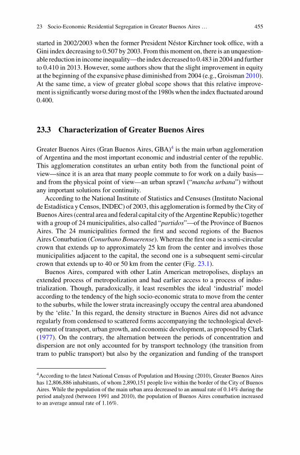
23 Socio-Economic Residential Segregation in Greater Buenos Aires … 455
started in 2002/2003 when the former President Néstor Kirchner took office, with aGini index decreasing to 0.507 by 2003. From thismoment on, there is an unquestion-able reduction in income inequality—the index decreased to 0.483 in 2004 and furtherto 0.410 in 2013. However, some authors show that the slight improvement in equityat the beginning of the expansive phase diminished from 2004 (e.g., Groisman 2010).At the same time, a view of greater global scope shows that this relative improve-ment is significantlyworse duringmost of the 1980swhen the indexfluctuated around0.400.
23.3 Characterization of Greater Buenos Aires
Greater Buenos Aires (Gran Buenos Aires, GBA)4 is the main urban agglomerationof Argentina and the most important economic and industrial center of the republic.This agglomeration constitutes an urban entity both from the functional point ofview—since it is an area that many people commute to for work on a daily basis—and from the physical point of view—an urban sprawl (“mancha urbana”) withoutany important solutions for continuity.
According to the National Institute of Statistics and Censuses (Instituto Nacionalde Estadística y Censos, INDEC) of 2003, this agglomeration is formed by the City ofBuenosAires (central area and federal capital city of theArgentineRepublic) togetherwith a group of 24 municipalities, also called “partidos”—of the Province of BuenosAires. The 24 municipalities formed the first and second regions of the BuenosAires Conurbation (Conurbano Bonaerense). Whereas the first one is a semi-circularcrown that extends up to approximately 25 km from the center and involves thosemunicipalities adjacent to the capital, the second one is a subsequent semi-circularcrown that extends up to 40 or 50 km from the center (Fig. 23.1).
Buenos Aires, compared with other Latin American metropolises, displays anextended process of metropolization and had earlier access to a process of indus-trialization. Though, paradoxically, it least resembles the ideal ‘industrial’ modelaccording to the tendency of the high socio-economic strata to move from the centerto the suburbs, while the lower strata increasingly occupy the central area abandonedby the ‘elite.’ In this regard, the density structure in Buenos Aires did not advanceregularly from condensed to scattered forms accompanying the technological devel-opment of transport, urban growth, and economic development, as proposed byClark(1977). On the contrary, the alternation between the periods of concentration anddispersion are not only accounted for by transport technology (the transition fromtram to public transport) but also by the organization and funding of the transport
4According to the latest National Census of Population and Housing (2010), Greater Buenos Aireshas 12,806,886 inhabitants, of whom 2,890,151 people live within the border of the City of BuenosAires. While the population of the main urban area decreased to an annual rate of 0.14% during theperiod analyzed (between 1991 and 2010), the population of Buenos Aires conurbation increasedto an average annual rate of 1.16%.
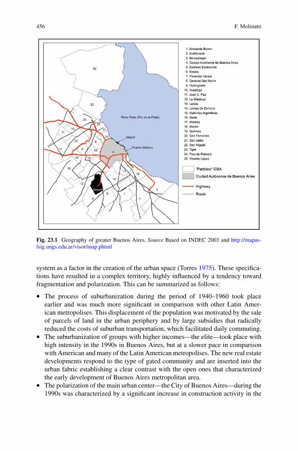
456 F. Molinatti
Fig. 23.1 Geography of greater Buenos Aires. Source Based on INDEC 2003 and http://mapas-lsig.ungs.edu.ar/visor/map.phtml
system as a factor in the creation of the urban space (Torres 1975). These specifica-tions have resulted in a complex territory, highly influenced by a tendency towardfragmentation and polarization. This can be summarized as follows:
• The process of suburbanization during the period of 1940–1960 took placeearlier and was much more significant in comparison with other Latin Amer-ican metropolises. This displacement of the population was motivated by the saleof parcels of land in the urban periphery and by large subsidies that radicallyreduced the costs of suburban transportation, which facilitated daily commuting.
• The suburbanization of groups with higher incomes—the elite—took place withhigh intensity in the 1990s in Buenos Aires, but at a slower pace in comparisonwith American and many of the Latin American metropolises. The new real estatedevelopments respond to the type of gated community and are inserted into theurban fabric establishing a clear contrast with the open ones that characterizedthe early development of Buenos Aires metropolitan area.
• The polarization of the main urban center—the City of Buenos Aires—during the1990s was characterized by a significant increase in construction activity in the
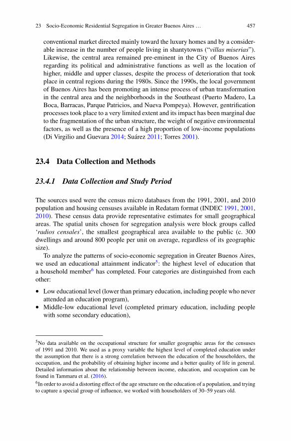
23 Socio-Economic Residential Segregation in Greater Buenos Aires … 457
conventional market directed mainly toward the luxury homes and by a consider-able increase in the number of people living in shantytowns (“villas miserias”).Likewise, the central area remained pre-eminent in the City of Buenos Airesregarding its political and administrative functions as well as the location ofhigher, middle and upper classes, despite the process of deterioration that tookplace in central regions during the 1980s. Since the 1990s, the local governmentof Buenos Aires has been promoting an intense process of urban transformationin the central area and the neighborhoods in the Southeast (Puerto Madero, LaBoca, Barracas, Parque Patricios, and Nueva Pompeya). However, gentrificationprocesses took place to a very limited extent and its impact has been marginal dueto the fragmentation of the urban structure, the weight of negative environmentalfactors, as well as the presence of a high proportion of low-income populations(Di Virgilio and Guevara 2014; Suárez 2011; Torres 2001).
23.4 Data Collection and Methods
23.4.1 Data Collection and Study Period
The sources used were the census micro databases from the 1991, 2001, and 2010population and housing censuses available in Redatam format (INDEC 1991, 2001,2010). These census data provide representative estimates for small geographicalareas. The spatial units chosen for segregation analysis were block groups called‘radios censales’, the smallest geographical area available to the public (c. 300dwellings and around 800 people per unit on average, regardless of its geographicsize).
To analyze the patterns of socio-economic segregation in Greater Buenos Aires,we used an educational attainment indicator5: the highest level of education thata household member6 has completed. Four categories are distinguished from eachother:
• Low educational level (lower than primary education, including people who neverattended an education program),
• Middle-low educational level (completed primary education, including peoplewith some secondary education),
5No data available on the occupational structure for smaller geographic areas for the censusesof 1991 and 2010. We used as a proxy variable the highest level of completed education underthe assumption that there is a strong correlation between the education of the householders, theoccupation, and the probability of obtaining higher income and a better quality of life in general.Detailed information about the relationship between income, education, and occupation can befound in Tammaru et al. (2016).6In order to avoid a distorting effect of the age structure on the education of a population, and tryingto capture a special group of influence, we worked with householders of 30–59 years old.
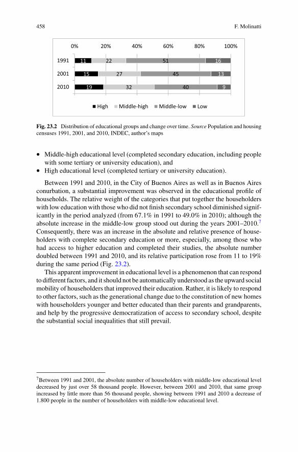
458 F. Molinatti
19
15
11
32
27
22
40
45
51
9
13
16
0% 20% 40% 60% 80% 100%
2010
2001
1991
High Middle-high Middle-low Low
Fig. 23.2 Distribution of educational groups and change over time. Source Population and housingcensuses 1991, 2001, and 2010, INDEC, author’s maps
• Middle-high educational level (completed secondary education, including peoplewith some tertiary or university education), and
• High educational level (completed tertiary or university education).
Between 1991 and 2010, in the City of Buenos Aires as well as in Buenos Airesconurbation, a substantial improvement was observed in the educational profile ofhouseholds. The relative weight of the categories that put together the householderswith low educationwith thosewho did not finish secondary school diminished signif-icantly in the period analyzed (from 67.1% in 1991 to 49.0% in 2010); although theabsolute increase in the middle-low group stood out during the years 2001–2010.7
Consequently, there was an increase in the absolute and relative presence of house-holders with complete secondary education or more, especially, among those whohad access to higher education and completed their studies, the absolute numberdoubled between 1991 and 2010, and its relative participation rose from 11 to 19%during the same period (Fig. 23.2).
This apparent improvement in educational level is a phenomenon that can respondto different factors, and it should not be automatically understood as the upward socialmobility of householders that improved their education. Rather, it is likely to respondto other factors, such as the generational change due to the constitution of new homeswith householders younger and better educated than their parents and grandparents,and help by the progressive democratization of access to secondary school, despitethe substantial social inequalities that still prevail.
7Between 1991 and 2001, the absolute number of householders with middle-low educational leveldecreased by just over 58 thousand people. However, between 2001 and 2010, that same groupincreased by little more than 56 thousand people, showing between 1991 and 2010 a decrease of1.800 people in the number of householders with middle-low educational level.
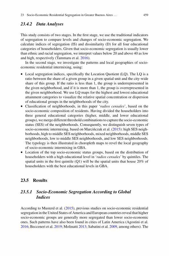
23 Socio-Economic Residential Segregation in Greater Buenos Aires … 459
23.4.2 Data Analyses
This study consists of two stages. In the first stage, we use the traditional indicatorsof segregation to compare levels and changes of socio-economic segregation. Wecalculate indices of segregation (IS) and dissimilarity (D) for all four educationalcategories of householders. Given that socio-economic segregation is usually lowerthan ethnic and racial segregation, we interpret values below 20 and above 40 as lowand high, respectively (Tammaru et al. 2016).
In the second stage, we investigate the patterns and local geographies of socio-economic residential intermixing, using:
• Local segregation indices, specifically the Location Quotient (LQ). The LQ is aratio between the share of a given group in a given spatial unit and the city-wideshare of this group. If the ratio is less than 1, the group is underrepresented inthe given neighborhood, and if it is more than 1, the group is overrepresented inthe given neighborhood. We use LQ maps for the highest and lowest educationalattainment categories to visualize the relative spatial concentration or dispersionof educational groups in the neighborhoods of the city.
• Classification of neighborhoods, in this paper ‘radios censales’, based on thesocio-economic composition of residents. Having divided the householders intothree general educational categories (higher, middle, and lower educationalgroups),wemerge different threshold combinations to capture the socio-economicstatus (SES) of the neighborhoods. Consequently, we distinguish seven types ofsocio-economic intermixing, based on Marcinczak et al. (2015): high SES neigh-borhoods, high to middle SES neighborhoods, mixed neighborhoods, middle SESneighborhoods, low to middle SES neighborhoods, and low SES neighborhoods.The typology is then illustrated in choropleth maps to revel the local geographyof socio-economic intermixing in GBA.
• Location of the top socio-economic status groups, based on the distribution ofhouseholders with a high educational level in ‘radios censales’ by quintiles. Thespatial units in the first quintile (Q1) will be the spatial units that house 20% ofhouseholders with the best educational levels in GBA.
23.5 Results
23.5.1 Socio-Economic Segregation According to GlobalIndices
According to Musterd et al. (2015), previous studies on socio-economic residentialsegregation in theUnited States ofAmerica andEuropean countries reveal that highersocio-economic groups are generally more segregated than lower socio-economicones. Such patterns have also been found in cities of Latin America (Agostini et al.2016; Becceneri et al. 2019; Molinatti 2013; Sabatini et al. 2009, among others). The
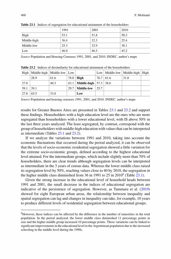
460 F. Molinatti
Table 23.1 Indices of segregation for educational attainment of the householders
1991 2001 2010
High 53.1 51.8 50.3
Middle-high 36.4 32.3 25.4
Middle-low 25.3 32.9 38.1
Low 46.0 46.5 45.2
Source Population and Housing Censuses 1991, 2001, and 2010. INDEC. author’s maps
Table 23.2 Indices of dissimilarity for educational attainment of the householders
High Middle-high Middle-low Low Low Middle-low Middle-high High
28.9 61.6 78.0 High 76.7 61.6 31.0
27.0 40.3 63.1 Middle-high 57.3 38.6
59.1 39.1 29.7 Middle-low 25.7
27.8 65.5 33.0 Low
Source Population and housing censuses 1991, 2001, and 2010. INDEC. author’s maps
results for Greater Buenos Aires are presented in Tables 23.1 and 23.2 and supportthese findings. Householders with a high education level are the ones who are moresegregated than householders with a lower educational level, with IS above 50% inthe last three years analyzed. The least segregated, by contrast, correspond with thegroup of householderswithmiddle-high educationwith values that can be interpretedas intermediate (Tables 23.1 and 23.2).
If we analyze the variations between 1991 and 2010, taking into account theeconomic fluctuations that occurred during the period analyzed, it can be observedthat the levels of socio-economic residential segregation showed a little variation forthe extreme socio-economic groups, defined according to the highest educationallevel attained. For the intermediate groups, which include slightly more than 70% ofhouseholders, there are clear trends although segregation levels can be interpretedas intermediate in the 3 years of census data. Whereas the lower middle class raisedits segregation level by 50%, reaching values close to 40 by 2010, the segregation inthe higher middle class diminished from 36 in 1991 to 25 in 20108 (Table 23.1).
Given the strong increase in the educational level of household heads between1991 and 2001, the small decrease in the indices of educational segregation areindicative of the persistence of segregation. However, as Tammaru et al. (2019)showed for eight European urban areas, the relationship between inequality andspatial segregation can lag and changes in inequality can take, for example, 10 yearsto produce different levels of residential segregation between educational groups.
8However, these indices can be affected by the difference in the number of minorities in the totalpopulation. In the period analyzed, the lower middle class diminished 11 percentage points insize and the higher middle group increased 10 percentage points. These variations can be linked tosignificant improvements in the educational level in the Argentinean population due to the increasedschooling in the middle level during the 1990s.
23 Socio-Economic Residential Segregation in Greater Buenos Aires … 461
Regarding the degree of residential segregation among the social categoriesanalyzed, especially between the opposite ends of the social hierarchy, the D betweenthe groups shows a narrow correlation between the educational level of the house-holders and their residential localization, suggesting a high correspondence betweenthe spatial distribution of the groups and the present education gap between them.The index reaches lower values when it is calculated between contiguous educationalgroups and higher values between the opposite ends (Table 23.2).
Among the variations observed between 1991 and 2010, it can be highlighted,on the one hand, the high values of residential segregation between low and higheducated householders with D over 70, despite a minor setback during the periodanalyzed. On the other hand, the increase in residential segregation of the heads ofhousehold with higher education in relation to those with medium-low educationand, especially, medium-high education. For example, among the social categorieswith greater educational achievements, the index increased almost 15 percentagepoints, signaling a progressive differentiation in the residential localization of theeducational elites (those householders that completed higher education) in relationto those that only finished compulsory education (Table 23.2).
23.5.2 Changing Local Patterns of Segregation
In the previous section, it was established, in a generalway, that themost concentratedand segregated educational group in relation to the remaining groups was the onecomposed of the most educated householders (complete higher education), followedby the group of householders with lower educational level. In order to analyze thelocal patterns of segregation, we used LQ maps, which show how concentrated aspecific group is in a particular area in comparison to the concentration in the city asa whole.
Figure 23.3 shows that the concentration of educational elites is higher in the Cityof Buenos Aires, mainly in the spatial units located in the communities of the centerand the north, and in the northern localities of Buenos Aires conurbation (San Isidroand Vicente López). Additionally, the householders with a low educational level areconcentrated mostly in the periphery of GBA—forming a ring—especially in thelocalities of GBA not adjacent to the capital city, which belong to the second crownof Buenos Aires conurbation (Florencio Varela at the south-east and José C. Paz,Malvinas Argentinas, Merlo, Moreno and San Miguel at the northwest and west).
Between the period between 1991 and 2001, this pattern of territorial organizationremains, generally speaking, but it has an in-depth increment of urban fragmenta-tion and residential polarization. On the one hand, the householders who belongto the educational elite are over-represented and growing over time in the centraland northern regions of the City of Buenos Aires (high-rise buildings of very goodquality). Similarly, in the districts of San Isidro and Vicente López (both with veryhigh average purchasing power and characterized by a large percentage of perma-nent housing in gated communities, and particularly, in Vicente López with high-rise
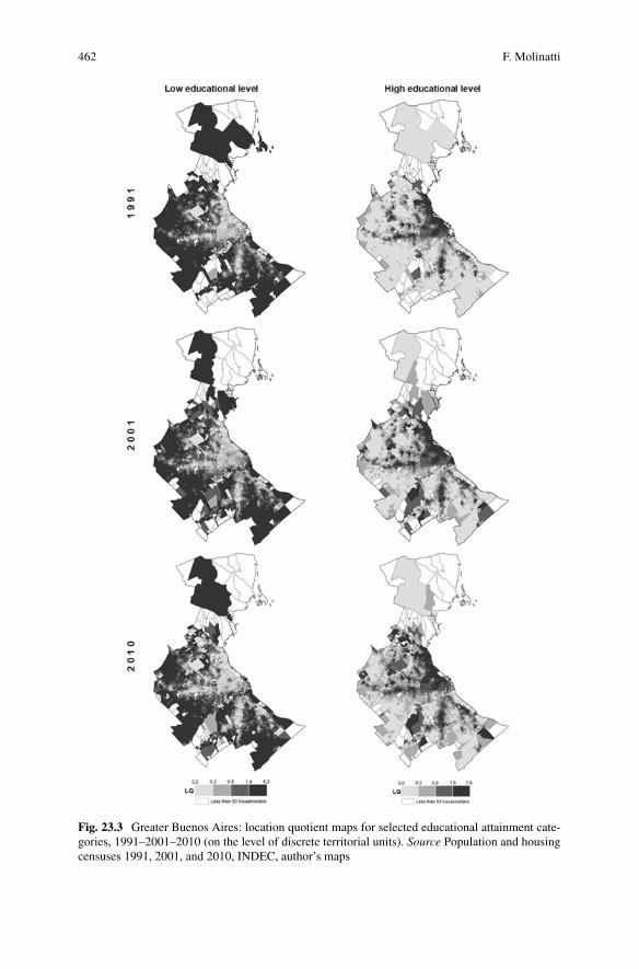
462 F. Molinatti
Fig. 23.3 Greater Buenos Aires: location quotient maps for selected educational attainment cate-gories, 1991–2001–2010 (on the level of discrete territorial units). Source Population and housingcensuses 1991, 2001, and 2010, INDEC, author’s maps
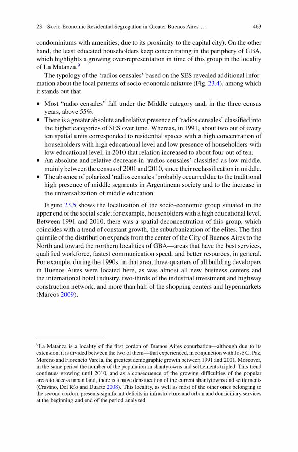
23 Socio-Economic Residential Segregation in Greater Buenos Aires … 463
condominiums with amenities, due to its proximity to the capital city). On the otherhand, the least educated householders keep concentrating in the periphery of GBA,which highlights a growing over-representation in time of this group in the localityof La Matanza.9
The typology of the ‘radios censales’ based on the SES revealed additional infor-mation about the local patterns of socio-economic mixture (Fig. 23.4), among whichit stands out that
• Most “radio censales” fall under the Middle category and, in the three censusyears, above 55%.
• There is a greater absolute and relative presence of ‘radios censales’ classified intothe higher categories of SES over time. Whereas, in 1991, about two out of everyten spatial units corresponded to residential spaces with a high concentration ofhouseholders with high educational level and low presence of householders withlow educational level, in 2010 that relation increased to about four out of ten.
• An absolute and relative decrease in ‘radios censales’ classified as low-middle,mainly between the census of 2001 and 2010, since their reclassification inmiddle.
• The absence of polarized ‘radios censales ’probably occurred due to the traditionalhigh presence of middle segments in Argentinean society and to the increase inthe universalization of middle education.
Figure 23.5 shows the localization of the socio-economic group situated in theupper end of the social scale; for example, householderswith a high educational level.Between 1991 and 2010, there was a spatial deconcentration of this group, whichcoincides with a trend of constant growth, the suburbanization of the elites. The firstquintile of the distribution expands from the center of the City of Buenos Aires to theNorth and toward the northern localities of GBA—areas that have the best services,qualified workforce, fastest communication speed, and better resources, in general.For example, during the 1990s, in that area, three-quarters of all building developersin Buenos Aires were located here, as was almost all new business centers andthe international hotel industry, two-thirds of the industrial investment and highwayconstruction network, and more than half of the shopping centers and hypermarkets(Marcos 2009).
9La Matanza is a locality of the first cordon of Buenos Aires conurbation—although due to itsextension, it is divided between the two of them—that experienced, in conjunction with José C. Paz,Moreno and Florencio Varela, the greatest demographic growth between 1991 and 2001. Moreover,in the same period the number of the population in shantytowns and settlements tripled. This trendcontinues growing until 2010, and as a consequence of the growing difficulties of the popularareas to access urban land, there is a huge densification of the current shantytowns and settlements(Cravino, Del Río and Duarte 2008). This locality, as well as most of the other ones belonging tothe second cordon, presents significant deficits in infrastructure and urban and domiciliary servicesat the beginning and end of the period analyzed.
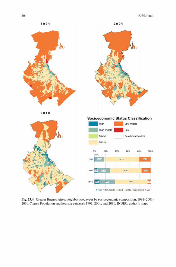
464 F. Molinatti
Fig. 23.4 Greater Buenos Aires: neighborhood types by socioeconomic composition, 1991–2001–2010. Source Population and housing censuses 1991, 2001, and 2010, INDEC, author’s maps
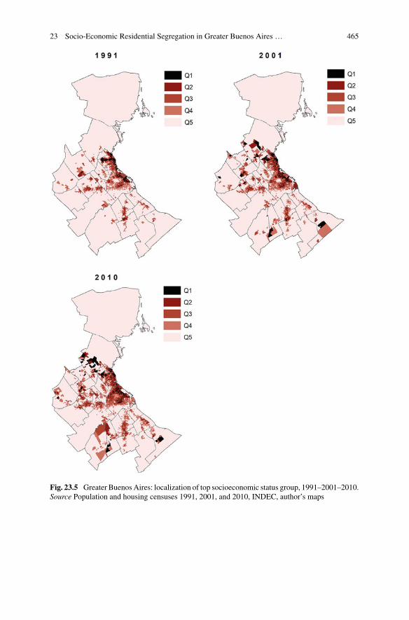
23 Socio-Economic Residential Segregation in Greater Buenos Aires … 465
Fig. 23.5 Greater Buenos Aires: localization of top socioeconomic status group, 1991–2001–2010.Source Population and housing censuses 1991, 2001, and 2010, INDEC, author’s maps
466 F. Molinatti
23.6 Discussion and Conclusions
Buenos Aires is complex in many ways, with its jurisdictional complexity being acharacteristic that pushes the current trends toward urban fragmentation and residen-tial polarization. GBA’s current structure crystallizes the historical north/south andcenter/periphery contrasts. Moreover, new contrasts are added which delimit full andinclusive access to the city for a part of its population (Marcos and Mera 2018).
During the study period, there were important structural economic changes inArgentina (Groisman 2010; Marcos 2009; Suárez 2011; Torres 2001). On the onehand, the establishment of an open accumulation model, which, although it wasimplemented from the mid-1970s onward, the most drastic transformations occurredin the 1990s—particularly the subsequent amendments in labor legislation aiming ata higher labor flexibilization. On the other hand, after the great crisis of 2001, therewas a change in the macroeconomic regime that gave rise to a period of sustainedand long-lasting economic recovery. Simultaneously, there were changes in the wayof planning and management of the city, which can be summarized in a transferenceof the management of urban development to private capital, and in the resultingresidential polarization.
The aim of this study was to investigate how the indicators related to socio-economic residential segregation developed in a context characterized by majorsocial, economic, and political transformations. These results confirm some tenden-cies probed by other researches in the process of urban spatial structuring and resi-dential segregation in GBA (Groisman 2010; Rodriguez 2016; Suárez 2011; Torres2001). First, the main trend of the 1990s was the residential polarization in the Cityof Buenos Aires as well as in the conurbation, where the group of a greater socio-economic level was the most significant actors of that period regarding the definitionof social spaces. Second, the process of suburbanization of the elites intensified; itwas a process that was parallel to the increase in closed urbanization (at the beginningof the 1990s, there were around 90 undertakings and by 2007 there were nearly 550).At the same time, there is a rise of precarious settlements, combinedwith the general-ized deterioration in traditional neighborhoods where people from lower and middleclasses lived. Third, the sustained growth of the economy after the great economiccrisis of 2001 would not have had a sharp effect on the reduction of segregation, fortwo main reasons: on the one hand, the values of the indices are still high, especially,between the two opposite ends of the social scale, and on the other hand, becauselocal patterns were not substantially modified and in some areas of GBA, residentialpolarization increased.
During the first period, 1991–2001, the growth—or the persistence of highlevels—of residential segregation, especially between the opposite ends of the socialscale, was the result of an ongoing trend of job insecurity and social exclusion ofcertain individuals, despite significant increases in the educational levels of the popu-lation. During the second period, 2001–2010, the educational improvement of thepopulation continued, but in a context of economic recovery and equity improvement.Evidence suggests that economic growth would not have had a profound effect as
23 Socio-Economic Residential Segregation in Greater Buenos Aires … 467
the ones observed in labor indicators, especially during the first period of the expan-sive phase (2002–2004) on socio-economic residential segregation. The levels ofresidential segregation remain high and continue to assert themselves through newforms of spatial separation, such as through gated communities. The arrival of elitesin traditionally popular residential areas would seem to reflect greater social hetero-geneity of the conurbation and a reduction in residential segregation. However, thecharacteristics of new neighborhoods intensify residential segregation on a reducedgeographical scale. Private fences, walls, and security checkpoints guarantee theisolation of elites from the surrounding poor areas and split the territory.
All these characteristics highlight a trend toward an extremely segregated anddivided city, and the determination of the processes of territorial fragmentation andresidential polarization, in spite of substantial improvements in the educational attain-ment of the population and the period of sustained economic growth that GBA anda great number of Latin American countries went through at the beginning of thetwenty-first century. The results of this study confirm the findings of other researchthat account for the great force of the processes of urban space development. There-fore, it must be emphasized the need for active public policies that promote socialdiversity space and full and inclusive access to the city, dismantling the areas of resi-dential and socio-occupational marginalization that deteriorate the conditions forurban integration and reproduce concentrated poverty.
References
Agostini CA, Hojman D, Román A, Valenzuela L (2016) Segregación residencial de ingresos en elGran Santiago, 1992-2002: una estimación robusta. EURE 42(127):159–184. https://doi.org/10.4067/S0250-71612016000300007
Alonso G, Di Costa V (2012) Cambios y continuidades en la política social argentina (2003–2010).Working papers. Grupo de Investigación enGobierno,Administración y Políticas Públicas.Instituto Universitario de Investigación Ortega y Gasset. Madrid
Altimir O, Beccaria L (1999) El mercado de trabajo bajo el nuevo régimen económico en Argentina.Working Paper. Comisión Económica para América Latina y el Caribe (CEPAL). http://www.eclac.cl/publicaciones/xml/0/4550/lcl1217e.pdf
Arceo N, Monsalvo A, Schorr M, Wainer A (2008) Empleo y salarios en la Argentina. Una visiónde largo plazo. Capital Intelectual, Buenos Aires
Báez J (2017). Distribución de ingresos y riqueza en Argentina. Resource document. http://cdes.org.ec/web/distribucion-en-argentina/
Basualdo EM (2008) La distribución del ingreso en la Argentina y sus condicionantes estructurales.Centro de Estudios Legales y Sociales (CELS), Derechos Humanos en Argentina: informe 2008.Buenos Aires, Siglo XXI Editores Argentina, pp 307–326
Becceneri L, Alves H, Vazquez D (2019) Estratificação Sócio-Ocupacional e Segregação Espacialna Metrópole de São Paulo nos Anos 2000. Revista Brasileira de Estudos Urbanos e Regionais21(1):137. http://dx.doi.org/10.22296/2317-1529.2019v21n1p137
Caldeira TP (2007) Ciudad de muros. Gedisa, BarcelonaCentro de Estudios para el Desarrollo Argentino (2007). El trabajo en Argentina. Condiciones yperspectivas. Informe trimestral. https://www.adum.org.ar/wordpress/wp-content/uploads/2008/10/cenda-el-trabajo-en-argentina.pdf
Clark C (1977) Population growth and land use. Palgrave Macmillan, London
468 F. Molinatti
Cravino MC, del Río JP, Duarte JI (2008) Magnitud y crecimiento de las villas y asentamientosen el Área Metropolitana de Buenos Aires en los últimos 25 años. Conference procceding. XIVEncuentro de la Red Universitaria Latinoamericana de Cátedras de Vivienda-Facultad de Arqui-tectura, Urbanismo y Diseño-Universidad de Buenos Aires. http://www.igc.org.ar/megaciudad/N3/Asentamientos%20Irregulares%20AMB.pdf
Di Virgilio M, Guevara T (2014) Gentrificación liderada por el Estado y empresarialismo urbano enla Ciudad Autónoma de Buenos Aires. Revista Estudios Sociales Contemporáneos (11):12–23.http://www.bdigital.uncu.edu.ar/objetos_digitales/6820/02-divirgilio-esc11.pdf
Economic Commission for Latin America and the Caribbean (ECLAC) (2010) Statistical Yearbookof Latin America and the Caribbean 2010. Economic commission for Latin America and theCaribbean. https://repositorio.cepal.org/bitstream/handle/11362/925/1/S1000780_es.pdf
Groisman F (2009) Segregación residencial socioeconómica en Argentina durante la recuperacióneconómica (2002–2007). Working paper. Instituto de Estudios Latinoamericanos. https://dialnet.unirioja.es/descarga/articulo/3664346.pdf
Groisman F (2010) La persistencia de la segregación residencial socioeconómica en Argentina.Estudios Demográficos y Urbanos 25(74):429–460. http://www.jstor.org/stable/20787558
INDEC (1991) 1991 National census of population and housing. National Institute of Statistics andCensuses, Buenos Aires
INDEC (2001) 2001 National census of population, households, and housing. National Institute ofStatistics and Censuses, Buenos Aires
INDEC (2010) 2010 national census of population, households, and housing. National Institute ofStatistics and Censuses, Buenos Aires
Marcinczak S, Tammaru T, Novák J, Gentile M, Kovács Z, Temelová J et al (2015) Patterns ofsocioeconomic segregation in the capital cities of fast-track reforming postsocialist countries.Ann Assoc Am Geogr 105(1):183–202. https://doi.org/10.1080/00045608.2014.968977
Marcos M (2009) Territorios fragmentados. La segregación socio-espacial en la AglomeraciónGran Buenos (1970–2000). Working paper. Cátedra de Demografía Social, Facultad de CienciasSociales. Universidad Nacional de Buenos Aires. http://www.catedras.fsoc.uba.ar/demografiasocial/infodeinv/II18.pdf
Marcos M, Mera G (2018) La dimensión territorial de las desigualdades sociodemográficas enBuenos Aires. Voces en el Fénix 8(71):14–23. http://www.vocesenelfenix.com/sites/default/files/pdf/02-Marcos-Mera.pdf
Molinatti F (2013) Segregación residencial socioeconómica en la ciudad de Córdoba (Argentina):Tendencias y patrones espaciales. Revista INVI 28(79):61–94. https://doi.org/10.4067/S0718-83582013000300003
Musterd S,Marcinczak S, vanHamM, Tammaru T (2015) Socio-economic segregation in Europeancapital cities: increasing separation between poor and rich. Discussion paper. Institute for theStudy of Labor
Rodríguez G (2016) Desigualdades socioeconómicas y segregación residencial en dos décadas designo político y económico opuesto. La aglomeración Gran Buenos Aires entre 1991 y 2010.Cuaderno Urbano. Espacio, cultura, sociedad, 21(21):5–28. http://www.scielo.org.ar/pdf/cuba/v21n21/v21n21a01.pdf
Sabatini F (2006) La segregación social del espacio en las ciudades de América Latina. WorkingPaper. División de Programas Sociales, Departamento de Desarrollo Sostenible, Banco Inter-americano de Desarrollo. https://publications.iadb.org/publications/spanish/document/La-segregaci%C3%B3n-social-del-espacio-en-las-ciudades-de-Am%C3%A9rica-Latina.pdf
Sabatini F, Wormald G, Sierralta C, Peters P.A (2009) Residential segregation in santiago: scale-related effects and trends, 1992–2002. In: Robertsy BR, Wilson RH (eds.), Urban segregationand governance in the Americas, pp 121–143, Palgrave Macmillan, New York
Suárez AL (2011) Segregación residencial en la región metropolitana de Buenos Aires. In: Baliande Tagtachian B, Suárez AL (comps.), Pobreza y solidaridad social en la Argentina: aportes desdeel enfoque de las capacidades humanas. Buenos Aires: Educa
23 Socio-Economic Residential Segregation in Greater Buenos Aires … 469
SvampaM (2004) La brecha urbana. Countries y barrios privados en Argentina. Capital Intelectual,Buenos Aires
Tammaru T, Marcinczak S, Aunap R, van HamM, Janssen H (2019) Relationship between incomeinequality and residential segregation of socioeconomic groups. Reg Stud. https://doi.org/10.1080/00343404.2018.1540035
Tammaru T,Musterd S, vanHamM,Marcinczak S (2016) Amulti-factor approach to understandingsocio-economic segregation in European capital cities. In: Tammaru T, Marcinczak S, an HamM, Musterd S (eds.), Socio-economic segregation in European capital cities. East meets West(1–29), Routledge, London
Torres H (1975) Evolución de los procesos de estructuración espacial urbana. El caso de BuenosAires. Desarrollo Económico 15(58):281–306. http://www.jstor.org/stable/3466262
Torres H (2001) Cambios socioterritoriales em Buenos Aires durante la década de 1990. Eure27(80):33–56. https://doi.org/10.4067/S0250-71612001008000003
Torres HG, Marques E, Ferreira PM, Bitar S (2003) Pobreza e espaço: padrões de segregação emSão Paulo. Estudos Avançados 17(47):13–42
World Bank, Development Research Group (2019). Gini Index (World Bank estimate). https://data.worldbank.org/indicator/SI.POV.GINI?locations=AR. Accessed 19 Feb 2019
Open Access This chapter is licensed under the terms of the Creative Commons Attribution 4.0International License (http://creativecommons.org/licenses/by/4.0/), which permits use, sharing,adaptation, distribution and reproduction in any medium or format, as long as you give appropriatecredit to the original author(s) and the source, provide a link to the Creative Commons license andindicate if changes were made.
The images or other third party material in this chapter are included in the chapter’s CreativeCommons license, unless indicated otherwise in a credit line to the material. If material is notincluded in the chapter’s Creative Commons license and your intended use is not permitted bystatutory regulation or exceeds the permitted use, you will need to obtain permission directly fromthe copyright holder.
Chapter 24Changes in Spatial Inequalityand Residential Segregationin Metropolitan Lima
Graciela Fernández-de-Córdova, Paola Moschella,and Ana María Fernández-Maldonado
Abstract Since the 2000s, Lima city shows important changes in its socio-spatialstructure, decreasing the long-established opposition between the centre and theperiphery, developing a more complex arrangement. Sustained national economicgrowth has allowed better socio-economic conditions in different areas of the city.However, high inequality still remains in the ways of production of urban space,which affects residential segregation. To identify possible changes in the segregationpatterns of Metropolitan Lima, this study focuses on the spatial patterns of occupa-tional groups, examining their causes and relation with income inequality. The anal-ysis is based on the 1993 and 2007 census data, measuring residential segregationby the Dissimilarity Index, comparing with the Diversity Index. The results confirmtrends towards increased segregation between occupational groups. Top occupa-tional groups are concentrated in central areas, expanding into adjacent districts.Bottom occupational groups are over-represented in distant neighbourhoods. In-between, a new, more mixed, transitional zone has emerged in upgraded formerlylow-income neighbourhoods. Areas of lower occupational diversity coincide withextreme income values, forming spaces of greater segregation. In the metropolitancentre–periphery pattern, the centre has expanded, while the periphery has beenshifted to outer peripheral rings.
Keywords Residential segregation · Spatial inequality · Index of dissimilarity ·Occupational diversity · Lima
G. Fernández-de-CórdovaAcademic Department of Architecture, Pontifical Catholic University of Peru, Lima, Peru
P. MoschellaDepartment of Humanities, Pontifical Catholic University of Peru, Lima, Peru
A. M. Fernández-Maldonado (B)Department of Urbanism, Delft University of Technology, Delft, The Netherlandse-mail: [email protected]
© The Author(s) 2021M. van Ham et al. (eds.), Urban Socio-Economic Segregation and Income Inequality,The Urban Book Series, https://doi.org/10.1007/978-3-030-64569-4_24
471
472 G. Fernández-de-Córdova et al.
24.1 Introduction
Inequality is a complex social condition with multiple dimensions that leads toeconomic, social and environmental imbalances and generates spatial disparitiesbetween andwithin different territories (ECLAC 2018; Jordán et al. 2017).Measuredby theGini index, LatinAmerican countries comprise themost unequal world region,a position verified through analysis of tax data on personal income in selected coun-tries (Barcena and Byanyima 2016). Inequality generates socio-spatial segregationwhen the formation of residential areas of groups of people with similar socio-economic status—be it voluntary or forced—limits the interactions between thosegroups. The intensity of residential segregation will then depend on the degree ofincome inequality (Chapin 1965; Sabatini 2006). Consequently, Latin Americancities are highly residentially segregated, which is illustrated by notorious examplesof gated communities and ‘fortified enclaves’ for the rich and upper middle class(Caldeira 2000; Coy and Pöhler 2002).
The objective of this chapter is to analyse the recent changes in residential segre-gation by socio-economic status in the city of Lima, the capital city of Peru. Andadditionally, to explore the extent of the effects that national economic trends havehad on the conditions of socio-spatial segregation inMetropolitan Lima. In a countryas Peru, whose societal relationships are characterized by highly asymmetrical powerrelations (Drinot 2006), socio-economic segregation has been a common and persis-tent urban phenomenon. However, socio-spatial segregation only became a mark ofthe city during the process of rapid urbanization that Lima experienced since themid-1950s. The impact of the widespread emergence of peripheral informal settlementson Lima was overwhelming. The process definitely modified the structure of the city(Driant 1992), shaping it into a strongly segregated pattern of centre–periphery.
Sustained improvement of the national economy in the 2000s has led to a substan-tial growth of purchasing power of population groups living in the older periphery,at the intermediate zone of urban expansion in Metropolitan Lima. This processpromoted the expansion of public and (mostly) private investments in infrastructure,services and housing towards this area (Chion 2002), contributing to social diver-sification and the improvement of quality of life. These changes have led to trendstowards the reduction of the degree of socio-spatial segregation, observed in someof these peripheral areas (Fernández-de-Córdova et al. 2011). Desegregation wasalso observed in many other cities in Latin America (Sabatini 2015; Aguilar andEscamilla 2015).
This study is carried out following Sabatini’s (2006) segregation scale approach,which pays attention to the spatial scale in measuring inequality. Its main assump-tion is that high levels of inequality are not necessarily negative, but the impactof high inequality depends on the size and hierarchy of socio-economic groups. “Ifsegregation occurs within a reduced geographic scale, like a small city or through theconformation of smaller, socially homogenous neighborhoods, the negative effects ofsegregation can be less significant or non-existent.” (Sabatini 2006: 9). The analysisis based on occupational categories, which are used as a proxy for socio-economic
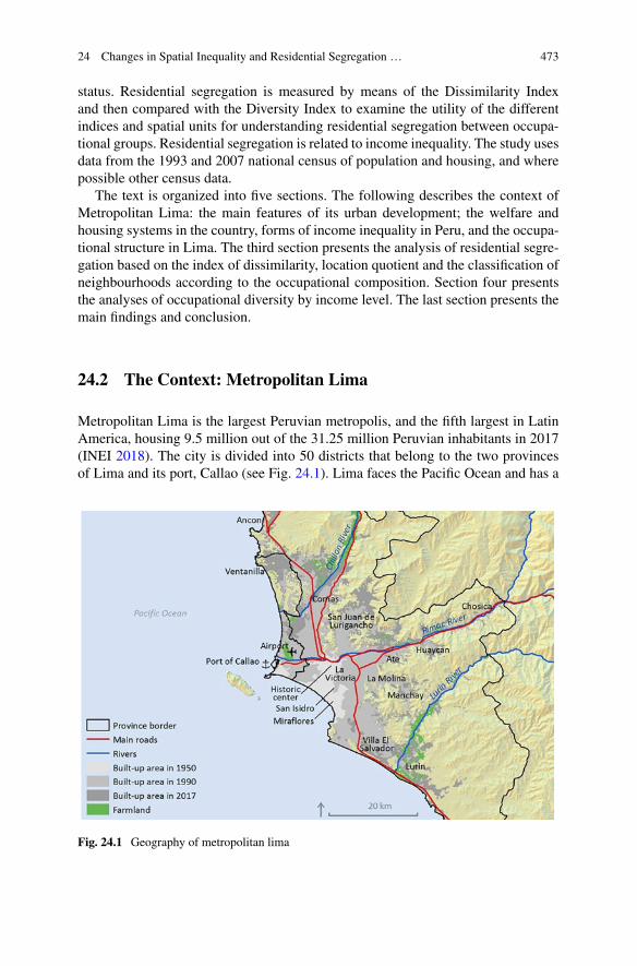
24 Changes in Spatial Inequality and Residential Segregation … 473
status. Residential segregation is measured by means of the Dissimilarity Indexand then compared with the Diversity Index to examine the utility of the differentindices and spatial units for understanding residential segregation between occupa-tional groups. Residential segregation is related to income inequality. The study usesdata from the 1993 and 2007 national census of population and housing, and wherepossible other census data.
The text is organized into five sections. The following describes the context ofMetropolitan Lima: the main features of its urban development; the welfare andhousing systems in the country, forms of income inequality in Peru, and the occupa-tional structure in Lima. The third section presents the analysis of residential segre-gation based on the index of dissimilarity, location quotient and the classification ofneighbourhoods according to the occupational composition. Section four presentsthe analyses of occupational diversity by income level. The last section presents themain findings and conclusion.
24.2 The Context: Metropolitan Lima
Metropolitan Lima is the largest Peruvian metropolis, and the fifth largest in LatinAmerica, housing 9.5 million out of the 31.25 million Peruvian inhabitants in 2017(INEI 2018). The city is divided into 50 districts that belong to the two provincesof Lima and its port, Callao (see Fig. 24.1). Lima faces the Pacific Ocean and has a
Fig. 24.1 Geography of metropolitan lima
474 G. Fernández-de-Córdova et al.
central position on both the Peruvian and the South American west coasts. Its urbanarea is developed along two main axes, extending themselves more than 100 kmsfrom north to south, and 60 kms from east to west. Its urban structure has two mainzones, central and peripheral.
The central zone is composed of the historic centre surrounded by districts urban-ized under formal patterns in the plain areas. It is extending from the historic centre ofLima to the coastalMiraflores district in the South, concentrating commerce, employ-ment and urban amenities. It also has a larger share of apartment buildings, althoughthe higher population density is located towards the east and north (Vega-Centenoet al. 2019). The informal peripheral zone follows an urban continuum of radial andirregular morphology that responds to the expanding of the self-built settlements onthe Andean slopes (Fernández-de-Córdova et al. 2016).
24.2.1 Metropolitan Lima’s Urban Development
Lima has experienced significant levels of residential segregation since its founda-tion. The historical patterns of social and economic exclusion inherited from thecenturies-long Spanish rule have guided the processes of urban growth and develop-ment since then (Fernández-de-Córdova et al. 2011). In the twentieth century, Lima’surban evolution has been strongly marked by the presence of informal self-builtneighbourhoods (Driant 1992). Between the 1940s and the 1970s, a demographictransition process radically increased the size of the Peruvian population, attractingpeople from over-populated rural areas to the cities, and especially to Lima, whichwas initiating a process of industrialization by imports substitution. From 1940 to1972, Lima’s population grewfive-fold, from0.64million to 3.3million (INEI 2007).Most newcomers were unskilled rural migrants, who were unable to find a place inthe formal labour market. Without other possibilities, they built their own settle-ments on the hillsides, during a period in which the state promoted the formationof massive informal neighbourhoods in peripheral areas in order to solve the acutehousing problem in the city (Calderón 2012).
After the 1970s, Lima continued extending itself horizontally, mostly throughlow-rise self-built housing in the urban periphery. In the 1981–1993 period, Lima’surban population increased by 37.3%, from 4.6 million to 6.3 million, while its urbanarea increased by 51.4% in the same period. Likewise, in the 1993–2007 period, thepopulation grew by 33.6%, up to 8.4 million. while its urban area extended itselfby 74.5% to 69,033 hectares (INEI 2008). Since the 2000s, visible transformationshave been observed in Lima’s segregated urban structure, associated with the struc-tural adjustment policies initiated in the 1990s. They prompted a significant growthin the service, financial, telecommunications, construction and employment sectors(Chion 2002). In spatial terms, they led to trends towards the formation of Lima’sintermediate zone located between the historic core and more distant neighbour-hoods. The recomposition brought along the diversification of social groups in thisintermediate zone according to income, occupation and migratory origin, as well
24 Changes in Spatial Inequality and Residential Segregation … 475
as by greater complexity of functional relations, leading to the formation of newsub-centres (Fernández-de-Córdova et al. 2016).
24.2.2 The Peruvian Welfare System
Peru clearly follows the liberal welfare model, shaped by the free-market ideologythat is dominant in the country’s political economy. In the liberal system, welfareis the responsibility of each individual, according to their own ability to respond tomarket conditions. The Peruvian state considers that social welfare will be gener-ated by a competitive economy delivering high rates of economic growth. Studiesabout the conditions of public welfare in Latin America consider that the regionhas welfare states ‘in transition’ (Esping-Andersen 1996), as their efforts to spreadpublic welfare to all are still fragmentary. The Peruvian welfare system, therefore,provides a relatively low coverage and exhibits a low level of social expenditureeven when compared to other Latin American countries. An OECD study on globalinequality (2015) verified this, noting that the Peruvian redistribution policies areminor in comparison to other Latin American and emerging countries, leading tolower redistributive effects.
Three priorities guide social interventions in Peru (El Peruano 2004): (1) thedevelopment of human capabilities; (2) the promotion of employment and genera-tion of economic opportunities; and (3) developing a network of social protection.Following this, Peru has increased public spending in the education sector, especiallyin basic education, in the last 10 years. However, in a comparative perspective thesespending levels aremuch below the average education expenditure inOECDmembercountries, below other countries of Latin America, and below countries with similarGDP per capita (Guadalupe et al. 2017). Furthermore, the generation of considerabletax revenues during the period of high economic growth (2004–2014) was helpful toincrease social investment and to expand assistance programmes for the most vulner-able population. The total budget for social expenditure increased by 230% between2004 and 2016 (Trivelli and Urrutia 2018). This contributed to important reductionsof child malnutrition; maternal mortality; and income poverty (from more than 50%in 2004 to less than 23% in 2014); while the coverage of basic services was extended(Mendoza Nava 2015).
The Peruvian Ministry of Development and Social Inclusion is in charge of socialprogrammes to tackle extreme poverty. These includeQaliWarma,Pensión 65, CunaMás, Juntos, Foncodes, Contigo y PAIS; executed through direct social assistance,localized investments and income redistribution throughmonetary transfers. Pension65 and Juntos, which deliver direct cash transfers to vulnerable households, are theones that havemore significantly contributed to socialwelfare. Together they received1.3% of the 2016 national budget and greatly contributed to reducing inequality(Trivelli and Urrutia 2018).
476 G. Fernández-de-Córdova et al.
24.2.3 Income Inequality in Peru
Peru has also experienced a period of high economic growth and macroeconomicimprovements in the 2000s, leading to one of the most significant poverty reductionsin Latin America. Poverty levels were reduced by 61% between 2004 and 2014when economic growth reached an annual average of 6.4%, which also enabled thereduction of inequality levels, although less significantly. This was more visible inLima, whose Gini index was reduced to 0.40, while the country’s index decreased to0.46 in 2017 (ECLAC 2018). In the same period, 40% of lower income households inLima increased their per capita income by 6.8%, a proportion higher than the nationalaverage (4.4%) (Grupo Banco Mundial 2015). In 2017, the average monthly incomeper capita in Lima was US$ 581.6, widely exceeding the national average of US$417.1 (Zucchetti and Freundt 2018).
Going into more detail when it comes to changes in income inequality in Peruas measured by the Gini index between 1997 and 2016 with data from the WorldBank (2019), we find a switch from increase to decrease. The values of the Indexpeaked in 1999 (56.3), decreasing during the period of high economic growth (2003–2015), down to 43.5 in 2015. Despite the decrease during the ‘economic miracleyears’, income inequality is still high in Peru. From the total country income, theshare of the first quintile is 5%, while that of the fifth quintile is 43% (ECLAC2018). Furthermore, the steep decrease of the Gini index in Peru has been questionedbecause its values are based on national household surveys (Encuesta Nacional deHogares), which are focused on measuring the needs of lower income groups, and donot properly include the highest income groups (Francke 2017; Alarco et al. 2019).Corrected estimates give higher values than the official ones, although they also showreduction trends as of 2005. Measures of economic inequality by means of the Giniindex of wealth and bank deposits, however, show upward trends in the last decade(Alarco et al. 2019).
24.2.4 The Housing System in Peru
According to the results of the 2017 census (INEI 2018), 76% (5.8 million) homeswere owner-occupied, 16.3% (1.2million)were rented and 7.5%were homeswithoutownership or rent exchange. Social housing is not considered as an apart category, soit is included in owner-occupied. An unequal country as Peru carries a long-standinghousing shortage, which deepened during the period of rapid urbanization. Afford-able housing has been a constant challenge. Laissez-faire political attitudes towardsinformal housing, coupled with the inexistence of deliberate housing policies, haveled to a vast housing shortage. Furthermore, in the early 1990s, the Peruvian statepractically withdrew from the housing sector. In 1992, the Fujimori administrationclosed the Ministry of Housing, the Central Mortgage Bank, the Housing Bank anddismantled housing cooperatives and public programmes for land delivery. Housing
24 Changes in Spatial Inequality and Residential Segregation … 477
finance lost all priority, and the right to adequate housing was removed from the1993 constitution (Fernández-Maldonado 2010). According to census data, homeconstruction in the 1990s—amounting to 120,000 homes per year—was mostlyproduced through informal urban processes.
In 2001, the new democratic government reorganized and rebuilt the housingsector, establishing a deliberate social housing policy to tackle the huge housingdemand. As a typical neoliberal policy, it promotes access to ‘formal markets’ subsi-dizing the housing demand and creating financial mechanisms to facilitate housingaffordability. The private construction sector is responsible for the production ofaffordable housing, the financial sector provides the mortgage loans (in which in theevent of non-payment the state assumes the debt), while the state provides directsubsidies to meet the demand. To encourage the private construction of affordablehomes, an effort was made to create favourable conditions for the builders, both interms of regulations and finance (Calderón 2012). The state had to take almost allrisks of the financial transactions (Calderón 2009).
The policy is implemented through two different programmes:Mivivienda (FMV)and Techo Propio. FMV targets middle-income households to finance the purchaseof new homes valued less than 127,000 US$, providing a subsidy to contribute tothe down payment, which depends on the amount of credit requested and the type ofbuilding materials (traditional or sustainable) of the new home. Techo Propio targetslower income households to finance the improvement of substandard dwellings; thebuilding of a home in own land; or the purchase of new homes valued less than 15,500US$. Its subsidy varies according to themodality to which the household is applying:home improvement, building or buying a new house (Fernández-Maldonado andBredenoord 2010).
The housing policy had a rebound effect, pushing downward the property prices,promoting a real estate push in the commercial housing market, which allowed theredirection of construction capital to income sectors never previously consideredbefore (Calderón 2009), producing a real estate boom inMetropolitan Lima and otherlarge cities during the mid-2000s. On the other hand, the free market dynamics inthe social housing sector—in aspects of home construction, land market and finan-cial market—gave the large construction companies almost free hands to decidewhere to invest and for whom. In this context, the social housing system has mainlybenefitted middle- and low-middle-income groups, considered more profitable forthe construction sector (Fernández-Maldonado and Bredenoord 2010). The socialhousing policies for low-income groups have had many problems, failing to meetthe policy goals. This is mainly due to limitations of these groups’ access to credit,as they generally lack formal (stable) employment (Romero et al. 2005). Only 30%of the national target—to build 100,000 houses between 2003 and 2012, 10,000 peryear—was met (Calderón 2014).
Despite the real estate boom, the total number of homes built has been very lowin relation to the enormous housing deficit. There was a slight reduction of the quan-titative deficit in the 1993–2007 inter-census period, but the deficit coming frominformal housing increased by 135% in the same period. This led to an increase
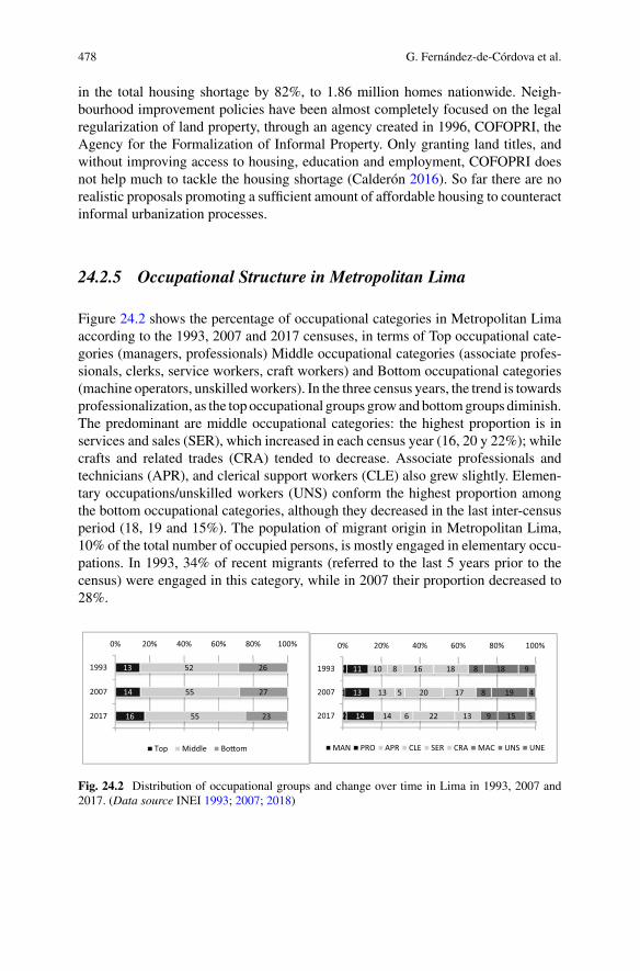
478 G. Fernández-de-Córdova et al.
in the total housing shortage by 82%, to 1.86 million homes nationwide. Neigh-bourhood improvement policies have been almost completely focused on the legalregularization of land property, through an agency created in 1996, COFOPRI, theAgency for the Formalization of Informal Property. Only granting land titles, andwithout improving access to housing, education and employment, COFOPRI doesnot help much to tackle the housing shortage (Calderón 2016). So far there are norealistic proposals promoting a sufficient amount of affordable housing to counteractinformal urbanization processes.
24.2.5 Occupational Structure in Metropolitan Lima
Figure 24.2 shows the percentage of occupational categories in Metropolitan Limaaccording to the 1993, 2007 and 2017 censuses, in terms of Top occupational cate-gories (managers, professionals) Middle occupational categories (associate profes-sionals, clerks, service workers, craft workers) and Bottom occupational categories(machine operators, unskilledworkers). In the three census years, the trend is towardsprofessionalization, as the top occupational groups growandbottomgroups diminish.The predominant are middle occupational categories: the highest proportion is inservices and sales (SER), which increased in each census year (16, 20 y 22%); whilecrafts and related trades (CRA) tended to decrease. Associate professionals andtechnicians (APR), and clerical support workers (CLE) also grew slightly. Elemen-tary occupations/unskilled workers (UNS) conform the highest proportion amongthe bottom occupational categories, although they decreased in the last inter-censusperiod (18, 19 and 15%). The population of migrant origin in Metropolitan Lima,10% of the total number of occupied persons, is mostly engaged in elementary occu-pations. In 1993, 34% of recent migrants (referred to the last 5 years prior to thecensus) were engaged in this category, while in 2007 their proportion decreased to28%.
16
14
13
55
55
52
23
27
26
0% 20% 40% 60% 80% 100%
2017
2007
1993
Top Middle Bo�om
2
1
2
14
13
11
14
13
10
6
5
8
22
20
16
13
17
18
9
8
8
15
19
18
5
4
9
0% 20% 40% 60% 80% 100%
2017
2007
1993
MAN PRO APR CLE SER CRA MAC UNS UNE
Fig. 24.2 Distribution of occupational groups and change over time in Lima in 1993, 2007 and2017. (Data source INEI 1993; 2007; 2018)
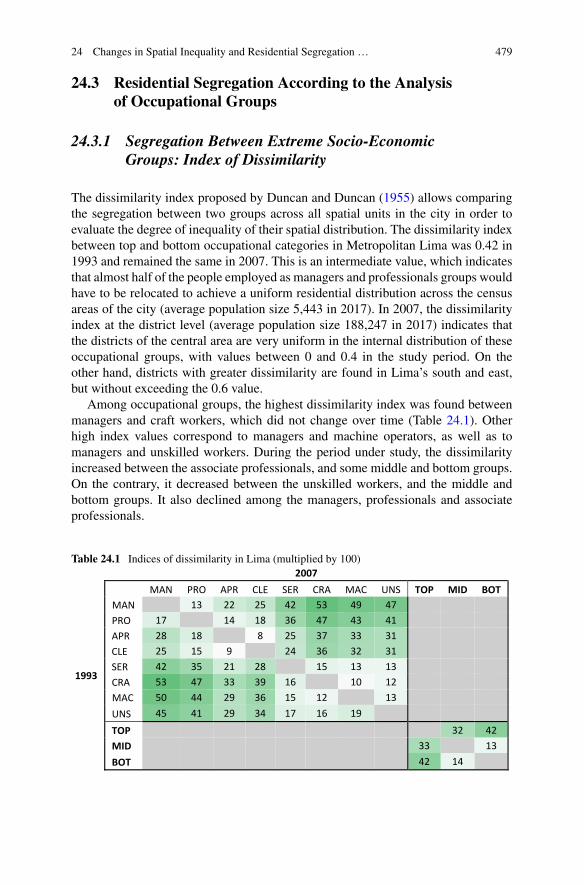
24 Changes in Spatial Inequality and Residential Segregation … 479
24.3 Residential Segregation According to the Analysisof Occupational Groups
24.3.1 Segregation Between Extreme Socio-EconomicGroups: Index of Dissimilarity
The dissimilarity index proposed by Duncan and Duncan (1955) allows comparingthe segregation between two groups across all spatial units in the city in order toevaluate the degree of inequality of their spatial distribution. The dissimilarity indexbetween top and bottom occupational categories in Metropolitan Lima was 0.42 in1993 and remained the same in 2007. This is an intermediate value, which indicatesthat almost half of the people employed as managers and professionals groups wouldhave to be relocated to achieve a uniform residential distribution across the censusareas of the city (average population size 5,443 in 2017). In 2007, the dissimilarityindex at the district level (average population size 188,247 in 2017) indicates thatthe districts of the central area are very uniform in the internal distribution of theseoccupational groups, with values between 0 and 0.4 in the study period. On theother hand, districts with greater dissimilarity are found in Lima’s south and east,but without exceeding the 0.6 value.
Among occupational groups, the highest dissimilarity index was found betweenmanagers and craft workers, which did not change over time (Table 24.1). Otherhigh index values correspond to managers and machine operators, as well as tomanagers and unskilled workers. During the period under study, the dissimilarityincreased between the associate professionals, and some middle and bottom groups.On the contrary, it decreased between the unskilled workers, and the middle andbottom groups. It also declined among the managers, professionals and associateprofessionals.
Table 24.1 Indices of dissimilarity in Lima (multiplied by 100)2007
1993
MAN PRO APR CLE SER CRA MAC UNS TOP MID BOTMAN 13 22 25 42 53 49 47PRO 17 14 18 36 47 43 41APR 28 18 8 25 37 33 31CLE 25 15 9 24 36 32 31SER 42 35 21 28 15 13 13CRA 53 47 33 39 16 10 12MAC 50 44 29 36 15 12 13UNS 45 41 29 34 17 16 19TOP 32 42MID 33 13BOT 42 14
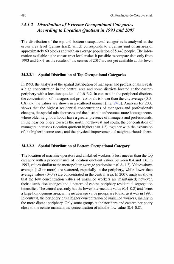
480 G. Fernández-de-Córdova et al.
24.3.2 Distribution of Extreme Occupational CategoriesAccording to Location Quotient in 1993 and 2007
The distribution of the top and bottom occupational categories is analysed at theurban area level (census tract), which corresponds to a census unit of an area ofapproximately 60 blocks and with an average population of 5,443 people. The infor-mation available at the census tract level makes it possible to compare data only from1993 and 2007, as the results of the census of 2017 are not yet available at this level.
24.3.2.1 Spatial Distribution of Top Occupational Categories
In 1993, the analysis of the spatial distribution of managers and professionals revealsa high concentration in the central area and some districts located at the easternperiphery with a location quotient of 1.6–3.2. In contrast, in the peripheral districts,the concentration of managers and professionals is lower than the city average (0.0–0.8) and the values are shown in a scattered manner (Fig. 24.3). Analysis for 2007shows that the highest residential concentrations of managers and professionalschanges, the special mix decreases and the distribution becomesmore homogeneous,where older neighbourhoods have a greater presence of managers and professionals.In the near periphery towards the north, north-west and south, the concentration ofmanagers increases (location quotient higher than 1.2) together with the expansionof the higher income areas and the physical improvement of neighbourhoods there.
24.3.2.2 Spatial Distribution of Bottom Occupational Category
The location of machine operators and unskilled workers is less uneven than the topcategory with a predominance of location quotient values between 0.4 and 1.6. In1993, values similar to themetropolitan average predominate (0.8–1.2). Values aboveaverage (1.2 or more) are scattered, especially in the periphery, while lower thanaverage values (0–0.8) are concentrated in the central area. In 2007, analysis showsthat the low concentration values of unskilled workers are maintained; however,their distribution changes and a pattern of centre–periphery residential segregationintensifies. The central area only has the lower intermediate value (0.4–0.8) and formsa large homogenous area, while no average value groups are found, as it was in 1993.In contrast, the periphery has a higher concentration of unskilled workers, mainly inthe more distant periphery. Only some groups at the northern and eastern peripheryclose to the centre maintain the concentration of middle-low value (0.4–0.8).
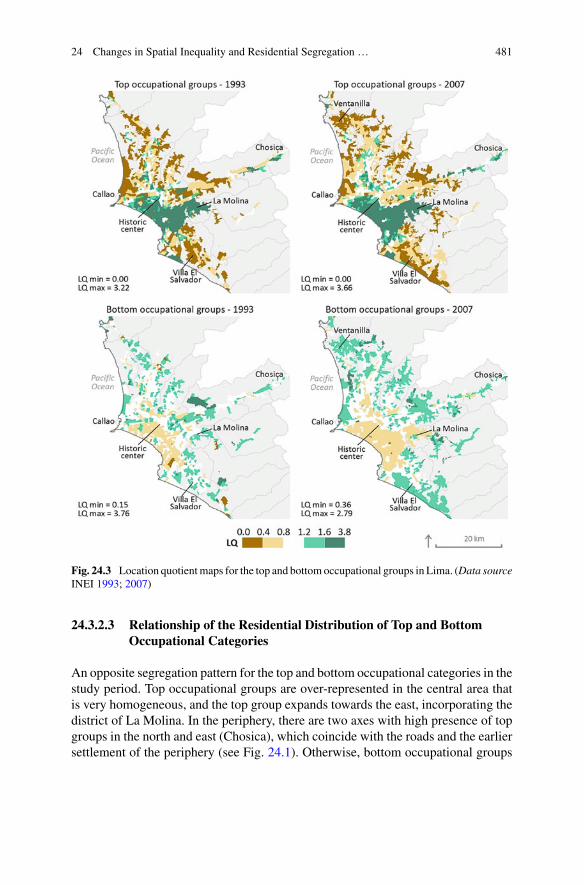
24 Changes in Spatial Inequality and Residential Segregation … 481
Fig. 24.3 Location quotientmaps for the top and bottomoccupational groups in Lima. (Data sourceINEI 1993; 2007)
24.3.2.3 Relationship of the Residential Distribution of Top and BottomOccupational Categories
An opposite segregation pattern for the top and bottom occupational categories in thestudy period. Top occupational groups are over-represented in the central area thatis very homogeneous, and the top group expands towards the east, incorporating thedistrict of La Molina. In the periphery, there are two axes with high presence of topgroups in the north and east (Chosica), which coincide with the roads and the earliersettlement of the periphery (see Fig. 24.1). Otherwise, bottom occupational groups
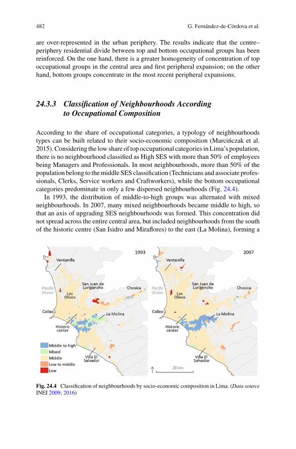
482 G. Fernández-de-Córdova et al.
are over-represented in the urban periphery. The results indicate that the centre–periphery residential divide between top and bottom occupational groups has beenreinforced. On the one hand, there is a greater homogeneity of concentration of topoccupational groups in the central area and first peripheral expansion; on the otherhand, bottom groups concentrate in the most recent peripheral expansions.
24.3.3 Classification of Neighbourhoods Accordingto Occupational Composition
According to the share of occupational categories, a typology of neighbourhoodstypes can be built related to their socio-economic composition (Marcinczak et al.2015). Considering the low share of top occupational categories inLima’s population,there is no neighbourhood classified as High SES with more than 50% of employeesbeing Managers and Professionals. In most neighbourhoods, more than 50% of thepopulation belong to themiddle SES classification (Technicians and associate profes-sionals, Clerks, Service workers and Craftworkers), while the bottom occupationalcategories predominate in only a few dispersed neighbourhoods (Fig. 24.4).
In 1993, the distribution of middle-to-high groups was alternated with mixedneighbourhoods. In 2007, many mixed neighbourhoods became middle to high, sothat an axis of upgrading SES neighbourhoods was formed. This concentration didnot spread across the entire central area, but included neighbourhoods from the southof the historic centre (San Isidro and Miraflores) to the east (La Molina), forming a
Fig. 24.4 Classification of neighbourhoods by socio-economic composition in Lima. (Data sourceINEI 2009; 2016)

24 Changes in Spatial Inequality and Residential Segregation … 483
Fig. 24.5 Location of the top occupational group in Lima. (Data source INEI 1993; 2007)
new centre–east axis from the centre of the bay to the east. This new axis is locatedat the south of the central–east foundational axis road linking the port with thehighlands. This new distribution shows the differences between the new central axisand the rest of the city, which is remarkable when taking into account the previousfindings showing a traditional centre–periphery structure (Fig. 24.5).
The distribution of employees belonging to the top occupational group (Fig. 24.5)shows their tendency to expand the central area with the highest proportion groups(Q1 andQ2). GroupQ1, corresponding to neighbourhoods with 20%of the top groupemployees, is dispersed and atomized throughout the central area. In 2007, neigh-bourhoods in this category form small groups in the central area and the surroundingeast and north areas.
24.4 Differences in Occupational Diversity by Income Level
24.4.1 Occupational Mix in Neighbourhoods
The residential distribution of socio-economic groups can also be analysed withdiversity indices that allow to examine the mix of different groups or categories.The diversity index of Simpson (1949) is one of the most often used measures ofspatial diversity. It has been widely used in ecology and also in social studies tomeasure income diversity (Fernández-de-Córdova et al. 2011; Talen 2006; Mileset al. 2010), race (Nguyen 2010), ethnicity (Laurence 2011; Walks and Maaranen
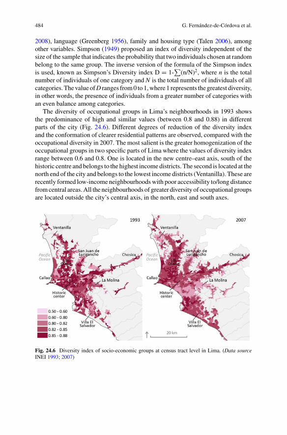
484 G. Fernández-de-Córdova et al.
2008), language (Greenberg 1956), family and housing type (Talen 2006), amongother variables. Simpson (1949) proposed an index of diversity independent of thesize of the sample that indicates the probability that two individuals chosen at randombelong to the same group. The inverse version of the formula of the Simpson indexis used, known as Simpson’s Diversity index D = 1-
∑(n/N)2, where n is the total
number of individuals of one category and N is the total number of individuals of allcategories. The value ofD ranges from0 to 1,where 1 represents the greatest diversity,in other words, the presence of individuals from a greater number of categories withan even balance among categories.
The diversity of occupational groups in Lima’s neighbourhoods in 1993 showsthe predominance of high and similar values (between 0.8 and 0.88) in differentparts of the city (Fig. 24.6). Different degrees of reduction of the diversity indexand the conformation of clearer residential patterns are observed, compared with theoccupational diversity in 2007. The most salient is the greater homogenization of theoccupational groups in two specific parts of Lima where the values of diversity indexrange between 0.6 and 0.8. One is located in the new centre–east axis, south of thehistoric centre and belongs to the highest income districts. The second is located at thenorth end of the city and belongs to the lowest income districts (Ventanilla). These arerecently formed low-income neighbourhoodswith poor accessibility to/long distancefromcentral areas.All the neighbourhoods of greater diversity of occupational groupsare located outside the city’s central axis, in the north, east and south axes.
Fig. 24.6 Diversity index of socio-economic groups at census tract level in Lima. (Data sourceINEI 1993; 2007)
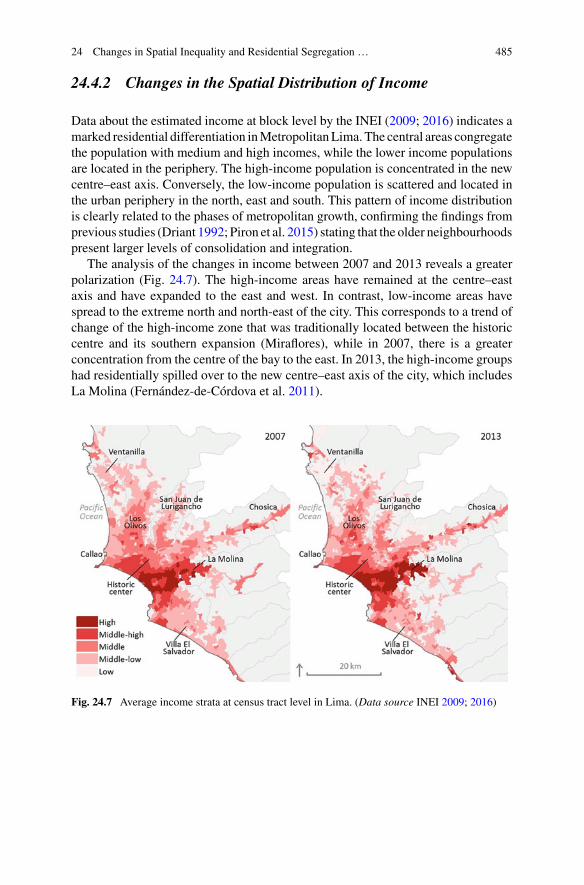
24 Changes in Spatial Inequality and Residential Segregation … 485
24.4.2 Changes in the Spatial Distribution of Income
Data about the estimated income at block level by the INEI (2009; 2016) indicates amarked residential differentiation inMetropolitanLima. The central areas congregatethe population with medium and high incomes, while the lower income populationsare located in the periphery. The high-income population is concentrated in the newcentre–east axis. Conversely, the low-income population is scattered and located inthe urban periphery in the north, east and south. This pattern of income distributionis clearly related to the phases of metropolitan growth, confirming the findings fromprevious studies (Driant 1992; Piron et al. 2015) stating that the older neighbourhoodspresent larger levels of consolidation and integration.
The analysis of the changes in income between 2007 and 2013 reveals a greaterpolarization (Fig. 24.7). The high-income areas have remained at the centre–eastaxis and have expanded to the east and west. In contrast, low-income areas havespread to the extreme north and north-east of the city. This corresponds to a trend ofchange of the high-income zone that was traditionally located between the historiccentre and its southern expansion (Miraflores), while in 2007, there is a greaterconcentration from the centre of the bay to the east. In 2013, the high-income groupshad residentially spilled over to the new centre–east axis of the city, which includesLa Molina (Fernández-de-Córdova et al. 2011).
Fig. 24.7 Average income strata at census tract level in Lima. (Data source INEI 2009; 2016)
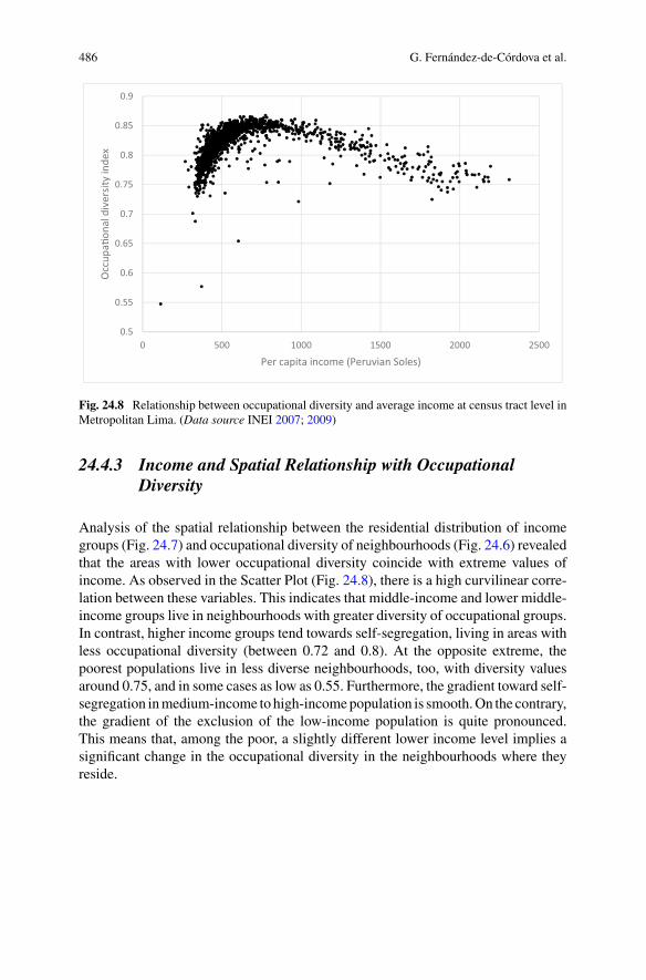
486 G. Fernández-de-Córdova et al.
0.5
0.55
0.6
0.65
0.7
0.75
0.8
0.85
0.9
0 500 1000 1500 2000 2500
Occ
upa�
onal
div
ersit
y in
dex
Per capita income (Peruvian Soles)
Fig. 24.8 Relationship between occupational diversity and average income at census tract level inMetropolitan Lima. (Data source INEI 2007; 2009)
24.4.3 Income and Spatial Relationship with OccupationalDiversity
Analysis of the spatial relationship between the residential distribution of incomegroups (Fig. 24.7) and occupational diversity of neighbourhoods (Fig. 24.6) revealedthat the areas with lower occupational diversity coincide with extreme values ofincome. As observed in the Scatter Plot (Fig. 24.8), there is a high curvilinear corre-lation between these variables. This indicates that middle-income and lower middle-income groups live in neighbourhoods with greater diversity of occupational groups.In contrast, higher income groups tend towards self-segregation, living in areas withless occupational diversity (between 0.72 and 0.8). At the opposite extreme, thepoorest populations live in less diverse neighbourhoods, too, with diversity valuesaround 0.75, and in some cases as low as 0.55. Furthermore, the gradient toward self-segregation inmedium-income to high-incomepopulation is smooth.On the contrary,the gradient of the exclusion of the low-income population is quite pronounced.This means that, among the poor, a slightly different lower income level implies asignificant change in the occupational diversity in the neighbourhoods where theyreside.
24 Changes in Spatial Inequality and Residential Segregation … 487
24.5 Conclusions
The objective of this chapter was to identify the conditions of socio-spatial segrega-tion inMetropolitanLima, exploring the effects that recent economic trendsmay havehad in those conditions. The study relies on an analysis of the residential distributionof occupational groups based on the Peruvian 1993 and 2007 national censuses data.In general terms, a process of professionalization is taking place inMetropolitanLimabut middle occupational groups are still the largest occupational groups. The resultsobtained from the analyses between 1993 and 2007, according to the different indicesindicate that, at the level of the metropolis, the dissimilarity between the extremecategories has an intermediate level with little changes over time. The analysis ofthe residential clustering of occupational categories and occupational diversity inthe neighbourhoods confirm the trends towards increased segregation. In the centralarea, a high concentration of top groups and low levels of diversity remains, and thesecharacteristics expand into adjacent districts. Bottom groups are over-represented inthe more distant neighbourhoods. In -between the centre and periphery, a new transi-tional zone has emerged where formerly low-income neighbourhoods have upgradedand become more mixed.
In the bottom occupational groups, there is a clear segregation between the centralzone and the periphery in 2007. The areas of lower occupational diversity coincidewith extreme income values, forming spaces of greater segregation. The locationpreferences of higher income groups are recent neighbourhoods in, or closer to, thecentral area.While lower incomegroups live segregated in recently formedperipheralneighbourhoods. Even when in the closer periphery the levels of inequality andsegregation have been reduced, between the more homogeneous urban spaces of thecentral and periphery zones, the dual city effect is reproduced. It appears that in thecentre–periphery pattern, the centre has been expanded, while the periphery has beenshifted to the outer peripheral rings.
The decrease in income inequality is related to the positioning of Peru as amiddle-income country during the 2000s (Grupo Banco Mundial, undated), whichcontributes to greater diversity in the middle sectors located in the periphery near thecentre. However, segregation is increased in the extreme groups, located downtown(higher SES) and recent peripheries (low SES). These findings coincide with theeffects of the trends in the country’s economic growth in the two last decades. First,a decline in socio-spatial segregation in the closer peripheries was observed, associ-ated with a visible improvement of income inequality and decrease of poverty at thecountry level and metropolitan level. However, the deceleration of economic growththat has occurred in recent years has mostly affected the groups living in the moredistant periphery, which usually are the most exposed to such negative economictrends (Jordán et al. 2017; Cohen and Debowixz 2001). Since the decisions guiding(public and) private urban investments respond to market criteria, income inequalityis then translated into limited access to mobility, infrastructure, urban services andemployment.
488 G. Fernández-de-Córdova et al.
It is now widely recognized that the reduction of inequalities is critical for allcountries and regions (OECD 2015). The development priorities towards inclusiveand sustainable growth require to act frontally against income inequality and resi-dential segregation, implementing public policies for the redistribution of income,employment and social welfare (Barba Solano 2011).
References
Aguilar A, Escamilla I (2015) Segregación urbana y espacios de exclusión: Ejemplos de México yAmérica Latina. Instituto de Geografía—UNAM y MA Porrúa, México DF
Alarco G, Castillo C, Leiva F (2019) Riqueza y desigualdad en el Perú: visión panorámica. Oxfam,Lima. https://cng-cdn.oxfam.org/peru.oxfam.org/s3fs-public/file_attachments/Riqueza-y-desigualdad-en-el-Peru-vision-panoramica.pdf 14 Mar 2019
Barcena A, Byanyima W (2016) Latin America is the world’s most unequal region. Here’s how tofix it. World Economic Forum. https://www.weforum.org/agenda/2016/01/inequality-is-getting-worse-in-latin-america-here-s-how-to-fix-it/ 14 March 2019
Barba Solano C (2011) Revisión teórica del concepto de cohesión social: hacia una perspectivanormativa para América Latina. In: Barba Solano C, Cohen N (eds) Perspectivas críticas sobrela Cohesión Social, Desigualdades y tentativas fallidas de integración social en América Latina.CLACSO, Buenos Aires, pp 67–86 https://bibliotecavirtual.clacso.org.ar/ar/libros/clacso/crop/BarbaSolano-Cohen.pdf 14 March 2019
Caldeira T (2000) City of walls: crime, segregation, and citizenship in São Paulo. University ofCalifornia Press
Calderón J (2009) El efecto Mivivienda. Política de vivienda para la clase media y diferenciaciónsocial. Sociológica. Revista del Colegio de Sociólogos del Perú 1(1):151–168
Calderón J (2012) Las políticas de vivienda social: entre la vivienda nueva y la construcción ensitio propio. Revista De Sociología 18(22):207–234
Calderón J (2014) Techo Propio Vivienda Nueva ¿Por qué falla? Wasi Revista De Estudios SobreVivienda 1(1):35–56
Calderón J (2016) La ciudad ilegal. Lima en el siglo XX, Punto Cardinal, LimaChapin F (1965) Urban land use planning, 1st edn. University of Illinois Press, IllinoisCohenMA,DebowiczD (2001) Las cinco ciudades deBuenosAires. Pobreza y desigualdad urbana.Medio Ambiente y Urbanizacion (56):3-20
Coy M, Pöhler M (2002) Gated communities in Latin American megacities: case studies in Braziland Argentina. Environ Plan B: Plan Des 29:355–370
Chion M (2002) Dimensión metropolitana de la globalización: Lima a fines del siglo XX. EURE(Santiago) 28(85):71–87
Driant JC (1992) Las barriadas de Lima: historia e interpretación. Instituto Francés de EstudiosAndinos, Lima
Drinot P (2006) Nation-building, Racism and Inequality: Institutional Development in Peruin Historical Perspective. In: Crabtree J (ed) Making institutions work in peru: democracy,development and inequality since 1980. Institute for the Study of the Americas, London, pp5–23
Duncan OD, Duncan B (1955) A methodological analysis of segregation indexes. Am Sociol Rev20(2):210–217
Economic Commission for Latin America and the Caribbean—ECLAC (2018) Social panorama ofLatin America. United Nations publication, Santiago. https://repositorio.cepal.org/bitstream/handle/11362/44396/4/S1900050_en.pdf 13 February 2019
24 Changes in Spatial Inequality and Residential Segregation … 489
Peruano EI (2004) Normas legales. Poder Ejecutivo. PCM. Aprueban el Plan Nacional para laSuperación de la Pobreza 2004–2006. Decreto Supremo Nº 064–2004-PCM. Lima, miércoles 8de setiembre de 2004
Esping-Andersen G (1996) Welfare states in transition: national adaptations in global economy.Sage Publications, London
Fernández-de-Córdova G,Moschella P, BogdanovichM (2011) Los sectores segregados periféricos¿son los nuevos espacios para el desarrollo urbano en lametrópoli de Lima yCallao? In: deMattosC, Ludeña W (eds) Lima_Santiago. Instituto de Estudios Urbanos y Territoriales, Santiago deChile and Centro de Investigación de la Arquitectura y la Ciudad, Lima, pp 237–272
Fernández-de-Córdova G, Fernández-Maldonado AM, Del Pozo J (2016) Recent changes in thepatterns of socio-spatial segregation in Metropolitan Lima. Habitat Int 54(1):28–36
Fernández-Maldonado AM (2010) Recent housing policies in Lima and their effects on sustain-ability. In: Presented at the 42nd ISOCARP conference on sustainable city/developing world,Nairobi, 19–23 Sept 2010
Fernández-Maldonado AM, Bredenoord J (2010) Progressive housing approaches in the currentPeruvian policies. Habitat Int 34(3):342–350
Francke P (2017) Una nota sobre la desigualdad de ingresos en el Perú: mediciones recientes ypreguntas pendientes. Economía XL 79:219–226
Greenberg J (1956) The measurement of linguistic diversity. Language 32(1):109–115Mundial GB (undated) Perú siguiendo la senda del éxito, Productividad para impulsar el crecimientoeconómico. Resumen Ejecutivo. https://documentos.bancomundial.org/curated/es/126671468189236830/pdf/99400-SPANISH-v2-Peru-Building-on-Success-ES-spanish-WEB.pdf 13 Feb2019
Guadalupe C, León J, Rodríguez J, Vargas S (2017) Estado de la educación en el Perú. Análisis yperspectivas de la educación básica. GRADE, Lima. https://www.grade.org.pe/forge/descargas/Estado%20de%20la%20educaci%C3%B3n%20en%20el%20Per%C3%BA.pdf 7 Mar 2019
INEI (1993) Censos Nacionales 1993: IX de Población y IV de ViviendaINEI (2007) Censos Nacionales 2007: XI de Población y VI de ViviendaINEI (2009) Planos estratificados de Lima Metropolitana a nivel de manzanas. INEI, LimaINEI (2016) Planos estratificados de Lima Metropolitana a nivel de manzanas. INEI, LimaINEI (2018) Censos Nacionales 2017: XII de Población y VII de ViviendaJordán R, Riffo L, Prado A (eds) (2017) Desarrollo sostenible, urbanización y desigualdad enAmérica Latina y el Caribe, Dinámicas y desafíos para el cambio estructural. CEPAL andCooperación Alemana, Santiago https://repositorio.cepal.org/bitstream/handle/11362/42141/1/S1700701_es.pdf 14 Mar 2019
Laurence J (2011) The effect of ethnic diversity and community disadvantage on social cohesion:a multi-level analysis of social capital and interethnic relations in UK communities. Eur SociolRev 27(1):70–89. https://doi.org/10.1093/esr/jcp057
Mendoza Nava A (2015) Inequality in Peru: reality and risks. OXFAM Working Paper Peru No 1Miles R, Song Y, Frank L (2010) Social diversity and construction era of neighbourhoods withtraditional design features: Portland and Atlanta compared. J Urban: Int Res Placemaking UrbanSustain 3(1):19–38. https://doi.org/10.1080/17549171003764470
Nguyen D (2010) Evidence of the impacts of urban sprawl on social capital. Environ Plan B: PlanDes 37(4):610–627
OECD (2015) In it together: why less inequality benefits all. OECD Publishing, Paris. https://doi.org/10.1787/9789264235120-en.Accessed14March2019
Piron M, Mesclier É, Lortic B (2015) Expansion de l’agglomération de Lima et différenciation del’espace résidentiel: analyse exploratoire d’un corpus de données diversifié. Eur J Geogr 732.https://doi.org/10.4000/cybergeo.27102
Romero JQ, Ávila, TA, Makedonski PM (2005) El problema de la vivienda en el Perú, retos yperspectivas. Revista Invi 20(53)
490 G. Fernández-de-Córdova et al.
Sabatini F (2006) The social spatial segregation in the cities of Latin America. Inter-Am DevBank. https://publications.iadb.org/en/publication/social-spatial-segregation-cities-latin-america14 Mar 2019
Sabatini F (2015) La ruptura del patrón de segregación y su significado teórico y práctico. In:Aguilar A, Escamilla I (eds) Segregación urbana y espacios de exclusión: ejemplos de México yAmérica Latina. Instituto de Geografía—UNAM y MA Porrúa, México D.F., pp 25–46
Simpson E (1949) Measurement of diversity. Nature 163:688Talen E (2006) Neighborhood-level social diversity, insights from Chicago. J Am Plan Assoc72(4):431–446
Trivelli C, Urrutia C (2018) Crecimiento y reducción de la pobreza. Desigualdad y pobreza en uncontexto de crecimiento económico. Instituto de Estudios Peruanos, Lima, pp 13–60
Vega-Centeno P, Dammert M, Moschella P, Vilela M, Bensús V, Fernández de Córdova G, PereyraO (2019) Las centralidades de Lima Metropolitana en el siglo XXI: Una aproximación empírica.Pontificia Universidad Católica del Perú, Lima
Walks R, Maaranen R (2008) Gentrification, social mix, and social polarization: testing the link-ages in large Canadian cities. Urban Geogr 29(4):293–326. https://doi.org/10.2747/0272-3638.29.4.293
World Bank (2019) Gini index estimation. Development Research Group. https://data.worldbank.org/indicator/SI.POV.GINI. 20 Feb 2019
Zucchetti A, Freundt D (2019) Ciudades del Perú. Primer Reporte Nacional de Indicadores Urbanos2018. Con un enfoque de sostenibilidad y resiliencia. WWF Perú and PERIFERIA, TerritoriosVivos, Lima
Open Access This chapter is licensed under the terms of the Creative Commons Attribution 4.0International License (http://creativecommons.org/licenses/by/4.0/), which permits use, sharing,adaptation, distribution and reproduction in any medium or format, as long as you give appropriatecredit to the original author(s) and the source, provide a link to the Creative Commons license andindicate if changes were made.
The images or other third party material in this chapter are included in the chapter’s CreativeCommons license, unless indicated otherwise in a credit line to the material. If material is notincluded in the chapter’s Creative Commons license and your intended use is not permitted bystatutory regulation or exceeds the permitted use, you will need to obtain permission directly fromthe copyright holder.
Chapter 25Socio-economic and Ethnic Segregationin the Greater Paramaribo Region,Suriname
Kimberley Fung-Loy and Anton Van Rompaey
Abstract Income inequality has steadily increased in Suriname and it is consideredto be at one of the highest levels in the Caribbean. This chapter analyses socio-economic and ethnic segregation between 2004 and 2012 in the Greater ParamariboRegion in Suriname. To investigate the link between income inequality and socio-economic segregation, occupation is used as a proxy for socio-economic status. TheDissimilarity Index is used to evaluate the level of segregation between differentsocio-economic and ethnic groups. The link between ethnicity and socio-economicstatus is also analysed. Results show that the highest level of socio-economic segre-gation exists between the higher socio-economic group (top occupational categories)and the lower socio-economic group (bottom occupational categories). It was alsofound that even though the Region is ethnically diverse, different ethnic groups tendto concentrate in different neighbourhoods. These segregated ethnicities are in turnlinked to the higher and lower level socio-economic groups.
Keywords Socio-economic segregation · Ethnic segregation · Residentialsegregation · Dissimilarity index · Suriname
25.1 Introduction
The Republic of Suriname lies at the northern coast of South America and is home to541,638 people (General Bureau of Statistics Suriname 2013). Suriname is made upof ten districts, with 62 ressorts (the smallest administrative unit established by law).Around70%of the total population livewithin theGreater ParamariboRegion (GPR),consisting of the three districts Paramaribo, Wanica and Commewijne (comprising22 ressorts). The ressorts are indicated in Fig. 25.1 with bold letters. The capital
K. Fung-Loy (B)Department of Infrastructure, Anton de Kom University of Suriname, Paramaribo, Surinamee-mail: [email protected]
K. Fung-Loy · A. Van RompaeyGeography and Tourism Research Group, Department Earth and Environmental Sciences, KULeuven, Leuven, Belgiume-mail: [email protected]
© The Author(s) 2021M. van Ham et al. (eds.), Urban Socio-Economic Segregation and Income Inequality,The Urban Book Series, https://doi.org/10.1007/978-3-030-64569-4_25
491
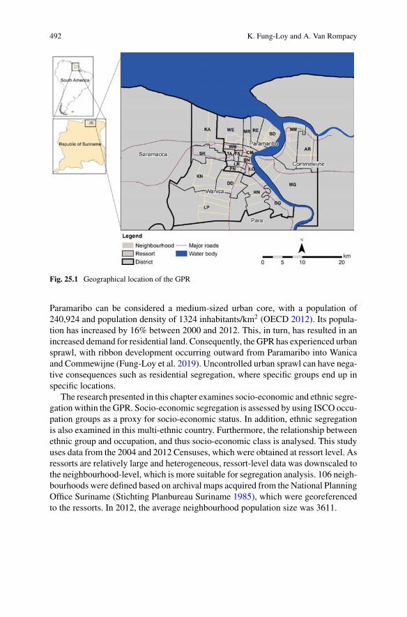
492 K. Fung-Loy and A. Van Rompaey
Fig. 25.1 Geographical location of the GPR
Paramaribo can be considered a medium-sized urban core, with a population of240,924 and population density of 1324 inhabitants/km2 (OECD 2012). Its popula-tion has increased by 16% between 2000 and 2012. This, in turn, has resulted in anincreased demand for residential land. Consequently, the GPR has experienced urbansprawl, with ribbon development occurring outward from Paramaribo into Wanicaand Commewijne (Fung-Loy et al. 2019). Uncontrolled urban sprawl can have nega-tive consequences such as residential segregation, where specific groups end up inspecific locations.
The research presented in this chapter examines socio-economic and ethnic segre-gation within the GPR. Socio-economic segregation is assessed by using ISCO occu-pation groups as a proxy for socio-economic status. In addition, ethnic segregationis also examined in this multi-ethnic country. Furthermore, the relationship betweenethnic group and occupation, and thus socio-economic class is analysed. This studyuses data from the 2004 and 2012 Censuses, which were obtained at ressort level. Asressorts are relatively large and heterogeneous, ressort-level data was downscaled tothe neighbourhood-level, which is more suitable for segregation analysis. 106 neigh-bourhoods were defined based on archival maps acquired from the National PlanningOffice Suriname (Stichting Planbureau Suriname 1985), which were georeferencedto the ressorts. In 2012, the average neighbourhood population size was 3611.
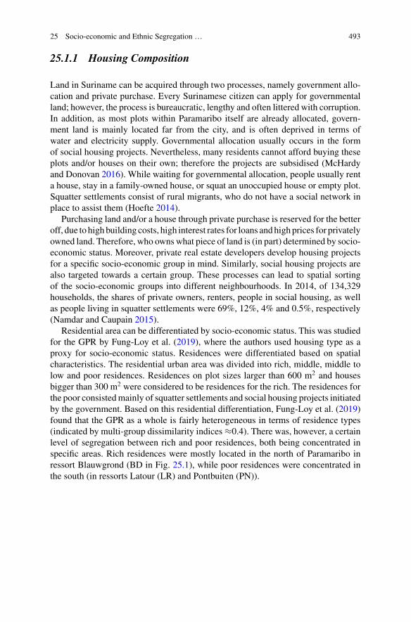
25 Socio-economic and Ethnic Segregation … 493
25.1.1 Housing Composition
Land in Suriname can be acquired through two processes, namely government allo-cation and private purchase. Every Surinamese citizen can apply for governmentalland; however, the process is bureaucratic, lengthy and often littered with corruption.In addition, as most plots within Paramaribo itself are already allocated, govern-ment land is mainly located far from the city, and is often deprived in terms ofwater and electricity supply. Governmental allocation usually occurs in the formof social housing projects. Nevertheless, many residents cannot afford buying theseplots and/or houses on their own; therefore the projects are subsidised (McHardyand Donovan 2016). While waiting for governmental allocation, people usually renta house, stay in a family-owned house, or squat an unoccupied house or empty plot.Squatter settlements consist of rural migrants, who do not have a social network inplace to assist them (Hoefte 2014).
Purchasing land and/or a house through private purchase is reserved for the betteroff, due to highbuilding costs, high interest rates for loans andhighprices for privatelyowned land. Therefore, who ownswhat piece of land is (in part) determined by socio-economic status. Moreover, private real estate developers develop housing projectsfor a specific socio-economic group in mind. Similarly, social housing projects arealso targeted towards a certain group. These processes can lead to spatial sortingof the socio-economic groups into different neighbourhoods. In 2014, of 134,329households, the shares of private owners, renters, people in social housing, as wellas people living in squatter settlements were 69%, 12%, 4% and 0.5%, respectively(Namdar and Caupain 2015).
Residential area can be differentiated by socio-economic status. This was studiedfor the GPR by Fung-Loy et al. (2019), where the authors used housing type as aproxy for socio-economic status. Residences were differentiated based on spatialcharacteristics. The residential urban area was divided into rich, middle, middle tolow and poor residences. Residences on plot sizes larger than 600 m2 and housesbigger than 300 m2 were considered to be residences for the rich. The residences forthe poor consistedmainly of squatter settlements and social housing projects initiatedby the government. Based on this residential differentiation, Fung-Loy et al. (2019)found that the GPR as a whole is fairly heterogeneous in terms of residence types(indicated by multi-group dissimilarity indices ≈0.4). There was, however, a certainlevel of segregation between rich and poor residences, both being concentrated inspecific areas. Rich residences were mostly located in the north of Paramaribo inressort Blauwgrond (BD in Fig. 25.1), while poor residences were concentrated inthe south (in ressorts Latour (LR) and Pontbuiten (PN)).
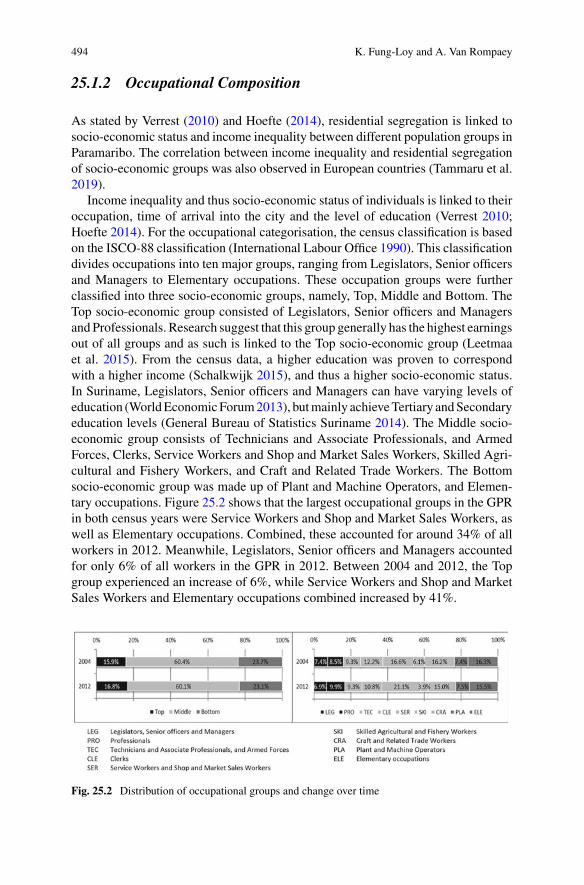
494 K. Fung-Loy and A. Van Rompaey
25.1.2 Occupational Composition
As stated by Verrest (2010) and Hoefte (2014), residential segregation is linked tosocio-economic status and income inequality between different population groups inParamaribo. The correlation between income inequality and residential segregationof socio-economic groups was also observed in European countries (Tammaru et al.2019).
Income inequality and thus socio-economic status of individuals is linked to theiroccupation, time of arrival into the city and the level of education (Verrest 2010;Hoefte 2014). For the occupational categorisation, the census classification is basedon the ISCO-88 classification (International Labour Office 1990). This classificationdivides occupations into ten major groups, ranging from Legislators, Senior officersand Managers to Elementary occupations. These occupation groups were furtherclassified into three socio-economic groups, namely, Top, Middle and Bottom. TheTop socio-economic group consisted of Legislators, Senior officers and Managersand Professionals. Research suggest that this group generally has the highest earningsout of all groups and as such is linked to the Top socio-economic group (Leetmaaet al. 2015). From the census data, a higher education was proven to correspondwith a higher income (Schalkwijk 2015), and thus a higher socio-economic status.In Suriname, Legislators, Senior officers and Managers can have varying levels ofeducation (WorldEconomicForum2013), butmainly achieveTertiary andSecondaryeducation levels (General Bureau of Statistics Suriname 2014). The Middle socio-economic group consists of Technicians and Associate Professionals, and ArmedForces, Clerks, Service Workers and Shop and Market Sales Workers, Skilled Agri-cultural and Fishery Workers, and Craft and Related Trade Workers. The Bottomsocio-economic group was made up of Plant and Machine Operators, and Elemen-tary occupations. Figure 25.2 shows that the largest occupational groups in the GPRin both census years were Service Workers and Shop and Market Sales Workers, aswell as Elementary occupations. Combined, these accounted for around 34% of allworkers in 2012. Meanwhile, Legislators, Senior officers and Managers accountedfor only 6% of all workers in the GPR in 2012. Between 2004 and 2012, the Topgroup experienced an increase of 6%, while Service Workers and Shop and MarketSales Workers and Elementary occupations combined increased by 41%.
Fig. 25.2 Distribution of occupational groups and change over time
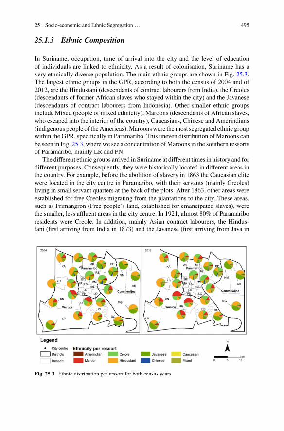
25 Socio-economic and Ethnic Segregation … 495
25.1.3 Ethnic Composition
In Suriname, occupation, time of arrival into the city and the level of educationof individuals are linked to ethnicity. As a result of colonisation, Suriname has avery ethnically diverse population. The main ethnic groups are shown in Fig. 25.3.The largest ethnic groups in the GPR, according to both the census of 2004 and of2012, are the Hindustani (descendants of contract labourers from India), the Creoles(descendants of former African slaves who stayed within the city) and the Javanese(descendants of contract labourers from Indonesia). Other smaller ethnic groupsinclude Mixed (people of mixed ethnicity), Maroons (descendants of African slaves,who escaped into the interior of the country), Caucasians, Chinese and Amerindians(indigenous people of theAmericas).Maroonswere themost segregated ethnic groupwithin the GPR, specifically in Paramaribo. This uneven distribution of Maroons canbe seen in Fig. 25.3, wherewe see a concentration ofMaroons in the southern ressortsof Paramaribo, mainly LR and PN.
The different ethnic groups arrived in Suriname at different times in history and fordifferent purposes. Consequently, they were historically located in different areas inthe country. For example, before the abolition of slavery in 1863 the Caucasian elitewere located in the city centre in Paramaribo, with their servants (mainly Creoles)living in small servant quarters at the back of the plots. After 1863, other areas wereestablished for free Creoles migrating from the plantations to the city. These areas,such as Frimangron (Free people’s land, established for emancipated slaves), werethe smaller, less affluent areas in the city centre. In 1921, almost 80% of Paramariboresidents were Creole. In addition, mainly Asian contract labourers, the Hindus-tani (first arriving from India in 1873) and the Javanese (first arriving from Java in
Fig. 25.3 Ethnic distribution per ressort for both census years
496 K. Fung-Loy and A. Van Rompaey
1890), were found for the colony to work on the plantations. The Maroons settledin tribal communities in the interior of Suriname, after escaping the plantations. TheAmerindians were also concentrated in the interior districts of Suriname and at thecoast.
As agriculture declined and many plantations closed in the 1930s, many inhab-itants were given small-scale agricultural holdings in the districts of Commewijneand Wanica. Thus, many Hindustani and Javanese settled in these districts. Duringthe Second World War, the demand for workers in the construction, bauxite andservice sector increased, thus attracting many Hindustani and Javanese to the city forbetter occupational, and later educational opportunities (Hoefte 2014). TheMaroonsbecame a significant group in Paramaribo, after fleeing the civil war in the interiorbetween 1986 and 1992. TheMaroons settled in and around the former social housingprojects, predominantly in the south of Paramaribo. As these newcomers arrived inthe city, the previous rich inhabitants moved to the north and southwest of the citycentre, towards the newly built suburbs (de Brujine and Namdar 2013).
According to the census of 2012, the ressorts are generally ethnically mixed.However, we can see that Creoles are still dominant in the centre, while Hindustanidominate west Paramaribo and Wanica (see Fig. 25.3). District Commewijne has ahigher concentration of Javanese people. As certain ethnic groups arrived in the citylater than others, they lagged behind in educational and occupational opportunities.Over time, a more equal distribution of ethnicities was achieved. As such, educa-tional and occupational opportunities were also more equally distributed among thedifferent ethnicities. Nevertheless, as stated by Verrest (2010) and Hoefte (2014),some occupational groups are still dominated by specific ethnic groups. Therefore,ethnic and socio-economic segregation can be linked (Reardon and Bischoff 2011).Such a link was also found in, for example, Belgium, where poorer neighbourhoodshad a higher concentration of non-European migrants (Costa and de Valk 2018).
25.2 Methods
25.2.1 Socio-economic Segregation
The dissimilarity index (DI) was used to measure segregation between the socio-economic groups within the GPR. The DI describes the overall evenness of thedistribution between two groups. It also provides the ability to evaluate each groupand each area separately (Sakoda 1981). DI values range from zero to one, withvalues below 0.3 indicating a low level of segregation, and values above 0.6 pointingat a high level of segregation. However, the DI is scale dependent and thus can beinfluenced by size of the areas analysed (Quillian and Lagrange 2016; Anderssonet al. 2018). In order to compare regions or countries, we also consider the changein DI (Ismail 2013). The DI and the change in DI were calculated between each
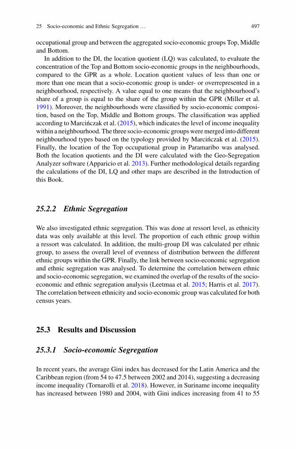
25 Socio-economic and Ethnic Segregation … 497
occupational group and between the aggregated socio-economic groups Top, Middleand Bottom.
In addition to the DI, the location quotient (LQ) was calculated, to evaluate theconcentration of the Top and Bottom socio-economic groups in the neighbourhoods,compared to the GPR as a whole. Location quotient values of less than one ormore than one mean that a socio-economic group is under- or overrepresented in aneighbourhood, respectively. A value equal to one means that the neighbourhood’sshare of a group is equal to the share of the group within the GPR (Miller et al.1991). Moreover, the neighbourhoods were classified by socio-economic composi-tion, based on the Top, Middle and Bottom groups. The classification was appliedaccording toMarcinczak et al. (2015), which indicates the level of income inequalitywithin a neighbourhood. The three socio-economic groupsweremerged into differentneighbourhood types based on the typology provided by Marcinczak et al. (2015).Finally, the location of the Top occupational group in Paramaribo was analysed.Both the location quotients and the DI were calculated with the Geo-SegregationAnalyzer software (Apparicio et al. 2013). Further methodological details regardingthe calculations of the DI, LQ and other maps are described in the Introduction ofthis Book.
25.2.2 Ethnic Segregation
We also investigated ethnic segregation. This was done at ressort level, as ethnicitydata was only available at this level. The proportion of each ethnic group withina ressort was calculated. In addition, the multi-group DI was calculated per ethnicgroup, to assess the overall level of evenness of distribution between the differentethnic groups within the GPR. Finally, the link between socio-economic segregationand ethnic segregation was analysed. To determine the correlation between ethnicand socio-economic segregation, we examined the overlap of the results of the socio-economic and ethnic segregation analysis (Leetmaa et al. 2015; Harris et al. 2017).The correlation between ethnicity and socio-economic group was calculated for bothcensus years.
25.3 Results and Discussion
25.3.1 Socio-economic Segregation
In recent years, the average Gini index has decreased for the Latin America and theCaribbean region (from 54 to 47.5 between 2002 and 2014), suggesting a decreasingincome inequality (Tornarolli et al. 2018). However, in Suriname income inequalityhas increased between 1980 and 2004, with Gini indices increasing from 41 to 55
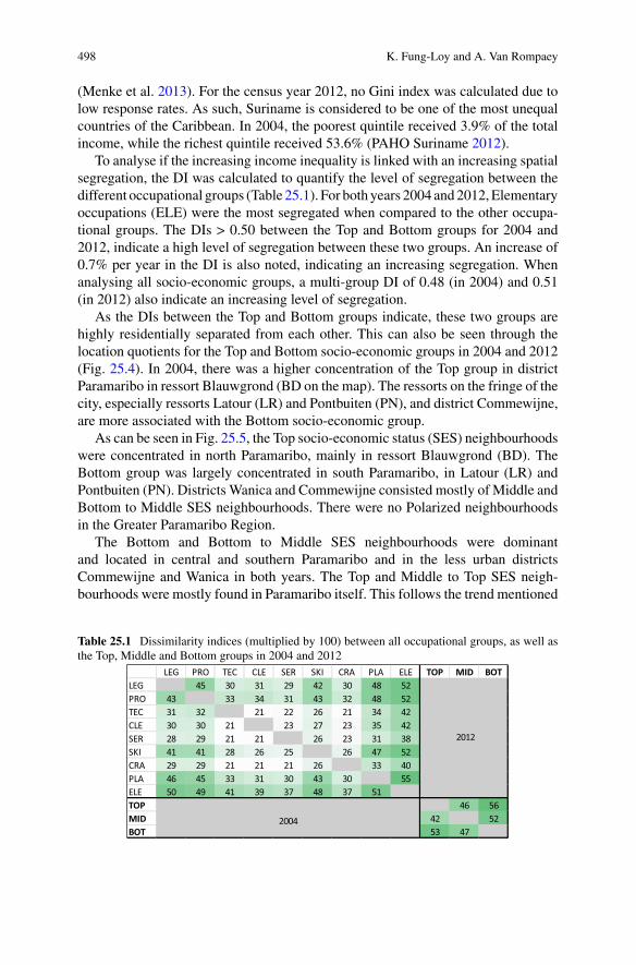
498 K. Fung-Loy and A. Van Rompaey
(Menke et al. 2013). For the census year 2012, no Gini index was calculated due tolow response rates. As such, Suriname is considered to be one of the most unequalcountries of the Caribbean. In 2004, the poorest quintile received 3.9% of the totalincome, while the richest quintile received 53.6% (PAHO Suriname 2012).
To analyse if the increasing income inequality is linked with an increasing spatialsegregation, the DI was calculated to quantify the level of segregation between thedifferent occupational groups (Table 25.1). For both years 2004 and2012,Elementaryoccupations (ELE) were the most segregated when compared to the other occupa-tional groups. The DIs > 0.50 between the Top and Bottom groups for 2004 and2012, indicate a high level of segregation between these two groups. An increase of0.7% per year in the DI is also noted, indicating an increasing segregation. Whenanalysing all socio-economic groups, a multi-group DI of 0.48 (in 2004) and 0.51(in 2012) also indicate an increasing level of segregation.
As the DIs between the Top and Bottom groups indicate, these two groups arehighly residentially separated from each other. This can also be seen through thelocation quotients for the Top and Bottom socio-economic groups in 2004 and 2012(Fig. 25.4). In 2004, there was a higher concentration of the Top group in districtParamaribo in ressort Blauwgrond (BD on the map). The ressorts on the fringe of thecity, especially ressorts Latour (LR) and Pontbuiten (PN), and district Commewijne,are more associated with the Bottom socio-economic group.
As can be seen in Fig. 25.5, the Top socio-economic status (SES) neighbourhoodswere concentrated in north Paramaribo, mainly in ressort Blauwgrond (BD). TheBottom group was largely concentrated in south Paramaribo, in Latour (LR) andPontbuiten (PN). Districts Wanica and Commewijne consisted mostly of Middle andBottom to Middle SES neighbourhoods. There were no Polarized neighbourhoodsin the Greater Paramaribo Region.
The Bottom and Bottom to Middle SES neighbourhoods were dominantand located in central and southern Paramaribo and in the less urban districtsCommewijne and Wanica in both years. The Top and Middle to Top SES neigh-bourhoods were mostly found in Paramaribo itself. This follows the trend mentioned
Table 25.1 Dissimilarity indices (multiplied by 100) between all occupational groups, as well asthe Top, Middle and Bottom groups in 2004 and 2012
LEG PRO TEC CLE SER SKI CRA PLA ELE TOP MID BOTLEG 45 30 31 29 42 30 48 52PRO 43 33 34 31 43 32 48 52TEC 31 32 21 22 26 21 34 42CLE 30 30 21 23 27 23 35 42SER 28 29 21 21 26 23 31 38SKI 41 41 28 26 25 26 47 52CRA 29 29 21 21 21 26 33 40PLA 46 45 33 31 30 43 30 55ELE 50 49 41 39 37 48 37 51TOP 46 56MID 42 52BOT 53 47
2004
2012
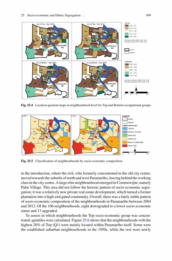
25 Socio-economic and Ethnic Segregation … 499
Fig. 25.4 Location quotient maps at neighbourhood level for Top and Bottom occupational groups
Fig. 25.5 Classification of neighbourhoods by socio-economic composition
in the introduction, where the rich, who formerly concentrated in the old city centre,moved towards the suburbs of north andwest Paramaribo, leaving behind theworkingclass in the city centre. A large elite neighbourhood emerged inCommewijne, namelyPalm Village. This area did not follow the historic pattern of socio-economic segre-gation; it was a relatively new private real estate development, which turned a formerplantation into a high-end gated community. Overall, there was a fairly stable patternof socio-economic composition of the neighbourhoods in Paramaribo between 2004and 2012. Of the 106 neighbourhoods, eight downgraded to a lower socio-economicstatus and 13 upgraded.
To assess in which neighbourhoods the Top socio-economic group was concen-trated, quintiles were calculated. Figure 25.6 shows that the neighbourhoods with thehighest 20% of Top (Q1) were mainly located within Paramaribo itself. Some werethe established suburban neighbourhoods in the 1950s, while the rest were newly
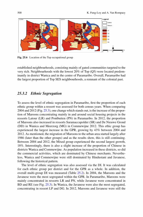
500 K. Fung-Loy and A. Van Rompaey
Fig. 25.6 Location of the Top occupational group
established neighbourhoods, consisting mainly of gated communities targeted to thevery rich. Neighbourhoods with the lowest 20% of Top (Q5) were located predom-inantly in district Wanica and in the centre of Paramaribo. Overall, Paramaribo hadthe largest proportion of Top SES neighbourhoods, a remnant of the colonial past.
25.3.2 Ethnic Segregation
To assess the level of ethnic segregation in Paramaribo, first the proportion of eachethnic group within a ressort was assessed for both census years. When comparing2004 and 2012 (Fig. 25.3), one change which stands out, is the increase of the propor-tion of Maroons concentrating mainly in and around social housing projects in theressorts Latour (LR) and Pontbuiten (PN) in Paramaribo. In 2012, the proportionof Maroons also increased in ressorts Saramaccapolder (SR) and De Nieuwe Grond(DD) in Wanica and Meerzorg (MG) in Commewijne 2012. This ethic group hasexperienced the largest increase in the GPR, growing by 43% between 2004 and2012. As mentioned, the migration of Maroons to the urban area started largely after1986 (later than the other groups) and as the results show, this is still continuing.Between 2004 and 2012, the Mixed group experienced the second largest growth,18%. Interestingly, there is also a slight increase of the proportion of Chinese indistricts Wanica and Commewijne. As population increased in these districts, so didthe commercial activities, which are dominated by Chinese merchants. Neverthe-less, Wanica and Commewijne were still dominated by Hindustani and Javanese,following the historical pattern.
The level of ethnic segregation was also assessed via the DI. It was calculatedfor each ethnic group per district and for the GPR as a whole. In addition, theoverall multi-group DI was measured (Table 25.2). In 2004, the Maroons and theJavanese were the most segregated within the GPR. In Paramaribo, Maroons weremainly concentrated in ressorts LR and PN, while Javanese were concentrated inBD and RE (see Fig. 25.3). In Wanica, the Javanese were also the most segregated,concentrating in ressort LP and DG. In 2012, Maroons and Javanese were still the
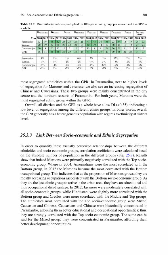
25 Socio-economic and Ethnic Segregation … 501
Table 25.2 Dissimilarity indices (multiplied by 100) per ethnic group, per ressort and the GPR asa whole
DAmerindian DMaroon DCreole DHindustani DJavanese DChinese DCaucasian DMixed Dall ethnic groups
Year 2004 2012 2004 2012 2004 2012 2004 2012 2004 2012 2004 2012 2004 2012 2004 2012 2004 2012Paramaribo 13 16 48 52 25 26 26 25 41 48 31 45 22 44 14 19 28 32Wanica 20 19 29 30 26 22 22 18 42 39 14 17 30 18 15 12 27 24Commewijne 30 8 20 13 10 3 16 7 13 8 9 24 26 21 8 5 13 7 GPR 16 14 44 48 35 29 33 28 44 43 37 29 30 36 22 23 34 33
Paramaribo 3% 1% 1% 0% 2% 5% 12% 5% 2% Wanica -1% 1% -2% -2% -1% 3% -5% -2% -1% Commewijne -9% -4% -9% -7% -5% 20% -2% -4% -6% GPR -1% 1% -2% -2% 0% -3% 2% 1% -1%
most segregated ethnicities within the GPR. In Paramaribo, next to higher levelsof segregation for Maroons and Javanese, we also see an increasing segregation ofChinese and Caucasians. These two groups were mainly concentrated in the citycentre and the northern ressorts of Paramaribo. For both years, Maroons were themost segregated ethnic group within the GPR.
Overall, all districts and the GPR as a whole have a low DI (<0.35), indicating alow level of segregation among the different ethnic groups. In other words, overallthe GPR generally has a heterogeneous population with regards to ethnicity at districtlevel.
25.3.3 Link Between Socio-economic and Ethnic Segregation
In order to quantify these visually perceived relationships between the differentethnicities and socio-economic groups, correlation coefficientswere calculated basedon the absolute number of population in the different groups (Fig. 25.7). Resultsshow that indeed Maroons were primarily negatively correlated with the Top socio-economic group. Where in 2004, Amerindians were the most correlated with theBottom group, in 2012 the Maroons became the most correlated with the Bottomoccupational group. This indicates that as the proportion of Maroons grows, they aremostly accessing occupations associated with the Bottom socio-economic group. Asthey are the last ethnic group to arrive in the urban area, they have an educational andthus occupational disadvantage. In 2012, Javanese were moderately correlated withall socio-economic groups, while Hindustani were slightly more correlated with theBottom group and Creoles were more correlated with the Middle and Top groups.The ethnicities most correlated with the Top socio-economic group were Mixed,Caucasian and Chinese. Caucasians and Chinese were historically concentrated inParamaribo, allowing them better educational and occupational opportunities; thus,they are strongly correlated with the Top socio-economic group. The same can besaid for the Mixed group; they were concentrated in Paramaribo, affording thembetter development opportunities.
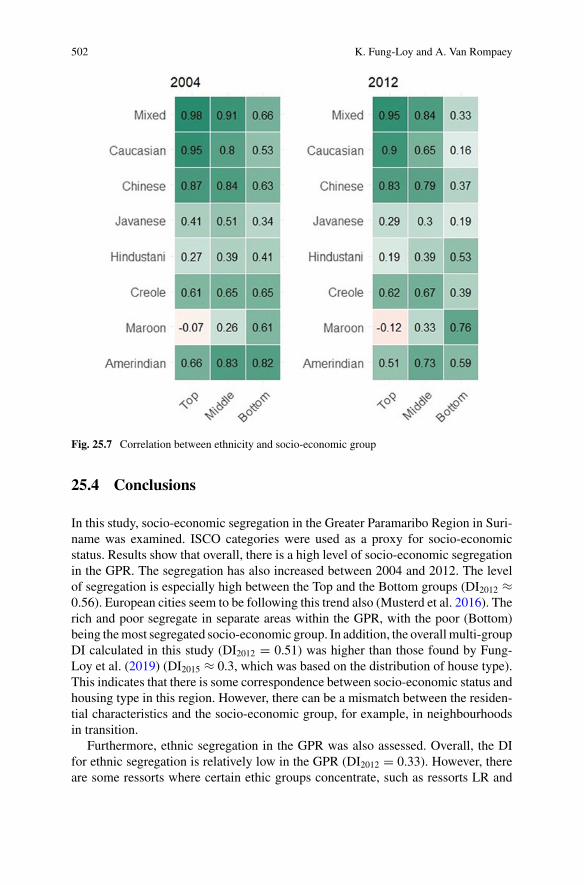
502 K. Fung-Loy and A. Van Rompaey
Fig. 25.7 Correlation between ethnicity and socio-economic group
25.4 Conclusions
In this study, socio-economic segregation in the Greater Paramaribo Region in Suri-name was examined. ISCO categories were used as a proxy for socio-economicstatus. Results show that overall, there is a high level of socio-economic segregationin the GPR. The segregation has also increased between 2004 and 2012. The levelof segregation is especially high between the Top and the Bottom groups (DI2012 ≈0.56). European cities seem to be following this trend also (Musterd et al. 2016). Therich and poor segregate in separate areas within the GPR, with the poor (Bottom)being themost segregated socio-economic group. In addition, the overall multi-groupDI calculated in this study (DI2012 = 0.51) was higher than those found by Fung-Loy et al. (2019) (DI2015 ≈ 0.3, which was based on the distribution of house type).This indicates that there is some correspondence between socio-economic status andhousing type in this region. However, there can be a mismatch between the residen-tial characteristics and the socio-economic group, for example, in neighbourhoodsin transition.
Furthermore, ethnic segregation in the GPR was also assessed. Overall, the DIfor ethnic segregation is relatively low in the GPR (DI2012 = 0.33). However, thereare some ressorts where certain ethic groups concentrate, such as ressorts LR and
25 Socio-economic and Ethnic Segregation … 503
PN where Maroons concentrate; they experience segregation in district Paramariboaccording to a DI > 0.40. When comparing the multi-group DI for socio-economicsegregation (DI2012 = 0.51) with the multi-group DI for ethnic segregation (DI2012= 0.33), we see that the GPR is less segregated by ethnicity, but more segregated bysocio-economic status. This was also found in other studies for Suriname and otherLatin American and Caribbean countries such as Brazil and Trinidad and Tobago(Brathwaite 1980; Lichter et al. 2012; Verrest 2010). For the United States, it wasfound that while ethnic segregation is still larger than socio-economic segregation,ethnic segregation has decreased, while socio-economic segregation has increased(Brady et al. 2017).
Assessing the link between ethnic and socio-economic segregation, we see thatfor certain ethnicities there exists a high correlation with a specific socio-economicstatuses. Maroons are increasingly correlated with the Bottom, while Mixed andCaucasians are highly correlated with the Top socio-economic group. This reflectsthe history of Suriname; Caucasians were traditionally the rich colonists and, similarto the Mixed, were concentrated in the urban centre while the Maroons fled into theinterior to escape slavery. Only after the mid-twentieth century Maroons migrated tothe city, experiencing a significant lag in education and consequently occupationalopportunities. As such, Maroons are far behind Mixed and Caucasians on the socio-economic ladder.
In this research, the socio-economic and ethnic segregation, and the link betweenthe two was analysed. As certain ethnic groups are more strongly correlated withcertain socio-economic statuses, increasing socio-economic segregation can limitthe upward socio-economic mobility opportunities for specific marginalised ethnicgroups. As income inequality continues to increase, it is likely that socio-economicsegregation will increase as well.
References
AnderssonEK,LyngstadTH,SleutjesB (2018)Comparing patterns of segregation inNorth-WesternEurope: a multiscalar approach. Eur J Popul 34(2):151–168
Apparicio P, Fournier É, Apparicio D (2013) Geo-segregation analyzer: a multiplatform application(version1.1). SpatialAnalysis andRegionalEconomicsLaboratory (SAREL), INRSUrbanisationCulture Société, Montreal
Brady D, Burton LM,Massey DS (2017) Segregation and the perpetuation of disadvantage. OxfordUniversity Press
Brathwaite FS (1980) Race, social class and the origins of occupational elites in Trinidad andTobago. Boletín De Estudios Latinoamericanos Y Del Caribe 28:13–30
Costa R, de Valk HAG (2018) Ethnic and socioeconomic segregation in Belgium: a multiscalarapproach using individualised neighbourhoods. Eur J Popul 34(2):225–250
de Brujine A, Namdar A (2013)Closer and closer to the Ocean. The Habitat and Housing structureof present day Paramaribo and the policies formulated for the near future—how to realize asustainable city? Caribbean Urban Forum 2013, Paramaribo
504 K. Fung-Loy and A. Van Rompaey
Fung-LoyK,VanRompaeyA,HemerijckxL-M(2019)Detection and simulation of urban expansionand socioeconomic segregation in the greater Paramaribo Region, Suriname. Tijdschrift VoorEconomische En Sociale Geografie 110(3):339–358
General Bureau of Statistics Suriname (2013) Suriname census 2012-volume 1: Demografische enSociale Karakteristieken en Migratie, Paramaribo 2013–05
General Bureau of Statistics Suriname (2014) Suriname census 2012-Volume 2: Onderwijs,Werkgelegenheid en Vervoer; Vruchtbaarheid en Sterfte; Gezondheid en Sport, Paramaribo299/2013 – 10x
Harris R, Johnston R, Manley D (2017) The changing interaction of ethnic and socioeconomicsegregation in England and Wales, 1991–2011. Ethnicities 17(3):320–349
Hoefte R (2014) Suriname in the long twentieth century. Palgrave Macmillan, New YorkInternational Labour Office (1990) International standard classification of occupations: ISCO-88.InternationalLabourOffice,Geneva.Available at: https://www.ilo.org/public/english/bureau/stat/isco/isco88/publ3.htm
Ismail A (2013)The hybrid outcome of urban change: global city, polarized city? Glocalism. J CultPolit Innov (1)
Leetmaa K, Tammaru T, Hess DB (2015) Preferences toward neighbor ethnicity and affluence:evidence from an inherited dual ethnic context in Post-Soviet Tartu, Estonia. Ann Assoc AmGeogr 105(1):162–182
Lichter DT, Parisi D, Taquino MC (2012)The geography of exclusion race, segregation, andconcentrated poverty. Soc Prob 59(3):364–388
Marcinczak S, Tammaru T, Novák J, Gentile M, Kovács Z, Temelová J, Valatka V, Kährik A,Szabó B (2015) Patterns of socioeconomic segregation in the capital cities of fast-track reformingpostsocialist countries. Ann Assoc Am Geogr 105(1):183–202
McHardy P, Donovan MG (2016) The state of social housing in six Caribbean Countries. Inter-American Development Bank, Washington D.C.
Menke J, Schalkwijk M, Schalkwijk J, Seligson MA (2012) (2013) The political culture of democ-racy in Suriname and in the Americas. Towards equality of opportunity Paramaribo, StichtingWetenschappelijke Informatie - Foundation for Information and Development
Miller M, Gibson LJ, Wright NG (1991) Location quotient: a basic tool for economic developmentanalysis. Econ Dev Rev 9(2):4
Musterd S, Marcinczak S, van HamM, Tammaru T (2016) Socioeconomic segregation in Europeancapital cities. Increasing separation between poor and rich. Urban Geogr 38(7):1062–1083
Namdar A, Caupain N (2015) Huisvesting in Suriname: een analyse van de resultaten van Census2012. In: Menke J (ed) Mozaïek van het Surinaamse volk: Volkstellingen in demografisch,economisch en sociaal perspectief. General Bureau of Statistics Suriname and Anton de KomUniversity of Suriname, Paramaribo, pp 203–221
OECD (2012) Redefining “Urban”: a new way to measure metropolitan areas. Available at: https://doi.org/10.1787/9789264174108-en
PAHO Suriname (2012) PAHO/WHO country cooperation strategy: Suriname 2012–2016. Para-maribo
Quillian L, Lagrange H (2016) Socioeconomic segregation in large cities in France and the UnitedStates. Demography 53(4):1051–1084
Reardon SF, Bischoff K (2011) Income inequality and income segregation. Am J Sociol116(4):1092–1153
Sakoda JM (1981) A generalized index of dissimilarity. Demography 18(2):245–250Schalkwijk J (2015) Onderwijs in Suriname: een analyse van de censusresultaten 2004 en 2012.In: Menke J (ed) Mozaïek van het Surinaamse volk: Volkstellingen in demografisch, economischen sociaal perspectief. General Bureau of Statistics Suriname and Anton de Kom University ofSuriname, Paramaribo, pp 169–184
Regio Groot Paramaribo: Sociaal geografische indeling in wijken en wijkcombinaties (1985)Stichting Planbureau Suriname
25 Socio-economic and Ethnic Segregation … 505
Tammaru T, Marcin´czak S, Aunap R, van HamM, Janssen H (2019)Relationship between incomeinequality and residential segregation of socioeconomic groups. Reg Stud 1–12
Tornarolli L, Ciaschi M, Galeano L (2018) Income distribution in Latin America. The evolution inthe last 20 years: a global approach. Available at: www.cedlas.econo.unlp.edu.ar
Verrest HJLM (2010) City profile: Paramaribo. Cities 27:50–60World Economic Forum (2013) The human capital report. World Economic Forum, Geneva
Open Access This chapter is licensed under the terms of the Creative Commons Attribution 4.0International License (http://creativecommons.org/licenses/by/4.0/), which permits use, sharing,adaptation, distribution and reproduction in any medium or format, as long as you give appropriatecredit to the original author(s) and the source, provide a link to the Creative Commons license andindicate if changes were made.
The images or other third party material in this chapter are included in the chapter’s CreativeCommons license, unless indicated otherwise in a credit line to the material. If material is notincluded in the chapter’s Creative Commons license and your intended use is not permitted bystatutory regulation or exceeds the permitted use, you will need to obtain permission directly fromthe copyright holder.
Chapter 26Measuring Changes in ResidentialSegregation in São Paulo in the 2000s
Flávia Feitosa, Joana Barros, Eduardo Marques, and Mariana Giannotti
Abstract Residential segregation is known as one of the most prevalent problemsof Latin American and Brazilian cities. This chapter looks into the changes in segre-gation levels in the Metropolitan Region of São Paulo between 2000 and 2010. Thisperiod was marked by economic growth and decreasing social inequalities in Brazilwith consequent improvement to the quality of life of lower income classes. Despitethose improvements, general patterns of urban segregation in Brazilian cities showedremarkable stability, albeit with important changes in the details of segregationpatterns. This chapter explores the spatial relationship between socio-occupationalgroups using global and local segregation indices. The analysis confirmed a highlysegregated distribution of social groups in the Metropolitan Region and revealedincreased levels of segregation, with global indices figures for 2010 higher thanfor 2000. Analysis demonstrated that peripheral areas of the Metropolitan Regionbecame more fragmented and heterogeneous in that period, and revealed that theirincreased heterogeneity is mainly composed of classes with close social proximity,rather than polarised ones. Results showed that while middle classes became moreintegrated amongst themselves and with lower classes, the separation between lowerand upper classes was not only maintained but also increased during the period. Allthese findings suggest a reconfiguration of the concentric pattern of segregation that
F. Feitosa (B)Center for Engineering, Modeling and Applied Social Sciences, Federal University of ABC, SantoAndré, Brazile-mail: [email protected]
J. BarrosGeography Department, Birkbeck, University of London, London, UKe-mail: [email protected]
E. MarquesCenter for Metropolitan Studies, Department of Political Science, University of São Paulo, SãoPaulo, Brazile-mail: [email protected]
M. GiannottiCenter for Metropolitan Studies, Polytechnic School, University of São Paulo, São Paulo, Brazile-mail: [email protected]
© The Author(s) 2021M. van Ham et al. (eds.), Urban Socio-Economic Segregation and Income Inequality,The Urban Book Series, https://doi.org/10.1007/978-3-030-64569-4_26
507
508 F. Feitosa et al.
maintained a spatial structure of strong social isolation during the period, althoughwith greater complexity.
Keywords Residential segregation patterns ·Metropolitan region of São Paulo ·Global and local indices of segregation · Dissimilarity index · Isolation andexposure indices
26.1 Introduction
Residential segregation is known as one of the most prevalent problems of LatinAmerican and Brazilian cities, together with poverty and precarious housing condi-tions. It is also known that residential segregation is an urban feature that reducesopportunities for the poor and contributes substantially to poverty reproduction(Wilson 1987; Massey and Denton 1993; Briggs 2005).
Although the spatial pattern of Latin American cities often has roots in their colo-nial formation, the case of São Paulo is peculiar since the city had no demographic noreconomic importance by the mid-nineteenth century. It was after the boom of coffeeplantations at the end of that century and the industrialisation of the first decadesof the twentieth century that São Paulo gradually became the most important cityin the country. São Paulo is rivalled with Rio de Janeiro, which was, for centuries,the colonial and later imperial capital of Brazil. The largest proportion of the territo-ries of metropolitan São Paulo were formed during the decades of intense migrationand fast urbanisation from the 1950s to the 1980s (Caldeira 2016). At that time, thecity became the primary metropolis of a highly urbanised Brazil, even though it hasnever been the capital city. Since the 1930s, housing policies were mostly focusedon the construction of new units, although slum upgrading programmes were startedas well in the last 20 years. However, this double emphasis on property and on unitconstruction left most of the populationwith no housing solutions except squatting orbuying an irregular plot, since buying or renting from the private sector was beyondthe reach of most urban dwellers. This historical process produced metropolitanstructures with clear core-periphery segregation patterns, with high-income groupslocated in central and well-serviced areas and lower income groups in more distantand less serviced areas intensely populated by precarious self-constructed houses infavelas (squatted areas) and irregular settlements. Such patterns have been resilientto long periods of fast urban growth and societal changes (Kowarick 1979; Bondukiand Rolnik 1982).
Although most cities in Latin America have a similar concentric spatial pattern ofsegregation, recent studies of Brazilian cities have highlighted changes to this macro-segregation structure. While the overall spatial structure remains radial and concen-tric, the spatial structure of segregation now also presents a number of sub-centralitiesand peripheral areas that are increasinglymore heterogeneous (Marques 2016; Prete-ceille and Cardoso 2008), echoing classical statements of territorial heterogeneity in
26 Measuring Changes in Residential Segregation in São Paulo in the 2000s 509
Brazilian cities (Valladares and Preteceille 2000). Such fragmentation in the core-periphery spatial pattern is understood to be a consequence of the combination ofchanges in residential preferences of higher income groups for gated communities(Caldeira 2000) and transformations in lower income residential regions caused bythe political and economic dynamics in the country since the return to democracy inthe 1980s (Arretche 2019).
In general terms, the recent democratic period that started in 1980s brought socialimprovements as a product of a cycle of increasing political activism and electoralaccountability (since the 1980s), economic stability (since the 1990s) and better andbroader social policies (also in the 1990s but especially in the 2000s), integratedin national federalist systems (Arretche 2019; Marques et al. 2012). In cities, thisinvolved a slow but continuous expansion of public policies and services in tradition-ally under-serviced areas. Even areas of precarious housing conditions such as favelasand irregular settlements have experienced substantial and systematic improvementsin recent decades with slum upgrading and infrastructure policies, although main-taining levels of inequalities (Marques and Saraiva 2017). The presence of precarioushousing decreased relatively in the Metropolitan Region of São Paulo from 15% in2000 to 14.5% in 2010, reaching around 800,000 precarious households in favelasand irregular settlements amongst a total of 6 million households in the region (CEM2014). It is important to add that from 2009 to 2015, a federal housing programmehas built approximately 100,000 housing units in the Metropolitan Region of SãoPaulo, possibly reducing the stock of precarious housing, but there are no recentstatistics yet that can measure this effect (Marques 2016).
In economic terms, the average income rose from R$630 to R$1283 between1991 and 2014 (Jannuzzi 2016), although it has decreased more recently due to acontinuous economic and political crisis since 2016. Income inequality, as measuredby Gini Index, also declined from 0.606 in 1992 to 0.517 in 2014, while povertyrates reduced from 31.1% in 1991 to 7% in 2014 due to the combination of economicgrowth, strong social policies and the continuous increase of the minimum salaryduring the 2000s (Jannuzzi 2016). Since 2014, however, Brazil has suffered fromincreasing economic and political instability, which has strongly affected the socialconditions of the country. The Gini Index increased from 0.517 in 2014 to 0.533 in2017, while poverty rates increased from 7% in 2014 to 10% in 2017 (IBGE 2019)and unemployment jumped from 5.5 in 2014 to 13% in 2017 (Góes and Karpowicz2017). Although the impacts of the country’s deteriorating social situation are visiblein our cities, they have not yet been systematically analysed.
Despite these improvements, general patterns of urban segregation in Braziliancities showed remarkable stability, as will be demonstrated throughout this chapter,albeit with important changes in the details of segregation patterns. Compared withother socio-economic changes, however, urban inequalities associated with spatialsegregation have changed little, highlighting the need for better financed and bolderurban policies, especially concerning urban planning and land-use control.
The subject of this chapter—São Paulo—is the most important MetropolitanRegion of South America, with around 20million inhabitants in an area of 7,946km2.It encompasses 39 municipalities across a continuous urban area, approximately
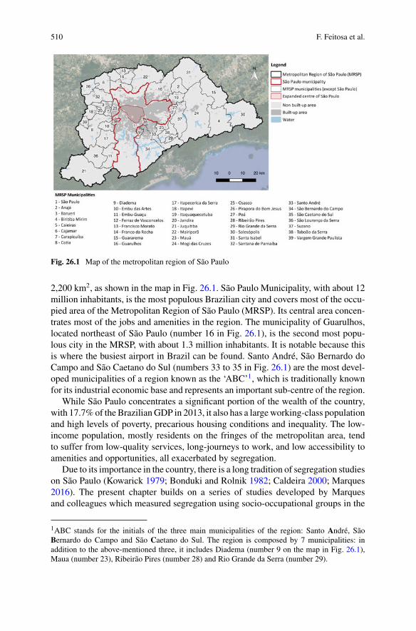
510 F. Feitosa et al.
Fig. 26.1 Map of the metropolitan region of São Paulo
2,200 km2, as shown in the map in Fig. 26.1. São Paulo Municipality, with about 12million inhabitants, is the most populous Brazilian city and covers most of the occu-pied area of the Metropolitan Region of São Paulo (MRSP). Its central area concen-trates most of the jobs and amenities in the region. The municipality of Guarulhos,located northeast of São Paulo (number 16 in Fig. 26.1), is the second most popu-lous city in the MRSP, with about 1.3 million inhabitants. It is notable because thisis where the busiest airport in Brazil can be found. Santo André, São Bernardo doCampo and São Caetano do Sul (numbers 33 to 35 in Fig. 26.1) are the most devel-oped municipalities of a region known as the ‘ABC’1, which is traditionally knownfor its industrial economic base and represents an important sub-centre of the region.
While São Paulo concentrates a significant portion of the wealth of the country,with 17.7% of the BrazilianGDP in 2013, it also has a largeworking-class populationand high levels of poverty, precarious housing conditions and inequality. The low-income population, mostly residents on the fringes of the metropolitan area, tendto suffer from low-quality services, long-journeys to work, and low accessibility toamenities and opportunities, all exacerbated by segregation.
Due to its importance in the country, there is a long tradition of segregation studieson São Paulo (Kowarick 1979; Bonduki and Rolnik 1982; Caldeira 2000; Marques2016). The present chapter builds on a series of studies developed by Marquesand colleagues which measured segregation using socio-occupational groups in the
1ABC stands for the initials of the three main municipalities of the region: Santo André, SãoBernardo do Campo and São Caetano do Sul. The region is composed by 7 municipalities: inaddition to the above-mentioned three, it includes Diadema (number 9 on the map in Fig. 26.1),Maua (number 23), Ribeirão Pires (number 28) and Rio Grande da Serra (number 29).
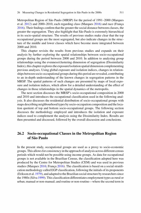
26 Measuring Changes in Residential Segregation in São Paulo in the 2000s 511
Metropolitan Region of São Paulo (MRSP) for the period of 1991–2000 (Marqueset al. 2012) and 2000–2010, each regarding class (Marques 2016) and race (França2016). Their findings confirm that the greater the social distance between classes, thegreater the segregation. They also highlight that São Paulo is extremely hierarchicalin its socio-spatial structure. The results of previous studies make clear that the topoccupational groups are the most segregated, but also indicate changes in the struc-ture of the middle and lower classes which have become more integrated between2000 and 2010.
This chapter revisits the results from previous studies and expands on theiranalysis by further exploring the spatial relationships between socio-occupationalgroups during the period between 2000 and 2010. In addition to analysing grouprelationships using the evenness/clustering dimension of segregation (DissimilarityIndex), this chapter explores the exposure/isolation spatial dimension complementingprevious analyses. Using global exposure and isolation indices, changes in relation-ships between socio-occupational groups during this period are revealed, contributingto an in-depth understanding of the known changes in segregation patterns in theMRSP. The spatial patterns of such changes are presented by maps of local expo-sure and isolation indices, which allow for a detailed understanding of the effect ofchanges in those relationships in the spatial dynamics of the metropolis.
The next section discusses the MRSP’s socio-occupational composition in 2000and 2010 and introduces the occupational classification used in the following anal-ysis. It also discusses the residential distribution of socio-occupational groups withmaps describing neighbourhood types by socio-occupation composition and the loca-tion quotient of top and bottom socio-occupational groups. The following sectiondiscusses the methodology employed and introduces the isolation and exposureindices used to complement the analysis using the Dissimilarity Index. Results arethen presented and discussed, followed by the overall discussion and conclusions.
26.2 Socio-occupational Classes in the Metropolitan Regionof São Paulo
In the present study, occupational groups are used as a proxy to socio-economicgroups. This allows for consistency in the approach of analysis across different censusperiods which would not be possible using income groups. As data for occupationalgroups is not available in the Brazilian Census, the classification adopted here wasproduced by the Centre for Metropolitan Studies (CEM) and was used in previousstudies (Marques 2016; França 2016). The classification is based on a social stratifi-cationmethodology called EGP classification, following the initials of its proponents(Erikson et al. 1979), and adapted to theBrazilian social structure by researchers sincethe 1980s (Silva 1999). This classification differentiates employment types as rural orurban; manual or non-manual; and routine or non-routine—where the second term in
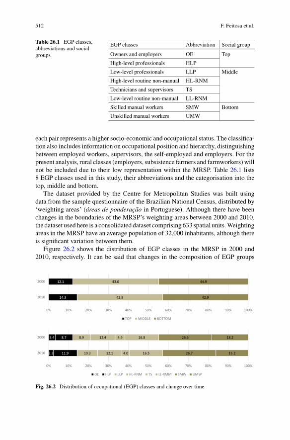
512 F. Feitosa et al.
Table 26.1 EGP classes,abbreviations and socialgroups
EGP classes Abbreviation Social group
Owners and employers OE Top
High-level professionals HLP
Low-level professionals LLP Middle
High-level routine non-manual HL-RNM
Technicians and supervisors TS
Low-level routine non-manual LL-RNM
Skilled manual workers SMW Bottom
Unskilled manual workers UMW
each pair represents a higher socio-economic and occupational status. The classifica-tion also includes information on occupational position and hierarchy, distinguishingbetween employed workers, supervisors, the self-employed and employers. For thepresent analysis, rural classes (employers, subsistence farmers and farmworkers) willnot be included due to their low representation within the MRSP. Table 26.1 lists8 EGP classes used in this study, their abbreviations and the categorisation into thetop, middle and bottom.
The dataset provided by the Centre for Metropolitan Studies was built usingdata from the sample questionnaire of the Brazilian National Census, distributed by‘weighting areas’ (áreas de ponderação in Portuguese). Although there have beenchanges in the boundaries of the MRSP’s weighting areas between 2000 and 2010,the dataset used here is a consolidated dataset comprising 633 spatial units.Weightingareas in the MRSP have an average population of 32,000 inhabitants, although thereis significant variation between them.
Figure 26.2 shows the distribution of EGP classes in the MRSP in 2000 and2010, respectively. It can be said that changes in the composition of EGP groups
14.3
12.1
42.8
43.0
42.9
44.9
0% 10% 20% 30% 40% 50% 60% 70% 80% 90% 100%
2010
2000
TOP MIDDLE BOTTOM
2.3
3.4
11.9
8.7
10.3
8.9
12.1
12.4
4.0
4.9
16.5
16.8
26.7
26.6
16.2
18.2
0% 10% 20% 30% 40% 50% 60% 70% 80% 90% 100%
2010
2000
OE HLP LLP HL-RNM TS LL-RMM SMW UMW
Fig. 26.2 Distribution of occupational (EGP) classes and change over time
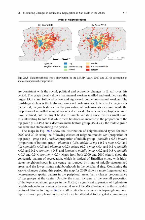
26 Measuring Changes in Residential Segregation in São Paulo in the 2000s 513
Fig. 26.3 Neighbourhood types distribution in the MRSP (years 2000 and 2010) according tosocio-occupational composition
are consistent with the social, political and economic changes in Brazil over thisperiod. The graph clearly shows that manual workers (skilled and unskilled) are thelargest EGP class, followed by low and high-level routine non-manual workers. Thethird-largest class is the high- and low-level professionals. In terms of change overthe period, the graph shows that the proportion of professionals increased while theproportion of unskilled manual workers decreased. Owners and employers seem tohave declined, but this might be due to sample variation since this is a small class.It is interesting to note that while there has been an increase in the proportion of thetop group (12–14%) and a decrease in the bottom group (45–43%), the middle grouphas remained stable during the period.
The maps in Fig. 26.3 show the distribution of neighbourhood types for both2000 and 2010, using the following classes of neighbourhoods: top (proportion oftop group—ptop > 0.4),middle (proportion of middle group—pmiddle > 0.5), bottom(proportion of bottom group—pbottom > 0.5), middle to top ( 0.2 < ptop < 0.4 and0.2 < pmiddle < 0.5 and pbottom < 0.2), mixed (0.2 < ptop < 0.4 and 0.2 < pmiddle< 0.5 and 0.2 < pbottom < 0.5) and bottom to middle (ptop < 0.2 and 0.3 < pmiddle< 0.5 and 0.3 < pbottom < 0.5). Maps from both 2000 and 2010 clearly show theconcentric pattern of segregation, which is typical of Brazilian cities, with high-status neighbourhoods in the centre surrounded by rings of middle-status/mixedareas, and the lowest status neighbourhoods in the peripheral ring. Confirming theknown changes during this period, the map for 2010 shows a more fragmented andheterogeneous spatial pattern in the peripheral areas, but a clearer predominanceof top groups at the centre. Despite the small increase in the overall proportionof the top occupational groups in the MRSP, a significant expansion of high-statusneighbourhoods can be seen in the central area of theMRSP—known as the expandedcentre of São Paulo. Figure 26.3 also illustrates the emergence of top neighbourhoodtypes in more peripheral areas, which can be attributed to the gated communities
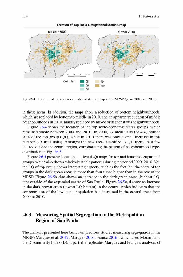
514 F. Feitosa et al.
Fig. 26.4 Location of top socio-occupational status group in the MRSP (years 2000 and 2010)
in those areas. In addition, the maps show a reduction of bottom neighbourhoods,which are replaced by bottom tomiddle in 2010, and an apparent reduction of middleneighbourhoods in 2010, mainly replaced bymixed or higher status neighbourhoods.
Figure 26.4 shows the location of the top socio-economic status groups, whichremained stable between 2000 and 2010. In 2000, 27 areal units (or 4%) housed20% of the top group (Q1), while in 2010 there was only a small increase in thisnumber (29 areal units). Amongst the new areas classified as Q1, there are a fewlocated outside the central region, corroborating the pattern of neighbourhood typesdistribution in Fig. 26.3.
Figure 26.5 presents location quotient (LQ)maps for top and bottom occupationalgroups, which also shows relatively stable patterns during the period 2000–2010. Yet,the LQ of top group shows interesting aspects, such as the fact that the share of topgroups in the dark green areas is more than four times higher than in the rest of theMRSP. Figure 26.5b also shows an increase in the dark green areas (highest LQ-top) outside of the expanded centre of São Paulo. Figure 26.5c, d show an increasein the dark brown areas (lowest LQ-bottom) in the centre, which indicates that theconcentration of the low-status population has decreased in the central areas from2000 to 2010.
26.3 Measuring Spatial Segregation in the MetropolitanRegion of São Paulo
The analysis presented here builds on previous studies measuring segregation in theMRSP (Marques et al. 2012; Marques 2016; França 2016), which used Moran I andthe Dissimilarity Index (D). It partially replicates Marques and França’s analyses of
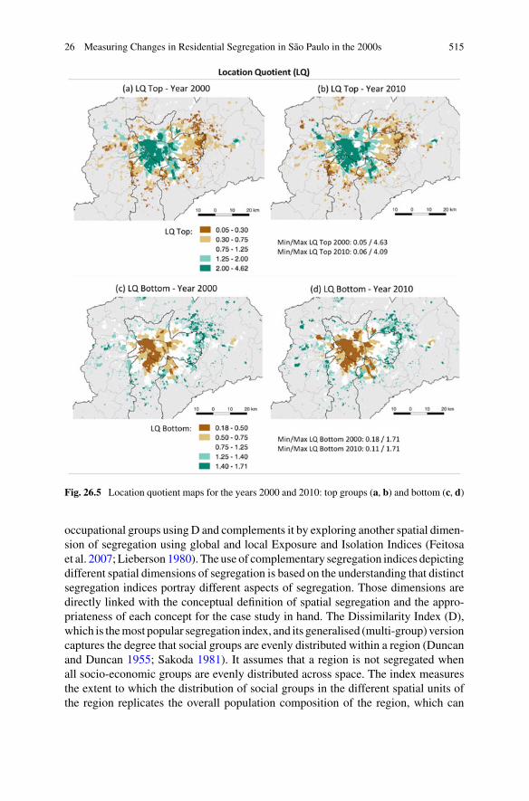
26 Measuring Changes in Residential Segregation in São Paulo in the 2000s 515
Fig. 26.5 Location quotient maps for the years 2000 and 2010: top groups (a, b) and bottom (c, d)
occupational groups using D and complements it by exploring another spatial dimen-sion of segregation using global and local Exposure and Isolation Indices (Feitosaet al. 2007; Lieberson 1980). The use of complementary segregation indices depictingdifferent spatial dimensions of segregation is based on the understanding that distinctsegregation indices portray different aspects of segregation. Those dimensions aredirectly linked with the conceptual definition of spatial segregation and the appro-priateness of each concept for the case study in hand. The Dissimilarity Index (D),which is themost popular segregation index, and its generalised (multi-group) versioncaptures the degree that social groups are evenly distributed within a region (Duncanand Duncan 1955; Sakoda 1981). It assumes that a region is not segregated whenall socio-economic groups are evenly distributed across space. The index measuresthe extent to which the distribution of social groups in the different spatial units ofthe region replicates the overall population composition of the region, which can
516 F. Feitosa et al.
range from 1 (complete segregation) to 0 (complete integration). The index can becomputed for each pair of groups (D Index proposed byDuncan andDuncan in 1951),which can include the evenness of each group in relation to all other groups, or forall groups taken together (Generalised D Index proposed by Sakoda in 1981). Theglobal dissimilarity figure indicates the proportion of the population (of the relevantgroup) that would have to relocate to a different neighbourhood in order to matchthe distribution of reference groups (all others or paired group).
Following Reardon and O’Sullivan’s (2004) proposal for the two axes of spatialsegregation (the first axis measuring evenness to clustering dimension and the secondexposure to isolationdimension), this chapter employsExposure and Isolation indices(Lieberson 1980) to complement the analysis using D. Unlike D, which focus on thedistribution of different groups across space, the Exposure Indexmeasures the poten-tial interaction between groups or, in other words, the extent of which one group isexposed to another based on spatial proximity. The Isolation Index is a special case ofthe Exposure Index, which measures the exposure of a social group to itself. Thoseindices range from 0 to 1 and are highly dependent on the city-wide proportionof groups: the more people of class m, the more likely the exposure/isolation. Thisdependency causes problems for comparative studies both across different geograph-ical areas and same areas across different time periods. Thus, to aid interpretationof the results across different time periods, this study uses normalised isolation andexposure indices, where the original figures were divided by the city-wide percentageof classm inMRSP. In this case, values closer to 1 indicate less segregation and valueshigher and lower than 1 indicate an exposure superior and inferior, respectively, thanthe one expected in an integrated region. The latter is understood as a region whereall exposure/isolation indices regarding one class are equal to its proportion in thewhole region. It should also be noted that while the traditional Exposure Index ofgroup m to n differs from the exposure of n to m, their normalised versions do not.
The spatial pattern of the exposure/isolation dimension is explored in this chapterby maps of the local version of Exposure and Isolation indices, which indicate thecontribution of each area to the composition of the global index (Feitosa et al. 2007).These local indices indicate the areas where exposure between groups (or from agroup to itself) is higher, allowing for areas of high and low segregation betweenspecific groups to be spatially identified. The advantage of the Exposure Index overthe Dissimilarity Index is that it directly measures the spatial relationship betweengroups. While D compares levels of spatial distribution between two groups, theExposure Index allows for a detailed account of how those two groups potentiallyinteract based on their spatial locations. In the case of the MRSP, where residentialsegregation has been extensively studied and measured over the years and its overallpattern is well-known, the Exposure Index provides the opportunity to unfold thespatial relationships between groups and investigate the increasing heterogeneity inperipheral areas highlighted by previous studies.
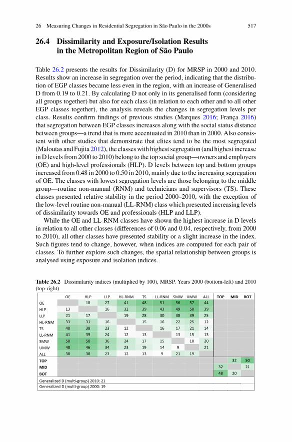
26 Measuring Changes in Residential Segregation in São Paulo in the 2000s 517
26.4 Dissimilarity and Exposure/Isolation Resultsin the Metropolitan Region of São Paulo
Table 26.2 presents the results for Dissimilarity (D) for MRSP in 2000 and 2010.Results show an increase in segregation over the period, indicating that the distribu-tion of EGP classes became less even in the region, with an increase of GeneralisedD from 0.19 to 0.21. By calculating D not only in its generalised form (consideringall groups together) but also for each class (in relation to each other and to all otherEGP classes together), the analysis reveals the changes in segregation levels perclass. Results confirm findings of previous studies (Marques 2016; França 2016)that segregation between EGP classes increases along with the social status distancebetween groups—a trend that is more accentuated in 2010 than in 2000. Also consis-tent with other studies that demonstrate that elites tend to be the most segregated(Maloutas andFujita 2012), the classeswith highest segregation (and highest increaseinD levels from 2000 to 2010) belong to the top social group—owners and employers(OE) and high-level professionals (HLP). D levels between top and bottom groupsincreased from 0.48 in 2000 to 0.50 in 2010, mainly due to the increasing segregationof OE. The classes with lowest segregation levels are those belonging to the middlegroup—routine non-manual (RNM) and technicians and supervisors (TS). Theseclasses presented relative stability in the period 2000–2010, with the exception ofthe low-level routine non-manual (LL-RNM) class which presented increasing levelsof dissimilarity towards OE and professionals (HLP and LLP).
While the OE and LL-RNM classes have shown the highest increase in D levelsin relation to all other classes (differences of 0.06 and 0.04, respectively, from 2000to 2010), all other classes have presented stability or a slight increase in the index.Such figures tend to change, however, when indices are computed for each pair ofclasses. To further explore such changes, the spatial relationship between groups isanalysed using exposure and isolation indices.
Table 26.2 Dissimilarity indices (multiplied by 100), MRSP. Years 2000 (bottom-left) and 2010(top-right)
OE HLP LLP HL-RNM TS LL-RNM SMW UMW ALL TOP MID BOT OE 18 27 41 48 51 56 57 44 HLP 13 16 32 39 43 49 50 39 LLP 21 17 19 28 30 38 39 25 HL-RNM 33 31 16 15 16 22 25 12 TS 40 38 23 12 16 17 21 14 LL-RNM 41 39 24 12 13 13 15 13 SMW 50 50 36 24 17 15 10 20 UMW 48 46 34 23 19 14 9 21 ALL 38 38 23 12 13 9 21 19 TOP 32 50MID 32 21BOT 48 20
Generalized D (mul -group) 2010: 21 Generalized D (mul -group) 2000: 19
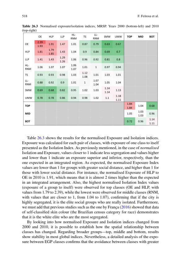
518 F. Feitosa et al.
Table 26.3 Normalised exposure/isolation indices, MRSP. Years 2000 (bottom-left) and 2010(top-right)
OE HLP LLP HL-RNM TS LL-
RNM SMW UMW TOP MID BOT
OE 2.39
1.91 1.47 1.01 0.87 0.79 0.63 0.67 1.93
HLP 1.81 1.79
1.43 1.04 0.9 0.84 0.69 0.7 1.85
LLP 1.41 1.43 1.29
1.06 0.96 0.92 0.81 0.8 1.26
HL-RNM 1.06 1.07 1.07
1.06 1.01 1 0.97 0.94
1.07
TS 0.93 0.93 0.98 1.03 1.12
1.01 1.03 1.01 1.08
LL-RNM 0.88 0.92 0.9 1.01 1
1.07 1.05 1.04
1.04
SMW 0.69 0.68 0.82 0.95 1.02 1.03 1.14
1.13 1.14
UMW 0.78 0.78 0.86 0.94 0.98 1.02 1.1 1.18 1.11
TOP 1.84
1.04 0.68 1.84
MID 1.05 1.03
0.96 1.03
BOT 0.72 0.96 1.14 1.11
Table 26.3 shows the results for the normalised Exposure and Isolation indices.Exposure was calculated for each pair of classes, with exposure of one class to itselfpresented as the Isolation Index. As previously mentioned, in the case of normalisedIsolation and Exposure, values closer to 1 indicate less segregation and values higherand lower than 1 indicate an exposure superior and inferior, respectively, than theone expected in an integrated region. As expected, the normalised Exposure Indexvalues are lower than 1 for groups with greater social distance, and higher than 1 forthose with lower social distance. For instance, the normalised Exposure of HLP toOE in 2010 is 1.91, which means that it is almost 2 times higher than the expectedin an integrated arrangement. Also, the highest normalised Isolation Index values(exposure of a group to itself) were observed for top classes (OE and HLP, withvalues from 1.79 to 2.39), while the lowest were observed for middle classes (RNM,with values that are closer to 1, from 1.04 to 1.07), confirming that if the city ishighly segregated, it is the elite social groups who are really isolated. Furthermore,we must add that previous studies such as the one by França (2016) showed that dataof self-classified skin colour (the Brazilian census category for race) demonstratesthat it is the white elite who are the most segregated.
By looking into how normalised Exposure and Isolation indices changed from2000 and 2010, it is possible to establish how the spatial relationship betweenclasses has changed. Regarding broader groups—top, middle and bottom, resultsshow stability in most global indices. Nevertheless, a detailed analysis of the expo-sure between EGP classes confirms that the avoidance between classes with greater
26 Measuring Changes in Residential Segregation in São Paulo in the 2000s 519
social distance, which was already high, increased during the analysed period. Theanalysis also shows a tendency of increase in integration between classes with lowersocial distance. Such results lead to the conclusion that, although it is possible toobserve an increase in heterogeneity in certain areas of the MRSP, this is mainlypromoted by a higher exposure of classes with similar levels of status. To illustratesuch trends, some classes deserve special attention. The first is the OE, confirmingresults from previous studies as well as analysis with D. The second is the loweststatus class (unskilled manual workers—UMW), which has also shown interestingchanges in this period.
OE have confirmed their position as the most segregated EGP class. It is alsothe one with the highest increase in segregation levels from 2000 to 2010 (in bothDissimilarity and Exposure/Isolation Indices), showing an increase in normalisedisolation from 1.93 to 2.39. OE’s levels of isolation are followed closely by HLP.Results for 2000 and 2010 showan increase in exposure between occupational classeswith higher status (OE, HLP and LLP) and a decrease in their exposure to middle andbottom groups, in particular to UMW. UMW presented a slight increase in isolationlevels from2000 to 2010.Meanwhile, results show a decrease in its exposure levels tothe three highest status occupational classes (OE,HLPandLLP), denoting an increasein segregation between UMW and those classes. Nevertheless, UMW’s exposureto bottom- and middle-status classes (except LLP) showed an increase, indicatingfurther integration between groups with lower social distance and, therefore, a higherheterogeneity of peripheral areas.
The least segregated classes, with normalised isolation and exposure figures closerto 1, are the middle ones, with the exception of low-level professionals (LLP), whichpresented high levels of isolation. The LLP also became more exposed to OE andless exposed to bottom classes (especially UMW).
Despite the relative stability of global indices computed for the broader groups(top, middle and bottom), maps of the local exposure of the bottom group to others(top, middle and bottom—the latter is an isolationmap) for 2000 and 2010 (Fig. 26.6)indicates some changes in residential patterns. Themaps show evidence of a decreasein exposure of top and middle groups to the bottom group in the central areas of theMRSP, reinforcing the conclusion that bottom classes have decreased their presencein central areas. Figure 26.6a, b show the local exposure of bottom to top group.While the overall spatial pattern remains essentially the same, these maps show anincrease in exposure of bottom to top group in some peripheral areas of the map(circled). In addition, the normalised global exposure value has decreased by 0.04(Exposure 2000 = 0.72/2010 = 0.68) and the maps show a decrease in exposurein the expanded centre of São Paulo. This suggests that although the top group hasclearly expanded residentially, this process did not promote further exposure withthe bottom group. This is mainly because the top group’s areas of expansion are notcharacterised by the presence of the bottom group.
Figure 26.6c, d show the local exposure of bottom to middle group. Similarlyto Fig. 26.6a, b, the overall structure remains the same but it is possible to observea decrease in exposure in the central area (expanded centre) and new peripheralareas of high exposure in the outskirts. It is important to note that the normalised
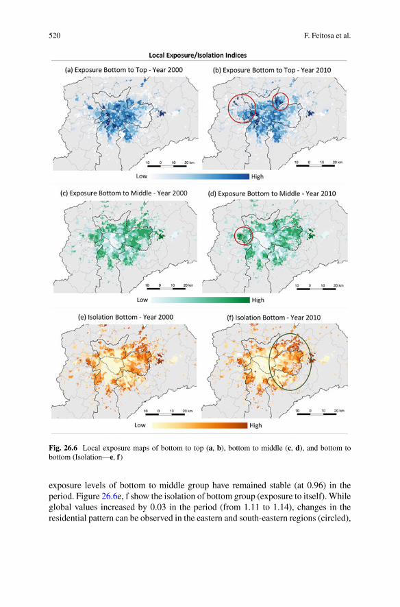
520 F. Feitosa et al.
Fig. 26.6 Local exposure maps of bottom to top (a, b), bottom to middle (c, d), and bottom tobottom (Isolation—e, f)
exposure levels of bottom to middle group have remained stable (at 0.96) in theperiod. Figure 26.6e, f show the isolation of bottom group (exposure to itself). Whileglobal values increased by 0.03 in the period (from 1.11 to 1.14), changes in theresidential pattern can be observed in the eastern and south-eastern regions (circled),
26 Measuring Changes in Residential Segregation in São Paulo in the 2000s 521
where the most peripheral areas presented an increase in the levels of isolation, whilethe opposite was observed in the areas located closer to the centre.
26.5 Discussion and Conclusions
This chapter is built on findings from previous studies regarding segregation in theMetropolitan Region of São Paulo. It explores the spatial relationship between socio-occupational groups using isolation and exposure indices. The analysis confirmeda highly segregated distribution of social groups in the Metropolitan Region andrevealed increased levels of segregation, with global indices figures for 2010 higherthan for 2000. Following previous studies, higher status classes presented the highestlevels of segregation amongst all EGP classes. Spatially, there is evidence that theexpanded centre of São Paulo has become further appropriated by the elite, with areduced presence of bottom classes. The study also demonstrated that the higheststatus classes are the most segregated in both 2000 and 2010 (OE, HLP and LLP,with OE in the leading position) and revealed the following most segregated groupis the lowest status class (UMW).
It is clear from the results that the MRSP peripheral areas have become morefragmented and heterogeneous in this period, confirming findings of previous studies.The analysis revealed that the increased heterogeneity of MRSP’s peripheral areas ismainly composed by classes with close social proximity, rather than polarised ones.While there is evidence of an increase in exposure areas of bottom to top classes inspecific locations, those are not significant. This points to another important findingthat high-income gated communities located side by side of low-income informalsettlements are the exception, rather than the rule, in the peripheral areas of theMRSP. In fact, results showed that while middle classes got more integrated amongstthemselves and with bottom classes, the separation between bottom and top classeswas not only maintained but also increased during the period. All these findingssuggest a reconfiguration of the concentric pattern of segregation that maintained aspatial structure of strong social isolation during the period, although with greatercomplexity.
It is important to reflect on the meaning of those findings and the fact that topclasses are more segregated than bottom classes, which is coincident with findingsin other cities. Results showed that the top groups have, indeed, a clear dynamic ofavoidance to the bottom group, although they are more segregated from other socialgroups, but not from amenities and opportunities (an aspect not addressed by theanalysis). The bottom groups, in addition to being significantly segregated to othergroups, are also located in areas with poor services and at great distances of ameni-ties, services and opportunities. This fact is at the heart of the segregation problemin the MRSP, as well as Brazil and Latin America. While the lack of integrationbetween social groups is concerning, in more pragmatic terms the issue is how resi-dential segregation matches the spatial pattern of urban opportunities; the locking-inprocesses of the bottom groups into certain areas and their poor access to services
522 F. Feitosa et al.
reproduce urban inequality. As such, for the increasingly segregated elite, segrega-tion means monopolizing opportunities, with important consequences to inequalityreproduction.
It is important to highlight that the period studied coincided with a phase ofeconomic growth and decreasing inequalities in Brazil, which since 2014 has beensubstantially reverted. The heterogeneity of the peripheral areas is likely a productof such economic growth with possible links to social mobility, but the structureof segregation tends to remain the same. There have been no studies on segrega-tion measurements looking beyond 2010, mainly due to lack of data availability.Nevertheless, considering that residential location choices are deeply influenced byeconomic power, it is expected that segregation will increase in the future.
This chapter has demonstrated that economic growth and decreasing inequali-ties did not translate into the alleviation of segregation problems in the MRSP. Assuch, further action is required to tackle residential segregation in Brazil. Segre-gation is often understood as a mere spatial expression of social inequalities, butit is actually produced by several processes related to space production, in whichpublic policies play an important role. There is a strong need for better financed andbolder urban policies, particularly concerning housing policies and land-use regula-tion. As demonstrated by this study, those are also required in periods of growth andincreasing equality. The effects of the current and future instability of the countryon segregation remain to be measured. It is clear that without active and continuouspolicies, segregation will not only remain as one of the larger trends in Braziliancities, but might be further aggravated.
References
ArretcheM (ed) (2019) Paths of inequality in Brazil: a half-century of changes. Springer, NewYorkBonduki N, Rolnik R (1982) Periferia da Grande São Paulo: reprodução do espaço como expedientede reprodução da força de trabalho”. In: Maricato E (ed) A Produção Capitalista da Casa (e dacidade) do Brasil Industrial. Alfa-ômega, São Paulo
BriggsX (2005) Social capital and segregation in theUnited States. In: VaradyD (ed) Desegregatingthe city. Suny Press, Albany
Caldeira T (2016) Peripheral urbanization: autoconstruction, transversal logics, and politics in citiesof the global south. Environ Plan D Soc Space 35(1):3–20
Caldeira T (2000) City of walls. University of California Berkeley, BerkeleyCEM (2014) Diagnóstico dos assentamentos precários nos municípios da MacrometrópolePaulista. Centro de Estudos da Metrópoole/Emplasa. https://centrodametropole.fflch.usp.br/pt-br/pesquisa/assentamentos-precarios-2013
Duncan O, Duncan B (1955) A methodological analysis of segregation indexes. Am Sociol Rev20:210. https://doi.org/10.2307/2088328
Erikson R, Goldthorpe JH, Portocarero L (1979) Intergenerational class mobility in three WesternEuropean societies: England, France and Sweden. Br J Sociol 30:415. https://doi.org/10.2307/589632
Feitosa FF, Câmara G, Monteiro AMV, Koschitzki T, Silva MPS (2007) Global and local spatialindices of urban segregation. Int J Geogr Inf Sci 21:299–323. https://doi.org/10.1080/13658810600911903
26 Measuring Changes in Residential Segregation in São Paulo in the 2000s 523
França D (2016) Segregation by class and race in São Paulo. In: Marques E (ed) São Paulo in thetwenty-first century spaces, heterogeneities, inequalities. Routledge, New York
Góes C, Karpowicz I (2017) Inequality in Brazil: a regional perspective. IMF working paperWP/17/225
IBGE (2019) Síntese de indicadores sociais. IBGE, Rio de Janeiro. https://www.ibge.gov.br/estatisticas-novoportal/sociais/populacao/9221-sintese-de-indicadores-sociais.html
Jannuzzi P (2016) Pobreza, Desigualdade e Mudança Social: trajetória no Brasil recente (1992 a2014). 10(3). Políticas Sociais na América Latina
Kowarick L (1979) Espoliação urbana. Paz e Terra, Rio de JaneiroLieberson S (1980) An asymmetrical approach to measuring residential segregation. Centre forUrban and Community Studies, University of Toronto, Toronto
Maloutas T, Fujita K (eds) (2012) Residential segregation in comparative perspective. Ashgate,London
Marques E, Saraiva C (2017) Urban integration or reconfigured inequalities? Analyzing housingprecarity in São Paulo, Brazil. Habit Int 69:18–26
Marques E (2016) São Paulo in the twenty-first century spaces, heterogeneities, inequalities.Routledge, New York
Marques E, Bichir R, Scalon C (2012) Residential segregation and social structure in São Paulo:continuity and change since the 1990s. In: Maloutas T, Fujita K (eds) Residential segregationaround the world: why context matters. Ashgate, London
Massey D, Denton N (1993) American apartheid: segregation and the making of the underclass.Harvard Univ. Press, Cambridge, MA
Preteceille E, Cardoso A (2008) Rio de Janeiro y São Paulo: ciudades duales? Comparación conParis. Ciudad y Território XL(158): 617–640
Reardon SF, O’Sullivan D (2004) Measures of spatial segregation. Sociol Methodol 34:121–162Sakoda J (1981) A generalized index of dissimilarity. Demography 18:245. https://doi.org/10.2307/2061096
Silva N (1999) Mobilidade social. In: Miceli S (ed) Sociologia 2: O que Ler na Ciência SocialBrasileira (1970-1995). Editora Sumaré, São Paulo
Valladares L, Preteceille E (2000) Favela, favelas: unidade ou diversidade da favela carioca”.In: Queiroz L (ed) O futuro das metrópoles: desigualdades e governabilidade. Rio de Janeiro,Observatório/Ed. Revan
WilsonW (1987) The truly disadvantage: the inner city, the underclass and public policy. UniversityChicago Press
Open Access This chapter is licensed under the terms of the Creative Commons Attribution 4.0International License (http://creativecommons.org/licenses/by/4.0/), which permits use, sharing,adaptation, distribution and reproduction in any medium or format, as long as you give appropriatecredit to the original author(s) and the source, provide a link to the Creative Commons license andindicate if changes were made.
The images or other third party material in this chapter are included in the chapter’s CreativeCommons license, unless indicated otherwise in a credit line to the material. If material is notincluded in the chapter’s Creative Commons license and your intended use is not permitted bystatutory regulation or exceeds the permitted use, you will need to obtain permission directly fromthe copyright holder.
Correction to: Income Inequality,Socio-Economic Status, and ResidentialSegregation in Greater Cairo: 1986–2006
Abdelbaseer A. Mohamed and David Stanek
Correction to:Chapter 3 in: M. van Ham et al. (eds.),Urban Socio-Economic Segregation and Income Inequality,The Urban Book Series,https://doi.org/10.1007/978-3-030-64569-4_3
The original version of the book was published with incorrect figure 3.3. The chapterand book have been updated with the changes.
The updated version of this chapter can be found athttps://doi.org/10.1007/978-3-030-64569-4_3
© The Author(s) 2021M. van Ham et al. (eds.), Urban Socio-Economic Segregation and Income Inequality,The Urban Book Series, https://doi.org/10.1007/978-3-030-64569-4_27
C1
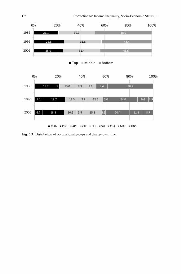
C2 Correction to: Income Inequality, Socio-Economic Status, …
25.0
25.8
21.1
31.4
31.8
30.9
43.6
42.4
48.0
0% 20% 40% 60% 80% 100%
2006
1996
1986
Top Middle Bo om
6.7
7.1
19.2
18.3
18.7
1.8
10.6
11.5
13.0
5.5
7.9
8.3
15.3
12.5
9.6
3.3
5.0
9.4
20.4
24.0
38.7
11.3
9.4
8.7
3.9
0% 20% 40% 60% 80% 100%
2006
1996
1986
MAN PRO APR CLE SER SKI CRA MAC UNS
Fig. 3.3 Distribution of occupational groups and change over time


![Complexitat i fenomen (socio)lingüístic [Complexity and (socio)linguistic phenomenon]](https://static.fdokumen.com/doc/165x107/63130623c32ab5e46f0c3b37/complexitat-i-fenomen-sociolingueistic-complexity-and-sociolinguistic-phenomenon.jpg)