lable at ScienceDirect

Estuarine, Coastal and Shelf Science 83 (2009) 379–391

Contents lists avai

Estuarine, Coastal and Shelf Science

journal homepage: www.elsevier .com/locate/ecss

Sediment segregation by biodiffusing bivalves

F. Montserrat a,b,*, C. Van Colen c, P. Provoost b, M. Milla b, M. Ponti d, K. Van den Meersche b,c,T. Ysebaert b,e, P.M.J. Herman b

a Delft University of Technology, Faculty of Civil engineering and Geosciences, Hydraulics Section, P.O. Box 5048, 2600 GA Delft, The Netherlandsb Netherlands Institute of Ecology, Centre for Estuarine and Marine Ecology, Korringaweg 7, 4401 NT, Yerseke, The Netherlandsc Ghent University, Marine Biology Department, Krijgslaan 281 – S8, B-9000, Ghent, Belgiumd Centro Interdipartimentale di Ricerca per le Scienze Ambientali in Ravenna (CIRSA), University of Bologna, Via S. Alberto 163, 48100 Ravenna, Italye Wageningen IMARES, P.O. Box 77, 4400 AB Yerseke, The Netherlands

a r t i c l e i n f o

Article history:Received 4 February 2009Accepted 3 April 2009Available online 18 April 2009

Keywords:intertidalcohesivesedimentsandmuderosiondepositionluminophoresimage analysisbioturbationecosystem engineering

* Corresponding author. Netherlands Institute of Eand Marine Ecology, Korringaweg 7, 4401 NT, Yerseke

E-mail address: f.montserrat@nioo.knaw.nl (F. Mo

0272-7714/$ – see front matter � 2009 Elsevier Ltd.doi:10.1016/j.ecss.2009.04.010

a b s t r a c t

The selective processing of sediment fractions (sand and mud; >63 mm and �63 mm median grain size)by macrofauna was assessed using two size classes of inert, UV-fluorescent sediment fraction tracers(luminophores). The luminophores were applied to the sediment surface in 16 m2 replicated plots,defaunated and control, and left to be reworked by infauna for 32 days. As the macrofaunal assemblagein the ambient sediment and the control plots was dominated by the common cockle Cerastoderma edule,this species was used in an additional mesocosm experiment. The diversity, abundance and biomass ofthe defaunated macrobenthic assemblage did not return to control values within the experimentalperiod. Both erosion threshold and bed elevation increased in the defaunated plots as a response to theabsence of macrofauna and an increase in microphytobenthos growth. In the absence of macrobenthos,we observed an accretion of 7 mm sediment, containing ca. 60% mud. Image analysis of the verticaldistribution of the different luminophore size classes showed that the cockles preferentially mobilisedfine material from the sediment, thereby rendering it less muddy and effectively increasing the sand:-mud ratio. Luminophore profiles and budgets of the mesocosm experiment under ‘‘no waves–no current’’conditions support the field data very well.

� 2009 Elsevier Ltd. All rights reserved.

1. Introduction

Intertidal soft sediments are governed in their dynamics (e.g.erosion, deposition, transport) by both physical and biologicalprocesses (Borsje et al., 2008; Daborn et al., 1993; Nowell et al.,1981; Rhoads, 1974). Intertidal sediments consist of a mixture ofgravel, sand and mud. Mud (<63 mm), in turn, consists of a mixtureof silt (quartz powder) and clay where for a particular estuarinesystem, the ratio between silt and clay is constant and in accor-dance with the specific hydrodynamic energy conditions (Flem-ming, 2000). A sediment matrix built up of coarse sedimentparticles (sand and gravel) in contact with each other displaysa granular behaviour. Gradually increasing the mud content of sucha matrix will cause the interstitial spaces to be filled up and thesand particles to lose contact with each other. Once the matrix is

cology, Centre for Estuarine, The Netherlands.

ntserrat).

All rights reserved.

dominated by mud instead of by sand particles, the sedimentbehaviour will change from non-cohesive to cohesive; the sedi-ment will behave less granular and more like a firm gel (Van Led-den, 2003; Winterwerp and Van Kesteren, 2004). As mud (clay)strongly influences mechanical properties like the cohesiveness ofthe sediment and thus erosive behaviour (Dade et al., 1992;Mitchener and Torfs, 1996; Van Ledden et al., 2004), coastal andestuarine sediment transport and morphology can differ withdifferent mud contents.

Besides being ca. two orders of magnitude smaller than sand,clay particles are not spherical but consist of layered platelets. Theirshape and size give them a high specific surface area and an elec-trical charge which interacts with ambient (water and organic)molecules and other particles (Winterwerp and Van Kesteren,2004). The sediment mud content is therefore positively correlatedwith organic matter (OM) content (Hedges and Keil, 1995) andrespiration and mineralisation rates (Aller, 1994), but also withother biogeochemical characteristics such as the capacity to bindheavy metals and other pollutants (Bouezmarni and Wollast, 2005).In sediment beds dominated by mud, cohesive forces between the

F. Montserrat et al. / Estuarine, Coastal and Shelf Science 83 (2009) 379–391380

particles are dominant as sand and silt particles are captured ina clay–water matrix.

In coastal lagoons, estuaries and tidal basins, the main physicaldrivers for sediment mud content are hydrodynamic energygradients (Oost, 1995; Van Ledden, 2003). Classical hydrodynamicmodels which treat sand-mud segregation in coastal areas do notincorporate biological processes (Van Ledden, 2003). Even the mostrecent state-of-the-art morphodynamic models which recognisethat small-scale benthic biologically-mediated processes reflect inlarge-scale sediment dynamics, have a grid size in the order of kmand a sub-grid level in the order of 200–800 m (Borsje et al., 2008).Unless averaged over the grid cells, these models cannot accountfor small- to mid-scale biological processes which can cause sharpboundaries between sandy and muddy areas in nature and createa patchy intertidal landscape (Van De Koppel et al., 2001).

Benthic animals can change the sediments’ erodability auto-genically (i.e. by their own physical structures; Luckenbach, 1986;Montserrat et al., 2008; Van Duren et al., 2006) or allogenically (i.e.bioturbation; Andersen et al., 2002; Rhoads and Young, 1970;Willows et al., 1998). Also, by modifying the composition (i.e. thesand:mud ratio), organisms can alter the sediments’ geomechanicalproperties like cohesiveness and erosion threshold (Le Hir et al.,2007; Winterwerp and Van Kesteren, 2004). For example, bio-deposition is a process in which suspension-feeding fauna capturefine sediment fractions from the water column and deposit themnearby as (pseudo)faeces (Haven and Morales-Alamo, 1966; Oost,1995). If this material is not immediately resuspended, thesurrounding sediment will become muddier, organically enrichedand more cohesive. Benthic invertebrates are also known to causeincorporation or expulsion of fine sediment fractions throughbioturbation (Volkenborn et al., 2007a), respectively, bioventilationor bioresuspension (De Deckere et al., 2000). Differential process-ing of sediment fractions through bioturbation is a process that canchange the sediment composition and have profound conse-quences for its biogeochemistry (Volkenborn et al., 2007b).

In order to study bioturbation processes numerous tracertechniques have been developed over the last three decades (Maireet al., 2008), including the use of phaeopigment concentrationprofiles (Gerino et al., 1998), radionuclides (Andersen et al., 2000;Mulsow et al., 2002; Sandnes et al., 2000; Wheatcroft and Martin,1996), inert fluorescent sediment tracers called luminophores(Gerino, 1990; Mahaut and Graf, 1987) and even silver and gold(Wheatcroft et al., 1994). Especially the use of luminophores hastaken a flight in bioturbation studies. Here, luminophores are usedto model and quantify vertical particle transport and to estimatebiodiffusion coefficients (Db) of both single species (Duport et al.,2006; Maire et al., 2007) and of multi-species communities (Duportet al., 2007; Gilbert et al., 2007). The luminophores have beenapplied in frozen ‘‘cakes’’ or as a layer either at the sedimentsurface, at a certain depth or both (Caradec et al., 2004) to distin-guish between transport directions. Solan et al. (2004) combinedthe use of luminophores with an in situ time-lapse sediment profilecamera, obtaining a series of cross-sectional images of the sedimentin which both the reworking of tracer and natural benthic activitywere captured. In all abovementioned cases only one size class ofluminophore was used. To our knowledge and as mentioned ina review by Maire et al. (2008), there have been no studies in whichtwo or more size classes of luminophores were deployed to studyparticular bioturbation processes. Here, we did use two size classesof luminophores, each as a tracer for the sediment fractions mud(<63 mm) and sand (>63 mm and < 2000 mm), to determine selec-tivity between sediment fractions by bioturbating macrofauna.

The focus of this study is to assess the temporal and spatial scaleof bioturbation of a natural benthic community and one that hasbeen removed. To investigate the net bioturbatory effect of

a intertidal benthic community we used defaunation to exclude theeffect of macrobenthos in situ following the exact same method andspatial scale as was done in Van Colen et al. (2008) and Montserratet al. (2008). Our hypothesis is that the net effect of the macro-faunal assemblage is removing the fine sediment fraction, to yieldless muddy sediment, with a consequent lower erosion threshold.To test our hypothesis, i.e. to detect possible differential processingof sediment fraction tracers and resulting possible changes insand:mud ratio in this field experiment, we used two size classes ofluminophores, each with a different colour, as conservative sedi-ment fraction (mud and sand) tracers.

In addition to the field experiment, we conducted a mesocosmexperiment under controlled conditions, using the same sedimentfraction tracers. In this mesocosm experiment we assessed thebioturbatory effects on sediment fraction segregation of the mostimportant species in terms of biomass in the ambient sediment atthe research site (Van Colen et al., 2008): the common cockleCerastoderma edule Linnaeus (1758).

2. Materials and methods

2.1. Site, defaunation treatment and luminophore application

The experiment was conducted in an intertidal flat area (Pauli-napolder) on the southern shore of the Westerschelde estuary(51�2102400 N and 3�4205100 E; SW Netherlands; Fig. 1a). Within thisarea, four 16 m2 square plots were randomly chosen to be used inthis study (Fig. 1b). Two plots were defaunated by covering thesediment in plastic foil, inducing severe hypoxia, for a period of 94days. After this period, the plastic foil was cut open at the sedimentsurface, referred to as day 0. A vertical subsurface lining of plasticfoil was left intact to prevent horizontal subsurface immigration ofmacrobenthic infauna. For more information and details about theexact defaunation method see Montserrat et al. (2008) and VanColen et al. (2008). Two other 16 m2 square plots consisted ofuntreated ambient sediment and were used as controls.

The fluorescent sediment tracers used (luminophores, i.e. fluo-rescent dyed thermoplastic polyamide powder, EnvironmentalTracing Systems, UK; http://www.environmentaltracing.com/)were coded ‘‘Magenta’’ and ‘‘UV Blue Mostyn’’ with a median grainsize (D50) of 41 mm and 129 mm, respectively. Overlap between thetwo fraction tracers existed in that the D90 of ‘‘Magenta’’ was 86 mmand the D10 of ‘‘UV Blue Mostyn’’ was 72 mm. Luminophores werevolumetrically mixed in the ambient sand:mud ratio of the sedi-ment and in turn volumetrically mixed 1:1 with sieved (1 mm)ambient sediment. The sediment–tracer mix was poured in plastermoulds of 25� 25� 0.5 cm and frozen at �20 �C to make sediment‘tiles’. At t¼ 0, the frozen tiles were then placed in a square of 2� 2tiles covering 0.25 m2, both in the north-west and in the south-eastcorners, at ca. 1 m from the edges of the experimental plots(Fig. 1c).

2.2. Sampling

The experiment started on 23 May 2005 by opening the plasticsheeting (referred to as t¼ 0, see above). The plots were sampled att¼ 1 h, 1 tide, 3 days, 7 days, 14 days and 32 days. The collectionconsisted of samples taken for luminophore analysis, macro-benthos abundance, macrobenthos biomass, erosion threshold andbed elevation. Samples were taken in quadrant 1 and 3 in each plot(i.e. two replicates per plot; Fig. 1c).

For luminophore sampling, cores made out of 30 cm long PVCpipes with an inner diameter of 36 mm and a wall thickness of2 mm were used. To minimise compaction of the sediment whilepushing down the core, a plunger of a 100 ml syringe was drawn

N

4 m

m 4

4 m

4 m

50 cm

50

cm

1 2

4 3

3.5°E

5 km

North

Sea

Nether-lands

Belgium

Westerschelde

4°E 6°E 4.0°E

51.5°N

51.4°N

51.3°N51°N

N

52°N

53°N

Paulinapolder areaa

b

c

Fig. 1. (a) The geographic position of the research site within the polyhaline part of the Westerschelde estuary, SW Netherlands. (b) Schematic representation of the defaunated(dark) and control (light) replicated plots. Distance between plots is not to scale. (c) Schematic representation of the placement of the luminophore tiles in (grey) 50� 50 cmsquares.

F. Montserrat et al. / Estuarine, Coastal and Shelf Science 83 (2009) 379–391 381

upwards. Luminophore cores were stored on dry ice (approx.�70 �C) in the field to arrest macrofaunal reworking, taken to thelab and further stored at �20 �C until processing.

Macrofauna was sampled to a depth of 30 cm, using an 11 cminner diameter stainless steel corer. Macrofauna samples weretaken to the lab, sieved over a 1 mm sieve and preserved in a neu-tralised 4% formaldehyde solution with 0.01% Bengal Rose untilprocessing. Macrofaunal biomass was determined according toSistermans et al. (2007) and given in grams ash-free dry mass persquare meter (g AFDM m�2).

The sediment strength, or erosion threshold is taken asa measure of erodability of the sediment under a certain bottomshear, and was measured using a cohesive strength meter Mk III(CSM, Sediment Services, UK; Tolhurst et al., 1999). The measure-ments were performed according to the ‘Mud 6’ programme of theCSM Mk III.

The sediment bed level elevation was measured relative to NAP(¼Normaal Amsterdams Peil; Amsterdam Ordnance Datum, similarto Mean Sea Level) according to Montserrat et al. (2008). Betweenfive and eight replicate measurements were taken per sampled

F. Montserrat et al. / Estuarine, Coastal and Shelf Science 83 (2009) 379–391382

quadrant. Bed level measurements were performed using a rotatinglaser mounted on a tripod (fixed at a point outside the experi-mental area) and a receiving unit on a portable measuring polewith a mm scale. There was evidence of baseline variability in thebed elevation measurements; to correct for this variability, the bedelevation values are given as the difference in elevation� standarddeviation (SD) between the defaunated and the control plots.Assuming there is no covariance between the treatments, the SD forthe difference in bed elevation is calculated according to:

s2defaunated-control ¼ s2

defaunated þ s2control

The luminophore cores were taken from within the 0.25 m2 tracerarea (Fig. 1c). All other samples were taken from the adjacentsediment within the experimental plots, max. 30 cm away from theluminophore tiles. To prevent disturbance of the sediment profile,all holes left in the sediment after extraction of the respectivevariables were filled up with PVC tubes of the same diameter andlength, which were closed at one side with duct tape.

2.3. Mesocosm experiment

In the mesocosm experiment, PVC cores (66 mm inner diameter,2 mm wall thickness, 85 mm height) were filled with 1 mm sievedambient sediment, of which half each received one live cockledrawn from a population with shell length 29.47� 2.35 mm(mean� SD) and wet weight 9.64� 2.18 g (mean� SD). Then,a 3 mm thick disc of frozen luminophore/sediment mix(B¼ 66 mm) was placed on top of the sediment in each experi-mental core. We replicated nine times to yield 18 cores in total.One-third, i.e. 3 ‘‘Cockle–No Cockle’’ (C–NC) pairs, was immediatelyfrozen at �20 �C to serve as a t¼ 0 where no sediment reworkingcould have taken place. The remaining six replicates of C–NC pairswere placed within each of the six 8 dm3 mesocosm units. Waveand/or current action generated by the simulated tidal watermovement in the mesocosm units was negligible. After 21 days, themesocosm experiment was terminated by removing all cores fromthe setup and placing them at �80 �C for 1.5 h, after which theywere placed at �20 �C until processed.

2.4. Luminophore image analysis

Both the PVC cores used to extract material from the tracer-enriched sediment surface from the field and the PVC cores used inthe mesocosm experiment were, while still frozen, longitudinallycross-sectioned using a band saw. The frozen smear left by the bandsaw was chafed away using a razor. Every half core was photo-graphed in the light and in the dark under blacklight, using a digitalmirror-reflex camera (Canon EOS 350D with 18–55 mm EFSobjective) mounted on a stand. The images measured 2304� 3456pixels, and were saved using JPEG compression. The area photo-graphed measured 43� 67 mm, resulting in a resolution of18.66 mm� 19.39 mm per pixel. The images were analyzed usingcustom-made Matlab scripts. First, the images were corrected forthe uneven sediment surface. The corrected sediment surface wassuperimposed on the corresponding images taken in the dark, tovertically translate the pixel columns of the image accordingly.Subsequently, discriminant analysis was used to classify all pixelsinto one of the classes ‘‘red luminophores’’ (i.e. mud fractionmimic), ‘‘blue luminophores’’ (i.e. sand fraction mimic) or ‘‘back-ground’’ (i.e. ambient sediment), based on their brightness valuesin the red, green and blue bands (each between 0 and 255). Atraining set was composed by manually selecting pixels pertainingto each of the three classes. The classification outcome was verifiedby comparing false-colour and original images. Finally, the number

of pixels belonging to the different classes was determined for eachpixel row.

2.5. Data analysis

All field results were analysed according to a Complete Rando-mised (CR) experimental design. We performed generalised linearmodelling analysis of variance (GLM-ANOVA) to test for differencesbetween time (i.e. sampling occasions), treatments, plots and, inthe case of bed level measurements, quadrants. To ensure normaldistribution of the residuals, visual inspection of Normal P-plotswas performed. Macrofauna data were (xþ 1)0.25 transformed inthe case of abundance and ln(xþ 1) transformed in the case ofbiomass (Quinn and Keough, 2002).

The general linear model (GLM) for macrofauna (both forabundance and biomass) included Time and Treatment as separatefixed factors and Plot nested in Treatment with Plot as a randomfactor, plus the interaction terms Time� Treatment and Time� Plotnested in Treatment. The GLM for erosion threshold included Time,Treatment, Plot nested in Treatment and the interaction termTime� Treatment. Containing an extra source of variation, the GLMfor bed level elevation included Time, Treatment, Quadrant nestedin Plot nested in Treatment and the interactions terms Time -� Treatment and Time�Quadrant nested in Plot nested in Treat-ment. Analyses on luminophore budgets from the field experimentwere done using analysis of covariance (ANCOVA), with treatmentas a covariate. Analyses of the sediment budgets from the labexperiment were done using a full-factorial ANOVA with Time,Treatment and Fraction, including all interaction terms as factors.All data analyses have been performed using R: a language andenvironment for statistical computing (R Development Core Team,2007; Vienna, Austria; http://www.R-project.org).

3. Results

3.1. Field experiment – general observations

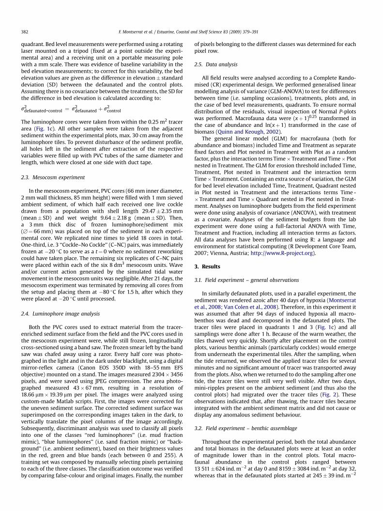
In similarly defaunated plots, used in a parallel experiment, thesediment was rendered azoic after 40 days of hypoxia (Montserratet al., 2008; Van Colen et al., 2008). Therefore, in this experiment itwas assumed that after 94 days of induced hypoxia all macro-benthos was dead and decomposed in the defaunated plots. Thetracer tiles were placed in quadrants 1 and 3 (Fig. 1c) and allsamplings were done after 1 h. Because of the warm weather, thetiles thawed very quickly. Shortly after placement on the controlplots, various benthic animals (particularly cockles) would emergefrom underneath the experimental tiles. After the sampling, whenthe tide returned, we observed the applied tracer tiles for severalminutes and no significant amount of tracer was transported awayfrom the plots. Also, when we returned to do the sampling after onetide, the tracer tiles were still very well visible. After two days,mini-ripples present on the ambient sediment (and thus also thecontrol plots) had migrated over the tracer tiles (Fig. 2). Theseobservations indicated that, after thawing, the tracer tiles becameintegrated with the ambient sediment matrix and did not cause ordisplay any anomalous sediment behaviour.

3.2. Field experiment – benthic assemblage

Throughout the experimental period, both the total abundanceand total biomass in the defaunated plots were at least an orderof magnitude lower than in the control plots. Total macro-faunal abundance in the control plots ranged between13 511�624 ind. m�2 at day 0 and 8159� 3084 ind. m�2 at day 32,whereas that in the defaunated plots started at 245� 39 ind. m�2

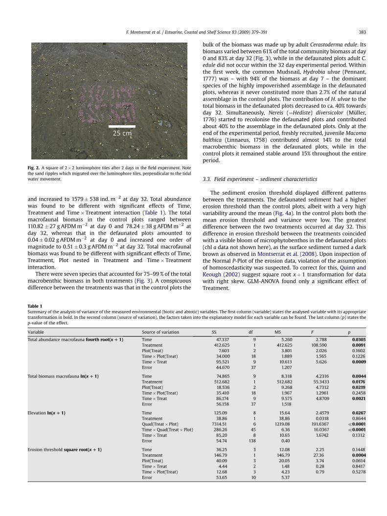
Fig. 2. A square of 2� 2 luminophore tiles after 2 days in the field experiment. Notethe sand ripples which migrated over the luminophore tiles, perpendicular to the tidalwater movement.

F. Montserrat et al. / Estuarine, Coastal and Shelf Science 83 (2009) 379–391 383

and increased to 1579� 538 ind. m�2 at day 32. Total abundancewas found to be different with significant effects of Time,Treatment and Time� Treatment interaction (Table 1). The totalmacrofaunal biomass in the control plots ranged between110.82� 27 g AFDM m�2 at day 0 and 78.24� 38 g AFDM m�2 atday 32, whereas that in the defaunated plots amounted to0.04� 0.02 g AFDM m�2 at day 0 and increased one order ofmagnitude to 0.51�0.3 g AFDM m�2 at day 32. Total macrofaunalbiomass was found to be different with significant effects of Time,Treatment, Plot nested in Treatment and Time� Treatmentinteraction.

There were seven species that accounted for 75–99 % of the totalmacrobenthic biomass in both treatments (Fig. 3). A conspicuousdifference between the treatments was that in the control plots the

Table 1Summary of the analysis of variance of the measured environmental (biotic and abiotic) vtransformation in bold. In the second column (source of variation), the factors taken intop-value of the effect.

Variable Source of variation

Total abundance macrofauna fourth root(x D 1) TimeTreatmentPlot(Treat)Time� Plot(Treat)Time� TreatError

Total biomass macrofauna ln(x D 1) TimeTreatmentPlot(Treat)Time� Plot(Treat)Time� TreatError

Elevation ln(x D 1) TimeTreatmentQuad(Treat� Plot)Time�Quad(Treat� Plot)Time� TreatError

Erosion threshold square root(x D 1) TimeTreatmentPlot(Treat)Time� TreatTime� Plot(Treat)Error

bulk of the biomass was made up by adult Cerastoderma edule. Itsbiomass varied between 61% of the total community biomass at day0 and 83% at day 32 (Fig. 3), while in the defaunated plots adult C.edule did not occur within the 32 day experimental period. Withinthe first week, the common Mudsnail, Hydrobia ulvae (Pennant,1777) was – with 94% of the biomass at day 7 – the dominantspecies of the highly impoverished assemblage in the defaunatedplots, whereas it never constituted more than 2.7% of the naturalassemblage in the control plots. The contribution of H. ulvae to thetotal biomass in the defaunated plots decreased to ca. 40% towardsday 32. Simultaneously, Nereis (¼Hediste) diversicolor (Muller,1776) started to recolonise the defaunated plots and contributedabout 40% to the assemblage in the defaunated plots. Only at theend of the experimental period, freshly recruited, juvenile Macomabalthica (Linnaeus, 1758) contributed almost 14% to the totalmacrobenthic biomass in the defaunated plots, while in thecontrol plots it remained stable around 15% throughout the entireperiod.

3.3. Field experiment – sediment characteristics

The sediment erosion threshold displayed different patternsbetween the treatments. The defaunated sediment had a highererosion threshold than the control plots, albeit with a very highvariability around the mean (Fig. 4a). In the control plots both themean erosion threshold and variance were low. The greatestdifference between the two treatments occurred at day 32. Thisdifference in erosion threshold between the treatments coincidedwith a visible bloom of microphytobenthos in the defaunated plots(chl a data not shown here), as the surface sediment turned a darkbrown as observed in Montserrat et al. (2008). Upon inspection ofthe Normal P-Plot of the erosion data, violation of the assumptionof homoscedasticity was suspected. To correct for this, Quinn andKeough (2002) suggest square root xþ 1 transformation for datawith right skew. GLM-ANOVA found only a significant effect ofTreatment.

ariables. The first column (variable) states the analysed variable with its appropriatethe explanatory model for each variable can be found. The last column (p) states the

SS df MS F p

47.337 9 5.260 2.788 0.0305412.625 1 412.625 108.590 0.0091

7.603 2 3.801 2.026 0.160234.000 18 1.889 1.565 0.122695.521 9 10.613 5.626 0.000944.670 37 1.207

74.865 9 8.318 4.2316 0.0044512.682 1 512.682 55.3433 0.0176

18.536 2 9.268 4.7312 0.021935.410 18 1.967 1.2961 0.245886.174 9 9.575 4.8709 0.002156.158 37 1.518

125.09 8 15.64 2.4579 0.026738.86 1 38.86 0.0318 0.8644

7314.51 6 1219.08 191.6367 �0.0001286.26 45 6.36 16.0367 �0.0001

85.20 8 10.65 1.6742 0.131254.74 138 0.40

36.25 3 12.08 2.25 0.1448146.79 1 146.79 27.36 0.0004

40.09 3 20.05 3.74 0.06144.44 2 1.48 0.28 0.8417

12.68 3 4.23 0.79 0.527853.65 10 5.37

0 10 20 30 40

0

20

40

60

80

100

120

time (days)

ero

sio

n th

resh

old

(kP

a)

ControlDefaunated

2

l)

values are mean elevation difference +/- stdev

a

b

0 5 10 20 30

0

20

40

60

80

100

Control

time (days)

percen

tag

e b

io

mass (%

)

0 5 10 20 30

0

20

40

60

80

100

Defaunated

time (days)

percen

tag

e b

io

mass (%

)

S. planaP. elegans

N. diversicolorM. balthicaH. ulvaeH. filiformisC. edule

Fig. 3. The relative contribution to the total biomass in both treatments of the seven most abundant species. In the right hand panel (defaunated) there is a minor contribution of(juvenile) C. edule at the end of the experimental period and no contribution of Scrobicularia plana.

F. Montserrat et al. / Estuarine, Coastal and Shelf Science 83 (2009) 379–391384

The sediment bed level elevation relative to NAP of the defau-nated plots started somewhat lower than the control plots. Fromday 7 onwards, the bed level of the defaunated plots started to rise.At the same time a decrease in the bed level of the control plots wasobserved (ANCOVA: p¼ 0.0072 and p¼ 0.0179, respectively;Multiple r2¼ 0.4174). The difference in elevation of the defaunatedplots increased to 4.2 mm above the control plots on day 32(Fig. 4b). As the Normal P-Plot of the elevation data did not showany evidence of heteroscedasticity, the data were not transformed.There were significant effects for the factors Time, Quadrant nestedin Treatment nested in Plot and Time�Quadrant nested in Treat-ment nested in Plot interaction, but not for Treatment or forTime� Treatment interaction. We explicitly refer to Table 1 for allresults of the statistical analyses of abovementioned macrobenthosand sediment parameters.

On day 7, ca. 2 mm of material had accreted on top of the sedi-ment in the defaunated plots (Fig. 5a and b). The accretion occurredin a linear fashion (linear regression: slope¼ 0.19 mm day�1,p¼ 0.0021, multiple r2¼ 0.9254), reaching approximately 7 mm atday 32. The percentage of mud in the accreted material (Fig. 5c) alsoincreased linearly, reaching around 60% at day 32, although thisincrease was not statistically significant (linear regression:slope¼ 0.36% day�1, p¼ 0.0587, Multiple r2¼ 0.3127). At the sametime in a parallel experiment, the top 1 cm of the ambient sedimentcontained 45% mud and similarly defaunated sediment containedca. 50% mud (Montserrat et al., 2008).

0 10 20 30 40

-2

-1

0

1

time (days)

elevatio

n (cm

+

C

on

tro

Fig. 4. (a) The mean� SEM eroding pressure (measured with CSM Mk IV) in bothtreatments as a function of time. (b) The mean� SD elevation difference of thedefaunated plots, compared to the controls, in cm.

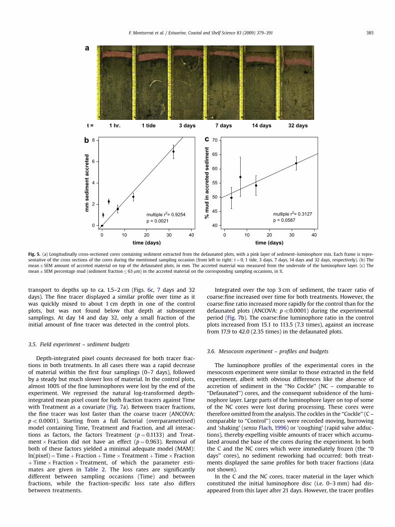
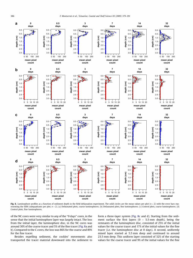
3.4. Field experiment – luminophore profiles

The vertical profiles of the luminophores are shown inFig. 6a–d. In the case of both the coarse and the fine tracer in thedefaunated plots, we observed a subsidence of the layer ofluminophores which is in effect the burial of the layer byaccreted sediment (see above). The peak of the pixel count overthe vertical can be seen to be gradually moving downwards(Fig. 6a and b). For both fractions of tracers within the defaunatedplots, we clearly observed a loss of material over time. In one ofthe two control plots, a small amount of the coarse tracer(Fig. 6c) was already found at 1–1.5 cm depth after 1 h (0 days,first panel). At day 3, a slight diffusion of the luminophore layerto approx. 1 cm can be seen, but by day 7 and onwards, a rapidloss of material had occurred. Apart from the advection–diffusiontransport processes, we did observe some non-local vertical

t = 1 hr. 1 tide 3 days 7 days 14 days 32 days

0

2

4

6

8b

a

c

mm

sed

im

en

t accreted

0 10 20 30 40 0 10 20 30 40

40

45

50

55

60

65

70

time (days) time (days)

% m

ud

in

accreted

sed

im

en

t

multiple r2= 0.9254p = 0.0021

multiple r2= 0.3127p = 0.0587

Fig. 5. (a) Longitudinally cross-sectioned cores containing sediment extracted from the defaunated plots, with a pink layer of sediment–luminophore mix. Each frame is repre-sentative of the cross sections of the cores during the mentioned sampling occasion (from left to right: t¼ 0, 1 tide, 3 days, 7 days, 14 days and 32 days, respectively). (b) Themean� SEM amount of accreted material on top of the defaunated plots, in mm. The accreted material was measured from the underside of the luminophore layer. (c) Themean� SEM percentage mud (sediment fraction� 63 mm) in the accreted material on the corresponding sampling occasions, in %.

F. Montserrat et al. / Estuarine, Coastal and Shelf Science 83 (2009) 379–391 385

transport to depths up to ca. 1.5–2 cm (Figs. 6c, 7 days and 32days). The fine tracer displayed a similar profile over time as itwas quickly mixed to about 1 cm depth in one of the controlplots, but was not found below that depth at subsequentsamplings. At day 14 and day 32, only a small fraction of theinitial amount of fine tracer was detected in the control plots.

3.5. Field experiment – sediment budgets

Depth-integrated pixel counts decreased for both tracer frac-tions in both treatments. In all cases there was a rapid decreaseof material within the first four samplings (0–7 days), followedby a steady but much slower loss of material. In the control plots,almost 100% of the fine luminophores were lost by the end of theexperiment. We regressed the natural log-transformed depth-integrated mean pixel count for both fraction tracers against Timewith Treatment as a covariate (Fig. 7a). Between tracer fractions,the fine tracer was lost faster than the coarse tracer (ANCOVA:p� 0.0001). Starting from a full factorial (overparametrised)model containing Time, Treatment and Fraction, and all interac-tions as factors, the factors Treatment (p¼ 0.1133) and Treat-ment� Fraction did not have an effect (p¼ 0.963). Removal ofboth of these factors yielded a minimal adequate model (MAM):ln(pixel)¼ Timeþ FractionþTime� Treatmentþ Time� Fractionþ Time� Fraction�Treatment, of which the parameter esti-mates are given in Table 2. The loss rates are significantlydifferent between sampling occasions (Time) and betweenfractions, while the fraction-specific loss rate also differsbetween treatments.

Integrated over the top 3 cm of sediment, the tracer ratio ofcoarse:fine increased over time for both treatments. However, thecoarse:fine ratio increased more rapidly for the control than for thedefaunated plots (ANCOVA: p�0.0001) during the experimentalperiod (Fig. 7b). The coarse:fine luminophore ratio in the controlplots increased from 15.1 to 113.5 (7.3 times), against an increasefrom 17.9 to 42.0 (2.35 times) in the defaunated plots.

3.6. Mesocosm experiment – profiles and budgets

The luminophore profiles of the experimental cores in themesocosm experiment were similar to those extracted in the fieldexperiment, albeit with obvious differences like the absence ofaccretion of sediment in the ‘‘No Cockle’’ (NC – comparable to‘‘Defaunated’’) cores, and the consequent subsidence of the lumi-nophore layer. Large parts of the luminophore layer on top of someof the NC cores were lost during processing. These cores weretherefore omitted from the analysis. The cockles in the ‘‘Cockle’’ (C –comparable to ‘‘Control’’) cores were recorded moving, burrowingand ‘shaking’ (sensu Flach, 1996) or ‘coughing’ (rapid valve adduc-tions), thereby expelling visible amounts of tracer which accumu-lated around the base of the cores during the experiment. In boththe C and the NC cores which were immediately frozen (the ‘‘0days’’ cores), no sediment reworking had occurred: both treat-ments displayed the same profiles for both tracer fractions (datanot shown).

In the C and the NC cores, tracer material in the layer whichconstituted the initial luminophore disc (i.e. 0–3 mm) had dis-appeared from this layer after 21 days. However, the tracer profiles

0 50 150 250

3.0

2.5

2.0

1.5

1.0

0.5

0.0

a

b

c

d

0

days

mean pixel

count

mean pixel

count

mean pixel

count

mean pixel

count

mean pixel

count

mean pixel

count

mean pixel

count

mean pixel

count

mean pixel

count

mean pixel

count

mean pixel

count

mean pixel

count

mean pixel

count

mean pixel

count

mean pixel

count

mean pixel

count

mean pixel

count

mean pixel

count

mean pixel

count

dep

th

(cm

)

0 50 150 250

3.0

2.5

2.0

1.5

1.0

0.5

0.0

0.5

days

mean pixel

count

dep

th

(cm

)

0 50 150 250

3.0

2.5

2.0

1.5

1.0

0.5

0.0

3

days

mean pixel

count

mean pixel

count

mean pixel

count

mean pixel

count

dep

th

(cm

)

0 50 150 250

3.0

2.5

2.0

1.5

1.0

0.5

0.0

7

days

dep

th

(cm

)

dep

th

(cm

)

dep

th

(cm

)d

ep

th

(cm

)

dep

th

(cm

)

dep

th

(cm

)

dep

th

(cm

)

dep

th

(cm

)

dep

th

(cm

)d

ep

th

(cm

)

dep

th

(cm

)

dep

th

(cm

)

dep

th

(cm

)d

ep

th

(cm

)

dep

th

(cm

)

dep

th

(cm

)d

ep

th

(cm

)

dep

th

(cm

)

dep

th

(cm

)

dep

th

(cm

)

dep

th

(cm

)

0 50 150 250

3.0

2.5

2.0

1.5

1.0

0.5

0.0

14

days

0 50 150 250

3.0

2.5

2.0

1.5

1.0

0.5

0.0

32

days

0 5 10 15 20

3.0

2.5

2.0

1.5

1.0

0.5

0.0

0

days

0 5 10 15 20

3.0

2.5

2.0

1.5

1.0

0.5

0.0

0.5

days

0 5 10 15 20

3.0

2.5

2.0

1.5

1.0

0.5

0.0

3

days

0 5 10 15 20

3.0

2.5

2.0

1.5

1.0

0.5

0.0

7

days

0 5 10 15 20

3.0

2.5

2.0

1.5

1.0

0.5

0.0

14

days

0 5 10 15 20

3.0

2.5

2.0

1.5

1.0

0.5

0.0

32

days

0 50 150 250

3.0

2.5

2.0

1.5

1.0

0.5

0.0

0

days

0 50 150 250

3.0

2.5

2.0

1.5

1.0

0.5

0.0

0.5

days

0 50 150 250

3.0

2.5

2.0

1.5

1.0

0.5

0.0

3

days

0 50 150 250

3.0

2.5

2.0

1.5

1.0

0.5

0.0

7

days

0 50 150 250

3.0

2.5

2.0

1.5

1.0

0.5

0.0

14

days

0 50 150 250

3.0

2.5

2.0

1.5

1.0

0.5

0.0

32

days

0 5 10 15 20

3.0

2.5

2.0

1.5

1.0

0.5

0.0

0

days

0 5 10 15 20

3.0

2.5

2.0

1.5

1.0

0.5

0.0

0.5

days

0 5 10 15 20

3.0

2.5

2.0

1.5

1.0

0.5

0.0

3

days

0 5 10 15 20

3.0

2.5

2.0

1.5

1.0

0.5

0.0

7

days

0 5 10 15 20

3.0

2.5

2.0

1.5

1.0

0.5

0.0

14

days

0 5 10 15 20

3.0

2.5

2.0

1.5

1.0

0.5

0.0

32

days

Fig. 6. Luminophore profiles as a function of sediment depth in the field defaunation experiment. The solid circles are the mean values per plot (n¼ 2) with the error bars rep-resenting the SEM (subquadrants per plot, n¼ 2). (a) Defaunated plots, coarse luminophores. (b) Defaunated plots, fine luminophores. (c) Control plots, coarse luminophores. (d)Control plots, fine luminophores.

F. Montserrat et al. / Estuarine, Coastal and Shelf Science 83 (2009) 379–391386

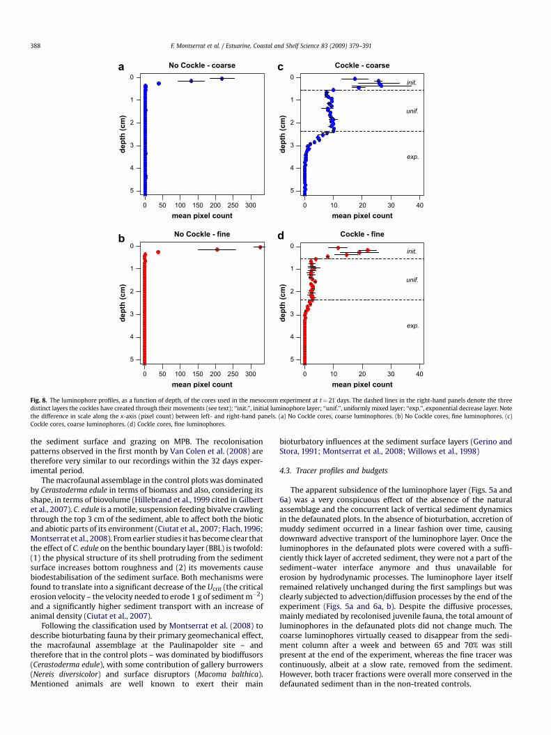
of the NC cores were very similar to any of the ‘‘0 days’’ cores, in thesense that the initial luminophore layer was largely intact. The lossfrom the initial layer, the luminophore disc, in the NC cores wasaround 30% of the coarse tracer and 5% of the fine tracer (Fig. 8a andb). Compared to the C cores, the loss was 86% for the coarse and 89%for the fine tracer.

Besides expelling sediment, the cockles’ movements alsotransported the tracer material downward into the sediment to

form a three-layer system (Fig. 8c and d). Starting from the sedi-ment surface the first layers (0 – 5.5 mm depth), being theremnants of the luminophore disc, consisted of 25% of the initialvalues for the coarse tracer and 17% of the initial values for the finetracer (i.e. the luminophore disc at 0 days). A second, uniformlymixed layer started at 5.5 mm deep and continued to around23.5 mm deep. This uniform layer consisted of 32% of the startingvalues for the coarse tracer and 9% of the initial values for the fine

0

1

2

3

4

5

6

7

a b

Defaunated coarseControl coarseDefaunated fineControl fine 0

20

40

60

80

100

120

140

0 10 20 30 40

luminophore loss rate

time (days)

lo

g(p

ixel co

un

t)

0 10 20 30 40

coarse : fine ratio

time (days)

co

arse : fin

e ratio

ControlDefaunated

Fig. 7. The luminophore loss rate as a function of time. The y-axis denotes the natural log-transformed pixel count for the coarse luminophores (triangles) and for the fineluminophores (circles). The open symbols and the dashed lines represent the values and linear regression for the control plots, the solid black symbols and solid black linesrepresent the values and linear regression for the defaunated plots. The ratio of coarse: fine luminophores as a function of time. The open symbols and the dashed line represent thevalues and linear regression for the control plots, the solid black symbols and solid black line represent the values and linear regression for the defaunated plots.

F. Montserrat et al. / Estuarine, Coastal and Shelf Science 83 (2009) 379–391 387

tracer. Below this uniform layer, the amount of tracer fractionsdecreased exponentially as a function of sediment depth. Thepercentage of initial coarse tracer found in these deeper layers was7%, against 1% of initial fine tracer.

In both the C and the NC cores we observed a decrease of tracermaterial from the sediment column as a whole during the experi-mental period. In the NC cores there was a decrease of 29% of coarsetracer and a 4% decrease of fine tracer (Table 3). In the C cores, werecorded a 37% decrease of coarse tracer and a 73% decrease of finetracer material.

ANOVA (Time, Treatment and Fraction as factors, full factorialdesign) showed highly significant effects of Time, Treatment andTime� Treatment interaction (p� 0.0001, p� 0.0001, p¼ 0.0007,respectively), but no significant effect of either the factor Fractionor the Time� Fraction interaction (p¼ 0.0915, p¼ 0.6791, respec-tively). The Time� Treatment interaction and the Time -� Treatment� Fraction interaction both had a significant effect(p¼ 0.0002 and p¼ 0.0018, respectively). The resultant coarse:fineratio decreased slightly between 0 and 21 days in the NC cores,whereas in the C cores, it increased almost two and a half times(Table 3).

Table 2Parameter estimates and their respective standard errors for the minimal adequatemodel (MAM) obtained by analysis of covariance (ANCOVA) of the natural logarithmtransformed luminophore fraction-specific pixel count for both treatments. See textfor explanation on the ANCOVA and model derivation.

Parameter Estimate Std. Error p

Intercept 3.767 0.096 �0.0001Time �0.119 0.008 �0.0001Fraction 2.903 0.136 �0.0001Time� Treatment 0.091 0.01 �0.0001Time� Fraction 0.058 0.012 �0.0001Time� Treatment� Fraction �0.033 0.014 0.0311

4. Discussion

4.1. Luminophore use in bioturbation experiments

The two different luminophore size classes have proven to bevery good visual tracers for bioturbation processes in the sediment.Both the direct profile-imaging as well as the budgeting of bothfractions in the sediment column yielded valuable results and haveimproved our understanding on how benthic macrofauna caninduce differential processing of sediment fractions, and its neteffect on local vertical grain size distribution. Also, the luminophorelayer in the defaunated plots enabled us to observe both gross andnet effects of the absence of bioturbation; the actual amount andcomposition of accreted material on top of the layer could bemeasured directly.

The reported overlap in size distributions between the twoluminophore types can be avoided by sieving them before appli-cation. We have not sieved the fractions due to logistical

constraints, but in this case the overlap most probably reflected thenatural situations where smaller particles can coagulate into largerflocs. Nevertheless, the use of two sizes of luminophores has beenvery successful in determining selectivity between sediment sizefractions.

4.2. Macrobenthic assemblage

The defaunation treatment was very successful in the sense thatwe succeeded to create two very different macrofaunal assem-blages with their respective bioturbatory effects to be studied.Within the experimental period of 32 days both the total macro-faunal density and the total macrofaunal biomass in the defaunatedplots did not reach control levels, indicating that recolonisation hasnot reached its end-stage during the course of the experiment. Ina parallel defaunation experiment in the same area both Van Colenet al. (2008) and Montserrat et al. (2008) described a rapid increaseof microphytobenthos biomass (MPB; chl a data not shown here)and a quick but temporary recolonisation of mobile species, like themudsnail Hydrobia ulvae, within the first month, whereas deeperburrowing macrofauna arrived only after two to three months.

Besides the mudsnail, the tellinid Macoma balthica and thepolychaetes Nereis diversicolor and Heteromastus filiformis alsocolonised the defaunated plots in this study, but as these were alljuvenile individuals – given their low biomass – their contributionto bioturbation processes within the experimental period can beconsidered marginal. H. ulvae is a highly mobile species, able tocover large distances (Andersen et al., 2002) while crawling over

0 50 100 150 200 250 300

5

4

3

2

1

0a c

db

No Cockle - coarse

mean pixel count

dep

th

(cm

)

0 10 20 30 40

5

4

3

2

1

0

Cockle - coarse

mean pixel count

dep

th

(cm

)

init.

unif.

exp.

0 50 100 150 200 250 300

5

4

3

2

1

0

No Cockle - fine

mean pixel count

dep

th

(cm

)

0 10 20 30 40

5

4

3

2

1

0

Cockle - fine

mean pixel count

dep

th

(cm

)

init.

unif.

exp.

Fig. 8. The luminophore profiles, as a function of depth, of the cores used in the mesocosm experiment at t¼ 21 days. The dashed lines in the right-hand panels denote the threedistinct layers the cockles have created through their movements (see text); ‘‘init.’’, initial luminophore layer; ‘‘unif.’’, uniformly mixed layer; ‘‘exp.’’, exponential decrease layer. Notethe difference in scale along the x-axis (pixel count) between left- and right-hand panels. (a) No Cockle cores, coarse luminophores. (b) No Cockle cores, fine luminophores. (c)Cockle cores, coarse luminophores. (d) Cockle cores, fine luminophores.

F. Montserrat et al. / Estuarine, Coastal and Shelf Science 83 (2009) 379–391388

the sediment surface and grazing on MPB. The recolonisationpatterns observed in the first month by Van Colen et al. (2008) aretherefore very similar to our recordings within the 32 days exper-imental period.

The macrofaunal assemblage in the control plots was dominatedby Cerastoderma edule in terms of biomass and also, considering itsshape, in terms of biovolume (Hillebrand et al., 1999 cited in Gilbertet al., 2007). C. edule is a motile, suspension feeding bivalve crawlingthrough the top 3 cm of the sediment, able to affect both the bioticand abiotic parts of its environment (Ciutat et al., 2007; Flach, 1996;Montserrat et al., 2008). From earlier studies it has become clear thatthe effect of C. edule on the benthic boundary layer (BBL) is twofold:(1) the physical structure of its shell protruding from the sedimentsurface increases bottom roughness and (2) its movements causebiodestabilisation of the sediment surface. Both mechanisms werefound to translate into a significant decrease of the Ucrit (the criticalerosion velocity – the velocity needed to erode 1 g of sediment m�2)and a significantly higher sediment transport with an increase ofanimal density (Ciutat et al., 2007).

Following the classification used by Montserrat et al. (2008) todescribe bioturbating fauna by their primary geomechanical effect,the macrofaunal assemblage at the Paulinapolder site – andtherefore that in the control plots – was dominated by biodiffusors(Cerastoderma edule), with some contribution of gallery burrowers(Nereis diversicolor) and surface disruptors (Macoma balthica).Mentioned animals are well known to exert their main

bioturbatory influences at the sediment surface layers (Gerino andStora, 1991; Montserrat et al., 2008; Willows et al., 1998)

4.3. Tracer profiles and budgets

The apparent subsidence of the luminophore layer (Figs. 5a and6a) was a very conspicuous effect of the absence of the naturalassemblage and the concurrent lack of vertical sediment dynamicsin the defaunated plots. In the absence of bioturbation, accretion ofmuddy sediment occurred in a linear fashion over time, causingdownward advective transport of the luminophore layer. Once theluminophores in the defaunated plots were covered with a suffi-ciently thick layer of accreted sediment, they were not a part of thesediment–water interface anymore and thus unavailable forerosion by hydrodynamic processes. The luminophore layer itselfremained relatively unchanged during the first samplings but wasclearly subjected to advection/diffusion processes by the end of theexperiment (Figs. 5a and 6a, b). Despite the diffusive processes,mainly mediated by recolonised juvenile fauna, the total amount ofluminophores in the defaunated plots did not change much. Thecoarse luminophores virtually ceased to disappear from the sedi-ment column after a week and between 65 and 70% was stillpresent at the end of the experiment, whereas the fine tracer wascontinuously, albeit at a slow rate, removed from the sediment.However, both tracer fractions were overall more conserved in thedefaunated sediment than in the non-treated controls.

Table 3Depth-integrated luminophore fraction-specific mean� SEM pixel counts for bothtreatments (NC and C) on both t¼ 0 days and t¼ 21 days. The coarse:fine lumino-phore ratio is stated in italics.

0 Days 21 Dayscoarse Fine Ratio coarse Fine Ratio

No Cockle (NC) 561� 6 599� 6 0.94 400� 4 575� 6 0.70Cockle (C) 504� 5 479� 5 1.05 320� 1 129� 1 2.48

F. Montserrat et al. / Estuarine, Coastal and Shelf Science 83 (2009) 379–391 389

In the control plots, the natural macrofaunal assemblage quicklyreworked the tracers and relocated a portion to deeper sedimentlayers. Within the control treatment, there was some variation inthe vertical distribution of the tracers between the two plots(Fig. 6c: 0 days [¼1 h], 7 days and 32 days). This spatial variability intracer distribution can be attributed to species known to beresponsible for non-local transport, mainly Macoma balthica(Gingras et al., 2008; Michaud et al., 2006) and Nereis diversicolor(Duport et al., 2006; Fernandes et al., 2006). Lateral heterogeneityin bioturbation, which occurs typically over short time scales(Maire et al., 2007), may explain why the variation is found only inone plot or only during one sampling occasion.

4.4. Differential tracer processing

In the absence of macrofaunal bioturbators in the field experi-ment, there was accretion of mud, stabilisation of the accretedmaterial and the sediment surface (Montserrat et al., 2008) andconsequent subduction of the sediment tracers. In the controlsediment we observed differential incorporation and processing ofboth tracer fractions. The data of these luminophore profiles couldbe used for estimating a biodiffusion coefficient (Db) as a measureof sediment reworking rate at the community level. Howeveruseful, the use of biodiffusion models to estimate Db should only beapplied on larger spatial scales and, more important, longertemporal scales (Meysman et al., 2008a, b). The 32 days-lastingfield experiment was simply too short of a period.

The presence of benthic animals in both the field and themesocosm experiments caused differential incorporation of lumi-nophores into the sediment but, more importantly, also a qualita-tively high rate of resuspension. This resulted in the short-term lossof a significant amount of the luminophores. Even in the defau-nated plots, there was loss of fine luminophores, but at a muchlower rate than in the presence of a natural assemblage. The resultsfrom the field experiment are moreover well supported by the datafrom the mesocosm experiment. There was a significant higher lossof fine luminophores from the mesocosm cores, while still a highpercentage of the coarse luminophores were retained, resulting inan increased coarse:fine ratio. We have shown here that the maineffect of both the cockle-dominated natural assemblage and thecockles in the mesocosm experiment is selective removal of finematerial from the sediment surface layers.

The selective removal of fines can be accomplished by thecharacteristic moving through the surface sediment layers or by thesudden adduction of the valves (respectively ‘ploughing’ and‘shaking’) (Flach, 1996). Although Cerastoderma edule tends to haveits natural abundance peak in fine to medium sands (Ysebaert et al.,2002), it does not directly utilise the bottom sediment and istherefore not dependent on its composition. However, cockles arenegatively influenced by higher suspended sediment concentra-tions (SSC) to which they respond with a higher shaking frequencyto get rid of fine material that clogs their gills (Ciutat et al., 2007).

We observed the shaking in the mesocosm experiment whenthe cockles were burrowing into the sediment as the water levelreceded. First, the agile foot was inserted into the sediment ina manner as described for crack propagation by burrowing marine

polychaetes (Dorgan et al., 2005). The cockle then slowly opened itsshell valves and adducted them quickly. In doing so, it forced thewater from its mantle cavity and created a small body of fluidisedsediment (quicksand) beneath its shell and, at almost the samemoment, pulled itself down into the sediment with its foot. Thiswas repeated until the cockle is burrowed beneath the sedimentsurface and only its siphons are visible. In nature, the burrowingbehaviour of cockles causes sediment to become resuspended(more than is already caused by waves or valve adductions) ofwhich the coarse fractions settle relatively fast. The fine fractionswill be transported away by the overlying water, and might becaptured from the water column by diatom mats (Austen et al.,1999; De Brouwer et al., 2003), vegetation (Bouma et al., 2005),reef-forming suspension feeders (Haven and Morales-Alamo, 1966)or dense aggregates of tubeworms (Montserrat et al., 2008).

4.5. Ecosystem engineering effects

Using the luminophore coarse:fine ratio as a proxy for thesediment sand:mud ratio, the cockle-dominated benthic assem-blage’s main effect was to render the sediment less muddy. Thecontrol sediment was characterised by a significantly highererodability, compared to the situation without benthic fauna, inwhich net accretion of mud occurred. An increase in mud content,and the fact that it was not homogeneously mixed into the sedi-ment by infauna as in a natural situation, can induce a local changein ecosystem functioning of the sediment through known biogeo-chemical cascades. First of all, a higher mud content entails a higherorganic matter (OM) content with concomitant higher respirationrates (Aller and Aller, 1998). Secondly, the increased mud contentdecreases the permeability of the sediment and flow of pore water,decreasing the oxygen penetration depth (Winterwerp and VanKesteren, 2004). Thirdly, a higher mud content will cause benthicprimary production and standing stocks to increase (Van De Koppelet al., 2001). These profound changes would in turn reflect on theentire benthic community (micro-, meio- and macro-) and couldhave possibly set back the system to an earlier successional state(Connell and Slatyer, 1977; Pearson and Rosenberg, 1978; Van Colenet al., 2008).

Thrush et al. (2006) demonstrated the important structuringrole of large surface-dwelling, suspension-feeding bivalves in thebiogeochemistry and makeup of the macrobenthic assemblage inintertidal systems. Volkenborn et al. (2007b) attribute similarmechanisms to the lugworm Arenicola marina in the GermanWadden Sea. A. marina is a model ecosystem engineer and has allthe characteristics of a climax species: a long-lived, slow-growing,deep-burrowing, sediment-regenerating bioturbator (Riisgård andBanta, 1998), able to inhibit the settlement of other (pioneer)species (Flach, 1992) and even plants (Van Wesenbeeck et al., 2007).The physical restructuring of the bottom by its bioturbationincreases the bottom roughness and resuspension of fine material,keeping the intertidal areas it inhabits more sandy (Volkenbornet al., 2007a). The influence A. marina exerts on the entire spectrumwithin the intertidal (grain size distribution – pore water flow –bacterial community – micro-/meio-/macrobenthos) enables it tomaintain its habitat in a preferred state, which can abruptly changewhen it is excluded (Van De Koppel et al., 2001; Volkenborn et al.,2007a). The cockles in our experiment appear to fulfil a similar rolein this particular system, including the inhibition of opportunistpioneer species (Bolam and Fernandes, 2003) and physicalecosystem engineering, through mechanical disturbance of thesediment.

The absence of the cockle-dominated assemblage in thedefaunated plots made it clear that these animals and theirbehaviour can cause large differences in sediment behaviour

F. Montserrat et al. / Estuarine, Coastal and Shelf Science 83 (2009) 379–391390

(Montserrat et al., 2008). As demonstrated in this study, the sedi-ment erosion threshold during the first month was much higher inthe defaunated plots than in the control plots. Although the sedi-ment bed level of the defaunated plots increased slightly due toaccumulation of muddy material, the difference was much lesspronounced compared to a difference in the order of cm, observedin a parallel study by Montserrat et al. (2008). This can beunequivocally attributed to the fact that the recruitment peak oftube-building spionids, particularly Pygospio elegans (Claparede,1863), did not occur due to the later initiation (i.e. opening of theplots) and the overall shorter duration of the experiment in thispaper.

The lower abundance of grazing and mechanically disturbingfauna in the defaunated plots enabled MPB to form dense mats(Montserrat et al., 2008) which armour the sediment and canentrain mud. Constituting an important part of the macrobenthicassemblage, and backed up by the mesocosm experiment results,Cerastoderma edule was responsible for a large part of the bio-turbatory effects in this system. This study has demonstrated thatthe burrowing and ploughing behaviour of these biodiffusingbivalves, often dominant species in intertidal sediments world-wide, is keeping the sediment matrix in a less muddy state – andtherefore less organically enriched and less cohesive – by removingfine material from the sediment through an interaction of organismtraits and hydrodynamic forcing.

5. Conclusions

(1) As true ecosystem engineers, cockles strongly shape their bioticand abiotic environment through a diverse array of effectswhich are specifically not trophic interactions, but are exertedvia the environment.

(2) The presence of a healthy, fully developed macrofaunalcommunity has a net erosive effect on muddy intertidal sedi-ment. The net effect of the cockle-dominated macrofaunalassemblage, as well as the cockles in the mesocosm experi-ment, is mobilising surface sediment, resulting in a lowersediment erosion threshold.

(3) The burrowing behaviour of the cockles causes selectiveremoval of fine material from the surface sediment, resulting ina shift in the sand:mud ratio. This shift can cause the sedimentto become less cohesive, changing its erosion behaviour,biogeochemistry and ultimately its ecosystem functioning.

Acknowledgements

The authors would like thank Jos van Soelen, Bas Koutstaal andthe masters’ students who helped during the fieldwork and theprocessing of the samples for their efforts. Jon Marsh and severalmembers of the team at Environmental Tracing Services helped uswith advice on how to apply and process the luminophores, forwhich they have our thanks. This research is supported by theDutch Technology Foundation STW, applied sciences division ofNWO and the Technology Program of the Ministry of EconomicAffairs. This is NIOO publication no. 4529.

References

Aller, R.C., 1994. Bioturbation and remineralization of sedimentary organic-matter –effects of redox oscillation. Chemical Geology 114, 331–345.

Aller, R.C., Aller, J.Y., 1998. The effect of biogenic irrigation intensity and soluteexchange on diagenetic reaction rates in marine sediments. Journal of MarineResearch 56, 905–936.

Andersen, T.J., Jensen, K.T., Lund-Hansen, L., Mouritsen, K.N., Pejrup, M., 2002.Enhanced erodibility of fine-grained marine sediments by Hydrobia ulvae.Journal of Sea Research 48, 51–58.

Andersen, T.J., Mikkelsen, O.A., Moller, A.L., Pejrup, M., 2000. Deposition and mixingdepths on some European intertidal mudflats based on Pb-210 and Cs-137activities. Continental Shelf Research 20, 1569–1591.

Austen, I., Andersen, T.J., Edelvang, K., 1999. The influence of benthic diatoms andinvertebrates on the erodibility of an intertidal a mudflat, the Danish WaddenSea. Estuarine, Coastal and Shelf Science 49, 99–111.

Bolam, S.G., Fernandes, T.F., 2003. Dense aggregations of Pygospio elegans (Clapar-ede) effect on macrofaunal community structure and sediments. Journal of SeaResearch 49, 171–185.

Borsje, B.W., De Vries, M.B., Huscher, S., De Boer, G.J., 2008. Modeling large-scalecohesive sediment transport affected by small-scale biological activity. Estua-rine, Coastal and Shelf Science 78, 468–480.

Bouezmarni, M., Wollast, R., 2005. Geochemical composition of sediments in theScheldt estuary with emphasis on trace metals. Hydrobiologia 540, 155–168.

Bouma, T.J., et al., 2005. Flow hydrodynamics on a mudflat and in salt marshvegetation: identifying general relationships for habitat characterisations.Hydrobiologia 540, 259–274.

Caradec, S., Grossi, V., Hulth, S., Stora, G., Gilbert, F., 2004. Macrofaunal reworkingactivities and hydrocarbon redistribution in an experimental sediment system.Journal of Sea Research 52, 199–210.

Ciutat, A, Widdows, J., Pope, N.D., 2007. Effect of Cerastoderma edule density onnear-bed hydrodynamics and stability of cohesive muddy sediments. Journal ofExperimental Marine Biology and Ecology 346, 114–126.

Connell, J.H., Slatyer, R.O., 1977. Mechanisms of succession in natural communitiesand their role in community stability and organization. American Naturalist 111,1119–1144.

Daborn, G.R., et al., 1993. An ecological cascade effect – migratory birds affectstability of intertidal sediments. Limnology and Oceanography 38, 225–231.

Dade, W.B., Nowell, A.R.M., Jumars, P.A., 1992. Predicting erosion resistance of muds.Marine Geology 105, 285–297.

De Brouwer, J.F.C., Neu, T.R., Stal, L.J., 2003. On the function of secretion of extra-cellular polymeric substances by benthic diatoms and their role in intertidalmudflats: a review of recent insights and views, p. 45–61. In: Kromkamp, J.C.,De Brouwer, J.F.C., Blanchard, G.F., Forster, R.M., Creach, V. (Eds.), Micro-phytbenthos in Estuaries. Royal Netherlands Academy of Arts & Sciences(KNAW).

De Deckere, E.M.G.T., Van De Koppel, J., Heip, C.H.R., 2000. The influence of Coro-phium volutator abundance on resuspension. Hydrobiologia 426, 37–42.

Dorgan, K.M., Jumars, P.A., Johnson, B., Boudreau, B.P., Landis, E., 2005. Burrowextension by crack propagation. Nature 433, 475.

Duport, E., Gilbert, F., Poggiale, J.C., Dedieu, K., Rabouille, C., Stora, G., 2007. Benthicmacrofauna and sediment reworking quantification in contrasted environ-ments in the Thau Lagoon. Estuarine, Coastal and Shelf Science 72, 522–533.

Duport, E., Stora, G., Tremblay, P., Gilbert, F., 2006. Effects of population density on thesediment mixing induced by the gallery-diffusor Hediste (Nereis) diversicolor O.F.Muller, 1776. Journal of Experimental Marine Biology and Ecology 336, 33–41.

Fernandes, S., Meysman, F.J.R., Sobral, P., 2006. The influence of Cu contaminationon Nereis diversicolor bioturbation. Marine Chemistry 102, 148–158.

Flach, E.C., 1992. Disturbance of benthic infauna by sediment-reworking activities ofthe Lugworm Arenicola-Marina. Netherlands Journal of Sea Research 30, 81–89.

Flach, E.C., 1996. The influence of the cockle, Cerastoderma edule, on the macro-zoobenthic community of tidal flats in the Wadden Sea. Marine Ecology –Pubblicazioni Della Stazione Zoologica di Napoli I 17, 87–98.

Flemming, B.W., 2000. A revised textural classification of gravel-free muddy sedi-ments on the basis of ternary diagrams. Continental Shelf Research 20,1125–1137.

Gerino, M., 1990. The effects of bioturbation on particle redistribution in mediter-ranean coastal sediment – preliminary results. Hydrobiologia 207, 251–258.

Gerino, M., et al., 1998. Comparison of different tracers and methods used toquantify bioturbation during a spring bloom: 234-thorium, luminophores andchlorophyll a. Estuarine, Coastal and Shelf Science 46, 531–547.

Gerino, M., Stora, G., 1991. Invitro quantitative-analysis of the bioturbation inducedby the polychaete Nereis Diversicolor. Comptes Rendus de l Academie desSciences Serie Iii-Sciences de la Vie-Life Sciences 313, 489–494.

Gilbert, F., et al., 2007. Sediment reworking by marine benthic species from theGullmar Fjord (Western Sweden): importance of faunal biovolume. Journal ofExperimental Marine Biology and Ecology 348, 133–144.

Gingras, M.K., Pemberton, S.G., Dashtgard, S., Dafoe, L., 2008. How fast do marineinvertebrates burrow? Palaeogeography, Palaeoclimatology, Palaeoecology 270,280–286.

Haven, D.S., Morales-Alamo, R., 1966. Aspects of biodeposition by oysters and otherinvertebrate filter feeders. Limnology and Oceanography 11, 487.

Hedges, J.I., Keil, R.G., 1995. Sedimentary organic matter preservation: an assess-ment and speculative synthesis. Marine Chemistry 49, 81–115.

Hillebrand, H., Duerselen, C.D., Kirschtel, D., Pollinger, U., Zohary, T., 1999. Bio-volume calculation for pelagic and benthic microalgae. Journal of Phycology 35,403–424.

Le Hir, P., Monbet, Y., Orvain, F., 2007. Sediment erodability in sediment transportmodelling: can we account for biota effects? Continental Shelf Research 27,1116–1142.

Luckenbach, M.W., 1986. Sediment stability around animal tubes: the roles ofhydrodynamic processes and biotic activity. Limnology and Oceanography 31,779–787.

Mahaut, M.L., Graf, G., 1987. A luminophore tracer technique for bioturbationstudies. Oceanologica Acta 10, 323–328.

F. Montserrat et al. / Estuarine, Coastal and Shelf Science 83 (2009) 379–391 391

Maire, O., Duchene, J.C., Gremare, A., Malyuga, V.S., Meysman, F.J.R., 2007. Acomparison of sediment reworking rates by the surface deposit-feeding bivalveAbra ovata during summertime and wintertime, with a comparison betweentwo models of sediment reworking. Journal of Experimental Marine Biologyand Ecology 343, 21–36.

Maire, O., Lecroart, P., Meysman, F., Rosenberg, R., Duchene, J.C., Gremare, A., 2008.Quantification of sediment reworking rates in bioturbation research: a review.Aquatic Biology 2, 219–238.

Meysman, F.J.R., Malyuga, V.S., Boudreau, B.P., Middelburg, J.J., 2008a. A generalizedstochastic approach to particle dispersal in soils and sediments. Geochimica EtCosmochimica Acta 72, 3460–3478.

Meysman, F.J.R., Malyuga, V.S., Boudreau, B.P., Middelburg, J.J., 2008b. Quantifyingparticle dispersal in aquatic sediments at short time scales: model selection.Aquatic Biology 2, 239–254.

Michaud, E., Desrosiers, G., Mermillod-Blondin, F., Sundby, B., Stora, G., 2006. Thefunctional group approach to bioturbation: II. The effects of the Macomabalthica community on fluxes of nutrients and dissolved organic carbon acrossthe sediment–water interface. Journal of Experimental Marine Biology andEcology 337, 178–189.

Mitchener, H., Torfs, H., 1996. Erosion of sand/mud mixtures. Coastal Engineering29, 1–25.

Montserrat, F., Van Colen, C., Degraer, S., Ysebaert, T., Herman, P.M.J., 2008. Benthiccommunity-mediated sediment dynamics. Marine Ecology – Progress Series372, 43–59.

Mulsow, S., Landrum, P.F., Robbins, J.A., 2002. Biological mixing responses to sublethalconcentrations of DDT in sediments by Heteromastus filiformis using a Cs-137marker layer technique. Marine Ecology – Progress Series 239, 181–191.

Nowell, A.R.M., Jumars, P.A., Eckman, J.E., 1981. Effects of biological-activity on theentrainment of marine-sediments. Marine Geology 42, 133–153.

Oost, A.P., 1995. Dynamics and Sedimentary Development of the Dutch Wadden Seawith Emphasis on the Frisian Inlet. Universiteit Utrecht.

Pearson, T.H., Rosenberg, R., 1978. Macrobenthic succession in relation to organicenrichment and pollution of the marine environment. Oceanography andMarine Biology Annual Review 16, 229–311.

Quinn, G.P., Keough, M.J., 2002. In: Experimental Design and Data Analysis forBiologists, first ed. Cambridge University Press.

Rhoads, D.C., 1974. Organism–sediment relations on the muddy sea floor. Ocean-ography and Marine Biology: An Annual Review 12, 263–300.

Rhoads, D.C., Young, D.K., 1970. The Influence of deposit-feeding organisms onsediment stability and community trophic structure. Journal of MarineResearch 28, 150.

Riisgård, H.U., Banta, G.T., 1998. Irrigation and deposit feeding by the lugwormArenicola marina, characteristics and secondary effects on the environment. Areview of current knowledge. Vie et Milieu-Life and Environment 48, 243–257.

Sandnes, J., Forbes, T., Hansen, R., Sandnes, B., Rygg, B., 2000. Bioturbation andirrigation in natural sediments, described by animal-community parameters.Marine Ecology – Progress Series 197, 169–179.

Sistermans, W.C.H., et al., 2007. Het macrobenthos van de Westerschelde, de Oos-terschelde, het Veerse Meer en het Grevelingenmeer in het voor – en najaar van

2006 (in Dutch). KNAW Netherlands Institute of Ecology – Centre for Estuarineand Marine Ecology, p. 133.

Solan, M., et al., 2004. In situ quantification of bioturbation using time-lapse fluo-rescent sediment profile imaging (f-SPI), luminophore tracers and modelsimulation. Marine Ecology – Progress Series 271, 1–12.

Thrush, S.F., Hewitt, J.E., Gibbs, M., Lundquist, C., Norkko, A., 2006. Functional role oflarge organisms in intertidal communities: community effects and ecosystemfunction. Ecosystems 9, 1029–1040.

Tolhurst, T.J., et al., 1999. Measuring the in situ erosion shear stress of intertidalsediments with the cohesive strength meter. Estuarine, Coastal and ShelfScience 49, 281–294.

Van Colen, C., Montserrat, F., Herman, P.M.J., Vincx, M., Ysebaert, T., Degraer, S.,2008. Macrobenthic recovery from hypoxia in an estuarine tidal mudflat.Marine Ecology – Progress Series 372, 31–42.

Van De Koppel, J., Herman, P.M.J., Thoolen, P., Heip, C.H.R., 2001. Do alternate stablestates occur in natural ecosystems? Evidence from a tidal flat. Ecology 82,3449–3461.

Van Duren, L.A., Herman, P.M.J., Sandee, A.J.J., Heip, C.H.R., 2006. Effects of musselfiltering activity on boundary layer structure. Journal of Sea Research 55, 3–14.

Van Ledden, M., 2003. Sand–mud segregation in estuaries and tidal basins.Communications on Hydraulic and Geotechnical Engineering. Delft Universityof Technology.

Van Ledden, M., Van Kesteren, W.G.M., Winterwerp, J.C., 2004. A conceptualframework for the erosion behaviour of sand-mud mixtures. Continental ShelfResearch 24, 1–11.

Van Wesenbeeck, B.K., Van De Koppel, J., Herman, P.M.J., Bakker, J.P., Bouma, T.J.,2007. Biomechanical warfare in ecology; negative interactions between speciesby habitat modification. Oikos 116, 742–750.

Volkenborn, N., Hedtkamp, S.I.C., Van Beusekom, J.E.E., Reise, K., 2007a. Effects ofbioturbation and bioirrigation by lugworms (Arenicola marina) on physical andchemical sediment properties and implications for intertidal habitat succession.Estuarine, Coastal and Shelf Science 74, 331–343.

Volkenborn, N., Polerecky, L., Hedtkamp, S.I.C., Van Beusekom, J.E.E., De Beer, D.,2007b. Bioturbation and bioirrigation extend the open exchange regions inpermeable sediments. Limnology and Oceanography 52, 1898–1909.

Wheatcroft, R.A., Martin, W.R., 1996. Spatial variation in short-term (Th-234)sediment bioturbation intensity along an organic-carbon gradient. Journal ofMarine Research 54, 763–792.

Wheatcroft, R.A., Olmez, I., Pink, F.X., 1994. Particle bioturbation in MassachusettsBay – preliminary-results using a new deliberate tracer technique. Journal ofMarine Research 52, 1129–1150.

Willows, R.I., Widdows, J., Wood, R.G., 1998. Influence of an infaunal bivalve on theerosion of an intertidal cohesive sediment: a flume and modeling study.Limnology and Oceanography 43, 1332–1343.

Winterwerp, J.C., Van Kesteren, W.G.M., 2004. In: Introduction to the Physics ofCohesive Sediment in the Marine Environment, first ed. Elsevier.

Ysebaert, T., Meire, P., Herman, P.M.J., Verbeek, H., 2002. Macrobenthic speciesresponse surfaces along estuarine gradients: prediction by logistic regression.Marine Ecology – Progress Series 225, 79–95.