Segregation Indices and their

Functional Inputs1

Rick Grannis

Cornell University and RAND

January 23, 2002

1 Direct all correspondence to Rick Grannis, Department of Sociology, Cornell

University, Ithaca, NY 14853 (rdg25@cornell.edu).

Functional Inputs

2

Segregation Indices and their Functional Inputs

Multi-Group Indices

Reardon and Firebaugh’s (2002) advocacy of multi-group segregation indices is

an important contribution to the index debate, a debate of central importance to

understanding segregation. Indices guide and circumscribe all comparisons both over

time and between cities, all correlations with other variables, and all classifications (Jahn,

Schmid, and Schrag 1947). More importantly, they operationalize segregation theory

itself and thus circumscribe all substantive understandings. Reardon and Firebaugh’s

(2002) review of multi-group indices highlights the fact that two-group indices have

guided our thinking about segregation.

Indices reduce huge data arrays into simpler, more readily understandable,

numbers. Regardless of the formula one uses to reduce such arrays, the formula itself is

merely a function of those arrays and only those arrays. Before choosing formulas,

segregation researchers need to consider how their choice of inputs guides their

theoretical development. Only when one has correctly determined which variables are

appropriately included in the discussion of segregation can one proceed to develop

indices and build definitions and theories.

Reardon and Firebaugh’s (2002) formula-based criterion for segregation indices

excluded other potentially important multi-group indices. They identified six measures

which they evaluated against desirable properties of segregation indices adapted from

Functional Inputs

3

Schwartz and Winship’s (1980) and James and Taeuber’s (1985) original four criteria:

the principle of transfers, compositional invariance, size invariance, and organizational

equivalence. These criteria, however, concern only the racial populations of each

neighborhood and thus have no meaning for indices that include other variables. In fact,

all of Reardon and Firebaugh’s (2002) multi-group measures can be derived from exactly

the same set of data, a matrix whose rows consist of neighborhoods, whose columns

consist of groups, and whose cell entries consist of the number of persons of the group

represented by the column in the neighborhood represented by the row.

Multi-Dimensional Indices

The distinction of considering multi-group segregation instead of dichotomous

segregation is profound; it involves including new variables in the functions (one for each

additional racial group) or adding new columns to the data matrix being reduced.

However, the decision to include or to exclude other variables such as neighborhood

contiguity, tract area, or proximity to the central city is as fundamental to the

understanding of segregation data as is the choice of whether or not to restrict the

scenario to a majority race and a single minority race or to allow for a multiple-race

scenario. This is the issue of multi-dimensional inputs to segregation indices, and it

reflects the multi-dimensional nature of spatial segregation. This is a topic that Reardon

and Firebaugh (2002) do not address, and it is at least as important as their distinction

between two-group and multi-group segregation.

Functional Inputs

4

Below, I consider some properties of multi-group segregation indices with multi-

dimensional inputs. I show that indices can best be understood in terms of the variables

they are functions of and that accounting for the location of neighborhoods with respect

to each other is as important as analyzing multiple racial groups. I conclude by proposing

a multi-group spatial proximity index.

Indices as Functions

In addition to the racial population of each neighborhood, what other variables

might we consider? In addition to Reardon and Firebaugh’s (2002) six multi-group

indices, Massey and Denton’s (1988) classic survey of segregation indices identified

twenty more distinct formulas used to measure aspects of segregation. We can reduce

these twenty-six indices to a set of simple functions and illustrate them in terms of the

variables they use as inputs to show how our choice of indices defines segregation and

profoundly influences our understanding of this phenomenon2. Table 1 lists the indices3

2 An Appendix, available from the author on request, discusses how analyzing

functional inputs relates to factor analyses.

3 For simplicity’s sake, I use only the generalized version of the Atkinson index.

The three versions of it used by Massey and Denton (1988) are easily derivable by

substitution. I also use only the interaction index, and its distance-decay counterpart.

The isolation index and its distance-decay counterpart are corollaries equaling unity

minus the interaction indices.

Functional Inputs

5

and cites their original appearance in the literature. Table 2 displays their computational

formulas.

Tables 1 and 2 about here

Table 3 lists the indices as functions of the variables4 they use as inputs.

Table 3 about here

Each index is a function of between two and eleven variables. Through inspection alone,

some patterns are obvious and algebra makes numerous other patterns apparent. Table 4

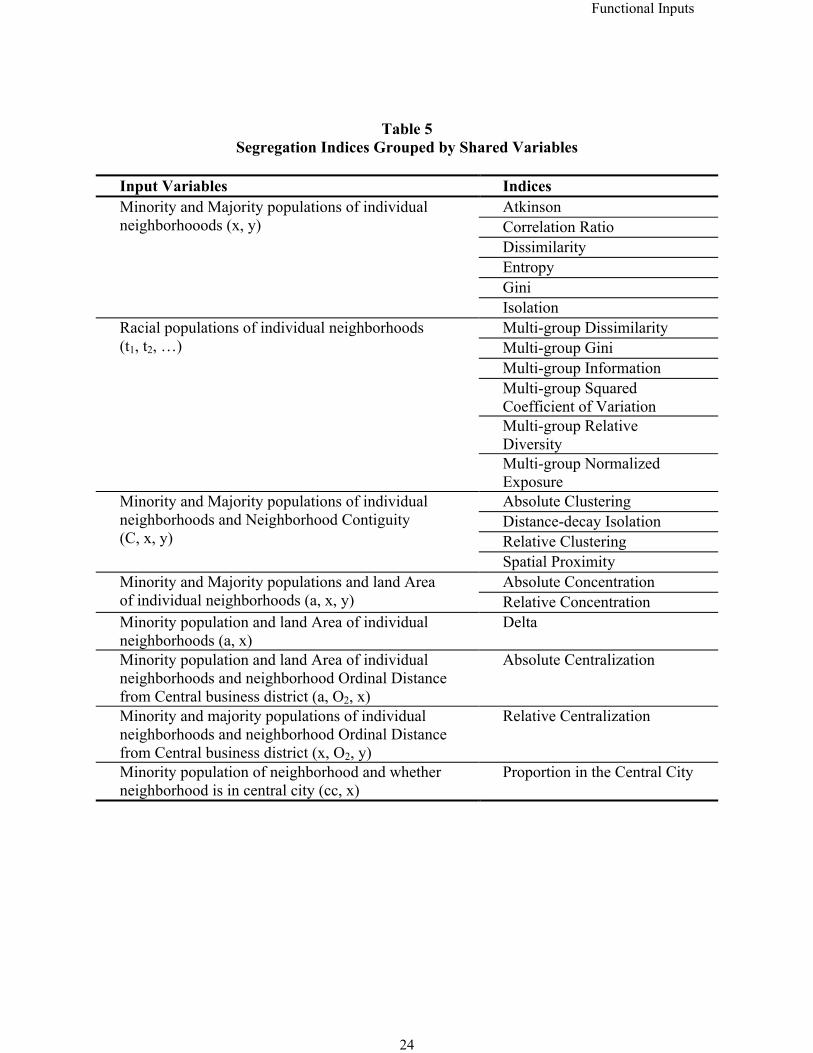
lists the indices as functions of this reduced set of input variables. Table 5 categorizes

indices by their common input variables and describes their inputs more fully.

Tables 4 and 5 about here

This new list represents those variables, and only those variables, which a segregation

researcher would have to find values for in order to calculate these indices5.

4 An Appendix, available from the author on request, discusses of how I identified

these variables and summarizes the algebraic transformations.

5 For example, one counts the number of minorities in a neighborhood or the

number of majority group members in a neighborhood, but one does not count a

Functional Inputs

6

Some indices (dissimilarity, Gini, entropy, Atkinson, isolation, and the correlation

ratio) are functions of the minority population and the majority population of each

neighborhood, and only those variables. These indices are more widely used than any

other segregation measures and much of the debates about indices refer only to these.

Most segregation researchers, by considering only members of this group, have implicitly

argued that the only two arrays of numbers, the majority population of the neighborhoods

and the population of a single minority group of each neighborhood, are important for

understanding segregation and that no other information is necessary. Reardon and

Firebaugh’s (2002) multi-group indices are extensions of these indices to the multi-group

case.

Spatial Proximity

Some indices (absolute and relative clustering, distance-decay isolation, and

spatial proximity) are primarily concerned, not with the distribution of the minority and

majority populations across neighborhoods, but with the distribution of minority and

majority neighborhoods with respect to each other. White (1983) termed this the

“checkerboard problem." If one allows the squares on a checkerboard to represent

neighborhoods, once the composition of each square is given, any spatial rearrangement

proportion. One calculates a proportion from counted values. Similarly, the sums of

neighborhood populations are just that, sums. One had to identify neighborhoods and

count their populations.

Functional Inputs

7

of them will result in the same calculation for most segregation indices. Thus, “A city in

which all the nonwhite parcels were concentrated into one single ghetto would have the

same calculated segregation as a city with dispersed pockets of minority residents”

(White 1983, pp. 1010-1011).

These “clustering” indices can all be rewritten in terms of a single function:

f(xi,yj) = i=1j=i cijxiyj (1)

This function focuses on the potential for interactions and is explicitly defined in terms of

the product of the number of individuals of the specified groups in the set of

neighborhoods defined by the contiguity matrix C. All of these indices can be thought of

as interaction measures except that, instead of assuming the potential for interaction

exists only among residents of a single neighborhood (e.g. census tract), they assume the

potential for interaction exists between residents of neighborhood i and all other

neighborhoods defined as contiguous to i by the contiguity matrix C. C could also be

defined as a weight such as inverse distance so that neighborhoods that were closer were

weighted more heavily while neighborhoods that were further away were weighted less

heavily.

The formulas for the clustering indices then translate into:

Distance-decay Isolation = f(xi/X,yj)/ f(tj,1) (2)

Absolute Clustering = {f(xi,xj) - f(X2,n-2)} / {f(xi,tj) - f(X

2,n-2)} (3)

Functional Inputs

8

Relative Clustering = Y2 f(xi,xj)/ X2 f(yi,yj) – 1 (4)

Spatial Proximity = {f(xi,xj)/X + f(yi,yj)/Y} / {f(ti,tj)/T} (5)

The distance-decay isolation index can be interpreted as the probability that the next

person a group X member meets is from group Y. The absolute clustering index

measures how much group x members are clustered so that they interact with each other

more than one would expect as a proportion of how much opportunity group x members

have to interact with anyone more than one would expect. The relative clustering index

compares the average proximity of members of group X to the average proximity of

members of group Y. The spatial proximity index is the average of intra-group

proximities weighted by each group’s fraction in the population. In short, the distance

between groups, or the geographic level at which they are segregated, as well as the fact

that they are separated, has been a concern of previous research. It would be useful to

combine Reardon and Firebaugh’s (2002) focus on multiple groups with this concern for

the dimension of distance.

An Example

While segregation researchers are certainly aware of the presence and importance

of ghettos and the spatial patterning of neighborhoods, there is a tendency to revert to

more simplistic measures when analyzing more complex relationships. I illustrate one

such complexity by re-examining some data from an article by Farley et. al. (1994) that

Functional Inputs

9

began by examining “residential segregation scores” (using the dissimilarity index) for

metropolitan Detroit in 1990, controlling separately for household income and for

educational attainment. Since they used only the dissimilarity index, Farley et. al.

(1994)’s analysis utilized only two arrays of numbers to compute their index scores for

each subset. Using the same data as Farley et. al. (1994), I computed the dissimilarity

index (to replicate their results), the isolation index, and the spatial proximity index for

each of their income and educational subsets. The isolation index is perhaps the second

most commonly cited index and, like the dissimilarity index, uses only information about

the number of white and black households in the tract. Computing the spatial proximity

index required using one additional array of numbers, which tracts in the Detroit

metropolitan area were contiguous and which were not. Figures 1 and 2 display the

results.

Figures 1 and 2 about here

In both figures, the line represented by long dashes and triangles represents the

dissimilarity index scores, the line with short dashes and circles represents the isolation

index, and the solid line with squares represents the spatial proximity index. As Farley

et. al. (1994) noted, the dissimilarity index is essentially unaffected by changes in

income. The isolation index behaves similarly. Using one or both of these indices,

which only use information about the numbers of white and black households in each

tract, one might reasonably conclude that segregation is unaffected by changes in income

Functional Inputs

10

or educational attainment, as did Farley et. al. (1994). Segregation as measured by the

spatial proximity index, however, drops dramatically with increases in income or

educational attainment.

Thus, two findings emerge from these figures. First, in Detroit, blacks with high

incomes and high education are just as likely to be segregated at the tract level as blacks

with low incomes and little education (as shown by the dissimilarity or isolation indices).

Second, however, the tracts that blacks with high incomes and high education live in are

much more likely to be adjacent to white tracts than are the tracts occupied by blacks

with low incomes and little education. While income and education do not allow blacks

in Detroit easy access into white tracts, they do allow them access into tracts in larger

white areas. Segregated neighborhoods of 1300 households (the average tract size in this

region) may be sufficiently large to segregate most face-to-face interactions, but may not

be sufficiently large to segregate supermarkets, school districts, or churches. Upper-class

blacks live in smaller “mostly-black” communities than do their less well-to-do

counterparts. Using indices that only account for the distribution of whites and blacks at

the tract level misses this second important and powerful finding.

Multi-Group Spatial Proximity

While Reardon and Firebaugh (2002) use “organizational units” instead of

neighborhoods to maximize generality (i.e. with school districts, etc.), this simplification

ignores important differences between neighborhoods and schools, not the least of which

Functional Inputs

11

is that school districts are often much bigger than the neighborhood equivalents we

typically measure residential segregation by (e.g. a high school feeder zone may include

several census tracts and numerous census block group). Much of the theorizing done

about residential segregation would not have any meaning at the micro-level at which

Reardon and Firebaugh’s (2002) indices (as well as many traditional segregation indices)

would measure it, concerning only very small communities of a few hundred or a

thousand households, oblivious to larger patterns. This has not been a critical issue in the

past since segregation has primarily been measured in a two-group scenario, black and

white. Given the ghettoization of blacks throughout America, segregation at the

neighborhood level typically implied larger scale segregation (Massey and Denton 1993).

As we begin to consider more complex, multi-group cases, however, the disparity

between micro-level segregation and larger patterns may become more acute.

It is appropriate that as we begin to consider more widespread use of multi-group

measures, we simultaneously consider using spatial proximity measures more. The

spatial proximity index has an obvious adaptation to the multi-group case

Multi-Group Spatial Proximity = m {f(xim,xjm)/Xm} / {f(ti,tj)/T} (6)

= m (1/Xm)(ij ximxjmcij) / (7)

( titjcij/T)

This new index is the average of intra-group proximities weighted by each

group’s fraction in the population. The numerator is the sum of several terms, one for

Functional Inputs

12

each racial group. Each term is the total number of potential interactions among

members of each racial averaged over the number of members of that racial group. The

denominator equals the total number of potential interactions between all individuals

averaged over the total number of people in the study area. Since this index is a sum of

an independent term for each racial group, this index could be used effectively to

measure spatial proximity among a single racial group, two racial groups, or several. It

could also be expanded to measure spatial proximity among different subcategories (e.g.

income, educational level, etc.) within a single racial group or among multiple racial

groups.

Researchers need to consider indices that account for nearby neighborhoods

unless they are certain the boundaries of census tracts, block groups, or other

neighborhood proxies completely confine the experience of segregation. Using

clustering indices, such as the multi-group spatial proximity index proposed above, also

allows one to deal with the Modifiable Areal Unit Problem (MAUP). MAUP results

from the imposition of artificial boundaries on a geographically correlated phenomenon

(Openshaw and Taylor 1979). Analytical results may be highly sensitive to the size and

boundaries of the zones used. Dramatically different results may be obtained from the

same set of data when the information is grouped in different levels of spatial resolution

(scale effect) or by merely altering the boundaries or configurations of the zones at a

given scale of analysis (zone effect). Using the smallest possible neighborhood

equivalent in combination with a clustering index would allow one to account for

Functional Inputs

13

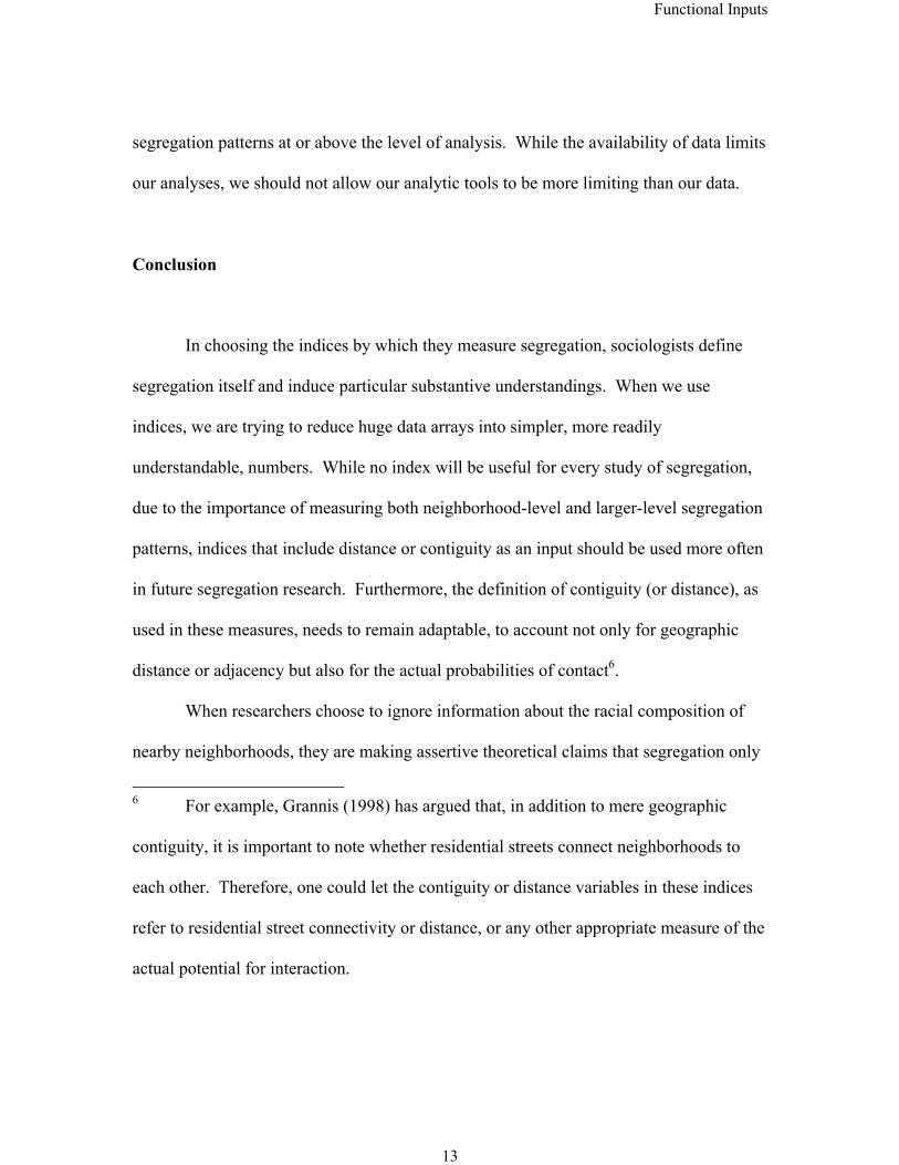
segregation patterns at or above the level of analysis. While the availability of data limits

our analyses, we should not allow our analytic tools to be more limiting than our data.

Conclusion

In choosing the indices by which they measure segregation, sociologists define

segregation itself and induce particular substantive understandings. When we use

indices, we are trying to reduce huge data arrays into simpler, more readily

understandable, numbers. While no index will be useful for every study of segregation,

due to the importance of measuring both neighborhood-level and larger-level segregation

patterns, indices that include distance or contiguity as an input should be used more often

in future segregation research. Furthermore, the definition of contiguity (or distance), as

used in these measures, needs to remain adaptable, to account not only for geographic

distance or adjacency but also for the actual probabilities of contact6.

When researchers choose to ignore information about the racial composition of

nearby neighborhoods, they are making assertive theoretical claims that segregation only

6 For example, Grannis (1998) has argued that, in addition to mere geographic

contiguity, it is important to note whether residential streets connect neighborhoods to

each other. Therefore, one could let the contiguity or distance variables in these indices

refer to residential street connectivity or distance, or any other appropriate measure of the

actual potential for interaction.

Functional Inputs

14

occurs at (or below) the level of the neighborhood they are using (e.g. census tract) and

that life in a minority community of a few hundred or a thousand households in the midst

of a majority population is not conceptually different from life in a minority community

of a hundred thousand households since they fail to incorporate data which would allow

them to distinguish these two situations. Just as multi-group segregation indices are

important for understanding complex demographic patterns, so indices that include data

on neighborhood contiguity are important for understanding segregation patterns

occurring at levels larger than a census tract.

Functional Inputs

15

References

Atkinson, A. B. 1970. “On the Measurement of Inequality.” American Sociological

Review 43:865-880.

Bell, Wendell. 1954. “A Probability Model for the Measurement of Ecological

Segregation.” Social Forces 32: 357-364.

Carlson, Susan M. 1992. “Trends in race/sex occupational inequality: Conceptual and

measurement issues.” Social Problems 39:269-290.

Dacey, Michael F. 1968. “A Review on Measures of Contiguity for Two and K-Color

Maps.” Pps. 479-495 in Spatial Analysis: A Reader in Statistical Geography

(Brian J. L. Berry and Duane F. Marble, editors). Prentice-Hall.

Duncan, Otis D., and Beverly Duncan. 1955. "A Methodological Analysis of

Segregation Indices.' American Sociological Review 20:210-217.

Duncan, Otis D., Ray P. Cuzzort, and Beverly Duncan. 1961. Statistical Geography:

Problems in Analyzing Area Data. Free Press.

Farley, Reynolds, Charlotte Steeh, Maria Krysan, Tara Jackson, and Keith Reeves. 1994.

“Stereotypes and Segregation: Neighborhoods in the Detroit Area.” American

Journal of Sociology 100:750-780.

Geary, R. C. 1954. “The Contiguity Ratio and Statistical Mapping.” Incorporated

Statistician 5:115-141.

Goodman, Leo and William H. Kruskal. 1954. “Measures of association for cross-

classifications.” Journal of the American Statistical Association 49: 731-764.

Functional Inputs

16

Grannis, Rick. 1998. “The Importance of Trivial Streets: Residential Streets and

Residential Segregation.” American Journal of Sociology 103: 1530-1564.

Hoover, Edgar M. 1941. “Interstate Redistribution of Population, 1850-1940.” Journal

of Economic History 1:199-205.

Jahn, Julius A., Calvin F. Schmid, and Clarence Schrag. 1947. “The Measurement of

Ecological Segregation” American Sociological Review 103: 293-303.

James, David R. and Karl E. Taeuber. 1985. “Measures of Segregation.” Pp. 1-32 in

Sociological Methodology 1985, edited by Nancy Tuma. Jossey-Bass.

James, Franklin J. 1986. “A new generalized “exposure-based” segregation index.”

Sociological Methods and Research 14:301-316.

Lieberson, Stanley. 1981. "An Asymmetrical Approach to Segregation." Pp. 61-82 in

Ethnic Segregation in Cities, edited by Ceri Peach, Vaughn Robinson, and Susan

Smith. Croom Helm.

Massey, Douglas S. and Nancy A. Denton. 1988. “The Dimensions of Residential

Segregation.” Social Forces 67: 281-305.

Morgan, Barrie S. 1975. “The segregation of socioeconomic groups in urban areas: A

comparative analysis.” Urban Studies 12:47-60.

_____. 1983. "An Alternate Approach to the Development of a Distance-Based

Measures of Racial Segregation." American Journal of Sociology 88:1237-1249.

Openshaw, S. and P. Taylor. 1979. “A Million or so Correlation Coefficients: Three

Experiments on the Modifiable Area Unit Problem.” Pp. 127-144 in Statistical

Applications in the Spatial Sciences, edited by Neil Wrigley. London. Pion.

Functional Inputs

17

Reardon, Sean F. and Glenn Firebaugh. 2002. “Measures of Multi-Group Segregation.”

Sociological Methodology.

Sakoda, J. 1981. “A generalized index of dissimilarity.” Demography 18:245-250.

Schwartz, J. and C. Winship. 1980. “The Welfare Approach to Measuring Inequality.”

Pp. 1-36 in Social Methods, edited by Schessler. Jossey Bass.

Theil, Henri. 1972. Statistical Decomposition Analysis. North-Holland.

Theil, Henri and Anthony J. Finezza. 1971. “A note on the measurement of racial

integration of schools by means of informational concepts.” Journal of

Mathematical Sociology 1:187-194.

White, Michael J. 1983. 'The Measurement of Spatial Segregation.” American Journal

of Sociology 98:1008-1019.

_____. 1986. 'Segregation and Diversity Measures in Population Distribution.”

Population Index 52 (2): 198-221.

Functional Inputs

18

Table 1Original Citation of Segregation Indices

Segregation Index CitationAbsolute Centralization Massey and Denton (1988)Absolute Clustering Massey and Denton (1988) adapted from Geary

(1954) and Dacey (1968)Absolute Concentration Massey and Denton (1988)Atkinson Atkinson (1970)Correlation Ratio Bell (1954); White (1986)Delta Duncan, Cuzzort, and Duncan (1961) adapted

from Hoover (1941)Dissimilarity Duncan and Duncan (1955)Distance-decay Isolation Morgan (1983)Entropy Theil and Finizza (1971); Theil (1972)Gini Duncan and Duncan (1955)Isolation Bell (1954); Lieberson (1981)Multi-group Dissimilarity Morgan (1975); Sakoda (1981)Multi-group Gini Reardon and Firebaugh (2002)Multi-group Information Theil and Finezza (1971); Theil (1972)Multi-group Normalized Exposure

James (1986)

Multi-group Relative Diversity Goodman and Kruskal (1954); Carlson (1992)Multi-group Squared Coefficient of Variation

Reardon and Firebaugh (2002)

Proportion in Central City Massey and Denton (1988)Relative Centralization Duncan and Duncan (1955)Relative Clustering Massey and Denton (1988)Relative Concentration Massey and Denton (1988)Spatial Proximity White (1986)

Functional Inputs

19

Table 2Computational Formulas for Segregation Indices

Segregation Index FormulaAbsolute Centralization ( Xi - 1Ai) - ( XiA i – 1)Absolute Clustering {[ (xi/X) (cijxj)] - [X/n2 cij]} /

{[ (xi/X) cijtj] - [X/n2 cij]}Absolute Concentration 1 – {[ (xiai/X) - n1

i=1(tiai/T1)] / [n

i=n2 (tiai/T2) - n1i=1 (tiai/T1)]}

Atkinson 1 - [P/(1 - P)]| [(1- pi)(1-k)pi

kti/PT]|(1/(1-k)

Correlation Ratio (xP*x – P)/(1 - P), where xP*x = [xi/X][xi/ti]

Delta ½ |[xi/X - ai/A]|Dissimilarity [ti|pi - P|/2TP(1- P)]Distance-decay Isolation xi/X Kijyj/tj, where

Kij = cijtj/ cijtjEntropy [ti(E - Ei)/ET], where

E = (P)log[1/P] + (1- P)log[1/(1- P)]Ei = (pi)log[1/ pi] + (1- pi)log[1/(1- pi)]

Gini [titj|pi - pj|/2T2P(1- P)]Isolation [xi/X][xi/ti]Multi-group Dissimilarity (1/2TI) tj |jm-m|Multi-group Gini (1/2T2I) titj |im-jm|Multi-group Information (1/TE) tj jm ln[jm/m]Multi-group Normalized Exposure (1/T) tj (jm-m)2 / (1-m)Multi-group Relative Diversity (1/TI) tj (jm-m)2

Multi-group Squared Coefficient of Variation (1/T(M-1)) tj (jm-m)2 / m

Proportion in Central City Xcc/XRelative Centralization ( Xi - 1YI) - ( XiY i - 1)Relative Clustering Pxx/Pyy – 1, where

Pxx = xixjcij/X2

Pyy = yiyjcij/Y2

Relative Concentration {[ (xiai/X)]/[ (yiai/Y)] - 1} /{[n1

i=1 (tiai/T1)]/[ni=n2 (tiai/T2)] - 1}

Spatial Proximity (XPxx + YPyy)/TPtt, wherePtt = titjcij/T

2

Pxx = xixjcij/X2

Pyy = yiyjcij/Y2

Functional Inputs

20

Table 2(continued)Notation

ai equals each neighborhood i's land areaA equals the urban region’s land areacij is a dichotomous variable that equals one when neighborhoods i and j are

contiguous and zero otherwise7

E = m=1M m(1-m)

I = m=1M m ln[1/m]

M the number of groups being consideredn equals the number of neighborhoods i in the urban areapi equals neighborhood i’s minority proportionP equals the urban region’s minority proportionti equals neighborhood i’s total populationT equals the urban region’s total populationxi equals each neighborhood i's minority populationX equals the urban region’s minority populationXcc equals the number of minorities living within the boundaries of the central cityyi equals each neighborhood i's majority group populationY equals the urban region’s majority populationjm equals the proportion in group mm equals the proportion in group m, of those in unit j

When the Neighborhoods are Ordered by Land Area, from smallest to largestn1 equals the rank of the neighborhood where the cumulative population of

neighborhoods equals X, the study area’s minority population, summing from the smallest neighborhood up

n2 equals the rank of the neighborhood where the cumulative population of neighborhoods equals Y, the study area’s majority group population, summing from the largest neighborhood down

T1 equals the cumulative population of neighborhoods one to n1

T2 equals the cumulative population of neighborhoods n2 to n

When the Neighborhoods are Ordered by increasing Distance from the Central Business DistrictAi equals the cumulative proportion of land area through neighborhood iXi equals the cumulative proportion of minorities through neighborhood iYi equals the cumulative proportion of majority group members through neighborhood i 7 Massey and Denton (1988) used exp(-dij), or the negative exponential of the

distance between the centroids of i and j, to estimate contiguity..

Functional Inputs

21

Table 3Input Variables for Segregation Indices

Input VariablesSegregation IndexConstants Vectors Matrices Orderings

Absolute Centralization a, x O2

Absolute Clustering n, X t, x CAbsolute Concentration n1, n2, T1 T2,

Xa, t, x O1

Atkinson P, T p, tCorrelation Ratio P, X t, xDelta A, X a, xDissimilarity P, T p, tDistance-decay Isolation X t, x, y CEntropy P, T p, tGini P, T p, tIsolation X t, xMulti-group Dissimilarity T, I t, Multi-group Gini T, I t, Multi-group Information T, E t, Multi-group Normalized Exposure

T T,

Multi-group Relative Diversity

T, I T,

Multi-group Squared Coefficient of Variation

M, T t,

Proportion in Central City X, Xcc

Relative Centralization x, y O2

Relative Clustering X, Y x, y CRelative Concentration n1, n2, T1 T2,

X, Ya, t, x, y O1

Spatial Proximity T, X, Y t, x, y C

Functional Inputs

22

Table 3(continued)Notation

a = [ai]cc = [cci]t = [ti] = [im] = [m]x = [xi]y = [yi]C = [cij]n1 (see Table 1)n2 (see Table 1)O1 = the ordering of the neighborhoods by land area, from smallest to largestO2 = the ordering of the neighborhoods by increasing distance from the central

business district

Functional Inputs

23

Table 4Reduced Set of Input Variables for Segregation Indices

Input VariablesSegregation IndexVectors Matrices Orderings

Absolute Centralization a, x O2

Absolute Clustering x, y CAbsolute Concentration a, x, yAtkinson x, yCorrelation Ratio x, yDelta a, xDissimilarity x, yDistance-decay Isolation x, y CEntropy x, yGini x, yIsolation x, yMulti-group Dissimilarity t1, t2, …Multi-group Gini t1, t2, …Multi-group Information t1, t2, …Multi-group Normalized Exposure t1, t2, …Multi-group Relative Diversity t1, t2, …Multi-group Squared Coefficient of Variation t1, t2, …Proportion in Central City cc, xRelative Centralization x, y O2

Relative Clustering x, y CRelative Concentration a, x, ySpatial Proximity x, y C

Functional Inputs

24

Table 5Segregation Indices Grouped by Shared Variables

Input Variables IndicesAtkinsonCorrelation RatioDissimilarityEntropyGini

Minority and Majority populations of individual neighborhooods (x, y)

IsolationMulti-group DissimilarityMulti-group GiniMulti-group InformationMulti-group Squared Coefficient of VariationMulti-group Relative Diversity

Racial populations of individual neighborhoods(t1, t2, …)

Multi-group Normalized ExposureAbsolute ClusteringDistance-decay IsolationRelative Clustering

Minority and Majority populations of individual neighborhoods and Neighborhood Contiguity(C, x, y)

Spatial ProximityAbsolute ConcentrationMinority and Majority populations and land Area

of individual neighborhoods (a, x, y) Relative ConcentrationMinority population and land Area of individual neighborhoods (a, x)

Delta

Minority population and land Area of individual neighborhoods and neighborhood Ordinal Distance from Central business district (a, O2, x)

Absolute Centralization

Minority and majority populations of individual neighborhoods and neighborhood Ordinal Distance from Central business district (x, O2, y)

Relative Centralization

Minority population of neighborhood and whether neighborhood is in central city (cc, x)

Proportion in the Central City

Functional Inputs

25

Figure 1Black-white Segregation in Detroit metropolitan area by Income

0.0

0.1

0.2

0.3

0.4

0.5

0.6

0.7

0.8

0.9

1.0

Less than$5,000

$5,000 to$9,999

$10,000to

$14,999

$15,000to

$24,999

$25,000to

$34,999

$35,000to

$49,999

$50,000to

$74,999

$75,000to

$99,999

$100,000or more

Dissimilarity Isolation Spatial Proximity

Functional Inputs

26

Figure 2Black-white Segregation in Detroit metropolitan area by Educational Attainment

0.0

0.1

0.2

0.3

0.4

0.5

0.6

0.7

0.8

0.9

1.0

Less than9th grade

9th to 12thgrade, nodiploma

High school Somecollege, no

degree

Associatedegree

Bachelor'sdegree

Graduate orprofessional

degree

Dissimilarity Isolation Spatial Proximity