Inefficiency in Latin-American market indices

Eur. Phys. J. B (2007)DOI: 10.1140/epjb/e2007-00316-y THE EUROPEAN

PHYSICAL JOURNAL B

Inefficiency in Latin-American market indices

L. Zunino1,2,3,a, B.M. Tabak4, D.G. Perez5, M. Garavaglia1,3, and O.A. Rosso6,7

1 Centro de Investigaciones Opticas, C.C. 124 Correo Central, 1900 La Plata, Argentina2 Departamento de Ciencias Basicas, Facultad de Ingenierıa, Universidad Nacional de La Plata (UNLP),

1900 La Plata, Argentina3 Departamento de Fısica, Facultad de Ciencias Exactas, Universidad Nacional de La Plata, 1900 La Plata, Argentina4 Banco Central do Brasil, SBS Quadra 3, Bloco B, 9 andar, DF 70074-900, Brazil5 Instituto de Fısica, Pontificia Universidad Catolica de Valparaıso (PUCV), 23-40025 Valparaıso, Chile6 Chaos & Biology Group, Instituto de Calculo, Facultad de Ciencias Exactas y Naturales, Universidad de Buenos Aires,

Pabellon II, Ciudad Universitaria, 1428 Ciudad de Buenos Aires, Argentina7 Centre for Bioinformatics, Biomarker Discovery and Information-Based Medicine, School of Electrical Engineering

and Computer Science, The University of Newcastle, University Drive, Callaghan NSW 2308, Australia

Received 23 July 2007 / Received in final form 14 September 2007Published online 23 November 2007 – c© EDP Sciences, Societa Italiana di Fisica, Springer-Verlag 2007

Abstract. We explore the deviations from efficiency in the returns and volatility returns of Latin-Americanmarket indices. Two different approaches are considered. The dynamics of the Hurst exponent is obtainedvia a wavelet rolling sample approach, quantifying the degree of long memory exhibited by the stockmarket indices under analysis. On the other hand, the Tsallis q entropic index is measured in order to takeinto account the deviations from the Gaussian hypothesis. Different dynamic rankings of inefficieny areobtained, each of them contemplates a different source of inefficiency. Comparing with the results obtainedfor a developed country (US), we confirm a similar degree of long-range dependence for our emergingmarkets. Moreover, we show that the inefficiency in the Latin-American countries comes principally fromthe non-Gaussian form of the probability distributions.

PACS. 05.45.Tp Time series analysis – 89.65.Gh Economics; econophysics, financial markets, businessand management – 05.40.-a Fluctuation phenomena, random processes, noise, and Brownian motion –89.75.-k Complex systems

1 Introduction

According to the Efficient Market Hypothesis (EMH), atany given time, the price of an asset fully reflects allavailable information. It should follow a martingale pro-cess in which each price change is unmodified by its pre-decessor. Therefore, the existence of autocorrelation be-tween distant observations violates the market efficiencybecause past prices can help to predict future prices. Thisquestion motivates the research on the subject, especiallyby portfolio managers and analysts who try to generatehigher returns. There are many examples of empirical re-sults for testing for long-range dependence, also known aslong memory, in the literature. Beben and Or�lowski [1]have found that emerging markets have greater correla-tion than developed markets, suggesting more predictabil-ity. Then, emerging economies seem to be less efficientthan developed ones. More recently, Di Matteo et al. [2,3]have also shown that deviations from efficiency are as-sociated with the degree of development. Another “styl-

a e-mail: [email protected]

ized fact” is that returns themselves have less evidenceof long memory. However, strong evidence of long-rangedependence is found for absolute returns1 [4–7]. Cajueiroand Tabak have shown that long-range dependence forreturns [8] and volatility returns [9] is time-varying andtherefore the dynamics of these Hurst exponents, thatquantify the degree of correlations, should be explored.These authors have also introduced a rank for market ef-ficiency by considering the median Hurst exponent as ameasure of it [10,11]. Other recent approaches to this is-sue seem to show that financial markets are increasingtheir efficiency over time [12,13]. These increasing effi-ciency can be mainly attributed to the variation of theeffects of (a) speed of information, (b) capital flows, and(c) nonsynchronous trading. More recently, Cajueiro andTabak [14] studied the dynamics of euro bilateral exchange

1 Following the arguments mentioned in reference [4], onereason to study the behavior of the absolute returns is that theinvestors are influenced not only by the evolution of the signof the investment, but also by the measure of the amplitude ofits change.

2 The European Physical Journal B

rates by estimating their Tsallis q entropic index. Theyprovide statistical evidence that this parameter can alsobe used as a measure of efficiency. In the standard EMHmodel the returns follow an uncorrelated Gaussian process(white noise). This process guarantees the basic proper-ties of an efficient market. Deviations from this model arepossible violating either the independence or the Gaussianassumptions2. So, there are two different sources of inef-ficiency. The Hurst exponent, as a measure of long-rangedependence, quantifies the former. It is widely known thatthe Tsallis q parameter measures the deviations from theGaussian hypothesis. Then, it takes into account the lattersource of inefficiency. Summarizing, the Hurst and Tsallisparameters provide us two independent ranks for marketefficiency. It should be remarked that both ranks are nec-essary for a properly characterization of the same stockmarket.

The aim of this study is to find out if long memoryand deviations from Gaussianity exist in the returns andvolatility returns of Latin-American market indices. Weput special attention into the efficiency question. For thispurpose we use the two approaches previously mentioned.

This paper is organized in the following way. Themethodologies used to estimate the Hurst exponent andthe Tsallis q entropic index are discussed in Sections 2.1and 2.2, respectively. In Section 3, the data used in thisstudy are detailed. In Section 4 we discuss the results,and in Section 5, we present the conclusions. Finally, theappendix briefly reviews the main properties of two well-known stochastic process, namely, fractional Brownianmotion (fBm) and fractional Gaussian noise (fGn). Theyare widely used to model long-range dependence.

2 Methodology

2.1 Estimation of Hurst exponent

The Wavelet Analysis is one of the most useful tools whendealing with data samples. Any signal can be decom-posed by using a wavelet dyadic discrete family ψj,k ={2−j/2ψ(2−jt− k)}, with j, k ∈ Z (the set of integers) —an orthonormal basis for L2(R) consisting of finite-energysignals — of translations and scaling functions based on afunction ψ: the mother wavelet [15,16]. In the following,given a continuous stochastic process s(t) its associateddiscrete signal is assumed to be given by the sampled val-ues S = {s(n), n = 1, . . . ,M}. Its wavelet expansion hasassociated wavelet coefficients given by

Cj(k) = 〈S, ψj,k〉, (1)

with j = 1, . . . , J , and J = log2M . The number of coef-ficients at each resolution level is Nj = 2−jM . Note thatthis correlation gives information on the signal at scale 2j

2 The occurrence of extreme events such as political distur-bances, terrorist attacks, bankruptcies of leading companies orwars imply the existence of power-law behaviors in the proba-bility distributions of returns (“fat tails”).

and time 2jk. The set of wavelet coefficients at level j,{Cj(k)}k, is also a stochastic process where k representsthe discrete time variable. It provides a direct estimationof local energies at different scales.

Following the arguments of Abry et al. [17], the waveletbased approach allows the threefold objective: detec-tion, identification and measurements of long-range de-pendence. These features are due to the fact that thewavelet family ψj,k exhibits scale invariance3. Moreover,the wavelet analysis is able to recognize quite differentkinds of scaling. In particular, it is well-suited to fBm andfGn — for details about these stochastic processes see Ap-pendix A. Properties of the wavelet coefficients of themcan be gathered into a unified framework [17]:

1. {Cj(k)}k is a stationary process if N ≥ (α − 1)/2,with N the number of vanishing moments associatedto the mother wavelet4, and α = 2H + 1 for fBm orα = 2H − 1 for fGn;

2. {Cj(k)}k has only short term residual correlations, i.e.,it does not have long-range dependence, on conditionthat N � α/2;

3. the underlying scaling behaviour of the data are repro-duced by the variance of the {Cj(k)}k process, withina given range of resolution levels j1 � j � j2:

E[C2

j (k)] ∝ 2αj, (2)

where E stands for the average using some, at first, un-known probability distribution associated to the coeffi-cients. It should be stressed that these results are valid forany self-similar process with stationary increments (α =2H+1) and long-range dependent processes (α = 2H−1).fBm and fGn are the archetypes of these two differentkinds of scaling.

These properties are widely used for estimating H orthe related spectral exponent α = 2H ± 1 [18–20]. Notethat 1 < α < 3 for fBm and −1 < α < 1 for fGn. Thevariance of the wavelet coefficients is estimated as usual:

µj =1Nj

Nj∑

k=1

|Cj(k)|2 , (3)

This is a non-parametric, unbiased estimator of the vari-ance of the process {Cj(k)}k. Then, plotting the log2(µj)versus j and fitting a minimum square line, the estimatedHurst exponent, H, is obtained from the slope. Basicallythe estimation problem turns into a linear regression slopeestimation and a fitting range of resolutions levels is re-quired. Using these issues, Abry and Veitch introduced awavelet-based analysis tool named the Logscale Diagram,which is defined as the plot of yj = log2 µj against j to-gether with confidence intervals assigned to each yj . Theassociated Matlab routine can be found in reference [21].

3 As it is widely known the long-range dependence is inti-mately related to scale invariance and self-similarity [18].

4 The mother wavelet ψ has N vanishing moments if∫tkψ(t)dt ≡ 0 for k = 0, 1, 2, . . . , N − 1. It is shown that any

polynomial trend of the signal can be rigorously eliminated byvarying this number of vanishing moments [18].

L. Zunino et al.: Inefficiency in Latin-American market indices 3

We calculate the time-dependent Hurst exponent byusing the Logscale Diagram and a rolling sample approachpreviously introduced [8,22,23]. The Hurst exponent is es-timated on the ensemble of points obtained from the in-tersection of the signal and a sliding window of size Ns.Then, the time window is rolled δs points forward elim-inating the first δs observations and including the nextones, and the Hurst exponent is re-estimated. These pro-cedure is repeated until the end of the time serie.

Multifractional Brownian motion (mBm) [24] was for-malized as a class of processes where the exponent H isno longer constant, but a continuous function of the timet (H → H(t)) 5. Artificial mBm were analyzed in orderto test the quality of our estimator. In Figure 1 one cancompare the theoretical and experimental results for amBm with H changing linearly from 0.1 to 0.9 with t.The Matlab code introduced by Coeurjolly [26] was im-plemented to simulate the mBm. Ns = 1024 and δs = 16were chosen for the rolling sample approach. Hereafter, weused the Daubechies (N = 3) as mother wavelet. We havealso implemented the special prefiltering required in theanalysis of intrinsically discrete time series6, included intothe Abry and Veitch Matlab routine (MRA initialization).Resolution levels from j = 2 to j = 7 were used for thelinear regression in each time window of this mBm simu-lation. It should be remarked that the Hurst exponent isalways underestimated. It was shown that the wavelet es-timator is asymptotically unbiased and Gaussian and thevariance of the estimation obtained from a sliding win-dow of size Ns is of order 1/Ns [17,18,28]. As it is anasymptotically efficient estimator, we assume that smallwindow lengths are a potential source of bias in the es-timates. We need to estimate the Hurst exponent overwindows that are short enough so that they can be takenas constant but long enough so that their statistical es-timates are robust. Furthermore, the finite segmentationlengths introduce noise into the estimates that should beremoved [29].

2.2 The Tsallis q entropic index

The maximization of the non-extensive entropy subject toappropriate constraints, for a fixed entropic index q, yieldsthe Tsallis distribution [30,31]:

pq(x) =

[1 + β(q − 1)(x− x)2

] −1q−1

Zq, (4)

where

Zq =[

π

β(q − 1)

]1/2Γ ((3 − q)/2(q − 1))

Γ (1/(q − 1))(5)

5 Moreover, this generalized fractional Brownian motionwas suggested as an alternative theoretical framework to ex-plain the multifractal behavior observed in financial time se-ries [22,25].

6 The discrete wavelet transform (DWT) is defined only forcontinuous-time processes. So, the discrete data are associatedto a continuous process, and then the usual wavelet method isapplied [27].

0.1 0.2 0.3 0.4 0.5 0.6 0.7 0.8 0.9−1.5

−1

−0.5

0

0.5

1

1.5

sign

al

t

0.1 0.2 0.3 0.4 0.5 0.6 0.7 0.8 0.9−0.2

0

0.2

0.4

0.6

0.8

H

t

Fig. 1. Top: synthetically generated mBm signal with Hchanging linearly from 0.1 to 0.9 with t. Bottom: theoretical(dashed curve) and measured (continuous curve) Hurst expo-nent for this simulated mBm.

is the appropriate normalization factor and β is theso-called Lagrange parameter associated with the con-straints. In the limit of q → 1, the Gaussian distributionis recovered. From equation (4) the ordinary variance canbe easily obtained

σ2 =

⎧⎨

⎩

1β(5−3q) , q < 5/3

∞, q ≥ 5/3.

It is also easy to show that the kurtosis coefficient K de-pends only on q and is given by

K =3(5 − 3q)

7 − 5q. (6)

This equation is particularly useful to calculate the en-tropic index from real data. Observe that with q = 1 weobtain K = 3, the expected value for the kurtosis of aGaussian process.

3 Data

We have collected daily closing prices for Argentina,Brazil, Chile, Colombia, Mexico, Peru, Venezuela and the


US. This last index is included for comparison purposes.The first three markets together with Mexico and the UScorrespond to large stock markets. On the other hand,Colombia, Peru and Venezuela can be considered smallerstock markets. The data samples cover the period fromJanuary 1995 to February 2007 with 3169 observationsfor all the countries except Venezuela with 3168 observa-tions and the US with 3141 observations. All series weregathered from the Morgan Stanley Capital Index (MSCI).This style index was employed in order to disentangle theeffects of autocorrelation and infrequent trading, whichare specially severe in emerging market. They are value-weighted indices of a large sample of companies in eachcountry and the indices do not include foreign companiesand are computed consistently across markets, thereby al-lowing for a close comparison across countries.

Let x(t) be the price of a stock on a time t, thereturns, rt, are calculated as its logarithmic difference,rt = ln(x(t+ 1)/x(t)).

Volatility is of very interest to traders because it quan-tifies the risk and is directly related to the amount of in-formation arriving in the financial market at a given time.The volatility of stock price changes is a measure of howmuch the market is liable to fluctuate. It is a “subsidiaryprocess” estimated from the original one. The series ofabsolute returns |rt| and squared returns r2t are usuallyused as proxies for volatility returns. It should be notedthat there are evidence of stronger long-range dependencefor absolute returns than for squared returns [4,5,9]. Wefollow Ding, Granger and Engle [32] who suggest measur-ing volatility directly from absolute returns. Furthermore,Davidian and Carroll [33] show absolute returns volatil-ity specification is more robust against asymmetry andnonnormality.

4 Empirical results

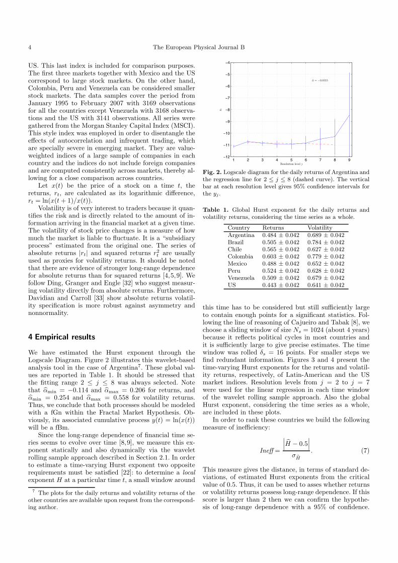
We have estimated the Hurst exponent through theLogscale Diagram. Figure 2 illustrates this wavelet-basedanalysis tool in the case of Argentina7. These global val-ues are reported in Table 1. It should be stressed thatthe fitting range 2 ≤ j ≤ 8 was always selected. Notethat αmin = −0.114 and αmax = 0.206 for returns, andαmin = 0.254 and αmax = 0.558 for volatility returns.Thus, we conclude that both processes should be modeledwith a fGn within the Fractal Market Hypothesis. Ob-viously, its associated cumulative process y(t) = ln(x(t))will be a fBm.

Since the long-range dependence of financial time se-ries seems to evolve over time [8,9], we measure this ex-ponent statically and also dynamically via the waveletrolling sample approach described in Section 2.1. In orderto estimate a time-varying Hurst exponent two oppositerequirements must be satisfied [22]: to determine a localexponent H at a particular time t, a small window around

7 The plots for the daily returns and volatility returns of theother countries are available upon request from the correspond-ing author.

1 2 3 4 5 6 7 8 9−12

−11

−10

−9

−8

−7

−6

−5

−4

yj

Resolution level j

α = −0.0315

Fig. 2. Logscale diagram for the daily returns of Argentina andthe regression line for 2 ≤ j ≤ 8 (dashed curve). The verticalbar at each resolution level gives 95% confidence intervals forthe yj .

Table 1. Global Hurst exponent for the daily returns andvolatility returns, considering the time series as a whole.

Country Returns VolatilityArgentina 0.484 ± 0.042 0.689 ± 0.042Brazil 0.505 ± 0.042 0.784 ± 0.042Chile 0.565 ± 0.042 0.627 ± 0.042Colombia 0.603 ± 0.042 0.779 ± 0.042Mexico 0.488 ± 0.042 0.652 ± 0.042Peru 0.524 ± 0.042 0.628 ± 0.042Venezuela 0.509 ± 0.042 0.679 ± 0.042US 0.443 ± 0.042 0.641 ± 0.042

this time has to be considered but still sufficiently largeto contain enough points for a significant statistics. Fol-lowing the line of reasoning of Cajueiro and Tabak [8], wechoose a sliding window of size Ns = 1024 (about 4 years)because it reflects political cycles in most countries andit is sufficiently large to give precise estimates. The timewindow was rolled δs = 16 points. For smaller steps wefind redundant information. Figures 3 and 4 present thetime-varying Hurst exponents for the returns and volatil-ity returns, respectively, of Latin-American and the USmarket indices. Resolution levels from j = 2 to j = 7were used for the linear regression in each time windowof the wavelet rolling sample approach. Also the globalHurst exponent, considering the time series as a whole,are included in these plots.

In order to rank these countries we build the followingmeasure of inefficiency:

Ineff =

∣∣∣H − 0.5

∣∣∣

σH

. (7)

This measure gives the distance, in terms of standard de-viations, of estimated Hurst exponents from the criticalvalue of 0.5. Thus, it can be used to asses whether returnsor volatility returns possess long-range dependence. If thisscore is larger than 2 then we can confirm the hypothe-sis of long-range dependence with a 95% of confidence.


12/1996 03/1998 06/1999 08/2000 11/2001 02/2003 05/2004 03/20050

0.1

0.2

0.3

0.4

0.5

0.6

0.7

0.8

0.9

1

Date

H

Argentina

12/1996 03/1998 06/1999 08/2000 11/2001 02/2003 05/2004 03/20050

0.1

0.2

0.3

0.4

0.5

0.6

0.7

0.8

0.9

1

Date

H

Brazil

12/1996 03/1998 06/1999 08/2000 11/2001 02/2003 05/2004 03/20050

0.1

0.2

0.3

0.4

0.5

0.6

0.7

0.8

0.9

1

Date

H

Chile

12/1996 03/1998 06/1999 08/2000 11/2001 02/2003 05/2004 03/20050

0.1

0.2

0.3

0.4

0.5

0.6

0.7

0.8

0.9

1

Date

H

Colombia

12/1996 03/1998 06/1999 08/2000 11/2001 02/2003 05/2004 03/20050

0.1

0.2

0.3

0.4

0.5

0.6

0.7

0.8

0.9

1

Date

H

Mexico

12/1996 03/1998 06/1999 08/2000 11/2001 02/2003 05/2004 03/20050

0.1

0.2

0.3

0.4

0.5

0.6

0.7

0.8

0.9

1

Date

H

Peru

12/1996 03/1998 06/1999 08/2000 11/2001 02/2003 05/2004 02/20050

0.1

0.2

0.3

0.4

0.5

0.6

0.7

0.8

0.9

1

Date

H

Venezuela

12/1996 03/1998 06/1999 08/2000 11/2001 02/2003 05/200403/20050

0.1

0.2

0.3

0.4

0.5

0.6

0.7

0.8

0.9

1

Date

H

US

Fig. 3. Plots of estimated Hurst exponent by using the wavelet rolling sample approach with a sliding window of size Ns = 1024and step δs = 16 for the daily returns of Latin-American and the US market indices. Dashed lines correspond to the globalHurst exponent considering the time series as a whole.


12/1996 03/1998 06/1999 08/2000 11/2001 02/2003 05/2004 03/20050

0.1

0.2

0.3

0.4

0.5

0.6

0.7

0.8

0.9

1

Date

H

Argentina

12/1996 03/1998 06/1999 08/2000 11/2001 02/2003 05/2004 03/20050

0.1

0.2

0.3

0.4

0.5

0.6

0.7

0.8

0.9

1

Date

H

Brazil

12/1996 03/1998 06/1999 08/2000 11/2001 02/2003 05/2004 03/20050

0.1

0.2

0.3

0.4

0.5

0.6

0.7

0.8

0.9

1

Date

H

Chile

12/1996 03/1998 06/1999 08/2000 11/2001 02/2003 05/2004 03/20050

0.1

0.2

0.3

0.4

0.5

0.6

0.7

0.8

0.9

1

Date

H

Colombia

12/1996 03/1998 06/1999 08/2000 11/2001 02/2003 05/2004 03/20050

0.1

0.2

0.3

0.4

0.5

0.6

0.7

0.8

0.9

1

Date

H

Mexico

12/1996 03/1998 06/1999 08/2000 11/2001 02/2003 05/2004 03/20050

0.1

0.2

0.3

0.4

0.5

0.6

0.7

0.8

0.9

1

Date

H

Peru

12/1996 03/1998 06/1999 08/2000 11/2001 02/2003 05/2004 02/20050

0.1

0.2

0.3

0.4

0.5

0.6

0.7

0.8

0.9

1

Date

H

Venezuela

12/1996 03/1998 06/1999 08/2000 11/2001 02/2003 05/200403/20050

0.1

0.2

0.3

0.4

0.5

0.6

0.7

0.8

0.9

1

Date

H

US

Fig. 4. Plots of estimated Hurst exponent by using the wavelet rolling sample approach with a sliding window of size Ns = 1024and step δs = 16 for the daily volatility returns of Latin-American and the US market indices. Dashed lines correspond to theglobal Hurst exponent considering the time series as a whole.


Table 2. Inefficiency ranking for the daily returns consideringthe relative efficiency approach of Lim [34] (long-range depen-dence).

Country Total number Total number Percentage

of rolling of significant of significant

windows windows windows (%)

Brazil 135 3 2.22

Mexico 135 6 4.44

Argentina 135 19 14.07

Venezuela 134 21 15.67

Peru 135 33 24.44

US 133 37 27.82

Chile 135 47 34.81

Colombia 135 102 75.56

Table 3. Inefficiency ranking for the daily volatility returnsconsidering the relative efficiency approach of Lim [34] (long-range dependence).

Country Total number Total number Percentage

of rolling of significant of significant

windows windows windows (%)

Chile 135 47 34.81

US 133 56 42.11

Peru 135 69 51.11

Mexico 135 101 74.81

Venezuela 134 112 83.58

Argentina 135 113 83.70

Brazil 135 123 91.11

Colombia 135 135 100.00

Figures 5 and 6 show the time-varying inefficiency mea-sure for the returns and volatility returns, respectively, ofLatin-American and the US market indices by consideringthe Hurst exponent sequences derived previously from thewavelet rolling sample approach. Following the line of rea-soning of Lim [34], a comparative analysis is achieved bycomparing the total time windows these markets exhibitsignificant long-range dependence. A window is consid-ered as significant if its associated inefficiency measure isgreater than or equal to 2, the threshold level chosen inour case. So, the percentage of significant windows couldbe a meaningful indicator for assessing the relative inef-ficiency of stock markets. In Tables 2 and 3 we rank thereturns and volatility returns of the Latin-American andthe US market indices by considering this relative ineffi-ciency approach.

If the returns and volatility returns are normally dis-tributed the Tsallis q entropic index would be close to one.The closer to one the more efficient is the time serie. InTable 4 we rank the returns and volatility returns by us-ing the Tsallis q entropic index. We use equation (6) toestimate this parameter. The entropic index can be easilyderived:

q =15 − 7K9 − 5K

. (8)

Table 4. Inefficiency ranking for the daily returns and volatil-ity returns according to the Tsallis q entropic index (deviationsfrom the Gaussian hypothesis).

Country Returns Volatility

US 1.3027 1.3487

Chile 1.3071 1.3589

Peru 1.3298 1.3604

Brazil 1.3368 1.3695

Colombia 1.3622 1.3804

Mexico 1.3692 1.3861

Argentina 1.3793 1.3906

Venezuela 1.3964 1.3981

As you can observe, the returns and its associated proxyfor volatility (absolute returns) provide the same rank. Wealso conclude that volatility returns have stronger devia-tions from the Gaussian hypothesis (q farther from one)than the associated returns. This should be expected asvolatility is bounded from below at zero.

To the best of our knowledge this is the first paper thatemploys a ranking methodology that does not depend onwhether we are focusing on returns or volatility (momentindependent). Furthermore, it provides reasonable results.Therefore, it is worth mentioning that the Tsallis q en-tropic index seems to be an interesting method that canbe used to characterize inefficiency.

5 Conclusions

We provide empirical evidence of long-range dependencein the daily returns and volatility returns of Latin-American market indices. Long memory is categoricallyshowed in the volatility measures, while there is little ev-idence of it in the returns. Portfolio and risk managersare interested in finding patterns of predictability. Sincevolatility has strong long-range dependence, it should bepredicted more easily and better than returns. These re-sults also imply that commonly used models for volatilitysuch as GARCH models are flawed and should be replacedby models that incorporate long memory.

The global results, considering the time series as awhole, suggest that there is stronger long-range depen-dence in returns for emerging markets than for developedones. What is more, the US return has a clear antiper-sistent behaviour (see Tab. 1). However, on average long-range dependence in global volatility returns seems to besimilar in mature liquid markets than in less developedones. This result is in accord with previous findings [2,35].

In some countries the Hurst exponent changes sub-stantially over time. This suggests that such countries arefacing structural changes in the dynamics of their stockmarkets, which could be due to changes in their regu-lation. Thus, we find that the efficiency of stock mar-kets should be examined as a dynamic characteristic. Itis evolving in time, with periods of inefficiency alter-nate with those of efficiency. The rolling sample approachis an excellent approach to this complex issue. We alsoconclude that different rankings can be derived, each ofthem taking into account different sources of inefficiency.


12/1996 03/1998 06/1999 08/2000 11/2001 02/2003 05/2004 03/20050

1

2

3

4

5

6

Date

Ineff

Argentina

12/1996 03/1998 06/1999 08/2000 11/2001 02/2003 05/2004 03/20050

1

2

3

4

5

6

Date

Ineff

Brazil

12/1996 03/1998 06/1999 08/2000 11/2001 02/2003 05/2004 03/20050

1

2

3

4

5

6

Date

Ineff

Chile

12/1996 03/1998 06/1999 08/2000 11/2001 02/2003 05/2004 03/20050

1

2

3

4

5

6

Date

Ineff

Colombia

12/1996 03/1998 06/1999 08/2000 11/2001 02/2003 05/2004 03/20050

1

2

3

4

5

6

Date

Ineff

Mexico

12/1996 03/1998 06/1999 08/2000 11/2001 02/2003 05/2004 03/20050

1

2

3

4

5

6

Date

Ineff

Peru

12/1996 03/1998 06/1999 08/2000 11/2001 02/2003 05/2004 02/20050

1

2

3

4

5

6

Date

Ineff

Venezuela

12/1996 03/1998 06/1999 08/2000 11/2001 02/2003 05/200403/20050

1

2

3

4

5

6

Date

Ineff

US

Fig. 5. Plots of the inefficiency measure (Eq. (7)) by using the wavelet rolling sample approach with a sliding window of sizeNs = 1024 and step δs = 16 for the daily returns of Latin-American and the US market indices. The horizontal lines correspondto the threshold level.


12/1996 03/1998 06/1999 08/2000 11/2001 02/2003 05/2004 03/20050

1

2

3

4

5

6

7

8

9

10

Date

Ineff

Argentina

12/1996 03/1998 06/1999 08/2000 11/2001 02/2003 05/2004 03/20050

1

2

3

4

5

6

7

8

9

10

Date

Ineff

Brazil

12/1996 03/1998 06/1999 08/2000 11/2001 02/2003 05/2004 03/20050

1

2

3

4

5

6

7

8

9

10

Date

Ineff

Chile

12/1996 03/1998 06/1999 08/2000 11/2001 02/2003 05/2004 03/20050

1

2

3

4

5

6

7

8

9

10

Date

Ineff

Colombia

12/1996 03/1998 06/1999 08/2000 11/2001 02/2003 05/2004 03/20050

1

2

3

4

5

6

7

8

9

10

Date

Ineff

Mexico

12/1996 03/1998 06/1999 08/2000 11/2001 02/2003 05/2004 03/20050

1

2

3

4

5

6

7

8

9

10

Date

Ineff

Peru

12/1996 03/1998 06/1999 08/2000 11/2001 02/2003 05/2004 02/20050

1

2

3

4

5

6

7

8

9

10

Date

Ineff

Venezuela

12/1996 03/1998 06/1999 08/2000 11/2001 02/2003 05/200403/20050

1

2

3

4

5

6

7

8

9

10

Date

Ineff

US

Fig. 6. Plots of the inefficiency measure (Eq. (7)) by using the wavelet rolling sample approach with a sliding window of sizeNs = 1024 and step δs = 16 for the daily volatility returns of Latin-American and the US market indices. The horizontal linescorrespond to the threshold level.


Therefore, they do not provide the same rank of ineffi-ciency for Latin-American market indices. For example,Chile is one of the worst ranked for the daily returns con-sidering the relative efficiency approach (see Tab. 2) but atthe same time is one of the best ranked countries accord-ing to the Tsallis q entropic index (see Tab. 4). So, we canconclude that the Chilean market index has stronger long-range dependence and weaker deviations from the Gaus-sian hypothesis.

Since the dynamics inefficiency rankings considered(see Tabs. 2, 3 and 4) we conclude that all the Latin-American countries under study experiment important de-viations from the Gaussian hypothesis, this is a commonsource of inefficiency.

It was shown that magnitude series contain informa-tion regarding the nonlinear properties of the original timeseries [36]. Moreover, long-range dependence in the volatil-ity is a proof for nonlinearity in the associated time se-rie [37]. Then, our results confirm nonlinear dependence(non-zero bicorrelation). Actually, this is another stylizedfact that can be considered as a source of inefficiency,and a new rank will emerge from it [34]. Nonlinearitywas previously detected in the rate of returns series forseven Latin-American stock market indices [38]. Its influ-ence should be quantified in future works. Further studyshould also focus on the economic determinants of thesedifferent sources of inefficiency.

The intention is to repeat the same analysis for high-frequency returns and volatility time series [28,39–41] inorder to understand the fine structure of the stock mar-ket. In this kind of studies we will have more observations.Thus, we expect more accuracy in the results obtainedvia our asymptotically efficient wavelet rolling sample ap-proach. We will also remove the noise due to finite seg-mentation lengths through the Papanicolaou and Sølnaapproach [29].

Luciano Zunino was supported by Consejo Nacional de In-vestigaciones Cientıficas y Tecnicas (CONICET), Argentina.Benjamin M. Tabak gratefully acknowledges financial sup-port from CNPq foundation. The opinions expressed in thepaper do not necessarily reflect those of the Banco Centraldo Brasil. Darıo G. Perez was supported by Comision Na-cional de Investigacion Cientıfica y Tecnologica (CONICYT,FONDECYT project No. 11060512), Chile, and partially byPontificia Universidad Catolica de Valparaıso (PUCV, ProjectNo. 123.788/2007), Chile. Osvaldo A. Rosso gratefully ac-knowledges support from Australian Research Council (ARC)Centre of Excellence in Bioinformatics, Australia. The authorsare very greateful to the reviewers, whose comments and sug-gestions helped to improve an earlier version of this paper.

Appendix A: Fractal Market Hypothesis

Mandelbrot and van Ness [42] introduced the fractionalBrownian motion (fBm) as a generalization of the or-dinary Brownian motion by considering correlations be-tween the increments of the process. Thus, this fractalstochastic model contemplates the presence of long-range

dependence, the first of the two sources of inefficiencymentioned at the end of Section 1. The fBm and its cor-responding generalized derivative process, the fractionalGaussian noise (fGn), are the benchmark of the so-calledFractal Market Hypothesis (FMH).

A.1 Fractional Brownian motion

This is the only one family of processes which is Gaus-sian, self-similar, and endowed with stationary incre-ments. The normalized family of these Gaussian processes,{BH(t), t > 0}, is the one with BH(0) = 0 almost surely(with probability 1), E

[BH(t)

]= 0 (zero mean), and co-

variance

E[BH(t)BH(s)

]=

12

(t2H + s2H − |t− s|2H

), (A.1)

for s, t ∈ R. Here E[·] refers to the average with Gaus-sian probability density. The power exponent H , com-monly known as Hurst exponent or Hurst parameter, hasa bounded range between 0 and 1. These processes ex-hibit memory, as can be observed from equation (A.1),for any Hurst exponent but H = 1/2, for which one re-covers the classical Brownian motion. In this case succes-sive Brownian motion increments are as likely to have thesame sign as the opposite, and thus there is no correla-tion among them. Precisely, this Hurst exponent definestwo distinct regions in the interval (0, 1). When H > 1/2,consecutive increments tend to have the same sign so thatthese processes are persistent. For H < 1/2, on the otherhand, consecutive increments are more likely to have op-posite signs, and it is said that these processes are anti-persistent. Fractional Brownian motions are continuousbut non-differentiable processes (in the classical sense). Asa nonstationary process, fractional Brownian motion doesnot possess a spectrum defined in the usual sense; how-ever, it is possible to define a generalized power spectrumof the form [43]:

ΦBH (f) ∝ 1|f |α , (A.2)

with α = 2H + 1 and 1 < α < 3. Remember that thisequation does not represent a valid power spectrum inthe theory of stationary processes since it yields a non-integrable function (in the classical sense).

A.2 Fractional Gaussian noise

We denoted by {WH(t), t > 0} the process derived fromthe increment of fractional Brownian motion, namely

WH(t) = BH(t) −BH(t+ 1). (A.3)

We face a stationary Gaussian process with mean zero andcovariance given by

ρ(k) = E[WH(t)WH(t+ k)

]

=12

[(k + 1)2H − 2k2H + |k − 1|2H

], k > 0. (A.4)


The last expression has the following asymptotic behavioras k → ∞ [44]

ρ(k)H(2H − 1)k2H−2

→ 1. (A.5)

Therefore, whenH > 1/2 this correlation decays to zero soslowly that the sum

∑k=∞k=−∞ ρ(k) = ∞ diverges [44]; this

sub-family of processes has long-memory. On the otherhand, for H < 1/2 the correlations of the incrementsare summable [44], and this sub-family exhibits short-memory. Equation (A.5) also allows one to corroborate theassertions about the persistent or anti-persistent behaviormentioned above. Note that forH = 1/2 all correlations atnon-zero lags vanish and {W 1/2(t), t > 0} is white noise.Naturally, time series of cumulative Gaussian white noiseconstitute samples of classical Brownian motions. Thepower spectrum associated to fractional Gaussian noisereads

ΦW H (f) ∝ 1|f |α , (A.6)

with α = 2H − 1 and −1 < α < 1.

References

1. M. Beben, A. Or�lowski, Eur. Phys. J. B 20, 527 (2001)2. T. Di Matteo, T. Aste, M.M. Dacorogna, Physica A 324,

183 (2003)3. T. Di Matteo, T. Aste, M.M. Dacorogna, J. Bank. Fin. 29,

827 (2005)4. P. Grau-Carles, Physica A 287, 396 (2000)5. T. Lux, Appl. Econom. Lett. 3, 701 (1996)6. B.K. Ray, R.S. Tsay, J. Bus. Econ. Stat. 18, 254 (2000)7. P. Sibbertsen, Empirical Econ. 29, 477 (2004)8. D.O. Cajueiro, B.M. Tabak, Physica A 336, 521 (2004)9. D.O. Cajueiro, B.M. Tabak, Physica A 346, 577 (2005)

10. D.O. Cajueiro, B.M. Tabak, Solitons & Fractals 22, 349(2004)

11. D.O. Cajueiro, B.M. Tabak, Chaos, Solitons & Fractals23, 671 (2005)

12. B. Toth, J. Kertesz, Physica A 360, 505 (2006)13. H.F. Coronel-Brizio, A.R. Hernandez-Montoya, R. Huerta-

Quintanilla, M. Rodrıguez-Achach, Physica A 380, 391(2007)

14. B.M. Tabak, D.O. Cajueiro, Physica A 367, 319 (2006)15. I. Daubechies, Ten lectures on wavelets, SIAM,

Philadelphia, 199216. S. Mallat, A wavelet tour of signal processing, 2nd edn.

(Academic Press, 1999)17. P. Abry, P. Flandrin, M.S. Taqqu, D. Veitch, Wavelets for

the analysis, estimation, and synthesis of scaling data, in:Self-similar Network Traffic and Performance Evaluation,edited by K. Park, W. Willinger (Wiley, 2000), pp. 39–87

18. P. Abry, D. Veitch, IEEE Trans. Inform. Theory 44, 2(1998)

19. L. Zunino, D.G. Perez, M. Garavaglia, O.A. Rosso,Fractals 12, 223 (2004)

20. L. Zunino, D.G. Perez, M. Garavaglia, O.A. Rosso, PhysicaA 364, 79 (2006)

21. http://www.cubinlab.ee.mu.oz.au/∼darryl/

secondorder code.html

22. R.L. Costa, G.L. Vasconcelos, Physica A 329, 231 (2003)23. A. Carbone, G. Castelli, H.E. Stanley, Physica A 344, 267

(2004)24. R.F. Peltier, J. Levy-Vehel, Multifractional Brownian mo-

tion: definition and preliminary results, Research ReportRR-2645, INRIA (1995)

25. S.V. Muniandy, S.C. Lim, R. Murugan, Physica A 301,407 (2001)

26. J.-F. Coeurjolly, Statistical inference for fractionaland multifractional Brownian motions, Ph.D. thesis,Laboratoire de Modelisation et Calcul – Institutd’Informatique el Mathematiques Appliquees de Grenoble,2000

27. D. Veitch, M.S. Taqqu, P. Abry, Sign. Process. 80, 1971(2000)

28. E. Bayraktar, H. Vincent Poor, K. Ronnie Sircar, Int. J.Theor. Appl. Finance 7, 615 (2004)

29. G. Papanicolaou, K. Sølna, Wavelet based estimationof local Kolmogorov turbulence, Long-Range Dependence:Theory and Applications, edited by P. Doukhan,G. Oppenheim, M.S. Taqqu (Birkhauser, 2003), pp. 473–505

30. C. Tsallis, S.V.F. Levy, A.M.C. Souza, R. Maynard, Phys.Rev. Lett. 75, 3589 (1995)

31. C. Tsallis, D.J. Bukman, Phys. Rev. E 54, R2197 (1996)32. Z. Ding, C. Granger, R. Engle, J. Empir. Fin. 1, 83 (1993)33. M. Davidian, R.J. Carroll, J. Am. Stat. Association 82,

1079 (1987)34. K.P. Lim, Physica A 376, 445 (2007)35. D.O. Cajueiro, B.M. Tabak, Chaos, Solitons & Fractals, in

press36. Y. Ashkenazy, P.C. Ivanov, S. Havlin, C.-K. Peng, A.L.

Goldberger, H.E. Stanley, Phys. Rev. Lett. 86, 1900 (2001)37. T. Kalisky, Y. Ashkenazy, S. Havlin, Phys. Rev. E 72,

011913 (2005)38. C.A. Bonilla, R. Romero-Meza, M.J. Hinich, Appl. Econ.

Lett. 13, 195 (2006)39. M. Raberto, E. Scalas, G. Cuniberti, M. Riani, Physica A

269, 148 (1999)40. C. Morana, Appl. Finan. Econ. Lett. 2, 361 (2006)41. R.T. Baillie, Y.-W. Han, R.J. Myers, J. Song, J. Futures

Mark. 27, 643 (2007)42. B.B. Mandelbrot, J.W. Van Ness, SIAM Rev. 4, 422 (1968)43. P. Flandrin, IEEE Trans. Inform. Theory IT-35, 197

(1989)44. J. Beran, Statistics for long-memory processes, in:

Monographs on Statistics and Applied Probability(Chapman & Hall, 1994), Vol. 61

Inefficiency in Latin-American market indices

Documents

Transcript of Inefficiency in Latin-American market indices