T ellus (1999), 51A, 773–789 Copyright © Munksgaard, 1999Printed in UK. All rights reserved TELLUS

ISSN 0280–6495

An intercomparison between low-frequencyvariability indices

By P. BONGIOANNINI CERLINI1*, S. CORTI2 and S. TIBALDI3, 1Department of Earth and

Geo-Environmental Sciences, V ia Zamboni 67, University of Bologna, Bologna, Italy; 2CINECA —

Inter-University Computing Centre, Bologna, Italy; 3SMR, Regional Meteorological Service of ARPA

Emilia-Romagna and Atmospheric Dynamics Group, Department of Physics, University of Bologna, Italy

(Manuscript received 14 September 1998; in final form 17 June 1999)

ABSTRACT

Possible connections between spatial patterns, of limited regional extent and identified in tele-connection patterns and in blocking climatology studies, with hemispheric planetary-wave activ-ity modes defined by the wave amplitude index (WAI) are investigated. The WAI probabilitydensity function (PDF) for the northern extratropics winter fields is estimated and the sensitivityof the WAI distribution to the presence of low-frequency variability modes is evaluated bystratifying the available dataset according to the sign of blocking and teleconnection indices.It is found that low-frequency variability modes affect both the mean and the variance of thewave amplitude index. Both the positive phase of the North Atlantic Oscillation (NAO) andthe negative phase of the Pacific North American pattern (PNA) are associated with anenhanced frequency of very large amplitude planetary waves. Furthermore, distributions charac-terised by a maximum corresponding to high WAI values also exhibit a large variance. NegativeNAO and positive PNA influence the mean and the variance of WAI PDF in the oppositesense. Similar results are found when the blocking index is considered. WAI PDFs relative tohighly blocked months are broader with a secondary maximum corresponding to very highWAI values.

1. Introduction the atmosphere is considered as a non-linear

dynamical system with chaotic, but not totally

random, behaviour oscillating between preferredDifferent observational and theoretical back-zones of the atmospheric phase space (‘‘flowgrounds motivated low-frequency variability stud-regimes’’). Although the idea of weather regimesies since Rossby et al. (1939) classic paper on mid-is a long standing one (Namias, 1950; Rex, 1950b,latitude wave motion. More recently, a numberLorenz 1963), this notion was made more clearof theoretical investigations and observationalonly in the last two decades. The existence ofstudies tend to support the idea of the existencequasi-stationary regimes has also been investi-of different weather regimes in the wintertimegated in modelling studies of the atmosphericnorthern extratropical circulation (Charney andglobal circulation (Reinhold and Pierrehumbert,DeVore, 1979; Sutera, 1986).1982; Legras and Ghil, 1985; Haines andThe concept of weather regimes is based on theHannachi, 1995). However, as far as the realnotion that the large-scale flow may evolve aroundatmosphere is concerned, flow regimes (in thevarious recurrent configurations. In other words,wintertime circulation of the Northern

Hemisphere) have been diagnosed principally on* Corresponding author.E-mail: paolina@bacino.geomin.unibo.it. the basis of: (a) multimodality of the one-dimen-

Tellus 51A (1999), 5

. .774

sional or multidimensional probability density clearly project onto the PNA teleconnection pat-

tern and the North Atlantic Oscillation (NAO,function of circulation indices (Sutera 1986;

Hansen and Sutera 1986; Molteni et al., 1988); Hurrel, 1995).

However, although such regime patterns are(b) cluster analysis in an appropriate atmospheric

phase space (Mo and Ghil, 1988; Molteni et al., associated with regional teleconnections, they also

correspond more generally to quasi-stationary1990; Kimoto and Ghil, 1993; Cheng and Wallace,

1993); and (c) the existence of areas in phase space structures (persistent anomalies) of low-frequency

variability, like for example blocking.where the state vector is quasi-stationary

(Vautard, 1990; Michelangeli et al., 1995). Historically, blocking is quoted as a classical

example of large-scale recurrent weather patternA synthetic indicator of the amplitude of planet-

ary waves (wave amplitude index, hereafter WAI) (Baur, 1951), but its classification as a global or

local anomaly and an accepted theoretical inter-showing a bimodal density distribution was intro-

duced by Sutera (1986). He found bimodality in pretation explaining its dynamics are still problems

of considerable interest and far from settled. In thethe distribution of the amplitude of geopotential

eddies at 500 hPa in the Northern extratropics global approach, blocked and zonal flows can be

seen as multiple stationary equilibria as in Charneyafter filtering the eddy fields in order to retain

only zonal wavenumbers 2, 3 and 4. The two and De Vore (1979), or quasi-stationary states of

the equation for the large-scale flow in which themaxima in the WAI distribution were interpreted

as two statistical flow regimes: the high and the Reynolds stresses due to small scales can lead to

multimodality (Vautard and Legras, 1988). Alow amplitude modes, respectively. Using a similar

idea, Molteni et al. (1988) found a relationship number of studies examined the relation between

the existence of multiple stationary solutions ofbetween the observed bimodality in the planetary-

scale wave amplitude and the variability of large- highly truncated models, in particular solutions of

the barotropic vorticity equation (Branstator andscale patterns. They showed that the distribution

of the large-scale eddies of the 500 hPa geopoten- Opsteegh, 1989; Anderson, 1995), and the existence

of multiple equilibria (Pierrehumbert andMalguzzi,tial height represented by the projection onto the

linear space generated by the 1st five empirical 1984; Benzi et al., 1986, 1988). Different dynamical

explanations of blocking based, for example, on theorthogonal functions (EOFs), is bimodal. More-

over, the time coefficients associated with the interactions between transient short-waves and low-

frequency planetary waves (Green, 1977; Shutts,amplitude of the 2nd EOF (characterised by a

pattern dominated by a zonal wavenumber 3) and 1983; Malguzzi, 1993) have been proposed, provid-

ing strong support to the idea of regime-like behavi-the 5th EOF (PNA-like, Wallace and Gutzler,

1981) also showed multimodality. The results of our (with rapid transitions between at least two,

blocked and zonal, states). Moreover, in manythis study suggest that the high-amplitude mode

is enhanced by more than one circulation-type observational studies (Dole and Gordon, 1983;

Toth, 1992), it is suggested that baroclinic instabilityregime, with different regimes showing opposite

phases of the wavenumber-3 anomaly. sets the timescales for the transition process between

such regimes. This time scale is much shorter thanCluster analyses of observational data have

outlined a sketch of those structures in the atmo- the typical residence time scale (the latter of the

order of weeks).spheric phase space corresponding to local prob-

ability density maxima, which can be identified All these observational and modelling results of

atmospheric low-frequency variability, weatheras recurrent anomaly patterns. As expected,

these anomalies are reminiscent of persistent and regimes, blocking and planetary wave activity all

come together to support the idea that differentrecursive patterns of the wintertime Northern

Hemispheric flow (with transition time much hemispheric large-scale regimes could contribute to

the same global modes of atmospheric planetaryshorter than residence time) as defined in well-

known low-frequency variability observational wave activity as diagnosed by synthetic indices.

Within this framework, the main purpose of thisworks (Wallace and Gutzler, 1981; Dole, 1986;

Yang and Reinhold, 1991). For example, Mo and paper is to study the possible connections between

these regional extent patterns and the hemisphericGhil (1988) and Molteni et al. (1990) indicate that

spatial structures associated with cluster centroids planetary wave modes as defined in Sutera (1986).

Tellus 51A (1999), 5

- 775

In fact, it is well known that low-frequency variabil- years 1949 through 1994. They were obtained byity modes, here identified either in blocking or in merging NMC analyses for the time periodteleconnections, are characterised by their own ‘‘cli- December 1949–December 1979 and ECMWFmate’’, which is different from the ‘‘true’’ climatology analyses for the subsequent period January 1980–(i.e., the mean flow). On the other hand, an indicator February 1994. In such a way, a daily dataset ofof planetary wave amplitude like the WAI can be 44 entire years plus three months of an additionalconsidered as the result of projecting daily maps winter were made available. However, apart fromobserved in (multi-dimensional) physical space onto the Wave Amplitude Index calculation, onlya mono-dimensional phase space. Thus, we want to winter (i.e., December, January and February)study whether the behaviour of this indicator may fields are considered in this study.reflect the different ‘‘climates’’ corresponding to The original NMC data consist of Northerndifferent low-frequency variability regimes. The Hemisphere geopotential height fields on theobvious link between atmospheric behaviour (recur- NMC octagonal polar stereographic grid with arent and persistent patterns) and planetary waves 381 km grid mesh, covering the whole Northernin the physical space does not necessarily imply that extratropics north of 20°N. ECMWF data arethe statistical proprieties of the atmosphere show

global fields represented by spherical harmonicsdifferent probability density maxima depending on

coefficients truncated at triangular truncation 40.wave amplitude and phase. In other words the WAI

All the data were reinterpolated on a regularPDF corresponding to blocked/zonal planetary

latitude–longitude grid (3.75×3.75) and onlywaves could apriori be similar to the climatological

regions north of 22.5°N were considered.WAI PDF.In order to assess whether the statistical proper-

ties of the WAI are sensitive to different circulationregimes, periods of time during which the atmo- 3. Low-frequency variability modessphere shows strong enough anomalies (of thetype defined by the given regime) are selected and 3.1. Blocking eventsgrouped. Then the WAI PDF for the northern

Atmospheric blocking contributes significantlyextratropic winter fields is estimated and theto the low-frequency variability of the atmosphere.sensitivity of the WAI distribution to such low-It has been one of the most intensely studiedfrequency variability modes is evaluated by strati-atmospheric phenomena since the early works offying the available dataset according to the signRex (1950a, b). The difficulties involved in formu-of such indices (namely blocking and teleconnec-lating a universally acceptable objective definitiontions). The resulting WAI PDFs are comparedof a blocking event have led to the use of manywith the WAI PDF of the complete dataset (thedifferent blocking criteria. Commonly used defini-climatological WAI PDF).tions include the occurrence of persistent positiveThe paper is organised as follows. Section 2height anomalies at particular locations (Dole andgives a short description of the dataset used in

this study. In Section 3, we define the blocking Gordon, 1983; Dole, 1978, 1986) or the occurrenceindex and the low-frequency variability patterns of persistent anomalous midlatitude easterly flowconsidered and we discuss which version of these (Lejenas and Økland, 1983; Tibaldi and Molteni,indicators we chose for each comparison. In 1990). More recently (Liu, 1994; Renwick andSection 4, Sutera’s planetary wave indicator (WAI) Wallace, 1996) a blocking index was calculated byis described. Section 5 illustrates the comparison projecting daily geopotential height anomaly fieldsbetween WAI and regional low-frequency variabil- on the synoptic patterns corresponding to sectority indices. In Section 6 global patterns are consid- (Pacific or Atlantic) blocking regimes.ered. Concluding remarks are to be found in This latter strategy, which is conceptually sim-Section 7. ilar to the definition of Dole (1986), is the one

used in this study, where the Tibaldi and Molteni

(1990) (hereafter TM90) blocking criterion, based2. Dataseton the TM90 modification of the original index

by Lejenas and Økland (1983), is only used toThe observed dataset used in this study consistsof daily 500 hPa geopotential height fields, for the define the (Atlantic and Pacific) spatial patterns

Tellus 51A (1999), 5

. .776

representing blocking onto which the anomaly

fields are projected.

TM90 defined the frequency of blocking at a

given longitude as the proportion of days in which

(geostrophic) easterlies occur in a latitudinal

band between 40°N and 60°N, while westerliesexceeding a given threshold are present North of

60°N. Here we use a 5 m/s threshold for thewesterly flow, as suggested by Corti et al. (1997;

the reader is referred to this paper for further

details). Similarly to TM90, we identified two main

regions of the Northern Hemisphere in which

blocking events are more likely to occur: a Euro-

Atlantic sector from 26.25°W to 41.25°E and aPacific sector from 150°E to 138.75°W. Each sectorexhibits a maximum blocking frequency at the

‘‘exit regions’’ of the two major Northern

Hemisphere storm-tracks. A sector is taken to be

blocked if three or more of its adjacent longitudes

within its longitudinal limits are blocked.

Moreover, following TM90, we have rejected

blocking episodes of duration less than five days.

To obtain the synoptic patterns corresponding

to sector blocking regimes, the following proced-

ure has been applied. Data has been classified

according to whether a day is zonal, Pacific

blocked, or Atlantic blocked (including the 5-day

minimum time duration requirement). Anomaly

maps of the blocked regimes have been con-

structed by compositing (i.e., ensemble averaging)

the maps of the two blocked categories and sub-

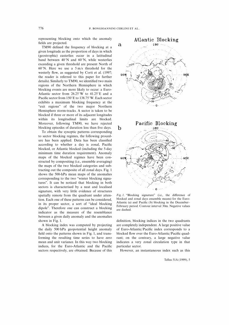
tracting out the composite of all zonal days. Fig. 1

shows the 500-hPa mean maps of the anomalies

corresponding to the two ‘‘winter blocking signa-

tures’’. It can be noticed that blocking in both

sectors is characterised by a neat and localised

signature, with very little evidence of structuresFig. 1. ‘‘Blocking signature’’ (i.e., the difference ofspatially remote from the quadrant under atten-blocked and zonal days ensemble means) for the Euro-tion. Each one of these patterns can be considered,Atlantic (a) and Pacific (b) blocking in the December–in its proper sector, a sort of ‘‘ideal blockingFebruary period. Contour interval 30m. Negative values

dipole’’. Therefore one can construct a blockingare dashed.

indicator as the measure of the resemblance

between a given daily anomaly and the anomalies

shown in Fig. 1. definition, blocking indices in the two quadrants

are completely independent. A large positive valueA blocking index was computed by projecting

the daily 500 hPa geopotential height anomaly of Euro-Atlantic/Pacific index corresponds to a

blocked flow over the Euro-Atlantic/Pacific quad-field onto the patterns shown in Fig. 1, and trans-

forming the resulting time series to have zero rant; on the contrary, a large negative value

indicates a very zonal circulation type in thatmean and unit variance. In this way two blocking

indices, for the Euro-Atlantic and the Pacific particular sector.

However, an instantaneous index such as thissectors respectively, are obtained. Because of this

Tellus 51A (1999), 5

- 777

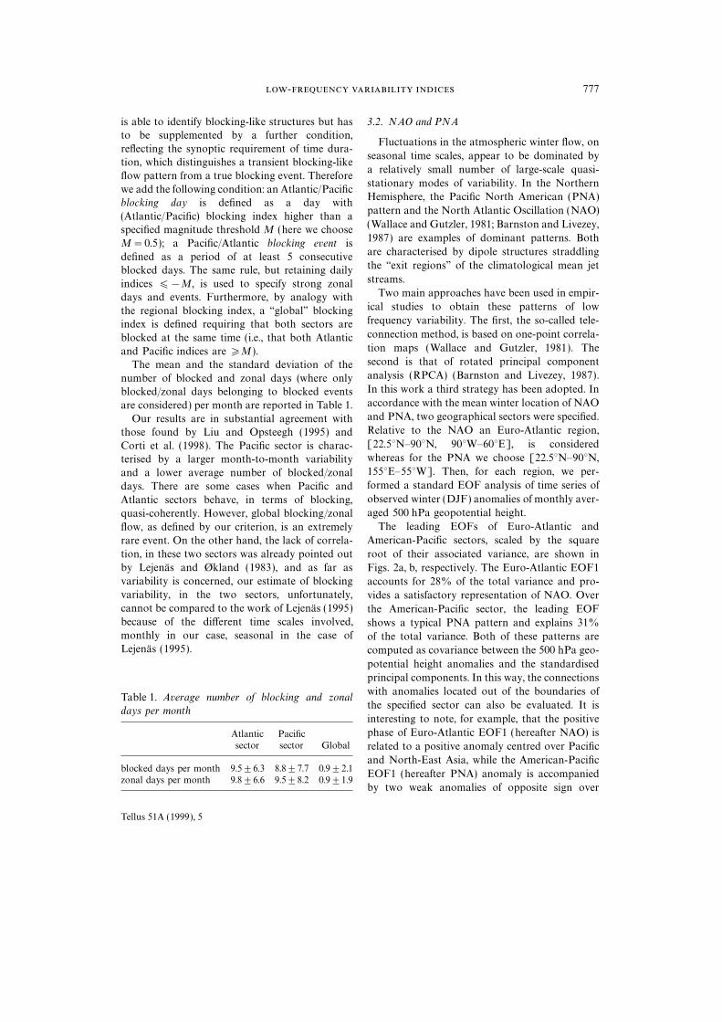
is able to identify blocking-like structures but has 3.2. NAO and PNA

to be supplemented by a further condition,Fluctuations in the atmospheric winter flow, on

reflecting the synoptic requirement of time dura-seasonal time scales, appear to be dominated by

tion, which distinguishes a transient blocking-likea relatively small number of large-scale quasi-

flow pattern from a true blocking event. Thereforestationary modes of variability. In the Northern

we add the following condition: an Atlantic/PacificHemisphere, the Pacific North American (PNA)

blocking day is defined as a day withpattern and the North Atlantic Oscillation (NAO)

(Atlantic/Pacific) blocking index higher than a(Wallace and Gutzler, 1981; Barnston and Livezey,

specified magnitude threshold M (here we choose1987) are examples of dominant patterns. Both

M=0.5); a Pacific/Atlantic blocking event isare characterised by dipole structures straddlingdefined as a period of at least 5 consecutivethe ‘‘exit regions’’ of the climatological mean jetblocked days. The same rule, but retaining dailystreams.indices ∏−M, is used to specify strong zonalTwo main approaches have been used in empir-days and events. Furthermore, by analogy with

ical studies to obtain these patterns of lowthe regional blocking index, a ‘‘global’’ blockingfrequency variability. The first, the so-called tele-index is defined requiring that both sectors areconnection method, is based on one-point correla-blocked at the same time (i.e., that both Atlantiction maps (Wallace and Gutzler, 1981). Theand Pacific indices are �M).second is that of rotated principal componentThe mean and the standard deviation of theanalysis (RPCA) (Barnston and Livezey, 1987).number of blocked and zonal days (where onlyIn this work a third strategy has been adopted. Inblocked/zonal days belonging to blocked eventsaccordance with the mean winter location of NAOare considered) per month are reported in Table 1.and PNA, two geographical sectors were specified.Our results are in substantial agreement withRelative to the NAO an Euro-Atlantic region,those found by Liu and Opsteegh (1995) and[22.5°N–90°N, 90°W–60°E], is consideredCorti et al. (1998). The Pacific sector is charac-whereas for the PNA we choose [22.5°N–90°N,terised by a larger month-to-month variability155°E–55°W]. Then, for each region, we per-and a lower average number of blocked/zonalformed a standard EOF analysis of time series ofdays. There are some cases when Pacific andobserved winter (DJF) anomalies of monthly aver-Atlantic sectors behave, in terms of blocking,aged 500 hPa geopotential height.quasi-coherently. However, global blocking/zonal

The leading EOFs of Euro-Atlantic andflow, as defined by our criterion, is an extremely

American-Pacific sectors, scaled by the squarerare event. On the other hand, the lack of correla-

root of their associated variance, are shown intion, in these two sectors was already pointed out

by Lejenas and Økland (1983), and as far as Figs. 2a, b, respectively. The Euro-Atlantic EOF1

variability is concerned, our estimate of blocking accounts for 28% of the total variance and pro-

variability, in the two sectors, unfortunately, vides a satisfactory representation of NAO. Over

cannot be compared to the work of Lejenas (1995) the American-Pacific sector, the leading EOFbecause of the different time scales involved, shows a typical PNA pattern and explains 31%monthly in our case, seasonal in the case of of the total variance. Both of these patterns areLejenas (1995). computed as covariance between the 500 hPa geo-

potential height anomalies and the standardised

principal components. In this way, the connections

with anomalies located out of the boundaries ofTable 1. Average number of blocking and zonal

the specified sector can also be evaluated. It isdays per month

interesting to note, for example, that the positive

phase of Euro-Atlantic EOF1 (hereafter NAO) isAtlantic Pacificsector sector Global related to a positive anomaly centred over Pacific

and North-East Asia, while the American-Pacificblocked days per month 9.5±6.3 8.8±7.7 0.9±2.1

EOF1 (hereafter PNA) anomaly is accompaniedzonal days per month 9.8±6.6 9.5±8.2 0.9±1.9

by two weak anomalies of opposite sign over

Tellus 51A (1999), 5

. .778

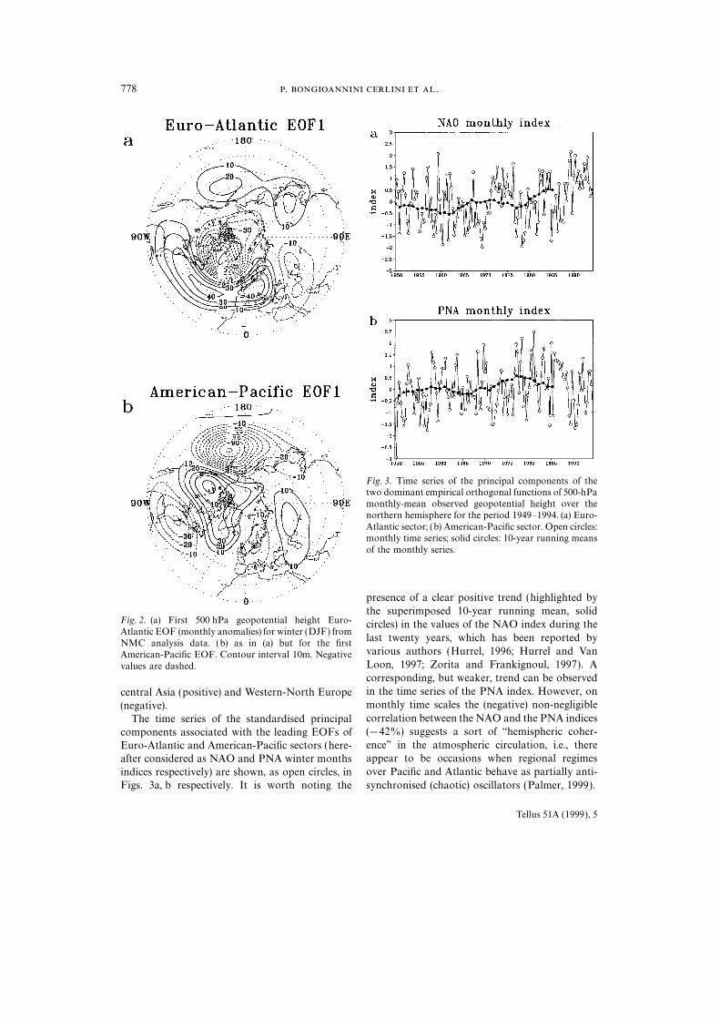
Fig. 3. Time series of the principal components of thetwo dominant empirical orthogonal functions of 500-hPamonthly-mean observed geopotential height over thenorthern hemisphere for the period 1949–1994. (a) Euro-Atlantic sector; (b) American-Pacific sector. Open circles:monthly time series; solid circles: 10-year running meansof the monthly series.

presence of a clear positive trend (highlighted by

the superimposed 10-year running mean, solidFig. 2. (a) First 500 hPa geopotential height Euro- circles) in the values of the NAO index during theAtlantic EOF (monthly anomalies) for winter (DJF) from

last twenty years, which has been reported byNMC analysis data. (b) as in (a) but for the first

various authors (Hurrel, 1996; Hurrel and VanAmerican-Pacific EOF. Contour interval 10m. NegativeLoon, 1997; Zorita and Frankignoul, 1997). Avalues are dashed.

corresponding, but weaker, trend can be observed

in the time series of the PNA index. However, oncentral Asia (positive) and Western-North Europemonthly time scales the (negative) non-negligible(negative).correlation between the NAO and the PNA indicesThe time series of the standardised principal(−42%) suggests a sort of ‘‘hemispheric coher-components associated with the leading EOFs ofence’’ in the atmospheric circulation, i.e., thereEuro-Atlantic and American-Pacific sectors (here-appear to be occasions when regional regimesafter considered as NAO and PNA winter months

over Pacific and Atlantic behave as partially anti-indices respectively) are shown, as open circles, in

Figs. 3a, b respectively. It is worth noting the synchronised (chaotic) oscillators (Palmer, 1999).

Tellus 51A (1999), 5

- 779

4. Wave amplitude index resynthesized after removal of periods ranging

from 22 to 9 months. The final result of this

analysis is a time series representing the timeThe rationale behind the definition and con-

struction of the wave amplitude index, introduced behaviour of the planetary wave amplitude

through the 44 years (plus one additional winter)by Sutera (1986), results primarily from the theor-

etical works of Charney and DeVore (1979) and considered. Since our study is devoted to the

winter season, we shall focus hereafter only on theWiin-Nielsen (1979) on simple, barotropic, low-

order models of midlatitude planetary wave/mean index time series during December, January and

February.flow interaction. They found multiple steady equi-

libria due to the presence of an instability associ- The probability density function of the WAI

anomaly, computed using a Gaussian kernel estim-ated to the topographically resonant flow. In

particular they found, for certain values of model ator (Marshall and Molteni, 1993), is shown in

Fig. 4a. This distribution exhibits two localparameters, two stable solutions characterised

respectively by ‘‘high’’ and ‘‘low’’ wave amplitude. maxima (M1 and M2) with amplitudes lower and

higher than normal respectively and a third localMany authors viewed these two stable equilibria

as idealisations of ‘‘zonal’’ and ‘‘blocked’’ states maximum (M3) with very high planetary wave

amplitude. The first two maxima are essentiallyof the real atmosphere and supported the idea

of a midlatitude winter atmosphere ‘‘fluctuating’’ to those found by HS86 from 15 winters (1964/65

through 1979/80) and more recently confirmed bybetween different flow regimes.

To assess the existence of such low-frequency the same authors (Hansen and Sutera, 1995) on a

larger dataset. Their statistical significance hasmultiple flow regimes in the middle latitudes of

the winter hemisphere, Sutera (1986) constructed been proved in HS95 by means of Monte Carlo

tests. The 3rd maximum belongs to the distribu-the wave amplitude index (WAI) as a combination

of the amplitudes of the first few planetary waves tion tail and is poorly populated.

To observe the mean anomalies correspondingmost susceptible to undergo resonance with the

lower boundary condition. In this study we use to high and low WAI values, HS86 have con-

structed composites of hemispheric geopotentialthis index as a measure of the extratropical large

scale circulation on a hemispheric coverage. height fields resulting from the partitioning of the

PDF into low (mode 1) and high (mode 2) ampli-Following Sutera’s description, the WAI is cal-

culated as follows. Each daily map of the observed tude modes. In particular, they defined ‘‘mode 1’’

and ‘‘mode 2’’ by compositing daily fields with500 hPa geopotential height, Z(l, w, t), is meridi-

onally averaged over the midlatitude band WAI anomaly values respectively lower and higher

than the distribution minimum. Using this defini-[45°–70°N] chosen according to Hansen andSutera (1986, hereafter HS86). The obtained field tion, we computed the two modes from our dataset

and the associated height anomalies are displayedZ (l, t) is then Fourier decomposed and zonal

wavenumbers 2 to 4 retained. Finally, the WAI is in Figs. 4b, c. These patterns compare very well

with those of HS86. As expected, the low-ampli-defined as the root-mean square value of the sum

of squares of the retained wavenumbers: tude mode (Fig. 4b) is associated with a fairly

zonal flow, while the high-amplitude mode

(Fig. 4c) corresponds to an amplified planetaryWAI=A ∑

4

i=2

|2Z9i(t)2 |B

1/2(1)

wave pattern. The two maps are dominated by

anomalies of substantial amplitude at planetary-

scale wavelengths, particularly wavenumber 2. InThe effect of the averaging procedure is to

remove or weaken the contribution to the index both cases the whole pattern is of hemispheric

extent, but the anomalies are larger over thefrom planetary waves with complicated meridional

structure and principally select waves with broad Pacific North American sector.

Temporal changes between low and high WAIlatitudinal extent. Furthermore, a 5-day low pass

filter is applied to the WAI time series. To remove values are quite rapid, while the residence time in

a given WAI ‘‘mode’’ is comparatively longer.the annual cycle and its subharmonics, the same

procedure used in HS86 has been applied: the Considering the entire 45-winter time series, the

total time over which a transition occurs (tran-time series has been Fourier transformed, then

Tellus 51A (1999), 5

. .780

Fig. 4. (a) Probability density estimation of the WAI computed in the [45°N-70°N] zone from the winters 1949–1994.(b) and (c) Mode 1 and Mode 2 composites (see text). Contour interval 10m. Negative values are dashed.

Tellus 51A (1999), 5

- 781

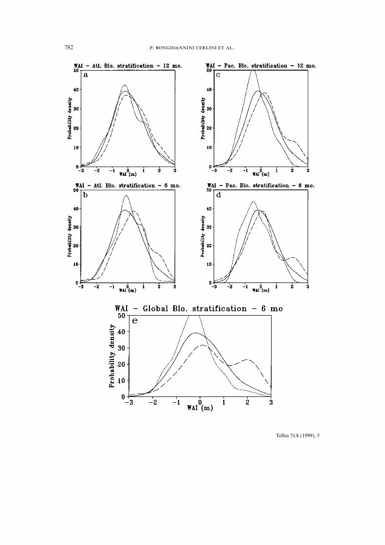
sitions have been defined in agreement with Fig. 5 shows 5 examples of WAI PDFs stratified

according to Atlantic blocking (panels a, b),Hansen, 1988) is, on average, 4 days, while the

duration of events of either mode is about 10 days. Pacific blocking (panels c, d) and Global blocking

(panel e) indices, respectively. WAI PDFs stratified

according to teleconnection indices are shown in5. Wave amplitude index and low-frequency

Fig. 6 (Fig. 6a, b: NAO; Fig. 6c, d: PNA; Fig. 6e:variability modes

NAO/PNA global mode). In all cases, the control

(climatological ) distribution (i.e., the PDF of theIn this section, we investigate the relationship

whole dataset) is shown as a solid line. The dashedbetween those patterns of limited regional extent

and dotted curves refer to periods of extremelylike blocking and teleconnections, as defined by

positive and negative indices, respectively. Thethe above indices, and the hemispheric planetary

upper panels of Figs. 5, 6 show the WAI distribu-wave activity modes defined by the wave ampli-

tions during the first 12 stratified months (i.e., thetude index. More precisely, the question we

12 winter months in which the relevant low-address here is whether and how the statistical

frequency index exhibits the most extreme posit-properties of the wave amplitude index are ‘‘sensit-

ive/negative values). Middle panels are relative toive’’ to different circulation regimes. In order to

6-month samples. They are subsets of the formerobtain homogeneous results from a statistical (and

12 months and consist of the most extreme events.graphical ) point of view, the following common

Finally, the lower panel shows, in both figures,methodology has been applied.

the WAI distributions of the 6-month samples

classified by the global version of blocking index5.1. T ools and methodology

(Fig. 5e) and teleconnection index (Fig. 6e),

respectively.To investigate the sensitivity of the planetary

wave amplitude index to low-frequency variability All the PDFs have been generated using a

Gaussian kernel estimator (Silverman 1986; seemodes, we start by classifying the (135) winter

months of our dataset according to the sign of also Marshall and Molteni 1993 for more details

in a similar application). The control WAI PDFblocking and teleconnections.

The classification of NAO and PNA months is (shown here for reference as a solid line) is virtually

that shown in Fig. 4a, except for the smoothing.made stratifying the Euro-Atlantic and Pacific

EOF1 principal components shown in Fig. 3. As In fact the smoothing (here the same for all the

distributions considered) is such that the probabil-far as blocking events are concerned, the strati-

fication criterion is made on the basis of the ity of obtaining a multimodal estimate from a (a

priori known) unimodal distribution is lower thannumber of blocked/zonal days (belonging to a

blocking/zonal event as defined in Subsection 3.1) 10% when applied to 12 or 6-month samples.

per month. There is something arbitrary about

using a monthly indicator, because the time scale5.2. WAI versus blocking index

of the evolution of blocking is mostly shorter than

one month. However it is an observational fact Figs. 5a–d shows the WAI PDFs stratified

according to the sign of Atlantic (a, b) and Pacificthat the mean flow of a blocked/zonal month is

different from the climatology itself. On the other (c, d) blocking indices respectively. Means and

standard deviations of the WAI index for differenthand, as discussed in the introduction, to assess

whether these differences in the mean flow affect flow regimes are listed in Table 2. The results

shown in both figures and table indicate that thethe statistical behaviour of the WAI, is exactly the

scope of this study. WAI PDFs relative to very blocked months are

broader with a secondary maximum correspond-After transforming the WAI time series to have

zero mean and unit variance, we compare, for ing to very high WAI values (in both sectors, more

pronounced during Pacific blocked months). Aneach low-frequency index, the WAI PDF of the

whole sample with those obtained from the classi- enhanced variability of WAI is found when the

Pacific sector is blocked. The opposite is true forfied samples. The resulting PDFs are shown in

Figs. 5, 6. Means and standard deviations of the low values of blocking indices (‘‘zonal’’ months).

The results, in terms of PDFs, of the stratifica-distributions are listed in Tables 1, 2.

Tellus 51A (1999), 5

. .782

Tellus 51A (1999), 5

- 783

Table 2. Mean and standard deviation of the WAI out when the 6-month extreme events samples are

PDFs shown in Fig. 5 considered. In such cases, the WAI distributions

also exhibit two maxima. The first is a ‘‘climatolo-Mean±std gical’’ maximum positioned around the distribu-

Control 0.00±1.00tion mean; the second maximum may correspond

to either high or low planetary wave amplitudes12 months 6 monthsdepending on the sign of NAO/PNA stratification.mean±std mean±stdIt is positive when negative PNA or positive NAO

Atlantic blocking 0.41±1.07 0.42±1.15 are considered; and negative otherwise.(Figs 5a, b, dashed line) These results indicate that the phases of theAtlantic zonal flow 0.2±1.0 0.12±1.07

NAO and the PNA can affect in some way the(Figs 5a, b, dotted line)

amplitude of the planetary waves as measured byPacific blocking 0.30±1.20 0.21±1.21Sutera’s WAI. On the other hand, even though(Figs 5c, d, dashed line)PNA and NAO patterns can fluctuate independ-Pacific zonal flow −0.27±0.87 −0.25±0.88

(Figs 5c, d, dotted line) ently for much of the time (Wallace, 1996), andglobal blocking — 0.60±1.24 therefore could be considered as independent(Fig. 5e, dashed line)

regional patterns, the relatively large negativeglobal zonal flow — −0.23±0.84

correlation (−0.42) between the two time series(Fig. 5e, dotted line)indicates that there are occasions when such

regional regimes over the Pacific and Atlantic do

vary coherently. In such cases, characterised by ation relative to global blocking are shown insort of PNA–NAO global mode, an even strongerFig.5e. The variance of WAI is enhanced for largeinfluence on the wave amplitude index distributionvalues of the index with a shift of the meanshould be expected. In particular, during periodstowards positive values (Table 2). The blockedcharacterised by positive PNA and negative NAOdistribution is clearly bimodal and both maximawe can observe a sharper WAI distribution withcorrespond to high planetary wave amplitudes.enhanced probability of low amplitude planetary

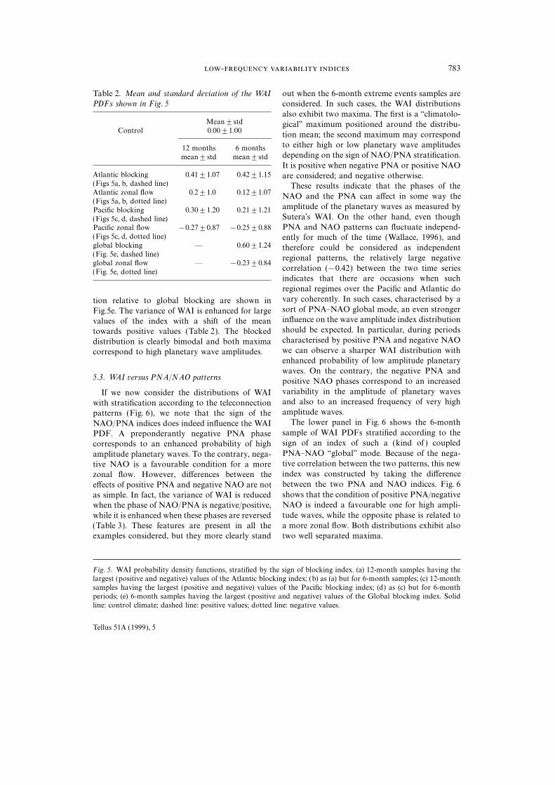
waves. On the contrary, the negative PNA and5.3. WAI versus PNA/NAO patterns positive NAO phases correspond to an increased

variability in the amplitude of planetary wavesIf we now consider the distributions of WAIand also to an increased frequency of very highwith stratification according to the teleconnectionamplitude waves.patterns (Fig. 6), we note that the sign of theThe lower panel in Fig. 6 shows the 6-monthNAO/PNA indices does indeed influence the WAI

sample of WAI PDFs stratified according to thePDF. A preponderantly negative PNA phasesign of an index of such a (kind of ) coupledcorresponds to an enhanced probability of highPNA–NAO ‘‘global’’ mode. Because of the nega-amplitude planetary waves. To the contrary, nega-tive correlation between the two patterns, this newtive NAO is a favourable condition for a moreindex was constructed by taking the differencezonal flow. However, differences between thebetween the two PNA and NAO indices. Fig. 6effects of positive PNA and negative NAO are notshows that the condition of positive PNA/negativeas simple. In fact, the variance of WAI is reducedNAO is indeed a favourable one for high ampli-when the phase of NAO/PNA is negative/positive,

tude waves, while the opposite phase is related towhile it is enhanced when these phases are reversed

a more zonal flow. Both distributions exhibit also(Table 3). These features are present in all the

examples considered, but they more clearly stand two well separated maxima.

Fig. 5. WAI probability density functions, stratified by the sign of blocking index. (a) 12-month samples having thelargest (positive and negative) values of the Atlantic blocking index; (b) as (a) but for 6-month samples; (c) 12-monthsamples having the largest (positive and negative) values of the Pacific blocking index; (d) as (c) but for 6-monthperiods; (e) 6-month samples having the largest (positive and negative) values of the Global blocking index. Solidline: control climate; dashed line: positive values; dotted line: negative values.

Tellus 51A (1999), 5

. .784

Tellus 51A (1999), 5

- 785

Table 3. Mean and standard deviation of the WAI

PDFs shown in Fig. 6

Mean±stdControl 0.00±1.00

12 months 6 monthsmean±std mean±std

Pos. NAO 0.53±1.18 0.33±1.17(Figs 6a, b, dashed line)Neg. NAO −0.04±0.97 −0.33±0.78(Figs 6a, b, dotted line)Pos. PNA 0.08±0.79 −0.01±0.76(Figs 6c, d, dashed line)Neg. PNA 0.55±1.11 0.62±1.13(Figs 6c, d, dotted line)Pos. PNA Neg. NAO — −0.01±0.76(Fig. 6e, dashed line)Neg. PNA Pos. NAO — 0.79±1.22(Fig. 6e, dotted line)

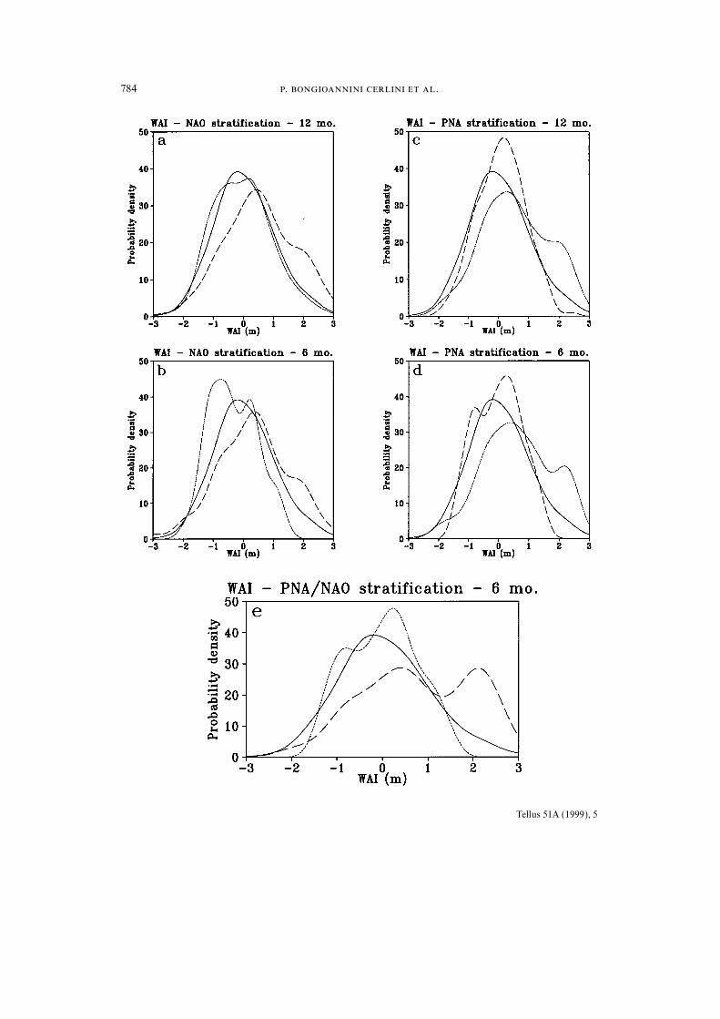
6. The PNA–NAO global mode

In order to test this hypothesis of a ‘‘global’’

PNA–NAO mode, an Empirical Orthogonal

Function analysis was applied to the hemispheric

domain monthly data. The spatial patterns of the

two leading EOFs are shown in Fig. 7. They are

very similar to those found by Kimoto and Ghil

(1993). The height anomaly associated with EOF1

projects both onto the negative PNA and the

positive NAO explaining the 18.3% of the total

variance. The second EOF (12% of the variance)

exhibits a good resemblance with the 500 hPa

geopotential height manifestation of the so-called

‘‘Cold Ocean Warm Land’’ pattern, which, to a

first approximation, describes recent climate

change in surface temperature on the decadal timeFig. 7. (a) First 500 hPa geopotential EOF monthlyscale (Wallace et al., 1995). Furthermore the spa-anomaly during winter (DJF) from NMC analysis data.

tial structure of both EOFs is very similar to that(b) As in (a) but for the second EOF. Contour interval

of well documented weather regimes (clusters in 10m. Negative values are dashed.phase space). These patterns correspond very

clearly with the so-called cluster-5 centroid well with centroids found using different cluster-

analysis methods (Mo and Ghil, 1988; Kimoto(EOF1) and cluster-2 centroid (EOF2) found by

Molteni et al. (1990), and based on 5-day mean and Ghil, 1993).

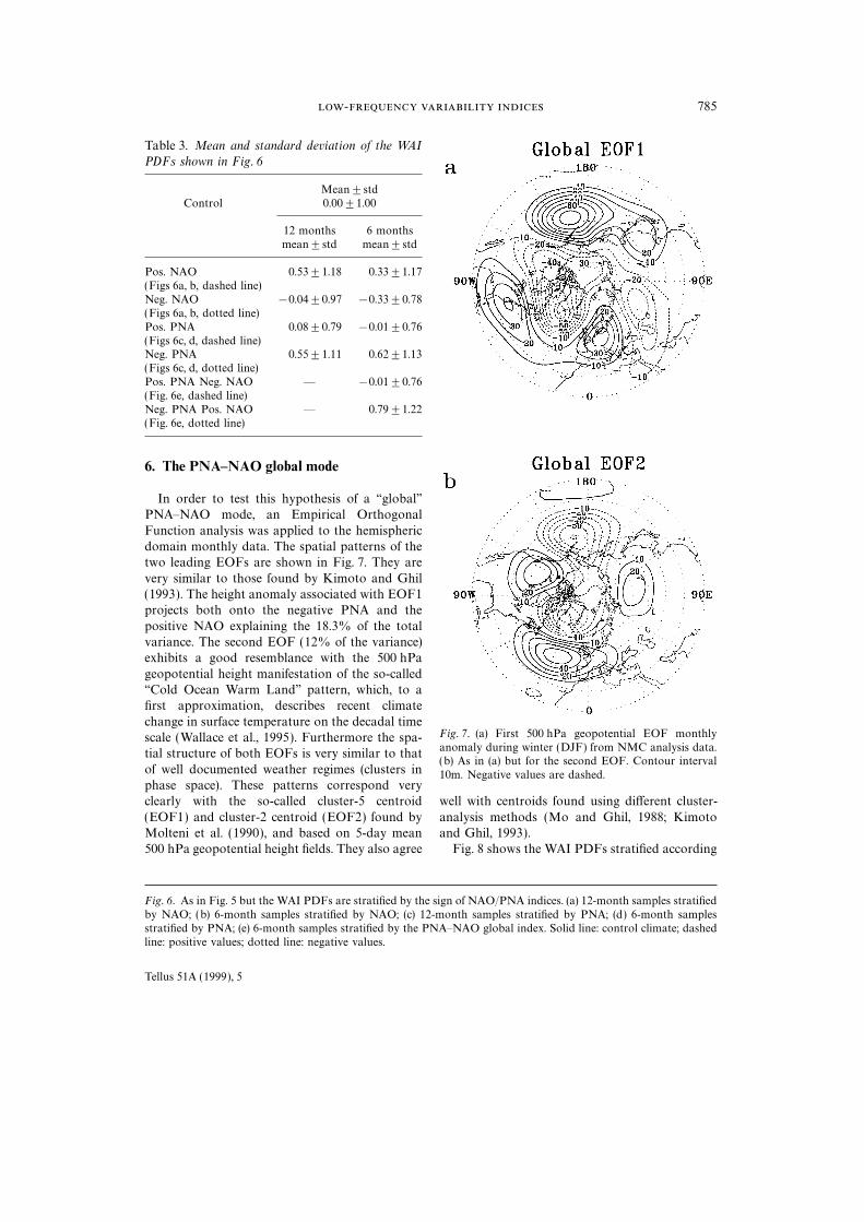
Fig. 8 shows the WAI PDFs stratified according500 hPa geopotential height fields. They also agree

Fig. 6. As in Fig. 5 but the WAI PDFs are stratified by the sign of NAO/PNA indices. (a) 12-month samples stratifiedby NAO; (b) 6-month samples stratified by NAO; (c) 12-month samples stratified by PNA; (d) 6-month samplesstratified by PNA; (e) 6-month samples stratified by the PNA–NAO global index. Solid line: control climate; dashedline: positive values; dotted line: negative values.

Tellus 51A (1999), 5

. .786

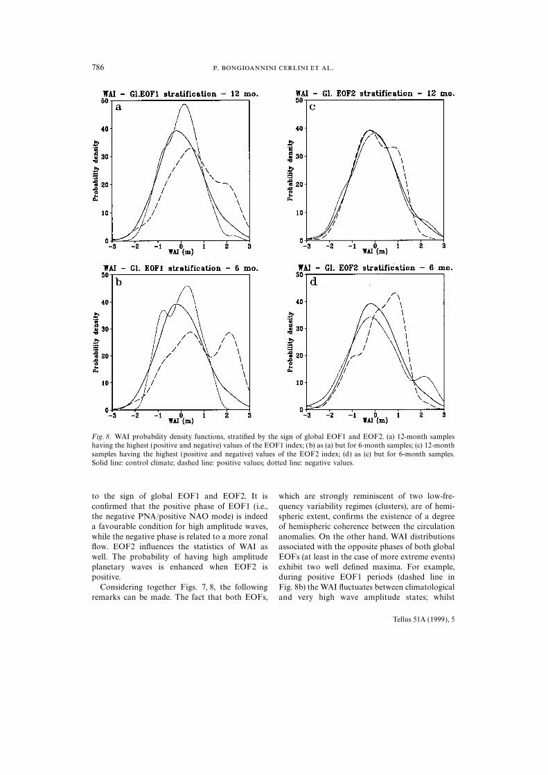
Fig. 8. WAI probability density functions, stratified by the sign of global EOF1 and EOF2. (a) 12-month sampleshaving the highest (positive and negative) values of the EOF1 index; (b) as (a) but for 6-month samples; (c) 12-monthsamples having the highest (positive and negative) values of the EOF2 index; (d) as (c) but for 6-month samples.Solid line: control climate; dashed line: positive values; dotted line: negative values.

to the sign of global EOF1 and EOF2. It is which are strongly reminiscent of two low-fre-

quency variability regimes (clusters), are of hemi-confirmed that the positive phase of EOF1 (i.e.,

the negative PNA/positive NAO mode) is indeed spheric extent, confirms the existence of a degree

of hemispheric coherence between the circulationa favourable condition for high amplitude waves,

while the negative phase is related to a more zonal anomalies. On the other hand, WAI distributions

associated with the opposite phases of both globalflow. EOF2 influences the statistics of WAI as

well. The probability of having high amplitude EOFs (at least in the case of more extreme events)

exhibit two well defined maxima. For example,planetary waves is enhanced when EOF2 is

positive. during positive EOF1 periods (dashed line in

Fig. 8b) the WAI fluctuates between climatologicalConsidering together Figs. 7, 8, the following

remarks can be made. The fact that both EOFs, and very high wave amplitude states; whilst

Tellus 51A (1999), 5

- 787

negative EOF1 periods (dotted line in Fig. 8b) blocked flow in the Pacific sector show an

increased variance. One could argue that thisare characterised by the same climatological

maximum and a further secondary maximum could be a (trivial ) consequence of the monthly-

averaged blocking index. Since the time scalecorresponding to very low amplitude waves.

This result seems to indicate that, within the typical of blocking lifetime is somewhat shorter

than a month, blocked-months-on-average may‘‘climate’’ of a given low-frequency variability

regime, one may have (in turn) two regimes show a larger variability of the planetary waves

simply due to the onset and decay of one or morecharacterised by high and low amplitude planet-

ary waves, respectively. blocking events during the month. However, the

fact that the enhanced variability concerns especi-

ally the Pacific region (together with the fact that

one-month long blocks are not so uncommon),7. Discussion and conclusionssuggests that, at least for this region, blocked flow

is particularly related to an enhanced planetaryIn this paper, we have addressed the problem

of the possible relationships between regional and wave activity.

Turning to the possible relationships betweenglobal indices of low-frequency variability and the

(global ) indicator of planetary wave amplitude regional teleconnections and wave amplitude

index, the first thing to note is that positive NAOsuggested by Sutera (1986).

First we have evaluated the observed indices in and negative PNA are confirmed to present some

evidence of spatial coherence on monthly timephysical space; then we have calculated WAI

PDFs for the northern extratropic winter fields scales. In practice, although Pacific and Atlantic

sectors regimes variabilities are normally quasiby stratifying the available dataset according to

the sign of such indices (namely blocking and independent, they become partially synchronised

from time to time. The correlation found (42%) isteleconnections) and comparing the resulting WAI

PDFs with the WAI PDF of the complete dataset. not particularly high, but it should be noted that

a linear correlation analysis may not be an appro-This stratification has been done using extreme

events of low-frequency variability in order to see priate way to study a possible ‘‘partial synchronis-

ation’’ since the phenomenon, certainly, involveswhether and how the specific ‘‘climate’’ of these

events is reflected by the statistical properties of nonlinear atmospheric chaotic synchronisation as

discussed by Duane (1997) in the (more general)the WAI index. It was found that low-frequency

variability modes affect both the mean and the context of interhemispheric synchronisation, which

goes well beyond the scope of this work.variance of the wave amplitude index probability

density functions. Furthermore, the positive phase of NAO and the

negative phase of PNA are both associated withAs far as blocking indices are concerned, we

confirmed the result of Lejenas and Økland, 1983 an enhanced frequency of very high amplitude

planetary waves. Distributions characterised by athat Pacific and Atlantic sector are not particularly

correlated in this respect. However, periods with maximum corresponding to high WAI exhibit also

large variance, while negative NAO and positivea prevalent ‘‘regional blocked flow’’ (Pacific or

Atlantic) are in general characterised by higher PNA influence the mean and the variance of WAI

PDF in the opposite sense. These features arevalues of the (hemispheric in nature) wave ampli-

tude index. These results are to be expected and particularly clear when WAI distributions of the

6-month sample stratified by the PNA–NAOcan be understood by simply noting that large

amplitude ridges of quasi-stationary planetary- global index are considered (extreme events). In

such case, both WAI distributions exhibit two wellscale waves (with the correct phase) are generally

needed to construct a blocking high. Furthermore, separated maxima.

In order to test the above somewhat speculativea number of observational studies showed that

blocking is in general associated with an enhance- conclusions on the relations between PNA and

NAO patterns and the high amplitude planetary-ment of the amplitude of stationary waves (Tung

and Lindzen, 1979; Austin, 1980; Hansen and scale regime as perceived by the WAI index, we

performed a hemispheric EOF analysis and strati-Sutera, 1993). It could perhaps be more interesting

to note that WAI PDFs relative to prevailing fied the WAI index according to it. We found

Tellus 51A (1999), 5

. .788

results very similar to those described by the on cluster analysis have identified a global

pattern which bears a close resemblance to thisglobal PNA–NAO index constructed with separ-amplified wave regime. For instance, cluster 2 ofate (regional ) PNA and NAO indices, recoveringMo and Ghil (Mo and Ghil, 1988) and clusterat the same time hemispheric spatial structures of5 of Molteni et al. (Molteni et al., 1990) arelow-frequency time-variability previously found inexamples of such pattern. More recently, Chengwell-accepted weather regimes studies.and Wallace (1993) and Corti et al. (1999)These observations suggest some furtheridentified clusters (i.e., Cheng and Wallace ‘‘A’’speculations about possible global regimes. Thecluster and Corti et al. ‘‘B’’ cluster) reminiscentlarger wave amplitude mode present in manyof the amplified wave regime.stratified WAI PDFs (corresponding mostly to

extreme cases) identifies with what Hansen and

Sutera (1995) call the ‘‘amplified wave regime’’. 8. AcknowledgementsThis regime seems to be particularly related to

what we have called a hemispheric-scale We are grateful to Dr. F. Molteni and Prof.PNA–NAO global mode, possibly due to the A. Sutera for many fruitful discussions and com-mostly constructive phase relation between PNA ments and to the referees for thorough reviews ofand NAO taking place in this case. On the other the original manuscript which led to substantial

improvements.hand, a number of flow regimes studies based

REFERENCES

Anderson, J. L. 1995. A simulation of atmospheric of recent climate change in frequencies of naturalatmospheric circulation regimes.Nature, 398, 799–802.blocking with a forced barotropic model. J. Atmos.

Sci. 52, 2593–2608. Dole, R. M. 1978. The objective representation ofblocking patterns. In T he general circulation: theory,Austin, J. F. 1980. The blocking of middle latitude west-

erly winds by planetary waves. Q. J. R. Meteorol. Soc. modelling and observations. Notes from a Colloquium,Summer, 1978. NCAR/CQ-6+1978 — ASP, 406–426.106, 327–350.

Barnston, A. G. and Livezey, R. E. 1987. Classification, Dole, R. M. 1986. Persistent anomalies of the extratropi-cal northern hemisphere wintertime circulation: struc-seasonality and persistence of low-frequency atmo-

spheric circulation patterns. Mon. Weather Rev. 115, ture. Mon. Weather Rev. 114, 178–207.Dole, R. M. and Gordon, N. D. 1983. Persistent anomal-1083–1126.

Baur, F. 1951. Extended range weather forecasting. In: ies of the Northern Hemisphere wintertime circulation.Geographical distribution and regional persistenceCompendium of Meteorology, American Meteorolo-

gical Society, 814–833. characteristics. Mon. Weather Rev. 106, 746–751.Duane, G. S. 1997. Synchronised chaos in extended sys-Benzi, R., Malguzzi, P., Speranza, A. and Sutera, A. 1986.

The statistical proprieties of general atmospheric cir- tems and meteorological teleconnections. Phys. Rev.E 56, 6475–6493.culation: Observational evidence and minimal theory

of bimodality. Q. J. R. Meteorol. Soc. 112, 661–674. Green, J. S. A. 1977. The weather during July 1977: somedynamical considerations of the drought. WeatherBenzi, R., Iarlori, S., Lippolis, G. and Sutera, A. 1988.

Steady non-linear response of a barotropic quasi-uni- 32, 120–128.Haines, K. and Hannachi A. 1995. Weather regimes indimensional model to complex topography. J. Atmos.

Sci. 45, 3313–3319. the Pacific from a GCM. J. Atmos. Sci. 52, 2444–2462.Hansen, A. R. 1988. Further observational characteristicsBranstator, G. and Opsteegh, J.D. 1989. Free solutions

of the barotropic vorticity equation. J. Atmos. Sci. 46, of bimodal planetary waves: Mean structure and tran-sitions. Mon. Weather Rev. 116, 386–400.1799–1814.

Charney, J. G. and De Vore, J. G. 1979. Multiple flow Hansen, A. R. and Sutera, A. 1986. On the probabilitydensity distribution of large-scale atmospheric waveequilibria in the atmosphere and blocking. J. Atmos.

Sci. 36, 1205–1216. amplitude. J. Atmos. Sci. 43, 3250–3265.Hansen, A. R. and Sutera, A. 1993. A comparisonCheng, X. and Wallace, J. M. 1993. Cluster analysis on

the Northern Hemisphere wintertime 500-hPa height between planetary-wave flow regimes and blocking.T ellus 45A, 281–288.field: Spatial patterns. J. Atmos. Sci. 50, 2674–2695.

Corti, S., Giannini, A., Tibaldi, S. and Molteni, F. 1997. Hansen, A. R. and Sutera, A. 1995. The probability den-sity distribution of the planetary-scale atmosphericPatterns of low-frequency variability in a three-level

quasi-geostrophic model. Clim. Dyn. 13, 883–904. wave amplitude revisited. J. Atmos. Sci. 52, 2463–2471.Hurrel, J. W. 1995. Decadal trends in the North AtlanticCorti, S., Molteni, F., and Palmer T. N., 1999. Signature

Tellus 51A (1999), 5

- 789

Oscillation: Regional temperature and precipitation. Reinhold, B. and Pierrehumbert, R. T. 1982. Dynamicsof weather regimes: quasi-stationary waves andScience 269, 676–679.blocking. Mon. Weather Rev. 110, 1105–1145.Hurrel, J. W. 1996. Influence of variations in extratropi-

Renwick J. A. and Wallace J. M. 1996. Relationshipscal wintertime teleconnections on Northern Hemi-between North Pacific Wintertime Blocking, El Nino,sphere temperatures. Geophys. Res. L ett. 23, 665–668.and the PNA pattern. Mon. Weather Rev. 124,Hurrel, J. W. and Van Loon, H. 1997. Decadal variations2071–2075.in climate associated with the North Atlantic oscilla-

Rex, D. F. 1950a. Blocking action in the middle tropo-tion. In: Climate change. Proc. Int. Workshop on Cli-sphere and its effect on regional climate. (I) An aerol-matic change at high elevation sites, Wengen,ogical study of blocking action. T ellus 2, 196–211.Switzerland.

Rex, D. F. 1950b. Blocking action in the middle tropo-Kimoto, M. and Ghil, M. 1993. Multiple flow regimessphere and its effect on regional climate. (II) Thein the Northern Hemisphere winter. Part I: Methodo-climatology of blocking action. T ellus 2, 275–301.logy and hemispheric regimes. J. Atmos. Sci. 50,

Rossby, C.-G. et al. 1939. Relation between variations in2645–2673.the intensity of the zonal circulation in the atmosphereLegras, B. and Ghil, M. 1985. Persistent anomalies,and the displacement of the semi-permanent centersblocking and variations in atmospheric predictability.of action. J. Mar. Res. 2, 38–55.J. Atmos. Sci. 42, 433–471.

Shutts, G. J. 1983. The propagation of eddies in diffluentLejenas, H. and Økland, H. 1983. Characteristic of north-jetstreams: eddy forcing of blocking flow fields. Q. J. R.ern hemisphere blocking as determinated from a longMeteorol. Soc. 109, 737–761.time series of observational data. T ellus 35A, 350–362.

Silverman, B. W. 1986. Density estimation for statisticsLejenas, H. 1995. Long term variations of atmosphericand data analysis. Chapman and Hall, 175 pp.blocking in the Northern Hemisphere. J. Met. Soc.

Sutera, A. 1986. Probability density distribution of largeJapan 73, 79–89.scale atmospheric flow. Adv. Geophys. 29, 319–338.Liu, Q. 1994. On the definition and persistence of

Tibaldi S. and Molteni, F. 1990. On the operationalblocking. T ellus 46A, 286–298.predictability of blocking. T ellus 42A, 343–365.Liu, Q. and Opsteegh, T. 1995. Interannual and decadal

Toth, Z. 1992. Quasi-stationary and transient periods invariations of blocking activity in a quasi-geostrophicthe Northern Hemisphere winter. Mon. Weather Rev.model. T ellus 47A, 941–954.119, 1602–1611.Lorenz E. N. 1963. Deterministic nonperiodic flow.

Tung, K. K. and Lindzen, R. S. 1979. A theory of station-J. Atmos. Sci. 20, 130–141.

ary long waves. Part I: A simple theory of blocking.Malguzzi, P. 1993. An analytical study on the feedback

Mon. Weather Rev. 107, 714–734.between large- and small-scale eddies. J. Atmos. Sci.

Vautard, R. 1990. Multiple weather regimes over the50, 1429–1436.

North Atlantic. Analysis of precursor and successors.Marshall, J. and Molteni, F. 1993. Toward a dynamical

Mon. Weather Rev. 118, 2056–2081.understanding of planetary-scale flow regimes.

Vautard, R. and Legras, B. 1988. On the source of low-J. Atmos. Sci. 50, 1792–1818.

frequency variability. Part II: Nonlinear equilibrationMichelangeli, P.-A., Vautard, R. and Legras, B. 1995.

of weather regimes. J. Atmos. Sci. 45, 2845–2867.Weather regimes: recurrence and quasi-stationarity. Wallace, J. M. 1996. Observed climatic variability: Spat-J. Atmos. Sci. 52, 1237–1256. ial structure. In: Decadal climate variability —

Mo, K.-C. and Ghil, M. 1988. Cluster analysis of multiple dynamics and predictability (eds. D. L. T. Andersonplanetary flow regimes. J. Geophys. Res. 93, and J. Willebrand). NATO ASI series, Vol. 44.10927–10952. Springer, 31–82.

Molteni, F., Sutera, A. and Tronci, N. 1988. EOFs of the Wallace, J. M. and Gutzler, D. S. 1981. Teleconnectionsgeopotential eddies at 500 mb in winter and their in the geopotential height field during the northernprobability density distributions. J. Atmos. Sci. 45, hemisphere winter. Mon. Weather Rev. 109, 784–81.3063–3080. Wallace, J. M., Zhang Y. And Bajuk L. 1995. Interpreta-

Molteni, F., Tibaldi, S. and Palmer, T. N. 1990. Regimes tion of interdecadal trends in Northern Hemispherein the winter-time circulation over northern extratrop- surface air temperature. J. of Clim. 9, 249–259.ics. I: Observational evidence. Q. J. R. Meteorol. Soc. Wiin-Nielsen, A. 1979. Steady states and stability propri-116, 31–67. eties of a low-order barotropic system with forcing

Namias, J. 1950. The index cycle and its role in the and dissipation. T ellus 31, 375–386.general circulation. J. Meteor. 7, 130–139. Yang, S. and Reinhold, B. 1991. How does low-frequency

Palmer, T. N. 1999. A nonlinear dynamical perspective variance vary? Mon. Weather Rev. 119, 119–127.on climate prediction. J. of Clim. 12, 575–591. Zorita, E. and Frankignoul, C. 1997. Modes of North

Pierrehumbert, R. T. and Malguzzi, P. 1984. Forced Atlantic decadal variability in the ECHAM1/LSGcoherent structures and local multiple equilibria in a coupled ocean–atmosphere general circulation model.

J. of Clim. 10, 183–200.barotropic atmosphere. J. Atmos. Sci. 41, 246–257.

Tellus 51A (1999), 5