AgriculturAl Drought inDicesProceedings of an exPert meeting

2–4 June 2010, MurciA, spAin

World Meteorological Organization

United States Department of Agriculture

World Agricultural Outlook Board

National DroughtMitigation Center

United Nations International Strategy for

Disaster Reduction

Government of Spain Ministry for

Environmental, Rural and Marine Affairs

Hydrographic Confederation of Segura

Ag

ricultu

rAl D

rou

gh

t inD

ices proceeD

ing

s of A

n expert M

eeting

Agricultural Drought Indices ________________________________________________________________________

Proceedings of an Expert Meeting

2-4 June, 2010, Murcia, Spain

Editors

Mannava V.K. Sivakumar Raymond P. Motha Donald A. Wilhite Deborah A. Wood

Sponsors

World Meteorological Organization

United Nations International Strategy for Disaster Reduction (UNISDR)

Hydrographic Confederation of Segura, Spain

United States Department of Agriculture

National Drought Mitigation Center University of Nebraska, Lincoln, Nebraska, USA

AGM-11 WMO/TD No. 1572

WAOB-2011

World Meteorological Organization

7bis, Avenue de la Paix 1211 Geneva 2

Switzerland

2011

ii

© World Meteorological Organization, 2011 The right of publication in print, electronic, and any other form and in any language is reserved by WMO. Short extracts from WMO publications may be reproduced without authorization provided that the complete source is clearly indicated. Editorial correspondence and requests to publish, reproduce or translate this publication (articles) in part or in whole should be addressed to: Chairperson, Publications Board World Meteorological Organization (WMO) 7 bis, avenue de la Paix Tel.: +41 (0)22 730 84 03 P.O. Box No. 2300 Fax: +41 (0)22 730 80 40 CH-1211 Geneva 2, Switzerland E-mail: Publications@wmo.int The designations employed in WMO publications and the presentation of material in this publication do not imply the expression of any opinion whatsoever on the part of the Secretariat of WMO concerning the legal status of any country, territory, city or area or of its authorities, or concerning the delimitation of its frontiers or boundaries. Opinions expressed in WMO publications are those of the authors and do not necessarily reflect those of WMO. The mention of specific companies or products does not imply that they are endorsed or recommended by WMO in preference to others of a similar nature which are not mentioned or advertised. This document is not an official publication of WMO and has not been subjected to its standard editorial procedures. The views expressed herein do not necessarily have the endorsement of the Organization.

iii

Proper citation is requested. Citation: Sivakumar, Mannava V.K., Raymond P. Motha, Donald A. Wilhite and Deborah A. Wood (Eds.). 2011. Agricultural Drought Indices. Proceedings of the WMO/UNISDR Expert Group Meeting on Agricultural Drought Indices, 2-4 June 2010, Murcia, Spain: Geneva, Switzerland: World Meteorological Organization. AGM-11, WMO/TD No. 1572; WAOB-2011. 197 pp.

About the Editors

Mannava V.K. Sivakumar Director

Climate Prediction and Adaptation Branch Climate and Water Department

World Meteorological Organization 7bis, Avenue de la Paix

1211 Geneva 2, Switzerland

Raymond P. Motha Chief Meteorologist

World Agricultural Outlook Board Mail Stop 3812

United States Department of Agriculture Washington D.C., 20250-3812 USA

Donald A. Wilhite Director and Professor

School of Natural Resources 903 Hardin Hall

3310 Holdrege Street University of Nebraska

Lincoln, Nebraska 68583-0989 USA

Deborah A. Wood Publications Specialist

National Drought Mitigation Center University of Nebraska

Lincoln, Nebraska 68583-0989 USA

iv

Agricultural Drought Indices Proceedings of a WMO Expert Meeting held in Murcia, Spain

Table of Contents

Page Preface ...................................................................................................................................... vi Agricultural Drought Indices—An Overview 1. Segura River Basin: Spanish Pilot River Basin Regarding Water Scarcity and Droughts M. A. Urrea Mallebrera, A. Mérida Abril, and S.G. García Galiano .................................... 2 2. Quantification of Agricultural Drought for Effective Drought Mitigation and Preparedness: Key Issues and Challenges Donald A. Wilhite .............................................................................................................. 13 3. Agricultural Drought—WMO Perspectives Mannava V.K. Sivakumar ................................................................................................. 22 4. Agricultural Drought: USDA Perspectives Raymond P. Motha .......................................................................................................... 35 Agricultural Drought Indices in Current Use in Selected Countries: Strengths,

Weaknesses, and Limitations 5. Monitoring Drought Risks in India with Emphasis on Agricultural Drought Jayanta Sarkar ................................................................................................................. 50 6. Agricultural Drought Indices in Current Use in Brazil Paulo Cesar Sentelhas ..................................................................................................... 60 7. Agricultural Drought Indices in Current Use in Australia: Strengths, Weaknesses, and Limitations Roger C. Stone ................................................................................................................ 72 8. Agricultural Drought Indices in France and Europe: Strengths, Weaknesses, and Limitations Emmanuel Cloppet ........................................................................................................... 83 9. Drought Monitoring in Spain Antonio Mestre and Jose Luis Camacho .......................................................................... 95 10. Agricultural Drought Indices in the Greater Horn of Africa (GHA) Countries P.A. Omondi ................................................................................................................... 106

v

Table of Contents (con’t) Page Agricultural Drought Indices: Integration of Crop, Climate, and Soil Issues 11. Incorporating a Composite Approach to Monitoring Drought in the United States Mark Svoboda ................................................................................................................ 114 12. Water Balance—Tools for Integration in Agricultural Drought Indices Paulo Cesar Sentelhas .................................................................................................. 124 13. Use of Crop Models for Drought Analysis Raymond P. Motha ........................................................................................................ 138 Local Experiences in Managing Droughts 14. Monitoring Regional Drought Conditions in the Segura River Basin from Remote Sensing S.G. García Galiano, M. Urrea Mallebrera, A. Mérida Abril, J.D. Giraldo Osorio, and C. Tetay Botía ......................................................................... 150 15. Experiences During the Drought Period 2005-2008 Javier Ferrer Polo .......................................................................................................... 156 16. Drought Assessment Using MERIS Images Alberto Rodríguez Fontal ............................................................................................... 165 Consensus Agricultural Drought Index 17. Agricultural Drought Indices: Summary and Recommendations

Mannava V.K. Sivakumar, R. Stone., P.C. Sentelhas., M. Svoboda., P. Omondi., J. Sarkar and B. Wardlow ............................................................................................... 172

vi

Preface With the world population projected to reach 7.5 billion, the world’s farmers will have to produce 40% more grain in 2020, and the challenge is to revive agricultural growth at the global level. The Fourth Assessment Report of the Intergovernmental Panel on Climate Change (IPCC) stated that the world has been more drought-prone during the past 25 years and that climate projections indicate an increased frequency in the future. This carries significant implications for the agriculture sector, especially in the developing countries. One of the critical components of national drought strategies is a comprehensive drought monitoring system that can provide early warning of the onset and ending of droughts, determine the severity, and deliver that information to the users in the agriculture sector. In February 2009, the Commission for Agricultural Meteorology of the World Meteorological Organization (WMO) held the International Workshop on Drought and Extreme Temperatures in Beijing, China, to review the increasing frequency and severity of droughts and extreme temperatures around the world. The workshop adopted several recommendations to cope with the effects of increasing droughts and extreme temperatures on agriculture, rangelands, and forestry. One of the main recommendations was for WMO to make appropriate arrangements to identify the methods and marshal resources for the development of standards for agricultural drought indices in a timely manner. WMO, together with the National Drought Mitigation Center (NDMC) and the School of Natural Resources of the University of Nebraska–Lincoln (USA), organized the Inter-Regional Workshop on Indices and Early Warning Systems for Drought at the University of Nebraska in December 2009. The Lincoln Declaration on Drought Indices recommended that a working group with representatives from different regions around the world and observers from UN agencies and research institutions (and water resource management agencies for hydrological droughts) be established to further discuss and recommend, by the end of 2010, the most comprehensive index to characterize agricultural drought. Accordingly, WMO and the United Nations International Strategy for Disaster Reduction (UNISDR), in collaboration with the Hydrographical Confederation of Segura River Basin and the State Agency for Meteorology of Spain (AEMET), organized the Expert Group Meeting on Agricultural Drought Indices in Murcia, Spain, June 2-4, 2010. The meeting reviewed drought indices currently used around the world for agricultural drought and assessed the capability of these indices to accurately characterize the severity of droughts and their impacts on agriculture. Fifteen papers presented at the expert group meeting are brought together in this volume. These papers present an overview of agricultural drought indices; the strengths, weaknesses, and limitations of different agricultural drought indices currently in use in selected countries; the integration of crop, climate, and soil issues in agricultural drought indices; and a summary and recommendations on agricultural drought indices. We wish to convey our sincere thanks to Mr. Michel Jarraud, the Secretary-General of WMO; Dr. Marta Moren Abat, Director General of Water of the Ministry of Environment, Rural and Marine Sector of Spain; and Dr. Rosario Quesada Gil, President of the Hydrographic Confederation of Segura, for their encouragement and support in the organization of the expert meeting in Murcia. We also wish to thank Mr. Mario Urrera Mallebrera, Chief of the Hydrological Planning Office, and Mr. Adolfo Merida Abril, Chief of the Service of the Hydrographic Confederation of Segura, for their excellent cooperation in coordinating the arrangements for the meeting.

Mannava V.K. Sivakumar Raymond P. Motha

Donald A. Wilhite Deborah A. Wood

Editors

Agricultural Drought Indices—An Overview

2

Segura River Basin: Spanish Pilot River Basin Regarding Water Scarcity and Droughts

M. A. Urrea Mallebrera1, A. Mérida Abril1, S.G. García Galiano2

1Hydrographic Confederation of the Segura River, Hydrological Planning Office, Murcia, Spain 2Technical University of Cartagena, Department of Civil Engineering, Cartagena, Spain

Abstract

The issues and strategies of planning and managing water resources during drought and water scarcity conditions in the Segura River Basin (SRB, Spain) are presented. This basin, located in the southeastern part of the Iberian Peninsula, was selected as a pilot basin under the framework of the European Group of Experts for Water Scarcity and Droughts. The SRB has the lowest percentage of renewable water resources of all Spanish basins. It is highly regulated and has a semiarid climate, and its main water demand is agriculture. Drought impacts and the SRB’s drought action plan are discussed.

Introduction: Main Characteristics of the Segura River Basin

Human activities and demographic, economic, and social processes exert pressures on water resources (WWDR3 2009). These pressures are in turn affected by factors such as public policies and climate change. According to the Intergovernmental Panel on Climate Change (IPCC), in southeast Spain, an intensification of the water cycle is expected, with an increase in extreme events.

The Segura River Basin is located in southeast Spain (Figure 1). Agricultural surface in the Segura River Basin accounts for more than 43% (809,045 ha) of the basin (SRBP 1998), but only one-third of that surface is under irrigation (more than 269,000 ha). Nevertheless, most efforts and investments are focused on irrigated areas because of their very high profitability, together with the fact that the most important management measures can only be taken on irrigated systems (such as dam management and water transfers). The basin’s main characteristics are summarized in Table 1.

Figure 1. The Segura River Basin.

3

Table 1. Segura River Basin main characteristics.

Table 2 and Figure 2 show the key meteorological and hydrological characteristics of the Segura River Basin. The mean annual rainfall and potential evapotranspiration (PET) correspond to 300 mm and 700 mm, respectively. Therefore, mean annual runoff is minimal.

Figure 2. Segura River Basin rainfall, PET, and runoff. Period: 1940/41-1995/96. Source: DBW 2000.

Table 2. Segura River Basin meteorological and hydrological characteristics (SRBR 2008).

Surface

(km2) Average rainfall

(mm) PET (mm)

Natural resources (hm3/year)

Ratio per inhabitant

S.R.B. 18815 (3.7%) 365 827 803 (0.7%) 442 m3/year Spain 506474 711 842 111186 2460 m3/year The Segura River Basin is a semiarid basin; it has the fewest renewable water resources of all the Spanish river basins. In addition, available water resources per inhabitant in the Segura River Basin (only 442 m³/inhabitant/year) are much lower than the national water scarcity threshold, which is set at 1000 m³/inhabitant/year, according to international organizations such as the United Nations and the World Health Organization. Consequently, water scarcity is a major issue in the Segura River Basin.

Water Resources and Demands: Main Problems Only those demands and resources that can be managed by means of the hydraulic system (dams, desalination plants, water transfer, and management rules) will be considered. Therefore, non-irrigated areas, or water resources that are not stored in a dam, will not be included in this analysis. Water Resources The water resources expected to be available in the Segura River Basin by 2015 are presented in Table 3. The relevance of non-conventional resources, with a contribution of 65.43 %, must be emphasized (Table 3).

Surface (km 2 ) 18.815 Population (inhabitants). Year 2009 1.969.370 Summer population (inhabitants). Year 2009 > 2.500.000 Total length of channel network (km) 1.470 Irrigated surface (ha) 269.029

4

Table 3. Segura River Basin resources (OSI 2010).

CONVENTIONAL RESOURCES

NON-CONVENTIONAL RESOURCES

Surface water

hm3 TOTAL

(80-05 average) Groundwater hm3 Water transfer hm3 Desalination

hm3 Reuse

hm3 Expected

2015 296 334 540 460 192 1822

% 16.25% 18.33% 29.64% 25.25% 10.54% 100%

Main Trends During the last 30 years, the runoff average of Segura River Basin (surface water) has decreased noticeably, increasing the water scarcity problem of the basin (Figure 3).

Figure 3. Time evolution of Segura River Basin runoff. Some groundwater sources are overexploited as a consequence of the water scarcity and drought problems of the basin (Figure 4).

5

Figure 4. Segura River Basin groundwater bodies. Ratio k=abstraction/recharge. Source: GRBD 2007.

Water Demands Table 4 summarizes the water demands of the basin. Agricultural water demand from irrigated areas must be highlighted because it accounted for 85% of the total water demand in 2007. Agriculture is important in the Segura River Basin not only because of its very high profitability (with an average value production of 1.93 €/m³ and a net margin of 0.72 €/m³), but also because of its role in the sustainability of rural areas and the environment. Table 4. Segura River Basin resources.

Demand/Time Horizon 2007 2015 2027 Urban supply and industrial demand 263.2 318.9 360 Irrigation 1662 1549 1549 Environmental demand 30 30 30 Total (hm3) 1955.2 1897.9 1939

Water Balance Despite efforts to increase water resources and to reduce demands by measures like investing in irrigation modernization or providing non-conventional water resources, there is still a deficit in the water balance (Figure 5). Against this background, recurrent and severe droughts that occur in the basin have become a major issue and have led to important developments in drought management aimed at reducing impacts.

6

Figure 5. Segura River Basin water balance. Expected by 2015.

Drought Management in the Basin—Indicators Legal Background Water policy in Europe has been established by the Water Framework Directive (WFD 2000). It sets the water management unit as the “River Basin District” (the area of land and sea made up of one or more neighboring river basins together with their associated groundwater and coastal waters), and it also directs all member states to develop water management plans. But only a few guidelines are given about drought management. The WFD has been adapted to Spanish regulations by the Refunded Water Law RDL 1/2001 (RWL 2001). Spain has developed more regulations for drought management since it is an important problem in the country. The National Hydrological Plan Law (NHPL 2001), released in 2001, established the obligation to develop drought action plans at the River Basin District level. The Segura River Basin Drought Action Plan (SRBDAP 2007) and other basins’ plans were endorsed in 2007. Spanish Drought Action Plans The plans have the following characteristics:

o They define the onset/appearance of drought. o They describe the measures to be taken, depending on the severity of the drought. They

also define when those measures have to be applied. o They establish the severity of a drought, using indicators. o They identify the parties responsible for carrying out the measures.

7

Droughts in the Segura River Basin In the search for drought indicators, the Standard Precipitation Index (SPI) was evaluated in the Segura River Basin for the last 65 years (Figure 6).

Figure 6. SPI in the Segura River Basin. The SPI shows several droughts in the basin. Some of them are quite severe, like the last one, which has lasted for 4 years. Indicators of the Segura River Basin Drought Action Plan Drought Indicator Assessment The Segura River Basin indicator has two parts: the first one dealing with the resources in the basin (basin subsystem) and the second one dealing with the water transfer system (water transfer subsystem). The indicator is intended to reproduce water deficit. Water released from reservoirs is closely linked with demands and it is a good way to assess deficits. Several factors were taken into account when selecting the most suitable parameters to create the indicator. The graph below includes factors time series together with the water released time series. As shown in Figure 7, runoff is the most similar factor to the water released from reservoirs time series.

Figure 7. Indicator parameters. Time series of hydrological variables of the global system.

8

Drought Indicator Expression After the assessment process, the resulting indicators were:

Once the indicator is established, an associated index is assessed (monthly) as follows: Index (Ie) varies between 0.5 and 1 when Ve>Vmed, and between 0 and 0.5 when assessed Ve>Vmed, as shown in Figure 8.

Figure 8. Drought index assessment.

Drought Severity Four levels of severity are defined according to the drought index value (Figure 9).

Figure 9. Drought severity and drought index evolution. Updated information can be found at https://www.chsegura.es/chs_en/cuenca/sequias/gestion/index.html. Measures of the Segura River Basin Drought Action Plan Several types of measures have been defined:

• Forecast, administrative, and management measures. • Operative measures, such as:

o Measures to provide additional water resources (measures to enhance supply, i.e., increase water resources).

o Measures to reduce demands significantly (measures aimed at managing the demands).

• Monitoring and recovery measures.

Ve = 0,66*Runoff(annual)+0,33*water in reservoirs Ve = 0,33*Runoff(annual)+0,66*water in E+B reservoirs Ve = a*Ve(basin)+b*Ve(water-transfer)

-Basin subsystem:

-Water transfer subsystem: -Global indicator

a, b depend on water rights given in each Sub-system (a=0,48; b=0,52)

9

Following the Drought Action Plan, several measures were implemented during the last drought period (2005–2010):

• Weekly monitoring system. • New desalination plants. • Operation of the Well Strategic Network. • Emergency investments in new infrastructures to increase water resources or to improve

demand management. • Water rights transfer, using water transfer infrastructure (up to 70 hm3/year) • Restrictions to irrigation supply, up to 50%. • Improving installations and networks to reduce water losses. • Modernization of irrigation systems. • Economic measures to compensate farmers for water supply restrictions. • Administrative measures, including a drought decree to improve water resource

management. One example of how measures were applied is the management of the Well Strategic Network (Figure 10).

Figure 10. Well Strategic Network.

Consequences of the Last Drought (2005–2010) On the positive side, by temporarily increasing water availability, and by a proper management of demands, there were no major constraints on domestic water supply, and urban water supply (services and industry), and environmental and socioeconomic impacts decreased. The impacts on agriculture, compared with former drought periods, are summarized in Table 5.

10

Table 5. Analysis of drought impacts.

On the negative side, there were still significant impacts: • Restrictions on irrigation supply, up to 50%. • Increased pressure on groundwater supplies (aquifers). • Great investment effort: 406.46 M€ from 2004-05 to 2008-09. • Water price (also connected with water scarcity):

o Desalination water costs: up to 0.72 €/m3 (in 2008). o Urban supply water price: 0.55 €/m3 (in 2008). o Abstracted water cost: up to 0.25 €/m3.

European Expert Network on Water Scarcity and Droughts

As a consequence of the release of the European Water Framework Directive (WFD 2000), the Common Implementation Strategy (CIS) was created to ease the implementation process. In the field of water scarcity and droughts, and within the WFD CIS structure, the European Expert Network on Water Scarcity and Droughts was set up in December 2006. The Network developed the technical document Drought Management Report, including Agricultural, Drought Indicators and Climate Change Aspects (DMP Report 2007). The main tasks (among others) are:

• Support the definition of commonly accepted indicators for water scarcity and droughts in Europe.

• Support the creation of drought risk maps, through commonly agreed-on methodology and scales.

The lead countries are Spain, France, and Italy. Pilot River Basins The Segura River Basin has been selected by the Spanish Ministry of the Environment and Rural and Marine Affairs as the Spanish Pilot River Basin, within the Expert Network on Water Scarcity and Droughts (Figure 11). The role of the pilot river basins is to share their experiences in the indicator selection process. Member states will evaluate the initial results in pilot river basins and check their effectiveness. The map server of the European Drought Observatory (EDO) at the European Commission Joint Research Centre (JRC) will be a valuable tool for implementing the results of this process: http://edo.jrc.ec.europa.eu/php/index.php?action=view&id=201

11

Figure 11. Segura River Basin: Water Scarcity and Drought Pilot River Basin. Next steps of the Expert Network The timetable for the Expert Group:

• Year 2010: First set of indicators to be tested in the pilot member states (including Spain, Italy, and France); contributions to EDO.

• Presentation of initial results at the International Conference “Droughts and Water Scarcity: The Way towards Adaptation to Climate Change”, Madrid, Spain, 18-19 February 2010.

• Year 2011: Practical application of indicators for additional member states (voluntarily); contributions to EDO, and potential contribution to the development of an integration of WS&D aspects under the Water Information System for Europe (WISE) on a voluntary basis.

• Year 2012: Support the creation of drought risk maps and assessment, contributions to EDO.

Conclusions

The Segura River Basin suffers recurrent and severe droughts, as well as an important water scarcity problem. Drought management has become a major issue in the basin, resulting in the development of a drought action plan, which includes the assessment of drought indicators to be applied in the basin. This plan has guidelines for determining when a drought appears, how severe it is, which measures have to be applied, and who is responsible for those measures. Some drought management measures:

• New desalination plants constructed. • Operation of the Well Strategic Network. • Restrictions to irrigation supply, up to 50%. • Emergency investments in new infrastructures to increase water resources or to improve

demand management. • Modernization of irrigation systems.

12

Even with this drought action plan in place, some impacts still occurred during the last drought period (although they were less severe than impacts of the former drought period):

• Restrictions on irrigation supply, up to 50%. • Increased pressure on groundwater sources. • Increased investment effort: 406,46 M€ from 2004-05 to 2008-09. • Increased water prices (also connected with water scarcity).

As a consequence, the basin will provide a good test to check the effectiveness of drought indicators. This is why the Segura River Basin has been selected by the Spanish Ministry of the Environment and Rural and Marine Affairs as the Spanish Pilot River Basin, within the European Expert Network on Water Scarcity and Droughts.

References DBW. 2000. Digital Book of Water. http://servicios3.mma.es/siagua/visualizacion/lda/index.jsp. DMP Report. 2007. Drought Management Report, including Agricultural, Drought Indicators and

Climate Change Aspects. http://ec.europa.eu/environment/water/quantity/pdf/dmp_report.pdf.

GRBD. 2007. General River Basin District Study 2007. https://www.chsegura.es/export/descargas/planificacionydma/planificacion/docsdescarga/Estudio_general_de_la_Demarcacion_V4.pdf

NHPL. 2001. National Hydrological Plan Law. http://www.boe.es/boe/dias/2001/07/24/pdfs/A26791-26817.pdf

OSI. 2010. Overview of the significant issues. Segura River Basin. https://www.chsegura.es/chs_en/planificacionydma/planificacion/eti/index.html

RWL. 2001. Refunded Water Law RDL 1/2001. SRBDAP. 2007. Segura River Basin Drought Action Plan.

https://www.chsegura.es/chs_en/cuenca/sequias/pes/eeapes.html. SRBP. 1998. Segura River Basin Management Plan 1998.

https://www.chsegura.es/chs_en/planificacionydma/plandecuenca/documentoscompletos/index.html.

SRBR, 2008. Segura River Basin 2008 Report. https://www.chsegura.es/export/descargas/informaciongeneral/elorganismo/memoriaanual/docsdescarga/MEMORIA_CHS_2008.pdf.

WFD. 2000. WFD-Directive 2000/60/EC. http://eur-lex.europa.eu/LexUriServ/LexUriServ.do?uri=CELEX:32000L0060:EN:NOT.

WWDR3. 2009. Water in a changing world. The United Nations World Water Development Report 3. World Water Assessment Program, UNESCO Publishing.

13

Quantification of Agricultural Drought for Effective Drought Mitigation and Preparedness: Key Issues and Challenges

Donald A. Wilhite

School of Natural Resources University of Nebraska–Lincoln

Abstract The goal of the WMO Expert Meeting on Agricultural Drought Indices was to move forward in the selection of a single drought index that would be used worldwide in the assessment of agricultural drought and its severity. This chapter discusses the challenges in identifying a single index to accomplish this task. Given the complexities of drought and its diverse sectoral impacts, this is a formidable task. However, highlighting the key issues and challenges and recognizing a process or methodology to move the science community forward to achieve aspects of this goal would be a critical step forward. As the next step, identifying a series of alternative approaches to characterize agricultural drought in various settings depending on available data and local capabilities would be an important achievement. Ultimately, all countries should continue to work toward implementing a composite approach in which multiple indices and indicators are used to characterize agricultural drought, its severity, and impacts.

Introduction Drought is a normal, recurring feature of climate; it occurs in virtually all climatic regimes. It is a temporary aberration, in contrast to aridity, which is a permanent feature of climate and is restricted to low rainfall areas. Subhumid, semiarid, and arid regions are especially drought prone because these regions are often characterized by highly variable interannual precipitation. Agriculture in these regions is frequently quite tenuous, even in normal years, but it is especially vulnerable in below-normal years. Even in more humid climatic zones, drought is often a common feature of the climate, so agriculture is one of the key sectors affected by drought. The agricultural sector would be a primary beneficiary of improved drought monitoring, early warning, and decision-support tools that would reduce the impacts of drought on society and the environment. Water scarcity is receiving increasing attention and is often confused with drought. Water scarcity can be defined in many ways, but for the purposes of this paper, it is equated with an excess of water demand over available supply (non-sustainable development). It can result from a series of factors, including prevailing institutional arrangements, prices, and the overdevelopment or overallocation of available water resources. Some of the key indicators of water scarcity are the mining of groundwater, increasing conflicts between water use sectors, streams becoming intermittent or permanently dry, and the degradation of land resources. Water scarcity may also be a product of affluence or the expectations of supply in excess of that which is commonly available, or an alteration of supply, such as may be associated with climate change (i.e., increased temperatures, decreased precipitation). Drought is the consequence of a natural reduction in the amount of precipitation received over an extended period of time, usually a season or more in length, although other climatic factors such as high temperatures, high winds, and low relative humidity are often associated with it in many regions of the world and can significantly aggravate the severity of the event. This natural reduction of precipitation may lead to a situation where supply is insufficient to meet the demands of human activities and the environment. The result is a series of cascading impacts in a wide range of economic sectors and the environment. Drought is also related to the timing (i.e., principal season of occurrence, delays in the start of the rainy season, occurrence of rains in relation to principal crop growth stages) and the effectiveness of the rains (i.e., rainfall intensity, number of rainfall events). Thus, each drought episode is unique in its climatic characteristics. Many of the world’s drylands are characterized by the seasonality of precipitation, a characteristic

14

that complicates water management because of the need to store surface water during the rainy season for use during an extended dry season by agriculture and other sectors.

Drought as a Natural Hazard Drought differs from other natural hazards in several ways. First, since the effects of drought often accumulate slowly over a considerable period of time and may linger for years after the termination of the event, the onset and end of drought are difficult to determine. Because of this characteristic, drought is often referred to as a creeping phenomenon. Climatologists continue to struggle with recognizing the onset of drought and scientists and policy makers continue to debate the basis (i.e., criteria) for declaring an end to drought. Second, the absence of a precise and universally accepted definition of drought adds to the confusion about whether or not a drought exists and, if it does, its degree of severity. Realistically, definitions of drought must be region and application (or impact) specific. This is one explanation for the scores of definitions that have been developed (Wilhite and Glantz 1985, Wilhite and Buchanan-Smith 2005). Although many definitions exist, many do not adequately define drought in meaningful terms for scientists, policy makers, and other end users. For example, the thresholds for declaring drought are arbitrary in that they are not linked to specific impacts in key economic sectors. These types of problems are the result of a misunderstanding of the concept by those formulating definitions and the lack of consideration given to how other scientists or disciplines will eventually need to apply the definition in actual drought situations (e.g., assessments of impact in multiple economic sectors, triggering drought mitigation programs, drought declarations or revocations for relief or emergency assistance programs). Third, drought impacts are nonstructural, in contrast to floods, hurricanes, and most other natural hazards. Its impacts are spread over a larger geographical area than are damages that result from other natural hazards. For these reasons, the quantification of impacts and the provision of disaster relief are far more difficult tasks for drought than they are for other natural hazards. Emergency managers, for example, are more accustomed to dealing with impacts that are structural and localized. Because impacts are largely nonstructural, the effects of drought are largely concealed and do not have the visual impact of quick-onset natural hazards such as floods and earthquakes. Fourth, several types of drought exist, and the factors or parameters that define drought will differ from one type to another. For example, meteorological drought is principally defined by a deficiency of precipitation from expected or “normal” over an extended period of time, while agricultural drought is best characterized by deficiencies in soil moisture, a critical factor in defining crop production potential. Hydrological drought, on the other hand, is best defined by deficiencies in surface and subsurface water supplies (i.e., reservoir and groundwater levels, streamflow, and snowpack). These types of drought may coexist or may occur separately. The existence of different types of drought confuses scientists, policy makers, and the public as to whether or not drought exists and its severity. These four characteristics of drought have impeded development of early warning systems and accurate, reliable, and timely estimates of severity and impacts and, ultimately, the formulation of drought preparedness plans. Drought Characteristics and Severity Three essential elements distinguish droughts from one another: intensity, duration, and spatial extent. Intensity refers to the degree of the precipitation shortfall and/or the severity of impacts associated with the shortfall. It is generally measured by the departure of some climatic indicator or index from normal and is closely linked to duration in the determination of impact. Many indices of drought are in widespread use today, such as the decile approach (Gibbs and Maher 1967, Lee 1979, Coughlan 1987) used in Australia and the Palmer Drought Severity Index and Crop Moisture Index (Palmer 1965 and 1968, Alley 1984) in the United States. A relatively new index that has gained considerable popularity worldwide is the Standardized Precipitation Index (SPI), developed

15

by McKee et al. (1993 and 1995). The SPI has undergone rigorous statistical testing (Guttman 1998) and has been shown to be effective in detecting the early emergence of drought because it can be calculated for multiple time scales. This characteristic lends itself well to the initiation of mitigation actions to reduce drought impacts. Another distinguishing feature of drought is its duration. Droughts usually require a minimum of two to three months to become established but then can continue for months or years. It is quite common for dryland regions to suffer consecutive drought years, but this may also occur in more humid climates. The magnitude of drought impact is closely related to the timing of the onset of the precipitation shortage, its intensity, and the duration of the event. As droughts extend from one season to another and from one year to another, potential impacts are magnified since surface and subsurface water supplies continue to be depleted and a larger number of users are affected. Frequent and multi-year drought events offer no opportunity for natural and managed systems to recover, a critical problem for fragile arid and semiarid ecosystems. Droughts also differ in terms of their spatial characteristics. Droughts are regional in nature and may affect millions of square kilometers (Figure 1). Because of drought’s long duration, its epicenter shifts from season to season and from year to year. Drought monitoring systems must rely on multiple indicators to adequately identify areas of maximum severity and be able to evaluate how changes in the spatial dimension of drought alter current and future impacts and the activation and termination of mitigation actions and emergency programs.

Figure 1. Percent area of the United States in severe and extreme drought, January 1895-May 2010. Drought Risk and Vulnerability Assessment Many people consider drought to be largely a natural or physical event. In reality, drought, like other natural hazards, has both a natural and a social component (Wilhite 2009). The risk associated with drought for any region is a product of both the region’s exposure to the event and the vulnerability of society to the event. Exposure to drought varies regionally and there is little, if anything, we can do to reduce the recurrence, frequency, or incidence of the event. It is of critical importance that countries develop a comprehensive understanding of the climatology of drought and how the frequency, severity, and duration of these extreme climatic events vary spatially.

16

Understanding the nature of the hazard helps identify those regions most at risk to drought because of varying degrees of exposure. In order to have a more complete picture of drought risk, however, we must also understand our vulnerability, which is the product of social factors. Population is not only increasing but also shifting from humid (i.e., water surplus) to more arid (i.e., water deficit) climates and from rural to urban settings for many locations. As population increases, so does pressure on natural resources. People are also forced to reside in climatically marginal, more drought-prone areas. Urbanization is placing more pressure on limited water supplies and the capacity of water supply systems to deliver that water to users, especially during periods of peak demand. An increasingly urbanized population is also increasing conflict between agricultural and urban water users, a trend that will only be exacerbated in the future. Increasingly sophisticated technology decreases our vulnerability to drought in some instances while increasing it in others. Greater awareness of our environment and the need to preserve and restore environmental quality is placing greater pressure on all of us to be better stewards of natural and biological resources. Environmental degradation (i.e., desertification) is reducing the productivity of some landscapes and increasing vulnerability to drought events. All of these factors emphasize that our vulnerability to drought is dynamic and must be reevaluated periodically so that we understand how these changes will affect us and who and what are most at risk for future drought events. We should expect the impacts of drought in the future to be different, more complex, and more significant for some economic sectors, population groups, and regions. The world’s dryland areas are most at risk to changes in exposure and the pressures of increasing populations. Improving drought management implies an attempt to use natural resources in a more sustainable manner. This will require a partnership between individuals and government. Droughts have occurred in the past and they will continue to occur in the future since they are a normal part of climate. The impacts associated with drought may increase because of an increased exposure to the event, increased societal vulnerability, or a combination of the two. For this reason, it is imperative that countries assess their exposure to drought (i.e., historical analysis of drought and its characteristics) and conduct a vulnerability assessment (i.e., create a vulnerability profile) to determine who and what is at risk and why. It is also important to critically assess how exposure to drought may change in the future because of changes in climate variability or climate state and how these changes may affect future vulnerability and adaptation strategies. Scientific investigations of climate change resulting from an increased concentration of greenhouse gases in the atmosphere suggest that the incidence and severity of meteorological drought may increase for some regions in the future (Pachauri and Reisinger 2007). In recent years, numerous countries have experienced an increased incidence of meteorological drought, but it is unknown at present whether this increase is the result of climate change or a part of normal climate variability. Regardless, this increased frequency of drought has resulted in significant consequences and greater awareness of the need to plan for drought events. Developing countries have been particularly affected because they often lack the institutional capacity to deal effectively with extended drought episodes.

Drought Monitoring and Early Warning Effective drought early warning systems (DEWS) are an integral part of efforts worldwide to improve drought preparedness. Timely and reliable data and information must be the cornerstone of effective drought policies and plans. Monitoring drought presents some unique challenges because of drought’s distinctive characteristics. An expert group meeting on early warning systems for drought preparedness, sponsored by the World Meteorological Organization (WMO) and others, recently examined the status, shortcomings, and needs of DEWS, and made recommendations on how these systems can help in achieving a greater level of drought preparedness (Wilhite et al. 2000b). This meeting was organized as part of WMO’s contribution to the UNCCD. The proceedings of this meeting documented recent efforts

17

in DEWS in countries such as Brazil, China, Hungary, India, Nigeria, South Africa, and the United States, but also noted the activities of regional drought monitoring centers in eastern and southern Africa and efforts in West Asia and North Africa. Shortcomings of current DEWS were noted in the following areas:

• data networks—inadequate density and data quality of meteorological and hydrological networks and lack of data networks on all major climate and water supply parameters;

• data sharing—inadequate data sharing between government agencies and the high cost of data limit the application of data in drought preparedness, mitigation, and response;

• early warning system products—data and information products are often not user friendly and users are often not trained in the application of this information to decision making;

• drought forecasts—unreliable seasonal forecasts and the lack of specificity of information provided by forecasts limit the use of this information by farmers and others;

• drought monitoring tools—inadequate indices for detecting the early onset and end of drought, although the Standardized Precipitation Index (SPI) was cited as an important new monitoring tool to detect the early emergence of drought;

• integrated drought/climate monitoring—drought monitoring systems should be integrated and based on multiple indicators to fully understand drought magnitude, spatial extent, and impacts;

• drought impact assessment methodology—lack of impact assessment methodology hinders impact estimates and the activation of mitigation and response programs;

• delivery systems—data and information on emerging drought conditions, seasonal forecasts, and other products are often not delivered to users in a timely manner;

• global drought early warning system—no historical drought database exists and there is no global drought assessment product that is based on one or two key indicators, which could be helpful to international organizations, NGOs, and others.

Participants of the expert group meeting on DEWS made several recommendations. Those recommendations that pertained directly to early warning systems were that these systems should be considered an integral part of drought preparedness and mitigation plans and that priority should be given to improving existing observation networks and establishing new meteorological, agricultural, and hydrological networks. Effective drought monitoring requires the integration of a variety of indices and indicators. Indices commonly used to monitor drought and rainfall conditions include the Standardized Precipitation Index, deciles, percent of normal rainfall/precipitation, the Palmer Drought Severity Index, the Surface Water Supply Index, and the Vegetation Condition Index, among others (see, for example, the U.S. Drought Monitor [http://drought.unl.edu/dm/]). Other indicators of drought often used to monitor conditions include soil moisture, snowpack, streamflow, groundwater levels, reservoir and lake levels, vegetation health, and short-, medium-, and long-range forecasts. Remote sensing offers new and exciting opportunities to monitor drought conditions because of higher resolution. These techniques are especially advantageous in regions lacking adequate weather station networks. Considering the complexity of drought and the many indices and indicators necessary to assess its severity and likely impacts, the most successful approach to date (drought.unl.edu/dm) is the U.S. Drought Monitor (Figure 2). This map is produced weekly through a collaborative partnership between the U.S. Department of Agriculture, the National Oceanic and Atmospheric Administration, and the National Drought Mitigation Center at the University of Nebraska. It incorporates multiple indices and indicators of drought, including impacts, into the assessment process. Although many countries do not have the range of data available to replicate this process fully, any approach that incorporates information beyond precipitation and, perhaps, temperature data is going to provide a more accurate picture of drought severity.

18

Figure 2. U.S. Drought Monitor for July 28, 2009.

Drought Policy and Preparedness Article 10 of the U.N. Convention to Combat Desertification (UNCCD) states that national action programs should be established to “identify the factors contributing to desertification and practical measures necessary to combat desertification and mitigate the effects of drought” (UNCCD 1999). In the past 10 years there has been considerable recognition by governments of the need to develop drought preparedness plans and policies to reduce the impacts of drought. Unfortunately, progress in drought preparedness during the last decade has been slow because most nations lack the institutional capacity and human and financial resources necessary to develop comprehensive drought plans and policies. Recent commitments by governments and international organizations and new drought monitoring technologies and planning and mitigation methodologies are cause for optimism. The challenge is the implementation of these new policies, methodologies, and technologies. One of the trends associated with recent drought events has been the growing complexity of drought impacts. Past drought impacts have been linked most closely to the agricultural sector, reducing the capacity of many nations to be food secure. In both developing and developed countries the impacts of drought are often an indicator of non-sustainable land and water management practices, and drought assistance or relief provided by governments and donors often encourages land managers and others to continue these practices. It is precisely these existing resource management practices that have often increased societal vulnerability to drought (i.e., exacerbated drought impacts). This often results in decreased resilience of individuals and communities and an increased dependence on government. One of the principal goals of drought policies and preparedness plans is to move societies away from the traditional approach of crisis management, which is reactive in nature, to a more pro-active, risk management approach. The goal of risk management is to promote the adoption of preventative or risk-reducing measures and strategies that will mitigate the impacts of future drought events, thus reducing societal vulnerability.

19

This paradigm shift emphasizes preparedness, mitigation, and improved early warning systems (EWS) over emergency response and assistance measures. Drought-prone nations should develop national drought policies and preparedness plans that place emphasis on risk management rather than the traditional approach of crisis management, where the emphasis is on reactive emergency response measures (Botterill and Wilhite 2005). Crisis management decreases self-reliance and increases dependence on government and donors. This approach has been ineffective because response is untimely (i.e., post-impact), poorly coordinated within and between levels of government and with donor organizations and NGOs, and poorly targeted to drought-stricken groups or areas. Many governments and others now understand the fallacy of crisis management and are striving to learn how to employ proper risk management techniques to reduce societal vulnerability to drought and therefore lessen the impacts associated with future drought events. Developing vulnerability profiles for regions, communities, population groups, and others will provide critical information on who and what is at risk and why. This information, when integrated into the planning process, can enhance the outcome of the process by identifying and prioritizing specific areas where progress can be made in risk management. In the past decade or so, drought policy and preparedness plans have received increasing attention from governments, international and regional organizations, and NGOs. Simply stated, a national drought policy should establish a clear set of principles or operating guidelines to govern the management of drought and its impacts (Wilhite 2000a). The policy should be consistent and equitable for all regions, population groups, and economic sectors and consistent with the goals of sustainable development. The overriding principle of drought policy should be an emphasis on risk management through the application of preparedness and mitigation measures. Preparedness refers to pre-disaster activities designed to increase the level of readiness or improve operational and institutional capabilities for responding to a drought episode. Mitigation actions, programs, or policies are implemented during and in advance of drought to reduce the degree of risk to human life, property, and productive capacity. Emergency response will always be a part of drought management because it is unlikely that government and others can anticipate, avoid, or reduce all potential impacts through mitigation programs. A future drought event may also exceed the “drought of record” and the capacity of a region to respond. However, emergency response should be used sparingly and only if it is consistent with longer-term drought policy goals and objectives. A national drought policy should be directed toward reducing risk by developing better awareness and understanding of the drought hazard and the underlying causes of societal vulnerability. The principles of risk management can be promoted by encouraging the improvement and application of seasonal and shorter-term forecasts, developing integrated monitoring and drought EWS and associated information delivery systems, developing preparedness plans at various levels of government, adopting mitigation actions and programs, and creating a safety net of emergency response programs that ensure timely and targeted relief. One thing is certain: continuing to address drought impacts in a reactive, crisis management mode will do little to reduce the impacts of these events in the future. If government continues to “bail out” those people most affected by drought, they will have no incentive to adopt methods that will improve protection of the natural resource base. Should society subsidize poor land managers or reward good land managers? Risk management is aimed at the latter; crisis management, the former. It is precisely these existing resource management practices that have often increased societal vulnerability to drought (i.e., exacerbated drought impacts). Many governments and others now understand the fallacy of crisis management and are striving to learn how to employ proper risk management techniques to reduce societal vulnerability to drought and therefore lessen the impacts associated with future drought events.

20

Summary Drought is a creeping phenomenon with no universal definition. Definitions of drought must be region and application or impact specific. Many indices and indicators are available to assist in the quantitative assessment of drought severity, and these should be evaluated carefully for their application to each region or location and sector. To best characterize drought it is critically important to use a combination of indices and indicators since no single one can capture the full severity of a particular drought event. This is an especially difficult assignment for agricultural and hydrological drought. Data sources are varied between countries, and the development of an effective drought early warning and delivery system requires interagency cooperation to assess drought severity, impacts, and the implementation of appropriate mitigation strategies. The development of systems to deliver that information to decision makers at all levels requires their active participation in the development of decision support tools from the earliest stages of that process. Drought risk is best defined as a combination of a location’s exposure to drought and its vulnerability to drought. Exposure to drought is characterized through an analysis of the historical climatology of a region, including an analysis of trends or changes in climate state and/or its variability. Drought impacts are a key indicator of vulnerability. Therefore, conducting a vulnerability assessment involves an analysis of the historical impacts associated with previous drought episodes. Since societies are constantly changing, vulnerabilities are also likely to change due to increasing population, land degradation, urbanization, technology, and many other factors. Each occurrence of drought for a particular region is layered upon a society with differing vulnerabilities. Early warning systems are the foundation of effective drought mitigation and preparedness plans. The goal of our meeting on the selection of appropriate drought indices or indicators to characterize agricultural drought was to reach consensus on a single index to accomplish this task. That is a formidable task given the complexities of agricultural drought and the variable institutional capacity of drought-prone nations. At best, we should strive to identify a series of alternative approaches to characterize agricultural drought in various settings depending on available data and local capabilities. As a part of this approach, we should continue to work toward implementing a composite approach (i.e., incorporate multiple indices and indicators) to characterizing agricultural drought.

References Alley, W.M. 1984. The Palmer Drought Severity Index: Limitations and assumptions. Journal of

Climate and Applied Meteorology 23:1,100-1,109. Botterill, L. Courtenay and D.A. Wilhite. 2005. From Disaster Response to Risk Management:

Australia’s National Drought Policy. Springer, Dordrecht, The Netherlands. Coughlan, M.J. 1987. Monitoring drought in Australia. Pages 131-144 in Planning for Drought:

Toward a Reduction of Societal Vulnerability (D. A. Wilhite and W. E. Easterling, eds.). Westview Press, Boulder, Colorado.

Gibbs, W.J. and J.V. Maher. 1967. Rainfall deciles as drought indicators. Bureau of Meteorology Bulletin No. 48. Melbourne, Australia.

Guttman, N.B. 1998. Comparing the Palmer Drought Index and the Standardized Precipitation Index. Journal of the American Water Resources Association 34 (1):113-21.

Lee, D.M. 1979. Australian drought watch system. Pages 173-187 in Botswana Drought Symposium (M.T. Hinchey, ed.). Botswana Society, Gaborone, Botswana.

McKee, T.B., N.J. Doesken, and J. Kleist. 1993. The relationship of drought frequency and duration to time scales. Eighth Conference on Applied Climatology. American Meteorological Society, Boston.

McKee, T.B., N.J. Doesken, and J. Kleist. 1995. Drought monitoring with multiple time scales. Ninth Conference on Applied Climatology. American Meteorological Society, Boston.

21

Pachauri, R.K. and A. Reisinger (eds.). 2007. Climate Change 2007: Synthesis Report. Intergovernmental Panel on Climate Change. Geneva, Switzerland.

Palmer, W.C. 1965. Meteorological drought. Research Paper No. 45. U.S. Weather Bureau, Washington, D.C.

Palmer, W. C. 1968. Keeping track of crop moisture conditions, nationwide: The new crop moisture index. Weatherwise 21(4):156-61.

UNCCD. 1999. United Nations Convention to Combat Desertification (text with annexes). Bonn, Germany.

Wilhite, D.A. and M.H. Glantz. 1985. Understanding the drought phenomenon: The role of definitions. Water International 10:111-120.

Wilhite, D.A. (ed.). 2000. Drought: A Global Assessment (2 volumes, 51 chapters, 700 pages). Hazards and Disasters: A Series of Definitive Major Works (7-volume series), edited by A.Z. Keller. Routledge Publishers, London, U.K.

Wilhite, D.A., M.J. Hayes, C. Knutson, and K.H. Smith. 2000a. Planning for drought: Moving from crisis to risk management. Journal of the American Water Resources Association 36:697-710.

Wilhite, D.A., M.K.V. Sivakumar, and D.A. Wood (eds.). 2000b. Early Warning Systems for Drought Preparedness and Management (Proceedings of an Experts Meeting). World Meteorological Organization, Geneva, Switzerland.

Wilhite, D.A. and M. Buchanan-Smith. 2005. Drought as hazard: Understanding the natural and social context. Chapter 1 in Drought and Water Crises: Science, Technology, and Management Issues (D.A. Wilhite, ed.). CRC Press, Boca Raton, Florida.

Wilhite, D.A. 2009. The role of monitoring as a component of preparedness planning: Delivery of information and decision support tools. Chapter 1 in Coping with Drought Risk and Agriculture and Water Supply Systems: Drought Policy and Policy Development in the Mediterranean (A. Iglesias, L. Garrote, A. Cancelliere, F. Cubillo, and D.A. Wilhite, eds.). Springer, Dordrecht, The Netherlands.

22

Agricultural Drought—WMO Perspectives

Mannava V.K. Sivakumar World Meteorological Organization, Switzerland

Abstract

The increasing frequency and magnitude of droughts in recent decades and the mounting losses from extended droughts in the agricultural sector emphasize the need for assigning an urgent priority to addressing the issue of agricultural droughts. As the United Nations specialized agency with responsibility for meteorology and operational hydrology, WMO, since its inception, has been addressing the issue of droughts. In this respect, WMO promotes systematic observation, collection, analysis, and exchange of meteorological, climatological, and hydrological data and information; drought planning preparedness and management; research into the causes and effects of climate variations and long-term climate predictions with a view to providing early warning; capacity building; and the transfer of knowledge and technology. The fight against drought receives a high priority in the Long-term Plan of WMO, particularly under the Agricultural Meteorology Programme, Hydrology and Water Resources Programme, and Technical Cooperation Programme. Within the context of this Plan, WMO continues to encourage the greater involvement of the national Meteorological and Hydrological Services (NMHSs) and regional and subregional meteorological and hydrological centers in addressing the issues of drought. This paper presents a short description of the perspectives of the World Meteorological Organization (WMO) on drought in general and agricultural drought in particular. This is followed by a short narrative on WMO’s activities in the area of drought. The Commission for Agricultural Meteorology (CAgM) of WMO since 1967 has appointed a number of working groups and rapporteurs with specific terms of reference. These have mainly addressed several applications, including drought monitoring, forecasting, and control; meteorological aspects of drought processes; operational use of agrometeorology; measures to alleviate the effects of droughts; assessment of the economic impacts; and capacity-building activities. A number of different indices have been used to describe agricultural droughts, and some examples are presented. The role played by NMHSs in drought monitoring, risk assessment, and early warning is described with examples from China, South Africa, and Portugal. WMO has also been placing considerable importance on organizing capacity-building activities in the area of drought preparedness and management, especially in the developing countries, and a list of activities carried out since 1990 is presented. WMO’s support in strengthening the capabilities of regional institutions with drought-related programs and in promoting collaboration with other institutions in drought- and desertification-prone regions is described.

Introduction Drought is a normal, recurrent climatic feature that occurs in virtually every climatic zone around the world, causing billions of dollars in loss annually for the farming community. Drought ranks first among all natural hazards according to Bryant (1991), who ranked natural hazard events based on various characteristics, such as severity, duration, spatial extent, loss of life, economic loss, social effect, and long-term impact. This is because, compared to other natural hazards like flood and hurricanes that develop quickly and last for a short time, drought is a creeping phenomenon that accumulates over a period of time across a vast area, and the effect lingers for years even after the end of drought (Tannehill 1947). Hence, the loss of life, economic impact, and effects on society are spread over a long period of time, which makes drought the worst among all natural hazards. For example, the Murray-Darling River Basin in Australia was subjected to periods of protracted drought with two decade-long droughts in the last century. Since 2001 it has been experiencing the worst drought in recorded history. System inflows in the three years ending

23

October 2008 were almost half the previous three-year minimum and less than a quarter of the long-term average. In 2010, the worst drought in six decades in southwest China has plunged more than 2 million people back into poverty. A severe drought has swept the southwestern region, including Yunnan, Sichuan, and Guizhou provinces; Guangxi Zhuang autonomous region; and Chongqing municipality. Because drought affects so many economic and social sectors, scores of definitions have been developed by a variety of disciplines. Wilhite and Glantz (1985) analyzed more than 150 such definitions of drought and then broadly grouped those definitions under four categories: meteorological, agricultural, hydrological, and socio-economic drought. Losses from extended droughts in the agricultural sector can often amount to hundreds of millions of dollars. Direct losses result from reduced crop yields, diminished pasture growth, and mortality of livestock while indirect losses include lost opportunities in agriculture and livestock sectors and losses to abandonment of land and changes in land use following droughts. According to the U.S. Federal Emergency Management Agency (FEMA), the United States loses $6-8 billion annually on average because of drought (FEMA 1995). During the 1998 drought, the state of Texas alone lost a staggering $5.8 billion (Chenault and Parsons 1998), which is about 39% of the $15 billion annual agriculture revenue of the state (Sharp 1996). The aggregate impact of drought can be quite negative on the economies of developing countries, in particular. For example, GDP fell by 8-9% in Zimbabwe and Zambia in 1992 and 4-6% in Nigeria and Niger in 1984. This paper presents a short description of the perspectives of the World Meteorological Organization (WMO) on drought in general and agricultural drought in particular. This is followed by a short narrative on WMO’s activities in the area of drought.

WMO’s Focus on Drought As the United Nations specialized agency with responsibility for meteorology and operational hydrology, WMO, since its inception, has been addressing the issue of droughts. In this respect, WMO promotes systematic observation, collection, analysis, and exchange of meteorological, climatological, and hydrological data and information; drought planning preparedness and management; research into the causes and effects of climate variations and long-term climate predictions with a view to providing early warning; capacity building; and the transfer of knowledge and technology. The fight against drought receives a high priority in the Long-term Plan of WMO, particularly under the Agricultural Meteorology Programme, Hydrology and Water Resources Programme, and Technical Cooperation Programme. Within the context of this Plan, WMO continues to encourage the greater involvement of the national Meteorological and Hydrological Services (NMHSs) and regional and subregional meteorological and hydrological centers in addressing the issues of drought. The Commission for Agricultural Meteorology (CAgM) of WMO has been very active in addressing the issue of agricultural drought and made recommendations regarding the role of agrometeorology in helping to solve drought problems in drought-stricken areas, particularly in Africa. The Commission appointed a number of working groups and rapporteurs with specific terms of reference. Based on the activities of these working groups and rapporteurs, a number of reports were published and distributed by WMO. Working Groups on Drought Appointed by CAgM (1967-2010) Following are the working groups on drought appointed by CAgM at its sessions since 1967:

a) Fourth Session of CAgM (CAgM-IV) (Manila, Philippines, 1967) – Working Group on Assessment of Drought

b) CAgM-V (Geneva, Switzerland, 1971) – Working Group on the Meteorological Factors Concerning Certain Aspects of Soil Deterioration and Erosion

24

c) CAgM-VI (Washington, USA, 1974) – Rapporteur on the Frequency and Impact of Water Deficiencies for Selected Plant-Soil Systems (Resolution 2) – Drought and Agriculture

d) CAgM-VII (Sofia, Bulgaria, 1979) – Working Group on the Agrometeorological Aspects of Land Management in the Arid and Semi-Arid Areas with special reference to Desertification Problems; Rapporteur on Drought Probability Maps

e) CAgM-VIII (Geneva, Switzerland, 1983) – Working Group on Meteorological Aspects of Agriculture in Drought-Prone and Semi-Arid Areas; Rapporteur on Drought Probability Maps

f) CAgM-IX (Madrid, Spain, 1986) – Working Group on Monitoring, Assessment and Combat of Drought and Desertification

g) CAgM-X (Florence, Italy, 1991) – Working Group on Extreme Meteorological Events h) CAgM-XI (Havana, Cuba, 1995) – Working Group on Desertification and Drought i) CAgM-XII (Accra, Ghana, 1999) – Working Group on the Impacts of Desertification and of

Drought and other Extreme Meteorological Events j) CAgM-XIII (Ljubljana, Slovenia, 2002) – Expert Team on Reduction of the Impact of Natural

Disasters and Mitigation of Extreme Events in Agriculture, Rangelands, Forestry and Fisheries

k) CAgM-XIV (New Delhi, India, 2006) - Expert Team on Drought and Extreme Temperatures: Preparedness and Management for Sustainable Agriculture, Rangelands, Forestry, and Fisheries

l) CAgM-XV (Belo Horizonte, Brazil, 2010) – Expert Team on Weather and Climate Extremes and Impacts and Preparedness Strategies in Agriculture, Rangelands, Forestry, and Fisheries

WMO Publications on Drought and Agrometeorological Applications Addressed Following are important titles on drought produced by CAgM since 1963:

a) Drought and Agriculture (WMO 1975) b) Drought Probability Maps (WMO 1987) c) Drought and Desertification in Asia (WMO 1988) d) Climate Applications Referral System – Desertification (WMO 1989) e) Report on Drought and Desertification (WMO 1992) f) Monitoring, Assessment, and Combat of Drought and Desertification (WMO 1992) g) Drought Preparedness and Management for Western African Countries (WMO 1995) h) WMO/UNEP Publication on Interactions of Desertification and Climate (Williams and

Balling 1996) i) Climate, Drought and Desertification (WMO 1997) j) La prévention et la gestion des situations de sécheresse dans les pays du Maghreb (WMO

1998) k) Early Warning Systems for Drought and Desertification: Role of National Meteorological

and Hydrological Services (WMO 1999) l) Early Warning Systems for Drought Preparedness and Drought Management (WMO 2000) m) Coping with Drought in Sub-Saharan Africa: Better Use of Climate Information (WMO 2000) n) Drought Monitoring and Early Warning: Concepts, Progress, and Future Challenges (WMO

2006) Drought Applications Addressed by WMO The activities of the different working groups and rapporteurs on drought appointed by CAgM, and the publications on drought produced over the years, mainly addressed the following applications:

• Drought monitoring, forecasting, and control • Meteorological aspects of drought processes • Operational use of agrometeorology • Measures to alleviate the effects of droughts • Assessment of economic impacts • Capacity-building activities

25

WMO’s Perspectives on Drought Given the extensive number of activities undertaken, it will be difficult to provide an exhaustive description of WMO’s perspectives on droughts in this short paper. Hence, a short description of different perspectives is provided below, using the material from the different publications listed above. Understanding of Droughts and Drought Definitions WMO’s early efforts placed emphasis on many meteorological facets of drought, including its definition and early recognition; its effect on plants, animals, and diseases; and methods of surviving under its influence. Clarifications were provided on the distinction between drought and aridity; the linkage between drought and water balance (soil water, precipitation, dew and fog, and surface runoff); fire hazards; drought, ecological imbalance, and soil erosion; the space and time characteristics of droughts; causes of droughts; and forecasting of droughts (WMO 1975). Some detailed studies of past droughts suggested that changes in the surface albedo, existence of a deep dust layer in the atmosphere, changes in sea surface temperatures, and an increase of carbon dioxide may lead to changes in the general circulation features, which may cause drought (WMO 1987). Drought definitions used over time vary from region to region and according to the purpose for which they are defined. A general survey of drought definitions has indicated that they can be classified according to the criteria used. A classification of drought definitions was given (WMO 1975) under each of the following subheadings:

a) Rainfall b) Rainfall with mean temperature c) Soil water and crop parameters d) Climatic indices and estimates of evapotranspiration e) General definitions and statements

As an example, looking more closely into definitions based solely on rainfall, it was shown that a number of these refer to short period “droughts” or “dry spells” (WMO 1975).

• Less than 2.5 mm in 48 hours • Rainfall half of normal or less for a week • 10 days with rainfall not exceeding 5 mm • 15 days with no rain • 15 consecutive days, none with 0.25 mm • 15 consecutive days, none with 1 mm • 21 days or more with rainfall less than 30% of normal • 21 days with precipitation less than one-third of normal

These appeared to be geared mainly to climatic experience in the British Isles or perhaps the northeastern United States, where rainfall is received at fairly frequent intervals and crop and animal husbandry and water-storage operations are not geared to the long spells of rainless weather that are seasonally normal in the semiarid regions (WMO 1975). Agricultural Drought and Drought Index Agriculture is often the first sector to be impacted by drought because access to water resources and soil moisture reserves determine crop productivity. Drought in the agricultural sense does not begin with the cessation of rain, but rather when available stored water will support actual evapotranspiration at only a small fraction of the potential evapotranspiration rate (WMO 1992). The rate of transpiration by a crop depends largely upon the availability of soil water as determined by the root systems of crops. In a drought situation, the dearth of soil water is often aggravated by an increased heat load imposed on the plant by net radiation because of less cloudiness and possibly lower albedo. The deficiency may result either from an unusually small moisture supply or

26

an unusually large moisture demand. Plants may be subjected to severe temperature stress with accompanying deleterious biochemical and physiological effects. A majority of the countries affected by agricultural drought are found in the drylands of the world, which include the arid, semiarid, and subhumid regions (Sivakumar and Stefanski 2007). Crop production in these regions is largely determined by climatic and edaphic features. Several researchers have stressed the need for quantification of the effects of climatic variables. Information on the onset, spread, intensification, and cessation of drought can contribute to better drought preparedness and management in the agricultural sector. Based on the defined drought criteria, the intensity and duration of agricultural drought can be expressed using a drought index. In principle, a drought index should integrate various parameters like rainfall, temperature, evapotranspiration (ET), runoff, and other water supply indicators that impact crop growth and development during incidences of drought into a single number and give a comprehensive picture for operational decision making in the agricultural sector. Values of drought indices may be plotted over a given region to quantify the areal distribution of drought at different time intervals. The purposes of a drought index are as follows: a) To evaluate climatic proneness to aridity b) To estimate areal irrigation requirements c) To evaluate drought in a local setting d) For periodic reporting of the severity and regional extent of drought Meteorological Indices of Agricultural Drought Rainfall data are widely used to calculate drought indices, because long-term rainfall records are often available. Although some scientists have used meteorological data to develop methods for computing the extent and severity of agricultural drought, others have maintained that meteorologically derived indices are useless (WMO 1975). The opponents of drought indices are, essentially, pointing out that the problem is so complex that no single index can possibly take full account of all the pertinent physical and biological factors. In as much as drought is regarded as abnormal dryness, rather than a climatic state or type, the various indices of aridity, designed to delineate or characterize climatic types, are not considered to be true drought indices. Agricultural Drought Indices—Some Examples The amount of available soil moisture in the root zone is a more critical factor for crop growth than the actual amount of precipitation deficit or excess. The soil moisture deficit in the root zone during various stages of the crop growth cycle has a profound impact on the crop yield. For example, a 10% water deficit during the tasseling, pollination stage of corn could reduce the yield by as much as 25% (Hane and Pumphrey 1984). A number of different indices have been used to describe agricultural droughts, and some examples described in WMO (1975) are given below:

• Potential evapotranspiration methods (WMO 1966) • Actual evapotranspiration methods (Baier and Robertson 1966, Baier 1967) • Drought for spring wheat (Mack and Ferguson 1968 – soil water accounting procedures) • Drought for maize (Barger and Thom 1949 – statistical analysis of yield and rainfall data at

six stations in Iowa) • Moisture stress days (Denmead and Shaw 1962 – turgor loss points for corn as a function

of evapotranspiration at field capacity and root zone moisture; Dale 1964; Dale and Shaw 1965; Dale 1968)

• Drought and fire in vegetation (Keetch and Byram 1968) • Drought in semiarid pastoral areas (White 1955) • Palmer Drought Index (Palmer 1965)

27

WMO Activities to Address Agricultural Droughts As vulnerability to drought has increased globally, greater attention has been directed to reducing the risks associated with its occurrence through the introduction of planning to enhance operational capabilities such as climate and water supply monitoring and building institutional capacity, and mitigation measures that are aimed at reducing the impacts of drought. Important components of effective drought management are improved drought monitoring and early warning systems. An effective monitoring, early warning, and delivery system continuously tracks key drought and water supply indicators and climate-based indices and delivers this information to decision makers. Early warning systems allow the farming community to act in sufficient time to reduce the damage to crops. An assessment of risk provides the basis for an effective warning system by identifying potential threats to agriculture from the drought hazard and establishing the degree of local vulnerability. This allows for the timely triggering of mitigation and emergency response measures, the main ingredients of a drought preparedness plan. An important component of early warning is weather and climate forecasts, and for droughts, predictions are still heavily reliant on monitoring observed patterns of monthly and seasonal rainfall, streamflow, groundwater levels, snowpack, and other parameters (WMO 2006). Developing predictive skill for large geographical regions on monthly and seasonal timescales (e.g., physically and statistically based Global Circulation Models) offers promise for increasingly useful forecasts of the onset, severity, and duration of droughts. Through WMO programs, the prediction of El Niño and its associated impacts are becoming possible, with reasonable skill, within time spans ranging from seasons to more than one year, thanks to the Tropical Ocean and Global Atmosphere (TOGA) project (successfully completed in 1994) of the World Climate Research Programme (WCRP). For example, a strong coherence of climate anomalies in the Asia-Pacific region is associated with the El Niño/Southern Oscillation (ENSO) phenomenon; this is the basis for current predictions on seasonal timescales. WMO’s Climate Information and Prediction Services (CLIPS) project, which is designed to promote the use of climate information and prediction services, capacity building, multidisciplinary research, and the development of new applications, actively promotes the generation and dissemination of seasonal to interannual climate forecasts. The ultimate aim of CLIPS is to assist decision makers and other users of climate information, including those concerned with drought and desertification. In this connection, WMO has been involved in the organization of several Regional Climate Outlook Fora in different continents. Consensus long-range forecasts on droughts, which were issued at these fora, provided good early-warning information to governments.

WMO promotes a better understanding of the issues of climate change and variability, and enhancing climate change assessment and monitoring. In this regard, WMO continues to encourage scientists to participate more actively in the work of the WMO/UNEP Intergovernmental Panel on Climate Change (IPCC) and to assist their governments in the development of strategies and actions aimed at meeting the future challenges in climate research and climate change. In particular, WMO encourages the enhanced prediction of seasonal variations and improved projections of human-induced climate change and regional variations and their impacts on ecosystems, including the dryland ecosystems where drought is a major preoccupation. At its sessions, which are held every four years, the WMO Congress has been urging member countries to continue to strengthen and expand their activities relating to research, training, and capacity building, and collection and exchange of observational data on matters relating to drought, early warning, preparedness, and public awareness. The Congress continues to emphasize the need to encourage and support actions to be undertaken by WMO Regional Meteorological Training Centres to include in their programs dealing with drought and desertification, monitoring and early warning, preparedness, and mitigation strategies. At a global level, the WMO Integrated Global Observing System (WIGOS) and the Hydrology and Water Resources Programme, which are coordinated by WMO, provide a solid operational framework on which to build improved warning capacity. The geographical coverage and around-

28

the-clock nature of WIGOS, the analytical capability of the Global Data Processing System, and the ability to disseminate the warnings through the Global Telecommunication System form the basis for early warnings for drought. Plans are aimed at rehabilitating and improving meteorological observing, telecommunications, data processing, and management and forecasting facilities, and in developing capability for manufacturing basic equipment and consumables in the member countries. These measures will no doubt contribute to the improvement of the quality and quantity of data and products available to the NMHSs and to user communities as well as regional and global meteorological centers.

WMO actively involves the NMHSs, the regional and sub-regional meteorological centers, and other bodies in the improvement of hydrological and meteorological networks for systematic observations and exchange and analysis of data. WMO also works closely with other UN agencies and international organizations to develop long-term strategies aimed at promoting meteorological and hydrological activities that contribute to better drought monitoring and use of medium- and long-range weather forecasts and to assist in the transfer of knowledge and technology. Role of NMHSs in Drought Monitoring, Risk Assessment, and Early Warning WMO’s Agricultural Meteorology Programme and the Hydrology and Water Resources Programme work through the NMHSs in drought preparedness and drought management. The provision of meteorological and hydrological support for drought early warning is perhaps the most fundamental service supplied by NMHSs, and they contribute to all four phases of Early Warning Systems (WMO 2000): a) Mitigation or prevention b) Preparedness c) Response d) Recovery NMHSs play a crucial role in the drought task force at the national level and provide seasonal forecasts and early warnings. They help build public awareness of droughts and teach people about drought. NMHSs provide information on

• Timing of droughts • Drought intensity • Drought duration • Spatial extent of a specific drought episode • An analysis of the risk of the phenomenon and its likely effect on agricultural production.

The following examples from China, South Africa, and Portugal (WMO 2006) illustrate the role of NMHSs in the provision of drought monitoring, risk assessment, and early warning. China The Beijing Climate Center (BCC) of the China Meteorological Administration (CMA) has used the Standardized Precipitation Index since 1995 to monitor drought occurrence and development in China on a 10-day basis. The monitoring results are published in the China Drought Monitoring Bulletin issued by the BCC. A Chinese drought monitoring and early warning system was developed between 1995 and 1999 and put into operation on a daily basis in 1999. This system provides accurate information on drought to various related governmental agencies and to the general public, which helps in the development of measures to mitigate the impacts of drought. The core of the system is the Comprehensive Index (CI) for drought monitoring developed by the BCC as a result of its long experience in drought monitoring and impact assessment. CI is a function of the last 30-day and 90-day SPI and the corresponding potential evapotranspiration. Based on CI and soil moisture monitoring from an agricultural meteorological station network and remote-sensing-based monitoring from CMA’s National Satellite Meteorological Center, a number of drought monitoring products have been produced:

29

• Bulletin of China Drought Monitoring, which targets governmental agencies and is published at varying intervals;

• A drought monitoring and impact assessment briefing, broadcast on CCTV every Wednesday since 2004;

• Daily drought monitoring maps, which have been available on the BCC homepage since February 2003 (http://www.bcc.cma.gov.cn/en).

South Africa In response to recurring drought in the country, the South African Weather Service (SAWS) established a drought monitoring desk where information regarding observed rainfall and long-range forecasts could be presented in one place for easy access. It also allows people to compare the current year’s rainfall with amounts from previous dry periods to assist them in their decision and planning practices. On 23 November 2005, the Department of Agriculture issued a report indicating that eight of South Africa’s nine provinces were being severely affected by drought. The severity of the situation was clearly reflected in the different timescales of the SPI maps on the SAWS Drought Monitoring Page (http://www.weathersa.co.za/DroughtMonitor/ DMDesk.jsp), updated at the beginning of December 2005 (Figure 1). A very dry winter and the lack of good spring rains exacerbated the dry conditions in some areas.

Figure 1. Standardized Precipitation Index (SPI) for South Africa, November 2005 (top left); September to November 2005 (top right); June to November 2005 (bottom). Source: South African Weather Service. Portugal The Institute of Meteorology of Portugal uses the Palmer Drought Severity Index (PDSI) to characterize drought in Portugal by adapting and calibrating the PDSI to the specific climatic conditions of mainland Portugal. Evolving drought patterns are presented in monthly PDSI maps that show the spatial distribution of drought in Portugal. These maps are used to monitor spatial

30

and temporal variations in drought across mainland Portugal, which is helpful in delineating potential disaster areas for agriculture and other sectors, allowing for improved on-farm decisions to reduce impacts. The spatial distribution of the PDSI index during 2004/2005 is represented in Figure 2. The maps reveal a deterioration of drought conditions during the winter months, with some attenuation in March because of the occurrence of precipitation in the country’s northern and inner regions. During June, July, and August, the drought situation worsened. The impacts of the drought on agriculture, energy, and urban water supply were significant. Capacity-Building Activities WMO has also been placing considerable importance on organizing capacity-building activities in the area of drought preparedness and management, especially in the developing countries. Following is a list of activities carried out since 1990. (a) Regional Workshop on the Impact of Agrometeorological Applications on Agriculture, Forestry

and Related Sectors in ECOWAS Member States, Yamoussoukro, Côte d’Ivoire, 14-19 February 1994.

(b) International Conference/Workshop on Agrometeorological Research and Applications in

South and Central America, La Paz, Bolivia, 23-27 May 1994. (c) Two Workshops/Training Seminars on Drought Preparedness and Management: the first

organized jointly with the United Nations Office to Combat Desertification and Drought (UNDP/UNSO), for the member countries of the Economic Commission of West African States (ECOWAS) in Banjul, the Gambia, 4 to 9 September 1995; and the second for the northern African countries, Casablanca, Morocco, 24 to 28 June 1996.

(d) Workshop on Drought and Desertification, in Bet Dagan Israel, 26 to 30 May 1997. (e) Three Roving Seminars on Agrometeorology Related to Extreme Events: in Pune, India, 28

April to 10 May 1997; Addis Ababa, Ethiopia, 9 to 21 April 1998; and San José, Costa Rica, 24 August to 4 September 1998.

(f) UNDP/UNSO/WMO International Workshop on Coping with Drought in sub-Saharan Africa:

Best Use of Climate Information, Zimbabwe, 4-6 October 1999. (g) Expert Group Meeting on Early Warning Systems for Drought Preparedness and Drought

Management, Portugal, 5-7 September 2000. (h) Roving Seminars on the Application of Climatic Data for Drought Preparedness and

Management of Sustainable Agriculture in a number of affected countries in Ghana, 1-12 November 1999; China, 15-24 May 2001; and Antigua and Barbuda, 21-30 April 2004.

(i) Training workshops for improving the capacity for national climate data management and

developing drought preparedness and management strategies in Burkina Faso, Djibouti, Ghana, Guinea, Kenya, Mauritania, Mozambique, Namibia, Niger, Senegal, and Swaziland .

(j) Workshops for CLIPS Focal Points and of Regional Climate Outlook Forums, which have led

to trained and skilled expertise in seasonal forecasts of climatic conditions.

31

Figure 2. Spatial distribution of the Palmer Drought Severity Index during 2004/2005 in Portugal (Source: Instituto de Meteorologia, I.P., Portugal.)

32

Support to Regional Institutions WMO is supporting the strengthening of the capabilities of regional institutions with drought-related programs and promoting collaboration with other institutions in drought- and desertification-prone regions, with emphasis on Africa, Asia, Latin America, the Caribbean, and the northern Mediterranean region. Examples of such institutions in Africa are the AGRHYMET Regional Centre and the African Centre of Meteorological Applications for Development (ACMAD), both located in Niamey, Niger, and the WMO Drought Monitoring Centres (DMCs) for eastern and southern Africa, located in Kenya and Zimbabwe, respectively. Following the severe droughts in the West African Sahel in the early 1970s, WMO expert missions in 1972 led to establishment in 1974 of the AGRHYMET Regional Centre in Niamey (Niger) under the auspices of the Permanent Interstate Committee for Drought Control in the Sahel (CILSS). The two Drought Monitoring Centres (DMCs) in Nairobi (Kenya) and Harare (Zimbabwe) were established in 1989/90 by 24 countries in eastern and southern Africa with WMO as executing agency and with initial funding from the United Nations Development Programme (UNDP). At the end of the UNDP-funded Project in 1998 and as a result of the increased demand for climate information and prediction services, the Nairobi and Harare components started operating independently. DMC–Nairobi caters for countries in IGAD (Intergovernmental Authority on Development) and other countries in the Horn of Africa region, while DMC–Harare is responsible for countries in southern Africa. In October 2003, the heads of state and governments of the Intergovernmental Authority on Development (IGAD) held their 10th Summit in Kampala, Uganda, where DMC–Nairobi was adopted as a specialized IGAD institution. The name of the institution was at the same time changed to IGAD Climate Prediction and Applications Centre (ICPAC) in order to better reflect all its mandates, mission, and objectives within the IGAD system. A protocol integrating the institution fully into IGAD was signed on 13 April 2007. WMO and the Economic Commission for Africa (ECA) sponsored the establishment of the African Centre of Meteorological Applications for Development (ACMAD) in Niamey (Niger) in 1993. WMO and the UNCCD Secretariat collaborated actively for the establishment of the Drought Management Centre for Southeastern Europe (DMCSEE) in 2007. The 11 countries in the region elected Slovenia to host this Centre and an international steering committee is now in place to guide its establishment and operations.

Conclusions Agricultural drought depends on the crop evapotranspiration demand and the soil moisture availability to meet this demand. Agricultural impacts of droughts are the result of short-term precipitation shortages, temperature anomalies that increase evapotranspiration demand, and soil water deficits that could adversely affect crop production. Hence an agricultural drought index should integrate various parameters like rainfall, temperature, evapotranspiration (ET), runoff, and other water supply indicators into a single number and give a comprehensive picture for decision making. Agricultural drought indices should be based on soil moisture and evapotranspiration deficits and should help effectively monitor agricultural drought. In order to ensure that information to cope with agricultural droughts is generated in a timely and effective manner and is disseminated widely for use by the farming community for drought management, it is important to ensure that: a) Comprehensive data are available to support development of an effective drought monitoring and early warning system. b) The most effective and reliable indices and indicators for drought assessment and common methodologies are developed for application. c) Effective drought risk assessments are carried out, including the identification of the principal stakeholders, in order to develop appropriate drought mitigation strategies and policies.

33

d) Specific training needs and exchange of expertise necessary to build capacity for drought management are identified. e) A comprehensive, timely, and effective data and information delivery system on drought management that incorporates stakeholder/end user is developed. f) Augmenting the growing capability to provide seasonal and interannual climate forecasts is necessary to mitigate the effects of drought and desertification. Research into the causes and effects of climate variations and long-term climate predictions with a view to providing early warning is an essential component of this effort. In this context, WMO will continue to place emphasis on sound monitoring and assessment of droughts, including hazard analysis and vulnerability assessment. WMO has a major role (through its early warning systems and preparedness strategies) to play in reducing the vulnerability of the farming community to risks associated with drought and will continue to place stress on capacity building related to drought preparedness and drought management.

References Baier, W. 1967. Recent advances in the use of standard climatic data for estimating soil moisture.

Annals of Arid Zone Research 6(1). Baier, W. and G.W. Robertson. 1966. Estimation of latent evaporation from simple weather

observations. Canadian Journal of Plant Science 45:276-284. Bryant, E.A. 1991. Natural Hazards. Cambridge University Press, Cambridge. Barger, G.L. and H.C.S. Thom. 1949. A method for characterizing drought intensity in Iowa.

Agronomy Journal 41:13-19. Chenault, E.A. and G. Parsons. 1998. Drought worse than 96; Cotton crops one of worst ever.

http://agnews.tamu.edu/stories/AGEC/Aug1998a.htm. Dale, R.F. 1964. Weather effects on experimental plot corn yields: Climatology of selected

favorable and unfavorable conditions. Ph.D. thesis. Iowa State University of Science and Technology, Ames, Iowa, USA.

Dale, R.F. 1968. The climatology of soil moisture, evaporation, and non-moisture stress days for corn in Iowa. Agricultural Meteorology 5:111-128.

Dale, R.F. and R.H. Shaw. 1965. The climatology of soil moisture, atmospheric evaporative demand and resulting moisture stress days for corn at Ames, Iowa. Journal of Applied Meteorology 4:661-669.

Denmead, O.T. and R.H. Shaw. 1962. Availability of soil water to plants as affected by soil moisture content and meteorological conditions. Agronomy Journal 45:385-390.

FEMA. 1995. National Mitigation Strategy: Partnerships for Building Safer Communities. Federal Emergency Management Agency, Washington, D.C.

Hane, D.C. and F.V. Pumphrey. 1984. Crop Water Use Curves for Irrigation Scheduling. Agricultural Experiment Station, Oregon State University, Corvallis.

Keetch, J.J. and G.M. Byram. 1968. A drought index for forest fire control. Forest Service Research, U.S. Department of Agriculture Paper SE-38.

Mack, A.R. and W.S. Ferguson. 1968. A moisture stress index for wheat by means of a modulated soil moisture budget. Canadian Journal of Plant Science 48:535-543.

Palmer, W.C. 1965. Meteorological drought. U.S. Weather Bureau, Washington DC. Research Paper No. 45.

Sharp, J. 1996. Texas and the 1996 Drought. Texas Comptroller of Public Accounts, Austin. Sivakumar, M.V.K. and R. Stefanski. 2007. Climate and land degradation – an overview. Pages

106-135 in Climate and Land Degradation (M.V.K. Sivakumar and Ndegwa Ndiang’ui, eds.). Springer, Berlin.

Tannehill, I.R. 1947. Drought: Its Causes and Effects. Princeton University Pres, Princeton, New Jersey.

Wilhite, D.A. and M.H. Glantz. 1985. Understanding the drought phenomenon: The role of definitions. Water International 10(3):111-120.

34

Williams, M.A.J. and R.C. Balling, Jr. 1996. Interaction of desertification and climate. WMO and UNEP.

White, R.C.L. 1955. Drought and effective rainfall frequency in pastoral New South Wales west of the wheat belt. Meteorological Study No. 5, Bureau of Meteorology, Australia.

WMO. 1966. Measurement and estimation of evaporation and evapotranspiration. WMO No. 201, Technical Note 83.

WMO. 1975. Drought and Agriculture. Report of the CAgM Working Group on the Assessment of Drought prepared by C.E. Hounam (Chairman), J.J. Burgos, M.S. Kalik, W.C. Palmer and J. Rodda. Technical Note No. 138, WMO No. 392, World Meteorological Organization, Geneva.

WMO. 1987. Drought Probability Maps. CAgM Report No. 24. WMO TD No. 207, World Meteorological Organization, Geneva.

WMO. 1988. Drought and Desertification in Asia. CAgM Report No. 32 prepared by G. Appa Rao. WMO TD No. 285, World Meteorological Organization, Geneva.

WMO. 1989. Climate Applications Referral System – Desertification (CARS - Desertification). CAgM Report No. 34. WMO TD No. 297, World Meteorological Organization, Geneva.

WMO. 1992. Monitoring, Assessment and Combat of Drought and Desertification. Report prepared by CAgM-IX Working Group on Monitoring, Assessment and Combat of Drought and Desertification. CAgM Report No. 47. WMO TD No. 505, World Meteorological Organization, Geneva.

WMO. 1997. Climate, Drought and Desertification. WMO No. 869, World Meteorological Organization, Geneva.

WMO. 1999. Early Warning Systems for Drought and Desertification: Role of National Meteorological and Hydrological Services. WMO No. 906, World Meteorological Organization, Switzerland.

WMO. 2000. Early Warning Systems for Drought Preparedness and Management (Proceedings of an Expert Group Meeting). D.A. Wilhite, M.V.K. Sivakumar, and D.A. Wood, eds. World Meteorological Organization, Geneva, Switzerland.

WMO. 2006. Drought Monitoring and Early Warning: Concepts, Progress and Future Challenges. WMO No. 1006, World Meteorological Organization, Geneva.

35

Agricultural Drought: USDA Perspectives

Raymond P. Motha USDA Chief Meteorologist, U.S. Department of Agriculture

Washington, D.C. USA

Abstract Drought has had a significant impact on American agriculture. The Dust Bowl years of the 1930s came as the nation suffered from severe economic depression, causing devastating socio-economic impacts. The U.S. Department of Agriculture (USDA) established agencies and programs to help American farmers cope with drought and its far-reaching impacts. In order make program decisions during drought emergencies, USDA actively utilized available drought monitoring tools that were at its disposal. The Palmer Drought Severity Index (PDSI) was used for more than 30 years as a drought indicator beginning in the 1960s. The U.S. Drought Monitor, a much-improved composite index, was introduced in 1999 and was used as the USDA drought trigger shortly thereafter. A review of these programs and activities is presented.

Introduction

The 1930s are a benchmark for the U.S. Department of Agriculture’s long history with drought monitoring and drought assistance for agriculture. That decade marked one of the worst droughts in American agriculture history, and it was made one of the worst by the “Great” economic depression. Thus, crop failures were compounded by a severely bad economy throughout the nation. The 1930s drought was the most widespread in areal extent, affecting about two-thirds of the country and extending into parts of Canada (Felch 1978). Agriculture was devastated throughout the Great Plains as farmers could not grow any crops, the bare soils were exposed to the hot winds, and severe dust storms of disastrous proportions expanded across the nation. Plains grasslands had been deeply plowed and planted to wheat. During the preceding years when there was adequate rainfall, the land produced bountiful crops. As the droughts of the early 1930s worsened, the farmers kept plowing and planting but nothing would grow. The ground cover that held the soil in place was gone. The Plains winds whipped across the fields, raising billowing clouds of dust to the sky. The sky could darken for days, and even the most well sealed homes would have a thick layer of dust on the furniture. In some regions, the dust would drift like snow, covering both rural areas and urban centers. Poor agricultural practices and years of sustained drought caused the Dust Bowl. The Dust Bowl The most visible evidence of how dry the 1930s became was the dust storm (Worster 1979). Tons of topsoil were blown off barren fields and carried in storm clouds for hundreds of miles. Technically, the driest region of the Plains—southeastern Colorado, southwest Kansas, and the panhandles of Oklahoma and Texas—became known as the Dust Bowl, and many dust storms started there. But the entire region, and eventually the entire country, was affected. The Dust Bowl got its name after Black Sunday, April 14, 1935. More and more dust storms had been blowing up in the years leading up to that day. In 1932, the Plains experienced 14 dust storms. In 1933, there were 38 storms. By 1934, an estimated 100 million acres of farmland had lost all or most of the topsoil to the winds. By April 1935, there had been weeks of dust storms, but the cloud that appeared on the horizon that Sunday was the worst. Winds were clocked at 60 mph. Then it hit. “The impact is like a shovelful of fine sand flung against the face,” Avis D. Carlson wrote in a New Republic article. “People caught in their own yards grope for the doorstep. Cars come to a standstill, for no light in the world can penetrate that swirling murk. We live with the dust, eat it, sleep with it, and watch it strip us of possessions and the hope of possessions. It is becoming real” (Hughes 1976).

36

The day after Black Sunday, an Associated Press reporter used the term Dust Bowl for the first time. “Three little words achingly familiar on the western farmer’s tongue, rule life in the dust bowl of the continent – if it rains.” The term stuck and was used by radio reporters and writers, in private letters and public speeches. In the Central and Northern Plains, dust was everywhere. New scientific evidence suggests that the drought of the 1930s was the worst in North America in the last 300 years, but it may pale in comparison with droughts in prehistoric times. The data suggests that droughts may have lasted decades or even longer, much longer than the seven years between 1933 and 1940. The impact of the Dust Bowl was felt all over the United States. During the same April as Black Sunday, 1935, one of FDR’s advisors, Hugh Hammond Bennett, was in Washington, D.C., on his way to testify before Congress about the need for soil conservation legislation as a dust storm arrived in Washington all the way from the Great Plains. As a dusty gloom spread over the nation’s capital and blotted out the sun, Bennett explained, “This, gentlemen, is what I have been talking about.” Congress passed the Soil Conservation Act that same year. The Soil Conservation Act enacted the Soil Conservation Service, which is currently the Natural Resources Conservation Service (NRCS). Climatic Extremes of the Late 1900s There were several years of severe drought during the 1950s, but the development of center pivot irrigation systems helped alleviate some of that pain for those who could afford them. Over the last half of the 20th century, climate extremes increased in intensity and frequency around the world, with severe socio-economic impacts. Studies have shown that the number of natural catastrophes per decade has increased fourfold and the number of economic losses 14 times during the last half century. Increased frequency of climate extremes, manifested in droughts, floods, heat waves, and tropical cyclones, among other natural hazards, has significant (and sometimes devastating) impacts on agriculture. Extreme climatic variability within the long-term trends has a profound influence on the agro-ecosystem of a region. In the United States, on average, drought causes $6 billion in agricultural losses annually, according to the National Climatic Data Center (NCDC). Agriculture changed dramatically after 1950, including new technologies, mechanization, seed hybrids, fertilizers and chemical use, and government policies that favored maximizing production. These changes have had many positive effects and reduced many farming risks as food production increased substantially. Thus, while new technologies generally helped American farms become larger and produce more during the latter part of the 20th century, farmers still had to cope with climate extremes and changing climate as part of their everyday farm management strategy to harvest their crops and nurture their livestock. People strove to get the most out of productive land, marginally productive land, or even unproductive land. However, there have also been significant costs. Prominent among these are topsoil erosion, groundwater contamination, water supply shortages, and the increasing economic costs of agricultural production. The three principle goals of sustainable agriculture are environmental quality, economic profitability, and socio-economic equity. Stewardship of land and natural resources involves maintaining or enhancing this vital resource base for the future. This requires an interdisciplinary effort in both research and applications to ensure the vitality of these resources. A systems perspective is essential to understanding and achieving sustainability. The next section briefly discusses the responsibilities of each agency in USDA for weather and climate, especially as they focus on drought. United States Department of Agriculture (USDA) Natural Resources Conservation Service (NRCS) On March 23, 1935, the USDA formed the Soil Conservation Service (SCS) as part of the Soil Conservation and Domestic Allotment Act of 1935. This act educated farmers on how to use their lands without damaging them and provided funds for planting trees to serve as wind breaks and

37

native grass to stop soil erosion. SCS changed its name to NRCS in 1994. NRCS has a national Water and Climate Center (WCC), which is responsible for climate information in natural resource assessment and conservation planning across the nation. Snowmelt provides approximately 80% of the streamflow in the West. The western reservoir system supplies irrigation water for agriculture and water reserves for major urban centers. Thus, during major drought episodes, competition between rural and urban sectors becomes particularly intense. The NRCS/WCC established the Snow Survey and Water Supply Forecasting (SS/WSF) Program to collect snow information through a network of more than 600 Snow Telemetry (SNOTEL) sites and traditional snow courses and develop more than 4,000 water supply forecasts annually for water users in 11 western states and Alaska. A new emphasis in the SNOTEL program activity is on improved measurement precision and data quality, increased sampling frequency, timely data availability, and support for new water supply forecast services. Additional sites containing sensors for soil moisture and soil temperature have been established to supply data required for soils research and water balance and forecast modeling. Agricultural, municipal, industrial, hydropower, and recreational water users are the primary recipients of these forecasts. Coordinated water supply forecasts are critical to the federal government in administering international water treaties with Canada and Mexico along with states that manage intrastate streams and interstate water compacts. Water supply forecasts and climate information help irrigators make the most effective use of available water supplies for achieving their agricultural production goals. Farmers who collectively irrigate more than 10 million acres of land in the western United States benefit from these information products. Other federal agencies and private organizations also use water supply forecast information to help them carry out their missions. Forest Service (FS) FS has collected meteorological data to assist in the prediction and control of forest and range fires and in the management of smoke from prescribed burning. A national weather program was established to coordinate all FS meteorological activities and to meet the increasing need for diverse weather information. The major objectives of the program are to 1) improve quality control of weather data, 2) improve the design and operation of data collection from networks, 3) increase data recovery from the weather stations, and 4) upgrade station maintenance. Meteorological data collected from manual weather stations and Remote Automated Weather Stations (RAWS) support research of weather effects on forestry management, forest fires, smoke management, visibility protection in wilderness areas, and atmospheric disposition. FS currently operates more than 1,200 RAWS and manual stations, many in the western United States. Air temperature, relative humidity, dew point temperature, wind direction and speed, and precipitation are transmitted via NOAA=s Geostationary Operational Environmental Satellite (GOES) telemetry or via radio modem. The primary use of the data is the calculation of fire danger rating for the FS and cooperating agencies. These data are also used by other resource managers, such as road engineers, wildlife biologists, and hydrologists who monitor precipitation; silviculturalists who are attempting to maximize tree-planting opportunities; and ecologists, soil scientists, and fisheries biologists who monitor the effects of runoff. The main secondary user of RAWS data is the National Weather Service for fire weather forecasting and flood warnings. Agricultural Research Service (ARS) The research efforts of ARS relate directly to the effects of climate on agricultural production and the natural resource base. They are directed toward developing technologies and systems for 1) managing precipitation and solar energy for optimum crop production, 2) improving our understanding of water-plant-atmosphere interactions, 3) optimizing the use of energy, water, and agricultural chemicals, 4) reducing plant and livestock losses from pests and environmental stress, 5) developing improved techniques for irrigation and drainage, and 6) minimizing the adverse effects of climate and weather, including atmospheric contaminants, on the environment. National Institute of Food and Agriculture (NIFA) NIFA coordinates research programs in the state agricultural experiment stations; the 1862, 1890, and 1994 Land Grant Distributions; and cooperating forestry schools. These institutions conduct a wide variety of research applicable to agriculture and range and forestry management.

38

Meteorological research at these institutions is conducted to improve our understanding of climatology and microclimatology as basic science and to evaluate their role in the control of agricultural, range, and forested ecosystem conditions and production capacity. A portion of each state=s program is consolidated into broad regional research projects that address common research priorities. Research is conducted at multiple scales and addresses the need for understanding climatological effects on individual plants and animals as well as the interactive effects of climate on aggregated ecosystems. Specific areas of focus are 1) the impact of possible environmental changes on the sustainability and economic viability of agriculture and forestry; 2) developing an improved understanding of the fundamental mechanisms of plant, insect, and animal responses to environmental factors, water, temperature, light (including UV-B), and nutrient and atmospheric chemical composition; 3) providing the basic information needed to assess environmental conditions and the sustainability of crop, forest, and rangeland production; 4) research on the potential, interactive, and beneficial effects of farming, range, forestry, and other agricultural practices on water resources; and 5) advancing information networks that integrate, synthesize, and provide users with access to biological, chemical, physical, social, and economic information. The research is also coordinated with an extension network to deliver weather information and management advice to agricultural managers and the public. National Agricultural Statistics Service (NASS) NASS monitors crop conditions in the United States and makes timely forecasts and estimates of crop acreage, yield, and production from survey information. The conventional survey component has three major sources of data: farmer reports, extension agency reports, and “objective” yield data such as plant counts, fruit counts, and fruit weights. Ongoing research continues to investigate models relating weather parameters to overall crop yield and individual yield components, such as corn ear weight and wheat head weight for operational use. Weather data from the NWS observing network has been an integral part of NASS’s state crop reporting system. NASS’s Remote Sensing Section develops map products utilizing satellite and ground-based weather data to provide supplementary information to help policy makers assess crop conditions and forecast crop production. These products are especially useful in years when floods or drought affect large areas. GIS-based yield forecasting, utilizing layers such as previous cropping history, soil types, field conditions, planting dates, varieties, plant populations, local weather, insects, and diseases, offers new potential tools in weather–yield analyses. Farm Service Agency (FSA) FSA uses agricultural weather data and related reports to trigger civil defense (in conjunction with the Federal Emergency Management Agency [FEMA]) and national or economic security programs. This includes food distribution, agricultural chemical supplies, and civil defense. FSA also uses agricultural weather for the Noninsured Crop Disaster Assistance Program and programs for dairy, trees, and livestock. The information is used to support Secretarial Disaster Designations, the Administrator for Physical Loss Designations, and the Presidential Emergency/Major Disaster Declarations, and by the Deputy Administrator for Farm Loan Programs for emergency and operating loans. FSA uses weekly agricultural weather information in commodity operations for the storage, transportation scheduling, and distribution of commodities. FSA also uses the data to support daily operation and policy decisions involving farm programs such as commodity loans, production adjustment programs and compliance monitoring programs, establishing and modifying reporting dates, and the release of conservation reserve acreage. Historical and current agricultural weather data are used for triggering the Emergency Conservation Program and for analyses of other environmental and conservation programs. FSA’s Economic and Policy Analysis Staff uses weather data for commodity programs to develop supply, demand, and price estimates and to analyze the economic and outlay impacts of proposed FSA programs. FSA works with NASS, FAS, and the World Agricultural Outlook Board to assess the domestic and foreign commodity production for USDA commodity reports. Risk Management Agency (RMA) RMA uses weather data or analyses containing the data in Research and Development, Insurance Services (claims, underwriting, reinsurance, and field investigation), and Compliance. It is used directly or indirectly in establishing rates and coverage, high risk areas, planting and harvesting

39

dates, crop hardiness areas, and new crop programs and developing new crop models and current year loss estimates. RMA and reinsured companies also use specific weather data such as precipitation, wind, and temperature to establish if insurable natural conditions caused the loss. Some of the causes of loss for crop damage include drought, wind, frost, freeze, and excess moisture. Historical and current weather data are used by Insurance Services and compliance programs as an additional information resource in determining if losses are reasonable and if producers and reinsured companies are in compliance with the insurance contracts under the Standard Reinsurance Agreement (SRA). World Agricultural Outlook Board (WAOB) and the Joint Agricultural Weather Facility (JAWF) WAOB is located within the Office of the Chief Economist (OCE). WAOB’s primary objectives are consistency, objectivity, and reliability of outlook and situation-related material, including weather information, developed within the U.S. Department of Agriculture. WAOB coordinates all weather and climate information and monitoring activities within USDA. WAOB also manages JAWF, which serves as the focal point in the Department for weather and climate information and impact assessment. JAWF is jointly operated by WAOB of the USDA and the National Oceanic and Atmospheric Administration (NOAA) of the Department of Commerce (DOC). Created in 1978, the primary mission of JAWF is to routinely collect data and information on global weather and agriculture, and to determine the impact of growing-season weather conditions on crops and livestock production prospects. NOAA meteorologists provide global weather information and products, weather analyses, and weather-satellite imagery for use in the agricultural assessments. A primary source of information is the standard meteorological station data provided over the World Meteorological Organization’s Global Telecommunication System (WMO/GTS) and provided through NOAA’s data network systems. WAOB agricultural meteorologists merge these data with climatological analyses and global agronomic data and derive indices that relate basic weather parameters to crop growth, to assess the weather=s impact on potential agricultural production. JAWF has the primary responsibility of disseminating global weather data to the other agencies within USDA. Thus, JAWF serves as the Department’s focal point for current global agricultural weather information. To improve the Department’s assessment capability with the increasing agency demands for greater spatial and temporal resolution, WAOB/JAWF has increased its resources to obtain domestic data from a variety of local and regional networks around the nation. These data networks concentrate on diverse agricultural areas where the success or failure of a crop season is strongly influenced by weather conditions. Basic Mission of JAWF The primary mission of JAWF is to routinely collect global weather data and agricultural information to assess the impact of growing-season weather conditions on crops and livestock production prospects (Puterbaugh et al. 1997). JAWF meteorologists monitor global weather conditions and crop developments on a daily basis and prepare real-time agricultural assessments. These assessments keep USDA commodity analysts, the OCE, and the Secretary of Agriculture and top staff well informed of worldwide weather-related developments and their effects on crops and livestock. OCE/WAOB agricultural meteorologists at JAWF prepare special assessments when adverse or anomalous weather conditions (e.g., droughts, heat waves, freezes, floods, and hurricanes) occur in major crop-producing regions. These special assessments are prepared using Geographic Information System (GIS) to overlay weather data, crop information, and any other special data for the detailed analysis. When integrated with economic analyses, these crop-weather assessments provide critical information to decision makers formulating crop production forecasts, trade policy, and disaster relief. Inputs from JAWF are integrated into USDA’s monthly foreign crop production estimates. The Senate and House Agricultural Committees periodically request agricultural weather briefings that focus on the severity and impact of drought. Daily JAWF agricultural assessments are prepared to keep USDA commodity analysts and the Secretary of Agriculture and top staff informed of worldwide weather conditions and their effects on crops and livestock. Each morning, a written summary of current weather affecting agriculture in

40

United States is sent to the Secretary’s office. Furthermore, alerts of anomalous weather conditions impacting agriculture around the globe are included in a daily report of agricultural developments that is sent to USDA policy makers each afternoon. Inputs from JAWF are integrated into USDA’s monthly foreign crop production estimates. JAWF provides an objective procedure for translating the flow of global weather information into assessments of crop-yield potentials, which are then integrated into USDA’s analytical process for estimation of global area, yield, and production statistics. These data are in turn used to evaluate global supply use estimates. The evaluation of a crop’s yield response is based upon the cumulative effects of weather during crop development. The crop’s response to anomalous weather is a function of crop type and growth stages. JAWF serves as the USDA focal point for weather data received from the Global Observing System, a worldwide network of nearly 8,000 meteorological reporting stations managed by the World Meteorological Organization (WMO). The WMO data are stored and maintained at JAWF in a sophisticated data warehouse that utilizes advanced database technology. These data are used at JAWF and other USDA agencies for a number of agricultural applications. The agricultural meteorologists of OCE/WAOB/JAWF merge these weather data with climatological analyses and global agronomic data to determine the weather’s impact on crop development and yield potential. A major source of domestic weather and climate data that are often used in special operational crop and weather analyses for the United States comes from the NWS’s Cooperative Observer (COOP) Network of more than 3,500 daily reporting stations. Weekly Weather and Crop Bulletin (WWCB) and other USDA Publications Weekly domestic and international crop-weather assessments are published in the Weekly Weather and Crop Bulletin (WWCB), which is JAWF’s flagship publication (Motha and Heddinghaus 1986). The WWCB is jointly produced by USDA/OCE/WAOB, USDA/National Agricultural Statistics Service (NASS), and the DOC/NOAA/NWS/NCEP/CPC. First published in 1872 as the Weekly Weather Chronicle, the publication has evolved over the past 138 years into one that provides a vital source of information on weather, climate, and agricultural developments worldwide. The publication is a unique example of how two major departments (USDA and DOC) within the federal government can cooperate, combining meteorology and agriculture to provide a service that benefits the economic well-being of the nation. Data and information contained within the WWCB are generated by the efforts of thousands of people, including about 3,000 county extension agents, NASS crop reporters, field office personnel, state universities, National Weather Service Forecast Offices, and more than 5,000 weather observers, mostly volunteer, working with the NWS. The WWCB highlights weekly meteorological and agricultural developments on a state, national, and international scale, providing written summaries of weather and climate conditions affecting agriculture as well as detailed maps and tables of agrometeorological information that is appropriate for the season. The WWCB emphasizes the cumulative influence of weather on crop growth and development. Weather conditions influence important farming operations such as planting and harvesting, and greatly influence yield at critical stages of crop development. The WWCB also provides timely weather and crop information between the monthly Crop Production and World Agricultural Supply and Demand Estimates reports, issued by USDA/NASS and USDA/OCE/WAOB, respectively. The WWCB is available in electronic form from the OCE web site at http://www.usda.gov/oce/weather/index.htm. The main users of the WWCB include crop and livestock producers, farm organizations, agribusinesses, state and national farm policy makers, and government agencies. Information contained in the WWCB keeps farmers, commodity analysts, economists, and producers up-to-date on worldwide weather related developments and their effects on crops and livestock. The WWCB provides critical information to decision makers formulating crop production forecasts and trade policy. Agricultural statistics are used to plan and administer other related federal and state programs in such areas as consumer protection, conservation, foreign trade, education, and recreation. Crop and weather reports are especially important in farming areas. A dry or wet

41

planting season may prompt farmers to switch to another crop. A poor grain harvest may affect the feeding activities of cattlemen. A regional drought can boost planted acres elsewhere to offset the expected production decline. Government policy makers may adjust farm programs to meet the changing conditions. Knowledge of historical climate data and agricultural production patterns in agricultural regions around the world is critical in JAWF’s assessments of weather’s impact on crop yields. In September 1994, OCE/WAOB/JAWF published the Major World Crop Areas and Climatic Profiles, Agricultural Handbook No. 664 (Joint Agricultural Weather Facility 1994). This reference handbook provides the framework for assessing the weather’s impact on world crop production by providing information on climate and crop data for key producing regions and countries. Coverage includes major agricultural regions and crops, including coarse grains, winter and spring wheat, rice, major oilseeds, sugar, and cotton. World maps show the normal crop developmental stage by month. An electronic version of the handbook was developed to provide periodic updates to the printed version as additional data become available. The electronic version is available from the OCE web site at: http://www.usda.gov/oce/weather/pubs/Other/MWCACP/index.htm. Drought is one of the most costly natural disasters affecting the United States. In the summer of 1999, the U.S. Drought Monitor was developed to help assess drought conditions in the United States. The Drought Monitor is a collaborative effort between federal and academic partners, including OCE/WAOB/JAWF, NOAA/NWS/CPC, NOAA/NESDIS/National Climatic Data Center, and the National Drought Mitigation Center (NDMC) at the University of Nebraska–Lincoln. Approximately ten lead authors rotate the responsibility of preparing the Drought Monitor. Produced on a weekly basis, the Drought Monitor is a synthesis of multiple indices, outlooks, and impacts depicted on a map and in narrative form. The official Web site for the Drought Monitor is http://www.drought.unl.edu/dm/monitor.html. The Drought Monitor is released each Thursday at 8:30 a.m. eastern time. Because the Drought Monitor is prepared in a GIS format, it can be overlaid on agricultural data to create agricultural weather products that quantify the spatial extent of drought affecting various agricultural commodities. These agricultural weather products, along with the Drought Monitor, serve as the main source of information for briefing the Department’s Drought Task Force on U.S. drought developments. The North American Drought Monitor (NADM) is a cooperative effort between drought experts in Canada, Mexico, and the United States to monitor drought across the continent. The NADM was initiated in 2002 and is part of a larger effort to improve the monitoring of climate extremes on the continent. Issued monthly since March 2003, the NADM is based on the end-of-month U.S. Drought Monitor analysis and input from scientists in Canada and Mexico. Major participants in the NADM program include the entities involved with the production of the U.S. Drought Monitor, as well as Agriculture and Agrifood Canada, the Meteorological Service of Canada, and the National Meteorological Service of Mexico. The NADM Web site is http://www.ncdc.noaa.gov/oa/climate/monitoring/drought/nadm/nadm-map.html. USDA Drought Monitoring Programs This section discusses the tools USDA has had at its disposal to make decisions to cope with drought in the United States. A fairly extensive network of weather stations was established throughout the United States in the late 1800s, operated by the U.S. Weather Bureau. The USDA assumed management of the U.S. Weather Bureau on July 1, 1891, when all weather instrumentation and staff were transferred from the Army Signal Corps to the Department of Agriculture. The Weather Bureau remained in USDA until 1940, when it was transferred to the Department of Commerce. Before the 1960s, operational drought monitoring was based mainly on analyses of precipitation deficiencies and temperature patterns in agricultural areas. Moisture deficiencies during the crop seasons combined with temperature anomalies were indicators of various levels of drought severity.

42

Palmer Drought Severity Index (PDSI) In 1965, Wayne Palmer, a researcher for the U.S. Weather Bureau (now the National Weather Service), developed an index to “measure the departure of the moisture supply” (Palmer 1965). Palmer based his drought index on the supply-and-demand concept of the water balance equation, taking into account more than just the precipitation deficit at specific locations. The Palmer Drought Severity Index (PDSI) uses temperature and rainfall in a formula to determine the degree of dryness. The PDSI was developed in 1965 following two decades of severe drought episodes in the United States (the 1930s and the 1950s). Using historical data, Palmer was able to devise an index based on only temperature, precipitation, the available water content of the soil, and Thornthwaite’s method for calculating potential evapotranspiration. The PDSI is most effective in determining long-term drought over a matter of several months, but it is not good with short-term forecasts over a matter of weeks. A peculiarity of the Palmer Index is backtracking—i.e., values previously reported for past months may be changed on the basis of the newly calculated values for the present month. Thus, using the index as an “operational” index is problematic because it may not be known until a later date whether the Palmer Index is actually in a dry or wet spell (Heddinghaus and Sabol 1991). Because of this tendency to change the index values at a later time, the index may not be representative of current conditions. The objective of the PDSI was to provide a measurement of moisture conditions that were “standardized” so that comparisons using the index could be made between locations and between months (Palmer 1965). Palmer developed the PDSI to include the duration of a drought (or wet spell). His motivation was as follows: an abnormally wet month in the middle of a long-term drought should not have a major impact on the index, and a series of months with near-normal rainfall following a serious drought does not mean that the drought is over. Therefore, Palmer developed criteria for determining when a drought or a wet spell begins and ends, which adjust the PDSI accordingly. The PDSI is a “meteorological” drought index and responds to weather conditions that have been abnormally dry or abnormally wet. When conditions change from dry to normal or wet, for example, the drought measured by the PDSI ends without taking into account streamflow, lake and reservoir levels, and other longer-term hydrologic impacts (Karl and Knight 1985). The PDSI is calculated based on precipitation and temperature data, as well as the local available water content (AWC) of the soil. From the inputs, all the basic terms of the water balance equation can be determined, including evapotranspiration, soil recharge, runoff, and moisture loss from the surface layer. Human impacts on the water balance, such as irrigation, are not considered. The PDSI is slow to detect fast-emerging droughts, and does not reflect snowpack, an important component of water supply in the western United States. Thus, the PDSI is not accurate in the winter or early spring months, nor is it particularly useful in the west where irrigation is an important factor in the water balance. Complete descriptions of the equations can be found in the original study by Palmer (1965) and in the more recent analysis by Alley (1984). The PDSI varies between less than -4.0 and greater than +4.0. Palmer arbitrarily selected the classification scale of moisture conditions (see Table 1) based on his original study areas in central Iowa and western Kansas (Palmer 1965). Ideally, the PDSI is designed so that a -4.0 in South Carolina has the same meaning in terms of the moisture departure from a climatological normal as a -4.0 in Idaho (Alley 1984). The PDSI has typically been calculated on a monthly basis, and a long-term archive of the monthly PDSI values for every Climate Division in the United States exists at the National Climatic Data Center from 1895 through the present. In addition, weekly Palmer Index values (actually modified PDSI values; Heim 2005) are calculated for the Climate Divisions during every growing season and are available in the WWCB.

43

Table 1. PDSI classifications.

PDSI Classifications for Dry and Wet Periods

Drought Severity Class

4.00 or more Extremely wet 3.00 to 3.99 Very wet 2.00 to 2.99 Moderately wet 1.00 to 1.99 Slightly wet 0.50 to 0.99 Incipient wet spell 0.49 to -0.49 Near normal -0.50 to -0.99 Incipient dry spell -1.00 to -1.99 Mild drought -2.00 to -2.99 Moderate drought -3.00 to -3.99 Severe drought -4.00 or less Extreme drought

There are considerable limitations when using the Palmer Index, and these are described in detail by Alley (1984) and Karl and Knight (1985). Drawbacks of the Palmer Index include:

• The arbitrary designation of drought severity classes resulted in rather loosely defined categories such as “severe” and “extreme.” The values quantifying the intensity of the drought and signaling the beginning and end of a drought or wet spell were arbitrarily selected based on Palmer’s study of central Iowa and western Kansas.

• The two soil layers within the water balance computations are simplified and may not be accurately representative for a location. The model assumes the capacities of the two layers are independent of seasonal or annual changes in vegetation cover or root development. These temporal changes are particularly important in cultivated areas.

• Snowfall, snow cover, and frozen ground are not included in the index. All precipitation is treated as rain, so that the timing of PDSI values may be inaccurate in the winter and spring months in regions where snow occurs.

• The natural lag between when precipitation falls and the resulting runoff is not considered. In addition, no runoff is allowed to take place in the model until the water capacity of the surface and subsurface soil layers is full, leading to an underestimation of the runoff.

• Potential evapotranspiration is estimated using the Thornthwaite method. This technique has wide acceptance, but it is still only an approximation. Thus, there is no universally accepted method of computing potential evapotranspiration.

What is most difficult to discern is onset and cessation of drought. This is, of course, dictated by the definition of drought and by appropriate terminology. However, several weeks or months may pass before it is truly recognized that a drought is occurring. A drought can end just as gradually as it began. Thus, drought is often referred to as a creeping disaster. Within a short period of time, the amount of moisture in soils can begin to decrease. The effects of a drought on flow in streams and rivers or on water levels in lakes and reservoirs may not be noticed for several weeks or months. Water levels in wells may not reflect a shortage of rainfall for a year or more after a drought begins. The PDSI was being used widely for many operational monitoring activities, in which the onset and end of drought was of importance. Heddinghaus and Sabol (1991) noted the operational problem in the PDSI formulation and presented an improved solution. The original formulation was not continuous, but was measured from the beginning of a wet or dry spell that was determined by calculating a 100% “probability” that the opposite spell was over. Problems arose in using the

44

PDSI as an operational index since often it was not known until a later date when the drought or wet spell ended. Thus, in 1989, a modified method to compute the PDSI was begun operationally (Heddinghaus and Sabol 1991). This modified PDSI differs from the PDSI during transition periods between dry and wet spells. During transition periods, the modified PDSI takes the sum of the wet and dry terms after they have been weighted by their respective probabilities. This method eliminates the flipping between positive and negative values when the probabilities cross 50%. The modified index is continuous, likely to be more normally distributed, and is similar to the original PDSI during established wet or dry spells. Despite these drawbacks, the PDSI has been popular and has been widely used for a variety of applications across the United States. It was relatively effective for measuring soil moisture conditions impacting agriculture (Willeke et al. 1994). In fact, the PDSI was the first comprehensive drought monitoring index and was used for about three decades in the United States, from the mid-1960s to the 1990s. The PDSI was widely utilized by a variety of users: the press and news media to depict areas and severity of drought across the United States; private consultants to describe U.S. crop conditions and assess commodity markets; hydrologists to survey levels of streamflow, lakes, reservoirs, and groundwater; agricultural meteorologists, economists, and policy decision makers to estimate soil moisture, rangeland conditions, and economic impacts; researchers to study spatial and temporal characteristics of dry and wet episodes; and foresters to indicate conditions for fire ignition and potential severity (Heddinghaus and Sabol 1991). The PDSI was used by USDA and a number of states to trigger drought relief programs, and was used to start or end drought contingency plans (Willeke et al. 1994). Alley (1984) identified three positive characteristics of the Palmer Index that contribute to its popularity: 1) it provided decision makers with a measurement of the abnormality of recent weather for a region; 2) it provided an opportunity to place current conditions in historical perspective; and 3) it provided spatial and temporal representations of historical droughts. Several states, including New York, Colorado, Idaho, and Utah, used the Palmer Index as one part of drought monitoring systems, and a number of states included the PDSI in their criteria for evaluating drought in their state drought plans. Despite significant limitations that have been fully documented and evaluated, the PDSI has been used for a wide variety of applications and has a historical archive. Moreover, early warning systems and state drought plans have used the PDSI criteria as one of the factors in their drought programs. Thus, while the PDSI was limited in its capabilities to fully address drought monitoring, it was recognized as a first major step for nearly three decades toward an effective integrated drought monitoring tool. During periods of drought, state governments also issued bans on open burning in an effort to reduce the risk of wildfire, based on the PDSI. In an example application of a climate forecast for the Northern Rockies, seasonal temperature forecasts using Pacific sea surface temperatures and proxies for soil moisture (PDSI) allow managers to anticipate extreme fire seasons in the Northern Rockies with a high degree of reliability. As is often the case with climate forecasts, however, forecasts for the Northern Rockies do not provide a large degree of precision: while they can indicate whether a mild or active wildfire season is likely, they cannot provide a precise estimate of the amount of area burned or suppression expenditures given a mild or extreme forecast (Westerling et al. 2003). The Forest Service has developed statistical relationships between number and location of large fire events in the West and climate, drought, and fire index variables. They found that a model to predict large fire occurrences using monthly mean temperature and the PDSI showed potential to distinguish areas of high probability of large fires from areas of low to moderate probability of large fires. The model was superior to predictions based on historical fire frequency.

45

Interagency Agrometeorological GIS Applications: The U.S. Drought Monitor In 1999, government and university scientists began working together to produce the U.S. Drought Monitor (USDM), a weekly product designed to provide a single snapshot of the spatial extent and intensity of drought across the United States (Svoboda et al. 2002). Drought experts from four organizations are responsible for coordinating USDM production each week. These institutions include the NWS Climate Prediction Center (CPC), National Climatic Data Center (NCDC), National Drought Mitigation Center (NDMC), and the World Agricultural Outlook Board (WAOB). On a rotating basis, an individual from one of these organizations serves as the product author for the week, and typically authors the product for two consecutive weeks. Each Monday, the author consults data from numerous sources, including products derived from various quantitative observational networks, model output, satellite and radar imagery, and subjective reports. The author uses these data to prepare a first draft of the USDM for that week and distributes the draft via an email list server to approximately 250 experts, including fellow authors and climate and water experts from around the country. Members of the drought list provide input, including validation and suggestions, to the author, who uses this information to refine the analysis. Through an iterative process, the author prepares and distributes at least two and as many as three drafts of the USDM on Monday, Tuesday, and Wednesday of each week to obtain the best product possible. The final product and an accompanying text summary are posted every Thursday at 0830 LT on the USDM web site (http://www.drought.unl.edu/dm/monitor.html). In 2002, the USDM authors began using ArcGIS to create the USDM, with each USDM author obtaining ArcGIS training to help familiarize them with the software. This training provided the basics necessary to create and draw drought areas, annotate the map, and print and export the product. ArcGIS provides a mode to more precisely quantify the spatial extent and intensity of drought across the United States. This analytical capability enables users to more accurately assess the impacts of drought on many of the nation’s resources, including agriculture, forests, water supplies, transportation, energy use, and the economy. For example, WAOB meteorologists have used ArcGIS and the USDM product to examine the spatial extent and intensity of drought relative to major domestic crop and livestock areas. Such analyses have helped WAOB meteorologists and economists obtain a better understanding of how livestock inventories, pasture and range conditions, and crop sowing patterns vary in response to drought. North American Drought Monitor Building upon the early success of the USDM in 2002, the USDM authors began collaborating with drought experts from Canada and Mexico to create a North American Drought Monitor (NADM) product. The primary goal of the NADM is to provide an assessment of drought across the continent. In addition to the four U.S. organizations that coordinate development of the USDM, the major contributors from Canada and Mexico include Agriculture and Agrifood Canada, the Meteorological Service of Canada, and the National Meteorological Service of Mexico (SMN - Servicio Meteorologico Nacional). In contrast to the USDM, which is produced weekly, the NADM is created monthly. Similar to the USDM, the NADM is prepared using ArcGIS. The United States contribution to the NADM each month is the most recent weekly USDM analysis. Currently, Mexican drought experts share their input on the spatial extent and intensity of drought within Mexico, but a USDM author draws the Mexican drought areas in ArcGIS. In contrast, the Canadian contribution to the NADM is prepared entirely by Canadian drought experts. The Canadian analysis is then merged with the U.S. and Mexican analyses in GIS to create the NADM each month. Although the NADM is being made available to the public each month, the product remains experimental as this collaboration continues to grow. The NADM analysis can be found on the NCDC web site at http://www.ncdc.noaa.gov/oa/climate/monitoring/drought/nadm/index.html. In recent decades, numerous organizations have begun to recognize the enormous benefits of using GIS to display, manage, and statistically evaluate spatial data and the relationships among multiple datasets. One feature that makes GIS so valuable is that the system is not discipline specific. A GIS can be used to map and analyze any dataset that has a spatial component, such as economic, landmark, population, and transportation data. For agricultural meteorologists at the

46

WAOB, GIS has become an important tool for displaying and analyzing agrometeorological data. Several examples were presented above in which WAOB meteorologists have used GIS to display and analyze agricultural and meteorological data. Additional examples demonstrated how GIS can be used to overlay these datasets to visualize and assess the spatial extent and intensity of favorable or unfavorable weather relative to major crop-producing areas worldwide. USDA Drought Assistance Programs However, even before the concept of NIDIS was developed, various agencies with USDA were actively working toward the creation of a comprehensive system to provide the public with early-warning agricultural weather information and drought disaster assistance. USDA’s WAOB takes part in several department-wide activities, including the coordination of weather-related activities among USDA agencies and representation of the department's interests in meteorological policy to outside agencies and organizations. WAOB, NRCS, FS and FSA have coordinated weather and climate activities over the past 50 years to ensure a seamless flow of data, products, and information to meet agency requirements, from the perspective of both producers of information and users of information.

FSA and Risk Management Agency (RMA) utilize the Drought Monitor as an aid to identify drought-stricken areas and to provide disaster assistance where needed. A number of USDA programs provide drought assistance to the agricultural community. Many of these programs are based on disaster declarations by the U.S. Secretary of Agriculture, who currently keeps up to date on the latest drought conditions with the U.S. Drought Monitor, which shows the status of the severity and duration of drought in each state at the county level. During severe drought, FSA issues the Emergency Conservation Program (ECP) to provide emergency water assistance for livestock and for irrigation systems for orchards and vineyards. ECP also provides funds for rehabilitating damaged farmland. FSA releases emergency haying and grazing land through the Conservation Reserve Program (CRP) and helps producers recover from production losses due to drought through the Emergency Loan Assistance (EM) program. The Emergency Disaster Designation and Declaration Process allows producers to apply for low-interest emergency (EM) loans in designated counties through FSA. The Noninsured Crop Disaster Assistance Program (NAP) provides financial assistance to producers of noninsurable crops when low yields, loss of inventory, or prevented planting occur because of drought or other natural disasters. RMA offers crop insurance policies for a large number of crops as one risk management option. Producers should always carefully consider how a policy will work in conjunction with their other risk management strategies. FSA also provides surplus USDA stocks of nonfat dry milk to livestock producers in areas hardest hit by continuing drought, based on the USDM.

In addition to FSA, NRCS undertakes emergency measures through the Emergency Watershed Protection Program (EWP) to purchase flood plain easements for runoff retardation and soil erosion prevention to safeguard lives and property from drought and floods. NRCS provides technical assistance to monitor climate and hydrologic conditions necessary to produce water supply forecasts in the western United States. The FS uses the National Fire Danger Rating System to monitor and predict the conditions for wildland fires throughout the fire season using daily input from more than 1,500 weather stations in their fire weather network to run various models and algorithms, and they closely monitor input data for the USDM.

National Drought Policy Commission (NDPC) In July 1998, the U.S. Congress enacted Public Law 105-199, the National Drought Policy Act. This law created the National Drought Policy Commission, hereafter referred to as NDPC, to advise Congress on the formulation of a national drought policy based on preparedness, mitigation, and risk management rather than on crisis management. The law directed the Commission to conduct a thorough study of ongoing drought programs, to present a strategy that shifts from an ad hoc federal action toward a systematic process similar to those for other natural disasters, and to integrate federal programs with state, local, and tribal programs to ensure a coordinated approach to drought response.

47

The task was immense. Although drought occurs frequently in most areas of the United States, there was no coordinated, national policy that focused on reducing the impacts of this natural disaster. Many states and local governments include drought in their comprehensive risk management, water management, land use, and long-term planning strategies. Some have devised separate drought plans. State, local, and tribal governments must deal individually with each federal agency involved with drought assistance. Although the federal government plays a major role in drought, there is no single federal agency in a lead or coordinating position regarding drought. Thus, crisis or reactive management generally typifies the federal response to drought emergencies rather than planning and proactive mitigation measures that can be more effectively carried out at the state and local level under the umbrella of a national drought policy. To succeed in the development of a national drought policy, the guiding principles should include favoring preparedness over insurance, insurance over relief, and incentives over regulation. Research priorities should be set based on the potential of the research results to reduce the drought impacts in the particular regions and for the particular sectors of concern. Finally, it is essential to coordinate the delivery of federal services through effective collaboration with all appropriate nonfederal entities to ensure that all partnerships are fully established. The National Drought Policy Commission established five goals of national drought policy. Goal 1 calls for proactive mitigation and planning measures, risk management, public education, and resource stewardship as key elements of effective national drought policy. Goal 2 urges greater collaboration to enhance the nation’s observation network and information delivery system to improve public understanding of and preparedness for drought. Goal 3 recommends that comprehensive insurance and financial strategies be incorporated into drought preparedness plans. Goal 4 recognizes that a safety net of emergency relief based on sound stewardship of natural resources and self-help must be maintained. Goal 5 requires coordination of drought programs and response in an effective, efficient, and customer-oriented manner and creates the National Drought Council to coordinate federal drought programs and ensure effective service delivery in support of non-federal drought programs. The Secretary of Agriculture was the federal co-chair of the National Drought Council, as proposed by the drought legislation. Although the national drought policy was never fully achieved, parts of the NDPC goals have been implemented. From Goal 2, the National Integrated Drought Information System (NIDIS) Act was signed into law in 2006 (Public Law 109-430). The NIDIS Act calls for an interagency, multi-partner approach to drought monitoring, forecasting, and early warning, led by the National Oceanic and Atmospheric Administration (NOAA). NIDIS has been developed to characterize current drought conditions, forecast future conditions, and provide a better basis to identify triggering mechanisms for federal drought assistance.

Summary USDA has been actively involved in drought monitoring, disaster assistance, emergency relief, and crop insurance related to agricultural drought, especially since the Dust Bowl years of the 1930s. USDA established agencies and programs to help farmers cope with drought and improve agricultural management strategies. The PDSI was used for more than 30 years as a drought indicator until USDA partnered with NOAA and the National Drought Mitigation Center to develop and implement the U.S. Drought Monitor. Fortunately, the USDM has been successful in its decade of operational application for agricultural drought monitoring to identify appropriate levels of drought to trigger disaster assistance and emergency response. Success has come slowly. The Natural Resources Conservation Service provides technical assistance to monitor drought, climate, and hydrologic elements in the western United States. The Forest Service provides technical assistance to monitor and predict conditions associated with drought for wildland fires throughout the fire season. The Risk Management Agency provides financial assistance to manage risk for agricultural producers in order to improve the economic stability of agriculture. The National Institute of Food and Agriculture provides grants and supporting research for environmental services to promote farming systems that support soil conservation and sustainable agriculture and contribute to climate change mitigation. In 2008, the USDA Farm Bill for the first time identified the

48

USDM as the official criteria for FSA to trigger authorization for disaster program payments for specific farm programs. The farm bill is a 5-year program.

References Alley, W.M. 1984. The Palmer Drought Severity Index: Limitations and assumptions. Journal of

Climate and Applied Meteorology 23:1100-1109. Felch, R.E. 1978. Drought: Characteristics and assessment. Pages 25-42 in North American

Droughts, AAAA Selected Symposia Series (N.J. Rosenberg, ed.). Westview Press, Boulder, Colorado.

Heddinghaus, T.R. and P. Sabol. 1991. A review of the Palmer Drought Severity Index and Where Do We Go From Here? Pages 242-246 in Proceeding of the Seventh Conference on Applied Climatology. American Meteorological Society, Boston.

Heim, R.R. Jr. 2005. Computing the monthly Palmer Drought Index on a weekly basis: A case study comparing data estimation techniques. Geophysical Research Letters 32(6), L06401.

Hughes, P. 1976. Drought: The land killer. Pages 77-87 in American Weather Stories. U.S. Dept. of Commerce, NOAA-EDS, Washington, D.C.

Joint Agricultural Weather Facility. 1994. Major World Crop Areas and Climatic Profiles. Agricultural Handbook No. 664. USDA, World Agricultural Outlook Board, Washington, D.C.

Karl, T.R. and R.W. Wright. 1985. Atlas of Monthly Palmer Hydrological Drought Indices (1931-1983) for the Contiguous United States. Historical Climatology Series 3-7. National Climatic Data Center, Asheville, North Carolina.

Motha, R.P. and T.R. Heddinghaus. 1986. The Joint Agricultural Weather Facility’s Operational Assessment Program. Bulletin of the American Meteorological Society 67:1114-1122.

Palmer, W.C. 1965. Meteorological drought. Research Paper No. 45. U.S. Weather Bureau. NOAA Library and Information Services Division, Washington, D.C.

Puterbaugh, T., R. Stefanski, and M. Brusberg. 1997. The Joint Agricultural Weather Facility’s operational procedures for processing and analyzing global crop and weather data. Pages 46-49 in Proceedings of the 13th Conference on Interactive Information and Processing Systems, Long Beach, California. American Meteorological Society, Boston.

Svoboda, M., D. LeComte, M. Hayes, R. Heim, K. Gleason, J. Angel, B. Rippey, R. Tinker, M. Palecki, D. Stooksbury, D. Miskus, and S. Stephens. 2002. The Drought Monitor: An integrated approach to water supply assessment. Bulletin of the American Meteorological Society 83:1181-1190.

Willeke, G., J.R.M. Hosking, J.R. Wallis, and N.B. Guttman. 1994. The National Drought Atlas. Institute for Water Resources Report 94-NDS-4, U.S. Army Corps of Engineers.

Worster, D. 1979. Dust Bowl: The Southern Great Plains in the 1930s. Oxford University Press, New York.

Westerling, A.L., T.J. Brown, A. Gershunov, D.R. Cayan, and M.D. Dettinger. 2003. Climate and Wildfire in the Western United States. Bulletin of the American Meteorological Society 84(5):595-604.

49

Agricultural Drought Indices in Current Use in Selected Countries: Strengths, Weaknesses, and Limitations

50

Monitoring Drought Risks in India with Emphasis on Agricultural Drought

Jayanta Sarkar

India Meteorological Department, Pune-411005, India

Abstract This paper highlights the drought indices that are currently in use for monitoring meteorological and agricultural drought risks in India. For meteorological drought monitoring in India, percentage rainfall departure from normal is used as an index. The Standardized Precipitation Index (SPI), which is being developed and tested, has also shown promise in monitoring meteorological drought. Drought risks have been identified by delineating the country into chronically (probability of drought occurrence exceeds 20%), frequently (probability of drought occurrence 10% -20%), and least drought prone (probability of drought occurrence less than 10%) areas. No trend in meteorological drought has been found to exist in India. For monitoring and assessing agricultural drought, an aridity anomaly index is used in India. Remote sensing applications could also be very effective in assessing severity of agricultural droughts, their impacts on sectors like agriculture, and related policy decisions.

Introduction The economy of India is greatly dependent on water resources as well as rainfall. The erratic nature of monsoon rainfall gives rise to low rainfall in some years (leading to drought) and normal to excess rainfall in others. Drought, which may lead to famine, is indeed one of the worst environmental hazards because its onset is slow, the affected area is quite widespread, and the adverse impacts are ruinous. Drought imparts a creeping long-term setback to the socio-economic fabric of the society which has the misfortune to be visited by it (Kulshrestha 1997). During the 30-year period 1963-1992, although the number of deaths directly attributable to droughts is much less (3%) compared to that caused by floods (26%) and tropical cyclones (19%), the number of persons affected by drought (33%) is the highest among all the natural disasters (number of persons affected by floods and tropical cyclones being 32% and 20%, respectively), and the damage caused by drought is significant (22%) and is comparable to the corresponding values of floods (32%) and tropical cyclones (30%) (WMO 1994). India gets nearly 80% of its annual rainfall during the southwest monsoon season (June to September). Delayed onset of the monsoon, prolonged breaks in the monsoon during the normally most active months of July and August, early withdrawal of the monsoon, and erratic distribution of rainfall during monsoon season make our country, especially the low rainfall belts, vulnerable to droughts. For proper monitoring and assessment of droughts, different drought indices are used. India Meteorological Department (IMD) monitors meteorological and agricultural drought based on “percentage of rainfall departure” and “aridity anomaly index,” respectively, whereas the National Remote Sensing Center (NRSC), Hyderabad, monitors agricultural drought using remote sensing techniques. The Standardized Precipitation Index (SPI) has also been found to be an effective tool in monitoring meteorological drought.

Drought Monitoring in India A well-established drought monitoring system exists in India. IMD and NRSC have been monitoring drought over the country by the conventional way of rainfall monitoring and remote sensing methods, respectively. IMD monitors both meteorological drought and agricultural droughts. Meteorological drought over an area is defined as a situation when the monsoon seasonal (June-September) rainfall over the area is less than 75% of its long-term average value. It is further classified as “moderate drought” if the rainfall deficit is 26-50% and “severe drought” when the deficit exceeds 50% of the normal.

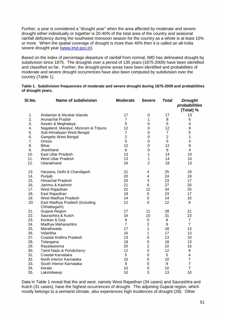
51

Further, a year is considered a “drought year” when the area affected by moderate and severe drought either individually or together is 20-40% of the total area of the country and seasonal rainfall deficiency during the southwest monsoon season for the country as a whole is at least 10% or more. When the spatial coverage of drought is more than 40% then it is called an all-India severe drought year (www.imd.gov.in). Based on the index of percentage departure of rainfall from normal, IMD has delineated drought by subdivision since 1875. The droughts over a period of 135 years (1875-2009) have been identified and classified so far. Further, the drought-prone areas have been identified and probabilities of moderate and severe drought occurrences have also been computed by subdivision over the country (Table 1). Table 1. Subdivision frequencies of moderate and severe drought during 1875-2009 and probabilities of drought years.

Sl.No. Name of subdivision Moderate Severe Total

Drought

probabilities (Total) %

1. Andaman & Nicobar Islands 17 0 17 13 2. Arunachal Pradsh 7 1 8 6 3. Assam & Meghalaya 5 0 5 4 4. Nagaland, Manipur, Mizoram & Tripura 12 0 12 9 5. Sub-Himalayan West Bengal 7 0 7 5 6. Gangetic West Bengal 2 0 2 1 7. Orissa 5 0 5 4 8. Bihar 12 0 12 9 9. Jharkhand 6 0 6 4 10. East Uttar Pradesh 13 1 14 10 11. West Uttar Pradesh 13 1 14 10 12. Uttarakhand 16 2 18 13

13. Haryana, Delhi & Chandigarh 21 4 25 19 14. Punjab 20 4 24 18 15. Himachal Pradesh 20 3 23 17 16. Jammu & Kashmir 21 6 27 20 17. West Rajasthan 22 12 34 25 18. East Rajasthan 18 5 23 17 19. West Madhya Pradesh 14 0 14 10 20 East Madhya Pradesh (including

Chhattisgarh) 12 0 12 9

21. Gujarat Region 17 11 28 21 22. Saurashtra & Kutch 16 15 31 23 23. Konkan & Goa 9 0 9 7 24. Madhya Maharashtra 7 2 9 7 25. Marathwada 17 1 18 13 26. Vidarbha 16 1 17 13 27. Coastal Andhra Pradesh 13 0 13 10 28. Telangana 18 0 18 13 29. Rayalaseema 20 2 22 16 30. Tamil Nadu & Pondicherry 12 0 12 9 31. Coastal Karnataka 5 0 5 4 32. North Interior Karnataka 10 0 10 7 33. South Interior Karnataka 9 0 9 7 34. Kerala 10 0 10 7 35. Lakshdweep 10 3 13 10

Data in Table 1 reveal that the arid west, namely West Rajasthan (34 cases) and Saurashtra and Kutch (31 cases), have the highest occurrences of drought. The adjoining Gujarat region, which mostly belongs to a semiarid climate, also experiences high incidences of drought (28). Other

52

areas recording large incidences of drought are Haryana, Delhi and Chandigarh, Punjab, Himachal Pradesh, and East Rajasthan in northwest India and Rayalaseema in the southern peninsula. The subhumid and humid areas of east and northeast India (Arunachal Pradesh, Assam and Meghalaya, Orissa, Gangetic West Bengal, and Jharkhand), for obvious reasons, have the lowest occurrences of drought. Based on the probabilities of occurrence of drought (percentage), the entire country has been divided (Figure 1) into chronically drought-prone areas (probability of occurrence of drought more than 20%), frequently drought-prone areas (probability of occurrence of drought 10-20%), and least drought-prone areas (probability of occurrence of drought less than 10%) (IMD 2005). Figure 1. Probability of occurrence of drought (%) and drought prone areas, 1875-2004. Figure 1 shows that West Rajasthan and the entire Gujarat State fall in the category of chronically drought-prone areas. Therefore, these areas deserve special attention for drought proofing, like evolving crop varieties resistant to moisture stress, better water management, and effective land management. East Uttar Pradesh, Uttarakhand, Haryana, Punjab, Himachal Pradesh, East Rajasthan, West Madhya Pradesh, Marathwada, Vidarbha, Telangana, Coastal Andhra Pradesh, and Rayalaseema fall in the category of frequently drought-prone areas, which can expect drought once in 6-10 years. These areas generally belong to the subhumid climate zone (IMD 2005).

53

Index Based on SPI Although rainfall deviation from the long-term mean continues to be a widely adopted indicator for drought intensity assessment because of its simplicity, its application is strongly limited by its inherent nature of dependence on mean. Rainfall deviations cannot be applied uniformly to different areas having different amounts of mean rainfall since a high and a low rainfall area can have the same rainfall deviation for two different amounts of actual rainfall. Therefore, rainfall deviations across space and time need to be interpreted with utmost care (Naresh Kumar et al. 2009). SPI expresses the actual rainfall as standardized departure from rainfall probability distribution function and, hence, this index has gained importance in recent years as a potential drought indicator permitting comparisons across space and time (Naresh Kumar et al. 2009). A few studies (Hughes and Saunders 2002, Hayes et al. 1999, Mihajlovic 2006) have been done on SPI-based drought monitoring on a monthly/seasonal time scale. Keeping this in mind, an attempt has been made to analyze drought (Table 2) over India based on SPI. The main objective was to see how effective SPI was in diagnosing drought intensity over a longer period of time. Rainfall data (All India Seasonal rainfall [June–September]) used for the study was from 1875 to 2009. Computation of SPI involved fitting a gamma probability density function to a given frequency distribution of precipitation totals. The alpha and beta, shape, and scale parameters of the gamma distribution were estimated for a suitable timescale for each year. Alpha and beta parameters were then used to find the cumulative probability of an observed precipitation amount, which was then transformed into the standardized normal distribution. Thus, SPI could be said to be normalized in space and time scale. SPI as a drought index is very versatile as it can be calculated on any timescale, so it is suitable for agricultural and hydrological applications. This versatility is also critical for monitoring the temporal dynamics of a drought, including its development and decline. These aspects of a drought have always been difficult to track with other indices; further, as SPI values are normally distributed, the frequencies of extreme and severe drought events for any location and timescale are consistent. Table 2. Drought intensity over India based on Standardized Precipitation Index (SPI).

Drought year Seasonal (June–Sept.) rainfall (cm)

SPI value Drought intensity per SPI value

1877 58.7 -3.47 ED 1899 62.1 -3.01 ED 1901 76.5 -1.21 MD 1904 77.6 -1.08 MD 1905 72.7 -1.66 SD 1911 75.1 -1.38 MD 1918 66.1 -2.48 ED 1920 73.3 -1.59 SD 1941 76.3 -1.23 MD 1951 71.5 -1.81 SD 1965 72.0 -1.75 SD 1966 76.4 -1.22 MD 1972 67.0 -2.37 ED 1974 77.4 -1.11 MD 1979 71.4 -1.82 SD 1982 75.2 -1.36 MD 1986 76.8 1.18 MD 1987 70.9 -1.88 SD 2002 71.3 -1.83 SD 2004 76.6 -1.20 MD 2009 69.8 -2.02 ED

ED = extreme drought (SPI: more than -2.0); SD= severe drought (SPI: -1.50 to -1.99); MD = moderate drought (SPI: -1.0 to -1.49)

54

The analysis revealed that out of 135 years (1875–2009), SPI diagnosed five years (1877, 1899, 1918, 1972 and 2009) as All India extreme drought years when the SPI value exceeded -2.0. This result was in agreement with the analysis of Mooley (1994), who while analyzing data from 1871 to 1996 found that in the years 1877, 1899, 1918, 1972, and 1987, Phenomenal All India droughts affected the country. Mooley (1994) defined Phenomenal All India drought as a phenomenon occurring when percent departure of monsoon season rainfall was ≤ -2 SD (i.e., -20%) and the percentage area under deficient monsoon rainfall was equal to or more than mean+2 SD (i.e., 47.7%). Therefore, Phenomenal drought years identified by Mooley (1994) have been effectively diagnosed as extreme drought years by SPI. SPI was also able to properly diagnose the other All India moderate/severe drought years that affected the country. Further, when SPI was used to examine whether any trend existed in drought over the country, no trend was found (Figure 2). However, it should be mentioned that despite the current optimism about SPI, it cannot solve all moisture monitoring concerns. Rather, it can be considered as a tool that can be used in coordination with other tools, such as the aridity anomaly index or remote sensing data, to detect the development of droughts and monitor their intensity and duration. This will further improve the timely identification of emerging drought conditions that can trigger appropriate responses by the policy makers.

Figure 2. Temporal variation of Standardized Precipitation Index (SPI) in India, 1875-2004.

55

Index Based on Aridity Anomaly Thornthwaite’s (1948) water balance technique is generally used to compute the aridity anomaly index at a location. This index is one of the tools to monitor agricultural drought. According to the methodology that is now widely used to represent crop moisture stress, an index known as aridity index (Ia) is computed as given below:

needWaterdeficitWaterIa =

PEETPE −

=

where ET is the actual evapotranspiration computed from the water balance technique and PE the potential evapotranspiration, which is supposed to represent the water need of the plant. For monitoring and mapping agricultural drought, a shorter time interval, say a week, is generally

considered. The difference between the actual Ia and its normal value for that week (i.e., Ia ) furnishes an anomaly that is expressed as percentage:

100XI

IIAnomalyAriditya

aa −=

When the anomaly is worked out for a large network of stations for different weeks, plotted, and analyzed, it is possible to identify areas where the crop might be suffering from moisture stress of various degrees. The anomaly is used to categorize agricultural drought of various types, as below :

Anomaly of Aridity Index Agricultural Drought Intensity 1 – 25 Mild 26 – 50 Moderate > 50 Severe

Using this technique, IMD is monitoring agricultural drought during both kharif and rabi seasons using a wide network of stations. This is done on real-time basis every fortnight of the two crop seasons and supplied to various users. Based on this aridity index, weekly/fortnightly Aridity Anomaly Maps/Reports for the southwest monsoon season for the whole country and for the northeast monsoon season for the five meteorological subdivisions (coastal Andhra Pradesh, Rayalaseema, south Interior Karnataka, Tamil Nadu and Pondicherry and Kerala) are prepared and sent to various user communities on a near real time basis for their use in agricultural planning and research purposes. The aridity anomaly maps are also uploaded to the departmental website (www.imd.gov.in). This index helps to assess the moisture stress experienced by growing plants. A few aridity anomaly maps, pertaining to the drought year 2009, are presented in Figures 3 and 4.

56

Figure 3. Aridity anomaly chart of India (June 11-17, 2009).

Figure 4. Aridity anomaly chart of India (June 18-24, 2009).

57

Monitoring Drought by Remote Sensing Method

NRSC (Department of Space, Government of India) has been assessing and monitoring agricultural drought since 1989 under the National Agricultural Drought Assessment and Monitoring Systems (NADAMS). Under NADAMS, agricultural conditions are monitored at the district level using daily observed coarse resolution (1.1 km) NOAA-AVHRR data for the entire country and at the subdistrict level using better spatial resolution Indian Remote Sensing Satellite (IRS) AWiFS/WiFS data . IRS series (IRS 1C, IRS 1D, and IRS P3) have WiFS (Wide Field Sensor) payload, which collects data in two spectral bands: 0.62-0.68 µm (red) and 0.77-0.86 µm (near infrared) with spatial resolution of 188 m and ground swath of 810 km with a revisit period of 5 days. The IRS P6 (Resource Sat) has advanced WiFS (AWiFS) sensors that provide data with spectra, radiometric, and spatial (56 m) resolutions for better monitoring of agriculture. The combination of AWiFS/WiFS would help increase the frequency of images with almost one coverage in two days time, which is useful to minimize cloud contamination. The crop/vegetation reflects high energy in the near infrared band because of its canopy geometry and health of the standing crops/vegetation and absorbs high in the red band due to its biomass and photosynthesis. Using these contrasting characteristics of vegetation in near infrared and red bands, which indicate both the health and condition of the crops/vegetation, the Normalized Difference Vegetation Index (NDVI) is derived by the difference of these measurements and divided by their sums. The vegetation index is generated from each of the available satellite data irrespective of the cloud cover present. To minimize the cloud, monthly time composite vegetation index is generated. The monthly vegetation index maps for the states with district boundaries overlaid are given in specific colors for the vegetation index ranges. Yellow through green to violet indicate increasing green leaf area and biomass of different vegetation types. Cloud and water are represented in black and blue colors, respectively. The bare soil, fallow, and other non-vegetation categories are represented in brown. The composite NDVI images are generated for each month of the monsoon separately for the total geographic area and for the agricultural area of the state. The seasonal progression of NDVI compared to that of normal and complementary ground data on rainfall and crop sowing progress are utilized in the assessment of agricultural drought. Figures 5 and 6 depict monitoring of agricultural drought by remote sensing during the monsoon season of 2009 (NRSC 2009).

58

Figure 5. Progression of surface wetness (NDWI) during sowing period (June-July) in 2009 in India (above) and AMSR-E soil moisture during the sowing period in 2009 in India (below).

Figure 6. AWIFS NDVI over agricultural area over Andhra Pradesh State during the 2009 rainy season (showing persistent low NDVI and delayed agricultural season due to agricultural drought).

59

Conclusions

This chapter has highlighted the drought indices that are currently in use for monitoring drought risks in India. Drought risks have been identified by delineating the country into chronically (probability of drought occurrence exceeds 20%), frequently (probability of drought occurrence 10% -20%) and least drought-prone (probability of drought occurrence less than 10%) areas. For meteorological drought monitoring in India, percentage rainfall departure from normal is used as an index. SPI, being developed and tested, has also shown promise in monitoring meteorological drought. No trend in meteorological drought has been found to exist in India. For monitoring and assessing, an agricultural drought aridity anomaly index is used in India. Remote sensing applications by NRSC could also be very effective in assessing drought severity and impacts on sectors like agriculture, and related policy decisions. Acknowledgements The author is thankful to the Director General of Meteorology, India meteorological Department, New Delhi, for his encouragement in preparing the paper.

References Hayes, M.J., M.D. Svoboda, D.A. Wilhite, and O.V. Vanyarkho. 1999. Monitoring the 1996 drought

using the Standardized Precipitation Index. Bulletin of the American Meteorological Society 80:429-438.

Hughes, B.L. and M.A. Saunders 2002. A drought climatology for Europe. International Journal of Climatology 22:1571-1592.

Kulshreshtha, S.M. 1997. Drought Management in India and Potential Contribution of Climate Prediction, South Joint COLA/CARE Technical Report No.1.

IMD. 2005. Climatological Features of Drought Incidences in India. Meteorological Monograph Climatology No. 21/2005, India Meteorological Department.

Mihajlovic, D. 2006. Monitoring the 2003-2004 meteorological drought over Pannonian part of Croatia. International Journal of Climatology 26:2213-2225.

Mooley, D.A.1994. Origin, incidence and impact of droughts over India and remedial measures for their mitigation. Sadhana (Academy Proceedings in Engineering Sciences), Indian Academy of Sciences 19(4).

Naresh Kumar, M., C.S. Murthy, M.V.R. Sesha Sai, and P.S. Roy. 2009, On the use of Standardized Precipitation Index (SPI) for drought intensity assessment. Meteorological Applications 16(3):381-389. Published online in Wiley Interscience, http://onlinelibrary.wiley.com/doi/10.1002/met.136/pdf.

NRSC. 2009. Drought Report. National Remote Sensing Centre, ISRO, Hyderabad. Thornthwaite, C.W. 1948. An approach toward a rational classification of climate. Geographic

Review 38:55-94. WMO. 1994. On the Frontline: Public Weather Services. WMO No. 816, Geneva.

60

Agricultural Drought Indices in Current Use in Brazil

Paulo Cesar Sentelhas AgMet Group, Department of Biosystems Eng., ESALQ, University of São Paulo

Piracicaba, SP, Brazil

Abstract The aim of this chapter is to give an overview of the agricultural drought indices in current use in Brazil, considering the products provided by the National and Regional Meteorological and Hydrological Services (M&HS). A systematic survey was done using the online information provided by the M&HSs at national and state levels. The survey considered the drought indices specifically available for agricultural applications. The country has three national and nine regional M&HSs. All of them provide some kind of meteorological and/or agricultural drought indices. Among the meteorological drought indices, the rainfall anomaly and Standard Precipitation Index (SPI) are the most common. For monitoring agricultural drought, the indices used are mainly based on the outputs of the water balance (WB): accumulated water deficiency, accumulated drought index, relative water deficiency index, Palmer drought severity index adapted, crop water development index, crop moisture index, and soil water storage. Different WB models are in current use, requiring distinct inputs and resulting in diverse outputs. Among them, the most used is Thornthwaite and Mather’s climatological WB, which requires as input potential evapotranspiration (ETP), rainfall (R), and soil water holding capacity (SWHC) and has as output soil water storage (SWS), actual evapotranspiration (ETa), and water deficiency (WD). In this case, some critical factors impose limitations on determining agricultural drought indices, such as ETP estimate methods, SWHC adopted, differences among crops and development phases, and crop management. All these factors will influence the drought index and cause different impacts on crops during the growing season. It makes agricultural drought monitoring very complex, especially in a country with continental dimensions and with climates ranging from temperate to tropical and from humid to semiarid.

Introduction Brazil is the largest country in South America. It has 26 states and the Federal District, covering an area of 8,514,876 km². The country is located between latitudes 5°16'20" N and 33°44'32" S, and longitudes 34°47'30" W and 73°59'32" W. As a function of its large dimensions and according to all the macroclimatic factors that control the weather systems in this region of the world, the country presents a huge variety of climates, ranging from tropical in the center-north to temperate in the south, and from humid at the north part of the Amazon region to semiarid in the greater part of the Northeast region, where the biome Caatinga prevails. Considering the diversity of climates of Brazil and the high interannual variability of rainfall observed in several regions of the country, droughts occur often, generating great impacts on water resources, agriculture, and the economy. Even humid regions, like the Amazon Rain Forest in the Amazonas state and the Pampas region in the Rio Grande do Sul state, have experienced severe drought spells during the few last years, causing disasters for several human activities, mainly agriculture (Berlato and Cordeiro 2005, Marengo et al. 2008, Phillips et al. 2009). An important source of climate variability in Brazil is the El Niño Southern Oscillation (ENSO) phenomenon (Stuck et al. 2006). The positive ENSO phase, known as El Niño, is normally related to droughts in the northern part of the country, including Northeast Brazil and the Amazon Rain Forest. On the other hand, the negative phase (La Niña) normally intensifies the drought spells in southern Brazil, including the states of Paraná, Santa Catarina, and Rio Grande do Sul. The drought impacts in Brazil are diverse, depending on the duration and intensity of the dry period, the region, and the season. Some of these adverse drought impacts include yield losses in

61

agriculture, which is one of the main economic activities in the country. Agricultural drought is detected when continuous and intense soil moisture stress leads to significant yield reduction, as shown in Figure 1.

0

500

1000

1500

2000

2500

300019

7519

7619

7719

7819

7919

8019

8119

8219

8319

8419

8519

8619

8719

8819

8919

9019

9119

9219

9319

9419

9519

9619

9719

9819

9920

0020

0120

0220

0320

0420

0520

0620

0720

08

Yiel

d (k

g ha-1

)

Soybean Yield in Rio Grande do Sul StateAnnual Yield Avg Yield Linear (Annual Yield)

Drought Impact

Figure 1. Historical soybean yield data for Rio Grande do Sul state, Brazil, showing the impact of intense droughts on yield losses. Source: IBGE/Brazil. According to Boken (2005), the most important kind of drought is agricultural drought, which can cause serious disasters for food security, since crop yields are directly affected by soil moisture shortage. Drought assessment, monitoring, and preparedness planning should be considered essential components of integrated water resources management systems, as mentioned by Wilhite (2005), to reduce societal vulnerability to future drought events. Meteorological drought occurs when the seasonal or annual precipitation falls below its long-term average. Hydrological drought develops when meteorological drought is prolonged and causes shortages of surface and groundwater in the region. Agricultural drought is detected when continuous and intense soil moisture stress leads to significant crop yield reduction. Finally, socio-economic drought is a manifestation of continued drought of severe intensity that causes economic and sociopolitical instabilities in a region or country. Whereas meteorological drought is just an indicator of precipitation deficiency, hydrological and agricultural droughts can be considered the physical manifestations of meteorological drought, and socioeconomic drought results from the impacts of hydrological and agricultural droughts on the society. Even considering the importance of monitoring agricultural droughts, selecting indices for monitoring is not easy because these indices will require information from different sources, like climate (rainfall and evapotranspiration), soils (holding capacity and moisture), crops (species, variety, root depth, and phenological phase), and crop management (sowing dates, crop rotation, irrigation, no tillage, and intercropping), which should be integrated to produce a unique value. The combination of these factors leads to different impacts on agriculture when a drought occurs, making it difficult to decide which is the best index to quantify the drought for agriculture. As there is an urgent need to mitigate the effects of agricultural droughts in the short term, the recommendation has been made that the national or regional Meteorological and Hydrological Services (M&HSs) provide assessment and monitoring of this natural disaster as part of their products. The objective of this chapter is to give an overview of the agricultural drought indices in current use in Brazil, considering the products provided by the M&HSs, as well as to discuss some of their strengths and limitations.

62

Meteorological and Agricultural Drought Assessment and Monitoring in Brazil A systematic survey of drought information was done using the online data provided by the regional and/or national M&HSs of Brazil. The survey identified services provided by three national and nine regional institutions, as shown in Table 1. Table 1. National and regional meteorological and hydrological services in Brazil and their respective websites.

Level State Name* Website address - INMET www.inmet.gov.br National - AGRITEMPO www.agritempo.gov.br - CPTEC/INPE www.cptec.inpe.br Bahia CEMBA www.inga.ba.gov.br/cemba/ Ceará FUNCEME www.funceme.br Goiás SIMEGO www.simego.sectec.go.gov.br/ Paraná IAPAR www.iapar.br Regional Paraná SMA/FABC sma.fundacaoabc.org.br Pernambuco LAMEPE www.itep.br/lamepe.asp Rio Grande do Sul Agrometeorologia RS www.agrometeorologia.rs.gov.br São Paulo INFOSECA www.infoseca.sp.gov.br Santa Catarina CIRAM ciram.epagri.sc.gov.br

* INMET = National Institute of Meteorology; AGRITEMPO = Agrometeorological Information System of EMBRAPA (Brazilian Agricultural Research Company); CPTEC/INPE = Center for Weather Forecast and Climatic Studies of National Institute for Space Research; CEMBA = Meteorological Center of Bahia State; FUNCEME = State of Ceará Foundation for Meteorology; SIMEGO = Meteorological System of Goiás State; IAPAR = Agronomic Institute of Paraná; SMA/FABC = Agrometeorological Information System of ABC Foundation; LAMEPE = Meteorological Center of Pernambuco State; Agrometeorologia RS = Agrometeorological Information System of the state of Rio Grande do Sul; INFOSECA = Center for Drought Mitigation of the State of São Paulo; CIRAM = Natural Resources and Hydrometeorological Information System of Santa Catarina State. The evaluation focused on all information related to drought assessment and monitoring, considering any time scale (e.g., daily, ten-day, monthly), and any format of publication (e.g., online data and maps, bulletins, advisories). The following information was considered: rainfall anomaly data and maps, water balance data and maps, satellite information, and meteorological and agricultural drought indices.

Meteorological and Agricultural Drought Indices in Current Use in Brazil

The systematic evaluation of the three national and nine regional M&HSs allowed the identification of a huge variety of meteorological and agricultural drought indices in current use in Brazil. These indices are presented below. Rainfall Anomaly: Maps of rainfall anomaly in relation to the climatological normal are provided by several of the M&HSs on a ten-day and monthly basis. INMET and AGRITEMPO provide these maps for the entire country based on observed data, whereas CPTEC/INPE generate this kind of map based on satellite data. Figure 2 illustrates the rainfall anomaly in Brazil during September 2010.

63

Rainfall anomaly – September 2010

Figure 2. Rainfall anomaly during September 2010 in Brazil. Source: www.inmet.gov.br. Standard Precipitation Index (SPI): SPI was developed primarily for defining and monitoring drought. It allows the user to determine the rarity of a drought at a given time scale of interest for any rainfall station with historic data. SPI is based on the cumulative probability of a given rainfall event occurring at a station (Blain 2005). The historic rainfall data of a given station is fitted to a gamma distribution. This is done through a process of maximum likelihood estimation of the gamma distribution parameters. The process described above allows the rainfall distribution for a station to be effectively represented by a mathematical cumulative probability function. Based on the historic rainfall data, one can then determine the probability of the rainfall being less than or equal to a certain amount. Thus, the probability of rainfall being less than or equal to the average rainfall for that area would be about 0.5, while the probability of rainfall being less than or equal to an amount much smaller than the average would be even lower, depending on the amount. Therefore if a particular rainfall event gives a low probability on the cumulative probability function, this is indicative of a drought event. SPI has been provided by national (INMET and AGRITEMPO) and regional (INFOSECA) M&HSs. Figure 3 presents SPI for 3 months for Brazil, to September 2010.

Standard Precipitation Index (SPI)September 2010 – Accumulated for 3 months

Extremely wetSeverely wetModerately wetNormalModerately drySeverely dryExtremely dry

Figure 3. SPI accumulated for 3 months (to September 2010) in Brazil. Source: www.inmet.gov.br.

64

Palmer Drought Severity Index Adapted to São Paulo State (PDSI-Adapted): The Palmer Drought Severity Index (PDSI) is widely used to characterize droughts. The PDSI is based on the water balance equation over an area of concern (Palmer 1965). Calculating PDSI requires data on precipitation, temperature (for potential evapotranspiration estimation), soil moisture, and the previous PDSI value. Although precipitation and temperature time series data are easily available for most locations, this is not always the case with soil moisture because of the lack of monitoring networks. PDSI is a drought index that involves aspects related to duration, magnitude, and severity of a drought and also includes information on the onset and termination of a drought event. PDSI was adapted to the climatic conditions of the state of São Paulo by Blain (2005) and has been used by the INFOSECA system as one of their drought monitoring indices, as presented in Figure 4, using the following classification (Table 2). Table 2. PDSI classification used by the INFOSECA system in the state of São Paulo, Brazil. Source: www.infoseca.sp.gov.br/.

PDSI interval Classification ≥ 3.00 Extremely wet 2.00 to 2.99 Very wet 1.00 to 1.99 Moderately wet 0.51 to 0.99 Beginning of wet -0.50 to 0.50 Normal -0.99 to -0.51 Beginning of dry -1.99 to -1.00 Moderately dry -2.99 to -2.00 Very dry ≤ -3.00 Extremely dry

Adapted SPI – São PauloAugust 2010

Legend

Figure 4. PDSI adapted for the state of São Paulo, Brazil, for August 2010. Source: www.infoseca.sp.gov.br. Number of days without rain (NDWR): This index simply accumulates the number of days without rain for a given region. When a rain event occurs, NDWR becomes zero and a new accounting starts. Two variations of this index are the number of days without rain above 5 mm (NDWR>5) and 10 mm (NDWR>10), which are considered more appropriate for agricultural drought monitoring. NDWR and NDWR>10 are used by INFOSECA, in the state of São Paulo, and NDWR>5 is used by AGRITEMPO on the national level.

65

Accumulated Drought Index (ADI): This drought index has rainfall (P) and potential evapotranspiration (ETP) as inputs. Its determination is based on the relationship between these two variables (Table 3), and the drought classification follows the categories of the accumulated index (Table 4). ADI is calculated as ADI = ∑ DI / (3 n N) (1) where DI is determined for each period by the P and ETP relationship presented in Table 3, n is the number of periods considered, and N is the number of periods without rain above 10 mm (NDWR>10). For N = 0, ADI is calculated by ADI = ∑ DI / (3 n) (2) Table 3. P and ETP relationship for determination of the drought index (DI). Source: www.infoseca.sp.gov.br.

P & ETP relationship Classification DI P ≥ 2 ETP Wet 5 ETP ≤ P < 2 ETP Lightly wet 4 ½ ETP ≤ P < ETP Normal 3 0 < P ≤ ½ ETP Lightly dry 2 P = 0 Dry 1

Table 4. ADI and drought classification. Source: www.infoseca.sp.gov.br.

ADI Classes Classification ADI ≥ 1.50 Extremely wet 0.80 ≤ ADI < 1.50 Very wet 0.40 ≤ ADI < 0.80 Wet 0.20 ≤ ADI < 0.40 Normal 0.04 ≤ ADI < 0.2 Dry ADI < 0.04 Very dry

Accumulated Water Deficit index (AWD): Water deficit is an output of the climatological water balance, determined by Thornthwaite and Mather’s WB model. The water deficit (WD) is the difference between potential (ETP) and actual (ETa) evapotranspiration. The WD magnitude for a given condition will depend on the soil water holding capacity (SWHC) adopted for the WB. When accumulated during the growing season, this index will have a good correlation with crop yield losses. Figure 5 presents two examples of the AWD maps for Brazil during the dry and wet seasons. Negative values represent the AWD, whereas positive values represent the accumulated water surplus (AWS).

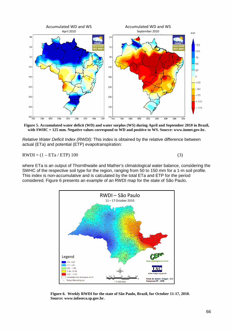
66

Accumulated WD and WSSeptember 2010

Accumulated WD and WSApril 2010

Figure 5. Accumulated water deficit (WD) and water surplus (WS) during April and September 2010 in Brazil,

with SWHC = 125 mm. Negative values correspond to WD and positive to WS. Source: www.inmet.gov.br. Relative Water Deficit Index (RWDI): This index is obtained by the relative difference between actual (ETa) and potential (ETP) evapotranspiration: RWDI = (1 – ETa / ETP) 100 (3) where ETa is an output of Thornthwaite and Mather’s climatological water balance, considering the SWHC of the respective soil type for the region, ranging from 50 to 150 mm for a 1-m soil profile. This index is non-accumulative and is calculated by the total ETa and ETP for the period considered. Figure 6 presents an example of an RWDI map for the state of São Paulo.

RWDI – São Paulo11 – 17 October 2010

Legend

Figure 6. Weekly RWDI for the state of São Paulo, Brazil, for October 11-17, 2010. Source: www.infoseca.sp.gov.br.

67

Crop Moisture Index (CMI): CMI is a non-cumulative index based on the difference between the current ETa and the expected ETa (climatological value) for the same period, as proposed by Palmer (1968): CMI = ETaobserved – ETaexpected (4) Negative values indicate that deficient evapotranspiration occurred, indicating a drought condition, whereas positive values show that ETa was more than expected for the period. Crop Water Development Index (CWDI): CWDI is an agricultural index used to follow the development conditions of crops in general. This index is based on the relationship between soil water storage (SWS) and SWHC, called the crop water development fraction (CWDF). SWS is obtained from the climatological water balance of Thornthwaite and Mather (1955), but can also be estimated with different WB models. CWDF and CWDI are calculated by the following procedures: CWDF = SWS / SWHC (5) CWDI = (CWDF * 0.4) – 1 (6) Accumulated CWDI (ACWDI) is then obtained for normalized conditions, by ACWDI = ∑ CWDI / (1.5 n) (7) where n is the number of periods considered. The classification of the crop development conditions is presented in Table 5. Table 5. Classification of ACWDI for crop development conditions. Source: www.infoseca.sp.gov.br.

ACWDI lasses Crop development conditions 0.8 ≤ ACWDI ≤ 1 Very good 0.6 ≤ ACWDI < 0.8 Good 0.4 ≤ ACWDI < 0.6 Reasonable 0.3 ≤ ACWDI < 0.4 Unfavorable 0.2 ≤ ACWDI < 0.3 Critical 0.1 ≤ ACWDI < 0.2 Severe ACWDI < 0.1 Extremely severe

Soil Water Storage (SWS) (or relative soil moisture): Another way to identify agricultural droughts is by soil water storage monitoring. SWS is an output of the water balance (WB). This variable can be obtained by different WB methods, such as those proposed by Thornthwaite and Mather (1955), Molinas and Andrade (1993), Allen et al. (1998), and Ritchie (1998). Each kind of WB method will require specific inputs, but basically they require climate (rainfall and potential evapotranspiration), soil (physical properties), and plant (crop type, leaf area, crop sensitivity to water stress, crop water requirement for each phenological phase, and management practices) information, depending on their complexity. In Brazil, Thornthwaite and Mather’s WB is used by INMET, AGRITEMPO, and several regional M&HSs. CPTEC/INPE employs Richards’s equation (Hillel 1998, Gevaerd and Freitas 2006), also known as the hydrological model, using rainfall and temperature data derived from satellite images as inputs, whereas FUNCEME uses MUSAG WB model (Molinas and Andrade 1993), which has rainfall, ETP, soil water storage in the previous period, and pedo-transfer functions for hydraulic soil characterization as inputs. Figures 7, 8, and 9 present examples of the products provided by INMET, CPTEC, and FUNCEME, where SWS data are spacialized in maps.

68

Soil Water Storage (SWS)September 2010

Figure 7. SWS in Brazil at the end of September 2010, determined by Thornthwaite and Mather’s WB, considering a SWHC = 125 mm. Source: www.inmet.gov.br.

Soil Water Storage (SWS)Depth: 37.5 cm – 28 OCT 2010

Soil Water Storage (SWS)Depth: 137.5 cm – 28 OCT 2010

Figure 8. SWS in South America, October 28, 2010, determined by a hydrological WB model, for two soil profiles (37.5 and 137.5 cm). Source: www.cptec.inpe.br.

69

Percentage of Soil Water Storage (SWS)28 OCT 2010

Figure 9. SWS, in percentages, for Ceará state, October 28, 2010, determined by MUSAG WB model. Source: www.funceme.br.

Normalized Difference Vegetation Index (NDVI): NDVI is a numerical indicator that uses visible and near-infrared bands of the electromagnetic spectrum, and is used to analyze remote sensing measurements and assess whether the target being observed contains live green vegetation. NDVI has found a wide application in vegetative studies, as it has been used to estimate crop yields and performance. It is often directly related to other ground parameters such as percent of ground cover, photosynthetic activity, surface water, leaf area index, and amount of biomass. Because of this, the severity of a drought situation can be assessed by the extent of NDVI deviation from its long-term mean. Maps using relative greenness are quite useful for assessing a drought situation, and hence this indicator has been used by CPTEC/INPE for monitoring agricultural drought indirectly.

Strengths, Weaknesses and Limitations of Agricultural Drought Indices Used in Brazil Among the different types of drought (meteorological, hydrological, and agricultural), agricultural drought is by far the most complex and difficult to determine. Part of this complexity is related to the fact that crop yield can be affected by several factors: abiotic (soil water, soil fertility, soil type, and weather); crop management (soil tillage, soil depth, fertilization, planting density, sowing date, weeding, pests, and disease control); land development (field size, terracing, drainage, and irrigation); socio-economic (infrastructure, market, prices, and costs); and catastrophic (flooding, frosts, hailstorms, and droughts), which can make establishing the relationship between yield losses and drought difficult. When an agricultural drought is expressed by indices that depend solely on rainfall data, despite the advantage of their simplicity (easy to apply and understand, and do not require much computational power), the relationship between the drought and yield losses will not be very clear, since other aspects, such as crop evapotranspiration, soil water storage, and crop phase, are not considered. On the other hand, when indices are based on the outputs of the crop water balance, the correlations between them and yield losses will be better defined. However, these indices will require more input variables, some of which are not always readily available, such as crop ET, soil

70

hydrological characteristics, and crop phase. Another limitation of more complex agricultural drought indices is the great complexity of agriculture itself, with several crops being cultivated during the growing season in the same region and having different stages of development at a given time. It is very well known that the same water deficit will impact yield differently if it occurs in distinct phases of crop development. Another source of uncertainty for agricultural drought indices that are based on WB outputs is related to the different ways to estimate ETP. Different ETP methods will result in different values for the same weather conditions. This will make agricultural drought indices vulnerable to these methods, in terms of the right dimension of the drought index. This is a problem when the Penman-Monteith method cannot be applied because of lack of data. So, agricultural drought indices based on ETP or ETa estimated by different methods are not comparable. The ideal would be the Penman-Monteith FAO56 model (Allen et al. 1998); however, this is not always possible, since this method requires a complete meteorological dataset, including net radiation. When alternative ET estimate models are employed, one should pay attention to the characteristics of the models. Some of them, like Thornthwaite, tend to underestimate ETP during dry periods, whereas the Hargreaves and Samani method can overestimate ETP during the wet season. The type of soil, the depth of the roots, and the resulting SWHC is another source of uncertainty for the WB-based agricultural drought indices. The greater the SWHC, the smaller the impact of a given drought on crop yield. Even considering their limitations, the WB-based agricultural drought indices are the best option for monitoring droughts for agriculture, presenting better correlations to yield losses than indices based only on rainfall data.

Conclusions

In Brazil, several national and regional M&HSs have different ways to monitor drought under agricultural perspectives. These M&HSs estimate water balance by four different methods: Thornthwaite and Mather, MUSAG, hydrological with satellite data, and hydrological with observed data. The method of Thornthwaite and Mather (1955) is the most used by the National Met Service (INMET and AGRITEMPO) and other regional agrometeorological services. In the state of São Paulo, several agricultural drought indices are in use, with the majority of them based on Thornthwaite ETP and Thornthwaite and Mather’s WB. Even considering the strengths of the WB-based agricultural drought indices, the WB, determined by any method, will depend on some critical factors, such as the ETP method, the SWHC adopted, crop/variety type and phase, and crop management. These factors will lead to different agricultural drought index values, which will require calibration and testing of them for each location and crop condition. However, agricultural drought indices based on WB outputs are expected to have better relationships with crop yield losses than meteorological drought indices, which are based only on rainfall.

References Allen, R.G., L.S. Pereira, D. Raes, and M. Smith. 1998. Crop Evapotranspiration.Guidelines for

Computing Crop Water Requirements. FAO Irrigation and Drainage Paper, No. 56. FAO, Rome, Italy.

Berlato, M.A. and A.P.A. Cordeiro. 2005. Variabilidade climática e agricultura do Rio Grande do Sul. Pages 43-58 in As estiagens e as perdas na agricultura – fenômeno natural ou imprevidência? (Nascimento, A.M.N., Silveira Filho, I.L., Berton, A.L. e outros, eds.). Federacite, Porto Alegre, Brasil.

Blain, G.C. 2005. Avaliação e adaptação do índice de severidade de seca de Palmer (PDSI) e do índice padronizado de precipitação (SPI) às condições do estado de São Paulo. Instituto Agronômico, Campinas, Brasil.

Boken, V.K. 2005. Agricultural drought and its monitoring and prediction: Some concepts. Pages 3-10 in Monitoring and Predicting Agricultural Drought (V.K. Boken, A.P. Cracknell, and R.L. Heathcote, eds.). Oxford University Press, New York.

71

Gevaerd, R. and S.R. Freitas. 2006. Estimativa operacional da umidade do solo para iniciação de modelos de previsão numérica da atmosfera. Parte I: Descrição da metodologia e validação. Revista Brasileira de Meteorologia 21:59-73.

Hillel, D. 1998. Environmental Soil Physics. Academic Press, New York. Marengo, J.A., C.A. Nobre, J. Tomasella, M.D. Oyama, G.S. Oliveira, R. Oliveira, H. Camargo, L.M.

Alves, and F. Brown. 2008. The drought of Amazonia in 2005. Journal of Climate 21:495-516.

Molinas, P.A. and F.C.M. Andrade. 1993. Modelo de umidade do solo para atividades agrícolas. Pages 136-145 in Simpósio Brasileiro de Recursos Hídricos, SBRH, Gramado, Brasil.

Palmer, W.C. 1965. Meteorological drought. US Weather Bureau Res. No. 45, Washington, D.C. Palmer, W.C. 1968. Keeping track of crop moisture conditions, nationwide: The new Crop Moisture

Index. Weatherwise 21:156–161. Phillips, O.L., L.E.O.C. Aragão, and S.L. Lewis. 2009. Drought sensitivity of the Amazon rainforest.

Science 323:1344–1347. Ritchie, J.T. 1998. Soil water balance and plant water stress. Pages 41-54 in Understanding

Options for Agricultural Production (G.Y. Tsugi, G. Hoogenboom, and P.K. Thornton, eds.). Kluwer Academic Publishers, Amsterdam, The Netherlands.

Stuck, J., A. Güntner, and B. Merz. 2006. ENSO impact on simulated South America hydro-climatology. Advances in Geosciences 6:227-236.

Thornthwaite, C.W. and J.R. Mather. 1955. The water balance. Publications in Climatology VIII(1):1-104. Drexel Institute of Technology, New Jersey, USA.

Wilhite, D.A. 2005. The role of disaster preparedness in national planning with specific reference to droughts. Pages 23-37 in Natural Disasters and Extreme Events in Agriculture (M.V.K. Sivakumar, R.P. Motha, and H.P. Das, eds.). Springer-Verlag, Berlin, Germany.

72

Agricultural Drought Indices in Current Use in Australia: Strengths, Weaknesses, and Limitations

Roger C. Stone

Australian Centre for Sustainable Catchments, University of Southern Queensland, Toowoomba, Australia

Abstract Although indices relevant to meteorological drought, based on rainfall deciles, have proved useful in Australia as a good first indicator of agricultural drought severity, the widely varying nature of Australia’s climate, soils, and farming systems has meant more sophisticated application of crop and pasture models have provided valuable insights into agricultural drought severity. This approach has somewhat overridden the application of potentially simpler to apply and more versatile agricultural drought indices such as the Palmer Drought Severity Index (PDSI) in drought assessments. However, surprisingly, indices such as the PDSI have proved very useful in analysis of agricultural drought in Australia under various climate change scenarios and general circulation model applications. The various attributes of a number of drought indices, including those subjectively derived, that have been utilized in some application areas in Australia are also described.

Background Australia has one of the most variable climates in the world, especially when considering year-to-year rainfall variability. This variability is particularly evident in more eastern and northern regions. Additionally, noticeably wet decades such as the 1950s contrast strongly with protracted dry periods and decades such as the 1990s or since 2002 (Nicholls and Wong 1991, Nicholls 1997, Productivity Commission 2009). An example of this high interannual rainfall variability is provided (Figure 1) in an example for Bowen, a major agricultural production center in northern Queensland.

In southwestern, southern, and eastern Australia, the recent meteorological drought from 2002 has been severe and prolonged, and has been compared with the infamous “Federation Drought” (1902-1904) and the severe and protracted drought of the 1940s. Droughts can have particularly devastating social and financial impacts on farmers and their communities in Australia, as well as adverse environmental effects (Productivity Commission 2009). Although it is believed that many in the agricultural community regard drought more as an unexpected deviation and aberration from the “normal” or “good” years and not a component of a long-term climatic continuum, a key aspect in the formation of the National Drought Policy (recently under major review) is a focus on self-reliance by farmers and farming communities to manage their enterprises through most drought events (Smith et al. 1992, White et al. 2005).

Agronomists will quickly argue that, for a country such as Australia with exceptionally high year-to-year rainfall variability, widely varying soil types, and associated variation in moisture holding capability, it may simply be too difficult to identify and measure drought by the quantity of rain alone, as the timing and frequency of precipitation “as well as soil type, topography, and land management practices will affect plant responsiveness and the effectiveness of the rainfall received” (White et al. 2005). This is despite the fact that Gibbs and Maher (1967) identified a high correlation between the incidences of (agricultural) drought based on production criteria with annual rainfall in the first decile in Australia.

73

Figure 1. Monthly rainfall variability at Bowen, North Queensland. The Federal National Drought Policy (NDP) (Australia Parliament 1992) was accompanied by State Drought Policy initiation with a key emphasis in both state and federal jurisdictions on the utilization of an improved understanding of the science aspects of droughts, including return periods, severity, and access to useful seasonal forecasting to better prepare for drought—all with a strong focus on aspects of self-reliance. In this respect, the NDP provided three objectives: “(1) to encourage primary producers and other segments of rural Australia to adopt self-reliant approaches in managing for climatic variation, (2) to facilitate the maintenance and protection of Australia’s agricultural and environmental resource base during periods of increasing climatic stress, and (3) to facilitate the early recovery of agricultural and rural industries to levels consistent with long-term sustainable production” (Australia Parliament 1992, White and Walcott 2009). As White and Walcott (2009) maintain, “all three objectives require comprehensive, but not necessarily identical, methods for monitoring and assessment to successfully reduce the effects of droughts” (Australia Parliament 1992, White and Walcott 2009). It is against this framework that the application of agricultural drought indices is explored as the aim of this chapter. Thus, “risk management” became a common-place term in Australia, focusing on objective, science-based decisions associated with improved preparation for drought. To further assist farmers and agricultural communities, as well as those providing exceptional drought relief assistance, the term “safety-net” also became common parlance to emphasize that governments recognized that it was almost impossible to prepare for extreme drought events such as 1 in 20 or 1 in 25 year events, although some state governments, such as Queensland (Department of Primary Industries, Queensland 1992), aimed to provide some assistance for 1 in 10 year events: all so-called “exceptional circumstances.” Aspects related to inputs of science, agronomy, and mathematics (drought frequency distributions) were highlighted in order to assist drought policy and the implementation of drought policy in Australia, particularly since 1992. Science issues have also come to the fore in policy and operational discussions regarding what “drought”—or especially “exceptional drought”—actually is, and it is within this context that

74

application of drought indices has particular relevance. However, in Australia, this author is aware that although declaration of “drought exceptional circumstances” (DEC) has been based on an assessment of objective scientific information, it has also incorporated independent advice that could be described as “subjective agricultural-drought indices,” presented by claimants to government agencies such as the Rural Adjustment Scheme Advisory Council (RASAC). Australian Drought Definitions McVicar and Jupp (1998) provide the following definitions of drought, relevant to Australia.

1. Meteorological drought—lower than average precipitation “for some time period”; in some cases, air temperature and precipitation anomalies may be combined.

2. Agricultural drought—occurs when plant available water, from precipitation and water stored in the soil, falls below that required by a plant community during a critical growth stage. This leads to below-average yields in both pastoral and grain-producing regions.

3. Hydrological drought—one parameter or a combination of parameters such as streamflow, reservoir storage, and groundwater.

4. Socio-economic drought—defined in terms of loss from an average or expected return. (It can be measured by both social and economic indicators, of which profit is only one.)

Approaches to the Development of “Drought Indices” in Australia In addition to Federal Drought Policy and assistance measures for exceptional agricultural drought, Australian states may also incorporate their own state drought policies and what they refer to as “drought indices,” although detail as to the actual types of indices that have been applied appear to be excluded in compilations of such measures. For example, in Queensland, as a pertinent example, a recommendation for a Queensland State Drought Declaration is made by the Local Drought Committee (LDC) after considering: 1. A one in ten-to-fifteen year rainfall deficiency over the past twelve months (note the

difference with Federal Drought Declaration criteria). 2. Rainfall distributions or other extenuating circumstances that relate to agricultural drought

and which may distort an area’s total yearly rainfall records should also be considered. State Local Drought Committees also consider a range of somewhat subjective measures that are considered as drought indices. They are more closely related to agricultural drought, and they include:

• Availability of pasture. • Availability of water. • Condition of stock. • The extent of drought movements of stock to forced sales or slaughter and to agistment. • Quantity of fodder introduced. • Importantly, to assist agricultural drought assessment, use is made of other “indicators or

indices” such as knowledge of the major water-holding capacities of soils (measured in mm) and, at the regional level, knowledge of plant available water holding capacity together, importantly, with the latest soil water recharge levels (V. Rudwick 2010, personal communication; Potgieter et al. 2005). Seasonal climate forecasts, often integrated with crop simulation modelling systems, assist agricultural drought assessment processes for rural areas.

Similarly, mapped soil moisture information is available as an “agricultural drought index” for core agricultural production regions, especially for crop production areas such as southwest Western Australia and eastern Queensland. This approach appears to have negated the application of soil moisture-based indices such as the PDSI. In Western Australia, soil moisture-based assessments are based on values calculated at 188 real-time rainfall stations using the STress INdex (STIN) model (Stephens et al. 1998).

75

Additionally, stress models can be used to ascertain crop yields as a function of soil moisture. This approach has been regularly used as a drought index in assessing exceptional agricultural droughts in winter-grain cropping regions. Application of the knowledge of soil moisture levels as well as application of crop simulation models to assist as an agricultural drought index has been developed in Queensland for winter wheat (Oz-Wheat; see Potgieter et al. 2006) and grain sorghum (Potgieter et al. 2005). An example of the latter is provided in Figure 2, where percentage soil recharge using the Agricultural Production Systems Simulation Model (APSIM) through a winter fallow is provided.

Figure 2. Example of percentage soil recharge using the APSIM model through a winter fallow for sorghum-growing regions in eastern Australia. In this example, the excessively dark shaded regions are where soil moisture recharge is over 90% (a recent example for November 2010). The opposite would be expected with major drought occurrence (from A. Potgieter 2005; A. Potgieter, personal communication, November 2010). For drought assessments associated with livestock production, the computer program GRAZPLAN has been developed to aid the management of livestock grazing temperate pastures in southern Australia; the GrassGro decision support system (Moore et al. 1997) predicts pasture growth and quality in a form suitable for input to GrazFeed (Freer et al. 1997), which is the GRAZPLAN animal production model. Donnelly et al. (1998) used GrassGro to provide an index of agricultural drought, especially to assess and rank agricultural droughts at sites near Wellington in the Dubbo Rural Lands Protection Board district of central New South Wales. They were able to estimate pasture production and supplementary feed requirements for the survival of grazing animals in a way that might have practical use in monitoring specific types of agricultural drought.

76

The Value of Crop and Pasture Simulation Models in Drought Assessment in Australia—Use as an Agricultural Drought “Index” The value of crop simulation models to provide value in drought assessment has been a major theme in the implementation of drought policy in Australia. The primary argument for this approach and the simulation of agricultural system performance is that meteorological conditions alone do not sufficiently capture the important issues of rainfall intensity and distribution in relation to the state of the agricultural system. In the models, rainfall at one time of the year can be carried over through fallows to be used at other times of the year. Failure of planting rains at a critical time may downgrade otherwise average seasonal rainfall conditions in terms of production potential. “A crop-soil management systems simulation model can then integrate the meteorological and agricultural dimensions of the production system and assist in creation of more objective criteria for estimating the severity of drought for cereal production regions in Australia” (Keating and Meinke 1998). Governed largely by the demands of providing inputs into national drought policy (and the complexity of implementation of that drought policy in Australia), the use of crop modelling systems has provided a unique opportunity to capture a multitude of crop production inputs that include rainfall timing and effectiveness. In particular, APSIM is a “software environment which consists of models of elements of a system (referred to as modules) and a communications system (engine and module interfaces) that allow modules to share information” (McCown et al. 1996), which can be applied to a variety of dryland cereal production systems in Australia. Importantly, APSIM does this in a manner that can provide a modelled drought index for that particular environment. This approach appears to work especially well in agricultural drought assessment as it has been noted that APSIM can simulate systems that are characterized by both summer and winter cereals interspersed with fallow periods of varying lengths in a region that exhibits extremely high rainfall variability (Keating and Meinke 1998). APSIM can be applied to characterize major agricultural drought periods over the historical climate record, which can reach 100 years (Figure 3). Additionally, Keating and Meinke (1998) point out that APSIM is a “model of a point in space, which is used in this context to assess a phenomenon that is expressed on a regional basis,” an approach that is inherently valuable in agricultural drought assessment. In this approach, the application of APSIM to multiple “points” in a region is used to build up a regional agricultural drought assessment. The approach has been demonstrated to have excellent application for wheat and sorghum cropping systems, appears robust, and constitutes a substantial improvement over using meteorological conditions alone for agricultural drought assessments. One wonders why this concept of application of sophisticated modelling systems such as APSIM in agricultural drought assessment has not been pursued further in order to also create a more generalized but nevertheless robust “agricultural drought index” that could also have widespread global application.

Figure 3. Characterizing wheat yield for the Wentworth Shire (county) in southern Australia over a 100-year period in order to assess the level of agricultural drought severity. The period questioned (denoted with “?”) is the period under examination in regard to the effectiveness of reduced rainfall in reducing actual crop yield and thus, provided an assessment of agricultural drought as opposed to meteorological (from Keating and Meinke 1998).

77

In Australia, an approach was developed that would capture a multitude of agricultural drought assessment methods to assist drought declarations, especially drought exceptional circumstances. This approach was pursued through the National Agricultural Monitoring System (NAMS) and appeared to contain all the requirements that would deliver scientific objectivity into the agricultural drought assessment process. Indeed, a science advisory group was included which would oversee that the “best indices and production models in Australia” (whether for rainfed cereals, pastures, or irrigated systems) were employed in order to help overcome disputes within the scientific community and between various scientific institutions regarding drought status. It is not known why NAMS has recently been discontinued. Valuable assessments have been made in Australia that show that when various drought indices are compared, especially for grazing enterprise purposes, in respect to rainfall, soil moisture, pasture growth, animal liveweight, and generated income, they will generally all identify the major droughts in the relevant regions of Australia (Stafford-Smith and McKeon 1998). However, Stafford-Smith and McKeon (1998) point out these measures may well differ in respect to ranking the more contentious droughts in which affected farmers may be very sensitive in eligibility for associated “exceptional drought” assistance (severe droughts of a 1 in 20 to 25 year occurrence). As individual grazing properties in Australia can be relatively large, these assessments on drought status will be also “dependent on assumptions about soil types and pasture condition which are quite specific to individual properties” (Stafford-Smith 2003). On the other hand, more straightforward, easily calculated drought indices and measures that are based on just rainfall or soil moisture and which can be calculated on a more universal manner appear, unfortunately, to be less closely aligned with issues of farmer hardship in Australia and maybe less relevant to application for assessment of exceptional drought assistance, to which drought indices in Australia are inexorably applied. Indeed, it has been noted that a single national measure (index) of exceptional and extreme drought is “likely to create inequity between regions” (Stafford-Smith 2003). This is especially the case of a country as large as Australia in that the timing and pattern of drought declarations is likely to differ between regions and types of agricultural land use (Stafford- Smith 2003, White and Walcott 2009). In a similar manner to that employed by Keating and Meinke (1998) in respect to assessment of agricultural drought for cereal cropping enterprises, Stafford-Smith and McKeon (1998) emphasize the need for an integrated index for application but focused on pastoral enterprise drought assessment. They applied 100-year pasture growth and animal liveweight-gain simulations (using the GRASP simulation model for pasture production) in relation to the monitoring, assessment, and declaration of droughts in Australia and recommended a form of an integrative index since information on soil moisture and pasture growth noticeably give differing results from a rainfall index alone (Stafford-Smith and McKeon 1998, White and Walcott 2009). Utilization of “Common” Single Agricultural Drought Indices To an Australian agronomist, drought tends to be defined as below-average rainfall that restricts typical plant growth for agricultural production. On the other hand, measurements of amounts of rainfall expressed as deciles are rarely questioned by drought relief agencies in terms of recognition of meteorological drought, unless a dispute on the density of rainfall gauges is raised. However, because of the widely varying nature of soils, crops, and pasture species, disputes may be initiated by farmers or different assessment agencies (usually state agencies) with other drought assessment agencies (usually federal agencies) over “which is the more reliable crop or pasture model to apply as an index in agricultural drought assessment,” especially if state governments provide their own scientific inputs, which may be at odds or even in competition for notoriety with federally produced scientific inputs—such has been the nature of state-federal politics in Australia and competition or even jealousy between scientific agencies and individuals.

78

To assist, many agriculturally-specific drought indices have been developed and proposed, based on rainfall data, soil moisture models, crop simulation models, and so forth, although, in the main, they have been found limiting for the purposes of ranking agricultural droughts for the very needs of government policy intervention, which could be a prime purpose in Australia. To assist in the identification of potential agricultural drought indices, White and Walcott (2009) compiled a remarkably useful listing of indices together with their positive attributes, weaknesses, and limitations for Australia (Table 1). Table 1. A listing of agricultural drought indices that have some application in Australia—drawn from White and Walcott 2009. Index Description Strengths Weaknesses and

limitations Palmer Drought Severity Index (PDSI) (Palmer 1965, 1968)

Water balance for droughts—potentially high value for agricultural droughts.

Widely used internationally— comparisons between PDSI and soil moisture quite promising— relevance under climate change (Burke and Brown 2008).

Value questioned in regions with high climate variability such as Australia.

Prescott (ratio) index (Prescott 1949)

Periods of plant stress.

It’s simple— includes evaporation losses.

Excludes transpiration losses —may be unsuited for accurately monitoring crops and losses.

Hutchison Drought Severity Index (HDSI) (Smith et al. 1992)

Progressive index aimed at targeting agricultural droughts.

Uses only rainfall data. Omits rainfall effectiveness and temperature.

Plant growth index (McDonald 1994)

Estimates the duration of the pasture growing season.

An intermediate level index. Requires further evaluation— including across a wider range of agricultural ecosystems.

Enhanced vegetation index (EVI) (Huete et al. 2002)

Improved monitoring— less atmospheric influence.

Remote sensed MODIS data. Limited dataset— launched in 2000 as a scientific rather than operational sensor.

Temperature Condition Index (TCI) (Kogan 1995)

Rising leaf temperatures with plant moisture stress.

Remotely sensed by NOAA AVHRR data.

No ability to normalize for variation in daily and seasonal meteorological conditions.

Normalized Difference Vegetation Index (NDVI)

Monitoring vegetation using NOAA/AVHRR data.

Remotely sensed repeatable and synoptic measurement.

Current data are best compared with long-term NDVI dataset “limited to 29 years”

Soil moisture anomaly and recharge levels (SMA) (e.g., Potgieter et al. 2005)

Soil moisture index Highly relevant for vegetative health and agricultural production.

Limited observations of soil moisture mean that operationally it may not always be practical.

Vegetation Condition Index (VCI) (Kogan 1990)

To assess the impact of changing weather on NDVI signals.

Remotely sensed repeatable and synoptic scale measurements.

The emphasis is on seasonal dryness rather than ranking extended droughts (from White and Walcott 2009)

The indices listed by White and Walcott (2009) provide a remarkably useful assessment of agricultural drought indices that may lead to application for Australian needs. However, as White and Walcott (2009) note, ‘it is unlikely that a single index will be suitable for use under all conditions in Australia’. It is therefore interesting that, to a considerable extent, crop and pasture simulation modelling has overtaken application of use of agricultural drought indices due to the

79

very nature of the requirements of drought relief assessment policy and implementation in Australia and the need for very detailed and specific assessments depending on the commodity in question and the region in question. However, it is also noted that for certain specific purposes, such as, for example, climate change studies, standard agricultural drought indices hold promise as an additional measure that can assist analyses and understanding of extreme drought likelihood in a country with such extreme variability in climate, soils, water holding capacity, and farming systems as Australia. The Value of Standard Agricultural Drought Indices, Especially the PDSI, in Australia in Application for Drought and Climate Change Research Standard, published agricultural drought indices have been identified as being potentially suitable for drought assessment in Australia. The PDSI, developed by Palmer (1965) (also see Alley 1984) to provide information on the “cumulative departure of moisture supply” from normal, may have potential for application in Australia, despite the well-known high levels of interannual climate variability in this country, an issue most often quoted as being counter-productive in the utilization of the PDSI. Sivakumar and Wilhite (2002) note “the Palmer Index” is more effective in determining long-term drought rather than shorter-term events. Nevertheless, they point out that the PDSI “is popular” in many world regions, especially the United States, where it is most effective in measuring agricultural impacts sensitive to soil moisture (Willeke et al. 1994). As noted by Burke et al. (2006), the potential evaporation required as input to the PDSI was calculated using the Penman-Monteith equation instead of the Thornthwaite (1948) equation. Analysis shows that the PDSI has a memory of ~12 months, resulting in effective use of this index in many world regions. It is also noteworthy that this index has such wide application in a country such as the United States, where modified values of the PDSI appear regularly in the Weekly Weather and Crop Bulletin, suggesting considerable value and application for policy makers, regulators, and general users from such an index if it were to prove an effective agricultural drought index for a country such as Australia. A useful summary of the “Palmer Index” may be obtained in Hayes (2006), who noted the problems in applying the PDSI in a region such as Australia if the index is used for ongoing assessment and associated regulatory purposes. Conversely, the PDSI has been successfully applied in Australia when used in a research framework. For example, the relationships between severe drought and the El Niño-Southern Oscillation (ENSO) have been effectively explored by Dai et al. (1998) through utilizing the PDSI for analyses in regions and countries that include Australia. These analyses using the PDSI suggest an increase in the combined percentage areas in severe drought—and also severe moisture surplus—since the late 1970s. In a further research application, it is noteworthy the PDSI has been effectively applied as an index in estimates of future drought frequency when utilizing climate change scenarios for Australia and elsewhere. Comparisons between PDSI and soil moisture (Sheffield et al. 2004) suggest that the PDSI might also provide useful indication of future agricultural drought in many world regions (Burke and Brown 2008). It has been noted that although there are uncertainties in these types of regional drought projections because of some uncertainty in the distributions of precipitation, “it is possible to show that there are major increases in potential evaporation and percent changes in area associated with PDSI” (Burke and Brown 2008). Burke et al. (2006) and Burke and Brown (2008) demonstrated that in utilizing climate change scenarios (Hadley Centre Model), the Standardized Precipitation Index (SPI) showed little change in the proportion of land surface in drought. However, agricultural drought indices “which included a measure of the atmospheric demand for moisture” showed a significant increase in the proportion of land surface in future drought. This was especially demonstrated to be the case where the PDSI was employed and which could provide information such as potential evaporation in Australia (Dai et al. 2004, Burke and Brown 2008). In a similar vein, Hobbins et al. (2008) utilized the simple water balance model underpinning the PDSI together with other attributes of the PDSI to estimate likely ecohydrologic impacts of climate

80

change in Australia. The PDSI provides such value as the authors note that it is an index based on a hydrologic model that effectively “predicts evaporative demand from the direct effect of surface warming.” Furthermore, Mpelasoka et al. (2001) demonstrated application of the PDSI for climate change implications for Australia using the CSIRO Mk3 General Circulation Model (GCM). They noted that under enhanced greenhouse conditions, the model shows an increase in drought relative frequency, intensity, and duration of droughts, particularly droughts defined by PDSI < -2 corresponding to moderate to severe droughts. In an assessment of Australia’s worst droughts, Ummenhofer et al. (2009) used a five-year running average of the PDSI in order to better understand, through linkages to near-global climate mechanisms (such as, for example, the Indian Ocean Dipole and ENSO), the more extreme and severe droughts in Australia. Interest in and popularity of remote sensing systems for a large country such as Australia for drought monitoring in a research mode has been relatively high and has resulted in development of a number of satellite-based agricultural drought indices such as the Normalized Difference Vegetation Index (NDVI), Temperature Condition Index, and Enhanced Vegetation Index, although these systems may have been regarded more as providing useful scientific research platforms at this stage rather than capability for fully operational systems. Exceptions to this have occurred in states such as Queensland, where NDVI applications have been forthcoming for needs of recent state drought assessments.

Conclusions Demands for simple “standard” drought indices would be attractive to policy and decision makers because of their ongoing needs to approve aspects such as “drought exceptional circumstances,” which are associated with drought relief payments in Australia. Thus, the application of agricultural drought indices in Australia has been more focused on whether simple indices, such as the SPI, may suffice or whether more complex agricultural drought indices, potentially indirectly available through use of crop or pasture simulation modelling, can provide needed requirements for drought assessment in a country with such diverse rainfall, soil, and farming systems. Application of robust crop and pasture simulation modelling in drought assessment now appears well established in Australia, and this approach may have overridden development of standard drought indices that otherwise may have also contributed to drought assessment needs in Australia. Additionally, some government agencies have sought to develop more subjectively based drought indices (based on local knowledge) as a means of exceptional drought occurrence assessment. It is now well established that agricultural droughts must be distinguished from meteorological and hydrological droughts (e.g., Wilhite 2000). Agronomists and crop simulation modellers have been quick to point out that there can be many instances where drought occurrence and severity (especially in terms of extreme events) based on rainfall data alone may well differ in terms of level of production loss for pastures or crops. Standard indices, such as the PDSI, have been used sparingly in year-to-year drought modelling and assessment in Australia, although these have, interestingly, found more recent application in research efforts that seek to determine likely future incidence of major droughts under climate change scenarios and modelling in Australia. Application of remote sensing systems (e.g., NDVI) as indices for drought assessment may be increasing, possibly because of the need to provide information to cover vast geographical regions, even at state government level. However, an overriding outcome from the comprehensive studies of potential application of drought indices in Australia is that, in the words of White and Walcott (2009), ‘it is unlikely that a single index will be suitable for use under all conditions in Australia.”

81

Acknowledgments The author is grateful to Dr. John Sims, Australian Bureau of Agriculture and Resource Economics (ABARE), for his kind assistance in providing some background information that helped in the preparation of this manuscript. The author is grateful to the Managing Climate Variability Program (formerly through Land and Water Australia) for project funding support that led to the many outputs provided in this manuscript being developed in Australia.

References Alley, W.M. 1984. The Palmer Drought Severity Index: Limitations and assumptions. Journal of Climate

and Applied Meteorology 23:1100-1109. Australia Parliament. 1992. Senate Standing Committee on Rural and Regional Affairs. A National

Drought Policy, Appropriate government responses to recommendations of the Drought Policy Review Task Force: Final Report. 97pp.

Burke, E.J., S.J. Brown, and N. Christidis. 2006. Modeling the recent evolution of global drought and projections for the twenty-first century with the Hadley Centre Climate Model. Journal of Hydrometeorology 7(5):1113-1125.

Burke, E.J. and S.J. Brown. 2008. Evaluating uncertainties in the projection of future drought. Journal of Hydrometeorology 9(2):292-299.

Dai, A., K.E. Trenberth, and T.R. Karl. 1998. Global variations in drought and wet spells. Geophysical Research Letters 25(17):3367-3380.

Dai, A., K. E. Trenberth, and T. Qian. 2004. A global data set of Palmer Drought Severity Index for 1870–2002: Relationship with soil moisture and effects of surface warming. Journal of Hydrometeorology 5(6):1117-1130.

Department of Primary Industries, Queensland. 1992. Drought: Managing for self-reliance: a policy paper. Queensland, Department of Primary Industries, Brisbane, 22pp.

Donnelly, J.R., M. Freer, and A.D. Moore. 1998. Using the GrassGro decision support tool to evaluate some objective criteria for the definition of exceptional drought. Agricultural Systems 57:301-313.

Freer, M., A.D. Moore, and J.R. Donnelly. 1997. GRAZPLAN: Decision support systems for Australian grazing enterprises-II. The animal biology model for feed intake, production and reproduction and the GrazFeed DSS. Agricultural Systems 54:77-126.

Gibbs, W.J. and J.V. Maher. 1967. Rainfall deciles as drought indicators. Bureau of Meteorology, Bulletin No. 48, Melbourne.

Hayes, M.J. 2006. What is drought—Drought indices. National Drought Mitigation Center, University of Nebraska, Lincoln. http://www.drought.unl.edu/whatis/indices.htm.

Hobbins, M.T., A. Dai, M.L. Roderick, and G.D. Farquhar. 2008. Revisiting the parameterization of potential evaporation as a driver of long-term water balance trends. Geophysical Research Letters 35:L12403, doi:10.1029/2008GL033840.

Huete, A., K. Didan, T. Miura, E.P. Rodriguez, X. Gau, and L.G. Ferriera. 2002. Overview of the radiometric and biophysical performance of the MODIS vegetation indices. Remote Sensing of Environment 83:195-213.

Keating, B. A. and H. Meinke. 1998. Assessing exceptional drought with a cropping systems simulator: A case study for grain production in northeast Australia. Agricultural Systems 57(3):315-332.

Kogan, F.N. 1990. Remote sensing of weather impacts on vegetation in non-homogeneous areas. International Journal of Remote Sensing 11:1405-1419.

Kogan, F.N. 1995. Droughts of the late 1980s in the United States as derived from NOAA polar orbiting satellite data. Bulletin of the American Meteorological Society 76:655-668.

McCown, R. L., G.L. Hammer, J.N.G. Hargreaves, D.M. Holzworth, and D.M. Freebairn. 1996. APSIM: A novel software system for model development, model testing and simulation in agricultural systems research. Agricultural Systems 50:255-271.

McDonald, C.K. 1994. Calculating climatic indices affecting plant growth. Tropical Agronomy Technical Memorandum No. 83, CSIRO Division of Tropical Crops and Pastures, Brisbane, Qld.

McVicar, T.R., and D.L.B Jupp.1998. The current and potential operational uses of remote sensing to aid decisions on Drought Exceptional Circumstances in Australia: A review. Agricultural Systems 57(3):399-468.

Moore, A.D., J.R. Donnelly, J.R., and M. Freer. 1997. GrazPlan: Decision support systems for Australian grazing enterprises. III. Pasture growth and soil moisture submodels and the GrassGro DSS. Agricultural Systems 55:535-582.

82

Mpelasoka, F.S., M.A. Collier, R. Suppiah, and J. Pena Arancibai. 2001. Application of Palmer Drought Severity Index to Observed and Enhanced Greenhouse Conditions using CSIRO Mk3 GCM Simulations. Pages 10-13 in MODSIM, Christchurch, New Zealand, December 2007.

Nicholls, N. and K.K. Wong. 1991. Dependence of rainfall variability on mean latitude and the Southern Oscillation. Journal of Climate 3:163-170.

Nicholls, N. 1997. Developments in climatology in Australia. Australian Meteorological Magazine 46:127-135.

Palmer, W.C. 1965. Meteorological drought. United States Weather Bureau, Research Paper No. 45. Palmer, W.C. 1968. Keeping track of crop moisture conditions, nationwide: The new Crop Moisture

Index. Weatherwise 21:156-161. Potgieter, A.B., G.L. Hammer, A. Doherty, and P. deVoil. 2005. A simple regional-scale model for

forecasting sorghum yield across North-Eastern Australia. Agricultural and Forest Meteorology 132(1-2):143-153.

Potgieter, A.B., G.L. Hammer, and A. Doherty. 2006. Oz-wheat: a regional-scale crop yield simulation model for Australian wheat. Queensland DPI&F Information Series, Queensland Department of Primary Industries and Fisheries, Brisbane, 15pp.

Prescott, J.A. 1949. Climate expressions and generalized climate zones in relation to soils and vegetation. Pages 27-33 in Plant and animal nutrition in relation to soil and climatic factors. Proceedings of Specialist Conference in Agriculture (British Commonwealth Scientific Official Conference, ed.). His Majesty’s Stationery Office, London.

Productivity Commission. 2009. Government Drought Report. Report No. 46. Final Enquiry Report, Melbourne. February 27, 2009. 431pp.

Sheffield, J., G. Goteti, F. Wen, and E.F. Wood. 2004. A simulated soil moisture based drought analysis for the United States. Journal of Geophysical Research 109, D24108, doi:10.1029/2004JD005182.

Sivakumar, M.V.K. and D.A. Wilhite. 2002. Drought preparedness and drought management. Paper 2 in Drought Mitigation and Prevention of Land Desertification, Proceedings International Conference, Bled, Slovenia. UNESCO and Slovenian Nat. Com. ICID, Ljubljana, CD-ROM.

Smith, D.I., M.F. Hutchinson, and R.J. McArthur. 1992. Climatic and Agricultural Drought: Payments and Policy. Centre for Resource and Environmental Studies, Australian National University, Canberra, ACT, Australia.

Stafford-Smith, D.M. and G.M. McKeon. 1998. Assessing the historical frequency of drought events on grazing properties in Australian rangelands. Agricultural Systems 57:271-299.

Stafford-Smith, M. 2003. Linking environments, decision-making and policy in handling climate variability. Pages 131-152 in Beyond Drought: People, Policy and Perspectives (L.C. Botterill and M. Fisher, eds.). CSIRO Publishing, Collingwood, Victoria, Australia.

Stephens, D.J. 1998. Objective criteria for estimating the severity of drought in the wheat cropping areas of Australia. Agricultural Systems 57(3):333-350.

Thornthwaite, C.W. 1948. An approach toward a rational classification of climate. Geographical Review 38:55-94.

Ummenhofer, C.C., M.H. England, P.C. McIntosh, G.A. Meyers, M.J. Pook, J.S. Risbey, A. Sen Gupta, and A.S. Taschetto. 2009. What causes southeast Australia’s worst droughts? Geophysical Research Letters 36:L04706, doi:10.1029/2008GL036801.

White, D.H., L. Botterill, and B. O’Meagher. 2005. At the intersection of drought and politics – Defining exceptional drought. Pages 99-111 in From Disaster Response to Risk Management Advances in Natural and Technological Hazards Research (L.C. Botterill and D.A.Wilhite, eds.). Springer, Dordrecht, The Netherlands.

White, D.H. and J.J. Walcott. 2009. The role of seasonal indices in monitoring and assessing agricultural and other droughts: A review. Crop and Pasture Science 60:599-616.

Wilhite, D.A., ed. 2000. Drought: A Global Assessment. Volume 1. Routledge, London. Willeke, G., J.R.M. Hosking, J.R. Wallis, and N.B. Guttman. 1994. The National Drought Atlas. Institute

for Water Resources Report 94-NDS-4, U.S. Army Corps of Engineers.

83

Agricultural Drought Indices in France and Europe: Strengths, Weaknesses, and Limitations

Emmanuel Cloppet

Météo-France, Toulouse Cedex (France)

Abstract Drought is a recurrent event in Europe and part of natural climate variability. It may occur in all European climatic zones. Different levels of complexity of droughts can be considered, and as a consequence, a huge diversity of drought indices are used in Europe, from rainfall-based indices to indices based on soil water content estimation and numerous input parameters like rainfall, temperature, relative humidity, solar radiation, wind speed, soil moisture, or soil characteristics. At the moment there is no uniform approach for drought monitoring in Europe. An overview of some agricultural drought indices used in Europe is presented with suitable examples. Two drought indices currently being used by Météo-France in an operational context are described. Experimental drought indices based on multilevel drought reanalysis in the framework of the Climsec project in France are presented. Drought reanalysis offers identification and description of past drought events at both local and national scale in France.

Introduction Drought is considered as an abnormal water deficit in at least one part of the land surface hydrological cycle. It can also be described in three dimensions: intensity, duration, and the area it covers. Drought is a recurrent event in Europe and part of natural climate variability. It may occur in all European climatic zones. It differs from aridity, which is restricted to low rainfall regions like Mediterranean area and which is a permanent feature of climate. Meteorological datasets show an increase in mean summer water deficit during the past 30 years, and climate change scenarios also predict significant decreases in summer precipitation in southern Europe, which could lead to an increase in drought frequency. Recent droughts in Europe, like the one in 2003, are a good illustration of the potential impact of increasing drought frequency. Different types of drought can be considered: meteorological, hydrological, agricultural, and socio-economic. Agricultural drought deals with agricultural impacts such as extensive damage to crops and loss of yield, focusing on precipitation shortages, evapotranspiration, and soil water deficits. This paper focuses on agricultural drought and drought indices used in Europe.

Drought Indices at the European Level

WMO defines a drought index as an index that is related to some of the cumulative effects of a prolonged and abnormal moisture deficiency. A drought index value is typically a single number, which is more useful than raw data for decision making. The choice of relevant drought indices depends on the socio-economic activity domain. There is no universal drought index. Drought monitoring can also be based on a synthesis of multiple drought indices. The complexity of drought indices depends on the number of parameters taken into account. Different levels of complexity can be considered and as a consequence a huge diversity of drought indices are used in Europe, from rainfall-based indices to indices that are based on soil water content estimation and numerous input parameters like rainfall, temperature, relative humidity, solar radiation, wind speed, soil moisture, or soil characteristics. Evapotranspiration estimation is usually a key issue. Data availability should allow potential evapotranspiration (PET) estimation with the Penman approach or Penman-Monteith formula. This approach is more accurate and is consistent with WMO recommendations. It is worth emphasizing the role that evapotranspiration plays in the development and therefore also the definition of a drought. It is therefore important to define evapotranspiration as overall water loss through evaporation and transpiration from plants. The PET depends on the meteorological factors listed above and follows the hypothesis that there is enough water in the soil for vegetation at any time. The difference between actual and potential evapotranspiration depends on soil moisture. Following this approach, both crop and soil water

84

supply and demand are fully taken into consideration. It is a key for more complex crop modelling, but it requires more data because of the increased number of parameters included. Data availability at the station level can be an issue, and different water balance models are usually location-specific and require local calibration, which makes intercomparison difficult. At this time, there is no uniform approach for drought monitoring in Europe (Hahne 2008). Table 1 gives an overview of some agricultural drought indices in use in Europe. Drought indices in different European countries usually refer to the intensity and spatial extent of droughts. Predictions can be made by coupling agrometeorological models with meteorological data. Table 1. Agricultural drought indices.

Indice Author Input data Pros Cons National Rainfall Index (RI)

Gommes and Petrassi (1994)

Yearly mean precipitation at regional level

Consistent results at national level, good correlation with agricultural production

National scale only

Dry Conditions and Excessive Moisture Index (DM Index)

Meshcher-skaya and Blazhevich (1997)

Precipitation Temperature

Easy to calculate Specific calibration for each region

Crop-Specific Drought Index (CSDI)

Meyer et al. (1993)

Mean evapotranspiration during crop season Normal evapotranspiration during crop season

Easy to calculate Specific for one crop

Keetch-Byram Drought Index (KBDI)

USDAFS, 1999

Precipitation Temperature

Based on fine fuel moisture calculation

Empirical Set up for forest fire index

Soil Water Index from ISBA land surface scheme

Météo-France

Output from soil vegetation atmosphere interface model Input data are eight meteorological parameters, soil parameters, and vegetation parameterization

Run by Météo-France in operational context (SVAT model from operational forecast model)

Daily soil water index is not integrated in time

Standardized Soil Water Index from ISBA land surface scheme

Météo-France

From SWI index –Use of a monthly variable summed/averaged over n months –Kernel density estimates for each calendar month and grid cell –Quantile-quantile projection onto normal distribution

Run by Météo-France in experimental context

Computation with reference to 50-year local climate Correspondence index value / non-exceedance probability Spatial consistency Different time scales: 1 to 24 months

85

Indice Author Input data Pros Cons

SVAT model AMBAV model

DWD Output from soil vegetation atmosphere interface model Input data are eight meteorological parameters, soil parameters, and vegetation parameterization

Run by DWD in operational context (SVAT model from operational forecast model) for 13 crops

Daily soil water index is not integrated in time

Crop Moisture Index (CMI)

Palmer (1968)

Precipitation Temperature

Independent from previous anomalies

The CMI reflects moisture supply in the short term across major crop-producing regions

Weekly time step only Because it is designed to monitor short-term moisture conditions affecting a developing crop, the CMI is not a good long-term drought monitoring tool

Recon-naissance Drought Index (RDI)

Tsakiris (2004)

Rainfall amount PET

Can be computed for different time scales Similar to SPI with evapotran-spiration

Few feedbacks Well suited for Mediterranean climate

Palmer Drought Severity Index (PDSI)

Palmer (1965)

Monthly rainfall amount Monthly mean temperature Soil water content

Popular The Palmer Index has been widely used for a variety of applications across the United States First comprehensive drought index developed in the United States

Complex Less well suited for mountainous area

Empirical The values quantifying the intensity and the beginning and end of drought were arbitrarily selected The two soil layers within the water balance computations are simplified Snowfall, snow cover, and frozen ground are not included in the index

PET is estimated using the Thornthwaite method

Self-Calibrating PDSI (SC-PDSI)

Monthly rainfall amount Monthly mean temperature Soil water content

PDSI empirical parameters calculated for each region

Complex Few feedbacks

Palmer Moisture Anomaly Index (Z-Index)

Palmer Monthly rainfall amount Monthly mean temperature Soil water content

Can take into account short drought events

Empirical Complex

86

In Germany, the Deutsche Wetterdienst (DWD) uses the Martonne index, Standardized Precipitation Index (SPI), and output from the water balance model in order to assess the intensity of droughts. The agrometeorological department publishes maps of the soil moisture and the current agromet conditions (soil moisture calculated for a region). The model AMBAV, part of a complex agrometeorological model toolbox of the German Weather Service, simulates the water balance in the crop-soil system using the Penman-Monteith formula on an hourly basis. The model separately calculates soil evaporation, transpiration, and interception for up to 13 different crop covers considering the relevant processes of heat, water, and vapor transport in the soil-crop-atmosphere interface, including water losses during irrigation. Crops considered are winter wheat, spring wheat, winter barley, rye, oats, maize, sugar beets, potatoes, oilseed rape, grassland, fruit trees, and coniferous and deciduous forest. The model is used to produce recommendations for irrigation amounts and scheduling, which are disseminated by the DWD by fax. Other European countries have carried out research studies on drought indices, but have not used this research for forecasting. In Great Britain, research has been done on the Meteorological Drought Severity Index (DSI); in Greece, on the Reconnaissance Drought Index (RDI); and in Portugal, on the Palmer Drought Severity Index (PDSI). PDSI is a good candidate as it performs a parameterized computation of the soil water balance and compares the estimated soil moisture content with its climatological mean. Drought patterns are presented in monthly PDSI maps that show the spatial distribution of drought in Portugal. These maps are used to monitor spatial and temporal variations in drought across mainland Portugal, which is helpful in delineating potential disaster areas for agriculture and other sectors, allowing for improved on-farm decisions to reduce impacts (WMO 2006). Instituto de Meteorologia of Portugal uses a Geographical Information System (GIS) to map the PDSI to monitor drought over the country. These maps are critical to determining drought-prone areas. The maps are available on the meteorological institute’s website, and are updated monthly. Drought indices and coefficients are also used as applications for operational agrometeorology in Bulgaria. This agrometeorological monitoring is performed by the division of Agrometeorology of the National Institute of Meteorology and Hydrology of Bulgaria. In this area, crop production is mainly limited by water stress. Different parameters and indicators can produce useful information for water stress monitoring as cumulative rainfall amounts or soil moisture monitoring. The Balance of Atmosphere Moisturizing (BAM) model is run by the division of Agrometeorology in Bulgaria. This model is defined as the difference between cumulative rainfall and cumulative PET. The drought index is defined in Bulgaria as the ratio between total cumulative rainfall amount and cumulative PET. This P/PET index can be used in operational context or for climatological purpose. Several international projects at the European level aim to standardize the definitions of drought and develop plans and actions to be taken in case of drought. One of these research projects is under the lead of the Joint Research Center (JRC) of the European Commission: the Natural Hazard of the Action Institute for Environment and Sustainability (NAHA-IES). This work was initiated after the severe droughts in recent years and is based on the experience gained with the implementation of the system of flood prevention (European Flood Alert System—EFAS). The aim is to establish a system for monitoring, detecting, and forecasting droughts at the European level. Precipitation anomalies, soil moisture, and soil moisture anomalies are available freely on the JRC website. Precipitation anomalies are represented by monthly SPI. SPI values reflect short-term changes in precipitation as compared to the long-term average of the respective month, and can be compared well to the top soil moisture as produced by LISFLOOD simulations. Positive SPI values indicate greater-than-median precipitation, and negative values indicate less-than-median precipitation. Values of SPI are commonly classified as McKee et al. 1993. In the forecasting mode, the European Flood Alert System produces information on the development of soil moisture in Europe for up to ten days ahead. The forecasted soil moisture seven days ahead is compared to the long-term average conditions of this date as derived from re-analysis data of the European Centre for Medium-Range Weather Forecasts (ERA-40) for the period 1958-2001 (i.e., 44 years) and provide a consistent set of forecasted meteorological parameters.

87

Another major European initiative is the Drought Management Center for South Eastern Europe (DMCSEE) within the context of the United Nations Convention to Combat Desertification (UNCCD) and is based in Slovenia. In the past few decades, it has become more evident that all countries in southeastern Europe are affected by drought. The idea to establish a drought management center for the southeastern European region was developed in the context of UNCCD. DMCSEE was established in 2006 as a joint venture of UNCCD and WMO initiatives. The Environmental Agency of Slovenia was mandated to host DMCSEE. DMCSEE is primarily a network: the DMCSEE consortium consists of representatives of NMHSs, national UNCCD focal points, and representatives of academic spheres. The mission of the Center is to coordinate and facilitate the development, assessment, and application of drought risk management tools and policies in SEE. The goal is to improve drought preparedness and reduce drought impacts. There are 13 founding countries: Albania, Bosnia and Herzegovina, Bulgaria, Croatia, Macedonia, Greece, Hungary, Moldavia, Romania, Slovenia, Turkey, Montenegro, and Serbia. With the assessment of vulnerability and risk, DMCSEE will be able to advise on improved drought management and policy. Drought monitoring is currently based on Global Precipitation Climatology Centre (GPCC) data, maps of the SPI, percentiles, and precipitation for the region (Figure 1). The SPI calculation is based on the distribution of precipitation over long time periods (1961-1990 period was used).

Figure 1. DMCSEE website outputs: SPI and precipitation percentiles maps for southeastern Europe. The long-term precipitation record is fit to a probability distribution, which is then normalized so that the mean (average) SPI for any place and time period is zero. Another way to define drought is with percentiles, using a 50-year period (1951-2000). The 5th percentile is the value below which 5% of the observations may be found. DMCSEE is also developing a suite of products to monitor drought and precipitation conditions in the southeastern European region. PDSI and SPI were chosen to be the first drought indicators implemented in the framework of DMCSEE. The aim of this system is to demonstrate that the combination of them is useful. Other tools might be implemented in the future, such as the limited area atmospheric models as analyzing tools and point water balance models for water demand calculation. A historical DMCSEE model climatology was computed by Non-hydrostatic Meso-scale Model (NMM), developed by the NOAA National Center for Environmental Prediction (NCEP). DMCSEE model climatology daily simulations are driven by ECMWF REA-Interim data. From these observations and and as a result of droughts in recent years that have affected large parts of Europe, there is interest in establishing a European drought center if funds become available. The idea of establishing such a center has existed since 2000. The basis of this center would be a virtual group of experts and organizations working on drought research and monitoring for Europe. The aim is to coordinate activities related to drought and reduce the impacts of droughts, with five major objectives: better understanding of the phenomenon of drought, improved exchange of knowledge between different research areas involved, a forum for discussing strategies on responses to drought, collaboration with several international organizations, and

88

creation of a system of European supervision of droughts that attempts to predict drought and develop guidelines to follow in case of drought. Operational drought indices in France Two drought indices are currently run by Météo-France in an operational context. The first index is based on a simplified operational water balance with two reservoirs and a fixed soil depth (Figure 2). This index is applied all over France on fescue grass. In order to take into account soil variability, four soil types are considered for the available water.

Figure 2. Water balance model with two reservoirs. Input data are daily rainfall and daily Penman-Monteith PET and output data are remaining water (value, percentage) and runoff. The main aim of this tool is to provide a synthetic view of the water balance without interaction of crop and soil kinds. It is easy to calculate at station level, and it is accurate. The main limitation of this model is that there is no interaction of crop and soil types, and spatialisation is not easy. Charts are generated automatically at station level and on daily time steps. Drought assessment can be performed through a comparison of modeled water content with different statistical thresholds based on percentiles in order to assess the relative frequency of the event. This drought index is thus directly derived from model outputs (soil water content). The first product refers to daily soil water content, which is defined as the ratio of soil moisture to soil moisture storage capacity (Figure 3). A reference dry year is plotted on this chart (1976; black line). Daily values (blue line) are compared to different statistical thresholds based on daily percentiles in order to characterize soil moisture. The 10th, 20th, and 50th percentiles are considered. The 10th (20th, 50th, etc.) percentile is the value below which 10 (20, 50, etc.) percent of the daily observations may be found.

• drier than 10th percentile: red • drier than 20th percentile: orange • drier than 50th percentile: yellow • wetter than 50th percentile: y

89

Figure 3. Characterization of daily soil water content at station level (Bordeaux 2005).

Agricultural impact is assessed by integrating water deficit from January 1 (Figure 4). This is a good indicator of drought magnitude. It also shows a good correlation with forage production anomalies.

Figure 4. Integration of daily water deficit at an annual time step.

First step: Calculation of daily soil water content. Second step: Calculation of daily water deficit (difference between field capacity – 100% – and daily ratio ST/STC) and sums of this daily value from January 1 to the day of the analysis. Third step: Cumulated daily water deficits are plotted and compared to daily statistical thresholds (Q10, Q20, and Q50). Annual drought magnitude is characterized.

90

The second index is extracted from the SAFRAN ISBA MODCOU hydrometeorological model, which is now used to provide consistent computation of variables within the hydrological cycle. The SIM hydrometeorological model (Figure 5) consists of three independent modules: the SAFRAN atmospherical analysis, the ISBA land surface model, and the MODCOU hydrogeological model. It deals with state-of-the-art hydrological modelling with a spatial resolution of 8 km. This hydrometeorological suite is described in Habets et al. (2008), Noilhan and Mahfouf (1996), and Quintana-Seguí et al. (2008).

Figure 5. The SIM hydrometeorological model run by Météo-France consists of three independent modules: the SAFRAN atmospherical analysis, the ISBA land surface model, and the MODCOU hydrological model. The first model, SAFRAN, is an atmospheric analysis system that combines ground observations with large-scale fields from a global reanalysis for producing gridded outputs of several variables with an 8-km resolution at an hourly time scale. These variables are used to force the ISBA land surface scheme, which computes water and energy budgets at the soil-vegetation-atmosphere interface. One output particularly relevant to this study is the Soil Wetness Index. The drainage and runoff outputs are then used by the MODCOU hydrogeological model to compute river flows at more than 900 hydrometric stations in France. The SAFRAN model deals with meteorological drought and the ISBA model deals with agricultural drought. The key output of this model is the Soil Water Index, which is defined as a normalized soil water content index ranging from 0 (water content at wilting point) to 1 (water content at field capacity).

Where w = water content

wwilt = wilting point wfc = field capacity

wiltfc

wilt

wwwwSWI−−

=

91

Soil Water Index maps are published and disseminated through the website of Météo-France on a monthly basis (Figure 6). Ratio to mean maps comparing the current year with climatology are also provided. These maps are disseminated every ten days throught the Météo-France website, and are free of charge. This index is useful in assessing impacts on agriculture.

Figure 6. Soil Water Index anomaly over France (December 2007). Negative values indicate drier conditions as compared to the normal, while positive values represent wetter than average conditions. This land surface scheme allows state-of-the-art hydrological modelling with realistic soil and vegetation parameterization and explicit snowpack modelling through the computation of water and energy budgets with soil and vegetation databases. Outputs are mainly soil moisture (SWI) but also actual evapotranspiration, snow cover, drainage, runoff, etc. Products are available on a regular 8 km grid over France. However, this approach has some inherent limitations: it is a complex hydrometeorological suite to run and it is available only at national level. Nevertheless, this surface scheme approach is undoubtedly the way to go in the future and is nearly mandatory in mountainous areas. Experimental Drought Indices in France The SIM operational suite has been used to derive a 50-year hydrometeorological reanalysis, running from 1958 to 2008. More details about the atmospheric part of the reanalysis performed by the Direction of Climatology of Météo-France can be found in Vidal et al. (2009a). This long dataset has been used to build experimental drought indices based on multilevel drought reanalysis in the framework of the ClimSec project (Vidal et al. 2010). The ClimSec project is a 2-year project dealing with the impact of climate change on drought and soil moisture in France. It was motivated by the extensive damage to buildings caused by the shrinking and swelling of clay soils following the 2003 drought. Method The method employed is inspired by the SPI computation, and it has been applied to the Soil Water Index instead of rainfall amounts in order to derive a Standardized Soil Wetness Index. The monthly variable is summed or averaged over n months and its distribution is projected onto a normal distribution. The computation here is done with reference to the 50-year local climate, so that we have a correspondence between the index value and a non-exceedance probability (Vidal 2010). That also ensures the spatial consistency of the index, and different time scales can be considered from 1 to 24 months. The Standardized Soil Water Index is considered an experimental index but is now automatically produced at a monthly time step by the Climatology Section of Météo-France. Four time scales (i.e., 1, 3, 6, and 12 months) are considered (Figure 7). A panel of standardized indices from 1958 to 2008 is also available for different time scales.

92

Figure 7. Standardized Soil Water Index maps (October 2010) for four different time steps (1 month, 3 months, 6 months, and 12 months). A severity assessment is performed as per Table 2. SSWI above 0 characterizes a water period greater than average and SSWI below 0 deals with drier soil conditions than average. Standard conditions range from –0.99 to +0.99. An extremely dry event is defined by SSWI below –2.0. Table 2. Standardized Soil Water Index (SSWI) categories. Value of SSWI Category Quantile ≥ 2.00 Extremely humid >= 43 years 1.50 - 1.99 Very humid >= 15 years 1.00 - 1.49 Moderately humid >= 6 years -0.99 to 0.99 Around normal 6 years <= -1.00 to -1.49 Moderately dry >= 6 years -1.50 to -1.99 Very dry >= 15 years ≤ -2.00 Extremely dry >= 43 years Drought Characterization With this index, drought events can be characterized at local scale for each specific grid cell. For instance, if we choose a drought threshold of 5%, Météo-France can identify different events over the last fifty years, and derive duration, severity, and magnitude from each of them. Different characteristics like the starting date, end date, or peak date can also be extracted (Vidal et al. 2010). A classification of drought events that have occurred in France over the last 50 years has been performed in the framework of this project. Spatio-temporal characteristics have been derived from the meteorological reanalysis. Most severe events drought events can be identified on Severity–Area–Time Scale (SAT) curves inspired from depth-area-duration analysis of storm precipitation (Vidal et al. 2010). Figure 8. Spatio-temporal characteristics of drought events in France from 1958 to 2008 (from Vidal et al. 2009).

93

Figure 8 shows the combination of mean area, mean duration, and mean severity. Similar mean severities have been reached for different events, but with different combinations of mean area and mean duration. The 1988-1990 drought stands out for this specific drought index and threshold. Figure 9 shows the evolution of the area affected by droughts, defined here by a threshold of 5% on 3-month indices. Different drought periods like the 1976 drought, autumn 1978 drought, multiyear 1989-1990 drought, and recent 2003 drought can be identified in this chart. There are differences between the three types of droughts. For example, the soil moisture deficits were much more severe in 2003 than the precipitation deficits. Standardized drought indices are undoubtedly powerful analytical tools for characterizing events in space and time. Drought reanalysis offers identification and description of past drought events at both the local and national scale in France (Vidal et al. 2010).

Figure 9. Evolution of the area affected by droughts, defined here by a threshold of 5% on 3-month indices (from Vidal et al. 2009).

Conclusions There is no universal drought index and there is no uniform approach for drought monitoring in Europe. The complexity of drought indices depends on the number of parameters taken into account, and different levels of complexity can be considered. However, a focus on drought indices that offer a consistent estimation of soil water content through a realistic calculation of evapotranspiration is recommended. Rainfall-based indices are unable to estimate severe soil moisture deficits when precipitation deficit is not the only driver (2003 drought, for example). The land surface scheme approach allows explicit snowpack modeling through the computation of water and energy budgets with soil and vegetation databases. This approach is undoubtedly the way forward and is nearly mandatory in mountainous areas where snowpack modeling is a key issue. Lastly, we showed that the SPI normalization approach is not restricted to rainfall and can be applied to soil moisture. Standardized drought indices are undoubtedly powerful analytical tools for characterizing events in space and time. Drought reanalysis offers identification and description of past drought events at both the local and national scale in France.

94

References

Durand, Y., E. Brun, L. Mérindol, G. Guyomarc'h, B. Lesaffre, and E. Martin. 1993. A

meteorological estimation of relevant parameters for snow models. Annals of Glaciology 18:65-71.

Durand, Y., G. Giraud, E. Brun, L. Merindol, and E. Martin. 1999. A computer-based system simulating snowpack structure as a tool for regional avalanche forecasting. Journal of Glaciology 45:469-484.

Habets, F., A. Boone, and J.L. Champeaux. 2008. The SAFRAN-ISBA-MODCOU hydrometeorological model applied over France. Journal of Geophysical Research D06113, doi:10.1029/2007JD008548.

Hahne, F. 2008. Les indices de sécheresse sur la France: recherche bibliographique et application. Météo-France.

McKee, T.B., N.J. Doesken, and J. Kleist. 1993. The relationship of drought frequency and duration to time scales. Eighth Conference on Applied Climatology. American Meteorological Society, Boston.

Noilhan, J. and J.F. Mahfouf. 1996. The ISBA land surface parameterisation scheme. Global and Planetary Change 13:145-159.

Quintana-Seguí, P., P. Le Moigne, and Y. Durand. 2008. Analysis of near-surface atmospheric variables: Validation of the SAFRAN analysis over France. Journal of Applied Meteorology and Climatology 47:92-107.

Vidal, J.-P., E. Martin, M. Baillon, L. Franchistéguy, and J.-M. Soubeyroux. 2009a. A 50-year high-resolution atmospheric reanalysis over France with the Safran system. International Journal of Climatology, http://onlinelibrary.wiley.com/doi/10.1002/joc.2003/full.

Vidal, J.-P., E. Martin, L. Franchistéguy, F. Habets, J.-M. Soubeyroux, M. Blanchard, and M. Baillon. 2010. Multilevel and multiscale drought reanalysis over France with the Safran-Isba-Modcou hydrometeorological suite. Hydrology and Earth System Sciences 14:459–478.

Wilhite, D.A. and M.H. Glantz. 1985. Understanding the drought phenomenon: The role of definitions. Water International 10(3):111–120.

WMO. 2006. Drought monitoring and early warning: Concepts, progress and future challenges. WMO No. 1006, Geneva, Switzerland.

95

Drought Monitoring in Spain

Antonio Mestre Spanish Meteorological Agency (AEMET)

Abstract Peninsular Spain is located in a geographical area that represents a transition zone between climatic regions influenced by polar and subtropical atmospheric circulation. In all regions of Spain, there is a high recurrence of drought events, which in some cases have greatly affected the activity of various productive sectors and caused important economic losses and severe environmental damage. The longest drought spell of the last 75 years was from 1991 to 1995, and it affected the southern half of Spain. The drought monitoring system of AEMET, based on the Standardized Precipitation Index (SPI), has been developed and applied to two of the recent droughts episodes (with quite different characteristics), and the system’s capacity of diagnosis has been made clear, especially in long-lasting episodes ending in hydrological droughts. Soil moisture estimation is an important tool for decision making in different sectors, particularly for farmers (evaluation of irrigation needs, soil workability, drought assessment, and early warning), forestry services (forest fire risk assessment and controlled burning authorization), and hydrology. Hence AEMET developed a 0.2º resolution gridded national water balance in 1997 aimed at providing a daily assessment of soil moisture conditions in order to meet the specific needs of the different users. At present, the drought monitoring program is being operationally carried out at AEMET on a national level. The operational application allows the monthly generation of a set of graphics and tabulated products related to the SPI for periods ranging from 1 month to 3 years. These applications are described with suitable examples.

Introduction Drought is a complex climatic phenomenon. Because of the accumulation, in a gradual process through time, of its impacts on several sectors (e.g., agriculture and hydrological resources), its limits are not easy to establish. Usually drought impacts last for a long time after the end of the meteorological episode. From an operational point of view, drought can be approached from several perspectives (each one taking into account different social, economic, biological, and physical factors) and concepts (meteorological, agricultural, hydrological, and structural droughts). Even considering just meteorological drought, the quantification of its intensity level is quite complex, taking into account that it depends not only on the precipitation deficit with respect to the climatic average, but also on its temporal and spatial extent. To characterize meteorological drought, several indices have been developed (Heim 2000). Among them, the Standardized Precipitation Index (SPI) (McKee et al. 1993, McKee et al. 1995) has been increasingly used since its formulation, to the point of progressively becoming a reference at a global level. The main advantages of this index are its operational simplicity, its ability to quantify and compare precipitation deficit intensity between zones of a varied range of climates, and, overall, the fact that it is possible to integrate it over a wide range of time scales. This last characteristic makes it useful as an indicator of different type of droughts: short-period episodes that affect the agricultural, forestry, and cattle sectors, and long-lasting episodes causing hydrological droughts.

Drought in Spain Peninsular Spain is located in a geographical area that represents a transition zone between climatic regions influenced by polar and subtropical atmospheric circulation. Because of this frontier situation, the precipitation regime is highly dependent on small latitudinal shifts of the Atlantic low pressure system trajectories associated with the northern hemisphere’s circumpolar vortex, especially to the south of the Cordillera Cantábrica. When the low pressure systems follow high latitude trajectories, their associated high pressure systems tend to extend over southwestern

96

Europe around the Iberian Peninsula, causing a dramatic decrease in precipitation. Sometimes this synoptical situation is persistent and provokes long periods of drought. Figures 1, 2, and 3 represent a series of annual precipitation volumes over the peninsular Spanish basins (Cantabrian, Atlantic, and Mediterranean). They show the high variability of the annual precipitation amount in Spain, as well as the irregular occurrence of drought cycles, the highly variable duration of droughts, and an average periodicity of 3-5 years. As a consequence of this high precipitation variability, numerous episodes of severe meteorological drought have occurred. Several drought episodes affected extended areas of Spain during the first 30 years of the last century, the late 1940s, and 1957-58. After the precipitation maximum of the 1960s, a gradual decrease in the amount of precipitation took place, with a severe drought episode between 1981 and 1983, and another at the end of the 1980s, especially in the peninsular northern part. This decreasing bias culminated with a long-lasting severe drought, which took place at the beginning of the 1990s and affected the southern half of the Iberian Peninsula. Between 1990 and 1995, in extended areas, 5 dry or very dry consecutive hydrological years followed one another (Peral et al. 2000). From 1996 to 2004, a general wet cycle occurred, although interrupted by dry years (1998-99, 1999-2000, 2001-2002). In November 2004, a new period of meteorological drought began, which lasted along the hydrological year 2004-2005 and resulted in the driest hydrological year since 1947 (the year that measurement of average precipitation over the main river basins began to be done in a systematic way) (Mestre 2005). More recently, a drought period occurred in the first half of the hydrological year 2007-2008. Its first semester was the driest of the whole series, although that rain deficit was later compensated by the abundant precipitation of spring 2008.

The National Water Balance of AEMET Soil moisture estimation is an important tool for decision making in different sectors, particularly for farmers (evaluation of irrigation needs, soil workability, drought assessment, and early warning), forestry services (forest fire risk assessment and controlled burning authorization), and hydrology. Hence AEMET developed a 0.2º resolution gridded national water balance in 1997 aimed at providing a daily assessment of soil moisture conditions in order to meet the specific needs of the different users. The main features of the water balance are described below (Navarro and Picatoste 1998, Mestre and Moreno 2004).

0

20000

40000

60000

80000

100000

120000

1940 1950 1960 1970 1980 1990 2000 2010 2020

Volu

me

( Hm

3)

Year

Series of annual precipitation volume over the northern Spanish basins

Figure 1. Precipitation variability in Spain; series of annual precipitation over the northern basins (period: 1947-2008).

97

Figure 2. Precipitation variability in Spain; series of annual precipitation over the Atlantic basins (period: 1947-2008).

Series of annual precipitation over the Spanish Mediterranean basins.

0

20000

40000

60000

80000

100000

120000

140000

160000

1940 1950 1960 1970 1980 1990 2000 2010 2020

Year

volu

me

( Hm

3)

Figure 3. Precipitation variability in Spain; series of annual precipitation over the Mediterranean basins (period: 1947-2008). Water Balance General Characteristics The water balance model inputs are: 10-m wind, 2-m temperature, and surface pressure from the analysis of HIRLAM 0.2º plus synoptic data, in real time, of sunshine and precipitation as well as physiographical and edaphological information. The water balance outputs are a set of variables like soil moisture content, soil moisture percentage with respect to the field capacity, reference and actual evapotranspiration and precipitation, and the anomalies of these parameters as compared with their normal values. All these outputs are issued in a grid of 0.2º resolution (see some examples of water balance outputs in Figures 4 and 5).

Series of annual precipitation over the Atlantic Spanish basins. (Duero, Tajo, Guadiana, and Guadalquivir) in Hm3

0

50000

100000

150000

200000

250000

300000

1940 1950 1960 1970 1980 1990 2000 2010 2020 Year

98

The incoming rainwater and the atmosphere extraction are not considered as direct processes, but dependent on the previous soil moisture content. The maximum soil water retention values are calculated at the original resolution of the physiographical files and then upscaled to the water balance grid resolution, based on the soil texture and land-use classes. Daily precipitation is the main input for computation of the water balance, and it is divided in two components, the effective precipitation (the fraction of total precipitation that feeds the soil moisture) and the surplus (runoff and groundwater infiltration). To calculate the effective precipitation, the total precipitation value is assigned to each grid point by interpolation of the synoptic stations data. A simplified model based on the concept of Curve Number (Soil Conservation Service) is applied to estimate the surplus as a function of precipitation, evapotranspiration, maximum soil water retention, and adimensional (dimensionless) coefficients. The real evapotranspiration is evaluated as a function of the reference evapotranspiration (obtained from the Penman-Monteith approach) and the ratio between actual soil moisture and maximum soil water retention. The soil resistance to loss of water when soil moisture decreases is also taken into account. In this regard, a non-linear water extraction function is being used.

Figure 4. Example of water balance output: map of soil water content in percentage over the field capacity.

Figure 5. Example of water balance output: map of soil water content anomaly.

99

Drought Monitoring in AEMET At present, a monitoring program to watch and evaluate drought is being operationally carried out at AEMET on a national level. SPI maps (Mckee et al. 1993) for Spain are produced monthly (Mestre and Moreno 2008). The program to calculate SPI uses climatic data from the National Climatic Data Base, as well as daily rainfall data obtained in quasi-real time from the synoptical stations network. The resulting products are SPI tables and graphics representing sites and basins over several accumulation periods ranging from one month to one year, with the aim of evaluating drought at different time scales. The drought module has been developed as an independent module in the framework of the National Water Balance. Climate data as well as daily precipitation data entering in quasi-real time are its input data. The operational application allows the monthly generation of a set of graphics and tabulated products related to the SPI for periods ranging from 1 month to 3 years. Input data for this application are local data from AEMET’s synoptic stations plus precipitation volumes calculated for the main hydrographic basins. Monthly series of precipitation for a total of 90 synoptic stations and monthly series of mean areal precipitation for the 12 geographical areas defined by the broader Spanish water basins are used as basic information for the system. For the stations, the data are obtained from the National Climate Database, and the gaps have been filled by interpolation in the corresponding monthly grid. For each water basin, data are obtained from the precipitation volume series that started in 1947. Recent data come from the AEMET National Water Balance. Precipitation volumes are estimated by integrating precipitation data into the 0.16º grid. Subsequently, these provisional volumes are replaced by more precise estimations once precipitation data from the whole set of AEMET’s climatological stations are available in the National Climate Database (usually with a delay of 1-2 months). From monthly precipitation series, the accumulated values for periods ranging from 1 month to 36 months are assessed. Data for every month, station, or water basin are fitted to a gamma distribution to get the corresponding series of SPI values. On the AEMET web page (internal page), the SPI values appear separately for every station and water basin. For accumulation times of 1, 3, and 6 months (representative of a short temporal scale) and 1, 2, and 3 years (representative of a long temporal scale), there are graphical presentations. The output of this monitoring system is available at the beginning of every month on the AEMET intranet web page as a set of products, including SPI maps for different accumulation periods, calculated from station data (Figure 6) and from averaged precipitation estimated over whole river basins (Figure 7). Time series with recent index values for stations and basins are also available, thus allowing a monitoring of recent values of SPI for different time scales (Figures 8 and 9).

Application of the Meteorological Drought Monitoring and Analysis System to Two Outstanding Drought Episodes of the Last 20 Years

In all regions of Spain, there is a high recurrence of drought events, which in some cases have greatly affected the activity of various productive sectors and caused important economic losses and severe environmental damage. The longest drought spell of the last 75 years was from 1991 to 1995, and it affected the southern half of Spain. The drought monitoring system of AEMET has been applied to analyze the characteristics of this drought event as well as the impacts and response measures.

100

Figure 6. Example of SPI map for a period of six months, using local data from 90 stations (AEMET’s network).

Figure 7. Example of SPI map for a period of six months, representing river basin values calculated from estimated precipitation volumes.

101

Figure 8. Example of SPI calculations for several time scales, using data from Segovia’s meteorological station.

Figure 9. Example of SPI calculations for several time scales in the Guadiana basin.

Figure 10. Map with SPI values for every river basin, estimated September 30th, 1995, and for a 36-month time scale.

102

The 1991-95 Drought Episode A long-lasting and severe drought episode took place between the years 1991 and 1995, especially affecting the central and southern part of the Iberian Peninsula. To take into account its duration, SPI values for 36-month periods have been used as a reference for its analysis. Figure 10 shows the SPI values for each one of the main river basins estimated for September 1995, the end of the long drought period. In the river basin located in the southern half of the Peninsula, as well as in the Ebros basin, SPI values were under -1.3, reaching -2 (extreme drought) in the basins of Guadiana, Guadalquivir, and Sur. The main characteristic of this drought was its long-lasting period. It had an extreme intensity and it extended over large areas in the central and southern part of the country, especially affecting its southwestern zone. Neither the peninsular northern part, where the period was wetter than average, nor the Catalonian basins, where it was near average, were affected. From the analysis of the SPI series (60 years of data) calculated for 3-year periods, it appears that SPI values reached their minimum values over the Guadiana and Guadalquivir basins at the end of summer 1995 (Figure 11 shows the Guadalquivir basin series). Also during this drought episode, in January 1993, the absolute minimum was reached in the Tajo basin series. There were SPI minimum values in other basins as well: Duero, Sur, Segura, Ebro, and Júcar. In the case of the northern and northwestern basins, minimum SPI values (-2.2) were reached in the summer of 1991, as a result of a drought episode that occurred in that zone at the end of the 1980s. Normal values were progressively recovered in that zone in the first half of the 1990s. Considering average precipitation for all of peninsular Spain (Figure 12), it can be seen that the 1990s drought episode was the most persistent of the series. The SPI values for 3-year periods and all of peninsular Spain did not reach the intensity of the 1981-83 drought event. The 1991-95 event affected the peninsula’s southern half, while that of 1981-83 extended over the whole zone, even the northern part.

Figure 11. SPI series for a time scale of 36 months in the Guadalquivir basin. The marked minimum at the end of the 1991-95 drought event can be seen.

Series of SPI 36 over the Guadalquivir Basin

-3

-2

-1

0

1

2

3

4

1950 1953 1956 1959 1962 1965 1968 1971 1974 1977 1980 1983 1986 1989 1992 1995 1998 2001 2004 2007

Year

SPI

103

Figure 12. SPI series for a time scale of 36 months for all of peninsular Spain. The drought intensity of 1991-95 can be compared with that of the first part of the 1980s. This persistent meteorological drought led to a severe hydrological drought, which in turn caused adverse impacts because the precipitation deficit was mainly concentrated in the winter period, when rainfall is more effective in producing surface runoff. The water resources stored in some big Atlantic Spanish basins such as Tajo, Guadiana, and Guadalquivir fell below 10% of total capacity at the end of the long drought spell, in September 1995. Because water supply was so limited for such a long period, various productive sectors experienced a number of direct impacts. The main impacts were the following:

• Domestic water supply problems: Most urban areas of the southwestern corner of Spain suffered shortages in domestic water supply, and at the beginning of autumn 1995, about 15% of the Spanish population experienced water shortages and another 15% faced reduced water supply.

• Overexploitation of aquifers: The shortage of water resources in 1995 forced a greater

exploitation of hydrogeological resources, especially for agricultural users, causing a depletion of groundwater levels. This resulted in the draining of wetlands in some parts of central Spain and increasing salinisation by marine intrusion in some coastal aquifers of southeast Spain.

• Reduction of irrigated land surface: Strong restrictions were placed on irrigation in this

period, and this seriously affected irrigated herbaceous crops, reducing the total land area in these crops by 18% between 1992 and 1993. During the 1992-1995 period, the average area in corn was reduced by 30% (compared with the previous five years), the area in cotton was reduced by 51%, and the area in rice was reduced by 33%.

• Decrease of hydroelectric energy production: The average production of hydroelectric

energy for the four hydrological years 1991-92 to 1994-95 was 14.5% less than the average during the five-year period 1986-1991; in 1992-93 the reduction was 30%. Electrical companies had to increase thermal energy production by 7% to compensate for this deficit.

The water shortages were centered in certain areas and crops of the southern half of Spain, but the growing diversification of the Spanish agrarian sector tended to limit the magnitude of the

Series of mean SPI 36 over peninsular Spain

-3

-2

-1

0

1

2

3

4

1950 1953 1956 1959 1962 1965 1968 1971 1974 1977 1980 1983 1986 1989 1992 1995 1998 2001 2004 2007

Year

104

adverse climatic impacts on agricultural production at the national level. The worst year for the agrarian sector in this period was 1995, with a reduction of 10% in final production. The main crops affected were irrigated herbaceous crops, mainly cereals. In the cereal-producing sector, the 1995 yield experienced a decrease of 30%, compared to the average of the 1986-1991 period. Perennial crops were less affected, but with the persistence of dry conditions, the vineyards, olives, and citrus fruits were affected from 1994 on. In the 1994-95 season, olive oil production was reduced by 20% from the average of the four previous seasons. The viticultural sector was also affected, and average vine production decreased in 1994 and 1995 by 25% compared with 1993 and 40% compared with 1992. Cattle production was also affected by the decrease in the capacity of pasture lands to sustain cattle. This prolonged drought severely affected the forested areas in southern Spain, where it caused a high mortality of Pinus pinaster and severe withering symptoms in oak groves, scrub, gall oaks, stone pines (Pinus pinea), and cork oak. Forest fire risk conditions also increased. In the southern half of Spain, the area affected by forest fires increased by 63% in 1991-95 in comparison with the mean of the previous 10 years. 2004-2005 (Hydrological Year) Drought Episode This drought episode had an extraordinary intensity at the time scale of one year. Figure 13 shows SPI values for a one-year scale and all the main peninsular Spanish basins. As can be seen, all of them are under -1, and under -2 in the case of the Atlantic basins. Peninsular Spain, taken as a whole, was also under -2, making the 2004-2005 hydrological year the driest of the series.

Figure 13. The map shows SPI values on September 30, 2005, for a 12-month scale, in the main Spanish basins.

SPI values for a 12-month scale reached a second minimum value on record in the series of Tajo and Guadiana basins in September 2005. The SPI value for all of peninsular Spain (-2.2) was near the absolute minimum value of the series (-2.5), reached in November 1981. The minimum of 2004-2005 was mainly due to a near-absolute absence of precipitation in the whole country in November, usually one of the wetter months in extended zones of Spain. Unlike the drought episodes of the 1990s, a striking aspect of the 2004-2005 drought episode was that it simultaneously affected all regions. This caused the 12-month SPI for the entire country to reach very low values when compared with those of the different basins.

105

The 2004-2005 drought that affected most of the Iberian peninsula caused losses of more than 2,500 million euros (two-thirds of it corresponding to the agricultural sector, and one-third to the cattle producing sector).

Conclusions Drought is a recurrent climate hazard that affects Spain. Precipitation deficits occur in cycles of highly variable duration and spatial distribution. From a strictly climatic point of view, the SPI is very useful for its capacity of establishing, operationally and in a simple and objective way, the start of a drought period, as well as its end and intensity level. By the application of a meteorological drought monitoring scheme, based on the SPI and developed at AEMET, to two recent droughts episodes (with quite different characteristics), the system's capacity of diagnosis has been made clear, especially in long-lasting episodes ending in hydrological droughts. In addition, using observational data from different meteorological stations with precipitation volumes averaged for river basins was found useful for characterizing drought. Nevertheless, there is a need to extend this drought monitoring system to explicitly include other drought indices aimed at the specific needs of the agricultural sector and to produce drought predictions under a probabilistic approach, taking advantage of the recent developments in monthly and seasonal prediction. This chapter highlights the need to plan and develop an integrated management system of water resources in order to prevent and mitigate the negative effects of drought.

References Heim, R. 2000. Drought Indices: A review. Pages 159-168 in Drought: A Global Assessment (D.

Wilhite, ed.). Routledge, London. McKee, T.B., N.J. Doesken, and J. Kleist. 1995. Drought monitoring with multiple time scales.

Preprints, 9th Conference on Applied Climatology, pp. 233-236. January 5-20, Dallas,Texas. McKee, T.B.; N.J. Doesken, and J. Kleist. 1993. The relationship of drought frequency and

duration to time scales. Preprints, 8th Conference on Applied Climatology, pp. 179-184.January 17-22, Anaheim, California.

Mestre, A. 2005. El año hidrometeorológico 2004-2005. Revista Ambienta, MIMAM. Madrid, Noviembre 2005.

Mestre, A. and V. Moreno. 2004. The operational water balance of the INM: A climate tool for the Spanish agrarian sector. 5th European Conference on Applied Climatology (ECAC). Nice, September 26-30, 2004.

Mestre, A. and V. Moreno. 2008. El seguimiento de la sequía en estaciones y sobre grandes cuencas a través del uso del índice SPI. Proceedings of the XXX Scientific Meeting of the Spanish Meteorological Society (Zaragoza, 6-8 May 2008).

Navarro, J.A. and J.R. Picatoste. 1998. Desarrollo de una nueva metodología para estimar de forma operativa la humedad del suelo mediante un balance hídrico. Calendario Meteorológico 1998, pages 141-152, Ministerio de Medio Ambiente. INM 1998.

Peral, C., A. Mestre, and J.L. Garcia-Merayo. 2000. The drought of 1991-95 in southern Spain: Analysis, economic repercussions and response measures. Pages 367-381 in Drought: A Global Assessment (D. Wilhite, ed.). Routledge, London.

106

Agricultural Drought Indices in the Greater Horn of Africa (GHA) Countries

P.A. Omondi

IGAD Climate Prediction and Applications Centre (ICPAC), Nairobi, Kenya

Abstract This chapter highlights some of the practical applications of agricultural drought monitoring over the Greater Horn of Africa based on the experiences gained and lessons learned on regional and national scales. The paper draws upon the longstanding and sustained efforts by the IGAD Climate Prediction and Applications Centre (ICPAC) with the drought monitoring system that has been in operation since 1989, when the Centre was established. ICPAC is a specialized institution of the Intergovernmental Authority for Development (IGAD), dealing in climate applications and disaster-related issues in the Greater Horn of Africa region. This drought monitoring system helps in detecting, early and easily, where and when a drought has occurred, and how the drought situation is slowly creeping into the sub-region. The onset and withdrawal dates of a drought can be defined clearly by this system. Also, it is useful for detecting changes in the rainfall regime. The Standardized Precipitation Index (SPI), which is an intensive measure that considers rainfall accumulation with the weighting function of time, is used on operational basis in the IGAD sub-region.

Introduction The Horn of Africa is prone to extreme climatic events such as droughts and floods, with severe negative impacts on the key socio-economic sectors. Natural resources (such as water, vegetation, wildlife, general flora and fauna, and biodiversity) that determine the livelihood of communities are impacted by temperature and rainfall. Thus climate variability has far-reaching implications for the livelihoods of most of the rural communities in the region. The IPCC Fourth Assessment Report (IPCC 2007a) has shown that any change in climate will have more adverse socio-economic impacts in Africa than in other parts of the world, because of the vulnerability of society and the sensitivity of the environment. Hazards such as floods, droughts, desertification, locust infestation, infectious diseases, epidemics, and resources-based armed conflicts continue to inflict loss of property, injury, death, food insecurity, health hazards, environmental degradation, poor economic performance, displacement of people, environmental refugees, and other miseries. In comparison to weather-related natural hazards such as floods and windstorm events, droughts develop slowly (Wilhite 2000). However, they are often more widespread and cause more extensive damage to the Greater Horn of Africa’s population than any other hazard. Climate change is projected to increase the risk of drought over many parts of Africa in the 21st century (IPCC 2007b), partly through altering the frequency of El Niño events. Drought impacts are often aggravated by poor policies, or, alternatively, conflicts over limited water, food, and grazing resources. Therefore, drought particularly affects societies that have little resilience and preparedness. Here, the effects can linger for years after the drought event. The Intergovernmental Authority on Development (IGAD) Climate Prediction and Applications Centre (ICPAC) is a specialized institution of the seven IGAD countries (Figure 1a) in the Greater Horn of Africa plus Tanzania, Burundi, and Rwanda (Figure 1b). ICPAC is charged with the responsibility of climate monitoring, prediction, early warning, and applications for the reduction of climate-related risks in its member countries. This is in support of specific sector applications for the mitigation of climate variability impacts, alleviation of poverty, management of the environment, and sustainable development over the IGAD sub-region.

107

(a) IGAD member countries (b) ICPAC member countries

Figure 1. Map showing the ten Greater Horn of Africa countries served by ICPAC. Monitoring and detection of agricultural droughts in the sub-region is difficult because it requires climate information such as evapotranspiration and soil moisture, which is not readily available. Ideally, this information should be integrated to produce unique indices. ICPAC uses the Standardized Precipitation Index (SPI) approach to monitor effects of agricultural droughts in the sub-region. Figure 2, for instance, shows the impacts of drought on agricultural production, which often result in total crop failure. The objective of this chapter is to present an overview of the agricultural drought indices in current use in the GHA sub-region, as well as to discuss some of their strengths and limitations.

Figure 2. Impacts of drought on agricultural production, leading to total crop failure due to prolonged drought.

Agricultural Drought Assessment and Monitoring over the GHA region Several indices measure how precipitation for a given period of time has deviated from historically established norms. Although none of the major indices is inherently superior to the rest in all circumstances, some indices are better suited than others for certain uses. There are different types of droughts for any given locality. Meteorological drought is defined as a deficiency of precipitation from expected or “normal” over an extended period of time. Hydrological drought

108

refers to deficiencies in surface and subsurface water supplies, leading to lack of water for meeting normal and specific water demands. Agricultural drought is a deficiency in water availability for specific agricultural needs, such as a deficiency in soil moisture, which is one of the most critical factors in defining crop production potential. Standardized Precipitation Index (SPI) Drought indices assimilate thousands of bits of data on rainfall, streamflow, and other water supply indicators into a comprehensible “big picture.” A drought index value is typically a single number, far more useful than raw data for decision making. Several indices measure how precipitation for a given period of time has deviated from historically established norms. The Standardized Precipitation Index (SPI) is an index based on the probability of precipitation for any time scale. It can be computed for different time scales to provide early warning of drought and help assess drought severity in any given locality. The SPI is designed to quantify the precipitation deficit for multiple time scales. These time scales reflect the impact of drought on the availability of the different water resources. Soil moisture conditions respond to precipitation anomalies on a relatively short scale. Groundwater, streamflow, and reservoir storage reflect the longer-term precipitation anomalies. McKee et al. (1993) originally calculated the SPI for 3-, 6-, 12-, 24-, and 48-month time scales. The SPI calculation for the various agro-ecological zones in the GHA sub-region is based on the long-term precipitation record of more than thirty years. This long-term record is fitted to a probability distribution, which is then transformed into a normal distribution so that the mean SPI for the zone and desired period is zero (Edwards and McKee 1997). Positive SPI values indicate greater than median precipitation, and negative values indicate less than median precipitation. Because the SPI is normalized, wetter and drier climates can be represented in the same way, and wet periods can also be monitored using the SPI. The spatial patterns of the observed rainfall and rainfall stress severity index on 10-day, monthly, and seasonal timescales are used in monitoring drought (Figure 3).

(a) Rainfall distribution (b) Drought severity index

Figure 3. Map showing (a) distribution of rainfall and (b) calculated drought severity index for February 2010.

109

The cumulative rainfall record is used by ICPAC to evaluate water stress over various parts of the GHA. Figure 4 shows the cumulative dekadal rainfall performance for some selected stations over an agro-ecological zone.

Figure 4. Cumulative rainfall series for Kigoma in western Tanzania.

Climate Severity

McKee et al. (1993) used the classification system shown in Table 1 to define drought intensities resulting from the SPI. McKee et al. (1993) also defined the criteria for a drought event for any of the time scales. A drought event occurs any time the SPI is continuously negative and reaches an intensity of -1.0 or less. The event ends when the SPI becomes positive. Each drought event, therefore, has a duration defined by its beginning and end and its intensity for each month that the event continues. Table 1. Classification of drought using SPI values (McKee et al. 1993).

SPI Values 2.0+ extremely wet 1.5 to 1.99 very wet 1.0 to 1.49 moderately wet -.99 to .99 near normal -1.0 to -1.49 moderately dry -1.5 to -1.99 severely dry -2 and less extremely dry

Based on this scheme and analysis of stations in various agricultural zones across the sub-region, it has been determined that the SPI is in mild drought 24% of the time (near normal), in moderate drought 9.2% of the time (dry), in severe drought 4.4% of the time (generally dry), and in extreme drought 2.3% of the time (severe drought). Because the SPI is standardized, these percentages are from a normal distribution of the SPI. The 2.3% of SPI values within the “Extreme Drought” category is a percentage that is typically expected for an “extreme” event. Rainfall severity indices for the GHA sub-region are also derived by considering all observations that are less than 25% (first quartile) of the ranked historical records to be dry while those that are more than 75% (third quartile) are considered wet (Figure 5).

110

Figure 5. Time series of standardized seasonal anomalies for different locations and seasons.

Early Warning Drought Indicators The Normalized Difference Vegetation Index (NDVI) is also used as drought indicator to assess vegetation conditions mainly in agro-pastoralist zones. Comparison of NDVI values of the current and previous dekads give a rough indication of vegetation conditions for agro-pastoralist communities (Figure 6).

Figure 6. Observed vegetation conditions during a given dekad.

111

Hydroelectric power in the sub-region is highly dependent on and sensitive to extreme climatic fluctuations such as droughts and floods. Droughts are known to be accompanied by low water levels in the major dams (Figure 7) while floods bring a lot of silt into the dams and can sometimes lead to destruction of and damage to the turbines. ICPAC provides statistical forecasts of drought situations with a lead time of three months (Figure 8) by monitoring global sea surface temperature patterns.

Figure 7. A view of Masinga Dam in Kenya during the 1999/2000 La Niña drought. The red arrow shows the normal water level.

Figure 8. Statistical model that predicted the drought three months lead time.

Generation and Timely Dissemination of Products and Services

ICPAC provides timely information regarding past, present, and future expectations of regional climate stress on 10-day, monthly, and seasonal time scales. In addition to monitoring climate stress, ICPAC provides information on climate extremes and other relevant information required for climate change monitoring, detection, and attribution. This information includes trends of the seasonal rainfall patterns, space–time characteristics of daily rainfall, and minimum and maximum temperatures.

112

Limitations of Agricultural Drought Indices Used in the GHA Subregion

Agricultural drought is by far the most complex and difficult type of drought to determine, compared to other drought types (meteorological and hydrological). In the sub-region, agricultural drought indices are determined only by rainfall data, despite recommendations that several parameters be considered. Although SPI can be computed for different time scales, provide early warning of drought, and help assess drought severity, its values are based on preliminary data, which may change. With these limitations, the SPI is the best option for monitoring droughts for agriculture, given the nature of rainfall data available in the sub-region.

Summary and Conclusions

Meteorological drought occurs when the seasonal or annual precipitation falls below its long-term average. Hydrological drought develops when the meteorological drought is prolonged and causes shortage of surface and groundwater in the region. Agricultural drought is detected when continuous and intense soil moisture stress leads to significant crop yield reduction. Finally, socio-economic drought is a manifestation of continued drought of severe intensity that causes economic and sociopolitical instabilities in a region or country. Whereas meteorological drought is just an indicator of precipitation deficiency, hydrological and agricultural droughts can be considered the physical manifestations of meteorological drought, and socioeconomic drought results from the impacts of hydrological and agricultural droughts on the society. This evaluation focused on all information related to drought assessment and monitoring, considering any time scale (10-day, monthly, and seasonal) and any format of publication (online data and maps, bulletins, advisories, etc). Rainfall anomaly data and maps, satellite information (NDVI), and meteorological and agricultural drought indices are considered in monitoring and disseminating drought information. The SPI has been used operationally to monitor conditions across the sub-region since 1989, when ICPAC was established as a regional drought monitoring center (DMC) in Nairobi. Dekadal, monthly, and seasonal maps of the SPI for the sub-region are provided operationally on the 8th and 28th of the month and at the beginning of every season, respectively. The products are always posted on the ICPAC website (www.icpac.net) and also sent to National Meteorological and Hydrological Services (NMHSs) of the ICPAC member countries.

References

Edwards, D.C. and T. B. McKee. 1997. Characteristics of 20th century drought in the United States at

multiple time scales. Climatology Report Number 97–2, Colorado State University, Fort Collins, Colorado.

ICPAC. 1999. Homogeneous Climatological Zoning. DMC Lecture Notes, chapter 3, 29-43. IPCC. 2007a. Summary for Policymakers. In Climate Change 2007: The Physical Science Basis.

Contribution of Working Group I to the Fourth Assessment Report (AR4) of the Intergovernmental Panel on Climate Change (S. Solomon, D. Qin, M. Manning, Z. Chen, M. Marquis, K.B. Averyt, M.Tignor, and H.L. Miller, eds.). Cambridge University Press, Cambridge.

IPCC. 2007b. Fourth Assessment Report, Climate Change 2007 (AR4), Working Group II summary for policy makers.

McKee, T.B., N.J. Doesken, and J. Kleist. 1993. The relationship of drought frequency and duration to time scales. Preprints, 8th Conference on Applied Climatology, pp. 179–184. January 17–22, Anaheim, California.

Wilhite, D. 2000. Drought Preparedness in the US. Pages 119-132 in Drought and Drought Mitigation in Europe (J.V. Vogt and F. Somma, eds.). Kluwer, The Netherlands.

113

Agricultural Drought Indices:

Integration of Crop, Climate, and Soil Issues

114

Incorporating a Composite Approach to Monitoring Drought in the United States

Mark Svoboda

National Drought Mitigation Center, University of Nebraska–Lincoln

Abstract

Drought is a recurring phenomenon without a universal definition. Because the timing, intensity, duration, and area affected vary with each drought event, we need methods of detecting drought that are flexible enough to take these differences into account. By combining traditional approaches to drought monitoring and assessment, which usually involve a single index or indicator, with new technology and integrated approaches, researchers have been able to improve drought monitoring and early warning system capacities. This chapter further explores the evolution of drought monitoring tools and methods.

Introduction

It is obvious why there is not, and should not be, just one definition (Wilhite et al. 1985) of drought for the entire world, yet many think that there can or should be just one drought index or indicator that addresses all types of drought. The timing, intensity, and duration of drought and the area affected are different each time and thus we need a uniquely flexible way of detecting and depicting drought through a diligent drought early warning system (DEWS). We do not have the luxury of seeing a drought approaching via satellite or radar, and forecasts are still very limited in their skill horizon, so it behooves us all to establish and utilize an early warning system that can watch and wait for drought to emerge. Drought indices and indicators have been around for nearly a century. However, we have only recently begun to use new technology and integrated approaches for drought monitoring. These new tools and approaches combined have helped us advance our drought monitoring and early warning system capacities around the world. Some of these methods and tools are described below.

An Integrated Composite Approach Traditional approaches to assessing and monitoring drought have usually employed a single index or indicator. In the United States, the Palmer Drought Severity Index (Palmer 1965) (Figure 1) was just such an index. It proved to be the dominant index used, and very little else in the way of drought indices (except for Palmer derivatives such as the CMI, Palmer-Z, and PHDI) emerged until the 1990s, when the Standardized Precipitation Index (SPI) (McKee et al. 1993, 1995) came on the scene.

Figure 1. The Palmer Drought Severity Index by climate division.

115

A drought indicator is simply any parameter (including an index) used to measure or describe drought conditions. Indicators can include parameters such as precipitation, temperature, soil moisture, streamflow, snowpack, and reservoir levels. A drought index takes it a step further and attempts to numerically quantify the qualitative as a means of representing reality on the landscape. It is a means of simplifying complex relationships in a way that can be (hopefully) easily communicated. This led to a period of a decade or so of crudely integrating multiple indices or indicators. But much of this, before GIS and increased computing/modeling capacity, was still integrated manually in a subjective nonsystematic way. In the late 1990s, the internet and GIS really began to make their mark on how we monitor and utilize drought early warning systems (DEWS) today. A resolution revolution began to emerge as well. The original versions of the PDSI, CMI, and SPI were all calculated using preliminary monthly data at the coarser climate division scale up to the late 1990s. After that (in the early to mid 2000s) we began to get data weekly (and even daily), and GIS allowed us to interpolate from stations and to extrapolate through gridded coverage at around 40 km2. Given the influence of topography and a generally erratic distribution of precipitation, this seems to be a relatively comfortable resolution to work with precipitation operationally, compared to a more uniform parameter like temperature. An example of the daily updated and gridded SPI on a national scale is seen below in Figure 2 and at a regional and county-level scale in Figure 3. As the name would suggest, a composite index is “hybrid” in nature, as it combines many parameters, indicators, and/or indices into a single product, or indicator. Decision makers prefer a single map with a simple classification system. In order for tools and indices to be used by decision and policy makers, it is important to understand and follow this simple premise. Another advantage of a composite index is that users can extract and utilize/analyze all of the input parameters individually as well.

Figure 2. Daily gridded (40 km resolution) SPI courtesy of the High Plains Regional Climate Center and the National Drought Mitigation Center at the University of Nebraska-Lincoln. (http://www.hprcc.unl.edu/maps/current/index.php?action=update_product&product=SPIData)

116

Figure 3. Daily gridded SPI by region with county overlay for the High Plains region of the United States. There are different ways to render this type of index. Commonly, a modeled approach is used. In the case of the indicators explained below, we look at a percentile ranking approach as the backbone of our composite efforts in the United States. The method is completely transferable and can be easily modified to fit those indicators and indices that are readily available around the world. The U.S. and North American Drought Monitors To build as comprehensive and flexible a drought early warning system (DEWS) as possible, it is important to monitor drought across the many sectors mentioned earlier. A single index will rarely work for all places at all times and for all types of droughts. Most coordinated monitoring efforts at the national level are going to need to track all types of droughts. In cases such as these, it is important to utilize and incorporate a consolidation of indices and indicators into one comprehensive “composite indicator.” A composite (hybrid) indicator approach allows for the most robust way of detecting and determining the magnitude (duration + intensity) of droughts as they occur. Through a convergence-of-evidence approach, one can best determine (for a particular state, province, country, or region for a particular time of the year) which indices and indicators do the best job of depicting and tracking various types of droughts. The users can then determine which indicators to use and how much weight to give each indicator/index in a “blended approach” that incorporates a multiple parameter and weighting scheme. Such approaches have been used in the U.S. Drought Monitor (USDM) and North American Drought Monitor (NADM) as described below and as part of a series of Objective Drought Indicator Blend (OBDI) products, which are produced weekly for integration into the USDM process. It is, in fact, the process of the USDM that makes it work, the collaborative nature and integration of the latest indicators coupled with expert field input from experts around the country. The U.S. Drought Monitor (USDM): Created in 1999, the weekly U.S. Drought Monitor (USDM) (Figure 4) was one of the first, if not the first, to use a composite indicator approach (Svoboda et al. 2002). The USDM is not a forecast, but rather an assessment, or snapshot, of current drought conditions. The product is not an index in and of itself, but rather a combination of indicators and

117

indices that are combined using a simple D0-D4 scheme and a percentile ranking methodology (Table 1) to look at addressing both short- and long-term drought across the United States. The key indicators/indices revolve around monitoring precipitation, temperature, streamflow, soil moisture, snowpack, and snow water equivalent. Various indices, such as the SPI and PDSI, are incorporated and integrated with remotely sensed vegetation indices to come up with a “blended convergence of evidence” approach in dealing with drought severity. The ranking percentile approach allows the user to compare and contrast indicators originally having different periods of record and units into one comprehensive indicator that addresses the customized needs of any given user. The approach also allows for flexibility and adaptation to the latest indices, indicators, and data that become available over time. It is a blending of objective science and subjective experience and guidance through the integration of impacts and reports from local experts at the field level. The impacts covered and labeled on the map are (A) for agricultural and (H) for hydrological drought. Nearly 300 local experts from across the country view the draft maps and provide their input, data, and impacts to either support or refute the initial depiction. An iterative process works through all the indicators, indices, data, and field input until a compromise is found for the week. The process then repeats itself the next week and so on. In addition, a set of Objective Drought Indicator Blends (OBDI) is used to help guide the process. This method combines a different set of indicators to produce separate short- and long-term blend maps that take various indices with variable weightings (depending on region and type of drought) to produce a composite set of maps, which are updated weekly. More details and information on the USDM, its classification scheme, and the Objective Blends can be found at http://drought.unl.edu/dm.

Figure 4. The USDM for March 1, 2011. Table 1. The U.S. Drought Monitor classification and ranking percentile scheme.

Category Description Ranking percentile D0 Abnormally Dry 30 D1 Moderate 20 D2 Severe 10 D3 Extreme 5 D4 Exceptional 2

Source: National Drought Mitigation Center, USDA, NOAA.

118

The North American Drought Monitor: Three years after the USDM was launched, the North American Drought Monitor (Lawrimore et al. 2002) (Figure 5) debuted in 2002 as an “experimental” monthly product that is forged out of a partnership between several entities in Canada, Mexico, and the United States. Since that time, the experimental label has been shed. As with the U.S. Drought Monitor, the NADM blends science and art. There is no one “correct” way to measure drought. Drought indices are used to detect and measure droughts, but different indices measure drought in different ways, and no single index works under all circumstances (Heim 2002). The ranking percentile principal is the same, but the inputs vary slightly depending on which parameters are readily available to the respective agencies involved in each country. As the process stands now, each country follows the same basic methodology, utilizing their own indicators to depict drought conditions within their borders. The monthly author (which rotates between the three countries) is then responsible for working out the merging of the GIS shape files and reconciling any disputes along the borders. Impact and data information are exchanged in working out any differences in an iterative fashion until all issues are resolved. More information and details on the NADM can be found at http://www.ncdc.noaa.gov/temp-and-precip/drought/nadm/index.html.

Figure 5. North American Drought Monitor for January 2011. (http://www.ncdc.noaa.gov/temp-and-precip/drought/nadm/nadm-maps.php) The Objective Blends Over time, the USDM authors have been asked at various professional meetings and forums why we do not create two separate USDMs for the short- and long-term periods and why we do not have a Flood Monitor. The questions have been relatively simple to answer: decision makers want one map with one number to interpret and the media want one product to display and disseminate, whether it be for droughts or floods. As a means of addressing the need for two maps and for those wanting to dig deeper into the science, a short-term (agricultural) (Figure 6) and a long-term (hydrological) (Figure 7) OBDI were initially tested experimentally over a 12-18 month period and are now used in giving an automated, computer-generated snapshot each week by climate division.

119

A climate division is a larger, coarser area made up of smaller political units called counties. When the USDM was gearing up in the late 1990s, most data were available weekly and usually in climate division format, except for streamflow and some snow data, which were point-based in nature. The idea was to combine and weight several different indicators/indices that reflect short- and long-term drought across the United States by region or season. The same ranking percentile approach incorporated into the USDM is followed in setting the classes of the OBDI, on both the dry and wet side. The same percentiles classes are used for the wet side, as seen in the figures below. In fact, given the strong emphasis on snow and water resources in the western United States, a customized different weighting scheme is employed across the West, as seen by the magenta outline in Figure 7 below.

The Short-Term Blend approximates drought-related impacts that respond to precipitation (and, secondarily, other factors) on time scales ranging from a few days to a few months, such as wildfire danger, non-irrigated agriculture, topsoil moisture, range and pasture conditions, and unregulated streamflow. The Long-Term Blend approximates drought-related impacts that respond to precipitation on time scales ranging from several months to a few years, such as reservoir stores, irrigated agriculture, groundwater levels, and well water depth. The following steps describe the make-up of and steps taken in creating the OBDI each week at NOAA’s Climate Prediction Center.

• These products are generated using the Climate Prediction Center’s real-time daily and weekly climate division data, and the National Climatic Data Center’s monthly climate division data archive, back to 1932.

• The indices used in the blends and their weights are as follows: o Short-term: 35% Palmer Z-Index; 25% 3-Month Precipitation; 20% 1-Month

Precipitation; 13% Climate Prediction Center Soil Moisture Model; and 7% Palmer (Modified) Drought Index.

o Long-term: 25% Palmer Hydrologic Drought Index; 20% 12-Month Precipitation; 20% 24-Month Precipitation; 15% 6-Month Precipitation; 10% 60-Month Precipitation; 10% Climate Prediction Center Soil Moisture Model.

• All parameters are first rendered as percentiles with respect to 1932-2000 data using a percent rank method. Most parameters are ranked relative to the National Climatic Data Center’s historic climate division data for the current month, except for the Z-Index, which is rendered relative to all months on record (this introduces evaporative seasonality into the short-term blend).

• For each blend, the averages of the percentile inputs are calculated, with each input weighted as described above. This yields a “weighted raw average” of the individual component percentiles for each blend. Then, each raw average is compared to its historic (1932-2000) distribution (these have been retrospectively generated from the climate division data archive). The real-time data are compared to ALL retrospective months, not just the current month, since the individual percentile inputs were each generated (for all but the Z-Index) relative to the history of the current month only. This allows for a more confident estimation of the percentile by using more data to define the historical array (12 times as many as if we assessed the blends’ raw weighted averages relative to the current month only).

• The precipitation percentile inputs are generated in a somewhat unusual way, combining month-to-date numbers from the Climate Prediction Center with the National Climatic Data Center’s monthly totals for prior months. As daily precipitation totals for the current month are ingested into the x-month totals, an identical proportion of the monthly precipitation that fell during the first month in the x-month period is eliminated (e.g., to determine a 6-month precipitation total, from which a percentile will be calculated and incorporated into the blend, for the period ending September 21, 2002, we add the daily preliminary precipitation amounts for September 1-21 to the 6-month total for March-August 2002, then subtract 21/30 of the March total from the result, since 21/30 of September have been added). This

120

process (a) emulates natural cycles by adding precipitation as it falls but eliminating early-period precipitation evenly over the course of a month, and (b) ensures that the data utilized in real time are as consistent with the historical array as possible. The near-real-time climate division precipitation data are biased in some areas relative to the final NCDC monthly archive, with wet near-real-time biases in the central and northern Rockies particularly extreme. The data are adjusted where appropriate at the end of each month, but the biases remain in the data for all precipitation time scales since the end of the previous calendar month. In addition, the biased near-real-time data are used in the Palmer Drought Index, the Palmer Hydrologic Drought Index, the Z-Index, and CPC’s modeled soil moisture data, and can remain in those calculations for several weeks.

The next steps always involve looking at ways to continually improve these OBDI through regional/seasonal assessment and trial and error, along with efforts to move the OBDI to a gridded format in order to increase the spatial resolution down to the county scale.

Figure 6. The Short-Term OBDI by climate division. Source: Climate Prediction Center.

Figure 7. The Long-Term OBDI by climate division. Source: Climate Prediction Center.

121

The Vegetation Drought Response Index Remote sensing products and derivatives obtained via satellites, radar, airplanes, and other technologies will continue to play a critical role in our ability to monitor drought and in filling in those areas where critical data voids exist. One example of a composite index utilizing remote sensing aimed primarily at rangeland conditions, the Vegetation Drought Response Index (VegDRI) (Figure 8), combines the often used satellite-based vegetation data with climate-based drought data and other biophysical parameters (soils, land use/land cover, elevation, and ecoregions) to classify vegetation stress due primarily to drought vs. any other number of hazards or maladies that may also cause a similar stress signal (Brown et al. 2008). An empirical-based data mining approach is used to combine and determine the relationships between satellite-based NDVI values and drought indices such as the SPI and self-calibrated PDSI as measures of climatic dryness at a 1-km resolution. The VegDRI is mapped and classified to generally mimic the PSDI classification scheme. The VegDRI has been operationally produced for the continental United States since 2008 (http://drought.unl.edu/vegdri/VegDRI_Main.htm). In addition, a twenty-year time series of bi-weekly VegDRI maps from 1989 to present has also been created for historical VegDRI anomaly analysis. Interest in expanding the VegDRI concept to other parts of the world has been expressed by several countries (e.g., Argentina, Czech Republic, India, and other European Union nations), with a pilot VegDRI project over southern Canada slated for 2011-2012.

Figure 8. The VegDRI for October 18, 2010.

122

Summary Given the complexity that drought brings to the table, it is essential to integrate and continue to find ways to simplify and quantify this hazard as part of a vigilant DEWS approach. For those who are only concerned with one aspect of drought (e.g., hydrological), then monitoring, analysis, and assessment may be much more focused on a particular reservoir level, groundwater, or streamflow trigger, but often the picture is not so obvious or clear. A multi-prong approach utilizing a composite index can be a way to stay on top of the big picture and identify hot spots before zeroing in on a particular sector or impact with specialized indicators or indices that require stringent or specific input data requirements at the local level. Composite indicators also allow the user to remain flexible in utilizing new tools, indices, and indicators as they become available and/or useful for a particular region or a particular season. Customization of such a hybrid indicator is a strength as a one size does not fit all when it comes to tracking drought for any particular region of the world. A DEWS that nests this global-to-local drill-down approach utilizing composite indicators can serve as a model in moving us forward by continually helping us to improve our capacity to monitor drought in the 21st century.

References Brown, J.F., B.D. Wardlow, T. Tadesse, M.J. Hayes, and B.C. Reed. 2008. The Vegetation

Drought Response Index (VegDRI): An integrated approach for monitoring drought stress in vegetation. GIScience and Remote Sensing 45(1):16-46.

Heim, R.R. Jr. 2002. A review of twentieth-century drought indices used in the United States. Bulletin American Meteorological Society 83:1149-1165.

Lawrimore, J., R.R. Heim Jr., M. Svoboda, V. Swail, and P.J. Englehart. 2002. Beginning a new era of drought monitoring across North America. Bulletin of the American Meteorological Society 83(8):1191-1192.

McKee, T.B., N.J. Doesken, and J. Kleist. 1993. The relationship of drought frequency and duration to time scales. Eighth Conference on Applied Climatology. American Meteorological Society, Boston.

McKee, T. B., N.J. Doesken, and J. Kleist. 1995. Drought monitoring with multiple time scales. Ninth Conference on Applied Climatology. American Meteorological Society, Boston.

Palmer, W.C. 1965. Meteorological drought. U.S. Weather Bureau, Washington, D.C. Research Paper No. 45.

Svoboda, M., D. LeComte, M. Hayes, R. Heim, K. Gleason, J. Angel, B. Rippey, R. Tinker, M. Palecki, D. Stooksbury, D. Miskus, and S. Stephens. 2002. The Drought Monitor. Bulletin of the American Meteorological Society 83(8):1181-1190.

Wilhite, D. A. and M.H. Glantz. 1985. Understanding the drought phenomenon: The role of definitions. Water International 10:111-20.

123

Water Balance—Tools for Integration in Agricultural Drought Indices

Paulo Cesar Sentelhas AgMet Group, Department of Biosystems Eng., ESALQ, University of São Paulo

Piracicaba, SP, Brazil

Abstract An overview of water balance models for integration with agricultural drought indices is presented in this chapter. The basic concepts of water balance for agricultural purposes are discussed, focusing on the complexity of the models used to simulate the soil water content. The models are divided in two groups of complexity according to weather, soil, and plant data availability. Simple models are those based on the computation of rainfall and evapotranspiration, whereas complex models deal with soil water dynamics as a function of the interaction among soil-plant-atmosphere systems. The basic errors associated with these different models are discussed and a clear distinction is made between systematic and calibration errors. The water balance models currently most used for agricultural drought index calculation are presented, with an emphasis on the following models: Thornthwaite and Mather, MUSAG, Ritchie, and Gevaerd and Freitas. Some examples are used to demonstrate both the potential and the limitations of each one of these models and how their results, as actual evapotranspiration and soil moisture, are used to calculate agricultural drought indices. Finally, strengths, weaknesses, and limitations of the water balance models for drought monitoring are presented and discussed. Based on this review, it was concluded that water balance is an indispensable tool for determining agricultural drought indices, but choosing a given model will depend on input data availability, which is related to the complexity of the models and errors associated with them.

Introduction

Agriculture is an economic activity that depends on several factors to be successful. According to Diepen and Wall (1995), agricultural crop yield can be affected by factors such as abiotic (soil water, soil fertility, soil type, and weather); crop management (soil tillage, soil depth, fertilization, planting density, sowing date, weeding, pests, and disease control); land development (field size, terracing, drainage, and irrigation); socio-economic (infrastructure, market, prices, and costs); and catastrophic (flooding, frosts, hailstorms, and droughts). Among these factors, weather and catastrophes associated with it are the most significant, since they affect crop growth, development, yield, and quality. Several weather parameters such as temperature, relative humidity, solar radiation, wind speed, and rainfall can affect crop yield, but in general, temperature and rainfall are considered the most significant (Boken et al. 2005). For a crop well adapted to a region, the interannual variability of temperature can affect crop cycle duration, and when associated with solar radiation, relative humidity, and wind speed, it can also affect crop water use or crop evapotranspiration. Rainfall is the source of water for the soil, and consequently it affects water availability for crops, which depends on the physical properties of the soil and also on the balance between water inputs and outputs. This balance is called the water balance, and it is an accounting of all water that enters and leaves a given volume of soil over a specified period of time, influencing the soil water content. When the objective is to monitor and evaluate the effect of droughts on agriculture, the use of the water balance data is essential, since it allows the determination of how much water is effectively used by crops as a consequence of soil moisture and atmospheric demand. However, an agricultural drought is very complex to quantify, considering several aspects from the soil-plant-atmosphere systems, such as soil water holding capacity, crop type, crop sensitivity to water stress, crop water requirement for each one of its phenological phases, and management practices. Moreover, taking all these aspects into account, the estimation of the water balance by models is very complex and difficult to use in an operational system. On the other hand, very simple water

124

balance models cannot be applied for all conditions because of their empirical limitations, requiring local calibration. The objective of this chapter is to present the basic concepts of the water balance process for agricultural purposes, and discuss the strengths, weaknesses, and limitations of some water balance models used for monitoring agricultural droughts based on indices.

Water Balance Basic Concepts

Water balance is conceptually the balance between the inputs and outputs of water of reservoirs, which can be a body of water, a catchment, or a volume of soil. For agricultural purposes, the water balance is normally determined for a volume of soil, following the principles of the law of conservation of mass: any change in the water content of the soil during a specific period of time is equal to the difference between the amount of water added to and withdrawn from the soil volume (Zhang et al. 2002). Figure 1 shows the main components of the water balance for an agricultural field, as presented by Zhang et al. (2002). The main water inputs are represented by rainfall (R) and capillary rise (CR), whereas soil evaporation (E), transpiration (T), and deep drainage (DD) are considered the main processes of water output. Surface run off (Ro) and subsurface (lateral) flow (SSF) occur both ways (in and out) and represent the horizontal flow of water when soil is saturated. The computation of all components of the water balance results in the change of soil water storage (∆SWS), which can be positive when the inputs are greater than the outputs or negative when the opposite is observed. The complete water balance equation is usually expressed as ±∆SWS = R + CR – E – T – DD ± Ro ± SSF (1) The water balance equation above has a clear conceptual basis and seems simple in principal, but in practice it is difficult to measure or estimate each of the components. Although rainfall (R) and evapotranspiration (E + T) can be relatively easy to measure or estimate, CR, DD, Ro, and SSF are more complex to determine, requiring site specific measurements of soil water movement.

Root Zone

Soil evaporation

Transpiration

Rainfall

Deep drainage

Capilarrise

Infiltration

Runoff

Lateral flow

∆SWS

Figure 1. Schematic representation of the water balance for a cultivated volume of soil. ∆SWS = soil water storage variation. Adapted from Zhang et al. (2002).

125

Depending on the objective of the study and data availability, water balance modeling can have different levels of complexity, although the model is a simplification of the real world, no matter how complex it may be (Zhang et al. 2002). Simple models normally are based on the balance between R and ET and are used for longer time scales (ten-day and monthly). These models when well adjusted for a given region can be as accurate as complex ones, which require multiple inputs not always readily available or estimated with enough precision. These models normally require as input rainfall, potential evapotranspiration, and soil water holding capacity. An example of such a model is the one presented by Thornthwaite and Mather (1955). On the other hand, complex models, which deal with soil water dynamics as a function of the interaction among soil-plant-atmosphere systems, can be more accurate, mainly for short time scales (daily). These models simulate more complex interactions between soil, plant, and atmosphere. Examples of complex models are presented by Ritchie (1972), Faria and Madramootoo (1996), Zhang et al. (2005), and Ji et al. (2009). However, independent of the complexity, all models inevitably have to be simple enough, and parameters can be estimated from known climate and system characteristics (Zhang et al. 2005). In other words, users should avoid unnecessary complexity but at the same time choose the best option to achieve a level of detail consistent with the importance of the process for the application in question. This is usually to improve the understanding of the influence of soil water storage on crop growth, development, yield, and quality. Several aspects must be considered when choosing between simple and complex water balance models for monitoring soil moisture. The main limitation in using more complex models is the number and complexity of the input variables, which sometimes are not available. Another aspect related to the use of a complex model is how understandable it is for users. Using a complex model without understanding its structure, parameters, coefficients, and input variables can lead to numerical and interpretation errors. On the other hand, when simple models are used, the errors are related to lack of details to describe all the processes involved. Under these conditions, such a model is not universal, requiring adjustments and calibration for each new application in different locations and conditions. When choosing a water balance model, users should be aware of two types of modeling errors: systematic and calibration (Zhang et al. 2002). Figure 2 presents these errors, which are associated with the type of the model used. The “systematic error” tends to be greater with simpler assumptions considered. This error tends to diminish when more processes are added to the model, which implies increasing its complexity. When the model becomes very complex, considering all the factors and processes involved with the modeled phenomena, the “systematic error” tends to zero, but on the other hand, under this condition, “calibration error” increases, associated with the greater risk of parameterization error resulting from lack of knowledge of the parameters that are required by the model. According to Figure 2, the best situation occurs when both errors are balanced, generating the minimum total error. However, it is not easy to define exactly the best balance between simplicity and complexity. Users should avoid unnecessary complexity but at the same time choose the best option to achieve a level of process detail consistent with the importance of the process for the application in question. The main factor that is crucial for choosing a water balance model is the availability of weather, soil, and plant data. Under limited availability of data, a relatively simple model is likely to be required. When weather, soil, and plant data are not limited, complex models can be used. However, complexity in this case is not a guarantee of accurate results. If it is not properly parameterized for the specific conditions of interest, a complex water balance model can give poor results as easily as a simple model can. (Zhang et al. 2002).

126

0

10

20

30

40

50

60

0 0,1 0,2 0,3 0,4 0,5 0,6 0,7 0,8 0,9 1

Erro

r

Complexity

Total Error

Systematic Error

Calibration Error

Figure 2. Relationship between model complexity and errors (systematic and calibration). Adapted from Zhang et al. (2002).

Water Balance Models in Current Use for Agricultural Purposes

Several water balance models are available in the literature, ranging from very simple models, based only on rainfall and evapotranspiration balance for a given volume of soil, to very complex ones, based on detailed weather, crop, and soil data and considering the soil as a multi-layer compartment where the water moves up and down depending on the different vertical and horizontal water inputs and outputs. Among the simpler models, the one proposed by Thornthwaite and Mather (1955) is the most used around the world for agricultural purposes. Meteorological services of countries like Argentina, Brazil, China, India, the United States, and Uruguay use Thornthwaite and Mather’s water balance for monitoring regional soil water conditions for agricultural crops as well as for monitoring drought conditions. The model proposed by Thornthwaite and Mather (1955) requires rainfall (R), potential evapotranspiration (ETP), and soil water holding capacity (SWHC) as inputs. ETP, also called reference evapotranspiration (ETo), is the evapotranspiration of a short grass crop covering all surfaces, actively growing, having leaf area index around 3, not suffering from water stress, and having a fetch area long enough to avoid advection of sensible heat from adjacent areas. ETP can be estimated by different methods, as for example those proposed by Thornthwaite (1948), Priestley and Taylor (1972), Hargreaves and Samani (1985), and Penman-Monteith, parameterized by Allen et al. (1998) and Camargo et al. (1999). Thornthwaite and Mather’s model assumes water withdrawal as negative exponential function, while water reposition is linear, based on the balance between R and ETP (Figure 3). When (R - ETP) < 0, soil moisture will decrease according to the accumulated negative (NAc) values of (R-ETP). When (R – ETP) > 0, soil moisture will increase proportional to the amount of R above ETP.

127

SW / SWHC

|NAc / SWHC|

1

00

If (R – ETP) < 0 ⇒ Withdrawn

if(R

–ET

P) >

0 ⇒

Rep

ositi

on

Figure 3. Soil water withdrawal and reposition as considered by Thornthwaite and Mather’s water balance model. Adapted from Pereira et al. (2002). Considering the model in Figure 3, the soil water storage (SWS) will be determined according to two opposite conditions: a) if (R – ETP) < 0, the accumulated negative (NAc) is calculated and then used to determine SWS by the following equation: SWS = SWHC * EXP [-(|NAc/SWHC|)] (2) b) if (R – ETP) > 0, the SWS is determined by the sum of the previous SWS and (R – ETP), and reminiscent NAc is calculated by the following equation: NAc = SWHC * Ln (SWS/SWHC) (3) After SWS determination, the next steps of Thornthwaite and Mather’s model are the calculation of the following:

• Soil water variation (∆SWS) ∆SWS = SWSi – SWSi-1 (4)

• Actual evapotranspiration (ETa) if (R – ETP) > 0, ETa = ETP (5) if (R – ETP) < 0, ETa = R + |∆SWS| (6)

• Water deficiency (WD) WD = ETP – ETa (7)

• Water Surplus (WS) if SWS = SWHC, WS = (R – ETP) - ∆SWS (8) if SWS < SWHC, WS = 0 (9)

The outputs of Thornthwaite and Mather’s model also allow calculating relative evapotranspiration (ETa/ETP) and relative water deficiency (1 – ETa/ETP), variables normally used in agricultural drought indices. Thornthwaite and Mather’s model allows calculating the normal water balance, which is calculated considering the climatological normal data for R and ETP (Figure 4). When data from specific years are used, the water balance is called serial, and represents what is happening with the soil moisture during the time period (Figure 5).

128

In Figure 4, examples of the normal water balance are presented for different Brazilian regions, clearly showing the humid and dry seasons during the year and characterizing the climatic differences among them. An example of the serial water balance is presented for Passo Fundo, in the state of Rio Grande do Sul, Brazil, during 1990 and 1991. In this case, the water balance was done on a ten-day time scale. In the upper graph, information about soil water withdrawal and reposition and water deficiency and water surplus are presented. In the lower graph, soil moisture storage in the soil (SWS) and soil water holding capacity (SWHC) are presented along the period. Periods with (R – ETP) < 0 represented WD and reduced SWS from end of November to the end of March, characterizing an intense drought period. Examples of products obtained with Thornthwaite and Mather’s water balance model are presented in Figures 6, 7, and 8. These products are elaborated, respectively, by the meteorological services of Argentina, Brazil, and Uruguay, in order to monitor the drought conditions in these countries on a monthly basis.

-100

-50

0

50

100

150

200

Jan Feb Mar Apr May Jun Jul Aug Sep Oct Nov Dec

mm

Manaus, AM, Brazil Water Deficiency Water Surplus

-100

-50

0

50

100

150

200

Jan Feb Mar Apr May Jun Jul Aug Sep Oct Nov Dec

mm

Garanhuns, PE, Brazil Water Deficiency Water Surplus

-100

-50

0

50

100

150

200

Jan Feb Mar Apr May Jun Jul Aug Sep Oct Nov Dec

mm

Uberaba, MG, Brazil Water Deficiency Water Surplus

-100

-50

0

50

100

150

200

Jan Feb Mar Apr May Jun Jul Aug Sep Oct Nov Dec

mm

Irecê, BA, Brazil Water Deficiency Water Surplus

-100

-50

0

50

100

150

200

Jan Feb Mar Apr May Jun Jul Aug Sep Oct Nov Dec

mm

Passo Fundo, RS, Brazil Water Deficiency Water Surplus

-100

-50

0

50

100

150

200

Jan Feb Mar Apr May Jun Jul Aug Sep Oct Nov Dec

mm

Cáceres, MT, Brazil Water Deficiency Water Surplus

Figure 4. Normal monthly water balances for different Brazilian regions, calculated by Thornthwaite and Mather’s (1995) model, for a SWHC of 100 mm. The graphs represent the summary of the water balance, with water surplus (positive values) and water deficiency (negative values). Source: Sentelhas et al. (1999).

129

-60

-40

-20

0

20

40

60

80

100

120

140

J1 J2 J3 A1 A2 A3 S1 S2 S3 O1 O2 O3 N1 N2 N3 D1 D2 D3 J1 J2 J3 F1 F2 F3 M1M2M3 A1 A2 A3 M1M2M3 J1 J2 J3

mm

Passo Fundo, RS, Brazil - from July/1990 to June/1991

Water Deficiency Water Surplus Water Withdrawal Water Reposition

1990 1991

0

10

20

30

40

50

60

J1 J2 J3 A1 A2 A3 S1 S2 S3 O1 O2 O3 N1 N2 N3 D1 D2 D3 J1 J2 J3 F1 F2 F3 M1 M2 M3 A1 A2 A3 M1 M2 M3 J1 J2 J3

mm

Passo Fundo, RS, Brazil - from July/1990 to June/1991

SWHC SWS

19911990

Figure 5. Serial water balance for Passo Fundo, state of Rio Grande do Sul, Brazil, from July 1990 to June 1991, calculated by Thornthwaite and Mather’s model, considering a SWHC of 50 mm. The upper graph is the summary of the water balance, with water surplus and water reposition in the soil (positive values) and water deficiency and water withdrawal (negative values). The lower graph is SWS and its relation to SWHC.

Figure 6. Water balance for Argentina, for SWHC = 100 mm, showing conditions from very intense drought (red) to very wet conditions (dark blue). Source: www.smn.gov.ar.

130

Figure 7. Water balance for Brazil, for SWHC = 125 mm. Negative values represent water deficiency and positive values water surplus. Source: www.inmet.gov.br.

Figure 8. Percentage of available water in the soil for Uruguay, considering variable SWHC in the different regions of the country. Source: www.inia.org.uy. Another model with a higher degree of complexity is presented by Allen et al. (1998). It is used to determine ET under soil water stress conditions, through the water stress coefficient (Ks), which is responsible for reduction of transpiration depending on the water available in the soil. The ET under soil water stress conditions refers to the ETa, as defined earlier. To estimate ETa, the determination of Ks is required, since ETa = ETP * Kc * Ks, where Ks is estimated by a daily water balance computation for the root zone. Ks is calculated as a function of SWHC, a fraction of SWHC that a crop can extract from the root zone without suffering water stress (p fraction), and root zone depletion (Dr):

Ks = (SWHC – Dr) / [(1 - p) * SWHC] (10) Root zone depletion (Dr) is calculated by a daily water balance, with the following components:

Dr i = Dri-1 − (P − RO)i − CRi + ETPi + DPi (11)

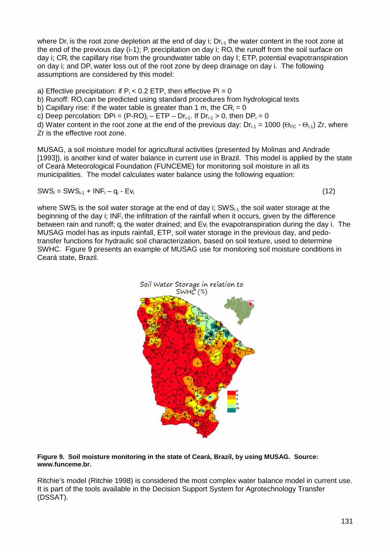
131

where Dri is the root zone depletion at the end of day i; Dri-1 the water content in the root zone at the end of the previous day (i-1); Pi precipitation on day i; ROi the runoff from the soil surface on day i; CRi the capillary rise from the groundwater table on day I; ETPi potential evapotranspiration on day i; and DPi water loss out of the root zone by deep drainage on day i. The following assumptions are considered by this model: a) Effective precipitation: if Pi < 0.2 ETP, then effective Pi = 0 b) Runoff: ROi can be predicted using standard procedures from hydrological texts b) Capillary rise: if the water table is greater than 1 m, the CRi = 0 c) Deep percolation: DPi = (P-RO)i – ETP – Dri-1. If Dri-1 > 0, then DPi = 0 d) Water content in the root zone at the end of the previous day: Dri-1 = 1000 (ΘFC - Θi-1) Zr, where Zr is the effective root zone. MUSAG, a soil moisture model for agricultural activities (presented by Molinas and Andrade [1993]), is another kind of water balance in current use in Brazil. This model is applied by the state of Ceará Meteorological Foundation (FUNCEME) for monitoring soil moisture in all its municipalities. The model calculates water balance using the following equation: SWSi = SWSi-1 + INFi – qi - Evi (12) where SWSi is the soil water storage at the end of day i; SWSi-1 the soil water storage at the beginning of the day i; INFi the infiltration of the rainfall when it occurs, given by the difference between rain and runoff; qi the water drained; and Evi the evapotranspiration during the day i. The MUSAG model has as inputs rainfall, ETP, soil water storage in the previous day, and pedo-transfer functions for hydraulic soil characterization, based on soil texture, used to determine SWHC. Figure 9 presents an example of MUSAG use for monitoring soil moisture conditions in Ceará state, Brazil.

Figure 9. Soil moisture monitoring in the state of Ceará, Brazil, by using MUSAG. Source: www.funceme.br. Ritchie’s model (Ritchie 1998) is considered the most complex water balance model in current use. It is part of the tools available in the Decision Support System for Agrotechnology Transfer (DSSAT).

132

The soil water balance module in the crop growth models of DSSAT computes one-dimensional soil water balance of a stratified profile in a daily time step. Soil characteristics, climate parameters, and crop management practices are standard inputs to the model (IBSNAT 1990). Values of plant growth variables estimated by other DSSAT modules are also input to this water balance. Water from either precipitation or irrigation infiltrates into the top soil layer after subtraction of runoff. Empirical procedures are used to calculate soil water flow upward and downward through the profile. Drainage flow is calculated by a “cascading” approach, in which water surplus above field capacity of a layer is passed directly to the layer below. Drainage does not occur when soil moisture is below field capacity. A normalized soil water diffusion equation, parameterized for general soil types of different textures, is used to simulate upward flux. ETP and SWS determine the magnitude of evaporation from the top soil layer (0 to 5 cm) and transpiration from the root zone. Potential evapotranspiration, estimated by Penman-Monteith or Priestley-Taylor equations, is partitioned into soil evaporation and plant transpiration, assuming that evaporation depends on the energy that reaches the soil surface and transpiration is proportional to the energy intercepted by crop canopy. Actual transpiration is the minimum between potential transpiration and total root water uptake (TRWU). At each soil layer, root water uptake by a single root (RWU) depends on soil water availability and rooting density, according to the following relationship:

RWU = 132 * Ke / (7,01 – Ln RLV) (13) where RWU is limited to a maximum value equal to 0.03 cm3 of water cm-1 of root day-1, RLV is root length density simulated daily by the growth model (cm of root cm-3 of soil), and Ke is hydraulic conductivity (cm day-1), empirically calculated as: Ke = 10-5 EXP [CON (SWS – LL)] (14) where SWS is actual soil moisture, LL is lower limit of soil available water (both in cm3cm3), and CON is 45 for LL higher than 0.3 cm3cm-3, or calculated by: CON = 120 – 250 * LL (15) Root water uptake from each soil layer in the rooting zone is integrated to calculate TRWU. Even with all its complexity, Ritchie’s model requires calibration for each new type of soil and crop, according to the differences imposed on the system by the combination of these variables. Results from Faria and Bowen (2003) demonstrated that an original soil water balance module of DSSAT v3.5 showed a low performance for simulating soil moisture profiles for bare and cropped soils because of inadequacies in the methods used to calculate soil water flux and root water absorption. The modification of the module with the introduction of Darcy’s equation to calculate soil water flux significantly improved soil moisture estimates. Subsequent modification by using hydraulic conductivity derived from measured data on the equation used to calculate root water uptake provided reasonable estimates of root water absorption under cropped conditions. Although application of the modified module is limited because reliable soil retention and hydraulic conductivity data are difficult to obtain, the existing errors in the current module limit its application in many studies in which crop yield depends on soil water status. Another type of water balance is provided by Center for Weather Forecast and Climatic Studies (CPTEC) of the National Institute for Space Research (INPE). The estimated water balance by the CPTEC/INPE model is obtained with an algorithm that combines numerical modeling and products from remote sensing (Gevaerd and Freitas 2006). The soil moisture (η, in volume of water by volume of soil) is given by Richards’ equation (Hillel 1998): ∂η / ∂t = ∂ / ∂z (Dη ∂η / ∂z - Kη) + Sη (16)

133

where Dη is the hydraulic diffusivity; Kη the hydraulic conductivity; z the depth of layer; and Sη the water uptake by roots, estimated as a functional relation among soil moisture in the layer, its field capacity and wilting point, and ETP. ETP is calculated by the Thornthwaite (1948) method. This water balance model also takes into account the effective rainfall estimated by satellite; variation of SWHC for different types of soil, classified by texture classes; leaf area index from satellite images; and runoff. The performance of this model was tested with data from the ABRACOS/LBA project, for pastures and forests in the Amazon region of Brazil. The results obtained by Gevaerd and Freitas (2006) showed moderate accuracy and high precision, as can be seen in the regression analyses presented below: a) for pasture: SWSest = 0.65 SWSobs + 186 and R2 = 0.82 b) for forest : SWSest = 0.87 SWSobs + 52 and R2 = 0.90 where SWSest is the estimated soil water storage and SWSobs the observed soil water storage, during the ABRACOS field experiment. An example of the maps produced with this kind of technique is presented for two different soil layers, from 0 to 19 cm and from 0 to 75 cm (Figure 10). The results are impressive since this model allows determining soil moisture for all South America, with a resolution of 5 km, giving a general view of the availability of water in different regions of the country, based on surface and satellite information.

Figure 10. Soil moisture for different soil depths (19 cm – left side and 75 cm – right side) as determined by the Gevaerd and Freitas (2006) model. Source: http://agricultura.cptec.inpe.br/.

134

Water Balance as a Tool for Agricultural Drought Monitoring Several agricultural drought indices in current use are based on information provided by the water balance models. Some of these indices are listed below, showing how the water balance outputs are used as inputs for them. Accumulated Water Deficiency Index (AWDI): This index is simply the sum of the water deficiency during the drought period. Water deficiency is calculated as the difference between ETP and ETa. The method to estimate these two variables can vary, and the results will vary proportionally. The most common procedure to determine water deficiency is through Thornthwaite and Mather’s water balance model, with ETP calculated by Thornthwaite (1948). However, the ETP method can be changed to produce more reliable results, since the Thornthwaite model used to underestimate ETP during the dry periods (Sentelhas et al. 2008). Relative soil moisture index (RSMI): This index is given by the relationship between actual soil water storage (SWS) and soil water holding capacity (SWHC), in percentage: RSMI = SWS / SWHC (17) Relative Water Deficiency Index (RWDI): This index is the water deficiency expressed in percentage, in relation to ETP: WDI = (1 – ETa/ETP) * 100 (18) Crop Moisture Index (CMI): This index is based on the difference between the observed ETa (ETaobs) and the expected ETa (ETaexp) for the period and was proposed by Palmer (1968) as a simple way for monitoring crop conditions: CMI = ETaobs – ETaexp (19) Observed ETa is provided by the serial climatological water balance of Thornthwaite and Mather (1955), whereas expected ETa is the climatological value for the period. Crop Water Development Index (CWDI): This index is based on soil moisture calculated by the water balance, according to the following calculations: • Crop water deficit factor (CWDF): CWDF = SWS/SWHC (20) • Crop water development index (CWDI): CWDI = (CWDF/0.4) – 1 (21) • Accumulated CWDI (ACWDI): ACWDI = ∑ [CWDI / (n * 1.5)] (22) The classes of ACWDI are presented in Table 1, showing the relationship between ACWDI and crop development conditions.

135

Table 1. Accumulated crop water development index (ACWDI) classes and their relationship to crop development conditions. Source: www.infoseca.sp.gov.br.

ACWDI Classes Crop development conditions 0.8 ≤ ACWDI ≤ 1.0 Very good 0.6 ≤ ACWDI ≤ 0.8 Good 0.4 ≤ ACWDI < 0.6 Reasonable 0.3 ≤ ACWDI < 0.4 Unfavorable 0.2 ≤ ACWDI < 0.3 Critical 0.1 ≤ACWDI < 0.2 Very critical

ACWDI < 0.1 Severe Another drought index that uses the outputs of the water balance models is the Palmer Drought Severity Index (PDSI). The PDSI is an agrometeorological drought index, and it responds to weather and consequent water balance conditions that have been abnormally dry or abnormally wet. When conditions change from dry to normal or wet, for example, the drought measured by the PDSI ends (Karl and Knight 1985). The PDSI is calculated based on precipitation and temperature data, as well as the local SWHC. From these inputs, all the basic terms of the water balance are determined by Thornthwaite and Mather’s model, including actual evapotranspiration (ETa), soil water storage (SWS), water deficiency (WD), and water surplus (WS). Complete descriptions of the equations can be found in the original study of Palmer (1965) and in Alley (1984).

Strengths, Weaknesses, and Limitations of Water Balance Models for Drought Monitoring The strengths and weaknesses of a water balance model are related, basically, to their complexity, as discussed above. The simpler water balance models, represented here by the Thornthwaite and Mather (1955) model, have as positive aspects the fact that they are simple to apply, requiring only rainfall and temperature data (for estimating ETP) and general information from the soil, in terms of water holding capacity (SWHC). Another advantage of these models is that their outputs are easy to understand and apply, and they do not require much computational power. Normally, water deficiency has a high correlation with crop yield losses. On the other hand, these models do not consider variables such as runoff, rain interception, and detailed soil characteristics, which make their results limited for more specific studies, generating systematic errors. The most complex models, which consider the majority of the processes involved with the water balance, will produce more reliable results when well calibrated for the location, having a very high correlation with what is happening in the field. However, the complexity will require many complex input data, which are not readily available for the majority of locations. They are complex to apply; require detailed information from soil, crop development, crop management, and climate; have more complex outputs; need higher computational power; and, if not properly calibrated, can present calibration errors. An example of the calibration problems related to complex water balance models was presented by Faria and Bowen (2003), when using Ritchie’s model in DSSAT. As mentioned earlier, users need to find a balance between simplicity and complexity when choosing a water balance model for drought monitoring with indices. In this way, the most reasonable option is to evaluate which data are available and which model is the better match for this data, producing suitable results. Calibration and tests are always recommended.

136

Conclusions The topics discussed previously led to the following conclusions:

• The water balance is an important tool for determining agricultural drought indices, since it

takes into account variables from soil, crop, and climate, and has a high correlation with yield losses. However, its use requires attention, mainly in terms of the errors associated with the estimates, since complexity does not necessarily represent an improvement in accuracy.

• Simple models can be as efficient as complex models if tested and adjusted for the regions of interest.

• Complex models vary, but in general they can produce very accurate results, mainly after parameterization for the crop, soil, management, and location.

• Data availability is crucial to the decision about the kind of water balance model to adopt. Simple models only require R, ETP, and SWHC data; complex models will also require detailed soil, crop, and management data.

• Independent of the type of water balance model adopted (simple or complex), calibration and testing are essential to their success as sources of input data for agricultural drought indices.

References

Allen, R.G., L.S. Pereira, D. Raes, and M. Smith. 1998. Crop Evapotranspiration. Guidelines for

Computing Crop Water Requirements. FAO Irrigation and Drainage Paper, No. 56. FAO, Rome, Italy.

Alley, W.M. 1984. The Palmer Drought Severity Index: Limitations and assumptions. Journal of Climate and Applied Meteorology 23:1100-1366.

Boken, V.K. 2005. Agricultural drought and its monitoring and prediction: Some concepts. Pages 3-10 in Monitoring and Predicting Agricultural Drought – A Global Study (V.K. Boken, A.P. Cracknell, and R.L. Heathcote, eds.). Oxford University Press, New York.

Camargo, A.P., F.R. Marin, P.C. Sentelhas, and A.G. Picini. 1999. Ajuste da equação de Thornthwaite para estimar a evapotranspiração potencial em climas áridos e superúmidos, com base na amplitude térmica. Revista Brasileira de Agrometeorologia 7: 251-257.

Diepen, C.A. and T. van der Wall. 1995. Crop growth monitoring and yield forecasting at regional and national scale. Pages 143-158 in Publication EUR 16008 EN of the Office for Official Publications of the EC. Luxembourg, Belgium.

Faria, R.T. and C.A. Madramootoo. 1996. Simulation of soil moisture profiles for wheat in Brazil. Agricultural Water Management 31:35-49.

Faria, R.T. and W.T. Bowen. 2003. Evaluation of DSSAT soil-water balance module under cropped and bare soil conditions. Brazilian Archives of Biology and Technology 46:489-498.

Gevaerd, R. and S.R. Freitas. 2006. Estimativa operacional da umidade do solo para iniciação de modelos de previsão numérica da atmosfera. Parte I: Descrição da metodologia e validação. Revista Brasileira de Meteorologia 21:59-73.

Hargreaves, G.H. and Z.A. Samani. 1985. Reference crop evapotranspiration from temperature. Applied Engineering Agriculture 1:96-99.

Hillel, D. 1998. Environmental Soil Physics. Academic Press, New York. IBSNAT. 1990. IBSNAT progress report 1987-1990. International Benchmark Site Network for

Agrotechnology Transfer, Honolulu, Hawaii. Ji, F., M. Littleboy, and G. Summerell. 2009. Water balance modeling – Impact of land use, soil

properties and rainfall seasonality. Pages 3386-3392 in MODSIM Congress, Cairns, Australia.

Karl, T.R. and R.W. Knight. 1985. Atlas of Monthly Palmer Hydrological Drought Indices (1931–1983) for the Contiguous United States. Historical Climatology Series 3–7, National Climatic Data Center, Asheville, USA.

Molinas, P.A. and F.C.M. Andrade. 1993. Modelo de umidade do solo para atividades agrícolas. Pages 136-145 in Simpósio Brasileiro de Recursos Hídricos, SBRH, Gramado, Brasil.

Palmer, W.C. 1965. Meteorological drought. US Weather Bureau Res. No. 45, Washington, D.C.

137

Palmer, W.C. 1968. Keeping track of crop moisture conditions, nationwide: The new Crop Moisture Index. Weatherwise 21:156–161.

Pereira, A.R., L.R. Angelocci, and P.C. Sentelhas. 2002. Agrometeorologia - fundamentos e aplicações práticas. Agropecuária, Guaíba, Brasil.

Priestley, C.H.B. and R.J. Taylor. 1972. On the assessment of surface heat-flux and evaporation using large-scale parameters. Monthly Weather Review 100:81-92.

Ritchie, J.T. 1998. Soil water balance and plant water stress. Pages 41-54 in Understanding Options for Agricultural Production (G.Y. Tsugi, G. Hoogenboom, and P.K. Thornton, eds.). Kluwer Academic Publishers, Amsterdam, The Netherlands.

Sentelhas, P.C., A.R. Pereira, F.R. Marin, L.R. Angelocci, R.R. Alfonsi, P.H. Caramori, and S. Swart. 1999. Balanço Hídrico Climatológico no Brasil [CD-ROM]. ESALQ/USP, Piracicaba, Brasil. Available at: www.leb.esalq.usp.br/nurma/bhbrasil.

Sentelhas, P.C., D.L. Santos, and R.E. Machado. 2008. Water deficit and water surplus maps for Brazil, based on FAO Penman-Monteith potential evapotranspiration. Revista Ambiente e Água – An Interdisciplinary Journal of Applied Science 3:28-42.

Thornthwaite, C.W. 1948. An approach toward a rational classification of climate. Geographical Review 38:55-94.

Thornthwaite, C.W. and J.R. Mather. 1955. The water balance. Drexel Institute of Technology, New Jersey, USA.

Zhang, L., G.R. Walker, and W.R. Dawes. 2002. Water balance modeling: Concepts and applications. Pages 31-47 in Regional Water and Soil Assessment for Managing Sustainable Agriculture in China and Australia (T.R. Mevicar, L. Rui, J. Walker, R.W. Fitzpatrick, and L. Changming, eds.). Monograph No. 84, ACIAR, Canberra, Australia.

Zhang, L., K. Hickel, and Q. Shao. 2005. Water balance modeling over variable time scales. Pages 2988-2994 in MODSIM Congress, Melbourne, Australia.

138

Use of Crop Models for Drought Analysis

Raymond P. Motha USDA Chief Meteorologist, U.S. Department of Agriculture

Washington, D.C.

Abstract

Crop models can play a role in this agricultural management decision making process to cope with drought and other natural disasters. Crop simulation models are designed to imitate the behavior of a plant system. These models separate yield prospects into components due to changing weather trends, genetic improvements, and improved technology. Simulation modeling is increasingly being applied in research, teaching, farm and resource management, policy analysis, and production forecasts. Crop simulation models can be used to simulate the drought-reduced crop yields, but a number of issues limit operational applications.

Introduction

Agricultural producers face a number of risks in their operations. The United States Department of Agriculture’s Risk Management Agency has defined five primary categories of risk: production, marketing, finance, legal, and human risk (Harwood et al. 1999). Seasonal climate variability is a major source of production risks. In fact, the majority of crop failures in the United States are associated with either a lack of moisture or excess rainfall (Ibarra and Hewitt 1999). Climate variability is also greatly associated with marketing risks. Drought conditions, extreme wetness and flooding, spring freezes, and similar conditions leading to crop failure can dramatically affect crop and livestock prices. A good market plan requires an analysis of supply and demand projections throughout the cropping season. Expectations early in the season are highly uncertain. Commodity markets respond decisively to these early projections, and seasonal climate variability plays an important role in modifying the balance between supply and demand. In order to accomplish the ultimate goal of providing useful information to the agricultural decision maker that will help to reduce the variety of risks, an integration of monitoring, modeling, and forecasting tools needs to be readily available in a management toolkit.

Background

Some of the most important decisions in agricultural production, such as what crops to grow and how much land to allocate, depend on the existing knowledge base of current and future physical conditions like soil and climate, and yields and prices. Modeling of the various processes in the system helps us to understand its flow and intricacies. Weather and climate continually alter some of these major decisions as natural disasters and extreme events disrupt agricultural activities. Agricultural drought is one of the major disruptive events affecting crop productivity at the farm level, and sustainable agriculture and food security around the world. Impacts on agriculture can be addressed at various levels, including crop yields, farm and village level outputs and income, regional and national production, and global production and prices. Each level requires different sets of criteria, including methods and input data. However, there is a multi-tier relationship between various scales. For example, the data inputs of the crop response can be fed into the farm level model. The output of the farm level model can then be used as input to the regional scale. The output from the regional scale can be used as input into the national assessment, and the resulting output can be used for global crop production assessments. The characterization of agricultural drought is entirely different from other types of droughts. The deficiency of water in sensitive growth stages can reduce production in some crops severely. The effect of one drought event may continue to affect an area for several growing seasons or even several years; thus, there is the need to analyze agricultural drought events on the basis of continuous weather data. The analysis of agricultural drought is also complicated by the fact that

139

the beginning and end of any drought is often difficult to determine. Furthermore, the impact of drought often accumulates slowly over a considerable period of time. The impact of drought may linger long after the termination of the event. The absence of a precise and universally accepted definition of drought has added to the complexity. Therefore, any realistic definition of drought must be region and application specific. Agricultural drought links various characteristics of meteorological drought to agricultural impacts, focusing on precipitation shortages, differences between actual and potential evapotranspiration, and soil moisture deficits. Any realistic definition of agricultural drought should account for the susceptibility of crops at different stages of crop development. The crop simulation-based analysis of drought may serve to identify crop losses due to agricultural drought because of the water loss accounting procedures. Crop simulation models can be very useful tools for the characterization of drought by calculating the water deficiency due to deficient rainfall, runoff (slope effect), deep percolation (soil effect), and evapotranspiration (temperature effect). Crop simulation models then can be used to simulate the drought-reduced crop yields. However, there are many issues to contend with regarding crop modeling. Some of these will be discussed in this chapter.

Crop Modeling Models are mathematical equations depicting the relationships between crop growth, development, yields, technology, and climate. For example, crop yield is a function of complex interactions of biotic and abiotic factors, including crop management (e.g., fertility, variety, and seeding rate), soil and field characteristics (e.g., drainage, topography, and soil water holding capacity), and weather conditions (e.g., temperature, precipitation, and light use efficiency). Crop production varies not only spatially but also temporally. The agricultural system is complex and, although it is nearly impossible to represent the system in mathematical terms, crop models can provide some sense of reality in terms of phenological development or response to climate extremes or other environmental or biological parameters affecting crop growth and development. However, universal models do not exist within the agricultural sector. Models are built for specific purposes and the level of complexity varies according to the application, data availability, and objective of the model. Inevitably, different models are built for different sub-systems, and several models may be built to simulate a particular crop or a particular aspect of the production system. One of the main aims of constructing operational crop models is to obtain an estimate of the harvestable (economic) yield. The operational applications generally focus on crop yield forecasting, which often includes an assessment of the soil moisture regime and crop growth and development. The assessment of crop development and yield response often includes crop management, such as fertilizing, cultivation, irrigation, and plant protection. However, models are rarely used for early warnings or mitigation of damages from extreme meteorological phenomena and natural disasters. There are different types of crop models. Empirical models are direct descriptions of observed data. They are generally expressed as regression equations (with one or a few factors) and used to estimate the final yield. Examples of such models include the response of crop yield to severe drought, the response of yield to fertilizer application, and the relationship between leaf area and leaf size in a given plant species. The limitation of this type of model is that it is generally location specific. An alternative approach involves the use of crop growth simulation models. Crop growth models encapsulate knowledge of eco-physiological processes and allow simulation of crop yield for specific varieties and locations. Simulation models form a group of models designed to imitate the behavior of a system. They are mechanistic and, in the majority of cases, deterministic. Since they are designed to mimic the system at short time intervals (daily weather data, for example), the aspect of variability related to daily change in weather and soil conditions is integrated. The short simulation time-step demands that a large amount of input data (climate parameters, soil characteristics, and crop parameters) be available to generate and run a model.

140

The parameters used in crop simulation models generally include meteorological, physical, and biological parameters, but a parameter of length of time should also be included. Simulation models require that meteorological data be reliable and complete. Meteorological sites may not fully represent the weather at a chosen location. In some cases, data may be available for only one (usually rainfall) or a few (rainfall and temperature) parameters, but data for solar radiation, which is important in the estimation of photosynthesis and biomass accumulation, may not be available. At times, records may be incomplete and gaps may have to be filled. A stochastic weather generator produces artificial time series of weather data of unlimited length for a location based on the statistical characteristics of observed weather at that location. These types of statistical models are generally developed in two steps, with the first step focusing on the modeling of daily precipitation and the second concentrating on the remaining variables of interest, such as maximum and minimum temperature, solar radiation, humidity, and wind speed, which are modeled conditional upon precipitation occurrence. For each month, different model parameters are used in order to reflect seasonal variations in both the values of the variables themselves and in their cross-correlations (i.e., in the relationships between the individual variables over time). There are two basic types of stochastic weather generator: the “Richardson” (Richardson 1981, Richardson and Wright 1984) or “serial” (Racsko et al. 1991, Semenov et al. 1998) types. The types of weather generator available are also described in Wilks and Wilby (1999). In a “Richardson” type weather generator (e.g., WGEN), precipitation occurrence is modeled using a first-order two-state Markov procedure, which describes two precipitation classes (i.e., wet or dry) and takes into account precipitation occurrence on the previous day only. More complex models may involve more than one precipitation class (e.g., low, medium, and high precipitation amounts) as well as the occurrence of precipitation on a number of days before the current day, rather than on just the previous day. The Markov process gives information on transition probabilities (e.g., on the probability of a wet day following a dry day or the probability of a wet day following a wet day), calculated from the observed station data. If precipitation occurs, then the amount of precipitation falling on wet days is determined usually by using a predefined frequency distribution, most commonly the gamma distribution, although mixed-exponential distributions may provide a better representation of precipitation amount at some locations. The remaining climate variables are then calculated based on their correlations with each other and on the wet or dry status of each day. One of the main criticisms of Richardson-type weather generators is their inability to adequately describe the length of wet or dry series (i.e., persistent events such as drought or prolonged rainfall), which are extremely important in some applications (e.g., agricultural impacts, where the occurrence of a drought during a particular phase of crop development may result in crop failure). The serial approach to weather generation was developed to attempt to overcome this problem. In this type of weather generator, the first step in the process is the modeling of the sequence of dry and wet series of days. The amount of precipitation and the remaining climate variables are then generated dependent on the wet or dry series. The serial-type weather generator, first developed by Racsko et al. (1991), has been substantially updated (LARS-WG; Semenov et al. 1998). Many different versions of weather generators have been developed over the past decade. Simulation models have been reported as useful in separating yield gain into components due to changing weather trends, genetic improvements, and improved technology. Simulation modeling is increasingly being applied in research, teaching, farm and resource management, policy analysis, and production forecasts. These models can be applied in three areas, namely, research tools, crop system management tools, and policy analysis tools. However, simulation models usually offer the possibility of specifying management options, and they can be used to investigate a wide range of management strategies at low costs. Most crop models that are used to estimate crop yield fall within this category. When a model is applied in a new situation (e.g., switching to a new variety), the calibration and validation steps are crucial for correct simulations. The need for model verification arises because

141

all processes are not fully understood and even the best mechanistic model still contains some empirism, making parameter adjustments vital in a new situation. Model performance is limited to the quality of input data. It is common in cropping systems to have large volumes of data relating to the above-ground crop growth and development, but data relating to root growth and soil characteristics are generally not as extensive. Using approximations may lead to erroneous results. Model users need to understand the structure of the chosen model, its assumptions, its limitations, and its requirements before any application is initiated. At times, model developers may raise the expectations of model users beyond model capabilities. Users, therefore, need to judiciously assess model capabilities and limitations before one is adopted for application and decision-making purposes. Generally, crop models are developed by crop scientists, and if interdisciplinary collaboration is not strong, the coding may not be well-structured and model documentation may be poor. This makes alteration and adaptation to simulate new situations difficult, especially for users with limited expertise. Finally, using a model for an objective for which it had not been designed or using a model in a situation that is drastically different from that for which it had been developed would lead to model failure. Optimizing models have the specific objective of developing the best option in terms of management inputs for practical operation of the system. These models use decision rules that are consistent with some optimizing algorithm for deriving solutions. This forces some rigidity into their model structure, resulting in restrictions in representing stochastic and dynamic aspects of the modeled agricultural systems. Applications have been developed to assess long-term changes in agriculture, regional competition, transportation studies, and integrated production and distribution systems as well as policy issues in the adoption of technology and natural resource conservation. Optimizing models do not allow the incorporation of many biological details and may be poor representations of reality. However, a useful option has been to use the simulation approach to identify a restricted set of management options that are then evaluated with the optimizing models. CERES is a series of crop simulation models, and DSSAT is also a framework of crop simulation models, including modules of CERES, CROPGRO and CROPSIM, that are incorporated into a system of optimizing models. Modeling Applications in Agriculture Crop modeling has been applied at various scales in agriculture, from precision farming, to farm planning, to watershed or regional policy development. CROPGRO Soybean (Hoogenboom et al. 1994) and CERES-Maize (Jones and Kiniry 1986) are process-oriented models that compute growth, development, and yield on homogeneous units from field to regional scales. Although crop modeling is a relatively effective tool for simulating yield and yield-limiting factors, as noted earlier, a large amount of input data is necessary to accurately predict spatial variations. It has also been expensive to measure dense spatial datasets for use in crop models. Reliable and cost-effective techniques must be developed to parameterize crop models across a field with high spatial resolution and to quantify in-field spatial variations. The crop management system models mentioned above are generally referred to as decision support system (DSS) models for agriculture. A set of crop models that share a common input/output data format has been developed and embedded in a software package called the Decision Support System for Agrotechnology Transfer (DSSAT). DSSAT (IBSNAT 1989, Jones 1993, Tsuji et al. 1994) is a shell that allows the user to organize and manipulate crop, soils, and weather data and to run crop models in various ways and analyze their outputs. CERES-Maize and CROGRO-Soybean models are included in the DSSAT v.3.5 software package (Hoogenboom et al. 1994) to simulate crop growth. These are mechanistic process-based models that, in response to daily weather inputs, predict soil traits, daily photosynthesis, growth, and crop management. Fraisse et al. (2001) and Wang et al. (2003) evaluated the CERES-Maize and CROPGRO-soybean models for simulating site-specific crop development and yield on Missouri claypan soils. Additional models running under DSSAT include the CERES (Crop Environment Resource Synthesis) models for rice, wheat, sorghum, pearl millet, and barley (Ritchie 1985, Ritchie and Otter 1985, Ritchie 1986); the CROPGRO model for peanut and phaseolus bean; and

142

a model for cassava and potato (Tsuji et al. 1994). Phenological development and growth in the CERES models are specified by cultivar-specific genotype coefficients depending on the photoperiod, thermal time, temperature response, and dry matter partitioning. Geographic information system (GIS) is a computer-assisted system that acquires, stores, analyzes, and displays geographic data. Because of the increasing pressure on land and water resources and the importance of forecasts at different spatial scales (crop, weather, fire, etc.), geographic information systems have become an essential decision-support tool. GIS has developed into a powerful tool at the disposition of policy and decision makers (Maracchi et al. 2000). Interfacing crop simulation models with a GIS helps to accomplish spatial and temporal analysis at the same time. Spatial model applications, such as interfacing models with GIS, further increase the possibilities of applying these models for regional planning and policy. GIS is a front-end tool for data preprocessing and a visualization tool for analyzing the final results. The user interface also resides within the GIS and facilitates location-specific and crop-specific data input. On completion of data input, the data access modules acquire the necessary spatial and non-spatial data from GIS layers and a Relational Database Management (RDBM) System, respectively. An RDBM system offers a data management system that comprises a set of operating-system processes and memory structures that interact with the storage. This scenario offers advantages such as better performance, scalability, and redundancy. Large data files can be stored from a number of different sources, processed, archived, and retrieved as necessary. GIS-based modelling of an agroecosystem offers a powerful tool to agricultural managers to simultaneously assess the effect of soil and water resources on crop production in addition to farm practices. At present, most of the crop models are location specific (point based) in nature, but to have a better understanding of the impact on agricultural systems, it is necessary to have spatially explicit analyses. Therefore, the development of spatially or raster based biophysical crop models helped to clarify many intricacies of modeling large areas. Hydrologic models are valuable tools for water resources management. For irrigation scheduling and crop water requirement estimation, hydrologic simulation models commonly use the water balance approach (Fangmeier et al. 1990, Fulton et al. 1990, Smajstrla 1990, George et al. 2000). Precision farming research has demonstrated that field-scale variations in crop yield are controlled by soil properties and landscape features that affect patterns in water available to plants, soil drainage, and aeration (Jaynes and Colvin 1997, Mulla and Schepers 1997). Inclusion of spatially distributed climate, soils, and land-use data dramatically increases the model’s computational and data requirements. Storage and application of spatial data continues to challenge traditional modeling approaches. Geographic information systems are capable of providing the necessary spatial database for hydrologic models. By exploiting the modeling power of GIS through integration of GIS with hydrologic models, a GIS can be transformed from a simple spatial query and visualization tool to a powerful analytical and spatially distributed modeling tool. Recent advances in GIS technology facilitate the seamless integration of GIS and computer-based modeling. Multiple approaches exist to integrate GIS and hydrological models (Maidment 1993, Abel et al. 1994, Sui and Maggio 1999). The two general categories of approaches are 1) coupling, providing a common interface or a linkage between the applications, and 2) embedding or merging the features of different applications into a single application. Rao et al. (2000), Tucker et al. (2000), and Xu et al. (2001) have successfully developed integrated GIS and hydrological models. Agro-climatic models consisting of coupled GIS and crop models, including AEGIS/WIN by Engel et al. (1997) and CropSyst by Stockle and Nelson (1994), have been used to enhance farm management practices. Both models simulate the soil water budget, soil-plant nutrient budgets, crop canopy and root growth, dry matter production, yield, residue production and decomposition, and erosion. These biological simulation models excel at quantifying the effect of different management systems on crop production and environmental impacts. AEGIS/WIN links DSSAT

143

v3 with ArcView to model spatially distributed crop growth (Engel et al. 1997). Crop-Syst, a multi-year and multi-crop model, spatially and temporally simulates the soil water budget components and crop growth potential by coupling the model with databases of soil type, long-term weather conditions, and crop management (Stockle et al. 1997). Both AEGIS/WIN and CropSyst characterize the soil variability on a regional scale, but assume a single soil layer within a field. The above models are capable of dealing with a limited variety of crops, homogeneous soil (on a farm scale), and climate information from a single location. The GIS-based Water Resources and Agricultural Permitting and Planning System (GWRAPPS) (Satti 2002) is a more comprehensive distributed model with several unique features: 1) estimates of crop water requirements are simultaneously simulated for multiple crops and allow for climate and soil variation as well as differing irrigation management practices, 2) spatial scales range from a single field to a regional scale, 3) annual and monthly drought water requirements are determined using a statistically robust frequency analysis of the simulated historical daily water demand, and 4) the system provides an easy-to-use Graphical User Interface (GUI) to access GIS data and an RDBMS. Though GIS is capable of storing and supporting large spatial data, it cannot readily maintain large temporal data. The data storage approach implemented in the GWRAPPS overcomes this shortcoming and efficiently handles large temporal and spatial databases by storing the temporally explicit data in a RDBMS and maintaining appropriate links from a GIS layer to the RDBMS tables. GWRAPPS is a decision support system for permitting and planning irrigation water demand. GWRAPPS operates in a Windows environment that tightly couples ArcGIS (ESRI) with the Agricultural Field Scale Irrigation Requirements Simulation (AFSIRS) model (Smajstrla and Zazueta 1988) using object-oriented technology. The AFSIRS numerical simulation model determines the statistical characteristics of the irrigation requirements for a crop based on soil type, irrigation system, growing season, long-term climate, and irrigation management practice (Smajstrla 1990). The model calculates the daily soil water budget using the water balance approach that effectively models crop water requirements in the southeastern United States (Smajstrla and Zazueta 1988, Villalobos and Fereres 1989). AFSIRS simulates the dynamic processes of soil water infiltration, redistribution, and extraction by evapotranspiration as steady state processes and schedules irrigation based on an allowable level of soil water depletion from a two-layer crop root zone. The analysis components determine water demand at two different scales, the single farm scale and the regional scale. The permitting tool operates at a single farm scale and allows the user to simulate water requirements for a crop using either a single soil or an area-weighted average of all the soils within the farm. The model results include monthly and annual crop water requirements for median conditions and different drought probabilities. Typical drought scenarios include 1-in-5 year and 1-in-10 year drought conditions. The planning tool analyzes the irrigation requirements at a regional scale. The planning tool is similar to the permitting tool in that the same AFSIRS model and GIS soils and climate data are used to generate the water requirements. However, the planning tool analyzes all water permits in the region simultaneously. The simultaneous analysis greatly reduces the time required to analyze a region’s water demand and facilitates the planning for multiple time horizons and land-use change scenarios. The generated GIS irrigation requirements layer provides monthly and annual crop water requirements for the median, 1-in-5 year drought, and 1-in-10 year drought irrigation scenarios. GWRAPPS provides a consistent tool for water use planning and permitting by extending the AFSIRS model from a farm-scale model to a regional-scale irrigation requirements simulation model. The integrated GIS system facilitates effective usage of spatial distributed data to estimate farm and regional-scale irrigation requirements. GWRAPPS, with multiple soils, provides a comprehensive picture of the total water demand that is not readily apparent because of the complex interaction of soil characteristics and their relative contribution to the area of interest. GWRAPPS provides water demand maps that facilitate the study of regional irrigation requirements using farm level inputs. A simple user-friendly interface provides easy access to the components of the system by maintaining the complex data and control transfer operations in the

144

background. The system’s most important feature is its ability to quickly and easily provide regional crop water requirements for different drought scenarios. The present research demonstrates that the integrated system is capable of providing critical information to planners and farmers about different crops’ plant–soil–water relationship under a range of drought conditions. In conclusion, GWRAPPS, with its ability to consider spatial variability of soils and climate at both farm and regional scales under normal and drought conditions, is a practical tool that is applicable to a wide range of water resources management and development problems. The Agricultural Production Systems Simulator (APSIM) has been designed as a multi-purpose simulation platform (McCown et al. 1996). The APSIM model concept is able to accommodate various levels of complexity, depending on the intended application. It is composed of a modular framework. Systems models such as APSIM take this concept further by providing a means for effective communication across all the disciplines involved to address issues affecting farming and agriculture. Originally, the crop models were developed to deal with risky crop management decisions in the face of climatic variability. The models simulated plant growth and crop development in response to environmental inputs (water, temperature, solar radiation, nutrients) with the ultimate aim of estimating the yield of harvestable material from a commercial crop as precisely as possible. At the heart of these models is the relationship between crop yield and various inputs (climatic conditions such as rain, temperature, and solar radiation; nutrients; and management interventions such as irrigation or fertilization) that may or may not be affected by crop residues left on the soil surface from a previous crop. These residues can affect surface runoff, soil temperature, surface evaporation, and soil moisture, and thus can affect many processes that contribute to crop growth and yield as well as the state of the environment in which the crop is being grown. This is where the need for good science arises so that the model simulates the processes appropriately and precisely, in ways that are easily computable, and the results are believable. In addition to crop yield, models such as APSIM generate a large range of complementary output variables that can be very helpful in analyzing resource management problems. Community concern about off-farm impacts of farm inputs such as nitrogen fertilizer has increased in recent years. Therefore, farm management practices that might cause long-term resource degradation have come under close scrutiny. Models such as APSIM are complex, and as such require specialist support and a range of skills to support simulation building. A soil scientist will need crop physiology or agronomy expertise to ensure that water use, dry matter production, and maybe yield (assuming a holistic soil scientist) are drivers for soil processes. Modelers often work in an environment where this broad expertise is available and essential for the development of useful and reliable systems tools. Although APSIM is primarily aimed at researchers, an increasing number of derived products have been developed. Adoption by commercial partners is also increasing, and it is through these arrangements that consultants and growers who have no prior modeling experience can evaluate a large range of alternative crop and fallow management options. Given the rapid changes that are currently taking place in rural industries (driven by economic as well as environmental factors such as climate change), the importance of APSIM as a quantitative, predictive tool for scenario development and evaluation is likely to increase. Heinemann et al. (2008) used a crop simulation model to determine the patterns of drought stress for short- and medium-duration upland rice around flowering and early grain-filling across 12 locations in Brazil. Simulation models can also provide a tool to assist in understanding, and incorporating, genotype-by-environment interaction, by combining mechanistic understanding of a drought (Chapman 2008). Given a historical record of weather for a location, the probability of a yield increase (and maybe a decrease) resulting from the incorporation of any trait into the crop can be simulated. Combining the probabilities for yield change with the farmers’ adversity to risk gives a strong indication to a breeder of the desirability of incorporating a particular drought trait for cultivars to be grown in a specific location. System analysis can hence allow breeding for specific drought-adaptive traits to be targeted to those geographical regions where their benefit will be

145

largest (Sinclair and Muchow 2001). However, in the case of rice, most simulation efforts have focused on irrigated environments, and an improved rice model needs to be developed or adapted specifically for the drought-prone rainfed systems, based on better physiological understanding of rice interaction with the environment under water deficits. In Europe, only a few models are applied operationally (Eitzinger et al. 2008). Most research institutions are working on research applications of crop modeling for climate change impact research on agriculture, whereas the operational applications have the focus on crop yield forecasting. The applications often include an assessment of soil moisture, crop growth and development, and crop yields. The assessment of crop development and yield response to related crop management, such as fertilizing, cultivation, irrigation, and plant protection, is another application. Crop models are rarely used for early warnings or mitigation of crop damages from extreme meteorological phenomena and processes. Crop model applications are influenced by several uncertainties determining limitations of their use in research and practice (e.g., Eitzinger et al. 2008). The main reported limitation for application of crop models in Europe is related to the input data. The most frequently reported problems are the availability or the low quality of the soil physical model input data (especially for spatial model applications), the lack of long-term biophysical crop data for model validation and calibration, and, in some cases, the availability or costs of meteorological data. This is related to the socio-economic conditions in countries and different local administration of data in the different regions of Europe. The reliability of data for climate scenarios or seasonal forecasts is another crucial point for the use of such models for operational purposes or for making long-term strategic decisions. Spatial model applications, such as interfacing models with GIS, increase the possibilities of applying these models in regional planning and policy. Because of their relatively simple calculation methods, agroclimatic indices are often implemented in GIS in order to show spatial distribution and developments of the relevant calculated index. These drought indices are used in the crop models for decision-making tools. The most promising method of estimating crop yield over larger areas is to combine crop growth models and remote sensing data. The main benefit of using remotely sensed information is that it provides a quantification of the actual state of the crop for a large area, while crop models give a continuous estimate of growth over time. Only a few applications of spatial crop growth monitoring systems are fully operational in Europe. However, the general theme of remote sensing data assimilation in crop models has been the subject of numerous research papers in the last few years. These papers have discussed practical solutions, but the operational application is still limited by the large amount of data to be processed. AquaCrop (Raes et al. 2008) is a water-driven stimulation model that requires a relatively small number of parameters and is a functional balance between simplicity, accuracy, and robustness. FAO evolved the AquaCrop model from an earlier crop simulation modeling approach that has been well recognized for operational applications. In AquaCrop, the crop system has five major components and associated dynamic responses: phenology, aerial canopy, rooting depth, biomass production, and harvestable yield. Five weather input variables are required to run AquaCrop: early maximum and minimum air temperatures, daily rainfall, daily evaporative demand of the atmosphere expressed as reference evapotranspiration (ET), and the mean annual carbon dioxide concentration in the bulk atmosphere (Mauna Lou Observatory records in Hawaii). The features that distinguish AquaCrop from other crop models are its focus on water, the use of ground canopy cover instead of leaf area index, the use of water productivity values normalized for atmospheric evaporative demand, and the carbon dioxide concentration that extends the capacity of the model to extrapolate to diverse locations and seasons, including future climate scenarios. With respect to the more complex approaches, namely simulation or process-oriented models, operational applications are still very limited, except for the simple models. Some simple crop models focus on irrigation scheduling, or the widely applied models for pest and disease

146

management. In research, however, process-oriented crop models play a very important role in the assessment of global and climate change impacts on agriculture. Most of these studies are carried out on a larger scale, neglecting the necessarily finer spatial resolution to be of relevance for local practical recommendations for farmers. One of the main difficulties for the spatial application of process-oriented crop models in a high spatial resolution at the research level is often the lack of model input data (not available, high costs, expensive data management, etc.). On the other hand, new methods are being developed to overcome these problems by using GIS and integrating remote sensing data. Operational crop yield forecasting that integrates all these available tools is only used at the expert level, and very few examples of it exist.

Summary Although models are developed by agricultural scientists, the user group includes agronomists, extension workers, policy makers, farmers, and plant breeders. Because different users possess varying degrees of expertise in modeling, the misuse of models may occur. Since crop models are not universal, the user has to choose the most appropriate model according to his objectives. Even when a judicious choice is made, it is important that aspects of model limitations be borne in mind such that modeling studies are put in the proper perspective and successful applications are achieved. Crop/soil simulation models are basically applied in three areas: 1) tools for research, 2) tools for decision making, and 3) tools for education, training, and technology transfer. The greatest use of crop/soil models so far has been by the research community, as models are primarily tools for building a knowledge base. However, effective crop models can be used for a vast array of operational applications, especially when integrated with GIS and remote sensing technologies. As research tools, model development and application can help identify gaps in our knowledge, thus enabling more efficient and targeted research planning. Models that are based on sound data are capable of providing significant agricultural drought analyses to assist management strategies.

References

Abel, D.J., P.J. Kilby, and J.R. Davis. 1994. The systems integration problem. International Journal

of Geographical Information Systems 8(1):1-12. Chapman, S.C. 2008. Use of crop models to understand genotype by environment interactions for

drought in real-world and simulated plant breeding trials. Euphytica 161:195-208. Eitzinger, J., H. Formayer, S. Thaler, M. Trnka, Z. Zalud, and V. Alexandrov. 2008. Results and

uncertainties of climate change impact research in agricultural crop production in Central Europe. Bodenkultur 59:1-4.

Engel, T., G. Hoogenboom, W.J. James, and W.W. Paul. 1997. AEGIS/WIN: A computer program for the application of crop simulation models across geographic areas. Agronomy Journal 89:919–928.

Fangmeier, D.D., D.J. Garrot Jr., C.F. Mancino, and S.H. Husman. 1990. Automated irrigation systems using plant and soil sensors. In Proceedings of the third National Irrigation Symposium on Visions of the Future, ASAE, St. Joseph, Michigan.

Fraisse, C.W., K. A. Sudduth, and N. R. Kitchen. 2001. Calibration of the CERES-Maize model for simulating site-specific crop development and yield on claypan soils. Applied Engineering in Agriculture 17(4):547-556.

Fulton, A.E., R.H. Beede, and R.C. Phene. 1990. Implementing CIMIS at the farm level: A grower’s experience in walnuts. In Proceedings of the third National Irrigation Symposium Visions of the Future, ASAE, St. Joseph, Michigan.

George, B.A., S.A. Shende, and N.S. Raghuwanshi. 2000. Development and testing of an irrigation scheduling model. Agricultural Water Management 46:121–136.

Harwood, J., R. Heifner, K. Coble, J. Perry, and A. Somwaru., 1999. Managing Risk in Farming: Concepts, Research, and Analysis. United States Department of Agriculture, Economic Research Service (AER-774).

Heinemann, A.B., M. Dingkuhn, D. Luquet, J.C. Combres, and S. Chapman. 2008. Characterization of drought stress environments for upland rice and maize in central Brazil. Euphytica 162(3):395-410.

147

Hoogenboom, G., J.W. Jones, P.W. Wilkens, W.D. Batchelor, W.T. Bowen, L.A. Hunt, N. Pickering, U. Singh, D.C. Godwin, B. Baer, K.J. Boote, J.T. Ritchie, and J.W. White. 1994. Crop models. In DSSAT v3, 2(2) (G. Y. Tsuji, G. Uehara, and S.Salas, eds.). University of Hawaii, Honolulu, Hawaii.

Ibarra, R. and T. Hewitt. 1999. Utilizing crop insurance to reduce production risk. Institute of Food and Agricultural Sciences (IFAS Publication FE-198). Florida Cooperative Extension Service, Gainesville, Florida.

IBSNAT. 1989. Decision Support System for Agrotechnology Transfer (DSSAT) v2.1. Department of Agronomy and Soil Science, University of Hawaii, Honolulu, Hawaii.

Jaynes, D.B. and T.S. Colvin. 1997. Spatiotemporal variability of corn and soybean yield. Agronomy Journal 89(1):30-37.

Jones, J.W. 1993. Decision support systems for agricultural development. Pages 459-472 in Proceedings, Systems Approach for Agricultural Development (F.W.T. Penning de Vries, P.S. Teng, and K. Metselaar, eds.). Kluwer Academic Press, Dordrecht, The Netherlands.

Jones, C.A. and J.R. Kiniry. 1986. CERES-Maize: A Simulation Model of Maize Growth and Development. Texas A&M University Press, College Station, Texas, pp.103-125.

Maidment, D.R. 1993. GIS and hydrologic modeling. Pages 147-167 in Environmental Modeling with GIS (M.F. Goodchild, B.O. Parks, and L.T. Steyaert, eds.). Oxford University Press, New York.

Maracchi, G., V. Perarnaoud, and A.D. Kleschenko. 2000. Applications of geographic information systems and remote sensing in agrometeorology. Agricultural and Forest Meteorology 103:119-136.

McCown, R.L., G.L. Hammer, J.N.G. Hargreaves, D.P. Holzworth, and D.M. Freebairn. 1996. APSIM: A novel software system for model development, model testing and simulation in agricultural systems research. Agricultural Systems 50:(3)255-271.

Mulla, D.J. and J.S. Schepers. 1997. Key processes and properties for site-specific soil and crop management. Pages 1-8 in The State of Site Specific Management for Agriculture (F.J. Pierce and E.J. Sadler, eds.). ASA/CSSA/SSSA, Madison, Wisconsin.

Racsko, P., L. Szeidl, and M.A. Semenov. 1991. A serial approach to local stochastic weather models. Ecological Modeling 57:27-41.

Raes, D., P. Steduto, T.C. Hsiao, E. Fereres, and L. Heng. 2008. AquaCrop Calculation Procedure, Prototype Version 2.3a. FAO, Rome, Italy, 64p.

Rao, M.N., D.A. Waits, and M.L. Neilsen. 2000. A GIS-based modeling approach for implementation of sustainable farm management practices. Environmental Modelling and Software 15:745-753.

Richardson, C.W. 1981. Stochastic simulation of daily precipitation, temperature and solar radiation. Water Resources Research 17:182-190.

Richardson, C.W. and D.A. Wright. 1984. WGEN: A model for generating daily weather variables. U.S. Department of Agriculture, Agricultural Research Service, ARS-8, 83pp.

Ritchie, J.T. 1985. A user-oriented model of the soil water balance in wheat. Pages 293-305 in Wheat Growth and Modelling (W. Day and R.K. Atkins, eds.). Plenum Publishing Corporation, NATO-ASI Series.

Ritchie, J.T. 1986. CERES-Wheat: A General Documentation. USDA–ARS. Grassland, Soil and Water Resource Laboratory, Temple, Texas.

Ritchie, J.T. and S. Otter. 1985. Description and performance of CERES-Wheat: A user oriented wheat yield model. ARS Wheat Yield Project, ARS–38. National Technical Information Service, Springfield, Virginia, pp.159–175.

Satti, S.R. 2002. GWRAPPS: A GIS-based decision support system for agricultural water resources management. Master of Science Thesis. University of Florida, Gainesville, Florida.

Semenov, M.A., R.J. Brooks, E.M. Barrow, and C.W. Richardson. 1998. Comparison of WGEN and LARS-WG stochastic weather generators for diverse climates. Climate Research 10:95-107.

Sinclair, T.R. and R.C. Muchow. 2001. System analysis of plant traits to increase grain yield on limited water supplies. Agronomy Journal 93:263-270.

148

Smajstrla, A.G. 1990. Technical Manual: Agricultural Field Scale Irrigation Requirements Simulation (AFSIRS) model, Version 5.5, Agricultural Engineering Department, University of Florida.

Smajstrla, A.G. and F.S. Zazueta. 1988. Simulation of irrigation requirements of Florida agronomic crops. Soil & Crop Science Society of Florida Proceedings 47:78-82.

Stockle, C.O. and R.L. Nelson. 1994. Cropsyst User’s Manual, Version 1.0. Biological Systems Engineering Department, Washington State University, Pullman, Washington.

Stockle, C.O., M. Cabelguenne, and P. Debacke. 1997. Comparison of CropSyst performance for water management in southwestern France using submodels of different levels of complexity. European Journal of Agronomy 7:89-98.

Sui, D.Z. and R.C. Maggio. 1999. Integrating GIS with hydrological modeling: Practices, problems, and prospects. Computers, Environment and Urban Systems 23:33-51.

Tsuji, G.Y., A. Uhera, and S. Balas. 1994. DSSAT v3. Department of Agronomy and Soil Science, University of Hawaii, Honolulu, Hawaii.

Tucker, M.A., D.L. Thomas, D.D. Bosch, and G. Vellidis. 2000. GIS-based coupling of GLEAMS and REMM hydrology. Part I. Development and sensitivity. Transactions of the American Society of Agricultural Engineers 43(6):1525-1534.

Villalobos, F.J. and E. Fereres. 1989. A simulation model for irrigation scheduling under variable rainfall. American Society of Agricultural Engineers 32(1):181-188.

Wang, E., M.R. Robertson, G.L. Hammer, P. Carberry, D. Holzworth, J. Hargreaves, N. Huth, S. Chapman, H. Meinke, and G. McLean. 2003. Design and implementation of a generic crop module template in the cropping system model APSIM. European Journal of Agronomy 18:121-140.

Wilks, D.S. and R.L. Wilby. 1999. The weather generation game: A review of stochastic weather models. Progress in Physical Geography 23:329-357.

Xu, Z.X., K. Ito, G.A. Schultz, and J.Y. Li. 2001. Integrated hydrologic modeling and GIS in water resources management. Journal of Computing in Civil Engineering 15(3):217-223.

149

Local Experiences in Managing Droughts

150

Monitoring Regional Drought Conditions in the Segura River Basin from Remote Sensing

S.G. García Galiano1, M. Urrea Mallebrera2, A. Mérida Abril2,

J.D. Giraldo Osorio1, C. Tetay Botía1 1Technical University of Cartagena, Research Group of Water Resources Management

2Confederación Hidrográfica del Segura, Murcia, Spain

Abstract The Segura River basin, located in southeast Spain, is a territory that is becoming more and more vulnerable to rainfall variability. This implies uncertainties in agricultural activities due to the scarcity of water and the increase in droughts. Early detection and spatio-temporal characterization of droughts, at a regional scale, could contribute to the development of strategies to mitigate their impact. Methodologies of spatio-temporal analysis of agricultural drought events, from indicators based on remote sensing and meteorological data are presented.

Introduction

Human activities and demographic, economic, and social processes exert pressures on water resources (WWDR3 2009). These pressures are in turn affected by factors such as public policies and climate change. According to the Intergovernmental Panel of Climate Change, in southeast Spain, an intensification of the water cycle is expected, with an increase in extreme events. The development of strategies to mitigate the impacts of climate change is fundamental in order to build “adaptive capacity,” which is considered a necessary condition to design and implement effective adaptation strategies. Adaptive capacity could be reached by increasing the knowledge of potential climate risks in individual basins (EC 2009). The Segura River Basin, located in the southeastern part of the Iberian Peninsula (Figure 1), presents the lowest percentage of renewable water resources of all Spanish basins. It is highly regulated and has a semiarid climate, and its main water demand is agriculture. As a result, the development and application of methodologies that permit an evaluation of spatial patterns of agricultural drought conditions would contribute to the development and evaluation of mitigation measures. Recently, the Segura River Basin was selected as a Spanish pilot basin in the framework of the European Group of Experts on Water Scarcity and Droughts, because of the correct management of severe drought events in recent years.

Figure 1. Segura River Basin in the Iberian Peninsula.

151

In this chapter, methodologies are presented for the operational estimation of indices at the regional scale related to water deficit in soils and water stress of vegetation, integrating remote sensing and meteorological data.

Methodology

The estimation of water stress indices from remote sensing has been studied by several authors (Moran et al. 1994, Wang 2001, Fensholt and Sandholt 2003). The classic method for the monitoring and evaluation of water stress of vegetation is the combined use of surface land temperature (LST) and multispectral reflectance of land, with the index of normalized difference vegetation index (NDVI) being derived from them. The range of values defined by LST vs. NDVI gives information about water stress of vegetation and soil moisture conditions (Figure 2).

Figure 2. LST-NDVI space for Segura River basin. Time period: September 14-29, 2001. On the base triangular space, several spatio-temporal indices have been proposed. Among them, the Temperature Vegetation Dryness Index (TVDI) developed by Sandholt et al. (2002) to evaluate the state of soil moisture is defined as

min.max.

min.

NDVIiNDVIi

NDVIiNDVIi

LSTLSTLSTLST

TVDI−

−= (1)

where: bNDVIiaLSTNDVIi +=max. (2)

NDVIibaLSTNDVIi ′+′=min. (3)

152

Figure 2 represents the regression lines LSTNDVImax and LSTNDVImin, which define the “dry edge” and “wet edge” of the triangle, respectively. The dry edge represents the rate of minimum evapotranspiration (dry areas), while the wet edge gives the maximum value (areas without water restrictions). Then, the Vegetation Temperature Condition Index proposed by Wang et al. (2001), and widely applied by Wan et al. (2004), for monitoring droughts, is defined as

min.max.

max.

NDVIiNDVIi

NDVIiNDVIi

LSTLSTLSTLST

VTCI−+

= (4)

Finally, the Water Deficit Index (WDI), proposed by Moran et al. (1994), is considered. The WDI is derived from the interpretation of the trapezoid based on the relationship between the difference of surface temperature and air temperature and from the vegetation index. In the present work, the WDI approach proposed by Verstraeten (2001; in Ranjan 2006) is applied, since it only requires Ta (air temperature) as input. This method can be applied at a regional scale, in near to real time. It is useful for surfaces completely covered by vegetation, and can also be applied to mixed surfaces (covered by vegetation and with bare land). WDI quantifies the relative rate of latent heat flux (or evapotranspiration), presenting a value of 0 for surfaces completely wet (evapotranspiration only limited by atmospheric demand) and 1 for dry surfaces where there is no latent heat flux. Following Verstraeten (2001; in Ranjan 2006),

max.min.

min.

NDVIiNDVIi

NDVIiNDVIi

LSTLSTLSTLSTWDI

∆−∆∆−∆

= (5)

where the equations of the edges of the trapezoid (or space) are defined as the regression lines that identify the minimum and maximum actual evapotranspiration rates: Min ETreal (dry edge): bNDVIiaLSTNDVIi +=∆ max. (6)

Max ETreal (wet edge): NDVIibaLSTNDVIi ′+′=∆ min. (7)

Processing of Remote Sensing and Meteorological Data The methodology for the proposed monitoring of drought conditions is based on surface reflectance data and thermal properties derived from the TERRA MODIS (Moderate Resolution Imaging Spectroradiometer) sensor, and from meteorological information (air temperature). The processing was carried out by applying the computational system SORPRESA (García et al. 2007), developed below GRASS GIS. Compositions of 8 days of satellite images for surface temperature, and 16 days for NDVI, both with 1-km spatial resolution (products MOD11A2 and MOD13A2, respectively), were used. In the generation of LST vs. NDVI and (LST-Ta) vs. NDVI spaces, on the basis of 16-day compositions, maximum values of LST were considered. Several authors demonstrated that maximum values of LST represent the surface conditions in a realistic form (Cihlar et al. 1991). The temperature data corresponded to the 42 stations of the Agriculture Information Service (IMIDA, Murcia Region). Analysis of Results The analysis of LST-NDVI spaces, generated for a sufficiently long and representative time period, permits the detection of changes in soil moisture conditions for the whole analysis zone (Figure 3). In general, the dry edge always describes a negative correlation with NDVI, while the wet edge can present positive and negative correlations, which could be related to dry conditions.

153

Figure 3. Example of the evolution over time of LST-NDVI spaces. Time period: January 1, 2005, to June 27, 2005. Figure 4 represents the time evolution of the spatial distribution of the WDI indicator, for the time period 2004-2006. From this figure, it can be observed that this index, with variation from 0 to 1, is inversely correlated with soil moisture. The driest areas will present the highest values of WDI.

Figure 4. Example of time evolution of spatial distribution of WDI, for 2004-2006.

154

Conclusions and Discussion

Several authors have applied methodologies based on remote sensing and climate data for monitoring drought conditions at the regional scale, generally showing that indicators based only on meteorological data are not enough to describe the spatial patterns of droughts (Bhuiyan et al. 2006). The time monitoring of spatial distributions of indicators correlated with soil moisture and vegetation water stress, such as VTCI, TDVI, and WDI, given the strong theoretical base on which they are founded, has been shown to provide a good approximation for conditions of water stress or drought at the regional level. In the present work, it has been demonstrated that during dry conditions (less availability of soil moisture), the increase in surface temperature (involving temperature of vegetation as well as soil temperature, according to the cell) serves as a good indicator of vegetation water stress preceding the onset of drought. The response of vegetation to conditions of high temperature can occur even when the vegetation is green, because of stomatal regulation to minimize water loss through transpiration (Wan et al. 2004). This leads to a reduction in latent heat flux and, consequently, to a noticeable increase in heat flux, resulting in a rise in leaf temperature with respect to the air temperature. This increase in leaf temperature is often used to identify stress in crops. The increasingly widespread availability of satellite images allows evaluation studies to address drought conditions and impacts from remote sensing, either based on indicators correlated with soil moisture, or directly on estimates of actual evapotranspiration. Acknowledgments This work was developed in the framework of the agreement between the UPCT and the CHS, “Development of indicators of water scarcity and droughts, in the context of climate change”, and the agreement “Development of early warning system for Jucar River and Segura River Basins”, between UPCT and the General Deputy of Water, of the Ministry for the Environment, Marine and Rural Affairs. The financial support, as well as the support of Project CGL, are acknowledged.

References

Bhuiyan, C., R.P. Singh, and F.N. Kogan. 2006. Monitoring drought dynamics in the Aravalli region

(India) using different indices based on ground and remote sensing data. International Journal of Applied Earth Observation and Geoinformation 8:289-302.

Cihlar, J., L. St. Laurent, and J. Dyer. 1991. Relation between the Normalized Difference Vegetation Index and ecological variables. Remote Sensing of Environment 35:279-298.

EC. 2009. Common Implementation Strategy for the Water Framework Directive (2000/60/EC). Technical Report – 2009 – 040, European Communities, 52 pp.

Fensholt, R. and I. Sandholt. 2003. Derivation of a shortwave infrared water stress index from MODIS near- and shortwave infrared data in a semiarid environment. Remote Sensing of Environment 87(1):111-121.

García, S.G., A. Baille, M.M. González, V. Martínez, M. Urrea, Z. Hernández, P. Nortes, and M. Tanguy. 2007. Desarrollo y aplicación de indicadores de alerta temprana frente a sequías a escala regional desde MODIS. Pages 223-229 in Proceedings Congreso de la Asociación Española de Teledetección. Hacia un mejor entendimiento de la dinámica global y regional.

Moran, M.S., T.R. Clarke, Y. Inoue, and A. Vidal. 1994. Estimating crop water deficit using the relation between surface-air temperature and spectral vegetation index. Remote Sensing of Environment 49:246-263.

Ranjan Parida, B. 2006. Analysing the Effect of Severity and Duration of Agricultural Drought on Crop Performance Using Terra/MODIS Satellite Data and Meteorological Data. International Institute for Geo-Information Science and Earth Observation Enschede, The

155

Netherlands. Indian Institute of Remote Sensing, National Remote Sensing Agency (NRSA). India.

Sandholt, I., K. Rasmussen, and J. Andersen, J. 2002. A simple interpretation of the surface temperature/vegetation index space for assessment of surface moisture status. Remote Sensing of Environment 79(2-3):213-224.

Verstraeten, W.W., F. Veroustreaete, and J. Feyen. 2001. Monitoring water limited carbon mass fluxes over Europe using NOAA-AVHRR imagery and an adapted PEM Model C-FIX. (In Ranjan Parida, 2006).

Wan, Z., P. Wang, and X. Li. 2004. Using MODIS Land Surface Temperature and Normalized Difference Vegetation Index products for monitoring drought in the southern Great Plains, USA. International Journal of Remote Sensing 25(1):61-72.

Wang, P.X., X. Li, J. Gong, and C. Song. 2001. Vegetation temperature condition index and its application for drought monitoring. Geoscience and Remote Sensing Symposium, 2001. IGARSS '01. IEEE 2001 International 1:141-143.

WWDR3. 2009. Water in a Changing World. The United Nations World Water Development Report 3. World Water Assessment Program, UNESCO Publishing, pp. 318.

156

Experiences During the Drought Period 2005-2008

Javier Ferrer Polo Hydrological Planning Department, Jucar River Basin Authority, Spain

Abstract

This paper presents the strategy of drought management in the Júcar River Basin Authority (JRBA, Spain). Law 10/2001 of 5 July 2001, of the Spanish National Hydrological Plan required the development of special action plans for alert and eventual drought situations. This plan was elaborated for the JRBA coinciding with an important drought in the Júcar and Turia river systems between 2005 and 2008. Among the measures undertaken is the creation of a Permanent Drought Commission in charge of the follow-up and the implementation of the management measures. Another measure is the definition of an indicator system that determines the drought scenarios, and finally the impact mitigation measures structured in four big groups of activities: 1) Measures to protect the environment; 2) Management and control measures; 3) Saving measures, and 4) Alternative sources and generation of additional resources.

Introduction

Within the scope of the Júcar River Basin Authority (JRBA), between 2005-2008, one of the droughts with the greatest magnitude in recent times took place. The drought started in mid 2005, at the end of the hydrological year 2004/05, and the beginning of 2005/06 and extended to the Turia system one year later, during the hydrological year 2006/07, ending in both systems by the end of 2008, during hydrological year 2008/09. In October 2005, the Royal Decree 1265/2005 of 21 October was published, by which exceptional administrative measures were adopted for the management of hydrological resources and for the correction of drought effects in the hydrological basins of rivers Júcar, Segura, and Tajo, which establishes in article 2.3, that for the compliance of the functions defined in this Decree, a Permanent Commission will be constituted, delegated from the Governing Board for droughts follow-up and management. The Permanent Droughts Commission (PDC), first constituted within the Júcar River Basin Authority in December 2005, following indications of Royal Decree 1265/2005, was in charge of developing and following-up actions to be established during the drought, through the approval of different action plans. This Commission, formed by representatives of the different sectors involved in water management, met around 30 times from December 2005 until the end of 2008 (Fig. 1).

Figure 1. Permanent Droughts Commission during its meetings.

157

Law 10/2001, of 5 July of the Hydrological National Plan includes in article 27 on Drought Management the need to carry out “The elaboration, by Basin Organisations, within their Hydrological Plans, of special action Plans in situations of alert and eventual drought, including the exploitation rules of the systems and measures to adopt in regards to the use of the public hydraulic domain”. The approval of Special Drought Plans (SDP) took place on 23 March 2007, through Ministerial Order MAM/698/2007, of 21 March, by which special action plans for alert and eventual drought situations are approved within hydrological plans for intercommunity basins. In this order, the approval of the SDP corresponding to the Júcar River Basin Authority was included ie., Special action plan in alert and eventual drought situations in the hydrological basin of Júcar, reported by the Water Council of the basin on 14 March 2007. The SDP includes the definition of the drought indicators system within the JRBA. The application of drought indicators calculation implies for the Júcar system the entry in alert scenario in June 2005 and the entry in the emergency scenario in January 2006, extending the emergency scenario until the month of September of 2007 and the alert scenario until November 2008 (Fig.2).

Figure 2. Evolution of the global indicator of the Júcar system together with the approval of the RD of droughts and the action plan.

The Permanent Droughts Commission (PDC) approved in the consecutive years action plans including a series of measures to mitigate drought impacts. The approved measures correspond to four important action lines: 1) Measures for environmental protection; 2) Management and control measures; 3) Saving measures, and 4) Alternative sources and additional resources generation. The measures for environmental protection had the objective of guaranteeing river ecosystems through the continuity in circulating flows and the protection of wetlands vulnerable to droughts. The main applied measures were the maintenance of the continuity of Júcar and Turia rivers, with special focus in the most vulnerable sections, such as the Júcar river section located between the Alarcón and El Molinar reservoirs, and the control and surveillance of the Albufera of Valencia. The measures adopted to guarantee the continuity of the Júcar river between the Alarcón and El Molinar reservoirs were: exhaustive surveillance of circulating flows in the section, outflow of the Alarcón reservoir, circulating flows in the gauging station Los Frailes and inflows to the El Molinar reservoir; the necessary water releases from the Alarcón reservoir with environmental objectives to guarantee the continuity of the section; the application of saving measures of the users located in this section and the development of Public Offers for Rights Acquisition (PORAs) with environmental objectives in this same section.

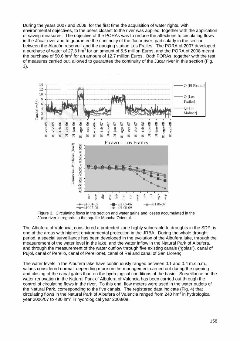
158

During the years 2007 and 2008, for the first time the acquisition of water rights, with environmental objectives, to the users closest to the river was applied, together with the application of saving measures. The objective of the PORAs was to reduce the affections to circulating flows in the Júcar river and to guarantee the continuity of the Júcar river, particularly in the section between the Alarcón reservoir and the gauging station Los Frailes. The PORA of 2007 developed a purchase of water of 27.3 hm3 for an amount of 5.5 million Euros, and the PORA of 2008 meant the purchase of 50.6 hm3 for an amount of 12.7 million Euros. Both PORAs, together with the rest of measures carried out, allowed to guarantee the continuity of the Júcar river in this section (Fig. 3).

Figure 3. Circulating flows in the section and water gains and losses accumulated in the Júcar river in regards to the aquifer Mancha Oriental.

The Albufera of Valencia, considered a protected zone highly vulnerable to droughts in the SDP, is one of the areas with highest environmental protection in the JRBA. During the whole drought period, a special surveillance has been developed in the evolution of the Albufera lake, through the measurement of the water level in the lake, and the water inflow in the Natural Park of Albufera, and through the measurement of the water outflow through five existing canals (“golas”), canal of Pujol, canal of Perelló, canal of Perellonet, canal of Rei and canal of San Llorenç. The water levels in the Albufera lake have continuously ranged between 0.1 and 0.4 m.s.n.m., values considered normal, depending more on the management carried out during the opening and closing of the canal gates than on the hydrological conditions of the basin. Surveillance on the water renovation in the Natural Park of Albufera of Valencia has been carried out through the control of circulating flows in the river. To this end, flow meters were used in the water outlets of the Natural Park, corresponding to the five canals. The registered data indicate (Fig. 4) that circulating flows in the Natural Park of Albufera of Valencia ranged from 240 hm3 in hydrological year 2006/07 to 480 hm3 in hydrological year 2008/09.

159

Figure 4. Level of the Albufera of Valencia lake (m.s.n.m.).

The second important group of applied measures corresponds to management and control measures. The application of the different management measures during the drought period significantly reduced the water releases from the Tous and Loriguilla reservoirs, since they are the last significant reservoirs with regulation capacity in the Júcar and Turia systems. In the Júcar system, water releases from the Tous reservoir went from 600 hm3 in the year 2004/05 to values between 300 and 350 hm3 in the following years, whilst in the Turia system, which entered the drought situation a year later, water releases from the Loriguilla reservoir went from 150 hm3 in the year 2005/06 to values around 80 hm3 (Fig.5).

Figure 5. Accumulated outflow of Júcar system, Tous reservoir (left) and Turia system, Loriguilla reservoir (right).

On the other hand, calculations for previsions of future evolution of water reserves in the reservoirs of the Júcar and Turia systems have been used, as efficiency indicators of the approved measures. The mitigation measures definition, such as: the start-up of drought wells in the Júcar riverside, the reuse of treated waste water in agriculture, the application of important saving efforts, etc., as well as the determination of their start-up and the effectiveness each one of them might have, required the use of different simulation models, with the objective of estimating the future behaviour of water resources systems during droughts, before the different alternatives of management and application of the proposed measures (Fig. 6).

160

Figure 6. Management simulation model in the Júcar system.

The hydrological conditions of the Júcar and Turia basins were analysed quarterly, or monthly in the most critical periods, as well as the status of water reserves in the reservoirs, and from this analysis different future hydrological scenarios, both deterministic and probabilistic, were established. As support during this phase, the model rainfall runoff used in the JRBA for the evaluation of resources was used, as well as the stochastic models of future discharge. From future hydrological scenarios, management simulations with the management models existing in the JRBA were developed for the Júcar and the Turia systems. The results of these simulations allowed the obtaining of the evolution previsions for water reserves in the water resources systems on each hydrological year, which were shown to the Permanent Drought Commission (PDC). The PDC, based on the obtained results, established the target water reserves volume to maintain at the end of each hydrological year, as well as the measures to establish and their degree of application to reach the above-mentioned target volume. This target volume at the end of the year constituted a water reserve for the following months in case the drought intensified (Fig. 7).

Figure 7. Alarcón reservoir with a volume lower than 70 hm3, November 2006 and 2007 (left) and previsional calculation of the Júcar system with and without the application of approved measures by the PDC (right). The third important group of measures were the saving measures implemented both on urban and agricultural uses. The diversions of water for urban supply in the metropolitan area of Valencia were reduced, thanks to efficiency improvement policies, from 126 hm3 at the beginning of the drought, hydrological year 2004/05, to 113 hm3 in the last year of drought, 2007/08, which represents a saving of 11% (Fig. 8). On the other hand, the joint use of resources of the Júcar and Turia, depending on resources availability on each system, also allowed an optimisation of the resources use in both systems.

161

Figure 8. Water diversions of urban use for the metropolitan area of Valencia.

The saving measures initiated by the Irrigators Communities, as well as the opening of the first phase of the modernisation of the Acequia ( irrigation ditch) Real del Júcar, allowed a very important water saving in agriculture, with reductions higher than 50% in diversions of surface water for irrigation in many irrigators communities. One of the most relevant agricultural areas in the JRBA scope, the Júcar riverside in Valencia, significantly reduced irrigation diversions during drought, with reductions higher than 50%. Drought reached the Turia system in the year 2006/07, one year after having started in the Júcar system. Nevertheless, and given the Júcar system’s situation, the agricultural areas of the Turia system initiated some water saving measures during hydrological year 2005/06. One of the main saving measures applied in the Turia system, once it entered the drought situation in 2006/07, was the application of irrigation turns amongst irrigators communities of the traditional irrigations in Turia, called “tandeos”(turns). “Tandeos” consisted in the alternative weekly irrigation between the Real Acequia of Moncada and the irrigation of the Valencia Vega (fertile lowland), maintaining an ecological flow in the river that allowed a significant saving in water use. The Real Acequia of Moncada went from a water use of 90 hm3 in the year 2004/05 to a use of 40 hm3 in hydrological years 2006/07 and 2007/08, which meant a water savings higher than 50% (Figure 9). The irrigation in the Valencia Vega went from using 110 hm3 in hydrological year 2004/05 to an approximate use of 60 hm3 in hydrological years 2006/07 and 2007/08, which meant an approximate water savings of 50%. The fourth and last group of measures consisted in alternative sources and additional resources generation, the most important elements of which were the use of drought wells, re-circulation of water in irrigation ditches (Acequias) through the so-called “re-pumping”, and the reuse of treated waste water in agriculture. The use of 135 drought wells and 25 re-pumping entailed an important control and surveillance effort to minimise the possible impacts they might have on the environment. In this sense, to homogenise the water extractions in the aquifer and avoid negative local effects, the maximum level of extraction allowed for each well was limited, maximum volume of 1 hm3, or a group of wells located in the same area, through the definition of exploitation sectors, maximum volume of 10 hm3. The extracted water volume for irrigation of aquifers through drought wells was 40 hm3 in the irrigation campaigns of 2006 and 2007, and 25 hm3 during the irrigation campaign of 2008 (Figure 10). The re-circulated water volume from re-pumping during drought, to optimise the use of water in irrigation ditches, was 40 hm3 during the irrigation campaign of 2006, 60 hm3 during the campaign of 2007 and 100 hm3 during the campaign of 2008.

162

Figure 9. Irrigation diversions in the Real Acequia of Moncada.

Figure 10. Drought wells and re-pumping in the Júcar riverside (left), extracted volumes from drought wells (right). One of the important elements for additional resources generation consisted in the reuse of treated waste water in agricultural areas of the Valencia Vega (Table 1). The reuse went from 28 hm3 in the hydrological year 2005/06 to 95 hm3 in the year 2007/08. The reuse of treated waste water was developed from the treatment plants of Pinedo II, Quart-Benàger, Carraixet and Paterna – Fuente del Jarro, for irrigators communities of the Real Acequia of Moncada, Acequia of Tormos, Acequia of Rascanya, Acequia of Favara, Acequia del Oro and Acequias of Xirivella, Andarella, Benàger and Faitanar. The development and application of this group of measures required the approval of a set of emergency works for a total amount of 75 million Euros, initiated during the years 2005 (19 million €), 2006 (35 million €), 2007 (15 million €) and 2008 (5 million €). These works were destined to environmental protection, improvement of the guarantee and quantity of water for urban use, improvement of efficiency of water use for agriculture and improvement of infrastructures of water supply.

163

Table 1. Reuse from treatment plans in the different irrigators communities (G for gravity, B through pumping).

EDAR (Waste Water Treatment

Plant) Pinedo II. Extension Quart-

Benatger Carraixet Paterna-Fte. del Jarro

TOTAL

UDA

Traditional Irrigation. Valencia

Vega. Rest of

Acequias

Acequia del Oro

Traditional Irrigation. Valencia

Vega. Rest of

Acequias

Traditional Irrigation. Valencia

Vega. Rest of

Acequias

Traditional Irrigation. Valencia

Vega. Rest of

Acequias

Traditional Irrigation. Valencia

Vega. Ac of

Moncada

User

Acequia of Favara (B)

Acequia del Oro

(G)

Acequias of Andarella

(B), Xirivella (B), Benager (B), Faitanar (B) y Favara

(G)

Acequia of Rascanya

(B)

Acequia of Tormos

(G)

Acequia of

Moncada (B)

(thousand m3)

(thousand m3)

(thousand m3)

(thousand m3)

(thousand m3)

(thousand m3)

(thousand m3)

2005/06 6.014 22.156 - - - - 28.170 2006/07 6.781 50.153 9.008 3.791 603 829 71.165 2007/08 9.946 66.857 12.782 3.444 214 913 94.157 2008/09 4.732 64.082 13.407 3.313 45 850 86.429

Investment

The development and application of this group of measures required the approval of a set of emergency works for a total amount of 75 million euros, initiated during the years 2005 (19 million €), 2006 (35 million €), 2007 (15 million €) and 2008 (5 million €). These works were destined for environmental protection, improvement of the guarantee and quantity of water for urban use, improvement of efficiency of water use for agriculture and improvement of infrastructures of water supply.

Conclusions As a result of the efficacy of proactive and reactive measures, the worst drought in modern times in the Jucar basin, lasting from year 2005 to 2008, passed with relatively low economic and environmental damages; urban supply was always fulfilled; and conflicts among users were solved in an atmosphere of transparency and cooperation promoted by participatory approaches. Some of the measures mentioned to deal with the drought were implemented for the first time in Jucar basin, as for instance: water rights purchases (PORA); voluntary cuttings in groundwater extraction from Mancha Oriental Aquifer; direct treated wastewater reuse by traditional irrigation in lower Turia basin; conjunctive use of surface and groundwater by traditional irrigation in the lower Jucar Basin, with energy expenses paid by users with junior rights; and improved control measures for control of water use and environmental flows. And they proved to be very effective in the mitigation of the drought impacts. Therefore, many of these measures adopted in the campaign plans approved by the Permanent Droughts Commission will become permanent practices, after a convenient remodeling to adapt for ordinary management, and the lessons learned from this experience will help in the production of new versions of the Basin Plan, and of the Special Drought Plan of Jucar basin.

164

References

Andreu, J., Ferrer Polo, J., Pérez, M.A and Solera, A. 2010. Drought planning and management in the Júcar river Basin. International Drought Symposium – Integrating Science and Policy. Andreu, J., Capilla, J. y Sanchis, E. 1996. AQUATOOL: A generalized decision support-system for water-resources planning and operational management. Journal of Hydrology 177, 269-291. CHJ (Júcar Water Agency). 2005. Provisional Art. 5 Report Pursuant to the Water Framework Directive. Confederación Hidrográfica del Júcar, Ministry of Environment, Spain. Estrela, T., Fidalgo, A., and M.A. Pérez. 2006. “Droughts and the European water framework directive: Implications on Spanish river basin disctricts”, in Drought Management and Planning for Water Resources, J. Andreu et alt. (ed.), ISBN 1-56670-672-6, CRC Press (Taylor & Francis), Boca Raton, Chapter six, 169-191, 2006. MARM (Ministerio de Medio Ambiente) 2000. Libro Blanco del Agua en España. Centro de Publicaciones. Madrid, 637.

165

Drought Assessment Using MERIS Images

Alberto Rodríguez Fontal General Directorate of Water Ministry

of the Environment and Rural and Marine Affairs, Madrid, Spain

Abstract

Use of satellite images for drought monitoring purposes provides water managers with valuable information. The National Drought Mitigation Center of the University of Nebraska has been successfully using this methodology in the United States, using MODIS satellite images. In the present work, the methodology developed by the University of Nebraska is adapted to the European background, and it is applied to Spain. Main differences between American satellite MODIS and European satellite MERIS are shown, and a modified index adapted to MERIS satellite images is proposed.

Introduction

The spectral drought index developed by the University of Nebraska, called Normalized Difference Drought Index (NDDI), for the drought assessment from images MODIS (resolution of 1 km), is based on the Normalized Difference Vegetation Index (NDVI) and the Normalized Difference Water Index (NDWI).

Where: RED red, NIR near infrared and SWIR infrared shortwave

Figure 1. Definition of Drought Index (University of Nebraska)

The initial demonstrations of the NDDI potential in drought assessment were developed in the North American grasslands of the region of Flint Hills (Kansas and Oklahoma), where there is one of the vastest extensions of prairie. The conclusion reached was that the NDDI presented a remarkable sensitivity to NDVI-NDWI differences and broader ranges of response during periods of drought than during the rainy season (Gu et al., 2007).

The application of drought index developed by the University of Nebraska in the Spanish territory is initially constrained by the characteristics of the data used in the study, which are images acquired from the MERIS sensor. A comparison of the MODIS and MERIS characteristics is shown in Table 1. Table 1. Comparison of MODIS and MERIS characteristics

VIS NIR SWIR TIR Min Max Min MaxMERIS 12 3 260 1.040 1 3 1.150MODIS 1 1 5 29 250 1.000 1 2 2.330

Sensor Revisit (days)Resolution (m)Number of bands Swath width(Km)

Where: VIS: visible; NIR: near infrared; SWIR: short-wave infrared; TIR: thermal infrared

166

Table 2. MERIS spectral bands MDS Nr. Band centre (nm) Bandwidth (nm) Potential Applications

B1 412,5 10 Yellow substance and detrital pigments

B2 442,5 10 Chlorophyll absorption maximum B3 490 10 Chlorophyll and other pigments B4 510 10 Suspended sediment, red tides B5 560 10 Chlorophyll absorption minimum B6 620 10 Suspended sediment

B7 665 10 Chlorophyll absorption and fluo. reference

B8 681,25 7,5 Chlorophyll fluorescence peak

B9 708,75 10 Fluo. Reference, atmospheric corrections

B10 753,75 7,5 Vegetation, cloud B11 761 3,75 Oxygen absorption R-branch B12 778,75 15 Atmosphere corrections B13 865 20 Vegetation, water vapour reference B14 885 10 Atmosphere corrections B15 900 10 Water vapour, land

Both sensors have bands near the red and infrared wavelengths, and the NDVI derived from images is a product usually obtained from the bands 8 and 13. For the estimation of NDWI, the MERIS images do not have band in the short-wave infrared, so it has been selected as an alternative band, the one around 0.56 μm (band 5) where the absorption of the chlorophyll is minimal and reflectance of maximum water. Therefore, the equations for MERIS images are as follows:

Figure 2. Equations for MERIS images

From the spectral responses of the same vegetation cover with different states of drying (1-10), using USGS spectral signatures2, both drought indices were calculated for MODIS (MO) and MERIS (ME) bands wavelengths.

Figure 3. Spectral response of the vegetation with different degrees of drying

167

Similar results were obtained, as can be seen by comparing the different indices represented at the following graphics:

Figure 4. Indices obtained from the real response to the wavelengths determined by the selected MERIS bands for the Spanish model and MODIS bands used by the University of Nebraska The NDDI drought index uses the NDVI and NDWI as indices of vegetation and moisture content, and is designed for natural areas densely vegetated. Its adaptation to the Spanish territory as the Spanish drought index model (NDDIE), in which the human being has an intensive influence on the natural surface, makes it necessary to leave the low vegetated areas apart from the analysis. To that effect, a mask containing the pixels with positive NDVI and NDWI values is generated after the calculation of both indices, so that the NDDIE is only obtained for the less populated areas. The changes applied to the NDDIE involve giving greater weight to the water and vegetation indices, for the reasons exposed above and because of the huge difference between the weather conditions of both areas of study. This means that the order of the elements in the NDDIE equation must be reversed. Contrary to what happens with the NDDI, the NDDIE increases as the vegetation dryness increases, as can be appreciated in the reversed slope the NDDIE shows in the graphics obtained. The resulting equation of the index is:

Figure 5. Drought index adapted to the Spanish case (NDDIE)

To facilitate the interpretation of the indices, the original values, ranging from -1 to 1, have been reclassified on a positive scale with values of 0 - 100. The following are some examples of the results.

168

Figure 6. Spanish NSDIE during 2008

169

Figure 7. Spanish NSDIE during 2009 and 2010

170

References Gu, Y., J. F. Brown, J. P. Verdin, and B. Wardlow. 2007, A five-year analysis of MODIS NDVI and NDWI for grassland drought assessment over the central Great Plains of the United States, Geophys. Res. Lett., 34. Link: http://drought.unl.edu/pubs/documents/wardlow%20GRL%202007.pdf R. N. Clark, G. A. Swayze, R. Wise, K. E. Livo, T. M. Hoefen, R. F. Kokaly, and S. J. Sutley. 2007, USGS Digital Spectral Library splib06a, U.S. Geological Survey, Data Series 231. Link: http://speclab.cr.usgs.gov/spectral.lib06/

171

Consensus Agricultural Drought Index

172

Agricultural Drought Indices: Summary and Recommendations

Mannava V.K. Sivakumar, World Meteorological Organization, Switzerland Roger Stone, University of Southern Queensland, Australia

Paulo Cesar Sentelhas, University of São Paulo, Brazil Mark Svoboda, University of Nebraska, USA

Philip Omondi, IGAD Climate Prediction and Analysis Centre, Kenya Jayanta Sarkar, India Meteorological Department, India

Brian Wardlow, University of Nebraska, USA

Abstract

Comprehensive drought monitoring that can provide early warnings of drought is a critical component of national drought strategies. Effective drought early warning systems for agriculture should integrate a number of climatic parameters with other relevant parameters such as soil moisture. The Inter-Regional Workshop on Indices and Early Warning Systems for Drought, held at the University of Nebraska–Lincoln in December 2009, stressed the need for undertaking a comprehensive review of all agricultural drought indices documented at the workshop to help identify the prime drought indices for early warning systems most suited for use in the agricultural sector. Hence the WMO/UNISDR Expert Meeting on Agricultural Drought Indices was organized and held June 2-4, 2010, in Murcia, Spain. The meeting reviewed several drought indices currently used around the world for agricultural drought and assessed the capability of these indices to accurately characterize the severity of drought and its impact on agriculture. This chapter summarizes the agricultural drought indices that were discussed at the meeting in seven distinct categories: precipitation-based indices; temperature-based indices; precipitation- and temperature-based indices; indices based on precipitation, temperature, and soil moisture/soil characteristics; indices based on precipitation, temperature, relative humidity, solar radiation, wind speed, and soil moisture/soil characteristics; indices based on remote sensing; and indices based on a composite approach (multiple indicators/indices). A brief review of each of these indices is presented. The meeting recommended that given the enhanced availability of and access to data, tools, and guidance materials, countries around the world should move beyond the use of just rainfall data in the computation of indices for the description of agricultural droughts and their impacts. This issue becomes very relevant, especially in the context of climate change, water scarcity, and food security, and hence it is important to use rainfall, temperature, and soils information.

Introduction

To meet the increasing global demand for cereals to feed the growing populations, the world's farmers will have to produce 40% more grain in 2020. The challenge is to revive agricultural growth at the global level and extend it to those left behind. The causes for the current food crisis are varied, but civil strife and adverse weather predominate. In the developing countries, where adoption of improved technologies is too slow to counteract the adverse effects of varying environmental conditions, climate fluctuations, especially droughts, are indeed the main factors that prevent a regular supply and availability of food, the key to food security.

Drought is an insidious natural hazard that results from a deficiency of precipitation from expected or “normal” that, when extended over a season or longer period of time, is insufficient to meet the demands of human activities and the environment. Drought must be considered a relative, rather than absolute, condition. A critical component of national drought strategies should be a comprehensive drought monitoring system that can provide early warning of drought’s onset and end, determine its severity, and deliver that information to a broad group of users in a timely manner. With this information, the impacts of drought can be reduced or avoided in many cases.

173

Numerous natural indicators of drought should be monitored routinely to determine the onset, ending, and spatial characteristics of drought. Severity must also be evaluated on frequent time steps. Although all types of droughts originate from a deficiency of precipitation, it is insufficient to rely solely on this climate element to assess severity and resultant impacts. Effective drought early warning systems (DEWS) must integrate precipitation and other climatic parameters with water information such as streamflow, snowpack, groundwater levels, reservoir and lake levels, and soil moisture into a comprehensive assessment of current and future drought and water supply conditions. In February 2009, the WMO Commission for Agricultural Meteorology held the International Workshop on Drought and Extreme Temperatures in Beijing, China, to review the increasing frequency and severity of droughts and extreme temperature events around the world. The workshop adopted several recommendations to cope with increasing droughts and extreme temperatures on agriculture, rangelands, and forestry. One of the main recommendations was for WMO to make appropriate arrangements to identify the methods and marshal resources for the development of standards for agricultural drought indices in a timely manner. The Inter-Regional Workshop on Indices and Early Warning Systems for Drought was held at the University of Nebraska–Lincoln December 8-11, 2009. It was jointly sponsored by the School of Natural Resources and the National Drought Mitigation Center of the University of Nebraska–Lincoln, the World Meteorological Organization (WMO), the U.S. National Oceanic and Atmospheric Administration (NOAA), the U.S. Department of Agriculture (USDA), and the United Nations Convention to Combat Desertification (UNCCD). The workshop brought together 54 participants from 22 countries from all the different regions of the world. The workshop reviewed the drought indices currently in use in different regions of the world to explain meteorological, agricultural, and hydrological droughts; assessed the capacity for collecting information on the impacts of drought; reviewed the current and emerging technologies for drought monitoring; and discussed the need for consensus standard indices for describing different types of droughts. The workshop stressed the need for undertaking a comprehensive review of all agricultural and hydrological drought indices documented at this workshop to help identify the prime drought indices for early warning systems most suited for use in the agricultural and water sectors. The workshop recommended that two working groups with representatives from different regions around the world and observers from UN agencies and research institutions (and water resource management agencies for hydrological droughts) be established to further discuss and recommend, by the end of 2010, the most comprehensive indices to characterize the agricultural droughts. Hence the WMO/UNISDR Expert Meeting on Agricultural Drought Indices was organized and held June 2-4, 2010, in Murcia, Spain. Nineteen experts from eight countries participated in the meeting, which was hosted by the Hydrographic Confederation of Segura. The meeting reviewed several drought indices currently used around the world for agricultural drought and assessed the capability of these indices to accurately characterize the severity of drought and its impact on agriculture. The different agricultural drought indices, along with their data needs, are summarized in Table 1.

174

Table 1. Agricultural drought indices currently in use and their data needs.

Agricultural Drought Index

Rainfall Temp. Estimated soil moisture

Vegetation index

Stream flow

Potential evapo-transpiration

Crop coefficient

Soil type

Palmer Drought Severity Index

X X

Deciles X Prescott Ratio Index Hutchinson Index X Plant Growth Index Soil Moisture Anomaly

X X X?

Enhanced Vegetation Index

TCI NDVI Aridity Anomaly Index X X X Two reservoir water balance model

X X

Soil Water Index X X X X scPDSI X X Drought Severity Index

X

Warm-spell duration Index

X

Cold-spell duration Index

X

Simple Daily Intensity Index

X

Relative Soil Moisture X X X X Relative Water Deficit X X X X Accumulated Water Deficiency

X X X X

Accumulated Drought Index

X X X

Crop Moisture Index (CMI)

X X

Days without rainfall X Soil Moisture X SPEI X X CMI-Palmer based X X Crop Specific ET X X Drought Monitor X X X X X X Standardized Precipitation Index (SPI)

X

Percent Normal X Relative Soil Moisture X X X Soil Moisture Anomaly

X X

Cumulative rainfall X VegDRI

175

The indices given in Table 1 above can be grouped into the following types.

Precipitation-based Indices

It is often noted that the simplest indices measure “meteorological drought,” the effects of which can then be measured in terms of agricultural, hydrological, and socioeconomic drought. In this case, drought is normally expressed solely on the basis of the degree of dryness (often in comparison to some “normal” or average amount) and the duration of the dry period. Here, rainfall is the most easily measured meteorological variable, with many records available for more than 100 years in many countries. Additionally, soil moisture that is derived directly from rainfall is commonly the factor that is most limiting to plant growth. It should, however, be noted, that even though the paucity of rain is a main cause of agricultural drought, rainfall data alone may often be insufficient to assess the effect of drought on agricultural productivity. Nevertheless, use of rainfall has considerable value in providing effective summaries of droughts, and, provided the purpose is clearly and precisely defined in terms of activity, location, and timing, rainfall data can greatly assist activities such as drought policy decisions (Heim 2000, 2002; White and Walcott 2009). For rural producers especially, the quantity, intensity, and timing of rain throughout the growing season determine its effectiveness. Therefore, while “simple rainfall-based indices” have considerable value, especially in drought policy decisions, it is also possible for meteorological droughts of apparently equal severity to have differing effects on the productivity of agricultural crops and pastures (e.g., White et al. 1998). In this respect, Heim (2000, 2002) and White and Walcott (2009) provide extensive and worthwhile overviews of commonly applied rainfall-based drought indices. The following is a short summary of such indices. Deciles For countries such as Australia, with especially high interannual rainfall variability, Gibbs and Maher (1967) observed that the occurrence of annual rainfall in the first decile range for the period 1885–1965 corresponded very well with information on drought occurrence (Foley 1957). To aid this appraisal, it is noteworthy that Foley (1957) based “agricultural assessments” on newspaper and other reports of the effects of rainfall in the first decile range on crop yield and livestock numbers. As a consequence, the Australian Bureau of Meteorology now operationally identifies “rainfall deficiencies” rather than defining “droughts,” with a serious rainfall deficiency occurring when the rainfall total over a critical period lies between the 5th and 10th percentile, and a severe rainfall deficiency occurs when the total is below the 5th percentile (White and Walcott 2009). (This approach may also tend to overcome the inherent problems associated with the need for normalized rainfall distributions in the “percent of normal” drought index.) The decile method (Table 2) was selected to describe droughts within the Australian Drought Watch System because of the capability to simply calculate the results, and the method requires less data and fewer assumptions than the Palmer Drought Severity Index (Smith et al. 1993, Hayes 2000). As part of Australian drought policy, growers and producers are advised to only seek exceptional drought assistance if the drought is shown to be an event that occurs only once in 20-25 years (deciles 1 and 2 over a 100-year record) and has lasted longer than 12 months (White and O’Meagher 1995, Hayes 2000).

Table 2. Decile classifications.

Decile numbers Rainfall category Description Deciles 1-2 lowest 20% much below normal Deciles 3-4 next lowest 20% below normal Deciles 5-6 middle 20% near normal Deciles 7-8 next highest 20% above normal Deciles 9-10 highest 20% much above normal

176

Accumulated Rainfall Deficits In an extension of the approach of using rainfall deciles, the duration and severity of drought may also be estimated by summing the rainfall anomalies for each month and graphing this accumulation over time. Although cumulative rainfall deficits may be difficult to directly interpret, they can be useful for highlighting a period of rainfall deficit that has been preceded by a period of above-average rainfall. These systems have also been useful in comparing the duration of current meteorological droughts with preceding droughts in the same location. However, the magnitude and importance of the rainfall deficits are very site-specific. They are therefore of limited value in assessing agricultural droughts. In another example, rainfall for more recent months can be weighted according to the seasonal variation in mean rainfall, but may be of little value for operationally determining exceptional droughts at different locations. For example, enhanced rainfall may be more valuable during periods typified by low vegetative cover than at the peak of the growing season (White 1988). Hutchinson Drought Severity Index (HDSI) Smith et al. (1993) calculated 6-monthly and 12-monthly percentiles on a month-by-month basis as the Hutchinson Drought Severity Index (HDSI), but this index may be too sensitive to minor fluctuations in rainfall to facilitate ranking of droughts. These percentiles may underestimate the durations of declared droughts, possibly because of probable historical anomalies in the declaration process. Standardized Precipitation Index (SPI) The Standardized Precipitation Index (SPI) has been developed utilizing the quantification and hence probability of precipitation for multiple time scales, generally between 1 and 48 months but with potential applicability up to 72 months. (McKee et al. 1993, 1995; Edwards and McKee 1997). A strong foundation in this approach stems from the understanding that a deficit of precipitation has markedly different impacts on groundwater, reservoir storage, soil moisture, snowpack, and streamflow (McKee et al. 1993, Hayes 2000). McKee et al. (1993) further defined a drought event as occurring any time the SPI is “continuously negative” and reaches an intensity of -1.0 or less (Table 3). The drought event ends when the SPI becomes positive. The enhanced value of this approach is that each drought event therefore has a recognized duration defined by its beginning and end, and an intensity for each month that the event continues. Additionally, the accumulated magnitude of drought can also be drought magnitude, and it is the positive sum of the SPI for all the months within a drought event (Hayes 2000). Table 3. Values of Standardized Precipitation Index (SPI) related to moisture conditions. SPI Value Moisture condition +2.0 extremely wet +1.5 to 1.99 very wet +1.0 to 1.49 moderately wet -.99 to .99 near normal -1.0 to -1.49 moderately dry -1.5 to -1.99 severely dry -2.0 and less extremely dry

Hayes (2000) notes that based on an analysis of stations across Colorado, McKee determined that the SPI is in mild drought 24% of the time, in moderate drought 9.2% of the time, in severe drought 4.4% of the time, and in extreme drought 2.3% of the time (McKee et al. 1993). Importantly, the SPI, which is in widespread use, shows evidence of being able to identify emerging droughts sooner than the Palmer Drought Severity Index (PDSI) in regions of the United States. In particular, Hayes et al. (1999) and Hayes (2000) report that the SPI is now widely

177

applied in the United States, especially by water resource managers, to provide an early warning of drought and assist in the assessment of drought severity. The SPI is considered simpler to use than the PDSI, although White and Walcott (2009) note that yearly averages of both may be placed into a frequency distribution for comparative purposes (Goodrich and Ellis 2006). Additionally, the SPI may be especially useful for application in developing countries because of its limited data requirements and relative simplicity of calculation. As with many other rainfall-only indices, the SPI is more suited to monitoring meteorological and hydrological droughts than agricultural droughts. Nevertheless, its flexibility in selecting time periods that correspond with growing seasons, or any particular season of interest, does give it additional utility to inform on aspects of agricultural drought. Effective Drought Index (EDI) Rainfall data may be used as a benchmark indicator for providing drought relief assistance. Byun and Wilhite (1999) developed the Effective Drought Index (EDI) as a function of the precipitation needed for a return to normal conditions (PRN), or the recovery from the accumulated rainfall deficit since the beginning of a drought. Morid et al. (2006) found the EDI to be especially responsive to emerging drought conditions in the studies he conducted in Iran, compared with the Decile Index of Gibbs and Maher (1967) and the SPI. The value in practical application of “simple” meteorological drought indices has been recognized in the development of software that automatically generates the EDI and SPI (Smakhtin and Hughes 2007). Percent of Normal This approach (McKee et al. 1993) has value in its simplicity and transparency, especially because all sectors tend to “know what it means,” and it is noteworthy that this approach has strong support in countries such as Indonesia. A downside of this approach is that it does not necessarily detect the extremes in drought conditions, and this can be a problem in very arid areas. This approach also requires a good knowledge of local conditions to make it useful. Hayes (2000) suggests analyses using percent of normal are most effective when used for a single region or a single season. Conversely, percent of normal may be misunderstood and provide different indications of conditions, depending on the location and season. It is calculated by simply dividing actual precipitation by normal (30-year mean) precipitation and multiplying the result by 100%. This approach can be calculated for a variety of time scales, which generally range from a single month to a group of months representing a particular season, up to a year. Hayes (2000) points out that one of the disadvantages of using the percent of normal precipitation is that the mean, or average, precipitation may differ considerably from the median precipitation (which is the value exceeded by 50% of the precipitation occurrences in a long-term climate record) in many world regions, especially those with high year-to-year rainfall variability. Thus, use of the percent of normal comparison requires a normal distribution in rainfall, where the mean and median are considered to be the same. Days without Rainfall Early in the 20th century, the U.S. Weather Bureau applied “days without rainfall” in an attempt to better identify and quantify drought. In this instance, drought was defined as occurring during any period of 21 or more days with rainfall 30% or more below normal for the period (Henry 1906, Steila 1987). An extension of this approach was through the associated “accumulated precipitation deficit” (see above in this section) or the “accumulated departure from normal.” Heim (2002) provides other examples of these early criteria: 1) 15 consecutive days with no rain, 2) 21 days or more with precipitation less than one-third of normal, 3) annual precipitation that is less than 75% of normal, 4) monthly precipitation that is less than 60% of normal, and 5) any amount of rainfall less than 85% of normal.

178

Heim (2002) notes that as recently as 1957, annual rainfall amount was used as a drought index in a study of drought in Texas. Similar criteria have been employed in other countries: 1) Britain: 15 consecutive days with less than 0.25 mm (0.01 in.); 2) India: rainfall half of normal or less for a week, or actual seasonal rainfall deficient by more than

twice the mean deviation; 3) Russia: 10 days with total rainfall not exceeding 5 mm (0.20 in.); 4) Bali: a period of 6 days without rain; 5) Libya: annual rainfall less than 180 mm (7 in.). Heim (2002) notes that most of these indices were developed and thus valid only for their specific application in their specific region and makes the point that indices developed for one region may not be applicable in other regions because the meteorological conditions that result in drought are highly variable around the world. Putting Precipitation-based Indices in Context Although the practical and functional aspects of the (sole) use of meteorological drought indices are now well recognized, it is also known that for agricultural application purposes, the quantity and timing of rain events throughout a growing season largely determines the value of such indices in agricultural production assessments. Meteorological drought indices can be normalized by using appropriate seasonal indices. However, indices based solely on rainfall data do not, by definition, take into account other factors such as ambient temperature, relative or absolute humidity, mean and extreme wind speed, net radiation, evapotranspiration, deep percolation, runoff, soil type, or the agricultural enterprise (White and Walcott 2009). Because the length of a growing season can vary between years depending on when rainfall occurs, tailoring indices to growing seasons to better assess whether drought conditions are affecting crops and pastures may remain a difficult task and negate the value of sole use of meteorological indices in drought assessment. White et al. (1998) and White (2000) note that other important meteorological factors besides rainfall can greatly influence plant growth in a country such as Australia in ways not necessarily foreseen, and so a second step is often recommended in drought assessments besides the sole use of a meteorological drought index. Modification of drought indices, including just slight modification to indices such as the SPI, can provide improved practical application in certain regions (Ntale and Gan 2003). In particular, in a comparison of the PDSI, BMDI, and SPI in different regions of East Africa, the SPI was rated superior to the other indices tested and greatly superior to the PDSI through utilization of this modification approach. Of the seven drought indices assessed in Iran by Morid et al. (2006), the meteorological drought index (the Deciles Index [DI]) (Gibbs and Maher 1967) was rated as “oversensitive,” leading to unrealistically high temporal and spatial variations in wet conditions, especially in summer. However, importantly, the authors noted that this sensitivity could be reduced by using temporal scales larger than 1 month. Additionally, the importance of using long-term precipitation records for drought analyses has been highlighted by Morid at al. (2006), who note that despite utilizing different underlying statistical distributions, the SPI and the China-Z index (CZI) performed similarly in their ability to detect and monitor drought. Interestingly, when a whole range of drought indices have been ranked according to robustness, tractability, transparency, sophistication, extendability, and dimensionality, the overall superior drought indices often emerge as those being simply based on rainfall data inputs and otherwise most relevant to meteorological drought assessment (Keyantash and Dracup 2002). In a study for Oregon (USA), Keyantash and Dracup (2002) found, when making an overall assessment, that the superior drought indices were rainfall deciles, total water deficit, and computed soil moisture, while the SPI also emerged as a highly valuable estimator of drought severity. Simulation studies (e.g., Donnelly et al. 1998, Stafford Smith and McKeon 1998, White et al.1998) have demonstrated that, indeed, grassland and agricultural droughts often coincide with

179

meteorological droughts, as illustrated by rainfall deficits. However, the severity and duration of grassland and agricultural droughts in a country such as Australia can vary according to the timing and distribution of the rainfall events. Thus, they point out, a minor rainfall deficiency can sometimes have major consequences in terms of agricultural production, whereas a moderate rainfall deficiency may not always seriously reduce crop and pasture growth. Such additional models are often invaluable in drought assessment.

Temperature-based Indices Changes in extreme weather and climate events have significant impacts and are among the most serious challenges to society in coping with a changing climate (CCSP 2008). Confidence has increased that some extremes will become more frequent, more widespread, and/or more intense during the 21st century (IPCC 2007). The sustainability of economic development and living conditions depends on our ability to analyze and hence manage the risks associated with extreme events. The creation of an efficient early warning system for climate anomalies and related extremes has been a focus of WMO and the National Meteorological and Hydrological Services (NMHSs) for more than a decade in order to improve climate risk management capabilities among nations (Zhai 2005). Cold-spell and warm-spell duration indices allow straightforward monitoring of trends in the frequency or intensity of events, which, while not particularly extreme, would nevertheless be stressful. These analyses average 10th and 90th percentile values of daily temperatures in order to predict extreme cold-warm spells risk. The motivation for analyzing extremes is often to find an optimum balance between adopting high safety standards that are very costly on the one hand, and preventing major damage to equipment and structures from extreme events that are likely to occur during the useful life of such infrastructure on the other hand (WMO 1983). The joint World Meteorological Organization Commission for Climatology (CCl)/World Climate Research Programme (WCRP) project on climate variability and predictability (CLIVAR) Expert Team on Climate Change Detection, Monitoring and Indices (ETCCDMI) have made an effort to develop these cold spell/warm spell indices as core climate extreme indices. Long-term extreme temperature change assessment is conducted by inspecting changes in percentile-based temperature indices that describe the percentage number of “extreme cold” days and nights (TN10p and TX10p) and “extreme warm” days and nights (TX90p and TN90p), in addition to other important temperature indices. One of the key approaches of the indices concept involves calculation of the number of days in a year exceeding specific thresholds. Examples of such “day-count” indices are number of days with minimum temperature below the long-term 10th percentile in the 1961-1990 base period. A threshold is calculated if at least 70% of data are present (Stott et al. 2010, Klein Tank et al. 2009). Day-count indices based on percentile thresholds are expressions of anomalies relative to the local climate. These anomalies have fixed rarity—i.e., the thresholds are chosen so as to be exceeded at a fixed frequency, often 10%, during the base period that is used to define the thresholds. Consequently, the values of the thresholds are site-specific. Such indices allow for spatial comparisons because they sample the same part of the probability distribution of temperature at each location. Cold spell duration indicator (CSDI) is defined as annual count of days with at least six consecutive days when minimum temperature is less than the 10th percentile in the 1961-1990 base period. The index for cold nights pTN10 is calculated based on the daily series of minimum temperature TN at any given station following ETCCDI definitions as the number of cold nights, as follows:

pTN10 , cold nights: count of days where 10thTN < percentile

Let TN ijbe the daily minimum temperature on day i in period j and let 10TN in be the calendar

day 10th percentile of daily minimum temperature calculated for a five-day window centered on

180

each calendar day in the base period n (1961-1990). Count the number of days where

TN ij< 10TN in .

pTN90 , warm nights: count of days where 90thTN > percentile

Let TN ijbe the daily minimum temperature on day i in period j and let 90TN in be the calendar

day 90th percentile of daily minimum temperature calculated for a five-day window centered on each calendar day in the base period n (1961-1990). Count the number of days where

TN ij> 90TN in .

Cold Spell Duration Index (CSDI): count of days in a span of at least six days where 10thTN > percentile. Let TN ij

be the daily minimum temperature on day i in period j and let 10TN in be the calendar

day 10th percentile of daily minimum temperature calculated for a five-day window centered on each calendar day in the base period n (1961-1990). Count the number of days where, in intervals of at least six consecutive days, TN ij

< 10TN in .

The indices for cold day-times pTX10 and warm day-times pTX 90 are calculated based on the daily series of maximum temperature TX at any given station following ETCCDI definitions as the number of cold and warm days, as follows:

pTX10 , cold day-times: count of days where 10thTX < percentile

Let TX ij be the daily maximum temperature on day i in period j and let 10TX in be the calendar day 10th percentile of daily maximum temperature calculated for a five-day window centered on each calendar day in the base period n (1961-1990). Count the number of days where

TX ij < 10TX in .

pTX 90 , warm day-times: count of days where 90thTX > percentile

Let TX ij be the daily maximum temperature on day i in period j and let 90TX in be the calendar day 90th percentile of daily maximum temperature calculated for a five-day window centered on each calendar day in the base period n (1961-1990). Count the number of days where

TX ij > 90TX in . The warm spell duration indicator (WSDI) is defined as annual count of days with at least six consecutive days when maximum temperature is greater than the 90th percentile. The percentile thresholds are calculated from the five–day windows centered on each calendar day to count for the mean annual cycle. Warm Spell Duration Index (WSDI): count of days in a span of at least six days where

90thTX > percentile. Let TX ij be the daily maximum temperature on day i in period j and let 90TX in be the calendar day 90th percentile of daily maximum temperature calculated for a five-day window centered on each calendar day in the base period n (1961-1990). Count the number of days where, in intervals of at least six consecutive days, TX ij > 90TX in .

181

Trends in the indices of cold nights TN10p and warm days TX90p are relevant for comparing changes in heating and cooling demands. Indices such as TN10p and TX90p are calculated relative to an annual cycle of thresholds. In order to have heating and cooling load interpretations, these indices have to be accumulated over winter and summer seasons, respectively, rather than over the entire year.

Precipitation- and Temperature-based Indices

The precipitation- and temperature-based drought indices are those calculated using information provided by water balance (WB) models. Among the several WB models, the one most commonly used for characterizing droughts is proposed by Thornthwaite and Mather (1955), which is simple to apply and easy to understand. The indices listed below are based on this methodology. Palmer Drought Severity Index (PDSI) The Palmer Drought Severity Index (PDSI) is widely used to characterize droughts. PDSI is a drought index that involves aspects related to duration, magnitude, and severity of a drought, and also includes information on the onset and termination of a drought event. The PDSI is based on the water balance equation over an area of concern (Palmer 1965). Calculating PDSI requires data on precipitation, temperature (for potential evapotranspiration estimation), soil moisture, and the previous PDSI value. Although precipitation and temperature time series data are easily available for most locations, this is not the case with soil moisture. Soil moisture data have been calibrated to the homogeneous climate zones. The PDSI has an inherent time scale of approximately 9 months and treats all forms of precipitation as rain. The PDSI has been widely used to trigger agricultural drought and can also be used to identify the abnormality of droughts in a region and show the historical aspects of current conditions. The main limitations of this drought index are that it may lag in the detection of drought over several months because the data depend on soil moisture and its properties, which have been simplified to one value in each climate division. It will not present accurate results during the winter and spring when the effects of frozen ground and snow are still present. PDSI also tends to underestimate runoff conditions. As described by Wells et al. (2004), the PDSI is calculated according to the following steps: Each month of every year, eight values related to the soil moisture are computed along with their complementary potential values. These eight values are evapotranspiration (ET), recharge (R), runoff (RO), loss (L), potential evapotranspiration (PE), potential recharge (PR), potential runoff (PRO), and potential loss (PL). The potential evapotranspiration is estimated using Thornthwaite’s method (Thornthwaite 1948). The calculation of these values depends heavily on the available water-holding capacity (AWC) of the soil. The PDSI itself depends on a two-stage ‘‘bucket’’ model of the soil. The top layer of soil is assumed to hold one inch of moisture. The amount of moisture that can be held by the rest of the underlying soil is a location-dependent value, which must be provided as an input parameter to the program. The four potential values are weighted according to the climate of the area using α, β, γ, and δ to give the climatically appropriate for existing conditions (CAFEC) potential values. The weighting factors are called the water-balance coefficients. The CAFEC potential values are combined to form the CAFEC precipitation, P, which represents the amount of precipitation needed to maintain a normal soil moisture level for a single month. The difference between the actual precipitation that fell in a specific month and the computed CAFEC precipitation is the moisture departure, d. The moisture departure, d, is the excess or shortage of precipitation compared to the CAFEC precipitation. Of course, the same d will mean different things at different times, as well as at different locations. This prevents straightforward comparisons from being made between different values of d. To correct for this, the moisture departure is weighted using K, which is called the climatic characteristic. Here K is actually a refinement of K’, which is Palmer’s general approximation for the climate characteristic of a location. Palmer derived equations for K’ and for K, as a function of average moisture departure for the appropriate month, D.

182

The purpose of the climatic characteristic, K, is to adjust the value of d according to the characteristics of the climate in such a way as to allow for accurate comparisons of PDSI values over time and space. The result of multiplying the moisture departure, d, by K is called the moisture anomaly index, or the Z Index. The Z index can be used to show how wet or dry it was during a single month without regard to recent precipitation trends. The Z index is used to calculate the PDSI value for a given month using the general formula: Xi = 0.897 Xi-1 + 1/3 Zi Palmer called the values 0.897 and 1/3 the duration factors. They were empirically derived by Palmer from two locations (western Kansas and central Iowa) and affect the sensitivity of the index to precipitation events. Three PDSI values are actually computed each month: X1, X2, and X3. The values of X1 and X2 are the severity of a wet or dry spell, respectively, that might become established. A spell becomes established when it reaches the threshold of ±0.5. This threshold follows from the fact that index values between -0.5 and 0.5 are regarded as ‘‘normal’’ values; X3 is the severity of a wet or dry spell that is currently established. If no spell is established, the PDSI value is set to either X1 or X2, according to which spell is most likely to become established. This is determined by which index is closer to the threshold of an established spell, which is simply the index with a larger absolute value. If a current spell is established (i.e., when X3 is not zero), the PDSI value for that month is X3. However, when the index is calculated at a later date, it may be discovered that the current spell actually ended earlier. In this case, the PDSI values will be replaced by values of either X1 or X2. This replacement of previously calculated PDSI values will be referred to as backtracking. The existence of backtracking means that a small change in how the indices are computed may cause backtracking, which has a substantial effect on the final values of the index. Self-Calibrated Palmer Drought Severity Index (sc-PDSI) The scPDSI is a variant of the original PDSI of Palmer (1965), with the aim of making results from different climate regimes more comparable (Wells et al. 2004). As described by Wells et al., the scPDSI is calculated from a time series of precipitation and temperature, together with a set of calibrated empirical constants. The process of replacing all empirical constants in Palmer’s procedure for calculating the sc-PDSI results in a process that is slightly more complicated than before. The steps required to calculate scPDSI include the following:

1) Calculate all moisture departures. 2) Calculate all moisture anomalies. 3) Calculate the duration factors, using the moisture anomalies computed in step 2. 4) Calculate the PDSI using the moisture anomalies and duration factors computed in steps 2 and

3, respectively. 5) Find the 98th and 2d percentile values of the PDSI. 6) Compute the new moisture anomalies. 7) Calculate the SC-PDSI. This is a more computationally intensive process than Palmer’s original procedure. However, the power of the current generation of computers means that the PDSI can be calculated in a matter of seconds, even for stations with more than a hundred years of data. Using the redefined climatic characteristics and a set of duration factors derived in the described manner to calculate the PDSI has several positive consequences:

• The range of the PDSI values is close to an expected range of 25.0 to 5.0, where values below 24 and above 4 represent extreme conditions.

• The sensitivity of the index is based upon the local climate. • Different sensitivity to moisture and lack of moisture. • The PDSI can be updated at different time intervals (e.g., weekly, biweekly, monthly).

183

The consequences of dynamically calculating the climatic characteristics and duration factors have the overall effect of calibrating the index based on the actual characteristics of a given location. This means the conditions of any climate should be realistically represented by the index within the definition of the PDSI. In other words, the index should show an extreme drought only when the conditions exemplify an extreme drought relative to that area and not relative to some default location. Thus, the sc-PDSI will allow more accurate comparisons between different locations and times. The sc-PDSI will also give more statistically accurate results by showing severe and extreme readings less frequently than the current implementations of the PDSI, which often show extreme readings with a frequency much higher than one would expect. Standardized Precipitation Evapotranspiration Index (SPEI) According to Vicente-Serrano (2010), the SPEI is very easy to calculate, and it is based on the original SPI calculation procedure. The SPI is calculated using monthly (or weekly) precipitation as the input data. The SPEI uses the monthly (or weekly) difference between precipitation and PET. This represents a simple climatic water balance (Thornthwaite 1948) that is calculated at different time scales to obtain the SPEI. The first step, the calculation of the PET, is difficult because of the involvement of numerous parameters. Different methods have been proposed to indirectly estimate the PET from meteorological parameters measured at weather stations. According to data availability, such methods include physically based methods and models based on empirical relationships, where PET is calculated with fewer data requirements. Although some methods in general provide better results than others for PET quantification, the purpose of including PET in the drought index calculation is to obtain a relative temporal estimation, and therefore the method used to calculate the PET is not critical. Mavromatis (2007) recently showed that the use of simple or complex methods to calculate the PET provides similar results when a drought index, such as the PDSI, is calculated. With a value for PET, the difference (Di) between the precipitation P and PET for the month i is calculated, which provides a simple measure of the water surplus or deficit for the analyzed month. This approach has some shortcomings: the parameter is not defined when PET = 0 (which is common in many regions of the world during winter), and the P/PET quotient reduces dramatically the range of variability and deemphasizes the role of temperature in droughts. The calculated Di values are aggregated at different time scales, following the same procedure as that for the SPI. The difference Di in a given month and year depends on the chosen time scale. For calculation of the SPI at different time scales, a probability distribution of the gamma family is used (the two-parameter gamma or three-parameter Pearson III distributions), because the frequencies of precipitation accumulated at different time scales are well modeled using these statistical distributions. Although the SPI can be calculated using a two-parameter distribution, such as the gamma distribution, a three-parameter distribution is needed to calculate the SPEI. The SPEI fulfills the requirements of a drought index since its multi-scalar character enables it to be used by different scientific disciplines to detect, monitor, and analyze droughts. Like the sc-PDSI and the SPI, the SPEI can measure drought severity according to its intensity and duration, and can identify the onset and end of drought episodes. The SPEI allows comparison of drought severity through time and space, since it can be calculated over a wide range of climates, as can the SPI. Drought indices must be statistically robust and easily calculated, and have a clear and comprehensible calculation procedure. All these requirements are met by the SPEI. Crop Moisture Index (CMI) CMI uses meteorological indices to monitor week-to-week crop conditions. Whereas the Palmer Drought Severity Index monitors long-term meteorological wet and dry spells, the CMI was specifically designed to evaluate short-term moisture conditions, but across major crop-producing regions. Hayes (2000) notes that the “CMI is based on the mean temperature and total precipitation for each week within a Climate Division, as well as the CMI value from the previous week.” Thus, the CMI responds rapidly to changing conditions, and it is weighted by location and time so that maps, which commonly display the weekly CMI across the United States, can be used

184

to compare moisture conditions at different locations (Hayes 2000). Thompson and Wehmanen (1979) utilized remote-sensing data (Green Number Index) for growth stages for wheat with segments classified as drought or non-drought. A high degree of agreement was found between the 18-day remote sensing data and the ground-based Crop Moisture Index. Similar close results were obtained in parts of the (then) USSR and Australia.

Indices Based on Precipitation, Temperature, Soil Moisture/Soil Characteristics

As compared to the precipitation- and temperature-based drought indices, the precipitation, temperature, and soil moisture based indices are generally those calculated and derived using information provided by water balance (WB) models. However, in this case, the WB information can be provided by different methodologies. These can range from the very simplistic models, such as those addressing the precipitation (P) and potential evapotranspiration (PET) relationship, to the very complex models, such as those proposed by Ritchie (1998) and Gevaerd and Freitas (2006). These varied approaches are critical both conceptually and operationally in tracking agricultural drought, which is dependent on what is occurring in terms of moisture in the plant/tree rooting zones throughout the growing season. Attempting to depict and understand this water balance approach through various indices will allow one to better understand how crops or the environment may be reacting or stressing during times of drought and at various stages of plant/crop development. This, in turn, can help us better determine how growth or yield may be influenced by drought during the growing season and throughout critical off-season recharge periods. Some examples are shown below. Relative Soil Moisture (RSM) Soil moisture (SM) or soil water storage (SWS) is an output of the water balance. This variable can be obtained by different WB methods, such as those proposed by Thornthwaite and Mather (1955), Molinas and Andrade (1993), Allen et al. (1998), Ritchie (1998), and Gevaerd and Freitas (2006). Each kind of WB method will require specific inputs, but basically they require climate (rainfall and potential evapotranspiration), soil (physical properties), and plant (crop type, leaf area, crop sensitivity to water stress, crop water requirement for each phenological phase, and management practices) information, depending on their complexity. The RSM index is the relationship between SWS and soil water holding capacity (SWHC). The results are given in percentage. Relative Water Deficit (RWD) This index is obtained by calculating the relative difference between actual (ETa) and potential (ETP) evapotranspiration: RWDI = (1 – AET / PET) 100 where AET is the actual evapotranspiration, an output of Thornthwaite and Mather’s climatological water balance, considering the SWHC of the respective soil type for the region, ranging from 50 to 150 mm for a 1-m soil profile, and PET is the potential evapotranspiration, calculated by physical or empirical methods. This index is non-accumulative and is calculated by the total AET and PET for the period considered. Accumulated Water Deficiency (AWD) Water deficiency is an output of the climatological water balance, as determined by Thornthwaite and Mather’s WB model. The water deficit (WD) is the difference between potential (PET) and actual (AET) evapotranspiration. The WD magnitude for a given condition will depend on the soil water holding capacity adopted for the WB. When water deficiency is accumulated during the growing season, this index will have a definite correlation with crop yield losses. Accumulated Drought Index (ADI) This drought index has as inputs rainfall (P) and potential evapotranspiration (PET). Its calculation is based on the relationship between these two variables (Table 4), and the drought classification follows the categories of the accumulated index (Table 5). ADI is calculated as:

185

ADI = ∑ DI / (3 n N) where DI is determined for each period by the P and ETP relationship presented in Table 4; n is the number of periods considered; and N is the number of periods without rain above 10 mm (NDWR>10). For N = 0, ADI is calculated by: ADI = ∑ DI / (3 n) Table 4. P and PET relationship for determination of the drought index (DI).

P & ETP Relationship Classification DI P ≥ 2 ETP Wet 5 ETP ≤ P < 2 ETP Lightly wet 4 ½ ETP ≤ P < ETP Normal 3 0 < P ≤ ½ ETP Lightly dry 2 P = 0 Dry 1

Source: CIIAGRO/IAC/Brazil Table 5. Accumulated Drought Index (ADI) and drought classification.

ADI Classes Classification ADI ≥ 1.50 Extremely wet 0.80 ≤ ADI < 1.50 Very wet 0.40 ≤ ADI < 0.80 Wet 0.20 ≤ ADI < 0.40 Normal 0.04 ≤ ADI < 0.2 Dry ADI < 0.04 Very dry

Source: CIIAGRO/IAC/Brazil

Indices based on Precipitation, Temperature, Relative Humidity, Solar Radiation, Wind Speed, and Soil Moisture/Soil Characteristics

Indices that are based on soil water content estimation and numerous input parameters (rainfall, temperature, relative humidity, solar radiation, wind speed, soil moisture or soil characteristics) allow evapotranspiration estimation with the Penman approach or Penman-Monteith equation. This approach is more accurate and is consistent with WMO recommendations. It is worth underlining the role evapotranspiration plays in crop development and therefore also in the definition of a drought. Hence it is important to define this evapotranspiration term as overall water loss through evaporation from soil and transpiration from plants. The potential evapotranspiration depends on the meteorological factors listed above and follows the hypothesis that there is enough water in the soil for vegetation at any time. The difference between the actual and potential evapotranspiration depends on soil moisture. In this approach, both crop and soil water supply and demand are fully taken into consideration, which holds the key for more complex crop modeling. However, this places greater demand on data needs, as the complexity of drought indices usually depends on the number of parameters taken into account. Data availability at station level can be an issue, and different water balance models are usually location-specific and require local calibration, which makes inter-comparison difficult. An overview of the diversity of drought indices based on rainfall, temperature, relative humidity, solar radiation, wind speed, soil moisture, and/or soil characteristics is given in Table 6.

186

Table 6. Overview of different drought indices based on multiple parameters. Drought Index Producer Input data Aridity Anomaly Index (AAI)

India Meteorological Department, India

Rainfall, PET, field capacity (soil)

Water balance with two reservoirs

Météo-France, France Rainfall and daily Penman-Monteith PET

Soil Water Index Météo-France, France Rainfall, temperature, relative humidity, solar radiation, wind speed, soil characteristics, and vegetation type

Soil Moisture Anomaly USA Relative Soil Moisture USA

Aridity Anomaly Index (AAI) This index is one of the tools used to monitor agricultural drought. A few scientists (Appa Rao et al. 1981, George and Ramasastry 1975, and, more recently, Sarkar 2001) have used this index to analyze agricultural drought scenarios in India. The methodology for calculating this index based on aridity anomaly is described by Sarkar (Chapter 5 in this volume). According to Sarkar (Chapter 5), when the anomaly is worked out for a large network of stations for different weeks, plotted, and analyzed, it is possible to identify areas where the crop might be suffering from moisture stress of various degrees. Using this technique, the India Meteorological Department has been monitoring agricultural drought during both the rainy (commonly referred to as kharif) and post-rainy (rabi) seasons using a wide network of stations. This is done on a real-time basis every week and every fortnight during the two crop seasons, and the information is supplied to various users. The aridity anomaly maps are also uploaded onto the departmental website (www.imd.gov.in). This index helps to assess the moisture stress experienced by growing plants. Water Balance Index with Two Reservoirs This index is based on a simplified operational water balance with two reservoirs and a fixed soil depth. This index is applied for standardized fescue grass vegetation. To take soil variability into account, four soil types are considered for the available water. As a consequence, four hypothesis are made for soil moisture storage capacity estimation (50, 100, 150, and 200 mm). Further details are presented by Cloppet (Chapter 8 in this volume). Soil Water Index The Soil Water Index is extracted from the SAFRAN ISBA MODCOU hydrometeorological model, which is used to provide consistent computation of variables within the hydrological cycle. Full details regarding the computation of this index are presented by Cloppet (Chapter 8). Soil Moisture Anomaly and Relative Soil Moisture Index The relative soil moisture approach is based on water balance, PET estimation, and climatology in order to estimate a climatological reference. Relative soil moisture indices are designed to measure and simulate how much water is available in soil for crops. It should be noted that indices based only on precipitation cannot reflect water consumption and water demand of crops. Although these indices are easy to apply, easy to understand, and do not require much computational power, they have certain limitations. These indices are vulnerable to the method of PET computation, because PET or ET estimated by different methods are not comparable. For example, the original Thornthwaite method underestimates PET for Brazil, but it is the main method used, since it requires only average temperature as input. Soil water holding capacity estimation is also complex at the national scale.

187

In China, relative soil moisture is defined by the Chinese Meteorological Administration (CMA) as

where Rw is relative soil moisture,W is percent soil moisture, and fc is field capacity. Relative soil moisture indices are very sensitive to crop type and crop management at different crop phases.

Soil moisture anomaly estimation is highly relevant for vegetative health and agricultural drought monitoring. However, limited observations of soil moisture mean that operationally this method may not always be practical. In Australia, monitoring soil moisture and plant available water holding capacity is important, but it is done on a regional/state scale rather than on a national scale—except for use in assessing national crop yields. In Europe, the current soil moisture map is modeled at the European level within the EFAS system and can be compared to the long-term daily average of soil moisture at each location, resulting in a normalized soil moisture product that allows for the evaluation of the current situation as compared to a climatological average. Two long-term meteorological datasets have been applied to simulate a pseudo-climatology of soil moisture for Europe:

• measured meteorological data from JRC-MARS that are received from the Global Telecommunication System of WMO and made available through MARS-STAT activity of IPSC-JRC. The original daily meteorological point data are spatially interpolated for the period 1990–2006 (i.e., a period of 17 years).

• Re-analysis data of the European Centre for Medium-Range Weather Forecasts (ERA-40) for the period 1958–2001 (i.e., 44 years) that provide a consistent set of forecasted meteorological parameters.

Indices Based on Remote Sensing

Satellite-based vegetation indices (VIs) have been widely used over the past 20+ years to map and monitor agricultural conditions and drought (Tucker et al. 1991, Kogan 1990). VIs are mathematical transformations of data from two or more spectral bands that are designed to be indicators of the general state and health of vegetation while minimizing the influence of non-vegetation-related factors such as atmospheric conditions (water vapor and aerosols), soil background, and varying sensor view and solar illumination angles over time. Global imagers such as NOAA’s Advanced Very High Resolution Radiometer (AVHRR) and the more recent Moderate Resolution Imaging Spectroradiometer (MODIS) from the National Aeronautics and Space Administration (NASA) and the Medium Resolution Imaging Spectrometer (MERIS) from the European Space Agency (ESA) have provided a time series of multi-spectral imagery appropriate for the derivation of several VIs in support of agricultural drought monitoring at national, regional, and global scales. These instruments collect spatially continuous spectral measurements of the earth’s land surface on a near-daily basis in several spectral regions that can be used to generate various VIs that have been developed. A number of VIs are available, and the theoretical underpinnings of each index are based on the fundamental understanding of how electromagnetic radiation in different spectral regions interacts with vegetation (i.e., absorption or reflection) and the specific biophysical characteristic(s) of plants that control the spectral response in each region. Most early VIs utilized data from the visible red and near-infrared (NIR) spectral regions that are responsive to changes in chlorophyll content and internal leaf structure, respectively. As VIs evolved and new remote sensing instruments with additional spectral bands were launched, new VIs were developed using shortwave (or middle) infrared (SWIR) and thermal data that are sensitive to plant water content and evapotranspiration (ET), respectively. Although many VIs have been developed, only a few are commonly used for operational agricultural drought monitoring, and these will be briefly summarized below. These VIs

188

have been adopted because of the availability of the required spectral data from instruments such as AVHRR and MODIS, which are easily accessible and available for most parts of the world, and their demonstrated utility for monitoring vegetation conditions. Normalized Difference Vegetation Index (NDVI) The Normalized Difference Vegetation Index (NDVI) (Rouse et al. 1974) has been the most widely used VI for agricultural drought monitoring over the past 20+ years. The NDVI is calculated from the following equation:

NDVI = (NIR – Red) / (NIR + Red) where Red and NIR correspond to the visible red and NIR bands, respectively. The NDVI calculation capitalizes on the differential response of the visible red (decreasing reflectance due to chlorophyll absorption) and NIR (increasing reflectance from the spongy mesophyll layer) wavelength regions to healthy green vegetation. Theoretically, NDVI values can range from -1.0 to +1.0, but globally most observed NDVI values range from near 0.0 for bare surfaces to approximately 0.9 for densely vegetated locations. The value of NDVI for vegetation monitoring has been well established, as it has been found to have a strong relationship with biophysical vegetation parameters such as green biomass and leaf area index (LAI) (Asrar et al. 1989, Baret and Guyot 1991), as well as precipitation and ET (Ji and Peters 2003). Most satellite-based remote sensing instruments designed for terrestrial applications include red and NIR bands, which makes the NDVI calculations easy to apply to data from various instruments. In addition, the normalization in the NDVI calculation minimizes some inter-observation variations such as varying illumination and viewing angles and atmospheric conditions producing equivalent index values over time, which is required for time series analysis and operational monitoring. One of the first studies to demonstrate the value of NDVI for agricultural drought monitoring was Tucker et al. (1991), who applied time-series AVHRR NDVI observations to characterize the early 1980s drought across the African Sahel region. Operationally, NDVI has become one of the most commonly used indices for agricultural drought monitoring throughout the world. Programs such as the Famine and Early Warning System (FEWS), U.S. Department of Agriculture (USDA) Foreign Agricultural Service (FAS), and European Drought Observatory (EDO), and individual countries such as Australia and the United States use the NDVI as a staple for their respective drought monitoring activities. The majority of these efforts generate NDVI anomaly products (e.g., percent or deviation from the historical NDVI mean for a given time and location) instead of the observed NDVI value to estimate the severity of drought conditions. NDVI has increasingly been adopted because of the index’s straightforward calculation and demonstrated relationship with physical vegetation characteristics, and the widespread availability of global NDVI datasets from AVHRR, MODIS, and MERIS. In addition, it has served as the basis for other VIs that have been developed, such as the Enhanced Vegetation Index (EVI; Huete et al. 1994), Vegetation Condition Index (VCI; Kogan 1995a), and Vegetation Drought Response Index (VegDRI; Brown et al. 2008). In general, the NDVI is universally applicable throughout most of the world, but the index does have limited utility in some environments, specifically locations with dense vegetation cover (e.g., tropical forests) where the NDVI signal has been shown to saturate and become invariant to vegetation changes at high index values (Gao et al. 2000). Enhanced Vegetation Index (EVI) The Enhanced Vegetation Index (Huete et al. 1994), which builds upon the NDVI concept, is designed to enhance the green vegetation signal over densely vegetated areas and overcome the saturation effect of the NDVI (Huete et al. 2002). In addition, EVI minimizes atmospheric and soil background effects on the multi-temporal VI observations to produce a time series of EVI values that are less influenced by non-vegetation-related variations, which have been shown to influence multi-temporal NDVI observations by producing unrepresentative VI values in some instances (Huete et al. 1997). The EVI is calculated from the following equation:

189

EVI = G(NIR – Red) / (NIR + C1 X Red – C2 X Blue + L)

where Blue, NIR, and Red correspond to data in the visible blue and red and near infrared bands, L is the canopy background adjustment, C1 and C2 are coefficients of aerosol resistance terms (C1 = 6 and C2 = 7.5) using the visible blue band to correct for aerosol influence in the other two spectral bands, and G is a gain factor (G = 2.5)(Huete et al. 1994). Currently, operational EVI data is being generated globally from MODIS observations (https://lpdaac.usgs.gov/lpdaac/products/modis_products_table/vegetation_indices/16_day_l3_global_500m/mod13a1) and is available at three spatial resolutions (250-, 500-, and 1000-m). To date, a limited number of research projects have tested EVI for agricultural drought monitoring over areas such as the Amazon (Saleska et al. 2007), but the index has yet to be routinely applied for operational activities. Vegetation Drought Response Index (VegDRI) The Vegetation Drought Response Index (VegDRI) is a “hybrid” index that integrates traditional, satellite-based NDVI data with climate-based drought indices and other general environmental information to classify “drought-related” vegetation stress (Brown et al. 2008). VegDRI capitalizes on the spatially detailed vegetation condition information that satellite-based NDVI imagery can provide across the landscape and incorporates coarser spatial resolution SPI and self-calibrated PDSI data as measures of climatic dryness. Several other environmental variables (i.e., ecoregion, elevation, land use/land cover type, and soils) that can influence climate-vegetation interactions are also incorporated into VegDRI. Although NDVI has proven effective for monitoring vegetation conditions, many environmental factors (e.g., fire, flooding, hail, pests, plant disease, and land cover change) can produce a VI anomaly signal that mimics drought, making it difficult to distinguish drought and non-drought impacted areas based solely on the analysis of NDVI data. In the VegDRI concept, the climate-based drought indices and other ancillary environmental information are used to isolate the NDVI anomalies that are associated with drought. An empirical-based, regression tree modeling approach based on 20 years of AVHRR NDVI, SPI, and self-calibrated PDSI data inputs is used to produce VegDRI. VegDRI generates 1-km resolution maps that depict “drought-related” vegetation stress that is classified using a modified version of the PDSI classification scheme. VegDRI has been operationally produced for the continental United States since 2008 (http://drought.unl.edu/vegdri/VegDRI_Main.htm). Initially, bi-weekly VegDRI maps were generated using AVHRR NDVI data, but in 2010 the production of weekly VegDRI maps began as MODIS NDVI became the remote sensing input. A 20+ year time series of bi-weekly VegDRI maps from 1989 to present has also been created for historical VegDRI anomaly analysis. Interest in expanding the VegDRI concept to other parts of the world has been expressed by several countries (e.g., Argentina, Czech Republic, India, and other European Union nations), with a pilot VegDRI project over southern Canada slated for 2011-2012. Temperature Condition Index (TCI) The Temperature Condition Index was developed by Kogan (1995b) and utilizes brightness temperature (BT) data from AVHRR’s two thermal bands. The TCI concept analyzes the historical records of BT observations of a specific location and period during the calendar year and compares the BT value for a specific date to the historical minimum and maximum BT values to determine vegetation drought conditions. The assumption is that the historical maximum BT value (resulting from significantly reduced ET) represents a minimum amount of vegetation development due to unfavorable weather (i.e., drought), whereas the historical maximum BT values (resulting in lower temperatures because of higher ET rates of unstressed vegetation) correspond to the most favorable weather conditions and maximum amount of vegetation growth. The drought severity for a given date is determined by the relative position of the BT value to the historically defined minimum and maximum BT boundaries. The TCI calculation takes the form

190

TCI = 100 (Tmax – T) / (Tmax – Tmin)

where T is the observed BT value for specific period and Tmin and Tmax are the historical minimum and maximum BT values in the AVHRR record. Global, AVHRR-based TCI gridded data are operationally generated at 4- and 16-km spatial resolutions as part of a suite of vegetation health data products produced by NOAA’s Center for Satellite Applications and Research (http://www.star.nesdis.noaa.gov/smcd/emb/vci/VH/ vh_ftp.php). The TCI has been widely applied for drought assessments throughout the world (Kogan 1995b, Kogan 1997, Unganai and Kogan 1998). The TCI has also been integrated into the Vegetation Health Index (VHI) (Kogan 1995a) that combines the TCI with the Vegetation Condition Index (VCI; Kogan 1995a), which is an NDVI-based index calculated in a similar fashion to the TCI using historical minimum and maximum NDVI boundary limits. The VHI equation is

VHI = α*VCI + (1 – α)*TCI where α and (1 - α) define the relative contributions of each index. Temperature-based indices such as TCI and VHI are based on the hypothesis that high land surface temperatures indicate soil moisture deficits and vegetation stress that can result from drought. Although this assumption holds true for most parts of the world that are “moisture-limited” environments, higher surface temperatures can actually be beneficial to vegetation growth in energy-limited environments (i.e., higher elevations and latitudes), and caution should be used when applying these types of indices in these locations (Karnieli et al. 2010). Normalized Difference Water Index (NDWI) The Normalized Difference Water Index (NDWI; Gao 1996) capitalizes on the differential response of the NIR (i.e., high reflectance by inter-cellular spaces of leaves) and the SWIR (i.e., high absorption by plant water content) spectral regions to healthy green vegetation. The NDWI calculation takes a similar form to NDVI, using the following equation:

NDWI = (NIR – SWIR) / (NIR + SWIR) where NIR and SWIR represent the recorded energy in these two spectral regions. As drought stress increases in vegetation, the reflected NIR radiation decreases because of wilting and absorption of SWIR radiation decreases due to desiccation, which results in less of a difference in the reflected energy in these two spectral regions and lower index values. The NDWI value range is from -1.0 to +1.0, with high values representing healthy vegetation conditions and lower values representing unhealthy or stressed vegetation. NDWI has received increasing interest as an agricultural drought monitoring index given the sensitivity of the SWIR input to plant water content. Gu et al. (2007) investigated the use of NDWI and NDVI for drought assessment over the U.S. Great Plains and found the NDWI was slightly more sensitive than NDVI to the initial onset and at the peak severity of drought conditions over grasslands. A primary limitation of the NDWI is the requirement for SWIR band data in the index calculation. The SWIR band is included in the AVHRR instrument and global, near-daily global acquisition of SWIR data was not possible until the launch of the MODIS and MERIS instruments in 2001 and 2002, respectively. As a result, only a short 10+ year history of NDWI data can be produced globally Recently, new indices that have built upon the NDWI concept and use SWIR data inputs have been developed; they include the Normalized Difference Drought Index (NDDI; Gu et al. 2007) and the Normalized Multi-band Drought Index (NMDI; Wang and Qu 2007).

Composite Approach (Multiple Indicators/Indices) In efforts to build as comprehensive and flexible a drought early warning system (DEWS) as possible, it is important to monitor drought across the many sectors mentioned earlier. The use of a single index will rarely work for all places at all times and for all types of droughts. Most coordinated monitoring efforts at the national level are going to need to track all types of droughts.

191

In cases such as these, it is important to utilize and incorporate a consolidation of indices and indicators into one comprehensive “composite index”. A composite index approach allows for the most robust way of detecting and determining the magnitude (duration + intensity) of droughts as they occur. Through a convergence of evidence approach, one can best determine (for a particular state, country, or region for a particular time of the year) which indices and indicators do the best job of depicting and tracking all types of droughts. The users can then determine which indicators to use and how much weight to give each indicator/index in a “blended approach” that incorporates a multiple parameter and weighting scheme. Such approaches have been used in the U.S. Drought Monitor (USDM) and North American Drought Monitor (NADM), as described below, and as part of a series of Objective Blend products, which are produced for the USDM. The U.S. Drought Monitor Created in 1999, the weekly U.S. Drought Monitor (USDM) (Figure 1) was the first to use a composite index/indicator approach (Svoboda et al. 2002). The product is not an index in and of itself, but rather a combination of indicators and indices that are combined using a simple D0-D4 scheme and a percentile ranking methodology (Table 7) to look at addressing both short- and long-term drought across the United States. The key indicators/indices revolve around monitoring precipitation, temperature, streamflow, soil moisture, snowpack, and snow water equivalent. Various indices, such as the SPI and PDSI, are incorporated and integrated with remotely sensed vegetation indices to come up with a “blended convergence of evidence” approach in dealing with drought severity. The ranking percentile approach allows the user to compare and contrast indicators originally having different periods of record and units into one comprehensive indicator that addresses the customized needs of any given user. The approach also allows for flexibility and adaptation to the latest indices, indicators, and data that become available over time. It is a blending of objective science and art through the integration of impacts and reports from local experts at the field level. The impacts covered and labeled on the map are (A) for agricultural and (H) for hydrological drought. Some 275 local experts from across the country are allowed to view the draft maps and provide their input, data, and impacts to either support or refute the initial depiction. An iterative process works through all the indicators, indices, data, and field input until a compromise is found for the week. The process then repeats itself the next week and so on. In addition, a set of Objective Blends are used to help guide the process. This method combines a different set of indicators to produce separate short- and long-term blend maps that take various indices with variable weightings (depending on region and type of drought) to produce a composite set of maps, which are updated weekly. More details and information on the USDM, its classification scheme, and the Objective Blends can be found at http://drought.unl.edu/dm.

Table 7. The U.S. Drought Monitor classification and ranking percentile scheme.

Category Description Ranking Percentile

D0 Abnormally dry 30

D1 Moderate 20

D2 Severe 10

D3 Extreme 5

D4 Exceptional 2

Source: National Drought Mitigation Center, USDA, NOAA.

192

Figure 1. The February 8, 2011, US Drought Monitor.

The North American Drought Monitor (NADM) Three years after the USDM was launched, the North American Drought Monitor (Lawrimore et al. 2002) (Figure 2) debuted in 2002 as an “experimental” monthly product that is forged out of a partnership between several entities in Canada, Mexico, and the United States. Since that time, the experimental label has been shed. As with the U.S. Drought Monitor, the NADM blends science and art. There is no one “correct” way to measure drought. Drought indices are used to detect and measure droughts, but different indices measure drought in different ways, and no single index works under all circumstances (Heim 2002). The ranking percentile principal is the same, but the inputs vary slightly depending on which parameters are readily available to the respective agencies involved in each country. As the process stands now, each country follows the same basic methodology, utilizing their own indicators to depict drought conditions within their borders. The monthly author (which rotates between the three countries) is then responsible for working out the merging of the GIS shape files and reconciling any disputes along the borders. Impact and data information are exchanged in working out any differences in an iterative fashion until all issues are resolved. More information and details on the NADM can be found at http://www.ncdc.noaa.gov/temp-and-precip/drought/nadm/index.html.

193

Figure 2. The December 2010 North American Drought Monitor.

Recommendations on Agricultural Drought Indices

1) Given the enhanced availability and access to data, tools, and guidance materials, the meeting recommends that countries around the world move beyond the use of just rainfall data in the computation of indices for the description of agricultural droughts and their impacts.

2) This issue becomes very relevant, especially in the context of climate change, water scarcity, and food security, and hence it is important to use more comprehensive data on rainfall, temperature, and soils in computing drought indices. Hence, greater cooperation is required between different ministries and agencies responsible for addressing drought issues at the sub-national, national, and regional levels.

3) Recognizing that diverse data and information are required for the use of a composite approach (such as the U.S. Drought Monitor), the meeting recommends that all countries examine this option.

4) Given the urgency to address drought monitoring and early warning in a comprehensive manner, there is a need to increase the efficiency in maintaining and enhancing weather data collection networks.

5) There is a strong need for better soils information and establishment of soil moisture monitoring networks where they do not currently exist.

6) Closer cooperation in data sharing and applications between meteorological, agricultural, hydrological, and remote sensing agencies and institutions is required for improved drought monitoring and impact assessment.

7) The systematic collection and archiving of drought impacts on agriculture is imperative, and more efforts should be made in this area.

194

8) There is a universal interest in understanding and reducing drought risk and impacts on agriculture. In this context, the effective communication of drought information to policy makers, managers, the user community, and the media is essential.

9) Deliverables such as maps, reports, and press advisories need to be produced at regular intervals and disseminated in a timely manner.

10) Realizing the need for easy exchange of data coming from different sources and institutions, enhanced access to a wide range of weather and soils data for drought monitoring is recommended.

11) Taking into account the increasing importance of applications of GIS, there is a need to explore existing capabilities of such systems and enhance the interoperability between different data platforms, particularly at the regional level.

12) In order to encourage the use of common agricultural drought indices around the world, there is an urgent need to develop common frameworks for drought monitoring/early warning systems.

13) In order to achieve this goal, an inventory of operational capabilities in the areas of data networks, deliverables, and indices used/calculated and disseminated, along with an assessment of user needs, should be prepared.

14) To this end, the meeting recommends that the WMO conduct a survey to compile and assess the capacities and future needs of National Meteorological and Hydrological Services around the world in building such common frameworks for national agricultural drought early warning systems.

References Allen, R.G., L.S. Pereira, D. Raes, and M. Smith. 1998. Crop Evapotranspiration. Guidelines for

Computing Crop Water Requirements. FAO Irrigation and Drainage Paper, No. 56. FAO, Rome, Italy.

Asrar, G., R.B. Myneni, and E.T. Kanemasu. 1989. Estimation of plan canopy attributes from spectral reflectance measurements. Pages 252-296 in Theory and Applications of Optical Remote Sensing (G. Asrar, ed.).Wiley, New York.

Appa Rao, G., V.P. Abhyankar, and A.V. Mahajan. 1981 . Analysis of 1979 kharif agricultural drought over India. India Met. Dep. Sci. Rep. No. 81/2.

Baret, F. and G. Guyot, 1991. Potentials and limits to vegetation indices for LAI and APAR assessments. Remote Sensing of Environment 35:161-173.

Brown, J.F., B.D. Wardlow, T. Tadesse, M.J. Hayes, and B.C. Reed. 2008. The Vegetation Drought Response Index (VegDRI): An integrated approach for monitoring drought stress in vegetation. GIScience and Remote Sensing 45(1):16-46.

Byun, H-R. and D.A Wilhite. 1999. Objective quantification of drought severity and duration. Journal of Climate 12:2747-2756.

CCSP. 2008. Weather and Climate Extremes in a Changing Climate. Regions of Focus: North America, Hawaii, Caribbean, and U.S. Pacific Islands. A Report by the U.S. Climate Change Science Program and the Subcommittee on Global Change Research (T.R. Karl, G.A. Meehl, C.D. Miller, S.J. Hassol, A.M. Waple, and W.L. Murray, eds.). Department of Commerce, NOAA National Climatic Data Center, Washington, D.C. Available from http://www.climatescience.gov/Library/sap/sap3-3/final-report/sap3-3-final-all.pdf.

Donnelly, J.R., M. Freer, and A.D. Moore. 1998. Using the GrassGro decision support tool to evaluate some objective criteria for the definition of exceptional drought. Agricultural Systems 57:301-313.

Edwards, D.C. and T.B. McKee. 1997. Characteristics of twentieth century drought in the United States at multiple time scales. Department of Atmospheric Sciences, Colorado State University, Climatology Report Number 97–2, Fort Collins, Colorado.

Foley, J.C. 1957. Drought in Australia. Bureau of Meteorology, Bulletin No. 43, Melbourne. Gao, X., A.R. Huete, W. Ni, and T. Miura. 2000. Optical-biophysical relationships of vegetation

spectra without background contamination. Remote Sensing of Environment 74:609-620. George, C.J. and W.S. Ramasastry. 1975. Agricultural drought of 1972 kharif season. Indian

Journal of Meteorology, Hydrology and Geophysics 26:89-96.

195

Gevaerd, R. and Freitas, S.R. 2006. Estimativa operacional da umidade do solo para iniciação de modelos de previsão numérica da atmosfera. Parte I: Descrição da metodologia e validação. Revista Brasileira de Meteorologia 21:59-73.

Gibbs, W.J. and J.V. Maher. 1967. Rainfall deciles as drought indicators. Bureau of Meteorology, Bulletin No. 48, Melbourne.

Goodrich, G.B., and A.W. Ellis. 2006. Climatological drought in Arizona: An analysis of indicators for guiding the Governor’s Drought Task Force. The Professional Geographer 58:460-469.

Gu, Y., J.F. Brown, J.P. Verdin, and B.D. Wardlow. 2007. A five-year analysis of MODIS NDVI and NDWI for grassland drought assessment over the central Great Plains of the United States. Geophysical Research Letters 34, doi:10.1029/2006GL029127.

Hayes, M.J., M.D. Svodoba, D.A.Wilhite, and O.V. Vanyarkho. 1999. Monitoring the 1996 drought using the Standardized Precipitation Index. Bulletin of the American Meteorological Society 80:429-438.

Hayes, M.J. 2000. Drought indices. National Drought Mitigation Center, University of Nebraska, Lincoln, Nebraska.

Heim, R.R. Jr. 2000. Drought indices: A review. Pages 159-167 in Drought: A Global Assessment (D.A. Wilhite, ed.). Routledge, London.

Heim, R.R. Jr. 2002. A review of twentieth-century drought indices used in the United States. Bulletin American Meteorological Society 83:1149-1165.

Henry, A.J. 1906. Climatology of the United States. Bulletin Q. U.S. Weather Bureau Bulletin. 361, Washington, DC, 51-58.

Huete, A., C. Justice, and H. Liu. 1994. Development of vegetation and soil indices for MODIS-EOS. Remote Sensing of Environment 49:224-234.

Huete, A., H.Q. Liu, K. Batchily, and W. van Leeuwen, 1997. A comparison of vegetation indices over a global set of TM images for EOS-MODIS. Remote Sensing of Environment 59:440-451.

Huete, A., K. Didan, T. Miura, E.P. Rodriguez, X. Gao, and L.G. Ferreira. 2002. Overview of the radiometric and biophysical performance of the MODIS vegetation indices. Remote Sensing of Environment 83:195-213.

IPCC. 2007. Climate Change 2007: The Physical Science Basis. Contribution of Working Group I to the Fourth Assessment Report (AR4) of the Intergovernmental Panel on Climate Change (S. Solomon, D. Qin, M. Manning, Z. Chen, M. Marquis, K.B. Averyt, M. Tignor, and H.L. Miller, eds.). Cambridge University Press, Cambridge.

Ji, L. and A.J. Peters. 2003. Assessing vegetation response to drought in the northern Great Plains using vegetation and drought indices. Remote Sensing of Environment 87:85-98.

Karnieli, A., N. Agam, R.T. Pinker, M. Anderson, M.L. Imhoff, G.G. Gutman, N. Panov, and A. Goldberg. 2010. Use of NDVI and land surface temperature for drought assessment: Merits and limitations. Journal of Climate 23:618-633.

Klein Tank, A.M.G., F.W. Zwiers, and X. Zhang. 2009. Climate Data and Monitoring. WCDMP-No. 72, WMO-TD No. 1500, pp14-15.

Keyantash, J. and J.A. Dracup. 2002. The quantification of drought: An evaluation of drought indices. Bulletin of the American Meteorological Society 83:1167-1180.

Kogan F.N. 1990. Remote sensing of weather impacts on vegetation in non-homogeneous areas. International Journal of Remote Sensing 11(8):1405-1419.

Kogan, F.N. 1995a. Droughts of the late 1980s in the United States as derived from NOAA polar orbiting satellite data. Bulletin of the American Meteorological Society 78(4):655-668.

Kogan, F.N. 1995b. Application of vegetation index and brightness temperature for drought detection. Advances in Space Research 15:91-100.

Kogan, F.N. 1997. Global drought watch from space. Bulletin of the American Meteorological Society 78:621-636.

Lawrimore, J., R.R. Heim Jr., M. Svoboda, V. Swail, and P.J. Englehart. 2002. Beginning a new era of drought monitoring across North America. Bulletin of the American Meteorological Society 83(8):1191-1192.

196

Mavromatis, T. 2007. Drought index evaluation for assessing future wheat production in Greece. International Journal of Climatology 27:911-924.

McKee, T.B., N.J. Doesken, and J. Kieist. 1993. The relationship of drought frequency and duration of time scales. Pages 179-184 in Proceedings of the 8th Conference on Applied Climatology. Anaheim, California. American Meteorological Society, Boston.

McKee, T.B., Doesken, N.J., and J. Kleist. 1995. Drought monitoring with multiple time scales. Pages 233-236 in Proceedings of the 9th Conference on Applied Climatology. Dallas, Texas. American Meteorological Society, Boston.

Molinas, P.A. and F.C.M. Andrade. 1993. Modelo de umidade do solo para atividades agrícolas. Pages 136-145 in Simpósio Brasileiro de Recursos Hídricos, SBRH, Gramado, Brasil.

Morid, S., V. Smakhtin, and M. Moghaddasi. 2006. Comparison of seven meteorological indices for drought monitoring in Iran. International Journal of Climatology 26:971-985.

Ntale, H.K. and T.V. Gan. 2003. Drought indices and their application to East Africa. International Journal of Climatology 23:1335-1357.

Palmer, W.C. 1965. Meteorological drought. United States Weather Bureau, Research Paper No. 45.

Ritchie, J.T. 1998. Soil water balance and plant water stress. Pages 41-54 in Understanding Options for Agricultural Production (G.Y. Tsugi, G. Hoogenboom, and P.K. Thornton, eds.). Kluwer Academic Publishers, Amsterdam, The Netherlands.

Rouse, J.W., R.H. Haas, J.A. Schell, and D.W. Deering. 1974. Monitoring vegetation systems in the Great Plains with ERTS. Proceedings of the 3rd ERTS-1 Symp. pp. 301-319.

Saleska, S.R., K. Didan, A.R. Huete, and H.R. da Rocha. 2007. Amazon forests green-up during 2005 drought. Science 318(5850):612.

Sarkar, J. 2001. Drought scenario vis-à-vis crop condition during monsoon-1999. Journal of Maharashtra Agricultural Universities 26(2):205-207.

Smakhtin, V.U. and D.A. Hughes. 2007. Automated estimation and analyses of meteorological drought characteristics from monthly rainfall data. Environmental Modelling & Software 22:880-890.

Smith, D.I., M.F. Hutchinson, and R.J. McArthur. 1993. Australian climatic and agricultural drought: Payments and policy. Drought Network News 5(3):11-12.

Stafford Smith, D.M. and G.M. McKeon. 1998. Assessing the historical frequency of drought events on grazing properties in Australian rangelands. Agricultural Systems 57:271-299.

Steila, D. 1987. Drought. Pages 388-395 in The Encyclopedia of Climatology (J.E. Oliver and R.W. Fairbridge, eds.). Van Nostrand Reinhold, New York.

Stott, P.A., N.P. Gillett, G.C. Hegerl, D.J. Karoly, D.A. Stone, X. Zhang, and F. Zwiers. 2010. Detection and attribution of climate change: A regional perspective. Wiley Interdisciplinary Reviews: Climate Change 1(2):192-211. http://onlinelibrary.wiley.com/doi/10.1002/wcc.34/full.

Svoboda, M., D. LeComte, M. Hayes, R. Heim, K. Gleason, J. Angel, B. Rippey, R. Tinker, M. Palecki, D. Stooksbury, D. Miskus, and S. Stephens. 2002. The Drought Monitor. Bulletin of the American Meteorological Society 83(8):1181-1190.

Thompson, D.R. and O.A. Wehmanen. 1979. Using Landsat digital data to detect moisture stress. Photogrammetric Engineering and Remote Sensing 45:201-207.

Thornthwaite, C.W. 1948. An approach toward a rational classification of climate. Geographical Review 38:55-94.

Thornthwaite, C.W. and J.R. Mather. 1955. The water balance. Publications in Climatology VIII(1):1-104, Drexel Institute of Climatology, Centerton, New Jersey.

Tucker, C.J., W.W. Newcomb, S.O. Los, and S.D. Prince. 1991. Mean and inter-year variation of growing-season normalized difference vegetation index for Dahel 1981-1989. International Journal of Remote Sensing 7:1571-1581.

Unganai, L.S. and F.N. Kogan. 1998. Drought monitoring and corn yield estimation in southern Africa from AVHRR data. Remote Sensing of Environment 63:219-232.

Vicente-Serrano, S.M., S. Beguería, and J.I. López-Moreno. 2010. A multiscalar drought index sensitive to global warming: The standardized precipitation evapotranspiration index. Journal of Climate 23:1696-1718.

197

Wang, L. and J. J. Qu. 2007. NMDI: A normalized multi-band drought index for monitoring soil and vegetation moisture with satellite remote sensing. Geophysical Research Letters 34, L20405, doi:10.1029/2007GL031021.

Wells, N., S. Goddard, and M.J. Hayes. 2004. A self-calibrating Palmer Drought Severity Index. Journal of Climate 17:2335-2351.

White, D.H., D. Collins, and S.M. Howden. 1993. Drought in Australia: Prediction, monitoring, management, and policy. Pages 213-236 in Drought Assessment, Management and Planning: Theory and Case Studies (D.A. Wilhite, ed.). Kluwer Academic Publishers, Dordrecht, The Netherlands.

White, D.H. 1988. The economic value of changing pasture characteristics in western Victoria—A simulation study. Proceedings of the Australian Society of Animal Production 17:362–365.

White, D.H. and B. O’Meagher. 1995. Coping with exceptional circumstances: Droughts in Australia. Drought Network News 7:13–17.

White, D.H., S.M. Howden, J.J. Walcott, and R.M. Cannon. 1998. A framework for estimating the extent and severity of drought, based on a grazing system in south-eastern Australia. Agricultural Systems 57:259-270.

White, D.H. 2000. Implementing drought policy in Australia. Agricultural Science 13:27-32. White, D.H. and J.J. Walcott. 2009. The role of seasonal indices in monitoring and assessing

agricultural and other droughts: A review. Crop and Pasture Science 60:599-616. Wilhite, D.A. and M.H. Glantz. 1985. Understanding the drought phenomenon: The role of

definitions. Water International 10:111-120. Wilhite, D.A. 1993. The enigma of drought. Pages 3-15 in Drought Assessment, Management and

Planning: Theory and Case Studies (D.A. Wilhite, ed.) Kluwer Academic Publishers, Dordrecht, The Netherlands.

Wilhite, D.A. 2000. Drought as a natural disaster: Concepts and definitions. Pages 3-18 in Drought: A Global Assessment (D.A. Wilhite, ed.). Routledge Publishers, London.

WMO. 1983. Guide to Climatological Practices, Second edition. WMO-No100. Third Edition working draft 3 May 2007 available from: http://www.int/pages/prog/wcp/ccl/ guide/guide climat practices.html.

Wu, H., M.J. Hayes, A. Weiss, and Q. Hu. 2001. An evaluation of the standardized precipitation index, the china-z index and the statistical z-score. International Journal of Climatology 21:745-758.

Zhai, P. (ed). 2005. Guidelines on Climate Watches. WCDMP No. 62 – WMO/TD-No. 1378.

AgriculturAl Drought inDicesProceedings of an exPert meeting

2–4 June 2010, MurciA, spAin

World Meteorological Organization

United States Department of Agriculture

World Agricultural Outlook Board

National DroughtMitigation Center

United Nations International Strategy for

Disaster Reduction

Government of Spain Ministry for

Environmental, Rural and Marine Affairs

Hydrographic Confederation of Segura

Ag

ricultu

rAl D

rou

gh

t inD

ices proceeD

ing

s of A

n expert M

eeting