WORKING PAPERS IN ECONOMICS & ECONOMETRICS

Market Inefficiency, Insurance Mandate and Welfare: U.S. Health Care Reform 2010

Juergen Jung Towson University

Chung Tran

Research School of Economics College of Business and Economics

Australian National University E-mail: chung.tran@anu.edu.au

JEL codes: H51, I18, I38, E62

Working Paper No: 539 ISBN: 0 86831 539 7

February 2011

Market Inefficiency, Insurance Mandate and Welfare:

U.S. Health Care Reform 2010∗

Juergen Jung†

Towson University

Chung Tran‡

Australian National University

4th February 2011

Abstract

In this paper we develop a stochastic dynamic general equilibrium overlapping gener-

ations (OLG) model with endogenous health capital to study the macroeconomic effects

of the Affordable Care Act of March 2010 also known as the Obama health care reform.

We find that the insurance mandate enforced with fines and premium subsidies success-

fully reduces adverse selection in private health insurance markets and subsequently leads

to almost universal coverage of the working age population. On other hand, spending on

health care services increases by almost 6 percent due to moral hazard of the newly in-

sured. Notably, this increase in health spending is partly financed by the larger pool of

insured individuals and by government spending. In order to finance the subsidies the gov-

ernment needs to either introduce a 2.7 percent payroll tax on individuals with incomes

over $200, 000, increase the consumption tax rate by about 1.1 percent, or cut government

spending about 1 percent of GDP. A stable outcome across all simulated policies is that the

reform triggers increases in health capital, decreases in labor supply, and decreases in the

capital stock due to crowding out effects and tax distortions. As a consequence steady state

output decreases by up to 2 percent. Overall, we find that the reform is socially beneficial

as welfare gains are observed for most generations along the transition path to the new long

run equilibrium.

JEL: H51, I18, I38, E21, E62

Keywords: Affordable Care Act 2010, endogenous health capital, life-cycle health

spending and financing, dynamic stochastic general equilibrium

∗This project was supported by grant number R03HS019796 from the Agency for Healthcare Research andQuality. The content is solely the responsibility of the authors and does not necessarily represent the official viewsof the Agency for Healthcare Research and Quality. We would like to thank Gianluca Violante, two anonymousreferees, and participants at the Colorado College Research Seminar Series in Economics and Business, ColoradoSprings, September 2010 for helpful comments.

†Juergen Jung, Department of Economics, Towson University, U.S.A. Tel.: 1 (812) 345-9182, E-mail:jjung@towson.edu

‡Research School of Economics, The Australian National, ACT 0200, AUS. Tel.: 61 41157-3820, E-mail:chung.tran@anu.edu.au

1

1 Introduction

Most industrialized countries have a health care system that is dominated by the public sector.

In the U.S. health care system, on the other hand, a large part of the working age population

obtains health insurance from their employers who can benefit from a tax deduction when

purchasing private health insurance for their employees. In the U.S. government run health

insurance programs are limited to cover the retired population (Medicare) and the poor (Medi-

caid). This fragmented health insurance system exposes households to considerable financial

risk and leaves over 45 million people uninsured. In addition the U.S. health care system is the

most expensive in the world with health care spending reaching 17 percent of GDP in 2010.

The increase in health care costs threatens the solvency of public health insurance programs

like Medicare and Medicaid and in extension the harms the overall government budget defi-

cit. The situation is made worse by demographic shifts that increase the fraction of the older

population which tends to spend more on health care.

In reaction to these challenges, a number of comprehensive health care reforms have been

implemented in recent years with the goal to control the rise of health care spending while also

increasing the number of individuals with health insurance. Of particular importance is the

recently passed Affordable Care Act (March 2010) or the “Obama health care reform,” as it

is often called.1 This reform represents a serious effort towards universal coverage. However,

many of the financing issues and therefore the long term financial viability of the program have

been questioned. Also, little is known about the reform’s wider implications on the economy,

especially with respect to the additional taxes that will be required to pay for this reform.

Critics maintain that the reform is underfunded and will worsen the U.S. budget deficit over

the next decade.

In this paper we conduct a general equilibrium analysis of the Obama health care reform

i.e. the Affordable Care Act that was passed in the Spring of 2010. We propose an augmented

stochastic dynamic general equilibrium framework that combines a stochastic dynamic general

equilibrium overlapping generations models with heterogenous agents (e.g. see Imrohoroglu,

Imrohoroglu and Joines (1995) and Huggett (1996)) with the Grossman health capital model

(Grossman (1972a)) developed in health economics. We also add idiosyncratic health risk and

public and private health insurance options to model. In addition we account for important

institutional details of the U.S. health insurance system and distinguish between employer

provided group insurance and insurance bought in the individual markets. The main difference

between these two types of insurances is that group insurance premiums are tax deductible

and community rated. Retired individuals are insured under Medicare. As a consequence,

the demand for medical services and the demand for health insurance are endogenously derived

from the household optimization problem together with consumption, labor supply and savings

1The bill was passed in two steps. The Patient Protection and Affordable Care Act was signed into lawon March 23, 2010 and was amended by the Health Care and Education Reconciliation Act on March 30,2010. The name “Affordable Care Act” is used to refer to the final, amended version of the bill (see alsohttp://www.healthcare.gov).

2

decision. The discipline of our approach requires the model to be consistent with an individual’s

behavior over the life-cycle. The model matches insurance take-up rates, health expenditures,

the labor supply, and the aggregate asset accumulation profile over the life-cycle. Important

adverse selection and moral hazard effects are captured due to the endogeneity of insurance

take-up rates and health capital accumulation. Since the model is a general equilibrium model

it also accounts for important price feedback effects that naturally arise as a consequence of

this sizeable health insurance reform.

To conduct quantitative analysis we first calibrate the model to data from the U.S. economy

before the reform. We find that our model is able to produce life-cycle profiles of health

expenditures and health insurance take up ratios that are consistent with data from the Medical

Expenditure Panel Survey (MEPS) as well as important macro economic aggregates. We next

apply the model to study the macroeconomic effects of the Obama health care reform. Our

key results can be summarized as follows.

First, the fraction of workers insured increases from 61.8 percent in the benchmark economy

to 97.8 percent after the reform. Indeed, mandatory health insurance, enforced by fines and

premium subsidies, alter the trade-off between efficiency losses and welfare benefits of buying

health insurance. The reform subsequently induces low risk workers who now face higher

cost of not having health insurance to participate in the health insurance market. Having

more healthy workers participating in the health insurance markets improves risk-sharing and

drives premiums down. This in return attracts more low risk agents to participate in the health

insurance market and demonstrates how the reform successfully eliminates the adverse selection

problem that plagues private health insurance markets. Most of the increase in insurance

coverage comes from individual markets as the coverage ratios in group markets where already

very high in the pre-reform equilibrium.

Second, health spending increases by about 6 percent due to a moral hazard effect triggered

by the newly insured agents. This increase in health spending is partly financed by the larger

pool of insured individuals as well as government subsidies. However, in order to finance

the reform the government needs to either introduce a 2.7 percent payroll tax on individuals

with incomes over $200, 000, cut government spending by about 1 percent of GDP, or increase

consumption taxes by about 1 percent.

Third, in all these experiments the reform triggers increases in health capital and decreases

in labor supply and capital stock due to crowding out effects and tax distortions. What follows

is an efficiency loss that results in decreases of steady state output (GDP) of up to 1.7 percent

in some experiments.

Finally, the reform is socially beneficial as welfare gains are observed for generations born up

to five periods (25 years) before the implementation of the reform. Generations born after the

reform experience welfare gains between 1 or 2 percent of their average per period consumption.

This result implies that the current health insurance system (i.e. the benchmark economy) does

not efficiently trade off the insurance (i.e. gains from risk sharing, reduction of adverse selection

etc.) and incentive effects (i.e. efficiency loss due to tax distortions, moral hazard, etc.). The

3

additional welfare gain from strengthening the insurance effect outweighs the possible welfare

reduction due to the efficiency loss caused by tax distortions and other adverse effects triggered

by almost universal health insurance coverage. The current old generation experiences welfare

losses as they do not live long enough to experience the gains from increases in health capital

due to better access to health care as the reform primarily benefits working age individuals.

Under some scenarios the old generation helps finance the reform (e.g. when the reform is

financed by consumption or lump-sum taxes) without receiving a direct benefit. The welfare

effects are amplified for the sick and poor as they react more strongly to changes in government

policies.

Related literature. Our paper is related to a growing macro-health literature. Jeske and

Kitao (2009) is one of the first efforts to conduct health policy reform using a large scale life-

cycle model with a rich set of institutional details (e.g. distinction between employer provided

group insurance and individually purchased health insurance, realistic taxes, etc.). Kashiwase

(2009) examines a number of fiscal policies for universal insurance as well as for financing the

growing health care costs. However, these models ignore the micro-foundations of endogenous

health accumulation, utilization of health care and health spending as they model health ex-

penditures as purely exogenous expenditure shocks. These models can therefore not account

for moral hazard effects triggered by changes in insurance coverage ratios. We therefore extend

the analysis and include the process of life-cycle health accumulation, health spending and fin-

ancing into a unified modeling framework in order to capture the most important interactions

between health spending and financing over the life-cycle. Our model therefore incorporates

the moral hazard and adverse selection effects that will influence the market equilibrium ad-

justments on insurance coverage and aggregate health spending. The model also captures

possible productivity effects of changes in health capital directly. Since these effects can be

large, there is a newly evolving macro-health literature that starts integrating health accumu-

lation processes into more realistic (general equilibrium) life-cycle models for the U.S. economy

(e.g. Suen (2006), Jung and Tran (2007), Jung and Tran (2009), Forseca, Michaud, Galama

and Kapteyn (2009), Feng (2009), ? and Mariacristina, French and Jones (2010)).

This paper introduces a rich institutional setup to specifically model the Affordable Care

Act from a macro dynamic perspective. Other recent papers that have looked at this reform

are Brugenmann and Manovskii (2010) who investigate the implications on firms decisions to

offer health insurance. They use an infinite horizon model with exogenous health expenditure

shocks and with institutional details of employer-provided health insurance markets. Closely

related to our study is Pashchenko and Porapakkarm (2010) who also study the welfare effects

of the health insurance reform bill 2010. However, their model abstracts from labor-leisure

choice, endogenous health accumulation, and endogenous health expenditures. In addition,

they focus on steady state welfare effects and neglect welfare implications over the transition to

the new steady state equilibrium. We believe that these omitted features are important to fully

understand the macroeconomic effects of the reform in both short-run and long-run horizons.

4

Our analysis therefore includes all these missing features.

The paper is structured as follows. Section 2 provides a brief overview of the Affordable Care

Act 2010. Section 3 presents the model. In section 4 we present the calibration of the model.

Section 5 contains the results of simulating the reform bill. Section 6 contains results from

alternative policy experiments and section 7 concludes. The appendix contains the definition

of equilibrium as well as all tables and figures. A technical appendix with additional details

about the solution algorithm and the data calibration is available on the authors’ website.2

2 The Affordable Care Act

The Affordable Care Act (ACA) introduces a variety of measures to decrease the number of

uninsured individuals and to protect individuals who already have insurance. Some of the

immediate changes include a $250 Medicare drug cost rebate to alleviate the problems caused

by the donut hole in Medicare Part D3 as well as a provision that allows young adults to

stay on their parents’ health insurance up to age 26. Among the most controversial policies

is the insurance mandate that introduces a penalty on individuals without health insurance

starting in 2014. Low income groups and some high risk groups are exempt from the penalty

which can be as high as 2 percent of an individual’s income. In addition, employers with more

than 50 workers will be required to offer group based health insurance or pay a contribution

of $2, 000 per worker. In order to assist low income families to buy health insurance the bill

expands the Medicaid eligibility threshold to 133 percent of the federal poverty level (FPL)

uniformly across all states. In addition, starting in 2014 individuals with income between 133

and 400 percent of the FPL who do not currently have health insurance via their employers

will have access to insurance exchanges where they can buy subsidized health insurance from

participating private insurance companies. The subsidies are income dependent as summarized

in table 1. Insurance companies will not be able to put spending caps into the contracts nor will

they be allowed to discriminate by health status or deny coverage to children with pre-existing

conditions. Limitations on price setting policies of insurance contracts also apply and a 40

percent excise tax on high-end insurance policies (“Gold Plated Insurance Contracts”) will be

introduced in 2018. The reform bill is financed by increases in payroll taxes (and expansions of

the payroll tax base) for individuals with incomes higher than $200, 000 per year (or $250, 000

for families). Various other sources are used to generate additional revenue in order to pay for

the reform (e.g. funds from social security, Medicare, student loans, and others).

2http://pages.towson.edu/jjung/research.htm3The Donut hole refers to a coverage gap for prescription drugs in Medicare Part D. Individuals spending

between $2, 700− $6, 154 on prescription drugs pay fully out of pocket.

5

3 The model

3.1 Demographics

We use an overlapping generations framework. Agents work for J1 periods and then retire for

J − J1 periods. In each period individuals of age j face an exogenous survival probability πj.

Agents die for sure after J periods. Deceased agents leave an accidental bequest that is taxed

and redistributed equally to all agents alive. The population grows exogenously at an annual

net rate n. We assume stable demographic patterns, so that age j agents make up a constant

fraction µj of the entire population at any point in time. The relative sizes of the cohorts

alive µj and the mass of individuals dying µj in each period (conditional on survival up to the

previous period) can be recursively defined as

µj =πj

(1 + n)yearsµj−1 and µj =

1− πj

(1 + n)yearsµj−1,

where years denotes the number of years per model period.

3.2 Technology and firms

In this economy, there is a continuum of identical firms that use physical capital K and human

capital L to produce one type of final good. The final good can be used as either a consumption

good c or as medical services m. We do not model the production of medical services m

separately. The price of consumption goods is normalized to one and the price of medical

services is denoted pm. Each unit of consumption good can be traded for 1pm

units of medical

services. Firms choose physical capital K and human capital L to solve the following profit

maximization problem

maxK, L

F (K,L)− qK −wL , (1)

taking the rental rate of capital q and the wage rate w as given. Capital depreciates at rate δ

in each period.

3.3 Preferences

Households value consumption c, leisure l, and services s that are derived from health h.

Household preferences are described by a utility function u (c, l, s) where u : R3++ → R is

C2 and satisfies the standard Inada conditions. The technology for the production of health

services that transfers health capital from the current period into health services in the current

period is

s = f (h) , (2)

where f ′ ≥ 0 and f ′′ ≤ 0.

6

3.4 Health and human capital accumulation

Health and human capital evolve over the lifetime of an agent and depend on the agent’s

investment into health as in Grossman (1972a).

Health capital accumulation. Agents produce health capital via investments into health

in the form of medical expenditures m. The health accumulation process is determined by

hj = i(mj, hj−1, ε

hj

), (3)

where hj denotes the current health capital (or health status), hj−1 denotes last period’s

health capital, mj is the amount of medical services bought in the current period, and εhj is

an exogenous health shock. Health capital depreciates at rate δh (j) which is a function of

age. The older the agent becomes the faster her health depreciates. Finally, the exogenous

health shock εhj follows a Markov process with age dependent transition probability matrix Pj.

Transition probabilities to next period’s health shock εj+1 depend on the current health shock

εhj so that an element of transition matrix Pj is defined as the conditional probability

pεhj+1,εhj= Pr

(εhj+1|ε

hj , j).

Effective human capital. The human capital profile e(hj−1, ε

lj

)depends on the health

status at the beginning of the current period hj−1 and on the age dependent idiosyncratic labor

productivity εlj. The transition probabilities for the idiosyncratic labor productivity follow an

age dependent Markov process with transition probability matrix Πj. Let an element of this

transition matrix be defined as the conditional probability

πεlj+1,εlj= Pr

(εlj+1|ε

lj , j),

where the probability of next period’s labor productivity εlj+1 depends on today’s productivity

εlj .4

3.5 Health insurance arrangements

In our benchmark model, agents can buy medical services to improve their health capital. An

agent’s total health expenditure in any given period is pmmj where pm is the price of medical

services andmj is the quantity of medical services purchased to replenish the health stock. Since

health shocks are age-dependent and stochastic, total health expenditures are stochastic.5 To

4We abstract from the link between health and life time i.e. health capital has no effect on survival prob-abilities in the current model. We are aware that this presents a limitation and that certain mortality effectscannot be captures (see Ehrlich and Chuma (1990) and Hall and Jones (2007)). However, given the complexityof the current model we opted to simplify this dimension to keep the computational structure more tractable.

5Note that we only model discretionary health expenditures pmmj in this paper so that income will have astrong effect on endogenous total medical expenses. Our setup assumes that given the same magnitude of healthshocks εj , a richer individual will outspend a poor individual. This may be realistic in some circumstances,

7

cover their health care cost, agents can buy an insurance contract. We assume that there

are two separate insurance arrangements: private health insurance markets for workers and

Medicare for retirees.

Private health insurance for workers. Working agents have two types of health in-

surance policies available: individual insurance and group insurance. In order to be covered

by insurance, agents have to buy insurance one period prior to the realization of their health

shock. The insurance policy will become active in the following period (one period contract).6

We distinguish between three possible insurance states and use insurance state variable inj

to indicate what type of health insurance an agent has bought in the previous period, where

inj = 0 indicates no insurance, inj = 1 indicates individual insurance, and inj = 2 stands for

group insurance.

Each period an agent has a certain probability to be matched with an employer that provides

group insurance which is indicated with indicator variable iGI = 1. If an employer provides

group insurance, the insurance premium p is tax deductible and insurance companies are not

allowed to screen workers by health or age. If a worker is not offered group insurance from the

employer, iGI = 0, then the worker has the option to buy health insurance in the individual

market at premium p (j, h). In this case the insurance premium is not tax deductible and

the insurance company screens the worker by age and health status. The probability of being

offered group insurance is highly correlated with income, so that the Markov process that

governs the group insurance offer probability will be a function of the income class that an

agent belongs to. Let

ωj+1,j = Pr (iGI,j+1|iGI,j , income)

be the conditional probability that an agent has group insurance status iGI,j+1 in period j + 1

given she had group insurance status iGI,j in period j. We collect all conditional probabilities

for group insurance status in the transition probability matrix Ωincome which has dimension

2× 2 for each income quantile.

The working household’s out of pocket health expenditure can now be summarized as

o (mj) =

pm,noIns ×m

min [pm,Ins ×mj , γ + ρ (pm,Ins ×mj − γ)]

if inj = 0 (no insurance),

if inj = 1, 2 (individual/group),

(4)

where γ is the deductible, ρ is the coinsurance rate, pm,Ins is the relative price of health care

paid by insured workers, and pm,noIns is the price of health care paid by uninsured workers. An

uninsured worker pays a higher price pm,noIns > pm,Ins for a unit of medical care everything

else equal. The coinsurance rate ρ is the fraction that the household pays after the insurance

company pays (1− ρ) of the post deductible amount pm,Ins ×mj − γ. Since households have

however, a large fraction of health expenditures in the U.S. is non-discretionary (e.g. health expenditures causedby catastrophic health events that require surgery etc.). In such cases a poor individual could still incur largehealth care costs. However, it is not unreasonable to assume that a rich person will outspend a poor person evenunder these circumstances.

6Agents in their first period are thus not covered by any insurance by construction.

8

to buy insurance before health shocks are revealed we assume that working households in their

last period j = J1 do not pay any insurance premium.

Medicare for retirees. After retirement all agents are covered by Medicare. The medicare

deductible is denoted γMed. Medicare pays a fixed proportion(1− ρMed

)of the post deductible

amount of health expenditures. The total out of pocket health expenditures of a retiree are

oR (mj) = min[pm,Medmj , γ

Med + ρMed(pm,Medmj − γMed

)], if j > J1, (5)

where pm,Med is the price of health services that retirees with Medicare have to pay. Retired

individuals pay a Medicare Plan B premium pMed. We assume that old agents j > J1 do not

purchase private health insurance.7

Private health insurance contracts. Health insurance contracts are offered by private

health insurance companies. We impose the following profit conditions on insurance contracts

in each period where we allow for cross subsidizing across generations.8 The profit condition

for insurance contracts in the individual market is

(1 + ω)×∑J1

j=2µj

∫ [1inj(xj)=1 (1− ρ) max (0, pm,Ins ×mj (xj)− γ)

]dΛ (xj) (6)

= R∑J1

j=1µj

∫ (1inj(xj)=1p (j, h)

)dΛ (xj) , and

and the profit condition for insurance contracts in the group market is

(1 + ω)×∑J1

j=2µj

∫ [1inj(xj)=2 (1− ρ) max (0, pm,Ins ×mj (xj)− γ)

]dΛ (xj) (7)

= R∑J1

j=1µj

∫ (1inj(xj)=2p

)dΛ (xj) ,

where ω is a markup factor that determines the loading costs (fixed costs or profits) of the insur-

ance companies, 1inj(xj)=1 is an indicator function equal to unity whenever agents bought the

individual health insurance policy, 1inj(xj)=2 is an indicator function equal to unity whenever

agents bought the group insurance policy, R is the after tax market interest rate, and xj is a

summary vector of states for every agent that will be described later. Profits are redistributed

in equal amounts to all surviving agents. Alternatively, we could discard the profits (“thrown

in the ocean”) in which case we could think of them as loading costs (fixed costs) associated

with running private insurance companies.

Moral hazard and adverse selection issues arise naturally in the model due to information

asymmetry. Insurance companies cannot directly observe the idiosyncratic health shocks and

7According to the Medical Expendiure Panel Survey (MEPS) 2001, only 15% of total health expenditures ofindividuals older than 65 are covered by supplementary insurances. Cutler and Wise (2003) report that 97%of people above age 65 are enrolled in Medicare which covers 56% of their total health expenditures. MedicarePlan B requires the payment of a monthly premium and a yearly deductible. See Medicare and You (2007) fora brief summary of Medicare.

8For tractability reasons we abstain from modeling insurance companies as profit maximizing firms.

9

have to reimburse agents based on the actual observed levels of health care spending. Adverse

selection arises because insurance companies cannot observe the risk type therefore cannot price

insurance premiums accordingly. They instead have to charge an average premium that clears

the insurance companies profit condition.9

3.6 Government

The government taxes current workers via a payroll tax and charges Medicare plan B premiums

to cover the cost of the Medicare program for retirees. The program is self-financing so that

∑J

j=J1+1µj

∫ (1− ρMed

)max

(0, pm,Med ×mj (xj)− γMed

)dΛ (xj) (8)

=∑J1

j=1µj

∫τMed

((1− lj (xj))we

(hj−1 (xj) , ε

lj

)− 1inj+1(xj)=2p

)dΛ (xj)

+∑J

j=J1+1µj

∫pMeddΛ (xj) .

In addition, the government runs a PAYG Social Security program which is self-financed via a

payroll tax so that

∑J

j=J1+1µj

∫TSocj (xj) dΛ (xj) (9)

=∑J1

j=1µj

∫τSoc

((1− lj (xj))we

(hj−1 (xj) , ε

lj

)− 1inj+1(xj)=2p

)dΛ (xj) .

Indicator function 1inj+1(xj)=2 equals unity whenever the agent type xj purchases group in-

surance via their employer. In this case the insurance premium is tax deductible.

Finally, the government taxes consumption at rate τC and income (i.e. wages, interest

income, interest on bequests) at a progressive tax rate τ (yj) which is a function of taxable

income y and finances a social insurance program TSI (e.g. foodstamps, Medicaid) as well as

exogenous government consumption G. The government budget is balanced in each period so

that

G+∑J

j=1µj

∫TSIj (xj)dΛ (xj) =

∑J

j=1µj

∫Taxj (xj) dΛ (xj)+

∑J

j=1µj

∫τCc (xj) dΛ (xj) .

(10)

Government spending G plays no further role. Accidental bequests are redistributed in a

lump-sum fashion to all households

∑J

j=1µj

∫TBeqj (xj) dΛ (xj) =

∑J

j=1

∫µjaj (xj)dΛ (xj) , (11)

where µj and µj denote the surviving and deceased number of agents with age j in time t,

respectively.

9 Individual insurance contracts do distinguish agents by age and health status but not by their health shock.

10

3.7 Household problem

Age j year old agents enter the period with state vector xj =(aj , hj−1, inj , εhj , ε

lj , iGI,j

), where

aj is the capital stock at the beginning of the period, hj−1 is the health state at beginning of the

period, inj is the insurance state at the beginning of the period, εhj is a negative health shock,

εlj is positive income shock, and iGI indicates whether group insurance from the employer

is available for purchase in this period. Old agents, j > J1 are retired and receive pension

payments. They do not experience income shocks anymore. In addition, they are assumed to

be covered by Medicare. The state vector of a household of age j can be summarized as

xj =

(aj , hj−1, inj , ε

hj , ε

lj , iGI,j

)∈ R+ ×R+ × 0, 1, 2 ×R− ×R+ × 0, 1 = DW for j ≤ J1,(

aj, hj−1, εhj

)∈ R+ ×R+ ×R− = DR for j > J1,

and

Dj =

DW for j ≤ J1,

DR for j > J1.

For each xj ∈ Dj let Λ (xj) denote the measure of age j agents with xj ∈ Dj . The fraction

µjΛ (xj) then denotes the measure of age-j agents with xj ∈ Dj with respect to the entire

population of agents in the economy.

3.7.1 Workers

Agents are endowed with one unit of time. Agents can work or enjoy their time as leisure.

Agents receive income in the form of wages, interest income, accidental bequests, and social

insurance. The latter guarantees a minimum consumption level of c. After all shocks are

realized, agents simultaneously decide their consumption cj, leisure lj, stocks of capital for the

next period aj+1, and health service expenditures mj.

Depending on the realization of the group insurance offer state iGI,j, an agent also chooses

the insurance state for the next period inj+1. If the agent is offered group insurance then the

agent can choose between inj+1 = 0, 1, 2 , paying premiums of zero, p (j, h) for individual

insurance and premium p for group insurance, respectively. If the agent is not offered group

insurance, that is iGI,j = 0, then her choice for next period’s health insurance is reduced to

inj+1 = 0, 1. The household optimization problem for workers j = 1, ..., J1 − 1 can be

formulated recursively as

V (xj) = maxcj ,lj ,mj,aj+1,inj+1

u (cj , sj, lj) + βπjEεh

j+1,εlj+1

,iGI |εhj,εlj,iGI

[V (xj+1)]

s.t. (12)

(1 + τC

)cj + (1 + g) aj+1 + oW (mj) + 1inj+1=1p (j, h) + 1inj+1=2p

= (1− lj)we(hj−1, ε

lj

)+ R

(aj + TBeq

)+ Insprofit1 + Insprofit2 − Taxj + TSI

j ,

11

0 ≤ aj+1, (2) and (3) where

Taxj = τ(yWj)

+(τSoc + τMed

)((1− lj)we

(j, hj−1, ε

lj

)− 1inj+1=2p

),

yWj =

(1− lj)we(hj−1, ε

lj

)+ raj + rTBeq + Insprofit1 + Insprofit2

−0.5(τSoc + τMed

) (w (1− lj) e

(hj−1, εlj

)− 1inj+1=2p

)− 1inj+1=2p,

TSIj = max

[0, c + oW (mj) + Taxj − (1− lj)we

(hj−1, ε

lj

)−R

(aj + TBeq

)− InsP1 − InsP2

].

Variable cj is consumption, lj is leisure, aj+1 is next period’s capital stock10, g is the exogenous

growth rate, oW (mj) is out-of-pocket health expenditure, mj is total health expenditure, R is

the gross interest rate paid on assets aj from the previous period and accidental bequests TBeqj ,

Taxj is total taxes paid11, and TSIj is Social Insurance (e.g. food stamp programs, Medicaid).

The effective wage income is w (1− lj) e(j, hj−1, ε

lj

), τ(yWj

)is the income tax, and yWj is

the tax base for the income tax composed of wage income and interest income on assets, interest

earned on accidental bequests, and profits from insurance companies minus the employee share

of payroll taxes and the premium for health insurance.12

The Social Insurance program TSIj guarantees a minimum consumption level c. If Social

Insurance is paid out then automatically aj+1 = 0 and inj = 0 (the no insurance state) so that

Social Insurance cannot be used to finance savings and private health insurance.13 Agents can

10Agents are borrowing constrained, in the sense that that aj+1 ≥ 0. Borrowing constraints can either bemodeled as a wedge between the interest rates on borrowing and lending, or a threshold on the minimum assetposition. See also Imrohoroglu, Imrohoroglu and Joines (1998) for a further discussion.

11 If health insurance was provided by the employer, so that premiums would be partly paid for by the employer,then the tax function would change to

Taxj = τ(yWj

)+ 0.5

(τSoc + τMed

)(wj − 1inj=2 (1− ψ) p

),

where ψ is the fraction of the premium paid for by the employer. Jeske and Kitao (2009) use a similar formulationto model private vs. employer provided health insurance. We simplify this aspect of the model and assume thatall group health insurance policies are offered via the employer but that the employee pays the entire premium,so that ψ = 0. The premium is therefore tax deductible in the employee (or household) budget constraint.

We allow for income tax deductibility of insurance premiums due to IRC provision 125 (Cafeteria Plans) thatallow employers to set up tax free accounts for their employees in order to pay qualified health expenses but alsothe employee share of health insurance premiums.

12We assume that only interest earned on bequests are taxed. The U.S. income tax code contains manyprovisions that allow for the exclusion of bequests from income taxes.

13The stipulations for Medicaid eligibility encompass maximum income levels but also maximum wealth levels.Some individuals who fail to be classified as ’categorically needy’ because their savingsa are too high could stillbe eligibile as ’medically needy’ (e.g. caretaker relatives, aged persons older than 65, blind individuals, etc.)

We will therefore make the simplifying assumption that before the Social Insurance program kicks in theindividual has to use up all her wealth. Jeske and Kitao (2009) follows a similar approach. See also:http://www.cms.hhs.gov/MedicaidEligibility

for details on Medicaid eligibility.

12

only buy individual or group insurance if they have sufficient funds to do so, that is whenever

1inj+1=1p (j, h) < w (1− lj) e(hj−1, ε

lj

)+ R

(aj + TBeq

j

)− oW (mj)− Taxj,

1inj+1=2pj < w (1− lj) e(hj−1, ε

lj

)+ R

(aj + TBeq

j

)− oW (mj)− Taxj.

The social insurance program will not pay for their health insurance. In their last working

period, workers will not buy private insurance anymore because they become eligible for Medi-

care when retired.

3.7.2 Retirees

Retired agents are insured under Medicare and by definition do not buy any more private health

insurance. The household problem for a retired agent j ≥ J1 + 1 can be formulated recursively

as

V (xj) = maxcj ,mj,aj+1

u (cj , sj) + βπjEεh

j+1|εhj

[V (xj+1)]

(13)

s.t.

(1 + τC

)cj + (1 + g)aj+1 + oR (mj) + pMed = R

(aj + TBeq

j

)− Taxj + TSoc

j + TSIj ,

0 ≤ aj+1, where

Taxj = τ(yRj),

yRj = raj + rTBeqj ,

TSIj = max

[0, c + oR (mj) + Taxj −R

(aj + TBeq

j

)− TSoc

j

].

Note that retired agents cannot buy private health insurance anymore so that inj+1 = 0 by

definition. The only remaining idiosyncratic shock for retirees is the health shock εhj .

4 Parameterization and estimation

We provide a definition of the competitive equilibrium of the benchmark economy in the ap-

pendix. We use a standard numeric algorithm to solve the model.14 For the calibration we

distinguish between two sets of parameters. The first set is estimated independently from our

model and based on either our own estimates using data from the Medical Expenditure Panel

Survey (MEPS) or estimates provided by other studies. We summarize these predetermined

parameters in table 2. The second set of parameters is chosen so that model-generated data

match a given set of targets from U.S. data. These free parameters are presented in table 3.

14We discuss the algorithm in the technical appendix, which is available on the authors’ website at:http://pages.towson.edu/jjung/research.htm

13

Model generated data moments and target moments from U.S. data are juxtaposed in table 4.

4.1 Demographics

One period is defined as 5 years. We model households from age 20 to age 90 which results in

J = 14 periods. The annual conditional survival probabilities are taken from U.S. life-tables in

2003 and adjusted for period length.15 The population growth rate for the U.S. was 1.2 percent

on average from 1950 to 1997 according to the of Economic Advisors (1998). In the model the

total population over the age of 65 is 17.35 percent which is very close to the 17.4 percent in

the census.

4.2 Technology and firms

We impose a standard Cobb-Douglas production technology,

F (K,L) = AKαL1−α,

and choose a capital share of α = 0.33 and an annual capital depreciation rate δ of 10 percent,

which are both similar to standard values in the calibration literature (e.g. Kydland and

Prescott (1982)).

4.3 Preferences

We choose a Cobb-Douglas type utility function of the form

u (c, l, s) =

((cηl1−η

)κs1−κ

)1−σ

1− σ,

where η is the intensity parameter of consumption relative to leisure, κ is the intensity parameter

of health services relative to consumption and leisure, and σ is the inverse of the intertemporal

rate of substitution (or relative risk aversion parameter). This functional form ensures that

marginal utility of consumption declines as health deteriorates which has been pointed out in

empirical work by Finkelstein, Luttmer and Notowidigdo (2008). In addition, this particular

functional form will facilitate the welfare analysis over the transitions as described later.

We set σ = 2.5 and the time preference parameter β = 1.0 to match the capital output ratio

and the interest rate. It is understood that in a general equilibrium model every parameter

affects all equilibrium variables. Here we associate parameters with those equilibrium variables

that are the most directly (quantitatively) affected. The intensity parameter η is 0.25 to match

the average labor supply and the shape of the life-cycle labor supply curve, and κ is 0.79 to

match the ratio between final goods consumption and medical consumption. In conjunction

with the health productivity parameters (φj and ξ) these preference weights also ensure that

15 ftp://ftp.cdc.gov/pub/Health_Statistics/NCHS/Publications/NVSR/54_14/Table01.xls

14

the model matches total health spending and the fraction of agents with health insurance per

age group.

We assume that health services are produced according to

s = f (h) = Bh#,

where B and 9 are parameters governing the process of transforming health capital into flows

of health services. In order to limit the number of parameters in the preferences we follow

Grossman (1972a) and assume a linear technology i.e. 9 = 1. Since we assume that the

preferences have a Cobb-Douglas form, parameter B is simply a scaling factor and has no

effect on the relative allocation of resources. We normalize B = 1.

4.4 Health capital accumulation

The law of motion of health capital consists of three components:

hj = i(mj , hj−1, ε

hj

)=

Smooth︷ ︸︸ ︷φjm

ξj +

Trend︷ ︸︸ ︷(1− δh,j)hj−1 +

Disturbance︷︸︸︷εhj . (14)

The first component is a health production function that uses health services m as inputs to

produce new quantities of health capital. Agents can use health services to smooth their hold-

ings of health capital. The second component presents the trend of natural health deterioration

over time. Depreciation rate δh,j is the per period health depreciation of an individual of age j.

Finally, the third component represents a stochastic disturbance to health which is assumed to

be age dependent. This law of motion for health is widely used in the Grossman literature. In-

deed, the first two components are employed in the original deterministic analysis of Grossman

(1972a). The third component can be thought of as a random depreciation rate as discussed in

Grossman (2000). Calibrating the law of motion for health is non-trivial for two reasons. First,

there is no consensus on how to measure health capital. Second, to the best of our knowledge

suitable estimates for health production processes within macro modeling frameworks do not

exist.

A proxy for health capital. The Medical Expenditure Panel Survey (MEPS) contains

two possible sources of information on health status that could serve as a measure of health

capital: self-reported health status and the health index Short-Form 12 Version 2 (SF−12v2).16

Many previous studies use the former as a proxy for health capital and health shocks (e.g.

Mariacristina, French and Jones (2010)). However this measure is very subjective and not

really comparable over age (i.e. the definition of “excellent” health may mean something

entirely different for a 20 or 60 year old individual). The SF − 12v2 is a more objective

16The SF − 12v2 includes twelve health measures about physical and mental health. There are two versionsof this index available, one for physical health and one for mental health. Both measures use the same variablesto construct the index but the physical health index puts more weight on variables measuring physical healthcomponents (compare Ware, Kosinski and Keller (1996) for further details about this health index). For thisstudy we will concentrate on the physical health component of the measure.

15

measure of health. This index is widely used in the health economics literature to assess health

improvements after medical treatments in hospitals. For this reason, we use the SF − 12v2 as

measure for health capital in our model.

A metric space for health capital. In order to construct a health capital grid in the

model based on data, we use a linear transformation function. We first find the distance between

actual thresholds for minimum and maximum holdings of health capital in the data and then

transform these thresholds into suitable model values. We do so by normalizing the distance

between the observed minimum value hmind and the observed maximum value hmaxd (subscript d

indicates that this variable originates from the data) of the SF − 12v2. This normalized range

of the health capital measure can be written as rd =(hmaxd

−hmind

hmind

). In the second step, we define

the lower bound of the health grid in the model hminm (subscript m indicates that this variable

originates from the model) and calculate the corresponding upper bound of health capital in

the model as hmaxm = rd × hminm + hminm . The lower bound hminm is treated as a free parameter

whose magnitude will influence the model outcome. It therefore has to be calibrated and is

chosen in conjunction with the health production parameters φj and ξ.

Health depreciation rates. We next approximate the natural rate of health depreciation

δh,j per age group. We again use MEPS data to calculate the average health capital hj (as

measured by the SF − 12v2 index) per age group of individuals with group insurance and zero

health spending in any given year. We then postulate that such individuals did not incur a

negative health shock in this period as they could easily afford to buy medical services m to

replenish their health due to their insurance status. This means that for those individuals

εhj = 0 and mj = 0. By setting mj and εhj in expression (14) equal to zero, we can approximate

the average law of motion to

hj =

Trend︷ ︸︸ ︷(1− δh,j) hj−1,

from which we can recover the age dependent natural rate of health depreciation δh,j . The

depreciation rates fall between 0.6 and 2.13 percent per period. Note that these values are

rather small because they do not contain the negative health shocks that are modeled separately.

Health shocks. We separate individuals into three groups: group 1, whose health capital

levels fall into the 33rd percentile of age j individuals, group 2 whose health capital levels fall

between the 33rd and the 66th percentile, and group 3 whose health capital is above the 66

health capital percentile. We then assume that group 1 experienced a “good” health shock,

group two experienced a “moderate” health shock, and group three suffered from a “bad”

health shock. We then construct the transition probability matrix of health shocks by counting

how many individuals move across groups between two consecutive years in MEPS data. The

health transition matrices range from

P (j = 1) =

0.81 0.19 0.01

0.81 0.19 0.01

0.79 0.19 0.01

to P (j = 13) =

0.15 0.58 0.28

0.11 0.57 0.33

0.09 0.56 0.35

.17 (15)

16

To construct the magnitude of health shocks, we normalize the size of the “good” health shock

to zero. The magnitude of the “moderate” and the “bad” health shocks, experienced by group

two and three, is the distance between the health capital averages of the three groups in the

data, scaled according to our health grid size(h1j − h

2j

)hmaxm −hminm

hmaxd

−hmind

,(h1j − h

3j

)hmaxm −hminm

hmaxd

−hmind

which

results in age dependent health shocks ranging from

εh1 = 0.0, −0.60, −1.53 to εh14 = 0.0, −0.82, −1.60 . (16)

The health production technology. Grossman (1972) and Stratmann (1999) estimate

positive effects of medical services on measures of health outcomes. However, we are not aware

of any precise estimates for parameters φj and ξ in expression (3) . Previous studies using

similar health production technology normalize the productivity parameter φj to unity and

set ξ to match medical expenditures as a share of GDP (e.g. see Suen (2006)). We follow a

similar approach to pin down the range for these parameter values. However, we allow φj to

be age-dependent and calibrate ξ and φj together to match aggregate health expenditures and

the medical expenditure profile over age (see figure 2).

4.5 Human capital accumulation

Effective human capital evolves according to

ej = e(hj−1, ε

lj

)=(εlj

)χ (hθj−1

)1−χfor j = 1, ..., J1 , (17)

where εlj is working productivity, hj−1 is the agent’s health capital in the previous period, θ ≥ 0

is a parameter governing how health capital contributes to effective labor (or human capital)

and χ ∈ [0, 1] is an aggregation parameter.

Labor productivity profiles. Profile εlj is exogenously estimated from MEPS data and

mimics the hump-shaped income process over the life-cycle for three separate income groups:

low, middle, and high and is based on hours worked. We estimate efficiency profiles for three

separate income quantiles and then calculate the transition probabilities of going from one

quantile to another, conditioning on the age of the worker. The resulting estimates for the age

dependent income transition probability matrices Πj used in the model range from

Π1 =

0.43 0.38 0.19

0.34 0.42 0.24

0.25 0.42 0.33

to Π8 =

0.78 0.16 0.53

0.35 0.48 0.16

0.06 0.24 0.70

, (18)

where j = 1, ..., J1 − 1 .

Health as an investment good. Effective human capital ej is dependent on the agent’s

productivity endowment εlj and health state hj−1 guided by parameters on θ and χ. We use

parameter θ to determine the degree of the investment function of health. In other words,

17

an otherwise identical individual will be more productive and have higher income if she has

relatively better health (e.g. fewer sick days, better career advancement of healthy individuals,

etc.). Tuning parameter θ allows us to gradually diminish the influence of health on the pro-

duction process while holding the exogenous age dependent component fixed. This parameter

determines to what degree health is an investment good. If θ = 0 then health is a consumption

good only and does not influence wage income anymore. If θ > 0, wage income becomes health

dependent and therefore health has investment good characteristics as well. In our benchmark

model we pick θ = 0 so that health is a pure consumption good. We then consider a case with

θ > 0 in a section on sensitivity analysis. We are not aware of any estimates for parameter χ

and set it equal to 0.9 to match labor supply over the life-cycle.

Taking the endogenous health capital accumulation into account, the model reproduces

the hump shaped average efficiency units that can be observed in the data (e.g. Fernandez-

Villaverde and Krueger (2004) show similar income patterns using data from the Consumer

Expenditures Survey).

4.6 Health insurance markets

Group insurance offer. MEPS data contains information about whether agents have re-

ceived a group health insurance offer from their employer. Since we need to track two possible

insurance offer states no − offer and offer, we need to construct a 2× 2 transition matrix.

We use variables from MEPS, OFFER31X, OFFER42X, and OFFER53X. These are dummy

variables that indicate whether an individual was offered health insurance by her employer in

the specific year. The numbers 31, 42, and 53 refer to the interview round within the year

(individuals are interviewed 5 times in two years). We assume that an individual was offered

group health insurance when either one of the three variables indicates so. Since the probability

of a group insurance offer will be highly correlated with income, we condition on the income

class of an individual when constructing the transition matrices. That is, for each income class

we count what fraction of individuals with a group offer in year 2004 was still offered group

insurance in 2005. This results in probability πs′,si , where s = no− offer, offer in year j,

s′ = no− offer, offer in year j + 1 and i denotes the income class. The following income

dependent group insurance offer transition probability matrices are used in the model:

Ωlow =

(0.61 0.39

0.55 0.45

)

, Ωmiddle =

(0.47 0.53

0.33 0.67

)

, and Ωhigh =

(0.40 0.60

0.21 0.79

)

. (19)

Insurance premiums, deductibles and coinsurance rates. Insurance premiums in the

individual markets are dependent on a person’s age and health status. Since age and health

status are highly correlated, we simplify the analysis and assume that insurance companies

in the individual market will price discriminate according to age only. We then use a base

premium and a vector of exogenous age dependent markup rates. Base premiums for group and

individual insurances pG0 and pI0 will adjust to clear the insurance companies profit conditions

18

(6) and (7) . We use data on average premiums provided in The Cost and Benefit of Individual

Health Insurance Plans (2005) to estimate the exogenous age dependent premium markup rate

gj according to

gj = β0 + β1 × j + β2 × j2 + uj, (20)

where uj is an iid random variable with E [uj|j] = 0. The age dependent insurance premium

in the individual market is then the base premium times the markup rate

pj = pI0 × gj, for all j ∈ 1, ..., J1 . (21)

We use MEPS data from 1996−2007 and estimate a median coinsurance rate ρ of 29 percent

for private insurance contracts (Suen (2006) uses a coinsurance rate of 25 percent). We assume

that individual and group insurance contracts have identical coinsurance rates. Deductibles

are endogenous in the model and are expressed as fractions of median income. We impose

that the deductible for private health insurance is γ = 6.4 percent of median income (vs.

1.7 percent based on our own calculations with information from Fronstin and Collins (2006),

Claxton, Gabel, Gil, Pickreign, HeidiWhitmore, Finder, DiJulio and Hawkins (2006), and U.S.

Department of Health 2006). We chose a slightly higher deductible in order to keep premiums

low enough to match the insurance take-up ratios from MEPS.

Price of medical services. In order to pin down the relative price of consumption goods

vs. medical services, we use the average ratio of the consumer price index (CPI) and the

Medical CPI between 1992 and 2006. We calculate the relative price to be pm = 1.15.18 The

price of medical services for uninsured agents is higher than for insured agents. Various studies

have pointed to the fact that uninsured individuals pay up to 50 percent (and more) higher

prices for prescription drugs as well as hospital services (see Playing Fair, State Action to Lower

Prescription Drug Prices (2000)). The national average is a markup of around 60 percent for

the uninsured population (Brown (2006)). We therefore pick pm,nIns = 1.55.

4.7 Government

Social security taxes are τSoc = 12.4 percent on earnings up to $97, 500. This contribution is

made by both, employees and employers. The Old-Age and Survivors Insurance Security tax

rate is a little lower at 10.6 percent and has been used by Jeske and Kitao (2009) in a similar

calibration. We therefore match τSoc at 9 percent by picking the appropriate pension replace-

ment ratio Ψ to be 43 percent.19 The resulting size of the social security program amounts to

6 percent of GDP. This is close to the number reported in the budget tables of the Office of

18Compare: http://data.bls.gov/cgi-bin/surveymost?cu19 In the model social security transfers are defined as TSocj (x) = Ψwej (hj−1) and they are the same for all

agents. Transfers are a function of the active wage of a worker in her last period of work, so that j = J1. In

addition we assume that hj−1 is a constant and the same for all agents. We pick it to be equalh0,J1

+hggridh,J12

,which is the “middle” health state of the health grid vector. Biggs, Brown and Springstead (2005) report a45% replacement rate for the average worker in the U.S. and Whitehouse (2003) finds similar rates for OECDcountries.

19

Management and Budget (OMB) for 2008 which is close to 5 percent.

The Medicare tax τMed adjusts to clear expression (8). We fix the premium for Medicare

pMed so that Medicare premium payments are 2.11 percent of GDP as in Jeske and Kitao

(2009). The model then results in a Medicare size of 3.2 percent of GDP which is close to

estimates ranging between 2.5 to 3 percent of GDP reported in Medicare and You (2007) with

a Medicare payroll tax of 2.53 percent in the model.20

Using the current U.S. income tax rates by income group we follow Guner, Kaygusuz and

Ventura (2007) and estimate the following polynomial

margTaxRate (income) = β0 + β1 log (income) + uincome, (22)

where margTaxRate(income) is the marginal tax rate that applies when taxable income equals

income and uincome is an iid random variable with E [uincome|income] = 0. Variable income is

household income normalized with an assumed maximum income level of $400, 000. We then fit

equation (22) to the normalized income data. The estimated coefficients for the tax function

are then β0 = 0.3411 and β1 = 0.0659 so that the approximate income tax per household

becomes

T (taxable income) = (0.3411 + 0.0659 log (income))× taxable income.21 (23)

In our model, we similarly normalize taxable income of every agent with the maximum income of

the richest agent in the economy to get the normalized variable income. We use this normalized

income directly in expression (23) to calculate income taxes for each individual.22

We finally choose residual government consumption G as a fraction of output Y to be 16.5

percent so that the consumption tax rate is 5.7 percent (Mendoza, Razin and Tesar (1994)

report 5.67 percent).

We use data from MEPS 2000-2007 and estimate the median Medicare coinsurance rate to

be 34 percent which includes copayments and expenditures on prescription drugs.23 Deductibles

are endogenous in the model and are expressed as fractions of median income. We impose that

the Medicare deductible is γMed = 9.9 percent of median income (6 percent based on our

calculations using data form the U.S. Department of Health 2006).

20Medicare payroll taxes are 2×1.45 percent on all earnings split in employer and employee contributions (seeSocial Security Update 2007 (2007)).

22Another method is to use the tax function estimated in Miguel and Strauss (1994).23According to Medicare News from November 2005 the coinsurance rates for hospital services under the

Outpatient Prospective Payment System (OPPS) will be reduced to 20% of the hospital’s total payment. Overall,average beneficiary copayments for all outpatient services are expected to fall from 33% of total payments in2005 to 29% in 2006.

Visit: http://www.cms.hhs.gov/apps/media/press/release.asp?Counter=1506

20

5 Results

In this section we present the results of the calibrated economy and report on the model fit.

We then simulate the main features of the Affordable Care Act and assess the effects of the

reform on output and welfare.

5.1 Benchmark model

The main goal in the calibration section was to match the model to the life-cycle profiles of

health expenditures, insurance take-up rates, labor supply, and assets holdings from MEPS

and other sources.

Life-Cycle Medical Expenditures. Medical consumption accounts for a substantial

part of consumption. The reported fraction of aggregate medical expenditure as share of GDP

is around 16 percent in 2007 according to OECD Health Data 2009. Our model generates total

medical expenditures of 16 percent in terms of GDP. More importantly, our model also matches

the life-cycle pattern of medical expenditures as a fraction of income. The standard models of

consumption and savings in the macroeconomic literature focus on explaining the hump-shape

of non-medical consumption over the life-cycle (e.g. see Fernandez-Villaverde and Krueger

(2007)) while neglecting medical consumption. It is documented that health expenditure is an

increasing function in age (e.g. see Jung and Tran (2010)), which indicates that agents are not

able to smooth their medical consumption over age. While the health economics literature has

discussed the effects of age as well as the effects of uncertainty and insurance on the demand

for health capital and the demand for health care over the life-cycle (e.g. Grossman (2000)),

the effects that the deterioration of health has on the consumption and savings portfolio has

been largely neglected. Only recently have there been studies investigating this connection.

Mariacristina, French and Jones (2010) uses exogenous health expenditure shocks to replicate

the upward trend in health expenditures over ages. Very few studies model an endogenous

health capital process that can react to policy changes in the insurance structure. Our macro-

health life-cycle model with endogenous health expenditures is one of these (see panel two in

figure 2). The distribution of medical expenditures is rather extreme. A very small percentage

of the population spends a large share of total health expenditures. A current limitation of

the model is that we cannot match this distribution. We therefore concentrate our life-cycle

analysis of health spending on group averages (i.e. poor vs. rich, sick vs. healthy).

Number of Insured Workers and Life-Cycle Take-up Ratio. Panel one in figure

2 presents the hump-shape profile of the fraction of insured agents over the life-cycle from

MEPS. Young agents with low income are less likely on average to buy private health insurance

compared to middle aged agents at the peak of their life-cycle income. Young individuals facing

low health risk are less willing to buy private health insurance than older individuals who are

both, more willing (i.e. they face higher expected negative health shocks) and more able to

buy health insurance. The model generates take-up rates over the life-cycle that are very close

21

to the data.

Life-Cycle Wealth and Income Distribution. Panel three in figure 2 displays average

normalized asset holdings over the life-cycle. The model reproduces the hump shaped pattern

in the data. The data is from Fernandez-Villaverde and Krueger (2009) who use data from the

Survey of Consumer Finances (SCF) to construct asset profiles. The model does not match

the U.S. wealth and income distribution. This is not a surprise since previous studies (e.g. see

De Nardi (2004)) have shown that life-cycle models fail to match the wealth distribution in the

U.S., especially the top end of the distribution unless additional savings motives like bequests

and intergenerational links are introduced. Panel four shows the labor supply profile over the

life-cycle using data from MEPS 2000-2007.

Life-Cycle Health Capital Accumulation. As discussed in the calibration section we

use the health index Short-Form 12 Version 2 to characterize the dynamics of health over the life-

cycle. Note that initial health endowments, depreciation rates and health shocks are exogenous

inputs to the model. We let individuals optimally decide on health capital accumulation over

their life time. The life-cycle pattern of health capital accumulation is completely determined

by equilibrium conditions within the model. To check whether health capital accumulation is

consistent with the data we plot average health capital levels per age group in panel five of

figure 2. The model is able to generate a life-cycle pattern of health capital close to the data.

We also compare the distribution of health capital to the data and find that the model tracks

the distribution well except that it overpredicts the very high health capital levels.

Table 4 summarizes the remaining model output and compares it to the data.

5.2 Benchmark experiment

In this section we study the effects of the ACA 2010. We concentrate on modeling the following

key elements of the reform bill.

• Mandate: Private health insurance is compulsory for all workers. Workers who do not

have health insurance face a tax penalty of 2 percent of their income.

• Insurance Exchange: Workers who are not offered insurance from their employers and

whose income is between 133 and 400 percent of the FPL are eligible to buy health

insurance at insurance exchanges at subsidized rates according to table 1. In the model

we divide agents with incomes between 133 and 400 percent of the FPL into three income

groups and assign subsidy rates of either 19, 52, or 86 percent to them. We choose the

thresholds for the FPL in the model to match the population proportions of agent groups

below the FPL and between the new eligibility thresholds of 133 to 400 percent of the

FPL. Table 5 summarizes the share of the newly subsidized individuals together with the

applied subsidy rates.

22

• Expansion of Medicaid: The reform bill expands the Medicaid eligibility threshold

uniformly to individuals whose income is below 133 percent of the FPL. In the model,

agents with incomes lower than 133 percent of the federal poverty level (FPL) are therefore

supported with a subsidy rate of 94 percent which according to table 1 is the highest

possible subsidy rate that the bill allows. Individuals who still cannot afford insurance

or whose income is so low that it does not support their minimum level of consumption

will by covered by the social insurance program (i.e. foodstamps) that will pay for

consumption and medical care and maintain a minimum level of consumption and health.

• Financing: The reform bill is financed by increases in payroll taxes (and expansions

of the payroll tax base) for individuals with incomes higher than $200, 000 per year (or

$250, 000 for families). Various other sources are used to generate additional revenue in

order to pay for the reform (e.g. funds from social security, Medicare, student loans, and

others). In our benchmark experiment, we implement a payroll tax on individuals with

incomes higher than 200k to cover the cost of the reform. We will also study alternative

financing instruments in the next section.

• Screening: The reform puts new restrictions on the price setting and screening pro-

cedures of insurance companies. Some of them do not allow screening for pre-existing

conditions etc. We therefore, in the model, do not allow for screening in the individual

market anymore, so that the price setting in group and individual markets is now identical

except for the fact that group insurance premiums are still tax deductible.

We report steady state results of the benchmark experiment in column 1 and 2 of table 6.

We also solve for the transition paths between the two steady state equilibria. Our results are

summarized next.

Health insurance coverage. The reform increases the fraction of insured workers from

61.8 percent in the benchmark economy to 97.8 percent in the new regime. This indicates that

the reform greatly reduces the adverse selection problem that plagues private health insurance

markets in general. The key mechanism behind this result is mandatory health insurance, en-

forced by a fine and premium subsidies. The reform imposes a higher cost of staying uninsured

to low risk individuals. Especially healthy and young workers, who tend to be very sensitive

to changes in the insurance premium, start buying health insurance due to the reform. Once

some of these low risk types start buying insurance, premiums decrease significantly i.e. premi-

ums for individual-based insurance and for group-based insurance drop by 20 and 2 percent,

respectively. This in return attracts additional low risk agents to participate in the health

insurance market. The almost universal insurance pool in the new equilibrium improves risk-

sharing across agents of all types and mitigates the negative effects of adverse selection that is

prevalent in the current health insurance system.

The expansion of the Medicaid program, another important element of the reform, could

potentially harm some segments of the private health insurance market as it “crowds out” low

23

income individuals from the private health insurance markets. If, on the other hand, it turns

out that most of these individuals are high costs agents with low health status levels, then

the expansion of the Medicare program can potentially have a positive effect on the private

health insurance markets (i.e. lower the premiums) despite the crowding out. This is similar

to automatic “cream skimming” where the private health insurance markets retain the low

risk types as Medicaid pools the costly high risk types. This can lower the premiums in the

private markets which in turn attracts additional low risk types. Since in our model most

of the Medicaid eligible population buys private health insurance with the help of the newly

established government subsidies, the size of the social insurance program (that pays for a

minimum level of consumption and health for the lowest income groups) will shrink from 0.6

percent of output to 0.48 percent.24

Health spending. Our results indicate that this particular health care reform increases

total health expenditures by almost 7 percent and the share of GDP spent on health care

increases from 16 to 17.25 percent. As individuals are insured they face a lower effective price

of medical services and they end up buying more of it (moral hazard). Under the reform a

large fraction of the population becomes newly insured and increases its health expenditures.

Note that this increase in health spending is financed partly via cost sharing within the larger

insurance pool of individual workers (i.e. healthier individuals cross finance sicker ones) and

partly by taxes on the rich.

The model captures the dynamics of the health insurance market adjustments to changes

in individuals’ choices of health, health insurance and health expenditures simultaneously.

So the interaction of moral hazard effects with adverse selection effects fully play out in the

model. Moral hazard is made worse as more people having health insurance tend to spend more

which increases insurance premiums and counteracts the reductions in adverse selection effects

described earlier. The previous studies with exogenous health expenditures fail to reflect these

important dynamics.

Fiscal cost. We find that a tax penalty of 2 percent of income of the uninsured together

with a new payroll tax of 2.7 percent on individuals with incomes higher than $200, 000 is

sufficient to pay for the subsidies. The new taxes, however, will have distortionary effects as

discussed next.

Aggregate variables. The introduction of a new public health insurance system results

in adverse effects on capital accumulation and labor supply. However, these effects tend to be

relatively small. Aggregate capital is reduced by 1.4 percent due to disincentives for precaution-

ary savings. Since individuals in the model face health and income risk they have two primary

options to insure against such adverse scenarios: (i) self-insurance, i.e. private income from

precautionary savings and extra labor and (ii) private or public health insurance contracts.

These two options are substitutable. Almost 35 percent of workers who were uninsured before

the reform and therefore relied on self-insurance in the benchmark economy now buy health

24 In the model the effects of crowding out of private insurance markets by Medicaid are likely to be underes-timated as parts of the Medicaid program in the model is run via private insurances.

24

insurance under the new insurance system. Under the subsidized system previously uninsured

agents substitute self-insurance for a market contract. Subsequently, aggregate capital stock

and labor supply decline, the latter is directly triggered by the payroll tax for higher income

individuals and by a general income effect on the newly insured (i.e. health care as part of their

consumption basket has just become cheaper which triggers income and substitution effects).

Increases in health care spending lead to higher health capital holdings. Since health capital

does not enter the formation of human capital in the benchmark economy (i.e. tuning parameter

θ = 0 in expression (17)), effective human capital decreases with the decrease in labor supply.

Lower human capital together with lower levels of physical capital result in a drop in output

of about 0.5 percent. Notably, the crowding out effect is small because the reform does not

lead to a great expansion of the public health insurance program. Only a small faction of the

population (roughly 10 percent) who are poor enough is eligible for the new subsidies. Indeed,

the reform “boosts” private health insurance markets as it induces “good” agents to switch

from precautionary savings to participate in the insurance market. On the other hand, capital

accumulated through insurance markets is not wasteful as insurance companies invest their

collected premiums in capital markets, which eventually augment the productive capacity of

the entire economy. In summary, the crowding out of capital accumulation is small since the

expansion of the public program is relatively modest.25

As the economy shrinks, so does household income (compare the drop in wage rates). Since

the government still has to pay for the social insurance program and the exogenously fixed

government consumption and we impose a balanced budget condition, we observe a slight rise

in the consumption tax rate from 5.7 to 6.5 percent. This increase in the sales tax together

with the decrease in the effective price of medical services of the newly insured leads to lower

aggregate consumption levels (2 percent drop).

Welfare. We next examine the welfare effects of the new health insurance system. The

main mechanism explaining the welfare outcomes in our benchmark experiment is the trade

off between (positive) insurance and (negative) incentive effects. As established in the social

insurance literature, when insurance markets are incomplete, the introduction of a social insur-

ance program can potentially improve welfare. However, the success of these programs depends

on how the welfare gains from the insurance effect compare to the efficiency losses created by

distortions of the incentive effect. The ACA, like any other publicly run program, should also

be evaluated in the context of this trade-off.

The new health insurance system leads more agents to buy into insurance which results in

higher levels of health capital and reduced exposure to risk, both of which are welfare improving

(positive insurance effects). On the other hand, the new policy discourages individuals to save

for self-insurance, increases tax rates, and encourages higher spending on health (moral hazard)

which leads to efficiency losses (negative incentive effects). The direct result is a drop in output

25 In previous work (Jung and Tran (2009)) we model a situation where the government directly providesuniversal health insurance via a medical voucher program so that the capital accumulation process is affectedmore drastically and declines of steady state capital of about 10 percent were realized under some specificfinancing policies.

25

which lowers household income.

To explore how these two effects interact in terms of consumer welfare after the reform we

use expected utility of new born generations. Our steady state results in column two of table

8 reveal that the new health insurance system results in an overall welfare gain. This result

implies that the health insurance system in the benchmark economy does not efficiently trade

off between the insurance and incentive effects. The reform indeed improves that trade off so

that the additional welfare gain from strengthening the insurance effect outweighs the welfare

losses triggered by the drop in output. We conclude that new born generations prefer the new

system.

To get a clearer picture of the welfare effects we solve for transitions and use compensating

consumption as a more intuitive measure of welfare. Transition dynamics are reported in figure

3 for the main macro aggregates. We then calculate (for every agent over transition time t) the

fixed percentage of consumption that has to be added/subtracted in each period to make the

agent indifferent between the steady state of the original health insurance system and the new

situation under the Obama reform 2010. If an agent’s compensation turns out to be positive,

then the agent loses from the reform as she has to be compensated in order to make her as well

off as she was before the reform was introduced. If the agent’s compensation is negative, then

the agent benefits from the reform. We report two measures of compensating consumption.

The first is the aggregate compensating consumption over all agents in each time period after

the reform expressed as fraction of GDP (first panel in figure 4). This measure puts a clear price

tag on the reform as it is measures lost (or gained) aggregate consumption in terms of GDP for

each period after the reform. The second measure concentrates on evaluating the reform from

the point of view of a particular generation. It expresses the average compensating consumption

of a generation as percentage of the average lifetime consumption of that generation (second

panel in figure 4). The second measure identifies the winner or loser generations from the

reform.26 We find that current retirees lose because of the reform (see panel [2]) while the

current working generation and generations born after the reform is implemented gain up to

about 1 percent of their average life-time consumption.

This is an interesting result, since the transition graph in figure 3 reveals that aggregate

consumption rates drop slightly. However, aggregate health capital levels increase and so does

the rate of leisure. Both these increases outweigh the drop in consumption rates. That is, the

value of health as a consumption good, outweighs the moderate loss of final consumption goods

so that in terms of welfare, agents are better off. Older agents do not benefit from this trade-off

since they only get to experience a higher consumption tax and the efficiency loss without the

benefit of increased health. Their health is primarily determined by Medicare which is not

affected in a major way by the reform.

Welfare effects by agent type. Finally, we evaluate the welfare effects by health status

and income group. We present compensating consumption levels for sick and healthy agents as

26We present details of the welfare measures in a technical appendix that is available on our website under:http://pages.towson.edu/jjung/research.htm

26

well as for rich and poor agents (see panels 3 and 4 of figure 4). We find that current retirees

lose while current workers gain, regardless of health status and income levels. However, the

magnitudes of the welfare effects differ substantially across intra cohort agent types. Current

retirees with poor health and low income suffer more from the reform compared to the healthy

and rich retirees. Since the poor and unhealthy retirees are already participants of public

health insurance programs before the reform, they do not benefit from the new health insurance

arrangement and therefore suffer from tax distortions and the decline in income. Meanwhile,

current workers with poor health gain significantly more from the reform, compared to healthy

workers. The intuition is straightforward. The reform makes the health insurance market more

accessible for the low income working population. Those agents, who are poor and sick and

were left out of the health insurance market before the reform now have better access to a more

efficient health insurance market.

These welfare results carry important political economy implications. Since the health

insurance reform results in uneven re-distributional effects, the current retiring population

should optimally oppose such a reform while the current working population should support

it. Note that the support from the rich workers is relatively weak, while the support from poor

or sick workers is strong as they benefit the most from the reform.

6 Alternative policies and sensitivity analysis

6.1 Alternative financing instruments

In this section we conduct a number of alternative policy experiments to examine how financing

the reform can affect the outcome. We consider two alternative financing instruments: a tax

neutral reduction of exogenous government consumption (Experiment 2) and a consumption

tax (Experiment 3). We summarize the steady state results in column 3 and 4 in table 6.

Adjusting government consumption. In our first alternative policy experiment we

assume the government adjusts its own consumption to finance the reform. We denote this as

a tax neutral reform since all tax rates remain unchanged. Note that government consumption

is not productive in our model. When we let government consumption adjust we can eliminate

any distortionary effects caused by new or higher taxes. This experiment allows for a rough

estimate of the pure fiscal cost of the reform absent any of the tax distortions. Second, this

experiment reveals how an insurance mandate with fines and premium subsidies affects the

individuals’ optimal portfolio choice independent of distortionary effects triggered by changes

in the tax system.

Our simulation results indicate that the cost of the reform is less than 1 percent of GDP.

Note that we assume that the government keeps tax rates unchanged and adjusts the level of

government consumption, which is wasteful in our model, to finance the extra spending. In-

creases in government spending for the insurance premium subsidy program and the expansion

of Medicaid is relatively small and very close to the results of the earlier reform. Similarly, this

27

reform results in efficiency losses while positive welfare effects are maintained.

Adjusting consumption taxes. In experiment number 3 we assume that the government

increases the consumption tax rate to finance the premium subsidies and the expansion of the

Medicaid program. We report the main results of this experiment in column 4 of table 6. The

reform leads to very similar outcomes, compared to Regime 1 where a payroll tax on the rich

financed the reform. As before, the reform triggers an increase in the number of individuals

buying health insurance contracts. The number of insured workers increases from 62 percent

to 97.85 percent. The intuition is similar. That is, the reform mitigates the adverse selection

issue in the private health insurance market. In addition, we also find that aggregate health

expenditures increase. Aggregate spending on health care as a fraction of GDP increases from

16 to 17.2 percent. The logic behind this is that first, the increase in health spending by

previously uninsured young agents increases due to moral hazard. Second, since the relative

price of the final consumption good increases significantly, agents who were previously insured

will also increase their health spending. In addition, the slight drop in output also increases

this ratio.

We find a small decrease in capital accumulation, which leads to a small decrease of steady

state output of 0.14 percent. The decline in the capital stock is much smaller than under

regime 1 as the tax distortion triggered by the consumption tax is more moderate than the tax

distortion triggered by the payroll tax in regime 1. Consumption taxes only increase moderately

from 5.7 percent to 6.8 percent in the new steady state. This relatively small increase in the

consumption tax rate compared to the 3 percent payroll tax in regime 1 is explained by the

fact that the entire population pays the consumption tax whereas the payroll tax under regime

1 was only levied on the relatively small fraction of individuals with incomes over $200, 000

(roughly 4 percent of the population). In response to the increase in the consumption tax

rate agents consume less of the final consumption good and direct their spending towards the

consumption of medical services and savings. However, since the negative income effects are

much smaller under the consumption tax regime, aggregate consumption drops by less than in

the benchmark experiment. Overall, we find that this reform results in an mild efficiency loss

while maintaining a positive welfare outcome.

6.2 Alternative subsidy and penalty rates

In this section we study the role of the penalties for not having insurance and the subsidies

as enforcement mechanisms of the insurance mandate. We first consider a situation without

any penalties for uninsured individuals and second, we analyze the effects of the policy without

subsidies to low income individuals.

Absence of tax penalty for individuals without health insurances. We set the

penalty rate for uninsured individuals to zero and re-run the experiment under the three fin-

ancing regimes: (i) payroll tax, (ii) government consumption, and (iii) consumption tax. We

report the results in table 7. We find that in the absence of a significant penalty for not buying

private health insurance, the private insurance coverage rates only increase to 72 percent leav-

28

ing a large portion of the population uninsured. This indicates that the subsidies alone have

a small effect on insurance coverage and if health insurance is not enforced by a tax penalty

on people without health insurance, the low risk type agents will opt out of insurance. From

column 2 in table 7 we also see that in the absence of the penalty, the payroll tax to finance

the reform is actually slightly higher than in the benchmark regime and the negative efficiency

effects (measured as drop in output) are slightly larger. This result carries an important policy

implication. If the reform is enacted using a flawed process (i.e. absence of real enforcement of

the mandate) the outcomes of the reform do not meet the target to significantly increase the

population with health insurance, while also worsening the growth prospects of the economy.

Zero subsidy rates. We next investigate the effects of a zero subsidy rate i.e. the

government enforces the health insurance mandate with a penalty on individuals without health

insurance but does not financially support low income families to buy health insurance.27 We

report the results of this experiment in table 8. This confirms that the subsidies have little

effect on the insurance take up ratio. This process is really driven more by the tax penalties

which implies that some of the uninsured do either not benefit at all or too little from the

subsidies. In addition, the subsidies to low income families have the most distortive effect on

the economy. So while a significant portion of the highly productive population is taxed, the

welfare gains triggered are modest.

6.3 Health as investment good

In the previous experiments we did abstract from any human capital effects triggered by changes

in health status. That is, a sick individual with a low health state had the same effective

human capital (and by extension labor income) as a healthy individual, everything else equal.

Differences in income between sick and healthy were only indirectly triggered by the persistence

of negative health shocks and the funding requirements that these health shocks impose on

households. In the following experiment we model a more direct channel by letting health

capital become a direct contributing factor to the production of effective human capital, so

that health affects an individual’s wage income directly. In order to do this we set the scaling

parameter θ in expression (17) equal to 0.5. We report steady state results in table 9.

The difference in the effects on output and the fraction of the newly insured population

is small compared to the experiment without this direct health effect on the formation of

human capital. However, we point to the fact that once health status has a direct effect on

an individual’s income, the respective tax financing instrument that will be used plays a more

important role than before. The difference in the output effect between regime 1 (payroll tax

on the rich) and regime 3 (consumption tax on everybody) are now significantly larger than

before as the tax distortion from the newly established payroll tax becomes amplified. Since

27 In the model, individuals with income lower than 133 percent of the FPL are still eligible for Medicaid andreceive a subsidy of 94 percent. Only individuals with income between 133 and 400 percent of the FPL do notreceive any more subsidies in this particular experiment. We can therefore observe a large drop in the subsidiescompared to the earlier experiments.

29

the health status contributes to worker productivity, the labor supply of richer workers becomes

more sensitive to increases in the payroll tax as this negative income effect can potentially hurt

their health which then feeds back into lower income etc. Under this scenario, we can observe

a clear preference for using a consumption tax, instead of a payroll tax, to finance the reform

as negative output effects can be alleviated by almost 1 percent of GDP while still insuring the

same number of additional people. Before, the differences between the financing regimes were

not as stark and in certain scenarios even reversed (compare table 6).

7 Conclusion

Confronted with an ever increasing number of uninsured Americans and health expenditures

exceeding 16 percent of GDP, President Obama signed the Affordable Care Act in early 2010.

This reform is believed to have unknown effects on the U.S. economy and on the welfare

of current and future generations. Many macroeconomic aspects of the reform are largely

unexplored and controversial and public opinion on the benefits of the reform has been divided.

In this paper we develop a realistic OLG general-equilibrium model with endogenous health

capital and evaluate the short and long run macroeconomic effects of the Obama health-care

reform 2010. The general equilibrium approach that we propose is novel and necessary to

capture the dynamics between health accumulation, health spending, health insurance, and

the remaining optimal portfolio decisions of U.S. households.

Our results indicate that the reform almost completely eliminates the adverse selection issue

that is prevalent in today’s private health insurance markets and partly responsible for the high

insurance premiums and the large number of uninsured individuals. The reform increases the

fraction of insured workers to over 98 percent in almost all scenarios. However, the large

number of newly insured workers is also responsible for a 7 percent increase in the aggregate

spending on health care. This is a typical moral hazard effect that often arises in conjunction

with the introduction of any type of insurance. In order to finance the reform the government

has to either introduce a 2.7 percent payroll tax on the rich, cut government spending by about

1 percent of GDP, or increase consumption taxes by about 1 percent. In most scenarios the

reform triggers an increase in the aggregate health stock, a decrease in labor supply and capital

stock due to tax distortions, and decreases in steady state output of up to 2 percent.

Our quantitative analysis is informative for academics and also useful for policymakers it

merges aspects of health economics, macro economics, and public finance to shed light on the

likely effects of an important comprehensive health care reform bill. Our paper contributes

to a rapidly growing literature that uses standard macroeconomic models to examine issues

pertaining to health care spending. This paper is another effort to bridge the gap between

macroeconomics and health economics.

Our model can be extended to address a wide range of other health related issues. For

example, the model can be easily modified to include long-term care, health-related behavior

(such as smoking or exercising), and dietary choice. The extended model can then be used

30

to examine issues such as long-term care insurance and obesity etc. Our model can also be

extended to include different education levels within each age group. The model can then be

used to examine the relationship between income inequality and inequality in health outcomes.

We leave these potential extensions for future work.

31

References

Barro, Robert J. and Chaipat Sahasakul. 1986. “Average Marginal Tax Rates on Social Security

and the Individual IncomeTax.” Journal of Business 59:555—566.

Biggs, Andrew, Jeffrey Brown and Glenn Springstead. 2005. “Alternative Methods of Price

Indexing Social Security: Implications forBenefits and System Financing.” NBER Working

Paper 11406.

Brown, Paul. 2006. Paying the Price: The High Cost of Prescription Drugs for Uninsured

Californians. CALPIRG Education Fund.

URL: http://calpirg.org/reports/PayingthePriceCA.pdf

Brugenmann, Bjorn and Iourii Manovskii. 2010. “Fragility: A Quantitative Analysis of the US

Health Insurance System.” Mimeo.

Claxton, Gary, Jon Gabel, Isadora Gil, Jeremy Pickreign, HeidiWhitmore, Benjamin Finder,

Bianca DiJulio and Samantha Hawkins. 2006. Employer Health Benefits: 2006 Annual Sur-

vey. Kaiser Family Foundation and Health Research and Educational Trust.

Cutler, David and David Wise. 2003. “The U.S. Medical Care System for the Elderly.” Harvard

and NBER.

De Nardi, Mariacristina. 2004. “Wealth Inequality and Intergenerational Links.” Review of

Economic Studies 71(743-768).

Ehrlich, Isaac and Hiroyuki Chuma. 1990. “A Model of the Demand for Longevity and the

Value of Life Extension.” Journal of Political Economy 98(4):761—82.

Feng, Zhigang. 2009. “Macroeconomic Consequences of Alternative Reforms to the Health

Insurance System in the U.S.” Working Paper No 908, University of Miami.

Fernandez-Villaverde, Jesus and Dirk Krueger. 2004. “Consumption and Savings over the

Life-Cycle: How Important are ConsumerDurables?” 2004 Meeting Papers from Society for

Economic Dynamics, No 357b.

Fernandez-Villaverde, Jesus and Dirk Krueger. 2007. “Consumption over the Life-Cycle: Some

Facts from Consumer Expenditure Survey Data.” The Review of Economics and Statistics

89(3):552—565,.

Fernandez-Villaverde, Jesus and Dirk Krueger. 2009. “Consumption and Savings over the Life-

Cycle: How Important are Consumer Durables?” 2004 Meeting Papers from Society for

Economic Dynamics, No 357b, Revision 2009.

Finkelstein, Amy, Erzo F.P. Luttmer and Matthew J. Notowidigdo. 2008. “What good is

wealth without health? The effect of health on the marginal utility of consumption.” NBER

Working Paper No. 14089.

32

Forseca, Raquel, Pierre-Carl Michaud, Titus Galama and Arie Kapteyn. 2009. “On the Rise

of Health Spending and Longevity.” RAND Working Paper.

Fronstin, Paul and Sara R. Collins. 2006. “The 2 Annual EBRI/Commonwealth Fund

Consumerism in Health Care Survey, 2006:Early Experience With High-Deductible and

Consumer-Driven Health Plans.” Employee Benefit Research Institute and The Common-

wealth Fund, EBRI IssueBrief No. 300.

Grossman, Michael. 1972. “The Demand for Health: A Theoretical and Empirical Investiga-

tion.” Columbia University Press for the National Bureau of Economic Research,New York.

Grossman, Michael. 1972a. “On the Concept of Health Capital and the Demand for Health.”

Journal of Political Economy 80:223—255.

Grossman, Michael. 2000. Handbook of Health Economics. Elsevier North Holland chapter The

Human Capital Model, pp. 347—408.

Guner, Nezih, Remzi Kaygusuz and Gustavo Ventura. 2007. “Taxation, Aggregates and the

Household.” mimeo, The Pennsylvania State University.

Hall, Robert E. and Charles I. Jones. 2007. “The Value of Life and the Rise in Health Spending.”

Quarterly Journal of Economics 122(1):39—72.

Huggett, Mark. 1996. “Wealth Distribution in Life-Cycle Economies.” Journal of Monetary

Economics 38:469—494.

Imrohoroglu, Ayse, Selahattin Imrohoroglu and Douglas H. Joines. 1998. “The Effect of

Tax-Favored Retirement Accounts on Capital Accumulation.” American Economic Review

88(4):749—768.

Imrohoroglu, Ayse, Selahattin Imrohoroglu and Douglas Joines. 1995. “A Life Cycle Analysis

of Social Security.” Economic Theory 6:83—114.

Jeske, Karsten and Sagiri Kitao. 2009. “U.S. Tax Policy and Health Insurance Demand: Can

a Regressive Policy Improve Welfare?” Journal of Monetary Economics 56(2):210—222.

Jung, Juergen and Chung Tran. 2007. “Macroeconomics of Health Saving Account.” Caepr

Working Papers 2007-023.

Jung, Juergen and Chung Tran. 2009. “Health Care Financing over the Life Cycle, Universal

Medical Vouchers and Welfare.” Working Paper.

Jung, Juergen and Chung Tran. 2010. “Medical Consumption over the Life Cycle: Facts from

a U.S. Medical Expenditure Panel Survey.” Towson University, Department of Economics,

Working Paper 2010-09.

33

Kashiwase, Kenichiro. 2009. “Macroeconomic Implications of Health Policy in the United

States.” Unpublished PhD Dissertation.

Kydland, Finn E. and Edward C. Prescott. 1982. “Time to Build and Aggregate Fluctuations.”

Econometrica 50(6):1345—1370.

Mariacristina, De Nardi, Eric French and John Bailey Jones. 2010. “Why do the Elderly Save?

The Role of Medical Expenses.” Journal of Political Economy 118(1):39—75.

Medicare and You. 2007. U.S. Department of Health and Human Services, Centers for Medicare

& MedicaidServices.

Mendoza, Enrique, G., Assaf Razin and Linda L. Tesar. 1994. “Effective Tax Rates in Macroe-

conomics: Cross-Country Estimates of Tax Ratees on Factor Incomes and Consumption.”

Journal of Monetary Economics 34(3):297—323.

Miguel, Gouveia and Robert P. Strauss. 1994. “Effective Federal Individual Inocme Tax Func-

tions: An Exploratory EmpiricalAnalysis.” National Tax Journal 47:317—339.

of Economic Advisors, Council. 1998. “Economic Report of the President.” Washington: United

States Government Printing Office.

Pashchenko, Svetlana and Ponpoje Porapakkarm. 2010. “Quantitative Analysis of Health In-

surance Reform: Seperating Community Rating from Income Redistribution.” Mimeo.

Playing Fair, State Action to Lower Prescription Drug Prices. 2000. Center for Policy Altern-

atives.

Social Security Update 2007. 2007. SSA Publication No. 05-10003.

Stephenson, Frank E. 1998. “Average Marginal Tax Rates Revisited.” Journal of Monetary

Economics 41:389—409.

Stratmann, Thomas. 1999. “What do Medical Services Buy? Effects of Doctor Visits on Work

Day Loss.” Eastern Economic Journal pp. 1—16.

Suen, Richard M. H. 2006. “Technological Advance and the Growth in Health Care Spending.”

Economie D’Avant Garde, Research Report No. 13. University of Rochester.

The Cost and Benefit of Individual Health Insurance Plans. 2005. eHealthInsurance.

URL: www.ehealthinsurance.com/content/ ReportNew/110905CandBReportFinal.pdf

Ware, John E., Mark Kosinski and Susan D. Keller. 1996. “A 12-Item Short-Form Health

Survey: construction of scales and preliminary tests of reliability and validity.” Medical Care

34(3):220—233.

Whitehouse, Edward. 2003. “The Value of Pension Entitlements: A Model of Nine OECD

Countries.” OECD Social Employment and Migration Working Papers (9).

34

8 Appendix

8.1 Equilibrium status quo

Definition 1 Given the transition probability matrices Pj,ΠjJj=1 , and Ωincome, the survival

probabilities πjJj=1 and the exogenous government policies

τ (y (xj)) , τ

CJj=1

, a competitive

equilibrium is a collection of sequences of distributionsµj ,Λj (xj)

Jj=1

of individual household

decisions

cj (xj) , lj (xj) , aj+1 (xj) ,mj (xj) , inj+1 (xj)Jj=1 , aggregate stocks of physical capital and hu-

man capital K,L , factor prices w, q,R , and insurance premiums p, p (j, h)Jj=1 such that

(a) cj (xj) , ll (xj) , aj+1 (xj) ,mj (xj) , inj+1 (xj)Jj=1 solves the consumer problem (12) and

(13) ,

(b) the firm first order conditions hold

w = FL (K,L) ,

q = FK (K,L) ,

R = q + 1− δ,

(c) markets clear

K =∑J

j=1µj

∫(a (xj))dΛ (xj) +

∑J

j=1j

∫µjaj (xj)dΛ (xj)

+∑J1

j=1µj

∫1inj+1=3 (xj) [iGI (xj) p + (1− iGI (xj) p (j, h))] dΛ (xj) ,

TBeq =∑J

j=1j

∫µjaj (xj) dΛ (xj) ,

L =∑J1

j=1µj

∫(1− lj (xj)) ej(xj)dΛ (xj) ,

(d) the aggregate resource constraint holds

G + (1 + g)S +∑J

j=1µj

∫(c (xj) + pm (xj)m (xj))dΛ (xj) = Y + (1− δ)K,

(e) the government programs clear so that (8) , (9) , (10) , and (11) hold,

(f) the zero profit conditions of the insurance companies (6) and (7) hold, and

(g) the distribution is stationary

(µj+1,Λ (xj+1)

)= Tµ,Λ

(µj ,Λ (xj)

),

where Tµ,Λ is a one period transition operator on the distribution.

35

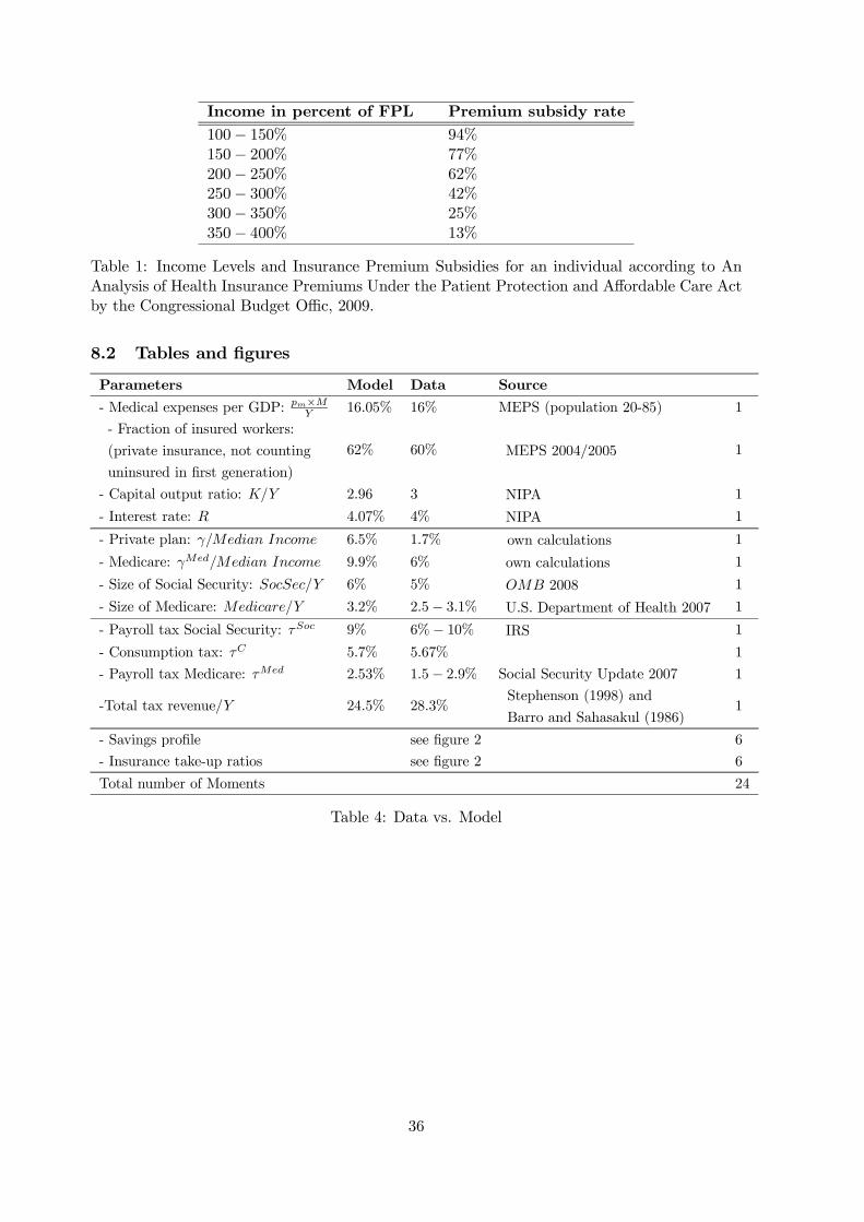
Income in percent of FPL Premium subsidy rate

100− 150% 94%150− 200% 77%200− 250% 62%250− 300% 42%300− 350% 25%350− 400% 13%

Table 1: Income Levels and Insurance Premium Subsidies for an individual according to AnAnalysis of Health Insurance Premiums Under the Patient Protection and Affordable Care Actby the Congressional Budget Offic, 2009.

8.2 Tables and figures

Parameters Model Data Source

- Medical expenses per GDP: pm×MY

16.05% 16% MEPS (population 20-85) 1

- Fraction of insured workers:

(private insurance, not counting

uninsured in first generation)

62% 60% MEPS 2004/2005 1

- Capital output ratio: K/Y 2.96 3 NIPA 1

- Interest rate: R 4.07% 4% NIPA 1

- Private plan: γ/Median Income 6.5% 1.7% own calculations 1

- Medicare: γMed/Median Income 9.9% 6% own calculations 1

- Size of Social Security: SocSec/Y 6% 5% OMB 2008 1

- Size of Medicare: Medicare/Y 3.2% 2.5− 3.1% U.S. Department of Health 2007 1

- Payroll tax Social Security: τSoc 9% 6%− 10% IRS 1

- Consumption tax: τC 5.7% 5.67% 1

- Payroll tax Medicare: τMed 2.53% 1.5− 2.9% Social Security Update 2007 1

-Total tax revenue/Y 24.5% 28.3%Stephenson (1998) and

Barro and Sahasakul (1986)1

- Savings profile see figure 2 6

- Insurance take-up ratios see figure 2 6

Total number of Moments 24

Table 4: Data vs. Model

36

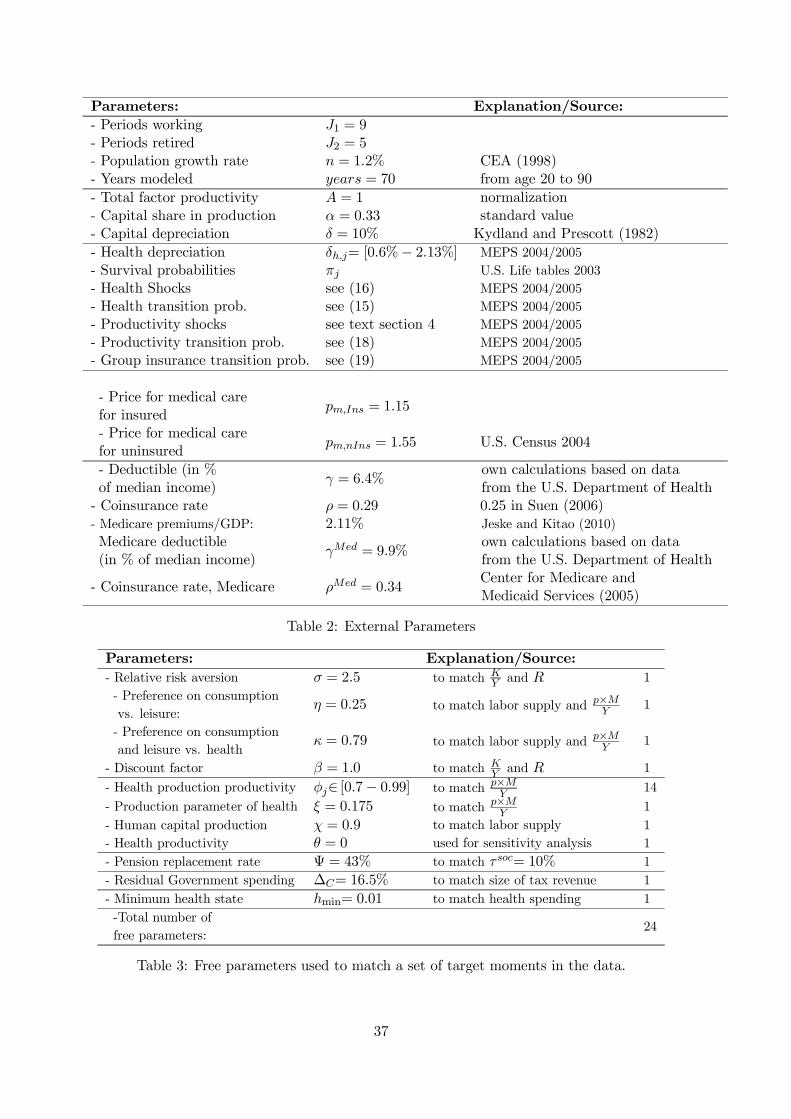
Parameters: Explanation/Source:

- Periods working J1 = 9- Periods retired J2 = 5- Population growth rate n = 1.2% CEA (1998)- Years modeled years = 70 from age 20 to 90

- Total factor productivity A = 1 normalization- Capital share in production α = 0.33 standard value- Capital depreciation δ = 10% Kydland and Prescott (1982)

- Health depreciation δh,j= [0.6%− 2.13%] MEPS 2004/2005

- Survival probabilities πj U.S. Life tables 2003

- Health Shocks see (16) MEPS 2004/2005

- Health transition prob. see (15) MEPS 2004/2005

- Productivity shocks see text section 4 MEPS 2004/2005

- Productivity transition prob. see (18) MEPS 2004/2005

- Group insurance transition prob. see (19) MEPS 2004/2005

- Price for medical carefor insured

pm,Ins = 1.15

- Price for medical carefor uninsured

pm,nIns = 1.55 U.S. Census 2004

- Deductible (in %of median income)

γ = 6.4%own calculations based on datafrom the U.S. Department of Health

- Coinsurance rate ρ = 0.29 0.25 in Suen (2006)- Medicare premiums/GDP: 2.11% Jeske and Kitao (2010)

Medicare deductible(in % of median income)

γMed = 9.9%own calculations based on datafrom the U.S. Department of Health

- Coinsurance rate, Medicare ρMed = 0.34Center for Medicare andMedicaid Services (2005)

Table 2: External Parameters

Parameters: Explanation/Source:

- Relative risk aversion σ = 2.5 to match KY

and R 1

- Preference on consumption

vs. leisure:η = 0.25 to match labor supply and p×M

Y1

- Preference on consumption

and leisure vs. healthκ = 0.79 to match labor supply and p×M

Y1

- Discount factor β = 1.0 to match KY

and R 1

- Health production productivity φj∈ [0.7− 0.99] to match p×MY

14

- Production parameter of health ξ = 0.175 to match p×MY

1

- Human capital production χ = 0.9 to match labor supply 1

- Health productivity θ = 0 used for sensitivity analysis 1

- Pension replacement rate Ψ = 43% to match τsoc= 10% 1

- Residual Government spending ∆C= 16.5% to match size of tax revenue 1

- Minimum health state hmin= 0.01 to match health spending 1

-Total number of

free parameters:24

Table 3: Free parameters used to match a set of target moments in the data.

37

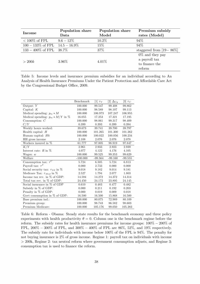
IncomePopulation shareData

Population shareModel

Premium subsidyrates (Model)

< 100% of FPL 9.6− 12% 10.2% 94%

100− 133% of FPL 14.5− 16.9% 15% 94%

133− 400% of FPL 38.7% 37% staggered from [19− 86%]

> 200k 3.96% 4.01%

0% and they paya payroll taxto finance thereform

Table 5: Income levels and insurance premium subsidies for an individual according to AnAnalysis of Health Insurance Premiums Under the Patient Protection and Affordable Care Actby the Congressional Budget Office, 2009.

Benchmark [1] τV [2] ∆Cg [3] τC

Output: Y 100.000 99.547 99.408 99.862Capital: K 100.000 98.589 98.107 99.113Medical spending: pm ∗M 100.000 106.973 107.247 106.955Medical spending: pm ∗M/Y in % 16.055 17.253 17.321 17.195Consumption: C 100.000 98.061 99.317 98.409C/Y 0.399 0.393 0.399 0.394

Weekly hours worked: 39.673 39.741 39.700 39.797Health capital: H 100.000 101.265 101.300 101.262Human capital: Hk 100.000 100.022 100.056 100.234HH gross income 2.108 2.076 2.076 2.078

Workers insured in % 61.777 97.805 98.919 97.847

K/Y 2.961 2.933 2.923 2.939Interest rate: R in % 4.077 4.122 4.176 4.105Wages: w 100.000 99.525 99.353 99.629

Welfare -100.000 -99.564 -99.160 -99.555

Consumption tax: τC 5.724 6.505 5.724 6.813Payroll tax: τV 0.000 2.733 0.000 0.000Social security tax: τSS in % 9.018 9.182 9.014 9.181Medicare Tax: τMed in % 2.527 1.794 2.077 1.803Income tax rev. in % of GDP: 14.594 14.272 14.372 14.314Total tax rev. in % of GDP: 24.450 24.172 23.895 24.145

Social insurance in % of GDP 0.610 0.483 0.477 0.482Subsidy in % of GDP: 0.000 0.211 0.192 0.203Penalty in % of GDP: 0.000 0.019 0.009 0.018Govt consumption in % of GDP: 16.500 16.500 15.868 16.500

Base premium ind.: 100.000 80.075 72.989 80.109Premium group: 100.000 98.743 86.582 98.603Premium Medicare: 100.000 105.176 99.050 105.383

Table 6: Reform - Obama: Steady state results for the benchmark economy and three policyexperiments with health productivity θ = 0. Column one is the benchmark regime before thereform. The subsidy rates for health insurance premiums for income groups: 100%− 200% ofFPL, 200% − 300% of FPL, and 300% − 400% of FPL are 86%, 52%, and 19% respectively.The subsidy rate for individuals with income below 100% of the FPL is 94%. The penalty fornot buying insurance is 2% of gross income. Regime 1: payroll tax on individuals with income> 200k, Regime 2: tax neutral reform where government consumption adjusts, and Regime 3:consumption tax is used to finance the reform.

38

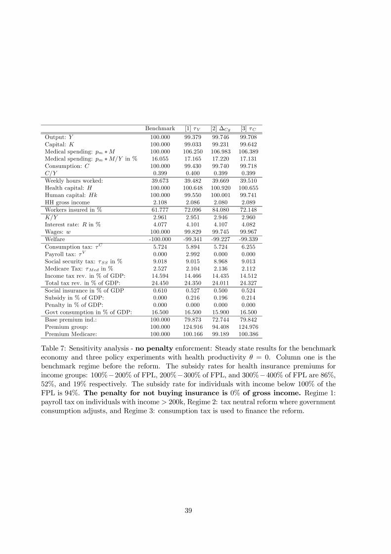
Benchmark [1] τV [2] ∆Cg [3] τC

Output: Y 100.000 99.379 99.746 99.708Capital: K 100.000 99.033 99.231 99.642Medical spending: pm ∗M 100.000 106.250 106.983 106.389Medical spending: pm ∗M/Y in % 16.055 17.165 17.220 17.131Consumption: C 100.000 99.430 99.740 99.718C/Y 0.399 0.400 0.399 0.399

Weekly hours worked: 39.673 39.482 39.669 39.510Health capital: H 100.000 100.648 100.920 100.655Human capital: Hk 100.000 99.550 100.001 99.741HH gross income 2.108 2.086 2.080 2.089

Workers insured in % 61.777 72.096 84.080 72.148

K/Y 2.961 2.951 2.946 2.960Interest rate: R in % 4.077 4.101 4.107 4.082Wages: w 100.000 99.829 99.745 99.967

Welfare -100.000 -99.341 -99.227 -99.339

Consumption tax: τC 5.724 5.894 5.724 6.255Payroll tax: τV 0.000 2.992 0.000 0.000Social security tax: τSS in % 9.018 9.015 8.968 9.013Medicare Tax: τMed in % 2.527 2.104 2.136 2.112Income tax rev. in % of GDP: 14.594 14.466 14.435 14.512Total tax rev. in % of GDP: 24.450 24.350 24.011 24.327

Social insurance in % of GDP 0.610 0.527 0.500 0.524Subsidy in % of GDP: 0.000 0.216 0.196 0.214Penalty in % of GDP: 0.000 0.000 0.000 0.000Govt consumption in % of GDP: 16.500 16.500 15.900 16.500

Base premium ind.: 100.000 79.873 72.744 79.842Premium group: 100.000 124.916 94.408 124.976Premium Medicare: 100.000 100.166 99.189 100.386

Table 7: Sensitivity analysis - no penalty enforcment: Steady state results for the benchmarkeconomy and three policy experiments with health productivity θ = 0. Column one is thebenchmark regime before the reform. The subsidy rates for health insurance premiums forincome groups: 100%−200% of FPL, 200%−300% of FPL, and 300%−400% of FPL are 86%,52%, and 19% respectively. The subsidy rate for individuals with income below 100% of theFPL is 94%. The penalty for not buying insurance is 0% of gross income. Regime 1:payroll tax on individuals with income > 200k, Regime 2: tax neutral reform where governmentconsumption adjusts, and Regime 3: consumption tax is used to finance the reform.

39

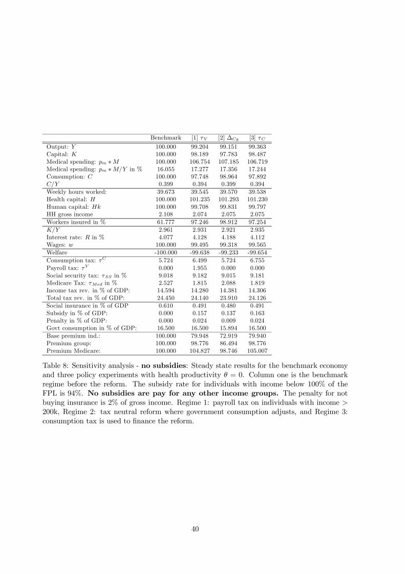
Benchmark [1] τV [2] ∆Cg [3] τC

Output: Y 100.000 99.204 99.151 99.363Capital: K 100.000 98.189 97.783 98.487Medical spending: pm ∗M 100.000 106.754 107.185 106.719Medical spending: pm ∗M/Y in % 16.055 17.277 17.356 17.244Consumption: C 100.000 97.748 98.964 97.892C/Y 0.399 0.394 0.399 0.394

Weekly hours worked: 39.673 39.545 39.570 39.538Health capital: H 100.000 101.235 101.293 101.230Human capital: Hk 100.000 99.708 99.831 99.797HH gross income 2.108 2.074 2.075 2.075

Workers insured in % 61.777 97.246 98.912 97.254

K/Y 2.961 2.931 2.921 2.935Interest rate: R in % 4.077 4.128 4.188 4.112Wages: w 100.000 99.495 99.318 99.565

Welfare -100.000 -99.638 -99.233 -99.654

Consumption tax: τC 5.724 6.499 5.724 6.755Payroll tax: τV 0.000 1.955 0.000 0.000Social security tax: τSS in % 9.018 9.182 9.015 9.181Medicare Tax: τMed in % 2.527 1.815 2.088 1.819Income tax rev. in % of GDP: 14.594 14.280 14.381 14.306Total tax rev. in % of GDP: 24.450 24.140 23.910 24.126

Social insurance in % of GDP 0.610 0.491 0.480 0.491Subsidy in % of GDP: 0.000 0.157 0.137 0.163Penalty in % of GDP: 0.000 0.024 0.009 0.024Govt consumption in % of GDP: 16.500 16.500 15.894 16.500

Base premium ind.: 100.000 79.948 72.919 79.940Premium group: 100.000 98.776 86.494 98.776Premium Medicare: 100.000 104.827 98.746 105.007

Table 8: Sensitivity analysis - no subsidies: Steady state results for the benchmark economyand three policy experiments with health productivity θ = 0. Column one is the benchmarkregime before the reform. The subsidy rate for individuals with income below 100% of theFPL is 94%. No subsidies are pay for any other income groups. The penalty for notbuying insurance is 2% of gross income. Regime 1: payroll tax on individuals with income >200k, Regime 2: tax neutral reform where government consumption adjusts, and Regime 3:consumption tax is used to finance the reform.

40

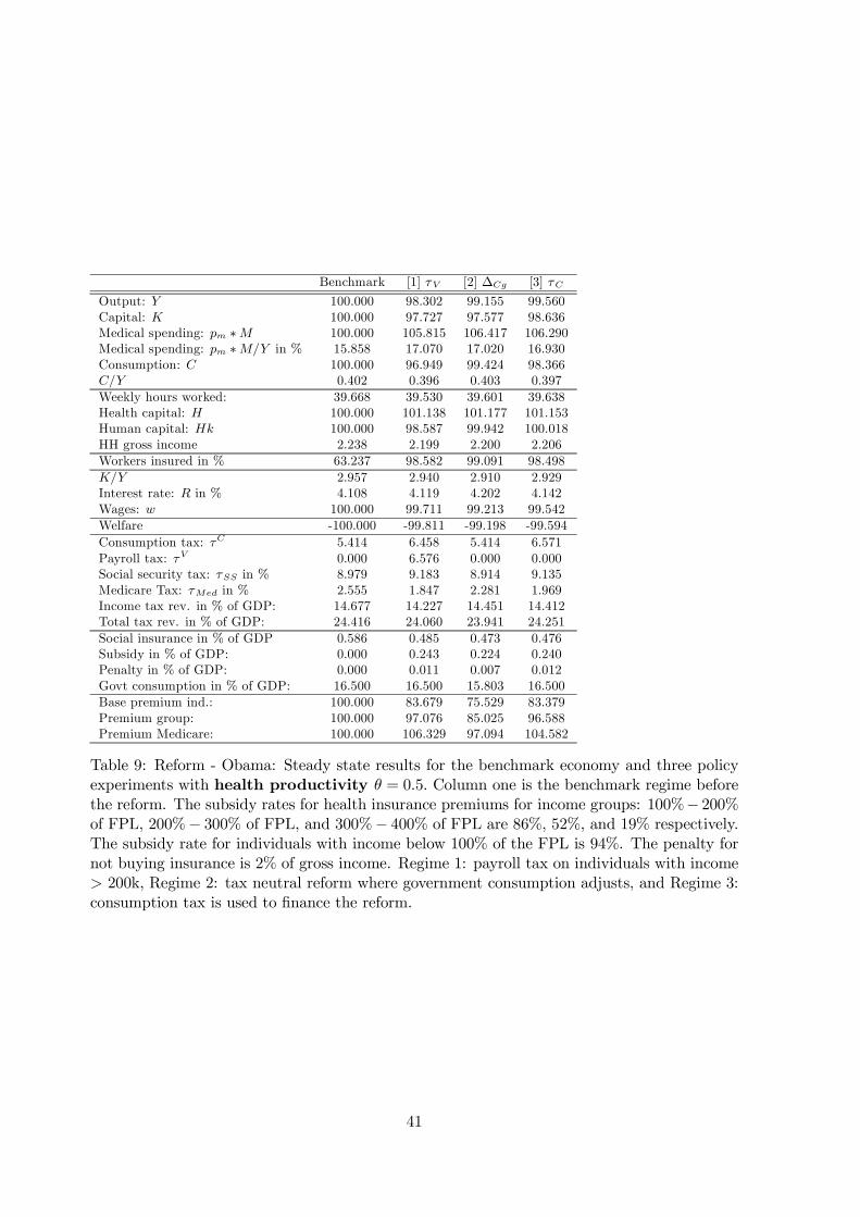
Benchmark [1] τV [2] ∆Cg [3] τC

Output: Y 100.000 98.302 99.155 99.560Capital: K 100.000 97.727 97.577 98.636Medical spending: pm ∗M 100.000 105.815 106.417 106.290Medical spending: pm ∗M/Y in % 15.858 17.070 17.020 16.930Consumption: C 100.000 96.949 99.424 98.366C/Y 0.402 0.396 0.403 0.397

Weekly hours worked: 39.668 39.530 39.601 39.638Health capital: H 100.000 101.138 101.177 101.153Human capital: Hk 100.000 98.587 99.942 100.018HH gross income 2.238 2.199 2.200 2.206

Workers insured in % 63.237 98.582 99.091 98.498

K/Y 2.957 2.940 2.910 2.929Interest rate: R in % 4.108 4.119 4.202 4.142Wages: w 100.000 99.711 99.213 99.542

Welfare -100.000 -99.811 -99.198 -99.594

Consumption tax: τC 5.414 6.458 5.414 6.571Payroll tax: τV 0.000 6.576 0.000 0.000Social security tax: τSS in % 8.979 9.183 8.914 9.135Medicare Tax: τMed in % 2.555 1.847 2.281 1.969Income tax rev. in % of GDP: 14.677 14.227 14.451 14.412Total tax rev. in % of GDP: 24.416 24.060 23.941 24.251

Social insurance in % of GDP 0.586 0.485 0.473 0.476Subsidy in % of GDP: 0.000 0.243 0.224 0.240Penalty in % of GDP: 0.000 0.011 0.007 0.012Govt consumption in % of GDP: 16.500 16.500 15.803 16.500

Base premium ind.: 100.000 83.679 75.529 83.379Premium group: 100.000 97.076 85.025 96.588Premium Medicare: 100.000 106.329 97.094 104.582

Table 9: Reform - Obama: Steady state results for the benchmark economy and three policyexperiments with health productivity θ = 0.5. Column one is the benchmark regime beforethe reform. The subsidy rates for health insurance premiums for income groups: 100%− 200%of FPL, 200%− 300% of FPL, and 300%− 400% of FPL are 86%, 52%, and 19% respectively.The subsidy rate for individuals with income below 100% of the FPL is 94%. The penalty fornot buying insurance is 2% of gross income. Regime 1: payroll tax on individuals with income> 200k, Regime 2: tax neutral reform where government consumption adjusts, and Regime 3:consumption tax is used to finance the reform.

41

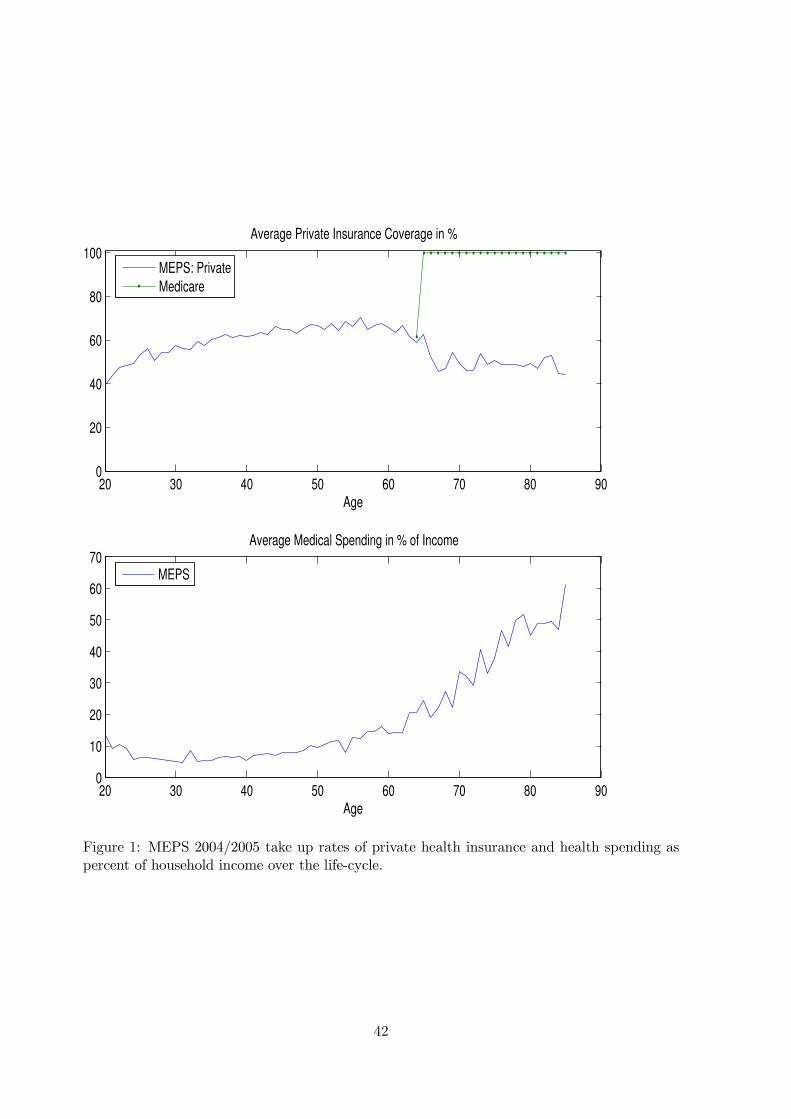
20 30 40 50 60 70 80 900

20

40

60

80

100

Age

Average Private Insurance Coverage in %

20 30 40 50 60 70 80 900

10

20

30

40

50

60

70

Age

Average Medical Spending in % of Income

MEPS: Private

Medicare

MEPS

Figure 1: MEPS 2004/2005 take up rates of private health insurance and health spending aspercent of household income over the life-cycle.

42

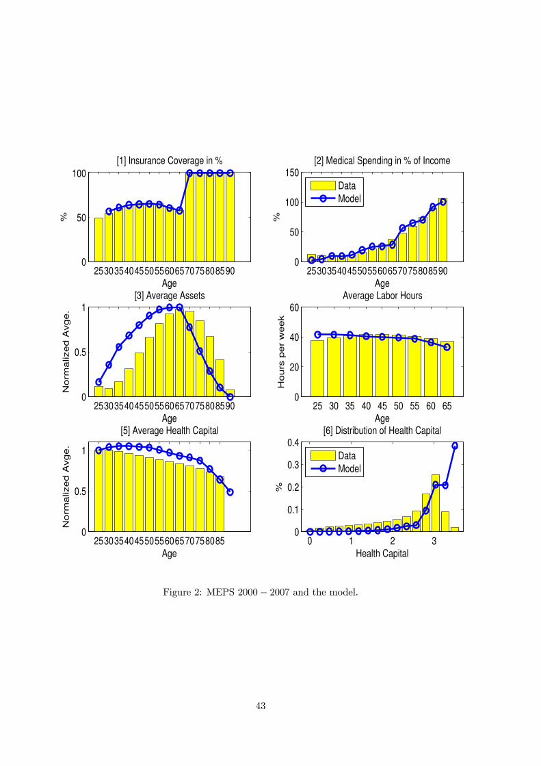
25303540455055606570758085900

50

100

Age

%

[1] Insurance Coverage in %

25303540455055606570758085900

50

100

150

%Age

[2] Medical Spending in % of Income

Data

Model

25303540455055606570758085900

0.5

1

Age

No

rma

lize

d A

vg

e.

[3] Average Assets

25 30 35 40 45 50 55 60 650

20

40

60

Age

Ho

urs

pe

r w

ee

k

Average Labor Hours

253035404550556065707580850

0.5

1

Age

No

rma

lize

d A

vg

e.

[5] Average Health Capital

0 1 2 30

0.1

0.2

0.3

0.4

Health Capital

%

[6] Distribution of Health Capital

Data

Model

Figure 2: MEPS 2000− 2007 and the model.

43

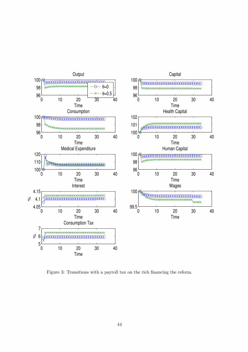
0 10 20 30 4096

98

100Output

Time

θ=0

θ=0.5

0 10 20 30 4096

98

100Capital

Time

0 10 20 30 4096

98

100Consumption

Time0 10 20 30 40

100

101

102Health Capital

Time

0 10 20 30 40100

110

120Medical Expenditure

Time0 10 20 30 40

96

98

100Human Capital

Time

0 10 20 30 404.05

4.1

4.15Interest

Time

%

0 10 20 30 4099.5

100Wages

Time

0 10 20 30 405

6

7Consumption Tax

Time

%

Figure 3: Transitions with a payroll tax on the rich financing the reform.

44

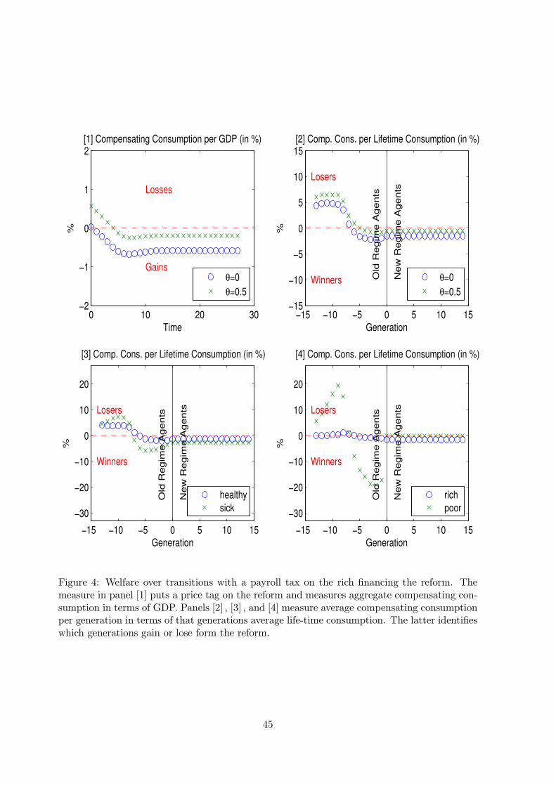
0 10 20 30−2

−1

0

1

2[1] Compensating Consumption per GDP (in %)

%

Time

Gains

Losses

θ=0

θ=0.5

−15 −10 −5 0 5 10 15−15

−10

−5

0

5

10

15[2] Comp. Cons. per Lifetime Consumption (in %)

%

Generation

Old

Re

gim

e A

ge

nts

Ne

w R

eg

ime

Ag

en

ts

Winners

Losers

θ=0

θ=0.5

−15 −10 −5 0 5 10 15

−30

−20

−10

0

10

20

[3] Comp. Cons. per Lifetime Consumption (in %)

%

Generation

Old

Re

gim

e A

ge

nts

Ne

w R

eg

ime

Ag

en

ts

Winners

Losers

healthy

sick

−15 −10 −5 0 5 10 15

−30

−20

−10

0

10

20

[4] Comp. Cons. per Lifetime Consumption (in %)

%

Generation

O

ld R

eg

ime

Ag

en

ts

Ne

w R

eg

ime

Ag

en

ts

Winners

Losers

rich

poor

Figure 4: Welfare over transitions with a payroll tax on the rich financing the reform. Themeasure in panel [1] puts a price tag on the reform and measures aggregate compensating con-sumption in terms of GDP. Panels [2] , [3] , and [4] measure average compensating consumptionper generation in terms of that generations average life-time consumption. The latter identifieswhich generations gain or lose form the reform.

45

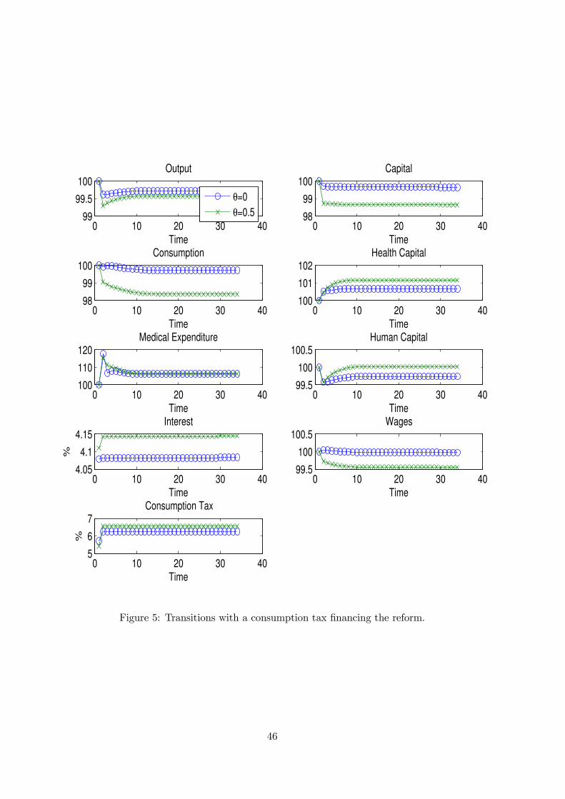
0 10 20 30 4099

99.5

100Output

Time

θ=0

θ=0.5

0 10 20 30 4098

99

100Capital

Time

0 10 20 30 4098

99

100Consumption

Time0 10 20 30 40

100

101

102Health Capital

Time

0 10 20 30 40100

110

120Medical Expenditure

Time0 10 20 30 40

99.5

100

100.5Human Capital

Time

0 10 20 30 404.05

4.1

4.15Interest

Time

%

0 10 20 30 4099.5

100

100.5Wages

Time

0 10 20 30 405

6

7Consumption Tax

Time

%

Figure 5: Transitions with a consumption tax financing the reform.

46

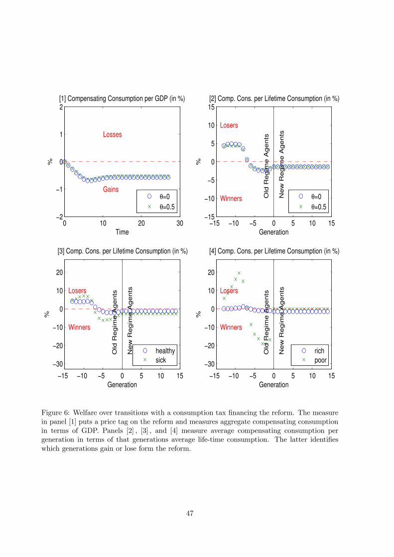
0 10 20 30−2

−1

0

1

2[1] Compensating Consumption per GDP (in %)

%

Time

Gains

Losses

θ=0

θ=0.5

−15 −10 −5 0 5 10 15−15

−10

−5

0

5

10

15[2] Comp. Cons. per Lifetime Consumption (in %)

%

Generation

Old

Re

gim

e A

ge

nts

Ne

w R

eg

ime

Ag

en

ts

Winners

Losers

θ=0

θ=0.5

−15 −10 −5 0 5 10 15

−30

−20

−10

0

10

20

[3] Comp. Cons. per Lifetime Consumption (in %)

%

Generation

Old

Re

gim

e A

ge

nts

Ne

w R

eg

ime

Ag

en

ts

Winners

Losers

healthy

sick

−15 −10 −5 0 5 10 15

−30

−20

−10

0

10

20

[4] Comp. Cons. per Lifetime Consumption (in %)

%

Generation

O

ld R

eg

ime

Ag

en

ts

Ne

w R

eg

ime

Ag

en

ts

Winners

Losers

rich

poor

Figure 6: Welfare over transitions with a consumption tax financing the reform. The measurein panel [1] puts a price tag on the reform and measures aggregate compensating consumptionin terms of GDP. Panels [2] , [3] , and [4] measure average compensating consumption pergeneration in terms of that generations average life-time consumption. The latter identifieswhich generations gain or lose form the reform.

47