Sources of Lifetime Inequality

Mark Huggett, Gustavo Ventura and Amir Yaron∗

November, 16 2010

Abstract

Is lifetime inequality mainly due to differences across people established early in life

or to differences in luck experienced over the working lifetime? We answer this question

within a model that features idiosyncratic shocks to human capital, estimated directly

from data, as well as heterogeneity in ability to learn, initial human capital, and initial

wealth. We find that, as of age 23, differences in initial conditions account for more of

the variation in lifetime earnings, lifetime wealth and lifetime utility than do differences

in shocks received over the working lifetime.

JEL Classification: E21, D3, D91.

KEYWORDS: Lifetime Inequality, Human Capital, Idiosyncratic Risk.

∗Affiliation: Georgetown University, University of Iowa, and The Wharton School–University of Penn-sylvania and NBER respectively. We thank Luigi Pistaferri and seminar participants at many venues forcomments. We thank the referees and the Co-Editor for improving the quality of this paper. We thank theNational Science Foundation Grant SES-0550867 and the Rodney L. White Center for Financial Research atWharton for research support. Ventura thanks the Research and Graduate Studies Office from The Penn-sylvania State University for support and the Economics Department of Pennsylvania State University forthe use of their UNIX workstations.Corresponding author: Amir Yaron.Address: The Wharton School; University of Pennsylvania, Philadelphia PA 19104- 6367.E-mail: yaron@wharton.upenn.edu.

1

1 Introduction

To what degree is lifetime inequality due to differences across people established early

in life as opposed to differences in luck experienced over the working lifetime? Among the

individual differences established early in life, which ones are the most important?

A convincing answer to these questions is of fundamental importance. First, and most

simply, an answer serves to contrast the potential importance of the myriad policies directed

at modifying or at providing insurance for initial conditions (e.g. public education) against

those directed at shocks over the working lifetime (e.g. unemployment insurance). Second,

a discussion of lifetime inequality cannot go too far before discussing which specific type of

initial condition is the most critical for determining how one fares in life. Third, a useful

framework for answering these questions should also be central in the analysis of a wide

range of policies considered in macroeconomics, public finance and labor economics.

We view lifetime inequality through the lens of a risky human capital model. Agents

differ in terms of three initial conditions: initial human capital, learning ability and financial

wealth. Initial human capital can be viewed as controlling the intercept of an agent’s mean

earnings profile, whereas learning ability acts to rotate this profile. Human capital and labor

earnings are risky as human capital is subject to idiosyncratic shocks each period.

We ask the model to account for key features of the dynamics of the earnings distribution.

To this end, we document how mean earnings and measures of earnings dispersion and

skewness evolve for cohorts of U.S. males. We find that mean earnings are hump shaped and

that earnings dispersion and skewness increase with age over most of the working lifetime.1

Our model produces a hump-shaped mean earnings profile by a standard human capital

channel. Early in life earnings are low because initial human capital is low and agents allocate

time to accumulating human capital. Earnings rise as human capital accumulates and as a

greater fraction of time is devoted to market work. Earnings fall later in life because human

capital depreciates and little time is put into producing new human capital.

Two forces within the model account for the increase in earnings dispersion. One force

is that agents differ in learning ability. Agents with higher learning ability have a steeper

1Mincer (1974) documents related patterns in U.S. cross-section data. Deaton and Paxson (1994),Storesletten, Telmer and Yaron (2004), Heathcote, Storesletten and Violante (2005) and Huggett, Venturaand Yaron (2006) examine cohort patterns in U.S. repeated cross section or panel data.

2

mean earnings profiles than low ability agents, other things equal.2 The other force is that

agents differ in idiosyncratic human capital shocks received over the lifetime. These shocks,

even when independent over time, produce persistent differences in earnings as they lead to

persistent differences in human capital.

To identify the contribution of each of these forces, we exploit the fact that the model

implies that late in life little or no new human capital is produced. As a result, moments of

the change in wage rates for these agents are almost entirely determined by shocks, rather

than by shocks and the endogenous response of investment in human capital to shocks and

initial conditions. We estimate the shock process using precisely these moments for older

males in U.S. data.3 Given an estimate of the shock process and other model parameters, we

choose the initial distribution of financial wealth, human capital and learning ability across

agents to best match the earnings facts described above.4 We find that learning ability

differences produce an important part of the rise in earnings dispersion over the lifetime,

given our estimate of the magnitude of human capital risk.

We use our estimates of shocks and initial conditions to quantify the importance of differ-

ent proximate sources of lifetime inequality. We find that initial conditions (i.e. individual

differences existing at age 23) are more important than are shocks received over the rest

of the working lifetime as a source of variation in realized lifetime earnings, lifetime wealth

and lifetime utility.5 In the benchmark model, variation in initial conditions accounts for

61.5 percent of the variation in lifetime earnings and 64.0 percent of the variation in lifetime

utility. When we extend the benchmark model to also include initial wealth differences as

measured in U.S. data, variation in initial conditions accounts for 61.2, 62.4 and 66.0 percent

of the variation in lifetime earnings, lifetime wealth and lifetime utility, respectively.

Among initial conditions, we find that, as of age 23, variation in human capital is sub-

stantially more important than variation in either learning ability or financial wealth for how

an agent fares in life after this age. This analysis is conducted for an agent with the median

2This mechanism is supported by the literature on the shape of the mean age-earnings profiles by yearsof education. It is also supported by the work of Lillard and Weiss (1979), Baker (1997) and Guvenen(2007). They estimate a statistical model of earnings and find important permanent differences in individualearnings growth rates.

3Heckman, Lochner and Taber (1998) use a similar line of reasoning to estimate rental rates across skillgroups within a model that abstracts from idiosyncratic risk.

4Since a measure of financial wealth is observable, we set the tri-variate initial distribution to be consistentwith features of the distribution of wealth among young households.

5Lifetime earnings equals the present value of earnings, whereas lifetime wealth equals lifetime earningsplus initial wealth.

3

value of each initial condition. In the benchmark model with initial wealth differences, we

find that a hypothetical one standard deviation increase in initial wealth increases expected

lifetime wealth by about 5 percent. In contrast, a one standard deviation increase in learning

ability or initial human capital increases expected lifetime wealth by about 8 percent and

47 percent, respectively. Intuitively, an increase in human capital affects lifetime wealth

by lifting upwards an agent’s mean earnings profile, whereas an increase in learning abil-

ity affects lifetime wealth by rotating this profile counterclockwise. We also calculate the

permanent percentage change in consumption which is equivalent in expected utility terms

to these changes in initial conditions. We find that these permanent percentage changes in

consumption are roughly in line with how a change in an initial condition impacts expected

lifetime wealth.

We stress an important caveat in interpreting results on the importance of variations in

initial conditions. The distribution of initial conditions at a specific age is an endogenously

determined distribution from the perspective of an earlier age. To better understand this

point, consider a dramatic example. In the last period of the working lifetime, only variation

in human capital and financial wealth is important. Variation in learning ability is of no

importance for lifetime utility or lifetime wealth over the remaining lifetime. However, from

the perspective of an earlier period this does not mean that variation in learning ability is

unimportant. In theory, potentially all of the variation in both human capital and financial

wealth in the last period of the working lifetime could be due to differences in learning ability

early in life. Thus, the results that we find for variation in human capital at age 23 need to

be understood as applying at that age. This paper is silent on the prior forces which shape

the individual differences that we analyze at age 23.

Background

A leading view of lifetime inequality is based on the standard, incomplete-markets model

in which labor earnings over the lifetime is exogenous. Storesletten et. al. (2004) analyze

lifetime inequality from the perspective of such a model. Similar models have been widely

used in the economic inequality and tax reform literatures.6 Storesletten et. al. (2004)

estimate an earnings process from U.S. panel data to match features of earnings over the

lifetime. Within their model, slightly less than half of the variation in realized lifetime utility

is due to differences in initial conditions as of age 22. On the other hand, and in the context

6See Huggett (1996), Castaneda, Diaz-Jimenez and Rios-Rull (2003), Krueger and Perri (2006), Heath-cote, Storesletten and Violante (2006) and Guvenen (2007) among many others.

4

of a career-choice model, Keane and Wolpin (1997) find a more important role for initial

conditions. They find that unobserved heterogeneity realized at age 16 accounts for about

90 percent of the variance in lifetime utility.

We highlight three difficulties with the incomplete-markets model with exogenous earn-

ings, given its connection to our model and given its standing as a workhorse model in

macroeconomics. First, the importance of idiosyncratic earnings risk may be overstated be-

cause all of the rise in earnings dispersion with age is attributed to shocks. In our model

initial conditions account for some of the rise in dispersion. Second, although the exogenous

earnings model produces the rise in U.S. within cohort consumption dispersion over the pe-

riod 1980-90, the rise in consumption dispersion is substantially smaller in U.S. data over

a longer time period. Our model produces less of a rise in consumption dispersion because

part of the rise in earnings dispersion is due to initial conditions and agents know their

initial conditions. Third, the incomplete-markets model is not useful for some purposes.

Specifically, since earnings are exogenous, the model can not shed light on how policy may

affect inequality in lifetime earnings or may affect welfare through earnings. Models with

exogenous wage rates (e.g. Heathcote et. al. (2006)) face this criticism, but to a lesser

extent, since most earnings variation is attributed to wage variation. It therefore seems

worthwhile to pursue a more fundamental approach that endogenizes wage rate differences

via human capital theory. In our view, a successful quantitative model of this type would

bridge an important gap between the macroeconomic literature with incomplete markets and

the human capital literature and would offer an important alternative workhorse model for

quantitative work and policy analysis.

The paper is organized as follows. Section 2 presents the model. Section 3 documents

earnings distribution facts and estimates properties of shocks. Section 4 sets model param-

eters. Sections 5 and 6 analyze the model and answer the two lifetime inequality questions.

Section 7 concludes.

5

2 The Model

An agent maximizes expected lifetime utility, taking initial financial wealth k1, initial human

capital h1 and learning ability a as given.7 The decision problem for an agent born at time

t is stated below.

max{cj ,lj ,sj ,hj ,kj}Jj=1E[

∑Jj=1 β

j−1u(cj)] subject to

(i) cj + kj+1 = kj(1 + rt+j−1) + ej − Tj,t+j−1(ej, kj), ∀j and kJ+1 = 0

(ii) ej = Rt+j−1hjlj if j < JR, and ej = 0 otherwise.

(iii) hj+1 = exp(zj+1)H(hj, sj, a) and lj + sj = 1, ∀j

The only source of risk to an agent over the working lifetime comes from idiosyncratic

shocks to an agent’s human capital. Let zj = (z1, ..., zj) denote the j-period history of these

shocks. Thus, the optimal consumption choice cj,t+j−1(x1, zj) for an age j agent at time

t+ j − 1 is risky as it depends on shocks zj as well as initial conditions x1 = (h1, k1, a). The

period budget constraint says that consumption cj plus financial asset holding kj+1 equals

earnings ej plus the value of assets kj(1+ rt+j−1) less net taxes Tj,t+j−1. Financial assets pay

a risk-free, real return rt+j−1 at time t+ j− 1. Earnings ej before a retirement age JR equal

the product of a rental rate Rt+j−1 for human capital services, an agent’s human capital hj

and the fraction lj of available time put into market work. Earnings are zero at and after

the retirement age JR. An agent’s future human capital hj+1 is an increasing function of an

idiosyncratic shock zj+1, current human capital hj, time devoted to human capital or skill

production sj, and an agent’s learning ability a. Learning ability is fixed over an agent’s

lifetime and is exogenous.

We now embed this decision problem within a general equilibrium framework and focus

on balanced-growth equilibria. There is an aggregate production function F (Kt, LtAt) with

constant returns in aggregate capital and labor (Kt, Lt) and with labor augmenting technical

change At+1 = At(1 + g). Aggregate variables are sums of the relevant individual decisions

across agents. In defining aggregates, ψ is a time-invariant distribution over initial conditions

7The model generalizes Ben-Porath (1967) to allow for risky human capital and extends Levhari andWeiss (1974) and Eaton and Rosen (1980) to a multi-period setting. Krebs (2004) analyzes a multi-periodmodel of human capital with idiosyncratic risk. Our work differs in its focus on lifetime inequality amongother differences.

6

x1 and µj is the fraction of age j agents in the population. Population fractions satisfy∑Jj=1 µj = 1 and µj+1 = µj/(1 + n), where n is a constant population growth rate. In the

analysis of equilibrium, we consider the case where initial financial assets are zero and, thus,

ψ is effectively a bivariate distribution over x1 = (h1, a).

Kt ≡∑J

j=1 µj

∫E[kj,t(x1, z

j)]dψ and Lt ≡∑J

j=1 µj

∫E[hj,t(x1, z

j)lj,t(x1, zj)]dψ

Ct ≡∑J

j=1 µj

∫E[cj,t(x1, z

j)]dψ and Tt ≡∑J

j=1 µj

∫E[Tj,t(ej,t, kj,t)]dψ

Definition: A balanced-growth equilibrium is a collection of decisions {{cj,t, lj,t, sj,t, hj,t, kj,t}Jj=1}∞t=−∞,

factor prices, government spending and taxes {Rt, rt, Gt, Tt}∞t=−∞ and a distribution ψ over

initial conditions such that

(1) Agent decisions are optimal, given factor prices.

(2) Competitive Factor Prices: Rt = AtF2(Kt, LtAt) and rt = F1(Kt, LtAt)− δ

(3) Resource Feasibility: Ct +Kt+1(1 + n) +Gt = F (Kt, LtAt) +Kt(1− δ)

(4) Government Budget: Gt = Tt

(5) Balanced Growth: (i) {cj,t, kj,t}Jj=1 grow at rate g as a function of time, whereas

{lj,t, sj,t, hj,t}Jj=1 are time invariant. (ii) (Gt, Tt, Rt) grow at rate g, whereas rt is time

invariant.

Our focus on balanced-growth equilibria requires that individual decisions, aggregate

variables and factor prices grow at constant rates. Balanced growth leads us to employ

homothetic preferences and a constant returns technology. More specifically, we use the

property that if preferences over lifetime consumption plans are homothetic and the budget

set for consumption plans is homogeneous of degree 1 in rental rates, then optimal consump-

tion plans are homogeneous of degree 1 in rental rates.8

8Let Γ(x1, R) denote the set of lifetime consumption plans satisfying budget conditions (i)-(iii), given

initial conditions x1 and rental rates R = (R1, ..., RJ). Γ(x1, R) is homogeneous in R provided c ∈ Γ(x1, R) ⇒λc ∈ Γ(x1, λR),∀λ > 0. Γ(x1, R) has this property when taxes Tjt are homogeneous of degree 1 in earningsand assets and when initial assets are zero. The model tax system (see section 4) induces this property when

Tjt(R, hj , lj , kj) is homogeneous of degree 1 in (R, kj).

7

The functional forms that we employ are provided below. The equilibrium concept does

not restrict the functional forms for the human capital production function H(h, s, a), the

distribution of initial conditions ψ or the nature of idiosyncratic shocks. The human capital

production function is of the Ben-Porath class which is widely used in empirical work. The

distribution ψ is a bivariate lognormal distribution which allows for a skewed distribution of

initial human capital. Recall that our equilibrium analysis considers the case where initial

assets are set to zero. Idiosyncratic shocks are independent and identically distributed over

time and follow a normal distribution.

u(c) = c(1−ρ)/(1− ρ), F (K,LA) = Kγ(LA)1−γ and H(h, s, a) = h+ a(hs)α

x = (h1, a) ∼ ψ = LN(µx,Σ) and z ∼ N(µ, σ2)

We comment on four key features of the model. First, while the earnings of an agent are

stochastic, the earnings distribution for a cohort of agents evolves deterministically. This

occurs because the model has idiosyncratic but no aggregate risk.9 Second, the model has

two sources of growth in earnings dispersion within a cohort - agents have different learning

abilities and different shock realizations. The next section characterizes empirically the rise

in U.S. earnings dispersion over the working lifetime. Third, although the model has a single

source of shocks, which are independently and identically distributed over time, we will show

that this structure is sufficient to endogenously produce many of the statistical properties

of earnings that researchers have previously estimated. Fourth, the model implies that the

nature of human capital shocks can be identified from wage rate data, independently from

all other model parameters. This holds, as an approximation, because the model implies

that the production of human capital goes to zero towards the end of the working lifetime.

The next section develops the logic of this point.

3 Empirical Analysis

We use data to address two issues. First, we characterize how mean earnings and measures

of earnings dispersion and skewness evolve with age for a cohort. Second, we estimate a

human capital shock process from wage rate data.

9More specifically, the probability that an agent receives a j-period shock history zj is also the fractionof the agents in a cohort that receive zj .

8

3.1 Age Profiles

We estimate age profiles for mean earnings and measures of earnings dispersion and skewness

for ages 23 to 60. We use earnings data for males who are the head of the household from

the Panel Study of Income Dynamics (PSID) 1969-2004 family files. To calculate earnings

statistics at a specific age and year, we employ a centered 5-year age bin.10 For males over

age 30, we require that they work between 520 and 5820 hours per year and earn at least

1500 dollars (in 1968 prices) a year. For males age 30 and below, we require that they work

between 260 and 5820 hours per year and earn at least 1000 dollars (in 1968 prices).

These selection criteria are motivated by several considerations. First, the PSID has

many observations in the middle but relatively fewer at the beginning or end of the working

life cycle. By focusing on ages 23-60, we have at least 100 observations in each age-year bin

with which to calculate earnings statistics. Second, labor force participation falls near the

traditional retirement age for reasons that are abstracted from in the model. This motivates

the use of a terminal age that is below the traditional retirement age. Third, the hours and

earnings restrictions are motivated by the fact that within the model the only alternative to

time spent working is time spent learning. For males above 30, the minimum hours restriction

amounts to a quarter of full-time work hours and the minimum earnings restriction is below

the annual earnings level of a full-time worker working at the federal minimum wage.11

For younger males, we lower both the minimum hours and earnings restrictions to capture

students doing summer work or working part-time while in school.

We now document how mean earnings, two measures of earnings dispersion and a measure

of earnings skewness evolve with age for cohorts. We consider two measures of dispersion:

the variance of log earnings and the Gini coefficient of earnings. We measure skewness by

the ratio of mean earnings to median earnings.

The methodology for extracting age effects is in two parts. First, we calculate the statistic

of interest for males in age bin j at time t and label this statj,t. For example, for mean

earnings we set statj,t = ln(ejt), where ejt is real mean earnings of all males in the age bin

centered at age j in year t.12 Second, we posit a statistical model governing the evolution of

the earnings statistic as indicated below. The earnings statistic is viewed as being generated

10To calculate statistics for the age 23 and the age 60 bin we use earnings for males age 21-25 and 58-62.11A full-time worker (working 40 hours per week and 52 weeks a year) who receives the federal minimum

wage in 1968 earns 3, 328 dollars in 1968 prices.12We use the Consumer Price Index to convert nominal earnings to real earnings.

9

by several factors that we label cohort (c), age (j), and time (t) effects. We wish to estimate

the age effects βstatj . We employ a statistical model as our economic model is not sufficiently

rich to capture all aspects of time variation in the data.

statj,t = αstatc + βstat

j + γstatt + ϵstatj,t

The linear relationship between time t, age j, and birth cohort c = t−j limits the applica-

bility of this regression specification. Specifically, without further restrictions the regressors

in this system are co-linear and these effects cannot be estimated. This identification prob-

lem is well known.13 Any trend in the data can be arbitrarily reinterpreted as due to year

(time) effects or alternatively as due to age or cohort effects.

Given this problem, we provide two alternative measures of age effects. These correspond

to the cohort effects view where we set γstatt = 0, ∀t and the time effects view where we set

αstatc = 0, ∀c. We use ordinary least squares to estimate the coefficients.14

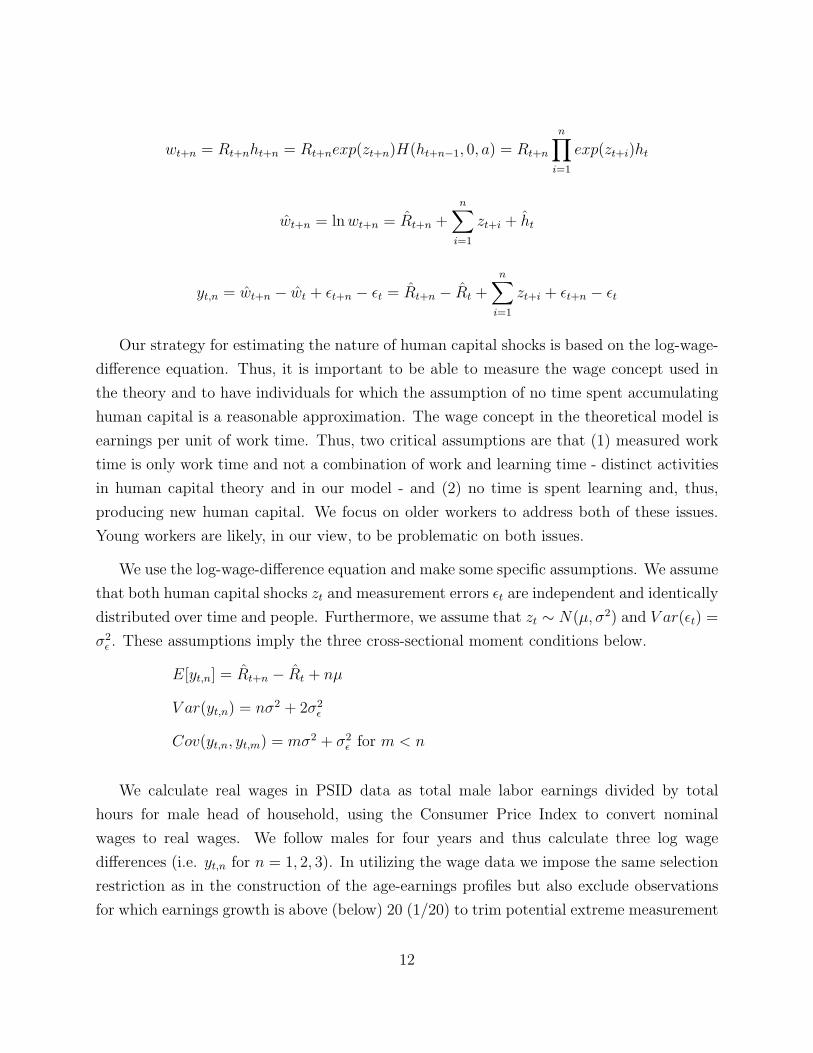
In Figure 1(a) we graph the age effects of the levels of mean earnings implied by each

regression. Figure 1 highlights the familiar hump-shaped profile for mean earnings. Mean

earnings almost doubles from the early 20’s to the peak earnings age. Figure 1 is constructed

using the coefficients exp(βj) from the regression based upon mean earnings. The age effects

in Figure 1(a) are first scaled so that mean earnings at age 38 in both views pass through

the mean value across panel years at this age and are then both scaled so the time effects

view is normalized to equal 100 at age 60.

Figure 1(b)-(d) graphs the age effects for measures of earnings dispersion and skewness.

Our measures of dispersion are the variance of log earnings and the Gini coefficient, whereas

skewness is measured by the ratio of mean earnings to median earnings. Each profile is

normalized to run through the mean value of each statistic across panel years at age 38.

Figures 1(b)-(d) show that measures of dispersion and skewness increase with age in both

the time and cohort effects views. The cohort effect view implies a rise in the variance of

log earnings of about 0.4 from age 23 to 60 whereas the time effects view implies a smaller

13See Weiss and Lillard (1978) and Deaton and Paxson (1994) among others.14A third approach, discussed in Huggett et. al. (2006), allows for age, cohort and time effects but with the

restriction that time effects are mean zero and are orthogonal to a time trend. That is (1/T )∑T

t=1 γstatt = 0

and (1/T )∑T

t=1 tγstatt = 0. Thus, trends over time are attributed to cohort and age effects rather than time

effects. The results of this approach for means, dispersion and skewness are effectively the same as those forcohort effects.

10

rise of about 0.2. Thus, there is an important difference in the rise in dispersion coming

from these two views. The same qualitative pattern holds for the Gini coefficient measure

of dispersion. Figure 1(d) shows that the rise in earnings skewness with age is also greater

for the cohort effects view than for the time effects view.

We will ask the economic model to match both views of the evolution of the earnings

distribution. Given the lack of a consensus in the literature, we are agnostic about which

view should be stressed. To conserve space, the paper highlights the results of matching

the time effects view in the main text but summarizes results for the cohort effects view in

section 6.3.15 It turns out that both views give similar answers to the two lifetime inequality

questions that we pose.

3.2 Human Capital Shocks

The model implies that an agent’s wage rate, defined within the model as earnings per unit

of work time, equals the product of the rental rate and an agent’s human capital. Here it is

important to recall that within the model work time and learning time are distinct activities.

The model also implies that late in the working lifetime human capital investments are

approximately zero. This occurs as the number of working periods over which an agent can

reap the returns to these investments falls as the agent approaches retirement. The upshot

is that when there is no human capital investment over a period of time, then the change in

an agent’s wage rate is in theory entirely determined by rental rates and the human capital

shock process and not by any other model parameters.

In what follows, assume that in periods t through t + n an individual devotes zero

time to learning. The first equation below states that the wage wt+n is determined by

the rental rate Rt+n, shocks (zt+1, ..., zt+n) and human capital ht. Here it is understood that

ht+1 = exp(zt+1)H(ht, st, a) = exp(zt+1)[ht+f(ht, st, a)] and that there is zero human capital

production in periods when there is no investment (i.e. f(h, s, a) = 0 when s = 0). The

second equation takes logs of the first equation, where a hat denotes the log of a variable.

The third equation states that measured n-period log wage differences (denoted yt,n) are

true log wage differences plus measurement error differences ϵt+n − ϵt. The third equation

highlights the point that log wage differences are due solely to rental rate differences and

shocks.

15Heathcote et. al. (2005) present an argument for stressing the importance of time effects.

11

wt+n = Rt+nht+n = Rt+nexp(zt+n)H(ht+n−1, 0, a) = Rt+n

n∏i=1

exp(zt+i)ht

wt+n = lnwt+n = Rt+n +n∑

i=1

zt+i + ht

yt,n = wt+n − wt + ϵt+n − ϵt = Rt+n − Rt +n∑

i=1

zt+i + ϵt+n − ϵt

Our strategy for estimating the nature of human capital shocks is based on the log-wage-

difference equation. Thus, it is important to be able to measure the wage concept used in

the theory and to have individuals for which the assumption of no time spent accumulating

human capital is a reasonable approximation. The wage concept in the theoretical model is

earnings per unit of work time. Thus, two critical assumptions are that (1) measured work

time is only work time and not a combination of work and learning time - distinct activities

in human capital theory and in our model - and (2) no time is spent learning and, thus,

producing new human capital. We focus on older workers to address both of these issues.

Young workers are likely, in our view, to be problematic on both issues.

We use the log-wage-difference equation and make some specific assumptions. We assume

that both human capital shocks zt and measurement errors ϵt are independent and identically

distributed over time and people. Furthermore, we assume that zt ∼ N(µ, σ2) and V ar(ϵt) =

σ2ϵ . These assumptions imply the three cross-sectional moment conditions below.

E[yt,n] = Rt+n − Rt + nµ

V ar(yt,n) = nσ2 + 2σ2ϵ

Cov(yt,n, yt,m) = mσ2 + σ2ϵ for m < n

We calculate real wages in PSID data as total male labor earnings divided by total

hours for male head of household, using the Consumer Price Index to convert nominal

wages to real wages. We follow males for four years and thus calculate three log wage

differences (i.e. yt,n for n = 1, 2, 3). In utilizing the wage data we impose the same selection

restriction as in the construction of the age-earnings profiles but also exclude observations

for which earnings growth is above (below) 20 (1/20) to trim potential extreme measurement

12

errors. In estimation we use all cross-sectional variances and all cross-sectional covariances

aggregated across panel years.16 For each year we generate the sample analog to the moments:

µt,n ≡ 1Nt

∑Nt

i=1 yit,n and 1

Nt

∑Nt

i=1(yit,n − µt,n)

2 and 1Nt

∑Nt

i=1(yit,n − µt,n)(y

it,m − µt,m). We stack

the moments across the panel years and use a 2-step General Method of Moments estimation

with an identity matrix as the initial weighting matrix.

Table 1 provides the estimation results. The top panel of Table 1 considers the sample

of males age 55-65 and a comparison sample of males age 50-60. The point estimate for the

age 55-65 sample is σ = .111 so that a one standard deviation shock moves wages by about

11 percent. This is the shock estimate that we employ in our analysis of lifetime inequality.

When we analyze the age 50-60 sample, we find that the point estimate is σ = .117. This

slightly younger sample may violate assumptions (1) and (2) to a greater degree but may

also display less selection out of the work force in response to shocks as compared to the

55-65 age group.

The remainder of Table 1 examines sensitivity in two directions. First, the middle panel

of Table 1 examines sensitivity to alternative minimum annual earnings levels stated in 1968

dollars. We find that the point estimate of σ increases for males age 55-65 as the minimum

earnings level in the sample is lowered. As a reference point, we note that a full-time worker

(working 40 hours per week and 52 weeks) who receives the federal minimum wage earns

3, 328 dollars in 1968 prices. Second, the bottom panel of Table 1 considers estimates based

on different subperiods. The point estimates for 55-65 age group are about the same for both

subperiods. The 50-60 age group has a smaller point estimate in the 1969-1981 subperiod

as compared to the 1982-2004 subperiod. It is well known that cross-sectional measures of

earnings and wage inequality increased over the period 1982-2004.

4 Setting Model Parameters

This section sets model parameters. The parameters are listed in Table 2 and are set in

two steps. The first collection of model parameters is set without solving the model. The

remaining model parameters are set so that the equilibrium properties of the model best

16The PSID data is not available for the years 1997, 1999, 2001, and 2003. Thus, we can not calculatethe sample analog to the covariance Cov(yt,n, yt,m) for t ≥ 1996 and m = n, given that the max n value weconsider is n = 3. Thus, in estimation we use all variances and covariances that can be calculated in thedata, given our choice of n = 3

13

match the earnings distribution facts documented in the previous section while matching

some steady-state quantities.

The first step is to set parameters governing demographics, preferences, technology, the

tax system and shocks.

Demographics:

Demographic parameters (J, JR, n) are set using a model period of one year. An agent

lives from a real-life age of 23 to a real-life age of 75 so that the lifetime is J = 53 periods. The

agent receives retirement benefits at age JR = 39 or a real-life age of 61. The population

growth rate is set to n = .012. This is the geometric average over 1959-2007 from the

Economic Report of the President (2008, Table B35).

Preferences:

The value of the parameter governing risk aversion and intertemporal substitution is set

to ρ = 2. This value lies in the middle of the range of estimates based upon micro-level data

which are surveyed by Browning, Hansen and Heckman (1999, Table 3.1) and is the value

used by Storesletten et. al. (2004) in their analysis of lifetime inequality.

Technology:

We set the parameter γ = .322 governing the capital elasticity of the Cobb-Douglas

production function (i.e. F (K,LA) = Kγ(LA)1−γ) to match capital and labor’s share of

output.17 The depreciation rate on physical capital δ = .067 is set so that the return to

capital and the capital-output ratio equal U.S. data values, given γ.18 The growth rate of

labor-augmenting technological change g = .0019 is set to equal the average growth rate of

mean male real earnings in PSID data over the period 1968-2001.

Tax System:

17Labor’s share is the 1959-2006 average based on Economic Report of the President (2008, Table B26and B28) and Bureau of Economic Analysis (2008, Table 1.1.2) and is calculated as the compensation ofemployees divided by national income plus depreciation less proprietor’s income and indirect taxes.

18We use two restrictions: K/Y = K/F (K,LA) and r = F1(K,LA)− δ. The first pins down K/LA givenγ, whereas the second pins down δ, given γ and K/LA. The return to capital r = .042 is the average ofthe annual real return to stock and long-term bonds over the period 1946-2001 from Siegel (2002, Table 1-1and 1-2). The capital-output ratio averages K/Y = 2.947 over the period 1959-2000. The capital measureincludes fixed private capital, durables, inventories and land. The data for capital and land are from Bureauof Economic Analysis (Fixed Asset Account Tables) and Bureau of Labor Statistics (Multifactor ProductivityProgram Data).

14

The tax system Tj includes a social security and an income tax: Tj = T ssj + T inc

j . Social

security has a proportional earnings tax of 10.6 percent, the old-age and survivors insurance

tax rate in the U.S., before the retirement age. The social security system pays a common

retirement transfer after the retirement age set equal 40 percent of mean economy-wide

earnings in the last period of an agent’s working lifetime - denoted e. We set this quantity

using the mean earnings profile in Figure 1. The income tax in the model captures the

pattern of effective average federal income tax rates as a function of income as documented

in Congressional Budget Office (2004, Table 3A and 4A). These average tax rates rise with

income in cross section. The average tax rate schedule applies to an agent’s income. Details

for how this income tax function is implemented are in Huggett and Parra (2010). The

income tax rates in the model are indexed over time to the growth in the rental rate of

human capital. This tax system produces a budget set which is homogeneous in rental rates

as discussed in section 2.

Shocks:

The parameters of the shock process are (µ, σ). The standard deviation of human capital

shocks is set to σ = 0.111 based on the estimate from Table 1. We set µ = −.029, governingthe mean human capital shock, so that the model matches the average rate of decline of

mean earnings for the cohorts of older workers in U.S. data documented in Figure 1. The

ratio of mean earnings between adjacent model periods equals (1 + g)eµ+σ2/2 when agents

make no human capital investments. Thus, µ is set, given the value g and σ, so that mean

earnings in the model late in life fall at the rates documented in Figure 1. The quantity

E[exp(z)] = eµ+σ2/2 can be viewed as one minus the mean rate of depreciation of human

capital. The values in Table 2 imply a mean depreciation rate of approximately two percent

per year.19

The remaining model parameters are set so that the equilibrium properties of the model

best match the earnings distribution facts. The Appendix describes the distance metric

between data and model statistics. The parameters selected are those governing the dis-

19We acknowledge that while the theory asserts that the total time allocated to work and learning is thesame at each age, our PSID sample displays a fall in work hours towards the end of the working lifetime.The fall in mean log PSID work hours for males age 50-60 is approximately 1 percent per year. This suggeststhat our implied mean depreciation rate may be somewhat too large. We also examined whether the agepatterns in the variance of log earnings are primarily due to movements in the variance of log wages or thevariance in PSID log work hours. In our sample, the variance of log earnings and log wages display verysimilar patterns. Hence, the pattern in earnings dispersion in our sample is not driven by the dispersionpattern in hours.

15

tribution of initial conditions ψ = LN(µx,Σ), the elasticity of the human capital produc-

tion function α and the agent’s discount factor β. We do this in two stages. Given any

trial guess of (µx,Σ, α), we set the remaining parameter β so that the model produces the

equilibrium real return to capital (i.e. r = .042) used earlier to set technology param-

eters. The elasticity parameter is then α = .70 and initial conditions are described by

(µh, µa, σ2h, σ

2a, σha) = (4.66,−1.12, .213, .012, .041).20

We have examined the fit of the model at pre-specified values of the parameter α, while

choosing the parameters of the initial distribution to best match the earnings distribution

facts. The distance between model and data statistics displays a U-shaped pattern in the

parameter α, where the bottom of the U is the value in Table 2. For values of α above

the value in Table 2 the model produces too large of a rise in dispersion and skewness

compared to the patterns in Figure 1. The parameter α has been estimated in the human

capital literature. The estimates, surveyed by Browning et. al. (1999, Table 2.3- 2.4), lie

in the range 0.5 to just over 0.9. These estimates are based on models that abstract from

idiosyncratic risk.

5 Properties of the Benchmark Model

In this section, we report on the ability of the benchmark model to produce the earnings facts

documented in section 3. We also provide a number of other properties of the benchmark

model. Specifically, we highlight the model implications for consumption dispersion over the

lifetime and for the statistical properties of earnings and wage rates.

5.1 Dynamics of the Earnings Distribution

The age profiles of mean earnings, earnings dispersion and skewness produced by the bench-

mark model are displayed in Figure 2. The model generates the hump-shaped earnings

profile for a cohort by a standard human capital argument. Early in the working life cycle,

individuals devote more time to human capital production than at later ages. These time

allocation decisions lead to a net accumulation of human capital in the early part of the

20It is important to note that the model does not trivially fit the age profiles. After estimating the processfor shocks, there are 5 parameters governing initial conditions and 1 parameter governing human capitalproduction to fit 3 age profiles, 3× 38 moments.

16

working life cycle. Thus, mean earnings increase with age as human capital and mean time

worked increase with age.

Towards the end of the working life-cycle, mean human capital levels fall. This happens as

the mean multiplicative shock to human capital is smaller than one (i.e. E[exp(z)] = exp(µ+

σ2/2) < 1). This corresponds to the notion that on average human capital depreciates. The

implication is that average earnings in Figure 2 fall late in life because growth in the rental

rate of human capital is not enough to offset the mean fall in human capital.

Figure 3 graphs the age profiles of the mean fraction of time allocated to human capital

production and the mean human capital levels that underlie the earnings dynamics in the

model. Figure 3(a) shows that approximately 25 percent of available time is directed at

human capital production at age 23 but less than 5 percent of available time is used after

age 55. This result is consistent with a key assumption we employ to identify human capital

shocks: human capital production is negligible towards the end of the working lifetime.

Figure 3(b) shows that the mean human capital profile is hump shaped and that it is

flatter than the earnings profile. A relatively flat mean human capital profile and a declining

time allocation profile to human capital production is how the model accounts for a hump-

shaped earnings profile. This point is quite important. The fact that the mean human

capital profile is flatter than the earnings profile means that average human capital as of

age 23 is quite high. This a key reason behind why we find in the next section that human

capital differences are such an important source of individual differences at age 23 compared

to ability differences.

Two forces account for the rise in earnings dispersion. First, since individual human

capital is repeatedly hit by shocks, these shocks are a source of increasing dispersion in

human capital and earnings as a cohort ages. Second, differences in learning ability across

agents produce mean earnings profiles with different slopes. This follows since within an age

group, agents with high learning ability choose to produce more human capital and devote

more time to human capital production than their low ability counterparts. Huggett et. al.

(2006, Proposition 1) establish that this holds in the absence of human capital risk. This

mechanism implies that earnings of high ability individuals are relatively low early in life

and relatively high late in life compared to agents with lower learning ability, holding initial

human capital equal.

17

5.2 Earnings Dispersion: Risk Versus Ability Differences

We now try to understand the quantitative importance of risk and ability differences for

producing the increase in earnings dispersion in the benchmark model. We do so by either

eliminating ability differences or eliminating shocks. The analysis holds factor prices constant

as risk or ability differences are varied.

We eliminate ability differences by changing the initial distribution so that all agents

have the same learning ability, which we set equal to the median ability. In the process

of changing learning ability, we do not alter any agent’s initial human capital. Figure 4(a)

shows that eliminating ability differences flattens the rise in the variance of log earnings with

age. Even more striking, earnings dispersion actually falls over part of the working lifetime.

This latter result is due to two opposing forces. First, human capital risk leads ex-ante

identical agents to differ ex-post in human capital and earnings. Second, the model has a

force which leads to decreasing dispersion in human capital and earnings with age. It is quite

amazing that this force has received almost no attention in work which interprets patterns

of earnings dispersion over the lifetime. Without risk and without ability differences, all

agents within an age group produce the same amount of new human capital regardless of

the current level of human capital – see Huggett et. al. (2006, Proposition 1). This holds

for any value of the elasticity parameter α ∈ (0, 1) of the human capital production function

and is independent of the utility function. This implies that as a cohort of agents ages both

the distribution of human capital and earnings become more equal. Specifically, the Lorenz

curves associated with these distributions shift inward towards the 45 degree line as a cohort

ages. Thus, measures of earnings or human capital dispersion that respect the Lorenz order

(e.g. the Gini coefficient) decrease for a cohort as the cohort ages in the model without risk

and ability differences.

Figure 4(a) shows that earnings dispersion increases at the very end of the working

lifetime. This occurs as human capital production at the end of life goes to zero because the

time allocated to production goes to zero. This means that the opposing force leading to

convergence is gradually eliminated with age.

To highlight the role of human capital risk, we eliminate idiosyncratic risk by setting

σ = 0. We adjust the mean log shock µ to keep the mean shock level constant. We do

not change the distribution of initial conditions. Removing idiosyncratic risk leads to a

counter-clockwise rotation of the mean earnings profile and an L-shaped earnings dispersion

18

profile. Figure 4(b) displays these results. When idiosyncratic risk is eliminated, human

capital accumulation becomes more attractive for risk-averse agents. Thus, all else equal,

agents spend a greater fraction of time accumulating human capital early in life. The result

is a counter-clockwise movement in the mean earnings profile.21 Eliminating risk results in

substantial changes in the time allocation decisions of agents with relatively high learning

ability. Absent risk, these agents allocate an even larger fraction of time into human capital

accumulation. This leads to very high earnings dispersion early in life as some of these agents

have very low earnings. Later in life these agents have higher earnings than agent’s with

lower learning ability, other things equal.

5.3 Properties of the Initial Distribution

Table 3 summarizes properties of the distribution of initial conditions. A key finding is that

human capital and learning ability are positively correlated at age 23. To develop some

intuition, consider two agents who differ in learning ability but have the same initial human

capital. The mean earnings profile for the agent with higher learning ability is rotated

counter clockwise from his lower ability counterpart due to the extra time spent in learning

early in life and the greater amount of human capital built up later in life. Thus, if there were

a zero correlation in learning ability and human capital at age 23, then the model would

produce a U-shaped earnings dispersion profile. The rise in dispersion later in life would

be due in part to high ability agents overtaking the earnings of low learning ability agents.

Given that Figure 1 does not support a strong U-shaped dispersion profile over ages 23-60

in U.S. data, the model accounts for this fact by making learning ability and human capital

positively correlated at age 23. Thus, if high learning ability agents also have high initial

human capital, then this produces an upward shift of an agent’s mean earnings profile to

eliminate the strong U-shaped dispersion profile that otherwise would occur.

Table 3 also summarizes the distribution of initial conditions in the model with initial

wealth differences. We choose this distribution to be in essence a tri-variate lognormal dis-

tribution. The parameters related to financial wealth are set to match features of financial

wealth holding of young households in U.S. data as is explained in section 6.1. The re-

maining parameters of this distribution are selected to match the earnings facts in Figure

21Levhari and Weiss (1974) examine this issue in a two-period model. They show that time input intohuman capital production is smaller with human capital risk than without when agents are risk averse.

19

1. Table 3 shows that the distribution of human capital and learning ability in the model

with initial wealth differences has similar properties compared to the model without initial

wealth differences. This foreshadows later results where we find that the two models have

similar implications for lifetime inequality.

5.4 Statistical Models of Earnings

We now examine what an empirical researcher might conclude about the nature of earn-

ings risk in the benchmark model from the vantage point of a standard statistical model of

earnings. A common view in the literature is that log earnings is the sum of a predictable

component capturing age and time effects among other things and an idiosyncratic compo-

nent with mean zero. The former is a function of observables X it . The latter is the sum of a

fixed effect αi, a growth rate effect βij, a persistent shock zij,t and a purely temporary shock

ϵij,t, where (i, j, t) index agents, age and time. That is log earnings are assumed to follow,

log eij,t = g(θ,X it) + αi + βij + zij,t + ϵij,t

zij,t = ρzij−1,t−1 + ηij,t, zi1,t = 0

where ρ is the autocorrelation of the persistent component and (σ2α, σ

2β, σ

2η, σ

2ϵ , σαβ) are

the respective variances and covariances. The variables (αi, ηij,t, ϵij,t) are uncorrelated as are

the variables (βi, ηij,t, ϵij,t).

This type of model has been extensively examined in the literature. The literature can

be separated into a strand (see MaCurdy (1982), Hubbard, Skinner and Zeldes (1995),

Storesletten, Telmer and Yaron (2004) among others) that imposes βi = 0 and a strand (see

Lillard and Weiss (1979), Baker (1997) and Guvenen (2007) among others) that allows for

heterogeneity in this coefficient. Following Guvenen (2007), we will call the former models

RIP models (restricted income profiles) and the latter HIP models (heterogeneous income

profiles). These two strands of the literature come to different conclusions about the degree

of persistence of shocks. The RIP literature finds that ρ is close to 1, whereas the HIP

literature finds that ρ is substantially below 1. Meghir and Pistaferri (2010) review this

literature.

20

Table 4 presents results from repeatedly estimating the parameters of RIP and HIP

models, using earnings data drawn from our benchmark model. Specifically, we simulate

the model 500 times with each simulation having 200 observations per age group. We add

zero mean and normally distributed measurement error to each realization of the log of

model earnings. The standard deviation of the measurement error is set to 0.15 following

the estimate in Guvenen and Smith (2008). For each simulated panel we use variances and

auto covariances to estimate model parameters.22 Table 4 provides the means and standard

deviations, in parentheses, of the parameter estimates across the 500 simulations.

We take away two main messages from the findings in Table 4. First, an empirical

researcher would conclude that our human capital model produces coefficients governing

persistent shocks (ρ, σ2η) that are similar to results found using U.S. data. This holds for

the RIP and HIP model under either of the two treatments for the number of auto covari-

ances used in estimation. For example, Guvenen (2007, Table 1) finds that in U.S. data

(ρ, σ2η) = (.988, .015) for the RIP model and (ρ, σ2

η) = (.821, .029) for the HIP model. Sec-

ond, one should be cautious in making statements about the true nature of shocks based on

information derived from such statistical models. Specifically, there seems to be the view in

the literature that the HIP model captures some of the structure of human capital models

and may therefore be useful in uncovering the underlying structure of shocks in human cap-

ital models. Shocks in our human capital model are independent and identically distributed

over time but produce what an empirical researcher might describe as persistent earnings

shocks. This occurs because the human capital accumulation mechanism propagates the

effect of our shocks into the future.

We also analyze the autocorrelation structure of the first differences of log earnings. It

is well known in the labor literature that these earnings growth rates display negative first-

order autocorrelation and close to zero higher-order autocorrelations (e.g. Abowd and Card

(1989)). Using the simulated earnings data from our model, we find that the first-order,

autocorrelation coefficient is −.386 and higher order coefficients are nearly zero.23 The first-

22First, estimate the deterministic component to calculate estimated residuals. This amounts to calculatingthe sample mean of log earnings at each age. Second, calculate sample variances and covariances of theresiduals. Third, the estimate is the parameter vector minimizing the equally-weighted squared distancebetween sample and model moments. All variance and covariance restrictions of the statistical model areused in estimation. Table 4 analyzes two cases: the first (labeled cov = 1) uses one auto covariance inestimation, whereas the second (labeled cov = 5) uses five auto covariances in estimation.

23Huggett, Ventura and Yaron (2006) document that the Ben-Porath model, which abstracts from shocks,generates autocorrelation coefficients for earnings growth rates that are large and positive.

21

order autocorrelation estimates in Abowd and Card (1989) range from −0.23 to −0.44 across

sample years.

In sum, the analysis in this subsection indicates that our benchmark human capital

model, with shocks inferred from the wage rates of older workers, is broadly consistent with

the dynamics of earnings and earnings growth rates as documented in the literature.

5.5 Statistical Models of Wage Rates

The benchmark model that we analyze imposes that shocks to human capital arriving each

period have a standard deviation set to σ = .111. While the previous section documented

that a number of the earnings properties of the resulting model are consistent with earnings

properties from previous empirical studies, one might ask whether such shocks are broadly

consistent with wage rate data?

Heathcote, Storesletten and Violante (2006) posit a statistical model for wage rates that

is broadly similar in structure to the earnings models reviewed in the last section. They

then estimate that the persistent component of wage rate shocks in their PSID sample has a

standard deviation that averages σHSV = .136 across years. Their estimate is based on wage

rate data for male workers age 20-59. Our estimate of human capital shocks is σ = .111.

Thus, one might question whether our shocks are too small. We note that, under the theory

developed here, it is not surprising that an estimate based on data for an older age group

is smaller than one based on a younger age group or based on pooling together many age

groups. The reason is that the variance of log wage differences for younger age groups is in

theory determined both by shocks as well as by endogenous responses to shocks and initial

conditions.

This logic is articulated below. The first three equations restate the human capital,

wage and measured log wage differences equations from section 3.2 while allowing for non-

zero human capital production. The hat notation below denotes the log of a variable. We

assume, for the sake of argument, that one can measure wages as earnings per unit of work

time - the theoretical wage concept. The key point is that measured n-period log wage

differences (i.e. yt,n) now have an extra human capital production term as for younger age

groups human capital production is non-zero.

22

ht+n = exp(zt+n)H(ht+n−1, st+n−1, a) = exp(zt+n)[ht+n−1 + f(ht+n−1, st+n−1, a)]

wt+n = Rt+nht+n = Rt+nexp(zt+n)(1 +f(ht+n−1, st+n−1, a)

ht+n−1

)ht+n−1

yt,n = Rt+n − Rt +n∑

i=1

zt+i +n∑

i=1

ln(1 +f(ht+i−1, st+i−1, a)

ht+i−1

) + ϵt+n − ϵt

The upshot is that the variance V ar(yt,n) may rise faster with the gap n between periods

for younger or for pooled age groups than for older age groups simply because human capital

production is a source of wage variation that differs across agents. This explanation is

consistent with our analysis of PSID data. We find that applying the methodology employed

in section 3.2 to wage data for males in the PSID age 23-60 over the period 1969-2004

produces a point estimate of σ = .146, which is close to σHSV = .136 but is substantially

above our estimate from Table 1 of σ = .111.

5.6 Consumption Implications

A common view is that a useful model for analyzing lifetime inequality within an incomplete-

markets framework should also be broadly consistent in terms of its implications for consump-

tion inequality. We therefore compare the model’s implications for the rise in consumption

dispersion over the lifetime with the patterns found in U.S. data. A number of studies ana-

lyze the variance of log adult-equivalent consumption in U.S. data by regressing the variance

of log adult-equivalent consumption for households in different age groups on age and time

dummies or alternatively on age and cohort dummies. The coefficients on age dummies are

then used to highlight how consumption dispersion varies for a cohort with age.

Figure 5 plots the variance of log adult-equivalent consumption in U.S. data from three

such studies and from the model economy. Deaton and Paxson (1994) analyze U.S. Consumer

Expenditure Survey (CEX) data from 1980 to 1990. Heathcote et. al. (2005), Slesnick and

Ulker (2005), Aguiar and Hurst (2008) and Primiceri and van Rens (2009) examine this issue

using CEX data over a longer time period. All of these later studies find that the rise in

23

dispersion with age is smaller than the rise in Deaton and Paxson (1994). Aguiar and Hurst

(2008) find that the rise is somewhat larger than that found by Heathcote et. al. (2005a),

Slesnick and Ulker (2005) and Primiceri and van Rens (2009). Aguiar and Hurst (2008) note

that the increase in the variance is about 12 log points when consumption is measured as

total nondurable expenditures but about 5 log points when consumption is measured as core

nondurable expenditures.

The exogenous earnings model analyzed in Storesletten et. al. (2004) produces the rise

in consumption dispersion documented in Deaton and Paxson (1994). This is the case when

their exogenous earnings model has a social insurance system. Without social insurance,

their model produces a rise in dispersion greater than the rise in Deaton and Paxson (1994).

Figure 5 shows that the rise in consumption dispersion within our benchmark model is less

than the rise in Deaton and Paxson (1994) and between the rise in Primiceri and van Rens

(2009) and Aguiar and Hurst (2008).

The benchmark model produces less of a rise in consumption dispersion than the model

analyzed by Storesletten et. al. (2004). A key reason for this is that part of the rise in

earnings dispersion in our model is due to initial conditions.24 These differences are foreseen

and therefore built into consumption decisions early in life. This mechanism relies on agents

knowing their initial conditions. Cunha, Heckman and Navarro (2005), Guvenen (2007) and

Guvenen and Smith (2008) analyze the information individuals have about future earnings

as revealed by economic choices. They conclude that much is known early in life about future

earnings prospects.

6 Lifetime Inequality

We now use the model to answer the two lifetime inequality questions posed in the intro-

duction.

24A separate possible reason for why our results on consumption dispersion differ from Storesletten et. al.(2004) is that they allow borrowing up to next period’s expected earnings, whereas we allow for a somewhatmore generous borrowing limit. However, this difference may not be very important. When they analyzed themore generous limit that we consider, they found that this had almost no impact on the rise in consumptiondispersion over the lifetime within their model.

24

6.1 Initial Conditions Versus Shocks

We decompose the variance in the relevant variable into variation due to initial conditions

versus variation due to shocks. This is done for lifetime utility, lifetime earnings and lifetime

wealth.25 Such a decomposition makes use of the fact that a random variable can be written

as the sum of its conditional mean plus the variation from its conditional mean. As these

two components are orthogonal, the total variance equals the sum of the variance in the

conditional mean plus the variance around the conditional mean.

Table 5 presents the results of this decomposition. Lifetime inequality is analyzed as of

the start of the working life cycle, which we set to a real-life age of 23. In the benchmark

model, we find that 61.5 percent of the variation in lifetime earnings and 64.0 percent of the

variation in lifetime utility is due to initial conditions.

The benchmark model abstracts from initial wealth differences. This is a potentially

important omission as wealth inequality is substantial among the young. Nevertheless, when

we extend the benchmark model to include initial wealth inequality of the nature found in

U.S. data, we find that the results are similar to the findings for the benchmark model.26

Accounting for wealth inequality, Table 5 documents that 61.2, 62.4 and 66.0 percent of the

variation in lifetime earnings, lifetime wealth and lifetime utility is due to initial conditions.

These results are quite similar to those for the benchmark model. This is not too surprising

as Table 3 from section 5.3 indicates that some central features of the distribution of initial

human capital and learning ability are very similar across these two models.

Our results for lifetime inequality with initial wealth differences are based on PSID net-

wealth data for households with a male head age 20 to 25.27 For each male household head

age 20 to 25 in a given year, we calculate net wealth as a ratio to mean earnings of males

in this age group. We then pool these ratios across years. We maintain the multi-variate

log-normal structure for describing initial conditions. However, we do allow for negative

25Lifetime utility and lifetime earnings along a shock history zJ from initial condition x1 = (h1, k1, a) are

defined as∑J

j=1 βj−1u(cj(x1, z

j)) and∑J

j=1 ej(x1, zj)/(1 + r)j−1. Lifetime wealth is lifetime earnings plus

the value of initial wealth. These decompositions are invariant to an affine transformation of the periodutility function.

26This is a partial equilibrium exercise. We fix all model parameters, except those describing the initialdistribution, at the values specified in Table 2 and fix factor prices to those in the benchmark model. Abalanced-growth equilibrium with non-zero initial wealth would require some mechanism for producing theinitial wealth distribution.

27The data is from the PSID wealth supplement for 1984, 1989, 1994, 1999, 2001 and 2003. The samplesize is 1176 when pooled across these years.

25

wealth holding. Specifically, we approximate the empirical pooled wealth distribution with

a lognormal distribution which is shifted a distance δ. We choose δ so that 95 percent of the

distribution has a wealth to mean earnings ratio above −δ. The distribution of the wealth

to mean earnings ratio in the model is given by ex − δ, where x is distributed N(µ1, σ21).

The parameters (µ1, σ21) are set equal to the sample mean and sample variance of the log of

the sum of the wealth to earnings ratio plus δ for ratios above −δ. In the PSID sample we

calculate that (µ1, σ21, δ) = (−0.277, 0.849, 0.381). The median, mean and standard deviation

of the wealth to mean earnings ratio in the model is then (0.377, 0.778, 1.340).28 This implies

that there is a substantial amount of initial wealth dispersion within the model.

The distribution of initial wealth, human capital and learning ability is selected to best

match the earnings facts documented earlier. The distribution is a tri-variate lognormal,

where the parameters describing the mean and variance of shifted log wealth are those

calculated above in U.S. data. Thus, wealth in the model is right skewed and mean wealth

is more than double median wealth.

6.2 How Important are Different Initial Conditions?

The analysis so far has not addressed how important variation in one type of initial condition

is compared to variation in other types. We analyze the importance of different initial

conditions at age 23 by asking an agent how much compensation is equivalent to starting at

age 23 with a one standard deviation change in any initial condition, other things equal. We

express this compensation, which we call an equivalent variation, in terms of the percentage

change in consumption in all periods that would leave an agent with the same expected

lifetime utility as an agent with a one standard deviation change in the relevant initial

condition. The baseline initial condition is set so the agent starts with the median value

of human capital, learning ability and initial wealth. These values are specified by the

parameters governing the mean terms of the lognormal distribution. We then change the

baseline initial condition by one standard deviation in terms of logged variables.

In the analysis of equivalent variations, Table 6 shows that a one standard deviation

movement in log human capital is substantially more important than a one standard devia-

tion movement in either log learning ability or log initial wealth. A one standard deviation

28In the PSID the median, mean and standard deviation of the wealth to mean earnings ratio is(0.313, 0.776, 1.432).

26

increase in initial human capital is equivalent to approximately a 39 percent increase in

consumption. In contrast, a one standard deviation increase in learning ability and initial

wealth is equivalent to approximately a 6 and a 7 percent increase in consumption, respec-

tively. Thus, we find that an increase in human capital leads to the largest impact and an

increase in learning ability or initial financial wealth have substantially smaller impacts at

age 23.

We also analyze the importance of different initial conditions by determining how changes

in initial conditions affect an agent’s budget constraint. More specifically, we determine the

percent by which an agent’s expected lifetime wealth changes in response to a one standard

deviation change in an initial condition. In interpreting the results, it is useful to keep two

points in mind. First, an increase in human capital acts as a vertical shift of the expected

earnings profile, whereas an increase in learning ability rotates this profile counter clockwise.

Second, the impact of additional initial financial wealth is both through a direct impact on

lifetime resources as well as the indirect impact through earnings arising from different time

allocation decisions.

Broadly speaking, Table 6 shows that the impact on expected lifetime wealth of changes

in initial conditions is roughly in line with the calculation of equivalent variations. Table

6 states that a one standard deviation increase in initial human capital increases expected

lifetime wealth by about 47 percent. Given that this is a fairly large effect, it seems useful to

examine the general plausibility of this result. We first note that this change increases initial

human capital by about 57 percent, based on the information in Table 2. So the impact in

Table 6 is somewhat less than the percentage change in human capital. The second thing

to note is that, absent risk, the present value of future earnings is linear in human capital

and learning ability contributes an additive effect to the present value of future earnings.

Both assertions are established for the deterministic model in the proof of Proposition 1

in Huggett et. al. (2006). Thus, the deterministic model implies an effect on the present

value of earnings nearly equal to the percentage increase in human capital provided that

the additive effect due to learning ability is small at age 23 for this agent compared to the

human capital component.

We stress that the results in Table 6 highlight the impact of these hypothetical changes

at age 23. They do not convey information about the impact of such changes at earlier or at

later ages. We acknowledge that the importance of variation in learning ability and financial

resources may be greater at earlier ages. Variation in learning ability or financial resources at

27

an earlier age might have a greater impact provided that such variations produce important

changes in human capital or financial wealth at age 23. While we could in principle use

the model to describe impacts of such changes at later ages, we think that it is especially

interesting to carry out an analysis at earlier ages, given that we find that the majority of

the variance in lifetime inequality is due to differences existing at age 23. We leave such an

analysis for future research, as a coherent interpretation of the initial conditions at earlier

ages will require a richer model that incorporates the role of one’s family. This type of

analysis will also benefit from data that speaks to what happens before age 23.

6.3 Sensitivity

We examine the sensitivity of our lifetime inequality findings along several dimensions.

Cohort Effects

The cohort effects view of the earnings distribution dynamics, analyzed in section 3, produces

a larger increase in earnings dispersion and a steeper mean earnings profile over the working

lifetime than the time effects view. The benchmark model addressed the time effects view.

We now choose the distribution of initial conditions and the elasticity parameter of the

human capital production function to match the earnings facts under the cohort effects

view. We find that the distribution of initial conditions at age 23 has a lower mean human

capital, less human capital dispersion, and a greater amount of dispersion in learning ability

compared to the time effects view. These changes help account for the steeper increase in

mean earnings and earnings dispersion under the cohort view. Initial conditions account

for 60.3 and 64.9 percent of the variation in lifetime earnings and lifetime utility under the

cohort effects view, compared to 61.5 and 64.0 percent under the time effects view. Thus,

the cohort effects view leads to effectively the same conclusion concerning the importance

of initial conditions in lifetime inequality. The key difference from the time effects view is

that the importance of variation in learning ability increases and the importance of variation

in human capital decreases. An increase in learning ability and initial human capital by

one standard deviation are now equivalent to an 8.0 percent and a 34.1 percent increase in

consumption, respectively, compared to effects of 5.7 and 39.3 percent for the analysis of the

time effects case.

28

Human Capital Shocks

A critical parameter is the standard deviation σ of human capital shocks. We now examine

a low shock case σ = .104 and a high shock case σ = .118 by decreasing or increasing

our point estimate by the estimated standard error in Table 1. In each case the parameter

controlling the mean shock is adjusted to match the fall in mean earnings at the end of the

working lifetime. Intuitively, when the driving shocks are smaller, then initial conditions

must play a larger role in accounting for the increase in earnings dispersion over the lifetime

and, thus, account for more of the variance in lifetime earnings and utility. This is precisely

what occurs. In the low shock case initial conditions account for fractions .656 and .695 of

the variance in lifetime earnings and lifetime utility. The corresponding results for the high

shock case are .570 and .620. Thus, for both cases, initial conditions continue to account for

the majority of the variation in lifetime inequality.29

Elasticity Parameter

We allow the elasticity parameter α of the human capital production function to vary over

the interval [.5, .9]. For each value, we then set the distribution of initial conditions to best

match the earnings facts. Figure 6 describes lifetime inequality as the elasticity parameter

is varied. Figure 6 shows that the fraction of the variance in lifetime earnings that is due to

initial conditions tends to fall as the elasticity parameter increases. This finding is related

to some results in Kuruscu (2006). He analyzes the importance of training in producing

differences in lifetime earnings in models without idiosyncratic risk. An interpretation of

one aspect of his work is that as the elasticity parameter increases, then the marginal benefit

and marginal cost curves from producing extra units of human capital move closer together.30

Lifetime earnings for agent’s with quite different learning abilities but the same initial human

capital will not differ strongly when this holds.

29These results fix the elasticity of the human capital production function to the value in Table 2.30In the Ben-Porath model, the marginal benefit of extra units of human capital is constant at any age,

whereas the marginal cost of producing an additional unit is MCj(q; a) =Rj

αa (qa )

1α−1 when total production

is q, a is learning ability, α is the elasticity parameter and Rj is the rental rate.

29

Moments to Match

We change the data moments that are used to select initial conditions. We now set initial

conditions to match both the mean earnings profile and the age profiles of the 90-10 and

75-25 quantile ratios of the earnings distributions. The quantile ratios are not sensitive to

earnings observations in the extreme tails of the distribution. With these new moments, ini-

tial conditions now account for 53.8 and 57.3 percent of the variance in lifetime earnings and

lifetime utility. Thus, by deemphasizing the tails of the earnings distribution the importance

of initial conditions falls by more than a handful of percentage points.

7 Concluding Remarks

This paper analyzes the proximate sources of lifetime inequality. We find that differences

in initial conditions as of a real-life age of 23 account for more of the variation in realized

lifetime earnings, lifetime wealth and lifetime utility than do shocks over the working lifetime.

Among initial conditions evaluated at age 23, a one standard deviation increase in human

capital is substantially more important as of age 23 than either a one standard deviation

increase in learning ability or initial wealth for how an agent fares over the remaining lifetime.

While our framework is silent on the forces that shape individuals from birth to age 23, we

think that the results of the paper help to motivate work which shines light on these forces.

The conclusions stated above come from a specific model and reflect the choice of a

specific age to evaluate lifetime inequality. Below we discuss three issues that are useful for

providing perspective on these choices and the conclusions that depend on them:

Issue 1: We address lifetime inequality as of age 23 - an age when many people will have

finished formal schooling. This choice brings up several issues. First, analyzing lifetime in-

equality at later ages would likely produce an even greater importance for “initial conditions”

established at later ages within our model. Second, analyzing lifetime inequality at earlier

ages might lead one to conjecture that the relative importance of learning ability compared

to initial human capital might increase. This might hold if learning ability is crystallized

well before age 23 and produces some of the human capital differences as of age 23. We

think that this is an interesting conjecture. However, pushing back the age at which lifetime

inequality is evaluated will raise the issue of the importance of one’s family more directly

30

than is pursued here. The importance of one’s family, or more broadly one’s environment,

up to age 23 is not modeled in our work but is implicitly captured through their impact on

initial conditions as of age 23: human capital, learning ability and financial wealth.

Issue 2: One can ask what key features of the data lead us to conclude that variation in

human capital must be so important as of age 23 compared to learning ability or to initial

wealth, given our model. Four features of the data are key: (i) the magnitude of the persistent

component of wage variation at the end of the working lifetime, (ii) the steepness of the mean

earnings profile, (iii) the amount of earnings dispersion early in the working lifetime together

with the nature of the rise in dispersion at later ages and (iv) the distribution of financial

wealth among young households.

These features of the data shape our answer. First, absent persistent wage variation

among older workers, learning ability differences would have to account for all of the rise

in earnings dispersion over the lifetime. Thus, a greater magnitude of such wage variation

implies a smaller role for ability differences in accounting for rising earnings dispersion over

the lifetime. Second, the shape of the mean human capital profile must be flatter than the

shape of the mean earnings profile implying that mean human capital is quite high early

in life. This limits the importance of learning ability differences as of age 23. Third, the

dispersion in earnings early in life is large and this needs to be accounted for largely by

differences in human capital. The lack of a strong U-shaped earnings dispersion profile in

the data dictates large differences in human capital early in life rather than solely large

differences in learning ability and dictates a positive correlation between human capital and

learning ability at age 23. Fourth, given our estimate of shocks, a larger rise in earnings

dispersion over the lifetime dictates a larger role for learning ability differences. Thus,

learning ability differences play a larger role under the cohort effects view of the dynamics

of the earnings distribution. Fifth, we find that a one standard deviation increase in initial

financial wealth moves wealth by 1.43 times the mean earnings of young males. Such a

change in initial wealth leads to only a small direct impact on expected lifetime wealth,

given a working lifetime of approximately 40 years.

Issue 3: Our model does not capture all the possible shocks impacting individuals after

age 23. Instead, the model has a single source of shocks impacting human capital. The model

successfully captures the permanent and persistent idiosyncratic earnings shocks highlighted

by statistical models of earnings. It does not capture purely temporary idiosyncratic earnings

shocks, any aggregate shocks or interactions between aggregate and idiosyncratic shocks.

31

We doubt that adding a source of temporary earnings shocks to our model will substantially

change our conclusions about lifetime inequality. Theoretical work by Yaari (1976) and

simulations of related models suggest that, with a long lifetime and a low interest rate, shocks

that impact earnings in a purely temporary way are reasonably well insured. It remains to be

determined if a richer modeling of multiple sources of idiosyncratic shocks or the interaction of

idiosyncratic and aggregate shocks will substantially change our conclusions. We conjecture

that moments of the changes in wages of older workers will continue to be valuable as part

of a procedure to identify shocks in multiple-shock models nesting our model.

32

References

Abowd, J. and D. Card (1989). On the Covariance Structure of Earnings and Hours Changes,

Econometrica, 57(2), 411-445.

Aguiar, M. and E. Hurst (2008), Deconstructing Lifecycle Expenditure, manuscript.

Baker, M. (1997), Growth-Rate Heterogeneity and the Covariance Structure of Life Cycle

Earnings, Journal of Labor Economics, 15, 338-75.

Ben-Porath, Y. (1967), The Production of Human Capital and the Life Cycle of Earnings,

Journal of Political Economy, 75, 352-65.

Browning, M., Hansen, L. and J. Heckman (1999), Micro Data and General Equilibrium

Models, in Handbook of Macroeconomics, ed. J.B. Taylor and M. Woodford, (Elsevier Science

B.V, Amsterdam).

Castaneda, A. Diaz-Jimenez, J. and V. Rios-Rull (2003), Accounting for Earnings and Wealth

Inequality, Journal of Political Economy, 111, 818- 57.

Congressional Budget Office (2004), Effective Federal Tax Rates 1979- 2001, available at

http://www.cbo.gov/.

Cunha, F., Heckman, J. and S. Navarro (2005), Separating Uncertainty from Heterogeneity

in Life Cycle Earnings, Oxford Economics Papers, 57, 191- 261.

Deaton, A. and C. Paxson (1994), Intertemporal Choice and Inequality, Journal of Political

Economy, 102, 437-67.

Economic Report of the President (2008), Washington DC: US Government Printing Office.

Eaton, J. and H. Rosen (1980), Taxation, Human Capital and Uncertainty, American Eco-

nomic Review, 70, 705- 15.

Guvenen, F. (2007), Learning your Earning: Are Labor Income Shocks Really Very Persis-

tent?, American Economic Review, 97, 687- 712.

Guvenen, F. and T. Smith (2008), Inferring Labor Income Risk From Economic Choices: An

Indirect Inference Approach, working paper.

Heathcote, J., Storesletten, K. and G. Violante (2005), Two Views on Inequality over the

Life Cycle, Journal of the European Economic Association: Papers and Proceedings, 765- 75.

33

Heathcote, J., Storesletten, K. and G. Violante (2006), The Cross-Sectional Implications of

Rising Wage Inequality in the United States, manuscript.

Heckman, J., Lochner, L. and C. Taber (1998), Explaining Rising Wage Inequality: Explo-

rations with a Dynamic General Equilibrium Model of Labor Earnings with Heterogeneous

Agents, Review of Economic Dynamics, 1, 1-58.

Hubbard, R., Skinner, J. and S. Zeldes (1995), Precautionary Saving and Social Insurance,

Journal of Political Economy, 103, 360- 399.

Huggett, M. (1996), Wealth Distribution in Life-Cycle Economies, Journal of Monetary Eco-

nomics, 38, 469- 94.

Huggett, M., Ventura, G. and A. Yaron (2006), Human Capital and Earnings Distribution

Dynamics, Journal of Monetary Economics, 53, 265- 90.

Huggett, M. and J.C. Parra (2010), How Well Does the U.S. Social Insurance System Provide

Social Insurance?, Journal of Political Economy, 118, 76-112.

Keane, M. and K. Wolpin (1997), The Career Decisions of Young Men, Journal of Political

Economy, 105, 473-522.

Krebs, T. (2004), Human Capital Risk and Economic Growth, Quarterly Journal of Eco-

nomics, 118, 709- 744.

Krueger, D. and F. Perri (2006), Does Income Inequality Lead to Consumption Inequality?

Evidence and Theory, Review of Economic Studies, 73, 163- 93.

Kuruscu, B. (2006), Training and Lifetime Income, American Economic Review, 96, 832-46.

Levhari, D. and Y. Weiss (1974), The Effect of Risk on the Investment in Human Capital,

American Economic Review, 64, 950-63.

Lillard, L. and Y. Weiss (1979), Components of Variation in Panel Earnings Data: American

Scientists 1960-70, Econometrica, 47, 437- 454.

MaCurdy, T. (1982), The Use of Time-Series Processes to Model the Error Structure of

Earnings in a Longitudinal Data Analysis, Journal of Econometrics, 18, 83-114.

Meghir, C. and L. Pistaferri (2010), Earnings, Consumption and Lifecycle Choices, NBER

Working Paper number 15914.

34

Mincer, J. (1974), Schooling, Experience and Earnings, Columbia University Press, New

York.

Press, W. et. al. (1992), Numerical recipes in FORTRAN, Second Edition, (Cambridge

University Press, Cambridge).

Primiceri, G. and T. van Rens (2009), Heterogeneous Life-Cycle Profiles, Income Risk and

Consumption Inequality, Journal of Monetary Economics, 56, 20-39.

Siegel, J. (2002), Stocks for the Long Run, Third Edition, (McGraw-Hill, New York).

Slesnick, D. and A. Ulker (2005), Inequality and the Life Cycle: Age, Cohort Effects and

Consumption, manuscript.

Storesletten, K., Telmer, C. and A. Yaron (2004), Consumption and Risk Sharing Over the

Life Cycle, Journal of Monetary Economics, 51, 609- 33.

Tauchen, G. (1986), Finite State Markov-Chain Approximations to Univariate and Vector

Autoregressions, Economics Letters, 20, 177-81.

Weiss, Y. and L. Lillard (1978), Experience, Vintage and Time Effects in the Growth of

Earnings: American Scientists 1960-1970, Journal of Political Economy, 86, 427- 47.

Yaari, M. (1976), A Law of Large Numbers in the Theory of Choice Under Uncertainty,

Journal of Economic Theory, 12, 202-17.

35

A Appendix: Computation

A.1 Algorithm

We compute a balanced-growth equilibrium to the benchmark model. The algorithm finds a dis-

count factor β so that the computed equilibrium has the factor prices specified below, given all

other model parameters.

Algorithm:

1. Set (Rj , r) = ((1.0019)j−1, .042). Find (K1/L1, A1) satisfying equilibrium condition 2 (i.e.

R1 = A1F2(K1, L1A1) and r = F1(K1, L1A1)− δ.

2. Compute solutions (cj , hj , lj , sj , kj) to the agent’s problem for the cohort of agents born at

time 1, given a guess of the agent’s discount factor β.

3. Compute the implied capital-labor ratio K ′1/L

′1 and net taxes T :

K ′1 ≡

∑j µj

∫E[

kj(x1,zj)(1+g)j−1 ]dψ and L′

1 ≡∑

j µj∫E[hj(x1, z

j)lj(x1, zj)]dψ

T ≡∑

j µj∫E[

Tj(ej(x1,zj),kj(x1,zj))(1+g)j−1 ]dψ

4. If K ′1/L

′1 = K1/L1 and T > 0, then stop. Otherwise, update β and repeat steps 2-3.

A.2 Solving the Agent’s Problem

We compute solutions to the agent’s problem using dynamic programming. The dynamic program-

ming problem is given below, where the state is x = (h, k, a). The model implies that the period

borrowing limits should depend upon age, human capital, learning ability and the distribution of

shocks. We impose ability-specific limits k(a) and relax these limits until they are not binding.

We also directly penalize choices leading to negative consumption later in life. This is a device for

effectively imposing the endogenous limits implied by the model.

Vj(x) = max(c,k′,l,s)

u(c) + βE[Vj+1(h′, k′, a)]

subject to c+k′ ≤ Rjhl+k(1+r)−Tj(Rjhl, k), h′ = exp(z′)H(h, s, a), l+s = 1, k′ ≥ k(a)

We compute solutions by backwards recursion. We use a rectangular grid on the state vari-

ables (h, k) which is learning-ability specific. For each grid point and age j, we numerically solve

36

the maximization problem on the right-hand-side of the Bellman’s equation. To evaluate the ob-

jective, we employ a bi-linear interpolation of Vj+1 across grid points. To compute expectations,

we follow Tauchen (1986) and discretize the shock into 5 equally-spaced values over the interval

[µ− 2σ, µ+ 2σ]. Proceeding in this way gives a computed value function Vj(x) and decision rules

(cj(x), kj(x), lj(x), sj(x)) at grid points.

A.3 Computing Capital-Labor Ratios

To calculate implied capital-labor ratios, we put a grid on initial conditions (h1, k1, a). We draw grid

point x1 = (h1, k1, a) with a probability proportional to the density of the distribution ψ at x1. For

any draw of an initial condition, we also draw a lifetime shock history zJ . We calculate realizations

(kj(x1, zJ), hj(x1, z

J), lj(x1, zJ)), using computed decision rules. Capital-labor ratios are computed

from age group sample averages using 20, 000 draws of initial conditions and lifetime histories. These

draws are fixed both across iterations in the algorithm that computes an equilibrium and across

the search over model parameters which we discuss next. To calculate aggregate capital and taxes,

we divide the mean wealth and mean taxes of a cohort over the life cycle by (1 + g)j−1 to capture

the mean wealth and taxes of age j agents in cross section.

A.4 Selecting Model Parameters

We set the parameter α and the parameters governing the distribution ψ to minimize the squared

distance of log model moments from log data moments. To do so, we compute balanced-growth

equilibria for given (α, ψ) and simulate to find the corresponding model moments. The objective

of the minimization problem is

JR−1∑j=1

[(log(m1j/d1j))2 + (log(m2j/d2j))

2 + (log(m3j/d3j))2],

where (m1j ,m2j ,m3j) denote mean earnings, var (log earnings) and earnings skewness at age j in

the model and where (d1j , d2j , d3j) are the corresponding data moments. The simplex minimization

routine AMOEBA, from Press et. al. (1992), is used to solve this minimization problem.

37

Table 1: Estimation of Human Capital Shocks

Age Range Period emin emax N σ S.E.(σ) σϵ S.E.(σϵ)55 - 65 1969-2004 2,000 1.8 M 103 0.111 0.007 0.137 0.00550 - 60 1969-2004 2,000 1.8 M 199 0.117 0.006 0.142 0.004

55 - 65 1969-2004 3,000 1.8 M 98 0.104 0.006 0.130 0.00455 - 65 1969-2004 2,000 1.8 M 103 0.111 0.007 0.137 0.00555 - 65 1969-2004 1,500 1.8 M 106 0.119 0.007 0.137 0.00455 - 65 1969-2004 1,000 1.8 M 110 0.132 0.007 0.134 0.005

55 - 65 1969-1981 2,000 1.8 M 104 0.108 0.008 0.130 0.00650 - 60 1969-1981 2,000 1.8 M 210 0.107 0.007 0.137 0.005

55 - 65 1982-2004 2,000 1.8 M 102 0.107 0.011 0.159 0.00950 - 60 1982-2004 2,000 1.8 M 193 0.142 0.009 0.146 0.006

Note: The entries provide the estimates for σ and σϵ for various samples. The first column

provides the minimum and maximum age in the sample, whereas the second specifies which

PSID years are included. The columns labeled emin and emax refer to the minimum and

maximum earnings levels in 1968 dollars, where M denotes a million. The column labeled N

refers to the median number of observation across panel years. Columns labeled S.E. refer to

standard errors.

38

Table 2: Parameter Values - Benchmark Model

Category Symbol Parameter Value

Demographics (J, JR, n) (J, JR, n) = (53, 39, .012)

Preferences β, u(c) = c(1−ρ)/(1− ρ) (β, ρ) = (.981, 2)

Technology (γ, δ, g) (γ, δ, g) = (.322, .067, .0019)

Tax System Tj = T ssj + T inc

j T ssj (ej) = .106ej for j < JR

T ssj (ej) = −.4e otherwise

T incj - see text

Human Capital Shocks z ∼ N(µ, σ2) (µ, σ) = (−.029, 0.111)

Human Capital Technology h′ = exp(z′)H(h, s, a) α = .70

H(h, s, a) = h+ a(hs)α

Initial Conditions ψ = LN(µx,Σ) µx = (µh, µa) = (4.66,−1.12)

(σ2h, σ2a, σha) = (.213, .012, .041)

39

Table 3: Properties of the Initial Distribution

Statistic Benchmark Model Benchmark Model with

Initial Wealth Differences

Mean Learning Ability (a) 0.329 0.328

Coefficient of Variation (a) 0.112 0.124

Mean Initial Human Capital (h1) 116.9 117.5

Coefficient of Variation (h1) 0.487 0.476

Correlation (a, h1) 0.746 0.655

Note: Entries show properties of the distribution of initial conditions for the parameters that

best match the profiles of mean earnings, earnings dispersion and skewness.

Table 4: Statistical Models of Earnings -Benchmark Model Data

Statistical Model ρ σ2α σ2η σ2ϵ σ2β σαβ

RIP Model

cov=1 .964 .283 .013 .025 - -

(.015) (.021) (.005) (.006) - -

cov=5 .963 .271 .014 .026 - -

(.013) (.021) (.004) (.009) - -

HIP Model

cov=1 .860 .264 .032 .006 .00006 .0003

(.010) (.024) (.007) (.006) (.00006) (.0010)

cov=5 .862 .268 .029 .010 .00006 .0005

(.007) (.023) (.005) (.009) (.00006) (.0011)

Note: Means and standard deviations of model parameters are based on drawing 500 samples,

where each sample has 200 agents at each age. cov=# indicates the number of covariance

terms per agent used in estimation. Measurement error, distributed N(0, .152), is added to

each value of log earnings. Estimation uses all variance and covariance restrictions.

40

Table 5: Sources of Lifetime Inequality

Statistic Benchmark Model Benchmark Model with

Initial Wealth Differences

Fraction of Variance in Lifetime Utility

Due to Initial Conditions .640 .661

Fraction of Variance in Lifetime Earnings

Due to Initial Conditions .615 .613

Fraction of Variance in Lifetime Wealth

Due to Initial Conditions .615 .626

Note: Entries show the fraction of the variance in the statistic accounted for by initial conditions (initial

human capital, learning ability and initial wealth). Wealth differences are measured directly from PSID data

as explained in the text.

Table 6: Changes in Initial Conditions

Change in Equivalent Change in

Variable Variable Variation (%) Lifetime Wealth (%)

Human Capital + 1 st. deviation 39.3 47.5

− 1 st. deviation -28.3 -31.7

Learning Ability + 1 st. deviation 5.7 8.1

− 1 st. deviation -2.6 -3.9

Initial Wealth + 1 st. deviation 7.1 5.0

− 1 st. deviation -1.6 -1.3

Note: The table states equivalent variations and the percentage change in the expected lifetime

wealth associated with changes in each initial condition. The baseline initial condition is set

equal to the mean log values of initial human capital, learning ability and wealth. Changes in

initial conditions are also in log units.

41

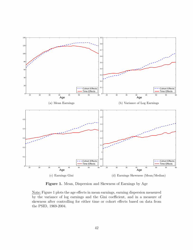
25 30 35 40 45 50 55 600

20

40

60

80

100

120

140

Age

Cohort EffectsTime Effects

(a) Mean Earnings

25 30 35 40 45 50 55 600

0.1

0.2

0.3

0.4

0.5

0.6

0.7

0.8

0.9

Age

Cohort EffectsTime Effects

(b) Variance of Log Earnings

25 30 35 40 45 50 55 600

0.1

0.2

0.3

0.4

0.5

Age

Cohort EffectsTime Effects

(c) Earnings Gini

25 30 35 40 45 50 55 600.8

0.9

1

1.1

1.2

1.3

1.4

1.5

1.6

Age

Cohort EffectsTime Effects

(d) Earnings Skewness (Mean/Median)

Figure 1. Mean, Dispersion and Skewness of Earnings by Age

Note: Figure 1 plots the age effects in mean earnings, earning dispersion measuredby the variance of log earnings and the Gini coefficient, and in a measure ofskewness after controlling for either time or cohort effects based on data fromthe PSID, 1969-2004.

42

25 30 35 40 45 50 55 600

20

40

60

80

100

120

140

Age

ModelData−Time

(a) Mean Earnings

25 30 35 40 45 50 55 600

0.1

0.2

0.3

0.4

0.5

0.6

0.7

0.8

0.9

Age

ModelData−Time

(b) Variance of Log Earnings

25 30 35 40 45 50 55 600

0.1

0.2

0.3

0.4

0.5

Age

ModelData−Time

(c) Earnings Gini

25 30 35 40 45 50 55 600.8

0.9

1

1.1

1.2

1.3

1.4

1.5

1.6

Age

ModelData−Time

(d) Earnings Skewness (Mean/Median)

Figure 2. Mean, Dispersion and Skewness of Earnings by Age: Time Effects

Note: Figure 2 plots the age effects in mean earnings, earnings dispersion mea-sured by the variance of log and the Gini coefficient, and in a measure of skewnessafter controlling for time effects based on data from the PSID, 1969-2004. Thefigure compares the model implication against the data estimates.

43

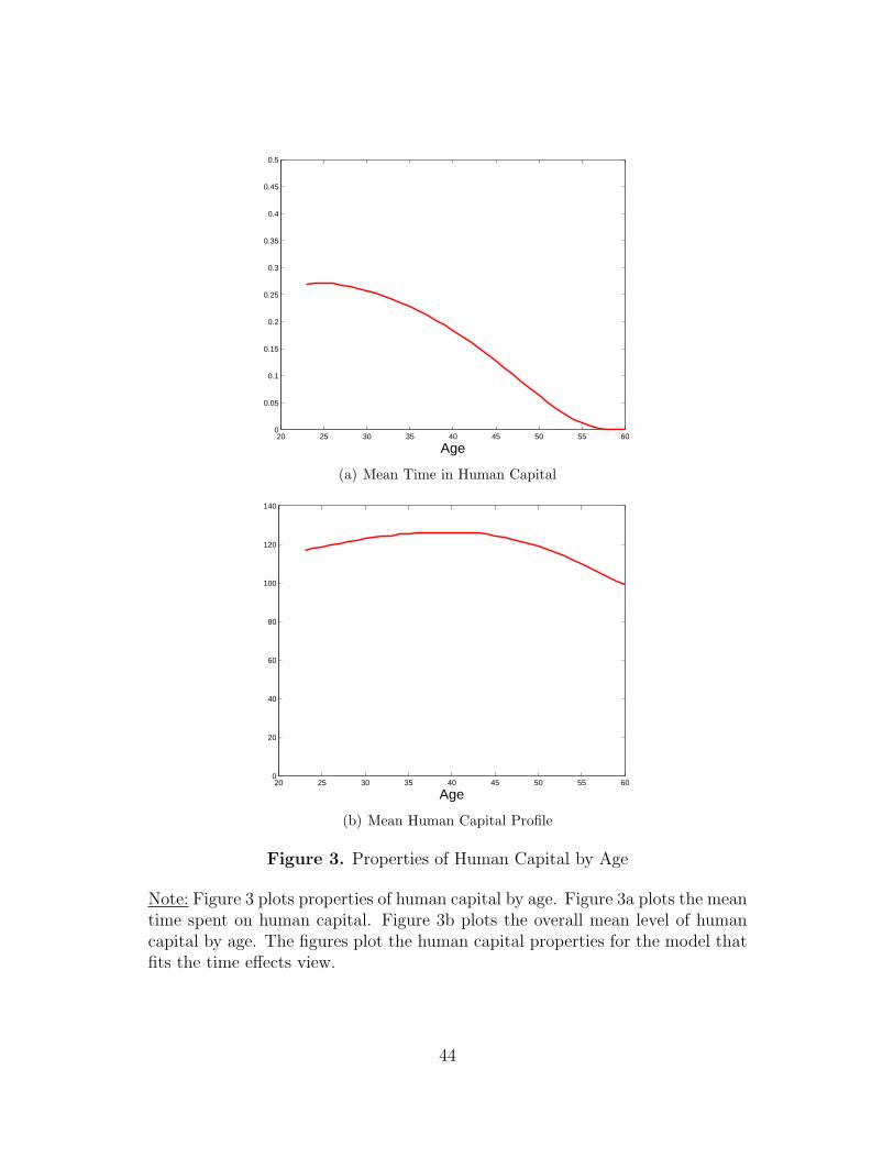
20 25 30 35 40 45 50 55 600

0.05

0.1

0.15

0.2

0.25

0.3

0.35

0.4

0.45

0.5

Age

(a) Mean Time in Human Capital

20 25 30 35 40 45 50 55 600

20

40

60

80

100

120

140

Age

(b) Mean Human Capital Profile

Figure 3. Properties of Human Capital by Age

Note: Figure 3 plots properties of human capital by age. Figure 3a plots the meantime spent on human capital. Figure 3b plots the overall mean level of humancapital by age. The figures plot the human capital properties for the model thatfits the time effects view.

44

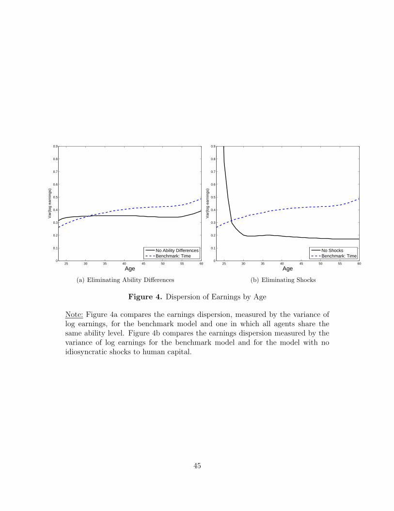
25 30 35 40 45 50 55 600

0.1

0.2

0.3

0.4

0.5

0.6

0.7

0.8

0.9

Age

Var

(log

earn

ings

)

No Ability DifferencesBenchmark: Time

(a) Eliminating Ability Differences

25 30 35 40 45 50 55 600

0.1

0.2

0.3

0.4

0.5

0.6

0.7

0.8

0.9

Age

Var

(log

earn

ings

)

No ShocksBenchmark: Time

(b) Eliminating Shocks

Figure 4. Dispersion of Earnings by Age

Note: Figure 4a compares the earnings dispersion, measured by the variance oflog earnings, for the benchmark model and one in which all agents share thesame ability level. Figure 4b compares the earnings dispersion measured by thevariance of log earnings for the benchmark model and for the model with noidiosyncratic shocks to human capital.

45

25 30 35 40 45 50 55 60−0.05

0

0.05

0.1

0.15

0.2

0.25

0.3

Age

Deaton and PaxsonPrimiceri and van−RensAguiar and HurstModel −− Time Effects

(a) Rise in Consumption Dispersion: Time Effects

Figure 5. Rise in Consumption Dispersion: Model and Data.

Note: Figure 5 plots the rise in the variance of log-consumption for ages 25-60both in U.S. data and the model. The data is based on Deaton and Paxson(1994), Primiceri and van Rens (2006), Aguiar and Hurst (2008). The modelresults are for the benchmark model with time effects.

46

0.5 0.55 0.6 0.65 0.7 0.75 0.8 0.85 0.90

0.1

0.2

0.3

0.4

0.5

0.6

0.7

0.8

0.9

1

Elasticity Parameter, α

o

Lifetime Earnings

Figure 6. Lifetime Inequality and the Elasticity Parameter α

Note: Figure 6 displays the fraction of the variance in lifetime earnings due toinitial conditions as the elasticity parameter α varies. The value correspondingto the best estimate of α is highlighted with a circle.

47