BS3b Statistical Lifetime-Models
115
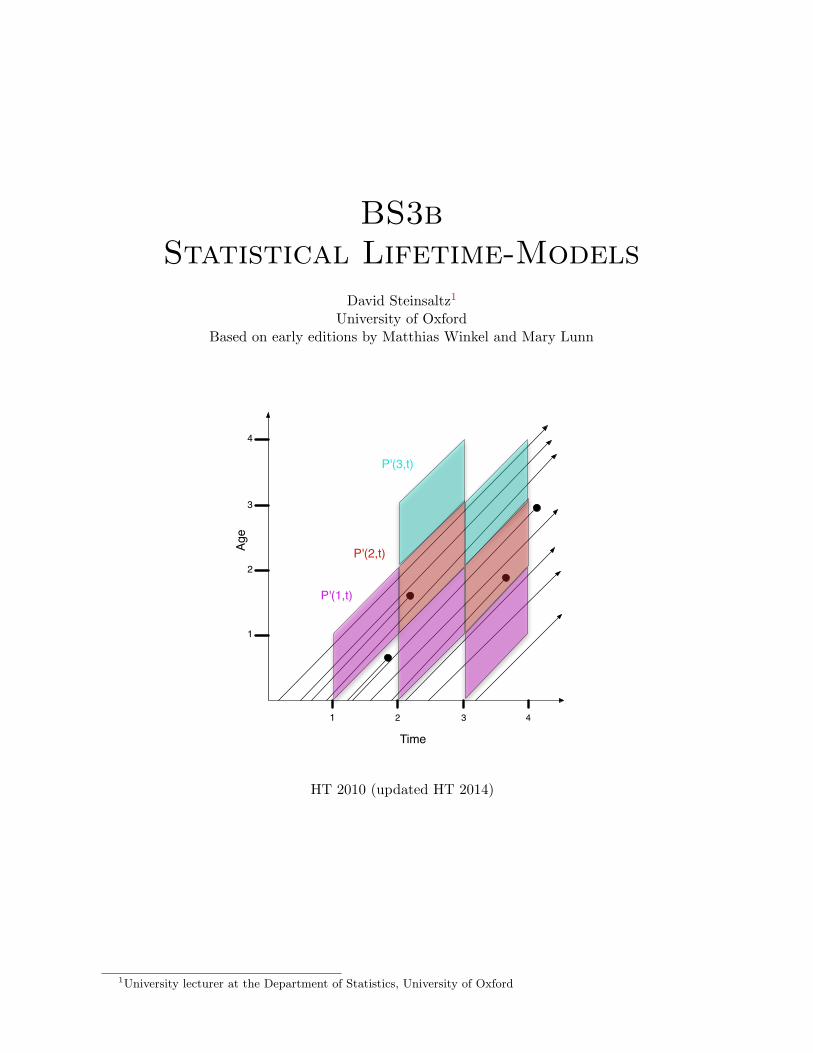
BS3b Statistical Lifetime-Models David Steinsaltz 1 University of Oxford Based on early editions by Matthias Winkel and Mary Lunn 1 2 3 4 1 2 3 4 Time Age P'(1,t) P'(2,t) P'(3,t) HT 2010 (updated HT 2014) 1 University lecturer at the Department of Statistics, University of Oxford
-
Upload
khangminh22 -
Category
Documents
-
view
0 -
download
0
Transcript of BS3b Statistical Lifetime-Models
BS3bStatistical Lifetime-Models
David Steinsaltz1
University of OxfordBased on early editions by Matthias Winkel and Mary Lunn
1 2 3 4
1
2
3
4
Time
Age
P'(1,t)
P'(2,t)
P'(3,t)
HT 2010 (updated HT 2014)
1University lecturer at the Department of Statistics, University of Oxford

BS3bStatistical Lifetime-Models
David Steinsaltz – 16 lectures HT [email protected]
Prerequisites
Part A Probability, Part A Statistics and Part B Applied Probability are prerequisites.
Website: http://www.steinsaltz.me.uk/BS3b/BS3b.html
Aims
Statistical Lifetime-Models follows on from Applied Probability. Models introduced there areexamined in the first part of the course more specifically in a life insurance context wheretransitions typically model the passage from ‘alive’ to ‘dead’, possibly with intermediate stageslike ‘loss of a limb’ or ‘critically ill’. The aim is to develop statistical methods to estimatetransition rates and more specifically to construct life tables that form the basis in the calculationof life insurance premiums.
We will then move on to survival analysis, which is widely used in medical research, inaddition to insurance, in which we consider the effect of covariates and of partially observeddata. We also explain demographic concepts, and how life tables are adapted to the context ofchanging mortality rates.
Synopsis
Survival models: general lifetime distributions, force of mortality (hazard rate), survival function,specific mortality laws, the single decrement model, curtate lifetimes, life tables, period andcohort.
Estimation procedures for lifetime distributions: empirical lifetime distributions, censoring,Kaplan-Meier estimate, Nelson-Aalen estimate. Parametric models, accelerated life modelsincluding Weibull, log-normal, log-logistic. Plot-based methods for model selection. Proportionalhazards, partial likelihood, semiparametric estimation of survival functions, use and overuse ofproportional hazards in insurance calculations and epidemiology.
Two-state and multiple-state Markov models, with simplifying assumptions. Estimationof Markovian transition rates: Maximum likelihood estimators, time-varying transition rates,census approximation. Applications to reliability, medical statistics, ecology.
Graduation, including fitting Gompertz-Makeham model, comparison with standard life table:tests including chi-square test and grouping of signs test, serial correlations test; smoothness.
iv
Exercises and Classes
Classes will be held on Fridays. There will be four sessions: 10-11, 11-12, 2-3, 3-4. Classassignments will be available on Minerva at https://minerva.stats.ox.ac.uk.
Scripts are to be handed in by Mondays 4pm in the Department of Statistics.The scope of exercises goes significantly beyond that of exam questions in many cases, but
understanding the exercises is essential to coping with the variety of exam questions that mightcome up. There is a great range of difficulty in the exercises, and most students should find atleast some of the exercises very challenging. Try all of them, but don’t spend hours and hourson questions if you are not making any progress.
Try to start solving exercises when you get the problem sheet, not the day before you haveto hand in your solutions. This allows you to have second attempts at exercises that you can’tsolve straight away.
Lecture notes are meant to be useful when solving exercises. You may use any result fromthe lectures, except where the contrary is explicitly stated.
Reading
There are lots of good books on survival analysis. Look for one that suits you. Some pointerswill be given in the lecture notes to readings that are connected, but look in the index to findtopics that confuse you and/or interest you.
The actuarial material in the course is modeled on the CT4 Core Reading from the Instituteof Actuaries.
CT4 Models Core Reading. Faculty & Institute of Actuaries
This is the core reading for the actuarial professional examination on survival models. In someplaces, the approach is more practically oriented and often placed in an insurance context,whereas the course is more academic and not only oriented towards insurance applications. Allin all, this is the main reference for about half the course. It is available for about £21.50 fromthe Institute of Actuaries on Worcester Street. (A few college libraries have it.)
D.R. Cox and D. Oakes: Analysis of Survival Data. Chapman & Hall (1984)
This is the classical text on survival analysis. The presentation is concise, but gives a broadview of the subject. The text contains exercises. This is the main reference for about half thecourse. It contains also much more related material beyond the scope of the course.
H.U. Gerber: Life Insurance Mathematics. 3rd edition, Springer (1997)
The presentation is concise. Only three chapters are relevant. Chapter 2 gives an introductionto lifetime distributions, Chapter 7 discusses the multiple decrement model and Chapter 11estimation procedures for lifetime distributions. The remainder combines the ideas with theinterest rate theory of BS4.
Klein & Moeschberger: Survival Analysis: Techniques for Censored and TruncatedData, 2nd edition, Springer (2003)
This is an excellent source for a lot of the survival analysis topics, particularly censoring andtruncation, and the Kaplan-Meier and Nelson-Aalen estimators. Lots of terrific examples.
Contents
1 Introduction: Survival Models 11.1 Early life tables . . . . . . . . . . . . . . . . . . . . . . . . . . . . . . . . . . . . . 11.2 Basic statistical methods for lifetime distributions . . . . . . . . . . . . . . . . . 2
1.2.1 Plot the data . . . . . . . . . . . . . . . . . . . . . . . . . . . . . . . . . . 31.2.2 Fit a model . . . . . . . . . . . . . . . . . . . . . . . . . . . . . . . . . . . 31.2.3 Significance test . . . . . . . . . . . . . . . . . . . . . . . . . . . . . . . . 6
1.3 Overview of the course . . . . . . . . . . . . . . . . . . . . . . . . . . . . . . . . . 7
2 Lifetime distributions 92.1 Survival function and hazard rate (force of mortality) . . . . . . . . . . . . . . . 92.2 Residual lifetimes . . . . . . . . . . . . . . . . . . . . . . . . . . . . . . . . . . . . 102.3 Force of mortality . . . . . . . . . . . . . . . . . . . . . . . . . . . . . . . . . . . 102.4 Defining mortality laws from hazards . . . . . . . . . . . . . . . . . . . . . . . . . 112.5 Curtate lifespan . . . . . . . . . . . . . . . . . . . . . . . . . . . . . . . . . . . . . 132.6 Single decrement model . . . . . . . . . . . . . . . . . . . . . . . . . . . . . . . . 132.7 Mortality laws: Simple or Complex? Parametric or Nonparametric? . . . . . . . 14
3 Life Tables 153.1 Notation for life tables . . . . . . . . . . . . . . . . . . . . . . . . . . . . . . . . . 183.2 Continuous and discrete models . . . . . . . . . . . . . . . . . . . . . . . . . . . . 18
3.2.1 General considerations . . . . . . . . . . . . . . . . . . . . . . . . . . . . . 183.2.2 Are life tables continuous or discrete? . . . . . . . . . . . . . . . . . . . . 19
3.3 Interpolation for non-integer ages . . . . . . . . . . . . . . . . . . . . . . . . . . . 203.4 Crude estimation of life tables – discrete method . . . . . . . . . . . . . . . . . . 213.5 Crude life table estimation – continuous method . . . . . . . . . . . . . . . . . . 223.6 Comparing continuous and discrete methods . . . . . . . . . . . . . . . . . . . . . 233.7 An example: Fractional lifetimes can matter . . . . . . . . . . . . . . . . . . . . . 24
4 Cohorts and Period Life Tables 254.1 Types of life tables . . . . . . . . . . . . . . . . . . . . . . . . . . . . . . . . . . . 254.2 Life Expectancy . . . . . . . . . . . . . . . . . . . . . . . . . . . . . . . . . . . . . 28
4.2.1 What is life expectancy? . . . . . . . . . . . . . . . . . . . . . . . . . . . . 284.2.2 Example . . . . . . . . . . . . . . . . . . . . . . . . . . . . . . . . . . . . . 294.2.3 Life expectancy and mortality . . . . . . . . . . . . . . . . . . . . . . . . . 29
4.3 An example of life-table computations . . . . . . . . . . . . . . . . . . . . . . . . 30
v
vi Contents
5 Central exposed to risk and the census approximation 32
5.1 Censoring . . . . . . . . . . . . . . . . . . . . . . . . . . . . . . . . . . . . . . . . 32
5.2 Insurance data . . . . . . . . . . . . . . . . . . . . . . . . . . . . . . . . . . . . . 32
5.3 Census approximation . . . . . . . . . . . . . . . . . . . . . . . . . . . . . . . . . 33
5.4 Lexis diagrams . . . . . . . . . . . . . . . . . . . . . . . . . . . . . . . . . . . . . 34
6 Comparing life tables 40
6.1 The binomial model . . . . . . . . . . . . . . . . . . . . . . . . . . . . . . . . . . 40
6.2 The Poisson model . . . . . . . . . . . . . . . . . . . . . . . . . . . . . . . . . . . 41
6.3 Testing hypotheses for qx and µx+ 12
. . . . . . . . . . . . . . . . . . . . . . . . . . 42
6.3.1 The tests . . . . . . . . . . . . . . . . . . . . . . . . . . . . . . . . . . . . 43
6.3.2 An example . . . . . . . . . . . . . . . . . . . . . . . . . . . . . . . . . . . 44
6.4 Graduation . . . . . . . . . . . . . . . . . . . . . . . . . . . . . . . . . . . . . . . 45
6.4.1 Parametric models . . . . . . . . . . . . . . . . . . . . . . . . . . . . . . . 45
6.4.2 Reference to a standard table . . . . . . . . . . . . . . . . . . . . . . . . . 45
6.4.3 Nonparametric smoothing . . . . . . . . . . . . . . . . . . . . . . . . . . . 46
6.4.4 Methods of fitting . . . . . . . . . . . . . . . . . . . . . . . . . . . . . . . 46
6.4.5 Examples . . . . . . . . . . . . . . . . . . . . . . . . . . . . . . . . . . . . 47
7 Multiple decrements model 51
7.1 The Poisson model . . . . . . . . . . . . . . . . . . . . . . . . . . . . . . . . . . . 51
7.2 Rates in the single decrement model . . . . . . . . . . . . . . . . . . . . . . . . . 52
7.3 Multiple decrement models . . . . . . . . . . . . . . . . . . . . . . . . . . . . . . 53
7.3.1 An introductory example . . . . . . . . . . . . . . . . . . . . . . . . . . . 53
7.3.2 Basic theory . . . . . . . . . . . . . . . . . . . . . . . . . . . . . . . . . . 55
7.3.3 Multiple decrements – time-homogeneous rates . . . . . . . . . . . . . . . 55
8 Multiple Decrements: Theory and Examples 56
8.1 Estimation for general multiple decrements . . . . . . . . . . . . . . . . . . . . . 56
8.2 Example: Workforce model . . . . . . . . . . . . . . . . . . . . . . . . . . . . . . 57
9 Multiple decrements: The distribution of the endpoint 58
9.1 Which state do we end up in? . . . . . . . . . . . . . . . . . . . . . . . . . . . . . 58
9.2 Cohabitation dissolution model . . . . . . . . . . . . . . . . . . . . . . . . . . . . 59
Contents vii
10 Continuous-time Markov chains 6310.1 General Markov chains . . . . . . . . . . . . . . . . . . . . . . . . . . . . . . . . . 63
10.1.1 Discrete time, estimation of Π-matrix . . . . . . . . . . . . . . . . . . . . 6310.1.2 Estimation of the Q-matrix . . . . . . . . . . . . . . . . . . . . . . . . . . 63
10.2 The induced Poisson process . . . . . . . . . . . . . . . . . . . . . . . . . . . . . 6410.3 Parametric and time-dependent models . . . . . . . . . . . . . . . . . . . . . . . 67
10.3.1 Example: Marital status model . . . . . . . . . . . . . . . . . . . . . . . . 6810.3.2 The general simple birth-and-death process . . . . . . . . . . . . . . . . . 6910.3.3 Lower-dimensional parametric models of simple birth-and-death processes 69
10.4 Time-varying transition rates . . . . . . . . . . . . . . . . . . . . . . . . . . . . . 7010.4.1 Maximum likelihood estimation . . . . . . . . . . . . . . . . . . . . . . . . 7010.4.2 Example . . . . . . . . . . . . . . . . . . . . . . . . . . . . . . . . . . . . . 7110.4.3 Construction of the stochastic process (Xt)t≥0 . . . . . . . . . . . . . . . 71
10.5 Occupation times . . . . . . . . . . . . . . . . . . . . . . . . . . . . . . . . . . . . 7310.5.1 The multiple decrements model . . . . . . . . . . . . . . . . . . . . . . . . 7410.5.2 The illness model . . . . . . . . . . . . . . . . . . . . . . . . . . . . . . . . 74
11 Survival analysis: Introduction 7611.1 [ . . . . . . . . . . . . . . . . . . . . . . . . . . . . . . . . . . . . . . . . . . . . . 7611.2 Likelihood and Censoring . . . . . . . . . . . . . . . . . . . . . . . . . . . . . . . 7711.3 Data . . . . . . . . . . . . . . . . . . . . . . . . . . . . . . . . . . . . . . . . . . . 7711.4 Non-parametric survial estimation . . . . . . . . . . . . . . . . . . . . . . . . . . 78
11.4.1 Review of basic concepts . . . . . . . . . . . . . . . . . . . . . . . . . . . . 7811.4.2 Kaplan-Meier estimator . . . . . . . . . . . . . . . . . . . . . . . . . . . . 8011.4.3 Nelson-Aalen estimator and new estimator of S . . . . . . . . . . . . . . . 8011.4.4 Invented data set . . . . . . . . . . . . . . . . . . . . . . . . . . . . . . . . 81
12 Confidence intervals and left truncation 8212.1 Greenwood’s formula . . . . . . . . . . . . . . . . . . . . . . . . . . . . . . . . . . 82
12.1.1 Reminder of the δ method . . . . . . . . . . . . . . . . . . . . . . . . . . . 8212.1.2 Derivation of Greenwood’s formula for var(S(t)) . . . . . . . . . . . . . . 83
12.2 Left truncation . . . . . . . . . . . . . . . . . . . . . . . . . . . . . . . . . . . . . 8412.3 Example: The AML study . . . . . . . . . . . . . . . . . . . . . . . . . . . . . . . 8512.4 Actuarial estimator . . . . . . . . . . . . . . . . . . . . . . . . . . . . . . . . . . . 88
13 Semiparametric models: accelerated life, proportional hazards 8913.1 Introduction to semiparametric modeling . . . . . . . . . . . . . . . . . . . . . . 8913.2 Accelerated Life models . . . . . . . . . . . . . . . . . . . . . . . . . . . . . . . . 89
13.2.1 Medians and Quantiles . . . . . . . . . . . . . . . . . . . . . . . . . . . . . 9013.3 Proportional Hazards models . . . . . . . . . . . . . . . . . . . . . . . . . . . . . 90
13.3.1 Plots . . . . . . . . . . . . . . . . . . . . . . . . . . . . . . . . . . . . . . . 9013.4 AL parametric models . . . . . . . . . . . . . . . . . . . . . . . . . . . . . . . . . 90
13.4.1 Plots for parametric models . . . . . . . . . . . . . . . . . . . . . . . . . . 9113.4.2 Regression in parametric AL models (assuming right censoring only) . . . 9213.4.3 Linear regression in parametric AL models . . . . . . . . . . . . . . . . . 93
viii Contents
14 Cox regression, Part I 9414.1 What is Cox Regression? . . . . . . . . . . . . . . . . . . . . . . . . . . . . . . . 9414.2 Relative Risk . . . . . . . . . . . . . . . . . . . . . . . . . . . . . . . . . . . . . . 9514.3 Baseline hazard . . . . . . . . . . . . . . . . . . . . . . . . . . . . . . . . . . . . . 96
15 Cox regression, Part II 9815.1 Dealing with ties . . . . . . . . . . . . . . . . . . . . . . . . . . . . . . . . . . . . 9815.2 Plot for PH assumption with continuous covariate . . . . . . . . . . . . . . . . . 9915.3 The AML example . . . . . . . . . . . . . . . . . . . . . . . . . . . . . . . . . . . 99
16 Testing Hypotheses 10316.1 Tests in the regression setting . . . . . . . . . . . . . . . . . . . . . . . . . . . . . 10316.2 Non-parametric testing of survival between groups . . . . . . . . . . . . . . . . . 103
16.2.1 General principles . . . . . . . . . . . . . . . . . . . . . . . . . . . . . . . 10316.2.2 Standard tests . . . . . . . . . . . . . . . . . . . . . . . . . . . . . . . . . 104
16.3 The AML example . . . . . . . . . . . . . . . . . . . . . . . . . . . . . . . . . . . 106
Bibliography 106
Lecture 1
Introduction: Survival Models
1.1 Early life tables
In one of the earliest treatises on probability George Leclerc Buffon considered the problem offinding the fundamental unit of risk, the smallest discernible probability. He wrote that “all fearor hope, whose probability equals that which produces the fear of death, in the moral realmmay be taken as unity against which all other fears are to be measured.” [Buf77, p. 56] In otherwords, because no healthy man in the prime of life (he argued) attends to the risk that he maydie in the next twenty-four hours, Buffon considered that events with this probability could betreated as negligible; after all, “since the intensity of the fear of death is a good deal greaterthan the intensity of any other fear or hope,” any other risk of equivalent probability of a lesstroubling event — such as winning a lottery — would leave a person equally indifferent. Hedecided that the appropriate age to consider for a man to be in the prime of health was 56 years.But what is that probability, that a 56 year old man dies in the next day?
To answer this, Buffon turned to mortality tables. A colleague (one M. Dupre of Saint-Maur)assembled the registers of 12 rural parishes and 3 parishes of Paris, in which 23,994 deaths wererecorded. The ages at death were all recorded, so that he knew that 174 of the deaths were atage 56; that is, between the 56th and 57th birthdays.1 Our naıve estimator for the probabilityof an event is
probability of occurrence =number of occurrences
number of opportunities.
The number of occurrences of the event (death of an individual aged 56) is observed to be174. But what about the denominator? The number of “opportunities” for this event is justthe number of individuals in the population at the appropriate age. The most direct way todetermine this number would be a time-consuming census. Buffon’s approach (and that ofother 17th and 18th creators of such life tables) depended upon the following implicit logic:Suppose the population is stable, so that the same number of people in each age group die eachyear. Since every person dies at some time (it is believed), the total number of people in thepopulation who live to their 56th birthday will be exactly the same as the number of peopleobserved to have died after their 56th birthday in the particular year under observation, whichhappens to be 5031. The probability of dying in one day may then be estimated as
1365
× 1745031
≈ 110000
,
1Actually, Buffon’s statistical procedure was a bit more complicated than this. The recorded numbers of deathsat ages 55,56,57,58,59,60 were 280,130,129,182,90,534 respectively. Buffon observed that the priests (“particularlythe country priests”) were likely to record round numbers for the age at death, rather than the exact age — whichthey may not know anyway. He thus decided that it would make more sense to smooth (as statisticians would callthe procedure today) or graduate (as actuaries call it) the data. We will learn about graduation in Lecture.
1

2 Lecture Notes – Part B Statistical Lifetime-Models – Oxford HT 2010-14
and Buffon proceeds to reason with this estimate.
From this elementary exercise we see that:
• Mortality probabilities can be estimated as the ratio of the number of deaths to the numberof individuals “at risk”.
• The numerator (the number of deaths) is usually straightforward to determine.
• The denominator (the number at risk) can be challenging.
• Mortality can serve as a model for thinking about risks (and opportunities) more generally,for events happening at random times.
• You don’t get very far in thinking about mortality and other risks without some sort oftheoretical model.
The last claim may require a bit more elucidation. What would a naıve, empirical approachto life tables look like? Given a census of the population by age, and a list of the ages at deathin the following year, we could compute the proportion of individuals aged x who died in thefollowing year. This is merely a free-floating fact, which could be compared with other facts,such as the measured proportion of individuals aged x who died in a different year (or at adifferent age, or a different place, etc.) If you want to talk about a probability of dying in thatyear (for which the proportion would serve as an estimate), this is a theoretical construct, whichcan be modelled (as we will see) in different ways. Once you have a probability model, thisallows you to pose (and perhaps answer) questions about the probability of dying in a given day,make predictions about past and future trends, and isolate the effect of certain medications orlife-style changes on mortality.
There are many different kinds of problems for which the same survival analysis statisticsmay be applied. Some examples which we will consider at various points in this course are:
• Time to failure of a machine with multiple internal components.
• Time from infection until a subject shows signs of illness.
• Time from starting to try to conceive a baby until a woman is pregnant.
• Time until a person diagnosed with (and perhaps treated for) a disease has a recurrence.
• Time until an unmarried couple marries or separates.
Often, though, we will use the term “lifetime” to represent any waiting time, along with itsattendant vocabulary: survival probability, mortality rate, cause of death, etc.
1.2 Basic statistical methods for lifetime distributions
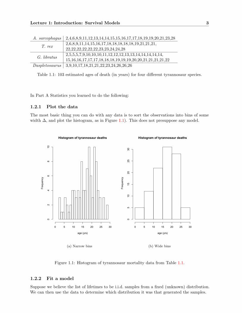
In Table 1.1 we see the estimated ages at death for 103 tyrannosaurs, from four different species,as reported in [ECIW06]. Let us treat them here as a single population.
Lecture 1: Introduction: Survival Models 3
A. sarcophagus 2,4,6,8,9,11,12,13,14,14,15,15,16,17,17,18,19,19,20,21,23,28
T. rex2,6,8,9,11,14,15,16,17,18,18,18,18,18,19,21,21,21,22,22,22,22,22,22,23,23,24,24,28
G. libratus2,5,5,5,7,9,10,10,10,11,12,12,12,13,13,14,14,14,14,14,15,16,16,17,17,17,18,18,18,19,19,19,20,20,21,21,21,21,22
Daspletosaurus 3,9,10,17,18,21,21,22,23,24,26,26,26
Table 1.1: 103 estimated ages of death (in years) for four different tyrannosaur species.
In Part A Statistics you learned to do the following:
1.2.1 Plot the data
The most basic thing you can do with any data is to sort the observations into bins of somewidth ∆, and plot the histogram, as in Figure 1.1). This does not presuppose any model.
Histogram of tyrannosaur deaths
age (yrs)
Frequency
0 5 10 15 20 25 30
02
46
810
(a) Narrow bins
Histogram of tyrannosaur deaths
age (yrs)
Frequency
0 5 10 15 20 25 30
05
1015
2025
30
(b) Wide bins
Figure 1.1: Histogram of tyrannosaur mortality data from Table 1.1.
1.2.2 Fit a model
Suppose we believe the list of lifetimes to be i.i.d. samples from a fixed (unknown) distribution.We can then use the data to determine which distribution it was that generated the samples.
4 Lecture Notes – Part B Statistical Lifetime-Models – Oxford HT 2010-14
In Part A statistics you learned parametric maximum likelihood estimation. Suppose theunknown distribution is believed to be one of a family of distributions that is indexed by apossibly multivariate (k-dimensional) parameter λ ∈ Λ ⊂ Rk. That is — taking just the caseof data from a continuous distribution — the distribution of the independent observations hasdensity f(T ; λ) at the point T , if the true value of the parameter is λ. Suppose we have observedn independent lifetimes T1, . . . , Tn. We define the log-likelihood function to be the (natural) logof the density of the observations, considered as a function of the parameter. By the assumptionof independence, this is
`T1,...,Tn(λ) = `T :=n∑
i=1
ln f(Ti;λ). (1.1)
(We use T to represent the vector (T1, . . . , Tn).) The maximum likelihood estimator (MLE) issimply the value of λ that makes this as large as possible:
λ = λ(T) = λ(T1, . . . , Tn) := arg maxλ∈Λ
n∏i=1
f(Ti;λ). (1.2)
Notice the nomenclature: maxλ∈Λ f(λ) picks the maximal value in the range of f , arg maxλ∈Λ f(λ)picks the λ-value in the domain of f for which this maximum is attained.
The most basic model for lifetimes is the exponential. This is the “memoryless” waiting-time distribution, meaning that the remaining waiting time always has the same distribution,conditioned on the event not having occurred up to any time t. This distribution has a singleparameter (k = 1) µ, and density
f(µ;T ) = µe−µT .
The parameter µ is chosen from the domain Λ = (0,∞). If we observe independent lifetimesT1, . . . , Tn from the exponential distribution with parameter µ, and let T := n−1
∑ni=1 Ti be the
average, the log likelihood is
`T(µ) =n∑
i=1
ln(µe−µTi
)= n
(lnµ− T µ
),
which has maximum at µ = 1/T = n/∑
Ti. This is an example of what we will see to be ageneral principle:
Estimated rate =# events
total time at risk. (1.3)
In some cases we will be thinking of the time as random, in other cases the number of events,but the formula (1.3) remains. The challenge will be to estimate the number of events and thetotal time in a way that they correspond to the same time period and the same population,since they are often estimated from different data sources and timed in different ways.
For large n, the estimator λ(T1, . . . , Tn) is approximately normally distributed, under someregularity conditions, and it has some other optimality properties (finite-sample and asymptotic).This allows us to construct approximate confidence intervals/regions to indicate the precision ofmaximum likelihood estimates. Specifically, for
λ ∼ N(λ, (I(λ))−1
), where Ij1j2(λ) = −E
[∂2
∂λj1∂λj2
n∑i=1
ln(f(Ti;λ))
]= −E
[∂2`T(λ)∂λj1∂λj2
]are the entries of the Fisher Information matrix. Of course, we generally don’t know what λis — otherwise, we probably would not be bothering to estimate it! — so we may approximate
Lecture 1: Introduction: Survival Models 5
the Information matrix by computing Ij1j2(λ) instead. Furthermore, we may not be able tocompute the expectation in any straightforward way; in that case, we use the principle of MonteCarlo estimation: We approximate the expectation of a random variable by the average of asample of observations. We already have the sample T1, . . . , Tn from the correct distribution, sowe define the observed information matrix
Jj1j2(λ, T1, . . . , Tn) = − 1n
n∑i=1
∂2 ln f(Ti;λ)∂λj1∂λj2
.
Again, we may substitute Jj1j2(λ, T1, . . . , Tn), since the true value of λ is unknown. Thus, inthe case of a one-dimensional parameter (where the covariance matrix is just the variance andthe matrix inverse (I(λ))−1 is just the multiplicative inverse in R), we obtain[
λ− 1.96
√1
I(λ), λ + 1.96
√1
I(λ)
]
as an approximate 95% confidence interval for the unknown parameter λ.In the case of the exponential model, we have
`′′T(µ) = − n
µ2,
so that the standard error for µ is µ/√
n, which we estimate by µ/√
n. For the tyrannosaur dataof Table 1.1, we have
T = 16.03,
µ = 0.062,
SEµ = 0.0061,
95% confidence interval for µ = (0.050, 0.074).
Aside: In the special case of exponential lifetimes, we can construct exact confidence intervals,since we know the distribution of n/µ ∼ Γ(n, µ), so that 2nµ/µ ∼ χ2
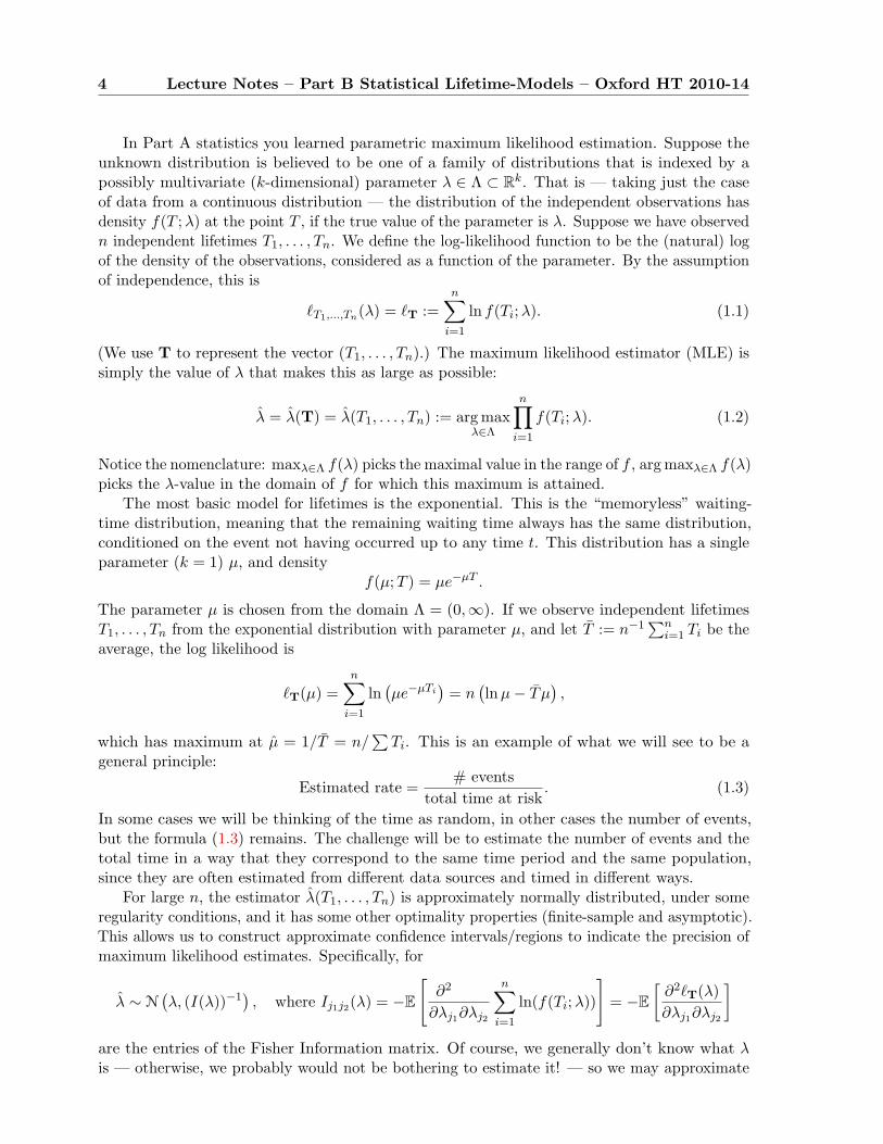
2n allows to use χ2-tables.Is the fit any good? We have various standard methods of testing goodness of fit — we
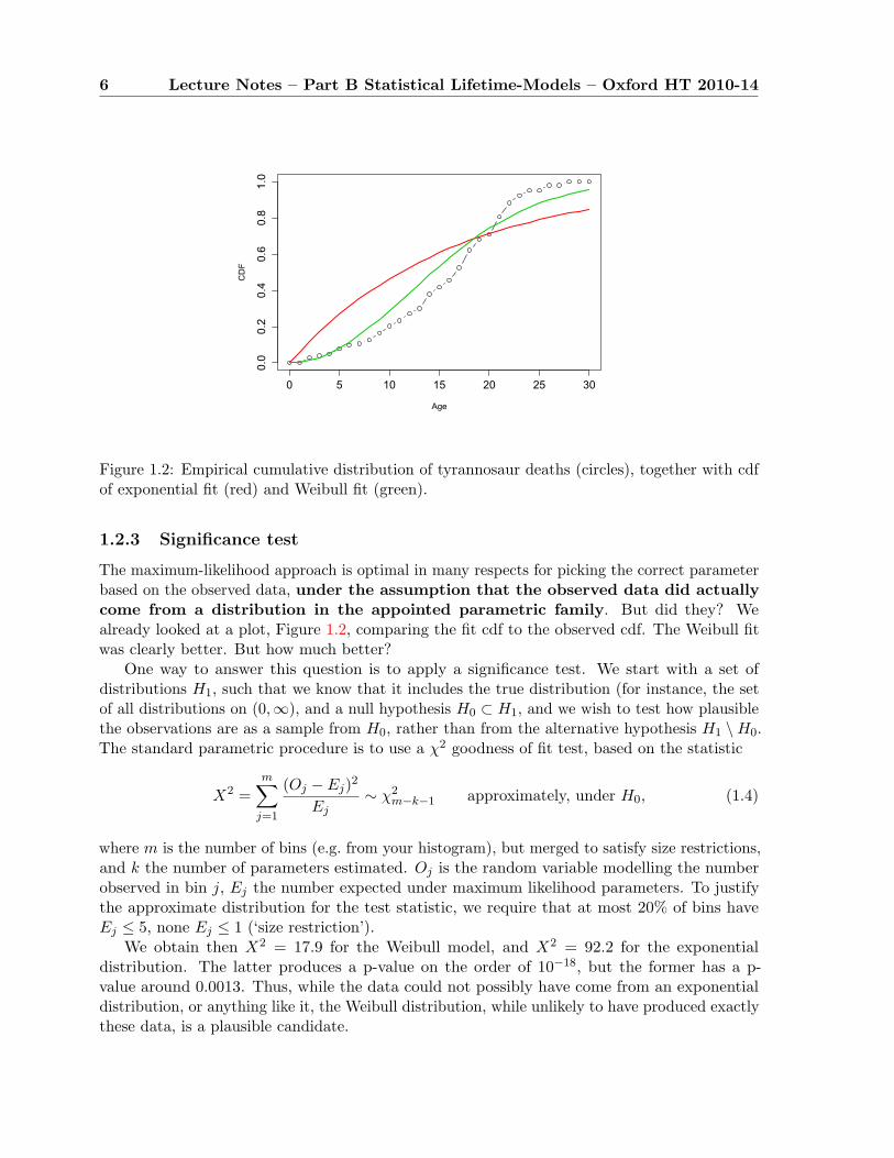
discuss an example in section 1.2.3 — but it’s pretty easy to see by eye that the histograms inFigure 1.1 aren’t going to fit an exponential distribution, which is a declining density, very well.In Figure 1.2 we show the empirical (observed) cumulative distribution of tyrannosaur deaths,together with the cdf of the best exponential fit, which is obviously not a very good fit at all.
We also show (in green) the fit to a class of distribution which is an example of a largerclass that we will meet later, called the “Weibull” distributions. Instead of the exponential cdfF (t) = 1− e−µt, suppose we take F (t) = 1− e−αt2 . Note that if we define Yi = T 2
i , we have
P (Yi ≤ y) = P (Ti ≤√
y) = 1− e−αy,
so Yi is actually exponentially distributed with parameter α. Thus, the MLE for α is
α =n∑T 2
i
.
We see in Figure 1.2 that this fits much better than the exponential distribution.
6 Lecture Notes – Part B Statistical Lifetime-Models – Oxford HT 2010-14
0 5 10 15 20 25 30
0.0
0.2
0.4
0.6
0.8
1.0
Age
CDF
Figure 1.2: Empirical cumulative distribution of tyrannosaur deaths (circles), together with cdfof exponential fit (red) and Weibull fit (green).
1.2.3 Significance test
The maximum-likelihood approach is optimal in many respects for picking the correct parameterbased on the observed data, under the assumption that the observed data did actuallycome from a distribution in the appointed parametric family. But did they? Wealready looked at a plot, Figure 1.2, comparing the fit cdf to the observed cdf. The Weibull fitwas clearly better. But how much better?
One way to answer this question is to apply a significance test. We start with a set ofdistributions H1, such that we know that it includes the true distribution (for instance, the setof all distributions on (0,∞), and a null hypothesis H0 ⊂ H1, and we wish to test how plausiblethe observations are as a sample from H0, rather than from the alternative hypothesis H1 \H0.The standard parametric procedure is to use a χ2 goodness of fit test, based on the statistic
X2 =m∑
j=1
(Oj − Ej)2
Ej∼ χ2
m−k−1 approximately, under H0, (1.4)
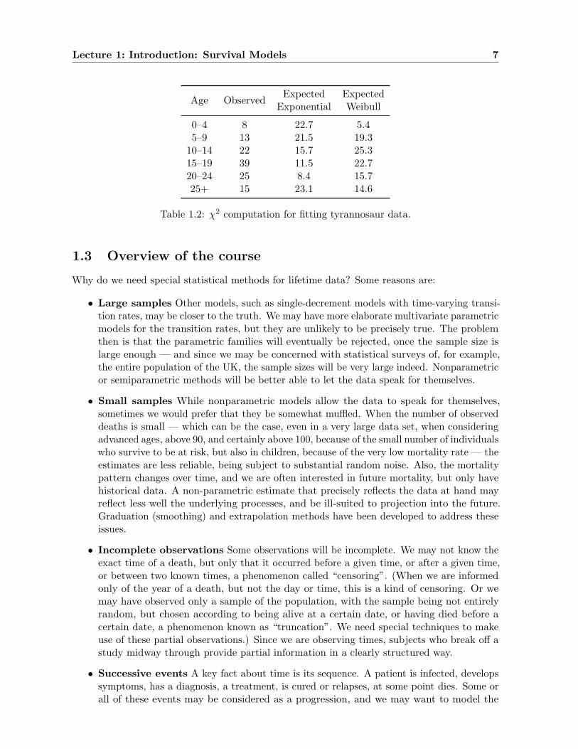
where m is the number of bins (e.g. from your histogram), but merged to satisfy size restrictions,and k the number of parameters estimated. Oj is the random variable modelling the numberobserved in bin j, Ej the number expected under maximum likelihood parameters. To justifythe approximate distribution for the test statistic, we require that at most 20% of bins haveEj ≤ 5, none Ej ≤ 1 (‘size restriction’).
We obtain then X2 = 17.9 for the Weibull model, and X2 = 92.2 for the exponentialdistribution. The latter produces a p-value on the order of 10−18, but the former has a p-value around 0.0013. Thus, while the data could not possibly have come from an exponentialdistribution, or anything like it, the Weibull distribution, while unlikely to have produced exactlythese data, is a plausible candidate.
Lecture 1: Introduction: Survival Models 7
Age ObservedExpected Expected
Exponential Weibull
0–4 8 22.7 5.45–9 13 21.5 19.3
10–14 22 15.7 25.315–19 39 11.5 22.720–24 25 8.4 15.725+ 15 23.1 14.6
Table 1.2: χ2 computation for fitting tyrannosaur data.
1.3 Overview of the course
Why do we need special statistical methods for lifetime data? Some reasons are:
• Large samples Other models, such as single-decrement models with time-varying transi-tion rates, may be closer to the truth. We may have more elaborate multivariate parametricmodels for the transition rates, but they are unlikely to be precisely true. The problemthen is that the parametric families will eventually be rejected, once the sample size islarge enough — and since we may be concerned with statistical surveys of, for example,the entire population of the UK, the sample sizes will be very large indeed. Nonparametricor semiparametric methods will be better able to let the data speak for themselves.
• Small samples While nonparametric models allow the data to speak for themselves,sometimes we would prefer that they be somewhat muffled. When the number of observeddeaths is small — which can be the case, even in a very large data set, when consideringadvanced ages, above 90, and certainly above 100, because of the small number of individualswho survive to be at risk, but also in children, because of the very low mortality rate — theestimates are less reliable, being subject to substantial random noise. Also, the mortalitypattern changes over time, and we are often interested in future mortality, but only havehistorical data. A non-parametric estimate that precisely reflects the data at hand mayreflect less well the underlying processes, and be ill-suited to projection into the future.Graduation (smoothing) and extrapolation methods have been developed to address theseissues.
• Incomplete observations Some observations will be incomplete. We may not know theexact time of a death, but only that it occurred before a given time, or after a given time,or between two known times, a phenomenon called “censoring”. (When we are informedonly of the year of a death, but not the day or time, this is a kind of censoring. Or wemay have observed only a sample of the population, with the sample being not entirelyrandom, but chosen according to being alive at a certain date, or having died before acertain date, a phenomenon known as “truncation”. We need special techniques to makeuse of these partial observations.) Since we are observing times, subjects who break off astudy midway through provide partial information in a clearly structured way.
• Successive events A key fact about time is its sequence. A patient is infected, developssymptoms, has a diagnosis, a treatment, is cured or relapses, at some point dies. Some orall of these events may be considered as a progression, and we may want to model the

8 Lecture Notes – Part B Statistical Lifetime-Models – Oxford HT 2010-14
sequence of random times. Some care is needed to carry out joint maximum likelihoodestimation of all transition rates in the model, from one or several individuals observed.This can be combined with time-varying transition rates.
• Comparing lifetime distributions We may wish to compare the lifetime distributionsof different groups (e.g., smokers and nonsmokers; those receiving a traditional cholesterolmedication and those receiving the new drug) or the effect of a continuous parameter (e.g.,weight) on the lifetime distribution.
• Changing rates Mortality rates are not static in time, creating disjunction betweenperiod measures — looking at a cross-section of the population by age as it exists at agiven time — and cohort measures — looking at a group of individuals born at a giventime, and following them through life.
Lecture 2
Lifetime distributions
All the stochastic models in this course will be within the class of discrete state-space Markovprocesses which may be time inhomogeneous. We will not be using the general form of thesemodels, but will be simplifying and specialising them substantially. What unifies this courseis the nature of the questions we will be asking. In the standard theory of Markov processes,we focus early on stationary processes. Our models will not be stationary, because they haveabsorbing states. The key questions will concern the absorbing states: When the process isabsorbed (the “lifetime”), and, in some models, which state absorbs it.
We need to be careful to distinguish between representations of the population and repre-sentations of the individual. In the present context, the Markov process always represents anindividual. The population consists of some number of independently running copies of the basicMarkov process. In simple cases — for instance, exponential mortality — the population-levelprocess (total population at time t) will also be a Markov process, a “pure-death” chain. Thisraises the complication that there are usually two different kinds of time running: The “internal”time of the individual process, which usually represents age in some way, and calendar time.The full implications of these interacting time-frames — also called the cohort and the periodperspective — are a major topic in demography, and we will only touch on them in this course.
2.1 Survival function and hazard rate (force of mortality)
As discussed in chapter 1, the simplest lifetime model is the single-decrement model: Theindividual is alive for some length of time L, at the end of which he/she becomes dead. This isa homogeneous Markov process if and only if L has an exponential distribution. In general, wemay describe a lifetime distribution — which is simply the distribution of a nonnegative randomvariable — in several different ways:
cdf F (t) = P{L ≤ t
};
survival function S(t) = F (t) = 1− F (t) = P{L > t
};
density function f(t) = dF/dt;hazard rate λ(t) = f(t)/F (t)
The hazard rate is also called mortality rate in survival contexts. The traditional name indemography is force of mortality. This may be thought of as the instantaneous rate of dying perunit time, conditioned on having already survived.s The exponential distribution with parameterλ ∈ (0,∞) is given by
9
10 Lecture Notes – Part B Statistical Lifetime-Models – Oxford HT 2010-14
cdf F (t) = 1− e−λt;survival function F (t) = e−λt;density function f(t) = λe−λt;
hazard rate λ(t) = λ.
Thus, the exponential is the distribution with constant force of mortality, which is a formalstatement of the “memoryless” property.
2.2 Residual lifetimes
Assume that there is an overall lifetime distribution, and every individual born has a randomlifetime according to this distribution. Then, if we observe sombody now aged x, and we denotehis residual lifetime T − x by Tx, then we have
FTx(t) = FT−x|T>x(t) =FT (x + t)
FT (x), fTx(t) = fT−x|T>x(t) =
fT (x + t)FT (x)
, t ≥ 0. (2.1)
So, any distribution of a full lifetime T is naturally associated with a family of conditionaldistributions of T given T > x.
2.3 Force of mortality
We now look more closely at the hazard rate, which may be defined as
hT (t) = µt = limε↓0
1εP(T ≤ t + ε|T > t) = lim
ε↓0
1εP(t < T ≤ t + ε)
P(T > t)=
fT (t)FT (t)
. (2.2)
The density fT (t) is the (unconditional) infinitesimal probability to die at age t. The hazardrate hT (t) is the (conditional) infinitesimal probability to die at age t of an individual known tobe alive at age t. It may seem that the hazard rate is a more complicated quantity than thedensity, but it is very well suited to modelling mortality. Whereas the density has to integrateto one and the distribution function (survival function) has boundary values 0 and 1, the forceof mortality has no constraints, other than being nonnegative — though if “death” is certain theforce of mortality has to integrate to infinity. Also, we can read its definition as a differentialequation and solve
F ′T (t) = −µtFT (t), F (0) = 1 ⇒ FT (t) = exp
{−∫ t
0µsds
}, t ≥ 0. (2.3)
We can now express the distribution of Tx as
FTx(t) =FT (x + t)
FT (x)= exp
{−∫ x+t
xµsds
}= exp
{−∫ t
0µx+rdr
}, t ≥ 0. (2.4)
Note that this implies that hTx(t) = hT (x + t), so it is really associated with age x + t only, notwith initial age x nor with time t after initial age. Also note that, given a measurable functionµ : [0,∞) → R, FTx(0) = 1 always holds, FTx decreasing if and only if µ ≥ 0. FTx(∞) = 0 if andonly if
∫∞0 µtdt = ∞. This leaves a lot of modelling freedom via the force of mortality.
Densities can now be obtained from the definition of the force of mortality (and consistency)as fTx(t) = µt+xFTx(t).
Lecture 2: Lifetime distributions 11
2.4 Defining mortality laws from hazards
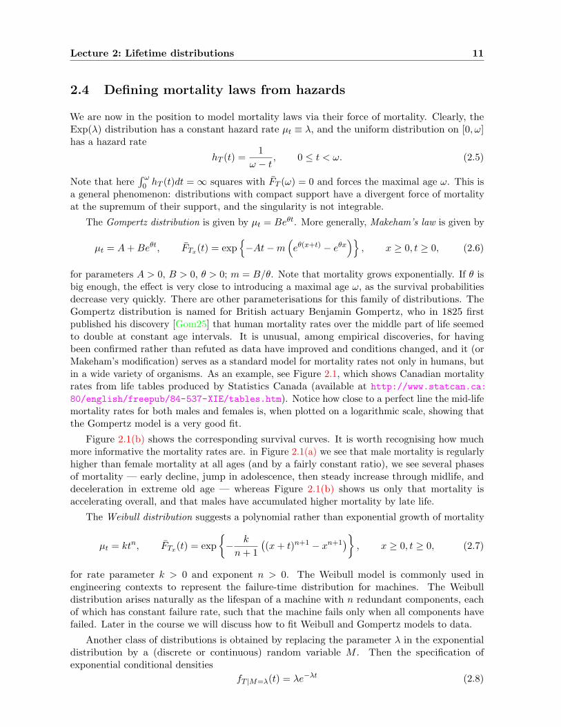
We are now in the position to model mortality laws via their force of mortality. Clearly, theExp(λ) distribution has a constant hazard rate µt ≡ λ, and the uniform distribution on [0, ω]has a hazard rate
hT (t) =1
ω − t, 0 ≤ t < ω. (2.5)
Note that here∫ ω0 hT (t)dt = ∞ squares with FT (ω) = 0 and forces the maximal age ω. This is
a general phenomenon: distributions with compact support have a divergent force of mortalityat the supremum of their support, and the singularity is not integrable.
The Gompertz distribution is given by µt = Beθt. More generally, Makeham’s law is given by
µt = A + Beθt, FTx(t) = exp{−At−m
(eθ(x+t) − eθx
)}, x ≥ 0, t ≥ 0, (2.6)
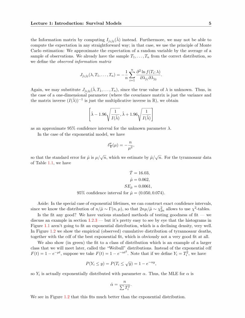
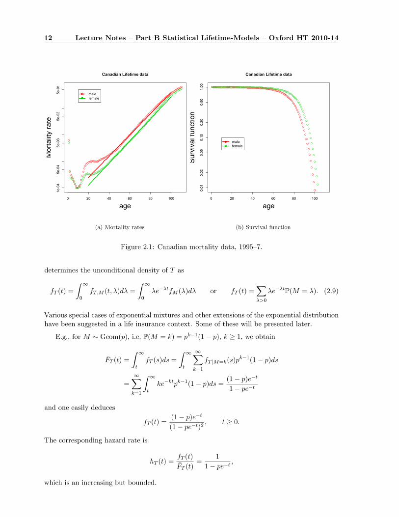
for parameters A > 0, B > 0, θ > 0; m = B/θ. Note that mortality grows exponentially. If θ isbig enough, the effect is very close to introducing a maximal age ω, as the survival probabilitiesdecrease very quickly. There are other parameterisations for this family of distributions. TheGompertz distribution is named for British actuary Benjamin Gompertz, who in 1825 firstpublished his discovery [Gom25] that human mortality rates over the middle part of life seemedto double at constant age intervals. It is unusual, among empirical discoveries, for havingbeen confirmed rather than refuted as data have improved and conditions changed, and it (orMakeham’s modification) serves as a standard model for mortality rates not only in humans, butin a wide variety of organisms. As an example, see Figure 2.1, which shows Canadian mortalityrates from life tables produced by Statistics Canada (available at http://www.statcan.ca:80/english/freepub/84-537-XIE/tables.htm). Notice how close to a perfect line the mid-lifemortality rates for both males and females is, when plotted on a logarithmic scale, showing thatthe Gompertz model is a very good fit.
Figure 2.1(b) shows the corresponding survival curves. It is worth recognising how muchmore informative the mortality rates are. in Figure 2.1(a) we see that male mortality is regularlyhigher than female mortality at all ages (and by a fairly constant ratio), we see several phasesof mortality — early decline, jump in adolescence, then steady increase through midlife, anddeceleration in extreme old age — whereas Figure 2.1(b) shows us only that mortality isaccelerating overall, and that males have accumulated higher mortality by late life.
The Weibull distribution suggests a polynomial rather than exponential growth of mortality
µt = ktn, FTx(t) = exp{− k
n + 1((x + t)n+1 − xn+1
)}, x ≥ 0, t ≥ 0, (2.7)
for rate parameter k > 0 and exponent n > 0. The Weibull model is commonly used inengineering contexts to represent the failure-time distribution for machines. The Weibulldistribution arises naturally as the lifespan of a machine with n redundant components, eachof which has constant failure rate, such that the machine fails only when all components havefailed. Later in the course we will discuss how to fit Weibull and Gompertz models to data.
Another class of distributions is obtained by replacing the parameter λ in the exponentialdistribution by a (discrete or continuous) random variable M . Then the specification ofexponential conditional densities
fT |M=λ(t) = λe−λt (2.8)
12 Lecture Notes – Part B Statistical Lifetime-Models – Oxford HT 2010-14
0 20 40 60 80 100
1e-04
5e-04
5e-03
5e-02
5e-01
Canadian Lifetime data
age
Mor
talit
y ra
te
malefemale
(a) Mortality rates
0 20 40 60 80 1000.01
0.02
0.05
0.10
0.20
0.50
1.00
Canadian Lifetime data
age
Sur
viva
l fun
ctio
n
malefemale
(b) Survival function
Figure 2.1: Canadian mortality data, 1995–7.
determines the unconditional density of T as
fT (t) =∫ ∞
0fT,M (t, λ)dλ =
∫ ∞
0λe−λtfM (λ)dλ or fT (t) =
∑λ>0
λe−λtP(M = λ). (2.9)
Various special cases of exponential mixtures and other extensions of the exponential distributionhave been suggested in a life insurance context. Some of these will be presented later.
E.g., for M ∼ Geom(p), i.e. P(M = k) = pk−1(1− p), k ≥ 1, we obtain
FT (t) =∫ ∞
tfT (s)ds =
∫ ∞
t
∞∑k=1
fT |M=k(s)pk−1(1− p)ds
=∞∑
k=1
∫ ∞
tke−ktpk−1(1− p)ds =
(1− p)e−t
1− pe−t
and one easily deduces
fT (t) =(1− p)e−t
(1− pe−t)2, t ≥ 0.
The corresponding hazard rate is
hT (t) =fT (t)FT (t)
=1
1− pe−t,
which is an increasing but bounded.
Lecture 2: Lifetime distributions 13
2.5 Curtate lifespan
We have implicitly assumed that the lifetime distribution is continuous. However, we can alwayspass from a continuous random variable T on [0,∞) to a discrete random variable K = [T ], itsinteger part, on N. If T models a lifetime, then K is called the associated curtate lifetime.
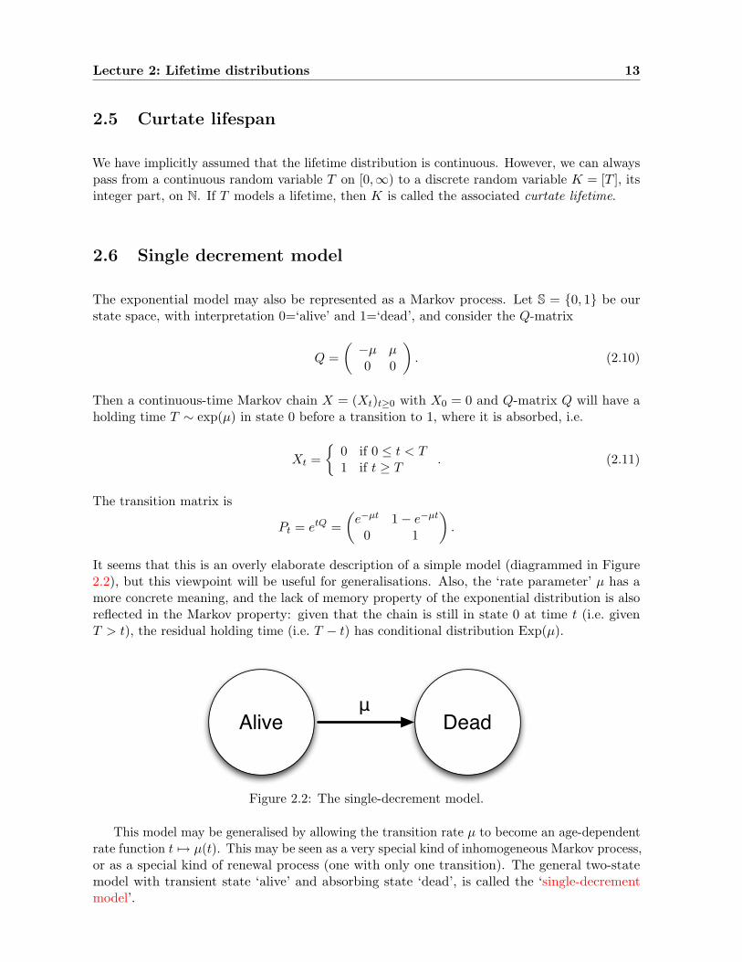
2.6 Single decrement model
The exponential model may also be represented as a Markov process. Let S = {0, 1} be ourstate space, with interpretation 0=‘alive’ and 1=‘dead’, and consider the Q-matrix
Q =(−µ µ0 0
). (2.10)
Then a continuous-time Markov chain X = (Xt)t≥0 with X0 = 0 and Q-matrix Q will have aholding time T ∼ exp(µ) in state 0 before a transition to 1, where it is absorbed, i.e.
Xt ={
0 if 0 ≤ t < T1 if t ≥ T
. (2.11)
The transition matrix is
Pt = etQ =(
e−µt 1− e−µt
0 1
).
It seems that this is an overly elaborate description of a simple model (diagrammed in Figure2.2), but this viewpoint will be useful for generalisations. Also, the ‘rate parameter’ µ has amore concrete meaning, and the lack of memory property of the exponential distribution is alsoreflected in the Markov property: given that the chain is still in state 0 at time t (i.e. givenT > t), the residual holding time (i.e. T − t) has conditional distribution Exp(µ).
Alive Deadμ
Figure 2.2: The single-decrement model.
This model may be generalised by allowing the transition rate µ to become an age-dependentrate function t 7→ µ(t). This may be seen as a very special kind of inhomogeneous Markov process,or as a special kind of renewal process (one with only one transition). The general two-statemodel with transient state ‘alive’ and absorbing state ‘dead’, is called the ‘single-decrementmodel’.
14 Lecture Notes – Part B Statistical Lifetime-Models – Oxford HT 2010-14
2.7 Mortality laws: Simple or Complex? Parametric or Non-parametric?
Consider the data for Albertosaurus sarcophagus in Table 1.1. We see here the estimated agesat death for 22 members of this species. Let us assume, for the sake of discussion, that theseestimates are correct, and that our skeleton collection represents a simple random sample of allAlbertosaurs that ever lived. If we assume that there was a large population of these dinosaurs,and that they died independently (and not, say, in a Cretaceous suicide pact), then these are 22independent samples T1, . . . , T22 of a random variable T whose distribution we would like toknow. Consider the probabilities
qx := P{x ≤ T < x + 1
}.
Then the number of individuals observed to have curtate lifespan x has binomial distri-bution Bin(22, qx). The MLE for a binomial probability is just the naıve estimate qx =# successes/# trials (where a “success”, in this case, is a death in the age interval under con-sideration). To compute q2, then, we observe that there were 22 Albertosaurs from our samplestill alive on their 22 birthdays, of which one unfortunate met its maker in the following year:q2 = 1/22 ≈ 0.046. As for q3, on the other hand, there were 21 Albertosaurs observed alive ontheir third birthdays, and all of them arrived safely at their fourth, making q3 = 0/21. Thisleads us to the peculiar conclusion that our best estimate for the probability of an albertosaurdying in its third year is 0.046, but that the probability drops to 0 in its fourth year, thenbecomes nonzero again in the fifth year, and so on. This violates our intuition that mortalityrates should be fairly smooth as a function of age. This problem becomes even more extremewhen we consider continuous lifetime models. With no constraints, the optimal estimator for themortality distribution would put all the mass on just those moments when deaths were observedin the sample, and no mass elsewhere — in other words, infinite hazard rate at a finite set ofpoints at which deaths have been observed, and 0 everywhere else.
As we see from Figure 1.1, the mortality distribution for the tyrannosaurs becomes muchsmoother and less erratic when we use larger bins for the histogram. This is no surprise, sincewe are then sampling from a larger baseline, leading to less random fluctuation. The simplestway to impose our intuition of regularity upon the estimators is to increase the time-step andreduce the number of parameters to estimate. An extreme version of this, of course, is to imposea parametric model with a small number of parameters. This is part of the standard tradeoff instatistics: a free, nonparametric model is sensitive to random fluctuations, but constraining themodel imposes preconceived notions onto the data.
Notation: When the hazard rate µx is being assumed constant over each year of life, thecontinuous mortality rate has been reduced to a discrete set of parameters. What do we callthese parameters? By convention, the value of µ that is in effect for all ages in [x, x + 1) isidentified with just one age, namely µx+ 1
2.
Lecture 3
Life Tables
Reading: Gerber Sections 2.4-2.5, CT4 Units 5-2, 6, 10-1Further reading: Cox-Oakes Sections 4.1-4.4, Gerber Sections 11.1-11.5
Life tables represent a discretised form of the hazard function for a population, often togetherwith raw mortality data. Apart from an aggregate table subsuming the whole population (ofthe UK, say), such tables exist for various groups of people characterized by their sex, smokinghabits, job type, insurance level etc. This immediately raises interesting questions concerningthe interdependence of such tables, but we focus here on some fundamental issues, which arealready present for the single aggregate table.
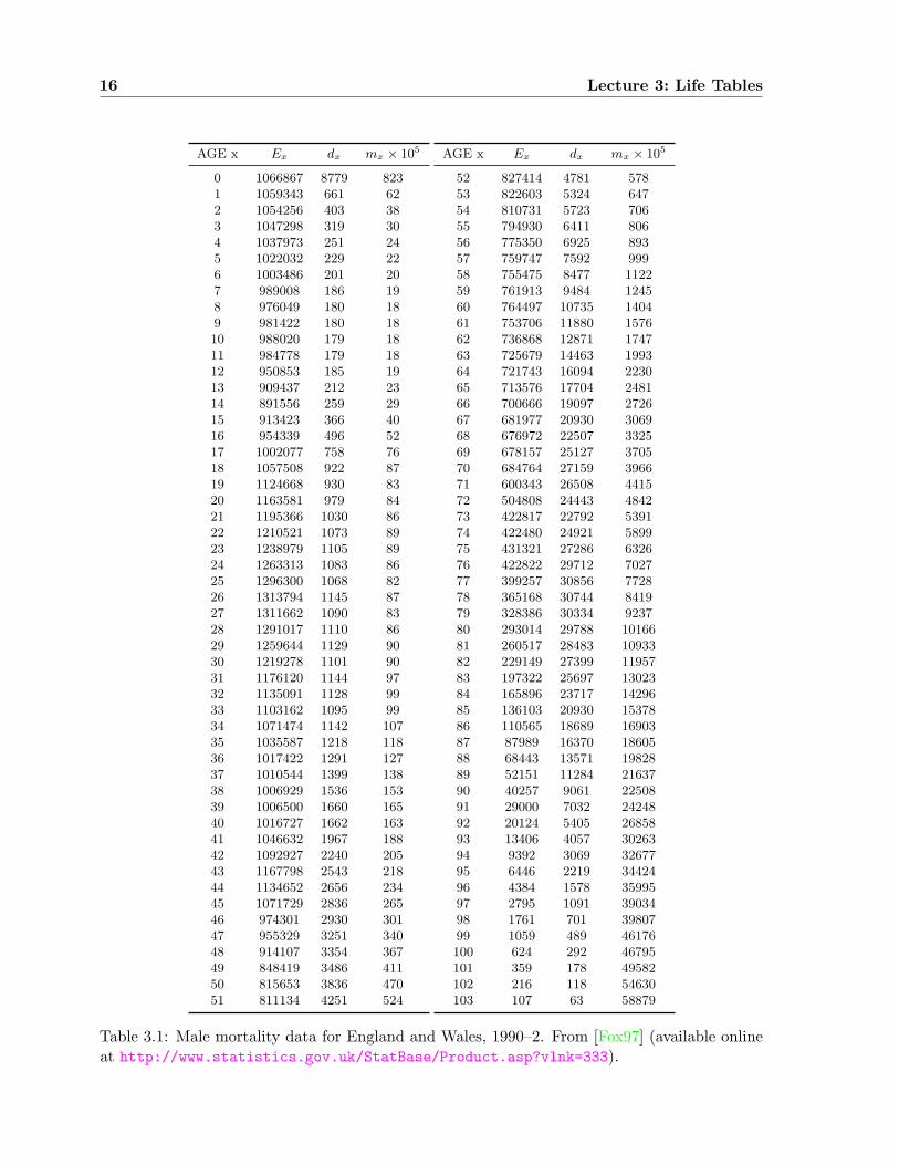
We begin with a naıve, empirical approach. In Table 3.2 we see a life table for men in theUK, in the years 1990–2, as provided by the Office of National Statistics. In the column labelledEx we see the number of years “exposed to risk” in age-class x. Since everyone alive is at risk ofdying, this should be exactly the sum of the number of individuals alive in the age class in years1990, 1991, and 1992. The 1991 number is obtained from the census of that year, and the othertwo years are estimated. The column dx shows the number of men of the given age known tohave died during this three-year period. The final column is mx := dx/Ex.
Again, this is an empirical fact, but we find ourselves in a quandary when we try to interpretit. What is mx? If the number of deaths is reasonably stable from year to year, then mx shouldbe close to the fraction of men aged x who died each year. How close? The number of men atrisk changes constantly, with each birthday, each death, each immigration or emigration. Wesense intuitively that the effect of these changes would be small, but how small? And whatwould we do to compensate for this in a smaller population, where the effects are not negligible?How do we make projections about future states of the population?
15
16 Lecture 3: Life Tables
AGE x Ex dx mx × 105
0 1066867 8779 8231 1059343 661 622 1054256 403 383 1047298 319 304 1037973 251 245 1022032 229 226 1003486 201 207 989008 186 198 976049 180 189 981422 180 1810 988020 179 1811 984778 179 1812 950853 185 1913 909437 212 2314 891556 259 2915 913423 366 4016 954339 496 5217 1002077 758 7618 1057508 922 8719 1124668 930 8320 1163581 979 8421 1195366 1030 8622 1210521 1073 8923 1238979 1105 8924 1263313 1083 8625 1296300 1068 8226 1313794 1145 8727 1311662 1090 8328 1291017 1110 8629 1259644 1129 9030 1219278 1101 9031 1176120 1144 9732 1135091 1128 9933 1103162 1095 9934 1071474 1142 10735 1035587 1218 11836 1017422 1291 12737 1010544 1399 13838 1006929 1536 15339 1006500 1660 16540 1016727 1662 16341 1046632 1967 18842 1092927 2240 20543 1167798 2543 21844 1134652 2656 23445 1071729 2836 26546 974301 2930 30147 955329 3251 34048 914107 3354 36749 848419 3486 41150 815653 3836 47051 811134 4251 524
AGE x Ex dx mx × 105
52 827414 4781 57853 822603 5324 64754 810731 5723 70655 794930 6411 80656 775350 6925 89357 759747 7592 99958 755475 8477 112259 761913 9484 124560 764497 10735 140461 753706 11880 157662 736868 12871 174763 725679 14463 199364 721743 16094 223065 713576 17704 248166 700666 19097 272667 681977 20930 306968 676972 22507 332569 678157 25127 370570 684764 27159 396671 600343 26508 441572 504808 24443 484273 422817 22792 539174 422480 24921 589975 431321 27286 632676 422822 29712 702777 399257 30856 772878 365168 30744 841979 328386 30334 923780 293014 29788 1016681 260517 28483 1093382 229149 27399 1195783 197322 25697 1302384 165896 23717 1429685 136103 20930 1537886 110565 18689 1690387 87989 16370 1860588 68443 13571 1982889 52151 11284 2163790 40257 9061 2250891 29000 7032 2424892 20124 5405 2685893 13406 4057 3026394 9392 3069 3267795 6446 2219 3442496 4384 1578 3599597 2795 1091 3903498 1761 701 3980799 1059 489 46176100 624 292 46795101 359 178 49582102 216 118 54630103 107 63 58879
Table 3.1: Male mortality data for England and Wales, 1990–2. From [Fox97] (available onlineat http://www.statistics.gov.uk/StatBase/Product.asp?vlnk=333).
Lecture 3: Life Tables 17
AGE x `x qx ex
0 100000 0.0082 73.41 99180 0.0006 73.02 99119 0.0004 72.13 99081 0.0003 71.14 99052 0.0002 70.15 99028 0.0002 69.16 99006 0.0002 68.27 98986 0.0002 67.28 98967 0.0002 66.29 98950 0.0002 65.210 98932 0.0002 64.211 98914 0.0002 63.212 98896 0.0002 62.213 98877 0.0002 61.214 98855 0.0003 60.215 98826 0.0004 59.316 98786 0.0005 58.317 98735 0.0008 57.318 98660 0.0009 56.419 98574 0.0008 55.420 98492 0.0008 54.521 98410 0.0009 53.522 98325 0.0009 52.523 98238 0.0009 51.624 98150 0.0009 50.625 98066 0.0008 49.726 97986 0.0009 48.727 97900 0.0008 47.828 97819 0.0009 46.829 97735 0.0009 45.830 97647 0.0009 44.931 97559 0.0010 43.932 97465 0.0010 43.033 97368 0.0010 42.034 97272 0.0011 41.035 97168 0.0012 40.136 97053 0.0013 39.137 96930 0.0014 38.238 96796 0.0015 37.239 96648 0.0016 36.340 96489 0.0016 35.441 96332 0.0019 34.442 96151 0.0021 33.543 95954 0.0022 32.544 95745 0.0023 31.645 95521 0.0027 30.746 95269 0.0030 29.847 94982 0.0034 28.948 94660 0.0037 28.049 94313 0.0041 27.150 93926 0.0047 26.251 93486 0.0052 25.3
AGE x `x qx ex
52 92997 0.0058 24.453 92461 0.0065 23.654 91865 0.0070 22.755 91219 0.0080 21.956 90486 0.0089 21.057 89682 0.0099 20.258 88791 0.0112 19.459 87800 0.0124 18.660 86714 0.0139 17.961 85505 0.0156 17.162 84168 0.0173 16.463 82710 0.0197 15.664 81078 0.0221 14.965 79290 0.0245 14.366 77347 0.0269 13.667 75267 0.0302 13.068 72992 0.0327 12.469 70605 0.0364 11.870 68037 0.0389 11.271 65391 0.0432 10.672 62567 0.0473 10.173 59610 0.0525 9.674 56481 0.0573 9.175 53246 0.0613 8.676 49982 0.0679 8.177 46590 0.0744 7.778 43125 0.0807 7.279 39643 0.0882 6.880 36145 0.0967 6.581 32651 0.1036 6.182 29270 0.1127 5.783 25971 0.1221 5.484 22800 0.1332 5.185 19763 0.1425 4.886 16946 0.1555 4.587 14310 0.1698 4.288 11881 0.1799 4.089 9744 0.1946 3.890 7848 0.2016 3.691 6266 0.2153 3.392 4917 0.2355 3.193 3759 0.2611 2.994 2777 0.2787 2.795 2003 0.2912 2.696 1420 0.3023 2.597 991 0.3232 2.398 670 0.3284 2.299 450 0.3698 2.1100 284 0.3737 2.0101 178 0.3909 1.9102 108 0.4209 1.8103 63 0.4450 1.7
Table 3.2: Life table for English men, computed from data in Table 3.1
18 Lecture Notes – Part B Statistical Lifetime-Models – Oxford HT 2010-14
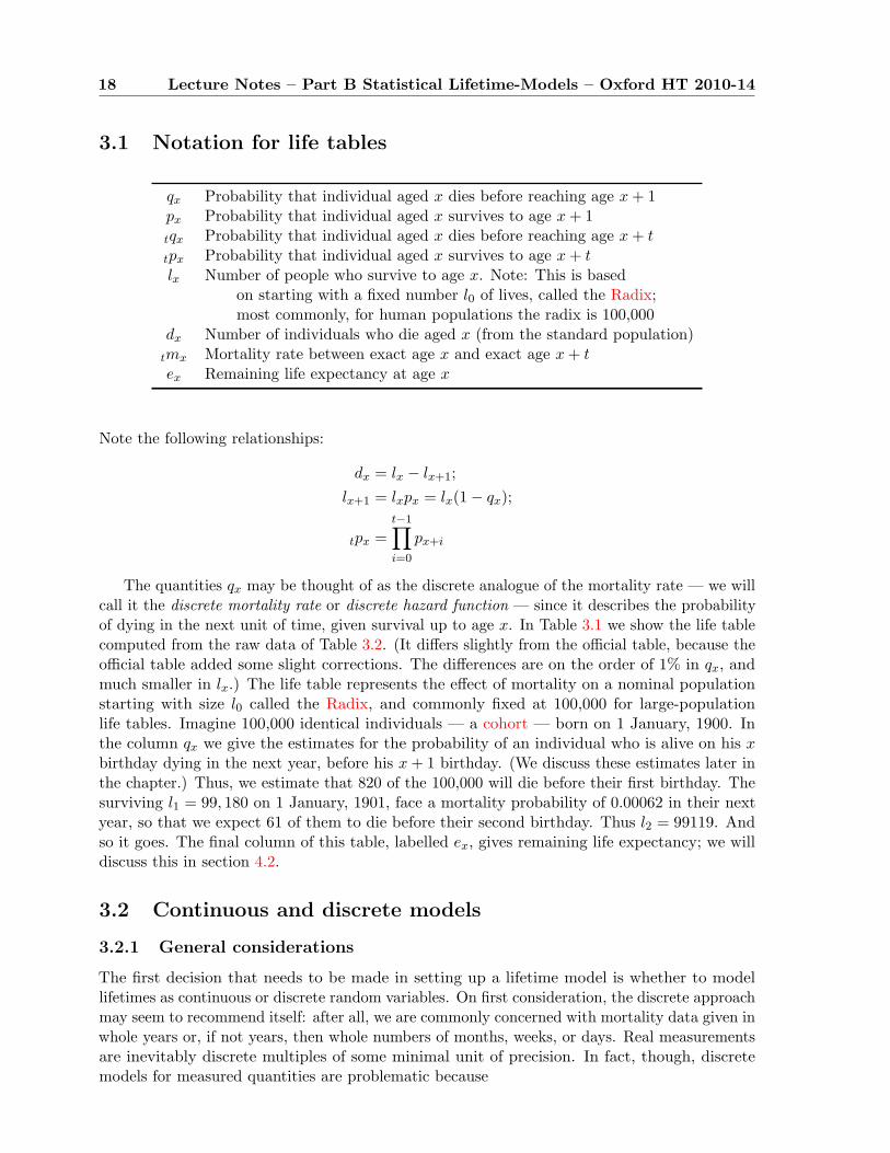
3.1 Notation for life tables
qx Probability that individual aged x dies before reaching age x + 1px Probability that individual aged x survives to age x + 1tqx Probability that individual aged x dies before reaching age x + t
tpx Probability that individual aged x survives to age x + tlx Number of people who survive to age x. Note: This is based
on starting with a fixed number l0 of lives, called the Radix;most commonly, for human populations the radix is 100,000
dx Number of individuals who die aged x (from the standard population)tmx Mortality rate between exact age x and exact age x + tex Remaining life expectancy at age x
Note the following relationships:
dx = lx − lx+1;lx+1 = lxpx = lx(1− qx);
tpx =t−1∏i=0
px+i
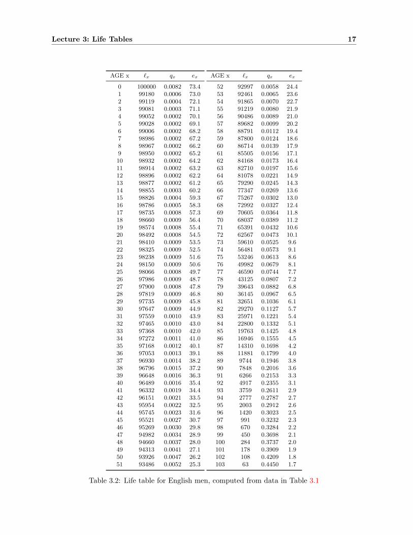
The quantities qx may be thought of as the discrete analogue of the mortality rate — we willcall it the discrete mortality rate or discrete hazard function — since it describes the probabilityof dying in the next unit of time, given survival up to age x. In Table 3.1 we show the life tablecomputed from the raw data of Table 3.2. (It differs slightly from the official table, because theofficial table added some slight corrections. The differences are on the order of 1% in qx, andmuch smaller in lx.) The life table represents the effect of mortality on a nominal populationstarting with size l0 called the Radix, and commonly fixed at 100,000 for large-populationlife tables. Imagine 100,000 identical individuals — a cohort — born on 1 January, 1900. Inthe column qx we give the estimates for the probability of an individual who is alive on his xbirthday dying in the next year, before his x + 1 birthday. (We discuss these estimates later inthe chapter.) Thus, we estimate that 820 of the 100,000 will die before their first birthday. Thesurviving l1 = 99, 180 on 1 January, 1901, face a mortality probability of 0.00062 in their nextyear, so that we expect 61 of them to die before their second birthday. Thus l2 = 99119. Andso it goes. The final column of this table, labelled ex, gives remaining life expectancy; we willdiscuss this in section 4.2.
3.2 Continuous and discrete models
3.2.1 General considerations
The first decision that needs to be made in setting up a lifetime model is whether to modellifetimes as continuous or discrete random variables. On first consideration, the discrete approachmay seem to recommend itself: after all, we are commonly concerned with mortality data given inwhole years or, if not years, then whole numbers of months, weeks, or days. Real measurementsare inevitably discrete multiples of some minimal unit of precision. In fact, though, discretemodels for measured quantities are problematic because
Lecture 3: Life Tables 19
• They tie the analysis to one unit of measurement. If you start by measuring lifespans inyears, and restrict the model accordingly you have no way of even posing a question about,for instance, the effect of shifting the reporting date within the year.
• Discrete methods are comfortable only when the numbers are small, whereas moving downto the smallest measurable unit turns the measurements into large whole numbers. Onceyou start measuring an average human lifespan as 30000 days (more or less), real numbersbecome easier to work with, as integrals are easier than sums.
• It is relatively straightforward to embed discrete measures within a continuous-time model,by considering the integer part of the continuous random lifetime, called the curtatelifetime in actuarial terminology.
(Compare this to the suggestion once made by the physicist Enrico Fermi, that lecturers mighttake their listeners’ investment of time more seriously if they thought of the 50-minute span ofa lecture as a “microcentury”.) The discrete model, it is pointed out by A. S. Macdonald in[Mac96] (and rewritten in [CT406, Unit 9]), “is not so easily generalised to settings with morethan one decrement. Even the simplest case of two decrements gives rise to difficult problems,”and involves the unnecessary complication of estimating an Initial Exposed To Risk. We willgenerally treat the continuous model as the fundamental object, and treat the discrete dataas coarse representations of an underlying continuous lifetime. However, looking beyond theactuarial setting, there are models which really do not have an underlying continuous timeparameter. For instance, in studies of human fertility, time is measured in menstrual cycles, andthere simply are no intermediate chances to have the event occur.
3.2.2 Are life tables continuous or discrete?
The standard approach to life tables mixes the continuous and discrete, in sometimes confusingways. The data upon which life tables are based are measured in discrete units, but in mostapplications we assume that the risk is actually continuous. If we were to observe a fixed numberof individuals for exactly one year, and count the number of deaths at the end of the year, and ifthe number of deaths during the year were a small fraction of the total number at risk, it wouldhardly matter whether we chose a discrete or continuous model. As we discuss in chapter 5.3,the distinction becomes significant to the extent that the number of individuals at risk changessubstantially over a single time unit; then we need to distinguish among Initial Exposed To Risk,Central Exposed To Risk, and the census approximation (see chapter 5.3).
The connection between discrete and continuous laws is fairly straightforward, at least inone direction. Suppose T is a lifetime with hazard rate µx at age x, and qx is the probability ofdying on or after birthday x, and before the x + 1 birthday. Then
tqx = e−R x+t
x µsds.
Another way of putting this is to say that the discrete model may be embedded in thecontinuous model, by considering the discrete random variable K = [T ], called the associatedcurtate lifetime. The remainder (fractional part) S = T − K = {T} can often be treatedseparately in a simplified way (see below). Clearly, the probability mass function of K on N is
20 Lecture Notes – Part B Statistical Lifetime-Models – Oxford HT 2010-14
given by
P(K = n) = P(n ≤ T < n + 1) =∫ n+1
nfT (t)dt = FT (n)− FT (n + 1)
= exp{−∫ n
0µT (t)dt
}(1− exp
{−∫ n+1
nµT (t)dt
})and if we denote the one-year death probabilities (discrete hazard function) by
qk = P(K = k|K ≥ k) =P(K = k)P(K ≥ k)
= 1− exp{−∫ k+1
kµT (t)dt
}and pk = 1− qk, k ∈ N, we obtain the probability of success after n independent Bernoulli trialswith varying success probabilities qk:
P(K = n) = p0 . . . pn−1qn.
Note that qk only depends on the hazard rate between ages k and k + 1. As a consequence, forKx = [Tx]
P(Kx = n) = px . . . px+n−1qx+n
are also easily represented in terms of (qk)k∈N.
3.3 Interpolation for non-integer ages
Suppose now that we have modeled the curtate lifetime K. The fractional part S of the lifetimeis a random variable on the interval [0, 1], commonly modeled in one of the following ways:
Constant force of mortality µ(x) is constant on the interval [k, k+1), and is called µT (k+ 12),
or sometimes µk+ 12
when T is clear from the context. Then
1qk = 1− e−µ
k+12 ; µk+ 1
2= − ln pk.
S has the distribution of an exponential random variable conditioned on S < 1, so it hasdensity
f(s) = µk+ 12
e−µ
k+12
s
1− e−µ
k+12
.
This assumption thus implies decreasing density of the lifetime through the interval. Wealso have, for 0 ≤ s ≤ 1, and k an integer,
spk = P(T > k + s|T > k) = exp{−∫ k+s
kµtdt
}= exp
{−sµk+ 1
2
}= (1− qk)s.
Note that K and S are not independent, under this assumption.
Uniform If S is uniform on [0, 1), this implies that for s ∈ [0, 1),
fT (k + s) = (FT (k)− FT (k + 1)) = FT (k)qk,
sqk = s · 1qk,
FT (k + s) = FT (k)(1− sqk
),
µT (k + s) =fT (k + s)FT (k + s)
=qk
1− sqk.
Lecture 3: Life Tables 21
So this assumption implies that the force of mortality is increasing over the time unit.Note that µ is discontinuous at (some if not all) integer times unless q0 = α = 1/n andqx+1 = qx/(1 − qx), i.e. qk = α
1−kα , k = 1, . . . , n − 1, with ω = n maximal age. Usually,one accepts discontinuities.
Balducci 1−tqk+t = (1− t)qk for t ∈ [0, 1), so that the probability of death in the remainingtime 1− t, having survived to k + t, is the product of the time left and the probability ofdeath in [k, k + 1). There is a trivial identity that the probability of surving 1 time unitfrom time k is the probability of surviving t time units from time k, times the probabilityof surviving 1− t time units from time k + t. Thus
qk = 1− (1− tqk) · (1− 1−tqk+t) = 1− (1− tqk) · (1− (1− t)qk),
so that
tqk = 1− 1− qk
1− (1− t)qk,
This implies that
FT (k + t) = FT (k)P{T > k + t
∣∣T > k}
= FT (k)1− qk
1− qk + tqk
fT (k + t) =d
dtFT (k + t) =
FT (k)qk(1− qk)(1− qk + tqk)2
,
µT (k + t) =fT (k + t)FT (k + t)
=qk
1− qk + tqk
So this assumption implies that the force of mortality is decreasing over the time unit.
Once we have made one of these assumptions, we can reconstruct the full distribution of a lifetimeT from the entries (qx)x∈N of a life table. When the force of mortality is small, these differentassumptions are all equivalent to µk+ 1
2= qk. Notice again that the choice of a measurement unit
for discretisation implies a certain level of smoothing, in continuous nonparametric life tablecomputations. Taking the evidence at face value, we would have to say that we have observedzero mortality rate, except at the instants at which deaths were observed, where mortalityjumps to ∞. Of course, we average over a period of time, either by imposing the constraint thatmortality rates be step functions, constant over a single measurement unit (or multiple units, ifwe wish to impose additional smoothing, usually because the number of observations is small).
Moving in the other direction is not so straightforward. The continuous model cannot beembedded in the discrete model, for obvious reasons: within the framework of the discretemodel, there is no such thing as a death midway through a time period. Traditionally, when thediscrete nature of lifetable data has been in the foreground, a model of the fractional part, suchas one of those listed above, has been adjoined to the model. As described in section 3.2.1, thisapproach quickly collapses under the weight of unnecessary complications, which is why we willalways treat the continuous lifetime as the fundamental object, except when the lifetime truly ismeasured only in discrete units.
3.4 Crude estimation of life tables – discrete method
Since their invention in the 17th century, the basic methodology for life table has been to collect(from the church registry or whoever kept records of births and deaths) lifetimes, truncate to
22 Lecture Notes – Part B Statistical Lifetime-Models – Oxford HT 2010-14
integer lifetimes, count the numbers dx of deaths between ages x and x + 1, relate this to thenumbers `x alive at age x, and use q
(0)x = dx/`x, or similar quantities as an estimate for the
one-year death probability qx.
In our model, the deaths are Bernoulli events with probability qx, so we know that theMaximum Likelihood Estimator for qx is q
(0)x = # successes/# trials = dx/`x for n = `0
independently observed curtate lifetimes k1, . . . , kn, observed from random variables with commonprobability mass function (m(x))x∈N parameterized by (qx)x∈N. If we denote m(x) = (1 −q0) . . . (1− qx−1)qx, the likelihood is
n∏i=1
m(k(i)) =∏x∈N
(m(x))dx =∏x∈N
(1− qx)`x−dxqdxx , (3.1)
where only max{k1, . . . , kn}+ 1 factors in the infinite product differ from 1, and
dx = dx(k1, . . . , kn) = #{
1 ≤ i ≤ n : k(i) = x}
,
`x = `x(k1, . . . , kn) = #{
1 ≤ i ≤ n : k(i) ≥ x}
.
This product is maximized when its factors are maximal (the xth factor only depending onparameter qx). An elementary differentiation shows that q 7→ (1−q)`−dqd is maximal for q = d/`,so that
q(0)x = q(0)
x (k1, . . . , kn) =dx(k1, . . . , kn)`x(k1, . . . , kn)
, 0 ≤ x ≤ max{k1, . . . , kn}.
Note that for x = max{k1, . . . , kn}, we have q(0)x = 1, so no survival beyond the highest age
observed is possible under the maximum likelihood parameters, so that (q(0))0≤x≤max{k1,...,kn}specifies a unique distribution. (Varying the unspecified parameters qx, x > max{k1, . . . , kn},has no effect.)
3.5 Crude life table estimation – continuous method
Alternatively, we can take a maximum likelihood approach on the continuous lifetimes, andobtain a different estimator. Assume that you observe n = `0 independent lives t1, . . . , tn. Thenthe likelihood function is
n∏i=1
fT (ti) =n∏
i=1
µti exp{−∫ ti
0µsds
}(3.2)
Now assume that the force of mortality µs is constant on [x, x + 1), x ∈ N and denote thesevalues by
µx+ 12
= − ln(px)(
remember px = exp{−∫ x+1
xµsds
}). (3.3)
Then, the likelihood takes the form∏x∈N
µdx
x+ 12
exp{−µx+ 1
2
˜x
}(3.4)
Lecture 3: Life Tables 23
where only max{t1, . . . , tn}+ 1 factors in the infinite product differ from 1, and
dx = dx(t1, . . . , tn) = # {1 ≤ i ≤ n : [ti] = x} ,
˜x = ˜
x(t1, . . . , tn) =n∑
i=1
∫ x+1
x1{ti>s}ds.
˜x is called the total exposed to risk.
The quantities µx+ 12, x ∈ N, are the parameters, and we can maximise the product by
maximising each of the factors. An elementary differentiation shows that µ 7→ µde−µ` has aunique maximum at µ = d/`, so that
µx+ 12
= µx+ 12(t1, . . . , tn) =
dx(t1, . . . , tn)˜x(t1, . . . , tn)
, 0 ≤ x ≤ max{t1, . . . , tn}.
Since maximum likelihood estimators are invariant under reparameterisation (the range of thelikelihood function remains the same, and the unique parameter where the maximum is obtainedcan be traced through the reparameterisation), we obtain
qx = qx(t1, . . . , tn) = 1− px = 1− exp{−µx+ 1
2
}= 1− exp
{−dx(t1, . . . , tn)
˜x(t1, . . . , tn)
}. (3.5)
For small dx/˜x, this is close to dx/˜
x, and therefore also close to dx/`x.Note that under qx, x ∈ N, there is a positive survival probability beyond the highest
observed age, and the maximum likelihood method does not fully specify a lifetime distribution,leaving free choice beyond the highest observed age.
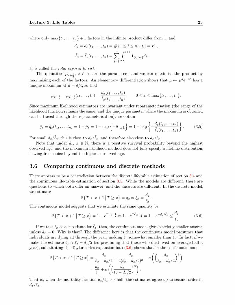
3.6 Comparing continuous and discrete methods
There appears to be a contradiction between the discrete life-table estimation of section 3.4 andthe continuous life-table estimation of section 3.5. While the models are different, there arequestions to which both offer an answer, and the answers are different. In the discrete model,we estimate
P{T < x + 1
∣∣T ≥ x}
= qx ≈ qx =dx
`x.
The continuous model suggests that we estimate the same quantity by
P{T < x + 1
∣∣T ≥ x}
= 1− e−µ
x+12 ≈ 1− e
−µx+1
2 = 1− e−dx/˜x ≤ dx
˜x
. (3.6)
If we take `x as a substitute for ˜x, then, the continuous model gives a strictly smaller answer,
unless dx = 0. Why is that? The difference here is that the continuous model presumes thatindividuals are dying all through the year, making ˜
x somewhat smaller than `x. In fact, if wemake the estimate ˜
x ≈ `x − dx/2 (so presuming that those who died lived on average half ayear), substituting the Taylor series expansion into (3.6) shows that in the continuous model
P{T < x + 1
∣∣T ≥ x}
=dx
`x − dx/2− dx
2(`x − dx/2)2+ o
(( dx
`x − dx/2
)3)
=dx
`x+ o
(( dx
`x − dx/2
)3)
.
That is, when the mortality fraction dx/`x is small, the estimates agree up to second order indx/`x.
24 Lecture Notes – Part B Statistical Lifetime-Models – Oxford HT 2010-14
3.7 An example: Fractional lifetimes can matter
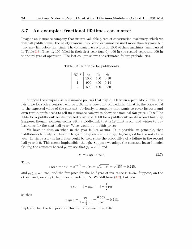
Imagine an insurance company that insures valuable pieces of construction machinery, which wewill call piddledonks. For safety reasons, piddledonks cannot be used more than 3 years, butthey may fail before that time. The company has records on 1000 of these machines, summarisedin Table 3.3. That is, 100 failed in their first year (age 0), 400 in the second year, and 400 inthe third year of operation. The last column shows the estimated failure probabilities.
Table 3.3: Life table for piddledonks.
age x lx dx qx
0 1000 100 0.101 900 400 0.442 500 400 0.80
Suppose the company sells insurance policies that pay £1000 when a piddledonk fails. Thefair price for such a contract will be £100 for a new-built piddledonk. (That is, the price equalto the expected value of the contract; obviously, a company that wants to cover its costs andeven turn a profit needs to sell its insurance somewhat above the nominal fair price.) It will be£444 for a piddledonk on its first birthday, and £800 for a piddledonk on its second birthday.Suppose, though, someone comes with a piddledonk that is 18 months old, and wishes to buyinsurance for the next half year. What would be the fair price?
We have no data on when in the year failure occurs. It is possible, in principle, thatpiddledonks fail only on their birthdays; if they survive that day, they’re good for the rest of theyear. In that case, the insurance could be free, since the probability of a failure in the secondhalf year is 0. This seems implausible, though. Suppose we adopt the constant-hazard model.Calling the constant hazard µ, we see that p1 = e−µ, and
p1 = 0.5p1 · 0.5p1.5. (3.7)
Thus,0.5p1.5 = 0.5p1 = e−µ/2 =
√p1 =
√1− q1 =
√.555 = 0.745,
and 0.5q1.5 = 0.255, and the fair price for the half year of insurance is £255. Suppose, on theother hand, we adopt the uniform model for S. We still have (3.7), but now
0.5p1 = 1− 0.5q1 = 1− 121q1,
so that
0.5p1.5 =p1
1− 121q1
=0.555.778
= 0.713,
implying that the fair price for this insurance would be £287.

Lecture 4
Cohorts and Period Life Tables
4.1 Types of life tables
You may have noticed a logical fallacy in the arguments of sections 3.4 and 3.5. The lifeexpectancy at birth should be the average length of life of individuals born in that year. Ofcourse, we would have to go back to about 1890 to find a birth year whose cohort — theindividuals born in that year — have completed their lives, so that the average lifespan can becomputed as an average.
Consider, for instance, the discrete-time non-homogeneous model. “Time” in the model isindividual age: An individual starts out at age 0, then progresses to age 1 if she survives, and soon. We estimate the probability of dying aged x by dividing the number of deaths observed agex by the number of individuals observed to have been at that age.
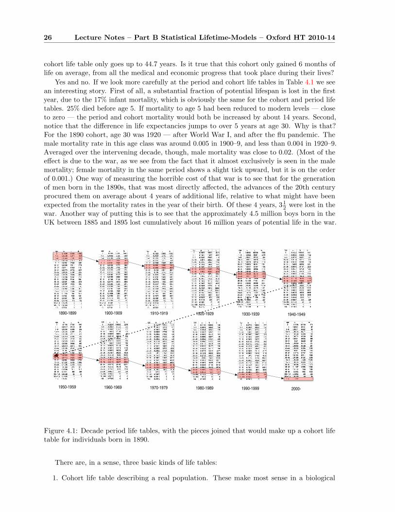
In our life-tables, called period life tables, these numbers came from a census of the individualsalive at one particular time, and the count of those who died in the same year, or period of a fewyears. No individual experiences those mortality rates. Those born in 2009 will experience themortality rates for age 10 in 2019, and the mortality rates for age 80 in 2089. Putting togetherthose mortality rates would give us a cohort life table. (Actually, this is not precisely true. Youmight think about why not. The answer is given in a footnote.1) If, as has been the case for thepast 150 years, mortality rates decline in the interval, that means that the survival rates will behigher than we see in the period table.
We show in Figure 4.1 a picture of how a cohort life table for the 1890 cohort would berelated to the sequence of period life tables from the 1890s through the 2000s. The mortalityrates for ages 0 through 9 (thus 1q0, 4q1, 5q5)2 are on the 1890s period life table, while theirmortality rates for ages 10 through 19 are on the 1900–1909 period life table, and so on. Notethat the mortality rates for the 1890s period life table yield a life expectancy at birth e0 = 44.2years. That is the average length of life that babies born in those years would have had, if theirmortality in each year of their lives had corresponded to the mortality rates which were realisedin for the whole population in the year of their birth. Instead, though, those that survived theirearly years entered the period of late-life high mortality in the mid- to late 20th century, whenmortality rates were much lower. It may seem surprising, then, that the life expectancy for the
1The main difference between a cohort life table and the life table constructed from the corresponding ageclasses of successive period life tables is immigration: The cohort life table for 1890 should include, in the row for(let us say) ages 60–4 the mortality rates of those born in 1890 in the relevant region — England and Wales inthis case — who are still alive at age 60. But these are not identical to the 60 year old men living in England andWales in 1950. Some of the original cohort have moved away, and some residing in the country were not bornthere.
2Actually, we have given µx for the intervals [0, 1), [1, 5), and [5, 10). We compute 1q0 = 1−e−µ0 , 4q1 = 1−e−4µ1 ,
5q5 = 1− e−5µ5 .
25
26 Lecture Notes – Part B Statistical Lifetime-Models – Oxford HT 2010-14
cohort life table only goes up to 44.7 years. Is it true that this cohort only gained 6 months oflife on average, from all the medical and economic progress that took place during their lives?
Yes and no. If we look more carefully at the period and cohort life tables in Table 4.1 we seean interesting story. First of all, a substantial fraction of potential lifespan is lost in the firstyear, due to the 17% infant mortality, which is obviously the same for the cohort and period lifetables. 25% died before age 5. If mortality to age 5 had been reduced to modern levels — closeto zero — the period and cohort mortality would both be increased by about 14 years. Second,notice that the difference in life expectancies jumps to over 5 years at age 30. Why is that?For the 1890 cohort, age 30 was 1920 — after World War I, and after the flu pandemic. Themale mortality rate in this age class was around 0.005 in 1900–9, and less than 0.004 in 1920–9.Averaged over the intervening decade, though, male mortality was close to 0.02. (Most of theeffect is due to the war, as we see from the fact that it almost exclusively is seen in the malemortality; female mortality in the same period shows a slight tick upward, but it is on the orderof 0.001.) One way of measuring the horrible cost of that war is to see that for the generationof men born in the 1890s, that was most directly affected, the advances of the 20th centuryprocured them on average about 4 years of additional life, relative to what might have beenexpected from the mortality rates in the year of their birth. Of these 4 years, 31
2 were lost in thewar. Another way of putting this is to see that the approximately 4.5 million boys born in theUK between 1885 and 1895 lost cumulatively about 16 million years of potential life in the war.
1890-1899 1900-1909 1910-1919 1920-1929 1930-1939 1940-1949
1950-1959 1960-1969 1970-1979 1980-1989 1990-1999 2000-
Figure 4.1: Decade period life tables, with the pieces joined that would make up a cohort lifetable for individuals born in 1890.
There are, in a sense, three basic kinds of life tables:
1. Cohort life table describing a real population. These make most sense in a biological
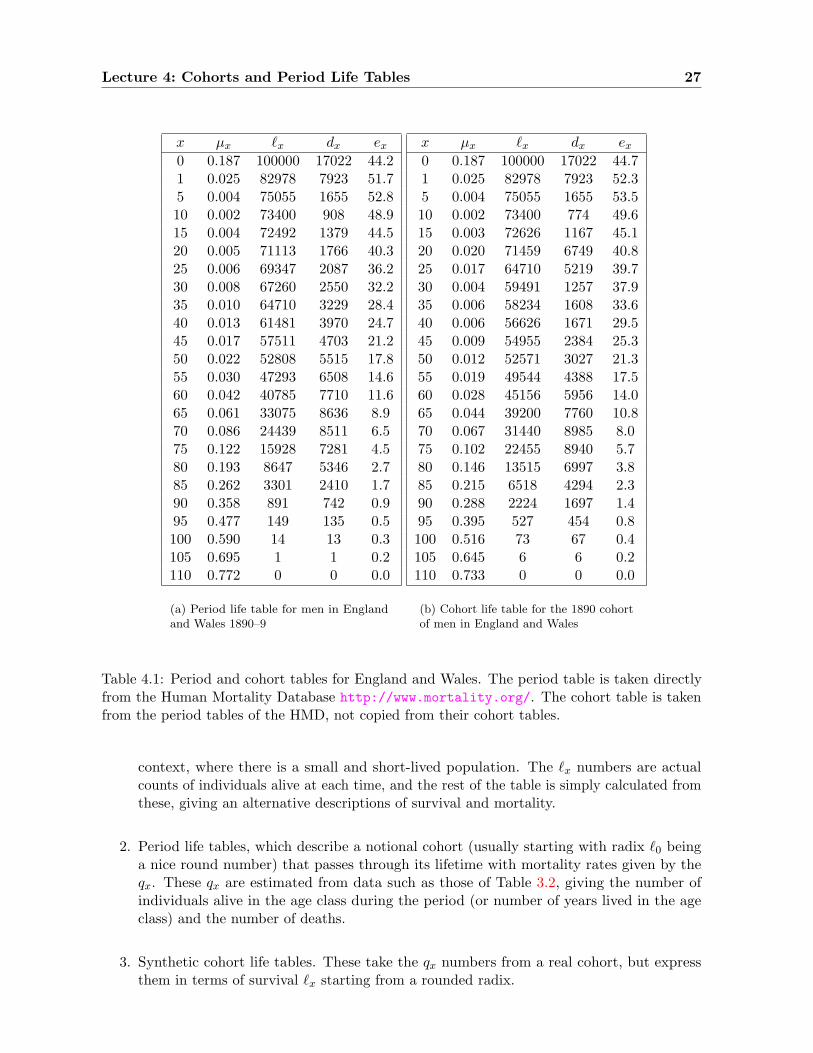
Lecture 4: Cohorts and Period Life Tables 27
x µx `x dx ex
0 0.187 100000 17022 44.21 0.025 82978 7923 51.75 0.004 75055 1655 52.810 0.002 73400 908 48.915 0.004 72492 1379 44.520 0.005 71113 1766 40.325 0.006 69347 2087 36.230 0.008 67260 2550 32.235 0.010 64710 3229 28.440 0.013 61481 3970 24.745 0.017 57511 4703 21.250 0.022 52808 5515 17.855 0.030 47293 6508 14.660 0.042 40785 7710 11.665 0.061 33075 8636 8.970 0.086 24439 8511 6.575 0.122 15928 7281 4.580 0.193 8647 5346 2.785 0.262 3301 2410 1.790 0.358 891 742 0.995 0.477 149 135 0.5100 0.590 14 13 0.3105 0.695 1 1 0.2110 0.772 0 0 0.0
(a) Period life table for men in Englandand Wales 1890–9
x µx `x dx ex
0 0.187 100000 17022 44.71 0.025 82978 7923 52.35 0.004 75055 1655 53.510 0.002 73400 774 49.615 0.003 72626 1167 45.120 0.020 71459 6749 40.825 0.017 64710 5219 39.730 0.004 59491 1257 37.935 0.006 58234 1608 33.640 0.006 56626 1671 29.545 0.009 54955 2384 25.350 0.012 52571 3027 21.355 0.019 49544 4388 17.560 0.028 45156 5956 14.065 0.044 39200 7760 10.870 0.067 31440 8985 8.075 0.102 22455 8940 5.780 0.146 13515 6997 3.885 0.215 6518 4294 2.390 0.288 2224 1697 1.495 0.395 527 454 0.8100 0.516 73 67 0.4105 0.645 6 6 0.2110 0.733 0 0 0.0
(b) Cohort life table for the 1890 cohortof men in England and Wales
Table 4.1: Period and cohort tables for England and Wales. The period table is taken directlyfrom the Human Mortality Database http://www.mortality.org/. The cohort table is takenfrom the period tables of the HMD, not copied from their cohort tables.
context, where there is a small and short-lived population. The `x numbers are actualcounts of individuals alive at each time, and the rest of the table is simply calculated fromthese, giving an alternative descriptions of survival and mortality.
2. Period life tables, which describe a notional cohort (usually starting with radix `0 beinga nice round number) that passes through its lifetime with mortality rates given by theqx. These qx are estimated from data such as those of Table 3.2, giving the number ofindividuals alive in the age class during the period (or number of years lived in the ageclass) and the number of deaths.
3. Synthetic cohort life tables. These take the qx numbers from a real cohort, but expressthem in terms of survival `x starting from a rounded radix.
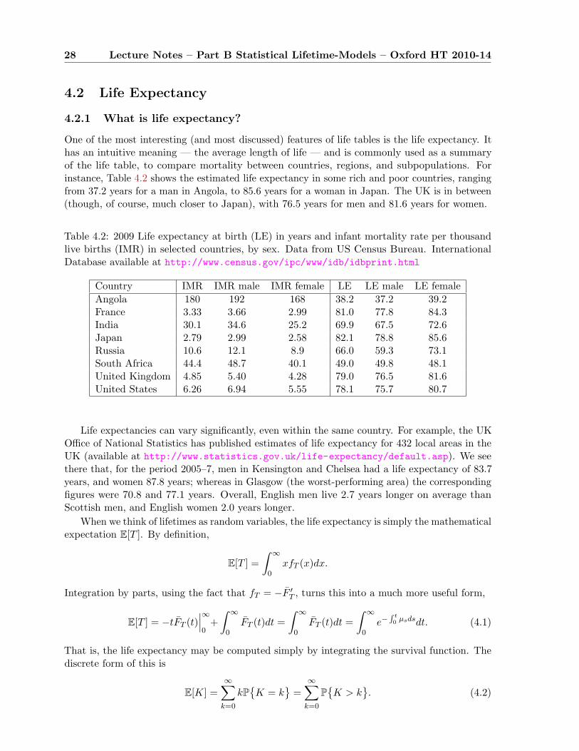
28 Lecture Notes – Part B Statistical Lifetime-Models – Oxford HT 2010-14
4.2 Life Expectancy
4.2.1 What is life expectancy?
One of the most interesting (and most discussed) features of life tables is the life expectancy. Ithas an intuitive meaning — the average length of life — and is commonly used as a summaryof the life table, to compare mortality between countries, regions, and subpopulations. Forinstance, Table 4.2 shows the estimated life expectancy in some rich and poor countries, rangingfrom 37.2 years for a man in Angola, to 85.6 years for a woman in Japan. The UK is in between(though, of course, much closer to Japan), with 76.5 years for men and 81.6 years for women.
Table 4.2: 2009 Life expectancy at birth (LE) in years and infant mortality rate per thousandlive births (IMR) in selected countries, by sex. Data from US Census Bureau. InternationalDatabase available at http://www.census.gov/ipc/www/idb/idbprint.html
Country IMR IMR male IMR female LE LE male LE femaleAngola 180 192 168 38.2 37.2 39.2France 3.33 3.66 2.99 81.0 77.8 84.3India 30.1 34.6 25.2 69.9 67.5 72.6Japan 2.79 2.99 2.58 82.1 78.8 85.6Russia 10.6 12.1 8.9 66.0 59.3 73.1South Africa 44.4 48.7 40.1 49.0 49.8 48.1United Kingdom 4.85 5.40 4.28 79.0 76.5 81.6United States 6.26 6.94 5.55 78.1 75.7 80.7
Life expectancies can vary significantly, even within the same country. For example, the UKOffice of National Statistics has published estimates of life expectancy for 432 local areas in theUK (available at http://www.statistics.gov.uk/life-expectancy/default.asp). We seethere that, for the period 2005–7, men in Kensington and Chelsea had a life expectancy of 83.7years, and women 87.8 years; whereas in Glasgow (the worst-performing area) the correspondingfigures were 70.8 and 77.1 years. Overall, English men live 2.7 years longer on average thanScottish men, and English women 2.0 years longer.
When we think of lifetimes as random variables, the life expectancy is simply the mathematicalexpectation E[T ]. By definition,
E[T ] =∫ ∞
0xfT (x)dx.
Integration by parts, using the fact that fT = −F ′T , turns this into a much more useful form,
E[T ] = −tFT (t)∣∣∣∞0
+∫ ∞
0FT (t)dt =
∫ ∞
0FT (t)dt =
∫ ∞
0e−
R t0 µsdsdt. (4.1)
That is, the life expectancy may be computed simply by integrating the survival function. Thediscrete form of this is
E[K] =∞∑
k=0
kP{K = k
}=
∞∑k=0
P{K > k
}. (4.2)
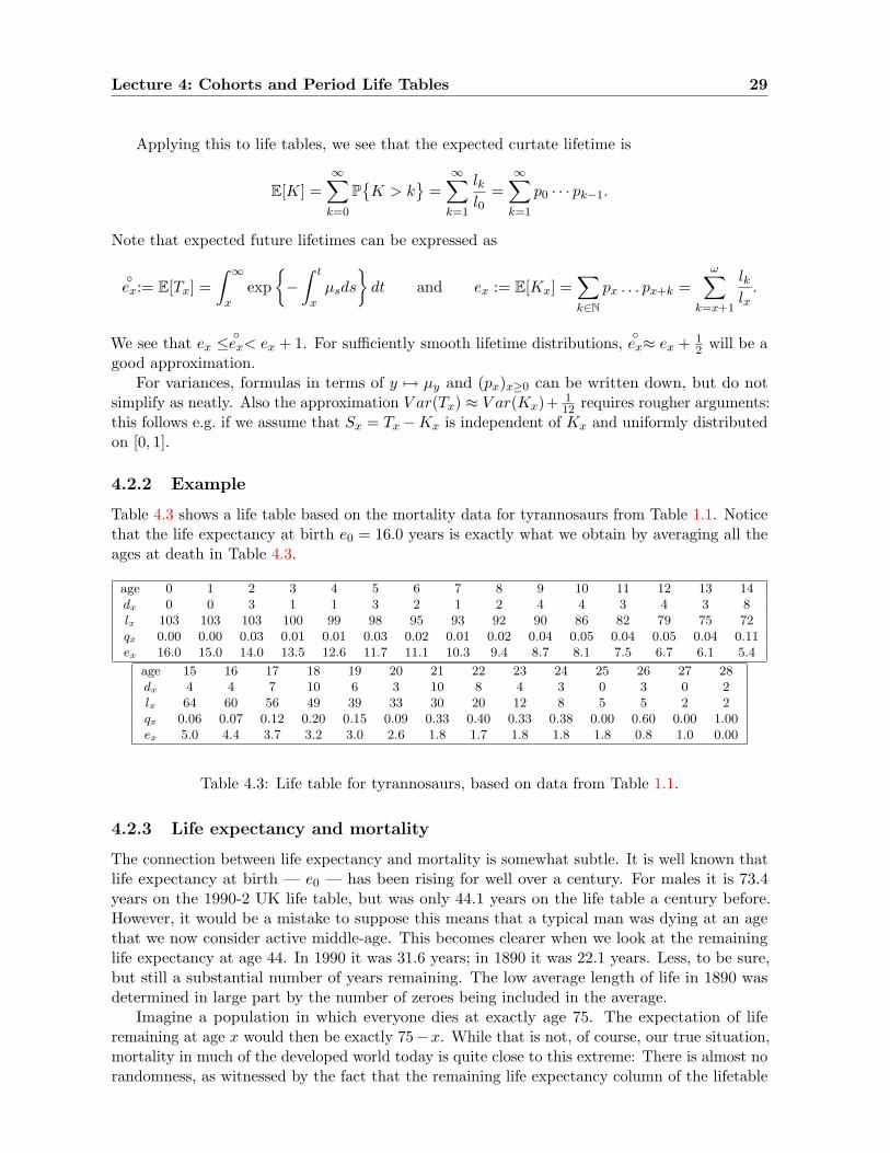
Lecture 4: Cohorts and Period Life Tables 29
Applying this to life tables, we see that the expected curtate lifetime is
E[K] =∞∑
k=0
P{K > k
}=
∞∑k=1
lkl0
=∞∑
k=1
p0 · · · pk−1.
Note that expected future lifetimes can be expressed as
◦ex:= E[Tx] =
∫ ∞
xexp
{−∫ t
xµsds
}dt and ex := E[Kx] =
∑k∈N
px . . . px+k =ω∑
k=x+1
lklx
.
We see that ex ≤◦ex< ex + 1. For sufficiently smooth lifetime distributions,
◦ex≈ ex + 1
2 will be agood approximation.
For variances, formulas in terms of y 7→ µy and (px)x≥0 can be written down, but do notsimplify as neatly. Also the approximation V ar(Tx) ≈ V ar(Kx)+ 1
12 requires rougher arguments:this follows e.g. if we assume that Sx = Tx −Kx is independent of Kx and uniformly distributedon [0, 1].
4.2.2 Example
Table 4.3 shows a life table based on the mortality data for tyrannosaurs from Table 1.1. Noticethat the life expectancy at birth e0 = 16.0 years is exactly what we obtain by averaging all theages at death in Table 4.3.
age 0 1 2 3 4 5 6 7 8 9 10 11 12 13 14dx 0 0 3 1 1 3 2 1 2 4 4 3 4 3 8lx 103 103 103 100 99 98 95 93 92 90 86 82 79 75 72qx 0.00 0.00 0.03 0.01 0.01 0.03 0.02 0.01 0.02 0.04 0.05 0.04 0.05 0.04 0.11ex 16.0 15.0 14.0 13.5 12.6 11.7 11.1 10.3 9.4 8.7 8.1 7.5 6.7 6.1 5.4
age 15 16 17 18 19 20 21 22 23 24 25 26 27 28dx 4 4 7 10 6 3 10 8 4 3 0 3 0 2lx 64 60 56 49 39 33 30 20 12 8 5 5 2 2qx 0.06 0.07 0.12 0.20 0.15 0.09 0.33 0.40 0.33 0.38 0.00 0.60 0.00 1.00ex 5.0 4.4 3.7 3.2 3.0 2.6 1.8 1.7 1.8 1.8 1.8 0.8 1.0 0.00
Table 4.3: Life table for tyrannosaurs, based on data from Table 1.1.
4.2.3 Life expectancy and mortality
The connection between life expectancy and mortality is somewhat subtle. It is well known thatlife expectancy at birth — e0 — has been rising for well over a century. For males it is 73.4years on the 1990-2 UK life table, but was only 44.1 years on the life table a century before.However, it would be a mistake to suppose this means that a typical man was dying at an agethat we now consider active middle-age. This becomes clearer when we look at the remaininglife expectancy at age 44. In 1990 it was 31.6 years; in 1890 it was 22.1 years. Less, to be sure,but still a substantial number of years remaining. The low average length of life in 1890 wasdetermined in large part by the number of zeroes being included in the average.
Imagine a population in which everyone dies at exactly age 75. The expectation of liferemaining at age x would then be exactly 75−x. While that is not, of course, our true situation,mortality in much of the developed world today is quite close to this extreme: There is almost norandomness, as witnessed by the fact that the remaining life expectancy column of the lifetable
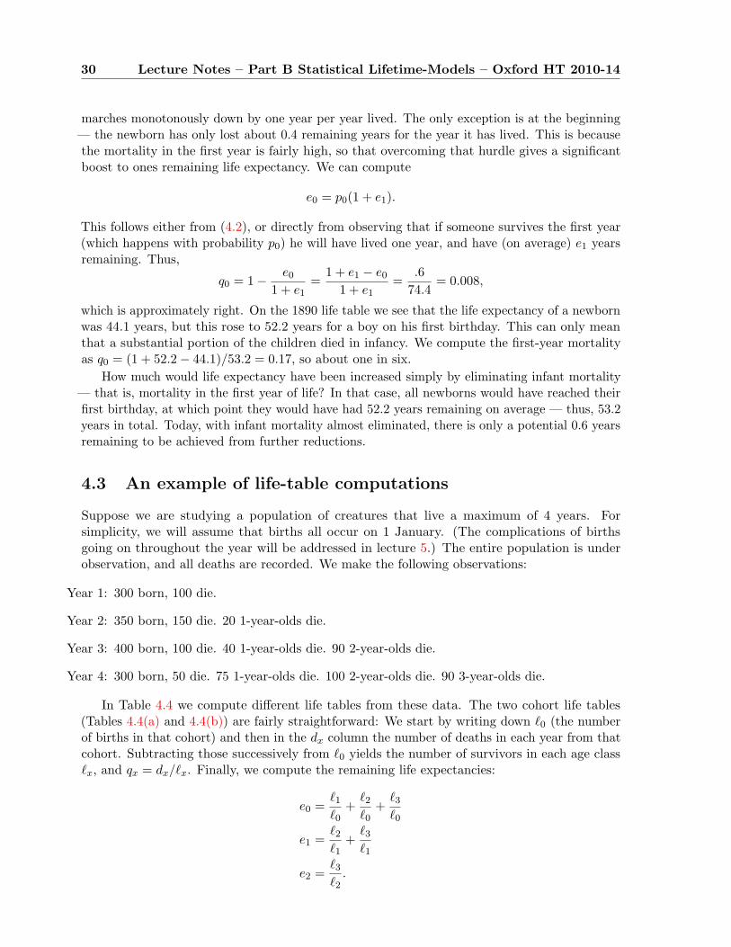
30 Lecture Notes – Part B Statistical Lifetime-Models – Oxford HT 2010-14
marches monotonously down by one year per year lived. The only exception is at the beginning— the newborn has only lost about 0.4 remaining years for the year it has lived. This is becausethe mortality in the first year is fairly high, so that overcoming that hurdle gives a significantboost to ones remaining life expectancy. We can compute
e0 = p0(1 + e1).
This follows either from (4.2), or directly from observing that if someone survives the first year(which happens with probability p0) he will have lived one year, and have (on average) e1 yearsremaining. Thus,
q0 = 1− e0
1 + e1=
1 + e1 − e0
1 + e1=
.674.4
= 0.008,
which is approximately right. On the 1890 life table we see that the life expectancy of a newbornwas 44.1 years, but this rose to 52.2 years for a boy on his first birthday. This can only meanthat a substantial portion of the children died in infancy. We compute the first-year mortalityas q0 = (1 + 52.2− 44.1)/53.2 = 0.17, so about one in six.
How much would life expectancy have been increased simply by eliminating infant mortality— that is, mortality in the first year of life? In that case, all newborns would have reached theirfirst birthday, at which point they would have had 52.2 years remaining on average — thus, 53.2years in total. Today, with infant mortality almost eliminated, there is only a potential 0.6 yearsremaining to be achieved from further reductions.
4.3 An example of life-table computations
Suppose we are studying a population of creatures that live a maximum of 4 years. Forsimplicity, we will assume that births all occur on 1 January. (The complications of birthsgoing on throughout the year will be addressed in lecture 5.) The entire population is underobservation, and all deaths are recorded. We make the following observations:
Year 1: 300 born, 100 die.
Year 2: 350 born, 150 die. 20 1-year-olds die.
Year 3: 400 born, 100 die. 40 1-year-olds die. 90 2-year-olds die.
Year 4: 300 born, 50 die. 75 1-year-olds die. 100 2-year-olds die. 90 3-year-olds die.
In Table 4.4 we compute different life tables from these data. The two cohort life tables(Tables 4.4(a) and 4.4(b)) are fairly straightforward: We start by writing down `0 (the numberof births in that cohort) and then in the dx column the number of deaths in each year from thatcohort. Subtracting those successively from `0 yields the number of survivors in each age class`x, and qx = dx/`x. Finally, we compute the remaining life expectancies:
e0 =`1
`0+
`2
`0+
`3
`0
e1 =`2
`1+
`3
`1
e2 =`3
`2.
Lecture 4: Cohorts and Period Life Tables 31
x dx `x qx ex
0 100 350 0.333 1.571 20 200 0.10 1.352 90 180 0.50 0.503 90 90 1.0 0
(a) Cohort 1 life table
x dx `x qx ex
0 150 350 0.43 1.21 40 200 0.20 1.12 100 160 0.625 0.3753 60 60 1.0 0
(b) Cohort 2 life table
x qx `x `x ex
0 0.167 1000 167 1.691 0.25 833 208 1.032 0.625 625 0.3753 1.0 235 1.0 0
(c) Period life table for year 4
Table 4.4: Alternative life tables from the same data.
The period life table is computed quite differently. We start with the qx numbers, whichcome from different cohorts:
q0 comes from cohort 4 newborn deaths;q1 comes from cohort 3 age 1 deaths;q2 comes from cohort 2 age 2 deaths;q3 comes from cohort 1 age 3 deaths.
We then write in the radix `0 = 1000. Of 1000 individuals born, with q0 = 0.167, we expect 167to die, giving us our d0. Subtracting that from `0 tells us that `1 = 833 of the 1000 newbornslive to their first birthday. And so it continues. The life expectancies are computed by the sameformula as before, but now the interpretation is somewhat different. The cohort remaining lifeexpectancies were the same as the actual average number of (whole) years remaining for thepopulation of individuals from that cohort who reached the given age. The period remaining lifeexpectancies are fictional, telling us how many individuals would have remained alive if we hada cohort of 1000 that experienced in each age the same mortality rates that were in effect forthe population in year 4.
Lecture 5
Central exposed to risk and thecensus approximation
Reading: CT4 Units 6-2 and 10, Cox-Oakes Section 1.3, Gerber Section 11.1Further reading: Cox-Oakes Chapter 3
5.1 Censoring
The term ‘Censoring’ refers to various types of incomplete information. The simplest exampleoccurs in any study where processes (e.g. lifetimes in a single or multiple decrement framework)are observed over a limited time range, as is unavoidably imposed since the study cannot goon until all participants have died; if the end of the study is a predetermined fixed time, thenthe fact that a participant survives bears important information, so survivors must be givenappropriate consideration in the likelihood.
In a single (or multiple) decrement model, this is e.g. the probability of survival: if rindividuals are observed for t years (or prior death), then the likelihood contribution from thosedying at time si < t, say, is the density fT (si); the likelihood contribution of those surviving tothe end of the study at time t is the probability of survival FT (t).
This is an example of right censoring, which, more generally, also occurs, when participantswithdraw from the study for other exterior reasons (e.g. expiry date of an insurance policy).More general types of censoring will be treated later.
5.2 Insurance data
Insurance data have several special features. In the best of cases, we have full information fromeach person insured as follows; for a simple life assurance paying death benefits on death only,for individual m:
• date of birth bm
• date of entry into observation: policy start date xm
• reason for exit from observation (death Dm = 1, or expiry/withdrawal Dm = 0)
• date of exit from observation Ym
32
Lecture 5: Central exposed to risk and the census approximation 33
This then easily translates into a likelihood
1{Dm=1}fTxm−bm(Ym−xm)+1{Dm=0}FTxm−bm
(ym−xm) = µDmYm−bm
exp{−∫ Ym−bm
xm−bm
µtdt
}, (5.1)
and it is clear how much time this individual was exposed to risk at age x, i.e. aged [x, x + 1)for all x ∈ N. We can calculate the Central exposed to risk Ec
x as the aggregate quantity acrossall individuals exactly. We can also read off the number of deaths aged [x, x + 1), dx, and hence
µx+ 12
=dx
Ecx
(5.2)
This is the maximum likelihood estimator under the assumption of a constant force of mortalityon [x, x + 1). Note that this estimator conforms with the Principle of Correspondence whichstates that
A life alive at time t should be included in the exposure at age x at time t if andonly if, were that life to die immediately, he or she would be counted in the deathdata dx at age x.
In practice, data are often not provided in this form and approximations are required. E.g.,policy start and end dates may not be available; instead, only total numbers of policies perage group at annual census dates are provided, and there is ambiguity as to when individualschange age group between the census dates. The solution to the problem is called the censusapproximation.
The key point is that we can tolerate a substantial amount of uncertainty in the numeratorand the denominator (number of events and total time at risk), but failing to satisfy the Principleof Correspondence can be disastrous. For example, [ME05] analyses the “Hispanic Paradox,”the observation that Latin American immigrants in the USA seem to have substantially lowermortality rates than the native population, despite being generally poorer (which is usuallyassociated with shorter lifespans). This difference is particularly pronounced at more advancedages. Part of the explanation seems to be return migration: Some old hispanics return to theirhome countries when they become chronically ill or disabled. Thus, there are some members ofthis group who count as part of the US hispanic population for most of their lives, but whosedeaths are counted in their home-country statistics.
5.3 Census approximation
The task is to approximate Ecx (and often also dx) given census data. There are various forms of
census data. The most common one is
Px,k = Number of policy holders aged [x, x + 1) at time k = 0, . . . , n.
The problem is that we do not know policy start and end dates. The basic assumption of thecensus approximation is that the number of policies changes linearly between any two consecutivecensus dates. It is easy to see that
Ecx =
∫ n
0Px,tdt (5.3)
We only know the integrand at integer times, and the linearity approximation gives
Ecx ≈
n∑k=1
12(Px,k−1 + Px,k). (5.4)
34 Lecture Notes – Part B Statistical Lifetime-Models – Oxford HT 2010-14
This allows us to estimate µx+ 12
if we also know dx, the number of deaths aged x.Now assume that, in fact, you are not given dx but only calender years of birth and death
leading to
d′x = Number of deaths aged x on the birthday in the calendar year of death.
Then, some of the deaths counted in d′x will be deaths aged x− 1, not x, in fact we should viewd′x as containing deaths aged in the interval (x− 1, x+ 1), but not all of them. If we assume thatbirthdays are uniformly spread over the year, we can also specify that the proportion of deathscounted under d′x changes linearly from 0 to 1 and back to 0 as x− 1 increases to x and x + 1.
In order to estimate a force of mortality, we need to identify the corresponding (approximationto) Central exposed to risk. The Principle of Correspondence requires
Ec′x =
∫ n
0P ′
x,tdt, (5.5)
where
P ′x,t = Number of policy holders at t with xth birthday in calendar year [t].
Again, suppose we know the integrand at integer times. Here the linear approximation requiressome care, since the policy holders do not change age group continuously, but only at censusdates. Therefore, all continuing policy holders counted in P ′
x,k−1 will be counted in P ′x,t for all
k − 1 ≤ t < k, but then in P ′x+1,k at the next census date. Therefore
Ec′x ≈
n∑k=1
12(P ′
x,k−1 + P ′x+1,k). (5.6)
The ratio d′x/Ec′x gives a slightly smoothed (because of the wider age interval) estimate of µx
(and not µx+ 12). Note however that it is not clear if this estimate is a maximum likelihood
estimate for µx under any suitable model assumptions such as constancy of the force of mortalitybetween half-integer ages.
Some other types of data appear on Assignment 3. The general problem is always to identifythe corresponding central exposed to risk and what the ratio of death counts and its centralexposed to risk estimates.
5.4 Lexis diagrams
A graphical tool that helps in making sense of estimates like the census approximation is theLexis diagram.1 These reduce the three dimensions of demographic data — date, age, andmoment of birth — to two, by an ingenious application of the diagonal.
Consider the diagram in Figure 5.1. The horizontal axis represents calendar time (which wewill take to be in years), while the vertical axis represents age. Lines representing the lifetimes ofindividuals start at their birthdate on the horizontal axis, then ascend at a 45◦ angle, reflectingthe fact that individuals age at the rate of one year (of age) per year (of calendar time). Eventsduring an individual’s life may be represented along the lifeline — for instance, the line might
1These diagrams are named for Wilhelm Lexis, a 19th century statistician and demographer of many accomplish-ments, none of which was the invention of these diagrams, in keeping with Stigler’s law of eponymy, which states that“No scientific discovery is named after its original discoverer.” (cf. Christophe Vanderschrick, “The Lexis diagram, amisnomer”, Demographic Research 4:3, pp. 97–124, http://www.demographic-research.org/Volumes/Vol4/3/.)
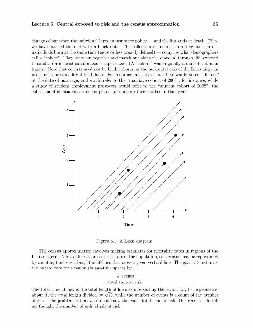
Lecture 5: Central exposed to risk and the census approximation 35
change colour when the individual buys an insurance policy — and the line ends at death. (Herewe have marked the end with a black dot.) The collection of lifelines in a diagonal strip —individuals born at the same time (more or less broadly defined) — comprise what demographerscall a “cohort”. They start out together and march out along the diagonal through life, exposedto similar (or at least simultaneous) experiences. (A “cohort” was originally a unit of a Romanlegion.) Note that cohorts need not be birth cohorts, as the horizontal axis of the Lexis diagramneed not represent literal birthdates. For instance, a study of marriage would start “lifelines”at the date of marriage, and would refer to the “marriage cohort of 2008”, for instance, whilea study of student employment prospects would refer to the “student cohort of 2008”, thecollection of all students who completed (or started) their studies in that year.
1 2 3 4
1
2
3
4
Time
Age
Figure 5.1: A Lexis diagram.
The census approximation involves making estimates for mortality rates in regions of theLexis diagram. Vertical lines represent the state of the population, so a census may be representedby counting (and describing) the lifelines that cross a given vertical line. The goal is to estimatethe hazard rate for a region (in age-time space) by
# eventstotal time at risk
The total time at risk is the total length of lifelines intersecting the region (or, to be geometricabout it, the total length divided by
√2), while the number of events is a count of the number
of dots. The problem is that we do not know the exact total time at risk. Our censuses do tellus, though, the number of individuals at risk
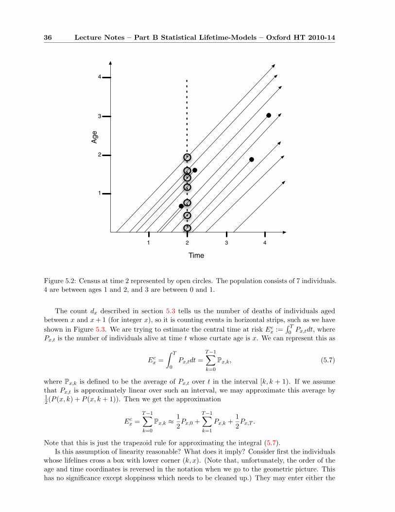
36 Lecture Notes – Part B Statistical Lifetime-Models – Oxford HT 2010-14
1 2 3 4
1
2
3
4
Time
Age
Figure 5.2: Census at time 2 represented by open circles. The population consists of 7 individuals.4 are between ages 1 and 2, and 3 are between 0 and 1.
The count dx described in section 5.3 tells us the number of deaths of individuals agedbetween x and x + 1 (for integer x), so it is counting events in horizontal strips, such as we haveshown in Figure 5.3. We are trying to estimate the central time at risk Ec
x :=∫ T0 Px,tdt, where
Px,t is the number of individuals alive at time t whose curtate age is x. We can represent this as
Ecx =
∫ T
0Px,tdt =
T−1∑k=0
Px,k, (5.7)
where Px,k is defined to be the average of Px,t over t in the interval [k, k + 1). If we assumethat Px,t is approximately linear over such an interval, we may approximate this average by12(P (x, k) + P (x, k + 1)). Then we get the approximation
Ecx =
T−1∑k=0
Px,k ≈12Px,0 +
T−1∑k=1
Px,k +12Px,T .
Note that this is just the trapezoid rule for approximating the integral (5.7).Is this assumption of linearity reasonable? What does it imply? Consider first the individuals
whose lifelines cross a box with lower corner (k, x). (Note that, unfortunately, the order of theage and time coordinates is reversed in the notation when we go to the geometric picture. Thishas no significance except sloppiness which needs to be cleaned up.) They may enter either the
Lecture 5: Central exposed to risk and the census approximation 37
left or the lower border. In the former case (corresponding to individuals born in year x− k)they will be counted in Px,k; in the latter (born in x− k + 1) case in Px,k+1. If the births in yearx− k + 1 differ from those in year x− k by a constant (that is, the difference between January 1births in the two years is the same as the difference between February 12 births, and so on, thenon average the births in the two years on a given date will contribute 1/2 year to the centralyears at risk, and will be counted once in the sum Px,k + Px,k+1. Important to note:
• This does not actually require that births be evenly distributed through the year.
• When we say births, we mean births that survive to age k. If those born in, say, Decemberof one year had substantially lowered survival probability relative to a “normal” December,this would throw the calculation off.
• These assumptions are not about births and deaths in general, but rather about birthsand deaths of the population of interest: those who buy insurance, those who join theclinical trial, etc.
If mortality levels are low, this will suffice, since nearly all lifelines will be counted amongthose that cross the box. If mortality rates are high, though, we need to consider the contributionof years at risk due to those lifelines which end in the box. In this case, we do need to assume thatbirths and deaths are evenly spread through the year. This assumption implies that conditionedon a death occurring in a box, it is uniformly distributed through the box. On the one hand, thatimplies that it contributes (on average) 1/4 year to the years at risk in the box. On the otherhand, it implies that the probability of it having been counted in our average 1
2(Px,k + Px,k+1)is 1
2 , since it is counted only if it is in the upper left triangle of box. On average, then, theseshould balance.
What happens when we count births and deaths only by calendar year? Note that P ′x,k = Px,k
for integers k and x. One difference is that the regions in question, which are parallelograms,follow the same lifelines from the beginning of the year to the end. This makes the analysismore straightforward. Lifelines that pass through the region are counted on both ends. Theother difference is that the region that begins with the census value Px,k ends not with Px,k+1,but with Px+1,k+1. Thus all the lifelines passing through the region will be counted in Px,k andin Px+1,k+1, hence also in their average. This requires no further assumptions. For the lifelinesthat end in the region to be counted appropriately, on the other hand, requires that the deathsbe evenly distributed throughout the year. (Other, slightly less restrictive assumptions, are alsopossible.) In this case, each death will contribute exactly 1/2 to the estimate 1
2(Px,k + Px+1,k+1)(since it is counted only in Px,k), and it contributes on average 1/2 year of time at risk.
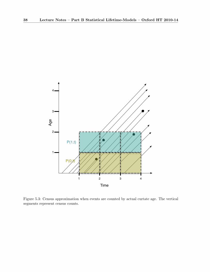
38 Lecture Notes – Part B Statistical Lifetime-Models – Oxford HT 2010-14
1 2 3 4
1
2
3
4
Time
Age
P(1,t)
P(0,t)
Figure 5.3: Census approximation when events are counted by actual curtate age. The verticalsegments represent census counts.
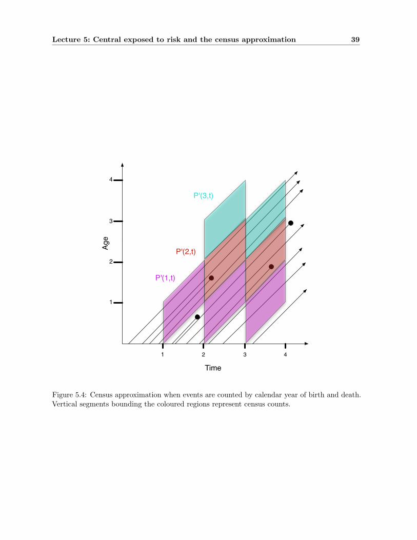
Lecture 5: Central exposed to risk and the census approximation 39
1 2 3 4
1
2
3
4
Time
Age
P'(1,t)
P'(2,t)
P'(3,t)
Figure 5.4: Census approximation when events are counted by calendar year of birth and death.Vertical segments bounding the coloured regions represent census counts.
Lecture 6
Comparing life tables
6.1 The binomial model
Suppose we observe n identically distributed, independent lives aged x for exactly 1 year, andrecord the number dx who die. Using the notation set up for the discrete model, a life dies withprobability qx within the year.
Hence Dx, the random variable representing the numbers dying in the year conditional on nalive at the beginning of the year, has distribution
Dx ∼ B(n, qx)
giving a maximum likelihood estimator
qx =Dx
n, with var(qx) =
qx (1− qx)n
where using previous notation we have set lx = n.
While attractively simple, this approach has significant problems. Normally failures, deaths,and other events of interest, happen continuously, even if we happen to observe or tabulate themat discrete intervals. While we get a perfectly valid estimate of qx, the probability of an eventhappening in this time interval, we have no way of generalising to a question about how manyindividuals died in half a year, for example. And real data may be interval truncated: That is,the life is not under observation during the entire year, but only during the interval of ages(x + a, x + b), where 0 ≤ a < b ≤ 1. If we write Di
x for the indicator of the event that individuali is observed to die at (curtate) age x, we have
P (Dix = 1) = bi−ai
qx+ai
Hence
EDx = E
(n∑
i=1
Dix
)=
n∑i=1
bi−aiqx+ai
There is no way to analyse (or even describe) this intra-interval refinement within the frameworkof the binomial model.
Nonetheless, the simplicity and tradition of the binomial model have led actuaries to developa kind of continuous prosthetic for the binomial model, in the form of a supplemental (andhidden) model for the unobserved continuous part of the lifetime. These have been discussed inLecture 3. In the end, these are applied through the terms Initial Exposed To Risk (E0
x) andCentral Exposed To Risk (Ec
x). These are defined more by their function than as a particular
40
Lecture 6: Comparing life tables 41
quantity: the Initial Exposed To Risk plays the role of n in a binomial model, and Ecx plays the
role of total time at risk in an exponential model. They are linked by the actuarial estimator
E0x ≈ Ec
x +12dx.
This may be justified from any of our fractional-lifetime models if the number of deaths is smallrelative to the number at risk. Thus, the actuarial estimator for qx is
qx =dx
Ecx + 1
2dx.
The denominator, Ecx + 1
2dx, comprises the observed time at risk (also called central exposed torisk) within the interval (x, x + 1), added to 1/2 the number of deaths (assumes deaths evenlyspread over the interval). This is an estimator for Ex which is the inital exposed to risk and iswhat is required for the binomial model.
NB assumptions (i)-(iii) collapse to the same model, essentially (i), if µx+ 12
is very small,since all become tqx ≈ tµx+ 1
2, 0 < t < 1.
Definitions, within year (x, x + 1)a) Ec
x = observed total time (in years) at risk = central exposed to risk, with approxima-tion Ec
x ≈ Ex − 12dx, if required.
b) E0x(= Ex) = initial exposed to risk = # in risk set at age x, with approximation
Ex ≈ Ecx + 1
2dx, if required.
6.2 The Poisson model
Under the assumption of a constant hazard rate (force of mortality) µx+ 12
over the year (x, x+1],we may view the estimation problem as a chain of separate hazard rate estimation problems, onefor each year of life. Each individual lives some portion of a year in the age interval (x, x + 1],the portion being 0 (if he dies before birthday x), 1 (if he dies after birthday x + 1), or between0 and 1 if he dies between the two birthdays. Suppose now we lay these intervals end to end,with a mark at the end of an interval where an individual died. It is not hard to see that whatresults is a Poisson process on the interval [0, Ec
x], where Ecx is the total observed years at risk.
Suppose we treat Ecx as though it were a constant. Then if Dx represents the numbers dying
in the year the model uses
P{Dx = k
}=
(µx+ 1
2Ec
x
)ke−µ
x+12
Ecx
k!, k = 0, 1, 2, · · ·
which is an approximation to the 2-state model, and which in fact yields the same likelihood.The estimator for the constant force of mortality over the year is
µx+ 12
=Dx
Ecx
, with estimatedx
Ecx
.
Under the Poisson model we therefore have that
varµx+ 12
=µx+ 1
2Ec
x
(Ecx)2
=µx+ 1
2
Ecx
.
42 Lecture Notes – Part B Statistical Lifetime-Models – Oxford HT 2010-14
So the estimate will bevarµx+ 1
2≈ dx
(Ecx)2
.
If we compare with the 2-state stochastic model over year (x, x + 1), assuming constantµ = µx+ 1
2, then the likelihood is
L =n∏1
µδie−µti ,
where δi = 1 if life i dies and ti = bi − ai in previous terminology (see the binomial model).Hence
L = µdxe−µEcx
and soµ =
Dx
Ecx
.
The estimator is exactly the same as for the Poisson model except that both Dx and Ecx are
random variables. Using asymptotic likelihood theory we see that the estimate for the varianceis
varµ ≈ µ2
dx≈ dx
(Ecx)2
.
6.3 Testing hypotheses for qx and µx+ 12
We note the following normal approximations:
(i) Binomial model:
Dx ∼ B(Ex, qx) =⇒ Dx ∼ N(Exqx, Exqx (1− qx)
and
qx =Dx
Ex∼ N
(qx,
qx (1− qx)Ex
).
(ii) Poisson model or 2-state model:
Dx ∼ N(Ecxµx+ 1
2, Ec
xµx+ 12)
and
µx+ 12∼ N
(µx+ 1
2,µx+ 1
2
Ecx
).
Tests are often done using comparisons with a published standard life table. These canbe from national tables for England and Wales published every 10 years, or insurance companydata collected by the Continuous Mortality Investigation Bureau, or from other sources. (Itneeds to be a source
A superscript ”s” denotes ”from a standard table”, such as qsx and µs
x+ 12
.
Test statistics are generally obtained from the following:
Binomial:
zx =dx − Exqs
x√Exqs
x (1− qsx)
(≈ O − E√
V
)
Lecture 6: Comparing life tables 43
Poisson/2-state:
zx =dx − Ec
xµsx+ 1
2√Ec
xµsx+ 1
2
(≈ O − E√
V
).
Both of these are denoted as zx since under a null hypothesis that the standard table isadequate Zx ∼ N(0, 1) approximately.
6.3.1 The tests
χ2 test
We takeX =
∑all ages x
z2x
This gives the sum of squares of standard normal random variables under the null hypothesisand so is a sum of χ2(1). Therefore
X ∼ χ2(m) , if m = # years of study.
H0 : there is no difference between the standard table and the data,
HA : they are not the same.
It is normal to use 5% significance and so the test fails if X > χ2(m)0.95.
It tests large deviations from the standard table.
Disadvantages:
1. There may be a few large deviations offset by substantial agreement over part of the table.The test will not pick this up.
2. There might be bias, that is, although not necessarily large, all the deviations may be ofthe same sign.
3. There could be significant groups of consecutive deviations of the same sign, even if notoverall.
Standardised deviations test
This tries to address point 1 above. Noting that each zx is an observation from a standardnormal distribution under H0, the real line is divided into intervals, say 6 with dividing pointsat −2,−1, 0, 1, 2. The number of zx in each interval is counted and compared with the expectednumber from a standard normal distribution. The test statistic is then
X =∑
intervals
(O − E)2
E∼ χ2(5)
under the null hypothesis since this is Pearson’s statistic. The problem here is that m is unlikelyto be large enough to give approximate validity to the chi-square distribution. So this test israrely appropriate.
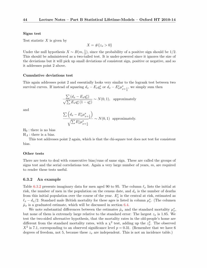
44 Lecture Notes – Part B Statistical Lifetime-Models – Oxford HT 2010-14
Signs test
Test statistic X is given byX = #{zx > 0}
Under the null hypothesis X ∼ B(m, 12), since the probability of a positive sign should be 1/2.
This should be administered as a two-tailed test. It is under-powered since it ignores the size ofthe deviations but it will pick up small deviations of consistent sign, positive or negative, and soit addresses point 2 above.
Cumulative deviations test
This again addresses point 2 and essentially looks very similar to the logrank test between twosurvival curves. If instead of squaring dx − Exqs
x or dx − Ecxµs
x+ 12
, we simply sum then∑(dx − Exqs
x)√∑Exqs
x (1− qsx)∼ N(0, 1), approximately
and ∑(dx − Ec
xµsx+ 1
2
)√∑
Ecxµs
x+ 12
∼ N(0, 1) approximately.
H0 : there is no biasHA : there is a bias.
This test addresses point 2 again, which is that the chi-square test does not test for consistentbias.
Other tests
There are tests to deal with consecutive bias/runs of same sign. These are called the groups ofsigns test and the serial correlations test. Again a very large number of years, m, are requiredto render these tests useful.
6.3.2 An example
Table 6.3.2 presents imaginary data for men aged 90 to 95. The column `x lists the initial atrisk, the number of men in the population on the census date, and dx is the number of deathsfrom this initial population over the course of the year. Ec
x is the central at risk, estimated as`x − dx/2. Standard male British mortality for these ages is listed in column µs
x. (The columenµx is a graduated estimate, which will be discussed in section 6.4.
We note substantial differences between the estimates µx and the standard mortality µsx,
but none of them is extremely large relative to the standard error: The largest zx is 1.85. Wetest the two-sided alternative hypothesis, that the mortality rates in the old-people’s home aredifferent from the standard mortality rates, with a χ2 test, adding up the z2
x. The observedX2 is 7.1, corresponding to an observed significance level p = 0.31. (Remember that we have 6degrees of freedom, not 5, because these zx are independent. This is not an incidence table.)
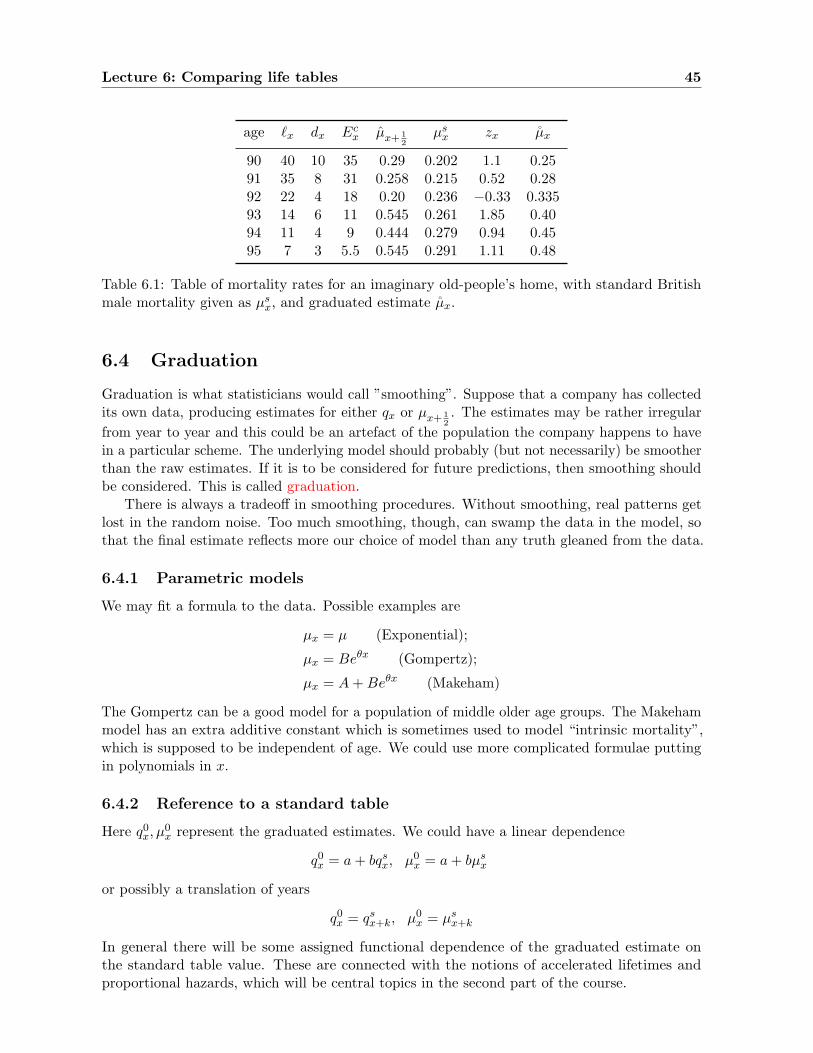
Lecture 6: Comparing life tables 45
age `x dx Ecx µx+ 1
2µs
x zx µx
90 40 10 35 0.29 0.202 1.1 0.2591 35 8 31 0.258 0.215 0.52 0.2892 22 4 18 0.20 0.236 −0.33 0.33593 14 6 11 0.545 0.261 1.85 0.4094 11 4 9 0.444 0.279 0.94 0.4595 7 3 5.5 0.545 0.291 1.11 0.48
Table 6.1: Table of mortality rates for an imaginary old-people’s home, with standard Britishmale mortality given as µs
x, and graduated estimate µx.
6.4 Graduation
Graduation is what statisticians would call ”smoothing”. Suppose that a company has collectedits own data, producing estimates for either qx or µx+ 1
2. The estimates may be rather irregular
from year to year and this could be an artefact of the population the company happens to havein a particular scheme. The underlying model should probably (but not necessarily) be smootherthan the raw estimates. If it is to be considered for future predictions, then smoothing shouldbe considered. This is called graduation.
There is always a tradeoff in smoothing procedures. Without smoothing, real patterns getlost in the random noise. Too much smoothing, though, can swamp the data in the model, sothat the final estimate reflects more our choice of model than any truth gleaned from the data.
6.4.1 Parametric models
We may fit a formula to the data. Possible examples are
µx = µ (Exponential);
µx = Beθx (Gompertz);
µx = A + Beθx (Makeham)
The Gompertz can be a good model for a population of middle older age groups. The Makehammodel has an extra additive constant which is sometimes used to model “intrinsic mortality”,which is supposed to be independent of age. We could use more complicated formulae puttingin polynomials in x.
6.4.2 Reference to a standard table
Here q0x, µ0
x represent the graduated estimates. We could have a linear dependence
q0x = a + bqs
x, µ0x = a + bµs
x
or possibly a translation of years
q0x = qs
x+k, µ0x = µs
x+k
In general there will be some assigned functional dependence of the graduated estimate onthe standard table value. These are connected with the notions of accelerated lifetimes andproportional hazards, which will be central topics in the second part of the course.
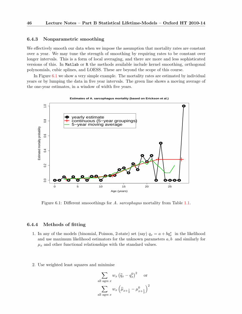
46 Lecture Notes – Part B Statistical Lifetime-Models – Oxford HT 2010-14
6.4.3 Nonparametric smoothing
We effectively smooth our data when we impose the assumption that mortality rates are constantover a year. We may tune the strength of smoothing by requiring rates to be constant overlonger intervals. This is a form of local averaging, and there are more and less sophisticatedversions of this. In Matlab or R the methods available include kernel smoothing, orthogonalpolynomials, cubic splines, and LOESS. These are beyond the scope of this course.
In Figure 6.1 we show a very simple example. The mortality rates are estimated by individualyears or by lumping the data in five year intervals. The green line shows a moving average ofthe one-year estimates, in a window of width five years.
● ●
●
●
●
●
●
●
● ●
●
● ● ●
●●
●
●
●
●
●
●
●
●
● ● ● ●
●
0 5 10 15 20 25
0.0
0.2
0.4
0.6
0.8
1.0
Estimates of A. sarcophagus mortality (based on Erickson et al.)
Age (years)
Estim
ated
mor
tality
pro
babi
lity
● yearly estimatecontinuous (5−year groupings)5−year moving average
Figure 6.1: Different smooothings for A. sarcophagus mortality from Table 1.1.
6.4.4 Methods of fitting
1. In any of the models (binomial, Poisson, 2-state) set (say) qx = a + bqsx in the likelihood
and use maximum likelihood estimators for the unknown parameters a, b and similarly forµx and other functional relationships with the standard values.
2. Use weighted least squares and minimise∑all ages x
wx
(qx − q0
x
)2 or
∑all ages x
wx
(µx+ 1
2− µ0
x+ 12
)2
Lecture 6: Comparing life tables 47
0 5 10 15 20 25
0.01
0.02
0.05
0.10
0.20
0.50
1.00
2.00
Tyrannosaur mortality rates
Age (yrs)
Mor
talit
y ra
te
Estimates from dataConstant hazard fitGompertz hazard fit
Figure 6.2: Estimated tyrannosaurus mortality rates from Table 4.3, together with exponentialand Gompertz fits.
as appropriate. For the weights suitable choices are either Ex or Ecx respectively. Alterna-
tively we can use 1/var, where the variance is estimated for qx or µx+ 12, respectively.
The hypothesis tests we have already covered above can be used to test the graduation fit tothe data, replacing qs
x, µsx+ 1
2
by the graduated estimates. Note that in the χ2 test we must
reduce the degrees of freedom of the χ2 distribution by the number of parametersestimated in the model for the graduation. For example if q0
x = a + bqsx, then we reduce
the degrees of freedom by 2 as the parameters a, b are estimated.
6.4.5 Examples
Standard life table
We graduate the estimates in Table 6.3.2, based on the standard mortality rates listed in thecolumn µs
x, using the parametric model µx = a + bµsx. The log likelihood is
` =∑
dx log µx+ 12− µx+ 1
2Ec
x.
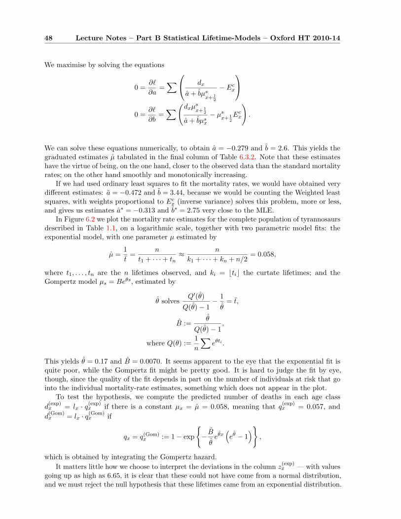
48 Lecture Notes – Part B Statistical Lifetime-Models – Oxford HT 2010-14
We maximise by solving the equations
0 =∂`
∂a=∑ dx
a + bµsx+ 1
2
− Ecx
0 =
∂`
∂b=∑(
dxµsx+ 1
2
a + bµsx
− µsx+ 1
2
Ecx
).
We can solve these equations numerically, to obtain a = −0.279 and b = 2.6. This yields thegraduated estimates µ tabulated in the final column of Table 6.3.2. Note that these estimateshave the virtue of being, on the one hand, closer to the observed data than the standard mortalityrates; on the other hand smoothly and monotonically increasing.
If we had used ordinary least squares to fit the mortality rates, we would have obtained verydifferent estimates: a = −0.472 and b = 3.44, because we would be counting the Weighted leastsquares, with weights proportional to Ec
x (inverse variance) solves this problem, more or less,and gives us estimates a∗ = −0.313 and b∗ = 2.75 very close to the MLE.
In Figure 6.2 we plot the mortality rate estimates for the complete population of tyrannosaursdescribed in Table 1.1, on a logarithmic scale, together with two parametric model fits: theexponential model, with one parameter µ estimated by
µ =1t
=n
t1 + · · ·+ tn≈ n
k1 + · · ·+ kn + n/2= 0.058,
where t1, . . . , tn are the n lifetimes observed, and ki = btic the curtate lifetimes; and theGompertz model µs = Beθs, estimated by
θ solvesQ′(θ)
Q(θ)− 1− 1
θ= t,
B :=θ
Q(θ)− 1,
where Q(θ) :=1n
∑eθti .
This yields θ = 0.17 and B = 0.0070. It seems apparent to the eye that the exponential fit isquite poor, while the Gompertz fit might be pretty good. It is hard to judge the fit by eye,though, since the quality of the fit depends in part on the number of individuals at risk that gointo the individual mortality-rate estimates, something which does not appear in the plot.
To test the hypothesis, we compute the predicted number of deaths in each age classd
(exp)x = lx · q(exp)
x if there is a constant µx = µ = 0.058, meaning that q(exp)x = 0.057, and
d(Gom)x = lx · q(Gom)
x if
qx = q(Gom)x := 1− exp
{−B
θeθx(eθ − 1
)},
which is obtained by integrating the Gompertz hazard.It matters little how we choose to interpret the deviations in the column z
(exp)x — with values
going up as high as 6.65, it is clear that these could not have come from a normal distribution,and we must reject the null hypothesis that these lifetimes came from an exponential distribution.
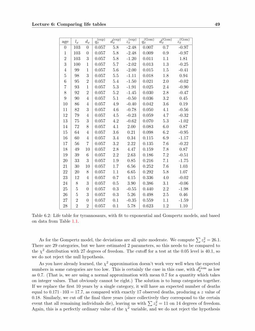
Lecture 6: Comparing life tables 49
age lx dx q(exp)x d
(exp)x z
(exp)x q
(Gom)x d
(Gom)x z
(Gom)x
0 103 0 0.057 5.8 -2.48 0.007 0.7 -0.971 103 0 0.057 5.8 -2.48 0.009 0.9 -0.972 103 3 0.057 5.8 -1.20 0.011 1.1 1.813 100 1 0.057 5.7 -2.02 0.013 1.3 -0.254 99 1 0.057 5.6 -2.00 0.015 1.5 -0.415 98 3 0.057 5.5 -1.11 0.018 1.8 0.946 95 2 0.057 5.4 -1.50 0.021 2.0 -0.027 93 1 0.057 5.3 -1.91 0.025 2.4 -0.908 92 2 0.057 5.2 -1.45 0.030 2.8 -0.479 90 4 0.057 5.1 -0.50 0.036 3.2 0.4510 86 4 0.057 4.9 -0.40 0.042 3.6 0.1911 82 3 0.057 4.6 -0.78 0.050 4.1 -0.5612 79 4 0.057 4.5 -0.23 0.059 4.7 -0.3213 75 3 0.057 4.2 -0.62 0.070 5.3 -1.0214 72 8 0.057 4.1 2.00 0.083 6.0 0.8715 64 4 0.057 3.6 0.21 0.098 6.2 -0.9516 60 4 0.057 3.4 0.34 0.115 6.9 -1.1717 56 7 0.057 3.2 2.22 0.135 7.6 -0.2218 49 10 0.057 2.8 4.47 0.159 7.8 0.8719 39 6 0.057 2.2 2.63 0.186 7.2 -0.5120 33 3 0.057 1.9 0.85 0.216 7.1 -1.7521 30 10 0.057 1.7 6.56 0.252 7.6 1.0322 20 8 0.057 1.1 6.65 0.292 5.8 1.0723 12 4 0.057 0.7 4.15 0.336 4.0 -0.0224 8 3 0.057 0.5 3.90 0.386 3.1 -0.0625 5 0 0.057 0.3 -0.55 0.440 2.2 -1.9826 5 3 0.057 0.3 5.26 0.498 2.5 0.4627 2 0 0.057 0.1 -0.35 0.559 1.1 -1.5928 2 2 0.057 0.1 5.78 0.623 1.2 1.10
Table 6.2: Life table for tyrannosaurs, with fit to exponential and Gompertz models, and basedon data from Table 1.1.
As for the Gompertz model, the deviations are all quite moderate. We compute∑
z2x = 26.1.
There are 29 categories, but we have estimated 2 parameters, so this needs to be compared tothe χ2 distribution with 27 degrees of freedom. The cutoff for a test at the 0.05 level is 40.1, sowe do not reject the null hypothesis.
As you have already learned, the χ2 approximation doesn’t work very well when the expectednumbers in some categories are too low. This is certainly the case in this case, with dGom
x as lowas 0.7. (That is, we are using a normal approximation with mean 0.7 for a quantity which takeson integer values. That obviously cannot be right.) The solution is to lump categories together.If we replace the first 10 years by a single category, it will have an expected number of deathsequal to 0.171 · 103 = 17.7, as compared with exactly 17 observed deaths, producing a z value of0.18. Similarly, we cut off the final three years (since collectively they correspond to the certainevent that all remaining individuals die), leaving us with
∑z2x = 11 on 14 degrees of freedom.
Again, this is a perfectly ordinary value of the χ2 variable, and we do not reject the hypothesis

50 Lecture Notes – Part B Statistical Lifetime-Models – Oxford HT 2010-14
of Gompertz mortality.
Lecture 7
Multiple decrements model
Reading: Gerber Sections 7.1-7.3 and 11.7, Cox-Oakes Sections 9.1-9.2,Norris Section 1.10, CT4 Units 9,10-3,10-4
Further reading: Cox-Oakes Section 9.3
7.1 The Poisson model
Under the assumption of a constant hazard rate (force of mortality) µx+ 12
over the year (x, x+1],we may view the estimation problem as a chain of separate hazard rate estimation problems, onefor each year of life. Each individual lives some portion of a year in the age interval (x, x + 1],the portion being 0 (if he dies before birthday x), 1 (if he dies after birthday x + 1), or between0 and 1 if he dies between the two birthdays. Suppose now we lay these intervals end to end,with a mark at the end of an interval where an individual died. It is not hard to see that whatresults is a Poisson process on the interval [0, Ec
x], where Ecx is the total observed years at risk.
Suppose we treat Ecx as though it were a constant. Then if Dx represents the numbers dying
in the year the model uses
P{Dx = k
}=
(µx+ 1
2Ec
x
)ke−µ
x+12
Ecx
k!, k = 0, 1, 2, · · ·
which is an approximation to the 2-state model, and which in fact yields the same likelihood.The estimator for the constant force of mortality over the year is
µx+ 12
=Dx
Ecx
, with estimatedx
Ecx
.
Under the Poisson model we therefore have that
varµx+ 12
=µx+ 1
2Ec
x
(Ecx)2
=µx+ 1
2
Ecx
.
So the estimate will bevarµx+ 1
2≈ dx
(Ecx)2
.
If we compare with the 2-state stochastic model over year (x, x + 1), assuming constantµ = µx+ 1
2, then the likelihood is
L =n∏1
µδie−µti ,
51
52 Lecture Notes – Part B Statistical Lifetime-Models – Oxford HT 2010-14
where δi = 1 if life i dies and ti = bi − ai in previous terminology (see the binomial model).Hence
L = µdxe−µEcx
and soµ =
Dx
Ecx
.
The estimator is exactly the same as for the Poisson model except that both Dx and Ecx are
random variables. Using asymptotic likelihood theory we see that the estimate for the varianceis
varµ ≈ µ2
dx≈ dx
(Ecx)2
.
Are we justified in treating Ecx as though it were fixed? Certainly it’s not exactly the same:
The numerator and denominator are both random, and they are not even independent. One wayof looking at this is to ask, how different would our estimate have been in a given realisation,had we fixed the total time under observation in advance. If we observe m lives from the startof year x, we see that Dx is approximately normal with mean mqx and variance mqx(1− qx),while Ec
x is normal with mean m−mqx(1− e∗), where e∗ is the expected remaining length of alife starting from age x, conditioned on its being less than 1; and variance mσ2, where σ2 isthe variance in time under observation of a single life. (If µx is not very large, e∗ is close to 1
2 .)Looking at the first-order Taylor series expansion, we see that the ratio Dx/Ec
x varies only by anormal error term times m−1/2, plus a bias of order m−1. For large m, then, the estimate onthe basis of fixed m (number of individuals) is almost the same as the estimate we would havemade from observing the Poisson model for the fixed total time at risk m−mqx(1− e∗).
7.2 Rates in the single decrement model
The rate parameter in the two-state Markov model with L ∼ Exp(λ) has the infinitesimalinterpretation
P(Xt+ε = 1|Xt = 0) = P(L ≤ t + ε|L > t) = 1− e−λε = λε + o(ε), (7.1)
and for a general L with right-continuous density and hence right-continuous force of mortalityt 7→ µt, we have
P(Xt+ε = 1|Xt = 0) = P(L ≤ t + ε|L > t) = 1− exp{−∫ t+ε
tµsds
}= µtε + o(ε), (7.2)
since, by l’Hopital’s rule
limε↓0
1ε
(1− exp
{−∫ t+ε
tµsds
})= lim
ε↓0µt+ε exp
{−∫ t+ε
tµsds
}= µt. (7.3)
It is therefore natural to express the two-state model by a time-dependent Q-matrix
Q(t) =(−λ(t) λ(t)
0 0
), where λ(t) = µt = hL(t). (7.4)
For estimation purposes, it has been convenient to add as additional assumption thatλ(t) = µt = µx+ 1
2= λ(x + 1
2) is constant on x ≤ t < x + 1, x ∈ N.
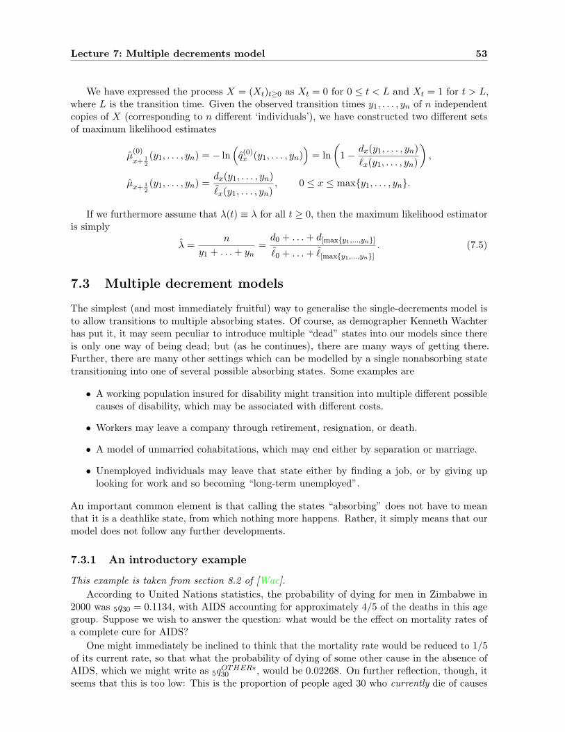
Lecture 7: Multiple decrements model 53
We have expressed the process X = (Xt)t≥0 as Xt = 0 for 0 ≤ t < L and Xt = 1 for t > L,where L is the transition time. Given the observed transition times y1, . . . , yn of n independentcopies of X (corresponding to n different ‘individuals’), we have constructed two different setsof maximum likelihood estimates
µ(0)
x+ 12
(y1, . . . , yn) = − ln(q(0)x (y1, . . . , yn)
)= ln
(1− dx(y1, . . . , yn)
`x(y1, . . . , yn)
),
µx+ 12(y1, . . . , yn) =
dx(y1, . . . , yn)˜x(y1, . . . , yn)
, 0 ≤ x ≤ max{y1, . . . , yn}.
If we furthermore assume that λ(t) ≡ λ for all t ≥ 0, then the maximum likelihood estimatoris simply
λ =n
y1 + . . . + yn=
d0 + . . . + d[max{y1,...,yn}]˜0 + . . . + ˜
[max{y1,...,yn}]. (7.5)
7.3 Multiple decrement models
The simplest (and most immediately fruitful) way to generalise the single-decrements model isto allow transitions to multiple absorbing states. Of course, as demographer Kenneth Wachterhas put it, it may seem peculiar to introduce multiple “dead” states into our models since thereis only one way of being dead; but (as he continues), there are many ways of getting there.Further, there are many other settings which can be modelled by a single nonabsorbing statetransitioning into one of several possible absorbing states. Some examples are
• A working population insured for disability might transition into multiple different possiblecauses of disability, which may be associated with different costs.
• Workers may leave a company through retirement, resignation, or death.
• A model of unmarried cohabitations, which may end either by separation or marriage.
• Unemployed individuals may leave that state either by finding a job, or by giving uplooking for work and so becoming “long-term unemployed”.
An important common element is that calling the states “absorbing” does not have to meanthat it is a deathlike state, from which nothing more happens. Rather, it simply means that ourmodel does not follow any further developments.
7.3.1 An introductory example
This example is taken from section 8.2 of [Wac].According to United Nations statistics, the probability of dying for men in Zimbabwe in
2000 was 5q30 = 0.1134, with AIDS accounting for approximately 4/5 of the deaths in this agegroup. Suppose we wish to answer the question: what would be the effect on mortality rates ofa complete cure for AIDS?
One might immediately be inclined to think that the mortality rate would be reduced to 1/5of its current rate, so that what the probability of dying of some other cause in the absence ofAIDS, which we might write as 5q
OTHER∗30 , would be 0.02268. On further reflection, though, it
seems that this is too low: This is the proportion of people aged 30 who currently die of causes
54 Lecture Notes – Part B Statistical Lifetime-Models – Oxford HT 2010-14
other than AIDS. If AIDS were eliminated, surely some of the people who now die of AIDSwould instead die of something else.
Of course, this is not yet a well-defined mathematical problem. To make it such, we need toimpose extra conditions. In particular, we impose the competing risks assumption: Individualcauses of death are assumed to act independently. You might imagine an individual drawinglots from multiple urns, labelled “AIDS”, “Stroke”, “Plane crash”, to determine whether he willdie of this cause in the next year. The fraction of black lots among the white is precisely qx,when the individual has age x. If he gets no black lot, he survives the year. If he draws twoor more, we only get to see the one drawn first, since he can only die once. The probability ofsurviving is then the product of the survival probabilities:
iqx = 1−(1− iq
CAUSE1x
)(1− iq
CAUSE2x
)· · · (7.6)
What is the fraction of deaths due to a given cause? Assuming constant mortality rate over thetime interval due to each cause, we have
1− tqCAUSE1x = e−tλCAUSE1
x .
Given a death, the probability of it being due to a given cause, is proportional to the associatedhazard rate. Consequently,
λCAUSE1x = fraction of deaths due to CAUSE 1× λx,
which implies that
tqCAUSE1x = 1− (1− tqx)fraction of deaths due to CAUSE 1 .
(Note that this is the same formula that we use for changing lengths of time intervals: tqx =1− (1− 1qx)t.) This tells us the probability of dying from cause 1 in the absence of any othercause. The probability of dying of any cause at all is then given by (7.6).
Applying this to our Zimbabwe AIDS example, treating the causes as being either AIDS orOTHER, we see that the probability of dying of AIDS in the absence of any other cause is
5qAIDS∗30 = 1− (1− 5q30)4/5 = 1− 0.88664/5 = 0.0918,
while the probability of dying of any other cause, in the absence of AIDS, is
5qOTHER∗30 = 1− (1− 5q30)4/5 = 1− 0.88661/5 = 0.0238.
Appropriately, we have the total cause of death 0.1138 = 1− (1− 0.0918)(1− 0.0238).Is the competing risks assumption reasonable? Another way of putting this is to ask, what
circumstances would cause the assumption to be violated? The answer is: Competing risksis violated when a subpopulation is at higher than average risk for multiple causes of deathsimultaneously; or conversely, when those at higher than average risk for one cause of death areprotected from another cause of death. For example, smokers have more than 10 times the risk ofdying from lung cancer that nonsmokers have; but they also have substantially higher mortalityfrom other cancers, heart disease, stroke, and so on. If a perfect cure for lung cancer were tobe found, it would not save nearly as many lives as one might suppose, from a competing-riskscalculation like the one above, because the lives that would be saved would be almost all thoseof smokers, and they would be more likely to die of something else than an equivalent numberof saved lives from the general population.
Lecture 7: Multiple decrements model 55
7.3.2 Basic theory
We consider here more general 1 + m-state Markov models with state space S = {0, . . . ,m} thatonly have one transition from 0 to j, for some 1 ≤ j ≤ m, with absorption in j. We can writedown an – in general time-dependet – Q-matrix
Q(t) =
−λ+(t) λ1(t) · · · λm(t)
0 0 · · · 0...
.... . .
...0 0 · · · 0
, where λ+(t) = λ1(t) + . . . + λm(t). (7.7)
Such models occur naturally where insurance policies provide different benefits for differentcauses of death, or distinguish death and disability, possibly in various different strengths orforms. This is also clearly a building block (one transition only) for general Markov models,where states j = 1, . . . ,m may not all be absorbing.
Such a model depends upon the assumption that different causes of death act independently— that is, the probability of dying is the product of what might be understood as the probabilityof dying from each individual cause acting alone.
7.3.3 Multiple decrements – time-homogeneous rates
In the time-homogenous case, we can think of the multiple decrement model as m exponentialclocks Cj with parameters λj , 1 ≤ j ≤ m, and when the first clock goes off, say, clock j, theonly transition takes place, and leads to state j. Alternatively, we can describe the model asconsisting of one L ∼ Exp(λ+) holding time in state 0, after which the new state j is chosenindependently with probability λj/λ+, 1 ≤ j ≤ m. The likelihood for a sample of size 1 consistsof two ingredients, the density λ+e−tλ+ of the exponential time, and the probability λj/λ+ ofthe transition observed. This gives λje
−tλ+ , or, for a sample of size n of lifetimes ti and statesji, 1 ≤ i ≤ n,
n∏i=1
λjie−tiλ+ =
m∏j=1
λnj
j e−λj(t1+...+tn), (7.8)
where nj is the number of transitions to j. Again, this can be solved factor by factor to give
λj =nj
t1 + . . . + tn, 1 ≤ j ≤ m. (7.9)
In particular, we find again λ+ = n/(t1 + . . . + tn), since n1 + . . . + nm = n.In the competing-clocks description, we can interpret the likelihood as consisting of m
ingredients, namely the density λje−λjt of clock j to go off at time t, and probabilities e−λkt of
clocks Ck, k 6= j, to go off after time t.
Lecture 8
Multiple Decrements: Theory andExamples
8.1 Estimation for general multiple decrements
We can deduce from either description in the previous section that the likelihood for a sampleof n independent lifetimes y1, . . . , yn and respective new states j1, . . . , jn, each (yi, ji) sampledfrom (L, J), is given by
n∏i=1
λji(yi) exp{−∫ yi
0λ+(t)dt
}. (8.1)
Let us assume that the forces of decrement λj(t) = λj(x + 12) are constant on x ≤ t < x + 1, for
all x ∈ N and 1 ≤ j ≤ m. Then the likelihood can be given as
∏x∈N
m∏j=1
(λj(x + 1
2))dj,x exp
{−˜
xλj(x + 12)}
, (8.2)
where dj,x is the number of decrements to state j between ages x and x + 1, and ˜x is the total
time spent alive between ages x and x + 1.Now the parameters are λj(x + 1
2), x ∈ N, 1 ≤ j ≤ m, and they are again well separated todeduce
λj(x + 12) =
dj,x
˜x
, 1 ≤ j ≤ m, 0 ≤ x ≤ max{L1, . . . , Ln}. (8.3)
Similarly, we can try to adapt the method to get maximum likelihood estimators from thecurtate lifetimes. We can write down the likelihood as
n∏i=1
p(J,K)(ji, [yi]) =∏x∈N
(1− qx)`x−dx
m∏j=1
qdj,x
j,x , (8.4)
but 1− qx = 1− q1,x − . . .− qm,x does not factorise, so we have to maximise simultaneously forall 1 ≤ j ≤ m expressions of the form
(1− q1 − . . .− qm)`−d1−...−dm
m∏j=1
qdj
j . (8.5)
(We suppress the indices x.) A zero derivative with respect to qj amounts to
(`− d1 − . . .− dm)qj = dj(1− q1 − . . .− qm), 1 ≤ j ≤ m, (8.6)
56
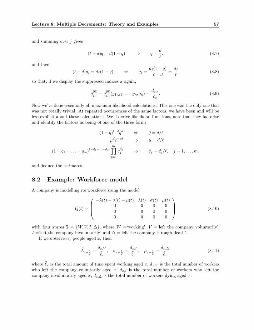
Lecture 8: Multiple Decrements: Theory and Examples 57
and summing over j gives
(`− d)q = d(1− q) ⇒ q =d
`. (8.7)
and then(`− d)qj = dj(1− q) ⇒ qj =
dj(1− q)`− d
=dj
`(8.8)
so that, if we display the suppressed indices x again,
q(0)j,x = q
(0)j,x(y1, j1, . . . , yn, jn) =
dj,x
`x. (8.9)
Now we’ve done essentially all maximum likelihood calculations. This one was the only one thatwas not totally trivial. At repeated occurrences of the same factors, we have been and will beless explicit about these calculations. We’ll derive likelihood functions, note that they factoriseand identify the factors as being of one of the three forms
(1− q)`−dqd ⇒ q = d/`
µde−µ` ⇒ µ = d/`
(1− q1 − . . .− qm)`−d1−...−dm
m∏j=1
qdj
j ⇒ qj = dj/`, j = 1, . . . ,m.
and deduce the estimates.
8.2 Example: Workforce model
A company is modelling its workforce using the model
Q(t) =
−λ(t)− σ(t)− µ(t) λ(t) σ(t) µ(t)
0 0 0 00 0 0 00 0 0 0
(8.10)
with four states S = {W,V, I,∆}, where W =‘working’, V =’left the company voluntarily’,I =’left the company involuntarily’ and ∆ =’left the company through death’.
If we observe nx people aged x, then
λx+ 12
=dx,V
˜x
, σx+ 12
=dx,I
˜x
, µx+ 12
=dx,∆
˜x
(8.11)
where ˜x is the total amount of time spent working aged x, dx,V is the total number of workers
who left the company voluntarily aged x, dx,I is the total number of workers who left thecompany involuntarily aged x, dx,∆ is the total number of workers dying aged x.
Lecture 9
Multiple decrements: Thedistribution of the endpoint
9.1 Which state do we end up in?
The time-homogeneous multiple-decrement model makes a transition at the minimum of mexponential clocks as opposed to one clock in the single decrement model. In the same way, wecan construct the time-inhomogeneous multiple-decrement model from m independent clocks Cj
with hazard function λj(t), 1 ≤ j ≤ m. Then the likelihood for a transition at time t to state jis the product of fCj (t) and FCk
(t).By Exercise A.1.2, the hazard function of L = min{C1, . . . , Cm} is given by hL(t) =
hC1(t) + . . . + hCm(t) = λ1(t) + . . . + λm(t) = λ+(t), and we can also calculate
P(L = Cj |L = t)= limε↓0
P(t ≤ Cj < t + ε, min{Ck : k 6= j} ≥ Cj)P(t ≤ L < t + ε)
≥ limε↓0
1εP(t ≤ Cj < t + ε, min{Ck : k 6= j} ≥ t + ε)
1εP(t ≤ L < t + ε)
≤ limε↓0
1εP(t ≤ Cj < t + ε, min{Ck : k 6= j} ≥ t)
1εP(t ≤ L < t + ε)
=fCj (t)
∏k 6=j FCk
(t)fL(t)
=hCj (t)hL(t)
=λj(t)λ+(t)
,
and we obtain
P(L = Cj) =∫ ∞
0P(L = Cj |L = t)fL(t)dt =
∫ ∞
0λj(t)FL(t)dt = E(Λj(L)), (9.1)
where Λj(t) =∫ t0 λj(s)ds is the integrated hazard function. (For the last step we used that
E(g(L)) =∫∞0 g′(t)FL(t)dt for all increasing differentiable g : [0,∞) → [0,∞) with g(0) = 0.)
The discrete (curtate) lifetime model: We can also split the curtate lifetime K = [L]according to the type of decrement J (J = j if L = Tj) and define
qj,x = P(L < x + 1, J = j|L > x), 1 ≤ j ≤ m, x ∈ N, (9.2)
then clearly for x ∈ Nq1,x + . . . + qm,x = qx (9.3)
58
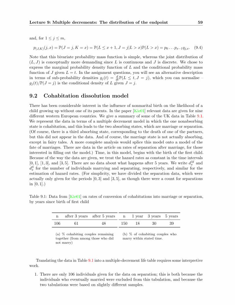
Lecture 9: Multiple decrements: The distribution of the endpoint 59
and, for 1 ≤ j ≤ m,
p(J,K)(j, x) = P(J = j, K = x) = P(L ≤ x + 1, J = j|L > x)P(L > x) = p0 . . . px−1qj,x. (9.4)
Note that this bivariate probability mass function is simple, whereas the joint distribution of(L, J) is conceptually more demanding since L is continuous and J is discrete. We chose toexpress the marginal probability density function of L and the conditional probability massfunction of J given L = t. In the assignment questions, you will see an alternative descriptionin terms of sub-probability densities gj(t) = d
dtP(L ≤ t, J = j), which you can normalise –gj(t)/P(J = j) is the conditional density of L given J = j.
9.2 Cohabitation dissolution model
There has been considerable interest in the influence of nonmarital birth on the likelihood of achild growing up without one of its parents. In the paper [Kie01] relevant data are given for ninedifferent western European countries. We give a summary of some of the UK data in Table 9.1.We represent the data in terms of a multiple decrement model in which the one nonabsorbingstate is cohabitation, and this leads to the two absorbing states, which are marriage or separation.(Of course, there is a third absorbing state, corresponding to the death of one of the partners,but this did not appear in the data. And of course, the marriage state is not actually absorbing,except in fairy tales. A more complete analysis would splice this model onto a model of thefate of marriages. There are data in the article on rates of separation after marriage, for thoseinterested in filling out the model.) Time, in this model, begins with the birth of the first child.Because of the way the data are given, we treat the hazard rates as constant in the time intervals[0, 1], [1, 3], and [3, 5]. There are no data about what happens after 5 years. We write dM
x anddS
x for the number of individuals marrying and separating, respectively, and similar for theestimation of hazard rates. (For simplicity, we have divided the separation data, which wereactually only given for the periods [0, 3] and [3, 5], as though there were a count for separationsin [0, 1].)
Table 9.1: Data from [Kie01] on rates of conversion of cohabitations into marriage or separation,by years since birth of first child
n after 3 years after 5 years
106 61 48
(a) % cohabiting couples remainingtogether (from among those who didnot marry)
n 1 year 3 years 5 years
150 18 30 39
(b) % of cohabiting couples whomarry within stated time.
Translating the data in Table 9.1 into a multiple-decrement life table requires some interpretivework.
1. There are only 106 individuals given for the data on separation; this is both because theindividuals who eventually married were excluded from this tabulation, and because thetwo tabulations were based on slightly different samples.
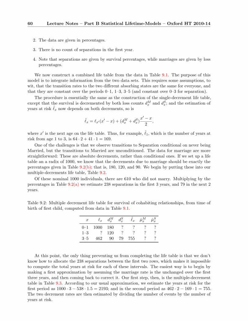
60 Lecture Notes – Part B Statistical Lifetime-Models – Oxford HT 2010-14
2. The data are given in percentages.
3. There is no count of separations in the first year.
4. Note that separations are given by survival percentages, while marriages are given by losspercentages.
We now construct a combined life table from the data in Table 9.1. The purpose of thismodel is to integrate information from the two data sets. This requires some assumptions, towit, that the transition rates to the two different absorbing states are the same for everyone, andthat they are constant over the periods 0–1, 1–3, 3–5 (and constant over 0–3 for separation).
The procedure is essentially the same as the construction of the single-decrement life table,except that the survival is decremented by both loss counts dM
x and dSx ; and the estimation of
years at risk ˜x now depends on both decrements, so is
˜x = `x′(x′ − x) + (dM
x + dSx )
x′ − x
2,
where x′ is the next age on the life table. Thus, for example, ˜1, which is the number of years at
risk from age 1 to 3, is 64 · 2 + 41 · 1 = 169.One of the challenges is that we observe transitions to Separation conditional on never being
Married, but the transitions to Married are unconditioned. The data for marriage are morestraightforward: These are absolute decrements, rather than conditional ones. If we set up a lifetable an a radix of 1000, we know that the decrements due to marriage should be exactly thepercentages given in Table 9.2(b); that is, 180, 120, and 90. We begin by putting these into ourmultiple-decrements life table, Table 9.2.
Of these nominal 1000 individuals, there are 610 who did not marry. Multiplying by thepercentages in Table 9.2(a) we estimate 238 separations in the first 3 years, and 79 in the next 2years.
Table 9.2: Multiple decrement life table for survival of cohabiting relationships, from time ofbirth of first child, computed from data in Table 9.1.
x `x dMx dS
x˜x µM
x µSx
0–1 1000 180 ? ? ? ?1–3 ? 120 ? ? ? ?3–5 462 90 79 755 ? ?
At this point, the only thing preventing us from completing the life table is that we don’tknow how to allocate the 238 separations between the first two rows, which makes it impossibleto compute the total years at risk for each of these intervals. The easiest way is to begin bymaking a first approximation by assuming the marriage rate is the unchanged over the firstthree years, and then coming back to correct it. Our first step, then, is the multiple-decrementtable in Table 9.3. According to our usual approximation, we estimate the years at risk for thefirst period as 1000 · 3 − 538 · 1.5 = 2193; and in the second period as 462 · 2 − 169 · 1 = 755.The two decrement rates are then estimated by dividing the number of events by the number ofyears at risk.
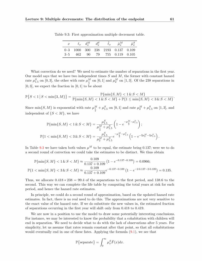
Lecture 9: Multiple decrements: The distribution of the endpoint 61
Table 9.3: First approximation multiple decrement table.
x `x dMx dS
x˜x µM
x µSx
0–3 1000 300 238 2193 0.137 0.1093–5 462 90 79 755 0.119 0.105
What correction do we need? We need to estimate the number of separations in the first year.Our model says that we have two independent times S and M , the former with constant hazardrate µS
1.5 on [0, 3], the other with rate µM12
on [0, 1] and µM2 on [1, 3]. Of the 238 separations in
[0, 3], we expect the fraction in [0, 1] to be about
P{S < 1
∣∣S < min{3,M}}
=P{min{S, M} < 1 &S < M}
P{min{S, M} < 1 &S < M}+ P{1 ≤ min{S, M} < 3 &S < M}.
Since min{S, M} is exponential with rate µM12
+ µS1.5 on [0, 1] and rate µM
2 + µS1.5 on [1, 3], and
independent of {S < M}, we have
P{min{S, M} < 1 &S < M} =µS
1.5
µM12
+ µS1.5
(1− e
−µM12
−µS1.5
);
P{1 < min{S, M} < 3 &S < M} =µS
1.5
µM2 + µS
1.5
e−µM
12
−µS1.5(1− e−2µM
2 −2µS1.5
).
In Table 9.3 we have taken both values µM to be equal, the estimate being 0.137; were we to doa second round of correction we could take the estimates to be distinct. We thus obtain
P{min{S, M} < 1 &S < M} ≈ 0.1090.137 + 0.109
(1− e−0.137−0.109
)= 0.0966;
P{1 < min{S, M} < 3 &S < M} ≈ 0.1090.137 + 0.109
e−0.137−0.109(1− e−2·0.137−2·0.109
)= 0.135.
Thus, we allocate 0.418 ∗ 238 = 99.4 of the separations to the first period, and 138.6 to thesecond. This way we can complete the life table by computing the total years at risk for eachperiod, and hence the hazard rate estimates.
In principle, we could do a second round of approximation, based on the updated hazard rateestimates. In fact, there is no real need to do this. The approximations are not very sensitive tothe exact value of the hazard rate. If we do substitute the new values in, the estimated fractionof separations occurring in the first year will shift only from 0.418 to 0.419.
We are now in a position to use the model to draw some potentially interesting conclusions.For instance, we may be interested to know the probability that a cohabitation with children willend in separation. We need to decide what to do with the lack of observations after 5 years. Forsimplicity, let us assume that rates remain constant after that point, so that all cohabitationswould eventually end in one of these fates. Applying the formula (9.1), we see that
P{separate
}=∫ ∞
0µS
x F (x)dx.
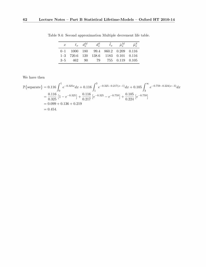
62 Lecture Notes – Part B Statistical Lifetime-Models – Oxford HT 2010-14
Table 9.4: Second approximation Multiple decrement life table.
x `x dMx dS
x˜x µM
x µSx
0–1 1000 180 99.4 860.2 0.209 0.1161–3 720.6 120 138.6 1183 0.101 0.1163–5 462 90 79 755 0.119 0.105
We have then
P{separate
}= 0.116
∫ 1
0e−0.325xdx + 0.116
∫ 3
1e−0.325−0.217(x−1)dx + 0.105
∫ ∞
3e−0.759−0.224(x−3)dx
=0.1160.325
[1− e−0.325
]+
0.1160.217
[e−0.325 − e−0.759
]+
0.1050.224
[e−0.759
]= 0.099 + 0.136 + 0.219= 0.454.
Lecture 10
Continuous-time Markov chains
10.1 General Markov chains
Let S be a countable state space, and M = (Mn)n≥0 or X = (Xt)t≥0 a time-homogeneousMarkov chain with unknown transition probabilities/rates. In this lecture, we will developmethods to construct maximum likelihood estimators for the transition probabilities/ rates.You may think of a population model where birth rates and death rates may depend on thepopulation size, and also multiple births (or maybe immigration) and multiple deaths (accidents,disasters, emigration) are allowed.
10.1.1 Discrete time, estimation of Π-matrix
Suppose we start a Markov chain at M0 = i0 and then observe (M0, . . . ,Mn) = (i0, . . . , in). Thegeneral transition matrix Π = (πij)i,j∈S contains our parameters πij , i, j ∈ S, and we can writedown the likelihood (probability mass function) for our observations
n∏k=1
πik−1,ik =∏i∈S
∏j∈S
πnij
ij (10.1)
where nij is the number of transitions from i to j. Now note that pii = 1−∑
j 6=i pij so that, asbefore, the maximum likelihood estimators are
pij =nij
ni, provided ni =
∑j∈S
nij = #{0 ≤ k ≤ n− 1 : ik = i} > 0. (10.2)
If ni = 0, then the likelihood is the same for all πij , j ∈ S.
10.1.2 Estimation of the Q-matrix
Suppose we start a continuous-time Markov chain at X0 = i0 and observe (Xs)0≤s≤Tn whereTn is the nth transition time and record the data as successive holding times Tj − Tj−1 = hj−1
and sequence of states of the jump chain (i0, . . . , in). The general Q-matrix (qij)i,j∈S containsthe parameters qij , i, j ∈ S, and the likelihood, as a product of densities of holding times andtransition probabilities, is given by
n∏k=1
λik−1exp{−λik−1
hj−1}qik−1,ik
λik−1
=∏i∈S
∏j 6=i
qnij
ij exp {−eiqij} , (10.3)
63
64 Lecture Notes – Part B Statistical Lifetime-Models – Oxford HT 2010-14
where λi = −qii =∑
j 6=i qij , nij is the number of transitions from i to j and ei is the total timespent in i. This is maximised factor by factor by
qij = qij(i0, h0, i1, . . . , hn−1, in) =nij
ei, i 6= j. (10.4)
In fact, the holding times and transitions may come from several chains (with the same unknownQ-matrix) without affecting the form of the likelihood, if we define
nij = n(1)ij + . . . + n
(r)ij and ei = e
(1)i + . . . + e
(r)i (10.5)
for observed chains (X(k)s )
0≤s≤T(k)nk
, 1 ≤ k ≤ r. This is useful to save time by simultaneous
observation, and to reach areas of the state space not previously visited (e.g. for reducible ortransient chains).
10.2 The induced Poisson process
In order to derive a rigorous estimation theory for a general finite-state Markov process, weconsider the embedded Poisson processes that comes from considering the process only when itis in a given state. You might imagine a “state-x estimator” that is tasked with estimating thetransition rates to all other states from state x; its clock runs while the process is in state x,and it counts the transitions, but it slumbers when the process is in any other state.
Suppose we run infinitely many copies of the Markov process, started in states X(1)0 , X
(2)0 , . . .
for some lengths of time S(1), S(2), . . . . Suppose that the times S(i) are stopping times: That is,they do not depend upon knowing the future of the process. (For a precise technical definition,see any basic text on stochastic processes, such as [KT81].) The realisation i makes transitionsat times T
(i)1 , . . . , T
(i)Ni
to states X(i)1 , . . . , X
(i)Ni
. (We do not wish to rule out the simple possibilitythat there is only one run of a positive recurrent Markov process. To admit that alternative,though, would complicate the notation. Instead, we may suppose that the single infinite runis broken into infinitely many pieces, for instance by stopping after each full unit of time, andrestarting with X
(i+1)0 = X
(i)Ni
.) We assume that the realisations are independent, except thatthe starting state of a realisation may be dependent on
Consider some fixed state x. Suppose all K realisations visit state x a total of Mx times,and let τx(j) be the length of the j-th sojourn in x — so that Ex := τx(1) + · · · τx(Mx) is thetotal of all the time intervals when the process is in state x. Of the sojourns in x, some endwith a transition to a new state, and some end because a stopping time S(i) intervened; define
δx(j) =
{1 if sojourn j ends with a transition;0 if sojourn j ends with a stopping time.
Consider now the random interval [0, Ex], and the set of points
Sx :={τx(1) + · · ·+ τx(j) : s.t. δx(j) = 1
}.
The idea is that we take the events that occur only while the process is waiting at state xout, and stitch them together. Theorem 2 tells us that we obtain thereby a Poisson process. Anillustration may be found in Figure 10.1. We start with a strong restatement of the “memoryless”property of the exponential distribution.
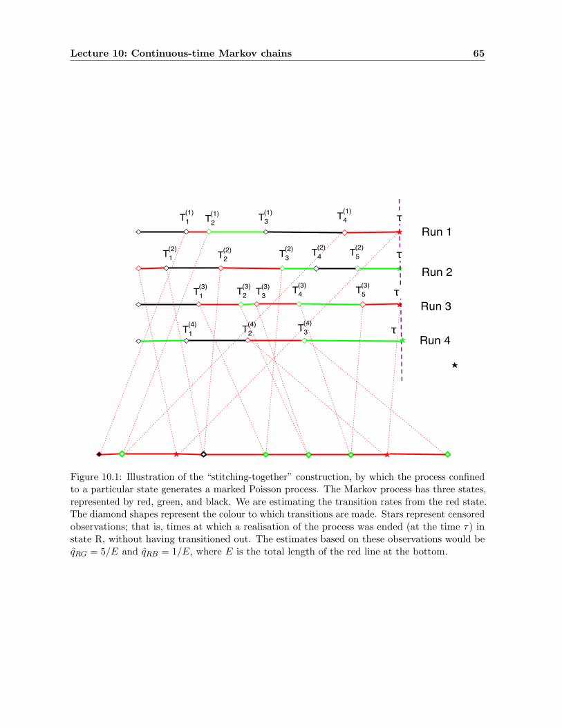
Lecture 10: Continuous-time Markov chains 65
Run 1
Run 2
Run 3
Run 4
T1(1)
T2(1) T3
(1) T4(1) τ
T1(2)
T2(2) T3
(2) T4(2) T5
(2) τ
T1(3) T2
(3) T3(3) T4
(3) T5(3) τ
T1(4) T2
(4) T3(4) τ
Figure 10.1: Illustration of the “stitching-together” construction, by which the process confinedto a particular state generates a marked Poisson process. The Markov process has three states,represented by red, green, and black. We are estimating the transition rates from the red state.The diamond shapes represent the colour to which transitions are made. Stars represent censoredobservations; that is, times at which a realisation of the process was ended (at the time τ) instate R, without having transitioned out. The estimates based on these observations would beqRG = 5/E and qRB = 1/E, where E is the total length of the red line at the bottom.
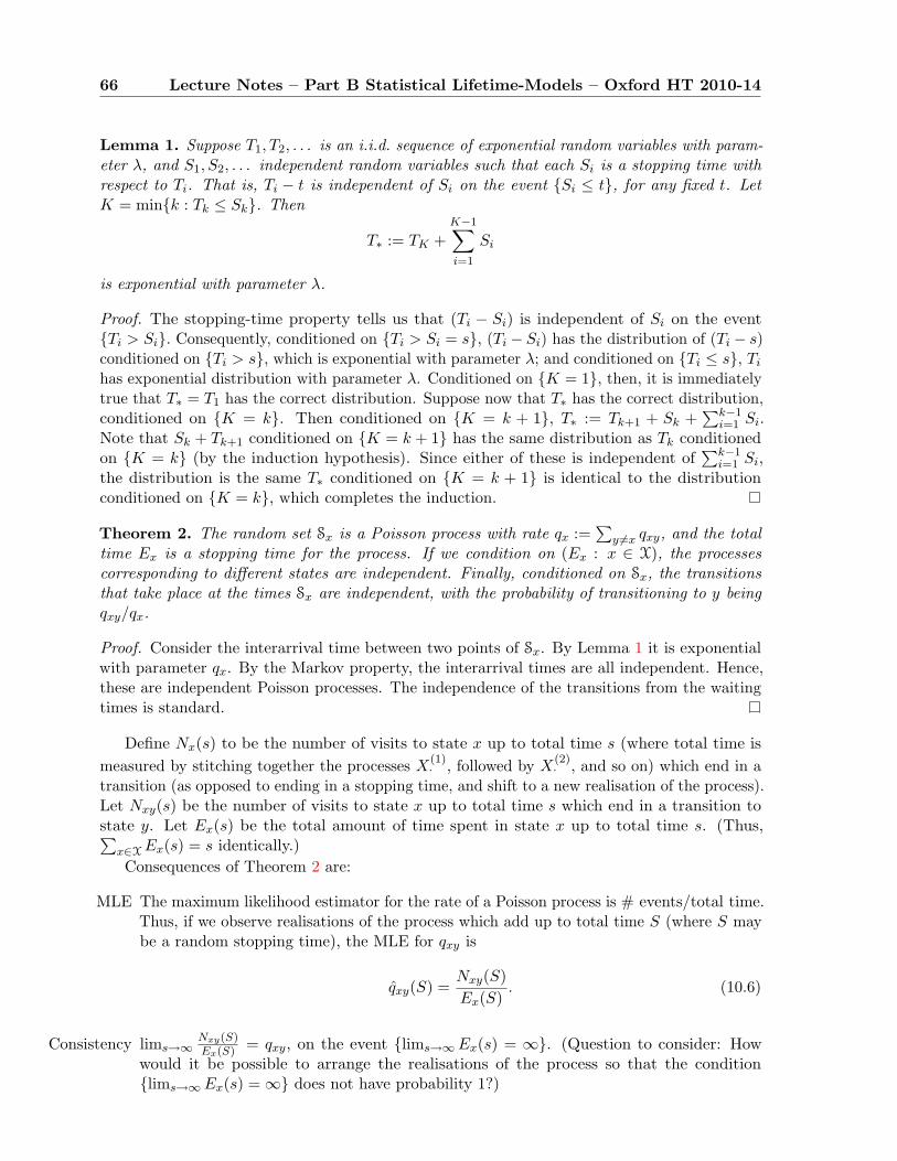
66 Lecture Notes – Part B Statistical Lifetime-Models – Oxford HT 2010-14
Lemma 1. Suppose T1, T2, . . . is an i.i.d. sequence of exponential random variables with param-eter λ, and S1, S2, . . . independent random variables such that each Si is a stopping time withrespect to Ti. That is, Ti − t is independent of Si on the event {Si ≤ t}, for any fixed t. LetK = min{k : Tk ≤ Sk}. Then
T∗ := TK +K−1∑i=1
Si
is exponential with parameter λ.
Proof. The stopping-time property tells us that (Ti − Si) is independent of Si on the event{Ti > Si}. Consequently, conditioned on {Ti > Si = s}, (Ti − Si) has the distribution of (Ti − s)conditioned on {Ti > s}, which is exponential with parameter λ; and conditioned on {Ti ≤ s}, Ti
has exponential distribution with parameter λ. Conditioned on {K = 1}, then, it is immediatelytrue that T∗ = T1 has the correct distribution. Suppose now that T∗ has the correct distribution,conditioned on {K = k}. Then conditioned on {K = k + 1}, T∗ := Tk+1 + Sk +
∑k−1i=1 Si.
Note that Sk + Tk+1 conditioned on {K = k + 1} has the same distribution as Tk conditionedon {K = k} (by the induction hypothesis). Since either of these is independent of
∑k−1i=1 Si,
the distribution is the same T∗ conditioned on {K = k + 1} is identical to the distributionconditioned on {K = k}, which completes the induction.
Theorem 2. The random set Sx is a Poisson process with rate qx :=∑
y 6=x qxy, and the totaltime Ex is a stopping time for the process. If we condition on (Ex : x ∈ X), the processescorresponding to different states are independent. Finally, conditioned on Sx, the transitionsthat take place at the times Sx are independent, with the probability of transitioning to y beingqxy/qx.
Proof. Consider the interarrival time between two points of Sx. By Lemma 1 it is exponentialwith parameter qx. By the Markov property, the interarrival times are all independent. Hence,these are independent Poisson processes. The independence of the transitions from the waitingtimes is standard.
Define Nx(s) to be the number of visits to state x up to total time s (where total time ismeasured by stitching together the processes X
(1)· , followed by X
(2)· , and so on) which end in a
transition (as opposed to ending in a stopping time, and shift to a new realisation of the process).Let Nxy(s) be the number of visits to state x up to total time s which end in a transition tostate y. Let Ex(s) be the total amount of time spent in state x up to total time s. (Thus,∑
x∈X Ex(s) = s identically.)Consequences of Theorem 2 are:
MLE The maximum likelihood estimator for the rate of a Poisson process is # events/total time.Thus, if we observe realisations of the process which add up to total time S (where S maybe a random stopping time), the MLE for qxy is
qxy(S) =Nxy(S)Ex(S)
. (10.6)
Consistency lims→∞Nxy(S)Ex(S) = qxy, on the event {lims→∞ Ex(s) = ∞}. (Question to consider: How
would it be possible to arrange the realisations of the process so that the condition{lims→∞ Ex(s) = ∞} does not have probability 1?)
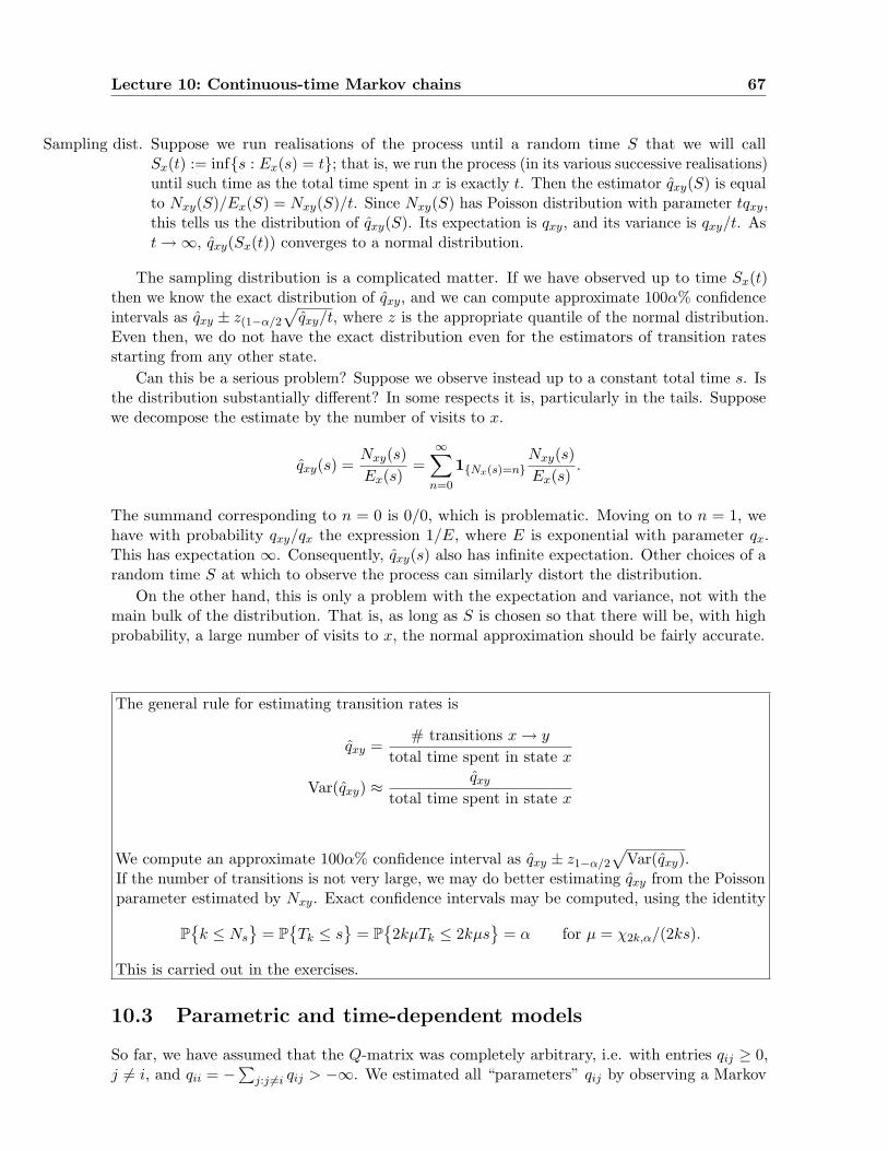
Lecture 10: Continuous-time Markov chains 67
Sampling dist. Suppose we run realisations of the process until a random time S that we will callSx(t) := inf{s : Ex(s) = t}; that is, we run the process (in its various successive realisations)until such time as the total time spent in x is exactly t. Then the estimator qxy(S) is equalto Nxy(S)/Ex(S) = Nxy(S)/t. Since Nxy(S) has Poisson distribution with parameter tqxy,this tells us the distribution of qxy(S). Its expectation is qxy, and its variance is qxy/t. Ast →∞, qxy(Sx(t)) converges to a normal distribution.
The sampling distribution is a complicated matter. If we have observed up to time Sx(t)then we know the exact distribution of qxy, and we can compute approximate 100α% confidenceintervals as qxy ± z(1−α/2
√qxy/t, where z is the appropriate quantile of the normal distribution.
Even then, we do not have the exact distribution even for the estimators of transition ratesstarting from any other state.
Can this be a serious problem? Suppose we observe instead up to a constant total time s. Isthe distribution substantially different? In some respects it is, particularly in the tails. Supposewe decompose the estimate by the number of visits to x.
qxy(s) =Nxy(s)Ex(s)
=∞∑
n=0
1{Nx(s)=n}Nxy(s)Ex(s)
.
The summand corresponding to n = 0 is 0/0, which is problematic. Moving on to n = 1, wehave with probability qxy/qx the expression 1/E, where E is exponential with parameter qx.This has expectation ∞. Consequently, qxy(s) also has infinite expectation. Other choices of arandom time S at which to observe the process can similarly distort the distribution.
On the other hand, this is only a problem with the expectation and variance, not with themain bulk of the distribution. That is, as long as S is chosen so that there will be, with highprobability, a large number of visits to x, the normal approximation should be fairly accurate.
The general rule for estimating transition rates is
qxy =# transitions x → y
total time spent in state x
Var(qxy) ≈qxy
total time spent in state x
We compute an approximate 100α% confidence interval as qxy ± z1−α/2
√Var(qxy).
If the number of transitions is not very large, we may do better estimating qxy from the Poissonparameter estimated by Nxy. Exact confidence intervals may be computed, using the identity
P{k ≤ Ns
}= P
{Tk ≤ s
}= P
{2kµTk ≤ 2kµs
}= α for µ = χ2k,α/(2ks).
This is carried out in the exercises.
10.3 Parametric and time-dependent models
So far, we have assumed that the Q-matrix was completely arbitrary, i.e. with entries qij ≥ 0,j 6= i, and qii = −
∑j:j 6=i qij > −∞. We estimated all “parameters” qij by observing a Markov
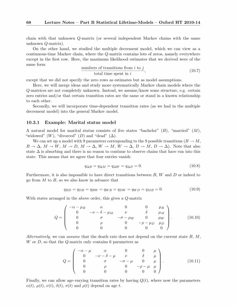
68 Lecture Notes – Part B Statistical Lifetime-Models – Oxford HT 2010-14
chain with that unknown Q-matrix (or several independent Markov chains with the sameunknown Q-matrix).
On the other hand, we studied the multiple decrement model, which we can view as acontinuous-time Markov chain, where the Q-matrix contains lots of zeros, namely everywhereexcept in the first row. Here, the maximum likelihood estimates that we derived were of thesame form
numbers of transitions from i to j
total time spent in i, (10.7)
except that we did not specify the zero rows as estimates but as model assumptions.Here, we will merge ideas and study more systematically Markov chain models where the
Q-matrices are not completely unknown. Instead, we assume/know some structure, e.g. certainzero entries and/or that certain transition rates are the same or stand in a known relationshipto each other.
Secondly, we will incorporate time-dependent transition rates (as we had in the multipledecrement model) into the general Markov model.
10.3.1 Example: Marital status model
A natural model for marital status consists of five states “bachelor” (B), “married” (M),“widowed” (W ), “divorced” (D) and “dead” (∆).
We can set up a model with 9 parameters corresponding to the 9 possible transitions (B → M ,B → ∆, M → W , M → D, M → ∆, W → M , W → ∆, D → M , D → ∆). Note that alsostate ∆ is absorbing and there is no reason to continue to observe chains that have run into thisstate. This means that we agree that four entries vanish:
q∆B = q∆M = q∆W = q∆D = 0. (10.8)
Furthermore, it is also impossible to have direct transitions between B, W and D or indeed togo from M to B, so we also know in advance that
qBD = qDB = qBW = qWB = qDW = qWD = qMB = 0. (10.9)
With states arranged in the above order, this gives a Q-matrix
Q =
−α− µB α 0 0 µB
0 −ν − δ − µM ν δ µM
0 σ −σ − µW 0 µW
0 ρ 0 −ρ− µD µD
0 0 0 0 0
. (10.10)
Alternatively, we can assume that the death rate does not depend on the current state B, M ,W or D, so that the Q-matrix only contains 6 parameters as
Q =
−α− µ α 0 0 µ
0 −ν − δ − µ ν δ µ0 σ −σ − µ 0 µ0 ρ 0 −ρ− µ µ0 0 0 0 0
. (10.11)
Finally, we can allow age-varying transition rates by having Q(t), where now the parametersα(t), µ(t), ν(t), δ(t), σ(t) and ρ(t) depend on age t.
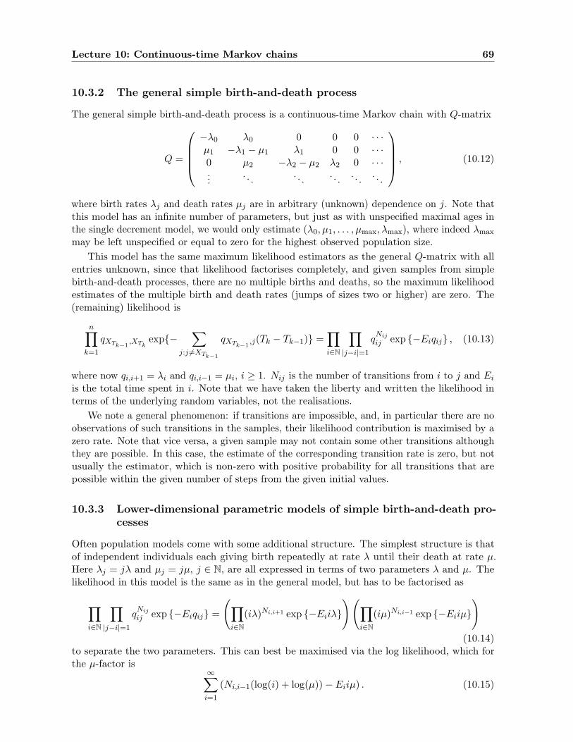
Lecture 10: Continuous-time Markov chains 69
10.3.2 The general simple birth-and-death process
The general simple birth-and-death process is a continuous-time Markov chain with Q-matrix
Q =
−λ0 λ0 0 0 0 · · ·µ1 −λ1 − µ1 λ1 0 0 · · ·0 µ2 −λ2 − µ2 λ2 0 · · ·...
. . . . . . . . . . . . . . .
, (10.12)
where birth rates λj and death rates µj are in arbitrary (unknown) dependence on j. Note thatthis model has an infinite number of parameters, but just as with unspecified maximal ages inthe single decrement model, we would only estimate (λ0, µ1, . . . , µmax, λmax), where indeed λmax
may be left unspecified or equal to zero for the highest observed population size.This model has the same maximum likelihood estimators as the general Q-matrix with all
entries unknown, since that likelihood factorises completely, and given samples from simplebirth-and-death processes, there are no multiple births and deaths, so the maximum likelihoodestimates of the multiple birth and death rates (jumps of sizes two or higher) are zero. The(remaining) likelihood is
n∏k=1
qXTk−1,XTk
exp{−∑
j:j 6=XTk−1
qXTk−1,j(Tk − Tk−1)} =
∏i∈N
∏|j−i|=1
qNij
ij exp {−Eiqij} , (10.13)
where now qi,i+1 = λi and qi,i−1 = µi, i ≥ 1. Nij is the number of transitions from i to j and Ei
is the total time spent in i. Note that we have taken the liberty and written the likelihood interms of the underlying random variables, not the realisations.
We note a general phenomenon: if transitions are impossible, and, in particular there are noobservations of such transitions in the samples, their likelihood contribution is maximised by azero rate. Note that vice versa, a given sample may not contain some other transitions althoughthey are possible. In this case, the estimate of the corresponding transition rate is zero, but notusually the estimator, which is non-zero with positive probability for all transitions that arepossible within the given number of steps from the given initial values.
10.3.3 Lower-dimensional parametric models of simple birth-and-death pro-cesses
Often population models come with some additional structure. The simplest structure is thatof independent individuals each giving birth repeatedly at rate λ until their death at rate µ.Here λj = jλ and µj = jµ, j ∈ N, are all expressed in terms of two parameters λ and µ. Thelikelihood in this model is the same as in the general model, but has to be factorised as
∏i∈N
∏|j−i|=1
qNij
ij exp {−Eiqij} =
(∏i∈N
(iλ)Ni,i+1 exp {−Eiiλ}
)(∏i∈N
(iµ)Ni,i−1 exp {−Eiiµ}
)(10.14)
to separate the two parameters. This can best be maximised via the log likelihood, which forthe µ-factor is
∞∑i=1
(Ni,i−1(log(i) + log(µ))− Eiiµ) . (10.15)
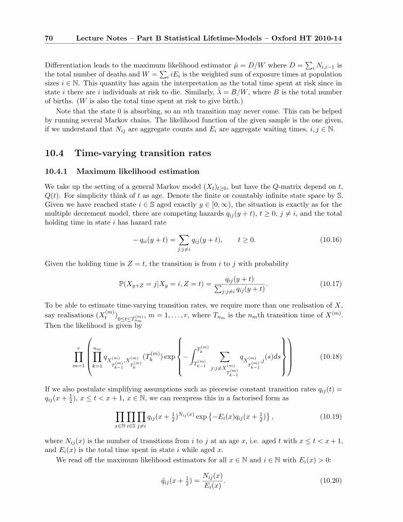
70 Lecture Notes – Part B Statistical Lifetime-Models – Oxford HT 2010-14
Differentiation leads to the maximum likelihood estimator µ = D/W where D =∑
i Ni,i−1 isthe total number of deaths and W =
∑i iEi is the weighted sum of exposure times at population
sizes i ∈ N. This quantity has again the interpretation as the total time spent at risk since instate i there are i individuals at risk to die. Similarly, λ = B/W , where B is the total numberof births. (W is also the total time spent at risk to give birth.)
Note that the state 0 is absorbing, so an nth transition may never come. This can be helpedby running several Markov chains. The likelihood function of the given sample is the one given,if we understand that Nij are aggregate counts and Ei are aggregate waiting times, i, j ∈ N.
10.4 Time-varying transition rates
10.4.1 Maximum likelihood estimation
We take up the setting of a general Markov model (Xt)t≥0, but have the Q-matrix depend on t,Q(t). For simplicity think of t as age. Denote the finite or countably infinite state space by S.Given we have reached state i ∈ S aged exactly y ∈ [0,∞), the situation is exactly as for themultiple decrement model, there are competing hazards qij(y + t), t ≥ 0, j 6= i, and the totalholding time in state i has hazard rate
− qii(y + t) =∑j:j 6=i
qij(y + t), t ≥ 0. (10.16)
Given the holding time is Z = t, the transition is from i to j with probability
P(Xy+Z = j|Xy = i, Z = t) =qij(y + t)∑
j:j 6=i qij(y + t). (10.17)
To be able to estimate time-varying transition rates, we require more than one realisation of X,say realisations (X(m)
t )0≤t≤T
(m)nm
, m = 1, . . . , r, where Tnm is the nmth transition time of X(m).Then the likelihood is given by
r∏m=1
nm∏k=1
qX
(m)
T(m)k−1
,X(m)
T(m)k
(T (m)k ) exp
−∫ T
(m)k
T(m)k−1
∑j:j 6=X
(m)
T(m)k−1
qX
(m)
T(m)k−1
,j(s)ds
(10.18)
If we also postulate simplifying assumptions such as piecewise constant transition rates qij(t) =qij(x + 1
2), x ≤ t < x + 1, x ∈ N, we can reexpress this in a factorised form as∏x∈N
∏i∈S
∏j 6=i
qij(x + 12)Nij(x) exp
{−Ei(x)qij(x + 1
2)}
, (10.19)
where Nij(x) is the number of transitions from i to j at an age x, i.e. aged t with x ≤ t < x + 1,and Ei(x) is the total time spent in state i while aged x.
We read off the maximum likelihood estimators for all x ∈ N and i ∈ N with Ei(x) > 0:
qij(x + 12) =
Nij(x)Ei(x)
. (10.20)
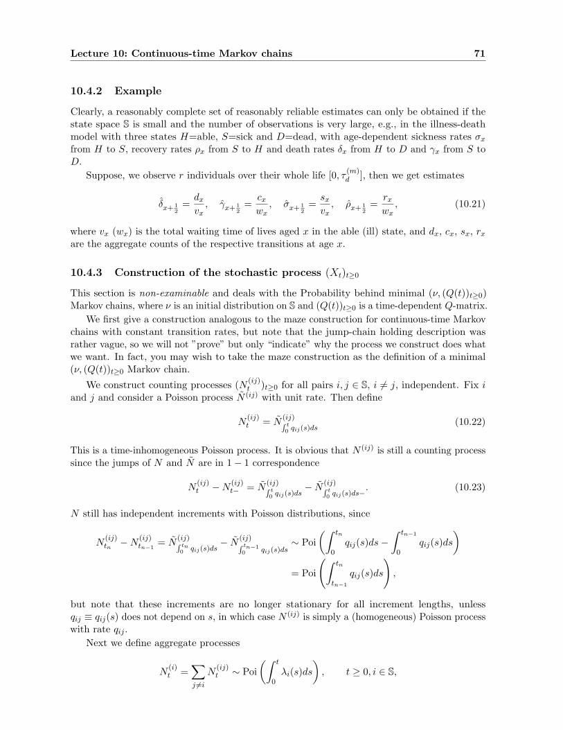
Lecture 10: Continuous-time Markov chains 71
10.4.2 Example
Clearly, a reasonably complete set of reasonably reliable estimates can only be obtained if thestate space S is small and the number of observations is very large, e.g., in the illness-deathmodel with three states H=able, S=sick and D=dead, with age-dependent sickness rates σx
from H to S, recovery rates ρx from S to H and death rates δx from H to D and γx from S toD.
Suppose, we observe r individuals over their whole life [0, τ(m)d ], then we get estimates
δx+ 12
=dx
vx, γx+ 1
2=
cx
wx, σx+ 1
2=
sx
vx, ρx+ 1
2=
rx
wx, (10.21)
where vx (wx) is the total waiting time of lives aged x in the able (ill) state, and dx, cx, sx, rx
are the aggregate counts of the respective transitions at age x.
10.4.3 Construction of the stochastic process (Xt)t≥0
This section is non-examinable and deals with the Probability behind minimal (ν, (Q(t))t≥0)Markov chains, where ν is an initial distribution on S and (Q(t))t≥0 is a time-dependent Q-matrix.
We first give a construction analogous to the maze construction for continuous-time Markovchains with constant transition rates, but note that the jump-chain holding description wasrather vague, so we will not ”prove” but only “indicate” why the process we construct does whatwe want. In fact, you may wish to take the maze construction as the definition of a minimal(ν, (Q(t))t≥0 Markov chain.
We construct counting processes (N (ij)t )t≥0 for all pairs i, j ∈ S, i 6= j, independent. Fix i
and j and consider a Poisson process N (ij) with unit rate. Then define
N(ij)t = N
(ij)R t0 qij(s)ds
(10.22)
This is a time-inhomogeneous Poisson process. It is obvious that N (ij) is still a counting processsince the jumps of N and N are in 1− 1 correspondence
N(ij)t −N
(ij)t− = N
(ij)R t0 qij(s)ds
− N(ij)R t0 qij(s)ds−
. (10.23)
N still has independent increments with Poisson distributions, since
N(ij)tn −N
(ij)tn−1
= N(ij)R tn0 qij(s)ds
− N(ij)R tn−10 qij(s)ds
∼ Poi(∫ tn
0qij(s)ds−
∫ tn−1
0qij(s)ds
)= Poi
(∫ tn
tn−1
qij(s)ds
),
but note that these increments are no longer stationary for all increment lengths, unlessqij ≡ qij(s) does not depend on s, in which case N (ij) is simply a (homogeneous) Poisson processwith rate qij .
Next we define aggregate processes
N(i)t =
∑j 6=i
N(ij)t ∼ Poi
(∫ t
0λi(s)ds
), t ≥ 0, i ∈ S,
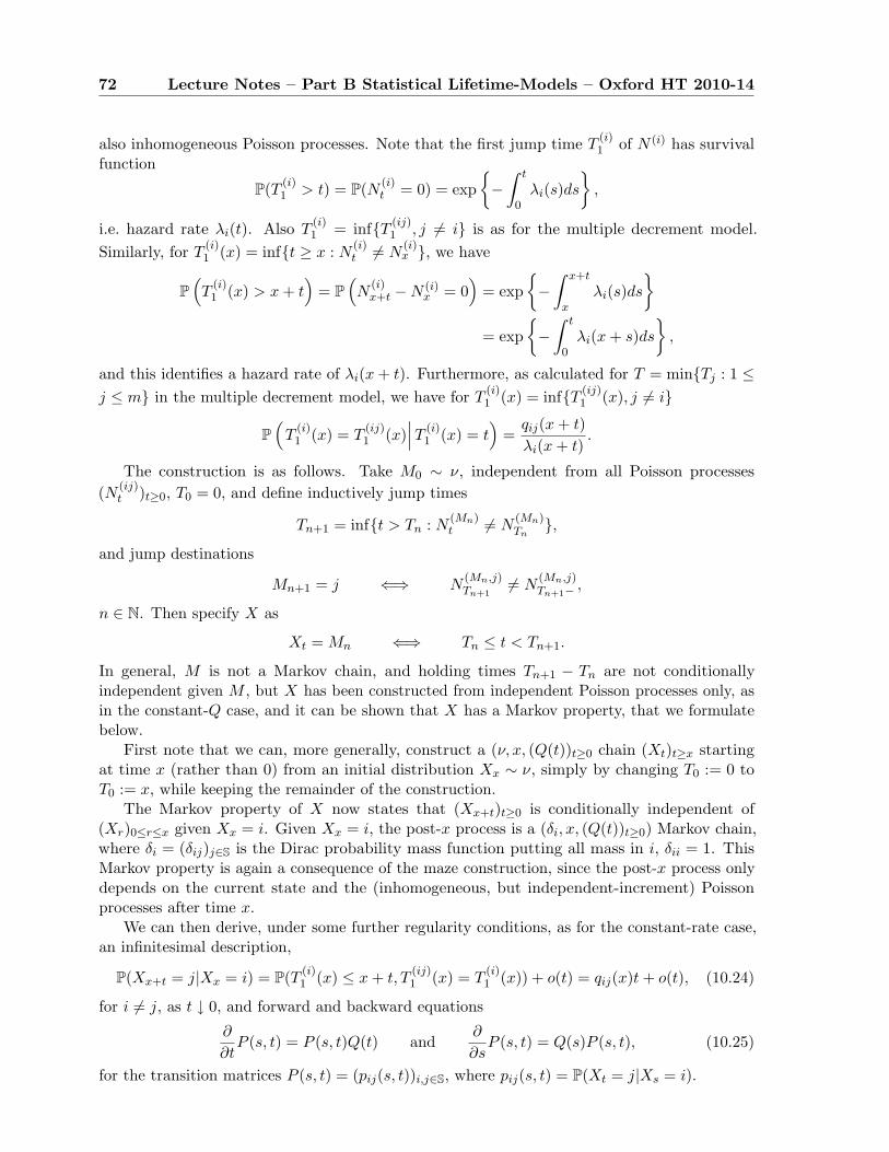
72 Lecture Notes – Part B Statistical Lifetime-Models – Oxford HT 2010-14
also inhomogeneous Poisson processes. Note that the first jump time T(i)1 of N (i) has survival
function
P(T (i)1 > t) = P(N (i)
t = 0) = exp{−∫ t
0λi(s)ds
},
i.e. hazard rate λi(t). Also T(i)1 = inf{T (ij)
1 , j 6= i} is as for the multiple decrement model.Similarly, for T
(i)1 (x) = inf{t ≥ x : N
(i)t 6= N
(i)x }, we have
P(T
(i)1 (x) > x + t
)= P
(N
(i)x+t −N (i)
x = 0)
= exp{−∫ x+t
xλi(s)ds
}= exp
{−∫ t
0λi(x + s)ds
},
and this identifies a hazard rate of λi(x + t). Furthermore, as calculated for T = min{Tj : 1 ≤j ≤ m} in the multiple decrement model, we have for T
(i)1 (x) = inf{T (ij)
1 (x), j 6= i}
P(
T(i)1 (x) = T
(ij)1 (x)
∣∣∣T (i)1 (x) = t
)=
qij(x + t)λi(x + t)
.
The construction is as follows. Take M0 ∼ ν, independent from all Poisson processes(N (ij)
t )t≥0, T0 = 0, and define inductively jump times
Tn+1 = inf{t > Tn : N(Mn)t 6= N
(Mn)Tn
},
and jump destinations
Mn+1 = j ⇐⇒ N(Mn,j)Tn+1
6= N(Mn,j)Tn+1− ,
n ∈ N. Then specify X as
Xt = Mn ⇐⇒ Tn ≤ t < Tn+1.
In general, M is not a Markov chain, and holding times Tn+1 − Tn are not conditionallyindependent given M , but X has been constructed from independent Poisson processes only, asin the constant-Q case, and it can be shown that X has a Markov property, that we formulatebelow.
First note that we can, more generally, construct a (ν, x, (Q(t))t≥0 chain (Xt)t≥x startingat time x (rather than 0) from an initial distribution Xx ∼ ν, simply by changing T0 := 0 toT0 := x, while keeping the remainder of the construction.
The Markov property of X now states that (Xx+t)t≥0 is conditionally independent of(Xr)0≤r≤x given Xx = i. Given Xx = i, the post-x process is a (δi, x, (Q(t))t≥0) Markov chain,where δi = (δij)j∈S is the Dirac probability mass function putting all mass in i, δii = 1. ThisMarkov property is again a consequence of the maze construction, since the post-x process onlydepends on the current state and the (inhomogeneous, but independent-increment) Poissonprocesses after time x.
We can then derive, under some further regularity conditions, as for the constant-rate case,an infinitesimal description,
P(Xx+t = j|Xx = i) = P(T (i)1 (x) ≤ x + t, T
(ij)1 (x) = T
(i)1 (x)) + o(t) = qij(x)t + o(t), (10.24)
for i 6= j, as t ↓ 0, and forward and backward equations
∂
∂tP (s, t) = P (s, t)Q(t) and
∂
∂sP (s, t) = Q(s)P (s, t), (10.25)
for the transition matrices P (s, t) = (pij(s, t))i,j∈S, where pij(s, t) = P(Xt = j|Xs = i).
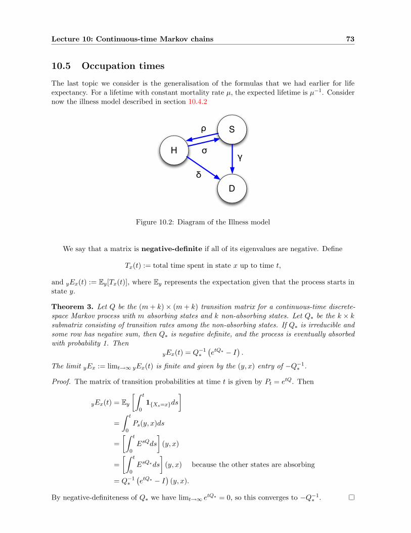
Lecture 10: Continuous-time Markov chains 73
10.5 Occupation times
The last topic we consider is the generalisation of the formulas that we had earlier for lifeexpectancy. For a lifetime with constant mortality rate µ, the expected lifetime is µ−1. Considernow the illness model described in section 10.4.2
H
S
Dδ
σ
ρ
γ
Figure 10.2: Diagram of the Illness model
We say that a matrix is negative-definite if all of its eigenvalues are negative. Define
Tx(t) := total time spent in state x up to time t,
and yEx(t) := Ey[Tx(t)], where Ey represents the expectation given that the process starts instate y.
Theorem 3. Let Q be the (m + k)× (m + k) transition matrix for a continuous-time discrete-space Markov process with m absorbing states and k non-absorbing states. Let Q∗ be the k × ksubmatrix consisting of transition rates among the non-absorbing states. If Q∗ is irreducible andsome row has negative sum, then Q∗ is negative definite, and the process is eventually absorbedwith probability 1. Then
yEx(t) = Q−1∗(etQ∗ − I
).
The limit yEx := limt→∞ yEx(t) is finite and given by the (y, x) entry of −Q−1∗ .
Proof. The matrix of transition probabilities at time t is given by Pt = etQ. Then
yEx(t) = Ey
[∫ t
01{Xs=x}ds
]=∫ t
0Ps(y, x)ds
=[∫ t
0EsQds
](y, x)
=[∫ t
0EsQ∗ds
](y, x) because the other states are absorbing
= Q−1∗(etQ∗ − I
)(y, x).
By negative-definiteness of Q∗ we have limt→∞ etQ∗ = 0, so this converges to −Q−1∗ .
74 Lecture Notes – Part B Statistical Lifetime-Models – Oxford HT 2010-14
We are also interested in the state that the process ends up in. We state the following resultin terms of the diagonalisation of Q. Of course, in the special case where Q is not diagonalisable,we can carry out the same construction with the Jordan Normal Form.
Theorem 4. Let v1, . . . , vm be the right-eigenvectors (columns) of Q with eigenvalue 0 (in otherwords, a basis for the kernel of Q), such that vi has a 1 in coordinate k + i and 0 for theremainder of the absorbing states. Then
Pj
{absorbed in state k + i
}= (vi)j .
Proof. Fix some i, and let vj = Pj
{absorbed in state k + i
}. Let Xt be the position of the
process at time t. Then Ej′ [vXt ] = P t(j′, ·)v. Note that this function is constant in time (by theChapman-Kolmogorov equation). By the Forward Equation, for all t > 0
0 =d
dtP t(j′, ·)v = P t(j′, ·)Qv,
which implies that Qv = 0, since limt↓0 P t is the identity matrix. Obviously v has the statedvalues on the absorbing states.
10.5.1 The multiple decrements model
The simplest application of this formula is to the multiple decrements model. In that case, wehave just a single non-absorbing state 0, and absorbing states 1, 2, . . . ,m. Then Q∗ = (−λ+), sothat the expected time spent in state 0 is 1/λ+, which we already knew.
The only non-trivial eigenvector is
(−1λ1
λ+· · · λm
λ+).
Thus
R−1 =
−1 λ1
λ+
λ2λ+
· · · λmλ+
0 1 0 · · · 00 0 1 · · · 0...
......
. . ....
0 0 0 · · · 1
Thus, the probability of ending up in state i is λi/λ+.
10.5.2 The illness model
Consider now the illness model, with σ = 0.1, δ = 0.1, γ = 0.5, and ρ = 0. The generator (takingthe states in the order H, S, D, is
Q =
−0.2 0.1 0.10 −0.5 0.50 0 0
Q∗ =(−0.2 0.1
0 −0.5
)
We calculate
Q−1∗ =
(−5 −10 −2
)
Lecture 10: Continuous-time Markov chains 75
Thus, a sick individual survives on average 2 years. A healthy individual survives on average 6years, of which 1 year, on average, is spent sick.
There is only one absorbing state. If we want to study the state that individuals died from(sick or healthy), one approach is to make two absorbing states, one corresponding to deathafter being healthy, the other after being sick. The core Q∗ matrix stays the same, but now Qbecomes
−0.2 0.1 0.1 00 −0.5 0 0.50 0 0 00 0 0 0
The eigenvectors with eigenvalue 0 are
0.5010
,
0.5101
These tell us that someone who starts sick will with certainty die from the sick state (since thereis no recovery in this model), while an initially healthy individual will have probability 1/2 ofdying from the healthy or the sick state.
Suppose the recovery rate ρ now becomes 1. Then
Q =
−0.2 0.1 0.1 0
1 −1.5 0 0.50 0 0 00 0 0 0
Q∗ =(−0.2 0.1
1 −1.5
)Q−1∗ =
(−7.5 −.5−5 −1
)
Thus, a healthy individual will now live, on average, 8 years, of which only 0.5 will be sick, andsomeone who is sick will have 6 years on average, with 1 of those sick.
The eigenvectors with eigenvalue 0 are now0.750.510
,
0.250.501
.
Thus we see that when starting from state H, the probability of transitioning to D from H hasgone up to 3/4. Starting from S, the probability is now 1/2 of transitioning to D from S, and1/2 of transitioning from H. This is consistent with the observation we make from the jumpchain, that the healthy person transitions to sick or to dead with equal probabilities. Thus,
PH(last state H) =12
+12PS(last state H) =
12
+14.
Lecture 11
Survival analysis: Introduction
Reading: Cox and Oakes, chapter 1, 4, section 11.6, CT4 Unit 6.3-6.5, Klein and Moeschbergersections 3.1–3.4, Chapter 4
11.1 [
Censoring and truncation]Incomplete observations: Censoring and truncationWe begin by considering simple analyses but we will lead up to and take a look at regression
on explanatory factors, as in linear regression part A. The important difference between survivalanalysis and other statistical analyses which you have so far encountered is the presence ofcensoring. This actually renders the survival function of more importance in writing down themodels.
Right censoring occurs when a subject leaves the study before an event occurs, or thestudy ends before the event has occurred. For example, we consider patients in a clinical trialto study the effect of treatments on stroke occurrence. The study ends after 5 years. Thosepatients who have had no strokes by the end of the year are censored. If the patient leaves thestudy at time te, then the event occurs in (te,∞) .
Left censoring is when the event of interest has already occurred before enrolment. Thisis very rarely encountered.
Truncation is deliberate and due to study design.Right truncation occurs when the entire study population has already experienced the
event of interest (for example: a historical survey of patients on a cancer registry).Left truncation occurs when the subjects have been at risk before entering the study (for
example: life insurance policy holders where the study starts on a fixed date, event of interest isage at death).
Generally we deal with right censoring & sometimes left truncation.Two types of independent right censoring:Type I: All subjects start and end the study at the same fixed time. All are censored at the
end of the study. If individuals have different but fixed censoring times, this is called progressivetype I censoring.
Type II: study ends when a fixed number of events amongst the subjects has occurred.Type III or random censoring: Individuals drop out or are lost to followup at times
that are random, rather than predetermined. We generally assume that the censoring times areindependent of the event times, in which case there is no need to distinguish this from Type I.
Skeptical question: Why do we need special techniques to cope with incomplete observa-tions? Aren’t all observations incomplete? After all, we never see all possible samples from thedistribution. If we did, we wouldn’t need any sophisticated statistical analysis.
76
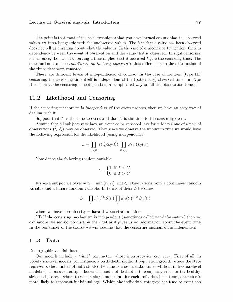
Lecture 11: Survival analysis: Introduction 77
The point is that most of the basic techniques that you have learned assume that the observedvalues are interchangeable with the unobserved values. The fact that a value has been observeddoes not tell us anything about what the value is. In the case of censoring or truncation, there isdependence between the event of observation and the value that is observed. In right-censoring,for instance, the fact of observing a time implies that it occurred before the censoring time. Thedistribution of a time conditioned on its being observed is thus different from the distribution ofthe times that were censored.
There are different levels of independence, of course. In the case of random (type III)censoring, the censoring time itself is independent of the (potentially) observed time. In TypeII censoring, the censoring time depends in a complicated way on all the observation times.
11.2 Likelihood and Censoring
If the censoring mechanism is independent of the event process, then we have an easy way ofdealing with it.
Suppose that T is the time to event and that C is the time to the censoring event.Assume that all subjects may have an event or be censored, say for subject i one of a pair of
observations(ti, ci
)may be observed. Then since we observe the minimum time we would have
the following expression for the likelihood (using independence)
L =∏
eti<eci
f(ti)SC(ti)∏eci<eti
S(ci)fC(ci)
Now define the following random variable:
δ ={
1 if T < C
0 if T > C
For each subject we observe ti = min(ti, ci
)and δi, observations from a continuous random
variable and a binary random variable. In terms of these L becomes
L =∏
i
h(ti)δiS(ti)∏
i
hC(ti)1−δiSC(ti)
where we have used density = hazard × survival function.NB If the censoring mechanism is independent (sometimes called non-informative) then we
can ignore the second product on the right as it gives us no information about the event time.In the remainder of the course we will assume that the censoring mechanism is independent.
11.3 Data
Demographic v. trial dataOur models include a “time” parameter, whose interpretation can vary. First of all, in
population-level models (for instance, a birth-death model of population growth, where the staterepresents the number of individuals) the time is true calendar time, while in individual-levelmodels (such as our multiple-decrement model of death due to competing risks, or the healthy-sick-dead process, where there is a single model run for each individual) the time parameter ismore likely to represent individual age. Within the individual category, the time to event can
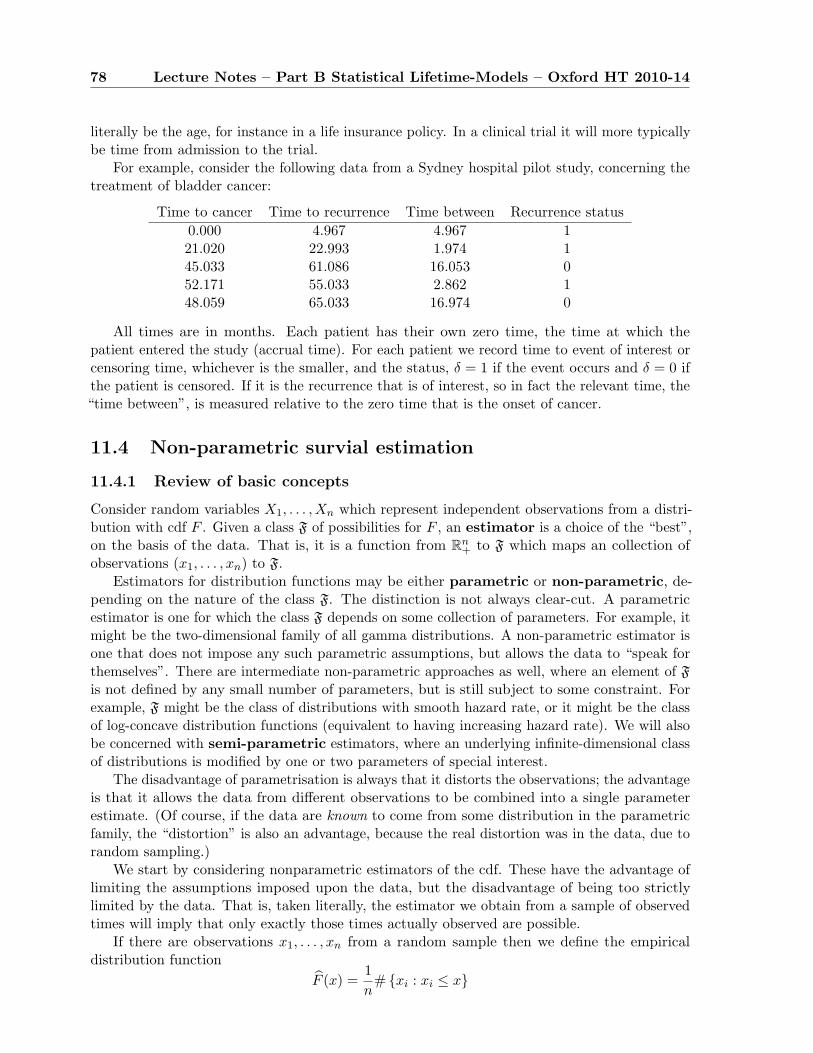
78 Lecture Notes – Part B Statistical Lifetime-Models – Oxford HT 2010-14
literally be the age, for instance in a life insurance policy. In a clinical trial it will more typicallybe time from admission to the trial.
For example, consider the following data from a Sydney hospital pilot study, concerning thetreatment of bladder cancer:
Time to cancer Time to recurrence Time between Recurrence status0.000 4.967 4.967 121.020 22.993 1.974 145.033 61.086 16.053 052.171 55.033 2.862 148.059 65.033 16.974 0
All times are in months. Each patient has their own zero time, the time at which thepatient entered the study (accrual time). For each patient we record time to event of interest orcensoring time, whichever is the smaller, and the status, δ = 1 if the event occurs and δ = 0 ifthe patient is censored. If it is the recurrence that is of interest, so in fact the relevant time, the“time between”, is measured relative to the zero time that is the onset of cancer.
11.4 Non-parametric survial estimation
11.4.1 Review of basic concepts
Consider random variables X1, . . . , Xn which represent independent observations from a distri-bution with cdf F . Given a class F of possibilities for F , an estimator is a choice of the “best”,on the basis of the data. That is, it is a function from Rn
+ to F which maps an collection ofobservations (x1, . . . , xn) to F.
Estimators for distribution functions may be either parametric or non-parametric, de-pending on the nature of the class F. The distinction is not always clear-cut. A parametricestimator is one for which the class F depends on some collection of parameters. For example, itmight be the two-dimensional family of all gamma distributions. A non-parametric estimator isone that does not impose any such parametric assumptions, but allows the data to “speak forthemselves”. There are intermediate non-parametric approaches as well, where an element of F
is not defined by any small number of parameters, but is still subject to some constraint. Forexample, F might be the class of distributions with smooth hazard rate, or it might be the classof log-concave distribution functions (equivalent to having increasing hazard rate). We will alsobe concerned with semi-parametric estimators, where an underlying infinite-dimensional classof distributions is modified by one or two parameters of special interest.
The disadvantage of parametrisation is always that it distorts the observations; the advantageis that it allows the data from different observations to be combined into a single parameterestimate. (Of course, if the data are known to come from some distribution in the parametricfamily, the “distortion” is also an advantage, because the real distortion was in the data, due torandom sampling.)
We start by considering nonparametric estimators of the cdf. These have the advantage oflimiting the assumptions imposed upon the data, but the disadvantage of being too strictlylimited by the data. That is, taken literally, the estimator we obtain from a sample of observedtimes will imply that only exactly those times actually observed are possible.
If there are observations x1, . . . , xn from a random sample then we define the empiricaldistribution function
F (x) =1n
# {xi : xi ≤ x}
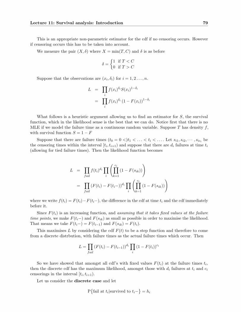
Lecture 11: Survival analysis: Introduction 79
This is an appropriate non-parametric estimator for the cdf if no censoring occurs. Howeverif censoring occurs this has to be taken into account.
We measure the pair (X, δ) where X = min(T,C) and δ is as before
δ ={
1 if T < C
0 if T > C
Suppose that the observations are (xi, δi) for i = 1, 2 . . . , n.
L =∏
i
f(xi)δiS(xi)1−δi
=∏
i
f(xi)δi (1− F (xi))1−δi
What follows is a heuristic argument allowing us to find an estimator for S, the survivalfunction, which in the likelihood sense is the best that we can do. Notice first that there is noMLE if we model the failure time as a continuous random variable. Suppose T has density f ,with survival function S = 1− F
Suppose that there are failure times (t0 = 0 <)t1 < . . . < ti < . . . . Let si1, si2, · · · , sici bethe censoring times within the interval [ti, ti+1) and suppose that there are di failures at time ti(allowing for tied failure times). Then the likelihood function becomes
L =∏fail
f(ti)di∏
i
(ci∏
k=1
(1− F (sik))
)
=∏fail
(F (ti)− F (ti−))di∏
i
(ci∏
k=1
(1− F (sik))
)
where we write f(ti) = F (ti)−F (ti−), the difference in the cdf at time ti and the cdf immediatelybefore it.
Since F (ti) is an increasing function, and assuming that it takes fixed values at the failuretime points, we make F (ti−) and F (sik) as small as possible in order to maximise the likelihood.That means we take F (ti−) = F (ti−1) and F (sik) = F (ti).
This maximises L by considering the cdf F (t) to be a step function and therefore to comefrom a discrete distrbution, with failure times as the actual failure times which occur. Then
L =∏fail
(F (ti)− F (ti−1))di∏
i
(1− F (ti))ci
So we have showed that amongst all cdf’s with fixed values F (ti) at the failure times ti,then the discrete cdf has the maximum likelihood, amongst those with di failures at ti and ci
censorings in the interval [ti, ti+1).
Let us consider the discrete case and let
P{fail at ti|survived to ti−
}= hi
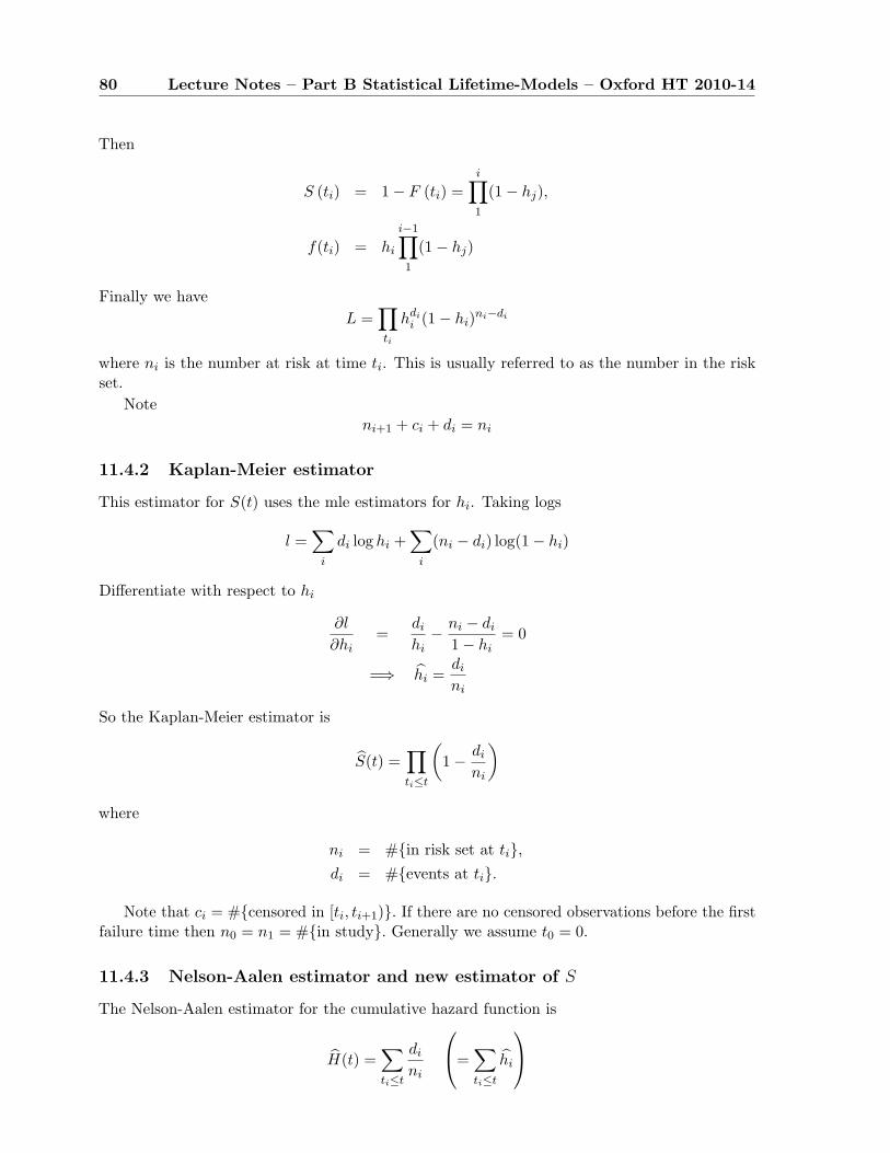
80 Lecture Notes – Part B Statistical Lifetime-Models – Oxford HT 2010-14
Then
S (ti) = 1− F (ti) =i∏1
(1− hj),
f(ti) = hi
i−1∏1
(1− hj)
Finally we haveL =
∏ti
hdii (1− hi)ni−di
where ni is the number at risk at time ti. This is usually referred to as the number in the riskset.
Noteni+1 + ci + di = ni
11.4.2 Kaplan-Meier estimator
This estimator for S(t) uses the mle estimators for hi. Taking logs
l =∑
i
di log hi +∑
i
(ni − di) log(1− hi)
Differentiate with respect to hi
∂l
∂hi=
di
hi− ni − di
1− hi= 0
=⇒ hi =di
ni
So the Kaplan-Meier estimator is
S(t) =∏ti≤t
(1− di
ni
)
where
ni = #{in risk set at ti},di = #{events at ti}.
Note that ci = #{censored in [ti, ti+1)}. If there are no censored observations before the firstfailure time then n0 = n1 = #{in study}. Generally we assume t0 = 0.
11.4.3 Nelson-Aalen estimator and new estimator of S
The Nelson-Aalen estimator for the cumulative hazard function is
H(t) =∑ti≤t
di
ni
=∑ti≤t
hi
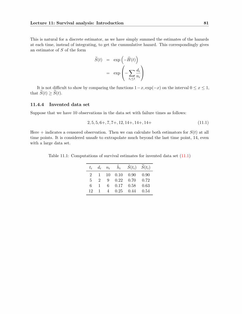
Lecture 11: Survival analysis: Introduction 81
This is natural for a discrete estimator, as we have simply summed the estimates of the hazardsat each time, instead of integrating, to get the cummulative hazard. This correspondingly givesan estimator of S of the form
S(t) = exp(−H(t)
)= exp
−∑ti≤t
di
ni
It is not difficult to show by comparing the functions 1−x, exp(−x) on the interval 0 ≤ x ≤ 1,
that S(t) ≥ S(t).
11.4.4 Invented data set
Suppose that we have 10 observations in the data set with failure times as follows:
2, 5, 5, 6+, 7, 7+, 12, 14+, 14+, 14+ (11.1)
Here + indicates a censored observation. Then we can calculate both estimators for S(t) at alltime points. It is considered unsafe to extrapolate much beyond the last time point, 14, evenwith a large data set.
Table 11.1: Computations of survival estimates for invented data set (11.1)
ti di ni hi S(ti) S(ti)
2 1 10 0.10 0.90 0.905 2 9 0.22 0.70 0.726 1 6 0.17 0.58 0.6312 1 4 0.25 0.44 0.54
Lecture 12
Confidence intervals and lefttruncation
We need to find confidence intervals (pointwise) for the estimators of S(t) at each time point.We differentiate the log-likelihood and use likelihood theory,
l =∑
i
di log hi +∑
i
(ni − di) log(1− hi),
differentiated twice to find the Hessian matrix{
∂2l∂hi∂hj
}.
Note that since l is a sum of functions of each individual hazard the Hessian must be diagonal.
The estimators{
h1, h2, . . . , hn
}are asymptotically unbiased and are asymptotically jointly
normally distributed with approximate variance I−1, where the information matrix is given by
I = E(−{
∂2l
∂hi∂hj
}).
Since the Hessian is diagonal, the covariances are all asymptotically zero, and coupled withasymptotic normality, this ensures that all pairs hi, hj are asymptotically independent.
− ∂2l
∂h2i
=di
h2i
+ni − di
(1− hi)2
We use the observed information J and so replace hi in the above by its estimator hi = dini
.Hence we have
var hi ≈di (ni − di)
n3i
.
12.1 Greenwood’s formula
12.1.1 Reminder of the δ method
If the random variation of Y around µ is small (for example if µ is the mean of Y and varY hasorder 1
n), we use:
g(Y ) ≈ g(µ) + (Y − µ)g′(µ) +12
(Y − µ)2 g′′(µ) + . . .
82
Lecture 12: Confidence intervals and left truncation 83
Taking expectations
E(g(Y )) = g(µ) + O
(1n
)var(g(Y)) = g′(µ)2varY + o
(1n
)
12.1.2 Derivation of Greenwood’s formula for var(S(t))
log S(t) =∑ti≤t
log(1− hi
)But
var hi ≈di (ni − di)
n3i
and hiP−→ hi
so that, given g(hi) = log (1− hi) ,
g′(hi) =−1
(1− hi)
we have
var log(1− hi
)≈ 1
(1− hi)2var hi
≈ 1(1− di
ni)2
di (ni − di)n3
i
=di
ni (ni − di)
Since hi, hj are asymptotically independent we can put all this together to get
var log(S(t)
)=∑ti≤t
di
ni (ni − di)(12.1)
Let Y = log S and note that we need var(eY)≈(eY)2 varY , again using the delta-method.
Finally we have Greenwood’s formula
var(S(t)
)≈ S(t)2
∑ti≤t
di
ni (ni − di). (12.2)
Applying this to the same sort of argument to the Nelson-Aalen estimator and its extensionto the survival function we also see
var H(t) ≈∑ti≤t
di (ni − di)n3
i
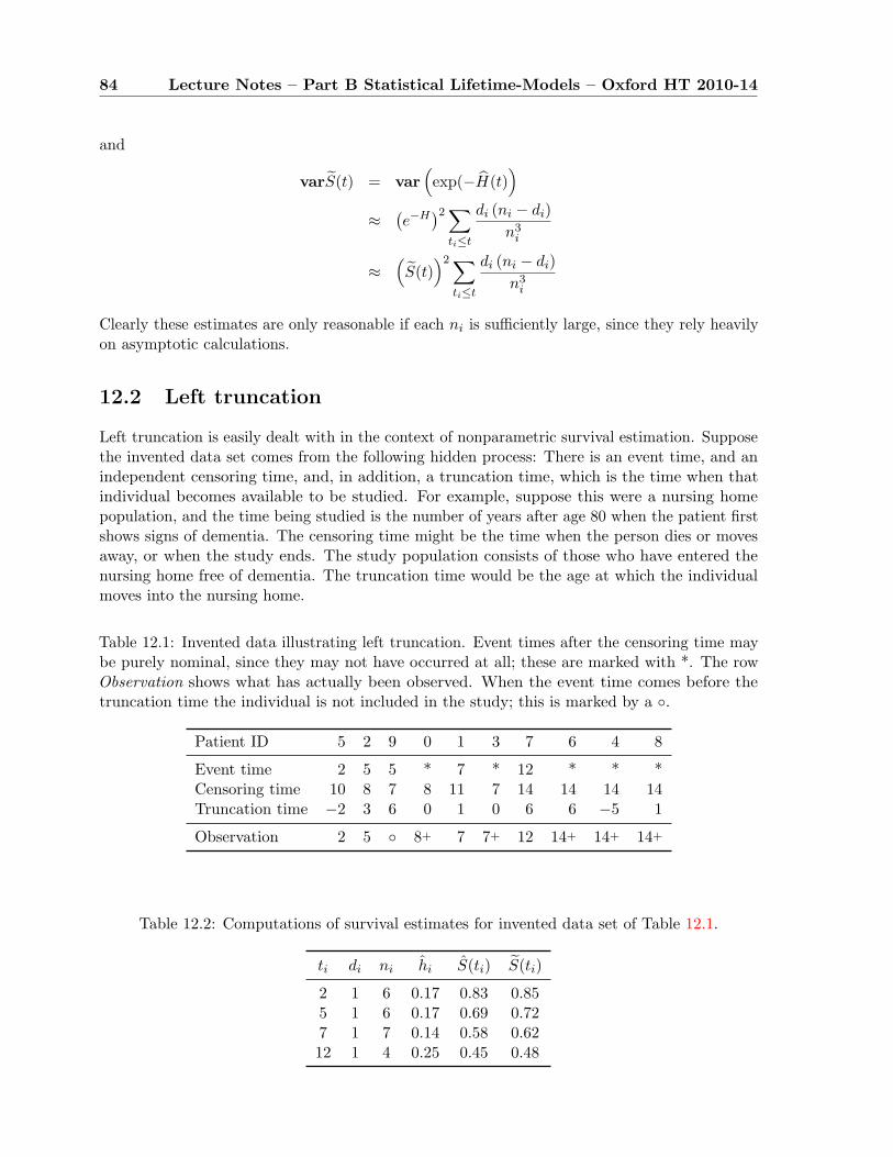
84 Lecture Notes – Part B Statistical Lifetime-Models – Oxford HT 2010-14
and
varS(t) = var(exp(−H(t)
)≈
(e−H
)2∑ti≤t
di (ni − di)n3
i
≈(S(t)
)2∑ti≤t
di (ni − di)n3
i
Clearly these estimates are only reasonable if each ni is sufficiently large, since they rely heavilyon asymptotic calculations.
12.2 Left truncation
Left truncation is easily dealt with in the context of nonparametric survival estimation. Supposethe invented data set comes from the following hidden process: There is an event time, and anindependent censoring time, and, in addition, a truncation time, which is the time when thatindividual becomes available to be studied. For example, suppose this were a nursing homepopulation, and the time being studied is the number of years after age 80 when the patient firstshows signs of dementia. The censoring time might be the time when the person dies or movesaway, or when the study ends. The study population consists of those who have entered thenursing home free of dementia. The truncation time would be the age at which the individualmoves into the nursing home.
Table 12.1: Invented data illustrating left truncation. Event times after the censoring time maybe purely nominal, since they may not have occurred at all; these are marked with *. The rowObservation shows what has actually been observed. When the event time comes before thetruncation time the individual is not included in the study; this is marked by a ◦.
Patient ID 5 2 9 0 1 3 7 6 4 8
Event time 2 5 5 * 7 * 12 * * *Censoring time 10 8 7 8 11 7 14 14 14 14Truncation time −2 3 6 0 1 0 6 6 −5 1
Observation 2 5 ◦ 8+ 7 7+ 12 14+ 14+ 14+
Table 12.2: Computations of survival estimates for invented data set of Table 12.1.
ti di ni hi S(ti) S(ti)
2 1 6 0.17 0.83 0.855 1 6 0.17 0.69 0.727 1 7 0.14 0.58 0.6212 1 4 0.25 0.45 0.48
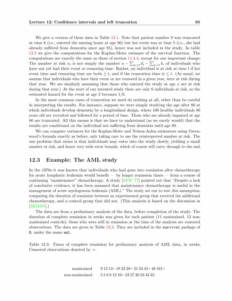
Lecture 12: Confidence intervals and left truncation 85
We give a version of these data in Table 12.1. Note that patient number 9 was truncatedat time 6 (i.e., entered the nursing home at age 86) but her event was at time 5 (i.e., she hadalready suffered from dementia since age 85), hence was not included in the study. In table12.2 we give the computations for the Kaplan-Meier estimate of the survival function. Thecomputations are exactly the same as those of section 11.4.4, except for one important change:The number at risk ni is not simply the number n −
∑ti<t di −
∑ti<t ki of individuals who
have not yet had their event or censoring time. Rather, an individual is at risk at time t if herevent time and censoring time are both ≥ t, and if the truncation time is ≤ t. (As usual, weassume that individuals who have their event or are censored in a given year, were at risk duringthat year. We are similarly assuming that those who entered the study at age x are at riskduring that year.) At the start of our invented study there are only 6 individuals at risk, so theestimated hazard for the event at age 2 becomes 1/6.
In the most common cases of truncation we need do nothing at all, other than be carefulin interpreting the results. For instance, suppose we were simply studying the age after 80 atwhich individuals develop dementia by a longitudinal design, where 100 healthy individuals 80years old are recruited and followed for a period of time. Those who are already impaired at age80 are truncated. All this means is that we have to understand (as we surely would) that theresults are conditional on the individual not suffering from dementia until age 80.
We can compute variances for the Kaplan-Meier and Nelson-Aalen estimators using Green-wood’s formula exactly as before, only taking care to use the reinterpreted number at risk. Theone problem that arises is that individuals may enter into the study slowly, yielding a smallnumber at risk, and hence very wide error bounds, which of course will carry through to the end.
12.3 Example: The AML study
In the 1970s it was known that individuals who had gone into remission after chemotherapyfor acute lymphatic leukemia would benefit — by longer remission times — from a course ofcontinuing “maintenance” chemotherapy. A study [EEH+77] pointed out that “Despite a lackof conclusive evidence, it has been assumed that maintenance chemotherapy is useful in themanagement of acute myelogenous leukemia (AML).” The study set out to test this assumption,comparing the duration of remission between an experimental group that received the additionalchemotherapy, and a control group that did not. (This analysis is based on the discussion in[MGM01].)
The data are from a preliminary analysis of the data, before completion of the study. Theduration of complete remission in weeks was given for each patient (11 maintained, 12 non-maintained controls); those who were still in remission at the time of the analysis are censoredobservations. The data are given in Table 12.3. They are included in the survival package ofR, under the name aml.
Table 12.3: Times of complete remission for preliminary analysis of AML data, in weeks.Censored observations denoted by +.
maintained 9 13 13+ 18 23 28+ 31 34 45+ 48 161+
non-maintained 5 5 8 8 12 16+ 23 27 30 33 43 45
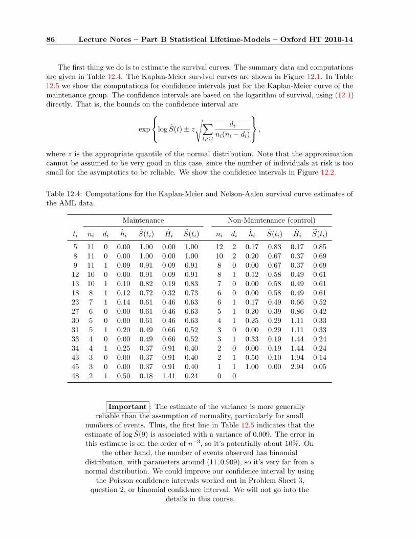
86 Lecture Notes – Part B Statistical Lifetime-Models – Oxford HT 2010-14
The first thing we do is to estimate the survival curves. The summary data and computationsare given in Table 12.4. The Kaplan-Meier survival curves are shown in Figure 12.1. In Table12.5 we show the computations for confidence intervals just for the Kaplan-Meier curve of themaintenance group. The confidence intervals are based on the logarithm of survival, using (12.1)directly. That is, the bounds on the confidence interval are
exp
log S(t)± z
√∑ti≤t
di
ni(ni − di)
,
where z is the appropriate quantile of the normal distribution. Note that the approximationcannot be assumed to be very good in this case, since the number of individuals at risk is toosmall for the asymptotics to be reliable. We show the confidence intervals in Figure 12.2.
Table 12.4: Computations for the Kaplan-Meier and Nelson-Aalen survival curve estimates ofthe AML data.
Maintenance Non-Maintenance (control)
ti ni di hi S(ti) Hi S(ti) ni di hi S(ti) Hi S(ti)
5 11 0 0.00 1.00 0.00 1.00 12 2 0.17 0.83 0.17 0.858 11 0 0.00 1.00 0.00 1.00 10 2 0.20 0.67 0.37 0.699 11 1 0.09 0.91 0.09 0.91 8 0 0.00 0.67 0.37 0.6912 10 0 0.00 0.91 0.09 0.91 8 1 0.12 0.58 0.49 0.6113 10 1 0.10 0.82 0.19 0.83 7 0 0.00 0.58 0.49 0.6118 8 1 0.12 0.72 0.32 0.73 6 0 0.00 0.58 0.49 0.6123 7 1 0.14 0.61 0.46 0.63 6 1 0.17 0.49 0.66 0.5227 6 0 0.00 0.61 0.46 0.63 5 1 0.20 0.39 0.86 0.4230 5 0 0.00 0.61 0.46 0.63 4 1 0.25 0.29 1.11 0.3331 5 1 0.20 0.49 0.66 0.52 3 0 0.00 0.29 1.11 0.3333 4 0 0.00 0.49 0.66 0.52 3 1 0.33 0.19 1.44 0.2434 4 1 0.25 0.37 0.91 0.40 2 0 0.00 0.19 1.44 0.2443 3 0 0.00 0.37 0.91 0.40 2 1 0.50 0.10 1.94 0.1445 3 0 0.00 0.37 0.91 0.40 1 1 1.00 0.00 2.94 0.0548 2 1 0.50 0.18 1.41 0.24 0 0
Important : The estimate of the variance is more generallyreliable than the assumption of normality, particularly for small
numbers of events. Thus, the first line in Table 12.5 indicates that theestimate of log S(9) is associated with a variance of 0.009. The error inthis estimate is on the order of n−3, so it’s potentially about 10%. On
the other hand, the number of events observed has binomialdistribution, with parameters around (11, 0.909), so it’s very far from anormal distribution. We could improve our confidence interval by using
the Poisson confidence intervals worked out in Problem Sheet 3,question 2, or binomial confidence interval. We will not go into the
details in this course.
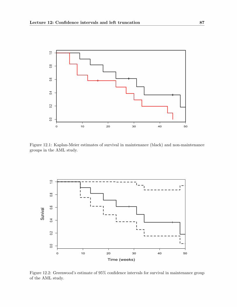
Lecture 12: Confidence intervals and left truncation 87
0 10 20 30 40 50
0.00.2
0.40.6
0.81.0
Figure 12.1: Kaplan-Meier estimates of survival in maintenance (black) and non-maintenancegroups in the AML study.
0 10 20 30 40 50
0.00.2
0.40.6
0.81.0
Time (weeks)
Survival
Figure 12.2: Greenwood’s estimate of 95% confidence intervals for survival in maintenance groupof the AML study.
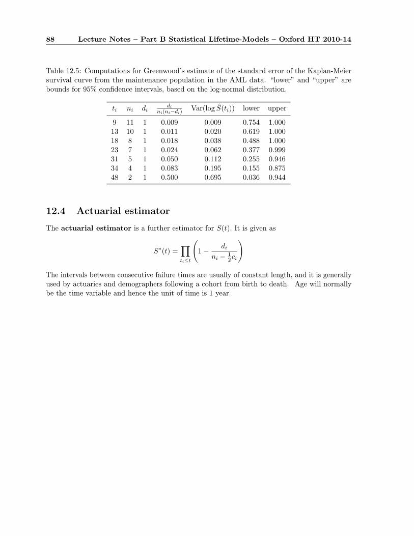
88 Lecture Notes – Part B Statistical Lifetime-Models – Oxford HT 2010-14
Table 12.5: Computations for Greenwood’s estimate of the standard error of the Kaplan-Meiersurvival curve from the maintenance population in the AML data. “lower” and “upper” arebounds for 95% confidence intervals, based on the log-normal distribution.
ti ni didi
ni(ni−di)Var(log S(ti)) lower upper
9 11 1 0.009 0.009 0.754 1.00013 10 1 0.011 0.020 0.619 1.00018 8 1 0.018 0.038 0.488 1.00023 7 1 0.024 0.062 0.377 0.99931 5 1 0.050 0.112 0.255 0.94634 4 1 0.083 0.195 0.155 0.87548 2 1 0.500 0.695 0.036 0.944
12.4 Actuarial estimator
The actuarial estimator is a further estimator for S(t). It is given as
S∗(t) =∏ti≤t
(1− di
ni − 12ci
)
The intervals between consecutive failure times are usually of constant length, and it is generallyused by actuaries and demographers following a cohort from birth to death. Age will normallybe the time variable and hence the unit of time is 1 year.
Lecture 13
Semiparametric models: acceleratedlife, proportional hazards
Reading: Cox & Oakes chapter 5.1–5.7, K & M chapter 8.1–8.4, 8.8, 12.1–5
13.1 Introduction to semiparametric modeling
We learned in section 6.3 how to compare observed mortality to a standard life table. In manysettings, though, we are interested to compare observed mortality (or more general event times)between groups, or between individuals with different values of a quantitative covariate, and inthe presence of censoring. For example,
Often we are interested to compare two (or more) different lifetime distributions. Anapproach that has been found to be effective is to think of there being a “standard” lifetimewhich may be modified in various simple ways to produce the lifetimes of the subpopulations.The standard lifetime is commonly estimated nonparametrically, while the modifications —usually the characteristic of primary interest — is reduced to one or a few parameters. Themodifications may either involve a discrete collection of parameters — one parameter for each ofa small number of subpopulations — or a regression-type parameter multiplied by a continuouscovariate.
Examples of the former type would be clinical trials, where we compare survival time betweentreatment and control groups, or an observational study where we compare survival rates ofsmokers and non-smokers. An example of the second time would be testing time to appearanceof full-blown AIDS symptoms as a function of measured T-cell counts.
There are two popular general classes of model as in the heading above - AL and PH.
13.2 Accelerated Life models
Suppose there are (several) groups, labelled by index i. The accelerated life model has a survivalcurve for each group defined by
Si(t) = S0(ρit)
where S0(t) is some baseline survival curve and ρi is a constant specific to group i.If we plot Si against log t, i = 1, 2, . . . , k, then we expect to see a horizontal shift as
Si(t) = S0(elog ρi+log t) .
89
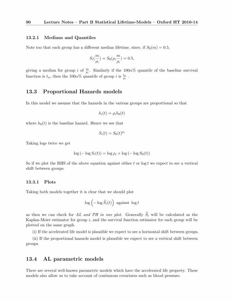
90 Lecture Notes – Part B Statistical Lifetime-Models – Oxford HT 2010-14
13.2.1 Medians and Quantiles
Note too that each group has a different median lifetime, since, if S0(m) = 0.5,
Si(m
ρi) = S0(ρi
m
ρi) = 0.5,
giving a median for group i of mρi
. Similarly if the 100α% quantile of the baseline survivalfunction is tα, then the 100α% quantile of group i is tα
ρi.
13.3 Proportional Hazards models
In this model we assume that the hazards in the various groups are proportional so that
hi(t) = ρih0(t)
where h0(t) is the baseline hazard. Hence we see that
Si(t) = S0(t)ρi
Taking logs twice we get
log (− log Si(t)) = log ρi + log (− log S0(t))
So if we plot the RHS of the above equation against either t or log t we expect to see a verticalshift between groups.
13.3.1 Plots
Taking both models together it is clear that we should plot
log(− log Si(t)
)against log t
as then we can check for AL and PH in one plot. Generally Si will be calculated as theKaplan-Meier estimator for group i, and the survival function estimator for each group will beplotted on the same graph.
(i) If the accelerated life model is plausible we expect to see a horizontal shift between groups.
(ii) If the proportional hazards model is plausible we expect to see a vertical shift betweengroups.
13.4 AL parametric models
There are several well-known parametric models which have the accelerated life property. Thesemodels also allow us to take account of continuous covariates such as blood pressure.
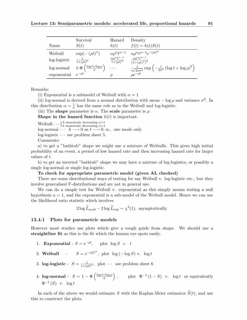
Lecture 13: Semiparametric models: accelerated life, proportional hazards 91
Survival Hazard DensityName S(t) h(t) f(t) = h(t)S(t)
Weibull exp(− (ρt)α) αραtα−1 αραtα−1e−(ρt)α
log-logistic 11+(ρt)α
αραtα−1
1+(ρt)ααραtα−1
(1+(ρt)α)2
log-normal 1-Φ(
log t+log ρσ
)· · · 1
t√
2πσ2exp
(− 1
2σ2 (log t + log ρ)2)
exponential e−ρt ρ ρe−ρt
Remarks:(i) Exponential is a submodel of Weibull with α = 1(ii) log-normal is derived from a normal distribution with mean − log ρ and variance σ2. In
this distribution α = 1σ has the same role as in the Weibull and log-logistic.
(iii) The shape parameter is α. The scale parameter is ρ.Shape in the hazard function h(t) is important.
Weibull · · ·{
h monotonic increasing α>1h monotonic decreasing α<1
log-normal · · · h −→ 0 as t −→ 0,∞, one mode onlylog-logistic · · · see problem sheet 5.Comments:a) to get a ”bathtub” shape we might use a mixture of Weibulls. This gives high initial
probability of an event, a period of low hazard rate and then increasing hazard rate for largervalues of t.
b) to get an inverted ”bathtub” shape we may have a mixture of log-logistics, or possibly asingle log-normal or single log-logistic.
To check for appropriate parametric model (given AL checked)There are some distributional ways of testing for say Weibull v. log-logistic etc., but they
involve generalised F-distributions and are not in general use.We can do a simple test for Weibull v. exponential as this simply means testing a null
hypothesis α = 1, and the exponential is a sub-model of the Weibull model. Hence we can usethe likelihood ratio statistic which involves
2 log Lweib − 2 log Lexp ∼ χ2(1), asymptotically.
13.4.1 Plots for parametric models
However most studies use plots which give a rough guide from shape. We should use astraightline fit as this is the fit which the human eye spots easily.
1. Exponential - S = e−ρt, plot log S v. t
2. Weibull - S = e−(ρt)α
, plot log (− log S) v. log t
3. log-logistic - S = 11+(ρt)α , plot · · · see problem sheet 6
4. log-normal - S = 1 − Φ(
log t+log ρσ
), plot Φ−1 (1− S) v. log t or equivalently
Φ−1 (S) v. log t
In each of the above we would estimate S with the Kaplan-Meier estimator S(t), and usethis to construct the plots.
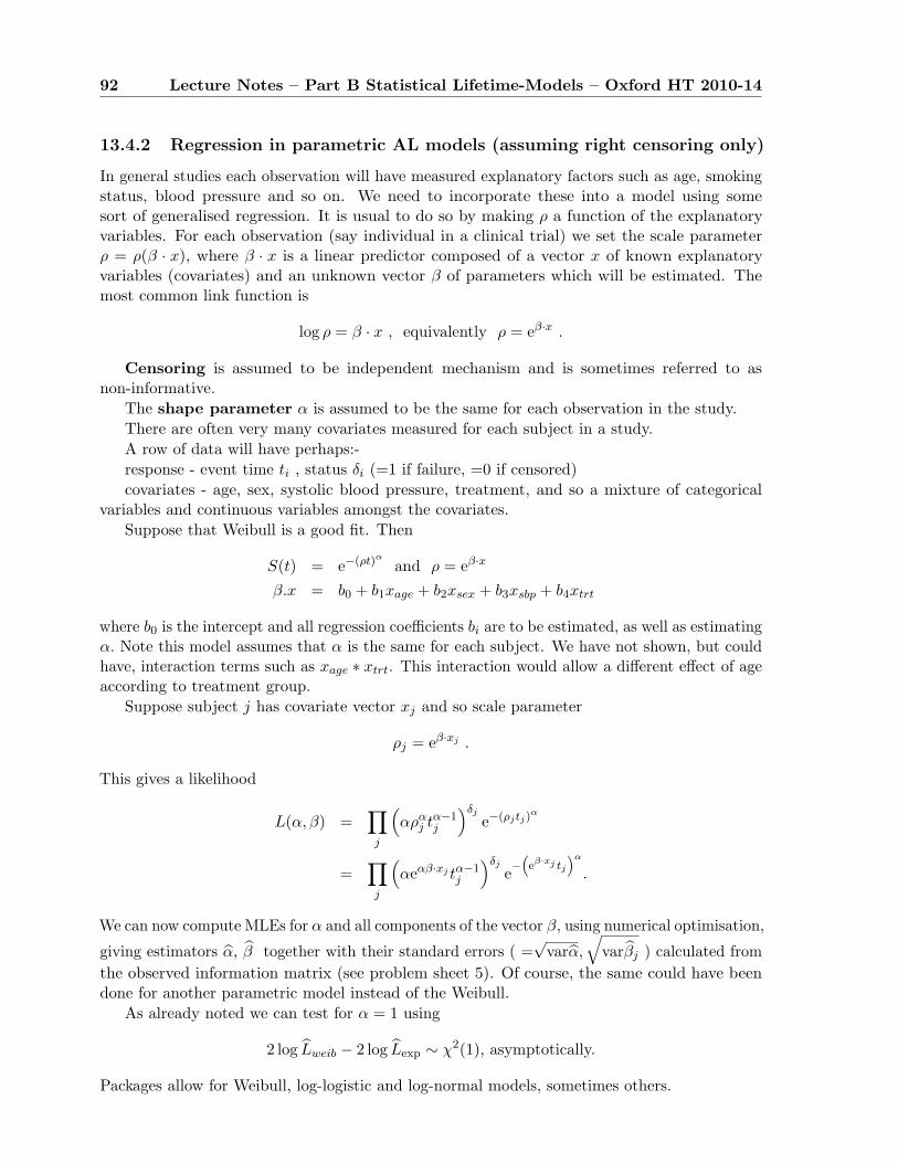
92 Lecture Notes – Part B Statistical Lifetime-Models – Oxford HT 2010-14
13.4.2 Regression in parametric AL models (assuming right censoring only)
In general studies each observation will have measured explanatory factors such as age, smokingstatus, blood pressure and so on. We need to incorporate these into a model using somesort of generalised regression. It is usual to do so by making ρ a function of the explanatoryvariables. For each observation (say individual in a clinical trial) we set the scale parameterρ = ρ(β · x), where β · x is a linear predictor composed of a vector x of known explanatoryvariables (covariates) and an unknown vector β of parameters which will be estimated. Themost common link function is
log ρ = β · x , equivalently ρ = eβ·x .
Censoring is assumed to be independent mechanism and is sometimes referred to asnon-informative.
The shape parameter α is assumed to be the same for each observation in the study.There are often very many covariates measured for each subject in a study.A row of data will have perhaps:-response - event time ti , status δi (=1 if failure, =0 if censored)covariates - age, sex, systolic blood pressure, treatment, and so a mixture of categorical
variables and continuous variables amongst the covariates.Suppose that Weibull is a good fit. Then
S(t) = e−(ρt)α
and ρ = eβ·x
β.x = b0 + b1xage + b2xsex + b3xsbp + b4xtrt
where b0 is the intercept and all regression coefficients bi are to be estimated, as well as estimatingα. Note this model assumes that α is the same for each subject. We have not shown, but couldhave, interaction terms such as xage ∗ xtrt. This interaction would allow a different effect of ageaccording to treatment group.
Suppose subject j has covariate vector xj and so scale parameter
ρj = eβ·xj .
This gives a likelihood
L(α, β) =∏j
(αρα
j tα−1j
)δj
e−(ρjtj)α
=∏j
(αeαβ·xj tα−1
j
)δj
e−“eβ·xj tj
”α
.
We can now compute MLEs for α and all components of the vector β, using numerical optimisation,
giving estimators α, β together with their standard errors ( =√
varα,
√varβj ) calculated from
the observed information matrix (see problem sheet 5). Of course, the same could have beendone for another parametric model instead of the Weibull.
As already noted we can test for α = 1 using
2 log Lweib − 2 log Lexp ∼ χ2(1), asymptotically.
Packages allow for Weibull, log-logistic and log-normal models, sometimes others.
Lecture 13: Semiparametric models: accelerated life, proportional hazards 93
13.4.3 Linear regression in parametric AL models
The idea is to mirror ordinary linear regression and find a baseline distribution which doesnot depend on ρ, similar to looking at the error term in least squares regression. We give thederivation just for the Weibull distribution, but similar arguments work for all AL parametricmodels. We have
S(t) = e−(ρt)α
= P{T > t
}= P
{log T > log t
}= P
{α (log T + log ρ) > α (log t + log ρ)
}Now let Y = α (log T + log ρ) and y = α (log t + log ρ) .
P{Y > y
}= SY (y)
= S(t)= e−(ρt)α
= exp(−ey)
Hence we havelog T = − log ρ +
1α
Y, where SY (y) = exp(−ey)
The distribution of Y is independent of the parameters ρ and α. And in the case of the Weibulldistribution its distribution is called the extreme value distribution and is as above.
In general we will write log T = − log ρ + 1αY for all AL parametric models, and Y has a
distribution in each case which is independent of the model parameters.
Name S(t) Y SY (y) distribution
Weibull exp(− (ρt)α) log T = − log ρ + 1αY exp(−ey): extreme value distrib.
log-logistic 11+(ρt)α log T = − log ρ + 1
αY (1 + ey)−1: logistic distribution
log-normal 1-Φ(
log t+log ρσ
)log T = − log ρ + σY 1− Φ(y): N(0, 1)
as before α = 1σ , for the log-normal.
In recent years, a semi-parametric model has been developed in which the baseline survivalfunction S0 is modelled non-parametrically, and each subject has time t scaled to ρjt. Thismodel is beyond the scope of this course.
Lecture 14
Cox regression, Part I
Again each subject j has a vector of covariates xj and scale parameter ρj = ρj (β · xj) . The basicassumption is that any two subjects have hazard functions whose ratio is a constant proportionwhich depends on the covariates. Hence we may write
hj(t) = ρjh0(t)
where h0 is the baseline hazard function, β is a vector of regression coefficients to be estimated,and ρj again depends on the linear predictor β.xj .
A general link could be used but in Cox regression ρj = eβ.xj . This model is termed semi-parametric because the functional form of the baseline hazard is not given, but is determinedfrom the data, similarly to the idea for estimating the survival function by the Kaplan-Meierestimator.
14.1 What is Cox Regression?
Cox regression is Proportional Hazards with a semi-parametric model.Suppose the event times are given by 0 < t1 < t2 < · · · < tm. At this stage we assume no
tied event times (list does not include censored times).Let [i] denote the subject with event at ti.Definition: Risk SetThe risk set Ri is the set of those subjects available for the event at time ti.Reminder : if we know that there are d subjects with hazard functions h1, · · · , hd then,
knowing there is an event at time t0, the probability that subject j has the event is
P{subject j
∣∣ t0} =hj(t0)
h1(t0) + · · ·+ hd(t0).
Under the proportional hazards assumption we have
P{[i]∣∣ ti} =
ρ[i]h0(ti)∑j∈Ri
ρjh0(ti)=
ρ[i]∑j∈Ri
ρj
and the probability that [i] has the event given it occurs at time ti no longer depends on ti.Under the Cox regression model we have
P{[i]∣∣ ti} =
eβ·x[i]∑j∈Ri
eβ·xj.
94
Lecture 14: Cox regression, Part I 95
This probability only depends on the order in which subjects have the events.The idea of the model is to specify a partial likelihood which depends only on the order in
which events occur, not the times at which they occur. This means that the functional form ofh0, the baseline hazard function, is not required.
Definition: Partial Likelihood
LP (β) =∏ti
eβ·x[i]∑j∈Ri
eβ·xj
where Ri is the risk set at ti, and subject [i] is the subject with the event at ti.We can think of the partial likelihood as the joint density function for subjects’ ranks in
terms of event order, if there were no censoring and no tied event times.Consequently if we use the partial likelihood for estimation of parameters we are losing
information, because we are suppressing the actual times of events even though they are known,hence the name “partial likelihood”.
Interestingly the partial likelihood acts in an exactly similar manner to the likelihood.Compute βP such that
LP
(βP
)= sup
β
∏ti
eβ·x[i]∑j∈Ri
eβ·xj
Then βP maximises the partial likelihood and has all the usual properties.Properties
(i) βPP−→ β as m −→∞ ( and hence the number in the study tends to infinity also),
(ii) varβP ≈ I−1P , where IP is calculated from LP in exactly the same way as for the usual
information and likelihood,(iii) asymptotic normality of βP also holds.
There are journal papers showing that the % information lost by ignoring actual eventtimes is smaller than one might expect. All of the above rests on the assumption that the Coxregression model fits the data, of course.
14.2 Relative Risk
There is a big difference between deductions from AL parametric analysis and PH semi-parametricanalysis. In PH the intercept is non-identifiable and so we are estimating relative risk betweensubjects, not absolute risk, when we estimate the model parameters.
Definition: relative riskThe relative risk at time t between two subjects with covariates x1, x2 and hazard functions
h2, h1 is defined to beh2(t)h1(t)
.
For the Cox regression model this becomes time independent and is given by
eβ.(x2−x1) .
The intercept is non-identifiable because
h(t;x) = eβ·xh0(t) = eα+β·x (e−αh0(t))
96 Lecture Notes – Part B Statistical Lifetime-Models – Oxford HT 2010-14
for any α. This means that any such intercept α included with the regression expression β · xsimply cancels out in the partial likelihood. Hence an intercept is never included in the linearregressor in this model.
14.3 Baseline hazard
However we do need to estimate the cumulative baseline hazard function and also the baselinesurvival function.
Definition: Breslow’s estimator for the baseline cumulative hazard functionSuppose the baseline survival is given by
S0(t) = e−cH0(t),
where the discrete hazard estimation h0 is given by
h0(ti) =1∑
j∈Ri
eβ·xj
Breslow’s estimator is given by
h0 =1∑
j∈Ri
eβ·xj(14.1)
In some sense the discrete estimates for h0(ti) can be thought of as the maximum likelihoodestimators from the full likelihood, provided we assume that the hazard distribution is discrete(which of course it generally is not). When β = 0 or when the covariates are all 0, thisreduces simply to the Nelson-Aalen estimator. Otherwise, we see that this is equivalent to amodified Nelson-Aalen estimator, where the size of the risk set is weighted by the relative risksof the individuals. In other words, the estimate of h0 is equivalent to the standard estimate# events/time at risk, but now time at risk is weighted by the relative risk.
The estimator may be loosely derived as follows:
`(h) =∑ti
log(1− e−h[i](ti))−∑j∈Ri
j 6=[i]
hj
=∑ti
log(1− e−ρ[i]h0(ti))−∑j∈Ri
j 6=[i]
ρjh0(ti).
We estimate h0(ti) by
0 =ρ[i]e
−ρ[i]h0(ti)
1− e−ρ[i]h0(ti)−∑j∈Ri
j 6=[i]
ρj
≈ρ[i](1− ρ[i]h0(ti))
ρ[i]h0(ti)−∑j∈Ri
j 6=[i]
ρj
=(1− ρ[i]h0(ti))
h0(ti)−∑j∈Ri
j 6=[i]
ρj .
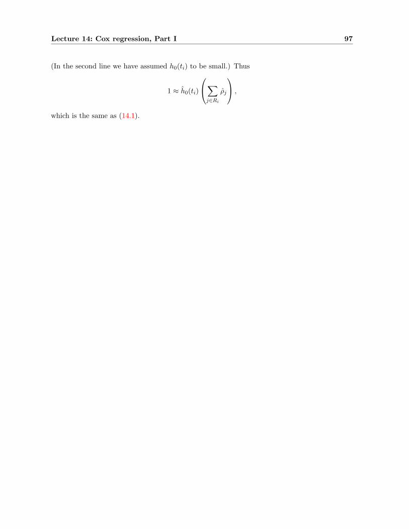
Lecture 14: Cox regression, Part I 97
(In the second line we have assumed h0(ti) to be small.) Thus
1 ≈ h0(ti)
∑j∈Ri
ρj
,
which is the same as (14.1).
Lecture 15
Cox regression, Part II
15.1 Dealing with ties
Until now in this section we have been assuming that the times of events are all distinct.In situations where event times are equal, we can carry out the same computations for Coxregression, only using a modified version of the partial likelihood. Suppose Ri is the set ofindividuals at risk at time ti, and Di the set of individuals who have their event at that time.We assume that the ties are not real ties, but only the result of discreteness in the observation.Then the probability of having precisely those individuals at time ti will depend on the orderin which they actually occurred. For example, suppose there are 5 individuals at risk at thestart, and two of them have their events at time t1. If the relative risks were {ρ1, . . . , ρ5}, whereρj = eβ·xj , then the first term in the partial likelihood would be
ρ1
ρ1 + ρ2 + ρ3 + ρ4 + ρ5· ρ2
ρ2 + ρ3 + ρ4 + ρ5+
ρ2
ρ1 + ρ2 + ρ3 + ρ4 + ρ5· ρ1
ρ1 + ρ3 + ρ4 + ρ5.
The number of terms is di!, so it is easy to see that this computation quickly becomes intractable.
A very good alternative — accurate and easy to compute — was proposed by B. Efron.Observe that the terms differ in the denominator merely by a small change due to the individualslost from the risk set. If the deaths at time ti are not a large proportion of the risk set, then wecan approximate this by deducting the average of the risks that depart. In other words, in theabove example, the first contribution to the partial likelihood becomes
ρ1ρ2
(ρ1 + ρ2 + ρ3 + ρ4 + ρ5)(12(ρ1 + ρ2) + ρ3 + ρ4 + ρ5)
.
More generally, the partial likelihood becomes
LP (β) =∏ti
eβ·
Pj∈Di
xj
di−1∏k=0
∑j∈Ri
eβ·xj − k
di
∑j∈Di
eβ·xj
−1
.
We take the same approach to estimating the baseline hazard:
h0(ti) =di−1∑k=0
∑j∈Ri
eβ·xj − k
di
∑j∈Di
eβ·xj
−1
.
98
Lecture 15: Cox regression, Part II 99
Another approach, due to Breslow, makes no correction for the progressive loss of risk in thedenominator:
LBreslowP (β) =
∏ti
eβ·
Pj∈Di
xi
∑j∈Ri
eβ·xi
−di
.
This approximation is always too small, and tends to shift the estimates of β toward 0. It iswidely used as a default in software packages (SAS, not R!) for purely historical reasons.
15.2 Plot for PH assumption with continuous covariate
Suppose we have a continuous covariate and we wish to check the proportional hazards assumptionfor that covariate. We do not have natural groups of subjects with the same value of thatcovariate.
Provided there is sufficient data we would group the subjects in quintiles of the covariate.Then we have 5 groups and can find the Kaplan-Meier estimator for each group. As before weplot
log(− log(Sk(t))) v. log t
for each k = 1, · · · , 5 on the same graph. There should be a roughly constant vertical separationof groups. It generally is not a wonderful method, but is better than nothing.
15.3 The AML example
We continue looking at the leukemia study that we started to consider in section 12.3. First,in Figure 15.1 we plot the iterated logarithm of survival against time, to test the proportionalhazards assumption. The PH assumption corresponds to the two curves differing by a verticalshift. The result makes this assumption at least credible.
We code the data with covariate x = 0 for the maintained group, and x = 1 for the non-maintained group. Thus, the baseline hazard will correspond to the maintained group, and eβ
will be the relative risk of the non-maintained group. From Table 12.4 we see that the Efronapproximate partial likelihood is given by
LP (β) =(
e2β
(12eβ + 11)(11eβ + 11)
)(e2β
(10eβ + 11)(9eβ + 11)
)×(
18eβ + 11
)(eβ
8eβ + 10
)(1
7eβ + 10
)(1
6eβ + 8
)×(
eβ · 1(6eβ + 7)(5.5eβ + 6.5)
)(eβ
5eβ + 6
)(eβ
4eβ + 5
)×(
13eβ + 5
)(eβ
3eβ + 4
)(1
2eβ + 4
)(eβ
2eβ + 3
)(eβ
eβ + 3
)(12
)(15.1)
A plot of LP (β) is shown in Figure 15.4.In the one-dimensional setting it is straightforward to estimate β by direct computation. We
see the maximum at β = 0.9155 in the plot of Figure 15.4. In more complicated settings, thereare good maximisation algorithms built in to the coxph function in the survival package of R.Applying this to the current problem, we obtain:
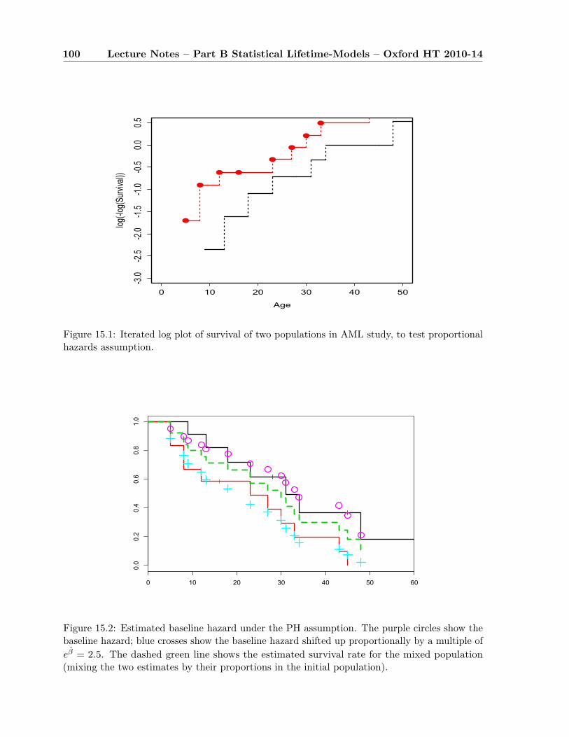
100 Lecture Notes – Part B Statistical Lifetime-Models – Oxford HT 2010-14
0 10 20 30 40 50
-3.0
-2.5
-2.0
-1.5
-1.0
-0.5
0.00.5
Age
log(-log(S
urvival))
Figure 15.1: Iterated log plot of survival of two populations in AML study, to test proportionalhazards assumption.
0 10 20 30 40 50 60
0.0
0.2
0.4
0.6
0.8
1.0
Figure 15.2: Estimated baseline hazard under the PH assumption. The purple circles show thebaseline hazard; blue crosses show the baseline hazard shifted up proportionally by a multiple ofeβ = 2.5. The dashed green line shows the estimated survival rate for the mixed population(mixing the two estimates by their proportions in the initial population).
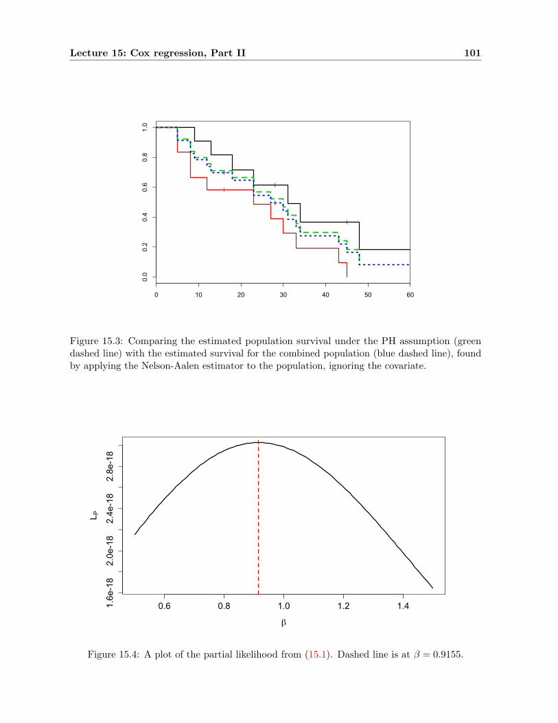
Lecture 15: Cox regression, Part II 101
0 10 20 30 40 50 60
0.0
0.2
0.4
0.6
0.8
1.0
Figure 15.3: Comparing the estimated population survival under the PH assumption (greendashed line) with the estimated survival for the combined population (blue dashed line), foundby applying the Nelson-Aalen estimator to the population, ignoring the covariate.
0.6 0.8 1.0 1.2 1.41.6e-18
2.0e-18
2.4e-18
2.8e-18
β
L P
Figure 15.4: A plot of the partial likelihood from (15.1). Dashed line is at β = 0.9155.
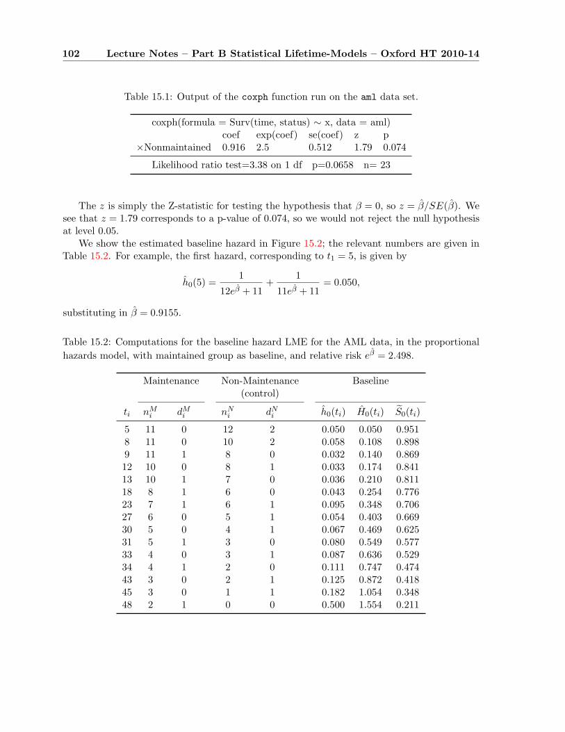
102 Lecture Notes – Part B Statistical Lifetime-Models – Oxford HT 2010-14
Table 15.1: Output of the coxph function run on the aml data set.
coxph(formula = Surv(time, status) ∼ x, data = aml)coef exp(coef) se(coef) z p
×Nonmaintained 0.916 2.5 0.512 1.79 0.074
Likelihood ratio test=3.38 on 1 df p=0.0658 n= 23
The z is simply the Z-statistic for testing the hypothesis that β = 0, so z = β/SE(β). Wesee that z = 1.79 corresponds to a p-value of 0.074, so we would not reject the null hypothesisat level 0.05.
We show the estimated baseline hazard in Figure 15.2; the relevant numbers are given inTable 15.2. For example, the first hazard, corresponding to t1 = 5, is given by
h0(5) =1
12eβ + 11+
1
11eβ + 11= 0.050,
substituting in β = 0.9155.
Table 15.2: Computations for the baseline hazard LME for the AML data, in the proportionalhazards model, with maintained group as baseline, and relative risk eβ = 2.498.
Maintenance Non-Maintenance Baseline(control)
ti nMi dM
i nNi dN
i h0(ti) H0(ti) S0(ti)
5 11 0 12 2 0.050 0.050 0.9518 11 0 10 2 0.058 0.108 0.8989 11 1 8 0 0.032 0.140 0.86912 10 0 8 1 0.033 0.174 0.84113 10 1 7 0 0.036 0.210 0.81118 8 1 6 0 0.043 0.254 0.77623 7 1 6 1 0.095 0.348 0.70627 6 0 5 1 0.054 0.403 0.66930 5 0 4 1 0.067 0.469 0.62531 5 1 3 0 0.080 0.549 0.57733 4 0 3 1 0.087 0.636 0.52934 4 1 2 0 0.111 0.747 0.47443 3 0 2 1 0.125 0.872 0.41845 3 0 1 1 0.182 1.054 0.34848 2 1 0 0 0.500 1.554 0.211
Lecture 16
Testing Hypotheses
Reading: C& O sections 8.6–8.7, K & M sections 7.1–7.3A common question that we may have is, whether two (or more) samples of survival times may
be considered to have been drawn from the same distribution: That is, whether the populationsunder observation are subject to the same hazard rate.
16.1 Tests in the regression setting
1) A package will produce a test of whether or not a regression coefficient is 0. It uses propertiesof mle’s. Let the coefficient of interest be b say. Then the null hypothesis is HO : b = 0 andthe alternative is HA : b 6= 0. At the 5% significance level, HO will be accepted if the p-valuep > 0.05, and rejected otherwise.
2) In an AL parametric model if α is the shape parameter then we can test HO : log α = 0against the alternative HA : log α 6= 0. Again mle properties are used and a p-value is producedas above. In the case of the Weibull if we accept log α = 0 then we have the simpler exponentialdistribution (with α = 1).
3) We have already mentioned that, to test Weibull v. exponential with null hypothesis HO :exponential is an acceptable fit, we can use
2 log Lweib − 2 log Lexp ∼ χ2(1), asymptotically.
16.2 Non-parametric testing of survival between groups
16.2.1 General principles
We will consider only the case where the data splits into two groups. There is a relatively easyextension to k > 2 groups.
We define the following notation
Event times are 0 < t1 < t2 < · · · < tm.
For i = 1, 2, . . . ,m, and j = 1, 2, dij = # events at ti in group j,
nij = # in risk set at ti from group j,
di = # events at ti,
ni = # in risk set at ti.
Thus, when the number of groups k = 2, we have di = di1 + di2 and ni = ni1 + ni2.
103
104 Lecture Notes – Part B Statistical Lifetime-Models – Oxford HT 2010-14
Generally we are interested in testing the null hypothesis H0, that there is no differencebetween the hazard rates of the two groups, against the two-sided alternative that there isa difference in the hazard rates. The guiding principle is quite elementary, quite similar toour approach to the proportional hazards model: We treat each event time ti as a new andindependent experiment. Under the null hypothesis, the next event is simply a random samplefrom the risk set. Thus, the probability of the death at time ti being from group 1 is ni1/ni,and the probability of it being from group 2 is ni2/ni.
This describes only the setting where the events all occur at distinct times: That is, di
are all exactly 1. More generally, the null hypothesis predicts that the group identities of theindividuals whose events are at time ti are like a sample of size di without replacement froma collection of ni1 ‘1’s and ni2 ‘2’s. The distribution of di1 under such sampling is called thehypergeometric distribution. It has
expectation = dini1
ni, and
variance =: σ2i =
ni1ni2(ni − di)di
n2i (ni − 1)
.
Note that if di is negligible with respect to ni, this variance formula reduces to di(ni1ni
)(ni2ni
),which is just the variance of a binomial distribution.
Conditioned on all the events up to time ti (hence on ni, ni1, ni2) and on di, the randomvariable di1 − ni1
dini
has expectation 0 and variance σ2i . If we multiply it by an arbitrary weight
W (ti), determined by the data up to time ti, we still have W (ti)(di1 − ni1dini
) being a randomvariable with (conditional) expectation 0, but now (conditional) variance W (ti)2σ2
i . This meansthat if we define for k = 1, . . . ,m
Mk :=
(k∑
i=1
W (ti)(di1 − ni1
di
ni
))m
k=1
,
these will be random variables with expectation 0 and variance∑k
i=1 W (ti)2σ2i . While the
increments are not independent, we may still apply a version of the Central Limit Theoremto show that Mk is approximately normal when the sample size is large enough. (In technicalterms, the sequence of random variables Mk is a martingale, and the appropriate theorem is theMartingale Central Limit Theorem. See [HH80] for more details.) We then base our tests onthe statistic
Z :=
∑mi=1 W (ti)
(di1 − ni1
dini
)√∑mi=1 W (ti)2
ni1ni2(ni−di)di
n2i (ni−1)
,
which should have a standard normal distribution under the null hypothesis.Note that, as in the Cox regression setting, right censoring and left truncation are automati-
cally taken care of, by appropriate choice of the risk sets.
16.2.2 Standard tests
Any choice of weights W (ti) defines a valid test. Why do we need weights? Since any choiceof weights produces a correct test, there is no canonical choice. Changing the weights changesthe power with respect to different alternatives. Which alternative you choose — hence, whichweights you choose — should depend on what deviations from equality you are most interested
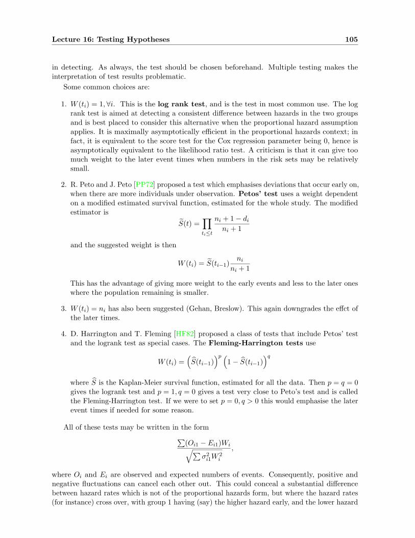
Lecture 16: Testing Hypotheses 105
in detecting. As always, the test should be chosen beforehand. Multiple testing makes theinterpretation of test results problematic.
Some common choices are:
1. W (ti) = 1,∀i. This is the log rank test, and is the test in most common use. The logrank test is aimed at detecting a consistent difference between hazards in the two groupsand is best placed to consider this alternative when the proportional hazard assumptionapplies. It is maximally asymptotically efficient in the proportional hazards context; infact, it is equivalent to the score test for the Cox regression parameter being 0, hence isasymptotically equivalent to the likelihood ratio test. A criticism is that it can give toomuch weight to the later event times when numbers in the risk sets may be relativelysmall.
2. R. Peto and J. Peto [PP72] proposed a test which emphasises deviations that occur early on,when there are more individuals under observation. Petos’ test uses a weight dependenton a modified estimated survival function, estimated for the whole study. The modifiedestimator is
S(t) =∏ti≤t
ni + 1− di
ni + 1
and the suggested weight is then
W (ti) = S(ti−1)ni
ni + 1
This has the advantage of giving more weight to the early events and less to the later oneswhere the population remaining is smaller.
3. W (ti) = ni has also been suggested (Gehan, Breslow). This again downgrades the effct ofthe later times.
4. D. Harrington and T. Fleming [HF82] proposed a class of tests that include Petos’ testand the logrank test as special cases. The Fleming-Harrington tests use
W (ti) =(S(ti−1)
)p (1− S(ti−1)
)q
where S is the Kaplan-Meier survival function, estimated for all the data. Then p = q = 0gives the logrank test and p = 1, q = 0 gives a test very close to Peto’s test and is calledthe Fleming-Harrington test. If we were to set p = 0, q > 0 this would emphasise the laterevent times if needed for some reason.
All of these tests may be written in the form∑(Oi1 − Ei1)Wi√∑
σ2i1W
2i
,
where Oi and Ei are observed and expected numbers of events. Consequently, positive andnegative fluctuations can cancel each other out. This could conceal a substantial differencebetween hazard rates which is not of the proportional hazards form, but where the hazard rates(for instance) cross over, with group 1 having (say) the higher hazard early, and the lower hazard
106 Lecture Notes – Part B Statistical Lifetime-Models – Oxford HT 2010-14
later. One way to detect such an effect is with a test statistic to which fluctuations contributeonly their absolute values. For instance, we could use the standard χ2 statistic
X :=m∑
i=1
k∑j=1
(Oij − Eij)2
Eij.
Asymptotically, this should have the χ2 distribution with (k − 1)m degrees of freedom. Ofcourse, if the number of groups k = 2, this is the same as
X :=m∑
i=1
(Oi1 − Ei1)2
dini1ni
(1− ni1ni
).
16.3 The AML example
We can use these tests to compare the survival of the two groups in the AML experimentdiscussed in section 12.3. The relevant quantities are tabulated in Table 16.1.
Time ni1 ni2 di1 di2 σ2i Peto weight
5 11 12 0 2 0.476 0.9588 11 10 0 2 0.474 0.8759 11 8 1 0 0.244 0.792
12 10 8 0 1 0.247 0.75013 10 7 1 0 0.242 0.70818 8 6 1 0 0.245 0.66123 7 6 1 1 0.456 0.61427 6 5 0 1 0.248 0.51930 5 4 0 1 0.247 0.46731 5 3 1 0 0.234 0.41633 4 3 0 1 0.245 0.36434 4 2 1 0 0.222 0.31243 3 2 0 1 0.240 0.26045 3 1 0 1 0.188 0.208
Table 16.1: Data for testing equality of survival in AML experiment.
When the weights are all taken equal, we compute Z = −1.84, whereas the Peto weights —which reduce the influence of later observations — give us Z = −1.67. This yields one-sidedp-values of 0.033 and 0.048 respectively — a marginally significant difference — or two-sidedp-values of 0.065 and 0.096.
Applying the χ2 test yields X = 16.86, which needs to be compared to χ2 with 14 degrees offreedom. The resulting p-value is 0.24, which is not at all significant. This should not be seenas surprising: The differences between the two survival curves are clearly mostly in the samedirection, so we lose power when applying a test that ignores the direction of the difference.
Bibliography
[Buf77] George Leclerc Buffon. Essai d’arithmetique morale. 1777.
[CT406] CT4: Models Core Reading. Faculty & Institute of Acutaries, 2006.
[ECIW06] Gregory M. Erickson, Philip J. Currie, Brian D. Inouye, and Alice A. Winn. Tyran-nosaur life tables: An example of nonavian dinosaur population biology. Science,313:213–7, 2006.
[EEH+77] Stephen H. Embury, Laurence Elias, Philip H. Heller, Charles E. Hood, Peter L.Greenberg, and Stanley L. Schrier. Remission maintenance therapy in acute myeloge-nous leukemia. The Western Journal of Medicine, 126:267–72, April 1977.
[Fox97] A. J. Fox. English life tables no. 15. Office of National Statistics, London, 1997.
[Gom25] Benjamin Gompertz. On the nature of the function expressive of the law of hu-man mortality and on a new mode of determining life contingencies. Philosophicaltransactions of the Royal Society of London, 115:513–85, 1825.
[HF82] David P. Harrington and Thomas R. Fleming. A class of rank test procedures forcensored survival data. Biometrika, 69(3):553–66, December 1982.
[HH80] Peter Hall and Christopher C. Heyde. Martingale Limit Theory and its Application.Academic Press, New York, London, 1980.
[Kie01] Kathleen Kiernan. The rise of cohabitation and childbearing outside marriage inwestern Europe. International Journal of Law, Policy and the Family, 15:1–21, 2001.
[KT81] Samuel Karlin and Howard M. Taylor. A Second Course in Stochastic Processes.Academic Press, 1981.
[Mac96] A. S. Macdonald. An actuarial survey of statistics models for decrement and transitiondata. I: Multiple state, Poisson and binomial models. British Actuarial Journal,2(1):129–55, 1996.
[ME05] Kyriakos S. Markides and Karl Eschbach. Aging, migration, and mortality: Currentstatus of research on the hispanic paradox. Journals of Gerontology: Series B,60B:68–75, 2005.
[MGM01] Rupert G. Miller, Gail Gong, and Alvaro Munoz. Survival Analysis. Wiley, 2001.
[PP72] Richard Peto and Julian Peto. Asymptotically efficient rank invariant test procedures.Journal of the Royal Statistical Society. Series A (General), 135(2):185–207, 1972.
[Wac] Kenneth W. Wachter. Essential demographic methods. Unpublished manuscript.
107