Head-Driven Statistical Models for Natural Language Parsing

c© 2003 Association for Computational Linguistics

Head-Driven Statistical Models forNatural Language Parsing

Michael Collins∗

MIT Computer Science andArtificial Intelligence Laboratory

This article describes three statistical models for natural language parsing. The models extendmethods from probabilistic context-free grammars to lexicalized grammars, leading to approachesin which a parse tree is represented as the sequence of decisions corresponding to a head-centered,top-down derivation of the tree. Independence assumptions then lead to parameters that encodethe X-bar schema, subcategorization, ordering of complements, placement of adjuncts, bigramlexical dependencies, wh-movement, and preferences for close attachment. All of these preferencesare expressed by probabilities conditioned on lexical heads. The models are evaluated on the PennWall Street Journal Treebank, showing that their accuracy is competitive with other models inthe literature. To gain a better understanding of the models, we also give results on differentconstituent types, as well as a breakdown of precision/recall results in recovering various types ofdependencies. We analyze various characteristics of the models through experiments on parsingaccuracy, by collecting frequencies of various structures in the treebank, and through linguisticallymotivated examples. Finally, we compare the models to others that have been applied to parsingthe treebank, aiming to give some explanation of the difference in performance of the variousmodels.

1. Introduction

Ambiguity is a central problem in natural language parsing. Combinatorial effectsmean that even relatively short sentences can receive a considerable number of parsesunder a wide-coverage grammar. Statistical parsing approaches tackle the ambiguityproblem by assigning a probability to each parse tree, thereby ranking competing treesin order of plausibility. In many statistical models the probability for each candidatetree is calculated as a product of terms, each term corresponding to some substructurewithin the tree. The choice of parameterization is essentially the choice of how torepresent parse trees. There are two critical questions regarding the parameterizationof a parsing approach:

1. Which linguistic objects (e.g., context-free rules, parse moves) should themodel’s parameters be associated with? In other words, which featuresshould be used to discriminate among alternative parse trees?

2. How can this choice be instantiated in a sound probabilistic model?

In this article we explore these issues within the framework of generative models,more precisely, the history-based models originally introduced to parsing by Black

∗ MIT Computer Science and Artificial Intelligence Laboratory, Massachusetts Institute of Technology,545 Technology Square, Cambridge, MA 02139. E-mail: [email protected].

590

Computational Linguistics Volume 29, Number 4

et al. (1992). In a history-based model, a parse tree is represented as a sequence ofdecisions, the decisions being made in some derivation of the tree. Each decision hasan associated probability, and the product of these probabilities defines a probabilitydistribution over possible derivations.

We first describe three parsing models based on this approach. The models wereoriginally introduced in Collins (1997); the current article1 gives considerably moredetail about the models and discusses them in greater depth. In Model 1 we showone approach that extends methods from probabilistic context-free grammars (PCFGs)to lexicalized grammars. Most importantly, the model has parameters correspondingto dependencies between pairs of headwords. We also show how to incorporate a“distance” measure into these models, by generalizing the model to a history-basedapproach. The distance measure allows the model to learn a preference for close at-tachment, or right-branching structures.

In Model 2, we extend the parser to make the complement/adjunct distinction,which will be important for most applications using the output from the parser. Model2 is also extended to have parameters corresponding directly to probability distribu-tions over subcategorization frames for headwords. The new parameters lead to animprovement in accuracy.

In Model 3 we give a probabilistic treatment of wh-movement that is loosely basedon the analysis of wh-movement in generalized phrase structure grammar (GPSG)(Gazdar et al. 1985). The output of the parser is now enhanced to show trace coin-dexations in wh-movement cases. The parameters in this model are interesting in thatthey correspond directly to the probability of propagating GPSG-style slash featuresthrough parse trees, potentially allowing the model to learn island constraints.

In the three models a parse tree is represented as the sequence of decisions cor-responding to a head-centered, top-down derivation of the tree. Independence as-sumptions then follow naturally, leading to parameters that encode the X-bar schema,subcategorization, ordering of complements, placement of adjuncts, lexical dependen-cies, wh-movement, and preferences for close attachment. All of these preferences areexpressed by probabilities conditioned on lexical heads. For this reason we refer to themodels as head-driven statistical models.

We describe evaluation of the three models on the Penn Wall Street Journal Tree-bank (Marcus, Santorini, and Marcinkiewicz 1993). Model 1 achieves 87.7% constituentprecision and 87.5% consituent recall on sentences of up to 100 words in length in sec-tion 23 of the treebank, and Models 2 and 3 give further improvements to 88.3%constituent precision and 88.0% constituent recall. These results are competitive withthose of other models that have been applied to parsing the Penn Treebank. Models 2and 3 produce trees with information about wh-movement or subcategorization. ManyNLP applications will need this information to extract predicate-argument structurefrom parse trees.

The rest of the article is structured as follows. Section 2 gives background materialon probabilistic context-free grammars and describes how rules can be “lexicalized”through the addition of headwords to parse trees. Section 3 introduces the three prob-abilistic models. Section 4 describes various refinments to these models. Section 5discusses issues of parameter estimation, the treatment of unknown words, and alsothe parsing algorithm. Section 6 gives results evaluating the performance of the mod-els on the Penn Wall Street Journal Treebank (Marcus, Santorini, and Marcinkiewicz1993). Section 7 investigates various aspects of the models in more detail. We give a

1 Much of this article is an edited version of chapters 7 and 8 of Collins (1999).

591

Collins Head-Driven Statistical Models for NL Parsing

detailed analysis of the parser’s performance on treebank data, including results ondifferent constituent types. We also give a breakdown of precision and recall resultsin recovering various types of dependencies. The intention is to give a better ideaof the strengths and weaknesses of the parsing models. Section 7 goes on to discussthe distance features in the models, the implicit assumptions that the models makeabout the treebank annotation style, and the way that context-free rules in the originaltreebank are broken down, allowing the models to generalize by producing new ruleson test data examples. We analyze these phenomena through experiments on parsingaccuracy, by collecting frequencies of various structures in the treebank, and throughlinguistically motivated examples. Finally, section 8 gives more discussion, by com-paring the models to others that have been applied to parsing the treebank. We aim togive some explanation of the differences in performance among the various models.

2. Background

2.1 Probabilistic Context-Free GrammarsProbabilistic context-free grammars are the starting point for the models in this arti-cle. For this reason we briefly recap the theory behind nonlexicalized PCFGs, beforemoving to the lexicalized case.

Following Hopcroft and Ullman (1979), we define a context-free grammar G as a4-tuple (N, Σ, A, R), where N is a set of nonterminal symbols, Σ is an alphabet, A is adistinguished start symbol in N, and R is a finite set of rules, in which each rule is ofthe form X → β for some X ∈ N, β ∈ (N ∪Σ)∗. The grammar defines a set of possiblestrings in the language and also defines a set of possible leftmost derivations underthe grammar. Each derivation corresponds to a tree-sentence pair that is well formedunder the grammar.

A probabilistic context-free grammar is a simple modification of a context-freegrammar in which each rule in the grammar has an associated probability P(β | X).This can be interpreted as the conditional probability of X’s being expanded usingthe rule X → β, as opposed to one of the other possibilities for expanding X listedin the grammar. The probability of a derivation is then a product of terms, eachterm corresponding to a rule application in the derivation. The probability of a giventree-sentence pair (T, S) derived by n applications of context-free rules LHSi → RHSi

(where LHS stands for “left-hand side,” RHS for “right-hand side”), 1 ≤ i ≤ n, underthe PCFG is

P(T, S) =

n∏

i=1

P(RHSi | LHSi)

Booth and Thompson (1973) specify the conditions under which the PCFG does in factdefine a distribution over the possible derivations (trees) generated by the underlyinggrammar. The first condition is that the rule probabilities define conditional distribu-tions over how each nonterminal in the grammar can expand. The second is a technicalcondition that guarantees that the stochastic process generating trees terminates in afinite number of steps with probability one.

A central problem in PCFGs is to define the conditional probability P(β | X) foreach rule X → β in the grammar. A simple way to do this is to take counts from atreebank and then to use the maximum-likelihood estimates:

P(β | X) =Count(X → β)

Count(X)(1)

592


If the treebank has actually been generated from a probabilistic context-free grammarwith the same rules and nonterminals as the model, then in the limit, as the trainingsample size approaches infinity, the probability distribution implied by these estimateswill converge to the distribution of the underlying grammar.2

Once the model has been trained, we have a model that defines P(T, S) for anysentence-tree pair in the grammar. The output on a new test sentence S is the mostlikely tree under this model,

Tbest = arg maxT

P(T | S) = arg maxT

P(T, S)

P(S)= arg max

TP(T, S)

The parser itself is an algorithm that searches for the tree, Tbest, that maximizes P(T, S).In the case of PCFGs, this can be accomplished using a variant of the CKY algorithmapplied to weighted grammars (providing that the PCFG can be converted to an equiv-alent PCFG in Chomsky normal form); see, for example, Manning and Schutze (1999).

If the model probabilities P(T, S) are the same as the true distribution generatingtraining and test examples, returning the most likely tree under P(T, S) will be op-timal in terms of minimizing the expected error rate (number of incorrect trees) onnewly drawn test examples. Hence if the data are generated by a PCFG, and there areenough training examples for the maximum-likelihood estimates to converge to thetrue values, then this parsing method will be optimal. In practice, these assumptionscannot be verified and are arguably quite strong, but these limitations have not pre-vented generative models from being successfully applied to many NLP and speechtasks. (See Collins [2002] for a discussion of other ways of conceptualizing the parsingproblem.)

In the Penn Treebank (Marcus, Santorini, and Marcinkiewicz 1993), which is thesource of data for our experiments, the rules are either internal to the tree, where LHSis a nonterminal and RHS is a string of one or more nonterminals, or lexical, whereLHS is a part-of-speech tag and RHS is a word. (See Figure 1 for an example.)

2.2 Lexicalized PCFGsA PCFG can be lexicalized3 by associating a word w and a part-of-speech (POS) tag twith each nonterminal X in the tree. (See Figure 2 for an example tree.)

The PCFG model can be applied to these lexicalized rules and trees in exactly thesame way as before. Whereas before the nonterminals were simple (for example, S orNP), they are now extended to include a word and part-of-speech tag (for example,S(bought,VBD) or NP(IBM,NNP)). Thus we write a nonterminal as X(x), where x =〈w, t〉 and X is a constituent label. Formally, nothing has changed, we have just vastlyincreased the number of nonterminals in the grammar (by up to a factor of |V| × |T |,

2 This point is actually more subtle than it first appears (we thank one of the anonymous reviewers forpointing this out), and we were unable to find proofs of this property in the literature for PCFGs. Therule probabilities for any nonterminal that appears with probability greater than zero in parsederivations will converge to their underlying values, by the usual properties of maximum-likelihoodestimation for multinomial distributions. Assuming that the underlying PCFG generating trainingexamples meet both criteria in Booth and Thompson (1973), it can be shown that convergence of ruleprobabilities implies that the distribution over trees will converge to that of the underlying PCFG, atleast when Kullback-Liebler divergence or the infinity norm is taken to be the measure of distancebetween the two distributions. Thanks to Tommi Jaakkola and Nathan Srebro for discussions on thistopic.

3 We find lexical heads in Penn Treebank data using the rules described in Appendix A of Collins (1999).The rules are a modified version of a head table provided by David Magerman and used in the parserdescribed in Magerman (1995).

593


Internal rules Lexical rulesTOP → S JJ → LastS → NP NP VP NN → weekNP → JJ NN NNP → IBMNP → NNP VBD → boughtVP → VBD NP NNP → LotusNP → NNP

Figure 1A nonlexicalized parse tree and a list of the rules it contains.

Internal Rules:TOP → S(bought,VBD)S(bought,VBD) → NP(week,NN) NP(IBM,NNP) VP(bought,VBD)NP(week,NN) → JJ(Last,JJ) NN(week,NN)NP(IBM,NNP) → NNP(IBM,NNP)VP(bought,VBD) → VBD(bought,VBD) NP(Lotus,NNP)NP(Lotus,NNP) → NNP(Lotus,NNP)

Lexical Rules:JJ(Last,JJ) → LastNN(week,NN) → weekNNP(IBM,NNP) → IBMVBD(bought,VBD) → boughtNNP(Lotus,NN) → Lotus

Figure 2A lexicalized parse tree and a list of the rules it contains.

where |V| is the number of words in the vocabulary and |T | is the number of part-of-speech tags).

Although nothing has changed from a formal point of view, the practical conse-quences of expanding the number of nonterminals quickly become apparent whenone is attempting to define a method for parameter estimation. The simplest solutionwould be to use the maximum-likelihood estimate as in equation (1), for example,

594


estimating the probability associated with S(bought,VBD) → NP(week,NN) NP(IBM,NNP)

VP(bought,VBD) as

P(NP(week,NN) NP(IBM,NNP) VP(bought,VBD) | S(bought,VBD)) =

Count(S(bought,VBD) → NP(week,NN) NP(IBM,NNP) VP(bought,VBD))

Count(S(bought,VBD))

But the addition of lexical items makes the statistics for this estimate very sparse: Thecount for the denominator is likely to be relatively low, and the number of outcomes(possible lexicalized RHSs) is huge, meaning that the numerator is very likely to bezero. Predicting the whole lexicalized rule in one go is too big a step.

One way to overcome these sparse-data problems is to break down the gener-ation of the RHS of each rule into a sequence of smaller steps, and then to makeindependence assumptions to reduce the number of parameters in the model. The de-composition of rules should aim to meet two criteria. First, the steps should be smallenough for the parameter estimation problem to be feasible (i.e., in terms of having suf-ficient training data to train the model, providing that smoothing techniques are usedto mitigate remaining sparse-data problems). Second, the independence assumptionsmade should be linguistically plausible. In the next sections we describe three statisti-cal parsing models that have an increasing degree of linguistic sophistication. Model 1uses a decomposition of which parameters corresponding to lexical dependencies are anatural result. The model also incorporates a preference for right-branching structuresthrough conditioning on “distance” features. Model 2 extends the decomposition toinclude a step in which subcategorization frames are chosen probabilistically. Model 3handles wh-movement by adding parameters corresponding to slash categories beingpassed from the parent of the rule to one of its children or being discharged as a trace.

3. Three Probabilistic Models for Parsing

3.1 Model 1This section describes how the generation of the RHS of a rule is broken down into asequence of smaller steps in model 1. The first thing to note is that each internal rulein a lexicalized PCFG has the form4

P(h) → Ln(ln) . . .L1(l1)H(h)R1(r1) . . .Rm(rm) (2)

H is the head-child of the rule, which inherits the headword/tag pair h from its parentP. L1(l1) . . .Ln(ln) and R1(r1) . . .Rm(rm) are left and right modifiers of H. Either n or mmay be zero, and n = m = 0 for unary rules. Figure 2 shows a tree that will be usedas an example throughout this article. We will extend the left and right sequences toinclude a terminating STOP symbol, allowing a Markov process to model the left andright sequences. Thus Ln+1 = Rm+1 = STOP.

For example, in S(bought,VBD) → NP(week,NN) NP(IBM,NNP) VP(bought,VBD):

n = 2 m = 0 P = S

H = VP L1 = NP L2 = NP

L3 = STOP R1 = STOP h = 〈bought, VBD〉l1 = 〈IBM, NNP〉 l2 = 〈week, NN〉

4 With the exception of the top rule in the tree, which has the form TOP → H(h).

595


Note that lexical rules, in contrast to the internal rules, are completely deterministic.They always take the form

P(h) → w

where P is a part-of-speech tag, h is a word-tag pair 〈w, t〉, and the rule rewrites to justthe word w. (See Figure 2 for examples of lexical rules.) Formally, we will always takea lexicalized nonterminal P(h) to expand deterministically (with probability one) inthis way if P is a part-of-speech symbol. Thus for the parsing models we require thenonterminal labels to be partitioned into two sets: part-of-speech symbols and othernonterminals. Internal rules always have an LHS in which P is not a part-of-speechsymbol. Because lexicalized rules are deterministic, they will not be discussed in theremainder of this article: All of the modeling choices concern internal rules.

The probability of an internal rule can be rewritten (exactly) using the chain ruleof probabilities:

P(Ln+1(ln+1) . . .L1(l1)H(h)R1(r1) . . .Rm+1(rm+1) | P, h) =

Ph(H | P, h) ×∏

i=1...n+1

Pl(Li(li) | L1(l1) . . .Li−1(li−1), P, h, H) ×

∏

j=1...m+1

Pr(Rj(rj) | L1(l1) . . .Ln+1(ln+1), R1(r1) . . .Rj−1(rj−1), P, h, H)

(The subscripts h, l and r are used to denote the head, left-modifier, and right-modifierparameter types, respectively.) Next, we make the assumption that the modifiers aregenerated independently of each other:

Pl(Li(li) | L1(l1) . . .Li−1(li−1), P, h, H) = Pl(Li(li) | P, h, H)

(3)Pr(Rj(rj) | L1(l1) . . .Ln+1(ln+1), R1(r1) . . .Rj−1(rj−1), P, h, H) = Pr(Rj(rj) | P, h, H)

(4)

In summary, the generation of the RHS of a rule such as (2), given the LHS, hasbeen decomposed into three steps:5

1. Generate the head constituent label of the phrase, with probabilityPh(H | P, h).

2. Generate modifiers to the left of the head with probability∏i=1...n+1 Pl(Li(li) | P, h, H), where Ln+1(ln+1) = STOP. The STOP symbol is

added to the vocabulary of nonterminals, and the model stopsgenerating left modifiers when the STOP symbol is generated.

3. Generate modifiers to the right of the head with probability∏i=1...m+1 Pr(Ri(ri) | P, h, H). We define Rm+1(rm+1) as STOP.

For example, the probability of the rule S(bought) → NP(week) NP(IBM) VP(bought)

would be estimated as

Ph(VP | S,bought) × Pl(NP(IBM) | S,VP,bought) × Pl(NP(week) | S,VP,bought)×Pl(STOP | S,VP,bought) × Pr(STOP | S,VP,bought)

5 An exception is the first rule in the tree, TOP → H(h), which has probability PTOP(H, h|TOP)

596


In this example, and in the examples in the rest of the article, for brevity we omitthe part-of-speech tags associated with words, writing, for example S(bought) ratherthan S(bought,VBD). We emphasize that throughout the models in this article, eachword is always paired with its part of speech, either when the word is generated orwhen the word is being conditioned upon.

3.1.1 Adding Distance to the Model. In this section we first describe how the modelcan be extended to be “history-based.” We then show how this extension can beutilized in incorporating “distance” features into the model.

Black et al. (1992) originally introduced history-based models for parsing. Equa-tions (3) and (4) of the current article made the independence assumption that eachmodifier is generated independently of the others (i.e., that the modifiers are generatedindependently of everything except P, H, and h). In general, however, the probabilityof generating each modifier could depend on any function of the previous modifiers,head/parent category, and headword. Moreover, if the top-down derivation order isfully specified, then the probability of generating a modifier can be conditioned on anystructure that has been previously generated. The remainder of this article assumesthat the derivation order is depth-first: that is, each modifier recursively generates thesubtree below it before the next modifier is generated. (Figure 3 gives an example thatillustrates this.)

The models in Collins (1996) showed that the distance between words standing inhead-modifier relationships was important, in particular, that it is important to capturea preference for right-branching structures (which almost translates into a preferencefor dependencies between adjacent words) and a preference for dependencies not tocross a verb. In this section we describe how this information can be incorporatedinto model 1. In section 7.2, we describe experiments that evaluate the effect of thesefeatures on parsing accuracy.

Figure 3A partially completed tree derived depth-first. “????” marks the position of the next modifierto be generated—it could be a nonterminal/headword/head-tag triple, or the STOP symbol.The distribution over possible symbols in this position could be conditioned on anypreviously generated structure, that is, any structure appearing in the figure.

597


Figure 4The next child, R3(r3), is generated with probability P(R3(r3) | P, H, h, distancer(2)). The distanceis a function of the surface string below previous modifiers R1 and R2. In principle the modelcould condition on any structure dominated by H, R1, or R2 (or, for that matter, on anystructure previously generated elsewhere in the tree).

Distance can be incorporated into the model by modifying the independence as-sumptions so that each modifier has a limited dependence on the previous modifiers:

Pl(Li(li) | H, P, h, L1(l1) . . .Li−1(li−1)) = Pl(Li(li) | H, P, h, distancel(i − 1))

(5)Pr(Ri(ri) | H, P, h, R1(r1) . . .Ri−1(ri−1)) = Pr(Ri(ri) | H, P, h, distancer(i − 1))

(6)

Here distancel and distancer are functions of the surface string below the previousmodifiers. (See Figure 4 for illustration.) The distance measure is similar to that inCollins (1996), a vector with the following two elements: (1) Is the string of zerolength? (2) Does the string contain a verb? The first feature allows the model to learna preference for right-branching structures. The second feature6 allows the model tolearn a preference for modification of the most recent verb.7

3.2 Model 2: The Complement/Adjunct Distinction and SubcategorizationThe tree depicted in Figure 2 illustrates the importance of the complement/adjunctdistinction. It would be useful to identify IBM as a subject and Last week as an adjunct(temporal modifier), but this distinction is not made in the tree, as both NPs are inthe same position8 (sisters to a VP under an S node). From here on we will identifycomplements9 by attaching a -C suffix to nonterminals. Figure 5 shows the tree inFigure 2 with added complement markings.

A postprocessing stage could add this detail to the parser output, but there are acouple of reasons for making the distinction while parsing. First, identifying comple-ments is complex enough to warrant a probabilistic treatment. Lexical information isneeded (for example, knowledge that week is likely to be a temporal modifier). Knowl-edge about subcategorization preferences (for example, that a verb takes exactly onesubject) is also required. For example, week can sometimes be a subject, as in Last weekwas a good one, so the model must balance the preference for having a subject against

6 Note that this feature means that dynamic programming parsing algorithms for the model must keeptrack of whether each constituent does or does not have a verb in the string to the right or left of itshead. See Collins (1999) for a full description of the parsing algorithms.

7 In the models described in Collins (1997), there was a third question concerning punctuation: (3) Doesthe string contain 0, 1, 2 or more than 2 commas? (where a comma is anything tagged as “,” or “:”).The model described in this article has a cleaner incorporation of punctuation into the generativeprocess, as described in section 4.3.

8 Except that IBM is closer to the VP, but note that IBM is also the subject in IBM last week bought Lotus.9 We use the term complement in a broad sense that includes both complements and specifiers under the

terminology of government and binding.

598


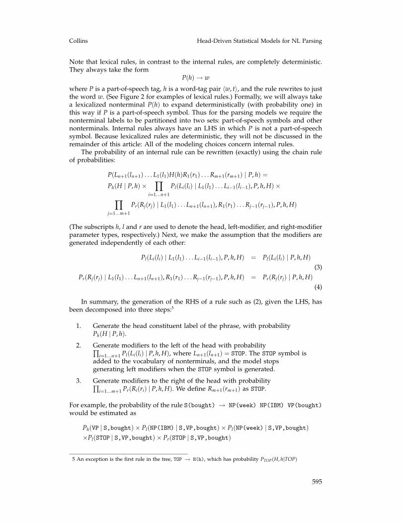
Figure 5A tree with the -C suffix used to identify complements. IBM and Lotus are in subject andobject position, respectively. Last week is an adjunct.

Figure 6Two examples in which the assumption that modifiers are generated independently of oneanother leads to errors. In (1) the probability of generating both Dreyfus and fund as subjects,P(NP-C(Dreyfus) | S,VP,was) ∗ P(NP-C(fund) | S,VP,was), is unreasonably high. (2) is similar:P(NP-C(bill),VP-C(funding) | VP,VB,was) = P(NP-C(bill) | VP,VB,was) ∗P(VP-C(funding) | VP,VB,was) is a bad independence assumption.

the relative improbability of week’s being the headword of a subject. These problemsare not restricted to NPs; compare The spokeswoman said (SBAR that the asbestos was dan-gerous) with Bonds beat short-term investments (SBAR because the market is down), in whichan SBAR headed by that is a complement, but an SBAR headed by because is an adjunct.

A second reason for incorporating the complement/adjunct distinction into theparsing model is that this may help parsing accuracy. The assumption that comple-ments are generated independently of one another often leads to incorrect parses. (SeeFigure 6 for examples.)

3.2.1 Identifying Complements and Adjuncts in the Penn Treebank. We add the -C

suffix to all nonterminals in training data that satisfy the following conditions:

1. The nonterminal must be (1) an NP, SBAR, or S whose parent is an S; (2)an NP, SBAR, S, or VP whose parent is a VP; or (3) an S whose parent isan SBAR.

599


2. The nonterminal must not have one of the following semantic tags: ADV,VOC, BNF, DIR, EXT, LOC, MNR, TMP, CLR or PRP. See Marcus et al.(1994) for an explanation of what these tags signify. For example, the NP

Last week in figure 2 would have the TMP (temporal) tag, and the SBAR in(SBAR because the market is down) would have the ADV (adverbial) tag.

3. The nonterminal must not be on the RHS of a coordinated phrase. Forexample, in the rule S → S CC S, the two child Ss would not be markedas complements.

In addition, the first child following the head of a prepositional phrase is marked asa complement.

3.2.2 Probabilities over Subcategorization Frames. Model 1 could be retrained ontraining data with the enhanced set of nonterminals, and it might learn the lexicalproperties that distinguish complements and adjuncts (IBM vs. week, or that vs. because).It would still suffer, however, from the bad independence assumptions illustrated inFigure 6. To solve these kinds of problems, the generative process is extended toinclude a probabilistic choice of left and right subcategorization frames:

1. Choose a head H with probability Ph(H | P, h).

2. Choose left and right subcategorization frames, LC and RC, withprobabilities Plc(LC | P, H, h) and Prc(RC | P, H, h). Each subcategorizationframe is a multiset10 specifying the complements that the head requiresin its left or right modifiers.

3. Generate the left and right modifiers with probabilities Pl(Li(li) |H, P, h, distancel(i − 1), LC) and Pr(Ri(ri) | H, P, h, distancer(i − 1), RC),respectively.

Thus the subcategorization requirements are added to the conditioning context. Ascomplements are generated they are removed from the appropriate subcategorizationmultiset. Most importantly, the probability of generating the STOP symbol will be zerowhen the subcategorization frame is non-empty, and the probability of generating aparticular complement will be zero when that complement is not in the subcatego-rization frame; thus all and only the required complements will be generated.

The probability of the phrase S(bought) → NP(week) NP-C(IBM) VP(bought) isnow

Ph(VP | S,bought) × Plc({NP-C} | S,VP,bought) × Prc({} | S,VP,bought) ×Pl(NP-C(IBM) | S,VP,bought, {NP-C}) × Pl(NP(week) | S,VP,bought, {}) ×Pl(STOP | S,VP,bought, {}) × Pr(STOP | S,VP,bought, {})

Here the head initially decides to take a single NP-C (subject) to its left and no com-plements to its right. NP-C(IBM) is immediately generated as the required subject, andNP-C is removed from LC, leaving it empty when the next modifier, NP(week), is gen-erated. The incorrect structures in Figure 6 should now have low probability, becausePlc({NP-C,NP-C} | S,VP,was) and Prc({NP-C,VP-C} | VP,VB,was) should be small.

10 A multiset, or bag, is a set that may contain duplicate nonterminal labels.

600


3.3 Model 3: Traces and Wh-MovementAnother obstacle to extracting predicate-argument structure from parse trees is wh-movement. This section describes a probabilistic treatment of extraction from relativeclauses. Noun phrases are most often extracted from subject position, object position,or from within PPs:

(1) The store (SBAR that TRACE bought Lotus)

(2) The store (SBAR that IBM bought TRACE)

(3) The store (SBAR that IBM bought Lotus from TRACE)

It might be possible to write rule-based patterns that identify traces in a parse tree.We argue again, however, that this task is best integrated into the parser: The taskis complex enough to warrant a probabilistic treatment, and integration may helpparsing accuracy. A couple of complexities are that modification by an SBAR does notalways involve extraction (e.g., the fact (SBAR that besoboru is played with a ball and a bat)),and it is not uncommon for extraction to occur through several constituents (e.g., Thechanges (SBAR that he said the government was prepared to make TRACE)).

One hope is that an integrated treatment of traces will improve the parameteri-zation of the model. In particular, the subcategorization probabilities are smeared byextraction. In examples (1), (2), and (3), bought is a transitive verb; but without knowl-edge of traces, example (2) in training data will contribute to the probability of bought’sbeing an intransitive verb.

Formalisms similar to GPSG (Gazdar et al. 1985) handle wh-movement by addinga gap feature to each nonterminal in the tree and propagating gaps through the treeuntil they are finally discharged as a trace complement (see Figure 7). In extractioncases the Penn Treebank annotation coindexes a TRACE with the WHNP head of the SBAR,so it is straightforward to add this information to trees in training data.

(1) NP → NP SBAR(+gap)

(2) SBAR(+gap) → WHNP S-C(+gap)

(3) S(+gap) → NP-C VP(+gap)

(4) VP(+gap) → VB TRACE NP

Figure 7A +gap feature can be added to nonterminals to describe wh-movement. The top-level NPinitially generates an SBAR modifier but specifies that it must contain an NP trace by addingthe +gap feature. The gap is then passed down through the tree, until it is discharged as aTRACE complement to the right of bought.

601


Given that the LHS of the rule has a gap, there are three ways that the gap canbe passed down to the RHS:

Head: The gap is passed to the head of the phrase, as in rule (3) in Figure 7.

Left, Right: The gap is passed on recursively to one of the left or right modifiersof the head or is discharged as a TRACE argument to the left or right ofthe head. In rule (2) in Figure 7, it is passed on to a right modifier, the S

complement. In rule (4), a TRACE is generated to the right of the head VB.

We specify a parameter type Pg(G |P, h, H) where G is either Head, Left, or Right. Thegenerative process is extended to choose among these cases after generating the headof the phrase. The rest of the phrase is then generated in different ways dependingon how the gap is propagated. In the Head case the left and right modifiers aregenerated as normal. In the Left and Right cases a +gap requirement is added to eitherthe left or right SUBCAT variable. This requirement is fulfilled (and removed fromthe subcategorization list) when either a trace or a modifier nonterminal that has the+gap feature, is generated. For example, rule (2) in Figure 7, SBAR(that)(+gap) →WHNP(that) S-C(bought)(+gap), has probability

Ph(WHNP | SBAR,that) × Pg(Right | SBAR,WHNP,that) × Plc({} | SBAR,WHNP,that) ×Prc({S-C} | SBAR,WHNP,that) × Pr(S-C(bought)(+gap) | SBAR,WHNP,that, {S-C,+gap}) ×Pr(STOP | SBAR,WHNP,that, {}) × Pl(STOP | SBAR,WHNP,that, {})

Rule (4), VP(bought)(+gap) → VB(bought) TRACE NP(week), has probability

Ph(VB | VP,bought) × Pg(Right | VP,bought,VB) × Plc({} | VP,bought,VB) ×Prc({NP-C} | VP,bought,VB) × Pr(TRACE | VP,bought,VB, {NP-C, +gap}) ×Pr(NP(week) | VP,bought,VB, {}) × Pl(STOP | VP,bought,VB, {}) ×Pr(STOP | VP,bought,VB, {})

In rule (2), Right is chosen, so the +gap requirement is added to RC. Generation ofS-C(bought)(+gap) fulfills both the S-C and +gap requirements in RC. In rule (4),Right is chosen again. Note that generation of TRACE satisfies both the NP-C and +gap

subcategorization requirements.

4. Special Cases: Linguistically Motivated Refinements to the Models

Sections 3.1 to 3.3 described the basic framework for the parsing models in this article.In this section we describe how some linguistic phenomena (nonrecursive NPs andcoordination, for example) clearly violate the independence assumptions of the generalmodels. We describe a number of these special cases, in each instance arguing that thephenomenon violates the independence assumptions, then describing how the modelcan be refined to deal with the problem.

4.1 Nonrecursive NPsWe define nonrecursive NPs (from here on referred to as base-NPs and labeled NPB

rather than NP) as NPs that do not directly dominate an NP themselves, unless thedominated NP is a possessive NP (i.e., it directly dominates a POS-tag POS). Figure 8gives some examples. Base-NPs deserve special treatment for three reasons:

• The boundaries of base-NPs are often strongly marked. In particular, thestart points of base-NPs are often marked with a determiner or another

602


Figure 8Three examples of structures with base-NPs.

distinctive item, such as an adjective. Because of this, the probability ofgenerating the STOP symbol should be greatly increased when theprevious modifier is, for example, a determiner. As they stand, theindependence assumptions in the three models lose this information. Theprobability of NPB(dog) → DT(the) NN(dog) would be estimated as11

Ph(NN | NPB,dog) × Pl(DT(the) | NPB,NN,dog) ×Pl(STOP | NPB,NN,dog) × Pr(STOP | NPB,NN,dog)

In making the independence assumption

Pl(STOP | DT(the), NPB,NN,dog) = Pl(STOP | NPB,NN,dog)

the model will fail to learn that the STOP symbol is very likely to followa determiner. As a result, the model will assign unreasonably highprobabilities to NPs such as [NP yesterday the dog] in sentences such asYesterday the dog barked.

• The annotation standard in the treebank leaves the internal structure ofbase-NPs underspecified. For example, both pet food volume (where petmodifies food and food modifies volume) and vanilla ice cream (where bothvanilla and ice modify cream) would have the structure NPB → NN NN NN.Because of this, there is no reason to believe that modifiers within NPBsare dependent on the head rather than the previous modifier. In fact, if itso happened that a majority of phrases were like pet food volume, thenconditioning on the previous modifier rather than the head would bepreferable.

• In general it is important (in particular for the distance measure to beeffective) to have different nonterminal labels for what are effectivelydifferent X-bar levels. (See section 7.3.2 for further discussion.)

For these reasons the following modifications are made to the models:

• The nonterminal label for base-NPs is changed from NP to NPB. Forconsistency, whenever an NP is seen with no pre- or postmodifiers, anNPB level is added. For example, [S [NP the dog] [VP barks] ] wouldbe transformed into [S [NP [NPB the dog] ] [VP barks ] ]. These“extra” NPBs are removed before scoring the output of the parser againstthe treebank.

11 For simplicity, we give probability terms under model 1 with no distance variables; the probabilityterms with distance variables, or for models 2 and 3, will be similar, but with the addition of variouspieces of conditioning information.

603


• The independence assumptions are different when the parentnonterminal is an NPB. Specifically, equations (5) and (6) are modified tobe

Pl(Li(li) | H, P, h, L1(l1) . . .Li−1(li−1)) = Pl(Li(li) | P, Li−1(li−1))

Pr(Ri(ri) | H, P, h, R1(r1) . . .Ri−1(ri−1)) = Pr(Ri(ri) | P, Ri−1(ri−1))

The modifier and previous-modifier nonterminals are always adjacent, sothe distance variable is constant and is omitted. For the purposes of thismodel, L0(l0) and R0(r0) are defined to be H(h). The probability of theprevious example is now

Ph(NN | NPB,dog) × Pl(DT(the) | NPB,NN,dog) ×Pl(STOP | NPB,DT,the) × Pr(STOP | NPB,NN,dog)

Presumably Pl(STOP | NPB,DT,the) will be very close to one.

4.2 CoordinationCoordination constructions are another example in which the independence assump-tions in the basic models fail badly (at least given the current annotation method inthe treebank). Figure 9 shows how coordination is annotated in the treebank.12 Touse an example to illustrate the problems, take the rule NP(man) → NP(man) CC(and)

NP(dog), which has probability

Ph(NP | NP,man) × Pl(STOP | NP,NP,man) × Pr(CC(and) | NP,NP,man) ×Pr(NP(dog) | NP,NP,man) × Pr(STOP | NP,NP,man)

The independence assumptions mean that the model fails to learn that there is alwaysexactly one phrase following the coordinator (CC). The basic probability models willgive much too high probabilities to unlikely phrases such as NP → NP CC or NP →NP CC NP NP. For this reason we alter the generative process to allow generation ofboth the coordinator and the following phrase in one step; instead of just generating anonterminal at each step, a nonterminal and a binary-valued coord flag are generated.coord = 1 if there is a coordination relationship. In the generative process, generationof a coord = 1 flag along with a modifier triggers an additional step in the generative

Figure 9(a) The generic way of annotating coordination in the treebank. (b) and (c) show specificexamples (with base-NPs added as described in section 4.1). Note that the first item of theconjunct is taken as the head of the phrase.

12 See Appendix A of Collins (1999) for a description of how the head rules treat phrases involvingcoordination.

604


process, namely, the generation of the coordinator tag/word pair, parameterized bythe Pcc parameter. For the preceding example this would give probability

Ph(NP | NP,man) × Pl(STOP | NP,NP,man) × Pr(NP(dog), coord=1 | NP,NP,man) ×Pr(STOP | NP,NP,man) × Pcc(CC,and | NP,NP,NP,man,dog)

Note the new type of parameter, Pcc, for the generation of the coordinator word andPOS tag. The generation of coord=1 along with NP(dog) in the example implicitlyrequires generation of a coordinator tag/word pair through the Pcc parameter. Thegeneration of this tag/word pair is conditioned on the two words in the coordinationdependency (man and dog in the example) and the label on their relationship (NP,NP,NPin the example, representing NP coordination).

The coord flag is implicitly zero when normal nonterminals are generated; for ex-ample, the phrase S(bought) → NP(week) NP(IBM) VP(bought) now has probability

Ph(VP | S,bought) × Pl(NP(IBM),coord=0 | S,VP,bought) ×Pl(NP(week),coord=0 | S,VP,bought) × Pl(STOP | S,VP,bought) ×Pr(STOP | S,VP,bought)

4.3 PunctuationThis section describes our treatment of “punctuation” in the model, where “punctu-ation” is used to refer to words tagged as a comma or colon. Previous work—thegenerative models described in Collins (1996) and the earlier version of these mod-els described in Collins (1997)—conditioned on punctuation as surface features of thestring, treating it quite differently from lexical items. In particular, the model in Collins(1997) failed to generate punctuation, a deficiency of the model. This section describeshow punctuation is integrated into the generative models.

Our first step is to raise punctuation as high in the parse trees as possible. Punc-tuation at the beginning or end of sentences is removed from the training/test dataaltogether.13 All punctuation items apart from those tagged as comma or colon (itemssuch as quotation marks and periods, tagged “ ” or . ) are removed altogether. Thesetransformations mean that punctuation always appears between two nonterminals, asopposed to appearing at the end of a phrase. (See Figure 10 for an example.)

Figure 10A parse tree before and after punctuation transformations.

13 As one of the anonymous reviewers of this article pointed out, this choice of discarding thesentence-final punctuation may not be optimal, as the final punctuation mark may well carry usefulinformation about the sentence structure.

605


Punctuation is then treated in a very similar way to coordination: Our intuitionis that there is a strong dependency between the punctuation mark and the modi-fier generated after it. Punctuation is therefore generated with the following phrasethrough a punc flag that is similar to the coord flag (a binary-valued feature equal toone if a punctuation mark is generated with the following phrase).

Under this model, NP(Vinken) → NPB(Vinken) ,(,) ADJP(old) would haveprobability

Ph(NPB | NP,Vinken) × Pl(STOP | NP,NPB,Vinken) ×Pr(ADJP(old),coord=0,punc=1 | NP,NPB,Vinken) ×Pr(STOP | NP,NPB,bought) × Pp(, , | NP,NPB,ADJP,Vinken,old) (7)

Pp is a new parameter type for generation of punctuation tag/word pairs. The genera-tion of punc=1 along with ADJP(old) in the example implicitly requires generation of apunctuation tag/word pair through the Pp parameter. The generation of this tag/wordpair is conditioned on the two words in the punctuation dependency (Vinken and old

in the example) and the label on their relationship (NP,NPB,ADJP in the example.)

4.4 Sentences with Empty (PRO) SubjectsSentences in the treebank occur frequently with PRO subjects that may or may not becontrolled: As the treebank annotation currently stands, the nonterminal is S whetheror not a sentence has an overt subject. This is a problem for the subcategorization prob-abilities in models 2 and 3: The probability of having zero subjects, Plc({} | S, VP,

verb), will be fairly high because of this. In addition, sentences with and without sub-jects appear in quite different syntactic environments. For these reasons we modifythe nonterminal for sentences without subjects to be SG (see figure 11). The resultingmodel has a cleaner division of subcategorization: Plc({NP-C} | S, VP, verb) ≈ 1 andPlc({NP-C} | SG, VP, verb) = 0. The model will learn probabilistically the environ-ments in which S and SG are likely to appear.

4.5 A Punctuation ConstraintAs a final step, we use the rule concerning punctuation introduced in Collins (1996)to impose a constraint as follows. If for any constituent Z in the chart Z → <..X Y..>

two of its children X and Y are separated by a comma, then the last word in Y must bedirectly followed by a comma, or must be the last word in the sentence. In trainingdata 96% of commas follow this rule. The rule has the benefit of improving efficiencyby reducing the number of constituents in the chart. It would be preferable to developa probabilistic analog of this rule, but we leave this to future research.

Figure 11(a) The treebank annotates sentences with empty subjects with an empty -NONE- elementunder subject position; (b) in training (and for evaluation), this null element is removed; (c) inmodels 2 and 3, sentences without subjects are changed to have a nonterminal SG.

606


Table 1The conditioning variables for each level of back-off. For example, Ph estimation interpolatese1 = Ph(H | P, w, t), e2 = Ph(H | P, t), and e3 = Ph(H | P). ∆ is the distance measure.

Back-off Ph(H | . . .) Pg(G | . . .) PL1(Li(lti), c, p | . . .) PL2(lwi | . . .)level Plc(LC | . . .) PR1(Ri(rti), c, p | . . .) PR2(rwi | . . .)

Prc(RC | . . .)

1 P, w, t P, H, w, t P, H, w, t, ∆, LC Li, lti, c, p, P, H, w, t, ∆, LC2 P, t P, H, t P, H, t, ∆, LC Li, lti, c, p, P, H, t, ∆, LC3 P P, H P, H, ∆, LC lti

5. Practical Issues

5.1 Parameter EstimationTable 1 shows the various levels of back-off for each type of parameter in the model.Note that we decompose PL(Li(lwi, lti), c, p | P, H, w, t, ∆, LC) (where lwi and lti are theword and POS tag generated with nonterminal Li, c and p are the coord and punc

flags associated with the nonterminal, and ∆ is the distance measure) into the product

PL1(Li(lti), c, p | P, H, w, t, ∆, LC) × PL2(lwi | Li, lti, c, p, P, H, w, t, ∆, LC)

These two probabilities are then smoothed separately. Eisner (1996b) originally usedPOS tags to smooth a generative model in this way. In each case the final estimate is

e = λ1e1 + (1 − λ1)(λ2e2 + (1 − λ2)e3)

where e1, e2, and e3 are maximum-likelihood estimates with the context at levels 1, 2,and 3 in the table, and λ1, λ2 and λ3 are smoothing parameters, where 0 ≤ λi ≤ 1. Weuse the smoothing method described in Bikel et al. (1997), which is derived from amethod described in Witten and Bell (1991). First, say that the most specific estimatee1 = n1

f1; that is, f1 is the value of the denominator count in the relative frequency

estimate. Second, define u1 to be the number of distinct outcomes seen in the f1 eventsin training data. The variable u1 can take any value from one to f1 inclusive. Then weset

λ1 =f1

f1 + 5u1

Analogous definitions for f2 and u2 lead to λ2 =f2

f2+5u2. The coefficient five was chosen

to maximize accuracy on the development set, section 0 of the treebank (in practice itwas found that any value in the range 2–5 gave a very similar level of performance).

5.2 Unknown Words and Part-of-Speech TaggingAll words occurring less than six times14 in training data, and words in test data thathave never been seen in training, are replaced with the UNKNOWN token. This allowsthe model to handle robustly the statistics for rare or new words. Words in test datathat have not been seen in training are deterministically assigned the POS tag that isassigned by the tagger described in Ratnaparkhi (1996). As a preprocessing step, the

14 In Collins (1999) we erroneously stated that all words occuring less than five times in training datawere classified as “unknown.” Thanks to Dan Bikel for pointing out this error.

607


tagger is used to decode each test data sentence. All other words are tagged duringparsing, the output from Ratnaparkhi’s tagger being ignored. The POS tags allowedfor each word are limited to those that have been seen in training data for that word(any tag/word pairs not seen in training would give an estimate of zero in the PL2and PR2 distributions). The model is fully integrated, in that part-of-speech tags arestatistically generated along with words in the models, so that the parser will make astatistical decision as to the most likely tag for each known word in the sentence.

5.3 The Parsing AlgorithmThe parsing algorithm for the models is a dynamic programming algorithm, which isvery similar to standard chart parsing algorithms for probabilistic or weighted gram-mars. The algorithm has complexity O(n5), where n is the number of words in thestring. In practice, pruning strategies (methods that discard lower-probability con-stituents in the chart) can improve efficiency a great deal. The appendices of Collins(1999) give a precise description of the parsing algorithms, an analysis of their compu-tational complexity, and also a description of the pruning methods that are employed.

See Eisner and Satta (1999) for an O(n4) algorithm for lexicalized grammars thatcould be applied to the models in this paper. Eisner and Satta (1999) also describe anO(n3) algorithm for a restricted class of lexicalized grammars; it is an open questionwhether this restricted class includes the models in this article.

6. Results

The parser was trained on sections 2–21 of the Wall Street Journal portion of thePenn Treebank (Marcus, Santorini, and Marcinkiewicz 1993) (approximately 40,000sentences) and tested on section 23 (2,416 sentences). We use the PARSEVAL measures(Black et al. 1991) to compare performance:

Labeled precision = number of correct constituents in proposed parsenumber of constituents in proposed parse

Labeled recall = number of correct constituents in proposed parsenumber of constituents in treebank parse

Crossing brackets = number of constituents that violate constituent boundarieswith a constituent in the treebank parse

For a constituent to be “correct,” it must span the same set of words (ignoring punctu-ation, i.e., all tokens tagged as commas, colons, or quotation marks) and have the samelabel15 as a constituent in the treebank parse. Table 2 shows the results for models 1, 2and 3 and a variety of other models in the literature. Two models (Collins 2000; Char-niak 2000) outperform models 2 and 3 on section 23 of the treebank. Collins (2000)uses a technique based on boosting algorithms for machine learning that reranks n-bestoutput from model 2 in this article. Charniak (2000) describes a series of enhancementsto the earlier model of Charniak (1997).

The precision and recall of the traces found by Model 3 were 93.8% and 90.1%,respectively (out of 437 cases in section 23 of the treebank), where three criteria must bemet for a trace to be “correct”: (1) It must be an argument to the correct headword; (2)It must be in the correct position in relation to that headword (preceding or following);

15 Magerman (1995) collapses ADVP and PRT into the same label; for comparison, we also removed thisdistinction when calculating scores.

608


Table 2Results on Section 23 of the WSJ Treebank. LR/LP = labeled recall/precision. CBs is theaverage number of crossing brackets per sentence. 0 CBs, ≤ 2 CBs are the percentage ofsentences with 0 or ≤ 2 crossing brackets respectively. All the results in this table are formodels trained and tested on the same data, using the same evaluation metric. (Note thatthese results show a slight improvement over those in (Collins 97); the main model changeswere the improved treatment of punctuation (section 4.3) together with the addition of the Pp

and Pcc parameters.)

Model ≤ 40 Words (2,245 sentences)

LR LP CBs 0 CBs ≤ 2 CBs

Magerman 1995 84.6% 84.9% 1.26 56.6% 81.4%Collins 1996 85.8% 86.3% 1.14 59.9% 83.6%

Goodman 1997 84.8% 85.3% 1.21 57.6% 81.4%Charniak 1997 87.5% 87.4% 1.00 62.1% 86.1%

Model 1 87.9% 88.2% 0.95 65.8% 86.3%Model 2 88.5% 88.7% 0.92 66.7% 87.1%Model 3 88.6% 88.7% 0.90 67.1% 87.4%

Charniak 2000 90.1% 90.1% 0.74 70.1% 89.6%Collins 2000 90.1% 90.4% 0.73 70.7% 89.6%

Model ≤ 100 Words (2,416 sentences)


Magerman 1995 84.0% 84.3% 1.46 54.0% 78.8%Collins 1996 85.3% 85.7% 1.32 57.2% 80.8%

Charniak 1997 86.7% 86.6% 1.20 59.5% 83.2%Ratnaparkhi 1997 86.3% 87.5% 1.21 60.2% —

Model 1 87.5% 87.7% 1.09 63.4% 84.1%Model 2 88.1% 88.3% 1.06 64.0% 85.1%Model 3 88.0% 88.3% 1.05 64.3% 85.4%

Charniak 2000 89.6% 89.5% 0.88 67.6% 87.7%Collins 2000 89.6% 89.9% 0.87 68.3% 87.7%

and (3) It must be dominated by the correct nonterminal label. For example, in Figure 7,the trace is an argument to bought, which it follows, and it is dominated by a VP. Of the437 cases, 341 were string-vacuous extraction from subject position, recovered with96.3% precision and 98.8% recall; and 96 were longer distance cases, recovered with81.4% precision and 59.4% recall.16

7. Discussion

This section discusses some aspects of the models in more detail. Section 7.1 gives amuch more detailed analysis of the parsers’ performance. In section 7.2 we examine

16 We exclude infinitival relative clauses from these figures (for example, I called a plumber TRACE to fix thesink, where plumber is coindexed with the trace subject of the infinitival). The algorithm scored 41%precision and 18% recall on the 60 cases in section 23—but infinitival relatives are extremely difficulteven for human annotators to distinguish from purpose clauses (in this case, the infinitival could be apurpose clause modifying called) (Ann Taylor, personal communication, 1997).

609


the distance features in the model. In section 7.3 we examine how the model interactswith the Penn Treebank style of annotation. Finally, in section 7.4 we discuss the needto break down context-free rules in the treebank in such a way that the model willgeneralize to give nonzero probability to rules not seen in training. In each case weuse three methods of analysis. First, we consider how various aspects of the modelaffect parsing performance, through accuracy measurements on the treebank. Second,we look at the frequency of different constructions in the treebank. Third, we considerlinguistically motivated examples as a way of justifying various modeling choices.

7.1 A Closer Look at the ResultsIn this section we look more closely at the parser, by evaluating its performance onspecific constituents or constructions. The intention is to get a better idea of the parser’sstrengths and weaknesses. First, Table 3 has a breakdown of precision and recall byconstituent type. Although somewhat useful in understanding parser performance,a breakdown of accuracy by constituent type fails to capture the idea of attachmentaccuracy. For this reason we also evaluate the parser’s precision and recall in recov-ering dependencies between words. This gives a better indication of the accuracy ondifferent kinds of attachments. A dependency is defined as a triple with the followingelements (see Figure 12 for an example tree and its associated dependencies):

1. Modifier: The index of the modifier word in the sentence.

Table 3Recall and precision for different constituent types, for section 0 of the treebank with model 2.Label is the nonterminal label; Proportion is the percentage of constituents in the treebanksection 0 that have this label; Count is the number of constituents that have this label.

Proportion Count Label Recall Precision

42.21 15146 NP 91.15 90.2619.78 7096 VP 91.02 91.1113.00 4665 S 91.21 90.9612.83 4603 PP 86.18 85.513.95 1419 SBAR 87.81 88.872.59 928 ADVP 82.97 86.521.63 584 ADJP 65.41 68.951.00 360 WHNP 95.00 98.840.92 331 QP 84.29 78.370.48 172 PRN 32.56 61.540.35 126 PRT 86.51 85.160.31 110 SINV 83.64 88.460.27 98 NX 12.24 66.670.25 88 WHADVP 95.45 97.670.08 29 NAC 48.28 63.640.08 28 FRAG 21.43 46.150.05 19 WHPP 100.00 100.000.04 16 UCP 25.00 28.570.04 16 CONJP 56.25 69.230.04 15 SQ 53.33 66.670.03 12 SBARQ 66.67 88.890.03 9 RRC 11.11 33.330.02 7 LST 57.14 100.000.01 3 X 0.00 —0.01 2 INTJ 0.00 —

610


“Raw” dependencies Normalized dependenciesRelation Modifier Head Relation Modifier HeadS VP NP-C L 0 1 S VP NP-C L 0 1TOP TOP S R 1 −1 TOP TOP S R 1 −1NPB NN DT L 2 3 NPB TAG TAG L 2 3VP VB NP-C R 3 1 VP TAG NP-C R 3 1NP-C NPB PP R 4 3 NP NPB PP R 4 3NPB NN DT L 5 6 NPB TAG TAG L 5 6PP IN NP-C R 6 4 PP TAG NP-C R 6 4

Figure 12A tree and its associated dependencies. Note that in “normalizing” dependencies, all POS tagsare replaced with TAG, and the NP-C parent in the fifth relation is replaced with NP.

2. Head: The index of the headword in the sentence.

3. Relation: A 〈Parent, Head, Modifier, Direction〉 4-tuple, where the fourelements are the parent, head, and modifier nonterminals involved in thedependency and the direction of the dependency (L for left, R for right).For example, 〈S, VP, NP-C, L〉 would indicate a subject-verb dependency.In coordination cases there is a fifth element of the tuple, CC. Forexample, 〈NP, NP, NP, R, CC〉 would be an instance of NP coordination.

In addition, the relation is “normalized” to some extent. First, all POS tags arereplaced with the token TAG, so that POS-tagging errors do not lead to errors independencies.17 Second, any complement markings on the parent or head nontermi-nal are removed. For example, 〈NP-C, NPB, PP, R〉 is replaced by 〈NP, NPB, PP, R〉. Thisprevents parsing errors where a complement has been mistaken to be an adjunct (orvice versa), leading to more than one dependency error. As an example, in Figure 12,if the NP the man with the telescope was mistakenly identified as an adjunct, then withoutnormalization, this would lead to two dependency errors: Both the PP dependency andthe verb-object relation would be incorrect. With normalization, only the verb-objectrelation is incorrect.

17 The justification for this is that there is an estimated 3% error rate in the hand-assigned POS tags in thetreebank (Ratnaparkhi 1996), and we didn’t want this noise to contribute to dependency errors.

611


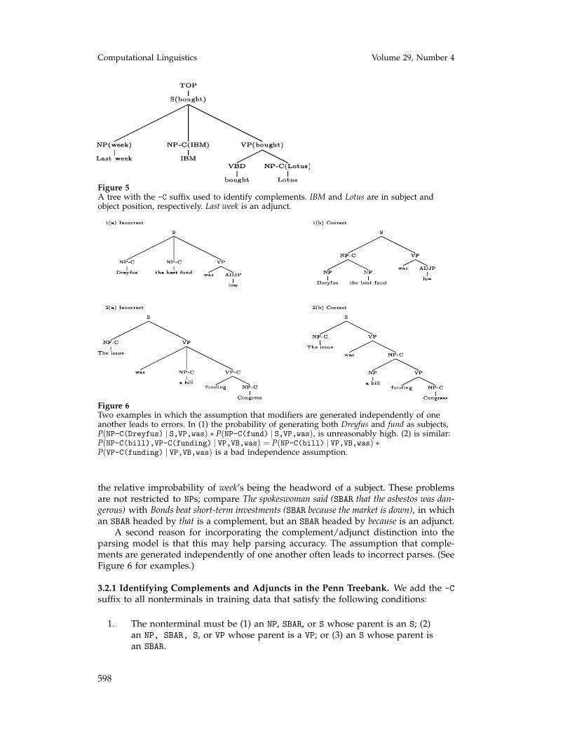
Table 4Dependency accuracy on section 0 of the treebank with Model 2. No labels means that only thedependency needs to be correct; the relation may be wrong; No complements means allcomplement (-C) markings are stripped before comparing relations; All means complementmarkings are retained on the modifying nonterminal.

Evaluation Precision Recall

No labels 91.0% 90.9%No complements 88.5% 88.5%All 88.3% 88.3%

Under this definition, gold-standard and parser-output trees can be converted tosets of dependencies, and precision and recall can be calculated on these dependencies.Dependency accuracies are given for section 0 of the treebank in table 4. Table 5 givesa breakdown of the accuracies by dependency type.

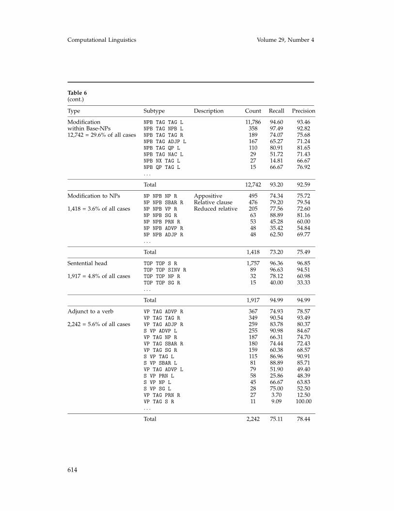
Table 6 shows the dependency accuracies for eight subtypes of dependency thattogether account for 94% of all dependencies:

1. Complement to a verb (93.76% recall, 92.96% precision): This subtypeincludes any relations of the form 〈 S VP ** 〉, where ** is anycomplement, or 〈 VP TAG ** 〉, where ** is any complement except VP-C(i.e., auxiliary-verb—verb dependencies are excluded). The most frequentverb complements, subject-verb and object-verb, are recovered with over95% precision and 92% recall.

2. Other complements (94.47% recall, 94.12% precision): This subtypeincludes any dependencies in which the modifier is a complement andthe dependency does not fall into the complement to a verb category.

3. PP modification (82.29% recall, 81.51% precision): Any dependencies inwhich the modifier is a PP.

4. Coordination (61.47% recall, 62.20% precision).

5. Modification within base-NPs (93.20% recall, 92.59% precision): Thissubtype includes any dependencies in which the parent is NPB.

6. Modification to NPs (73.20% recall, 75.49% precision): This subtypeincludes any dependencies in which the parent is NP, the head is NPB,and the modifier is not a PP.

7. Sentential head (94.99% recall, 94.99% precision): This subtype includesany dependencies involving the headword of the entire sentence.

8. Adjunct to a verb (75.11% recall, 78.44% precision): This subtype includesany dependencies in which the parent is VP, the head is TAG, and themodifier is not a PP, or in which the parent is S, the head is VP, and themodifier is not a PP.

A conclusion to draw from these accuracies is that the parser is doing very well atrecovering the core structure of sentences: complements, sentential heads, and base-NPrelationships (NP chunks) are all recovered with over 90% accuracy. The main sourcesof errors are adjuncts. Coordination is especially difficult for the parser, most likely

612


Table 5Accuracy of the 50 most frequent dependency types in section 0 of the treebank, as recoveredby model 2.

Rank Cumulative Percentage Count Relation Recall Precisionpercentage

1 29.65 29.65 11786 NPB TAG TAG L 94.60 93.462 40.55 10.90 4335 PP TAG NP-C R 94.72 94.043 48.72 8.17 3248 S VP NP-C L 95.75 95.114 54.03 5.31 2112 NP NPB PP R 84.99 84.355 59.30 5.27 2095 VP TAG NP-C R 92.41 92.156 64.18 4.88 1941 VP TAG VP-C R 97.42 97.987 68.71 4.53 1801 VP TAG PP R 83.62 81.148 73.13 4.42 1757 TOP TOP S R 96.36 96.859 74.53 1.40 558 VP TAG SBAR-C R 94.27 93.9310 75.83 1.30 518 QP TAG TAG R 86.49 86.6511 77.08 1.25 495 NP NPB NP R 74.34 75.7212 78.28 1.20 477 SBAR TAG S-C R 94.55 92.0413 79.48 1.20 476 NP NPB SBAR R 79.20 79.5414 80.40 0.92 367 VP TAG ADVP R 74.93 78.5715 81.30 0.90 358 NPB TAG NPB L 97.49 92.8216 82.18 0.88 349 VP TAG TAG R 90.54 93.4917 82.97 0.79 316 VP TAG SG-C R 92.41 88.2218 83.70 0.73 289 NP NP NP R CC 55.71 53.3119 84.42 0.72 287 S VP PP L 90.24 81.9620 85.14 0.72 286 SBAR WHNP SG-C R 90.56 90.5621 85.79 0.65 259 VP TAG ADJP R 83.78 80.3722 86.43 0.64 255 S VP ADVP L 90.98 84.6723 86.95 0.52 205 NP NPB VP R 77.56 72.6024 87.45 0.50 198 ADJP TAG TAG L 75.76 70.0925 87.93 0.48 189 NPB TAG TAG R 74.07 75.6826 88.40 0.47 187 VP TAG NP R 66.31 74.7027 88.85 0.45 180 VP TAG SBAR R 74.44 72.4328 89.29 0.44 174 VP VP VP R CC 74.14 72.4729 89.71 0.42 167 NPB TAG ADJP L 65.27 71.2430 90.11 0.40 159 VP TAG SG R 60.38 68.5731 90.49 0.38 150 VP TAG S-C R 74.67 78.3232 90.81 0.32 129 S S S R CC 72.09 69.9233 91.12 0.31 125 PP TAG SG-C R 94.40 89.3934 91.43 0.31 124 QP TAG TAG L 77.42 83.4835 91.72 0.29 115 S VP TAG L 86.96 90.9136 92.00 0.28 110 NPB TAG QP L 80.91 81.6537 92.27 0.27 106 SINV VP NP R 88.68 95.9238 92.53 0.26 104 S VP S-C L 93.27 78.8639 92.79 0.26 102 NP NP NP R 30.39 25.4140 93.02 0.23 90 ADJP TAG PP R 75.56 78.1641 93.24 0.22 89 TOP TOP SINV R 96.63 94.5142 93.45 0.21 85 ADVP TAG TAG L 74.12 73.2643 93.66 0.21 83 SBAR WHADVP S-C R 97.59 98.7844 93.86 0.20 81 S VP SBAR L 88.89 85.7145 94.06 0.20 79 VP TAG ADVP L 51.90 49.4046 94.24 0.18 73 SINV VP S L 95.89 92.1147 94.40 0.16 63 NP NPB SG R 88.89 81.1648 94.55 0.15 58 S VP PRN L 25.86 48.3949 94.70 0.15 58 NX TAG TAG R 10.34 75.0050 94.83 0.13 53 NP NPB PRN R 45.28 60.00

613


Table 6Accuracy for various types/subtypes of dependency (part 1). Only subtypes occurring morethan 10 times are shown.

Type Sub-type Description Count Recall Precision

Complement to a verb S VP NP-C L Subject 3,248 95.75 95.11VP TAG NP-C R Object 2,095 92.41 92.15

6,495 = 16.3% of all cases VP TAG SBAR-C R 558 94.27 93.93VP TAG SG-C R 316 92.41 88.22VP TAG S-C R 150 74.67 78.32S VP S-C L 104 93.27 78.86S VP SG-C L 14 78.57 68.75. . .

Total 6,495 93.76 92.96

Other complements PP TAG NP-C R 4,335 94.72 94.04VP TAG VP-C R 1,941 97.42 97.98

7,473 = 18.8% of all cases SBAR TAG S-C R 477 94.55 92.04SBAR WHNP SG-C R 286 90.56 90.56PP TAG SG-C R 125 94.40 89.39SBAR WHADVP S-C R 83 97.59 98.78PP TAG PP-C R 51 84.31 70.49SBAR WHNP S-C R 42 66.67 84.85SBAR TAG SG-C R 23 69.57 69.57PP TAG S-C R 18 38.89 63.64SBAR WHPP S-C R 16 100.00 100.00S ADJP NP-C L 15 46.67 46.67PP TAG SBAR-C R 15 100.00 88.24. . .

Total 7,473 94.47 94.12

PP modification NP NPB PP R 2,112 84.99 84.35VP TAG PP R 1,801 83.62 81.14

4,473 = 11.2% of all cases S VP PP L 287 90.24 81.96ADJP TAG PP R 90 75.56 78.16ADVP TAG PP R 35 68.57 52.17NP NP PP R 23 0.00 0.00PP PP PP L 19 21.05 26.67NAC TAG PP R 12 50.00 100.00. . .

Total 4,473 82.29 81.51

Coordination NP NP NP R 289 55.71 53.31VP VP VP R 174 74.14 72.47

763 = 1.9% of all cases S S S R 129 72.09 69.92ADJP TAG TAG R 28 71.43 66.67VP TAG TAG R 25 60.00 71.43NX NX NX R 25 12.00 75.00SBAR SBAR SBAR R 19 78.95 83.33PP PP PP R 14 85.71 63.16. . .

Total 763 61.47 62.20

614


Table 6(cont.)

Type Subtype Description Count Recall Precision

Modification NPB TAG TAG L 11,786 94.60 93.46within Base-NPs NPB TAG NPB L 358 97.49 92.8212,742 = 29.6% of all cases NPB TAG TAG R 189 74.07 75.68

NPB TAG ADJP L 167 65.27 71.24NPB TAG QP L 110 80.91 81.65NPB TAG NAC L 29 51.72 71.43NPB NX TAG L 27 14.81 66.67NPB QP TAG L 15 66.67 76.92. . .

Total 12,742 93.20 92.59

Modification to NPs NP NPB NP R Appositive 495 74.34 75.72NP NPB SBAR R Relative clause 476 79.20 79.54

1,418 = 3.6% of all cases NP NPB VP R Reduced relative 205 77.56 72.60NP NPB SG R 63 88.89 81.16NP NPB PRN R 53 45.28 60.00NP NPB ADVP R 48 35.42 54.84NP NPB ADJP R 48 62.50 69.77. . .

Total 1,418 73.20 75.49

Sentential head TOP TOP S R 1,757 96.36 96.85TOP TOP SINV R 89 96.63 94.51

1,917 = 4.8% of all cases TOP TOP NP R 32 78.12 60.98TOP TOP SG R 15 40.00 33.33. . .

Total 1,917 94.99 94.99

Adjunct to a verb VP TAG ADVP R 367 74.93 78.57VP TAG TAG R 349 90.54 93.49

2,242 = 5.6% of all cases VP TAG ADJP R 259 83.78 80.37S VP ADVP L 255 90.98 84.67VP TAG NP R 187 66.31 74.70VP TAG SBAR R 180 74.44 72.43VP TAG SG R 159 60.38 68.57S VP TAG L 115 86.96 90.91S VP SBAR L 81 88.89 85.71VP TAG ADVP L 79 51.90 49.40S VP PRN L 58 25.86 48.39S VP NP L 45 66.67 63.83S VP SG L 28 75.00 52.50VP TAG PRN R 27 3.70 12.50VP TAG S R 11 9.09 100.00. . .

Total 2,242 75.11 78.44

615


Table 7Results on section 0 of the WSJ Treebank. A “YES” in the A column means that the adjacencyconditions were used in the distance measure; likewise, a “YES” in the V column indicatesthat the verb conditions were used in the distance measure. LR = labeled recall; LP = labeledprecision. CBs is the average number of crossing brackets per sentence. 0 CBs ≤ 2 CBs are thepercentages of sentences with 0 and ≤ 2 crossing brackets, respectively.

Model A V LR LP CBs 0 CBs ≤ 2 CBs

Model 1 No No 75.0% 76.5% 2.18 38.5% 66.4Model 1 Yes No 86.6% 86.7% 1.22 60.9% 81.8Model 1 Yes Yes 87.8% 88.2% 1.03 63.7% 84.4

Model 2 No No 85.1% 86.8% 1.28 58.8% 80.3Model 2 Yes No 87.7% 87.8% 1.10 63.8% 83.2Model 2 Yes Yes 88.7% 89.0% 0.95 65.7% 85.6

because it often involves a dependency between two content words, leading to verysparse statistics.

7.2 More about the Distance MeasureThe distance measure, whose implementation was described in section 3.1.1, deservesmore discussion and motivation. In this section we consider it from three perspectives:its influence on parsing accuracy; an analysis of distributions in training data thatare sensitive to the distance variables; and some examples of sentences in which thedistance measure is useful in discriminating among competing analyses.

7.2.1 Impact of the Distance Measure on Accuracy. Table 7 shows the results formodels 1 and 2 with and without the adjacency and verb distance measures. It is clearthat the distance measure improves the models’ accuracy.

What is most striking is just how badly model 1 performs without the distancemeasure. Looking at the parser’s output, the reason for this poor performance is thatthe adjacency condition in the distance measure is approximating subcategorizationinformation. In particular, in phrases such as PPs and SBARs (and, to a lesser extent,in VPs) that almost always take exactly one complement to the right of their head,the adjacency feature encodes this monovalency through parameters P(STOP|PP/SBAR,adjacent) = 0 and P(STOP|PP/SBAR, not adjacent) = 1. Figure 13 shows some par-ticularly bad structures returned by model 1 with no distance variables.

Another surprise is that subcategorization can be very useful, but that the dis-tance measure has masked this utility. One interpretation in moving from the leastparameterized model (Model 1 [No, No]) to the fully parameterized model (Model 2[Yes, Yes]) is that the adjacency condition adds around 11% in accuracy; the verbcondition adds another 1.5%; and subcategorization finally adds a mere 0.8%. Underthis interpretation subcategorization information isn’t all that useful (and this was myoriginal assumption, as this was the order in which features were originally addedto the model). But under another interpretation subcategorization is very useful: Inmoving from Model 1 (No, No) to Model 2 (No, No), we see a 10% improvement as aresult of subcategorization parameters; adjacency then adds a 1.5% improvement; andthe verb condition adds a final 1% improvement.

From an engineering point of view, given a choice of whether to add just distanceor subcategorization to the model, distance is preferable. But linguistically it is clearthat adjacency can only approximate subcategorization and that subcategorization is

616


Figure 13Two examples of bad parses produced by model 1 with no distance or subcategorizationconditions (Model 1 (No, No) in table 7). In (a) one PP has two complements, the other hasnone; in (b) the SBAR has two complements. In both examples either the adjacency conditionor the subcategorization parameters will correct the errors, so these are examples in which theadjacency and subcategorization variables overlap in their utility.

Table 8Distribution of nonterminals generated as postmodifiers to an NP (see tree to the left), atvarious distances from the head. A = True means the modifier is adjacent to the head, V =True means there is a verb between the head and the modifier. Distributions were calculatedfrom the first 10000 events for each of the three cases in sections 2-21 of the treebank.

A = True, V = False A = False, V = False A = False, V = True

Percentage ? Percentage ? Percentage ?

70.78 STOP 88.53 STOP 97.65 STOP17.7 PP 5.57 PP 0.93 PP3.54 SBAR 2.28 SBAR 0.55 SBAR3.43 NP 1.55 NP 0.35 NP2.22 VP 0.92 VP 0.22 VP0.61 SG 0.38 SG 0.09 SG0.56 ADJP 0.26 PRN 0.07 PRN0.54 PRN 0.22 ADVP 0.04 ADJP0.36 ADVP 0.15 ADJP 0.03 ADVP0.08 TO 0.09 -RRB- 0.02 S0.08 CONJP 0.02 UCP 0.02 -RRB-0.03 UCP 0.01 X 0.01 X0.02 JJ 0.01 RRC 0.01 VBG0.01 VBN 0.01 RB 0.01 RB0.01 RRC0.01 FRAG0.01 CD0.01 -LRB-

more “correct” in some sense. In free-word-order languages, distance may not approx-imate subcategorization at all well: A complement may appear to either the right orleft of the head, confusing the adjacency condition.

7.2.2 Frequencies in Training Data. Tables 8 and 9 show the effect of distance on thedistribution of modifiers in two of the most frequent syntactic environments: NP andverb modification. The distribution varies a great deal with distance. Most striking isthe way that the probability of STOP increases with increasing distance: from 71% to89% to 98% in the NP case, from 8% to 60% to 96% in the verb case. Each modifierprobability generally decreases with distance. For example, the probability of seeinga PP modifier to an NP decreases from 17.7% to 5.57% to 0.93%.

617


Table 9Distribution of nonterminals generated as postmodifiers to a verb within a VP (see tree to theleft), at various distances from the head. A = True means the modifier is adjacent to the head;V = True means there is a verb between the head and the modifier. The distributions werecalculated from the first 10000 events for each of the distributions in sections 2–21. Auxiliaryverbs (verbs taking a VP complement to their right) were excluded from these statistics.

A = True, V = False A = False, V = False A = False, V = True

Percentage ? Percentage ? Percentage ?

39 NP-C 59.87 STOP 95.92 STOP15.8 PP 22.7 PP 1.73 PP8.43 SBAR-C 3.3 NP-C 0.92 SBAR8.27 STOP 3.16 SG 0.5 NP5.35 SG-C 2.71 ADVP 0.43 SG5.19 ADVP 2.65 SBAR 0.16 ADVP5.1 ADJP 1.5 SBAR-C 0.14 SBAR-C3.24 S-C 1.47 NP 0.05 NP-C2.82 RB 1.11 SG-C 0.04 PRN2.76 NP 0.82 ADJP 0.02 S-C2.28 PRT 0.2 PRN 0.01 VBN0.63 SBAR 0.19 PRT 0.01 VB0.41 SG 0.09 S 0.01 UCP0.16 VB 0.06 S-C 0.01 SQ0.1 S 0.06 -RRB- 0.01 S0.1 PRN 0.03 FRAG 0.01 FRAG0.08 UCP 0.02 -LRB- 0.01 ADJP0.04 VBZ 0.01 X 0.01 -RRB-0.03 VBN 0.01 VBP 0.01 -LRB-0.03 VBD 0.01 VB0.03 FRAG 0.01 UCP0.03 -LRB- 0.01 RB0.02 VBG 0.01 INTJ0.02 SBARQ0.02 CONJP0.01 X0.01 VBP0.01 RBR0.01 INTJ0.01 DT0.01 -RRB-

7.2.3 Distance Features and Right-Branching Structures. Both the adjacency and verbcomponents of the distance measure allow the model to learn a preference for right-branching structures. First, consider the adjacency condition. Figure 14 shows someexamples in which right-branching structures are more frequent. Using the statisticsfrom Tables 8 and 9, the probability of the alternative structures can be calculated. Theresults are given below. The right-branching structures get higher probability (althoughthis is before the lexical-dependency probabilities are multiplied in, so this “prior”preference for right-branching structures can be overruled by lexical preferences). Ifthe distance variables were not conditioned on, the product of terms for the twoalternatives would be identical, and the model would have no preference for onestructure over another.

Probabilities for the two alternative PP structures in Figure 14 (excluding probabil-ity terms that are constant across the two structures; A=1 means distance is adjacent,A=0 means not adjacent) are as follows:

618


Figure 14Some alternative structures for the same surface sequence of chunks (NPB PP PP in the firstcase, NPB PP SBAR in the second case) in which the adjacency condition distinguishes betweenthe two structures. The percentages are taken from sections 2–21 of the treebank. In both casesright-branching structures are more frequent.

Right-branching:

P(PP|NP,NPB,A=1)P(STOP|NP,NPB,A=0)P(PP|NP,NPB,A=1)P(STOP|NP,NPB,A=0)= 0.177 × 0.8853 × 0.177 × 0.8853 = 0.02455

Non-right-branching:

P(PP|NP,NPB,A=1)P(PP|NP,NPB,A=0)P(STOP|NP,NPB,A=0)P(STOP|NP,NPB,A=1)= 0.177 × 0.0557 × 0.8853 × 0.7078 = 0.006178

Probabilities for the SBAR case in Figure 14, assuming the SBAR contains a verb (V=0means modification does not cross a verb, V=1 means it does), are as follows:

Right-branching:

P(PP|NP,NPB,A=1,V=0)P(SBAR|NP,NPB,A=1,V=0)P(STOP|NP,NPB,A=0,V=1)P(STOP|NP,NPB,A=0,V=1)= 0.177 × 0.0354 × 0.9765 × 0.9765 = 0.005975

Non-right-branching:

P(PP|NP,NPB,A=1)P(STOP|NP,NPB,A=1)P(SBAR|NP,NPB,A=0)P(STOP|NP,NPB,A=0,V=1)= 0.177 × 0.7078 × 0.0228 × 0.9765 = 0.002789

619


Figure 15Some alternative structures for the same surface sequence of chunks in which the verbcondition in the distance measure distinguishes between the two structures. In both cases thelow-attachment analyses will get higher probability under the model, because of the lowprobability of generating a PP modifier involving a dependency that crosses a verb. (X standsfor any nonterminal.)

7.2.4 Verb Condition and Right-Branching Structures. Figure 15 shows some exam-ples in which the verb condition is important in differentiating the probability of twostructures. In both cases an adjunct can attach either high or low, but high attachmentresults in a dependency’s crossing a verb and has lower probability.

An alternative to the surface string feature would be a predicate such as were anyof the previous modifiers in X, where X is a set of nonterminals that are likely to containa verb, such as VP, SBAR, S, or SG. This would allow the model to handle cases like thefirst example in Figure 15 correctly. The second example shows why it is preferable tocondition on the surface string. In this case the verb is “invisible” to the top level, asit is generated recursively below the NP object.

7.2.5 Structural versus Semantic Preferences. One hypothesis would be that lexicalstatistics are really what is important in parsing: that arriving at a correct interpretationfor a sentence is simply a matter of finding the most semantically plausible analysis,and that the statistics related to lexical dependencies approximate this notion of plau-sibility. Implicitly, we would be just as well off (maybe even better off) if statistics werecalculated between items at the predicate-argument level, with no reference to struc-ture. The distance preferences under this interpretation are just a way of mitigatingsparse-data problems: When the lexical statistics are too sparse, then falling back onsome structural preference is not ideal, but is at least better than chance. This hypoth-esis is suggested by previous work on specific cases of attachment ambiguity suchas PP attachment (see, e.g., Collins and Brooks 1995), which has showed that modelswill perform better given lexical statistics, and that a straight structural preference ismerely a fallback.

But some examples suggest this is not the case: that, in fact, many sentenceshave several equally semantically plausible analyses, but that structural preferences

620


distinguish strongly among them. Take the following example (from Pereira and War-ren 1980):

(4) John was believed to have been shot by Bill.

Surprisingly, this sentence has two analyses: Bill can be the deep subject of eitherbelieved or shot. Yet people have a very strong preference for Bill to be doing theshooting, so much so that they may even miss the second analysis. (To see that thedispreferred analysis is semantically quite plausible, consider Bill believed John to havebeen shot.)

As evidence that structural preferences can even override semantic plausibility,take the following example (from Pinker 1994):

(5) Flip said that Squeaky will do the work yesterday.

This sentence is a garden path: The structural preference for yesterday to modify themost recent verb is so strong that it is easy to miss the (only) semantically plausibleinterpretation, paraphrased as Flip said yesterday that Squeaky will do the work.

The model makes the correct predictions in these cases. In example (4), the statisticsin Table 9 show that a PP is nine times as likely to attach low as to attach high whentwo verbs are candidate attachment points (the chances of seeing a PP modifier are15.8% and 1.73% in columns 1 and 5 of the table, respectively). In example (5), theprobability of seeing an NP (adjunct) modifier to do in a nonadjacent but non-verb-crossing environment is 2.11% in sections 2–21 of the treebank (8 out of 379 cases); incontrast, the chance of seeing an NP adjunct modifying said across a verb is 0.026% (1out of 3,778 cases). The two probabilities differ by a factor of almost 80.

7.3 The Importance of the Choice of Tree RepresentationFigures 16 and 17 show some alternative styles of syntactic annotation. The PennTreebank annotation style tends to leave trees quite flat, typically with one level ofstructure for each X-bar level; at the other extreme are completely binary-branchingrepresentations. The two annotation styles are in some sense equivalent, in that itis easy to define a one-to-one mapping between them. But crucially, two differentannotation styles may lead to quite different parsing accuracies for a given model,even if the two representations are equivalent under some one-to-one mapping.

A parsing model does not need to be tied to the annotation style of the treebankon which it is trained. The following procedure can be used to transform trees in bothtraining and test data into a new representation:

Figure 16Alternative annotation styles for a sentence S with a verb head V, left modifiers X1, X2, andright modifiers Y1, Y2: (a) the Penn Treebank style of analysis (one level of structure for eachbar level); (b) an alternative but equivalent binary branching representation.

621


Figure 17Alternative annotation styles for a noun phrase with a noun head N, left modifiers X1, X2,and right modifiers Y1, Y2: (a) the Penn Treebank style of analysis (one level of structure foreach bar level, although note that both the nonrecursive and the recursive noun phrases arelabeled NP; (b) an alternative but equivalent binary branching representation; (a′) ourmodification of the Penn Treebank style to differentiate recursive and nonrecursive NPs (insome sense NPB is a bar 1 structure and NP is a bar 2 structure).

1. Transform training data trees into the new representation and train themodel.

2. Recover parse trees in the new representation when running the modelover test data sentences.

3. Convert the test output back into the treebank representation for scoringpurposes.

As long as there is a one-to-one mapping between the treebank and the new rep-resentation, nothing is lost in making such a transformation. Goodman (1997) andJohnson (1997) both suggest this strategy. Goodman (1997) converts the treebank intobinary-branching trees. Johnson (1997) considers conversion to a number of differentrepresentations and discusses how this influences accuracy for nonlexicalized PCFGs.

The models developed in this article have tacitly assumed the Penn Treebankstyle of annotation and will perform badly given other representations (for example,binary-branching trees). This section makes this point more explicit, describing exactlywhat annotation style is suitable for the models and showing how other annotationstyles will cause problems. This dependence on Penn Treebank–style annotations doesnot imply that the models are inappropriate for a treebank annotated in a differentstyle: In this case we simply recommend transforming the trees into flat, one-level-per-X-bar-level trees before training the model, as in the three-step procedure outlinedabove.

Other models in the literature are also very likely to be sensitive to annotationstyle. Charniak’s (1997) models will most likely perform quite differently with binary-branching trees (for example, his current models will learn that rules such as VP →V SG PP are very rare, but with binary-branching structures, this context sensitivitywill be lost). The models of Magerman (1995) and Ratnaparkhi (1997) use contextualpredicates that would most likely need to be modified given a different annotationstyle. Goodman’s (1997) models are the exception, as he already specifies that thetreebank should be transformed into his chosen representation, binary-branching trees.

7.3.1 Representation Affects Structural, not Lexical, Preferences. The alternative rep-resentations in Figures 16 and 17 have the same lexical dependencies (providing thatthe binary-branching structures are centered about the head of the phrase, as in theexamples). The difference between the representations involves structural preferencessuch as the right-branching preferences encoded by the distance measure. Applyingthe models in this article to treebank analyses that use this type of “head-centered”

622


Figure 18BB = binary-branching structures; FLAT = Penn treebank style annotations. In each case thebinary-branching annotation style prevents the model from learning that these structuresshould receive low probability because of the long distance dependency associated with thefinal PP (in boldface).

binary-branching tree will result in a distance measure that incorrectly encodes a pref-erence for right-branching structures.

To see this, consider the examples in Figure 18. In each binary-branching example,the generation of the final modifying PP is “blind” to the distance between it and thehead that it modifies. At the top level of the tree, it is apparently adjacent to the head;crucially, the closer modifier (SG in (a), the other PP in (b)) is hidden lower in the treestructure. So the model will be unable to differentiate generation of the PP in adjacentversus nonadjacent or non-verb-crossing versus verb-crossing environments, and thestructures in Figure 18 will be assigned unreasonably high probabilities.

This does not mean that distance preferences cannot be encoded in a binary-branching PCFG. Goodman (1997) achieves this by adding distance features to the non-terminals. The spirit of this implementation is that the top-level rules VP → VP PP andNP → NP PP would be modified to VP → VP(+rverb) PP and NP → NP(+rmod) PP,respectively, where (+rverb) means a phrase in which the head has a verb in its rightmodifiers, and (+rmod) means a phrase that has at least one right modifier to thehead. The model will learn from training data that P(VP → VP(+rverb) PP|VP) �P(VP → VP(-rverb) PP|VP), that is, that a prepositional-phrase modification is muchmore likely when it does not cross a verb.

7.3.2 The Importance of Differentiating Nonrecursive from Recursive NPs. Figure 19shows the modification to the Penn Treebank annotation to relabel base-NPs as NPB.It also illustrates a problem that arises if a distinction between the two is not made:Structures such as that in Figure 19(b) are assigned high probabilities even if they

Figure 19(a) The way the Penn Treebank annotates NPs. (a′) Our modification to the annotation, todifferentiate recursive (NP) from nonrecursive (NPB) noun phrases. (b) A structure that is neverseen in training data but will receive much too high a probability from a model trained ontrees of style (a).

623


Figure 20Examples of other phrases in the Penn Treebank in which nonrecursive and recursive phrasesare not differentiated.

are never seen in training data. (Johnson [1997] notes that this structure has a higherprobability than the correct, flat structure, given counts taken from the treebank fora standard PCFG.) The model is fooled by the binary-branching style into modelingboth PPs as being adjacent to the head of the noun phrase, so 19(b) will be assigned avery high probability.

This problem does not apply only to NPs: Other types of phrases such as adjectivalphrases (ADJPs) or adverbial phrases (ADVPs) also have nonrecursive (bar 1) and recur-sive (bar 2) levels, which are not differentiated in the Penn Treebank. (See Figure 20 forexamples.) Ideally these cases should be differentiated too: We did not implement thischange because it is unlikely to make much difference in accuracy, given the relativeinfrequency of these cases (excluding coordination cases, and looking at the 80,254instances in sections 2–21 of the Penn Treebank in which a parent and head nonter-minal are the same: 94.5% are the NP case; 2.6% are cases of coordination in which apunctuation mark is the coordinator;18 only 2.9% are similar to those in Figure 20).

7.3.3 Summary. To summarize, the models in this article assume the following:

1. Tree representations are “flat”: that is, one level per X-bar level.

2. Different X-bar levels have different labels (in particular, nonrecursiveand recursive levels are differentiated, at least for the most frequent caseof NPs).

7.4 The Need to Break Down RulesThe parsing approaches we have described concentrate on breaking down context-freerules in the treebank into smaller components. Lexicalized rules were initially brokendown to bare-bones Markov processes, then increased dependency on previously gen-erated modifiers was built back up through the distance measure and subcategoriza-tion. Even with this additional context, the models are still able to recover rules in testdata that have never been seen in training data.

An alternative, proposed in Charniak (1997), is to limit parsing to those context-free rules seen in training data. A lexicalized rule is predicted in two steps. First,the whole context-free rule is generated. Second, the lexical items are filled in. Theprobability of a rule is estimated as19

P(Ln(ln) . . .L1(l1)H(h)R1(r1) . . .Rm(rm) | P, h) =

P(Ln . . .L1HR1 . . .Rm) | P, h) ×∏

i=1...n

Pl(li | Li, P, h) ×∏

j=1...m

Pr(rj | Rj, P, h)

18 For example, (S (S John eats apples); (S Mary eats bananas)).19 Charniak’s model also conditions on the parent of the nonterminal being expanded; we omit this here

for brevity.

624


The estimation technique used in Charniak (1997) for the CF rule probabilities inter-polates several estimates, the lowest being P(Ln . . .L1HR1 . . .Rm) | P). Any rules notseen in training data will be assigned zero probability with this model. Parse trees intest data will be limited to include rules seen in training.

A problem with this approach is coverage. As shown in this section, many test datasentences will require rules that have not been seen in training. This gives motivationfor breaking down rules into smaller components. This section motivates the need tobreak down rules from four perspectives. First, we discuss how the Penn Treebankannotation style leads to a very large number of grammar rules. Second, we assess theextent of the coverage problem by looking at rule frequencies in training data. Third,we conduct experiments to assess the impact of the coverage problem on accuracy.Fourth, we discuss how breaking rules down may improve estimation as well ascoverage.

7.4.1 The Penn Treebank Annotation Style Leads to Many Rules. The “flatness” ofthe Penn Treebank annotation style has already been discussed, in section 7.3. Theflatness of the trees leads to a very large (and constantly growing) number of rules,primarily because the number of adjuncts to a head is potentially unlimited: For ex-ample, there can be any number of PP adjuncts to a head verb. A binary-branching(Chomsky adjunction) grammar can generate an unlimited number of adjuncts withvery few rules. For example, the following grammar generates any sequence VP → V

NP PP*:

VP → V NP

VP → VP PP

In contrast, the Penn Treebank style would create a new rule for each number of PPsseen in training data. The grammar would be

VP → V NP

VP → V NP PP

VP → V NP PP PP

VP → V NP PP PP PP

and so on

Other adverbial adjuncts, such as adverbial phrases or adverbial SBARs, can also modifya verb several times, and all of these different types of adjuncts can be seen together inthe same rule. The result is a combinatorial explosion in the number of rules. To givea flavor of this, here is a random sample of rules of the format VP → VB modifier*

that occurred only once in sections 2–21 of the Penn Treebank:

VP → VB NP NP NP PRN

VP → VB NP SBAR PP SG ADVP

VP → VB NP ADVP ADVP PP PP

VP → VB RB

VP → VB NP PP NP SBAR

VP → VB NP PP SBAR PP

It is not only verb phrases that cause this kind of combinatorial explosion: Otherphrases, in particular nonrecursive noun phrases, also contribute a huge number ofrules. The next section considers the distributional properties of the rules in moredetail.

625


Note that there is good motivation for the Penn Treebank’s decision to repre-sent rules in this way, rather than with rules expressing Chomsky adjunction (i.e., aschema in which complements and adjuncts are separated, through rule types 〈VP →VB {complement}*〉 and 〈VP → VP {adjunct}〉). First, it allows the argument/adjunctdistinction for PP modifiers to verbs to be left undefined: This distinction was foundto be very difficult for annotators. Second, in the surface ordering (as opposed to deepstructure), adjuncts are often found closer to the head than complements, thereby yield-ing structures that fall outside the Chomsky adjunction schema. For example, a rulesuch as 〈VP → VB NP-C PP SBAR-C〉 is found very frequently in the Penn Treebank;SBAR complements nearly always extrapose over adjuncts.

7.4.2 Quantifying the Coverage Problem. To quantify the coverage problem, ruleswere collected from sections 2–21 of the Penn Treebank. Punctuation was raised ashigh as possible in the tree, and the rules did not have complement markings or thedistinction between base-NPs and recursive NPs. Under these conditions, 939,382 ruletokens were collected; there were 12,409 distinct rule types. We also collected the countfor each rule. Table 10 shows some statistics for these rules.

A majority of rules in the grammar (6,765, or 54.5%) occur only once. These rulesaccount for 0.72% of rules by token. That is, if one of the 939,382 rule tokens in sections2–21 of the treebank were drawn at random, there would be a 0.72% chance of its beingthe only instance of that rule in the 939,382 tokens. On the other hand, if a rule weredrawn at random from the 12,409 rules in the grammar induced from those sections,there would be a 54.5% chance of that rule’s having occurred only once.

The percentage by token of the one-count rules is an indication of the coverageproblem. From this estimate, 0.72% of all rules (or 1 in 139 rules) required in test datawould never have been seen in training. It was also found that 15.0% (1 in 6.67) of allsentences have at least one rule that occurred just once. This gives an estimate thatroughly 1 in 6.67 sentences in test data will not be covered by a grammar inducedfrom 40,000 sentences in the treebank.

If the complement markings are added to the nonterminals, and the base-NP/non-recursive NP distinction is made, then the coverage problem is made worse. Table 11gives the statistics in this case. By our counts, 17.1% of all sentences (1 in 5.8 sentences)contain at least 1 one-count rule.

Table 10Statistics for rules taken from sections 2–21 of the treebank, with complement markings notincluded on nonterminals.

Rule count Number of Rules Percentage Number of Rules Percentage of rulesby type by type by token by token

1 6765 54.52 6765 0.722 1688 13.60 3376 0.363 695 5.60 2085 0.224 457 3.68 1828 0.195 329 2.65 1645 0.18

6 . . . 10 835 6.73 6430 0.6811 . . . 20 496 4.00 7219 0.7721 . . . 50 501 4.04 15931 1.70

51 . . . 100 204 1.64 14507 1.54> 100 439 3.54 879596 93.64

626


Table 11Statistics for rules taken from sections 2–21 of the treebank, with complement markingsincluded on nonterminals.

Rule count Number of Rules Percentage of rules Number of Rules Percentage of rulesby type by type by token by token

1 7865 55.00 7865 0.842 1918 13.41 3836 0.413 815 5.70 2445 0.264 528 3.69 2112 0.225 377 2.64 1885 0.20

6 . . . 10 928 6.49 7112 0.7611 . . . 20 595 4.16 8748 0.9321 . . . 50 552 3.86 17688 1.88

51 . . . 100 240 1.68 16963 1.81> 100 483 3.38 870728 92.69

Table 12Results on section 0 of the Treebank. The label restricted means the model is restricted torecovering rules that have been seen in training data. LR = labeled recall. LP = labeledprecision. CBs is the average number of crossing brackets per sentence. 0 CBs and ≤ 2 CBs arethe percentages of sentences with 0 and ≤ 2 crossing brackets, respectively.

Model Accuracy


Model 1 87.9 88.3 1.02 63.9 84.4Model 1 (restricted) 87.4 86.7 1.19 61.7 81.8

Model 2 88.8 89.0 0.94 65.9 85.6Model 2 (restricted) 87.9 87.0 1.19 62.5 82.4

7.4.3 The Impact of Coverage on Accuracy. Parsing experiments were used to assessthe impact of the coverage problem on parsing accuracy. Section 0 of the treebank wasparsed with models 1 and 2 as before, but the parse trees were restricted to includerules already seen in training data. Table 12 shows the results. Restricting the rulesleads to a 0.5% decrease in recall and a 1.6% decrease in precision for model 1, and a0.9% decrease in recall and a 2.0% decrease in precision for model 2.

7.4.4 Breaking Down Rules Improves Estimation. Coverage problems are not theonly motivation for breaking down rules. The method may also improve estimation.To see this, consider the rules headed by told, whose counts are shown in Table 13.Estimating the probability P(Rule | VP, told) using Charniak’s (1997) method wouldinterpolate two maximum-likelihood estimates:

λPml(Rule | VP, told) + (1 − λ)Pml(Rule | VP)

Estimation interpolates between the specific, lexically sensitive distribution in Table 13and the nonlexical estimate based on just the parent nonterminal, VP. There are manydifferent rules in the more specific distribution (26 different rule types, out of 147tokens in which told was a VP head), and there are several one-count rules (11 cases).From these statistics λ would have to be relatively low. There is a high chance thata new rule for told will be required in test data; therefore a reasonable amount of

627


Table 13(a) Distribution over rules with told as the head (from sections 2–21 of the treebank); (b)distribution over subcategorization frames with told as the head.

(a)

Count Rule

70 VP told → VBD NP-C SBAR-C23 VP told → VBD NP-C

6 VP told → VBD NP-C SG-C5 VP told → VBD NP-C NP SBAR-C5 VP told → VBD NP-C : S-C4 VP told → VBD NP-C PP SBAR-C4 VP told → VBD NP-C PP4 VP told → VBD NP-C NP3 VP told → VBD NP-C PP NP SBAR-C2 VP told → VBD NP-C PP PP2 VP told → VBD NP-C NP PP2 VP told → VBD NP-C , SBAR-C2 VP told → VBD NP-C , S-C2 VP told → VBD2 VP told → ADVP VBD NP-C SBAR-C1 VP told → VBD NP-C SG-C SBAR1 VP told → VBD NP-C SBAR-C PP1 VP told → VBD NP-C SBAR , PP1 VP told → VBD NP-C PP SG-C1 VP told → VBD NP-C PP NP1 VP told → VBD NP-C PP : S-C1 VP told → VBD NP-C NP : S-C1 VP told → VBD NP-C ADVP SBAR-C1 VP told → VBD NP-C ADVP PP NP1 VP told → VBD NP-C ADVP1 VP told → VBD NP-C , PRN , SBAR-C

147 Total

(b)

Count Subcategorization frame

89 {NP-C, SBAR-C}39 {NP-C}

9 {NP-C, S-C}8 {NP-C, SG-C}2 {}

147 Total

probability mass must be left to the backed-off estimate Pml(Rule | VP).This estimation method is missing a crucial generalization: In spite of there being

many different rules, the distribution over subcategorization frames is much sharper.Told is seen with only five subcategorization frames in training data: The large numberof rules is almost entirely due to adjuncts or punctuation appearing after or betweencomplements. The estimation method in model 2 effectively estimates the probabilityof a rule as

Plc(LC | VP, told) × Prc(RC | VP, told) × P(Rule | VP, told, LC, RC)

The left and right subcategorization frames, LC and RC, are chosen first. The entirerule is then generated by Markov processes.

Once armed with the Plc and Prc parameters, the model has the ability to learn thegeneralization that told appears with a quite limited, sharp distribution over subcatego-rization frames. Say that these parameters are again estimated through interpolation,for example

λPml(LC | VP, told) + (1 − λ)Pml(LC | VP)

In this case λ can be quite high. Only five subcategorization frames (as opposed to26 rule types) have been seen in the 147 cases. The lexically specific distribution

628


Pml(LC | VP, told) can therefore be quite highly trusted. Relatively little probabilitymass is left to the backed-off estimate.

In summary, from the distributions in Table 13, the model should be quite uncertainabout what rules told can appear with. It should be relatively certain, however, aboutthe subcategorization frame. Introducing subcategorization parameters allows themodel to generalize in an important way about rules. We have carefully isolated the“core” of rules—the subcategorization frame—that the model should be certain about.

We should note that Charniak’s method will certainly have some advantages inestimation: It will capture some statistical properties of rules that our independenceassumptions will lose (e.g., the distribution over the number of PP adjuncts seen for aparticular head).

8. Related Work

Unfortunately, because of space limitations, it is not possible to give a complete reviewof previous work in this article. In the next two sections we give a detailed comparisonof the models in this article to the lexicalized PCFG model of Charniak (1997) and thehistory-based models of Jelinek et al. (1994), Magerman (1995), and Ratnaparkhi (1997).

For discussion of additional related work, chapter 4 of Collins (1999) attempts togive a comprehensive review of work on statistical parsing up to around 1998. Ofparticular relevance is other work on parsing the Penn WSJ Treebank (Jelinek et al.1994; Magerman 1995; Eisner 1996a, 1996b; Collins 1996; Charniak 1997; Goodman1997; Ratnaparkhi 1997; Chelba and Jelinek 1998; Roark 2001). Eisner (1996a, 1996b)describes several dependency-based models that are also closely related to the mod-els in this article. Collins (1996) also describes a dependency-based model appliedto treebank parsing. Goodman (1997) describes probabilistic feature grammars andtheir application to parsing the treebank. Chelba and Jelinek (1998) describe an in-cremental, history-based parsing approach that is applied to language modeling forspeech recognition. History-based approaches were introduced to parsing in Black etal. (1992). Roark (2001) describes a generative probabilistic model of an incrementalparser, with good results in terms of both parse accuracy on the treebank and alsoperplexity scores for language modeling.

Earlier work that is of particular relevance considered the importance of relationsbetween lexical heads for disambiguation in parsing. See Hindle and Rooth (1991) forone of the earliest pieces of research on this topic in the context of prepositional-phraseattachment ambiguity. For work that uses lexical relations for parse disambiguation—all with very promising results—see Sekine et al. (1992), Jones and Eisner (1992a,1992b), and Alshawi and Carter (1994). Statistical models of lexicalized grammaticalformalisms also lead to models with parameters corresponding to lexical dependen-cies. See Resnik (1992), Schabes (1992), and Schabes and Waters (1993) for work onstochastic tree-adjoining grammars. Joshi and Srinivas (1994) describe an alternative“supertagging” model for tree-adjoining grammars. See Alshawi (1996) for work onstochastic head-automata, and Lafferty, Sleator, and Temperley (1992) for a stochasticversion of link grammar. De Marcken (1995) considers stochastic lexicalized PCFGs,with specific reference to EM methods for unsupervised training. Seneff (1992) de-scribes the use of Markov models for rule generation, which is closely related tothe Markov-style rules in the models in the current article. Finally, note that not allmachine-learning methods for parsing are probabilistic. See Brill (1993) and Hermjakoband Mooney (1997) for rule-based learning systems.

In recent work, Chiang (2000) has shown that the models in the current articlecan be implemented almost unchanged in a stochastic tree-adjoining grammar. Bikel

629


(2000) has developed generative statistical models that integrate word sense informa-tion into the parsing process. Eisner (2002) develops a sophisticated generative modelfor lexicalized context-free rules, making use of a probabilistic model of lexicalizedtransformations between rules. Blaheta and Charniak (2000) describe methods for therecovery of the semantic tags in the Penn Treebank annotations, a significant stepforward from the complement/adjunct distinction recovered in model 2 of the cur-rent article. Charniak (2001) gives measurements of perplexity for a lexicalized PCFG.Gildea (2001) reports on experiments investigating the utility of different features inbigram lexical-dependency models for parsing. Miller et al. (2000) develop generative,lexicalized models for information extraction of relations. The approach enhances non-terminals in the parse trees to carry semantic labels and develops a probabilistic modelthat takes these labels into account. Collins et al. (1999) describe how the models inthe current article were applied to parsing Czech. Charniak (2000) describes a pars-ing model that also uses Markov processes to generate rules. The model takes intoaccount much additional context (such as previously generated modifiers, or nonter-minals higher in the parse trees) through a maximum-entropy-inspired model. The useof additional features gives clear improvements in performance. Collins (2000) showssimilar improvements through a quite different model based on boosting approachesto reranking (Freund et al. 1998). An initial model—in fact Model 2 described in thecurrent article—is used to generate N-best output. The reranking approach attempts torerank the N-best lists using additional features that are not used in the initial model.The intention of this approach is to allow greater flexibility in the features that can beincluded in the model. Finally, Bod (2001) describes a very different approach (a DOPapproach to parsing) that gives excellent results on treebank parsing, comparable tothe results of Charniak (2000) and Collins (2000).

8.1 Comparison to the Model of Charniak (1997)We now give a more detailed comparison of the models in this article to the parser ofCharniak (1997). The model described in Charniak (1997) has two types of parameters:

1. Lexical-dependency parameters. Charniak’s dependency parameters aresimilar to the L2 parameters of section 5.1. Whereas our parameters are

PL2(lwi | Li, lti, c, p, P, H, w, t, ∆, LC)

Charniak’s parameters in our notation would be

PL2(lwi | Li, P, w)

For example, the dependency parameter for an NP headed by profits,which is the subject of the verb rose, would beP(profits | NP, S, rose).

2. Rule parameters. The second type of parameters are associated withcontext-free rules in the tree. As an example, take the S node in thefollowing tree:

630


This nonterminal could expand with any of the rules S → β in thegrammar. The rule probability is defined as P(S → β|rose, S, VP). So therule probability depends on the nonterminal being expanded, itsheadword, and also its parent.

The next few sections give further explanation of the differences between Charniak’smodels and the models in this article.

8.1.1 Additional Features of Charniak’s Model. There are some notable additionalfeatures of Charniak’s model. First, the rule probabilities are conditioned on the par-ent of the nonterminal being expanded. Our models do not include this information,although distinguishing recursive from nonrecursive NPs can be considered a reducedform of this information. (See section 7.3.2 for a discussion of this distinction; the argu-ments in that section are also motivation for Charniak’s choice of conditioning on theparent.) Second, Charniak uses word-class information to smooth probabilities and re-ports a 0.35% improvement from this feature. Finally, Charniak uses 30 million wordsof text for unsupervised training. A parser is trained from the treebank and used toparse this text; statistics are then collected from this machine-parsed text and mergedwith the treebank statistics to train a second model. This gives a 0.5% improvementin performance.

8.1.2 The Dependency Parameters of Charniak’s Model. Though similar to ours,Charniak’s dependency parameters are conditioned on less information. As notedpreviously, whereas our parameters are PL2(lwi | Li, lti, c, p, P, H, w, t, ∆, LC), Charniak’sparameters in our notation would be PL2(lwi | Li, P, w). The additional informationincluded in our models is as follows:

H The head nonterminal label (VP in the previous profits/rose example). At firstglance this might seem redundant: For example, an S will usually takea VP as its head. In some cases, however, the head label can vary: Forexample, an S can take another S as its head in coordination cases.

lti, t The POS tags for the head and modifier words. Inclusion of these tags al-lows our models to use POS tags as word class information. Charniak’smodel may be missing an important generalization in this respect. Char-niak (2000) shows that using the POS tags as word class information inthe model is important for parsing accuracy.

c The coordination flag. This distinguishes, for example, coordination cases fromappositives: Charniak’s model will have the same parameter—P(modifier|head, NP, NP)—in both of these cases.

p, ∆,LC/RC The punctuation, distance, and subcategorization variables. It is dif-ficult to tell without empirical tests whether these features are important.

631


8.1.3 The Rule Parameters of Charniak’s Model. The rule parameters in Charniak’smodel are effectively decomposed into our L1 parameters (section 5.1), the head pa-rameters, and—in models 2 and 3—the subcategorization and gap parameters. Thisdecomposition allows our model to assign probability to rules not seen in trainingdata: See section 7.4 for an extensive discussion.

8.1.4 Right-Branching Structures in Charniak’s Model. Our models use distance fea-tures to encode preferences for right-branching structures. Charniak’s model does notrepresent this information explicitly but instead learns it implicitly through rule prob-abilities. For example, for an NP PP PP sequence, the preference for a right-branchingstructure is encoded through a much higher probability for the rule NP → NP PP thanfor the rule NP → NP PP PP. (Note that conditioning on the rule’s parent is needed todisallow the structure [NP [NP PP] PP]; see Johnson [1997] for further discussion.)

This strategy does not encode all of the information in the distance measure. Thedistance measure effectively penalizes rules NP → NPB NP PP where the middle NP

contains a verb: In this case the PP modification results in a dependency that crosses averb. Charniak’s model is unable to distinguish cases in which the middle NP containsa verb (i.e., the PP modification crosses a verb) from those in which it does not.

8.2 A Comparison to the Models of Jelinek et al. (1994), Magerman (1995), and Rat-naparkhi (1997)

We now make a detailed comparison of our models to the history-based models of Rat-naparkhi (1997), Jelinek et al. (1994), and Magerman (1995). A strength of these modelsis undoubtedly the powerful estimation techniques that they use: maximum-entropymodeling (in Ratnaparkhi 1997) or decision trees (in Jelinek et al. 1994 and Magerman1995). A weakness, we will argue in this section, is the method of associating parame-ters with transitions taken by bottom-up, shift-reduce-style parsers. We give examplesin which this method leads to the parameters’ unnecessarily fragmenting the trainingdata in some cases or ignoring important context in other cases. Similar observationshave been made in the context of tagging problems using maximum-entropy models(Lafferty, McCallum, and Pereira 2001; Klein and Manning 2002).

We first analyze the model of Magerman (1995) through three common examplesof ambiguity: PP attachment, coordination, and appositives. In each case a word se-quence S has two competing structures, T1 and T2, with associated decision sequences〈d1, . . . , dn〉 and 〈e1, . . . , em〉, respectively. Thus the probability of the two structures canbe written as

P(T1|S) =∏

i=1...n

P(di|d1 . . . di−1, S)

P(T2|S) =∏

i=1...m

P(ei|e1 . . . ei−1, S)

It will be useful to isolate the decision between the two structures to a single probabilityterm. Let the value j be the minimum value of i such that di �= ei. Then we can rewritethe two probabilities as follows:

P(T1|S) =∏

i=1...j−1

P(di|d1 . . . di−1, S) × P(dj|d1 . . . dj−1, S) ×∏

i=j+1...n

P(di|d1 . . . di−1, S)

P(T2|S) =∏

i=1...j−1

P(ei|e1 . . . ei−1, S) × P(ej|e1 . . . ej−1, S) ×∏

i=j+1...m

P(ei|e1 . . . ei−1, S)

632


The first thing to note is that∏

i=1...j−1 P(di|d1 . . . di−1, S) =∏

i=1...j−1 P(ei|e1 . . . ei−1, S),so that these probability terms are irrelevant to the decision between the two structures.We make one additional assumption, that

∏

i=j+1...n

P(di|d1 . . . di−1, S) ≈∏

i=j+1...m

P(ei|e1 . . . ei−1, S) ≈ 1

This is justified for the examples in this section, because once the jth decision is made,the following decisions are practically deterministic. Equivalently, we are assumingthat P(T1|S)+ P(T2|S) ≈ 1, that is, that very little probability mass is lost to trees otherthan T1 or T2. Given these two equalities, we have isolated the decision between thetwo structures to the parameters P(dj|d1 . . . dj−1, S) and P(ej|e1 . . . ej−1, S).

Figure 21 shows a case of PP attachment. The first thing to note is that the PP

attachment decision is made before the PP is even built. The decision is linked to theNP preceding the preposition: whether the arc above the NP should go left or right.

The next thing to note is that at least one important feature, the verb, falls outsideof the conditioning context. (The model considers only information up to two con-stituents preceding or following the location of the decision.) This could be repairedby considering additional context, but there is no fixed bound on how far the verbcan be from the decision point. Note also that in other cases the method fragmentsthe data in unnecessary ways. Cases in which the verb directly precedes the NP, or isone place farther to the left, are treated separately.

Figure 22 shows a similar example, NP coordination ambiguity. Again, the pivotaldecision is made in a somewhat counterintuitive location: at the NP preceding thecoordinator. At this point the NP following the coordinator has not been built, and itshead noun is not in the contextual window. Figure 23 shows an appositive examplein which the head noun of the appositive NP is not in the contextual window whenthe decision is made.

These last two examples can be extended to illustrate another problem. The NP

after the conjunct or comma could be the subject of a following clause. For example,

Figure 21(a) and (b) are two candidate structures for the same sequence of words. (c) shows the firstdecision (labeled “?”) where the two structures differ. The arc above the NP can go either left(for verb attachment of the PP, as in (a)) or right (for noun attachment of the PP, as in (b)).

633


Figure 22(a) and (b) are two candidate structures for the same sequence of words. (c) shows the firstdecision (labeled “?”) where the two structures differ. The arc above the NP can go either left(for high attachment (a) of the coordinated phrase) or right (for low attachment (b) of thecoordinated phrase).

Figure 23(a) and (b) are two candidate structures for the same sequence of words. (c) shows the firstdecision (labeled “?”) in which the two structures differ. The arc above the NP can go eitherleft (for high attachment (a) of the appositive phrase) or right (for noun attachment (b) of theappositive phrase).

in John likes Mary and Bill loves Jill, the decision not to coordinate Mary and Bill is madejust after the NP Mary is built. At this point, the verb loves is outside the contextualwindow, and the model has no way of telling that Bill is the subject of the followingclause. The model is assigning probability mass to globally implausible structures asa result of points of local ambiguity in the parsing process.

Some of these problems can be repaired by changing the derivation order or theconditioning context. Ratnaparkhi (1997) has an additional chunking stage, whichmeans that the head noun does fall within the contextual window for the coordinationand appositive cases.

9. Conclusions

The models in this article incorporate parameters that track a number of linguisticphenomena: bigram lexical dependencies, subcategorization frames, the propagationof slash categories, and so on. The models are generative models in which parsetrees are decomposed into a number of steps in a top-down derivation of the tree

634


and the decisions in the derivation are modeled as conditional probabilities. With acareful choice of derivation and independence assumptions, the resulting model hasparameters corresponding to the desired linguistic phenomena.

In addition to introducing the three parsing models and evaluating their perfor-mance on the Penn Wall Street Journal Treebank, we have aimed in our discussion(in sections 7 and 8) to give more insight into the models: their strengths and weak-nesses, the effect of various features on parsing accuracy, and the relationship of themodels to other work on statistical parsing. In conclusion, we would like to highlightthe following points:

• Section 7.1 showed, through an analysis of accuracy on different types ofdependencies, that adjuncts are the main sources of error in the parsingmodels. In contrast, dependencies forming the “core” structure ofsentences (for example, dependencies involving complements, sententialheads, and NP chunks) are all recovered with over 90% precision andrecall.

• Section 7.2 evaluated the effect of the distance measure on parsingaccuracy. A model without either the adjacency distance feature orsubcategorization parameters performs very poorly (76.5% precision,75% recall), suggesting that the adjacency feature is capturing somesubcategorization information in the model 1 parser. The results inTable 7 show that the subcategorization, adjacency, and “verb-crossing”features all contribute significantly to model 2’s (and by implicationmodel 3’s) performance.

• Section 7.3 described how the three models are well-suited to the PennTreebank style of annotation, and how certain phenomena (particularlythe distance features) may fail to be modeled correctly given treebankswith different annotation styles. This may be an important point to bearin mind when applying the models to other treebanks or otherlanguages. In particular, it may be important to perform transformationson some structures in treebanks with different annotation styles.

• Section 7.4 gave evidence showing the importance of the models’ abilityto break down the context-free rules in the treebank, therebygeneralizing to produce new rules on test examples. Table 12 shows thatprecision on section 0 of the treebank decreases from 89.0% to 87.0% andrecall decreases from 88.8% to 87.9% when the model is restricted toproduce only those context-free rules seen in training data.

• Section 8 discussed relationships to the generative model of Charniak(1997) and the history-based (conditional) models of Ratnaparkhi (1997),Jelinek et al. (1994), and Magerman (1995). Although certainly similar toCharniak’s model, the three models in this article have some significantdifferences, which are identified in section 8.1. (Another importantdifference—the ability of models 1, 2, and 3 to generalize to producecontext-free rules not seen in training data—was described in section 7.4.)Section 8.2 showed that the parsing models of Ratnaparkhi (1997),Jelinek et al. (1994), and Magerman (1995) can suffer from very similarproblems to the “label bias” or “observation bias” problem observed intagging models, as described in Lafferty, McCallum, and Pereira (2001)and Klein and Manning (2002).

635


AcknowledgmentsMy Ph.D. thesis is the basis of the work inthis article; I would like to thank MitchMarcus for being an excellent Ph.D. thesisadviser, and for contributing in many waysto this research. I would like to thank themembers of my thesis committee—AravindJoshi, Mark Liberman, Fernando Pereira,and Mark Steedman—for the remarkablebreadth and depth of their feedback. Thework benefited greatly from discussionswith Jason Eisner, Dan Melamed, AdwaitRatnaparkhi, and Paola Merlo. Thanks toDimitrios Samaras for giving feedback onmany portions of the work. I haddiscussions with many other people atIRCS, University of Pennsylvnia, whichcontributed quite directly to this research:Breck Baldwin, Srinivas Bangalore, DanBikel, James Brooks, Mickey Chandresekhar,David Chiang, Christy Doran, Kyle Hart, AlKim, Tony Kroch, Robert Macintyre, MaxMintz, Tom Morton, Martha Palmer, JeffReynar, Joseph Rosenzweig, Anoop Sarkar,Debbie Steinig, Matthew Stone, Ann Taylor,John Trueswell, Bonnie Webber, Fei Xia, andDavid Yarowsky. There was also somecrucial input from sources outside of Penn.In the summer of 1996 I worked at BBNTechnologies: discussions with Scott Miller,Richard Schwartz, and Ralph Weischedelhad a deep influence on the research.Manny Rayner and David Carter from SRICambridge supervised my master’s thesis atCambridge University: Their technicalsupervision was the beginning of thisresearch. Finally, thanks to the anonymousreviewers for their comments.

ReferencesAlshawi, Hiyan. 1996. Head automata and

bilingual tiling: Translation with minimalrepresentations. Proceedings of the 34thAnnual Meeting of the Association forComputational Linguistics, pages 167–176.

Alshawi, Hiyan and David Carter. 1994.Training and scaling preference functionsfor disambiguation. ComputationalLinguistics, 20(4):635–648.

Bikel, Dan. 2000. A statistical model forparsing and word-sense disambiguation.In Proceedings of the Student ResearchWorkshop at ACL 2000.

Bikel, Dan, Scott Miller, Richard Schwartz,and Ralph Weischedel. 1997. Nymble: Ahigh-performance learning name-finder.In Proceedings of the Fifth Conference onApplied Natural Language Processing, pages194–201.

Black, Ezra, Steven Abney, Dan Flickinger,Claudia Gdaniec, Ralph Grishman, PhilipHarrison, Donald Hindle, Robert Ingria,Frederick Jelinek, Judith Klavans, MarkLiberman, Mitch Marcus, Salim Roukos,Beatrice Santorini, and TomekStrzalkowski. 1991. A Procedure forquantitatively comparing the syntacticcoverage of english grammars. InProceedings of the February 1991 DARPASpeech and Natural Language Workshop.

Black, Ezra, Frederick Jelinek, John Lafferty,David Magerman, Robert Mercer andSalim Roukos. 1992. Towardshistory-based grammars: Using richermodels for probabilistic parsing. InProceedings of the Fifth DARPA Speech andNatural Language Workshop, Harriman, NY.

Blaheta, Don, and Eugene Charniak. 2000.Assigning function tags to parsed text. InProceedings of the First Annual Meeting of theNorth American Chapter of the Association forComputational Linguistics, pages 234–240,Seattle.

Bod, Rens. 2001. What is the minimal set offragments that achieves maximal parseaccuracy? In Proceedings of ACL 2001.

Booth, Taylor L., and Richard A. Thompson.1973. Applying probability measures toabstract languages. IEEE Transactions onComputers, C-22(5):442–450.

Brill, Eric. 1993. Automatic grammarinduction and parsing free text: Atransformation-based approach. InProceedings of the 21st Annual Meeting of theAssociation for Computational Linguistics.

Charniak, Eugene. 1997. Statistical parsingwith a context-free grammar and wordstatistics. In Proceedings of the FourteenthNational Conference on Artificial Intelligence,AAAI Press/MIT Press, Menlo Park, CA.

Charniak, Eugene. 2000. Amaximum-entropy-inspired parser. InProceedings of NAACL 2000.

Charniak, Eugene. 2001. Immediate-headparsing for language models. InProceedings of the 39th Annual Meeting of theAssociation for Computational Linguistics.

Chelba, Ciprian, and Frederick Jelinek. 1998.Exploiting syntactic structure forlanguage modeling. In Proceedings ofCOLING-ACL 1998, Montreal.

Chiang, David. 2000. Statistical parsing withan automatically-extracted tree adjoininggrammar. In Proceedings of ACL 2000,Hong Kong, pages 456–463.

Collins, Michael, and James Brooks. 1995.Prepositional phrase attachment througha backed-off model. Proceedings of the Third

636


Workshop on Very Large Corpora, pages27–38.

Collins, Michael. 1996. A new statisticalparser based on bigram lexicaldependencies. Proceedings of the 34thAnnual Meeting of the Association forComputational Linguistics, pages 184–191.

Collins, Michael. 1997. Three generative,lexicalised models for statistical parsing.In Proceedings of the 35th Annual Meeting ofthe Association for Computational Linguisticsand 8th Conference of the European Chapter ofthe Association for Computational Linguistics,pages 16–23.

Collins, Michael. 1999. Head-drivenstatistical models for natural languageparsing. Ph.D. thesis, University ofPennsylvania, Philadelphia.

Collins, Michael, Jan Hajic, Lance Ramshaw,and Christoph Tillmann. 1999. Astatistical parser for Czech. In Proceedingsof the 37th Annual Meeting of the ACL,College Park, Maryland.

Collins, Michael. 2000. Discriminativereranking for natural language parsing.Proceedings of the Seventeenth InternationalConference on Machine Learning (ICML2000).

Collins, Michael. 2002. Parameter estimationfor statistical parsing models: Theory andpractice of distribution-free methods. Toappear as a book chapter.

De Marcken, Carl. 1995. On theunsupervised induction ofphrase-structure grammars. In Proceedingsof the Third Workshop on Very Large Corpora.

Eisner, Jason. 1996a. Three new probabilisticmodels for dependency parsing: Anexploration. Proceedings of COLING-96,pages 340–345.

Eisner, Jason. 1996b. An empiricalcomparison of probability models fordependency grammar. Technical ReportIRCS-96-11, Institute for Research inCognitive Science, University ofPennsylvania, Philadelphia.

Eisner, Jason. 2002. Transformational priorsover grammars. In Proceedings of theConference on Empirical Methods in NaturalLanguage Processing (EMNLP),Philadelphia.

Eisner, Jason, and Giorgio Satta. 1999.Efficient parsing for bilexical context-freegrammars and head automatongrammars. In Proceedings of the 37th AnnualMeeting of the ACL.

Freund, Yoav, Raj Iyer, Robert E. Schapire,and Yoram Singer. 1998. An efficientboosting algorithm for combiningpreferences. In Machine Learning:Proceedings of the Fifteenth International

Conference. Morgan Kaufmann.Gazdar, Gerald, E. H. Klein, G. K. Pullum,

and Ivan Sag. 1985. Generalized PhraseStructure Grammar. Harvard UniversityPress, Cambridge, MA.

Gildea, Daniel. 2001. Corpus variation andparser performance. In Proceedings of 2001Conference on Empirical Methods in NaturalLanguage Processing (EMNLP), Pittsburgh,PA.

Goodman, Joshua. 1997. Probabilisticfeature grammars. In Proceedings of theFourth International Workshop on ParsingTechnologies.

Hermjakob, Ulf, and Ray Mooney. 1997.Learning parse and translation decisionsfrom examples with rich context. InProceedings of the 35th Annual Meeting of theAssociation for Computational Linguistics and8th Conference of the European Chapter of theAssociation for Computational Linguistics,pages 482–489.

Hindle, Don, and Mats Rooth. 1991.Structural Ambiguity and LexicalRelations. In Proceedings of the 29th AnnualMeeting of the Association for ComputationalLinguistics.

Hopcroft, John, and J. D. Ullman. 1979.Introduction to automata theory, languages,and computation. Addison-Wesley,Reading, MA.

Jelinek, Frederick, John Lafferty, DavidMagerman, Robert Mercer, AdwaitRatnaparkhi, and Salim Roukos. 1994.Decision tree parsing using a hiddenderivation model. In Proceedings of the 1994Human Language Technology Workshop,pages 272–277.

Johnson, Mark. 1997. The effect ofalternative tree representations on treebank grammars. In Proceedings of NeMLAP3.

Jones, Mark and Jason Eisner. 1992a. Aprobabilistic parser applied to softwaretesting documents. In Proceedings ofNational Conference on Artificial Intelligence(AAAI-92), pages 322–328, San Jose, CA.

Jones, Mark and Jason Eisner. 1992b. Aprobabilistic parser and its application. InProceedings of the AAAI-92 Workshop onStatistically-Based Natural LanguageProcessing Techniques, San Jose, CA.

Joshi, Aravind and Bangalore Srinivas. 1994.Disambiguation of super parts of speech(or supertags): Almost parsing. InInternational Conference on ComputationalLinguistics (COLING 1994), KyotoUniversity, Japan, August.

Klein, Dan and Christopher Manning. 2002.Conditional structure versus conditionalestimation in NLP models. In Proceedings

637


of the Conference on Empirical Methods inNatural Language Processing (EMNLP),Philadelphia.

Lafferty, John, Andrew McCallum, andFernando Pereira. 2001. Conditionalrandom fields: Probabilistic models forsegmenting and labeling sequence data.In Proceedings of ICML 2001.

Lafferty, John, Daniel Sleator, and DavidTemperley. 1992. Grammatical trigrams: Aprobabilistic model of link grammar.Proceedings of the 1992 AAAI Fall Symposiumon Probabilistic Approaches to NaturalLanguage.

Magerman, David. 1995. Statisticaldecision-tree models for parsing. InProceedings of the 33rd Annual Meeting of theAssociation for Computational Linguistics,pages 276–283.

Manning, Christopher D., and HinrichSchutze. 1999. Foundations of StatisticalNatural Language Processing. MIT Press,Cambridge, MA.

Marcus, Mitchell, Grace Kim, Mary AnnMarcinkiewicz, Robert MacIntyre, AnnBies, Mark Ferguson, Karen Katz, andBritta Schasberger. 1994. The PennTreebank: Annotating predicate argumentstructure. Proceedings of the 1994 HumanLanguage Technology Workshop, pages110–115.

Marcus, Mitchell, Beatrice Santorini and M.Marcinkiewicz. 1993. Building a largeannotated corpus of English: The PennTreebank. Computational Linguistics,19(2):313–330.

Miller, Scott, Heidi Fox, Lance Ramshaw,and Ralph Weischedel. 2000. A novel useof statistical parsing to extractinformation from text. In Proceedings of the1st Meeting of the North American Chapter ofthe Association for Computational Linguistics(NAACL), pages 226–233.

Pereira, Fernando, and David Warren. 1980.Definite clause grammars for languageanalysis: A survey of the formalism and a

comparison with augmented transitionnetworks. Artificial Intelligence, 13:231–278.

Pinker, Stephen. 1994. The Language Instinct.William Morrow, New York.

Ratnaparkhi, Adwait. 1996. A maximumentropy model for part-of-speech tagging.In Proceedings of the Conference on EmpiricalMethods in Natural Language Processing,May.

Ratnaparkhi, Adwait. 1997. A linearobserved time statistical parser based onmaximum entropy models. In Proceedingsof the Second Conference on EmpiricalMethods in Natural Language Processing,Brown University, Providence, RI.

Resnik, Philip. 1992. Probabilistictree-adjoining grammar as a frameworkfor statistical natural language processing.In Proceedings of COLING 1992, vol. 2,pages 418–424.

Roark, Brian. 2001. Probabilistic top-downparsing and language modeling.Computational Linguistics, 27(2):249–276.

Schabes, Yves. 1992. Stochastic lexicalizedtree-adjoining grammars. In Proceedings ofCOLING 1992, vol. 2, pages 426–432.

Schabes, Yves and Richard Waters. 1993.Stochastic lexicalized context-freegrammar. In Proceedings of the ThirdInternational Workshop on ParsingTechnologies.

Sekine, Satoshi, John Carroll, S. Ananiadou,and J. Tsujii. 1992. Automatic Learning forSemantic Collocation. In Proceedings of theThird Conference on Applied NaturalLanguage Processing.

Seneff, Stephanie. 1992. TINA: A naturallanguage system for spoken languageapplications. Computational Linguistics,18(1):61-86.

Witten, Ian and Timothy C. Bell. 1991. Thezero-frequency problem: Estimating theprobabilities of novel events in adaptivetext compression. IEEE Transactions onInformation Theory, 37(4):1085–1094.

Head-Driven Statistical Models for Natural Language Parsing

Documents

Transcript of Head-Driven Statistical Models for Natural Language Parsing