Simple and Accurate Dependency Parsing Using Bidirectional ...
Upload
khangminh22Category
view
1download
0
Grammars and Parsing
Johan JeuringDoaitse Swierstra

1
Copyright c© 2001 by Johan Jeuring and Doaitse Swierstra.

2
Contents
1 Goals 91.1 History 101.2 Grammar analysis of context-free grammars 111.3 Compositionality 111.4 Abstraction mechanisms 12
2 Context-Free Grammars 132.1 Languages 142.2 Grammars 17
2.2.1 Notational conventions 202.3 The language of a grammar 21
2.3.1 Some basic languages 222.4 Parse trees 24
2.4.1 From context-free grammars to datatypes 262.5 Grammar transformations 272.6 Concrete and abstract syntax 322.7 Constructions on grammars 35
2.7.1 SL: an example 362.8 Parsing 382.9 Exercises 39
3 Parser combinators 453.1 The type ‘Parser’ 473.2 Elementary parsers 493.3 Parser combinators 52
3.3.1 Matching parentheses: an example 573.4 More parser combinators 59
3.4.1 Parser combinators for EBNF 593.4.2 Separators 61
3.5 Arithmetical expressions 643.6 Generalised expressions 663.7 Exercises 67
4 Grammar and Parser design 694.1 Step 1: A grammar for the language 704.2 Step 2: Analysing the grammar 704.3 Step 3: Transforming the grammar 714.4 Step 4: Deciding on the types 714.5 Step 5: Constructing the basic parser 72
3
4 CONTENTS
4.5.1 Basic parsers from strings 734.5.2 A basic parser from tokens 74
4.6 Step 6: Adding semantic functions 754.7 Step 7: Did you get what you expected 764.8 Exercises 76
5 Regular Languages 795.1 Finite-state automata 79
5.1.1 Deterministic finite-state automata 805.1.2 Nondeterministic finite-state automata 825.1.3 Implementation 855.1.4 Constructing a DFA from an NFA 875.1.5 Partial evaluation of NFA’s 90
5.2 Regular grammars 915.2.1 Equivalence of Regular grammars and Finite automata 94
5.3 Regular expressions 955.4 Proofs 995.5 Exercises 103
6 Compositionality 1076.1 Lists 108
6.1.1 Built-in lists 1086.1.2 User-defined lists 1096.1.3 Streams 111
6.2 Trees 1116.2.1 Binary trees 1126.2.2 Trees for matching parentheses 1126.2.3 Expression trees 1156.2.4 General trees 1166.2.5 Efficiency 117
6.3 Algebraic semantics 1186.4 Expressions 118
6.4.1 Evaluating expressions 1186.4.2 Adding variables 1196.4.3 Adding definitions 1216.4.4 Compiling to a stack machine 123
6.5 Block structured languages 1256.5.1 Blocks 1256.5.2 Generating code 126
6.6 Exercises 129
7 Computing with parsers 1317.1 Insert a semantic function in the parser 1317.2 Apply a fold to the abstract syntax 1317.3 Deforestation 1327.4 Using a class instead of abstract syntax 1337.5 Passing an algebra to the parser 134
CONTENTS 5
8 Programming with higher-order folds 1358.1 The rep min problem 136
8.1.1 A straightforward solution 1368.1.2 Lambda lifting 1378.1.3 Tupling computations 1378.1.4 Merging tupled functions 138
8.2 A small compiler 1408.2.1 The language 1408.2.2 A stack machine 1418.2.3 Compiling to the stackmachine 141
8.3 Attribute grammars 143
9 Pumping Lemmas: the expressive power of languages 1479.1 The Chomsky hierarchy 147
9.1.1 Type-0 grammars 1489.1.2 Type-1 grammars 1489.1.3 Type-2 grammars 1489.1.4 Type-3 grammars 148
9.2 The pumping lemma for regular languages 1499.3 The pumping lemma for context-free languages 1519.4 Proofs of pumping lemmas 1549.5 exercises 156
10 LL Parsing 15910.1 LL Parsing: Background 159
10.1.1 A stack machine for parsing 16010.1.2 Some example derivations 16010.1.3 LL(1) grammars 164
10.2 LL Parsing: Implementation 16710.2.1 Context-free grammars in Haskell 16710.2.2 Parse trees in Haskell 16910.2.3 LL(1) parsing 16910.2.4 Implementation of isLL(1) 17110.2.5 Implementation of lookahead 17110.2.6 Implementation of empty 17510.2.7 Implementation of first and last 17710.2.8 Implementation of follow 179
A The Stack module 185
B Answers to exercises 187

6 CONTENTS

Voorwoord
Het hiervolgende dictaat is gebaseerd op teksten uit vorige jaren, die onder anderegeschreven zijn in het kader van het project Kwaliteit en Studeerbaarheid.Het dictaat is de afgelopen jaren verbeterd, maar we houden ons van harte aanbev-olen voor suggesties voor verdere verbetering, met name daar waar het het aangevenvan verbanden met andere vakken betreft.Veel mensen hebben een bijgedrage geleverd aan de totstandkoming van dit dictaatdoor een gedeelte te schrijven, of (een gedeelte van) het dictaat te becommentarieren.Speciale vermelding verdienen Jeroen Fokker, Rik van Geldrop, en Luc Duponcheel,die mee hebben geholpen door het schrijven van (een) hoofdstuk(ken) van het dic-taat. Commentaar is onder andere geleverd door: Arthur Baars, Arnoud Berendsen,Gijsbert Bol, Breght Boschker, Martin Bravenboer, Pieter Eendebak, Rijk-Jan vanHaaften, Graham Hutton, Daan Leijen, Andres Loh, Erik Meijer, en Vincent Oost-indie.Tenslotte willen we van de gelegenheid gebruik maken enige studeeraanwijzingen tegeven:
• Het is onze eigen ervaring dat het uitleggen van de stof aan iemand andersvaak pas duidelijk maakt welke onderdelen je zelf nog niet goed beheerst. Alsje dus van mening bent dat je een hoofdstuk goed begrijpt, probeer dan eensin eigen woorden uiteen te zetten.
• Oefening baart kunst. Naarmate er meer aandacht wordt besteed aan de pre-sentatie van de stof, en naarmate er meer voorbeelden gegeven worden, is hetverleidelijker om, na lezing van een hoofdstuk, de conclusie te trekken dat jeeen en ander daadwerkelijk beheerst. “Begrijpen is echter niet hetzelfde als“kennen”, “kennen” is iets anders dan “beheersen” en “beheersen” is weer ietsanders dan “er iets mee kunnen”. Maak dus de opgaven die in het dictaatopgenomen zijn zelf, en doe dat niet door te kijken of je de oplossingen dieanderen gevonden hebben, begrijpt. Probeer voor jezelf bij te houden welkstadium je bereikt hebt met betrekking tot alle genoemde leerdoelen. In hetideale geval zou je in staat moeten zijn een mooi tentamen in elkaar te zettenvoor je mede-studenten!
• Zorg dat je up-to-date bent. In tegenstelling tot sommige andere vakken is hetbij dit vak gemakkelijk de vaste grond onder je voeten kwijt te raken. Het isniet “elke week nieuwe kansen”. We hebben geprobeerd door de indeling vande stof hier wel iets aan te doen, maar de totale opbouw laat hier niet heelveel vrijheid toe. Als je een week gemist hebt is het vrijwel onmogelijk denieuwe stof van de week daarop te begrijpen. De tijd die je dan op college en
7
8 CONTENTS
werkcollege doorbrengt is dan weinig effectief, met als gevolg dat je vaak voorhet tentamen heel veel tijd (die er dan niet is) kwijt bent om in je uppie alleste bestuderen.
• We maken gebruik van de taal Haskell om veel concepten en algoritmen tepresenteren. Als je nog moeilijkheden hebt met de taal Haskell aarzel dan nietdirect hier wat aan te doen, en zonodig hulp te vragen. Anders maak je jezelfhet leven heel moeilijk. Goed gereedschap is het halve werk, en Haskell is hierons gereedschap.
Veel sterkte, en hopelijk ook veel plezier,
Johan Jeuring en Doaitse Swierstra
Chapter 1
Goals
introduction
Courses on Grammars, Parsing and Compilation of programming languages havealways been some of the core components of a computer science curriculum. Thereason for this is that from the very beginning of these curricula it has been oneof the few areas where the development of formal methods and the applicationof formal techniques in actual program construction come together. For a longtime the construction of compilers has been one of the few areas where we had amethodology available, where we had tools for generating parts of compilers out offormal descriptions of the tasks to be performed, and where such program generatorswere indeed generating programs which would have been impossible to create byhand. For many practicing computer scientists the course on compiler constructionstill is one of the highlights of their education.One of the things which were not so clear however is where exactly this joy originatedfrom: the techniques taught definitely had a certain elegance, we could constructprograms someone else could not —thus giving us the feeling we had “the rightstuff”—, and when completing the practical exercises, which invariably consisted ofconstructing a compiler for some toy language, we had the usual satisfied feeling.This feeling was augmented by the fact that we would not have had the foggiest ideahow to complete such a product a few months before, and now we knew “how to doit”.This situation has remained so for years, and it is only in the last years that wehave started to discover and make explicit the reasons why this area attracted somuch interest. Many of the techniques which were taught on a “this is how you solvethis kind of problems” basis, have been provided with a theoretical underpinningwhich explains why the techniques work. As a beneficial side-effect we also graduallylearned to see where the discovered concept further played a role, thus linking thearea with many other areas of computer science; and not only that, but also givingus a means to explain such links, stress their importance, show correspondences andtransfer insights from one area of interest to the other.
goals
The goals of these lecture notes can be split into primary goals, which are associatedwith the specific subject studied, and secondary —but not less important— goalswhich have to do with developing skills which one would expect every educated
9
10 Goals
computer scientist to have. The primary, somewhat more traditional, goals are:
• to understand how to describe structures (i.e. “formulas”) using grammars;• to know how to parse, i.e. how to recognise (build) such structures in (from)
a sequence of symbols;• to know how to analyse grammars to see whether or not specific properties
hold;• to understand the concept of compositionality;• to be able to apply these techniques in the construction of all kinds of programs;• to familiarise oneself with the concept of computability.
The secondary, more far reaching, goals are:
• to develop the capability to abstract;• to understand the concepts of abstract interpretation and partial evaluation;• to understand the concept of domain specific languages;• to show how proper formalisations can be used as a starting point for the
construction of useful tools;• to improve the general programming skills;• to show a wide variety of useful programming techniques;• to show how to develop programs in a calculational style.
1.1 History
When at the end of the fifties the use of computers became more and more wide-spread, and their reliability had increased enough to justify applying them to a widerange of problems, it was no longer the actual hardware which posed most of theproblems. Writing larger and larger programs by more and more people sparked thedevelopment of the first more or less machine-independent programming languageFORTRAN (FORmula TRANslator), which was soon to be followed by ALGOL-60and COBOL.For the developers of the FORTRAN language, of which John Backus was the primearchitect, the problem of how to describe the language was not a hot issue: muchmore important problems were to be solved, such as, what should be in the languageand what not, how to construct a compiler for the language that would fit into thesmall memories which were available at that time (kilobytes instead of megabytes),and how to generate machine code that would not be ridiculed by programmers whohad thus far written such code by hand. As a result the language was very muchimplicitly defined by what was accepted by the compiler and what not.Soon after the development of FORTRAN an international working group startedto work on the design of a machine independent high-level programming language,to become known under the name ALGOL-60. As a remarkable side-effect of thisundertaking, and probably caused by the need to exchange proposals in writing,not only a language standard was produced, but also a notation for describing pro-gramming languages was proposed by Naur and used to describe the language inthe famous Algol-60 report. Ever since it was introduced, this notation, which soonbecame to be known as the Backus-Naur formalism (BNF), has been used as theprimary tool for describing the basic structure of programming languages.It was not for long that computer scientists, and especially people writing compilers,
1.2 Grammar analysis of context-free grammars 11
discovered that the formalism was not only useful to express what language shouldbe accepted by their compilers, but could also be used as a guideline for structuringtheir compilers. Once this relationship between a piece of BNF and a compilerbecame well understood, programs emerged which take such a piece of languagedescription as input, and produce a skeleton of the desired compiler. Such programsare now known under the name parser generators.Besides these very mundane goals, i.e., the construction of compilers, the BNF-formalism also became soon a subject of study for the more theoretically oriented. Itappeared that the BNF-formalism actually was a member of a hierarchy of grammarclasses which had been formulated a number of years before by the linguist NoamChomsky in an attempt to capture the concept of a “language”. Questions aroseabout the expressibility of BNF, i.e., which classes of languages can be expressedby means of BNF and which not, and consequently how to express restrictions andproperties of languages for which the BNF-formalism is not powerful enough. In thelectures we will see many examples of this.
1.2 Grammar analysis of context-free grammars
Nowadays the use of the word Backus-Naur is gradually diminishing, and, inspiredby the Chomsky hierarchy, we most often speak of context-free grammars. For theconstruction of everyday compilers for everyday languages it appears that this classis still a bit too large. If we use the full power of the context-free languages weget compilers which in general are inefficient, and probably not so good in handlingerroneous input. This latter fact may not be so important from a theoretical point ofview, but it is from a pragmatical point of view. Most invocations of compilers stillhave as their primary goal to discover mistakes made when typing the program, andnot so much generating actual code. This aspect is even stronger present in stronglytyped languages, such as Java and Hugs, where the type checking performed bythe compilers is one of the main contributions to the increase in efficiency in theprogramming process.When constructing a recogniser for a language described by a context-free gram-mar one often wants to check whether or not the grammar has specific desirableproperties. Unfortunately, for a human being it is not always easy, and quite oftenpractically impossible, to see whether or not a particular property holds. Further-more, it may be very expensive to check whether or not such a property holds. Thishas led to a whole hierarchy of context-free grammars classes, some of which aremore powerful, some are easy to check by machine, and some are easily checkedby a simple human inspection. In this course we will see many examples of suchclasses. The general observation is that the more precise the answer to a specificquestion one wants to have, the more computational effort is needed and the soonerthis question cannot be answered by a human being anymore.
1.3 Compositionality
As we will see the structure of many compilers follows directly from the grammarthat describes the language to be compiled. Once this phenomenon was recognisedit went under the name syntax directed compilation. Under closer scrutiny, and
12 Goals
under the influence of the more functional oriented style of programming, it wasrecognised that actually compilers are a special form of homomorphisms, a conceptthus far only familiar to mathematicians and more theoretically oriented computerscientist that study the description of the meaning of a programming language.This should not come as a surprise since this recognition is a direct consequenceof the tendency that ever greater parts of compilers are more or less automaticallygenerated from a formal description of some aspect of a programming language;e.g. by making use of a description of their outer appearance or by making use ofa description of the semantics (meaning) of a language. We will see many exam-ples of such mappings. As a side effect you will acquire a special form of writingfunctional programs, which makes it often surprisingly simple to solve at first sightrather complicated programming assignments. We will see that the concept of lazyevaluation plays an important role in making these efficient and straightforwardimplementations possible.
1.4 Abstraction mechanisms
One of the main reasons for that what used to be an endeavour for a large team inthe past can now easily be done by a couple of first year’s students in a matter ofdays or weeks, is that over the last thirty years we have discovered the right kind ofabstractions to be used, and an efficient way of partitioning a problem into smallercomponents. Unfortunately there is no simple way to teach the techniques whichhave led us thus far. The only way we see is to take a historians view and to comparethe old and the new situations.Fortunately however there have also been some developments in programming lan-guage design, of which we want to mention the developments in the area of functionalprogramming in particular. We claim that the combination of a modern, albeit quiteelaborate, type system, combined with the concept of lazy evaluation, provides anideal platform to develop and practice ones abstraction skills. There does not existanother readily executable formalism which may serve as an equally powerful tool.We hope that by presenting many algorithms, and fragments thereof, in a modernfunctional language, we can show the real power of abstraction, and even find someinspiration for further developments in language design: i.e. find clues about how toextend such languages to enable us to make common patterns, which thus far haveonly been demonstrated by giving examples, explicit.

Chapter 2
Context-Free Grammars
introduction
We often want to recognise a particular structure hidden in a sequence of symbols.For example, when reading this sentence, you automatically structure it by meansof your understanding of the English language. Of course, not any sequence ofsymbols is an English sentence. So how do we characterise English sentences? Thisis an old question, which was posed long before computers were widely used; in thearea of natural language research the question has often been posed what actuallyconstitutes a “language”. The simplest definition one can come up with is to say thatthe English language equals the set of all grammatically correct English sentences,and that a sentence consists of a sequence of English words. This terminology hasbeen carried over to computer science: the programming language Java can be seenas the set of all correct Java programs, whereas a Java program can be seen as asequence of Java symbols, such as identifiers, reserved words, specific operators etc.This chapter introduces the most important notions of this course: the conceptof a language and a grammar. A language is a, possibly infinite, set of sentencesand sentences are sequences of symbols taken from a finite set (e.g. sequences ofcharacters, which are referred to as strings). Just as we say that the fact whetheror not a sentence belongs to the English language is determined by the Englishgrammar (remember that before we have used the phrase “grammatically correct”),we have a grammatical formalism for describing artificial languages.A difference with the grammars for natural languages is that this grammatical for-malism is a completely formal one. This property may enable us to mathematicallyprove that a sentence belongs to some language, and often such proofs can be con-structed automatically by a computer in a process called parsing. Notice that thisis quite different from the grammars for natural languages, where one may easilydisagree about whether something is correct English or not. This completely formalapproach however also comes with a disadvantage; the expressiveness of the class ofgrammars we are going to describe in this chapter is rather limited, and there aremany languages one might want to describe but which cannot be described, giventhe limitations of the formalism
goals
The main goal of this chapter is to introduce and show the relation between themain concepts for describing the parsing problem: languages and sentences, and
13

14 Context-Free Grammars
grammars.In particular, after you have studied this chapter you will:
• know the concepts of language and sentence;• know how to describe languages by means of context-free grammars;• know the difference between a terminal symbol and a nonterminal symbol;• be able to read and interpret the BNF notation;• understand the derivation process used in describing languages;• understand the role of parse trees;• understand the relation between context-free grammars and datatypes;• understand the EBNF formalism;• understand the concepts of concrete and abstract syntax;• be able to convert a grammar from EBNF-notation into BNF-notation by
hand;• be able to construct a simple context-free grammar in EBNF notation;• be able to verify whether or not a simple grammar is ambiguous;• be able to transform a grammar, for example for removing left recursion.
2.1 Languages
The goal of this section is to introduce the concepts of language and sentence.In conventional texts about mathematics it is not uncommon to encounter a defini-tion of sequences that looks as follows:
Definition 1: SequenceLet X be a set. The set of sequences over X, called X∗, is defined as follows:sequence
• ε is a sequence, called the empty sequence, and• if xs is a sequence and x is an element of X, then x:xs is also a sequence, and• nothing else is a sequence over X.
2
There are two important things to note about this definition of the set X∗.
1. It is an instance of a very common definition pattern: it is defined by induction,inductioni.e. the definition of the concept refers to the concept itself.
2. It corresponds almost exactly to the definition of the type [x] of lists of el-ements of a type x in Haskell; except for the final clause — nothing else isa sequence of X-elements (in Haskell you can define infinite lists, sequencesare always finite). Since this pattern of definition is so common when defin-ing a recursive data type, the last part of the definition is always implicitlyunderstood: if it cannot be generated it does not exist.
We will use Haskell datatypes and functions for the implementation of X∗ in thesequel.Functions on X∗ such as reverse, length and concatenation (++ in Haskell) are induc-tively defined and these definitions often follow a recursion pattern which is similarto the definition of X∗ itself. (Recall the foldr’s that you have used in the courseon Functional Programming.)One final remark on sequences is on notation: In Haskell one writes

2.1 Languages 15
[x1,x2, ... ,xn] for x1 : x2 : ... xn : ε"abba" for [’a’,’b’,’b’,’a’]
When discussing languages and grammars traditionally one uses
abba for a : b : b : a : []xy for x ++ y
So letters from the beginning of the alphabet represent single symbols, and lettersfrom the end of the alphabet represent sequences of symbols.Note that the distinction between single elements (like a) and sequences (like aa)is not explicit in this notation; it is traditional however to let characters from thebeginning of the alphabet stand for single symbols (a, b, c,..) and symbols fromthe end of the alphabet for sequences of symbols (x, y, z). As a consequence axshould be interpreted as a sequence which starts with a single symbol called a andhas a tail called x.Now we move from individual sequences to finite or infinite sets of sequences. Westart with some terminology:
Definition 2: Alphabet, Language, Sentence
• An alphabet is a finite set of symbols. alphabet• A language is a subset of T ∗, for some alphabet T . language• A sentence is an element of a language. sentence
2
Some examples of alphabets are:
• the conventional Roman alphabet: {a, b, c, . . . , z};• the binary alphabet {0, 1} ;• sets of reserved words {if, then, else}• the set of characters l = {a, b, c, d, e, i, k, l, m, n, m, o, p, r, s, t, u, w, x};• the set of English words {course, practical, exercise, exam}.
Examples of languages are:
• T ∗, Ø (the empty set), {ε} and T are languages over alphabet T ;• the set {course, practical, exercise, exam} is a language over the alphabetl of characters and exam is a sentence in it.
The question that now arises is how to specify a language. Since a language is a setwe immediately see three different approaches:
• enumerate all the elements of the set explicitly;• characterise the elements of the set by means of a predicate;• define which elements belong to the set by means of induction.
We have just seen some examples of the first (the Roman alphabet) and third (theset of sequences over an alphabet) approach. Examples of the second approach are:
• the even natural numbers { n | n ∈ {0, 1, .., 9}∗, n mod 2 = 0};• PAL, the palindromes, sequences which read the same forward as backward,
over the alphabet {a, b, c}: { s | s ∈ {a, b, c}∗, s = sR }, where sR denotes thereverse of sequence s.
16 Context-Free Grammars
One of the fundamental differences between the predicative and the inductive ap-proach to defining a language is that the latter approach is constructive, i.e., itprovides us with a way to enumerate all elements of a language. If we define alanguage by means of a predicate we only have a means to decide whether or notan element belongs to a language. A famous example of a language which is easilydefined in a predicative way, but for which the membership test is very hard, is theset of prime numbers.Quite often we want to prove that a language L, which is defined by means ofan inductive definition, has a specific property P . If this property is of the formP (L) = ∀x ∈ L : P (x), then we want to prove that L ⊆ P .Since languages are sets the usual set operators such as union, intersection and dif-ference can be used to construct new languages from existing ones. The complementof a language L over alphabet T is defined by L = {x|x ∈ T ∗, x /∈ L}.In addition to these set operators, there are more specific operators, which apply onlyto sets of sequences. We will use these operators mainly in the chapter on regularlanguages, Chapter 5. Note that ∪ denotes set union, so {1, 2} ∪ {1, 3} = {1, 2, 3}.
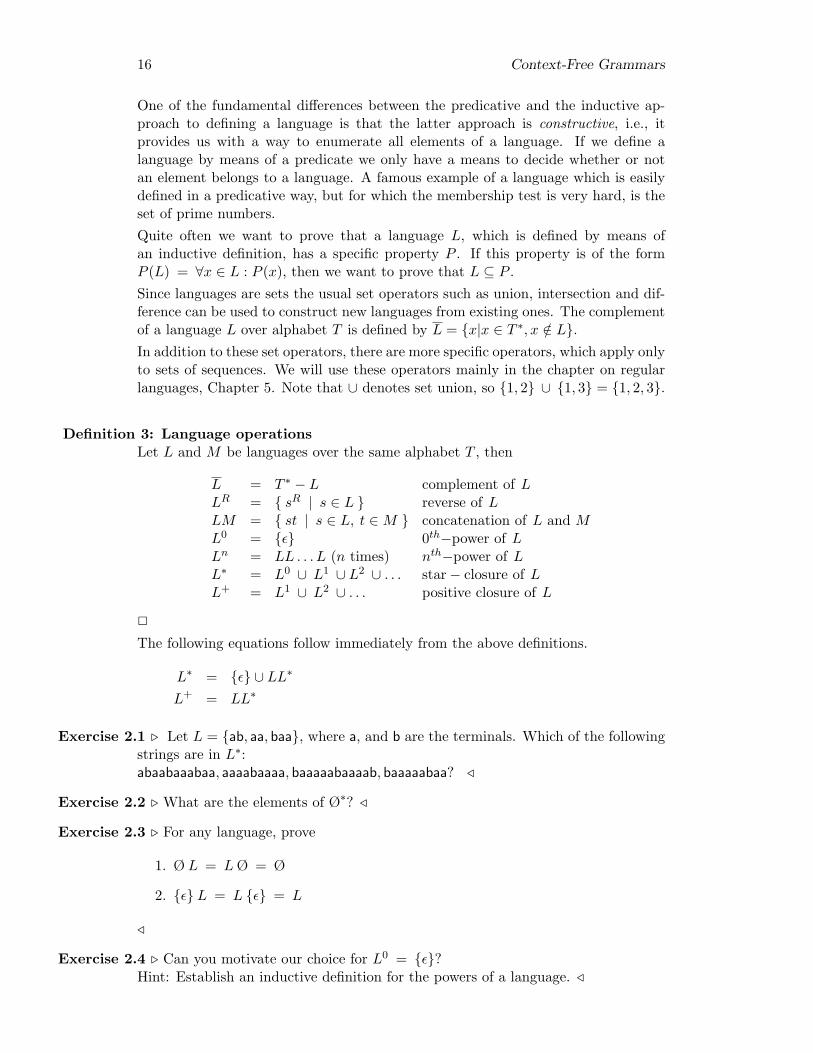
Definition 3: Language operationsLet L and M be languages over the same alphabet T , then
L = T ∗ − L complement of LLR = { sR | s ∈ L } reverse of LLM = { st | s ∈ L, t ∈M } concatenation of L and ML0 = {ε} 0th−power of LLn = LL . . . L (n times) nth−power of LL∗ = L0 ∪ L1 ∪ L2 ∪ . . . star− closure of LL+ = L1 ∪ L2 ∪ . . . positive closure of L
2
The following equations follow immediately from the above definitions.
L∗ = {ε} ∪ LL∗
L+ = LL∗
Exercise 2.1 . Let L = {ab, aa, baa}, where a, and b are the terminals. Which of the followingstrings are in L∗:abaabaaabaa, aaaabaaaa, baaaaabaaaab, baaaaabaa? /
Exercise 2.2 . What are the elements of Ø∗? /
Exercise 2.3 . For any language, prove
1. Ø L = LØ = Ø
2. {ε} L = L {ε} = L
/
Exercise 2.4 . Can you motivate our choice for L0 = {ε}?Hint: Establish an inductive definition for the powers of a language. /

2.2 Grammars 17
Exercise 2.5 . In this section we defined two ”star” operators: one for arbitrary sets (Defi-nition 1) and one for languages (Definition 3). Is there a difference between theseoperators? /
2.2 Grammars
The goal of this section is to introduce the concept of context-free grammars.Working with sets might be fun, but it is complicated to manipulate sets, and toprove properties of sets. For these purposes we introduce syntactical definitions,called grammars, of sets. This section will only discuss so-called context-free gram-mars, a kind of grammars that are convenient for automatical processing, and thatcan describe a large class of languages. But the class of languages that can bedescribed by context-free grammars is limited.In the previous section we defined PAL, the language of palindromes, by means ofa predicate. Although this definition defines the language we want, it is hard touse in proofs and programs. An important observation is the fact that the set ofpalindromes can be defined inductively as follows.
Definition 4: Palindromes by induction
• The empty string, ε, is a palindrome;• the strings consisting of just one character, a, b, and c, are palindromes;• if P is a palindrome, then the strings obtained by prepending and appending
the same character, a, b, and c, to it are also palindromes, that is, the strings
aPa
bPb
cPc
are palindromes.
2
The first two parts of the definition cover the basic cases. The last part of thedefinition covers the inductive cases. All strings which belong to the language PALinductively defined using the above definition read the same forwards and backwards.Therefore this definition is said to be sound (every string in PAL is a palindrome). soundConversely, if a string consisting of a’s, b’s, and c’s reads the same forwards andbackwards then it belongs to the language PAL. Therefore this definition is said tobe complete (every palindrome is in PAL). completeFinding an inductive definition for a language which is described by a predicate (likethe one for palindromes) is often a nontrivial task. Very often it is relatively easyto find a definition that is sound, but you also have to convince yourself that thedefinition is complete. A typical method for proving soundness and completeness ofan inductive definition is mathematical induction.Now that we have an inductive definition for palindromes, we can proceed by givinga formal representation of this inductive definition.Inductive definitions like the one above can be represented formally by making use
18 Context-Free Grammars
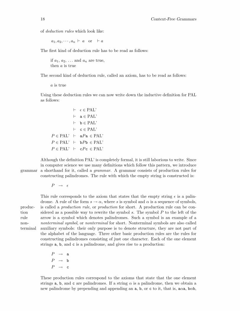
of deduction rules which look like:
a1, a2, · · · , an ` a or ` a
The first kind of deduction rule has to be read as follows:
if a1, a2, . . . and an are true,then a is true
The second kind of deduction rule, called an axiom, has to be read as follows:
a is true
Using these deduction rules we can now write down the inductive definition for PALas follows:
` ε ∈ PAL’` a ∈ PAL’` b ∈ PAL’` c ∈ PAL’
P ∈ PAL’ ` aPa ∈ PAL’P ∈ PAL’ ` bPb ∈ PAL’P ∈ PAL’ ` cPc ∈ PAL’
Although the definition PAL’ is completely formal, it is still laborious to write. Sincein computer science we use many definitions which follow this pattern, we introducea shorthand for it, called a grammar. A grammar consists of production rules forgrammarconstructing palindromes. The rule with which the empty string is constructed is:
P → ε
This rule corresponds to the axiom that states that the empty string ε is a palin-drome. A rule of the form s→ α, where s is symbol and α is a sequence of symbols,is called a production rule, or production for short. A production rule can be con-produc-
tionrule
sidered as a possible way to rewrite the symbol s. The symbol P to the left of thearrow is a symbol which denotes palindromes. Such a symbol is an example of anonterminal symbol, or nonterminal for short. Nonterminal symbols are also callednon-
terminal auxiliary symbols: their only purpose is to denote structure, they are not part ofthe alphabet of the language. Three other basic production rules are the rules forconstructing palindromes consisting of just one character. Each of the one elementstrings a, b, and c is a palindrome, and gives rise to a production:
P → a
P → b
P → c
These production rules correspond to the axioms that state that the one elementstrings a, b, and c are palindromes. If a string α is a palindrome, then we obtain anew palindrome by prepending and appending an a, b, or c to it, that is, aαa, bαb,
2.2 Grammars 19
and cαc are also palindromes. To obtain these palindromes we use the followingrecursive productions:
P → aPa
P → bPb
P → cPc
These production rules correspond to the deduction rules that state that, if P is apalindrome, then one can deduce that aPa, bPb and cPc are also palindromes. Thegrammar we have presented so far consists of three components:
• the set of terminals {a, b, c}; terminal• the set of nonterminals {P};• and the set of productions (the seven productions that we have introduced so
far).
Note that the intersection of the set of terminals and the set of nonterminals isempty. We complete the description of the grammar by adding a fourth component:the nonterminal start-symbol P . In this case we have only one choice for a start start-
symbolsymbol, but a grammar may have many nonterminal symbols.This leads to the following grammar for PAL
P → ε
P → a
P → b
P → c
P → aPa
P → bPb
P → cPc
The definition of the set of terminals, {a, b, c}, and the set of nonterminals, {P},is often implicit. Also the start-symbol is implicitly defined since there is only onenonterminal.We conclude this example with the formal definition of a context-free grammar.
Definition 5: Context-Free GrammarA context-free grammar G is a four tuple (T,N,R, S) where context-
freegram-mar
• T is a finite set of terminal symbols;• N is a finite set of nonterminal symbols (T and N are disjunct);• R is a finite set of production rules. Each production has the form A → α,
where A is a nonterminal and α is a sequence of terminals and nonterminals;• S is the start-symbol, S ∈ N .
2
The adjective “context-free” in the above definition comes from the specific produc-tion rules that are considered: exactly one nonterminal in the left hand side. Notevery language can be described via a context-free grammar. The standard examplehere is {anbncn | n ∈ IIN }. We will encounter this example again later in theselecture notes.
20 Context-Free Grammars
2.2.1 Notational conventions
In the definition of the grammar for PAL we have written every production on asingle line. Since this takes up a lot of space, and since the production rules form theheart of every grammar, we introduce the following shorthand. Instead of writing
S → α
S → β
we combine the two productions for S in one line as using the symbol |.
S → α | β
We may rewrite any number of rewrite rules for one nonterminal in this fashion, sothe grammar for PAL may also be written as follows:
P → ε | a | b | c | aPa | bPb | cPc
The notation we use for grammars is known as BNF - Backus Naur Form -, afterBNFBackus and Naur, who first used this notation for defining grammars.Another notational convention concerns names of productions. Sometimes we wantto give names to production rules. The names will be written in front of the pro-duction. So, for example,
Alpha rule : S → αBeta rule : S → β
Finally, if we give a context-free grammar just by means of its productions, thestart-symbol is usually the nonterminal in the left hand side of the first production,and the start-symbol is usually called S.
Exercise 2.6 . Give a context free grammar for the set of sentences over alphabet X where
1. X = {a}
2. X = {a, b}
/
Exercise 2.7 . Give a grammar for palindromes over the alphabet {a, b} /
Exercise 2.8 . Give a grammar for the language
L = { s sR | s ∈ {a, b}∗ }
This language is known as the mirror-palindromes language. /
Exercise 2.9 . A parity-sequence is a sequence consisting of 0’s and 1’s that has an even numberof ones. Give a grammar for parity-sequences. /
Exercise 2.10 . Give a grammar for the language
L = {w | w ∈ {a, b}∗ ∧ nr(a, w) = nr(b, w)}
where nr(c, w) is the number of c-occurrences in w. /
2.3 The language of a grammar 21
2.3 The language of a grammar
The goal of this section is to describe the relation between grammars and languages:to show how to derive sentences of a language given its grammar.We have seen how to obtain a grammar from a given language. Now we considerthe reverse question: how to obtain a language from a given grammar? Before wecan answer this question we first have to say what we can do with a grammar. Theanswer is simple: we can derive sequences with it.How do we construct a palindrome? A palindrome is a sequence of terminals, in ourcase the characters a, b and c, that can be derived in zero or more direct derivationsteps from the start-symbol P using the productions of the grammar for palindromesgiven above.For example, the sequence bacab can be derived using the grammar for palindromesas follows:
P⇒
bPb⇒
baPab⇒
bacab
Such a construction is called a derivation. In the first step of this derivation pro- derivationduction P → bPb is used to rewrite P into bPb. In the second step productionP → aPa is used to rewrite bPb into baPab. Finally, in the last step productionP → c is used to rewrite baPab into bacab. Constructing a derivation can be seenas a constructive proof that the string bacab is a palindrome.We will now describe derivation steps more formally.
Definition 6: DerivationSuppose X → β is a production of a grammar, where X is a nonterminal symboland β is a sequence of (nonterminal or terminal) symbols. Let αXγ be a sequence of(nonterminal or terminal) symbols. We say that αXγ directly derives the sequence direct
deriva-tion
αβγ, which is obtained by replacing the left hand side X of the production by thecorresponding right hand side β. We write αXγ ⇒ αβγ and we also say that αXγrewrites to αβγ in one step. A sequence ϕn is derived from a sequence ϕ1, written derivationϕ1
∗⇒ ϕn, if there exist sequences ϕ1, . . . , ϕn with n ≥ 1 such that
∀i, 1 ≤ i < n : ϕi ⇒ ϕi+1
If n = 1 this statement is trivially true, and it follows that we can derive eachsentence from itself in zero steps:
ϕ∗⇒ ϕ
A partial derivation is a derivation of a sequence that still contains nonterminals. partialderiva-tion
2
Finding a derivation ϕ1∗⇒ ϕn is, in general, a nontrivial task. A derivation is only
one branch of a whole search tree which contains many more branches. Each branch
22 Context-Free Grammars
represents a (successful or unsuccessful) direction in which a possible derivation mayproceed. Another important challenge is to arrange things in such a way that findinga derivation can be done in an efficient way.From the example derivation above it follows that
P∗⇒ bacab
Because this derivation begins with the start-symbol of the grammar and results in asequence consisting of terminals only (a terminal string), we say that the string bacabbelongs to the language generated by the grammar for palindromes. In general, wedefine
Definition 7: Language of a grammar (or language generated by a grammar)The language of a grammar G = (T,N,R, S), usually denoted by L(G), is definedas
L(G) = { s | S ∗⇒ s , s ∈ T ∗}
2
We sometimes also talk about the language of a nonterminal, which is defined by
L(A) = { s | A ∗⇒ s , s ∈ T ∗}
for nonterminal A. The language of a grammar could have been defined as thelanguage of its start-symbol.Note that different grammars may have the same language. For example, if weextend the grammar for PAL with the production P → bacab, we obtain a grammarwith exactly the same language as PAL. Two grammars that generate the samelanguage are called equivalent. So for a particular grammar there exists a uniquelanguage, but the reverse is not true: given a language we can usually construct manygrammars that generate the language. In mathematical language: the mappingbetween a grammar and its language is not a bijection.
Definition 8: Context-free languageA context-free language is a language that is generated by a context-free grammar.context-
freelan-guage
2
All palindromes can be derived from the start-symbol P . Thus, the language ofour grammar for palindromes is PAL, the set of all palindromes over the alphabet{a, b, c} and PAL is context-free.
2.3.1 Some basic languages
Digits occur in a lot of programming and other languages, and so do letters. In thissubsection we will define some grammars that specify some basic languages such asdigits and letters. These grammars will be used often in later sections.
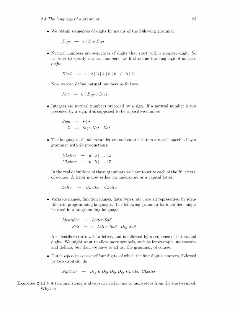
• The language of single digits is specified by a grammar with 10 productionrules for the nonterminal Dig .
Dig → 0 | 1 | 2 | 3 | 4 | 5 | 6 | 7 | 8 | 9
2.3 The language of a grammar 23
• We obtain sequences of digits by means of the following grammar:
Digs → ε | Dig Digs
• Natural numbers are sequences of digits that start with a nonzero digit. Soin order to specify natural numbers, we first define the language of nonzerodigits.
Dig-0 → 1 | 2 | 3 | 4 | 5 | 6 | 7 | 8 | 9
Now we can define natural numbers as follows.
Nat → 0 | Dig-0 Digs
• Integers are natural numbers preceded by a sign. If a natural number is notpreceded by a sign, it is supposed to be a positive number.
Sign → + | -Z → Sign Nat | Nat
• The languages of underscore letters and capital letters are each specified by agrammar with 26 productions:
ULetter → a | b | . . . | zCLetter → A | B | . . . | Z
In the real definitions of these grammars we have to write each of the 26 letters,of course. A letter is now either an underscore or a capital letter.
Letter → ULetter | CLetter
• Variable names, function names, data types, etc., are all represented by iden-tifiers in programming languages. The following grammar for identifiers mightbe used in a programming language:
Identifier → Letter SoSSoS → ε | Letter SoS | Dig SoS
An identifier starts with a letter, and is followed by a sequence of letters anddigits. We might want to allow more symbols, such as for example underscoresand dollars, but then we have to adjust the grammar, of course.
• Dutch zipcodes consist of four digits, of which the first digit is nonzero, followedby two capitals. So
ZipCode → Dig-0 Dig Dig Dig CLetter CLetter
Exercise 2.11 . A terminal string is always derived in one or more steps from the start-symbol.Why? /

24 Context-Free Grammars
Exercise 2.12 . What language is generated by the grammar with the single production rule
S → ε
/
Exercise 2.13 . What language does the grammar with the following productions generate?
S → Aa
A → B
B → Aa
/
Exercise 2.14 . Give a simple description of the language generated by the grammar withproductions
S → aA
A → bS
S → ε
/
Exercise 2.15 . Is the language L defined in exercise 2.1 context free ? /
2.4 Parse trees
The goal of this section is to introduce parse trees, and to show how parse treesrelate to derivations. Furthermore, this section defines (non)ambiguous grammars.For any partial derivation, i.e. a derivation that contains nonterminals in its righthand side, there may be several productions of the grammar that can be used toproceed the partial derivation with and, as a consequence, there may be differentderivations for the same sentence. There are two reasons why derivations for aspecific sentence differ:
• Only the order in which the derivation steps are chosen differs. All suchderivations are considered to be equivalent.
• Different derivation steps have been chosen. Such derivations are consideredto be different.
Here is a simple example. Consider the grammar SequenceOfS with productions:
S → SS
S → s
Using this grammar we can derive the sentence sss as follows (we have underlinedthe nonterminal that is rewritten).
S∗⇒ SS
∗⇒ SSS∗⇒ SsS
∗⇒ ssS∗⇒ sss
S∗⇒ SS
∗⇒ sS∗⇒ sSS
∗⇒ sSs∗⇒ sss
2.4 Parse trees 25
These derivations are the same up to the order in which derivation steps are taken.However, the following derivation does not use the same derivation steps:
S∗⇒ SS
∗⇒ SSS∗⇒ sSS
∗⇒ ssS∗⇒ sss
In this derivation, the first S is rewritten to SS instead of s.The set of all equivalent derivations can be represented by selecting a, so called,canonical element. A good candidate for such a canonical element is the leftmostderivation. In a leftmost derivation, only the leftmost nonterminal is rewritten. If leftmost
deriva-tion
there exists a derivation of a sentence x using the productions of a grammar, thenthere exists a leftmost derivation of x. The leftmost derivation corresponding to thetwo equivalent derivations above is
S∗⇒ SS
∗⇒ sS∗⇒ sSS
∗⇒ ssS∗⇒ sss
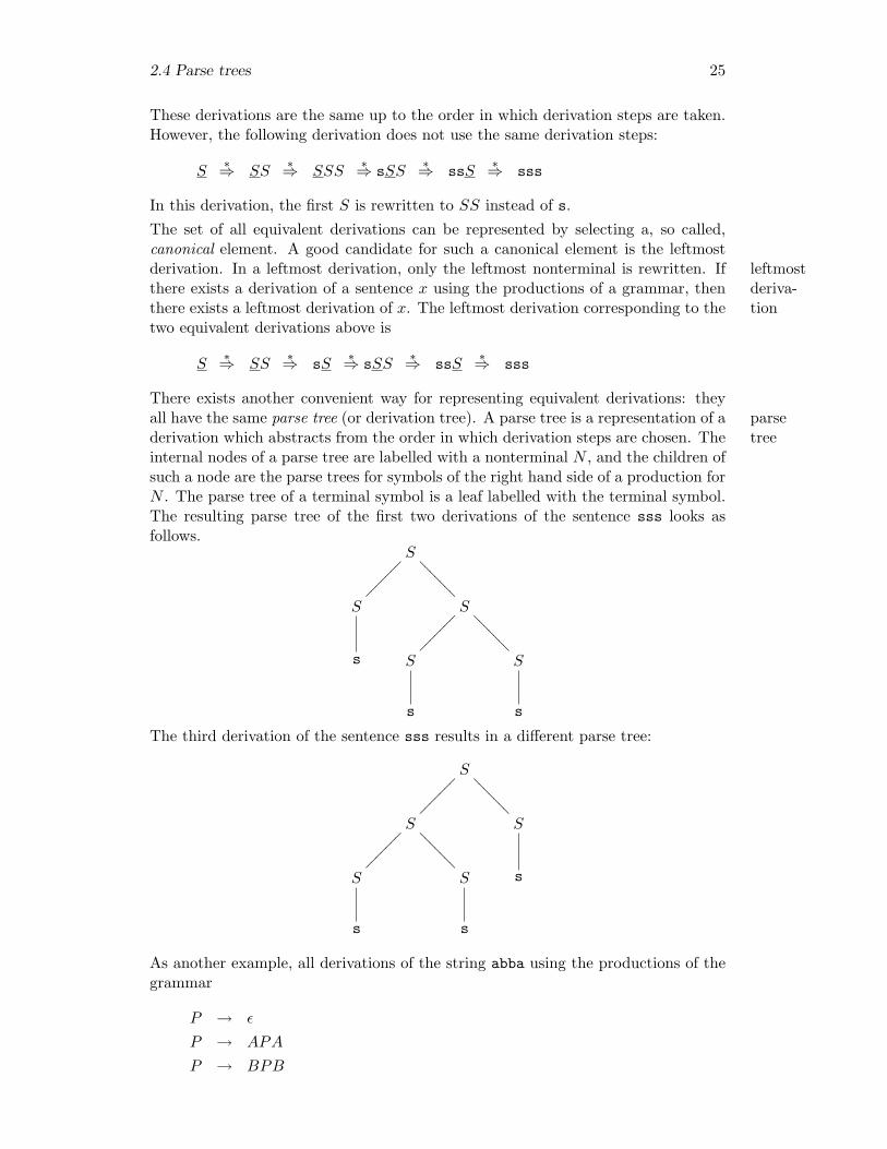
There exists another convenient way for representing equivalent derivations: theyall have the same parse tree (or derivation tree). A parse tree is a representation of a parse
treederivation which abstracts from the order in which derivation steps are chosen. Theinternal nodes of a parse tree are labelled with a nonterminal N , and the children ofsuch a node are the parse trees for symbols of the right hand side of a production forN . The parse tree of a terminal symbol is a leaf labelled with the terminal symbol.The resulting parse tree of the first two derivations of the sentence sss looks asfollows.
S
����
���
????
???
S S
����
���
????
???
s S S
s s
The third derivation of the sentence sss results in a different parse tree:
S
����
���
????
???
S
����
���
????
??? S
S S s
s s
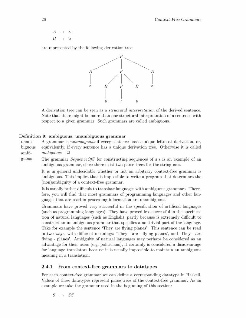
As another example, all derivations of the string abba using the productions of thegrammar
P → ε
P → APA
P → BPB
26 Context-Free Grammars
A → a
B → b
are represented by the following derivation tree:
P
ooooooooooooooo
OOOOOOOOOOOOOOO
A P
~~~~
~~~
@@@@
@@@ A
a B P B a
b ε b
A derivation tree can be seen as a structural interpretation of the derived sentence.Note that there might be more than one structural interpretation of a sentence withrespect to a given grammar. Such grammars are called ambiguous.
Definition 9: ambiguous, unambiguous grammarA grammar is unambiguous if every sentence has a unique leftmost derivation, or,unam-
biguous equivalently, if every sentence has a unique derivation tree. Otherwise it is calledambiguous. 2ambi-
guous The grammar SequenceOfS for constructing sequences of s’s is an example of anambiguous grammar, since there exist two parse trees for the string sss.It is in general undecidable whether or not an arbitrary context-free grammar isambiguous. This implies that is impossible to write a program that determines the(non)ambiguity of a context-free grammar.It is usually rather difficult to translate languages with ambiguous grammars. There-fore, you will find that most grammars of programming languages and other lan-guages that are used in processing information are unambiguous.Grammars have proved very successful in the specification of artificial languages(such as programming languages). They have proved less successful in the specifica-tion of natural languages (such as English), partly because is extremely difficult toconstruct an unambiguous grammar that specifies a nontrivial part of the language.Take for example the sentence ‘They are flying planes’. This sentence can be readin two ways, with different meanings: ‘They - are - flying planes’, and ‘They - areflying - planes’. Ambiguity of natural languages may perhaps be considered as anadvantage for their users (e.g. politicians), it certainly is considered a disadvantagefor language translators because it is usually impossible to maintain an ambiguousmeaning in a translation.
2.4.1 From context-free grammars to datatypes
For each context-free grammar we can define a corresponding datatype in Haskell.Values of these datatypes represent parse trees of the context-free grammar. As anexample we take the grammar used in the beginning of this section:
S → SS
2.5 Grammar transformations 27
S → s
First, we give each of the productions of this grammar a name:
Beside : S → SSSingle : S → s
And now we interpret the start-symbol of the grammar S as a datatype, using thenames of the productions as constructors:
data S = Beside S S| Single Char
Note that this datatype is too general: the type Char should really be the singlecharacter s. This datatype can be used to represent parse trees of sentences ofS . For example, the parse tree that corresponds to the first two derivations of thesequence sss is represented by the following value of the datatype S.
Beside (Single ’s’) (Beside (Single ’s’) (Single ’s’))
The third derivation of the sentence sss produces the following parse tree:
Beside (Beside (Single ’s’) (Single ’s’)) (Single ’s’)
Because the datatype S is too general, we will reconsider the construction of datatypesfrom context-free grammars in Section 2.6.
Exercise 2.16 . Consider the grammar for palindromes that you have constructed in exercise2.7. Give parse trees for the palindromes cPal1 = "abaaba" and cPal2 = "baaab".Define a datatype Palc corresponding to the grammar and represent the parse treesfor cPal1 and cPal2 as values of Palc. /
2.5 Grammar transformations
The goal of this section is to discuss properties of grammars, grammar transforma-tions, and to show how grammar transformations can be used to obtain grammarsthat satisfy particular properties.Grammars satisfy properties. Examples of properties are:
• a grammar may be unambiguous, that is, every sentence of its language has aunique parse tree;
• a grammar may have the property that only the start-symbol can derive theempty string; no other nonterminal can derive the empty string;
• a grammar may have the property that every production either has a singleterminal, or two nonterminals in its right-hand side. Such a grammar is saidto be in Chomsky normal form.

28 Context-Free Grammars
So why are we interested in such properties? Some of these properties imply that itis possible to build parse trees for sentences of the language of the grammar in onlyone way. Some other properties imply that we can build these parse trees very fast.Other properties are used to prove facts about grammars. Yet other properties areused to efficiently compute some other information from parse trees of a grammar.For example, suppose we have a program p that builds parse trees for sentencesof grammars in Chomsky normal form, and that we can prove that each grammarcan be transformed in a grammar in Chomsky normal form. (When we say that agrammar G can be transformed in another grammar G′, we mean that there existsgrammar
trans-forma-tion
some procedure to obtainG′ fromG, and thatG andG′ generate the same language.)Then we can use this program p for building parse trees for any grammar.Since it is sometimes convenient to have a grammar that satisfies a particular prop-erty for a language, we would like to be able to transform grammars in other gram-mars that generate the same language, but that possibly satisfy different properties.This section describes a number of grammar transformations
• Removing duplicate productions.• Substituting right-hand sides for nonterminals.• Left factoring.• Removing left recursion.• Associative separator.• Introduction of priorities.
There are many more transformations than we describe here; we will only show asmall but useful set of grammar transformations. In the following transformations wewill assume that u, v, w, x, y, and z denote sequences of terminals and nonterminals,i.e., are elements of (N ∪ T )∗.Removing duplicate productionsThis grammar transformation is a transformation that can be applied to any gram-mar of the correct form. If a grammar contains two occurrences of the same pro-duction rule, one of these occurrences can be removed. For example,
A → u | u | v
can be transformed into
A → u | v
Substituting right-hand sides for nonterminalsIf a nonterminal N occurs in a right-hand side of a production, the production maybe replaced by just as many productions as there exist productions for N , in whichN has been replaced by its right-hand sides. For example,
A → uBv | zB → x | w
may be transformed into
A → uxv | uwv | zB → x | w
2.5 Grammar transformations 29
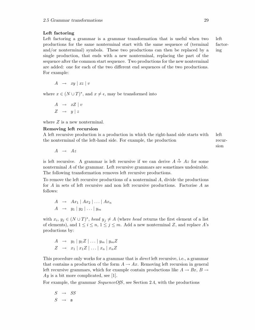
Left factoringLeft factoring a grammar is a grammar transformation that is useful when two left
factor-ing
productions for the same nonterminal start with the same sequence of (terminaland/or nonterminal) symbols. These two productions can then be replaced by asingle production, that ends with a new nonterminal, replacing the part of thesequence after the common start sequence. Two productions for the new nonterminalare added: one for each of the two different end sequences of the two productions.For example:
A → xy | xz | v
where x ∈ (N ∪ T )∗, and x 6= ε, may be transformed into
A → xZ | vZ → y | z
where Z is a new nonterminal.Removing left recursionA left recursive production is a production in which the right-hand side starts with left
recur-sion
the nonterminal of the left-hand side. For example, the production
A → Az
is left recursive. A grammar is left recursive if we can derive A ∗⇒ Az for somenonterminal A of the grammar. Left recursive grammars are sometimes undesirable.The following transformation removes left recursive productions.To remove the left recursive productions of a nonterminal A, divide the productionsfor A in sets of left recursive and non left recursive productions. Factorise A asfollows:
A → Ax1 | Ax2 | . . . | Axn
A → y1 | y2 | . . . | ym
with xi, yj ∈ (N ∪ T )∗, head yj 6= A (where head returns the first element of a listof elements), and 1 ≤ i ≤ n, 1 ≤ j ≤ m. Add a new nonterminal Z, and replace A’sproductions by:
A → y1 | y1Z | . . . | ym | ymZ
Z → x1 | x1Z | . . . | xn | xnZ
This procedure only works for a grammar that is direct left recursive, i.e., a grammarthat contains a production of the form A→ Ax . Removing left recursion in generalleft recursive grammars, which for example contain productions like A→ Bx , B →Ay is a bit more complicated, see [1].For example, the grammar SequenceOfS , see Section 2.4, with the productions
S → SSS → s

30 Context-Free Grammars
is a left recursive grammar. The above procedure for removing left recursion givesthe following productions:
S → s | sZZ → S | SZ
Associative separatorThe following grammar generates a list of declarations, separated by a semicolon ;.
Decls → Decls ; DeclsDecls → Decl
where the productions for Decl , which generates a single declaration, are omit-ted. This grammar is ambiguous, for the same reason as SequenceOfS is ambigu-ous. The operator ; is an associative separator in the generated language, that is:d1 ; (d2 ; d3) = (d1 ; d2) ; d3 where d1, d2, and d3 are declarations. There-fore, we may use the following unambiguous grammar for generating a language ofdeclarations:
Decls → Decl ; DeclsDecls → Decl
An alternative grammar for the same language is
Decls → Decls ; DeclDecls → Decl
This grammar transformation can only be applied because the semicolon is asso-ciative in the generated language; it is not a grammar transformation that can beapplied blindly to any grammar.The same transformation can be applied to grammars with productions of the form:
A → AaA
where a is an associative operator in the generated language. As an example youmay think of natural numbers with addition.Introduction of prioritiesAnother form of ambiguity often arises in the part of a grammar for a programminglanguage which describes expressions. For example, the following grammar generatesarithmetic expressions:
E → E + E
E → E * E
E → (E)
E → Digs
where Digs generates a list of digits, see Section 2.3.1. This grammar is ambiguous:the sentence 2+4*6 has two parse trees: one corresponding to (2+4)*6, and onecorresponding to 2+(4*6). If we make the usual assumption that * has higher

2.5 Grammar transformations 31
priority than +, the latter expression is the intended reading of the sentence 2+4*6.In order to obtain parse trees that respect these priorities, we transform the grammaras follows:
E → T
E → E + T
T → F
T → T * F
F → (E)
F → Digs
This grammar generates the same language as the previous grammar for expressions,but it respects the priorities of the operators.In practice, often more than two levels of priority are used. Then, instead of writ-ing a large number of identically formed production rules, we use parameterisednonterminals. For 1 ≤ i < n,
Ei → Ei+1
Ei → Ei OP i Ei+1
Operator OP i is a parameterised nonterminal that generates operators of priorityi. In addition to the above productions, there should also be a production forexpressions of the highest priority, for example:
En → (E1) | Digs
A grammar transformation transforms a grammar into another grammar that gen-erates the same language. For each of the above transformations we should provethat the generated language remains the same. Since the proofs are too complicatedat this point, they are omitted. The proofs can be found in any of the theoreticalbooks on language and parsing theory [12].There exist many more grammar transformations, but the ones given in this sectionsuffice for now. Note that everywhere we use ‘left’ (left recursion, left factoring),we can replace it by ‘right’, and obtain a dual grammar transformation. We willdiscuss a larger example of a grammar transformation after the following section.
Exercise 2.17 . The standard example of ambiguity in programming languages is the danglingelse. Let G be a grammar with terminal set { if, b, then, else , a } and productions
S → if b then S else S
S → if b then S
S → a
1 Give two derivation trees for the sentence if b then if b then a else a.2 Give an unambiguous grammar that generates the same language as G.3 How does Java prevent this dangling else problem?
/
32 Context-Free Grammars
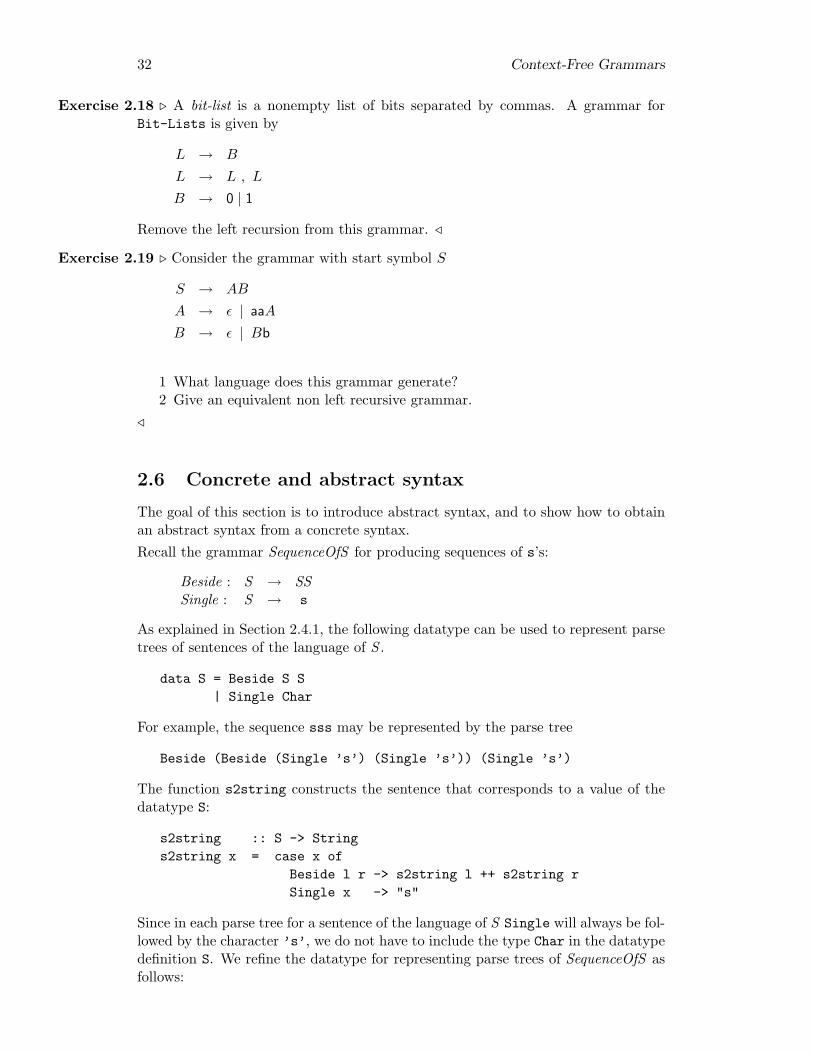
Exercise 2.18 . A bit-list is a nonempty list of bits separated by commas. A grammar forBit-Lists is given by
L → B
L → L , L
B → 0 | 1
Remove the left recursion from this grammar. /
Exercise 2.19 . Consider the grammar with start symbol S
S → AB
A → ε | aaA
B → ε | Bb
1 What language does this grammar generate?2 Give an equivalent non left recursive grammar.
/
2.6 Concrete and abstract syntax
The goal of this section is to introduce abstract syntax, and to show how to obtainan abstract syntax from a concrete syntax.Recall the grammar SequenceOfS for producing sequences of s’s:
Beside : S → SSSingle : S → s
As explained in Section 2.4.1, the following datatype can be used to represent parsetrees of sentences of the language of S .
data S = Beside S S| Single Char
For example, the sequence sss may be represented by the parse tree
Beside (Beside (Single ’s’) (Single ’s’)) (Single ’s’)
The function s2string constructs the sentence that corresponds to a value of thedatatype S:
s2string :: S -> Strings2string x = case x of
Beside l r -> s2string l ++ s2string rSingle x -> "s"
Since in each parse tree for a sentence of the language of S Single will always be fol-lowed by the character ’s’, we do not have to include the type Char in the datatypedefinition S. We refine the datatype for representing parse trees of SequenceOfS asfollows:
2.6 Concrete and abstract syntax 33
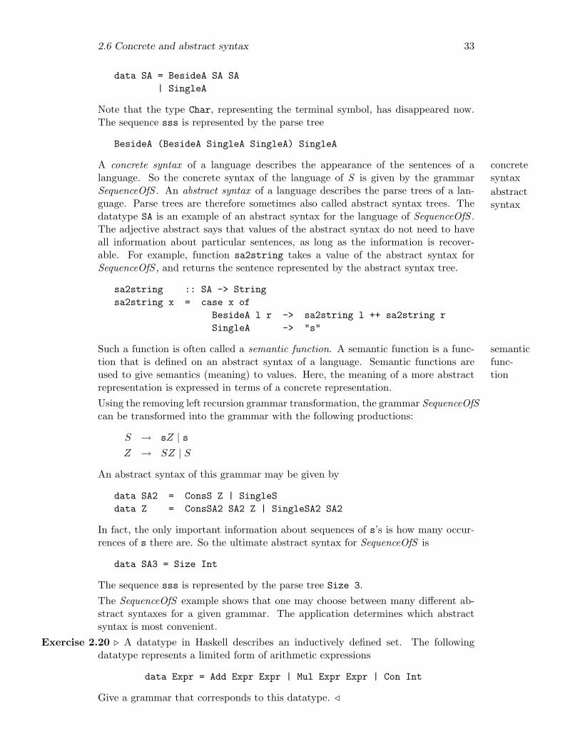
data SA = BesideA SA SA| SingleA
Note that the type Char, representing the terminal symbol, has disappeared now.The sequence sss is represented by the parse tree
BesideA (BesideA SingleA SingleA) SingleA
A concrete syntax of a language describes the appearance of the sentences of a concretesyntaxlanguage. So the concrete syntax of the language of S is given by the grammar
SequenceOfS . An abstract syntax of a language describes the parse trees of a lan- abstractsyntaxguage. Parse trees are therefore sometimes also called abstract syntax trees. The
datatype SA is an example of an abstract syntax for the language of SequenceOfS .The adjective abstract says that values of the abstract syntax do not need to haveall information about particular sentences, as long as the information is recover-able. For example, function sa2string takes a value of the abstract syntax forSequenceOfS , and returns the sentence represented by the abstract syntax tree.
sa2string :: SA -> Stringsa2string x = case x of
BesideA l r -> sa2string l ++ sa2string rSingleA -> "s"
Such a function is often called a semantic function. A semantic function is a func- semanticfunc-tion
tion that is defined on an abstract syntax of a language. Semantic functions areused to give semantics (meaning) to values. Here, the meaning of a more abstractrepresentation is expressed in terms of a concrete representation.Using the removing left recursion grammar transformation, the grammar SequenceOfScan be transformed into the grammar with the following productions:
S → sZ | sZ → SZ | S
An abstract syntax of this grammar may be given by
data SA2 = ConsS Z | SingleSdata Z = ConsSA2 SA2 Z | SingleSA2 SA2
In fact, the only important information about sequences of s’s is how many occur-rences of s there are. So the ultimate abstract syntax for SequenceOfS is
data SA3 = Size Int
The sequence sss is represented by the parse tree Size 3.The SequenceOfS example shows that one may choose between many different ab-stract syntaxes for a given grammar. The application determines which abstractsyntax is most convenient.
Exercise 2.20 . A datatype in Haskell describes an inductively defined set. The followingdatatype represents a limited form of arithmetic expressions
data Expr = Add Expr Expr | Mul Expr Expr | Con Int
Give a grammar that corresponds to this datatype. /

34 Context-Free Grammars
Exercise 2.21 . Consider your answer to exercise 2.7, which describes the concrete syntax forpalindromes over {a, b}.
1 Define a datatype Pal that describes the abstract syntax corresponding to yourgrammar. Give the two abstract palindromes aPal1 and aPal2 that corre-spond to the concrete palindromes cPal1 = "abaaba" and cPal2 = "baaab"
2 Write a (semantic) function that transforms an abstract representation of apalindrome into a concrete one. Test your function with the abstract palin-dromes aPal1 and aPal2.
3 Write a function that counts the number of a’s occurring in a palindrome. Testyour function with the abstract palindromes aPal1 and aPal2.
/
Exercise 2.22 . Consider your answer to exercise 2.8, which describes the concrete syntax formirror-palindromes.
1 Define a datatype Mir that describes the abstract syntax corresponding toyour grammar. Give the two abstract mirror-palindromes aMir1 and aMir2that correspond to the concrete mirror-palindromes cMir1 = "abaaba" andcMir2 = "abbbba"
2 Write a (semantic) function that transforms an abstract representation of amirror-palindrome into a concrete one. Test your function with the abstractmirror-palindromes aMir1 and aMir2.
3 Write a function that transforms an abstract representation of a mirror-palin-drome into the corresponding abstract representation of a palindrome. Testyour function with the abstract mirror-palindromes aMir1 and aMir2.
/
Exercise 2.23 . Consider your anwer to exercise 2.9, which describes the concrete syntax forparity-sequences.
1 Describe the abstract syntax corresponding to your grammar. Give the twoabstract parity-sequences aEven1 and aEven2 that correspond to the concreteparity-sequences cEven1 = "00101" and cEven2 = "01010"
2 Write a (semantic) function that transforms an abstract representation of aparity-sequence into a concrete one. Test your function with the abstractparity-sequences aEven1 and aEven2.
/
Exercise 2.24 . Consider your answer to exercise 2.18, which describes the concrete syntax forbit-lists by means of a grammar that is not left recursive.
1 Define a datatype BitList that describes the abstract syntax corresponding toyour grammar. Give the two abstract bit-lists aBitList1 and aBitList2 thatcorrespond to the concrete bit-lists cBitList1 = "0,1,0" and cBitList2 ="0,0,1".
2 Write a function that transforms an abstract representation of a bit-list intoa concrete one. Test your function with the abstract bit-lists aBitList1 andaBitList2.
3 Write a function that concatenates two abstract representations of a bit-listsinto a bit-list. Test your function with the abstract bit-lists aBitList1 andaBitList2.
/
2.7 Constructions on grammars 35
2.7 Constructions on grammars
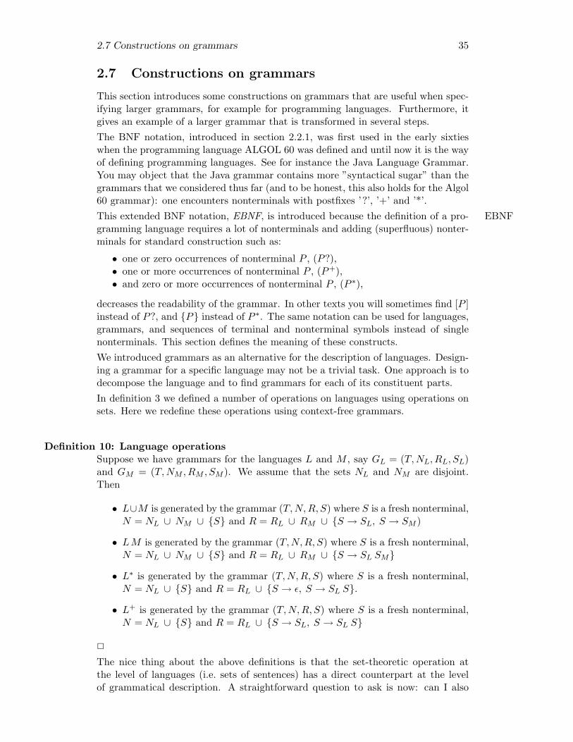
This section introduces some constructions on grammars that are useful when spec-ifying larger grammars, for example for programming languages. Furthermore, itgives an example of a larger grammar that is transformed in several steps.The BNF notation, introduced in section 2.2.1, was first used in the early sixtieswhen the programming language ALGOL 60 was defined and until now it is the wayof defining programming languages. See for instance the Java Language Grammar.You may object that the Java grammar contains more ”syntactical sugar” than thegrammars that we considered thus far (and to be honest, this also holds for the Algol60 grammar): one encounters nonterminals with postfixes ’?’, ’+’ and ’*’.This extended BNF notation, EBNF, is introduced because the definition of a pro- EBNFgramming language requires a lot of nonterminals and adding (superfluous) nonter-minals for standard construction such as:
• one or zero occurrences of nonterminal P , (P?),• one or more occurrences of nonterminal P , (P+),• and zero or more occurrences of nonterminal P , (P ∗),
decreases the readability of the grammar. In other texts you will sometimes find [P ]instead of P?, and {P} instead of P ∗. The same notation can be used for languages,grammars, and sequences of terminal and nonterminal symbols instead of singlenonterminals. This section defines the meaning of these constructs.We introduced grammars as an alternative for the description of languages. Design-ing a grammar for a specific language may not be a trivial task. One approach is todecompose the language and to find grammars for each of its constituent parts.In definition 3 we defined a number of operations on languages using operations onsets. Here we redefine these operations using context-free grammars.
Definition 10: Language operationsSuppose we have grammars for the languages L and M , say GL = (T,NL, RL, SL)and GM = (T,NM , RM , SM ). We assume that the sets NL and NM are disjoint.Then
• L∪M is generated by the grammar (T,N,R, S) where S is a fresh nonterminal,N = NL ∪ NM ∪ {S} and R = RL ∪ RM ∪ {S → SL, S → SM )
• LM is generated by the grammar (T,N,R, S) where S is a fresh nonterminal,N = NL ∪ NM ∪ {S} and R = RL ∪ RM ∪ {S → SL SM}
• L∗ is generated by the grammar (T,N,R, S) where S is a fresh nonterminal,N = NL ∪ {S} and R = RL ∪ {S → ε, S → SL S}.
• L+ is generated by the grammar (T,N,R, S) where S is a fresh nonterminal,N = NL ∪ {S} and R = RL ∪ {S → SL, S → SL S}
2
The nice thing about the above definitions is that the set-theoretic operation atthe level of languages (i.e. sets of sentences) has a direct counterpart at the levelof grammatical description. A straightforward question to ask is now: can I also

36 Context-Free Grammars
define languages as the difference between two languages or as the intersection of twolanguages? Unfortunately there are no equivalent operators for composing grammarsthat correspond to such intersection and difference operators.Two of the above constructions are important enough to also define them as grammaroperations. Furthermore, we add a new construction for choice.
Definition 11: Grammar operationsLet G = (T,N,R, S) be a context-free grammar and let S′ be a fresh nonterminal.Then
G∗ = (T, N ∪ {S′}, R ∪ {S′ → ε, S′ → SS′}, S′) star GG+ = (T, N ∪ {S′}, R ∪ {S′ → S, S′ → SS′}, S′) plus GG? = (T, N ∪ {S′}, R ∪ {S′ → ε, S′ → S}, S′) optional G
2
The definition of P?, P+, and P ∗ is very similar to the definitions of the operationson grammars. For example, P ∗ denotes zero or more occurrences of nonterminal P ,so Dig∗ denotes the language consisting of zero or more digits.
Definition 12: EBNF for sequencesLet P be a sequence of nonterminals and terminals, then
L(P ∗) = L(Z) with Z → ε | PZL(P+) = L(Z) with Z → P | PZL(P?) = L(Z) with Z → ε | P
where Z is a new nonterminal in each definition. 2
Because the concatenation operator for sequences is associative, the operators + and∗ can also be defined symmetrically:
L(P ∗) = L(Z) with Z → ε | ZPL(P+) = L(Z) with Z → P | ZP
There are many variations possible on this theme:
L(P ∗Q) = L(Z) with Z → Q | PZ (2.1)
2.7.1 SL: an example
To illustrate EBNF and some of the grammar transformations given in the previoussection, we give a larger example. The following grammar generates expressions ina very small programming language, called SL.
Expr → if Expr then Expr else ExprExpr → Expr where DeclsExpr → AppExpr
AppExpr → AppExpr Atomic | AtomicAtomic → Var | Number | Bool | (Expr)
Decls → DeclDecls → Decls ; DeclsDecl → Var = Expr
2.7 Constructions on grammars 37
where the nonterminals Var , Number , and Bool generate variables, number expres-sions, and boolean expressions, respectively. Note that the brackets around theExpr in the production for Atomic, and the semicolon in between the Decls in thesecond production forDecls are also terminal symbols. The following ‘program’ is asentence of this language:
if true then funny true else false where funny = 7
It is clear that this is not a very convenient language to write programs in.The above grammar is ambiguous (why?), and we introduce priorities to resolvesome of the ambiguities. Application binds stronger than if, and both applicationand if bind stronger then where. Using the introduction of priorities grammar trans-formation, we obtain:
Expr → Expr1Expr → Expr1 where Decls
Expr1 → Expr2Expr1 → if Expr1 then Expr1 else Expr1Expr2 → AtomicExpr2 → Expr2 Atomic
where Atomic, and Decls have the same productions as before.The nonterminal Expr2 is left recursive. Removing left recursion gives the followingproductions for Expr2 .
Expr2 → Atomic | Atomic ZZ → Atomic | Atomic Z
Since the new nonterminal Z has exactly the same productions as Expr2 , theseproductions can be replaced by
Expr2 → Atomic | Atomic Expr2
So Expr2 generates a nonempty sequence of atomics. Using the +-notation intro-duced in this section, we may replace Expr2 by Atomic+.Another source of ambiguity are the productions for Decls. Decls generates anonempty list of declarations, and the separator ; is assumed to be associative.Hence we can apply the associative separator transformation to obtain
Decls → Decl | Decl ; Decls
or, according to (2.1),
Decls → (Decl;)∗ Decl
which, using an omitted rule for that star-operator ∗, may be transformed into
Decls → Decl (;Decl)∗

38 Context-Free Grammars
The last grammar transformation we apply is left factoring. This transformationapplies to Expr , and gives
Expr → Expr1 ZZ → ε | where Decls
Since nonterminal Z generates either nothing or a where clause, we may replace Zby an optional where clause in the production for Expr .
Expr → Expr1 (where Decls)?
After all these grammar transformations, we obtain the following grammar.
Expr → Expr1 (where Decls)?Expr1 → Atomic+
Expr1 → if Expr1 then Expr1 else Expr1Atomic → Var | Number | Bool | (Expr)
Decls → Decl (;Decl)∗
Exercise 2.25 . Give the EBNF notation for each of the basic languages defined in section2.3.1. /
Exercise 2.26 . What language is generated by G? ? /
Exercise 2.27 . In case we define a language by means of a predicate it is almost trivial todefine the intersection and the difference of two languages. Show how. /
Exercise 2.28 . Let L1 = {anbncm | n,m ∈ IIN} and L2 = {anbmcm | n,m ∈ IIN}.• Give grammars for L1 and L2.• Is L1 ∩ L2 context free, i.e. can you give a context-free grammar for this
language?
/
2.8 Parsing
This section formulates the parsing problem, and discusses some of the future topicsof the course.
Definition 13: Parsing problemGiven the grammar G and a string s the parsing problem answers the questionwhether or not s ∈ L(G). If s ∈ L(G), the answer to this question may be either aparse tree or a derivation. 2
This question may not be easy to answer given an arbitrary grammar. Until nowwe have only seen simple grammars for which it is easy to determine whether or nota string is a sentence of the grammar. For more complicated grammars this maybe more difficult. However, in the first part of this course we will show how givena grammar with certain reasonable properties, we can easily construct parsers by

2.9 Exercises 39
hand. At the same time we will show how the parsing process can quite often becombined with the algorithm we actually want to perform on the recognised object(the semantic function). As such it provides a simple, although surprisingly efficient,introduction into the area of compiler construction.A compiler for a programming language consists of several parts. Examples of suchparts are a scanner, a parser, a type checker, and a code generator. Usually, a parseris preceded by a scanner , which divides an input sentence in a list of so-called tokens. scannerFor example, given the sentence
if true then funny true else false where funny = 7
a scanner might return the following list of tokens:
["if","true","then","funny","true","else","false","where","funny","=","7"]
So a token is a syntactical entity. A scanner usually performs the first step towards tokenan abstract syntax: it throws away layout information such as spacing and newlines.In this course we will concentrate on parsers, but some of the concepts of scannerswill sometimes be used.In the second part of this course we will take a look at more complicated grammars,which do not always conform to the restrictions just referred to. By analysing thegrammar we may nevertheless be able to generate parsers as well. Such generatedparsers will be in such a form that it will be clear that writing such parsers by handis far from attractive, and actually impossible for all practical cases.One of the problems we have not referred to yet in this rather formal chapter is ofa more practical nature. Quite often the sentence presented to the parser will notbe a sentence of the language since mistakes were made when typing the sentence.This raises another interesting question: What are the minimal changes that haveto be made to the sentence in order to convert it into a sentence of the language?It goes almost without saying that this is an important question to be answered inpractice; one would not be very happy with a compiler which, given an erroneousinput, would just reply that the “Input could not be recognised”. One of the mostimportant aspects here is to define metric for deciding about the minimality of achange; humans usually make certain mistakes more often than others. A semicoloncan easily be forgotten, but the chance that an if-symbol was forgotten is far fromlikely. This is where grammar engineering starts to play a role.
summary
Starting from a simple example, the language of palindromes, we have introducedthe concept of a context-free grammar. Associated concepts, such as derivations andparse trees were introduced.
2.9 Exercises
Exercise 2.29 . Do there exist languages L such that (L∗) = (L)∗? /
Exercise 2.30 . Give a language L such that L = L∗ /

40 Context-Free Grammars
Exercise 2.31 . Under what circumstances is L+ = L∗ − {ε} ? /
Exercise 2.32 . Let L be a language over alphabet {a, b, c} such that L = LR. Does L containonly palindromes? /
Exercise 2.33 . Consider the grammar with productions
S → AA
A → AAA
A → a
A → bA
A → Ab
1. Which terminal strings can be produced by derivations of four or fewer steps?
2. Give at least four distinct derivations for the string babbab
3. For any m,n, p ≥ 0, describe a derivation of the string bmabnabp.
/
Exercise 2.34 . Consider the grammar with productions
S → aaB
A → bBb
A → ε
B → Aa
Show that the string aabbaabba cannot be derived from S. /
Exercise 2.35 . Give a grammar for the language
L = { ωcωR | ω ∈ {a, b}∗}
This language is known as the center marked palindromes language. Give a deriva-tion of the sentence abcba. /
Exercise 2.36 . Describe the language generated by the grammar:
S → ε
S → A
A → aAb
A → ab
Can you find another (preferably simpler) grammar for the same language? /
Exercise 2.37 . Describe the languages generated by the grammars.
S → ε
S → A
A → Aa
A → a

2.9 Exercises 41
and
S → ε
S → A
A → AaA
A → a
Can you find other (preferably simpler) grammars for the same languages? /
Exercise 2.38 . Show that the languages generated by the grammars G1, G2 en G3 are thesame.
G1 : G2 : G3 :S → εS → aS
S → εS → Sa
S → εS → aS → SS
/
Exercise 2.39 . Consider the following property of grammars:
1. the start-symbol is the only nonterminal which may have an empty production(a production of the form X → ε),
2. the start symbol does not occur in any alternative.
A grammar having this property is called non-contracting The grammar A = aAb |ε does not have this property. Give a non-contracting grammar which describes thesame language as A = aAb | ε. /
Exercise 2.40 . Describe the language L of the grammar A = AaA | a. Give a grammar forL that has no left recursive productions. Give a grammar for L that has no rightrecursive productions. /
Exercise 2.41 . Describe the language L of the grammar X = a | Xb. Give a grammarfor L that has no left recursive productions. Give a grammar for L that has no leftrecursive productions and which is non-contracting. /
Exercise 2.42 . Consider the language L of the grammar
S = T | UST = aSa | UaU = S | SUT
Give a grammar for L which uses only alternatives of length ≤ 2. Give a grammarfor L which uses only 2 nonterminals. /
Exercise 2.43 . Give a grammar for the language of all sequences of 0’s and 1’s which startwith a 1 and contain exactly one 0. /
Exercise 2.44 . Give a grammar for the language consisting of all nonempty sequences ofbrackets,
{ ( , ) }

42 Context-Free Grammars
in which the brackets match. ()( () )() is a sentence of the language, give a derivationtree for it. /
Exercise 2.45 . Give a grammar for the language consisting of all nonempty sequences of twokinds of brackets,
{ ( , ) , [ , ] }
in which the brackets match. [ ( ) ] ( ) is a sentence of the language. /Exercise 2.46 . This exercise shows an example (attributed to Noam Chomsky) of an ambigu-
ous English sentence. Consider the following grammar for a part of the Englishlanguage:
Sentence → Subject Predicate.
Subject → they
Predicate → Verb NounPhrasePredicate → AuxVerb Verb Noun
Verb → are
Verb → flying
AuxVerb → are
NounPhrase → Adjective NounAdjective → flying
Noun → planes
Give two different left most derivations for the sentence
they are flying planes.
/
Exercise 2.47 . Try to find some ambiguous sentences in your own natural language. Here aresome ambiguous Dutch sentences seen in the newspapers:
Vliegen met hartafwijking niet gevaarlijk
Jessye Norman kan niet zingen
Alcohol is voor vrouwen schadelijker dan mannen
/
Exercise 2.48 . • Is your grammar of exercise 2.45 unambiguous? If not, find one which isunambiguous. /
Exercise 2.49 . This exercise deals with a grammar that uses unusual terminal and nonterminalsymbols.
� → �4⊗� → ⊗⊗ → ⊗3⊕⊗ → ⊕⊕ → ♣⊕ → ♠
2.9 Exercises 43
Find a derivation for the sentence ♣3♣4♠. /
Exercise 2.50 . • Prove, using induction, that the grammar G for palindromes of section 2.2does indeed generate the language of palindromes. /
Exercise 2.51 . •• Prove that the language generated by the grammar of exercise 2.33 containsall strings over {a, b} with a number of a’s that is even and greater than zero. /
Exercise 2.52 . Consider the natural numbers in unary notation where only the symbol I isused; thus 4 is represented as IIII. Write an algorithm that, given a string w ofI’s, determines whether or not w is divisible by 7. /
Exercise 2.53 . Consider the natural numbers in reverse binary notation; thus 4 is representedas 001. Write an algorithm that, given a string w of zeros and ones, determineswhether or not w is divisible by 7. /
Exercise 2.54 . Let w be a string consisting of a’s en b’s only. Write an algorithm that de-termines whether or not the number of a’s in w equals the number of b’s in w./

44 Context-Free Grammars

Chapter 3
Parser combinators
introduction
This chapter is an informal introduction to writing parsers in a lazy functional lan-guage using ‘parser combinators’. Parsers can be written using a small set of basicparsing functions, and a number of functions that combine parsers into more com-plicated parsers. The functions that combine parsers are called parser combinators.The basic parsing functions do not combine parsers, and are therefore not parsercombinators in this sense, but they are usually also called parser combinators.Parser combinators are used to write parsers that are very similar to the grammar ofa language. Thus writing a parser amounts to translating a grammar to a functionalprogram, which is often a simple task.Parser combinators are built by means of standard functional language constructslike higher-order functions, lists, and datatypes. List comprehensions are used ina few places, but they are not essential, and could easily be rephrased using themap, filter and concat functions. Type classes are only used for overloading theequality and arithmetic operators.We will start by motivating the definition of the type of parser functions. Usingthat type, we can build parsers for the language of (possibly ambiguous) grammars.Next, we will introduce some elementary parsers that can be used for parsing theterminal symbols of a language.In Section 3.3 the first parser combinators are introduced, which can be used forsequentially and alternatively combining parsers, and for calculating so-called se-mantic functions during the parse. Semantic functions are used to give meaning tosyntactic structures. As an example, we construct a parser for strings of match-ing parentheses in Section 3.3.1. Different semantic values are calculated for thematching parentheses: a tree describing the structure, and an integer indicating thenesting depth.In Section 3.4 we introduce some new parser combinators. Not only do these makelife easier later, but their definitions are also nice examples of using parser combi-nators. A real application is given in Section 3.5, where a parser for arithmeticalexpressions is developed. Finally, the expression parser is generalised to expressionswith an arbitrary number of precedence levels. This is done without coding thepriorities of operators as integers, and we will avoid using indices and ellipses.It is not always possible to directly construct a parser from a context-free grammarusing parser combinators. If the grammar is left recursive, it has to be transformed
45
46 Parser combinators
into a non left recursive grammar before we can construct a combinator parser. An-other limitation of the parser combinator technique as described in this chapter isthat it is not trivial to write parsers for complex grammars that perform reason-ably efficient. However, there do exist implementations of parser combinators thatperform remarkably well, see [11, 13]. For example, there exist good parsers usingparser combinator for Haskell.Most of the techniques introduced in this chapter have been described by Burge [4],Wadler [14] and Hutton [7]. Recently, the use of so-called monads has become quitepopular in connection with parser combinators [15, 8]. We will not use them inthis article, however, to show that no magic is involved in using parser combinators.You are nevertheless encouraged to study monads at some time, because they forma useful generalisation of the techniques described here.This chapter is a revised version of [5].
goals
This chapter introduces the first programs for parsing in these lecture notes. Parsersare composed from simple parsers by means of parser combinators. Hence, importantprimary goals of this chapter are:
• to understand how to parse, i.e. how to recognise structure in a sequence ofsymbols, by means of parser combinators;
• to be able to construct a parser when given a grammar;• to understand the concept of semantic functions.
Two secondary goals of this chapter are:
• to develop the capability to abstract;• to understand the concept of domain specific language.
required prior knowledge
To understand this chapter, you should be able to formulate the parsing problem,and you should understand the concept of context-free grammar. Furthermore, youshould be familiar with functional programming concepts such as type, class, andhigher-order functions.
3.1 The type ‘Parser’ 47
3.1 The type ‘Parser’
The goals of this section are:
• develop a type Parser that is used to give the type of parsing functions;• show how to obtain this type by means of several abstraction steps.
The parsing problem is (see Section 2.8): Given a grammar G and a string s, de-termine whether or not s ∈ L(G). If s ∈ L(G), the answer to this question maybe either a parse tree or a derivation. For example, in Section 2.4 you have seen agrammar for sequences of s’s:
S → SS | s
A parse tree of an expression of this language is a value of the datatype SA (or avalue of S, SA2, SA3, see Section 2.6, depending on what you want to do with theresult of the parser), which is defined by
data SA = BesideA SA SA | SingleA
A parser for expressions could be implemented as a function of the following type:
type Parser = String -> SA
For parsing substructures, a parser can call other parsers, or call itself recursively.These calls do not only have to communicate their result, but also the part of theinput string that is left unprocessed. For example, when parsing the string sss, aparser will first build a parse tree BesideA SingleA SingleA for ss, and only thenbuild a complete parse tree
BesideA (BesideA SingleA SingleA) SingleA
using the unprocessed part s of the input string. As this cannot be done usinga global variable, the unprocessed input string has to be part of the result of theparser. The two results can be grouped in a tuple. A better definition for the typeParser is hence:
type Parser = String -> (SA,String)
Any parser of type Parser returns an SA and a String. However, for differentgrammars we want to return different parse trees: the type of tree that is returneddepends on the grammar for which we want to parse sentences. Therefore it is betterto abstract from the type SA, and to make the parser type into a polymorphic type.The type Parser is parametrised with a type a, which represents the type of parsetrees.
type Parser a = String -> (a,String)
For example, a parser that returns a structure of type Oak (whatever that is) nowhas type Parser Oak. A parser that parses sequences of s’s has type Parser SA.We might also define a parser that does not return a value of type SA, but insteadthe number of s’s in the input sequence. This parser would have type Parser Int.
48 Parser combinators
Another instance of a parser is a parse function that recognises a string of digits, andreturns the number represented by it as a parse ‘tree’. In this case the function isalso of type Parser Int. Finally, a recogniser that either accepts or rejects sentencesof a grammar returns a boolean value, and will have type Parser Bool.Until now, we have assumed that every string can be parsed in exactly one way. Ingeneral, this need not be the case: it may be that a single string can be parsed invarious ways, or that there is no way to parse a string. For example, the string ”sss”has the following two parse trees:
BesideA (BesideA SingleA SingleA) SingleABesideA SingleA (BesideA SingleA SingleA)
As another refinement of the type definition, instead of returning one parse tree(and its associated rest string), we let a parser return a list of trees. Each elementof the result consists of a tree, paired with the rest string that was left unprocessedafter parsing. The type definition of Parser therefore becomes:
type Parser a = String -> [(a,String)]
If there is just one parsing, the result of the parse function is a singleton list. If noparsing is possible, the result is an empty list. In case of an ambiguous grammar,the result consists of all possible parsings.This method for parsing is called the list of successes method, described by Wadlerlist of
suc-cesses
[14]. It can be used in situations where in other languages you would use so-calledbacktracking techniques. In the Bird and Wadler textbook it is used to solve combi-natorial problems like the eight queens problem [3]. If only one solution is requiredrather than all possible solutions, you can take the head of the list of successes.Thanks to lazy evaluation, not all elements of the list are computed if only the firstlazy
evalua-tion
value is needed, so there will be no loss of efficiency. Lazy evaluation provides abacktracking approach to finding the first solution.Parsers with the type described so far operate on strings, that is lists of characters.There is however no reason for not allowing parsing strings of elements other thancharacters. You may imagine a situation in which a preprocessor prepares a list oftokens (see Section 2.8), which is subsequently parsed. To cater for this situationwe refine the parser type once more: we let the type of the elements of the inputstring be an argument of the parser type. Calling it b, and as before the result typea, the type of parsers is now defined by:
type Parser b a = [b] -> [(a,[b])]
or, if you prefer meaningful identifiers over conciseness:
type Parser symbol result = [symbol] -> [(result,[symbol])]
We will use this type definition in the rest of this chapter. This type is defined inlisting 1, the first part of our parser library. The list of successes appears in resulttype of a parser. Each element of this list is a possible parsing of (an initial part of)the input. We will hardly use the generality provided by the Parser type: the typeof the input b (or symbol) will almost always be Char.

3.2 Elementary parsers 49
-- The type of parsers
type Parser symbol result = [symbol] -> [(result,[symbol])]
Listing 1: ParserType.hs
3.2 Elementary parsers
The goals of this section are:
• introduce some very simple parsers for parsing sentences of grammars withrules of the form:
A → ε
A → a
A → x
where x is a sequence of terminals;
• show how one can construct useful functions from simple, trivially correctfunctions by means of generalisation and partial parametrisation.
This section defines parsers that can only be used to parse fixed sequences of terminalsymbols. For a grammar with a production that contains nonterminals in its right-hand side we need techniques that will be introduced in the following section.We will start with a very simple parse function that just recognises the terminalsymbol a. The type of the input string symbols is Char in this case, and as a parse‘tree’ we also simply use a Char:
symbola :: Parser Char Charsymbola [] = []symbola (x:xs) | x == ’a’ = [(’a’,xs)]
| otherwise = []
The list of successes method immediately pays off, because now we can return anempty list if no parsing is possible (because the input is empty, or does not startwith an a).In the same fashion, we can write parsers that recognise other symbols. As always,rather than defining a lot of closely related functions, it is better to abstract from thesymbol to be recognised by making it an extra argument of the function. Further-more, the function can operate on lists of characters, but also on lists of symbols ofother types, so that it can be used in other applications than character oriented ones.The only prerequisite is that the symbols to be parsed can be tested for equality. InHugs, this is indicated by the Eq predicate in the type of the function.Using these generalisations, we obtain the function symbol that is given in listing 2.The function symbol is a function that, given a symbol, returns a parser for thatsymbol. A parser on its turn is a function too. This is why two arguments appearin the definition of symbol.

50 Parser combinators
-- Elementary parsers
symbol :: Eq s => s -> Parser s ssymbol a [] = []symbol a (x:xs) | x == a = [(x,xs)]
| otherwise = []
satisfy :: (s -> Bool) -> Parser s ssatisfy p [] = []satisfy p (x:xs) | p x = [(x,xs)]
| otherwise = []
token :: Eq s => [s] -> Parser s [s]token k xs | k == take n xs = [(k,drop n xs)]
| otherwise = []where n = length k
failp :: Parser s afailp xs = []
succeed :: a -> Parser s asucceed r xs = [(r,xs)]
-- Applications of elementary parsers
digit :: Parser Char Chardigit = satisfy isDigit
Listing 2: ParserType.hs
3.2 Elementary parsers 51
We will now define some elementary parsers that can do the work traditionally takencare of by lexical analysers (see Section 2.8). For example, a useful parser is onethat recognises a fixed string of symbols, such as while or switch. We will call thisfunction token; it is defined in listing 2. As in the case of the symbol function wehave parametrised this function with the string to be recognised, effectively makingit into a family of functions. Of course, this function is not confined to strings ofcharacters. However, we do need an equality test on the type of values in the inputstring; the type of token is:
token :: Eq s => [s] -> Parser s [s]
The function token is a generalisation of the symbol function, in that it recognisesa list of symbols instead of a single symbol. Note that we cannot define symbol interms of token: the two functions have incompatible types.Another generalisation of symbol is a function which may, depending on the in-put, return different parse results. Instead of specifying a specific symbol, we canparametrise the function with a condition that the symbol should fulfill. Thus thefunction satisfy has a function s -> Bool as argument. Where symbol tests forequality to a specific value, the function satisfy tests for compliance with thispredicate. It is defined in listing 2. This generalised function is for example usefulwhen we want to parse digits (characters in between ’0’ and ’9’):
digit :: Parser Char Chardigit = satisfy isDigit
where the function isDigit is the standard predicate that tests whether or not acharacter is a digit:
isDigit :: Char -> BoolisDigit x = ’0’ <= x && x <= ’9’
In books on grammar theory an empty string is often called ‘epsilon’. In this tradi-tion, we will define a function epsilon that ‘parses’ the empty string. It does notconsume any input, and hence always returns an empty parse tree and unmodifiedinput. A zero-tuple can be used as a result value: () is the only value of the type().
epsilon :: Parser s ()epsilon xs = [((),xs)]
A more useful variant is the function succeed, which also doesn’t consume input,but always returns a given, fixed value (or ‘parse tree’, if you can call the result ofprocessing zero symbols a parse tree). It is defined in listing 2.Dual to the function succeed is the function failp, which fails to recognise anysymbol on the input string. As the result list of a parser is a ‘list of successes’,and in the case of failure there are no successes, the result list should be empty.Therefore the function failp always returns the empty list of successes. It is definedin listing 2. Note the difference with epsilon, which does have one element in itslist of successes (albeit an empty one).
52 Parser combinators
Do not confuse failp with epsilon: there is an important difference between re-turning one solution (which contains the unchanged input as ‘rest’ string) and notreturning a solution at all!
Exercise 3.1 . Define a function capital :: Parser Char Char that parses capital letters. /
Exercise 3.2 . Since satisfy is a generalisation of symbol, the function symbol can be definedas an instance of satisfy. How can this be done? /
Exercise 3.3 . Define the function epsilon using succeed /.
3.3 Parser combinators
Using the elementary parsers from the previous section, parsers can be constructedfor terminal symbols from a grammar. More interesting are parsers for nonterminalsymbols. It is convenient to construct these parsers by partially parametrisinghigher-order functions.The goals of this section are:
• show how parsers can be constructed directly from the productions of a gram-mar. The kind of productions for which parsers will be constructed are
A → x | yA → x y
where x, y ∈ (N ∪ T )∗;
• show how we can construct a small, powerful combinator language (a domainspecific language) for the purpose of parsing;
• understand and use the concept of semantic functions in parsers.
Let us have a look at the grammar for expressions again, see also Section 2.5:
E → T+E | TT → F*T | FF → Digs | (E)
where Digs is a nonterminal that generates the language of sequences of digits,see Section 2.3.1. An expression can be parsed according to any of the two rulesfor E. This implies that we want to have a way to say that a parser consists ofseveral alternative parsers. Furthermore, the first rule says that in order to parsean expression, we should first parse a term, then a terminal symbol +, and then anexpression. This implies that we want to have a way to say that a parser consists ofseveral parsers that are applied sequentially.So important operations on parsers are sequential and alternative composition: amore complex construct can consist of a simple construct followed by another con-struct (sequential composition), or by a choice between two constructs (alternativecomposition). These operations correspond directly to their grammatical counter-parts. We will develop two functions for this, which for notational convenience
3.3 Parser combinators 53
are defined as operators: <*> for sequential composition, and <|> for alternativecomposition. The names of these operators are chosen so that they can be easilyremembered: <*> ‘multiplies’ two constructs together, and <|> can be pronouncedas ‘or’. Be careful, though, not to confuse the <|>-operator with Hugs’ built-inconstruct |, which is used to distinguish cases in a function definition.Priorities of these operators are defined so as to minimise parentheses in practicalsituations:
infixl 6 <*>infixr 4 <|>
Both operators take two parsers as argument, and return a parser as result. Byagain combining the result with other parsers, you may construct even more involvedparsers.In the definitions in listing 3, the functions operate on parsers p and q. Apart fromthe arguments p and q, the function operates on a string, which can be thought ofas the string that is parsed by the parser that is the result of combining p and q.We start with the definition of operator <*>. For sequential composition, p must beapplied to the input first. After that, q is applied to the rest string of the result.The first parser, p, returns a list of successes, each of which contains a value and arest string. The second parser, q, should be applied to the rest string, returning asecond value. Therefore we use a list comprehension, in which the second parser isapplied in all possible ways to the rest string of the first parser:
(p <*> q) xs = [(combine r1 r2, zs)|(r1,ys) <- p xs,(r2,zs) <- q ys]
The rest string of the parser for the sequential composition of p and q is whateverthe second parser q leaves behind as rest string.Now, how should the results of the two parsings be combined? We could, of course,parametrise the whole thing with an operator that describes how to combine theparts (as is done in the zipWith function). However, we have chosen for a differentapproach, which nicely exploits the ability of functional languages to manipulatefunctions. The function combine should combine the results of the two parse treesrecognised by p and q. In the past, we have interpreted the word ‘tree’ liberally:simple values, like characters, may also be used as a parse ‘tree’. We will now alsoaccept functions as parse trees. That is, the result type of a parser may be a functiontype.If the first parser that is combined by <*> would return a function of type b -> a,and the second parser a value of type b, a straightforward choice for the combinefunction would be function application. That is exactly the approach taken in thedefinition of <*> in listing 3. The first parser returns a function, the second parsera value, and the combined parser returns the value that is obtained by applying thefunction to the value.Apart from ‘sequential composition’ we need a parser combinator for representing‘choice’. For this, we have the parser combinator operator <|>. Thanks to the listof successes method, both p1 and p2 return lists of possible parsings. To obtain all
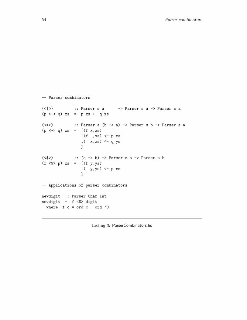
54 Parser combinators
-- Parser combinators
(<|>) :: Parser s a -> Parser s a -> Parser s a(p <|> q) xs = p xs ++ q xs
(<*>) :: Parser s (b -> a) -> Parser s b -> Parser s a(p <*> q) xs = [(f x,zs)
|(f ,ys) <- p xs,( x,zs) <- q ys]
(<$>) :: (a -> b) -> Parser s a -> Parser s b(f <$> p) xs = [(f y,ys)
|( y,ys) <- p xs]
-- Applications of parser combinators
newdigit :: Parser Char Intnewdigit = f <$> digit
where f c = ord c - ord ’0’
Listing 3: ParserCombinators.hs
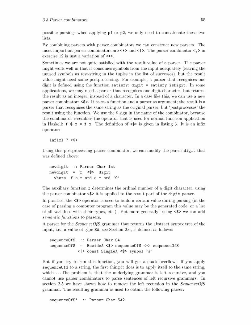
3.3 Parser combinators 55
possible parsings when applying p1 or p2, we only need to concatenate these twolists.By combining parsers with parser combinators we can construct new parsers. Themost important parser combinators are <*> and <|>. The parser combinator <,> inexercise 12 is just a variation of <*>.Sometimes we are not quite satisfied with the result value of a parser. The parsermight work well in that it consumes symbols from the input adequately (leaving theunused symbols as rest-string in the tuples in the list of successes), but the resultvalue might need some postprocessing. For example, a parser that recognises onedigit is defined using the function satisfy: digit = satisfy isDigit. In someapplications, we may need a parser that recognises one digit character, but returnsthe result as an integer, instead of a character. In a case like this, we can use a newparser combinator: <$>. It takes a function and a parser as argument; the result is aparser that recognises the same string as the original parser, but ‘postprocesses’ theresult using the function. We use the $ sign in the name of the combinator, becausethe combinator resembles the operator that is used for normal function applicationin Haskell: f $ x = f x. The definition of <$> is given in listing 3. It is an infixoperator:
infixl 7 <$>
Using this postprocessing parser combinator, we can modify the parser digit thatwas defined above:
newdigit :: Parser Char Intnewdigit = f <$> digit
where f c = ord c - ord ’0’
The auxiliary function f determines the ordinal number of a digit character; usingthe parser combinator <$> it is applied to the result part of the digit parser.In practice, the <$> operator is used to build a certain value during parsing (in thecase of parsing a computer program this value may be the generated code, or a listof all variables with their types, etc.). Put more generally: using <$> we can addsemantic functions to parsers.A parser for the SequenceOfS grammar that returns the abstract syntax tree of theinput, i.e., a value of type SA, see Section 2.6, is defined as follows:
sequenceOfS :: Parser Char SAsequenceOfS = BesideA <$> sequenceOfS <*> sequenceOfS
<|> const SingleA <$> symbol ’s’
But if you try to run this function, you will get a stack overflow! If you applysequenceOfS to a string, the first thing it does is to apply itself to the same string,which . . . The problem is that the underlying grammar is left recursive, and youcannot use parser combinators to parse sentences of left recursive grammars. Insection 2.5 we have shown how to remove the left recursion in the SequenceOfSgrammar. The resulting grammar is used to obtain the following parser:
sequenceOfS’ :: Parser Char SA2

56 Parser combinators
sequenceOfS’ =const ConsZ <$> symbol ’s’ <*> parseZ
<|> const SingleS <$> symbol ’s’where parseZ = ConsSA2 <$> sequenceOfS’ <*> parseZ
<|> SingleSA2 <$> sequenceOfS’
This example is a direct translation of the grammar obtained by using the removingleft recursion grammar transformation. There exists a much simpler parser forparsing sequences of s’s.
Exercise 3.4 . Prove that for all f :: a -> b
f <$> succeed a = succeed (f a)
In the sequel we will often use this rule for constant functions f, i.e. f = \a -> c,where c is a value that does not contain a. /
Exercise 3.5 . Consider the parser list <$> symbol ’a’, where list a as = a:as. Give itstype and show its results on inputs [] and x:xs. /
Exercise 3.6 . Consider the parser list <$> symbol ’a’ <*> p. Give its type and show itsresults on inputs [] and x:xs. /
Exercise 3.7 . Define a parser for Booleans. /
Exercise 3.8 . Define parsers for each of the basic languages defined in section 2.3.1. /Exercise 3.9 . Consider the grammar for palindromes that you have constructed in exercise
2.7.
1. Give the datatype Pal2 that corresponds to this grammar.
2. Define a parser palin2 that returns parse trees for palindromes. Test yourfunction with the palindromes cPal1 = "abaaba" and cPal2 = "baaab". Com-pare the results with your answer to exercise 2.16.
3. Define a parser palina that counts the number of a’s occurring in a palin-drome.
/
Exercise 3.10 . Consider the grammar for a part of the English language that is given inexercise 2.46.
1. Give the datatype English that corresponds to this grammar.
2. Define a parser english that returns parse trees for the English language.Test your function with the sentence they are flying planes. Comparethe result to your answer of exercise 2.46.
/
Exercise 3.11 . When defining the priority of the <|> operator with the infixr keyword, wealso specified that the operator associates to the right. Why is this a better choicethan association to the left? /
3.3 Parser combinators 57
Exercise 3.12 . Define a parser combinator <,> that combines two parsers. The value returnedby the combined parser is a tuple containing the results of the two componentparsers. What is the type of this parser combinator? /
Exercise 3.13 . The term ‘parser combinator’ is in fact not an adequate description for <$>.Can you think of a better word? /
Exercise 3.14 . Compare the type of <$> with the type of the standard function map. Can youdescribe your observations in an easy-to-remember, catchy phrase? /
Exercise 3.15 . Define <*> in terms of <,> and <$>. Define <,> in terms of <*> and <$>. /
Exercise 3.16 . If you examine the definitions of <*> and <$> in listing 3, you can observe that<$> is in a sense a special case of <*>. Can you define <$> in terms of <*>? /
3.3.1 Matching parentheses: an example
Using parser combinators, it is often fairly straightforward to construct a parser fora language for which you have a grammar. Consider, for example, the grammar thatyou wrote in exercise 2.44:
S → ( S ) S | ε
This grammar can be directly translated to a parser, using the parser combinators<*> and <|>. We use <*> when symbols are written next to each other, and <|>when | appears in a production (or when there is more than one production for anonterminal).
parens :: Parser Char ???parens = symbol ’(’ <*> parens <*> symbol ’)’ <*> parens
<|> epsilon
However, this function is not correctly typed: the parsers in the first alternativecannot be composed using <*>, as for example symbol ’(’ is not a parser returninga function.But we can postprocess the parser symbol ’(’ so that, instead of a character, thisparser does return a function. So, what function should we use? This dependson the kind of value that we want as a result of the parser. A nice result wouldbe a tree-like description of the parentheses that are parsed. For this purpose weintroduce an abstract syntax, see Section 2.6, for the parentheses grammar. A firstabstract syntax is given by the datatype Parentheses1.
data Parentheses1 = Match1 Char Parentheses1 Char Parentheses1| Empty1
For example, the sentence ()() is represented by
Match1 ’(’ Empty1 ’)’ (Match1 ’(’ Empty1 ’)’ Empty1)
Suppose we want to calculate the number of parentheses in a sentence. The numberof parentheses is calculated by the function nrofpars, which is defined by inductionon the datatype Parentheses1.
58 Parser combinators
data Parentheses = Match Parentheses Parentheses| Emptyderiving Show
open = symbol ’(’close = symbol ’)’
parens :: Parser Char Parenthesesparens = f <$> open <*> parens <*> close <*> parens
<|> succeed Emptywhere f a b c d = Match b d
nesting :: Parser Char Intnesting = f <$> open <*> nesting <*> close <*> nesting
<|> succeed 0where f a b c d = max (1+b) d
Listing 4: ParseParentheses.hs
nrofpars :: Parentheses1 -> Intnrofpars (Match1 cl pl cr pr) = nrofpars pl + nrofpars pr + 2nrofpars Empty1 = 0
Since the values cl and cr in the case for Match1 are not used (and should neverbe used) by functions defined on Parentheses1, we use the following datatype forthe abstract syntax for the grammar of parentheses.
data Parentheses = Match Parentheses Parentheses| Empty
Now we can add ‘semantic functions’ to the parser. Thus, we get the definition ofparens in listing 4.By varying the function used before <$> (the ‘semantic function’), we can returnother things than parse trees. As an example we construct a parser that calculatesthe nesting depth of nested parentheses, see the function nesting defined in listing 4.A session in which nesting is used may look like this:
? nesting "()(())()"[(2,[]), (2,"()"), (1,"(())()"), (0,"()(())()")]? nesting "())"[(1,")"), (0,"())")]
As you can see, when there is a syntax error in the argument, there are no solutionswith empty rest string. It is fairly simple to test whether a given string belongs tothe language that is parsed by a given parser.
Exercise 3.17 .What is the type of the function f which appears in function parens in listing 4?What is the type of the parser open? Using the type of <$>, what is the type off <$> open ? Can f <$> open be used as a left hand side of <*> parens? Whatis the type of the result? /
3.4 More parser combinators 59
Exercise 3.18 . What is a convenient way for <*> to associate? Does it? /
Exercise 3.19 . Write a function test that determines whether or not a given string belongsto the language parsed by a given parser. /
3.4 More parser combinators
In principle you can build parsers for any context-free language using the combina-tors <*> and <|>, but in practice it is easier to have some more parser combinatorsavailable. In traditional grammar formalisms, additional symbols are used to de-scribe for example optional or repeated constructions. Consider for example theBNF formalism, in which originally only sequential and alternative composition canbe used (denoted by juxtaposition and vertical bars, respectively), but which waslater extended to EBNF to also allow for repetition, denoted by a star. The goal ofthis section is to show how the set of parser combinators can be extended.
3.4.1 Parser combinators for EBNF
It is very easy to make new parser combinators for EBNF. As a first example weconsider repetition. Given a parser for a construction, many constructs a parser forzero or more occurrences of that construction:
many :: Parser s a -> Parser s [a]many p = list <$> p <*> many p
<|> succeed []
So the EBNF expression P ∗ is implemented by many P. The auxiliary function listtakes an element and a list, and combines them in a simple list:
list x xs = x:xs
So list is just (:), and we might have written that in the definition of many, butthen the definition might have looked too cryptic at first sight.The order in which the alternatives are given only influences the order in whichsolutions are placed in the list of successes.For example, the many combinator can be used in parsing a natural number:
natural :: Parser Char Intnatural = foldl f 0 <$> many newdigit
where f a b = a*10 + b
Defined in this way, the natural parser also accepts empty input as a number. Ifthis is not desired, we had better use the many1 parser combinator, which acceptsone or more occurrences of a construction, and corresponds to the EBNF expressionP+, see Section 2.7. It is defined in listing 5.Another combinator from EBNF is the option combinator P?. It takes a parser asargument, and returns a parser that recognises the same construct, but which alsosucceeds if that construct is not present in the input string. The definition is given
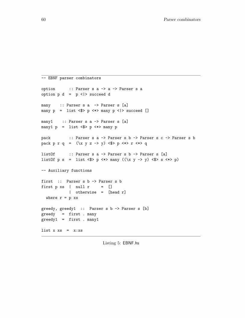
60 Parser combinators
-- EBNF parser combinators
option :: Parser s a -> a -> Parser s aoption p d = p <|> succeed d
many :: Parser s a -> Parser s [a]many p = list <$> p <*> many p <|> succeed []
many1 :: Parser s a -> Parser s [a]many1 p = list <$> p <*> many p
pack :: Parser s a -> Parser s b -> Parser s c -> Parser s bpack p r q = (\x y z -> y) <$> p <*> r <*> q
listOf :: Parser s a -> Parser s b -> Parser s [a]listOf p s = list <$> p <*> many ((\x y -> y) <$> s <*> p)
-- Auxiliary functions
first :: Parser s b -> Parser s bfirst p xs | null r = []
| otherwise = [head r]where r = p xs
greedy, greedy1 :: Parser s b -> Parser s [b]greedy = first . manygreedy1 = first . many1
list x xs = x:xs
Listing 5: EBNF.hs
3.4 More parser combinators 61
in listing 5. It has an additional argument: the value that should be used as resultin case the construct is not present. It is a kind of ‘default’ value.By the use of the option and many functions, a large amount of backtracking possi-bilities are introduced. This is not always advantageous. For example, if we definea parser for identifiers by
identifier = many1 (satisfy isAlpha)
a single word may also be parsed as two identifiers. Caused by the order of thealternatives in the definition of many (succeed [] appears as the second alternative),the ‘greedy’ parsing, which accumulates as many letters as possible in the identifieris tried first, but if parsing fails elsewhere in the sentence, also less greedy parsingsof the identifier are tried – in vain. You will give a better definition of identifierin Exercise 3.26.In situations where from the way the grammar is built we can predict that it ishopeless to try non-greedy results of many, we can define a parser transformer first,that transforms a parser into a parser that only returns the first possible parsing.It does so by taking the first element of the list of successes.
first :: Parser a b -> Parser a bfirst p xs | null r = []
| otherwise = [head r]where r = p xs
Using this function, we can create a special ‘take all or nothing’ version of many:
greedy = first . manygreedy1 = first . many1
If we compose the first function with the option parser combinator:
obligatory p d = first (option p d)
we get a parser which must accept a construction if it is present, but which does notfail if it is not present.
3.4.2 Separators
The combinators many, many1 and option are classical in compiler constructions —there are notations for it in EBNF (*, + and ?, respectively)—, but there is no needto leave it at that. For example, in many languages constructions are frequentlyenclosed between two meaningless symbols, most often some sort of parentheses.For this case we design a parser combinator pack. Given a parser for an openingtoken, a body, and a closing token, it constructs a parser for the enclosed body, asdefined in listing 5. Special cases of this combinator are:
parenthesised p = pack (symbol ’(’) p (symbol ’)’)bracketed p = pack (symbol ’[’) p (symbol ’]’)compound p = pack (token "begin") p (token "end")

62 Parser combinators
-- Chain expression combinators
chainr :: Parser s a -> Parser s (a -> a -> a) -> Parser s achainr pe po = h <$> many (j <$> pe <*> po) <*> pe
where j x op = (x ‘op‘)h fs x = foldr ($) x fs
chainl :: Parser s a -> Parser s (a -> a -> a) -> Parser s achainl pe po = h <$> pe <*> many (j <$> po <*> pe)
where j op x = (‘op‘ x)h x fs = foldl (flip ($)) x fs
Listing 6: Chains.hs
Another frequently occurring construction is repetition of a certain construction,where the elements are separated by some symbol. You may think of lists of ar-guments (expressions separated by commas), or compound statements (statementsseparated by semicolons). For the parse trees, the separators are of no importance.The function listOf below generates a parser for a (possibly empty) list, given aparser for the items and a parser for the separators:
listOf :: Parser s a -> Parser s b -> Parser s [a]listOf p s = list <$> p <*> many ((\x y -> y) <$> s <*> p )
Useful instantiations are:
commaList, semicList :: Parser Char a -> Parser Char [a]commaList p = listOf p (symbol ’,’)semicList p = listOf p (symbol ’;’)
A somewhat more complicated variant of the function listOf is the case where theseparators carry a meaning themselves. For example, in arithmetical expressions,where the operators that separate the subexpressions have to be part of the parsetree. For this case we will develop the functions chainr and chainl. These functionsexpect that the parser for the separators returns a function (!); that function is usedby chain to combine parse trees for the items. In the case of chainr the operator isapplied right-to-left, in the case of chainl it is applied left-to-right. The functionschainr and chainl are defined in listing 6 (remember that $ is function application:f $ x = f x).The definitions look quite complicated, but when you look at the underlying gram-mar they are quite straightforward. Suppose we apply operator ⊕ (⊕ is an operatorvariable, it denotes an arbitrary right-associative operator) from right to left, so
e1 ⊕ e2 ⊕ e3 ⊕ e4=e1 ⊕ (e2 ⊕ (e3 ⊕ e4))
=((e1⊕) · (e2⊕) · (e3⊕)) e4
3.4 More parser combinators 63
It follows that we can parse such expressions by parsing many pairs of expressionsand operators, turning them into functions, and applying all those functions to thelast expression. This is done by function chainr, see listing 6.If operator ⊕ is applied from left to right, then
e1 ⊕ e2 ⊕ e3 ⊕ e4=
((e1 ⊕ e2)⊕ e3)⊕ e4=
((⊕e4) · (⊕e3) · (⊕e2)) e1
So such an expression can be parsed by first parsing a single expression (e1), andthen parsing many pairs of operators and expressions, turning them into functions,and applying all those functions to the first expression. This is done by functionchainl, see listing 6.Functions chainl and chainr can be made more efficient by avoiding the construc-tion of the intermediate list of functions. The resulting definitions can be found in[5].Note that functions chainl and chainr are very similar, the only difference is thateverything is ‘turned around’: function j of chainr takes a value and an operator,and returns the function obtained by ‘left’ applying the operator; function j ofchainl takes an operator and a value, and returns the function obtained by ‘right’applying the operator to the value. Such functions are sometimes called dual. dual
Exercise 3.20 . What is the value of
many (symbol ’a’) xs
for xs ∈ [],[’a’],[’b’],[’a’,’b’],[’a’,’a’,’b’]? /
Exercise 3.21 . Consider the application of the parser many (symbol ’a’) to the string "aaa".In what order do the four possible parsings appear in the list of successes? /
Exercise 3.22 . Using the parser combinators option, many and many1 define parsers for eachof the basic languages defined in 2.3.1. /
Exercise 3.23 . As another variation on the theme ‘repetition’, define a parser combinatorpsequence that transforms a list of parsers for some type into a parser returninga list of elements of that type. What is the type of psequence? Also define acombinator choice that iterates the operator <|>. /
Exercise 3.24 . As an application of psequence, define the function token that was discussedin Section 3.2. /
Exercise 3.25 . Carefully analyse the semantic functions in the definition of chainl in listing 6./
Exercise 3.26 . In real programming languages, identifiers follow more flexible rules: the firstsymbol must be a letter, but the symbols that follow (if any) may be a letter, digit,or underscore symbol. Define a more realistic parser identifier. /
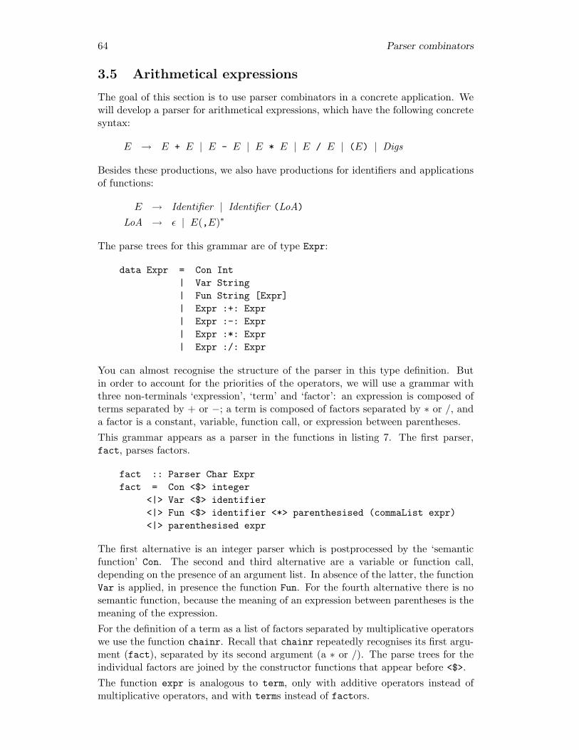
64 Parser combinators
3.5 Arithmetical expressions
The goal of this section is to use parser combinators in a concrete application. Wewill develop a parser for arithmetical expressions, which have the following concretesyntax:
E → E + E | E - E | E * E | E / E | (E) | Digs
Besides these productions, we also have productions for identifiers and applicationsof functions:
E → Identifier | Identifier (LoA)LoA → ε | E(,E)∗
The parse trees for this grammar are of type Expr:
data Expr = Con Int| Var String| Fun String [Expr]| Expr :+: Expr| Expr :-: Expr| Expr :*: Expr| Expr :/: Expr
You can almost recognise the structure of the parser in this type definition. Butin order to account for the priorities of the operators, we will use a grammar withthree non-terminals ‘expression’, ‘term’ and ‘factor’: an expression is composed ofterms separated by + or −; a term is composed of factors separated by ∗ or /, anda factor is a constant, variable, function call, or expression between parentheses.This grammar appears as a parser in the functions in listing 7. The first parser,fact, parses factors.
fact :: Parser Char Exprfact = Con <$> integer
<|> Var <$> identifier<|> Fun <$> identifier <*> parenthesised (commaList expr)<|> parenthesised expr
The first alternative is an integer parser which is postprocessed by the ‘semanticfunction’ Con. The second and third alternative are a variable or function call,depending on the presence of an argument list. In absence of the latter, the functionVar is applied, in presence the function Fun. For the fourth alternative there is nosemantic function, because the meaning of an expression between parentheses is themeaning of the expression.For the definition of a term as a list of factors separated by multiplicative operatorswe use the function chainr. Recall that chainr repeatedly recognises its first argu-ment (fact), separated by its second argument (a ∗ or /). The parse trees for theindividual factors are joined by the constructor functions that appear before <$>.The function expr is analogous to term, only with additive operators instead ofmultiplicative operators, and with terms instead of factors.

3.5 Arithmetical expressions 65
-- Type definition for parse tree
data Expr = Con Int| Var String| Fun String [Expr]| Expr :+: Expr| Expr :-: Expr| Expr :*: Expr| Expr :/: Expr
--------------------------------------------------------------- Parser for expressions with two priorities
fact :: Parser Char Exprfact = Con <$> integer
<|> Var <$> identifier<|> Fun <$> identifier <*> parenthesised (commaList expr)<|> parenthesised expr
integer :: Parser Char Intinteger = (const negate <$> (symbol ’-’)) ‘option‘ id <*> natural
term :: Parser Char Exprterm = chainr fact
( const (:*:) <$> symbol ’*’<|> const (:/:) <$> symbol ’/’)
expr :: Parser Char Exprexpr = chainr term
( const (:+:) <$> symbol ’+’<|> const (:-:) <$> symbol ’-’)
Listing 7: ExpressionParser.hs

66 Parser combinators
This example clearly shows the strength of parsing with parser combinators. There isno need for a separate formalism for grammars; the production rules of the grammarare combined with higher-order functions. Also, there is no need for a separateparser generator (like ‘yacc’); the functions can be viewed both as description of thegrammar and as an executable parser.
Exercise 3.27 . Modify the functions in listing 7, in such a way that + is parsed as a rightassociative operator, and − is parsed as a left associative operator. /
3.6 Generalised expressions
This section generalises the parser in the previous section with respect to priorities.Arithmetical expressions in which operators have more than two levels of prioritycan be parsed by writing more auxiliary functions between term and expr. Thefunction chainr is used in each definition, with as first argument the function ofone priority level lower.If there are nine levels of priority, we obtain nine copies of almost the same text.This is not as it should be. Functions that resemble each other are an indicationthat we should write a generalised function, where the differences are described usingextra arguments. Therefore, let us inspect the differences in the definitions of termand expr again. These are:
• The operators and associated tree constructors that are used in the secondargument of chainr
• The parser that is used as first argument of chainr
The generalised function will take these two differences as extra arguments: the firstin the form of a list of pairs, the second in the form of a parse function:
type Op a = (Char,a -> a -> a)
gen :: [Op a] -> Parser Char a -> Parser Char agen ops p = chainr p (choice (map f ops))
where f (s,c) = const c <$> symbol s
If furthermore we define as shorthand:
multis = [ (’*’,(:*:)), (’/’,(:/:)) ]addis = [ (’+’,(:+:)), (’-’,(:-:)) ]
then expr and term can be defined as partial parametrisations of gen:
expr = gen addis termterm = gen multis fact
By expanding the definition of term in that of expr we obtain:
expr = addis ‘gen‘ (multis ‘gen‘ fact)
which an experienced functional programmer immediately recognises as an applica-tion of foldr:

3.7 Exercises 67
-- Parser for expressions with aribitrary many priorities
type Op a = (Char,a -> a -> a)
fact’ :: Parser Char Exprfact’ = Con <$> integer
<|> Var <$> identifier<|> Fun <$> identifier <*> parenthesised (commaList expr’)<|> parenthesised expr’
gen :: [Op a] -> Parser Char a -> Parser Char agen ops p = chainr p (choice (map f ops))
where f (s,c) = const c <$> symbol s
expr’ :: Parser Char Exprexpr’ = foldr gen fact’ [addis, multis]
multis = [ (’*’,(:*:)), (’/’,(:/:)) ]addis = [ (’+’,(:+:)), (’-’,(:-:)) ]
Listing 8: GExpressionParser.hs
expr = foldr gen fact [addis, multis]
From this definition a generalisation to more levels of priority is simply a matter ofextending the list of operator-lists.The very compact formulation of the parser for expressions with an arbitrary numberof priority levels is possible because the parser combinators can be used together withthe existing mechanisms for generalisation and partial parametrisation in Haskell.Contrary to conventional approaches, the levels of priority need not be coded expli-citly with integers. The only thing that matters is the relative position of an operatorin the list of ‘list with operators of the same priority’. Also, the insertion of newpriority levels is very easy. The definitions are summarised in listing 8.
summary
This chapter shows how to construct parsers from simple combinators. It showshow a small parser combinator library can be a powerful tool in the construction ofparsers. Furthermore, this chapter gives a rather basic implementation of the parsercombinator library. More advanced implementations are discussed elsewhere.
3.7 Exercises
Exercise 3.28 . Prove the following laws
1. h <$> (f <$> p) = (h.f) <$> p

68 Parser combinators
2. h <$> (p <|> q) = (h <$> p) <|> (h <$> q)
3. h <$> (p <*> q) = ((h.) <$> p) <*> q
/
Exercise 3.29 . Consider your answer to exercise 2.22. Define a combinator parser pMir thattransforms a concrete representation of a mirror-palindrome into an abstract one.Test your function with the concrete mirror-palindromes cMir1 and cMir2. /
Exercise 3.30 . Consider your answer to exercise 2.24. Assuming the comma is an associativeoperator, we can give the following abstract syntax for bit-lists:
data BitList = SingleB Bit | ConsB Bit BitList
Define a combinator parser pBitList that transforms a concrete representation of abit-list into an abstract one. Test your function with the concrete bit-lists cBitList1and cBitList2. /
Exercise 3.31 .Define a parser for fixed-point numbers, that is numbers like 12.34 and−123.456.Also integers are acceptable. Notice that the part following the decimal point lookslike an integer, but has a different semantics! /
Exercise 3.32 . Define a parser for floating point numbers, which are fixed point numbersfollowed by an optional E and an (positive or negative, integer) exponent. /
Exercise 3.33 . Define a parser for Java assignments that consist of a variable, an = sign, anexpression and a semicolon. /
Exercise 3.34 . Define a parser for (simplified) Java statements. /Exercise 3.35 . Outline the construction of a parser for Java programs. /

Chapter 4
Grammar and Parser design
The previous chapters have introduced many concepts related to grammars andparsers. The goal of this chapter is to review these concepts, and to show how theyare used in the design of grammars and parsers.The design of a grammar and parser for a language consists of several steps: youhave to
1. give a grammar for the language for which you want to have a parser;
2. analyse this grammar to find out whether or not it has some desirable prop-erties;
3. possibly transform the grammar to obtain some of these desirable properties;
4. decide on the type of the parser: Parser a b, that is, decide on both theinput type a of the parser (which may be the result type of a scanner), andthe result type b of the parser.
5. construct a basic parser;
6. add semantic functions;
7. check whether or not you have obtained what you expected.
We will describe and exemplify each of these steps in detail in the rest of this section.As a running example we will construct a grammar and parser for travelling schemesfor day trips, of the following form:
Groningen 8:37 9:44 Zwolle 9:49 10:15 Utrecht 10:21 11:05 Den Haag
We might want to do several things with such a schema, for example:
1. compute the net travel time, i.e. the travel time minus the waiting time (2hours and 17 minutes in the above example);
2. compute the total time one has to wait on the intermediate stations (11 min-utes).
This chapter defines functions to perform these computations.
69
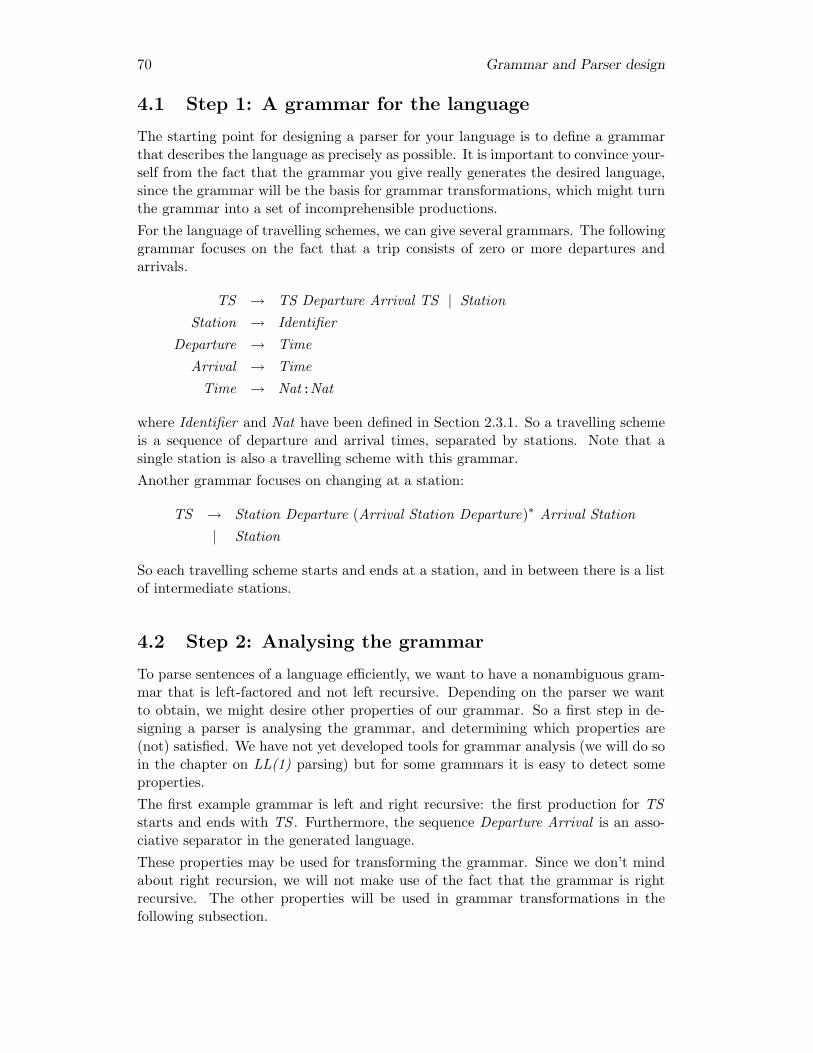
70 Grammar and Parser design
4.1 Step 1: A grammar for the language
The starting point for designing a parser for your language is to define a grammarthat describes the language as precisely as possible. It is important to convince your-self from the fact that the grammar you give really generates the desired language,since the grammar will be the basis for grammar transformations, which might turnthe grammar into a set of incomprehensible productions.For the language of travelling schemes, we can give several grammars. The followinggrammar focuses on the fact that a trip consists of zero or more departures andarrivals.
TS → TS Departure Arrival TS | StationStation → Identifier
Departure → TimeArrival → Time
Time → Nat:Nat
where Identifier and Nat have been defined in Section 2.3.1. So a travelling schemeis a sequence of departure and arrival times, separated by stations. Note that asingle station is also a travelling scheme with this grammar.Another grammar focuses on changing at a station:
TS → Station Departure (Arrival Station Departure)∗ Arrival Station| Station
So each travelling scheme starts and ends at a station, and in between there is a listof intermediate stations.
4.2 Step 2: Analysing the grammar
To parse sentences of a language efficiently, we want to have a nonambiguous gram-mar that is left-factored and not left recursive. Depending on the parser we wantto obtain, we might desire other properties of our grammar. So a first step in de-signing a parser is analysing the grammar, and determining which properties are(not) satisfied. We have not yet developed tools for grammar analysis (we will do soin the chapter on LL(1) parsing) but for some grammars it is easy to detect someproperties.The first example grammar is left and right recursive: the first production for TSstarts and ends with TS . Furthermore, the sequence Departure Arrival is an asso-ciative separator in the generated language.These properties may be used for transforming the grammar. Since we don’t mindabout right recursion, we will not make use of the fact that the grammar is rightrecursive. The other properties will be used in grammar transformations in thefollowing subsection.

4.3 Step 3: Transforming the grammar 71
4.3 Step 3: Transforming the grammar
Since the sequence Departure Arrival is an associative separator in the generatedlanguage, the productions for TS may be transformed into:
TS → Station | Station Departure Arrival TS (4.1)
Thus we have removed the left recursion in the grammar. Both productions forTS start with the nonterminal Station, so TS can be left factored. The resultingproductions are:
TS → Station ZZ → ε | Departure Arrival TS
We can also apply equivalence (2.1) to the two productions for TS from (4.1), andobtain the following single production:
TS → (Station Departure Arrival)∗ Station (4.2)
So which productions do we take for TS? This depends on what we want to do withthe parsed sentences. We will show several choices in the next section.
4.4 Step 4: Deciding on the types
We want to write a parser for travel schemes, that is, we want to write a functionts of type
ts :: Parser ? ?
The question marks should be replaced by the input type and the result type, re-spectively. For the input type we can choose between at least two possibilities:characters, Char or tokens Token. The type of tokens can be chosen as follows:
data Token = Station_Token Station | Time_Token Time
type Station = Stringtype Time = (Int,Int)
We will construct a parser for both input types in the next subsection. So ts hasone of the following two types.
ts :: Parser Char ?ts :: Parser Token ?
For the result type we have many choices. If we just want to compute the totaltravelling time, Int suffices for the result type. If we want to compute the totaltravelling time, the total waiting time, and a nicely printed version of the travellingscheme, we may do several things:
• define three parsers, with Int (total travelling time), Int (total waiting time),and String (nicely printed version) as result type, respectively;

72 Grammar and Parser design
• define a single parser with the triple (Int,Int,String) as result type;
• define an abstract syntax for travelling schemes, say a datatype TS, and definethree functions on TS that compute the desired results.
The first alternative parses the input three times, and is rather inefficient comparedwith the other alternatives. The second alternative is hard to extend if we wantto compute something extra, but in some cases it might be more efficient than thethird alternative. The third alternative needs an abstract syntax. There are severalways to define an abstract syntax for travelling schemes. The first abstract syntaxcorresponds to definition (4.1) of grammar TS .
data TS1 = Single1 Station| Cons1 Station Time Time TS1
where Station and Time are defined above. A second abstract syntax correspondsto the grammar for travelling schemes defined in (4.2).
type TS2 = ([(Station,Time,Time)],Station)
So a travelling scheme is a tuple, the first component of which is a list of triplesconsisting of a departure station, a departure time, and an arrival time, and thesecond component of which is the final arrival station. A third abstract syntaxcorresponds to the second grammar defined in Section 4.1:
data TS3 = Single3 Station| Cons3 (Station,Time,[(Time,Station,Time)],Time,Station)
Which abstract syntax should we take? Again, this depends on what we want to dowith the abstract syntax. Since TS2 and TS1 combine departure and arrival times ina tuple, they are convenient to use when computing travelling times. TS3 is usefulwhen we want to compute waiting times since it combines arrival and departuretimes in one constructor. Often we want to exactly mimic the productions of thegrammar in the abstract syntax, so if we use (4.1) for the grammar for travellingschemes, we use TS1 for the abstract syntax. Note that TS1 is a datatype, whereasTS2 is a type. TS1 cannot be defined as a type because of the two alternativeproductions for TS . TS2 can be defined as a datatype by adding a constructor.Types and datatypes each have their advantages and disadvantages; the applicationdetermines which to use. The result type of the parsing function ts may be one oftypes mentioned earlier (Int, etc.), or one of TS1, TS2, TS3.
4.5 Step 5: Constructing the basic parser
Converting a grammar to a parser is a mechanical process that consists of a setof simple replacement rules. Functional programming languages offer some extraflexibility that we sometimes use, but usually writing a parser is a simple translation.We use the following replacement rules.
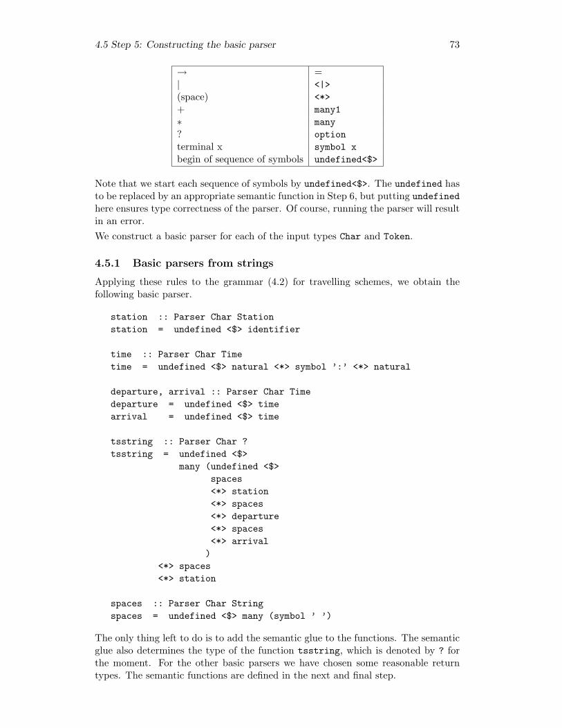
4.5 Step 5: Constructing the basic parser 73
→ =| <|>(space) <*>+ many1∗ many? optionterminal x symbol xbegin of sequence of symbols undefined<$>
Note that we start each sequence of symbols by undefined<$>. The undefined hasto be replaced by an appropriate semantic function in Step 6, but putting undefinedhere ensures type correctness of the parser. Of course, running the parser will resultin an error.We construct a basic parser for each of the input types Char and Token.
4.5.1 Basic parsers from strings
Applying these rules to the grammar (4.2) for travelling schemes, we obtain thefollowing basic parser.
station :: Parser Char Stationstation = undefined <$> identifier
time :: Parser Char Timetime = undefined <$> natural <*> symbol ’:’ <*> natural
departure, arrival :: Parser Char Timedeparture = undefined <$> timearrival = undefined <$> time
tsstring :: Parser Char ?tsstring = undefined <$>
many (undefined <$>spaces<*> station<*> spaces<*> departure<*> spaces<*> arrival)
<*> spaces<*> station
spaces :: Parser Char Stringspaces = undefined <$> many (symbol ’ ’)
The only thing left to do is to add the semantic glue to the functions. The semanticglue also determines the type of the function tsstring, which is denoted by ? forthe moment. For the other basic parsers we have chosen some reasonable returntypes. The semantic functions are defined in the next and final step.
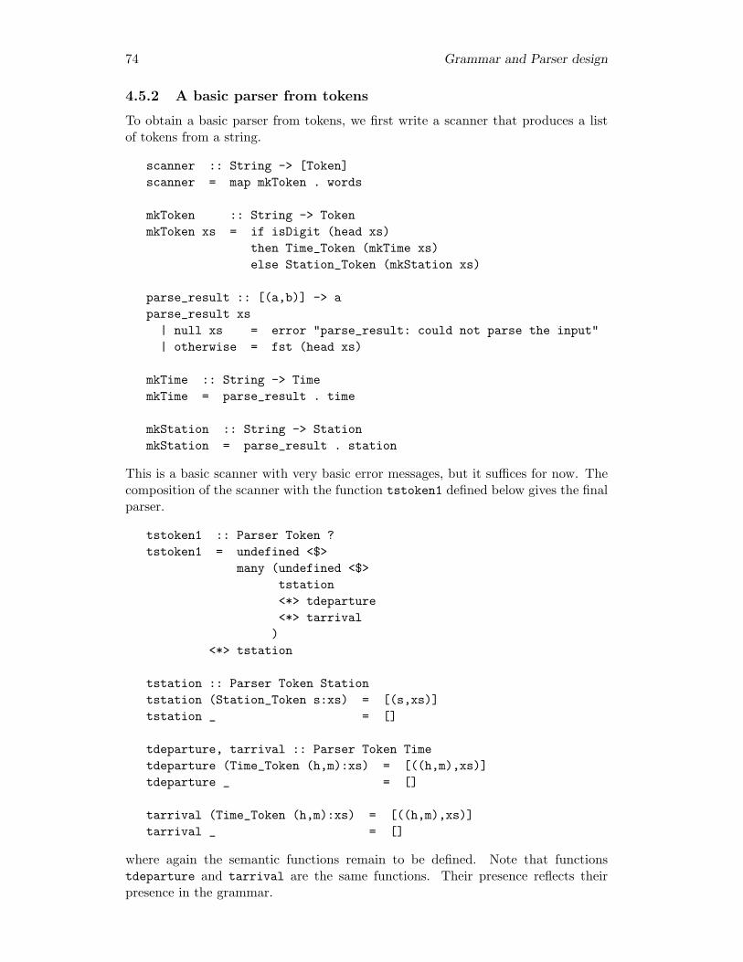
74 Grammar and Parser design
4.5.2 A basic parser from tokens
To obtain a basic parser from tokens, we first write a scanner that produces a listof tokens from a string.
scanner :: String -> [Token]scanner = map mkToken . words
mkToken :: String -> TokenmkToken xs = if isDigit (head xs)
then Time_Token (mkTime xs)else Station_Token (mkStation xs)
parse_result :: [(a,b)] -> aparse_result xs
| null xs = error "parse_result: could not parse the input"| otherwise = fst (head xs)
mkTime :: String -> TimemkTime = parse_result . time
mkStation :: String -> StationmkStation = parse_result . station
This is a basic scanner with very basic error messages, but it suffices for now. Thecomposition of the scanner with the function tstoken1 defined below gives the finalparser.
tstoken1 :: Parser Token ?tstoken1 = undefined <$>
many (undefined <$>tstation<*> tdeparture<*> tarrival)
<*> tstation
tstation :: Parser Token Stationtstation (Station_Token s:xs) = [(s,xs)]tstation _ = []
tdeparture, tarrival :: Parser Token Timetdeparture (Time_Token (h,m):xs) = [((h,m),xs)]tdeparture _ = []
tarrival (Time_Token (h,m):xs) = [((h,m),xs)]tarrival _ = []
where again the semantic functions remain to be defined. Note that functionstdeparture and tarrival are the same functions. Their presence reflects theirpresence in the grammar.
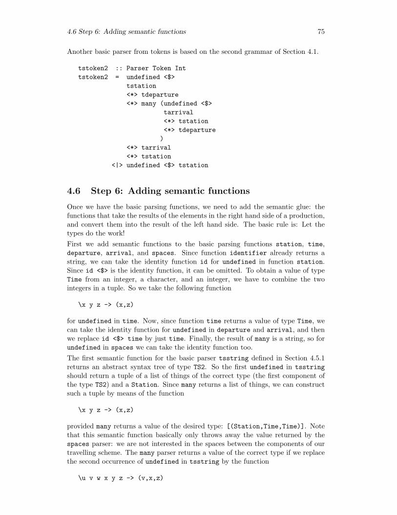
4.6 Step 6: Adding semantic functions 75
Another basic parser from tokens is based on the second grammar of Section 4.1.
tstoken2 :: Parser Token Inttstoken2 = undefined <$>
tstation<*> tdeparture<*> many (undefined <$>
tarrival<*> tstation<*> tdeparture
)<*> tarrival<*> tstation
<|> undefined <$> tstation
4.6 Step 6: Adding semantic functions
Once we have the basic parsing functions, we need to add the semantic glue: thefunctions that take the results of the elements in the right hand side of a production,and convert them into the result of the left hand side. The basic rule is: Let thetypes do the work!First we add semantic functions to the basic parsing functions station, time,departure, arrival, and spaces. Since function identifier already returns astring, we can take the identity function id for undefined in function station.Since id <$> is the identity function, it can be omitted. To obtain a value of typeTime from an integer, a character, and an integer, we have to combine the twointegers in a tuple. So we take the following function
\x y z -> (x,z)
for undefined in time. Now, since function time returns a value of type Time, wecan take the identity function for undefined in departure and arrival, and thenwe replace id <$> time by just time. Finally, the result of many is a string, so forundefined in spaces we can take the identity function too.The first semantic function for the basic parser tsstring defined in Section 4.5.1returns an abstract syntax tree of type TS2. So the first undefined in tsstringshould return a tuple of a list of things of the correct type (the first component ofthe type TS2) and a Station. Since many returns a list of things, we can constructsuch a tuple by means of the function
\x y z -> (x,z)
provided many returns a value of the desired type: [(Station,Time,Time)]. Notethat this semantic function basically only throws away the value returned by thespaces parser: we are not interested in the spaces between the components of ourtravelling scheme. The many parser returns a value of the correct type if we replacethe second occurrence of undefined in tsstring by the function
\u v w x y z -> (v,x,z)

76 Grammar and Parser design
Again, the results of spaces are thrown away. This completes a parser for travellingschemes.The next semantic functions we define compute the net travel time. To compute thenet travel time, we have to compute the travel time of each trip from a station to astation, and to add the travel times of all of these trips. We obtain the travel timeof a single trip if we replace the second occurrence of undefined by:
\u v w (xh,xm) y (zh,zm) -> (zh-xh)*60 + zm-xm
and Haskell’s prelude function sum sums these times, so for the first occurrence ofundefined we take:
\x y z -> sum x
The final set of semantic functions we define are used for computing the total waitingtime. Since the second grammar of Section 4.1 combines arrival times and departuretimes, we use a parser based on this grammar: the basic parser tstoken2. We haveto give definitions of the three undefined semantic functions. If a trip consists ofa single station, there is now waiting time, so the last occurrence of undefined isthe function const 0. The second occurrence of function undefined computes thewaiting time for one intermediate station:
\(uh,um) v (wh,wm) -> (wh-uh)*60 + wm-um
Finally, the first occurrence of undefined sums the list of waiting time obtained bymeans of the function that replaces the second occurrence of undefined:
\s t x y z -> sum x
4.7 Step 7: Did you get what you expected
In the last step you test your parser(s) to see whether or not you have obtainedwhat you expected, and whether or not you have made errors in the above process.
summary
This chapter describes the different steps that have to be considered in the designof a grammar and a language.
4.8 Exercises
Exercise 4.1 . Write a parser for Java float-literals. The EBNF grammar for float-literals isgiven by:
Digits → Digits Digit | DigitFloatLiteral → IntPart . FractPart? ExponentPart? FloatSuffix?
| . FractPart ExponentPart? FloatSuffix?| IntPart ExponentPart FloatSuffix?

4.8 Exercises 77
| IntPart ExponentPart? FloatSuffixIntPart → SignedInteger
FractPart → DigitsExponentPart → ExponentIndicator SignedIntegerSignedInteger → Sign? Digits
ExponentIndicator → e | ESign → + | −
FloatSuffix → f | F | d | D
To keep your parser simple, assume that all nonterminals, except for the nonterminalFloatLiteral , are represented by a String in the abstract syntax. /
Exercise 4.2 . Write a evaluator for Java float-literals (the float-suffix may be ignored). /
Exercise 4.3 . Up to the definition of the semantic functions, parsers constructed on a (fixed)abstract syntax have the same shape. Give this parsing scheme for Java float literals./

78 Grammar and Parser design
Chapter 5
Regular Languages
introduction
The first phase of a compiler takes an input program, and splits the input into alist of terminal symbols: keywords, identifiers, numbers, punctuation, etc. Reg-ular expressions are used for the description of the terminal symbols. A regulargrammar is a particular kind of context-free grammar that can be used to describeregular expressions. Finite-state automata can be used to recognise sentences ofregular grammars. This chapter discusses all of these concepts, and is organisedas follows. Section 5.1 introduces finite-state automata. Finite-state automata ap-pear in two versions, nondeterministic and deterministic ones. Section 5.1.4 showsthat a nondeterministic finite-state automaton can be transformed into a determin-istic finite-state automaton, so you don’t have to worry about whether or not yourautomaton is deterministic. Section 5.2 introduces regular grammars (context-freegrammars of a particular form), and regular languages. Furthermore, it shows theirequivalence with finite-state automata. Section 5.3 introduces regular expressions asfinite descriptions of regular languages and shows that such expressions are another,equivalent, tool for regular languages. Finally, Section 5.4 gives some of the proofsof the results of the previous sections.
goals
After you have studied this chapter you will know that
• regular languages are a subset of context-free languages;• it is not always possible to give a regular grammar for a context-free grammar;• regular grammars, finite-state automata and regular expressions are three dif-
ferent tools for regular languages;• regular grammars, finite-state automata and regular expressions have the same
expressive power;• finite-state automata appear in two, equally expressive, versions: deterministic
and nondeterministic.
5.1 Finite-state automata
The classical approach to recognising sentences from a regular language uses finite-state automata. A finite-state automaton can be viewed as a simple form of digital
79
80 Regular Languages
computer with only a finite number of states, no temporary storage, an input file butonly the possibility to read it, and a control unit which records the state transitions.A rather limited medium, but a useful tool in many practical subproblems. A finite-state automaton can easily be implemented by a function that takes time linear inthe length of its input, and constant space. This implies that problems that can besolved by means of a finite-state automaton, can be implemented by means of veryefficient programs.
5.1.1 Deterministic finite-state automata
Finite-state automata come in two flavours: deterministic and nondeterministic. Westart with a description of deterministic finite-state automata, the simplest form ofautomata.
Definition 1: Deterministic finite-state automaton, DFAA deterministic finite-state automaton (DFA) is a 5-tuple (X,Q, d, S, F ) wheredeter-
mi-nisticfinite-stateauto-maton
• X is the input alphabet,• Q is a finite set of states,• d :: Q→ X → Q is the state transition function,• S ∈ Q is the start state,• F ⊆ Q is the set of accepting states.
2
As an example, consider the DFA M0 = (X,Q, d, S, F ) with
X = {a, b, c}Q = {S,A,B,C}F = {C}
where state transition function d is defined by
d S a = C
d S b = A
d S c = S
d A a = B
d B c = C
For human beings, a finite-state automaton is more comprehensible in a graphicalrepresentation. The following representation is customary: states are depicted asthe nodes in a graph; accepting states get a double circle; start states are explicitlymentioned or indicated otherwise. The transition function is represented by theedges: whenever d Qi x is a state Qj , then there is an arrow labelled x from Qi
to Qj . The input alphabet is implicit in the labels. For automaton M0 above, thepictorial representation is:
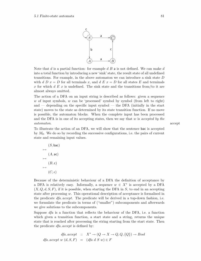
5.1 Finite-state automata 81
S?>=<89:;EDGFc@A
// a //
b
��
C?>=<89:;/.-,()*+
A?>=<89:; a // B?>=<89:;
c
OO
Note that d is a partial function: for example d B a is not defined. We can make dinto a total function by introducing a new ‘sink’ state, the result state of all undefinedtransitions. For example, in the above automaton we can introduce a sink state Dwith d D x = D for all terminals x, and d E x = D for all states E and terminalsx for which d E x is undefined. The sink state and the transitions from/to it arealmost always omitted.The action of a DFA on an input string is described as follows: given a sequencew of input symbols, w can be ‘processed’ symbol by symbol (from left to right)and — depending on the specific input symbol — the DFA (initially in the startstate) moves to the state as determined by its state transition function. If no moveis possible, the automaton blocks. When the complete input has been processedand the DFA is in one of its accepting states, then we say that w is accepted by theautomaton. acceptTo illustrate the action of an DFA, we will show that the sentence bac is acceptedby M0. We do so by recording the successive configurations, i.e. the pairs of currentstate and remaining input values.
(S, bac)7→
(A, ac)7→
(B, c)7→
(C, ε)
Because of the deterministic behaviour of a DFA the definition of acceptance bya DFA is relatively easy. Informally, a sequence w ∈ X∗ is accepted by a DFA(X,Q, d, S, F ), if it is possible, when starting the DFA in S, to end in an acceptingstate after processing w. This operational description of acceptance is formalised inthe predicate dfa accept . The predicate will be derived in a top-down fashion, i.e.we formulate the predicate in terms of (“smaller”) subcomponents and afterwardswe give solutions to the subcomponents.Suppose dfa is a function that reflects the behaviour of the DFA, i.e. a functionwhich given a transition function, a start state and a string, returns the uniquestate that is reached after processing the string starting from the start state. Thenthe predicate dfa accept is defined by:
dfa accept :: X∗ → (Q→ X → Q,Q, {Q})→ Bool
dfa accept w (d, S, F ) = (dfa d S w) ∈ F

82 Regular Languages
It remains to construct a definition of function dfa that takes a transition function,a start state, and a list of input symbols, and reflects the behaviour of a DFA. Thedefinition of dfa is straightforward
dfa :: (Q→ X → Q)→ Q→ X∗ → Qdfa d q ε = qdfa d q (ax) = dfa d (d q a) x
Note that both the type and the definition of dfa match the pattern of the functionfoldl , and it follows that we can write function dfa as a foldl .
dfa d q = foldl d q.
Definition 2: Acceptance by a DFAThe sequence w ∈ X∗ is accepted by DFA (X,Q, d, S, F ) if
dfa accept w (d, S, F )
where
dfa accept w (d, qs, fs) = dfa d qs w ∈ fsdfa d qs = foldl d qs
2
Using the predicate dfa accept , the language of a DFA is defined as follows.
Definition 3: Language of a DFAFor DFA M = (X,Q, d, S, F ), the language of M , Ldfa(M), is defined by
Ldfa(M) = {w ∈ X∗ | dfa accept w (d, S, F )}
2
5.1.2 Nondeterministic finite-state automata
This subsection introduces nondeterministic finite-state automata and defines theirsemantics, i.e. the language of a nondeterministic finite-state automaton.The transition function of a DFA returns a state, which implies that for all terminalsymbols x and for all states t there can only be one edge starting in t labelled withx. Sometimes it is convenient to have two or more edges labelled with the sameterminal symbol from a state. In these cases one can use a nondeterministic finite-state automaton. Nondeterministic finite state automata are defined as follows.
Definition 4: Nondeterministic finite-state automaton, NFAA nondeterministic finite-state automaton (NFA) is a 5-tuple (X,Q, d,Q0, F ), wherenonde-
termi-nisticfinite-stateauto-maton
• X is the input alphabet,• Q is a finite set of states,• d :: Q→ X → {Q} is the state transition function,

5.1 Finite-state automata 83
• Q0 ⊆ Q is the set of start states,• F ⊆ Q is the set of accepting states.
2
An NFA differs from a DFA in that there may be more than one start state and thatthere may be more than one possible move for each state and input symbol. Hereis an example of an NFA:
S?>=<89:;EDGFc@A
// a //
b
��
C?>=<89:;/.-,()*+
A?>=<89:; a //BC
EDa
oo
B?>=<89:;
c
OO
Note that this NFA is very similar to the DFA in the previous section: the onlydifference is that there are two outgoing arrows labelled with a from state A. Thusthe DFA becomes an NFA.Formally, this NFA is defined as M1 = (X,Q, d,Q0, F ) with
X = {a, b, c}Q = {S,A,B,C}Q0 = {S}F = {C}
where state transition function d is defined by
d S a = {C}d S b = {A}d S c = {S}d A a = {S,B}d B c = {C}
Again d is a partial function, which can be made total by adding d D x = { } forall states D and all terminal symbols x for which d D x is undefined.Since an NFA can make an arbitrary (nondeterministic) choice for one of its possiblemoves, we have to be careful in defining what it means that a sequence is acceptedby an NFA. Informally, sequence w ∈ X∗ is accepted by NFA (X,Q, d,Q0, F ), if itis possible, when starting the NFA in a state from Q0, to end in an accepting stateafter processing w. This operational description of acceptance is formalised in thepredicate nfa accept .Assume that we have a function, say nfa, which reflects the behaviour of the NFA.That is a function which given a transition function, a set of start states and a string,returns all possible states that can be reached after processing the string starting insome start state. Then the predicate nfa accept can be expressed as
nfa accept :: X∗ → (Q→ X → {Q}, {Q}, {Q})→ Boolnfa accept w (d,Q0, F ) = nfa d Q0 w ∩ F 6= Ø

84 Regular Languages
Now it remains to find a function nfa d qs of type X∗ → {Q} that reflects thebehaviour of the NFA. For lists of length 1 such a function, called deltas, is definedby
deltas :: (Q→ X → {Q})→ {Q} → X → {Q}deltas d qs a = {r | q ∈ qs, r ∈ d q a}
The behaviour of the NFA on X-sequences of arbitrary length follows from this “onestep” behaviour:
nfa :: (Q→ X → {Q})→ {Q} → X∗ → {Q}nfa d qs ε = qsnfa d qs (ax) = nfa d (deltas d qs a) x
Again, it follows that nfa can be written as a foldl.
nfa d qs = foldl (deltas d) qs
This concludes the definition of predicate nfa accept . In summary we have derived
Definition 5: Acceptance by an NFAThe sequence w ∈ X∗ is accepted by NFA (X,Q, d,Q0, F ) if
nfa accept w (d,Q0, F )
where
nfa accept w (d, qs, fs) = nfa d qs w ∩ fs 6= Ønfa d qs = foldl (deltas d) qsdeltas d qs a = {r | q ∈ qs, r ∈ d q a}
2
Using the nfa accept-predicate, the language of an NFA is defined by
Definition 6: Language of an NFAFor NFA M = (X,Q, d,Q0, F ), the language of M , Lnfa(M), is defined by
Lnfa(M) = {w ∈ X∗ | nfa accept w (d,Q0, F )}
2
Note that it is computationally expensive to determine whether or not a list is anelement of the language of a nondeterministic finite-state automaton. This is due tothe fact that all possible transitions have to be tried in order to determine whether ornot the automaton can end in an accepting state after reading the input. Determin-ing whether or not a list is an element of the language of a deterministic finite-stateautomaton can be done in time linear in the length of the input list, so from a com-putational view, deterministic finite-state automata are preferable. Fortunately, foreach nondeterministic finite-state automaton there exists a deterministic finite-stateautomaton that accepts the same language. We will show how to construct a DFAfrom an NFA in subsection 5.1.4.
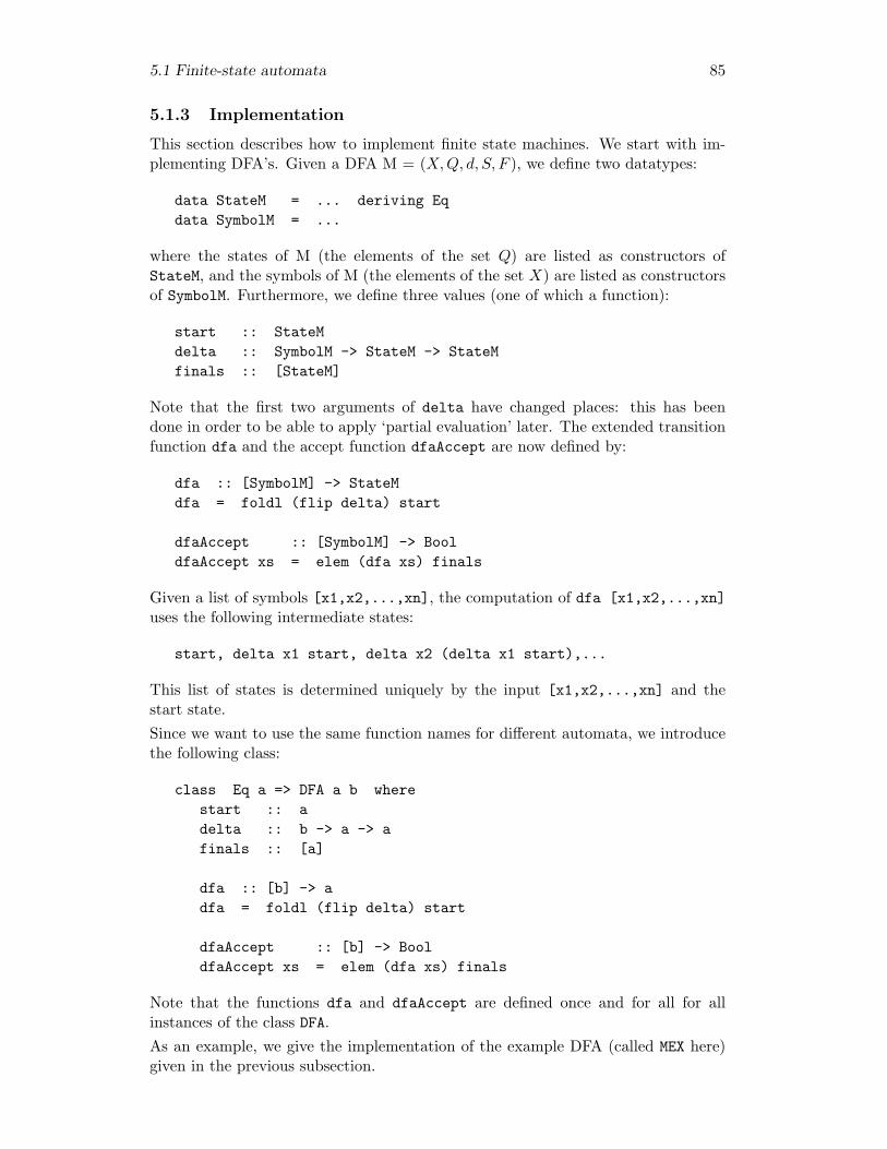
5.1 Finite-state automata 85
5.1.3 Implementation
This section describes how to implement finite state machines. We start with im-plementing DFA’s. Given a DFA M = (X,Q, d, S, F ), we define two datatypes:
data StateM = ... deriving Eqdata SymbolM = ...
where the states of M (the elements of the set Q) are listed as constructors ofStateM, and the symbols of M (the elements of the set X) are listed as constructorsof SymbolM. Furthermore, we define three values (one of which a function):
start :: StateMdelta :: SymbolM -> StateM -> StateMfinals :: [StateM]
Note that the first two arguments of delta have changed places: this has beendone in order to be able to apply ‘partial evaluation’ later. The extended transitionfunction dfa and the accept function dfaAccept are now defined by:
dfa :: [SymbolM] -> StateMdfa = foldl (flip delta) start
dfaAccept :: [SymbolM] -> BooldfaAccept xs = elem (dfa xs) finals
Given a list of symbols [x1,x2,...,xn], the computation of dfa [x1,x2,...,xn]uses the following intermediate states:
start, delta x1 start, delta x2 (delta x1 start),...
This list of states is determined uniquely by the input [x1,x2,...,xn] and thestart state.Since we want to use the same function names for different automata, we introducethe following class:
class Eq a => DFA a b wherestart :: adelta :: b -> a -> afinals :: [a]
dfa :: [b] -> adfa = foldl (flip delta) start
dfaAccept :: [b] -> BooldfaAccept xs = elem (dfa xs) finals
Note that the functions dfa and dfaAccept are defined once and for all for allinstances of the class DFA.As an example, we give the implementation of the example DFA (called MEX here)given in the previous subsection.

86 Regular Languages
data StateMEX = A | B | C | S deriving Eqdata SymbolMEX = SA | SB | SC
So the state A is represented by A, and the symbol a is represented by SA, and similarfor the other states and symbols. The automaton is made an instance of class DFAas follows:
instance DFA StateMEX SymbolMEX wherestart = S
delta x S = case x of SA -> CSB -> ASC -> S
delta SA A = Bdelta SC B = C
finals = [C]
We can improve the performance of the automaton (function) dfa by means ofpartial evaluation. The main idea of partial evaluation is to replace computationspartial
evalua-tion
that are performed often at run-time by a single computation that is performed onlyonce at compile-time. A very simple example is the replacement of the expressionif True then f1 else f2 by the expression f1. Partial evaluation applies to finiteautomatons in the following way.
dfa [x1,x2,...,xn]=
foldl (flip delta) start [x1,x2,...,xn]=
foldl (flip delta) (delta x1 start) [x2,...,xn]=
case x1 ofSA -> foldl (flip delta) (delta SA start) [x2,...,xn]SB -> foldl (flip delta) (delta SB start) [x2,...,xn]SC -> foldl (flip delta) (delta SC start) [x2,...,xn]
All these equalities are simple transformation steps for functional programs. Notethat the first argument of foldl is always flip delta, and the second argument isone of the four states S, A, B, or C (the result of delta). Since there are only a finitenumber of states (four, to be precise), we can define a transition function for eachstate:
dfaS, dfaA, dfaB, dfaC :: [Symbol] -> State
Each of these functions is a case expression over the possible input symbols.
dfaS [] = SdfaS (x:xs) = case x of SA -> dfaC xs
SB -> dfaA xsSC -> dfaS xs

5.1 Finite-state automata 87
dfaA [] = AdfaA (x:xs) = case x of SA -> dfaB xs
dfaB [] = BdfaB (x:xs) = case x of SC -> dfaC xs
dfaC [] = C
With this definition of the finite automaton, the number of steps required for com-puting the value of dfaS xs for some list of symbols xs is reduced considerably.The implementation of NFA’s is similar to the implementation of DFA’s. The onlydifference is that the transition and accept functions have to take care of sets (lists)of states now. We will use the following class, in which we use some names thatalso appear in the class DFA. This is a problem if the two classes appear in the samemodule.
class Eq a => NFA a b wherestart :: [a]delta :: b -> a -> [a]finals :: [a]
nfa :: [b] -> [a]nfa = foldl (flip deltas) start
deltas :: b -> [a] -> [a]deltas a = union . map (delta a)
nfaAccept :: [b] -> BoolnfaAccept xs = intersect (nfa xs) finals /= []
Here, functions union and intersect are implemented as follows:
union :: Eq a => [[a]] -> [a]union = nub . concat
nub :: Eq a => [a] -> [a]nub = foldr (\x xs -> x:filter (/=x) xs) []
intersect :: Eq a => [a] -> [a] -> [a]intersect xs ys = intersect’ (nub xs)
where intersect’ =foldr (\x xs -> if x ‘elem‘ ys then x:xs else xs) []
5.1.4 Constructing a DFA from an NFA
Is it possible to express more languages by means of nondeterministic finite-stateautomata than by deterministic finite-state automata? For each nondeterministicautomaton it is possible to give a deterministic finite-state automaton such thatboth automata accept the same language, so the answer to the above question is
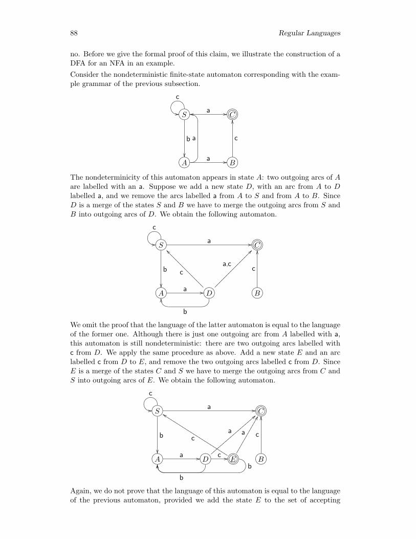
88 Regular Languages
no. Before we give the formal proof of this claim, we illustrate the construction of aDFA for an NFA in an example.Consider the nondeterministic finite-state automaton corresponding with the exam-ple grammar of the previous subsection.
S?>=<89:;EDGFc@A
// a //
b
��
C?>=<89:;/.-,()*+
A?>=<89:; a //BC
EDa
oo
B?>=<89:;
c
OO
The nondeterminicity of this automaton appears in state A: two outgoing arcs of Aare labelled with an a. Suppose we add a new state D, with an arc from A to Dlabelled a, and we remove the arcs labelled a from A to S and from A to B. SinceD is a merge of the states S and B we have to merge the outgoing arcs from S andB into outgoing arcs of D. We obtain the following automaton.
S?>=<89:;EDGFc@A
// a //
b
��
C?>=<89:;/.-,()*+
A?>=<89:; a // D?>=<89:;BC@Ab
OO
c
__????????????????
a,c
??����������������B?>=<89:;
c
OO
We omit the proof that the language of the latter automaton is equal to the languageof the former one. Although there is just one outgoing arc from A labelled with a,this automaton is still nondeterministic: there are two outgoing arcs labelled withc from D. We apply the same procedure as above. Add a new state E and an arclabelled c from D to E, and remove the two outgoing arcs labelled c from D. SinceE is a merge of the states C and S we have to merge the outgoing arcs from C andS into outgoing arcs of E. We obtain the following automaton.
S?>=<89:;EDGFc@A
// a //
b
��
C?>=<89:;/.-,()*+
A?>=<89:; a // D?>=<89:;BC@Ab
OO
a
=={{{{{{{{{{{{{{{{{{ c // E?>=<89:;/.-,()*+
a
FF
c
eeKKKKKKKKKKKKKKKKKKKKKKK
EDBC b@AOO B?>=<89:;
c
OO
Again, we do not prove that the language of this automaton is equal to the languageof the previous automaton, provided we add the state E to the set of accepting
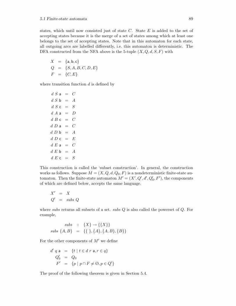
5.1 Finite-state automata 89
states, which until now consisted just of state C. State E is added to the set ofaccepting states because it is the merge of a set of states among which at least onebelongs to the set of accepting states. Note that in this automaton for each state,all outgoing arcs are labelled differently, i.e. this automaton is deterministic. TheDFA constructed from the NFA above is the 5-tuple (X,Q, d, S, F ) with
X = {a, b, c}Q = {S,A,B,C,D,E}F = {C,E}
where transition function d is defined by
d S a = C
d S b = A
d S c = S
d A a = D
d B c = C
d D a = C
d D b = A
d D c = E
d E a = C
d E b = A
d E c = S
This construction is called the ‘subset construction’. In general, the constructionworks as follows. Suppose M = (X,Q, d,Q0, F ) is a nondeterministic finite-state au-tomaton. Then the finite-state automaton M ′ = (X ′, Q′, d′, Q′
0, F′), the components
of which are defined below, accepts the same language.
X ′ = X
Q′ = subs Q
where subs returns all subsets of a set. subs Q is also called the powerset of Q. Forexample,
subs :: {X} → {{X}}subs {A,B} = {{ }, {A}, {A,B}, {B}}
For the other components of M ′ we define
d′ q a = {t | t ∈ d r a, r ∈ q}Q′
0 = Q0
F ′ = {p | p ∩ F 6= Ø, p ∈ Q′}
The proof of the following theorem is given in Section 5.4.
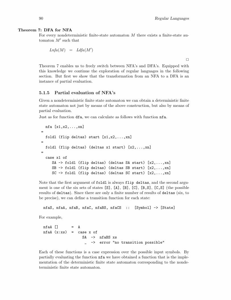
90 Regular Languages
Theorem 7: DFA for NFAFor every nondeterministic finite-state automaton M there exists a finite-state au-tomaton M ′ such that
Lnfa(M) = Ldfa(M ′)
2
Theorem 7 enables us to freely switch between NFA’s and DFA’s. Equipped withthis knowledge we continue the exploration of regular languages in the followingsection. But first we show that the transformation from an NFA to a DFA is aninstance of partial evaluation.
5.1.5 Partial evaluation of NFA’s
Given a nondeterministic finite state automaton we can obtain a deterministic finitestate automaton not just by means of the above construction, but also by means ofpartial evaluation.Just as for function dfa, we can calculate as follows with function nfa.
nfa [x1,x2,...,xn]=
foldl (flip deltas) start [x1,x2,...,xn]=
foldl (flip deltas) (deltas x1 start) [x2,...,xn]=
case x1 ofSA -> foldl (flip deltas) (deltas SA start) [x2,...,xn]SB -> foldl (flip deltas) (deltas SB start) [x2,...,xn]SC -> foldl (flip deltas) (deltas SC start) [x2,...,xn]
Note that the first argument of foldl is always flip deltas, and the second argu-ment is one of the six sets of states [S], [A], [B], [C], [B,S], [C,S] (the possibleresults of deltas). Since there are only a finite number of results of deltas (six, tobe precise), we can define a transition function for each state:
nfaS, nfaA, nfaB, nfaC, nfaBS, nfaCS :: [Symbol] -> [State]
For example,
nfaA [] = AnfaA (x:xs) = case x of
SA -> nfaBS xs_ -> error "no transition possible"
Each of these functions is a case expression over the possible input symbols. Bypartially evaluating the function nfa we have obtained a function that is the imple-mentation of the deterministic finite state automaton corresponding to the nonde-terministic finite state automaton.
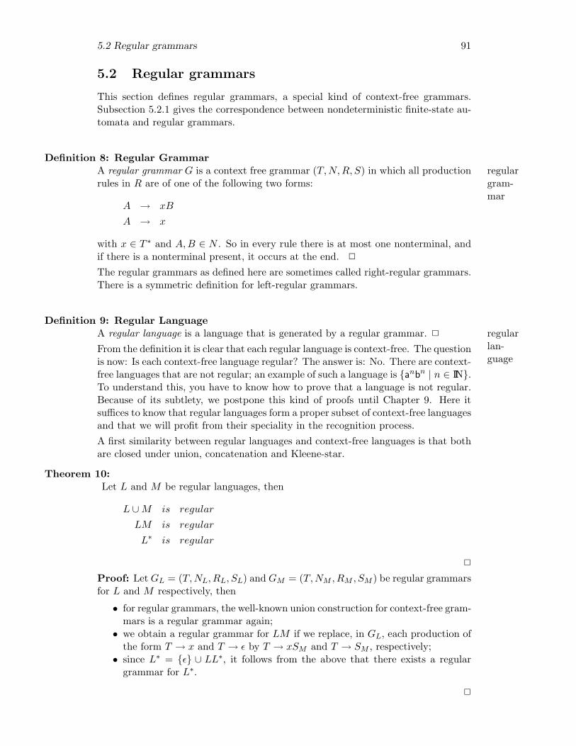
5.2 Regular grammars 91
5.2 Regular grammars
This section defines regular grammars, a special kind of context-free grammars.Subsection 5.2.1 gives the correspondence between nondeterministic finite-state au-tomata and regular grammars.
Definition 8: Regular GrammarA regular grammar G is a context free grammar (T,N,R, S) in which all production regular
gram-mar
rules in R are of one of the following two forms:
A → xB
A → x
with x ∈ T ∗ and A,B ∈ N . So in every rule there is at most one nonterminal, andif there is a nonterminal present, it occurs at the end. 2
The regular grammars as defined here are sometimes called right-regular grammars.There is a symmetric definition for left-regular grammars.
Definition 9: Regular LanguageA regular language is a language that is generated by a regular grammar. 2 regular
lan-guage
From the definition it is clear that each regular language is context-free. The questionis now: Is each context-free language regular? The answer is: No. There are context-free languages that are not regular; an example of such a language is {anbn | n ∈ IIN}.To understand this, you have to know how to prove that a language is not regular.Because of its subtlety, we postpone this kind of proofs until Chapter 9. Here itsuffices to know that regular languages form a proper subset of context-free languagesand that we will profit from their speciality in the recognition process.A first similarity between regular languages and context-free languages is that bothare closed under union, concatenation and Kleene-star.
Theorem 10:Let L and M be regular languages, then
L ∪M is regular
LM is regular
L∗ is regular
2
Proof: Let GL = (T,NL, RL, SL) and GM = (T,NM , RM , SM ) be regular grammarsfor L and M respectively, then
• for regular grammars, the well-known union construction for context-free gram-mars is a regular grammar again;• we obtain a regular grammar for LM if we replace, in GL, each production of
the form T → x and T → ε by T → xSM and T → SM , respectively;• since L∗ = {ε} ∪ LL∗, it follows from the above that there exists a regular
grammar for L∗.
2

92 Regular Languages
In addition to these closure properties, regular languages are closed under intersec-tion and complement too. See the exercises. This is remarkable because context-freelanguages are not closed under these operations. Recall the language L = L1 ∩ L2
where L1 = {anbncm | n,m ∈ IIN} and L2 = {anbmcm | n,m ∈ IIN}.As for context-free languages, there may exist more than one regular grammar fora given regular language and these regular grammars may be transformed into eachother. We conclude this section with a grammar transformation:
Theorem 11:For each regular grammar G there exists a regular grammar G′ with start-symbolS′ such that
L(G) = L(G′)
and such that G′ has no productions of the form U → V and W → ε, with W 6= S′.In other words: every regular grammar can be transformed to a form where everyproduction has a nonempty terminal string in its righthandside (with a possibleexception for S → ε). 2
The proof of this transformation is omitted, we only briefly describe the constructionof such a regular grammar, and illustrate the construction with an example.Given a regular grammar G, a regular grammar with the same language but withoutproductions of the form U → V and W → ε for all U , V , and all W 6= S is obtainedas follows. First, consider all pairs Y , Z of nonterminals of G such that Y ∗⇒ Z.Add productions Y → z to the grammar, with Z → z a production of the originalgrammar, and z not a single nonterminal. Remove all productions U → V fromG. Finally, remove all productions of the form W → ε for W 6= S, and for eachproduction U → xW add the production U → x. The following example illustratesthis construction.Consider the following regular grammar G.
S → aA
S → bB
S → A
S → C
A → bB
A → S
A → ε
B → bB
B → ε
C → c
The grammar G′ of the desired form is constructed in 3 steps.Step 1Let G′ equal G.Step 2Consider all pairs of nonterminals Y and Z. If Y ∗⇒ Z, add the productions Y → z to
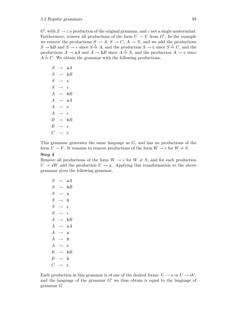
5.2 Regular grammars 93
G′, with Z → z a production of the original grammar, and z not a single nonterminal.Furthermore, remove all productions of the form U → V from G′. In the examplewe remove the productions S → A, S → C, A → S, and we add the productionsS → bB and S → ε since S ∗⇒ A, and the production S → c since S ∗⇒ C, and theproductions A → aA and A → bB since A ∗⇒ S, and the production A → c sinceA
∗⇒ C. We obtain the grammar with the following productions.
S → aA
S → bB
S → c
S → ε
A → bB
A → aA
A → c
A → ε
B → bB
B → ε
C → c
This grammar generates the same language as G, and has no productions of theform U → V . It remains to remove productions of the form W → ε for W 6= S.Step 3Remove all productions of the form W → ε for W 6= S, and for each productionU → xW add the production U → x. Applying this transformation to the abovegrammar gives the following grammar.
S → aA
S → bB
S → a
S → b
S → c
S → ε
A → bB
A → aA
A → a
A → b
A → c
B → bB
B → b
C → c
Each production in this grammar is of one of the desired forms: U → x or U → xV ,and the language of the grammar G′ we thus obtain is equal to the language ofgrammar G.
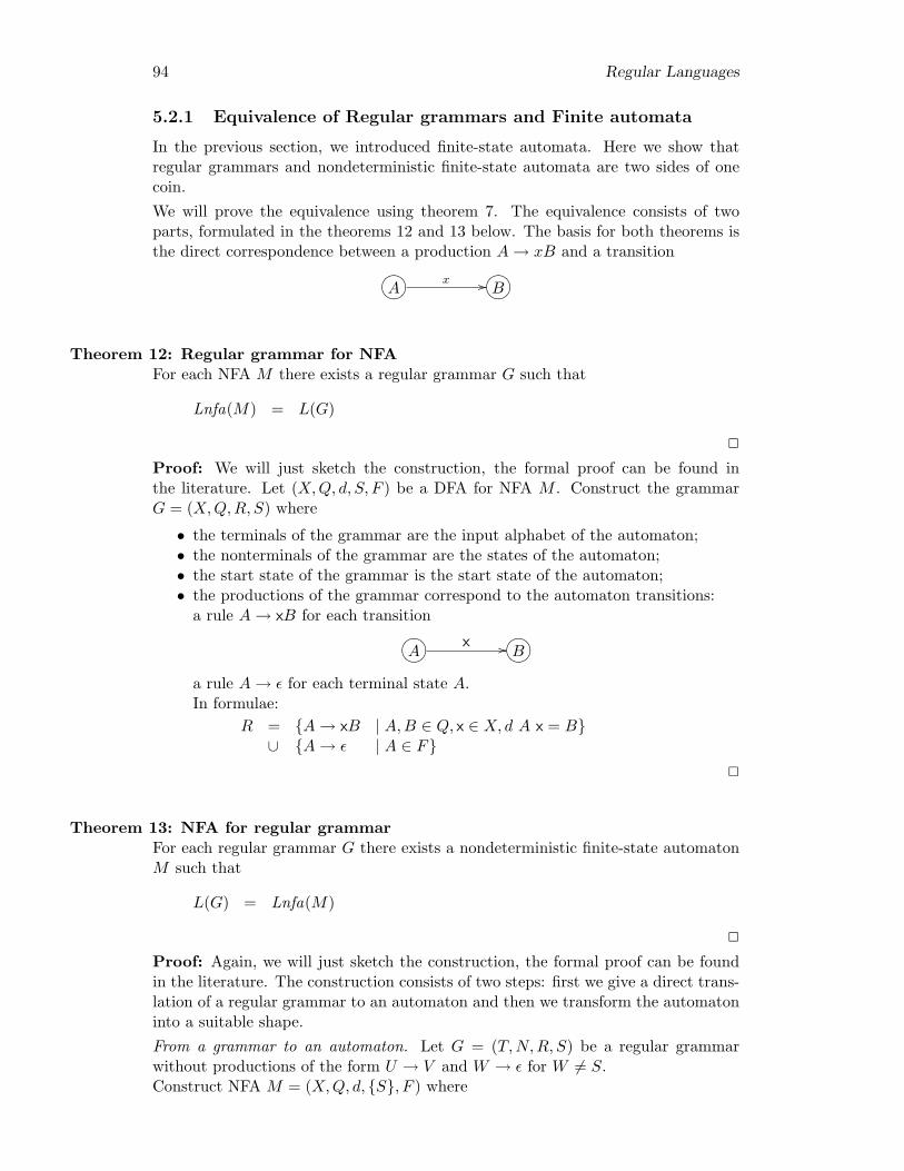
94 Regular Languages
5.2.1 Equivalence of Regular grammars and Finite automata
In the previous section, we introduced finite-state automata. Here we show thatregular grammars and nondeterministic finite-state automata are two sides of onecoin.We will prove the equivalence using theorem 7. The equivalence consists of twoparts, formulated in the theorems 12 and 13 below. The basis for both theorems isthe direct correspondence between a production A→ xB and a transition
A?>=<89:; x // B?>=<89:;
Theorem 12: Regular grammar for NFAFor each NFA M there exists a regular grammar G such that
Lnfa(M) = L(G)
2
Proof: We will just sketch the construction, the formal proof can be found inthe literature. Let (X,Q, d, S, F ) be a DFA for NFA M . Construct the grammarG = (X,Q,R, S) where
• the terminals of the grammar are the input alphabet of the automaton;• the nonterminals of the grammar are the states of the automaton;• the start state of the grammar is the start state of the automaton;• the productions of the grammar correspond to the automaton transitions:
a rule A→ xB for each transition
A?>=<89:; x // B?>=<89:;a rule A→ ε for each terminal state A.In formulae:
R = {A→ xB | A,B ∈ Q, x ∈ X, d A x = B}∪ {A→ ε | A ∈ F}
2
Theorem 13: NFA for regular grammarFor each regular grammar G there exists a nondeterministic finite-state automatonM such that
L(G) = Lnfa(M)
2
Proof: Again, we will just sketch the construction, the formal proof can be foundin the literature. The construction consists of two steps: first we give a direct trans-lation of a regular grammar to an automaton and then we transform the automatoninto a suitable shape.From a grammar to an automaton. Let G = (T,N,R, S) be a regular grammarwithout productions of the form U → V and W → ε for W 6= S.Construct NFA M = (X,Q, d, {S}, F ) where
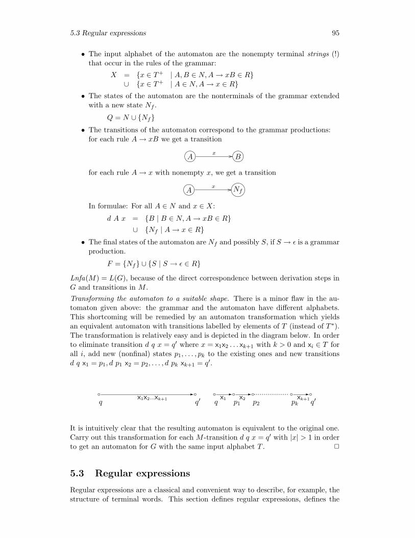
5.3 Regular expressions 95
• The input alphabet of the automaton are the nonempty terminal strings (!)that occur in the rules of the grammar:
X = {x ∈ T+ | A,B ∈ N,A→ xB ∈ R}∪ {x ∈ T+ | A ∈ N,A→ x ∈ R}
• The states of the automaton are the nonterminals of the grammar extendedwith a new state Nf .
Q = N ∪ {Nf}• The transitions of the automaton correspond to the grammar productions:
for each rule A→ xB we get a transition
A?>=<89:; x // B?>=<89:;for each rule A→ x with nonempty x, we get a transition
A?>=<89:; x // NfGFED@ABC
In formulae: For all A ∈ N and x ∈ X:
d A x = {B | B ∈ N,A→ xB ∈ R}∪ {Nf | A→ x ∈ R}
• The final states of the automaton are Nf and possibly S, if S → ε is a grammarproduction.
F = {Nf} ∪ {S | S → ε ∈ R}
Lnfa(M) = L(G), because of the direct correspondence between derivation steps inG and transitions in M .Transforming the automaton to a suitable shape. There is a minor flaw in the au-tomaton given above: the grammar and the automaton have different alphabets.This shortcoming will be remedied by an automaton transformation which yieldsan equivalent automaton with transitions labelled by elements of T (instead of T ∗).The transformation is relatively easy and is depicted in the diagram below. In orderto eliminate transition d q x = q′ where x = x1x2 . . . xk+1 with k > 0 and xi ∈ T forall i, add new (nonfinal) states p1, . . . , pk to the existing ones and new transitionsd q x1 = p1, d p1 x2 = p2, . . . , d pk xk+1 = q′.
bq
x1x2...xk+1
bq′
bq
x1
bp1
x2
bp2
bpk
xk+1
bq′
- - - p p p p p p p p p p p p p p p p p p -
It is intuitively clear that the resulting automaton is equivalent to the original one.Carry out this transformation for each M -transition d q x = q′ with |x| > 1 in orderto get an automaton for G with the same input alphabet T . 2
5.3 Regular expressions
Regular expressions are a classical and convenient way to describe, for example, thestructure of terminal words. This section defines regular expressions, defines the

96 Regular Languages
language of a regular expression, and shows that regular expressions and regulargrammars are equally expressive formalisms. We do not discuss implementations of(datatypes and functions for matching) regular expressions; implementations can befound in the literature, see [9, 6].
Definition 14: RET , regular expressions over alphabet TThe set RET of regular expressions over alphabet T is inductively defined as follows:regular
expres-sion
for regular expressions R,S
Ø ∈ RET
ε ∈ RET
a ∈ RET
R+ S ∈ RET
RS ∈ RET
R∗ ∈ RET
where a ∈ T . The operator + is associative, commutative, and idempotent; the con-catenation operator, written as juxtaposition (so x concatenated with y is denotedby xy), is associative, and ε is the unit of it. In formulae this reads, for all regularexpressions R, S, and V ,
R+ (S + U) = (R+ S) + U
R+ S = S +R
R+R = R
R (S U) = (RS)UR ε = R (= εR)
2
Furthermore, the star operator, ∗, binds stronger than concatenation, and concate-nation binds stronger than +. Examples of regular expressions are:
(bc)∗+ Øε+ b(ε∗)
The language (i.e. the “semantics”) of a regular expression over T is a set of T -sequences compositionally defined on the structure of regular expressions. As follows.
Definition 15: Language of a regular expressionFunction Lre :: RET → {T ∗} returns the language of a regular expression. It isdefined inductively by:
Lre(Ø) = ØLre(ε) = {ε}Lre(b) = {b}

5.3 Regular expressions 97
Lre(x+ y) = Lre(x)) ∪ Lre(y)Lre(xy) = Lre(x)Lre(y)Lre(x∗) = (Lre (x))∗
2
Since ∪ is associative, commutative, and idempotent, set concatenation is associativewith {ε} as its unit, and function Lre is well defined. Note that the language Lreb∗is the set consisting of zero, one or more concatenations of b, i.e., Lre(b∗) = ({b})∗.As an example of a language of a regular expression, we compute the language ofthe regular expression (ε+ bc)d.
Lre((ε+ bc)d)=
(Lre(ε+ bc)) (Lre(d))=
(Lre(ε) ∪ Lre(bc)){d}=
({ε} ∪ (Lre(b))(Lre(c))){d}
={ε, bc} {d}
={d, bcd}
Regular expressions are used to describe the tokens of a language. For example, thelist
if p then e1 else e2
contains six tokens, three of which are identifiers. An identifier is an element in thelanguage of the regular expression
letter(letter + digit)∗
where
letter = a + b + . . .+ z +A + B + . . .+ Z
digit = 0 + 1 + . . .+ 9
see subsection 2.3.1.In the beginning of this section we claimed that regular expressions and regulargrammars are equivalent formalisms. We will prove this claim later, but first weillustrate the construction of a regular grammar out of a regular expressions in anexample. Consider the following regular expression.
R = a∗+ ε+ (a + b)∗
We aim at a regular grammar G such that Lre(R) = L(G) and again we take atop-down approach.

98 Regular Languages
Suppose that nonterminal A generates the language Lre(a∗), nonterminal B gener-ates the language Lre(ε), and nonterminal C generates the language Lre((a + b)∗).Suppose furthermore that the productions for A, B, and C satisfy the conditionsimposed upon regular grammars. Then we obtain a regular grammar G withL(G) = Lre(R) by defining
S → A
S → B
S → C
where S is the start-symbol of G. It remains to construct productions for nonter-minals A, B, and C.
• The nonterminal A with productions
A → aA
A → ε
generates the language Lre(a∗).
• Since Lre(ε) = {ε}, the nonterminal B with production
B → ε
generates the language {ε}.
• Nonterminal C with productions
C → aC
C → bC
C → ε
generates the language Lre((a + b)∗).
For a specific example it is not difficult to construct a regular grammar for a regularexpression. We now give the general result.
Theorem 16: Regular Grammar for Regular ExpressionFor each regular expression R there exists a regular grammar G such that
Lre(R) = L(G)
2
The proof of this theorem is given in Section 5.4.To obtain a regular expression that generates the same language as a given regulargrammar we go via an automaton. Given a regular grammar G, we can use thetheorems from the previous sections to obtain a DFA D such that
L(G) = Ldfa(D)

5.4 Proofs 99
So if we can obtain a regular expression for a DFA D, we have found a regularexpression for a regular grammar. To obtain a regular expression for a DFA D, weinterpret each state of D as a regular expression defined as the sum of the concate-nation of outgoing terminal symbols with the resulting state. For our example DFAwe obtain:
S = aC + bA+ cS
A = aB
B = cC
C = ε
It is easy to merge these four regular expressions into a single regular expression,partially because this is a simple example. Merging the regular expressions obtainedfrom a DFA that may loop is more complicated, as we will briefly explain in theproof of the following theorem. In general, we have:
Theorem 17: Regular Expression for Regular GrammarFor each regular grammar G there exists a regular expression R such that
L(G) = Lre(R)
2
The proof of this theorem is given in Section 5.4.
5.4 Proofs
This section contains the proofs of some of the theorems given in this chapter.Proof: of Theorem 7.Suppose M = (X,Q, d,Q0, F ) is a nondeterministic finite-state automaton. Definethe finite-state automaton M ′ = (X ′, Q′, d′, Q′
0, F′) as follows.
X ′ = X
Q′ = subs Q
where subs returns the powerset of a set. For example,
subs {A,B} = {{ }, {A}, {A,B}, {B}}
For the other components of M ′ we define
d′ q a = {t | t ∈ d r a, r ∈ q}Q′
0 = Q0
F ′ = {p | p ∩ F 6= Ø, p ∈ Q′}
We have
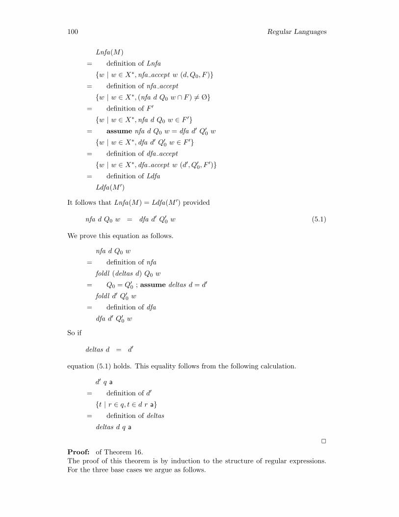
100 Regular Languages
Lnfa(M)
= definition of Lnfa
{w | w ∈ X∗,nfa accept w (d,Q0, F )}= definition of nfa accept
{w | w ∈ X∗, (nfa d Q0 w ∩ F ) 6= Ø}= definition of F ′
{w | w ∈ X∗,nfa d Q0 w ∈ F ′}= assume nfa d Q0 w = dfa d′ Q′
0 w
{w | w ∈ X∗, dfa d′ Q′0 w ∈ F ′}
= definition of dfa accept
{w | w ∈ X∗, dfa accept w (d′, Q′0, F
′)}= definition of Ldfa
Ldfa(M ′)
It follows that Lnfa(M) = Ldfa(M ′) provided
nfa d Q0 w = dfa d′ Q′0 w (5.1)
We prove this equation as follows.
nfa d Q0 w
= definition of nfa
foldl (deltas d) Q0 w
= Q0 = Q′0 ; assume deltas d = d′
foldl d′ Q′0 w
= definition of dfa
dfa d′ Q′0 w
So if
deltas d = d′
equation (5.1) holds. This equality follows from the following calculation.
d′ q a
= definition of d′
{t | r ∈ q, t ∈ d r a}= definition of deltas
deltas d q a
2
Proof: of Theorem 16.The proof of this theorem is by induction to the structure of regular expressions.For the three base cases we argue as follows.
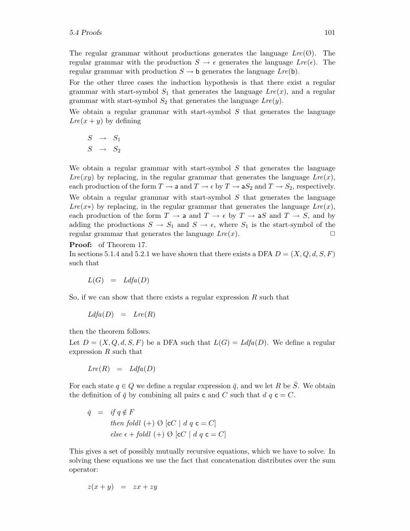
5.4 Proofs 101
The regular grammar without productions generates the language Lre(Ø). Theregular grammar with the production S → ε generates the language Lre(ε). Theregular grammar with production S → b generates the language Lre(b).For the other three cases the induction hypothesis is that there exist a regulargrammar with start-symbol S1 that generates the language Lre(x), and a regulargrammar with start-symbol S2 that generates the language Lre(y).We obtain a regular grammar with start-symbol S that generates the languageLre(x+ y) by defining
S → S1
S → S2
We obtain a regular grammar with start-symbol S that generates the languageLre(xy) by replacing, in the regular grammar that generates the language Lre(x),each production of the form T → a and T → ε by T → aS2 and T → S2, respectively.We obtain a regular grammar with start-symbol S that generates the languageLre(x∗) by replacing, in the regular grammar that generates the language Lre(x),each production of the form T → a and T → ε by T → aS and T → S, and byadding the productions S → S1 and S → ε, where S1 is the start-symbol of theregular grammar that generates the language Lre(x). 2
Proof: of Theorem 17.In sections 5.1.4 and 5.2.1 we have shown that there exists a DFAD = (X,Q, d, S, F )such that
L(G) = Ldfa(D)
So, if we can show that there exists a regular expression R such that
Ldfa(D) = Lre(R)
then the theorem follows.Let D = (X,Q, d, S, F ) be a DFA such that L(G) = Ldfa(D). We define a regularexpression R such that
Lre(R) = Ldfa(D)
For each state q ∈ Q we define a regular expression q, and we let R be S. We obtainthe definition of q by combining all pairs c and C such that d q c = C.
q = if q /∈ Fthen foldl (+) Ø [cC | d q c = C]else ε+ foldl (+) Ø [cC | d q c = C]
This gives a set of possibly mutually recursive equations, which we have to solve. Insolving these equations we use the fact that concatenation distributes over the sumoperator:
z(x+ y) = zx+ zy
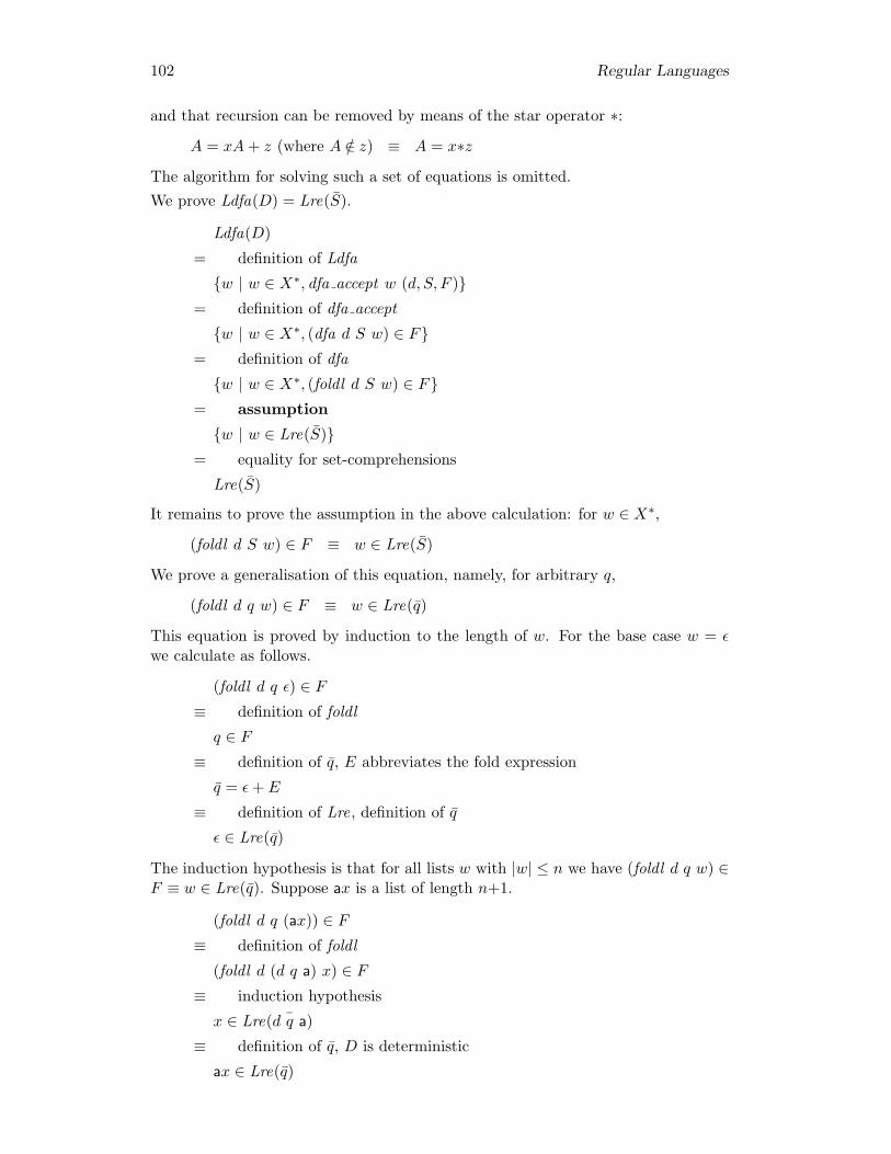
102 Regular Languages
and that recursion can be removed by means of the star operator ∗:
A = xA+ z (where A /∈ z) ≡ A = x∗z
The algorithm for solving such a set of equations is omitted.We prove Ldfa(D) = Lre(S).
Ldfa(D)
= definition of Ldfa
{w | w ∈ X∗, dfa accept w (d, S, F )}= definition of dfa accept
{w | w ∈ X∗, (dfa d S w) ∈ F}= definition of dfa
{w | w ∈ X∗, (foldl d S w) ∈ F}= assumption
{w | w ∈ Lre(S)}= equality for set-comprehensions
Lre(S)
It remains to prove the assumption in the above calculation: for w ∈ X∗,
(foldl d S w) ∈ F ≡ w ∈ Lre(S)
We prove a generalisation of this equation, namely, for arbitrary q,
(foldl d q w) ∈ F ≡ w ∈ Lre(q)
This equation is proved by induction to the length of w. For the base case w = εwe calculate as follows.
(foldl d q ε) ∈ F≡ definition of foldl
q ∈ F≡ definition of q, E abbreviates the fold expression
q = ε+ E
≡ definition of Lre, definition of q
ε ∈ Lre(q)
The induction hypothesis is that for all lists w with |w| ≤ n we have (foldl d q w) ∈F ≡ w ∈ Lre(q). Suppose ax is a list of length n+1.
(foldl d q (ax)) ∈ F≡ definition of foldl
(foldl d (d q a) x) ∈ F≡ induction hypothesis
x ∈ Lre( ¯d q a)
≡ definition of q, D is deterministic
ax ∈ Lre(q)
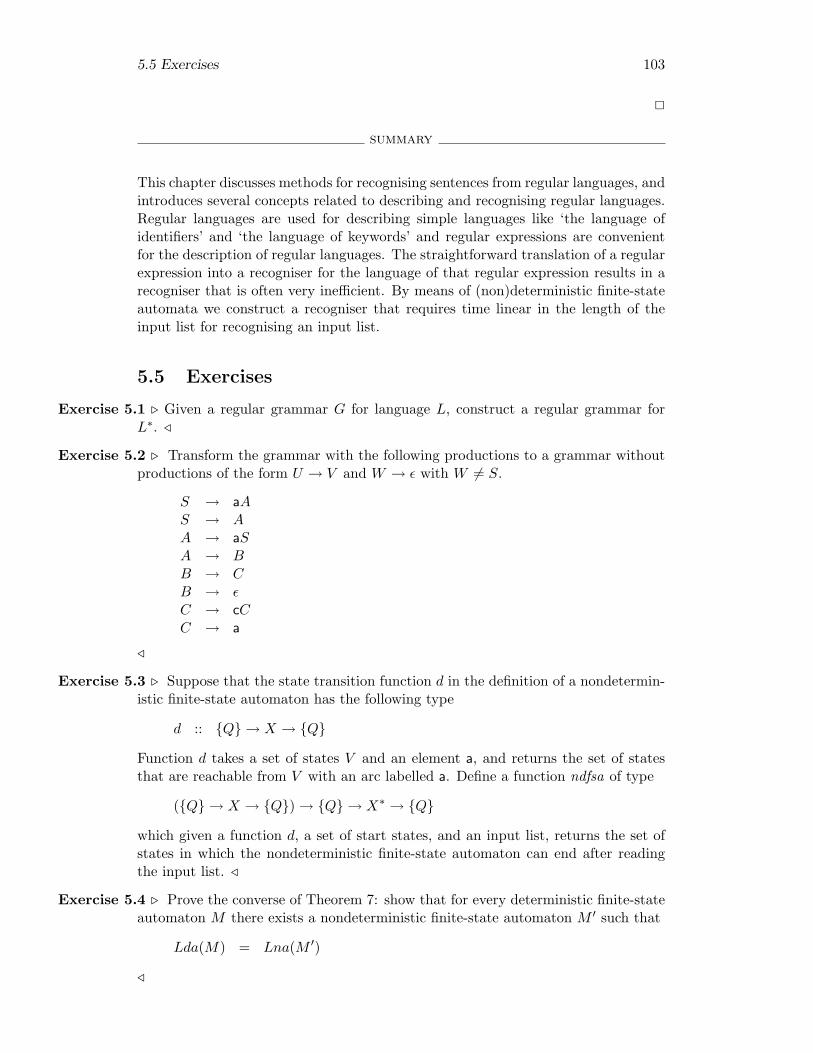
5.5 Exercises 103
2
summary
This chapter discusses methods for recognising sentences from regular languages, andintroduces several concepts related to describing and recognising regular languages.Regular languages are used for describing simple languages like ‘the language ofidentifiers’ and ‘the language of keywords’ and regular expressions are convenientfor the description of regular languages. The straightforward translation of a regularexpression into a recogniser for the language of that regular expression results in arecogniser that is often very inefficient. By means of (non)deterministic finite-stateautomata we construct a recogniser that requires time linear in the length of theinput list for recognising an input list.
5.5 Exercises
Exercise 5.1 . Given a regular grammar G for language L, construct a regular grammar forL∗. /
Exercise 5.2 . Transform the grammar with the following productions to a grammar withoutproductions of the form U → V and W → ε with W 6= S.
S → aAS → AA → aSA → BB → CB → εC → cCC → a
/
Exercise 5.3 . Suppose that the state transition function d in the definition of a nondetermin-istic finite-state automaton has the following type
d :: {Q} → X → {Q}
Function d takes a set of states V and an element a, and returns the set of statesthat are reachable from V with an arc labelled a. Define a function ndfsa of type
({Q} → X → {Q})→ {Q} → X∗ → {Q}
which given a function d, a set of start states, and an input list, returns the set ofstates in which the nondeterministic finite-state automaton can end after readingthe input list. /
Exercise 5.4 . Prove the converse of Theorem 7: show that for every deterministic finite-stateautomaton M there exists a nondeterministic finite-state automaton M ′ such that
Lda(M) = Lna(M ′)
/

104 Regular Languages
Exercise 5.5 . Regular languages are closed under complementation. Prove this claim. Hint:construct a finite automaton for L out of an automaton for regular language L. /
Exercise 5.6 . Regular languages are closed under intersection.1 Prove this claim using the result from the previous exercise.2 A direct proof form this claim is the following:
Let M1 = (X,Q1, d1, S1, F1) and M2 = (X,Q2, d2, S2, F2) be DFA’s for theregular languages L1 and L2 respectively. Define the (product) automatonM = (X,Q1 ×Q2, d, (S1, S2), F1 ×F2) by d (q1, q2) x = (d1 q1 x, d2 q2 x) Nowprove that Ldfa(M) = Ldfa(M1) ∩ Ldfa(M2)
/
Exercise 5.7 . Define nondeterministic finite-state automata that accept languages equal tothe languages of the following regular grammars.
1.
S → (AS → εS → )AA → )A → (
2.
S → 0AS → 0BS → 1AA → 1A → 0B → 0B → ε
/
Exercise 5.8 . Describe the language of the following regular expressions.
1. ε+ b(ε∗)
2. (bc)∗+ Ø
3. a(b∗) + c∗
/
Exercise 5.9 . Prove that for arbitrary regular expressions R, S, and T the following equiva-lences hold.
Lre(R(S + T )) = Lre(RS +RT )Lre((R+ S)T ) = Lre(RT + ST )
/
Exercise 5.10 . Give regular expressions S and R such that
Lre(RS) = Lre(SR)Lre(RS) 6= Lre(SR)
/
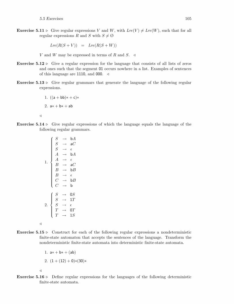
5.5 Exercises 105
Exercise 5.11 . Give regular expressions V and W , with Lre(V ) 6= Lre(W ), such that for allregular expressions R and S with S 6= Ø
Lre(R(S + V )) = Lre(R(S +W ))
V and W may be expressed in terms of R and S. /
Exercise 5.12 . Give a regular expression for the language that consists of all lists of zerosand ones such that the segment 01 occurs nowhere in a list. Examples of sentencesof this language are 1110, and 000. /
Exercise 5.13 . Give regular grammars that generate the language of the following regularexpressions.
1. ((a + bb)∗+ c)∗
2. a∗+ b∗+ ab
/
Exercise 5.14 . Give regular expressions of which the language equals the language of thefollowing regular grammars.
1.
S → bAS → aCS → εA → bAA → εB → aCB → bBB → εC → bBC → b
2.
S → 0SS → 1TS → εT → 0TT → 1S
/
Exercise 5.15 . Construct for each of the following regular expressions a nondeterministicfinite-state automaton that accepts the sentences of the language. Transform thenondeterministic finite-state automata into deterministic finite-state automata.
1. a∗+ b∗+ (ab)
2. (1 + (12) + 0)∗(30)∗
/
Exercise 5.16 . Define regular expressions for the languages of the following deterministicfinite-state automata.

106 Regular Languages
1. Start state is S.
S?>=<89:;/.-,()*+ a //EDGFb@A
// A?>=<89:; b //EDGFa@A
// B?>=<89:;/.-,()*+EDGF
a,b
@A//
2. Start state is S.
S?>=<89:;/.-,()*+ a //EDGFb@A
// A?>=<89:; b //BC@Ab
OO B?>=<89:;BC@Ab
OO
/
Chapter 6
Compositionality
introduction
Many recursive functions follow a common pattern of recursion. These commonpatterns of recursion can conveniently be captured by higher order functions. Forexample: many recursive functions defined on lists are instances of the higher orderfunction foldr. It is possible to define a function such as foldr for a whole range ofdatatypes other than lists. Such functions are called compositional. Compositionalfunctions on datatypes are defined in terms of algebras of semantic actions that cor-respond to the constructors of the datatype. Compositional functions can typicallybe used to define the semantics of programming languages constructs. Such seman-tics is referred to as algebraic semantics. Algebraic semantics often uses algebrasthat are functions from tuples to tuples. Such functions can be seen as computationsthat read values from a component of the domain and write values to a componentof the codomain. The former values are called inherited attributes and the lattervalues are called synthesised attributes. Attributes can be both inherited and syn-thesised. As explained in Section 2.4.1, there is an important relationship betweengrammars and compositionality: with every grammar, which describes the concretesyntax of a language, one can associate a (possibly mutually recursive) datatype,which describes the abstract syntax of the language. Compositional functions onthese datatypes are called syntax driven.
goals
After studying this chapter and making the exercises you will
• know how to generalise constructors of a datatype to an algebra;• know how to write compositional functions, also known as folds, on (possibly
mutually recursive) datatypes;• understand the advantages of using folds, and have seen that many problems
can be solved with a fold;• know that a fold applied to the constructors algebra is the identity function;• have seen the notions of fusion and deforestation;• know how to write syntax driven code;• understand the connection between datatypes, abstract syntax and concrete
syntax;• understand the notions of synthesised and inherited attributes;• can associate inherited and synthesised attributes with the different alterna-
107
108 Compositionality
tives of (possibly mutually recursive) datatypes (or the different nonterminalsof grammars);• can define algebraic semantics in terms of compositional (or syntax driven)
code that is defined using algebras of computations which make use of inheritedand synthesised attributes.
organisation
The chapter is organised as follows. Section 6.1 shows how to define compositionalrecursive functions on built-in lists using a function which is similar to foldr andshows how to do the same thing with user-defined lists and streams. Section 6.2shows how to define compositional recursive functions on several kinds of trees.Section 6.3 defines algebraic semantics. Section 6.4 shows the usefulness of algebraicsemantics by presenting an expression evaluator, an expression interpreter whichmakes use of a stack and expression compiler to a stack machine. They only differin the way they handle basic expressions (variables and local definitions are handledin the same way). All three examples use an algebra of computations which canread values from and write values to an environment which binds names to values.In a second version of the expression evaluator the use of inherited and synthesisedattributes is made more explicit by using tuples. Section 6.5 presents a relativelycomplex example of the use of tuples in combination with compositionality. It dealswith the problem of variable scope when compiling block structured languages.
6.1 Lists
This section introduces compositional functions on the well known datatype of lists.Compositional functions are defined on the built-in datatype [a] for lists (Section6.1.1), on a user-defined datatype List a for lists (Section 6.1.2), and on streams orinfinite lists (Section 6.1.3). We also show how to construct an algebra that directlycorresponds to a datatype.
6.1.1 Built-in lists
The datatype of lists is perhaps the most important example of a datatype. A listis either the empty list [] or a nonempty list (x:xs) consisting of an element x atthe head of the list, followed by a tail xs which itself is again a list. Thus, the type[x] is recursive. In Hugs the type [x] for lists is built-in. The informal definitionof above corresponds to the following (pseudo) datatype.
data [x] = x : [x] | []
Many recursive functions on lists look very similar. Computing the sum of theelements of a list of integers (sumL, where the L denotes that it is a sum functiondefined on lists) is very similar to computing the product of the elements of a list ofintegers (prodL).
sumL, prodL :: [Int] -> IntsumL (x:xs) = x + sumL xssumL [] = 0

6.1 Lists 109
prodL (x:xs) = x * prodL xsprodL [] = 1
The function sumL replaces the list constructor (:) by (+) and the list construc-tor [] by 0 and the function prodL replaces the list constructor (:) by (*) andthe list constructor [] by 1. Note that we have replaced the constructor (:) (aconstructor with two arguments) by binary operators (+) and (*) (i.e. functionswith two arguments) and the constructor [] (a constructor with zero variables) byconstants 0 and 1 (i.e. ‘functions’ with zero variables). The similarity between thedefinitions of the functions sumL and prodL can be captured by the following higherorder recursive function foldL, which is nothing else but an uncurried version of thewell known function foldr. Don’t confuse foldL with Haskell’s prelude functionfoldl, which works the other way around.
foldL :: (x -> l -> l,l) -> [x] -> lfoldL (op,c) = fold where
fold (x:xs) = op x (fold xs)fold [] = c
The function foldL recursively replaces the constructor (:) by an operator op andthe constructor [] by a constant c. We can now use foldL to compute the sum andproduct of the elements of a list of integers as follows.
? foldL ((+),0) [1,2,3,4]10? foldL ((*),1) [1,2,3,4]24
The pair (op,c) is often referred to as a list-algebra. More precisely, a list-algebraconsists of a type l (the carrier of the algebra), a binary operator op of type x->l->land a constant c of type l. Note that a type (like Int) can be the carrier of a list-algebra in more than one way (for example using ((+),0) and ((*),1)). Here isanother example of how to turn Int into a list-algebra.
? foldL (\_ n -> n+1,0) [1,2,3,4]4
This list-algebra ignores the value at the head of a list, and increments the resultobtained thus far with one. It corresponds to the function sizeL defined by:
sizeL :: [x] -> IntsizeL (_:xs) = 1 + sizeL xssizeL [] = 0
Note that the type of sizeL is more general than the types of sumL and prodL. Thetype of the elements of the list does not play a role.
6.1.2 User-defined lists
In this subsection we present an example of a fold function defined on anotherdatatype than built-in lists. To keep things simple we redo the list example foruser-defined lists.

110 Compositionality
data List x = Cons x (List x) | Nil
User-defined lists are defined in the same way as built-in ones. The constructors(:) and [] are replaced by constructors Cons and Nil. Here are the types of theconstructors Cons and Nil.
? :t ConsCons :: a -> List a -> List a? :t NilNil :: List a
A algebra type ListAlgebra corresponding to the datatype List directly followsthe structure of that datatype.
type ListAlgebra x l = (x -> l -> l,l)
The left hand side of the type definition is obtained from the left hand side of thedatatype as follows: a postfix Algebra is added at the end of the name List and atype variable l is added at the end of the whole left hand side of the type definition.The right hand side of the type definition is obtained from the right hand side of thedata definition as follows: all List x valued constructors are replaced by l valuedfunctions which have the same number of arguments (if any) as the correspondingconstructors. The types of recursive constructor arguments (i.e. arguments of typeList x) are replaced by recursive function arguments (i.e. arguments of type l).The types of the other arguments are simply left unchanged. In a similar way, thedefinition of a fold function can be generated automatically from the data definition.
foldList :: ListAlgebra x l -> List x -> lfoldList (cons,nil) = fold where
fold (Cons x xs) = cons x (fold xs)fold Nil = nil
The constructors Cons and Nil in the left hand sides of the definition of the localfunction fold are replaced by functions cons and nil in the right hand sides. Thefunction fold is applied recursively to all recursive constructor arguments of typeList x to return a value of type l as required by the functions of the algebra (in thiscase Cons and cons have one such recursive argument). The other arguments areleft unchanged. Recursive functions on user-defined lists which are defined by meansof foldList are called compositional. Every algebra defines a unique compositionalfunction. Here are three examples of compositional functions. They correspond tothe examples of section 6.1.1.
sumList, prodList :: List Int -> IntsumList = foldList ((+),0)prodList = foldList ((*),1)
sizeList :: List x -> IntsizeList = foldList (const (1+),0)
It is worth mentioning one particular ListAlgebra: the trivial ListAlgebra thatreplaces Cons by Cons and Nil by Nil. This algebra defines the identity functionon user-defined lists.
6.2 Trees 111
idListAlgebra :: ListAlgebra x (List x)idListAlgebra = (Cons,Nil)
idList :: List x -> List xidList = foldList idListAlgebra
? idList (Cons 1 (Cons 2 Nil))Cons 1 (Cons 2 Nil)
6.1.3 Streams
In this section we consider streams (or infinite lists).
data Stream x = And x (Stream x)
Here is a standard example of a stream: the infinite list of fibonacci numbers.
fibStream :: Stream IntfibStream = And 0 (And 1 (restOf fibStream)) where
restOf (And x stream@(And y _)) = And (x+y) (restOf stream)
The algebra type StreamAlgebra, and the fold function foldStream can be gener-ated automatically from the datatype Stream.
type StreamAlgebra x s = x -> s -> s
foldStream :: StreamAlgebra x s -> Stream x -> sfoldStream and = fold where
fold (And x xs) = and x (fold xs)
Note that the algebra has only one component because Stream has only one con-structor. For the same reason the fold function is defined using only one equation.Here is an example of using a compositional function on user defined streams. Itcomputes the first element of a monotone stream that is greater or equal than agiven value.
firstGreaterThan :: Ord x => x -> Stream x -> xfirstGreaterThan n = foldStream (\x y -> if x>=n then x else y)
6.2 Trees
Now that we have seen how to generalise the foldr function on built-in lists tocompositional functions on user-defined lists and streams we proceed by explaininganother common class of datatypes: trees. We will treat four different kinds of treesin the subsections below:
• binary trees;• trees for matching parentheses;• expression trees;• and general trees.
Furthermore, we will briefly mention the concepts of fusion and deforestation.

112 Compositionality
6.2.1 Binary trees
A binary tree is either a node where the tree splits into two subtrees or a leaf whichholds a value.
data BinTree x = Bin (BinTree x) (BinTree x) | Leaf x
One can generate the corresponding algebra type BinTreeAlgebra and fold functionfoldBinTree from the datatype automatically. Note that Bin has two recursivearguments and that Leaf has one non-recursive argument.
type BinTreeAlgebra x t = (t -> t -> t,x -> t)
foldBinTree :: BinTreeAlgebra x t -> BinTree x -> tfoldBinTree (bin,leaf) = fold where
fold (Bin l r) = bin (fold l) (fold r)fold (Leaf x) = leaf x
In the BinTreeAlgebra type, the bin part of the algebra has two arguments oftype t and the leaf part of the algebra has one argument of type x. Similarly,in the foldBinTree function, the local fold function is applied recursively to botharguments of bin and is not called on the argument of leaf. We can now definecompositional functions on binary trees much in the same way as we defined them onlists. Here is an example: the function sizeBinTree computes the size of a binarytree.
sizeBinTree :: BinTree x -> IntsizeBinTree = foldBinTree ((+),const 1)
?sizeBinTree (Bin (Bin (Leaf 3) (Leaf 7)) (Leaf 11))3
If a tree consists of a leaf, then sizeBinTree ignores the value at the leaf and returns1 as the size of the tree. If a tree consists of two subtrees, then sizeBinTree returnsthe sum of the sizes of those subtrees as the size of the tree. Functions for computingthe sum and the product of the integers at the leafs of a binary tree can be definedin a similar way. It suffices to define appropriate semantic actions bin and leaf ona type t (in this case Int) that correspond to the syntactic constructs Bin and Leafof the datatype BinTree.
6.2.2 Trees for matching parentheses
Section 3.3.1 defines the datatype Parentheses for matching parentheses.
data Parentheses = Match Parentheses Parentheses| Empty
For example, the sentence ()() of the concrete syntax for matching parentheses isrepresented by the value Match Empty (Match Empty Empty) in the abstract syn-tax Parentheses. Remember that the abstract syntax ignores the terminal bracketsymbols of the concrete syntax.
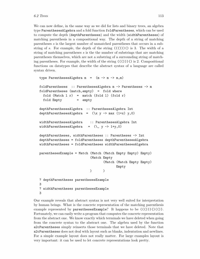
6.2 Trees 113
We can now define, in the same way as we did for lists and binary trees, an algebratype ParenthesesAlgebra and a fold function foldParentheses, which can be usedto compute the depth (depthParentheses) and the width (widthParentheses) ofmatching parenthesis in a compositional way. The depth of a string of matchingparentheses s is the largest number of unmatched parentheses that occurs in a sub-string of s. For example, the depth of the string ((()))() is 3. The width of astring of matching parentheses s is the the number of substrings that are matchingparentheses themselves, which are not a substring of a surrounding string of match-ing parentheses. For example, the width of the string ((()))() is 2. Compositionalfunctions on datatypes that describe the abstract syntax of a language are calledsyntax driven.
type ParenthesesAlgebra m = (m -> m -> m,m)
foldParentheses :: ParenthesesAlgebra m -> Parentheses -> mfoldParentheses (match,empty) = fold where
fold (Match l r) = match (fold l) (fold r)fold Empty = empty
depthParenthesesAlgebra :: ParenthesesAlgebra IntdepthParenthesesAlgebra = (\x y -> max (1+x) y,0)
widthParenthesesAlgebra :: ParenthesesAlgebra IntwidthParenthesesAlgebra = (\_ y -> 1+y,0)
depthParentheses, widthParentheses :: Parentheses -> IntdepthParentheses = foldParentheses depthParenthesesAlgebrawidthParentheses = foldParentheses widthParenthesesAlgebra
parenthesesExample = Match (Match (Match Empty Empty) Empty)(Match Empty
(Match (Match Empty Empty)Empty
) )
? depthParentheses parenthesesExample3? widthParentheses parenthesesExample3
Our example reveals that abstract syntax is not very well suited for interpretationby human beings. What is the concrete representation of the matching parenthesisexample represented by parenthesesExample? It happens to be ((()))()(()).Fortunately, we can easily write a program that computes the concrete representationfrom the abstract one. We know exactly which terminals we have deleted when goingfrom the concrete syntax to the abstract one. The algebra used by the functiona2cParentheses simply reinserts those terminals that we have deleted. Note thata2cParentheses does not deal with layout such as blanks, indentation and newlines.For a simple example layout does not really matter. For large examples layout isvery important: it can be used to let concrete representations look pretty.

114 Compositionality
a2cParenthesesAlgebra :: ParenthesesAlgebra Stringa2cParenthesesAlgebra = (\xs ys -> "("++xs++")"++ys,"")
a2cParentheses :: Parentheses -> Stringa2cParentheses = foldParentheses a2cParenthesesAlgebra
? a2cParentheses parenthesesExample((()))()(())
This example illustrates that a computer can easily interpret abstract syntax (some-thing human beings have difficulties with). Strangely enough, human beings caneasily interpret concrete syntax (something computers have difficulties with). Whatwe would really like is that computers can interpret concrete syntax as well. Thisis the place where parsing enters the picture: computing an abstract representationfrom a concrete one is precisely what parsers are used for.Consider the functions parens and nesting of Section 3.3.1 again.
open = symbol ’(’close = symbol ’)’
parens :: Parser Char Parenthesesparens = f <$> open <*> parens <*> close <*> parens
<|> succeed Emptywhere f a b c d = Match b d
nesting :: Parser Char Intnesting = f <$> open <*> nesting <*> close <*> nesting
<|> succeed 0where f a b c d = max (1+b) d
Function nesting could have been defined by means of function parens and a fold:
nesting’ :: Parser Char Intnesting’ = depthParentheses <$> parens
(Remember that depthParentheses has been defined as a fold.) Functions nestingand nesting’ compute exactly the same result. The function nesting is the fusionof the fold function with the parser parens from the function nesting’. Using lawsfor parsers and folds (which we have not and will not give) we can prove that thetwo functions are equal.Note that function nesting’ first builds a tree by means of function parens, andthen flattens it by means of the fold. Function nesting never builds a tree, and isthus preferable for reasons of efficiency. On the other hand: in function nesting’ wereuse the parser parens and the function depthParentheses, in function nestingwe have to write our own parser, and convince ourselves that it is correct. So forreasons of ‘programming efficiency’ function nesting’ is preferable. To obtain thebest of both worlds, we would like to write function nesting’ and have our compilerfigure out that it is better to use function nesting in computations. The automatictransformation of function nesting’ into function nesting is called deforestation(trees are removed). Some (very few) compilers are clever enough to perform thistransformation automatically.
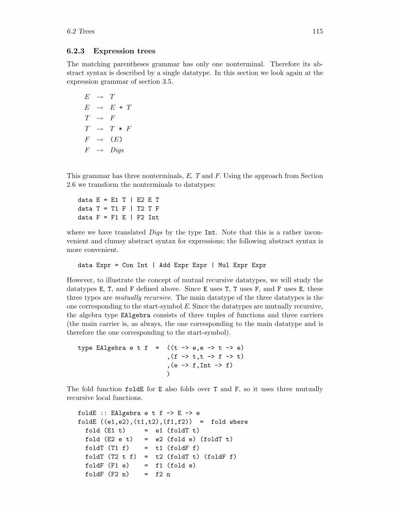
6.2 Trees 115
6.2.3 Expression trees
The matching parentheses grammar has only one nonterminal. Therefore its ab-stract syntax is described by a single datatype. In this section we look again at theexpression grammar of section 3.5.
E → T
E → E + T
T → F
T → T * F
F → (E)
F → Digs
This grammar has three nonterminals, E, T and F. Using the approach from Section2.6 we transform the nonterminals to datatypes:
data E = E1 T | E2 E Tdata T = T1 F | T2 T Fdata F = F1 E | F2 Int
where we have translated Digs by the type Int. Note that this is a rather incon-venient and clumsy abstract syntax for expressions; the following abstract syntax ismore convenient.
data Expr = Con Int | Add Expr Expr | Mul Expr Expr
However, to illustrate the concept of mutual recursive datatypes, we will study thedatatypes E, T, and F defined above. Since E uses T, T uses F, and F uses E, thesethree types are mutually recursive. The main datatype of the three datatypes is theone corresponding to the start-symbol E. Since the datatypes are mutually recursive,the algebra type EAlgebra consists of three tuples of functions and three carriers(the main carrier is, as always, the one corresponding to the main datatype and istherefore the one corresponding to the start-symbol).
type EAlgebra e t f = ((t -> e,e -> t -> e),(f -> t,t -> f -> t),(e -> f,Int -> f))
The fold function foldE for E also folds over T and F, so it uses three mutuallyrecursive local functions.
foldE :: EAlgebra e t f -> E -> efoldE ((e1,e2),(t1,t2),(f1,f2)) = fold where
fold (E1 t) = e1 (foldT t)fold (E2 e t) = e2 (fold e) (foldT t)foldT (T1 f) = t1 (foldF f)foldT (T2 t f) = t2 (foldT t) (foldF f)foldF (F1 e) = f1 (fold e)foldF (F2 n) = f2 n

116 Compositionality
We can now use foldE to write a syntax driven expression evaluator evalE. In thealgebra that is used in the foldE, all type variables e, f, and t are instantiated withInt.
evalE :: E -> IntevalE = foldE ((id,(+)),(id,(*)),(id,id))
exE = E2 (E1 (T2 (T1 (F2 2)) (F2 3))) (T1 (F2 1))
? evalE exE7
Once again our example shows that abstract syntax cannot easily be interpreted byhuman beings. Here is a function a2cE which does this job for us.
a2cE :: E -> Stringa2cE = foldE ((e1,e2),(t1,t2),(f1,f2))where e1 = \t -> t
e2 = \e t -> e++"+"++tt1 = \f -> ft2 = \t f -> t++"*"++ff1 = \e -> "("++e++")"f2 = \n -> show n
? a2cE exE"2*3+1"
6.2.4 General trees
A general tree consist of a node, holding a value, where the tree splits into a listof subtrees. Notice that this list may be empty (in which case, of course, only thevalue at the node is of interest). As usual, the type TreeAlgebra and the functionfoldTree can be generated automatically from the data definition.
data Tree x = Node x [Tree x]
type TreeAlgebra x a = x -> [a] -> a
foldTree :: TreeAlgebra x a -> Tree x -> afoldTree node = fold where
fold (Node x gts) = node x (map fold gts)
Notice that the constructor Node has a list of recursive arguments. Therefore thenode function of the algebra has a corresponding list of recursive arguments. Thelocal fold function is recursively called on all elements of a list using the map func-tion.One can compute the sum of the values at the nodes of a general tree as follows:
sumTree :: Tree Int -> IntsumTree = foldTree (\x xs -> x + sum xs)
Computing the product of the values at the nodes of a general tree and computingthe size of a general tree can be done in a similar way.
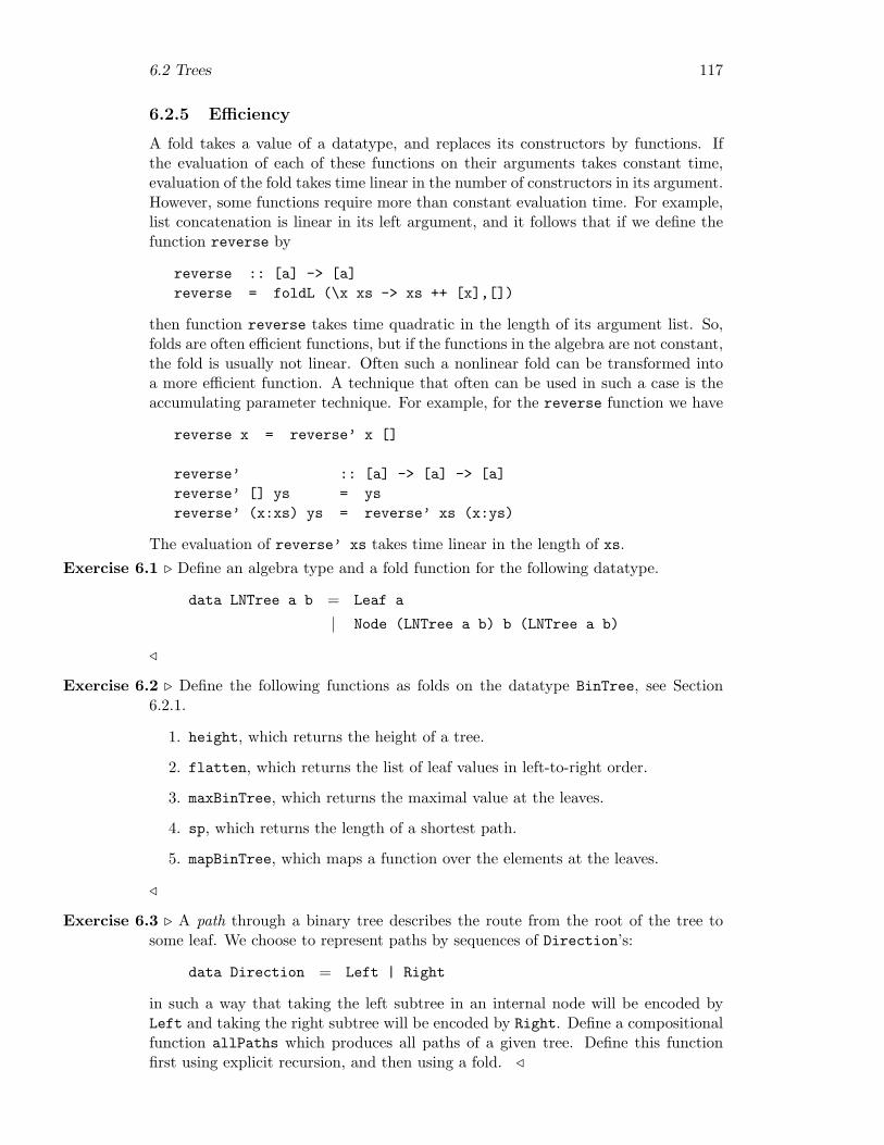
6.2 Trees 117
6.2.5 Efficiency
A fold takes a value of a datatype, and replaces its constructors by functions. Ifthe evaluation of each of these functions on their arguments takes constant time,evaluation of the fold takes time linear in the number of constructors in its argument.However, some functions require more than constant evaluation time. For example,list concatenation is linear in its left argument, and it follows that if we define thefunction reverse by
reverse :: [a] -> [a]reverse = foldL (\x xs -> xs ++ [x],[])
then function reverse takes time quadratic in the length of its argument list. So,folds are often efficient functions, but if the functions in the algebra are not constant,the fold is usually not linear. Often such a nonlinear fold can be transformed intoa more efficient function. A technique that often can be used in such a case is theaccumulating parameter technique. For example, for the reverse function we have
reverse x = reverse’ x []
reverse’ :: [a] -> [a] -> [a]reverse’ [] ys = ysreverse’ (x:xs) ys = reverse’ xs (x:ys)
The evaluation of reverse’ xs takes time linear in the length of xs.Exercise 6.1 . Define an algebra type and a fold function for the following datatype.
data LNTree a b = Leaf a
| Node (LNTree a b) b (LNTree a b)
/
Exercise 6.2 . Define the following functions as folds on the datatype BinTree, see Section6.2.1.
1. height, which returns the height of a tree.
2. flatten, which returns the list of leaf values in left-to-right order.
3. maxBinTree, which returns the maximal value at the leaves.
4. sp, which returns the length of a shortest path.
5. mapBinTree, which maps a function over the elements at the leaves.
/
Exercise 6.3 . A path through a binary tree describes the route from the root of the tree tosome leaf. We choose to represent paths by sequences of Direction’s:
data Direction = Left | Right
in such a way that taking the left subtree in an internal node will be encoded byLeft and taking the right subtree will be encoded by Right. Define a compositionalfunction allPaths which produces all paths of a given tree. Define this functionfirst using explicit recursion, and then using a fold. /

118 Compositionality
Exercise 6.4 . This exercise deals with resistances. There are some basic resistances with afixed (floating point) capacity and, given two resistances, they can be put in parallel(:|:) or in sequence (:*:).
1. Define the datatype Resist to represent resistances. Also, define the datatypeResistAlgebra and the corresponding function foldResist.
2. Define a compositonal function result which determines the capacity of aresistance. (Recall the rules 1
r = 1r1
+ 1r2
and r = r1 + r2.)
/
6.3 Algebraic semantics
With every (possibly mutually recursive) datatype one can associate an algebra typeand a fold function. The algebra is a tuple (one component for each datatype) oftuples (one component for each constructor of the datatype) of semantic actions.The algebra uses a set of auxiliary carriers (one for each datatype). One of them(the one corresponding to the main datatype) is the main carrier of the algebra.The fold function recursively replaces syntactic constructors of the datatypes bycorresponding semantic actions of the algebra. Functions which are defined in termsof a fold function and an algebra are called compositional functions. There is onespecial algebra: the one whose components are the constructor functions of themutually recursive datatypes. This algebra defines the identity function on thedatatype. The compositional function that corresponds to an algebra is the unique,so called, algebra homomorphism from the datatype to the given algebra. Thereforethe datatype is often called the initial algebra and compositional functions are saidto define algebraic semantics. We summarise this important statement as follows.
algebraicSemantics :: InitialAlgebra -> Algebra
6.4 Expressions
The first part of this section presents a basic expression evaluator. The evaluatoris extended with variables in the second part and with local definitions in the thirdpart.
6.4.1 Evaluating expressions
In this subsection we start with a more involved example: an expression evaluator.We will use another datatype for expressions than the one introduced in Section6.2.3: here we will use a single, and hence non mutual recursive datatype for expres-sions. We restrict ourselves to float valued expressions on which addition, subtrac-tion, multiplication and division are defined. The datatype and the correspondingalgebra type and fold function are as follows:
infixl 7 ‘Mul‘infix 7 ‘Dvd‘
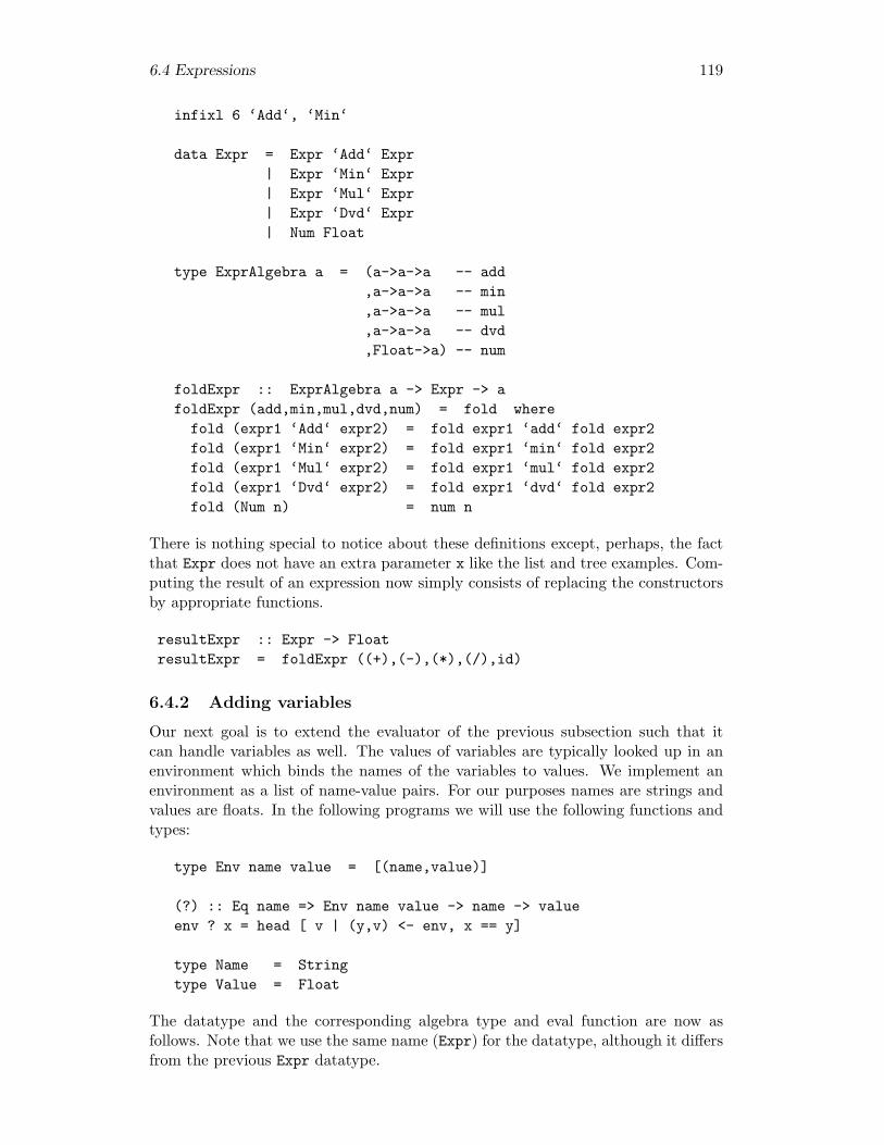
6.4 Expressions 119
infixl 6 ‘Add‘, ‘Min‘
data Expr = Expr ‘Add‘ Expr| Expr ‘Min‘ Expr| Expr ‘Mul‘ Expr| Expr ‘Dvd‘ Expr| Num Float
type ExprAlgebra a = (a->a->a -- add,a->a->a -- min,a->a->a -- mul,a->a->a -- dvd,Float->a) -- num
foldExpr :: ExprAlgebra a -> Expr -> afoldExpr (add,min,mul,dvd,num) = fold where
fold (expr1 ‘Add‘ expr2) = fold expr1 ‘add‘ fold expr2fold (expr1 ‘Min‘ expr2) = fold expr1 ‘min‘ fold expr2fold (expr1 ‘Mul‘ expr2) = fold expr1 ‘mul‘ fold expr2fold (expr1 ‘Dvd‘ expr2) = fold expr1 ‘dvd‘ fold expr2fold (Num n) = num n
There is nothing special to notice about these definitions except, perhaps, the factthat Expr does not have an extra parameter x like the list and tree examples. Com-puting the result of an expression now simply consists of replacing the constructorsby appropriate functions.
resultExpr :: Expr -> FloatresultExpr = foldExpr ((+),(-),(*),(/),id)
6.4.2 Adding variables
Our next goal is to extend the evaluator of the previous subsection such that itcan handle variables as well. The values of variables are typically looked up in anenvironment which binds the names of the variables to values. We implement anenvironment as a list of name-value pairs. For our purposes names are strings andvalues are floats. In the following programs we will use the following functions andtypes:
type Env name value = [(name,value)]
(?) :: Eq name => Env name value -> name -> valueenv ? x = head [ v | (y,v) <- env, x == y]
type Name = Stringtype Value = Float
The datatype and the corresponding algebra type and eval function are now asfollows. Note that we use the same name (Expr) for the datatype, although it differsfrom the previous Expr datatype.
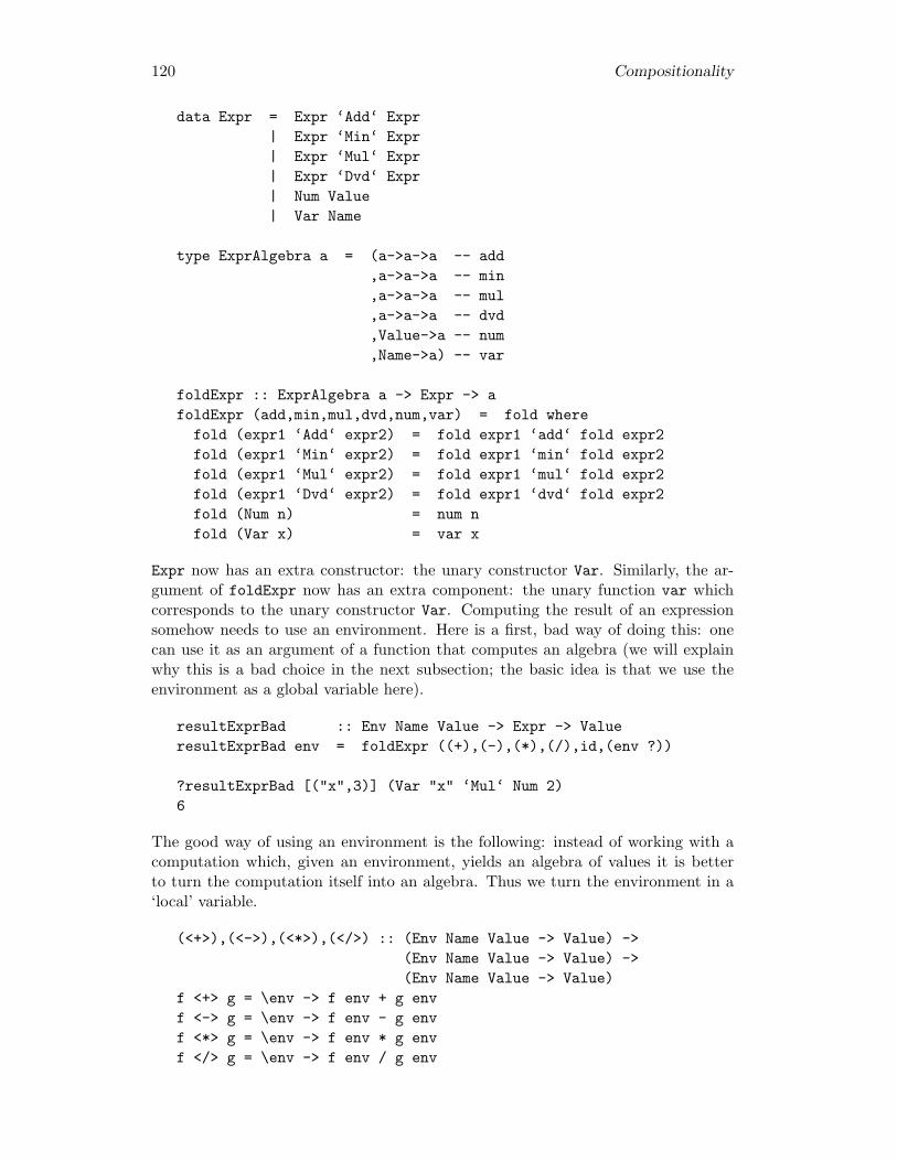
120 Compositionality
data Expr = Expr ‘Add‘ Expr| Expr ‘Min‘ Expr| Expr ‘Mul‘ Expr| Expr ‘Dvd‘ Expr| Num Value| Var Name
type ExprAlgebra a = (a->a->a -- add,a->a->a -- min,a->a->a -- mul,a->a->a -- dvd,Value->a -- num,Name->a) -- var
foldExpr :: ExprAlgebra a -> Expr -> afoldExpr (add,min,mul,dvd,num,var) = fold where
fold (expr1 ‘Add‘ expr2) = fold expr1 ‘add‘ fold expr2fold (expr1 ‘Min‘ expr2) = fold expr1 ‘min‘ fold expr2fold (expr1 ‘Mul‘ expr2) = fold expr1 ‘mul‘ fold expr2fold (expr1 ‘Dvd‘ expr2) = fold expr1 ‘dvd‘ fold expr2fold (Num n) = num nfold (Var x) = var x
Expr now has an extra constructor: the unary constructor Var. Similarly, the ar-gument of foldExpr now has an extra component: the unary function var whichcorresponds to the unary constructor Var. Computing the result of an expressionsomehow needs to use an environment. Here is a first, bad way of doing this: onecan use it as an argument of a function that computes an algebra (we will explainwhy this is a bad choice in the next subsection; the basic idea is that we use theenvironment as a global variable here).
resultExprBad :: Env Name Value -> Expr -> ValueresultExprBad env = foldExpr ((+),(-),(*),(/),id,(env ?))
?resultExprBad [("x",3)] (Var "x" ‘Mul‘ Num 2)6
The good way of using an environment is the following: instead of working with acomputation which, given an environment, yields an algebra of values it is betterto turn the computation itself into an algebra. Thus we turn the environment in a‘local’ variable.
(<+>),(<->),(<*>),(</>) :: (Env Name Value -> Value) ->(Env Name Value -> Value) ->(Env Name Value -> Value)
f <+> g = \env -> f env + g envf <-> g = \env -> f env - g envf <*> g = \env -> f env * g envf </> g = \env -> f env / g env
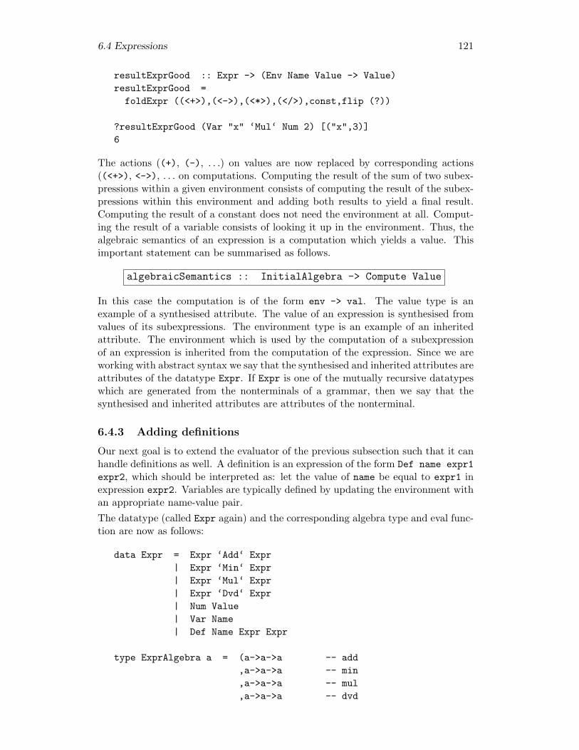
6.4 Expressions 121
resultExprGood :: Expr -> (Env Name Value -> Value)resultExprGood =
foldExpr ((<+>),(<->),(<*>),(</>),const,flip (?))
?resultExprGood (Var "x" ‘Mul‘ Num 2) [("x",3)]6
The actions ((+), (-), . . .) on values are now replaced by corresponding actions((<+>), <->), . . . on computations. Computing the result of the sum of two subex-pressions within a given environment consists of computing the result of the subex-pressions within this environment and adding both results to yield a final result.Computing the result of a constant does not need the environment at all. Comput-ing the result of a variable consists of looking it up in the environment. Thus, thealgebraic semantics of an expression is a computation which yields a value. Thisimportant statement can be summarised as follows.
algebraicSemantics :: InitialAlgebra -> Compute Value
In this case the computation is of the form env -> val. The value type is anexample of a synthesised attribute. The value of an expression is synthesised fromvalues of its subexpressions. The environment type is an example of an inheritedattribute. The environment which is used by the computation of a subexpressionof an expression is inherited from the computation of the expression. Since we areworking with abstract syntax we say that the synthesised and inherited attributes areattributes of the datatype Expr. If Expr is one of the mutually recursive datatypeswhich are generated from the nonterminals of a grammar, then we say that thesynthesised and inherited attributes are attributes of the nonterminal.
6.4.3 Adding definitions
Our next goal is to extend the evaluator of the previous subsection such that it canhandle definitions as well. A definition is an expression of the form Def name expr1expr2, which should be interpreted as: let the value of name be equal to expr1 inexpression expr2. Variables are typically defined by updating the environment withan appropriate name-value pair.The datatype (called Expr again) and the corresponding algebra type and eval func-tion are now as follows:
data Expr = Expr ‘Add‘ Expr| Expr ‘Min‘ Expr| Expr ‘Mul‘ Expr| Expr ‘Dvd‘ Expr| Num Value| Var Name| Def Name Expr Expr
type ExprAlgebra a = (a->a->a -- add,a->a->a -- min,a->a->a -- mul,a->a->a -- dvd

122 Compositionality
,Value->a -- num,Name->a -- var,Name->a->a->a) -- def
foldExpr :: ExprAlgebra a -> Expr -> afoldExpr (add,min,mul,dvd,num,var,def) = fold where
fold (expr1 ‘Add‘ expr2) = fold expr1 ‘add‘ fold expr2fold (expr1 ‘Min‘ expr2) = fold expr1 ‘min‘ fold expr2fold (expr1 ‘Mul‘ expr2) = fold expr1 ‘mul‘ fold expr2fold (expr1 ‘Dvd‘ expr2) = fold expr1 ‘dvd‘ fold expr2fold (Num n) = num nfold (Var x) = var xfold (Def x value body) = def x (fold value) (fold body)
Expr now has an extra constructor: the ternary constructor Def, which can be usedto introduce a local variable. For example, the following expression can be used tocompute the number of seconds per year.
seconds = Def "days_per_year" (Num 365) (Def "hours_per_day" (Num 24) (Def "minutes_per_hour" (Num 60) (Def "seconds_per_minute" (Num 60) (
Var "days_per_year" ‘Mul‘Var "hours_per_day" ‘Mul‘Var "minutes_per_hour" ‘Mul‘Var "seconds_per_minute" ))))
Similarly, the parameter of foldExpr now has an extra component: the ternaryfunction def which corresponds to the ternary constructor Def. Notice that thelast two arguments are recursive ones. We can now explain why the first use ofenvironments is inferior to the second one. Trying to extend the first definitiongives something like:
resultExprBad :: Env Name Value -> Expr -> ValueresultExprBad env =
foldExpr ((+),(-),(*),(/),id,(env ?),error "def")
The last component causes a problem: a body that contains a local definition has tobe evaluated in an updated environment. We cannot update the environment in thissetting: we can read the environment but afterwards it is not accessible any morein the algebra (which consists of values). Extending the second definition causesno problems: the environment is now accessible in the algebra (which consists ofcomputations). We can easily add a new action which updates the environment.The computation corresponding to the body of an expression with a local definitioncan now be evaluated in the updated environment.
f <+> g = \env -> f env + g envf <-> g = \env -> f env - g envf <*> g = \env -> f env * g envf </> g = \env -> f env / g env
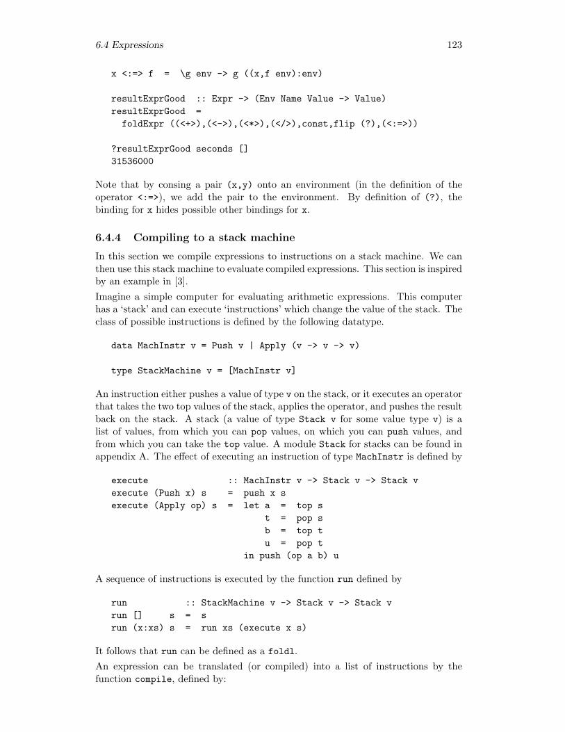
6.4 Expressions 123
x <:=> f = \g env -> g ((x,f env):env)
resultExprGood :: Expr -> (Env Name Value -> Value)resultExprGood =
foldExpr ((<+>),(<->),(<*>),(</>),const,flip (?),(<:=>))
?resultExprGood seconds []31536000
Note that by consing a pair (x,y) onto an environment (in the definition of theoperator <:=>), we add the pair to the environment. By definition of (?), thebinding for x hides possible other bindings for x.
6.4.4 Compiling to a stack machine
In this section we compile expressions to instructions on a stack machine. We canthen use this stack machine to evaluate compiled expressions. This section is inspiredby an example in [3].Imagine a simple computer for evaluating arithmetic expressions. This computerhas a ‘stack’ and can execute ‘instructions’ which change the value of the stack. Theclass of possible instructions is defined by the following datatype.
data MachInstr v = Push v | Apply (v -> v -> v)
type StackMachine v = [MachInstr v]
An instruction either pushes a value of type v on the stack, or it executes an operatorthat takes the two top values of the stack, applies the operator, and pushes the resultback on the stack. A stack (a value of type Stack v for some value type v) is alist of values, from which you can pop values, on which you can push values, andfrom which you can take the top value. A module Stack for stacks can be found inappendix A. The effect of executing an instruction of type MachInstr is defined by
execute :: MachInstr v -> Stack v -> Stack vexecute (Push x) s = push x sexecute (Apply op) s = let a = top s
t = pop sb = top tu = pop t
in push (op a b) u
A sequence of instructions is executed by the function run defined by
run :: StackMachine v -> Stack v -> Stack vrun [] s = srun (x:xs) s = run xs (execute x s)
It follows that run can be defined as a foldl.An expression can be translated (or compiled) into a list of instructions by thefunction compile, defined by:
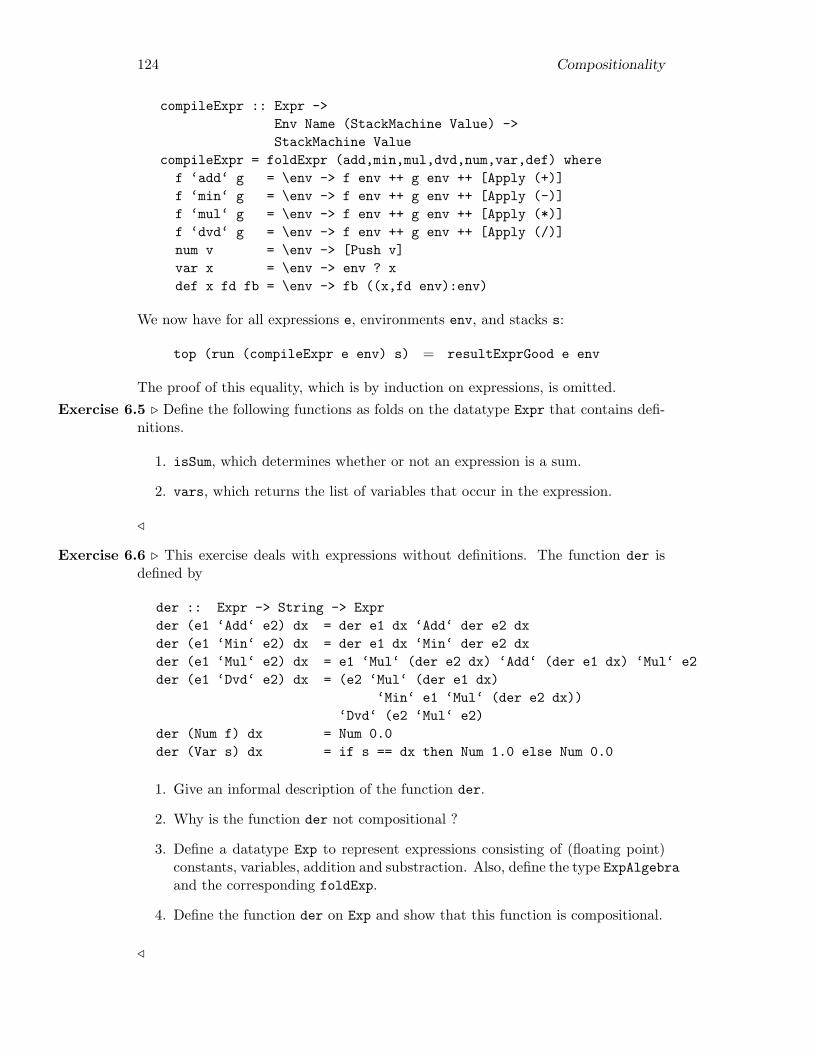
124 Compositionality
compileExpr :: Expr ->Env Name (StackMachine Value) ->StackMachine Value
compileExpr = foldExpr (add,min,mul,dvd,num,var,def) wheref ‘add‘ g = \env -> f env ++ g env ++ [Apply (+)]f ‘min‘ g = \env -> f env ++ g env ++ [Apply (-)]f ‘mul‘ g = \env -> f env ++ g env ++ [Apply (*)]f ‘dvd‘ g = \env -> f env ++ g env ++ [Apply (/)]num v = \env -> [Push v]var x = \env -> env ? xdef x fd fb = \env -> fb ((x,fd env):env)
We now have for all expressions e, environments env, and stacks s:
top (run (compileExpr e env) s) = resultExprGood e env
The proof of this equality, which is by induction on expressions, is omitted.Exercise 6.5 . Define the following functions as folds on the datatype Expr that contains defi-
nitions.
1. isSum, which determines whether or not an expression is a sum.
2. vars, which returns the list of variables that occur in the expression.
/
Exercise 6.6 . This exercise deals with expressions without definitions. The function der isdefined by
der :: Expr -> String -> Exprder (e1 ‘Add‘ e2) dx = der e1 dx ‘Add‘ der e2 dxder (e1 ‘Min‘ e2) dx = der e1 dx ‘Min‘ der e2 dxder (e1 ‘Mul‘ e2) dx = e1 ‘Mul‘ (der e2 dx) ‘Add‘ (der e1 dx) ‘Mul‘ e2der (e1 ‘Dvd‘ e2) dx = (e2 ‘Mul‘ (der e1 dx)
‘Min‘ e1 ‘Mul‘ (der e2 dx))‘Dvd‘ (e2 ‘Mul‘ e2)
der (Num f) dx = Num 0.0der (Var s) dx = if s == dx then Num 1.0 else Num 0.0
1. Give an informal description of the function der.
2. Why is the function der not compositional ?
3. Define a datatype Exp to represent expressions consisting of (floating point)constants, variables, addition and substraction. Also, define the type ExpAlgebraand the corresponding foldExp.
4. Define the function der on Exp and show that this function is compositional.
/
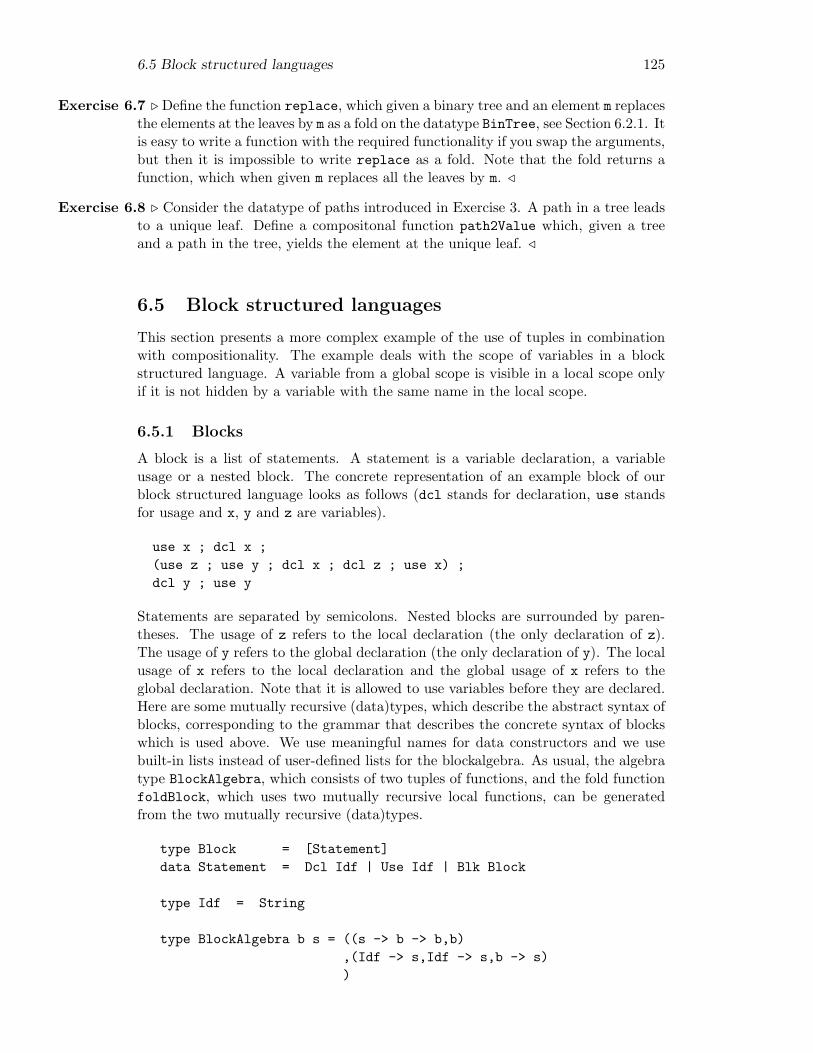
6.5 Block structured languages 125
Exercise 6.7 . Define the function replace, which given a binary tree and an element m replacesthe elements at the leaves by m as a fold on the datatype BinTree, see Section 6.2.1. Itis easy to write a function with the required functionality if you swap the arguments,but then it is impossible to write replace as a fold. Note that the fold returns afunction, which when given m replaces all the leaves by m. /
Exercise 6.8 . Consider the datatype of paths introduced in Exercise 3. A path in a tree leadsto a unique leaf. Define a compositonal function path2Value which, given a treeand a path in the tree, yields the element at the unique leaf. /
6.5 Block structured languages
This section presents a more complex example of the use of tuples in combinationwith compositionality. The example deals with the scope of variables in a blockstructured language. A variable from a global scope is visible in a local scope onlyif it is not hidden by a variable with the same name in the local scope.
6.5.1 Blocks
A block is a list of statements. A statement is a variable declaration, a variableusage or a nested block. The concrete representation of an example block of ourblock structured language looks as follows (dcl stands for declaration, use standsfor usage and x, y and z are variables).
use x ; dcl x ;(use z ; use y ; dcl x ; dcl z ; use x) ;dcl y ; use y
Statements are separated by semicolons. Nested blocks are surrounded by paren-theses. The usage of z refers to the local declaration (the only declaration of z).The usage of y refers to the global declaration (the only declaration of y). The localusage of x refers to the local declaration and the global usage of x refers to theglobal declaration. Note that it is allowed to use variables before they are declared.Here are some mutually recursive (data)types, which describe the abstract syntax ofblocks, corresponding to the grammar that describes the concrete syntax of blockswhich is used above. We use meaningful names for data constructors and we usebuilt-in lists instead of user-defined lists for the blockalgebra. As usual, the algebratype BlockAlgebra, which consists of two tuples of functions, and the fold functionfoldBlock, which uses two mutually recursive local functions, can be generatedfrom the two mutually recursive (data)types.
type Block = [Statement]data Statement = Dcl Idf | Use Idf | Blk Block
type Idf = String
type BlockAlgebra b s = ((s -> b -> b,b),(Idf -> s,Idf -> s,b -> s))
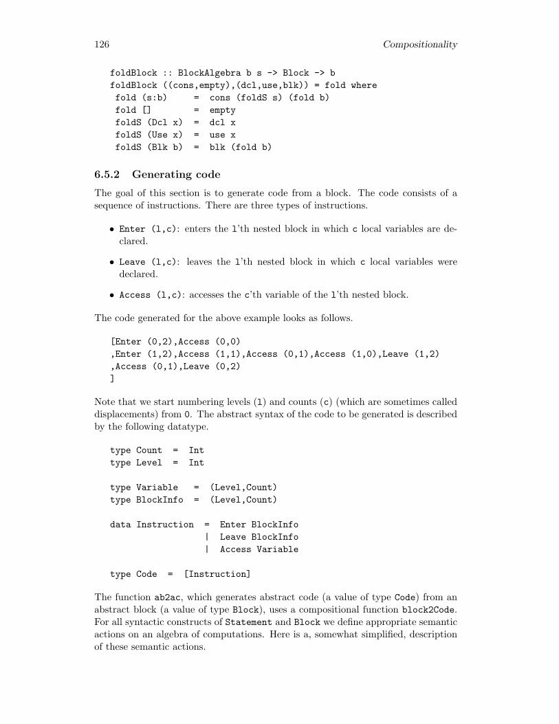
126 Compositionality
foldBlock :: BlockAlgebra b s -> Block -> bfoldBlock ((cons,empty),(dcl,use,blk)) = fold wherefold (s:b) = cons (foldS s) (fold b)fold [] = emptyfoldS (Dcl x) = dcl xfoldS (Use x) = use xfoldS (Blk b) = blk (fold b)
6.5.2 Generating code
The goal of this section is to generate code from a block. The code consists of asequence of instructions. There are three types of instructions.
• Enter (l,c): enters the l’th nested block in which c local variables are de-clared.
• Leave (l,c): leaves the l’th nested block in which c local variables weredeclared.
• Access (l,c): accesses the c’th variable of the l’th nested block.
The code generated for the above example looks as follows.
[Enter (0,2),Access (0,0),Enter (1,2),Access (1,1),Access (0,1),Access (1,0),Leave (1,2),Access (0,1),Leave (0,2)]
Note that we start numbering levels (l) and counts (c) (which are sometimes calleddisplacements) from 0. The abstract syntax of the code to be generated is describedby the following datatype.
type Count = Inttype Level = Int
type Variable = (Level,Count)type BlockInfo = (Level,Count)
data Instruction = Enter BlockInfo| Leave BlockInfo| Access Variable
type Code = [Instruction]
The function ab2ac, which generates abstract code (a value of type Code) from anabstract block (a value of type Block), uses a compositional function block2Code.For all syntactic constructs of Statement and Block we define appropriate semanticactions on an algebra of computations. Here is a, somewhat simplified, descriptionof these semantic actions.
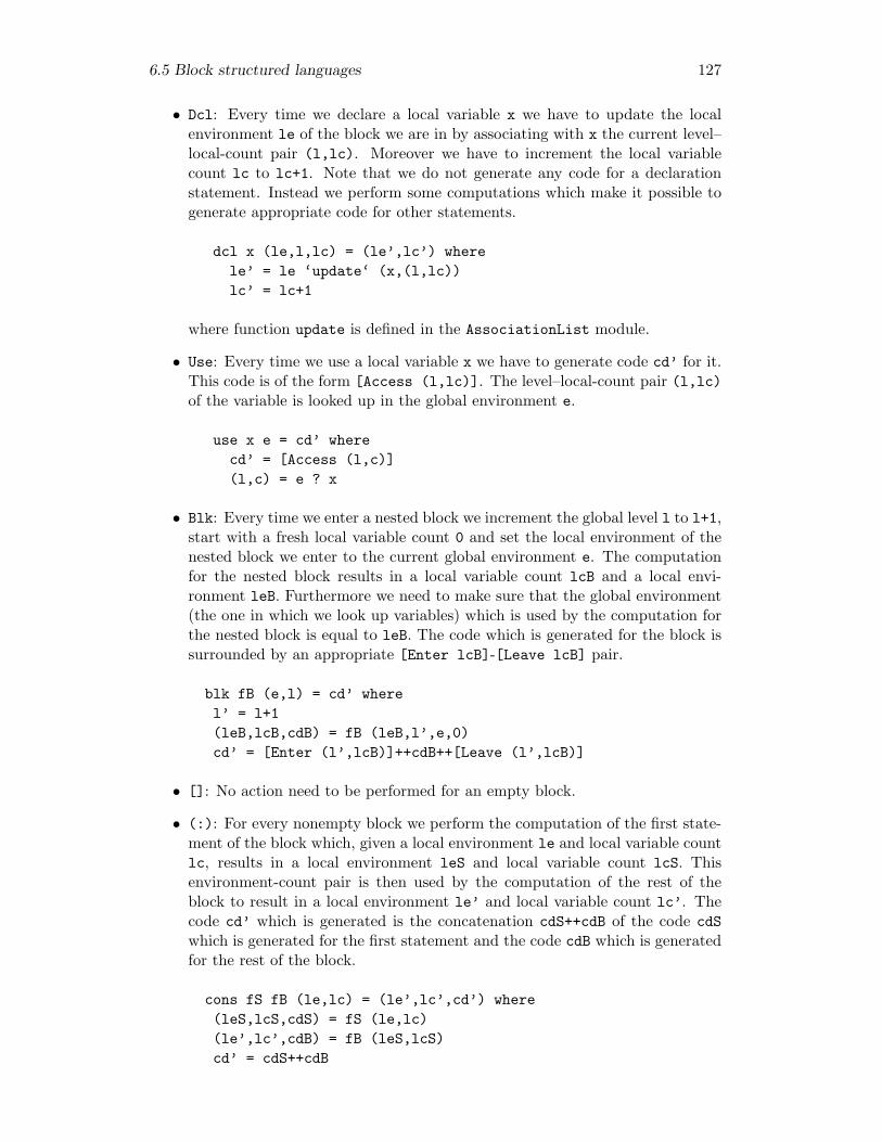
6.5 Block structured languages 127
• Dcl: Every time we declare a local variable x we have to update the localenvironment le of the block we are in by associating with x the current level–local-count pair (l,lc). Moreover we have to increment the local variablecount lc to lc+1. Note that we do not generate any code for a declarationstatement. Instead we perform some computations which make it possible togenerate appropriate code for other statements.
dcl x (le,l,lc) = (le’,lc’) wherele’ = le ‘update‘ (x,(l,lc))lc’ = lc+1
where function update is defined in the AssociationList module.
• Use: Every time we use a local variable x we have to generate code cd’ for it.This code is of the form [Access (l,lc)]. The level–local-count pair (l,lc)of the variable is looked up in the global environment e.
use x e = cd’ wherecd’ = [Access (l,c)](l,c) = e ? x
• Blk: Every time we enter a nested block we increment the global level l to l+1,start with a fresh local variable count 0 and set the local environment of thenested block we enter to the current global environment e. The computationfor the nested block results in a local variable count lcB and a local envi-ronment leB. Furthermore we need to make sure that the global environment(the one in which we look up variables) which is used by the computation forthe nested block is equal to leB. The code which is generated for the block issurrounded by an appropriate [Enter lcB]-[Leave lcB] pair.
blk fB (e,l) = cd’ wherel’ = l+1(leB,lcB,cdB) = fB (leB,l’,e,0)cd’ = [Enter (l’,lcB)]++cdB++[Leave (l’,lcB)]
• []: No action need to be performed for an empty block.
• (:): For every nonempty block we perform the computation of the first state-ment of the block which, given a local environment le and local variable countlc, results in a local environment leS and local variable count lcS. Thisenvironment-count pair is then used by the computation of the rest of theblock to result in a local environment le’ and local variable count lc’. Thecode cd’ which is generated is the concatenation cdS++cdB of the code cdSwhich is generated for the first statement and the code cdB which is generatedfor the rest of the block.
cons fS fB (le,lc) = (le’,lc’,cd’) where(leS,lcS,cdS) = fS (le,lc)(le’,lc’,cdB) = fB (leS,lcS)cd’ = cdS++cdB
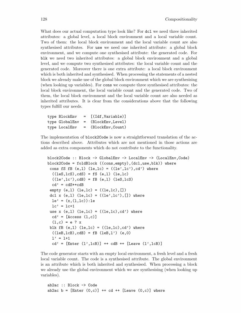
128 Compositionality
What does our actual computation type look like? For dcl we need three inheritedattributes: a global level, a local block environment and a local variable count.Two of them: the local block environment and the local variable count are alsosynthesised attributes. For use we need one inherited attribute: a global blockenvironment, and we compute one synthesised attribute: the generated code. Forblk we need two inherited attributes: a global block environment and a globallevel, and we compute two synthesised attributes: the local variable count and thegenerated code. Moreover there is one extra attribute: a local block environmentwhich is both inherited and synthesised. When processing the statements of a nestedblock we already make use of the global block environment which we are synthesising(when looking up variables). For cons we compute three synthesised attributes: thelocal block environment, the local variable count and the generated code. Two ofthem, the local block environment and the local variable count are also needed asinherited attributes. It is clear from the considerations above that the followingtypes fulfill our needs.
type BlockEnv = [(Idf,Variable)]type GlobalEnv = (BlockEnv,Level)type LocalEnv = (BlockEnv,Count)
The implementation of block2Code is now a straightforward translation of the ac-tions described above. Attributes which are not mentioned in those actions areadded as extra components which do not contribute to the functionality.
block2Code :: Block -> GlobalEnv -> LocalEnv -> (LocalEnv,Code)block2Code = foldBlock ((cons,empty),(dcl,use,blk)) wherecons fS fB (e,l) (le,lc) = ((le’,lc’),cd’) where((leS,lcS),cdS) = fS (e,l) (le,lc)((le’,lc’),cdB) = fB (e,l) (leS,lcS)cd’ = cdS++cdB
empty (e,l) (le,lc) = ((le,lc),[])dcl x (e,l) (le,lc) = ((le’,lc’),[]) wherele’ = (x,(l,lc)):lelc’ = lc+1
use x (e,l) (le,lc) = ((le,lc),cd’) wherecd’ = [Access (l,c)](l,c) = e ? x
blk fB (e,l) (le,lc) = ((le,lc),cd’) where((leB,lcB),cdB) = fB (leB,l’) (e,0)l’ = l+1cd’ = [Enter (l’,lcB)] ++ cdB ++ [Leave (l’,lcB)]
The code generator starts with an empty local environment, a fresh level and a freshlocal variable count. The code is a synthesised attribute. The global environmentis an attribute which is both inherited and synthesised. When processing a blockwe already use the global environment which we are synthesising (when looking upvariables).
ab2ac :: Block -> Codeab2ac b = [Enter (0,c)] ++ cd ++ [Leave (0,c)] where
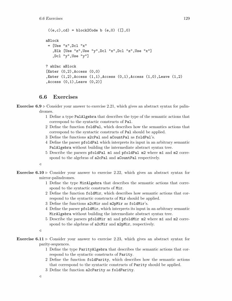
6.6 Exercises 129
((e,c),cd) = block2Code b (e,0) ([],0)
aBlock= [Use "x",Dcl "x"
,Blk [Use "z",Use "y",Dcl "x",Dcl "z",Use "x"],Dcl "y",Use "y"]
? ab2ac aBlock[Enter (0,2),Access (0,0),Enter (1,2),Access (1,1),Access (0,1),Access (1,0),Leave (1,2),Access (0,1),Leave (0,2)]
6.6 Exercises
Exercise 6.9 . Consider your answer to exercise 2.21, which gives an abstract syntax for palin-dromes.
1 Define a type PalAlgebra that describes the type of the semantic actions thatcorrespond to the syntactic constructs of Pal.
2 Define the function foldPal, which describes how the semantics actions thatcorrespond to the syntactic constructs of Pal should be applied.
3 Define the functions a2cPal and aCountPal as foldPal’s.4 Define the parser pfoldPal which interprets its input in an arbitrary semanticPalAlgebra without building the intermediate abstract syntax tree.
5 Describe the parsers pfoldPal m1 and pfoldPal m2 where m1 and m2 corre-spond to the algebras of a2cPal and aCountPal respectively.
/
Exercise 6.10 . Consider your answer to exercise 2.22, which gives an abstract syntax formirror-palindromes.
1 Define the type MirAlgebra that describes the semantic actions that corre-spond to the syntactic constructs of Mir.
2 Define the function foldMir, which describes how semantic actions that cor-respond to the syntactic constructs of Mir should be applied.
3 Define the functions a2cMir and m2pMir as foldMir’s.4 Define the parser pfoldMir, which interprets its input in an arbitrary semanticMirAlgebra without building the intermediate abstract syntax tree.
5 Describe the parsers pfoldMir m1 and pfoldMir m2 where m1 and m2 corre-spond to the algebras of a2cMir and m2pMir, respectively.
/
Exercise 6.11 . Consider your answer to exercise 2.23, which gives an abstract syntax forparity-sequences.
1 Define the type ParityAlgebra that describes the semantic actions that cor-respond to the syntactic constructs of Parity.
2 Define the function foldParity, which describes how the semantic actionsthat correspond to the syntactic constructs of Parity should be applied.
3 Define the function a2cParity as foldParity./
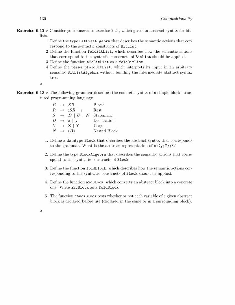
130 Compositionality
Exercise 6.12 . Consider your answer to exercise 2.24, which gives an abstract syntax for bit-lists.
1 Define the type BitListAlgebra that describes the semantic actions that cor-respond to the syntactic constructs of BitList.
2 Define the function foldBitList, which describes how the semantic actionsthat correspond to the syntactic constructs of BitList should be applied.
3 Define the function a2cBitList as a foldBitList.4 Define the parser pfoldBitList, which interprets its input in an arbitrary
semantic BitListAlgebra without building the intermediate abstract syntaxtree.
/
Exercise 6.13 . The following grammar describes the concrete syntax of a simple block-struc-tured programming language
B → SR BlockR → ;SR | ε RestS → D | U | N StatementD → x | y DeclarationU → X | Y UsageN → (B) Nested Block
1. Define a datatype Block that describes the abstract syntax that correspondsto the grammar. What is the abstract representation of x;(y;Y);X?
2. Define the type BlockAlgebra that describes the semantic actions that corre-spond to the syntactic constructs of Block.
3. Define the function foldBlock, which describes how the semantic actions cor-responding to the syntactic constructs of Block should be applied.
4. Define the function a2cBlock, which converts an abstract block into a concreteone. Write a2cBlock as a foldBlock
5. The function checkBlock tests whether or not each variable of a given abstractblock is declared before use (declared in the same or in a surrounding block).
/
Chapter 7
Computing with parsers
Parsers produce results. For example, the parsers for travelling schemes given inChapter 4 return an abstract syntax, or an integer that represents the net travellingtime in minutes. The net travelling time is computed directly by inserting thecorrect semantic functions. Another way to compute the net travelling time is byfirst computing the abstract syntax, and then applying a function to the abstractsyntax that computes the net travelling time. This section shows several ways tocompute results using parsers:
• insert a semantic function in the parser;• apply a fold to the abstract syntax;• use a class instead of abstract syntax;• pass an algebra to the parser.
7.1 Insert a semantic function in the parser
In Chapter 4 we have defined two parsers: a parser that computes the abstractsyntax for a travelling schema, and a parser that computes the net travelling time.These functions are obtained by inserting different functions in the basic parser. Ifwe want to compute the total travelling time, we have to insert different functionsin the basic parser. This approach works fine for a small parser, but it has somedisadvantages when building a larger parser:
• semantics is intertwined with the parsing process;• it is difficult to locate all positions where semantic functions have to be inserted
in the parser.
7.2 Apply a fold to the abstract syntax
Instead of inserting operations in a basic parser, we can write a parser that parsesthe input to an abstract syntax, and computes the desired result by applying a foldto the abstract syntax.An example of such an approach has been given in Section 6.2.2, where we definedtwo functions with the same functionality: nesting and nesting’; both computethe maximum nesting depth in a string of parentheses. Function nesting is definedby inserting functions in the basic parser. Function nesting’ is defined by applyinga fold to the abstract syntax. Each of these definitions has its own merits; we repeatthe main arguments below.
131
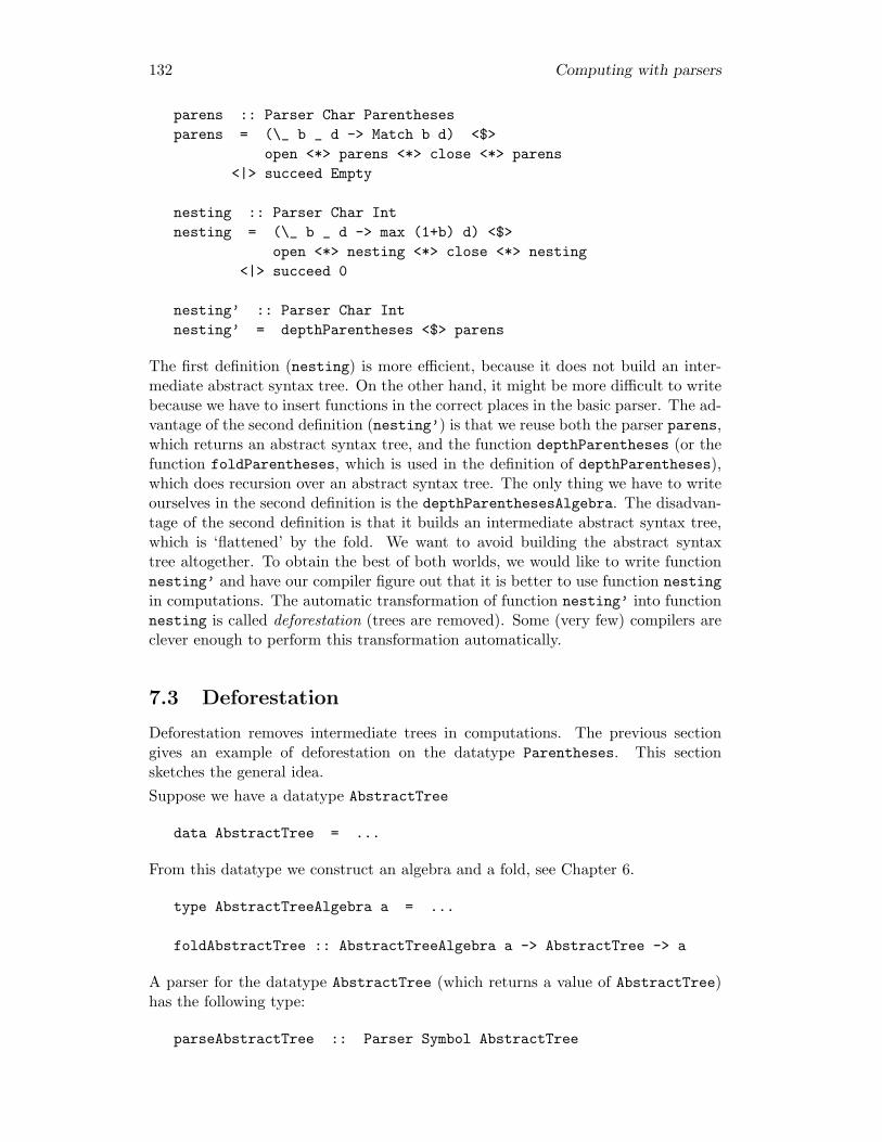
132 Computing with parsers
parens :: Parser Char Parenthesesparens = (\_ b _ d -> Match b d) <$>
open <*> parens <*> close <*> parens<|> succeed Empty
nesting :: Parser Char Intnesting = (\_ b _ d -> max (1+b) d) <$>
open <*> nesting <*> close <*> nesting<|> succeed 0
nesting’ :: Parser Char Intnesting’ = depthParentheses <$> parens
The first definition (nesting) is more efficient, because it does not build an inter-mediate abstract syntax tree. On the other hand, it might be more difficult to writebecause we have to insert functions in the correct places in the basic parser. The ad-vantage of the second definition (nesting’) is that we reuse both the parser parens,which returns an abstract syntax tree, and the function depthParentheses (or thefunction foldParentheses, which is used in the definition of depthParentheses),which does recursion over an abstract syntax tree. The only thing we have to writeourselves in the second definition is the depthParenthesesAlgebra. The disadvan-tage of the second definition is that it builds an intermediate abstract syntax tree,which is ‘flattened’ by the fold. We want to avoid building the abstract syntaxtree altogether. To obtain the best of both worlds, we would like to write functionnesting’ and have our compiler figure out that it is better to use function nestingin computations. The automatic transformation of function nesting’ into functionnesting is called deforestation (trees are removed). Some (very few) compilers areclever enough to perform this transformation automatically.
7.3 Deforestation
Deforestation removes intermediate trees in computations. The previous sectiongives an example of deforestation on the datatype Parentheses. This sectionsketches the general idea.Suppose we have a datatype AbstractTree
data AbstractTree = ...
From this datatype we construct an algebra and a fold, see Chapter 6.
type AbstractTreeAlgebra a = ...
foldAbstractTree :: AbstractTreeAlgebra a -> AbstractTree -> a
A parser for the datatype AbstractTree (which returns a value of AbstractTree)has the following type:
parseAbstractTree :: Parser Symbol AbstractTree
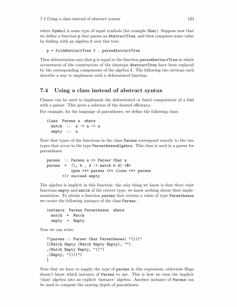
7.4 Using a class instead of abstract syntax 133
where Symbol is some type of input symbols (for example Char). Suppose now thatwe define a function p that parses an AbstractTree, and then computes some valueby folding with an algebra f over this tree:
p = foldAbstractTree f . parseAbstractTree
Then deforestation says that p is equal to the function parseAbstractTree in whichoccurrences of the constructors of the datatype AbstractTree have been replacedby the corresponding components of the algebra f. The following two sections eachdescribe a way to implement such a deforestated function.
7.4 Using a class instead of abstract syntax
Classes can be used to implement the deforestated or fused computation of a foldwith a parser. This gives a solution of the desired efficiency.For example, for the language of parentheses, we define the following class:
class Parens a wherematch :: a -> a -> aempty :: a
Note that types of the functions in the class Parens correspond exactly to the twotypes that occur in the type ParenthesesAlgebra. This class is used in a parser forparentheses:
parens :: Parens a => Parser Char aparens = (\_ b _ d -> match b d) <$>
open <*> parens <*> close <*> parens<|> succeed empty
The algebra is implicit in this function: the only thing we know is that there existfunctions empty and match of the correct type; we know nothing about their imple-mentation. To obtain a function parens that returns a value of type Parentheseswe create the following instance of the class Parens.
instance Parens Parentheses wherematch = Matchempty = Empty
Now we can write:
?(parens :: Parser Char Parentheses) "()()"[(Match Empty (Match Empty Empty), ""),(Match Empty Empty, "()"),(Empty, "()()")]
Note that we have to supply the type of parens in this expression, otherwise Hugsdoesn’t know which instance of Parens to use. This is how we turn the implicit‘class’ algebra into an explicit ‘instance’ algebra. Another instance of Parens canbe used to compute the nesting depth of parentheses:
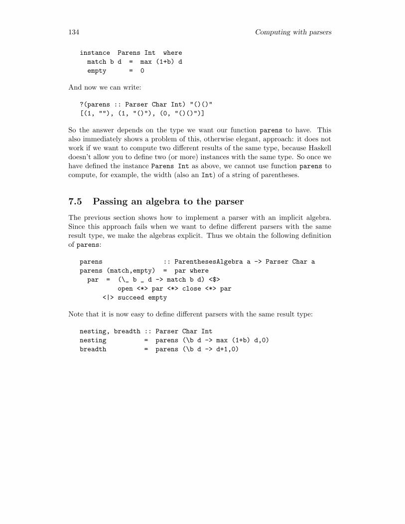
134 Computing with parsers
instance Parens Int wherematch b d = max (1+b) dempty = 0
And now we can write:
?(parens :: Parser Char Int) "()()"[(1, ""), (1, "()"), (0, "()()")]
So the answer depends on the type we want our function parens to have. Thisalso immediately shows a problem of this, otherwise elegant, approach: it does notwork if we want to compute two different results of the same type, because Haskelldoesn’t allow you to define two (or more) instances with the same type. So once wehave defined the instance Parens Int as above, we cannot use function parens tocompute, for example, the width (also an Int) of a string of parentheses.
7.5 Passing an algebra to the parser
The previous section shows how to implement a parser with an implicit algebra.Since this approach fails when we want to define different parsers with the sameresult type, we make the algebras explicit. Thus we obtain the following definitionof parens:
parens :: ParenthesesAlgebra a -> Parser Char aparens (match,empty) = par where
par = (\_ b _ d -> match b d) <$>open <*> par <*> close <*> par
<|> succeed empty
Note that it is now easy to define different parsers with the same result type:
nesting, breadth :: Parser Char Intnesting = parens (\b d -> max (1+b) d,0)breadth = parens (\b d -> d+1,0)

Chapter 8
Programming with higher-order folds
introduction
In the previous chapters we have seen that algebras play an important role whendescribing the meaning of a recognised structure (a parse tree). For each recursivedatatype T we have a function foldT, and for each constructor of the datatype wehave a corresponding function as a component in the algebra. Chapter 6 introducesa language in which local declarations are permitted. Evaluating expressions inthis language can be done by choosing an appropriate algebra. The domain ofthat algebra is a higher order (data)type (a (data)type that contains functions).Unfortunately, the resulting code comes as a surprise to many. In this chapterwe will illustrate a related formalism, which will make it easier to construct suchinvolved algebras. This related formalism is the attribute grammar formalism. Wewill not formally define attribute grammars, but instead illustrate the formalismwith some examples, and give an informal definition.We start with developing a somewhat unconventional way of looking at functionalprograms, and especially those programs that use functions that recursively descendover datatypes a lot. In our case one may think about these datatypes as abstractsyntax trees. When computing a property of such a recursive object (for example, aprogram) we define two sets of functions: one set that describes how to recursivelyvisit the nodes of the tree, and one set of functions (an algebra) that describes whatto compute at each node when visited.One of the most important steps in this process is deciding what the carrier typeof the algebras is going to be. Once this step has been taken, these types area guideline for further design steps. We will see that such carrier types may befunctions themselves, and that deciding on the type of such functions may not alwaysbe simple. In this chapter we will present a view on recursive computations thatwill enable us to “design” the carrier type in an incremental way. We will do so byconstructing algebras out of other algebras. In this way we define the meaning of alanguage in a semantically compositional way.We will start with the rep min example, which looks a bit artificial, and deals witha non-interesting, highly specific problem. However, it has been chosen for its sim-plicity, and to not distract our attention to specific, programming language related,semantic issues. The second example of this chapter demonstrates the techniqueson a larger example: a small compiler for part of a programming language.
135

136 Programming with higher-order folds
data Tree = Leaf Int| Bin Tree Tree deriving Show
type TreeAlgebra a = (Int -> a, a -> a -> a)
foldTree :: TreeAlgebra a -> Tree -> afoldTree alg@(leaf, _ ) (Leaf i) = leaf ifoldTree alg@(_ , bin) (Bin l r) = bin (foldTree alg l)
(foldTree alg r)
Listing 9: rm.start.hs
goals
In this chapter you will learn:
• how to write ‘circular’ functional programs, or ‘higher-order folds’;• how to combine algebras;• (informally) the concept of an attribute grammar.
8.1 The rep min problem
One of the famous examples in which the power of lazy evaluation is demonstrated isthe so-called rep min problem [2]. Many have wondered how this program achievesits goal, since at first sight it seems that it is impossible to compute anything withthis program. We will use this problem, and a sequence of different solutions, tobuild up an understanding of a whole class of such programs.In listing 9 we present the datatype Tree, together with its associated algebra. Thecarrier type of an algebra is the type that describes the objects of the algebra. Werepresent it by a type parameter of the algebra type:
type TreeAlgebra a = (Int -> a, a -> a -> a)
The associated evaluation function foldTree systematically replaces the construc-tors Leaf and Bin by corresponding operations from the algebra alg that is passedas an argument.We now want to construct a function rep_min :: Tree -> Tree that returns aTree with the same “shape” as its argument Tree, but with the values in its leavesreplaced by the minimal value occurring in the original tree. For example,
?rep_min (Bin (Bin (Leaf 1) (Leaf 7)) (Leaf 11))Bin (Bin (Leaf 1) (Leaf 1)) (Leaf 1)
8.1.1 A straightforward solution
A straightforward solution to the rep min problem consists of a function in whichfoldTree is used twice: once for computing the minimal value of the leaf values,and once for constructing the resulting Tree. The function rep_min that solves
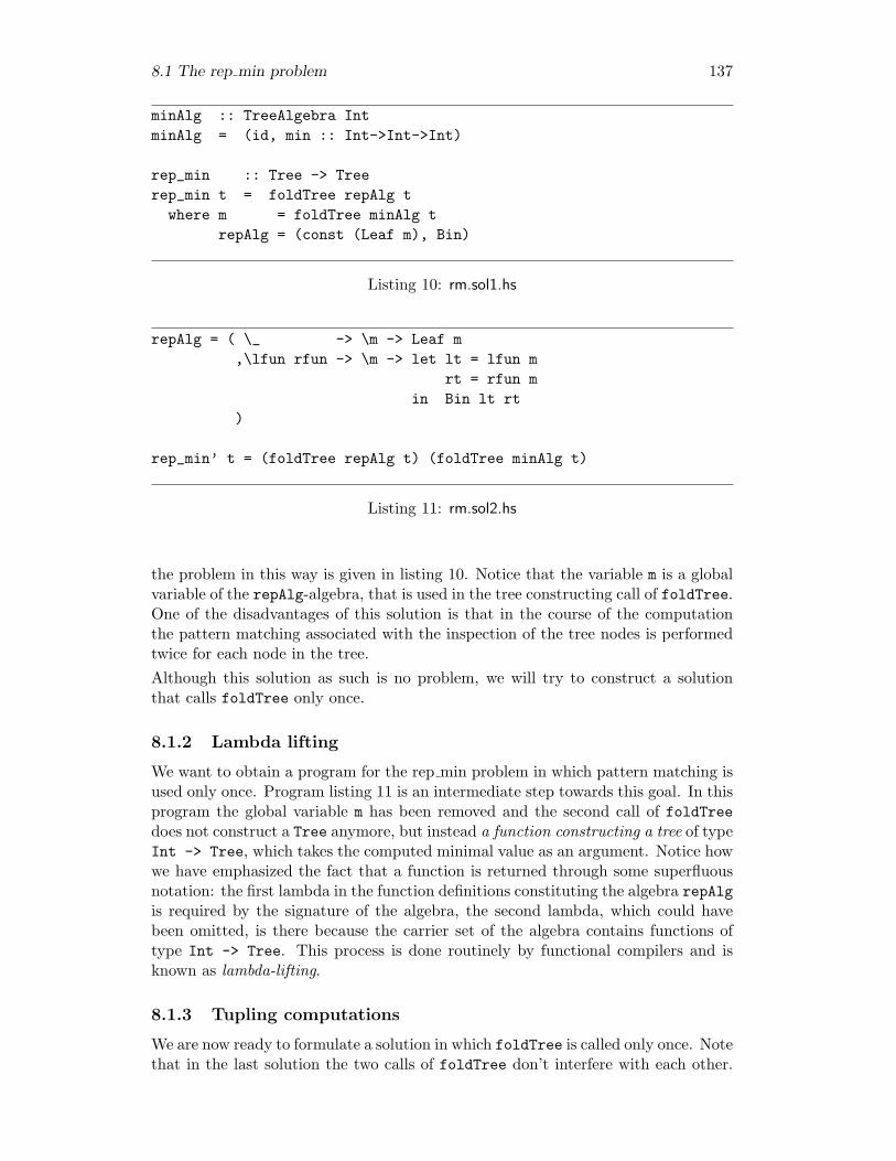
8.1 The rep min problem 137
minAlg :: TreeAlgebra IntminAlg = (id, min :: Int->Int->Int)
rep_min :: Tree -> Treerep_min t = foldTree repAlg t
where m = foldTree minAlg trepAlg = (const (Leaf m), Bin)
Listing 10: rm.sol1.hs
repAlg = ( \_ -> \m -> Leaf m,\lfun rfun -> \m -> let lt = lfun m
rt = rfun min Bin lt rt
)
rep_min’ t = (foldTree repAlg t) (foldTree minAlg t)
Listing 11: rm.sol2.hs
the problem in this way is given in listing 10. Notice that the variable m is a globalvariable of the repAlg-algebra, that is used in the tree constructing call of foldTree.One of the disadvantages of this solution is that in the course of the computationthe pattern matching associated with the inspection of the tree nodes is performedtwice for each node in the tree.Although this solution as such is no problem, we will try to construct a solutionthat calls foldTree only once.
8.1.2 Lambda lifting
We want to obtain a program for the rep min problem in which pattern matching isused only once. Program listing 11 is an intermediate step towards this goal. In thisprogram the global variable m has been removed and the second call of foldTreedoes not construct a Tree anymore, but instead a function constructing a tree of typeInt -> Tree, which takes the computed minimal value as an argument. Notice howwe have emphasized the fact that a function is returned through some superfluousnotation: the first lambda in the function definitions constituting the algebra repAlgis required by the signature of the algebra, the second lambda, which could havebeen omitted, is there because the carrier set of the algebra contains functions oftype Int -> Tree. This process is done routinely by functional compilers and isknown as lambda-lifting.
8.1.3 Tupling computations
We are now ready to formulate a solution in which foldTree is called only once. Notethat in the last solution the two calls of foldTree don’t interfere with each other.
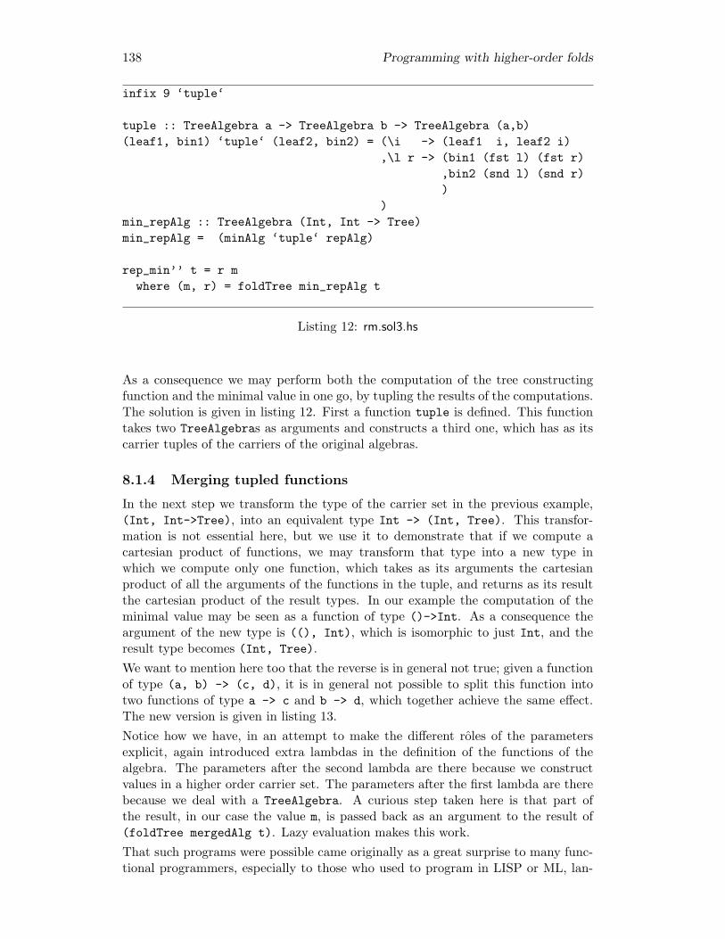
138 Programming with higher-order folds
infix 9 ‘tuple‘
tuple :: TreeAlgebra a -> TreeAlgebra b -> TreeAlgebra (a,b)(leaf1, bin1) ‘tuple‘ (leaf2, bin2) = (\i -> (leaf1 i, leaf2 i)
,\l r -> (bin1 (fst l) (fst r),bin2 (snd l) (snd r))
)min_repAlg :: TreeAlgebra (Int, Int -> Tree)min_repAlg = (minAlg ‘tuple‘ repAlg)
rep_min’’ t = r mwhere (m, r) = foldTree min_repAlg t
Listing 12: rm.sol3.hs
As a consequence we may perform both the computation of the tree constructingfunction and the minimal value in one go, by tupling the results of the computations.The solution is given in listing 12. First a function tuple is defined. This functiontakes two TreeAlgebras as arguments and constructs a third one, which has as itscarrier tuples of the carriers of the original algebras.
8.1.4 Merging tupled functions
In the next step we transform the type of the carrier set in the previous example,(Int, Int->Tree), into an equivalent type Int -> (Int, Tree). This transfor-mation is not essential here, but we use it to demonstrate that if we compute acartesian product of functions, we may transform that type into a new type inwhich we compute only one function, which takes as its arguments the cartesianproduct of all the arguments of the functions in the tuple, and returns as its resultthe cartesian product of the result types. In our example the computation of theminimal value may be seen as a function of type ()->Int. As a consequence theargument of the new type is ((), Int), which is isomorphic to just Int, and theresult type becomes (Int, Tree).We want to mention here too that the reverse is in general not true; given a functionof type (a, b) -> (c, d), it is in general not possible to split this function intotwo functions of type a -> c and b -> d, which together achieve the same effect.The new version is given in listing 13.Notice how we have, in an attempt to make the different roles of the parametersexplicit, again introduced extra lambdas in the definition of the functions of thealgebra. The parameters after the second lambda are there because we constructvalues in a higher order carrier set. The parameters after the first lambda are therebecause we deal with a TreeAlgebra. A curious step taken here is that part ofthe result, in our case the value m, is passed back as an argument to the result of(foldTree mergedAlg t). Lazy evaluation makes this work.That such programs were possible came originally as a great surprise to many func-tional programmers, especially to those who used to program in LISP or ML, lan-
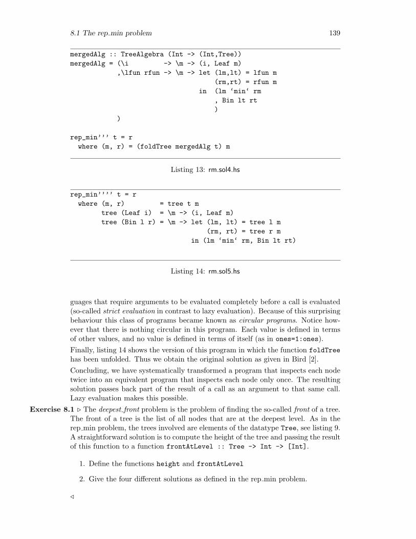
8.1 The rep min problem 139
mergedAlg :: TreeAlgebra (Int -> (Int,Tree))mergedAlg = (\i -> \m -> (i, Leaf m)
,\lfun rfun -> \m -> let (lm,lt) = lfun m(rm,rt) = rfun m
in (lm ‘min‘ rm, Bin lt rt)
)
rep_min’’’ t = rwhere (m, r) = (foldTree mergedAlg t) m
Listing 13: rm.sol4.hs
rep_min’’’’ t = rwhere (m, r) = tree t m
tree (Leaf i) = \m -> (i, Leaf m)tree (Bin l r) = \m -> let (lm, lt) = tree l m
(rm, rt) = tree r min (lm ‘min‘ rm, Bin lt rt)
Listing 14: rm.sol5.hs
guages that require arguments to be evaluated completely before a call is evaluated(so-called strict evaluation in contrast to lazy evaluation). Because of this surprisingbehaviour this class of programs became known as circular programs. Notice how-ever that there is nothing circular in this program. Each value is defined in termsof other values, and no value is defined in terms of itself (as in ones=1:ones).Finally, listing 14 shows the version of this program in which the function foldTreehas been unfolded. Thus we obtain the original solution as given in Bird [2].Concluding, we have systematically transformed a program that inspects each nodetwice into an equivalent program that inspects each node only once. The resultingsolution passes back part of the result of a call as an argument to that same call.Lazy evaluation makes this possible.
Exercise 8.1 . The deepest front problem is the problem of finding the so-called front of a tree.The front of a tree is the list of all nodes that are at the deepest level. As in therep min problem, the trees involved are elements of the datatype Tree, see listing 9.A straightforward solution is to compute the height of the tree and passing the resultof this function to a function frontAtLevel :: Tree -> Int -> [Int].
1. Define the functions height and frontAtLevel
2. Give the four different solutions as defined in the rep min problem.
/

140 Programming with higher-order folds
data ExprAS = If ExprAS ExprAS ExprAS| Apply ExprAS ExprAS| ConInt Int| ConBool Bool deriving Show
type ExprASAlgebra a = (a -> a -> a -> a,a -> a -> a,Int -> a,Bool -> a)
foldExprAS :: ExprASAlgebra a -> ExprAS -> afoldExprAS (iff,apply,conint,conbool) = fold
where fold (If ce te ee) = iff (fold ce) (fold te) (fold ee)fold (Apply fe ae) = apply (fold fe) (fold ae)fold (ConInt i) = conint ifold (ConBool b) = conbool b
Listing 15: ExprAbstractSyntax.hs
Exercise 8.2 . Redo the previous exercise for the highest front problem /
8.2 A small compiler
This section constructs a small compiler for (a part of) a small language. Thecompiler compiles this code into code for a hypothetical stack machine.
8.2.1 The language
The language we consider in this section has integers, booleans, function application,and an if-then-else expression. A language with just these constructs is useless, andyou will extend the language in the exercises with some other constructs, which makethe language a bit more interesting. We take the following context-free grammar forthe concrete syntax of the language.
Expr0 → if Expr1 then Expr1 else Expr1 | Expr1Expr1 → Expr2 Expr2∗
Expr2 → Int | Bool
where Int generates integers, and Bool booleans. An abstract syntax for our lan-guage is given in listing 15. Note that we use a single datatype for the abstractsyntax instead of three datatypes (one for each nonterminal); this simplifies thecode a bit. The listing 15 also contains a definition of a fold and an algebra type forthe abstract syntax.A parser for expressions is given in listing 16.
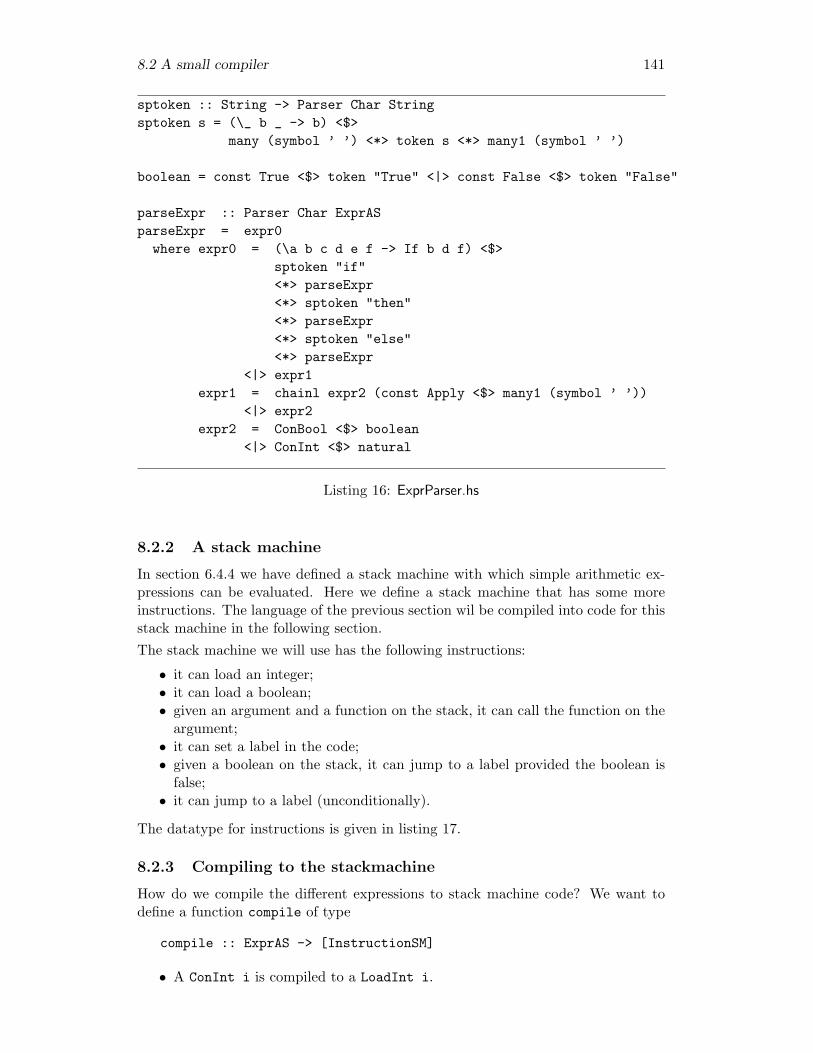
8.2 A small compiler 141
sptoken :: String -> Parser Char Stringsptoken s = (\_ b _ -> b) <$>
many (symbol ’ ’) <*> token s <*> many1 (symbol ’ ’)
boolean = const True <$> token "True" <|> const False <$> token "False"
parseExpr :: Parser Char ExprASparseExpr = expr0
where expr0 = (\a b c d e f -> If b d f) <$>sptoken "if"<*> parseExpr<*> sptoken "then"<*> parseExpr<*> sptoken "else"<*> parseExpr
<|> expr1expr1 = chainl expr2 (const Apply <$> many1 (symbol ’ ’))
<|> expr2expr2 = ConBool <$> boolean
<|> ConInt <$> natural
Listing 16: ExprParser.hs
8.2.2 A stack machine
In section 6.4.4 we have defined a stack machine with which simple arithmetic ex-pressions can be evaluated. Here we define a stack machine that has some moreinstructions. The language of the previous section wil be compiled into code for thisstack machine in the following section.The stack machine we will use has the following instructions:
• it can load an integer;• it can load a boolean;• given an argument and a function on the stack, it can call the function on the
argument;• it can set a label in the code;• given a boolean on the stack, it can jump to a label provided the boolean is
false;• it can jump to a label (unconditionally).
The datatype for instructions is given in listing 17.
8.2.3 Compiling to the stackmachine
How do we compile the different expressions to stack machine code? We want todefine a function compile of type
compile :: ExprAS -> [InstructionSM]
• A ConInt i is compiled to a LoadInt i.
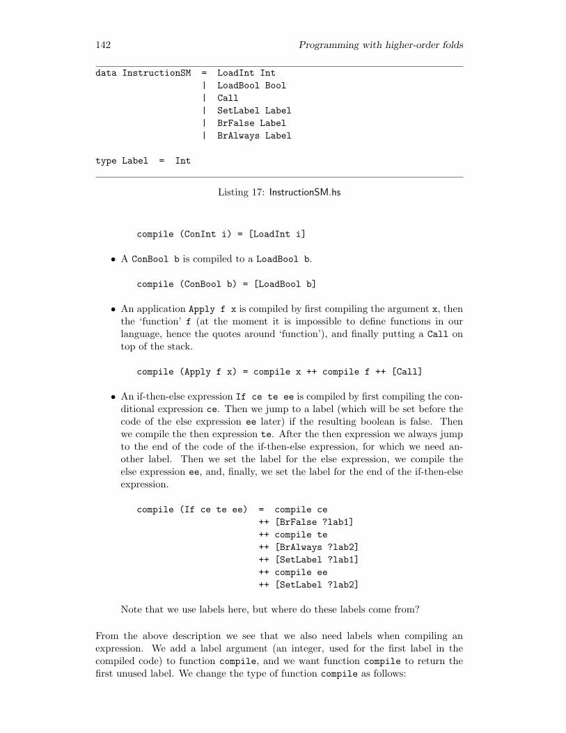
142 Programming with higher-order folds
data InstructionSM = LoadInt Int| LoadBool Bool| Call| SetLabel Label| BrFalse Label| BrAlways Label
type Label = Int
Listing 17: InstructionSM.hs
compile (ConInt i) = [LoadInt i]
• A ConBool b is compiled to a LoadBool b.
compile (ConBool b) = [LoadBool b]
• An application Apply f x is compiled by first compiling the argument x, thenthe ‘function’ f (at the moment it is impossible to define functions in ourlanguage, hence the quotes around ‘function’), and finally putting a Call ontop of the stack.
compile (Apply f x) = compile x ++ compile f ++ [Call]
• An if-then-else expression If ce te ee is compiled by first compiling the con-ditional expression ce. Then we jump to a label (which will be set before thecode of the else expression ee later) if the resulting boolean is false. Thenwe compile the then expression te. After the then expression we always jumpto the end of the code of the if-then-else expression, for which we need an-other label. Then we set the label for the else expression, we compile theelse expression ee, and, finally, we set the label for the end of the if-then-elseexpression.
compile (If ce te ee) = compile ce++ [BrFalse ?lab1]++ compile te++ [BrAlways ?lab2]++ [SetLabel ?lab1]++ compile ee++ [SetLabel ?lab2]
Note that we use labels here, but where do these labels come from?
From the above description we see that we also need labels when compiling anexpression. We add a label argument (an integer, used for the first label in thecompiled code) to function compile, and we want function compile to return thefirst unused label. We change the type of function compile as follows:

8.3 Attribute grammars 143
compile :: ExprAS -> Label -> ([InstructionSM],Label)
type Label = Int
The four cases in the definition of compile have to take care of the labels. We obtainthe following definition of compile:
compile (ConInt i) = \l -> ([LoadInt i],l)compile (ConBool b) = \l -> ([LoadBool b],l)compile (Apply f x) = \l -> let (xc,l’) = compile x l
(fc,l’’) = compile f l’in (xc ++ fc ++ [Call],l’’)
compile (If ce te ee) = \l -> let (cc,l’) = compile ce (l+2)(tc,l’’) = compile te l’(ec,l’’’) = compile ee l’’
in ( cc++ [BrFalse l]++ tc++ [BrAlways (l+1)]++ [SetLabel l]++ ec++ [SetLabel (l+1)],l’’’)
Function compile is a fold, the carrier type of its algebra is a function of typeLabel -> ([InstructionSM],Label). The definition of function compile as a foldis given in listing 18.
Exercise 8.3 . Extend the code generation example by adding variables to the datatype Expr./
Exercise 8.4 . Extend the code generation example by adding definitions to the datatype Exprtoo. /
8.3 Attribute grammars
In Section 8.1 we have written a program that solves the rep min problem. Thisprogram computes the minimum of a tree, and it computes the tree in which all theleaf values are replaced by the minimum value. The minimum is computed bottom-up: it is synthesized from its children. The minimum value is then passed on to thefunctions that build the tree with the minimum value in its leaves. These functionsreceive the minimum value from their parent tree node: they inherit the minimumvalue from their parent.We can see the rep min computation as a computation on a value of type Tree,on which two attributes are defined: the minimum and result tree attributes. Theminimum is computed bottom-up, and is then passed down to the result tree, and istherefore a synthesized and inherited attribute. The result tree is computed bottom-up, and is hence a synthesized attribute.The formalism in which it is possible to specify such attributes and computationson datatypes or grammars is called attribute grammars, and was originally proposed

144 Programming with higher-order folds
compile = foldExprAS compileAlgebra
compileAlgebra :: ExprASAlgebra (Label -> ([InstructionSM],Label))compileAlgebra = (\cce cte cee -> \l ->
let (cc,l’) = cce (l+2)(tc,l’’) = cte l’(ec,l’’’) = cee l’’
in ( cc++ [BrFalse l]++ tc++ [BrAlways (l+1)]++ [SetLabel l]++ ec++ [SetLabel (l+1)]
,l’’’)
,\cf cx -> \l -> let (xc,l’) = cx l(fc,l’’) = cf l’
in (xc ++ fc ++ [Call],l’’),\i -> \l -> ([LoadInt i],l),\b -> \l -> ([LoadBool b],l))
Listing 18: CompileExpr.hs
8.3 Attribute grammars 145
by Donald Knuth in [10]. Attribute grammars provide a solution for the system-atic description of the phases of the compiler that come after scanning and parsing.Although they look different from what we have encountered thus far and are prob-ably a little easier to write, they can straightforwardly be mapped onto a functionalprogram. The programs you have seen in this chapter could also have been obtainedby means of such a mapping from an attribute grammar specification. Traditionallysuch attribute grammars are used as the input of a compiler generator. Just as wehave seen how by introducing a suitable set of parsing combinators one may avoidthe use of a special parser generator and even gain a lot of flexibility in extend-ing the grammatical formalism by introducing more complicated combinators, wehave shown how one can do without a special purpose attribute grammar processingsystem. But, just as the concept of a context free grammar was useful in understand-ing the fundamentals of parser combinators, understanding attribute grammars willhelp significantly in describing the semantic part of the recognition and compilationprocess. This chapter does not further introduce attribute grammars, but they willappear again in the course in implementing programming languages.
146 Programming with higher-order folds

Chapter 9
Pumping Lemmas: the expressivepower of languages
introduction
In these lecture notes we have presented several ways to show that a languageis regular or context-free, but until now we did not give any means to show thenonregularity or noncontext-freeness of a language. In this chapter we fill this gapby introducing the so-called Pumping Lemmas. For example, the pumping lemmafor regular languages says
IF language L is regular,
THEN it has the following property P : each sufficiently long word w ∈ L hasa substring that can be repeated any number of times, every time yieldinganother word of L
In applications, pumping lemmas are used in the contrapositive way. In the regularcase this means that one may conclude that L is not regular, if P does not hold.Although the ideas behind pumping lemmas are very simple, a precise formulationis not. As a consequence, it takes some effort to get familiar with applying pumpinglemmas. Regular grammars and context-free grammars are part of the Chomskyhierarchy, which consists of four different kinds of grammars and their correspondinglanguages. Pumping lemmas are used to show that the expressive power of thedifferent elements of the Chomsky hierarchy is different.
goals
After you have studied this chapter you will be able to
• prove that a language is not regular;• prove that a language is not context-free;• identify languages and grammars as regular, context-free or none of these;• give examples of languages that are not regular, and/or not context-free;• explain the Chomsky hierarchy.
9.1 The Chomsky hierarchy
In the preceding chapters we have seen contex-free grammars and regular grammars.You may now wonder: is it possible to express any language with these grammars?
147

148 Pumping Lemmas: the expressive power of languages
And: is it possible to obtain any context-free language from a regular grammar? Theanswer to these questions is no. The Chomsky hierarchy explains why the answeris no. The Chomsky hierarchy consists of four elements, each of which is explainedbelow.
9.1.1 Type-0 grammars
The most powerful grammars are the type-0 grammars, in which a production hasthe form φ → ψ, where φ ∈ V +, ψ ∈ V ∗, where V is the set of symbols of thegrammar. So the left-hand side of a production may consist of a list of nonterminaland terminal symbols, instead of a single nonterminal as in context-free grammars.Type-0 grammars have the same expressive power as Turing machines, and thelanguages described by these grammars are the recursive enumerable languages.This expressive power comes at a cost though: it is very difficult to parse sentencesfrom type-0 grammars.
9.1.2 Type-1 grammars
We can slightly restrict the form of the productions to obtain type-1 grammars. Ina type-1, or context-sensitive grammar, each production has the form φAψ → φδψ,where φ, ψ ∈ V ∗, δ ∈ V +. So a production describes how to rewrite a nonterminalA, in the context of lists of symbols φ and ψ. A language generated by a context-sensitive grammar is called a context-sensitive language. Although context-sensitivegrammars are less expressive than type-0 grammars, parsing is still very difficult forcontext-sensitive grammars.
9.1.3 Type-2 grammars
The type-2 grammars are the context-free grammars which you have seen a lot in thepreceding chapters. As the name says, in a context-free grammar you can rewritenonterminals without looking at the context in which they appear. Actually, it isimpossible to look at the context when rewriting symbols. Context-free grammarsare less expressive than context-sensitive grammars. This statement can be provedusing the pumping lemma for context-free languages.However, it is much easier to parse sentences from context-free languages. In fact, asentence of length n can be parsed in time at most O(n3) (or even a bit less than this)for any sentence of a context-free language. And if we put some more restrictionson context-free grammars (for example LL(1)), we obtain linear-time algorithms forparsing sentences of such grammars.
9.1.4 Type-3 grammars
The type-3 grammars in the Chomsky hierarchy are the regular grammars. Anysentence from a regular language can be processed by means of a finite-state au-tomaton, which takes linear time and constant space in the size of its input. Theset of regular languages is strictly smaller than the set of context-free languages, afact we will prove below by means of the pumping lemma for regular languages.

9.2 The pumping lemma for regular languages 149
9.2 The pumping lemma for regular languages
In this section we give the pumping lemma for regular languages. The lemma givesa property that is satisfied by all regular languages. The property is a statementof the form: in sentences longer than a certain length a substring can be identifiedthat can be duplicated while retaining a sentence. The idea behind this propertyis simple: regular languages are accepted by finite automata. Given a DFA for aregular language, a sentence of the language describes a path from the start state tosome finite state. When the length of such a sentence exceeds the number of states,then at least one state is visited twice; consequently the path contains a cycle thatcan be repeated as often as desired. The proof of the following lemma is given inSection 9.4.
Theorem 1: Regular Pumping LemmaLet L be a regular language. Then
there exists n ∈ IIN :for all x, y, z : xyz ∈ L and |y| ≥ n :there exist u, v, w : y = uvw and |v| > 0 :for all i ∈ IIN : xuv iwz ∈ L
2
Note that |y| denotes the length of the string y. Also remember that for all x ∈ X :· · · is true if X = Ø, and there exists x ∈ X : · · · is false if X = Ø.For example, consider the following automaton.
S?>=<89:; a // A?>=<89:; b // B
c
��
?>=<89:;
C?>=<89:;a
__????????????????
d
��D?>=<89:;/.-,()*+
This automaton accepts: abcabcd, abcabcabcd, and, in general, a(bca)∗bcd. Thestatement of the pumping lemma amounts to the following. Take for n the numberof states in the automaton (5). Let x, y, z be such that xyz ∈ L, and |y| ≥ n.Then we know that in order to accept y, the above automaton has to pass at leasttwice through state A. The part that is accepted in between the two momentsthe automaton passes through state A can be pumped up to create sentences thatcontain an arbitrary number of copies of the string v = bca.This pumping lemma is useful in showing that a language does not belong to thefamily of regular languages. Its application is typical of pumping lemmas in general;they are used negatively to show that a given language does not belong to somefamily.
150 Pumping Lemmas: the expressive power of languages
Theorem 1 enables us to prove that a language L is not regular by showing that
for all n ∈ IIN :there exist x, y, z : xyz ∈ L and |y| ≥ n :for all u, v, w : y = uvw and |v| > 0 :there exists i ∈ IIN : xuv iwz 6∈ L
In all applications of the pumping lemma in this chapter, this is the formulation wewill use.Note that if n = 0, we can choose y = ε, and since there is no v with |v| > 0 suchthat y = uvw, the statement above holds for all such v (namely none!).As an example, we will prove that language L = {ambm | m ≥ 0} is not regular.Let n ∈ IIN.Take s = anbn with x = ε, y = an, and z = bn.Let u, v, w be such that y = uvw with v 6= ε, that is, u = ap, v = aq and w = ar
with p+ q + r = n and q > 0.Take i = 2, then
xuv2wz 6∈ L⇐ defn. x, u, v, w, z, calculus
ap+2q+rbn 6∈ L⇐ p+ q + r = n
n+ q 6= n
⇐ arithmetic
q > 0
⇐ q > 0
true
Note that the language L = {ambm | m ≥ 0} is context-free, and together with thefact that each regular grammar is also a context-free grammar it follows immediatelythat the set of regular languages is strictly smaller than the set of context-freelanguages.Note that here we use the pumping lemma (and not the proof of the pumping lemma)to prove that a language is not regular. This kind of proof can be viewed as a kind ofgame: ‘for all’ is about an arbitrary element which can be chosen by the opponent;‘there exists’ is about a particular element which you may choose. Choosing the rightelements helps you ‘win’ the game, where winning means proving that a language isnot regular.
Exercise 9.1 . Prove that the following language is not regular
{ak2 | k ≥ 0}
/
Exercise 9.2 . Show that the following language is not regular.
{x | x ∈ {a, b}∗ ∧ nr a x < nr b x}
where nr a x is the number of occurrences of a in x. /
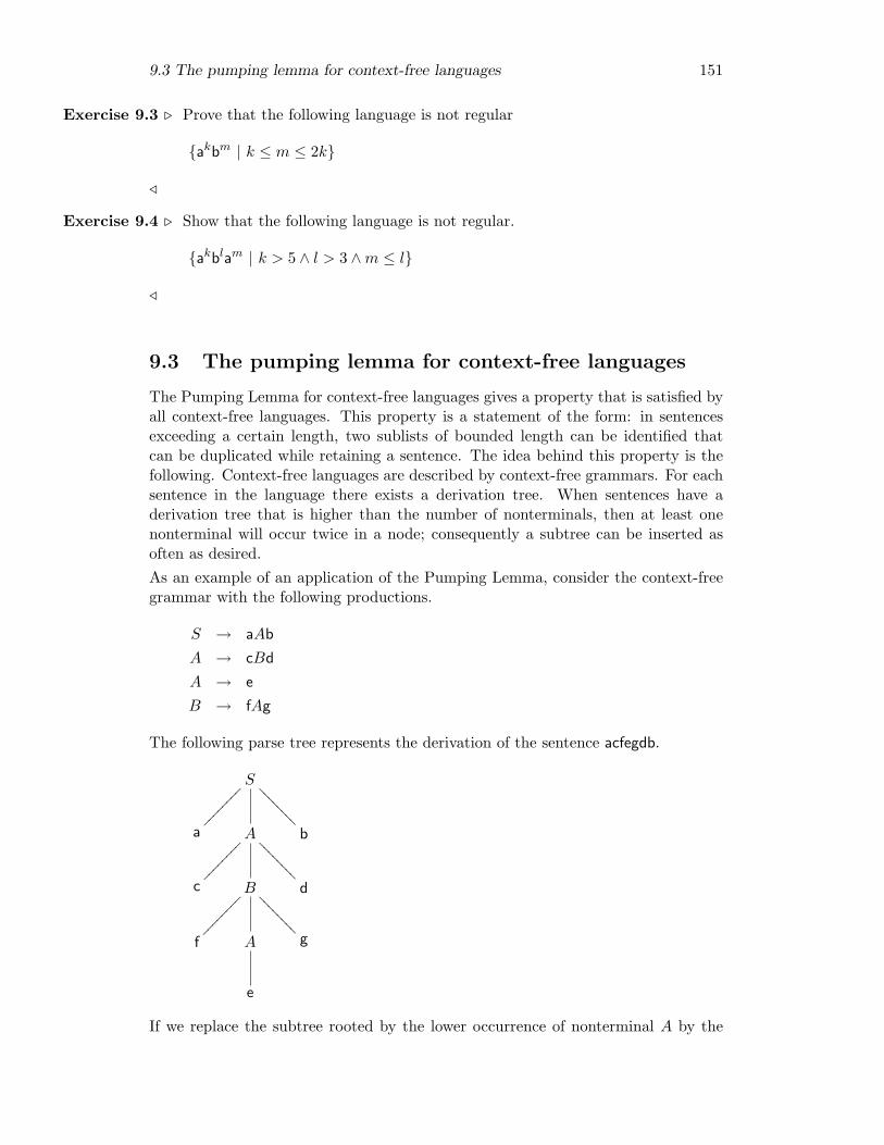
9.3 The pumping lemma for context-free languages 151
Exercise 9.3 . Prove that the following language is not regular
{akbm | k ≤ m ≤ 2k}
/
Exercise 9.4 . Show that the following language is not regular.
{akblam | k > 5 ∧ l > 3 ∧m ≤ l}
/
9.3 The pumping lemma for context-free languages
The Pumping Lemma for context-free languages gives a property that is satisfied byall context-free languages. This property is a statement of the form: in sentencesexceeding a certain length, two sublists of bounded length can be identified thatcan be duplicated while retaining a sentence. The idea behind this property is thefollowing. Context-free languages are described by context-free grammars. For eachsentence in the language there exists a derivation tree. When sentences have aderivation tree that is higher than the number of nonterminals, then at least onenonterminal will occur twice in a node; consequently a subtree can be inserted asoften as desired.As an example of an application of the Pumping Lemma, consider the context-freegrammar with the following productions.
S → aAb
A → cBd
A → e
B → fAg
The following parse tree represents the derivation of the sentence acfegdb.
S
����
����
????
????
a A
����
����
????
????
b
c B
����
����
????
????
d
f A g
e
If we replace the subtree rooted by the lower occurrence of nonterminal A by the
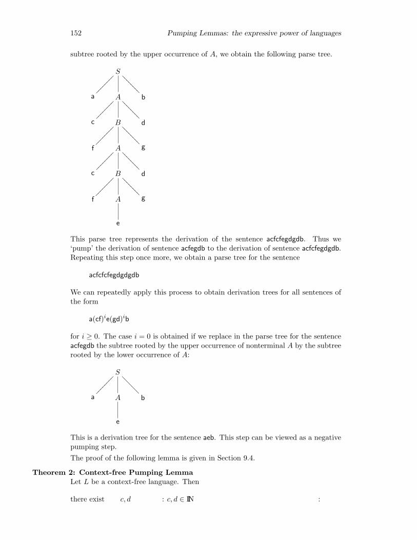
152 Pumping Lemmas: the expressive power of languages
subtree rooted by the upper occurrence of A, we obtain the following parse tree.
S
����
����
????
????
a A
����
����
????
????
b
c B
����
����
????
????
d
f A
����
����
????
????
g
c B
����
����
????
????
d
f A g
e
This parse tree represents the derivation of the sentence acfcfegdgdb. Thus we‘pump’ the derivation of sentence acfegdb to the derivation of sentence acfcfegdgdb.Repeating this step once more, we obtain a parse tree for the sentence
acfcfcfegdgdgdb
We can repeatedly apply this process to obtain derivation trees for all sentences ofthe form
a(cf)ie(gd)ib
for i ≥ 0. The case i = 0 is obtained if we replace in the parse tree for the sentenceacfegdb the subtree rooted by the upper occurrence of nonterminal A by the subtreerooted by the lower occurrence of A:
S
����
����
>>>>
>>>
a A b
e
This is a derivation tree for the sentence aeb. This step can be viewed as a negativepumping step.The proof of the following lemma is given in Section 9.4.
Theorem 2: Context-free Pumping LemmaLet L be a context-free language. Then
there exist c, d : c, d ∈ IIN :

9.3 The pumping lemma for context-free languages 153
for all z : z ∈ L and |z| > c :there exist u, v, w, x, y : z = uvwxy and |vx | > 0 and |vwx | ≤ d :for all i ∈ IIN : uv iwx iy ∈ L
2
The Pumping Lemma is a tool with which we prove that a given language is notcontext-free. The proof obligation is to show that the property shared by all context-free languages does not hold for the language under consideration.Theorem 2 enables us to prove that a language L is not context-free by showing that
for all c, d : c, d ∈ IIN :there exists z : z ∈ L and |z| ≥ c :for all u, v, w, x, y : z = uvwxy and |vx | > 0 and |vwx | ≤ d :there exists i ∈ IIN : uv iwx iy 6∈ L
As an example, we will prove that the language T defined by
T = {anbncn | n > 0}
is not context-free.Proof: Let c, d ∈ IIN.Take z = arbrcr with r = max(c, d).Let u, v, w, x, y be such that z = uvwxy, |vx| > 0 and |vwx | ≤ dNote that our choice for r guarantees that substring vwx has one of the followingshapes:
• vwx consists of just a’s, or just b’s, or just c’s.• vwx contains both a’s and b’s, or both b’s and c’s.
So vwx does not contain a’s, b’s, and c’s.Take i = 0, then
• If vwx consists of just a’s, or just b’s, or just c’s, then it is impossible to writethe string uwy as asbscs for some s, since only the number of terminals of onekind is decreased.• If vwx contains both a’s and b’s, or both b’s and c’s it lies somewhere on the
border between a’s and b’s, or on the border between b’s and c’s. Then thestring uwy can be written as
uwy = asbtcr
uwy = arbpcq
for some s, t, p, q, respectively. At least one of s and t or of p and q is lessthan r. Again this list is not an element of T .
2
Exercise 9.5 . Prove that the following language is not context-free
{ak2 | k ≥ 0}
/

154 Pumping Lemmas: the expressive power of languages
Exercise 9.6 . Prove that the following language is not context-free
{ai | i is a prime number }
/
Exercise 9.7 . Prove that the following language is not context-free
{ww | w ∈ {a, b}∗}
/
9.4 Proofs of pumping lemmas
This section gives the proof of the pumping lemmas.Proof: of the Regular Pumping Lemma, Theorem 1.Since L is a regular language, there exists a deterministic finite-state automaton Dsuch that L = Ldfa D.Take for n the number of states of D.Let s be an element of L with sublist y such that |y| ≥ n, say s = xyz .Consider the sequence of states D passes through while processing y. Since |y| ≥ n,this sequence has more than n entries, hence at least one state, say state A, occurstwice.Take u, v, w as follows
• u is the initial part of y processed until the first occurrence of A,• v is the (nonempty) part of y processed from the first to the second occurrence
of A,• w is the remaining part of y
Note that D could have skipped processing v, and hence would have accepted xuwz .Furthermore, D can repeat the processing in between the first occurrence of A andthe second occurrence of A as often as desired, and hence it accepts xuv iwz for alli ∈ IIN. Formally, a simple proof by induction shows that (∀i : i ≥ 0 : xuviwz ∈ L).2
Proof: of the Context-free Pumping Lemma, Theorem 2.Let G = (T,N,R, S) be a context-free grammar such that L = L(G). Let m be thelength of the longest right-hand side of any production, and let k be the number ofnonterminals of G.Take c = mk. In Lemma 3 below we prove that if z is a list with |z| > c, then in allderivation trees for z there exists a path of length at least k+1.Let z ∈ L such that |z| > c. Since grammar G has k nonterminals, there is at leastone nonterminal that occurs more than once in a path of length k+1 (which containsk+2 symbols, of which at most one is a terminal, and all others are nonterminals)of a derivation tree for z. Consider the nonterminal A that satisfies the followingrequirements.
• A occurs at least twice in the path of length k+1 of a derivation tree for z.
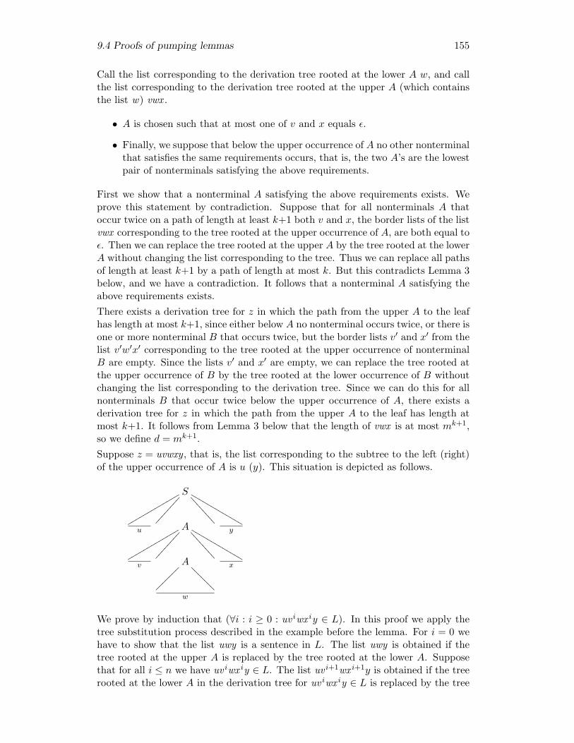
9.4 Proofs of pumping lemmas 155
Call the list corresponding to the derivation tree rooted at the lower A w, and callthe list corresponding to the derivation tree rooted at the upper A (which containsthe list w) vwx .
• A is chosen such that at most one of v and x equals ε.
• Finally, we suppose that below the upper occurrence of A no other nonterminalthat satisfies the same requirements occurs, that is, the two A’s are the lowestpair of nonterminals satisfying the above requirements.
First we show that a nonterminal A satisfying the above requirements exists. Weprove this statement by contradiction. Suppose that for all nonterminals A thatoccur twice on a path of length at least k+1 both v and x, the border lists of the listvwx corresponding to the tree rooted at the upper occurrence of A, are both equal toε. Then we can replace the tree rooted at the upper A by the tree rooted at the lowerA without changing the list corresponding to the tree. Thus we can replace all pathsof length at least k+1 by a path of length at most k. But this contradicts Lemma 3below, and we have a contradiction. It follows that a nonterminal A satisfying theabove requirements exists.There exists a derivation tree for z in which the path from the upper A to the leafhas length at most k+1, since either below A no nonterminal occurs twice, or there isone or more nonterminal B that occurs twice, but the border lists v′ and x′ from thelist v′w′x′ corresponding to the tree rooted at the upper occurrence of nonterminalB are empty. Since the lists v′ and x′ are empty, we can replace the tree rooted atthe upper occurrence of B by the tree rooted at the lower occurrence of B withoutchanging the list corresponding to the derivation tree. Since we can do this for allnonterminals B that occur twice below the upper occurrence of A, there exists aderivation tree for z in which the path from the upper A to the leaf has length atmost k+1. It follows from Lemma 3 below that the length of vwx is at most mk+1,so we define d = mk+1.Suppose z = uvwxy , that is, the list corresponding to the subtree to the left (right)of the upper occurrence of A is u (y). This situation is depicted as follows.
S
rrrrrrrrrrrrr
����
����
<<<<
<<<<
LLLLLLLLLLLLL
u A
rrrrrrrrrrrrr
����
����
<<<<
<<<<
LLLLLLLLLLLLL y
v A
����
���
????
??? x
w
We prove by induction that (∀i : i ≥ 0 : uv iwx iy ∈ L). In this proof we apply thetree substitution process described in the example before the lemma. For i = 0 wehave to show that the list uwy is a sentence in L. The list uwy is obtained if thetree rooted at the upper A is replaced by the tree rooted at the lower A. Supposethat for all i ≤ n we have uv iwx iy ∈ L. The list uv i+1wx i+1y is obtained if the treerooted at the lower A in the derivation tree for uv iwx iy ∈ L is replaced by the tree

156 Pumping Lemmas: the expressive power of languages
rooted above it A. This proves the induction step.2
The proof of the Pumping Lemma above frequently refers to the following lemma.
Theorem 3:Let G be a context-free grammar, and suppose that the longest right-hand side ofany production has length m. Let t be a derivation tree for a list z ∈ L G. Ifheight t ≤ j, then |z| ≤ mj . 2
Proof: We prove a slightly stronger result: if t is a derivation tree for a list z, butthe root of t is not necessarily the start-symbol, and height t ≤ j, then |z| ≤ mj .We prove this statement by induction on j.For the base case, suppose j = 1. Then tree t corresponds to a single production inG, and since the longest right-hand side of any production has length m, we havethat |z| ≤ m = mj .For the induction step, assume that for all derivation trees t of height at most jwe have that |z| ≤ mj , where z is the list corresponding to t. Suppose we havea tree t of height j+1. Let A be the root of t, and suppose the top of the treecorresponds to the production A→ v in G. For all trees s rooted at the symbols ofv we have height s ≤ j, so the induction hypothesis applies to these trees, and thelists corresponding to the trees rooted at the symbols of v all have length at mostmj . Since A→ v is a production of G, and since the longest right-hand side of anyproduction has length m, the list corresponding to the tree rooted at A has lengthat most m×mj = mj+1, which proves the induction step. 2
summary
This section introduces pumping lemmas. Pumping lemmas are used to prove thatlanguages are not regular or not context-free.
9.5 exercises
Exercise 9.8 . Show that the following language is not regular.
{x | x ∈ {0, 1}∗ ∧ nr 1 x = nr 0 x}
where function nr takes an element a and a list x, and returns the number ofoccurrences of a in x. /
Exercise 9.9 . Consider the following language:
{aibj | 0 ≤ i ≤ j}
1. Is this language context-free? If it is, give a context-free grammar and provethat this grammar generates the language. If it is not, why not?
2. Is this language regular? If it is, give a regular grammar and prove that thisgrammar generates the language. If it is not, why not?
/
Exercise 9.10 . Consider the following language:
{wcw | w ∈ {a, b}∗}
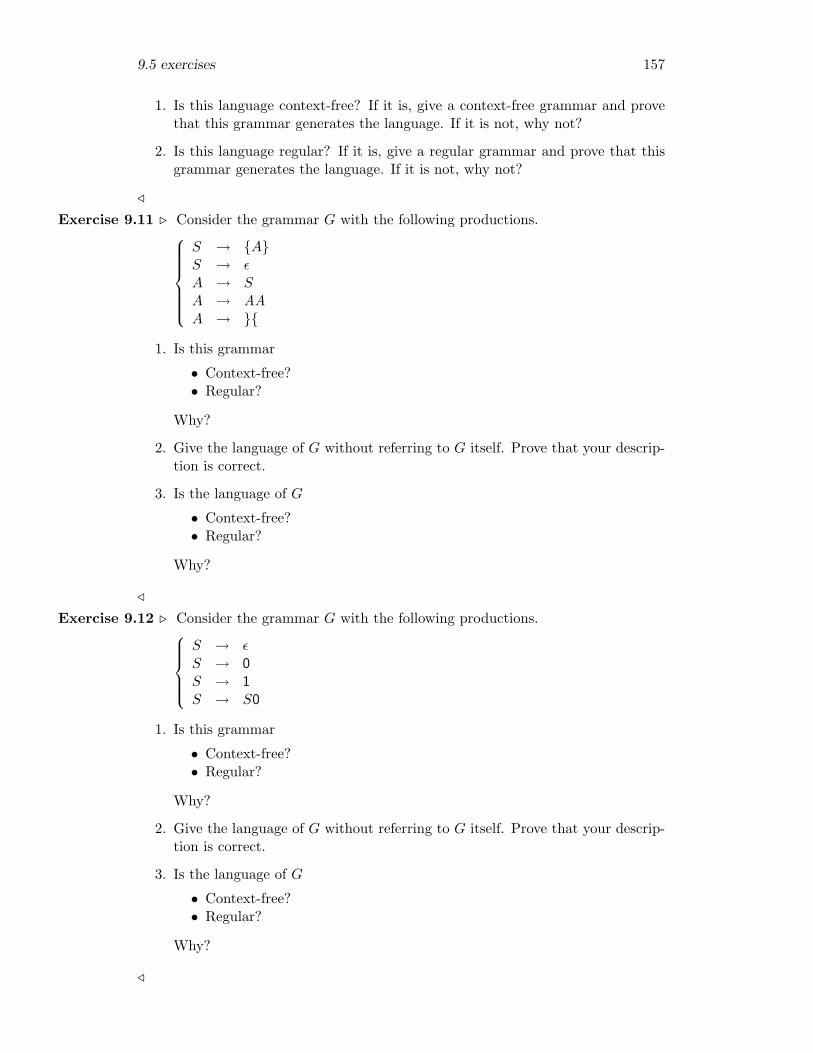
9.5 exercises 157
1. Is this language context-free? If it is, give a context-free grammar and provethat this grammar generates the language. If it is not, why not?
2. Is this language regular? If it is, give a regular grammar and prove that thisgrammar generates the language. If it is not, why not?
/
Exercise 9.11 . Consider the grammar G with the following productions.
S → {A}S → εA → SA → AAA → }{
1. Is this grammar
• Context-free?• Regular?
Why?
2. Give the language of G without referring to G itself. Prove that your descrip-tion is correct.
3. Is the language of G
• Context-free?• Regular?
Why?
/
Exercise 9.12 . Consider the grammar G with the following productions.S → εS → 0S → 1S → S0
1. Is this grammar
• Context-free?• Regular?
Why?
2. Give the language of G without referring to G itself. Prove that your descrip-tion is correct.
3. Is the language of G
• Context-free?• Regular?
Why?
/
158 Pumping Lemmas: the expressive power of languages
Chapter 10
LL Parsing
introduction
This chapter introduces LL(1) parsing. LL(1) parsing is an efficient (linear in thelength of the input string) method for parsing that can be used for all LL(1) gram-mars. A grammar is LL(1) if at each step in a derivation the next symbol in theinput uniquely determines the production that should be applied. In order to de-termine whether or not a grammar is LL(1), we introduce several kinds of grammaranalyses, such as determining whether or not a nonterminal can derive the emptystring, and determining the set of symbols that can appear as the first symbol in aderivation from a nonterminal.
goals
After studying this chapter you will
• know the definition of LL(1) grammars;
• know how to parse a sentence from an LL(1) grammar;
• be able to apply different kinds of grammar analyses in order to determinewhether or not a grammar is LL(1).
This chapter is organised as follows. Section 10.1 describes the background of LL(1)parsing, and Section 10.2 describes an implementation in Haskell of LL(1) parsingand the different kinds of grammar analyses needed for checking whether or not agrammar is LL(1).
10.1 LL Parsing: Background
In the previous chapters we have shown how to construct parsers for sentences ofcontext-free languages using combinator parsers. Since these parsers may backtrack,the resulting parsers are sometimes a bit slow. There are several ways in whichwe can put extra restrictions on context-free grammars such that we can parsesentences of the corresponding languages efficiently. This chapter discusses one suchrestriction: LL(1). Other restrictions, not discussed in these lecture notes are LR(1),LALR(1), SLR(1), etc.
159
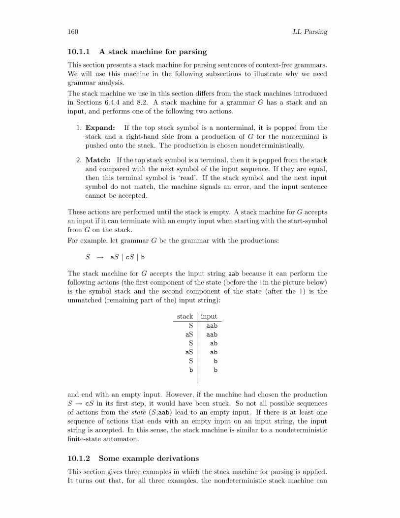
160 LL Parsing
10.1.1 A stack machine for parsing
This section presents a stack machine for parsing sentences of context-free grammars.We will use this machine in the following subsections to illustrate why we needgrammar analysis.The stack machine we use in this section differs from the stack machines introducedin Sections 6.4.4 and 8.2. A stack machine for a grammar G has a stack and aninput, and performs one of the following two actions.
1. Expand: If the top stack symbol is a nonterminal, it is popped from thestack and a right-hand side from a production of G for the nonterminal ispushed onto the stack. The production is chosen nondeterministically.
2. Match: If the top stack symbol is a terminal, then it is popped from the stackand compared with the next symbol of the input sequence. If they are equal,then this terminal symbol is ‘read’. If the stack symbol and the next inputsymbol do not match, the machine signals an error, and the input sentencecannot be accepted.
These actions are performed until the stack is empty. A stack machine for G acceptsan input if it can terminate with an empty input when starting with the start-symbolfrom G on the stack.For example, let grammar G be the grammar with the productions:
S → aS | cS | b
The stack machine for G accepts the input string aab because it can perform thefollowing actions (the first component of the state (before the |in the picture below)is the symbol stack and the second component of the state (after the |) is theunmatched (remaining part of the) input string):
stack inputS aabaS aabS abaS abS bb b
and end with an empty input. However, if the machine had chosen the productionS → cS in its first step, it would have been stuck. So not all possible sequencesof actions from the state (S,aab) lead to an empty input. If there is at least onesequence of actions that ends with an empty input on an input string, the inputstring is accepted. In this sense, the stack machine is similar to a nondeterministicfinite-state automaton.
10.1.2 Some example derivations
This section gives three examples in which the stack machine for parsing is applied.It turns out that, for all three examples, the nondeterministic stack machine can

10.1 LL Parsing: Background 161
act in a deterministic way by looking ahead one (or two) symbols of the sequenceof input symbols. Each of the examples exemplifies why different kinds of grammaranalyses are useful in parsing.
The first example
Our first example is gramm1. The set of terminal symbols of gramm1 is {a, b, c}, theset of nonterminal symbols is {S,A,B,C}, the start symbol is S; and the productionsare
S → cA | bA → cBC | bSA | aB → cc | CbC → aS | ba
We want to know whether or not the string ccccba is a sentence of the language ofthis grammar. The stack machine produces, amongst others, the following sequence,corresponding with a leftmost derivation of ccccba.
stack inputS ccccba
cA ccccbaA cccba
cBC cccbaBC ccbaccC ccbacC cbaC baba baa a
Starting with S the machine chooses between two productions:
S → cA | b
but, since the first symbol of the string ccccba to be recognised is c, the onlyapplicable production is the first one. After expanding S a match-action removesthe leading c from ccccba and cA. So now we have to derive the string cccba fromA. The machine chooses between three productions:
A → cBC | bSA | a
and again, since the next symbol of the remaining string cccba to be recognised isc, the only applicable production is the first one. After expanding A a match-actionremoves the leading c from cccba and cBC. So now we have to derive the stringccba from BC. The top stack symbol of BC is B. The machine chooses betweentwo productions:
B → cc | Cb

162 LL Parsing
The next symbol of the remaining string ccba to be recognised is, once again, c. Thefirst production is applicable, but the second production may be applicable as well.To decide whether it also applies we have to determine the symbols that can appearas the first element of a string derived from B starting with the second production.The first symbol of the alternative Cb is the nonterminal C. From the productions
C → aS | ba
it is immediately clear that a string derived from C starts with either an a or a b.The set {a, b} is called the first set of the nonterminal C. Since the next symbolin the remaining string to be recognised is a c, the second production cannot beapplied. After expanding B and performing two match-actions it remains to derivethe string ba from C. The machine chooses between two productions C → aS andC → ba. Clearly, only the second one applies, and, after two match-actions, leadsto success.From the above derivation we conclude the following.
Deriving the sentence ccccba using gramm1 is a deterministic computa-tion: at each step of the derivation there is only one applicable alternativefor the nonterminal on top of the stack.
Determinicity is obtained by looking at the first set of the nonterminals.
The second example
A second example is the grammar gramm2 whose productions are
S → abA | aaA → bb | bS
Now we want to know whether or not the string abbb is a sentence of the language ofthis grammar. The stack machine produces, amongst others, the following sequence
stack inputS abbb
abA abbbbA bbbA bbbb bbb b
Starting with S the machine chooses between two productions:
S → abA | aa
since both alternatives start with an a, it is not sufficient to look at the first symbol aof the string to be recognised. The problem is that the lookahead sets (the lookaheadset of a production N → α is the set of terminal symbols that can appear as the firstsymbol of a string that can be derived from N starting with the production N → α,the definition is given in the following subsection) of the two productions for S both
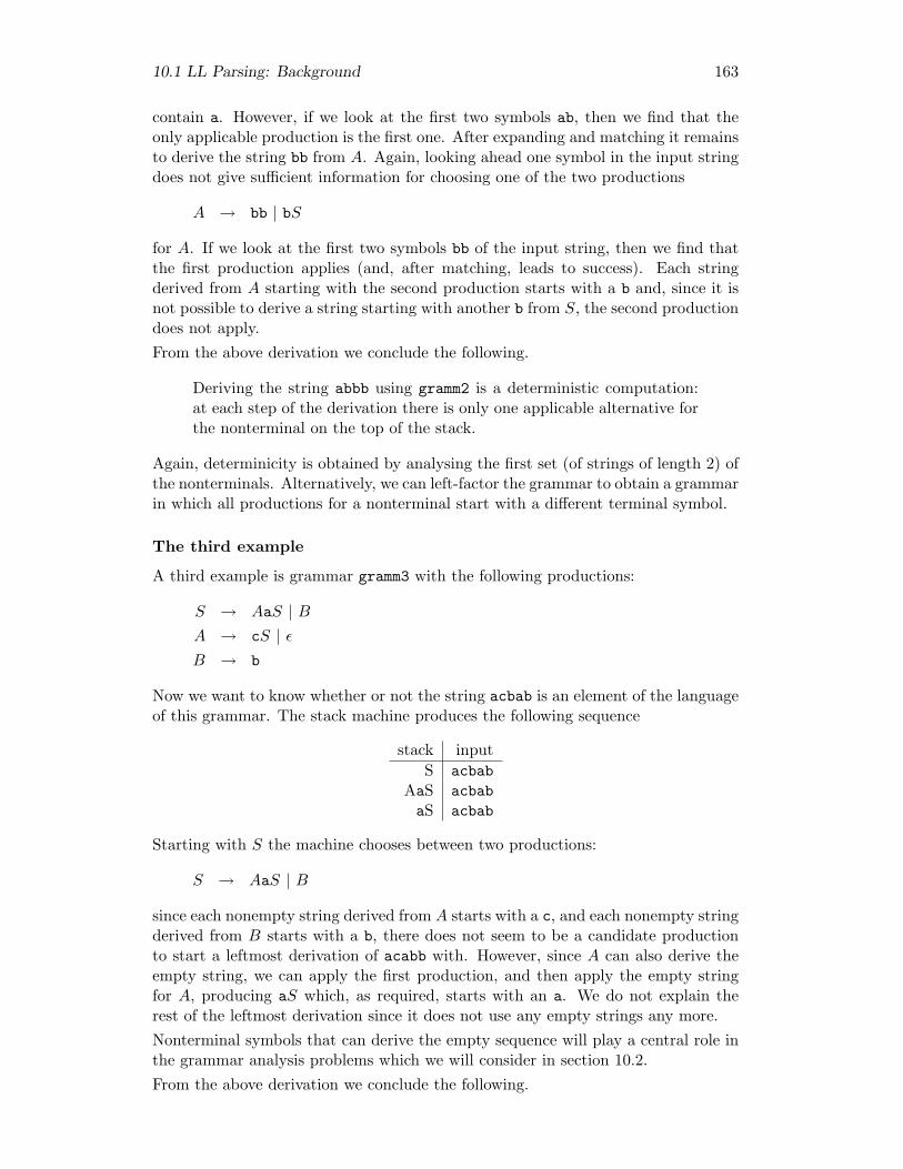
10.1 LL Parsing: Background 163
contain a. However, if we look at the first two symbols ab, then we find that theonly applicable production is the first one. After expanding and matching it remainsto derive the string bb from A. Again, looking ahead one symbol in the input stringdoes not give sufficient information for choosing one of the two productions
A → bb | bS
for A. If we look at the first two symbols bb of the input string, then we find thatthe first production applies (and, after matching, leads to success). Each stringderived from A starting with the second production starts with a b and, since it isnot possible to derive a string starting with another b from S, the second productiondoes not apply.From the above derivation we conclude the following.
Deriving the string abbb using gramm2 is a deterministic computation:at each step of the derivation there is only one applicable alternative forthe nonterminal on the top of the stack.
Again, determinicity is obtained by analysing the first set (of strings of length 2) ofthe nonterminals. Alternatively, we can left-factor the grammar to obtain a grammarin which all productions for a nonterminal start with a different terminal symbol.
The third example
A third example is grammar gramm3 with the following productions:
S → AaS | BA → cS | εB → b
Now we want to know whether or not the string acbab is an element of the languageof this grammar. The stack machine produces the following sequence
stack inputS acbab
AaS acbabaS acbab
Starting with S the machine chooses between two productions:
S → AaS | B
since each nonempty string derived from A starts with a c, and each nonempty stringderived from B starts with a b, there does not seem to be a candidate productionto start a leftmost derivation of acabb with. However, since A can also derive theempty string, we can apply the first production, and then apply the empty stringfor A, producing aS which, as required, starts with an a. We do not explain therest of the leftmost derivation since it does not use any empty strings any more.Nonterminal symbols that can derive the empty sequence will play a central role inthe grammar analysis problems which we will consider in section 10.2.From the above derivation we conclude the following.

164 LL Parsing
Deriving the string acbab using gramm3 is a deterministic computation:at each step of the derivation there is only one applicable alternative forthe nonterminal on the top of the stack.
Determinicity is obtained by analysing whether or not nonterminals can derive theempty string, and which terminal symbols can follow upon a nonterminal in a deriva-tion.
10.1.3 LL(1) grammars
The examples in the previous subsection show that the derivations of the examplesentences are deterministic, provided we can look ahead one or two symbols inthe input. An obvious question now is: for which grammars are all derivationsdeterministic? Of course, as the second example shows, the answer to this questiondepends on the number of symbols we are allowed to look ahead. In the rest ofthis chapter we assume that we may look 1 symbol ahead. A grammar for whichall derivations are deterministic with 1 symbol lookahead is called LL(1): Leftmostwith a Lookahead of 1. Since all derivations of sentences of LL(1) grammars aredeterministic, LL(1) is a desirable property of grammars.To formalise this definition, we define lookAhead sets.
Definition 1: lookAhead setThe lookahead set of a production N → α is the set of terminal symbols thatcan appear as the first symbol of a string that can be derived from Nδ (where Nδappears as a tail substring in a derivation from the start-symbol) starting with theproduction N → α. So
lookAhead (N → α) = {x | S ∗⇒ γNδ ⇒ γαδ∗⇒ γxβ}
2
For example, for the productions of gramm1 we have
lookAhead (S → cA) = {c}lookAhead (S → b) = {b}lookAhead (A→ cBC) = {c}lookAhead (A→ bSA) = {b}lookAhead (A→ a) = {a}lookAhead (B → cc) = {c}lookAhead (B → Cb) = {a, b}lookAhead (C → aS) = {a}lookAhead (C → ba) = {b}
We use lookAhead sets in the definition of LL(1) grammar.
Definition 2: LL(1) grammarA grammar G is LL(1) if all pairs of productions of the same nonterminal havedisjoint lookahead sets, that is: for all productions N → α, N → β of G:
lookAhead (N → α) ∩ lookAhead (N → β) = Ø
2

10.1 LL Parsing: Background 165
Since all lookAhead sets for productions of the same nonterminal of gramm1 aredisjoint, gramm1 is an LL(1) grammar. For gramm2 we have:
lookAhead (S → abA) = {a}lookAhead (S → aa) = {a}lookAhead (A→ bb) = {b}lookAhead (A→ bS) = {b}
Here, the lookAhead sets for both nonterminals S and A are not disjoint, and itfollows that gramm2 is not LL(1). gramm2 is an LL(2) grammar, where an LL(k)grammar for k ≥ 2 is defined similarly to an LL(1) grammar: instead of one symbollookahead we have k symbols lookahead.How do we determine whether or not a grammar is LL(1)? Clearly, to answer thisquestion we need to know the lookahead sets of the productions of the grammar.The lookAhead set of a production N → α, where α starts with a terminal symbol x,is simply x. But what if α starts with a nonterminal P , that is α = Pβ, for some β?Then we have to determine the set of terminal symbols with which strings derivedfrom P can start. But if P can derive the empty string, we also have to determinethe set of terminal symbols with which a string derived from β can start. As yousee, in order to determine the lookAhead sets of productions, we are interested in
• whether or not a nonterminal can derive the empty string (empty);• which terminal symbols can appear as the first symbol in a string derived from
a nonterminal (firsts);• and which terminal symbols can follow upon a nonterminal in a derivation
(follow).
In each of the following definitions we assume that a grammar G is given.
Definition 3: EmptyFunction empty takes a nonterminal N , and determines whether or not the emptystring can be derived from the nonterminal:
empty N = N∗⇒ ε
2
For example, for gramm3 we have:
empty S = False
empty A = True
empty B = False
Definition 4: FirstThe first set of a nonterminal N is the set of terminal symbols that can appear asthe first symbol of a string that can be derived from N :
firsts N = {x | N ∗⇒ xβ}
2

166 LL Parsing
For example, for gramm3 we have:
firsts S = {a, b, c}firsts A = {c}firsts B = {b}
We could have given more restricted definitions of empty and firsts, by only lookingat derivations from the start-symbol, for example,
empty N = S∗⇒ αNβ
∗⇒ αβ
but the simpler definition above suffices for our purposes.
Definition 5: FollowThe follow set of a nonterminal N is the set of terminal symbols that can follow onN in a derivation starting with the start-symbol S from the grammar G:
follow N = {x | S ∗⇒ αNxβ}
2
For example, for gramm3 we have:
follow S = {a}follow A = {a}follow B = {a}
In the following section we will give programs with which lookahead, empty, firsts,and follow are computed.
Exercise 10.1 . Give the results of the function empty for the grammars gramm1 and gramm2./
Exercise 10.2 . Give the results of the function firsts for the grammars gramm1 and gramm2./
Exercise 10.3 . Give the results of the function follow for the grammars gramm1 and gramm2./
Exercise 10.4 . Give the results of the function lookahead for grammar gramm3.Is gramm3 an LL(1) grammar ? /
Exercise 10.5 . Grammar gramm2 is not LL(1), but it can be transformed into an LL(1) gram-mar by left factoring. Give this equivalent grammar gramm2’ and give the results ofthe functions empty, first, follow and lookAhead on this grammar. Is gramm2’an LL(1) grammar? /
Exercise 10.6 . A non-leftrecursive grammar for Bit-Lists is given by the following grammar(see your answer to exercise 2.18):
L → BR
R → ε | ,BR
B → 0 | 1

10.2 LL Parsing: Implementation 167
Give the results of functions empty, firsts, follow and lookAhead on this gram-mar. Is this grammar LL(1)? /
10.2 LL Parsing: Implementation
Until now we have written parsers with parser combinators. Parser combinators usebacktracking, and this is sometimes a cause of inefficiency. If a grammar is LL(1)we do not need backtracking anymore: parsing is deterministic. We can use thisfact by either adjusting the parser combinators so that they don’t use backtrackinganymore, or by writing a special purpose LL(1) parsing program. We present thelatter in this section.This section describes the implementation of a program that parses sentences ofLL(1) grammars. The program works for arbitrary context-free LL(1) grammars,so we first describe how to represent context-free grammars in Haskell. Anotherconsequence of the fact that the program parses sentences of arbitrary context-freeLL(1) grammars is that we need a generic representation of parse trees in Haskell.The second subsection defines a datatype for parse trees in Haskell. The thirdsubsection presents the program that parses sentences of LL(1) grammars. Thisprogram assumes that the input grammar is LL(1), so in the fourth subsection wegive a function that determines whether or not a grammar is LL(1). Both thisand the LL(1) parsing function use a function that determines the lookahead of aproduction. This function is presented in the fifth subsection. The last subsectionsof this section define functions for determining the empty, first, and follow symbolsof a nonterminal.
10.2.1 Context-free grammars in Haskell
A context-free grammar may be represented by a pair: its start symbol, and itsproductions. How do we represent terminal and nonterminal symbols? There are atleast two possibilities.
• The rigorous approach uses a datatype Symbol:
data Symbol a b = N a | T b
The advantage of this approach is that nonterminals and terminals are strictlyseparated, the disadvantage is the notational overhead of constructors thathas to be carried around. However, a rigorous implementation of context-free grammars should keep terminals and nonterminals apart, so this is thepreferred implementation. But in this section we will use the following imple-mentation:
• class Eq s => Symbol s whereisT :: s -> BoolisN :: s -> BoolisT = not . isN
where isN and isT determine whether or not a symbol is a nonterminal or aterminal, respectively. This notation is compact, but terminals and nontermi-nals are no longer strictly separated, and symbols that are used as nonterminals
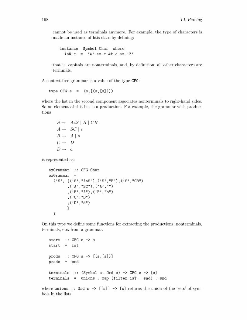
168 LL Parsing
cannot be used as terminals anymore. For example, the type of characters ismade an instance of htis class by defining:
instance Symbol Char whereisN c = ’A’ <= c && c <= ’Z’
that is, capitals are nonterminals, and, by definition, all other characters areterminals.
A context-free grammar is a value of the type CFG:
type CFG s = (s,[(s,[s])])
where the list in the second component associates nonterminals to right-hand sides.So an element of this list is a production. For example, the grammar with produc-tions
S → AaS | B | CBA→ SC | εB → A | bC → D
D → d
is represented as:
exGrammar :: CFG CharexGrammar =
(’S’, [(’S’,"AaS"),(’S’,"B"),(’S’,"CB"),(’A’,"SC"),(’A’,""),(’B’,"A"),(’B’,"b"),(’C’,"D"),(’D’,"d")]
)
On this type we define some functions for extracting the productions, nonterminals,terminals, etc. from a grammar.
start :: CFG s -> sstart = fst
prods :: CFG s -> [(s,[s])]prods = snd
terminals :: (Symbol s, Ord s) => CFG s -> [s]terminals = unions . map (filter isT . snd) . snd
where unions :: Ord s => [[s]] -> [s] returns the union of the ‘sets’ of sym-bols in the lists.
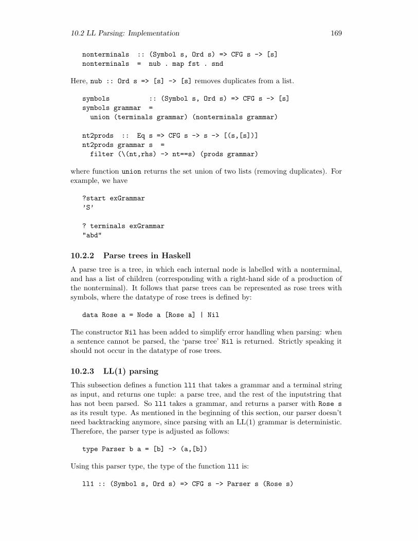
10.2 LL Parsing: Implementation 169
nonterminals :: (Symbol s, Ord s) => CFG s -> [s]nonterminals = nub . map fst . snd
Here, nub :: Ord s => [s] -> [s] removes duplicates from a list.
symbols :: (Symbol s, Ord s) => CFG s -> [s]symbols grammar =
union (terminals grammar) (nonterminals grammar)
nt2prods :: Eq s => CFG s -> s -> [(s,[s])]nt2prods grammar s =
filter (\(nt,rhs) -> nt==s) (prods grammar)
where function union returns the set union of two lists (removing duplicates). Forexample, we have
?start exGrammar’S’
? terminals exGrammar"abd"
10.2.2 Parse trees in Haskell
A parse tree is a tree, in which each internal node is labelled with a nonterminal,and has a list of children (corresponding with a right-hand side of a production ofthe nonterminal). It follows that parse trees can be represented as rose trees withsymbols, where the datatype of rose trees is defined by:
data Rose a = Node a [Rose a] | Nil
The constructor Nil has been added to simplify error handling when parsing: whena sentence cannot be parsed, the ‘parse tree’ Nil is returned. Strictly speaking itshould not occur in the datatype of rose trees.
10.2.3 LL(1) parsing
This subsection defines a function ll1 that takes a grammar and a terminal stringas input, and returns one tuple: a parse tree, and the rest of the inputstring thathas not been parsed. So ll1 takes a grammar, and returns a parser with Rose sas its result type. As mentioned in the beginning of this section, our parser doesn’tneed backtracking anymore, since parsing with an LL(1) grammar is deterministic.Therefore, the parser type is adjusted as follows:
type Parser b a = [b] -> (a,[b])
Using this parser type, the type of the function ll1 is:
ll1 :: (Symbol s, Ord s) => CFG s -> Parser s (Rose s)
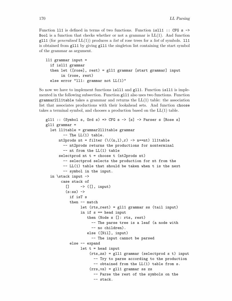
170 LL Parsing
Function ll1 is defined in terms of two functions. Function isll1 :: CFG s ->Bool is a function that checks whether or not a grammar is LL(1). And functiongll1 (for generalised LL(1)) produces a list of rose trees for a list of symbols. ll1is obtained from gll1 by giving gll1 the singleton list containing the start symbolof the grammar as argument.
ll1 grammar input =if isll1 grammarthen let ([rose], rest) = gll1 grammar [start grammar] input
in (rose, rest)else error "ll1: grammar not LL(1)"
So now we have to implement functions isll1 and gll1. Function isll1 is imple-mented in the following subsection. Function gll1 also uses two functions. Functiongrammar2ll1table takes a grammar and returns the LL(1) table: the associationlist that associates productions with their lookahead sets. And function choosetakes a terminal symbol, and chooses a production based on the LL(1) table.
gll1 :: (Symbol s, Ord s) => CFG s -> [s] -> Parser s [Rose s]gll1 grammar =
let ll1table = grammar2ll1table grammar-- The LL(1) table.
nt2prods nt = filter (\((n,l),r) -> n==nt) ll1table-- nt2prods returns the productions for nonterminal-- nt from the LL(1) table
selectprod nt t = choose t (nt2prods nt)-- selectprod selects the production for nt from the-- LL(1) table that should be taken when t is the next-- symbol in the input.
in \stack input ->case stack of
[] -> ([], input)(s:ss) ->if isT sthen -- match
let (rts,rest) = gll1 grammar ss (tail input)in if s == head input
then (Node s []: rts, rest)-- The parse tree is a leaf (a node with-- no children).
else ([Nil], input)-- The input cannot be parsed
else -- expandlet t = head input
(rts,zs) = gll1 grammar (selectprod s t) input-- Try to parse according to the production-- obtained from the LL(1) table from s.
(rrs,vs) = gll1 grammar ss zs-- Parse the rest of the symbols on the-- stack.
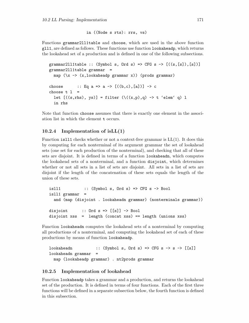
10.2 LL Parsing: Implementation 171
in ((Node s rts): rrs, vs)
Functions grammar2ll1table and choose, which are used in the above functiongll1, are defined as follows. These functions use function lookaheadp, which returnsthe lookahead set of a production and is defined in one of the following subsections.
grammar2ll1table :: (Symbol s, Ord s) => CFG s -> [((s,[s]),[s])]grammar2ll1table grammar =
map (\x -> (x,lookaheadp grammar x)) (prods grammar)
choose :: Eq a => a -> [((b,c),[a])] -> cchoose t l =
let [((s,rhs), ys)] = filter (\((x,p),q) -> t ‘elem‘ q) lin rhs
Note that function choose assumes that there is exactly one element in the associ-ation list in which the element t occurs.
10.2.4 Implementation of isLL(1)
Function isll1 checks whether or not a context-free grammar is LL(1). It does thisby computing for each nonterminal of its argument grammar the set of lookaheadsets (one set for each production of the nonterminal), and checking that all of thesesets are disjoint. It is defined in terms of a function lookaheadn, which computesthe lookahead sets of a nonterminal, and a function disjoint, which determineswhether or not all sets in a list of sets are disjoint. All sets in a list of sets aredisjoint if the length of the concatenation of these sets equals the length of theunion of these sets.
isll1 :: (Symbol s, Ord s) => CFG s -> Boolisll1 grammar =
and (map (disjoint . lookaheadn grammar) (nonterminals grammar))
disjoint :: Ord s => [[s]] -> Booldisjoint xss = length (concat xss) == length (unions xss)
Function lookaheadn computes the lookahead sets of a nonterminal by computingall productions of a nonterminal, and computing the lookahead set of each of theseproductions by means of function lookaheadp.
lookaheadn :: (Symbol s, Ord s) => CFG s -> s -> [[s]]lookaheadn grammar =
map (lookaheadp grammar) . nt2prods grammar
10.2.5 Implementation of lookahead
Function lookaheadp takes a grammar and a production, and returns the lookaheadset of the production. It is defined in terms of four functions. Each of the first threefunctions will be defined in a separate subsection below, the fourth function is definedin this subsection.
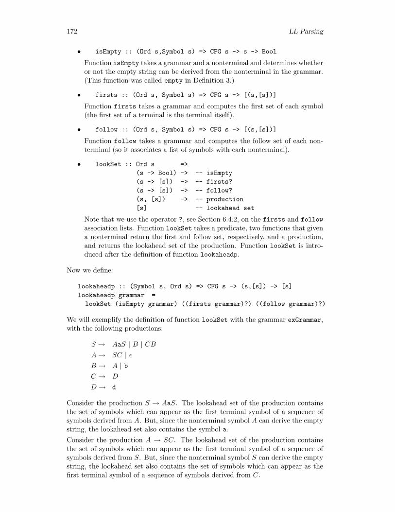
172 LL Parsing
• isEmpty :: (Ord s,Symbol s) => CFG s -> s -> Bool
Function isEmpty takes a grammar and a nonterminal and determines whetheror not the empty string can be derived from the nonterminal in the grammar.(This function was called empty in Definition 3.)
• firsts :: (Ord s, Symbol s) => CFG s -> [(s,[s])]
Function firsts takes a grammar and computes the first set of each symbol(the first set of a terminal is the terminal itself).
• follow :: (Ord s, Symbol s) => CFG s -> [(s,[s])]
Function follow takes a grammar and computes the follow set of each non-terminal (so it associates a list of symbols with each nonterminal).
• lookSet :: Ord s =>(s -> Bool) -> -- isEmpty(s -> [s]) -> -- firsts?(s -> [s]) -> -- follow?(s, [s]) -> -- production[s] -- lookahead set
Note that we use the operator ?, see Section 6.4.2, on the firsts and followassociation lists. Function lookSet takes a predicate, two functions that givena nonterminal return the first and follow set, respectively, and a production,and returns the lookahead set of the production. Function lookSet is intro-duced after the definition of function lookaheadp.
Now we define:
lookaheadp :: (Symbol s, Ord s) => CFG s -> (s,[s]) -> [s]lookaheadp grammar =
lookSet (isEmpty grammar) ((firsts grammar)?) ((follow grammar)?)
We will exemplify the definition of function lookSet with the grammar exGrammar,with the following productions:
S → AaS | B | CBA→ SC | εB → A | bC → D
D → d
Consider the production S → AaS. The lookahead set of the production containsthe set of symbols which can appear as the first terminal symbol of a sequence ofsymbols derived from A. But, since the nonterminal symbol A can derive the emptystring, the lookahead set also contains the symbol a.Consider the production A → SC. The lookahead set of the production containsthe set of symbols which can appear as the first terminal symbol of a sequence ofsymbols derived from S. But, since the nonterminal symbol S can derive the emptystring, the lookahead set also contains the set of symbols which can appear as thefirst terminal symbol of a sequence of symbols derived from C.

10.2 LL Parsing: Implementation 173
Finally, consider the production B → A. The lookahead set of the productioncontains the set of symbols which can appear as the first terminal symbol of asequence of symbols derived from A. But, since the nonterminal symbol A canderive the empty string, the lookahead set also contains the set of terminal symbolswhich can follow the nonterminal symbol B in some derivation.The examples show that it is useful to have functions firsts and follow in which,for every nonterminal symbol n, we can look up the terminal symbols which canappear as the first terminal symbol of a sequence of symbols in some derivationfrom n and the set of terminal symbols which can follow the nonterminal symbol nin a sequence of symbols occurring in some derivation respectively. It turns out thatthe definition of function follow also makes use of a function lasts which is similarto the function firsts, but which deals with last nonterminal symbols rather thanfirst terminal ones.The examples also illustrate a control structure which will be used very often in thefollowing algorithms: we will fold over right-hand sides. While doing so we computesets of symbols for all the symbols of the right-hand side which we encounter andcollect them into a final set of symbols. Whenever such a list for a symbol iscomputed, there are always two possibilities:
• either we continue folding and return the result of taking the union of the setobtained from the current element and the set obtained by recursively foldingover the rest of the right-hand side
• or we stop folding and immediately return the set obtained from the currentelement.
We continue if the current symbol is a nonterminal which can derive the emptysequence and we stop if the current symbol is either a terminal symbol or a non-terminal symbol which cannot derive the empty sequence. The following functionmakes this statement more precise.
foldrRhs :: Ord s =>(s -> Bool) ->(s -> [s]) ->[s] ->[s] ->[s]
foldrRhs p f start = foldr op startwhere op x xs = f x ‘union‘ if p x then xs else []
The function foldrRhs is, of course, most naturally defined in terms of the functionfoldr. This function is somewhere in between a general purpose and an applicationspecific function (we could easily have made it more general though). In the exerciseswe give an alternative characterisation of foldRhs. We will also need a functionscanrRhs which is like foldrRhs but accumulates intermediate results in a list.The function scanrRhs is most naturally defined in terms of the function scanr.
scanrRhs :: Ord s =>(s -> Bool) ->(s -> [s]) ->
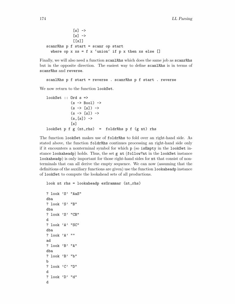
174 LL Parsing
[s] ->[s] ->[[s]]
scanrRhs p f start = scanr op startwhere op x xs = f x ‘union‘ if p x then xs else []
Finally, we will also need a function scanlRhs which does the same job as scanrRhsbut in the opposite direction. The easiest way to define scanlRhs is in terms ofscanrRhs and reverse.
scanlRhs p f start = reverse . scanrRhs p f start . reverse
We now return to the function lookSet.
lookSet :: Ord s =>(s -> Bool) ->(s -> [s]) ->(s -> [s]) ->(s,[s]) ->[s]
lookSet p f g (nt,rhs) = foldrRhs p f (g nt) rhs
The function lookSet makes use of foldrRhs to fold over an right-hand side. Asstated above, the function foldrRhs continues processing an right-hand side onlyif it encounters a nonterminal symbol for which p (so isEmpty in the lookSet in-stance lookaheadp) holds. Thus, the set g nt (follow?nt in the lookSet instancelookaheadp) is only important for those right-hand sides for nt that consist of non-terminals that can all derive the empty sequence. We can now (assuming that thedefinitions of the auxiliary functions are given) use the function lookaheadp instanceof lookSet to compute the lookahead sets of all productions.
look nt rhs = lookaheadp exGrammar (nt,rhs)
? look ’S’ "AaS"dba? look ’S’ "B"dba? look ’S’ "CB"d? look ’A’ "SC"dba? look ’A’ ""ad? look ’B’ "A"dba? look ’B’ "b"b? look ’C’ "D"d? look ’D’ "d"d
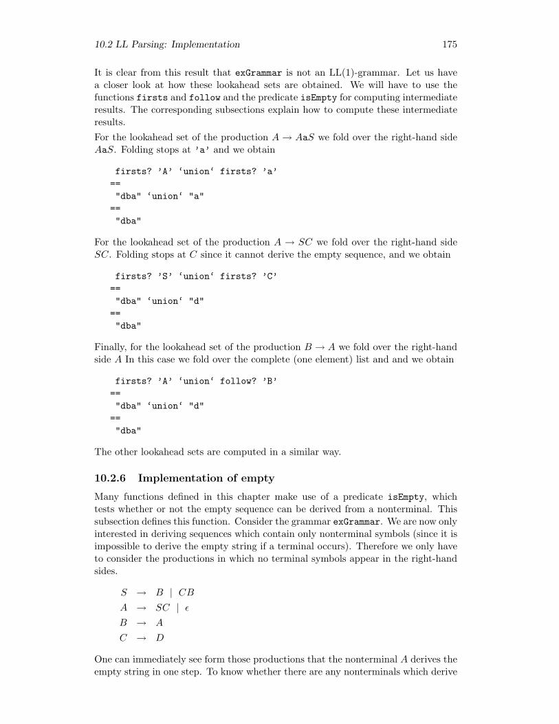
10.2 LL Parsing: Implementation 175
It is clear from this result that exGrammar is not an LL(1)-grammar. Let us havea closer look at how these lookahead sets are obtained. We will have to use thefunctions firsts and follow and the predicate isEmpty for computing intermediateresults. The corresponding subsections explain how to compute these intermediateresults.For the lookahead set of the production A→ AaS we fold over the right-hand sideAaS. Folding stops at ’a’ and we obtain
firsts? ’A’ ‘union‘ firsts? ’a’=="dba" ‘union‘ "a"
=="dba"
For the lookahead set of the production A → SC we fold over the right-hand sideSC. Folding stops at C since it cannot derive the empty sequence, and we obtain
firsts? ’S’ ‘union‘ firsts? ’C’=="dba" ‘union‘ "d"
=="dba"
Finally, for the lookahead set of the production B → A we fold over the right-handside A In this case we fold over the complete (one element) list and and we obtain
firsts? ’A’ ‘union‘ follow? ’B’=="dba" ‘union‘ "d"
=="dba"
The other lookahead sets are computed in a similar way.
10.2.6 Implementation of empty
Many functions defined in this chapter make use of a predicate isEmpty, whichtests whether or not the empty sequence can be derived from a nonterminal. Thissubsection defines this function. Consider the grammar exGrammar. We are now onlyinterested in deriving sequences which contain only nonterminal symbols (since it isimpossible to derive the empty string if a terminal occurs). Therefore we only haveto consider the productions in which no terminal symbols appear in the right-handsides.
S → B | CBA → SC | εB → A
C → D
One can immediately see form those productions that the nonterminal A derives theempty string in one step. To know whether there are any nonterminals which derive

176 LL Parsing
the empty string in more than one step we eliminate the productions for A and weeliminate all occurrences of A in the right hand sides of the remaining productions
S → B | CBB → ε
C → D
One can now conclude that the nonterminal B derives the empty string in two steps.Doing the same with B as we did with A gives us the following productions
S → ε | CC → D
One can now conclude that the nonterminal S derives the empty string in three steps.Doing the same with S as we did with A and B gives us the following productions
C → D
At this stage we can conclude that there are no more new nonterminals which derivethe empty string.We now give the Haskell implementation of the algorithm described above. Thealgorithm is iterative: it does the same steps over and over again until some desiredcondition is met. For this purpose we use function fixedPoint, which takes afunction and a set, and repeatedly applies the function to the set, until the set doesnot change anymore.
fixedPoint :: Ord a => ([a] -> [a]) -> [a] -> [a]fixedPoint f xs | xs == nexts = xs
| otherwise = fixedPoint f nextswhere nexts = f xs
fixedPoint f is sometimes called the fixed-point of f. Function isEmpty determineswhether or not a nonterminal can derive the empty string. A nonterminal can derivethe empty string if it is a member of the emptySet of a grammar.
isEmpty :: (Symbol s, Ord s) => CFG s -> s -> BoolisEmpty grammar = (‘elem‘ emptySet grammar)
The emptySet of a grammar is obtained by the iterative process described in theexample above. We start with the empty set of nonterminals, and at each step n ofthe computation of the emptySet as a fixedPoint, we add the nonterminals thatcan derive the empty string in n steps. Function emptyStepf adds a nonterminal ifthere exists a production for the nonterminal of which all elements can derive theempty string.
emptySet :: (Symbol s, Ord s) => CFG s -> [s]emptySet grammar = fixedPoint (emptyStepf grammar) []
emptyStepf :: (Symbol s, Ord s) => CFG s -> [s] -> [s]emptyStepf grammar set =
nub (map fst (filter (\(nt,rhs) -> all (‘elem‘ set) rhs)(prods grammar)
) )
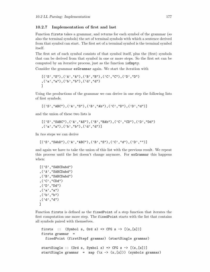
10.2 LL Parsing: Implementation 177
10.2.7 Implementation of first and last
Function firsts takes a grammar, and returns for each symbol of the grammar (soalso the terminal symbols) the set of terminal symbols with which a sentence derivedfrom that symbol can start. The first set of a terminal symbol is the terminal symbolitself.The first set of each symbol consists of that symbol itself, plus the (first) symbolsthat can be derived from that symbol in one or more steps. So the first set can becomputed by an iterative process, just as the function isEmpty.Consider the grammar exGrammar again. We start the iteration with
[(’S’,"S"),(’A’,"A"),(’B’,"B"),(’C’,"C"),(’D’,"D"),(’a’,"a"),(’b’,"b"),(’d’,"d")]
Using the productions of the grammar we can derive in one step the following listsof first symbols.
[(’S’,"ABC"),(’A’,"S"),(’B’,"Ab"),(’C’,"D"),(’D’,"d")]
and the union of these two lists is
[(’S’,"SABC"),(’A’,"AS"),(’B’,"BAb"),(’C’,"CD"),(’D’,"Dd"),(’a’,"a"),(’b’,"b"),(’d’,"d")]
In two steps we can derive
[(’S’,"SAbD"),(’A’,"ABC"),(’B’,"S"),(’C’,"d"),(’D’,"")]
and again we have to take the union of this list with the previous result. We repeatthis process until the list doesn’t change anymore. For exGrammar this happenswhen:
[(’S’,"SABCDabd"),(’A’,"SABCDabd"),(’B’,"SABCDabd"),(’C’,"CDd"),(’D’,"Dd"),(’a’,"a"),(’b’,"b"),(’d’,"d")]
Function firsts is defined as the fixedPoint of a step function that iterates thefirst computation one more step. The fixedPoint starts with the list that containsall symbols paired with themselves.
firsts :: (Symbol s, Ord s) => CFG s -> [(s,[s])]firsts grammar =
fixedPoint (firstStepf grammar) (startSingle grammar)
startSingle :: (Ord s, Symbol s) => CFG s -> [(s,[s])]startSingle grammar = map (\x -> (x,[x])) (symbols grammar)
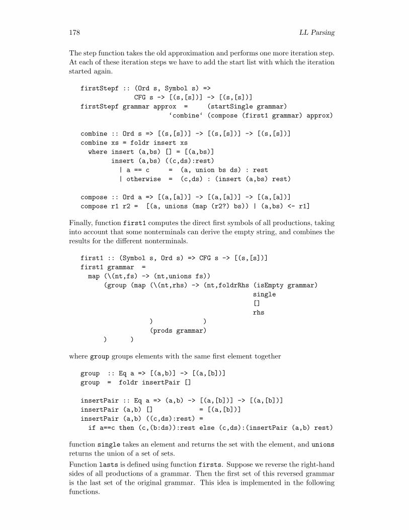
178 LL Parsing
The step function takes the old approximation and performs one more iteration step.At each of these iteration steps we have to add the start list with which the iterationstarted again.
firstStepf :: (Ord s, Symbol s) =>CFG s -> [(s,[s])] -> [(s,[s])]
firstStepf grammar approx = (startSingle grammar)‘combine‘ (compose (first1 grammar) approx)
combine :: Ord s => [(s,[s])] -> [(s,[s])] -> [(s,[s])]combine xs = foldr insert xs
where insert (a,bs) [] = [(a,bs)]insert (a,bs) ((c,ds):rest)
| a == c = (a, union bs ds) : rest| otherwise = (c,ds) : (insert (a,bs) rest)
compose :: Ord a => [(a,[a])] -> [(a,[a])] -> [(a,[a])]compose r1 r2 = [(a, unions (map (r2?) bs)) | (a,bs) <- r1]
Finally, function first1 computes the direct first symbols of all productions, takinginto account that some nonterminals can derive the empty string, and combines theresults for the different nonterminals.
first1 :: (Symbol s, Ord s) => CFG s -> [(s,[s])]first1 grammar =
map (\(nt,fs) -> (nt,unions fs))(group (map (\(nt,rhs) -> (nt,foldrRhs (isEmpty grammar)
single[]rhs
) )(prods grammar)
) )
where group groups elements with the same first element together
group :: Eq a => [(a,b)] -> [(a,[b])]group = foldr insertPair []
insertPair :: Eq a => (a,b) -> [(a,[b])] -> [(a,[b])]insertPair (a,b) [] = [(a,[b])]insertPair (a,b) ((c,ds):rest) =
if a==c then (c,(b:ds)):rest else (c,ds):(insertPair (a,b) rest)
function single takes an element and returns the set with the element, and unionsreturns the union of a set of sets.Function lasts is defined using function firsts. Suppose we reverse the right-handsides of all productions of a grammar. Then the first set of this reversed grammaris the last set of the original grammar. This idea is implemented in the followingfunctions.
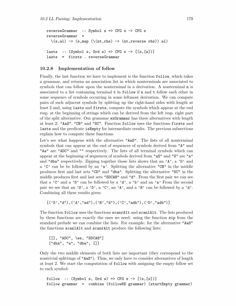
10.2 LL Parsing: Implementation 179
reverseGrammar :: Symbol s => CFG s -> CFG sreverseGrammar =
\(s,al) -> (s,map (\(nt,rhs) -> (nt,reverse rhs)) al)
lasts :: (Symbol s, Ord s) => CFG s -> [(s,[s])]lasts = firsts . reverseGrammar
10.2.8 Implementation of follow
Finally, the last function we have to implement is the function follow, which takesa grammar, and returns an association list in which nonterminals are associated tosymbols that can follow upon the nonterminal in a derivation. A nonterminal n isassociated to a list containing terminal t in follow if n and t follow each other insome sequence of symbols occurring in some leftmost derivation. We can computepairs of such adjacent symbols by splitting up the right-hand sides with length atleast 2 and, using lasts and firsts, compute the symbols which appear at the endresp. at the beginning of strings which can be derived from the left resp. right partof the split alternative. Our grammar exGrammar has three alternatives with lengthat least 2: "AaS", "CB" and "SC". Function follow uses the functions firsts andlasts and the predicate isEmpty for intermediate results. The previous subsectionsexplain how to compute these functions.Let’s see what happens with the alternative "AaS". The lists of all nonterminalsymbols that can appear at the end of sequences of symbols derived from "A" and"Aa" are "ADC" and "" respectively. The lists of all terminal symbols which canappear at the beginning of sequences of symbols derived from "aS" and "S" are "a"and "dba" respectively. Zipping together those lists shows that an ’A’, a ’D’ anda ’C’ can be be followed by an ’a’. Splitting the alternative "CB" in the middleproduces first and last sets "CD" and "dba". Splitting the alternative "SC" in themiddle produces first and last sets "SDCAB" and "d". From the first pair we can seethat a ’C’ and a ’D’ can be followed by a ’d’, a ’b’ and an ’a’ From the secondpair we see that an ’S’, a ’D’, a ’C’, an ’A’, and a ’B’ can be followed by a ’d’.Combining all these results gives:
[(’S’,"d"),(’A’,"ad"),(’B’,"d"),(’C’,"adb"),(’D’,"adb")]
The function follow uses the functions scanrAlt and scanlAlt. The lists producedby these functions are exactly the ones we need: using the function zip from thestandard prelude we can combine the lists. For example: for the alternative "AaS"the functions scanlAlt and scanrAlt produce the following lists:
[[], "ADC", \es, "SDCAB"]["dba", "a", "dba", []]
Only the two middle elements of both lists are important (they correspond to thenontrivial splittings of "AaS"). Thus, we only have to consider alternatives of lengthat least 2. We start the computation of follow with assigning the empty follow setto each symbol:
follow :: (Symbol s, Ord s) => CFG s -> [(s,[s])]follow grammar = combine (followNE grammar) (startEmpty grammar)

180 LL Parsing
startEmpty grammar = map (\x -> (x,[])) (symbols grammar)
The real work is done by functions followNE and function splitProds. Func-tion followNE passes the right arguments on to function splitProds, and removesall nonterminals from the first set, and all terminals from the last set. FunctionsplitProds splits the productions of length at least 2, and pairs the last nontermi-nals with the first terminals.
followNE :: (Symbol s, Ord s) => CFG s -> [(s,[s])]followNE grammar = splitProds
(prods grammar)(isEmpty grammar)(isTfirsts grammar)(isNlasts grammar)
where isTfirsts = map (\(x,xs) -> (x,filter isT xs)) . firstsisNlasts = map (\(x,xs) -> (x,filter isN xs)) . lasts
splitProds :: (Symbol s, Ord s) =>[(s,[s])] -> -- productions(s -> Bool) -> -- isEmpty[(s,[s])] -> -- terminal firsts[(s,[s])] -> -- nonterminal lasts[(s,[s])]
splitProds prods p fset lset =map (\(nt,rhs) -> (nt,nub rhs)) (group pairs)where pairs = [(l, f)
| rhs <- map snd prods, length rhs >= 2, (fs, ls) <- zip (rightscan rhs) (leftscan rhs), l <- ls, f <- fs]
leftscan = scanlRhs p (lset?) []rightscan = scanrRhs p (fset?) []
Exercise 10.7 . Give the Rose tree representation of the parse tree corresponding to the deriva-tion of the sentence ccccba using grammar gramm1. /
Exercise 10.8 . Give the Rose tree representation of the parse tree corresponding to the deriva-tion of the sentence abbb using grammar gramm2’ defined in the exercises of theprevious section . /
Exercise 10.9 . Give the Rose tree representation of the parse tree corresponding to the deriva-tion of the sentence acbab using grammar gramm3. /
Exercise 10.10 . In this exercise we will take a closer look at the functions foldrRhs andscanrRhs which are the essential ingredients of the implementation of the grammaranalysis algorithms. From the definitions it is clear that grammar analysis is easilyexpressed via a calculus for (finite) sets. A calculus for finite sets is implicit in theprograms for LL(1) parsing. Since the code in this module is obscured by several
10.2 LL Parsing: Implementation 181
implementation details we will derive the functions foldrRhs and scanrRhs in astepwise fashion. In this derivation we will use the following:A (finite) set is implemented by a list with no duplicates. In order to construct aset, the following operations may be used:
[] :: [a] the empty set of a-elementsunion :: [a] → [a] → [a] the union of two setsunions :: [[a]] → [a] the generalised unionsingle :: a → [a] the singleton function
These operations satisfy the well-known laws for set operations.
1. Define a function list2Set :: [a] → [a] which returns the set of elementsoccurring in the argument.
2. Define list2Set as a foldr.
3. Define a function pref p :: [a] → [a] which given a list xs returns theset of elements corresponding to the longest prefix of xs all of whose elementssatisfy p.
4. Define a function prefplus p :: [a] → [a] which given a list xs returnsthe set of elements in the longest prefix of xs all of whose elements satisfy ptogether with the first element of xs that does not satisfy p (if this elementexists at all).
5. Define prefplus p as a foldr.
6. Show that prefplus p = foldrRhs p single [].
7. It can be shown that
foldrRhs p f [] = unions . map f . prefplus p
for all set-valued functions f. Give an informal description of the functionsfoldrRhs p f [] and foldrRhs p f start.
8. The standard function scanr is defined by
scanr f q0 = map (foldr f q0) . tails
where tails is a function which takes a list xs and returns a list with alltailsegments (postfixes) of xs in decreasing length. The function scanrRhs isdefined is a similar way
scanrRhs p f start = map (foldrRhs p f start) . tails
Give an informal description of the function scanrRhs.
/

182 LL Parsing
Exercise 10.11 . The computation of the functions empty and firsts is not restricted tononterminals only. For terminal symbols s these functions are defined by
empty s = Falsefirsts s = {s}
Using the definitions in the previous exercise, compute the following.
1. For the example grammar gramm1 and two of its productions A → bSA andB → Cb.
(a) foldrRhs empty firsts [] bSA
(b) foldrRhs empty firsts [] Cb
2. For the example grammar gramm3 and its production S → AaS
(a) foldrRhs empty firsts [] AaS
(b) scanrRhs empty firsts [] AaS
/
Bibliography
[1] A.V. Aho, Sethi R., and J.D. Ullman. Compilers — Principles, Techniques andTools. Addison-Wesley, 1986.
[2] R.S. Bird. Using circular programs to eliminate multiple traversals of data.Acta Informatica, 21:239–250, 1984.
[3] R.S. Bird and P. Wadler. Introduction to Functional Programming. PrenticeHall, 1988.
[4] W.H. Burge. Parsing. In Recursive Programming Techniques. Addison-Wesley,1975.
[5] J. Fokker. Functional parsers. In J. Jeuring and E. Meijer, editors, AdvancedFunctional Programming, volume 925 of Lecture Notes in Computer Science.Springer-Verlag, 1995.
[6] R. Harper. Proof-directed debugging. Journal of Functional Programming,1999. To appear.
[7] G. Hutton. Higher-order functions for parsing. Journal of Functional Program-ming, 2(3):323 – 343, 1992.
[8] G. Hutton and E. Meijer. Monadic parsing in haskell. Journal of FunctionalProgramming, 8(4):437 – 444, 1998.
[9] B.W. Kernighan and R. Pike. Regular expressions — languages, algorithms,and software. Dr. Dobb’s Journal, April:19 – 22, 1999.
[10] D.E. Knuth. Semantics of context-free languages. Math. Syst. Theory, 2(2):127–145, 1968.
[11] Niklas Rojemo. Garbage collection and memory efficiency in lazy functionallanguages. PhD thesis, Chalmers University of Technology, 1995.
[12] S. Sippu and E. Soisalon-Soininen. Parsing Theory, Vol. 1: Languages andParsing, volume 15 of EATCS Monographs on THeoretical Computer Science.Springer-Verlag, 1988.
[13] S.D. Swierstra and P.R. Azero Alcocer. Fast, error correcting parser combina-tors: a short tutorial. In SOFSEM’99, 1999.
[14] P. Wadler. How to replace failure by a list of successes: a method for excep-tion handling, backtracking, and pattern matching in lazy functional languages.In J.P. Jouannaud, editor, Functional Programming Languages and ComputerArchitecture, pages 113 – 128. Springer, 1985. LNCS 201.
183
184 BIBLIOGRAPHY
[15] P. Wadler. Monads for functional programming. In J. Jeuring and E. Meijer,editors, Advanced Functional Programming. Springer, 1995. LNCS 925.
Appendix A
The Stack module
module Stack( Stack, emptyStack, isEmptyStack, push, pushList, pop, popList, top, split, mystack)
where
data Stack x = MkS [x] deriving (Show,Eq)
emptyStack :: Stack xemptyStack = MkS []
isEmptyStack :: Stack x -> BoolisEmptyStack (MkS xs) = null xs
push :: x -> Stack x -> Stack xpush x (MkS xs) = MkS (x:xs)
pushList :: [x] -> Stack x -> Stack xpushList xs (MkS ys) = MkS (xs ++ ys)
pop :: Stack x -> Stack xpop (MkS xs) = if isEmptyStack (MkS xs)
then error "pop on emptyStack"else MkS (tail xs)
popIf :: Eq x => x -> Stack x -> Stack xpopIf x stack = if top stack == x
185
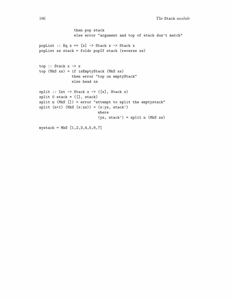
186 The Stack module
then pop stackelse error "argument and top of stack don’t match"
popList :: Eq x => [x] -> Stack x -> Stack xpopList xs stack = foldr popIf stack (reverse xs)
top :: Stack x -> xtop (MkS xs) = if isEmptyStack (MkS xs)
then error "top on emptyStack"else head xs
split :: Int -> Stack x -> ([x], Stack x)split 0 stack = ([], stack)split n (MkS []) = error "attempt to split the emptystack"split (n+1) (MkS (x:xs)) = (x:ys, stack’)
where(ys, stack’) = split n (MkS xs)
mystack = MkS [1,2,3,4,5,6,7]

Appendix B
Answers to exercises
2.1 Three of the fours strings are elements of L∗: abaabaaabaa, aaaabaaaa, baaaaabaa.2.2 {ε}.2.3
Ø L
= Definition of concatenation of languages
{st | s ∈ Ø, t ∈ L}= s ∈ Ø
Ø
and the other equalities are proved in a similar fashion.2.4 Ln should satisfy:
L0 = ?Ln+1 = LnL
It follows that we want L0 to satisfy
L0L = L
If we choose L0 = {ε}, we have
L0L
= Definition of concatenation of languages
{st | s ∈ {ε}, t ∈ L}= Definition of string concatenation
{t | t ∈ L}= Definition of set comprehension
L
as desired.2.5 The star operator on sets injects the elements of a set in a list; the star operatoron languages concatenates the sentences of the language. The former star operatorpreserves more structure.2.6 Section 2.1 contains an inductive definition of the set of sequences over anarbitrary set X. Syntactical definitions for such sets follow immediately from this.
187
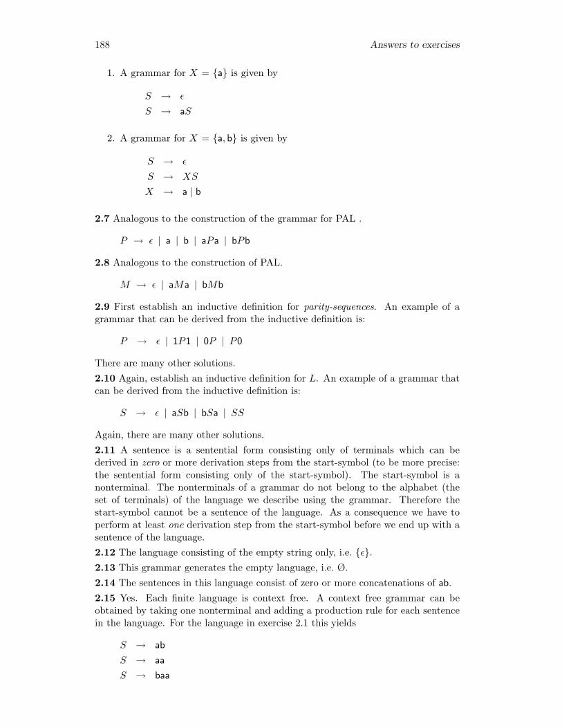
188 Answers to exercises
1. A grammar for X = {a} is given by
S → ε
S → aS
2. A grammar for X = {a, b} is given by
S → ε
S → XS
X → a | b
2.7 Analogous to the construction of the grammar for PAL .
P → ε | a | b | aPa | bPb
2.8 Analogous to the construction of PAL.
M → ε | aMa | bMb
2.9 First establish an inductive definition for parity-sequences. An example of agrammar that can be derived from the inductive definition is:
P → ε | 1P1 | 0P | P0
There are many other solutions.2.10 Again, establish an inductive definition for L. An example of a grammar thatcan be derived from the inductive definition is:
S → ε | aSb | bSa | SS
Again, there are many other solutions.2.11 A sentence is a sentential form consisting only of terminals which can bederived in zero or more derivation steps from the start-symbol (to be more precise:the sentential form consisting only of the start-symbol). The start-symbol is anonterminal. The nonterminals of a grammar do not belong to the alphabet (theset of terminals) of the language we describe using the grammar. Therefore thestart-symbol cannot be a sentence of the language. As a consequence we have toperform at least one derivation step from the start-symbol before we end up with asentence of the language.2.12 The language consisting of the empty string only, i.e. {ε}.2.13 This grammar generates the empty language, i.e. Ø.2.14 The sentences in this language consist of zero or more concatenations of ab.2.15 Yes. Each finite language is context free. A context free grammar can beobtained by taking one nonterminal and adding a production rule for each sentencein the language. For the language in exercise 2.1 this yields
S → ab
S → aa
S → baa
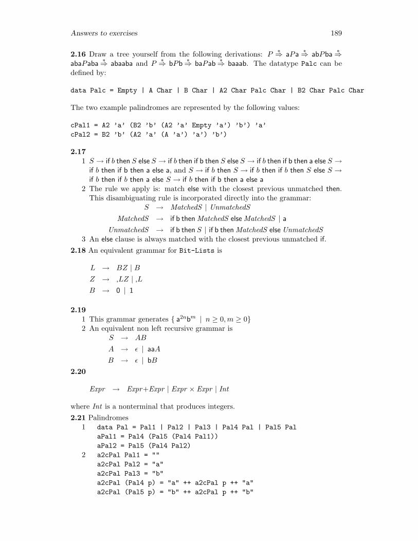
Answers to exercises 189
2.16 Draw a tree yourself from the following derivations: P∗⇒ aPa
∗⇒ abPba∗⇒
abaPaba∗⇒ abaaba and P
∗⇒ bPb∗⇒ baPab
∗⇒ baaab. The datatype Palc can bedefined by:
data Palc = Empty | A Char | B Char | A2 Char Palc Char | B2 Char Palc Char
The two example palindromes are represented by the following values:
cPal1 = A2 ’a’ (B2 ’b’ (A2 ’a’ Empty ’a’) ’b’) ’a’cPal2 = B2 ’b’ (A2 ’a’ (A ’a’) ’a’) ’b’)
2.171 S → if b then S else S → if b then if b then S else S → if b then if b then a else S →
if b then if b then a else a, and S → if b then S → if b then if b then S else S →if b then if b then a else S → if b then if b then a else a
2 The rule we apply is: match else with the closest previous unmatched then.This disambiguating rule is incorporated directly into the grammar:
S → MatchedS | UnmatchedSMatchedS → if b then MatchedS else MatchedS | a
UnmatchedS → if b then S | if b then MatchedS else UnmatchedS3 An else clause is always matched with the closest previous unmatched if.
2.18 An equivalent grammar for Bit-Lists is
L → BZ | BZ → ,LZ | ,LB → 0 | 1
2.191 This grammar generates { a2nbm | n ≥ 0,m ≥ 0}2 An equivalent non left recursive grammar is
S → AB
A → ε | aaA
B → ε | bB
2.20
Expr → Expr+Expr | Expr × Expr | Int
where Int is a nonterminal that produces integers.2.21 Palindromes
1 data Pal = Pal1 | Pal2 | Pal3 | Pal4 Pal | Pal5 PalaPal1 = Pal4 (Pal5 (Pal4 Pal1))aPal2 = Pal5 (Pal4 Pal2)
2 a2cPal Pal1 = ""a2cPal Pal2 = "a"a2cPal Pal3 = "b"a2cPal (Pal4 p) = "a" ++ a2cPal p ++ "a"a2cPal (Pal5 p) = "b" ++ a2cPal p ++ "b"
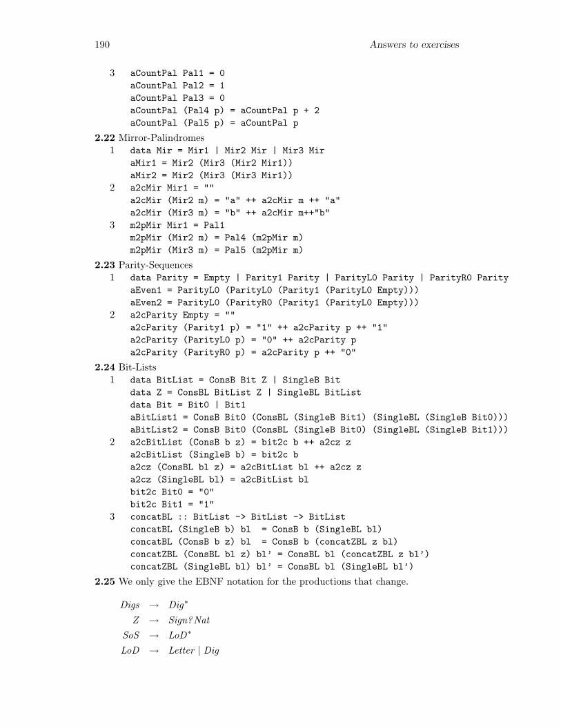
190 Answers to exercises
3 aCountPal Pal1 = 0aCountPal Pal2 = 1aCountPal Pal3 = 0aCountPal (Pal4 p) = aCountPal p + 2aCountPal (Pal5 p) = aCountPal p
2.22 Mirror-Palindromes1 data Mir = Mir1 | Mir2 Mir | Mir3 Mir
aMir1 = Mir2 (Mir3 (Mir2 Mir1))aMir2 = Mir2 (Mir3 (Mir3 Mir1))
2 a2cMir Mir1 = ""a2cMir (Mir2 m) = "a" ++ a2cMir m ++ "a"a2cMir (Mir3 m) = "b" ++ a2cMir m++"b"
3 m2pMir Mir1 = Pal1m2pMir (Mir2 m) = Pal4 (m2pMir m)m2pMir (Mir3 m) = Pal5 (m2pMir m)
2.23 Parity-Sequences1 data Parity = Empty | Parity1 Parity | ParityL0 Parity | ParityR0 Parity
aEven1 = ParityL0 (ParityL0 (Parity1 (ParityL0 Empty)))aEven2 = ParityL0 (ParityR0 (Parity1 (ParityL0 Empty)))
2 a2cParity Empty = ""a2cParity (Parity1 p) = "1" ++ a2cParity p ++ "1"a2cParity (ParityL0 p) = "0" ++ a2cParity pa2cParity (ParityR0 p) = a2cParity p ++ "0"
2.24 Bit-Lists1 data BitList = ConsB Bit Z | SingleB Bit
data Z = ConsBL BitList Z | SingleBL BitListdata Bit = Bit0 | Bit1aBitList1 = ConsB Bit0 (ConsBL (SingleB Bit1) (SingleBL (SingleB Bit0)))aBitList2 = ConsB Bit0 (ConsBL (SingleB Bit0) (SingleBL (SingleB Bit1)))
2 a2cBitList (ConsB b z) = bit2c b ++ a2cz za2cBitList (SingleB b) = bit2c ba2cz (ConsBL bl z) = a2cBitList bl ++ a2cz za2cz (SingleBL bl) = a2cBitList blbit2c Bit0 = "0"bit2c Bit1 = "1"
3 concatBL :: BitList -> BitList -> BitListconcatBL (SingleB b) bl = ConsB b (SingleBL bl)concatBL (ConsB b z) bl = ConsB b (concatZBL z bl)concatZBL (ConsBL bl z) bl’ = ConsBL bl (concatZBL z bl’)concatZBL (SingleBL bl) bl’ = ConsBL bl (SingleBL bl’)
2.25 We only give the EBNF notation for the productions that change.
Digs → Dig∗
Z → Sign?NatSoS → LoD∗
LoD → Letter | Dig
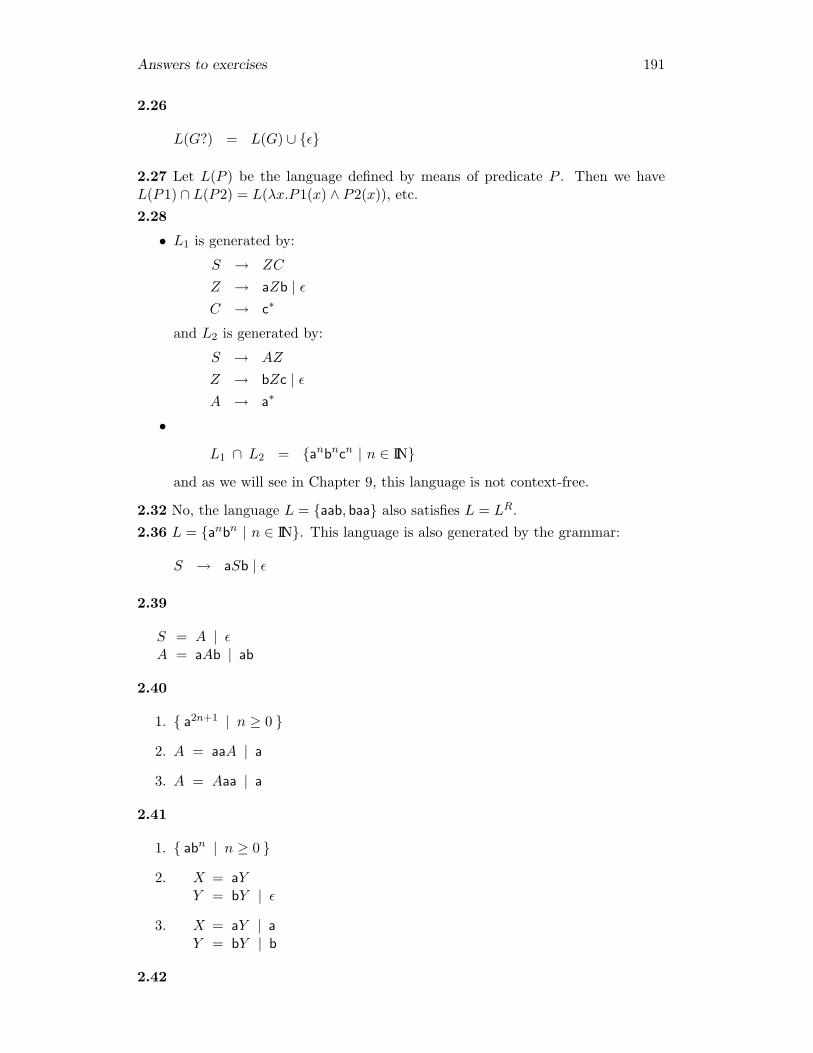
Answers to exercises 191
2.26
L(G?) = L(G) ∪ {ε}
2.27 Let L(P ) be the language defined by means of predicate P . Then we haveL(P1) ∩ L(P2) = L(λx.P1(x) ∧ P2(x)), etc.2.28
• L1 is generated by:
S → ZC
Z → aZb | εC → c∗
and L2 is generated by:
S → AZ
Z → bZc | εA → a∗
•
L1 ∩ L2 = {anbncn | n ∈ IIN}
and as we will see in Chapter 9, this language is not context-free.
2.32 No, the language L = {aab, baa} also satisfies L = LR.2.36 L = {anbn | n ∈ IIN}. This language is also generated by the grammar:
S → aSb | ε
2.39
S = A | εA = aAb | ab
2.40
1. { a2n+1 | n ≥ 0 }
2. A = aaA | a
3. A = Aaa | a
2.41
1. { abn | n ≥ 0 }
2. X = aYY = bY | ε
3. X = aY | aY = bY | b
2.42

192 Answers to exercises
1. S = T | UST = Xa | UaX = aSU = S | Y TY = SU
The sentential forms aS and SU have been abstracted to nonterminals X andY .
2. S = aSa | Ua | USU = S | SUaSa | SUUa
The nonterminal T has been substituted for its alternatives aSa and Ua.
2.43
S → 1O
O → 1O | 0NN → 1∗
2.46
1. first leftmost derivation:
Sentence⇒
Subject Predicate⇒
theyPredicate⇒
theyVerbNounPhrase⇒
theyareNounPhrase⇒
theyareAdjective Noun⇒
theyareflyingNoun⇒
theyareflyingplanes
2. second leftmost derivation:
Sentence⇒
Subject Predicate⇒
theyPredicate⇒
theyAuxVerb Verb Noun⇒
theyareVerb Noun
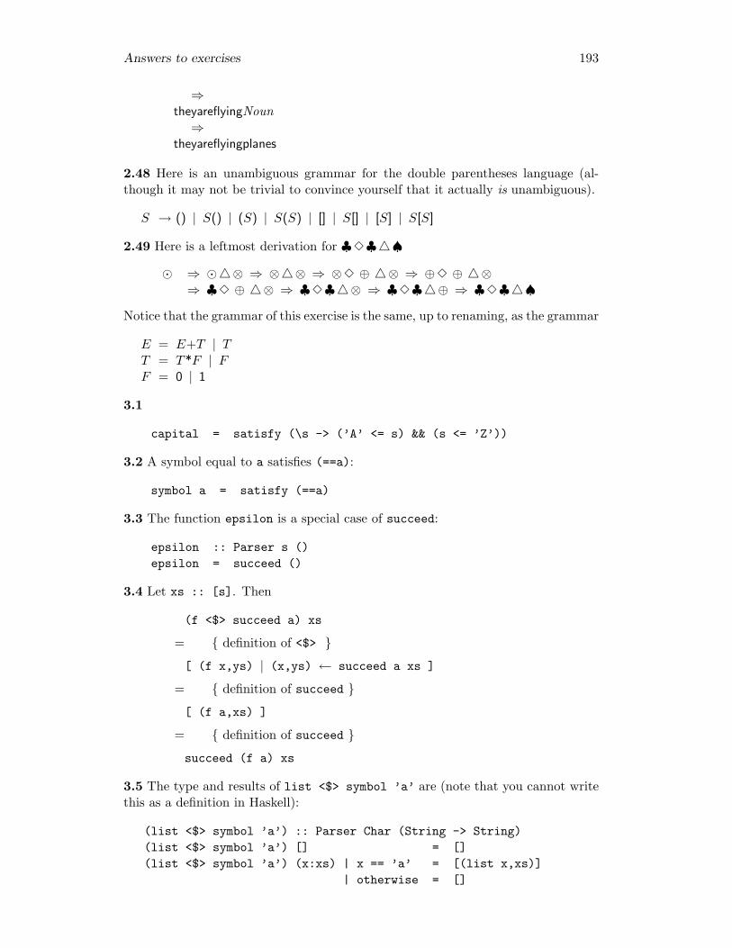
Answers to exercises 193
⇒theyareflyingNoun⇒
theyareflyingplanes
2.48 Here is an unambiguous grammar for the double parentheses language (al-though it may not be trivial to convince yourself that it actually is unambiguous).
S → () | S() | (S) | S(S) | [] | S[] | [S] | S[S]
2.49 Here is a leftmost derivation for ♣3♣4♠
� ⇒ �4⊗ ⇒ ⊗4⊗ ⇒ ⊗3 ⊕ 4⊗ ⇒ ⊕3 ⊕ 4⊗⇒ ♣3 ⊕ 4⊗ ⇒ ♣3♣4⊗ ⇒ ♣3♣4⊕ ⇒ ♣3♣4♠
Notice that the grammar of this exercise is the same, up to renaming, as the grammar
E = E+T | TT = T*F | FF = 0 | 1
3.1
capital = satisfy (\s -> (’A’ <= s) && (s <= ’Z’))
3.2 A symbol equal to a satisfies (==a):
symbol a = satisfy (==a)
3.3 The function epsilon is a special case of succeed:
epsilon :: Parser s ()epsilon = succeed ()
3.4 Let xs :: [s]. Then
(f <$> succeed a) xs
= { definition of <$> }
[ (f x,ys) | (x,ys) ← succeed a xs ]
= { definition of succeed }
[ (f a,xs) ]
= { definition of succeed }
succeed (f a) xs
3.5 The type and results of list <$> symbol ’a’ are (note that you cannot writethis as a definition in Haskell):
(list <$> symbol ’a’) :: Parser Char (String -> String)(list <$> symbol ’a’) [] = [](list <$> symbol ’a’) (x:xs) | x == ’a’ = [(list x,xs)]
| otherwise = []

194 Answers to exercises
3.6 The type and results of list <$> symbol ’a’ <*> p are:
(list <$> symbol ’a’ <*> p) :: Parser Char String(list <$> symbol ’a’ <*> p) [] = [](list <$> symbol ’a’ <*> p) (x:xs)
| x == ’a’ = [(list ’a’ x,ys) | (x,ys) <- p xs]| otherwise = []
3.7
pBool :: Parser Char BoolpBool = const True <$> token "True"
<|> const False <$> token "False"
3.91 data Pal2 = Nil | Leafa | Leafb | Twoa Pal2 | Twob Pal22 palin2 :: Parser Char Pal2
palin2 = (\x y z -> Twoa y) <$>symbol ’a’ <*> palin2 <*> symbol ’a’
<|> (\x y z -> Twob y) <$>symbol ’b’ <*> palin2 <*> symbol ’b’
<|> const Leafa <$> symbol ’a’<|> const Leafb <$> symbol ’b’<|> succeed Nil
3 palina :: Parser Char Intpalina = (\x y z -> y+2) <$>
symbol ’a’ <*> palina <*> symbol ’a’<|> (\x y z -> y) <$>
symbol ’b’ <*> palina <*> symbol ’b’<|> const 1 <$> symbol ’a’<|> const 0 <$> symbol ’b’<|> succeed 0
3.101 data English = E1 Subject Pred
data Subject = E2 Stringdata Pred = E3 Verb NounP | E4 AuxV Verb Noundata Verb = E5 String | E6 Stringdata AuxV = E7 Stringdata NounP = E8 Adj Noundata Adj = E9 Stringdata Noun = E10 String
2 english :: Parser Char Englishenglish = E1 <$> subject <*> predsubject = E2 <$> token "they"pred = E3 <$> verb <*> nounp
<|> E4 <$> auxv <*> verb <*> nounverb = E5 <$> token "are"
<|> E6 <$> token "flying"auxv = E7 <$> token "are"

Answers to exercises 195
nounp = E8 <$> adj <*> nounadj = E9 <$> token "flying"noun = E10 <$> token "planes"
3.11 As <|> uses ++, it is more efficiently evaluated right associative.3.12 The function is the same as <*>, but instead of applying the result of the firstparser to that of the second, it pairs them together:
(<,>) :: Parser s a -> Parser s b -> Parser s (a,b)(p <,> q) xs = [((x,y),zs)
|(x,ys) <- p xs,(y,zs) <- q ys]
3.13 ‘Parser transformator’, or ‘parser modifier’ or ‘parser postprocessor’, etcetera.3.14 The transformator <$> does to the result part of parsers what map does to theelements of a list.3.15 The parser combinators <*> and <,> can be defined in terms of each other:
p <*> q = h <$> (p <,> q)where -- h :: (b -> a,b) -> a
h (f,y) = f yp <,> q = (h <$> p) <*> q
where -- h :: a -> (b -> (a,b))h x y = (x, y)
3.16 Yes. You can combine the parser parameter of <$> with a parser that consumesno input and always yields the function parameter of <$>:
f <$> p = succeed f <*> p
3.17
f ::Char->Parentheses->Char->Parentheses->Parentheses
open ::Parser Char Char
f <$> open ::Parser Char (Parentheses->Char->Parentheses->Parentheses)
parens ::Parser Char Parentheses
(f <$> open) <*> parens ::Parser Char (Char->Parentheses->Parentheses)
3.18 To the left. Yes.3.19
test p s = not (null (filter (null . snd) (p s)))test p = not . null . filter (null . snd) . p
3.20 Introduce the abbreviation
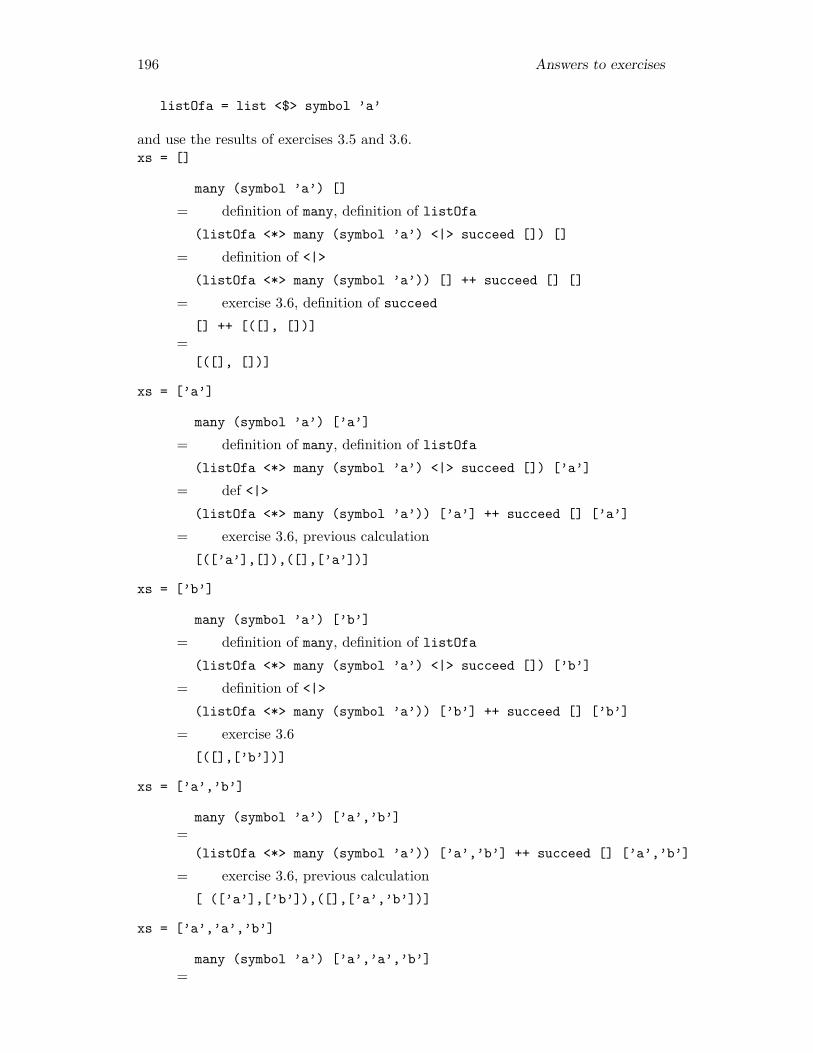
196 Answers to exercises
listOfa = list <$> symbol ’a’
and use the results of exercises 3.5 and 3.6.xs = []
many (symbol ’a’) []
= definition of many, definition of listOfa
(listOfa <*> many (symbol ’a’) <|> succeed []) []
= definition of <|>
(listOfa <*> many (symbol ’a’)) [] ++ succeed [] []
= exercise 3.6, definition of succeed
[] ++ [([], [])]=
[([], [])]
xs = [’a’]
many (symbol ’a’) [’a’]
= definition of many, definition of listOfa
(listOfa <*> many (symbol ’a’) <|> succeed []) [’a’]
= def <|>
(listOfa <*> many (symbol ’a’)) [’a’] ++ succeed [] [’a’]
= exercise 3.6, previous calculation
[([’a’],[]),([],[’a’])]
xs = [’b’]
many (symbol ’a’) [’b’]
= definition of many, definition of listOfa
(listOfa <*> many (symbol ’a’) <|> succeed []) [’b’]
= definition of <|>
(listOfa <*> many (symbol ’a’)) [’b’] ++ succeed [] [’b’]
= exercise 3.6
[([],[’b’])]
xs = [’a’,’b’]
many (symbol ’a’) [’a’,’b’]=
(listOfa <*> many (symbol ’a’)) [’a’,’b’] ++ succeed [] [’a’,’b’]
= exercise 3.6, previous calculation
[ ([’a’],[’b’]),([],[’a’,’b’])]
xs = [’a’,’a’,’b’]
many (symbol ’a’) [’a’,’a’,’b’]=
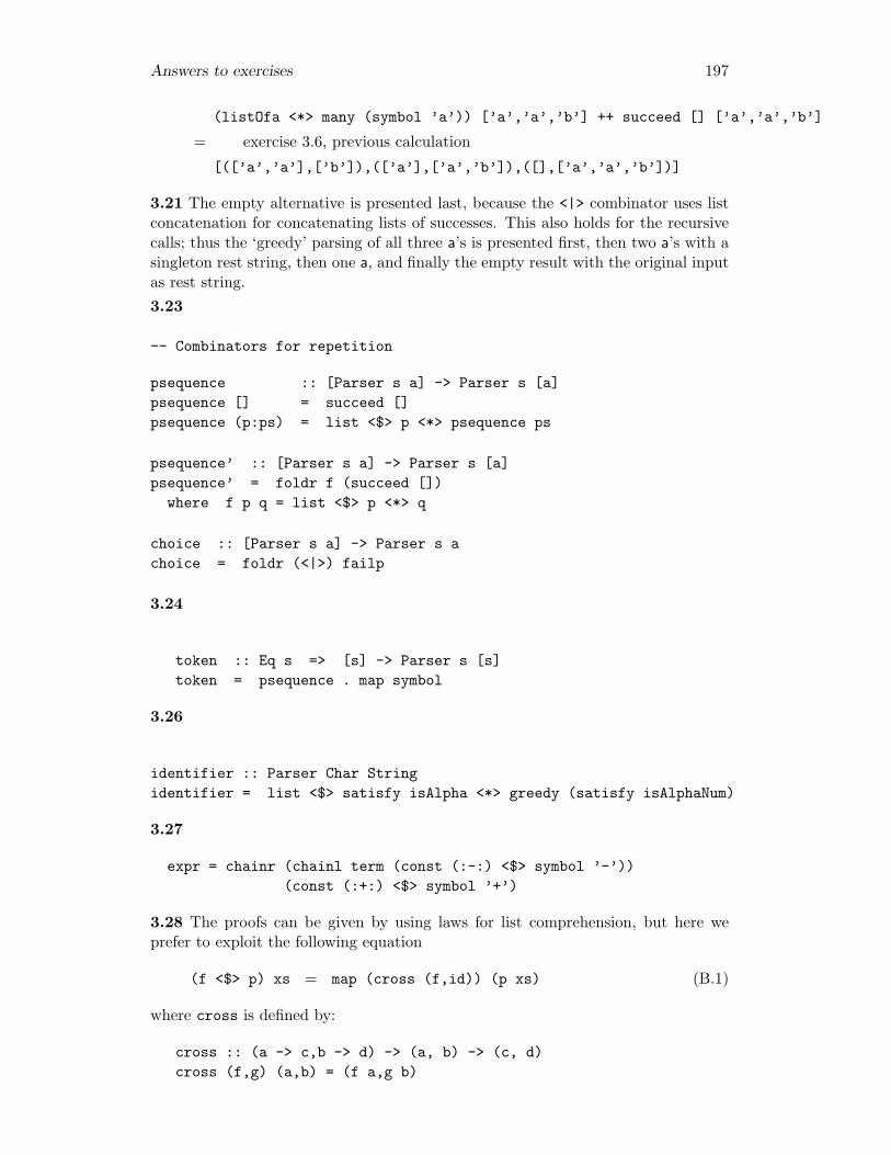
Answers to exercises 197
(listOfa <*> many (symbol ’a’)) [’a’,’a’,’b’] ++ succeed [] [’a’,’a’,’b’]
= exercise 3.6, previous calculation
[([’a’,’a’],[’b’]),([’a’],[’a’,’b’]),([],[’a’,’a’,’b’])]
3.21 The empty alternative is presented last, because the <|> combinator uses listconcatenation for concatenating lists of successes. This also holds for the recursivecalls; thus the ‘greedy’ parsing of all three a’s is presented first, then two a’s with asingleton rest string, then one a, and finally the empty result with the original inputas rest string.3.23
-- Combinators for repetition
psequence :: [Parser s a] -> Parser s [a]psequence [] = succeed []psequence (p:ps) = list <$> p <*> psequence ps
psequence’ :: [Parser s a] -> Parser s [a]psequence’ = foldr f (succeed [])
where f p q = list <$> p <*> q
choice :: [Parser s a] -> Parser s achoice = foldr (<|>) failp
3.24
token :: Eq s => [s] -> Parser s [s]token = psequence . map symbol
3.26
identifier :: Parser Char Stringidentifier = list <$> satisfy isAlpha <*> greedy (satisfy isAlphaNum)
3.27
expr = chainr (chainl term (const (:-:) <$> symbol ’-’))(const (:+:) <$> symbol ’+’)
3.28 The proofs can be given by using laws for list comprehension, but here weprefer to exploit the following equation
(f <$> p) xs = map (cross (f,id)) (p xs) (B.1)
where cross is defined by:
cross :: (a -> c,b -> d) -> (a, b) -> (c, d)cross (f,g) (a,b) = (f a,g b)

198 Answers to exercises
It has the following property
cross (f,g) . cross (h,k) = cross (f.h,g.k) (B.2)
Furthermore, we will use the following laws about map in our proof: map distributesover composition, concatenation, and function concat.
map f . map g = map (f.g) (B.3)map f (x ++ y) = map f x ++ map f y (B.4)map f . concat = concat . map (map f) (B.5)
1. (h <$> (f <$> p)) xs=
map (cross (h,id)) ((f <$> p) xs)=
map (cross (h,id)) (map (cross (f,id)) (p xs))
= { map distributes over composition: B.3}
map ((cross (h,id)) . (cross (f,id))) (p xs)
= { equation B.2 for cross }
map (cross (h.f,id)) (p xs)
= { equation B.1 for <$> }
((h.f) <$> p) xs
2. (h <$> (p <|> q)) xs=
map (cross (h,id)) ((p <|> q) xs)=
map (cross (h,id)) (p xs ++ q xs)
= { map distributes over concatenation: B.4 }
map (cross (h,id)) (p xs) ++ map (cross (h,id)) (q xs)
= { equation B.1 for <$> }
(h <$> p) xs ++ (h <$> q) xs
= { definition of <|> }
((h <$> p) <|> (h <$> q)) xs
3. First note that (p <*> q) xs can be written as
(p <*> q) xs = concat (map (mc q) (p xs)) (B.6)
where
mc q (f,ys) = map (cross (f,id)) (q ys)
Now we calculate
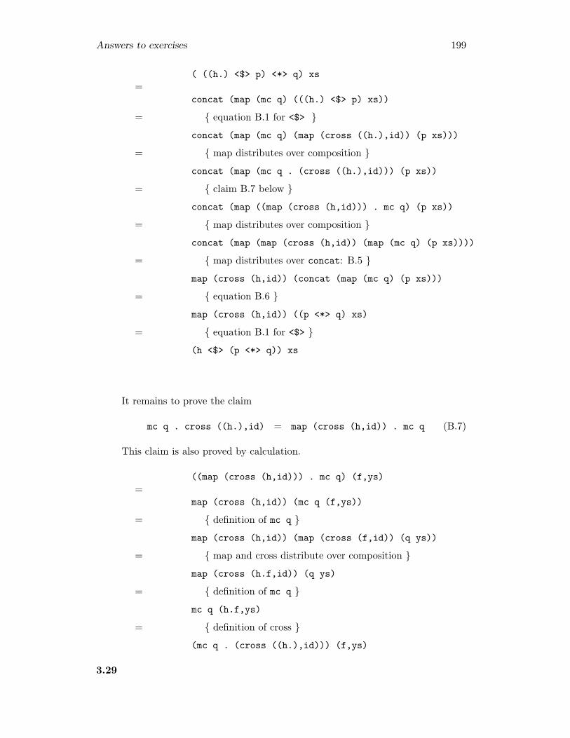
Answers to exercises 199
( ((h.) <$> p) <*> q) xs=
concat (map (mc q) (((h.) <$> p) xs))
= { equation B.1 for <$> }
concat (map (mc q) (map (cross ((h.),id)) (p xs)))
= { map distributes over composition }
concat (map (mc q . (cross ((h.),id))) (p xs))
= { claim B.7 below }
concat (map ((map (cross (h,id))) . mc q) (p xs))
= { map distributes over composition }
concat (map (map (cross (h,id)) (map (mc q) (p xs))))
= { map distributes over concat: B.5 }
map (cross (h,id)) (concat (map (mc q) (p xs)))
= { equation B.6 }
map (cross (h,id)) ((p <*> q) xs)
= { equation B.1 for <$> }
(h <$> (p <*> q)) xs
It remains to prove the claim
mc q . cross ((h.),id) = map (cross (h,id)) . mc q (B.7)
This claim is also proved by calculation.
((map (cross (h,id))) . mc q) (f,ys)=
map (cross (h,id)) (mc q (f,ys))
= { definition of mc q }
map (cross (h,id)) (map (cross (f,id)) (q ys))
= { map and cross distribute over composition }
map (cross (h.f,id)) (q ys)
= { definition of mc q }
mc q (h.f,ys)
= { definition of cross }
(mc q . (cross ((h.),id))) (f,ys)
3.29
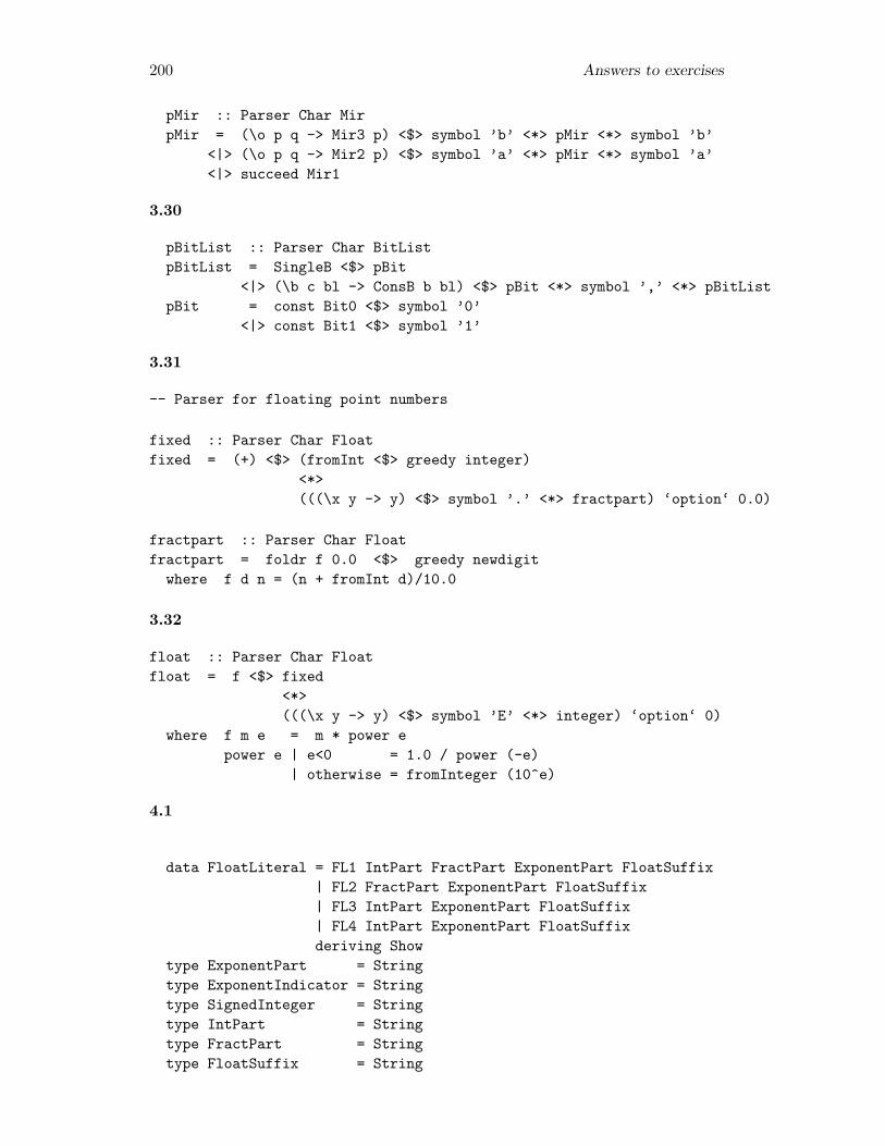
200 Answers to exercises
pMir :: Parser Char MirpMir = (\o p q -> Mir3 p) <$> symbol ’b’ <*> pMir <*> symbol ’b’
<|> (\o p q -> Mir2 p) <$> symbol ’a’ <*> pMir <*> symbol ’a’<|> succeed Mir1
3.30
pBitList :: Parser Char BitListpBitList = SingleB <$> pBit
<|> (\b c bl -> ConsB b bl) <$> pBit <*> symbol ’,’ <*> pBitListpBit = const Bit0 <$> symbol ’0’
<|> const Bit1 <$> symbol ’1’
3.31
-- Parser for floating point numbers
fixed :: Parser Char Floatfixed = (+) <$> (fromInt <$> greedy integer)
<*>(((\x y -> y) <$> symbol ’.’ <*> fractpart) ‘option‘ 0.0)
fractpart :: Parser Char Floatfractpart = foldr f 0.0 <$> greedy newdigit
where f d n = (n + fromInt d)/10.0
3.32
float :: Parser Char Floatfloat = f <$> fixed
<*>(((\x y -> y) <$> symbol ’E’ <*> integer) ‘option‘ 0)
where f m e = m * power epower e | e<0 = 1.0 / power (-e)
| otherwise = fromInteger (10^e)
4.1
data FloatLiteral = FL1 IntPart FractPart ExponentPart FloatSuffix| FL2 FractPart ExponentPart FloatSuffix| FL3 IntPart ExponentPart FloatSuffix| FL4 IntPart ExponentPart FloatSuffixderiving Show
type ExponentPart = Stringtype ExponentIndicator = Stringtype SignedInteger = Stringtype IntPart = Stringtype FractPart = Stringtype FloatSuffix = String
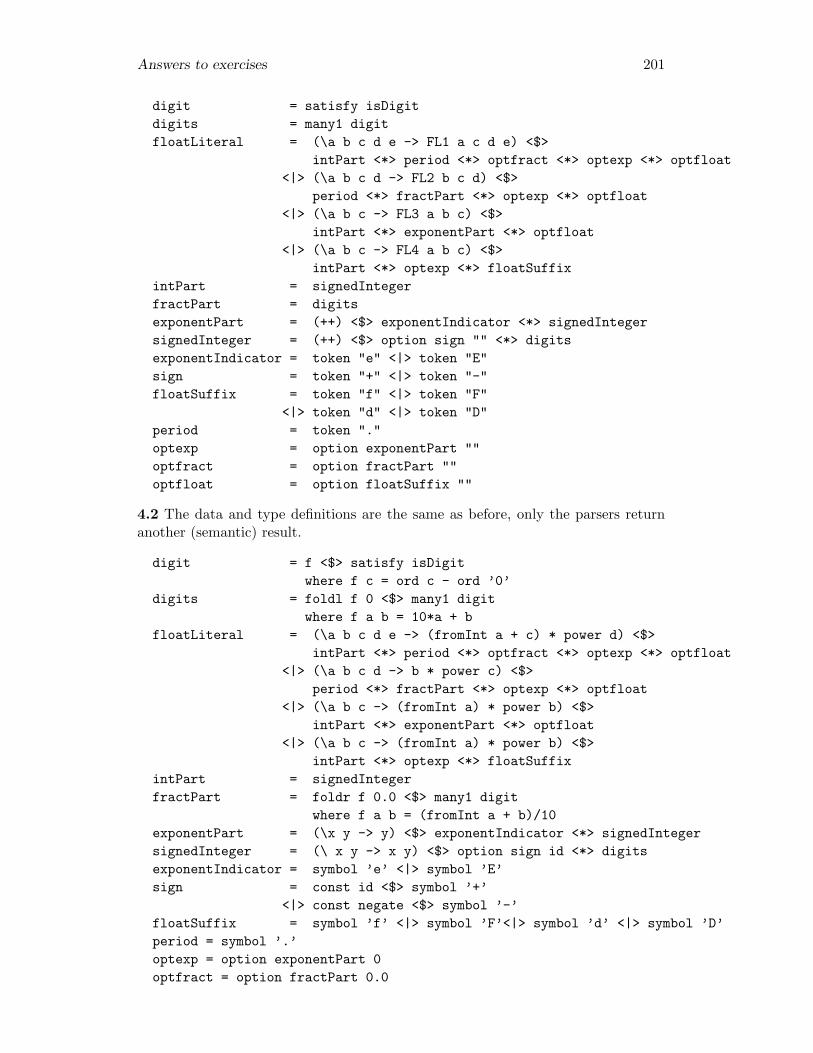
Answers to exercises 201
digit = satisfy isDigitdigits = many1 digitfloatLiteral = (\a b c d e -> FL1 a c d e) <$>
intPart <*> period <*> optfract <*> optexp <*> optfloat<|> (\a b c d -> FL2 b c d) <$>
period <*> fractPart <*> optexp <*> optfloat<|> (\a b c -> FL3 a b c) <$>
intPart <*> exponentPart <*> optfloat<|> (\a b c -> FL4 a b c) <$>
intPart <*> optexp <*> floatSuffixintPart = signedIntegerfractPart = digitsexponentPart = (++) <$> exponentIndicator <*> signedIntegersignedInteger = (++) <$> option sign "" <*> digitsexponentIndicator = token "e" <|> token "E"sign = token "+" <|> token "-"floatSuffix = token "f" <|> token "F"
<|> token "d" <|> token "D"period = token "."optexp = option exponentPart ""optfract = option fractPart ""optfloat = option floatSuffix ""
4.2 The data and type definitions are the same as before, only the parsers returnanother (semantic) result.
digit = f <$> satisfy isDigitwhere f c = ord c - ord ’0’
digits = foldl f 0 <$> many1 digitwhere f a b = 10*a + b
floatLiteral = (\a b c d e -> (fromInt a + c) * power d) <$>intPart <*> period <*> optfract <*> optexp <*> optfloat
<|> (\a b c d -> b * power c) <$>period <*> fractPart <*> optexp <*> optfloat
<|> (\a b c -> (fromInt a) * power b) <$>intPart <*> exponentPart <*> optfloat
<|> (\a b c -> (fromInt a) * power b) <$>intPart <*> optexp <*> floatSuffix
intPart = signedIntegerfractPart = foldr f 0.0 <$> many1 digit
where f a b = (fromInt a + b)/10exponentPart = (\x y -> y) <$> exponentIndicator <*> signedIntegersignedInteger = (\ x y -> x y) <$> option sign id <*> digitsexponentIndicator = symbol ’e’ <|> symbol ’E’sign = const id <$> symbol ’+’
<|> const negate <$> symbol ’-’floatSuffix = symbol ’f’ <|> symbol ’F’<|> symbol ’d’ <|> symbol ’D’period = symbol ’.’optexp = option exponentPart 0optfract = option fractPart 0.0

202 Answers to exercises
optfloat = option floatSuffix ’ ’power e | e < 0 = 1 / power (-e)
| otherwise = fromInt (10^e)
4.3 The parsing scheme for Java floats is
digit = f <$> satisfy isDigitwhere f c = .....
digits = f <$> many1 digitwhere f ds = ..
floatLiteral = f1 <$>intPart <*> period <*> optfract <*> optexp <*> optfloat
<|> f2 <$>period <*> fractPart <*> optexp <*> optfloat
<|> f3 <$>intPart <*> exponentPart <*> optfloat
<|> f4 <$>intPart <*> optexp <*> floatSuffixwheref1 a b c d e = .....f2 a b c d = .....f3 a b c = .....f4 a b c = .....
intPart = signedIntegerfractPart = f <$> many1 digit
where f ds = ....exponentPart = f <$> exponentIndicator <*> signedInteger
where f x y = .....signedInteger = f <$> option sign ?? <*> digits
where f x y = .....exponentIndicator = f1 <$> symbol ’e’ <|> f2 <$> symbol ’E’
wheref1 c = ....f2 c = ..
sign = f1 <$> symbol ’+’ <|> f2 <$> symbol ’-’wheref1 h = .....f2 h = .....
floatSuffix = f1 <$> symbol ’f’<|> f2 <$> symbol ’F’<|> f3 <$> symbol ’d’<|> f4 <$> symbol ’D’
wheref1 c = .....f2 c = .....f3 c = .....f4 c = .....
period = symbol ’.’optexp = option exponentPart ??optfract = option fractPart ??

Answers to exercises 203
optfloat = option floatSuffix ??
5.1 Let G = (T,N,R, S). Define the regular grammar G′ = (T,N ∪ {S′}, R′, S′) asfollows. S′ is a new nonterminal symbol. For the productions R′, divide the pro-ductions of R in two sets: the productions R1 of which the right-hand side consistsjust of terminal symbols, and the productions R2 of which the right-hand side endswith a nonterminal. Define a set R3 of productions by adding the nonterminal Sat the right end of each production in R1. Define R′ = R ∪ R3 ∪ S′ → S | ε. Thegrammar G′ thus defined is regular, and generates the language L∗.5.2 In step 2, add the productions
S → aSS → εS → cCS → aA→ εA→ cCA→ aB → cCB → a
and remove the productions
S → A
A→ B
B → C
In step 3, add the production S → a, and remove the productions A→ ε, B → ε.5.3
ndfsa d qs [ ] = qs
ndfsa d qs (x : xs) = ndfsa d (d qs x) xs
5.4 LetM = (X,Q, d, S, F ) be a deterministic finite-state automaton. Then the non-deterministic finite-state automaton M ′ defined by M ′ = (X,Q, d′, {S}, F ), whered′ q x = {d q x} accepts the same language.5.5 Let M = (X,Q, d, S, F ) be a deterministic finite-state automaton that acceptslanguage L. Then the deterministic finite-state automaton M ′ = (X,Q, d, S,Q−F ),where Q − F is the set of states Q from which all states in F have been removed,accepts the language L. Here we assume that d q a is defined for all q and a.5.6
1 L1 ∩ L2 = (L1 ∪ L2), so it follows that regular languages are closed underintersection if they are closed under complementation and union. Regularlanguages are closed under union, see Theorem 10, and they are closed undercomplementation, see exercise 5.5.
2 Ldfa M={w ∈ X∗ | dfa accept w (d, (S1, S2), (F1 × F2))}
=

204 Answers to exercises
{w ∈ X∗ | dfa d (S1, S2) w ∈ F1 × F2}= This requires a proof by induction
{w ∈ X∗ | (dfa d1 S1 w, dfa d2 S2 w) ∈ F1 × F2}={w ∈ X∗ | dfa d1 S1 w ∈ F1 ∧ dfa d2 S2 w ∈ F2}
={w ∈ X∗ | dfa d1 S1 w ∈ F1} ∩ {w ∈ X∗ | dfa d2 S2 w ∈ F2}
=Ldfa M1 ∩ Ldfa M2
5.71
S?>=<89:;/.-,()*+ (//@A BC)
OOA?>=<89:; )
//@A BC(OOB?>=<89:;/.-,()*+
2
S?>=<89:; 0 //GF ED
1
��
0
��
A?>=<89:;
0
��
1 // C?>=<89:;/.-,()*+
B?>=<89:;/.-,()*+ 0 // D?>=<89:;/.-,()*+5.8 Use the definition of Lre to calculate the languages:
1 {ε, b}2 (bc∗)3 {a}b∗ ∪ c∗
5.9
1 Lre(R(S + T ))=
(Lre(R))(Lre(S + T ))=
(Lre(R))(Lre(S) ∪ Lre(T ))=
(Lre(R))(Lre(S)) ∪ (Lre(R))(Lre(T ))=
Lre(RS +RT )
2 Similar to the above calculation.5.10 Take R = a, S = a, and R = a, S = b.5.11 If both V and W are subsets of S, then Lre(R(S + V )) = Lre(R(S + W )).Since S 6= Ø, V = S and W = Ø satisfy the requirement. Another solution is
V = S ∩RW = S ∩R
Since S 6= Ø, at least one of S ∩ R and S ∩ R is not empty, and it follows thatV 6= W . There exist other solutions than these.
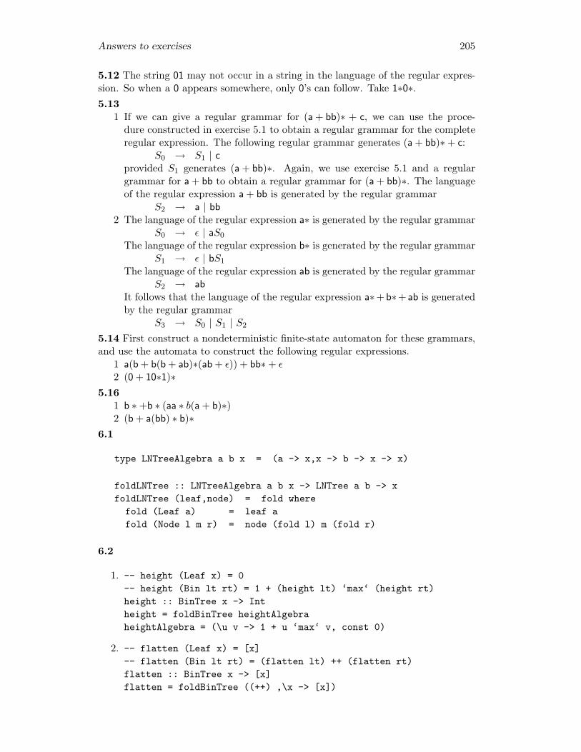
Answers to exercises 205
5.12 The string 01 may not occur in a string in the language of the regular expres-sion. So when a 0 appears somewhere, only 0’s can follow. Take 1∗0∗.5.13
1 If we can give a regular grammar for (a + bb)∗ + c, we can use the proce-dure constructed in exercise 5.1 to obtain a regular grammar for the completeregular expression. The following regular grammar generates (a + bb)∗+ c:
S0 → S1 | cprovided S1 generates (a + bb)∗. Again, we use exercise 5.1 and a regulargrammar for a + bb to obtain a regular grammar for (a + bb)∗. The languageof the regular expression a + bb is generated by the regular grammar
S2 → a | bb2 The language of the regular expression a∗ is generated by the regular grammar
S0 → ε | aS0
The language of the regular expression b∗ is generated by the regular grammarS1 → ε | bS1
The language of the regular expression ab is generated by the regular grammarS2 → ab
It follows that the language of the regular expression a∗+ b∗+ ab is generatedby the regular grammar
S3 → S0 | S1 | S2
5.14 First construct a nondeterministic finite-state automaton for these grammars,and use the automata to construct the following regular expressions.
1 a(b + b(b + ab)∗(ab + ε)) + bb∗+ ε2 (0 + 10∗1)∗
5.161 b ∗+b ∗ (aa ∗ b(a + b)∗)2 (b + a(bb) ∗ b)∗
6.1
type LNTreeAlgebra a b x = (a -> x,x -> b -> x -> x)
foldLNTree :: LNTreeAlgebra a b x -> LNTree a b -> xfoldLNTree (leaf,node) = fold where
fold (Leaf a) = leaf afold (Node l m r) = node (fold l) m (fold r)
6.2
1. -- height (Leaf x) = 0-- height (Bin lt rt) = 1 + (height lt) ‘max‘ (height rt)height :: BinTree x -> Intheight = foldBinTree heightAlgebraheightAlgebra = (\u v -> 1 + u ‘max‘ v, const 0)
2. -- flatten (Leaf x) = [x]-- flatten (Bin lt rt) = (flatten lt) ++ (flatten rt)flatten :: BinTree x -> [x]flatten = foldBinTree ((++) ,\x -> [x])
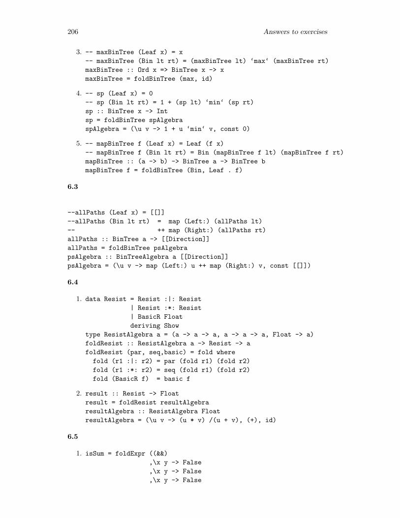
206 Answers to exercises
3. -- maxBinTree (Leaf x) = x-- maxBinTree (Bin lt rt) = (maxBinTree lt) ‘max‘ (maxBinTree rt)maxBinTree :: Ord x => BinTree x -> xmaxBinTree = foldBinTree (max, id)
4. -- sp (Leaf x) = 0-- sp (Bin lt rt) = 1 + (sp lt) ‘min‘ (sp rt)sp :: BinTree x -> Intsp = foldBinTree spAlgebraspAlgebra = (\u v -> 1 + u ‘min‘ v, const 0)
5. -- mapBinTree f (Leaf x) = Leaf (f x)-- mapBinTree f (Bin lt rt) = Bin (mapBinTree f lt) (mapBinTree f rt)mapBinTree :: (a -> b) -> BinTree a -> BinTree bmapBinTree f = foldBinTree (Bin, Leaf . f)
6.3
--allPaths (Leaf x) = [[]]--allPaths (Bin lt rt) = map (Left:) (allPaths lt)-- ++ map (Right:) (allPaths rt)allPaths :: BinTree a -> [[Direction]]allPaths = foldBinTree psAlgebrapsAlgebra :: BinTreeAlgebra a [[Direction]]psAlgebra = (\u v -> map (Left:) u ++ map (Right:) v, const [[]])
6.4
1. data Resist = Resist :|: Resist| Resist :*: Resist| BasicR Floatderiving Show
type ResistAlgebra a = (a -> a -> a, a -> a -> a, Float -> a)foldResist :: ResistAlgebra a -> Resist -> afoldResist (par, seq,basic) = fold where
fold (r1 :|: r2) = par (fold r1) (fold r2)fold (r1 :*: r2) = seq (fold r1) (fold r2)fold (BasicR f) = basic f
2. result :: Resist -> Floatresult = foldResist resultAlgebraresultAlgebra :: ResistAlgebra FloatresultAlgebra = (\u v -> (u * v) /(u + v), (+), id)
6.5
1. isSum = foldExpr ((&&),\x y -> False,\x y -> False,\x y -> False

Answers to exercises 207
,const True,const True,\x -> (&&))
2. vars = foldExpr ((++),(++),(++),(++),const [],\x -> [x],\x y z -> x : (y ++ z))
6.6
1. der computes a symbolic differentiation of an expression.
2. The function der is not a compositional function on Expr because the right-hand sides of the ‘Mul‘ and ‘Dvd‘ expressions do not only use der e1 dx andder e2 dx, but also e1 and e2 themselves.
3. data Exp = Exp ‘Plus‘ Exp| Exp ‘Sub‘ Exp| Con Float| Idf Stringderiving Show
type ExpAlgebra a = (a -> a -> a,a -> a -> a,Float -> a,String -> a)
foldExp :: ExpAlgebra a -> Exp -> afoldExp (plus, sub, con, idf) = fold where
fold (e1 ‘Plus‘ e2) = plus (fold e1) (fold e2)fold (e1 ‘Sub‘ e2) = sub (fold e1) (fold e2)fold (Con n) = con nfold (Idf s) = idf s
4. -- der :: Exp -> String -> Exp-- der (e1 ‘Plus‘ e2) dx = (der e1 dx) ‘Plus‘ (der e2 dx)-- der (e1 ‘Sub‘ e2) dx = (der e1 dx) ‘Sub‘ (der e2 dx)-- der (Con f) dx = Con 0.0-- der (Idf s) dx = if s == dx then Con 1.0 else Con 0.0der = foldExp derAlgebraderAlgebra :: ExpAlgebra (String -> Exp)derAlgebra = (\f g -> \s -> f s ‘Plus‘ g s
,\f g -> \s -> f s ‘Sub‘ g s,\n -> \s -> Con 0.0,\s -> \t -> if s == t then Con 1.0 else Con 0.0)

208 Answers to exercises
6.7
-- replace (Leaf x) y = Leaf y-- replace (Bin lt rt) y = Bin (replace lt y) (replace rt y)replace :: BinTree a -> a -> BinTree areplace = foldBinTree repAlgebrarepAlgebra = (\f g -> \y -> Bin (f y) (g y), \x y -> Leaf y)
6.8
--path2Value (Leaf x) = \bs -> if null bs then x else error"no roothpath"--path2Value (Bin lt rt) =-- \bs -> case bs of-- [] -> error "no roothpath"-- (Left:rs) -> path2Value lt rs-- (Right:rs) -> path2Value rt rs--path2Value :: BinTree a -> [Direction] -> apath2Value = foldBinTree pvAlgebrapvAlgebra :: BinTreeAlgebra a ([Direction] -> a)pvAlgebra = (\fl fr -> \ bs -> case bs of
{[] -> error "no roothpath";(Left:rs) -> fl rs;(Right:rs) -> fr rs}
, \x -> \ bs -> if null bsthen xelse error "no roothpath")
6.91 type PalAlgebra p = (p, p, p, p -> p, p -> p)
2 foldPal :: PalAlgebra p -> Pal -> pfoldPal (pal1,pal2,pal3,pal4,pal5) = fPal where
fPal Pal1 = pal1fPal Pal2 = pal2fPal Pal3 = pal3fPal (Pal4 p) = pal4 (fPal p)fPal (Pal5 p) = pal5 (fPal p)
3 a2cPal = foldPal ("","a","b",\p ->"a"++p++"a",\p ->"b"++p++"b")
aCountPal = foldPal (0,1,0,\p->p+2,\p->p)
4 pfoldPal :: PalAlgebra p -> Parser Char ppfoldPal (pal1, pal2, pal3, pal4, pal5) = pPal where
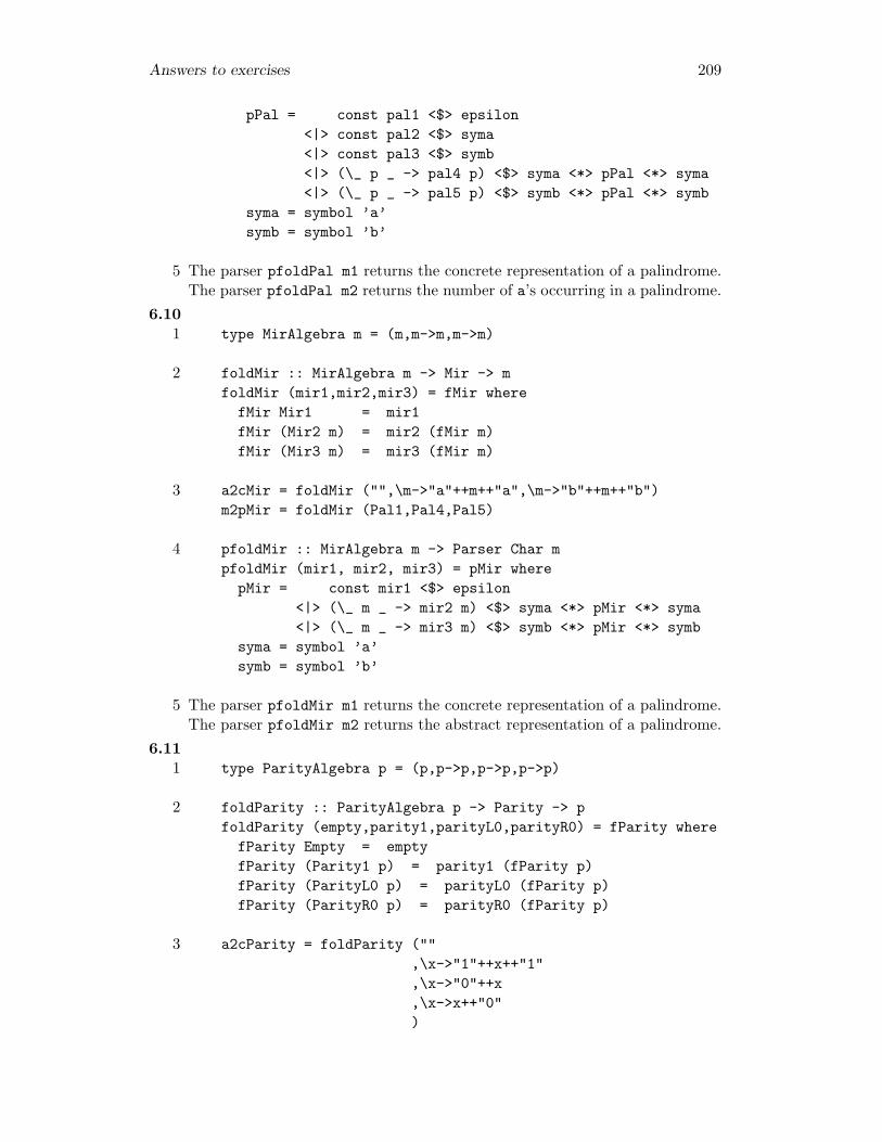
Answers to exercises 209
pPal = const pal1 <$> epsilon<|> const pal2 <$> syma<|> const pal3 <$> symb<|> (\_ p _ -> pal4 p) <$> syma <*> pPal <*> syma<|> (\_ p _ -> pal5 p) <$> symb <*> pPal <*> symb
syma = symbol ’a’symb = symbol ’b’
5 The parser pfoldPal m1 returns the concrete representation of a palindrome.The parser pfoldPal m2 returns the number of a’s occurring in a palindrome.
6.101 type MirAlgebra m = (m,m->m,m->m)
2 foldMir :: MirAlgebra m -> Mir -> mfoldMir (mir1,mir2,mir3) = fMir where
fMir Mir1 = mir1fMir (Mir2 m) = mir2 (fMir m)fMir (Mir3 m) = mir3 (fMir m)
3 a2cMir = foldMir ("",\m->"a"++m++"a",\m->"b"++m++"b")m2pMir = foldMir (Pal1,Pal4,Pal5)
4 pfoldMir :: MirAlgebra m -> Parser Char mpfoldMir (mir1, mir2, mir3) = pMir where
pMir = const mir1 <$> epsilon<|> (\_ m _ -> mir2 m) <$> syma <*> pMir <*> syma<|> (\_ m _ -> mir3 m) <$> symb <*> pMir <*> symb
syma = symbol ’a’symb = symbol ’b’
5 The parser pfoldMir m1 returns the concrete representation of a palindrome.The parser pfoldMir m2 returns the abstract representation of a palindrome.
6.111 type ParityAlgebra p = (p,p->p,p->p,p->p)
2 foldParity :: ParityAlgebra p -> Parity -> pfoldParity (empty,parity1,parityL0,parityR0) = fParity wherefParity Empty = emptyfParity (Parity1 p) = parity1 (fParity p)fParity (ParityL0 p) = parityL0 (fParity p)fParity (ParityR0 p) = parityR0 (fParity p)
3 a2cParity = foldParity ("",\x->"1"++x++"1",\x->"0"++x,\x->x++"0")

210 Answers to exercises
6.121 type BitListAlgebra bl z b = ((b->z->bl,b->bl),(bl->z->z,bl->z),(b,b))
2 foldBitList :: BitListAlgebra bl z b -> BitList -> blfoldBitList ((consb,singleb),(consbl,singlebl),(bit0,bit1)) = fBitList
wherefBitList (ConsB b z) = consb (fBit b) (fZ z)fBitList (SingleB b) = singleb (fBit b)fZ (ConsBL bl z) = consbl (fBitList bl) (fZ z)fZ (SingleBL bl) = singlebl (fBitList bl)fBit Bit0 = bit0fBit Bit1 = bit1
3 a2cBitList = foldBitList (((++),id),((++),id),("0","1"))
4 pfoldBitList :: BitListAlgebra bl z b -> Parser Char blpfoldBitList ((consb,singleb),(consbl,singlebl),(bit0,bit1)) = pBitList
wherepBitList = consb <$> pBit <*> pZ
<|> singleb <$> pBitpZ = (\_ bl z -> consbl bl z) <$> symbol ’,’
<*> pBitList<*> pZ
<|> singlebl <$> pBitListpBit = const bit0 <$> symbol ’0’
<|> const bit1 <$> symbol ’1’
6.13
1. data Block = B1 Stat Restdata Rest = R1 Stat Rest | Nixdata Stat = S1 Decl | S2 Use | S3 Nestdata Decl = Dx | Dydata Use = UX | UYdata Nest = N1 Block
The abstract representation of x;(y;Y);X is
B1 (S1 Dx) (R1 stat2 rest2) wherestat2 = S3 (N1 block)block = B1 (S1 Dy) (R1 (S2 UY) Nix)rest2 = R1 (S2 UX) Nix
2. type BlockAlgebra b r s d u n =(s -> r -> b,(s -> r -> r, r),(d -> s, u -> s, n -> s)
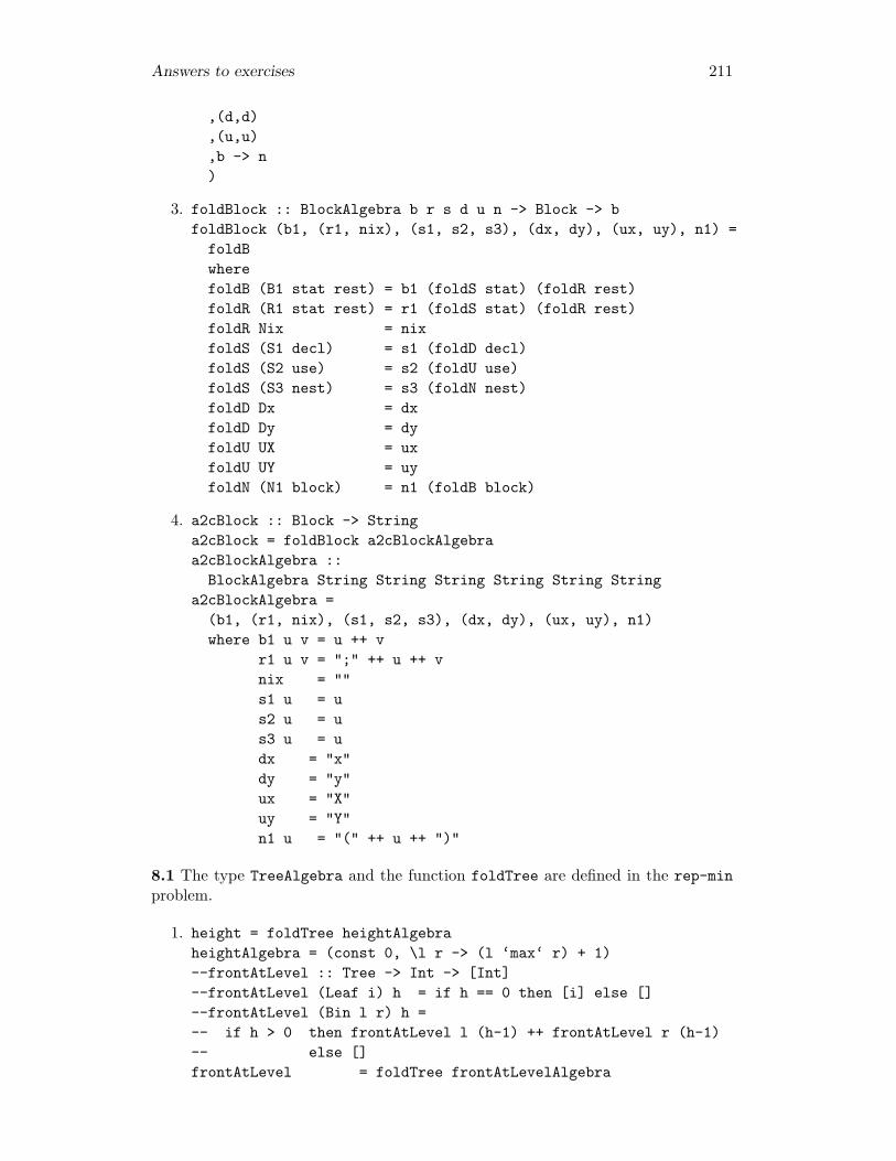
Answers to exercises 211
,(d,d),(u,u),b -> n)
3. foldBlock :: BlockAlgebra b r s d u n -> Block -> bfoldBlock (b1, (r1, nix), (s1, s2, s3), (dx, dy), (ux, uy), n1) =
foldBwherefoldB (B1 stat rest) = b1 (foldS stat) (foldR rest)foldR (R1 stat rest) = r1 (foldS stat) (foldR rest)foldR Nix = nixfoldS (S1 decl) = s1 (foldD decl)foldS (S2 use) = s2 (foldU use)foldS (S3 nest) = s3 (foldN nest)foldD Dx = dxfoldD Dy = dyfoldU UX = uxfoldU UY = uyfoldN (N1 block) = n1 (foldB block)
4. a2cBlock :: Block -> Stringa2cBlock = foldBlock a2cBlockAlgebraa2cBlockAlgebra ::
BlockAlgebra String String String String String Stringa2cBlockAlgebra =
(b1, (r1, nix), (s1, s2, s3), (dx, dy), (ux, uy), n1)where b1 u v = u ++ v
r1 u v = ";" ++ u ++ vnix = ""s1 u = us2 u = us3 u = udx = "x"dy = "y"ux = "X"uy = "Y"n1 u = "(" ++ u ++ ")"
8.1 The type TreeAlgebra and the function foldTree are defined in the rep-minproblem.
1. height = foldTree heightAlgebraheightAlgebra = (const 0, \l r -> (l ‘max‘ r) + 1)--frontAtLevel :: Tree -> Int -> [Int]--frontAtLevel (Leaf i) h = if h == 0 then [i] else []--frontAtLevel (Bin l r) h =-- if h > 0 then frontAtLevel l (h-1) ++ frontAtLevel r (h-1)-- else []frontAtLevel = foldTree frontAtLevelAlgebra
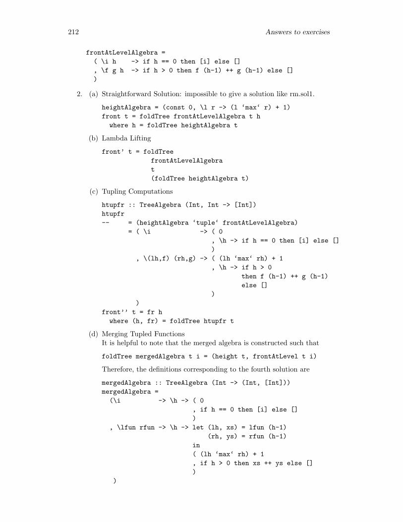
212 Answers to exercises
frontAtLevelAlgebra =( \i h -> if h == 0 then [i] else [], \f g h -> if h > 0 then f (h-1) ++ g (h-1) else [])
2. (a) Straightforward Solution: impossible to give a solution like rm.sol1.
heightAlgebra = (const 0, \l r -> (l ‘max‘ r) + 1)front t = foldTree frontAtLevelAlgebra t h
where h = foldTree heightAlgebra t
(b) Lambda Lifting
front’ t = foldTreefrontAtLevelAlgebrat(foldTree heightAlgebra t)
(c) Tupling Computations
htupfr :: TreeAlgebra (Int, Int -> [Int])htupfr-- = (heightAlgebra ‘tuple‘ frontAtLevelAlgebra)
= ( \i -> ( 0, \h -> if h == 0 then [i] else [])
, \(lh,f) (rh,g) -> ( (lh ‘max‘ rh) + 1, \h -> if h > 0
then f (h-1) ++ g (h-1)else []
))
front’’ t = fr hwhere (h, fr) = foldTree htupfr t
(d) Merging Tupled FunctionsIt is helpful to note that the merged algebra is constructed such that
foldTree mergedAlgebra t i = (height t, frontAtLevel t i)
Therefore, the definitions corresponding to the fourth solution are
mergedAlgebra :: TreeAlgebra (Int -> (Int, [Int]))mergedAlgebra =
(\i -> \h -> ( 0, if h == 0 then [i] else [])
, \lfun rfun -> \h -> let (lh, xs) = lfun (h-1)(rh, ys) = rfun (h-1)
in( (lh ‘max‘ rh) + 1, if h > 0 then xs ++ ys else [])
)

Answers to exercises 213
front’’’ t = frwhere (h, fr) = foldTree mergedAlgebra t h
8.2 The highest front problem is the problem of finding the first non-empty listof nodes which are at the lowest level. The solutions are similar to these of thedeepest front problem.
1. --lowest :: Tree -> Int--lowest (Leaf i) = 0--lowest (Bin l r) = ((lowest l) ‘min‘ (lowest r)) + 1lowest = foldTree lowAlgebralowAlgebra = (const 0, \ l r -> (l ‘min‘ r) + 1)
2. (a) Straightforward Solution: impossible to give a solution like rm.sol1.
lfront t = foldTree frontAtLevelAlgebra t lwhere l = foldTree lowAlgebra t
(b) Lambda Lifting
lfront’ t = foldTreefrontAtLevelAlgebrat(foldTree lowAlgebra t)
(c) Tupling Computations
ltupfr :: TreeAlgebra (Int, Int -> [Int])ltupfr =
( \i -> ( 0, (\l -> if l == 0 then [i] else []))
, \ (lh,f) (rh,g) -> ( (lh ‘min‘ rh) + 1, \l -> if l > 0
then f (l-1) ++ g (l-1)else []
))
lfront’’ t = fr lwhere (l, fr) = foldTree ltupfr t
(d) Merging Tupled FunctionsIt is helpful to note that the merged algebra is constructed such that
foldTree mergedAlgebra t i = (lowest t, frontAtLevel t i)
Therefore, the definitions corresponding to the fourth solution are
lmergedAlgebra :: TreeAlgebra (Int -> (Int, [Int]))lmergedAlgebra =
( \i -> \l -> ( 0, if l == 0 then [i] else [])
, \lfun rfun -> \l ->let (ll, lres) = lfun (l-1)
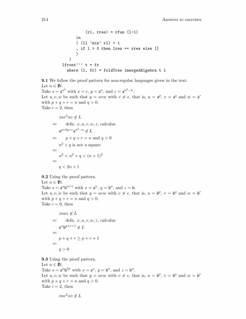
214 Answers to exercises
(rl, rres) = rfun (l-1)in( (ll ‘min‘ rl) + 1, if l > 0 then lres ++ rres else [])
)lfront’’’ t = fr
where (l, fr) = foldTree lmergedAlgebra t l
9.1 We follow the proof pattern for non-regular languages given in the text.Let n ∈ IIN.Take s = an2
with x = ε, y = an, and z = an2−n.Let u, v, w be such that y = uvw with v 6= ε, that is, u = ap, v = aq and w = ar
with p+ q + r = n and q > 0.Take i = 2, then
xuv2wz 6∈ L⇐ defn. x, u, v, w, z, calculus
ap+2q+ran2−n 6∈ L⇐ p+ q + r = n and q > 0
n2 + q is not a square⇐
n2 < n2 + q < (n+ 1)2
⇐q < 2n+ 1
9.2 Using the proof pattern.Let n ∈ IIN.Take s = anbn+1 with x = an, y = bn, and z = b.Let u, v, w be such that y = uvw with v 6= ε, that is, u = bp, v = bq and w = br
with p+ q + r = n and q > 0.Take i = 0, then
xuwz 6∈ L⇐ defn. x, u, v, w, z, calculus
anbp+r+1 6∈ L⇐
p+ q + r ≥ p+ r + 1⇐
q > 0
9.3 Using the proof pattern.Let n ∈ IIN.Take s = anb2n with x = an, y = bn, and z = bn.Let u, v, w be such that y = uvw with v 6= ε, that is, u = bp, v = bq and w = br
with p+ q + r = n and q > 0.Take i = 2, then
xuv2wz 6∈ L
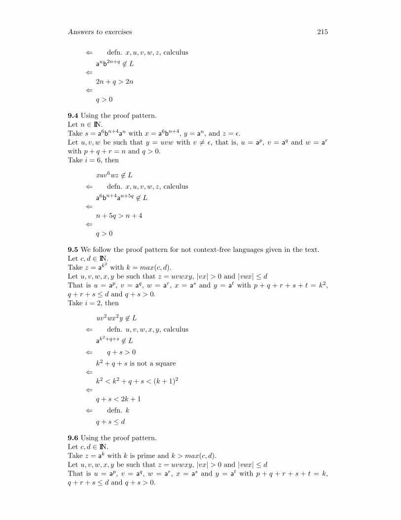
Answers to exercises 215
⇐ defn. x, u, v, w, z, calculus
anb2n+q 6∈ L⇐
2n+ q > 2n⇐
q > 0
9.4 Using the proof pattern.Let n ∈ IIN.Take s = a6bn+4an with x = a6bn+4, y = an, and z = ε.Let u, v, w be such that y = uvw with v 6= ε, that is, u = ap, v = aq and w = ar
with p+ q + r = n and q > 0.Take i = 6, then
xuv6wz 6∈ L⇐ defn. x, u, v, w, z, calculus
a6bn+4an+5q 6∈ L⇐
n+ 5q > n+ 4⇐
q > 0
9.5 We follow the proof pattern for not context-free languages given in the text.Let c, d ∈ IIN.Take z = ak2
with k = max(c, d).Let u, v, w, x, y be such that z = uvwxy, |vx| > 0 and |vwx | ≤ dThat is u = ap, v = aq, w = ar, x = as and y = at with p + q + r + s + t = k2,q + r + s ≤ d and q + s > 0.Take i = 2, then
uv2wx 2y 6∈ L⇐ defn. u, v, w, x, y, calculus
ak2+q+s 6∈ L⇐ q + s > 0
k2 + q + s is not a square⇐
k2 < k2 + q + s < (k + 1)2
⇐q + s < 2k + 1
⇐ defn. k
q + s ≤ d
9.6 Using the proof pattern.Let c, d ∈ IIN.Take z = ak with k is prime and k > max(c, d).Let u, v, w, x, y be such that z = uvwxy, |vx| > 0 and |vwx | ≤ dThat is u = ap, v = aq, w = ar, x = as and y = at with p + q + r + s + t = k,q + r + s ≤ d and q + s > 0.

216 Answers to exercises
Take i = k + 1, then
uvk+1wxk+1y 6∈ L⇐ defn. u, v, w, x, y, calculus
ak+kq+ks 6∈ L⇐
k(1 + q + s) is not a prime⇐
q + s > 0
9.7 Using the proof pattern.Let c, d ∈ IIN.Take z = akbkakbk with k = max(c, d).Let u, v, w, x, y be such that z = uvwxy, |vx| > 0 and |vwx | ≤ dNote that our choice for k guarantees that substring vwx has one of the followingshapes:
• vwx consists of just a’s, or just b’s.• vwx contains both a’s and b’s.
Take i = 0, then
• If vwx consists of just a’s, or just b’s, then it is impossible to write the stringuwy as ww for some string w, since only the number of terminals of one kindis decreased.
• If vwx contains both a’s and b’s, it lies somewhere on the border between a’sand b’s, or on the border between b’s and a’s. Then the string uwy can bewritten as
uwy = asbtapbq
for some s, t, p, q, respectively. At least one of s ,t, p and q is less than k,while two of them are equal to k. Again this sentence is not an element of thelanguage.
10.1 For both grammars we have:
empty = const False
10.2 For grammar1 we have:
firsts S = {b,c}firsts A = {a,b,c}firsts B = {a,b,c}firsts C = {a,b}
For grammar2:
firsts S = {a}firsts A = {b}
10.3 For gramm1 we have:

Answers to exercises 217
follow S = {a,b,c}follow A = {a,b,c}follow B = {a,b}follow C = {a,b,c}
For gramm2:
follow = const {}
10.4 For the productions of gramm3 we have:
lookAhead (S → AaS) = {a,c }lookAhead (S → B) = {b}lookAhead (A → cS) = {c}lookAhead (A → []) = {a}lookAhead (B → b) = {b}
Since all lookAhead sets for productions of the same nonterminal are disjoint, gramm3is an LL(1) grammar.10.5 After left factoring gramm2 we obtain gramm2’ with productions
S → aC
C → bA | a
A → bD
D → b | S
For this transformed grammar gramm2’ we have:
The empty function
empty = const False
The first function
firsts S = {a}firsts C = {a,b}firsts A = {b}firsts D = {a,b}
The follow function
follow = const {}
The lookAhead function
lookAhead (S → aC) = {a}lookAhead (C → bA) = {b}lookAhead (C → a) = {a}lookAhead (A → bD) = {b}lookAhead (D → b) = {b}lookAhead (D → S) = {a}
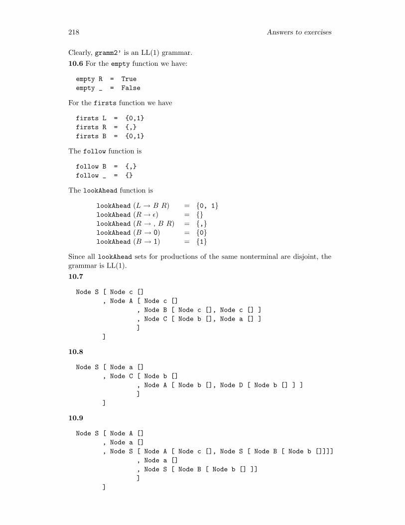
218 Answers to exercises
Clearly, gramm2’ is an LL(1) grammar.10.6 For the empty function we have:
empty R = Trueempty _ = False
For the firsts function we have
firsts L = {0,1}firsts R = {,}firsts B = {0,1}
The follow function is
follow B = {,}follow _ = {}
The lookAhead function is
lookAhead (L → B R) = {0, 1}lookAhead (R→ ε) = {}lookAhead (R → , B R) = {,}lookAhead (B → 0) = {0}lookAhead (B → 1) = {1}
Since all lookAhead sets for productions of the same nonterminal are disjoint, thegrammar is LL(1).10.7
Node S [ Node c [], Node A [ Node c []
, Node B [ Node c [], Node c [] ], Node C [ Node b [], Node a [] ]]
]
10.8
Node S [ Node a [], Node C [ Node b []
, Node A [ Node b [], Node D [ Node b [] ] ]]
]
10.9
Node S [ Node A [], Node a [], Node S [ Node A [ Node c [], Node S [ Node B [ Node b []]]]
, Node a [], Node S [ Node B [ Node b [] ]]]
]

Answers to exercises 219
10.10
1. list2Set :: Ord s => [s] -> [s]list2Set = unions . map single
2. list2Set :: Ord s => [s] -> [s]list2Set = foldr op []
whereop x xs = single x ‘union‘ xs
3. pref :: Ord s => (s -> Bool) -> [s] -> [s]pref p = list2Set . takeWhile p
or
pref p [] = []pref p (x:xs) = if p x then single x ‘union‘ pref p xs else []
or
pref p = foldr op []whereop x xs = if p x then single x ‘union‘ xs else []
4. prefplus p [] = []prefplus p (x:xs) = if p x then single x ‘union‘ prefplus p xs
else single x
5. prefplus p = foldr op []whereop x us = if p x then single x ‘union‘ us
else single x
6. prefplus p=
foldr op []whereop x us = if p x then single x ‘union‘ us else single x
=foldr op []whereop x us = single x ‘union‘ rest
whererest = if p x then us else []
=foldrRhs p single []
7. The function foldrRhs p f [] takes a list xs and returns the set of all f-images of the elements of the prefix of xs all of whose elements satisfy ptogether with the f-image of the first element of xs that does not satisfy p (ifthis element exists).The function foldrRhs p f start takes a list xs and returns the set start‘union‘ foldrRhs p f [] xs.

220 Answers to exercises
8.
10.11
1. For gramm1
(a) foldrRhs empty first [] bSA=
unions (map first (prefplus empty bSA))
= empty b = False
unions (map first [b])=
unions [{b}]=
{b}(b) foldrRhs empty first [] Cb
=unions (map first (prefplus empty Cb))
= empty C = False
unions (map first [C])=
unions [{a, b }]=
{ a, b }
2. For gramm3
(a) foldrRhs empty first [] AaS=
unions (map first (prefplus empty AaS))
= empty A = True
unions (map first ([A] ‘union‘ prefplus empty aS))
empty a = False
unions (map first ([A] ‘union‘ [a]))=
unions (map first ([A, a]))=
unions [first A, first a]=
unions [{c}, {a}]=
{a, c}(b) scanrRhs empty first [] AaS
=map (foldrRhs empty first []) (tails AaS)
=map (foldrRhs empty first []) [AaS, aS, S, []]

Answers to exercises 221
=[ foldrRhs empty first [] AaS, foldrRhs empty first [] aS, foldrRhs empty first [] S, foldrRhs empty first [] []]
= calculus
[ {a, c}, {a}, {a, b, c }, [] ]
Copyright © 2022 FDOKUMEN