J15B.3 ROBUST AND INTERPRETABLE STATISTICAL MODELS FOR PREDICTING THE INTENSIFICATION OF TROPICAL...

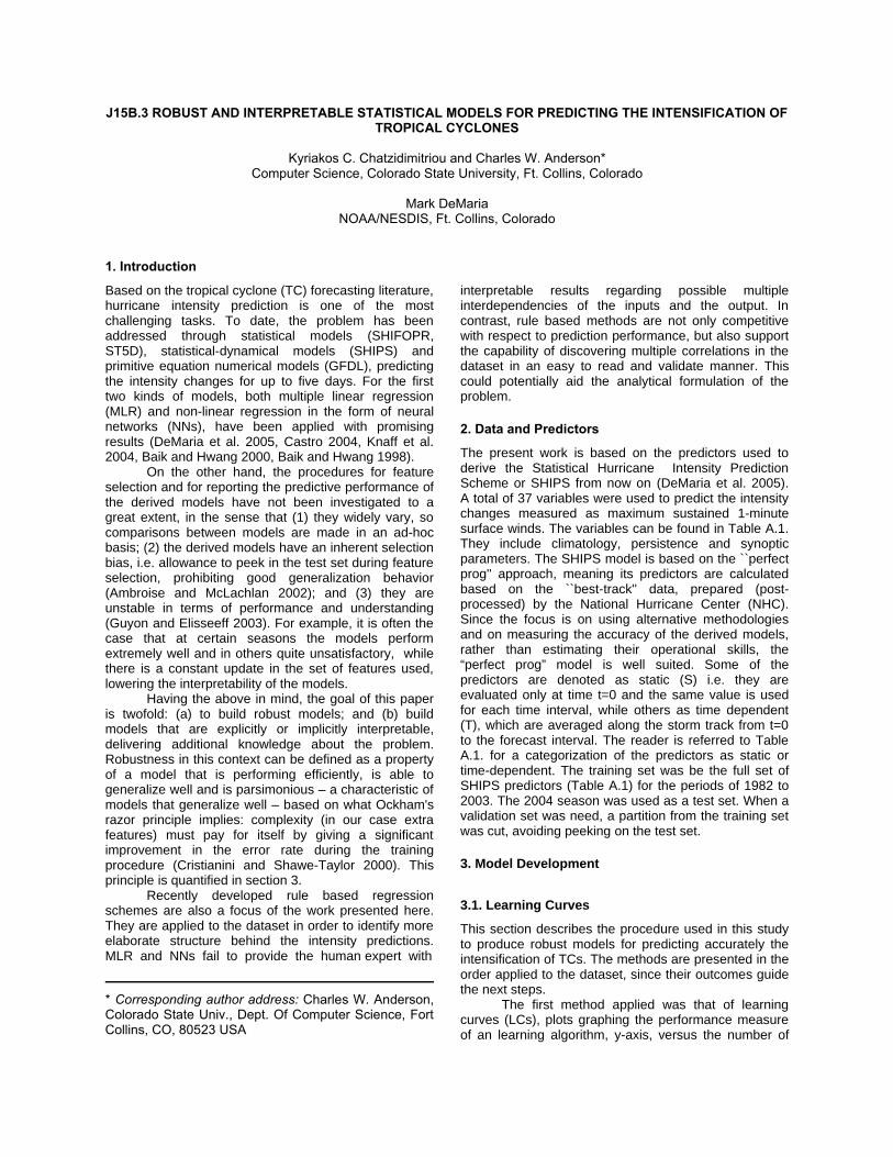
J15B.3 ROBUST AND INTERPRETABLE STATISTICAL MODELS FOR PREDICTING THE INTENSIFICATION OF TROPICAL CYCLONES

Kyriakos C. Chatzidimitriou and Charles W. Anderson*Computer Science, Colorado State University, Ft. Collins, Colorado

Mark DeMariaNOAA/NESDIS, Ft. Collins, Colorado

1. Introduction

Based on the tropical cyclone (TC) forecasting literature, hurricane intensity prediction is one of the most challenging tasks. To date, the problem has been addressed through statistical models (SHIFOPR, ST5D), statistical-dynamical models (SHIPS) and primitive equation numerical models (GFDL), predicting the intensity changes for up to five days. For the first two kinds of models, both multiple linear regression (MLR) and non-linear regression in the form of neural networks (NNs), have been applied with promising results (DeMaria et al. 2005, Castro 2004, Knaff et al. 2004, Baik and Hwang 2000, Baik and Hwang 1998).

On the other hand, the procedures for feature selection and for reporting the predictive performance of the derived models have not been investigated to a great extent, in the sense that (1) they widely vary, so comparisons between models are made in an ad-hoc basis; (2) the derived models have an inherent selection bias, i.e. allowance to peek in the test set during feature selection, prohibiting good generalization behavior (Ambroise and McLachlan 2002); and (3) they are unstable in terms of performance and understanding (Guyon and Elisseeff 2003). For example, it is often the case that at certain seasons the models perform extremely well and in others quite unsatisfactory, while there is a constant update in the set of features used, lowering the interpretability of the models.

Having the above in mind, the goal of this paper is twofold: (a) to build robust models; and (b) build models that are explicitly or implicitly interpretable, delivering additional knowledge about the problem. Robustness in this context can be defined as a property of a model that is performing efficiently, is able to generalize well and is parsimonious – a characteristic of models that generalize well – based on what Ockham's razor principle implies: complexity (in our case extra features) must pay for itself by giving a significant improvement in the error rate during the training procedure (Cristianini and Shawe-Taylor 2000). This principle is quantified in section 3.

Recently developed rule based regression schemes are also a focus of the work presented here. They are applied to the dataset in order to identify more elaborate structure behind the intensity predictions. MLR and NNs fail to provide the human expert with

* Corresponding author address: Charles W. Anderson, Colorado State Univ., Dept. Of Computer Science, Fort Collins, CO, 80523 USA

interpretable results regarding possible multiple interdependencies of the inputs and the output. In contrast, rule based methods are not only competitive with respect to prediction performance, but also support the capability of discovering multiple correlations in the dataset in an easy to read and validate manner. This could potentially aid the analytical formulation of the problem.

2. Data and Predictors

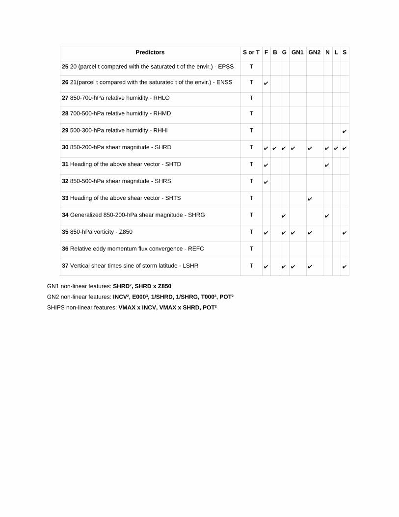
The present work is based on the predictors used to derive the Statistical Hurricane Intensity Prediction Scheme or SHIPS from now on (DeMaria et al. 2005). A total of 37 variables were used to predict the intensity changes measured as maximum sustained 1-minute surface winds. The variables can be found in Table A.1. They include climatology, persistence and synoptic parameters. The SHIPS model is based on the ``perfect prog'' approach, meaning its predictors are calculated based on the ``best-track'' data, prepared (post-processed) by the National Hurricane Center (NHC). Since the focus is on using alternative methodologies and on measuring the accuracy of the derived models, rather than estimating their operational skills, the “perfect prog” model is well suited. Some of the predictors are denoted as static (S) i.e. they are evaluated only at time t=0 and the same value is used for each time interval, while others as time dependent (T), which are averaged along the storm track from t=0 to the forecast interval. The reader is referred to Table A.1. for a categorization of the predictors as static or time-dependent. The training set was be the full set of SHIPS predictors (Table A.1) for the periods of 1982 to 2003. The 2004 season was used as a test set. When a validation set was need, a partition from the training set was cut, avoiding peeking on the test set.

3. Model Development

3.1. Learning Curves

This section describes the procedure used in this study to produce robust models for predicting accurately the intensification of TCs. The methods are presented in the order applied to the dataset, since their outcomes guide the next steps.

The first method applied was that of learning curves (LCs), plots graphing the performance measure of an learning algorithm, y-axis, versus the number of

training examples, x-axis (Russel and Norving 2003). With LCs one is able to (1) detect if there is a pattern governing the data that can be learned; (2) decide whether the data are sufficient to build robust models; (3) identify the number of folds (k) for performing a k-fold cross-validation procedure; and (4) learn something about the noise laying on the data.

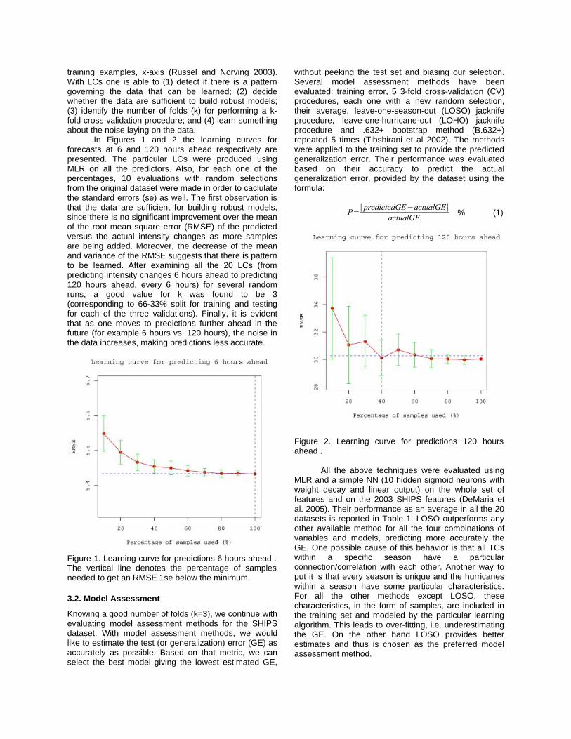
In Figures 1 and 2 the learning curves for forecasts at 6 and 120 hours ahead respectively are presented. The particular LCs were produced using MLR on all the predictors. Also, for each one of the percentages, 10 evaluations with random selections from the original dataset were made in order to caclulate the standard errors (se) as well. The first observation is that the data are sufficient for building robust models, since there is no significant improvement over the mean of the root mean square error (RMSE) of the predicted versus the actual intensity changes as more samples are being added. Moreover, the decrease of the mean and variance of the RMSE suggests that there is pattern to be learned. After examining all the 20 LCs (from predicting intensity changes 6 hours ahead to predicting 120 hours ahead, every 6 hours) for several random runs, a good value for k was found to be 3 (corresponding to 66-33% split for training and testing for each of the three validations). Finally, it is evident that as one moves to predictions further ahead in the future (for example 6 hours vs. 120 hours), the noise in the data increases, making predictions less accurate.

Figure 1. Learning curve for predictions 6 hours ahead . The vertical line denotes the percentage of samples needed to get an RMSE 1se below the minimum.

3.2. Model Assessment

Knowing a good number of folds (k=3), we continue with evaluating model assessment methods for the SHIPS dataset. With model assessment methods, we would like to estimate the test (or generalization) error (GE) as accurately as possible. Based on that metric, we can select the best model giving the lowest estimated GE,

without peeking the test set and biasing our selection. Several model assessment methods have been evaluated: training error, 5 3-fold cross-validation (CV) procedures, each one with a new random selection, their average, leave-one-season-out (LOSO) jacknife procedure, leave-one-hurricane-out (LOHO) jacknife procedure and .632+ bootstrap method (B.632+) repeated 5 times (Tibshirani et al 2002). The methods were applied to the training set to provide the predicted generalization error. Their performance was evaluated based on their accuracy to predict the actual generalization error, provided by the dataset using the formula:

P=∣predictedGE−actualGE∣actualGE % (1)

Figure 2. Learning curve for predictions 120 hours ahead .

All the above techniques were evaluated using MLR and a simple NN (10 hidden sigmoid neurons with weight decay and linear output) on the whole set of features and on the 2003 SHIPS features (DeMaria et al. 2005). Their performance as an average in all the 20 datasets is reported in Table 1. LOSO outperforms any other available method for all the four combinations of variables and models, predicting more accurately the GE. One possible cause of this behavior is that all TCs within a specific season have a particular connection/correlation with each other. Another way to put it is that every season is unique and the hurricanes within a season have some particular characteristics. For all the other methods except LOSO, these characteristics, in the form of samples, are included in the training set and modeled by the particular learning algorithm. This leads to over-fitting, i.e. underestimating the GE. On the other hand LOSO provides better estimates and thus is chosen as the preferred model assessment method.

3.3. Feature Selection

Five feature selection (FS) methods were used: backward elimination (B) (Guyon ans Elisseeff 2003), forward selection (F) (Guyon and Elisseeff 2003), genetic algorithm (G) (Vinterbo and Ohno-Machado 1999), Neural Networks (N) (Leray and Gallinari 1999) and Lasso (L) (Hastie et al 2001). Each one of them is compared against the SHIPS 2003 model both in terms of the LOSO error estimate and the 2004 season intensity deviation errors. The 2003 SHIPS predictors can be found in Table A.1. marked as column S. From the seven methods, the best were used to select additional non-linear features that exist in the SHIPS model and have shown promising improvements.

Table 1. The estimation performance, P, of model assessment algorithms. LOSO (in boldface characters) outperforms any other method.

Variables Full set SHIPS 2003

Methods MLR (%) NN (%) MLR (%) NN (%)

Train 22.83 52.46 8.08 33.72

CV1 21.5 30.63 7.38 16.69

CV2 21.58 30.22 7.37 16.17

CV3 21.62 29.81 7.42 16.19

CV4 21.59 29.83 7.39 15.53

CV5 21.54 29.66 7.47 16.64

CV avg 21.57 30.03 7.39 16.25

LOSO 14.63 10.98 6.84 8.34

LOHO 21.43 14.68 12.89 12.64

B.632+ 22.24 38.25 7.69 22.38

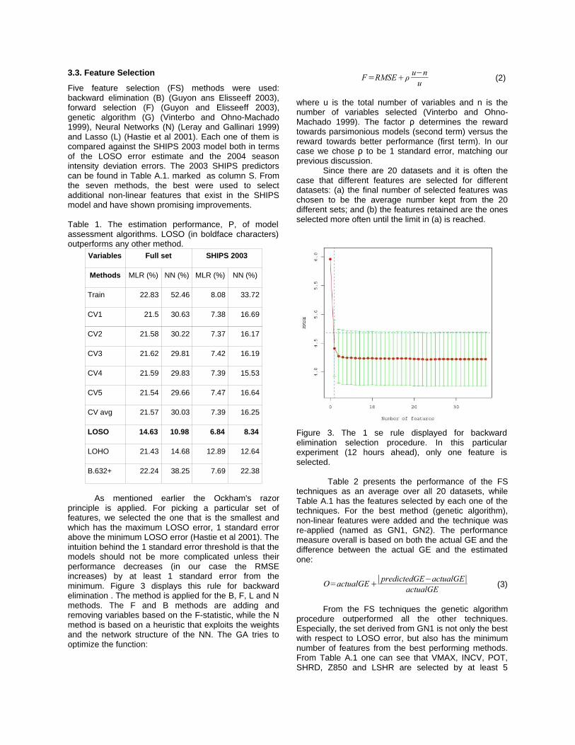
As mentioned earlier the Ockham's razor principle is applied. For picking a particular set of features, we selected the one that is the smallest and which has the maximum LOSO error, 1 standard error above the minimum LOSO error (Hastie et al 2001). The intuition behind the 1 standard error threshold is that the models should not be more complicated unless their performance decreases (in our case the RMSE increases) by at least 1 standard error from the minimum. Figure 3 displays this rule for backward elimination . The method is applied for the B, F, L and N methods. The F and B methods are adding and removing variables based on the F-statistic, while the N method is based on a heuristic that exploits the weights and the network structure of the NN. The GA tries to optimize the function:

F=RMSEρ u−nu (2)

where u is the total number of variables and n is the number of variables selected (Vinterbo and Ohno-Machado 1999). The factor determines the rewardρ towards parsimonious models (second term) versus the reward towards better performance (first term). In our case we chose to be 1 standard error, matching ourρ previous discussion.

Since there are 20 datasets and it is often the case that different features are selected for different datasets: (a) the final number of selected features was chosen to be the average number kept from the 20 different sets; and (b) the features retained are the ones selected more often until the limit in (a) is reached.

Figure 3. The 1 se rule displayed for backward elimination selection procedure. In this particular experiment (12 hours ahead), only one feature is selected.

Table 2 presents the performance of the FS techniques as an average over all 20 datasets, while Table A.1 has the features selected by each one of the techniques. For the best method (genetic algorithm), non-linear features were added and the technique was re-applied (named as GN1, GN2). The performance measure overall is based on both the actual GE and the difference between the actual GE and the estimated one:

O=actualGE∣predictedGE−actualGE∣actualGE (3)

From the FS techniques the genetic algorithm procedure outperformed all the other techniques. Especially, the set derived from GN1 is not only the best with respect to LOSO error, but also has the minimum number of features from the best performing methods. From Table A.1 one can see that VMAX, INCV, POT, SHRD, Z850 and LSHR are selected by at least 5

procedures, while SHIPS uses non-linear combinations of the three most selected features. SHIPS outperforms all other methods for the 2004 test set (and of course overall), but it is quite possible that the particular season was appropriate for the SHIPS predictors. Training and testing for more seasons will be performed later in the study. The main conclusion drawned by this section is the fact that there is a small set of features that is required to obtain good error rates. Additionally, the fact that genetic algorithmic procedures found better subsets can be attributed to their capability of making a better search in the space of features, identifying possible reduntant variables that help each other and finding variables useless by themselves, but usefull with other combinations (Guyon and Elisseeeff 2003). On the contrary backward and forward elimination are brute force approaches, removing less important variables without establishing evidence that even with the help of others, their contribution is minimal.

Table 2. Ranking the feature selection methods based on their mean RMSE performance on all 20 datasets. The asterisks denote models with non-linear features, while the number in the parenthesis present the number of the linear features.

Methods LOSO 2004 Overall Selected

Full 17.85 21.00 24.13 37

F 18.02 19.8 21.57 13

B 18.76 20.23 21.7 4

Lasso 23.82 24.68 26.29 4

G 17.41 19.13 20.86 12

GN 1* 16.80 19.17 21.33 10 (8)

GN 2* 16.85 19.76 22.66 19 (13)

N 19.19 21.1 23.02 7

SHIPS* 17.41 17.62 18.65 16 (13)

3.4. Performance Comparisons

In this section we will compare the 2003 SHIPS model against the best linear and non-linear methods: the two sets derived from the GA FS techniques with non-linear features, two non-linear methods, NNs and Support Vector Machines (SVMs), and two rule-based methods, rule ensembles derived with the RuleFit framework (Friedman and Popescu 2005) and rules based on association rules derived with the RBA framework (Ozgur et al. 2004). Based on a sensitivity analysis the best SVM kernel found was polynomial of degree 3. The set of input variables for NNs and SVMs was the set of linear features found from the initial GA procedure, since they are capable of producing necessary non-linearities by themselves.

Table 3 Ranking the feature selection methods based on their mean RMSE performance on all 20 datasets.Hour SHIPS GN1 GN2 RF RBA NN SVM

6 5.38 5.43 5.43 5.33 5.99 5.39 5.48

12 8.38 8.58 8.55 8.26 9.83 8.23 8.55

18 10.70 11.06 11.04 10.85 13.46 10.68 11.57

24 12.64 13.16 13.10 12.84 16.08 12.59 14.29

30 14.14 14.89 14.82 14.06 19.87 14.47 16.18

36 15.43 16.37 16.31 15.09 20.04 15.91 17.86

42 16.57 17.45 17.46 17.02 21.77 17.39 19.05

48 17.6 18.37 18.55 17.55 24.2 18.84 19.94

54 18.69 19.44 19.74 19.32 27.34 19.98 20.49

60 19.56 20.43 20.87 18.22 27.7 21.18 20.87

66 20.2 21.45 21.92 20.06 26.04 22.09 21.76

72 20.81 22.37 22.81 21.25 31.54 23.16 21.98

78 21.29 23.06 23.59 22.06 30.85 24.23 21.67

84 21.66 23.62 24.28 21.32 31.17 24.95 21.3

90 21.79 23.99 24.91 21.21 31.11 25.44 21.62

96 21.88 24.31 25.45 22.41 31.71 25.91 22.03

102 21.73 24.57 25.97 21.14 34.47 26.12 21.9

108 21.56 24.82 26.36 23.88 30.84 27.23 21.04

114 21.27 24.97 26.73 22.33 30.26 25.48 20.84

120 21.12 25.14 27.31 19.19 31.00 26.00 21.32

Mean 17.62 19.17 19.76 17.66 24.76 19.76 18.49

SHIPS has the best mean skills in the 2004 data, with RuleFit following very close. SVMs outperform NNs and provide a promising candidate for non-linear regression, in that they are easier to analyze and train. We should mention though that there was not a extensive experimentation regarding the NN structure and its parameters, since our interest was on how models perform on a standard basis. RBA was not efficient for this specific dataset, and even though results have shown that it can be competent in other datasets (Ozgur et al. 2005) further improvements are needed. RuleFit (RF) was the model with the maximum number of best performances (10 out of 20). One should also put into perspective the fact that the measurements of the wind speed deviation have an error of -/+ 5 knots.

Thus in retrospect, all the models except RBA can be considered equivalent with respect to estimating intensity deviation.

Other observations that can be made is the fact that the NN performed poorly when the prediction period increased. This is probably due to the fact that noise increases as forecasts are made further ahead. Thus the NN overfits and is unable to generalize well, even though techniques like early stopping and weight decay were used. Up to the first day NNs are the best model. This conclusion is a new drawback for NNs, since previous studies considered forecasts up to 3 days ahead, instead of 5. For RuleFit one can say that the combination of linear and non-linear aspects in a model can greatly help the performance. On the other hand SHIPS after 12 years of development is still one of the best models available. An example of rules discovered by RuleFit and RBA can be found in Appendix B.

We also considerd incremental training and testing for the periods 2001 to 2004 (training from 1982 to 2000 and testing for 2001, then training from 1982 to 2001 and testing for 2002 etc.). This could help us identify the stability of each model over several seasons. Table 4 summarizes the findings. RuleFit is the best method with SHIPS and GA1 following close. It is also evident that as we go from linear to non-linear models variability increases, especially due to the predictions after 3 days (case of SVMs and GN2). Taking into account Ockhams razor principle and the error in the measurement of the wind speed the GN1 model seems like a very good alternative candidate for SHIPS. Moreover the interpretability and efficiency of RuleFit is also another promising candidate.

3.5. Interpretation

In this section we will focus on the interpretational capabilities of RuleFit. RuleFit as a framework provides the opportunity to translate the derived rules into easily read diagrams, displaying the importance of each input variable and its iteraction effects with other variables. This comes in addition to studying the rules in their original format.

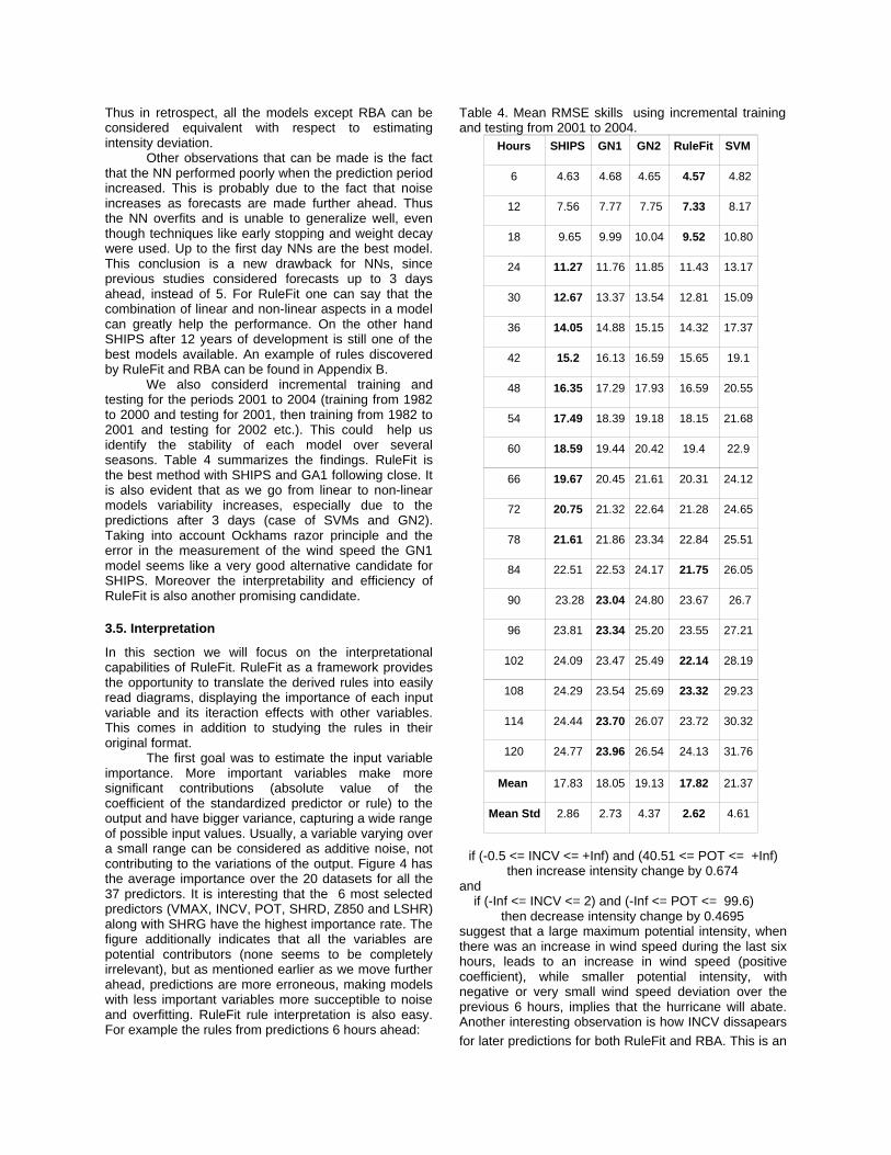
The first goal was to estimate the input variable importance. More important variables make more significant contributions (absolute value of the coefficient of the standardized predictor or rule) to the output and have bigger variance, capturing a wide range of possible input values. Usually, a variable varying over a small range can be considered as additive noise, not contributing to the variations of the output. Figure 4 has the average importance over the 20 datasets for all the 37 predictors. It is interesting that the 6 most selected predictors (VMAX, INCV, POT, SHRD, Z850 and LSHR) along with SHRG have the highest importance rate. The figure additionally indicates that all the variables are potential contributors (none seems to be completely irrelevant), but as mentioned earlier as we move further ahead, predictions are more erroneous, making models with less important variables more succeptible to noise and overfitting. RuleFit rule interpretation is also easy. For example the rules from predictions 6 hours ahead:

Table 4. Mean RMSE skills using incremental training and testing from 2001 to 2004.

Hours SHIPS GN1 GN2 RuleFit SVM

6 4.63 4.68 4.65 4.57 4.82

12 7.56 7.77 7.75 7.33 8.17

18 9.65 9.99 10.04 9.52 10.80

24 11.27 11.76 11.85 11.43 13.17

30 12.67 13.37 13.54 12.81 15.09

36 14.05 14.88 15.15 14.32 17.37

42 15.2 16.13 16.59 15.65 19.1

48 16.35 17.29 17.93 16.59 20.55

54 17.49 18.39 19.18 18.15 21.68

60 18.59 19.44 20.42 19.4 22.9

66 19.67 20.45 21.61 20.31 24.12

72 20.75 21.32 22.64 21.28 24.65

78 21.61 21.86 23.34 22.84 25.51

84 22.51 22.53 24.17 21.75 26.05

90 23.28 23.04 24.80 23.67 26.7

96 23.81 23.34 25.20 23.55 27.21

102 24.09 23.47 25.49 22.14 28.19

108 24.29 23.54 25.69 23.32 29.23

114 24.44 23.70 26.07 23.72 30.32

120 24.77 23.96 26.54 24.13 31.76

Mean 17.83 18.05 19.13 17.82 21.37

Mean Std 2.86 2.73 4.37 2.62 4.61

if (-0.5 <= INCV <= +Inf) and (40.51 <= POT <= +Inf) then increase intensity change by 0.674

and if (-Inf <= INCV <= 2) and (-Inf <= POT <= 99.6)

then decrease intensity change by 0.4695suggest that a large maximum potential intensity, when there was an increase in wind speed during the last six hours, leads to an increase in wind speed (positive coefficient), while smaller potential intensity, with negative or very small wind speed deviation over the previous 6 hours, implies that the hurricane will abate. Another interesting observation is how INCV dissapears

for later predictions for both RuleFit and RBA. This is an

extra advantage of rule based methods being capable of performing feature selection, while training.

Figure 4. Variable importance based on the rules derived by RuleFit for all 20 datasets.

Both RuleFit and RBA frameworks improve upon previously used rule-based methods in the context of hurricane intensity forecasting (Tang et al 2005) mainly because both boundaries in the antecedents and the output are quantified, rather than being qualitative with a prespecified number of levels. Finally, rule importance can be considered as another form of feature selection.

The most important aspect of the RuleFit framework with respect to MLR, Nns or SVMs is providing both through rules and interaction diagrams interdependecies between one or two variables with other predictors in the set. Interaction effects are based on the fact that the final function maping the linear predictors and the rules into intensity changes, is exhibiting interaction between two varialbes, x and y, when the difference in its values for different values of x depends on the value of y. Some examples of the most often seen two variable interactions can be found in Figures 5, 6 and 7. Interactions with three variables were not important, if any.

Different iteractions were found for different datasets. Further investigation could contribute in the analytical formulation of the problem. In our case, we used the most common and major interactions of variables X and Y to create features in the form X x Y and build a hand-picked model using MRL, in an effort of incorporating knowledge to aid the efficiency.

The 7 most important predictors, as mentioned earlier were selected, along with LAT that showed interaction effects with VMAX. Also POT squared (POT2) was included because it was selected by both SHIPS and GN2. The other features were: POT x INCV, VMAX x LAT, VMAX x SHRD, VMAX x LSHR, VMAX x SHRG, POT x Z850 for a total of 14 features, 8 of them linear. Among them VMAX x SHRD an important interaction of the SHIPS set of independent variables.

The model's LOSO RMSE was 17.43, while its test 2004 RMSE was 17.36 and its overal 18.19, making it the best model. Furthermore, incremental training and testing was performed, giving a mean of 16.82 and a mean standard deviation of 1.97 making it also the most stable model. Its performance was better among other models especially in the periods after 72 hours.

Figure 5. Interaction of INCV with VMAX and POT (12 hours ahead).

Figure 6. Interaction of POT with Z850 (54 hours ahead).

4. Conclusions

The intensity prediction task is still a challenging problem. For the statistical-dynamical representation of the problem: (a) all the variables exhibit certain interactions effects making the goal of selecting a good dataset increasingly difficult; and (b) even though it is possible to decrease the RMSE error to be equal to the reporting intensity deviation error for 6 hours ahead, it

remains elusive for predictions further ahead. On the other hand, it is possible to identify certain important predictor combinations that perform adequatelly.

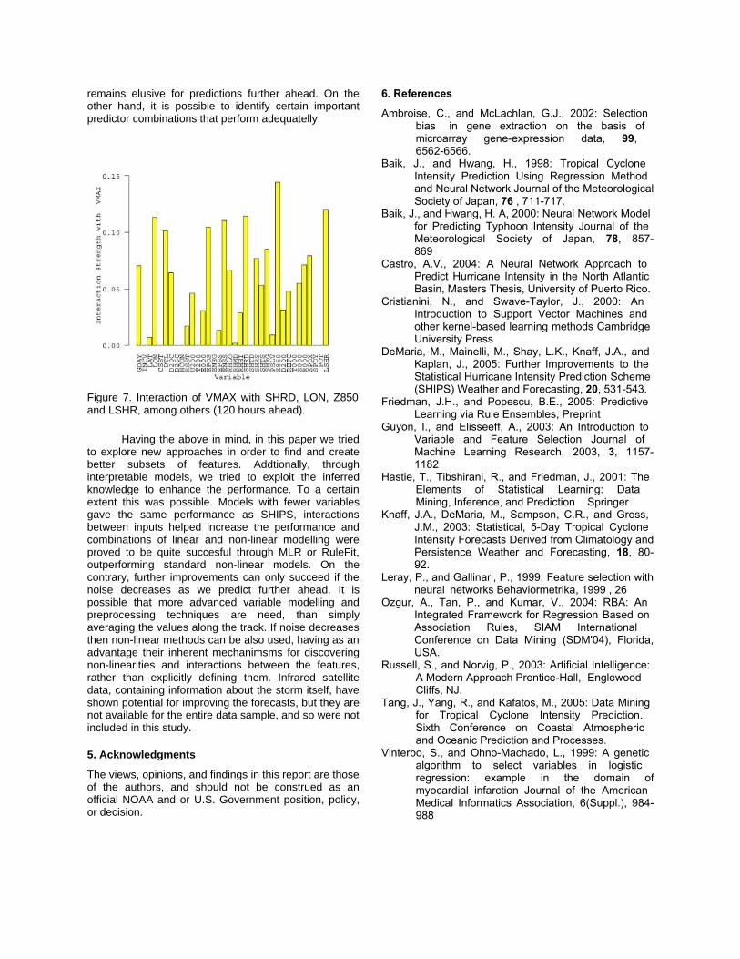
Figure 7. Interaction of VMAX with SHRD, LON, Z850 and LSHR, among others (120 hours ahead).

Having the above in mind, in this paper we tried to explore new approaches in order to find and create better subsets of features. Addtionally, through interpretable models, we tried to exploit the inferred knowledge to enhance the performance. To a certain extent this was possible. Models with fewer variables gave the same performance as SHIPS, interactions between inputs helped increase the performance and combinations of linear and non-linear modelling were proved to be quite succesful through MLR or RuleFit, outperforming standard non-linear models. On the contrary, further improvements can only succeed if the noise decreases as we predict further ahead. It is possible that more advanced variable modelling and preprocessing techniques are need, than simply averaging the values along the track. If noise decreases then non-linear methods can be also used, having as an advantage their inherent mechanimsms for discovering non-linearities and interactions between the features, rather than explicitly defining them. Infrared satellite data, containing information about the storm itself, have shown potential for improving the forecasts, but they are not available for the entire data sample, and so were not included in this study.

5. Acknowledgments

The views, opinions, and findings in this report are those of the authors, and should not be construed as an official NOAA and or U.S. Government position, policy, or decision.

6. References

Ambroise, C., and McLachlan, G.J., 2002: Selection bias in gene extraction on the basis of microarray gene-expression data, 99, 6562-6566.

Baik, J., and Hwang, H., 1998: Tropical Cyclone Intensity Prediction Using Regression Method and Neural Network Journal of the Meteorological Society of Japan, 76 , 711-717.

Baik, J., and Hwang, H. A, 2000: Neural Network Model for Predicting Typhoon Intensity Journal of the Meteorological Society of Japan, 78, 857-869

Castro, A.V., 2004: A Neural Network Approach to Predict Hurricane Intensity in the North Atlantic Basin, Masters Thesis, University of Puerto Rico.

Cristianini, N., and Swave-Taylor, J., 2000: An Introduction to Support Vector Machines and other kernel-based learning methods Cambridge University Press

DeMaria, M., Mainelli, M., Shay, L.K., Knaff, J.A., and Kaplan, J., 2005: Further Improvements to the Statistical Hurricane Intensity Prediction Scheme (SHIPS) Weather and Forecasting, 20, 531-543.

Friedman, J.H., and Popescu, B.E., 2005: Predictive Learning via Rule Ensembles, Preprint

Guyon, I., and Elisseeff, A., 2003: An Introduction to Variable and Feature Selection Journal of Machine Learning Research, 2003, 3, 1157-1182

Hastie, T., Tibshirani, R., and Friedman, J., 2001: The Elements of Statistical Learning: Data Mining, Inference, and Prediction Springer

Knaff, J.A., DeMaria, M., Sampson, C.R., and Gross, J.M., 2003: Statistical, 5-Day Tropical Cyclone Intensity Forecasts Derived from Climatology and Persistence Weather and Forecasting, 18, 80-92.

Leray, P., and Gallinari, P., 1999: Feature selection with neural networks Behaviormetrika, 1999 , 26

Ozgur, A., Tan, P., and Kumar, V., 2004: RBA: An Integrated Framework for Regression Based on Association Rules, SIAM International Conference on Data Mining (SDM'04), Florida,USA.

Russell, S., and Norvig, P., 2003: Artificial Intelligence: A Modern Approach Prentice-Hall, Englewood Cliffs, NJ.

Tang, J., Yang, R., and Kafatos, M., 2005: Data Mining for Tropical Cyclone Intensity Prediction. Sixth Conference on Coastal Atmospheric and Oceanic Prediction and Processes.

Vinterbo, S., and Ohno-Machado, L., 1999: A genetic algorithm to select variables in logistic regression: example in the domain ofmyocardial infarction Journal of the American Medical Informatics Association, 6(Suppl.), 984-988

Appendix A

Table A.1. The initial set of features used and the sets of features selected by each of the algorithms .

Predictors S or T F B G GN1 GN2 N L S

1 Initial maximum wind - VMAX S ✔ ✔ ✔ ✔ ✔ ✔ ✔ ✔

2 Max wind change during the past 6h – INCV or PER S ✔ ✔ ✔ ✔ ✔ ✔ ✔

3 Storm latitude - LAT S ✔ ✔

4 Storm longitude - LON S

5 Climatological sea surface temperature - CSST S

6 Zonal component of storm motion - SPDX S ✔ ✔ ✔ ✔

7 Meridional component of storm motion - SPDY S

8 Pressure level of storm steering - PSLV S ✔

9 200-hPa divergence - D200 S ✔

10 1000-hPa divergence - Z000 S

11 Gaussian function of (Julian day - peak value) - GDAY S ✔ ✔

12 Max potential intensity - current intensity - POT T ✔ ✔ ✔ ✔ ✔ ✔ ✔

13 Distance to land mass - DTL T

14 Climatological depth of 20 C isotherm - D20C T ✔ ✔

15 Same as above for 26 C - D26C T

16 Climatological ocean heat content - HCON T

17 Reynolds SST - RSST T ✔

18 200-hPa zonal wind - U200 T ✔ ✔

19 1000-hPa relative humidity- R000 T ✔

20 200-hPa temperature - T200 T ✔ ✔ ✔ ✔

21 1000-hPa temperature - T000 T ✔

22 1000-hPa t (surface equivalent potential temperature) - E000 T ✔ ✔

23 Average t for positive differences - EPOS T ✔

24 Average t for negative differences - ENEG T

Predictors S or T F B G GN1 GN2 N L S

25 20 (parcel t compared with the saturated t of the envir.) - EPSS T

26 21(parcel t compared with the saturated t of the envir.) - ENSS T ✔

27 850-700-hPa relative humidity - RHLO T

28 700-500-hPa relative humidity - RHMD T

29 500-300-hPa relative humidity - RHHI T ✔

30 850-200-hPa shear magnitude - SHRD T ✔ ✔ ✔ ✔ ✔ ✔ ✔ ✔

31 Heading of the above shear vector - SHTD T ✔ ✔

32 850-500-hPa shear magnitude - SHRS T ✔

33 Heading of the above shear vector - SHTS T ✔

34 Generalized 850-200-hPa shear magnitude - SHRG T ✔ ✔

35 850-hPa vorticity - Z850 T ✔ ✔ ✔ ✔ ✔

36 Relative eddy momentum flux convergence - REFC T

37 Vertical shear times sine of storm latitude - LSHR T ✔ ✔ ✔ ✔ ✔

GN1 non-linear features: SHRD2, SHRD x Z850

GN2 non-linear features: INCV2, E0003, 1/SHRD, 1/SHRG, T0003, POT2

SHIPS non-linear features: VMAX x INCV, VMAX x SHRD, POT2

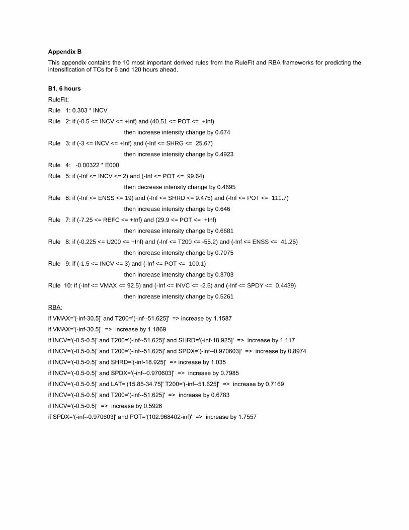
Appendix B

This appendix contains the 10 most important derived rules from the RuleFit and RBA frameworks for predicting the intensification of TCs for 6 and 120 hours ahead.

B1. 6 hours

RuleFit:

Rule 1: 0.303 * INCV

Rule 2: if (-0.5 <= INCV <= +Inf) and (40.51 <= POT <= +Inf)

then increase intensity change by 0.674

Rule 3: if (-3 <= INCV <= +Inf) and (-Inf <= SHRG <= 25.67)


Rule 4: -0.00322 * E000

Rule 5: if (-Inf <= INCV <= 2) and (-Inf <= POT <= 99.64)

then decrease intensity change by 0.4695

Rule 6: if (-Inf <= ENSS <= 19) and (-Inf <= SHRD <= 9.475) and (-Inf <= POT <= 111.7)


Rule 7: if (-7.25 <= REFC <= +Inf) and (29.9 <= POT <= +Inf)


Rule 8: if (-0.225 <= U200 <= +Inf) and (-Inf <= T200 <= -55.2) and (-Inf <= ENSS <= 41.25)


Rule 9: if (-1.5 <= INCV <= 3) and (-Inf <= POT <= 100.1)


Rule 10: if (-Inf <= VMAX <= 92.5) and (-Inf <= INVC <= -2.5) and (-Inf <= SPDY <= 0.4439)


RBA:

if VMAX='(-inf-30.5]' and T200='(-inf--51.625]' => increase by 1.1587

if VMAX='(-inf-30.5]' => increase by 1.1869

if INCV='(-0.5-0.5]' and T200='(-inf--51.625]' and SHRD='(-inf-18.925]' => increase by 1.117

if INCV='(-0.5-0.5]' and T200='(-inf--51.625]' and SPDX='(-inf--0.970603]' => increase by 0.8974

if INCV='(-0.5-0.5]' and SHRD='(-inf-18.925]' => increase by 1.035

if INCV='(-0.5-0.5]' and SPDX='(-inf--0.970603]' => increase by 0.7985

if INCV='(-0.5-0.5]' and LAT='(15.85-34.75]' T200='(-inf--51.625]' => increase by 0.7169

if INCV='(-0.5-0.5]' and T200='(-inf--51.625]' => increase by 0.6783

if INCV='(-0.5-0.5]' => increase by 0.5926

if SPDX='(-inf--0.970603]' and POT='(102.968402-inf)' => increase by 1.7557

B2. 120 hours

RuleFit:

Rule 1: 0.2532 * POT

Rule 2: if (42.5 <= VMAX <= +Inf) and (80.45 <= EPOS <= 150.6) and (13.25 <= SHRD <= 38.49)


Rule 3: if (-Inf <= VMAX <= 69) and (7.857 <= Z850 <= +Inf)


Rule 4: if (-0.4143<= U200 <= +Inf) and (-Inf <= EPSS <= 74.71) and (-Inf <= ENSS <= 14.07)


Rule 5: if (2.578 <= LSHR <= +Inf) and (-Inf <= POT <= 72.64)


Rule 6: if (-Inf <= VMAX <= 77.5) and (103.1 <= EPOS <= +Inf) and (-Inf <= SHRG <= 23.05)


Rule 7: if (-Inf <= EPOS <= 152.4) and (-Inf <= RHHI <= 45.31) and (20.88 <= SHRG <= +Inf)


Rule 8: if (-Inf <= T200 <= -51.81) and (-Inf <= SHRG <= 16.78)


Rule 9: if (-Inf <= VMAX <= 87.5) and (14.12 <= ENSS <= +Inf) and (0.4048 <= REFC <= +Inf)

and (-Inf <= Z000 <= 83.5) and (3.662 <= LSHR <= +Inf)


Rule 10: if (-Inf <= VMAX <= 87.5) and (3499 <= E000 <= +Inf) and (146.5 <= SHTS <= +Inf)

and (-1.405 <= REFC <= +Inf)


RBA:

if POT='(30.594633-72.991362]' => increase by -10.1508

if VMAX='(-inf-41.5]' and SHRD='(14.330952-inf)' and SHRG='(16.802381-inf)' => increase by 19.2896

if VMAX='(-inf-41.5]' and SHRD='(14.330952-inf)' => increase by 19.3589

if LAT='(17.25-inf)' and POT='(72.991362-inf)' => increase by 19.1011

if VMAX='(-inf-41.5]' and SHRG='(16.802381-inf)' and LSHR='(3.887604-inf)' => increase by 19.9903

if VMAX='(41.5-72.5]' and LSHR='(3.887604-inf)' => increase by 1.7391

if SHRD='(14.330952-inf)' and SHRG='(16.802381-inf)' and POT='(72.991362-inf)' and LSHR='(3.887604-inf)' => increase by 14.5526

if VMAX='(-inf-41.5]' and SHRG='(16.802381-inf)' => increase by 22.7259

if SHRD='(14.330952-inf)' and SHRG='(16.802381-inf)' and POT='(72.991362-inf)' => increase by 15.4955

if SHRG='(16.802381-inf)' and POT='(72.991362-inf)' and LSHR='(3.887604-inf)' => increase by 16.0543

J15B.3 ROBUST AND INTERPRETABLE STATISTICAL MODELS FOR PREDICTING THE INTENSIFICATION OF TROPICAL...

Documents

Transcript of J15B.3 ROBUST AND INTERPRETABLE STATISTICAL MODELS FOR PREDICTING THE INTENSIFICATION OF TROPICAL...