Processes setting the characteristics of sea surface cooling induced by tropical cyclones

Processes setting the characteristics of sea surface cooling inducedby tropical cyclones

Emmanuel M. Vincent,1 Matthieu Lengaigne,1 Gurvan Madec,1,2 Jérôme Vialard,1

Guillaume Samson,1 Nicolas C. Jourdain,3 Christophe E. Menkes,1,4 and Swen Jullien5

Received 23 June 2011; revised 21 November 2011; accepted 22 November 2011; published 9 February 2012.

[1] A 1/2° resolution global ocean general circulation model is used to investigate theprocesses controlling sea surface cooling in the wake of tropical cyclones (TCs). Windforcing related to more than 3000 TCs occurring during the 1978–2007 period isblended with the CORE II interannual forcing, using an idealized TC wind patternwith observed magnitude and track. The amplitude and spatial characteristics of theTC-induced cooling are consistent with satellite observations, with an average coolingof �1°C that typically extends over 5 radii of maximum wind. A Wind power index(WPi) is used to discriminate cooling processes under TCs with high-energy transfer tothe upper ocean (strong and/or slow cyclones) from the others (weak and/or fastcyclones). Surface heat fluxes contribute to �50 to 80% of the cooling for weak WPi aswell as away from the cyclone track. Within 200 km of the track, mixing-induced coolingincreases linearly with WPi, explaining �30% of the cooling for weak WPis and up to�80% for large ones. Mixing-induced cooling is strongly modulated by pre-storm oceanicconditions. For a given WPi, vertical processes can induce up to 8 times more cooling forshallow mixed layer and steep temperature stratification than for a deep mixed layer.Vertical mixing is the main source of rightward bias of the cold wake for weak andmoderate WPi, but along-track advection becomes the main contributor to the asymmetryfor the largest WPis.

Citation: Vincent, E. M., M. Lengaigne, G. Madec, J. Vialard, G. Samson, N. C. Jourdain, C. E. Menkes, and S. Jullien (2012),Processes setting the characteristics of sea surface cooling induced by tropical cyclones, J. Geophys. Res., 117, C02020,doi:10.1029/2011JC007396.

1. Introduction

[2] The ocean surface can cool by up to 10°C in the wakeof tropical cyclones [Chiang et al., 2011]. Such cooling wasuntil recently mostly documented from ship measurements[Leipper, 1967], bathythermographs [Shay et al., 1992] andbuoy arrays [Cione et al., 2000; D’Asaro, 2003]. Theavailability of satellite microwave sea surface temperature(SST) measurements, which are less sensitive to masking byclouds than infrared measurements [Wentz et al., 2000], nowallows a more extensive description of the SST response inseveral TC case studies [e.g., Lin et al., 2005; Chiang et al.,2011]. Lloyd and Vecchi [2011] describe TC-induced cool-ing at the global scale for the entire microwave satelliteperiod. Their study reveals that the cold wake amplitudeincreases monotonically with the cyclone intensity up tocategory 2 but saturates for larger TC wind forcing. This

result led the authors to assume that oceanic feedbacks couldinhibit intensification of cyclones.[3] Because TCs draw their energy from evaporation at the

ocean surface [Emanuel, 1986, 2003], sea surface tempera-ture (SST) changes under the storm’s eye can negatively feedback on cyclone intensification, as suggested by observa-tional [Cione and Uhlhorn, 2003; Kaplan and DeMaria,2003] and modeling results [Schade and Emanuel, 1999;Bender and Ginis, 2000; Shen and Ginis, 2003; Schade,2000]. Among other influences–such as the storm’s innercore dynamics or the structure of the synoptic-scale envi-ronment–processes that control the upper-ocean temperatureunder the TC remain one of the major uncertainties forimproving TC intensity forecasts [Marks et al., 1998].[4] Dominant processes in the oceanic response to TCs

have mainly been discussed through cases studies in bothobservations [Sanford et al., 1987; D’Asaro, 2003; D’Asaroet al., 2007] and models [Price, 1981; Morey et al., 2006;Chiang et al., 2011; Huang et al., 2009; Chen et al., 2010].These studies show that three main processes control SSTfluctuations under TCs: oceanic vertical mixing, advectionand air-sea heat exchange. The upper ocean cooling is pri-marily controlled by the entrainment of cold water from thethermocline into the mixed layer through vertical mixing,

1LOCEAN, IRD/CNRS/UPMC/MNHN, Paris, France.2NOC, Southampton, UK.3LEGI, CNRS/UJF/INPG, Grenoble, France.4IRD, Noumea, New Caledonia.5LEGOS, IRD/CNRS/UPS, Toulouse, France.

Copyright 2012 by the American Geophysical Union.0148-0227/12/2011JC007396

JOURNAL OF GEOPHYSICAL RESEARCH, VOL. 117, C02020, doi:10.1029/2011JC007396, 2012

C02020 1 of 18

http://dx.doi.org/10.1029/2011JC007396

principally generated by the vertical shear of horizontalcurrents [Pollard et al., 1973; Price, 1981; Huang et al.,2009]. This entrainment mixing accounts for about 80% ofthe SST drop in TCs wakes [Price, 1981; Sanford et al.,1987; Shay et al., 1992; Huang et al., 2009], but its contri-bution to the total cooling varies depending on the casestudy considered, from 70% in the case of TC Gilbert [Jacobet al., 2000] to more than 90% in the case of TC Frances[D’Asaro et al., 2007] or TC Gloria [Bender et al., 1993].Vertical mixing also seems to be responsible for the asym-metry of the cold anomaly with respect to the TC translationdirection. Most intense inertial oscillations (and associatedvertical shear) are indeed generated to the right (left) of thetrack in the Northern (Southern) Hemisphere, where TCwinds rotate in the same direction as inertial currents, thusincreasing the energy transfer to these currents [e.g., Price,1981].[5] Although of secondary importance, enhanced surface

heat fluxes and advection processes also contribute to theTC-induced cooling. Evaporation (latent heat) dominatesTC-related heat fluxes, while sensible, shortwave, longwaveand precipitation-related fluxes play a lesser role [Jacobet al., 2000; Huang et al., 2009]. A coupled simulationof Hurricane Dennis revealed that air-sea heat exchangeswere responsible for a widespread cooling of the sea surfaceand largely contributed to the total cooling far from the TCtrack for this cyclone [Morey et al., 2006]. While cyclone-induced vertical suction cools the subsurface ocean near thecyclone track (S. Jullien et al., Impact of tropical cyclones onthe South Pacific Ocean heat budget, submitted to Journal ofPhysical Oceanography, 2011), the effect of water advectionon the structure of surface temperature anomalies requiresfurther description. Indeed, horizontal advection has beenshown to be locally important and it is suggested thatit modulates the spatial pattern of the cold wake [Huanget al., 2009; Chen et al., 2010] as well as its asymmetry[Greatbatch, 1983].[6] Most of the aforementioned studies investigate the

mechanisms controlling the cold wake characteristics forcase studies of individual or a limited number of TCs.Although vertical mixing was identified as the major con-tributor to the cooling around the TC eye, the respectivecontribution of each process to the observed cooling isshown to vary from one cyclone to another. The heat balancehas also generally been examined in the region of maximumcooling or at a few points sampled by moored instrumenta-tion of drifting buoys, while the cyclone-induced coolingoften extends over hundreds of kilometers. A systematicstudy of the processes controlling the SST anomaly off thecyclone core region is however still missing [D’Asaro et al.,2007].[7] Past case studies have illustrated the influence of sub-

surface oceanic background conditions on the TC-inducedSST signature [Shay et al., 2000; Cione and Uhlhorn, 2003;Jacob and Shay, 2003; Shay and Brewster, 2010]. Furthersupport for sub-surface oceanic control of the amplitude ofthe TC-induced cooling has recently been provided on aglobal scale [Lloyd and Vecchi, 2011; E. M. Vincent et al.,Assessing the oceanic control on the amplitude of sea sur-face cooling induced by tropical cyclones, submitted toJournal of Geophysical Research, 2011]. Vincent et al.(submitted manuscript, 2011) show that the widely varying

characteristics of upper-ocean pre-cyclone stratification canmodulate the amplitude of TC-induced cooling by up to anorder of magnitude for a given level of TC wind energyinput to the upper ocean, but processes responsible for thismodulation still need to be assessed.[8] Because detailed observations under TCs are scarce,

modeling offers a promising alternative to perform such aninvestigation. A few modeling studies [Liu et al., 2008;Sriver and Huber, 2010; Scoccimarro et al., 2011] havealready performed global ocean simulations including TCsforcing. Using a simplified four layer ocean model forced byidealized hurricane wind forcing, Liu et al. [2008] estimatedthe rate of mechanical energy input to the world oceaninduced by TCs. Sriver and Huber [2010] evaluated theinfluence of TCs on the mean ocean state and poleward heattransport from a global ocean general circulation modelsimulation in which they prescribe TC winds estimated fromhigh resolution satellite wind data. None of these studies,however, investigated the processes involved in TC-inducedcooling.[9] The aim of this study is to characterize surface tem-

perature response to TCs at a global scale, and to quantifyhow the related processes depend on TCs characteristics andoceanic background conditions. To that end, we forced aglobal ocean model with a modified version of CORE IIforcing [Large and Yeager, 2009] including an analyticformulation of two-dimensional TC winds along observedTC tracks between 1978 and 2007. High-resolution datafrom satellite scatterometers do not provide reliable esti-mates for wind larger than 50 m s�1 and are only availablefrom 2000 onward [Brennan et al., 2009]. Our approach hasthe advantage of covering the entire range of TC intensitiesover a 30 years period, hence providing a large database ofsimulated ocean responses to more than 3000 TCs, with thecaveat being that wind spatial structure for each individualcyclone is less accurate than satellites estimates.[10] The paper is structured as follows. Section 2 describes

the observed data set used in this study, the model configu-ration and the proposed modeling strategy to account for TCwind forcing. Section 3 validates our numerical experimentfrom statistical comparison of the simulated cold wakes tosatellite estimates. The main processes that control thecooling, as well as their dependency to the cyclone windpower, distance to the track and oceanic background stateare discussed in section 4. Section 5 provides a summary ofour results as well as a discussion of their implications.

2. Data Sets and Methods

2.1. Observed Data Sets

2.1.1. Ocean Sub-Surface Temperature[11] The depth of the mixed layer (ML) and the upper

ocean thermohaline stratification are two important para-meters controlling the response of near-surface ocean to theatmospheric forcing [Jacob and Shay, 2003; Vincent et al.,submitted manuscript, 2011]. We use the recently updatedmixed layer depth climatology of de Boyer Montégut et al.[2004], which includes ARGO profiles to September 2008and temperature and salinity of the World Ocean Atlas 2009climatology (WOA09) [Locarnini et al., 2010] to validatethe model climatology.

VINCENT ET AL.: PROCESSES OF HURRICANES COLD WAKE C02020C02020

2 of 18

2.1.2. Sea Surface Temperature (SST)[12] We use a blend of Tropical Rainfall MeasuringMission

(TRMM) Microwave Imager (TMI) and Advanced Micro-wave Scanning Radiometer AMSR-E SST daily data set(http://www.ssmi.com/sst/microwave_oi_sst_data_description.html) to characterize the observed SST response to TCs overthe 1998–2007 period. Despite its inability to retrieve SSTdata under heavy precipitation [Wentz et al., 2000], TMI andAMSR-E offer the advantage of being insensitive to atmo-spheric water vapor and provide accurate observations ofSST beneath clouds, a few days before and after TC passage.The inner-core cooling (i.e., cooling under the eye) cannot beassessed confidently with TMI-AMSR; data are most of thetime missing in a 400 km radius around the current TCposition. This data set however provides a reliable estimate ofthe cooling in the TCs wake, data being typically available 1to 2 days after TC passage. It has however to be noted that thecooling amplitude in the TCs’ wake may not be fully cap-tured by this data set, especially for slow moving TCs.2.1.3. Tropical Cyclone Position and Strength[13] Observed TC position and strength are derived from

the International Best Track Archive for Climate Steward-ship (IBTrACS) [Knapp et al., 2010]. In this study, we focuson the 1978–2007 period, over which worldwide satellitecoverage provides the position and estimated maximumwind speed every 6 h for more than 3000 TCs. The maxi-mum wind speed value characterizing the TC strength istaken as the 10-minute averaged wind at 10 meters.

2.2. Methodology to Monitor the Ocean Responseto TCs

[14] To characterize the ocean response to TCs, the meanseasonal cycle of each field collocated to TC tracks is firstsubtracted from model and observations; TC track locations,available at 6-h intervals, are then used to retrieve the oceanresponse to TCs through these fields (SST, ML currents andML heat budget terms). Those data are projected along andacross track axes, with cross-translation axis oriented to theright (left) of the moving TC in the Northern (Southern)Hemisphere. A fixed radius of 200 km (about 3–4 RMW)around each TC-track position is used to characterize themaximum cooling amplitude. This region encompasses acrucial area where SST is known to influence TC intensity[Cione and Uhlhorn, 2003; Schade, 2000].[15] The reference unperturbed pre-storm SST conditions

(SST0) is defined as the 7-day average from 10 to 3 daysbefore the TC passage. The inner-core SST (SSTeye) isdefined as the daily average 12 hours before to 12 hours afterthe storm passage. The SST in the wake of the TC (SSTCW)is defined as the 3-day average starting 24 hours after thestorm passage. The amplitude of the SST response is char-acterized by the cooling amplitude in the cold wake (CW) asDTCW = SSTCW � SST0 and the cooling amplitude in theinner-core region as DTeye = SSTeye � SST0. We will see insection 3 that these choices for spatial and temporal aver-aging are justified by the observations and modeling results.Because satellite observations do not offer reliable estimatesfor SSTeye, only DTCW is validated against satellite esti-mates. However, results for DTeye in the model will also bediscussed owing to the importance of temperature rightunder the TC eye on cyclone intensity [Cione and Uhlhorn,2003]. Note that while the definitions above are generally

reasonable for most storms, they may induce some errors forvery slow (where our definition of SST0 or SSTCW maycapture some of the eye signal) or very fast moving storms.[16] Following Vincent et al. (submitted manuscript,

2011), two variables are used in this study to diagnose theamplitude of the TC atmospheric forcing and the subsurfaceoceanic background conditions. The Wind Power index(WPi) characterizes the strength of the TC forcing. Thisindex integrates in a single measure several parametersknown to influence the cold wake amplitude: storm size,maximum winds and translation speed of the TC. The WPibuilds on the Power Dissipated by friction at the air-seainterface (PD) [Emanuel, 2005] that is a good proxy of thekinetic energy transferred from the winds to the ocean sur-face currents (Vincent et al., submitted manuscript, 2011).The PD is calculated for each cyclone track position as

PD ¼Z tc

to

r CDV3 dt;

and the WPi writes as follows:

WPi ¼ PD=PD0½ � 1=3;

where ∣V∣ is the local magnitude of surface wind, CD

the dimensionless surface drag coefficient, r the surfaceair density, to the time when a cyclone starts influencingthe considered location and tc the current time; PD0 =Rtotc rCD∣V0∣3dt is a normalization constant corresponding

to a weak storm with a translation speed of 7 m.s�1

(25 km.h�1) and a maximum 10-minute averaged windspeed of 15 m.s�1 (the wind speed defining a TropicalDepression: the weakest cyclonic system classified).[17] WPi is a proxy of the amount of kinetic energy

available for mixing under the storm (Vincent et al., sub-mitted manuscript, 2011). As the cooling mainly resultsfrom mixing induced by vertical shear of oceanic currents[Price, 1981], this is a pertinent variable to describe theresulting ocean cooling. We use the term ‘power’ to refer toa TC’sWPi while the term ‘intensity’ is kept to comment themaximum wind speed (Vmax) for consistency with mostprevious studies.[18] The magnitude of the cooling also depends on the

ocean background conditions (i.e., shallow and steep or deepand diffuse thermocline). We use the Cooling Inhibitionindex (CI) introduced by Vincent et al. (submitted manu-script, 2011) to describe that effect. The definition of the CIis based on the physical process responsible for the cooling:conversion of kinetic energy to potential energy by verticalmixing. Vincent et al. (submitted manuscript, 2011) showthat the amplitude of the cooling is proportional to the cuberoot of the potential energy change. CI is hence defined asthe cube root of the potential energy necessary to produce a2°C cooling via a heat-conserving vertical mixing. Thisquantity can easily be computed from any available pre-storm temperature and salinity profiles. It measures theinhibition of mixing-induced ocean surface cooling by theocean background state. Vincent et al. (submitted manu-script, 2011) showed that TC-induced variations in oursimulation are largely a function of WPi and CI, with CImodulating the cooling amplitude by up to an order ofmagnitude for a given WPi.


3 of 18

2.3. Model Setup

2.3.1. Model Configuration[19] The model configuration used here is built from the

“Nucleus for European Modeling of the Ocean” ocean/sea-ice numerical framework (NEMO v3.2) [Madec, 2008]. Thisconfiguration (known as ORCA05) uses a tripolar, quasi-isotropic grid with a nominal resolution of 1/2° (i.e., cell size�50 km in the tropics). It has 46 vertical levels, with 10levels in the upper 100 m and 250 m resolution at depth.Partial filling of the deepest cells is allowed [Bernard et al.,2006; Barnier et al., 2009]. Such a configuration has beenshown to successfully reproduce tropical ocean variability attime scales ranging from intra-seasonal to inter-annual[Penduff et al., 2010].[20] The mixed layer dynamics is parameterized using an

improved Turbulent Kinetic Energy (TKE) closure scheme[Madec, 2008] with a Langmuir cell [Axell, 2002], a surfacewave breaking parameterization [Mellor and Blumberg, 2004]and an energetically consistent time and space discretization[Burchard, 2002;Marsaleix et al., 2008]. Additional subgrid-scale mixing parameterizations include a bi-Laplacian vis-cosity and an iso-neutral Laplacian diffusivity. For traceradvection, a total variance dissipation scheme —a second-order, two-step monotonic scheme with moderate numericaldiffusion— is used [Lévy et al., 2001].[21] In this configuration, the mixed layer depth is defined

as the depth where the vertical density is 0.01 kg m�3 higherthan the surface density. The different terms contributing tothe heat budget in the ocean mixed layer (ML) are calculatedonline and stored. As with Vialard et al. [2001], the MLtemperature evolution equation reads

∂t �T ¼ � u∂xT þ v∂yT þ w∂zT� �|fflfflfflfflfflfflfflfflfflfflfflfflfflfflfflfflfflfflffl{zfflfflfflfflfflfflfflfflfflfflfflfflfflfflfflfflfflfflffl}

ðaÞ

þ DlðTÞh i|fflfflfflffl{zfflfflfflffl}ðbÞ

� 1

h

∂h∂t

�T � T jz¼h

� �|fflfflfflfflfflfflfflfflfflfflffl{zfflfflfflfflfflfflfflfflfflfflffl}

ðcÞ

þ k∂zTð Þjz¼h

h|fflfflfflfflfflfflffl{zfflfflfflfflfflfflffl}ðdÞ

þQ* þ Qs 1� Fðz ¼ hÞð ÞroCph|fflfflfflfflfflfflfflfflfflfflfflfflfflfflfflfflfflfflffl{zfflfflfflfflfflfflfflfflfflfflfflfflfflfflfflfflfflfflffl}

ðeÞ

; ð1Þ

where �T = ⟨T⟩ ≈ SST is the mean temperature in the ML, Tthe temperature, (u, v, w) the three components of oceancurrents, Dl(T) the lateral diffusion operator, k is the verticaldiffusion coefficient, h the time varying MLD, Cp = 4.103 J.K�1. kg�1 is the specific heat of seawater, and ro is a ref-erence density. Brackets denote the vertical average over h.Term a is the advection, term b is the lateral diffusion, term cis the entrainment/detrainment at the ML base, term d is thevertical diffusion flux at the ML base and term e is heat fluxstorage in the ML (with Qs the solar heat flux and Q* thenon-solar heat fluxes: sensible, latent, radiative heat fluxes;F(z = h) is the fraction of surface solar irradiance thatpenetrates below the mixed layer.[22] We will use this heat budget calculation to infer the

respective contribution of these processes to the amplitudeof the TCs-induced cooling. The term b for lateral diffusionis negligible in the wake of TCs. In the following, term b isneglected, terms c and d are grouped together in a verticalprocesses term and referred to as MIX; term e is the surfaceforcing term is referred to as FOR; term a is the advectionterm is referred to as ADV. In fact ADV is almost only thehorizontal advection term, the vertical one being always

negligible. Indeed, the temperature equation (1) is a budgetover the time varying ML (defined on a density criterion),the base of which is a surface moving up and down withvertical currents. In this Lagrangian framework, it is largelythe MIX term that operates for exchanging heat between theML and subsurface layers. The Eulerian vertical advection isknown to be an important contributor to the ocean coolingunder TCs [Greatbatch, 1985; Yablonsky and Ginis, 2009;Jullien et al., submitted manuscript, 2011], but its effect onML temperature only appears indirectly in (1): it contributesto term d by both reducing the MLD (thus increasing shear-induced mixing and so k), and tightening the stratification atthe base of the ML (thus increasing ∂zT).[23] To quantify the relative contribution of all processes

to the cooling magnitude, each term of the ML heat budget isintegrated starting 10 days prior to TC passage. The coolingmagnitude DTCW and DTeye associated with each term arethen calculated as explained in part 2.2.2.3.2. Model Surface Boundary Conditions[24] The three simulations performed in this paper use

the atmospheric data sets and formulations proposed byLarge and Yeager [2009] as surface boundary conditions.This approach was developed in the design of the “coordi-nated ocean-ice reference experiments (COREs)” program[Griffies et al., 2009] and is referred to as COREII forcing.The forcing data sets presented by Large and Yeager [2009]are based on NCEP/NCAR reanalysis products over the1958–2007 period combined with various satellite data sets.Turbulent fluxes are computed from bulk formulae as afunction of the prescribed atmospheric state and the simu-lated ocean surface state (SST and surface currents). Data areprovided at six-hourly (wind speed, humidity and atmo-spheric temperature), daily (short- and long-wave radiation)and monthly (precipitation) resolution, with inter-annualvariability over the 1978–2007 period, except for river run-off that remains climatological. To avoid an artificial modeldrift, the sea surface salinity is damped towards monthly-mean climatological values with a piston velocity of 50 mper 300 days [Griffies et al., 2009]. It must be noted that theLarge and Yeager [2009] formulation of the forcingaccounts for the observed saturation at strong winds[Donelan et al., 2004], the dimensionless surface dragcoefficient (CD) is bounded to a value of 2.34 � 10�3 forwinds greater than 33 m s�1. The use of a threshold on thesurface drag coefficient CD also implies a similar bound onthe latent heat exchange CE and sensible heat exchange CH

coefficients (calculated from CD following Large andYeager [2009, equations 9 and 11]).[25] The model starts from an ocean at rest initialized with

temperature and salinity fields from the World Ocean Atlas2005 [Locarnini et al., 2010]. It is then spun up for a 30-yearperiod using the interannual 1948–1977 COREII forcing.The final state is then used to start the simulations describedbelow (which are run over 1978–2007). The first of theseexperiments simply continues with the original COREIIforcing, and will be referred to as COREII. As illustrated inFigure 1a, the COREII wind forcing contains weaker-than-observed TC wind signatures (TC-like vortices). Theseresidual TCs signatures have been filtered out by applying a11-day running mean to the zonal and meridional windcomponents of the original COREII wind forcing, within600 km around each cyclone track position, with a linear


4 of 18

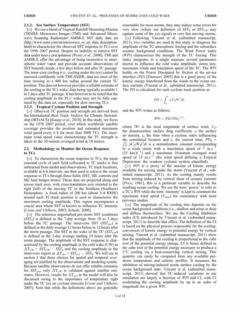
transition from filtered to unfiltered winds between 600 and1200 km. In this simulation (FILT), most of the TC-likevortex is suppressed (Figure 1b). It will therefore be ourreference simulation for ocean response without TC.[26] The third simulation, which is the main focus of this

paper, is obtained by adding idealized TC wind forcingalong cyclone tracks to the filtered COREII forcing. TCwind patterns are computed using the Willoughby et al.[2006] idealized vortex, which is based on a statistical fitto observed TC winds [Willoughby and Rahn, 2004]. Thisidealized wind pattern is computed at each model time step(36 min) using interpolated position and maximum windspeed of each cyclone from the 6-hourly IBTrACs database.This strategy ensures that both temporal evolution and spa-tial structure of the TC wind forcing are properly captured inthe simulation. This procedure results in a simulation(CYCL) where TC wind magnitude is realistic (Figure 1c).Note that we chose not to take into account the translationspeed of the storm in the wind vortex we added. Indeed,even if it is known to affect the wind asymmetry, Samsonet al. [2009] have shown that it has a limited effect on theCW asymmetry and can be neglected. The validity of ourmethodology for simulating the ocean response to TCswill be further illustrated in the next section.2.3.3. Model Resolution[27] The 1/2° horizontal resolution employed in the pres-

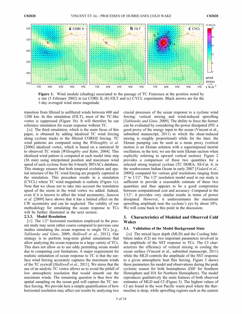
ent study may seem rather coarse compared to previous casestudies simulating the ocean response to single TCs [e.g.,Yablonsky and Ginis, 2009; Halliwell et al., 2011]. Ourstrategy is to perform long-term global simulations thatallow analyzing the ocean response to a large variety of TCs.This does not allow us to use eddy permitting ocean modeldue to computing cost limitations. A major requirement forrealistic simulation of ocean response to TC is that the sur-face wind forcing accurately captures the maximum windsof the TC eyewall [Halliwell et al., 2011]. We stress that theuse of an analytic TC vortex allows us to avoid the pitfall oflow atmospheric resolution that would smooth out themaximum winds. The remaining question is thus how thespatial sampling on the ocean grid will capture the TC sur-face forcing. We provide here a simple quantification of howhorizontal resolution may affect our results by analyzing two

crucial processes of the ocean response to a cyclone windforcing: vertical mixing and wind-induced upwelling[Yablonsky and Ginis, 2009]. The ability to force the formercan be evaluated by considering the power dissipated (PD: agood proxy of the energy input to the ocean (Vincent et al.,submitted manuscript, 2011) to which the shear-inducedmixing is roughly proportional) while for the later, theEkman pumping can be used as a mean proxy (verticalmotion is an Ekman solution with a superimposed inertialoscillation; in the text, we use the term Ekman suction whenexplicitly referring to upward vertical motion). Figure 2provides a comparison of these two quantities for aselected strong tropical cyclone (TC DORA; SS-Cat. 4; inthe southwestern Indian Ocean in early 2007 [Vialard et al.,2009]) computed for various grid resolutions ranging from2° to 1/12°. The 1/2° resolution model used in our study issufficient to provide a reasonable estimate of these twoquantities and thus appears to be a good compromisebetween computational cost and accuracy. Compared to the1/12°, it provides very similar results in terms of powerdissipated. However, it underestimates the maximumupwelling amplitude near the cyclone’s eye by about 30%.We will come back to this point in the discussion.

3. Characteristics of Modeled and Observed ColdWakes

3.1. Validation of the Model Background State

[28] The mixed layer depth (MLD) and the Cooling Inhi-bition index (CI) are two important parameters involved inthe amplitude of the SST response to TCs. The CI char-acterizes the efficiency of vertical mixing in cooling theocean surface (Vincent et al., submitted manuscript, 2011)while the MLD controls the amplitude of the SST responseto a given atmospheric heat flux forcing. Figure 3 showsthese parameters for model and observations during the peakcyclonic season for both hemispheres (DJF for SouthernHemisphere and JJA for Northern Hemisphere). The modelreproduces qualitatively the main features of both observedestimates of MLD and CI (Figure 3). The highest values ofCI are found in the west Pacific warm pool where the ther-mocline is deep, while upwelling regions such as the eastern

Figure 1. Wind module (shading) associated to the passage of TC Francesca at the position noted bya star (5 February 2002) in (a) CORE II, (b) FILT and (c) CYCL experiments. Black arrows are for the1-day averaged wind stress magnitude.


5 of 18

equatorial Pacific or the Seychelles-Chagos thermoclineridge [e.g., Vialard et al., 2009] are characterized by low CI.The model generally tends to underestimate CI, most nota-bly in three cyclonic basins: northeastern and southwesternPacific, northern Indian Ocean. This may lead to over-estimated cooling response in those regions, especially in thenortheastern Pacific where the mean CI value is rather low.Similarly, in those three regions, the mixed layer depth tendsto be underestimated.

3.2. Amplitude of TC-Induced Ocean Response

[29] The efficiency of our experimental design to accountfor a realistic TC wind forcing is illustrated on Figure 4. The

figure displays a scatter plot of the amplitude of modeledagainst observed TC-induced cold wake amplitude (DTCW)at individual locations for the three experiments discussed insection 2.4. The original COREII forcing contains weakerthan observed TC-like vortices along the observed TCtracks, triggering weaker than observed sea surface coolingthat saturate around �1°C (Figure 4a). Filtering these vor-tices (FILT experiment) allows suppressing most of thoseweak cooling events (Figure 4b); further applying idealizedTC wind along the observed tracks (CYCL experiment)allows a realistic simulation of the cold wake (CW) ampli-tude. In CYCL, there is a 0.71 correlation between modeledand observed TC-induced cooling magnitude at individual

Figure 2. Comparison of average (a) power dissipated (W m�2) and (b) Ekman pumping (m d�1) forgrids of increasing resolution (1/12°, black; 1/4°, blue; 1/2°, green; 1°, orange; 2°, red). These figures wereobtained from reproducing category 4 TC DORA surface forcing (from 25 January to 7 February 2007)over different ocean grids. Cross section are averages of all cross sections for each 6-h track-position madein the averaged PD and cumulated Ekman pumping fields over the storm’s lifetime.


6 of 18

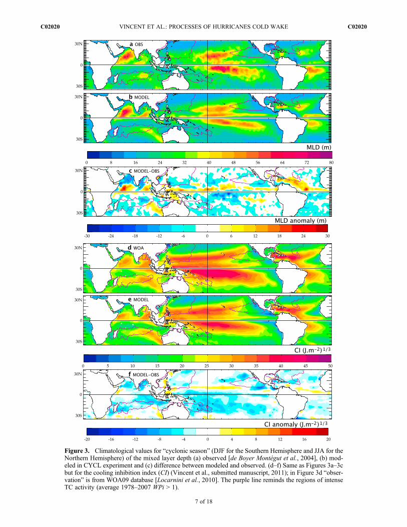
Figure 3. Climatological values for “cyclonic season” (DJF for the Southern Hemisphere and JJA for theNorthern Hemisphere) of the mixed layer depth (a) observed [de Boyer Montégut et al., 2004], (b) mod-eled in CYCL experiment and (c) difference between modeled and observed. (d–f) Same as Figures 3a–3cbut for the cooling inhibition index (CI) (Vincent et al., submitted manuscript, 2011); in Figure 3d “obser-vation” is from WOA09 database [Locarnini et al., 2010]. The purple line reminds the regions of intenseTC activity (average 1978–2007 WPi > 1).


7 of 18

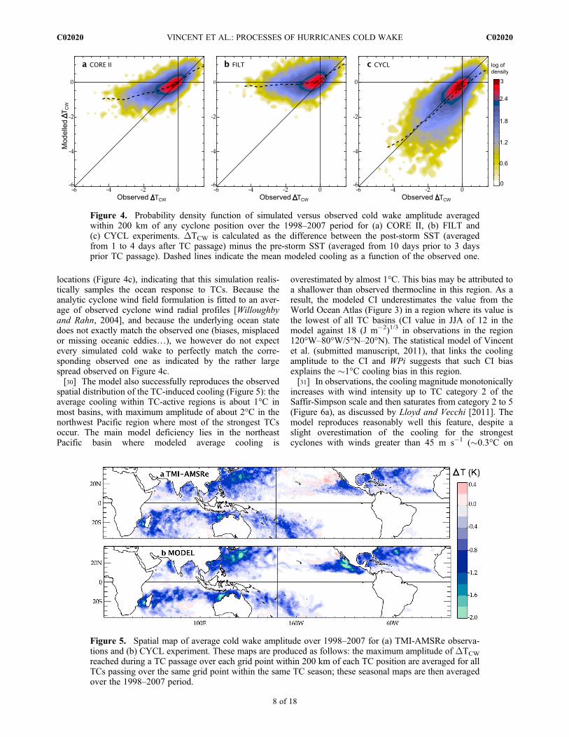
locations (Figure 4c), indicating that this simulation realis-tically samples the ocean response to TCs. Because theanalytic cyclone wind field formulation is fitted to an aver-age of observed cyclone wind radial profiles [Willoughbyand Rahn, 2004], and because the underlying ocean statedoes not exactly match the observed one (biases, misplacedor missing oceanic eddies…), we however do not expectevery simulated cold wake to perfectly match the corre-sponding observed one as indicated by the rather largespread observed on Figure 4c.[30] The model also successfully reproduces the observed

spatial distribution of the TC-induced cooling (Figure 5): theaverage cooling within TC-active regions is about 1°C inmost basins, with maximum amplitude of about 2°C in thenorthwest Pacific region where most of the strongest TCsoccur. The main model deficiency lies in the northeastPacific basin where modeled average cooling is

overestimated by almost 1°C. This bias may be attributed toa shallower than observed thermocline in this region. As aresult, the modeled CI underestimates the value from theWorld Ocean Atlas (Figure 3) in a region where its value isthe lowest of all TC basins (CI value in JJA of 12 in themodel against 18 (J m�2)1/3 in observations in the region120°W–80°W/5°N–20°N). The statistical model of Vincentet al. (submitted manuscript, 2011), that links the coolingamplitude to the CI and WPi suggests that such CI biasexplains the �1°C cooling bias in this region.[31] In observations, the cooling magnitude monotonically

increases with wind intensity up to TC category 2 of theSaffir-Simpson scale and then saturates from category 2 to 5(Figure 6a), as discussed by Lloyd and Vecchi [2011]. Themodel reproduces reasonably well this feature, despite aslight overestimation of the cooling for the strongestcyclones with winds greater than 45 m s�1 (�0.3°C on

Figure 5. Spatial map of average cold wake amplitude over 1998–2007 for (a) TMI-AMSRe observa-tions and (b) CYCL experiment. These maps are produced as follows: the maximum amplitude of DTCW

reached during a TC passage over each grid point within 200 km of each TC position are averaged for allTCs passing over the same grid point within the same TC season; these seasonal maps are then averagedover the 1998–2007 period.

Figure 4. Probability density function of simulated versus observed cold wake amplitude averagedwithin 200 km of any cyclone position over the 1998–2007 period for (a) CORE II, (b) FILT and(c) CYCL experiments. DTCW is calculated as the difference between the post-storm SST (averagedfrom 1 to 4 days after TC passage) minus the pre-storm SST (averaged from 10 days prior to 3 daysprior TC passage). Dashed lines indicate the mean modeled cooling as a function of the observed one.


8 of 18

average). Lloyd and Vecchi [2011] interpreted this saturationas evidence of the ocean control on TCs: they suggest that, onaverage, the strongest observed cyclones are those for whichpre-storm oceanic conditions do not allow large cooling.[32] As discussed by Vincent et al. (submitted manuscript,

2011), theWPi is a proxy of the kinetic energy transferred tothe upper ocean by the cyclone and is thus a better predictorof the cooling than the maximum wind of a TC. When dis-played as a function of WPi, the mean cooling increasesalmost linearly and hardly saturates for the most intense windpower (Figure 6b). The model also reproduces the observed

linear increase of the cooling with the WPi, but with a clearoverestimation (�0.8°C) of the cooling for the highest rangeof WPi (>5). The modeled overestimation is partly related tothe CI bias in the northeast Pacific that promotes strongercooling than observed. Excluding the northeast Pacific basinin Figure 6b results in a 40% reduction of the cooling biasobserved for WPi > 5 (bias of 0.5°C instead of 0.8°C).Another reason for this bias may also stem from data lim-itations: the highest WPi can only be reached for slow mov-ing storms (typically translating at about 1.5 m s�1 for WPiabove 5 (Vincent et al., submitted manuscript, 2011)); in this

Figure 6. Mean observed and simulated cooling (a) as a function of 10-min averaged maximum windspeed (Saffir Simpson scale is reminded by the horizontal bars) and (b) as a function of the wind powerindex (WPi). Comparison is made for all TCs occurring during the 1998–2007 period. Shading indicatesthe 95% confidence level from a bootstrap test for the calculation of the average DT. Diamonds arefor the median cooling per bin and vertical bar indicates the dispersion between the lower and upperquartiles per bin.


9 of 18

case the TC covers�250 km in 2 days and part of the 200 kmarea over which the cooling is evaluated is still affected byprecipitation: the cooling amplitude DTCW is thus very likelyunderestimated by satellite observations. Excluding the slow-est TCs (translation speed < 2.5 m s�1 (10 km h�1)) fromFigure 6b and the northeast Pacific basin, the model overesti-mation forWPi > 5 is reduced by 75% (bias of 0.2°C instead of0.8°C). The overestimation of modeled cooling to the stron-gest TCs may thus be linked to sampling issues rather than toinaccurate model representation of the ocean response.

3.3. Temporal Evolution and Spatial Extentof TC-Induced Ocean Response

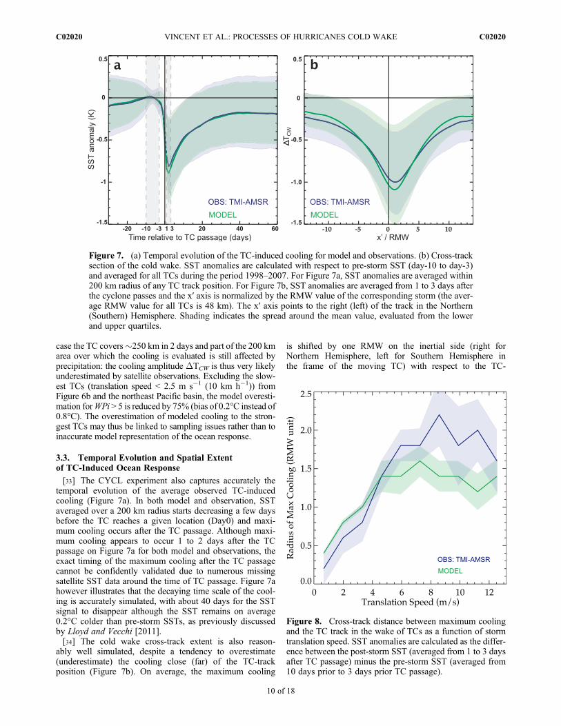
[33] The CYCL experiment also captures accurately thetemporal evolution of the average observed TC-inducedcooling (Figure 7a). In both model and observation, SSTaveraged over a 200 km radius starts decreasing a few daysbefore the TC reaches a given location (Day0) and maxi-mum cooling occurs after the TC passage. Although maxi-mum cooling appears to occur 1 to 2 days after the TCpassage on Figure 7a for both model and observations, theexact timing of the maximum cooling after the TC passagecannot be confidently validated due to numerous missingsatellite SST data around the time of TC passage. Figure 7ahowever illustrates that the decaying time scale of the cool-ing is accurately simulated, with about 40 days for the SSTsignal to disappear although the SST remains on average0.2°C colder than pre-storm SSTs, as previously discussedby Lloyd and Vecchi [2011].[34] The cold wake cross-track extent is also reason-

ably well simulated, despite a tendency to overestimate(underestimate) the cooling close (far) of the TC-trackposition (Figure 7b). On average, the maximum cooling

is shifted by one RMW on the inertial side (right forNorthern Hemisphere, left for Southern Hemisphere inthe frame of the moving TC) with respect to the TC-

Figure 7. (a) Temporal evolution of the TC-induced cooling for model and observations. (b) Cross-tracksection of the cold wake. SST anomalies are calculated with respect to pre-storm SST (day-10 to day-3)and averaged for all TCs during the period 1998–2007. For Figure 7a, SST anomalies are averaged within200 km radius of any TC track position. For Figure 7b, SST anomalies are averaged from 1 to 3 days afterthe cyclone passes and the x′ axis is normalized by the RMW value of the corresponding storm (the aver-age RMW value for all TCs is 48 km). The x′ axis points to the right (left) of the track in the Northern(Southern) Hemisphere. Shading indicates the spread around the mean value, evaluated from the lowerand upper quartiles.

Figure 8. Cross-track distance between maximum coolingand the TC track in the wake of TCs as a function of stormtranslation speed. SST anomalies are calculated as the differ-ence between the post-storm SST (averaged from 1 to 3 daysafter TC passage) minus the pre-storm SST (averaged from10 days prior to 3 days prior TC passage).


10 of 18

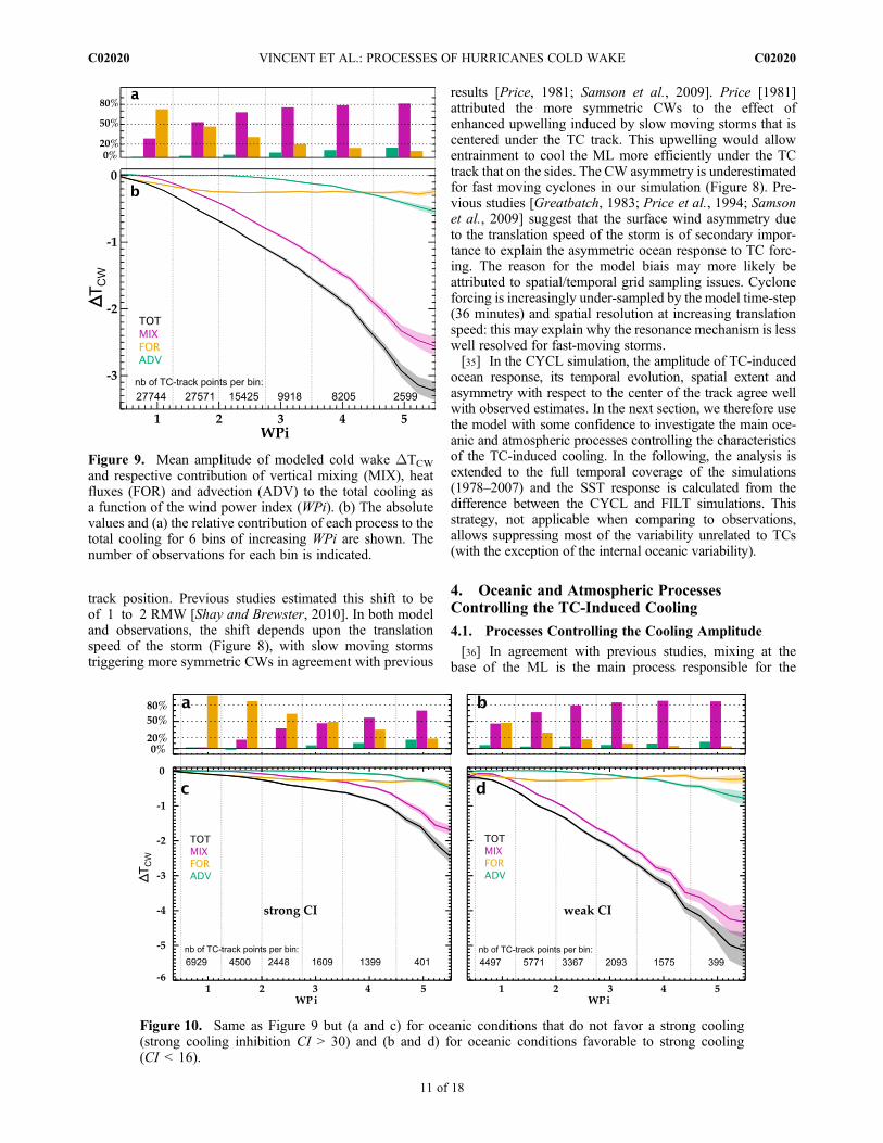
track position. Previous studies estimated this shift to beof 1 to 2 RMW [Shay and Brewster, 2010]. In both modeland observations, the shift depends upon the translationspeed of the storm (Figure 8), with slow moving stormstriggering more symmetric CWs in agreement with previous

results [Price, 1981; Samson et al., 2009]. Price [1981]attributed the more symmetric CWs to the effect ofenhanced upwelling induced by slow moving storms that iscentered under the TC track. This upwelling would allowentrainment to cool the ML more efficiently under the TCtrack that on the sides. The CW asymmetry is underestimatedfor fast moving cyclones in our simulation (Figure 8). Pre-vious studies [Greatbatch, 1983; Price et al., 1994; Samsonet al., 2009] suggest that the surface wind asymmetry dueto the translation speed of the storm is of secondary impor-tance to explain the asymmetric ocean response to TC forc-ing. The reason for the model biais may more likely beattributed to spatial/temporal grid sampling issues. Cycloneforcing is increasingly under-sampled by the model time-step(36 minutes) and spatial resolution at increasing translationspeed: this may explain why the resonance mechanism is lesswell resolved for fast-moving storms.[35] In the CYCL simulation, the amplitude of TC-induced

ocean response, its temporal evolution, spatial extent andasymmetry with respect to the center of the track agree wellwith observed estimates. In the next section, we therefore usethe model with some confidence to investigate the main oce-anic and atmospheric processes controlling the characteristicsof the TC-induced cooling. In the following, the analysis isextended to the full temporal coverage of the simulations(1978–2007) and the SST response is calculated from thedifference between the CYCL and FILT simulations. Thisstrategy, not applicable when comparing to observations,allows suppressing most of the variability unrelated to TCs(with the exception of the internal oceanic variability).

4. Oceanic and Atmospheric ProcessesControlling the TC-Induced Cooling

4.1. Processes Controlling the Cooling Amplitude

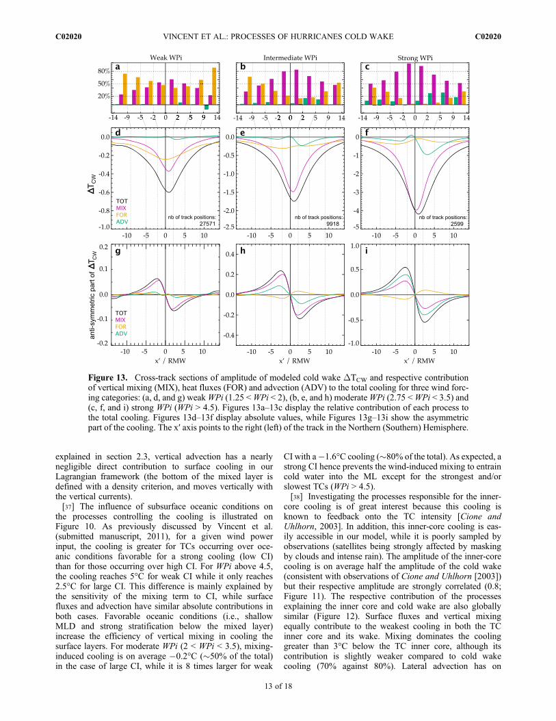
[36] In agreement with previous studies, mixing at thebase of the ML is the main process responsible for the

Figure 9. Mean amplitude of modeled cold wake DTCW

and respective contribution of vertical mixing (MIX), heatfluxes (FOR) and advection (ADV) to the total cooling asa function of the wind power index (WPi). (b) The absolutevalues and (a) the relative contribution of each process to thetotal cooling for 6 bins of increasing WPi are shown. Thenumber of observations for each bin is indicated.

Figure 10. Same as Figure 9 but (a and c) for oceanic conditions that do not favor a strong cooling(strong cooling inhibition CI > 30) and (b and d) for oceanic conditions favorable to strong cooling(CI < 16).


11 of 18

TC-induced cooling, accounting for 56% of the SST signalwithin 200 km of the TC track on average for all TCs, whileheat fluxes explain the largest part of the remaining signal(43%). The relative contribution of each term howeverstrongly varies depending on the TC power (Figure 9). Therelative contribution of mixing is shown to increase withWPi, evolving from �30% of the total cooling for theweakest WPis (WPi ≈ 1, i.e., weak and/or fast TCs) to 80%for the largest one (WPi ≥ 3, i.e., strong and/or slow TCs).This estimation of the mixing contribution for strongcyclonic forcing (i.e., slow and/or intense cyclones) is inbroad agreement with previous estimates [Shay et al., 1992;Price, 1981] that mainly investigated the SST response inthe wake of intense TCs [Jansen et al., 2010]. For low WPi,the weaker cooling is to a large extent explained (�70%) byenhanced surface fluxes associated with cyclone winds. Thecooling amplitude induced by surface heat fluxes saturatesaround �0.25°C for WPi larger than 2, resulting in adecrease of the heat flux relative contribution to SST coolingfor the strongest TCs (10%). Three main processes mayexplain this feature: (1) the saturation of heat exchangecoefficients for the strongest winds, (2) the strong deepeningof the mixed layer induced for the largest TC wind forcing(not shown) and (3) the limitation of latent heat flux by theincreasingly cold SST anomaly in the wake of TCs ofincreasing power. Although of secondary importance, ouranalysis also reveals that advection, dominated by its hori-zontal component, significantly contributes to the coolingamplitude for the largest wind forcing (WPi > 3.5),accounting for more than 10% of the total cooling. As we

Figure 11. Probability density function of inner core cool-ing DTeye versus cold wake DTCW averaged within 200 kmof any cyclone position. The plain line indicates the meanDTeye as a function of DTCW, while the dashed blue lineis the linear fit of DTeye onto DTCW. The correspondingregression and correlation coefficients are provided.

Figure 12. Respective contribution of vertical mixing (MIX), heat fluxes (FOR) and advection (ADV) asa function of the total cooling amplitude for (a and c) cold wake DTCW and (b and d) inner core coolingDTeye. Figures 12c and 12 d display absolute values, while Figures 12a and 12b display the relative con-tribution of each process to the total cooling for 6 bins of increasing cooling amplitude.


12 of 18

explained in section 2.3, vertical advection has a nearlynegligible direct contribution to surface cooling in ourLagrangian framework (the bottom of the mixed layer isdefined with a density criterion, and moves vertically withthe vertical currents).[37] The influence of subsurface oceanic conditions on

the processes controlling the cooling is illustrated onFigure 10. As previously discussed by Vincent et al.(submitted manuscript, 2011), for a given wind powerinput, the cooling is greater for TCs occurring over oce-anic conditions favorable for a strong cooling (low CI)than for those occurring over high CI. For WPi above 4.5,the cooling reaches 5°C for weak CI while it only reaches2.5°C for large CI. This difference is mainly explained bythe sensitivity of the mixing term to CI, while surfacefluxes and advection have similar absolute contributions inboth cases. Favorable oceanic conditions (i.e., shallowMLD and strong stratification below the mixed layer)increase the efficiency of vertical mixing in cooling thesurface layers. For moderate WPi (2 < WPi < 3.5), mixing-induced cooling is on average �0.2°C (�50% of the total)in the case of large CI, while it is 8 times larger for weak

CI with a�1.6°C cooling (�80% of the total). As expected, astrong CI hence prevents the wind-induced mixing to entraincold water into the ML except for the strongest and/orslowest TCs (WPi > 4.5).[38] Investigating the processes responsible for the inner-

core cooling is of great interest because this cooling isknown to feedback onto the TC intensity [Cione andUhlhorn, 2003]. In addition, this inner-core cooling is eas-ily accessible in our model, while it is poorly sampled byobservations (satellites being strongly affected by maskingby clouds and intense rain). The amplitude of the inner-corecooling is on average half the amplitude of the cold wake(consistent with observations of Cione and Uhlhorn [2003])but their respective amplitude are strongly correlated (0.8;Figure 11). The respective contribution of the processesexplaining the inner core and cold wake are also globallysimilar (Figure 12). Surface fluxes and vertical mixingequally contribute to the weakest cooling in both the TCinner core and its wake. Mixing dominates the coolinggreater than 3°C below the TC inner core, although itscontribution is slightly weaker compared to cold wakecooling (70% against 80%). Lateral advection has on

Figure 13. Cross-track sections of amplitude of modeled cold wake DTCW and respective contributionof vertical mixing (MIX), heat fluxes (FOR) and advection (ADV) to the total cooling for three wind forc-ing categories: (a, d, and g) weakWPi (1.25 <WPi < 2), (b, e, and h) moderateWPi (2.75 <WPi < 3.5) and(c, f, and i) strong WPi (WPi > 4.5). Figures 13a–13c display the relative contribution of each process tothe total cooling. Figures 13d–13f display absolute values, while Figures 13g–13i show the asymmetricpart of the cooling. The x′ axis points to the right (left) of the track in the Northern (Southern) Hemisphere.


13 of 18

average a slightly larger relative contribution to the inner-core cooling than to the cold wake.

4.2. Processes Controlling the Cooling Spatial Extent

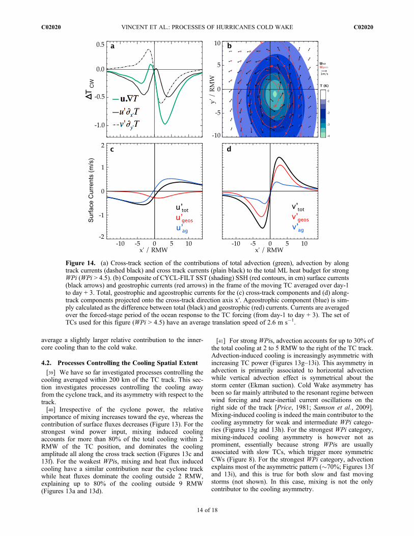
[39] We have so far investigated processes controlling thecooling averaged within 200 km of the TC track. This sec-tion investigates processes controlling the cooling awayfrom the cyclone track, and its asymmetry with respect to thetrack.[40] Irrespective of the cyclone power, the relative

importance of mixing increases toward the eye, whereas thecontribution of surface fluxes decreases (Figure 13). For thestrongest wind power input, mixing induced coolingaccounts for more than 80% of the total cooling within 2RMW of the TC position, and dominates the coolingamplitude all along the cross track section (Figures 13c and13f). For the weakest WPis, mixing and heat flux inducedcooling have a similar contribution near the cyclone trackwhile heat fluxes dominate the cooling outside 2 RMW,explaining up to 80% of the cooling outside 9 RMW(Figures 13a and 13d).

[41] For strong WPis, advection accounts for up to 30% ofthe total cooling at 2 to 5 RMW to the right of the TC track.Advection-induced cooling is increasingly asymmetric withincreasing TC power (Figures 13g–13i). This asymmetry inadvection is primarily associated to horizontal advectionwhile vertical advection effect is symmetrical about thestorm center (Ekman suction). Cold Wake asymmetry hasbeen so far mainly attributed to the resonant regime betweenwind forcing and near-inertial current oscillations on theright side of the track [Price, 1981; Samson et al., 2009].Mixing-induced cooling is indeed the main contributor to thecooling asymmetry for weak and intermediate WPi catego-ries (Figures 13g and 13h). For the strongest WPi category,mixing-induced cooling asymmetry is however not asprominent, essentially because strong WPis are usuallyassociated with slow TCs, which trigger more symmetricCWs (Figure 8). For the strongest WPi category, advectionexplains most of the asymmetric pattern (�70%; Figures 13fand 13i), and this is true for both slow and fast movingstorms (not shown). In this case, mixing is not the onlycontributor to the cooling asymmetry.

Figure 14. (a) Cross-track section of the contributions of total advection (green), advection by alongtrack currents (dashed black) and cross track currents (plain black) to the total ML heat budget for strongWPi (WPi > 4.5). (b) Composite of CYCL-FILT SST (shading) SSH (red contours, in cm) surface currents(black arrows) and geostrophic currents (red arrows) in the frame of the moving TC averaged over day-1to day + 3. Total, geostrophic and ageostrophic currents for the (c) cross-track components and (d) along-track components projected onto the cross-track direction axis x′. Ageostrophic component (blue) is sim-ply calculated as the difference between total (black) and geostrophic (red) currents. Currents are averagedover the forced-stage period of the ocean response to the TC forcing (from day-1 to day + 3). The set ofTCs used for this figure (WPi > 4.5) have an average translation speed of 2.6 m s�1.


14 of 18

[42] The role of horizontal advection on the CW asym-metry has so far been poorly documented [Chen et al.,2010]. Figure 14a displays separately the along and cross-track advection terms in the frame of the moving TC (v ′∂y′Tand u′∂x′T, respectively, with u/x′ the cross-track surfacecurrent/axis, and v/y′ the along-track current and axis) forthe largest wind forcing. This analysis reveals that asym-metry related to the heat advection mainly results from thealong-track component. A two dimensional composite ofhorizontal currents in the TC-moving frame (Figure 14b)allows understanding this feature. Figure 14 corresponds toa 4-day average, so that near-inertial currents triggered bythe TC forcing are largely smoothed (and their residual, i.e.,the stationary Ekman flow, is contained in the ageostrophiccomponent). Surface currents anomalies are primarilyrelated to the geostrophic response to the TC-induced neg-ative SSH anomaly under the track (Figure 14b). The neg-ative SSH anomaly centered on the TC position is associatedwith a cyclonic geostrophic surface circulation (Figure 14b).The ageostrophic part of the current is largely consistentwith the stationary Ekman transport response to cyclonicwind forcing (veered to the right of the surface wind stress,Figure 14b).[43] Along the cross-track axis, geostrophic currents

dominate along-track currents (Figure 14d), with forward(backward) currents to the right (left) of the track. Thiscurrent asymmetry combines with the cold wake asym-metry, with coldest anomalies in the rear-right quadrant(Figure 14b). Along-track currents advect water from thecold wake forward to the right of the track, while theyadvect relatively warmer water backward on the left side.This explains why along-track currents are a strong sourceof asymmetry (Figure 14a). As indicated above, crosstrack currents are dominated by the divergent stationarysurface Ekman flow, which is symmetric with respect tothe TC-track (Figure 14c). The cross-track componentadvects cold water from the wake away from the cyclone

track, hence cooling both sides in roughly equal propor-tions (Figure 14a). Asymmetric effect of the cooling forstrong cyclones is hence largely due to forward advectionof the cold wake by geostrophic currents to the right ofthe track.

4.3. Processes Controlling the Cold Wake Damping

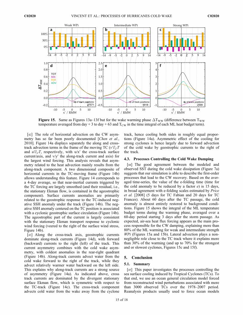
[44] The good agreement between the modeled andobserved SST during the cold wake dissipation (Figure 7a)suggests that our simulation is able to describe the first-orderprocesses that lead to the CW recovery. Based on the aver-aged time-series, the value of the e-folding time (time forthe cold anomaly to be reduced by a factor e) is 15 days,in broad agreement with e-folding scales estimated by Priceet al. [2008] (5 days for TC Fabian and 20 days for TCFrances). About 60 days after the TC passage, the coldanomaly is almost entirely restored to background condi-tions. Figure 15 shows the integral of the ML temperaturebudget terms during the warming phase, averaged over a60-day period starting 3 days after the storm passage. Asexpected, air-sea heat flux forcing appears as the main pro-cess responsible for the CW damping, explaining more than80% of the ML warming for weak and intermediate strengthWPi (Figures 15a and 15b). Lateral advection plays a non-negligible role close to the TC track where it explains morethan 30% of the warming (and up to 70% for the strongestand or slowest cyclones, Figures 15c and 15f).

5. Conclusion

5.1. Summary

[45] This paper investigates the processes controlling thesea surface cooling induced by Tropical Cyclones (TCs). Tothat end, we use an ocean general circulation model forcedfrom reconstructed wind perturbations associated with morethan 3000 observed TCs over the 1978–2007 period.Reanalysis products usually used to force ocean models

Figure 15. Same as Figures 13a–13f but for the wake warming phase DTWW (difference between TWW

temperature averaged from day + 3 to day + 63 and TCW in the time integral of each ML heat budget term).


15 of 18

strongly underestimate the amplitude of TCs wind forcingand the resulting TC-induced cooling. We developed anoriginal methodology that allows realistic TC wind forcingbased on an idealized vortex [Willoughby et al., 2006] to beincluded, constrained by observed TC characteristics (loca-tion, amplitude) and applied at each ocean model time step.[46] The statistics of the simulated ocean surface temper-

ature response to TC compare reasonably well to satelliteestimates. Average surface temperature anomaly is �1°Cand extends typically over 5 radii of maximum wind(RMW). The modeled cold anomaly amplitude also agreeswell with observations at individual locations (0.71 correla-tion), although the model tends to overestimate cold wakesassociated with the strongest and slowest TCs. Overall, thegood agreement between the model and observations allowsus to estimate the contribution of various oceanic processesto TC cooling for a very diverse sample of observedcyclones over 1978–2007, providing a more general insightthan case studies.[47] The amplitude of the TC-induced cooling depends on

the strength of the TC forcing. Following Vincent et al.(submitted manuscript, 2011), we use the wind power index(WPi) as an integrated measure of the cyclone’s wind forc-ing.WPi is a proxy of kinetic energy transferred to the upperocean by the cyclone, and integrates important parametersfor the cold wake amplitude (cyclone size, intensity andtranslation speed). TC-induced cooling within 200 km of theTC eye increases linearly with WPi: vertical mixing at thebase of the mixed layer explains from �30% of the coolingfor weak WPi up to �80% for large WPi (above 2.75).Surface heat fluxes however overcome the mixing contri-bution for lowest WPis (for WPi < 2, surface fluxes con-tribute to �50%–70% of the cold wake). Away from thecyclone’s eye, latent heat fluxes contribute increasingly tothe cooling: surface fluxes explain 50 to 80% of the weakcooling further than �250 km away from the track.[48] Lateral advection plays a modest role compared to

mixing and surface fluxes. For the strongest and/or slowestcyclones, it can however explain up to 30% of the cooling tothe right of the TC track. While mixing dominates the cold-wake asymmetry for weak and intermediate WPis, ourresults suggest that the anti-symmetric pattern of along-trackcurrents is the main contributor to the cooling asymmetry forthe most intense cyclones (WPi > 4.5). This asymmetry isprimarily related to the forward advection of cold wakewater by geostrophic currents on the right side of the TC.While heat fluxes control to a large extent the dampingof the CW in the months following the TC passage, ouranalysis also reveals that advective processes play a non-negligible role, contributing to as much as 70% close to theTC track for the strongest TC wind forcing.[49] The pre-storm ocean state also modulates the ampli-

tude of the TC-induced cooling. The Cooling Inhibitionindex (CI) is a measure of the ocean “resistance” to coolingby the TC (measured as the amount of potential energyrequired to cool the ocean surface by 2°C (Vincent et al.,submitted manuscript, 2011)). Using this measure, Vincentet al. (submitted manuscript, 2011) showed that oceanbackground state can modulate the cooling amplitude by upto an order of magnitude for a given cyclone wind powerinput. We show here that this modulation is related to theincreasing efficiency of mixing to cool the ocean surface

when CI decreases. In the case of strong CI, the surfacecurrent kinetic energy is dissipated to produce vertical mix-ing but in this case, little cold water is entrained into the ML.In contrast, weak CI is usually associated to a shallow MLand/or steep temperature stratification below the ML beforethe TC passage, allowing mixing to efficiently incorporatecold water into the ML.

5.2. Limitations of the Present Study

[50] Although the model response to TCs agrees well withobservations, we believe that our modeling strategy can befurther improved. An inherent limitation to our study is thatwe rely on analytical formulations for the RMW and surfacewind field of TCs. The latest version of the IBTrACS data-base provide radius estimations for some cyclones, whichcould be a first step in defining the geometry of the cyclonebetter. Using satellite observations of surface TC wind fromQSCAT would provide more accurate wind pattern butsatellites do not provide accurate estimates of the strongestwinds. Sriver and Huber [2010] used QSCAT surface windsextracted around observed TC tracks to force an oceangeneral circulation model; they noted that this methodunderestimates the observed cooling and had to multiply thewind amplitude by a factor 2 to yield realistic coolingamplitude. By contrast, our strategy is based on observedTCs amplitudes and allows us to accurately represent theamplitude of TC-induced cooling in spite of the rather lowresolution of the ocean model. This may be due to the factthat we resolve better temporal variations of the cyclonewinds, and hence energy transfers to the upper ocean. Weindeed apply wind perturbations every time-step (36 min-utes) using an interpolated cyclone position, while QSCATtemporal sampling is at best daily, and a cyclone typicallytravels over �400 km in 1 day.[51] We have shown that our 1/2° resolution model

simulates reasonably the CW magnitude and spatial extent.The simple analysis of Figure 2 indeed suggests that the 1/2°resolution is enough to capture the transfer of cyclonekinetic energy to the upper ocean, which is the main driverof mixing, a dominant process in the cold wake formation.Figure 2 however suggests that Ekman suction maximumamplitude is probably underestimated by �30% near thecyclone eye. As demonstrated by several studies[Greatbatch, 1985; Yablonsky and Ginis, 2009; Jullien et al.,submitted manuscript, 2011], Ekman suction can promoteincreased cooling by shallowing the thermocline near theeye, thus making mixing more efficient. Higher resolutionexperiments (at least 1/4°) may hence be needed to strengthenthe present results. But again, the relatively good agreementbetween the simulated cold wake and available observationssuggest that the current study probably resolves most of thedominant processes.[52] The wind forcing asymmetry due to the translation

speed of TCs has been designated as a secondary orderprocess in regulating the asymmetry of the SST response toTCs [Price et al., 1994; Samson et al., 2009]. We confirmthe secondary order importance of this process as the simu-lation produces asymmetric cold wakes without this effect.We however believe that including this effect may improvecharacteristics of the simulated CW asymmetry, in particularfor fast cyclones.


16 of 18

[53] Cloudiness, precipitation, temperature and humidityanomalies associated to TCs are poorly accounted for in ourexperimental design. We indeed rely on COREII forcing(i.e., a crude resolution re-analysis) to provide the air tem-perature and humidity perturbations associated with cyclones,and neglect TC rainfall. Strong uncertainties thus remainon surface fluxes because of air temperature, humidity, andcloud cover perturbations associated with the cyclone. Wedid not take into account the strong precipitation associatedto TC passage either, neglecting the stabilizing effect theymay have on the water column and hence potentially over-estimate the mixing induced by TCs associated with heavyprecipitation.[54] Finally, mesoscale eddies are known to modulate the

ocean response to TCs [Jacob and Shay, 2003] and the mostintense TCs are often developing over warm core eddies [Linet al., 2005, 2008] where SST cooling is inhibited. Becauseour model does not include data assimilation, the position ofsuch eddies in our model is uncorrelated to the observed one.This explains in part why the correlation between simulatedand observed cold wakes is “only” 0.71. Moreover, the mostintense TCs occur randomly over warm or cold core eddiesin our simulation while they tend to occur preferentially overwarm core eddies in reality. This sampling discrepancy maybe responsible for the overestimation of the average modeledcooling for intense TCs.

5.3. Perspectives

[55] Results described in this paper have practical con-sequences for statistical operational forecasts of TC inten-sity. For strongest TC forcing, cooling under the eye is to alarge extent controlled by vertical entrainment and mixing.Including an index describing the ocean sub-surface strati-fication as proposed by Vincent et al. (submitted manuscript,2011) or Lloyd and Vecchi [2011] could hence greatlybenefit to cyclone intensity statistical forecast schemes[DeMaria et al., 2005; Mainelli et al., 2008]. However, forweaker cyclones, the effect of surface fluxes cannot beneglected and alternative indices should be proposed toaccount for their effect on TC-induced cooling.[56] These results can also be interpreted in the light of the

potential impacts of TCs on the ocean at climatic timescales[Emanuel, 2001; Sriver and Huber, 2010; Scoccimarro et al.,2011]. TC-induced mixing warms water under the ML at thesame time as it cools the ML temperature. If surface coldanomaly is entirely damped by surface fluxes, a net warmingof the water column results and has to be equilibrated bylateral heat transport [Emanuel, 2001]. Sriver et al. [2008]argued that TCs significantly modify the poleward heattransport out of the tropics assuming that the observed sur-face cooling is entirely due to vertical mixing within a 6°footprint around the cyclone. This assumption presumablyled the authors to overestimate the amount of heat pumpeddownward: mixing indeed only explains 52% of the totalcooling within 6° of the TC track in our simulation.[57] Finally, because cooling by surface fluxes affect large

areas, we argue that any attempt to diagnose the effects ofTCs on the ocean heat budget at the climatic timescaleshould account for the influence of surface heat fluxes.Further studies are required to investigate the relative effectsof mixing and surface fluxes induced by TCs, and theirrelated impacts on the ocean at climatic timescale.

[58] Acknowledgments. Experiments were conducted at the Institutdu Développement et des Ressources en Informatique Scientifique (IDRIS)Paris, France. We thank the Nucleus for European Modelling of the Ocean(NEMO) Team for its technical support and particularly Simona Flavoniand Christian Ethé for their technical assistance. The analysis was supportedby the project Les Enveloppes Fluides et l’Environnement (LEFE)CYCLOCEAN AO2010-538863 and European MyOcean project EUFP7. TMI/AMSR-E data are produced by Remote Sensing Systems andsponsored by the NASA Earth Science MEaSUREs DISCOVER Project.We thank Daniel Nethery for useful comments.

ReferencesAxell, L. B. (2002), Wind-driven internal waves and Langmuir circulationsin a numerical ocean model of the southern Baltic Sea, J. Geophys. Res.,107(C11), 3204, doi:10.1029/2001JC000922.

Barnier, B., et al. (2009), Erratum: Impact of partial steps and momentumadvection schemes in a global ocean circulation model at eddy-permittingresolution, Ocean Dyn., 59, 537, doi:10.1007/s10236-009-0180-y.

Bender, M. A., and I. Ginis (2000), Real-case simulations of hurricane-ocean interaction using a high-resolution coupled model: Effects on hur-ricane intensity, Mon. Weather Rev., 128, 917–946, doi:10.1175/1520-0493(2000)128<0917:RCSOHO>2.0.CO;2.

Bender, M. A., I. Ginis, and Y. Kurihara (1993), Numerical simulations oftropical cyclone-ocean interaction with a high-resolution coupled model,J. Geophys. Res., 98(23), 245–263.

Bernard, B., et al. (2006), Impact of partial steps and momentum advectionschemes in a global ocean circulation model at eddy-permitting resolu-tion, Ocean Dyn., 56, 543–567, doi:10.1007/s10236-006-0082-1.

Brennan, M. J., C. C. Hennon, and R. D. Knabb (2009), The opera-tional use of QuikSCAT ocean surface vector winds at the NationalHurricane Center, Weather Forecasting, 24(3), 621–645, doi:10.1175/2008WAF2222188.1.

Burchard, H. (2002), Energy-conserving discretisation of turbulent shearand buoyancy production, Ocean Modell., 4, 347–361, doi:10.1016/S1463-5003(02)00009-4.

Chen, S., T. J. Campbell, H. Jin, S. Gaberšek, R. M. Hodur, and P. Martin(2010), Effect of two-way air–sea coupling in high and low wind speedregimes, Mon. Weather Rev., 138, 3579–3602, doi:10.1175/2009MWR3119.1.

Chiang, T. L., C. R. Wu, and L. Y. Oey (2011), Typhoon Kai-Tak: Anocean’s perfect storm, J. Phys. Oceanogr., 41, 221–233, doi:10.1175/2010JPO4518.1.

Cione, J. J., and E. W. Uhlhorn (2003), Sea surface temperature variabilityin hurricanes: Implications with respect to intensity change, Mon.Weather Rev., 131, 1783–1796, doi:10.1175//2562.1.

Cione, J. J., P. G. Black, and S. H. Houston (2000), Surface observations inthe hurricane environment, Mon. Weather Rev., 128, 1550–1561,doi:10.1175/1520-0493(2000)128<1550:SOITHE>2.0.CO;2.

D’Asaro, E. A. (2003), The ocean boundary layer below Hurricane Dennis,J. Phys. Oceanogr., 33, 561–579, doi:10.1175/1520-0485(2003)033<0561:TOBLBH>2.0.CO;2.

D’Asaro, E. A., T. B. Sanford, P. P. Niiler, and E. J. Terrill (2007), Coldwake of Hurricane Frances, Geophys. Res. Lett., 34, L15609,doi:10.1029/2007GL030160.

de Boyer Montégut, C., G. Madec, A. S. Fischer, A. Lazar, and D. Iudicone(2004), Mixed layer depth over the global ocean: An examination of pro-file data and a profile-based climatology, J. Geophys. Res., 109, C12003,doi:10.1029/2004JC002378.

DeMaria, M., M. Mainelli, L. K. Shay, J. A. Knaff, and J. Kaplan (2005),Further improvements to the statistical hurricane intensity predictionscheme (SHIPS), Weather Forecast., 20, 531–543, doi:10.1175/WAF862.1.

Donelan, M. A., B. K. Haus, N. Reul, W. J. Plant, M. Stiassnie, H. C.Graber, O. B. Brown, and E. S. Saltzman (2004), On the limiting aero-dynamic roughness of the ocean in very strong winds, Geophys. Res.Lett., 31, L18306, doi:10.1029/2004GL019460.

Emanuel, K. A. (1986), An air-sea interaction theory for tropical cyclones.Part I: Steady-state maintenance, J. Atmos. Sci., 43, 585–605,doi:10.1175/1520-0469(1986)043<0585:AASITF>2.0.CO;2.

Emanuel, K. A. (2001), Contribution of tropical cyclones to meridional heattransport by the oceans, J. Geophys. Res., 106, 14,771–14,781,doi:10.1029/2000JD900641.

Emanuel, K. A. (2003), Tropical cyclones, Annu. Rev. Earth Planet. Sci.,31, 75–104, doi:10.1146/annurev.earth.31.100901.141259.

Emanuel, K. A. (2005), Increasing destructiveness of tropical cyclones overthe past 30 years, Nature, 436, 686–688, doi:10.1038/nature03906.


17 of 18

Greatbatch, R. J. (1983), On the response of the ocean to a movingstorm: The nonlinear dynamics, J. Phys. Oceanogr., 13, 357–367,doi:10.1175/1520-0485(1983)013<0357:OTROTO>2.0.CO;2.

Greatbatch, R. J. (1985), On the role played by upwelling of water in low-ering sea surface temperatures during the passage of a storm, J. Geophys.Res., 90, 11,751–11,755, doi:10.1029/JC090iC06p11751.

Griffies, S., et al. (2009), Coordinated ocean-ice reference experiments(COREs), Ocean Modell., 26, 1–46, doi:10.1016/j.ocemod.2008.08.007.

Halliwell, G. R., L. K. Shay, J. K. Brewster, and W. J. Teague (2011), Eval-uation and sensitivity analysis of an ocean model response to HurricaneIvan, Mon. Weather Rev., 139, 921–945, doi:10.1175/2010MWR3104.1.

Huang, P., T. B. Sanford, and J. Imberger (2009), Heat and turbulent kineticenergy budgets for surface layer cooling induced by the passage of Hur-ricane Frances (2004), J. Geophys. Res., 114, C12023, doi:10.1029/2009JC005603.

Jacob, S. D., and L. K. Shay (2003), The role of oceanic mesoscale featureson the tropical cyclone-induced mixed layer response: A case study,J. Phys. Oceanogr., 33, 649–676, doi:10.1175/1520-0485(2003)33<649:TROOMF>2.0.CO;2.

Jacob, S. D., L. K. Shay, A. J. Mariano, and P. G. Black (2000), The 3Doceanic mixed layer response to Hurricane Gilbert, J. Phys. Oceanogr.,30, 1407–1429, doi:10.1175/1520-0485(2000)030<1407:TOMLRT>2.0.CO;2.

Jansen, M. F., R. Ferrari, and T. A. Mooring (2010), Seasonal versus per-manent thermocline warming by tropical cyclones, Geophys. Res. Lett.,37, L03602, doi:10.1029/2009GL041808.

Kaplan, J., and M. DeMaria (2003), Large-scale characteristics of rapidlyintensifying tropical cyclones in the North Atlantic Basin, Weather Fore-casting, 18, 1093–1108.

Knapp, K. R., M. C. Kruk, D. H. Levinson, H. J. Diamond, and C. J.Neumann (2010), The International Best Track Archive for ClimateStewardship (IBTrACS): Unifying tropical cyclone data, Bull. Am.Meteorol. Soc., 91, 363–376, doi:10.1175/2009BAMS2755.1.

Large, W., and S. Yeager (2009), The global climatology of an interannu-ally varying air–sea flux data set, Clim. Dyn., 33, 341–364,doi:10.1007/s00382-008-0441-3.

Leipper, D. F. (1967), Observed ocean conditions and Hurricane Hilda,1964, J. Atmos. Sci., 24, 182–186, doi:10.1175/1520-0469(1967)024<0182:OOCAHH>2.0.CO;2.

Lévy, M., A. Estublier, and G. Madec (2001), Choice of an advectionscheme for biogeochemical models, Geophys. Res. Lett., 28(19),3725–3728, doi:10.1029/2001GL012947.

Lin, I. I., C. C.Wu, K. A. Emanuel, I. H. Lee, C. R. Wu, and I. F. Pun (2005),The interaction of Supertyphoon Maemi (2003) with a warm ocean eddy,Mon. Weather Rev., 133, 2635–2649, doi:10.1175/MWR3005.1.

Lin, I. I., C. C. Wu, I. F. Pun, and D. S. Ko (2008), Upper-ocean thermalstructure and the western North Pacific category 5 typhoons. Part I:Ocean features and the category 5 typhoons’ intensification, Mon.Weather Rev., 136, 3288–3306, doi:10.1175/2008MWR2277.1.

Liu, L. L., W. Wang, and R. X. Huang (2008), The mechanical energyinput to the ocean induced by tropical cyclones, J. Phys. Oceanogr.,38, 1253–1266, doi:10.1175/2007JPO3786.1.

Lloyd, I. D., and G. A. Vecchi (2011), Observational evidence of oceaniccontrols on hurricane intensity, J. Clim., 24, 1138–1153, doi:10.1175/2010JCLI3763.1.

Locarnini, R. A., et al. (2010), World Ocean Atlas 2009, vol. 1, Tempera-ture, NOAA Atlas NESDIS, vol. 68, edited by S. Levitus, NOAA, SilverSpring, Md.

Madec, G. (2008), NEMO ocean engine, Note Pôle Modél. 27, Inst. Pierre-Simon Laplace, Paris.

Mainelli, M., M. DeMaria, L. K. Shay, and G. Goni (2008), Application ofoceanic heat content estimation to operational forecasting of recent Atlan-tic category 5 hurricanes, Weather Forecasting, 23, 3–16, doi:10.1175/2007WAF2006111.1.

Marks, F., et al. (1998), Landfalling tropical cyclones: Forecast problems andassociated research opportunities, Bull. Am. Meteorol. Soc., 79, 305–323.

Marsaleix, P., et al. (2008), Energy conservation issues in sigma-coordinatefree-surface ocean models, Ocean Modell., 20, 61–89, doi:10.1016/j.ocemod.2007.07.005.

Mellor, G., and A. Blumberg (2004), Wave breaking and ocean surface layerthermal response, J. Phys. Oceanogr., 34(3), 693–698, doi:10.1175/2517.1.

Morey, S. L., M. A. Bourassa, D. S. Dukhovskoy, and J. J. O’brien (2006),Modeling studies of the upper ocean response to a tropical cyclone,Ocean Dyn., 56, 594–606, doi:10.1007/s10236-006-0085-y.

Penduff, T., et al. (2010), Impact of global ocean model resolution on sea-level variability with emphasis on interannual time scales, Ocean Sci., 6,269–284, doi:10.5194/os-6-269-2010.

Pollard, R., P. Rhines, and R. Thompson (1973), The deepening of thewind-mixed layer, Geophys. Fluid Dyn., 3, 381–404.

Price, J. F. (1981), Upper ocean response to a hurricane, J. Phys. Oceanogr.,11, 153–175, doi:10.1175/1520-0485(1981)011<0153:UORTAH>2.0.CO;2.

Price, J. F., T. B. Sanford, and G. Z. Forristall (1994), Forced stage responseto a moving hurricane, J. Phys. Oceanogr., 24, 233–260, doi:10.1175/1520-0485(1994)024<0233:FSRTAM>2.0.CO;2.

Price, J. F., J. Morzel, and P. P. Niiler (2008), Warming of SST in the coolwake of a moving hurricane, J. Geophys. Res., 113, C07010,doi:10.1029/2007JC004393.

Samson, G., H. Giordani, G. Caniaux, and F. Roux (2009), Numericalinvestigation of an oceanic resonant regime induced by hurricane winds,Ocean Dyn., 59, 565–586, doi:10.1007/s10236-009-0203-8.

Sanford, B., et al. (1987), Ocean response to a hurricane. Part I: Observa-tions, J. Phys. Oceanogr., 17, 2065–2083, doi:10.1175/1520-0485(1987)017<2065:ORTAHP>2.0.CO;2.

Schade, L. R. (2000), Tropical cyclone intensity and sea surface tempera-ture, J. Atmos. Sci., 57, 3122–3130, doi:10.1175/1520-0469(2000)057<3122:TCIASS>2.0.CO;2.

Schade, L. R., and K. A. Emanuel (1999), The ocean’s effect on the inten-sity of tropical cyclones: Results from a simple coupled atmosphere–ocean model, J. Atmos. Sci., 56, 642–651, doi:10.1175/1520-0469(1999)056<0642:TOSEOT>2.0.CO;2.

Scoccimarro, E., S. Gualdi, A. Bellucci, A. Sanna, P. G. Fogli, E. Manzini,M. Vichi, P. Oddo, and A. Navarra (2011), Effects of tropical cyclones onocean heat transport in a high resolution coupled general circulationmodel, J. Clim., 24, 4368–4384, doi:10.1175/2011JCLI4104.1.

Shay, L. K., and J. K. Brewster (2010), Oceanic heat content variability inthe eastern Pacific Ocean for hurricane intensity forecasting, Mon.Weather Rev., 138, 2110–2131, doi:10.1175/2010MWR3189.1.

Shay, L. K., P. Black, A. Mariano, J. Hawkins, and R. Elsberry (1992),Upper ocean response to Hurricane Gilbert, J. Geophys. Res., 97(20),227–248.

Shay, L. K., G. J. Goni, and P. G. Black (2000), Effects of a warm oceanicfeature on Hurricane Opal, Mon. Weather Rev., 128, 1366–1383,doi:10.1175/1520-0493(2000)128<1366:EOAWOF>2.0.CO;2.

Shen, W., and I. Ginis (2003), Effects of surface heat flux-induced sea sur-face temperature changes on tropical cyclone intensity, Geophys. Res.Lett., 30(18), 1933, doi:10.1029/2003GL017878.

Sriver, R. L., and M. Huber (2010), Modeled sensitivity of upper thermo-cline properties to tropical cyclone winds and possible feedbacks on theHadley circulation, Geophys. Res. Lett., 37, L08704, doi:10.1029/2010GL042836.

Sriver, R. L., M. Huber, and J. Nusbaumer (2008), Investigating tropicalcyclone-climate feedbacks using the TRMM Microwave Imager and theQuick Scatterometer, Geochem. Geophys. Geosyst., 9, Q09V11,doi:10.1029/2007GC001842.

Vialard, J., C. E. Menkes, J.-P. Boulanger, P. Delecluse, and E. Guilyardi(2001), A model study of oceanic mechanisms affecting equatorialPacific sea surface temperature during the 1997–98 El Niño, J. Phys.Oceanogr., 31, 1649–1675, doi:10.1175/1520-0485(2001)031<1649:AMSOOM>2.0.CO;2.

Vialard, J., et al. (2009), Cirene: Air sea interactions in the Seychelles-Chagos thermocline ridge region, Bull. Am. Meteorol. Soc., 90, 45–61,doi:10.1175/2008BAMS2499.1.

Wentz, F. J., C. Gentemann, D. Smith, and D. Chelton (2000), Satellitemeasurements of sea surface temperature through clouds, Science, 288,847–850, doi:10.1126/science.288.5467.847.

Willoughby, H. E., and M. E. Rahn (2004), Parametric representation of theprimary hurricane vortex. Part I: Observations and evaluation of the Hol-land (1980) Model, Mon. Weather Rev., 132, 3033–3048, doi:10.1175/MWR2831.1.

Willoughby, H. E., R. W. R. Darling, and M. E. Rahn (2006), Parametricrepresentation of the primary hurricane vortex. Part II: A new family ofsectionally continuous profiles, Mon. Weather Rev., 134, 1102–1120,doi:10.1175/MWR3106.1.

Yablonsky, R. M., and I. Ginis (2009), Limitation of one-dimensionalocean models for coupled hurricane-ocean model forecasts, Mon.Weather Rev., 137, 4410–4419, doi:10.1175/2009MWR2863.1.

N. C. Jourdain, LEGI, CNRS/UJF/INPG, BP 53, Grenoble F-38401CEDEX 09, France.S. Jullien, LEGOS, IRD/CNRS/UPS, 18, Ave. Edouard Belin, Toulouse

F-31401 CEDEX 09, France.M. Lengaigne, G. Madec, G. Samson, J. Vialard, and E. M. Vincent,

LOCEAN, IRD/CNRS/UPMC/MNHN, Tour 45-55 4ème 4, Place Jussieu,Paris F-75252 CEDEX 05, France. ([email protected])C. E. Menkes, IRD, 101 Promenade Roger Laroque, BP A5, 98848

Noumea, New Caledonia.


18 of 18

Processes setting the characteristics of sea surface cooling induced by tropical cyclones

Documents

Transcript of Processes setting the characteristics of sea surface cooling induced by tropical cyclones