Assessing the oceanic control on the amplitude of sea surfacecooling induced by tropical cyclones

Emmanuel M. Vincent,1 Matthieu Lengaigne,1 Jérôme Vialard,1 Gurvan Madec,1,2

Nicolas C. Jourdain,3 and Sébastien Masson1

Received 24 October 2011; revised 28 March 2012; accepted 30 March 2012; published 15 May 2012.

[1] Tropical cyclones (TCs) induce sea surface cooling that feeds back negativelyon their intensity. Previous studies indicate that the cooling magnitude depends on oceanicconditions as well as TC characteristics, but this oceanic control has been poorlydocumented. We investigate the oceanic influence on TC-induced cooling using aglobal ocean model experiment that realistically samples the ocean response to more than3,000 TCs over the last 30 years. We derive a physically grounded oceanic parameter,the Cooling Inhibition index (CI), which measures the potential energy input required tocool the ocean surface through vertical mixing, and hence accounts for the pre-stormupper-ocean stratification resistance to TC-induced cooling. The atmospheric control isdescribed using the wind power index (WPi), a proxy of the kinetic energy transferred tothe ocean by a TC, which accounts for both the effects of maximum winds and translationspeed. The cooling amplitude increases almost linearly with WPi. For a given WPi, thecooling amplitude can however vary by an order of magnitude: a strong wind energyinput can either result in a 0.5�C or 5�C cooling, depending on oceanic background state.Using an oceanic parameter such as CI in addition to wind energy input improves statisticalhindcasts of the cold wake amplitude by �40%. Deriving an oceanic parameter based onthe potential energy required to cool the ocean surface through vertical mixing is thusa promising way to better account for ocean characteristics in TCs studies.

Citation: Vincent, E. M., M. Lengaigne, J. Vialard, G. Madec, N. C. Jourdain, and S. Masson (2012), Assessing the oceaniccontrol on the amplitude of sea surface cooling induced by tropical cyclones, J. Geophys. Res., 117, C05023,doi:10.1029/2011JC007705.

1. Introduction

[2] Tropical cyclones (TCs) are one of the most destruc-tive natural disasters known to man. Accurately forecastingtheir intensity is a key to mitigating their huge human andfinancial costs. Most of the kinetic energy lost by TCs isdissipated by friction at the air-sea interface [Emanuel,2003]. This friction is a source of kinetic energy for theocean and drives strong upper-layer currents. The resultingoceanic vertical shear triggers instabilities that mix warmsurface water with colder water below. This is by far thedominant mechanism contributing to the sea surface tem-perature (SST) cooling observed in the wake of TCs. Bycontrast, air-sea heat fluxes play a much smaller role [Price,1981; Jacob et al., 2000; Vincent et al., 2012]. TCs primarilydraw their energy from evaporation at the surface of theocean [Riehl, 1950]. While higher ambient SSTs provide the

potential for stronger tropical cyclones, the SST coolingunder the storm eye is the oceanic parameter to whichcyclone intensity is most sensitive [Schade, 2000]. TC-induced cooling limits evaporation, thereby resulting in anegative air-sea feedback [Cione and Uhlhorn, 2003]. Forinstance, a modest 1�C cooling can lead to a �40% decreasein surface enthalpy fluxes [Cione and Uhlhorn, 2003], whilea 2.5�C decrease seems sufficient to shut down energy pro-duction entirely [Emanuel, 1999]. Emanuel et al. [2004]demonstrated that coupling a single-column ocean modelto a simple axisymmetric hurricane model did clearlyimprove intensity forecasts of a few selected storms, sug-gesting that further improvement in operational TC intensityforecasts may be achieved by taking the surface coolingfeedback into account. Using a coupled hurricane-oceanmodel, Schade and Emanuel [1999] showed that the surfacecooling feedback can reduce TC intensity by more than50%; the intensity of this feedback depending on the stormtranslation speed and oceanic parameters such as the mixedlayer depth and upper ocean stratification.[3] Past case studies have illustrated the influence of sub-

surface oceanic background conditions onto the amplitude ofthe TC-induced cooling and related TCs intensification [e.g.,Cione and Uhlhorn, 2003; Jacob and Shay, 2003; Shay andBrewster, 2010; Lloyd and Vecchi, 2011]. These studies

1LOCEAN, IRD/CNRS/UPMC/MNHN, Paris, France.2NOC, Southampton, UK.3LEGI, CNRS/UJF/INPG, Grenoble, France.

Corresponding author: E. M. Vincent, LOCEAN, IRD/CNRS/UPMC/MNHN, Tour 45-55 4ème 4, Place Jussieu, Paris F-75252 CEDEX 05,France. (emvincent@phare.normalesup.org)

Copyright 2012 by the American Geophysical Union.0148-0227/12/2011JC007705

JOURNAL OF GEOPHYSICAL RESEARCH, VOL. 117, C05023, doi:10.1029/2011JC007705, 2012

C05023 1 of 14

indeed suggest that the TC-induced mixing is particularlyefficient in cooling the ocean surface when the mixed layer isshallow and/or the upper temperature profile is strongly strat-ified. These conditions often results in a small Ocean HeatContent (OHC) [Leipper and Volgenau, 1972], a commonlyused metric of TC sensitivity to the ocean subsurface calcu-lated as the temperature integral from the surface down to the26�C isotherm depth. Further support for oceanic control onTC-induced cooling arises from observations of TCs intensi-fication over the passage of a warm loop current or warm corering allowing an increase of the ocean to atmosphere enthalpyflux [e.g., Jacob and Shay, 2003; Ali et al., 2007]. A well-documented example of the oceanic impact onto TC intensityis the Hurricane Opal (1995) that rapidly intensified as itcrossed a warm core ring in the Gulf of Mexico, unexpectedlyincreasing from Category 1 to Category 4 in 14 h [Shay et al.,2000; Bosart et al., 2000;Hong et al., 2000]. Lloyd and Vecchi[2011] illustrated this influence of the upper-ocean stratifica-tion on the TCs’ intensity evolution on a global basis. Lloydet al. [2011] further showed that the performance of an oper-ational hurricane forecasting system can be improved by abetter representation of the horizontal structure of upper-oceanstratification. These findings are also confirmed by theimprovements in statistical intensity forecasting resulting fromthe simple inclusion of OHC as a supplementary predictor[DeMaria et al., 2005; Mainelli et al., 2008]. However, theseimprovements are still modest, reducing the intensity forecasterrors by �5%, on average. In a recent review, Goni et al.[2009] underlined the need to adequately investigate andquantify the role of the upper ocean in TC intensification andto improve oceanic metrics of cyclone air-sea interactions.Cione and Uhlhorn [2003] underlined that under most TCsconditions, the upper-ocean heat content is at least an order ofmagnitude greater than the energy actually extracted by thestorm, suggesting that OHC may not be the most appropriateparameter to account for the upper-ocean effect on TC inten-sity. Price [2009] also suggested that a metric based on avertical average of temperature would be more relevant forcyclone-ocean interaction studies than a metric based on ver-tically integrated temperature (such as OHC) as it betterreflects the way TCs interact with the ocean.[4] The ocean influences TCs through changes in SST.

Schade [2000] argued that the SST effect can be split intotwo distinct contributions: the ambient SSTs ahead of thestorm and the SST cooling induced by the storm under theeyewall. Satellite observations accurately capture the ambi-ent SST ahead of the storm but do not provide reliableestimates of inner-core SST due to intense rainfall [Wentzet al., 2000]. The usefulness of a metric of the oceanicinfluence on the TC should therefore be measured throughits ability to quantify the amplitude of the storm-inducedcooling. While idealized studies (such as Schade andEmanuel, 1999) already demonstrated that oceanic condi-tions can modulate the amplitude of the negative air-seafeedback on TCs, they did not propose an integrated oceanicparameter that accounts for this control. Our goal in thispaper is hence to derive a simple, physically based measureof the control of oceanic vertical stratification on the surfacecooling under TCs conditions and to assess by how much theoceanic vertical stratification modulates the CW magnitude.[5] The limited number of sub-surface observations under

TCs (especially in the inner core region) prevents a direct

and precise quantification of the influence of the upperocean structure on the TC-induced cooling at a global scalefrom observations alone. While dedicated field campaigns[Chen et al., 2007] and autonomous profilers [Roemmichet al., 2009] now provide access to ocean sub-surface datain the cyclone’s vicinity, they do not sample the widelyvaried oceanic conditions over which TCs transit. As sug-gested by Goni et al. [2009], numerical modeling can pro-vide a useful indirect methodology to investigate the oceaniccontrol of the amplitude of the TC-induced cooling. In thispaper, we use an Ocean General Circulation Model (OGCM)driven by TC wind-forcing from an historical TC database,that samples the ocean response to more than 3000 TCs overthe last 30 years. The realism of the simulated TC-inducedcooling in this data set has been extensively validated in acompanion paper [Vincent et al., 2012]. This simulationhence provides a comprehensive data set, allowing in-depthanalysis of the influence of a wide spectrum of realisticoceanic stratifications on TC-induced cooling.[6] The paper is organized as follow. Section 2 presents

our strategy to include TC wind-forcing in our OGCM. Insection 3, we lay out the physical concept and idealizedanalytical approach that justify two simple (one oceanic andone atmospheric) parameters that account for the amplitudeof the TC-induced cooling. Based on the use of these indi-ces, section 4 quantifies the role of the ocean stratification inmodulating the cooling amplitude. This section furtherdescribes the improvement brought by accounting for the CIindex in predicting the cooling and compares this index toother recently suggested alternatives to the OHC [Price,2009; Buarque et al., 2009; Lloyd and Vecchi, 2011].Section 5 provides a summary of our results as well as adiscussion of their implications.

2. Methods

2.1. Data

[7] Observed TCs positions and intensities are derivedfrom the International Best Track Archive for ClimateStewardship (IBTrACS) [Knapp et al., 2010]. The observedSST response to tropical cyclones (TCs) is characterizedusing the optimally interpolated blend of Tropical RainfallMeasuring Mission (TRMM) Microwave Imager (TMI) andAdvanced Microwave Scanning Radiometer AMSR-E SSTdaily data set over 1998–2007. Despite its inability to pro-vide SST data under heavy precipitation, TMI and AMSR-Eprovide observations of SST beneath clouds a few daysbefore and after a TC’s passage.

2.2. Experimental Design and Model Validation

[8] The model configuration, strategy to include the TCwind-forcing and the experiments analyzed in the presentpaper have been extensively described and validated inVincent et al. [2012]. The following section provides a shortsummary of this modeling framework and of the validationof TC-induced cooling.[9] We use an OGCM configuration built from the NEMO

framework [Madec, 2008], with 1/2� horizontal resolutionand 46 levels (10 m resolution in the upper 100 m). Themixed layer dynamics are represented by an improved Tur-bulent Kinetic Energy (TKE) closure scheme [Madec,2008]. This configuration successfully reproduces tropical

VINCENT ET AL.: OCEANIC CONTROL OF TC-INDUCED COOLING C05023C05023

2 of 14

ocean variability at intraseasonal to interannual time scales[Penduff et al., 2010; Lengaigne et al., 2012], and is able tosimulate TC-induced cooling reasonably well [Vincent et al.,2012]. Vincent et al. [2012] show in particular that the 1/2�resolution is a good compromise between accuracy andnumerical cost for a realistic global simulation of the oceanresponse to TCs, thanks to the high temporal resolution of

the wind-forcing that allows each grid point to properlysample the wind sequence during TC passage.[10] The model starts from an ocean at rest, initialized with

temperature and salinity fields from the World Ocean Atlas2005 [Locarnini et al., 2006]. It is then spun up for a 30-yearperiod using the CORE-II bulk formulae and interannualforcing data set (1948–1977) [Large and Yeager, 2009;Griffies et al., 2009]. The final state is then used to start thesimulations described below, which are run over 1978–2007.[11] The CORE-II forcing data set does not resolve intense

winds associated with tropical cyclones, but contains weakerthan observed TC wind signatures. The cyclone free simu-lation (FILT) is forced by the original interannual COREforcing from which TC-like vortices are filtered out byapplying an 11-day running mean to the wind within 600 kmof each cyclone track position (a smooth transition zone,between 600 km and 1,200 km, is also prescribed). Thecyclone simulation (CYCL) is forced by realistic TC-windsignatures superimposed to FILT forcing. The 6-hourlycyclone position and strength of the 3,000 named TCbetween 1978 and 2007 from IBTrACS database [Knappet al., 2010] are interpolated to the model time step (i.e.,every 36 min). This information is used to reconstruct the10-m wind vector from an idealized TC wind vortex fitted toobservations [Willoughby et al., 2006]. A more detaileddescription of this forcing strategy can be found in Vincentet al. [2012].[12] Our model reproduces the average observed cooling

within 200 km of TC tracks quite realistically (Figure 1a).The average maximum cooling for all observed cyclonesbetween 1998 and 2007 is about 1�C in both model andobservations. SST starts cooling 3 days prior to the TCpassage, and the maximum cooling occurs in its wake of theTC after the passage of the eye. Hereafter, we define the coldwake amplitude DTCW as the difference between the wake(days 1 to 3) and the pre-storm (days �10 to �3) SSTaverage values (Figure 1a). We also define the cooling underthe eyeDTeye, as the difference between the eye (12 h beforeto 12 h after the cyclone passage) and the pre-storm SST(days �10 to �3) average values.[13] There is a 0.71 correlation between modeled and

observed DTCW at individual locations (Figure 1b), indi-cating that our simulation realistically samples the oceanresponse to the wide spectrum of TC characteristics. Themodel also successfully reproduces the observed spatialdistribution of the cold wake amplitude (see Vincent et al.[2012] for more details about the model validation).

3. Introducing a Metric of Oceanic Controlof TC-Induced Cooling

[14] In this section, we introduce the basic physical con-cepts behind our approach. We derive two indices, usinganalytical calculations from a highly idealized case, todescribe the expected dependence of the cooling amplitudeto the TC and ocean characteristics.

3.1. Physical Basis

[15] Cooling under TCs largely results from mixing, i.e.,from the conversion of kinetic energy to potential energy[Price, 1981]. The kinetic energy transferred to the oceanresults from the work of surface wind stress on ocean

Figure 1. (a) Composite SST evolution averaged under allTCs in observations (blue) and in the model (green).Anomalies are calculated with respect to average pre-stormSST time (days �10 to �3) over a 200 km radius from theTC’s position. Day 0 refers to the time when the TC reachesthe track position. Color shading shows the �1/2 standarddeviation around the mean composite value. (b) Probabilitydensity function of modeled versus observed DT due tothe passage of the TC: SST averaged over day +1 to day+4 less the SST averaged over day �10 to day �3. The val-idation samples 1100 storms over the 1998–2007 period(both figures are from Vincent et al. [2012]).

VINCENT ET AL.: OCEANIC CONTROL OF TC-INDUCED COOLING C05023C05023

3 of 14

currents. The strong resulting currents are driving mixingthrough strong vertical shear that promotes instabilities.Most of the energy transferred to the ocean radiates away inthe surface waves field but a fraction of the kinetic energy isconverted into potential energy [Liu et al., 2008]. Warm,light particles are indeed displaced downward while cold,denser particles are displaced upward leading to an increaseof the water column potential energy. Based on these simpleconsiderations, a simple relation between the cooling andchange in potential energy is derived as follows.[16] Let us consider an ocean with a linear equation of

state depending on temperature only: r(z) = r0(1 � a T(z)).We present here a very simple case with constant stratifica-tion N2, all the way up to the surface. The temperature pro-file is TðzÞ ¼ Ti þ N2

a g z. Let us now assume that the surfacelayer has been homogeneously mixed down to the depth hm,at the temperature Tf.[17] Conservation of heat yields an equation linking hm

with the surface cooling DT

hm þ 2ag

N2DT ¼ 0: ð1Þ

The potential energy difference between the initial and finalprofile (DEp) provides an equation linking hm, DT and DEp

hm3 þ 3

2

ag

N 2DT hm

2 ¼ 3DEp

r0N2: ð2Þ

By combining equations (1) and (2), we obtain an equationlinking the cooling and the increase of potential energy ofthe water column

DT ¼ � 1

ag3 N4

2r0DEp

� �1=3

: ð3Þ

[18] In the idealized framework above, the surface coolingDT is associated to an increase of the water column potentialenergy DEp and DT scales as the cube root of this potentialenergy increase. Calculations using a more realistic tem-perature profile that includes a mixed layer are provided insection A1. These calculations show that the relationshipfound in the simple case above (where the initial mixed layerdepth vanishes) remains valid when the initial mixed layer isshallower than a characteristic mixing length. For deeperinitial mixed layer, DT scales linearly with the potentialenergy increase DEp. In our simulation, we found thatthe mixed layer before the cyclone passage is shallowerthan the characteristic mixing length in �80% of the cases(Figure A2). This motivates the definition of an oceanicmetric based on the cube root of a potential energy change inthe next paragraph.

3.2. A Metric of Oceanic Controlof TC-Induced Cooling

[19] Given a pre-storm upper-ocean density profile, one cancalculate the potential energy increase DEp(DT) necessary toproduce a givenDT cooling assuming heat conservation and aperfectly homogeneous mixed layer after the mixing (as wedid in the idealized case of section 3.1, but this time with theactual profile before the storm). The larger thisDEp, the moreenergy has to be injected into the ocean to produce this cool-ing. The idea is thus to characterize the propensity of the pre-storm ocean state to yield a weak or strong surface cooling inresponse to a surface kinetic energy input.[20] The mixing depth hm that is necessary to produce a

cooling DT is first computed from the equation of conser-vation of heat (see the example with a model profile, for aDT of �2�C, on Figure 2). The associated potential energyincrease is then computed as

DEp DTð Þ ¼Z 0

hm

rf � riðzÞ� �

g zdz; ð4Þ

where ri is the initial unperturbed profile of density, g is theacceleration of gravity, z is ocean depth, rf is the homoge-neous final density profile. After the mixing, temperature Tis assumed to be constant and equal to SST + DT within themixed layer (Figure 2, top). Similarly, salinity S is assumedto be constant within the mixed layer and its value is com-puted from conservation of salt. Density rf can then beobtained using these (T,S) values. DEp(DT) is finally com-puted from the density difference between the initial andfinal profiles, using equation (4). This computation ofDEp(DT) hence only requires knowledge of the temperatureand salinity profiles before the cyclone passage.[21] In the following, we define the cooling inhibition (CI)

as the cube root of the necessary potential energy to induce a2�C SST cooling:

CI ¼ ½DEpð�2�CÞ�1=3: ð5Þ

Figure 2. Typical tropical temperature and density profilesbefore the storm passage (black) and after an idealized heatand mass conserving mixing (dashed green line) used forcalculation of the Cooling Inhibition.

VINCENT ET AL.: OCEANIC CONTROL OF TC-INDUCED COOLING C05023C05023

4 of 14

CI is defined as a cube root on the basis of the idealizedanalysis of section 3.1, which suggested that the coolingshould scale as the cube root of a potential energy. Theanalysis preformed in Section 4 will provide further evi-dence of the relevance of this scaling. We compute coolinginhibition CI from a cooling of �2�C, a rather typical valueunder a tropical cyclone. The typical variations of CI overthe cyclone-affected regions are anyway relatively insensi-tive to a choice of 1�C (CI1), 2�C (CI) or 3�C (CI3)(Figure 3): CI1 and CI3 are highly correlated (0.98 and 0.99)to CI.[22] We call this index “Cooling Inhibition” (CI) because

it measures the resistance of the ocean to surface coolingthrough mixing. CI is a useful metric to describe the oceanicinhibition to a wind-induced cooling because it integratestwo relevant parameters for the cooling amplitude: the initialmixed layer depth and the strength of the stratification justbelow it. Indeed, the deeper the initial mixed layer, the more

kinetic energy is required to produce mixing at its base. Andthe deeper the initial mixed layer, the greater the thermalcapacity of the surface layer: for a given entrainment cool-ing, a thicker layer cools less. The stratification at the base ofthe mixed layer is another relevant parameter because it setsthe temperature of water that can be entrained into the mixedlayer. Figure 4a shows that CI accounts for both theseparameters: it increases with the mixed layer depth (hi) anddecreases with the stratification at its base (N). Largest CIare only found when the mixed layer is deep and the strati-fication at its base is weak. We will show in the followingthat CI accurately describes the ocean propensity to mitigate

Figure 3. Probability density functions of (a) Cooling Inhi-bition calculated using a 1�C threshold (CI1) versus a 2�Cthreshold (CI) and (b) Cooling Inhibition calculated usinga 3�C threshold (CI3) versus a 2�C threshold (CI). Correla-tions between these indices are, respectively, 0.98 and0.99. Units are in (J.m�2)1/3.

Figure 4. (a) Average CI values as a function of the mixedlayer depth (MLD) and the stratification at its base (N) eval-uated as N2 ¼ ag TML�2�C

h2�hi, where h2 is the depth of the iso-

therm “TML-2�C” and hi the mixed layer depth. (b) AverageWPi = [PD/PD0]

1/3 as a function of the maximum 10-minsustained wind (Vmax) and TC translation speed. For repre-sentativeness, the mean is limited to regions with 6 samplesor more. Saffir–Simpson tropical cyclone scale is remindedfor reference.

VINCENT ET AL.: OCEANIC CONTROL OF TC-INDUCED COOLING C05023C05023

5 of 14

the SST response to a cyclone. In the rest of the paper, wecompute CI in our simulation based on the pre-storm oceancolumn density (averaged over 10 to 3 days before TCpassage, and within 200 km from the TC track position).Figure 5b illustrates the average CI value under all TCs trackin our simulation, for all pre-cyclone oceanic profiles during1978–2007 (this figure does not strongly differ from thefigure of the CI computed from the oceanic climatologicalstate during the cyclonic season in Vincent et al. [2012,Figure 3e]). This map partially reflects the depth of thethermocline (larger energy is required to bring cold waterparcels to the surface when the thermocline is deep), withlarge CI values in the western Pacific warm Pool or in theNorthwestern Tropical Atlantic. CI does not only reflectthermal stratification, but also haline stratification: CI islarger in the Bay of Bengal than in the Arabian Sea, partly

due to the very strong river runoffs and resulting halinestratification in the Bay, that prevents vertical mixing[Sengupta et al., 2008; M. Neetu et al., Influence of upperocean stratification on tropical cyclones-induced surfacecooling in the Bay of Bengal, unpublished manuscript,2012].

3.3. A Metric of the Atmospheric Controlof TC-Induced Cooling

[23] The kinetic energy transferred by the storm to theupper ocean can be computed from the work W of surfacewind stress on the ocean W ¼ R tc

tot⋅uoce dt where t is the

surface wind stress, uoce the surface ocean current, to thetime when the storm starts influencing a certain point and tcthe current time. In this paper, to is set to day �3 (3 daysbefore a TC reaches a given ocean point). Taking to equal today �5 or day �10 however yields very similar results, asmost of the energy transferred to the ocean occurs within acouple of days before and after the cyclone reaches a givenlocation. tc is taken as day +3 to integrate the wind-forcingover the full period during which the TC influences theocean column and relate it to the cooling occurring in thewake of the TC.[24] While W can easily be calculated in our simulation, it

is not available in observations due to the lack of reliablehigh-frequency estimates of observed surface currents. Amore easily computable quantity is the power dissipated byfriction at the air-sea interface. Bister and Emanuel [1998]showed that, in a hurricane, dissipation occurs mostly inthe atmospheric surface layer, with a dissipation rate per unitarea, D, given by: D = rCD∣V∣3. In our simulation, we findthat the time integral of this dissipation (Power Dissipation(PD)) [Emanuel, 2005] is highly related to W (correlation of0.9) as shown on Figure 6. It can hence be used as a proxy toestimate the kinetic energy transferred to the ocean W.Because it is more easily estimated from observations and

Figure 5. Maps over 1978–2007 of average (a) windpower index, (b) CI (in (J.m�2)1/3), (c) TC-induced coolingin the ocean model and (d) cooling predicted with the bivar-iate fit on WPi and CI (in �C). For each cyclonic season, amap is obtained by first recording the integrated-WPi, CIor DTCW within 200 km of each TC position and averagingfor all TCs of the season. Figure 5 shows the 30-years aver-age of these seasonal maps. Isoline “WPi = 1” is repeatedover each panel for reference.

Figure 6. Probability density function of the wind work onsurface currents (W) versus the Power Dissipated (PD) aver-aged within 200 km of each TC track position. Correlationbetween these two quantities is 0.91. Units are in (J.m�2)1/3.

VINCENT ET AL.: OCEANIC CONTROL OF TC-INDUCED COOLING C05023C05023

6 of 14

can be used for future studies, we will hereafter use PD,calculated at every point along cyclone tracks as

PD ¼Z tc

to

r CD∣V∣ 3 dt; ð6Þ

where ∣V∣ is the local magnitude of surface wind, CD thedimensionless surface drag coefficient [Large and Yeager,2009] and r the surface air density.[25] The cooling amplitude can be related to TC wind-

forcing by the very crude assumption that the kinetic energyinput W (approximated by PD) linearly relates to thepotential energy increase in the ocean. Using the idealizedapproach of section 3.1 and equation (3), this leads to a DTthat should be proportional toW1/3 for cases where the initialmixed layer is shallow (�80% of the TC cases). It is how-ever far from being obvious that the fraction of kineticenergy transformed into potential energy is constant as it islikely to depend for instance on the relative ML depth andwind-induced mixing depth. A similar dependence of DT toW1/3 can also be derived using a different framework thatdirectly relates surface cooling to wind-forcing such as theone developed in the appendix of Korty et al. [2008]. Usingthis framework based on the Price [1979] assumption thatthe bulk Richardson number remains constant during TCmixing, one can demonstrate that the temperature changescales as the cube root of the wind power input for shallowMLDs. This provides further theoretical justification for thechoice of the scaling for the index proposed below.[26] We hence define a dimensionless “wind power

index” as

WPi ¼ PD=PD0½ � 1=3; ð7Þ

where PD0 ¼R tctor CD ∣V0∣3 dt is a normalization constant

corresponding to a typical weak storm with a translationspeed of 7 m.s�1 (25 km.h�1) and maximum 10-min aver-aged wind speed of 15 m.s�1 (the wind speed defining aTropical Depression: the weakest cyclonic system classi-fied). PD is computed using the same choices for t0 and tc asfor W. The almost linear relationship between average DTand WPi (that will be shown later in the paper) illustrates thefirst order validity of this simple approach for the scalingdefinition.[27] Previous studies have underlined that not only cyclone

intensity, but also translation speed influences the amplitudeof the cold wake, slower cyclones being associated withintense cooling [Greatbatch, 1984; Lloyd and Vecchi, 2011].Figure 4b shows that WPi gathers information about thesetwo factors. WPi increases (decreases) monotonically withstorm intensity (translation speed), and reaches its highestvalues (�5) for TCs that are both strong and slow (Category4 or more on the Saffir-Simpson scale and translationspeed <4 m/s). Bigger storms are also characterized by alonger influence of strong wind-forcing at a given point;WPi

also naturally integrates the storm size effect.[28] Figure 5a shows the average WPi by basin. It under-

lines familiar regions of TC occurrence. Most powerful TCsoccur in the northeast and northwest tropical Pacific. Thereis also a high averaged wind power North of Australia (bothon the Indian ocean and Pacific sides), and in the South-western Indian Ocean. The Caribbean and Northern Indian

Ocean display the weakest averaged wind power. In thefollowing section, we will discuss the upper-ocean cooling,in response to this forcing.

4. Dependence of the Cold Wake Magnitudeto TC and Ocean Characteristics

[29] Using the two metrics described above, the followingsection quantifies the dependency of the cooling amplitudeon the oceanic background state. The improvement broughtby including this oceanic metric in the CW intensity hindcastis then assessed. The efficiency of CI against other proposedoceanic metrics is finally discussed.

4.1. Surface Cooling as a Function of WPi and CI

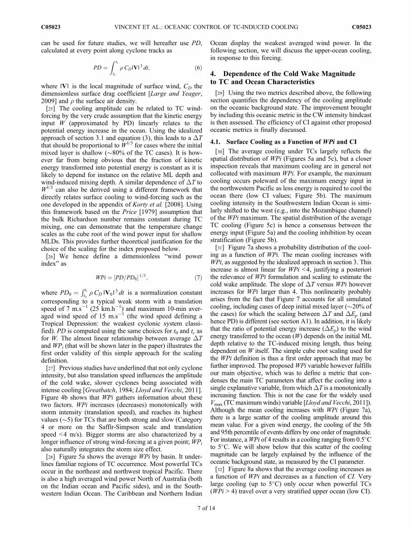
[30] The average cooling under TCs largely reflects thespatial distribution of WPi (Figures 5a and 5c), but a closerinspection reveals that maximum cooling are in general notcollocated with maximum WPi. For example, the maximumcooling occurs poleward of the maximum energy input inthe northwestern Pacific as less energy is required to cool theocean there (low CI values; Figure 5b). The maximumcooling intensity in the Southwestern Indian Ocean is simi-larly shifted to the west (e.g., into the Mozambique channel)of the WPi maximum. The spatial distribution of the averageTC cooling (Figure 5c) is hence a consensus between theenergy input (Figure 5a) and the cooling inhibition by oceanstratification (Figure 5b).[31] Figure 7a shows a probability distribution of the cool-

ing as a function of WPi. The mean cooling increases withWPi, as suggested by the idealized approach in section 3. Thisincrease is almost linear for WPi <4, justifying a posteriorithe relevance of WPi formulation and scaling to estimate thecold wake amplitude. The slope of DT versus WPi howeverincreases for WPi larger than 4. This nonlinearity probablyarises from the fact that Figure 7 accounts for all simulatedcooling, including cases of deep initial mixed layer (�20% ofthe cases) for which the scaling between DT and DEp (andhence PD) is different (see section A1). In addition, it is likelythat the ratio of potential energy increase (DEp) to the windenergy transferred to the ocean (W) depends on the initial MLdepth relative to the TC-induced mixing length, thus beingdependent on W itself. The simple cube root scaling used forthe WPi definition is thus a first order approach that may befurther improved. The proposedWPi variable however fulfillsour main objective, which was to define a metric that con-denses the main TC parameters that affect the cooling into asingle explanative variable, fromwhichDT is a monotonicallyincreasing function. This is not the case for the widely usedVmax (TCmaximumwinds) variable [Lloyd and Vecchi, 2011]).Although the mean cooling increases with WPi (Figure 7a),there is a large scatter of the cooling amplitude around thismean value. For a given wind energy, the cooling of the 5thand 95th percentile of events differs by one order of magnitude.For instance, aWPi of 4 results in a cooling ranging from 0.5�Cto 5�C. We will show below that this scatter of the coolingmagnitude can be largely explained by the influence of theoceanic background state, as measured by the CI parameter.[32] Figure 8a shows that the average cooling increases as

a function of WPi and decreases as a function of CI. Verylarge cooling (up to 5�C) only occur when powerful TCs(WPi > 4) travel over a very stratified upper ocean (low CI).

VINCENT ET AL.: OCEANIC CONTROL OF TC-INDUCED COOLING C05023C05023

7 of 14

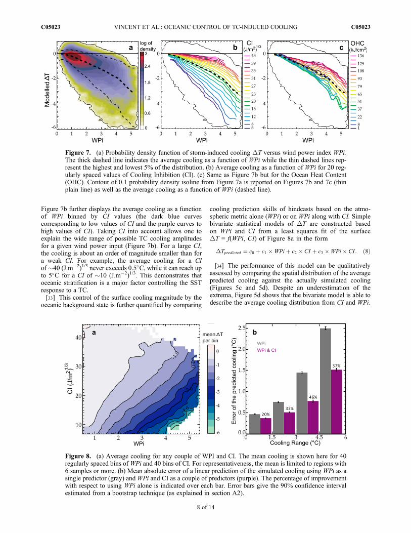
Figure 7b further displays the average cooling as a functionof WPi binned by CI values (the dark blue curvescorresponding to low values of CI and the purple curves tohigh values of CI). Taking CI into account allows one toexplain the wide range of possible TC cooling amplitudesfor a given wind power input (Figure 7b). For a large CI,the cooling is about an order of magnitude smaller than fora weak CI. For example, the average cooling for a CIof�40 (J.m�2)1/3 never exceeds 0.5�C, while it can reach upto 5�C for a CI of �10 (J.m�2)1/3. This demonstrates thatoceanic stratification is a major factor controlling the SSTresponse to a TC.[33] This control of the surface cooling magnitude by the

oceanic background state is further quantified by comparing

cooling prediction skills of hindcasts based on the atmo-spheric metric alone (WPi) or on WPi along with CI. Simplebivariate statistical models of DT are constructed basedon WPi and CI from a least squares fit of the surfaceDT = f(WPi, CI) of Figure 8a in the form

DTpredicted ¼ c0 þ c1 �WPiþ c2 � CI þ c3 �WPi� CI : ð8Þ

[34] The performance of this model can be qualitativelyassessed by comparing the spatial distribution of the averagepredicted cooling against the actually simulated cooling(Figures 5c and 5d). Despite an underestimation of theextrema, Figure 5d shows that the bivariate model is able todescribe the average cooling distribution from CI and WPi.

Figure 7. (a) Probability density function of storm-induced cooling DT versus wind power index WPi.The thick dashed line indicates the average cooling as a function of WPi while the thin dashed lines rep-resent the highest and lowest 5% of the distribution. (b) Average cooling as a function of WPi for 20 reg-ularly spaced values of Cooling Inhibition (CI). (c) Same as Figure 7b but for the Ocean Heat Content(OHC). Contour of 0.1 probability density isoline from Figure 7a is reported on Figures 7b and 7c (thinplain line) as well as the average cooling as a function of WPi (dashed line).

Figure 8. (a) Average cooling for any couple of WPI and CI. The mean cooling is shown here for 40regularly spaced bins ofWPi and 40 bins of CI. For representativeness, the mean is limited to regions with6 samples or more. (b) Mean absolute error of a linear prediction of the simulated cooling using WPi as asingle predictor (gray) and WPi and CI as a couple of predictors (purple). The percentage of improvementwith respect to using WPi alone is indicated over each bar. Error bars give the 90% confidence intervalestimated from a bootstrap technique (as explained in section A2).

VINCENT ET AL.: OCEANIC CONTROL OF TC-INDUCED COOLING C05023C05023

8 of 14

More quantitatively, using both CI and WPi clearly reducesthe error of the predicted cooling compared to using WPialone. Using WPi alone yields a �50% relative error on thecooling prediction for all range of cooling magnitude. UsingWPi and CI allows to reduce this relative error to an averageof�30%. For instance, while the prediction error is 1.4�C fora 3�C cooling usingWPi alone, this error is reduced to 0.8�Cwhen using both CI and WPi. The improvement of the rela-tive error is larger for the most intense cooling, ranging from33% to 46% for cooling between 1.5�C and 6�C (Figure 8b).The relative improvement brought by the inclusion of CI isweaker for weak cooling (20%). This may be related to thelarger contribution of surface heat fluxes to the total coolingfor weakest cooling [Vincent et al., 2012] that are notexpected to be sensitive to sub-surface stratification.[35] The above results discuss the modeled cyclone cold

wake DTCW (i.e., cooling after the cyclone passage). Therelevant parameter to investigate ocean influence on TCintensity is not cooling in the cyclone wake DTCW, butinner-core cooling DTeye (cooling under the storm eye)[Cione and Uhlhorn, 2003; Schade, 2000] for which satelliteobservations are not reliable. In our model, however, we canestimate the ability of the various metrics to predict theinner-core cooling DTeye. Inner-core cooling and cold wakeare in fact highly correlated in our simulation (correlationcoefficient of 0.8, as discussed by Vincent et al. [2012]). CIalso improves the predictive skills of WPi for the inner-corecooling, most substantially for intermediate cooling intensi-ties (improvement of more than 30% for cooling between1.5�C and 4.5�C) (Table 1). Finally, using CI (calculatedfrom model outputs) also improves estimates of the observedDTCW cooling (from TMI-AMSRE) by up to 16% comparedto atmospheric information alone (Table 1). This weakerskill compared to the modeled cooling prediction is easilyunderstandable. Our model without data assimilation doesnot realistically simulate locations of oceanic mesoscalestructures, and suffers from systematic bias in some regions.The improvement above would hence arguably be betterwith a model properly constrained by observations throughdata assimilation [e.g., Drevillon et al., 2008]. This resulthowever suggests that CI not only allows predicting theTC-cooling in the model world, but is also helpful toimprove the prediction of observed cooling under TCs.

4.2. Comparison of CI to Other Metrics

[36] This paper proposes a physically based metric toaccount for the influence of the upper ocean stratificationonto TC-induced cooling. Aside from OHC, recent papers

have proposed other alternatives to quantify the effect ofoceanic background state on TCs. These alternatives includeT100 (temperature averaged in the upper 100 m, the typicalmixing depth of a strong TC) [Price, 2009] the InteractingTropical Cyclone Heat Content (ITCHC, the heat content inthe mixed layer) [Buarque et al., 2009], or the depth of themixed layer temperature isotherm minus 2�C, hereafter h2[Lloyd and Vecchi, 2011]. In this subsection, we gauge allthese metrics by their ability to estimate the TC-inducedcooling globally, over the last 30 years.[37] OHC is the most popular index of oceanic control of

air-sea interactions below cyclones. However, unlike CI,OHC only explains a small fraction of the wide range in TC-induced cooling amplitudes for a given wind power(Figure 7c): the lowest values of OHC are shown to beunable to describe the most intense cooling events, in con-trast to CI. The relation between OHC and the cooling is alsonot monotonous: for weak OHC, the cooling first increasesand then decreases with OHC. A measure of the thermalenergy of the upper ocean hence only partially describes theCW dependence to ocean characteristics.[38] A more quantitative comparison is provided by

comparing the improvement brought by each ocean metric tohindcast the cooling magnitude using the bivariate modeldescribed above. Metrics based on a thermal energy defini-tion (OHC, ITCHC, T100) do not perform as well (only upto 20% improvement) compared to CI and h2. These twovariables both induce up to �45% improvement to the pre-dicted cooling. They display a similar performance, exceptfor the weakest cooling range (<1.5�C) for which CI allowsa significantly greater improvement. The modest perfor-mance of the measures based on thermal energy (OHC,ITCHC, T100) is related to the use of the absolute temper-ature in those metrics, which is useful to predict the absolutetemperature after the cyclone, but not the cooling magnitude.Modifying T100 by subtracting the SST to it (SST-T100)indeed results in a considerable improvement of the predic-tion skills (Figure 9), with the largest improvement (�43%)for the strongest cooling range (>4.5�C). A measure such asSST-T100 is indeed appropriate to describe a surface coolingassociated to a deep mixing (100 m is a typical mixing depthfor a category 3 hurricane [Price, 2009]).[39] While not explicitly taking physical processes of the

cooling into account, h2 performs as well as CI. This metric ishighly correlated to CI (correlation coefficient of 0.94) andbasically measures the same information as CI does: namelythe depth of the ML and the importance of the temperaturestratification at its base. h2 can actually be expressed in asimilar way as CI if we assume that density is proportional totemperature. In the simple case where hi = 0 (presented in

section 3.1), h2 can be written as h2 ¼ 32

DEp

r0 N2

� �1=3, hence h2

is expected to scale as CI (see Annex A1 for the calculation).In our global analysis, h2 skills are very similar to CI and itsdefinition is somehow simpler. However, the h2 definitiondoes not account for the effect of salinity on stratification.This effect can be important in some regions, for example inthe Bay of Bengal where haline stratification can reduce theamplitude of TC-induced cooling after the monsoon[Sengupta et al., 2008; Neetu et al., unpublished manuscript,2012]. CI brings a larger improvement than h2 for coolingpredictions over the Bay of Bengal (Table 2). This is an

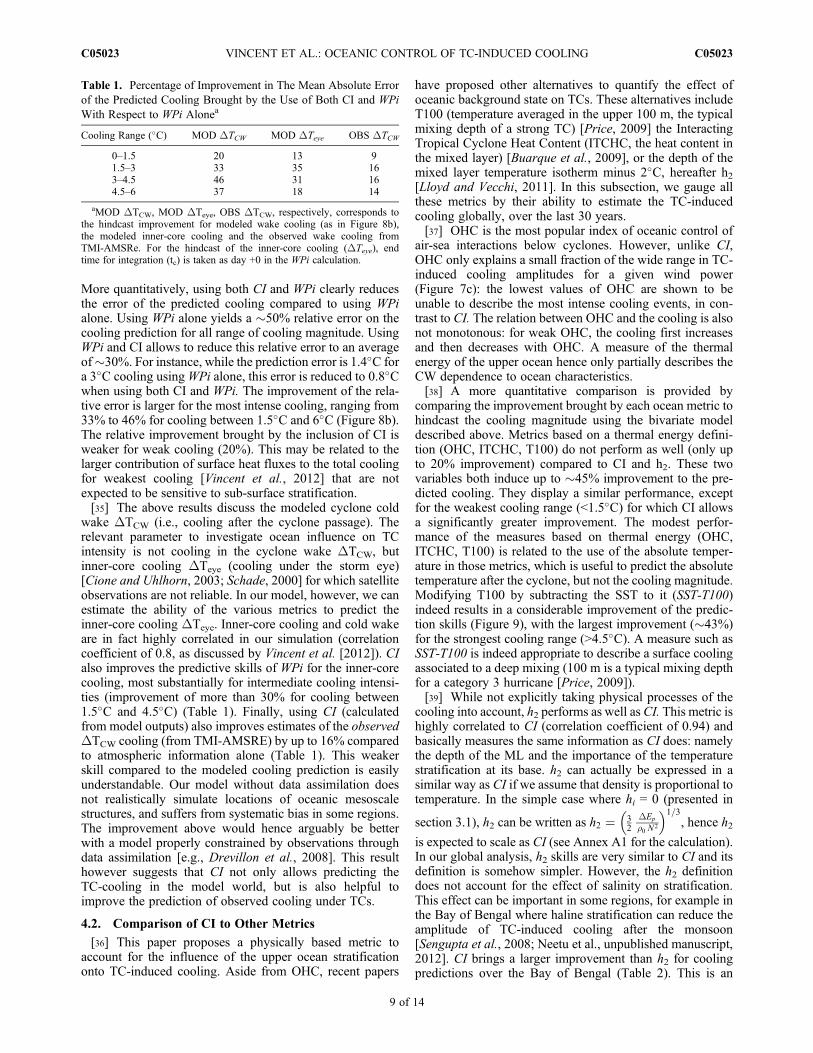
Table 1. Percentage of Improvement in The Mean Absolute Errorof the Predicted Cooling Brought by the Use of Both CI and WPiWith Respect to WPi Alonea

Cooling Range (�C) MOD DTCW MOD DTeye OBS DTCW

0–1.5 20 13 91.5–3 33 35 163–4.5 46 31 164.5–6 37 18 14

aMOD DTCW, MOD DTeye, OBS DTCW, respectively, corresponds tothe hindcast improvement for modeled wake cooling (as in Figure 8b),the modeled inner-core cooling and the observed wake cooling fromTMI-AMSRe. For the hindcast of the inner-core cooling (DTeye), endtime for integration (tc) is taken as day +0 in the WPi calculation.

VINCENT ET AL.: OCEANIC CONTROL OF TC-INDUCED COOLING C05023C05023

9 of 14

illustration that, although h2 is generally a good indicator ofthe cooling, the integration of salinity effects into the CIindex makes it appropriate for a wider range of oceanicconditions.

5. Conclusion

[40] Sea surface temperature (SST) influences tropicalcyclones (TCs) intensity through two mechanisms: (1) ambi-ent SST that sets the maximum potential intensity for TCs and(2) the negative feedback associated with the cooling under theTC eye. TCs intensity is more sensitive to the feedback asso-ciated with the cooling than to the ambient SST [Schade,2000]. Lloyd and Vecchi [2011] further demonstrated thatthe TC intensity evolution is linked to the observed coolingmagnitude in the wake of TCs, and suggested that the oceansub-surface temperature stratification is a key parameter incontrolling the TC intensity evolution through its modulationof the SST feedback.[41] This paper provides a comprehensive and global

quantification of the sensitivity of TC-induced coolingamplitude to pre-storm ocean state. In order to overcomelimited availability of ocean in situ data below tropicalcyclones, we use an ocean general circulation model exper-iment that realistically samples the ocean response to morethan 3,000 TCs. As cooling largely results from mixing, i.e.,a conversion of mechanical into potential energy, we pro-pose to describe the ocean effect on the TC-induced coolingby two metrics: a wind power index (WPi) and a CoolingInhibition index (CI). WPi is a proxy of the kinetic energyprovided to the ocean by a TC, which triggers upper-oceanmixing. It integrates the effects of various TC parameters(maximum winds, translation speed, size) that affect the TC-induced cooling. CI is a measure of the input of potential

energy required to cool the surface ocean by 2�C throughvertical mixing. It thus accounts for the pre-storm upperocean stratification and its resistance to surface coolingvia mixing.[42] We show that these two simple metrics are relevant to

explain the wide TC-induced cooling amplitude distribution.While average cooling increases withWPi, a givenWPi (i.e.,a given kinetic energy deposit in the ocean) can be associ-ated to a wide range of cooling. Our results demonstrate thatcontrasts in upper ocean stratification, as measured by CI,explain most of this range. Ocean pre-storm stratificationmodulates the cooling magnitude by up to an order ofmagnitude for a given wind energy input. For example, forhigh WPi, the cooling amplitude varies from 0.5�C to 5�Cdepending on CI (a high CI resulting in a small cooling).Upper ocean stratification is thus a key factor for the CWmagnitude.[43] We further show that using CI in addition to WPi

improves statistical hindcasts of the cold wake amplitude by�40% (for cooling larger than 1.5�C). Previously proposedmetrics that are based on a fixed threshold and/or absolutetemperature (i.e., OHC, T100, ITCHC) do not predict accu-rately the CW magnitude. In contrast, metrics that accountfor both mixed layer depth and the steepness of the stratifi-cation at its base (e.g., h2, SST-T100) display comparablehindcast skills to CI. The main interest of CI is however torely on the physical mechanism responsible for the oceaniccontrol of the CW namely the amount of potential energyrequired to yield a given surface cooling. Still, our resultssuggest that CI is a better alternative than previously pro-posed metrics of cyclone-ocean interactions in regions wherehaline stratification plays an important role in controlling thesurface cooling, like the Bay of Bengal [Sengupta et al.,2008; Neetu et al., unpublished manuscript, 2012].[44] We think that this work may have practical con-

sequences for cyclone intensity forecasts. While OHC onlybrought modest�5% improvement to TC intensity statisticalforecast schemes [DeMaria et al., 2005; Mainelli et al.,2008], a metric like CI, which properly captures the oceanpropensity to modulate TC-induced surface cooling (andhence the storm growth rate), could be tested in TC intensityforecast schemes. CI calculation requires both salinity andtemperature profiles in front of the storm track and is thusharder to compute operationally than metrics based on tem-perature profile alone. Temperature and salinity data areprovided by ARGO measurements, but their spatial andtemporal coverage is not sufficient to sample all pre-cyclonesoceanic conditions. Even though salinity stratification partlycontrols the surface cooling in some regions such as theBay of Bengal, a first approach could be to calculate CI

Figure 9. Percentage of improvement in the mean absoluteerror of the predicted cooling brought by the inclusion ofvarious ocean metric in addition to WPi in the predictors(as in Figure 8b): OHC (dark blue), ITCHC (light blue),T100 (green), SST-T100 (yellow), h2 (red), and CI (purple).Error bars give the 90% confidence interval estimated from abootstrap technique (as explained in section A2).

Table 2. Percentage of Improvement in the Mean Absolute Errorof the Predicted Cooling Brought by the Inclusion of VariousOcean Metrics in Addition to WPi for the Bay of Bengal

CoolingRange (�C)

Percent Improvement for Bay of Bengal MOD DTCW

OHC ITCHC T100 SST-T100 h2 CI

0–1 3 14 4 10 12 201–2 2 6 4 20 23 32>2 10 8 10 26 37 45

VINCENT ET AL.: OCEANIC CONTROL OF TC-INDUCED COOLING C05023C05023

10 of 14

with temperature stratification only, which can be recon-structed from altimetry measurements in the same manner asOHC [Shay et al., 2000]. Alternatively, CI could also becomputed from currently available operational oceanographyproducts constrained by oceanic observations [e.g.,Drevillonet al., 2008].[45] Although CI rather accurately captures the upper

ocean propensity to modulate the amplitude of TC-inducedcooling, we believe that our approach can be furtherimproved. The scaling used to define both CI and WPi arebased on rather crude assumptions. For instance, wehypothesized a linear relationship between the energy inputfrom the wind and the potential energy increase in the oceanto derive the cube root scaling of WPi. It is however likelythat the fraction of kinetic energy transformed into potentialenergy depends on oceanic parameters such as the mixedlayer depth and the wind-induced mixing depth. A carefulinvestigation of the mechanical energy budget under TCs isrequired to shed light on the energy transfer from surfacewinds to surface currents and quantify the respective amountof energy that is locally converted to potential energy orradiated away in the form of internal waves.[46] Our aim in this paper was to quantify the influence of

the oceanic stratification on TC-induced cooling globally,not to include all the physically relevant processes into ananalytic prediction of the TC-induced cooling. In a waysimilar to Schade and Emanuel [1999], a potential route fora more accurate prediction of TC-induced cooling would beto include other relevant parameters of the TC-ocean inter-action. An inherent limitation to the CI definition is indeedto only account for the TC-induced cooling driven by pen-etrative vertical mixing. Mixing generally dominates surfacecooling for moderate to high wind power but cooling by air-sea fluxes also plays a significant role for weak TCs [Vincentet al., 2012]. The surface cooling also depends on theamplitude of the upwelling induced by the TC that alters thethermal stratification [Yablonsky and Ginis, 2009]. Account-ing for these processes (surface fluxes and advection) mayfurther improve the forecast skills of the TC-induced cooling.In addition, while our results allow us to illustrate the strongimpact of the oceanic background conditions on the ampli-tude of the TC-induced surface cooling, we did not directlyassess the influence of the oceanic background conditions ofthe cyclone intensification itself. As demonstrated by Schadeand Emanuel [1999], the effect of a given cooling on a TCalso depends on characteristics of the TC itself such as itsintensity and translation speed. A statistical forecastingtechnique of TC intensity including the parameters proposedin the present study should allow to address this issue.[47] Finally, some studies suggest that ocean eddies [e.g.,

Jacob and Shay, 2003] or low frequency climate variations[e.g., Xie et al., 2002] impact tropical cyclones activitythrough modification of the TC-induced cooling magnitude.Our approach offers potential for quantifying the extent towhich ocean stratification changes linked to natural oceanvariability can mitigate cyclone intensity. Changes in theatmospheric background state driven by anthropogenicforcing could also alter cyclone distributions in present andfuture climate [Knutson et al., 2008]. Our approach may alsoallow to estimate the potential influence of upper-oceanstratification changes driven by climate change on future

TCs cooling amplitude and ultimately on TCs intensifica-tion. In contrast to OHC, T100 or ITCHC, CI is suited toperform such an investigation, as its definition does neitherdepend on absolute temperature nor on fixed thresholdsrepresentative of the present-day climate [Royer et al., 1998].

Appendix A

A1. Idealized Framework to Illustrate SurfaceCooling Scaling

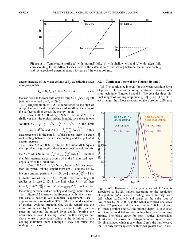
[48] The purpose of this appendix is to develop theapproach in section 3.1 to the more realistic case where amixed layer is present (i.e., the ocean is not linearly stratifiedall the way up to the surface). Depending on the mixed layerdepth, two forms of solutions can be derived for the scalingbetween surface cooling and potential energy input associ-ated to vertical mixing.[49] Let us consider an ocean with constant stratification

N2 under a ML of initial depth hi as illustrated onFigure A1a, and a linear equation of state with densitydepending on temperature only: r(z) = r0(1 � a T(z)). The

temperature profile is TðzÞ ¼ Ti ; z > �hiTi þ Gðzþ hiÞ ; z < �hi

�

with N 2 ¼ � gr0

∂r∂z ¼ ag ∂T

∂z ¼ agG. a is the coefficient for

thermal expansion of seawater, r0 is a reference densityand G is the temperature gradient under the ML.[50] Let us now assume that after the ‘passage of the

cyclone;’ the surface layer has been homogeneously mixeddown to the depth hm, at the temperature Tf (Figure A1a).[51] Conservation of heat yields an equation linking hm

with the surface cooling DT = Tf � TiZ 0

�hm

roCPðTf � TiðzÞÞdz ¼ 0: ðA1Þ

Assuming constant CP and ro (r ≈ ro at the first order inr � T) and hm ≠ 0 yields:

hm2 � 2h2 hm þ hi

2 ¼ 0; ðA2Þ

where h2 ¼ hi � a gN2 DT (as defined on Figure A1a is the

variable discussed by Lloyd and Vecchi [2011] when DT =�2�C).[52] The potential energy difference between the initial

and final profile is

DEp ¼Z 0

�hm

rf � ri� �

g zdz; ðA3Þ

providing an equation linking hm, DT and DEp

hm3 � 3

2h2 hm

2 þ hi3

2¼ H3; ðA4Þ

with H ≡ 3DEp

r0 N2

� �1=3. H can be seen as a characteristic mixing

length associated to a potential energy input DEp.[53] From (A2) and (A4), it is possible to derive the

dependence of the surface cooling DT to the potential

VINCENT ET AL.: OCEANIC CONTROL OF TC-INDUCED COOLING C05023C05023

11 of 14

energy increase of the water column DEp. Substituting (A2)into (A4) yields

hm3 � 3hi

2hm þ 2ðhi3 � 2H3Þ ¼ 0 ðA5Þ

that can be set in the reduced Cardan’s form hm3 + 3phm + 2q = 0

(with p = � hi2 and q = hi

3 � 2H3).[54] The resolution of (A5) is conditioned to the sign of

L ≡ p3 + q2 and the different cases lead to different scaling ofthe surface cooling versus the energy input:[55] Case 1. If L > 0 ⇔ hi < H (i.e., the initial MLD is

shallower than the typical mixing length), then there is one

solution hm ¼ffiffiffiffiffiffiffiffiffiffiffiffiffiffiffiffiffiffiffiffi�q� ffiffiffiffi

Lp

3

qþ

ffiffiffiffiffiffiffiffiffiffiffiffiffiffiffiffiffiffiffiffi�qþ ffiffiffiffi

Lp

3

q. In the limit

hi → 0, hm ≈ 41/3H and DT ≈� 1ag

3 N4

2 r0DEp

� �1=3; in this

case (presented in the part 3.1 of the paper), there is a cuberoot scaling between the surface cooling and the potentialenergy increase.[56] Case 2. If L = 0⇔ hi = H (i.e., the initial MLD equals

the typical mixing length), there is one positive solution for

hm: hm = 2hi, and DT ¼ �N2hi4ag ¼ �1

4ag3N4

r0DEp

� �1=3. We note

that this intermediate case occurs when the final mixed layerdepth is twice the initial one.[57] Case 3. IfL < 0⇔ hi >H (i.e., the initial MLD is deeper

than the typical mixing length) there are 3 solutions for hmbut only one real positive: hm ¼ 2hi cos 1

3 arccos2H3

hi3 � 1

� �� �.

(1) In the limit when hi =H, hm = 2hi, the cube root scaling stillapplies as in case 2. (2) In the limit when hi � H, then

hm ≈ hi 1þ 2ffiffiffiffiffiH3

3hi3

q� �and DT ≈� 2

agr0hi2DEp ; in this case

the scaling between surface cooling and energy input is linear.[58] Figure A2 illustrates the frequency with which case 1

and case 3 occur in our numerical experiment. Case 1appears to occur more often: 80% of the time under systemsof tropical cyclones strength. One would remark that theupwelling induced by TCs under their track further partici-pates in reducing the mixed layer depth, favoring theoccurrence of case 1 scaling. Based on this analysis, wechose to use a cube root scaling in the definition of thecooling inhibition index although it may not reflect thescaling for all cases.

A2. Confidence Interval for Figures 8b and 9

[59] The confidence interval for the Mean Absolute Errorof predicted TC-induced cooling is estimated using a boot-strap technique (Figures 8b and 9). We consider three dis-tinct ranges of cooling amplitude ([0,2], [2,4], [4,6]�C). Ineach range, the N observations of the absolute difference

Figure A1. Temperature profile (a) with “normal” ML, (b) with shallow ML and (c) with “deep” MLcorresponding to the different cases used in the calculation of the scaling between the surface coolingand the associated potential energy increase of the water column.

Figure A2. Histogram of the percentage of TC eventsassociated to hm-2hi values; according to the resolutionof equation (A5), surface cooling scales linearly withDEp when hm-2hi ≪0 and scales as the cube root ofDEp when hm-2hi > 0. hi is the MLD measured one weekbefore TC passage and averaged within 200 km of eachTC track position and hm (the mixing depth) is calculatedto obtain the modeled surface cooling by a heat conservingmixing. The black curve for both Tropical Depressions(TDs) and TCs shows the histogram for all systems with10-min averaged winds greater than 15 m/s, the purple curvefor TCs only shows systems with winds greater than 33 m/s.

VINCENT ET AL.: OCEANIC CONTROL OF TC-INDUCED COOLING C05023C05023

12 of 14

between the predicted cooling DTpredicted and the actualcooling DT are called events. We randomly select N eventsfrom the total number of events in each range. Overlappingselection is allowed, meaning that one event can be selectedmore than once. From the selected N events, we calculate theaverage absolute error. By repeating this process 1,000 times,we obtain 1,000 values for the MAE. The upper and lowerlimit of each error bar (in Figures 8b and 9) represents the 5%and 95% percentile of the probability distribution function. Ifthe MAE value usingWPi and CI lies outside the error bar ofthe WPi alone, the improvement is significant at the 90%confidence level.

[60] Acknowledgments. Experiments were conducted at the Institutdu Développement et des Ressources en Informatique Scientifique (IDRIS)Paris, France. We thank the Nucleus for European Modeling of the Ocean(NEMO) Team for its technical support. The analysis was supported bythe project CYCLOCEAN from Les Enveloppes Fluides et l’Environne-ment (LEFE) AO2010-538863. We thank Daniel Nethery for useful com-ments. We thank Kerry Emanuel and an anonymous reviewer for theiruseful comments that led to improve the present manuscript.

ReferencesAli, M. M., P. S. V. Jagadeesh, and S. Jain (2007), Effect of eddies on theBay of Bengal cyclone intensity, Eos Trans. AGU, 88, 93, doi:10.1029/2007EO080001.

Bister, M., and K. A. Emanuel (1998), Dissipative heating and hurricaneintensity, Meteorol. Atmos. Phys., 65, 233–240, doi:10.1007/BF01030791.

Bosart, L. F., W. E. Bracken, J. D. Molinari, C. S. Velden, and P. G. Black(2000), Environmental influences on the rapid intensification of Hurri-cane Opal (1995) over the Gulf of Mexico, Mon. Weather Rev., 128,322–352, doi:10.1175/1520-0493(2000)128<0322:EIOTRI>2.0.CO;2.

Buarque, S. R., C. Vanroyen, and C. Agier (2009), Tropical cyclone heatpotential index revisited, Mercator Ocean Q. Newsl., 33, 24–30.

Chen, S., W. Zhao, and M. A. Donelan (2007), The CBLAST-Hurricaneprogram and the next-generation fully coupled atmosphere-wave-oceanmodels for hurricane research and prediction, Bull. Am. Meteorol. Soc.,88, 311–317, doi:10.1175/BAMS-88-3-311.

Cione, J. J., and E. W. Uhlhorn (2003), Sea surface temperature variabilityin hurricanes: Implications with respect to intensity change, Mon.Weather Rev., 131, 1783–1796, doi:10.1175//2562.1.

DeMaria, M., M. Mainelli, L. K. Shay, J. A. Knaff, and J. Kaplan (2005),Further improvements to the Statistical Hurricane Intensity PredictionScheme (SHIPS), Weather Forecasting, 20, 531–543, doi:10.1175/WAF862.1.

Drevillon, M., et al. (2008), The GODAE/Mercator-Ocean global oceanforecasting system: Results, applications and prospects, J. Oper. Oceanogr.,1, 51–57.

Emanuel, K. A. (1999), Thermodynamic control of hurricane intensity,Nature, 401, 665–669, doi:10.1038/44326.

Emanuel, K. A. (2003), Tropical cyclones, Annu. Rev. Earth Planet. Sci.,31, 75–104, doi:10.1146/annurev.earth.31.100901.141259.

Emanuel, K. A. (2005), Increasing destructiveness of tropical cyclones overthe past 30 years, Nature, 436, 686–688, doi:10.1038/nature03906.

Emanuel, K. A., C. DesAutels, C. Holloway, and R. Korty (2004), Environ-mental control of tropical cyclone intensity, J. Atmos. Sci., 61, 843–858,doi:10.1175/1520-0469(2004)061<0843:ECOTCI>2.0.CO;2.

Goni, G., et al. (2009), Applications of satellite-derived ocean measure-ments to tropical cyclone intensity forecasting, Oceanography, 22, 190–197,doi:10.5670/oceanog.2009.78.

Greatbatch, R. J. (1984), On the response of the ocean to a moving storm:Parameters and scales, J. Phys. Oceanogr., 14, 59–78, doi:10.1175/1520-0485(1984)014<0059:OTROTO>2.0.CO;2.

Griffies, S., et al. (2009), Coordinated Ocean-ice Reference Experiments(COREs), Ocean Modell., 26, 1–46, doi:10.1016/j.ocemod.2008.08.007.

Hong, X., S. W. Chang, S. Raman, L. K. Shay, and R. Hodur (2000), Theinteraction between Hurricane Opal (1995) and a warm core ring in theGulf of Mexico, Mon. Weather Rev., 128, 1347–1365, doi:10.1175/1520-0493(2000)128<1347:TIBHOA>2.0.CO;2.

Jacob, S. D., and L. K. Shay (2003), The role of oceanic mesoscale features onthe tropical cyclone-induced mixed layer response: A case study, J. Phys.Oceanogr., 33, 649–676, doi:10.1175/1520-0485(2003)33<649:TROOMF>2.0.CO;2.

Jacob, S. D., L. K. Shay, A. J. Mariano, and P. G. Black (2000), The 3Doceanic mixed layer response to Hurricane Gilbert, J. Phys. Oceanogr.,

30, 1407–1429, doi:10.1175/1520-0485(2000)030<1407:TOMLRT>2.0.CO;2.

Knapp, K. R., M. C. Kruk, D. H. Levinson, H. J. Diamond, and C. J. Neumann(2010), The International Best Track Archive for Climate Stewardship(IBTrACS): Unifying tropical cyclone data, Bull. Am. Meteor. Soc., 91,363–376.

Knutson, T. R., J. J. Sirutis, S. T. Garner, G. A. Vecchi, and I. M. Held(2008), Simulated reduction in Atlantic hurricane frequency undertwenty-first-century warming conditions, Nat. Geosci., 1, 359–364,doi:10.1038/ngeo202.

Korty, R. L., K. A. Emanuel, and J. R. Scott (2008), Tropical cyclone-induced upper-ocean mixing and climate: Application to equable climates,J. Clim., 21, 638–654.

Large, W., and S. Yeager (2009), The global climatology of an interannu-ally varying air-sea flux data set, Clim. Dyn., 33, 341–364, doi:10.1007/s00382-008-0441-3.

Leipper, D. F., and D. Volgenau (1972), Hurricane heat potential of theGulf of Mexico, J. Phys. Oceanogr., 2, 218–224, doi:10.1175/1520-0485(1972)002<0218:HHPOTG>2.0.CO;2.

Lengaigne, M., U. Haussman, G. Madec, C. Menkes, J. Vialard, and J. M.Molines (2012), Mechanisms controlling warm water volume interannualvariations in the equatorial Pacific: Diabatic versus adiabatic processes,Clim. Dyn., 38, 1031–1046.

Liu, L. L., W. Wang, and R. X. Huang (2008), The mechanical energyinput to the ocean induced by tropical cyclones, J. Phys. Oceanogr., 38,1253–1266, doi:10.1175/2007JPO3786.1.

Lloyd, I. D., and G. A. Vecchi (2011), Observational evidence of oceaniccontrols on hurricane intensity, J. Clim., 24, 1138–1153, doi:10.1175/2010JCLI3763.1.

Lloyd, I. D., T. Marchok, and G. A. Vecchi (2011), Diagnostics comparing seasurface temperature feedbacks from operational hurricane forecasts to obser-vations, J. Adv.Model. Earth Syst., 3, M11002, doi:10.1029/2011MS000075.

Locarnini, R. A., A. V. Mishonov, J. I. Antonov, T. P. Boyer, and H. E.Garcia (2006), World Ocean Atlas 2005, vol. 1, Temperature, NOAAAtlas NESDIS, vol. 61, edited by S. Levitus, 182 pp., NOAA, SilverSpring, Md.

Madec, G. (2008), NEMO ocean engine, Note Pôle Modél. 27, Inst. Pierre-Simon Laplace, Paris.

Mainelli, M., M. DeMaria, L. K. Shay, and G. Goni (2008), Application ofoceanic heat content estimation to operational forecasting of recent Atlan-tic category 5 hurricanes, Weather Forecasting, 23, 3–16, doi:10.1175/2007WAF2006111.1.

Penduff, T., M. Juza, L. Brodeau, G. C. Smith, B. Barnier, J.-M. Molines,A.-M. Treguier, and G. Madec (2010), Impact of global ocean model res-olution on sea-level variability with emphasis on interannual time scales,Ocean Sci., 6, 269–284, doi:10.5194/os-6-269-2010.

Price, J. F. (1979), On the scaling of stress-driven entrainment experiments,J. Fluid Mech., 90(3), 509–529, doi:10.1017/S0022112079002366.

Price, J. F. (1981), Upper ocean response to a hurricane, J. Phys. Oceanogr.,11, 153–175, doi:10.1175/1520-0485(1981)011<0153:UORTAH>2.0.CO;2.

Price, J. F. (2009), Metrics of hurricane-ocean interaction: Verticallyintegrated or vertically averaged ocean temperature?, Ocean Sci., 5,351–368, doi:10.5194/os-5-351-2009.

Riehl, H. (1950), A model of hurricane formation, J. Appl. Phys., 21, 917–925,doi:10.1063/1.1699784.

Roemmich, D., G. C. Johnson, S. Riser, R. Davis, J. Gilson, W. B. Owens,S. L. Garzoli, C. Schmid, and M. Ignaszewski (2009), The Argo program:Observing the global ocean with profiling floats,Oceanography, 22, 34–43,doi:10.5670/oceanog.2009.36.

Royer, J. F., F. Chauvin, B. Timbal, P. Araspin, and D. Grimal (1998), AGCM study of the impact of greenhouse gas increase on the frequency ofoccurrence of tropical cyclones, Clim. Change, 38, 307–343, doi:10.1023/A:1005386312622.

Schade, L. R. (2000), Tropical cyclone intensity and sea surface tempera-ture, J. Atmos. Sci., 57, 3122–3130, doi:10.1175/1520-0469(2000)057<3122:TCIASS>2.0.CO;2.

Schade, L. R., and K. A. Emanuel (1999), The ocean’s effect on the intensityof tropical cyclones: Results from a simple coupled atmosphere-oceanmodel, J. Atmos. Sci., 56, 642–651, doi:10.1175/1520-0469(1999)056<0642:TOSEOT>2.0.CO;2.

Sengupta, D., B. R. Goddalehundi, and D. S. Anitha (2008), Cyclone-induced mixing does not cool SST in the post-monsoon north Bay ofBengal, Atmos. Sci. Lett., 9, 1–6, doi:10.1002/asl.162.

Shay, L. K., and J. K. Brewster (2010), Oceanic heat content variability inthe eastern Pacific Ocean for hurricane intensity forecasting, Mon.Weather Rev., 138, 2110–2131, doi:10.1175/2010MWR3189.1.

Shay, L. K., G. J. Goni, and P. G. Black (2000), Effects of a warm oceanicfeature on Hurricane Opal, Mon. Weather Rev., 128, 1366–1383,doi:10.1175/1520-0493(2000)128<1366:EOAWOF>2.0.CO;2.

VINCENT ET AL.: OCEANIC CONTROL OF TC-INDUCED COOLING C05023C05023

13 of 14

Vincent, E. M., M. Lengaigne, G. Madec, J. Vialard, G. Samson, N. C.Jourdain, C. E. Menkes, and S. Jullien (2012), Processes setting thecharacteristics of sea surface cooling induced by tropical cyclones,J. Geophys. Res., 117, C02020, doi:10.1029/2011JC007396.

Wentz, F. J., C. Gentemann, D. Smith, and D. Chelton (2000), Satellitemeasurements of sea surface temperature through clouds, Science, 288,847–850, doi:10.1126/science.288.5467.847.

Willoughby, H. E., R. W. R. Darling, and M. E. Rahn (2006), Parametricrepresentation of the primary hurricane vortex. Part II: A new family of

sectionally continuous profiles, Mon. Weather Rev., 134, 1102–1120,doi:10.1175/MWR3106.1.

Xie, S. P., H. Annamalai, F. A. Schott, and J. P. McCreary (2002), Structureand mechanisms of South Indian Ocean climate variability, J. Clim., 15(8),864–878, doi:10.1175/1520-0442(2002)015<0864:SAMOSI>2.0.CO;2.

Yablonsky, R. M., and I. Ginis (2009), Limitation of one-dimensionalocean models for coupled hurricane-ocean model forecasts, Mon.Weather Rev., 137, 4410–4419, doi:10.1175/2009MWR2863.1.

VINCENT ET AL.: OCEANIC CONTROL OF TC-INDUCED COOLING C05023C05023

14 of 14