Climate Dynamics

Influence of air-sea coupling on Indian Ocean Tropical Cyclones--Manuscript Draft--

Manuscript Number: CLDY-D-17-00779R2

Full Title: Influence of air-sea coupling on Indian Ocean Tropical Cyclones

Article Type: Original Article

Keywords: tropical cyclonesair-sea couplingIndian Oceancold wakeregional coupled ocean-atmosphere model

Corresponding Author: Matthieu Lengaigne, Ph. D.LOCEANParis, FRANCE

Corresponding Author SecondaryInformation:

Corresponding Author's Institution: LOCEAN

Corresponding Author's SecondaryInstitution:

First Author: Matthieu Lengaigne, Ph. D.

First Author Secondary Information:

Order of Authors: Matthieu Lengaigne, Ph. D.

S Neetu

Guillaume Samson

Jerôme Vialard

KS Krishnamohan

Sebastien Masson

Swen Jullien

I Suresh

Christophe Menkes

Order of Authors Secondary Information:

Funding Information: IFCPAR(4907-1)

Dr. Matthieu Lengaigne

Abstract: This paper assesses the impact of air-sea coupling on Indian Ocean Tropical Cyclones(TCs) by comparing a 20-year long simulation of a ¼° regional coupled ocean-atmosphere model with a twin experiment, where the atmospheric component is forcedby sea surface temperature from the coupled simulation. The coupled simulationreproduces the observed spatio-temporal TCs distributions and TC-induced surfacecooling reasonably well, but overestimates the number of TCs. Air-sea coupling doesnot affect the cyclogenesis spatial distribution but reduces the number of TCs by ~20%and yields a better-resolved bimodal seasonal distribution in the northern hemisphere.Coupling also affects intensity distribution, inducing a four-fold decrease in theproportion of intense TCs (stronger than Cat-1). Air-sea coupling damps TC growththrough a reduction of the inner-core upward enthalpy fluxes due to the TC-inducedcooling. This reduction is particularly large for the most intense TCs of the northernIndian Ocean (up to 250W.m-2), due to higher ambient surface temperatures andlarger TC-induced cooling there. The negative feedback of air-sea coupling onstrongest TCs is mainly associated with slow-moving storms. Sensitivity experimentsusing a different convective parameterization yield qualitatively similar results, with a

Powered by Editorial Manager® and ProduXion Manager® from Aries Systems Corporation

larger (~65%) reduction in the number of TCs. Because of their relatively coarseresolution (¼°), both set of experiments however fail to reproduce the strongestobserved TCs (Cat-4-5). Further studies with finer resolution models capable ofsimulating the strongest TCs in the Bay of Bengal will be needed to assess theexpectedly large impact of air-sea coupling on those deadly TCs.

Powered by Editorial Manager® and ProduXion Manager® from Aries Systems Corporation

Reviewer original comment – Authors answer – Actions taken in the text

Reply to the review comments

Reviewer #1:

Reviewer comments:

The paper entitled "Influence of air-sea coupling on Indian Ocean Tropical Cyclones"

by Lengaigne et al. investigated roles of air-sea coupling and subsurface ocean to SST

cooling during TC passage. From regional air-sea coupled model experiments, the

authors suggest that SST cooling (cold wake) causes TC reduction particular in

intense TCs (Fig.5 and 6) and cold wake is larger over the northern IO than southern

IO (Fig.8 and 9). Impact of subsurface ocean on intense TC over the northern IO is

also summarized in Fig.10 and 11. I think that this paper is well written based on

suitable analysis, and therefore I would like to accept this paper after minor revision.

We thank the reviewer for his positive views on our manuscript.

Comments:

- Our previous work (Ogata et al. 2016) also pointed out the importance of subsurface

water distribution over the tropical Indian Ocean (although our result was more

significant over the southern IO than northern IO) on intense/extreme TC distribution.

Could you please discuss similarity and different between Ogata et al. (2016) and this

paper? Particularly, it is interesting that this paper shows weakening of intense TCs

and air-sea coupling effect is weak in the southern IO. This result is different from

Ogata et al. (2016) that the thermocline ridge over the southwestern IO causes

significant air-sea coupling effect in the southern IO.

We thank the reviewer for this reference. Results from this paper are now discussed in

the introduction (p4 first paragraph and p6 second paragraph) and compared to our

results at the end of Section 3 (p15 first paragraph). The following discussion has

been added: “In agreement with Ogata et al. (2016), we do not find any significant

change in the location of the region of strongest TCs when air-sea coupling is

accounted for, neither in the northern nor in the southern IO (not shown). However,

while Ogata et al. (2016) found a considerably larger decrease of the number of strong

TCs in the southern than in the northern IO, our results indicate a more symmetrical

decrease on both sides of the equator.”

- In Fig.4, is it possible to quantify (or detect) which component (potential intensity,

vorticity, and vertical shear) is important for bi-modal seasonality? For example,

converting units of Fig.4b-4e and 4g-4j to GPI may also give a useful information.

The assessment of the respective influence of each term on the GPI seasonal evolution

is not straightforward. As this index is the product (and not the sum) of different

terms, these terms interact non-linearly to shape the GPI evolution. Menkes et al.

(2011) applied an efficient method to quantify the relative roles of each of the large-

scale environmental factors in causing the bimodal distribution of the GPI in the

northern IO. This method, based on Camargo et al. (2007), used a first order Taylor

expansion of the logarithm of the GPI equation to express the GPI variations as the

sum of different terms (see Menkes et al. 2011 for details). Menkes et al. (2011)

found using this method that the combined effect of increased vertical wind shear and

decreased maximum potential intensity overcome the increased relative humidity

during the summer monsoon. To ascertain the robustness of their results, we applied

Authors Click here to download Authors' response to reviewers'comments Lengaigne Cyc Coupling reply final.docx

Reviewer original comment – Authors answer – Actions taken in the text

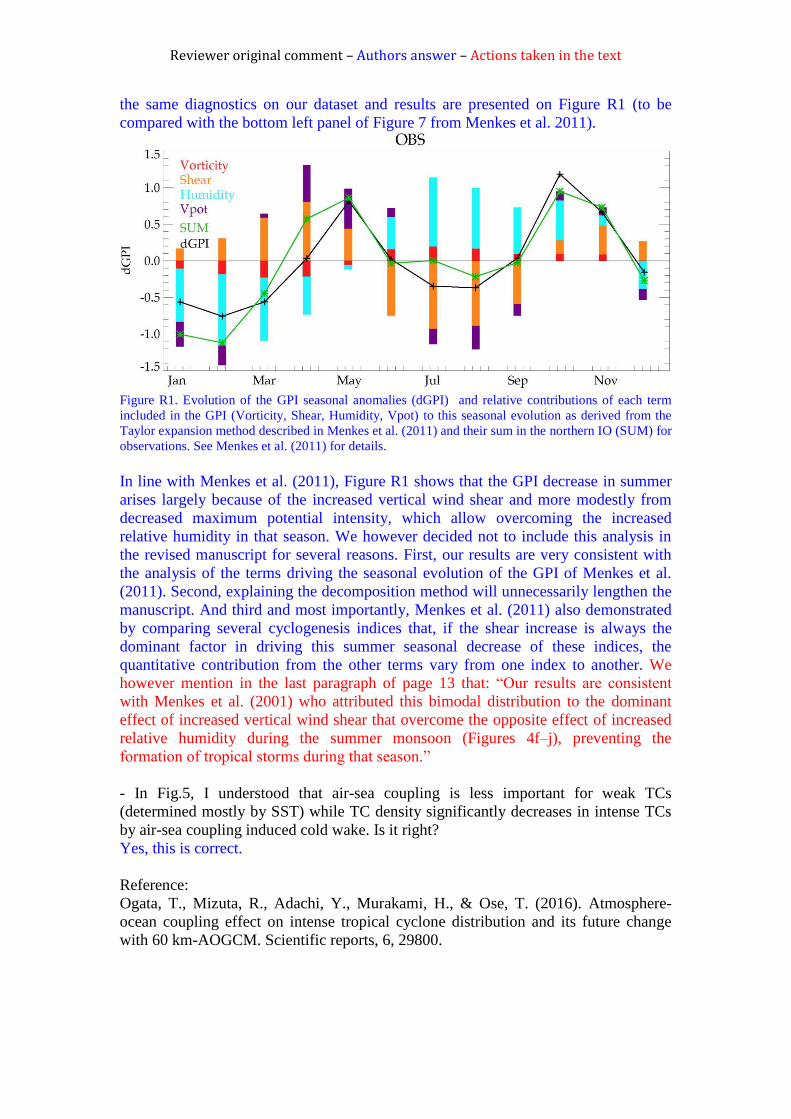
the same diagnostics on our dataset and results are presented on Figure R1 (to be

compared with the bottom left panel of Figure 7 from Menkes et al. 2011).

Figure R1. Evolution of the GPI seasonal anomalies (dGPI) and relative contributions of each term

included in the GPI (Vorticity, Shear, Humidity, Vpot) to this seasonal evolution as derived from the

Taylor expansion method described in Menkes et al. (2011) and their sum in the northern IO (SUM) for

observations. See Menkes et al. (2011) for details.

In line with Menkes et al. (2011), Figure R1 shows that the GPI decrease in summer

arises largely because of the increased vertical wind shear and more modestly from

decreased maximum potential intensity, which allow overcoming the increased

relative humidity in that season. We however decided not to include this analysis in

the revised manuscript for several reasons. First, our results are very consistent with

the analysis of the terms driving the seasonal evolution of the GPI of Menkes et al.

(2011). Second, explaining the decomposition method will unnecessarily lengthen the

manuscript. And third and most importantly, Menkes et al. (2011) also demonstrated

by comparing several cyclogenesis indices that, if the shear increase is always the

dominant factor in driving this summer seasonal decrease of these indices, the

quantitative contribution from the other terms vary from one index to another. We

however mention in the last paragraph of page 13 that: “Our results are consistent

with Menkes et al. (2001) who attributed this bimodal distribution to the dominant

effect of increased vertical wind shear that overcome the opposite effect of increased

relative humidity during the summer monsoon (Figures 4f–j), preventing the

formation of tropical storms during that season.”

- In Fig.5, I understood that air-sea coupling is less important for weak TCs

(determined mostly by SST) while TC density significantly decreases in intense TCs

by air-sea coupling induced cold wake. Is it right?

Yes, this is correct.

Reference:

Ogata, T., Mizuta, R., Adachi, Y., Murakami, H., & Ose, T. (2016). Atmosphere-

ocean coupling effect on intense tropical cyclone distribution and its future change

with 60 km-AOGCM. Scientific reports, 6, 29800.

Reviewer original comment – Authors answer – Actions taken in the text

Reviewer #2:

Review of "Influence of air-sea coupling on Indian Ocean tropical cyclones" by

Lengaigne et al.

This study uses a 0.25-deg couple model to simulate Indian Ocean tropical cyclones

and estimate the impact of SST coupling on TC tracks and intensities. The results are

mostly what would be expected: air-sea coupling reduces TC frequency and intensity,

especially for the strongest storms. The reductions are due mainly to the presence of

storm-induced cold wakes in the coupled run, which reduce the upward energy

transfer to the TCs. The effect is strongest for the most slowly moving storms, which

spend the longest time over their cold wakes, and is strongest in the northern Indian

Ocean (Bay of Bengal), where the upper-ocean temperature stratification is stronger.

This is an interesting and well written manuscript that presents new and important

results. The 0.25-deg resolution model that is used is not ideal because it can't

simulate the strongest TCs, and it produces significantly more TCs compared to

observations (about 4 times as many for the coupled run). However, the model does

compare well to observations in other aspects such as spatial distribution of TCs and

seasonal distribution of TC number in each basin. The model is also capable of

producing TCs with well-defined eyes and reasonable radii of maximum winds,

suggesting that the horizontal resolution is adequate for examining large-scale

statistics of simulated TCs. I do not see it as a major limitation that the model

produces too many TCs (except for one minor point that I include below). The fact

that the model does not produce enough strong TCs could mean that the results err

toward the conservative side, since stronger storms tend to produce more mixing and

SST cooling, with a stronger negative feedback. It is good to see that the authors

experimented with two different convective parameterizations and that the overall

features are similar despite one method failing to produce any strong storms. It's

valuable to know the sensitivity of modeled TCs to this parameterization.

I have some mostly minor points for the authors to consider, after which the

manuscript should be suitable for publication.

We thank the reviewer for his positive views on our manuscript.

Because there are so many more TCs in the model compared to observations, there

may be a spurious negative feedback induced by prior storms' cold wakes (Balaguru

et al., GRL, 2014, doi:10.1002/2014GL061489). I would expect this might be most

important in the Bay of Bengal due to its small area. Can you quantify this effect, or

estimate the chance of one TC encountering the wake of a previous TC?

This is a good point. We hence calculated the probability for each TC location to be

within 400km and 14 days-lag of a previous TC, for both the northern and southern

hemispheres. The 400km and 14 days have been chosen here to broadly match criteria

in Balaguru et al. (2014). Our results indicate that this probability is low in

observations for both northern and southern IO (7.4 and 5.1% respectively). Although

larger for the coupled simulation because of the larger number of TCs (18.6 and 7.5%

respectively), it still small enough to conclude that the effect of spurious negative

feedback induced by previous cold wake to be of second order compared to the direct

Reviewer original comment – Authors answer – Actions taken in the text

negative feedback induced by the TC itself. This probability decreases further when

less conservative criteria are used. The cooling 400km away from a TC is indeed very

weak (3 to 4 times less than the maximum cooling, see Figure 7b from Vincent et al.

2012 and Figure 8 and 9 from the present study) and is unlikely to affect significantly

another TC passing several days after. Using a more realistic 200km criterion, this

probability decreases to 1% in observations and 8% in the model.

p. 4, first paragraph: Others have shown the importance of an accuate representation

of ocean stratification on basin scales and might be worth citing (Balaguru et al.,

GRL, 2015, doi:10.1002/2015GL064822 and Miyamoto et al., GRL, 2017,

doi:10.1002/2017GL073670).

Thanks for these references. They are now discussed in the introductory section (first

paragraph of p4) of the revised manuscript.

p. 5, line 11: Delete 'the' after 'improves'

Corrected.

p. 9, lines 9-19: I'm curious how well the wake removal algorithm works. It would be

easy enough to test by doing an experiment in which random synthetic "tracks" are

removed from the coupled model output and then filled using your technique. The

filled values could then be compared to the actual values. Its unclear whether such a

validation was done previously in another paper, and if so it should be mentioned.

The filling technique used in our manuscript and Samson et al. (2014) was also used

in Jullien et al. (2014), as already mentioned in the manuscript. Figure 2 illustrates

that this technique efficiently removes the TC cold wake with affecting the SST away

from the TC track. Similar consistency checks have been performed for numerous

other TC cases, with similar results. In addition, due to the chaotic nature of the

atmosphere, TCs occur at different location in the forced and coupled simulation,

making it very unlikely that they will be heavily influenced by other TCs cold wakes,

even if they were not perfectly “filled”. The composite of figure 9 illustrates this:

while there is a very clear cold wake signature in the coupled model, this signature is

absent from the forced model.

p. 12, lines 21 and 23: I think you mean to refer to Figure 3, not Figure 2.

We actually referred to Figure 1. Thanks for noticing. This has been changed.

p. 14, line 17: Change 'simulates' to 'simulate'

Corrected.

p. 19, line 19: Change 'to' to 'on'

Corrected.

p. 20, line 14: Change 'twice larger' to 'twice as large'

Corrected.

Reviewer original comment – Authors answer – Actions taken in the text

Reviewer #3:

Review of "Influence of air-sea coupling on Indian Ocean tropical cyclones" by

Lengaigne et al.

Most present-day models do not have adequate skill in cyclone intensity simulation or

forecasts, partly due to poor representation of the physics of air-sea interaction. This

is a scientific problem of great applied interest.

The authors have made a significant contribution, in the modeling context, to the role

of air-sea interaction in Indian Ocean tropical cyclone numbers, their seasonality,

spatial distribution, and intensification. They analyse 20-year simulations from a ¼

degree resolution regional coupled model; compare the results with a standalone

atmosphere model forced by SST from the coupled model, and thus elicit the

influence of cyclone-induced SST cooling on intensification of tropical cyclones in

the north and south Indian Ocean.

The present work draws upon previous studies of tropical cyclones published by one

or more of the authors with their collaborators, and it can be seen as part of

a sequence of studies. The authors use the NEMO-WRF coupled model, and the

analysis employs indices of intensity and inhibition developed earlier, as well as

proxies of background upper ocean stratification. The ¼ degree model generates too

many weak systems relative to observations, and does not simulate the most intense

(category 3 or higher) storms.

The main conclusions are: Air-sea coupling does not change the spatial distribution of

Indian Ocean cyclogenesis, but reduces the overall number of TCs by 20%. Coupling

reduces the number of TCs in the north Indian Ocean in the summer monsoon season,

bringing the model seasonality closer to observations. Reduction in enthalpy flux and

TC intensity due to coupling is more pronounced in the north Indian Ocean than in the

south. These results are robust under a change of convective parameterization

scheme; the reduction in overall TC numbers is much larger when the Kain-Fritsch

parameterization is employed.

The model simulations, experiment design and analysis are all sound, model

shortcomings are explicitly discussed, and the simulations are compared with

observations at each step. The results are placed in the context of the handful of

previous studies that use similar long model simulations focused on Pacific and

Atlantic TC’s. The paper is well organized, although the writing does need more

clarity in several places.

Recommendation: Accept with minor revisions.

We thank the reviewer for his positive views on our manuscript.

The present study generally clubs the cyclone seasons together while examining

cyclone inhibition. The pre-summer monsoon and post-summer monsoon temperature

and salinity stratification in the north Indian Ocean have significant differences, as

Reviewer original comment – Authors answer – Actions taken in the text

shown in previous observational studies. Although seasonal differences are not the

focus of this study, the authors may mention this explicitly in the Discussion Section.

We did not want to include a discussion on this aspect as we felt the paper was long

enough.

Many sentences in the text need to be rewritten for greater clarity. I mention a few

examples later; first, I suggest changing the Abstract slightly to:

This paper assesses the impact of air-sea coupling on Indian Ocean Tropical Cyclones

(TCs) by comparing a 20-year long simulation of a ¼° regional coupled ocean-

atmosphere model with a twin experiment, where the atmospheric model is forced by

sea surface temperature (SST) from the coupled simulation. The coupled simulation

reproduces the observed spatio-temporal TC distribution and TC-induced surface

cooling reasonably well, but overestimates the number of TCs. Air-sea coupling does

not affect the spatial distribution of cyclogenesis, but reduces the number of TCs by

~20% and yields a better-resolved bimodal seasonal distribution of TCs in the

northern hemisphere. Coupling also affects intensity distribution, inducing a four-fold

decrease in the proportion of intense TCs (stronger than category-2). Air-sea coupling

damps TC intensity through a reduction of the inner-core upward enthalpy flux due to

TC-induced SST cooling. This reduction is particularly large for the most intense TCs

of the northern Indian Ocean (up to 250 Wm-2), due to higher ambient surface

temperatures and larger TC-induced SST cooling. The negative feedback of air-sea

coupling on the strongest TCs is associated mainly with slow-moving storms.

Sensitivity experiments using a different atmospheric convective parameterization

yield qualitatively similar results, with a larger (~65%) reduction in the number of

TCs. Because of the relatively coarse model resolution (¼°), however, both sets of

experiments fail to reproduce the strongest observed TCs (category 4-5). Further

studies with finer resolution models capable of simulating category 4-5 TCs will be

needed to assess the full impact of air-sea coupling, particularly on the deadly

cyclones in the Bay of Bengal.

We implemented most of the changes suggested by the reviewer in the abstract.

Specific examples of sentences/lines that need more clarity or grammar checks, by

page and line number; there are more.

We went throughout the manuscript again and did our best to clarify the text and

correct grammar checks.

• Page 2, lines 13-14 –“This air-sea coupling .....cold wake they induce”.

Changed.

• Page 4, line 13 – “idealized case studies”.

Corrected.

• Page 4, line 26 – “Only a handfull of studies.....”.

We believe the right spelling is « handful » and not « handfull ».

• Page 6, line 6 – “observation-based studies”.

Corrected.

Reviewer original comment – Authors answer – Actions taken in the text

• Page 6, line 14 – “favouring an enhanced cooling”.

Corrected.

• Page 9, line 9 – space after “Jullien et al. (2014),”

Done.

• Page 9, line 12 – Extra space.

Done.

• Page 10, lines 11-12 – “3, 6 and 9 radii”.

We don’t understand the suggested correction.

• Page 11, line 7 – Extra spaces.

Done.

• Page 11, line 8 – “Vshear”.

Corrected.

• Page 12, lines 6-7.

We don’t understand this comment.

• Page 12, line 21 – Change (Figure 2bc) to (Figure 1b, c).

Thanks, this has been corrected.

• Page 12, line 23 – Change (Figure 2d) to (Figure 1d).

Corrected.

• Page 14, line 1 – Change (Figure 3bf) to (Figure 3b, f) – many more like this.

Corrected everywhere.

• Page 14, line 17 – “does not simulates”

We don’t think this is the correct spelling.

• Page 17, lines 16 – “In the southern hemisphere main .....”.

Done.

• Page 18, line 6 – add “wind stress, Ekman pumping and westward moving

planetary/Rossby waves” ? Rossby waves may be important in both hemispheres

Yes, done.

• Page 18, lines 10-18 – a little more clarity possible ?

We tried to do so.

• Page 19, line 8 – use “radius of maximum wind’ instead of RMW.

Changed.

• Page 20, lines 23 – Figure 10.

Changed.

Reviewer original comment – Authors answer – Actions taken in the text

• Page 23, line 5 – “adjusted towards”

Corrected.

• Page 35, lines 5-6 – "TC track from the is shown…” sentence is incomplete.

Corrected.

• Page 36 – Modify Figure 3 – left and right columns should be interchanged.

We kept it as it was.

• Page 44, lines 5-7 – blank space before brackets.

Changed.

Unité mixte de recherches 7159 UPMC, CNRS, MNHN, IRD Université Pierre et Marie Curie, case 100, 4 place Jussieu, 75252 Paris cedex 05

Matthieu Lengaigne LOCEAN – Université Pierre et Marie Curie Case 100 – 4, place Jussieu 75252 Paris Cedex 05 - France matlaldp@gmail.com About: Revised version of CLDY-D-17-00779, by Lengaigne et al. Dear editor,

We thank the Editor and Reviewers for providing valuable comments on our

manuscript. Both reviewers suggested minor edits, which we all implemented. We also

provide a separate document including point-by-point answers to reviewers. We believe

that all the queries raised by the Reviewers have been addressed in the revised manuscript.

We hope that this revised manuscript will meet the Climate Dynamics requirements.

Sincerely, M. Lengaigne

Cover letter

1

1

Influence of air-sea coupling on Indian Ocean Tropical Cyclones 2

3

4

Lengaigne, M.1,2, S. Neetu3, G. Samson4, J. Vialard1, K.S Krishnamohan1, S. Masson1, S. Jullien5, I. 5

Suresh3, C. E. Menkes1,6 6

7

8

1- Sorbonne Universités (UPMC, Univ Paris 06)-CNRS-IRD-MNHN, LOCEAN Laboratory, IPSL, Paris, France 9

2- Indo-French Cell for Water Sciences, IISc-NIO-IITM–IRD Joint International Laboratory, NIO, Goa, India 10

3- CSIR-National Institute of Oceanography, Goa, India 11

4- Mercator Océan, Ramonville-Saint-Agne, France 12

5- Laboratoire d'Océanographie Physique et Spatiale (LOPS), Univ. Brest, CNRS, IRD, Ifremer, IUEM, 29280 Plouzané, France 13

6- Centre IRD, Nouméa, New Caledonia 14

15

Revised for Climate Dynamics 16

5th February 2018 17

18

19

Corresponding author: 20

M. Lengaigne 21

National Institute of Oceanography 22

403004 Dona Paula 23

Goa, India 24

Email: lengaign@locean-ipsl.upmc.fr 25

26

Manuscript Click here to download Manuscript Lengaigne Cyc Couplingtext revised final.docx

Click here to view linked References

2

1

Abstract 2

This paper assesses the impact of air-sea coupling on Indian Ocean Tropical Cyclones (TCs) by 3

comparing a 20-year long simulation of a ¼° regional coupled ocean-atmosphere model with a twin 4

experiment, where the atmospheric component is forced by sea surface temperature from the coupled 5

simulation. The coupled simulation reproduces the observed spatio-temporal TCs distributions and TC-6

induced surface cooling reasonably well, but overestimates the number of TCs. Air-sea coupling does not 7

affect the cyclogenesis spatial distribution but reduces the number of TCs by ~20% and yields a better-8

resolved bimodal seasonal distribution in the northern hemisphere. Coupling also affects intensity 9

distribution, inducing a four-fold decrease in the proportion of intense TCs (stronger than Cat-12). Air-sea 10

coupling damps TC growth through a reduction of the inner-core upward enthalpy fluxes due to the TC-11

induced cooling. This reduction is particularly large for the most intense TCs of the northern Indian Ocean 12

(up to 250W.m-2), due to higher ambient surface temperatures and larger TC-induced cooling there. The 13

negative feedback of air-sea coupling on strongest TCs is mainly associated with slowly-moving storms. 14

Sensitivity experiments using a different convective parameterization yield qualitatively similar results, 15

with a larger (~65%) reduction in the number of TCs. Because of their relatively coarse resolution (¼°), 16

both set of experiments however fail to reproduce the strongest observed TCs (Cat-4-5). Further studies 17

with finer resolution models capable of simulating the strongest TCs in the Bay of Bengal will be needed to 18

assess the expectedly large impact of air-sea coupling on those deadly TCs. 19

20

3

1. Introduction 1

2

Tropical cyclones (TCs) track prediction has dramatically improved over the last decades, yet intensity 3

forecasts improvements are more limited (DeMaria et al. 2014). Internal dynamics, environmental forcing, 4

and interactions with the ocean are generally identified as important elements affecting TC intensity 5

evolution (Wang and Wu 2004). Various atmospheric large-scale conditions influence TC intensification, 6

such as strong vertical wind shear that increases inner-core static stability due to the vortex tilting (DeMaria 7

1996) or a dry mid-troposphere, which inhibits convective buoyancy (Emanuel et al. 2004). As TC 8

primarily draw their energy from evaporation at the surface of the ocean (e.g. Riehl 1950; Emmanuel 9

1986), the enthalpy fluxes at the air–sea interface also play an essential role on TCs intensification (e.g. 10

Emmanuel 1999). While the ocean provides the necessary thermal energy for TCs through moist surface 11

enthalpy flux, TC intensity is also sensitive to the local evolution of Sea Surface Temperature (SST) under 12

the storm eye (Schade 2000). The kinetic energy dissipated due to the strong wind stress at the air-sea 13

interface (Emanuel 2003) results in a significant SST cooling under the TC, largely through vertical mixing 14

(e.g. Price 1981; Jullien et al. 2012; Vincent et al. 2012a). This TC-induced cooling acts to limit the TC 15

intensification (Cione and Uhlhorn 2003). The fundamental role of air-sea heat exchanges in the TC 16

intensification paradigms hence emphasizes the need for quantifying and understanding the feedback of this 17

TC-induced cooling on TC characteristics. 18

19

Through a statistical analysis of 23 TCs in the Atlantic, Cione and Ulhorn (2003) provided observational 20

evidences to support the key role played by air-sea coupled feedbacks on TCs intensification: in this limited 21

dataset, TCs inducing large SST cooling indeed generally experience a weaker upward surface enthalpy 22

flux (up to 40% reduction for a ~1°C change) and a weaker TC intensification rate. The levelling-off of 23

TC-induced cooling with increasing TC intensity (from Cat-2) was further interpreted as an indirect 24

evidence of the negative ocean feedback onto TC intensification (Lloyd and Vecchi 2011). The faster TC 25

translation speed for increasing TC intensity was also interpreted as indirect evidence of air-sea coupling 26

(Mei et al. 2012): faster-moving TCs spend less time over a given ocean location and consequently imprint 27

4

a weaker SST cooling, hence favoring a stronger TC intensification. Including an upper ocean parameter in 1

statistical intensity forecasting reduces TC intensity forecast errors by ~5% on average (DeMaria et al. 2

2005; Mainelli et al. 2008). Similarly, accounting for ocean stratification allows increasing the explained 3

variance of TC intensification accounted by the maximum potential intensity theory (Balaguru et al. 2015; 4

Miyamoto et al. 2017). This indicates that the oceanic subsurface stratification also influences the cooling 5

under the TC, with more pronounced cooling in regions of shallow thermocline, such as cyclonic eddies, 6

that may feedback more on the TC. This is supported by the numerous observational case studies that 7

reported a rapid change of the intensification rate of TCs passing over oceanic eddies (e.g., Shay et al. 8

2000; Lin et al. 2005). Similarly, at the large-scale, the ocean negative feedback on the TCs varies due to 9

contrasted oceanic stratifications in different basins (e.g. Vincent et al. 2014). 10

11

A large body of literature using coupled atmosphere–ocean models further demonstrated that North 12

Atlantic and Pacific TCs intensity forecasts were significantly improved when the TC-induced ocean 13

feedback was accounted for (some cyclones were otherwise over-intensifying; e.g., Bender and Ginis 2000; 14

Hong et al. 2000; Lin et al. 2005; Ito et al. 2015). Other coupled modelling idealized case studies confirmed 15

that the TC-induced cooling limits TC intensification (e.g. Bender et al. 1993; Schade and Emmanuel 1999; 16

Zhu et al. 2004; Chen et al. 2010; Liu et al. 2011; Ma et al. 2013; Halliwell et al. 2015) but could also 17

impact the TC size (Chen et al. 2010; Ma et al. 2013) and asymmetrical structures (Zhu et al. 2004; Chen et 18

al. 2010). TC tracks are on the other hand rather insensitive to air-sea coupling (Zhu et al. 2004; Chen et al. 19

2010; Liu et al. 2011). Finally, it has become increasingly evident that the oceanic component of these 20

models needs to include three-dimensional processes to correctly simulate the TC-induced upper ocean 21

response, especially for slow-moving TCs (Yablonsky and Ginis 2009; Halliwell et al. 2011). 22

23

The studies discussed above assessed the impact of air-sea coupling on TCs from case studies of specific 24

TCs, using short-term coupled model integrations. This is enlightening for the processes involved, but does 25

not allow estimating the climatological effect of air-sea coupling on TCs statistics (count, distribution, 26

5

intensity, etc…). Only a handful of studies using high-resolution climate models, able to explicitly simulate 1

realistic TCs, did investigate this climatological effect by comparing long-term (~20 years) coupled and 2

uncoupled model integrations at global scale (Ogata et al. 2016) and regionally for the Pacific (Jullien et al. 3

2014) and Atlantic TCs-prone regions (Ogata et al. 2015; Zarzycki 2016). These studies indicate that air-4

sea coupling reduce the number of TCs numbers by 5 to 9% in the North Atlantic and Pacific (Zarzycki 5

2016) and by 10% in the South Pacific (Jullien et al. 2014). Air-sea coupling in particular reduces 6

cyclogenesis in the Coral Sea, where a shallow thermocline promotes large TC-induced cooling, leading to 7

a more realistic cyclogenesis pattern in the South Pacific (Jullien et al. 2014). In contrast, cyclogenesis 8

patterns were not considerably affected by air-sea coupling in the north Pacific and Atlantic (Zarzycki 9

2016). These studies also indicate that accounting for air-sea coupling yields a strong reduction of the 10

number most intense TCs simulated in those models. This reduction is not spatially uniform in the northern 11

hemisphere (Ogata et al. 2015, 2016) resulting in an equatorward shift of the maximum of intense TC 12

distribution in the North Atlantic and North Pacific that improves the representation of their climatological 13

distribution and north-south asymmetry. The shallow northwest Pacific and Atlantic thermocline indeed 14

promotes intense TC-induced cooling, hence limiting TC intensification and reducing the number of most 15

intense TCs there. The impact of air-sea coupling operates through a reduction of the enthalpy flux fuelling 16

the TC in response to the TC induced cooling. The enthalpy flux reduction is ~20% when averaged over all 17

TCs (Jullien et al. 2014; Zarzycki 2016) but reaches up to ~26% for hurricanes (>33 m.s-1) in north Pacific 18

and Atlantic (Zarzycki 2016). 19

20

Except for the global study of Ogata et al. (2016), all short and long-term coupled modelling studies 21

mentioned above have been performed either in the Atlantic or Pacific basins. The Indian Ocean (IO) is 22

however home to about 20% of the global TC activity. TCs in the northern IO mainly occur in the western 23

and central part of the Bay of Bengal (BoB; Fig. 1a). The strong vertical shear during the southwest 24

monsoon inhibits cyclones, leading to a bimodal seasonal distribution, with preferential occurrences during 25

the pre- and post-monsoon (Menkes et al. 2011, Li et al. 2013). Although northern IO just accounts for 7% 26

6

of TCs worldwide, those TCs have catastrophic impacts, with 14 of the 20 deadliest world TCs in recent 1

history having occurred in the BoB (Longshore 2008). TCs in the southern IO occur over an elongated 2

band centred on 15°S from November to April (Fig. 1a), with enhanced TC occurrence over the 3

southwestern IO around the Mauritius, La Reunion and Madagascar islands (Mavume et al. 2009). Only a 4

few studies reported a TC-induced upper ocean cooling in the northern (e.g., Sengupta et al. 2008; 5

McPhaden et al. 2009; Neetu et al. 2012; Girishkumar et al. 2014) and southern IO (Vialard et al. 2009). 6

Even fewer observation-based studies discussed the potential feedback of this oceanic response on IO TC 7

intensification, and only for the case of the BoB (Ali et al. 2007; Lin et al. 2009; Yu and McPhaden 2011). 8

Analyses of moored buoys data for instance indicated that a combined warm subsurface layer and strong 9

salinity stratification played an essential role in the rapid intensification of the Nargis TC in the BoB (e.g. 10

Lin et al. 2009; Yu and McPhaden 2011). 11

12

Very different upper ocean thermohaline structures in the two IO TC-prone regions may result in a different 13

sensitivity of TCs to ocean-atmosphere coupling. The BoB is indeed characterized by a strong haline 14

stratification that may limit the amplitude of TC-induced cooling and promote TC intensification (Sengupta 15

et al. 2008; Neetu et al. 2012). In stark contrast, the cyclogenesis region in the southwestern IO is one of 16

the rare oceanic regions where warm SSTs coexist with a shallow thermocline ridge (Vialard et al. 2009), 17

hence potentially favouring an enhanced cooling below the storm and a strengthened negative oceanic 18

feedback at the early stages of the storm intensification (Xie et al. 2002). Ogata et al. (2016) results suggest 19

that these differences may be responsible for a stronger reduction of intense TCs in the southwestern IO 20

than in the BoB but their global perspective and their focus on intense TCs did not allow a detailed 21

quantification of the influence of air-sea coupling on TC characteristics in the IO. To our knowledge, this 22

study is the first one to address this question using a regional coupled model simulation over a long period. 23

24

We use a regional IO, ~25-km resolution coupled ocean-atmosphere model (Samson et al. 2014) to assess 25

the negative feedback of air-sea coupling on the TC amplitude in this basin. This model simulates realistic 26

spatial and seasonal distributions of IO tropical cyclones, as well as their variations in association with the 27

7

leading modes of IO interannual climate variability (Samson et al. 2014). We will compare TC statistics 1

from two twenty year-long experiments (a reference coupled experiment and forced atmospheric 2

experiment, i.e. with no air-sea coupling) to provide a reliable statistical assessment of the impact of air-sea 3

coupling on IO TCs. This approach has already been successfully used to study the effect of air-sea 4

coupling on the south Pacific TC climatology (Jullien et al. 2014). The rest of the paper is organised as 5

follows. Section 2 describes the observed datasets and the modelling framework. In section 3, we first 6

validate the climatological TC spatio-temporal distribution and assess the impact of air-sea coupling on IO 7

TC characteristics. Section 4 will validate the TC-induced cooling in the coupled simulation and discuss the 8

mechanisms of the negative air-sea coupling feedback on TCs. Section 5 discusses the robustness of results 9

presented in the previous sections when choosing a different convective parameterization in the 10

atmospheric model. The final section provides a summary and a discussion of our results. 11

12

13

2. Datasets and methods 14

15

2.1. The NOW regional coupled model 16

17

In this study, we use an IO configuration of the NOW (NEMO-OASIS3-WRF) regional coupled model. 18

NOW couples the NEMO (Nucleus for European Modelling of the Ocean) ocean general circulation model 19

(Madec et al. 2008) to the WRF (Weather Research and Forecasting Model) regional atmospheric model 20

(Skamarock and Klemp 2008) through the OASIS3 coupler (Valcke 2013). This configuration has been 21

extensively described and validated in Samson et al. (2014). We therefore only provide a brief summary of 22

this configuration in the following. 23

24

The ocean model parameterizations include a turbulent kinetic energy scheme for vertical mixing (Blanke 25

and Delecluse 1993), bi-laplacian viscosity and an iso-neutral laplacian diffusivity for subgrid-scale mixing 26

(Lengaigne et al. 2003). Atmospheric model physics include the WRF single-moment six-class 27

8

microphysics scheme (Hong and Lim 2006), the Goddard shortwave radiation scheme (Chou and Suarez 1

1999), the Rapid Radiation Transfer Model for longwave radiation (Mlawer et al. 1997), the Yonsei 2

University planetary boundary layer (Noh et al. 2003) and the four-layer Noah land surface model (Chen et 3

al. 1996). It also includes the updated Kain-Fritsch (KF) atmospheric convective scheme (Kain 2004), a 4

mass-flux convergence scheme that allows shallow convection, includes a minimum entrainment rate to 5

suppress widespread convection in marginally unstable relatively dry environments, and an updated 6

downdraft formulation. This scheme provides the best simulations of TC intensity and track prediction in 7

the northern IO (Srinivas et al. 2013), with higher convective warming and stronger vertical motions 8

relative to the other tested cumulus schemes. As discussed in Samson et al. (2014), the KF scheme allows 9

simulating stronger TCs (up to 56 m.s-1) than the Betts-Miller-Janjic (BMJ) moist convective adjustment 10

scheme (up to 45 m.s-1, Janjic 1994) but leads to a large overestimation of the number of IO TCs. Deep 11

convection is an essential mechanism for TCs, and the results presented here may be sensitive to the 12

convective scheme. The sensitivity of our results to the choice of convective scheme will thus be addressed 13

in section 5 by comparing results obtained using KF with those obtained using the BMJ convective scheme. 14

The wind stress drag coefficient parameterization over the ocean is based on the work of Donelan et al. 15

(2004). 16

17

This configuration covers the IO region [25.5°E-142.5°E, 34.5°S-26°N], with the oceanic and atmospheric 18

component sharing the same 1/4o horizontal grid. The ocean component has 46 vertical levels, with an 19

enhanced 5 m resolution in the upper ocean. The atmospheric component has 28 sigma vertical levels, with 20

a higher resolution of 30 m near the surface. NEMO lateral boundary conditions are prescribed from a 1/4o 21

resolution global ocean model forced by Drakkar forcing dataset (Brodeau et al. 2010). Those of WRF are 22

taken from 6 hourly ERA-Interim reanalysis (Dee et al. 2011). The 1st of January 1989 initial condition is 23

provided from ERA-Interim for the atmosphere and from the ¼° DRAKKAR simulation mentioned above 24

for the ocean. A 21 year coupled simulation is performed with this setup using 1989–2009 lateral boundary 25

conditions, and will be referred to as KF-CPL (for Kain-Fritsch coupled). The first year of this experiment 26

9

is discarded, and this simulation is hence analysed over a 20-years period. 1

2

Samson et al. (2014) demonstrated that this configuration is able to capture the main features of the Indian 3

Ocean climate. At seasonal timescales, it reproduces the seasonal rainfall distribution and the northward 4

seasonal migration of monsoon rainfall over the Indian subcontinent. It also captures the observed 5

interannual variability associated with the Indian Ocean Dipole (Saji et al. 1999; Webster et al. 1999) and 6

El Niño Southern Oscillation (e.g. Xie et al. 2009). More importantly for our study, its relatively high 7

horizontal resolution allows to explicitly simulate TCs, with realistic cyclogenesis, track density patterns 8

and a realistic seasonal cycle, including the observed bimodal distribution in the northern IO (Samson et al. 9

2014). The seasonal evolution of the large-scale atmospheric parameters involved in TC genesis is also 10

properly captured. 11

12

2.2. Sensitivity experiments 13

14

We follow a similar strategy to Jullien et al. (2014) to isolate the influence of air-sea coupling on TCs. We 15

perform a twin uncoupled atmospheric simulation (referred to as KF-FOR) using the same WRF 16

atmospheric configuration, lateral boundary conditions and SST fields from the KF-CPL simulation, from 17

which TC-induced cold wakes have been suppressed. Cold wake signals are removed by masking the 18

coupled model SST within 3° of each TC positions and from 1 day before to 30 days after the TC passage. 19

Masked regions are then filled using bilinear interpolation from neighbouring regions. As a result, these 20

forced simulations do not account for any ocean feedback. Comparing TCs in the coupled and forced 21

simulations will therefore allow us to infer the impact of air-sea coupling on TC characteristics in the IO. 22

An illustration of the strategy employed to remove the SST signature of TCs in the forced experiment is 23

provided on Figure 2: as can be seen on that particular example, the cold wake is efficiently supressed from 24

the KF-FOR surface boundary condition. 25

26

The small perturbations induced by the cold wake removal are sufficient to change the courses of TCs 27

10

between the forced and coupled simulations, due to the chaotic nature of the atmosphere. Trajectories of 1

simulated TCs in the forced and coupled experiments will therefore be different and TCs in these two 2

simulations cannot be compared individually. Comparing the statistics of the simulated TCs in the forced 3

and coupled experiments will however allow us to infer the influence of air-sea coupling on IO TC 4

characteristics. A similar strategy was successfully used by Jullien et al. (2014) to assess the impact of air-5

sea feedback under South Pacific TCs. 6

7

2.3. Tracking methodology and cyclogenesis indices 8

9

TCs from both simulations are tracked using the same methodology as in Samson et al. (2014). The 10

following criteria are used to distinguish tropical cyclones from intense mid-latitude systems at each time 11

step: 12

10 m wind > 17.5 m.s-1 associated with a local sea level pressure minimum 13

850 hPa vorticity > 3*10-4 s-1 14

700–300 hPa mean temperature anomaly > 1°K 15

TC temperature anomalies are calculated with respect to their large-scale environment: the TC region is 16

defined as 3 radii of maximum wind around the TC centre while the environmental temperature is averaged 17

between 6 and 9 radii. Trajectories are then constructed by recursively detecting the closest neighbouring 18

grid points that meet all above criteria. If no matching point is identified, all criteria are relaxed except 19

vorticity. This relaxation technique allows following TCs over land and avoids counting the same TC 20

twice. Tracks shorter than 1 day are eliminated. The vorticity and temperature thresholds are similar to 21

those considered in previous studies (Jourdain et al. 2011; Jullien et al. 2014; Samson et al. 2014). 22

23

In the rest of the paper, we define TCs as storms verifying the above criteria. TC definition from official 24

centres can differ from one TC-prone basin to another, rendering comparison of TCs characteristics 25

between basins difficult: for instance, a TC is defined as a tropical system with sustained 10-m winds of at 26

least 17 m.s-1 in the west Australian and the northern IO basins, while this threshold is 33 m.s-1 for the 27

11

southwestern IO. Following the TCs official definition from the World Meteorological Organization, we 1

define TCs using a 17.5 m-s-1 on the sustained 10-m winds and use the Saffir-Simpson scale to define TC 2

categories as: tropical storm (Cat-0 TC for 17.5 m.s-1<Vmax<33 m.s-1), Category 1 TC (Cat-1 TC for 33 m.s-3

1<Vmax<43 m.s-1), Category 2 TC (Cat-2 TC for 43 m.s-1<Vmax<50 m.s-1), Category 3 TC (Cat-3 TC for 50 4

m.s-1<Vmax<59 m.s-1), Category 4 TC (Cat-4 TCs for 59 m.s-1<Vmax<70 m.s-1) and Category 5 TC (Cat-5 5

TC for Vmax>70 m.s-1). 6

7

Following Emmanuel and Nolan (2004), we use the Genesis Potential Index (GPI) to better understand the 8

influence of large-large environmental parameters on the cyclogenesis. The GPI monthly index is 9

constructed as in Emanuel and Nolan (2004) as 10

(1) 11

where is the absolute vorticity at 850 hPa in s-1, H is the relative humidity at 600 hPa, Vpot is the 12

maximum potential intensity calculated using a routine provided by K. Emanuel (http://emanuel.mit.edu 13

/products) and Vshear is the magnitude of vertical wind shear between 850 and 200 hPa in m.s-1. 14

15

2.4. Validation datasets 16

17

Observed TC positions and magnitudes are derived from the International Best Track Archive for Climate 18

Stewardship (IBTrACS) (Knapp et al. 2010), that merges TC tracks and intensities data from various 19

operational meteorological forecast centres. The maximum wind speed value characterizing the TC strength 20

is taken as the 10-minute averaged wind at 10 meters. Observed SST response under TCs is characterized 21

using a blend of Tropical Rainfall Measuring Mission (TRMM) Microwave Image (TMI) and advanced 22

Microwave Scanning Radiometer (AMSR-E) SST data (http://www.remss.com/measurements/sea-surface-23

temperature/oisst-description), which offer the advantage of being insensitive to atmospheric water vapour 24

and provide accurate observations of SST beneath clouds and is available from 1998 onwards. The 25

atmospheric parameters that control TC intensification (vertical wind shear, mid-tropospheric humidity, 26

12

and maximum potential intensity) are extracted from the ERA-Interim atmospheric reanalysis (Dee et al. 1

2011). 2

3

3. Influence of air-sea coupling in IO TCs climatology 4

5

Figure 1 compares the spatial distribution of IO TCs genesis and density for observations, KF-CPL and KF-6

FOR simulations. In the northern Indian Ocean, cyclogenesis is maximum in the southern part of the BoB 7

and Arabian Sea (around 5°N), although cyclogenesis also occurs further north in the BoB (Figure 1a). In 8

this basin, most observed TCs travel northward and/or westward (not shown). Maximum TC density is 9

consequently found northwestward of the maximum cyclogenesis between 5°N and 20°N in the western 10

half of the BoB. While weakening over the Indian peninsula, some storms cross the Indian peninsula and 11

re-intensify when reaching the Arabian Sea to pursue their trajectory further westward (not shown). TCs 12

form less frequently over the Arabian Sea, with four times less TCs as compared to the BoB. In the 13

southern IO, cyclogenesis occurs mostly between 5°S and 20°S with a maximum located in the central part 14

of the basin (around 80°E), and a weaker, secondary maximum northwest of Australia. Maximum TC 15

density is shifted poleward relative to cyclogenesis. In this region, TCs usually travel southwestward 16

between 10°S to 15°S to then deviate and travel in a southeastward direction between 20°S and 30°S, being 17

advected by climatological tropospheric winds (not shown). The KF-CPL simulation successfully captures 18

these spatial patterns for both the northern and southern IO (Figure 1b). The modelled cyclogenesis exhibits 19

a poleward bias in the BoB and a slight equatorward bias in the southern hemisphere. The maximum 20

simulated TC density is shifted eastward in the southern IO and the model does not reproduce the gap in 21

TC density around 100°E, offshore the west Australian coast. The major bias in the KF-CPL simulation is 22

to produce three times more TCs than in observations (Figure 1d). 23

24

Air-sea coupling does not significantly impact the spatial patterns of cyclogenesis and TC tracks in the IO 25

(Figure 1b,c). The only apparent change is a 20° eastward shift of the maximum TC density region in the 26

southern IO from 85°E to 65°E, which is not statistically significant (not shown). The most robust impact 27

13

of the oceanic feedback is a ~20% decrease in the numbers of TCs (Figure 1d), which is slightly larger in 1

the northern IO (~25%) than in the southern IO (~17%). 2

3

In the southern IO, TCs preferentially occur in austral summer, i.e. from November to April, with very few 4

cyclones forming during boreal winter (Figure 3a). This seasonal cycle is reasonably well captured by the 5

re-analysis GPI (Figure 4a): in this region, high mid-tropospheric relative humidity, low vertical shear and 6

high maximum potential intensity combine to favour cyclogenesis during austral summer in the southern 7

IO (Figure 4b-e), when the Intertropical Convergence Zone is well established (e.g. Menkes et al. 2011). 8

The seasonal evolution of southern IO TC statistics is generally well captured by KF-CPL, with a 9

maximum TC activity (Figure 3b) and related large-scale favourable environmental conditions during 10

austral summer (Figure 4a-e). The vorticity is however strongly overestimated in the model (Figure 4d). 11

12

In the northern IO, the observed seasonal TC distribution exhibits a very peculiar bimodal distribution 13

(Figure 3e). TCs preferentially occur during pre-monsoon (April–June) and post-monsoon (September–14

December), with much fewer TCs in July-August and January-April. Our results are consistent with 15

Menkes et al. (2001) who attributed this bimodal distribution to the dominant effect of increased vertical 16

wind shear that overcome the opposite effect of increased relative humidity during the summer monsoon 17

(Figures 4f–j), preventing the formation of tropical storms during that season. The KF-CPL simulation 18

captures this specific bimodal cyclogenesis distribution reasonably well (Figure 3f), although it 19

overestimates the proportion of TCs occurring during the core of the summer monsoon (July-August). Only 20

Cat-0 TCs (with Vmax<33 m.s-1) however develop in KF-CPL (and observations) during this period (not 21

shown). The seasonal evolution of the large-scale atmospheric drivers of the modelled TCs is also generally 22

well captured (Figures 4g–j). As in the ERA-I re-analysis, the large increase of vertical shear during the 23

monsoon results in a GPI minimum. This minimum is less marked than in ERA-I, probably because of a 24

more favourable vorticity, which is consistent with too many TCs during the monsoon (Figure 3f). Another 25

noticeable mismatch is the tendency for the post-monsoon TC-prone season to occur one month earlier 26

14

(September-October) than in observations (October-November). This bias can be tracked back to a similar 1

bias in seasonal GPI (Figure 4f), most likely related to an earlier post-monsoon humidity decrease in the 2

model (Figure 4h). 3

4

The oceanic feedback reduces the number of TCs throughout the year (Figure 3b,f). TCs are indeed ~15-5

25% less numerous in coupled simulations during the TC-prone seasons of both hemisphere, and this 6

decrease reaches ~30% during boreal winter in the southern hemisphere (Figure 3d), and 40% during the 7

summer monsoon in the northern IO (Figure 3h). This impact is thus larger during non-cyclonic seasons, 8

i.e. when the large-scale environmental conditions are less favourable to TC development (Figure 3b,c and 9

3f,g). Overall, this brings the coupled model seasonal cycle closer to observations than the forced model 10

(Figure 3e,f,g), i.e. air-sea coupling seems to contribute to the observed bimodal seasonal distribution of 11

TCs in the northern IO. 12

13

Figure 5 summarizes the simulated and observed IO TC intensity distribution. In observations, 12% of the 14

TCs are Cat-2 or more in the northern IO and 22% in the southern IO (see inset in Figure 5), with 15

maximum TC winds that can exceed 70 m.s-1. For both hemispheres, the KF-CPL experiment is able to 16

simulate TCs with winds of up to 56 m.s-1 but very rarely exceeds Cat-2. This results in a general tendency 17

for KF-CPL to considerably underestimate the percentage of intense TCs (Cat-2 and more), with only 2-3% 18

of the TCs exceeding Cat-1 (see inset in Figure 5). Symmetrically, KF-CPL overestimates the percentage 19

of Cat-0 TCs by ~10% (Figure 5). As in Ogata et al. (2015, 2016) and Jullien et al. (2014), our rather coarse 20

25-km resolution indeed does not simulate the sharp eyewall structure of tangential winds for strongest TCs 21

correctly. The radius of maximum wind speed is indeed overestimated in KF-CPL (75 km) relative to 22

observations (50 km; not shown), as expected from a ¼° resolution (Gentry and Lackmann 2010). 23

24

The oceanic feedback has a considerable impact on the TCs intensity distribution: there is a four-fold 25

decrease of strong (Cat-2 and above) TCs in the KF-CPL simulation (2%) relative to KF-FOR (8%). For 26

15

instance, the most intense TC simulated in KF-FOR reaches 64.5 m.s-1, while it is limited to 56 m.s-1 in KF-1

CPL. As a consequence, the proportion of tropical storms (Cat-0) is 10% larger in the coupled than in the 2

forced experiment. In agreement with Ogata et al. (2016), we do not find any significant change in the 3

location of the region of strongest TCs when air-sea coupling is accounted for, neither in the northern nor in 4

the southern IO (not shown). However, while Ogata et al. (2016) found a considerably larger decrease of 5

the number of strong TCs in the southern than in the northern IO, our results indicate a more symmetrical 6

decrease on both sides of the equator. 7

8

We also checked that the decrease in tropical cyclogenesis and the weaker TC intensity in KF-CPL 9

compared to KF-FOR cannot be attributed to changes in large-scale environmental parameters that remain 10

very similar in the two simulations (Figure 4). These changes in TC characteristics can hence confidently 11

be attributed to the oceanic feedback on the TC, rather than to a change in the large-scale background 12

atmospheric conditions. The mechanisms of this TC intensity reduction as a result of air-sea coupling are 13

further investigated in the next section. 14

15

4. Mechanisms of air-sea coupling under TCs 16

17

The oceanic feedback onto TC characteristics operates through the TC-induced SST changes. TCs cool the 18

ocean surface along their track, mainly through vertical mixing and upwelling (e.g. Price et al. 1981; Jullien 19

et al. 2012; Vincent et al. 2012ab). We estimate cooling under TCs as in Vincent et al. (2012ab). To 20

characterize the ocean response to TCs, we first subtract the mean SST seasonal cycle to obtain SST 21

anomalies. The ocean response to TCs is then retrieved along their tracks. Average SST anomalies within a 22

fixed 200 km radius around each TC track position are computed, from 10 days before to 30 days after TC 23

passage. This 200 km radius corresponds to the area where SST influences TC intensity (Cione and 24

Uhlhorn 2003; Schade 2000). 25

The observed and modelled composite evolution of the cooling along all IO TCs tracks is shown in Figure 26

6a. On average, the model simulates the temporal evolution and amplitude of TC-induced cooling 27

16

accurately. SST starts decreasing a few days before the TC reaches a given location and maximum cooling 1

occurs 1 day after the TC passage (Figure 6a). The decay timescale is far slower: it takes about 30 days for 2

SST to stabilize and remain on average 0.2°C colder than pre-storm SST, as previously discussed by Lloyd 3

and Vecchi (2011) and Vincent et al (2012a). The temporal evolutions of the composite SST cooling under 4

TCs are very similar for the southern and northern IO for both model and observations (not shown). The 5

amplitude variations of the cooling as a function of TC maximum wind however differs between the two 6

hemispheres (Figure 6b,c). Although the observed cooling magnitude monotonically increases with wind 7

intensity in both hemispheres, this increase is ~50% larger for the northern IO (-0.43°C per 10 m.s-1) than 8

for the southern IO (-0.30°C per 10 m.s-1; Figure 6b). There is hence a tendency for TCs to induce a larger 9

oceanic cooling for a given TC wind intensity in the northern than in the southern IO. This behaviour is 10

reasonably well captured by the model, despite an overestimated slope in both hemispheres (0.72 11

and 0.51°C per 10.m.s-1 for the northern and Southern hemisphere, respectively; Figure 6c). 12

13

Two different reasons may explain this larger cooling in the northern hemisphere. First, differences in TC 14

translation speeds can affect the amplitude of the TC-induced cooling (Zedler 2009; Mei et al. 2012): 15

slower-moving TCs indeed result in a larger TC-induced cooling for a given TC wind intensity, as they 16

spend a longer time at a given location and hence input more momentum into the ocean, which eventually 17

leads to enhanced vertical mixing and upwelling. Figure 7a however reveals that the modelled TCs 18

translation speed distribution does not differ much between the two hemispheres, with a 4.60 m.s-1 average 19

over the northern IO compared to 4.77 m.s-1 average in the southern IO. Although generally slower than in 20

the model, translation speed distributions do not significantly differ in observations between the two 21

hemispheres (not shown), with a 3.73 m.s-1 average over the northern IO compared to 3.77 m.s-1 average in 22

the southern IO. These results suggest that differences in TC translation speed cannot explain the 23

differences in TC-induced cooling amplitude between the two hemispheres. 24

25

The other plausible hypothesis relates to the differences in oceanic stratification between the two 26

17

hemispheres. Those can indeed influence the amplitude of TC-induced SST signature (e.g. Lloyd and 1

Vecchi 2011; Vincent et al. 2012b; Neetu et al. 2012, Jullien et al. 2014). Vincent et al. (2012b) indeed 2

demonstrated that the upper-ocean pre-cyclone stratification modulates the TC-induced cooling amplitude 3

by up to an order of magnitude for a given level of TC kinetic energy input to the upper ocean. Following 4

Vincent et al. (2012b), we characterize TC-induced surface cooling inhibition by the ocean background 5

state by the Cooling Inhibition Index (CI). The CI is defined as the cube root of the potential energy 6

necessary to produce a 2°C surface cooling via vertical mixing. CI is a physically relevant measure of this 7

inhibition since it integrates two important parameters for the cooling amplitude: the mixed layer depth 8

before the cyclone passage, and the strength of stratification underneath. As illustrated on Figure 7b, the CI 9

distribution underneath TCs is different between the two hemispheres, with generally weaker upper ocean 10

stratification in the northern IO (average CI of 23) compared to the southern hemisphere (average CI of 29). 11

Figure 7c displays the IO CI spatial distribution during the cyclonic season of each hemisphere. Most of the 12

Northern IO TCs occur over the western BoB (contours on Figure 7c), which is characterized by relatively 13

low CI, ranging from 20 to 30. In the southern IO, the core of the TC-prone region (between 10°S and 14

25°S) is characterized by larger CI, exceeding 30. 15

16

Figure 7d shows the depth of the SST-2°C isotherm, a proxy for the thermocline depth that is currently 17

used as an alternative to CI for estimating the influence of oceanic stratification on the TC-induced cooling 18

(e.g. Lloyd and Vecchi 2011). The SST-2°C isotherm map is very similar to that of CI (Figure 7c,d), which 19

includes the effect of salinity. This indicates that, although salinity can influence CI close to the coasts in 20

the Bay of Bengal (Neetu et al. 2012), the large-scale CI structure is largely controlled by the thermocline 21

depth in both hemispheres. In the southern hemisphere main TC development region, there is a strong 22

effect of westward-propagating waves forced by the seasonally-varying Ekman pumping signal (Perigaud 23

and Delecluse 1992; Masumoto and Meyers 1998), so that the deep thermocline there is a result of the 24

wind-stress curl induced downwelling a couple of months before (i.e. during austral winter). During that 25

season, the positive wind stress curl associated to the southern flank of the easterlies (south of 25°S on 26

18

Figure 7d) is located much more north, and results in the deep thermocline under cyclones, that favour a 1

higher CI (Figure 7b) and weaker cooling for a given TC intensity (Figure 6b,c). Most NIO TCs occur in 2

the western BoB, where thermocline is shallow (Figure 7d), leading to a low CI (Figure 7c). The shallow 3

thermocline in the western BoB is due to upwelling-conducive positive wind stress curl there during the 4

extended cyclonic season (Figure 7d). The wind structure hence promotes a shallow thermocline under the 5

main TCs area in the NIO, favouring a lower CI (Figure 7b) and a stronger cooling for a given TC intensity 6

(Figure 6b,c). 7

8

Overall, the larger TC-induced cooling for a given TC-category in the northern hemisphere is not due to 9

differences in propagation speed between the two hemispheres. Rather, it is due to the climatologically 10

deeper thermocline under the main TCs region in the southern than in the northern hemisphere, that can 11

itself be linked to the wind stress and Ekman pumping in each hemisphere. Because of those different 12

oceanic responses to TCs, we will detail the processes associated with the TC coupling separately for each 13

hemisphere below. 14

15

Figure 8 provides a southern IO composite of wind speed, SST and upward enthalpy flux at the air-sea 16

interface (latent plus sensible heat flux) under TCs, for KF-CPL and KF-FOR. In this composite, we aim at 17

comparing the SST and flux response for a given TC strength. As the TCs intensity distribution is skewed 18

towards stronger TCs in KF-FOR than in KF-CPL, averaging all TCs in each simulation would result in 19

stronger composited TCs winds in KF-FOR (not shown). We hence first build composite for each 20

experiment for a given wind intensity, by averaging all TCs within 5 m.s-1 wide bins. The composite of 21

Figure 8 is the average of those given wind intensity composites, so that differences between KF-FOR and 22

KF-CPL only reflect the impact of air-sea coupling and not that of the different TC wind distributions. As a 23

result, the TC wind composites exhibit very similar wind speeds in both simulations (Figure 8a,b,c), 24

indicating that our compositing strategy efficiently filters out TC intensity differences between the two 25

simulations. The 10-m wind speed composite features a clear cyclone eye with weaker winds and 26

19

asymmetric eye wall for both simulations (Figure 8a,b). Tangential winds are stronger on the storm’s left-1

hand side because TC translation speed adds up on the left-hand side and subtracts on the right-hand side. 2

The SST beneath TCs is warmer on the lower quadrant and cooler on the upper quadrant in KF-FOR 3

(Figure 8e), due to the tendency of southern IO TCs to move poleward from warm tropical SSTs to cold 4

subtropical SSTs. The SST beneath TCs is very different in KF-CPL, with an additional strong cooling 5

towards the rear-left of the TC track (Figure 8d). The TC cold wake exhibits a clear asymmetrical structure 6

(Figure 8d,f), with a one Radius of Maximum Wind shift to the left-hand side of the TC in agreement with 7

observations (e.g., Vincent et al. 2012a). This asymmetry is the result of enhanced vertical mixing on the 8

left hand side of the TC due to translation speed and to wind-current resonance at near-inertial periods 9

(Jullien et al. 2012; Vincent et al. 2012a). Most intense inertial oscillations (and associated vertical shear) 10

are indeed generated to the left of the track in the southern hemisphere, where TC winds rotate in the same 11

direction as inertial currents, thus increasing the energy transfer to these currents (e.g., Price 1981). The 12

radial structure of the enthalpy flux from the ocean to the atmosphere, that are largely dominated by latent 13

heat fluxes (from 85-90% within the TC core to 90-95% outside one radius of maximum wind), resembles 14

that of the wind structure, with stronger latent heat release in regions of larger winds for both KF-FOR and 15

KF-CPL experiments. These fluxes are rather weak in the eye region, reaching a maximum within the eye 16

wall and then slowly reduce outside the eye wall (Figure 8g,h). Regarding the asymmetrical features, the 17

enthalpy flux is larger in the lower right quadrant (Figure 8h) in KF-FOR, most likely because SST is 18

higher there (see Figure 8e). This is expected from the Clausius-Clapeyron relation, which yields an 19

exponential growth of upward latent heat fluxes with SST when relative humidity and air-sea temperature 20

differences are assumed to be constant: 21

(2) 22

where A and are positive constants characteristic of the Clausius-Clapeyron relation and u10 is the 10-m 23

wind speed. Despite the slightly larger wind speeds in the left quadrant (see Figure 8b), the radial structure 24

of the enthalpy flux is dominated by its exponential dependence on SST, resulting in larger latent heat 25

release in the lower right quadrant where SST is warmer. This feature is not as clear in KF-CPL, because of 26

20

the strong TC-induced cooling in this quadrant. In addition to these differences in spatial structure, TC-1

induced oceanic cooling also reduces the amplitude of this upward enthalpy flux (Figure 8i). As expected, 2

this reduction is maximum under the maximum TC-induced cooling, in the lower left quadrant of the TC 3

(~120W.m-2 reduction, i.e ~20% of the maximum enthalpy flux). The average enthalpy reduction within 4

200 km of the TC centre is ~40W.m-2, representing a 6% reduction of the total enthalpy flux fuelling the 5

TC in the southern IO. 6

7

Figure 9 provides a similar picture for northern hemisphere TCs. As for southern hemisphere TCs, northern 8

IO TCs wind composites are very similar for the KF-CPL and KF-FOR experiments (Figure 9a,b,c), 9

implying that our compositing methods has removed the effect of different wind speed distributions and 10

focuses on air-sea coupling. The KF-FOR SST beneath the TC is generally warmer in the northern than in 11

the southern IO (Figure 9e vs. 8e; 29°C vs. 28°C) and is rather homogeneous spatially (the BoB is 12

uniformly warm during the cyclonic seasons). The slightly warmer SSTs at the rear of the TC are due to the 13

poleward decrease of SST (TCs form close to the equator and move poleward). KF-CPL exhibits a strong 14

cooling at the rear of the TC on its right hand side, as a result of translation speed and resonance between 15

inertial oscillations and wind vector rotation that occurs to the right of the track in the northern hemisphere 16

(e.g., Price, 1981). As expected from Figure 6b,c, the cooling is larger in the northern (Figure 9f) than in 17

the southern IO (Figure 8f), reaching up to 1.1°C. As for the southern IO, KF-FOR enthalpy fluxes are 18

generally larger on the lower left quadrant where SST is slightly warmer (Figure 9e,h). The maximum 19

enthalpy flux reduction due to coupling with the ocean is approximately twice as large in the northern than 20

in the southern IO (~230 W.m-2 vs. 120 W.m-2): this probably results from the combined effect of larger 21

TC-induced cooling and warmer SST in the northern hemisphere. While this reduction is mainly localized 22

at the rear of the TC in southern IO (Figure 8i), this reduction is also prominent right under the TC in the 23

northern IO. This results in a considerably larger upward latent heat flux reduction within 200km of the TC 24

centre (~63W.m-2, representing a 10% reduction of the total enthalpy flux fuelling the TC against 6% in the 25

southern IO). 26

21

1

We first investigate the intensity dependency of the upward enthalpy flux, SST and intensification rate of 2

intensifying TCs in KF-FOR (Figure 10). The intensification rate is calculated here as the difference 3

between the TC intensity 12h after and 12h before for each TC point. As expected from eqn. (2), the 4

amplitude of the enthalpy flux fuelling the TC increases with TC intensity for both hemispheres (Figure 5

10a). For a given TC wind intensity, the enthalpy flux is however systematically larger in the northern 6

compared to the southern IO in KF-FOR experiment. It is for instance ~850W.m-2 for 45-50 m.s-1 TCs in 7

the southern IO, against ~1050W.m-2 in the northern IO. This difference can be attributed to the 8

systematically ~1°C warmer SSTs in the northern IO (Figure 10c), which lead to higher enthalpy fluxes as 9

indicated by eqn. (2). Consistently with those larger enthalpy fluxes, the TC intensification rates are 10

generally larger in the northern than in the southern IO for the KF-FOR experiment, especially for 11

maximum wind speeds above 35 m.s-1 (Figure 10b). It must however be noted that these differences in 12

intensification rate may also partly be driven by the different large-scale environmental parameters that are 13

also different in the two basins (Figure 4). 14

15

Figure 11 further compares the impact of air-sea coupling on TC intensification in the southern and 16

northern IO by showing the intensifying TCs KF-CPL minus KF-FOR enthalpy fluxes, intensification rates 17

and SST differences, as a function of wind intensity. In the southern IO, air-sea coupling reduces the 18

enthalpy flux by ~10% for a given storm strength, i.e. from ~20 W.m-2 for weak storms to ~50W.m-2 for the 19

strongest TCs. This translates into a reduction of TC intensification rate of up to ~0.8 m.s-1 per day for 20

storms of intermediate strength (25 to 40 m.s-1), i.e. a 10% reduction of the intensification rate compared to 21

the uncoupled simulation. This picture is quantitatively very different for the northern IO. In this region, 22

air-sea coupling reduces the enthalpy flux from 30 W.m-2 for weak TCs to up to 260 W.m-2 for the 23

strongest TCs. This reduction for strongest TCs in the northern IO is hence five times larger than that in the 24

southern IO and corresponds to a 25% enthalpy flux decrease relative to the forced simulation. This 25

translates into a considerably larger reduction, of up to 3.2 m.s-1 per day, of the intensification rate of 26

22

strongest TCs, i.e. a 40% reduction. This reduction is ~ 20-30% for TCs of intermediate intensity (i.e. 35 to 1

45 m.s-1). The different background SST allows understanding the larger sensitivity of northern IO TCs to 2

air-sea coupling. Based on eqn. (2), the air-sea coupling influence on the latent heat flux under TCs can be 3

approximated as: 4

(3) 5

where LCPL-FOR is the KF-CPL minus KF-FOR upward latent heat flux for a given wind storm intensity 6

u10 , SSTFOR is the ambient SST under the TC (i.e. the KF-FOR SST, which does not account for air-sea 7

coupling) and SSTCPL-FOR is the TC-induced cooling under the storm track. From equation (3), two factors 8

can contribute to the larger impact of air-sea coupling on the heat flux. First, as displayed on Figure 6b,c, 9

SSTCPL-FOR is larger in the northern IO than in the southern IO for a given TC intensity, arguably because 10

of the difference in the ocean stratification in these two basins. Second, the ambient SSTFOR is also larger in 11

the northern than in the southern IO (Figure 10b). These two factors contribute to a larger upward latent 12

heat flux reduction due to coupling in the northern hemisphere, and hence a larger impact on the cyclone 13

growth rate. This illustrates the important contribution of background SST and air-sea interactions on the 14

TC number and intensity distributions for the northern compared to southern IO. 15

16

Previous studies (e.g. Mei et al. 2012) indicate that air-sea coupling has a larger influence on slowly-17

moving cyclones. We have hence repeated Figure 11a,c analysis separately for NIO slowly and fast moving 18

TCs (separating the dataset into two equal parts using a 4 m.s-1 threshold). This analysis demonstrates that 19

the strong impact of air-sea coupling on northern IO intense cyclones mainly arises from slowly-moving 20

TCs. The coupling-induced intensification rate reduction indeed hardly reaches ~0.15 m.s-1 for fast-moving 21

TCs stronger than 35 m.s-1 (i.e. a 8% reduction), while it is as high as 0.9 m.s-1 (i.e. a 50% reduction) for 22

slow moving TCs (Figure 11e). The larger impact of coupling for slow TCs is generally attributed to their 23

tendency to induce larger oceanic cooling (e.g. Zedler 2009; Mei et al. 2012). The oceanic cooling under 24

northern IO slow cyclones is however hardly larger than that under slow cyclones in our simulations 25

(Figure 11f), yielding almost no change in the upward latent heat flux. This suggests that, in our 26

23

simulations at least, the main cause for a larger impact of coupling on slow cyclones is that they spend 1

more time over the cold wake they have induced, and hence experience the decreased upward enthalpy 2

fluxes for a longer time. 3

4

5. Sensitivity of the results to the atmospheric convective scheme 5

6

Deep atmospheric convection is central to processes by which TCs grow. It is hence possible that our 7

results would be radically changed with a different convective parameterization. As discussed in section 2, 8

we hence performed an additional set of experiments with the Bett-Miller-Janjic cumulus parameterization 9

instead of that of Kain-Fritsch (BMJ-CPL and BMJ-FOR). As detailed in Samson et al. (2014), these two 10

schemes largely differ in their formulation. BMJ scheme is a moist convective adjustment scheme, where 11

the thermodynamic profile is adjusted towards an observed reference profile in a quasi-equilibrium state. 12

The Kain-Fritsch scheme is designed to simulate a vertical rearrangement of mass that eliminates 13

convective available potential energy. Surface convergence has hence a much bigger impact on the KF 14

convective parameterization than on the BMJ convective parameterization. 15

16

As KF-CPL, BMJ-CPL successfully captures the observed cyclogenesis and TC density spatial patterns 17

both for the northern and southern IO (Figure 12a,b). This simulation however yields a far more realistic 18

number of IO TCs (Figure 12d), in contrast to KF-CPL that produces three times more TCs as in 19

observations (see Figure 1d). As in KF, air-sea coupling does not significantly impact the IO cyclogenesis 20

and TC track spatial patterns (Figure 12b,c). As in KF, the ocean feedback considerably decreases the 21

number of TCs developing in both hemispheres in the IO (Figure 12d), with an even larger decrease in 22

BMJ (~65%) than in KF experiments (~20%). In BMJ-CPL, the TC counts are consequently in very good 23

agreement with observations. 24

25

The mean seasonal cycle of the number of IO TCs is generally well captured by BMJ-CPL, with a 26

maximum TC activity during austral summer in the southern IO (Figure 13b), and a bimodal TC 27

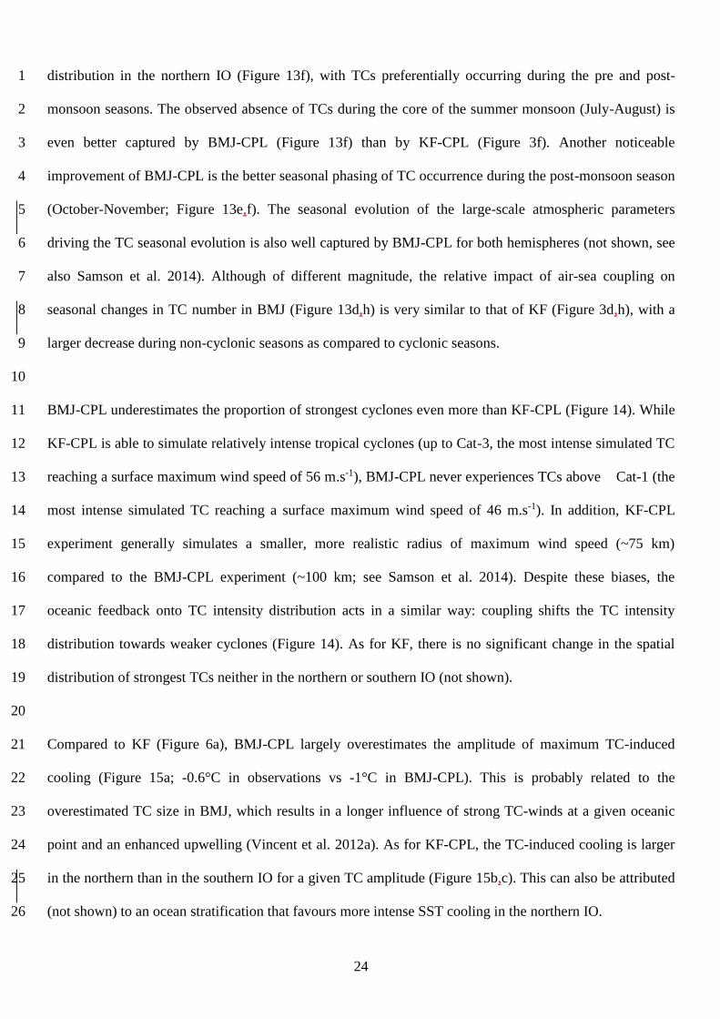
24

distribution in the northern IO (Figure 13f), with TCs preferentially occurring during the pre and post-1

monsoon seasons. The observed absence of TCs during the core of the summer monsoon (July-August) is 2

even better captured by BMJ-CPL (Figure 13f) than by KF-CPL (Figure 3f). Another noticeable 3

improvement of BMJ-CPL is the better seasonal phasing of TC occurrence during the post-monsoon season 4

(October-November; Figure 13e,f). The seasonal evolution of the large-scale atmospheric parameters 5

driving the TC seasonal evolution is also well captured by BMJ-CPL for both hemispheres (not shown, see 6

also Samson et al. 2014). Although of different magnitude, the relative impact of air-sea coupling on 7

seasonal changes in TC number in BMJ (Figure 13d,h) is very similar to that of KF (Figure 3d,h), with a 8

larger decrease during non-cyclonic seasons as compared to cyclonic seasons. 9

10

BMJ-CPL underestimates the proportion of strongest cyclones even more than KF-CPL (Figure 14). While 11

KF-CPL is able to simulate relatively intense tropical cyclones (up to Cat-3, the most intense simulated TC 12

reaching a surface maximum wind speed of 56 m.s-1), BMJ-CPL never experiences TCs above Cat-1 (the 13

most intense simulated TC reaching a surface maximum wind speed of 46 m.s-1). In addition, KF-CPL 14

experiment generally simulates a smaller, more realistic radius of maximum wind speed (~75 km) 15

compared to the BMJ-CPL experiment (~100 km; see Samson et al. 2014). Despite these biases, the 16

oceanic feedback onto TC intensity distribution acts in a similar way: coupling shifts the TC intensity 17

distribution towards weaker cyclones (Figure 14). As for KF, there is no significant change in the spatial 18

distribution of strongest TCs neither in the northern or southern IO (not shown). 19

20

Compared to KF (Figure 6a), BMJ-CPL largely overestimates the amplitude of maximum TC-induced 21

cooling (Figure 15a; -0.6°C in observations vs -1°C in BMJ-CPL). This is probably related to the 22

overestimated TC size in BMJ, which results in a longer influence of strong TC-winds at a given oceanic 23

point and an enhanced upwelling (Vincent et al. 2012a). As for KF-CPL, the TC-induced cooling is larger 24

in the northern than in the southern IO for a given TC amplitude (Figure 15b,c). This can also be attributed 25

(not shown) to an ocean stratification that favours more intense SST cooling in the northern IO. 26

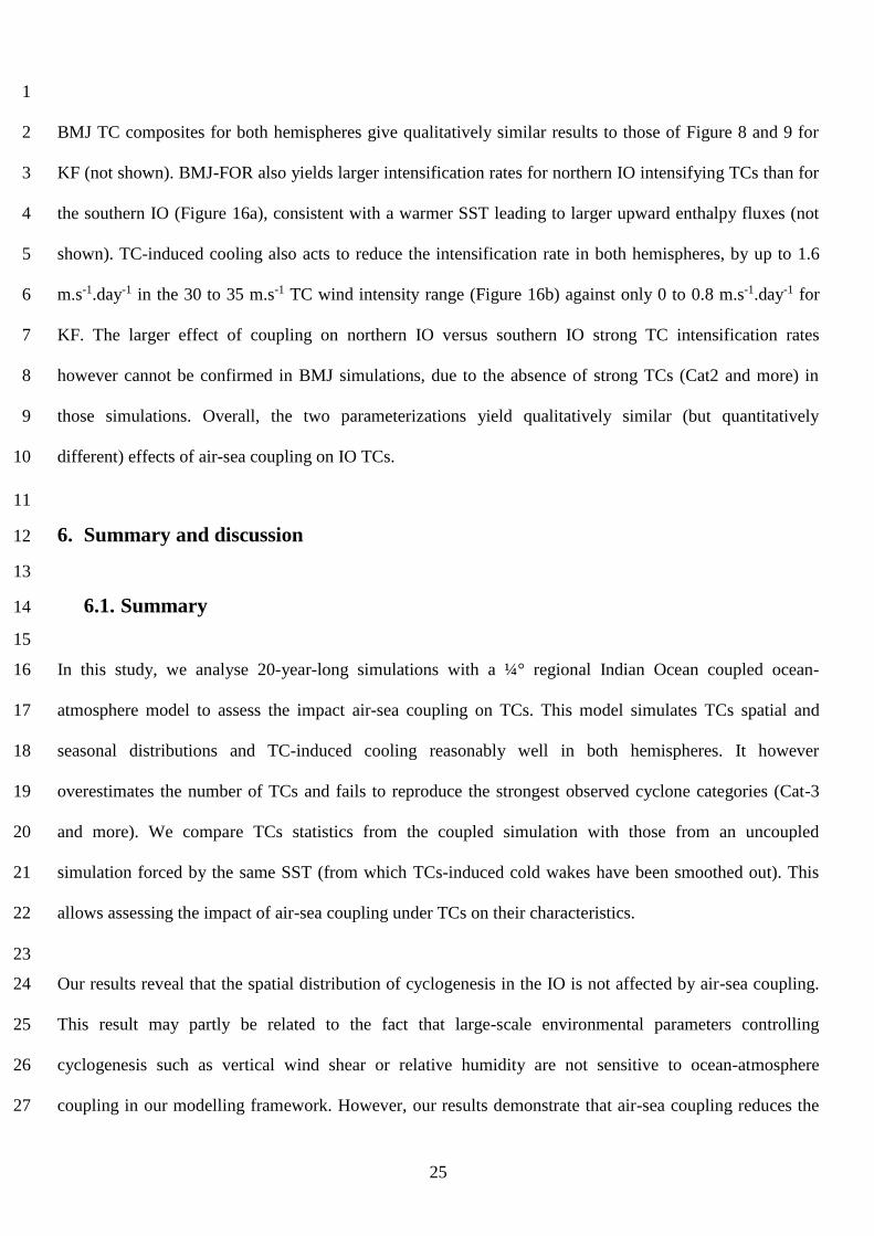
25

1

BMJ TC composites for both hemispheres give qualitatively similar results to those of Figure 8 and 9 for 2

KF (not shown). BMJ-FOR also yields larger intensification rates for northern IO intensifying TCs than for 3

the southern IO (Figure 16a), consistent with a warmer SST leading to larger upward enthalpy fluxes (not 4

shown). TC-induced cooling also acts to reduce the intensification rate in both hemispheres, by up to 1.6 5

m.s-1.day-1 in the 30 to 35 m.s-1 TC wind intensity range (Figure 16b) against only 0 to 0.8 m.s-1.day-1 for 6

KF. The larger effect of coupling on northern IO versus southern IO strong TC intensification rates 7

however cannot be confirmed in BMJ simulations, due to the absence of strong TCs (Cat2 and more) in 8

those simulations. Overall, the two parameterizations yield qualitatively similar (but quantitatively 9

different) effects of air-sea coupling on IO TCs. 10

11

6. Summary and discussion 12

13

6.1. Summary 14

15

In this study, we analyse 20-year-long simulations with a ¼° regional Indian Ocean coupled ocean-16

atmosphere model to assess the impact air-sea coupling on TCs. This model simulates TCs spatial and 17

seasonal distributions and TC-induced cooling reasonably well in both hemispheres. It however 18

overestimates the number of TCs and fails to reproduce the strongest observed cyclone categories (Cat-3 19

and more). We compare TCs statistics from the coupled simulation with those from an uncoupled 20

simulation forced by the same SST (from which TCs-induced cold wakes have been smoothed out). This 21

allows assessing the impact of air-sea coupling under TCs on their characteristics. 22

23

Our results reveal that the spatial distribution of cyclogenesis in the IO is not affected by air-sea coupling. 24

This result may partly be related to the fact that large-scale environmental parameters controlling 25

cyclogenesis such as vertical wind shear or relative humidity are not sensitive to ocean-atmosphere 26

coupling in our modelling framework. However, our results demonstrate that air-sea coupling reduces the 27

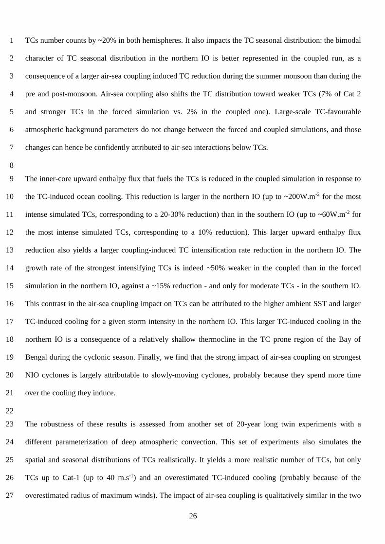
26

TCs number counts by ~20% in both hemispheres. It also impacts the TC seasonal distribution: the bimodal 1

character of TC seasonal distribution in the northern IO is better represented in the coupled run, as a 2

consequence of a larger air-sea coupling induced TC reduction during the summer monsoon than during the 3

pre and post-monsoon. Air-sea coupling also shifts the TC distribution toward weaker TCs (7% of Cat 2 4

and stronger TCs in the forced simulation vs. 2% in the coupled one). Large-scale TC-favourable 5

atmospheric background parameters do not change between the forced and coupled simulations, and those 6

changes can hence be confidently attributed to air-sea interactions below TCs. 7

8

The inner-core upward enthalpy flux that fuels the TCs is reduced in the coupled simulation in response to 9

the TC-induced ocean cooling. This reduction is larger in the northern IO (up to ~200W.m-2 for the most 10

intense simulated TCs, corresponding to a 20-30% reduction) than in the southern IO (up to ~60W.m-2 for 11

the most intense simulated TCs, corresponding to a 10% reduction). This larger upward enthalpy flux 12

reduction also yields a larger coupling-induced TC intensification rate reduction in the northern IO. The 13

growth rate of the strongest intensifying TCs is indeed ~50% weaker in the coupled than in the forced 14

simulation in the northern IO, against a ~15% reduction - and only for moderate TCs - in the southern IO. 15

This contrast in the air-sea coupling impact on TCs can be attributed to the higher ambient SST and larger 16

TC-induced cooling for a given storm intensity in the northern IO. This larger TC-induced cooling in the 17

northern IO is a consequence of a relatively shallow thermocline in the TC prone region of the Bay of 18

Bengal during the cyclonic season. Finally, we find that the strong impact of air-sea coupling on strongest 19

NIO cyclones is largely attributable to slowly-moving cyclones, probably because they spend more time 20

over the cooling they induce. 21

22

The robustness of these results is assessed from another set of 20-year long twin experiments with a 23

different parameterization of deep atmospheric convection. This set of experiments also simulates the 24

spatial and seasonal distributions of TCs realistically. It yields a more realistic number of TCs, but only 25

TCs up to Cat-1 (up to 40 m.s-1) and an overestimated TC-induced cooling (probably because of the 26

overestimated radius of maximum winds). The impact of air-sea coupling is qualitatively similar in the two 27

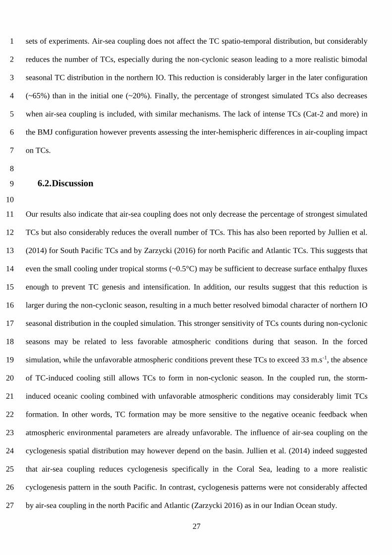
27

sets of experiments. Air-sea coupling does not affect the TC spatio-temporal distribution, but considerably 1

reduces the number of TCs, especially during the non-cyclonic season leading to a more realistic bimodal 2

seasonal TC distribution in the northern IO. This reduction is considerably larger in the later configuration 3

(~65%) than in the initial one (~20%). Finally, the percentage of strongest simulated TCs also decreases 4

when air-sea coupling is included, with similar mechanisms. The lack of intense TCs (Cat-2 and more) in 5

the BMJ configuration however prevents assessing the inter-hemispheric differences in air-coupling impact 6

on TCs. 7

8

6.2. Discussion 9

10

Our results also indicate that air-sea coupling does not only decrease the percentage of strongest simulated 11

TCs but also considerably reduces the overall number of TCs. This has also been reported by Jullien et al. 12

(2014) for South Pacific TCs and by Zarzycki (2016) for north Pacific and Atlantic TCs. This suggests that 13

even the small cooling under tropical storms (~0.5°C) may be sufficient to decrease surface enthalpy fluxes 14

enough to prevent TC genesis and intensification. In addition, our results suggest that this reduction is 15

larger during the non-cyclonic season, resulting in a much better resolved bimodal character of northern IO 16

seasonal distribution in the coupled simulation. This stronger sensitivity of TCs counts during non-cyclonic 17

seasons may be related to less favorable atmospheric conditions during that season. In the forced 18

simulation, while the unfavorable atmospheric conditions prevent these TCs to exceed 33 m.s-1, the absence 19

of TC-induced cooling still allows TCs to form in non-cyclonic season. In the coupled run, the storm-20

induced oceanic cooling combined with unfavorable atmospheric conditions may considerably limit TCs 21

formation. In other words, TC formation may be more sensitive to the negative oceanic feedback when 22

atmospheric environmental parameters are already unfavorable. The influence of air-sea coupling on the 23

cyclogenesis spatial distribution may however depend on the basin. Jullien et al. (2014) indeed suggested 24

that air-sea coupling reduces cyclogenesis specifically in the Coral Sea, leading to a more realistic 25

cyclogenesis pattern in the south Pacific. In contrast, cyclogenesis patterns were not considerably affected 26

by air-sea coupling in the north Pacific and Atlantic (Zarzycki 2016) as in our Indian Ocean study. 27

28

1

Our results reveal the sensitivity of TCs intensification to air-sea coupling is very different between the 2

northern and southern IO. This sensitivity is rather modest in the southern IO: there is a ~10% enthalpy flux 3

reduction, similar for all TCs strength, but the response in terms of intensification rate changes mainly 4

affect modest TCs, with weak intensification rate changes for the strongest simulated TCs. In contrast, this 5

impact is stronger and larger (~25% enthalpy flux reduction) for the most intense simulated TCs (45 to 50 6

m.s-1) than for modest for weak TCs (~10% enthalpy flux reduction) in the northern IO. This results in a 7

modest impact of air-sea coupling on TCs intensification rate for weak TCs but in a considerable impact for 8

the strongest simulated TCs (Vmax>35 m.s-1), with a ~30% reduction when air-sea coupling is accounted 9

for. Our results further reveal that this impact is even larger when considering only slow moving TCs 10

(~50% reduction). The amplitude of the coupled feedback derived from this analysis is in line with the 11

observational estimates from Cione and Uhlhorn (2003), who reported a total enthalpy fluxes reduction 12

within the core (radius of 60 km) of ~40% for strong TCs. They are also in line with model estimate of 13

Zarzycki (2016) who reported a 20% enthalpy flux reduction for all TCs and a ~30% reduction for Cat-1 14

and more TCs. This larger impact of air-sea coupling on strongest TCs has already been reported in several 15

studies (Jullien et al. 2014; Zarzycki 2016; Vincent et al. 2014). 16

17

The fact that two convective parameterizations that yield quite different TC numbers, radius and intensity 18

in general provide qualitatively similar results about the influence of air-sea coupling is re-assuring. 19

However, the inability of BMJ to yield strong cyclones limits our ability to evaluate the robustness of our 20

results with respect to TC intensity. Our results additionally suggest that the TC-intensity dependence of 21

our results is sensitive to the convective parameterization. Using the Bett-Miller-Janjic cumulus 22

parameterization instead of that of Kain-Fritsch indeed yields a stronger sensitivity (1 to 2 m.s-1.day-1) for 23

modest TCs (30-35 m.s-1) as compared to our reference configuration (0 to 0.6 m.s-1.day-1). This suggests 24

that the modelled reduction rate may depend on the convective parameterization, calling for further studies 25

employing varying atmospheric configurations as well as a higher spatial resolution allowing to resolve 26

strongest TCs. 27

29

1

As discussed above, most studies discussing the impact of air-sea coupling on TCs suggest a considerably 2

larger impact of air-sea coupling on the strongest simulated TCs. As for other regional modelling studies 3

(Jullien et al., 2014; Ogata et al., 2015), the rather coarse resolution of our model (1/4°) does not allow to 4

simulate strongest TCs (Category 3 and above), as this resolution smoothens the sharp tangential winds 5

eyewall structure and underestimates the strongest eyewall updrafts and compensating inner-eye subsidence 6

(Gentry and Lackmann 2010). A more realistic distribution of extreme TCs would require an atmospheric 7

model with finer resolution of ~10km (Jung et al., 2012; Manganello et al. 2012; Satoh et al., 2012; 8

Murakami et al., 2015). A promising follow-up to the present work would hence be to develop a ~10km 9

resolution regional air-sea coupled model using the same oceanic and atmospheric components for the 10

BoB, where air-sea coupling seems to have a particularly strong negative feedback on slowly-moving 11

intense TCs (which are also the most destructive ones),due to warm SST and a relatively shallow 12

thermocline. This would allow assessing the impact of air-sea coupling in this region, where 14 of the 20 13

deadliest cyclones in history have developed (Longshore 2008). 14

15

16

Acknowledgments: ML, NS and JV thank IFCPAR (Indo French Centre for Promotion of 17

Advanced Research), New Delhi for funding of the proposal 4907-1. NS and IS thank Director, CSIR-NIO 18

for his encouragement. This work was done while ML was a visiting scientist at the CSIR-National 19

Institute of Oceanography (NIO) in Goa, under Institut de Recherche pour le Développement (IRD) 20

funding. JV also acknowledges IRD support for regular visits to NIO. This is NIO contribution number 21

xxxx. 22

23

30

References: 1

Ali MM, Jagadeesh PSV, Jain S (2007) Effects of eddies on Bay of Bengal cyclone intensity. Eos Trans Amer

Geophys. Union 88: 93-95. doi: 10.1029/2007EO080001.

Balaguru K, GR Foltz, LR Leung, ED Asaro, KA Emanuel, H Liu, and SE Zedler (2015) Dynamic Potential

Intensity: An improved representation of the ocean's impact on tropical cyclones. Geophys Res Lett, 42 : 6739-

6746, doi :10.1002/2015GL064822

Bender MA, I Ginis and Y Kurihara (1993) Numerical simulations of tropical cyclone- ocean interaction with a high-

resolution coupled model. J Geophys Res 98:23245-23263. doi:10.1029/93JD02370

Bender MA and I Ginis (2000) Real-case simulations of hurricane-ocean interaction using a high-resolution coupled

model: Effects on hurricane intensity. Mon Wea Rev, 128:917-946. doi:10.1175/1520-

0493(2000)128<0917:RCSOHO>2.0.CO;2

Blanke B, and P Delecluse (1993) Variability of the tropical Atlantic ocean simulated by a general circulation model

with two different mixed layer physics. J Phys Oceanogr, 23:1363-1388. doi:10.1175/1520-

0485(1993)023<1363:VOTTAO>2.0.CO;2

Brodeau L, B Barnier, A-M Treguier, T Penduff and S Gulev (2010) An ERA40-based atmospheric forcing for

global ocean circulation models, Ocean Modelling 31:88-104. doi:10.1016/j.ocemod.2009.10.005. doi: 10.1016/j.ocemod.2009.10.005.

Cione JJ and EW Uhlhorn (2003) Sea surface temperature variability in hurricanes: Implications with respect to

intensity change. Mon Wea Rev 131:1783–1796.

Chen F, K Mitchell, J Schaake, Y Xue, H-L Pan, V Koren, QY Duan, M Ek and A Betts (1996) Modeling of land

surface evaporation by four schemes and comparison with FIFE observations. J Geophys Res, 101:7251-7268.

doi:10.1029/95JD02165.

Chen S, TJ Campbell, H Jin, S Gabersek, RM Hodur, P Martin (2010) Effect of Two-Way Air–Sea Coupling in High

and Low Wind Speed Regimes. Mon Wea Rev 138:3579–3602. doi: 10.1175/2009MWR3119.1.

Chou M and M Suarez (1999) A solar radiation parameterization for atmospheric studies, Tech Rep NASA/TM-

1999-104606, NASA/GSFC.

Dee DP, SM Uppala, AJ Simmons et al. (2011) The ERA-Interim reanalysis: Configuration and performance of the

data assimilation system. Q J Roy Meteorol Soc 137:553–597. doi: 10.1002/qj.828

DeMaria M (1996) The effect of vertical shear on tropical cyclone intensity change. J Atmos Sci 53:2076–2087.

doi:10.1175/1520-0469(1996)053<2076:TEOVSO>2.0.CO;2

DeMaria M, M Mainelli, LK Shay, JA Knaff and J Kaplan (2005) Further Improvements in the Statistical Hurricane

Intensity Prediction Scheme (SHIPS). Wea Forecasting 20:531-543. doi:10.1175/WAF862.1

DeMaria M, CR Sampson, JA Knaff, KD Musgrave (2014) Is tropical cyclone intensity guidance improving? Bull

Amer Meteor Soc,95:387-398. doi:10.1175/BAMS-D-12-00240.1

Donelan MA, BK Haus, N Reul, WJ Plant, M Stiassnie, HC Graber, OB Brown and ES Saltzman (2004) On the

limiting aerodynamic roughness of the ocean in very strong winds. Geophys Res Lett 31 L18306.

doi:10.1029/2004GL019460.

Emanuel KA (1986) An air-sea interaction theory for tropical cyclones. Part 1 : Steady-state maintenance. J Atmos

Sci 43:585–604. doi:10.1175/1520-0469(1986)043<0585:AASITF>2.0.CO;2

Emanuel KA (1999) Thermodynamic control of hurricane intensity. Nature, 401:665-669.doi:10.1038/44326.

Emanuel K (2003) Tropical cyclones. Annu Rev Earth Planet Sci 31:75-104. doi:

10.1146/annurev.earth.31.100901.141259

Emanuel KA, DS Nolan (2004) Tropical cyclone activity and global climate. 26th Conf. on Hurricanes and Tropical

Meteorology, Miami, FL, Amer. Meteor. Soc. pp 240–241.

Gentry MS and G Lackmann (2010) Sensitivity of simulated tropical cyclone structure and intensity to horizontal

resolution. Mon Wea Rev 138:688–704. doi: 10.1175/2009MWR2976.1.

Girishkumar MS, K Suprit, J Chiranjivi, TVS Udaya Bhaskar, M Ravichandran, R Venkat Shesu and E Pattabhi

Rama Rao (2014) Observed Oceanic response to tropical cyclone Jal from a moored buoy in the south-western

Bay of Bengal. Ocean Dyn 64:325-335. doi:10.1007/s10236-014-0689-6.

31

Halliwell GR, LK Shay, J Brewster and WJ Teague (2011) Evaluation and sensitivity analysis to an ocean model

response to hurricane Ivan. Mon Wea Rev 139:921-945. doi:10.1175/2010MWR3104.1.

Halliwell GR, S Gopalakrishnan, F Marks, D Willey (2015) Idealized study of ocean impacts on tropical cyclone

intensity forecasts. Mon Wea Rev 143:1142-1165. doi: 10.1175/MWR-D-14-00022.1.

Hong X, SW Chang, S Raman, LK Shay and R Hodur (2000) The interaction between Hurricane Opal (1995) and a

warm core eddy in the Gulf of Mexico. Mon Wea Rev 128:1347-1365. doi:10.1175/1520-

0493(2000)128<1347:TIBHOA>2.0.CO;2

Hong S-Y and J-OJ Lim (2006) The WRF Single-Moment 6-Class Microphysics Scheme (WSM6), Asia-Pacific, J.

Atmos. Sci. 42:129–151.

Ito K, T Kuroda and K Saito (2015) Forecasting a large number of tropical cyclone intensities around Japan using a

high-resolution atmosphere-ocean coupled model. Wea Forecasting 30:793–808. doi:10.1175/WAF-D-14-

00034.1.

Janjic ZI (1994) The step-mountain Eta coordinate model: Further developments of the convection, viscous sublayer,

and turbulence closure schemes. Mon Wea Rev 122:927–945. doi:10.1175/1520-

0493(1994)122<0927:TSMECM>2.0.CO;2.

Jourdain NC, Marchesiello P, Menkes CE, et al (2011) Mesoscale Simulation of Tropical Cyclones in the South

Pacific: Climatology and Interannual Variability. J Clim 24:3–25. doi: 10.1175/2010JCLI3559.1

Jullien S, CE Menkes, P Marchesiello, NC Jourdain, M Lengaigne, A Koch-Larrouy, J Lefèvre, EM Vincent and V

Faure (2012) Impact of tropical cyclones on the heat budget of the South Pacific Ocean. J Phys Oceanogr

42(11):1882-1906. doi :10.1175/JPO-D-11-0133.1.

Jullien S, P Marchesiello, CE Menkes, J Lefevre, NC Jourdain, G Samson and M Lengaigne (2014) Ocean feedback

to tropical cyclones: Climatology and processes. Clim Dyn 43:,2831–2854. doi:10.1007/s00382-014-2096-6

Kain JS (2004) The Kain-Fritsch convective parameterization: An update. J Appl Meteorol 43:170-181,

doi:10.1175/1520-0450(2004)043<0170:TKCPAU>2.0.CO;2.

Knapp KR, MC Kruk, DH Levinson, HJ Diamond and CJ Neumann (2010) The International Best Track Archive for

Climate Stewardship (IBTrACS): Unifying Tropical Cyclone Data. Bull Amer Meteor Soc 91(3):363-376.

doi:10.1175/2009BAMS2755.1.

Lengaigne M, G Madec, CE Menkes and G Alory (2003) Impact of isopycnal mixing on the tropical ocean

circulation. J Geophys Res 108 C11. doi:10.1029/2002JC001704.

Li Z, W Yu, T Li, VSN Murty and F Tangang (2013) Bimodal character of cyclone climatology in Bay of Bengal

modulated by monsoon seasonal cycle. J Clim 26:1033-1046. doi:10.1175/JCLI-D-11-00627.1

Lin II, CC Wu, KA Emanuel, IH Lee, CR Wu and IF Pun (2005) The interaction of Supertyphoon Maemi (2003)

with a warm ocean eddy. Mon Wea Rev 133:2635–2649. doi: 10.1175/MWR3005.1.

Lin II, CH Chen, IF Pun, WT Liu and CC Wu (2009) Warm ocean anomaly, air sea fluxes, and the rapid

intensification of tropical cyclone Nargis (2008). Geophys Res Lett 36 L03817. doi:10.1029/ 2008GL035815.

Liu B, H Liu, L Xie, C Guan and D Zhao (2011) A coupled atmosphere-wave-ocean modeling system: Simulation of

the intensity of an idealized tropical cyclone. Mon Wea Rev 139:132-152. doi:10.1175/2010MWR3396.1

Lloyd ID and GA Vecchi (2011) Observational evidence of oceanic controls on hurricane intensity. J Clim. 24:1138–

1153. doi: 10.1175/2010JCLI3763.1.

Longshore D (2008) Encyclopedia of Hurricanes, Typhoons, and Cyclones. Checkmark books. 468 pp, ISBN 978-0-

8160-7409-9.

Ma Z, J Fei, L Liu, X Huang and X Cheng (2013) Effects of the cold core eddy on tropical cyclone intensity and

structure under idealized air-sea interaction conditions, Mon Wea Rev 141 :1285-1303. doi:10.1175/MWR-D-

12-00123.1

Madec G (2008) NEMO ocean engine. Note du Pôle de modélisation, Institut Pierre-Simon Laplace (IPSL),27, ISSN

No 1288-1619.

Mainelli M, M DeMaria, LK Shay and G Goni (2008) Application of oceanic heat content estimation to operational

forecasting of recent Atlantic category 5 hurricanes. Wea Forecasting 23:3-16. doi: 10.1175/2007WAF2006111.1.

Masumoto, Y., & Meyers, G. (1998). Forced Rossby waves in the southern tropical Indian Ocean. J. Geophys. Res.:

103:27589-27602. doi: 10.1029/98JC02546.

32

Mavume AF, L Rydberg, M Rouault, JRE Lutjeharms (2009) Climatology and landfall of tropical cyclones in the

south-west Indian Ocean. Western Indian Ocean Journal of Marine Science 8:15-36. doi: 0.4314/wiojms.v8i1.56672.

McPhaden MJ, GR Foltz, T Lee, VSN Murty, M Ravichandran, GA Vecchi, J Vialard, JD Wiggert and L Yu (2009)

Ocean-atmosphere interactions during cyclone Nargis. Eos Trans Amer Geophys Union 90:53-54,

doi:10.1029/2009EO070001.

Mei W, C Pasquero and F Primeau (2012) The effect of translation speed upon the intensity of tropical cyclones over

the tropical ocean. Geophys Res Lett 39 L07801. doi:10.1029/2011GL050765.

Menkes CE, M Lengaigne, P Marchesiello, N Jourdain, EM Vincent, J Lefèvre, F Chauvin, J-F Royer

(2012) Comparison of tropical cyclogenesis indices on seasonal to interannual timescales. Clim Dyn 38(1-

2):301-321 doi 10.1007/s00382-011-1126-x.

Mlawer EJ, SJ Taubman, PD Brown, MJ Iacono and SA Clough (1997) Radiative transfer for inhomogeneous

atmospheres: RRTM, a validated correlated-k model for the longwave. J Geophys Res 102(D14):16663–

166682, doi:10.1029/97JD00237.

Miyamoto Y, GH Bryan and R Rotunno (2017) An analytical model of maximum potential intensity for tropical

cyclones incorporating the effect of ocean mixing, Geophys Res Lett, 44:5826–5835,

doi:10.1002/2017GL073670.

Neetu S, Lengaigne M, Vincent EM, et al (2012) Influence of upper‐ocean stratification on tropical cyclone‐induced

surface cooling in the Bay of Bengal. J. Geophys. Res. 117:C12020. doi: 10.1029/2012JC008433

Noh Y, WG Cheon, SY Hong and S Raasch (2003) Improvement of the K-profile model for the planetary boundary

layer based on large eddy simulation data. Boundary Layer Meteorol 107(2):401-427.

doi:10.1023/A:1022146015946.

Ogata T, R Mizuta, Y Adachi, H Murakami and T Ose (2015) Effect of air-sea coupling on the frequency distribution

of intense tropical cyclones over the northwestern Pacific, Geophys Res Lett 42:10415–10421. doi:10.1002/

2015GL066774.

Ogata, T., Mizuta, R., Adachi, Y., Murakami, H., & Ose, T. (2016). Atmosphere-ocean coupling effect on intense

tropical cyclone distribution and its future change with 60 km-AOGCM. Scientific reports, 6, 29800.

Périgaud, C., & Delecluse, P. (1992). Annual sea level variations in the southern tropical Indian Ocean from Geosat

and shallow‐water simulations. J Geophys Res 97 :20169-20178. doi : 10.1029/92JC01961.

Price JF (1981) Upper ocean response to a Hurricane. J Phys Oceanogr 11:153-175. doi:10.1175/1520-

0485(1981)011<0153:UORTAH>2.0.CO;2

Riehl H (1950) A model of hurricane formation. J Applied Physics 21, 917–925. doi: 10.1063/1.1699784.

Saji, N. H., B. N. Goswami, P. N. Vinayachandran and T. Yamagata, 1999: A dipole mode in the tropical Indian

Ocean. Nature 401:360-363. doi: 10.1038/43854.

Samson G, S Masson, M Lengaigne, MG Keerthi, J Vialard, S Pous, G Madec, N Jourdain, S Jullien, C Menkes, P

Marchesiello (2014) The NOW regional coupled model: Application to the tropical Indian Ocean climate and

tropical cyclone activity. J. Adv Mod Earth Syst 6(3):700-722. doi:10.1002/2014MS000324.

Schade LR (2000) Tropical cyclone intensity and sea surface temperature. J Atmos Sci 57:3122–3130. doi: 10.1175/1520-0469(2000)057<3122:TCIASS>2.0.CO;2.

Schade LR and KA Emanuel (1999) The ocean’s effect on the inten- sity of tropical cyclones: Results from a simple

coupled atmosphere– ocean model. J Atmos Sci 56:642–651. doi:10.1175/1520-0469

(1999)056<0642:TOSEOT>2.0.CO;2.

Sengupta D, RG Bharath, DS Anitha (2008) Cyclone-induced mixing does not cool SST in the post-monsoon north

Bay of Bengal. Atmos Sci Lett, 9:1-6. doi: 10.1002/asl.162.

Shay LK, G Goni and PG Black (2000) Effects of a warm oceanic feature on Hurricane Opal. Mon Wea Rev

128:1366–1383. doi: 10.1175/1520-0493(2000)128<1366:EOAWOF>2.0.CO;2.

Skamarock WC and JB Klemp (2008) A time-split nonhydrostatic atmospheric model for weather research and

forecasting applications. J Comput Phys 227(7):3465-3485. doi:10.1016/j.jcp.2007.01.037.

Srinivas CV, DV Bhaskar Rao, V Yesubabu, R Baskaran, and B Venkatraman (2013) Tropical cyclone predictions

over the Bay of Bengal using the high-resolution Advanced Research Weather Research and Forecasting

33

(ARW) model. Q J Roy. Meteorol Soc 139(676):1810– 1825. doi:10.1002/qj.2064.

Valcke S (2013) The OASIS3 coupler: A European climate modelling community software, Geosci Model Dev, 6(2),

373–388, doi:10.5194/gmd-6-373-2013.

Vialard J et al. (2009) Cirene: Air sea interactions in the Seychelles-Chagos thermocline ridge region. Bull Am

Meteorol Soc 90,:45–61. doi:10.1175/2008BAMS2499.1.

Vincent EM, M Lengaigne, G Madec, J Vialard, G Samson, N Jourdain, CE Menkes, S Jullien (2012a) Processes

setting the characteristics of sea surface cooling induced by tropical cyclones. J Geophys Res 117 C02020.

doi:10.1029/2011JC007396.

Vincent EM, M Lengaigne, J Vialard, G Madec, N Jourdain, S Masson (2012b) Assessing the Oceanic Control on the

Amplitude of sea Surface Cooling induced by Tropical Cyclones. J Geophys Res 117 C05023.

doi:10.1029/2011JC007705.

Vincent EM, KA Emanuel, M Lengaigne, J Vialard, G Madec (2014) Influence of upper ocean stratification

interannual variability on tropical cyclones. J Adv Mod Earth Syst 6(3):680-699. doi: 10.1002/2014MS000327

Wang Y and CC Wu (2004) Current understanding of tropical cyclone structure and intensity changes—A review.

Meteor Atmos Phys 87:257–278. doi:10.1007/s00703-003-0055-6.

Webster, P. J., A. M. Moore, J. P. Loschnigg, and R. R. Leben, 1999: Coupled oceanic–atmospheric dynamics in the

Indian Ocean during 1997–98. Nature 401:356–360. doi:10.1038/43848

Xie S-P, H Annamalai, FA Schott and JP McCreary Jr. (2002) Structure and mechanisms of south Indian Ocean

climate variability. J Clim 15(8):864–878. doi: 10.1175/1520-0442(2002)015<0864:SAMOSI>2.0.CO;2.

Xie, S. P., Hu, K., Hafner, J., Tokinaga, H., Du, Y., Huang, G., & Sampe, T. (2009). Indian Ocean capacitor effect on

Indo–western Pacific climate during the summer following El Niño. J Clim 22 :730-747. doi: 10.1175/2008JCLI2544.1.

Yablonsky RM, and I Ginis (2009) Limitation of one-dimensional ocean models for coupled hurricane-ocean model

forecasts. Mon Wea Rev 137:4410–4419. doi:10.1175/2009MWR2863.1.

Yu L and MJ McPhaden (2011) Ocean Preconditioning of Cyclone Nargis in the Bay of Bengal: Interaction between

Rossby Waves, Surface Fresh Waters, and Sea Surface Temperatures. J Phys Oceanogr 41:1741–1755. doi:

10.1175/2011JPO4437.1

Zarzycki CM (2016) Tropical Cyclone Intensity Errors Associated with Lack of Two-Way Ocean Coupling in High-

Resolution Global Simulations. J Clim 29:8589–8610. doi: 10.1175/JCLI-D-16-0273.1.

Zedler SE (2009) Simulations of the ocean response to a hurricane: Nonlinear processes. J Phys Oceanogr 39:2618–

2634. doi: 10.1175/2009JPO4062.1.

Zhu H, U Wolfgang and SK Roger (2004) Ocean effects on tropical cyclone intensification and inner-core

asymmetries. J Atmos Sci 61:1245-1258. doi: 10.1175/1520-0469(2004)061<1245:OEOTCI>2.0.CO;2.

1

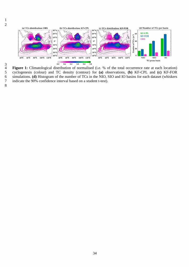
34

1

2

3 Figure 1: Climatological distribution of normalised (i.e. % of the total occurrence rate at each location) 4

cyclogenesis (colour) and TC density (contour) for (a) observations, (b) KF-CPL and (c) KF-FOR 5

simulations. (d) Histogram of the number of TCs in the NIO, SIO and IO basins for each dataset (whiskers 6

indicate the 90% confidence interval based on a student t-test). 7

8

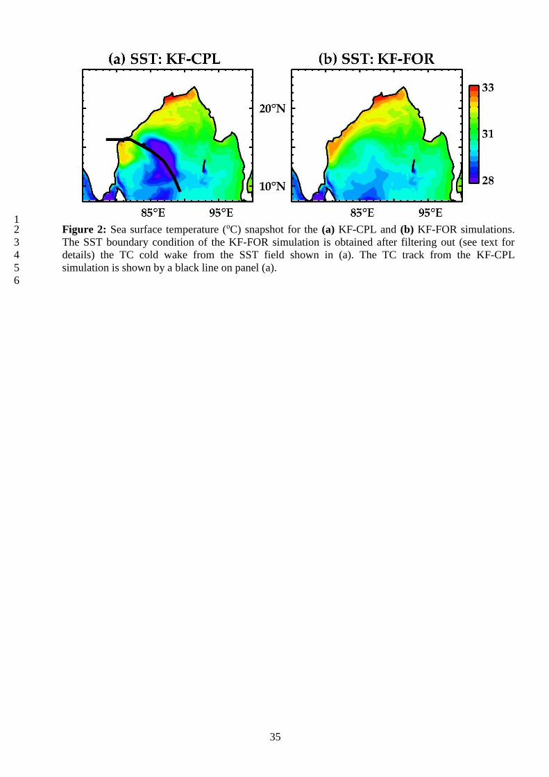
35

1 Figure 2: Sea surface temperature (oC) snapshot for the (a) KF-CPL and (b) KF-FOR simulations. 2

The SST boundary condition of the KF-FOR simulation is obtained after filtering out (see text for 3

details) the TC cold wake from the SST field shown in (a). The TC track from the KF-CPL 4

simulation is shown by a black line on panel (a). 5

6

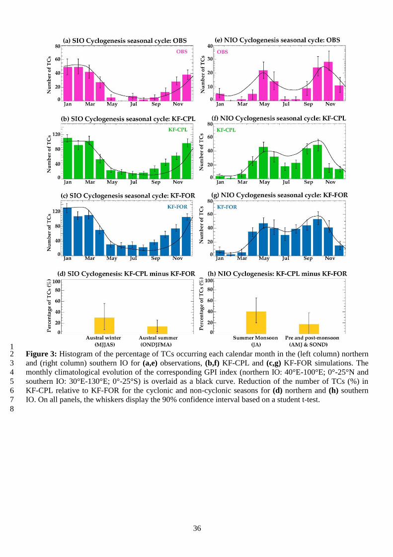
36

1 Figure 3: Histogram of the percentage of TCs occurring each calendar month in the (left column) northern 2

and (right column) southern IO for (a,e) observations, (b,f) KF-CPL and (c,g) KF-FOR simulations. The 3

monthly climatological evolution of the corresponding GPI index (northern IO: 40°E-100°E; 0°-25°N and 4

southern IO: 30°E-130°E; 0°-25°S) is overlaid as a black curve. Reduction of the number of TCs (%) in 5

KF-CPL relative to KF-FOR for the cyclonic and non-cyclonic seasons for (d) northern and (h) southern 6

IO. On all panels, the whiskers display the 90% confidence interval based on a student t-test. 7

8

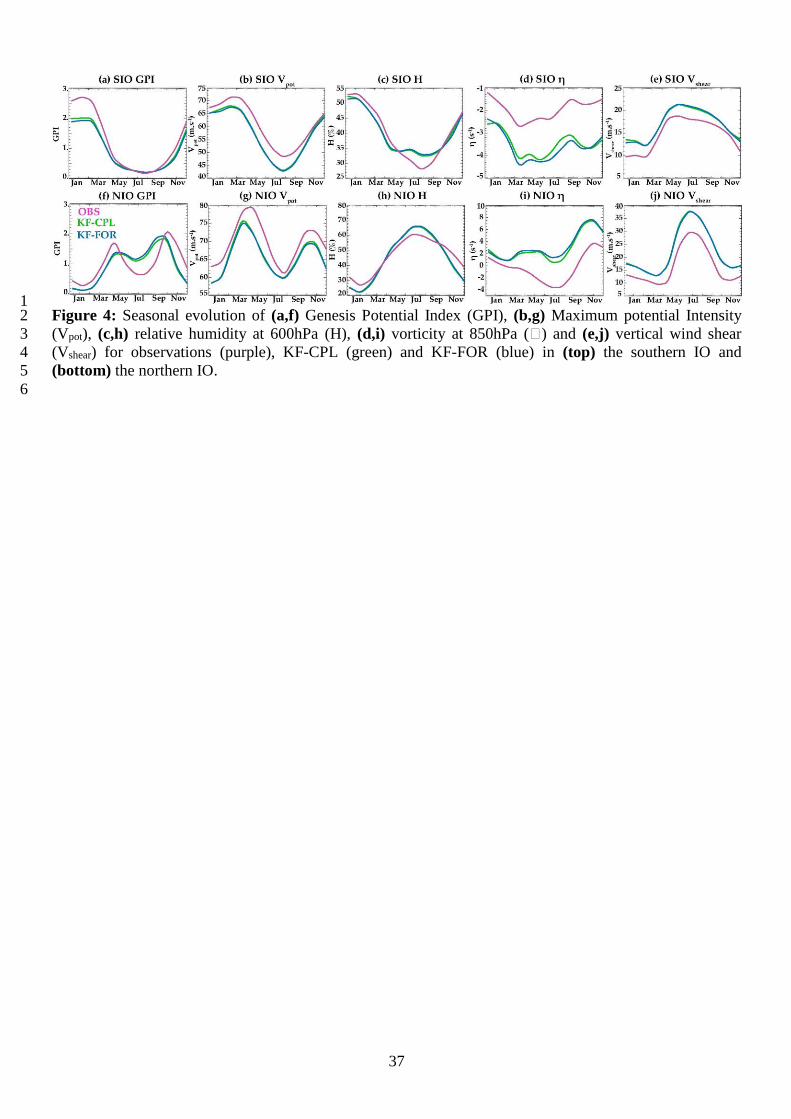
37

1 Figure 4: Seasonal evolution of (a,f) Genesis Potential Index (GPI), (b,g) Maximum potential Intensity 2

(Vpot), (c,h) relative humidity at 600hPa (H), (d,i) vorticity at 850hPa () and (e,j) vertical wind shear 3

(Vshear) for observations (purple), KF-CPL (green) and KF-FOR (blue) in (top) the southern IO and 4

(bottom) the northern IO. 5

6

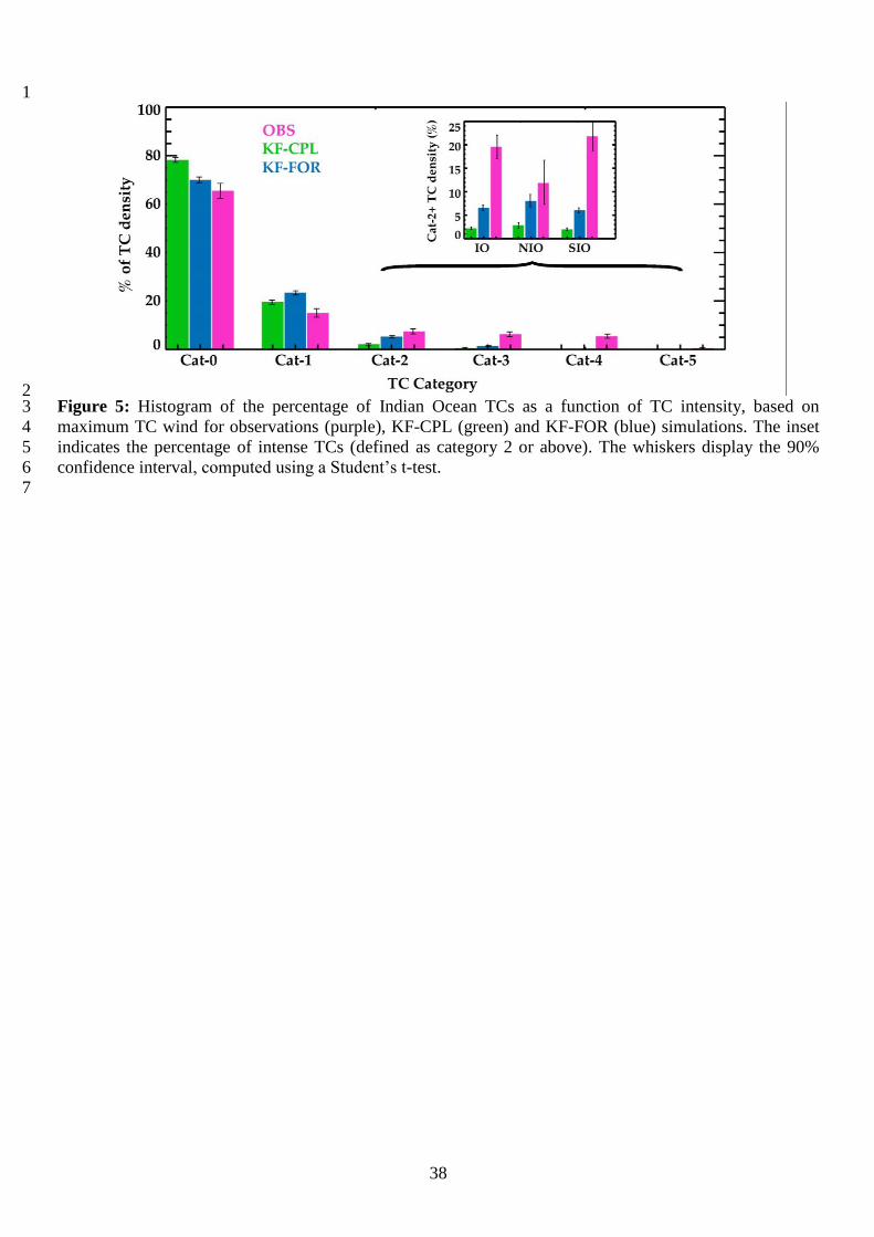
38

1

2 Figure 5: Histogram of the percentage of Indian Ocean TCs as a function of TC intensity, based on 3

maximum TC wind for observations (purple), KF-CPL (green) and KF-FOR (blue) simulations. The inset 4

indicates the percentage of intense TCs (defined as category 2 or above). The whiskers display the 90% 5

confidence interval, computed using a Student’s t-test. 6

7

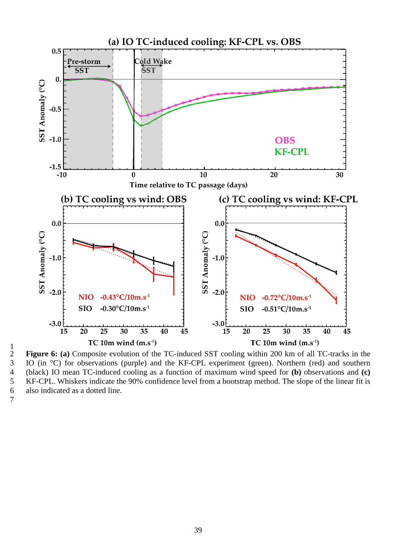
39

1 Figure 6: (a) Composite evolution of the TC-induced SST cooling within 200 km of all TC-tracks in the 2

IO (in °C) for observations (purple) and the KF-CPL experiment (green). Northern (red) and southern 3

(black) IO mean TC-induced cooling as a function of maximum wind speed for (b) observations and (c) 4

KF-CPL. Whiskers indicate the 90% confidence level from a bootstrap method. The slope of the linear fit is 5

also indicated as a dotted line. 6

7

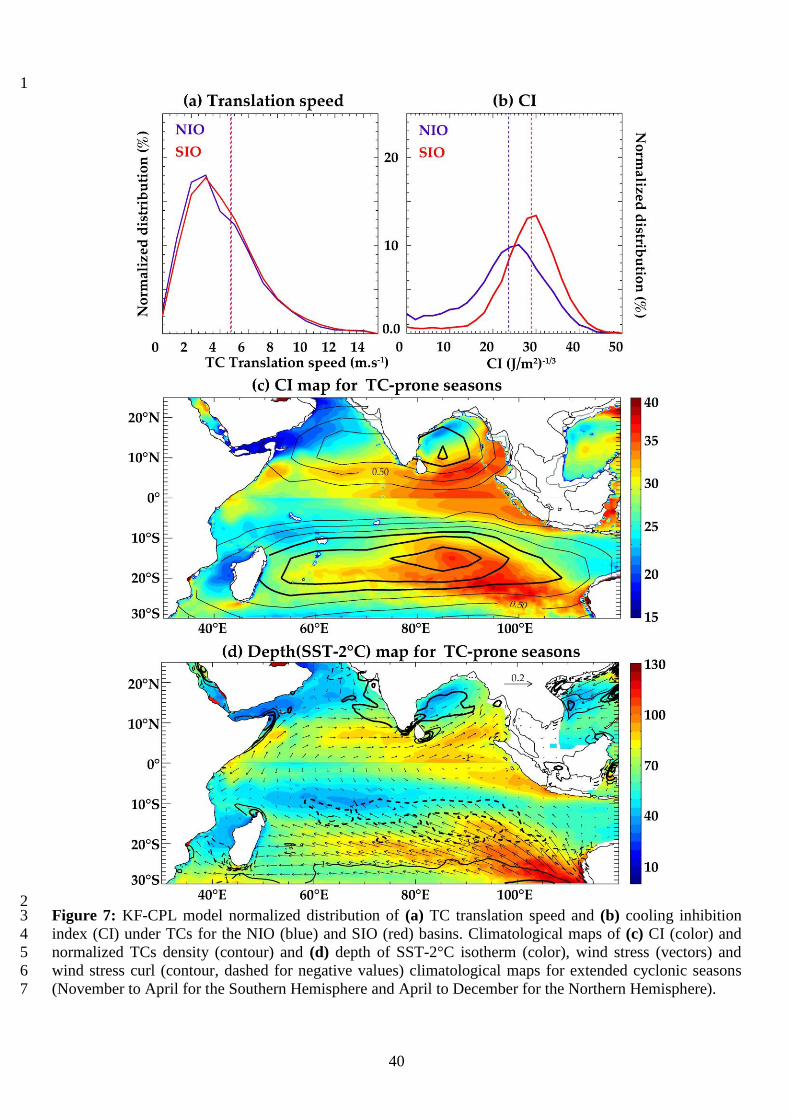
40

1

2 Figure 7: KF-CPL model normalized distribution of (a) TC translation speed and (b) cooling inhibition 3

index (CI) under TCs for the NIO (blue) and SIO (red) basins. Climatological maps of (c) CI (color) and 4

normalized TCs density (contour) and (d) depth of SST-2°C isotherm (color), wind stress (vectors) and 5

wind stress curl (contour, dashed for negative values) climatological maps for extended cyclonic seasons 6

(November to April for the Southern Hemisphere and April to December for the Northern Hemisphere). 7

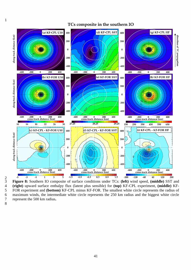
41

1

2 Figure 8: Southern IO composite of surface conditions under TCs: (left) wind speed, (middle) SST and 3

(right) upward surface enthalpy flux (latent plus sensible) for (top) KF-CPL experiment, (middle) KF-4

FOR experiment and (bottom) KF-CPL minus KF-FOR. The smallest white circle represents the radius of 5

maximum winds, the intermediate white circle represents the 250 km radius and the biggest white circle 6

represent the 500 km radius. 7

8

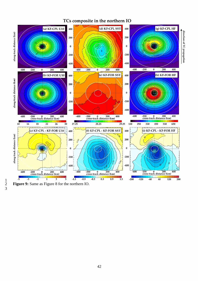
42

1 Figure 9: Same as Figure 8 for the northern IO. 2

3

43

1 Figure 10: Mean (a) inner-core (i.e. within 200 km of the TC centre) upward surface enthalpy flux, (b) 2

time-derivative of maximum wind speed and (c) inner-core (i.e. within 200 km of the TC centre) SST as a 3

function of the wind speed for intensifying TCs in the KF-FOR experiment, over the northern(blue) and 4

southern(red) IO. This figure was performed by averaging within 5 m.s-1 bins. 5

6

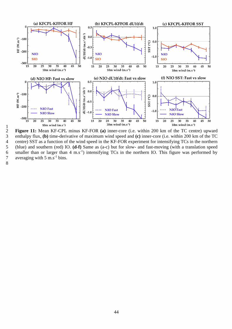
44

1 Figure 11: Mean KF-CPL minus KF-FOR (a) inner-core (i.e. within 200 km of the TC centre) upward 2

enthalpy flux, (b) time-derivative of maximum wind speed and (c) inner-core (i.e. within 200 km of the TC 3

centre) SST as a function of the wind speed in the KF-FOR experiment for intensifying TCs in the northern 4

(blue) and southern (red) IO. (d-f) Same as (a-c) but for slow- and fast-moving (with a translation speed 5

smaller than or larger than 4 m.s-1) intensifying TCs in the northern IO. This figure was performed by 6

averaging with 5 m.s-1 bins. 7

8

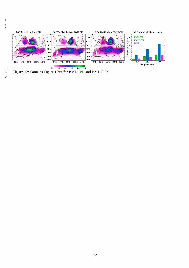
45

1

2

3

4 Figure 12: Same as Figure 1 but for BMJ-CPL and BMJ-FOR. 5

6

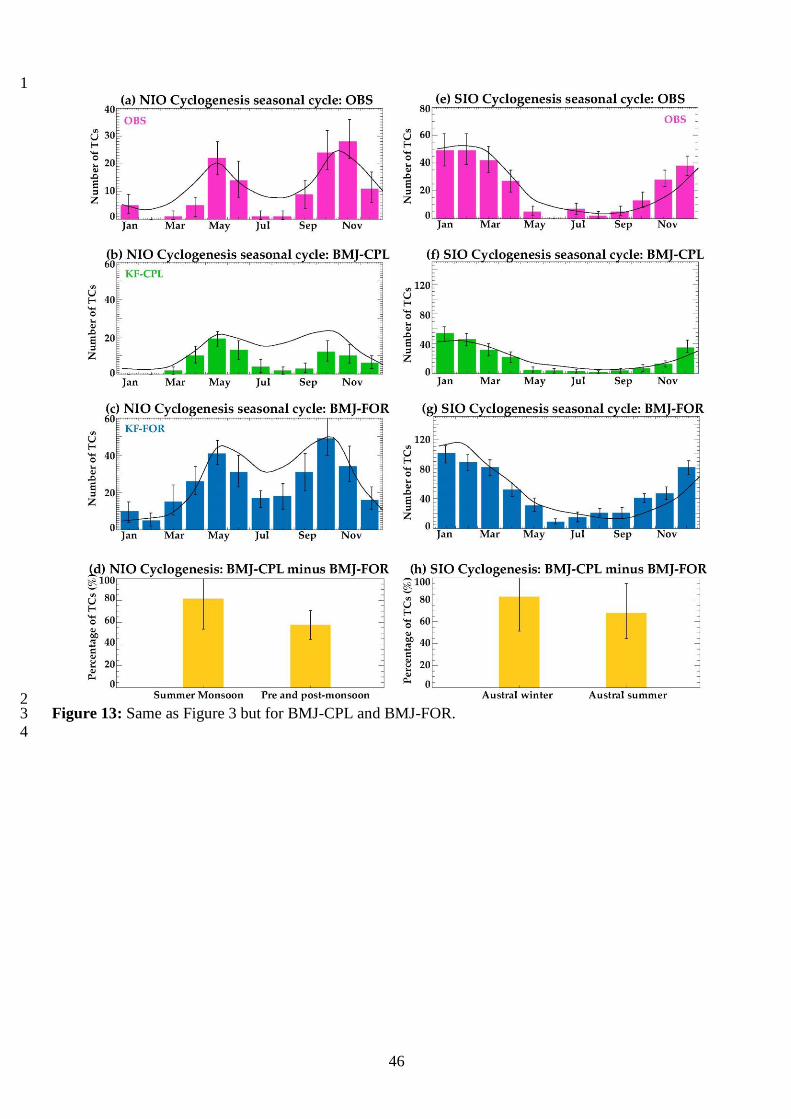
46

1

2 Figure 13: Same as Figure 3 but for BMJ-CPL and BMJ-FOR. 3

4

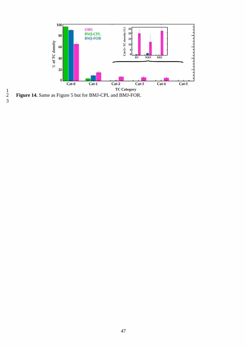
47

1 Figure 14. Same as Figure 5 but for BMJ-CPL and BMJ-FOR. 2

3

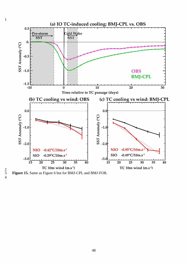
48

1

2 Figure 15. Same as Figure 6 but for BMJ-CPL and BMJ-FOR. 3

4

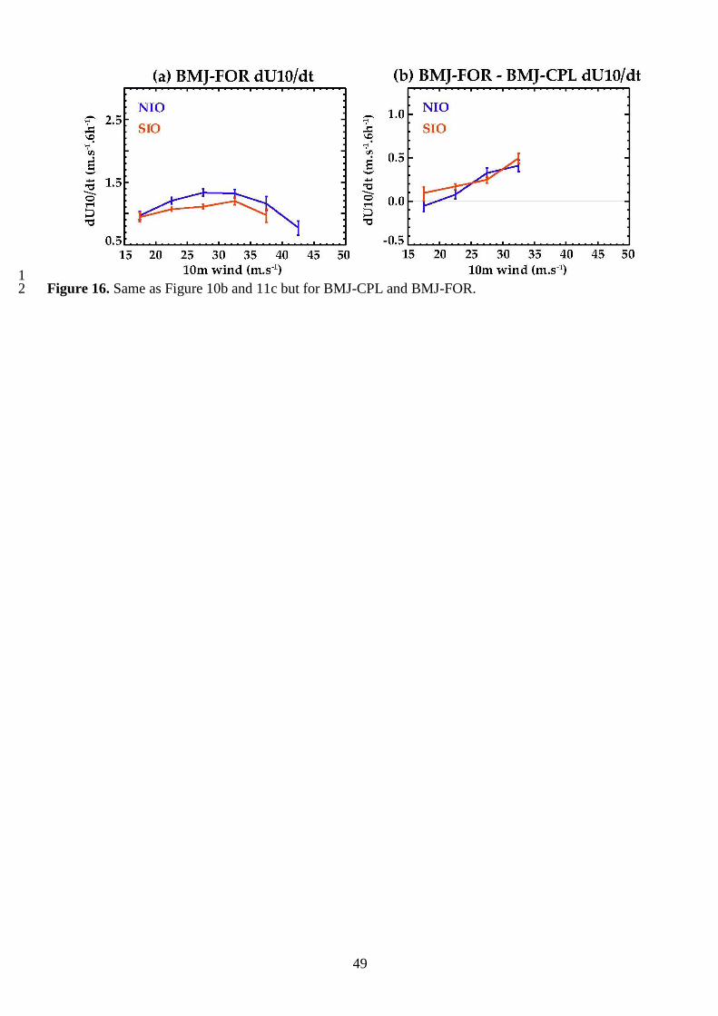
49

1 Figure 16. Same as Figure 10b and 11c but for BMJ-CPL and BMJ-FOR. 2

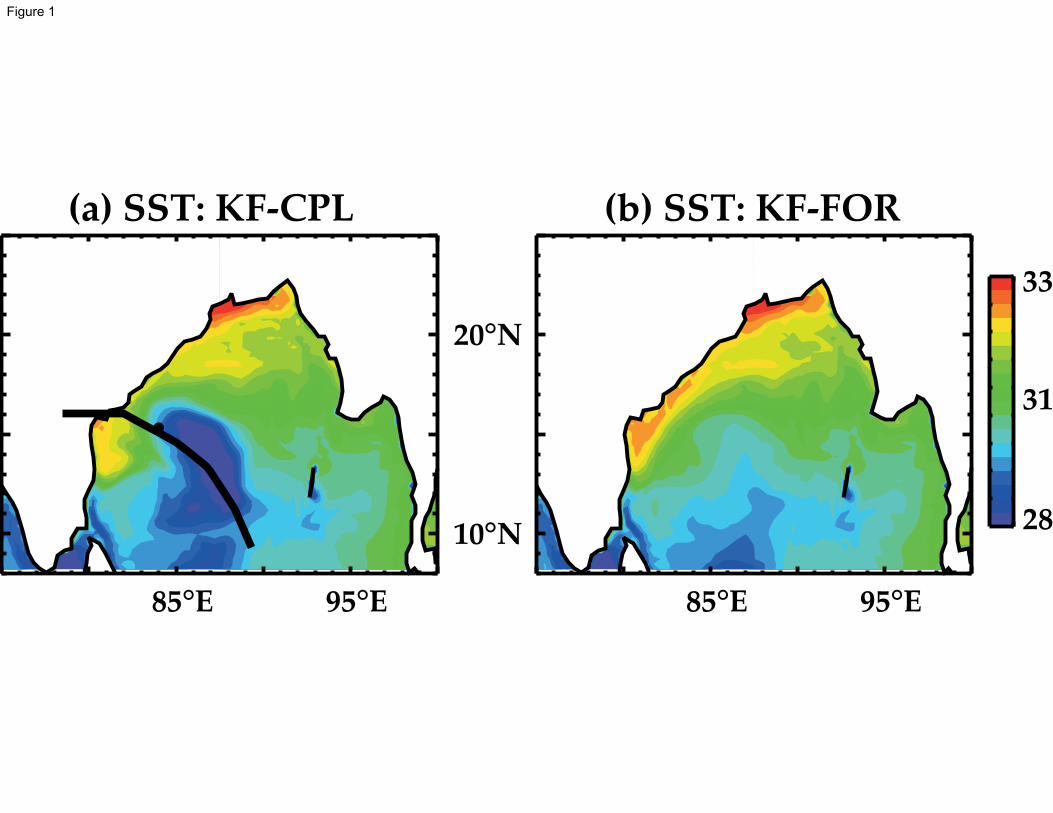
85°E 95°E

.

85°E 95°E

10°N

20°N

28

31

33

(a) SST: KF-CPL (b) SST: KF-FOR

Figure 1

(a) TCs distribution: OBS

0.5

0.5

1.5

40°E 60°E 80°E 100°E 120°E

0.5

1.0

1.0

1.5

40°S

30°S

20°S

10°S

0°

10°N

20°N

30°N

0.0 0.6 1.2 1.8 2.4 3.0

0.5

1.0

1.00

0

20

40

60

Nu

mb

er

of

TC

s .(

yr-1

)

NIO SIO IO

OBS

KF-FOR

KF-CPL

(b) TCs distribution: KF-CPL (c) TCs distribution: KF-FOR

40°E 60°E 80°E 100°E 120°E40°S

30°S

20°S

10°S

0°

10°N

20°N

30°N(d) Number of TCs per basin

40°E 60°E 80°E 100°E 120°E

TC-prone basin

Figure 2

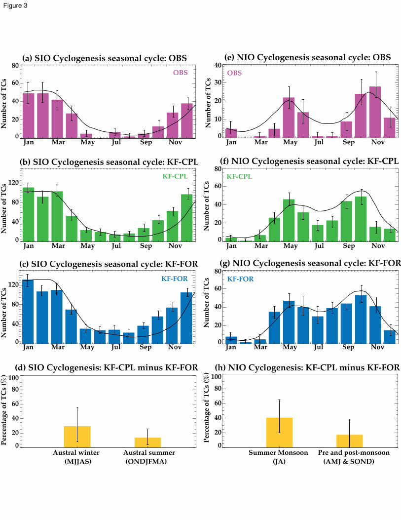
0

20

40

60

80

Jan Mar May Jul Sep Nov0

10

20

30

40

Nu

mb

er o

f T

Cs

OBS

0

20

40

60

80KF-CPL

0

40

80

120

0

20

40

60

80KF-FOR

0

40

80

120

0

20

40

60

80

100

Summer Monsoon Pre and post-monsoon 0

20

40

60

80

100

Per

cen

tag

e o

f T

Cs

(%)

Austral winter Austral summer

(e) NIO Cyclogenesis seasonal cycle: OBS

(f) NIO Cyclogenesis seasonal cycle: KF-CPL

(g) NIO Cyclogenesis seasonal cycle: KF-FOR

(a) SIO Cyclogenesis seasonal cycle: OBS

(b) SIO Cyclogenesis seasonal cycle: KF-CPL

(c) SIO Cyclogenesis seasonal cycle: KF-FOR

Nu

mb

er o

f T

Cs

Nu

mb

er o

f T

Cs

Nu

mb

er o

f T

Cs

Nu

mb

er o

f T

Cs

Nu

mb

er o

f T

Cs

Per

cen

tag

e o

f T

Cs

(%)

OBS

KF-CPL

KF-FOR

(h) NIO Cyclogenesis: KF-CPL minus KF-FOR(d) SIO Cyclogenesis: KF-CPL minus KF-FOR

Jan Mar May Jul Sep Nov

Jan Mar May Jul Sep Nov Jan Mar May Jul Sep Nov

Jan Mar May Jul Sep Nov Jan Mar May Jul Sep Nov

(AMJ & SOND)(JA)(ONDJFMA)(MJJAS)

Figure 3

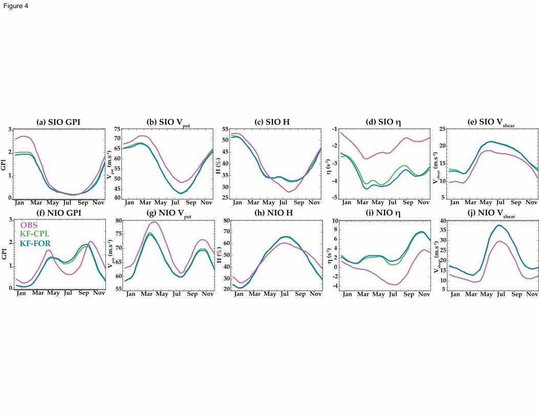
(b) SIO Vpot

Jan Mar May Jul Sep Nov40

45

50

55

60

65

70

75

Vp

ot (

m.s

-1)

(c) SIO H

Jan Mar May Jul Sep Nov25

30

35

40

45

50

55

H (

%)

(d) SIO η

Jan Mar May Jul Sep Nov-5

-4

-3

-2

-1

η (

s-1)

(e) SIO Vshear

Jan Mar May Jul Sep Nov5

10

15

20

25

Vsh

ear (

m.s

-1)

(a) SIO GPI

Jan Mar May Jul Sep Nov0.

1.

2.

3.

GP

I

Jan Mar May Jul Sep Nov55

60

65

70

75

80

Jan Mar May Jul Sep Nov20

30

40

50

60

70

80

Jan Mar May Jul Sep Nov

-4

-2

0

2

4

6

8

10

Jan Mar May Jul Sep Nov5

10

15

20

25

30

35

40

Mar May Jul Sep Nov0.

1.

2.

3.

Jan

OBSKF-CPLKF-FOR

(g) NIO Vpot

(h) NIO H (i) NIO η (j) NIO Vshear(f) NIO GPI

Vp

ot (

m.s

-1)

H (

%)

η (

s-1)

Vsh

ear (

m.s

-1)

GP

IFigure 4

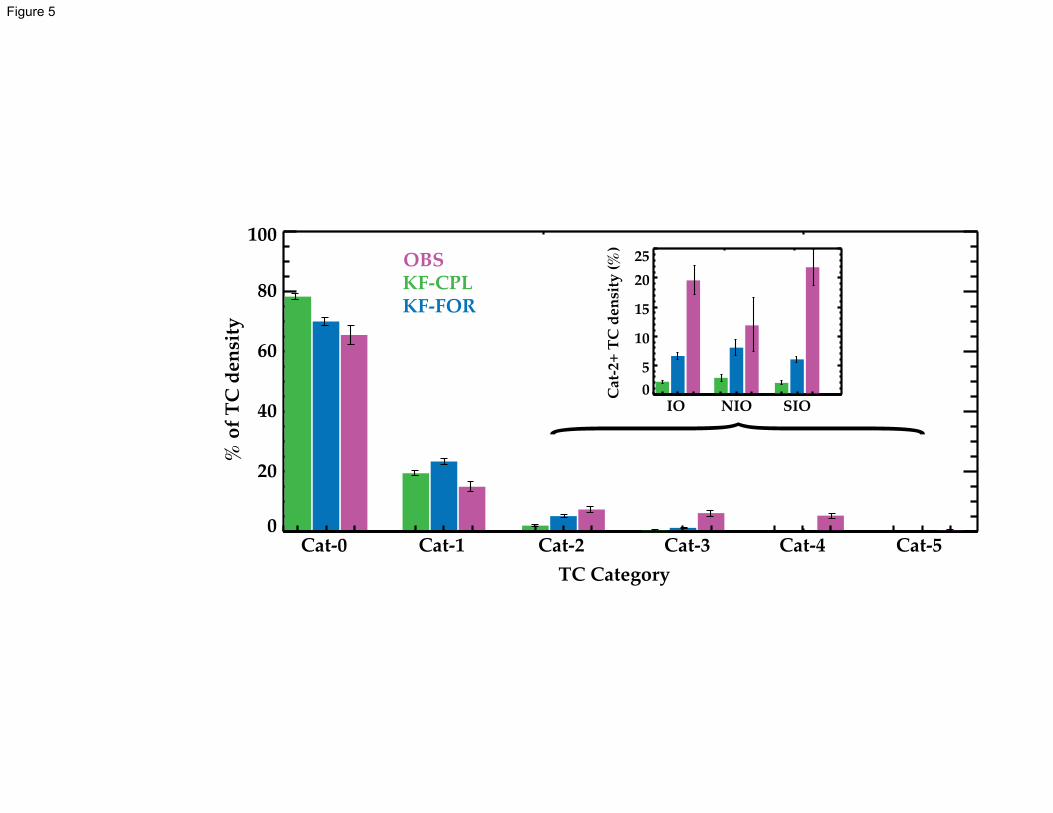
0

20

40

60

80

100 %

of

TC

den

sity

Cat-0 Cat-1 Cat-2 Cat-3 Cat-4 Cat-5

0

5

10

15

20

25

Cat

-2+

TC

den

sity

(%

)

IO NIO SIO

OBSKF-CPLKF-FOR

TC Category

Figure 5

15 20 25 30 35 40 45

TC 10m wind (m.s-1)

-3.0

-2.0

-1.0

0.0

-0.43°C/10m.s-1

-0.30°C/10m.s-1

NIO

SIO

15 20 25 30 35 40 45

TC 10m wind (m.s-1)

-3.0

-2.0

-1.0

0.0

-1.5

-1.0

-0.5

0.

0.5(a) IO TC-induced cooling: KF-CPL vs. OBS

-10 0 10 20 30

Time relative to TC passage (days)

Pre-storm SST

Cold Wake SSTCold WakeCold WakeCold W SST SST

OBSKF-CPL

(b) TC cooling vs wind: OBS (c) TC cooling vs wind: KF-CPL

SS

T A

no

mal

y (

°C)

SS

T A

no

mal

y (

°C)

-0.72°C/10m.s-1

-0.51°C/10m.s-1

NIO

SIO

SS

T A

no

mal

y (

°C)

Figure 6

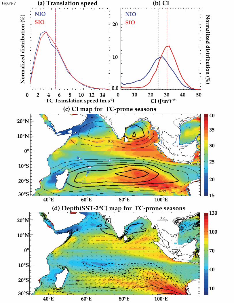
0 10 20 30 40 50CI (J/m2)-1/3

0.0

10

20

NIO

(b) CI

SIO

0.50

0.50

40°E 60°E 80°E 100°E30°S

20°S

10°S

0°

10°N

20°N

15

20

25

30

35

40(c) CI map for TC-prone seasons

0 2 4 6 8 10 12 14TC Translation speed (m.s-1)

(a) Translation speed

NIO

SION

orm

aliz

ed d

istr

ibu

tio

n (

%)

-3

-3

-1

-1

-1

-1

-1

-1-1

-1

-1

-1

1

1

1

1

1

1

1

11

1 11

0.2

No

rmalized

distrib

utio

n (%

)

10

40

70

100

130

40°E 60°E 80°E 100°E30°S

20°S

10°S

0°

10°N

20°N

(d) Depth(SST-2°C) map for TC-prone seasons

Figure 7

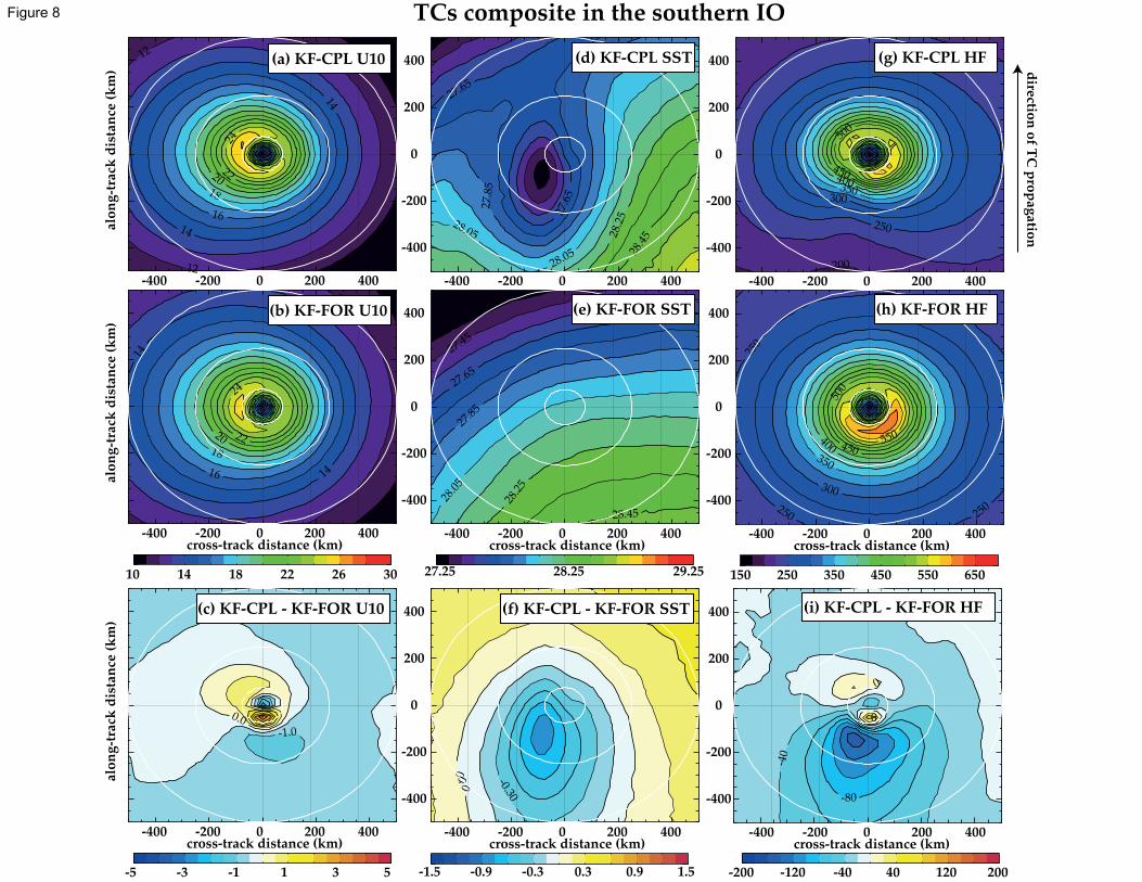
12

1212

14

14

16

18

2022

24

-400 -200 0 200 400

alo

ng

-tra

ck d

ista

nce

(k

m)

12

14

1416

18

20 22

24

-400 -200 0 200 400cross-track distance (km)

alo

ng

-tra

ck d

ista

nce

(k

m)

10 14 18 22 26 30

-1.0

0.0

-400 -200 0 200 400cross-track distance (km)

alo

ng

-tra

ck d

ista

nce

(k

m)

-5 -3 -1 1 3 5

27.65

27.6

5

27.8

5

28.05

28.05 28.2

5

28.4

5

-400 -200 0 200 400

-400

-200

0

200

400

27.45

27.65

27.8

5

28.0

5

28.2

528.45

-400 -200 0 200 400cross-track distance (km)

-400

-200

0

200

400

27.25 28.25 29.25

-400 -200 0 200 400cross-track distance (km)

-400

-200

0

200

400

200

250

300

350

400

450

500

-400 -200 0 200 400

-400

-200

0

200

400

250 250

250

300

350

400 450

500

550

-400 -200 0 200 400cross-track distance (km)

-400

-200

0

200

400

150 250 350 450 550 650

-400 -200 0 200 400cross-track distance (km)

-400

-200

0

200

400

(a) KF-CPL U10

(b) KF-FOR U10

(c) KF-CPL - KF-FOR U10

(d) KF-CPL SST

(e) KF-FOR SST

(g) KF-CPL HF

(h) KF-FOR HF

TCs composite in the southern IO

dire

ction

of T

C p

rop

ag

atio

n

-80

-40

00

-200 -120 -40 40 120 200

(i) KF-CPL - KF-FOR HF

-0.3

0

0.0

0

0.30

-1.5 -0.9 -0.3 0.3 0.9 1.5

(f) KF-CPL - KF-FOR SST

Figure 8

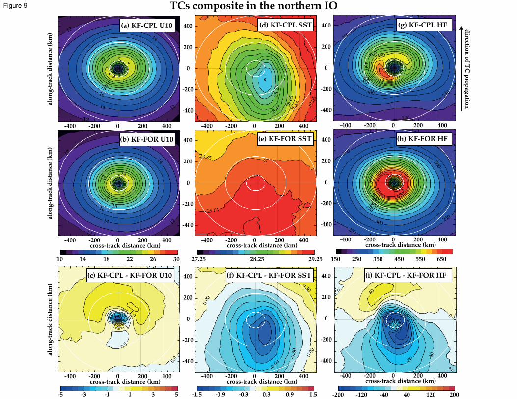
12

12

12

14

14

16

1820

22 22

24

-400 -200 0 200 400

alo

ng

-tra

ck d

ista

nce

(k

m)

12

12

12

14

14

1618

20

22

24

-400 -200 0 200 400cross-track distance (km)

alo

ng

-tra

ck d

ista

nce

(k

m)

10 14 18 22 26 30

0.0

0.0

0.0

0.0 1.0

-400 -200 0 200 400cross-track distance (km)

alo

ng

-tra

ck d

ista

nce

(k

m)

-5 -3 -1 1 3 5

28.2

5

28.45 2

8.6

528.8

5

29.0

5

-400 -200 0 200 400

-400

-200

0

200

400

28.85

29.05

-400 -200 0 200 400cross-track distance (km)

-400

-200

0

200

400

27.25 28.25 29.25

-400 -200 0 200 400cross-track distance (km)

-400

-200

0

200

400

200

250

250

300

350

400

450

500550

-400 -200 0 200 400

-400

-200

0

200

400

250

250

250

300

300

350

400

450

500

550

600

650

-400 -200 0 200 400cross-track distance (km)

-400

-200

0

200

400

150 250 350 450 550 650

-400 -200 0 200 400cross-track distance (km)

-400

-200

0

200

400

(a) KF-CPL U10

(b) KF-FOR U10

(c) KF-CPL - KF-FOR U10

(d) KF-CPL SST

(e) KF-FOR SST

(g) KF-CPL HF

(h) KF-FOR HF

TCs composite in the northern IO

dire

ction

of T

C p

rop

ag

atio

n

-0.6

0

-0.3

0

0.0

0

0.0

0

0.3

0

-120

-80 -4

0

0

0

40

(f) KF-CPL - KF-FOR SST (i) KF-CPL - KF-FOR HF

-200 -120 -40 40 120 200

-1.5 -0.9 -0.3 0.3 0.9 1.5

Figure 9

(a) KF-FOR HF

15 20 25 30 35 40 45 50

10m wind (m.s-1)

0

400

800

1200

HF

(W

.m-2)

NIO

SIO

(b) KF-FOR dU10/dt

15 20 25 30 35 40 45 50

10m wind (m.s-1)

0.5

1.5

2.5

dU

10

/dt

(m.s

-1.6

h-1)

NIO

SIO

(c) KF-FOR SST

15 20 25 30 35 40 45 50

10m wind (m.s-1)

26

28

30

SS

T (

°C)

NIO

SIO

Figure 10

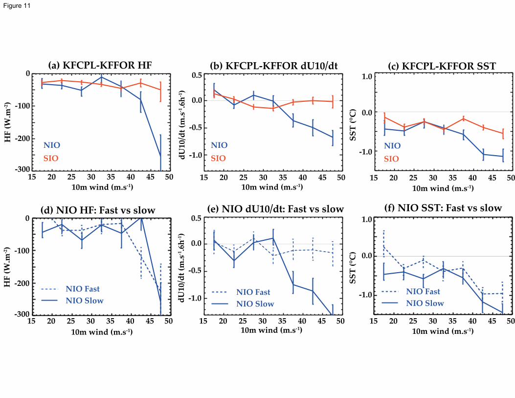
(a) KFCPL-KFFOR HF

15 20 25 30 35 40 45 50-300

-200

-100

0

HF

(W

.m-2)

(c) KFCPL-KFFOR SST

15 20 25 30 35 40 45 50

-1.0

0.0

1.0

SS

T (

°C)

(b) KFCPL-KFFOR dU10/dt

15 20 25 30 35 40 45 50

-0.5

0.0

0.5

-1.0dU

10

/dt

(m.s

-1.6

h-1)

10m wind (m.s-1) 10m wind (m.s-1)10m wind (m.s-1)

NIO

SIO

NIO

SIO

NIO Fast

NIO Slow

(d) NIO HF: Fast vs slow

15 20 25 30 35 40 45 50-300

-200

-100

0

HF

(W

.m-2)

10m wind (m.s-1)

(e) NIO dU10/dt: Fast vs slow

15 20 25 30 35 40 45 50

-0.5

0.0

0.5

-1.0dU

10

/dt

(m.s

-1.6

h-1)

10m wind (m.s-1)

NIO Fast

NIO Slow

(f) NIO SST: Fast vs slow

NIO Fast

NIO Slow

15 20 25 30 35 40 45 50

-1.0

0.0

1.0

SS

T (

°C)

10m wind (m.s-1)

NIO

SIO

Figure 11

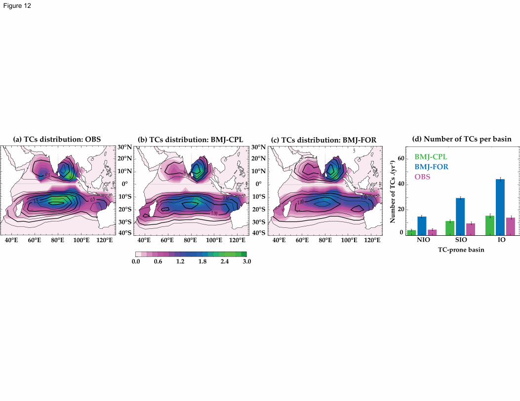
(a) TCs distribution: OBS

0.5

0.5

1.5

40°E 60°E 80°E 100°E 120°E40°S

30°S

20°S

10°S

0°

10°N

20°N

30°N

0.0 0.6 1.2 1.8 2.4 3.0

0

20

40

60

Nu

mb

er

of

TC

s .(

yr-1

)

NIO SIO IO

OBS

BMJ-FOR

BMJ-CPL

(b) TCs distribution: BMJ-CPL (c) TCs distribution: BMJ-FOR

40°E 60°E 80°E 100°E 120°E40°S

30°S

20°S

10°S

0°

10°N

20°N

30°N(d) Number of TCs per basin

40°E 60°E 80°E 100°E 120°E

TC-prone basin

0.50

0.50

0.50

1.00

1.00

5

0.50

0.50

0.50

1.00

1.00

1.00

Figure 12

0

20

40

60

80

Jan Mar May Jul Sep Nov0

10

20

30

40

Nu

mb

er o

f T

Cs

OBS

0

20

40

60

0

40

80

120

0

20

40

60

0

40

80

120

0

20

40

60

80

100

Summer Monsoon Pre and post-monsoon0

20

40

60

80

100

Per

cen

tag

e o

f T

Cs

(%)

Austral winter Austral summer

(a) NIO Cyclogenesis seasonal cycle: OBS

(b) NIO Cyclogenesis seasonal cycle: BMJ-CPL

(c) NIO Cyclogenesis seasonal cycle: BMJ-FOR

(e) SIO Cyclogenesis seasonal cycle: OBS

(f) SIO Cyclogenesis seasonal cycle: BMJ-CPL

(g) SIO Cyclogenesis seasonal cycle: BMJ-FOR

Nu

mb

er o

f T

Cs

Nu

mb

er o

f T

Cs

Nu

mb

er o

f T

Cs

Nu

mb

er o

f T

Cs

Nu

mb

er o

f T

Cs

Per

cen

tag

e o

f T

Cs

(%)

OBS

KF-CPL

KF-FOR

(d) NIO Cyclogenesis: BMJ-CPL minus BMJ-FOR (h) SIO Cyclogenesis: BMJ-CPL minus BMJ-FOR

Jan Mar May Jul Sep Nov

Jan Mar May Jul Sep Nov Jan Mar May Jul Sep Nov

Jan Mar May Jul Sep Nov Jan Mar May Jul Sep Nov

Figure 13

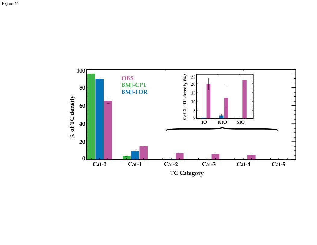
0

20

40

60

80

100 %

of

TC

den

sity

Cat-0 Cat-1 Cat-2 Cat-3 Cat-4 Cat-5

0

5

10

15

20

25

Cat

-2+

TC

den

sity

(%

)

IO NIO SIO

OBSBMJ-CPLBMJ-FOR

TC Category

Figure 14

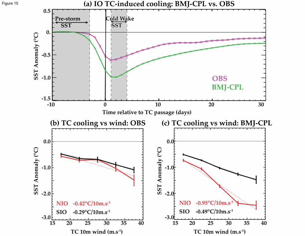
15 20 25 30 35 40

TC 10m wind (m.s-1)

-3.0

-2.0

-1.0

0.0

-0.42°C/10m.s-1

-0.29°C/10m.s-1

NIO

SIO

15 20 25 30 35 40

TC 10m wind (m.s-1)

-3.0

-2.0

-1.0

0.0

-1.5

-1.0

-0.5

0.

0.5(a) IO TC-induced cooling: BMJ-CPL vs. OBS

-10 0 10 20 30

Time relative to TC passage (days)

Pre-storm SST

Cold Wake SSTCold WakeCold WakeCold W SST SST

OBSBMJ-CPL

(b) TC cooling vs wind: OBS

SS

T A

no

mal

y (

°C)

SS

T A

no

mal

y (

°C)

-0.95°C/10m.s-1

-0.49°C/10m.s-1

NIO

SIO

SS

T A

no

mal

y (

°C)

(c) TC cooling vs wind: BMJ-CPL

Figure 15

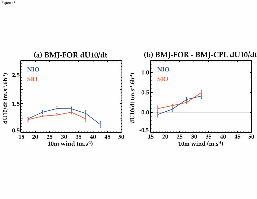
(a) BMJ-FOR dU10/dt

15 20 25 30 35 40 45 5010m wind (m.s-1)

0.5

1.5

2.5

dU

10

/dt

(m.s

-1.6

h-1)

NIO

SIO

(b) BMJ-FOR - BMJ-CPL dU10/dt

15 20 25 30 35 40 45 50-0.5

0.0

0.5

1.0

dU

10

/dt

(m.s

-1.6

h-1)

10m wind (m.s-1)

NIO

SIO

Figure 16