arX

iv:h

ep-l

at/9

4120

98v2

9 J

an 1

995

IFUP-TH 63/94

Strong-coupling expansion of chiral models

Massimo Campostrini, Paolo Rossi, and Ettore VicariDipartimento di Fisica dell’Universita and I.N.F.N., I-56126 Pisa, Italy

Abstract

The strong-coupling character expansion of lattice models is reanalyzed in

the perspective of its complete algorithmization. The geometric problem of

identifying, counting, and grouping together all possible contributions is disen-

tangled from the group-theoretical problem of weighting them properly. The

first problem is completely solved for all spin models admitting a character-

like expansion and for arbitrary lattice connectivity. The second problem is

reduced to the evaluation of a class of invariant group integrals defined on

simple graphs. Since these integrals only depend on the global symmetry of

the model, results obtained for principal chiral models can be used without

modifications in lattice gauge theories.

By applying the techniques and results obtained we study the two-

dimensional principal chiral models on the square and honeycomb lattice.

These models are a prototype field theory sharing with QCD many prop-

erties. Strong-coupling expansions for Green’s functions are derived up to

15th and 20th order respectively. Large-N and N = ∞ results are presented

explicitly. Related papers are devoted to a discussion of the results.

Typeset using REVTEX

1

I. INTRODUCTION

It is certainly appropriate to consider two-dimensional principal chiral models as a the-oretical physics laboratory. These models display a rich physical structure, and share withfour-dimensional gauge theories a number of fundamental properties: nonabelian symmetrywith fields in the matrix representation, asymptotic freedom, dynamical mass generation.Moreover, principal chiral models admit a 1/N expansion and a large-N limit which is asum over planar diagrams, in total analogy with nonabelian gauge theories.

However, the absence of local gauge invariance and the reduced number of dimensionsmake chiral models much simpler to handle both by analytical and by numerical methods.Moreover, the on-shell solution of the models is known by Bethe-Ansatz methods: a factor-ized S-matrix exists and the particle spectrum is explicitly known. We can therefore try tomake progress, both in analytical and in numerical techniques, by testing these methods onchiral models and, in case of success, applying them to four-dimensional gauge theories.

The spirit of this approach is well expressed in the papers by Green and Samuel [1–3],who advocated a systematic study of lattice chiral models as a preliminary step towards anunderstanding of lattice gauge theories, especially in the large-N limit. One of the techniquesfavored by the above-mentioned authors was the strong-coupling character expansion. How-ever, the existence of a large-N phase transition from strong to weak coupling phase seemedto indicate at that time an obstruction to further pushing this method of investigation.

In much more recent times, a few facts came to suggest that this “no-go” result mightbe over-pessimistic. It was indeed observed by the present authors [4–6] that scaling ofphysical observables is present in finite-N chiral models already in a coupling region withinthe convergence radius of the strong-coupling expansion. Moreover, a change of variablescorresponding to adopting the so-called “energy scheme” for the definition of the temperaturesmoothens the lattice β-function to the point that asymptotic scaling is observed within thestrong-coupling region. These patterns are unaffected by growing N , and therefore survivethe large-N phase transition. These “experimental” observations led us to reconsidering thepossibility that a strong-coupling approach could be turned into a predictive method for theevaluation of physical quantities in the neighborhood of the continuum fixed point of themodels.

A second theoretical motivation for a renewed effort towards extending strong-couplingseries of chiral models, especially for large N , comes in connection with the possibility thatthe above-mentioned transition, while uninteresting for the standard continuum physics,may be related to a description of quantum gravity by the so-called “double scaling limit”[7–10]. In simple models, this limit is studied by analytical techniques, but more complexsituations might need perturbative methods, and strong-coupling seems well suited for suchan analysis, which corresponds to exploring the region in the vicinity of the first singularityin the complex coupling constant plane.

Another significant change, of a completely different nature, has occurred since the orig-inal studies on the strong-coupling character expansion (cf. Ref. [11] for a review) wereperformed. The increased availability of symbolic-manipulation computer programs and theenormous increase in performance of computers have now made the strong-coupling expan-sion a plausible candidate for an algorithmic implementation, that might extend series wellbeyond the level that can be reached by purely human resources, while granting a definitely

2

higher reliability of results.The purpose of the present work is to set the stage and make a significant effort towards

a complete algorithmization of the strong-coupling character expansion.Two major classes of problems must be handled and solved. The first has to do with

counting the multiplicities of terms appearing in the expansion. It is basically a geometricalproblem and it leads to the definition of a “geometrical factor”. We must stress the factthat this geometrical factor depends only on the lattice connectivity, and therefore applieswithout any modification to the strong-coupling expansion of all spin models admitting acharacter-like expansion, including O(N) and CPN−1 models with nearest-neighbour inter-actions [12]. We have completely solved this problem, with no conceptual restrictions onthe dimensionality and connectivity of the lattice. We have not addressed the correspondingproblem for lattice gauge theories, but we are confident that no major conceptual obstructionshould arise in pursuing that program.

The second class of problems is related to the evaluation of group integrals that appearas coefficients of the expansion. Evaluating group integrals is an algebraic problem, and inprinciple a solved one. However, algorithmic implementation is not in practice a trivial task,and therefore we limited ourselves to a general classification and to an explicit evaluation ofthe cases of direct interest to our calculations, with a few useful generalizations. We stressthat the evaluation of “group-theoretical factors” is universal, and results may be appliedas they stand to lattice gauge theories.

The representation of the strong-coupling expansion in terms of explicitly evaluatedgeometrical factors and symbolically denoted group-theoretical factors can be achieved by afully computerized approach, and applies as it stands to all nonlinear sigma models definedon group manifolds. This is probably the main result of the present paper. However we shallnot exhibit here the explicit general formulae resulting from our approach, because they areso long that their pratical use does necessarily involve computer manipulation; therefore weshall make available our results in form of computer files, publicly available by anonymousftp on the host ftp.difi.unipi.it, in the directory pub/campo/StrongCoupling.

The application of our results to O(N) and CPN−1 models is definitely simpler thenthe case discussed here, since the evaluation of group-theoretical factors lends itself to acompletely algorithmic implementation. The corresponding results will be presented in aforthcoming paper.

The present paper is organized as follows.In Sect. II we review the character expansion, fix our notation and present some useful

formulae.In Sect. III we outline the procedure of the expansion by identifying the logical steps and

defining the relevant geometrical and algebraic objects entering the computation. Amongthese we introduce the basic notion of a skeleton diagram, whose multiplicity is the geomet-rical factor and whose connected value, or potential, is the group-theoretical factor.

In Sect. IV we explain how one may algorithmically evaluate the geometrical factor.In Sect. V we introduce the problem of computing the group-theoretical factor.Sect. VI is devoted to some technical remarks on group integration.Sect. VII offers some details on the computation of potentials for principal chiral models.In Sect. VIII we analyze the main features of the strong-coupling expansion of the two-

point fundamental Green’s functions, introducing a parametrization for the propagator in

3

the case of a two-dimensional square lattice.In Sect. IX we discuss the relevant features of the honeycomb lattice, and we present a

few results for physical quantities.Appendix A is devoted to a presentation of some of our results concerning the explicit

evaluation of potentials.Appendix B is a list of potentials ordered according to their appearance in the strong-

coupling expansion.Appendix C is a presentation our results for large but finite N in the square-lattice

formulation of the models.Appendix D clarifies some non-standard features of honeycomb-lattice models using the

Gaussian model as a guide.Appendix E is the same as App. C for the honeycomb-lattice formulation.The present paper is the first of a series of papers devoted to the strong-coupling analysis

of two-dimensional lattice chiral models. In a second paper we will present our analysis ofthe large-N strong-coupling series by series-resummation techniques, while a third paperwill be devoted to a comparison with Monte Carlo studies of the large-N critical behavior.

II. THE CHARACTER EXPANSION: GENERALITIES

The strong-coupling expansion of field theories involving matrix-valued fields and en-joying G × G group symmetry is best performed applying the character expansion, whichreduces the number of contributions to a given order in the expansion and decouples thegeometrical counting of configurations from the group-theoretical factor.

The whole subject is reviewed in detail in Ref. [11], and we recall here only those proper-ties that are essential in order to make our presentation as far as possible self-contained. Weshall only discuss the symmetry groups G = U(N): extensions to SU(N) can be achievedfollowing Ref. [1] and applying the results presented in Ref. [5].

In the theory described by the lattice action

SL = −Nβ∑

x,µ

[Tr{U(x) U †(x+µ)} + Tr{U(x+µ) U †(x)}], (1)

the character expansion is achieved by replacing the Boltzmann factors with their Fourierdecomposition

exp{Nβ[Tr{U(x) U †(x+µ)} + Tr{U(x+µ) U †(x)}]}= exp{N2F (β)}

∑

(r)

d(r)z(r)(β) χ(r)(U(x) U †(x+µ)), (2)

where

F (β) =1

N2ln∫

dU exp{Nβ(Tr U + Tr U †)}= 1

N2ln det Ij−i(2Nβ) (3)

is the free energy of the single-matrix model,∑

(r) denotes the sum over all irreduciblerepresentations of G, χ(r)(U) and d(r) are the corresponding characters and dimensions

4

respectively, and Ij−i (i, j = 1, ..., N) is a N×N matrix of modified Bessel functions. Werecall here the orthogonality relations for representations:

∫dUD

(r)ab (U) D

(s) ∗cd (U) =

1

d(r)

δ(r),(s) δa,c δb,d, χ(r)(U) = D(r)aa (U). (4)

In U(N) groups (r) is characterized by two sets of decreasing positive integers {l} =l1, ..., ls, {m} = m1, ..., mt and we define the order n of (r) by

n = n+ + n−, n+ =s∑

i=1

li, n− =t∑

j=1

mj . (5)

We may define the ordered set of integers {λ} = λ1, ..., λN by the relationships

λk = lk, k ≤ s;

λk = 0, s < k < N − t + 1;

λk = − mN−k+1, k ≥ N − t + 1. (6)

It is then possible to write down explicit representations of all characters and dimensions:

χ{λ}(U) =det|exp{iφi(λj + N − j)}|

det|exp{iφi(N − j)}| , (7)

d{λ} =

∏i<j(λi − λj + j − i)

∏i<j(j − i)

= χ{λ}(1), (8)

where φi are the eigenvalues of the matrix U . As a consequence, it is possible to evaluateexplicitly the character coefficients z(r) by the orthogonality relations

d{λ}z{λ} =∫

dU exp{Nβ(Tr U + Tr U †)}χ{λ}(U) exp{−N2F (β)}

=det Iλi+j−i(2Nβ)

det Ij−i(2Nβ). (9)

Eq. (9) becomes rapidly useless with growing N , due to the difficulty of evaluatingdeterminants of large matrices. It is however possible to obtain considerable simplifications,in the strong coupling regime and for sufficiently large N , when we consider representationssuch that n < N . In this case, character coefficients are simply expressed by [1]

d{l;m}z{l;m} =1

n+!

1

n−!σ{l}σ{m}(Nβ)n[1 + O(β2N)], (10)

where we have introduced the quantity σ{l}, the dimension of the representation l1, ..., ls ofthe permutation group, enjoying the property

∫χ{l}(U)(Tr U †)pdU = σ{l}δp,n+ . (11)

It is important to notice that the strong-coupling expansion and the large-N limit donot commute: large-N character coefficients have jumps and singularities at β = 1

2[1], and

therefore the relevant region for a strong-coupling character expansion is β < 12.

5

A consequence of Eq. (10) is the relationship

z ≡ z1;0(β) = β + O(β2N+1), (12)

and in turn, because of the property

z(β) =1

2

∂

∂βF (β), (13)

one may obtain the large-N relationship

F (β) = β2 + O(β2N+2). (14)

According to the above observations, at N = ∞ the relationship F = β2 may only holdwhen β < 1

2, even if the function β2 is perfectly regular for all β.

For the purpose of actual computations it is convenient to have expressions in closedform for the quantities σ{l} and d{l;m} not involving infinite sums or products even in theN → ∞ limit. We found such expressions in the form

1

n+!σl1,...,ls =

∏1≤j<k≤s(lj − lk + k − j)!∏s

i=1(li + s − i)!(15)

and a similar relationship for σ{m}. Notice that these quantities are independent of N . Nowby manipulating appropriately Eq. (8) we can show that

d{l;m} =σ{l}

n+!

σ{m}

n−!C{l;m} , (16)

where

C{l;m} =s∏

i=1

(N − t − i + li)!

(N − t − i)!

t∏

j=1

(N − s − j + mj)!

(N − s − j)!

s∏

i=1

t∏

j=1

N + 1 − i − j + li + mj

N + 1 − i − j. (17)

The essential feature of Eq. (17) is the possibility of extracting results with a finite numberof operations even in the large-N limit. As a byproduct we obtain the large-N charactercoefficients in the useful form

z{l;m}

zn→ Nn

C{l;m}. (18)

III. OUTLINE OF THE PROCEDURE

The general purpose of the strong-coupling expansion is an evaluation of the Green’sfunctions of the model as power series in β. If we are interested in the mass spectrum of themodel, we may focus on the class of two-point Green’s functions defined by

G(r)(x) =1

d(r)

⟨χ(r)(U

†(x) U(0))⟩

, (19)

6

and even more specifically we may decide to evaluate the fundamental two-point Green’sfunction

G(x) =1

N

⟨Tr(U †(x) U(0))

⟩. (20)

Evaluating such expectation values by the character expansion involves performing thegroup integrals that are generated from choosing an arbitrary representation for each link ofthe lattice. As a consequence of Eq. (10), only a finite number of nontrivial representationscontribute to any definite order in the series expansion of G(x) in powers of β; we musthowever find a systematic way of identifying the relevant contributions.

As a preliminary condition for the definition of an algorithmic approach to the strong-coupling expansion of G(x), it is convenient to identify explicitly all the logical steps of sucha computation and define a number of objects that play a special role in it.

A. Assignments

Each lattice integration variable U(y) can only appear in the integrand either throughthe representation characters defined on links terminating on the lattice site y or throughthe observable whose expectation value is to be evaluated. According to the rules of groupintegration, nontrivial contributions are obtained only if the product of all representationsinvolving U(y) contains the identity (the trivial representation).

We define an assignment {r} to be a choice of a representation for each link of the latticethat is consistent with the above requirement. Necessary conditions for an assignment canbe obtained by a close examination of the rules for the composition of two irreducible rep-resentations of U(N). When we consider Green’s functions in the class defined by Eq. (19),we recognize that the operator whose expectation value we are evaluating, when consideredfrom the point of view of group integration, plays the role of a unit length link connectingthe sites x and 0, weighted with a factor d−2

(r). Therefore all the relevant group integralscan be put into correspondence with integrals appearing in the character expansion of thepartition function (possibly in higher dimensions).

Changing the convention for the orientation of links changes each representation r intoits conjugate r (l ↔ m), but, since z(r) = z(r), it does not affect the expansion. Hence wecan consider all links terminating in a given site as “ingoing”. It is now possible to provethat an assignment must satisfy the following conditions at each lattice site:

∑

i

(ni+ − ni

−) = 0, (21)

nj± ≤

∑

i6=j

ni∓ (non-backtracking condition), (22)

where the summation is extended to all ingoing links.Order by order in the strong-coupling expansion, the relevant assignments involve non-

trivial representations only on a finite number of links, which allows the possibility of drawingon the lattice the diagram of each assignment. Such a diagram is characterized by vertices,where more then two nontrivial representations meet, and paths, i.e. chains of links con-necting vertices. Orthogonality of representations implies that the choice of representation

7

→ + + + +

+ + + 12

FIG. 1. All the non-trivial disconnections of a diagram.

along a given path cannot change. We will denote the length of each path p by Lp, andthe corresponding (nontrivial) representation by rp. The topology S of a diagram may berepresented by the connectivity matrix between its vertices. As we shall show later, thevalue of the group integral associated with each assignment can only be a function of rp, Lp,

and S ; we shall denote it by R(S ){r,L}.

B. Configurations

The set (n+, n−) does not in general identify uniquely a representation. It is convenient todefine oriented configurations: they are the sets of all assignments having the same (nl

+, nl−)

for each link of the lattice. The relevance of oriented configurations in the context of thestrong-coupling expansion stays in the fact that they are in a one-to-one correspondencewith the monomials one would obtain in the integrand after the series expansion of theBoltzmann factor in powers of β. They are therefore the simplest objects admitting ameaningful definition for their connected contributions.

Eq. (10) tells us that the lowest-order contribution of any character coefficient to thestrong-coupling series depends only on n = n++n−. Hence it is useful to define (unoriented)configurations by summing up all the oriented configurations characterized by the same valueof nl for each link of the lattice. The set {n} = (n1, ...) uniquely identifies a configuration.We might have defined configurations directly as the sets of all assignments sharing the same{n}; our procedure insures us about the possibility of defining the connected contributionof a configuration.

We may introduce the diagrammatic representation of oriented configurations, by draw-ing each oriented link (n+, n−) as a bundle of n links, of which n+ bear a positively-orientedarrow and n− bear a negatively-oriented arrow. Removing the arrows leaves us with a di-agrammatic representation of (unoriented) configurations. One may easily get convincedthat the algebraic notion of disconnection turns out to coincide with the geometrical one.In this representation, a disconnection is a set of subdiagrams such that their superpositionreproduces the original diagram. An example of disconnection is drawn in Fig. 1.

Without belaboring on this topic, which is widely discussed in the literature [13,14], weonly remind that the connected part of a collection of n (abstract) objects is recursivelydefined by the condition that the set of n objects coincides with the sum of the connectedparts of all its partitions, including the collection itself. In presence of multiple copies ofthe same object, in standard perturbation theory a combinatorial factor appears, which is

8

hidden in the character expansion; as a consequence, when subtracting disconnections onemust take care of dividing by the corresponding symmetry factors in order to restore thecorrect normalization.

The definitions imply that the geometric features S and {L} of all assignments belongingto a given configuration are the same; therefore the path p of a configuration is characterizedby Lp and by the value np of the order of rp.

C. Skeleton diagrams

It is convenient to reduce each configuration to its skeleton diagram, whose links arethe paths of the configuration. The topology S is obviously unchanged, and each link ischaracterized by the pair of numbers (np, Lp).

In order to clarify the relevance of such a definition, let us consider the problem ofevaluating the group integrals R

(S ){r,L} for the assignments belonging to a given configuration.

An elementary consequence of Eq. (4) is the evaluation of the simplest nontrivial groupintegral entering our calculations:

∫dUχ(r)(A

†U) χ(r)(U†B) =

1

d(r)

χ(r)(A†B). (23)

By applying repeatedly Eq. (23) along the paths we easily obtain

R(S ){r,L} =

{ν∏

p=1

[z(rp)]Lp

}S

(S ){r} , (24)

where ν the number of paths of the configuration (with n 6= 0), and S(S ){r} is the value of

the group integral associated with the skeleton diagram, in which all links are assigned unitlength and weight, and representations are chosen according to the assignment. Furthersimplification is obtained by noticing that the effective strong-coupling variable in the char-acter expansion is z(β) (for large N actually z(β) ≈ β because of Eq. (12)). Therefore byreplacing the character coefficients z(r) with the ratios

z(r) =z(r)

zn(25)

we may express the strong coupling series as a series in powers of z, with coefficients thatare functions of z(r); by the way, these quantities for large enough N are pure numbers,dependent on N but independent of β, because of Eq. (18). We can rewrite Eq. (24) as

R(S ){r,L} = z

∑p

npLp

{ν∏

p=1

zLp

(rp)

}S

(S ){r} ; (26)

since z1;0 ≡ 1, there is no dependence on the lengths of the links with n = 1, apart from theoverall factor of z, depending only on the total length of the configuration L =

∑p npLp.

Therefore the corresponding Lp indices can be dropped, thus defining a reduced skeleton. The

9

contribution of a configuration to the functional integral is simply the sum of the contribu-tions of all its assignments. It then follows from Eq. (26) that whenever two configurationscan be reduced to the same skeleton, they will give the same contribution.

An exchange in the ordering of the vertices will not change the topology of a skeletondiagram; therefore configurations that are related by this symmetry will give the same contri-bution. Moreover, configurations sharing the same reduced skeleton will give contributionsdiffering only by an overall proportionality factor, depending on the total length L. Wecan group together all configurations with the same reduced skeleton (taking into accountthe abovementioned symmetry) and the same value of L: their number is what we call thegeometrical factor. The common value of each of these configurations is proportional to thegroup-theoretical factor of the reduced skeleton:

T(S ){n,L} =

∑

{r}{n}fixed

ν∏

p=1

[z(rp)

]Lp

S(S ){r} (27)

with a proportionality factor zL.The strong-coupling character expansion of a group integral can therefore be organized

as a series in the powers of z ≡ z1;0, with coefficients obtained by taking sums of productsof geometrical and group-theoretical factors. In order to understand the computationalsimplifications achieved at this stage, let us only notice that, at different orders in theexpansion, the same reduced skeletons may appear again and again in association withdifferent values of L; their group-theoretical factors however are computed once and forall, while extracting the geometrical factors is a task that, as we shall show later, can becompletely automatized.

D. Superskeletons

Both for the purpose of bookkeeping and in view of the problem of actually computingthe group-theoretical factors, at this stage we need a classification and labeling of (reduced)skeleton diagrams, which must keep track of their topological properties and try to putinto evidence whatever further simplification we may conceive. We found it convenient toisolate for each topology S a “core” topology T which we call superskeleton, defined bythe condition that each vertex in it is connected by at most a single link to any other vertex(i.e. the entries in the connectivity matrix are either 0 or 1).

The essential ingredient for the reduction of a skeleton to a superskeleton is the extractionof bubbles, defined as sets of two links in a skeleton connecting the same pair of vertices. Letus now recall the decomposition rule for a product of characters:

χ(r)(U) χ(s)(U) =∑

t

C(rst) χ(t)(U) , (28)

where C(rst) is a set of integer numbers counting the multiplicity of (t) in the product ofrepresentations (r)⊗ (s). For all assignments of (r), (s) consistent with a given skeleton, (t)must be such that the triplet (r), (s), (t) satisfies Eqs. (21) and (22). Therefore replacinga bubble with a single link and allowing for all χ(t) obtained from Eq. (28) to be inserted

10

W

3 1

4

2

Y

4 1

5 X

3 2

4 14 1

6 5 H

3 2

6 5

3 2

L R4

5

2 3

1

FIG. 2. Superskeleton topologies.

in it defines new consistent assignments. Notice however that in general we may not expectall these assignments to belong to the same skeleton, since n may vary within the class ofadmissible (t).

We can repeat the procedure, replacing paths with links when needed, consistently withorthogonality of representations and Eq. (23), until all the bubbles in the skeleton havedisappeared. The resulting diagram is the superskeleton of our original diagram. We muststress that a superskeleton is not a skeleton diagram, because it does not make sense toassign a value of (n, L) to its links. It is however important to observe that the value

S(S ){r} of the group integral corresponding to any assignment {r} on the skeleton S can be

expressed as a weighted sum of factors S(T ){t} corresponding to the consistent assignments of

the superskeleton T , with weights that are related to the factors

C(rst)

d(r)d(s)

d(t)

(29)

obtained by replacing bubbles with single links.A superskeleton is completely identified by its topology, and it is worth mentioning that,

as in the case of skeletons, supersksletons differing only by a permutation of vertices areequivalent, and therefore they can be reduced to a standard form. The number of differentsuperskeletons that are relevant to a given order of the strong-coupling expansion is boundto grow with the order; however for sufficiently low orders their number is so small that wefound it convenient to label superskeletons by capital letters, in many cases related to theiractual shapes. A provisional list of labelings is provided by Fig. 2.

This is the starting point of our classification scheme for skeletons. Reduced skeletonsare named by the symbol denoting the topology of their superskeleton; the full informationconcerning superskeleton links, denoted by σ, will appear as arguments; using the pair ofintegers ij to denote the link connecting node i to node j, with node numbering fixed byFig. 2, the skeletons will be named

W(σ), Y(σ12; σ23; σ31; σ14; σ24; σ34),X(σ12; σ23; σ34; σ41; σ15; σ25; σ35; σ45), H(σ12; σ23; σ34; σ41; σ15; σ25; σ36; σ46; σ56),L(σ12; σ23; σ34; σ41; σ36; σ46; σ15; σ25; σ56; σ45), R(σ12; σ23; σ31; σ14; σ24; σ25; σ35; σ34; σ45).

11

n1, L1

n, q

n2, L2

n, p + q, [n1, L1; n2, L2]n, p• • n, p• n, p, [n1, L1; [n2, L2; n3, L3]]•

n1, L1

n2, L2

n3, L3

FIG. 3. Examples of bubbles.

σ contains information about n; for n 6= 1, also about the length L in the original skeletonand the bubble content. For reasons to be clarified later, we need not consider bubbles alongn = 1 lines.

In general, a bubble will be denoted by [σ1; σ2], where σ1 and σ2 contains the informationabout the bubble links. In summary, a link information will take one of the forms

σ = 1 (n = 1), (30)

σ = n, L (n 6= 1, no bubble insertions), (31)

σ = n, L, [σ1,1; σ1,2][σ2,1; σ2,2]... (one or more bubble insertions on a line), (32)

σ = [σ1,1; σ1,2][σ2,1; σ2,2]... (one or more bubble between two nodes), (33)

the σi,j themselves taking one of the above forms; insertion of b identical bubbles will bedenoted by exponential notation, i.e. [σ1; σ2]

b. Examples of this notation are illustrated inFig. 3.

E. Potentials

As we mentioned before, the possibility of defining the skeletons as sets of orientedconfigurations insures us about the fact that we may consistently define the connectedcontribution of each skeleton diagram to the vacuum expectation value of an observable.

Since the geometrical notion of a disconnection only depends on the topology of a dia-gram, as a consequence of definitions we can define the (algebraic) connected contributionof a skeleton starting from its geometrical formulation. As a matter of fact, it is mostconvenient to exploit the fact that n = 1 lines cannot be split, and define the connectedcontribution of a reduced skeleton, i.e. the connected group-theoretical factor, which we shallcall potential :

P(S ){n,L} =

∑

{r}{n}fixed

∏

p

[z(rp)

]Lp

S(S ){r}

connected

. (34)

An example of the chain leading from an assignment to the superskeleton and to the potentialis illustrated in Fig. 4.

When we are evaluating the skeletons contributing to the partition function, the sumof their potentials with the same geometrical factors is just the free energy. Unfortunately,

12

Skeleton

1,3

1,1

2,3

1,1

3,1

1,3

1,5

2,2

2,1

1,2

2,1

Configuration

(1;0)

(1;1)2,1

(2;0)

(2;0)

(1;1)(1,1;0)

Assignment

(2;0)

(2;0)(2;0)

(2;0)(2;1)

Oriented configuration

(2;1) ⊕ (1;0)

(2;1)

Superskeleton

Unlabeled links are (1;0)

• •

•

•

• •

•

•

•

•

•••

• •

•

•

•

•

(1;0)

(2;0)

FIG. 4. Steps showing that a sample assignment contributes to the potential

Y(1, [1; 2, 1]; 1; 2, 4, 1; 1; 1; [1; 2, 2]) = W(2, 1)Y(1; 1; 2, 4, 1; 1; 1; [1; 2, 2]).

there will be in general no correspondence between the connected contributions to an arbi-trary Green’s function and the corresponding contributions to the free energy. A notableexception is that of the fundamental two-point function G(x). In this case no disconnectionof the vacuum diagram can split the n = 1 line associated with the fundamental characterTr U †(x) U(0), and there is therefore a one-to-one correspondence between the connectedcontribution of a given skeleton diagram and the contribution of the associated vacuumdiagram to the free energy. Moreover the weight d−2

1;0 = 1/N2 is the correct normalization,insuring that in the large-N limit finite contributions to the Green’s functions correspond tofinite contributions to the free energy. From now on we may therefore focus on the evaluationof potentials related to vacuum skeleton diagrams.

It is worth mentioning that we might have defined oriented potentials, but this notion,while conceptually useful, does not find any use in our actual computations.

A final observation concern notations: we shall label potentials with the same symbols

13

adopted in the labeling of the corresponding reduced skeletons.We must draw some attention to the fact that our definition of potentials, although

referred to unoriented diagrams, is originated by the problem of evaluating Green’s functions.Therefore we are assuming that the orientation of one of the links has been fixed. By a trivialsymmetry of conjugate representations, our potentials will be one half of the correspondingvacuum contributions to the free energy.

Including this factor of 2, the disconnections drawn in Fig. 1 can be written as

disc(2W(2, L1, [2, L2; 2, 0, 1])) = 2 × 22W(1) W(2, L1, 1) + 2 × 22W(1) W(2, L2, 1)

+ 22W(1) W(2, L1+L2) + 52× 23W(1)3. (35)

IV. COMPUTING THE GEOMETRICAL FACTOR

The enumeration of all configurations possessing the same reduced skeleton can be com-pletely automatized by the following considerations and procedures.

Eqs. (21) and (22) insure us about the existence of a (non necessarily unique) non-backtracking random walk of length

∑p npLp reproducing the diagrammatic representation

of each configuration. We therefore generate all non-backtracking random walks with fixedlength, fixed origin 0, and fixed end x, and we compute the corresponding configuration {n},i.e. we compute nl (the number of times each link is visited) for each link of the lattice. Wenow compare the generated configurations, and discard multiple copies, choosing one (andonly one) walk for each different configuration.

The total (bulk) free energy can be computed by summing over all the configurations.Therefore the free energy per site can be computed by summing over all the configura-tion that are not related by a translation. These are easily obtained by generating allnon-backtracking closed random walks touching a given site, identifying the correspondingconfigurations, and chosing one configuration for each equivalence class under translationsymmetry. From this point on, the computation is identical both for the Green’s functionand for the free energy.

We must notice that at this point we have generated all the sets {n} obeying Eqs. (21)and (22), but not all of them lead to nonvanishing group integrals; we get rid of these “null”configurations by defining their group-theoretical factor to be zero. Our computer programrecognizes and automatically discards two classes of null diagrams:

Diagrams that can be disconnected by removing a single node. A very simple propertyof invariant group integration allows for the possibility of setting a single integration vari-able to 1. As a consequence, one may prove that, whenever the removal of a vertex in askeleton leaves us with disconnected subdiagrams, the value of the group integral factorizesinto a product of terms that are just the values of its disconnected parts. Therefore, thecorresponding potentials vanish identically.

Diagrams that can be disconnected by removing two links, unless the links share thesame value of n. Such diagrams vanish as a trivial consequence of the orthogonality ofrepresentations.

Examples of this phenomena are drawn in Fig. 5.

14

FIG. 5. Two null configurations: the first can be disconnected by removing a single node; the

second can be disconnected by removing a n = 1 and a n = 3 link.

We compute the reduced skeleton of each of these configurations. We now group togetherall the configurations originating equivalent reduced skeletons (i.e. which are equal apartfrom a permutation of vertices); the geometrical factor is the number of such configurations,and we choose one representative configuration for each group.

We factorize each skeleton “cutting” along n = 1 paths, identify bubbles according tothe scheme of Subs. IIID, and compute the connectivity of the corresponding superskeleton.The superskeleton is then either identified as in Fig. 2, or shown to originate from a nullconfiguration. Finally we put together all this information to obtain the potential, and usethe superskeleton symmetry to bring it in a standard form.

While the data needed in the intermediate stages of this computation can be extremelylarge, the results of the last step (potentials and geometrical factors) are rather compactand can be stored for further processing.

The limiting factor in this procedure is the available RAM. On a workstation with 140Mbytes of RAM we were able to generate Green’s functions up to 18th order and the freeenergy up to 20th order on the square lattice (they of course involve several new superskele-tons beside those drawn in Fig. 2). Computer time is not a limiting factor, since the longestcomputations take about one CPU hour on a HP-730/125.

At this stage we must clarify what we mean by standard form of a superskeleton. Insufficiently complex cases, an ambiguity may arise as a consequence of different sequences ofelimination of the bubbles. While the resulting superskeleton is always the same, equivalentskeletons may receive superficially inequivalent labelings. We have not made an effort toreduce completely all these different namings to a standard form, but we were satisfied withthe reduction to a common form in most cases. We checked explicitly that the computedvalues of differently labeled equivalent potentials are equal.

V. COMPUTING THE GROUP-THEORETICAL FACTOR

In contrast with the previous Section, we must say that the evaluation of potentials isnot yet fully automatized.

We can routinely generate all the sets {l; m} needed to identify the representations ofU(N) to a definite order. The closed formulae presented in Sect. II enable us to evaluateautomatically of their dimensions and their large-N character coefficients.

We can perform the decomposition of the products of these representations, thus identi-fying the coefficients C(rst) and the factors defined in Eq. (29). We can therefore reduce theevaluation of the group-theoretical factors, by computer manipulations, to a linear combi-nation with known coefficients of factors S

(T ){r} , that are nothing but group integrals corre-

15

sponding to consistent assignments of representations on the (unit length, unit weight) linksof a superskeleton with topology T .

Computing the factors S(T ){r} is basically a sophisticated exercise in group integration,

and it is therefore completely solved from a conceptual point of view. The group integrationover a multiple product of representations can always be performed by decomposing theproduct into sums of representations, via the introduction of appropriate Clebsch-Gordancoefficients, and applying orthogonality of representations (Eq. (4)) in the last step. Thismay however become a very inconvenient procedure, essentially because of the fantasticproliferation of indices (all to be finally contracted, but appearing at intermediate stagesalready in the simplest examples) resulting from writing higher-order representations in thebasis of polynomials of the fundamental representation.

We have not seriously tried to overcome this problem in general, i.e. we have no algorithmcapable of generating the Clebsch-Gordan coefficients for the decomposition of the productof two arbitrary representations of U(N), which would allow to implement the relevant groupintegrations in a computer program. Instead we followed a slightly different approach, morelimited in purpose and simpler to implement, within our self-imposed limits, without fullycomputerizing the computation.

The essentials of our approach are the following.We observed that, for not very high orders of strong coupling, only a small number of

superskeletons and low-order representations enter the calculation. Therefore, by makinguse of a few well known results of group integration (that can basically be reported to theknowledge of the six-matrix deWit-’t Hooft integral [15]), we managed to compute explicitly

all the factors S(T ){r} entering in our calculations.

However, the possibility of inserting bubbles and varying the lengths Ls allows the genera-tion of a huge number of different skeletons even starting from a very small set of assignmentson a superskeleton. The group-theoretical factors of these skeletons can thus be evaluatedsymbolically on wide classes, as functions of the above parameters (which are the same en-tering the labeling of skeletons), and the explicit evaluation of the potentials entering anactual calculation can be implemented in a computer algebra program.

The procedure consisting in the generalization of each new object occurring at a definiteorder in the expansion to a whole family of more complicated objects and the symbolicevaluation of all the members of the family insures a considerable reduction in the numberof new objects appearing at each further step in the extension of the series.

A final comment concerns the opportunity of applying the above strategy directly to thecomputation of connected group-theoretical factors, i.e. of the potentials. The generationof disconnections can be performed algorithmically; however we did not develop a specificcomputer program, resorting to geometric arguments in the cases we analyzed explicitly. Allthese cases were simple enough for us to be able to write down compact symbolic expressionsreferring directly to the potentials. Some of our results will be presented in detail in thefollowing Sections.

16

VI. TECHNICAL REMARKS ON GROUP INTEGRATION

In evaluating quantities like S(T ){r} , one may take advantage of the invariance properties

of the Haar measure for group integration

dµ(U) = dµ(UA) = dµ(AU) (36)

in order to eliminate (“gauge”) one of the variables (defined on the nodes of the diagram). Ajudicious use of gauging can induce notable simplifications in the actual computations, by re-placing “open indices” (representations) with “closed indices” (characters) in the integrands,and decoupling many variables from each other.

As an illustrative example, let us consider the simplest nontrivial superskeleton. Inprinciple we must evaluate

S(Y)r1,r2,r3,r4,r5,r6

∝∫

χ(r1)(AB†) χ(r2)(BC†) χ(r3)(CA†) χ(r4)(A†D) χ(r5)(B

†D) χ(r6)(C†D)

dA dB dC dD . (37)

However, by gauging the variable D we can reduce the previous expression to the factorizedintegral

S(Y)r1,r2,r3,r4,r5,r6

∝∫

χ(r4)(A†) D

αβ(r1)(A) D

µν(r3)(A) dA

×∫

χ(r5)(B†) D

γδ(r2)(B) D

βα(r1)(B) dB

∫χ(r6)(C

†) Dνµ(r3)(C) D

δγ(r2)

(C) dC , (38)

whose factors in turn will be expressible in terms of the representations of the identity viathe relationship

∫χ(t)(A

†) Dαβ(r) (A) D

γδ(s)(A) dA =

∑

(u)

∫χ(t)(A

†) Dµν(u)(A) C(rsu)

µναβγδ

dA

=1

d(t)

δµν(t)C(rst)

µναβγδ

=1

d(t)

δ(t)αγ,βδ , (39)

where C(rst)µναβγδ

are the Clebsch-Gordan coefficients and δ(t)αγ,βδ are the (not necessarily irre-

ducible) representations of the identity.We shall call these factors “gauged vertices”, and present a few explicit examples, because

they are essential ingredients of most of the actual computations we have performed; it isimmediately apparent that proper gauging can reduce the evaluation of all X (as well as Y)superskeletons to contractions of gauged vertices.

The simplest nontrivial vertex involves two n = 1 representations and one n = 2 rep-resentations. There are three n = 2 representation, which we write down adopting thenotation

Dik,jl± (A) = 1

2[AijAkl ± AilAkj], (40)

Dik,jl1;1 (A) = AijA

†lk −

1

Nδikδjl , (41)

17

where D+ = D2;0 and D− = D1,1;0. One can easily show that the (ungauged) vertices are

∫D

ik,jl± (A)A†

abA†cd =

1

d±

δ(±)ik,bd δ

(±)ac,jl

=1

4d±

(δibδkd ± δidδkb)(δajδcl ± δalδcj), (42)

∫D

ik,jl1;1 (A)AbaA

†cd =

1

d1;1

δ(1;1)ik,dbδ

(1;1)ca,jl

=1

d1;1

(δidδbk −

1

Nδikδdb

)(δcjδal −

1

Nδcaδjl

). (43)

The gauged vertices are trivially obtained by contraction of indices, and correspond to therepresentations of the identity matrix in the form (40), (41). Eqs. (42) and (43) may alsobe used in the evaluation of a few integrals belonging to superskeletons with topology H.

The next vertices in order of difficulty involve one each of the n = 1, n = 2, and n = 3representations. Adopting for n = 3 representations the notation

χ(3)+ = χ3;0, χ

(3)− = χ1,1,1;0, χ

(2,1)+ = χ2;1, χ

(2,1)− = χ1,1;1, (44)

we may express the corresponding vertices in the form

∫χ

(3)± (A) D

ik,jl± (A†) A†

mn dA =1

d(3)±

δ(3)± (ikm, jln), (45)

∫χ2,1;0(A) D

ik,jl± (A†) A†

mn dA =1

d(1,2;0)δ(1,2;0)± (ikm, jln), (46)

∫χ

(2;1)± (A) D

ik,jl1;1 (A) A†

mn dA =1

d(2;1)±

δ(2;1)± (ikn, jlm), (47)

∫χ

(2;1)± (A) D

lm,kn± (A†) Aij dA =

1

d(2;1)±

δ(2;1)± (ikn, jlm), (48)

where

δ(3)± (ikm, jln) = 1

6[δijδklδmn + δilδknδmj + δinδkjδml

± δilδkjδmn ± δijδknδml ± δinδklδmj ], (49)

δ(1,2;0)± (ikm, jln) = 1

6[2δijδklδmn − δilδknδmj − δinδkjδml

± 2δilδkjδmn ∓ δijδknδml ∓ δinδklδmj ], (50)

δ(2;1)± (ikn, jlm) = 1

2[δijδklδnm ± δijδkmδnl]

− 1

2(N ± 1)[δikδjlδnm ± δikδjmδnl ± δinδjlδkm + δinδjmδkl]. (51)

Aside from a few technicalities, the results from group integration presented in thissection are essentially all that is needed for an evaluation of the full 15th-order strong-coupling contribution to the fundamental two-point Green’s functions of the two-dimensionalchiral model on the square lattice.

18

VII. COMPUTING THE POTENTIALS

The quantities that we have denoted with the general symbol P(S ){n,L} and called potentials

are the connected parts of sums over the sets of representations consistent withy the geome-try of a given skeleton diagram. Needless to say, knowledge of compact analytic expressionsfor wide classes of potentials can only dramatically simplify the task of evaluating explicitlyhigh orders of the character expansion. In turn, since the reduction of any diagram to itssuperskeleton can be performed algorithmically, simplifying the problem of diagram recog-nition, it would be obviously pleasant to possess expressions for potentials general enoughto be referred to superskeletons instead of individual skeletons.

We made some progress in this direction, classifying all and evaluating most of theskeleton diagrams whose superskeletons are drawn in Fig. 2 and obey the constraint n ≤ 3for all links. In this section we shall present some general considerations and all the resultsthat are needed for an explicit evaluation of all G(x) up to 12th order. We computed manymore potentials, but often results are too cumbersome to make their presentation useful inany sense; they are available upon request from the authors.

We recall that the potentials are labeled by the same symbols attributed to the corre-sponding skeleton diagrams.

We already mentioned that the length of the n = 1 links does not enter the definitionof the potentials. Moreover, the bubble content of the n = 1 links is factorized, i.e. theconnected value of the full diagram is simply the product of the connected values of thediagram without bubble insertion and the diagram obtained by closing the bubble on itselfand dividing by N2; both these quantities are just lower-order potentials. The proof offactorization is very simple, and can be obtained immediately by gauging one of the verticesof the bubble and integrating over the second vertex variable.

This explains why we decided not to have a notation for skeletons with bubbles alongn = 1 paths: their name and value are expressed by the product of their factors.

Let us now consider bubble insertions on nontrivial links n 6= 1, in order of difficulty.The simplest case involves insertion of a bubble formed by two n = 1 lines between twovertices. Let us work out this example in detail in order to explain the general procedure.We take the product of representations

((1; 0) ⊕ (0; 1)) ⊗ ((1; 0) ⊕ (0; 1))

= (2; 0) ⊕ (1, 1; 0) ⊕ (0; 2) ⊕ (0; 1, 1) ⊕ (1; 1) ⊕ (1; 1) ⊕ (0; 0) ⊕ (0; 0). (52)

We must recognize that the existence of such a bubble implies the possibility of two dis-connections of the total diagram, corresponding of the two orientations of the closed pathrunning around the bubble. Therefore the connected contribution of the bubble is obtainedby removing the two (0; 0) representations from the product, and amounts simply to replac-ing the bubble with a single n = 2 line (of length L = 0), with weight obtained from Eq. (29)and expressible in the form

B± ≡ N2

d±

for D± , B1;1 ≡2N2

d1;1

for D1;1 . (53)

Given the ubiquitous presence of insertions of such bubbles along n = 2 lines, we will adoptthe shorthand notation

19

σ = 2, L, b, ... ≡ 2, L, [1; 1]b... (54)

for the insertion of b [1; 1] bubbles. Such insertions imply the replacements

d± → d±(B±)b, (55)

d1;1 → d1;1(B1;1)b (56)

in the expression for the value of the corresponding superskeleton, and the inclusion of afactor 2b in front of all the disconnections corresponding to a splitting of the n = 2 line.

We may now consider the insertion of a bubble [1; 2] between two vertices. According tothe rules for the product of representations, the corresponding contribution is obtained byreplacing the bubble either with a n = 1 line or with a n = 3 line (with different weightsattached to different n = 3 representations). In the first case we may apply the previouslydiscussed factorization, while in the second case it is convenient to define the bubble factors

B(a, b) as

d(3)± B

(3)± (a, b) = Nd±za

±Bb±, (57)

d2,1;0B2,1;0(a, b) = Nd+za+Bb

+ + Nd−za−Bb

−, (58)

d(2,1)± B

(2,1)± (a, b) = Nd±za

±Bb± + Nd1;1z

a1;1B

b1;1. (59)

The insertion of the set of k bubbles [2, a1, b1; 1]...[2, ak, bk; 1] along a n = 3 line can now beaccounted for by the following substitutions in the expression of the superskeleton:

d(3)± → d

(3)±

k∏

i=1

B(3)± (ai, bi), (60)

d2,1;0 → d2,1;0

k∏

i=1

B2,1;0(ai, bi), (61)

d(2,1)± → d

(2,1)±

k∏

i=1

B(2,1)(ai, bi). (62)

Moreover one must introduce factors of 2bi in the disconnections involving the splitting ofthe ith n = 2 line, and a factor 3k in the disconnections involving the full splitting of then = 3 line into n = 1 lines.

Next in order of difficulty are the rules concerning the insertions of [1, 3] and [2; 2] bubbles.In each case the allowed replacements involve either a n = 2 or a n = 4 line.

The bubble factors to be inserted along a n = 4 line are essentially trivial generalizationsof our previous examples whose expressions we shall not exhibit explicitly.

The n = 2 case is more interesting, because it is the first instance of a new phenomenon:the occurrence of disconnections of the skeleton diagram not corresponding to disconnec-tions of the superskeleton. As one may easily understand, these disconnections correspondto lower-order bubbles that may be removed from the skeleton turning it into another ac-ceptable skeleton. This possibility can be systematically taken into account by definingconnected bubble insertions.

20

FIG. 6. Potentials.

Let us therefore introduce the bubble factors B(p; a1, b1; ...; ar, br), corresponding to theinsertion of [1; 3, p, [1; 2, a1, b1]...[1; 2, ar, br]], and C(a1, b1; a2, b2), corresponding to the inser-tion of [2, a1, b1; 2, a2, b2]:

d±B±(p; a1, b1; ...; ar, br) = Nd(3)± (z

(3)± )p

r∏

i=1

B(3)± (ai, bi) + Nd2,1;0z

p2,1;0

r∏

i=1

B2,1;0(ai, bi)

+ Nd(2,1)± (z

(2,1)± )p

r∏

i=1

B(2,1)± (ai, bi)

− 2N2d±zp±

r∏

i=1

(zai

± Bbi

± + 2biB±

), (63)

d1;1B1;1(p; a1, b1; ...; ar, br) = Nd(2,1)+ (z

(2,1)+ )p

r∏

i=1

B(2,1)+ (ai, bi)

+ Nd(2,1)− (z

(2,1)− )p

r∏

i=1

B(2,1)− (ai, bi)

− N2d1;1zp1;1

r∏

i=1

(zai

1;1Bbi

1;1 + 2biB1;1

), (64)

d±C±(a1, b1; a2, b2) = d1;1za11;1B

b11;1

[d+za2

+ Bb2+ + d−za2

− Bb2−

]

+ d1;1za21;1B

b21;1

[d+za1

+ Bb1+ + d−za1

− Bb1−

]− 2N42b1+b2, (65)

d1;1C1;1(a1, b1; a2, b2) = d21;1z

a1+a21;1 Bb1+b2

1;1

+[d+za1

+ Bb1+ + d−za1

− Bb1−

] [d+za2

+ Bb2+ + d−za2

− Bb2−

]

− 2N42b1+b2. (66)

When considering disconnections of these diagrams, one must be careful to include onlythose that have a corresponding term among the disconnections of the superskeleton.

These rules are the essential ingredients for the construction of the connected contri-butions of all the skeleton diagrams entering our 15th-order calculations. In particular, allpotentials entering 12th-order calculations can be obtained by the abovementioned insertionsinto the superskeletons drawn in Fig. 6.

21

The values of these potentials are reported in Appendix A. Here we will only report theresults concerning W(2, ...), for reference and illustration of our formalism.

We first recall that W(1) is completely trivial: W(1) = 1 and the associate geometricalfactor is related to the number of self-avoiding random walks of length equal to the powerof z.

For the most general potential related to W(2, L) we are interested in, the main n = 2line splits into q [1; 1] bubbles, r [2; 2] bubbles (the bubble links themselves splitting into bi,1

and bi,2 [1; 1] bubbles), and s [3; 1] bubbles (the n = 3 link splitting into uj [2; 1] bubbles,each n = 2 link splitting into b′jk [1; 1] bubbles). We obtained the value of the potentials inthe form

N2W(2, L, q, [2, a1,1, b1,1; 2, a1,2, b1,2]...[2, ar,1, br,1; 2, ar,2, br,2]

× [1; 3, p1, [2, a′1,1, b

′1,1; 1]...[2, a′

1,u1, b′1,u1

; 1]]...[1; 3, ps, [2, a′s,1, b

′s,1; 1]...[2, a′

s,us, b′s,us

; 1]])

= zL+d2

+Bq+

s∏

j=1

B+(pj , a′j,1, b

′j,1, ..., a

′j,uj

, b′j,uj)

r∏

i=1

C+(ai,1, bi,1, ai,2, bi,2)

+ zL−d2

−Bq−

s∏

j=1

B−(pj , a′j,1, b

′j,1, ..., a

′j,uj

, b′j,uj)

r∏

i=1

C−(ai,1, bi,1, ai,2, bi,2)

+ 12zL1;1d

21;1B

q1;1

s∏

j=1

B1;1(pj, a′j,1, b

′j,1, ..., a

′j,uj

, b′j,uj)

r∏

i=1

C1;1(ai,1, bi,1, ai,2, bi,2)

− 2q+r+sN4s∏

j=1

∑

P(uj )

2∑

m6∈P(uj )b′j,mW(2, pj +

∑k∈P(uj)a

′j,k, uj +

∑k∈P(uj)(b

′j,k − 1))

×r∏

i=1

(2bi,2W(2; ai,1, bi,1) + 2bi,1W(2; ai,2, bi,2)), (67)

where P(uj) are all the subsets of {1, ..., uj}, and∑

m6∈P(uj ) is a shorthand for∑m∈{1,...,uj}\P(uj ).

VIII. THE TWO-POINT GREEN’S FUNCTIONS AND THE INVERSE

PROPAGATOR

The techniques and results presented in the previous Sections set up the stage for theevaluation of the strong-coupling series for the two-point Green’s functions G(x) of U(N)×U(N) principal chiral models on a two-dimensional square lattice, as functions of x, z(β),and of the potentials. At any finite order q of the strong-coupling expansion, only a finitenumber of coordinate space Green’s functions are nonzero, owing to the fact that the leadingcontribution comes from the shortest walk connecting x with the origin, which is proportionalto z|x1|+|x2|; therefore all the Green’s functions such that |x1|+ |x2| > q vanish. The numberof nontrivial Green’s functions, exploiting discrete symmetries, is therefore

14(q + 2)2 (q even), 1

4(q + 1)(q + 3) (q odd). (68)

Coordinate space Green’s functions are the natural output of a strong-coupling com-putation. Listing their individual strong-coupling series is however by no means the most

22

compact and physically most appealing way of presenting the results. It is certainly conve-nient to introduce the lattice momentum transform

G(p) =∑

x

G(x) exp(ip · x) (69)

which, because of the lattice symmetries, turns out to be a function of the symmetriccombinations of cosn1p1 and cos n2p2, with n1, n2 ≤ q.

A really dramatic simplification however occurs only when we take into consideration theinverse lattice propagator G−1(p). Indeed, due to the recursive nature of the path-generatingprocess, any strong-coupling expansion admitting a reinterpretation as a summation overpaths can be seen, at any definite order in the expansion, as originated by a generalizedGaussian model in which the appearance of new structures violating lower-order recursionequations can be seen as the effect of quasi-local interactions that appear in the inversepropagator as Fourier transforms of non-nearest neighbor couplings. A new structure capableof violating the recursion must correspond to a nontrivial path topology, with the propertyof multiply connecting the endpoints. Such a path must necessarily be at least three timesas long as the minimal path. This arguments shows that, in contrast with Eq. (69), in theinverse propagator combinations of cosn1p1 and cos n2p2 may appear only for n1, n2 ≤ q/3.A more refined analysis shows that the highest values of n1 and n2 generated in G−1(p) toorder q in the expansion are

n1, n2 ≤ u − 2 (q = 3u − 2), n1, n2 ≤ u − 1 (q = 3u − 1),

n1, n2 ≤ u (q = 3u), (u integer). (70)

A more immediate physical interpretation of the results is obtained by introducing thetraditional function

pµ = 2 sinpµ

2, (71)

and expressing G−1(p) as a function of p2µ = 2(1−cos pµ). One may easily get convinced that

the number of independent symmetric combinations of powers of p2µ entering a given order in

the expansion of G−1(p) is equal to the number of independent effective couplings one mightdefine at the same order, consistently with the abovementioned considerations. This is inturn related to the number of lattice sites, not related by a lattice symmetry transformation,such that |x1| + |x2| ≤ u. We found that a natural basis for the parametrization of theseindependent combinations is offered by

p2s((p2)2 − p4)t, s + 2t ≤ u, (72)

where

p0 = 1, p2s =∑

µ

p2sµ (s ≥ 1). (73)

We also found that terms with t 6= 0 appear in G−1(p) at order q = 3(s + 2t), while termswith t = 0 appear only at order q = 3s + 2; the implication of this phenomenon will bediscussed later.

23

We will therefore make use of the parametrization

G−1(p) = A0 + A1p2 +

∞∑

u=2

u∑

s=0u−s even

Au,sp2s((p2)2 − p4)(u−s)/2, (74)

to present our strong-coupling results for the inverse propagator in the form of expansionsfor the coefficients Au,s. As already mentioned, the expansions of Au,s will be power serieson z, starting with z3u when s 6= u and with z3u+2 when s = u, with coefficients that arepolynomials in the potentials.

The large-N limit of the Au,s is

A0 = 1 − 4 z + 4 z2 − 4 z3 + 12 z4 − 28 z5 + 52 z6 − 132 z7 + 324 z8 − 908 z9 + 2020 z10

− 6284 z11 + 15284 z12 − 48940 z13 + 116612 z14 − 393132 z15 + O(z16), (75a)

A1 = z + z3 + 7 z5 + 4 z6 + 33 z7 + 32 z8 + 243 z9 + 324 z10 + 1819 z11 + 2520 z12

+ 14859 z13 + 23084 z14 + 123883 z15 + O(z16), (75b)

A2,0 = −z6 − 6 z8 − 8 z9 − 57 z10 − 116 z11 − 500 z12 − 1152 z13 − 5155 z14 − 11632 z15

+ O(z16), (75c)

A2,2 = −2 z8 − 4 z9 − 24 z10 − 70 z11 − 242 z12 − 816 z13 − 2824 z14 − 8528 z15

+ O(z16), (75d)

A3,1 = z9 + 292

z11 + 26 z12 + 144 z13 + 482 z14 + 1806 z15 + O(z16), (75e)

A3,3 = 2 z11 + 4 z12 + 40 z13 + 140 z14 + 548 z15 + O(z16), (75f)

A4,0 = −52z12 − 37 z14 − 84 z15 + O(z16), (75g)

A4,2 = −z12 − 31 z14 − 64 z15 + O(z16), (75h)

A4,4 = −2 z14 − 4 z15 + O(z16), (75i)

A5,1 = 7 z15 + O(z16), (75j)

A5,3 = z15 + O(z16). (75k)

We have computed all Au,s to O(z15) as functions of the potentials, but the results willnot be presented here, for reasons explained in the Introduction. We shall limit ourselves tothe presentation in Appendix C of 15th-order expressions as explicit functions of z and N .These functions are obtained by substituting Eq. (10) for the character expansion coefficients,obtaining the values of the potentials as N -dependent coefficients, and summing up allhomogeneous contributions.

The limitations of such a procedure can easily be identified: qth-order expressions arecorrect for U(N) groups with N ≥ q/2 and for SU(N) groups with N ≥ q + 2. Evensymbolic expressions for potentials suffer from some limitations, essentially because for smallN not all the representations formally introduced are really nontrivial or independent. Amanifestation of this fact is the appearance of the so-called ’t Hooft-DeWit poles, whichplague U(N) strong-coupling expressions when N ≤ (q−2)/4. In SU(N) another limitationcomes from the occurrence of self-dual representations, which spoil the applicability of U(N)results already for N ≤ q/2.

In practice the results we have presented hold as they stand for all U(N) groups withN > 7, while by using 12th-order expressions in terms of potentials one might obtain with

24

a minor effort 15th-order expressions correct for all N > 3. SU(N) groups are correctlyreproduced for N > 16, and by use of 8th-order potentials one might obtain all N > 7.

We must however stress that in their most abstract formulation, i.e. when expressed asweighted combinations of connected group-theoretical factors, our results are fully generaland apply not only to principal chiral models but also to all nonlinear sigma models ongroup manifolds admitting a character expansion, including O(N) and CPN−1 models.

A number of physically interesting quantities can be extracted from G−1(p) by appropri-ate manipulations. In the present Section we will only present the large-N limit of some ofthem. In particular we obtain the magnetic susceptibility

χ =∑

x

G(x) =1

A0

= 1 + 4 z + 12 z2 + 36 z3 + 100 z4 + 284 z5 + 796 z6 + 2276 z7 + 6444 z8 + 18572 z9

+ 53292 z10 + 155500 z11 + 451516 z12 + 1330796 z13 + 3904908 z14 + 11617356 z15

+ O(z16). (76)

By defining the second moment of the correlation functions

χ⟨x2⟩

G=

1

4

∑

x

x2G(x) =A1

A20

, (77)

we can introduce the second-moment definition of the correlation length

M2G =

1

〈x2〉G=

A0

A1

=1

z− 4 + 3 z + 2 z3 − 4 z4 + 12 z5 − 40 z6 + 84 z7 − 296 z8 + 550 z9 − 1904 z10

+ 3316 z11 − 15248 z12 + 27756 z13 + O(z14) (78)

and the corresponding wavefunction renormalization

ZG =1

A1

= z + z3 + 7 z5 + 4 z6 + 33 z7 + 32 z8 + 243 z9 + 324 z10

+ 1819 z11 + 2520 z12 + 14859 z13 + 23084 z14 + 123883 z15 + O(z16). (79)

The true mass gap should in principle be extracted from the long-distance behavior ofthe two-point Green’s function:

µ = − lim|x|→∞

lnG(x)

|x| . (80)

This quantity is however related by standard analyticity properties to the imaginary mo-mentum pole singularity of G(p), and we can therefore extract the mass gap by solving theequation

G−1(p1=iµs, p2=0) = 0. (81)

25

In absence of strict rotation invariance, this quantity is to be interpreted as the wall-wallcorrelation length. Let us notice that Eq. (81) involves only the coefficients Au,u in theexpansion (74) of G−1(p). the power series of these coefficient in turn start with z3u+2 andare associated with factors p2u. Eq. (81) is therefore, order by order in the strong-couplingexpansion, algebraic and series-expandable in the variable

zM2s = 2z(cosh µs − 1). (82)

By recalling the properties of Au,u one can easily get convinced that knowledge of G−1(p)to O(z3u−1) and O(z3u) allows for the determination of µs to O(z2u) and O(z2u+1) respec-tively. There is a deep connection between the orders of the strong-coupling expansion “lost”in the evaluation of µs and the above-mentioned considerations on the appearance of struc-tures violating the recursive relationships among paths. Indeed these structures break downthe exponentiation of the wall-wall correlation functions at short distances [16,17,2], andone is easily convinced that loss of exponentiation at a distance ∼ u implies from Eq. (80)a residual precision ∼ 2u in the determination of µ.

The resulting value is

µs = − log z − 2 z − 23z3 − 2 z4 − 42

5z5 − 8 z6 − 310

7z7 − 70 z8 − 3188

9z9 − 520 z10 − 28778

11z11

− 131543

z12 + O(z13). (83)

In full analogy with the discussion above, we may consider the equation for the diagonalmass gap (i.e. the diagonal wall-wall correlation length)

G−1(p1=iµd/√

2, p2=iµd/√

2) = 0. (84)

Eq. (84) is algebraic and series-expandable in

zM2d = 4z

(cosh

µd√2− 1

). (85)

Moreover one may show that zM2d is an even function of z, and knowledge of G−1(p) to

O(z3u) allows for the determination of µd to O(z2u). The result is

µd = − log 2z − z2 − 3 z4 − 1196

z6 − 136 z8 − 4196340

z10 + O(z12). (86)

Our results for the side and diagonal mass gap in terms of potentials, up to O(z12) andO(z11) respectively, are available as expained in the Introduction. They are presented inform of explicit functions of N and z in Appendix C. In order to compute the 12th-ordercontribution to µs, we evaluated a few long-distance Green’s functions to O(z16) and O(z17).

The analytic properties of the strong-coupling series (radius of convergence, zeroes ofpartition function, critical behavior) are best studied by considering such bulk quantities asthe free energy

F (β) =1

N2Vln∫ ∏

x

dU(x) exp(−SL), (87)

the internal energy

26

E(β) = 1 − 1

4

∂F

∂β= 1 − G((1, 0)), (88)

and the specific heat

C(β) = −β2 ∂E

∂β=

1

4β2 ∂2F

∂β2. (89)

We were able to generate 20th-order series for the free energy per site F in terms of thepotentials introduced in Fig. 6; the results are available as explained in the Introduction.We shall only present here the explicit expression for large N up to 18th order, and reportthe result in terms of N and β in Appendix C, with the usual warning that they hold onlyfor U(N), N ≥ 9, and SU(N), N > 18.

F = 2 z2 + 2 z4 + 4 z6 + 19 z8 + 96 z10 + 604 z12 + 4036 z14 + 584712

z16 + 6631843

z18

+ O(z20). (90)

For large but finite N , we can use Eq. (12) to replace the derivative with respect to βin Eq. (88) with a derivative with respect to z, thus obtaining a relationship between Fand G((1, 0)), which we verified explicitly. It should be noticed that no simple relationshipbetween F and G((1, 0)) can be obtained in terms of potentials.

IX. STRONG COUPLING EXPANSION ON THE HONEYCOMB LATTICE.

On the honeycomb lattice we consider the action with nearest-neighbor interaction, whichcan be written as a sum over all links of the lattice

Sh = −2Nβ∑

links

ReTr [Ul U†r ], (91)

where l, r indicate the sites at the ends of each link. As on the square lattice, the link lengtha is choosen as lattice spacing, i.e. as length unit. The continuum action of chiral models isobtained from the a → 0 limit of Sh by identifying

T =

√3

Nβ. (92)

For what concerns the strong-coupling expansion, we only mention that the determina-tion of the geometrical factor is straightforward in the light of our general discussion. Theonly difference with the square lattice concerns the generation of non-backtracking randomwalks. It is easy to see that the honeycomb lattice can be mapped in a subset of the squarelattice, having the same sites, the same links in y direction, and only the links in x direc-tions starting from even sites: therefore the walks on the honeycomb lattice are a subsetof the walks on the square lattice. The value of the potentials is obviously unchanged, butsince the computation can be pushed some orders further on the honeycomb lattice a fewnew calculations are needed. The only subtle point is that, since only half of the sites of

27

the lattice are related by translation invariance, the free energy per site is one half of thequantity computed according to Sect. IV.

We generated strong coupling series of the free energy up to O(z26), and of the fundamen-tal Green’s function up to O(z20). Our results as functions of the potentials are availableas explained in the Introduction. We present here only the large-N results; we refer toAppendix E for results for large but finite N .

In analogy wityh the square lattice, we evaluated the strong coupling series of the fun-damental correlation function G(x) = 1

N

⟨Tr [U(x)U †(0)]

⟩as function of x, z(β), and of the

potentials. The number of nontrivial components of G(x) which must evaluated at a givenorder q is

q2 + 3q + 4

4if q = 4k, 4k + 1 ,

q2 + 3q + 2

4if q = 4k + 2, 4k + 3 , (93)

with k integer.The magnetic susceptibility χ and second-moment correlation length ξG are defined on

the honeycomb lattice in perfect analogy with square lattice definitions: χ =∑

x G(x),χξ2

G = 14

∑x x2G(x).

The analysis of models on honeycomb lattices presents some complications, which will beillustrated in some detail in Appendix E by considering a simple Gaussian model of randomwalk. The point is that, unlike square and triangular lattices, not all sites are related bya translation; this fact does not allow a straightforward definition of a Fourier transform.Only sites at an even distance (in the number of links) are related by a translation. Wetherefore define even and odd fields Ue, Uo; Ue(x) = U(x) for even x, zero for odd x, andUo(x) = U(x) for odd x, zero for even x (the parity is defined with respect to an arbitrarilychosen origin). We then define and even and odd correlation functions

Ge(x − y) =1

N

⟨Tr [Ue(x)U †

e (y)]⟩

=1

N

⟨Tr [Uo(x)U †

o (y)]⟩

,

Go(x − y) =1

N

⟨Tr [Ue(x)U †

o (y)]⟩

=1

N

⟨Tr [Uo(x)U †

e (y)]⟩

. (94)

Since even and odd sites lie on two distinct triangular sublattices, it is possible to defineconsistent Fourier transforms on each sublattice.

Guided by the analysis of the Gaussian model, we considered two orthogonal wall-wallcorrelation functions:

G(w)1 (x) =

∑

y

Ge(x, y), (95)

G(w)2 (x) =

∑

y

[Ge(x, y) + Go(x, y)] . (96)

In the strong-coupling domain both G(w)1 (x) and G

(w)2 (x) enjoy exponentiation for sufficiently

large lattice distance, allowing the definition of two corresponding masses µ1 and µ2:

28

G(w)1 (x) ∝ exp(−3

2µ1x), (97)

G(w)2 (x) ∝ exp(−1

2

√3µ2x). (98)

In the continuum limit µ1 = µ2 and they both should reproduce the physical mass M propa-gating in the fundamental channel. The ratio µ1/µ2 allows a test of rotational invariance, inanalogy with the side/diagonal mass ratio of the square lattice. It is also possible to definethe quantities

zM21 = 4

9z(cosh 3

2µ1 − 1), (99)

zM22 = 4

3z(cosh 1

2

√3µ2 − 2), (100)

which play the role of zM2s and zM2

d in the determination of imaginary momentum pole ofthe inverse Fourier-transformed Green’s function.

In full analogy with the square lattice, we define the magnetic susceptibility

χ =∑

x

G(x) = 1 + 3 z + 6 z2 + 12 z3 + 24 z4 + 48 z5 + 90 z6 + 174 z7 + 348 z8 + 702 z9

+ 1392 z10 + 2814 z11 + 5658 z12 + 11532 z13 + 23706 z14 + 49368 z15 + 101436 z16

+ 211290 z17 + 440598 z18 + 928614 z19 + 1950390 z20 + O(z21), (101)

the second moment of the correlation functions

χ⟨x2⟩

G=

1

4

∑

x

{(9x21 + 3x2

2)Ge(x) + [(3x1 − 1)2 + 3x22]Go(x)}, (102)

and the second-moment definition of the correlation length

M2G =

1

〈x2〉G= 4

3z−1 − 4 + 8

3z − 8 z6 + 40

3z7 + 8 z8 − 16 z9 − 88 z10 + 96 z11

− 144 z12 + 5843

z13 − 40 z14 − 200 z15 − 5520 z16 + 5848 z17 − 4208 z18 + O(z19). (103)

We were able to obtain 26th-order results in terms of potentials for the free energy persite:

F = 32z2 + z6 + 3 z10 + 9 z12 + 12 z14 + 114 z16 + 829

3z18 + 1080 z20 + 5754 z22

+ 340152

z24 + 87396 z26 + O(z28). (104)

The internal energy (per link) and the specific heat can be obtained by

E(β) = 1 − 1

3

∂F (β)

∂β= 1 − G((1, 0)), (105)

C(β) = −β2 ∂E

∂β=

1

3β2∂2F (β)

∂β2. (106)

The same caveats of the square lattice case apply to the relationship between F and G((1, 0)).

29

APPENDIX A: VALUES OF SELECTED POTENTIALS

In Sect. VII we reported a rather general form for potentials related to W(2, L) by bubbleinsertions. Here we present all potentials needed for a 12th-order computation, and somegeneralizations. We also list all other potentials we computed; their expressions are too longand cumbersome to be reported here, and they are available upon request from the authors.

Let us introduce a shorthand notation for bubble insertion. A sequence of r [1; 2] bubbleswill be denoted by

Ir(a1, b1, ..., ar, br) ≡ [1; 2, a1, b1]...[1; 2, ar, br]; (A1)

the arguments (a1, b1, ..., ar, br) will often be left understood. A sequence of r [2; 2] bubblesand s [1; 3] bubbles (with [1; 2] splittings along the n = 3 line) will be denoted by

Ir,s(a1,1, b1,1, a2,1, b2,1, ..., a1,r, b1,r, a2,r, b2,r; p1, a11, b

11, ..., a

1u1

, b1u1

; ...; ps, as1, b

s1, ..., a

sus

, bsus

) ≡[2, a1,1, b1,1; 2, a2,1, b2,1]...[2, a1,r, b1,r; 2, a2,r, b2,r]

× [1; 3, p1, Iu1(a11, b

11, ..., a

1u1

, b1u1

)]...[1; 3, ps, Ius(as

1, bs1, ..., a

sus

, bsus

)]; (A2)

the arguments (a1,1, ..., bsus

) will also be left understood.The shorthand notation

Z(r)(p, q) ≡ zp(r)d

q(r). (A3)

will also be used.Potentials related to W(3, L) are easily obtained from the identity

W(3, L, Ir) = W(2, ar, br, [1; 3, L, Ir−1]). (A4)

One must however compute explicitly the r = 0 case

W(3, L) =1

N2

[Z

(3)+ (L, 2) + Z

(3)− (L, 2) + Z2,1;0(L, 2) + Z

(2;1)+ (L, 2) + Z

(2;1)− (L, 2)

]

− 2N2W(2, L) − 2

3N4. (A5)

We have also computed W(4, L, Ir,s), whose structure is similar to W(2, L, b, Ir,s) pre-sented in Sect. VII. More generally, we must mention that a generating functional forW(n, L) can easily be constructed by exploiting the general strong-coupling solution of thechiral chain problem [16,17,2]. It is easy to get convinced that

1

2N2ln∑

n

∑

(r)

Z(r)(L, 2)znL =∑

n

W(n, L)znL, (A6)

where the sum on the l.h.s. is extended to all representations with the same value of n.In principle, generating functionals for potentials with bubble insertions can also be con-structed.

Let us now consider the first nontrivial superskeleton Y:

30

Y(2, a1, b1; 1; 1; 1; 1; 2, a2, b2) = za1+a21;1 Bb1+b2

1;1 + 12N2za1

1;1Bb1−11;1

(za2+ Bb2+1

+ + za2− Bb2+1

−

)

+ 12N2za2

1;1Bb2−11;1

(za1+ Bb1+1

+ + za1− Bb1+1

−

)− 2N22b1+b2 ; (A7)

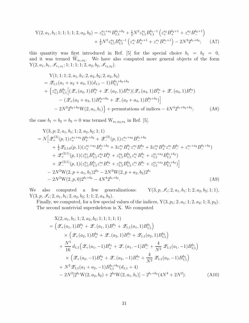
this quantity was first introduced in Ref. [5] for the special choice b1 = b2 = 0,and it was termed Wa1,a2 . We have also computed more general objects of the formY(2, a1, b1, Ir1,s1; 1; 1; 1; 1; 2, a2, b2, Ir2,s2).

Y(1; 1; 1; 2, a1, b1; 2, a2, b2; 2, a3, b3)

= Z1;1(a1 + a2 + a3, 1)(d1;1 − 1)Bb1+b2+b31;1

+{za11;1B

b11;1

[(Z+(a2, 1)Bb2

+ + Z−(a2, 1)Bb2− )(Z+(a3, 1)Bb3

+ + Z−(a3, 1)Bb3− )

− (Z+(a2 + a3, 1)Bb2+b3+ + Z−(a2 + a3, 1)Bb2+b3

− )]

− 2N22b2+b3W(2, a1, b1)}

+ permutations of indices − 4N42b1+b2+b3 ; (A8)

the case b1 = b2 = b3 = 0 was termed Wa1,a2,a3 in Ref. [5].

Y(3, p; 2, a1, b1; 1; 2, a2, b2; 1; 1)

= N[Z

(3)+ (p, 1)za1+a2

+ Bb1+b2+ + Z

(3)− (p, 1)za1+a2

− Bb1+b2−

+ 14Z2,1;0(p, 1)(za1+a2

+ Bb1+b2+ + 3za1

+ Bb1+ za2

− Bb2− + 3za2

+ Bb2+ za1

− Bb1− + za1+a2

− Bb1+b2− )

+ Z(2;1)

+ (p, 1)(za11;1B

b11;1z

a2+ Bb2

+ + za21;1B

b21;1z

a1+ Bb1

+ + za1+a21;1 Bb1+b2

1;1 )

+ Z(2;1)− (p, 1)(za1

1;1Bb11;1z

a2− Bb2

− + za21;1B

b21;1z

a1− Bb1

− + za1+a21;1 Bb1+b2

1;1 )]

− 2N2W(2, p + a1, b1)2b2 − 2N2W(2, p + a2, b2)2

b1

− 2N2W(2, p, 0)2b1+b2 − 4N42b1+b2 . (A9)

We also computed a few generalizations: Y(3, p, Ir; 2, a1, b1; 1; 2, a2, b2; 1; 1),Y(3, p, Ir; 2, a1, b1; 2, a2, b2; 1; 1; 2, a3, b3).

Finally, we computed, for a few special values of the indices, Y(3, p1; 2, a1; 1; 2, a2; 1; 3, p2).The second nontrivial superskeleton is X. We computed

X(2, a1, b1; 1; 2, a2, b2; 1; 1; 1; 1; 1)

=(Z+(a1, 1)Bb1

+ + Z−(a1, 1)Bb1− + Z1;1(a1, 1)Bb1

1;1

)

×(Z+(a2, 1)Bb2

+ + Z−(a2, 1)Bb2− + Z1;1(a2, 1)Bb2

1;1

)

+N4

16d1;1

(Z+(a1,−1)Bb1

+ + Z−(a1,−1)Bb1− +

4

N2Z1;1(a1,−1)Bb1

1;1

)

×(Z+(a2,−1)Bb2

+ + Z−(a2,−1)Bb2− +

4

N2Z1;1(a2,−1)Bb2

1;1

)

+ N2Z1;1(a1 + a2,−1)Bb1+b2

1;1 (d1;1 + 4)

− 2N2[2b1W(2, a2, b2) + 2b2W(2, a1, b1)] − 2b1+b2(4N4 + 2N2). (A10)

31

APPENDIX B: LIST OF POTENTIALS

We list here all the potentials appearing for the first time at each order of the strong-coupling expansion; we identify potentials differing only for the values of L and for thenumber b of [1; 1] bubbles provided that b > 0 (i.e. we don’t identify b = 0 with b 6= 0). Inthe following formulae, L will indicate a generic value, and multiple occurrences of L in thesame expressions indicate any combinations of Ls (i.e. they can take different values).

5th order:

W(2, L, b). (B1)

9th order:

W(3, L, [1; 2, L]), W(3, L, [1; 2, L, b]), Y(2, L; 1; 1; 1; 1; 2, L). (B2)

10th order:

Y(2, L; 2, L; 1; 1; 2, L; 1). (B3)

11th order:

W(2, L, [2, L; 2, L, b]), Y(3, L; 2, L; 1; 2, L; 1; 1), Y(2, L; 1; 1; 1; 1; 2, L, b). (B4)

12th order:

W(2, L, b, [2, L; 2, L]), W(3, L, [1; 2, L]2), Y(2, L; 2, L; 1; 1; 2, L, b; 1),

Y(2, L, b; 1; 1; 1; 1; 2, L), X(2, L; 1; 2, L; 1; 1; 1; 1; 1). (B5)

13th order:

W(3, L, [1; 2, L, [1; 3, L]]), W(4, L, [1; 3, L]), W(4, L, [2, L; 2, L, b]), W(2, L, b, [2, L; 2, L, b]),

Y(3, L; 2, L; 1; 2, L, b; 1; 1), Y(3, L; 2, L; 2, L; 1; 1; 2, L), Y(2, L; 1; 1; 1; 1; [1; 3, L]),

Y(2, L, b; 1; 1; 1; 1; 2, L, b), Y(2, L, b; 2, L; 1; 1; 2, L; 1), X(2, L; 1; 1; 1; 1; 1; 2, L; 2, L),

H(2, L; 1; 2, L; 1; 1; 1; 1; 1; 2, L). (B6)

14th order:

W(3, L, [1; 2, L, b, [1; 3, L]]), W(4, L, [1; 3, L, [1; 2, L]]), W(2, L, [1; [1; 2, L]2]),

W(2, L, [2, L, b; 2, L, b]), W(3, L, [1; 2, L] [1; 2, L, b]), Y(3, L; 3, L; 2, L; 1; 2, L; 1),

Y(3, L; 2, L, b; 1; 2, L; 1; 1), Y(2, L; 1; 1; 1; [1; 2, L]; 2, L), Y(2, L; 2, L; 1; 1; [1; 3, L]; 1),

Y(2, L; 2, L, b; 1; 1; 2, L; 1), Y(2, L, [1; 3, L]; 1; 1; 1; 1; 2, L), X(1; 1; 1; 1; 2, L; 2, L; 2, L; 2, L),

X(2, L; 1; 2, L; 1; 3, L; 1; 1; 1), X(2, L; 1; 2, L, b; 1; 1; 1; 1; 1), X(2, L, b; 1; 1; 1; 1; 1; 2, L; 2, L),

H(1; 2, L; 1; 2, L; 1; 1; 1; 1; 2, L), H(2, L; 2, L; 1; 1; 1; 2, L; 1; 2, L; 1),

R(1; 1; 2, L; 1; 1; 1; 2, L; 1; 1). (B7)

15th order:

32

W(3, L, [1; 2, L, [2, L; 2, L]]), W(3, L, [1; 2, L, [2, L; 2, L, b]]), W(3, L, [3, L; 2, L, b]),

W(3, L, [[1; 2, L]; 2, L]), W(4, L, [2, L, b; 2, L, b]), W(3, L, [1; 2, L]3),

Y(3, L; 2, L; 1; [1; 3, L]; 1; 1), Y(3, L; 2, L; 1; 2, L; 1; 3, L), Y(3, L; 2, L; 2, L; 1; 1; 2, L, b),

Y(3, L; 2, L, b; 1; 2, L, b; 1; 1), Y(3, L; 2, L, b; 2, L; 1; 1; 2, L), Y(4, L; 3, L; 2, L; 2, L; 1; 1),

Y(2, L; 1; 1; 1; 1; [2, L; 2, L]), Y(2, L; 1; 1; 1; 1; 2, L, [1; 3, L]), Y(2, L; 2, L; 1; [1; 2, L]; 2, L; 1),

Y(2, L, b; 1; 1; 1; 1; [1; 3, L]), Y(2, L, b; 2, L; 1; 1; 2, L, b; 1), Y(3, L, [1; 2, L]; 2, L; 1; 2, L; 1; 1),

Y(2, L, [1; 3, L]; 2, L; 1; 1; 2, L; 1), X(1; 1; 1; 1; 2, L; 2, L; 2, L; 2, L, b),

X(3, L; 2, L; 1; 2, L; 1; 1; 1; 1), X(2, L; 1; 1; 1; 1; 1; 2, L; 2, L, b),

X(2, L; 1; 1; 1; 3, L; 1; 2, L; 2, L), X(2, L; 2, L; 1; 1; 1; 2, L; 1; 2, L),

H(3, L; 2, L; 1; 1; 2, L; 1; 1; 2, L; 1), H(2, L; 1; 2, L; 1; 1; 1; 1; 1; 2, L, b),

H(2, L; 1; 2, L; 3, L; 1; 1; 1; 1; 2, L), H(2, L; 1; 2, L, b; 1; 1; 1; 1; 1; 2, L),

H(2, L; 3, L; 2, L; 1; 1; 1; 1; 1; 2, L), H(2, L; 2, L; 2, L; 1; 1; 2, L; 2, L; 1; 1),

L(1; 2, L; 1; 2, L; 1; 2, L; 1; 1; 1; 1), L(2, L; 1; 1; 1; 2, L; 1; 1; 1; 1; 1),

L(2, L; 1; 2, L; 1; 1; 2, L; 1; 1; 1; 1). (B8)

APPENDIX C: SQUARE LATTICE RESULTS FOR FINITE N

We list in the present Appendix the values of the quantities defined in Sect. VIII withoutfurther comments. The definition of these quantities and the range of validity of the resultspresented here is discussed in Sect. VIII.

A0 = 1 − 4 z + 4 z2 − 4 z3 + 12 z4 − 28 z5 + 4 z6 −17 + 13 N2

N2 − 1

+ 12 z7 −13 + 22 N2 − 11 N4

(N2 − 1)2+ 4 z8 101 − 158 N2 + 81 N4

(N2 − 1)2

+ 4 z9 −243 + 358 N2 − 227 N4

(N2 − 1)2

+ 4 z10 2444 − 6391 N2 + 7193 N4 − 3577 N6 + 505 N8

(N2 − 4) (N2 − 1)3

+ 4 z11 (−23568 + 89928 N2 − 154753 N4 + 145700 N6

− 74058 N8 + 17674 N10 − 1571 N12)

× 1

(N2 − 4)2 (N2 − 1)4

+ 4 z12 (59312 − 227352 N2 + 401499 N4 − 379396 N6

+ 189036 N8 − 43842 N10 + 3821 N12)

× 1

(N2 − 4)2 (N2 − 1)4

+ 4 z13 (−145008 + 560056 N2 − 1018759 N4 + 986360 N6

− 519366 N8 + 128954 N10 − 12235 N12)

33

× 1

(N2 − 4)2 (N2 − 1)4

+ 4 z14 (3296016− 16590056 N2 + 38621009 N4

− 50952462 N6 + 40255375 N8 − 18791194 N10 + 4822317 N12

− 617438 N14 + 29153 N16)

× 1

(N2 − 9) (N2 − 4)2 (N2 − 1)5

+ 4 z15 (−73339344 + 453776040 N2 − 1300249437 N4

+ 2195554892 N6 − 2367482622 N8 + 1669383326 N10 − 759240644 N12

+ 212701682 N14 − 34650066 N16 + 2929064 N18 − 98283 N20)

× 1

(N2 − 9)2 (N2 − 4)2 (N2 − 1)6 + O(z16), (C1)

A1 = z + z3 + 7 z5 + 4 z6 N2 + 1

N2 − 1+ 3 z7 13 − 22 N2 + 11 N4

(N2 − 1)2

+ 8 z8 −5 − 2 N2 + 4 N4

(N2 − 1)2 + z9 251 − 294 N2 + 243 N4

(N2 − 1)2

+ 4 z10 −284 − 13 N2 + 441 N4 − 369 N6 + 81 N8

(N2 − 4) (N2 − 1)3

+ z11 (24208 − 76936 N2 + 129833 N4 − 134180 N6 + 76114 N8

− 19562 N10 + 1819 N12)

× 1

(N2 − 4)2 (N2 − 1)4

+ 8 z12 −3632 + 2616 N2 + 3565 N4 − 8734 N6 + 7962 N8 − 2821 N10 + 315 N12

(N2 − 4)2 (N2 − 1)4

+ z13 (148848 − 456760 N2 + 879351 N4 − 922184 N6

+ 540230 N8 − 146906 N10 + 14859 N12)

× 1

(N2 − 4)2 (N2 − 1)4

+ 4 z14 (−422352 + 796520 N2 − 475949 N4 − 864192 N6

+ 2055327 N8 − 1703150 N10 + 634345 N12 − 102496 N14 + 5771 N16)

× 1

(N2 − 9) (N2 − 4)2 (N2 − 1)5

+ z15 (75941712− 403857000 N2 + 1114656565 N4

− 1899839324 N6 + 2117909054 N8 − 1584540590 N10 + 779561548 N12

− 235498610 N14 + 40734002 N16 − 3591112 N18 + 123883 N20)

× 1

(N2 − 9)2 (N2 − 4)2 (N2 − 1)6 + O(z16), (C2)

34

A2,0 = −z6 N2 + 1

N2 − 1+ 2 z8 4 + 2 N2 − 3 N4

(N2 − 1)2 − 4 z9 1 + 8 N2 + 2 N4

(N2 − 1)2

+ z10 212 − 25 N2 − 355 N4 + 255 N6 − 57 N8

(N2 − 4) (N2 − 1)3

+ 4 z11 −5 − 100 N2 + 137 N4 − 12 N6 − 29 N8

(N2 − 1)4

+ 2 z12 2608 − 1944 N2 + 195 N4 + 1992 N6 − 4278 N8 + 2001 N10 − 250 N12

(N2 − 4)2 (N2 − 1)4

+ 8 z13 60 + 1485 N2 − 1735 N4 + 520 N6 + 396 N8 − 144 N10

(N2 − 4) (N2 − 1)4

+ z14 (303120 − 666632 N2 + 1554257 N4 − 1748152 N6

+ 205601 N8 + 831342 N10 − 468499 N12 + 86566 N14 − 5155 N16)

× 1

(N2 − 9) (N2 − 4)2 (N2 − 1)5

+ 4 z15 (−3984 − 68344 N2 + 247735 N4 − 387636 N6

+ 321005 N8 − 97944 N10 − 30420 N12 + 21362 N14 − 2908 N16)

× 1

(N2 − 4)2 (N2 − 1)6 + O(z16), (C3)

A2,2 = −2 z8 N2 + 1

N2 − 1− 2 z9 1 + 8 N2 + 2 N4

(N2 − 1)2

+ 2 z10 −9 − 7 N2 + 9 N4 − 12 N6

(N2 − 1)3

+ 2 z11 −5 − 112 N2 + 155 N4 − 12 N6 − 35 N8

(N2 − 1)4

+ 2 z12 64 + 54 N2 + 100 N4 − 52 N6 − 121 N8

(N2 − 1)4

+ 4 z13 60 + 1917 N2 − 1843 N4 + 640 N6 + 606 N8 − 204 N10

(N2 − 4) (N2 − 1)4

+ 2 z14 (−7392 + 8144 N2 − 55774 N4 + 92342 N6 − 35882 N8

− 16810 N10 + 10745 N12 − 1412 N14)

× 1

(N2 − 4)2 (N2 − 1)5

+ 2 z15 (−4336 − 96968 N2 + 298881 N4 − 461772 N6

+ 413767 N8 − 131684 N10 − 48836 N12 + 32296 N14 − 4264 N16)

× 1

(N2 − 4)2 (N2 − 1)6+ O(z16), (C4)

A3,1 = z9 1 + 8 N2 + 2 N4

2 (N2 − 1)2 + z11 5 + 100 N2 − 137 N4 + 12 N6 + 29 N8

2 (N2 − 1)4

35

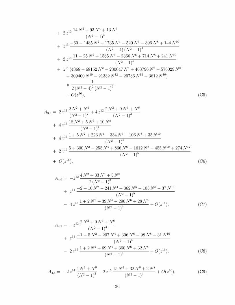
+ 2 z12 14 N2 + 93 N4 + 13 N6

(N2 − 1)3

+ z13 −60 − 1485 N2 + 1735 N4 − 520 N6 − 396 N8 + 144 N10

(N2 − 4) (N2 − 1)4

+ 2 z14 11 − 25 N2 + 1585 N4 − 2366 N6 + 714 N8 + 241 N10

(N2 − 1)5

+ z15 (4368 + 68152 N2 − 230047 N4 + 463796 N6 − 576029 N8

+ 309400 N10 − 21332 N12 − 20786 N14 + 3612 N16)

× 1

2 (N2 − 4)2 (N2 − 1)6

+ O(z16), (C5)

A3,3 = 2 z11 2 N2 + N4

(N2 − 1)2 + 4 z12 2 N2 + 9 N4 + N6

(N2 − 1)3

+ 4 z13 18 N2 + 5 N6 + 10 N8

(N2 − 1)4

+ 4 z14 1 + 5 N2 + 223 N4 − 334 N6 + 106 N8 + 35 N10

(N2 − 1)5

+ 2 z15 5 + 300 N2 − 255 N4 + 866 N6 − 1612 N8 + 455 N10 + 274 N12

(N2 − 1)6

+ O(z16), (C6)

A4,0 = −z12 4 N2 + 33 N4 + 5 N6

2 (N2 − 1)3

+ z14 −2 + 10 N2 − 241 N4 + 362 N6 − 105 N8 − 37 N10

(N2 − 1)5

− 3 z15 1 + 2 N2 + 39 N4 + 296 N6 + 28 N8

(N2 − 1)4 + O(z16), (C7)

A4,2 = −z12 2 N2 + 9 N4 + N6

(N2 − 1)3

+ z14 −1 − 5 N2 − 207 N4 + 306 N6 − 98 N8 − 31 N10

(N2 − 1)5

− 2 z15 1 + 2 N2 + 69 N4 + 360 N6 + 32 N8

(N2 − 1)4 + O(z16), (C8)

A4,4 = −2 z14 4 N4 + N6

(N2 − 1)3− 2 z15 15 N4 + 32 N6 + 2 N8

(N2 − 1)4+ O(z16), (C9)

36

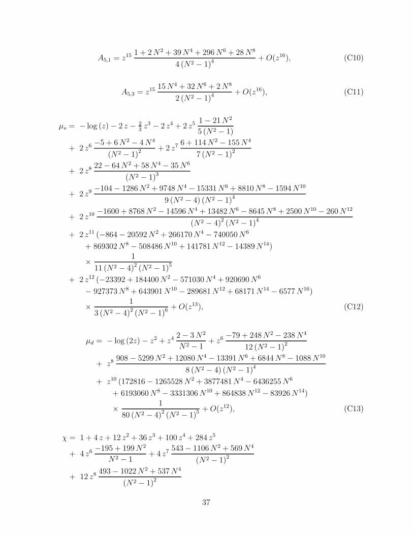
A5,1 = z15 1 + 2 N2 + 39 N4 + 296 N6 + 28 N8

4 (N2 − 1)4+ O(z16), (C10)

A5,3 = z15 15 N4 + 32 N6 + 2 N8

2 (N2 − 1)4+ O(z16), (C11)

µs = − log (z) − 2 z − 23z3 − 2 z4 + 2 z5 1 − 21 N2

5 (N2 − 1)

+ 2 z6 −5 + 6 N2 − 4 N4

(N2 − 1)2 + 2 z7 6 + 114 N2 − 155 N4

7 (N2 − 1)2

+ 2 z8 22 − 64 N2 + 58 N4 − 35 N6

(N2 − 1)3

+ 2 z9 −104 − 1286 N2 + 9748 N4 − 15331 N6 + 8810 N8 − 1594 N10

9 (N2 − 4) (N2 − 1)4

+ 2 z10 −1600 + 8768 N2 − 14596 N4 + 13482 N6 − 8645 N8 + 2500 N10 − 260 N12

(N2 − 4)2 (N2 − 1)4

+ 2 z11 (−864 − 20592 N2 + 266170 N4 − 740050 N6

+ 869302 N8 − 508486 N10 + 141781 N12 − 14389 N14)

× 1

11 (N2 − 4)2 (N2 − 1)5

+ 2 z12 (−23392 + 184400 N2 − 571030 N4 + 920690 N6

− 927373 N8 + 643901 N10 − 289681 N12 + 68171 N14 − 6577 N16)

× 1

3 (N2 − 4)2 (N2 − 1)6 + O(z13), (C12)

µd = − log (2z) − z2 + z4 2 − 3 N2

N2 − 1+ z6 −79 + 248 N2 − 238 N4

12 (N2 − 1)2

+ z8 908 − 5299 N2 + 12080 N4 − 13391 N6 + 6844 N8 − 1088 N10

8 (N2 − 4) (N2 − 1)4

+ z10 (172816 − 1265528 N2 + 3877481 N4 − 6436255 N6

+ 6193060 N8 − 3331306 N10 + 864838 N12 − 83926 N14)

× 1

80 (N2 − 4)2 (N2 − 1)5+ O(z12), (C13)

χ = 1 + 4 z + 12 z2 + 36 z3 + 100 z4 + 284 z5

+ 4 z6 −195 + 199 N2

N2 − 1+ 4 z7 543 − 1106 N2 + 569 N4

(N2 − 1)2

+ 12 z8 493 − 1022 N2 + 537 N4

(N2 − 1)2

37

+ 4 z9 4067 − 8550 N2 + 4643 N4

(N2 − 1)2

+ 4 z10 44100 − 149869 N2 + 182355 N4 − 90083 N6 + 13323 N8

(N2 − 4) (N2 − 1)3

+ 4 z11 (481168 − 2256648 N2 + 4239673 N4 − 4010564 N6

+ 1961034 N8 − 452890 N10 + 38875 N12)

× 1

(N2 − 4)2 (N2 − 1)4

+ 4 z12 (1299728 − 6161736 N2 + 11712625 N4

− 11228076 N6 + 5568300 N8 − 1301614 N10 + 112879 N12)

× 1

(N2 − 4)2 (N2 − 1)4

+ 4 z13 (3526000 − 16894776 N2 + 32535287 N4

− 31650616 N6 + 15957638 N8 − 3784938 N10 + 332699 N12)

× 1

(N2 − 4)2 (N2 − 1)4

+ 4 z14 (85479984− 509240632 N2 + 1277936387 N4

− 1742114314 N6 + 1385750301 N8 − 641889782 N10 + 163736431 N12

− 20707322 N14 + 976227 N16)

× 1

(N2 − 9) (N2 − 4)2 (N2 − 1)5

+ 4 z15 (2078977104− 14813458920 N2 + 45842748421 N4

− 80400814700 N6 + 87447748126 N8 − 60663055822 N10 + 26640570340 N12

− 7157578626 N14 + 1112718466 N16 − 90043336 N18 + 2904339 N20)

× 1

(N2 − 9)2 (N2 − 4)2 (N2 − 1)6 + O(z16), (C14)

M2G = z−1 − 4 + 3 z + 2 z3 − 4 z4 N2 + 1

N2 − 1+ 2 z5 −5 − 4 N2 + 6 N4

(N2 − 1)2

+ 8 z6 6 + 2 N2 − 5 N4

(N2 − 1)2+ 4 z7 −32 − 42 N2 + 21 N4

(N2 − 1)2

+ 8 z8 184 + 98 N2 − 376 N4 + 203 N6 − 37 N8

(N2 − 4) (N2 − 1)3

+ 2 z9 −6576 − 3656 N2 + 30629 N4 − 32810 N6 + 14735 N8 − 3245 N10 + 275 N12

(N2 − 4)2 (N2 − 1)4

+ 8 z10 4016 + 4136 N2 − 16789 N4 + 15608 N6 − 7937 N8 + 2257 N10 − 238 N12

(N2 − 4)2 (N2 − 1)4

+ 2 z11 (−34560 − 63904 N2 + 148416 N4 − 142210 N6

+ 74870 N8 − 19631 N10 + 1658 N12)

38

× 1

(N2 − 4)2 (N2 − 1)4

+ 8 z12 (186048 + 87904 N2 − 727204 N4 + 1149812 N6

− 1175339 N8 + 716157 N10 − 232150 N12 + 34766 N14 − 1906 N16)

× 1

(N2 − 9) (N2 − 4)2 (N2 − 1)5

+ 2 z13 (−14774400 + 8055072 N2 + 58712088 N4

− 170052698 N6 + 261060513 N8 − 232073848 N10 + 117200494 N12

− 33867953 N14 + 5360045 N16 − 433255 N18 + 13878 N20)

× 1

(N2 − 9)2 (N2 − 4)2 (N2 − 1)6+ O(z14), (C15)

F = 2 z2 + 2 z4 + 4 z6 + z8 14 − 30 N2 + 19 N4

(N2 − 1)2

+ 8 z10 7 − 16 N2 + 12 N4

(N2 − 1)2

+ 2 z12 (5952 − 30144 N2 + 63364 N4 − 67746 N6 + 37500 N8

− 9589 N10 + 906 N12)

× 1

3 (N2 − 4)2 (N2 − 1)4

+ 4 z14 (4704 − 25200 N2 + 55366 N4 − 62068 N6 + 36768 N8

− 10012 N10 + 1009 N12)

× 1

(N2 − 4)2 (N2 − 1)4

+ z16 (15230592− 119651328 N2 + 409792072 N4

− 799817292 N6 + 974422200 N8 − 760569676 N10 + 375693595 N12

− 112460534 N14 + 19258826 N16 − 1690814 N18 + 58471 N20)

× 1

2 (N2 − 9)2 (N2 − 4)2 (N2 − 1)6

+ 8 z18 (237447936− 2045848320 N2 + 7796836128 N4

− 17299894704 N6 + 24693730379 N8 − 23648019056 N10 + 15403609647 N12

− 6787736700 N14 + 1995934103 N16 − 381749639 N18 + 45159907 N20

− 2974083 N22 + 82898 N24)

× 1

3 (N2 − 9)2 (N2 − 4)4 (N2 − 1)6 + O(z20). (C16)

39

APPENDIX D: THE GAUSSIAN MODEL ON THE HONEYCOMB LATTICE

There are a few subtleties in the analysis of models on the honeycomb lattice, that arebest illustrated by considering a simple Gaussian model of random walks. The essentialpoint is related to the fact that lattice sites are not all related by a translation group: onlypoints at an even distance (in the number of lattice links) are related by such a symmetry.As a consequence, it is convenient to define even and odd fields φe, φo, according to theparity of the corresponding lattice sites with respect to an arbitrarily chosen origin, andeven and odd correlation functions Ge = 〈φeφe〉 = 〈φoφo〉, Go = 〈φeφo〉 = 〈φoφe〉.

Let us represent the Cartesian coordinates of the (finite, periodic) lattice sites by

(x, y)e =(

32m, 1

2

√3n)a, (D1a)

(x, y)o =(

32m + 1, 1

2

√3n)

a, (D1b)

where m and n are integer numbers satisfying the conditions 0 ≤ m < L1, 0 ≤ n < 2L2,and m + n is even. The total number of lattice points is 2L1×L2, the number of links is3L1×L2, and the number of plaquettes is L1×L2.

The finite-lattice Fourier transform is consistently defined by

Ge(p) =∑

x even

eip·xGe(x), (D2)

and similarly for Go(p); the set of momenta is

p =2π

a

(2

3

m

L1

,1√3

n

L2

), (D3)

with m and n integers, and 0 ≤ m < L1, 0 ≤ n < L2.In a random walk model where walks of length ν are weighted by a factor βν , it is easy

to establish from the recursion relations the following relationships:

Ge(p) = βe−ip1

[1 + 2 cos 1

2

√3p2 e3ip1/2

]Go(p) + 1, (D4a)

Go(p) = βeip1

[1 + 2 cos 1

2

√3p2 e−3ip1/2

]Ge(p), (D4b)

where Ge(p) and Go(p) are the Fourier transform of Ge(x) and Go(x) respectively. As aconsequence, we obtain the even momentum-space Green’s functions in the form

Ge(p) =1

1 − β2[1 + 4 cos2 1

2

√3p2 + 4 cos 1

2

√3p2 cos 3

2p1

] . (D5)

The critical value of β is easily found to be βc = 13, and as a consequence we find the

massless lattice (even) propagator

∆e(p) =9

8 − 4 cos2 12

√3p2 + 4 cos 1

2

√3p2 cos 3

2p1

−→p→0

2

p2. (D6)

The odd propagator is simply

40

∆o(p) = 13eip1

[1 + 2 cos 1

2

√3p2 e−3ip1/2

]∆e(p). (D7)

The structure of the propagator in the Gaussian model offers an important indicationabout the possibility of exponentiation in wall-wall correlations. Let us indeed recall thatexponentiation corresponds to a simple structure

1

A − B cos p(D8)

in the corresponding propagator. Let us now observe that Eq. (D5) implies

Ge(p1, 0) =1

1 − β2[5 + 4 cos 3

2p1

] , (D9)

Ge(0, p2) + Go(0, p2) =1

1 − β[1 + 2 cos 1

2

√3p2

] . (D10)

We have therefore the possibility of defining two different exponentiated “wall-wall” corre-lation functions, i.e.

G(w)1 (x) =

∑

y

Ge(x, y), (D11)

G(w)2 (x) =

∑

y

[Ge(x, y) + Go(x, y)] . (D12)

Even in more general models, in the strong-coupling domain, for sufficiently large latticedistance exponentiation will hold for the correlation functions G

(w)1 (x) and G

(w)2 (x). If we

take into account the discrete rotational symmetry of the honeycomb lattice we may easilyrecognize that the above correlations can be referred to directions differing by a π/6 angle,and this is the maximal violation of the full rotational symmetry one can find on thiskind of lattice. Therefore the ratio of the two different correlation lengths one may defineis an optimal measurement of the violation of rotational invariance in the model underexamination, in analogy with the side/diagonal mass ratio of the square lattice.

APPENDIX E: HONEYCOMB LATTICE RESULTS FOR FINITE N

We list in the present Appendix the values of the quantities defined in Sect. IX withoutfurther comments. The definition of these quantities presented here is discussed in Sect. IX.

µ1 = 23

[− log 2z2 − z2 − 1

2z4 + z6 −14 + 46 N2 − 41 N4

6 (N2 − 1)2

+ z8 9 − 27 N2 + 35 N4 − 37 N6

4 (N2 − 1)3

+ z10 −194 + 1136 N2 − 2539 N4 + 2546 N6 − 1174 N8

20 (N2 − 1)4

+ z12 (−6208 + 49952 N2 − 175780 N4 + 360896 N6 − 469546 N8

41

+ 395168 N10 − 205477 N12 + 56246 N14 − 6169 N16)

× 1

24 (N2 − 4)2 (N2 − 1)6

+ z14 (−204800 + 2013696 N2 − 8684352 N4 + 21407856 N6

− 33518156 N8 + 34888595 N10 − 24526859 N12 + 11475108 N14

− 3337802 N16 + 545557 N18 − 39943 N20)

× 1

56 (N2 − 4)3 (N2 − 1)7

+ z16 (−253184 + 2885888 N2 − 14879968 N4 + 46028112 N6

− 95149021 N8 + 138282732 N10 − 144193790 N12 + 108442897 N14

− 58120117 N16 + 21234008 N18 − 4926461 N20 + 646061 N22 − 36361 N24)

× 1

8 (N2 − 4)4 (N2 − 1)8

]+ O(z18), (E1)

µ2 = 23

√3[− log z − z + 1

2z2 − 1

3z3 − 3

4z4 − 1

5z5 − z6 1 + 11 N2

6 (N2 − 1)

+ 2 z7 −4 + N2 − 18 N4

7 (N2 − 1)2+ z8 11 − 81 N2 + N4 + 29 N6

8 (N2 − 1)3

+ 5 z9 2 + 12 N2 + 24 N4 − 11 N6

9 (N2 − 1)3

+ z10 19 − 277 N2 + 127 N4 − 319 N6

10 (N2 − 1)3

+ z11 −34 + 26 N2 − 622 N4 + 587 N6 − 452 N8

11 (N2 − 1)4

+ z12 −132 + 1045 N2 − 1813 N4 + 2158 N6 − 558 N8 − 115 N10 − 69 N12

4 (N2 − 4) (N2 − 1)5

+ z13 (−1472 + 5408 N2 − 24716 N4 + 48156 N6 − 97577 N8

+ 118419 N10 − 65911 N12 + 18318 N14 − 2614 N16)

× 1

13 (N2 − 4)2 (N2 − 1)6

+ z14 (5568 − 91344 N2 + 393204 N4 − 964687 N6 + 1168570 N8

− 845302 N10 + 432359 N12 − 133335 N14 + 18275 N16 − 885 N18)

× 1

7 (N2 − 4)3 (N2 − 1)6

+ z15 (−25024 + 122896 N2 − 380772 N4 + 569163 N6 − 1634619 N8

+ 3326040 N10 − 3347466 N12 + 1923822 N14 − 642978 N16 + 116764 N18

− 7576 N20)

× 1

15 (N2 − 4)3 (N2 − 1)7

42

+ z16 (43712 − 656912 N2 + 3472772 N4 − 10632331 N6

+ 18690504 N8 − 20221284 N10 + 15125616 N12 − 8770834 N14 + 4069272 N16

− 1342540 N18 + 260364 N20 − 24083 N22)

× 1

16 (N2 − 4)3 (N2 − 1)8

]+ O(z17), (E2)

χ = 1 + 3 z + 6 z2 + 12 z3 + 24 z4 + 48 z5 + 90 z6 + 174 z7

+ 12 z8 −28 + 29 N2

N2 − 1+ 18 z9 36 − 74 N2 + 39 N4

(N2 − 1)2

+ 6 z10 −203 + 625 N2 − 649 N4 + 232 N6

(N2 − 1)3

+ 6 z11 388 − 1592 N2 + 2469 N4 − 1725 N6 + 469 N8

(N2 − 1)4

+ 6 z12 736 − 3056 N2 + 4802 N4 − 3407 N6 + 943 N8

(N2 − 1)4

+ 6 z13 1398 − 5850 N2 + 9318 N4 − 6743 N6 + 1922 N8

(N2 − 1)4

+ 6 z14 −10520 + 47078 N2 − 82728 N4 + 70812 N6 − 28891 N8 + 3951 N10

(N2 − 4) (N2 − 1)4

+ 6 z15 (79712 − 380208 N2 + 730934 N4 − 716200 N6

+ 372088 N8 − 91009 N10 + 8228 N12)

× 1

(N2 − 4)2 (N2 − 1)4

+ 6 z16 (600192 − 3641312 N2 + 9388472 N4 − 13344618 N6

+ 11337734 N8 − 5813592 N10 + 1719475 N12 − 267280 N14 + 16906 N16)

× 1

(N2 − 4)3 (N2 − 1)5

+ 6 z17 (4531200 − 33355776 N2 + 107774336 N4

− 200423616 N6 + 236373604 N8 − 183407604 N10 + 93969088 N12

− 31097639 N14 + 6341524 N16 − 722188 N18 + 35215 N20)

× 1

(N2 − 4)4 (N2 − 1)6

+ 6 z18 (−8505600 + 71553024 N2 − 268314976 N4

+ 590267696 N6 − 843497305 N8 + 818280951 N10 − 546354607 N12

+ 249146769 N14 − 75461014 N16 + 14404142 N18 − 1562138 N20

+ 73433 N22)

× 1

(N2 − 4)4 (N2 − 1)7

+ 6 z19 (16021504− 151615488 N2 + 647496704 N4

43

− 1646428032 N6 + 2769093400 N8 − 3234820688 N10 + 2679887383 N12

− 1577573745 N14 + 650694030 N16 − 182224525 N18 + 32769509 N20

− 3399903 N22 + 154769 N24)

× 1

(N2 − 4)4 (N2 − 1)8

+ 6 z20 (−270452736 + 2603295744N2 − 11339998976 N4

+ 29517395456 N6 − 51057737736 N8 + 61725236828 N10 − 53378649928 N12

+ 33218024089 N14 − 14765553520 N16 + 4594385593 N18 − 966784918 N20

+ 129788872 N22 − 9932849 N24 + 325065 N26)

× 1

(N2 − 9) (N2 − 4)4 (N2 − 1)8+ O(z21), (E3)

M2G = 4

3z−1 − 4 + 8

3z − 8 z6 N2 + 1

N2 − 1+ 8 z7 −7 − 10 N2 + 5 N4

3 (N2 − 1)2

+ 8 z8 −3 − 7 N2 + 4 N4 + N6

(N2 − 1)3 + 8 z9 −12 − 20 N2 + 29 N6 − 6 N8

3 (N2 − 1)4

+ 8 z10 12 − 6 N2 + 15 N4 + 8 N6 − 11 N8

(N2 − 1)4

+ 8 z11 −82 − 34 N2 + 165 N4 − 247 N6 + 36 N8

3 (N2 − 1)4

+ 8 z12 −160 − 432 N2 + 698 N4 − 409 N6 − 2 N8 − 18 N10

(N2 − 4) (N2 − 1)4

+ 8 z13 −1776 − 12392 N2 + 3665 N4 + 1850 N6 − 1811 N8 − 666 N10 + 73 N12

3 (N2 − 4)2 (N2 − 1)4

+ 8 z14 (3328 + 9920 N2 + 23760 N4 − 41452 N6 + 12242 N8

+ 5969 N10 − 5077 N12 + 657 N14 − 5 N16)

× 1

(N2 − 4)3 (N2 − 1)5

+ 8 z15 (−114432 + 400128 N2 − 1536160 N4 + 1733488 N6

− 323935 N8 − 602516 N10 + 449683 N12 − 124964 N14 + 5895 N16

+ 1675 N18 − 75 N20)

× 1

3 (N2 − 4)4 (N2 − 1)6

+ 8 z16 (−91136 + 441856 N2 − 1078144 N4 + 768256 N6

+ 450812 N8 − 1054246 N10 + 839396 N12 − 464465 N14 + 194981 N16

− 54586 N18 + 9491 N20 − 690 N22)

× 1

(N2 − 4)4 (N2 − 1)7

+ 8 z17 (−425728 + 1766144 N2 − 1985440 N4 − 5221520 N6

44

+ 17290561 N8 − 24613836 N10 + 24266712 N12 − 17725908 N14

+ 9035120 N16 − 2989557 N18 + 594069 N20 − 63766 N22 + 2193 N24)

× 1

3 (N2 − 4)4 (N2 − 1)8

+ 8 z18 (−1661184 + 3794944 N2 + 7844000 N4

− 54955728 N6 + 119244695 N8 − 171667137 N10 + 175851305 N12

− 120836371 N14 + 53853632 N16 − 15114634 N18 + 2512157 N20

− 229837 N22 + 9716 N24 − 526 N26)

× 1

(N2 − 9) (N2 − 4)4 (N2 − 1)8 + O(z19), (E4)

F = 32z2 + z6 + 3 z10

+ z12 4 − 18 N2 + 32 N4 − 27 N6 + 18 N8

2 (N2 − 1)4 + 12 z14

+ 6 z16 3 − 16 N2 + 32 N4 − 29 N6 + 19 N8

(N2 − 1)4

+ z18 (49920 − 268032 N2 + 595744 N4 − 732080 N6

+ 536515 N8 − 239924 N10 + 65162 N12 − 10174 N14 + 829 N16)

× 1

3 (N2 − 4)4 (N2 − 1)4

+ 3 z20 (92 − 890 N2 + 3756 N4 − 9052 N6 + 13836 N8

− 14023 N10 + 9380 N12 − 3690 N14 + 720 N16)

× 1

2 (N2 − 1)8

+ 3 z22 (36864 − 368640 N2 + 1666560 N4 − 4505344 N6

+ 8111248 N8 − 10267152 N10 + 9373736 N12 − 6230112 N14

+ 3011024 N16 − 1020866 N18 + 227573 N20 − 30248 N22 + 1918 N24)

× 1

(N2 − 4)4 (N2 − 1)8

+ z24 (7215630336− 96566722560 N2 + 592839316224 N4

− 2214635962752 N6 + 5639017965384 N8 − 10385973650808 N10

+ 14322131449584 N12 − 15072994434276 N14 + 12212762091344 N16

− 7627059006688 N18 + 3656946091530 N20 − 1335009872497 N22

+ 366664198242 N24 − 74601540139 N26 + 11013519148 N28 − 1144634371 N30

+ 79672354 N32 − 3373733 N34 + 68030 N36)

× 1

4 (N2 − 9)4 (N2 − 4)4 (N2 − 1)10

+ 3 z26 (−275712 + 3201536 N2 − 17022176 N4

+ 54825776 N6 − 119171333 N8 + 184722213 N10 − 210428660 N12

45

+ 178609366 N14 − 112928266 N16 + 52388456 N18 − 17133329 N20

+ 3699171 N22 − 474540 N24 + 29132 N26)

× 1

(N2 − 4)4 (N2 − 1)9 + O(z28). (E5)

46

REFERENCES

[1] F. Green and S. Samuel, Nucl. Phys. B190, 113 (1981).[2] F. Green and S. Samuel, Phys. Lett. 103B, 110 (1981).[3] F. Green and S. Samuel, Nucl. Phys. B194, 107 (1982).[4] P. Rossi and E. Vicari, Phys. Rev. D49, 1621 (1994).[5] P. Rossi and E. Vicari, Phys. Rev. D49, 6072 (1994); D50, 4718 (1994) (E).[6] M. Campostrini, P. Rossi, and E. Vicari, Asymptotic scaling from strong coupling,

preprint IFUP-TH 36/94, 1994.[7] M. R. Douglas and S. H. Shenker, Nucl. Phys. B335, 635 (1990).[8] D. J. Gross and A. A. Migdal, Phys. Rev. Lett. 64, 127 (1990).[9] E. Brezin and V. A. Kazakov, Phys. Lett. B236, 144 (1990).

[10] V. Periwal and D. Shevitz, Phys. Rev. Lett. 64, 1326 (1990).[11] J.-M. Drouffe and J.-B. Zuber, Phys. Rep. 102, 1 (1983).[12] E. Rabinovici and S. Samuel, Phys. Lett. 101B, 323 (1981).[13] G. Parisi, Statistical Field Theory (Addison-Wesley, Redwood City, CA, 1988).[14] C. Itzikson and J.-M. Drouffe, Statistical Field Theory (Cambridge University Press,

Cambridge, 1989).[15] B. de Wit and G. ’t Hooft, Phys. Lett. 69B, 61 (1977).[16] R. C. Brower, P. Rossi, and C.-I. Tan, Phys. Rev. D23, 942 (1981).[17] R. C. Brower, P. Rossi, and C.-I. Tan, Phys. Rev. D23, 953 (1981).

47