arX

iv:h

ep-l

at/9

4060

14v1

20

Jun

1994

IFUP-TH 36/94

Asymptotic scaling from strong coupling

Massimo Campostrini, Paolo Rossi, and Ettore VicariDipartimento di Fisica dell’Universita and I.N.F.N., I-56126 Pisa, Italy

Abstract

Strong-coupling analysis of two-dimensional chiral models, extended to 15th

order, allows for the identification of a scaling region where known continuum

results are reproduced with great accuracy, and asymptotic scaling predictions

are fulfilled. The properties of the large-N second-order phase transition are

quantitatively investigated.

Typeset using REVTEX

1

Recent developments in the analytical and numerical study of lattice two-dimensionalSU(N)× SU(N) principal chiral models have shown the existence of a scaling region, wherecontinuum predictions for dimensionless ratios of physical quantities are substantially verified[1].

The scaling region begins at very small values of the correlation length: ξ >∼ 2, wellwithin the region of convergence of the strong-coupling series. Moreover by performing anonperturbative change of variables [2] from the standard Lagrangian (inverse) coupling βto

βE =N2 − 1

8N2E, (1)

where E is the internal energy of the system (which can be measured in a Monte Carlosimulation), one can find agreement in the whole scaling region between the measured massscale and the prediction for the mass gap – Λ parameter ratio offered by the two-loopcontinuum renormalization group supplemented by a Bethe-Ansatz evaluation [3]. As amatter of fact, this may be thought as evidence for asymptotic scaling within the strong-coupling regime.

We therefore felt motivated for a significant effort in improving our analytical knowledgeof the strong-coupling series for principal chiral models, in order to check the accuracy ofpredictions for physical (continuum) quantities solely based on strong-coupling computa-tions.

As a byproduct, strong-coupling series can be analyzed to investigate the critical behaviorof the N = ∞ theory, where Monte Carlo data seem to indicate the existence of a transitionat finite β.

Strong-coupling calculations for matrix models are best performed by means of the char-acter expansion. Even the character expansion however eventually runs into almost in-tractable technical difficulties, related to two concurrent phenomena:

1. the proliferation of configurations contributing to large orders of the series, whosenumber essentially grows like that of non-backtracking random walks;

2. the appearance of topologically nontrivial configurations corresponding to group in-tegrations that cannot be performed by applying the orthogonality of characters andthe decomposition of their products into sums.

We shall devote an extended paper to a complete presentation of our 15th-order strong-coupling character expansions for arbitrary U(N) groups (extension to SU(N) is then ob-tained by the techniques discussed in Refs. [4] and [1]). We only mention that we had torely on a mixed approach: problem 1 above was tackled by a computer program generatingall non-backtracking random walks, computing their correct multiplicities, and classifyingthem according to their topology; problem 2, requiring the analytical evaluation of manyclasses of nontrivial group integrals, and extraction of their connected contribution to therelevant physical quantities, was solved by more conventional algebraic techniques.

We pushed our computational techniques close to their limit; in order to extend ourresults to higher orders, a more algorithmic approach would be in order, especially forrecognition of diagram topologies and group integration.

2

In the present letter we shall only exhibit the results we obtained by taking the large-Nlimit of all the quantities we computed. In the strong-coupling domain, convergence to N =∞ is usually fast, and therefore large-N results are a good illustration of a phenomenologythat repeats itself (with small corrections) for finite values of N .

Starting from the standard nearest-neighbour interaction

SL = −2Nβ∑

x,µ

ReTr{U(x) U †(x+µ)}, (2)

we computed the large-N free energy

F =1

N2ln∫

dUn exp(−SL) (3)

to 18th order in the expansion in powers of β. The resulting series is

F = β2 + 2β4 + 4β6 + 19β8 + 96β10 + 604β12 + 4036β14

+58471

2β16 +

663568

3β18 + O(β20). (4)

The two-point Green’s functions, normalized to obtain a finite large-N limit, are

G(x) =1

NTr{U †(x)U(0)}. (5)

We computed all nontrivial two-point Green’s functions up to O(β15). The correspondinginformation is appropriately summarized by introducing the lattice Fourier transform

G(p) =∑

x

G(x) exp(ip · x) (6)

and evaluating the inverse propagator

G−1(p) = A0 + p2A1 + ((p2)2 − p4)A2,0 + p4A2,2 + p2((p2)

2 − p4)A3,1 + p6A3,3

+ ((p2)2 − p4)

2A4,0 + p4((p2)

2 − p4)A4,2 + p8A4,4 + p2((p2)2 − p4)

2A5,1

+ p6((p2)2 − p4)A5,3 + ... , (7)

where

A0 = 1 − 4β + 4β2 − 4β3 + 12β4 − 28β5 + 52β6 − 132β7 + 324β8 − 908β9 + 2020β10

− 6284β11 + 15284β12 − 48940β13 + 116596β14 − 393052β15 + O(β16),

A1 = β(1 + β2 + 7β4 + 4β5 + 33β6 + 32β7 + 243β8 + 324β9 + 1819β10 + 2520β11

+ 14859β12 + 23124β13 + 123767β14) + O(β16),

A2,0 = −β6(

1 + 6β2 + 8β3 + 57β4 + 116β5 + 500β6 + 1152β7 + 5173β8 + 11600β9)

+ O(β16),

A2,2 = −2β8(

1 + 2β + 12β2 + 35β3 + 121β4 + 408β5 + 1424β6 + 4244β7)

+ O(β16),

A3,1 = β9(

1 +29

2β2 + 26β3 + 144β4 + 488β5 + 1802β6

)

+ O(β16),

3

A3,3 = 2β11(

1 + 2β + 20β2 + 72β3 + 272β4)

+ O(β16),

A4,0 = −β12(

5

2+ 37β2 + 84β3

)

+ O(β16),

A4,2 = −β12(

1 + 32β2 + 64β3)

+ O(β16),

A4,4 = −2β14 (1 + 2β) + O(β16),

A5,1 = 7β15 + O(β16),

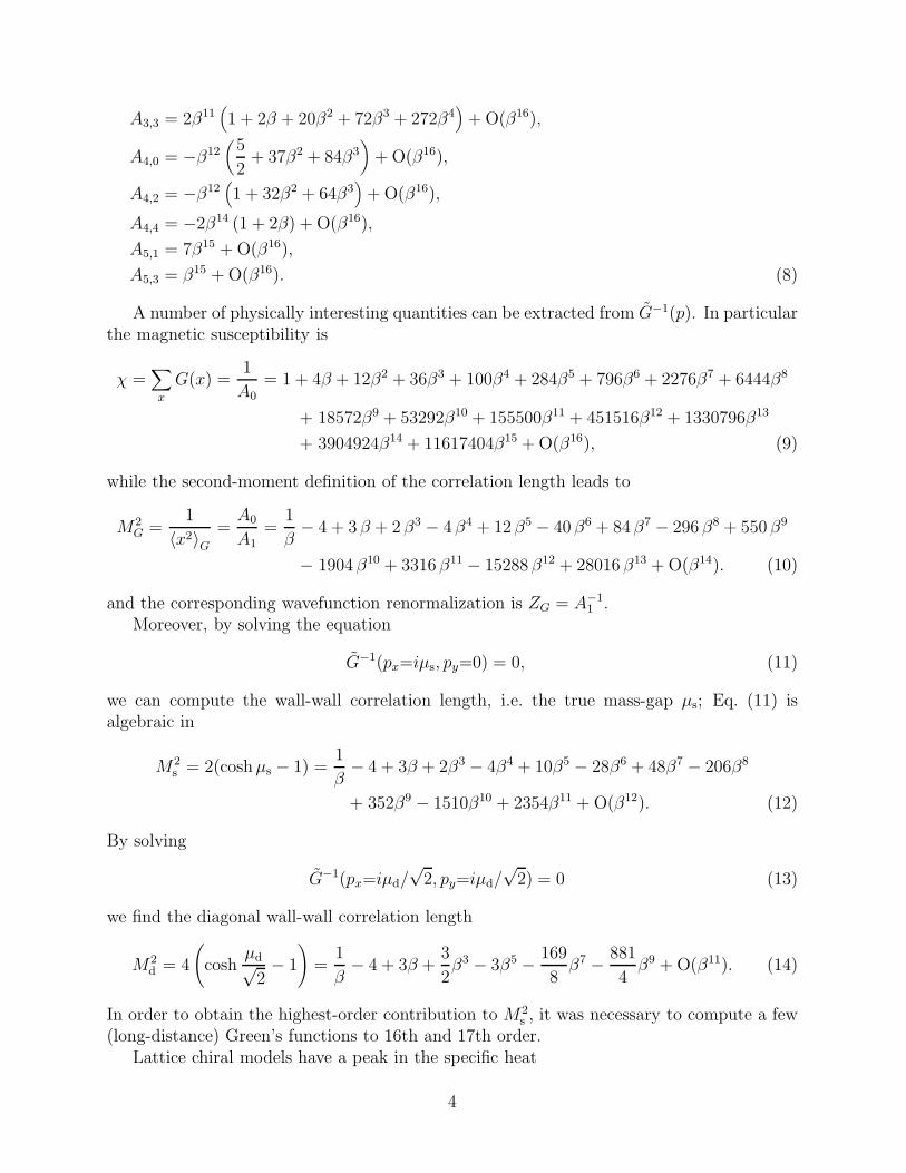
A5,3 = β15 + O(β16). (8)

A number of physically interesting quantities can be extracted from G−1(p). In particularthe magnetic susceptibility is

χ =∑

x

G(x) =1

A0

= 1 + 4β + 12β2 + 36β3 + 100β4 + 284β5 + 796β6 + 2276β7 + 6444β8

+ 18572β9 + 53292β10 + 155500β11 + 451516β12 + 1330796β13

+ 3904924β14 + 11617404β15 + O(β16), (9)

while the second-moment definition of the correlation length leads to

M2G =

1

〈x2〉G=

A0

A1=

1

β− 4 + 3 β + 2 β3 − 4 β4 + 12 β5 − 40 β6 + 84 β7 − 296 β8 + 550 β9

− 1904 β10 + 3316 β11 − 15288 β12 + 28016 β13 + O(β14). (10)

and the corresponding wavefunction renormalization is ZG = A−11 .

Moreover, by solving the equation

G−1(px=iµs, py=0) = 0, (11)

we can compute the wall-wall correlation length, i.e. the true mass-gap µs; Eq. (11) isalgebraic in

M2s = 2(cosh µs − 1) =

1

β− 4 + 3β + 2β3 − 4β4 + 10β5 − 28β6 + 48β7 − 206β8

+ 352β9 − 1510β10 + 2354β11 + O(β12). (12)

By solving

G−1(px=iµd/√

2, py=iµd/√

2) = 0 (13)

we find the diagonal wall-wall correlation length

M2d = 4

(

coshµd√

2− 1

)

=1

β− 4 + 3β +

3

2β3 − 3β5 − 169

8β7 − 881

4β9 + O(β11). (14)

In order to obtain the highest-order contribution to M2s , it was necessary to compute a few

(long-distance) Green’s functions to 16th and 17th order.Lattice chiral models have a peak in the specific heat

4

C =1

N

dE

dT, T =

1

Nβ, (15)

which becomes more and more pronounced with increasing N [1]. Fig. 1 shows MonteCarlo data for the specific heat of SU(N) models for N = 21, 30, and U(N) models forN = 15, 21. (We recall that U(N) models at finite N should experience a phase transitionwith a pattern similar to the XY model, but its location is beyond the specific heat peak).With increasing N , the positions of the peaks in SU(N) and U(N) seems to approach thesame value of β, consistently with the fact that SU(N) and U(N) models must have the samelarge-N limit. This should be considered an indication of a phase transition at N = ∞; arough extrapolation of the C data indicates a critical coupling βc ≃ 0.306. Extrapolating thevalues of ξG = 1/MG and βE at the peak of C to N = ∞, we obtain respectively ξ

(c)G ≃ 2.8

and β(c)E ≃ 0.220.

The above picture is confirmed by an analysis of the large-N 18th order strong-couplingseries of C, based on the method of the integral approximants [5,6]. We indeed obtainedquite stable results showing the critical behavior

C ∼ |β − βc|−α , (16)

with βc∼= 0.3054 and α ∼= 0.21, in agreement with the extrapolation of Monte Carlo data.

Fig. 1 shows that simulation data of C approach, for growing N , the strong-coupling deter-mination.

In spite of the existence of a phase transition at N = ∞, Monte Carlo data show scalingand asymptotic scaling (in the βE scheme) even for β smaller then the peak of the specificheat, suggesting an effective decoupling of the modes responsible for the phase transitionfrom those determining the physical continuum limit; this phenomenon motivated us touse the strong-coupling approach to test scaling and asymptotic scaling. In Fig. 2 we plotthe dimensionless ratio µs/MG vs. the correlation length ξG ≡ 1/MG, as obtained from ourstrong-coupling series. Notice the stability of the curve for a large region of values of ξG andthe good agreement (within a few per mille) with the continuum large-N value extrapolatedby Monte Carlo data µs/MG = 0.991(1) [1].

In order to test asymptotic scaling we perform the variable change indicated in Eq.(1),evaluating the energy from its strong-coupling series

E = 1 − 1

4

∂F

∂β= 1 − G((1, 0)). (17)

(cf. Eq. (3)). The asymptotic scaling formula for the mass gap in the βE scheme is, in thelarge-N limit,

µ ∼=√

π

e16 exp

(

π

4

)

ΛE,2l(βE), ΛE,2l(βE) =√

8πβE exp(−8πβE); (18)

βE can be expressed as a strong-coupling expanded function of β by means of Eq. (17).In Fig. 3 the strong-coupling estimates of µs/ΛE,2l and MG/ΛE,2l are plotted vs. βE , for aregion of coupling corresponding to correlation lengths 1 <∼ ξG

<∼ 3. These quantities agreewith the exact continuum prediction within 5% in the whole region.

5

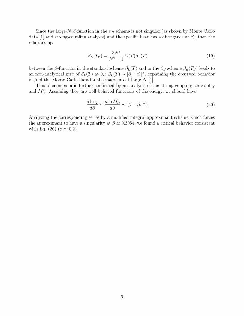
Since the large-N β-function in the βE scheme is not singular (as shown by Monte Carlodata [1] and strong-coupling analysis) and the specific heat has a divergence at βc, then therelationship

βE(TE) =8N2

N2 − 1C(T )βL(T ) (19)

between the β-function in the standard scheme βL(T ) and in the βE scheme βE(TE) leads toan non-analytical zero of βL(T ) at βc: βL(T ) ∼ |β − βc|α, explaining the observed behaviorin β of the Monte Carlo data for the mass gap at large N [1].

This phenomenon is further confirmed by an analysis of the strong-coupling series of χand M2

G. Assuming they are well-behaved functions of the energy, we should have

d lnχ

dβ∼ d lnM2

G

dβ∼ |β − βc|−α. (20)

Analyzing the corresponding series by a modified integral approximant scheme which forcesthe approximant to have a singularity at β ≃ 0.3054, we found a critical behavior consistentwith Eq. (20) (α ≃ 0.2).

6

REFERENCES

[1] P. Rossi and E. Vicari, “Two dimensional SU(N)× SU(N) Chiral Models on the Lattice(II): the Green’s Function”, Pisa preprint IFUP-TH 8/94, Phys. Rev. D, in press.

[2] G. Parisi, in High Energy Physics 1980, Proceedings of the XXth Conference on HighEnergy Physics, Madison, Wisconsin, 1980, edited by L. Durand and L. G. Pondrom,AIP Conf. Proc. No. 68 (AIP, New York, 1981).

[3] J. Balog, S. Naik, F. Niedermayer, and P. Weisz, Phys. Rev. Lett. 69, 873 (1992).[4] F. Green and S. Samuel, Nucl. Phys. B190, 113 (1981).[5] D. L. Hunter and G. A. Baker Jr., Phys. Rev. B 49 (1979) 3808.[6] M. E. Fisher and H. Au-Yang, J. Phys. A12 (1979) 1677.

7

FIGURES

FIG. 1. Specific heat vs. β. The solid line represents the resummation of the strong-coupling

series, whose estimate of the critical β is indicated by the vertical dashed lines.

FIG. 2. µs/MG vs. ξG ≡ 1/MG. The dashed line represents the continuum result from Monte

Carlo data.

FIG. 3. Asymptotic scaling test by using strong-coupling estimates. The dotted line represents

the exact result (18).

8

This figure "fig1-1.png" is available in "png" format from:

http://arXiv.org/ps/hep-lat/9406014v1

This figure "fig1-2.png" is available in "png" format from:

http://arXiv.org/ps/hep-lat/9406014v1