New Applications of Asymptotic Symmetries ... - Inspire HEP

New Applications of AsymptoticSymmetries Involving

Maxwell Fields

Pujian Mao

New Applications of Asymptotic Symmetries Involving Maxwell FieldsPujian Mao

In this thesis, several new aspects of asymptotic symmetries have been exploited.

Firstly, we have shown that the asymptotic symmetries can be enhanced to symplecticsymmetries in three dimensional asymptotically Anti-de Sitter (AdS) space-time withDirichlet boundary conditions. Such enhancement provides a natural connection be-tween the asymptotic symmetries in the far region (i.e. close to the boundary) and thenear-horizon region, which leads to a consistent treatment for both cases. The secondinvestigation in three dimensional space-time is to study the Einstein-Maxwell theoryincluding asymptotic symmetries, solution space and surface charges with asymptot-ically flat boundary conditions at null infinity. This model allows one to illustrateseveral aspects of the four dimensional case in a simplified setting. Afterwards, we givea parallel analysis of Einstein-Maxwell theory in the asymptotically AdS case.

Another new aspect consists in demonstrating a deep connection between certain asymp-totic symmetry and soft theorem. Recently, a remarkable equivalence was found be-tween the Ward identity of certain residual (large) U(1) gauge transformations andthe leading piece of the soft photon theorem. It is well known that the soft photontheorem includes also a sub-leading piece. We have proven that the large U(1) gaugetransformation responsible for the leading soft factor can also explain the sub-leadingone.

In the last part of the thesis, we will investigate the asymptotic symmetries near theinner boundary. As a null hypersurface, the black hole horizon can be considered as aninner boundary. The near horizon symmetries create “soft” degrees of freedom. We havegeneralised such argument to isolated horizon and have shown that those “soft” degreesof freedom of an isolated horizon are equivalent to its electric multipole moments.

UNIVERSITE LIBRE DE BRUXELLESFaculte des Sciences

Physique Mathematique des Interactions Fondamentales

New Applications of AsymptoticSymmetries Involving Maxwell Fields

Pujian MAO

These de doctorat presentee en vue de l’obtentiondu grade academique de Docteur en Sciences

Directeur: Prof. Glenn BarnichAnnee academique 2015-2016

The picture on the cover is taken from the book Spinors and space-time Vol. 2 page 426

Acknowledgements

Many people played a significant role during my fantastic four-years jour-ney in Brussels, whom I would like to acknowledge. Without the countlesshelp, support and companionship I have gained from them, it will be quitedifficult if not impossible to accomplish this thesis. In particular, I want tothank:

My supervisor Glenn Barnich, for being the illuminative guide of my scien-tific life and for everything I have learnt from him. His insight, quest forperfection, and passion for science are always inspiring me. He is alwayspatient, and ensured that I have understood the right physics.

My “consultant” Hongbao Zhang, for the numerous chats about physics andlife in general, for his encouragement and unconditional support.

The other PhD students of my generation: Laura Donnay, Marco Fazzi, andBlagoje Oblak, for the wonderful time spent during these four years, forsharing the feelings of different stages of the doctorate years.

The football team members: Eduardo Conde, Gaston Giribet, Gustavo Lu-cena Gomez, Hernan Gonzalez, Jelle Hartong, Andrea Marzolla, IgnacioCortese Mombelli, Robson Nascimento, and Diego Redigolo, for all the en-joyable games we have played; The young generation: Paolo Gregori, VictorLekeu, Daniel Naegels, Roberto Oliveri, Arash Ranjbar, Celine Zwikel, forkeeping me updated with fresh thoughts; The “technical supporter” MichaMoskovic, for bringing me to a digital life; The joke maker Rakibur Rhaman,for all the funny stories I have heard from him. All the members of theService de Physique Mathematique des Interactions Fondamentales at Uni-versite Libre de Bruxelles, for the help, support and companionship.

My office mates: Sergio Hortner and Amaury Leonard, for allowing me tohave the whole office mostly.

My scientific collaborators: Geoffrey Compere, Eduardo Conde, Pierre-Henry Lambert, Ali Seraj, M.M. Sheikh-Jabbari, and Xiaoning Wu, for the

i

ii

projects finished and in progress. It is a pleasure to collaborate with themand I hope that we can manage to work together again in the future.

The members of the jury of my thesis: Riccardo Argurio, Glenn Barnich,Xavier Bekaert, Nicolas Boulanger, Stephane Detournay, Thomas Hambye.

Next, I should give my gratitude to my Chinese friends in Belgium, whoare managing my native surroundings, and without whom I would definitelyhave a totally different life in Brussels.

Finally, I owe my family: my ever-encouraging mother and my always wor-rying father, and my girlfriend, for forgiving me not enough accompanying.My love and gratitude to them can never reach the boundary.

Contents

1 Preface 1

2 Background material 7

2.1 Conformal boundary . . . . . . . . . . . . . . . . . . . . . . . 7

2.2 Asymptotic structure at null infinity . . . . . . . . . . . . . . 9

2.2.1 Asymptotic flatness at null infinity . . . . . . . . . . . 9

2.2.2 Symmetries at null infinity . . . . . . . . . . . . . . . 10

2.2.3 Physical fields at null infinity . . . . . . . . . . . . . . 14

2.3 Newman-Penrose formalism . . . . . . . . . . . . . . . . . . . 18

2.4 Charges in the first order formalism . . . . . . . . . . . . . . 25

2.5 Metric formalism . . . . . . . . . . . . . . . . . . . . . . . . . 29

3 Applications in 3 dimensional space-time 31

3.1 Symplectic symmetries . . . . . . . . . . . . . . . . . . . . . . 32

3.1.1 Symplectic symmetries in Fefferman-Graham coordi-nates . . . . . . . . . . . . . . . . . . . . . . . . . . . . 33

3.1.2 Symplectic symmetries in Gaussian null coordinates . 41

3.1.3 The two Killing symmetries and their charges . . . . . 43

3.1.4 Phase space as Virasoro coadjoint orbits . . . . . . . . 47

3.1.5 Extremal phase space and decoupling limit in Fefferman-Graham coordinates . . . . . . . . . . . . . . . . . . . 50

3.1.6 Extremal phase space and and near horizon limit inGaussian null coordinates . . . . . . . . . . . . . . . . 54

3.1.7 Discussion and outlook . . . . . . . . . . . . . . . . . 57

3.2 Three-dimensional asymptotically flat Einstein-Maxwell theory 59

3.2.1 Asymptotic symmetries . . . . . . . . . . . . . . . . . 60

3.2.2 Solution space . . . . . . . . . . . . . . . . . . . . . . 62

3.2.3 Surface charge algebra . . . . . . . . . . . . . . . . . . 63

3.2.4 Switching off the news . . . . . . . . . . . . . . . . . . 65

3.2.5 Discussion . . . . . . . . . . . . . . . . . . . . . . . . . 65

3.3 Three-dimensional asymptotically AdS Einstein-Maxwell the-ory . . . . . . . . . . . . . . . . . . . . . . . . . . . . . . . . . 67

3.3.1 Asymptotic symmetries . . . . . . . . . . . . . . . . . 67

iii

iv CONTENTS

3.3.2 Solution space . . . . . . . . . . . . . . . . . . . . . . 693.3.3 Surface charge algebra . . . . . . . . . . . . . . . . . . 713.3.4 Comparison with the asymptotically flat case . . . . . 72

4 Applications in Quantum ElectroDynamics amplitudes 734.1 The solution space for Maxwell theory . . . . . . . . . . . . . 764.2 Charges . . . . . . . . . . . . . . . . . . . . . . . . . . . . . . 784.3 Soft theorems . . . . . . . . . . . . . . . . . . . . . . . . . . . 804.4 Brief summary and open questions . . . . . . . . . . . . . . . 83

5 Four-dimensional near horizon Einstein-Maxwell theory 855.1 Solution space of Einstein-Maxwell theory near isolated horizon 875.2 Asymptotic symmetries and conserved current near the iso-

lated horizon . . . . . . . . . . . . . . . . . . . . . . . . . . . 885.3 Soft electric hairs on isolated horizon . . . . . . . . . . . . . . 905.4 Supertranslation and foliation of an isolated horizon . . . . . 92

A Details on computations 95A.1 Comparison of the charges between first order formalism and

metric formalism . . . . . . . . . . . . . . . . . . . . . . . . . 95A.2 Conserved charges for field dependent vectors . . . . . . . . . 96

A.2.1 Expression for the charges . . . . . . . . . . . . . . . . 97A.2.2 Integrability of charges . . . . . . . . . . . . . . . . . . 101

A.3 3 dimensional asymptotically flat case . . . . . . . . . . . . . 101A.3.1 Residual symmetries . . . . . . . . . . . . . . . . . . . 101A.3.2 Asymptotic symmetry algebra . . . . . . . . . . . . . 102A.3.3 Solution space . . . . . . . . . . . . . . . . . . . . . . 103

A.4 3 dimensional asymptotically AdS case . . . . . . . . . . . . . 106A.4.1 Residual symmetries . . . . . . . . . . . . . . . . . . . 106A.4.2 Asymptotic symmetry algebra . . . . . . . . . . . . . 107A.4.3 Solution space . . . . . . . . . . . . . . . . . . . . . . 108

A.5 Newman-Penrose charges of linear Maxwell theory . . . . . . 111A.6 Near horizon solution space of Einstein-Maxwell theory . . . 114

Chapter 1

Preface

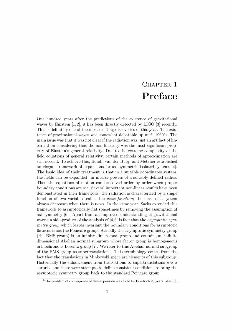
One hundred years after the predictions of the existence of gravitationalwaves by Einstein [1, 2], it has been directly detected by LIGO [3] recently.This is definitely one of the most exciting discoveries of this year. The exis-tence of gravitational waves was somewhat debatable up until 1960’s. Themain issue was that it was not clear if the radiation was just an artifact of lin-earization considering that the non-linearity was the most significant prop-erty of Einstein’s general relativity. Due to the extreme complexity of thefield equations of general relativity, certain methods of approximation arestill needed. To achieve this, Bondi, van der Burg, and Metzner establishedan elegant framework of expansions for axi-symmetric isolated systems [4].The basic idea of their treatment is that in a suitable coordinates system,the fields can be expanded1 in inverse powers of a suitably defined radius.Then the equations of motion can be solved order by order when properboundary conditions are set. Several important non-linear results have beendemonstrated in their framework: the radiation is characterized by a singlefunction of two variables called the news function; the mass of a systemalways decreases when there is news. In the same year, Sachs extended thisframework to asymptotically flat spacetimes by removing the assumption ofaxi-symmetry [6]. Apart from an improved understanding of gravitationalwaves, a side-product of the analysis of [4,6] is fact that the asymptotic sym-metry group which leaves invariant the boundary conditions for asymptoticflatness is not the Poincare group. Actually this asymptotic symmetry group(the BMS group) is an infinite dimensional group and contains an infinitedimensional Abelian normal subgroup whose factor group is homogeneousorthochronous Lorentz group [7]. We refer to this Abelian normal subgroupof the BMS group as supertranslations. This terminology comes from thefact that the translations in Minkowski space are elements of this subgroup.Historically the enhancement from translations to supertranslations was asurprise and there were attempts to define consistent conditions to bring theasymptotic symmetry group back to the standard Poincare group.

1The problem of convergence of this expansion was fixed by Friedrich 20 years later [5].

1

2 Chapter 1. Preface

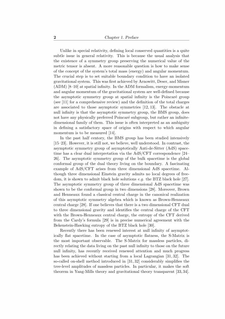
Unlike in special relativity, defining local conserved quantities is a quitesubtle issue in general relativity. This is because the usual analysis thatthe existence of a symmetry group preserving the numerical value of themetric tensor is absent. A more reasonable question is how to make senseof the concept of the system’s total mass (energy) and angular momentum.The crucial step is to set suitable boundary condition to have an isolatedgravitational system. This was first achieved by Arnowitt, Deser, and Misner(ADM) [8–10] at spatial infinity. In the ADM formalism, energy-momentumand angular momentum of the gravitational system are well-defined becausethe asymptotic symmetry group at spatial infinity is the Poincare group(see [11] for a comprehensive review) and the definition of the total chargesare associated to those asymptotic symmetries [12, 13]. The obstacle atnull infinity is that the asymptotic symmetry group, the BMS group, doesnot have any physically preferred Poincare subgroup, but rather an infinite-dimensional family of them. This issue is often interpreted as an ambiguityin defining a satisfactory space of origins with respect to which angularmomentum is to be measured [14].

In the past half centory, the BMS group has been studied intensively[15–23]. However, it is still not, we believe, well understood. In contrast, theasymptotic symmetry group of asymptotically Anti-de-Sitter (AdS) space-time has a clear dual interpretation via the AdS/CFT correspondence [24–26]. The asymptotic symmetry group of the bulk spacetime is the globalconformal group of the dual theory living on the boundary. A fascinatingexample of AdS/CFT arises from three dimensional AdS spacetime. Al-though three dimensional Einstein gravity admits no local degrees of free-dom, it is shown to admit black hole solutions e.g. the BTZ black hole [27].The asymptotic symmetry group of three dimensional AdS spacetime wasshown to be the conformal group in two dimensions [28]. Moreover, Brownand Henneaux found a classical central charge in the canonical realizationof this asymptotic symmetry algebra which is known as Brown-Henneauxcentral charge [28]. If one believes that there is a two dimensional CFT dualto three dimensional gravity and identifies the central charge of the CFTwith the Brown-Henneaux central charge, the entropy of the CFT derivedfrom the Cardy’s formula [29] is in precise numerical agreement with theBekenstein-Hawking entropy of the BTZ black hole [30].

Recently there has been renewed interest at null infinity of asymptot-ically flat spacetime. In the case of asymptotic flatness, the S-Matrix isthe most important observable. The S-Matrix for massless particles, di-rectly relating the data living on the past null infinity to those on the futurenull infinity, has recently received renewed attention and much progresshas been achieved without starting from a local Lagrangian [31, 32]. Theso-called on-shell method introduced in [31, 32] considerably simplifies thetree-level amplitudes of massless particles. In particular, it makes the softtheorem in Yang-Mills theory and gravitational theory transparent [33, 34].

3

The universal properties of the soft theorems are suggesting that some sym-metries might be responsible. Very recently, Strominger and collaboratorsargued that the S-Matrix of massless particles should have BMS symme-try [35] and have found a deep connection between BMS supertranslationsand Weinberg’s soft graviton theorem [36]. Since the supertranslations cannot preserve the Minkowski vacuum, they are spontaneously broken. It hasbeen shown precisely in [36] that the soft graviton theorem is nothing butthe Ward identity of supertranslations and the soft gravitons are just theGoldstone particles of the supertranslations.

Apart from the remarkable perspectives in the understanding of the softtheorem, the degenerate vacuum on a null boundary brings new physicaldegrees of freedom which are related to the spontaneously broken symme-tries i.e. the supertranslations. The inequivalent vacua differ from oneanother by the creation or annihilation of soft gravitons. Interestingly thenull infinity is not the only null boundary when a black hole is formed inthe bulk spacetime. As a null hypersurface, the black hole horizon can serveas an inner boundary. A straightforward question would be what are theasymptotic symmetries of the near horizon region. Surprisingly, the nearhorizon symmetries also include a supertranslation part as shown in [37].Taking into account of the near horizon supertranslations, a highly mean-ingful question arises that if stationary black holes are nearly bald due tothe no-hair theorem [38]. Since the no-hair theorem is a basic assumption inthe black hole information paradox issue, the emergence of new symmetriesin the near horizon region may shed new insights on the black hole physics.Based on those facts, Hawking, Perry, and Strominger proposed that blackholes can carry a large amount of soft hairs which gives the effective soft de-grees of freedom and the complete information about the quantum states ofthose soft hairs are stored on a holographic plate [39]. Moreover, soft hairshave a description as quantum pixels in a holographic plate which lives ona two sphere at the future boundary of the horizon. They further arguedthat the effective number of soft hairs should be proportional to the area ofthe horizon in Planck units as it was the case in the string-theoretic blackhole [40].

The aim of the present thesis is to exploit new asymptotic symmetriesand new applications of asymptotic symmetries both at infinity and in thenear horizon region, especially for systems involving Maxwell fields.

Outline of the thesis

This thesis contains four main parts and a few appendices. In part one,we review several methods to perform asymptotic analysis. Those are con-formal compactification, Newman-Penrose formalism and metric formalism.The point is to establish a complete framework of physics on the conformal

4 Chapter 1. Preface

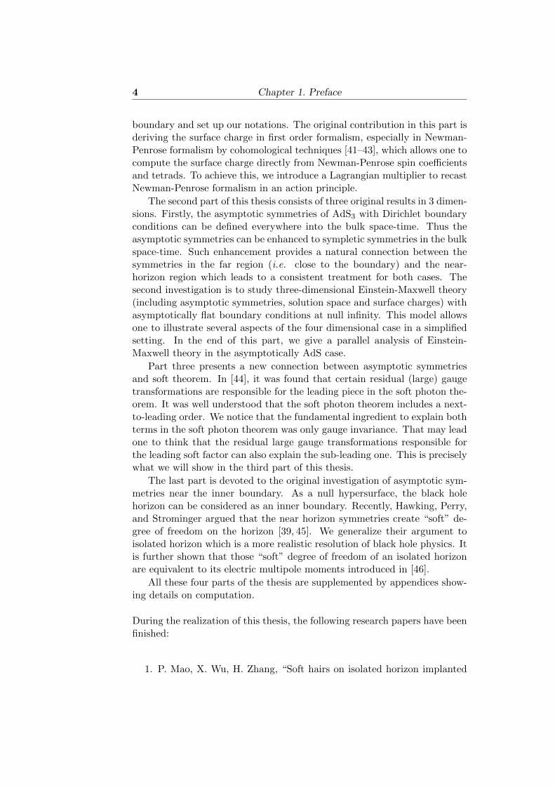
boundary and set up our notations. The original contribution in this part isderiving the surface charge in first order formalism, especially in Newman-Penrose formalism by cohomological techniques [41–43], which allows one tocompute the surface charge directly from Newman-Penrose spin coefficientsand tetrads. To achieve this, we introduce a Lagrangian multiplier to recastNewman-Penrose formalism in an action principle.

The second part of this thesis consists of three original results in 3 dimen-sions. Firstly, the asymptotic symmetries of AdS3 with Dirichlet boundaryconditions can be defined everywhere into the bulk space-time. Thus theasymptotic symmetries can be enhanced to sympletic symmetries in the bulkspace-time. Such enhancement provides a natural connection between thesymmetries in the far region (i.e. close to the boundary) and the near-horizon region which leads to a consistent treatment for both cases. Thesecond investigation is to study three-dimensional Einstein-Maxwell theory(including asymptotic symmetries, solution space and surface charges) withasymptotically flat boundary conditions at null infinity. This model allowsone to illustrate several aspects of the four dimensional case in a simplifiedsetting. In the end of this part, we give a parallel analysis of Einstein-Maxwell theory in the asymptotically AdS case.

Part three presents a new connection between asymptotic symmetriesand soft theorem. In [44], it was found that certain residual (large) gaugetransformations are responsible for the leading piece in the soft photon the-orem. It was well understood that the soft photon theorem includes a next-to-leading order. We notice that the fundamental ingredient to explain bothterms in the soft photon theorem was only gauge invariance. That may leadone to think that the residual large gauge transformations responsible forthe leading soft factor can also explain the sub-leading one. This is preciselywhat we will show in the third part of this thesis.

The last part is devoted to the original investigation of asymptotic sym-metries near the inner boundary. As a null hypersurface, the black holehorizon can be considered as an inner boundary. Recently, Hawking, Perry,and Strominger argued that the near horizon symmetries create “soft” de-gree of freedom on the horizon [39, 45]. We generalize their argument toisolated horizon which is a more realistic resolution of black hole physics. Itis further shown that those “soft” degree of freedom of an isolated horizonare equivalent to its electric multipole moments introduced in [46].

All these four parts of the thesis are supplemented by appendices show-ing details on computation.

During the realization of this thesis, the following research papers have beenfinished:

1. P. Mao, X. Wu, H. Zhang, “Soft hairs on isolated horizon implanted

5

by electromagnetic fields,” Submitted to journal,arXiv:1606.03226.

2. E. Conde and P. Mao, “Comments on Asymptotic Symmetries andthe Sub-leading Soft Photon Theorem,” Submitted to journal,arXiv:1605.09731.

3. G. Compere, P. Mao, A. Seraj, M.M. Sheikh-Jabbari, “Symplectic andKilling Symmetries of AdS3 Gravity: Holographic vs Boundary Gravi-tons,” JHEP 01 (2016) 080, arXiv:1511.06079.

4. G. Barnich, P. -H. Lambert, P. Mao, “Three-dimensional asymptoti-cally flat Einstein-Maxwell theory,” Class. Quantum Grav. 32 (2015)245001, arXiv:1503.00856.

http://arxiv.org/abs/1606.03226




Chapter 2

Background material

2.1 Conformal boundary

Originally, infinity is not part of spacetime. However the causal structure ofspacetime is unchanged by a conformal transformation:

ds2 → ds2 = Ω2ds2. (2.1)

We can choose it in such a way that all points at infinity in the originalmetric are at finite affine parameter in the new metric. To achieve this, wemust choose

Ω→ 0. (2.2)

In this case, infinity can be identified as those points for which Ω = 0. Thesepoints are not part of the original spacetime but they can be added to it toyield a conformal boundary of spacetime.

Example: Minkowski space [47]

ds2 = −dt2 + dr2 + r2(dθ2 + sin θ2dφ2). (2.3)

Let u = t− rv = t+ r

→ ds2 = −du dv +

(u− v)2

4(dθ2 + sin θ2dφ2). (2.4)

Now setu = tan U −π/2 < U < π/2

v = tan V −π/2 < V < π/2

with V ≥ Usince r ≥ 0

(2.5)

In these coordinates,

ds2 =(

2 cos U cos V)−2 [

−4dU dV + sin2(V − U

)(dθ2 + sin θ2dφ2)

](2.6)

7

8 Chapter 2. Background material

Figure 2.1: Each point represents a 2-sphere, except points on r = 0 andi0, i±. Light rays travel at 45

0from =− through r = 0 and then out to =+.

This picture is taken from [47] page 44.

To approach ∞ in this metric we must take∣∣∣U ∣∣∣→ π/2 or

∣∣∣V ∣∣∣→ π/2, so by

choosing

Ω = 2 cos U cos V (2.7)

we bring these points to finite affine parameter in the new metric

ds2 = Ωds2 = −4dUdV + sin2(V − U

)(dθ2 + sin θ2dφ2) (2.8)

We can now add the points at infinity. Taking the restriction V ≥ Uinto account, these are

U = −π/2V = π/2

⇔

r →∞t finite

spatial infinity, i0

U = ±π/2V = ±π/2

⇔

t→ ±∞r finite

past and futuretemporal infinity, i±

U = −π/2|V | 6= π/2

⇔

r →∞t→ −∞r + t finite

past null infinity=−

|U | 6= π/2

V = π/2

⇔

r →∞t→∞

r − t finite

future null infinity=+

2.2. Asymptotic structure at null infinity 9

Minkowski spacetime is conformally embedded in the new spacetime withmetric ds2 with boundary at Ω = 0. Figure 2.1 is the Carter-Penrose dia-gram of Minkowski spacetime.

2.2 Asymptotic structure at null infinity

2.2.1 Asymptotic flatness at null infinity

We have introduced the conformal technique in general previously. Nullinfinity will be analyzed in details here. At first, we give a general definitionof asymptote for a generic 4 dimensional manifoldM with smooth C∞ metricof Lorentz signature gab following [11]. By asymptotes of (M, gab) we meana manifold M with boundary I, together with a smooth Lorentz metric gabon M , a smooth function Ω on M , and a diffeomorphism from M to M − I,satisfying the following conditions:

1) On M , gab = Ω2gab.

2) At I, Ω = 0, ∇aΩ 6= 0, and gab∇aΩ∇bΩ = 0,where ∇a denotes thegradient on M .

This gab is called the unphysical metric (to distinguish it from the physi-cal metric gab) , while I is called the boundary at null infinity. Note that thedefinition requires that the unphysical metric be defined and have Lorentzsignature also at points of the boundary.

The definition represents the intuitive idea of “the attachment to thespace-time manifold M of additional ideal points at null infinity”. Theadditional points are of course those of I, while the diffeomorphism insertsM in M ; thus, M itself represents the physical space-time manifold. Thefirst condition from the definition states that the conformal factor rescalesthe physical metric to the unphysical one. The first part of the secondcondition, together with the requirement that the unphysical metric beingwell-behaved on I, states that “infinity is far away in the physical space-time”. The second part of the second condition fixes the asymptotic behavior

of Ω. Effectively, it states that Ω falls to zero as1

r. The third part of the

second condition states essentially that I is a null hypersurface. Hence,we are working at null infinity. These remarks reflect the intuitive idea of“asymptotic flatness at null infinity”. The conformal boundary of Minkowskispace we have discussed in the previous section is absolutely in consistentwith this intuitive idea.

Another aspect of this issue as pointed in [11] is the question of whetheror not the existence of a boundary at infinity is persistent. In other words,we are wondering if asymptotic flatness is stable against disturbance in thespace-time, e.g. by emitting gravitational radiation. One would wish it to betrue that such a disturbance could not result in destruction of the boundary.


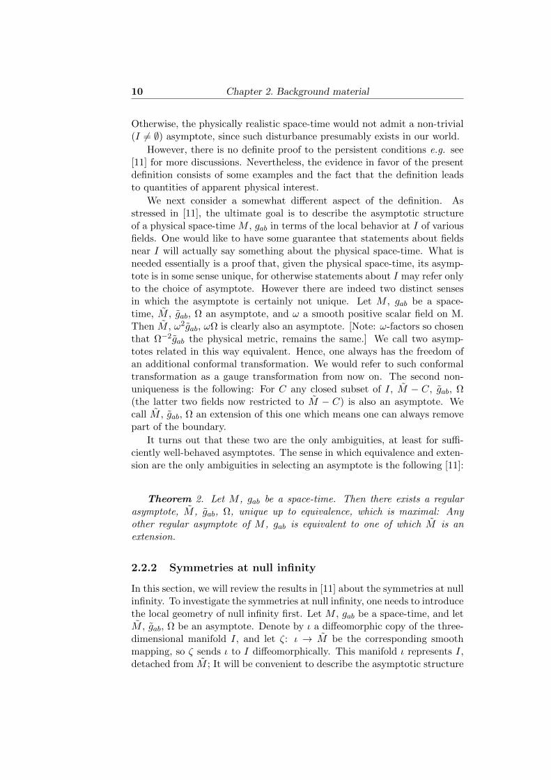
Otherwise, the physically realistic space-time would not admit a non-trivial(I 6= ∅) asymptote, since such disturbance presumably exists in our world.

However, there is no definite proof to the persistent conditions e.g. see[11] for more discussions. Nevertheless, the evidence in favor of the presentdefinition consists of some examples and the fact that the definition leadsto quantities of apparent physical interest.

We next consider a somewhat different aspect of the definition. Asstressed in [11], the ultimate goal is to describe the asymptotic structureof a physical space-time M , gab in terms of the local behavior at I of variousfields. One would like to have some guarantee that statements about fieldsnear I will actually say something about the physical space-time. What isneeded essentially is a proof that, given the physical space-time, its asymp-tote is in some sense unique, for otherwise statements about I may refer onlyto the choice of asymptote. However there are indeed two distinct sensesin which the asymptote is certainly not unique. Let M , gab be a space-time, M , gab, Ω an asymptote, and ω a smooth positive scalar field on M.Then M , ω2gab, ωΩ is clearly also an asymptote. [Note: ω-factors so chosenthat Ω−2gab the physical metric, remains the same.] We call two asymp-totes related in this way equivalent. Hence, one always has the freedom ofan additional conformal transformation. We would refer to such conformaltransformation as a gauge transformation from now on. The second non-uniqueness is the following: For C any closed subset of I, M − C, gab, Ω(the latter two fields now restricted to M − C) is also an asymptote. Wecall M , gab, Ω an extension of this one which means one can always removepart of the boundary.

It turns out that these two are the only ambiguities, at least for suffi-ciently well-behaved asymptotes. The sense in which equivalence and exten-sion are the only ambiguities in selecting an asymptote is the following [11]:

Theorem 2. Let M , gab be a space-time. Then there exists a regularasymptote, M , gab, Ω, unique up to equivalence, which is maximal: Anyother regular asymptote of M , gab is equivalent to one of which M is anextension.

2.2.2 Symmetries at null infinity

In this section, we will review the results in [11] about the symmetries at nullinfinity. To investigate the symmetries at null infinity, one needs to introducethe local geometry of null infinity first. Let M , gab be a space-time, and letM , gab, Ω be an asymptote. Denote by ι a diffeomorphic copy of the three-dimensional manifold I, and let ζ: ι → M be the corresponding smoothmapping, so ζ sends ι to I diffeomorphically. This manifold ι represents I,detached from M ; It will be convenient to describe the asymptotic structure


in terms of it. We denote by ζ? the pullback: the operator, now to bedefined, which carries certain fields from M to ι. Let na = ∇aΩ be thenormal vector of the null infinity. Then, ζ?na = 0. Set na = ζ?na andgab

= ζ?gab. These two fields on ι essentially describe the universal geometry

of this manifold. Furthermore, applying ζ? to gabnb, one obtains g

abnb = 0.

Thus, gab

is not invertible; indeed, it is clear from the fact that I is a nullsurface and g

abhas the signature (0,+,+). A final consequence follows

from the Einstein’s equation. It is convenient to define a combination S ba =

R ba −

1

6Rδ ba . Let Lab = gacS

cb . The behavior of the Ricci tensor under

conformal transformation implies

ΩSab + Lna gab − fgab = Ω−1Lab, (2.9)

where f = Ω−1nana. Let us now suppose that the stress-energy vanishesasymptotically to order two which is a very weak supposition. Then, ap-plying ζ? to (2.9), we obtain Lngcd = fg

cdwhere we have used f = ζ?(f).

Thus, na is a conformal Killing field for gab

.

The gauge-function ω on M is represented, in terms of ι, by the (positive)function ω = ζ?ω on this manifold. Applying ζ? to g′ab = ω2gab and ton′a = ω−1na + ω−2Ω∇aω, we obtain

g′ab

= ω2gab, n′a = ω−1na. (2.10)

That is to say, gab

, na and g′ab

, n′a, related by (2.10) for some positiveω, are to represent the same geometrical situation. Applying ζ? to f ′ =ω−1f + 2ω−2Lnω + ω−3Ω∇mω∇mω gives

f ′ = ω−1f + 2ω−2Lnω. (2.11)

Set Γab cd = nanbgcd

. Then this tensor field Γab cd is gauge-invariant.

Its properties are the following: 1) Γab cd = Γ(ab)

(cd) 6= 0 and Γa[bcdΓ

e]fgh =

0, 2) Γamcm = 0 (ensures that nagab

= 0), 3) whenever wcv[aΓ

b]cde 6= 0,

wawbvcvdΓab cd is positive (signature of g

ab) and 4) whenever v[aΓ

b]cde = 0,

LvΓab cd is a multiple of Γab cd (ensures thet na is a gab

-conformal Killing

field). Thus, we may regard Γab cd as representing the complete universalstructure of ι in a gauge-invariant way. By an asymptotic geometry we shallmean a three-dimensional manifold ι with a tensor field Γab cd satisfying thefour properties above.

Set f ′ = 0 in (2.11) to obtain −2Ln lnω = f . Clearly, there alwaysexists, at least locally, a positive ω satisfying this equation. That is to say,by a gauge transformation we can always arrange locally to have Lngcd = 0.Furthermore, f = 0 is preserved by (2.11) when and only when Lnω = 0,i. e., when and only when ω is constant along the n-integral curves. For ι,


Γab cd an asymptotic geometry, by a decomposition of Γab cd we mean fieldsna and g

absuch that Γab cd = nanbg

cdand Lngcd = 0. What we have shown,

then, is that every asymptotic geometry possesses, locally, a decomposition,and that it is unique up to a gauge transformation by ω which is constantalong the n-integral curves.

A symmetry on (ι, Γab cd) is a diffeomorphism from ι to ι which sendsΓab cd to itself. An infinitesimal symmetry on (ι, Γab cd) is a vector fieldξa on ι satisfying LξΓab cd = 0. Under the bracket of vector fields, theinfinitesimal symmetries, we denote by χ, have the structure of a Lie algebra.An alternative statement that ξa is an infinitesimal symmetry will be

Lξgab = 2κgab, Lξna = −κna. (2.12)

An infinitesimal symmetry ξa is called an infinitesimal supertranslation ifξa is proportional to na. We denote the set of infinitesimal supertranslationsby ℘. The terminology is motivated by the fact that the translations inMinkowski space give rise to elements of ℘. Let ξa = αna. Then Lξgab = 0,

and Lξna = −Lnαna. Thus, αna is in ℘ if and only if Lnα = 01. ℘ is avector subspace of the vector space χ and, an infinite-dimensional subspace.One can further conclude that ℘ is even an abelian subalgebra and formsan ideal in Lie algebra of χ. This can be checked by the bracket of aninfinitesimal symmetry ξa with an element of ℘

Lξ(αna) = Lξαna + αLξna = (Lξα− ακ)na. (2.13)

Now, we have “understood” the ℘-part of χ. What remains is to un-derstand the rest of χ. This is accomplished as follows. Since ℘ is an idealin χ, one can form the quotient algebra, χ/℘. This quotient algebra justrepresents the “rest” of χ; we wish, therefore, to understand its structure.It turns out that χ/℘ can be represented explicitly within ι. Fix a decom-position of Γab cd, let ξa be any infinitesimal symmetry, and set ξa = g

abξb.

Then, this ξa satisfies

naξa = 0, D(aξb) = κgab, Lnξa = 0, (2.14)

where D is the derivative compatible with gab

, i.e. Dagab = 0. We can

further claim, conversely, that any ξa satisfying (2.14) is of the form gabξb

for some infinitesimal symmetry ξb. Let such a ξa be given. Then the firstequation in (2.14) implies that ξa = g

abηb for some ηb; set ξa = ηa + αna.

Then the second equation in (2.14) yields Lξgab = 2κgab

while the thirdyields Lξna = −Lnαna. This ξa will therefore be an infinitesimal symmetryif and only if α satisfies Lnα = κ. But, we can always find some α satisfyingthis equation, i.e., we can always find some infinitesimal symmetry ξa such

1Without choosing the decomposition, a supertranslation will lead to different con-straint on α.


Figure 2.2: The base space is a two-sphere (circle in the figure). The map-ping π acts vertically downward; the vertical lines in ι are integral curves ofna. This picture is taken from [11] page 27.

that ξa = gabηb is our original solution of (2.14). Finally, we note that

infinitesimal symmetries ξa and ρa differ by an infinitesimal supertranslationif and only if g

abξb = g

abρb,i.e., if and only if ξa and ρa define the same

solution of (2.14). Thus, a solution of (2.14) determines an element of χ upto addition of an arbitrary element of ℘ i.e., the solutions of (2.14) realizethe quotient algebra χ/℘.

We next introduce the base space B following [11] to have a better in-terpretation of χ from the geometrical point of view. Let ι, Γab cd be anasymptotic geometry. A maximally extended integral curve τ of na is said tobe almost closed if, for some point p of ι, τ reenters every sufficiently smallneighborhood of p. Suppose an asymptotic geometry having no almost-closed integral curves of na. Denote by B the set of all maximally extendedintegral curves of na, and let π: ι → B be the mapping which sends eachpoint of ι to the integral curve on which it lies in B. Now, given an openset U in ι, such that no n-integral curve passes through U more than once,and such that there are two of the coordinate functions which are constantalong the n-integral curves in U , after projecting these two coordinate func-tions to B by the mapping π, we obtain a chart in B based on π[U ]. Thus,B becomes a two-dimensional manifold. When B is Hausdorff, we call itthe base space of the asymptotic geometry. In this case, the mapping π issmooth, and the manifold ι is just B ×R. One can define a cross section ofι by a smooth mapping ε from B to ι, such that π ε is the identity on B.We can consider a cross section of ι represents a “lifting” of B back into ιsuch that each point p of B is sent to a point of the integral curve in ι whichdefines p.


With a base space, we are able to introduce the geometrical meaning ofχ. Let αna be a supertranslation on ι. Such α’s on ι are precisely those ofthe form α = π?(β) for some scalar field β on the base space B. Thus, ℘is essentially the same as the set of scalar fields on B. This representationof an element of ℘ by a field α depends of course, on the particular choiceof decomposition of Γab cd. In order to have α′n′a = αna, i.e. (2.10), wemust set α′ = ωα. Hence, the set ℘ is in fact the same as the set of scalarfields on B with dimension +1. The second equation in (2.14) is then justπ? applied to the conformal Killing equation for any vector µa on B withmetric hab. Finally, the solutions of (2.14) are precisely the pullbacks ofconformal Killing vectors on B. The Lie algebra χ/℘, then, is naturallyisomorphic to the Lie algebra of conformal Killing fields on the base spaceB.

All of the remarks above complete the symmetries at null infinity. TheLie algebra of infinitesimal symmetries discussed in this section reproducethe BMS (Bondi-Metzner-Sachs) algebra originally derived in [4,6,7] wheremetric language was used.

2.2.3 Physical fields at null infinity

We have so far studied two notions: that of an asymptote and of an asymp-totic geometry. These two merely provide a geometrical framework. Thephysics itself is to be characterized in terms of certain other fields whicharise on ι from the various physical fields in the physical space-time. In thissection, we will discuss such fields introduced in [11]. There are of coursenumerous possibilities, for there are numerous physical fields in general rel-ativity. Rather than attempt to give an exhaustive list, we shall largelyrestrict consideration to the main one - the gravitational - and one otherexample - Maxwell.

Let M , gab be a space-time. By a Maxwell field on M , gab, we mean anantisymmetric tensor field Fab satisfying

∇[aFbc] = 0, ∇[a?Fbc] = 0, (2.15)

where ? denotes the dual: ?Fab = 12εabcdF

cd. Since we only focus on physicsnear the boundary, we may omit sources on the right hand side of (2.15),provided they vanish in a neighborhood of the boundary (or, still moregenerally, vanish to an appropriate asymptotic order).

Let M , gab, Ω be an asymptote of the physical space-time. We will callthe Maxwell field asymptotically regular, with respect to this asymptote, ifthe fields Fab = Fab and ?Fab = ?Fab on M have smooth extension to I onM . We refer to Fab and ?Fab as the physical field; to Fab and ?Fab as theunphysical ones.

Having now introduced Maxwell field which contribute to the stress-energy, we may now return to the question of to what asymptotic order that


stress-energy should vanish. The stress-energy of Maxwell field is given by

Tab = F ma Fbm + ?F m

a?Fbm. (2.16)

Replacing Tab by the Lab, and replacing physical fields everywhere by un-physical ones, we have

Lam = Ω4(F ba Fbm + ?F b

a?Fbm), (2.17)

with indices now raised and lowered with the unphysical metric. We con-clude, therefore, that regular Maxwell field produces stress-energy vanishingasymptotically to order four.

Since the Maxwell field on M has a smooth extension to M , we canintroduce the corresponding fields on ι given by F ab = ζ?(Fab) and ?F ab =ζ?(?Fab) (Note that the two stars on the right in the second equation havedifferent meanings). We first note that, by definition of the dual, ?Famn

m =12 gamε

mcdqnqFcd. Applying ζ? to this equation, and to the analogous one

obtained by interchange of Fab and ?Fab, we obtain

?F amnm =

1

2gamεmcdF cd, F amn

m = −1

2gamεmcd?F cd. (2.18)

(2.18), then, reflects in ι the fact that F ab and ?F ab begin as mutual dual.Further applying ζ? to Maxwell’s equations in terms of the unphysical fieldsyields

D[aF bc] = 0, D[a?F bc] = 0. (2.19)

Thus, a Maxwell field is described asymptotically by two fields, F ab and?F ab on ι, satisfying (2.18) and (2.19).

We turn now to the gravitational field. It turns out that one obtains fourobjects on ι in the gravitational case: a derivative operator, its curvaturetensor, and two other fields. One can consider the derivative operator as the“potential” of the curvature tensor, and the curvature tensor as the potentialof the two remaining fields.

Again, let M , gab be a space-time, and M , gab, Ω an asymptote. Westart with the following observation. Let µb be a covariant vector field on ι.Then µb = ζ?(νb) for some νb on M , and this νb is uniquely determined up toaddition of terms of the form αnb+Ωτb. But, in M , we have ∇a(αnb+Ωτb) =∇aαnb+α∇anb+naτb+Ω∇aτb. Now choose the conformal factor such thatf = 0 on I, accordingly na and gab lead to a decomposition of Γab cd. Thenζ?[∇a(αnb+Ωτb)] = 0. Thus, ζ?(∇aνb) on ι depends only on the original fieldµb on ι. We define this field as Daµb. In this way, we obtain a derivativeoperator (on covariant vector fields, and hence on all tensor fields) on ι.We have immediately that Dan

b = 0 from the fact that Lnagbc = 0. Thus,

DmΓab cd = 0. This derivative operator is the first object of our gravitationalfields.


The second field is obtained from the Einstein equation. Contracting(2.9) with nb, we have

Sabnb + ∇af = Ω−2Labn

b. (2.20)

Let the stress-energy vanish asymptotically to order three, and keep ourgauge-choice f = 0 on I. Then, at points of I, ∇af is proportional to na,whence this gives that S b

a nb will be proportional to na there. Set S ba =

ζ?(S ba ). This is the second gravitational field, essentially the pullback of the

unphysical Ricci tensor. Since naS ba is a multiple of nb, we have, applying

ζ?, that naS ba = σnb for some σ on ι. Set S = S m

m , and Sab = S ma g

mb.

Then Sabnb = 0, and gabSab = S − σ. These are the algebraic properties of

Sab. A differential property follows from (2.20). Taking the curl of (2.9),we obtain

Ω∇[aSb]c + n[aSb]c + 2∇[a∇b]nc − ∇[afgb]c = ∇[a(Ω−1Lb]c). (2.21)

The third term on the left hand side equals to Rabcdnd. Inserting Rabcd =

Cabcd + ga[cSd]b − gb[cSd]a, and using (2.20) to eliminate Sabnb term, we get

Ω∇[aSb]c + Cabcdnd = ∇[a(Ω

−1Lb]c)− Ω−2gc[aLb]dnd. (2.22)

Contracting the Bianchi identity ∇[aRbc]de = 0 once and eliminating the

Ricci tensor by Sab, one has

∇mCabcm + ∇[aSb]c = 0. (2.23)

Contracting this again, it will be reduced to

∇mSam − ∇aSmm = 0. (2.24)

Eliminating the second term in (2.23) via (2.22), (2.23) can be written as

∇m(Ω−1Cabcm) = −Ω−2∇[a(Ω−1Lb]c) + Ω−4gc[aLb]dn

d. (2.25)

Finally, by inserting Rabcd = Cabcd+ga[cSd]b−gb[cSd]a to the Bianchi identity,we obtain

∇[a(Ω−1C de

bc] ) = 2Ω−2δ[d

[a ∇b(Ω−1L

e]c] )− 2Ω−4δ

[d[a δ

e]b Lc]mn

m. (2.26)

These are the equations needed.Assume the vanishing of the stress-energy to order four. We have ∇[a(S

cb] nc) =

∇[a(Scb] )nc+ S c

[b ∇a]nc. Evaluate on I. Then the left side vanishes by (2.21)and vanishing of the stress-energy to order four, while the second term onthe right vanishes by (2.9). Hence, ∇[a(S

cb] )nc = 0. Since ζ? of the contrac-

tion of ∇[a(Scb] ) equals the contraction of ζ?. But the former vanishes, by

(2.24). Hence,

Db(Sba − Sδ b

a ) = 0. (2.27)


In particular, contracting this equation with na and using Dbna = 0 and

naS ba = σnb, we obtain naDa(S − σ) = 0: That is, S − σ = gabSab is

constant along the n-integral curves.The last two gravitational fields, as expected, come from the unphysical

Weyl tensor. We first have

Theorem 3: Let M , gab be a space-time, and M , gab, Ω an asymptote,such that the stress-energy vanishes asymptotically to order four, and suchthat the asymptotic geometry is Minkowskian. Then the unphysical Weyltensor, Cabcd vanishes at I.

The complete proof is given in [11]. In order to obtain the remain-ing two gravitational fields, we must restrict consideration to those casesin which the unphysical Weyl tensor vanishes at I. Then, Ω−1Cabcd issmooth up to and including I. Set Kab = εcmnεdpqζ?(Ω−1Cabcd) and ?Kab =εcmnεdpqζ?(Ω−1?Cabcd), where ?Cabcd = 1

2εabmngmpgnqCpqcd is the dual of the

Weyl tensor. These are the remaining two gravitational fields.We will derive some properties of Kab and ?Kab. Since the Weyl tensor

and its dual are trace-free, we have that Kab and ?Kab are also trace-free.Multiplying Ω−1 on the dual of Weyl tensor, applying ζ?, and expressingthe result in terms of the K’s, we obtain

gamKmb = −εampnp?Kmb, g

am?Kmb = −εampnpKmb. (2.28)

These equations are analogous to (2.18) in the electromagnetic case. Theseare the only algebraic properties. Multiplying (2.22) by Ω−1 and applyingζ? leads to

D[aScb] =

1

4εabm

?Kmc. (2.29)

The trace of this equation again gives (2.27). The final two differentialequations come from (2.25) and (2.26). Again, we suppose that the stress-energy vanishes asymptotically to order four, and let Lab = Ω4L0ab, withL0ab finite on I. Then (2.26) can be written as

∇[a(Ω−1Cbc]de) = 2Ωgd[a∇bL0c]e − 2gd[agb|e|]L0c]mn

m + 6gd[anbL0c]e, (2.30)

where antisymmetrization over “de” is to be applied on the right. Nowapply ζ? to this equation. The first two terms on the right give zero. SettingLab = ζ?(L0ab), we then obtain

DmKam = −4na(Lmnn

mnn). (2.31)

Proceeding in the same way on (2.25), we obtain

Dm?Kam = 0. (2.32)


Effectively, the asymptotic stress-energy, interpreted as the field Lab on ι, isa source for the K’s. (2.31) and (2.32) are the gravitational analogue of theelectromagnetic wave equations (2.19).

There is, in fact, one more differential equation in this system which isa consequence of the vanishing of the unphysical Weyl tensor on I. For anykc in the unphysical space-time, we have ∇[a∇b]kc = 1

2Rd

abc kd. Substitutingthe curvature tensor by the Weyl tensor, applying ζ?, and using the factthat Cabcd is vanishing on I, one gets

D[aDb]kc =1

2(gc[aS db] + Sc[aδ

db] )kd, (2.33)

where kc = ζ?(kc). This equation holds for all fields kc on ι. Hence, werecover the curvature tensor R d

abc of the derivative operator Da on ι, whichis the tensor field in parentheses on the right hand side of (2.33).

2.3 Newman-Penrose formalism

The Newman-Penrose formalism [48] is a tetrad system with a null basel, n,m,m satisfying the orthogonality conditions l · m = l · m = n · m =n ·m = 0 and the normalization conditions l · n = −m ·m = 1. The variousRicci rotation-coefficients, now called the spin coefficients, are designatedby special symbols as following

κ = ω311 = lνmµ∇ν lµ, π = −ω421 = −lνmµ∇νnµ,

ε =1

2(ω211 − ω431) =

1

2(lνnµ∇ν lµ − lνmµ∇νmµ),

τ = ω312 = nνmµ∇ν lµ, ν = −ω422 = −nνmµ∇νnµ,

γ =1

2(ω212 − ω432) =

1

2(nνnµ∇ν lµ − nνmµ∇νmµ),

σ = ω313 = mνmµ∇ν lµ, µ = −ω423 = −mνmµ∇νnµ,

β =1

2(ω213 − ω433) =

1

2(mνnµ∇ν lµ −mνmµ∇νmµ),

ρ = ω314 = mνmµ∇ν lµ, λ = −ω424 = −mνmµ∇νnµ,

ε =1

2(ω214 − ω434) =

1

2(mνnµ∇ν lµ − mνmµ∇νmµ),

In the Newman-Penrose formalism, derivative operators D, ∆, δ aredefined as lµ∂µ, nµ∂µ, mµ∂µ respectively. The ten independent componentsof the Weyl tensor are represented by five complex scalars,

Ψ0 = −Cabcdlamblcmd,

Ψ1 = −Cabcdlanblcmd,

Ψ2 = −Cabcdlambmcnd, (2.34)

Ψ3 = −Cabcdlanbmcnd,

Ψ4 = −Cabcdnambncmd.

2.3. Newman-Penrose formalism 19

The Weyl tensor has the following form

Cabcd = −Ψ0nambncmd −Ψ1[lanbncmd+ nambmcmd]+Ψ2[lambncmd+ lanbmcmd − lanblcnd − mambmcmd]+Ψ3[lanblcmd − lambmcmd]−Ψ4lamblcmd+complex conjugates, (2.35)

where abcd denotes

abcd = abcd− abdc− bacd+ badc+ cdab− cdba− dcab+ dcba.

Finally the ten components of the Ricci tensor are defined in terms of fourreal and three complex scalars:

Φ00 = −1

2R11, Φ22 = −1

2R22, Φ02 = −1

2R33, Φ20 = −1

2R44,

Φ11 = −1

4(R12 +R34), Φ01 = −1

2R13, ,Φ12 = −1

2R23

Λ =1

24R =

1

12(R12 −R34), Φ10 = −1

2R14, Φ21 = −1

2R24,

while Λ is the cosmological constant.

When Maxwell field is coupled, the antisymmetric Maxwell-tensor is re-placed by the three complex scalars

φ0 = Fablamb,

φ1 =1

2Fab(l

anb +mamb), (2.36)

φ2 = Fabmanb.

Maxwell-tensor will be represented by

Fµν = φ0[mµnν − nµmν ] + φ1[nµlν − lµnν +mµmν −mµmν ]

+φ2[lµmν −mµlν ] + complex conjugates. (2.37)

The full Newman-Penrose equations for Einstein-Maxwell theory arelisted as following:


• Hypersurface equations

δρ− δσ = ρ(α+ β)− σ(3α− β) + (ρ− ρ)τ + (µ− µ)κ−Ψ1 + Φ01,

δα− δβ = (µρ− λσ) + αα+ ββ − 2αβ + γ(ρ− ρ) + ε(µ− µ)−Ψ2

+Φ11 + Λ,

δλ− δµ = (ρ− ρ)ν + (µ− µ)π + µ(α+ β) + λ(α− 3β)−Ψ3 + Φ21,

∆λ− δν = −(µ+ µ)λ− (3γ − γ)λ+ (3α+ β + π − τ)ν −Ψ4, (2.38)

∆ρ− δτ = −(ρµ+ σλ) + (β − α− τ)τ + (γ + γ)ρ+ νκ−Ψ2 − 2Λ,

∆α− δγ = (ρ+ ε)ν − (τ + β)λ+ (γ − µ)α+ (β − τ)γ −Ψ3,

δν −∆µ = (µ2 + λλ) + (γ + γ)µ− νπ + (τ − 3β − α)ν + Φ22,

δγ −∆β = (τ − β − α)γ + µτ − σν − εν − β(γ − γ − µ) + αλ+ Φ12,

δτ −∆σ = (σµ+ ρλ) + (τ + β − α)τ − (3γ − γ)σ − κν + Φ02,

δ∆−∆δ = −νD + (τ − α− β)∆ + λδ + (µ− γ + γ)δ,

δδ − δδ = (µ− µ)D + (ρ− ρ)∆ + (β − α)δ + (α− β)δ,

• Radial equations

Dρ− δκ = (ρ2 + σσ) + (ε+ ε)ρ− κτ − κ(3α+ β − π) + Φ00,

Dσ − δκ = (ρ+ ρ)σ + (3ε− ε)σ − κ(τ + 3β + α− π) + Ψ0,

Dτ −∆κ = (τ + π)ρ+ (π + τ)σ + (ε− ε)τ − (3γ + γ)κ+ Ψ1 + Φ01,

Dα− δε = (ρ+ ε− 2ε)α+ βσ − βε− κλ− κγ + (ε+ ρ)π + Φ10,

Dβ − δε = (α+ π)σ + (ρ− ε)β − (µ+ γ)κ− (α− π)ε+ Ψ1, (2.39)

Dγ −∆ε = (τ + π)α+ (π + τ)β − (ε+ ε)γ − (γ + γ)ε+ τπ − νκ+Ψ2 + Φ11 − Λ,

Dλ− δπ = (ρλ+ σµ) + π2 + (α− β)π − νκ− (3ε− ε)λ+ Φ20,

Dµ− δπ = (ρµ+ σλ) + ππ − µ(ε+ ε)− π(α− β)− νκ+ Ψ2 + 2Λ,

Dν −∆π = (π + τ)µ+ (τ + π)λ+ (γ − γ)π − (3ε+ ε)ν + Ψ3 + Φ21,

∆D −D∆ = (γ + γ)D + (ε+ ε)∆− (τ + π)δ − (τ + π)δ,

δD −Dδ = (β + α− π)D + κ∆− σδ − (ρ+ ε− ε)δ,

• Bianchi identities

DΨ1 − δΨ0 = −3κΨ2 + (2ε+ 4ρ)Ψ1 + (π − 4α)Ψ0 +DΦ01 − δΦ00

−2(ε+ ρ)Φ01 − 2σΦ10 + 2κΦ11 + κΦ02 − (π − 2α− 2β)Φ00, (2.40)

DΨ2 − δΨ1 = −2κΨ3 + 3ρΨ2 + (2π − 2α)Ψ1 − λΨ0 + δΦ01 −∆Φ00 − 2τΦ10

−2(α+ τ)Φ01 + 2ρΦ11 + σΦ02 − (µ− 2γ − 2γ)Φ00 − 2DΛ, (2.41)

DΨ3 − δΨ2 = −κΨ4 + (2ρ− 2ε)Ψ3 + 3πΨ2 − 2λΨ1 +DΦ21 − δΦ20

−2(ρ− ε)Φ21 + 2µΦ10 − 2πΦ11 + κΦ22 + (2α− 2β − π)Φ20 + 2δΛ, (2.42)


DΨ4 − δΨ3 = (ρ− 4ε)Ψ4 + (4π + 2α)Ψ3 − 3λΨ2 −∆Φ20 + δΦ21

+2(α− τ)Φ21 + 2νΦ10 − 2λΦ11 + σΦ22 − (µ+ 2γ − 2γ)Φ20, (2.43)

∆Ψ0 − δΨ1 = (4γ − µ)Ψ0 − (4τ + 2β)Ψ1 + 3σΨ2 −DΦ02 + δΦ01

+2(π − β)Φ01 − 2κΦ12 − λΦ00 + 2σΦ11 + (ρ+ 2ε− 2ε)Φ02, (2.44)

∆Ψ1 − δΨ2 = νΨ0 + (2γ − 2µ)Ψ1 − 3τΨ2 + 2σΨ3 + ∆Φ01 − δΦ02

+2(µ− γ)Φ01 − 2ρΦ12 − νΦ00 + 2τΦ11 + (τ + 2α− 2β)Φ02 + 2δΛ, (2.45)

∆Ψ2 − δΨ3 = 2νΨ1 − 3µΨ2 + (2β − 2τ)Ψ3 + σΨ4 −DΦ22 + δΦ21

+2(π + β)Φ21 − 2µΦ11 − λΦ20 + 2πΦ12 + (ρ− 2ε− 2ε)Φ22 − 2∆Λ, (2.46)

∆Ψ3 − δΨ4 = 3νΨ2 − (2γ + 4µ)Ψ3 + (4β − τ)Ψ4 + ∆Φ21 − δΦ22

+2(µ+ γ)Φ21 − 2νΦ11 − νΦ20 + 2λΦ12 + (τ − 2α− 2β)Φ22. (2.47)

• Maxwell equations

Φab = φaφb, (2.48)

δφ1 −∆φ0 = (µ− 2γ)φ0 + 2τφ1 − σφ2, (2.49)

δφ2 −∆φ1 = −νφ0 + 2µφ1 + (τ − 2β)φ2, (2.50)

Dφ1 − δφ0 = (π − 2α)φ0 + 2ρφ1 − κφ2, (2.51)

Dφ2 − δφ1 = −λφ0 + 2πφ1 + (ρ− 2ε)φ2. (2.52)

The standard Newman-Penrose prescription can always make the follow-ing choice:

κ = π = ε = 0, ρ = ρ, τ = α+ β.

The geometrical interpretation of such disposal is that l-vector forms a con-gruence of null geodesics with affine parameter and all the rest basis vectorsn,m,m will be parallely propagated along l. Moreover, the congruence ofthe null geodesics will be hyper-surface orthogonal and l will be equal tothe gradient of a scalar field. Thus let us choose a Bondi-like coordinate(u, r, z, z) with l = du. This gives the tetrad system the following ansatz

lµ = [0, 1, 0, 0], nµ = [1, U,XA], mµ = [0, ω, LA].

lµ = [1, 0, 0, 0], nµ = [−U −XA(ωLA + ωLA), 1, ωLA + ωLA],

mµ = [−XALA, 0, LA],

where LALA = 0, LALA = −1.

We will focus on the pure gravity case with the constraint made abovein this section. E. T. Newman and T. W. J. Unti have shown the gen-eral solutions of Newman-Penrose equations in [49] with asymptotically flatboundary condition. We present the solutions adapted to our convention as


follows:

Ψ0 =Ψ0

0

r5+O(r−6),

Ψ1 =Ψ0

1

r4− ðΨ0

0

r5+O(r−6),

Ψ2 =Ψ0

2

r3− ðΨ0

1

r4+O(r−5),

Ψ3 =Ψ0

3

r2− ðΨ0

2

r3+O(r−4),

Ψ4 =Ψ0

4

r− ðΨ0

3

r2+O(r−3),

ρ = −1

r− σ0σ0

r3+O(r−5), σ =

σ0

r2+O(r−4), τ = −Ψ0

1

r3+O(r−4),

α =α0

r+σ0α0

r2+σ0σ0α0

r3+O(r−4), α0 =

1

2P ∂ lnP,

β = −α0

r− σ0α0

r2−σ0σ0α0 + 1

2Ψ01

r3+O(r−4),

µ =µ0

r− σ0λ0 + Ψ0

2

r2+O(r−3), µ0 = −1

2PP∂∂ lnPP

λ =λ0

r− σ0µ0

r2+O(r−3), λ0 = σ0 + σ0(3γ0 − γ0),

γ = γ0 − Ψ02

r2+O(r−3), γ0 = −1

2∂u ln P ,

ν = ν0 − Ψ03

r+

ðΨ02

r2+O(r−3), ν0 = ð(γ0 + γ0) (2.53)

XA = O(r−3), ω =ðσ0

r−σ0ðσ0 + 1

2Ψ02

r2+O(r−3),

U = −r(γ0 + γ0) + µ0 − Ψ02 + Ψ

02

2r+O(r−2),

Lz = −σ0P

r2+O(r−4), Lz =

P

r+σ0σ0P

r3+O(r−4),

Lz = − rP

+O(r−2), Lz = −σ0

P+O(r−2),

Ψ03 = ðµ0 − ðλ0, Ψ0

4 = ðν0 − ∂uλ0 − 4γ0λ0

Ψ02 −Ψ

02 = ð2

σ0 − ð2σ0 + σ0λ0 − σ0λ0

∂uΨ00 + (γ0 + 5γ0)Ψ0

0 = ðΨ01 + 3σ0Ψ0

3

∂uΨ01 + 2(γ0 + 2γ0)Ψ0

1 = ðΨ02 + 2σ0Ψ0

3

∂uΨ02 + 3(γ0 + γ0)Ψ0

2 = ðΨ03 + σ0Ψ0

4

∂uΨ03 + 2(2γ0 + γ0)Ψ0

3 = ðΨ04

∂uµ0 = −2(γ0 + γ0)µ0 + ðð(γ0 + γ0), ∂uα

0 = −2γ0α0 − ðγ0.


Table 2.1: Spin and conformal weights

ð ∂u γ0 ν0 µ0 σ0 λ0 Ψ04 Ψ0

3 Ψ02 Ψ0

1 Ψ00 Y

s 1 0 0 −1 0 2 −2 −2 −1 0 1 2 −1

w −1 −1 −1 −2 −2 −1 −2 −3 −3 −3 −3 −3 1

The “eth” operator is given by

ðη = PP−s∂(P sη) = P ∂ηs + sP ∂ ln P η = P ∂η + 2sα0η,

ðη = PP s∂(P−sη) = P ∂ηs − sP ∂ lnPη = P ∂η − 2sα0η.

where s is the spin weights of the field η.Szekeres gave an interpretation of the different Weyl scalars at large

distances in [50]: Ψ02 is a “Coulomb” term, representing the gravitational

monopole of the source; Ψ01 and Ψ0

3 are ingoing and outgoing “longitudinal”radiation terms; Ψ0

0 and Ψ04 are ingoing and outgoing “transverse” radia-

tion terms. This can be understood as a translation in Newman-Penroseformalism of the physical fields at null infinity in the previous section. Theelectromagnetic analogue will be: φ0

1 is a “Coulomb” term, representing theelectromagnetic monopole of the source; φ0

0 and φ02 are ingoing and outgoing

radiation terms.As a first order formalism, the system has both diffeomorphism and local

Lorentz rotation invariant. The infinitesimal transformation on the tetradvectors and spin coefficients are given by

δeµa = ξρ∂ρeµa − eρa∂ρξµ − Λ b

a eµb , (2.54)

δωabc = ξρ∂ρωabc + eµc ∂µΛab − ωdbcΛ da − ωadcΛ d

b − ωabdΛ dc , (2.55)

where ξµ is a spacetime vector generating the infinitesimal diffeomorphismtransformation while Λ b

a ’s are the components of Lorentz group elements.The transformations preserving this solution space are specified by

ξu = f, ∂uf =1

2(ðY + ðY) + f(γ0 + γ0) +

1

2(Ω + Ω),

ξz = Y − Pðfr

+σ0Pðfr2

+O(r−3), ξz = Y − Pðfr

+σ0Pðfr2

+O(r−3),

ξr = −r∂uf +1

2∆f − ðσ0ðf + ðσ0ðf

r+O(r−2),

Λ21 = ∂uf +O(r−3),

Λ32 =ðfr− σ0ðf

r2+σ0σ0ðfr3

+O(r−4),

Λ42 =ðfr− σ0ðf

r2+σ0σ0ðfr3

+O(r−4),


Λ31 = (γ0 + γ0)ðf − ð∂uf +λ0ðf + µ0ðf

r

−σ0µ0ðf + σ0λ0ðf

r2− Ψ0

2ðf2r2

+O(r−3),

Λ41 = (γ0 + γ0)ðf − ð∂uf +λ

0ðf + µ0ðfr

−σ0µ0ðf + σ0λ

0ðfr2

− Ψ02ðf

2r2+O(r−3),

Λ43 =1

2(ðY − ðY) + Y ∂ ln P − Y ∂ lnP + f(γ0 − γ0) +

1

2(Ω− Ω)

+2α0ðf − 2α0ðf

r+

2σ0α0ðf − 2σ0α0ðfr2

+O(r−3),

(2.56)

where Y =Y

P. The components of the Lorentz rotation are determined

by the asymptotic Killing vector completely. Thus the whole asymptoticsymmetry is characterized by the asymptotic Killing vector who forms theextended BMS algebra including Weyl transformation introduced in [21].

The transformation properties of the fields can be worked out directly

δP = ΩP, δµ0 = µ0(Ω + Ω)− 1

2ðð(Ω + Ω),

δν0 = ν0Ω− 1

2ð∂u(Ω + Ω), δγ0 =

1

2∂uΩ,

δσ0 = [Y ∂ + Y ∂ + f∂u + ∂uf + 2Λ430 ]σ0 − ð2f,

δλ0 = [Y ∂ + Y ∂ + f∂u + ∂uf − 2Λ430 ]λ0 − ∂uð

2f + (γ0 − 3γ0)ð2

f,

δΨ00 = [Y ∂ + Y ∂ + f∂u + 3∂uf + 2Λ43

0 ]Ψ00 + 4Ψ0

1ðf,δΨ0

1 = [Y ∂ + Y ∂ + f∂u + 3∂uf + Λ430 ]Ψ0

1 + 3Ψ02ðf,

δΨ02 = [Y ∂ + Y ∂ + f∂u + 3∂uf ]Ψ0

2 + 2Ψ03ðf,

δΨ03 = [Y ∂ + Y ∂ + f∂u + 3∂uf − Λ43

0 ]Ψ03 + Ψ0

4ðf,δΨ0

4 = [Y ∂ + Y ∂ + f∂u + 3∂uf − 2Λ430 ]Ψ0

4,

with the help of

∂uðY = 2Yν0, ∂uðY = 2Yν0, ðν0 = ðν0, ððY = 2µ0Y,[ð, ∂u]ηs = 2(γ0ðηs + sðγ0ηs), [ð, ∂u]ηs = 2(γ0ðηs − sðγ0ηs),

[ð, ð]ηs = −2sµ0ηs, ð2f = P ∂ðf + 2α0ðf,

∂2uf = Yν0 + Yν0 + ∂u(fγ0 + fγ0) +

1

2∂u(Ω + Ω)

Y ∂ηs + Y ∂ηs + sΛ430 η

s = Yðηs + Yðηs +1

2(ðY − ðY)ηs

+f(γ0 − γ0)ηs +1

2(Ω− Ω)ηs.

2.4. Charges in the first order formalism 25

One can see directly Λ430 shows the spin weight and −∂uf shows the confor-

mal weight.

2.4 Charges in the first order formalism

We start with the Cartan action

S[eµa , ωbcν ] =

1

16πG

∫d4xe(Rabµνe

µaeνb ) (2.57)

Since, the cosmological constant will not contribute to the charge, we neglectit for simplicity.

Let ∇ be the spacetime covariant derivative and D be the Lorentz co-variant derivative defined by

DµAa = ∂µA

a + ωabµAb (2.58)

The covariant derivative of the tetrad will be given as Dµeνa = −Γνµρe

ρa.

Where Γνµρ is a metric connection satisfying ∇gµν = 0 and ωabµ = eaν∇µebν .The curvature two form is given by

Rabµν = ∂µωabν + ωacµω

cbν − (µ↔ ν) (2.59)

The variation of the action is

16πGδS =

∫d4xe[Dµδω

abν − (µ↔ ν)]eµae

νb + e[2Raµ − eaµR]δeµa

=

∫d4x∂µ[δωabνe(e

µaeνb − e

µb eνa)]

+δωabνDρ(eeνaeρb − ee

νb eρa) + e[2Raµ − eaµR]δeµa

. (2.60)

By dropping the total derivative, one gets the equation of motion as

16πGδLδeµa

= e[2Raµ − eaµR], (2.61)

16πGδLδωabν

= Dρ(eeνaeρb − ee

νb eρa). (2.62)

The second EOM can be adapted to

e[eρbe

τa(Γνρτ − Γντρ) + (Γρτρ − Γρρτ )(eτb e

νa − eνb eτa)

], (2.63)

which is equivalent to Γνρτ − Γντρ = 0 on-shell, where the fact ∂ρe = eΓττρhas been used. And Γνµρ = 1

2gντ [∂µgτρ+∂ρgτµ−∂τgµρ] is the Christoffel and

it is related to metric connection by Γνµρ = Γνµρ+ 12(T ν

ρ µ+T νµ ρ+T νµρ) and

T νµρ = Γνµρ − Γνρµ is the torsion.


We continue to derive the surface charge. The gauge transformation ofthe fields are given by

δeµa = ξρ∂ρeµa − eρa∂ρξµ − Λ b

a eµb (2.64)

δωabµ = ξρ∂ρωabµ + ωabρ∂µξ

ρ + ∂µΛab − ωacµΛbc − ωcb µΛac.(2.65)

According to the cohomological techniques [41–43], the n − 1 current isdefined by

Sµ =1

16πG

[eξµR− 2eξρRµρ + 2(ξρωabρ + Λab)Dτ (eeµae

τb )]

(2.66)

Acting with the homotopy operator defined in [41–43] on the n− 1 cur-rent, we get the n− 2 current as

k[µν]ξΛ =

1

2δeσc

∂

∂∂νeσcSµ +

1

2δωcdσ

∂

∂∂νωcdσSµ − (µ↔ ν). (2.67)

Using

∂

∂∂νωcdσRabλρ = δac δ

bd(δ

νλδσρ − δνρδσλ), (2.68)

one gets

∂

∂∂νωcdσRµρ = eµc (eσdδ

νρ − eνdδσρ )

∂

∂∂νωcdσR = eνce

σd − eσc eνd. (2.69)

Finally the n− 2 current will be given as

k[µν]ξΛ =

e

16πG

δωabρ[e

µaeνb ξρ + 2ξµeρbe

νa]

+(2δeµaeνb − eµaeνb ecτδeτc )(ξρωabρ + Λab)

− (µ↔ ν). (2.70)

It can be written in the integrable and non-integrable part

k[µν]ξΛ = δKµν

ξ,Λ −Kµνδξ,δΛ

+ Θµν − (µ↔ ν). (2.71)

where

Kµνξ,Λ =

e

16πGeµae

νb (ξρωabρ + Λab)

Θµν =e

8πGξµeνae

ρbδω

abρ.

As shown in Appendix A.1, the n − 2 current derived from first order for-malism is completely equivalent to metric formalism formulated in [41].

2.4. Charges in the first order formalism 27

To recast Newman-Penrose formalism in an action principle, one needsto include a Lagrangian multiplier. The action is formulated as

S[eµa , ωabc, Rabcd, λabcd] =

1

16πG

∫d4x e

[12Rabcd(η

acηbd − ηadηbc)−Rabcdλabcd

+(λabcd − λabdc)(eµc ∂µωabd + ωafcωfbd + ωabfe

µc eνd∂µe

fν )]. (2.72)

The variation of the action is

16πGδS =

∫d4xe[

1

2(ηacηbd − ηadηbc)− λabcd]δRabcd

−e[Rabcd − (eµc ∂µωabd + ωafcωfbd + ωabfe

µc eνd∂µe

fν − e

µd∂µωabc

−ωafdωfbc − ωabfeµdeνc∂µe

fν )]δλabcd

[e(λabcd − λabdc)(eµc eνd∂µefν + ω fc d)−Dµ

(eeµc (λabcf − λabfc)

)]δωabf

+e(λabhc − λabch)[∂τωabc + ωabfeνc (∂τe

fν − ∂νefτ )] + ehνe

fτ∂µ[e(λabcd − λabdc)eµc eνd]

−eehτ [R−Rabcdλabcd + (λabcd − λabdc)(eµc ∂µωabd + ωafcωfbd + ωabfe

µc eνd∂µe

fν )]δeτh

+∂µ[e(λabch − λabhc)(eµc δωabh − ωabfeµc efτ δeτh)].

(2.73)

Dropping the total derivative, one gets the equation of motion as

16πGδL

δRabcd= e[

1

2(ηacηbd − ηadηbc)− λabcd],

16πGδL

δλabcd= −e[Rabcd − (eµc ∂µωabd + ωafcω

fbd + ωabfe

µc eνd∂µe

fν − (c↔ d))],

16πGδLδωabf

= e(λabcd − λabdc)(eµc eνd∂µefν + ω fc d)−Dµ[eeµc (λabcf − λabfc)],

16πGδLδeτh

= e(λabhc − λabch)[∂τωabc + ωabfeνc (∂τe

fν − ∂νefτ )]

+ehνefτ∂µ[e(λabcd − λabdc)eµc eνd]

−eehτ [R−Rabcdλabcd + (λabcd − λabdc)×(eµc ∂µωabd + ωafcω

fbd + ωabfe

µc eνd∂µe

fν )]

On-shell those equations are totally equivalent to Cartan formalism.

The gauge transformation on ω, R and λ are given by

δωabc = ξρ∂ρωabc + eµc ∂µΛab − ωdbcΛ da − ωadcΛ d

b − ωabdΛ dc ,

δλabcd = ξρ∂ρλabcd − λfbcdΛaf − λafcdΛbf − λabfdΛcf − λabcfΛdf

δRabcd = ξρ∂ρRabcd −RfbcdΛ fa −RafcdΛ

fb −RabfdΛ

fc −RabcfΛ f

d .

(2.74)


Via those gauge transformations, the n− 1 current is given by

Sµ = Λab∂ν [e(λabcf − λabfc)eµc eνf ] + ξτ∂ν [e(λabcf − λabfc)ωabdeµc eνfedτ ]

+e(λabcf − λabfc)eτf (ξµeνc − ξνeµc )∂ν(ωabdedτ ) + non-derivative terms.

(2.75)

Acting the homotopy operator, the n− 2 current can be computed as

k[µν]ξΛ = δKµν

ξ,Λ −Kµνδξ,δΛ

+ Θµν − (µ↔ ν). (2.76)

where

Kµνξ,Λ =

e

32πG(λabfc − λabcf )eµf e

νc (ξρωabde

dρ + Λab)

Θµν =e

16πGξµ(λabcf − λabfc)ξµeνceτfδ(ωabdedτ ).

Inserting the EOM λabcd = 12(ηacηbd − ηadηbc), we find the n − 2 current is

exactly the same as Cartan formalism (2.71).

Insert the solution (2.53) and the symmetry parameters(2.56) in (2.76),the n−2 current in the Newman-Penrose formalism can be computed easilyas

8πGkur = δ 1

PP[f(Ψ0

2 + σ0λ0)− 1

2(Ω + Ω)σ0σ0 + Y(σ0ðσ0 +

1

2ð(σ0σ0)

+Ψ01)]

+1

PP

1

2σ0σ0δðY − (Ψ0

2 + λ0σ0)δf + ðσ0ðfδ lnP

−fλ0δσ0 + fλ0σ0δ lnP − fΨ02δ lnP − fPðσ0δ∂ ln P

+ c.c.,

(2.77)

8πGkzr = −δ 1

P[YΨ

02 + fΨ

03 +

1

2Y(λ0σ0 − λ0

σ0)

+1

2ðσ0(ðY − ðY + Ω− Ω)

−1

2σ0ð(ðY − ðY + Ω + Ω) + λ

0ðf ]

+1

P

2ðfµ0δ ln P − ðfδµ0 + Ψ

03δf + λ

0δðf

−ðσ0[δΛ430 − (γ0 − γ0)δf ]− σ0δð∂uf + σ0δ[ðf(γ0 + γ0)]

+σ0(γ0 + γ0)ðfδ lnP + (σ0ðf − Yσ0σ0)δ(γ0 + γ0)

−σ0ðf(γ0 + γ0)δ lnPP − 2µ0ðfδ lnPP +1

2P∆fδ∂ ln P

+Y[λ0σ0δ lnP + λ

0σ0δ ln P − λ0δσ0 − λ0

δσ0

−Ψ02δ lnP −Ψ

02δ ln P − Pðσ0δ∂ ln P − Pðσ0δ∂ lnP

]. (2.78)

2.5. Metric formalism 29

A n− 3 current

ηurz = r[δ(Yσ0

P) +

1

2∂fδ lnPP − 1

2fδ∂ lnP ∂] + δ(

Yσ0σ0

2P), (2.79)

ηzrz = 0, (2.80)

has been dropped.

2.5 Metric formalism

The metric in (+,−,−,−) signature is defined via gab = lana+nala−mamb−mamb from the Newman-Penrose formalism. The ansatz we have taken forthe tetrad l, n,m,m leads to the Newman-Unti gauge [49, 51] in the metricformalism as

gµν =

0 1 01 W V B

0 V B gAB

. (2.81)

Under this gauge, the solution of Einstein equation is related to (2.53) by

W = 2(U − ωω) = −2r∂uϕ+ 2e−2ϕ∂∂ϕ− Ψ02 + Ψ

02

r+O(r−2),

V z = Xz − ωLz − ωLz = − Pðσ0

r2+O(r−3),

gzz = −LzLz − LzLz =2P 2σ0

r3+O(r−4),

gzz = −LzLz − LzLz = −PPr2

+O(r−4),

(2.82)

where ϕ = −12 lnPP . As fully discussed in [51], the Newman-Unti coordi-

nate is related to the BMS one by the changing of the radial coordinate

rBMS = r − σ0σ0

2r+O(r−2). (2.83)

Thus the solution (2.82) is connected to the one derived in BMS gauge [21]by such a transformation.

The transformations preserving the solution space (2.82) asymptoticallywas derived in [51,52]. We list them as following

ξu = f, ∂uf =1

2(ðY + ðY) + f(γ0 + γ0) +

1

2(Ω + Ω),

ξz = Y − Pðfr

+σ0Pðfr2

+O(r−3),

ξz = Y − Pðfr

+σ0Pðfr2

+O(r−3),

ξr = −r∂uf +1

2∆f − ðσ0ðf + ðσ0ðf

r+O(r−2).

(2.84)


This is in consistent with (2.56) by turning off the Lorentz rotation.Lastly, we come to the would-be conserved current associated to the

asymptotic Killing vector (2.84). When restraining ourself by turning offthe Weyl transformation (i.e. Ω = 0), the current can be computed fromthe metric formalism as

kur =1

PP

δ[f(Ψ0

2 + σ0λ0) + Y(σ0ðσ0 +1

2ð(σ0σ0) + Ψ0

1)]− fλ0δσ0

+ δ[f(Ψ02 + σ0λ

0) + Y(σ0ðσ0 +

1

2ð(σ0σ0) + Ψ

01)]− fλ0

δσ0,

kzr =− 1

P

δ[YΨ

02 + fΨ

03 +

1

2Y(λ0σ0 − λ0

σ0) +1

2ðσ0(ðY − ðY)

− 1

2σ0ð(ðY − ðY) + λ

0ðf ] + Y[λ0δσ0 + λ

0δσ0].

(2.85)

If we only focus on the case of u-independent P and P , the current (2.85)just reproduces the one obtained in [51,53] explicitly.

Chapter 3

Applications in 3dimensional space-time

Although it admits no propagating degrees of freedom (“bulk gravitons”),three dimensional Einstein gravity is known to admit black holes [27, 54],particles [55, 56], wormholes [57–59] and boundary dynamics [28, 60, 61].Moreover, it can arise as a consistent subsector of higher dimensional matter-gravity theories, see e.g. [62, 63]. Therefore, three-dimensional gravity inthe last three decades has been viewed as a simplified and fruitful setup toanalyze and address issues related to the physics of black holes and quantumgravity.

In three dimensions the Riemann tensor is completely specified in termsof the Ricci tensor, except at possible defects, and hence all Einstein so-lutions with generic cosmological constant are locally maximally symmet-ric. The fact that AdS3 Einstein gravity can still have a nontrivial dy-namical content was first discussed in the seminal work of Brown and Hen-neaux [28, 64]. There, it was pointed out that one may associate nontriv-ial conserved charges, defined at the AdS3 boundary, to diffeomorphismswhich preserve prescribed (Brown-Henneaux) boundary conditions. Thesediffeomorphisms and the corresponding surface charges obey two copies ofthe Virasoro algebra and the related bracket structure may be viewed asa Dirac bracket defining (or arising from) a symplectic structure for these“boundary degrees of freedom” or “boundary gravitons”. It was realizedthat the Virasoro algebra should be interpreted in terms of a holographicdictionary with a conformal field theory [30]. These ideas found a more pre-cise and explicit formulation within the celebrated AdS3/CFT2 dualities instring theory [65]. Many other important results in this context have beenobtained [63,66–78].

31

32 Chapter 3. Applications in 3 dimensional space-time

3.1 Symplectic symmetries

A recent proposal in [79] has shown that the asymptotic symmetries of dS3

with Dirichlet boundary conditions defined as an analytic continuation of theBrown-Henneaux symmetries to the case of positive cosmological constant[80] can be defined everywhere into the bulk spacetime. A similar result isexpected to follow for AdS3 geometries by analytical continuation, however,few details were given in [79] (see also [81, 82] for related observations). Inthis work, we revisit the Brown-Henneaux analysis from the first principlesand show that the surface charges and the associated algebra and dynamicscan be defined not only on the circle at spatial infinity, but also on any circleinside of the bulk obtained by a smooth deformation which does not crossany geometric defect or topological obstruction. This result is consistentwith the expectation that if a dual 2d CFT exists, it is not only “defined atthe boundary”, but it is defined in a larger sense from the AdS bulk.

Our derivation starts with the set of Banados geometries [70] whichconstitute all locally AdS3 geometries with Brown-Henneaux boundary con-ditions. We show that the invariant presymplectic form [83] (but not theLee-Wald presymplectic form [84]) vanishes in the entire bulk spacetime.The charges defined from the presymplectic form are hence conserved ev-erywhere, i.e. they define sympletic symmetries, and they obey an algebrathrough a Dirac bracket, which is isomorphic to two copies of the Virasoroalgebra. In turn, this Dirac bracket defines a lower dimensional non-trivialsymplectic form, the Kirillov-Kostant symplectic form for coadjoint orbitsof the Virasoro group [85]. In that sense the boundary gravitons may beviewed as holographic gravitons: they define a lower dimensional dynamicsinside of the bulk. Similar features were also observed in the near-horizonregion of extremal black holes [86,87].

Furthermore, we will study in more detail the extremal sector of thephase space. Boundary conditions are known in the decoupled near-horizonregion of the extremal BTZ black hole which admit a chiral copy of theVirasoro algebra [73]. Here, we extend the notion of decoupling limit tomore general extremal metrics in the Banados family and show that onecan obtain this (chiral) Virasoro algebra as a limit of the bulk symplecticsymmetries, which are defined from the asymptotic AdS3 region all the wayto the near-horizon region. We discuss two distinct ways to take the near-horizon limit: at finite coordinate radius (in Fefferman-Graham coordinates)and at wiggling coordinate radius (in Gaussian null coordinates), dependingupon the holographic graviton profile at the horizon. We will show thatthese two coordinate systems lead to the same conserved charges and aretherefore equivalent up to a gauge choice. Quite interestingly, the vectorfields defining the Virasoro symmetries take a qualitatively different form inboth coordinate systems which are also distinct from all previous ansatzesfor near-horizon symmetries [73,79,86–89].

3.1. Symplectic symmetries 33

In [76] it was noted that Banados geometries in general have (at least)two global U(1) Killing vectors (defined over the whole range of the Banadoscoordinate system). We will study the conserved charges J± associated withthese two Killing vectors. We will show that these charges commute withthe surface charges associated with symplectic symmetries (the Virasorogenerators). We then discuss how the elements of the phase space maybe labeled using the J± charges. This naturally brings us to the questionof how the holographic gravitons may be labeled through representations ofVirasoro group, the Virasoro coadjoint orbits, e.g. see [85,90]. The existenceof Killing horizons in the set of Banados geometries was studied in [76]. Wediscuss briefly that if the Killing horizon exists, its area defines an entropywhich together with J±, satisfies the first law of thermodynamics.

3.1.1 Symplectic symmetries in Fefferman-Graham coordi-nates

The AdS3 Einstein gravity is described by the action and equations of mo-tion,

S =1

16πG

∫d3x√−g(R+

2

`2), Rµν = − 2

`2gµν . (3.1)

As discussed in the introduction, all solutions are locally AdS3 with radius`. To represent the set of these solutions, we adopt the Fefferman-Grahamcoordinate system1 [67, 91,92],

grr =`2

r2, gra = 0, a = 1, 2, (3.2)

where the metric reads

ds2 = `2dr2

r2+ γab(r, x

c) dxa dxb. (3.3)

Being asymptotically locally AdS3, close to the boundary r → ∞ one has

the expansion γab = r2g(0)ab (xc) +O(r0) [67]. A variational principle is then

defined for a subset of these solutions which are constrained by a boundarycondition. Dirichlet boundary conditions amount to fixing the boundary

metric g(0)ab . The Brown-Henneaux boundary conditions [28] are Dirichlet

boundary conditions with a fixed flat boundary metric,

g(0)ab dx

adxb = −dx+dx−, (3.4)

1We will purposely avoid to use the terminology of Fefferman-Graham gauge whichwould otherwise presume that leaving the coordinate system by any infinitesimal dif-feomorphism would be physically equivalent in the sense that the associated canonicalgenerators to this diffeomorphism would admit zero Dirac brackets with all other physicalgenerators. Since this coordinate choice precedes the definitions of boundary conditions,and therefore the definition of canonical charges, the gauge terminology is not appropriate.


together with the periodic identifications (x+, x−) ∼ (x+ + 2π, x− − 2π)which identify the boundary metric with a flat cylinder (the identificationreads φ ∼ φ + 2π upon defining x± = t/` ± φ). Other relevant Dirichletboundary conditions include the flat boundary metric with no identification(the resulting solutions are usually called “Asymptotically Poincare AdS3”),and the flat boundary metric with null orbifold identification (x+, x−) ∼(x+ + 2π, x−) which is relevant to describing near-horizon geometries [73,76,93].2

The set of all solutions to AdS3 Einstein gravity with flat boundary met-ric was given by Banados [70] in the Fefferman-Graham coordinate system.The metric takes the form

ds2 = `2dr2

r2−(rdx+ − `2L−(x−)dx−

r

)(rdx− − `2L+(x+)dx+

r

)(3.5)

where L± are two single-valued arbitrary functions of their argument. Thedeterminant of the metric is

√−g = `

2r3 (r4 − `4L+L−) and the coordinatepatch covers the radial range r4 > `4L+L−. These coordinates are particu-larly useful in stating the universal sector of all AdS3/CFT2 correspondencessince the expectation values of holomorphic and anti-holomorphic compo-nents of the energy-momentum tensor of the CFT can be directly related toL± [28, 66].

The constant L± cases correspond to better known geometries [27,54,56]:L+ = L− = −1/4 corresponds to AdS3 in global coordinates, −1/4 <L± < 0 correspond to conical defects (particles on AdS3), L− = L+ = 0correspond to massless BTZ and generic positive values of L± correspond togeneric BTZ geometry of mass and angular momentum respectively equalto (L+ +L−)/(4G) and `(L+−L−)/(4G). The selfdual orbifold of AdS3 [93]belongs to the phase space with null orbifold identification and L− = 0, L+ 6=0.

We would now like to establish that the set of Banados metrics (3.5)together with a choice of periodic identifications of x± forms a well-definedon-shell phase space. To this end, we need to take two steps: specify theelements in the tangent space of the on-shell phase space and then definethe presymplectic structure over this phase space. Given that the set of allsolutions are of the form (3.5), the on-shell tangent space is clearly given bymetric variations of the form

δg = g(L+ δL)− g(L) , (3.6)

where δL± are arbitrary single-valued functions. The vector space of allon-shell perturbations δg can be written as the direct sum of two typesof perturbations: those which are generated by diffeomorphisms and thosewhich are not, and that we will refer to as parametric perturbations.

2Other boundary conditions which lead to different symmetries were discussed in [94–96].


As for the presymplectic form, there are two known definitions for Ein-stein gravity: the one ωLW by Lee-Wald [84] (see also Crnkovic and Wit-ten [97]) and invariant presymplectic form ωinv as defined in [83].3 Theinvariant presymplectic form is determined from Einstein’s equations only,while the Lee-Wald presymplectic form is determined from the Einstein-Hilbert action, see [98] for details. Upon explicit evaluation, we obtain thatthe invariant presympletic form exactly vanishes on-shell on the phase spacedetermined by the set of metrics (3.5), that is,

ωinv[δg, δg; g] ≈ 0. (3.7)

On the contrary, the Lee-Wald presymplectic form is equal to a boundaryterm

ωLW [δg, δg; g] ≈ −dE[δg, δg; g],

?E[δg, δg; g] =1

32πGδgµαg

αβδgνβdxµ ∧ dxν (3.8)

Indeed, the two presymplectic forms are precisely related by this boundaryterm [83], as reviewed in appendix.

As mentioned earlier, the most general form of on-shell perturbationspreserving Fefferman-Graham coordinates is of the form (3.6). Among themthere are perturbations generated by an infinitesimal diffeomorphism alonga vector field χ. The components of such vector field are of the form

χr = r σ(xa), χa = εa(xb)− `2∂b σ∫ ∞r

dr′

r′γab(r′, xa) (3.9)

where σ(xa) and εa(xb) are constrained by the requirement δg(0)ab ≡ L~ε g

(0)ab +

2σg(0)ab = 0. That is, ~ε ≡ (ε+(x+), ε−(x−)) is restricted to be a conformal

Killing vector of the flat boundary metric and σ is defined as the Weyl factorin terms of ~ε.

One can in fact explicitly perform the above integral for a given Banadosmetric and solve for σ(x) to arrive at

χ =− r

2(ε′+ + ε′−)∂r +

(ε+ +

`2r2ε′′− + `4L−ε′′+

2(r4 − `4L+L−)

)∂+

+(ε− +

`2r2ε′′+ + `4L+ε′′−

2(r4 − `4L+L−)

)∂−, (3.10)

where ε± are two arbitrary single-valued periodic functions of x± and pos-sibly of the fields L+(x+), L−(x−), and the prime denotes derivative w.r.t.the argument. As we see,

3More precisely, ω is a (2; 2) form i.e. a two-form on the manifold and a two-form infield space. For short we call ω a presymplectic form, and given any spacelike surface Σ,Ω =

∫Σω the associated presymplectic structure, which is the (possibly degenerate) (0; 2)

form. A non-degenerate (0; 2) form defines a symplectic structure. We also refer to ω asa bulk presymplectic form.


1. χ is a field-dependent vector field. That is, even if the two arbitraryfunctions ε± are field independent, it has explicit dependence uponL±: χ = χ(ε±;L±).

2. The vector field χ is defined in the entire coordinate patch spanned bythe Banados metric, not only asymptotically.

3. Close to the boundary, at large r, χ reduces to the Brown-Henneauxasymptotic symmetries [28]. Also, importantly, at large r the field-dependence of χ drops out if one also takes ε± field-independent.

The above points bring interesting conceptual and technical subtleties, ascompared with the better known Brown-Henneaux case, that we will fullyaddress.

The above vector field can be used to define a class of on-shell pertur-bations, δχgµν ≡ Lχgµν . It can be shown that

δχgµν = gµν(L+ + δχL+, L− + δχL−)− gµν(L+, L−), (3.11)

where

δχL+ = ε+∂+L+ + 2L+∂+ε+ −1

2∂3

+ε+,

δχL− = ε−∂−L− + 2L−∂−ε− −1

2∂3−ε−.

(3.12)

As it is well-known in the context of AdS3/CFT2 correspondence [62,65] thevariation of L± under diffeomorphisms generated by χ is the same as thevariation of a 2d CFT energy-momentum tensor under generic infinitesimalconformal transformations. Notably, the last term related to the centralextension of the Virasoro algebra is a quantum anomalous effect in a 2dCFT while in the dual AdS3 gravity it appears classically.

The vector field χ determines symplectic symmetries as defined in [86](they were defined as asymptotic symmetries everywhere in [79]). The reasonis that the invariant presymplectic form contracted with the Lie derivativeof the metric with respect to the vector vanishes on-shell,

ωinv[g; δg,Lχg] ≈ 0, (3.13)

which is obviously a direct consequence of (3.7), while Lχg does not vanish.Then according to (A.33), the charges associated to symplectic symmetriescan be defined over any closed codimension two surface S (circles in 3d)anywhere in the bulk. Moreover, as we will show next, the surface chargeassociated to χ is non-vanishing and integrable. That is, the concept of“symplectic symmetry” extends the notion of “asymptotic symmetry” insidethe bulk.


A direct computation gives the formula for the infinitesimal charge one-forms as defined by Barnich-Brandt [41], see appendix, as

kBBχ [δg; g] = kχ[δg; g] + dBχ[δg; g], (3.14)

where

kχ[δg; g] =`

8πG

[ε+(x+, L+(x+))δL+(x+)dx+

−ε−(x−, L−(x−))δL−(x−)dx−], (3.15)

is the expected result and

Bχ =`(ε′+ + ε′−)(L+δL− − L−δL+)

32πG(r4 − L+L−),

is an uninteresting boundary term which vanishes close to the boundary andwhich drops after integration on a circle.

Now, since the Lee-Wald presymplectic form does not vanish, the Iyer-Wald [99] surface charge one-form is not conserved in the bulk. From thegeneral theory, it differs from the Barnich-Brandt charge by the supplemen-tary termE[δg,Lχg; g], see (3.8). In Fefferman-Graham coordinates we haveLχgrµ = 0 therefore E+ = E− = 0 and only Er is non-vanishing. In factwe find Er = O(r−6) which depends upon L±(x±). Since E is clearly not atotal derivative, the Iyer-Wald charge is explicitly radially dependent whichis expected since χ does not define a symplectic symmetry for the Lee-Waldpresymplectic form.

We shall therefore only consider the invariant presymplectic form andBarnich-Brandt charges here. The standard charges are obtained by con-sidering ε± to be field-independent. In that case the charges are directlyintegrable, see also the general analysis of appendix A.2. We define the leftand right-moving stress-tensors as T = c

6L+(x+) and T = c6L−(x−) where

c = 3`2G is the Brown-Henneaux central charge. The finite surface charge

one-form then reads

Qχ[g] ≡∫ g

gkχ[δg; g] =

1

2π(ε+(x+)T (x+)dx+ − ε−(x−)T (x−)dx−). (3.16)

Here we chose to normalize the charges to zero for the zero mass BTZblack hole g for which L± = 0.4 In AdS3/CFT2, the functions T, T areinterpreted as components of the dual stress-energy tensor. In the caseof periodic identifications leading to the boundary cylinder (asymptoticallyglobal AdS3), we are led to the standard Virasoro charges

Qχ[g] =

∫SQχ[g] =

`

8πG

∫ 2π

0dφ(ε+(x+)L+(x+) + ε−(x−)L−(x−)

),(3.17)

4As we will discuss in section 3.1.4, the zero mass BTZ can only be used as a referenceto define charges over a patch of phase space connected to it. For other disconnectedpatches, one should choose other reference points.


where φ ∼ φ + 2π labels the periodic circle S. The charges are manifestlydefined everywhere in the bulk in the range of the Banados coordinates.

Let us finally extend the Banados geometries beyond the coordinatepatch covered by Fefferman-Graham coordinates and comment on the exis-tence of singularities. In the globally asymptotically AdS case, the charges(3.17) are defined by integration on a circle. Since the charges are conservedin the bulk, one can arbitrarily smoothly deform the integration circle andthe charge will keep its value, as long as we do not reach a physical sin-gularity or a topological obstruction. Now, if one could deform the circlein the bulk to a single point, the charge would vanish which would be acontradiction. Therefore, the geometries with non-trivial charges, or “hair”,are singular in the bulk or contain non-trivial topology which would preventthe circle at infinity to shrink to zero. In the case of global AdS3 equippedwith Virasoro hair, the singularities would be located at defects, where thegeometry would not be well-defined. Such defects are just generalizationsof other well known defects. For example, in the case of conical defects wehave an orbifold-type singularity (deficit angle) and for the BTZ black hole,the singularities arise from closed time-like curves (CTC) which are locatedbehind the locus r = 0 in BTZ coordinates [54]. Removal of the CTC’screates a topological obstruction which is hidden behind the inner horizonof the BTZ geometry.

The algebra of conserved charges is defined from the Dirac bracket

Qχ1 , Qχ2 = −δχ1Qχ2 , (3.18)

where the charges have been defined in appendix.Let us denote the charge associated with the vector χ+

n = χ(ε+ =einx

+, ε− = 0) by Ln and the charge associated with the vector χ−n =

χ(ε+ = 0, ε− = einx−

) by Ln. From the definition of charges (3.17) andthe transformation rules (3.12), we directly obtain the charge algebra

Lm, Ln = (m− n)Lm+n +c

12m3δm+n,0,

Lm, Ln = 0, (3.19)

Lm, Ln = (m− n)Lm+n +c

12m3δm+n,0,

where

c =3`

2G, (3.20)

is the Brown-Henneaux central charge. These are the famous two copies ofthe Virasoro algebra. In the central term there is no contribution propor-tional to m as a consequence of the choice of normalization of the chargesto zero for the massless BTZ black hole.

In fact, the algebra represents, up to a central extension, the algebraof symplectic symmetries. There is however one subtlety. The symplectic


symmetry generators χ are field dependent and hence in computing theirbracket we need to “adjust” the Lie bracket by subtracting off the termscoming from the variations of fields within the χ vectors [21,100]. Explicitly,[χ(ε1;L), χ(ε2;L)

]∗ =

[χ(ε1;L), χ(ε2;L)

]L.B−(δLε1χ(ε2;L)− δLε2χ(ε1;L)

),

(3.21)

where the variations δLε are defined as

δLε1χ(ε2;L) = δε1L∂

∂Lχ(ε2;L). (3.22)

This is precisely the bracket which lead to the representation of the algebraby conserved charges in the case of field-dependent vector fields. We call [, ]∗the adjusted bracket. Here the field dependence is stressed by the notationχ(ε;L). We also avoided notational clutter by merging the left and rightsectors into a compressed notation, ε = (ε+, ε−) and L = (L+, L−).

Using the adjusted bracket, one can show that symplectic symmetrygenerators form a closed algebra[

χ(ε1;L), χ(ε2;L)]∗ = χ(ε1ε

′2 − ε′1ε2;L). (3.23)

Upon expanding in modes χ±n , one obtains two copies of the Witt algebra[χ+m, χ

+n

]∗ = (m− n)χ+

m+n,[χ+m, χ

−n

]∗ = 0, (3.24)[

χ−m, χ−n

]∗ = (m− n)χ−m+n,

which is then represented by the conserved charges as the centrally extendedalgebra (3.19).

We discussed in the previous subsections that the phase space of Banadosgeometries admits a set of non-trivial tangent perturbations generated bythe vector fields χ. Then, there exists finite coordinate transformations(obtained by “exponentiating the χ’s”) which map a Banados metric toanother one. That is, there are coordinate transformations

x± → X± = X±(x±, r) , r → R = R(x±, r), (3.25)

with X±, R such that the metric gµν = gαβ∂xα

∂Xµ∂xβ

∂Xν is a Banados geometrywith appropriately transformed L±. Such transformations change the phys-ical charges. They are not gauge transformations but are instead solutionor charge generating transformations.

Here, we use the approach of Rooman-Spindel [71]. We start by notingthat the technical difficulty in “exponentiating” the χ’s arise from the factthat χ’s are field dependent and hence their form changes as we change thefunctions L±, therefore the method discussed in section 3.3 of [87] cannot


be employed here. However, this feature disappears in the large r regime.Therefore, if we can find the form of (3.25) at large r we can read how theL± functions of the two transformed metrics should be related. Then, thesubleading terms in r are fixed such that the form of the Banados metricis preserved. This is guaranteed to work as a consequence of Fefferman-Graham’s theorem [91]. From the input of the (flat) boundary metric andfirst subleading piece (the boundary stress-tensor), one can in principle re-contruct the entire metric.

It can be shown that the finite coordinate transformation preserving(3.2) is

x+ → X+ = h+(x+) +`2

2r2

h′′−h′−

h′+h+

+O(r−4),

r → R =r√h′+h

′−

+O(r−1), (3.26)

x− → X− = h−(x−) +`2

2r2

h′′+h′+

h′−h−

+O(r−4),

where h±(x± + 2π) = h±(x±)± 2π, h± are monotonic (h′± > 0) so that thecoordinate change is a bijection. At leading order (in r), the functions h±parametrize a generic conformal transformation of the boundary metric.

Acting upon the metric by the above transformation one can read howthe functions L± transform:

L+(x+) → L+ = h′+2L+ −

1

2S[h+;x+], (3.27)

L−(x−) → L− = h′−2L− −

1

2S[h−;x−], (3.28)

where S[h;x] is the Schwarz derivative

S[h(x);x] =h′′′

h′− 3h′′2

2h′2. (3.29)

It is readily seen that in the infinitesimal form, where h±(x) = x± + ε±(x),the above reduced to (3.12). It is also illuminating to explicitly implementthe positivity of h′± through

h′± = eΨ± , (3.30)

where Ψ± are two real single-valued functions. In terms of Ψ fields theSchwarz derivative takes a simple form and the expressions for L± become

L+[Ψ+, L+] = e2Ψ+L+(x+) +1

4Ψ′2+ −

1

2Ψ′′+,

L−[Ψ−, L−] = e2Ψ−L−(x−) +1

4Ψ′2− −

1

2Ψ′′−.

(3.31)


This reminds the form of a Liouville stress-tensor and dovetails with thefact that AdS3 gravity with Brown-Henneaux boundary conditions may beviewed as a Liouville theory [93] (see also [78] for a recent discussion).

We finally note that not all functions h± generate new solutions. Thesolutions to L+ = L+, L− = L− are coordinate transformations which leavethe fields invariant: they are finite transformations whose infinitesimal ver-sions are generated by the isometries. There are therefore some linear com-binations of symplectic symmetries which do not generate any new charges.These “missing” symplectic charges are exactly compensated by the chargesassociated with the Killing vectors that we will discuss in section 3.1.3.

3.1.2 Symplectic symmetries in Gaussian null coordinates

In working out the symplectic symmetry generators, their charges and theiralgebra we used Fefferman-Graham coordinates which are very well adaptedto the holographic description. One may wonder if similar results may beobtained using different coordinate systems. This question is of interest be-cause the symplectic symmetries (3.10) were obtained as the set of infinitesi-mal diffeomorphisms which preserved the Fefferman-Graham condition (3.2)and one may wonder whether the whole phase space and symplectic sym-metry setup is dependent upon that particular choice.

Another coordinate frame of interest may be defined a Gaussian nullcoordinate system,

grr = 0, gru = −1, grφ = 0, (3.32)

in which ∂r is an everywhere null vector field. We note along the way thatthe `→∞ limit can be made well-defined in this coordinate system after acareful choice of the scaling of other quantities [74]. This leads to the BMS3

group and phase space.The set of all locally AdS3 geometries subject to Dirichlet boundary

conditions with flat cylindrical boundary metric in such coordinate systemtakes the form

ds2 =

(−r

2

`2+ 2`M(u+, u−)

)du2 − 2dudr + 2`J(u+, u−)dudφ+ r2dφ2,

(3.33)

where u± = u/` ± φ. Requiring (3.33) to be solutions to AdS3 Einstein’sequations (3.1) implies

`M(u+, u−) = L+(u+) + L−(u−), J(u+, u−) = L+(u+)− L−(u−). (3.34)

As in the Fefferman-Graham coordinates, one may then view the set ofmetrics g in (3.33) and generic metric perturbations within the same classδg (i.e. metrics with L± → L± + δL±) as members of an on-shell phase


space and its tangent space. Since the coordinate change between the twoFefferman-Graham and Gaussian null coordinate systems is field dependent,the presymplectic form cannot be directly compared between the two. Afterdirect evaluation, we note here that both the Lee-Wald and the invariantpresymplectic forms vanish on-shell

ωLW [δg, δg; g] ≈ 0, ωinv[δg, δg; g] ≈ 0, (3.35)

since the boundary term which relates them vanishes off-shell, E[δg, δg; g] =0. This implies in particular that the conserved charges defined from eitherpresymplectic form (either Iyer-Wald or Barnich-Brandt charges) will auto-matically agree.

The phase space of metrics in Gaussian null coordinate system (3.33) ispreserved under the action of the vector field ξ

ξ =1

2

`(Y+ + Y−)∂u +

((Y+ − Y−)− `

r(Y ′+ − Y ′−)

)∂φ

+

(−r(Y ′+ + Y ′−) + `(Y ′′+ + Y ′′−)− `2

r(L+ − L−)(Y ′+ − Y ′−)

)∂r

,

(3.36)

where Y+ = Y+(u+), Y− = Y−(u−). More precisely, we have

δξg = Lξgµν(L+, L−) = gµν(L+ + δξL+, L− + δξL−)− gµν(L+, L−),(3.37)

where

δξL± = Y±∂±L± + 2L±Y′± −

1

2Y ′′′± , (3.38)

stating that (Fourier modes of) L± are related to generators of a Virasoroalgebra.

It is easy to show that the surface charge one-forms are integrable kξ[δg; g] =δ(Qξ[g]) in the phase space. The surface charge one-forms are determinedup to boundary terms. It is then convenient to subtract the following sub-leading boundary term at infinity,

Bξ =`2

32πG

(1

r(L+ − L−)(Y+ + Y−)

)(3.39)

so that the total charge Q′ξ is given by the radius independent expression

Q′ξ ≡ Qξ − dBξ =`

8πG(L+Y+du

+ − L−Y−du−). (3.40)

The two sets of Virasoro charges can then be obtained by integration onthe circle spanned by φ. They obey the centrally extended Virasoro algebra


under the Dirac bracket as usual, as a consequence of (3.38). Since the resultis exact, the Virasoro charges and their algebra is defined everywhere in thebulk. The symplectic symmetry generators ξ are field dependent (i.e. theyexplicitly depend on L±), and hence their algebra is closed once we use theadjusted bracket defined in subsection 3.1.1. Also note that in the reasoningabove we did not use the fact that φ is periodic until the very last step wherethe Virasoro charges are defined as an integral over the circle. If instead thecoordinate φ is not periodic, as it is relevant to describe AdS3 with a planarboundary, the Virasoro charge can be replaced by charge densities, definedas the one-forms (3.40).

We conclude this section with the fact that both phase spaces constructedabove in Fefferman-Graham coordinates and Gaussian null coordinates arespanned by two holomorphic functions and their symmetry algebra and cen-tral extension are the same. This implies that there is a one-to-one mapbetween the two phase spaces, and therefore the corresponding holographicdynamics (induced by the Dirac bracket) is not dependent upon choosingeither of these coordinate systems. We shall return to this point in thediscussion section.

3.1.3 The two Killing symmetries and their charges

So far we discussed the symplectic symmetries of the phase space. Theseare associated with non-vanishing metric perturbations which are degener-ate directions of the on-shell presymplectic form. A second important classof symmetries are the Killing vectors which are associated with vanishingmetric perturbations. In this section we analyze these vector fields, theircharges and their commutation relations with the symplectic symmetries.We will restrict our analysis to the case of asymptotically globally AdS3

where φ is 2π-periodic. We use Fefferman-Graham coordinates for definite-ness but since Killing vectors are geometrical invariants, nothing will dependupon this specific choice.

Killing vectors are vector fields along which the metric does not change.All diffeomorphisms preserving the Fefferman-Graham coordinate systemare generated by the vector fields given in (3.10). Therefore, Killing vectorshave the same form as χ’s, but with the extra requirement that δL± givenby (3.12) should vanish. Let us denote the functions ε± with this propertyby K± and the corresponding Killing vector by ζ (instead of χ). Then, ζ isa Killing vector if and only if

K ′′′+ − 4L+K′+ − 2K+L

′+ = 0, K ′′′− − 4L−K

′− − 2K−L

′− = 0. (3.41)

These equations were thoroughly analyzed in [76] and we only provide asummary of the results relevant for our study here. The above linear thirdorder differential equations have three linearly independent solutions andhence Banados geometries in general have six (local) Killing vectors which


form an sl(2,R)×sl(2,R) algebra, as expected. The three solutions take theform K+ = ψiψj , i, j = 1, 2 where ψ1,2 are the two independent solutions tothe second order Hill’s equations

ψ′′ = L+(x+)ψ (3.42)

where L+(x+ + 2π) = L+(x+). Therefore, the function K+ functionallydepends upon L+ but not on L′+, i.e. K+ = K+(L+). This last point will becrucial for computing the commutation relations and checking integrabilityas we will shortly see. The same holds for the right moving sector. In general,ψi are not periodic functions under φ ∼ φ + 2π and therefore not all sixvectors described above are global Killing vectors of the geometry. However,Floquet’s theorem [101] implies that the combination ψ1ψ2 is necessarilyperiodic. This implies that Banados geometries have at least two globalKilling vectors. Let us denote these two global Killing vectors by ζ±,

ζ+ = χ(K+,K− = 0;L±), ζ− = χ(K+ = 0,K−;L±), (3.43)

where χ is the vector field given in (3.10). These two vectors define twoglobal U(1) isometries of Banados geometries.

The important fact about these global U(1) isometry generators is thatthey commute with each symplectic symmetry generator χ (3.10): Sincethe vectors are field-dependent, one should use the adjusted bracket (3.21)which reads explicitly as[χ(ε;L), ζ(K;L)

]∗ =

[χ(ε;L), ζ(K;L)

]L.B.−(δLε ζ(K;L)− δLKχ(ε;L)

),

where the first term on the right-hand side is the usual Lie bracket. SinceK = K(L), the adjustment term reads as

δLε ζ(K(L);L) = δεL∂

∂Lζ(K;L) + ζ(δLεK;L), (3.44)

δLKχ(ε;L) = δKL∂

∂Lχ(ε;L) = 0 (3.45)

where we used the fact that ζ, χ are linear in their first argument as one cansee from (3.10) and we used Killing’s equation. We observe that we will getonly one additional term with respect to the previous computation (3.23)due to the last term in (3.44). Therefore,[

χ(ε;L), ζ(K(L);L)]∗ = ζ(εK ′ − ε′K;L)− ζ(δLεK;L). (3.46)

Now the variation of Killing’s condition (3.41) implies that

(δK)′′′ − 4L(δK)′ − 2L′δK = 4δLK ′ + 2(δL)′K.

Then, recalling (3.12) and using again (3.41) we arrive at

δLεK = εK ′ − ε′K, (3.47)


and therefore [χ(ε;L), ζ(K(L);L)

]∗ = 0. (3.48)

The above may be intuitively understood as follows. ζ being a Killing vectorfield does not transform L, while a generic χ transforms L. Now the functionK is a specific function of the metric, K = K(L). The adjusted bracket isdefined such that it removes the change in the metric and only keeps thepart which comes from Lie bracket of the corresponding vectors as if L didnot change.

It is interesting to compare the global Killing symmetries and the sym-plectic symmetries. The symplectic symmetries are given by (3.10) anddetermined by functions ε±. The functions ε± are field independent, so thatthey are not transformed by moving in the phase space. On the other hand,although the Killing vectors have the same form (3.10), their correspondingfunctions ε± which are now denoted by K±, are field dependent as a resultof (3.41). Therefore the Killing vectors differ from one geometry to another.Accordingly if we want to write the Killing vectors in terms of the symplecticsymmetry Virasoro modes χ±n (3.24), we have

ζ+ =∑n

c+n (L+)χ+

n , ζ− =∑n

c−n (L−)χ−n . (3.49)

For example for a BTZ black hole, one can show using (3.41) that the globalKilling vectors are ζ± = χ±0 while for a BTZ black hole with Virasoro hair or“BTZ Virasoro descendant”, which is generated by the coordinate transfor-mations in section 3.1.1, it is a complicated combination of Virasoro modes.For the case of global AdS3 with L± = −1

4 (but not for its descendents),(3.41) implies that there are six global Killing vectors which coincide withthe subalgebras χ+

1,0,−1 and χ−1,0,−1 of symplectic symmetries.We close this part by noting the fact that although we focused on single-

valued K functions, one may readily check that this analysis and in particu-lar (3.48) is true for any K which solves (3.41). Therefore, all six generatorsof local sl(2,R) × sl(2,R) isometries commute with symplectic symmetrygenerators χ (3.10). This is of course expected as all geometries (3.5) arelocally sl(2,R) × sl(2,R) invariant. We shall discuss this point further insection 3.1.7.

Similarly to the Virasoro charges (3.15), the infinitesimal charges asso-ciated to Killing vectors can be computed using (A.32), leading to

δJ+ =`

8πG

∫ 2π

0dφ K+(L+)δL+, δJ− =

`

8πG

∫ 2π

0dφ K−(L−)δL−.(3.50)

Integrability of Killing charges. Given the field dependence of the K-functions, one may inquire about the integrability of the charges J± over


the phase space. In appendix A.2.2, we find the necessary and sufficientcondition for the integrability of charges associated with field dependentvectors. However, in the present case, the integrability of J± can be directlychecked as follows

δ1(δ2J) =`

8πG

∮δ1K(L) δ2L =

`

8πG

∮∂K

∂Lδ1L δ2L, (3.51)

and therefore δ1(δ2J)− δ2(δ1J) = 0.Having checked the integrability, we can now proceed with finding the

explicit form of charges through an integral along a suitable path over thephase space connecting a reference field configuration to the configuration ofinterest. However, as we will see in section 3.1.4, the Banados phase space isnot simply connected and therefore one cannot reach any field configurationthrough a path from a reference field configuration. As a result, the chargesshould be defined independently over each connected patch of the phasespace. In section 3.1.4 we will give the explicit form of charges over a patchof great interest, i.e. the one containing BTZ black hole and its descendants.We then find a first law relating the variation of entropy to the variation ofthese charges.

Algebra of Killing and symplectic charges. We have already shownin the beginning of this section that the adjusted bracket between generatorsof respectively symplectic and Killing symmetries vanish. If the charges arecorrectly represented, it should automatically follow that the correspondingcharges Ln, J+ (and Ln, J−) also commute:

J±, Ln = J±, Ln = 0. (3.52)

Let us check (3.52). By definition we have

J+, Ln = −δKLn, (3.53)

where one varies the dynamical fields in the definition of Ln with respectto the Killing vector K. Since K leaves the metric unchanged, we haveδKL+(x+) = 0 and therefore directly δKLn = 0. Now, let us also check thatthe bracket is anti-symmetric by also showing

Ln, J+ ≡ −δLnJ+ = 0. (3.54)

This is easily shown as follows:

δLnJ+ =`

8πG

∫ 2π

0dφ K+δε+nL

=`

8πG

∫ 2π

0dφ K+(ε+

nL′+ + 2L+ε

+n′ − 1

2ε+n′′′)

=`

8πG

∫ 2π

0dφ (−L′+K+ − 2L+K

′+ +

1

2K ′′′+ )ε+,n = 0 (3.55)


after using (3.12), integrating by parts and then using (3.41). The samereasoning holds for J− and Ln.

In general, the Banados phase space only admits two Killing vectors. Anexception is the descendants of the vacuum AdS3 which admit six globallydefined Killing vectors. In that case, the two U(1) Killing charges are J± =

−14 and the other four SL(2,R)

U(1) ×SL(2,R)U(1) charges are identically zero. In the

case of the decoupled near-horizon extremal phase space defined in section3.1.5 we will have four global Killing vectors with the left-moving U(1)+

charge J+ arbitrary, but the SL(2,R)− charges all vanishing Ja− = 0, a =+1, 0,−1.

3.1.4 Phase space as Virasoro coadjoint orbits

As discussed in the previous sections, one can label each element of the phasespace in either Fefferman-Graham coordinates or Gaussian null coordinates,described respectively by (3.5) and (3.33), by its symplectic charges Ln, Lnand its global commuting Killing charges J±. Moreover, the phase spacefunctions L± transform under the coadjoint action of the Virasoro algebra,see (3.12). Hence, we are led to the conclusion that the phase space forms areducible representation of the Virasoro group composed of distinct Virasorocoadjoint orbits.

Construction of Virasoro coadjoint orbits has a long and well-establishedliterature, see e.g. [90] and references therein. In this literature the δL± = 0(i.e. (3.41)) equation is called the stabilizer equation [85] and specifies theset of transformations which keeps one in the same orbit. The stabilizerequation and classification of its solutions is hence the key to the classifi-cation of Virasoro coadjoint orbits. Since an orbit is representation of theVirasoro group it might as well be called a conformal multiplet. The ele-ments in the same orbit/conformal multiplet may be mapped to each otherupon the action of coordinate transformations (3.27). Explicitly, a genericelement/geometry in the same orbit (specified by L±) is related to a singleelement/geometry with L± given as (3.31) for arbitrary periodic functionsΨ±. One can hence classify the orbits by the set of periodic functions L±(x±)which may not be mapped to each other through (3.31). One may also finda specific L±, the representative of the orbit, from which one can generatethe entire orbit by conformal transformations (3.31). In the language ofa dual 2d CFT, each orbit may be viewed as a primary operator togetherwith its conformal descendants. Each geometry is associated with (one ormany) primary operators or descendants thereof, in the dual 2d CFT. Fromthis discussion it also follows that there is no regular coordinate transfor-mation respecting the chosen boundary conditions, which moves us amongthe orbits.

Let us quickly summarize some key results from [90]. In order to avoidnotation clutter we focus on a single sector, say the + sector (which we refer


to as left-movers). One may in general distinguish two classes of orbits:those where a constant representative exists and those where it doesn’t. Theconstant L+ representatives correspond to the better studied geometries, e.g.see [76,102] for a review. They fall into four categories:

• Exceptional orbits En with representative L = −n2/4, n = 1, 2, 3, · · · .The E1×E1 orbit admits global AdS3 as a representative and thereforecorresponds to the vacuum Verma module in the language of a 2d CFTon the cylinder. For n ≥ 2, En × En is represented by an n-fold coverof global AdS3.

• Elliptic orbits C(ν), with representative L = −ν2/4, 0 < ν < 1.The geometries with elliptic orbit representatives correspond to conicspaces, particles on AdS3 [56] and geometries in this orbit may beviewed as “excitations” (descendants) of particles on AdS3.

• Hyperbolic orbits B0(b), with representative L = b2/4, where b isgeneric real number b > 0. The geometries with both L± = b2±/4are BTZ black holes.

• Parabolic orbit P+0 , with representative L = 0. The geometries asso-

ciated with P+0 × B0(b) orbits correspond to the extremal BTZ. The

P+0 ×P

+0 orbit corresponds to AdS3 in the Poincare patch and its de-

scendants, which in the dual 2d CFT corresponds to vacuum Vermamodule of the CFT on 2d plane.

The non-constant representative orbits, come into three categories, thegeneric hyperbolic orbits Bn(b) and two parabolic orbits P±n , n ∈ N. Ge-ometries associated with these orbits are less clear and understood. Thisquestion has been addressed in [103].

To summarize, if we only focus on the labels on the orbits, the En,P±norbits have only an integer label, the C(ν) is labeled by a real number be-tween 0 and 1, and the hyperbolic ones Bn(b) with an integer and a realpositive number.

As shown in (3.55), all the geometries associated with the same orbithave the same J± charges. In other words, J± do not vary as we makecoordinate transformations using χ diffeomorphisms (3.10); J± are “orbitinvariant” quantities. One may hence relate them with the labels on theorbits, explicitly, J+ should be a function of b or ν for the hyperbolic orelliptic orbits associated to the left-moving copy of the Virasoro group andJ− a similar function of labels on the right-moving copy of the Virasorogroup.

The Banados phase space has a rich topological structure. It consists ofdifferent disjoint patches. Some patches (labeled by only integers) consistof only one orbit, while some consist of a set of orbits with a continuous


parameter. On the other hand, note that the conserved charges in covari-ant phase space methods are defined through an integration of infinitesimalcharges along a path connecting a reference point of phase space to a point ofinterest. Therefore, the charges can be defined only over the piece of phasespace simply connected to the reference configuration. For other patches,one should use other reference points. In this work we just present explicitanalysis for the B0(b+)×B0(b−) sector of the phase space. Since this sectorcorresponds to the family of BTZ black holes of various mass and angularmomentum and their descendants, we call it the BTZ sector. Note that thereis no regular coordinate transformation respecting the chosen boundary con-ditions, which moves us among the orbits. In particular for the BTZ sector,this means that there is no regular coordinate transformation which relatesBTZ black hole geometries with different mass and angular momentum, i.e.geometries with different b±.

We now proceed with computing the charges J± for an arbitrary fieldconfiguration in the BTZ sector of the phase space. Since the charges areintegrable, one can choose any path from a reference configuration to thedesired point. We fix the reference configuration to be the massless BTZwith L± = 0. We choose the path to pass by the constant representativeL± of the desired solution of interest L±(x±). Let us discuss J+ (the othersector follows the same logic). Then the charge is defined as

J+ =

∫γδJ+ =

∫ L+

0δJ+ =

∫ L+

0δJ+ +

∫ L+

L+

δJ+. (3.56)

We decomposed the integral into two parts: first the path across the orbits,between constant representatives L+ = 0 and L+ and second the path along(within) a given orbit with representative L+. Since the path along theorbit does not change the values J± (δχJ± = 0), the second integral is zero.Accordingly, the charge is simply given by

J+ =`

8πG

∫ L+

0

∮dϕK+(L)δL (3.57)

where L+ is a constant over the spacetime. Solving (3.41) for constant L±and assuming periodicity of φ, we find that K± = const. Therefore theKilling vectors are ∂± up to a normalization constant, which we choose tobe 1. Hence K+(L) = 1, and

J+ =`

4GL+, J− =

`

4GL−. (3.58)

Therefore the Killing charges are a multiple of the Virasoro zero mode ofthe constant representative.

Since the BTZ descendants are obtained through a finite coordinatetransformation from the BTZ black hole, the descendants inherit the causal


structure and other geometrical properties of the BTZ black hole. We didnot prove that the finite coordinate transformation is non-singular awayfrom the black hole Killing horizon but the fact that the Virasoro chargesare defined all the way to the horizon gives us confidence that there is nosingularity between the horizon and the spatial boundary. The geometry ofthe Killing horizon was discussed in more detail in [76].

The area of the outer horizon defines a geometrical quantity which is in-variant under diffeomorphisms. Therefore the BTZ descendants admit thesame area along the entire orbit. The angular velocity and surface gravityare defined geometrically as well, given a choice of normalization at infinity.This choice is provided for example by the asymptotic Fefferman-Grahamcoordinate system which is shared by all BTZ descendants. Therefore thesechemical potentials τ± are also orbit invariant and are identical for all de-scendants and in particular are constant. This is the zeroth law for the BTZdescendant geometries.

One may define more precisely τ± as the chemical potentials conjugateto J± [103]. Upon varying the parameters of the solutions we obtain alinearized solution which obeys the first law

δS = τ+δJ+ + τ−δJ−. (3.59)

This first law is an immediate consequence of the first law for the BTZ blackhole since all quantities are geometrical invariants and therefore independentof the orbit representative. In terms of L±, the constant representatives ofthe orbits in the BTZ sector, one has (3.58) and [65]

τ± =π√L±

(3.60)

and the entropy takes the usual Cardy form

S =π

3c(√L+ +

√L−). (3.61)

One can also write the Smarr formula in terms of orbit invariants as

S = 2(τ+J+ + τ−J−). (3.62)

The only orbits which have a continuous label (necessary to write in-finitesimal variations) and which admit a bifurcate Killing horizon are thehyperbolic orbits [76,103]. The extension of the present discussion to generichyperbolic orbits (and not just for the BTZ sector) has been discussedin [103].

3.1.5 Extremal phase space and decoupling limit in Fefferman-Graham coordinates

We define the “extremal phase space” as the subspace of the set of allBanados geometries (equipped with the invariant presymplectic form) with


the restriction that the right-moving function L− vanishes identically. TheKilling charge J− is therefore identically zero. Also, perturbations tangent tothe extremal phase space obey δL− = 0 but δL+ is an arbitrary left-movingfunction.

A particular element in the extremal phase space is the extremal BTZgeometry with M` = J . It is well-known that this geometry admits adecoupled near-horizon limit which is given by the self-dual spacelike orbifoldof AdS3 [93]

ds2 =`2

4

(−r2dt2 +

dr2

r2+

4|J |k

(dφ− r

2√|J |/k

dt)2

), φ ∼ φ+ 2π, (3.63)

where k ≡ `4G . A Virasoro algebra exists as asymptotic symmetry in the

near-horizon limit and this Virasoro algebra has been argued to be related tothe asymptotic Virasoro algebra defined close to the AdS3 spatial boundary[73]. Since these asymptotic symmetries are defined at distinct locationsusing boundary conditions it is not entirely obvious that they are uniquelyrelated. Now, using the concept of symplectic symmetries which extend theasymptotic symmetries to the bulk spacetime, one deduces that the extremalblack holes are equipped with one copy of Virasoro hair. The Virasoro hairtransforms under the action of the Virasoro symplectic symmetries, whichare also defined everywhere outside of the black hole horizon.

One subtlety is that the near-horizon limit is a decoupling limit obtainedafter changing coordinates to near-horizon comoving coordinates. We findtwo interesting ways to take the near-horizon limit. In Fefferman-Grahamcoordinates the horizon is sitting at r = 0 and it has a constant angular veloc-ity 1/` independently of the Virasoro hair. Therefore taking a near-horizonlimit is straightforward and one readily obtains the near-horizon Virasorosymmetry. It is amusing that the resulting vector field which generates thesymmetry differs from the ansatz in [73], as well as the original Kerr/CFTansatz [89] and the newer ansatz for generic extremal black holes [79, 87].The difference is however a vector field which is pure gauge, i.e. chargesassociated with it are zero.

A second interesting way to take the near-horizon limit consists in work-ing with coordinates such that the horizon location depends upon the Vi-rasoro hair. This happens in Gaussian null coordinates. Taking the near-horizon limit then requires more care. This leads to a yet different Virasoroansatz for the vector field which is field dependent. After working out thedetails, a chiral half of the Virasoro algebra is again obtained, which alsoshows the equivalence with the previous limiting procedure.

The general metric of the extremal phase space of AdS3 Einstein gravitywith Brown-Henneaux boundary conditions and in the Fefferman-Graham


coordinate system is given by

ds2 =`2

r2dr2 − r2dx+dx− + `2L(x+)dx+2

, x± = t/`± φ, φ ∼ φ+ 2π

(3.64)

where we dropped the + subscript, L+ = L. It admits two global Killingvectors: ∂− and ζ+ defined in subsection 3.1.3. In the case of the extremalBTZ orbit, the metrics (3.64) admit a Killing horizon at r = 0 which isgenerated by the Killing vector ∂− [76].

One may readily see that a diffeomorphism χ(ε+, ε− = 0) defined from(3.10) with arbitrary ε+(x+), namely

χext =`2ε′′+2r2

∂− + ε+∂+ −1

2rε′+∂r, (3.65)

is tangent to the phase space. Indeed, it preserves the form of the met-ric (3.64). Remarkably, the field dependence, i.e. the dependence on L+,completely drops out in χext. Note however that although χext is field inde-pendent, the Killing vector ζ+ is still field dependent. From the discussionsof section 3.1.1 it immediately follows that χext generates symplectic sym-metries.

One may then take the decoupling limit

t→ ` t

λ, φ→ φ+ Ωext

` t

λ, r2 → 2`2 λr, λ→ 0 (3.66)

where Ωext = −1/` is the constant angular velocity at extremality. As a

result x+ → φ and x− → 2 tλ − φ. Functions periodic in x+ are hencewell-defined in the decoupling limit while functions periodic in x− are not.Therefore, the full Banados phase space does not admit a decoupling limit.Only the extremal part of the Banados phase space does. Also, since t

λis dominant with respect to φ in the near-horizon limit, the coordinate x−

effectively decompactifies in the limit while x+ remains periodic.In this limit the metric (3.64) and symplectic symmetry generators (3.65)

become

ds2

`2=dr2

4r2− 4rdtdφ+ L(φ)dφ2 (3.67)

χext =ε′′(φ)

8r∂t − rε

′(φ)∂r + ε(φ)∂φ, (3.68)

where we dropped again the + subscript, ε+ = ε. As it is standard insuch limits, this geometry acquires an enhanced global SL(2,R)− × U(1)+

isometry [75,76]. The sl(2,R)− Killing vectors are given as

ξ1 =1

2∂t, ξ2 = t∂t − r∂r, ξ3 = [(2t2 +

L

8r2)∂t +

1

2r∂φ − 4tr∂r]. (3.69)


and obey the algebra

[ξ1, ξ2] = ξ1, [ξ1, ξ3] = 2ξ2, [ξ2, ξ3] = ξ3, (3.70)

The u(1)+ is still generated by ζ+.As it is explicitly seen from the metric (3.67), absence of Closed Timelike

Curves (CTC) requires L(φ) ≥ 0. This restricts the possibilities for orbitswhich admit a regular decoupling limit. The obvious example is the extremalBTZ orbit for which the decoupling limit is a near-horizon limit. Representa-tives of these orbits are the extremal BTZ black holes with L+ ≥ 0 constantand the near-horizon metric (3.67) is precisely the self-dual orbifold (3.63)after recognizing J = `

4GL = c6L and setting t =

√L+t/4 and r = r.5

From the analysis provided in [90] one can gather that all orbits otherthan the hyperbolic B0(b) and the parabolic P+

0 orbits, admit a function L(φ)which can take negative values. The corresponding geometries therefore con-tain CTCs. The only regular decoupling limit is therefore the near-horizonlimit of generic extremal BTZ (including massless BTZ [104]). Therefore,the near-horizon extremal phase space is precisely the three-dimensional ana-logue of the phase space of more generic near-horizon extremal geometriesdiscussed in [86,87].

Under the action of χext above, one has

δχL(φ) = εL(φ)′ + 2L(φ)ε′ − 1

2ε′′′ (3.71)

in the decoupling limit. With the mode expansion ε = einφ, one may definethe symplectic symmetry generators ln which satisfy the Witt algebra,

i[lm, ln] = (m− n)lm+n. (3.72)

The surface charge is integrable and given by

Hχ[Φ] =`

8πG

∮dφ ε(φ)L(φ). (3.73)

Moreover, one may show that the surface charges associated to the SL(2,R)−Killing vectors, Ja−, vanish. Interestingly, we find that the t and r compo-nents of χext (3.68) do not contribute to the surface charges. The variousansatzes described in [73,79,87,89] which differ precisely by the ∂t term aretherefore physically equivalent to the one in (3.68).

One may also work out the algebra of charges Hn associated with ε =einφ:

Hm, Hn = (m− n)Hm+n +c

12m3δm+n,0, (3.74)

5For the case of the massless BTZ, one should note that there are two distinct near-horizon limits; the first leads to null self-dual orbifold of AdS3 and the second to thepinching AdS3 orbifold [104].


where c is the usual Brown-Henneaux central charge.

The charge J+ associated with the Killing vector ζ+ commutes withthe Hn’s, as discussed in general in section 3.1.3. Following the analysisof section 3.1.4, one may associate an entropy S and chemical potential τ+

which satisfy the first law and Smarr relation

δS = τ+δJ+ , S = 2τ+J+. (3.75)

These are the familiar laws of “near horizon extremal geometry (thermo)dynamics”presented in [105,106].

3.1.6 Extremal phase space and and near horizon limit inGaussian null coordinates

Let us now consider the analogue extremal phase space but in Gaussian nullcoordinates. It is defined from the complete phase space discussed in section3.1.2 by setting the right-moving function L− = 0. The metric is

ds2 = (−r2

`2+ 2L+(u+))du2 − 2dudr + 2`L+(u+)dudφ+ r2dφ2, (3.76)

where u± = u/`±φ, φ ∼ φ+2π. It depends upon a single function L+(u+).One may analyze the isometries of metrics (3.76). The Killing vectors arewithin the family of ξ’s (3.36) with δξL± = 0 (cf. (3.38)). Since L− = 0in this family, there are three local Killing vectors associated with solutionsof Y ′′′− = 0, i.e. Y− = 1, u−, (u−)2. The first Killing vector is ξ1 = ∂− =12(`∂u−∂φ). The other two are not globally single-valued but we will displaythem for future use,

ξ2 = u−∂− +`

2r∂φ −

1

2(r − `2L+

r)∂r,

ξ3 = (u−)2∂− + u−`

r∂φ +

[`− u−(r − `2L+

r)]∂r.

(3.77)

Together they form an sl(2,R) algebra (3.70). There is also a global U(1)+

associated with the Y+ functions, which is the periodic solution to δξL+ = 0.

The set of geometries (3.76) together with ξ(Y+, Y− = 0) (cf. (3.36))form a phase space, elements of which fall into the Virasoro coadjoint orbits.Orbits are labeled by J+. We consider for simplicity only the extremal BTZorbit. The above geometries then have a Killing horizon at variable radiusr = rH(u+), unlike the Fefferman-Graham coordinate system studied in theprevious section. The function rH(u+) is defined from the function L+(u+)through

`drHdu+

+ r2H = `2L+(u+) . (3.78)


This Killing horizon is generated by the Killing vector ∂−. Requiring thefunction rH to be real imposes a constraint on the Virasoro zero mode∫ 2π

0 du+L+(u+) ≥ 0 which is obeyed in the case of the hyperbolic B0(b)

orbit. It is notable that upon replacing rH = `ψ′

ψ , (3.78) exactly reduces to

Hill’s equation ψ′′ = L+ψ.

Let us now perform the following near-horizon limit,

r = rH(u+) + εr, u =u

ε, φ = φ+ Ωext

u

ε, ε→ 0 (3.79)

where Ωext = −1` is the extremal angular velocity. In this limit u+ = φ is

kept finite. The metric takes the form

ds2 = −2drdu− 4rrH(φ)

`dudφ+ r2

H(φ)dφ2. (3.80)

Note also that rH(φ) is a function of L+(φ), as is given in (3.78). Forconstant rH the metric (3.80) is the self-dual AdS3 metric. In general, itadmits a SL(2,R)−×U(1)+ global isometry. The explicit form of generatorsof SL(2,R)− are obtained from (3.77) upon the limit (3.79) as

ξ1 =`

2∂u, ξ2 = u∂u − r∂r +

`

2rH(φ)∂φ,

ξ3 =2u2

`∂u + (`− 4ur

`)∂r +

2u

rH(φ)∂φ.

(3.81)

Let us now analyze the presymplectic form and the corresponding charges.To this end, we first recall that we obtained in section 3.1.2 that both theLee-Wald and the invariant presymplectic form vanish on-shell for the gen-eral case. Therefore, both presymplectic structures also vanish for the spe-cial case L− = 0. All transformations that preserve the phase space aretherefore either symplectic symmetries or pure gauge transformations, de-pending on whether or not they are associated with non-vanishing conservedcharges.

The symplectic symmetry vector field generators ξ may naively be de-fined from (3.36), where we set L− = Y− = 0 and take the above nearhorizon limit. Doing so we obtain:

ξ = (Y − `

2rHY ′)∂φ −

1

ε

(rHY −

`Y ′

2

)′∂r,

where Y = Y (φ), rH = rH(φ) and primes denotes derivatives with respect toφ. Since this vector field admits a diverging 1/ε term, it is not well-defined inthe near-horizon limit. Moreover, this vector field does not generate pertur-bations tangent to the near-horizon phase space. In doing the near-horizon


change of coordinates, it is required to change the generator of symplecticsymmetries. One may check that a term like f(φ)∂r for both Barnich-Brandtor Iyer-Wald charges is pure gauge since it does not contribute to the charges.Therefore, the problematic 1/ε term may be dropped from ξ to obtain

ξ = (Y − `

2rHY ′)∂φ . (3.82)

In fact, the vector field (3.82) is the correct vector field in the near-horizonphase space since Lξgµν is tangent to the phase space (3.80) with the trans-formation law

δξrH = rH∂φY + Y ∂φrH −`

2∂2φY . (3.83)

This transformation law is consistent with the definition (3.78) and the Vi-rasoro transformation law (3.38). It is tricking that the resulting symplecticsymmetry generator (3.82) takes a quite different form from (3.68) as wellas all other ansatzes in the literature [73,79,87,89].

Using the expansion in modes Y = einφ we define the resulting vectorfield ln. Since the vector field is field-dependent, we should use the “adjustedbracket” defined in section 3.1.1. Doing so, we obtain the Witt algebra

i[lm, ln]∗ = (m− n)lm+n. (3.84)

One may then check that the surface charges associated with ξ are in-tegrable, using the integrability condition for general field dependent gen-erators, cf. discussions of Appendix A.2.2. For the surface charges theBarnich-Brandt and Iyer-Wald prescriptions totally agree since the invari-ant and Lee-Wald presymplectic forms coincide off-shell. We then obtain

Qξ =1

8πG

∫ (r2H

`Y − rHY ′

)dφ. (3.85)

After adding a boundary term dBξ where,

Bξ =1

8πGrHY, (3.86)

to the integrand and after using (3.78), we find the standard Virasoro charge

Qξ =`

8πG

∫L+(φ)Y (φ)dφ. (3.87)

We have therefore shown that the near-horizon Virasoro symplectic symme-try can be directly mapped to the Brown-Henneaux asymptotic symmetryat the boundary of AdS3.


3.1.7 Discussion and outlook

We established that the set of all locally AdS3 geometries with Brown-Henneaux boundary conditions form a phase space whose total symmetrygroup is in general a direct product between the left and right sector andbetween U(1) Killing and Virasoro symplectic symmetries quotiented by acompact U(1):(

U(1)+ ×V ir+

U(1)+

)×(U(1)− ×

V ir−U(1)−

). (3.88)

Elements of the phase space are solutions with two copies of “Virasoro hair”which can have two different natures: either Killing symmetry charges orsymplectic symmetry charges. One special patch of the phase space consistsof the set of descendants of the global AdS3 vacuum, where the two compactU(1)’s are replaced with two SL(2,R)’s with compact U(1) subgroup:(

SL(2,R)+ ×V ir+

SL(2,R)+

)×(SL(2,R)− ×

V ir−SL(2,R)−

). (3.89)

In the case of the phase space with Poincare AdS boundary conditions, theU(1)’s are instead non-compact.

In the case of the decoupling (near-horizon) limit of extremal black holes,the (let say) right sector is frozen to L− = 0 in order to be able to define thedecoupling limit. In the limit the U(1)− isometry is enhanced to SL(2,R)−and the U(1)− subgroup decompactifies. The exact symmetry group of thenear-horizon phase space is a direct product of the left-moving Killing andleft-moving non-trivial symplectic symmetries, isomorphic to Virasoro groupquotiented by a compact U(1)+,

SL(2,R)− ×(U(1)+ ×

V ir+

U(1)+

). (3.90)

The global Killing SL(2,R)− charges are fixed to zero, and there is no right-moving symplectic symmetry. We studied two particular decoupling limitswhich realized this symmetry. Taking the decoupling limit in Fefferman-Graham coordinates leads to zooming at fixed coordinate horizon radiuswhile taking the decoupling limit in Gaussian null coordinates amounts tozooming on a wiggling horizon radius. We noticed that both decouplinglimits lead to the same charge algebra. In principle it should also be possibleto have geometries associated with(

SL(2,R)+ ×V ir+

SL(2,R)+

)×(U(1)− ×

V ir−U(1)−

),

where the representative of the left-movers is fixed to have L+ = −1/4.


Orbits and Killing charges. The above obviously parallels the construc-tion of Virasoro coadjoint orbits where the group that quotients the Virasorogroup is the “stabilizer group” [85, 90]. The stabilizer group, as intuitivelyexpected, appears as the Killing isometry algebra of the locally AdS3 geome-tries. Importantly for making connection with Virasoro orbits, the Killingvectors commute with the Virasoro symmetries. Their associated conservedcharges J± therefore label individual orbits. There are, nonetheless, otheroptions for the stabilizer group besides compact U(1) and SL(2,R) whichare, in general, labeled by n-fold cover of these stabilizer groups. This willlead to an extra integer label which being discrete, is not covered in the anal-ysis of the type we presented here. This may be associated with a topologicalcharge [103].

Relationship with asymptotic symmetries. It is well-known that allgeometries with Brown-Henneaux boundary conditions admit two copies ofthe Virasoro group as asymptotic symmetry group [28]:

V ir+ × V ir− . (3.91)

In the case of the vacuum AdS3 orbit, the global asymptotic SL(2,R)+ ×SL(2,R)− subgroup of the Virasoro group exactly coincides with the SL(2,R)×SL(2,R) isometries with constant charges and the asymptotic symmetriesreduce to (3.89). For generic orbits, only a U(1)+ × U(1)− subgroup of theSL(2,R)+ × SL(2,R)− is an isometry while the remaining generators aresymplectic symmetries, which matches with (3.88). The novelty is that theconserved charges are not defined at infinity only, they are defined at finiteradius.

Symplectic charges and the Gauss law. The electric charge of a set ofelectrons can be computed as the integral of the electric flux on an enclosingsurface. It was observed some time ago that Killing symmetries lead tothe same property for gravity [107]. The total mass of a set of isolatedmasses at equilibrium can be obtained by integrating the Killing surfacecharge on an enclosing surface. This property arises after viewing gravity asa gauge theory on the same footing as Maxwell theory. Here, we generalizedthe result of [107] to symplectic symmetries. Given a configuration witha symplectic symmetry and given a surface in a given homology class, onecan define associated symplectic charge which is conserved upon smoothlydeforming the surface.

On the presymplectic form. We reviewed the definition of the Lee-Waldand the invariant presymplectic forms and noticed that only the invariantone was vanishing on-shell in both Fefferman-Graham and Gaussian nullcoordinates. This enabled us to define symplectic symmetries on any closed

3.2. Three-dimensional asymptotically flat Einstein-Maxwell theory 59

circle which encloses all geometrical and topological defects. Together withthe Killing symmetries, they extend the asymptotic symmetries of Brown-Henneaux in the bulk spacetime with identical results in both coordinatesystems. However, the Lee-Wald presymplectic structure is equal on-shellto a boundary term in Fefferman-Graham coordinates. A natural questionis whether a suitable boundary term can be added to the Lee-Wald presym-plectic structure which fits among the known ambiguities in order that itvanishes exactly on-shell. We expect that it would be possible, but for ourpurposes the existence of an on-shell vanishing presymplectic structure wassufficient.

Coordinate independence and gauge transformations. Every struc-ture we could find in Fefferman-Graham coordinates could be mapped ontothe same structure in Gaussian null coordinates. We therefore expect thatthere is a gauge transformation between these coordinate systems whichcan be defined in the bulk spacetime. On general grounds, we expect thatone could enhance the set of metrics with additional gauge transformationredundancy and incorporate more equivalent coordinate systems. Such aprocedure would however not add any physics classically since the physicalphase space and charges would be left invariant. The advantage of eitherFefferman-Graham or Gaussian null coordinates is that their only admissiblecoordinate transformations (which preserve the coordinates) are the physi-cal symplectic and Killing symmetries. In that sense, they allow to expressthe phase space in a fixed gauge.

Generalization to other boundary conditions. Boundary conditionsalternative to Dirichlet boundary conditions exist for AdS3 Einstein grav-ity [94–96]. Our considerations directly apply to these boundary conditionsas well. As an illustration, the semi-direct product of Virasoro and Kac-Moody asymptotic symmetries found for chiral boundary conditions [95] canbe extended to symplectic symmetries in the corresponding phase space. In-deed, it is easy to check that both the Lee-Wald and the invariant symplecticstructures vanish for arbitrary elements in, and tangent to, the phase space.The BTZ black holes equipped with Virasoro and Kac-Moody charges canbe qualified as BTZ black holes with Virasoro and Kac-Moody hair all theway to the horizon.

3.2 Three-dimensional asymptotically flat Einstein-Maxwell theory

The original studies of four-dimensional asymptotically flat spacetimes atnull infinity [4, 6, 108] and their extensions to include the electromagneticfield [109,110] rely on an expansion in inverse powers of the radial coordinate


r for the metric components or the spin and tetrad coefficients. In order toguarantee a self-consistent solution space, some of these expansions needwell-chosen gaps so as to prevent the appearance of logarithmic terms in r.

In more recent investigations, this assumption has been relaxed. Moregeneral consistent solution spaces have been proposed that involve doubleseries with inverse powers and logarithms in r from the very beginning.Details on such “polyhomogeneous spacetimes” can be found for instancein [111–113].

Another non trivial aspect of 4d spacetimes with non trivial asymptoticsat Scri is that charges associated to the asymptotic symmetry transforma-tions, even though well-defined, are neither conserved nor integrable [114].Furthermore, when considering a local version of the asymptotic symmetryalgebra [20, 21], the associated current algebra acquires a field dependentcentral extension [22,53].

In contrast, three-dimensional asymptotically flat Einstein gravity atnull infinity is much easier, in the sense that the expansion in inverse pow-ers of r of the general solution with non trivial asymptotics can be shownnot to admit logarithms and to truncate after the leading order terms [21].The symmetry algebra [115] is bms3, the charges are conserved, integrable(and also r independent [79]), while their algebra involves a constant centralextension [116], closely related to the one for asymptotically anti-de Sitterspacetimes [28].

The purpose of the present section is to study three-dimensional Einstein-Maxwell theory with asymptotically flat boundary conditions at null infinity.This model allows one to illustrate several aspects of the four dimensionalcase in a simplified setting. On the one hand, there is a clear physical reasonfor the occurrence of logarithms as such a term is needed in the time com-ponent of the gauge potential in order to generate electric charge. This termleads to a self-consistent polyhomogeneous solution space that includes thecharged analog of particle [55] and cosmological solutions [74,117–119]. Thelatter correspond to the flat space limit of the three-dimensional chargedrotating asymptotically anti-de Sitter black holes [120]. On the other hand,the asymptotic symmetry algebra is a Virasoro-Kac-Moody type algebrathat extends the bms3 algebra of the purely gravitational case. The associ-ated surface charges turn out to be neither conserved nor integrable due tothe presence of electromagnetic news. Furthermore the algebra of surfacecharges now involves a field dependent central charge that persists whenswitching off the news.

3.2.1 Asymptotic symmetries

To work out the asymptotic symmetries, we follow closely the original lit-erature [7] and adapt it to the current context. More generally, for theEinstein-Yang-Mills system in all dimensions greater than 3, this problem


has been addressed recently in detail in a unified way both for flat and anti-de Sitter backgrounds in [121]. In this approach, the gauge fixing conditionin the definition of asymptotic flat spacetimes fix the radial dependence ofgauge parameters completely, while the fall-off conditions fix the temporaldependence. In the current set-up, the fall-off conditions on Au are morerelaxed as compared to those considered in section 5.5 of [121] in order toaccount for non-vanishing electric charge. As a consequence, the time de-pendence of the electromagnetic gauge parameter is no longer fixed, unlessone switches off the news.

In order to define asymptotic flatness of the three-dimensional Einstein-Maxwell at future null infinity, coordinates u, r, φ are used together with thegauge fixing ansatz

gµν =

V e2β + r2U2 −e2β −r2U−e2β 0 0−r2U 0 r2

, Ar = 0, (3.92)

where U, β, V and Au, Aφ are functions of u, r, φ. Suitable fall-off conditionsthat allow for non-vanishing electric charge are

U = o(r−1), V = o(r), β = o(r0),

Au = O(lnr

r0), Aφ = O(ln

r

r0),

(3.93)

where r0 is a constant radial scale.

The gauge structure of Einstein-Maxwell theory can be described asfollows. Gauge parameters are pairs (ξµ, ε) consisting of a vector field ξµ∂µand a scalar ε. A generating set of gauge symmetries can be chosen as

− δ(ξ,ε)gµν = Lξgµν , −δ(ξ,ε)Aµ = LξAµ + ∂µε. (3.94)

When the gauge parameters are field dependent, as will be the case forthe parameters of asymptotic symmetries below, the commutator of gaugetransformations contains additional terms:[

δ(ξ1,ε1), δ(ξ2,ε2)

](gµν , Aµ) = δ[(ξ1,ε1),(ξ2,ε2)]M

(gµν , Aµ), (3.95)

where the Lie (algebroid) bracket for field dependent gauge parameters isdefined through

[(ξ1, ε1), (ξ2, ε2)]M = (ξ, ε),

ξ = [ξ1, ξ2] + δ(ξ1,ε1)ξ2 − δ(ξ2,ε2)ξ1 , ε = ξ1(ε2) + δ(ξ1,ε1)ε2 − (1↔ 2).(3.96)

Gauge transformations preserving asymptotically flat configurations areexplicitly worked out in Appendix A.3.1. They are determined by gauge


parameters depending linearly and homogeneously on arbitrary functionsT (φ), Y (φ), E(u, φ) according to

ξu = f = T + uY ′,

ξφ = Y − f ′∫ ∞r

e2β

r′2dr′ = Y − f ′

r+ o(r−2),

ξr = −r∂φξφ + rUf ′ = −rY ′ + f ′′ + o(1),

ε = E(u, φ) + f ′∫ ∞r

e2βAφr′2

dr′ = E(u, φ) +O(ln r

r0

r),

(3.97)

where dot and prime denote u and φ derivatives, respectively.Consider then the “bms3/Maxwell” Lie algebra consisting of triples s =

(T, Y,E) with bracket

[s1, s2] =(T , Y , E

), (3.98)

where

T = Y1T′2+T1Y

′2−(1↔ 2), Y = Y1Y

′2−(1↔ 2), E = Y1E

′2+f1E2−(1↔ 2).

(3.99)This is the asymptotic symmetry algebra of the system in the followingsense:

When equipped with the modified bracket (3.96), the parameters (3.97)of the residual gauge symmetries form a representation of the Lie algebra(3.98).

The proof, following the one originally worked out in [21], is sketched inAppendix A.3.2.

3.2.2 Solution space

In this section, we present the polyhomogeneous solution space for ourmodel, following mainly [6, 112,122].

We start from the Einstein-Maxwell Lagrangian density in three dimen-sions

L =

√−g

16πG(R− F 2), (3.100)

with equations of motion

∂ν(√−gFµν) = 0, Lµν := Gµν − Tµν = 0, (3.101)

where Tµν = 2FµρFρ

ν − 12gµνF

2.The detailed analysis in Appendix A.3.3 then yields the following re-

sults: given the ansatz

Aφ = α(u, φ) lnr

r0+A0

φ(u, φ) +∞∑m=1

m∑n=0

Amn(u, φ)(ln rr0

)n

rm, (3.102)


at a fixed time u0, the general solution to the Einstein-Maxwell systemin three dimensions with the prescribed asymptotics is completely deter-mined in terms of the initial data A0

φ(u0, φ), Amn(u0, φ), the news functions

A0u(u, φ) and integration functions ω(φ), λ(φ), θ(φ), χ(φ) according to

α = −ω − uλ′, N = χ+ uθ′

β = − α2

2r2 +∞∑m=1

m∑n=0

βmn(ln rr0

)n

rm+2 ,

U =4λα ln r

r0+2λα−N

2r2 +∞∑m=1

m∑n=0

Umn(ln rr0

)n

rm+2 ,

Au = −λ ln rr0

+A0u + α′

r +∞∑m=1

m∑n=0

Bmn(ln rr0

)n

rm+1 ,

V = 2λ2 ln rr0

+ θ + 2αλ′−2λα′

r +∞∑m=1

m∑n=0

Vmn(ln rr0

)n

rm+1 ,

(3.103)

where the functions βmn, Umn, Bmn, Vmn are determined recursively in termsof the initial data, the news, the integration functions and their φ derivatives.In particular,

A0φ = −λ′ + (A0

u)′. (3.104)

Furthermore, the leading parts of the metric and electromagnetic gaugepotentials are given by

ds2 = [2λ2 lnr

r0+ θ +O(r−1)]du2 − [2 +O(r−2)]dudr

−[4λα lnr

r0+ 2λα− χ− uθ′ +O(r−1 ln

r

r0)]dudφ+ r2dφ2,(3.105)

Aφ = α lnr

r0+A0

φ +O(r−1 lnr

r0), Au = −λ ln

r

r0+A0

u +O(r−1).(3.106)

Asymptotic symmetries transform solutions to solutions. This allows oneto work out the transformation properties of the functions characterisingasymptotic solution space:

Lξguu : − δθ = Y θ′ + 2(θ − λ2)Y ′ − 2Y ′′′,

− δλ = Y λ′ + λY ′,

Lξguφ : − δχ = Y χ′ + 2(χ− 2ωλ)Y ′ + Tθ′ + 2(θ − λ2)T ′ − 2T ′′′,

− δω = Y ω′ + ωY ′ + Tλ′ + λT ′,

LξAu + ε : − δA0u = Y (A0

u)′ + (A0u + λ)Y ′ + fA0

u + E,

LξAφ + ε′ : − δA0φ = Y (A0

φ)′ + (A0φ − α)Y ′ + fA0

φ +A0uf′ + E′.

(3.107)

3.2.3 Surface charge algebra

Associating charges to asymptotic symmetries in general relativity is a no-toriously subtle question. The approach followed here consists in deriving


conserved co-dimension 2 forms in the linearized theory that can be shown tobe uniquely associated, up to standard amiguities, to the exact symmetriesof the background [41, 42, 123]. When using these expressions for asymp-totic symmetries in the full theory, neither conservation nor integrability isguaranteed [22,53,83,114].

More concretely, using the general expressions for the linearized Einstein-Maxwell system derived in [124], the surface charge one form of the linearizedtheory reduces to∮

S∞δ/kξ,ε = −δ

∮S∞

Kξ,ε +

∮S∞

Kδξ,δε −∮S∞

ξ ·Θ, (3.108)

where

Kξ,ε = (dxn−2)µν

√−g

16πG[∇µξν −∇νξµ + 4Fµν(ξσAσ + ε)],

Θ = (dxn−1)µ

√−g

16πG[∇σδgµσ −∇µδgνν + 4F σµδAσ],

(3.109)

and S∞ is the circle at constant u = u0 and r = R→∞. At this stage, wehave used already that expressions in

∮S∞ δ/kξ,ε that are proportional to the

exact generalized Killing equations vanish,

1

16πG

∮S∞

δgνρ(∇µξρ +∇ρξµ)√−g(dn−2x)µν = 0,

1

4πG

∮S∞

gµρδAν(LξAρ + ∂ρε)√−g(dn−2x)µν = 0,

(3.110)

when evaluated for solutions and asymptotic symmetry parameters (3.97).As in four-dimensional asymptotically flat pure Einstein gravity [114], theremaining expression then splits into an integrable part and a non-integrablepart proportional to the electromagnetic news,∮

S∞δ/kξ,ε = δQs + Θs, (3.111)

with

Qs[g,A] =1

16πG

∫ 2π

0dφ[θT + Y (χ+ 4λA0

φ) + 4λE],

Θs[δg, δA; g,A] =1

4πG

∫ 2π

0dφfA0

uδλ.

(3.112)

It follows that (8G)−1θ, (8G)−1(χ + 4λA0φ), (2G)−1λ can be interpreted as

the mass, angular momentum and electric charge aspect, respectively.Applying now the proposal of [22, 53] for the modified bracket of the

integrable part of the charges,

Qs1 , Qs2 = −δs2Qs1 + Θs2 [−δs1g,−δs1A; g,A], (3.113)


givesQs1 , Qs2 = Q[s1,s2] +Ks1,s2 , (3.114)

where

Ks1,s2 =1

8πG

∫ 2π

0dφ

[Y ′1T

′′2 − 2λf1E2 − λ2T1Y

′2 − (1↔ 2)

]. (3.115)

It is then straightforward to check that the field dependent central extensionsatisfies the generalised cocycle condition

K[s1,s2],s3 − δs3Ks1,s2 + cyclic (1, 2, 3) = 0. (3.116)

3.2.4 Switching off the news

In the analysis above, we are in an unusual situation where the asymptoticsymmetry algebra depends arbitrarily on time through the dependence ofE on u. This can be fixed by requiring the electromagnetic news functionto vanish, A0

u = 0. Since asymptotic symmetries need to preserve thiscondition, we find from (3.107) that E = E −

∫ uu0du′λY ′. The asymptotic

symmetry algebra then becomes time independent, but field dependent sincethe last of (3.99) gets replaced by

ˆE = Y1E′2 − T1Y

′2λ− (1↔ 2). (3.117)

Charges become integrable and conserved: the second, non integrable partvanishes while in the first line of (3.112), E,A0

φ get replaced by E, A0φ. In

order to see this, one has to go back to (3.108) where the second term nowcontributes to remove the u-dependent terms when using that, on shell,E = E(φ) − uλ(φ)Y ′, and A0

φ = A0φ(φ) − uλ′. Finally, the field dependent

central charge becomes

Ks1,s2 =1

8πG

∫ 2π

0dφ

[Y ′1T

′′2 + λ2T1Y

′2 − (1↔ 2)

]. (3.118)

3.2.5 Discussion

Apart from its intrinsic interest, one might hope that the elaborate sym-metry structure and the explicit solution of the three-dimensional Einstein-Maxwell system with non trivial asymptotics at Scri presented here couldbe suitably tuned so as to have applications in the context of holographiccondensed matter models in 1+1 dimensions. Indeed, the Einstein-Maxwellsystem with various backgrounds, asymptotics, and additional scalar or formfields is ubiquitous in this context, see for instance [125–127], and morespecifically [128–130] in three bulk dimensions. From the viewpoint of sym-metries as well, this is quite reasonable since the bms3 algebra is isomorphicto gca2, the Galilean conformal algebra in 2 dimensions [131,132].


Independently of such speculations, let us compare the three-dimensionalresults derived here to those of the four dimensional case. First, we notethat in the four dimensional Einstein-Maxwell system, one imposes the con-ditions Ar = 0 and Au = O(r−1) (see e.g. [109] and [133] section II.C for adetailed discussion of pure electromagnetism). As shown in [121], from theviewpoint of asymptotic symmetries, the absence of a term in Au of orderzero in r−1 also guarantees a time independent symmetry algebra similarto the one discussed here in three dimensions, but with an additional ar-bitrary dependence on the supplementary polar angle. In four dimensions,the electromagnetic news nevertheless persists since it is encoded in differentcomponents of the vector potential.

Concerning the algebra of charges, there does not exist, to our knowledge,a complete study of the Einstein-Maxwell system in the four-dimensionalcase. That is the reason why we compare the rest of the results here to thepurely gravitational ones in four dimensions.

As recalled in the introduction, in four dimensions, self-consistent asymp-totically flat solution spaces at Scri including charged black hole solutionshave been constructed in spaces involving integer powers of 1/r.

The simplest solution in three dimensions is the flat limit of the chargedBTZ black hole. It is characterized by ω = 0 = A0

φ = Amn = A0u and

θ = 8GM , χ = 8GJ , λ = 2GQ, where M,J,Q are constants that, accordingto (3.112), are interpreted as the mass, angular momentum and electriccharge of the solution. Let us recall that the uncharged solutions withQ = 0 describe three dimensional cosmologies [74, 118, 119] when M ≥ 0and spinning particles, i.e., the angular defects and excesses of [55], whenM < 0.

In both cases, it is the news, electromagnetic in the former and gravi-tational in the latter, that is responsible for the non-integrability and nonconservation of the charges. In the latter case, there is no (field-dependent)central extension, unless one admits singular symmetry generators at nullinfinity and considers a local extension of the bms4 algebra including su-perrotations [21, 22, 53]. It disappears when switching off the news, as thisreduces superrotations to standard Lorentz rotations. In the former case,superrotations always exist and are globally well-defined at null infinity. Thefield dependent central extension persists even after switching off the elec-tromagnetic news. To our knowledge, this is the first example in the contextof asymptotic symmetries where there is a field dependent term in the sym-metry algebra and in the central extension of the algebra of conserved andintegrable charges.

The first field independent term in (3.118) exists also for pure gravity inthree dimensions and is well understood from a cohomological point of view[116,134]. It has also been used in an argument pertaining to the Bekenstein-Hawking entropy of the three-dimensional cosmological solutions [135,136],modeled on the one in [30] for the BTZ black holes.

3.3. Three-dimensional asymptotically AdS Einstein-Maxwell theory 67

The second field dependent term involving the electric charge aspect, isnovel and much less understood. It certainly deserves further study, bothfrom the viewpoint of Lie algebroid cohomology and from a physical per-spective.

A final comment will be given on the nature of the solutions consideredhere. As in the majority of the papers on the subject since the pioneeringwork by Bondi et al. [4], the solutions are constructed as formal powerseries in the radial coordinate. In the polyhomogeneous case, there hasbeen an investigation of convergence and existence of such solutions forlinear massless higher spin fields on Minkowski spacetime as a preliminarystudy for the gravitational problem [137]. Addressing this question is clearlyrelevant in this set-up as well, but beyond the scope of the current work. Wejust note that the asymptotic symmetry algebra itself is not very sensitiveto the details of solution space, as it is based solely on (3.119), (3.93) andthe absence of news in later considerations.

3.3 Three-dimensional asymptotically AdS Einstein-Maxwell theory

As already pointed in the discussion previously, the Einstein-Maxwell systemis ubiquitous for the understanding of holographic condensed matter modelsin 1+1 dimensions. Since the standard AdS/CFT dictionary [24–26] requiresan asymptotically AdS boundary, it is natural to expect the extension of theanalysis in the previous section to the AdS case. This is precisely what wewill show in the coming section. To achieve this, we will follow closely theprocedure of the previous section.

3.3.1 Asymptotic symmetries

We use coordinates (u, r, φ) and the gauge fixing ansatz

gµν =

V e2β + r2U2 −e2β −r2U−e2β 0 0−r2U 0 r2

, Ar = 0, (3.119)

with U, β, V and Au, Aφ functions of u, r, φ. Suitable fall-off conditions thatallow for non-vanishing electric charge are

U = o(r−1), V = −r2

l2+ o(r), β = o(r0),

Au = O(lnr

l), Aφ = O(ln

r

l).

(3.120)

The gauge structure of Einstein-Maxwell theory can be described asfollows. Gauge parameters are pairs (ξµ, ε) consisting of a vector field ξµ∂µ


and a scalar ε. A generating set of gauge symmetries can be chosen as

− δ(ξ,ε)gµν = Lξgµν , −δ(ξ,ε)Aµ = LξAµ + ∂µε. (3.121)

When the gauge parameters are field dependent, one finds that[δ(ξ1,ε1), δ(ξ2,ε2)

](gµν , Aµ) = δ[(ξ1,ε1),(ξ2,ε2)]M

(gµν , Aµ), (3.122)

where the Lie (algebroid) bracket for field dependent gauge parameters isdefined through

[(ξ1, ε1), (ξ2, ε2)]M = (ξ, ε),

ξ = [ξ1, ξ2] + δ(ξ1,ε1)ξ2 − δ(ξ2,ε2)ξ1 , ε = ξ1(ε2) + δ(ξ1,ε1)ε2 − (1↔ 2).

(3.123)

Gauge transformations preserving asymptotically flat configurations aredetermined by gauge parameters depending linearily and homogeneously onarbitary functions f(u, φ), Y (u, φ), E(u, φ) according to

ξu = f,

ξφ = Y − f ′∫ ∞r

e2β

r′2dr′ = Y − f ′

r+ o(r−2),

ξr = −r∂φξφ + rUf ′ = −rY ′ + f ′′ + o(1),

ε = E + f ′∫ ∞r

e2βAφr′2

dr′ = E +O(ln r

l

r),

(3.124)

with f = Y ′ and f ′ = l2Y , where dot and prime denote u and φ derivatives,respectively. They are worked out precisely in Appendix A.4.1.

Consider the “/Maxwell” Lie algebra consisting of triples s = (f, Y,E)with bracket

[s1, s2] =(f , Y , E

), (3.125)

with

f = f1f2+Y1f′2−(1↔ 2), Y = f1Y2+Y1Y

′2−(1↔ 2), E = f1E2+Y1E

′2−(1↔ 2).(3.126)

This is the asymptotic symmetry algebra of the system in the followingsense:

When equipped with the modified bracket (3.123), the parameters (3.124)of the residual gauge symmetries form a realization of the Lie algebra (3.125).The asymptotic symmetry algebra is a Virasoro-Kac-Moody type algebrathat extends the two copies of Virasoro algebra of the purely gravitationalcase.


3.3.2 Solution space

We start from the Einstein-Maxwell Lagrangian density in three dimensions

L =

√−g

16πG(R+

2

l2− F 2), (3.127)

with equations of motion

∂ν(√−gFµν) = 0, Lµν := Gµν −

gµνl2− Tµν = 0, (3.128)

where Tµν = 2FµρFρ

ν − 12gµνF

2.

Given the ansatz

Aφ = α(u, φ) lnr

l+A0

φ(u, φ) +A1(u, φ)

r

+

∞∑m=1

m∑n=1

[Aφm(u, φ)

r2m+Aφm(u, φ)

r2m+1+Amn(ln r

l )n

r2m+Amn(ln r

l )n

r2m+1

],

(3.129)

at a fixed time u0, the general solution to the Einstein-Maxwell system inthree dimensions with the prescribed asymptotics is calculated in AppendixA.4.3. The solution space is completely determined in terms of the initialdata α(u0, φ), A0

φ(u0, φ), A1(u0, φ), Aφm(u0, φ), Aφm(u0, φ) and integration

functions λ(u, φ), A0u(u, φ), θ(u, φ), N(u, φ) as follows:

β = − α2

2r2 + 2αA13r3 +

∞∑m=1

m∑n=0

[βmn(ln r

l)n

r2m+2 +βmn(ln r

l)n

r2m+3

],

U =4λα ln r

l+2λα−N

2r2 + 4λA1+2αα′

3r3 +∞∑m=1

m∑n=0

[Umn(ln r

l)n

r2m+2 +Umn(ln r

l)n

r2m+3

],

Au = −λ ln rl +A0

u + α′

r +∞∑m=1

m∑n=0

[Bmn(ln r

l)n

r2m +Bmn(ln r

l)n

r2m+1

],

V = − r2

l2+ 2(λ2 + α2

l2) ln r

l + θ + 2αλ′−2λα′

r + 8αA13rl2− 4λ2α2(ln r

l)2

r2

+∞∑m=1

m∑n=0

[Vmn(ln r

l)n

r2m +Vmn(ln r

l)n

r2m+1

],

(3.130)

where the functions Amn, Amn, βmn, βmn, Umn, Umn, Bmn, Bmn, Vmn, Vmn aredetermined recursively in terms of the initial data, the integration functions


and their φ derivatives. In particular,

α+ λ′ = 0,

λ+α′

l2= 0,

A0φ + λ′ − (A0

u)′ +A1

l2= 0,

N = θ′ +2αα′

l2+

4λA1

l2

θ =1

l2N ′ − 6αλ′

l2− 4αA1

l2.

Note that the logarithmic term leads to a self-consistent polyhomogeneoussolution space with a finely chosen logarithmic expansion. The series withinverse of r split into even powers and odd powers and the series with loga-rithms in r are completely determined by the series of the inverse powers ofr.

Furthermore, the leading parts of the metric and Maxwell fields are givenby

ds2 = [−r2

l2+ 2(λ2 +

α2

l2) ln

r

l+ θ +

α2

l2+O(r−1)]du2

−2[1− α2

r2+O(r−3)]dudr

−[4λα lnr

l+ 2λα−N +O(r−1)]dudφ+ r2dφ2, (3.131)

Aφ = α lnr

r0+A0

φ +O(r−1), Au = −λ lnr

r0+A0

u +O(r−1).(3.132)

Asymptotic symmetries transform solutions to solutions. This allows oneto work out the transformation properties of the functions characterisingasymptotic solution space.

LξAu + ε : − δλ = fλ+ λf − Y α− αY ,− δA0

u = fA0u + Y (A0

u)′ +A0uf +A0

φY + λY ′ + E,

LξAφ + ε′ : − δα = Y α′ + αY ′ − fλ′ − λf ′,− δA0

φ = fA0φ + Y (A0

φ)′ +A0uf′ +A0

φY′ − αY ′ + E′,

Lξguu : − δθ = Y θ′ + 2(θ − λ2 − α2

l2)Y ′ + fθ + 2(N − λα)Y − 2Y ′′′,

Lξguφ : − δN = Y N ′ + 2(N + 2αλ)Y ′ + fN + 2(θ − λ2)f ′ − 2f ′′′.

(3.133)


3.3.3 Surface charge algebra

Using the general expressions derived in [41,123,124], the surface charge oneform reduces to∮

S∞δ/kξ,ε = −δ

∮S∞

Kξ,ε +

∮S∞

Kδξ,δε −∮S∞

ξ ·Θ, (3.134)

where

Kξ,ε = (dxn−2)µν

√−g

16πG[∇µξν −∇νξµ + 4Fµν(ξσAσ + ε)],

Θ = (dxn−1)µ

√−g

16πG[∇σδgµσ −∇µδgνν + 4F σµδAσ],

(3.135)

and S∞ is the circle at constant u = u0 and r = R→∞. At this stage, wehave used already that expressions in

∮S∞ δ/kξ,ε that are proportional to the

exact generalised Killing equations vanish,

1

16πG

∮S∞

δgνρ(∇µξρ +∇ρξµ)√−g(dn−2x)µν = 0,

1

4πG

∮S∞

gµρδAν(LξAρ + ∂ρε)√−g(dn−2x)µν = 0,

(3.136)

when evaluated for solutions and asymptotic symmetry parameters (3.124).As in four-dimensional asymptotically flat pure Einstein gravity [114], theremaining expression then splits into an integrable part and a non-integrablepart ∮

S∞δ/kξ,ε = δQs + Θs, (3.137)

with

Qs[g,A] =1

16πG

∫ 2π

0dφ[f(θ − α2

l2−αA0

φ

l2) + Y (N + 4λA0

φ) + 4λE],

Θs[δg, δA; g,A] =1

4πG

∫ 2π

0dφ f

[A0uδλ+

A0φδα

l2

].

(3.138)

The associated surface charges turn out to be neither conserved nor inte-grable.

Applying the proposal of [22,53] for the modified bracket of the integrablepart of the charges,

Qs1, Qs2 = −δs2Qs1 + Θs2[−δs1g,−δs1A; g,A], (3.139)

givesQs1, Qs2 = Q[s1,s2] +Ks1,s2 , (3.140)


where

Ks1,s2 =1

8πG

∫ 2π

0dφ[Y ′1f

′′2 − 2λf1E2 − (λ2 +

α2

l2)f1Y

′2

+2(αA0u − λA0

φ)f1f′2

l2− (1↔ 2)

]. (3.141)

It is then straightforward to check that the field dependent central extensionsatisfies the generalised cocycle condition

K[s1,s2],s3 − δs3Ks1,s2 + cyclic (1, 2, 3) = 0. (3.142)

3.3.4 Comparison with the asymptotically flat case

The interest of Einstein-Maxwell system in 3 dimensions has been wellstressed in the previous section. Here, we summarize promptly by com-paring the main result between the asymptotically flat and asymptoticallyAdS case. From (3.103) and (3.130), one can recognize immediately thatthe solution space of the AdS case is much more complicated than the flatcase. The main difference between those two cases is the fact that thereis no natural analog of the news function to characterize electromagneticradiation in the AdS case. Thus a physical interpretation is missing for anon-conserved nor integrable surface charges (3.138). An alternative ap-proach was proposed in [138,139] with integrability condition a priori.

Nevertheless, with a time-like boundary, in any case, one needs an addi-tional boundary condition to make the evolution well-defined and it turns outthat the natural choice would be the reflective boundary condition [140–142].Such constraint leads a “no outgoing radiation condition”. It would be inter-esting to investigate the consequence of the reflective boundary condition inour prescription and its relation with the integrability condition of [138,139]elsewhere.

Chapter 4

Applications in QuantumElectroDynamics amplitudes

Ordinary flat-space Quantum Field Theories without mass gap are peculiarin the sense that the structure of null infinity is accessible to the massless ex-citations of the theory. The perturbative S-matrix of many of these theories,like gravity or Yang-Mills1 turns out to be simpler than expected. Since theS-matrix is an object who inherently lives at the boundary of space-time, afair question to pose is whether this simplicity might be somehow connectedto the structure of null infinity.

A more down-to-earth question that we can pose in these theories iswhether something particular happens in the scattering of very low-energymassless quanta, since this limit only makes sense for zero-mass particles.That is actually an old subject of study to which many people contributed.

Although not the first in chronological order, Weinberg showed quitegenerally in [143, 144] that, for theories with long-range interactions medi-ated by a spin-s boson (s= 1, 2), when emitting one of these bosons withvery low frequency, the tree-level scattering amplitude develops a pole whoseresidue is given by the universal formula:

Mn+1

(p1, . . . , pn,

q; ε±s

)= S(0)(ε±s, pk, q)Mn(p1, . . . , pn) +O

(ω0),

(4.1)where ω = q0 and ε±s are respectively the energy and polarization tensor ofthe soft boson, and

S(0) =

n∑k=1

gk(pk · ε±)

s

pk · q(4.2)

is called a soft factor, with gk being the cubic couplings controlling theemission of the soft particle from the external legs. For the case of s = 2,equation (4.1) has come to be known as Weinberg’s soft graviton theorem.

1Of course Yang-Mills is a confining theory, but the mass gap arises non-perturbatively.It is the S-matrix of perturbative Yang-Mills the one that is simple.

73

74 Chapter 4. Applications in Quantum ElectroDynamics amplitudes

In reality, long before Weinberg; Low [145] and Gell-Mann and Gold-berger [146] had realized that the scattering of light by arbitrary targetsdisplayed universal properties through the next-to-leading order in a low-frequency expansion. Such a result was put in amplitude form by Low [147],essentially predating the soft theorem (4.1) for photons with the formula:

Mn+1

(p1, . . . , pn,

q; ε±

)=(S(0) + S(1)

)Mn(p1, . . . , pn)+O

(ω1), (4.3)

where now there appears a sub-leading soft factor that involves the angularmomentum operator Jµν :

S(1) =

n∑k=1

ekqµε±ν J

µνk

pk · q. (4.4)

The original derivation by Low (typically referred to as Low’s theorem)works for spinless sources, but it was later extended to Maxwell theory cou-pled to generic sources by [148,149]2. While many other works investigatedin the past the issue of sub-leading, multiple as well as loop corrections to softlimits of photons, gluons and gravitons, that line of research was somewhatabandoned before a new spark reignited the field. That spark was providedby the recent conjecture (or tree-level discovery) of a sub-sub-leading softtheorem for gravitons by Cachazo and Strominger [34]. The main interestof their work comes however not so much from the discovery of the sub-sub-leading piece, but rather from the reasons that prompted them to lookfor it. This connects with our initial question about the structure of nullinfinity.

The relations (4.1) and (4.3) for tree-level amplitudes are maybe not toospectacular – after all they are expected in the classical theory – and tocall them theorems sounds a bit excessive. What is exciting about themis the fact that they can be argued not to get loop corrected (this is asubtle issue, whose discussion is out of the scope of this note concernedjust with the tree level3). That may suggest that behind these relationsthere is some symmetry which does not become anomalous at the quantumlevel. This is precisely the idea that Strominger and collaborators havebeen trying to put forward in a series of papers whose origins can be tracedback to 2013 [35,153]. The basic idea is that the soft theorems are nothingbut the Ward identities of asymptotic symmetries, that can be interpretedas spontaneously broken symmetries whose Goldstone particle is the softboson. Let us sketch the reasoning behind this idea.

2An interesting revisiting of these old works in a more modern language can be foundin the initial sections of [150].

3For completeness, and restricting ourselves just to photons, we mention that loopmodifications do appear at the sub-leading level when massless sources are considered [151,152]. The expectation though is that within a framework where IR divergencies can bedecoupled, the soft theorems will hold.

75

In S-matrix language, a symmetry is just a relation between matrix el-ements 〈out′|in′〉 = 〈out|in〉, where the in and out states have been trans-formed as |in′/out′〉 = Uin/out|in/out〉. The operators implementing the

symmetry must verify Uout†U in = 1. If this symmetry is generated by acharge Q (i.e. U in/out = eiθ Q

in/out), the associated Ward identity reads as

〈out|Qout −Qin|in〉 = 0 . (4.5)

The charge for a spontaneously broken symmetry must act non-linearly onthe states – otherwise it would annihilate the vacuum – so it can be decom-posed into linear and non-linear pieces Q = QL + QNL. The Ward identityfor a broken charge becomes

〈out|QoutNL −Qin

NL|in〉 = −〈out|QoutL −Qin

L |in〉 . (4.6)

Neglecting issues about a proper, non-divergent definition of a broken charge,if QNL creates zero-momentum Goldstone bosons, equation (4.6) looks verymuch like (4.1) or (4.3). To make a more precise identification, we need topinpoint which is the symmetry allegedly responsible for the soft theoremand its associated charge.

From here on we restrict ourselves to the case of Maxwell theory mini-mally coupled4 to a general source (for definiteness, one can think of scalarQuantum ElectroDynamics). We know that in this theory the emission ofa soft photon is controlled by the two universal terms of (4.3), the leadingand sub-leading soft-photon factors. In [44] (see also [155–159]) it was foundthat certain residual (large) gauge transformations, which become a globalsymmetry at null infinity, are responsible for the leading soft factor, andthe authors showed how to translate the Ward identity for this asymptoticsymmetry into (4.1). Regarding the sub-leading order, the work [160] de-rived from the known sub-leading soft factor (4.4) the form that the chargeof the asymptotic symmetry should have, although the origin and nature ofthe symmetry could not be identified.

The purpose of this chapter is to shed light into the symmetry behindthe sub-leading soft photon factor. If we search for inspiration in the oldworks on the soft photon theorem [145–149], we notice that the fundamentalingredient to explain both terms in (4.3) was gauge invariance. That maylead one to think that no new symmetry needs to be invoked. Or in otherwords, that the residual large gauge transformations responsible for theleading soft factor can also explain the sub-leading one.

Now, if one is to believe that no new symmetry needs to be invoked, theonly charge that we have is the one associated to the residual large gaugetransformations. Then the only place where the sub-leading (in ω) soft

4Soft theorems can be modified in the presence of non-minimal couplings, as it happensfor instance for the sub-sub-leading soft graviton theorem [154].


theorem can come from seems to be the sub-leading (in the inverse radialcoordinate 1/r) term in the charge. This is precisely what we will show inthe next pages.

4.1 The solution space for Maxwell theory

Having a good control over the solution space of four-dimensional Maxwelltheory coupled to an external source theory will allow us to make a clearerdiscussion of the asymptotic symmetries present in our system. The solutionspace of source-free Maxwell equations has been discussed in [161,162] in theNewman-Penrose formalism. Contrary to what these old works were doing,here we will favour the use of the gauge field Aµ over the field strength Fµν ,as gauge transformations will play an important role later on. Our analysisis similar in spirit to that in [163], where the asymptotic structure at nullinfinity of three-dimensional Einstein-Maxwell theory was worked out.

Our theory lives in Minkowski space-time, which has two null “bound-aries”, past null infinity =−, and future null infinity =+. They are betterappreciated when adopting advanced or retarded coordinates respectively.In what follows we concentrate on =+, although everything can be simi-larly repeated on =−. We introduce retarded spherical coordinates with thefollowing change of coordinates:

u = t− r , r =√xixi , x1 + ix2 =

2rz

1 + zz, x3 = r

1− zz1 + zz

. (4.7)

Minkowski space-time becomes

ds2 = −du2 − 2dudr + 2r2γzzdzdz , γzz =2

(1 + zz)2. (4.8)

The piece 2r2γzzdzdz is just the metric of the round sphere S2, and =+ isprecisely the submanifold r =∞ in the retarded spherical coordinates, withtopology S2 × R. The sphere at u = ±∞ is denoted by =+

±. In the bulkwe have a gauge field Aµ and matter. We will avoid talking about the kindof matter we have (e.g. scalar, fermionic) by introducing just a conservedcurrent Jµ. As [44], we choose the following (radial) gauge and asymptoticconditions for the gauge fields and the current

Ar = 0 , Au = O(r−1) , Az = O(1),

Jr = 0 , Ju = O(r−2) , Jz = O(r−2) . (4.9)

Notice that we have used the ambiguities of a conserved current5 to set theradial component of the current to zero. This is consistent with working in

5When a conserved current is derived from a global symmetry, it is naturally definedup to the equivalence Jµ ∼ Jµ +∇νk[µν], so it makes more sense to consider equivalenceclasses of currents [Jµ] [41].

4.1. The solution space for Maxwell theory 77

the radial gauge. More specifically, let us assume the following ansatz for

the1

r-expansion of the gauge field

Au =A0u(u, z, z)

r+O

( 1

r2

), Az(z) = A0

z(z)(u, z, z) +

∞∑m=1

Amz(z)(u, z, z)

rm,

(4.10)and the current

Ju =J0u(u, z, z)

r2+O

(1

r3

), Jz(z) =

J0z(z)(u, z, z)

r2+∞∑m=1

Jmz(z)(u, z, z)

rm+2.

(4.11)The reason for not specifying further the expansions of the u-components ofAµ and Jµ is that they are determined by the equations of motion. Actually,let us be more precise about what boundary data we need to specify in orderto characterize a solution. For this purpose it is convenient to arrange allMaxwell equations in Minkowski space-time (4.8) with a conserved sourceJµ as follows:

• One hypersurface equation:

∇µFµu = Ju , (4.12)

• Two standard equations:

∇µFµz = Jz , (4.13)

∇µFµz = J z , (4.14)

• The current conservation equa-tion:

∇µJµ = 0 . (4.15)

• One supplementary equation:

∇µFµr = Jr . (4.16)

The reason for splitting equations in this way is that the hypersurface equa-tion contains no derivative of the fields with respect to the retarded timeu while the standard equations contain ∂uAz, ∂uAz. When (4.12)-(4.15)are satisfied, the electromagnetic Bianchi equation ∇ν [∇µFµν − Jν ] = 0 re-duces to ∂r[

√−g(∇µFµr − Jr)] = 0. This implies that we can just impose

∇µFµr = Jr at order O(r0), and all the sub-leading orders will automati-cally vanish. Thus it is called the supplementary equation.

Let us start by solving for the u-components of the fields. From thecurrent conservation equation we get

Ju =J0u(u, z, z)

r2− 1

r2

∫ +∞

rdr′[γ−1zz (∂zJz + ∂zJz)

], (4.17)

while integrating the hypersurface equation yields

Au =A0u(u, z, z)

r−∫ +∞

rdr′

1

r′2

∫ r′

−∞dr′′

[γ−1zz (∂z∂r′′Az + ∂z∂r′′Az)

].

(4.18)


The standard equations control the time evolution of the coefficients ofAmz(z)(u, z, z). We can see that (4.14) reduces to

2∂uA1z = ∂zA

0u + ∂z[γ

−1zz (∂zA

0z − ∂zA0

z)] + J0z , (4.19)

∂uAmz =

Jm−1z

2m− m− 1

2Am−1z − ∂z[γ

−1zz (∂zA

m−1z )]

m, (m ≥ 2) . (4.20)

Hence all the coefficients in the expansion of Az have uniquely determinedretarded time derivatives except the leading A0

z. We will refer to ∂uA0z as the

electromagnetic “news” since it reflects the propagation of electromagneticwaves. The other standard equation (4.13) has an analogous structure (justchange z z above), giving another “news” ∂uA

0z. Let us remark here

that the equation for the time evolution of A1z is different from those for Amz

(m ≥ 2). We will come back to this point later on.Finally, the supplementary equation (4.16) gives the time evolution of

the integration constant A0u(u, z, z) as

∂uA0u = γ−1

zz ∂u(∂zA0z + ∂zA

0z) + J0

u . (4.21)

To summarize, we have shown that the general solution to the Maxwell sys-tem in four-dimensional Minkowski space-time (4.8) with the prescribedasymptotics (4.9) is completely determined in terms of the initial dataA0u(u0, z, z), A

mz (u0, z, z), A

mz (u0, z, z) (m ≥ 1), the functions A0

z(u, z, z),A0z(u, z, z) and the current. The latter is characterized by the source func-

tions J0u(u, z, z), Jmz (u, z, z), Jmz (u, z, z) (m ≥ 0).

4.2 Charges

The radial gauge condition that we imposed in (4.9) leaves residual gaugetransformations of the form

δAz = ∂zε(z, z) , δAz = ∂zε(z, z) . (4.22)

It is clear from the analysis in the previous section that (4.22) does not spoilthe well-definition of the boundary problem . Therefore, since the equationsof motion are not affected, these transformations can be interpreted as sym-metries at null infinity, or symmetries of the S-matrix following [44, 153].The associated charge is [41,44,133]:

Qεout =

∫=+−

dzdz γzz ε(z, z) r2 Fru = −

∫=+

dzdzdu γzz ε(z, z) r2 ∂uFru ,

(4.23)where in the second equality we assumed A0

u|=++

= 0, meaning that in the far

future the system contains no bulk electric charge. This integration by partsis convenient to later express everything in terms of the “news” functions

4.2. Charges 79

∂uA0z, ∂uA

0z , which can be achieved using (4.21) and (4.19)-(4.20). Let us

plug the expansion (4.10) in (4.18), yielding:

r2∂uFru = −∂uA0u+

γ−1zz ∂u(∂zA

1z + ∂zA

1z)

r+∞∑m=1

γ−1zz ∂u(∂zA

m+1z + ∂zA

m+1z )

rm+1,

(4.24)

This clearly gives a1

r-expansion of the charge (4.23):

Qεout = Q(0)εout

+Q

(1)εout

r+∞∑m=2

Q(m)εout

rm. (4.25)

Using (4.21), we can see that the leading (constant in r) piece,

Q(0)ε = −

∫=+−

dzdz γzz ε(z, z)A0u = −

∫=+

dzdzdu ε[∂u(∂zA

0z + ∂zA

0z) + γzzJ

0u

],

(4.26)gives the charge that was identified in [44] as responsible for the leading soft

photon theorem. We want to investigate here the sub-leading piece Q(1)ε .

Using (4.19) we can immediately write

Q(1)εout

=

∫=+

dzdzdu ε ∂u(∂zA

1z + ∂zA

1z

)=

∫=+

dzdzdu ε

[∂z∂zA

0u +

1

2(∂zJ

0z + ∂zJ

0z )

]. (4.27)

In order to have everything in terms of “news”, we massage the integral asfollows:

Q(1)εout

=

∫=+

dzdzdu

[∂u(u ε ∂z∂zA

0u

)− u ε ∂z∂z∂uA0

u −1

2

(∂zε J

0z + ∂zε J

0z

)]=

∫=+

dzdzdu

[u(D2zD

zε ∂uA0z +D2

zDzε ∂uA

0z

)− 1

2u (DzDzε+DzDzε) J

0u

−1

2

(Dzε J

0z +Dzε J

0z

)],

(4.28)where we have used again (4.21), and in the second step we have dropped theboundary term

∫=+ dzdzdu ∂u

(u ε ∂z∂zA

0u

)= − lim

u→−∞u∫=+−

dzdz ∂z∂zεA0u =

0, which holds when bracketed between in and out states. This is simply

a consequence of 〈out|Q(0)ε |in〉 = 0. The notation Dz(z) is for the two-

dimensional covariant derivative on the sphere. If one now calls

Y z = Dzε , Y z = Dzε , (4.29)

we see that the sub-leading charge Q(1)εout is exactly the one that was written

in [160]! This is the charge that one gets when translating the sub-leading


soft photon theorem into an S-matrix Ward identity. Therefore, we reachedthe announced conclusion that the sub-leading soft photon theorem is aconsequence of same symmetry responsible for the leading one.

4.3 Soft theorems

For completeness, we quickly review the results in [44] and [160], in orderto appreciate better the interplay between leading and sub-leading terms inthe present context. We just aim at sketching the physical picture withoutgetting into the more mathematical details, which have been already workedout in the previous references.

We decompose the leading and sub-leading charges into a piece contain-ing the “news” and the rest, containing the sources. These are respectivelythe non-linear and linear pieces that we mentioned around equation (4.6).For notational brevity, we momentarily suppress the out label.

Q(0)NL =

∫=+

dud2z ε ∂u(∂zA

0z + ∂zA

0z

), (4.30)

Q(1)NL =

∫=+

dzdzdu[u(D2zD

zε ∂uA0z +D2

zDzε ∂uA

0z

)], (4.31)

Q(0)L =

∫=+

dud2z γzz ε J0u , (4.32)

Q(1)L = −1

2

∫=+

dzdzdu[u (DzDzε+DzDzε) J

0u +

(Dzε J

0z +Dzε J

0z

)].

(4.33)

Let us now write a more convenient form of the soft-photon theorems. Wecan parametrize null momenta by their energy and direction on the sphereas

pk µ =ωk

1 + wkwk(1 + wkwk, wk + wk, i(wk − wk), 1− wkwk) , (4.34)

qµ =ωq

1 + ww(1 + ww,w + w, i(w − w), 1− ww) . (4.35)

Similarly we parametrize polarization tensors in flat space-time indices as6

ε−µ (q) =1√2

(w, 1,−i,−w) , ε+µ (q) =1√2

(w, 1, i,−w) . (4.36)

Now we particularize to an outgoing negative(positive)-helicity soft photonfor the leading (sub-leading) soft theorem, for reasons that will becomeapparent below. Other cases can be treated in a similar manner. We can

6When q = (1, 0, 0, 1), the polarization tensors are ε± = 1√2(0, 1,±i, 0). Just rotate

these to get them in a general frame.

4.3. Soft theorems 81

rewrite the corresponding leading and sub-leading pieces of the soft-photontheorem (4.3) as

limωq→0

〈out|ωq a+(q)|in〉 =1 + |w|2√

2

n∑k=1

ekw − wk

〈out|in〉 , (4.37)

limωq→0

∂ωq〈out|ωq a−(q)|in〉=

n∑k=1

ek√2

(1 + w wkw − wk

∂ωk +(1 + |wk|2)(w − wk)

ωk(w − wk)∂wk

)〈out|in〉 , (4.38)

where ek is the electric charge of the k-th particle, and a+(−)(q) the an-nihilation operator, which creates outgoing negative(positive)-helicity softphotons with momentum q. Moreover, for simplicity and following [160],we have assumed scalar matter so that the angular momentum operator is

simply Jµνk = −i(p µk

∂∂pk ν

− p νk

∂∂pk µ

), without extra helicity terms.

To see how (4.37) and (4.3) arise from (4.6), one just needs to plug inthere the (out) charges (4.30)-(4.33) (and their analogues for the in charges),and make a concrete choice of ε(z, z). For the cases under consideration, aconvenient choice is

ε(z, z) =1

w − z. (4.39)

In order to obtain the proper action of the charges on the out states, onehas to define canonical commutation relations at infinity [133]. For the“news” fields, it is enough to perform a stationary-phase approximation ofthe gauge-field mode expansion:

A0z(z)(x) = − i

8π2

√2

1 + zz

∫ ∞0

dωq

[a+(−)(ωqx) e−iωqu − a†−(+)(ωqx) eiωqu

],

(4.40)where the creation and annihilation operators satisfy the standard commu-tation relations. Then, using the simple Fourier relations (defining F (u) =∫∞−∞ dω eiωuF (ω)):

∫ ∞−∞

du ∂uF (u) = 2πi limω→0

[ωF (ω)

],∫ ∞

−∞duu ∂uF (u) = −2π lim

ω→0

[∂ω

(ωF (ω)

)], (4.41)

and the special form that that ∂zε = −2πδ2(z−w) takes for the choice (4.39),


we obtain for the non-linear pieces of the charges7:

〈out|Q(0)NL|in〉 =

1

2

√2

1 + |w|2limωq→0

〈out|ωq a+(q)|in〉 , (4.42)

〈out|Q(1)NL|in〉 = −

√2 i

4γwwD2w

[1

1 + |w|2limωq→0

∂ωq〈out|ωq a−(q)|in〉], (4.43)

where we are denoting γww = 2(1+|w|2)2 . Regarding the linear pieces, restrict-

ing ourselves to scalar charged (with chargeQe) matter: Φ =∑∞

m=0Φm(u,z,z)rm+1

with current J0µ = iQe(Φ

0∂µΦ0 − Φ0∂µΦ0) at leading order8, we just needto use the boundary canonical commutation relation [160]:

[Φ0(u, z, z),Φ0(u′, w, w)] =i

4γww Θ(u′ − u)δ2(z − w) , (4.44)

to see that

〈out|Q(0)L |in〉 =

n∑k=1

− ek2(w − wk)

〈out|in〉 , (4.45)

〈out|Q(1)L |in〉 =

n∑k=1

−πi ek2

(∂w(γ−1

wwδ(w − wk))∂ωq + γ−1ww ω

−1q δ(w − wk)∂wk

)〈out|in〉 .

(4.46)

Assembling all these expressions, it is immediate to recover the leading softtheorem (4.37) from (4.6). To also recover the sub-leading (4.3), we justneed to use the extra identity:

D2w

[1

1 + |w|2

(1 + w wkw − wk

∂ωk +(1 + |wk|2)(w − wk)

ωk(w − wk)∂wk

)]= −2π γww

(∂w(γ−1wwδ(w − wk)

)∂ωk + γ−1

ww ω−1q δ(w − wk)∂wk

). (4.47)

We recall that we have only paid attention to the out part of (4.6). Theanalysis of the in part can be carried out analogously, up to an anti-podalidentification. These details have been laid out in [44, 160], and are notneeded for our only-illustrative purposes of this section, which does notcontain new results.

7We are just keeping the anti-holomorphic parts of the the charges (4.30)-(4.33), mean-ing those containing only ∂zε. In particular one has to split (4.32) via J0

u → 12J0u + 1

2J0u,

which is essentially the same arbitrary separation we have for the first term in (4.33). Oth-erwise one has to introduce some extra factors of 2, that arise from a proper treatment ofthe radiative phase space [44,156].

8Recall from (4.9) we are taking the current to have zero radial component. Thiscan be done by adding a total derivative to the usual current as Jµ = iQe(Φ∇µΦ −Φ∇µΦ) +∇νk[µν] , with an anti-symmetric two-tensor whose only non-zero component is

k[ur] =1√−g

∫dr√−g(Φ∂rΦ− Φ∂rΦ) . Therefore J0

r = 0 .

4.4. Brief summary and open questions 83

4.4 Brief summary and open questions

We hope to have convinced the reader familiar with the works [44] and [160]that the connection between the leading soft photon theorem (4.1) and theasymptotic symmetry associated to residual large gauge transformations ofthe Maxwell system can be extended to the sub-leading order. In otherwords, one does not need to invoke a new asymptotic symmetry for explain-ing Low’s theorem.

By properly studying the asymptotic structure of Maxwell equations,what we showed is that the charge associated to the asymptotic symme-try (4.22) can be expanded in powers of 1

r . This induces a similar expansionfor the Ward identities of such charge. It was already established in [44] thatthe O(r0) Ward identity was equivalent to the leading soft photon theorem.Our finding here is that the O(r−1) Ward identity produces the sub-leadingsoft-photon theorem. In particular, the O(r−1) term of the charge (4.23)matches the one conjectured in [160].

The charge (4.23) actually contains an infinite number of charges, parametrisedby the function ε(z, z). A curious observation is that the function that natu-rally gives the form of the leading soft theorem for an outgoing photon withnegative helicity, namely (4.39), gives the sub-leading soft theorem for anoutgoing photon with positive helicity (differentiated twice with respect tothe angular direction of the soft photon).

Two simple questions immediately come to mind. The first one is that,in light of the procedure here, it seems one should get an infinite numberof soft theorems, by just considering the remaining O(r−n) (n ≥ 2) ordersof the charge. We can see from (4.24) and (4.20) that this is not the case.There is no way to massage these sub-sub-leading charges the way we didin (4.28) without running into infinities. It is amusing to see this way inwhich the classical Maxwell conspires for the soft photon theorem to stopat sub-leading order.

A more intuitive way to understand this is to notice that the boundaryfields, defined as those appearing at leading order in the different componentsof the field-strength [44], are only A0

u, A0z(z) and A1

z(z). We should interpretthat the other fields do not really “live at the boundary”. Therefore, assoon as Amz (m ≥ 2) appears in the charge, which happens at sub-sub-leading order, we cannot rewrite it in terms of only boundary fields. See theappendix A.5 for yet another perspective on this.

The second question is to apply the line of reasoning presented in thismanuscript to the case of gravity, where the soft theorem stretches to sub-sub-leading order. It was shown in [36] that the leading soft factor can beunderstood as the Ward identity of BMS supertranslations [4,6]. While therehave been several works exploring the possibility of having new symmetries(like superrotations [20–22,134]) explaining the sub-leading orders [164–167],it would be very interesting to see to which degree only supertranslations


can determine the behavior of soft gravitons.

Chapter 5

Four-dimensional nearhorizon Einstein-Maxwell

theory

We have shown an explicit example in application of asymptotic symmetryin scattering amplitudes in the previous chapter. Such a scenario has beenextended and succeeded in different gauge theories [44,153,155,157–160,168–171] and gravity [35, 36, 164, 172, 173] recently, which gives the asymptoticsymmetry a new lease of life. Apart from the fruitful result, the applicationin gravitational theory [35, 36] is highly sensitive to the existence of blackholes in the bulk. On the symmetry level, the asymptotic symmetry groupat future null infinity(BMS+) and the asymptotic symmetry group at pastnull infinity(BMS−) are isomorphic to each other but they are independentsymmetries on different null infinities. To be a symmetry of the S-matrix,a canonical relation between BMS+ and BMS− is required to act on bothincoming and outgoing state. Only in a finite neighborhood of the Minkowskispacetime, a canonical identification between elements of BMS+ and BMS−

can be achieved [174]. The presence of black holes, though the spacetime isstill asymptotically flat, will definitely challenge this identification. At thequantum level, the unitarity is not guaranteed due to black hole formation,which is known as the information paradox [175].

Nevertheless, the obstacle of the black hole formation does not blockthe progress of understanding the asymptotic symmetries, but sheds newinsights to black hole physics [37, 39, 45, 176–182]. As a null hypersurface,the black hole horizon can be treated as an inner boundary. If one startsto believe that the soft particles create new degrees of freedom at the nullinfinity, one natural and interesting question arises immediately that if therecan be new degrees of freedom on the black hole horizon. However, the well-known uniqueness theorem [38] tells us that the non-zero conserved chargeof a stationary black hole in Einstein-Maxwell theory should be only M , Jand Q. A stationary horizon seems insensitive to the possible new degrees

85

86 Chapter 5. Four-dimensional near horizon Einstein-Maxwell theory

of freedom. As also pointed in [39], the dynamical process such as black holeformation/evaporation will cause the changing of vacuum state of gravity.This means that one needs to investigate non-stationary process instead ofjust considering stationary black hole. In order to do so, the isolated horizonshould be a better candidate for understanding the near horizon physics.Isolated horizon was introduced in [183], which describes later state of blackholes. All dynamical processes in the neighborhood of the horizon have beenalmost settled down, but the space-time far away from the horizon can bestill dynamical. Consequently, the isolated horizon framework serves as amore realistic resolution of black hole physics and is playing an importantrole in numerical simulations. Though the exact symmetry of an isolatedhorizon is not rich enough [184], it was shown in [46] that the isolatedhorizon structure has some ambiguity which is supposed to count for therecently revealed near horizon supertranslation in [37]. The action of asupertranslation on the isolated horizon can map one set of isolated horizonstructure into another one which is equivalent to a dynamical process e.g.radiation crossing the horizon. This can be understood as a isolated horizonanalogue of memory effect at null infinity [185]. Hence, it would be highlymeaningful to have a fully asymptotic analysis of an isolated horizon.

In this chapter, the asymptotic structure of Einstein-Maxwell systemnear the isolated horizon will be worked out explicitly. We will show atractable solution space and asymptotic symmetries of Einstein-Maxwelltheory near the isolated horizon H. The asymptotic symmetries consist ofsupertranslation, superrotation, and the asymptotic U(1) symmetry whichis an expected enhancement of the new discovery in [37]. Those symme-tries form a closed algebra. The local conserved current can be constructedassociated to the asymptotic symmetries. To have a concrete physical inter-pretation, we would restrain ourself in a special class of the solution spacewhich is the approximation of a Schwarzschild black hole surrounded by elec-tromagnetic fields. In such a physical specification, one can define an infinitenumber of conserved charges with respect to the asymptotic U(1) symme-try. According to the terminology of [39], apart from the electric charge, wewould call them as soft electric hairs. It’s further shown that those soft hairsare equivalent to the electric multipole moments of isolated horizons definedin [46]. The supertranslation charges can be also introduced but they arevanishing except the zero mode. Remarkably, the presence of Maxwell fieldsdoes not affect the zero mode of the supertranslation charge. This is a di-rect evidence that the soft electric hairs are implanted by soft photons whocontain no energy. The existence of soft hairs reveals new dynamical degreesof freedom meaning that isolated horizons with different soft electric hairsshould be considered as different physical states. This may inspire a directcounting of horizon degrees of freedom.

5.1. Solution space of Einstein-Maxwell theory near isolated horizon 87

5.1 Solution space of Einstein-Maxwell theory nearisolated horizon

The concept of isolated horizons was introduced to approximate event hori-zons of black holes at late stages of gravitational collapse and of black holemergers when back-scattered radiation falling into the black hole can beneglected [183].

In the present section, we will use the Newman-Penrose formalism asintroduced in the preliminary. Let us choose n to be the normal vector1 ofthe isolated horizon H. According to [184, 186], the definition of a genericIsolated Horizon in Newman-Penrose formalism is

Definition 1: A 3-dimensional null sub-manifold H is called an isolatedhorizon if(1) H is diffeomorphic to the product S2 ×<, where S2 is a 2-dimensionalspace-like manifold, and the fibers of the projection

Π : S2 ×< → S2

are null curves in H;(2) the expansion of its normal vector n vanishes everywhere on H;(3) Einstein’s equations hold on H and the stress-tensor satisfies Φ22=Φ12=Φ21=0,where = means on horizon H only;(4) the entire geometry of H and the gauge potential Aµ are stationary, i.e.time-independent.

To admit an isolated horizon structure, the horizon data will have severalconstraints. Since H is null, the normal vector n is the generator of nullgeodesic on the horizon H. Hence, the spin coefficients relation

∇nn = −(γ + γ)n+ νm+ νm

gives ν=0. κ(n) := −(γ + γ) will be called surface gravity of H. The or-thogonality and normalization conditions of the tetrad system now uniquelyspecify a two-parameter subset of geodesic of a null geodesic congruenceby displacement vectors m,m. From the definition of the spin coefficients,requirement (2) implies µ = −m∇mn=0; (3) fixes the complex scalar φ2=0;the last condition requires the Lie derivative of all spin coefficients and gaugefields alone n vanish on the horizon. Moreover, κ(n) is a constant on thehorizon. Those constraints are derived explicitly in [184,186].

In a Bondi-like coordinate (u, r, z, z), the horizon will be located at r = 0.We will further choose the following gauge and boundary conditions on

1Our convention of the normal vector is different from [184,186] to be consistent withthe notation at null infinity. To compare with [184,186], one just needs to exchange l andn.


Maxwell potential Aµ as Ar = 0, Au=0. The full solution of Newman-Penrose equations has been derived in Appendix A.6. We summarize asfollowing:

A solution of Einstein-Maxwell theory in the neighborhood of an isolatedhorizon will be specified by the initial data Ψ0(r, z, z), φ0(r, z, z) and the

data on S2 including its metric qab =2dzdz

P (z, z)P (z, z), its extrinsic curvature

τ(z, z), electromagnetic fields Au(z, z), Az(z, z)2.

The near horizon metric in (+,−,−,−) signature and gauge fields aregiven by

ds2 = [4γ0r + (Ψ02 + Ψ

02 + 2φ0

1φ01)r2 +O(r3)]du2 + 2dudr

+[4τ0

Pr +

2σ0

P(Ψ

01 + φ

00φ

01 − τ0)r2 +O(r3)]dudz

+[4τ0

Pr +

2σ0

P(Ψ0

1 + φ00φ

01 − τ0)r2 +O(r3)]dudz

+[2σ0

P 2r − 4Ψ

00

P 2r2 +O(r3)]dz2 + [

2σ0

P 2r − 4Ψ0

0

P 2r2 +O(r3)]dz2

+2[− 1

PP− 2σ0σ0

PPr2 +O(r3)]dzdz, (5.1)

Au = (φ01 + φ

01)r + (ðφ0

0 + ðφ00)r2 +O(r3), (5.2)

Az = A0z +

φ00

Pr +

1

2(φ

10

P− φ0

0σ0

P)r2 +O(r3), (5.3)

where σ0 =1

2γ0[τ2

0 − ðτ0].

5.2 Asymptotic symmetries and conserved currentnear the isolated horizon

The asymptotic behavior of our solution (5.1) is consistent with the bound-ary choice of [37], which means the Bondi-like coordinate is compatible withsuch boundary condition. In the following, we will work out the asymptoticsymmetry of Einstein-Maxwell theory near isolated horizon with the gauge

2The local existence for the characteristic initial value has been proven in [187] in aneighborhood in the future of the light cone for vacuum Einstein equations. Using similarmethod, it is not difficult to extend the local existence to Einstein-Maxwell equations withthe conditions we have set on Maxwell fields.

5.2. Asymptotic symmetries and conserved current near the isolatedhorizon 89

and boundary condition given as

grr = grz = grz = Ar = 0, gur = 1, (5.4)

guu = 4γ0r +O(r2), guz = O(r), guz = O(r), ∂ugab = O(r2),(5.5)

Au = O(r), Az = O(1), Az = O(1), ∂uAµ = O(r). (5.6)

The gauge condition (5.4) will fix the asymptotic Killing vector andasymptotic U(1) symmetry parameter ζ up to an integration constant

ξu = f(u, z, z),ξr = Rr(u, z, z)− r∂uf + ∂zf

∫dr (gzzguz + gzzguz) + ∂zf

∫dr (gzzguz + gzzguz),

ξz = Y z(u, z, z)− ∂zf∫dr gzz − ∂zf

∫dr gzz,

ξz = Y z(u, z, z)− ∂zf∫dr gzz − ∂zf

∫dr gzz,

ζ = ζ0(u, z, z) +∫dr (Az∂zf +Az∂zf).

(5.7)

Then, the boundary condition (5.5) and (5.6) will fix the u dependence of theintegration constants. Hence, the asymptotic Killing vector and asymptoticU(1) symmetry parameter ζ are further constrained to

ξu = T (z, z),ξr = ∂zT

∫dr (gzzguz + gzzguz) + ∂zT

∫dr (gzzguz + gzzguz) = O(r2),

ξz = Y (z)− ∂zT∫dr gzz − ∂zT

∫dr gzz = Y (z) +O(r),

ξz = Y (z)− ∂zT∫dr gzz − ∂zT

∫dr gzz = Y (z) +O(r),

ζ = ζ(z, z) +∫dr (Az∂zT +Az∂zT ) = ζ(z, z) +O(r).

(5.8)

Near horizon, the complete asymptotic symmetries of Einstein-Maxwell forma closed algebra as

[(ξ1, ζ1), (ξ2, ζ2)]M = (ξ, ζ), (5.9)

ξ = [ξ1, ξ2], ζ = ξ1(ζ2)− ξ2(ζ1). (5.10)

By turning off Maxwell fields, our asymptotic symmetry algebra will recoverthe one found in [37,188]. Following the strategy of [53], one can compute theconserved current associated to the asymptotic symmetries and the currentis derived by3

J uξ,ζ = − 1

PP

2Tγ0 + Y [

τ0

P+ (φ0

1 + φ01)A0

z]

+Y [τ0

P+ (φ0

1 + φ01)A0

z] + ζ(φ01 + φ

01)

, (5.11)

3We have set 8πG = c = 1 and the Lagrangian of Einstein-Maxwell theory is L =12

√g(R+ 1

2F 2).


J z = 0, (5.12)

with a locally well-defined current algebra

δ(ξ2,ζ2)J u(ξ1,ζ1) = J u(ξ,ζ)

+ ∂aL[ua](ξ1,ζ2),(ξ2,ζ2), (5.13)

while

L[uz](ξ1,ζ2),(ξ2,ζ2) = Y2J u(ξ1,ζ1). (5.14)

The asymptotic current can be adapted into a more consistent way

J uξ,ζ =1

PP

[ξ · ω + ξ · A(φ0

1 + φ01) + ζ(φ0

1 + φ01)], (5.15)

where the extrinsic curvature one-form on the horizon is defined by

ωa=lb∇anb=− 2γ0la + τ0ma + τ0ma

and ξ=Tn+ Ym+ Ym is the asymptotic Killing vector while

Y =Y (z)

P, Y =

Y (z)

P, A = PA0

zm+ PA0zm.

Amazingly, the current associated to supertranslation gets no contribu-tion from electromagnetic fields. This reveals the fact that the electromag-netic fields become soft on the isolated horizon and do not contribute toblack hole energy which is consistent with the statement in [39]. The super-rotation parts indeed have been modified from the polarization of the softphotons.

5.3 Soft electric hairs on isolated horizon

In this section we will deal with a special case of solution with more concretephysical interpretation. The isolated horizon is spherically symmetric and

has unit radius, i.e. P = P =1√2

(1 + zz) and τ0 = 0. Electromagnetic

fields are not vanishing near the horizon. This case can be considered as thelater state of electromagnetic fields around a Schwarzschild black hole withmass M = 1

2 . Back-scattered radiation can be neglected but wave can stillradiate in the region far away from the horizon, eventually will be scatteredat null infinity. This choice will lead to a globally well-defined horizon chargefrom the conserved current with respect to asymptotic U(1) symmetry andsupertranslation. The charge associated to asymptotic U(1) symmetry willbe deduced to

QHζ =

∫S2

dΩ2ζ(φ01 + φ

01), (5.16)

5.3. Soft electric hairs on isolated horizon 91

where dΩ2 is the unit spherical surface element. By expanding the asymp-totic U(1) symmetry parameter ζ in spherical harmonics

ζ =∞∑h=0

h∑g=−h

ζh,gYh,g(z, z),

one can further define the modes of the horizon charge as

QHζh,g =

∫S2

dΩ2(φ01 + φ

01)Yh,g. (5.17)

Interestingly, the modes we have defined in (5.17) are equivalent to theelectric multipoles introduced in [46]. The supertranslation charges will van-ish except the zero mode which becomes a combination proportional to thesurface gravity multiplying the horizon area [37,176]. This also has a coun-terpart from the mass multipoles in [46], where the mass monopole M0 is theonly non-zero mass multipoles of a spherically symmetric isolated horizon.Thus, one immediate application of the soft electric hairs is to capture theelectric multipoles information on the horizon4. This indeed confirms thatthe later stage of a black hole collapse carries infinite numbers of soft electrichairs. As we have shown in the previous section that the electromagneticfields become soft on the isolated horizon, the modes (5.17) can be under-stood as soft photons located on the horizon during the dynamical processbefore the isolated horizon formed. As shown in Chapter 5.1, the Maxwellfields are fully characterized by the electromagnetic fields A0

z and the realpart of φ0

1. To track the whole information of the electromagnetic fields,one still needs to consult to the local information from the superrotationcurrent.

The isolated horizon is admitted by a black hole who itself is in equilib-rium but whose exterior contains radiation (i.e. the whole spacetime is notyet stationary). The huge amount of classical charges we have introducedon the isolated horizon have nothing to violate the no hair theorem becauseit is only valid when the whole spacetime is stationary. One may wonderwhether the charges will act on a quantum state trivially or not, whichwould be equivalent to ask the asymptotic U(1) symmetry is spontaneouslybroken or not. As far as we can understand, it’s not necessary to have theasymptotic U(1) symmetry spontaneously broken. The reason is that thesystem is already in equilibrium around the isolated horizon. There will beno longer photon or soft photon reaching the horizon. Thus, the systemhas no interaction and becomes a free theory. Hence, the quantum statesare supposed to be the engine states of the quantized operators QHh,g. Thiscan be also seen from the fact that the horizon charges, we have defined in

4In [189], multipoles are considered as required parameters in the construction of theensemble to calculate the black hole entropy.


(5.16), do not include a soft part compared to the one defined in [44]. How-ever, this symmetry will be broken by the appearance of radiation crossingthe horizon. It will be highly interesting to investigate the charges on adynamical horizon [190]. One could expect that it will be very similar tothe case of null infinity where the asymptotic charges have both the hardpart and the soft part. Accordingly these charges will act on quantum statesnon-trivially.

5.4 Supertranslation and foliation of an isolatedhorizon

We would like to have a deeper investigation of the action of the supertrans-lation on the horizon. A supertranslation will preserve the induced horizonmetric, which is degenerate, and the null normal vector n. But the extrinsiccurvature one-form will be transformed like the gradient of a scalar

ω′a → ωa − 2γ0df. (5.18)

Such a transformation is related to the ambiguity of the foliation of anisolated horizon which was discussed in [46,186].

Let’s consider a non-extremal(γ0 6= 0) isolated horizon (H, n). We willignore the Maxwell fields and focus only on the horizon geometry determinedby the induced metric qab and the induced derivative operator D in thissection. Then a fixed cross-section S of H can be treated as a leaf of afoliation u =constant such that naDau = 1 and the normal la of this foliationcan be set as la = Dau with lan

a = 1. A projection operator qba on the leavesof the foliation is defined by qba = δba − lanb. Since qab is degenerate, D cannot be fully determined by qab. But on the cross-section S, one has a unique(torsion-free) derivative operator D compatible with qab the projection of qabon S. To determine the derivative operator D on the horizon, one only needsto specify its action on la

5. Let’s define Sab := Dalb who satisfies Sabnb=−ωa

on the horizon. Then the horizon geometry is completely specified by thetriplet (qab, ωa, Sab).

Suppose the triplet (qab, ωa, Sab) is given on the horizon with one foliationu =constant, hence on cross-section S, the free data (qab, ωa, Sab) can bederived by the projection operator from the horizon H as

qab = qab, (5.19)

ωa = ωa + 2γ0la, (5.20)

Sab = Sab + laωb + ωalb + 2γ0lalb. (5.21)

Let’s now consider another cross section S′ which does not belong to thesame foliation. One can choose u′ =constant as the corresponding foliation.

5The action of D on na is Danb=ωan

b.

5.4. Supertranslation and foliation of an isolated horizon 93

Let f = u′ − u and Lnf = 0. The two sets of free data are related by

qab = q′ab, (5.22)

ωa = ω′a − 2γ0df, (5.23)

Sab = S′ab +DaDbf. (5.24)

This is the ambiguity of choosing foliation of an isolated horizon. Thisambiguity can be also understood in an inverse way that the same set of freedata can create different foliation. The difference of ωa matches preciselythe transformation under a supertranslation on the horizon given in (5.18)in the beginning of this section.

The study of null infinity reveals an fascinating relation between thesupertranslation on the null infinity and the memory effect. It seems quitepromising that there should exist the analogue of the memory effect on thehorizon. The memory effect is non-zero change of asymptotic shear, whichis caused by some dynamical processes. Such result has been realized by asupertranslation at null infinity recently in [185]. Similar things also happenon a horizon. As discussed previously, the foliation of an isolated horizonhas some ambiguities and different foliations are related by supertranslationon the horizon. A foliation of an isolated horizon can be connected toanother one by a dynamical process before it formed. Since the foliation ofdynamical horizon is unique [191], the final foliation of isolated horizon isfixed by continuity condition, i.e. different foliation corresponds to differentdynamical process of black hole. This is quite similar to what happens atnull infinity. It would be definitely worthwhile to investigate such an effectelsewhere.

Appendix A

Details on computations

A.1 Comparison of the charges between first orderformalism and metric formalism

To compare with the results in the metric formalism in [41], we are allowed touse any on-shell result and reducibility parameters to show the equivalence.So we have the following results

ωabµ = eaτ∇µebτ ,Λab = ωbaρξ

ρ + ebρeaτ∇ρξτ ,

∇τξρ +∇ρξτ = 0. (A.1)

From (A.1), one can deduce to

ωabαξα + Λab = ebρe

aτ∇ρξτ , (A.2)

δωabρ = δeaτ∇ρebτ + eaτ∇ρδebτ + eaαδΓαρτe

bτ . (A.3)

Thus, the n− 2 current will be simplified as

k[µν]ξΛ =

e

16πG

[δeaτ∇ρebτ + eaτ∇ρδebτ + eaαδΓ

αρτe

bτ ][eµaeνb ξρ + 2ξµeρbe

νa]

+(2δeµaeaσ∇νξσ −∇νξµeaρδeρa)

− (µ↔ ν). (A.4)

with the help of δ(eaαeβa) = 0 and ∇(eaαeβa) = 0, the current can be further

reduced to

k[µν]ξΛ =

e

16πG

ξρ∇ρ(δeµaeaν) + 2ξµ∇ρ(δeνaeaρ) + eaαδΓ

αρτe

bτ [eµaeνb ξρ + 2ξµeρbe

νa]

+(2δeνaeaρ∇ρξµ −∇νξµeaρδeρa)

− (µ↔ ν),

=e

16πG

∇ρ(ξρδeµaeaν) + 2∇ρ(ξµδeνaeaρ) + [δΓµρτg

ντξρ + 2δΓνρτgρτξµ]

−∇νξµeaρδeρa− (µ↔ ν) (A.5)

95

96 Annexe A. Details on computations

Since the term ∇ρ(ξρδeµaeaν) +∇ρ(ξµδeνaeaρ) +∇ρ(ξνδeρaeaµ)− (µ↔ ν) doesnot change the equivalence class, the current can be deduced to

k[µν]ξΛ =

e

16πG

∇ρ(ξµδeνaeaρ)−∇ρ(ξνδeρaeaµ) + [δΓµρτg


−∇νξµeaρδeρa− (µ↔ ν)

=e

16πG

∇ρ(ξµδeνaeaρ) +∇ρ(ξµδeρaeaν) + [δΓµρτg


−∇νξµeaρδeρa− (µ↔ ν)

=e

16πG

∇ρ[ξµδ(eνaeaρ)] + [δΓµρτg


−∇νξµeaρδeρa− (µ↔ ν) (A.6)

We have the relation between δe, δΓ and h as

hαβ = −δgαβ = −δ(eαaeβa),

h = −2eaαδeαa ,

δΓαρτ =1

2(∇ρhατ +∇τhαρ −∇αhρτ ),

Insert all these relations to current, one has

k[µν]ξΛ =

e

16πG

−∇ρ[ξµhνρ] +

1

2h∇νξµ + δΓµρτg

ντξρ + 2δΓνρτgρτξµ

−(µ↔ ν),

=e

16πG

ξν∇σhµσ +

1

2h∇νξµ − hνσ∇σξµ +

1

2(∇ρhµτ +∇τhµρ

−∇µhρτ )gντξρ + (∇ρhντ +∇τhνρ −∇νhρτ )gρτξµ− (µ↔ ν),

=e

16πG

ξν∇σhµσ +

1

2h∇νξµ − hνσ∇σξµ + ξσ∇νhµσ + ξν∇µh

−2ξν∇σhµσ− (µ↔ ν),

=e

16πG

ξν∇µh− ξν∇σhµσ + ξσ∇νhµσ +

1

2h∇νξµ − hνσ∇σξµ

−(µ↔ ν). (A.7)

Compare to eq.(6.23) of the [41], it is exactly the same. It can be also shownthe equivalence from the integrable form (2.71).

A.2 Conserved charges for field dependent vectors

In this appendix, we provide with the formalism of conserved charges inEinstein gravity in the case of field dependent vectors like those in (3.10)and establish that the expression of charges obtained from covariant phasespace methods [99] or cohomological methods [83] apply to this case as well.We also discuss the integrability of charge variations in the case of fielddependent vectors. We will keep the spacetime dimension arbitrary since nospecial feature arises in three dimensions.

A.2. Conserved charges for field dependent vectors 97

A.2.1 Expression for the charges

Field dependence and the Iyer-Wald charge. Assume we have a vec-tor χ which is a function of the dynamical fields Φ such as the metric. In ourexample, the metric dependence reduces to χ = χ(L+, L−). We call this afield dependent vector. We want to find the corresponding charge δQχ andthe integrability condition for such vectors. We proceed using the approachof Iyer-Wald [99] and carefully keep track of the field dependence. We adoptthe convention that δΦ are Grassman even. First define the Noether currentassociated to the vector χ as

Jχ[Φ] = Θ[δχΦ,Φ]− χ ·L[Φ], (A.8)

where L[Φ] is the Lagrangian (as a top form), and Θ[δχΦ,Φ] is equal tothe boundary term in the variation of the Lagrangian, i.e δL = δL

δΦδΦ +dΘ[δΦ,Φ]. Using the Noether identities one can then define the on-shellvanishing Noether current as δL

δΦLχΦ = dSχ[Φ]. It follows that Jχ + Sχ isclosed off-shell and therefore Jχ ≈ dQχ, where Qχ is the Noether chargedensity (we use the symbol ≈ to denote an on-shell equality). Now take avariation of the above equation

δJχ = δΘ[δχΦ,Φ]− δ(χ ·L)

= δΘ[δχΦ,Φ]− χ · δL− δχ ·L≈ δΘ[δχΦ,Φ]− χ · dΘ[δΦ,Φ]− δχ ·L . (A.9)

Using the Cartan identity Lχσ = χ · dσ + d(χ · σ) valid for any vector χand any form σ, we find

δJχ =(δΘ[δχΦ,Φ]− δχΘ[δΦ,Φ]

)+ d(χ ·Θ[δΦ,Φ])− δχ ·L. (A.10)

The important point here is that

δΘ[δχΦ,Φ] = δ[Φ]Θ[δχΦ,Φ] + Θ[δδχΦ,Φ] , (A.11)

where we define δ[Φ] to act only on the explicit dependence on dynamicalfields and its derivatives, but not on the implicit field dependence in χ.Therefore, we find

δJχ =(δ[Φ]Θ[δχΦ,Φ]− δχΘ[δΦ,Φ]

)+ d(χ ·Θ[δΦ,Φ]) +

(Θ[δδχΦ,Φ]− δχ ·L

)= ωLW [δΦ , δχΦ ; Φ] + d(χ ·Θ[δΦ,Φ]) + Jδχ , (A.12)

where

ωLW [δΦ , δχΦ ; Φ] = δ[Φ]Θ[δχΦ,Φ]− δχΘ[δΦ,Φ], (A.13)

is the Lee-Wald presymplectic form [84]. Note that the variation acting onΘ[δχΦ,Φ], only acts on the explicit field dependence. This is necessary in


order for ωLW [δΦ , δχΦ ; Φ] to be bilinear in its variations. Reordering theterms we find

ωLW [δΦ , δχΦ ; Φ] = δJχ − Jδχ − d(χ ·Θ[δΦ,Φ])

= δ[Φ]Jχ − d(χ ·Θ[δΦ,Φ]). (A.14)

If δΦ solves the linearized field equations, then Jχ ≈ dQχ implies

δ[Φ]Jχ ≈ d(δ[Φ]Qχ). As a result we obtain

ωLW [δΦ , δχΦ ; Φ] ≈ dkIWχ [δΦ; Φ] (A.15)

where kIWχ is the Iyer-Wald surface charge form

kIWχ =(δ[Φ]Qχ − χ ·Θ[δΦ,Φ]

). (A.16)

Therefore the infinitesimal charge associated to a field dependent vector anda codimension two, spacelike compact surface S is defined as the Iyer-Waldcharge

δHχ =

∮SkIWχ [δΦ; Φ] =

∮S

(δ[Φ]Qχ − χ ·Θ[δΦ,Φ]

). (A.17)

The key point in the above expression is that the variation does not act onχ. One may rewrite the charge as

δHχ =

∮S

(δQχ −Qδχ − χ ·Θ[δΦ,Φ]

). (A.18)

From the above, there is an additional term in the Iyer-Wald charge in thecase of field dependent vectors.

Field dependence and the Barnich-Brandt charge. There is anotherdefinition of the presymplectic structure which leads to a consistent covariantphase space framework. This is the so-called invariant presymplectic form[83] defined through Anderson’s homotopy operator [43]:

ωinv[δ1Φ, δ2Φ; Φ] = −1

2Inδ1Φ

(δ2Φi δL

δΦi

)− (1↔ 2), (A.19)

InδΦ ≡(δΦi ∂

Φi,µ

− δΦi∂ν∂

Φi,νµ

+ δΦ,ν∂

∂Φ,νµ

)∂

∂dxµ.

The invariant presymplectic form only depends on the equations of motionof the Lagrangian and is therefore independent on the addition of boundaryterms in the action. This presymplectic structure differs from the Lee-Waldpresymplectic structure by a specific boundary term E

ωinv[δ1Φ, δ2Φ; Φ] = ωLW [δ1Φ, δ2Φ; Φ] + dE[δ1Φ, δ2Φ,Φ], (A.20)

A.2. Conserved charges for field dependent vectors 99

where E is given by [83,98]

E[δ1Φ, δ2Φ,Φ] = −1

2In−1δ1Φ Θ[δ2Φ,Φ]− (1↔ 2). (A.21)

Here, Θ[δΦ,Φ] is defined as InδΦL, which agrees with the Lee-Wald prescrip-tion and Anderson’s homotopy operator for a n− 1 form is given for secondorder theories by

In−1δΦ ≡

(1

2δΦi ∂

∂Φi,ν

− 1

3δΦi∂ρ

∂

∂Φi,ρν

+2

3δΦi

,ρ

∂

∂Φi,ρν

)∂

∂dxν. (A.22)

The identity (A.20) follows from [δ, IpδΦ] = 0 and the equalities

0 6 p < n : Ip+1δΦ d+ dIpδΦ = δ, (A.23)

p = n : δΦi δ

δΦi+ dInδΦ = δ. (A.24)

The presymplectic structure evaluated on the field transformation gen-erated by the (possibly field-dependent) vector field χ, ωinv[δ1Φ, δχΦ; Φ], isdefined from a contraction as

ωinv[δ1Φ, δχΦ; Φ] = (∂(µ)δχΦ)∂

δ2Φi(µ)

ωinv[δ1Φ, δ2Φ; Φ]. (A.25)

It then follows from (A.20) that

ωinv[δΦ, δχΦ; Φ] = ωLW [δΦ , δχΦ ; Φ] + dE[δΦ, δχΦ,Φ]. (A.26)

Inserting (A.15) from the above analysis, we find

ωinv[δΦ , δχΦ ; Φ] ≈ dkBBχ [δΦ; Φ] (A.27)

where kBBχ is the Barnich-Brandt surface charge form,

kBBχ [δΦ; Φ] = δ[Φ]Qχ − χ ·Θ[δΦ,Φ] +E[δΦ, δχΦ,Φ]. (A.28)

After evaluation on a codimension two, spacelike compact surface S, theinfinitesimal charge is

δHχ ≡∮SkBBχ [δΦ; Φ] =

∮S

(δ[Φ]Qχ − χ ·Θ[δΦ,Φ] +E[δΦ, δχΦ,Φ]

).

(A.29)

This formula is identical to the standard Barnich-Brandt formula, which istherefore valid even when χ has an implicit field dependence.

The Barnich-Brandt surface charge form can be alternatively defined askBBχ [δΦ; Φ] = In−1

δΦ Sχ[Φ] where Sχ is the on-shell vanishing Noether current


defined earlier. Here the formalism requires that the homotopy operatoronly acts on the explicit field dependence in Sχ[Φ] but not on the possi-ble implicit field dependence in χ. Otherwise the commutation relations(A.23) would not be obeyed. (Also, if the operator In−1

δΦ acts anyways onthe field-dependence in χ, the resulting terms will vanish on-shell by defini-tion of Sχ[Φ].) One can then show that this definition is equivalent on-shellto kBBχ [δΦ; Φ] = In−1

χ ωinv[δΦ , δχΦ ; Φ] where the homotopy operator In−1χ

obeys dIn−2χ + In−1

χ d = 1 [83, 98]. For the purposes of this homotopy oper-ator, χ is considered as a field by itself and the implicit field dependence inΦ is irrelevant. One always obtains the same expression (A.28).

A special feature of the cohomological formalism is that the presymplec-tic form is not identically closed in the sense that

δ[Φ]1 ωinv[δ2Φ, δ3Φ,Φ] + (2, 3, 1) + (3, 1, 2) =

d[δ

[Φ]1 E[δ2Φ, δ3Φ,Φ] + (2, 3, 1) + (3, 1, 2)

](A.30)

is a boundary term, not zero. A prerequisite in order to have a well-definedcharge algebra is that in the phase space∮ (

δ[Φ]1 E[δ2Φ, δχΦ,Φ] + δ

[Φ]2 E[δχΦ, δ1Φ,Φ] + δχE[δ1Φ, δ2Φ,Φ]

)= 0.(A.31)

This condition will be obeyed for the phase spaces considered here.In 3d Einstein theory, the charges are given explicitly by

kEinsteinχ =

√−g

8πG(dn−2x)µν

χν∇µh− χν∇σhµσ + χσ∇νhµσ

+1

2h∇νχµ − hρν∇ρχµ +

α

2hσν(∇µχσ +∇σχµ)

,

(A.32)

where α = 0 according to the definition of Iyer-Wald and α = +1 accord-ing to the definition by Barnich-Brandt. Here (dn−2x)µν = 1

2εµναdxα in 3

dimensions. The last prescription also coincides with the one of Abbott-Deser [12]. In the case of Killing symmetries, there is no difference betweenthe Iyer-Wald and Barnich-Brandt or Abbott-Deser charges. However, thereis a potential difference for symplectic symmetries.

Equations (A.15) or (A.27) relates the charges computed on differentsurfaces. Consider the infinitesimal charges (A.17) or (A.29) evaluated ontwo different codimension two, spacelike compact surface S1 and S2. Denotea surface joining these two by Σ. Then taking the integral of (A.15) or (A.27)over Σ and using Stokes’ theorem, one obtains

δHχ

∣∣∣S2

− δHχ

∣∣∣S1

=

∫Σω[δΦ , δχΦ ; Φ]. (A.33)

Killing symmetries (δχΦ ≈ 0) or symplectic symmetries (ω[δΦ , δχΦ ; Φ] ≈0, δχΦ 6= 0) therefore lead to conserved charges.

A.3. 3 dimensional asymptotically flat case 101

A.2.2 Integrability of charges

In order the charge perturbation defined in (A.17) or (A.29) to be the varia-tion of a finite charge Hχ[Φ] defined over any field configuration Φ connectedto the reference configuration Φ in the phase space, it should satisfy inte-grability conditions. More precisely, integrability implies that the chargesdefined as Hχ =

∫ ΦΦ δHχ along a path γ over the phase space does not de-

pend upon γ. In the absence of topological obstructions in the phase space,it amounts to the following integrability conditions

I ≡ δ1δ2Hχ − δ2δ1Hχ = 0. (A.34)

which can be conveniently written as

I ≡ δ[Φ]1 δ2Hχ + δ2Hδ1χ − (1↔ 2) = 0. (A.35)

Using (A.29) in the first term we note that the Noether charge termdrops by anti-symmetry in (1↔ 2). We obtain

I =

∮ (δ

[Φ]1 E[δ2Φ, δχΦ; Φ]− χ · δ[Φ]

1 Θ[δ2Φ; Φ])

+ δ2Hδ1χ − (1↔ 2).

(A.36)

We can then use the cocyle condition (A.31) to obtain

I =

∮ (−δχE[δ1Φ, δ2Φ; Φ]− χ · δ[Φ]

1 Θ[δ2Φ; Φ] + χ · δ[Φ]2 Θ[δ1Φ; Φ]

)+δ2Hδ1χ − δ1Hδ2χ.

We can replace δχ by δΦχ or Lχ in the first term. With the help of Cartan

identity Lχ = dχ · +χ · d and using the definition of the invariant presym-plectic form (A.20) we finally obtain

I = −∮χ · ωinv[δ1Φ, δ2Φ; Φ]−

(δ1Hδ2χ − δ2Hδ1χ

)= 0 . (A.37)

The term in parentheses arises due to the field dependence of vectors.By dropping the E term, one obtains the integrability condition for field

dependent vectors according to the definition of charges of Iyer-Wald. Theresult is simply

I = −∮χ · ωLW [δ1Φ, δ2Φ; Φ]−

(δ1Hδ2χ − δ2Hδ1χ

)= 0 . (A.38)

A.3 3 dimensional asymptotically flat case

A.3.1 Residual symmetries

Gauge parameters ξµ that preserve the metric ansatz depend on two arbi-trary functions T (φ), Y (φ):


• Lξgrr = 0 implies ∂rξu = 0 and so ξu = f(u, φ),

• Lξgrφ = 0 implies ∂rξφ =

e2β

r2∂φf and so ξφ = Y (u, φ)−

∫∞r dr′

e2β

r′2∂φf ,

• Lξgφφ = 0 implies ξr = −r(∂φξφ − U∂φf),

• Lξguφ = o(r) implies ∂uY = 0 and so Y = Y (φ),

• Lξgur = o(r0) implies ∂uf = ∂φY and so f = T (φ) + u∂φY ,

• Lξguu = o(r) implies no further conditions.

The gauge parameter ε preserving the gauge and fall-off conditions of thegauge potentials depends on an arbitrary function E(u, φ) according to

• LξAr + ∂rε = 0 implies ε = E(u, φ) + ∂φξu∫∞r

e2βAφr′2 dr′,

• LξAu + ∂uε = O(ln rr0

) = LξAφ + ∂φε imply no further conditions.

A.3.2 Asymptotic symmetry algebra

We want to show that the gauge parameters (3.97), when equipped withthe bracket (3.96), provide a representation of the Lie algebra (3.98). Byevaluating Lξgµν , we find−δβ = ξα∂αβ + 1

2

[∂uf + ∂rξ

r + ∂φfU ],

−δU = ξα∂αU + U[∂uf + ∂φfU − ∂φξφ

]− ∂uξφ − ∂rξφV + ∂φξ

r e2β

r2 ,

(A.39)

while −δAφ = ξα∂αAφ +Aα∂φξα + ∂φε. It follows that

δ1ξu2 = 0,

δ1(∂rξφ2 ) = ∂φf2

e2β

r2 2δ1β,

δ1ξr2 = −r

[∂φ(δ1ξ

φ2 )− ∂φf2δ1U

],

δ1(∂rε2) = − 1r2

(∂φf2e

2βδ1Aφ + ∂φf2e2βAφ2δ1β

).

(A.40)

Direct computation then shows that

∂r ξu = ∂rf = 0, ∂uf = ∂φY , f = T + u∂φY ,

∂r ξφ =

e2β f

r2, lim

r→∞ξφ = Y ,

ξr = −∂φξφ + U∂φf ,

∂r ε = −∂φf e

2βAφr2

, limr→∞

ε = E,

which proves the result since these conditions determine uniquely gaugeparameters (3.97) where (T, Y,E) have been replaced by (T , Y , E).


A.3.3 Solution space

The equations of motion can be organized as as follows

∂ν(√−gF uν) = 0, (A.41)

∂ν(√−gF φν) = 0, (A.42)

∂ν(√−gF rν) = 0, (A.43)

Lrα = Grα − Trα = 0, (A.44)

Lφφ = Gφφ − Tφφ = 0, (A.45)

Luφ = Guφ − Tuφ = 0, (A.46)

Luu = Guu − Tuu = 0. (A.47)

When equations (A.41) and (A.42) hold, the electromagnetic Bianchi equa-tion reduces to ∂r[∂ν(

√−gF rν)] = 0. This means that if ∂ν(

√−gF rν) = 0

for some constant r, it vanishes for all r. The gravitational Bianchi identitiescan be written as

0 = 2√−g∇νGνµ = 2∂ν(

√−gLνµ) +

√−gLρσ∂µgρσ + 2

√−g∇νT νµ . (A.48)

When (A.41)-(A.44) are satisfied and µ = r in (A.48), one gets Lφφ∂rgφφ = 0

which implies Lφφ = 0. In this case, the remaining Bianchi identities reduceto 2∂ν(

√−gLνφ) = 0 = 2∂ν(

√−gLνu). The first one gives ∂r(rLuφ) = 0. This

means that if rLuφ = 0 for some fixed r, it vanishes everywhere. Finally,when Luφ = 0, the last Bianchi identity reads ∂r(rLuu) = 0. Thus the onlynon-vanishing term of rLuu is the constant one.

Accordingly, the equations of motions are solved in the following order:

• 4 main equations: Lrr = 0, ∂ν(√−gF uν) = 0, Lrφ = 0, Lru = 0,

• 1 standard equation: ∂ν(√−gF φν) = 0,

• 3 supplementary equations: ∂ν(√−gF rν) = 0, Luφ = 0, Luu = 0,

• 1 trivial equation: Lφφ = 0.

Starting with Lrr = 0, we have grr = 0, Rrr = 2∂rβ

r, Trr =

2

r2(Frφ)2.

Hence ∂rβ =1

r(Frφ)2 and thus β = β0(u, φ)−

∫∞r dr′

1

r′(Frφ)2 with β0 an

integration constant. The fall-off condition β = o(r0) puts β0 to zero andthus,

β = −∫ ∞r

dr1

r′(Frφ)2. (A.49)

Consider now the equation ∂ν(√−gF uν) = 0. Explicitly, this equation

reads ∂r(re2βF ur) + ∂φ(re2βF uφ) = 0. Defining

m := e2βF ur = −e−2β(Fur − UFrφ), (A.50)


and using e2βF uφ = − 1

r2Frφ, this equation of motion is a first order differ-

ential equation for m,

∂r(rm) =∂φFrφr

=⇒ m =−λ−

∫∞r dr′

∂φFrφr′

r, (A.51)

with λ(u, φ) a constant of integration.

For Lrφ = 0, we have grφ = 0, Rrφ = −∂φrβ +∂φβ

r− r2e−2β∂rβ∂rU +

3

2re−2β∂rU +

r2

2e−2β∂rrU , Trφ = 2Frφm. Defining

n :=r2

2e−2β∂rU, (A.52)

Rrφ = −∂φrβ +∂φβ

r+

(∂r +

1

r

)n, the equation is a first order differential

equation for n,

∂rn+n

r= 2Frφm+ ∂rφβ −

∂φβ

r

=⇒ n =N − 2

∫∞r dr′ r′(2Frφm+ ∂rφβ −

∂φβ

r)

2r, (A.53)

with N(u, φ) an integration constant. As a consequence of the fall-off con-dition on U , we end up with

U = −∫ ∞r

dr′ (2e2β

r′2n). (A.54)

For Lur = 0, we have Gru = −12gru(Rφφg

φφ + 2Rrφgrφ +Rrrg

rr), Rφφ =

re−2β(∂rV + 2∂φU) − 2∂φφβ + r2e−2β∂φrU − 2(∂φβ)2 − e−4β

2r4(∂rU)2 and

−2r2(Trugru + Trφg

rφ + 12Trrg

rr) = 2r2m2. This gives

∂rV = 2re2βm2 +2e2β∂φφβ

r−r∂φrU +

2e2β(∂φβ)2

r+

1

2e−2βr3(∂rU)2−2∂φU,

(A.55)and

V = θ −∫ ∞r

dr′(

2re2βm2 +2e2β∂φφβ

r− r∂φrU +

2e2β(∂φβ)2

r+

+1

2e−2βr3(∂rU)2 − 2∂φU

), (A.56)

with θ(u, φ) a constant of integration.


For j ≥ 0, we have

∂r[ri lnj r] =

∑j

k=0Cijkri−1 lnk r, i 6= 0,

jr−1 lnj−1 r, i = 0,

(A.57)

∫ri lnj r dr =

∑j

k=0Dijkri+1 lnk r, i 6= −1,

lnj+1 r

j + 1, i = −1,

(A.58)

for some coefficients Cijk and Dijk, and up to constants for the integrations.Consider then series Sn with elements of the form∑

i≤−n, 0≤j≤−i−nsij(u, φ)ri lnj r, (A.59)

with n ≥ 0. These series satisfy Sn+1 ⊂ Sn, Sn∗Sm ⊂ Sn+m, (Sn)′ ⊂ Sn+1.For integration however,

∫dr Sn+1 ⊂ Sn, up to constants for n 6= 0 and the

divergent logarithmic term for n = 0.

The ansatz (3.102) belongs to S0, up to the divergent logarithmic termproportional to α(u, φ). This implies Frφ ∈ S1 and β in (A.49), because ofthe absence of the constant, belongs to S2 with all coefficients determinedby the coefficients α(u, φ), Amn(u, φ) of (3.102).

In the same way, from (A.51), it follows that m ∈ S1 with all coefficientsdetermined by those of (3.102) and the integration function λ.

For U , we have in a first stage that n belongs to S0 and is determinedby the data in (3.102) and the integration constants λ,N . For U itself, itfollows from (A.54), that it belongs to S1, with no new integration constantbecause of the assumed fall-off.

Finally, it follows from (A.56) that V belongs to S0, up to a logarith-mic divergence, with coefficients determined by the data in (3.102) and theintegration functions α, λ,N, θ.

In summary, by integrating m in r in order to get Au and making the αdependence explicit, we find that all main equations are solved as

m = −λr− α′

r2+

∞∑m=1

m∑n=0

mmn(ln rr0

)n

rm+2, (A.60)

β = − α2

2r2+∞∑m=1

m∑n=0

βmn(ln rr0

)n

rm+2, (A.61)

U =4λα ln r

r0+ 2λα−N

2r2+

∞∑m=1

m∑n=0

Umn(ln rr0

)n

rm+2, (A.62)


Au = −λ lnr

r0+A0

u +α′

r+∞∑m=1

m∑n=0

Bmn(ln rr0

)n

rm+1, (A.63)

V = 2λ2 lnr

r0+ θ +

2αλ′ − 2λα′

r, (A.64)

+

∞∑m=1

m∑n=0

Vmn(ln rr0

)n

rm+1, (A.65)

where mmn, βmn, Umn, Vmn, Bmn are determined by α(u, φ), Amn(u, φ), theintegration constants λ(u, φ), N(u, φ) and their φ derivatives.

The standard equation determines the u evolution of α,A0φ andAmn(u, φ).

Indeed, ∂ν(√−gF φν) = ∂u(re2βF φu) + ∂r(re

2βF φr) = 0. Since e2βF φr =

Um+1

r2(Fuφ + V Frφ), e2βF φu =

1

r2Frφ, we get

∂uFrφ = −r2

(∂r +

1

r

)[Um+

1

r2(Fuφ + V Frφ)

],

which is a differential equation governing the u-dependence of Frφ and thusof Aφ. In terms of coefficients, we get

α = −λ′, A0φ = −λ′ + (A0

u)′, Amn+1 =(2m+ 1)Amn +Xmn

2(n+ 1), (A.66)

whereAmn+1 = 0 when n = m andXmn is a linear combination of α,A0φ, Amn,

integration functions λ,A0u, N, θ and their φ derivative.

The first supplementary equation reads explicitly 0 = ∂ν(√−gF rν) =

∂u(re2βF ru)+∂φ(re2βF rφ). Since e2βF ru = −m = λr +O(r−2) and e2βF rφ =[

Um− 1

r2

(Fuφ +

V

rFrφ

)]= O(r−2), limr→∞ ∂ν(

√−gF rν) = 0 implies

λ = 0 so that λ = λ(φ). The first of equation (A.66) then implies α =−ω(φ)− uλ′.

For the second supplementary equation, Luφ = 0, we have Luφ =1

2r(θ′−

N) +O(r−2). Hence, limr→∞(rLuφ) = 0 implies N = θ′.

For the last supplementary equation Luu = 0, we have Luu =θ

r+O(r−2).

limr→∞(rLuu) = 0 then implies ∂uθ = 0 and thus θ = θ(φ) and then alsothat N = χ(φ) + uθ′.

A.4 3 dimensional asymptotically AdS case

A.4.1 Residual symmetries

Gauge parameters ξµ that preserve the metric ansatz depend on two arbitaryfunctions T (φ), Y (φ):

A.4. 3 dimensional asymptotically AdS case 107

• Lξgrr = 0 implies ∂rξu = 0 and so ξu = f(u, φ),

• Lξgrφ = 0 implies ∂rξφ =

e2β

r2∂φf and so ξφ = Y (u, φ)−

∫∞r dr′

e2β

r′2∂φf ,

• Lξgφφ = 0 implies ξr = −r(∂φξφ − U∂φf),

• Lξguφ = o(r) implies ∂uY =1

l2∂φf ,

• Lξgur = o(r0) implies ∂uf = ∂φY ,

• Lξguu = o(r) implies no further conditions.

The gauge parameter ε preserving the gauge and fall-off conditions of thegauge potentials depends on an arbitrary function E(u, φ) according to

• LξAr + ∂rε = 0 implies ε = E(u, φ) + ∂φξu∫∞r

e2βAφr′2 dr′,

• LξAu + ∂uε = O(ln rl ) = LξAφ + ∂φε imply no further conditions.

A.4.2 Asymptotic symmetry algebra

We want to show that the gauge parameters (3.124), when equipped withthe bracket (3.123), provide a representation of the Lie algebra (3.125). Byevaluating Lξgµν , we find−δβ = ξα∂αβ + 1

2

[∂uf + ∂rξ

r + ∂φfU ],

−δU = ξα∂αU + U[∂uf + ∂φfU − ∂φξφ

]− ∂uξφ − ∂rξφV + ∂φξ

r e2β

r2 ,

(A.67)

while −δAφ = ξα∂αAφ +Aα∂φξα + ∂φε. It follows that

δ1ξu2 = 0,

δ1(∂rξφ2 ) = ∂φf2

e2β

r2 2δ1β,

δ1ξr2 = −r

[∂φ(δ1ξ

φ2 )− ∂φf2δ1U

],

δ1(∂rε2) = − 1r2

(∂φf2e

2βδ1Aφ + ∂φf2e2βAφ2δ1β

).

(A.68)

Direct computation then shows that

∂r ξu = ∂rf = 0, ∂uf = ∂φY , ∂φf = l2∂φY ,

∂r ξφ =

e2β f

r2, lim

r→∞ξφ = Y ,

ξr = −∂φξφ + U∂φf ,

∂r ε = −∂φf e

2βAφr2

, limr→∞

ε = E,

which proves the result since these conditions determine uniquely gaugeparameters (3.124) where (T, Y,E) have been replaced by (T , Y , E).


A.4.3 Solution space

The equations of motion can be organized as as follows

∂ν(√−gF uν) = 0, (A.69)

∂ν(√−gF φν) = 0, (A.70)

∂ν(√−gF rν) = 0, (A.71)

Lrα = Grα −grαl2− Trα = 0, (A.72)

Lφφ = Gφφ −gφφl2− Tφφ = 0, (A.73)

Luφ = Guφ −guφl2− Tuφ = 0, (A.74)

Luu = Guu −guul2− Tuu = 0. (A.75)

When equations (A.69) and (A.70) hold, the electromagnetic Bianchi equa-tion reduces to ∂r[∂ν(

√−gF rν)] = 0. This means that if ∂ν(

√−gF rν) = 0

for some constant r, it vanishes for all r. The gravitational Bianchi identitiescan be written as

0 = 2√−g∇νGνµ = 2∂ν(

√−gLνµ) +

√−gLρσ∂µgρσ + 2

√−g∇νT νµ . (A.76)

When (A.69)-(A.72) are satisfied and µ = r in (A.76), one gets Lφφ∂rgφφ = 0

which implies Lφφ = 0. In this case, the remaining Bianchi identities reduceto 2∂ν(

√−gLνφ) = 0 = 2∂ν(

√−gLνu). The first one gives ∂r(rLuφ) = 0. This

means that if rLuφ = 0 for some fixed r, it vanishes everywhere. Finally,when Luφ = 0, the last Bianchi identity reads ∂r(rLuu) = 0. Thus the onlynon-vanishing term of rLuu is the constant one.

Accordingly, the equations of motions are solved in the following order:

• 4 main equations: Lrr = 0, ∂ν(√−gF uν) = 0, Lrφ = 0, Lru = 0,

• 1 standard equation: ∂ν(√−gF φν) = 0,

• 3 supplementary equations: ∂ν(√−gF rν) = 0, Luφ = 0, Luu = 0,

• 1 trivial equation: Lφφ = 0.

Starting with Lrr = 0, we have grr = 0, Rrr = 2∂rβ

r, Trr =

2

r2(Frφ)2.

Hence ∂rβ =1

r(Frφ)2 and thus β = β0(u, φ)−

∫∞r dr′

1

r′(Frφ)2 with β0 an

integration constant. The fall-off condition β = o(r0) puts β0 to zero andthus,

β = −∫ ∞r

dr1

r′(Frφ)2. (A.77)

A.4. 3 dimensional asymptotically AdS case 109

Consider now the equation ∂ν(√−gF uν) = 0. Explicitly, this equation

reads ∂r(re2βF ur) + ∂φ(re2βF uφ) = 0. Defining

m := e2βF ur = −e−2β(Fur − UFrφ), (A.78)

and using e2βF uφ = − 1

r2Frφ, this equation of motion is a first order differ-

ential equation for m,

∂r(rm) =∂φFrφr

=⇒ m =−λ−

∫∞r dr′

∂φFrφr′

r, (A.79)

with λ(u, φ) a constant of integration.

For Lrφ = 0, we have grφ = 0, Rrφ = −∂φrβ +∂φβ

r− r2e−2β∂rβ∂rU +

3

2re−2β∂rU +

r2

2e−2β∂rrU , Trφ = 2Frφm. Defining

n :=r2

2e−2β∂rU, (A.80)

Rrφ = −∂φrβ +∂φβ

r+

(∂r +

1

r

)n, the equation is a first order differential

equation for n,

∂rn+n

r= 2Frφm+ ∂rφβ −

∂φβ

r

=⇒ n =N − 2

∫∞r dr′ r′(2Frφm+ ∂rφβ −

∂φβ

r)

2r, (A.81)

with N(u, φ) an integration constant. As a consequence of the fall-off con-dition on U , we end up with

U = −∫ ∞r

dr′ (2e2β

r′2n). (A.82)

For Lur = 0, we have Gru = −12gru(Rφφg

φφ + 2Rrφgrφ + Rrrg

rr), gru =

−e2β, Rφφ = re−2β(∂rV+2∂φU)−2∂φφβ+r2e−2β∂φrU−2(∂φβ)2−e−4β

2r4(∂rU)2

and −2r2(Trugru + Trφg

rφ + 12Trrg

rr) = 2r2m2. This gives

∂rV = −2re2β

l2+2re2βm2+

2e2β∂φφβ

r−r∂φrU+

2e2β(∂φβ)2

r+

1

2e−2βr3(∂rU)2−2∂φU,

(A.83)and

V = θ−∫ ∞r

dr′(− 2re2β

l2+ 2re2βm2 +

2e2β∂φφβ

r− r∂φrU +

2e2β(∂φβ)2

r+

+1

2e−2βr3(∂rU)2 − 2∂φU

), (A.84)


with θ(u, φ) a constant of integration.In summary, with the ansatz

Aφ = α(u, φ) lnr

l+A0

φ(u, φ) +A1(u, φ)

r

+

∞∑m=1

m∑n=1

[Aφm(u, φ)

r2m+Aφm(u, φ)

r2m+1+Amn(ln r

l )n

r2m+Amn(ln r

l )n

r2m+1

](A.85)

by integrating m in r in order to get Au, we find that all main equations aresolved as

β = − α2

2r2+

2αA1

3r3+

∞∑m=1

m∑n=0

[βmn(ln r

l )n

r2m+2+βmn(ln r

l )n

r2m+3

],

m = −λr− α′

r2+A′12r3

+

∞∑m=1

m∑n=0

[mmn(ln r

l )n

r2m+2+mmn(ln r

l )n

r2m+3

],

U =4λα ln r

r0+ 2λα−N

2r2+

4λA1 + 2αα′

3r3

+∞∑m=1

m∑n=0

[Umn(ln r

l )n

r2m+2+Umn(ln r

l )n

r2m+3

],

Au = −λ lnr

l+A0

u +α′

r+

∞∑m=1

m∑n=0

[Bmn(ln r

l )n

r2m+Bmn(ln r

l )n

r2m+1

],

V = −r2

l2+ 2(λ2 +

α2

l2) ln

r

l+ θ +

2αλ′ − 2λα′

r+

8αA1

3rl2−

4λ2α2(ln rl )

2

r2

+

∞∑m=1

m∑n=0

[Vmn(ln r

l )n

r2m+Vmn(ln r

l )n

r2m+1

], (A.86)

where βmn, βmn, Umn, Umn, Bmn, Bmn, Vmn, Vmn are determined by α(u, φ),A1(u0, φ), Aφm(u0, φ), Aφm(u0, φ), Amn, Amn the integration constants λ(u, φ), N(u, φ)and their φ derivatives.

The standard equation determines Amn, Amn and the u evolution ofα,A0

φ A1(u0, φ), Aφm, Aφm. Indeed, ∂ν(√−gF φν) = ∂u(re2βF φu)+∂r(re

2βF φr) =

0. Since e2βF φr = Um+1

r2(Fuφ + V Frφ), e2βF φu =

1

r2Frφ, we get

∂uAφr2−

2∂u∂rAφr

= ∂r

[rUm+

V

r∂rAφ −

∂φAur

]. (A.87)

We can see from the RHS of (A.87) directly that −2λ2α ln rl

r2 and the

leading of [− rl2

+ 2(λ2 + α2

l2)

ln rlr − 4λ2α2 (ln r

l)2

r3 ]∂rAφ on every inverse or-der of r do not have counter terms on the LHS. Thus they must be can-

celed by themselves. We can solve out Amm = −α(2α2)m

2m . Since Amm has

A.5. Newman-Penrose charges of linear Maxwell theory 111

been fixed, the u derivative of Amm from the LHS will fix Amm terms byλ, λ′, α, α′, A1, A

′1. Then the u derivative of Amm will fix Amm−1, and so on.

Finally, all Amn, Amn terms will be fixed by initial data α, A0φ, Aφm, Aφm,

the integration constant λ, θ,N , the φ derivative of them and the u derivativeof the integration constants which are not known at this point. But it willbe fixed by the supplementary equations later. In the end, Amn, Amn termswill be fixed by initial data, integration constants and their φ derivative.

The u evolution of the initial data will be given by

α = −λ′, A0φ = −λ′ + (A0

u)′ − A1

l2, ˙Aφm = Xm,

˙Aφm = Ym (A.88)

where Xm and Ym are linear combination of α(u, φ), A0φ, A1, Aφm, Aφm, in-

tegration functions θ, λ,A0u, N and their φ derivative.

The first supplementary equation reads explicitly 0 = ∂ν(√−gF rν) =

∂u(re2βF ru)+∂φ(re2βF rφ). Since e2βF ru = −m = λr +O(r−2) and e2βF rφ =[

Um− 1

r2

(Fuφ +

V

rFrφ

)]= α

l2+O(r−2), limr→∞ ∂ν(

√−gF rν) = 0 implies

λ = −α′

l2.

For the second supplementary equation, Luφ = 0, we have

Luφ =1

r

[1

2θ′ − 1

2N + 2λ(A0

u)′ − 2λλ′ − 2λA0φ +

αα′

l2

]+O(r−2). (A.89)

Hence, limr→∞(rLuφ) = 0 implies N = θ′ + 4λ(A0u)′ − 4λλ′ − 4λA0

φ +2αα′

l2.

For the last supplementary equation Luu = 0, we have

Luu =1

r

[−1

2θ +

1

2l2N ′ − 2α(A0

u)′

l2+

2αA0φ

l2+αα

l2

]+O(r−2). (A.90)

limr→∞(rLuu) = 0 then implies θ =1

l2N ′ − 4α(A0

u)′

l2+

4αA0φ

l2+

2αα

l2.

A.5 Newman-Penrose charges of linear Maxwelltheory

As proposed in [44], it is very suggesting to think of the charge controllingthe leading soft photon theorem as a generalization of the usual electriccharge, so as to make it dependent on the angle at the S2 at infinity. Inthe late 60’s Newman and Penrose [162] discovered new conserved chargesfor several theories possessing massless particles. These charges cannot beassociated to bulk divergenceless vectors as usual; instead they are expressedas surface integrals at infinity. For the Maxwell theory, of course one of theseNewman-Penrose charges is the electric charge.


It would seem reasonable to think that the charge in control of the sub-leading soft photon theorem should be an angle-dependent generalization ofthe other Newman-Penrose charges. It was hinted in [160] that one shouldconsider generalizing the “sub-leading” charge in a multipole expansion ofthe electromagnetic field, namely dipole charge. In order to investigate thispossibility, we will review the main results of the Maxwell theory part in [162]in this appendix.

First we collect some mathematical results. We define the ð,ð operatorsas

ðη = γ− 1

2zz ∂zη + s η ∂zγ

− 12

zz , ðη = γ− 1

2zz ∂zη − s η ∂zγ

− 12

zz , (A.91)

where s is the spin weight of the field η, meaning that it has the commutationrelation1 [ð, ð]η = −sη. An important property of ð and ð is their action onthe spherical harmonics Yl,m (l = 0, 1, 2, . . . ; m = −l, . . . , l). Defining thespin s spherical harmonics as

sYl,m =

√(l − s)!2(l + s)!

ðsYl,m (0 ≤ s ≤ l)

(−1)s

√(l + s)!

2(l − s)!ð−sYl,m (−l ≤ s ≤ 0)

, (A.92)

the following relations can be deduced:∫dzdz γzz sYl,m ðl−s+1η = 0 ,

∫dzdz γzz sYl,m ðl−s+1

ζ = 0 ,

ððsYl,m = −1

2(l − s)(l + s+ 1)sYl,m ,

∫dzdz γzz AðB = −

∫dzdz γzz BðA .

(A.93)where η and ζ have spin weight −l−1 and l+1 respectively, while AðB hasno spin weight. These properties allow for a compact definition of conservedcharges below.

Following [162], the Maxwell-tensors are replaced by three complex scalars:

φ0 = Frzγ− 1

2zz

r, φ1 =

1

2(Fru+Fzz

γ−1zz

r2) , φ2 =

γ− 1

2zz

r(Fzu−

1

2Fzr) , (A.94)

With these quantities, the vacuum Maxwell equations can be organized inthe Newman-Penrose formalism as

∂r(r2φ1) = rðφ0 (∂u −

1

2∂r −

1

2r)φ0 =

ðφ1

r,

∂r(rφ2) = rðφ1 , (∂u −1

2∂r −

1

r)φ1 =

ðφ2

r.

(A.95)

1There is no factor 2 compared to [162] since we are working on a unit sphere.

A.5. Newman-Penrose charges of linear Maxwell theory 113

Assuming the ansatz (4.10), the solution is

φ0 =∞∑n=0

φn0 (u, z, z)

rn+3, ∂uφ

01 = ðφ0

2 ,

φ1 =φ0

1

r2−∞∑n=0

ðφn0 (u, z, z)

(n+ 1)rn+3, ∂uφ

00 = ðφ0

1 ,

φ2 =φ0

2

r− ðφ0

1

r2+∞∑n=0

ð2φn0 (u, z, z)

(n+ 1)(n+ 2)rn+3, ∂uφ

n+10 = −n+ 2

2φn0 −

ððφn0n+ 1

.

(A.96)Confirming the analysis that we did in Section 4.1, we see that, in the end,φ0

2(u, z, z) is the news function of this system, associated to electromagneticradiations. To be more specific, the concrete translation to the expressionsin the main text is

φn0 = −(n+1)γ− 1

2zz A

n+1z , φ0

1 = −1

2[A0

u−γ−1zz (∂zA

0z−∂zA0

z)] , φ02 = −γ−

12

zz ∂uA0z ,

(A.97)where it is understood that n is a non-negative integer. Notice that φ0

i

(i = 0, 1, 2) only involve the boundary fields A0u, A0

z(z) and A1z(z). The

physical meaning of φ01 and φn0 was already identified in [161]. The real and

imaginary parts of φ01 are the electric and magnetic charges respectively.

Similarly, real and imaginary parts of ðφn0 are the electric and magneticmultipoles. In particular, the dipole corresponds to ðφ0

0. Moreover, thespin weights of φ0

2, φ01 and φn0 are respectively −1, 0, 1. Then, using (A.96)

and (A.93), we can construct conserved quantities

∂u

∫dzdz γzz 0Y0,0 φ

01 = 0 , (A.98)

∂u

∫dzdz γzz 0Yl,m ðφl0 = 0 . (l = 0, 1, 2, . . .) . (A.99)

Notice that these conserved quantities all follow from the different orders ofφ1. When l = 0 we can see that

∫dzdz 0Y0,0 ðφ0

0 is automatically vanishing.This means that none of the Newman-Penrose charges correspond to dipolecharge. Therefore, to us it does not seem possible to interpret (4.28) as ageneralization of dipole charge.

As a final remark, let us on comment on the fact that the Newman-Penrose construction for Einstein gravity is very similar. But instead of thethree boundary fields that we had in (A.94) (i.e. the “news” φ0

2, plus φ01,

and φ00), there we will have four boundary fields, namely the Bondi “news”

and other three (Ψ02, Ψ0

1 and Ψ00 in the standard Newman-Penrose notation)

coming from the Weyl tensor. This clearly hints at the fact that in Einsteingravity there is an extra sub-sub-leading order in the soft theorem [34].


A.6 Near horizon solution space of Einstein-Maxwelltheory

Under the Bondi gauge choice, the Newman-Penrose equations can be solvedout recursively. Firstly, the solutions on the horizon can be worked outthrough hypersurface equations (2.38), Bianchi identities (2.45)-(2.47) andMaxwell equations (2.49)-(2.50). Apart from Ψ0, φ0 who have to be givenat any order of r as initial data, the asymptotic r dependence of all the restvariables can be calculated by the radial equations (2.39), Bianchi identi-ties (2.40)-(2.43) and Maxwell equations (2.51)-(2.52). Finally, (2.37) willdetermine Maxwell potential Aµ under the gauge condition we have chosen.

The full solutions are listed up to order O(r3) as following:

γ = γ0 + γ1r + γ2r2 +O(r3), γ0 is a real constant., (A.100)

γ1 = α0τ0 + β0τ0 + Ψ02 + φ0

1φ01,

γ2 =1

2(τ0α1 + τ1α0 + τ0β1 + τ1β0 + Ψ1

2 + φ01φ

01 + φ1

1φ01),

τ = τ0 + τ1r + τ2r2 +O(r3), τ1 = Ψ0

1 + φ00φ

01, (A.101)

τ2 =1

2(τ0ρ1 + τ1ρ0 + τ0σ1 + τ1σ0Ψ1

1 + φ10φ

00φ

00φ

10),

ρ = ρ0 + ρ1r + ρ2r2 +O(r3), (A.102)

ρ0 =1

4γ0[Ψ0

2 + Ψ02 − ðτ0 − ðτ0 + 2τ0τ0], ρ1 = φ0

0φ00,

ρ2 =1

2(σ0σ1 + σ1σ0 + 2ρ0ρ1 + φ1

0φ00 + φ0

0φ10),

σ = σ0 + σ1r + σ2r2 +O(r3), σ0 =

1

2γ0[τ2

0 − ðτ0], σ1 = Ψ00, (A.103)

σ2 =1

2(2σ0ρ1 + 2σ1ρ0 + Ψ1

0),

α = α0 + α1r + α2r2 +O(r3), α0 =

1

2(τ0 + δ lnP ), α1 = φ0

1φ00, (A.104)

α2 =1

2(ρ0α1 + ρ1α0 + σ0β1 + σ1β0 + φ1

1φ00 + φ0

1φ10),

β = β0 + β1r + β2r2 +O(r3), β0 =

1

2(τ0 − δ ln P ), β1 = Ψ0

1, (A.105)

β2 =1

2(α0σ1 + α1σ0 + Ψ1

1),

µ = Ψ02r +

1

2Ψ1

2r2 +O(r3), (A.106)

λ =1

2(µ1σ0 + φ1

2φ00)r2 +O(r3), (A.107)

ν =1

2(µ1τ0 + Ψ1

3 + φ12φ

01)r2 +O(r3), (A.108)

φ0 = φ00 + φ1

0r +O(r2), (A.109)

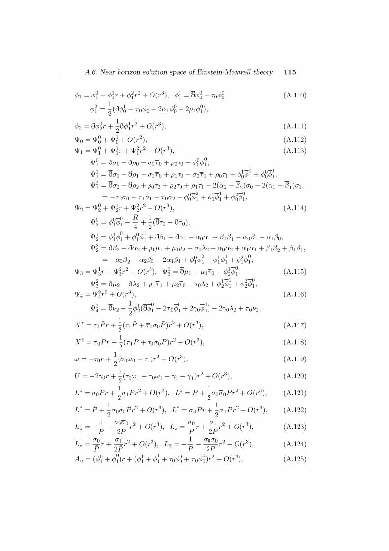
A.6. Near horizon solution space of Einstein-Maxwell theory 115

φ1 = φ01 + φ1

1r + φ21r

2 +O(r3), φ11 = ðφ0

0 − τ0φ00, (A.110)

φ21 =

1

2(ðφ1

0 − τ0φ10 − 2α1φ

00 + 2ρ1φ

01),

φ2 = ðφ02r +

1

2ðφ1

1r2 +O(r3), (A.111)

Ψ0 = Ψ00 + Ψ1

0 +O(r2), (A.112)

Ψ1 = Ψ01 + Ψ1

1r + Ψ21r

2 +O(r3), (A.113)

Ψ01 = ðσ0 − ðρ0 − σ0τ0 + ρ0τ0 + φ0

0φ01,

Ψ11 = ðσ1 − ðρ1 − σ1τ0 + ρ1τ0 − σ0τ1 + ρ0τ1 + φ1

0φ01 + φ0

0φ11,

Ψ21 = ðσ2 − ðρ2 + ρ0τ2 + ρ2τ0 + ρ1τ1 − 2(α2 − β2)σ0 − 2(α1 − β1)σ1,

= −τ2σ0 − τ1σ1 − τ0σ2 + φ00φ

21 + φ1

0φ11 + φ2

0φ01,

Ψ2 = Ψ02 + Ψ1

2r + Ψ22r

2 +O(r3), (A.114)

Ψ02 = φ0

1φ01 −

R

4+

1

2(ðτ0 − ðτ0),

Ψ12 = φ1

1φ01 + φ0

1φ11 + ðβ1 − ðα1 + α0α1 + β0β1 − α0β1 − α1β0,

Ψ22 = ðβ2 − ðα2 + ρ1µ1 + ρ0µ2 − σ0λ2 + α0α2 + α1α1 + β0β2 + β1β1,

= −α0β2 − α2β0 − 2α1β1 + φ01φ

21 + φ1

1φ11 + φ2

1φ01,

Ψ3 = Ψ13r + Ψ2

3r2 +O(r3), Ψ1

3 = ðµ1 + µ1τ0 + φ12φ

01, (A.115)

Ψ23 = ðµ2 − ðλ2 + µ1τ1 + µ2τ0 − τ0λ2 + φ1

2φ11 + φ2

2φ01,

Ψ4 = Ψ24r

2 +O(r3), (A.116)

Ψ24 = ðν2 −

1

2φ1

2(ðφ01 − 2τ0φ

01 + 2γ0φ

00)− 2γ0λ2 + τ0ν2,

Xz = τ0P r +1

2(τ1P + τ0σ0P )r2 +O(r3), (A.117)

X z = τ0Pr +1

2(τ1P + τ0σ0P )r2 +O(r3), (A.118)

ω = −τ0r +1

2(σ0ω0 − τ1)r2 +O(r3), (A.119)

U = −2γ0r +1

2(τ0ω1 + τ0ω1 − γ1 − γ1)r2 +O(r3), (A.120)

Lz = σ0P r +1

2σ1P r

2 +O(r3), Lz = P +1

2σ0σ0Pr

2 +O(r3), (A.121)

Lz

= P +1

2σ0σ0P r

2 +O(r3), Lz

= σ0Pr +1

2σ1Pr

2 +O(r3), (A.122)

Lz = − 1

P− σ0σ0

2Pr2 +O(r3), Lz =

σ0

Pr +

σ1

2Pr2 +O(r3), (A.123)

Lz =σ0

Pr +

σ1

2Pr2 +O(r3), Lz = − 1

P− σ0σ0

2Pr2 +O(r3), (A.124)

Au = (φ01 + φ

01)r + (φ1

1 + φ11 + τ0φ

00 + τ0φ

00)r2 +O(r3), (A.125)


Az = A0z +

φ00

Pr +

1

2(φ

10

P− φ0

0σ0

P)r2 +O(r3), ∂zA

0z − ∂zA0

z =φ

01 − φ0

1

PP,

where τ0, P, φ01, A

0z are arbitrary functions depending on (z, z) only, and R =

2(δδ lnP + δδ ln P − 2δ lnPδ ln P ) = 2PP∂z∂z ln PP is the scalar curvatureof S2. τ0 is the extrinsic curvature of the S2 on the horizon. The ð operatoris defined by ðη = δη + sδ ln P η and ðη = δη − sδ lnPη where s is the spinweight of the field η. The time evolution of Ψ0 and φ0 are fully controlledby (321.e) and (332).

Bibliography

[1] A. Einstein, “Approximative Integration of the Field Equations ofGravitation,” Sitzungsber. Preuss. Akad. Wiss. Berlin (Math. Phys.)1916 (1916) 688–696.

[2] A. Einstein, “Uber Gravitationswellen,” Sitzungsber. Preuss. Akad.Wiss. Berlin (Math. Phys.) 1918 (1918) 154–167.

[3] Virgo, LIGO Scientific Collaboration, B. P. Abbott et al.,“Observation of Gravitational Waves from a Binary Black HoleMerger,” Phys. Rev. Lett. 116 no. 6, (2016) 061102,arXiv:1602.03837 [gr-qc].

[4] H. Bondi, M. G. J. van der Burg, and A. W. K. Metzner,“Gravitational waves in general relativity. 7. Waves fromaxisymmetric isolated systems,” Proc. Roy. Soc. Lond. A269 (1962)21–52.

[5] H. Friedrich, “On the Existence of Analytic Null Asymptotically FlatSolutions of Einstein’s Vacuum Field Equations,” Proc. Roy. Soc.Lond. A381 (1982) 361–371.

[6] R. K. Sachs, “Gravitational waves in general relativity. 8. Waves inasymptotically flat space-times,” Proc. Roy. Soc. Lond. A270 (1962)103–126.

[7] R. Sachs, “Asymptotic symmetries in gravitational theory,” Phys.Rev. 128 (1962) 2851–2864.

[8] R. L. Arnowitt, S. Deser, and C. W. Misner, “Dynamical Structureand Definition of Energy in General Relativity,” Phys. Rev. 116(1959) 1322–1330.

[9] R. L. Arnowitt, S. Deser, and C. W. Misner, “Coordinate invarianceand energy expressions in general relativity,” Phys. Rev. 122 (1961)997.

117

http://dx.doi.org/10.1103/PhysRevLett.116.061102


http://dx.doi.org/10.1098/rspa.1962.0161






http://dx.doi.org/10.1103/PhysRev.128.2851






118 BIBLIOGRAPHY

[10] R. L. Arnowitt, S. Deser, and C. W. Misner, “The Dynamics ofgeneral relativity,” Gen. Rel. Grav. 40 (2008) 1997–2027,arXiv:gr-qc/0405109 [gr-qc].

[11] R. Geroch, “Asymptotic structure of space-time,” in Asymptoticstructure of space-time, P. Esposito and L. Witten, ed., ch. 1,pp. 1–105. Plenum, New York, 1977.

[12] L. F. Abbott and S. Deser, “Stability of Gravity with a CosmologicalConstant,” Nucl. Phys. B195 (1982) 76.

[13] L. F. Abbott and S. Deser, “Charge Definition in Nonabelian GaugeTheories,” Phys. Lett. B116 (1982) 259–263.

[14] A. D. Helfer, “Angular momentum of isolated systems,” Gen. Rel.Grav. 39 (2007) 2125–2147, arXiv:0709.1078 [gr-qc].

[15] E. T. Newman and R. Penrose, “Note on the Bondi-Metzner-Sachsgroup,” J. Math. Phys. 7 (1966) 863–870.

[16] P. J. M. Mccarthy, “Asymptotically flat space-times and elementaryparticles,” Phys. Rev. Lett. 29 (1972) 817–819.

[17] M. Crampin, “Physical significance of the topology of thebondi-metzner-sachs group,” Phys. Rev. Lett. 33 (1974) 547–550.

[18] L. Girardello and G. Parravicini, “Continuous spins in thebondi-metzner-sachs group of asymptotic symmetry in generalrelativity,” Phys. Rev. Lett. 32 (1974) 565–568.

[19] A. Piard, “Representations of the Bondi-Metzner-Sachs Group withthe Hilbert Topology,” Rept. Math. Phys. 11 (1977) 279–283.

[20] G. Barnich and C. Troessaert, “Symmetries of asymptotically flat 4dimensional spacetimes at null infinity revisited,” Phys. Rev. Lett.105 (2010) 111103, arXiv:0909.2617 [gr-qc].

[21] G. Barnich and C. Troessaert, “Aspects of the BMS/CFTcorrespondence,” JHEP 05 (2010) 062, arXiv:1001.1541 [hep-th].

[22] G. Barnich and C. Troessaert, “BMS charge algebra,” JHEP 12(2011) 105, arXiv:1106.0213 [hep-th].

[23] G. Barnich and C. Troessaert, “Finite BMS transformations,” JHEP03 (2016) 167, arXiv:1601.04090 [gr-qc].

[24] J. M. Maldacena, “The Large N limit of superconformal field theoriesand supergravity,” Int. J. Theor. Phys. 38 (1999) 1113–1133,arXiv:hep-th/9711200 [hep-th]. [Adv. Theor. Math.Phys.2,231(1998)].

http://dx.doi.org/10.1007/s10714-008-0661-1

http://arxiv.org/abs/gr-qc/0405109

http://dx.doi.org/10.1016/0550-3213(82)90049-9

http://dx.doi.org/10.1016/0370-2693(82)90338-0

http://dx.doi.org/10.1007/s10714-007-0509-0

http://dx.doi.org/10.1007/s10714-007-0509-0


http://dx.doi.org/10.1063/1.1931221




http://dx.doi.org/10.1016/0034-4877(77)90068-4




http://dx.doi.org/10.1007/JHEP05(2010)062








http://dx.doi.org/10.1023/A:1026654312961

http://arxiv.org/abs/hep-th/9711200

BIBLIOGRAPHY 119

[25] S. S. Gubser, I. R. Klebanov, and A. M. Polyakov, “Gauge theorycorrelators from noncritical string theory,” Phys. Lett. B428 (1998)105–114, arXiv:hep-th/9802109 [hep-th].

[26] E. Witten, “Anti-de Sitter space and holography,” Adv. Theor.Math. Phys. 2 (1998) 253–291, arXiv:hep-th/9802150 [hep-th].

[27] M. Banados, C. Teitelboim, and J. Zanelli, “The Black hole inthree-dimensional space-time,” Phys. Rev. Lett. 69 (1992)1849–1851, arXiv:hep-th/9204099 [hep-th].

[28] J. D. Brown and M. Henneaux, “Central Charges in the CanonicalRealization of Asymptotic Symmetries: An Example fromThree-Dimensional Gravity,” Commun. Math. Phys. 104 (1986)207–226.

[29] J. L. Cardy, “Effect of Boundary Conditions on the OperatorContent of Two-Dimensional Conformally Invariant Theories,” Nucl.Phys. B275 (1986) 200–218.

[30] A. Strominger, “Black hole entropy from near horizon microstates,”JHEP 02 (1998) 009, arXiv:hep-th/9712251 [hep-th].

[31] R. Britto, F. Cachazo, B. Feng, and E. Witten, “Direct proof oftree-level recursion relation in Yang-Mills theory,” Phys. Rev. Lett.94 (2005) 181602, arXiv:hep-th/0501052 [hep-th].

[32] F. Cachazo, S. He, and E. Y. Yuan, “Scattering of Massless Particlesin Arbitrary Dimensions,” Phys. Rev. Lett. 113 no. 17, (2014)171601, arXiv:1307.2199 [hep-th].

[33] E. Casali, “Soft sub-leading divergences in Yang-Mills amplitudes,”JHEP 08 (2014) 077, arXiv:1404.5551 [hep-th].

[34] F. Cachazo and A. Strominger, “Evidence for a New Soft GravitonTheorem,” arXiv:1404.4091 [hep-th].

[35] A. Strominger, “On BMS Invariance of Gravitational Scattering,”JHEP 07 (2014) 152, arXiv:1312.2229 [hep-th].

[36] T. He, V. Lysov, P. Mitra, and A. Strominger, “BMSsupertranslations and Weinberg’s soft graviton theorem,” JHEP 05(2015) 151, arXiv:1401.7026 [hep-th].

[37] L. Donnay, G. Giribet, H. A. Gonzalez, and M. Pino,“Supertranslations and Superrotations at the Black Hole Horizon,”Phys. Rev. Lett. 116 no. 9, (2016) 091101, arXiv:1511.08687[hep-th].

http://dx.doi.org/10.1016/S0370-2693(98)00377-3

http://dx.doi.org/10.1016/S0370-2693(98)00377-3






http://dx.doi.org/10.1007/BF01211590

http://dx.doi.org/10.1007/BF01211590

http://dx.doi.org/10.1016/0550-3213(86)90596-1

http://dx.doi.org/10.1016/0550-3213(86)90596-1

http://dx.doi.org/10.1088/1126-6708/1998/02/009



















120 BIBLIOGRAPHY

[38] P. T. Chrusciel, J. L. Costa, and M. Heusler, “Stationary BlackHoles: Uniqueness and Beyond,” Living Rev. Rel. 15 (2012) 7,arXiv:1205.6112 [gr-qc].

[39] S. W. Hawking, M. J. Perry, and A. Strominger, “Soft Hair on BlackHoles,” Phys. Rev. Lett. 116 no. 23, (2016) 231301,arXiv:1601.00921 [hep-th].

[40] A. Strominger and C. Vafa, “Microscopic origin of theBekenstein-Hawking entropy,” Phys. Lett. B379 (1996) 99–104,arXiv:hep-th/9601029 [hep-th].

[41] G. Barnich and F. Brandt, “Covariant theory of asymptoticsymmetries, conservation laws and central charges,” Nucl. Phys.B633 (2002) 3–82, arXiv:hep-th/0111246 [hep-th].

[42] I. M. Anderson and C. G. Torre, “Asymptotic conservation laws infield theory,” Phys. Rev. Lett. 77 (1996) 4109–4113,arXiv:hep-th/9608008 [hep-th].

[43] I. Anderson, The variational bicomplex. Formal Geometry andMathematical Physics, Department of Mathematics, Utah StateUniversity technical report, unpublished, 1989.

[44] T. He, P. Mitra, A. P. Porfyriadis, and A. Strominger, “NewSymmetries of Massless QED,” JHEP 10 (2014) 112,arXiv:1407.3789 [hep-th].

[45] S. W. Hawking, “The Information Paradox for Black Holes,” 2015.arXiv:1509.01147 [hep-th].

[46] A. Ashtekar, J. Engle, T. Pawlowski, and C. Van Den Broeck,“Multipole moments of isolated horizons,” Class. Quant. Grav. 21(2004) 2549–2570, arXiv:gr-qc/0401114 [gr-qc].

[47] P. K. Townsend, “Black holes: Lecture notes,”arXiv:gr-qc/9707012 [gr-qc].

[48] E. Newman and R. Penrose, “An Approach to gravitational radiationby a method of spin coefficients,” J. Math. Phys. 3 (1962) 566–578.

[49] E. T. Newman and T. W. J. Unti, “Behavior of Asymptotically FlatEmpty Spaces,” J. Math. Phys. 3 no. 5, (1962) 891.

[50] P. Szekeres, “The Gravitational compass,” J. Math. Phys. 6 (1965)1387–1391.

[51] G. Barnich and P.-H. Lambert, “A note on the Newman-Unti group,”Adv. Math. Phys. 2012 (2012) 197385, arXiv:1102.0589 [gr-qc].

http://dx.doi.org/10.12942/lrr-2012-7




http://dx.doi.org/10.1016/0370-2693(96)00345-0


http://dx.doi.org/10.1016/S0550-3213(02)00251-1

http://dx.doi.org/10.1016/S0550-3213(02)00251-1







http://dx.doi.org/10.1088/0264-9381/21/11/003

http://dx.doi.org/10.1088/0264-9381/21/11/003



http://dx.doi.org/10.1063/1.1724257

http://dx.doi.org/10.1063/1.1724303

http://dx.doi.org/10.1063/1.1704788

http://dx.doi.org/10.1063/1.1704788


BIBLIOGRAPHY 121

[52] P.-H. Lambert, Conformal symmetries of gravity from asymptoticmethods: further developments. PhD thesis, Brussels U., 2014.arXiv:1409.4693 [gr-qc]. https://inspirehep.net/record/1317227/files/arXiv:1409.4693.pdf.

[53] G. Barnich and C. Troessaert, “Comments on holographic currentalgebras and asymptotically flat four dimensional spacetimes at nullinfinity,” JHEP 11 (2013) 003, arXiv:1309.0794 [hep-th].

[54] M. Banados, M. Henneaux, C. Teitelboim, and J. Zanelli, “Geometryof the (2+1) black hole,” Phys. Rev. D48 (1993) 1506–1525,arXiv:gr-qc/9302012 [gr-qc]. [Erratum: Phys.Rev.D88,069902(2013)].

[55] S. Deser, R. Jackiw, and G. ’t Hooft, “Three-Dimensional EinsteinGravity: Dynamics of Flat Space,” Annals Phys. 152 (1984) 220.

[56] S. Deser and R. Jackiw, “Three-Dimensional Cosmological Gravity:Dynamics of Constant Curvature,” Annals Phys. 153 (1984)405–416.

[57] D. R. Brill, “Multi - black hole geometries in (2+1)-dimensionalgravity,” Phys. Rev. D53 (1996) 4133–4176, arXiv:gr-qc/9511022[gr-qc].

[58] D. Brill, “Black holes and wormholes in (2+1)-dimensions,”arXiv:gr-qc/9904083 [gr-qc]. [Lect. Notes Phys.537,143(2000)].

[59] K. Skenderis and B. C. van Rees, “Holography and wormholes in2+1 dimensions,” Commun. Math. Phys. 301 (2011) 583–626,arXiv:0912.2090 [hep-th].

[60] A. Ashtekar, J. Bicak, and B. G. Schmidt, “Asymptotic structure ofsymmetry reduced general relativity,” Phys. Rev. D55 (1997)669–686, arXiv:gr-qc/9608042 [gr-qc].

[61] G. Barnich and G. Compere, “Classical central extension forasymptotic symmetries at null infinity in three spacetimedimensions,” Class. Quant. Grav. 24 (2007) F15–F23,arXiv:gr-qc/0610130 [gr-qc].

[62] O. Aharony, S. S. Gubser, J. M. Maldacena, H. Ooguri, and Y. Oz,“Large N field theories, string theory and gravity,” Phys. Rept. 323(2000) 183–386, arXiv:hep-th/9905111 [hep-th].

[63] M. M. Sheikh-Jabbari and H. Yavartanoo, “EVH Black Holes, AdS3Throats and EVH/CFT Proposal,” JHEP 10 (2011) 013,arXiv:1107.5705 [hep-th].


https://inspirehep.net/record/1317227/files/arXiv:1409.4693.pdf

https://inspirehep.net/record/1317227/files/arXiv:1409.4693.pdf



http://dx.doi.org/10.1103/PhysRevD.48.1506, 10.1103/PhysRevD.88.069902


http://dx.doi.org/10.1016/0003-4916(84)90085-X

http://dx.doi.org/10.1016/0003-4916(84)90025-3

http://dx.doi.org/10.1016/0003-4916(84)90025-3

http://dx.doi.org/10.1103/PhysRevD.53.4133




http://dx.doi.org/10.1007/s00220-010-1163-z





http://dx.doi.org/10.1088/0264-9381/24/5/F01, 10.1088/0264-9381/24/11/C01


http://dx.doi.org/10.1016/S0370-1573(99)00083-6

http://dx.doi.org/10.1016/S0370-1573(99)00083-6




122 BIBLIOGRAPHY

[64] J. D. Brown and M. Henneaux, “On the Poisson Brackets ofDifferentiable Generators in Classical Field Theory,” J. Math. Phys.27 (1986) 489–491.

[65] P. Kraus, “Lectures on black holes and the AdS(3) / CFT(2)correspondence,” Lect. Notes Phys. 755 (2008) 193–247,arXiv:hep-th/0609074 [hep-th].

[66] J. M. Maldacena and A. Strominger, “AdS(3) black holes and astringy exclusion principle,” JHEP 12 (1998) 005,arXiv:hep-th/9804085 [hep-th].

[67] K. Skenderis, “Lecture notes on holographic renormalization,” Class.Quant. Grav. 19 (2002) 5849–5876, arXiv:hep-th/0209067[hep-th].

[68] A. Maloney and E. Witten, “Quantum Gravity Partition Functionsin Three Dimensions,” JHEP 02 (2010) 029, arXiv:0712.0155[hep-th].

[69] E. Witten, “Three-Dimensional Gravity Revisited,”arXiv:0706.3359 [hep-th].

[70] M. Banados, “Three-dimensional quantum geometry and blackholes,” arXiv:hep-th/9901148 [hep-th]. [AIP Conf.Proc.484,147(1999)].

[71] M. Rooman and P. Spindel, “Uniqueness of the asymptotic AdS(3)geometry,” Class. Quant. Grav. 18 (2001) 2117–2124,arXiv:gr-qc/0011005 [gr-qc].

[72] S. Ryu and T. Takayanagi, “Aspects of Holographic EntanglementEntropy,” JHEP 08 (2006) 045, arXiv:hep-th/0605073 [hep-th].

[73] V. Balasubramanian, J. de Boer, M. M. Sheikh-Jabbari, andJ. Simon, “What is a chiral 2d CFT? And what does it have to dowith extremal black holes?,” JHEP 02 (2010) 017, arXiv:0906.3272[hep-th].

[74] G. Barnich, A. Gomberoff, and H. A. Gonzalez, “The Flat limit ofthree dimensional asymptotically anti-de Sitter spacetimes,” Phys.Rev. D86 (2012) 024020, arXiv:1204.3288 [gr-qc].

[75] C. Li and J. Lucietti, “Three-dimensional black holes anddescendants,” Phys. Lett. B738 (2014) 48–4, arXiv:1312.2626[hep-th].

http://dx.doi.org/10.1063/1.527249

http://dx.doi.org/10.1063/1.527249


http://dx.doi.org/10.1088/1126-6708/1998/12/005


http://dx.doi.org/10.1088/0264-9381/19/22/306

http://dx.doi.org/10.1088/0264-9381/19/22/306








http://dx.doi.org/10.1088/0264-9381/18/11/309


http://dx.doi.org/10.1088/1126-6708/2006/08/045








http://dx.doi.org/10.1016/j.physletb.2014.09.012



BIBLIOGRAPHY 123

[76] M. M. Sheikh-Jabbari and H. Yavartanoo, “On quantization of AdS3

gravity I: semi-classical analysis,” JHEP 07 (2014) 104,arXiv:1404.4472 [hep-th].

[77] A. Maloney, “Geometric Microstates for the Three DimensionalBlack Hole?,” arXiv:1508.04079 [hep-th].

[78] J. Kim and M. Porrati, “On a Canonical Quantization of 3D Anti deSitter Pure Gravity,” JHEP 10 (2015) 096, arXiv:1508.03638[hep-th].

[79] G. Compere, L. Donnay, P.-H. Lambert, and W. Schulgin, “Liouvilletheory beyond the cosmological horizon,” JHEP 03 (2015) 158,arXiv:1411.7873 [hep-th].

[80] A. Strominger, “The dS / CFT correspondence,” JHEP 10 (2001)034, arXiv:hep-th/0106113 [hep-th].

[81] J. M. Mitchell, “Where are the BTZ Black Hole Degrees ofFreedom?,” Class. Quant. Grav. 32 no. 23, (2015) 235009,arXiv:1506.04343 [gr-qc].

[82] J. M. Mitchell, “Where are the BTZ Black Hole Degrees of Freedom?The Rotating Case,” Class. Quant. Grav. 33 no. 13, (2016) 135003,arXiv:1510.01033 [gr-qc].

[83] G. Barnich and G. Compere, “Surface charge algebra in gaugetheories and thermodynamic integrability,” J. Math. Phys. 49 (2008)042901, arXiv:0708.2378 [gr-qc].

[84] J. Lee and R. M. Wald, “Local symmetries and constraints,” J.Math. Phys. 31 (1990) 725–743.

[85] E. Witten, “Coadjoint Orbits of the Virasoro Group,” Commun.Math. Phys. 114 (1988) 1.

[86] G. Compere, K. Hajian, A. Seraj, and M. M. Sheikh-Jabbari,“Wiggling Throat of Extremal Black Holes,” JHEP 10 (2015) 093,arXiv:1506.07181 [hep-th].

[87] G. Compere, K. Hajian, A. Seraj, and M. M. Sheikh-Jabbari,“Extremal Rotating Black Holes in the Near-Horizon Limit: PhaseSpace and Symmetry Algebra,” Phys. Lett. B749 (2015) 443–447,arXiv:1503.07861 [hep-th].

[88] S. Carlip, Quantum gravity in 2+1 dimensions. CambridgeUniversity Press, 2003. http://www.cambridge.org/uk/catalogue/catalogue.asp?isbn=0521545889.









http://dx.doi.org/10.1088/1126-6708/2001/10/034

http://dx.doi.org/10.1088/1126-6708/2001/10/034


http://dx.doi.org/10.1088/0264-9381/32/23/235009


http://dx.doi.org/10.1088/0264-9381/33/13/135003


http://dx.doi.org/10.1063/1.2889721

http://dx.doi.org/10.1063/1.2889721


http://dx.doi.org/10.1063/1.528801

http://dx.doi.org/10.1063/1.528801

http://dx.doi.org/10.1007/BF01218287

http://dx.doi.org/10.1007/BF01218287



http://dx.doi.org/10.1016/j.physletb.2015.08.027


http://www.cambridge.org/uk/catalogue/catalogue.asp?isbn=0521545889

http://www.cambridge.org/uk/catalogue/catalogue.asp?isbn=0521545889

124 BIBLIOGRAPHY

[89] M. Guica, T. Hartman, W. Song, and A. Strominger, “TheKerr/CFT Correspondence,” Phys. Rev. D80 (2009) 124008,arXiv:0809.4266 [hep-th].

[90] J. Balog, L. Feher, and L. Palla, “Coadjoint orbits of the Virasoroalgebra and the global Liouville equation,” Int. J. Mod. Phys. A13(1998) 315–362, arXiv:hep-th/9703045 [hep-th].

[91] C. Fefferman and R. Graham, “Conformal Invariants,” Elie Cartanet les Mathematiques d’aujourd’hui, Asterisque (1985) 95.

[92] I. Papadimitriou and K. Skenderis, “Thermodynamics ofasymptotically locally AdS spacetimes,” JHEP 08 (2005) 004,arXiv:hep-th/0505190 [hep-th].

[93] O. Coussaert and M. Henneaux, “Selfdual solutions of (2+1)Einstein gravity with a negative cosmological constant,” in TheBlack Hole 25 Years After Santiago, Chile, January 17-21, 1994.1994. arXiv:hep-th/9407181 [hep-th].http://alice.cern.ch/format/showfull?sysnb=0185011.

[94] G. Compere and D. Marolf, “Setting the boundary free inAdS/CFT,” Class. Quant. Grav. 25 (2008) 195014,arXiv:0805.1902 [hep-th].

[95] G. Compere, W. Song, and A. Strominger, “New BoundaryConditions for AdS3,” JHEP 05 (2013) 152, arXiv:1303.2662[hep-th].

[96] C. Troessaert, “Enhanced asymptotic symmetry algebra of AdS3,”JHEP 08 (2013) 044, arXiv:1303.3296 [hep-th].

[97] C. Crnkovic and E. Witten, “Covariant description of canonicalformalism in geometrical theories, 1986, Print-86-1309 (Princeton),”.

[98] G. Compere, Symmetries and conservation laws in Lagrangian gaugetheories with applications to the mechanics of black holes and togravity in three dimensions. PhD thesis, Vrije U., Brussels, 2007.arXiv:0708.3153 [hep-th]. http://inspirehep.net/record/758992/files/arXiv:0708.3153.pdf.

[99] V. Iyer and R. M. Wald, “Some properties of Noether charge and aproposal for dynamical black hole entropy,” Phys. Rev. D50 (1994)846–864, arXiv:gr-qc/9403028 [gr-qc].

[100] G. Barnich, “A Note on Gauge Systems from the Point of View ofLie Algebroids,” in American Institute of Physics Conference Series,P. Kielanowski, V. Buchstaber, A. Odzijewicz, M. Schlichenmaier,



http://dx.doi.org/10.1142/S0217751X98000147

http://dx.doi.org/10.1142/S0217751X98000147


http://dx.doi.org/10.1088/1126-6708/2005/08/004



http://alice.cern.ch/format/showfull?sysnb=0185011

http://dx.doi.org/10.1088/0264-9381/25/19/195014








http://inspirehep.net/record/758992/files/arXiv:0708.3153.pdf

http://inspirehep.net/record/758992/files/arXiv:0708.3153.pdf




http://dx.doi.org/10.1063/1.3527427

http://dx.doi.org/10.1063/1.3527427

BIBLIOGRAPHY 125

and T. Voronov, eds., vol. 1307 of American Institute of PhysicsConference Series, pp. 7–18. Nov., 2010. arXiv:1010.0899[math-ph].

[101] W. Magnus and S. Winkler, Hill’s equation. Courier Corporation,2013.

[102] A. Garbarz and M. Leston, “Classification of Boundary Gravitons inAdS3 Gravity,” JHEP 05 (2014) 141, arXiv:1403.3367 [hep-th].

[103] M. M. Sheikh-Jabbari and H. Yavartanoo, “On 3d bulk geometry ofVirasoro coadjoint orbits: orbit invariant charges and Virasoro hairon locally AdS3 geometries,” Eur. Phys. J. C76 no. 9, (2016) 493,arXiv:1603.05272 [hep-th].

[104] J. de Boer, M. M. Sheikh-Jabbari, and J. Simon, “Near HorizonLimits of Massless BTZ and Their CFT Duals,” Class. Quant. Grav.28 (2011) 175012, arXiv:1011.1897 [hep-th].

[105] K. Hajian, A. Seraj, and M. M. Sheikh-Jabbari, “NHEG Mechanics:Laws of Near Horizon Extremal Geometry (Thermo)Dynamics,”JHEP 03 (2014) 014, arXiv:1310.3727 [hep-th].

[106] K. Hajian, A. Seraj, and M. M. Sheikh-Jabbari, “Near HorizonExtremal Geometry Perturbations: Dynamical Field Perturbationsvs. Parametric Variations,” JHEP 10 (2014) 111, arXiv:1407.1992[hep-th].

[107] G. Barnich, “Boundary charges in gauge theories: using Stokestheorem in the bulk,” Classical and Quantum Gravity 20 (Aug.,2003) 3685–3697, hep-th/0301039.

[108] E. Newman, L. Tamubrino, and T. Unti, “Empty spacegeneralization of the Schwarzschild metric,” J. Math. Phys. 4 (1963)915.

[109] M. G. J. van der Burg, “Gravitational Waves in General Relativity.10.Asymptotic Expansions for the Einstein-Maxwell Field,” Proc.Roy. Soc. Lond. A310 (1969) 221–230.

[110] A. R. Exton, E. T. Newman, and R. Penrose, “Conserved quantitiesin the Einstein-Maxwell theory,” J. Math. Phys. 10 (1969)1566–1570.

[111] W. J., “Logarithmic asymptotic flatness,” Foundations of Physics 15no. 05, (1985) 605–616.





http://dx.doi.org/10.1140/epjc/s10052-016-4326-z


http://dx.doi.org/10.1088/0264-9381/28/17/175012

http://dx.doi.org/10.1088/0264-9381/28/17/175012







http://dx.doi.org/10.1088/0264-9381/20/16/310

http://dx.doi.org/10.1088/0264-9381/20/16/310


http://dx.doi.org/10.1063/1.1704018

http://dx.doi.org/10.1063/1.1704018



http://dx.doi.org/10.1063/1.1665006

http://dx.doi.org/10.1063/1.1665006

http://dx.doi.org/10.1007/BF01882485

http://dx.doi.org/10.1007/BF01882485

126 BIBLIOGRAPHY

[112] P. T. Chrusciel, M. A. H. MacCallum, and D. B. Singleton,“Gravitational waves in general relativity: 14. Bondi expansions andthe polyhomogeneity of Scri,” arXiv:gr-qc/9305021 [gr-qc].

[113] J. A. Valiente Kroon, “Logarithmic Newman-Penrose constants forarbitrary polyhomogeneous space-times,” Class. Quant. Grav. 16(1999) 1653–1665, arXiv:gr-qc/9812004 [gr-qc].

[114] R. M. Wald and A. Zoupas, “A General definition of ’conservedquantities’ in general relativity and other theories of gravity,” Phys.Rev. D61 (2000) 084027, arXiv:gr-qc/9911095 [gr-qc].

[115] A. Ashtekar, J. Bicak, and B. G. Schmidt, “Asymptotic structure ofsymmetry reduced general relativity,” Phys. Rev. D55 (1997)669–686, arXiv:gr-qc/9608042 [gr-qc].

[116] G. Barnich and G. Compere, “Classical central extension forasymptotic symmetries at null infinity in three spacetimedimensions,” Class. Quant. Grav. 24 (2007) F15–F23,arXiv:gr-qc/0610130 [gr-qc].

[117] K. Ezawa, “Transition amplitude in (2+1)-dimensionalChern-Simons gravity on a torus,” Int. J. Mod. Phys. A9 (1994)4727–4746, arXiv:hep-th/9305170 [hep-th].

[118] L. Cornalba and M. S. Costa, “A New cosmological scenario in stringtheory,” Phys. Rev. D66 (2002) 066001, arXiv:hep-th/0203031[hep-th].

[119] L. Cornalba and M. S. Costa, “Time dependent orbifolds and stringcosmology,” Fortsch. Phys. 52 (2004) 145–199,arXiv:hep-th/0310099 [hep-th].

[120] C. Martinez, C. Teitelboim, and J. Zanelli, “Charged rotating blackhole in three space-time dimensions,” Phys. Rev. D61 (2000) 104013,arXiv:hep-th/9912259 [hep-th].

[121] G. Barnich and P.-H. Lambert, “Einstein-Yang-Mills theory:Asymptotic symmetries,” Phys. Rev. D88 (2013) 103006,arXiv:1310.2698 [hep-th].

[122] L. A. Tamburino and J. H. Winicour, “Gravitational Fields in Finiteand Conformal Bondi Frames,” Phys. Rev. 150 (1966) 1039–1053.

[123] G. Barnich, “Boundary charges in gauge theories: Using Stokestheorem in the bulk,” Class. Quant. Grav. 20 (2003) 3685–3698,arXiv:hep-th/0301039 [hep-th].


http://dx.doi.org/10.1088/0264-9381/16/5/314

http://dx.doi.org/10.1088/0264-9381/16/5/314








http://dx.doi.org/10.1088/0264-9381/24/5/F01, 10.1088/0264-9381/24/11/C01


http://dx.doi.org/10.1142/S0217751X94001898

http://dx.doi.org/10.1142/S0217751X94001898





http://dx.doi.org/10.1002/prop.200310123







http://dx.doi.org/10.1088/0264-9381/20/16/310


BIBLIOGRAPHY 127

[124] G. Barnich and G. Compere, “Conserved charges andthermodynamics of the spinning Godel black hole,” Phys. Rev. Lett.95 (2005) 031302, arXiv:hep-th/0501102 [hep-th].

[125] S. A. Hartnoll, C. P. Herzog, and G. T. Horowitz, “Building aHolographic Superconductor,” Phys. Rev. Lett. 101 (2008) 031601,arXiv:0803.3295 [hep-th].

[126] S. Kachru, X. Liu, and M. Mulligan, “Gravity duals of Lifshitz-likefixed points,” Phys. Rev. D78 (2008) 106005, arXiv:0808.1725[hep-th].

[127] K. Balasubramanian and J. McGreevy, “Gravity duals fornon-relativistic CFTs,” Phys. Rev. Lett. 101 (2008) 061601,arXiv:0804.4053 [hep-th].

[128] D. Maity, S. Sarkar, N. Sircar, B. Sathiapalan, and R. Shankar,“Properties of CFTs dual to Charged BTZ black-hole,” Nucl. Phys.B839 (2010) 526–551, arXiv:0909.4051 [hep-th].

[129] J. Ren, “One-dimensional holographic superconductor fromAdS3/CFT2 correspondence,” JHEP 11 (2010) 055,arXiv:1008.3904 [hep-th].

[130] K. Jensen, “Chiral anomalies and AdS/CMT in two dimensions,”JHEP 01 (2011) 109, arXiv:1012.4831 [hep-th].

[131] A. Bagchi, R. Gopakumar, I. Mandal, and A. Miwa, “GCA in 2d,”JHEP 08 (2010) 004, arXiv:0912.1090 [hep-th].

[132] A. Bagchi, “The BMS/GCA correspondence,” Phys. Rev. Lett. 105(2010) 171601, arXiv:1006.3354 [hep-th].

[133] A. Ashtekar, ASYMPTOTIC QUANTIZATION: BASED ON 1984NAPLES LECTURES. 1987.

[134] G. Barnich and C. Troessaert, “Supertranslations call forsuperrotations,” PoS (2010) 010, arXiv:1102.4632 [gr-qc]. [Ann.U. Craiova Phys.21,S11(2011)].

[135] G. Barnich, “Entropy of three-dimensional asymptotically flatcosmological solutions,” JHEP 10 (2012) 095, arXiv:1208.4371[hep-th].

[136] A. Bagchi, S. Detournay, R. Fareghbal, and J. Simn, “Holography of3D Flat Cosmological Horizons,” Phys. Rev. Lett. 110 no. 14, (2013)141302, arXiv:1208.4372 [hep-th].











http://dx.doi.org/10.1016/j.nuclphysb.2010.06.012

http://dx.doi.org/10.1016/j.nuclphysb.2010.06.012


















128 BIBLIOGRAPHY

[137] J. A. Valiente-Kroon, “On the existence and convergence ofpolyhomogeneous expansions of zero rest mass fields,” Class. Quant.Grav. 17 (2000) 4365–4376, arXiv:gr-qc/0005087 [gr-qc].

[138] A. Perez, M. Riquelme, D. Tempo, and R. Troncoso, “Conservedcharges and black holes in the Einstein-Maxwell theory on AdS3

reconsidered,” JHEP 10 (2015) 161, arXiv:1509.01750 [hep-th].

[139] A. Perez, M. Riquelme, D. Tempo, and R. Troncoso, “Asymptoticstructure of the Einstein-Maxwell theory on AdS3,” JHEP 02 (2016)015, arXiv:1512.01576 [hep-th].

[140] S. J. Avis, C. J. Isham, and D. Storey, “Quantum Field Theory inanti-De Sitter Space-Time,” Phys. Rev. D18 (1978) 3565.

[141] S. W. Hawking, “The Boundary Conditions for GaugedSupergravity,” Phys. Lett. B126 (1983) 175–177.

[142] A. Ashtekar and A. Magnon, “Asymptotically anti-de Sitterspace-times,” Class. Quant. Grav. 1 (1984) L39–L44.

[143] S. Weinberg, “Photons and Gravitons in s Matrix Theory:Derivation of Charge Conservation and Equality of Gravitational andInertial Mass,” Phys. Rev. 135 (1964) B1049–B1056.

[144] S. Weinberg, “Infrared photons and gravitons,” Phys. Rev. 140(1965) B516–B524.

[145] F. E. Low, “Scattering of light of very low frequency by systems ofspin 1/2,” Phys. Rev. 96 (1954) 1428–1432.

[146] M. Gell-Mann and M. L. Goldberger, “Scattering of low-energyphotons by particles of spin 1/2,” Phys. Rev. 96 (1954) 1433–1438.

[147] F. E. Low, “Bremsstrahlung of very low-energy quanta in elementaryparticle collisions,” Phys. Rev. 110 (1958) 974–977.

[148] T. H. Burnett and N. M. Kroll, “Extension of the low soft photontheorem,” Phys. Rev. Lett. 20 (1968) 86.

[149] J. S. Bell and R. Van Royen, “On the low-burnett-kroll theorem forsoft-photon emission,” Nuovo Cim. A60 (1969) 62–68.

[150] Z. Bern, S. Davies, P. Di Vecchia, and J. Nohle, “Low-EnergyBehavior of Gluons and Gravitons from Gauge Invariance,” Phys.Rev. D90 no. 8, (2014) 084035, arXiv:1406.6987 [hep-th].

[151] V. Del Duca, “High-energy Bremsstrahlung Theorems for SoftPhotons,” Nucl. Phys. B345 (1990) 369–388.

http://dx.doi.org/10.1088/0264-9381/17/21/302

http://dx.doi.org/10.1088/0264-9381/17/21/302








http://dx.doi.org/10.1016/0370-2693(83)90585-3

http://dx.doi.org/10.1088/0264-9381/1/4/002

http://dx.doi.org/10.1103/PhysRev.135.B1049







http://dx.doi.org/10.1007/BF02823297




http://dx.doi.org/10.1016/0550-3213(90)90392-Q

BIBLIOGRAPHY 129

[152] A. J. Larkoski, D. Neill, and I. W. Stewart, “Soft Theorems fromEffective Field Theory,” JHEP 06 (2015) 077, arXiv:1412.3108[hep-th].

[153] A. Strominger, “Asymptotic Symmetries of Yang-Mills Theory,”JHEP 07 (2014) 151, arXiv:1308.0589 [hep-th].

[154] M. Bianchi, S. He, Y.-t. Huang, and C. Wen, “More on SoftTheorems: Trees, Loops and Strings,” Phys. Rev. D92 no. 6, (2015)065022, arXiv:1406.5155 [hep-th].

[155] D. Kapec, V. Lysov, and A. Strominger, “Asymptotic Symmetries ofMassless QED in Even Dimensions,” arXiv:1412.2763 [hep-th].

[156] A. Mohd, “A note on asymptotic symmetries and soft-photontheorem,” JHEP 02 (2015) 060, arXiv:1412.5365 [hep-th].

[157] D. Kapec, M. Pate, and A. Strominger, “New Symmetries of QED,”arXiv:1506.02906 [hep-th].

[158] M. Campiglia and A. Laddha, “Asymptotic symmetries of QED andWeinberg’s soft photon theorem,” JHEP 07 (2015) 115,arXiv:1505.05346 [hep-th].

[159] A. Strominger, “Magnetic Corrections to the Soft Photon Theorem,”Phys. Rev. Lett. 116 no. 3, (2016) 031602, arXiv:1509.00543[hep-th].

[160] V. Lysov, S. Pasterski, and A. Strominger, “Low’s Subleading SoftTheorem as a Symmetry of QED,” Phys. Rev. Lett. 113 no. 11,(2014) 111601, arXiv:1407.3814 [hep-th].

[161] A. I. Janis and E. T. Newman, “Structure of Gravitational Sources,”J. Math. Phys. 6 (1965) 902–914.

[162] E. T. Newman and R. Penrose, “New conservation laws for zerorest-mass fields in asymptotically flat space-time,” Proc. Roy. Soc.Lond. A305 (1968) 175–204.

[163] G. Barnich, P.-H. Lambert, and P. Mao, “Three-dimensionalasymptotically flat EinsteinMaxwell theory,” Class. Quant. Grav. 32no. 24, (2015) 245001, arXiv:1503.00856 [gr-qc].

[164] D. Kapec, V. Lysov, S. Pasterski, and A. Strominger, “SemiclassicalVirasoro symmetry of the quantum gravity S-matrix,” JHEP 08(2014) 058, arXiv:1406.3312 [hep-th].





















http://dx.doi.org/10.1063/1.1704349



http://dx.doi.org/10.1088/0264-9381/32/24/245001

http://dx.doi.org/10.1088/0264-9381/32/24/245001





130 BIBLIOGRAPHY

[165] M. Campiglia and A. Laddha, “Asymptotic symmetries andsubleading soft graviton theorem,” Phys. Rev. D90 no. 12, (2014)124028, arXiv:1408.2228 [hep-th].

[166] M. Campiglia and A. Laddha, “New symmetries for the GravitationalS-matrix,” JHEP 04 (2015) 076, arXiv:1502.02318 [hep-th].

[167] M. Campiglia and A. Laddha, “Sub-subleading soft gravitons: Newsymmetries of quantum gravity?,” arXiv:1605.09094 [gr-qc].

[168] T. He, P. Mitra, and A. Strominger, “2D Kac-Moody Symmetry of4D Yang-Mills Theory,” arXiv:1503.02663 [hep-th].

[169] T. T. Dumitrescu, T. He, P. Mitra, and A. Strominger,“Infinite-Dimensional Fermionic Symmetry in SupersymmetricGauge Theories,” arXiv:1511.07429 [hep-th].

[170] E. Conde and P. Mao, “Comments on Asymptotic Symmetries andthe Sub-leading Soft Photon Theorem,” arXiv:1605.09731

[hep-th].

[171] M. Campiglia and A. Laddha, “Subleading soft photons and largegauge transformations,” arXiv:1605.09677 [hep-th].

[172] D. Kapec, V. Lysov, S. Pasterski, and A. Strominger,“Higher-Dimensional Supertranslations and Weinberg’s SoftGraviton Theorem,” arXiv:1502.07644 [gr-qc].

[173] D. Kapec, P. Mitra, A.-M. Raclariu, and A. Strominger, “A 2DStress Tensor for 4D Gravity,” arXiv:1609.00282 [hep-th].

[174] D. Christodoulou and S. Klainerman, The Global nonlinear stabilityof the Minkowski space. Princeton University Press, Princeton, 1993.

[175] S. W. Hawking, “Breakdown of Predictability in GravitationalCollapse,” Phys. Rev. D14 (1976) 2460–2473.

[176] C. Eling and Y. Oz, “On the Membrane Paradigm and SpontaneousBreaking of Horizon BMS Symmetries,” JHEP 07 (2016) 065,arXiv:1605.00183 [hep-th].

[177] A. Averin, G. Dvali, C. Gomez, and D. Lust, “Gravitational BlackHole Hair from Event Horizon Supertranslations,” JHEP 06 (2016)088, arXiv:1601.03725 [hep-th].

[178] G. t. Hooft, “Black hole unitarity and antipodal entanglement,”arXiv:1601.03447 [gr-qc].





















BIBLIOGRAPHY 131

[179] G. Compere and J. Long, “Classical static final state of collapse withsupertranslation memory,” arXiv:1602.05197 [gr-qc].

[180] D. Kapec, A.-M. Raclariu, and A. Strominger, “Area, EntanglementEntropy and Supertranslations at Null Infinity,” arXiv:1603.07706

[hep-th].

[181] M. M. Sheikh-Jabbari, “Residual Diffeomorphisms and SymplecticHair on Black Holes,” arXiv:1603.07862 [hep-th].

[182] M. Hotta, J. Trevison, and K. Yamaguchi, “Gravitational MemoryCharges of Supertranslation and Superrotation on Rindler Horizons,”arXiv:1606.02443 [gr-qc].

[183] A. Ashtekar, C. Beetle, and S. Fairhurst, “Isolated horizons: AGeneralization of black hole mechanics,” Class. Quant. Grav. 16(1999) L1–L7, arXiv:gr-qc/9812065 [gr-qc].

[184] A. Ashtekar, C. Beetle, and J. Lewandowski, “Mechanics of rotatingisolated horizons,” Phys. Rev. D64 (2001) 044016,arXiv:gr-qc/0103026 [gr-qc].

[185] A. Strominger and A. Zhiboedov, “Gravitational Memory, BMSSupertranslations and Soft Theorems,” JHEP 01 (2016) 086,arXiv:1411.5745 [hep-th].

[186] A. Ashtekar, C. Beetle, and J. Lewandowski, “Geometry of genericisolated horizons,” Class. Quant. Grav. 19 (2002) 1195–1225,arXiv:gr-qc/0111067 [gr-qc].

[187] J. Luk, “On the Local Existence for the Characteristic Initial ValueProblem in General Relativity,” Int. Math. Res. Not. 20 (2012)4625, arXiv:1107.0898 [gr-qc].

[188] L. Donnay, Symmetries and dynamics for non-AdS backgrounds inthree-dimensional gravity. PhD thesis, Universite Libre de Bruxelles,2016.

[189] A. Ashtekar, J. Engle, and C. Van Den Broeck, “Quantum horizonsand black hole entropy: Inclusion of distortion and rotation,” Class.Quant. Grav. 22 (2005) L27–L34, arXiv:gr-qc/0412003 [gr-qc].

[190] A. Ashtekar and B. Krishnan, “Dynamical horizons and theirproperties,” Phys. Rev. D68 (2003) 104030, arXiv:gr-qc/0308033[gr-qc].

[191] A. Ashtekar and G. J. Galloway, “Some uniqueness results fordynamical horizons,” Adv. Theor. Math. Phys. 9 no. 1, (2005) 1–30,arXiv:gr-qc/0503109 [gr-qc].






http://dx.doi.org/10.1088/0264-9381/16/2/027

http://dx.doi.org/10.1088/0264-9381/16/2/027






http://dx.doi.org/10.1088/0264-9381/19/6/311


http://dx.doi.org/10.1093/imrn/rnr201

http://dx.doi.org/10.1093/imrn/rnr201


http://dx.doi.org/10.1088/0264-9381/22/4/L02

http://dx.doi.org/10.1088/0264-9381/22/4/L02





http://dx.doi.org/10.4310/ATMP.2005.v9.n1.a1


New Applications of Asymptotic Symmetries ... - Inspire HEP

Documents

Transcript of New Applications of Asymptotic Symmetries ... - Inspire HEP