ALMA MATER STUDIORUM - UNIVERSITA’ DI BOLOGNA

Dottorato di Ricerca in FisicaCiclo XXXI

Settore concorsuale di afferenza: 02/A2Settore scientifico disciplinare: FIS/02

Inflation and Dark MatterFrom String Theory

Presentata da: Victor AlfonzoDiaz

Coordinatrice Dottorato:Prof.ssa Silvia Arcelli

Supervisore:Prof. Michele Cicoli

Esame finale anno 2019

ii

“...Not only is the Universe stranger than we think, it is stranger thanwe can think...”

Werner Heisenberg

Dedicada a mí.

iii

iv

Acknowledgements

I would like to thank all the collaborators who made possible the creation of thisremarkable work: Michele Cicoli, David Ciupke, Veronica Guidetti, Francesco Muia,Francisco Pedro, Marcus Rummel, Pramod Shukla. I’m particularly grateful to mysupervisor, Michele Cicoli, who trusted me to decide what type of research I wouldlike to do and also for give me the freedom to do it at my own pace. I am alsoreally grateful for the figures who taught basically everything that I know aboutstring theory: Anamaria Font and Fernando Quevedo, two amazing people that willalways be in my mind

This thesis was assembled during my stay at the Max-Planck Institute for Physicsin Munich, Germany. I am really grateful for the amazing hospitality given by Prof.Ralph Blumenhagen and the Max-Planck Institute in the finishing stage of my PhD.

v

DeclarationThis thesis is based on the results presented in the following papers:

[1] 2017, August.M. Cicoli, V. A. Diaz, V. Guidetti and M. Rummel,“The 3.5 keV Line from Stringy Axions,”JHEP 1710, 192 (2017), arXiv:1707.02987 [hep-th].

[2] 2017, September.M. Cicoli, D. Ciupke, V. A. Diaz, V. Guidetti, F. Muia and P. Shukla,“Chiral Global Embedding of Fibre Inflation Models,”JHEP 1711, 207 (2017), arXiv:1709.01518 [hep-th].

[3] 2018, March.M. Cicoli, V. A. Diaz and F. G. Pedro,“Primordial Black Holes from String Inflation,”JCAP 1806, no. 06, 034 (2018), arXiv:1803.02837 [hep-th].

vi

AbstractIn the present thesis I have described my research work in particle phenomenol-

ogy and cosmology, arising mainly from a class of string models called fibre inflation.The work is presented as a merge of models. It is divided into two parts. In thefirst part, inflation from string theory, we show the construction of explicit exam-ples of fibre inflation models which are globally embedded in type IIB orientifoldswith chiral matter on D7-branes and full closed string moduli stabilisation, whichhas never been built before. For the second part, dark matter from string theory,we present two independent models describing dark matter. One work shows howa single-field string inflationary model, which allows the generation of primordialblack holes in the low mass region, can account for a significant fraction of the darkmatter abundance, while in the second one we present how stringy axions can beused to described the 3.5 keV line observed in galaxy clusters.

vii

viii

Contents

I Introduction 5

1 Introduction 71.1 The standard model of cosmology . . . . . . . . . . . . . . . . . . . . 71.2 Inflation . . . . . . . . . . . . . . . . . . . . . . . . . . . . . . . . . . 121.3 Dark Matter . . . . . . . . . . . . . . . . . . . . . . . . . . . . . . . . 151.4 String theory . . . . . . . . . . . . . . . . . . . . . . . . . . . . . . . 18

1.4.1 String compactification . . . . . . . . . . . . . . . . . . . . . . 191.4.2 Calabi-Yau manifolds . . . . . . . . . . . . . . . . . . . . . . . 211.4.3 Moduli space . . . . . . . . . . . . . . . . . . . . . . . . . . . 231.4.4 Orientifolds . . . . . . . . . . . . . . . . . . . . . . . . . . . . 241.4.5 N = 1 Type IIB Orientifold . . . . . . . . . . . . . . . . . . . 271.4.6 Supersymmetry and no-scale structure . . . . . . . . . . . . . 34

II Inflationfrom String Theory 39

2 Chiral Global Embedding of Fibre Inflation Models 412.1 Chiral global inflationary models . . . . . . . . . . . . . . . . . . . . 45

2.1.1 Fibre inflation in a nutshell . . . . . . . . . . . . . . . . . . . 452.1.2 Requirements for chiral global embedding . . . . . . . . . . . 47

2.2 A chiral global example . . . . . . . . . . . . . . . . . . . . . . . . . . 482.2.1 Toric data . . . . . . . . . . . . . . . . . . . . . . . . . . . . . 492.2.2 Orientifold involution . . . . . . . . . . . . . . . . . . . . . . . 512.2.3 Brane setup . . . . . . . . . . . . . . . . . . . . . . . . . . . . 522.2.4 Gauge fluxes . . . . . . . . . . . . . . . . . . . . . . . . . . . . 532.2.5 FI-term and chirality . . . . . . . . . . . . . . . . . . . . . . . 552.2.6 Inflationary potential . . . . . . . . . . . . . . . . . . . . . . . 56

2.3 Inflationary dynamics . . . . . . . . . . . . . . . . . . . . . . . . . . . 58

ix

2.3.1 Single-field evolution . . . . . . . . . . . . . . . . . . . . . . . 592.3.2 Multi-field evolution . . . . . . . . . . . . . . . . . . . . . . . 70

2.4 Summary . . . . . . . . . . . . . . . . . . . . . . . . . . . . . . . . . 78

III Dark MatterFrom String Theory 81

3 Primordial Black Holes from String Inflation 833.1 Fibre inflation models . . . . . . . . . . . . . . . . . . . . . . . . . . 863.2 PBH formation . . . . . . . . . . . . . . . . . . . . . . . . . . . . . . 903.3 PBHs from Fibre inflation . . . . . . . . . . . . . . . . . . . . . . . . 933.4 Summary . . . . . . . . . . . . . . . . . . . . . . . . . . . . . . . . . 99

4 The 3.5 keV Line from Stringy Axions 1014.1 Phenomenology and microscopic realisation . . . . . . . . . . . . . . . 106

4.1.1 Observational constraints . . . . . . . . . . . . . . . . . . . . . 1074.1.2 Phenomenological features . . . . . . . . . . . . . . . . . . . . 1084.1.3 Calabi-Yau threefold . . . . . . . . . . . . . . . . . . . . . . . 1144.1.4 Brane set-up and fluxes . . . . . . . . . . . . . . . . . . . . . 1164.1.5 Low-energy 4D theory . . . . . . . . . . . . . . . . . . . . . . 119

4.2 Moduli stabilisation . . . . . . . . . . . . . . . . . . . . . . . . . . . . 1214.2.1 Stabilisation at O(1/V2) . . . . . . . . . . . . . . . . . . . . . 1224.2.2 Stabilisation at O(1/V3) . . . . . . . . . . . . . . . . . . . . . 1234.2.3 Stabilisation at O(1/V3+p) . . . . . . . . . . . . . . . . . . . . 125

4.3 Mass spectrum and couplings . . . . . . . . . . . . . . . . . . . . . . 1274.3.1 Canonical normalisation . . . . . . . . . . . . . . . . . . . . . 1274.3.2 Mass spectrum . . . . . . . . . . . . . . . . . . . . . . . . . . 1284.3.3 DM-ALP coupling . . . . . . . . . . . . . . . . . . . . . . . . 129

4.4 Summary . . . . . . . . . . . . . . . . . . . . . . . . . . . . . . . . . 132

IV Conclusions 135

5 Summary and final remarks 137

A Warped Type IIB SUGRA: equations of motion 141A.0.1 Equation of motion for the metric gMN . . . . . . . . . . . . . 142A.0.2 Equation of motion for the 5-form F5 . . . . . . . . . . . . . . 143

x

B Another chiral global example 145B.0.1 Toric data . . . . . . . . . . . . . . . . . . . . . . . . . . . . . 145B.0.2 Orientifold involution . . . . . . . . . . . . . . . . . . . . . . . 147B.0.3 Brane setup . . . . . . . . . . . . . . . . . . . . . . . . . . . . 148B.0.4 Gauge fluxes . . . . . . . . . . . . . . . . . . . . . . . . . . . . 149B.0.5 FI-term and chirality . . . . . . . . . . . . . . . . . . . . . . . 150B.0.6 Inflationary potential . . . . . . . . . . . . . . . . . . . . . . . 152

C Computational details 157C.0.1 Closed string axion decay constants . . . . . . . . . . . . . . . 157C.0.2 Canonical normalisation . . . . . . . . . . . . . . . . . . . . . 158C.0.3 Mass matrix . . . . . . . . . . . . . . . . . . . . . . . . . . . . 161

Bibliography 163

xi

xii

Preface

The history of our universe had been described for several decades. The appealingto unveil the unknown or ask questions such as how do we got here? or what arewe made from? are natural and they have been wandering for hundreds of years.Just to even find a glimmering look of how they could be solved is really exciting.For that reason, we have focused so much work and resources to have a drop of that‘glimmering true’. In order to do so, we have developed different tools and methodsto try to unravel all the mystery with the minimal amount of ambiguity.

Several years of theoretical research and experimental measurements [4, 5, 6] haveestablished the ΛCDM model as the standard model of cosmology. A few facts areknown about our Universe, in particular in the ΛCDM model the Universe is filledwith 68% of dark energy (DE), 27% of dark matter (DM), and only 5% of baryonicmass (ordinary atoms) [7]. Despite the lack of knowledge an important fact, which iswell understood, is that our Universe is well-described by the Friedmann-Robertson-Walker metric

ds2 = −dt2 + a2(t)dx2, (1)

where a(t) is the scale factor. In the Universe described by the ΛCDM model,causal signal travels a finite distance between the time of the initial singularity andthe time of formation of the first neutral atoms. Although, it has been observed thatCosmic Microwave Background (CMB) anisotropies have powerful correlations toscale grater that this finite distance. Such correlation remains unexplained by thismodel. In the beginning of the 1980s inflation was introduced to explain differentproblems of the ΛCDM model, such as these possible correlations on large scales,also known as the Horizon problem; together with the lack of explanation of theoverall homogeneity, isotropy, and flatness of the Universe [8, 9]. Inflation is anearly phase of a quasi-de Sitter evolution that drives the primordial Universe towardsthese conditions. Quantum fluctuations during this period of exponential acceleratedexpansion are the origin of all structures in the Universe [10, 11]. Many modelshave been made trying to give a microscopic description of inflation, [12, 13, 14, 15]but until today there has not been a definitive answer. The inflationary models

1

constructed so far are mainly embedded in a low energy effective theory and arebased on the premise that a single field (or multi-field), called the inflaton, drivesthe inflationary evolution. Two methods are generally used to build these models,the ‘top-down’ and the ‘bottom-up’ approaches. In the ‘top-down’ approach onestarts with a completed theory in the ultraviolet (UV) and try to derive inflationas a low energy consequence. In the case of the ‘bottom-up’ approach a low energytheory is given and degrees of freedom are added in a controlled way to completethe UV theory. In both cases a potential for the inflaton is generated or given. Fora single field inflation this potential has certain features. In particular, a flat regionand a global minimum.

The inflaton potential might suffer from fundamental problems such as insta-bilities of the flat region due to extra quantum corrections. Therefore, the mostnatural step is to embed inflation in a theory where the potential is protected bythe presence of symmetries against possible quantum corrections which can spoilits flatness, a ‘top-down’ approach. An example of these theories is given by stringtheory. String theory is the best candidate known so far to give a complete UVdescription of the standard model of particle physics (SM) and general relativity(GR). For physical consistency the theory needs to be formulated in 10 dimensions.In order to make contact with the usual 4-dimensional physics that is testable in thecurrent labs like the Large Hadron Collider (LHC) in Switzerland, 6 out of those10 dimensions need to be compactified. The 6 dimensional space is taken to be acompact with a size usually of order ∼ (10−33 cm)6. Regrettably the 4-dimensionalphysics that is generated will depend on the compact space. However, regardless ofthe compact space, the presence of these extra-dimensions gives rise to several scalarfield uncharged by the SM, called moduli, that might play the role of the inflaton.

This thesis was created as a merge of models that try to give an explanationto various puzzles inside the standard model of cosmology, using string theory asthe main playground for the solutions. Initially, we gave a basic introduction tothe concept needed to understand each one of the models. We explained the basicsaspects of the standard model of cosmology, together with a brief introduction ofinflation and dark matter. After that we reviewed some basic knowledge of stringcompactification later used in the development of the models within this thesis.

The main text of this work is organized in two parts. The first part is dedi-cated to inflation, and is called inflation from string theory. In this chapter, weconstruct explicit examples of fibre inflation models which are globally embedded intype IIB orientifolds with chiral matter on D7-branes and full closed string modulistabilisation. One of the interesting features this model is that is the first one to in-

2

clude full moduli stabilisation with a chiral matter sector. The second part is calleddark matter from string theory. This section is divided into two works. The firstone is called primordial black holes from string inflation, where we described howa single-field string inflationary model, which allows the generation of primordialblack holes in the low mass region, can account for a significant fraction of the darkmatter abundance. In the second one we show how axion like particles coming fromstring compactifications can be used to described the 3.5 keV line observed in galaxyclusters. The model described in this chapter explain the morphology of the 3.5 keVsignal and its non-observation in dwarf spheroidal galaxies, involving a 7 keV darkmatter particle decaying into a pair of ultra-light axions that convert into photonsin the magnetic field of the clusters.

Finally, we finish with an overall summary and conclusion of the thesis. Weinclude as well few appendices where we further developed some of the topics ineach chapter. This work is more than just a merge of models, is the unification oftwo amazing areas of physics which for long time it was thought to be impossibleto put together. These areas are phenomenological cosmology and string theory. Ihope it is useful and easy to read.

3

4

Part I

Introduction

5

Chapter 1

Introduction

In this chapter we introduce some aspects needed for the development of the modelsin this thesis. Initially, we give an brief summary of the standard model of cosmologyand its shortcomings, to give rise to the introduction of the period of inflationaryexpansion of the Universe at early times, also called Inflation. We also give a briefdescription of dark matter and its possible candidates. After we have finished withthe cosmological description we moved on to the review of the best candidate toembed all these cosmological models, which is string theory. We give a short reviewof string compatification and moduli stabilisation.

1.1 The standard model of cosmology

The standard model of cosmology was created by the combination of the standardmodel of particle physics and general relativity describing gravity at the classicallevel. In this section we focus in the description of the general relativity buildingblock. In general the dynamics of the space-time is described by a metric tensorgµν . The equation of motion for the metric is derived by taking the variation of theEinstein-Hilbert action

SEH =M2

p

2

∫d4x√−g R , (1.1)

with g = det(gµν) and R is the Ricci scalar. The coupling constant Mp is called thereduced Mass Planck and is given by

Mp =1√8πG

' 2.4 · 1018 GeV , (1.2)

7

where G is the universal gravitational constant. Taking the variation respect to themetric of (1.1), we find the Einstein equations

Rµν −1

2Rgµν = 0 , (1.3)

with Rµν the Ricci tensor. The above equation is valid in absence of extra sourcesin the action (1.1), when we have extra terms in the action, the equation (1.3) ceaseto be homogeneous and can be written in general as

Rµν −1

2Rgµν = 8πGTµν , (1.4)

where Tµν is the energy-momentum tensor associated to the extra sources.

The standard model of cosmology assume the Universe started hot and densewhich adiabatically expands. The first assumption is that the space-time can bedescribed by the metric

ds2 = dt2 − a(t)2

[dr2

1− kr2+ r2

(dθ2 + sin2 θdϕ2

)]. (1.5)

Also called the Friedamann-Robertson-Walker metric (FRW). This metric describesa slicing of the space-time where the spatial section is re-scaled by the scale factora(t). The constant k takes the values k = −1, 0, 1, which represent a hyperbolic,flat, and spherical spaces respectively. Basically, the dynamics of this model isattached to the evolution of the scale factor. The form of the scale factor dependson the source of energy which dominate the Universe at a given time. We can classifythe sources of energy mainly in three classes and these are: radiation, matter, anddark energy associated to the Cosmological Constant Λ. Due to the form of themetric (1.5) and the symmetries of the space-time we can write the equation (1.4)in a perfect fluid form where

Tµν =

ρ 0 0 0

0 −P 0 0

0 0 −P 0

0 0 0 −P

, (1.6)

with P the pressure and ρ the energy density. Therefore, the general 10 equations

8

reduce to just two equations

H2 =

(a

a

)2

=8πG

3

[ρ− 3 k

8πGa2

]; (1.7)

H +H2 =a

a= −4πG

3(ρ+ 3P ) , (1.8)

where we have defined the Hubble parameter H = a/a. The above equations arealso known as the Friedamann equations. Here the energy density ρ can be writtenas ρ = ρradiation + ρmatter + ρΛ, where each term corresponds to the contribution ofeach class of energy density mentioned before. Combining the equation (1.7) and(1.8), we find the energy conservation law

dρ

dt+ 3H(ρ+ P ) = 0 , (1.9)

which can also be found from the Bianchi identity ∇µTµν = 0. Assuming that theequation of state takes the form

P = ωρ , (1.10)

where ω a constant, we can see from the equation (1.9) that

ρ ∝ a−3(1+ω) (1.11)

and

a(t) ∝

t

23(1+ω) , ω 6= −1

eHt , ω = −1. (1.12)

The value of ω describe which class of energy density we have. For example, forradiation ω = 1/3 which implies ρradiation ∝ a−4 and for matter ω = 0 havingρmatter ∝ a−3.

Using (1.11) we can re-write the first Friendamann equation (1.7) in terms of thecurrent fraction of energy density

Ωi =ρiρcr

, Ωcurv = − k

a20H

20

, (1.13)

where i = matter, radiation,Λ. Here, we have defined the critical energy density

9

ρcr = 38πG

H20 = 5 · 10−6 GeV/cm3, then (1.7) is given by(

H

H0

)2

=

[Ωmatter

(a0

a

)3

+ Ωradiation

(a0

a

)4

+ ΩΛ + Ωcurv

(a0

a

)2]. (1.14)

At present time we have∑i

Ωi + Ωcurv = 1. From the above equation we can ac-

tually deduce which energy density was dominating in a given period of time. Forexample, it is clear that at early time, when a a0, the radiation was domi-nating the Universe. Subsequently a matter dominated era began around a timetmatter ' 105 yrs. Finally, an epoch of dark energy, a period in which the contribu-tion of the cosmological constant Λ dominates, started around a time tΛ ' 7 · 109

yrs. Although, the power corresponding to the curvature fraction is greater thanthe one of dark energy this one is suppressed by experimental observation where|Ωcurv| < 0.005. At the present time this fractions are given by [7]

Ωmatter ' 0.315 , Ωradiation ' 5 · 10−5 , ΩΛ ' 0.685 , and |Ωcurv| < 0.005 .(1.15)

The fraction corresponding to the matter can be divided into two classes

Ωbaryonic ' 0.045 and ΩDM ' 0.27. (1.16)

Here, Ωbaryonic correspond to the fraction of baryonic matter which include atoms ofany sort, and ΩDM correspond to the fraction of Dark Matter.

Although, the standard model of cosmology has been well tested, still it hasfew problems specially related to initial conditions. The evolution of any dynamicalsystem is governed by its initial conditions. The Universe itself is consider a system,where the matter is distributed homogeneously and isotropically on scales largerthan several megaparsecs. Therefore, it is natural to ask what were the initialconditions that lead such homogeneity and isotropy.

In order to solve this question, we need to made few assumptions, such as [16]:

• In-homogeneity cannot be dissolved by expansion;

• Non-perturbative quantum gravity does not play any role at sub-Planckiancurvatures.

Once we have made these assumptions, we can try to characterize the initial condi-tions. There are two independent sets that describe matter in our universe:

1. The spatial distribution of matter in the system that can be described by theenergy density ρ(x);

10

2. The initial velocities of the distribution.

Trying to unveil the origin of these two independent sets, we find that they lead totwo very well-known problems of the standard model of cosmology. These are:

• The horizon problem. Let us assume that the Universe started at some time ti.Then, the maximum distance travelled by light, also called particle horizon, isgiven by

χp(t) =

∫ t

ti

dt′

a(t′)=

∫ a

ai

da

Ha2∼ a(1+3ω)/2 − a(1+3ω)/2

i , (1.17)

where we have used the equation (1.12). During the standard Big Bang evo-lution, a < 0 and the comoving Hubble radius (aH)−1 = (a)−1 grows withtime. For values of ω > −1/3 we notice that the particle horizon grows intime and is dominated by late times. This means that at every instant oftime new regions enter in causal contact. Therefore, If the Universe startedin a homogeneous state, they should look very different from one to another.However, it has been observed that the Universe seems to be homogeneous onscales that came in causal contact recently.

• The flatness problem. The Universe today appears to be extremely flat, with|Ωcurv| < 0.005. Given the current content of matter it seems that in the earlytimes it was even closer to zero of the order ρ(ti)

ρcr∼ 10−61. We can connect this

high fine-tuning of the initial density energy with the total energy of the system(and clearly its velocity). We can see that for a given energy density distribu-tion the initial Hubble velocities must be adjusted so that the huge negativegravitational energy, associated to gravitational self-interaction, is compen-sated by a huge positive kinetic energy to an order of 10−59%. Therefore,an error exceeding this percentage implies: either the Universe re-collapses orbecome empty too early.

Together with these fundamentals problems there exists other issues within thestandard model of cosmology. For example, the monopole problem which statesthat topological defects such as monopoles would have been created in the earlyuniverse. Since they are stable objects, they should be still present to date in sucha quantity that they would dominate the energy density of the universe, but stillthey have not been observed. As well as the unexplained CMB anisotropies whichare small temperature fluctuations in the black body radiation left over from theBig Bang. Therefore, we need to extend or propose a new model where all these

11

problems might be solved. Here is where the introduction of a transient phase ofaccelerated expansion arrive. This phase of the early Universe is known as Inflation.

1.2 Inflation

Nowadays Inflation has become a standard topic in cosmology books. We give a briefreview on this subject. Mainly we described single-field inflation, but this can beeasily be generalize in a multi-field case. For further reading we refer to [16, 17, 18].

As we mentioned in the previous section for values of ω > −1/3 the particlehorizon is dominated by contributions from late times. So, if we postulate thatthe comoving Hubble radius was decreasing on time, the particle horizon would bedominated by early times, it would give us an additional span of conformal timebetween the initial singularity of the Big Bang and the creation of neutral atoms.This imply that all points in the CMB originate from a causally connected region,solving in principle the Horizon problem. The assumption of shrinking comovingHubble radius implies

d

dt(aH)−1 = −1

a

[H

H2+ 1

]< 0 ⇒ ε ≡ − H

H2< 1. (1.18)

The definition of inflation can be stated as the period where the Hubble parameterevolves slowly, ε < 1. Therefore, in the case where we have a de Sitter space (ε→ 0),the space grows exponentially a(t) ∝ eHt. So, from the equation (1.12), we see thatthis correspond to a period dominated by an equation of state with ω = −1. Thesimplest example to generate such equation of state is given by the addition of asingle scalar field, φ called inflaton, on top a rather flat potential. This is realizedby the adding to the action (1.1), the following terms

Sφ =

∫d4x√−g[

1

2gµν∂µφ∂νφ− V (φ)

], (1.19)

where V (φ) is the scalar potential. For simplification, we will work in the unitswhere Mp = 1, and Mp will be appropriately restored when we discuss cosmologicalapplications. Assuming the scalar field is homogeneous φ(t,x) = φ(t), the equationof motion can be written as

δSφδφ

=1√−g

∂µ(√−g gµν∂νφ

)+∂V (φ)

∂φ= 0 ⇒ φ+ 3Hφ+

∂V (φ)

∂φ= 0 ,(1.20)

12

and the Friedamann equations can be written as

H2 =1

3

(1

2φ2 + V (φ)

), (1.21)

a

a= H2

(1− φ2

H2

). (1.22)

If we assume a perfect fluid form, we can easily identify the energy density and thepressure as

ρφ =1

2φ2 + V (φ) , (1.23)

Pφ =1

2φ2 − V (φ) . (1.24)

Then, we can see that the ω parameter can be written as

ωφ =Pφρφ

=12φ2 − V (φ)

12φ2 + V (φ)

. (1.25)

An equation of state with ωφ ' −1, would require φ2 V (φ), i.e. the potentialenergy dominates the evolution of the scalar field, and the field ‘rolls slowly’. Thiscondition can be also written as

ε = − H

H2∼ φ

V (φ) 1. (1.26)

If the friction is term in equation (1.20) is large enough then φ ∼ 13H

∂V∂φ

is anattractor solution. To be in this trajectory we would need to satisfy

η = − φ

Hφ 1 . (1.27)

Both conditions (1.26) and (1.27) are called slow-roll conditions, and characterizethe well-known ‘slow-roll inflation’. Once we adapt the slow-roll solution, we canexpress all parameter in terms of the scalar potential as

ε ' 1

2

(∂φV

V

)2

1 , η ' (∂φφV )2

V 1 . (1.28)

As well we have that

H2 ' V

3' const. , a ∼ eHt . (1.29)

13

This period of accelerated expansion ends when ω cease to be -1, i.e. when ε ∼ η ∼ 1.We have seen how we can solve the horizon problem creating this new period

before the Big Bang. However, how can we address the flatness problem? In orderto see this, we need to look at the energy density fraction of the curvature Ωcurv,which is given by

Ωcurv = − k

a2H2→ 0 during inflation. (1.30)

Therefore, if we start with a given value at the beginning of inflation, lets sayΩcurv(ain) = 1, at the end of inflation is given by

Ωcurv(aend) = Ωcurv(ain)a2in

a2end

∼ a2in

a2end

= e−2N , (1.31)

where N is the number of e-folding defined as N = log(aenda

)and it’s used as a clock

to measure the duration of inflation. So, if we observe that at the epoch of the BigBang Nucleosynthesis (BBN), period where the first nuclei were form, the fractionis given by Ωcurv(aBBN) ∼ 10−18 and this epoch just started after inflation. Theduration of the accelerated expansion should last around 20 e-folds but this valuecould change depending on the initial temperature of the Universe. In general if thetemperature is around the GUT scale (1016 GeV), inflation should last around 60e-folds.

All the previous discussion was purely at the classical level and described auniform Universe, which is not what we observe. We still need to explain the tem-perature anisotropies found in the CMB as well as try to explain the formation oflarge scales structures. All these phenomena can be explained as consequences ofquantum fluctuations of the inflaton field δφ and the metric δgµν around the homo-geneous background. These fluctuations have substantial amplitudes only on scalesclose to the Planck length, but during the inflationary expansion they get stretchedto galactic scales with almost unchanged amplitudes. Therefore, inflation links thelarge-scales structure with the microscopical aspects of the theory. Also we can givea clean explanation and prediction for the CMB anisotropies tracing them throughthe spectrum of these inhomogeneities. The most important measures of these fluc-tuations are the power spectrum Pk and Ph, associated to the scalar and tensorfluctuations respectively,

Pk = ∆2R(k) , 〈RkRk′〉 = (2π)3δ(k + k′)

2π2

k3∆2R(k) ; (1.32)

Ph = ∆2h(k) , 〈hk hk′〉 = (2π)3δ(k + k′)

π2

k3∆2h(k) , (1.33)

14

where R is the comoving curvature perturbation and h represent the degrees offreedom of the metric. Here, the subscript k denotes the Fourier mode expansionof R and h. The explicit form of the dimensionless power spectrum in the slow-rollapproximation is given by

∆2R(k) =

1

8π2

H4∗

φ2∗

, ∆2h(k) = 2

(H∗π

)2

. (1.34)

Here the ∗ denotes the quantities are evaluated at horizon exit, i.e. when k = aH.Fluctuations that are scale invariant would require ∆2

R(k) = constant. Therefore,deviation of this can be measure by the spectral tilt

ns − 1 ≡ d ln ∆2R

d ln k. (1.35)

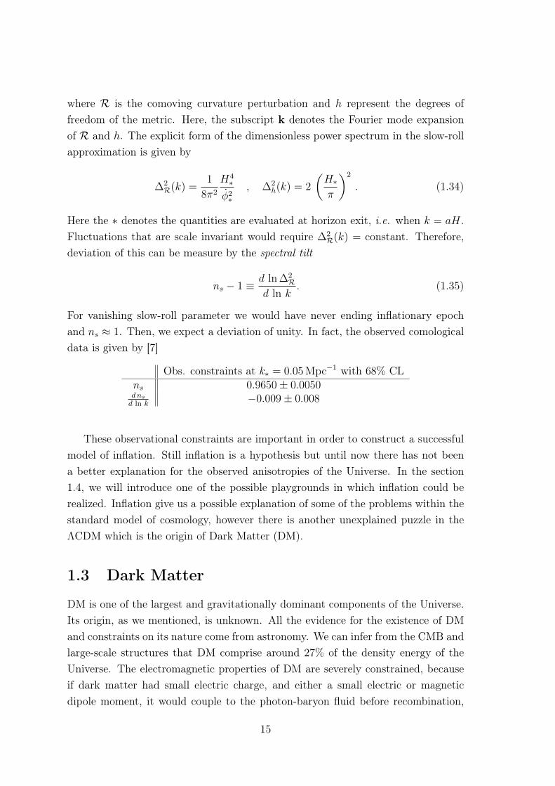
For vanishing slow-roll parameter we would have never ending inflationary epochand ns ≈ 1. Then, we expect a deviation of unity. In fact, the observed comologicaldata is given by [7]

Obs. constraints at k∗ = 0.05Mpc−1 with 68% CLns 0.9650± 0.0050dnsd ln k

−0.009± 0.008

These observational constraints are important in order to construct a successfulmodel of inflation. Still inflation is a hypothesis but until now there has not beena better explanation for the observed anisotropies of the Universe. In the section1.4, we will introduce one of the possible playgrounds in which inflation could berealized. Inflation give us a possible explanation of some of the problems within thestandard model of cosmology, however there is another unexplained puzzle in theΛCDM which is the origin of Dark Matter (DM).

1.3 Dark Matter

DM is one of the largest and gravitationally dominant components of the Universe.Its origin, as we mentioned, is unknown. All the evidence for the existence of DMand constraints on its nature come from astronomy. We can infer from the CMB andlarge-scale structures that DM comprise around 27% of the density energy of theUniverse. The electromagnetic properties of DM are severely constrained, becauseif dark matter had small electric charge, and either a small electric or magneticdipole moment, it would couple to the photon-baryon fluid before recombination,

15

thus altering the sub-degree-scale features of the CMB as well as the matter powerspectrum.

DM is part of a new sector of physics. We expect that is self-interacting or justinteract with other new particles beyond the standard model (BSM). Even thoughthese new BSM particles just interact within the ‘hidden sector’ and have no couplingwith the SM, they might affect some astrophysical phenomena such as the structureof DM halos observe in galaxy clusters [19].

There has been a lot of proposal for the origin of this new particle, we enumeratefew of the possible candidates as follows:

1. Weakly-interacting massive particles (WIMPs). This class of modelwas originally introduced by Steigman & Turner [23]. The model assumes theDM as a BSM particle, which is stable, initially in thermal equilibrium in theearly Universe, and decoupling as a non-relativistic species. An interestingfeature of the model is that it might make up for all DM in the Universe. IfWIMPs are in thermal bath in the early Universe with other particles, havingbeen born out of decays of the inflaton, then we can solve Boltzmann equa-tions to find that WIMPs ‘freeze out’ at a comoving density that is inverselyproportional to the WIMP annihilation cross section σa. Unless decays areimportant, this comoving number density is fixed for all future time. Usingdimensional analysis, the annihilation cross section should be σ ∝ α2/m2, withα ∼ 0.01 and m the mass. Replacing this cross section into the early-UniverseBoltzmann equations, the comoving number density of WIMPs matches thenumber density inferred from cosmological observations. This matching isknown as ‘the WIMP miracle’.

Due to the fact that WIMPs only interact gravitationally and weakly, they arereally difficult to detect. Basically, there exist two ways for their detection:

• Direct detection: This type of detection refers to observations of effectsof a WIMP-nucleus collision as the DM passes through a detector inan Earth laboratory. There exist several techniques for this type ofdetections, such as Cryogenic Crystal Detectors used in the CryogenicDark Matter Search (CDMS), as well as Noble Gas Scintillators used byXENON and LUX-ZEPLIN experiments [20, 21].

• Indirect detection. Unlike direct detection that focused in detection ina laboratory, indirect detection focusses on locations where WIMP DMis thought to be more present such as: in centres of galaxies and galaxyclusters. Experiments essentially search for gamma rays excess, which are

16

predicted by Compton scattering. Problems with this type of detection isthat the bounds will be model dependent. Experiments that have manageto put some bounds on WIMP annihilation is the Fermi-LAT gamma raytelescope [22].

2. QCD axion. Another candidate as DM particles is the QCD axion. The QCDaxion was introduced by Pecci and Quinn (PQ) [24] as a possible solution ofthe CP problem of the strong interactions. The solution essentially come fromthe Chern-Simons term

LθQCD =θQCD32 π2

TrGµν Gµν , (1.36)

where Gµν is the gluon field and Gµν = εµνσρGσρ is the Hodge-dual. Here thetrace is over the color indices of the SU(3) color group, and θ in this case is aconstant. The extra contribution (1.36) does not affect the equation of motionof the G field, hence its name topological. The important feature of (1.36)is that it violates CP invariance explicitly, explaining the CP violation of thestrong interaction. In order to restore the CP symmetry, we just need to setθQCD = 0. The way in which PQ solve the CP problem was introducing twoessential ingredients which are: the Goldstone theorem and non-perturbativeeffects. A global chiral U(1)PQ symmetry is introduced, which is broken spon-taneously. Then, the Goldstone boson φ,the axion, with a vacuum expectationvalue (VEV) 〈φ〉 = fa/

√2, with fa the axion ‘decay constant’. In the quan-

tum theory the U(1)PQ symmetry is anomalous. Via the anomaly, the axionis couple to the QCD Chern-Simons term (1.36), where θQCD ∝ φ/fa. Sincethe only other term in the axion action is the kinetic term, we are free toshift the axion field by an arbitrary constant and absorb the value of θQCDinto φ by a field redefinition, making φ/fa dynamical. The non-perturbativeeffects come into play for the generation of the axion mass, through instantonscontributions, which are classical solutions of the field equations. By dilutionof these instantons a potential energy for the vacuum energy is generated

Vvac ∝[1− cos(C φ

fa)

], (1.37)

where C is the color anomalous coefficient. The potential is easily minimizefor C 〈φ〉

fa= 0 mod 2π, explaining why θQCD has such a small value. In the

early universe, there is no reason for the QCD axion to sit exactly at the CPconserving minimum, and it is usually assumed that the initial position, φ∗/fa,

17

is of order of unity. Then, the QCD axion starts to oscillate about the CPconserving minimum around the QCD phase transition, and the coherentlyoscillating axion becomes DM.

3. String axions. In general, we can defined axions as pseudoscalars fieldsenjoying the U(1)PQ PQ symmetry. Not necessarily they have to be the QCDaxion explained above. For example, axions ai arise in string compactificationsfrom the integration of p-form gauge potentials Ap over p-cycles Cp,i of thecompact space

ai =

∫Cp,i

Ap . (1.38)

In type IIB string theory, there are axions associated with the NS-NS two formB2, and the R-R forms C2, C4. The generation of these fields will be discussedin section 1.4. These important fields can be used as building blocks for theconstruction of DM models, as we will present in the chapter 4.

4. Primordial black holes (PBHs). The only major non-particle candidate forDM are primordial black holes. PBHs are Black Holes (BHs) formed when localover density collapsed due to gravitational instabilities. The formation of thesePBHs relies on the amplification of the density perturbations during inflationof order δρ ∼ 0.1 ρ collapsing to form a BH at horizon re-entry[25]. Recentdetection of gravitational waves (GWs) emitted by a BH binary observed by theLIGO/VIRGO collaboration re-opened the consideration of DM as PBHs[26,27].

As we can see we have a plethora of candidates for DM. In this work, we focusmainly on axions, as well as PBHs. All the models presented come from stringcompactifications. Therefore, it is natural to give some basic introduction to stringtheory.

1.4 String theory

As we just saw in section 1.2, the dynamics of the inflationary models are fullydependent of the scalar potential V of the inflaton field φ. The inflaton potentialmight suffer from fundamental problems such as instabilities of the flat region due toextra quantum corrections. Then, we need to build models where this flat region isprotected by symmetries. A ‘top-down’ approach is one of the best ways to achievesuch task. An example of these theories is given by string theory. String theory

18

can be defined as a theory in which the elementary objects are not point-like as inparticle physics, but rather they are one-dimensional objects with a given length.In this section we want to give a brief review of string compactification. For furtherreading we recommend the following references [28, 29, 30, 31].

1.4.1 String compactification

The critical dimension of supersymmetric string theories is D = 10, which arisefrom the conservation of Lorentz invariance as a global symmetry. The dimensionin string theory presents a big problem for the construction of possible realisticmodels. However, there exist some mechanisms, for instance, Kaluza-Klein (KK)compactification [32], in which the 10-dimensional spaceM10 can be written as theproduct of a 4-dimensional space M4 times a compact space X6, that is, M10 =

M4 × X6. By making this assumption, we are saying that the metric of the full10-dimensional space can be split as

ds210 = gµν(x) dxµdxν + gmn(y) dymdyn, (1.39)

where xµ and ym are local coordinates on M4 and X6 respectively. A possiblegeneralization of this ansatz is considering the warped metric

ds210 = e2A(y) gµν(x) dxµdxν + e−2A(y)gmn(y) dymdyn, (1.40)

where A(y) is called the warp factor.

Under the branching ofM10, the Lorentz group SO(1, 9) breaks into

SO(1, 3)× SO(6), (1.41)

inducing a change in the transformation laws of different fields. For example, avector AM , M = 0, . . . , 9, transforming in the fundamental representation 10 ofSO(10) will be split in 10 = (4,1) ⊕ (1,6), where the first entry of the bracketsrepresent the dimension of a SO(1, 3) representation and the second a representationof dimension of SO(6). In terms of fields, this branching means the presence of avector Aµ, where µ = 0, . . . , 3, ofM4 transforming in the (4,1) of SO(1, 3)×SO(6)

and six scalars Am, where m = 4, . . . , 9, ofM4 transforming in the (1,6).

The procedure applied above for a vector can be performed on spinors of SO(1, 9)

with the peculiar difference that spinors on M10 will transform only as a spinorson M4. For example, a Weyl spinor ψ in D = 10 transform in the 16 of SO(1, 9)

19

under the branching given in (1.41). More precisely,

16 = (2L,4)⊕ (2R,4), (1.42)

where 2L and 2R denote the left- and right-handedness under SO(1, 3). Hence, wecan see that KK compactification of spinors leads only to spinors onM4.

Our main interest is to review compactifications which preserve supersymmetry.The condition of supersymmetry invariance under the compactification is non-trivialand quite restrictive and can be described as follows. In type II theories, we have 32supercharges transforming locally onM10 in the spinor representation of SO(1, 9). Ifwe want to have supersymmetry onM4 after the compactification, a subset of thesesupercharges have to be well defined on X6, that is, only the subset of superchargesthat remain invariant under a parallel transport through a closed path C will leadto supersymmetry onM4. Hence, the condition of supersymmetry invariance afterthe compactification is translated to the existence of 6-dimensional Killing spinorsξ(ym) on X6, which satisfies

∇X6ξ(ym) = 0, (1.43)

where ∇X6= ∂m + ωABm

14ΓAB, where A,B,m = 1, . . . , 6, ΓAB is the generator of

the spinor representation of SO(6), and ωABm is the spin connection.

The existence of the Killing spinors to preserve supersymmetry on the compact-ification can be seen in terms of the holonomy group H of X6. The set of rotationssuffered by the spinors for all possible closed paths C on X6, in general given bySO(6), is called holonomy group H of X6. The case in which H = SO(6), any ofthe spinors get unrotated, as we can see in (1.42) (none of the spinors are singlets ofSO(6)). In order to preserve supersymmetry onM4, X6 have to be a manifold withspecial holonomy group H ′. A simple example is the case when we take H ′ = SU(3)

(SO(6) ⊃ SU(3)), then after the compactification we have

SO(1, 9), −→ SO(1, 3)× SO(6), −→ SO(1, 3)× SU(3),

16, (2L,4)⊕ (2R,4), (2L,3)⊕ (2R,3)⊕ (2L,1)⊕ (2R,1).(1.44)

Choosing H ′ = SU(3), we manage to find 2 spinors Qα and Qα transforming into2L, 2R of SO(1, 3), respectively, hence leading to N = 2 supersymmetry onM4.

20

1.4.2 Calabi-Yau manifolds

A set of manifolds with SU(N) holonomy groups have been classified and are calledCalabi-Yau manifolds or Calabi-Yau N -folds (CYN). A Calabi-Yau manifold is a2N -dimensional Ricci-flat Kähler manifold. There are several examples of thesespaces. A very simple and often used example is the torus T2 with SU(1) holonomy.Another famous example is the Z-manifold which can be found by solving the sin-gularities of the T6/Z3 orbifold. The last example is the K3 complex surface whichhas SU(2) holonomy.

In the following discussion, we will focus only on compact Calabi-Yau 3-folds butthis can be easily generalized to Calabi-Yau N -folds. Every compact CY3 manifoldis equipped with a mixed tensor Inm, where m,n = 1, . . . , 6, satisfying Imn In` = −δm`which is called the complex structure, and a (3, 0) holomorphic harmonic form Ω3

called the complex volume form. On a real basis (yj, yj), where j = 1, 2, 3, Inm canbe written as

I =

(0 I3

−I3 0

). (1.45)

Making use of Inm and (yj, yj), we can construct a set of local complex coordinates(zj, zj) with j = 1, 2, 3, as

dzj = dyj + iIji yi , dzj = dyj − iIji yi. (1.46)

In this basis, the only non zero components of the metric gmn are the ones withmixed indices gij, where the index i (j) means the components contracted with dzi

(dzj). Therefore, using the metric to lower down one index of Iji , we find a (1,1)form. Then, we can write

J = igij dzi ∧ z j, (1.47)

where the factor i is just convention. If J is a closed form (dJ = 0), then it is calledthe Kähler form. On this basis the volume forms Ω3 can be written as

Ω3 = (dy1 + iI1i y

i) ∧ (dy2 + iI2i y

i) ∧ (dy3 + iI3i y

i). (1.48)

For example, on a torus T6 = T2 × T2 × T2 is

Ω3 = (dy1 + iU1y1) ∧ (dy2 + iU2y

2) ∧ (dy3 + iU3y3), (1.49)

21

where Ui are called the complex structure moduli of the torus T2i .

The Kähler form will play an important role in the development of the storieswithin this book. As we can see in (1.47), J is described in terms of the metric gij.So, its natural to ask how many free parameters has gij in order to be an SU(3)

holonomy metric. The answer of this question relies on some topological invariantscalled the hodge numbers. The hodge numbers hp,q are the generalization of the bettinumbers bp on a complex manifold. The betti numbers bp are the numbers of inde-pendent harmonic p-forms which are equals to the numbers of irreducible p-cyclesof a given real manifold. Hence, bp = dimHp (Hp), where Hp (Hp) is the cohomol-ogy (homology) group of the manifold. In the complex case, the classification ofthe p-forms can be studied in terms of its holomorphic and antiholomrphic part.For example, the 3-cohomology group H3(X6) can be split in a sum of H3,0(X6),H2,1(X6), H1,2(X6), and H0,3(X6), where Hp,q(X6) is the cohomology group of formswith p holomorphic and q antiholomrphic indices. Using the analogy with the bettinumbers, the hodge numbers give hp,q = dimHp,q.

In our case, where X6 is a Calabi-Yau 3-fold, the hodge numbers are arrangedin the so-called hodge diamond where some of them are displayed below.

h0,0

h1,0 h0,1

h2,0 h1,1 h0,2

h3,0 h2,1 h1,2 h0,3

h3,1 h2,2 h1,3

h3,2 h2,3

h3,3

=

1

0 0

0 h1,1 0

1 h2,1 h1,2 1

0 h1,1 0

0 0

1

(1.50)

Another useful quantity to know is the Euler characteristic χ which is defined as

χ(X6) ≡3∑

p,q=0

(−1)p+q hp,q(X6) = 2(h1,1(X6)− h1,2(X6)

). (1.51)

As a connection with the discussion in the Section 1.4.1, the existence of 6-dimensional invariant Killing spinors ξ is required to preserve supersymmetry incompactifications. We can use these spinors and construct the forms

Jij = −iξ†ΓiΓjξ , Ωijk = ξTΓiΓjΓkξ , (1.52)

where Γi are the generalize Dirac gamma matrices. This is a natural descriptionin the context of string compactification, where it can be proved that these forms

22

satify the correct geometrical properties.

1.4.3 Moduli space

As mentioned in Section 1.4.1, the splitting of the 10-dimensional space-timeM10

implies the branching of the metric as shown in (1.39). We can see this branching asthe dimensional reduction of the metric, that is, we can look for the zero modes ofthe 10-dimensional metric. These zero modes are exactly the 4-dimensional metricgµν , and a set of scalars gmn (from the 4-dimensional point of view), which giveorigin to the internal metric.

Since, we are interested in supersymmetric invariant compactifications, whichimplies compactifications on Calabi-Yau manifolds having a special holonomy met-ric. Studying fluctuations of this metric, we can find a number of ways in which thebackground metric can be deformed preserving supersymmetry and its Calabi-Yautopology. The vev’s of these deformations are called moduli fields.

In order to study the metric fluctuations, we just have to analyze small variationsof the metric

gmn −→ gmn + δgmn, (1.53)

and demand that the new background still satisfies the Calabi-Yau conditions. Inparticular,

R(g + δg) = 0. (1.54)

Imposing this condition leads to differential equations of δg. The number of solutionsof these equations give the number of independent ways in which the metric canbe deformed preserving supersymmetry and the topology. Using the basis (zj, zj)

introduced in (1.46), it can be proved that the equations for the mixed componentsδgij and the pure components δgij decouple. Each of these solutions have differentgeometric meaning, which is explained below.

• δgij

The deformations δgij are closely related to fluctuations of the Kähler form J ,because Jij = igij. To discuss these fluctuations is equivalent to discuss aboutKähler form deformations. To ensure positiveness of the metric, we need toimpose ∫

C

J > 0 ,

∫S

J ∧ J > 0 ,

∫X6

J ∧ J ∧ J > 0, (1.55)

23

for any path C and surface S on X6. The Kähler form can not be an exactform, (J 6= df) because

∫J ∧ J ∧ J ∝ volume of X6. Precisely,

V =1

6

∫X6

J ∧ J ∧ J, (1.56)

where V is the volume of X6. Since J is not an exact form, this implies thatit is cohomologically non-trivial. Then, J can be written in a basis ωa ofH1,1(X6) as

J =h1,1∑a=1

taωa, (1.57)

where the coefficients ta are called the Kähler moduli. The geometric inter-pretations of these moduli is that they control the size of the 2-cycles of X6.

On string theory, in particular on type IIB compactifications, the Kähler formreceives a contribution from the compactificacion of the Ramond/Ramond 4-form C4.

• δgij

In this case, the fluctuations δgij are related to symmetric deformations of theholomorphic or anti-holomorphic form Ω3. We can not expand δgij on a basisof H2,0(X6) because h2,0 = 0. Making use of Ω3 we can put H2,0(X6) in oneto one correspondence with H1,2(X6) in the following way

δgij =i

‖Ω3‖2Uα (χα)ik ¯Ωk ¯

j , (1.58)

where ‖Ω3‖2 = ΩijkΩijk/3! and χα is a basis for H1,2(X6) with α = 1, . . . , h1,2.

The coefficients Uα are called the complex structure moduli.

In the end, at tree level, the full moduli space can be separated as

Mmoduli =MKh1,1 ×Mcs

h1,2 , (1.59)

whereMK andMcs are spaces parametrized by ta and Uα, respectively.

1.4.4 Orientifolds

The idea of orientifolds came from the construction of orbifold compactifications inwhich the worldsheet parity Ω is gauged away. The worldsheet parity Ω interchanges

24

the left movers with the right movers. Gauging away this symmetry leads to acolletion of non-oriented surfaces spanned by string propagation. These ideas havebeen carried out on Calabi-Yau compactifications. In these cases, together with theparity Ω an internal symmetry σ, which acts solely on X6 and leaveM4 untouched,is modded out. One can show that for 3-folds, σ leaves the Kähler form J invariantbut acts non-trivially on Ω3. Depending on the transformation properties of Ω3 twodifferent symmetry operations O can be modded out, that is,

Oε = (−1)εFL Ωσ∗ , σ∗Ω3 = (−1)ε Ω3 , ε = 0, 1. (1.60)

Here, FL is the space-time fermion number in the left moving sector and σ∗ denotesthe action of σ on forms. Modding out by O0, leads to the possibility of having O5-and O9-planes while O1 allows O3- and O7-planes.

We are interested in studying the orientifold compactifications of type IIB stringtheory. Before going through the orientifold compactification, let us review thesimplest compactification of type IIB string theory on a Calabi-Yau 3-fold. Themassless spectrum of type IIB string theory in D = 10 consists in:

• NSNS sector: the dilaton ϕ, a 2-form B2, and the graviton (metric) g;

• RR sector: the axion C0, a 2-form C2, and a 4-form C4 with field strengthself-dual.

Under the compactification on a Calabi-Yau 3-fold, these 10-dimensional fieldwill change. For instance, the dilaton and the axion will remain massless scalarfields under the compactification but the metric g is splited as (1.39). On the otherhand, the forms on the spectrum have the following decomposition:

• NSNS sector.

In the NSNS sector, we only have the form B2.

B2 :

Decomposition DegeneracyBµν 1

Bµm h1,0 + h0,1 = 0

Bmn h2,0 + h1,1 + h0,2 = h1,1

(1.61)

where µ, ν = 0, . . . , 3 and m,n = 1, . . . , 6. Using the basis ωa of H1,1(X6), wecan write

B2 = B2(x) + ba(x)ωa , a = 1, . . . , h1,1. (1.62)

25

Here, B2 is a 4-dimensional two form and ba’s are a set of 4-dimensional scalarfields.

• RR sector.

In this case, we have two forms C2 and C4. The decomposition of C2 is exactlysame as B2. Therefore, we show only the decomposition of C4.

C4 :

Descomposition DegeneracyCµνσρ 1

Cµνσm h1,0 + h0,1 = 0

Cµνmn h2,0 + h1,1 + h0,2 = h1,1

Cµmn` h3,0 + h1,2 + h2,1 + h0,3 = 2h1,2 + 2

Cmn`p h2,2 = h1,1

(1.63)

As before, we can write C2 and C4 as

C2 = C2(x) + ca(x)ωa , a = 1, . . . .h1,1 (1.64)

C4 = Da2(x) ∧ ωa + V K(x) ∧ αK −QK(x) ∧ βK + ρa(x)ωa , K = 0, . . . , h1,2.

(1.65)

Here, we are using a basis ωa of H2,2(X6), which is dual to ωa, and a realsymplectic basis (αK , β

K) of H3(X6), which satisfies∫αK ∧ βL = δLK ,

∫αK ∧ αL =

∫βK ∧ βL = 0. (1.66)

The 4-dimensional fields appearing in (1.64) and (1.65) are the scalar fieldsca(x), ρa(x), the 1-forms V K(x), QK(x), and the 2-forms C2(x), Da

2(x). The4-form Cµνσρ has no dynamics because is proportional to the 4-dimensionalvolume form εµνσρ. The self-duality of the field stretch of C4 removes half ofthe degrees of freedom. In favour of V K and ρa , we choose to eliminate Da

2

and QK . The other choice is possible, which leads to a different spectrum butwe are not considering this case. We need to keep in mind that we still havethe geometric moduli ta and Uα coming from the metric deformations.

Altogether, the N= 2 massless 4-dimensional spectrum of type IIB on a Calabi-Yau 3-fold consists in:

• one gravity multiplet (gµν , V0);

26

• h1,2 vector multiplets (V α, Uα);

• h1,1 hypermultiplets (ta, ba, ca, ρa);

• one double tensor multiplet (B2, C2, ϕ, C0);

• one 4-form C4.

Every multiplet has its fermionic components, which are not shown here. To getthe orientifold compactification we need to mod out the non-invariant states underthe action of (−1)εFL Ωσ∗. The projection of the states is explained in the followingsection.

1.4.5 N = 1 Type IIB Orientifold

The models present in the next chapters are based on one type of orientifold com-pactification, we will focus only on ε = 1 having possible O3/O7-planes. To projectout the states in the spectrum, we need to know how (−1)FL Ωσ∗ acts on the fields.The field transformations under Ω and FL are well known. Under the worldsheetparity, Ω the fields ϕ, g, and C2 are even while B2, C0 and C4 are odd. The operator(−1)FL leaves NSNS fields invariant but changes the sign in the RR sector. The newingredient is the addition of the internal symmetry σ., which acts on the Calabi-Yaubut leavesM4 invariant. Other requirements of σ are: to be an involution (σ2 = 1)and to act holomorphically on the Calabi-Yau coordinates. With all these informa-tion, we can easily check that ϕ, C0, g, and C4 are even under (−1)FL Ω while B2

and C2 are odd. Therefore, we can deduce the action of σ∗ on the 10-dimensionalforms as

σ∗ ϕ = ϕ , σ∗C0 = C0,

σ∗ g = g , σ∗ C2 = −C2,

σ∗ B2 = −B2 , σ∗ C4 = C4.

(1.67)

keeping in mind that σ has to satisfy σ∗ J = J and σ∗Ω3 = −Ω3.Since σ is a holomorphic involution, the cohomology groups Hp,q(X6) split into

two eigenspaces under σ∗, that is

Hp,q(X6) = Hp,q+ (X6)⊕Hp,q

− (X6), (1.68)

where the + (−) shows whether the elements of the group are even (odd) underthe action of σ∗. The dimension of Hp,q(X6) became hp,q = hp,q+ + hp,q− , wherehp,q+ = dimHp,q

+ (X6) and hp,q− = dimHp,q− (X6). All of these hodge numbers are not

27

independent. The action of σ∗ fix them. For instance, in a Calabi-Yau 3-fold wehave:

• h1,1± = h2,2

± because the Hodge ∗-operator commutes with σ∗;

• h2,1± = h1,2

± due to the holomorphicity of σ;

• h3,0+ = h0,3

− = 0 and h3,0− = h0,3

− = 1 because we need to satisfy σ∗Ω3 = −Ω3;

• h0,0+ = h3,3

+ = 1 and h0,0− = h3,3

− = 0 because the volume form, which isproportional to Ω3 ∧ Ω3, is σ∗ invariant.

Collecting all the transformation laws under the action of (−1)FL Ωσ∗, we canwrite the invariant in each sector as:

• NSNS sector.

In this sector the invariant states are the dilaton ϕ and the metric g splitsas described in (1.39), where deformations of gmn give rise to the geometricmoduli ta and Uα. Under the projection σ∗, the Kähler form is even while the(3,0)-form is odd. Then, we can write

J = ta+(x)wa+ , a+ = 1, . . . , h1,1+ . (1.69)

For deformations of the metric δgij, we find that

δgij =i

‖Ω3‖2Uα− (χα−)ik ¯Ωk ¯

j , α− = 1, . . . , h1,2− . (1.70)

Here we are using bases ωa+ and χα− of H1,1+ (X6) and H1,2

− (X6), respectively.Using (1.67), we can mod out all the even components of B2 on (1.62) whichgives

B2 = ba−(x)ωa− , a− = 1, . . . , h1,1− , (1.71)

where ωa− is a basis for H1,1− (X6).

• RR sector.

In this case, we have to perform the projection (1.67) on the forms C0, C2,and C4. We find that C0 is invariant, and only the odd part of C2 and the

28

even part C4 survive. Therefore, we can write

C2 = ca−(x)ωa− , a− = 1, . . . , h1,1− (1.72)

C4 = Da+

2 (x) ∧ ωa+ + V κ(x) ∧ ακ −Qκ(x) ∧ βκ + ρa+(x)ωa+ , κ = 1, . . . , h1,2+ .

(1.73)

Here we are using the bases ωa− and ωa+ of H1,1− (X6) and H2,2

+ (X6), respec-tively. Also we introduced a sympletic basis (ακ, β

κ) of H3(X6), which satisfies(1.66) with K,L→ κ, λ.

The 4-dimensional fields on (1.71), (1.72), and (1.73) are three scalar fieldsba−(x), ca−(x), and ρa+(x), two 1-forms V κ(x), Qκ(x), and one 2-form D

a+

2 (x).Again the self duality of the field strength of C4 removes half of the degrees of free-dom and keep only (V κ, ρa+). Altogether theN= 1 massless 4-dimensional spectrumconsist in:

• One gravitational multiplet gµν ;

• h1,2+ vector multiplets Vκ;

• h1,1 + h1,2− + 1 chiral multiplets (ba− , ca− , ρa+ , t

a+ , Uα− , ϕ, C0).

After the compactification, we will work with the 4-dimensional low energy ef-fective theory. It is established that the N= 1 4-dimensional supergravity action isexpressed in terms of the Kähler potential K, a holomorphic superpotential W , anda holomorphic gauge-kinetic coupling functions f , which is given by [33]

S(4) = −1

2

∫R∗1 +KIJDΦI∧∗DΦJ + Refab F a∧∗F b + Imfab F a∧F b + 2V∗1,(1.74)

where

V = eK(KIJDIWDJW − 3|W |2

)+

1

2(Ref)−1κλDκDλ. (1.75)

Here, R is the Ricci scalar, ΦI is the set of scalars fields (ba− , ca− , ρa+ , ta+ , Uα− , ϕ, C0),

and KIJ is a Kähler metric satisfying KIJ = ∂I∂JK(Φ, Φ). It is important to saythat the powers ofMp will be restored when cosmological applications are discussed.The potential V is given in terms of the covariant derivative DIW = ∂IW+(∂IK)W

and the D-terms given as

Dκ =

[KI +

WI

W

](Tκ)IJ ΦJ , (1.76)

29

where Tκ are the generators of the gauge group.The fields ΦI in the action (1.74) are not necessarily (ba− , ca− , ρa+ , t

a+ , Uα− , ϕ, C0).For O3/O7-planes, one finds [34]

• The axion/dilaton S = e−ϕ − iC01;

• Two-form moduli Ga− = ca− − iSba− , a− = 1, . . . , h1,1− ;

• Complex structure moduli Uα− , α− = 1, . . . , h1,2− ;

• Kähler moduli

Ta+ = τa+ −1

2(S + S)ka+b−c− G

b−(G− G)c− + iρa+ . (1.77)

The variable τa+ must be understood as a function of the ta+ and is given by

τa+ =∂V∂ta+

, (1.78)

where V is the volume of X6 given by (1.56). The coefficients ka+b−c− are called theintersection numbers and are defined as

ka+b−c− =

∫X6

ωa+ ∧ ωb− ∧ ωc− . (1.79)

In terms of the intersection numbers V can be written as V = 16kabct

atbtc. Then,

τa+ =1

2ka+b−c−t

b−tc− . (1.80)

With these new variables, the Kähler potential can be written as

Ktree = Kk(S, T,G) +KS(S, S) +Kcs(U, U)

= −2 ln[V ]− ln[S + S

]− ln

[−i∫

Ω3(U) ∧ Ω3(U)

], (1.81)

where the volume V = V(T + T ).From now on, we will only consider compactifications with h1,1

− = 0, whichimplies h1,1 = h1,1

+ . Therefore, the Kähler form can be written as (1.57) and theKähler moduli became

Ta = τa + iρa. (1.82)

1Also there exist the definition τ = iS = C0 + ie−ϕ.

30

For the case in which h1,1+ = 1 its easy to find the form of the Kähler potential

Kk(S, T,G), which becomes

Kk = −3 ln[T + T

]. (1.83)

With all this information, the resulting moduli space to work (at tree level) is

Mmoduli =Mcsh1,2−×MK

h1,1 + 1, (1.84)

where the 1 inMK is the axion/dilaton.

Let us consider the low energy approximation of the type IIB string theorycompactified on a Calabi-Yau in presence of a non-trivial background composed byNSNS and RR 3-forms H3 and F3, respectively. The interaction of these forms ispurely gravitational which shows that the 10-dimensional spaceM10 does not splitin the productM4 ×X6. The full solution is described as follows.

The 10-dimensional action of type IIB supergravity in Einstein frame is given by[31]

SIIB =1

2κ210

∫d10x√−g(R− ∂Mτ∂

M τ

2(Imτ)2− 1

2|F1|2 −

|G3|2

2 Imτ− 1

4|F5|2

)+

1

2κ210

∫C4 ∧

G3 ∧ G3

4i Imτ+ Slocal. (1.85)

Here 2κ210 = (2π)7 α′4, with α′ = 1

2π Twhere T is the string tension. The fields in

the action (1.85) are

τ = C0 + ie−ϕ , G3 = F3 − τH3, (1.86)

with H3 = dB2 and F3 = dC2, and

F5 = F5 −1

2C2 ∧H3 +

1

2B2 ∧ F3, (1.87)

with F5 = dC4. The self-duality condition ∗10F5 = F5 is imposed at the level ofthe equations of motion. The term Slocal is the action of localized objects of the10-dimensional supergravity fields, for instance, D3-branes or O3-planes.

We are considering compactifications with warped metric (1.40) and components

31

of G3 only along the compact directions. Precisely,

ds210 = e2A(y) ηµν dx

µdxν + e−2A(y)gmn(y) dymdyn, (1.88)

LG = − 1

4κ210

∫d10x√−g |G3|2

Imτ= − 1

8κ210

∫X6

d6yG3 ∧ ∗6G3

Imτ. (1.89)

In addition, we set F1 = 0 and τ = constant. Furthermore, we require H3 and F3 tobe source-less (dH3 = 0, dF3 = 0) and to satisfy the Dirac quantization condition

1

2πα′

∫γ

F3 ∈ 2πZγ ,1

2πα′

∫γ

H3 ∈ 2πZγ, (1.90)

where γ’s are 3-cycles in X6. Assuming 4-dimensional Poincaré invariance, we pro-pose

F5 = (1 + ∗10)[dα ∧ dx0 ∧ dx1 ∧ dx2 ∧ dx3

], (1.91)

where the function α only depends on the compact directions ym with m = 1, . . . , 6.

We want to find restrictions for the ansatz (1.88), (1.89), and (1.91), that is,restrictions for the form G3, the function α(y), and the warp factor A(y). It isknown that under these assumptions G3 is an imaginary self-dual (ISD) form andα = e4A [35]. In order to prove this statement we use of the equations of motion.

The equation of motion for the non-compact components of the metric is2

Rµν = −ηµνe2A

(GmnpG

mnp

48 Imτ+e−8A

4∂mα∂

mα

)+ κ2

10

(T locµν −

1

8ηµνe

2A T loc).(1.92)

For the contractions of the indices m, n, and p, we use the Calabi-Yau metric gmn.Using the ansatz for the metric (1.88), we can compute the non-compact componentsof the Ricci tensor Rµν , given by

Rµν = −ηµνe4A(∂n∂

nA+ Γmmn∂nA)≡ −ηµνe4A∇2A, (1.93)

where Γpmn are the Christoffel symbols using the metric gmn. We can rewrite theequation (1.93) as

−ηµνe4A∇A = −1

4

(∇2e4A − e−4A∂me

4A∂me4A). (1.94)

2The computation of the equations of motion for the action (1.85) are in the Appendix A.

32

Replacing this equation in (1.92) and then tracing, we find

∇2e4A = e2A GmnpGmnp

12 Imτ+ e−6A

[∂mα∂

mα + ∂me4A∂me4A

]+κ2

10

2e2A(Tmm − T µµ

)loc.(1.95)

In addition, we have the equation of motion/Bianchi identity for the RR 5-form

dF5 = d ∗10 F5 = H3 ∧ F3 + 2κ210µ3ρ

loc3 , (1.96)

where µ3ρloc3 is the localized source contribution coming from the D3-branes and

O3-planes. In terms of the function, α, (1.96) can be written as

∇2α = ie2A Gmnp(∗6Gmnp)

12 Imτ+ 2e−6A∂mα∂

me4A + 2κ210e

2Aµ3ρloc3 . (1.97)

Now, subtracting equations (1.95) with (1.97), we obtain

∇2(e4A − α) =e2A

12 Imτ|iG3 − ∗6G3|2 + e−6A|∂(e4A − α)|2 + 2κ2

10e2A

[1

4

(Tmm − T µµ

)loc−µ3ρ

loc3

]. (1.98)

By integrating the above expression over X6, we find that the left-hand side becomeszero and all the terms in the right-hand side are positive, assuming 1

4

(Tmm − T µµ

)loc=

µ3ρloc3 . Therefore, we obtain conditions for G3 and α, which are:

• Imaginary self-duality (ISD): ∗6G3 = iG3;

• α = e4A.

As we will see in the section 2.2, the ISD condition is important for having super-symmetric invariant 4-dimensional space.

From the Bianchi equation (1.96), we find another important condition, whichhas to be satisfied. This condition constraints the values of the number of D3-branesand O3-planes in the theory. We can find it as follows. Integrating the equation(1.96) over the compact space X6 gives

1

2κ210µ3

∫X6

H3 ∧ F3 +Qloc3 = 0, (1.99)

where Qloc3 is the total charge of the localized objects, for examples, D3-branes and

O3-planes. Recalling the definitions of 2κ210 = (2π)7α′4, µ3 = (2π)−3α′−2, and the

33

charge of O3-planes −14µ3, we can write [31]

1

2Nflux +ND3 −

1

4NO3 = 0. (1.100)

Here, ND3 and NO3 are the number of D3-branes and O3-planes, respectively. Thequantity Nflux is defined as

Nflux =1

((2π)2α′)2

∫X6

H3 ∧ F3. (1.101)

The equation (1.100) is known as the RR tadpole cancellation condition and restrictthe number of D3-branes and O3-planes in the theory.

From imaginary self-duality of G3 one can prove that the contribution of thefluxes Nflux to the RR tadpole condition has to be positive. Precisely, we can writethe ISD condition of G3 as

e−ϕ ∗6 H3 = −(F3 − C0H3). (1.102)

Then, replacing this equation into (1.101), we obtain

Nflux =e−ϕ

((2π)2α′)2

∫X6

H3 ∧ ∗6H3 =e−ϕ

((2π)2α′)2

∫X6

|H3|2 > 0. (1.103)

Hence, the RR tadpole cancellation condition require the presence of negative D3-branes charges, making this ansatz a suitable scenario for string theory becausethese objects are present in this theory, for example, O3-planes.

1.4.6 Supersymmetry and no-scale structure

We want to study the 4-dimensional effective supersymmetric theory of the construc-tion explained in the section 2.1, in particular, we want to discuss the structure ofthe scalar potential and the conditions to preserve supersymmetry. As we mentionedin section 1.2.1, the 4-dimensional effective theory is expressed in terms of the Käh-ler potential K, a holomorphic superpotential W , and a holomorphic gauge-kineticcoupling functions f ’s. The form of the superpotential is given by [35]

Wtree(S, U) =

∫X6

G3 ∧ Ω3. (1.104)

This superpotential is known as the Gukov-Vafa-Witten (GVW) superpotential.In the following discussion, we will consider only the case of one Kähler moduli

34

T and κ24 = 1. In this case, we know that the Kähler potential is of the form

K = −3 ln[T + T

]− ln

[S + S

]− ln

[−i∫

Ω3(U) ∧ Ω3(U)

], (1.105)

and the scalar potential is

V = eK[KSSDSWDSW +KUαUβDUαWDUβW +KT TDTWDT W − 3|W |2

],(1.106)

where K is the Kähler potential (1.105). The dependence of W and the form of theKähler potential K implies the existence of a no-scale structure of the potential V ,that is, a potential of the form

V = eK[KSSDSWDSW +KUαUβDUαWDUβW

]. (1.107)

We can see in the above equation that V ≥ 0. Therefore, in order to have asupersymmetric preserving minimum, we need to satisfy the equation

DIW = 0, (1.108)

where I = S, Ui, Tj.

The supersymmetric conditions in our case take the following form:

The condition for the axion/dilaton is

DSW = − 1

S + S

∫X6

G3 ∧ Ω3 = 0. (1.109)

For the complex structure moduli, we use the relation

∂UαΩ3 = KUαΩ3 + χα, (1.110)

where KUα = ∂αK and χα is a basis for (2,1)-forms. Therefore,

DUαW =

∫X6

G3 ∧ χα = 0. (1.111)

We also have the condition for the Kähler moduli

DTW = − 3

T + T

∫X6

G3 ∧ Ω3 = 0. (1.112)

35

All these equations implies the following conditions over G3

G3|(3, 0)= 0 , G3|(1, 2)

= 0 , G3|(0, 3)= 0, (1.113)

where (p, q) indicates the (holomorphic, anti-holomorphic) components ofG3. There-fore, we conclude that in order to have supersymmetric invariant minimum, we needa G3 ∈ H2,1(X6), where G3 is ISD and G3 ∧ J = 0. The last condition comes fromthe fact that in a Calabi-Yau 3-fold there is not 5-form.

The presence of fluxes allows the stabilisation of the complex structure moduliUα and the axion dilaton S at the SUSY global minimum. However, the Kählermoduli remained as flat directions. Intuitively speaking the presence of fluxes forcethe ISD condition of G3 but this condition is invariant under rescaling of the in-ternal metric in ∗6, the Hodge-dual map in 6-dimension. Therefore, rescaling thesize of internal cycles is allowed. However, we could add corrections, perturbativeand non-perturbative, that break this freedom of rescaling and then give a non-vanishing potential to the Kähler moduli. These corrections can be encoded in thesuperpotential W and in the Kähler potential K, schematically we can write

W = W0 +Wnp and K = K0 +Kp +Knp . (1.114)

Here, the subscript p and np correspond to perturbative and non-perturbative con-tributions respectively. The superpotential can only receive non-perturbative cor-rections due the non-renormalization theorem.

As we just said the introduction of this extra corrections break SUSY and thenon-scale structure of the theory, generating a non-vanishing scalar potential forthe Kähler moduli. From the 10-dimensitional perspective, the corrections producenon-vanishing components for G(3, 0)

3 , G(1, 2)3 , and G

(0, 3)3 . An interesting feature is

that they are produced at sub-leading order in the effective field theory, because theKähler scalar potential is generated at order O(V−3) while the SUSY fluxes at orderO(V−2). For the large volume regime, V 1, they are considered a perturbationaround the SUSY minima.

We can enumerate few of these corrections as:

1. α’-corrections. These contributions come from higher order derivative cor-rections of the effective action in 10 dimensions. In particular, one of thepossible contributions come from the tensorial structure of the Ricci scalar R4

in 10 dimensions. This tensorial structure is completely understood and give

36

rise to a correction to the tree level Kähler potential of the form [36]

K ⊃ −2 log

(V +

ξ

2

), (1.115)

where ξ = − (α′)3 ζ(3)χ(X6)

25/2 (2π)3 (S + S)3/2 with χ(X6) the Euler characteristic of theCY 3-fold X6, and ζ(3) ' 1.202. Extra contributions coming from orientifoldplanes might affect the equation (1.115) by shifting the Euler characteristic to[37]

χ(X6) → χ(X6) + 2

∫X6

DO7 ∧DO7 ∧DO7 , (1.116)

where DO7 is the divisor wrapped by the O7-plane.

2. String loop corrections. The 10 dimensional effective action for type IIBstrings also receive string loop contributions. These contributions are unknownin a generic CY compactification. Despite of the lack of information, we canclassify them into two classes [38, 39, 40, 41, 42]:

• KK-correction. These contributions come from the exchange betweenD3-branes (or O3-planes) and D7-branes (or O7-planes) of closed stringswhich carry KK momentum. Schematically we can write their contribu-tion in the Kähler potential as

δKKK(gs) ∝

h1,1∑i=1

CKKi (U, U)

Re(S)Vt⊥i , (1.117)

where CKKi (U, U) are unknown coefficients depending on the complexstructure moduli Uα, and t⊥i are the cycles controlling the distance be-tween the D3-branes/O3-planes and D7-branes/ O7-planes.

• Winding corrections. In this case, the contributions are generated fromthe exchange of winding strings between intersecting stacks of D7-branes(or between intersecting D7-branes and O7-planes). Their contributionto the scalar potential can be written as

δV W(gs) ∝ −

gsW20

V2

∑i

CWi (U, U)

t∩i, (1.118)

where gs is the sting loop coupling constant, W0 is the tree level super-potential, CWi (U, U) are unknown coefficients depending on Uα, and t∩i is

37

the volume of the cycle intersected by the D7-branes and the O7-planes.

3. Non-perturbative corrections. Mainly the non-perturbative contributionscome from instantons. Instantons are classical solutions of the classical fieldequations in Euclidean space with finite action. For example, for D3-braneinstantons the superpotential takes the form

W = W0 +∑j

Aj(U, φ, S) e−ajTj . (1.119)

This form of the superpotential can be also obtained by gaugino condensationof stacks of D7-branes. Here, Aj(U, φ, S) is a coefficient that depends onthe complex structure moduli Uα, the axion/dilaton S, and possible fields φparametrizing the positions of stack of D7-branes wrapping the cycle tj. Thevalues of aj will depend on the generation of the correction. For example forD3-branes instantons aj = 2π and for gaugino condensation aj ∼ 2π

Nwith N

the number of D7-branes in the stack.

The first example which used these corrections to stabilise the Kähler moduliin the large volume regime is given in the references [43, 44], and it is also calledthe LARGE Volume Scenario (LVS). The LVS has become a standard topic in thebranch of moudli stabilisation, we recommend the reader to check the reference[43, 44], for full review in the topic. The models constructed in this thesis are basedon the LARGE volume together with the addition of the string loop corrections. Weadapt the CY manifold accordingly in each model in order to build the cosmologicalmodels. Each chapter is self-contained and easy to read. We hope you enjoy them.

38

Part II

Inflationfrom String Theory

39

Chapter 2

Chiral Global Embedding of FibreInflation Models

Cosmic inflation is an early period of accelerated expansion of our universe whichcan provide a solution to the flatness and horizon problems of standard Big Bangcosmology. Moreover, quantum fluctuations during inflation can source primordialperturbations that caused the formation of large scale structures and the tempera-tures anisotropies observed in the cosmic microwave background.

From a microscopic point of view, inflation is expected to be driven by the dy-namics of a scalar field undergoing a slow-roll motion along a very shallow potentialthat mimics a positive cosmological constant. An important feature of inflationarymodels is the distance travelled by the inflaton in field space during inflation since itis proportional to the amount of primordial gravitational waves which get produced[45]. From an effective field theory point of view, in small field models with a sub-Planckian inflaton excursion, dimension six operators can easily spoil the flatnessof the inflationary potential. On the other hand, quantum corrections to large fieldmodels with a trans-Planckian field range lead to an infinite series of unsuppressedhigher-dimensional operators which seem to bring the effective field theory approachout of control.

These dangerous operators can be argued to be absent or very suppressed onlyin the presence of a symmetry whose origin can only be postulated from an ef-fective field theory perspective but can instead be derived from an underlying UVcomplete theory. For this reason inflationary model building in string theory hasreceived a lot of attention [46, 47, 13, 48]. Besides the presence of additional sym-metries, string compactifications naturally provide many 4D scalars which can playthe rôle of the inflaton. Promising inflaton candidates are type IIB Kähler moduliwhich parametrise the size of the extra dimensions and enjoy non-compact rescaling

41

symmetries inherited from the underlying no-scale structure [49].

Identifying a natural inflaton candidate with an appropriate symmetry that pro-tects the flatness of its potential against quantum corrections is however not suffi-cient to trust inflationary model building in string compactifications. In fact, threeadditional requirements to have a successful string inflationary model are (i) fullmoduli stabilisation, (ii) a global embedding into consistent Calabi-Yau orientifoldswith D-branes and fluxes and (iii) the realisation of a chiral visible sector.

The first condition is crucial to determine all the energy scales in the model andto check the stability of the inflationary dynamics by controlling the behaviour ofthe scalar directions orthogonal to the inflaton one. The second condition is insteadfundamental to guarantee the consistency of the inflation model from the microscopicpoint of view by checking the cancellation of all D-brane tadpoles and Freed-Wittenanomalies and the actual generation of all the effects needed to stabilise the moduliand to develop the inflationary potential. Finally the requirement of having a modelwhich can give rise to inflation and reproduce at the same time a chiral visible sectoris crucial for two main reasons: to ensure the absence of any dangerous interplaybetween chirality and moduli stabilisation which can forbid the generation of D-terms or non-perturbative effects needed to fix the moduli [50], and to determinethe post-inflationary evolution of our universe starting from the reheating processwhere the inflaton energy density gets converted into the production of visible sectordegrees of freedom [51, 52, 53, 54]. Other important post-inflationary issues whichcan affect the predictions of important inflationary observables like the numberof efoldings Ne, the scalar spectral index ns and the tensor-to-scalar ratio r areperiods of matter domination due to light moduli [55, 56, 57], the production ofaxionic dark radiation from moduli decays [58, 59, 60, 61], non-thermal dark matter[62, 63, 63, 64, 221], moduli-induced baryogenesis [65, 66] and the interplay betweenthe inflationary and the supersymmetry breaking scale [67, 68, 69, 70].

A comprehensive global chiral model which satisfies all these conditions for mod-els where the inflaton is a local blow-up mode [71] has been recently constructed in[72]. The chiral visible sector lives on D3-branes at an orientifolded singularity andfull closed string moduli stabilisation in a dS vacuum is achieved by following theLVS procedure [43, 42]. The main limitation of this model is the emergence of anη-problem associated with the presence of large gs corrections to the effective actionwhich tend to spoil the flatness of the inflationary potential if their flux-dependentcoefficients are not tuned small.

In this regard, fibre inflation models [14] look more promising. In these construc-tions, the inflaton is a fibration modulus which remains exactly massless when only

42

the leading order no-scale breaking effects are included. The inflationary potentialis then generated only at subleading order by a combination of string loop correc-tions [39, 40, 73, 74] and higher derivative terms [75, 76]. This hierarchy of scalesis guaranteed by the extended no-scale cancellation and provides a natural solutionto the η-problem [41]. This solution can also be understood from the point of viewof an effective non-compact rescaling symmetry for the Kähler moduli [49].

Different versions of fibre inflation models have been constructed so far depend-ing on the microscopic nature of the effects which drive the inflationary dynamics:Kaluza-Klein and winding string loops [14], Kaluza-Klein loops and O(α′3) F 4 terms[77], and winding gs loops combined with higher derivative terms [78]. In all casesthe inflationary potential is plateau-like and takes a simple form with a constantterm and negative exponentials. Additional positive exponentials show up withcoefficients which are naturally very small and give rise to a rising behaviour atlarge field values. Ref. [79] provided a generalised description of fibre inflationmodels showing how they can reproduce the correct spectral index observed byPlanck [80, 7] while the predicted value of the tensor-to-scalar ratio is in the range0.001 . r . 0.01. Such a large value of r is compatible with the fact that theseare large field models where the inflaton range is around 5 Planck units. An effec-tive supergravity description of fibre inflation models as α-attractors has also beenrecently given in [81].

Despite all these successes, fibre inflation models are still lacking a completeglobal embedding into chiral string compactifications. However a first step forwardhas already been made in [82] where these inflationary models have been successfullyembedded in consistent type IIB orientifolds with moduli stabilisation but withouta chiral visible sector. In order to have a viable inflationary and moduli stabilisationmechanism, the internal Calabi-Yau manifold has to have at least h1,1 = 3 Kählermoduli and its volume form has to feature a K3 or T 4 fibration over a P1 base anda rigid shrinkable blow-up mode [42, 83]. Starting from concrete Calabi-Yau three-folds with these topological properties, ref. [82] provided several different exampleswith an explicit choice of orientifold involution and D3/D7 brane setups which areglobally consistent and can generate corrections to the 4D effective action that canfix all closed string moduli inside the Kähler cone and reproduce the form of theinflationary potential of fibre inflation models. However the case with h1,1 = 3 istoo simple to allow for non-trivial D7 worldvolume fluxes which give rise to chiralmatter. In fact, non-zero gauge fluxes induce moduli dependent Fayet-Iliopoulosterms which, in combination with soft term contributions for U(1)-charged matterfields, would lift the leading order flat direction, making the inflaton too heavy to

43

drive inflation.In this chapter we shall extend the results of [82] by considering more compli-

cated Calabi-Yau threefolds with h1,1 = 4 in order to build global fibre inflationmodels with a chiral visible sector. After analysing the topological conditions onthe underlying compactification manifold to allow a successful chiral global embed-ding of fibre inflation models, we find that the simplest examples involve Calabi-Yauthreefolds with 3 K3 divisors and a toroidal-like volume with a diagonal del Pezzodivisor suitable to support non-perturbative effects to freeze the moduli. The in-ternal volume is therefore controlled by 3 Kähler moduli and can equivalently beseen as different K3 fibrations over 3 different P1 bases. After searching throughthe Kreuzer-Skarke list of Calabi-Yau manifolds embedded in toric varieties [84], wefind several concrete examples which admit these topological features.

We then focus on one of them and describe several possible choices of orientifoldinvolution, D-brane setup and gauge fluxes which satisfy global consistency condi-tions and generate perturbative gs and α′ corrections to the 4D Kähler potentialand non-perturbative effects in the superpotential that are suitable to both stabilisethe moduli and reproduce the typical potential of fibre inflation models. In par-ticular, non-zero gauge fluxes induce chiral matter on D7-branes wrapped aroundsmooth combinations of the four-cycles which control the overall volume.1 More-over, a moduli-dependent Fayet-Iliopoulos term lifts one of the Kähler moduli, sothat after D-term stabilisation the effective number of Kähler moduli is reduced to3 and the internal volume simplifies to the standard expression of fibre inflationmodels used in the examples of [82].

After computing all relevant loop and higher derivative effects in full detail, weanalyse the resulting inflationary dynamics finding an interesting result: the Kählercone bounds set severe constraints on the allowed inflaton field range when theyare combined with other phenomenological requirements, like the generation of thecorrect amplitude of the power spectrum by the inflaton quantum fluctuations, andconsistency conditions like the stability of the inflaton evolution against possible or-thogonal runaway directions, the fact that the gravitino mass remains always smallerthan any Kaluza-Klein scale in the model and finally that dangerous higher deriva-tive effects do not spoil the flatness of the inflationary potential before achievingenough efoldings of inflation.2 Because of this tension, we also perform a full multi-field numerical analysis of the inflationary evolution showing how an early period of

1We do not consider K3 fibred cases where the visible sector lives on D3 branes at singularitiessince they would lead to dark radiation overproduction [85].

2These last two consistency conditions are qualitatively similar since the superspace derivativeexpansion is under control if m3/2 MKK [86].

44

accelerated expansion occurs generically. On the other hand, the inflaton quantumfluctuations can generate the right amplitude of the density perturbations only ifthe microscopic parameters take appropriate values.

We believe that our results make fibre inflation models more robust since theyrepresent the first concrete models which are globally consistent and chiral. Nonethe-less several issues still need to be investigated further. The most important ones arethe inclusion of an explicit uplifting mechanism to realise a dS vacuum, a thoroughderivation of the perturbative corrections to the 4D effective action and a betterdetermination of the Calabi-Yau Kähler cone, going beyond its approximated ex-pression inherited from the toric ambient space. We leave the study of these issuesfor the future.

This chapter is organised as follows. In Sec. 2.1, after presenting a basic reviewof fibre inflation models, we summarise the minimal requirements that are needed forthe construction of a fully consistent global embedding with a chiral visible sector.In Sec. 2.2 we provide a concrete Calabi-Yau example, describing the orientifoldinvolution, the D-brane setup, the choice of gauge fluxes and the resulting chiralspectrum, Fayet-Iliopoulos term and inflationary potential generated by gs and α′

effects. The inflationary evolution is analysed in full detail in Sec. 2.3 by focusingfirst on the single-field approximation and by studying then the multi-field dynamics.In Sec. 2.4 we draw our conclusions and we discuss a few open issues. App. Bcontains additional explicit chiral global examples.

2.1 Chiral global inflationary models

Let us begin by briefly reviewing the setup of fibre inflation and proceed afterwardby displaying the minimal requirements for a successful chiral global embedding offibre inflation models.

2.1.1 Fibre inflation in a nutshell

Fibre inflation models are based on a class of type IIB orientifold flux compactifica-tions with D3/D7-branes and O3/O7-planes where the Calabi-Yau (CY) threefoldtakes a so-called ‘weak Swiss-cheese’ form:

V = f3/2(τj)−Nsmall∑i=1

λiτ3/2i with j = 1, ..., Nlarge , (2.1)

45

where h1,1 = Nlarge+Nsmall and f3/2 is a homogeneous function of degree 3/2. In thesemodels, the stabilisation of the Kähler moduli is performed in two steps. Firstly, thetotal volume V as well as the volumes of the Nsmall rigid blow-up divisors τi are fixedfollowing the LVS procedure [43, 42] where the leading order α′3 corrections to theKähler potential [36, 37, 87] are balanced against non-perturbative contributions tothe superpotential [88]. This leaves Nflat = Nlarge−1 = h1,1−Nsmall−1 flat directionswhich are natural inflaton candidates. These directions can receive a potential atsubleading order by gs corrections due to the exchange of Kaluza-Klein (KK) andwinding modes [39, 40, 73, 74, 41] as well as by (α′)3 F 4-terms [75, 76]. In thesimplest fibre inflation models h1,1 = 3 and Nsmall = 1, so that Nflat = 1. Thisleading order flat direction corresponds to a Kähler modulus τf which parametrisesthe volume of a K3 surface and the total scalar potential schematically looks like[14, 77, 78, 79]:

V = VLV S(V , τs) + VdS(V) + Vinf(V , τs, τf ) , (2.2)

where Vinf(V , τs, τf ) = V KKgs + V W

gs + VF 4 VLV S(V , τi) is the inflationary potential.VLV S is the leading order LVS potential which fixes V and τs, VdS is an upliftingcontribution to get a dS vacuum which can originate from anti D3-branes [88, 89,90, 91, ?], hidden sector T-branes [92] or non-perturbative effects at singularities[93], while V KK

gs , V Wgs and VF 4 are respectively KK and winding string loops and F 4

terms.In fibre inflation models, the underlying CY threefold is a K3 fibration over a P1

base which has two decompactification limits, corresponding to either the K3 fibreor the base growing large. Thus, kinematically it is expected that the fibre volumecan traverse several Planck units. These LVS inflationary models present a varietyof distinct features that make them very promising candidates to realise large fieldinflation and to discuss explicit global embeddings:

1. The de Sitter uplift is independent of the inflaton. This is contrary to a hypo-thetical KKLT embedding [88], where the uplift would be inflaton-dependentand, thus, large field inflation would typically destroy the KKLT minimum.

2. The back-reaction of heavy moduli is incorporated and under control, in par-ticular, due to the fact that moduli stabilisation is done in two steps and theleading order potential is independent of the inflaton because of the extendedno-scale cancellation [41]. This is in contrast with the majority of large fieldmodels of inflation [94].

3. The possibility to achieve tensor-to-scalar ratios between r ∼ 0.01 and r ∼

46

0.001 which can be tested by future CMB observations [95, 96].

An explicit realisation of fibre inflation not only places several constraints on theunderlying CY geometry, but also on the setup of D-branes and O-planes. In thefollowing section we list the sufficient requirements to build a viable global modelwhich also allows for a chiral visible sector.

2.1.2 Requirements for chiral global embedding

The simplest global embedding of fibre inflation models requires at least three Kählermoduli [82]. However, in order to incorporate also a chiral visible sector we needat least h1,1 = 4 Kähler moduli. Here we will focus on obtaining chiral matter onD7-branes wrapped around a suitable divisor with world-volume gauge fluxes turnedon. In this case D7 gauge fluxes induce a D-term potential for the Kähler modulithat fixes a particular combination thereof. Thus, D-term fixing and the leadingorder LVS stabilisation mechanism leave just a single flat direction, in our case aK3 fibre, which will play the rôle of the inflaton. In order to obtain a viable chiralglobal model we require the following ingredients and consistency conditions:

1. A Calabi-Yau with h1,1 = 4 featuring three large cycles and a shrinkable rigiddivisor, so that the internal volume takes the form (2.1) with Nsmall = 1. Inthe explicit example described in Sec. 2.2 the volume simplifies further to:

V = ca√τ1 τ2 τ3 − cb τ 3/2

s , (2.3)

with ca > 0 and cb > 0. Each of the 3 moduli τ1, τ2 and τ3 controls the volumeof a K3 surface while τs parametrises the size of a ‘diagonal’ del Pezzo divisor[83]. D-term stabilisation will fix τ3 ∝ τ2 while the standard LVS procedurewill freeze the overall volume V ' ca

√τ1 τ2 τ3 and the blow-up mode τs. The

leading order flat direction can be parametrised by τ1 which will drive inflation.

2. An orientifold involution and a D3/D7-brane setup with gauge fluxes on thevisible D7-brane stacks such that tadpole cancellation is satisfied with enoughroom for bulk three-form fluxes to be turned on for complex structure anddilaton stabilisation. The D-brane and O-plane setup must also allow forthe generation of KK- and/or winding string loop corrections which have thecorrect form to generate a suitable inflationary potential.

3. A choice of world-volume fluxes which cancels all Freed-Witten anomalies [97,98] but leads, at the same time, to just a single moduli-dependent Fayet-Iliopoulos (FI) term [99, 100] in order to leave a leading order inflationary

47

flat direction by lifting just one of the two flat directions leftover by the LVSstabilisation mechanism.

4. There should be no chiral intersection between the visible sector and the delPezzo divisor supporting non-perturbative effects required for LVS moduli fix-ing as otherwise the prefactor of the non-perturbative superpotential would bevanishing [50]. The absence of these dangerous chiral intersections should beguaranteed by an appropriate choice of gauge fluxes.

5. Moduli stabilisation and inflation have to take place inside the CY Kähler coneand the effective field theory should be well under control with 〈V〉 1 andgs 1.

6. In order to trust inflationary model building within an effective field theory,the following hierarchy of scales should be satisfied from horizon exit to theend of inflation:

minf < H < m3/2 < M(i)KK < Ms < Mp , (2.4)

where minf is the inflaton mass, H is the Hubble constant, m3/2 is the grav-itino mass which sets the mass scale of all the heavy moduli during inflation,M

(i)KK denote various KK scales associated with bulk modes and open string

excitations on D7-branes wrapped around four-cycles, Ms is the string scaleand Mp is the reduced Planck mass Mp = 2.4 · 1018 GeV. Notice that, apartfrom Mp, all these energy scales are moduli dependent and so evolve duringinflation. After stabilising V and τs a la LVS and fixing one large modulus interms of another large direction via setting the FI-term to zero, we find thatthe ‘reduced’ moduli space of the inflationary direction is in fact a compactinterval. Therefore the field space available for inflation is kinematically finite(albeit in general trans-Planckian), a feature of the model which has so farbeen overlooked. We will state the precise phenomenological and consistencyconditions for successful inflation in Sec. 2.3.

2.2 A chiral global example

In this section, we shall present all the topological and model-building details of theglobal embedding of fibre inflation models into explicit chiral CY orientifolds withh1,1 = 4.

48

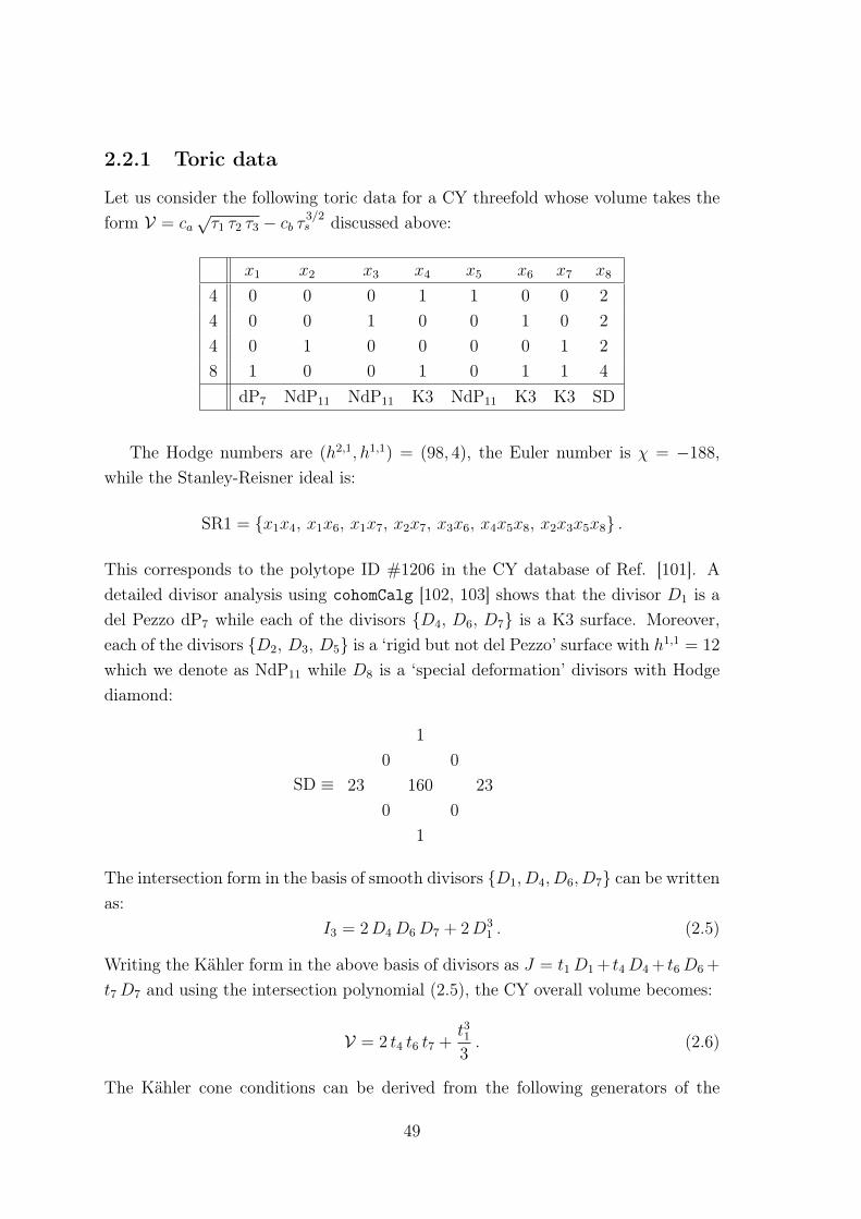
2.2.1 Toric data

Let us consider the following toric data for a CY threefold whose volume takes theform V = ca

√τ1 τ2 τ3 − cb τ 3/2

s discussed above:

x1 x2 x3 x4 x5 x6 x7 x8

4 0 0 0 1 1 0 0 24 0 0 1 0 0 1 0 24 0 1 0 0 0 0 1 28 1 0 0 1 0 1 1 4

dP7 NdP11 NdP11 K3 NdP11 K3 K3 SD

The Hodge numbers are (h2,1, h1,1) = (98, 4), the Euler number is χ = −188,while the Stanley-Reisner ideal is:

SR1 = x1x4, x1x6, x1x7, x2x7, x3x6, x4x5x8, x2x3x5x8 .

This corresponds to the polytope ID #1206 in the CY database of Ref. [101]. Adetailed divisor analysis using cohomCalg [102, 103] shows that the divisor D1 is adel Pezzo dP7 while each of the divisors D4, D6, D7 is a K3 surface. Moreover,each of the divisors D2, D3, D5 is a ‘rigid but not del Pezzo’ surface with h1,1 = 12

which we denote as NdP11 while D8 is a ‘special deformation’ divisors with Hodgediamond:

SD ≡

10 0

23 160 230 0

1

The intersection form in the basis of smooth divisors D1, D4, D6, D7 can be writtenas:

I3 = 2D4D6D7 + 2D31 . (2.5)

Writing the Kähler form in the above basis of divisors as J = t1D1 + t4D4 + t6D6 +

t7D7 and using the intersection polynomial (2.5), the CY overall volume becomes:

V = 2 t4 t6 t7 +t313. (2.6)

The Kähler cone conditions can be derived from the following generators of the

49

Kähler cone:

K1 = −D1 +D4 +D6 +D7 , K2 = D7 , K3 = D4 , K4 = D6 . (2.7)

Expanding the Kähler form as J =∑4

i=1 riKi, the Kähler cone is defined via thefollowing conditions on the two-cycle moduli:

r1 = − t1 > 0 , r2 = t1+t7 > 0 , r3 = t1+t4 > 0 , r4 = t1+t6 > 0 . (2.8)

Notice that this expression of the CY Kähler cone is only approximate since it isinherited from the Kähler cone of the ambient toric variety.3 However this proce-dure can either overcount some curves of the CY threefold, for example if they donot intersect with the CY hypersurface, or miss some of them, if they cannot beobtained as the intersection between two divisors of the ambient space and the CYhypersurface. Hence the actual CY Kähler cone can turn out to be either largeror smaller. This analysis would require a deeper investigation which is however be-yond the scope of this chapter.4 Here we just mention that this analysis has beenperformed in detail in [104] where the CY Kähler cone turned out to be larger thanthe approximated version.

The four-cycle moduli, which can be computed as τi = ∂tiV , look like:

τ1 = t21 , τ4 = 2 t6 t7 , τ6 = 2 t4 t7 , τ7 = 2 t4 t6 , (2.9)

and so, using the Kähler cone conditions (2.8), the overall volume reduces to:

V = t4τ4 −1

3τ

3/21 = t6τ6 −

1

3τ

3/21 = t7τ7 −

1

3τ

3/21 =

1√2

√τ4 τ6 τ7 −

1

3τ

3/21 , (2.10)

which shows clearly that the CY threefold X features three K3 fibrations over dif-ferent P1 bases. The second Chern class of X is given by:

c2(X) = D4D5 + 4D25 + 12D5D6 + 12D5D7 + 12D6D7 , (2.11)

3If the same CY threefold can be realised as a hypersurface embedded in different ambientspaces, the CY Kähler cone is approximated as the intersection of the Kähler cones of the differenttoric varieties [101].

4We however expect that the CY Kähler cone cannot get smaller. In fact, if this were the case,there should exist an extra constraint from requiring the positivity of a curve of the CY whichis trivial in the ambient space. But this does not seem to be possible since each CY divisor isinherited from a single toric divisor (i.e. we do not have a toric divisor which splits into two CYdivisors, and so where h1,1 of the CY is larger than h1,1 of the ambient space). In fact, if thistrivial curve existed, it should have a dual divisors, and so h1,1 of the CY should be larger thanh1,1 of the ambient case, which is however not the case.

50

which results in the following values of the topological quantities Πi =∫Xc2 ∧ Di:

Π1 = 8 , Π2 = Π3 = 16 , Π4 = 24 , Π5 = 16 , Π6 = Π7 = 24 , Π8 = 128 .

(2.12)The intersection curves between two coordinate divisors are given in Tab. 2.1 whiletheir volumes are listed in Tab. 2.2.

D1 D2 D3 D4 D5 D6 D7 D8

D1 C3 T2 T2 ∅ T2 ∅ ∅ C3

D2 T2 P1 t P1 P1 t P1 T2 P1 t P1 T2 ∅ C3

D3 T2 P1 t P1 P1 t P1 T2 P1 t P1 ∅ T2 C3

D4 ∅ T2 T2 ∅ ∅ T2 T2 C9

D5 T2 P1 t P1 P1 t P1 ∅ P1 t P1 T2 T2 C3

D6 ∅ T2 ∅ T2 T2 ∅ T2 C9

D7 ∅ ∅ T2 T2 T2 T2 ∅ C9

D8 C3 C3 C3 C9 C3 C9 C9 C81

Table 2.1: Intersection curves of two coordinate divisors. Here Cg denotes a curvewith Hodge numbers h0,0 = 1 and h1,0 = g.

D1 D2 D3 D4 D5 D6 D7 D8

D1 2 t1 −2 t1 −2 t1 0 −2 t1 0 0 −4 t1D2 −2 t1 2 t1 2(t1 + t4) 2 t6 2(t1 + t6) 2 t4 0 4(t1 + t4 + t6)D3 −2 t1 2(t1 + t4) 2 t1 2 t7 2(t1 + t7) 0 2 t4 4(t1 + t4 + t7)D4 0 2 t6 2 t7 0 0 2 t7 2 t6 4(t6 + t7)D5 −2 t1 2(t1 + t6) 4(t1 + t7) 0 2 t1 2 t7 2 t6 4(t1 + t6 + t7)D6 0 2 t4 0 2 t7 2 t7 0 2 t4 4(t4 + t7)D7 0 0 2 t4 2 t6 2 t6 2 t4 0 4(t4 + t6)D8 −4 t1 4(t1 + t4 + t6) 4(t1 + t4 + t7) 4(t6 + t7) 4(t1 + t6 + t7) 4(t4 + t7) 4(t4 + t6) 8(t1 + 2(t4 + t6 + t7))

Table 2.2: Volumes of intersection curves between two coordinate divisors.

2.2.2 Orientifold involution

We focus on orientifold involutions of the form σ : xi → −xi with i = 1, ..., 8 whichfeature an O7-plane on Di and O3-planes at the fixed points listed in Tab. 2.3. Theeffective non-trivial fixed point set in Tab. 2.3 has been obtained after taking careof the SR ideal symmetry. Moreover, the total number of O3-planes NO3 is obtainedfrom the triple intersections restricted to the CY hypersurface, while the effective

51

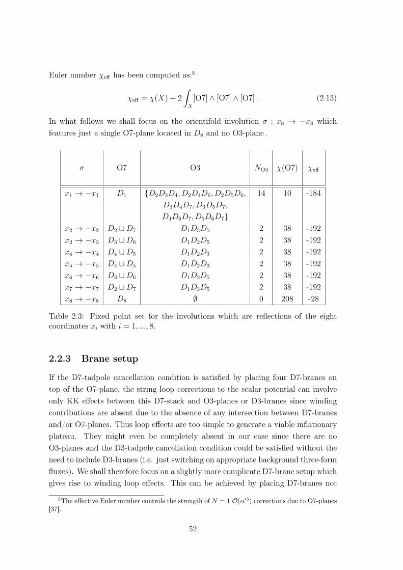
Euler number χeff has been computed as:5

χeff = χ(X) + 2

∫X

[O7] ∧ [O7] ∧ [O7] . (2.13)

In what follows we shall focus on the orientifold involution σ : x8 → −x8 whichfeatures just a single O7-plane located in D8 and no O3-plane .

σ O7 O3 NO3 χ(O7) χeff

x1 → −x1 D1 D2D3D4, D2D4D6, D2D5D6, 14 10 -184D3D4D7, D3D5D7,

D4D6D7, D5D6D7x2 → −x2 D2 tD7 D1D3D5 2 38 -192x2 → −x3 D3 tD6 D1D2D5 2 38 -192x4 → −x4 D4 tD5 D1D2D3 2 38 -192x5 → −x5 D4 tD5 D1D2D3 2 38 -192x6 → −x6 D3 tD6 D1D2D5 2 38 -192x7 → −x7 D2 tD7 D1D3D5 2 38 -192x8 → −x8 D8 ∅ 0 208 -28

Table 2.3: Fixed point set for the involutions which are reflections of the eightcoordinates xi with i = 1, ..., 8.

2.2.3 Brane setup

If the D7-tadpole cancellation condition is satisfied by placing four D7-branes ontop of the O7-plane, the string loop corrections to the scalar potential can involveonly KK effects between this D7-stack and O3-planes or D3-branes since windingcontributions are absent due to the absence of any intersection between D7-branesand/or O7-planes. Thus loop effects are too simple to generate a viable inflationaryplateau. They might even be completely absent in our case since there are noO3-planes and the D3-tadpole cancellation condition could be satisfied without theneed to include D3-branes (i.e. just switching on appropriate background three-formfluxes). We shall therefore focus on a slightly more complicate D7-brane setup whichgives rise to winding loop effects. This can be achieved by placing D7-branes not

5The effective Euler number controls the strength of N = 1 O(α′3) corrections due to O7-planes[37].

52

entirely on top of the O7-plane as follows:

8[O7] ≡ 8([D8]) = 16 ([D2] + [D4] + [D6]) . (2.14)

This brane setup involves three stacks of D7-branes wrapped around the divisorsD2, D4 and D6. Moreover, the condition for D3-tadpole cancellation becomes:

ND3 +Nflux

2+Ngauge =

NO3

4+χ(O7)

12+∑a

Na (χ(Da) + χ(D′a))

48= 38 ,

showing that there is space for turning on both gauge and background three-formfluxes for complex structure and dilaton stabilisation.6 As shown in [105], three-form fluxes stabilise also D7 position moduli and open string moduli living at theintersection between two different stacks of D7-branes since they generate soft super-symmetry breaking mass terms for each of these scalars. On the other hand, thereare no Wilson line moduli in our model since h1,0(D2) = h1,0(D4) = h1,0(D6) = 0.

Let us point out that other orientifold involutions which could allow for D7-branes not entirely on top of the O7-plane are x4 → −x4, x6 → −x6 or x7 → −x7.In each of these cases, the O7-plane is located on a K3 surface. However, given thatD4 = D1 + D5, D6 = D1 + D3 and D7 = D1 + D2, from Tab. 2.1 and 2.2 we seethat the resulting D7-brane stacks are either non-intersecting (and so no windingcorrections are generated) or the volumes of the intersection curves depend just onthe ‘small’ dP7 divisor (and so winding loops are inflaton-independent). This is thereason why we chose the involution x8 → −x8 where the O7-plane is located onthe ‘special deformation’ divisor D8 which gives more freedom for D7-brane modelbuilding.

2.2.4 Gauge fluxes

In order to obtain a chiral visible sector on the D7-brane stacks wrapping D2, D4

and D6 we need to turn on worldvolume gauge fluxes of the form:

Fi =h1,1∑j=1

fijDj −1

2c1(Di)− ι∗DiB with fij ∈ Z and i = 2, 4, 6 , (2.15)

where the half-integer contribution is due to Freed-Witten anomaly cancellation[97, 98].

6We focus on flux vacua where the dilaton is fixed in a regime where our perturbative type IIBanalysis is under control.

53

However we want to generate just one moduli-dependent Fayet-Iliopoulos term inorder to fix only one Kähler modulus via D-term stabilisation. In fact, if the numberof FI-terms is larger than one, there is no light Kähler modulus which can play therôle of the inflaton. Moreover we wrap a D3-brane instanton on the rigid divisor D1

in order to generate a non-perturbative contribution to the superpotential which iscrucial for LVS moduli stabilisation. In order to cancel the Freed-Witten anomaly,the D3-instanton has to support a half-integer flux, and so the general expression ofthe total gauge flux on D1 becomes (with c1(D1) = −D1):

F1 =h1,1∑j=1

f1jDj +1

2D1 − ι∗DiB with f1j ∈ Z . (2.16)

However a non-vanishing F1 would not be gauge invariant, and so would prevent anon-perturbative contribution to the superpotential. We need therefore to check ifit is possible to perform an appropriate choice of B-field which can simultaneouslyset F4 = F6 = 0 (we choose to have a non-vanishing gauge flux only on D2 to havejust one moduli-dependent FI-term) and F1 = 0. Recalling that both D4 and D6

are K3 surfaces which are spin divisors with c1(D4) = c1(D6) = 0 (since the K3 is aCY two-fold), if we set:

B =1

2D1 , (2.17)

the condition F1 = F4 = F6 = 0 reduces to the requirement that the following formsare integer:

ι∗D4

(1

2D1

)and ι∗D6

(1

2D1

), (2.18)

since in this case the integer flux quanta fij can always be adjusted to yield vanishinggauge fluxes. Taking an arbitrary integer form A ∈ H2(Z, X) which can be expandedas A = ajDj with aj ∈ Z, the pullbacks in (2.18) give rise to integer forms if:

b4 ≡∫X

(1

2D1

)∧ D4 ∧ A ∈ Z

b6 ≡∫X

(1

2D1

)∧ D6 ∧ A ∈ Z

Using the intersection polynomial (2.5) we find b4 = b6 = 0, showing how the choiceof B-field in (2.17) can indeed allow for F1 = F4 = F6 = 0. The only non-zero gaugeflux is F2 whose half-integer contribution can be cancelled by adding an additionalterm to the B-field of the form 1

2D2. Given that all the intersection numbers are

even, this new term in B does not modify our previous results on the pullbacks of

54

the B-field on D1, D4 and D6. Moreover the pullback of the B-field on D2 will alsogenerate an integer flux contribution. We shall therefore consider a non-vanishinggauge flux on the worldvolume of D2 of the form:

F2 =h1,1∑j=1

f2jDj with f2j ∈ Z . (2.19)

2.2.5 FI-term and chirality

Given that the divisor D2 is transversely invariant under the orientifold involutionand it is wrapped by eight D7-branes, it supports an Sp(16) gauge group which isbroken down to U(8) = SU(8) × U(1) by a non-zero flux F2 along the diagonalU(1). This non-trivial gauge flux F2 induces also a U(1)-charge qi2 for the i-thKähler modulus of the form:

qi2 =

∫X

Di ∧ D2 ∧ F2 . (2.20)

Thus F2 6= 0 yields (using D2 = D7 −D1):

q12 = −2f21 q42 = 2f26 q62 = 2f24 q72 = 0 , (2.21)

together with a flux-dependent correction to the gauge kinetic function which lookslike:

Re(f2) = α−12 =

4π

g22

= τ2 − h(F2)Re(S) , (2.22)

where:h(F2) =

1

2

∫X

D2 ∧ F2 ∧ F2 =1

2(f21q12 + f24q42 + f26q62) . (2.23)

Moreover a non-vanishing gauge flux F2 induces a moduli-dependent FI-term of theform:

ξ =1

4πV

∫X

D2 ∧ J ∧ F2 =1

4πV

h1,1∑j=1

qj2 tj =1

4πV(q12 t1 + q42 t4 + q62 t6) . (2.24)

For vanishing open string VEVs (induced for example by non-tachyonic scalar masses),a leading-order supersymmetric stabilisation requires ξ = 0 which implies:

t4 = −q12

q42

t1 −q62

q42

t6 . (2.25)

55

This U(1) factor becomes massive via the Stückelberg mechanism and develops anO(Ms) mass by eating up a linear combination of an open and a closed string axionwhich is mostly given by the open string mode.

Besides breaking the worldvolume gauge group and inducing moduli-dependentFI-terms, non-trivial gauge fluxes on D7-branes generate also 4D chiral modes. Infact, open strings stretching between the D7-branes on D2 and the O7-planes or theimage branes give rise to the following zero-modes in the symmetric and antisym-metric representations of U(8):

I(S)2 = −1

2

∫X

D2 ∧ [O7] ∧ F2 −∫X

D2 ∧ D2 ∧ F2 = 2q12 − q42 − q62 , (2.26)

I(A)2 =

1

2

∫X

D2 ∧ [O7] ∧ F2 −∫X

D2 ∧ D2 ∧ F2 = q42 + q62 . (2.27)

Due to the absence of worldvolume fluxes on the D7-branes wrapped around D4

and D6, both of these two D7-stacks support an Sp(16) gauge group (since bothD4 and D6 are transversely invariant) which are both unbroken. Thus open stringsstretched between the D7-branes on D2 and D4 or D6 (or their image branes) giverise to 4D chiral zero-modes in the bi-fundamental representation (8,16) of U(8) andSp(16) whose number is:

I24 =

∫X

D2 ∧ D4 ∧ F2 = q42 , I26 =

∫X

D2 ∧ D6 ∧ F2 = q62 . (2.28)

We need finally to check that there are no chiral intersections between the D7s onD2 and the instanton on D1 to make sure that the prefactor of the non-perturbativecontribution to the superpotential is indeed non-zero. This is ensured if:

I21 =

∫X

D2 ∧ D1 ∧ F2 = q12 = −2f21 = 0 . (2.29)

This condition can be easily satisfied by choosing f21 = 0. In turn, this choicesimplifies the D-term constraint (2.25) to:

t4 = −q62

q42

t6 ≡ α t6 . (2.30)

2.2.6 Inflationary potential

Using the D-term fixing relation (2.30), the Kähler cone conditions (2.8) simplifyto t7 > −t1 > 0 together with t6 > −t1 > 0 if α ≥ 1 or αt6 > −t1 > 0 if α ≤ 1.

56

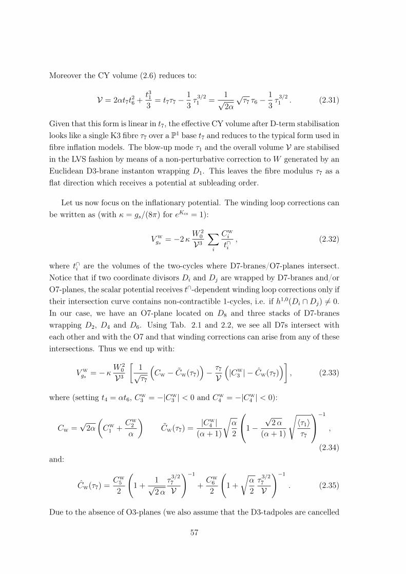
Moreover the CY volume (2.6) reduces to:

V = 2αt7t26 +

t313

= t7τ7 −1

3τ

3/21 =

1√2α

√τ7 τ6 −

1

3τ

3/21 . (2.31)

Given that this form is linear in t7, the effective CY volume after D-term stabilisationlooks like a single K3 fibre τ7 over a P1 base t7 and reduces to the typical form used infibre inflation models. The blow-up mode τ1 and the overall volume V are stabilisedin the LVS fashion by means of a non-perturbative correction to W generated by anEuclidean D3-brane instanton wrapping D1. This leaves the fibre modulus τ7 as aflat direction which receives a potential at subleading order.

Let us now focus on the inflationary potential. The winding loop corrections canbe written as (with κ = gs/(8π) for eKcs = 1):

V W

gs = −2κW 2

0

V3

∑i

CWi

t∩i, (2.32)

where t∩i are the volumes of the two-cycles where D7-branes/O7-planes intersect.Notice that if two coordinate divisors Di and Dj are wrapped by D7-branes and/orO7-planes, the scalar potential receives t∩-dependent winding loop corrections only iftheir intersection curve contains non-contractible 1-cycles, i.e. if h1,0(Di ∩Dj) 6= 0.In our case, we have an O7-plane located on D8 and three stacks of D7-braneswrapping D2, D4 and D6. Using Tab. 2.1 and 2.2, we see all D7s intersect witheach other and with the O7 and that winding corrections can arise from any of theseintersections. Thus we end up with:

V W

gs = −κ W20

V3

[1√τ7

(CW − CW(τ7)

)− τ7

V

(|CW

3 | − CW(τ7))]

, (2.33)

where (setting t4 = αt6, CW3 = −|CW

3 | < 0 and CW4 = −|CW

4 | < 0):

CW =√

2α

(CW

1 +CW

2

α

)CW(τ7) =

|CW4 |

(α + 1)

√α

2

1−√

2α

(α + 1)

√〈τ1〉τ7

−1

,

(2.34)and:

CW(τ7) =CW

5

2

(1 +

1√2α

τ3/27

V

)−1

+CW

6

2

(1 +

√α

2

τ3/27

V

)−1

. (2.35)

Due to the absence of O3-planes (we also assume that the D3-tadpoles are cancelled

57

without including any spacetime-filling D3-branes) and the fact that all D7s intersectwith each other and with the O7-plane, there are no 1-loop corrections due to theexchange of closed strings carrying KK momentum.7

On the other hand, higher derivative α′3 F 4 corrections to the scalar potentialcan be written as [75]:8

VF 4 = −κ2 λW 40

g3/2s V4

h1,1∑i=1

Πi ti , (2.36)

where λ is an unknown combinatorial factor which is expected to be of order 10−3

[75, 76] and the topological quantities Πi are given in (2.12). After imposing theD-term condition (2.30), the F 4 contributions can be rewritten as (ignoring thet1-dependent term):

VF 4 = −24κ2 λW 40

g3/2s V3

[(α + 1)√

2α

√τ7

V+

1

τ7

]. (2.37)

Therefore the total inflationary potential becomes:

V = V W

gs + VF 4 = κW 2

0

V3

(A1

τ7

− A2√τ7

+B1√τ7

V+B2 τ7

V

), (2.38)

where (with λ = −|λ| < 0):

A1 =3

π

|λ|W 20√

gsA2 = CW− CW(τ7) B1 =

(α + 1)√2α

A1 B2 = |CW

3 |− CW(τ7) .

2.3 Inflationary dynamics

In this section we shall analyse the inflationary dynamics by studying first the single-field approximation and then by focusing on the full multi-field evolution.

7Strictly speaking, there might be 1-loop corrections associated with the exchange of KK modesbetween the Euclidean D3-instanton on D1 and the D7-branes which do not intersect D1. However,we expect such corrections to be exponentially suppressed and, thus, not relevant for the analysis.

8This expression displays merely the leading orderO(V−4) terms which are corrected at sublead-ing order in inverse volume by additional corrections as discussed in [78]. Furthermore, additionalhigher-derivative corrections mediated by the auxiliary fields sitting in the supergravity multipletmight emerge at order O(V−5) [78, 106].

58

2.3.1 Single-field evolution

In order to realise single-field slow-roll inflation where the potential for the inflatonτ7 features a plateau-type region [14, 78], the overall volume has to be approximatelyconstant during the whole inflationary dynamics. Therefore, in order to get enoughefoldings before reaching the dangerous limit where the base of the fibration t7

becomes smaller than the string scale, we need to focus on the region in field spacewhere the inflaton minimum is of order 〈τ7〉 V2/3. For gs . O(0.1), |λ| ∼ O(10−3)

and natural O(1) values of the coefficients of the string loop effects, in the vicinityof the minimum the terms in (2.38) proportional to B1 and B2 are therefore bothnegligible with respect to the terms proportional to A1 and A2. Numerical estimatesshow that we need values of order 〈τ7〉 ∼ O(1) and V ∼ O(104) which, in turn, implyW0 ∼ O(100) in order to match the observed amplitude of the density perturbations.

The scalar potential (2.38) written in terms of the canonically normalised inflatonshifted from its minimum φ = 〈φ〉+ φ, where τ7 = 〈τ7〉 ekφ with k = 2/

√3, becomes:

V = κA2W

20

V3√〈τ7〉

(CdS + c e−kφ − e−

kφ2 +R1 e

kφ2 +R2 e

kφ), (2.39)

where:c =

3

π(CW − CW(τ7)

) |λ|W 20√

gs〈τ7〉∼ O(1) ,

while for 〈τ7〉 ∼ O(1) V2/3:

R1 =(α + 1)c√

2α

〈τ7〉3/2

V 1 and R2 =

(|CW

3 | − CW(τ7))

(CW − CW(τ7)

) 〈τ7〉3/2

V 1 .

Notice that in (2.39) we added a constant CdS = 1 − c − R1 − R2 to obtain aMinkowski (or slightly dS) vacuum. It is important to say that at this stage we areworking in units whereMp = 1, for the later cosmological discussion we will restoredthe power of Mp.

Given that no O3-planes are present in our model, the usual uplift mechanismwhere an anti D3-brane is located in a resolved conifold region of the extra dimen-sions would require additional effort to implement. We leave the explicit embeddingof the source of uplift to future research.

The two negative exponentials in (2.39) compete to give a minimum at 〈τ7〉 ∼O(1) while the two positive exponentials cause a steepening behaviour at largeφ. Thus we need to make sure that both R1 1 and R2 1 to prevent thetwo positive exponentials from destroying the inflationary plateau before achieving

59

enough efoldings of inflation.9 The condition R1 1 could be satisfied for c 1,for example for W0 ∼ O(1) and 〈τ7〉 1, in which case the minimum could beobtained by balancing the two terms in the coefficient A2. However, as we shall seebelow, if 〈τ7〉 1, the Kähler cone bounds restrict the allowed field space so muchthat it becomes impossible to realise enough efoldings of inflation. Hence we shallfocus the region where R1 1 and R2 1 are satisfied by 〈τ7〉 ∼ O(1) V2/3

(and possibly by allowing some tuning of the complex structure moduli-dependentcoefficients of the loop corrections or by considering |λ| 1).

Turning now to the explicit numerical examples, let us formulate the necessaryconditions that have to be satisfied in order to have a viable model:

1. Stringy effects can be neglected if each four-cycle in string frame has a volumelarger than the string scale: Vol1/4s

√α′. Given that string and Einstein

frame volumes are related as Vols = gsVolE = gsτE`s with `s = 2π√α′, we end

up with the condition:

ετi ≡1

gs(2π)4 τi 1 ∀ i . (2.40)

2. The whole inflationary dynamics should take place inside the Kähler cone.This implies in particular that:

2α〈τ1〉 < τ7 <V√〈τ1〉

if α ≥ 1 ,

2

α〈τ1〉 < τ7 <

V√〈τ1〉

if α ≤ 1 . (2.41)

Notice that these conditions guarantee the absence of any singularity in theinflationary potential (2.39) which could originate from the shrinking of atwo-cycle to zero size. Rewriting these conditions in terms of the canonicallynormalised inflaton field, we end up with:

√3

2ln

(2α〈τ1〉〈τ7〉

)< φ <

√3

2ln

(V

〈τ7〉√〈τ1〉

)if α ≥ 1 ,

√3

2ln

(2〈τ1〉α〈τ7〉

)< φ <

√3

2ln

(V

〈τ7〉√〈τ1〉

)if α ≤ 1 . (2.42)

In order to be able to describe within a consistent EFT, not just inflation but

9If this is the case, these steepening terms could then be responsible for an interesting powerloss at large angular scales [107].

60

also the post-inflationary evolution of our model, φ should reach its minimumbefore hitting the lower bounds in (2.42). Moreover the inflaton should driveenough efoldings of inflation before hitting the upper bounds in (2.42).

3. Horizon exit at φ = φ∗ should yield the required number of efoldings:

Ne ' 57 +1

4ln (r∗ V∗)−

1

3ln

(Vend

Trh

), (2.43)

where the reheating temperature Trh can be estimated in terms of the inflatonmass at the minimum mφ as:

Trh '(

90

π2g∗(Trh)

)1/4√ΓφMp ' 0.1mφ

√mφ

Mp

. (2.44)

4. Horizon exit at φ = φ∗ should reproduce the observed amplitude of the densityperturbations:

V 3∗

V ′2∗' 2.6 · 10−7 . (2.45)

5. The α′ expansion of the potential can be trusted only if:

εξ =ξ

2g3/2s V

1 . (2.46)

6. The effective field theory is under control if throughout all the inflationarydynamics:

minf < H < m3/2 < M(i)KK < Ms < Mp ∀i = bulk, 2, 4, 6 , (2.47)

whereminf is the inflaton mass, H ' V3M2

pis the Hubble scale,m3/2 = eK/2W0 =

√κ W0

V Mp is the gravitino mass which sets the mass scale of all complex struc-ture moduli, the dilaton and the Kähler modulus T1 = τ1 + i

∫D1C4 and

M(i)KK =

√π√

V τ1/4i

Mp are the different KK scales in the model associated with

bulk KK modes for τ 3/2bulk = V and KK replicas of open string modes living

on D7-branes wrapped around D2, D4 and D6. The bulk KK scale shouldbe below the string scale Ms = g

1/4s√π√V Mp while we do not need to impose

V 1/4 < M(i)KK since no energy can be extracted from the vacuum during an

adiabatic inflationary expansion where H M(i)KK.

7. Besides the two ultra-light axions associated with the base and the fibre which

61

develop just negligible isocurvature fluctuations during inflation if they do notcontribute significantly to dark matter, only the volume mode has a massbelow m3/2. In order to trust our single field approximation, we need thereforeto check that the mass of the volume mode mV does not become smaller thanthe Hubble scale H. This condition boils down to:

δ =H

mV'√

V∗3Vα′

. 1 , (2.48)

where Vα′ is the leading O(α′3) contribution to the scalar potential and reads[36]:

Vα′ = κ3ξW 2

0

4g3/2s V3

with ξ = −ζ(3)χ(X)

2(2π)3. (2.49)

If δ ' 1, the inflationary energy density can either destabilise the volume direc-tion or cause a significant shift of the volume minimum. Hence the inflationarydynamics can effectively become a multi-field evolution. However, as analysedin [14], the motion might still remain mainly along the τ7 direction, and sothe predictions for the inflationary observables could be basically unalteredapart from the fact that the number of allowed efoldings slightly increases.Notice also that in LVS models the CY Euler number together with the stringcoupling fixes the minimum of the blow-up mode τ1 as: 〈τ1〉 = (3ξ/2)2/3 g−1

s .This value is important to evaluate the Kähler cone conditions in (2.42).

We shall now focus on single-field slow-roll inflation where:

ε(φ) =1

2

(V ′

V

)2

1 and η(φ) =V ′′

V 1 .

Notice that the condition η 1 guarantees that the inflaton is lighter thanH duringinflation. In order to illustrate the main features of our inflationary model, we shallnow consider two different choices of the underlying parameters characterised bydifferent values of the coefficients ξ and λ which control the strength of the O(α′3)

corrections to the effective action at O(F 2) and O(F 4). According to [37], N = 1

O(α′3) corrections due to O7-planes cause a shift of the CY Euler number χ(X)

to χeff(X) defined in (2.13) and given in Tab. 2.3. From (2.49) this modificationwould give ξ = 0.067. Moreover the coefficient λ of higher derivative O(α′3) effectshas been estimated to be negative and of order 10−3 [75, 76]. Hence the first set ofparameters will be characterised by ξ = 0.067 and λ = −0.001. However both ofthese corrections still lack a full supersymmetric analysis, and so in the second casewe shall focus on a situation where the CY Euler number is not modified, and so

62

ξ = 0.456, and the size of the coefficient λ is much smaller: |λ| . 10−6.

Case 1: ξ = 0.067 and |λ| = 0.001

Let us now provide an explicit numerical example set to demonstrate the featuresof our inflationary model:

α = 1 , CW

1 = CW

2 = 15 , |CW

3 | = 0.013 , |CW

4 | = 18 , CW

5 = CW

6 = −5 ,

gs = 0.114 , V = 104 , 〈τ1〉 = 1.91 , W0 = 80 , |λ| = 0.001 , (2.50)

with χ(X) = χeff(X) = −28 in (2.49) which gives ξ = 0.067. Notice that the tuningof the steepening term here is mild since the difference between the largest and thesmallest winding coefficient is between one and two orders of magnitude. The formof the inflationary potential is plotted in Fig. 2.1 and it is characterised by:

Figure 2.1: Plot of the inflationary potential for the example set (2.50). The redvertical lines correspond to the walls of the Kähler cone while the dashed verticallines denote horizon exit and the end of inflation where ε = 1. We work in units ofMp = 1.

• 〈τ7〉 = 4.002 leading to ε〈τ7〉 = 0.0014. Moreover 2〈τ1〉 ' 3.8, and so thedistance of the minimum from the lower bound of the Kähler cone is ∆τ7 '0.178 which is still larger than the string scale since, using (2.40), we havethat:

ε∆τ7 =1

gs(2π)4∆τ7

' 0.03 . (2.51)

• The Kähler cone bounds (2.42) in terms of the canonically normalised inflatonbecome φmin ' −0.04 < φ < φmax ' 6.49. Inflation ends at φ = φend ' 0.96

where ε(φend) = 1 and Vend ' (7 · 1015 GeV)4. Horizon exit takes place at

63

φ = φ∗ ' 6.24 where r = 16ε = 0.009, ns = 1 + 2η∗ − 6ε∗ = 0.983, V∗ '(1 · 1016 GeV)

4 and the amplitude normalisation (2.45) is satisfied. Noticethat such a largish value of the scalar spectral index is in perfect agreementwith Planck data in the presence of dark radiation since, using ∆Neff = 0.39

as a prior, [7] gives as best fit ns = 0.983±0.006. This prior is fully justified instring models like ours where reheating is driven by the decay of the lightestmodulus which naturally tends to produce extra axionic contributions to darkradiation [58, 59, 60, 61].

• Horizon exit occurs well inside the Kähler cone since from (2.41) we have:

τ ∗7 = eκ(〈φ〉+φ∗) ' 5404.82 < τmax7 =

V√〈τ1〉' 7231.87 ⇒ τmax

7 −τ ∗7 ' 1827.06 .

• The mass of the inflaton around the minimum is mφ ' 4.25 · 1013 GeV whichfrom (2.44) implies a reheating temperature Trh ' 1.8 · 1010 GeV.

• The number of efoldings computed as:

Ne =

∫ φ∗

φend

V

V ′dφ , (2.52)

gives Ne = 52 as required by the estimate (2.43). The maximum number ofefoldings between φend and φmax is Nmax

e ' 60.

• The α′ expansion is under control even if in our inflationary model the inflatontravels over a trans-Planckian distance of order ∆φ = φ∗ − φend = 5.28 sincewe have εξ ∼ 10−4.

• The mass of the volume mode is of order the Hubble scale during inflationsince δ ' 1.6. Hence the inflationary energy density could either cause a sig-nificant shift of the original LVS minimum or destabilise the volume direction.A definite answer to this question would require a more careful multi-fieldanalysis. As mentioned above, a similar situation has been studied in [14],where the authors found that for δ ∼ 1 the minimum for the volume modegets a large shift but the inflationary evolution still remains mostly single-fieldsince minf mV ∼ H. However if δ ∼ 1, the inflationary potential generatedby string loops and α′3 F 4 terms is of the same order as the α′3 F 2 contri-bution, and so one also should carefully check if additional higher derivativecorrections can be safely neglected.

64

• The effective field theory approximation is valid during the whole inflationaryevolution since H ' 2 · 1013 GeV < m3/2 ' 1 · 1015 GeV < Mbulk

KK ' 9 ·1015 GeV < Ms ' 2.5 · 1016 GeV.

Figure 2.2: Comparison between the different KK masses, m3/2 and the inflationaryenergy density V 1/4 from horizon exit to the end of inflation. Note thatM (4)

KK = M(6)KK

which is why only one of them is displayed here.

We display the evolution of the different KK masses as compared to the gravitinomass and the inflationary scale Minf = V 1/4 in Fig. 2.2. Notice, in particular, thatat the end of inflation the inflationary scale is of order Mbulk

KK and, above all, mildlyexceeds the KK scale M (4)

KK by a factor of roughly 1.3. As we stressed above, duringan adiabatic expansion no energy can be extracted from the vacuum, and so ourEFT is still valid even if some KK scales become smaller than V 1/4 since they areall always larger than m3/2 which is, in turn, larger than H. However, since all theinflationary energy density could instead be converted into particle production atreheating, one should make sure that there is enough Hubble friction between theend of inflation and reheating to bring the inflaton energy density below the relevantKK scale. This effect can be estimated by noticing that from:

ρ(φ) =1

2φ2 + V (φ) = 3H2M2

p ⇔ ∂tρ(φ) = −3Hφ2 , (2.53)

we can obtain the following relation between the energy density at the end of inflationand at reheating:

ρrh = ρend − 3〈φ2〉∫ rh

end

da

a= ρend − 3Nrh〈φ2〉 , (2.54)

65

where 〈φ2〉 is the time average between the end of inflation and reheating and Nrh =

ln(arh/aend) is the number of efoldings of the reheating epoch. At the end of inflationwhen ε = 1 we have:

1

2φ2 = H2M2

p ⇔ ρend =3

2Vend ' 10

(M

(4)KK

)4

. (2.55)

On the other hand at reheating V (φrh) ' 0, and so ρrh ' φ2rh/2. If we then write

the time-average kinetic energy as 〈φ2〉 = φ2rh/x ' 2ρrh/x with x > 0, we end up

with the following bound:

ρrh '10

1 + 6xNrh

(M

(4)KK

)4

<(M

(4)KK

)4

. (2.56)

Using the fact that:

Nrh '1

3ln

(H2

endM2p

T 4rh

)− 1

3ln

(π2g∗90

)' 16 , (2.57)

the bound (2.56) becomes x < 23Nrh ' 10. Our model should satisfy this bound since

we expect φend to approach φrh relatively quickly due to the steepness of the potentialnear the end of inflation. However a definite answer would require a detailed studyof the post-inflationary epoch which is beyond the scope of this chapter.10

Let us also mention that, due to the absence of KK corrections, this scenariorepresents a chiral global embedding of the α′-inflation models discussed in [78].Moreover, no KK scale becomes smaller than the gravitino mass even if r ' 0.01

and ∆φ ' 5 in Planck units. In fact, if we focus for example on the KK scale M (2)KK

associated with the K3 fibre (similar considerations apply to the KK scale M (6)KK

associated with the base), we have:

m3/2

M(2)KK

= α1 eα2φ ' 0.03 eα2φ , (2.58)

with:

α1 =

√W0

2π

( gs2π

)1/4√m3/2

Mp

' 0.03 and α2 =1

2√

3. (2.59)

10Let us also point out that, even if ρrh &(M

(4)KK

)4, our model is not necessarily ruled out but

we would just need to describe reheating within a 6D EFT where the base of the fibration is muchlarger than the characteristic size of the fibre. It would also be interesting to find brane setupswhere this problem is automatically absent since there is no D7-brane wrapped around the base.

66

If we set φ = φ0 + φhe ' 7.44, the ratio in (2.58) becomes m3/2/M(2)KK ' 0.26, and

so the KK scale M (2)KK is always larger than the gravitino mass throughout all the

inflationary dynamics. Notice that this result seems to be in slight disagreementwith the swampland conjecture of [108, 109] where the underlying parameters α1

and α2 were generically assumed to be of order unity.As explained above, given that in this case δ ' 1.6, the inflationary dynamics

can be fully trusted only after determining the proper multi-field evolution. Dueto the difficulty to perform a full numerical analysis, in the next section we shallinstead still focus on a single-field case where δ ∼ 0.05 since ξ is larger, and so thevolume mode mass is larger, while |λ| is smaller, and so F 4 steepening terms canbe easily neglected throughout the whole inflationary dynamics. The full three-fieldevolution for both of these cases will then be presented in Sec. 2.3.2.

Case 2: ξ = 0.456 and |λ| = 10−7

According the discussion above, we shall now focus on the following different choiceof the underlying parameters:

α = 1 , CW

1 = CW

2 = 0.034 , |CW

3 | = 10−5 , |CW

4 | = 0.068 , CW

5 = CW

6 = −0.024 ,

gs = 0.25 , V = 4500 , 〈τ1〉 = 3.10 , W0 = 150 , |λ| = 10−7 , (2.60)

with χ(X) = χeff(X) = −188 in (2.49) which gives ξ = 0.456. A larger value of thecoefficient ξ is helpful to increase the control on the single-field approximation since,as can be seen from (2.49), the leading O(α′3) contribution to the scalar potential isproportional to ξ. The form of the inflationary potential is plotted in Fig. 2.3 andit is characterised by:

• 〈τ7〉 ' 6.41 leading to ε〈τ7〉 ' 0.0004 and 〈φ〉 ' 1.61. Moreover 2〈τ1〉 ' 6.2,and so the minimum is located close to the walls of the Kähler cone but ata distance ∆τ7 ' 0.21 which is still larger than the string scale since, using(2.40), we have that:

ε∆τ7 =1

gs(2π)4∆τ7

' 0.01 . (2.61)

• The Kähler cone bounds (2.42) in terms of the canonically normalised inflatonbecome φmin ' −0.028 < φ < φmax ' 5.19. Inflation ends at φ = φend ' 0.93

where ε(φend) = 1 and Vend = (4.4 · 1015 GeV)4. Horizon exit takes place

at φ = φ∗ ' 5.10 where r = 16ε = 0.0014, ns = 1 + 2η∗ − 6ε∗ = 0.963,

67

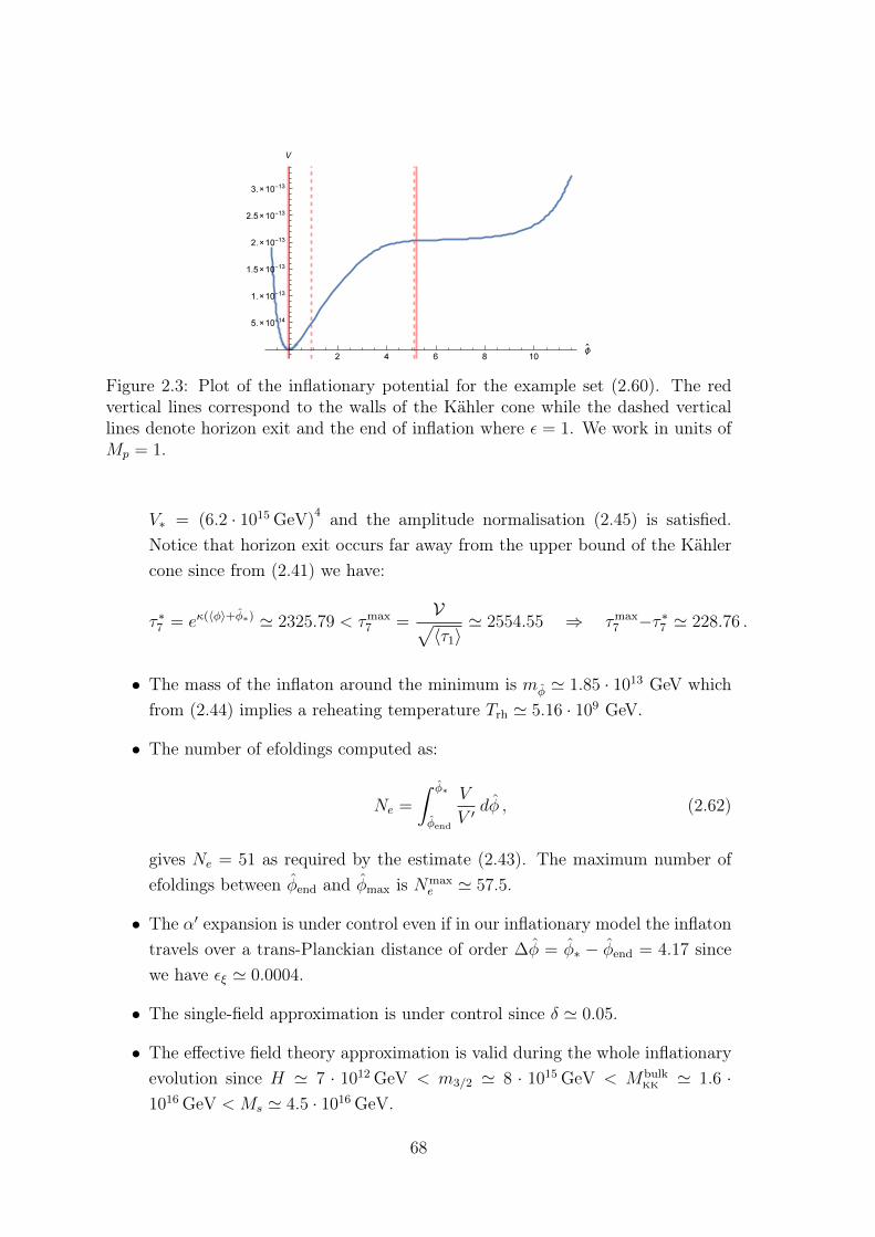
Figure 2.3: Plot of the inflationary potential for the example set (2.60). The redvertical lines correspond to the walls of the Kähler cone while the dashed verticallines denote horizon exit and the end of inflation where ε = 1. We work in units ofMp = 1.

V∗ = (6.2 · 1015 GeV)4 and the amplitude normalisation (2.45) is satisfied.

Notice that horizon exit occurs far away from the upper bound of the Kählercone since from (2.41) we have:

τ ∗7 = eκ(〈φ〉+φ∗) ' 2325.79 < τmax7 =

V√〈τ1〉' 2554.55 ⇒ τmax

7 −τ ∗7 ' 228.76 .

• The mass of the inflaton around the minimum is mφ ' 1.85 · 1013 GeV whichfrom (2.44) implies a reheating temperature Trh ' 5.16 · 109 GeV.

• The number of efoldings computed as:

Ne =

∫ φ∗

φend

V

V ′dφ , (2.62)

gives Ne = 51 as required by the estimate (2.43). The maximum number ofefoldings between φend and φmax is Nmax

e ' 57.5.

• The α′ expansion is under control even if in our inflationary model the inflatontravels over a trans-Planckian distance of order ∆φ = φ∗ − φend = 4.17 sincewe have εξ ' 0.0004.

• The single-field approximation is under control since δ ' 0.05.

• The effective field theory approximation is valid during the whole inflationaryevolution since H ' 7 · 1012 GeV < m3/2 ' 8 · 1015 GeV < Mbulk

KK ' 1.6 ·1016 GeV < Ms ' 4.5 · 1016 GeV.

68

Figure 2.4: Comparison between the different KK masses, the gravitino mass m3/2

and the inflationary energy V 1/4 from horizon exit to the end of inflation. Note thatM

(4)KK = M

(6)KK which is why only one of them is displayed here.

We display the evolution of the different KK masses as compared to the gravitinomass and the inflationary energy density Minf = V 1/4 in Fig. 2.4. Notice that,contrary to case 1 where r = 0.01, all KK scales remain above Minf throughout allthe inflationary dynamics. The reason is that in this scale the tensor-to-scalar ratio,and so also the inflationary scale, is smaller since r = 0.001. Moreover, as stressedabove, no energy can be extracted from the vacuum during an adiabatic expansion,and so the consistency condition to be imposed during inflation is H M

(i)KK which

is clearly satisfied since H = Minf√3

(Minf

Mp

)< Minf . Moreover, no KK scale becomes

smaller than the gravitino mass m3/2 ' 8 · 1015 GeV. If we focus for example on theKK scale M (2)

KK associated with the K3 fibre (similar considerations apply to the KKscale M (6)

KK associated with the base of the fibration), we have:

m3/2

M(2)KK

= α1 eα2φ ' 0.126 eα2φ , (2.63)

with:

α1 =

√W0

2π

( gs2π

)1/4√m3/2

Mp

' 0.126 and α2 =1

2√

3. (2.64)

If we set φ = φ0 + φhe ' 6.71, the ratio in (2.63) becomes m3/2/M(2)KK ' 0.87,

and so the KK scale M(2)KK is always larger than the gravitino mass throughout

all the inflationary dynamics. This result seems to be more in agreement withthe swampland conjecture of [108, 109] than the one of case 1 since r is smaller,

69

r ' 0.001, and the field range is slightly reduced, ∆φ ' 4. Moreover larger valuesof φ would bring the effective field theory approach out of control.

Even if this example satisfies all consistency and phenomenological constraintsand the single-field inflationary analysis is under control, in Sec. 2.3.2 we shallperform a more precise multifield analysis where the motion along the orthogonaldirections enlarges the field space as well as the allowed number of efoldings.

2.3.2 Multi-field evolution

The following five consistency conditions require generically a multi-field study of theinflationary evolution (which might however still be mainly along a single directionin field space):

1. The whole inflationary dynamics takes place well inside the Kähler cone de-scribed by the conditions in (2.41);

2. The quantum fluctuations of the inflaton produce a correct amplitude of thedensity perturbations at horizon exit;

3. The directions orthogonal to the inflaton are not destabilised by the inflation-ary dynamics. This is guaranteed if inflation occurs in field space along athrough which can however bend;

4. Throughout all the inflationary dynamics, no Kaluza-Klein scale becomessmaller than the gravitino mass;

5. The steepening of the inflationary potential due to F 4 corrections is negligible,so that enough efoldings can be obtained before destroying slow roll inflation.

If V ∼ 103 and W0 ∼ O(1), the last four conditions can be easily satisfied but theKähler cone conditions (2.41) for such a small value of the volume would give anupper bound on the inflaton direction which would not allow to generate enoughefoldings. In order to enlarge the inflaton field space, the value of the volume hastherefore to be larger, of order V ∼ 104. In the large volume regime where we cantrust the 4D EFT, the inflationary potential then becomes more suppressed, and sothe COBE normalisation condition (2) above can be satisfied only if W0 ∼ O(100).However, given that the gravitino mass is proportional to W0, for such a large valueof the flux-generated superpotential, it is hard to satisfty the fourth condition abovekeeping m3/2 below all KK scales during the whole inflationary evolution. Moreover,it becomes harder to suppress higher derivative corrections (condition (5) above)

70

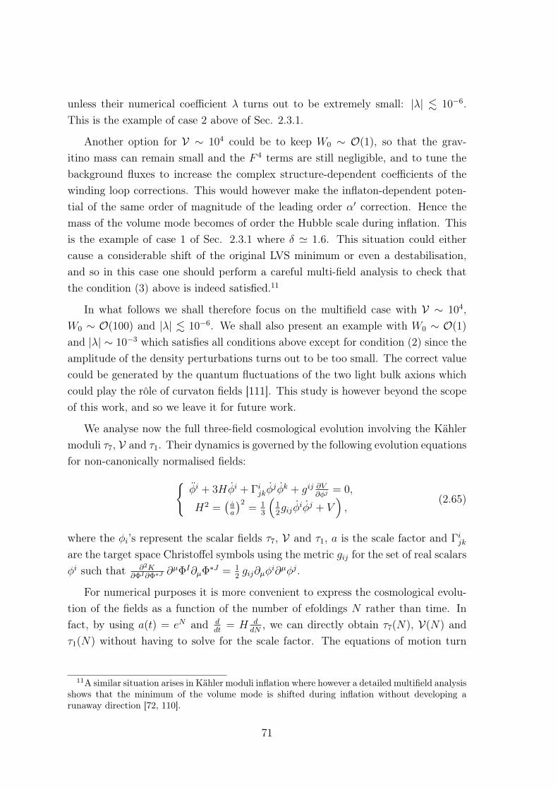
unless their numerical coefficient λ turns out to be extremely small: |λ| . 10−6.This is the example of case 2 above of Sec. 2.3.1.

Another option for V ∼ 104 could be to keep W0 ∼ O(1), so that the grav-itino mass can remain small and the F 4 terms are still negligible, and to tune thebackground fluxes to increase the complex structure-dependent coefficients of thewinding loop corrections. This would however make the inflaton-dependent poten-tial of the same order of magnitude of the leading order α′ correction. Hence themass of the volume mode becomes of order the Hubble scale during inflation. Thisis the example of case 1 of Sec. 2.3.1 where δ ' 1.6. This situation could eithercause a considerable shift of the original LVS minimum or even a destabilisation,and so in this case one should perform a careful multi-field analysis to check thatthe condition (3) above is indeed satisfied.11

In what follows we shall therefore focus on the multifield case with V ∼ 104,W0 ∼ O(100) and |λ| . 10−6. We shall also present an example with W0 ∼ O(1)

and |λ| ∼ 10−3 which satisfies all conditions above except for condition (2) since theamplitude of the density perturbations turns out to be too small. The correct valuecould be generated by the quantum fluctuations of the two light bulk axions whichcould play the rôle of curvaton fields [111]. This study is however beyond the scopeof this work, and so we leave it for future work.

We analyse now the full three-field cosmological evolution involving the Kählermoduli τ7, V and τ1. Their dynamics is governed by the following evolution equationsfor non-canonically normalised fields:

φi + 3Hφi + Γijkφjφk + gij ∂V

∂φj= 0,

H2 =(aa

)2= 1

3

(12gijφ

iφj + V),

(2.65)

where the φi’s represent the scalar fields τ7, V and τ1, a is the scale factor and Γijkare the target space Christoffel symbols using the metric gij for the set of real scalarsφi such that ∂2K

∂ΦI∂Φ∗J∂µΦI∂µΦ∗J = 1

2gij∂µφ

i∂µφj.

For numerical purposes it is more convenient to express the cosmological evolu-tion of the fields as a function of the number of efoldings N rather than time. Infact, by using a(t) = eN and d

dt= H d

dN, we can directly obtain τ7(N), V(N) and

τ1(N) without having to solve for the scale factor. The equations of motion turn

11A similar situation arises in Kähler moduli inflation where however a detailed multifield analysisshows that the minimum of the volume mode is shifted during inflation without developing arunaway direction [72, 110].

71

out to be (with ′ denoting a derivative with respect to N):

τ ′′7 = − (Lkin + 3)

(τ ′7 + τ7V

V,VV

+ 2τ 27

V,τ7V

+ 2τ7τ1V,τ1V

)+τ ′27

τ7

+τ7τ′1

V

(τ ′1√τ1

− τ ′72√τ7

),

V ′′ = − (Lkin + 3)

(V ′ + 3V2

2

V,VV

+ τ7VV,τ7V

+ τ1VV,τ1V

)+V ′2

V, (2.66)

τ ′′1 = − (Lkin + 3)

(τ ′1 + τ1V

V,VV

+ 2τ7τ1V,τ7V

+ 4V√τ1V,τ1V

)+

τ ′ 21

4τ1

+τ1V ′

V

(τ ′1τ1

− τ ′7τ7

)+τ1τ′7

2τ7

(3τ ′72τ7

−√τ1

Vτ ′1

),

where the kinetic Lagrangian reads:

Lkin =1

2

(−V

′ 2

V2+V ′τ ′7Vτ7

− 3τ ′ 27

4τ 27

+

√τ1τ′7τ′1

2Vτ7

− τ ′ 21

4V√τ1

), (2.67)

and the full inflationary potential V is given by the sum of the standard LVS po-tential, the gs loops and F 4 terms given in (2.38) and an uplifting contributionproportional to δup which could come from an anti D3-brane at the tip of a warpedthroat:

V = κ

[32A2

sπ2

√τ1

Ve−4πτ1 − 8πAs

W0τ1

V2e−2πτ1 +

3ζ

4g3/2s

W 20

V3

+W 2

0

V3

(A1

τ7

− A2√τ7

+B1√τ7

V+B2 τ7

V

)+

δup

V4/3

]. (2.68)

|λ| = 10−6 and correct amplitude of the density perturbations

Setting α = 1 and performing the following choice of the underlying parameters:

As = 6 · 105 χ = −188 ⇒ ζ = −ζ(3)χ(X)

2(2π)3= 0.456 W0 = 50 gs = 0.25

CW

1 = CW

2 = 0.05 |CW

3 | = 10−4 |CW

4 | = 0.1 CW

5 = CW

6 = −0.05 λ = −10−6 ,

the total potential (2.68) admits a Minkowski global minimum at:

〈V〉 = 2690.625 , 〈τ7〉 = 6.503 〈τ1〉 = 3.179 for δup = 5.9598 · 10−4 .

Notice that this minimum is inside the Kähler cone since 〈τ7〉 > 2〈τ1〉 = 6.358, whichrespects the lower bound in (2.41). At this level of approximation, the closed stringaxions associated to V and τ7 are flat directions. They receive a tiny potential fromhighly suppressed non-perturbative effects, and so they remain very light. Being so

72

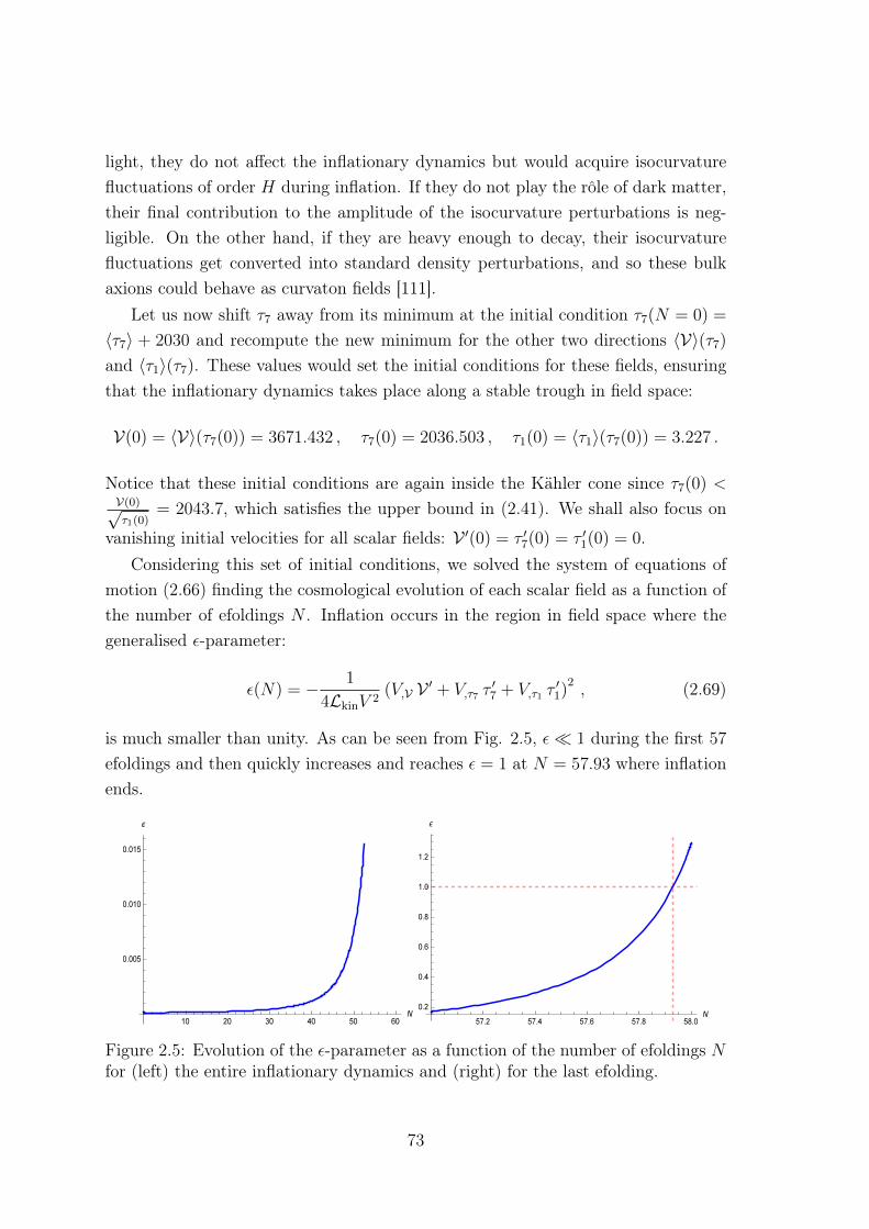
light, they do not affect the inflationary dynamics but would acquire isocurvaturefluctuations of order H during inflation. If they do not play the rôle of dark matter,their final contribution to the amplitude of the isocurvature perturbations is neg-ligible. On the other hand, if they are heavy enough to decay, their isocurvaturefluctuations get converted into standard density perturbations, and so these bulkaxions could behave as curvaton fields [111].

Let us now shift τ7 away from its minimum at the initial condition τ7(N = 0) =

〈τ7〉 + 2030 and recompute the new minimum for the other two directions 〈V〉(τ7)

and 〈τ1〉(τ7). These values would set the initial conditions for these fields, ensuringthat the inflationary dynamics takes place along a stable trough in field space:

V(0) = 〈V〉(τ7(0)) = 3671.432 , τ7(0) = 2036.503 , τ1(0) = 〈τ1〉(τ7(0)) = 3.227 .

Notice that these initial conditions are again inside the Kähler cone since τ7(0) <V(0)√τ1(0)

= 2043.7, which satisfies the upper bound in (2.41). We shall also focus on

vanishing initial velocities for all scalar fields: V ′(0) = τ ′7(0) = τ ′1(0) = 0.Considering this set of initial conditions, we solved the system of equations of

motion (2.66) finding the cosmological evolution of each scalar field as a function ofthe number of efoldings N . Inflation occurs in the region in field space where thegeneralised ε-parameter:

ε(N) = − 1

4LkinV 2(V,V V ′ + V,τ7 τ

′7 + V,τ1 τ

′1)

2, (2.69)

is much smaller than unity. As can be seen from Fig. 2.5, ε 1 during the first 57

efoldings and then quickly increases and reaches ε = 1 at N = 57.93 where inflationends.

Figure 2.5: Evolution of the ε-parameter as a function of the number of efoldings Nfor (left) the entire inflationary dynamics and (right) for the last efolding.

73

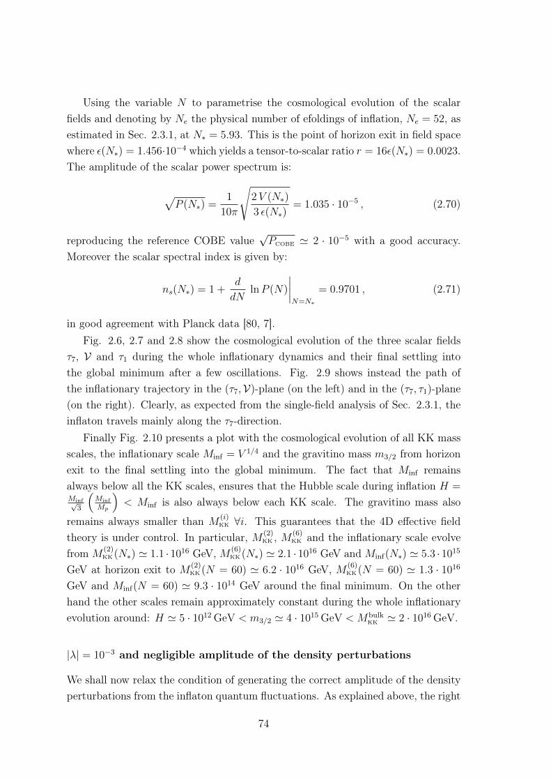
Using the variable N to parametrise the cosmological evolution of the scalarfields and denoting by Ne the physical number of efoldings of inflation, Ne = 52, asestimated in Sec. 2.3.1, at N∗ = 5.93. This is the point of horizon exit in field spacewhere ε(N∗) = 1.456·10−4 which yields a tensor-to-scalar ratio r = 16ε(N∗) = 0.0023.The amplitude of the scalar power spectrum is:

√P (N∗) =

1

10π

√2V (N∗)

3 ε(N∗)= 1.035 · 10−5 , (2.70)

reproducing the reference COBE value√PCOBE ' 2 · 10−5 with a good accuracy.

Moreover the scalar spectral index is given by:

ns(N∗) = 1 +d

dNlnP (N)

∣∣∣∣N=N∗

= 0.9701 , (2.71)

in good agreement with Planck data [80, 7].Fig. 2.6, 2.7 and 2.8 show the cosmological evolution of the three scalar fields

τ7, V and τ1 during the whole inflationary dynamics and their final settling intothe global minimum after a few oscillations. Fig. 2.9 shows instead the path ofthe inflationary trajectory in the (τ7,V)-plane (on the left) and in the (τ7, τ1)-plane(on the right). Clearly, as expected from the single-field analysis of Sec. 2.3.1, theinflaton travels mainly along the τ7-direction.

Finally Fig. 2.10 presents a plot with the cosmological evolution of all KK massscales, the inflationary scale Minf = V 1/4 and the gravitino mass m3/2 from horizonexit to the final settling into the global minimum. The fact that Minf remainsalways below all the KK scales, ensures that the Hubble scale during inflation H =Minf√

3

(Minf

Mp

)< Minf is also always below each KK scale. The gravitino mass also

remains always smaller than M(i)KK ∀i. This guarantees that the 4D effective field

theory is under control. In particular, M (2)KK , M

(6)KK and the inflationary scale evolve

from M(2)KK (N∗) ' 1.1 ·1016 GeV, M (6)

KK (N∗) ' 2.1 ·1016 GeV and Minf(N∗) ' 5.3 ·1015

GeV at horizon exit to M (2)KK (N = 60) ' 6.2 · 1016 GeV, M (6)

KK (N = 60) ' 1.3 · 1016

GeV and Minf(N = 60) ' 9.3 · 1014 GeV around the final minimum. On the otherhand the other scales remain approximately constant during the whole inflationaryevolution around: H ' 5 · 1012 GeV < m3/2 ' 4 · 1015 GeV < Mbulk

KK ' 2 · 1016 GeV.

|λ| = 10−3 and negligible amplitude of the density perturbations

We shall now relax the condition of generating the correct amplitude of the densityperturbations from the inflaton quantum fluctuations. As explained above, the right

74

Figure 2.6: Evolution of τ7 as a function of the number of efoldings N for (left) theentire inflationary dynamics and (right) for the last 2 efoldings. The dashed red linerepresents the position of the final global minimum. We work in units of Mp = 1.

Figure 2.7: Evolution of V as a function of the number of efoldings N for (left) theentire inflationary dynamics and (right) for the last 6 efoldings. The dashed red linerepresents the position of the final global minimum. We work in units of Mp = 1.

COBE value of the amplitude of the power spectrum could instead be reproduced in anon-standard way by a curvaton-like mechanism involving the quantum fluctuationsof the two light bulk axions [111]. In this case we can focus on V ∼ 5·103,W0 ∼ O(1),λ ∼ 10−3 and relatively small values of the coefficients of the winding loop correctionswhich generate the plateau, so that all the remaining four conditions listed at thebeginning of Sec. 2.3.2 are fully satisfied.

We shall set α = 1 and perform the following choice of the underlying parameters:

As = 1 · 104 χ = −188 ⇒ ζ = −ζ(3)χ(X)

2(2π)3= 0.455 W0 = 1 gs = 0.25

CW

1 = CW

2 = 0.05 CW

3 = −10−4 CW

4 = −0.1 CW

5 = CW

6 = −0.05 λ = −0.001 ,

75

Figure 2.8: Evolution of τ1 as a function of the number of efoldings N for (left) theentire inflationary dynamics and (right) for the last 6 efoldings. The dashed red linerepresents the position of the final global minimum.

Figure 2.9: Plot of the whole inflationary evolution in the (τ7,V)-plane (on the left)and in the (τ7, τ1)-plane (on the right). Notice that the scales are different on thetwo axes since the inflaton travels mainly along the τ7-direction.

which yield a global Minkowski minimum inside the Kähler cone at:

〈V〉 = 3220.899 , 〈τ7〉 = 6.403 〈τ1〉 = 3.179 for δup = 1.76588 · 10−7 .

The initial conditions for the inflationary evolution are again derived in the sameway: the fibre modulus τ7 is shifted away from its minimum at τ7(N = 0) = 〈τ7〉+

2450 and the other two directions 〈V〉(τ7) and 〈τ1〉(τ7) are set at the new minimum:

V(0) = 〈V〉(τ7(0)) = 4436.094 , τ7(0) = 2456.403 , τ1(0) = 〈τ1〉(τ7(0)) = 3.228 .

Notice that these initial conditions are inside the Kähler cone since τ7(0) < V(0)√τ1(0)

=

76

Figure 2.10: Evolution of all KK masses (with M (4)KK = M

(2)KK ), the inflationary scale

Minf = V 1/4 and the gravitino mass m3/2 in GeV units from horizon exit to the finalsettling into the global minimum.

2468.95, which satisfies the upper bound in (2.41). Focusing again on vanishinginitial velocities for all scalar fields, i.e. V ′(0) = τ ′7(0) = τ ′1(0) = 0, we worked outthe cosmological evolution of each scalar field as a function of N by solving thesystem of equations of motion (2.66). Looking for a slow-roll region in field spacewhere the generalised ε-parameter (2.69) is much smaller than unity, we found thatε 1 during the first 69 efoldings and then quickly increases and reaches ε = 1

at N = 69.15 where inflation ends. The point of horizon exit corresponding to aphysical number of efoldings of inflation Ne = 52 is localised at N∗ = 17.15 whereε(N∗) = 1.36 · 10−4. The main cosmological observables at horizon exit take thefollowing values:

ns(N∗) = 1 +d

dNlnP (N)

∣∣∣∣N=N∗

= 0.9676 , r = 16ε(N∗) = 0.0022 ,

√P (N∗) =

1

10π

√2V (N∗)

3 ε(N∗)= 1.64 · 10−7 .

The scalar spectral index ns and the tensor-to-scalar ratio r are in good agreementwith Planck data [80, 7] while the amplitude of the scalar power spectrum, as ex-pected, is much smaller than the reference COBE value

√PCOBE ' 2 · 10−5. As

can be seen from Fig. 2.11, in this case the low-energy 4D effective field theory isfully under control since throughout all the inflationary evolution all KK scales aremuch higher than both the gravitino mass and the inflationary scale (and so also

77

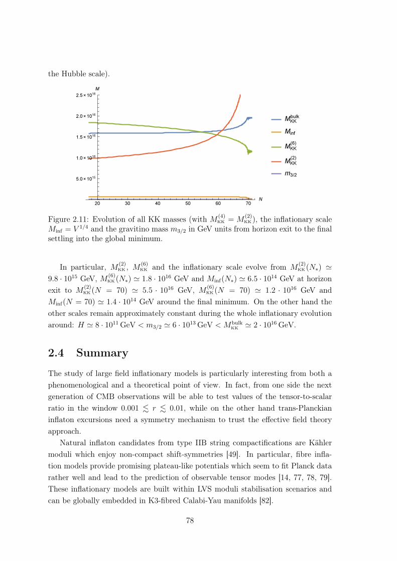
the Hubble scale).

Figure 2.11: Evolution of all KK masses (with M (4)KK = M

(2)KK ), the inflationary scale

Minf = V 1/4 and the gravitino mass m3/2 in GeV units from horizon exit to the finalsettling into the global minimum.

In particular, M (2)KK , M

(6)KK and the inflationary scale evolve from M

(2)KK (N∗) '

9.8 · 1015 GeV, M (6)KK (N∗) ' 1.8 · 1016 GeV and Minf(N∗) ' 6.5 · 1014 GeV at horizon

exit to M(2)KK (N = 70) ' 5.5 · 1016 GeV, M (6)

KK (N = 70) ' 1.2 · 1016 GeV andMinf(N = 70) ' 1.4 · 1014 GeV around the final minimum. On the other hand theother scales remain approximately constant during the whole inflationary evolutionaround: H ' 8 · 1011 GeV < m3/2 ' 6 · 1013 GeV < Mbulk

KK ' 2 · 1016 GeV.

2.4 Summary

The study of large field inflationary models is particularly interesting from both aphenomenological and a theoretical point of view. In fact, from one side the nextgeneration of CMB observations will be able to test values of the tensor-to-scalarratio in the window 0.001 . r . 0.01, while on the other hand trans-Planckianinflaton excursions need a symmetry mechanism to trust the effective field theoryapproach.

Natural inflaton candidates from type IIB string compactifications are Kählermoduli which enjoy non-compact shift-symmetries [49]. In particular, fibre infla-tion models provide promising plateau-like potentials which seem to fit Planck datarather well and lead to the prediction of observable tensor modes [14, 77, 78, 79].These inflationary models are built within LVS moduli stabilisation scenarios andcan be globally embedded in K3-fibred Calabi-Yau manifolds [82].

78

In this chapter we found that the inflationary dynamics is strongly constrainedby the Kähler cone conditions which never allow for enough efoldings of inflation ifthe internal volume is of order V ∼ 103. For larger values of the Calabi-Yau volumeof order V ∼ 104, the Kähler cone becomes large enough for the inflaton to driveNe ' 52 efoldings, as required by an estimate of the post-inflationary evolution.However such a large value of V tends to suppress the amplitude of the densityperturbations below the reference COBE value. This can be avoided by consideringlarge values of either the coefficients of the winding loops which generate the plateau,or the flux superpotential W0. Let us stress that in the string landscape this choiceis guaranteed to be possible by the fact that both of these microscopic parametersare flux-dependent.

However, as shown in Sec. 2.3.1, large values of the coefficients of the windinggs corrections make the Hubble scale during inflation of the same order of magni-tude of the mass of the volume mode. This could either cause a large shift of theoriginal LVS minimum or even a problem for the stability of the inflationary direc-tion against orthogonal runaway directions. A definite answer to this issue hencerequires a proper multi-field analysis even if the two-field study of [14] revealed thatthe inflationary motion is still mostly single-field.

On the other hand, if the flux superpotential is of order W0 ∼ 100, the gravitinomass can become too close to some KK scale in the model, destroying the 4D effectivefield theory. Moreover, F 4 terms are proportional to |λ|W 4

0 . Thus if W0 is large,these higher derivative effects can spoil the flatness of the inflationary potentialbefore achieving enough efoldings of inflation if |λ| is not small enough. Hence inSec. 2.3.1 we presented a model withW0 ∼ 100 and a very small value of |λ| of order|λ| = 10−7 which makes the F 4 terms harmless. The gravitino mass also turns out tobe slightly smaller than any KK scale throughout the whole inflationary dynamics.

79

80

Part III

Dark MatterFrom String Theory

81

Chapter 3

Primordial Black Holes from StringInflation

The origin of dark matter remains one of the biggest mysteries in fundamentalphysics. One of the simplest explanations, which would rely neither on the presenceof new particles nor on modifications of the gravitational interaction, is black holes.An interesting region in parameter space where the contribution of black holes tothe total dark matter abundance could be between 10% and 100% depending onastrophysical uncertainties is 10−17M .MBH . 10−13M [124, 25, 116], where thelower bound comes from extra-galatic γ rays produced due to Hawking evaporation[117]. This region, even if it is far from the one probed by LIGO, is very interestingsince there is no known astrophysical explanation for black hole formation in thissmall mass window.1 On the other hand, these tiny black holes could be seeded bythe dynamics of the early universe [121, 122]. A tantalizing idea for the formationof these primordial black holes (PBHs) relies on an amplification of the densityperturbations during inflation of order δρ ∼ 0.1 ρ which then collapse to form PBHsat horizon re-entry.

This enhancement of the scalar power spectrum has to take place at momentumscales which are much larger than the ones associated with CMB observations whereδρ ∼ 10−5ρ. From the theoretical point of view, it is therefore important to identifymechanisms to generate the necessary enhancement at the right scales. Guided againby simplicity, we focus on single-field inflationary models which also reproduce the

1Depending on the interpretation of astrophysical and cosmological data, X-ray and CMBobservations seem to rule out the case where black holes in the LIGO mass region can constitutea fraction of the dark matter abundance above 10% [118, 119, 120]. Moreover the single-fieldinflationary dynamics seems to be very unlikely to generate black holes with masses as large as afew solar masses when the scalar spectral index is required to be compatible with CMB data [25].

83

Planck data rather well [80].2 It has already been pointed out that the requiredinflationary potentials feature a slow-roll behaviour followed by a near inflectionpoint region where the power spectrum is amplified since the system enters an ultraslow-roll regime [126, 127, 128, 129, 25].

Despite the fact that dark matter as PBHs formed during single-field inflationmight seem a very appealing idea, its explicit realisation in concrete models hasturned out to be rather complicated since the inflationary potential has to possessenough tuning freedom to allow for such dynamics [130]. Examples based on a ra-diative plateau have been recently studied in [128, 129, 25]. This is a bottom upperspective which tries to single out the simplest potential which allows for PBH for-mation via an inflationary plateau followed by a near inflection point. However thisapproach ignores the fundamental issue of deriving the model from a UV consistenttheory.

In this chapter we shall instead take a more top down approach and search forconcrete examples of inflationary models in string theory whose structure is richenough to allow for PBH formation. One of the main advantages of embeddinginflation in string theory is the possibility to motivate the presence of a symmetrywhich can protect the inflaton potential against quantum corrections which canspoil its flatness [47, 48]. Particularly interesting cases include inflaton candidateswhich are pseudo Nambu-Goldstone bosons associated with slightly broken shiftsymmetries. Abelian symmetries involves both axions [131], which are associatedto compact U(1) factors, and Kähler moduli [13], which are associated with non-compact rescaling symmetries [49].3

This global rescaling symmetry is explicitly realised at tree-level in type IIB no-scale models since the Kähler moduli τ remain exact flat directions but needs tobe slightly broken to generate the inflationary potential. This can be done eitherby non-perturbative effects or by perturbative power-law corrections which becomeexponential in terms of the canonically normalised inflaton: V0/τ

n ∼ V0 e−nφ/f .

Notice that the shape of the inflationary potential is determined by both the ef-fective ‘decay constant’ f , i.e. the geometry of the moduli space (determined bythe topology of the divisor whose volume is parameterised by the inflaton) and n,i.e. the exact moduli-dependence of the symmetry-breaking effects which developthe inflationary potential [79]. Once a proper uplifting to dS has been achieved viathe addition of a constant contribution (which can have several dynamical origins[88, 89, 90, 91, 132, 192, 92, 93]), these models tend to give rise to an inflationary

2For PBH formation in multi-field inflationary models see [123, 124, 125].3The non-Abelian case leads to a multi-field inflationary scenario which tends to be disfavoured

by non-Gaussianity observations [80].

84

potential of the schematic form [79]:

Vinf = V0

(1− e−nφ/f

). (3.1)

These models go under the name of Fibre Inflation since the underlying Calabi-Yaucompactification manifold has a typical fibration structure [14, 77, 78]. They areinteresting since they drive inflation successfully via a plateau-like region at largeφ and also allow for a detailed analysis of the post-inflationary evolution [54, 113,114]. Moreover they provide string theory embeddings of Starobinsky inflation [133]and supergravity α-attractors [134, 135, 136] (where in our notation α ' (f/n)2).Nevertheless the potential (3.1) is too simple to generate PHBs via a period of ultraslow-roll dynamics towards the end of inflation. However recent global constructionsof fibre inflation models in concrete Calabi-Yau orientifolds with explicit brane setupand closed string moduli stabilisation have revealed the existence of new string loopcorrections which look schematically like [82, 2]:

δVinf = −ε1V0e2nφ/f

1 + ε2 e3nφ/f, (3.2)

where ε1 1 and ε2 1 are two parameters which are tunable since they dependon background fluxes and the Calabi-Yau intersection numbers, and turn out to benaturally small since they are suppressed by inverse powers of the compactificationvolume, an exponentially large quantity [43, 42]. Thanks to the additional pertur-bative contribution (3.2), we will show that fibre inflation models are rich enough toproduce a near inflection point region before the end of inflation which is perfectlysuitable to generate PBHs in the mass window 10−17M .MPBH . 10−13M wherethey could constitute a significant fraction of the total dark matter abundance.

As pointed out in [137, 129, 25, 138], the slow-roll approximation ceases to bevalid in the near inflection point region. The primordial power spectrum has tobe computed by solving the Mukhanov-Sasaki equations for the curvature pertur-bations [139, 140]. By following this procedure, we shall show that the primordialpower spectrum can feature the required enhancement for appropriate values of theunderlying parameters. Let us stress that even if the choice of microscopic param-eters needed for successful PBH formation looks very non-generic from the stringlandscape point of view, the values of these parameters are technically natural sincethey are protected against large quantum corrections by the effective rescaling shiftsymmetry typical of these models [49].

This chapter is organised as follows. In Sec. 3.1 we provide a very brief review offibre inflation models while in Sec. 3.2 we describe the mechanism of PBH generation

85

in some detail. In Sec. 3.3 we then perform a careful analysis of the process of PBHformation in fibre inflation by implementing the Mukhanov-Sasaki formalism toderive the primordial power spectrum. We finally discuss our results and presentour conclusions in Sec. 4.4.

3.1 Fibre inflation models

Fibre inflation is a class of string inflationary models built within the frameworkof type IIB flux compactifications [14, 77, 78, 79]. The inflaton τK3 is a Kählermodulus controlling the size of a K3 divisor fibred over a P1 base with volume tP1 .The simplest fibre inflation models feature a Calabi-Yau (CY) volume which lookslike:

V = tP1τK3 − τ 3/2dP , (3.3)

where τdP is the volume of a diagonal del Pezzo divisor which supports non-perturbativeeffects. Several effects come into play to stabilise the Kähler moduli in a typicallarge volume scenario (LVS) vacuum [43, 42]. At leading order in a 1/V 1 ex-pansion only two directions, V and τdP, are lifted by non-perturbative contributionsto the superpotential W [88] and perturbative α′ corrections to the Kähler poten-tial K [36, 37, 87].4 Hence the remaining flat direction, which can be parametrisedby τK3, represents a very promising inflaton candidate since it enjoys an effectivenon-compact rescaling symmetry which can be used to protect the flatness of theinflationary potential against quantum corrections [49].5

In order to generate the inflationary potential, this effective shift symmetry hasto be slightly broken. This is realised by open string 1-loops which depend on allKähler moduli [39, 40, 73, 74] but are subdominant with respect to the leadingα′ effects thanks to the extended no-scale structure typical of these models [41].Higher loops are expected to be suppressed by positive powers of the string couplinggs 1 and negative powers of the exponentially large volume V 1 [14, 79]. Othercontributions to the inflationary potential arise from higher derivative α′ effects

4At this level of approximation, also the axionic partner of τdP is fixed by non-perturbativeeffects.

5There are actually other two flat directions corresponding to the axions associated with the baseand the fibre which turn out to be much lighter than τK3 since they acquire tiny masses only at non-perturbative level (suppressed with respect to the mass of τK3 by e−πτK3 ∼ e−πV

2/3 ∼ 10−137 1for V ∼ 103 from Tab. 3.1). Hence these fields are in practice massless and acquire isocurvaturefluctuations during inflation. However present strong bounds on isocurvature fluctuations do notapply to our case since these axions tend to be too light to behave as dark matter (see eq. (B.16)of [187]). On the other hand, these ultra-light axions could behave as extra relativistic degrees offreedom produced from the inflaton decay [60].

86

[75, 76] but these are also V-suppressed if the superspace derivative expansion isunder control [86]. Moreover, all these corrections give rise to an AdS vacuumwhich needs to be uplifted to dS by the inclusion of anti-branes [88, 89, 90, 91],hidden sector T-branes [132, 192, 92] or non-perturbative effects at singularities[93]. It is important to stress that all these uplifting effects are inflaton-independentsince they depend just on the overall volume V . Thus they give rise to a constantcontribution to the inflationary potential which is crucial to develop a plateau-likebehaviour at large inflaton values.

After canonical normalisation of the inflaton field, the resulting potential is qual-itatively very similar to the one of Starobinsky inflation [133] and α-attractor su-pergravity models [134, 135, 136]. In fact, fibre inflation models require a trans-Planckian field range to obtain enough e-foldings of inflationary expansion, and sothey can predict a tensor-to-scalar ratio as large as r ∼ 0.005− 0.01. These modelsare particularly interesting also because they can be embedded into globally consis-tent CY orientifold compactifications with an explicit brane setup and chiral matter[82, 2]. In the study of concrete CY realisations of string models where the inflatonis a Kähler modulus, it has been recently realised that the underlying Kähler coneconditions set strong geometrical constraints on the allowed inflaton range [112]. In-terestingly, it has been found that the distance travelled by inflaton in field space cangenerically be trans-Planckian only for K3-fibred CY threefolds which are exactlythe necessary ingredients to construct fibre inflation models.

The two moduli which are stabilised at leading order in 1/V are heavier than theHubble constant whose size is set by the uplifting contribution. Hence V and τdP donot play a significant rôle during inflation which is instead driven mainly by the lightfield τK3. Fibre inflation models are therefore, to a very good level of approximation,single-field inflationary models whose potential looks like [14, 77, 78]:

Vinf =

(Cup

V4/3+ g2

s

CKK

τ 2K3

+W 2

0√gs

εF4

V τK3

− CW

V√τK3

+ g2s DKK

τK3

V2+ δF4

W 20√gs

√τK3

V2

)W 2

0

V2,

(3.4)where gs 1 is the string coupling and W0 ∼ O(1 − 10) is the superpotentialgenerated by background fluxes which is constant after the dilaton and the complexstructure moduli are stabilised at tree-level. Cup controls the uplifting contributionand, depending on the particular mechanism employed it can have a different de-pendence on the internal volume V , background or gauge fluxes. CKK > 0, DKK > 0

and CW are the coefficients of 1-loop open string corrections which have been con-jectured to come respectively from the tree-level exchange of closed Kaluza-Kleinstrings between non-intersecting stacks of branes, and winding closed strings be-

87

tween intersecting branes [39, 40, 73, 74]. These constants are also functions of thevacuum expectation values of the complex structure moduli and are expected to beof order unity: CKK ∼ DKK ∼ CW ∼ O(1). On the other hand, εF4 and δF4 are thecoefficients of higher derivative α′ F 4 effects which depend just on the topologicalproperties of the underlying geometry and are expected to be positive but relativelysmall: εF4 ∼ δF4 ∼ O(10−3) [75, 76].

The potential (3.4) is rich enough to generate a minimum for small τK3, aninflationary plateau-like behaviour at large τK3 and finally a steepening region atvery large τK3 where the system is in a fast-roll regime.6 In order to perform aproper study of the inflationary dynamics, the field τK3 has to be written in termsof its canonically normalised counterpart φ as [14]:

τK3 = e2√3φ

= 〈τK3〉 e2√3φ, (3.5)

where we have expanded φ around its minimum as φ =√

32

ln〈τK3〉+ φ. Substituting(3.5) in (3.4), we end up with:

Vinf = V0

(C1 + C2 e

− 4√3φ

+ C3 e− 2√

3φ − e

− 1√3φ

+ C4 e2√3φ

+ C5 e1√3φ), (3.6)

where, parameterising the inflaton minimum as 〈τK3〉3/2 ≡ γ V , we have:

V0 =CW W

20

γ1/3V10/3, C1 = γ1/3 Cup

CW

, C2 = g2s

CKK

γ CW

,

C3 =W 2

0

γ1/3CW

√gs

εF4

V1/3, C4 = γ g2

s

DKK

CW

, C5 = γ C3δF4

εF4. (3.7)

Notice that we work in units of Mp = 1. The potential (3.6) can have a plateau-like region which can support enough efoldings of inflation only if the coefficients ofthe positive exponentials are suppressed, i.e. C4 1 and C5 1, which, in turn,requires γ 1. This is naturally achieved if the three negative exponentials competeto give a minimum since this can happen when γ ∼ g2

s 1. The inflationaryplateau is then generated mainly by the fourth term in (3.6). Notice that theHubble constant during inflation is set by V0 and scales as H2 ∼ M2

p/V10/3.7 Themass of the inflaton around the minimum is of order H but then quickly becomesexponentially smaller than H for φ > 0.

Even if (3.6) is a very promising potential to drive inflation, it is not rich enough

6Pre-inflationary fast to slow-roll transitions in fibre inflation models can give rise to a powerloss at large angular scales [107, 141].

7Mp denotes the reduced Planck mass Mp = 1/√8πG ' 2.4 · 1018 GeV.

88

to generate primordial black holes due to the requirement of a significant enhance-ment of the power spectrum at large momentum scales. However recent explicitconstructions of fibre inflation models in concrete type IIB CY compactificationswith D3/D7-branes and O3/O7-planes have reproduced the potential (3.4) in aslightly generalised form since [82, 2]:

• In general the coefficient CW is not a constant but a function of the fibremodulus τK3 of the form:

CW → CW(τK3) = CW −AW

√τK3√

τK3 −BW

, (3.8)

where the parameters CW ∼ O(1) and AW ∼ O(1) depend on the vacuumexpectation values of the complex structure moduli, while BW ∼ O(1) dependson topological properties of the underlying CY threefold like the intersectionnumbers and the Euler number.

• The effective action features additional winding 1-loop corrections to the in-flationary potential which will turn out to be crucial for the formation ofprimordial black holes and look like:

δVW = W 20

τK3

V4

DW −GW

1 +RW

τ3/2K3

V

, (3.9)

where again DW ∼ O(1) and GW ∼ O(1) become constants only after complexstructure moduli stabilisation, while RW ∼ O(1) depends on the topologicalfeatures of the extra dimensions.

Depending on the details of a given brane setup (in particular the presence of inter-sections between D-branes and O-planes and the topological properties of two-cycleswhere different stacks can intersect), several contributions to the generic scalar po-tential (3.4), supplemented with (3.8) and (3.9), can be absent by construction. Inwhat follows, we shall therefore focus just on winding 1-loop corrections that repre-sent the simplest situation which can lead to a successful generation of primordialblack holes. This is justified for example by the fact that the global chiral embeddingof fibre inflation presented in [2] does not feature any Kaluza-Klein loop correction,i.e. CKK = DKK = 0.8 Moreover higher derivative F 4 terms tend also to be negligible

8Even if both CKK and DKK are non-zero, in a vast region of the parameter space, Kaluza-Kleinloops would still be subdominant with respect to winding loops due to the extra factors of g2s 1in (3.7). This is due to the fact that Kaluza-Klein loops feature an extended no-scale cancellation,and so they contribute to the scalar potential effectively only at 2-loop order [41].

89

since, as can be seen from (3.7), they should be suppressed by both inverse volumepowers and by εF4 1 and δF4 1. Hence in Sec. 3.3 we shall study primordialblack hole formation for the following simplified inflationary potential:

Vinf =W 2

0

V3

Cup

V1/3− CW√

τK3

+AW√

τK3 −BW

+τK3

V

DW −GW

1 +RW

τ3/2K3

V

, (3.10)

which, when expressed in terms of the canonically normalised inflaton shifted fromits minimum, takes the form:

Vinf = V0

[C1 − e

− 1√3φ

(1− C6

1− C7 e− 1√

3φ

)+ C8 e

2√3φ

(1− C9

1 + C10 e√

3φ

)],

(3.11)with:

C1 = γ1/3 Cup

CW

∼ O(1) , C6 =AW

CW

∼ O(1) , C7 =BW

γ1/3V1/3∼ O(1) ,

C8 = γDW

CW

1 , C9 =GW

DW

∼ O(1) , C10 = γ RW 1 . (3.12)

Notice that the potential (3.11) scales as V0 ∼ H2M2p ∼M4

p/V10/3 while the leadingorder potential which gives mass to V and τdP scales as Vlead ∼M4

p/(g3/2s V3) [43, 42].

Hence for gs 1 and V 1, the dynamics which generates PBHs is effectivelysingle-field.

3.2 PBH formation

Primordial black holes form when large and relatively rare density perturbationsre-enter the Hubble horizon and undergo gravitational collapse. The fraction of thetotal energy density in PBHs with mass M at PBH formation is given by:

βf(M) =ρPBH(M)

ρtot

∣∣∣f. (3.13)

The curvature perturbations are assumed to follow a Gaussian distribution withwidth σM ≡ σ(M).9 The probability of large fluctuations leading to the formation

9See [142] for the case when non-Gaussianity effects cannot be neglected.

90

of PBHs with mass M is then given by:

βf(M) =

∫ ∞ζc

1√2π σM

e− ζ2

2σ2M dζ , (3.14)

where ζc denotes the critical value for the collapse into a PBH to take place andplays a fundamental rôle in this discussion. It is usually taken to be close to unity,see e.g. [25, 138, 129].10 For such a Gaussian distribution σ2

M ∼ 〈ζζ〉 which on CMBscales is O(10−9). As we will show below, σM ζc and so we can approximate (3.14)as:

βf(M) ∼ σM√2π ζc

e− ζ2c

2σ2M . (3.15)

If PBHs are to be a significant fraction of dark matter, the fluctuations that give riseto them must not be too rare, meaning that σM cannot be arbitrarily smaller thanζc. This implies that on smaller distance scales the scalar power spectrum must beorders of magnitude larger than on CMB scales. Let us quantify this statement anddiscuss how it may be achieved in single field models of inflation.

The mass of a PBH forming when a large density perturbation re-enters thehorizon is assumed to be proportional to the horizon mass:

M = γG

4π

3

ρtot

H3

∣∣∣f

= 4πγG

M2p

Hf

, (3.16)

where γG is a correction factor which depends on the details of the gravitationalcollapse and Hf denotes the Hubble parameter at the moment the perturbation re-enters the horizon. Noting that PBHs behave as matter, the fraction of the totalenergy density in PBHs at formation time (3.13) can be related to the present PBHenergy density as:

βf(M) =

(H0

Hf

)2ΩDM

a3f

fPBH(M) , (3.17)

where af denotes the scale factor at PBH formation time, H0 is the Hubble scaletoday, ΩDM = 0.26 is the present fraction of the total energy density in dark matterand fPBH(M) is the fraction of the total dark matter energy density in PBHs withmass M today. PBHs in the low mass region, which can be interesting dark mattercandidates, get formed before matter-radiation equality in an epoch of radiation

10We note that some authors [127, 128] take it to be of the order 10−1 or 10−2. Given theexponential dependence of β on ζc this significantly decreases the level of tuning required of theinflationary potential in models where PBHs are created within single field inflation.

91

dominance. Hence the Hubble scale at PBH formation redshifts as:

H2f = Ωr

H20

a4f

(g∗fg∗0

)−1/3

, (3.18)

where Ωr = 8× 10−5 is the present fraction of the total energy density in radiation,while g∗0 and g∗f are respectively the number of relativistic degrees of freedom todayand at PBH formation time. Combining (3.16) with (3.18), (3.17) can be rewrittenin terms of present day observables and in units of the solar mass M as [143, 144]:

βf(M) ' 4√γG

× 10−9

(g∗fg∗0

)1/4√

M

MfPBH(M) . (3.19)

We can now get an estimate of the level of enhancement of the power spectrumrequired to have PBHs which constitute a significant fraction of dark matter. SettingγG = 1 to be conservative and assuming that only SM degrees of freedom are presentso that g∗0 = 3.36 and g∗ = 106.75, if PBHs with mass M constitute all of darkmatter, i.e. fPBH(M) = 1 , (3.19) reduces to:

βf(M) ' 10−8

√M

M. (3.20)

If we now focus on a mass distribution sharply peaked at M = 10−15M, we findβf(M) ' 3 × 10−16. Comparing (3.20) with (3.15) for ζc = 1, we finally obtainσM = 0.12. This implies that the scalar power spectrum must be enhanced toO(10−2), a value 7 orders of magnitude larger that its value on CMB scales.11 Thislarge enhancement can in principle be achieved within single field inflationary modelsby inducing an extremely flat and sufficiently long region in the scalar potential.Therefore the problem of PBHs in single field inflation is one of having a sufficientlyrich structure in the scalar potential and the freedom to tune in a flat plateau inthe later part of inflation.

Let us finally make two important observations:

• In the estimate above of the enhancement of the power spectrum, we consid-ered PBHs with a given mass M . However, more generically, the PBH massfunction is broadly peaked, and so the fraction of the total dark matter density

11Had we assumed ζc = 0.1, we would have found σ = 0.012, in agreement with the estimates of[127, 128]. This corresponds to an enhancement of the power spectrum by 5 orders of magnitudebetween PBH and CMB scales and requires less tuning of the inflationary potential.

92

in PBHs looks like [145, 116]:

fPBH =

∫dfPBH(M) =

∫dfPBH(M)

d lnMd lnM , (3.21)

where dfPBH(M) is the fraction of PBHs with mass betweenM andM+d lnM ,and the integration domain is bounded below by Hawking evaporation of verylight PBHs and above by the mass corresponding to PBHs which re-enter thehorizon after matter-radiation equality, see e.g. [138].

• Assuming that the Hubble scale during inflation Hinf is approximately con-stant, (3.16) and (3.18) can be used to write the number of efoldings betweenCMB and PBH horizon exit as [138]:

∆NPBH

CMB = ln

(aPBHHinf

aCMBHinf

)= ln

(afHf

0.05 Mpc−1

)= 18.4− 1

12ln

(g∗g∗0

)+

1

2ln γG −

1

2ln

(M

M

). (3.22)

Setting again γG = 1, g∗0 = 3.36 and g∗ = 106.75 as in the SM case, theformation of PBHs with masses in the [10−16, 10−14]M range implies thatPBH scales leave the horizon approximately 34.2 to 36.5 efoldings after theCMB scales.

3.3 PBHs from Fibre inflation

In order to produce a significant fraction of PBHs from inflationary density per-turbations, we shall use the rich structure of the fibre inflation potential (3.10) toinduce a near inflection point close to the minimum as depicted in Fig. 3.1 .

Based on the scaling of each term in eq. (3.10) with the fibre modulus τK3 onecan see that the second and third terms dominate at small field values and inducea minimum for the modulus around:

〈τK3〉 ∼CWB

2W

(√CW −

√AW)2

. (3.23)

The forth term, being proportional to τK3, dominates V at large field values, whilethe fifth term has a maximum at 22/3

(RW/V)2/3 and scales as −τK3 at small and as −τ−1/2K3

at large field values respectively. It is this last term that will be instrumental ingenerating the enhancement in the scalar power spectrum that will ultimately leadto the formation of primordial black holes in this setup. This can be achieved for

93

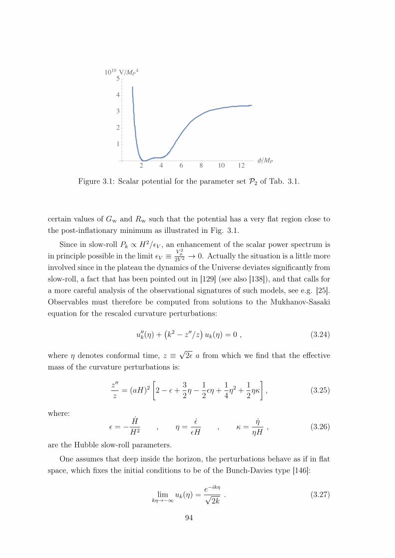
ϕ/

/

Figure 3.1: Scalar potential for the parameter set P2 of Tab. 3.1.

certain values of GW and RW such that the potential has a very flat region close tothe post-inflationary minimum as illustrated in Fig. 3.1.

Since in slow-roll Pk ∝ H2/εV , an enhancement of the scalar power spectrum isin principle possible in the limit εV ≡

V 2φ

2V 2 → 0. Actually the situation is a little moreinvolved since in the plateau the dynamics of the Universe deviates significantly fromslow-roll, a fact that has been pointed out in [129] (see also [138]), and that calls fora more careful analysis of the observational signatures of such models, see e.g. [25].Observables must therefore be computed from solutions to the Mukhanov-Sasakiequation for the rescaled curvature perturbations:

u′′k(η) +(k2 − z′′/z

)uk(η) = 0 , (3.24)

where η denotes conformal time, z ≡√

2ε a from which we find that the effectivemass of the curvature perturbations is:

z′′

z= (aH)2

[2− ε+

3

2η − 1

2εη +

1

4η2 +

1

2ηκ

], (3.25)

where:

ε = − H

H2, η =

ε

εH, κ =

η

ηH, (3.26)

are the Hubble slow-roll parameters.

One assumes that deep inside the horizon, the perturbations behave as if in flatspace, which fixes the initial conditions to be of the Bunch-Davies type [146]:

limkη→−∞

uk(η) =e−ikη√

2k. (3.27)

94

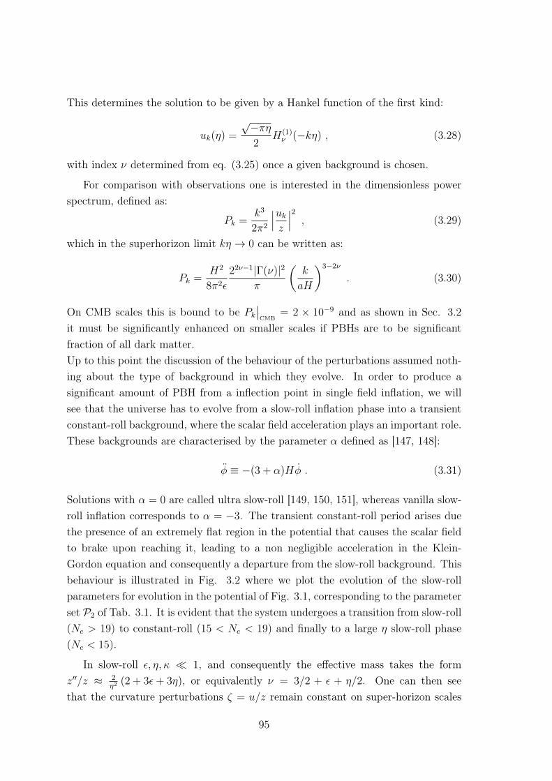
This determines the solution to be given by a Hankel function of the first kind:

uk(η) =

√−πη2

H(1)ν (−kη) , (3.28)

with index ν determined from eq. (3.25) once a given background is chosen.

For comparison with observations one is interested in the dimensionless powerspectrum, defined as:

Pk =k3

2π2

∣∣∣ukz

∣∣∣2 , (3.29)

which in the superhorizon limit kη → 0 can be written as:

Pk =H2

8π2ε

22ν−1|Γ(ν)|2

π

(k

aH

)3−2ν

. (3.30)

On CMB scales this is bound to be Pk∣∣CMB

= 2 × 10−9 and as shown in Sec. 3.2it must be significantly enhanced on smaller scales if PBHs are to be significantfraction of all dark matter.Up to this point the discussion of the behaviour of the perturbations assumed noth-ing about the type of background in which they evolve. In order to produce asignificant amount of PBH from a inflection point in single field inflation, we willsee that the universe has to evolve from a slow-roll inflation phase into a transientconstant-roll background, where the scalar field acceleration plays an important role.These backgrounds are characterised by the parameter α defined as [147, 148]:

φ ≡ −(3 + α)Hφ . (3.31)

Solutions with α = 0 are called ultra slow-roll [149, 150, 151], whereas vanilla slow-roll inflation corresponds to α = −3. The transient constant-roll period arises duethe presence of an extremely flat region in the potential that causes the scalar fieldto brake upon reaching it, leading to a non negligible acceleration in the Klein-Gordon equation and consequently a departure from the slow-roll background. Thisbehaviour is illustrated in Fig. 3.2 where we plot the evolution of the slow-rollparameters for evolution in the potential of Fig. 3.1, corresponding to the parameterset P2 of Tab. 3.1. It is evident that the system undergoes a transition from slow-roll(Ne > 19) to constant-roll (15 < Ne < 19) and finally to a large η slow-roll phase(Ne < 15).

In slow-roll ε, η, κ 1, and consequently the effective mass takes the formz′′/z ≈ 2

η2 (2 + 3ε+ 3η), or equivalently ν = 3/2 + ε + η/2. One can then seethat the curvature perturbations ζ = u/z remain constant on super-horizon scales

95

ϵ

|η|

|κ|

-

-

-

ϵ

|η|

|κ|

-

Figure 3.2: Slow-roll parameters as functions of the number of efoldings Ne fromthe end of inflation for parameter set P2. It is clear that the background evolvesfrom slow-roll (Ne > 19) to constant-roll (15 < Ne < 19) and back to slow-roll again(Ne < 15). Dashed lines represent 10, 6 and 1.

and the two point function can therefore be evaluated at horizon crossing, yieldingthe familiar slow-roll result:

Pk =H2

8π2ε

∣∣∣k=aH

. (3.32)

Eq. (3.30) also captures the momentum dependence of the two point function, whichcan be written in terms of the spectral index ns and its running α, given by:

ns ≡d lnPkd ln k

= 1− 2ε− η , (3.33)

and:dnsd ln k

= −2εη − ηκ . (3.34)

Both these quantities are subject of tight observational constraints [80]. For thiswork we take:

ns = 0.9650± 0.0050 anddnsd ln k

= −0.009± 0.008 (3.35)

at 68%CL and at a scale k∗ = 0.05 Mpc−1.

In the transient constant-roll regime one has η ≈ −2(3 + α − ε) which impliesε ∝ a−2(3+α). In the cases we consider α ∈ [0, 1]. In such a background the super-horizon behaviour of the power spectrum is determined by:

Pk ∝ H |2α+3|−1a3+2α+|3+2α| . (3.36)

Note that since ε is small and decreasing rapidly with the expansion (for α > −3),one can take H to be constant. We therefore see that for −3 ≤ α < −3/2 the

96

curvature perturbations are frozen beyond the horizon (this includes the previouslydiscussed case of slow-roll inflation, α = −3), whereas for α > −3/2, Pk ∝ a2(3+2α),signaling the presence of a growing solution to the MS equation, and the breakdownof the approximation of (3.32). In order to determine the two-point function in suchbackgrounds one must therefore solve the MS equation and evaluate Pk at the endof inflation.

-

-

-

-

-

-

Figure 3.3: Power spectrum (3.29) for the potential of Fig. 3.1 with parameter setP2. The dashed line represents the slow-roll estimate of (3.32) while the continuousline is obtained from the solutions to the MS equation. The circle correspond to theCMB scales if the peak is to be associated with PBH of mass M = 10−14M.

In Fig. 3.3 we plot the power spectrum for scalar perturbations for the potentialof Fig. 3.1 (parameter set P2) calculated from the solutions of (3.24) (continuousline) and the slow-roll estimate of (3.32) (dashed line). As expected the slow-rollapproximation breaks down for modes that cross the horizon close to the onset ofthe constant-roll phase. Crucially for the production of PBH, the slow-roll resultunderestimates the power spectrum by several orders of magnitude in this range ofmomentum modes. This is to be expected given the existence of a growing modesolution in constant-roll backgrounds with α ∈ [0, 1]. The presence of the growingmode also implies that the actual position of the peak in the power spectrum isshifted towards larger scales/PBH masses with respect to the slow-roll estimate.12

In Fig. 3.4 we plot the evolution of the power spectrum for modes leaving thehorizon 53 and 22 efoldings before the end of inflation, corresponding to CMB andPBH scales respectively. While both scales are affected by the growing mode during

12These results are qualitatively similar to the findings of [25] since both models feature thesame dynamics.

97

the constant roll phase, their superhorizon growth is determined by kaH

at the onsetof the constant roll period. This quantity is minute for modes on CMB scales butnot for those on the PBH region. As a result the CMB mode essentially followthe slow-roll estimate of (3.32) after crossing the horizon, while on small scales wesee that there is a large amplification of Pk leading to a breakdown of the slow-roll approximation. Finally let us note that the O(1) deviation from the slow-rollestimate for modes on the smallest scales (Ne . 15) can be attributed to the factthat in the final phase of expansion before the end of inflation, η = O(1).

× -

× -× -

× -× -

× -× -

-

-

-

-

Figure 3.4: Evolution of the curvature perturbations on different scales for exampleP2. On the left panel a mode that corresponds to CMB scales, leaving the horizon53 efoldings before the end of inflation, and keeping a constant value thereafter.On the right panel a mode that corresponds to PBH scales, leaving the horizon 22efoldings before the end of inflation and undergoing super-horizon growth duringthe constant-roll phase (the same evolution was found in Fig. 2 of [152]). In bothplots the dashed line corresponds to the slow-roll estimate of (3.32).

In Tables 3.1 and 3.2 we present three numerical examples corresponding to caseswhere all DM is composed of 10−14M PBHs, assuming ζc = 1. We stress that thechoices of the underlying parameters are in line with their microscopic origin asexplained in Sec. 3.1.and that the desire to have PBH DM does not constrain thecompactification volume, which varies by several orders of magnitude in betweenthe three examples. All the digits presented in Tab. 3.1 are required in order tofully reproduce our results. In particular, GW and RW control the position of thenear inflection point and the velocity with which the field goes through that region.Changing any of these two quantities will change the amplitude and position of thepeak of Fig. 3.3, and therefore the mass and abundance of PBHs.

All examples lead to a spectral index that is slightly more than 3 sigma redderthan the current best fit, while giving rise to a spectral index running and a tensorfraction that are in line with current bounds. Notice that, for sake of simplicity,we did not analyse the full potential (3.4) but we just considered the simplest form

98

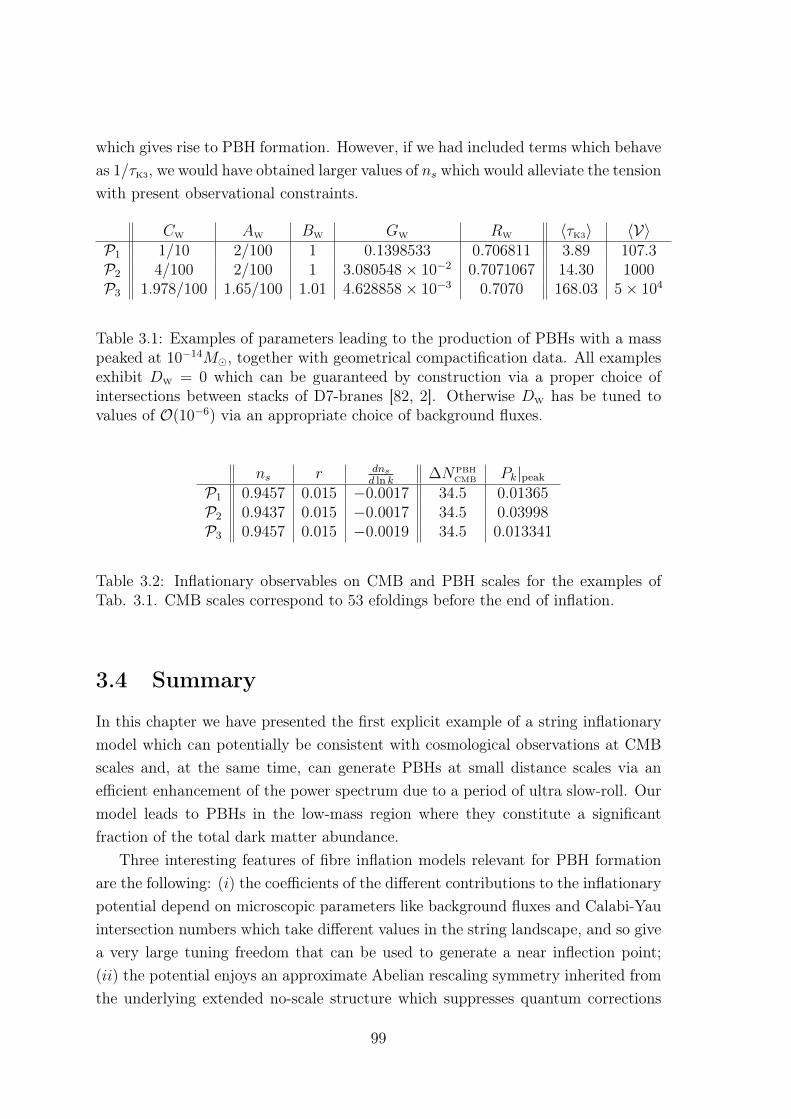
which gives rise to PBH formation. However, if we had included terms which behaveas 1/τK3, we would have obtained larger values of ns which would alleviate the tensionwith present observational constraints.

CW AW BW GW RW 〈τK3〉 〈V〉P1 1/10 2/100 1 0.1398533 0.706811 3.89 107.3P2 4/100 2/100 1 3.080548× 10−2 0.7071067 14.30 1000P3 1.978/100 1.65/100 1.01 4.628858× 10−3 0.7070 168.03 5× 104

Table 3.1: Examples of parameters leading to the production of PBHs with a masspeaked at 10−14M, together with geometrical compactification data. All examplesexhibit DW = 0 which can be guaranteed by construction via a proper choice ofintersections between stacks of D7-branes [82, 2]. Otherwise DW has be tuned tovalues of O(10−6) via an appropriate choice of background fluxes.

ns r dnsd ln k

∆NPBHCMB Pk|peak

P1 0.9457 0.015 −0.0017 34.5 0.01365P2 0.9437 0.015 −0.0017 34.5 0.03998P3 0.9457 0.015 −0.0019 34.5 0.013341

Table 3.2: Inflationary observables on CMB and PBH scales for the examples ofTab. 3.1. CMB scales correspond to 53 efoldings before the end of inflation.

3.4 Summary

In this chapter we have presented the first explicit example of a string inflationarymodel which can potentially be consistent with cosmological observations at CMBscales and, at the same time, can generate PBHs at small distance scales via anefficient enhancement of the power spectrum due to a period of ultra slow-roll. Ourmodel leads to PBHs in the low-mass region where they constitute a significantfraction of the total dark matter abundance.

Three interesting features of fibre inflation models relevant for PBH formationare the following: (i) the coefficients of the different contributions to the inflationarypotential depend on microscopic parameters like background fluxes and Calabi-Yauintersection numbers which take different values in the string landscape, and so givea very large tuning freedom that can be used to generate a near inflection point;(ii) the potential enjoys an approximate Abelian rescaling symmetry inherited fromthe underlying extended no-scale structure which suppresses quantum corrections

99

to the inflationary dynamics; (iii) the contribution to the inflationary potentialresponsible for the emergence of a near inflection point at large momentum scaleshas been derived in global embeddings of fibre inflation models in explicit Calabi-Yaucompactifications with chiral brane setup compatible with moduli stabilisation.

Moreover our model is characterised by a trans-Planckian field range duringinflation, and so it predicts a large tensor-to-scalar ratio of order r ∼ 0.01 whichmight be detected by the next generation of cosmological measurements. Similarly toprevious works on PBH formation in single-field inflation [128, 25], the scalar spectralindex turns out to be a bit too red since it is more than 3σ away from the Planckreference value. This tension might be resolved by the inclusion of non-zero neutrinomasses which might make our result compatible with CMB data within just 2σ

[25, 153]. The tension in the values of ns can also decrease in compactifications wherethe approach to the inflationary plateau occurs faster than the 1/

√τK3 considered

here, a possibility in potentials of the form (3.4). Another interesting cosmologicalobservable in our model is the running of the spectral index which turns out to besizable.

Notice that the tension with the observed value of the scalar spectral index isthe main reason why our mechanism cannot produce PBHs in the large mass regionprobed by LIGO since they would correspond to scales which are too close to CMBscales. Hence the large enhancement required for PBHs to be a significant fractionof DM, would make ns in strong conflict with present data. Given that the resultsof previous works focused on PHB formation in similar setups are qualitativelyequivalent [25], the generation of PBHs in the small mass window seems to be ageneric property of single-field models with an inflationary plateau followed by anear inflection point.

100

Chapter 4

The 3.5 keV Line from StringyAxions

Recently several studies have shown the appearance of a photon line at E ∼ 3.5

keV, based on stacked X-ray data from galaxy clusters and the Andromeda galaxy[161, 162]. The line has been detected in galaxy clusters by the X-ray observatoriesXMM-Newton, Chandra and Suzaku [163, 164] and in Andromeda with XMM-Newton [162]. The Hitomi satellite would have been able to study the 3.5 keV linewith unprecedented energy resolution. However, unfortunately Hitomi was lost afteronly a few weeks in operation and the limited exposure time on the Perseus clusteronly allows to put upper bounds on the 3.5 keV line which are consistent with thedetection of the other satellites [165]. The findings of [161, 162] have inspired furthersearches in other astrophysical objects such as the galactic center [166, 167, 168, 169],galaxies [170], dwarfs [171, 172, 173] and other galaxy clusters [174, 175].1 Currently,a compelling standard astrophysical explanation, e.g. in terms of atomic lines of the(cluster) gas is lacking.2 This gives rise to the possibility that the 3.5 keV line is asignal related to dark matter (DM) physics.

A much explored model is that of dark matter decay, e.g. a sterile neutrino withmass mDM ∼ 7 keV decaying into an active neutrino and a photon [178, 179]. Inthis case, the photon flux from an astrophysical object is solely determined by thelifetime of the dark matter particle and the dark matter column density. The widthof the line is due to Doppler broadening. There are several observational tensions, ifone wants to explain the (non-)observation of the 3.5 keV line in currently analysedastrophysical objects. Most prominently, these are:

• Non-observation of the 3.5 keV line from dwarf spheroidal galaxies [171, 172,1For a summary of observations and models on the 3.5 keV line see [176].2See however [167, 177].

101

173]. The dark matter density of these objects is rather well known and the X-ray background is low, making dwarf spheroidals a prime target for detectingdecaying dark matter.

• Non-observation of the 3.5 keV line from spiral galaxies [170], where again theX-ray background is low. According to the dark matter estimates of [170], thenon-observation of a 3.5 keV signal from spiral galaxies excludes a dark matterdecay origin of the 3.5 keV line very strongly at 11σ.

• The radial profile of the 3.5 keV line in the Perseus cluster peaks on shorterscales than the dark matter profile, rather following the gas profile than thedark matter profile [161, 169]. However, the observed profile with Suzaku isonly in mild tension with the dark matter profile [164].

These tensions, even though they could be potentially explained by uncertainties inthe dark matter distributions in these objects [176], motivate different dark mattermodels than direct dark matter decay into a pair of 3.5 keV photons.

A dark matter model that is consistent with all the present (non-)observationswas given in [180]. A dark matter particle with mass mDM ∼ 7 keV decays into analmost massless (mALP . 10−12 eV) axion-like particle (ALP) with energy 3.5 keVwhich successively converts into 3.5 keV photons that are finally observed. Comparedto direct dark matter decay into photons, the observed photon flux does not dependjust on the dark matter column density, but also on the probability for ALPs toconvert into photons. This is determined by the size and coherence scale of themagnetic field and the electron density in e.g. a galaxy cluster.

The 3.5 keV emission is stronger in astrophysical regions with relatively largeand coherent magnetic field. This is verified by the experimental fact that cool coreclusters like the Perseus cluster have stronger magnetic fields than non-cool coreclusters and also a higher 3.5 keV flux is observed from such an object. Furthermore,the fact that central regions of a cool core cluster host particularly strong magneticfields explains the radial morphology of the 3.5 keV flux from Perseus as the signalcomes disproportionally from the central region of the cluster. The model has madethe prediction that galaxies can only generate a non-negligible 3.5 keV photon flux ifthey are spiral and edge-on as for instance the Andromeda galaxy [180]. In this case,the full length of the regions with regular magnetic field can be used efficiently forALP to photon conversion. These predictions agree with the experimental resultsof non-observation of the 3.5 keV signal from generic (edge-on and face-on) spiralgalaxies and dwarf galaxies [181].3

3Despite the successful interpretation of all these observations, this model would not be able

102

Given that the 4D low-energy limit of string compactifications generically leadsto several light ALPs [183, 184, 185, 186, 187], it is natural to try to embed the modelof [180] in string theory. This is the main goal of this chapter where we focus inparticular on type IIB flux compactifications where moduli stabilisation has alreadybeen studied in depth.

In 4D string models, ALPs can emerge either as closed string modes arisingfrom the dimensional reduction of 10D anti-symmetric forms or as phases of openstring modes charged under anomalous U(1) symmetries on stacks of D-branes[183, 184, 185, 186, 187]. Some of these modes can be removed from the low-energy spectrum by the orientifold projection which breaks N = 2 supersymmetrydown to N = 1, others can be eaten up by anomalous U(1)’s via the Green-Schwarzmechanism for anomaly cancellation or can become as heavy as the gravitino ifthe corresponding saxions are stabilised by the same non-perturbative effects whichgive mass to the axions. However the axions enjoy a shift symmetry which is brokenonly at non-perturbative level. Therefore when the corresponding saxions are frozenby perturbative corrections to the effective action, the axions remain exactly mass-less at this level of approximation. They then develop a mass via non-perturbativeeffects which are however exponentially suppressed with respect to perturbative cor-rections. Hence whenever perturbative contributions to the effective scalar potentialplay a crucial rôle for moduli stabilisation, the axions are exponentially lighter thanthe associated saxions [63]. Notice that this case is rather generic in string com-pactifications for two main reasons: (i) if the background fluxes are not tuned,non-perturbative effects are naturally subleading with respect to perturbative ones;(ii) it is technically difficult to generate non-perturbative contributions to the su-perpotential which depend on all moduli (because of possible extra fermionic zeromodes [188], chiral intersections with the visible sector [50] or non-vanishing gaugefluxes due to Freed-Witten anomaly cancellation [98]).

String compactifications where some moduli are fixed by perturbative effects aretherefore perfect frameworks to derive models for the 3.5 keV line with light ALPswhich can behave as either the 7 keV decaying DM particle or as the ultra-lightALP which converts into photons. The main moduli stabilisation mechanism whichexploits perturbative corrections to the Kähler potential is the LARGE VolumeScenario (LVS) [43, 44, 42]. We shall therefore present an LVS model with thefollowing main features (see Fig. 4.1 for a pictorial view of our microscopic setup):

• The underlying Calabi-Yau (CY) manifold is characterised by h1,1 = 5 Kähler

to explain the dip around 3.5 keV in the Perseus AGN spectrum which might arise from Chandradata [182].

103

moduli Ti = τi + ici where the ci’s are closed string axions while the τi’scontrol the volume of 5 different divisors: a large four-cycle Db, a rigid delPezzo four-cycle Ds which intersects with a ‘Wilson divisor’ Dp (h0,1(Dp) = 1

and h0,2(Dp) = 0) and two non-intersecting blow-up modes Dq1 and Dq2 .

• The two blow-up modes Dq1 and Dq2 shrink down to zero size due to D-term stabilisation and support D3-branes at the resulting singularities. Theseconstructions are rather promising to build a semi-realistic visible sector withSM-like gauge group, chiral spectrum and Yukawa couplings [189, 190]. If Dq1

and Dq2 are exchanged by the orientifold involution, the visible sector featurestwo anomalous U(1) symmetries (this is always the case for any del Pezzosingularity) [104, 191, 192], while if the two blow-up modes are separatelyinvariant, one of them supports the visible sector and the other a hiddensector [193, 72]. Each of the two sectors is characterised by a single anomalousU(1) factor.

• A smooth combination of Ds and Dp is wrapped by a stack of D7-braneswhich give rise to string loop corrections to the Kähler potential K [39, 40,41]. Moreover, non-vanishing world-volume fluxes generate moduli-dependentFayet-Iliopoulos (FI) terms [99, 100]. An ED3-instanton wraps the rigid divisorDs and generates standard Ts-dependent non-perturbative corrections to thesuperpotentialW . A second ED3-instanton wraps the Wilson divisor Dp. Dueto the presence of Wilson line modulini, this ED3-instanton contributes to thesuperpotential only via Tp-dependent poly-instanton effects [194, 195].

• At leading order in an inverse volume expansion, the moduli are fixed super-symmetrically by requiring vanishing D- and F-terms. These conditions fix thedilaton and the complex structure moduli in terms of three-form flux quantatogether with the blow-up modes τq1 and τq2 in terms of charged open stringfields, and hidden matter fields on the D7-stack in terms of τp.

• Quantum corrections beyond tree-level break supersymmetry and stabilisemost of the remaining flat directions: α′ corrections to K [36] and single non-perturbative corrections to W [88] fix τb, τs and cs, while soft supersymmetrybreaking mass terms and gs loop corrections to K fix τp.

• Subdominant Tp-dependent poly-instanton corrections toW stabilise the localclosed string axion cp while a highly suppressed Tb-dependent non-perturbativesuperpotential fixes the bulk closed string axion cb. Sequestered soft term

104

contributions stabilise instead the radial component of U(1)-charged matterfields C = |C| ei θ living on the D3-brane stacks.

• Both cb and cp are exponentially lighter than the gravitino, and so could playthe rôle of the decaying DM particle with mDM ∼ 7 keV. On the other handthe ultra-light ALP with mALP . 10−12 eV which converts into photons isgiven by the open string phase θ. Notice that if Dq1 and Dq2 are identifiedby the orientifold involution, there are two open string phases in the visiblesector: one behaves as the standard QCD axion, which is however heavier than10−12 eV, and the other is the ultra-light ALP θ. If instead Dq1 and Dq2 areseparately invariant under the involution, θ is an open string axion belongingto a hidden sector.

• The coupling of the closed string axions cb and cp to the open string ALP θ isinduced by kinetic mixing due to non-perturbative corrections to the Kählerpotential. However we shall show that the scale of the induced DM-ALPcoupling can be compatible with observations only if the DM candidate is thelocal closed string axion cp.

• If the ultra-light ALP θ belongs to the hidden sector, its coupling to ordinaryphotons can be induced by U(1) kinetic mixing which gets naturally generatedby one-loop effects [196]. Interestingly, the strength of the resulting interactioncan easily satisfy the observational constraints if the open string sector on theD3-brane stack is both unsequestered and fully sequestered from the sourcesof supersymmetry breaking in the bulk.

• The branching ratio for the direct axion DM decay into ordinary photons isnegligible by construction since it is induced by kinetic mixing between Abeliangauge boson on the D7-stack and ordinary photons on the D3-stack which givesrise to an interaction controlled by a scale which is naturally trans-Planckian.

This chapter is organised as follows. In Sec. 4.1 we first discuss the phenomenol-ogy of the dark matter to ALP to photon model for the 3.5 keV line and its obser-vational constraints, and then we describe how these phenomenological conditionsturn into precise requirements on the Calabi-Yau geometry, the brane setup andgauge fluxes, the 4D fields which can successfully play the rôle of either the DMparticle or the ultra-light ALP, the form of the various interactions and the result-ing low-energy 4D supergravity. Sec. 4.2 provides a thorough discuss of modulistabilisation showing how different sources of corrections to the effective action canfix all closed string moduli and the U(1)-charged open string modes. In Sec. 4.3

105

Figure 4.1: Pictorial view of our setup: a stack of D7-branes wraps the combinationτs + τp, two ED3-instantons wrap respectively the rigid cycle τs and the Wilsondivisor τp while two stacks of D3-branes at singularities support the visible and ahidden sector. The DM particle is the closed string axion cp which acquires a 7keV mass due to tiny poly-instanton effects and decays to the ultra-light open stringALP θ that gives the 3.5 keV line by converting into photons in the magnetic fieldof galaxy clusters.

we first derive the expressions for the canonically normalised fields and their massesand then we use these results to work out the strength of the DM-ALP couplingbefore presenting our conclusions in Sec. 4.4. Several technical details are relegatedto App. C.

4.1 Phenomenology and microscopic realisation

In this section we first discuss the observational constraints of the model of [180]for the 3.5 keV line, and we outline the main phenomenological features of ourembedding in LVS type IIB flux compactifications. We then provide the technicaldetails of the microscopic realisation of the DM to ALP to photon model for the3.5 keV line. We start by illustrating the geometry of the underlying Calabi-Yaucompactification manifold. We then present the brane setup and gauge fluxes, andwe finally describe the main features of the resulting low-energy 4D effective fieldtheory.

106

4.1.1 Observational constraints

The effective Lagrangian of the dark matter to ALP to photon model for the 3.5

keV line can be described as follows:

L = −1

4F µνFµν −

aALP4M

F µνFµν +1

2∂µaALP∂

µaALP −1

2m2

ALPa2ALP

+aDM

Λ∂µaALP∂

µaALP +1

2∂µaDM∂

µaDM −1

2m2

DMa2DM , (4.1)

where aALP is an ALP with mass mALP that converts into photons in astrophysicalmagnetic fields via the coupling suppressed byM . aDM is a pseudoscalar which is thedark matter particle with massmDM ∼ 7 keV. It decays via the kinetic mixing term in(4.1) with characteristic scale Λ. In order for ALP-photon conversion to be efficientin galaxy cluster magnetic field environments, we require mALP . 10−12 eV which isthe characteristic energy scale of the electron-photon plasma [180]. Otherwise, theALP to photon conversion is suppressed by ∼ (10−12 eV/mALP )4. Therefore aALP istoo light to be the standard QCD axion but it has instead to be a stringy axion-likeparticle.

The observed photon flux at an X-ray detector is given by:

FDM→ aALP→ γ ∝ ΓaDM→aALP aALP PaALP→γ ρDM , (4.2)

where ρDM is the dark matter column density and:

ΓaDM→aALP aALP =1

32π

m3DM

Λ2, (4.3)

is the dark matter decay rate and PaALP→γ is the ALP to photon conversion prob-ability. It is given as PaALP→γ ∝ M−2 and furthermore depends on the electrondensity in the plasma, the energy of the ALP/photon, the coherence length andthe strength of the magnetic field. Hence, FDM→aALP→γ ∝ Λ−2M−2. For the ALPto photon conversion conditions in the Perseus cluster magnetic field, the observed3.5 keV flux then implies [180]:

Λ ·M ∼ 7 · 1028 GeV2 . (4.4)

The scales M and Λ are subject to certain constraints. There is a lower boundM & 1011 GeV from observations of SN1987A [197, 198, 199], the thermal spectrumof galaxy clusters [200] and active galactic nuclei [201, 202, 203]. This lower boundimplies an upper bound on Λ via (4.4). To get sufficiently stable dark matter,we assume that the dark matter particle has a lifetime larger than the age of the

107

universe, i.e. Λ & 5 · 1012 GeV. This implies an upper bound on M via (4.4). Tosummarise, the parametersM and Λ have to satisfy (4.4) together with the followingphenomenological constraints:

1011 GeV . M . 1016 GeV , 5 · 1012 GeV . Λ . 7 · 1017 GeV . (4.5)

Notice that ultra-light ALPs with intermediate scale couplings to photons will bewithin the detection reach of helioscope experiments like IAXO [204] and potentiallylight-shining-through-a-wall experiments like ALPS [205].

4.1.2 Phenomenological features

The phenomenological requirements for a viable explanation of the 3.5 keV line fromdark matter decay to ALPs which then convert into photons, can be translated intoprecise conditions on the topology and the brane setup of the microscopic realisation.We shall focus on type IIB flux compactifications where moduli stabilisation hasalready been studied in depth. According to (4.4) and (4.5), we shall focus on theparameter space region where the DM to ALP coupling is around the GUT/Planckscale, Λ ∼ 1016-1018 GeV, whereas the ALP to photon coupling is intermediate:M ∼ 1011-1013 GeV. This region is particularly interesting since an ALP with thisdecay constant could also explain the diffuse soft X-ray excess from galaxy cluster viaaxion-photon conversion in the cluster magnetic field [206]. This phenomenologicalrequirement, together with the observation that mDM ∼ 10 keV while mALP . 10−12

eV, sets the following model building constraints:

• ALP as an open string axion at a singularity: From the microscopicpoint of view, aALP can be either a closed or an open string axion. In the case ofclosed string axions, aALP could be given by the reduction of C4 on orientifold-even four-cycles or by the reduction of C2 on two-cycles duals to orientifold-oddfour-cycles. As explained in [184, 187] and reviewed in App. C.0.1, since axionsare the imaginary parts of moduli, Ti = τi+i ci (ci is a canonically unnormalisedaxion), whose interaction with matter is gravitational, they tend to be coupledto photons with Planckian strength. However this is true only for bulk axionswhich have M 'Mp, while the coupling to photons of local axions, associatedto blow-up modes of point-like singularities, is controlled by the string scale:M ' Ms. Ms ∼ Mp/

√V can be significantly lower than Mp if the volume of

the extra dimensions in string units V is very large, and so local closed stringaxions could realise M ∼Ms ∼ 1011-1013 GeV.

A moduli stabilisation scheme which leads to an exponentially large V is the

108

LARGE Volume Scenario [43, 44, 42] whose simplest realisation requires aCalabi-Yau volume of the form:

V = τ3/2b − τ 3/2

s . (4.6)

The moduli are fixed by the interplay of the leading order α′ correction tothe Kähler potential and non-perturbative effects supported on the rigid cycleτs. The decay constant of the axionic partner of τs, which we denote as cs,is set by the string scale, M ∼ Ms, but this mode develops a mass of orderthe gravitino mass mcs ∼ m3/2 ∼ Mp/V . The large divisor τb is lighter thanthe gravitino due to the underlying no-scale structure of the 4D effective fieldtheory, mτb ∼ m3/2/

√V , but it has to be heavier than about 50 TeV in order

to avoid any cosmological moduli problem. Hence the local axion cs is muchheavier than 10−12 eV, and so cannot play the rôle of aALP . Moreover, the bulkaxion cb cannot be the desired ALP as well since, even if it is almost massless,its coupling scale to photons would be too high: M ∼Mp.

We are therefore forced to consider an open string axion realisation for aALP .Anomalous U(1) factors appear ubiquitously in both D7-branes wrapped aroundfour-cycles in the geometric regime and in D3-branes at singularities. In theprocess of anomaly cancellation, the U(1) gauge boson becomes massive byeating up an axion [207]. As explained in [63], the combination of axionswhich gets eaten up is mostly given by an open string axion for D7-branes andby a closed string axion for D3-branes. The resulting low-energy theory belowthe gauge boson mass, features a global U(1) which is an ideal candidate fora Peccei-Quinn like symmetry. In the case of D3-branes at singularities, theresulting D-term potential looks schematically like:

VD = g2(q|C|2 − ξ

)2

, (4.7)

where we focused just on one canonically normalised charged matter fieldC = |C| ei θ whose phase θ can play the rôle of an axion with decay constantset by the VEV of the radial part |C|. The FI term ξ ∼ τq/V is controlledby the four-cycle τq which gets charged under the anomalous U(1) and whosevolume resolves the singularity. A leading order supersymmetric solution fixes|C|2 = ξ/q, leaving a flat direction in the (|C|, τq)-plane. This remaining flatdirection is fixed by subdominant supersymmetry breaking contributions from

109

background fluxes which take the form [192]:

VF (|C|) = c2m20|C|2 + c3A|C|3 +O(|C|4) , (4.8)

where c2 and c3 areO(1) coefficients. If we parametrise the volume dependenceof the soft scalar masses as m0 ∼ Mp/Vα2 and the trilinear A-term as A ∼Mp/Vα3 , and we use the vanishing D-term condition to write τq in terms of|C| as τq ∼ |C|2V , the matter field VEV scales as:

(i) If c2 > 0 |C| = 0 ⇔ τq = 0 ,

(ii) If c2 < 0 |C| ' Mp

V2α2−α3⇔ τq '

1

V4α2−2α3−1.

Only in case (ii) the matter field |C| becomes tachyonic and breaks the Peccei-Quinn symmetry, leading to a viable axion realisation. In the presence offlavour D7-branes intersecting the D3-brane stack at the singularity, the softterms are unsequestered and α2 = α3 = 1 [208], giving |C| ∼ Mp/V ∼ m3/2

and τq ' V−1 1 which ensures that τq is still in the singular regime. If theinternal volume is of order V ∼ 108, the large modulus τb is heavy enough toavoid the cosmological moduli problem: mτb ∼ 100 TeV. In turn the gravitinomass, all soft terms and the axion decay constant faALP = |C| are around 109

GeV. Setting θ = aALP/faALP , the axion to photon coupling then takes theform:

g2

32π2

aALPfaALP

FµνFµν ⇔ M =

32π2 faALPg2

=32π2 faALP

gs∼ 1012 GeV ,

(4.9)since for D3-branes the coupling g−2 = Re(S) = g−1

s is set by the dilaton S

which controls also the size of the string coupling that we assume to be in theperturbative regime: gs ' 0.1.

On the other hand, in the absence of flavour D7-branes the soft terms aresequestered with α3 = 2 and α2 = 3/2 or α2 = 2 depending on the form ofthe quantum corrections to the Kähler metric for matter fields and the effectsresponsible for achieving a dS vacuum [209, 210]. Notice that possible non-perturbative desequestering effects from couplings in the superpotential of theformWnp ⊃ Omatter e

−asTs with Omatter a gauge-invariant operator composed ofmatter fields, cannot actually change the volume dependence of either the softscalar masses or the A-terms [211]. Thus if α2 = 3/2 we have faALP = |C| 'Mp/V and τq ∼ V−1 1, while if α2 = 2 the open axion decay constant scales

110

as faALP = |C| ' Mp/V2 and τq ∼ V−3 1. In both cases without flavourD7-branes the gaugino masses scale as M1/2 ∼ 0.1Mp/V2 and lie around theTeV scale for V ∼ 107. Considering this value of the volume, the axion-photoncoupling therefore becomes:

(a) If α2 =3

2M =

32π2 faALPgs

∼ 103m3/2 ∼ 1013 GeV , (4.10)

(b) If α2 = 2 M =32π2 faALP

gs∼ 103 m3/2

V∼ 106 GeV . (4.11)

• ALP-photon coupling induced by U(1) kinetic mixing: We have shownabove that, if the matter field |C| charged under the anomalous U(1) developsa non-zero VEV due to a tachyonic soft scalar mass contribution, the openstring axion θ can have an intermediate scale coupling to photons. Howeverθ in general plays the rôle of the standard QCD axion which becomes muchheavier than mALP . 10−12 eV due to QCD instanton effects. Hence thesimplest realisation of an ultralight ALP with the desired phenomenologicalfeatures to reproduce the 3.5 keV line requires the existence of at least twoopen string axions. The Calabi-Yau volume (4.6) has then to be generalisedto:

V = τ3/2b − τ 3/2

s − τ 3/2q1− τ 3/2

q2, (4.12)

where τq1 and τq2 are both collapsed to a singularity via D-term fixing andsupport a stack of D3-branes. There are two possibilities to realise a viableaALP :

1. The two blow-up modes τq1 and τq2 are exchanged by the orientifold in-volution [104, 191, 192]. The resulting quiver gauge theory on the visiblesector stack of D3-branes generically features two anomalous U(1) sym-metries. This is for example always the case for del Pezzo singularities.Hence the visible sector is characterised by the presence of two open stringaxions: one behaves as the QCD axion while the other can be an almostmassless aALP with M ∼ 1011-1012 GeV as in (4.9) or (4.10). In this casethe matter field |C| which develops a VEV of order the gravitino mass hasto be a Standard Model gauge singlet in order not to break any visiblesector gauge symmetry at a high scale.

2. The two blow-up divisors τq1 and τq2 are invariant under the orientifoldinvolution [193, 72]. Therefore one D3-stack has to reproduce the visiblesector while the other represents a hidden sector. Each of the two sectors

111

features an anomalous U(1) which gives rise to an open string axion with acoupling to the respective photons controlled by the scaleM . The visiblesector axion plays the rôle of the QCD axion while the hidden sector openstring axion can behave as aALP . Its coupling to ordinary photons can beinduced by a U(1) kinetic mixing of the form [196, 212, 213]:

L ⊃ −1

4FµνF

µν− 1

4GµνG

µν +χ

2FµνG

µν− aQCD4Mvis

FµνFµν− aALP

4Mhid

GµνGµν ,

(4.13)where we denoted the QCD axion as aQCD, the kinetic mixing parameteras χ and the visible sector Maxwell tensor as Fµν while the hidden oneas Gµν . The kinetic mixing parameter is induced at one-loop level andscales as:

χ ∼ gvisghid

16π2=

gs16π2

' 10−3 . (4.14)

After diagonalising the gauge kinetic terms in (4.13) via Gµν = G′µν +

χFµν , aALP acquires a coupling to ordinary photons of the form:

L ⊃ −χ2 aALP

4Mhid

FµνFµν ⇔ M ' Mhid

χ2Mhid . (4.15)

Given that M Mhid, aALP can be a hidden sector open string axiononly in case (4.11) where the scale of the coupling to hidden photons oforder Mhid ∼ 106 GeV is enhanced via U(1) kinetic mixing to M ∼ 1012

GeV for the coupling to ordinary photons.

• DM as a local closed string axion fixed by poly-instanton effects: Inorder to produce a monochromatic 3.5 keV line, the DM mass has to be aroundmDM ∼ 7 keV. Such a light DM particle can be a sterile neutrino realised as anopen string mode belonging to either the visible or the hidden sector. Howeverwe shall focus on a more model-independent realisation of the decaying DMparticle as a closed string axion. A generic feature of any 4D string modelwhere the moduli are stabilised by perturbative effects, is the presence ofvery light axions whose mass is exponentially suppressed with respect to thegravitino mass [63]. Thus closed string axions are perfect candidates for ultra-light DM particles. In LVS models, there are two kinds of axions which remainlight:

1. Bulk closed string axion cb since the corresponding supersymmetric part-ner τb is fixed by α′ corrections to the Kähler potential K. This axionicmode develops a tiny mass only via Tb-dependent non-perturbative con-

112

tributions to the superpotential W : mcb ∼ mτb e−πτb mτb ∼ m3/2/

√V .

2. Local closed string axion cp whose associated modulus τp is stabilised by gsloop corrections to K. This can happen for so-called ‘Wilson divisors’ Dp

which are rigid, i.e. h2,0(Dp) = 0, with a Wilson line, i.e. h1,0(Dp) = 1

[195]. Under these topological conditions, an ED3-instanton wrappingsuch a divisor does not lead to a standard non-perturbative contributionto W but it generates a non-perturbative correction to another ED3-instanton wrapping a different rigid divisor τs. This gives rise to poly-instanton corrections to W of the form [194]:

Wnp = As e−2π(Ts+Ape−2πTp) ' As e

−2πTs − 2πAsAp e−2πTse−2πTp . (4.16)

In LVS models, the blow-up mode τs is fixed by the dominant non-perturbative correction in (4.16) since the leading loop contribution tothe scalar potential is vanishing due to the ‘extended no-scale’ struc-ture [41]. Thus the corresponding axion cs becomes too heavy to playthe rôle of aDM since it acquires a mass of the same order of magni-tude: mτs ∼ mcs ∼ m3/2. On the other hand, the Tp-dependent non-perturbative correction in (4.16) has a double exponential suppression,and so τp gets frozen by perturbative gs effects [39, 40]. Given that cp en-joys a shift symmetry which is broken only at non-perturbative level, thisaxion receives a potential only due to tiny poly-instanton contributionstoW which make it much lighter than τp. Hence cp is a natural candidatefor aDM since mcp ∼ mτp e

−πτp/2 mτp ∼ m3/2. Notice that the presenceof a ‘Wilson divisors’ τp would modify the volume form (4.12) to [195]:

V = τ3/2b − τ 3/2

s − (τs + τp)3/2 − τ 3/2

q1− τ 3/2

q2. (4.17)

• DM to ALP decay induced by non-perturbative effects in K: A DMto ALP coupling controlled by the scale Λ of the form shown in (4.1) can arisefrom the kinetic mixing between a closed string DM axion and an open stringALP. Given that the kinetic terms are determined by the Kähler potential,a kinetic mixing effect can be induced by non-perturbative corrections to the

113

Kähler metric for matter fields which we assume to take the form:4

Knp ⊃ Bi e−biτi cos(bici)CC , (4.18)

where i = b if aDM is a bulk closed string axion or i = p if aDM is a localclosed string axion fixed by poly-instanton effects. As we shall show in Sec.4.3.3 after performing a proper canonical normalisation of both axion fields,the resulting scale which controls the DM-ALP coupling is given by:

Λ ∼

ebbτb

Bb V4/3Mp ∼

ebbV2/3

Bb V4/3Mp Mp for aDM = cb

ebpτp

Bp V7/6Mp ∼

Mp

Bp V7/6−κ/N for aDM = cp

(4.19)

where bp = 2π/N , κ = τp/τs and we have approximated V ∼ τ3/2b ∼ e2πτs .

From (4.19) it is clear that Λ can be around the GUT/Planck scale only ifthe DM particle is a local closed string axion stabilised by tiny poly-instantoncorrections to W which can give it a small mass of order mDM ∼ 7 keV.

4.1.3 Calabi-Yau threefold

As explained in Sec. 4.1.2, the minimal setup which can yield a viable microscopicrealisation of the aDM → aALP → γ model for the 3.5 keV line of [180], is characterisedby a Calabi-Yau with h1,1 = 5 Kähler moduli and a volume of the form (4.17). Aconcrete Calabi-Yau threefold built via toric geometry which reproduces the volumeform (4.17) for h1,1 = 4 (setting either τq1 = 0 or τq2 = 0) is given by example C of[195]. We therefore assume the existence of a Calabi-Yau threefold X with one largedivisor controlling the overall volume Db, three del Pezzo surfaces, Ds, Dq1 and Dq2

and a ‘Wilson divisor’ Dp.

We expand the Kähler form J in a basis of Poincaré dual two-forms as J =

tbDb − tsDs − tq1Dq1 − tq2Dq2 − tpDp, where the ti’s are two-cycle volumes and wetook a minus sign for the rigid divisors so that the corresponding ti’s are positive.

4Similar non-perturbative corrections to K induced by ED1-instantons wrapped around two-cycles have been computed for type I vacua in [214] and for type IIB vacua in [215], while similarnon-perturbative effects in K from an ED3-instanton wrapped around the K3 divisor in type I′string theory, i.e. type IIB compactified on K3×T 2/Z2, have been derived in [216].

114

The Calabi-Yau volume then looks like:

V =1

6

∫X

J ∧ J ∧ J =1

6

[kbbbt

3b − ksss (ts + λtp)

3 − µt3p − kq1q1q1t3q1 − kq2q2q2t3q2

],

(4.20)where the coefficients λ and µ are determined by the triple intersection numberskijk =

∫XDi ∧ Dj ∧ Dk as:

λ =ksspksss

=ksppkssp

and µ = kppp −k3ssp

k2sss

.

The volume of the curve resulting from the intersection of the del Pezzo divisor Ds

with the Wilson surface Dp is given by:

Vol(Ds ∩Dp) =

∫X

J ∧ Ds ∧ Dp = − (ksspts + kspptp) = −kssp (ts + λtp) . (4.21)

The volume of this curve is positive and the signature of the matrix ∂2V∂ti∂tj

is guar-anteed to be (1, h1,1 − 1) (so with 1 positive and 4 negative eigenvalues) [217] ifkssp < 0 while all the other intersection numbers are positive and ts +λtp > 0.5 Thefour-cycle moduli can be computed as:

τi =1

2

∫X

J ∧ J ∧ Di , (4.22)

and so they become:

τb =1

2kbbb t

2b , τq1 =

1

2kq1q1q1 t

2q1, τq2 =

1

2kq2q2q2 t

2q2,

τs =1

2

(ksss t

2s + kspp t

2p + 2kssp tstp

)=

1

2ksss (ts + λtp)

2 , (4.23)

τp =1

2

(kppp t

2p + kssp t

2s + 2kspp tstp

)=

1

2kssp (ts + λtp)

2 +1

2µt2p .

The overall volume (4.20) can therefore be rewritten in terms of the four-cycle modulias:

V = λbτ3/2b − λsτ 3/2

s − λp (τp + xτs)3/2 − λq1τ 3/2

q1− λq2τ 3/2

q2, (4.24)

where:

λi =1

3

√2

kiii, ∀ i = b, s, q1, q2 , λp =

1

3

√2

µand x = −kssp

ksss> 0 .

5This analysis includes example C of [195] where ksss = kspp = −kssp = 9 and kppp = 0.

115

Notice that (4.24) reproduces exactly the volume form (4.17).

4.1.4 Brane set-up and fluxes

As explained in Sec. 4.1.2, aALP can be realised as an open string axion belongingeither to the visible sector or to a hidden sector. In the first case the two rigiddivisors Dq1 and Dq2 are exchanged by a proper orientifold involution whereas inthe second case they are invariant. As we shall see more in detail in Sec. 4.2.1,these two blow-up modes shrink down to zero size due to D-term stabilisation andsupport a stack of D3-branes at the resulting singularity.

Full moduli stabilisation requires the presence of non-perturbative corrections tothe superpotential. We shall therefore consider an ED3-instanton wrapped aroundthe ‘small’ rigid divisorDs which generates a standard non-perturbative contributionto W , together with another ED3-instanton wrapped around the Wilson surface Dp

which gives rise to poly-instanton effects. In order to make τp heavier than the DMaxion cp, we need also to include a D7-stack that generates τp-dependent string loopcorrections to the Kähler potential. This can be achieved if a stack of D7-braneswraps the divisor DD7 (which we assume to be smooth and connected) given by:

DD7 = msDs +mpDp , with ms,mp ∈ Z . (4.25)

In what follows we shall assume the existence of a suitable orientifold involutionand O7-planes which allow the presence of such a D7-stack in a way compatiblewith D7-tadpole cancellation. The cancellation of Freed-Witten anomalies requiresto turn on half-integer world-volume fluxes on the instantons and the D7-stack ofthe form [98]:

FD7 = fs Ds + fp Dp +1

2DD7 , Fs =

1

2Ds , Fp =

1

2Dp , (4.26)

with fs, fp ∈ Z. In order to guarantee a non-vanishing contribution to W , the totalflux Fj = Fj − ι∗jB (with ι∗jB the pull-back of the NSNS B-field on Dj) on bothinstantons has to be zero: Fs = Fp = 0. This can be achieved if the B-field is chosensuch that:

B =1

2Ds +

1

2Dp , (4.27)

and the pull-back of Ds/2 on Dp and of Dp/2 on Ds are both integer forms sincein this case we can always turn on integer flux quanta to cancel their contributionto the total gauge flux. This is indeed the case if, for an arbitrary integer form

116

ω = ωiDi ∈ H2(Z, X) with ωi ∈ Z, we have that:

1

2

∫X

Ds ∧ Dp ∧ ω =1

2(kssp ωs + kspp ωp) ∈ Z . (4.28)

This condition can be easily satisfied if both kssp and kspp are even.The total gauge flux on the D7-stack instead becomes:

FD7 = fs Ds + fp Dp +1

2(ms − 1) Ds +

1

2(mp − 1) Dp = fs Ds + fp Dp ,

where without loss of generality, we have chosen ms = mp = 1 so that FD7 is aninteger flux. The presence of this flux has several implications:

• The blow-up moduli Ts and Tp get charged under the diagonal U(1) of theD7-stack with charges:

qi =

∫X

FD7 ∧ DD7 ∧ Di = fs (kssi + kspi) + fp (kspi + kppi) , i = s, p , (4.29)

which implies qp = µfp − x qs.

• The coupling constant of the gauge theory living on DD7 acquires a flux-dependent shift of the form:

g−2D7 = τs + τp − h(FD7) Re(S) , (4.30)

where Re(S) = e−ϕ = g−1s is the real part of the axio-dilaton while the flux-

dependent shift reads:

h(FD7) =1

2

∫X

FD7 ∧ FD7 ∧ DD7 =fs2qs +

fp2qp . (4.31)

• FD7 generates a moduli-dependent FI-term which looks like:

ξD7 =1

4π V

∫X

J ∧ FD7 ∧ DD7 =1

4π V(qs ts + qp tp) . (4.32)

• A non-vanishing gauge flux on DD7 might induce chiral intersections betweenthe D7 stack and the instantons on Ds and Dp. Their net number is countedby the moduli U(1)-charges as:

ID7-E3 =

∫X

FD7∧DD7∧Ds = qs , ID7-poly =

∫X

FD7∧DD7∧Dp = qp . (4.33)

117

The relations (4.33) imply that, whenever an instanton has a non-vanishing chiralintersection with a stack of D-branes, the four-cycle modulus Tinst wrapped by theinstanton gets charged under the diagonal U(1) on the D-brane stack. Therefore anon-perturbative contribution to the superpotential of the form Wnp ⊃ e−Tinst wouldnot be gauge invariant. Thus a proper combination of U(1)-charged matter fieldsφi has to appear in the prefactor in order to make the whole contribution gaugeinvariant: Wnp ⊃

∏i φi e

−Tinst . If however the φi are visible sector matter fields,they have to develop a vanishing VEV in order not to break any Standard Modelgauge group at high energies [50]. In our case the absence of chiral intersectionsbetween the instantons on Ds and Dp and the visible sector is guaranteed by thestructure of the intersection numbers since ksqij = 0 and kpqij = 0 ∀j for either i = 1

or i = 2.

On the other hand, as can be seen from (4.33), there are chiral intersectionsbetween the hidden D7-stack on DD7 and the two instantons on Ds and Dp. Wecould kill both of these intersections by setting FD7 = 0. However this choice ofthe gauge flux on DD7 would also set to zero the FI-term in (4.32) which is insteadcrucial to make τp heavier than the DM axion cp. We shall therefore perform achoice of the gauge flux FD7 which sets ID7-E3 = qs = 0 but leaves ID7-poly = qp 6= 0

so that ξD7 can develop a non-trivial dependence on τp. This can take place if theflux quanta fp and fs are chosen such that:

fp = −ksss + ksspkssp + kspp

fs ⇔ qs = 0 and qp = µfp . (4.34)

The FI-term in (4.32) then becomes:

ξD7 =qp4π

tpV

=fp√

2µ

4π

√τp + xτsV

, (4.35)

while the shift of the gauge coupling in (4.31) simplifies to h(FD7) = µ2f 2p . Due

to non-zero chiral intersections between the D7-stack and the divisor Dp, the poly-instanton contribution to the superpotential comes with a prefactor that dependson a U(1)-charged matter field φ. In Sec. 4.2.1 we will show that the interplaybetween D-terms and string loop effects can fix φ at a non-zero VEV, so that thepoly-instanton correction is non-vanishing. Notice that φ belongs to a hidden sector,and so it can safely develop a non-zero VEV at high energies without violating anyphenomenological requirement.

118

4.1.5 Low-energy 4D theory

Type IIB string theory compactified on an orientifold of the Calabi-Yau threefolddescribed in Sec. 4.1.3 with the brane setup and gauge fluxes of Sec. 4.1.4 givesrise to an N = 1 4D supergravity effective field theory characterised by a Kählerpotential K and a superpotential W of the form:

K = Kmod +Kmatter and W = Wtree +Wnp , (4.36)

where:

• The moduli Kähler potential receives perturbative α′ and gs corrections beyondthe tree-level approximation:

Kmod = Ktree +Kα′ +Kgs , (4.37)

with:

Ktree = −2 lnV +τ 2q1

V+τ 2q2

V, Kα′ = − ζ

g3/2s V

, Kgs = gs∑i

CKKi t⊥iV

.

(4.38)In (4.38) we neglected the tree-level Kähler potential for the dilaton S = e−ϕ−iC0 and the complex structure moduli Ua− , a− = 1, · · · , h1,2

− and we expandedthe effective theory around the singularities obtained by collapsing the twoblow-up modes τq1 and τq2 (hence the volume V in (4.38) should be thoughtof as (4.24) with τq1 = τq2 = 0). Moreover, we included only the leadingorder α′ correction which depends on ζ = − ζ(3)χ(X)

2(2π)3 [36] since in the largevolume limit higher derivative α′ effects yield just subdominant contributions[75]. Finally in Kgs we considered only string loop corrections arising from theexchange of Kaluza-Klein modes between non-intersecting stacks of D-branesand O-planes (CKK

i are complex structure dependent coefficients and t⊥i is thetwo-cycle controlling the distance between two parallel stacks of D-branes/O-planes) while we did not introduce any gs effects coming from the exchange ofwinding modes since these arise only in the presence of intersections betweenD-branes which are however absent in our setup [41, 39, 40].

• In the matter Kähler potential we focus just on the dependence on the matterfields which will develop a non-zero VEV. These are two U(1)-charged matterfields: φ = |φ| eiψ which belongs to the hidden D7-stack on DD7 and C = |C| eiθ

which can be either a visible sector gauge singlet (if Dq1 and Dq2 are exchangedby the orientifold involution) or a hidden sector field (if both Dq1 and Dq2 are

119

invariant under the orientifold involution) living on a D3-brane stack [218, 219]:

Kmatter =φφ

Re(S)+ K(Ti, Ti)CC . (4.39)

In (4.39) we wrote down just the tree-level Kähler metric for φ while we shallconsider both perturbative and non-perturbative corrections to the Kählermetric for C which we assume to take the form:

K(Ti, Ti) =f(S, U)

V2/3+ Kpert +Bi e

−biτi cos(bici) with i = b, p , (4.40)

where f(S, U) is an undetermined function of the dilaton and complex struc-ture moduli, Kpert represents perturbative corrections which do not dependon the axionic fields because of their shift symmetry and the last term is anon-perturbative correction which can in principle depend on either the largeor the poly-instanton cycle. This term induces a kinetic mixing between theopen string axion θ and either of the two ultra-light closed string axions cband cp. As we shall see in Sec. 4.2.1, the open string axion ψ gets eaten up bythe anomalous U(1) on the D7-stack, and so light closed string axions cannotdecay to this heavy mode. This is the reason why we did not include anynon-perturbative effect in the Kähler metric for φ.

• The tree-level superpotential Wtree =∫XG3∧Ω, with Ω the Calabi-Yau (3, 0)-

form, is generated by turning on background three-form fluxes G3 = F3−iSH3

and depends just on the dilaton and the U -moduli but not on the T -moduli[35].

• The non-perturbative superpotential receives a single contribution from theED3-instanton wrapped around Ds together with poly-instanton effects fromthe ED3-instanton wrapped around the Wilson surface Dp and takes the sameform as (4.16):

Wnp = As e−2πTs − 2πAsAp e

−2πTse−2πTp . (4.41)

The prefactors As and Ap depend on S and U -moduli. Given that Tp is chargedunder the anomalous diagonal U(1) on the D7-stack, Ap has to depend also onthe charged matter field φ in order to make Wnp gauge invariant. If we makethe dependence of Ap on φ explicit by replacing Ap → Apφ

n with arbitrary n,

120

and we use the fact that φ and Tp behave under a U(1) transformation as:

δφ = i qφ φ and δTp = iqp2π

, (4.42)

the variation of Wnp under a U(1) transformation becomes:

δWnp = Wnp

(nδφ

φ− 2πδTp

)= iWnp (n qφ − qp) . (4.43)

Hence W is gauge invariant only if n = qp/qφ. Notice that n > 0 since, as weshall see in Sec. 4.2.1, a consistent D-term stabilisation can yield a non-zeroVEV for φ only if qφ and qp have the same sign.

4.2 Moduli stabilisation

In this section we shall show how to stabilise all closed string moduli together withthe two charged open string modes φ and C. The total N = 1 supergravity scalarpotential descending from the K and W described in Sec. 4.1.5, includes both F-and D-term contributions of the form:

V = VF + VD = eK(KIJDIWDJW − 3|W |2

)+g2D7

2D2D7 +

g2D3

2D2D3 , (4.44)

where the Kähler covariant derivative is DIW = ∂IW +W∂IK, the gauge couplingof the field theory living on the D7-stack is given by (4.30) while g−2

D3 = Re(S) forthe quiver gauge theory on the D3-stack. The two D-term contributions look like:

DD7 = qφ φ∂K

∂φ− ξD7 , and DD3 = qC C

∂K

∂C− ξD3 , (4.45)

where the FI-term for the D7-stack is given by (4.35) whereas the FI-term for theD3-brane stack is:

ξD3 = qi∂K

∂Tqi= qi

τqiV

for either i = 1 or i = 2 . (4.46)

In LVS models the Calabi-Yau volume is exponentially large in string units, and so1/V 1 is a small parameter which can be used to control the relative strength ofdifferent contributions to the total scalar potential (4.44). Let us analyse each ofthese contributions separately.

121

4.2.1 Stabilisation at O(1/V2)

As can be seen from the volume scaling of the two FI-terms (4.35) and (4.46), thetotal D-term potential scales as VD ∼ M4

p/V2 ∼ M4s . Therefore its leading order

contribution has to be vanishing since otherwise the effective field theory would notbe under control since the scalar potential would be of order the string scale. As weshall see in more detail below, this leading order supersymmetric stabilisation fixes|φ| in terms of τp ≡ τp+xτs and τqi in terms of |C|. The open string axion ψ and theclosed string axion cqi are eaten up by the two anomalous U(1)’s living respectivelyon the D7 and D3-stack. Additional O(1/V2) tree-level contributions to the scalarpotential arise from background fluxes which stabilise the dilaton and the complexstructure moduli in a supersymmetric manner at DSWtree = DUa−

Wtree = 0 [35].At this level of approximation the Kähler moduli are still flat due to the no-scalecancellation. They can be lifted by subdominant corrections to the effective actionwhich can be studied by assuming a constant tree-level superpotential W0 = 〈Wtree〉that is naturally of O(1). Summarising the total O(1/V2) contribution to the scalarpotential looks schematically like (we show the dependence just on the scalar fieldswhich get frozen):

VO(1/V2) = VD(|φ|, τqi) + V treeF (S, U) . (4.47)

Let us focus in particular on the dynamics of the total D-term potential which from(4.35), (4.44) and (4.46) reads:

VD =g2D7

2

(qφ|φ|2

Re(S)− fp√

2µ

4π

√τp

V

)2

+g2D3

2

(qC K(Ti, Ti) |C|2 − qi

τqiV

)2

. (4.48)

Supersymmetry is preserved if:

qφ|φ|2

Re(S)=fp√

2µ

4π

√τp

Vand qC K(Ti, Ti) |C|2 = qi

τqiV. (4.49)

These two relations fix one direction in the (|φ|, τp)-plane and one direction in the(|C|, τqi)-plane. Each of these two directions corresponds to the supersymmetricpartner of the axion which is eaten up by the relative anomalous U(1) gauge bosonin the process of anomaly cancellation. The axions which become the longitudinalcomponents of the massive gauge bosons are combinations of open string axions withdecay constant fop and closed string axions with decay constant fcl. The Stückelbergmass of the anomalous U(1)’s scales as [220]:

M2U(1) ' g2

(f 2

op + f 2cl

), (4.50)

122

where:

D7 case: f 2op =

|φ|2

Re(S)=fp√

2µ

4π qφ

√τp

V f 2

cl =1

4

∂2K

∂τ 2p

=1

4√

2µ

1

V√τp,

D3 case: f 2op = K(Ti, Ti) |C|2 =

qiqC

τqiV f 2

cl =1

4

∂2K

∂τ 2qi

=1

2V, (4.51)

for:τp zp ≡

π qφ2µfp

and τqi zqi ≡qC2qi

. (4.52)

In Sec. 4.2.2 and 4.2.3 we shall explain how to fix the remaining flat directions,showing that the conditions in (4.52) can be satisfied dynamically. These conditionsimply that for the D7 case the combination of axions eaten up is mostly given bythe open string axion ψ, and so (4.49) should be read off as fixing |φ| in terms of τp,while for the D3 brane case the combination of axions eaten up is mostly given bythe closed string axion cqi which means that (4.49) fixes τqi in terms of |C|. Noticethat from (4.52) the U(1) gauge bosons acquire a mass of order the string scale:MU(1) ∼Mp/

√V ∼Ms.

4.2.2 Stabilisation at O(1/V3)

As we shall explain more in detail below, O(1/V3) effects arise from both the leadingα′ and τp-dependent gs corrections to K in (4.38) together with the single instantoncontribution in (4.41). They give rise to a scalar potential which depends on τs, cs, τpand τb but not on the associated axions cp and cb since both Tp- and Tb-dependentnon-perturbative corrections to W are much more suppressed due to the doubleexponential suppression of poly-instanton effects and the exponentially large valueof τb ∼ V2/3. TheseO(1/V3) contributions alone would yield an AdS minimum whichbreaks supersymmetry spontaneously [43, 44, 42]. Additional contributions of thesame order of magnitude can arise rather naturally from a hidden D7 T-brane stack[92] or from anti-D3 branes at the tip of a warped throat [88, 90, 91] and can be tunedto obtain a dS vacuum. The Kähler moduli develop non-zero F-terms and mediatesupersymmetry breaking to each open string sector via gravitational interactions.Matter fields on the D7-stack are unsequestered, and so acquire soft masses of orderm3/2. After using the vanishing D-term condition to write |φ| in terms of τp, theresulting F-term potential for the matter fields also scales as O(1/V3). Thus the fullO(1/V3) scalar potential behaves as:

VO(1/V3) = V α′

F (V) + V gsF (V , τp) + V E3

F (τs, cs,V) + V matterF (V , τp) + Vup(V) . (4.53)

123

All these O(1/V3) contributions take the following precise form:

V α′

F (V) =3 ζ

32π√gs

W 20

V3, V gs

F (V , τp) =3 gs λp64π

(gsC

KK

p

)2 W 20

V3√τp,

V E3

F (τs, cs,V) =4gsπA

2s

3λs

√τs e−4πτs

V+ gsAs cos(2πcs)

W0 τs e−2πτs

V2,

V matterF (V , τp) = m2

3/2

|φ|2

Re(S)=

3 gs λp64πzp

W 20

√τp

V3, (4.54)

where the string loop potential includes only the leading Kaluza-Klein contributionfrom Kgs in (4.38) which is given by [41]:

V gsF (V , τp) =

( gs8π

) (gsC

KK

p

)2 W 20

V2

∂2K

∂τ 2p

,

and in V matterF we substituted the relation (4.49) which expresses |φ| in terms of τp.

Summing up the four contributions in (4.54), the total scalar potential at O(1/V3)

has a minimum at (for 2πτs 1):

cs = k +1

2with k ∈ Z , V =

3λs8πAs

W0

√τs e

2πτs , (4.55)

τs =

(ζ

2λs

)2/31

gs(1 + ε) ∼ 1

gs, τp = zp (gsC

KK

p )2 ∼ 1

gs,

for CKKp ∼ g

−3/2s 1 and:

ε =

(2λp3ζzp

)g3/2s

√τp ∼ g5/2

s CKK

p ∼ gs 1 . (4.56)

Notice that the condition τp zp in (4.52), which ensures that the closed stringaxion cp is not eaten up by the anomalous U(1) on the D7-stack and so can play therôle of DM, can be easily satisfied if CKK

p ∼ g−3/2s 1. We point out that the coef-

ficients of the string loop corrections are complex structure moduli dependent, andso their values can be tuned by appropriate choices of background fluxes. Thereforefor zp ∼ O(1), τp ∼ τs ∼ τp ∼ g−1

s 1. This behaviour justifies also the scaling ofthe small parameter ε in (4.56).

As stressed above, this minimum is AdS but can be uplifted to dS via several dif-ferent positive definite contributions. Two examples which emerge rather naturallyin type IIB flux compactifications are T-branes [92] or anti-D3 branes [88, 90, 91].

124

4.2.3 Stabilisation at O(1/V3+p)

Taking into account all contributions to the scalar potential up to O(1/V3), thereare still four flat directions: the charged matter field |C|, the open string axion θ

and the two closed string axions cp and cb. We shall now show how to stabilisethe DM axion cp and |C| which sets the decay constant of the ALP θ and fixes τqifrom (4.49). The bulk closed string axion cb receives scalar potential contributionsonly from Tb-dependent non-perturbative corrections, and so it is almost massless:mcb ∼ mτb e

−π V2/3 ∼ 0.

The closed string axion cp and the open string matter field |C| receive a potentialrespectively via poly-instanton corrections to the effective action and soft supersym-metry breaking terms. As we shall see below, these terms scale as O(1/V3+p) withp > 0. The only exception which leads to p = 0 is the case where flavour D7-branesdesequester the open string sector on the D3-brane at a singularity. However, asshown in Sec. 4.1.2, these effects would not modify the VEV of |C| which sets theopen string axion decay constant, and so, without loss of generality, we shall considerjust the sequestered case. The resulting O(1/V3+p) scalar potential looks schemati-cally as (showing again just the dependence on the fields which get stabilised at thisorder in the inverse volume expansion of V ):

VO(1/V3+p) = V polyF (cs) + V matter

F (|C|) . (4.57)

The leading order expression of the C-dependent soft supersymmetry breaking termsis given by (4.8). A more complete expression in terms of the canonically normalisedfield C = |C| eiθ =

√K C (see Sec. 4.3.1 for more details) is (the ci’s are O(1)

coefficients) [192]:

VF (|C|) = c2m20|C|2 + c3A|C|3 + c4λ|C|4 +O(|C|5) + c5

τ 2qi

V3

[1 +O

(1

V

)], (4.58)

where the first three terms originate from expanding the F-term potential in powersof |C| up to fourth order, whereas the last term comes from the fact that the τqi-dependent term in (4.38) breaks the no-scale structure. Using (4.49) we can rewritethe last term in (4.58) in terms of |C| and parameterising the soft terms in Planckunits as m0 ∼ V−α2 , A ∼ V−α3 and λ ∼ V−α4 , we obtain (up to fourth order in |C|):

VF (|C|) =c2

Vα2|C|2 +

c3

Vα3|C|3 +

k4

Vα4|C|4 with k4 = c4λ+

4c5z2qi

V1−α4. (4.59)

125

If the soft masses are non-tachyonic, the VEV of the matter field |C| is zero, and sothe open string axion θ cannot play the rôle of the ALP aALP which gives the 3.5

keV line by converting into photons in astrophysical magnetic fields. On the otherhand, as explained in Sec. 4.1.2, if c2 < 0 |C| can develop a non-vanishing VEV.Open string modes living on D3-branes localised at singularities are geometricallysequestered from the sources of supersymmetry breaking in the bulk, resulting inα3 = 2, α4 = 1 and α2 = 3/2 or α2 = 2 depending on the exact moduli dependence ofKpert in (4.40) and the details of the uplifting mechanism to a dS vacuum [209, 210].The VEVs of |C| and τqi from (4.49) are therefore:

α2 =3

2case: |C| = faALP =

Mp

V⇔ τqi =

2 zqiV zqi , (4.60)

α2 = 2 case: |C| = faALP =Mp

V2⇔ τqi =

2 zqiV3 zqi , (4.61)

where we have identified the open string axion θ with the ALP aALP = faALP θ.Notice that the ALP decay constant in (4.60) reproduces exactly the ALP couplingto gauge bosons in (4.10) while the faALP in (4.61) gives the coupling in (4.11). Westress that (4.60) and (4.61) show also how the condition τqi zqi in (4.52) is easilysatisfied for 1/V 1. This ensures that the blow-up mode τqi is indeed collapsedto a singularity. Let us remind the reader that i can be either i = 2 or i = 3. Whenτq1 and τq2 are identified by the orientifold involution, an open string axion is thestandard QCD axion aQCD while the other is aALP with |C| a Standard Model gaugesinglet with a large VEV. On the other hand, when the two blow-up modes τq1 andτq2 are separately invariant under the involution, C belongs to a hidden sector and,as described in Sec. 4.1.2, its axion θ has a coupling to ordinary photons of the form(4.15) which is induced by U(1) kinetic mixing.

The axionic partner cp of the Kähler modulus τp which controls the volume ofthe Wilson divisor supporting poly-instanton effects, receives the following scalarpotential contributions from the second term in (4.41) with Ap → Apφ

n and n =

qp/qφ:

V polyF (cp) = −2gsπAsApφ

n

[8(1− x)πAs

3λscos(2πcp)

√τs e−2πτs

+ W0 cos[2π(cs + cp)]((1− x)τs + τp)

V

]e−2πτs e−2πτp

V,

which, after using the first D-term relation in (4.49) and substituting the VEVs in

126

(4.55), reduces to (setting without loss of generality φ = |φ| with ψ = 0):

V polyF (cp) =

A

V3+pcos(2πcp) , (4.62)

where:

A =3gsλsAp

4

(3λpC

KKp

8√zp

)n/2(3λs√τs

8πAs

)κτp√τsW

2+κ0 ,

with:κ ≡ τp

τs> 0 and p =

n

2+ κ > 0 . (4.63)

Therefore the DM axion cp is stabilised at O(1/V3+p) at cp = 1/2 + k with k ∈ Zand A > 0.

4.3 Mass spectrum and couplings

In this section we shall first determine the expressions for all canonically normalisedfields and their mass spectrum, and then we will compute the strength of the cou-pling of the light DM axion cp to the open string ALP θ which is induced by non-perturbative corrections to the matter Kähler metric in (4.40).

4.3.1 Canonical normalisation

Similarly to the scalar potential, also the kinetic Lagrangian derived from the Kählerpotential for the moduli given by the three terms in (4.38) and for the matter fieldsgiven by (4.39), can be organised in an expansion in 1/V 1. Hence the kineticterms can be canonically normalised order by order in this inverse volume expansion.The detailed calculation is presented in App. C.0.2 and here we just quote themain results which are useful to work out the strength of the DM-ALP coupling.The expressions for the canonically normalised fields at leading order look like (themoduli and the matter fields are dimensionless while canonically normalised scalarfields have standard mass dimensions):

|C|Mp

=√

2K|C| , aALP = |C|θ = faALP θ ,|φ|Mp

=

√2

Re(S)|φ| , φqi

Mp

=τqi√V,

φbMp

=

√3

2ln τb ,

abMp

=

√3

2

cbτb,

φsMp

=

√4λs3V

τ 3/4s , (4.64)

asMp

=

√3λs

4V√τscs ,

φpMp

=

√4λp3V

τ 3/4p ,

apMp

=

√3λp

4V√τpcp ,

127

where we did not include the axions ψ and cqi which are eaten up by two anomalousU(1)’s on the D7- and D3-brane stack respectively. Notice that the Kähler modulusTp = τp + i cp is given by the following combinations of the canonically normalisedfields Φs = φs + i as and Φp = φp + i ap:

τp = τp − xτs =

(3V4

)2/3 1

λ2/3p

(φpMp

)4/3

− x

λ2/3s

(φsMp

)4/3 , (4.65)

and:

cp = cp − xcs =

√4V3

(τ

1/4p√λp

apMp

− xτ1/4s√λs

asMp

). (4.66)

4.3.2 Mass spectrum

The mass matrix around the global minimum and its eigenvalues are derived in detailin App. C.0.3. Here we just show the leading order volume scaling of the mass of allmoduli and charged matter fields for gs ∼ 0.1 (in order to trust our approach basedon perturbation theory) and V ∼ 107. As explained in Sec. 4.1.2, this choice ofthe internal volume leads naturally to TeV-scale soft terms for sequestered scenarioswith D3-branes at singularities, while it guarantees the absence of any cosmologicalmoduli problem for unsequestered cases with flavour D7-branes. The resulting massspectrum looks like:

128

mcqi∼ mτqi

∼ mψ ∼ m|φ| ∼Ms ∼ g1/4s

√πMp√V∼ 1015 GeV ,

mτs ∼ mcs ∼√gs8π

Mp

VlnV ∼ 1011 GeV ,

m3/2 ∼√gs8π

Mp

V∼ 1010 GeV ,

mτp ∼√gs8π

Mp

V√

lnV∼ 109 GeV ,

mτb ∼√gs8π

Mp

V3/2√

lnV∼ 106 GeV ,

m|C| ∼√gs8π

Mp

V2∼ 1 TeV , (4.67)

mcp ∼√gs8π

Mp

V1+p/2

√lnV ∼ 10 keV for p =

9

2,

mθ ∼Λ2

hid

faALP. 10−12 eV ,

mcb ∼√gs8π

Mp

V2/3e−π V

2/3 ∼ 0 ,

where we focused on the sequestered case with α2 = 2 illustrated in Sec. 4.2.3 andΛhid represents the scale of strong dynamics in the hidden sector which gives mass tothe open string axion θ = aALP/faALP whose decay constant is faALP = |C| 'Mp/V2.As explained in Sec. 4.1.2, this decay constant leads to a coupling to hidden photonscontrolled by the scaleMhid ∼ 106 GeV that can yield a coupling to ordinary photonsvia U(1) kinetic mixing given by (4.15) which can be naturally suppressed by aneffective scale of order M ∼ 1012 GeV. Notice that the DM axion cp can acquire amass from poly-instanton effects of order mcp ∼ 10 keV if p = n

2+ κ = 9

2, which can

be obtained for any O(1) value of n by appropriately choosing the flux dependentunderlying parameters so that κ ≡ τp

τs= 1

2(9− n).

4.3.3 DM-ALP coupling

As shown by the mass spectrum in (4.67) and by the coupling to ordinary photonsin (4.15), the open string axion θ is a natural candidate for the ALP mode aALPwhich converts into photons in the magnetic field of galaxy clusters and generatesthe 3.5 keV line. However a monochromatic line requires the decay into a pair ofALP particles of a DM particle aDM with mass mDM ∼ 7 keV. According to the massspectrum in (4.67) aDM could be either the local closed string axion cp or the bulk

129

closed string mode cb (if Tb-dependent non-perturbative effects do not suppress itsmass too much). We shall now show that non-perturbative corrections to the matterKähler metric in (4.39) can induce a coupling of the form aDM

Λ∂µaALP∂

µaALP due tokinetic mixing between the closed string axion aDM and the open string axion aALP .We shall also work out the value of the coupling Λ, finding that it can lie aroundthe Planck/GUT scale only if the DM particle is the local axion cp (cb would givea trans-Planckian Λ). Finally we will explain how in our model a direct DM decayto photons induced by potential couplings of the form aDM

4MDMF µνFµν is naturally

suppressed by construction.

In order to compute the DM-ALP coupling, let us focus on contributions to thekinetic Lagrangian of the form:

Lkin ⊃∂2K

∂C∂C∂µC∂

µC = K(Ti, Ti)(∂µ|C|∂µ|C|+ |C|2 ∂µθ∂µθ

). (4.68)

If we now expand the closed string axions ci and the charged open string modeC = |C| ei θ around the minimum as:

ci(x)→ 〈ci〉+ ci(x) , |C|(x)→ 〈|C|〉+ |C(x)| , θ(x)→ 〈θ〉+ θ(x) , (4.69)

the kinetic terms (4.68) become:[〈K〉 −Bi e

−biτi(

cos(bi〈ci〉)bi2c2i + sin(bi〈ci〉) bici

)] (∂µ|C|∂µ|C|+ |C|2 ∂µθ∂µθ

).

(4.70)If we now express the open string mode C in terms of the canonically normalisedfields C and aALP using (4.64), (4.70) contains DM-ALP interaction terms of theform:

Bi

2〈K〉e−bi〈τi〉

(cos(bi〈ci〉)

bi2c2i + sin(bi〈ci〉) bi ci

)∂µaALP∂

µaALP , (4.71)

showing that, in order to obtain a three-leg vertex which can induce a two-body DMdecay into a pair of ultra-light ALPs, the VEV of ci has to be such that bi〈ci〉 =

(2k + 1)π2with k ∈ Z. Let us therefore focus on this case and consider separately

the two options with either i = b or i = p:

• i = b case: Plugging in (4.71) the canonical normalisation for cb from (4.64),

130

we find a DM-ALP coupling of the form:

abΛ∂µaALP∂

µaALP with Λ =

√6〈K〉Bbbb

ebb〈τb〉

〈τb〉Mp ∼

ebbV2/3

Bb V4/3Mp Mp ,

(4.72)which reproduces the value of Λ in (4.19) for aDM = cb. According to thephenomenological constraints discussed in Sec. 4.1.1, cb cannot play the rôleof the DM particle since the scale of its ALP coupling is trans-Planckian.

• i = p case: Writing bp = 2πN

and using the fact that the minimum for cp liesat 〈cp〉 = 1

2+ k1 with k1 ∈ Z, the condition bp〈cp〉 = (2k2 + 1)π

2with k2 ∈ Z

can be satisfied if N2

= (2k1+1)(2k2+1)

. Hence in the simplest case with k1 = k2 = 0 wejust need N = 2. Plugging in (4.71) the canonical normalisation for cp from(4.66), the DM-ALP coupling turns out to be:

apΛ∂µaALP∂

µaALP with Λ =

√3λp

τ1/4p

〈K〉Bpbp

ebp〈τp〉√V

Mp ∼Mp

Bp V7/6−κ/N ,

(4.73)which reproduces the value of Λ in (4.19) for aDM = cp. This scale of the DM-ALP coupling can easily be around the Planck/GUT scale. For example ifN = 2 and the underlying parameters are chosen such that κ ≡ τp/τs = 2, Λ ∼Mp/V1/6 ∼ 1017 GeV for V ∼ 107 and Bp ∼ O(1). Due to the poly-instantonnature of the non-perturbative effects supported by the Wilson divisor Dp, theprefactor Bp can however be exponentially small. Comparing Tp-dependentpoly-instanton corrections to the superpotential in (4.41) with Tp-dependentnon-perturbative corrections to the matter Kähler metric in (4.40), Bp at theminimum could scale as Bp ∼ O(V−1). In this case Λ can be below the Planckscale only if κ N .

Let us conclude this section by showing that the branching ratio for direct DMdecay into ordinary photons is negligible. Using the fact that the gauge kineticfunction for the D7-stack is given by fD7 = Ts + Tp (we neglect the flux dependentshift) and the canonical normalisation (4.66), the closed string axion cp = 〈cp〉+ cp

couples to Abelian gauge bosons living on the hidden D7-stack via an interactionterm of the form:

cp4 (〈τs〉+ 〈τp〉)

F µνhidF

hidµν ∼

ap4Ms

F µνhidF

hidµν . (4.74)

One-loop effects generate a kinetic mixing between hidden photons on the D7-stackand ordinary photons on the D3-stack which is controlled by the mixing parameter

131

χ ∼ 10−3 given in (4.14). Thus the DM axion cp develops an effective coupling tovisible sector photons which from (4.15) looks like:

ap4MDM

FµνFµν ∼ χ2 ap

4Ms

FµνFµν ⇔ MDM ∼

Ms

χ2∼ 105 Mp√

V∼ 1020 GeV ,

(4.75)which is naturally much larger than the scale Λ controlling the DM coupling toALPs.

4.4 Summary

In this chapter we described how to perform a successful global embedding in typeIIB string compactifications of the model of [180] for the recently observed 3.5 keVline from galaxy clusters. The main feature of this model is the fact that themonochromatic 3.5 keV line is not generated by the direct decay of a 7 keV darkmatter particle into a pair of photons but it originates from DM decay into ultra-light ALPs which subsequently convert into photons in the cluster magnetic field.Therefore the final signal strength does not depend just on the DM distributionbut also on the magnitude of the astrophysical magnetic field and its coherencelength which, together with the ALP to photon coupling, determine the probabilityfor ALPs to convert into photons. These additional features make the model of[180] particularly interesting since it manages to explain not just the observationof a 3.5 keV line from galaxy clusters but also the morphology of the signal (e.g.the intensity of the line from Perseus seems to be picked at the centre where themagnetic field is in fact more intense) and its non-observation in dwarf spheroidalgalaxies (due to the fact that their magnetic field is not very intense and has arelatively small spatial extension). These phenomenological features seem to makethis model more promising than standard explanations where DM directly decaysinto a pair of photons.

Despite this observational success, the model of [180] for the 3.5 keV line didnot have a concrete microscopic realisation. In this work we filled this gap by de-scribing how to construct an explicit type IIB Calabi-Yau compactification whichcan reproduce all the main phenomenological features of the DM to ALP to photonmodel. We focused in particular on LVS models since they generically lead to verylight axions because some of the moduli are stabilised by perturbative corrections tothe effective action. The DM particle is realised as a local closed string axion whichdevelops a tiny mass due to poly-instanton corrections to the superpotential. By anappropriate choice of background and gauge fluxes, the DM mass can be around 7

132

keV. The ultra-light ALP is instead given by the phase of an open string mode livingon D3-branes at singularities. The ALP decay constant is set by the radial part ofthis open string mode which is charged under an anomalous U(1). Thus the radialpart gets fixed in terms of a moduli-dependent FI-term. In sequestered models withlow-energy supersymmetry, the resulting decay constant is naturally in the rightballpark to reproduce a coupling to ordinary photons via U(1) kinetic mixing whichis around the intermediate scale, in full agreement with current observations. No-tice that future helioscope experiments like IAXO might be able to detect ultra-lightALPs with intermediate scale couplings to photons [204]. Moreover the DM-ALPcoupling is generated by kinetic mixing induced by non-perturbative corrections tothe Kähler potential. For suitable choices of the underlying flux dependent parame-ters, the scale which controls the associated coupling can be around the GUT/Planckscale, again in good agreement with present observational constraints.

133

134

Part IV

Conclusions

135

Chapter 5

Summary and final remarks

Let us give a brief summary with possible extensions of the models in this thesis:

• In the chapter 2, we extended previous work by constructing the first ex-plicit realisations of fibre inflation models in concrete type IIB Calabi-Yauorientifolds with consistent brane setups, full closed string moduli fixing andchiral matter on D7-branes. The underlying compactification manifold fea-tures h1,1 = 4 Kähler moduli which after D-term stabilisation gets effectivelyreduced to the standard 3 moduli of fibre inflation models.

Due to the fact that in the single-field case not all our approximations arefully under control, in Sec. 2.3.2 we performed a complete numerical analysisof the 3-field cosmological evolution. For W0 ∼ 100 and |λ| = 10−6, the multi-field analysis of Sec. 2.3.2 revealed that the accuracy of our approximationsimproves. In particular, the allowed number of efoldings of inflation increasesdue to the extra motion along the volume and blow-up directions. Henceinflation can successfully work also for smaller values of V which cause a smallerKähler cone for the fibre modulus. This, in turn, requires smaller values ofW0 to match the COBE normalisation of the density perturbations, whichenlarges the hierarchy between m3/2 and the KK scales in the model.

We point out however that some of the underlying parameters are not flux-dependent, and so are not tunable in the string landscape. Two examples ofthis kind of parameters are the effective Euler number χeff which controls thestrength of O(α′3) corrections due to O7-planes [37] and the combinatorialfactor λ which is the coefficient of O(α′3) higher derivatives [75]. Both ofthese microscopic parameters have not been computed in full detail yet, evenif λ has been estimated to be of order 10−3 [76]. Hence in Sec. 2.3.2 we alsopresented a case with |λ| = 0.001 where it is hard to obtain enough efoldings

137

inside the Kähler cone and generate, at the same time, the correct amplitudeof the density perturbations in a framework where all the approximationsare fully under control. Hence we chose the flux superpotential so that thecontribution of the inflaton quantum fluctuations to the scalar power spectrumis negligible. In this case a viable inflationary phenomenology can therefore beachieved only in the presence of a non-standard mechanism for the generationof the density perturbations. A promising case could be the curvaton scenariowhere the initial isocurvature fluctuations could be produced by the quantumoscillations of the two light bulk closed string axions [111].

Besides a complete computation of the exact value of both χeff and λ, andthe detailed derivation of a curvaton-like mechanism, there are several otherimportant open issues for future work. A crucial one is a better determina-tion of the actual Calabi-Yau Kähler cone since the one that we used is justan approximation inherited from the Mori cone of the ambient toric variety.It would also be interesting to develop a more systematic study of the con-straints that the Kähler cone sets on the inflationary dynamics by performinga complete scan over all h1,1 = 3 and h1,1 = 4 K3 fibred CY threefolds withat least a del Pezzo divisor [112]. Moreover, our chiral global models still lackan explicit implementation of a mechanism responsible for the realisation of adS vacuum. Finally, the study of the post-inflationary cosmological evolutionof our universe is of primary importance in order to discriminate among dif-ferent models that feature the same inflationary predictions of fibre inflationmodels. A first step forward towards understanding (p-)reheating has beentaken in [113, 114]. A full understanding of this mechanism requires furtherinvestigation of the underlying microscopic dynamics.

• In chapter 3, we investigated the possibility to generate PBHs from stringinflation by taking the most conservative point of view since we focused onmodels which are effectively single-field and, above all, we considered PBHformation with horizon re-entry in a radiation dominated era. However, twogeneric features of string compactifications are the presence of several scalarfields which might play an important rôle during inflation [154, 155, 156, 157,110, 111, 158, 159], and light moduli with only gravitational couplings toordinary matter which are long-lived and tend to give rise to early periods ofmatter domination [62, 65, 58, 59, 63, 55, 56, 66]. Hence in the future it wouldbe very interesting to study the impact on PBH formation in string models ofadditional light fields, like for example the axionic partner of the inflaton offibre inflation models.

138

We finally mention the fact that PBHs can be generated with the requiredefficiency only if δρ ∼ 0.1 ρ at small distance scales. It would therefore beimportant to perform a more careful analysis of stochastic effects since theperturbative expansion might not be fully justified [160]. Finally, we stress thatnon-gaussianities in large momentum fluctuations might alter significantly thePBH production mechanism and, in turn, their present abundance [142]. Weleave a deeper study of both stochastic and non-gaussianity effects for futureinvestigation.

• In the chapter 4, we have discussed in full depth moduli stabilisation, themass spectrum and the resulting strength of all relevant couplings but we justdescribed the geometrical and topological conditions on the underlying Calabi-Yau manifold without presenting an explicit example built via toric geometry.Let us however stress that the construction of a concrete Calabi-Yau examplewith all the desired features for a successful microscopic realisation of ourmodel for the 3.5 keV line is crucial to have a fully trustworthy scenario.Moreover, it would be very interesting to have a more concrete computationof non-perturbative corrections to the 4D N = 1 Kähler potential.

Another aspect which would deserve further investigation is the cosmologicalhistory of our setup from inflation to the present epoch. Here we just pointout that the rôle of the inflaton could be played by a small blow-up modelike τs [72, 71]. On the other hand, reheating might be due to the volumemode τb which gets displaced from its minimum during inflation [56] and lateron decays giving rise to a reheating temperature of order Trh ∼ 1 − 10 GeV[63]. Such a low reheating temperature would dilute standard thermal WIMPdark matter and reproduce it non-thermally [63]. Given that in sequesteredmodels with unified gaugino masses the WIMP is generically a Higgsino-likeneutralino with an under-abundant non-thermal production in vast regions ofthe underlying parameter space [64, 221], an additional DM component in theform of a very light axion like cp would be needed. Finally, one should makesure that tight dark radiation bounds are satisfied since τb could decay bothto a pair of ultra-light closed string axions cb and to a pair of DM axionscp which could behave as extra neutrino-like species [58, 61]. It is importantto notice, however that the decay of τb to open string axions θ living on D3-branes at singularities is negligible since it is highly suppressed by sequesteringeffects [58]. The DM axions cp are produced non-thermally at the QCD phasetransition via the standard misalignment mechanism. Given that the decayconstant of the local closed string axion cp is of order the string scale which

139

from (4.67) is rather high, i.e. Ms ∼ 1015 GeV, axion DM overproduction canbe avoided only if the initial misalignment angle is very small. This mightbe due to a selection effect from the inflationary dynamics [222]. We finallystress that if inflation is driven by a blow-up mode like τs, the Hubble scaleduring inflation is rather low, H ∼ mτb ∼ 106 GeV, and so axion isocurvatureperturbations would not be in tension with CMB data [223].

The models within this thesis are just one prove of how to reconcile phenomeno-logical cosmology and string theory. One of the main characters in this work wasfibre inflation. In fact, fibre inflation has been shown one of the most useful modelswithin string theory to reproduce cosmological data. The ‘simplicity’ of the modelmakes it more appealing and easier to work. One further step in the advancement ofthese works could be a full unification with the standard model of particle physics.We could try to construct a working model with fibre inflation where we could havethe chiral matter and the gauge group present in the standard model. There is stilla lot of work that needs to be done but this thesis tells us the beginnings of thewonderful adventures of the fibre inflationary model and its use into cosmology. Wehope that this thesis in fact inspire to construct more adventures of this wonderfultheory.

140

Appendix A

Warped Type IIB SUGRA:equations of motion

In this appendix, we compute the equations of motion for the fields in the action(1.85). Precisely,

SIIB =1

2κ210

∫d10x√−g(R− ∂Mτ∂

M τ

2(Imτ)2− 1

2|F1|2 −

|G3|2

2 Imτ− 1

4|F5|2

)+

1

2κ210

∫C4 ∧

G3 ∧ G3

4i Imτ+ Slocal. (A.1)

We consider the anzat F1 = 0, (1.88), (1.89), and (1.91), that is,

ds210 = gµν(y) dxµdxν + gmn(y) dymdyn, (A.2)

LG = − 1

4κ210

∫d10x√−g |G3|2

Imτ= − 1

8κ210

∫X6

d6yG3 ∧ ∗6G3

Imτ, (A.3)

F5 = (1 + ∗10)[dα ∧ dx0 ∧ dx1 ∧ dx2 ∧ dx3

]. (A.4)

Here, gµν = e2A(y) ηµν and gmn = e−2A(y)gmn. Now, the equations of motion to becomputed are:

1. equation for gMN with M,N = 0, . . . , 9;

2. equation for the 5-form F5.

Now, we will compute these equation one by one.

141

A.0.1 Equation of motion for the metric gMN

To find the equation of motion for gMN , we perform

− 2√−g

δSIIB

δgMN= 0 ⇒ RMN −

1

2gMNR = κ2

10TMN , (A.5)

where RMN is the 10-dimensional Ricci tensor, R is the Ricci scalar, and TMN =

T sugraMN + T local

MN . The term TMN is the total stress tensor of the supergravity fieldsand the localized objects. We can rewrite the equation (A.5) as the trace reversedEinstein equation, given by

RMN = κ210

(TMN −

1

8gMNT

), (A.6)

where T = gMNTMN . From equation (A.2), we can see that only the compact andnon-compact components of gMN are different from zero. In this work, the compactcomponents are not necessary. For that reason, we only compute the non-compactones. Setting M,N → µ, ν in (A.6), we obtain

Rµν = κ210

(Tµν −

1

8gµνT

). (A.7)

The stress tensor T sugraµν is given by

T sugraµν = − 2√

−gδ

δgµν

[e−8A

2κ210

√−g ∂mα∂mα−

√−g GmnpG

mnp

24κ210 Imτ

]= −gµν

κ210

(GmnpG

mnp

24 Imτ+e−8A

2∂mα∂

mα

). (A.8)

Here, the compact indices m, n, and p are contracted using the metric gmn. There-fore, replacing (A.8) in (A.7), we find

Rµν = −gµν(GmnpG

mnp

48 Imτ+e−8A

4∂mα∂

mα

)+ κ2

10

(T locµν −

1

8gµν T

loc). (A.9)

From the anzat for the metric (A.2), we can compute the components of theRicci tensor. To do that, we compute the Christoffel symbols, given by

ΓLMN =1

2gLP (∂MgNP + ∂NgMP − ∂PgMN) . (A.10)

142

The only non-zero components of the Cristoffel symbols areΓmµν = −1

2ηµνe

2Agmn∂n(e2A) , Γµmν = 12δµν e−2A∂m(e2A),

Γmn` = Γmn` + 12

[δm` ∂n(e−2A) + δmn ∂`(e

−2A)− gn`∂m(e−2A)].

(A.11)

Therefore, the Ricci tensor is given by

Rµν = ∂m Γmµν + ΓmmnΓnµν + ΓρρnΓnµν − ΓmµρΓρmν − ΓρµmΓmρν

= −1

2ηµν

[e2A∂m(e2A)

(Γnnm + 3e2A∂m(e−2A)

)+ 2∂m

(e2A∂mA

)+ ∂m(e2A)∂m(e2A)

].

(A.12)

Then, using (A.11) in (A.12), we obtain

Rµν = −ηµνe4A(∂n∂

nA+ Γmmn∂nA)

= −ηµνe4A∇2A

= −1

4

(∇2e4A − e−4A∂me

4A∂me4A). (A.13)

Finally, replacing (A.13) in (A.9) and tracing, we find

∇2e4A = e2A GmnpGmnp

12 Imτ+ e−6A

[∂mα∂

mα + ∂me4A∂me4A

]+κ2

10

2e2A(Tmm − T µµ

)loc.(A.14)

A.0.2 Equation of motion for the 5-form F5

The equation of motion for F5 is given by

d ∗10 F5 = J, (A.15)

where J is a 6-form source for F5. The source J is given by the form of the action(A.1), which is given by

J = H3 ∧ F3 + 2κ210µ3ρ

loc3 . (A.16)

Here, we use as an action of localized source given by

Slocal = −µ3

∫M4×Σ

√−gd4χ+ µ3

∫M4×Σ

C4, (A.17)

where Σ is a 3-cycle on X6. The condition d∗10 F5 = dF5 comes from the self dualityof the F5.

143

144

Appendix B

Another chiral global example

B.0.1 Toric data

Let us consider the following toric data for a CY threefold with h1,1 = 4 which is aK3-fibration over a P1 base along with a so-called ‘small’ divisor:

x1 x2 x3 x4 x5 x6 x7 x8

8 0 0 0 1 1 1 1 46 0 0 1 0 1 0 1 36 0 1 0 0 0 1 1 34 1 0 0 0 0 0 1 2

dP5 NdP11 NdP11 dP7 K3 K3 SD1 SD2

with Hodge numbers (h2,1, h1,1) = (106, 4) and Euler number χ = −204. TheStanley-Reisner ideal is:

SR = x1x4, x1x7, x3x5, x4x5, x2x3x7, x2x6x8, x4x6x8 .

This corresponds to the CY threefold used in [115] to build global models with chiralmatter on D7-branes and Kähler moduli stabilisation but without any inflationarydynamics. A detailed divisor analysis using cohomCalg [102, 103] shows that thedivisor D4 is a del Pezzo dP7 which we find to be shrinkable after investigatingthe CY volume form. Further, each of the divisors D2, D3 are non-diagonal delPezzo surfaces and D5, D6 are two K3 surfaces while the divisors D7, D8 are

145

two ‘special deformation’ divisors with Hodge diamond:

SD1 ≡

10 0

3 38 30 0

1

and SD2 ≡

10 0

25 172 250 0

1

The intersection form in the basis of smooth divisors D1, D4, D5, D6 can be writtenas:

I3 = 2D1D5D6 − 2D21 D5 − 2D2

1 D6 + 2D34 + 4D3

1 . (B.1)

Writing the Kähler form in the above basis of divisors as J = t1D1 + t4D4 + t5D5 +

t6D6 and using the intersection polynomial (B.1), the CY overall volume takes theform:

V = 2 t1 t5 t6 − t21 t5 − t21 t6 +t343

+2

3t31 . (B.2)

In order to express V in terms of four-cycle moduli, we need to know the Kählercone conditions which can be determined from the following Kähler cone generators:

K1 = D1 +D5 +D6, K2 = D1 −D4 +D5 +D6, K3 = D5, K4 = D6 . (B.3)

Expanding the Kähler form J in these Kähler cone generators as J =∑4

i=1 riKi

results in the following conditions for the two-cycle moduli:

r1 = t1+t4 > 0 , r2 = −t4 > 0 , r3 = t5−t1 > 0 , r4 = t6−t1 > 0 . (B.4)

Using the four-cycle moduli, τi = ∂tiV , given by:

τ1 = 2 (t5 − t1)(t6 − t1), τ4 = t24, τ5 = t1(2 t6 − t1), τ6 = t1(2 t5 − t1) , (B.5)

the overall volume can be rewritten as:

V =1

3

(t1τ1 + t5τ5 + t6τ6 − τ 3/2

4

). (B.6)

The second Chern class of the CY threefold X is instead given by:

c2(X) = 2D6D8 + 8D7D8 − 2D26 − 4D6D7 − 12D2

7 , (B.7)

146

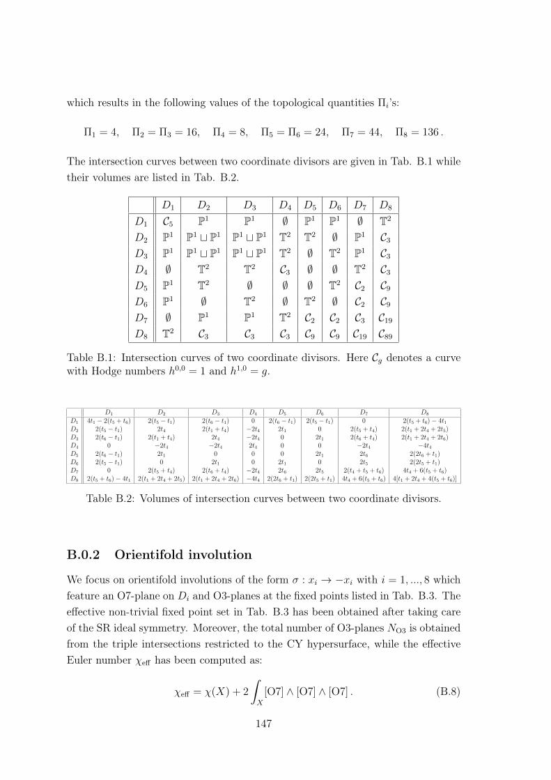
which results in the following values of the topological quantities Πi’s:

Π1 = 4, Π2 = Π3 = 16, Π4 = 8, Π5 = Π6 = 24, Π7 = 44, Π8 = 136 .

The intersection curves between two coordinate divisors are given in Tab. B.1 whiletheir volumes are listed in Tab. B.2.

D1 D2 D3 D4 D5 D6 D7 D8

D1 C5 P1 P1 ∅ P1 P1 ∅ T2

D2 P1 P1 t P1 P1 t P1 T2 T2 ∅ P1 C3

D3 P1 P1 t P1 P1 t P1 T2 ∅ T2 P1 C3

D4 ∅ T2 T2 C3 ∅ ∅ T2 C3

D5 P1 T2 ∅ ∅ ∅ T2 C2 C9

D6 P1 ∅ T2 ∅ T2 ∅ C2 C9

D7 ∅ P1 P1 T2 C2 C2 C3 C19

D8 T2 C3 C3 C3 C9 C9 C19 C89

Table B.1: Intersection curves of two coordinate divisors. Here Cg denotes a curvewith Hodge numbers h0,0 = 1 and h1,0 = g.

D1 D2 D3 D4 D5 D6 D7 D8

D1 4t1 − 2(t5 + t6) 2(t5 − t1) 2(t6 − t1) 0 2(t6 − t1) 2(t5 − t1) 0 2(t5 + t6)− 4t1D2 2(t5 − t1) 2t4 2(t1 + t4) −2t4 2t1 0 2(t5 + t4) 2(t1 + 2t4 + 2t5)D3 2(t6 − t1) 2(t1 + t4) 2t4 −2t4 0 2t1 2(t6 + t4) 2(t1 + 2t4 + 2t6)D4 0 −2t4 −2t4 2t4 0 0 −2t4 −4t4D5 2(t6 − t1) 2t1 0 0 0 2t1 2t6 2(2t6 + t1)D6 2(t5 − t1) 0 2t1 0 2t1 0 2t5 2(2t5 + t1)D7 0 2(t5 + t4) 2(t6 + t4) −2t4 2t6 2t5 2(t4 + t5 + t6) 4t4 + 6(t5 + t6)D8 2(t5 + t6)− 4t1 2(t1 + 2t4 + 2t5) 2(t1 + 2t4 + 2t6) −4t4 2(2t6 + t1) 2(2t5 + t1) 4t4 + 6(t5 + t6) 4[t1 + 2t4 + 4(t5 + t6)]

Table B.2: Volumes of intersection curves between two coordinate divisors.

B.0.2 Orientifold involution

We focus on orientifold involutions of the form σ : xi → −xi with i = 1, ..., 8 whichfeature an O7-plane on Di and O3-planes at the fixed points listed in Tab. B.3. Theeffective non-trivial fixed point set in Tab. B.3 has been obtained after taking careof the SR ideal symmetry. Moreover, the total number of O3-planes NO3 is obtainedfrom the triple intersections restricted to the CY hypersurface, while the effectiveEuler number χeff has been computed as:

χeff = χ(X) + 2

∫X

[O7] ∧ [O7] ∧ [O7] . (B.8)

147

In what follows we shall focus on the orientifold involution σ : x7 → −x7 whichfeatures two non-intersecting O7-planes located in D1 and D7 and two O3-planes atD2D3D4 .

σ O7 O3 NO3 χ(O7) χeff

x1 → −x1 D1 tD7 D2D3D4 2 54 -192x2 → −x2 D2 D1D6D8, D3D4D7, D6D7D8 2, 2, 6 14 -208x3 → −x3 D3 D1D5D8, D2D4D7, D5D7D8 2, 2, 6 14 -208x4 → −x4 D4 D1D2D3, D1D5D6, 2, 2, 4, 4, 2 10 -200

D2D5D8, D3D6D8, D5D6D7x5 → −x5 D5 D1D3D8, D3D7D8, D2D4D8 2, 2, 4 24 -204x6 → −x6 D6 D1D2D8, D2D7D8, D3D4D8 2, 2, 4 24 -204x7 → −x7 D1 tD7 D2D3D4 2 54 -192x8 → −x8 D8 ∅ 0 224 -28

Table B.3: Fixed point set for the involutions which are reflections of the eightcoordinates xi with i = 1, ..., 8.

B.0.3 Brane setup

If the D7-tadpole cancellation condition is satisfied by placing four D7-branes on topof the O7-plane, the string loop corrections to the scalar potential involve only KKeffects since winding contributions are absent due to the absence of any intersectionbetween D7-branes and/or O7-planes. Thus loop effects are too simple to generatea viable inflationary plateau. We shall therefore focus on a slightly more complicateD7-brane setup which gives rise also to winding loop effects. This can be achievedby placing D7-branes not entirely on top of the O7-plane as follows:

8[O7] ≡ 8([D1] + [D7]) = 8 (2[D1] + [D2] + [D5]) . (B.9)

This brane setup involves three stacks of D7-branes wrapped around the divisorsD1, D2 and D5. Moreover, the condition for D3-tadpole cancellation becomes:

ND3 +Nflux

2+Ngauge =

NO3

4+χ(O7)

12+∑a

Na (χ(Da) + χ(D′a))

48= 14 ,

showing that there is space for turning on both gauge and background three-formfluxes for complex structure and dilaton stabilisation.

148

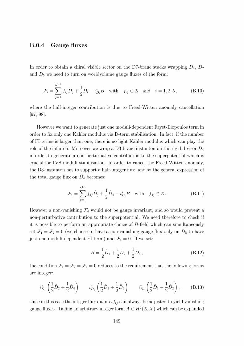
B.0.4 Gauge fluxes

In order to obtain a chiral visible sector on the D7-brane stacks wrapping D1, D2

and D5 we need to turn on worldvolume gauge fluxes of the form:

Fi =h1,1∑j=1

fijDj +1

2Di − ι∗DiB with fij ∈ Z and i = 1, 2, 5 , (B.10)

where the half-integer contribution is due to Freed-Witten anomaly cancellation[97, 98].

However we want to generate just one moduli-dependent Fayet-Iliopoulos term inorder to fix only one Kähler modulus via D-term stabilisation. In fact, if the numberof FI-terms is larger than one, there is no light Kähler modulus which can play therôle of the inflaton. Moreover we wrap a D3-brane instanton on the rigid divisor D4

in order to generate a non-perturbative contribution to the superpotential which iscrucial for LVS moduli stabilisation. In order to cancel the Freed-Witten anomaly,the D3-instanton has to support a half-integer flux, and so the general expression ofthe total gauge flux on D4 becomes:

F4 =h1,1∑j=1

f4jDj +1

2D4 − ι∗DiB with f4j ∈ Z . (B.11)

However a non-vanishing F4 would not be gauge invariant, and so would prevent anon-perturbative contribution to the superpotential. We need therefore to check ifit is possible to perform an appropriate choice of B-field which can simultaneouslyset F1 = F2 = 0 (we choose to have a non-vanishing gauge flux only on D5 to havejust one moduli-dependent FI-term) and F4 = 0. If we set:

B =1

2D1 +

1

2D2 +

1

2D4 , (B.12)

the condition F1 = F2 = F4 = 0 reduces to the requirement that the following formsare integer:

ι∗D1

(1

2D2 +

1

2D4

)ι∗D2

(1

2D1 +

1

2D4

)ι∗D4

(1

2D1 +

1

2D2

), (B.13)

since in this case the integer flux quanta fij can always be adjusted to yield vanishinggauge fluxes. Taking an arbitrary integer form A ∈ H2(Z, X) which can be expanded

149

as A = ajDj with aj ∈ Z, the pullbacks in (B.13) give rise to integer forms if:

b1 ≡∫X

(1

2D2 +

1

2D4

)∧ D1 ∧ A ∈ Z

b2 ≡∫X

(1

2D1 +

1

2D4

)∧ D2 ∧ A ∈ Z

b4 ≡∫X

(1

2D1 +

1

2D2

)∧ D4 ∧ A ∈ Z

Using the intersection polynomial (B.1) we find b1 = a5 − a1 ∈ Z, b2 = b1 − a4 ∈ Zand b4 = −a4 ∈ Z, showing how the choice of B-field in (B.12) can indeed allow forF1 = F2 = F4 = 0. The only non-zero gauge flux is F5 which does not feature anyhalf-integer contribution since c1(D5) = 0 given that D5 is a K3 surface. Given thatall the intersection numbers are even, the pullback of the B-field on D5 does alsonot generate an half-integer flux. We shall therefore consider a non-vanishing gaugeflux on the worldvolume of D5 of the form:

F5 =h1,1∑j=1

f5jDj with f5j ∈ Z . (B.14)

B.0.5 FI-term and chirality

Given that the divisor D5 is transversely invariant under the orientifold involutionand it is wrapped by four D7-branes, it supports an Sp(8) gauge group which isbroken down to U(4) = SU(4) × U(1) by a non-zero flux F5 along the diagonalU(1). This non-trivial gauge flux F5 induces also a U(1)-charge qi5 for the i-thKähler modulus of the form:

qi5 =

∫X

Di ∧ D5 ∧ F5 . (B.15)

Thus F5 6= 0 yields:

q15 = 2(f56 − f51) q45 = q55 = 0 q65 = 2f51 , (B.16)

together with a flux-dependent correction to the gauge kinetic function which lookslike:

Re(f5) = α−15 =

4π

g25

= τ5 − h(F5)Re(S) , (B.17)

where:h(F5) =

1

2

∫X

D5 ∧ F5 ∧ F5 =1

2(f51q15 + f56q65) . (B.18)

150

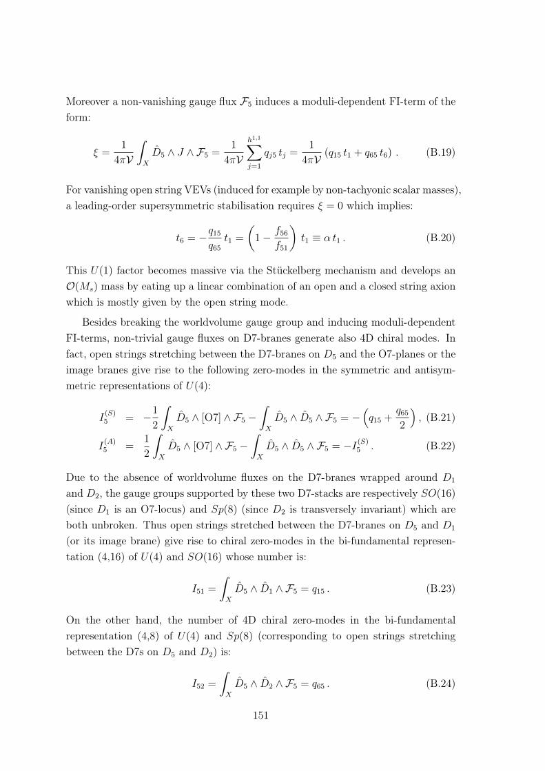
Moreover a non-vanishing gauge flux F5 induces a moduli-dependent FI-term of theform:

ξ =1

4πV

∫X

D5 ∧ J ∧ F5 =1

4πV

h1,1∑j=1

qj5 tj =1

4πV(q15 t1 + q65 t6) . (B.19)

For vanishing open string VEVs (induced for example by non-tachyonic scalar masses),a leading-order supersymmetric stabilisation requires ξ = 0 which implies:

t6 = −q15

q65

t1 =

(1− f56

f51

)t1 ≡ α t1 . (B.20)

This U(1) factor becomes massive via the Stückelberg mechanism and develops anO(Ms) mass by eating up a linear combination of an open and a closed string axionwhich is mostly given by the open string mode.

Besides breaking the worldvolume gauge group and inducing moduli-dependentFI-terms, non-trivial gauge fluxes on D7-branes generate also 4D chiral modes. Infact, open strings stretching between the D7-branes on D5 and the O7-planes or theimage branes give rise to the following zero-modes in the symmetric and antisym-metric representations of U(4):

I(S)5 = −1

2

∫X

D5 ∧ [O7] ∧ F5 −∫X

D5 ∧ D5 ∧ F5 = −(q15 +

q65

2

), (B.21)

I(A)5 =

1

2

∫X

D5 ∧ [O7] ∧ F5 −∫X

D5 ∧ D5 ∧ F5 = −I(S)5 . (B.22)

Due to the absence of worldvolume fluxes on the D7-branes wrapped around D1

and D2, the gauge groups supported by these two D7-stacks are respectively SO(16)

(since D1 is an O7-locus) and Sp(8) (since D2 is transversely invariant) which areboth unbroken. Thus open strings stretched between the D7-branes on D5 and D1

(or its image brane) give rise to chiral zero-modes in the bi-fundamental represen-tation (4,16) of U(4) and SO(16) whose number is:

I51 =

∫X

D5 ∧ D1 ∧ F5 = q15 . (B.23)

On the other hand, the number of 4D chiral zero-modes in the bi-fundamentalrepresentation (4,8) of U(4) and Sp(8) (corresponding to open strings stretchingbetween the D7s on D5 and D2) is:

I52 =

∫X

D5 ∧ D2 ∧ F5 = q65 . (B.24)

151

We need finally to check that there are no chiral intersections between the D7s onD5 and the instanton on D4 to make sure that the prefactor of the non-perturbativecontribution to the superpotential is indeed non-zero. This is ensured by the factthat:

I54 =

∫X

D5 ∧ D4 ∧ F5 = 0 . (B.25)

B.0.6 Inflationary potential

Using the D-term fixing relation (B.20), the Kähler cone conditions (B.4) simplifyto t5 > t1 > −t4 > 0 and α > 1. Moreover the CY volume (B.6) reduces to:

V = (2α− 1) t5t21 −

(α− 2

3

)t31 +

t343

= tbτf −1

3τ

3/24 . (B.26)

Given that this form is linear in t5, the effective CY volume after D-term stabilisationlooks like a K3 fibre τf over a P1 base tb whose volumes are given by:

τf = τ5 = (2α− 1) t21 and tb = t5 −(α− 2

3

)(2α− 1)

t1 . (B.27)

Notice that the Kähler cone condition t5 > t1 can be rewritten as:

τf < σ(α)V2/3 , (B.28)

where:

σ(α) ≡ (2α− 1)

(3

3α− 1

)2/3

with α > 1 . (B.29)

In terms of the canonically normalised inflaton shifted from its minimum, the con-dition (B.28) reads:

τf = 〈τf〉 e2φ/√

3 < σ V2/3 ⇔ φ <

√3

2ln

(σ

〈τf〉V2/3

). (B.30)

Let us now focus on the inflationary potential. The winding loop corrections looklike (with κ = gs/(8π) for eKcs = 1):

V W

gs = −κW20

V3

CW√τf, (B.31)

where:CW =

√2α− 1

(CW

1 +CW

2

α

). (B.32)

152

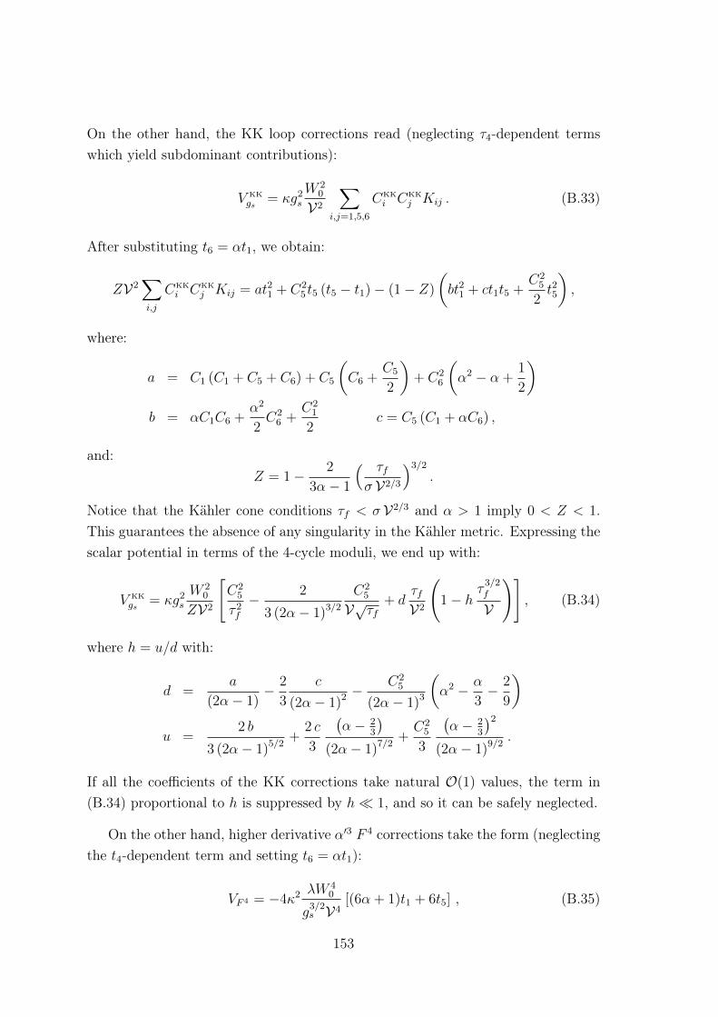
On the other hand, the KK loop corrections read (neglecting τ4-dependent termswhich yield subdominant contributions):

V KK

gs = κg2s

W 20

V2

∑i,j=1,5,6

CKK

i CKK

j Kij . (B.33)

After substituting t6 = αt1, we obtain:

ZV2∑i,j

CKK

i CKK

j Kij = at21 + C25 t5 (t5 − t1)− (1− Z)

(bt21 + ct1t5 +

C25

2t25

),

where:

a = C1 (C1 + C5 + C6) + C5

(C6 +

C5

2

)+ C2

6

(α2 − α +

1

2

)b = αC1C6 +

α2

2C2

6 +C2

1

2c = C5 (C1 + αC6) ,

and:Z = 1− 2

3α− 1

( τfσ V2/3

)3/2

.

Notice that the Kähler cone conditions τf < σ V2/3 and α > 1 imply 0 < Z < 1.This guarantees the absence of any singularity in the Kähler metric. Expressing thescalar potential in terms of the 4-cycle moduli, we end up with:

V KK

gs = κg2s

W 20

ZV2

[C2

5

τ 2f

− 2

3 (2α− 1)3/2

C25

V√τf+ d

τfV2

(1− h

τ3/2f

V

)], (B.34)

where h = u/d with:

d =a

(2α− 1)− 2

3

c

(2α− 1)2 −C2

5

(2α− 1)3

(α2 − α

3− 2

9

)u =

2 b

3 (2α− 1)5/2+

2 c

3

(α− 2

3

)(2α− 1)7/2

+C2

5

3

(α− 2

3

)2

(2α− 1)9/2.

If all the coefficients of the KK corrections take natural O(1) values, the term in(B.34) proportional to h is suppressed by h 1, and so it can be safely neglected.

On the other hand, higher derivative α′3 F 4 corrections take the form (neglectingthe t4-dependent term and setting t6 = αt1):

VF 4 = −4κ2 λW40

g3/2s V4

[(6α + 1)t1 + 6t5] , (B.35)

153

which in terms of four-cycle moduli looks like:

VF 4 = −4κ2 λW40

g3/2s V4

[12α2 + 2α− 5

(2α− 1)3/2

√τf + 6

Vτf

]. (B.36)

Therefore the total inflationary potential becomes:

V = V W

gs + V KK

gs + VF 4 = κW 2

0

V2

(A1

τ 2f

+A2

Vτf− A3

V√τf+B1√τf

V2+B2 τfV2

), (B.37)

where (with λ = −|λ| < 0):

A1 =g2s

ZC2

5 A2 =3

π

|λ|W 20√

gsA3 = CW +

g2s

Z

2C25

3 (2α− 1)3/2' CW (B.38)

and:B1 =

12α2 + 2α− 5

6(2α− 1)3/2A2 B2 =

g2s d

Z. (B.39)

The potential (B.37) could support single-field slow-roll inflation driven by τf [14,78]. In order to get enough efoldings before hitting the walls of the Kähler conegiven in (B.30), we need to focus on the region in field space where the inflatonminimum is of order 〈τf〉 V2/3. Numerical estimates show that we need valuesof order 〈τf〉 ∼ O(1) and V ∼ O(104) which, in turn, imply W0 ∼ O(100) in orderto match the observed amplitude of the density perturbations. For gs . O(0.1),|λ| ∼ O(10−3) and natural O(1) values of the coefficients of the string loop effects,the terms in (B.37) proportional to B1 and B2 are both negligible with respect tothe first three terms in the vicinity of the minimum where τf ∼ O(1) V2/3.

The scalar potential (B.37) written in terms of the canonically normalised infla-ton φ = 〈φ〉+ φ looks like (with k = 2/

√3):

V = κA1W

20

〈τf〉2V2

(CdS + e−2kφ + λ1Z e

−kφ − λ2Z e− kφ

2 +R1Z ekφ2 +R2 e

kφ), (B.40)

where we added a constant CdS = λ2Z−λ1Z−1−R1Z−R2 to obtain a Minkowski(or slightly dS) vacuum and:

λ1 =3〈τf〉πC2

5

|λ|W 20

g5/2s V

∼ O(1− 10) λ2 '〈τf〉3/2

C25

CW

g2s V∼ O(1− 10) ,

154

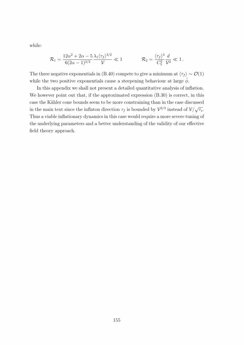
while:

R1 =12α2 + 2α− 5

6(2α− 1)3/2

λ1〈τf〉3/2

V 1 R2 =

〈τf〉3

C25

d

V2 1 .

The three negative exponentials in (B.40) compete to give a minimum at 〈τf〉 ∼ O(1)

while the two positive exponentials cause a steepening behaviour at large φ.In this appendix we shall not present a detailed quantitative analysis of inflation.

We however point out that, if the approximated expression (B.30) is correct, in thiscase the Kähler cone bounds seem to be more constraining than in the case discussedin the main text since the inflaton direction τf is bounded by V2/3 instead of V/√τs.Thus a viable inflationary dynamics in this case would require a more severe tuning ofthe underlying parameters and a better understanding of the validity of our effectivefield theory approach.

155

156

Appendix C

Computational details

C.0.1 Closed string axion decay constants

In type IIB string compactifications on Calabi-Yau orientifolds axion-like particlesemerge in the low-energy N = 1 effective field theory from the dimensional reductionof the Ramond-Ramond forms Cp with p = 2, 4. The Kaluza-Klein decompositionunder the orientifold projection of these forms is given by [224]:

C2 = ci−(x) Di− and C4 = ci+(x)Di+ +Qi+2 (x)∧Di+ +V a+(x)∧αa+−Va+(x)∧βa+ ,

where i± = 1, ..., h1,1± , a+ = 1, ..., h1,2

+ , Di+ is a basis of H2,2+ dual to the (1, 1)-forms

Di+ and (αa+ , βa+) is a real, symplectic basis of H3

+ = H1,2+ ⊕H

2,1+ .

As explained in Sec. 4.2.1, in our model the orientifold-odd axions ci− , if present,are eaten up by anomalous U(1)’s in the process of anomaly cancellation. We shalltherefore focus on the case with h1,1

− = 0 where the Kähler moduli take the simpleexpression Ti = τi + i ci with i = 1, ..., h1,1

+ = h1,1.The coupling of orientifold-even closed string axions to F ∧ F can be derived

from the Kaluza-Klein reduction of the Chern-Simons term of the D-brane action.Moreover, the periods of the canonically unnormalised axions ci are integer multiplesof Mp and their kinetic terms read [187]:

Lkin = Kij∂µci∂µcj =

1

8ηi ∂µc

′i∂µc′i , (C.1)

where the c′i’s are the axions which diagonalise the Kähler metric Kij and ηi areits eigenvalues. A proper canonical normalisation of the kinetic terms can then beeasily obtained by defining:

1

8ηi∂µc

′i∂µc′i ≡

1

2∂µai∂

µai with ai =1

2

√ηi c′i , (C.2)

157

which shows that the canonically normalised axions ai acquire periods of the form:

2√ηiai =

2√ηiai +Mp ⇒ ai = ai +

√ηi

2Mp . (C.3)

We can then set the conventional axionic period as:

ai = ai + 2πfai with fai =

√ηiMp

4π, (C.4)

where fai is the standard axion decay constant. Closed string axions which propagatein the bulk of the extra dimensions have a decay constant of order the Kaluza-Klein scale MKK ∼ Mp/V2/3, whereas the decay constant of closed string axionswhose corresponding saxion parameterises the volume of localised blow-up modes iscontrolled by the string scale Ms ∼Mp/

√V :

fai '

Mp/τi ∼MKK bulk axionMp/√V ∼Ms local axion

(C.5)

Notice however that the axion coupling to the Abelian gauge bosons living on theD-brane wrapping the four-cycle whose volume is controlled by the associated saxionτi, is given by:

g2i

32π2

aifai

F (i)µν F

µν(i) =

1

32π2

aiτifai

F (i)µν F

µν(i) , (C.6)

since the gauge coupling is set by the saxion as g2i = τi. Hence combining (C.5) with

(C.6) we realise that that the coupling of bulk closed string axions to gauge bosonsis controlled by M ∼ τifai ∼ Mp, in agreement with the fact that moduli coupleto ordinary matter with gravitational strength. On the other hand the coupling oflocal closed string axions to gauge bosons is set by the string scale Ms which inLVS models with exponentially large volume can be considerably smaller than thePlanck scale.

C.0.2 Canonical normalisation

The kinetic terms for all Kähler moduli and the charged open string modes φ and Ccan be derived from the total Kähler potential K = Kmod +Kmatter, where Kmod isgiven by the three contributions in (4.38) and Kmatter is shown in (4.39) and (4.40),as follows:

Lkin =∂2K

∂χi∂χj∂µχi∂

µχj , (C.7)

158

where χi denotes an arbitrary scalar field of our model. As can be seen from (4.39),the D7 open string mode φ mixes only with the dilaton S, and so can be easilywritten in terms of the corresponding canonically normalised field φ as:

φ

Mp

=

√2

Re(S)φ . (C.8)

From the first term in (4.38) we also realise that cross-terms between the blow-upmode τqi and any of the other Kähler moduli are highly suppressed when evaluatedat the minimum for τqi ' 0 (more precisely, as discussed in Sec. 4.2.3, dependingon the level of sequestering of soft masses, we can have either τqi ∼ V−1 1

or τqi ∼ V−3 1). Hence it is straightforward to write also τqi in terms of thecorresponding canonically normalised field φqi as:

φqiMp

=τqi√V

for i = 1, 2 . (C.9)

The remaining fields Tb, Ts, Tp and C mix with each other, leading to a non-trivialKähler metric whose components take the following leading order expressions forV ' λbτ

3/2b 1:

KTiTj' 3

8V

2λb√τb

− 3τb

(λs√τs + xλp

√τp)− 3τbλp√τp

− 3τb

(λs√τs + xλp

√τp)

λs√τs

+ x2λp√τp

xλp√τp

− 3τbλp√τp

xλp√τp

λp√τp

KTbC ' − K

2 τbC , KTsC '

K

2V

(λs√τs + xλp

√τp

)C ,

KTpC ' K

2Vλp√τpC , KCC = K .

In the large volume limit, different contributions to the kinetic Lagrangian can beorganised in an expansion in 1/V 1 as follows:

Lkin = LO(1)kin + LO(V−1)

kin + LO(V−4/3)kin ,

159

where, trading Tp for Tp = Tp + xTs, we have:

LO(1)kin =

3

4 τ 2b

∂µτb∂µτb ,

LO(V−1)kin =

3

8V

[λs√τs

(∂µτs∂µτs + ∂µcs∂

µcs) +λp√τp

(∂µτp∂µτp + ∂µcp∂

µcp)

]− 9

4V∂µτbτb

(λs√τs ∂

µτs + λp√τp ∂

µτp

),

LO(V−4/3)kin =

3

4 τ 2b

∂µcb∂µcb .

At leading order the kinetic terms become canonical if τb is replaced by φb definedas:

φbMp

=

√3

2ln τb , (C.10)

whereas LO(V−1)kin becomes diagonal if the small modulus Ts and the Wilson modulus

Tp are substituted by:

φsMp

=

√4λs3V

τ 3/4s ,

asMp

=

√3λs

4V√τscs ,

φpMp

=

√4λp3V

τ 3/4p ,

apMp

=

√3λp

4V√τpcp , (C.11)

and the canonical normalisation (C.10) for τb gets modified by the inclusion of asubleading mixing with τs and τp of the form:

φbMp

=

√3

2ln τb −

√2

3

1

V(λsτ

3/2s + λpτ

3/2p

). (C.12)

Finally the kinetic term in LO(V−4/3)kin are canonically normalised if the bulk axion cb

gets redefined as:abMp

=

√3

2

cbτb. (C.13)

The U(1)-charged open string mode C appears in the kinetic Lagrangian only atO(|C|2V−2/3) which according to (4.60) and (4.61) can scale as either V−8/3 or V−14/3.This part of the kinetic Lagrangian looks like:

Lkin ⊃ K |C|2(∂µ|C||C|

∂µ|C||C|

+ ∂µθ∂µθ − ∂µτb

τb

∂µ|C||C|

), (C.14)

160

and becomes diagonal by redefining:

|C|Mp

=√

2K|C| and aALP = |C|θ = faALP θ .

C.0.3 Mass matrix

As described in Sec. 4.2.1, the moduli stabilised at tree-level are τqi and |φ| whilethe corresponding axions are eaten up by two anomalous U(1)’s. Given that theyfixed at O(1/V2), all these modes develop a mass of order the string scale:

mτqi∼ mcqi

∼ m|φ| ∼ mψ ∼Ms = g1/4s

√πMp√V. (C.15)

On the other hand, τb, τs, τp and the closed string axion cs are stabilised at O(1/V3).The masses of the corresponding canonically normalised fields derived in App. C.0.2are given by the eigenvalues of the mass matrix evaluated at the minimum of theO(1/V3) scalar potential. The leading order contributions of all the elements of this4× 4 matrix read:

∂2V

∂φb∂φb=

( gs8π

) 9λs τ3/2s

2

W 20

V3,

∂2V

∂φb∂φs=

( gs8π

) 3√

2λs τ3/4s√V

(W0

V

)2

(2πτs) ,

∂2V

∂φs∂φs=

∂2V

∂as∂as= 4

( gs8π

)(W0

V

)2

(2πτs)2 ,

∂2V

∂φp∂φp=

( gs8π

) 1

4zpτp

(W0

V

)2

,

∂2V

∂φb∂φp=

∂2V

∂φb∂as=

∂2V

∂φs∂φp=

∂2V

∂φs∂as=

∂2V

∂φp∂as= 0 ,

The eigenvalues of this mass matrix turn out to be:

m2φs = m2

as = 4( gs

8π

)(W0

V

)2

(2πτs)2 ' m2

3/2 (lnV)2 ,

m2φp

=( gs

8π

) π

2zp

(W0

V

)21

2πτp'm2

3/2

lnVand m2

φb= 0 , (C.16)

where the gravitino mass is given by:

m23/2 = eK |W |2 '

( gs8π

)(W0

V

)2

. (C.17)

161

The mass of the canonically normalised large modulus φb becomes non-zero once weinclude subleading 1/(2πτs) ∼ 1/ lnV 1 corrections to the elements of the massmatrix, and scales as (with c an O(1) numerical coefficient):

m2φb

= c λsτ3/2s

( gs8π

)W 20

V3

1

2πτs'

m23/2

V lnV. (C.18)

As explained in Sec. 4.2.3, the charged matter field |C| is fixed by soft supersymme-try breaking contributions to the scalar potential and can acquire a mass of orderm3/2/

√V or m3/2/V depending on the level of sequestering. The corresponding

phase θ = aALP/faALP behaves as an open string ALP which develops a mass oforder:

maALP ∼Λ2

hid

faALP∼ Λ2

hid

|C|, (C.19)

where Λhid is the scale of strong dynamics effects in the hidden sector. In orderto obtain a phenomenologically viable value maALP . 10−12 eV, we need to haveΛhid . 104 eV if faALP ∼ m3/2 ∼ 1010 GeV or Λhid . 1 eV if faALP ∼ m3/2/V ∼ 1

TeV.The DM axion cp is stabilised by tiny poly-instanton corrections at O(1/V3+p).

Using the fact that K−1TpTp∼ V

√τp and the expression (4.62) for the scalar potential

for cp, its mass can be easily estimated as:

m2ap ∼ K−1

TpTp

∂2V polyF (cp)

∂c2p

∼( gs

8π

) W 20

V2+p2πτp ∼

m23/2

VplnV . (C.20)

If the volume is of order V ∼ 107, this mass can be around 10 keV if p = 9/2.As explained in Sec. 4.3.2 this value of p can be accommodated by an appropriatechoice of underlying flux parameters. Finally the axion cb of the large modulusTb = τb + i cb can receive a potential only from highly suppressed non-perturbativecontributions to the superpotential of the formWnp ⊃ Ab e

−2πTb which can be shownto lead to a mass for the axion cb that scales as:

m2ab∼( gs

8π

) M2p

V4/3e− 2π

λ2/3b

V2/3

∼ 0 . (C.21)

162

Bibliography

[1] M. Cicoli, V. A. Diaz, V. Guidetti and M. Rummel, JHEP 1710, 192 (2017)

[2] M. Cicoli, D. Ciupke, V. A. Diaz, V. Guidetti, F. Muia and P. Shukla, JHEP1711, 207 (2017).

[3] M. Cicoli, V. A. Diaz and F. G. Pedro, JCAP 1806, no. 06, 034 (2018).

[4] D. N. Spergel et al. [WMAP Collaboration], Astrophys. J. Suppl. 148, 175(2003).

[5] D. N. Spergel et al. [WMAP Collaboration], Astrophys. J. Suppl. 170, 377(2007).

[6] E. Komatsu et al. [WMAP Collaboration], Astrophys. J. Suppl. 180, 330(2009).

[7] N. Aghanim et al. [Planck Collaboration], “Planck 2018 results. VI. Cosmolog-ical parameters,” arXiv:1807.06209 [astro-ph.CO].

[8] A. H. Guth, Phys. Rev. D 23, 347 (1981).

[9] A. D. Linde, Phys. Lett. 108B, 389 (1982).

[10] V. F. Mukhanov and G. V. Chibisov, JETP Lett. 33, 532 (1981) [Pisma Zh.Eksp. Teor. Fiz. 33, 549 (1981)].

[11] A. H. Guth and S. Y. Pi, Phys. Rev. Lett. 49, 1110 (1982).

[12] A. D. Linde, Phys. Lett. 129B, 177 (1983).

[13] M. Cicoli and F. Quevedo, Class. Quant. Grav. 28, 204001 (2011).

[14] M. Cicoli, C. P. Burgess and F. Quevedo, JCAP 0903, 013 (2009).

[15] L. McAllister, E. Silverstein and A. Westphal, Phys. Rev. D 82, 046003 (2010).

163

[16] V. Mukanov, “Physical Foundations of Cosmology,” Cambridge UniversityPress, (2008).

[17] D. Baumann and L. McAllister, “Inflation and String Theory,” Cambridge Uni-versity Press, (2015).

[18] C. P. Burgess, “Intro to Effective Field Theories and Inflation,”arXiv:1711.10592 [hep-th].

[19] O. Y. Gnedin and J. P. Ostriker, “Limits on collisional dark matter from ellip-tical galaxies in clusters,” Astrophys. J. 561, 61 (2001).

[20] E. Aprile et al. [XENON100 Collaboration], “Dark Matter Results from 225Live Days of XENON100 Data,” Phys. Rev. Lett. 109, 181301 (2012).

[21] D. S. Akerib et al. [LUX Collaboration], “Results from a search for dark matterin the complete LUX exposure,” Phys. Rev. Lett. 118, no. 2, 021303 (2017).

[22] W. B. Atwood et al. [Fermi-LAT Collaboration], “The Large Area Telescopeon the Fermi Gamma-ray Space Telescope Mission,” Astrophys. J. 697, 1071(2009).

[23] G. Steigman and M. S. Turner, “Cosmological Constraints on the Properties ofWeakly Interacting Massive Particles,” Nucl. Phys. B 253, 375 (1985).

[24] R. D. Peccei and H. R. Quinn, “CP Conservation in the Presence of Instantons,”Phys. Rev. Lett. 38, 1440 (1977).

[25] G. Ballesteros and M. Taoso, Phys. Rev. D 97, no. 2, 023501 (2018)doi:10.1103/PhysRevD.97.023501 [arXiv:1709.05565 [hep-ph]].

[26] B. P. Abbott et al. [LIGO Scientific and Virgo Collaborations], Phys.Rev. Lett. 116, no. 6, 061102 (2016) doi:10.1103/PhysRevLett.116.061102[arXiv:1602.03837 [gr-qc]].

[27] B. P. Abbott et al. [LIGO Scientific and VIRGO Collaborations], Phys.Rev. Lett. 118, no. 22, 221101 (2017) doi:10.1103/PhysRevLett.118.221101[arXiv:1706.01812 [gr-qc]].

[28] R. Blumenhagen, D. Lüst, and S. Theisen, “Basic Concepts of String Theory",Cambridge University Press, (2013).

[29] L. E. Ibáñez and A. M. Uranga, “String Theory and Particle Physics: AnIntroduction to String Phenomenology", Cambridge University Press, (2012).

164

[30] K. Becker, M. Becker, and J. H. Schwarz,“String Theory and M-Theory: AModern Introduction", Cambridge University Press, (2007).

[31] J. Polchinski, “String Theory, Vols. 1 y 2", Cambridge University Press, (2005).

[32] M. Duff, B.E.W. Nilsson, and C. Pope, “Kaluza-Klein Supergravity", Phys.Rept. 130 (1986) 1-142.

[33] J. Wess and J. Bagger, “Supersymmetry And Supergravity", Princeton Univer-sity Press, Princeton, (1992).

[34] T. W. Grimm and J. Louis, Nucl. Phys. B699 (2004) 387-426

[35] S. B. Giddings, S. Kachru and J. Polchinski, “Hierarchies from fluxes in stringcompactifications,” Phys. Rev. D 66 (2002) 106006.

[36] K. Becker, M. Becker, M. Haack and J. Louis, “Supersymmetry breaking andalpha-prime corrections to flux induced potentials,” JHEP 0206 (2002) 060.

[37] R. Minasian, T. G. Pugh and R. Savelli, “F-theory at order α′3,” JHEP 1510(2015) 050.

[38] G. von Gersdorff and A. Hebecker, Phys. Lett. B 624, 270 (2005).

[39] M. Berg, M. Haack and B. Kors, “String loop corrections to Kahler potentialsin orientifolds,” JHEP 0511 (2005) 030.

[40] M. Berg, M. Haack and E. Pajer, “Jumping Through Loops: On Soft Termsfrom Large Volume Compactifications,” JHEP 0709 (2007) 031.

[41] M. Cicoli, J. P. Conlon and F. Quevedo, “Systematics of String Loop Correctionsin Type IIB Calabi-Yau Flux Compactifications,” JHEP 0801 (2008) 052.

[42] M. Cicoli, J. P. Conlon and F. Quevedo, “General Analysis of LARGE VolumeScenarios with String Loop Moduli Stabilisation,” JHEP 0810 (2008) 105.

[43] V. Balasubramanian, P. Berglund, J. P. Conlon and F. Quevedo, “Systematics ofmoduli stabilisation in Calabi-Yau flux compactifications,” JHEP 0503 (2005)007

[44] J. P. Conlon, F. Quevedo and K. Suruliz, “Large-volume flux compactifications:Moduli spectrum and D3/D7 soft supersymmetry breaking,” JHEP 0508 (2005)007

165

[45] D. H. Lyth, “What would we learn by detecting a gravitational wave signalin the cosmic microwave background anisotropy?,” Phys. Rev. Lett. 78 (1997)1861 doi:10.1103/PhysRevLett.78.1861 [hep-ph/9606387].

[46] L. McAllister and E. Silverstein, “String Cosmology: A Review,” Gen. Rel.Grav. 40 (2008) 565 doi:10.1007/s10714-007-0556-6 [arXiv:0710.2951 [hep-th]].

[47] D. Baumann and L. McAllister, “Advances in Inflation in String Theory,” Ann.Rev. Nucl. Part. Sci. 59 (2009) 67 doi:10.1146/annurev.nucl.010909.083524[arXiv:0901.0265 [hep-th]].

[48] C. P. Burgess, M. Cicoli and F. Quevedo, “String Inflation After Planck 2013,”JCAP 1311 (2013) 003 doi:10.1088/1475-7516/2013/11/003 [arXiv:1306.3512[hep-th]].

[49] C. P. Burgess, M. Cicoli, F. Quevedo and M. Williams, “Inflating with LargeEffective Fields,” JCAP 1411 (2014) 045 doi:10.1088/1475-7516/2014/11/045[arXiv:1404.6236 [hep-th]].

[50] R. Blumenhagen, S. Moster and E. Plauschinn, “Moduli Stabilisation ver-sus Chirality for MSSM like Type IIB Orientifolds,” JHEP 0801 (2008) 058doi:10.1088/1126-6708/2008/01/058 [arXiv:0711.3389 [hep-th]].

[51] D. R. Green, “Reheating Closed String Inflation,” Phys. Rev. D 76 (2007)103504 doi:10.1103/PhysRevD.76.103504 [arXiv:0707.3832 [hep-th]].

[52] R. H. Brandenberger, A. Knauf and L. C. Lorenz, “Reheating in a BraneMonodromy Inflation Model,” JHEP 0810 (2008) 110 doi:10.1088/1126-6708/2008/10/110 [arXiv:0808.3936 [hep-th]].

[53] N. Barnaby, J. R. Bond, Z. Huang and L. Kofman, “Preheating After Mod-ular Inflation,” JCAP 0912 (2009) 021 doi:10.1088/1475-7516/2009/12/021[arXiv:0909.0503 [hep-th]].

[54] M. Cicoli and A. Mazumdar, “Reheating for Closed String Inflation,” JCAP1009 (2010) no.09, 025 doi:10.1088/1475-7516/2010/09/025 [arXiv:1005.5076[hep-th]]; M. Cicoli and A. Mazumdar, “Inflation in string theory: AGraceful exit to the real world,” Phys. Rev. D 83 (2011) 063527doi:10.1103/PhysRevD.83.063527 [arXiv:1010.0941 [hep-th]].

[55] K. Dutta and A. Maharana, “Inflationary constraints on modu-lus dominated cosmology,” Phys. Rev. D 91 (2015) no.4, 043503doi:10.1103/PhysRevD.91.043503 [arXiv:1409.7037 [hep-ph]].

166

[56] M. Cicoli, K. Dutta, A. Maharana and F. Quevedo, “Moduli Vacuum Misalign-ment and Precise Predictions in String Inflation,” JCAP 1608 (2016) no.08,006 doi:10.1088/1475-7516/2016/08/006 [arXiv:1604.08512 [hep-th]].

[57] S. Bhattacharya, K. Dutta and A. Maharana, “Constrains on Kähler ModuliInflation from Reheating,” arXiv:1707.07924 [hep-ph].

[58] M. Cicoli, J. P. Conlon and F. Quevedo, “Dark radiation inLARGE volume models,” Phys. Rev. D 87 (2013) no.4, 043520doi:10.1103/PhysRevD.87.043520 [arXiv:1208.3562 [hep-ph]].

[59] T. Higaki and F. Takahashi, “Dark Radiation and Dark Matter in Large Vol-ume Compactifications,” JHEP 1211 (2012) 125 doi:10.1007/JHEP11(2012)125[arXiv:1208.3563 [hep-ph]].

[60] A. Hebecker, P. Mangat, F. Rompineve and L. T. Witkowski, “Dark Radia-tion predictions from general Large Volume Scenarios,” JHEP 1409 (2014) 140doi:10.1007/JHEP09(2014)140 [arXiv:1403.6810 [hep-ph]].

[61] M. Cicoli and F. Muia, “General Analysis of Dark Radiation in SequesteredString Models,” JHEP 1512 (2015) 152 doi:10.1007/JHEP12(2015)152[arXiv:1511.05447 [hep-th]].

[62] B. S. Acharya, P. Kumar, K. Bobkov, G. Kane, J. Shao and S. Watson, “Non-thermal Dark Matter and the Moduli Problem in String Frameworks,” JHEP0806 (2008) 064 doi:10.1088/1126-6708/2008/06/064 [arXiv:0804.0863 [hep-ph]].

[63] R. Allahverdi, M. Cicoli, B. Dutta and K. Sinha, “Nonthermal dark mat-ter in string compactifications,” Phys. Rev. D 88 (2013) no.9, 095015doi:10.1103/PhysRevD.88.095015 [arXiv:1307.5086 [hep-ph]]; R. Allahverdi,M. Cicoli, B. Dutta and K. Sinha, “Correlation between Dark Matterand Dark Radiation in String Compactifications,” JCAP 1410 (2014) 002doi:10.1088/1475-7516/2014/10/002 [arXiv:1401.4364 [hep-ph]].

[64] L. Aparicio, M. Cicoli, B. Dutta, S. Krippendorf, A. Maharana, F. Muia andF. Quevedo, “Non-thermal CMSSM with a 125 GeV Higgs,” JHEP 1505 (2015)098 doi:10.1007/JHEP05(2015)098 [arXiv:1502.05672 [hep-ph]]; L. Aparicio,B. Dutta, M. Cicoli, F. Muia and F. Quevedo, “Light Higgsino Dark Mat-ter from Non-thermal Cosmology,” JHEP 1611 (2016) 038 [arXiv:1607.00004[hep-ph]].

167

[65] G. Kane, J. Shao, S. Watson and H. B. Yu, “The Baryon-Dark Matter RatioVia Moduli Decay After Affleck-Dine Baryogenesis,” JCAP 1111 (2011) 012doi:10.1088/1475-7516/2011/11/012 [arXiv:1108.5178 [hep-ph]].

[66] R. Allahverdi, M. Cicoli and F. Muia, “Affleck-Dine Baryogenesis in TypeIIB String Models,” JHEP 1606 (2016) 153 doi:10.1007/JHEP06(2016)153[arXiv:1604.03120 [hep-th]].

[67] J. P. Conlon, R. Kallosh, A. D. Linde and F. Quevedo, “Volume Mod-ulus Inflation and the Gravitino Mass Problem,” JCAP 0809 (2008) 011doi:10.1088/1475-7516/2008/09/011 [arXiv:0806.0809 [hep-th]]; M. Cicoli,F. Muia and F. G. Pedro, “Microscopic Origin of Volume Modulus In-flation,” JCAP 1512 (2015) no.12, 040 doi:10.1088/1475-7516/2015/12/040[arXiv:1509.07748 [hep-th]].

[68] T. He, S. Kachru and A. Westphal, “Gravity waves and the LHC: To-wards high-scale inflation with low-energy SUSY,” JHEP 1006 (2010) 065doi:10.1007/JHEP06(2010)065 [arXiv:1003.4265 [hep-th]].

[69] S. Antusch, K. Dutta and S. Halter, “Combining High-scale Inflation withLow-energy SUSY,” JHEP 1203 (2012) 105 doi:10.1007/JHEP03(2012)105[arXiv:1112.4488 [hep-th]].

[70] W. Buchmuller, E. Dudas, L. Heurtier and C. Wieck, “Large-FieldInflation and Supersymmetry Breaking,” JHEP 1409 (2014) 053doi:10.1007/JHEP09(2014)053 [arXiv:1407.0253 [hep-th]].

[71] J. P. Conlon and F. Quevedo, “Kahler moduli inflation,” JHEP 0601 (2006)146 doi:10.1088/1126-6708/2006/01/146 [hep-th/0509012].

[72] M. Cicoli, I. García-Etxebarria, C. Mayrhofer, F. Quevedo, P. Shukla and R. Va-landro, “Global Orientifolded Quivers with Inflation,” arXiv:1706.06128 [hep-th].

[73] M. Berg, M. Haack, J. U. Kang and S. Sjörs, “Towards the one-loop Kähler metric of Calabi-Yau orientifolds,” JHEP 1412 (2014) 077doi:10.1007/JHEP12(2014)077 [arXiv:1407.0027 [hep-th], arXiv:1407.0027].

[74] M. Haack and J. U. Kang, “One-loop Einstein-Hilbert term in min-imally supersymmetric type IIB orientifolds,” JHEP 1602 (2016) 160doi:10.1007/JHEP02(2016)160 [arXiv:1511.03957 [hep-th]].

168

[75] D. Ciupke, J. Louis and A. Westphal, “Higher-Derivative Supergravity andModuli Stabilization,” JHEP 1510 (2015) 094 doi:10.1007/JHEP10(2015)094[arXiv:1505.03092 [hep-th]].

[76] T. W. Grimm, K. Mayer and M. Weissenbacher, “Higher derivatives in Type IIand M-theory on Calabi-Yau threefolds,” arXiv:1702.08404 [hep-th].

[77] B. J. Broy, D. Ciupke, F. G. Pedro and A. Westphal, “Starobinsky-TypeInflation from α′-Corrections,” JCAP 1601 (2016) 001 doi:10.1088/1475-7516/2016/01/001 [arXiv:1509.00024 [hep-th]].

[78] M. Cicoli, D. Ciupke, S. de Alwis and F. Muia, “α′ Inflation: moduli stabili-sation and observable tensors from higher derivatives,” JHEP 1609 (2016) 026doi:10.1007/JHEP09(2016)026 [arXiv:1607.01395 [hep-th]].

[79] C. P. Burgess, M. Cicoli, S. de Alwis and F. Quevedo, “Robust Infla-tion from Fibrous Strings,” JCAP 1605 (2016) no.05, 032 doi:10.1088/1475-7516/2016/05/032 [arXiv:1603.06789 [hep-th]].

[80] Y. Akrami et al. [Planck Collaboration], “Planck 2018 results. X. Constraintson inflation,” arXiv:1807.06211 [astro-ph.CO].

[81] R. Kallosh, A. Linde, D. Roest, A. Westphal and Y. Yamada, “Fibre Inflationand α-attractors,” arXiv:1707.05830 [hep-th].

[82] M. Cicoli, F. Muia and P. Shukla, “Global Embedding of Fibre Inflation Mod-els,” JHEP 1611 (2016) 182 doi:10.1007/JHEP11(2016)182 [arXiv:1611.04612[hep-th]].

[83] M. Cicoli, M. Kreuzer and C. Mayrhofer, “Toric K3-Fibred Calabi-Yau Mani-folds with del Pezzo Divisors for String Compactifications,” JHEP 1202 (2012)002 doi:10.1007/JHEP02(2012)002 [arXiv:1107.0383 [hep-th]].

[84] M. Kreuzer and H. Skarke, “Complete classification of reflexive polyhedra infour-dimensions,” Adv. Theor. Math. Phys. 4 (2002) 1209 [hep-th/0002240].

[85] S. Angus, “Dark Radiation in Anisotropic LARGE Volume Compactifications,”JHEP 1410 (2014) 184 doi:10.1007/JHEP10(2014)184 [arXiv:1403.6473 [hep-ph]].

[86] M. Cicoli, J. P. Conlon, A. Maharana and F. Quevedo, “A Note onthe Magnitude of the Flux Superpotential,” JHEP 1401 (2014) 027doi:10.1007/JHEP01(2014)027 [arXiv:1310.6694 [hep-th]].

169

[87] F. Bonetti and M. Weissenbacher, “The Euler characteristic correc-tion to the KÃďhler potential âĂŤ revisited,” JHEP 1701 (2017) 003doi:10.1007/JHEP01(2017)003 [arXiv:1608.01300 [hep-th]].

[88] S. Kachru, R. Kallosh, A. D. Linde and S. P. Trivedi, “De Sitter vacua in stringtheory,” Phys. Rev. D 68 (2003) 046005 doi:10.1103/PhysRevD.68.046005 [hep-th/0301240].

[89] R. Kallosh and T. Wrase, “Emergence of Spontaneously Broken Supersym-metry on an Anti-D3-Brane in KKLT dS Vacua,” JHEP 1412 (2014) 117doi:10.1007/JHEP12(2014)117 [arXiv:1411.1121 [hep-th]];

R. Kallosh, F. Quevedo and A. M. Uranga, “String Theory Realizations of theNilpotent Goldstino,” JHEP 1512 (2015) 039 doi:10.1007/JHEP12(2015)039[arXiv:1507.07556 [hep-th]]; L. Aparicio, F. Quevedo and R. Valandro, “ModuliStabilisation with Nilpotent Goldstino: Vacuum Structure and SUSY Break-ing,” JHEP 1603 (2016) 036 doi:10.1007/JHEP03(2016)036 [arXiv:1511.08105[hep-th]]; M. P. Garcia del Moral, S. Parameswaran, N. Quiroz and I. Zavala,“Anti-D3 branes and moduli in non-linear supergravity,” arXiv:1707.07059 [hep-th]; J. Moritz, A. Retolaza and A. Westphal, “Towards de Sitter from 10D,”arXiv:1707.08678 [hep-th].

[90] E. A. Bergshoeff, K. Dasgupta, R. Kallosh, A. Van Proeyen andT. Wrase, “D3 and dS,” JHEP 1505 (2015) 058 doi:10.1007/JHEP05(2015)058[arXiv:1502.07627 [hep-th]].

[91] I. GarcÃŋa-Etxebarria, F. Quevedo and R. Valandro, “Global StringEmbeddings for the Nilpotent Goldstino,” JHEP 1602 (2016) 148doi:10.1007/JHEP02(2016)148 [arXiv:1512.06926 [hep-th]].

[92] M. Cicoli, F. Quevedo and R. Valandro, “De Sitter from T-branes,” JHEP 1603(2016) 141 doi:10.1007/JHEP03(2016)141 [arXiv:1512.04558 [hep-th]].

[93] M. Cicoli, A. Maharana, F. Quevedo and C. P. Burgess, “De Sitter StringVacua from Dilaton-dependent Non-perturbative Effects,” JHEP 1206 (2012)011 doi:10.1007/JHEP06(2012)011 [arXiv:1203.1750 [hep-th]].

[94] A. Westphal, “String Cosmology âĂŤ Large-Field Inflation in String Theory,”Adv. Ser. Direct. High Energy Phys. 22 (2015) 351.

[95] M. Remazeilles, C. Dickinson, H. K. K. Eriksen and I. K. Wehus, “Sensitivityand foreground modelling for large-scale cosmic microwave background B-mode

170

polarization satellite missions,” Mon. Not. Roy. Astron. Soc. 458 (2016) no.2,2032 doi:10.1093/mnras/stw441 [arXiv:1509.04714 [astro-ph.CO]].

[96] M. Remazeilles, C. Dickinson, H. K. Eriksen and I. K. Wehus, “Joint Bayesianestimation of tensor and lensing B-modes in the power spectrum of CMB po-larization data,” arXiv:1707.02981 [astro-ph.CO].

[97] R. Minasian and G. W. Moore, “K theory and Ramond-Ramond charge,” JHEP9711 (1997) 002 doi:10.1088/1126-6708/1997/11/002 [hep-th/9710230].

[98] D. S. Freed and E. Witten, “Anomalies in string theory with D-branes,” AsianJ. Math. 3 (1999) 819 [hep-th/9907189].

[99] M. Dine, N. Seiberg and E. Witten, “Fayet-Iliopoulos Terms in String Theory,”Nucl. Phys. B 289 (1987) 589. doi:10.1016/0550-3213(87)90395-6

[100] M. Dine, I. Ichinose and N. Seiberg, “F Terms and d Terms in String Theory,”Nucl. Phys. B 293 (1987) 253. doi:10.1016/0550-3213(87)90072-1

[101] R. Altman, J. Gray, Y. H. He, V. Jejjala and B. D. Nelson, “A Calabi-YauDatabase: Threefolds Constructed from the Kreuzer-Skarke List,” JHEP 1502(2015) 158 doi:10.1007/JHEP02(2015)158 [arXiv:1411.1418 [hep-th]].

[102] R. Blumenhagen, B. Jurke, T. Rahn and H. Roschy, “Cohomology of LineBundles: A Computational Algorithm,” J. Math. Phys. 51 (2010) 103525doi:10.1063/1.3501132, 10.1063/1.3523343 [arXiv:1003.5217 [hep-th]].

[103] R. Blumenhagen, B. Jurke and T. Rahn, “Computational Tools for Coho-mology of Toric Varieties,” Adv. High Energy Phys. 2011 (2011) 152749doi:10.1155/2011/152749 [arXiv:1104.1187 [hep-th]].

[104] M. Cicoli, S. Krippendorf, C. Mayrhofer, F. Quevedo and R. Valandro, “D-Branes at del Pezzo Singularities: Global Embedding and Moduli Stabilisation,”JHEP 1209, 019 (2012) doi:10.1007/JHEP09(2012)019 [arXiv:1206.5237 [hep-th]].

[105] P. G. Camara, L. E. Ibanez and A. M. Uranga, “Flux-induced SUSY-breaking soft terms on D7-D3 brane systems,” Nucl. Phys. B 708 (2005) 268doi:10.1016/j.nuclphysb.2004.11.035 [hep-th/0408036].

[106] D. Ciupke, “Scalar Potential from Higher Derivative N = 1 Superspace,”arXiv:1605.00651 [hep-th].

171

[107] M. Cicoli, S. Downes and B. Dutta, “Power Suppression at Large Scales inString Inflation,” JCAP 1312 (2013) 007 doi:10.1088/1475-7516/2013/12/007[arXiv:1309.3412 [hep-th]]; M. Cicoli, S. Downes, B. Dutta, F. G. Pedro andA. Westphal, “Just enough inflation: power spectrum modifications at largescales,” JCAP 1412 (2014) no.12, 030 doi:10.1088/1475-7516/2014/12/030[arXiv:1407.1048 [hep-th]].

[108] D. Klaewer and E. Palti, “Super-Planckian Spatial Field Variations andQuantum Gravity,” JHEP 1701 (2017) 088 doi:10.1007/JHEP01(2017)088[arXiv:1610.00010 [hep-th]].

[109] R. Blumenhagen, I. Valenzuela and F. Wolf, “The Swampland Conjecture andF-term Axion Monodromy Inflation,” arXiv:1703.05776 [hep-th].

[110] J. J. Blanco-Pillado, D. Buck, E. J. Copeland, M. Gomez-Reino andN. J. Nunes, “Kahler Moduli Inflation Revisited,” JHEP 1001 (2010) 081doi:10.1007/JHEP01(2010)081 [arXiv:0906.3711 [hep-th]].

[111] D. H. Lyth and D. Wands, “Generating the curvature perturbation withoutan inflaton,” Phys. Lett. B 524 (2002) 5 doi:10.1016/S0370-2693(01)01366-1[hep-ph/0110002]; T. Moroi and T. Takahashi, “Effects of cosmological mod-uli fields on cosmic microwave background,” Phys. Lett. B 522 (2001) 215Erratum: [Phys. Lett. B 539 (2002) 303] doi:10.1016/S0370-2693(02)02070-1, 10.1016/S0370-2693(01)01295-3 [hep-ph/0110096]; C. P. Burgess, M. Cicoli,M. Gomez-Reino, F. Quevedo, G. Tasinato and I. Zavala, “Non-standard pri-mordial fluctuations and nongaussianity in string inflation,” JHEP 1008 (2010)045 doi:10.1007/JHEP08(2010)045 [arXiv:1005.4840 [hep-th]].

[112] M. Cicoli, D. Ciupke, C. Mayrhofer and P. Shukla, “A Geometrical UpperBound on the Inflaton Range,” arXiv:1801.05434 [hep-th].

[113] P. Cabella, A. Di Marco and G. Pradisi, “Fiber inflation and reheat-ing,” Phys. Rev. D 95 (2017) no.12, 123528 doi:10.1103/PhysRevD.95.123528[arXiv:1704.03209 [astro-ph.CO]].

[114] S. Antusch, F. Cefala, S. Krippendorf, F. Muia, S. Orani and F. Quevedo,“Oscillons from String Moduli,” arXiv:1708.08922 [hep-th].

[115] M. Cicoli, C. Mayrhofer and R. Valandro, “Moduli Stabilisation for ChiralGlobal Models,” JHEP 1202 (2012) 062 [arXiv:1110.3333 [hep-th]].

172

[116] M. Sasaki, T. Suyama, T. Tanaka and S. Yokoyama, Class. Quant. Grav. 35,no. 6, 063001 (2018).

[117] S. W. Hawking, “Black hole explosions,” Nature 248, 30 (1974).

[118] Y. Ali-Haïmoud and M. Kamionkowski, “Cosmic microwave background limitson accreting primordial black holes,” Phys. Rev. D 95, no. 4, 043534 (2017).

[119] V. Poulin, P. D. Serpico, F. Calore, S. Clesse and K. Kohri, “CMB bounds ondisk-accreting massive primordial black holes,” Phys. Rev. D 96, no. 8, 083524(2017).

[120] D. Gaggero, G. Bertone, F. Calore, R. M. T. Connors, M. Lovell, S. Markoffand E. Storm, Phys. Rev. Lett. 118, no. 24, 241101 (2017).

[121] S. Hawking, ‘Gravitationally collapsed objects of very low mass,” Mon. Not.Roy. Astron. Soc. 152, 75 (1971).

[122] B. J. Carr and S. W. Hawking, Mon. Not. Roy. Astron. Soc. 168, 399 (1974).

[123] M. Kawasaki, N. Kitajima and T. T. Yanagida, Phys. Rev. D 87, no. 6, 063519(2013).

[124] B. Carr, F. Kuhnel and M. Sandstad, Phys. Rev. D 94, no. 8, 083504 (2016)doi:10.1103/PhysRevD.94.083504 [arXiv:1607.06077 [astro-ph.CO]].

[125] J. Garcia-Bellido, M. Peloso and C. Unal, JCAP 1612, no. 12, 031 (2016)doi:10.1088/1475-7516/2016/12/031 [arXiv:1610.03763 [astro-ph.CO]].

[126] P. Ivanov, P. Naselsky and I. Novikov, Phys. Rev. D 50, 7173 (1994).

[127] J. Garcia-Bellido and E. Ruiz Morales, Phys. Dark Univ. 18, 47 (2017)doi:10.1016/j.dark.2017.09.007 [arXiv:1702.03901 [astro-ph.CO]].

[128] J. M. Ezquiaga, J. Garcia-Bellido and E. Ruiz Morales, Phys. Lett. B 776, 345(2018) doi:10.1016/j.physletb.2017.11.039 [arXiv:1705.04861 [astro-ph.CO]].

[129] C. Germani and T. Prokopec, Phys. Dark Univ. 18, 6 (2017)doi:10.1016/j.dark.2017.09.001 [arXiv:1706.04226 [astro-ph.CO]].

[130] M. P. Hertzberg and M. Yamada, Phys. Rev. D 97, no. 8, 083509 (2018)doi:10.1103/PhysRevD.97.083509 [arXiv:1712.09750 [astro-ph.CO]].

[131] E. Pajer and M. Peloso, Class. Quant. Grav. 30, 214002 (2013)doi:10.1088/0264-9381/30/21/214002 [arXiv:1305.3557 [hep-th]].

173

[132] C. P. Burgess, R. Kallosh and F. Quevedo, JHEP 0310, 056 (2003)doi:10.1088/1126-6708/2003/10/056 [hep-th/0309187].

[133] A. A. Starobinsky, Phys. Lett. B 91, 99 (1980) [Phys. Lett. 91B, 99 (1980)][Adv. Ser. Astrophys. Cosmol. 3, 130 (1987)]. doi:10.1016/0370-2693(80)90670-X

[134] R. Kallosh and A. Linde, JCAP 1310, 033 (2013) doi:10.1088/1475-7516/2013/10/033 [arXiv:1307.7938 [hep-th]].

[135] R. Kallosh and A. Linde, Comptes Rendus Physique 16, 914 (2015)doi:10.1016/j.crhy.2015.07.004 [arXiv:1503.06785 [hep-th]].

[136] J. J. M. Carrasco, R. Kallosh and A. Linde, JHEP 1510, 147 (2015)doi:10.1007/JHEP10(2015)147 [arXiv:1506.01708 [hep-th]].

[137] K. Kannike, L. Marzola, M. Raidal and H. VeermÃďe, JCAP 1709, no. 09, 020(2017) doi:10.1088/1475-7516/2017/09/020 [arXiv:1705.06225 [astro-ph.CO]].

[138] H. Motohashi and W. Hu, Phys. Rev. D 96, no. 6, 063503 (2017)doi:10.1103/PhysRevD.96.063503 [arXiv:1706.06784 [astro-ph.CO]].

[139] M. Sasaki, Prog. Theor. Phys. 76, 1036 (1986).

[140] V. F. Mukhanov, Sov. Phys. JETP 67, 1297 (1988) [Zh. Eksp. Teor. Fiz.94N7, 1 (1988)].

[141] F. G. Pedro and A. Westphal, JHEP 1404, 034 (2014)doi:10.1007/JHEP04(2014)034 [arXiv:1309.3413 [hep-th]].

[142] G. Franciolini, A. Kehagias, S. Matarrese and A. Riotto, JCAP 1803, no.03, 016 (2018) doi:10.1088/1475-7516/2018/03/016 [arXiv:1801.09415 [astro-ph.CO]].

[143] B. J. Carr, K. Kohri, Y. Sendouda and J. Yokoyama, Phys. Rev. D 81, 104019(2010) doi:10.1103/PhysRevD.81.104019 [arXiv:0912.5297 [astro-ph.CO]].

[144] K. Inomata, M. Kawasaki, K. Mukaida, Y. Tada and T. T. Yanagida,Phys. Rev. D 96, no. 4, 043504 (2017) doi:10.1103/PhysRevD.96.043504[arXiv:1701.02544 [astro-ph.CO]].

[145] B. Carr, M. Raidal, T. Tenkanen, V. Vaskonen and H. VeermÃďe, Phys. Rev.D 96, no. 2, 023514 (2017) doi:10.1103/PhysRevD.96.023514 [arXiv:1705.05567[astro-ph.CO]].

174

[146] T. S. Bunch and P. C. W. Davies, Proc. Roy. Soc. Lond. A 360, 117 (1978).

[147] J. Martin, H. Motohashi and T. Suyama, Phys. Rev. D 87, no. 2, 023514(2013) doi:10.1103/PhysRevD.87.023514 [arXiv:1211.0083 [astro-ph.CO]].

[148] H. Motohashi, A. A. Starobinsky and J. Yokoyama, JCAP 1509, 018 (2015)doi:10.1088/1475-7516/2015/09/018 [arXiv:1411.5021 [astro-ph.CO]].

[149] W. H. Kinney, Phys. Rev. D 72, 023515 (2005)doi:10.1103/PhysRevD.72.023515 [gr-qc/0503017].

[150] N. C. Tsamis and R. P. Woodard, Phys. Rev. D 69, 084005 (2004)doi:10.1103/PhysRevD.69.084005 [astro-ph/0307463].

[151] M. H. Namjoo, H. Firouzjahi and M. Sasaki, EPL 101, no. 3, 39001 (2013)doi:10.1209/0295-5075/101/39001 [arXiv:1210.3692 [astro-ph.CO]].

[152] S. M. Leach and A. R. Liddle, Phys. Rev. D 63, 043508 (2001)doi:10.1103/PhysRevD.63.043508 [astro-ph/0010082].

[153] M. Gerbino, K. Freese, S. Vagnozzi, M. Lattanzi, O. Mena, E. Giusarma andS. Ho, Phys. Rev. D 95, no. 4, 043512 (2017) doi:10.1103/PhysRevD.95.043512[arXiv:1610.08830 [astro-ph.CO]].

[154] S. Dimopoulos, S. Kachru, J. McGreevy and J. G. Wacker, JCAP 0808, 003(2008) doi:10.1088/1475-7516/2008/08/003 [hep-th/0507205].

[155] R. Easther and L. McAllister, JCAP 0605, 018 (2006) doi:10.1088/1475-7516/2006/05/018 [hep-th/0512102].

[156] J. R. Bond, L. Kofman, S. Prokushkin and P. M. Vaudrevange, Phys. Rev. D75, 123511 (2007) doi:10.1103/PhysRevD.75.123511 [hep-th/0612197].

[157] P. Berglund and G. Ren, arXiv:0912.1397 [hep-th].

[158] M. Cicoli, G. Tasinato, I. Zavala, C. P. Burgess and F. Quevedo, JCAP 1205,039 (2012) doi:10.1088/1475-7516/2012/05/039 [arXiv:1202.4580 [hep-th]].

[159] M. Cicoli, K. Dutta and A. Maharana, JCAP 1408, 012 (2014)doi:10.1088/1475-7516/2014/08/012 [arXiv:1401.2579 [hep-th]].

[160] C. Pattison, V. Vennin, H. Assadullahi and D. Wands, JCAP 1710, no. 10,046 (2017) doi:10.1088/1475-7516/2017/10/046 [arXiv:1707.00537 [hep-th]].

175

[161] E. Bulbul, M. Markevitch, A. Foster, R. K. Smith, M. Loewensteinand S. W. Randall, “Detection of An Unidentified Emission Line in theStacked X-ray spectrum of Galaxy Clusters,” Astrophys. J. 789 (2014) 13doi:10.1088/0004-637X/789/1/13 [arXiv:1402.2301 [astro-ph.CO]].

[162] A. Boyarsky, O. Ruchayskiy, D. Iakubovskyi and J. Franse, “UnidentifiedLine in X-Ray Spectra of the Andromeda Galaxy and Perseus Galaxy Clus-ter,” Phys. Rev. Lett. 113 (2014) 251301 doi:10.1103/PhysRevLett.113.251301[arXiv:1402.4119 [astro-ph.CO]].

[163] O. Urban, N. Werner, S. W. Allen, A. Simionescu, J. S. Kaastra and L. E. Stri-gari, “A Suzaku Search for Dark Matter Emission Lines in the X-ray Bright-est Galaxy Clusters,” Mon. Not. Roy. Astron. Soc. 451 (2015) no.3, 2447doi:10.1093/mnras/stv1142 [arXiv:1411.0050 [astro-ph.CO]].

[164] J. Franse et al., “Radial Profile of the 3.55 keV line out to R200 in the PerseusCluster,” Astrophys. J. 829 (2016) no.2, 124 doi:10.3847/0004-637X/829/2/124[arXiv:1604.01759 [astro-ph.CO]].

[165] F. A. Aharonian et al. [Hitomi Collaboration], “Hitomi constraints on the 3.5keV line in the Perseus galaxy cluster,” arXiv:1607.07420 [astro-ph.HE].

[166] S. Riemer-SÃÿrensen, “Constraints on the presence of a 3.5 keV dark matteremission line from Chandra observations of the Galactic centre,” Astron. As-trophys. 590 (2016) A71 doi:10.1051/0004-6361/201527278 [arXiv:1405.7943[astro-ph.CO]].

[167] T. E. Jeltema and S. Profumo, “Discovery of a 3.5 keV line in the GalacticCentre and a critical look at the origin of the line across astronomical targets,”Mon. Not. Roy. Astron. Soc. 450 (2015) no.2, 2143 doi:10.1093/mnras/stv768[arXiv:1408.1699 [astro-ph.HE]].

[168] A. Boyarsky, J. Franse, D. Iakubovskyi and O. Ruchayskiy, “Checking theDark Matter Origin of a 3.53 keV Line with the Milky Way Center,” Phys. Rev.Lett. 115 (2015) 161301 doi:10.1103/PhysRevLett.115.161301 [arXiv:1408.2503[astro-ph.CO]].

[169] E. Carlson, T. Jeltema and S. Profumo, “Where do the 3.5 keV photons comefrom? A morphological study of the Galactic Center and of Perseus,” JCAP1502 (2015) no.02, 009 doi:10.1088/1475-7516/2015/02/009 [arXiv:1411.1758[astro-ph.HE]].

176

[170] M. E. Anderson, E. Churazov and J. N. Bregman, “Non-Detection of X-Ray Emission From Sterile Neutrinos in Stacked Galaxy Spectra,” Mon.Not. Roy. Astron. Soc. 452 (2015) no.4, 3905 doi:10.1093/mnras/stv1559[arXiv:1408.4115 [astro-ph.HE]].

[171] D. Malyshev, A. Neronov and D. Eckert, “Constraints on 3.55 keV line emissionfrom stacked observations of dwarf spheroidal galaxies,” Phys. Rev. D 90 (2014)103506 doi:10.1103/PhysRevD.90.103506 [arXiv:1408.3531 [astro-ph.HE]].

[172] T. E. Jeltema and S. Profumo, “Deep XMM Observations of Draco rule out atthe 99% Confidence Level a Dark Matter Decay Origin for the 3.5 keV Line,”Mon. Not. Roy. Astron. Soc. 458 (2016) no.4, 3592 doi:10.1093/mnras/stw578[arXiv:1512.01239 [astro-ph.HE]].

[173] O. Ruchayskiy et al., “Searching for decaying dark matter in deep XMM-Newton observation of the Draco dwarf spheroidal,” Mon. Not. Roy. As-tron. Soc. 460 (2016) no.2, 1390 doi:10.1093/mnras/stw1026 [arXiv:1512.07217[astro-ph.HE]].

[174] D. Iakubovskyi, E. Bulbul, A. R. Foster, D. Savchenko and V. Sadova, “Testingthe origin of 3.55 keV line in individual galaxy clusters observed with XMM-Newton,” arXiv:1508.05186 [astro-ph.HE].

[175] F. Hofmann, J. S. Sanders, K. Nandra, N. Clerc and M. Gaspari, “7.1 keVsterile neutrino constraints from X-ray observations of 33 clusters of galaxieswith Chandra ACIS,” Astron. Astrophys. 592 (2016) A112 doi:10.1051/0004-6361/201527977 [arXiv:1606.04091 [astro-ph.CO]].

[176] D. Iakubovskyi, “Observation of the new emission line at 3.5 keV in X-ray spec-tra of galaxies and galaxy clusters,” Advances in Astronomy and Space Physics2016, Vol. 6, No. 1, p. 3-15 doi:10.17721/2227-1481.6.3-15 [arXiv:1510.00358[astro-ph.HE]].

[177] L. Gu, J. Kaastra, A. J. J. Raassen, P. D. Mullen, R. S. Cumbee, D. Lyonsand P. C. Stancil, “A novel scenario for the possible X-ray line feature at 3.5keV: Charge exchange with bare sulfur ions,” Astron. Astrophys. 584 (2015)L11 doi:10.1051/0004-6361/201527634 [arXiv:1511.06557 [astro-ph.HE]].

[178] S. Dodelson and L. M. Widrow, “Sterile-neutrinos as dark matter,” Phys. Rev.Lett. 72 (1994) 17 doi:10.1103/PhysRevLett.72.17 [hep-ph/9303287].

177

[179] T. Asaka and M. Shaposhnikov, “The nuMSM, dark matter andbaryon asymmetry of the universe,” Phys. Lett. B 620 (2005) 17doi:10.1016/j.physletb.2005.06.020 [hep-ph/0505013].

[180] M. Cicoli, J. P. Conlon, M. C. D. Marsh and M. Rummel, “3.55 keV photonline and its morphology from a 3.55 keV axionlike particle line,” Phys. Rev. D90 (2014) 023540 doi:10.1103/PhysRevD.90.023540 [arXiv:1403.2370 [hep-ph]].

[181] P. D. Alvarez, J. P. Conlon, F. V. Day, M. C. D. Marsh and M. Rummel,“Observational consistency and future predictions for a 3.5 keV ALP to pho-ton line,” JCAP 1504 (2015) no.04, 013 doi:10.1088/1475-7516/2015/04/013[arXiv:1410.1867 [hep-ph]].

[182] J. P. Conlon, F. Day, N. Jennings, S. Krippendorf and M. Rummel, “Con-sistency of Hitomi, XMM-Newton and Chandra 3.5 keV data from Perseus,”arXiv:1608.01684 [astro-ph.HE].

[183] P. Svrcek and E. Witten, “Axions In String Theory,” JHEP 0606 (2006) 051doi:10.1088/1126-6708/2006/06/051 [hep-th/0605206].

[184] J. P. Conlon, “The QCD axion and moduli stabilisation,” JHEP 0605 (2006)078 doi:10.1088/1126-6708/2006/05/078 [hep-th/0602233].

[185] A. Arvanitaki, S. Dimopoulos, S. Dubovsky, N. Kaloper andJ. March-Russell, “String Axiverse,” Phys. Rev. D 81 (2010) 123530doi:10.1103/PhysRevD.81.123530 [arXiv:0905.4720 [hep-th]].

[186] B. S. Acharya, K. Bobkov and P. Kumar, “An M Theory Solution to theStrong CP Problem and Constraints on the Axiverse,” JHEP 1011 (2010) 105doi:10.1007/JHEP11(2010)105 [arXiv:1004.5138 [hep-th]].

[187] M. Cicoli, M. Goodsell and A. Ringwald, “The type IIB string ax-iverse and its low-energy phenomenology,” JHEP 1210 (2012) 146doi:10.1007/JHEP10(2012)146 [arXiv:1206.0819 [hep-th]].

[188] R. Blumenhagen, M. Cvetic, S. Kachru and T. Weigand, “D-Brane Instan-tons in Type II Orientifolds,” Ann. Rev. Nucl. Part. Sci. 59 (2009) 269doi:10.1146/annurev.nucl.010909.083113 [arXiv:0902.3251 [hep-th]].

[189] G. Aldazabal, L. E. Ibanez, F. Quevedo and A. M. Uranga, “D-branes at singu-larities: A Bottom up approach to the string embedding of the standard model,”JHEP 0008 (2000) 002 doi:10.1088/1126-6708/2000/08/002 [hep-th/0005067].

178

[190] J. P. Conlon, A. Maharana and F. Quevedo, “Towards Realistic String Vacua,”JHEP 0905 (2009) 109 doi:10.1088/1126-6708/2009/05/109 [arXiv:0810.5660[hep-th]].

[191] M. Cicoli, S. Krippendorf, C. Mayrhofer, F. Quevedo and R. Valandro,“D3/D7 Branes at Singularities: Constraints from Global Embedding andModuli Stabilisation,” JHEP 1307 (2013) 150 doi:10.1007/JHEP07(2013)150[arXiv:1304.0022 [hep-th]].

[192] M. Cicoli, D. Klevers, S. Krippendorf, C. Mayrhofer, F. Quevedo and R. Valan-dro, “Explicit de Sitter Flux Vacua for Global String Models with Chiral Mat-ter,” JHEP 1405 (2014) 001 doi:10.1007/JHEP05(2014)001 [arXiv:1312.0014[hep-th]].

[193] M. Wijnholt, “Geometry of Particle Physics,” Adv. Theor. Math. Phys. 13(2009) no.4, 947 [hep-th/0703047].

[194] R. Blumenhagen and M. Schmidt-Sommerfeld, “Power Towers of StringInstantons for N=1 Vacua,” JHEP 0807 (2008) 027 doi:10.1088/1126-6708/2008/07/027 [arXiv:0803.1562 [hep-th]].

[195] R. Blumenhagen, X. Gao, T. Rahn and P. Shukla, “A Note on Poly-InstantonEffects in Type IIB Orientifolds on Calabi-Yau Threefolds,” JHEP 1206 (2012)162 doi:10.1007/JHEP06(2012)162 [arXiv:1205.2485 [hep-th]].

[196] S. A. Abel, M. D. Goodsell, J. Jaeckel, V. V. Khoze and A. Ringwald, “KineticMixing of the Photon with Hidden U(1)s in String Phenomenology,” JHEP0807 (2008) 124 doi:10.1088/1126-6708/2008/07/124 [arXiv:0803.1449 [hep-ph]].

[197] J. W. Brockway, E. D. Carlson and G. G. Raffelt, “SN1987A gamma-raylimits on the conversion of pseudoscalars,” Phys. Lett. B 383 (1996) 439doi:10.1016/0370-2693(96)00778-2 [astro-ph/9605197].

[198] J. A. Grifols, E. Masso and R. Toldra, “Gamma-rays from SN1987Adue to pseudoscalar conversion,” Phys. Rev. Lett. 77 (1996) 2372doi:10.1103/PhysRevLett.77.2372 [astro-ph/9606028].

[199] A. Payez, C. Evoli, T. Fischer, M. Giannotti, A. Mirizzi and A. Ringwald, “Re-visiting the SN1987A gamma-ray limit on ultralight axion-like particles,” JCAP1502 (2015) no.02, 006 doi:10.1088/1475-7516/2015/02/006 [arXiv:1410.3747[astro-ph.HE]].

179

[200] J. P. Conlon, M. C. D. Marsh and A. J. Powell, “Galaxy cluster thermal x-rayspectra constrain axionlike particles,” Phys. Rev. D 93 (2016) no.12, 123526doi:10.1103/PhysRevD.93.123526 [arXiv:1509.06748 [hep-ph]].

[201] M. Berg, J. P. Conlon, F. Day, N. Jennings, S. Krippendorf, A. J. Powell andM. Rummel, “Searches for Axion-Like Particles with NGC1275: Observation ofSpectral Modulations,” arXiv:1605.01043 [astro-ph.HE].

[202] M. C. D. Marsh, H. R. Russell, A. C. Fabian, B. P. McNamara, P. Nulsenand C. S. Reynolds, “A New Bound on Axion-Like Particles,” arXiv:1703.07354[hep-ph].

[203] J. P. Conlon, F. Day, N. Jennings, S. Krippendorf and M. Rummel, “Con-straints on Axion-Like Particles from Non-Observation of Spectral Modula-tions for X-ray Point Sources,” JCAP 1707 (2017) no.07, 005 doi:10.1088/1475-7516/2017/07/005 [arXiv:1704.05256 [astro-ph.HE]].

[204] I. Irastorza et al. [IAXO Collaboration], “The International Axion ObservatoryIAXO. Letter of Intent to the CERN SPS committee,” CERN-SPSC-2013-022.

[205] A. Spector, “ALPS II technical overview and status report,” arXiv:1611.05863[physics.ins-det].

[206] J. P. Conlon and M. C. D. Marsh, “Excess Astrophysical Photons from a0.1âĂŞ1 keV Cosmic Axion Background,” Phys. Rev. Lett. 111 (2013) no.15,151301 doi:10.1103/PhysRevLett.111.151301 [arXiv:1305.3603 [astro-ph.CO]].

[207] M. B. Green and J. H. Schwarz, “Anomaly Cancellation in SupersymmetricD=10 Gauge Theory and Superstring Theory,” Phys. Lett. 149B (1984) 117.doi:10.1016/0370-2693(84)91565-X

[208] J. P. Conlon and F. G. Pedro, “Moduli Redefinitions and Moduli Stabilisation,”JHEP 1006 (2010) 082 doi:10.1007/JHEP06(2010)082 [arXiv:1003.0388 [hep-th]].

[209] R. Blumenhagen, J. P. Conlon, S. Krippendorf, S. Moster and F. Quevedo,“SUSY Breaking in Local String/F-Theory Models,” JHEP 0909 (2009) 007doi:10.1088/1126-6708/2009/09/007 [arXiv:0906.3297 [hep-th]].

[210] L. Aparicio, M. Cicoli, S. Krippendorf, A. Maharana, F. Muia and F. Quevedo,“Sequestered de Sitter String Scenarios: Soft-terms,” JHEP 1411, 071 (2014)doi:10.1007/JHEP11(2014)071 [arXiv:1409.1931 [hep-th]].

180

[211] M. Berg, D. Marsh, L. McAllister and E. Pajer, “Sequestering in StringCompactifications,” JHEP 1106 (2011) 134 doi:10.1007/JHEP06(2011)134[arXiv:1012.1858 [hep-th]].

[212] M. Goodsell, J. Jaeckel, J. Redondo and A. Ringwald, “Naturally Light HiddenPhotons in LARGE Volume String Compactifications,” JHEP 0911 (2009) 027doi:10.1088/1126-6708/2009/11/027 [arXiv:0909.0515 [hep-ph]].

[213] M. Cicoli, M. Goodsell, J. Jaeckel and A. Ringwald, “Testing String Vacuain the Lab: From a Hidden CMB to Dark Forces in Flux Compactifications,”JHEP 1107 (2011) 114 doi:10.1007/JHEP07(2011)114 [arXiv:1103.3705 [hep-th]].

[214] P. G. Camara and E. Dudas, “Multi-instanton and string loop correc-tions in toroidal orbifold models,” JHEP 0808 (2008) 069 doi:10.1088/1126-6708/2008/08/069 [arXiv:0806.3102 [hep-th]].

[215] D. Robles-Llana, M. Rocek, F. Saueressig, U. Theis and S. Vandoren,“Nonperturbative corrections to 4D string theory effective actions fromSL(2,Z) duality and supersymmetry,” Phys. Rev. Lett. 98 (2007) 211602doi:10.1103/PhysRevLett.98.211602 [hep-th/0612027].

[216] P. Berglund and P. Mayr, “Non-perturbative superpotentials in F-theory andstring duality,” JHEP 1301 (2013) 114 doi:10.1007/JHEP01(2013)114 [hep-th/0504058].

[217] P. Candelas and X. de la Ossa, “Moduli Space of Calabi-Yau Manifolds,” Nucl.Phys. B 355 (1991) 455. doi:10.1016/0550-3213(91)90122-E

[218] L. Aparicio, D. G. Cerdeno and L. E. Ibanez, “Modulus-dominated SUSY-breaking soft terms in F-theory and their test at LHC,” JHEP 0807 (2008) 099doi:10.1088/1126-6708/2008/07/099 [arXiv:0805.2943 [hep-ph]].

[219] J. P. Conlon, D. Cremades and F. Quevedo, “Kahler potentials of chiral mat-ter fields for Calabi-Yau string compactifications,” JHEP 0701 (2007) 022doi:10.1088/1126-6708/2007/01/022 [hep-th/0609180].

[220] N. Arkani-Hamed, M. Dine and S. P. Martin, “Dynamical supersymmetrybreaking in models with a Green-Schwarz mechanism,” Phys. Lett. B 431 (1998)329 doi:10.1016/S0370-2693(98)00494-8 [hep-ph/9803432].

181

[221] L. Aparicio, M. Cicoli, B. Dutta, F. Muia and F. Quevedo, “Light Hig-gsino Dark Matter from Non-thermal Cosmology,” JHEP 1611 (2016) 038doi:10.1007/JHEP11(2016)038 [arXiv:1607.00004 [hep-ph]].

[222] A. D. Linde, “Axions in inflationary cosmology,” Phys. Lett. B 259 (1991) 38.doi:10.1016/0370-2693(91)90130-I

[223] P. Fox, A. Pierce and S. D. Thomas, “Probing a QCD string axion with pre-cision cosmological measurements,” hep-th/0409059.

[224] T. W. Grimm and J. Louis, “The Effective action of N = 1 Calabi-Yau ori-entifolds,” Nucl. Phys. B 699 (2004) 387 doi:10.1016/j.nuclphysb.2004.08.005[hep-th/0403067].

182