INTRODUCTORY LECTURES ON JET ... - Inspire HEP
64
Vol. 38 (2007) ACTA PHYSICA POLONICA B No 12 INTRODUCTORY LECTURES ON JET QUENCHING IN HEAVY ION COLLISIONS ∗ Jorge Casalderrey-Solana Lawrence Berkeley National Laboratory, Berkeley, CA 94720, USA [email protected] Carlos A. Salgado Dipartimento di Fisica, Università di Roma “La Sapienza” and INFN, Roma, Italy and Departamento de Física de Partículas and IGFAE Universidade de Santiago de Compostela, Spain [email protected] (Received November 20, 2007) Jet quenching has become an essential signal for the characterization of the medium formed in experiments of heavy-ion collisions. After a brief in- troduction to the field, we present the full derivation of the medium-induced gluon radiation spectrum, starting from the diagrammatical origin of the Wilson lines and the medium averages and including all intermediate steps. The application of this spectrum to actual phenomenological calculations is then presented, making comparisons with experimental data and indi- cating some improvements of the formalism to the future LHC program. The last part of the lectures reviews calculations based on the AdS/CFT correspondence on the medium parameters controlling the jet quenching phenomenon. PACS numbers: 12.38.Mh, 25.75.Bh, 13.87.–e, 11.15.Me 1. Contents of the lectures The lectures are organized as follows, in Sec. 2 and 3 the properties of QCD matter and the use of heavy-ions to study these extreme condi- tions are briefly reviewed; Sec. 4 presents the general formalism to describe highly energetic particles propagating in matter which is then applied to the case of medium-induced gluon radiation in Sec. 5; Sec. 6 summarizes ∗ Presented at the XLVII Cracow School of Theoretical Physics, Zakopane, Poland, June 14–22, 2007. (3731)
-
Upload
khangminh22 -
Category
Documents
-
view
2 -
download
0
Transcript of INTRODUCTORY LECTURES ON JET ... - Inspire HEP

Vol. 38 (2007) ACTA PHYSICA POLONICA B No 12
INTRODUCTORY LECTURES ON JET QUENCHINGIN HEAVY ION COLLISIONS∗
Jorge Casalderrey-Solana
Lawrence Berkeley National Laboratory, Berkeley, CA 94720, [email protected]
Carlos A. Salgado
Dipartimento di Fisica, Università di Roma “La Sapienza”and INFN, Roma, Italy
andDepartamento de Física de Partículas and IGFAE
Universidade de Santiago de Compostela, Spain
(Received November 20, 2007)
Jet quenching has become an essential signal for the characterization ofthe medium formed in experiments of heavy-ion collisions. After a brief in-troduction to the field, we present the full derivation of the medium-inducedgluon radiation spectrum, starting from the diagrammatical origin of theWilson lines and the medium averages and including all intermediate steps.The application of this spectrum to actual phenomenological calculationsis then presented, making comparisons with experimental data and indi-cating some improvements of the formalism to the future LHC program.The last part of the lectures reviews calculations based on the AdS/CFTcorrespondence on the medium parameters controlling the jet quenchingphenomenon.
PACS numbers: 12.38.Mh, 25.75.Bh, 13.87.–e, 11.15.Me
1. Contents of the lectures
The lectures are organized as follows, in Sec. 2 and 3 the propertiesof QCD matter and the use of heavy-ions to study these extreme condi-tions are briefly reviewed; Sec. 4 presents the general formalism to describehighly energetic particles propagating in matter which is then applied tothe case of medium-induced gluon radiation in Sec. 5; Sec. 6 summarizes
∗ Presented at the XLVII Cracow School of Theoretical Physics, Zakopane, Poland,June 14–22, 2007.
(3731)
3732 J. Casalderrey-Solana, C.A. Salgado
how this formalism is implemented in actual phenomenological calculationsand gives a brief review of the comparison with experimental data; Sec. 7presents some new developments on the calculation of the transport co-efficient using the Anti-de-Sitter/Conformal-Field-Theory correspondence;finally, some conclusions are presented. Readers interested on the formal-ism of medium-induced gluon radiation could directly jump to Sec. 4. Thederivation of the medium-induced gluon radiation presented here is new andentirely based on resummation of the multiple scattering diagrams which wefind more intuitive.
2. Heavy-ion collisions and extreme QCD matter
QCD is the theory which describe the strong interaction. Its asymp-totic states are hadrons which are colorless objects composed by quarksand gluons, the degrees of freedom of the QCD Lagrangian. Confinement isa property of the strong interaction which forbids the existence of asymptoticcolored states in normal conditions of temperature and densities. Quarksare fermions with fractional electric charge and very different masses. Lightquark masses are O(10 MeV) for up and down and O (100MeV) for strange.Heavy quark masses are ∼ 1.5GeV for charm, ∼ 5GeV for beauty and∼ 175GeV for top. The masses of the hadrons formed by light quarks ismuch larger than the sum of the individual masses of their constituents,indicating a large dynamical origin for the first. The spectroscopy of bothlight and heavy mesons and baryons is an interesting area to study the QCDdynamics. A main observation is that the chiral symmetry — an exact sym-metry of the Lagrangian when the quark masses are neglected — is notobserved. This symmetry breaking is not realized by the presence of a newparticle as the Higgs boson in the EW sector, but by the structure of theQCD vacuum, in which the symmetry is spontaneously broken. In this case,the associated Goldstone bosons are identified to be the pions and kaons,which are almost massless when their mass is compared with that of otherhadrons.
So, two basic properties of the QCD vacuum are the confinement ofquarks and gluons and the chiral symmetry breaking. One relevant questionis, then, is there a regime where these symmetries are restored?
Another essential property of QCD is asymptotic freedom, the fact thatthe interaction disappears at small distances/large scales. As a consequence,QCD medium at asymptotic temperatures is predicted to be a gas of freequarks and gluons with a restoration of the symmetries mentioned above.For a null net baryon number in the medium, the transition temperatureis found to be in the range Tc ∼ 175–190MeV — see e.g. [1] for a recentdiscussion. Most of the theoretical information we have in the transition
Introductory Lectures on Jet Quenching in . . . 3733
region comes from lattice QCD calculations where different quantities canbe studied1 such as the equation of state, the chiral condensate or the freeenergy.
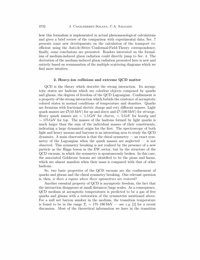
A first example of this collective behavior is the equation of state. Thepressure or the energy density measured in units of T 4 of an ideal gas are,according to the Stefan–Boltzman law, proportional to the number of degreesof freedom in the system: so, for a free gas of pions this quantity is Ndof = 3,while for a free gas of quarks and gluons this quantity is much larger, Ndof =2× 2× 3 + 2× 8 counting spin, color and (two) flavor states. This differentbehavior is observed in lattice calculations where a jump at the transitiontemperature, Tc, appears — see Fig. 1. Interestingly, the lattice resultsalso signal to a significant departure of the ideal gas behavior, ε = 3p attemperatures close to Tc — see Fig. 1.
0
5
10
15
20
100 200 300 400 500 600 700
0.4 0.6 0.8 1 1.2 1.4 1.6
T [MeV]
s/T3Tr0 sSB/T3
p4: Nτ=46
asqtad: Nτ=6
0
2
4
6
8
10
12
100 200 300 400 500 600 700 800
0.4 0.6 0.8 1.0 1.2 1.4 1.6 1.8 2.0
T [MeV]
Tr0 (ε-3p)/T4
p4: Nτ=468
Fig. 1. Left: entropy, s ≡ ε + p in units of T 4 versus temperature computed in
lattice. Right: trace anomaly in units of T 4 as a function of the temperature.
Figures from [3].
In order to understand the nature of the transition order parametersare needed. In QCD with massless quarks, the chiral condensate is theorder parameter, while in the infinite mass limit the order parameter is thePolyakov Loop. The order of the transition depends on the actual value ofthe quark masses and most calculations agree in the absence of a real phasetransition at zero baryochemical potential — the transition would just bea rapid cross-over.
The behavior of the potential between heavy quarks is also of inter-est for phenomenological applications. Although some discussion about theprecise meaning and the definition of a potential exists in the case of a hotmedium [4], a screening leading to a non-confining potential is expected toappear at some point above the phase transition and, correspondingly, theheavy quark bound states would cease to exist if this temperature is reached.
1 See e.g. [2] for a description of the QCD thermodynamics as studied by lattice.

3734 J. Casalderrey-Solana, C.A. Salgado
A prediction of the presence of a deconfined medium in heavy ion collisionsis then the disappearance of heavy-quark bound states (quarkonium) and inparticular the J/Ψ .
2.1. Heavy-ion collisions to characterize hot QCD states
The description of hadronic collisions in terms of the formation of a ther-mal state, which then evolves according to a hydrodynamical behavior, hasan old story. In the 50’s, Landau [5] proposed a model in which a tran-sient thermal state — little fireball — is formed by energy deposition ina small slice of space, of the size of the Lorentz-contracted nuclei, at thecenter of mass of the collision. The subsequent hydrodynamical evolutionproduces an expansion and cooling of the system up to a freeze-out tem-perature T ∼mπ when the formed hadrons free stream to the detectors.A rapidity-independent version of this model was proposed by Bjorken [6]— see e.g. [7] for a review on hydrodynamical models in heavy-ion collisions.Although more sophisticated implementations are used nowadays, very de-manding from the computational point of view, for the hydrodynamicaldescription of nuclear collisions, the Bjorken model estimate gives a conve-nient and simple parametrization of some medium properties, as a functionof the proper time τ , as the energy density or the temperature of the createdmedium
ǫ(τ) ≃ ǫ0
τ4/3, T ≃ T0
τ1/3. (1)
Present facilities to study this active field of research — see [8] for a recentreview on the experimental situation — are the CERN SPS, with fixed targetcollisions of different nuclei up to
√s ≃ 20GeV/A; the RHIC at Brookhaven,
a dedicated collider which reaches much larger energies,√
s = 200GeV/A;and in the near future the LHC at CERN, with an important programof nuclear collisions which will provide a spectacular jump in the collisionenergy upto
√s = 5500GeV/A. Here, the quoted figures refer to the total
available energy in center of mass of the collision divided by the numberof nucleons from the two nuclei — energy per nucleon — so that it can bedirectly compared to a corresponding proton–proton collision energy.
The lifetime of the hot medium produced in heavy ion collisions is sosmall, of the order of its own transverse size, that only indirect probes areavailable to characterize its properties. Here we will only focus on hardprobes and specially on the study of the high transverse momentum partof the spectrum of produced particles. Jet quenching is the generic nameunder which the corresponding effects on high-p⊥ particles are known. Theoriginal proposal [9], a suppression of the large transverse momentum yieldsdue to the energy lost by interaction of the fast partons with the mediumhas been observed at RHIC [10] and partially also at the SPS [11].
Introductory Lectures on Jet Quenching in . . . 3735
3. Hard probes to heavy-ion collisions
Hard processes are those involving large momentum exchanges. Asymp-totic freedom allows, in these conditions, to perform calculations by a per-turbative expansion in terms of αs(Q
2), where Q is the large scale of theprocess, as, e.g. a large mass or a large transverse momentum of the pro-duced particles. This perturbative expansion is, however, computed in termsof quarks and gluons, the degrees of freedom of the QCD Lagrangian, andsome extra information is usually needed to connect it with the initial andfinal hadrons appearing as asymptotic states. A crucial simplification of theproblem is possible thanks to the factorization theorems of QCD which allowto separate long- and short-distance contributions to the cross section in theform2:
σAB→h = fA(x1, Q2) ⊗ fB(x2, Q
2) ⊗ σ(x1, x2, Q2) ⊗ Di→h(z,Q2) , (2)
where the short-distance perturbative cross section, σ(x1, x2, Q2), is compu-
table in powers of αs(Q2) and the long-distance terms are non-perturbative
quantities involving scales O(ΛQCD). More specifically, the proton/nuclearparton distribution functions (PDF), fA(x,Q2), encode the partonic struc-ture of the colliding objects and can be interpreted as the probability to finda parton (quark or gluon) inside the hadron with fraction of momentum x;the fragmentation functions (FF), D(z,Q2), describe the hadronization ofthe parton i into a final hadron h with a fraction of momentum z.
Although the PDFs and the FFs are non-perturbative quantities, theirevolution in Q2 can be computed by the Dokshitzer–Gribov–Lipatov–Altarelli–Parisi (DGLAP) equations [12]. This equations resum higher or-ders in αs which, due to enhanced contributions in some regions of phase-space, cannot be neglected. For example, we will see Sec. 5 that the spectrumof gluons radiated with energy fraction z out of a quark produced in a hardprocess is
dI
dzdt=
αs
2π2
1
tP (z) ≃ αs
π2
1
t
CR
z, (3)
with t the invariant mass of the produced pair. This radiation is divergentin the infrared and collinear limits giving large O(αs log t) terms to the crosssection which need to be taken into account. These terms are resummed bythe DGLAP evolution equations3
∂D(x, t)
∂ log t=
1∫
x
dz
z
αs
2πP (z)D
(x
z, t)
. (4)
2 For simplicity we have made all the scales the same, although, strictly speaking, thefactorization, renormalization and fragmentation scales can be different.
3 To simplify the notation, we include only one flavor, see, e.g. [13] for a completedescription.

3736 J. Casalderrey-Solana, C.A. Salgado
where D(x, t) can be the PDFs or the FFs and P (z) are the splitting func-tions. At the lowest order (LO) these equations admit a probabilistic inter-pretation in which a parton shower is formed by subsequent branching of theinitial quark or gluon. We will come back to this interpretation in Sec. 6.
These equations provide an excellent description of experimental data asdeep inelastic lepton–proton scattering (DIS) or jets.
3.1. Hard processes as probes of the medium
The hard process described by the perturbative cross section σ(x1, x2, Q2)
in (2) takes place in a very short time, O(1/Q), and is basically unchangedfor most of the processes of interest. The interest of hard processes as probesof the medium is that the long distance parts are modified when they com-municate with the extension of the medium. Measuring these modificationsallows for a characterization of the medium properties — see e.g. [14] fora recent review.
A conceptually simple example is the J/Ψ , whose production cross sec-tion can be written as
σhh→J/Ψ =fi(x1, Q2)⊗fj(x2, Q
2)⊗σij→[cc](x1, x2, Q2)〈O([cc] → J/Ψ)〉 , (5)
where now 〈O([cc] → J/Ψ)〉 describes the hadronization of a cc pair ina given state (for example a color octet) into a final J/Ψ . In the casethat the pair is produced inside a hot medium this long-distance part ismodified. Actually, the potential between the pair is screened in a hotmedium and the hadron is dissolved, making 〈O([cc] → J/Ψ)〉 → 0. Theexperimental observation of this effect is a disappearance of the J/Ψ innuclear collisions [15]. This suppression has been discovered in experimentsat the CERN SPS [16] and then also at RHIC [17]. The interpretation of theexperimental data is, however, not simple; one of the reasons being the lackof good theoretical control over the modification of a purely non-perturbativequantity as the hadronization of a cc pair into a charmonium state.
From the computational point of view, a theoretically simpler case isthe modification of the evolution of fragmentation functions of high-pT par-ticles due to the presence of a dense or finite-temperature medium. Here,highly energetic partons, produced in a hard process, propagate through theproduced matter, loosing energy by medium-induced gluon radiation. Thisphenomenon is generically known as jet quenching and its implementationinto the perturbative formula (2) will be discussed in the next sections.
Introductory Lectures on Jet Quenching in . . . 3737
3.2. Nuclear parton distribution functions
A good knowledge of the PDFs is essential in any calculation of hardprocesses. The usual way of obtaining these distributions is by a global fitof data on different hard processes (mainly deep inelastic scattering, DIS) toobtain a set of parameters for the initial, non-perturbative, input f(x,Q2
0)to be evolved by DGLAP equations [12].
In the nuclear case, the initial condition, fA(x,Q20), is modified com-
pared to the proton. Moreover, at small enough x, non-linear correctionsto the evolution equations [18–21] are expected to become relevant. GlobalDGLAP analyses, paralleling those for free protons are available [22–28].These studies fit the available data on DIS and Drell–Yan with nuclei pro-viding the needed benchmark for additional mechanisms.
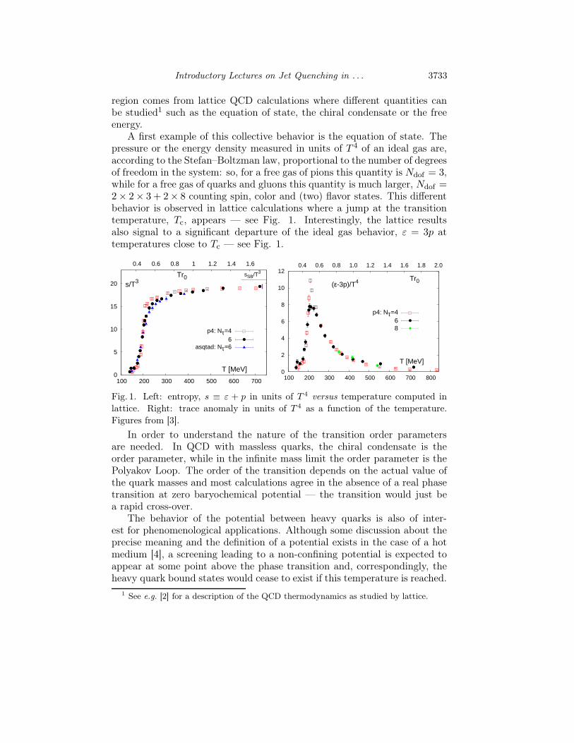
The DGLAP analyses of nuclear PDFs from [27] is shown in Fig. 2, in-cluding the corresponding error estimates. An important issue, partiallyvisible in Fig. 2, is that present nuclear DIS and DY data can only constrainthe distributions for x & 0.01 in the perturbative region. By chance, thisregion covers most of the RHIC kinematics, so that, the description of e.g.J/Ψ -suppression or inclusive particle production in dAu collisions as givenby the nuclear PDFs can be taken as a check of universality of these distri-butions. These checks present a quite reasonable agreement with data [29],but some extra suppression for the inclusive yields at forward rapidities isprobably present. The strong gluon shadowing plotted in Fig. 2 improves
0.00.20.40.60.81.01.21.4
this workEKS98
0.00.20.40.60.81.01.21.4
Fit errorsLarge errorsTotal errors
10-4
10-3
10-2
10-10.0
0.20.40.60.81.01.2
strong gluonshadowing
10-4
10-3
10-2
10-1
10.00.20.40.60.81.01.2
RA V
RA S
RA G
RA F
2A = 208, Q2
0= 1.69 GeV
2
Fig. 2. Ratios of nuclear to free proton PDFs for different flavors at the initial scale
Q2
0= 1.69 GeV2 from [27] with error estimates. The green line in the gluon panel
is an attempt to check the strongest gluon shadowing supported by present data.

3738 J. Casalderrey-Solana, C.A. Salgado
the situation at forward rapidities without worsening the fit of DIS or DYdata — χ2/dof < 1. Whether a DGLAP analysis can accommodate allsets of data is an open question, but the finding in Ref. [27] are encouraging.A suppression at forward rapidities was also predicted in terms of saturationof partonic densities [30].
4. Particle propagation in matter
To describe the jet quenching phenomenon, we start from a high-p⊥quark or gluon produced in an elementary hard collision which subsequentlyinteracts with the surrounding matter. So, the first question we need to ad-dress is how a highly energetic particle propagates through a dense medium.In this section we will present the most widely used formalism based ona semiclassical approach in which the changes in the medium configurationdue to the passage of the fast particle, recoil, are neglected. In this approx-imation the medium can be considered as a background field.
A convenient formulation of the problem is in terms of Wilson lines
W (x) = P exp
[
ig
∫
dx+A−(x+,x)
]
(6)
describing the propagation of a particle through a medium field A−(x+,x).Its origin will be explained in the next subsection. Here we introduce thelight cone variables
x± =1√2
(x0 ± x3) , p± =1√2
(p0 ± p3) . (7)
So that the scalar product is
p · x = p+x− + p−x+ − p⊥ · x⊥ (8)
and the rapidity
y =1
2ln
[
p0 + p3
p0 − p3
]
=1
2ln
[
p+
p−
]
. (9)
4.1. Wilson lines, eikonal approximation
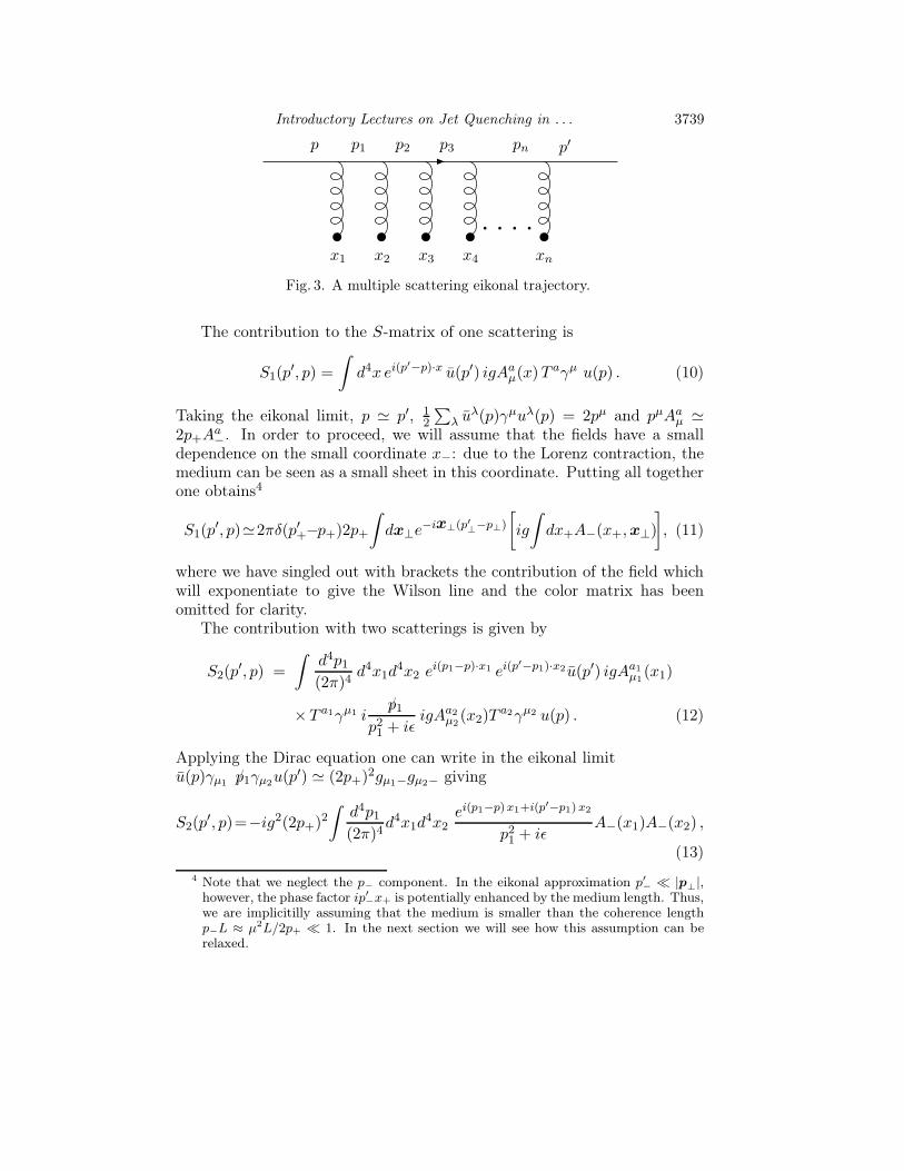
A simple derivation of the Wilson line is obtained in terms of multiplescatterings, providing a clear physical picture of the eikonal propagation.Consider the diagram of Fig. 3, where static centers of scattering are placedat x1, x2, . . . xn. Let us fix that the quark is moving in the positive x3
direction, i.e. the large component of the momentum is p+.
Introductory Lectures on Jet Quenching in . . . 3739
x1 x2 x3 x4 xn
p p′p1 p2 p3 pn
Fig. 3. A multiple scattering eikonal trajectory.
The contribution to the S-matrix of one scattering is
S1(p′, p) =
∫
d4x ei(p′−p)·x u(p′) igAaµ(x)T aγµ u(p) . (10)
Taking the eikonal limit, p ≃ p′, 12
∑
λ uλ(p)γµuλ(p) = 2pµ and pµAaµ ≃
2p+Aa−. In order to proceed, we will assume that the fields have a small
dependence on the small coordinate x−: due to the Lorenz contraction, themedium can be seen as a small sheet in this coordinate. Putting all togetherone obtains4
S1(p′, p)≃2πδ(p′+−p+)2p+
∫
dx⊥e−ix⊥(p′⊥−p⊥)
[
ig
∫
dx+A−(x+,x⊥)
]
, (11)
where we have singled out with brackets the contribution of the field whichwill exponentiate to give the Wilson line and the color matrix has beenomitted for clarity.
The contribution with two scatterings is given by
S2(p′, p) =
∫
d4p1
(2π)4d4x1d
4x2 ei(p1−p)·x1 ei(p′−p1)·x2 u(p′) igAa1µ1
(x1)
×T a1γµ1 i/p1
p21 + iǫ
igAa2µ2
(x2)Ta2γµ2 u(p) . (12)
Applying the Dirac equation one can write in the eikonal limitu(p)γµ1 /p1γµ2u(p′) ≃ (2p+)2gµ1−gµ2− giving
S2(p′, p)=−ig2(2p+)2
∫
d4p1
(2π)4d4x1d
4x2ei(p1−p)x1+i(p′−p1) x2
p21 + iǫ
A−(x1)A−(x2) ,
(13)
4 Note that we neglect the p− component. In the eikonal approximation p′
− ≪ |p⊥|,
however, the phase factor ip′
−x+ is potentially enhanced by the medium length. Thus,we are implicitilly assuming that the medium is smaller than the coherence lengthp−L ≈ µ2L/2p+ ≪ 1. In the next section we will see how this assumption can berelaxed.

3740 J. Casalderrey-Solana, C.A. Salgado
where again the color matrices have been omitted as will be omitted in thefollowing. In the high-energy limit, the integrals in d4p1 can be performed:
∫
dp1−ei(x1+−x2+)p1−
2p1+p1− + iǫ= −Θ(x2+ − x1+)
2πi
2p+, (14)
∫
dp1+ei(x1−−x2−)p1+ = 2πδ(x1− − x2−) , (15)∫
d2p1⊥e−i(x1⊥−x2⊥)p1⊥ = (2π)2δ(x1⊥ − x2⊥) . (16)
Doing the x−-integration as in the case of one scattering one obtains
S2(p′, p)≃2πδ(p′+ − p+)2p+
∫
dx⊥e−ix⊥(p′⊥−p⊥) 1
2P[
ig
∫
dx+A−(x+, x⊥)
]2
,
(17)where again the second term in the expansion of (6) appears. In order toobtain (17) we have used that
∫
dx1dx2 . . . dxnΘ(x2 − x1) . . . Θ(xn − xn−1)A(x1) . . . A(xn)
=1
n!P[∫
dxA(x)
]n
, (18)
where P means path-ordering of the fields A(x).The generalization to n-scattering centers follows the same lines and the
corresponding contribution is given by
Sn(p′, p) ≃ 2πδ(p′+ − p+)2p+
∫
dx⊥e−ix⊥(p′⊥−p⊥)
× 1
n!P[
ig
∫
dx+A−(x+,x⊥)
]n
, (19)
So that the total S-matrix is
S(p′, p) =∞∑
n=0
Sn(p′, p) ≃ 2πδ(p′+ − p+)2p+
∫
dx⊥e−ix⊥(p′⊥−p⊥)W (x⊥) ,
(20)with W (x⊥) given by Eq. (6). Similar expressions are obtained in the caseof a fast gluon of momentum k with the only replacement of the externalfields in (6), now in the adjoint representation — see e.g. [31]. In order tosee this, the external fields coupled to three gluon vertices (four gluon vertexare subleading in energy) are written in the adjoint representation
AA = Aa(T aA)bc = −iAafabc . (21)

Introductory Lectures on Jet Quenching in . . . 3741
The sum of gluon polarization vectors can be written as
2∑
i=1
ǫµ(i)ǫ
ν(i) = gµν − mµkν
m · k − kµmν
m · k (22)
with m a light-like vector with non-zero minus component, m = (0, 1, 0, 0)and the polarization vectors defined by ǫ · k = ǫ · m = 0; ǫ2 = −1
ǫ(i) =
(
0,k⊥ · ǫ(i)⊥
k+, ǫ(i)⊥
)
(23)
and ǫ(1)⊥ = (1, 0), ǫ(2)⊥ = (0, 1). This prescription allows to simplify thestructure of the gluon line since, due to gauge invariance, only the first termin Eq. (22) contributes in the high-energy limit when the propagator is inbetween two three-gluon vertices. So that, one can write for each gluonpropagator
gµν ≃2∑
i=1
ǫµ(i)ǫ
ν(i) (24)
and now the contribution from each vertex Vµνσ can be simplified as
ǫµ(i′)(k
′)Vµνσ(−k′, k, k′ − k)AσAǫν
(i)(k) ≃ −i2gk+AA−δii′ (25)
which has a structure similar to the quark case allowing for a resummationto obtain a Wilson line now with fields in the adjoint representation. Wewill denote this gluon line with a superscript, W A(x⊥).
Eq. (20) describes the scattering of a quark (or gluon, with the changesexplained above) in a medium with a given field configuration, determined bythe scattering centers. The effect of the medium is to induce color rotationat each scattering center without changing the helicity (polarization) of thequark (gluon), which loses a negligible amount of energy and propagatesin straight lines. In order to have the final answer for a physical crosssection, these medium configurations need to be averaged within an ensembledescribing the medium. This issue will be discussed later.
4.2. Relaxing the eikonal approximation
In some cases, the restrictions applied in the above formulation need tobe relaxed to allow small changes in the transverse position of the propa-gating particle. This is the case, for instance, of the medium-induced gluonradiation, where the gluon position follows Brownian motion in the trans-verse plane. The eikonal Wilson line is now replaced by the propagator
G(b, a) =
∫
Dr(x+) exp
ip+
2
∫
dx+
[
dr
dx+
]2
W (r) . (26)

3742 J. Casalderrey-Solana, C.A. Salgado
This change can be derived in the multiple soft scattering presented in theprevious section. In order to do that, we have to keep the subleading p2
⊥terms in the poles of the propagators. So, now the integration in pi− reads
∫
dp−eip−(xi+−x(i+1)+)
2p+p− − p2⊥ + iǫ
= − i2π
2p+Θ(x(i+1)+ − xi+) e
ip2⊥
2p+(xi+−x(i+1)+)
(27)
and instead of (16) the integration in pi⊥ is Gaussian, giving
∫
d2pi⊥(2π)2
ei
p2⊥
2p+((xi+−x(i+1)+)
e−ipi⊥(xi⊥−x(i+1)⊥)
=p+
2πi(xi+ − x(i+1)+)exp
−ip+
2
(xi⊥ − x(i+1)⊥)2
xi+ − x(i+1)+
. (28)
Eq.(28) is the Feynman propagator of a free particle that propagates in thetransverse plane from xi⊥ at time xi+ to x(i+1)⊥ at time x(i+1)+ (see e.g. [33])G0(x(i+1)⊥ − xi⊥;x(i+1)+ − xi+). Thus, Eq. (28) can be expressed as
G0(x(i+1)⊥−xi⊥;x(i+1)+−xi+)=
∫
Dx⊥(xp) exp
ip+
2
∫
dx+
[
dx⊥dx+
]2
,
(29)where the paths x⊥(x+) connect the two endpoints of the propagator.
The scattering matrix now reads
S(p′, p) = 2πδ(p′+ − p+)2p+
∞∑
n=0
∫
Pn∏
i=0
dxi+dxi⊥igA(xi+,xi⊥)
×G0(∆x(i+1)⊥;∆x(i+1)+)igA(x(i+1)+,x(i+1)⊥) , (30)
where ∆x(i+1)⊥ = x(i+1)⊥−xi⊥, ∆x(i+1)+ = x(i+1)+−xi+. This expressioncan be reorganized as
S(p′, p) = 2πδ(p′+ − p+)2p+
∫
dx⊥e−ix⊥(p′⊥−p⊥)
×∫
Dr(x+) exp
ip+
2
∫
dx+
[
dr
dx+
]2
W (r) , (31)
with W (x⊥) given by (6).Eq. (31) describes the propagation of a highly energetic particle through
a medium when changes in the transverse position are allowed. The prop-agation takes phases both from the motion in the transverse plane and thecolor rotation by interaction with the medium field.
Introductory Lectures on Jet Quenching in . . . 3743
4.3. The medium averages
The S-matrices derived in the previous sections are valid for a givenconfiguration of the fields and should be averaged over the proper ensembleof the medium field configurations. Several prescriptions have been used inthe literature. Here we will present two of them used for the calculation ofthe jet quenching. Notice first that any physical quantity must contain, atleast, the medium average of two Wilson lines since the average is done at thelevel of the cross section where only colorless states are allowed. In general,we will be interested in quantities like
1
NTr 〈W †(x⊥)W (y⊥)〉 , (32)
where the trace and the 1/N term correspond to average the initial colorindices — correspondingly, a factor 1/(N2−1)would appear in the case ofWilson lines in the adjoint representation.
Two main approximations to the averages (32) are used in jet quenchingphenomenology, the multiple soft scattering approximation and the opacityexpansion. Both can be understood in the multiple scattering picture weare employing. The main assumption is that the centers of scattering areindependent, i.e. no color flow appears between scattering centers separatedmore than a distance λ ∼ 1/µ, µ being a typical scale in the medium as theDebye screening length. So, we want to calculate
1
NTr 〈W †(x⊥)W (y⊥)〉 =
1
NTr⟨
exp−ig
∫
dx+A†−(x+,x⊥)
× expig∫
dx+A−(x+,y⊥)⟩
. (33)
Expanding the exponents and taking the contribution from one scatteringcenter, the leading contribution is quadratic in the fields — the linear con-tributions cancels due to the color trace
⟨
1 +1
2(ig)2
[∫
dx+A†−(x+,x⊥)
]2
+1
2(ig)2
[∫
dx+A−(x+,y⊥)
]2
− (ig)2[∫
dx+A†−(x+,x⊥)
] [∫
dx+A−(x+,y⊥)
]
⟩
. (34)
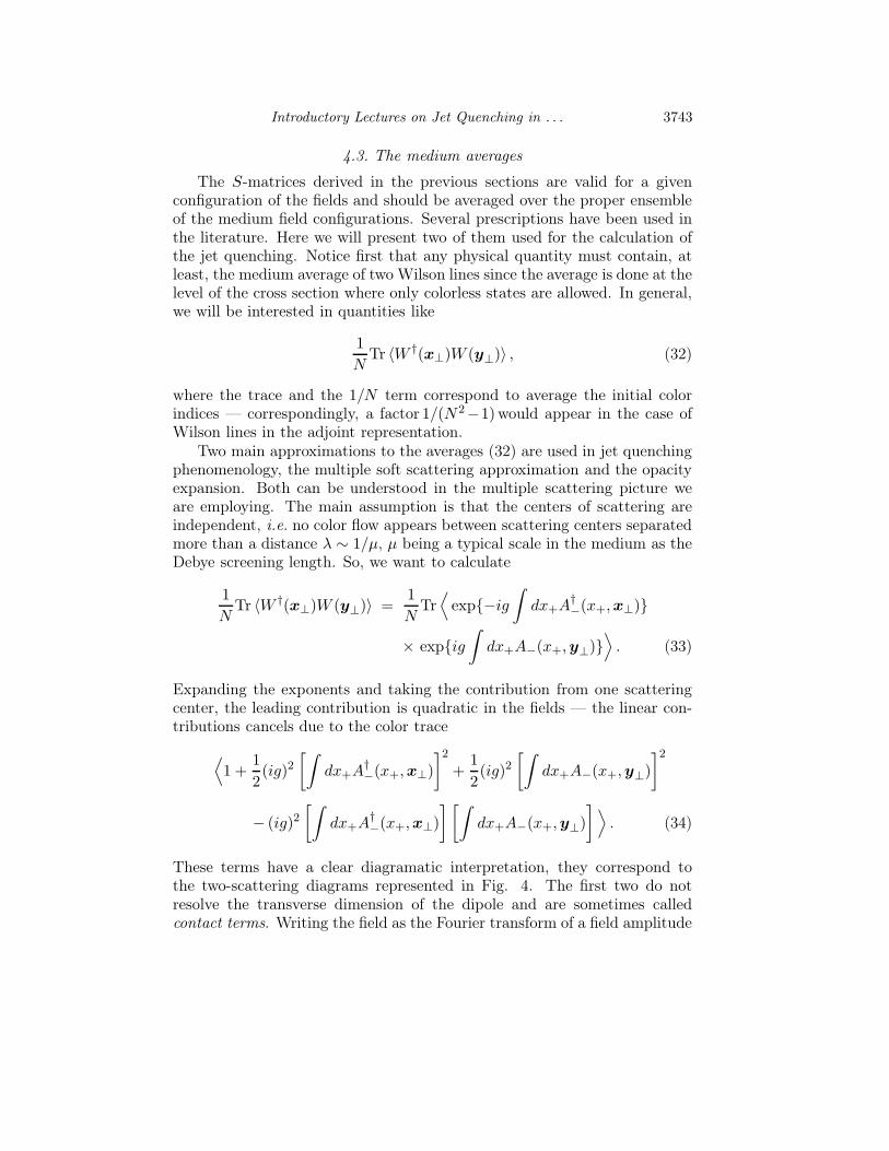
These terms have a clear diagramatic interpretation, they correspond tothe two-scattering diagrams represented in Fig. 4. The first two do notresolve the transverse dimension of the dipole and are sometimes calledcontact terms. Writing the field as the Fourier transform of a field amplitude

3744 J. Casalderrey-Solana, C.A. Salgado
produced by a scattering center at position (xi+,xi⊥)
T bAb−(x+,x⊥) =
∫
d2q
(2π)2ei(x⊥−xn⊥)q T bab
−(q)δ(x+, xi+) . (35)
The medium averages 〈 . . . 〉 are done by integrating in the longitudinal xi+
Fig. 4. Different contributions to the dipole cross section.
and transverse coordinates xn⊥ of the scattering centers. For example, thethird term in (34) gives
∫
dx+dxi+dxi⊥
∫
d2q1
(2π)2d2q2
(2π)2e−i(x⊥ −xi⊥ )q1 ei(y⊥−xi⊥ )q2
× a∗−(q1) a−(q2)δ(x+ − xi+) =
∫
dx+
∫
d2q
(2π)2ei(y⊥−x⊥ )q |a(q)|2 . (36)
Putting all together, Eq. (34) can be written in terms of the cross sectionof a dipole, where the quark and the antiquark are located at y⊥ and x⊥respectively, with one of the scattering centers of the medium.
(34) = 1−CF
∫
d2q
(2π)2|a(q)|2 (1− ei(y⊥ −x⊥ )q) = 1− 1
2σ(y⊥ − x⊥) . (37)
The factor CF comes from the color average and the traces over the matrices
1
N
∑
a,b
Tr T aT b = CF =N2 − 1
2N=
4
3. (38)
The corresponding factor for a gluon would be CA = N = 3.There is a subtlety in the derivation we have just presented. Strictly
speaking, the contact terms are not included in the multiple scatteringderivation of the Wilson lines made before, where each scattering centercontributes with a factor A− and path ordering appears. What we haveimplicitly assumed is that scattering centers separated by distances smallerthan λ ∼ 1/µ resolve color correlations while those separated by more than
Introductory Lectures on Jet Quenching in . . . 3745
λ do not. This is usually implemented by considering the contribution of onescattering center by defining a density n(x+) =
∑
i δ(x+ − xi+) and takingthe continuum by an integration in x+
1
NTr 〈W †(x⊥)W (y⊥)〉1 scatt ≃ 1 − CF
2
∫
dx+n(x+)σ(y⊥ − x⊥) . (39)
Eq. (39) is the first order in an opacity expansion of the medium, the sumof all orders exponentiate and the average (33) can be written as
1
NTr 〈W †(x⊥)W (y⊥)〉 ≃ exp
−CF
2
∫
dx+n(x+)σ(y⊥ − x⊥)
. (40)
Eqs. (39) and (40) are the two main medium averages used in the literatureof jet quenching. In order to proceed, the functional form of the dipole crosssection needs to be specified. In the opacity expansion a Yukawa-type elasticscattering center with Debye screening mass µ is usually taken in (37)
|a(q)|2 =µ2
π(q2 + µ2). (41)
When the number of scattering centers is very large, all of them need to beresummed and the first orders of the opacity are not enough. In this condi-tions, it is convenient to take the dipole cross section at leading logarithmicaccuracy [34] and write the small distance component of the cross section
σ(r) ≃ Cr2 . (42)
The proportionality factor C with the squared dipole size is usually taken tobe constant and defines the transport coefficient q(ξ) ≡ 2
√2n(ξ)C, encoding
all the information about the dynamical properties of the medium. This isthe main parameter to be determined by fits to experimental data and tobe compared with theoretical calculations. The Wilson line averages definethis parameter by5
1
N2 − 1Tr 〈W A†(x⊥)W A(y⊥)〉 ≃ exp
− 1
4√
2
∫
dx+q(x+)(x⊥ − y⊥)2
.
(43)Here we have considered a gluon instead of a quark as the fast particletraversing the medium. This is the most relevant quantity as we will see inthe next sections.
5 The factor√
2 is included here as the transport coefficient is usually defined in ordi-nary coordinates, where the longitudinal distance for a z ≃ x+/
√2.

3746 J. Casalderrey-Solana, C.A. Salgado
It is worth noticing that similar medium averages are used in the studyof deep inelastic scattering (DIS) with nuclei, where a phenomenon of satu-ration of partonic densities is expected. In this case, the convention is to callthe relevant parameter saturation scale Qsat and the Wilson line average isgiven by
1
NTr 〈W †(x⊥)W (y⊥)〉 ≃ exp
−1
4Q2
sat(x⊥ − y⊥)2
. (44)
Now the saturation scale contains not only the dynamical informationabout the target but also the geometry. A simple model for this saturationscale gives [35]
Q2sat =
8π2αsNc
N2c − 1
A1/3 xG(x, 1/(x⊥ − y⊥)2) , (45)
where the factor A1/3 comes from the proportionality to the nuclear medium— the radius for a nucleus is approximately RA ≃ 1.2A1/3 fm. In (45),xG(x,Q2) is the gluon distribution of a nucleon inside a nucleus giving anenergy dependence to the saturation scale which, as we have said, is usuallyneglected for the case of q.
4.4. A simple application: the dipole model
The above rules allow us to write the cross section for the scattering ofa (colorless) dipole of size r2 = x2
⊥ with a medium. Taking the (forwardscattering) amplitude as iT = 1 − S and applying the optical theorem,σ = 2ImT
σdiptot (r) = 2 − 2
NTr 〈W †(x⊥)W (0)〉 ≃ 2
[
1 − exp
−1
4Q2
sat r2
]
. (46)
This dipole cross section finds a direct application in the calculation ofthe deep inelastic scattering at small values of the Bjorken variable x. Thedipole model tells us that in these conditions, the collision can be seen asa two-step process in which the virtual photon from the lepton splits intoa qq dipole and then this fluctuation scatters with the hadronic target. Theproblem now reduces to compute the photon-dipole vertex Ψγ∗
T,L for a trans-
versely or longitudinaly polarized photon (see e.g. [36]) which factorizes togive the cross section for the virtual photon–hadron as
σγ∗hT,L(x,Q2) =
∫
d2r
1∫
0
dz |Ψγ∗T,L|2σ
diptot (r, x) . (47)

Introductory Lectures on Jet Quenching in . . . 3747
Eq. (47) is extensively used in the phenomenology of DIS to include sat-uration effects — simpler to include in configuration space as we do here.As the photon wave function is known, the problem reduces, in general, tocompute the dipole cross section for different medium averages and includingdifferent resummation techniques for the non-linear terms.
4.5. Relation with the momentum broadening
From the parton S matrix one can readily compute the momentumbroadening. After passing though the medium, the particle distributionis given by
dNd2p′
⊥∝∫
dp′+δ(
p′2 − m2) 1
NTr⟨
∣
∣S(p′, p)∣
∣
2.⟩
(48)
And the transverse momentum broadening is given by
⟨
p2⊥⟩
=1
N
∫
d2p′⊥p′2
⊥dN
d2p′⊥
. (49)
From Eq. (31) we find
N⟨
p2⊥⟩
∝∫
dp′⊥
∫
dx⊥dx′⊥p′
⊥2eip′
⊥(x⊥−x′
⊥)∫
DrDr′
×exp
ip+
2
∫
dx+
(
[
dr
dx+
]2
−[
dr′
dx+
]2)
1
NTr⟨
W †(r′)W (r)⟩
. (50)
A simple manipulation leads to
N⟨
p2⊥⟩
∝ lim∆x⊥→0
−∇2∆x⊥
∫
DrDr′ exp
ip+
2
∫
dx+
(
[
dr
dx+
]2
−[
dr′
dx+
]2)
× 1
NTr⟨
W †(r′)W (r)⟩
. (51)
In the high energy limit, p+ ≫ µ, we can approximate the path integral bythe classical path with smallest action, dr/dx+ = 0. Performing a similarmanipulation for the normalization we obtain
⟨
p2⊥⟩
= − 1
Tr 〈W †(x⊥)W (x⊥)〉
∇2∆x⊥
Tr
⟨
W †(
x⊥ − ∆x⊥2
)
W
(
x⊥ +∆x⊥
2
)⟩
, (52)

3748 J. Casalderrey-Solana, C.A. Salgado
with x⊥ = (x⊥ + x′⊥)/2. If the medium is large in the transverse direction,
the dependence in x⊥ drops.The expression derived above is general. In the particular case of the
multiple soft scattering, we find
⟨
p2⊥⟩
=1√2
∫
dx+q(x+) . (53)
Thus, we can interpret the q parameter as the momentum broadening perunit length [37].
Note also that within this approximation, in a homogeneous medium thenumber particle distribution at a certain transverse position after passingthough a medium of lenght L is
N (x⊥) =
∫
dp⊥2π
e−ix⊥p⊥N (p⊥) ∝ Tr⟨
W †(0)W (x⊥)⟩
. (54)
Thus, the particle distribution follows a diffusion equation in transversespace:
∂+N =1
4√
2q∇2
p⊥
N . (55)
From this fact, the interpretation of q as a jet transport parameter is clear.
5. The medium-induced gluon radiation
With the formalism developed in the last sections we can now computethe medium-induced gluon radiation needed for jet quenching studies. In thisformalism, the fast particle is produced at a given point inside the mediumwhere the hard process, h, takes place, see Fig. 5. Then this particle andthe emitted gluon suffer multiple scattering described by the path integralpropagators (26). We will work in the approximation p+ ≫ k+ ≫ k⊥ butkeep terms in k2
⊥/k+ as explained in the previous section.
h p+ p+− k+ = (1−z)p+
k+ = zp+
Fig. 5. The medium-induced gluon radiation diagram.
Introductory Lectures on Jet Quenching in . . . 3749
5.1. The gluon emission vertex
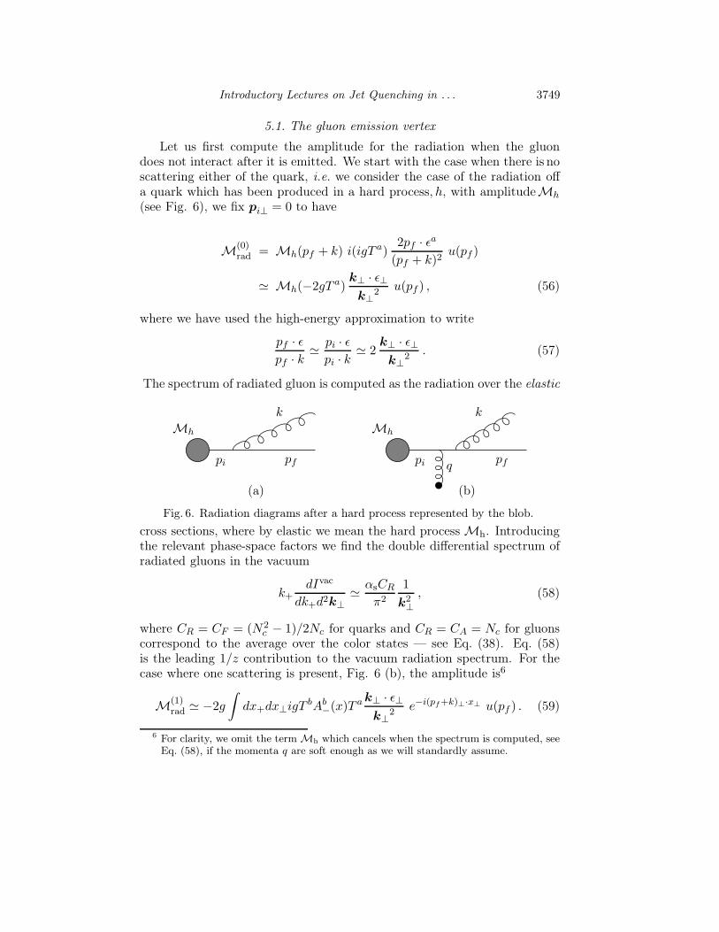
Let us first compute the amplitude for the radiation when the gluondoes not interact after it is emitted. We start with the case when there is noscattering either of the quark, i.e. we consider the case of the radiation offa quark which has been produced in a hard process, h, with amplitudeMh
(see Fig. 6), we fix pi⊥ = 0 to have
M(0)rad = Mh(pf + k) i(igT a)
2pf · ǫa
(pf + k)2u(pf )
≃ Mh(−2gT a)k⊥ · ǫ⊥
k⊥2 u(pf ) , (56)
where we have used the high-energy approximation to write
pf · ǫpf · k ≃ pi · ǫ
pi · k≃ 2
k⊥ · ǫ⊥k⊥
2 . (57)
The spectrum of radiated gluon is computed as the radiation over the elastic
pi pf
k
pi pfq
k
Mh Mh
(a) (b)
Fig. 6. Radiation diagrams after a hard process represented by the blob.
cross sections, where by elastic we mean the hard process Mh. Introducingthe relevant phase-space factors we find the double differential spectrum ofradiated gluons in the vacuum
k+dIvac
dk+d2k⊥≃ αsCR
π2
1
k2⊥
, (58)
where CR = CF = (N2c − 1)/2Nc for quarks and CR = CA = Nc for gluons
correspond to the average over the color states — see Eq. (38). Eq. (58)is the leading 1/z contribution to the vacuum radiation spectrum. For thecase where one scattering is present, Fig. 6 (b), the amplitude is6
M(1)rad ≃ −2g
∫
dx+dx⊥igT bAb−(x)T a k⊥ · ǫ⊥
k⊥2 e−i(pf +k)⊥·x⊥ u(pf ) . (59)
6 For clarity, we omit the term Mh which cancels when the spectrum is computed, seeEq. (58), if the momenta q are soft enough as we will standardly assume.

3750 J. Casalderrey-Solana, C.A. Salgado
This expression contains a factorization of the radiation amplitude (56) andthe collision term which can be identified as the first term in the expansionof the Wilson line. The corresponding contribution resumming an arbitrarynumber of scatterings gives then
Mradq ≃ −2g
∫
dx⊥W (x⊥, x0+, L+)T a k⊥ · ǫa⊥
k⊥2 e−i(pf +k)⊥·x⊥ u(pf ) , (60)
where x0+ and L+ are the positions where the medium begins and ends inlight-cone variables — so that the x+-integral in the Wilson line has theselimits — and the subscript q is included to signal that the gluon does notinteract with the medium.
The case when the emitted gluon interacts with the medium can be com-puted similarly and the corresponding contribution from the vertex wouldgive k1⊥/k1⊥
2, which is now an internal integration variable. In order todeal with it, we will write the delta function for the momentum conservationin the radiation vertex as
(2π)4δ4(k1 − pn+1 + pn) =
∫
d4y ei(k−pn+1+pn)·y (61)
and integrate over the three momenta k1, pn+1, pn. By doing this, y signalsnow the spatial position of the radiation vertex. Let us define the contribu-tion from a gluon radiated at y from a quark with momentum pn before thesplitting and pn+1 after it (see Fig. 7), as7
V µ(n)g =
∫
d4y e−i(pn+1−pn)·yn∏
j=1
∫
d4kj
(2π)4dx2
j ǫµ(i)(k1)
[
−2gkj+A−(xj)
k2j + iǫ
]
× exp i(kj+1 − kj) · xj exp ik1 · y , (62)
pn pn+1
k
Fig. 7. Radiation vertex when the gluon reinteracts with the medium.
7 We have used here the steps explained in Sec. 4.1, in particular Eq. (24), to simplifythe triple gluon vertices in the high-energy limit.

Introductory Lectures on Jet Quenching in . . . 3751
(we write kn+1≡kf for the final momentum of the gluon). Writing ǫ−=k1⊥·ǫ⊥/k1+ and proceeding as explained in Sec. 4.2 it is easy to see that the“−” component of (62), which will be used later, is
V −(n)g ≃
∫
d4y e−i(pn+1−pn)·y i
k+ǫ⊥ · ∂
∂y⊥G0(y⊥, y+;x1⊥, x1+)A−(x1)
×n∏
j=2
∫
d2xj⊥dxj+G0(xj−1⊥, xj−1+;xj⊥, xj+)A−(xj) eikf⊥·xn⊥ , (63)
so that the sum over scattering centers gives8
V −g ≃ i
k+
∫
d4y e−i(pn+1−pn)·yǫ⊥ ,
× ∂
∂y⊥
∫
d2x⊥G(y⊥, y+;xn⊥, xn+))eikf⊥·xn⊥ . (64)
And we define for future convenience
A−(y) ≡ i
k+ǫ⊥ · ∂
∂y⊥
∫
d2x⊥G(y⊥, y+;xn⊥, xn+))eikf⊥·xn⊥ . (65)
In the way Eq. (62) has been defined, the amplitude for the processq → qg corresponds to the replacement A(y) → A(y) for one of the scatteringcenters in the derivation of the quark Wilson line described in Sec. 4.1,so that the calculation is now similar to the one performed before. Morespecifically, the amplitude of Fig. 5 can be written as
Mm =
∫ m∏
i=0
[
d4pi
(2π)4d4xi
]
eip·x1
×n∏
j=0
[
(−2gT aj )Aaj (xj) · pj
p2j + iǫ
eipj ·(xj−xj+i)
]
× (−2gT b)Ab(xn+1) · pn+1
p2n+1 + iǫ
eipn+1·(xn+1−xn+2)
×m∏
k=n+2
[
(−2gT ak )Aak(xk) · pk
p2k + iǫ
eipk·(xk−xk+i)
]
eipf ·xm u(pf ) . (66)
The structure in poles and phases is the same as the one studied in Sec. 4.1.The poles give again an ordering in the longitudinal variable x+, so that the
8 We include here the case when the gluon does not interact once it is emitted inside
the medium, otherwise a factor G0(y⊥, y+; xn⊥, xn+) should be subtracted.

3752 J. Casalderrey-Solana, C.A. Salgado
position of the radiation contribution A−(x+,x⊥) is ordered with the restof the external fields A−(x+,x⊥) to give
Mrad =
L+∫
x0+
dx+
∫
dy⊥ ei(pf−pi)⊥·y⊥P exp
ig
x+∫
x0+
dy+A(y+,y⊥)
× i2gT bAb(x+,y⊥)P exp
ig
L+∫
x+
dy+A(y+,y⊥)
. (67)
We have made explicit the color matrix T b at the radiation vertex while itis included as a redefinition of the external fields in the rest of the cases asdone in previous sections. We are interested in the case where the quark iscompletely eikonal, so, we fix y⊥ = 0 to get
Mradg = − 2g
k+
L+∫
x0+
dx+
∫
dx2⊥ eik⊥·x⊥W (0;x0+, x+)
×T bǫ⊥ · ∂
∂y⊥Gb(y⊥ = 0, x+;x⊥, L+)W (0;x+, L+) . (68)
The total amplitude for the medium-induced gluon radiation is then thesum of (60) and (68)
Mrad = Mradq + Mrad
g . (69)
We will now compute the spectrum of radiated gluons in the presence ofa medium, including all the relevant color factors to perform the mediumaverages.
5.2. The medium-induced gluon radiation
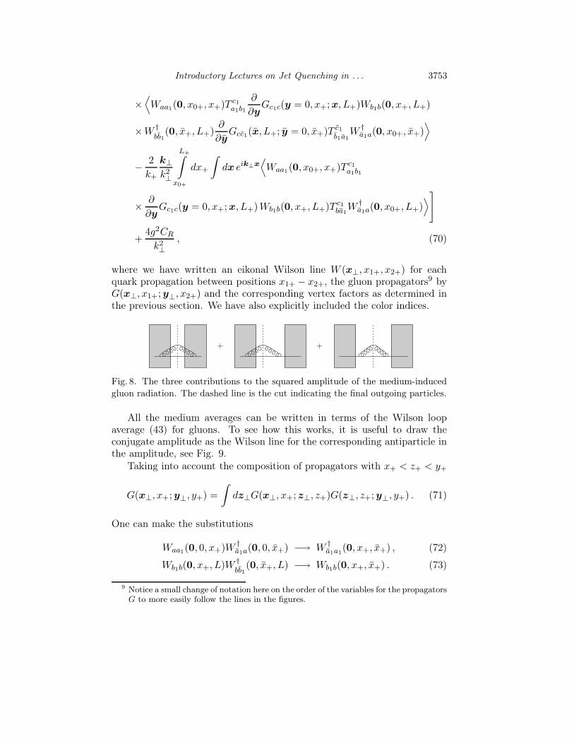
The locality of the medium averages, see also below, allows for a simplediagramatical interpretation, in which three different cases appear when theamplitude (69) is squared depending on the position of the radiation vertex:when the gluon is emitted inside the medium in both amplitude and con-jugate amplitude; when it is emitted inside the medium in amplitude andoutside the medium in conjugate amplitude; and finally when the gluon isemitted outside the medium in both amplitude and conjugate amplitude,see Fig. 8. We take the case that x+ < x+ to obtain
〈|Ma→bc|2〉 =g2
N2c − 1
2Re
[
1
k2+
L+∫
x0+
dx+
L+∫
x+
dx+
∫
dxdx eik⊥(x−x)
Introductory Lectures on Jet Quenching in . . . 3753
×⟨
Waa1(0, x0+, x+)T c1a1b1
∂
∂yGc1c(y = 0, x+;x, L+)Wb1b(0, x+, L+)
×W †bb1
(0, x+, L+)∂
∂yGcc1(x, L+; y = 0, x+)T c1
b1a1W †
a1a(0, x0+, x+)⟩
− 2
k+
k⊥k2⊥
L+∫
x0+
dx+
∫
dx eik⊥x⟨
Waa1(0, x0+, x+)T c1a1b1
× ∂
∂yGc1c(y = 0, x+;x, L+)Wb1b(0, x+, L+)T c1
ba1W †
a1a(0, x0+, L+)⟩
]
+4g2CR
k2⊥
, (70)
where we have written an eikonal Wilson line W (x⊥, x1+, x2+) for eachquark propagation between positions x1+ − x2+, the gluon propagators9 byG(x⊥, x1+;y⊥, x2+) and the corresponding vertex factors as determined inthe previous section. We have also explicitly included the color indices.
+ +
Fig. 8. The three contributions to the squared amplitude of the medium-induced
gluon radiation. The dashed line is the cut indicating the final outgoing particles.
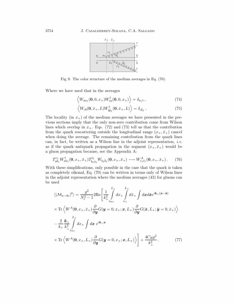
All the medium averages can be written in terms of the Wilson loopaverage (43) for gluons. To see how this works, it is useful to draw theconjugate amplitude as the Wilson line for the corresponding antiparticle inthe amplitude, see Fig. 9.
Taking into account the composition of propagators with x+ < z+ < y+
G(x⊥, x+;y⊥, y+) =
∫
dz⊥G(x⊥, x+;z⊥, z+)G(z⊥, z+;y⊥, y+) . (71)
One can make the substitutions
Waa1(0, 0, x+)W †a1a(0, 0, x+) −→ W †
a1a1(0, x+, x+) , (72)
Wb1b(0, x+, L)W †bb1
(0, x+, L) −→ Wb1b(0, x+, x+) . (73)
9 Notice a small change of notation here on the order of the variables for the propagatorsG to more easily follow the lines in the figures.
3754 J. Casalderrey-Solana, C.A. Salgado
a
a
b
b
a1
a1
b1
b1
c1
c1 c
cx+ x+
Fig. 9. The color structure of the medium averages in Eq. (70).
Where we have used that in the averages⟨
Waa1(0, 0, x+)W †ca(0, 0, x+)
⟩
= δa1 c , (74)⟨
Wcb(0, x+, L)W †bb1
(0, x+, L)⟩
= δcb1 . (75)
The locality (in x+) of the medium averages we have presented in the pre-vious sections imply that the only non-zero contribution come from Wilsonlines which overlap in x+. Eqs. (72) and (73) tell us that the contributionfrom the quark rescattering outside the longitudinal range (x+, x+) cancelwhen doing the average. The remaining contribution from the quark linescan, in fact, be written as a Wilson line in the adjoint representation, i.e.as if the quark–antiquark propagation in the segment (x+, x+) would bea gluon propagation because, see the Appendix A:
T c1ab1
W †aa1
(0, x+, x+)T c1b1a1
Wb1 b1(0, x+, x+) −→ W Ac1c1(0, x+, x+) . (76)
With these simplifications, only possible in the case that the quark is takenas completely eikonal, Eq. (70) can be written in terms only of Wilson linesin the adjoint representation where the medium averages (43) for gluons canbe used
〈|Ma→bc|2〉 =g2
N2c − 1
2Re
[
1
k2+
L+∫
x0+
dx+
L+∫
x+
dx+
∫
dxdxeik⊥(x−x)
×Tr⟨
W A(0, x+, x+)∂
∂yG(y = 0, x+;x, L+)
∂
∂yG(x, L+; y = 0, x+)
⟩
− 2
k+
k⊥k2⊥
L+∫
x0+
dx+
∫
dx eik⊥x
×Tr⟨
W A(0, x+, L+)∂
∂yG(y = 0, x+;x, L+)
⟩
]
+4CRg2
k2⊥
. (77)

Introductory Lectures on Jet Quenching in . . . 3755
Using the relation Eq. (71) we have the average of only two Wilson lines ateach segment in Fig. 9 — we write explicitly the two transverse components,then y and y will be put to 0 again:
Tr⟨
W A(y, x+, x+)G(y, x+;x, x+)⟩
, (78)
Tr 〈G(y, x+;x, L+)G(x, L+; y, x+)〉 , (79)
Tr⟨
W A(y, x+, L+)G(y, x+;x, L+)⟩
. (80)
The averages (78) and (79), taking x+ = L+, give
1
N2c − 1
Tr⟨
W A(y, x+, x+)G(y, x+;x, x+)⟩
=
∫
Dr exp
ip+
2
x+∫
x+
dξ r2(ξ)
exp
[
−1
2n(ξ)σ(r)
]
, (81)
with the boundary conditions r(x+) = y− y and r(x+) = x− y. The otheraverage gives [42–44]
1
N2c − 1
Tr 〈G(y, x+;x, L+)G(x, L+; y, x+)〉
=
∫
Dr1
∫
Dr2 exp
i
x+∫
x+
dξ
[
p+
2
(
r21(ξ) − r2
2(ξ))
+i
2n(ξ)σ(r1 − r2)
]
=
∫
Du
∫
Dv exp
i
x+∫
x+
dξ
[
p+
2u(ξ) · v(ξ) +
i
2n(ξ)σ(v(ξ))
]
, (82)
where we have made the change of variables
u(ξ) = r1 + r2 ,
v(ξ) = r1 − r2 . (83)
The integration in u gives a δ-function constraining v to a straight line
vs(ξ) = v(x+)ξ − x+
x+ − x++ v(x+)
x+ − ξ
x+ − x+(84)
the result is [42]
1
N2c − 1
Tr 〈G(y, x+;x, L+)G(x, L+; y, x+)〉 =
(
p+
2π∆ξ
)2
× exp
ip+
2∆ξ
[
(y − x)2 − (y − x)2]
− 1
2
∫
dξn(ξ)σ(w(ξ))
, (85)

3756 J. Casalderrey-Solana, C.A. Salgado
with
w(ξ) = (y − y)L+ − ξ
∆ξ+ (x − x)
ξ − x+
∆ξ, ∆ξ = L+ − x+ . (86)
Eq. (81) and (86) allow to compute the average of the first term in (77)
∫
dx dxeik⊥(x−x)
N2c − 1
Tr⟨
W A(y, x+, x+)G(y, x+;x, L+)G(y, x+; x, L+)⟩
=1
N2c − 1
∫
dx dx dz eik⊥(x−x) Tr⟨
W A(y, x+, x+)G(y, x+;z, x+)⟩
×Tr 〈G(z, x+;x, L+)G(x, L+; y, x+)〉
=
∫
dz eik⊥·zK(y−y, x+;z + y − y, x+) exp
[
−1
2
∫
dξn(ξ)σ(z)
]
, (87)
where we have defined
K (r(x+), x+; r(x+), x+)=
∫
Dr exp
x+∫
x+
dξ
(
ip+
2r2− 1
2n(ξ)σ(r)
)
. (88)
Putting all together, we obtain the radiation spectrum in the presence ofa medium.
k+dI
dk+d2k⊥=
αSCR
(2π)2k+2Re
L+∫
x0+
dx+
∫
d2x e−ik⊥·x
×[
1
k+
L+∫
x+
dx+ e− 1
2
L+R
x+
dξn(ξ)σ(x) ∂
∂y· ∂
∂xK(y = 0, x+;x, x+)
− 2k⊥k2⊥· ∂
∂yK(y = 0, x+;x, L+)
]
+αSCR
π2
1
k2⊥
. (89)
5.3. The multiple soft scattering approximation
In Sec. 4.3 we have presented different averaging procedures to solve (89)with (88). In the multiple soft scattering approximation, valid for opaquemedia, the dipole cross section is approximated by its quadratic term andthe medium averages of two Wilson lines are given by (43). In this ap-proximation, the path integrals (88) correspond to a harmonic oscillator ofimaginary frequency

Introductory Lectures on Jet Quenching in . . . 3757
K (r(x+), x+; r(x+), x+)=
∫
Dr exp
ip+
2
x+∫
x+
dξ
(
r2+iq(ξ)
2√
2p+
r2
)
. (90)
In order to proceed, we need to say something about the temporal depen-dence of the transport coefficient. Two classes of media have been studied:a static medium in which q(ξ) = q is a constant; an expanding mediumin which the density of scattering centers is expected to produce a dilutionas q(ξ) = q0(ξ0/ξ)
α, with α characterizing the speed of the dilution, andα = 1 for the Bjorken scaling scenario — see Sec. 2.1. Explicit solutionsfor this path integral and the corresponding spectrum (89) are given in theAppendix B. In the next sections we will present numerical calculations ofthese spectra, study their properties and explain how they are included inpresent phenomenology of jet quenching in heavy ion collisions.
5.4. Numerical results and heuristic discussion: static medium
In Fig. 10 we present the results for the double-differential medium-induced gluon radiation spectrum for a quark traversing a static medium.The results are given as a function of the variables
ωc ≡1
2qL2 , κ2 ≡ k2
⊥qL
. (91)
Fig. 10. Left: numerical results for the medium induced gluon radiation spectrum
(89) of a quark in a static medium as a function of the dimensionless variables (91).
Right: same but integrated in kt < ω.
3758 J. Casalderrey-Solana, C.A. Salgado
One important feature of the spectrum is the presence of small-k⊥ and large-ω cuts which can be understood by the formation time of the gluon
tform ≃ 2ω
k2⊥
. (92)
The presence of this coherence length can be traced back to the non-eikonalterms in the propagators (31). Recalling that these terms come from keep-ing k2
⊥/2p+ corrections in the phases and translating light-cone to ordinaryvariables
∏
ei
k2⊥
2p+(xi+−x(i+1)+) ≃ ei
k2⊥
2ωL , (93)
these contributions define the coherence time (92). When tform ≪ L mul-tiple incoherent collisions are present and parametrically the spectrum isproportional to L/tform. In the opposite limit, when tform ≫ L the gluonformation time is much larger than the medium size and the whole mediumacts as a single scattering center. As a result, a reduction of the gluon ra-diation is produced in the last case. This is the generalization to QCD ofthe Landau–Pomeranchuk–Migdal effect [39, 40, 45]. The numerical effectappears clearly in Fig. 10 as a suppression of the spectrum for small valuesof κ2. An important consequence is that the spectrum is neither collineardivergent (i.e. it can be safely integrated to k⊥ = 0) nor infrared divergent(i.e. it can be integrated to ω = 0) as can be seen in Fig. 10. In contrast, thevacuum part of the spectrum (89) present both collinear and soft divergences
dIvac
dωd2k⊥=
αsCR
π2
1
k2⊥
1
ω. (94)
The position of the infrared cut in the k⊥-integrated spectrum, Fig. 10 right-hand side, can also be understood in terms of the formation time: integratingthe spectrum in the kinematically allowed region 0 < kt < ω, and noticing10
that 〈k2t 〉 ∼ √
qω then a suppression of the spectrum for ω . q1/3 shouldappear.
5.5. Expanding medium
In the physical situation of a heavy-ion collision, the medium formedis rapidly evolving and expanding both longitudinally and (as data seemto indicate) also transversely. A simple way of including at least part ofthe effect of this evolution in the formalism is to consider a medium whichis diluting with time, so that the density of scattering centers decreaseswith some power-like behavior n(ξ) ∼ 1/ξα. The corresponding transport
10 This can be estimated by taking 〈k2t 〉 ∼ qtform, using Eq. (92) 〈k2
t 〉 ∼√
qω.
Introductory Lectures on Jet Quenching in . . . 3759
coefficient will follow a similar behavior q(ξ) = q0(ξ0/ξ)α as discussed before.
In the Appendix B the corresponding spectra for different values of α arecomputed. For practical applications, however, it is very convenient to usea scaling law which relates any expanding medium to an equivalent staticscenario with time-averaged transport coefficient
¯q =2
L2
L+ξ0∫
ξ0
dξ(ξ − ξ0)q(ξ) . (95)
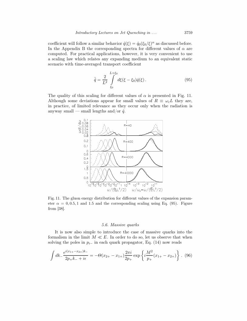
The quality of this scaling for different values of α is presented in Fig. 11.Although some deviations appear for small values of R ≡ ωcL they are,in practice, of limited relevance as they occur only when the radiation isanyway small — small lengths and/or q.
Fig. 11. The gluon energy distribution for different values of the expansion param-
eter α = 0, 0.5, 1 and 1.5 and the corresponding scaling using Eq. (95). Figure
from [38].
5.6. Massive quarks
It is now also simple to introduce the case of massive quarks into theformalism in the limit M ≪ E. In order to do so, let us observe that whensolving the poles in pi− in each quark propagator, Eq. (14) now reads
∫
dk−ei(x1+−x2+)k−
2p+k− + iǫ= −Θ(x2+ − x1+)
2πi
2p+exp
iM2
p+(x1+ − x2+)
. (96)

3760 J. Casalderrey-Solana, C.A. Salgado
This introduces only a multiplicative factor in the eikonal trajectories. Thisfactor depends on the energy of the quark. The relevant “+′′ componentof the momentum is thus p+ before the gluon splitting and (1 − z)p+ afterthe gluon splitting. So, the total contribution from the amplitude times thecomplex conjugate amplitude to be included in the integrand of (89) is
exp
iM2
p+(x0+ − x+)
× exp
iM2
(1 − z)p+(x+ − L+)
× exp
−iM2
p+(x0+ − x+)
× exp
−iM2
(1 − z)p+(x+ − L+)
(97)
which, expanding 1/(1− z) ≃ 1− z and writing in terms of the gluon energyis just [46]
exp
ix2M2
k+(x+ − x+)
. (98)
So, in the limit of small-z and M ≪ E, the leading mass correction to themedium-induced gluon radiation corresponds to include the multiplicativefactor (98) inside the integrand of (89) — see also [46–49].
In Fig. 12 we compare the spectra of gluons radiated off massless andmassive quarks. The effect of including quark masses into the propagatorsis to reduce the amount of radiation. This is known in the vacuum underthe name of dead cone effect, as the mass terms in the propagators definea minimum angle θdc ∼ M/E below which the radiation is suppressed. Inthe medium the situation is a bit more complicated because as we havediscussed, formation time effects already suppress the radiation for small
Fig. 12. k2t (left-hand side) and angular, (right-hand side) spectra of medium-
induced radiated gluons off a massless (red), charm (blue) and bottom (green)
quarks [46].

Introductory Lectures on Jet Quenching in . . . 3761
angles. In this case, two competing effects exist, on the one hand, there isa genuine suppression produced by mass terms in the propagators; on theother hand, the formation time is now smaller tform ∼ 2ω/(M2+k2
⊥) and theLPM suppression appears at smaller values of k⊥, enhancing the radiationat small angles as compared with the massless case. This effect is, however,restricted to a limited region of phase space, negligible for most observables,and the net effect of the mass terms is to reduce the amount of radiation.The energy loss of heavy quarks is, in this manner, smaller than that for lightquarks and the formalism predicts an one-to-one correspondence between thetwo. This smaller radiation translates, in general, into smaller suppressionof high-p⊥ heavy than light quarks.
6. Application of the formalism for jet quenching studies
As we discussed in Sec. 3, the cross section for producing a hadron h athigh transverse momentum pT and rapidity y can be written in the factorizedform
dσAB→h
dp2Tdy
=
∫
dx2
x2
dz
zx1fi/A(x1, Q
2)x2fj/B(x2, Q2)
dσij→kl
dtD
vac/medk→h (z, µ2
F ) ,
(99)where a summation over flavors is implicit — see e.g. [50] for an explicitexpression including kinematical limits, etc. For proton–proton collisions,parton distribution functions, fi/p(x,Q2), and vacuum fragmentation func-
tions, Dvack→h(z, µ2
F ), are known from global fits to experimental data us-ing the DGLAP evolution equations [12]. In the nuclear case, the PDFsare known from similar global fits [22–28]. On the other hand, the FF,Dmed
k→h(z, µ2F ), contain the information about the medium we want to study.
In the following we explain how the formalism of medium-induced gluon ra-diation can be implemented in (99) to compute the medium modification ofthe fragmentation functions and how to use them to characterize the mediumproperties.
6.1. Medium-modified fragmentation functions
The theoretical description of the fragmentation of a high-pT particle inthe presence of a medium is not completely known from first principle calcu-lations and some degree of modeling is needed. One possibility is to includeall the modifications of the fragmentation functions into a modified splittingfunction in the DGLAP evolution equations. For a simplified discussion letus take into account only gluon FF — including other flavors translate intoa summation over flavors — whose DGLAP evolution is
3762 J. Casalderrey-Solana, C.A. Salgado
t∂
∂tDg→h(x, t) =
1∫
x
dz
z
αs
2πPgg(z)Dg→h
(x
z, t)
, (100)
where t ≡ µ2F and Pgg(z) is the splitting function describing the probability
that a daughter gluon has been radiated from a parent gluon with fractionof momentum z. The probabilistic interpretation of the DGLAP evolutionis more clear from its equivalent (at LO) integral formulation (see e.g. [13])
D(x, t) = ∆(t)D(x, t0) + ∆(t)
t∫
t0
dt1t1
1
∆(t1)
∫
dz
zP (z)D
(x
z, t1
)
. (101)
The first term on the right-hand side in this expression corresponds to thecontribution with no splittings between t0 and t while the second one givesthe evolution when some finite amount of radiation is present. The evolutionis controlled by the Sudakov form factors
∆(t) = exp
−t∫
t0
dt′
t′
∫
dzαs(t
′, z)
2πP (z, t′)
, (102)
with the interpretation of the probability of no resolvable branching betweenthe two scales t and t0. The definition of the Sudakov form factors andits probabilistic interpretation depend on the cancellation of the differentdivergencies appearing in the corresponding Feynman diagrams, see e.g. [51].Although such cancellation has never been proved on general grounds forpartons re-scattering in a medium, it has been found in [52] that, undercertain assumptions, all the medium effects can be included in a redefinitionof the splitting function
P tot(z) = P vac(z) + ∆P (z, t) . (103)
This possibility was exploited in [54] where the additional term in the split-ting probability is just taken from the medium-induced gluon radiation bycomparing the leading contribution in the vacuum case — see Eq. (3)
∆P (z, t) ≃ 2πt
αs
dImed
dzdt. (104)
Implementing (103) and (104) into (101) the medium-modified fragmen-tation functions can be computed — see also [55] for a related approach.Only the initial conditions of the evolution need to be specified. In [54] the
Introductory Lectures on Jet Quenching in . . . 3763
KKP set of FF [56] was used for the vacuum as well as for the medium atthe initial scale Q2
0, i.e. Dmed(x,Q20) = Dvac(x,Q2
0). In this model all themedium-effects are built during the evolution. The motivation for this ansatzis the following: in hadronic collisions, particles produced at high enoughtransverse momentum hadronize outside the medium. So, this assumes thatthe non-perturbative hadronization is not modified by the medium, whoseeffect is only to modify the perturbative associated radiation11. All presentradiative energy loss formalisms rely on this assumption.
The fact that the medium-induced gluon radiation is infrared andcollinear finite allows for a simplification of this formulation, valid whenE ∼ Q ≫ 1. Under these conditions, Eqs. (101) and (102) can be writtenas [54]
Dmed(x, t) = p0Dvac(x, t) +
∫
dǫ
1 − ǫp(ǫ)Dvac
(
x
1 − ǫ, t
)
, (105)
with the probability of energy loss given by a Poisson distribution
p0 = exp
−∞∫
0
dω
ω∫
0
dk⊥dImed
dωdk⊥
(106)
p(∆E) = p0
∞∑
k=1
1
k!
∫
k∏
i=1
dωi
ωi∫
0
dk⊥dImed(ωi)
dωdk⊥
δ
k∑
j=1
ωj−∆E
(107)
and ǫ = ∆E/E. The total distribution is normally written as
P (∆E) = p0δ(∆E) + p(∆E) . (108)
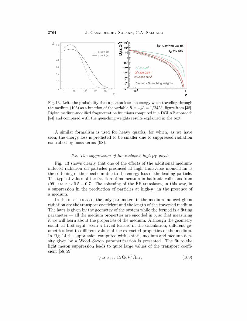
Eqs. (106), (107) and (108) are normally called quenching weights. Theyhave been first proposed in [53] and together with Eq. (105) constitute thebasis of most of the phenomenology of jet quenching in heavy-ion collisions.Notice that the probability that a parton loses no energy when travelingthrough the medium, given by p0, can be large if the medium length and/orthe transport coefficient are small. In Fig. 13 we plot this probability andthe corresponding medium-modified fragmentation functions. Also plottedare the results from [54] when the medium effects are included at everyindividual splitting — notice that for the case of hadronic collisions, themost relevant virtuality is precisely that of the order of the initial partonenergy, µF ∼ E.
11 For processes with different kinematic conditions [57] this assumption could not hold,but the negligible effects seen in dAu data at RHIC [10] indicate that this is a rea-sonable assumption for particle production at high-pt in nuclear collisions.
3764 J. Casalderrey-Solana, C.A. Salgado
Fig. 13. Left: the probability that a parton loses no energy when traveling through
the medium (106) as a function of the variable R ≡ ωcL = 1/2qL3, figure from [38].
Right: medium-modified fragmentation functions computed in a DGLAP approach
[54] and compared with the quenching weights results explained in the text.
A similar formalism is used for heavy quarks, for which, as we haveseen, the energy loss is predicted to be smaller due to suppressed radiationcontrolled by mass terms (98).
6.2. The suppression of the inclusive high-pT yields
Fig. 13 shows clearly that one of the effects of the additional medium-induced radiation on particles produced at high transverse momentum isthe softening of the spectrum due to the energy loss of the leading particle.The typical values of the fraction of momentum in hadronic collisions from(99) are z ∼ 0.5 − 0.7. The softening of the FF translates, in this way, ina suppression in the production of particles at high-pT in the presence ofa medium.
In the massless case, the only parameters in the medium-induced gluonradiation are the transport coefficient and the length of the traversed medium.The later is given by the geometry of the system while the formed is a fittingparameter — all the medium properties are encoded in q, so that measuringit we will learn about the properties of the medium. Although the geometrycould, at first sight, seem a trivial feature in the calculation, different ge-ometries lead to different values of the extracted properties of the medium.In Fig. 14 the suppression computed with a static medium and medium den-sity given by a Wood–Saxon parametrization is presented. The fit to thelight meson suppression leads to quite large values of the transport coeffi-cient [58, 59]
q ≃ 5 . . . 15GeV2/fm , (109)
Introductory Lectures on Jet Quenching in . . . 3765
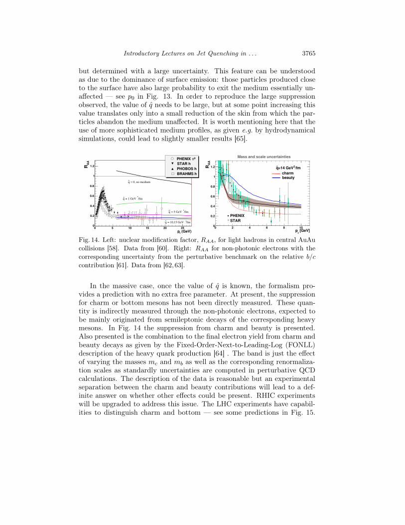
but determined with a large uncertainty. This feature can be understoodas due to the dominance of surface emission: those particles produced closeto the surface have also large probability to exit the medium essentially un-affected — see p0 in Fig. 13. In order to reproduce the large suppressionobserved, the value of q needs to be large, but at some point increasing thisvalue translates only into a small reduction of the skin from which the par-ticles abandon the medium unaffected. It is worth mentioning here that theuse of more sophisticated medium profiles, as given e.g. by hydrodynamicalsimulations, could lead to slightly smaller results [65].
Fig. 14. Left: nuclear modification factor, RAA, for light hadrons in central AuAu
collisions [58]. Data from [60]. Right: RAA for non-photonic electrons with the
corresponding uncertainty from the perturbative benchmark on the relative b/c
contribution [61]. Data from [62,63].
In the massive case, once the value of q is known, the formalism pro-vides a prediction with no extra free parameter. At present, the suppressionfor charm or bottom mesons has not been directly measured. These quan-tity is indirectly measured through the non-photonic electrons, expected tobe mainly originated from semileptonic decays of the corresponding heavymesons. In Fig. 14 the suppression from charm and beauty is presented.Also presented is the combination to the final electron yield from charm andbeauty decays as given by the Fixed-Order-Next-to-Leading-Log (FONLL)description of the heavy quark production [64] . The band is just the effectof varying the masses mc and mb as well as the corresponding renormaliza-tion scales as standardly uncertainties are computed in perturbative QCDcalculations. The description of the data is reasonable but an experimentalseparation between the charm and beauty contributions will lead to a def-inite answer on whether other effects could be present. RHIC experimentswill be upgraded to address this issue. The LHC experiments have capabil-ities to distinguish charm and bottom — see some predictions in Fig. 15.

3766 J. Casalderrey-Solana, C.A. Salgado
0
0.2
0.4
0.6
0.8
1
0 10 20 30 40 50
RA
A
pT (GeV)
mesons from charm
q = 10q = 25
q = 100
0
0.2
0.4
0.6
0.8
1
0 10 20 30 40 50
RA
A
pT (GeV)
electrons from bottom
q = 10q = 25
q = 100
Fig. 15. RAA for D’s (left) and for electrons coming from bottom decays (right) at
y = 0 for 10% PbPb collisions at√
s = 5.5 TeV/A, for different q (in GeV2/fm).
Figures from [66].
6.3. Jets in heavy-ion collisions
The amount of information about the medium extracted by measuringinclusive particle suppression is limited as we have just seen. More differen-tial observables could lead to a more accurate determination of the transportcoefficient and to pindown the interplay with geometry. Relevant questionsare where and how the energy of the initial parton is lost by interactions withthe medium. For that, reconstructing the whole history of the parton whiletraveling through the medium would clearly be an ideal situation. Fortu-nately, some experimental handle on this is provided by jet measurements.
Jets are extended objects composed of collimated bunches of particlescontained into a reduced region of phase space extending in azimuthal an-gle, ∆Φ, and rapidity, ∆y. A jet can be characterized by the opening angleR =
√
∆Φ2 + ∆η2 defining a cone around the jet axis where the energy isdeposited, but more sophisticated definitions are possible [68]. The descrip-tion of jets in the vacuum, as e.g. in experiments of e+e− annihilation, isone of the most precise tests of perturbative QCD. With different degreesof refinement, a jet is computed as the output of a parton branching pro-cess starting by a highly virtual quark or gluon produced in the elementarypartonic collision. Each branching is controlled by the splitting function,known at LO, NLO and NNLO.
In the medium case, with modified splitting probabilities, the jet prop-erties are modified. We have already presented modifications to the longitu-dinal structure as given by the fragmentation functions. Jet properties are,
Introductory Lectures on Jet Quenching in . . . 3767
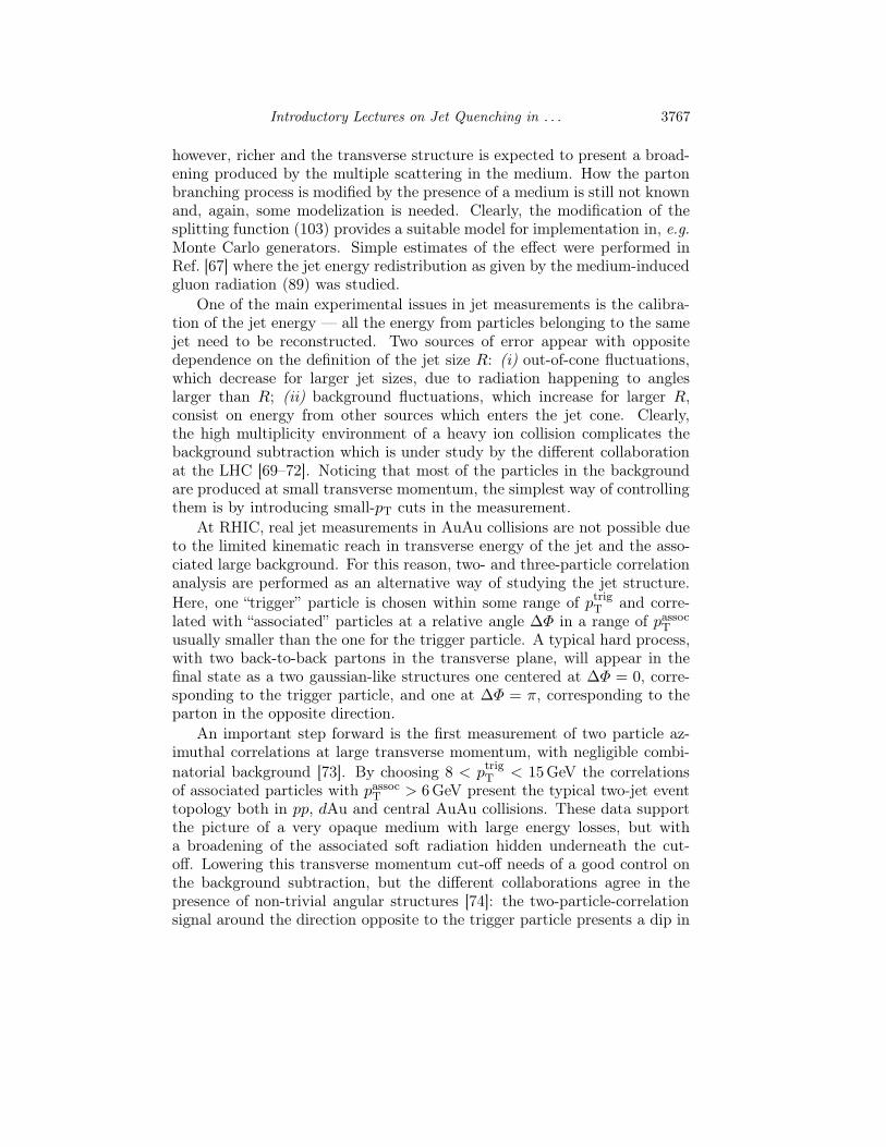
however, richer and the transverse structure is expected to present a broad-ening produced by the multiple scattering in the medium. How the partonbranching process is modified by the presence of a medium is still not knownand, again, some modelization is needed. Clearly, the modification of thesplitting function (103) provides a suitable model for implementation in, e.g.Monte Carlo generators. Simple estimates of the effect were performed inRef. [67] where the jet energy redistribution as given by the medium-inducedgluon radiation (89) was studied.
One of the main experimental issues in jet measurements is the calibra-tion of the jet energy — all the energy from particles belonging to the samejet need to be reconstructed. Two sources of error appear with oppositedependence on the definition of the jet size R: (i) out-of-cone fluctuations,which decrease for larger jet sizes, due to radiation happening to angleslarger than R; (ii) background fluctuations, which increase for larger R,consist on energy from other sources which enters the jet cone. Clearly,the high multiplicity environment of a heavy ion collision complicates thebackground subtraction which is under study by the different collaborationat the LHC [69–72]. Noticing that most of the particles in the backgroundare produced at small transverse momentum, the simplest way of controllingthem is by introducing small-pT cuts in the measurement.
At RHIC, real jet measurements in AuAu collisions are not possible dueto the limited kinematic reach in transverse energy of the jet and the asso-ciated large background. For this reason, two- and three-particle correlationanalysis are performed as an alternative way of studying the jet structure.
Here, one “trigger” particle is chosen within some range of ptrigT and corre-
lated with “associated” particles at a relative angle ∆Φ in a range of passocT
usually smaller than the one for the trigger particle. A typical hard process,with two back-to-back partons in the transverse plane, will appear in thefinal state as a two gaussian-like structures one centered at ∆Φ = 0, corre-sponding to the trigger particle, and one at ∆Φ = π, corresponding to theparton in the opposite direction.
An important step forward is the first measurement of two particle az-imuthal correlations at large transverse momentum, with negligible combi-
natorial background [73]. By choosing 8 < ptrigT < 15GeV the correlations
of associated particles with passocT > 6GeV present the typical two-jet event
topology both in pp, dAu and central AuAu collisions. These data supportthe picture of a very opaque medium with large energy losses, but witha broadening of the associated soft radiation hidden underneath the cut-off. Lowering this transverse momentum cut-off needs of a good control onthe background subtraction, but the different collaborations agree in thepresence of non-trivial angular structures [74]: the two-particle-correlationsignal around the direction opposite to the trigger particle presents a dip in

3768 J. Casalderrey-Solana, C.A. Salgado
central collisions, in striking contrast with the typical Gaussian-like shape inproton–proton or peripheral AuAu collisions. The origin of this structure isstill unclear. In the presence of an ordering variable (as virtuality or angu-lar ordering in the vacuum parton shower) the implementation of (103) withthe usual Sudakov form factors (102) produce similar angular structures forenergies ω . 2q1/3 ∼ 3GeV in central AuAu [75]. At present, the mostwidely accepted interpretation is in terms of shock wave formation due tothe hydrodynamical behavior of the energy deposition in the medium [76].Cherenkov gluons have also been proposed as a possible source of these non-trivial angular structures [77]. Theoretical improvements on the used mod-els, together with new experimental data, would help elucidating the originof this interesting effect, which takes place, however, in a rather complicatekinematical region between the soft and the hard parts of the spectra.
6.4. Is there an energy dependence on q?
In all the application we have discussed q has been treated as a con-stant. This is a good approximation in the description of high transversemomentum particles at RHIC. However, the LHC will explore jets in a muchbroader range of energies which could allow to study the energy dependenceof the momentum broadening.
As we have seen in Sec. 4.3, q can be related to saturation physics. Infact, the momentum broadening of a probe propagating through the plasmacan be expressed as
qR ≈ CR
Nc
Q2s
L, (110)
where R is the color representation of the probe Q2s is the saturation scale of
the medium and L is the length. The quenching spectrum depends on thegluon broadening. The saturation scale depends on the value of x probed inthe interaction of the particle with the medium
In a thermal medium, the saturation scale for typical thermal particles isgiven by µD ∼ gT [93]. As the energy of the probe increases, the saturationscale increases because of evolution. In [93] it is argued that the typical xprobed by a parton propagating in the medium is
x ∼ Q2s
ET, (111)
where E is the energy of the probe. Thus, the saturation scale grows andso does q. Since saturation is a non-linear process, it is not surprising thata non linear dependence of the Q2
s with the medium length appears too.
Introductory Lectures on Jet Quenching in . . . 3769
This effect has been studied in [93], where a simplified treatment of theevolution, based on the leading logarithmic approximation was performed.Their findings are summarized in Fig 16. A significant dependence on thejet energy of q is observed which could be measured in the LHC. As alsoproposed in [93], the broadening could be measured directly by studyingthe jet acoplanarity as a function of the jet energy, which constitutes a newobservable for heavy ion collisions.
E (GeV)0 50 100 150 200 250 300
/fm
)2
(G
eVq
0
5
10
15
20 T=0.6 GeV cL>L
T=0.4 GeV cL>L
L=1 fm T=0.6 GeV
L=1 fm T=0.4 GeV
Fig. 16. Jet quenching parameter q as a function of the jet energy for different
path lengths. The square (triangle) marks the value of q for thermal particle at
T = 0.4 GeV (T = 0.6 GeV). Lc = 1/xT is the coherence length, i.e. the length
below which the particle scatters coherently with the medium. Above this length,
no dependence on L is observed. Figure from [93].
7. New developments
In Sec. 5 we have seen that the spectrum of radiated gluon can be ex-pressed in terms of the expectation value of two adjoint light-like Wilsonlines. The phenomenological applications of the formalism described inSec. 6 are based in a particular model of this object, based on perturba-tion theory. As we have seen, the value of q extracted from the data is3–4 times larger than what one expects from perturbation theory. This factsuggests that strong coupling non-perturbative effects are important.
The computation of these effects in QCD is hard. Lattice QCD givesnon-perturbative access to equilibrium properties. However, it is very com-plicated to extract dynamical quantities from the lattice, since the compu-tations are performed in Euclidean time. What is more, the object we areinterested in involves light-like trajectories, which is an intrinsic Minkowskiproperty.
This difficulty has led recently to significant interest in strong couplingcomputation in N = 4 Super-Symmetric Yang–Mills in the infinity numberof colors limit. This is, like QCD, a SU(Nc) gauge theory. However, unlike

3770 J. Casalderrey-Solana, C.A. Salgado
QCD, it is a supersymmetic theory with no conformal anomaly. It also possesa different matter content, since apart from the common gluons, it containsfermions and scalars in the adjoint color representation. Despite of all thesedifferences, computations in this theory are of interest due to a recent the-oretical development, the AdS/CFT correspondence. This correspondenceallows to address the dynamical (real time) properties of the gauge theory atstrong coupling in a regime in which traditional non perturbative methods,such as lattice, are not applicable.
Even though the relation between QCD and N = 4 SYM is still ques-tionable there are experimental (strong elliptic flow and particle suppression)and theoretical indications (lattice computations of the coupling constant)that suggest that the relevant physics of QCD close to the phase transitionis the one of the strong coupling. Thus, the computations within the frame-work described below are of great value, since the AdS/CFT correspondenceis the only method known to address these problems in a dynamical gaugetheory. One of the great success of this approach is the computation ofη/s = 1/4π. Current fits of hydrodynamical models to the elliptic flow yielda value of the shear viscosity close to that predicted from the AdS/CFTcorrespondence. This is a remarkable achievement for a theory in principleso different from QCD. Below we will review another computation in whicha similar success has been obtained, the jet quenching parameter, and themomentum diffusion coefficient.
7.1. Brief introduction to the AdS/CFT correspondence
In this subsection we will introduce the basic concepts of the AdS/CFTcorrespondence [78] necessary for the computation of light-like Wilson lineswithin this framework. It is not the scope of this lectures to give a systematicintroduction to this subject, which can be found in excellent reviews suchas [79, 80].
In its weakest form, the AdS/CFT correspondence states that type II BSupergravity (SUGRA) in a particular gravitational background, the Antide Sitter space times a five dimensional sphere AdS5 × S5, is dual to thelarge number of colors (Nc → ∞), strong coupling limit of N = 4 SYM,a conformal field theory. SUGRA is a supersymmetric theory of gravity in10 dimensions and it can be obtained as the low energy effective action ofType II B string theory. From this point of view, SUGRA is the effectivetheory that describes the string excitation with energy E2 ≪ 1/α′, the stringtension.
The AdS5 space is a five dimensional space with constant (negative)curvature, R−1. A convenient choice for the AdS5 × S5 background metricis given by
Introductory Lectures on Jet Quenching in . . . 3771
ds2 = − r2
R2
(
−dt2 + dx21 + dx2
2 + dx23
)
+R2
r2dr2 + R2dΩ5 , (112)
where dΩ5 is the metric of the five dimensional sphere. As can be seen,in the boundary, r → ∞, the metric tends to the usual Minkowski metric(times a prefactor).
The duality maps the operators of the field theory to the boundary valuesof the SUGRA fields. In the gravity theory, all the dynamics are described bythe classical equations of motion of those fields with the boundary conditionsdictated by the correspondence. The expectation value of the operators inthe field theory are obtained by evaluating the action of the gravity field onthe classical solution. The coupling constant of the gauge theory, gYM, isrelated to the string tension and the curvature as
R2 =√
g2YMNcα
′ =√
λα′ , (113)
where we have defined the ’t Hooft coupling λ = g2YMNc. The SUGRA
approximation is valid if R2 ≫ α′, thus, the ’t Hooft coupling λ → ∞.In order to describe the field theory at finite temperature, it is necessary
to introduce a “black brane”. From the SUGRA point of view, this object isanalog to an extended black hole which leads to a 3 dimensional horizon ata given value of the coordinate r0. In the presence of this object, the metricEq. (112) is modified
ds2 =r2
R2
(
−fdt2 + dx21 + dx2
2 + dx23
)
+R2
r2
1
fdr2 + R2dΩ5 , (114)
where f = 1 − r40/r
4. The Hawking temperature of the black brane is thetemperature of the field theory. In the metric Eq. (114), the temperature isgiven by
T =r0
πR2. (115)
7.2. Wilson lines in AdS/CFT
According to the correspondence, an external heavy probe in the fun-damental representation of the gauge group (“quark”) is described in thedual theory by a classical string which pends from the boundary of the AdSspace [81]. The string is a two dimensional surface parametrized by theinternal coordinates τ, σ 12
(τ, σ) → XM =(
t(τ, σ), xi(τ, σ), r(τ, σ))
, (116)
12 The string also has coordinates in the 5-dimensional sphere. However in all the appli-cations below these remain constant and, thus, we will suppress them for simplicity.
3772 J. Casalderrey-Solana, C.A. Salgado
where the index i = 1, 2, 3. In analogy with the relativistic point particle,the action of the string is given by its area; this is known as the Nambu–Gotoaction
SNG = − 1
2πα′
∫
dσdτ√
−det GMN∂aXM∂bXN , (117)
where a, b = τ, σ and GMN is the background metric Eq. (112), (Eq. (114)if we are interested in a finite temperature system).
As we have obtained in the previous sections, the propagation of a heavyprobe in the field theory is described in terms of a Wilson line in the fun-damental representation along the path of the quark. This path is also theboundary condition to solve the equations of motion derived from Eq. (117).After the solution of the classical equation of motion is found XM
cl , the ex-pectation value of the corresponding Wilson line is given by
〈W 〉 ∝ e−iSNG(XMcl ) . (118)
As a simple example, let us consider a single massive quark at rest. Itsspace time trajectory is described by a line at constant position x0. Due tosymmetry, the solution of the Nambu–Goto action with the lowest action isthe surface
XMcl =
(
t, xi0, r)
. (119)
According to the correspondence, the expectation value of the Wilson line is
〈W 〉 ∝ exp
− i
2πα′
T /2∫
−T /2
dt
rmax∫
ro
dr
, (120)
where rmax is an upper cut off. At zero temperature we can set r0 = 0. Inthis case, the divergent prefactor is naturally interpreted as the mass of thequark
M =rmax
2πα′ . (121)
At finite temperature, the free energy of a single quark is given by
F1 = − r0
2πα′ = −√
λT
2. (122)
It has been also shown in [82] that as long as M ≫ −F1 the thermal massof the quark is given by
Mth = M −√
λT
2. (123)

Introductory Lectures on Jet Quenching in . . . 3773
7.3. Computing the jet-quenching parameter
We now turn our attention to the computation of two parallel Wilsonlines in the fundamental representation [83, 84].
⟨
Tr[
W †C(
x1 = −y
2
)
WC(
x =y
2
)]⟩
, (124)
where C is the line of constant rapidity
tC = t′ cosh η , x3C = −t′ sinh η . (125)
Light-like trajectories are obtained by taking the limit η → ∞ The line coverthe interval t′ = (−T ′/2,T ′/2) with T ′ >> y. In this limit, we can assumethat the dynamics are independent of t′. Due to this, it is convenient tointroduce the following change of coordinate (boost to the rest frame)
dt = dt′ cosh η − dx′3 sinh η , (126)
dx3 = −dt′ sinh η + dx′3 cosh η . (127)
To continue further, we need to choose a particular set of coordinates(τ, σ). Since the string solution we are interested on is independent of t′,we choose τ = t; it is also convenient to chose σ = x1. It is also clear thatthe action is smaller if the the string world-sheet does not extend in thelongitudinal direction x′
3. Thus, we need to find a solution
XMcl =
(
t′, x1, 0, 0, r(x1))
, (128)
which should be symmetric under the change x1 → −x1. Thus, if the stringconnects the two endpoints, it should have turning point at x1 = 0, i.e.
r(x1 = 0) = 0 , (129)
where r = dr/dx1.The Nambu–Goto action reads,
S = − 1
2πα′ T′2
y/2∫
0
dx1
√
1
R2
(
r4 − r40 cosh2 η
)
(
1
R2+
R2r2
r4 − r40
)
. (130)
Note that this expression remains real only if r > r0 cosh η (r > r0 sincethe string is outside the horizon). As we have seen, the maximum value ofr, rmax is proportional to the mass of the probe Eq. (121). Thus, for a givenvalue of the mass, there is a critical value of the rapidity
cosh ηc =M2
(√λT2
)2 , (131)

3774 J. Casalderrey-Solana, C.A. Salgado
above which, the Wilson loop is exponentially suppressed. It is clear, then,that the limits M → ∞ and η → ∞ do not commute. According to [84],the light-like Wilson loops are obtained by taking the η → ∞ first and thenM → ∞. In this limit, the action is simplified to
S = − i
πα′ T′ cosh η
y/2∫
0
dx1r20
R
√
1
R2+
R2r2
r4 − r40
. (132)
Since the action does not depend on x1, we have a conserved Hamiltonian
h = L− r∂L∂r
, (133)
where
L =
√
1
R2+
R2r2
r4 − r40
. (134)
From this expression, we obtain
r =1
R3h
√
(
r4 − r40
)
(1 − R2h2) . (135)
Thus, in order to have real coordinates, R2h2 ≪ 1. Note also that in thisapproximation, the only point where the r vanishes in the horizon r = r0.Thus, the string world-sheet always touches the horizon.
From Eq. (135) we obtain an expression for the position of the string x1
x1(r) =R3h√
1 − R2h2
r∫
0
dr1
√
r4 − r40
. (136)
The constant of motion is determined by the condition
x1(r → ∞) =y
2, (137)
which leads to
y
2=
R3h
r0
√1 − R2h2
√π
Γ (54)
Γ (34)
. (138)
Substituting Eq. (136) into the action Eq. (132) we find
S = −i√
λT√
πΓ (5
4)
Γ (34)
L
√
√
√
√1 +
(
yT
2
√π
Γ (34)
Γ (54)
)2
, (139)
where L = T ′ cosh η is the length traveled by the parton.
Introductory Lectures on Jet Quenching in . . . 3775
At small transverse distance we obtain⟨
Tr[
W †C
(
x1 = −y
2
)
WC(
x =y
2
)]⟩
∝ exp
−√
λT√
πΓ (5
4)
Γ (34)
L
(
1 +y2T 2
8π
Γ 2(34 )
Γ 2(54 )
)
. (140)
The term independent of the transverse position y corresponds to two in-dependent quarks. In [84] it is argued that this contribution should besubtracted. The remaining piece has the form of Eq. (43) and we can read
qF =√
λT 3 π3/2
2
Γ (34)
Γ (54)
. (141)
The index F indicates that the calculation has been performed with Wilsonlines in the fundamental representation. This is not quite the object thatappears in the radiative spectrum, where the Wilson lines were evaluated inthe adjoint representation. However, these two objects are related in SU(Nc)theories [83]
TrWA = Tr WF Tr W †F − 1 (142)
and thus in the large Nc limit we obtain
q =√
g2Nc T 3π3/2 Γ (34)
Γ (54)
. (143)
Despite the fact that the above computation is performed in the infinitecoupling, infinite number of colors limit, we would like to have a numericestimate as a comparison to perturbative expectations. To do so, we willassume typical values for αs = 0.3 and Nc = 3 of RHIC physics. Recallingthat αs = g2/4π, we obtain
q = 4.5, 10.6, 20.7GeV2/fm for T = 300, 400, 500MeV . (144)
Remarkably, the values obtained are much larger than the typical scale of themedium, set by the temperature. This is also what it has been observed inthe phenomenological fits presented in Sec. 6. What is more, these numericvalues are comparable to what was obtained in the phenomenological fitsto RHIC data. Once again, this is a remarkable success, since the theoryin which this parameter has been obtained, N = 4 SYM, is not QCD.This observation, together with the small values of the viscosity at RHIC,constitute a compelling indication (but, clearly, not an evidence) that therelevant physics at RHIC are those of strong coupling.

3776 J. Casalderrey-Solana, C.A. Salgado
However, we should be careful in comparing this values to RHIC phe-nomenology. As we can see, the jet quenching parameter depends explicitlyin the number of colors and the coupling. This is different from other trans-port parameters computed in AdS/CFT such as the shear viscosity. Theexplicit dependence on the number of colors hints that, unlike the η/s ratio,the result Eq. (143) is not universal. This statement has been corrobo-rated by explicit calculation in other theories with gravity duals. In fact,the number of colors is the only measurement of the medium density in theN = 4 SYM theory. Based on this and on the explicit computations in othertheories, the authors of [84] have proposed the following scaling
qQCD =
√
sQCD
sN=4qN=4 ≈ 0.6 qN=4 , (145)
where sQCD and sN=4 are the entropy density of QCD and N = 4 SYM,respectively. Even with this correction, the obtained values are comparablewith those obtained from the phenomenological fits.
7.4. Momentum broadening in gauge theories
In the previous discussion, we have elevated the dipole formula Eq. (43)to a non perturbative definition of the jet quenching parameter, the mediumscale responsible for the emission of hard gluons. The values obtained forthis parameter are in surprisingly good agreement with those obtained fromexperimental data. This is a great success, however the correspondence isa powerful theoretical tool that allows to address issues that go beyond theestimation of the value of parameters.
One of those issues is the relation of q with the momentum broadening.In Sec. 4.5 we have shown that in the dipole approximation q coincides withthe mean momentum transferred squared per unit length. Since this is aquantity that could potentially be explicitly measured, it is interesting tocheck whether this relation still holds at strong coupling.
The goal is to compute the momentum broadening of a probe within theAdS/CFT correspondence. We study a very heavy (almost) static probe. Inthis case, its motion in the plasma can be described by a classical equationof motion under a random force
dpi
dt= Fi , (146)
where the force F is due to the thermal fluctuations of the (chromo) electricfields in the bath [85]
Introductory Lectures on Jet Quenching in . . . 3777
F ≡∫
d3xQ†(t,x)T aQ(t,x)Ea(t, x) , (147)
with Q(x, t) the heavy quark field.When the quark mass is very heavy, the time required to change its
momentum is much greater than the typical scale of the medium, T . Thus,the distribution of “kicks” can be characterized by its second moment,
〈Fi(t)Fj(t′)〉 = κδijδ(t − t′) , (148)
where the constant κ is the mean squared momentum transferred to theprobe. From this, it is clear that
κ =
∫
dt 〈F(t)F(0)〉HQ , (149)
where the average is taken with the partition function of the gauge theoryplus the heavy quark.
In this expression there is a technical subtlety. The correlator in Eq. (149)is not time ordered and, thus, its extraction from the partition functionshould be treated with care. It is convenient to express κ in terms of theretarded correlator. By using the Kubo–Martin–Schwinger (KMS) [86] re-lations we can relate it to the retarded correlator
κ = limω→0
(
−2T
ωIm GR(ω)
)
, (150)
where
iGR(t) = θ(t) 〈[F(t),F(0)]〉HQ . (151)
This is a rather technical step but it is motivated by the fact that there isa well defined prescription to compute retarded correlators in the AdS/CFTcorrespondence.
The partition function of the bath in the presence of a heavy quark isgiven by [87]
ZHQ =∑
s
⟨
s∣
∣
∣e−βH
∣
∣
∣s⟩
=
∫
d3x∑
s′
⟨
s′∣
∣
∣Q(x,−T )e−βHQ†(x,−T )∣
∣
∣ s′⟩
, (152)
where the states |s′〉 are states of the gauge theory without the heavy quark.
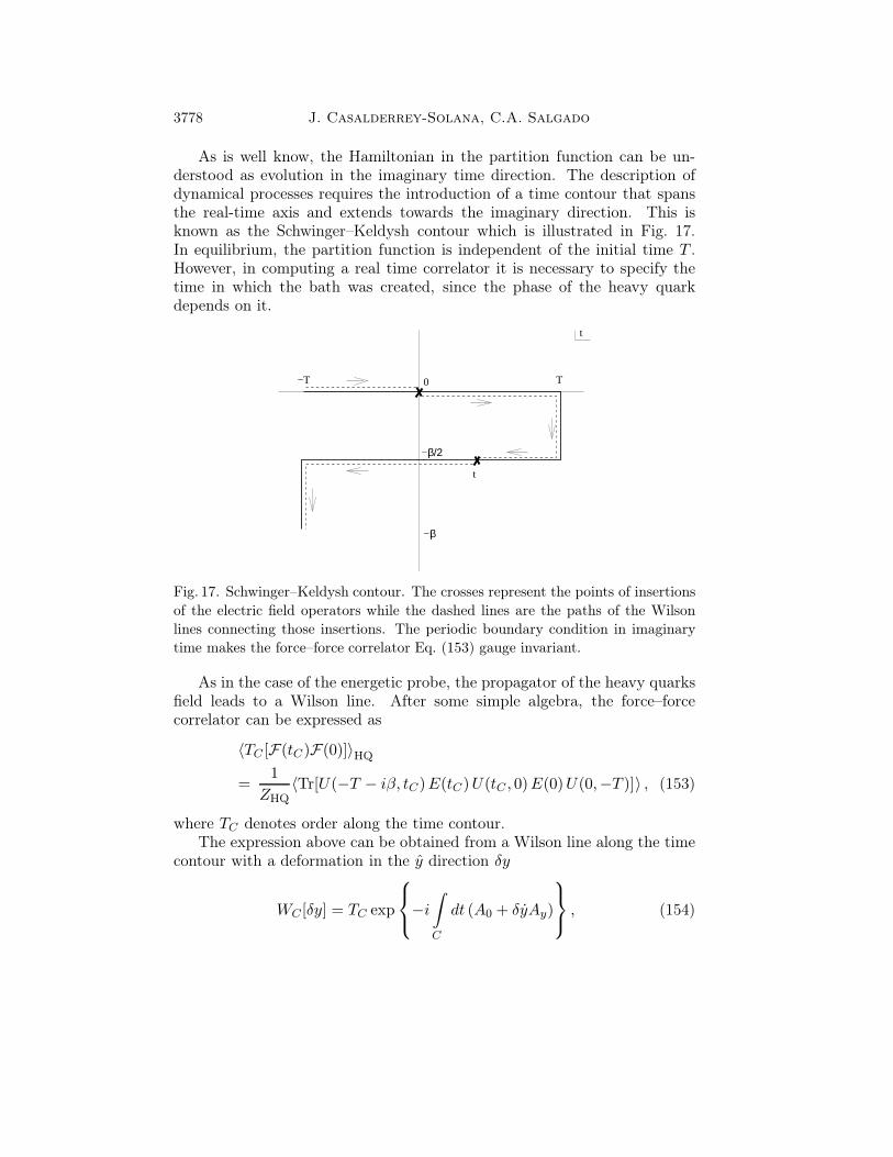
3778 J. Casalderrey-Solana, C.A. Salgado
As is well know, the Hamiltonian in the partition function can be un-derstood as evolution in the imaginary time direction. The description ofdynamical processes requires the introduction of a time contour that spansthe real-time axis and extends towards the imaginary direction. This isknown as the Schwinger–Keldysh contour which is illustrated in Fig. 17.In equilibrium, the partition function is independent of the initial time T .However, in computing a real time correlator it is necessary to specify thetime in which the bath was created, since the phase of the heavy quarkdepends on it.
t
−i
−iβ/2
−T T0
t
β
Fig. 17. Schwinger–Keldysh contour. The crosses represent the points of insertions
of the electric field operators while the dashed lines are the paths of the Wilson
lines connecting those insertions. The periodic boundary condition in imaginary
time makes the force–force correlator Eq. (153) gauge invariant.
As in the case of the energetic probe, the propagator of the heavy quarksfield leads to a Wilson line. After some simple algebra, the force–forcecorrelator can be expressed as
〈TC [F(tC)F(0)]〉HQ
=1
ZHQ〈Tr[U(−T − iβ, tC)E(tC)U(tC , 0)E(0)U(0,−T )]〉 , (153)
where TC denotes order along the time contour.The expression above can be obtained from a Wilson line along the time
contour with a deformation in the y direction δy
WC [δy] = TC exp
−i
∫
C
dt (A0 + δyAy)
, (154)
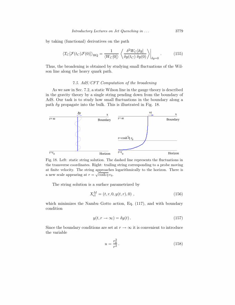
Introductory Lectures on Jet Quenching in . . . 3779
by taking (functional) derivatives on the path
〈TC [F(tC)F(0)]〉HQ =1
〈WC [0]〉
⟨
δ2WC [δy]
δy(tC) δy(0)
⟩∣
∣
∣
∣
δy=0
. (155)
Thus, the broadening is obtained by studying small fluctuations of the Wil-son line along the heavy quark path.
7.5. AdS/CFT Computation of the broadening
As we saw in Sec. 7.2, a static Wilson line in the gauge theory is describedin the gravity theory by a single string pending down from the boundary ofAdS. Our task is to study how small fluctuations in the boundary along apath δy propagate into the bulk. This is illustrated in Fig. 18.
y
Boundary
Horizon
r= 8
r=r0
xδ
1/2
Boundary
Horizon
r= 8
r=r
xvt
r=cosh η r
0
0
Fig. 18. Left: static string solution. The dashed line represents the fluctuations in
the transverse coordinates. Right: trailing string corresponding to a probe moving
at finite velocity. The string approaches logarithmically to the horizon. There is
a new scale appearing at r =√
cosh η r0.
The string solution is a surface parametrized by
XMcl = (t, r, 0, y(t, r), 0) , (156)
which minimizes the Nambu–Gotto action, Eq. (117), and with boundarycondition
y(t, r → ∞) = δy(t) . (157)
Since the boundary conditions are set at r → ∞ it is convenient to introducethe variable
u =r20
r2. (158)

3780 J. Casalderrey-Solana, C.A. Salgado
We also introduce the dimensionless variables
πT t = t , (159)
πTy = y . (160)
Since we are interested in small fluctuations, we expand the action to quad-ratic order and we obtain
SNG =R2
2πα′
∫
dt du
2u3/2
[
1 − 1
2
(
˙y2‖
f− 4fu
(
y′‖)2)]
, (161)
where f = 1 − u2. Performing a Fourier transform
y(t, u) =
∫
e−iwt y(w)Yw(u)dw
2π, (162)
where Yw(u = 0) = 1 and, thus, y(w) is the Fourier transformed of the pathon the boundary. The equations of motion are
∂2uYw − (2 + 6u2)
4uf∂uYw +
w2
4uf2Yw = 0 . (163)
This differential equation has a regular singular point at the horizon, u = 1.Close to this point its solutions behave as
Yw = (1 − u)±iw/4 F±(u) , (164)
where the functions F±(u) are regular. These two solutions correspond tomodes that are in-falling (−) and outgoing at the horizon (+). This canbe seen from the fact that, close to the horizon, the lines of constant phasefollow the path t = ± ln(1 − u)/4. Retarded correlators are obtained byimposing the physically intuitive condition that all the modes close to thehorizon are in-falling [88, 89].
The above prescription for the retarded correlators imposes the boundarycondition at the horizon. Our task is to find the regular function F−(u).Inserting Eq. (164) into Eq. (163) we find
∂2uF−(u) +
(
iω
2f− 2 + 6u2
4uf
)
∂uF−(u)
+
(
2u − 1 − 3u2
8f2uiw +
4 − u
16f2uw
2
)
F−(u) = 0 . (165)

Introductory Lectures on Jet Quenching in . . . 3781
Since F−(u) is regular, we can expand it in a power series in w. Taking intoaccount the boundary condition Eq. (162) we find
F−(u) = 1
+iw
8
π − 4 tan−1(√
u) − 6 log 2 + 4 log(1 +√
u) + 2 log(1 + u)
+ O(w2) . (166)
Finally, the retarded correlator can be computed from the quadraticaction. Following the prescription for Lorentzian correlators [88] we obtain
GR(ω) = −A(u)Y−ω(u)∂uYω(u)|u→0 , A(u) =R2 (πT )2
πα′f
u1/2. (167)
Inserting Eq. (166) into Eq. (167) and Eq. (150) we have
κ = limω→0
−2T
ωImGR(ω) (168)
=√
λ T 3 π , (169)
where, as before, R2/α′ =√
λ.Our computation of the momentum diffusion constant κ has the same
temperature and coupling dependence than the jet-quenching parameter.This is not surprising, since the theory is conformal and the
√λ dependence
is common in the observables that involve semiclassical strings in AdS. How-ever, the numeric coefficient is different. In fact, the relation between q andthe momentum broadening derived in Eq. (55) would imply
qF = 2κ , (170)
which does not hold. However, before drawing any conclusion we must pointout that the computation we just performed is in the static limit, while theq is in the light-like limit. Thus, in the next subsection, we extend the abovecomputation to quarks moving with a finite velocity.
7.6. Drag force and broadening at finite velocity
We study now a single heavy quark propagating in the thermal bath ata finite rapidity η along the x1 direction [82, 90]. As before, the quark isdescribed in the gravity theory by a semiclassical string. Assuming that thequark is in a stationary situation, the string may be parametrized as
XM = (t, vt + ξ(r), 0, 0, r) (171)

3782 J. Casalderrey-Solana, C.A. Salgado
with v = tanh η and ξ(r → ∞) = 0. With this parametrization, the Nambu–Gotto action is
SNG =1
2πα′ T∞∫
r0
dr
√
1/ cosh2 η − r40/r
4
f+
r4
R4fξ′2 . (172)
Since the action only depends on ξ′, the solutions to the equations of motionscompatible with the specified boundary conditions are parametrized in termsof a constant of motion
r4
R4fξ′
1√
1/ cosh2 η−r40/r4
f + r4
R4 fξ′2
= C . (173)
For these solutions, the classical action is given by
Scl =1
2πα′
∞∫
r0
drf − C2R4/r4
f(
1/ cosh2 η − r40/r
4) , (174)
Note that the action has an imaginary part unless
Cs = ± r20
R2sinh η . (175)
Thus, for sufficiently long times, all other solutions are (exponentially) sup-pressed and the only relevant ones are those fulfilling Eq. (175). InsertingEq. (175) into Eq. (173) we have
ξ′ = ±R2r20
r4fv , (176)
which can be easily solved
ξ = ± v
2πT
(
arctan(r0
r
)
− arctanh(r0
r
))
. (177)
From these two solutions, only the (+) one is physical, since the string trailsback form the quark13. This string solution is illustrated in Fig. 18.
As opposed to the static case discussed in the previous section, the stingbends behind the probe. Since the string has tension, work must be per-formed in order to keep the stationary situation. The momentum flux fromthe boundary to the bulk along the string is given by [82,90]
π1µ = − 1
2πα′ Gµν
(
X ′X)
X′ν − (X ′)2
(
X)2
√−h
, (178)
13 A more rigorous derivation of this fact can be found in [82,90].
Introductory Lectures on Jet Quenching in . . . 3783
where X ′, X represent the derivatives with respect to σ and τ respectively,and
−h =(
X ′X)
−(
X ′)2(
X)2
, (179)
the determinant of the induced metric. Substituting the solution Eq. (177)into this expression we find that there is a non vanishing flux of momentum inthe x direction. This means that the probe loses momentum at a rate [82,90]
dp
dt= π1
x = −π
2
√λT 2 v√
1 − v2. (180)
The reader may immediately find that the velocity dependence is that of therelativistic momentum. Multiplying and dividing by the mass we find
dp
dt= −ηDp , ηD = π
√λT 3 1
2TM. (181)
At small momentum, the hard probe is expected to follow Langevine dynam-ics [91] where the average momentum loss has the drag form of Eq. (181).For slow probes, the fluctuation dissipation theorem relates the value of thedrag force and the momentum broadening
ηD = κ1
2TM. (182)
From this expression we see that the drag coefficient and the momentumbroadening computed before fulfill this relation. The combination of thesetwo independent computations can be taken as an explicit check of theAdS/CFT correspondence.
Remarkably, Eq. (181) is, in principle, valid for all momentum. As inthe previous section, we would like to compute the (transverse) momentumbroadening of the probe at a finite velocity. As in the previous case, weneed to study small transverse fluctuation of the string and compute theretarded correlator. The computation is greatly simplified if we introducethe following change of coordinates [92]:
t =1√
cosh η
(
t +1
2arctan
(r0
r
)
− 1
2arctanh
(r0
r
)
(183)
−1
2
√
cosh η arctan(
√
cosh ηr0
r
)
+1
2
√
cosh η arctanh(
√
cosh ηr0
r
)
)
,
r =r√
cosh η. (184)
3784 J. Casalderrey-Solana, C.A. Salgado
In these coordinates, the induced metric in the string hab =GMN∂aXM∂bX
N
is
htt = − r2
R2f(r) , (185)
hrr =R2
r2R2 1
f(r), (186)
htr = 0 , (187)
where f(r) = 1 − r40/r
4. This is formally the same as the induced metric inthe static string studied in Sec. 7.5 but replacing the (t, r) coordinates with(t, r).
Since the induced metric has the same functional form, the equationof motion for transverse fluctuations is also the same as in the static case.However, there is a subtlety: from the point of view of the moving string thehorizon is lifted from its original location r0 up to a higher scale r0
√cosh η.
This is the scale where the local speed of light in the AdS space coincideswith the speed of propagation of the probe. Thus, for excitations originatedin the boundary, this scale plays the role of the black hole.
To obtain the momentum broadening we repeat the same steps as be-fore. The only difference is that the in-falling boundary condition should beimposed at the lifted horizon. Since, as we have remarked, the equations inthese coordinates are the same, we do not repeat the computation and writeonly the final result [92]
κT =√
cosh η√
λT 3π . (188)
The obtained transverse momentum broadening grows with the rapidityof the particle propagating in the medium. This is an unexpected result,since the jet quenching parameter q yields an energy independent result. Asmentioned, these quantities coincide in perturbation theory but they do notseem to do at strong coupling. However, before drawing this conclusion weshould note that the computation presented in this section is not valid forarbitrarily large values of the rapidity.
Since the quark loses momentum, the stationary situation is only reachedwhen there is an external source. This can be thought of as a non vanishingelectric field E coupled to the quark living on the brane. The magnitude ofthe electric field grows with the velocity of the quark
E =π
2
√λT 2 v√
1 − v2. (189)
However, the brane does not support arbitrary values of the electric field,since it becomes unstable under pair creation. This occurs at a critical value

Introductory Lectures on Jet Quenching in . . . 3785
of the electric field [92]
Ec =M2
√λ
. (190)
As a result, there is an upper limit on the rapidity of the probe describedby the solution Eq. (177)
cosh η <
(
M√λT
)2
. (191)
The limiting value of the rapidity coincides (parametrically) with the oneencountered in the computation of the jet quenching parameter, Eq. (131).Thus, the computations based on the trailing string cover a different rangeof rapidities than the computation of the jet quenching parameter.
Thus, we cannot yet resolve the issue of whether the broadening and theq are related beyond perturbation theory. However, it is remarkable that wehave obtained an energy dependent result for “small” values of the rapidity,while the ultra-relativistic limit is rapidity independent, as indicated by q.Having a consistent dynamical picture that is valid in both regimes wouldbe desirable and could lead to new observables able to point out whetherthe matter created at RHIC is indeed strongly coupled.
The computation of the broadening is also interesting on its own. Slowlymoving quarks follow Langevine dynamics and the heavy quark diffusionconstant obtained from our computations
D =2T 2
κ≈ 0.9
2πT
(
1.5
αsNc
)1/2
, (192)
is comparable with the value obtained from fits to the single electron suppres-sion and v2 (originated from charm and bottom quarks) within a Langevinemodel [91]. The energy dependence of the broadening constitutes a new ob-servable which could, in principle, be measured by measuring the jet acopla-narity with fully reconstructed jets [93].
As a final remark, we would like to mention that the drag forced ob-tained for the heavy quarks is limited to the same constraint in the valueof the rapidity. At very large rapidities (close to the light-cone) the massof the probe should be irrelevant for its dynamics. Even though an explicitcalculation has not been performed, it is clear that the mass dependenceobtained in Eq. (181) is not valid in the ultra-relativistic limit.

3786 J. Casalderrey-Solana, C.A. Salgado
8. Last comments
The formalism described in Sec. 4 to 6 and others [52, 95] have beenvery successful for the description of high-p⊥ data from RHIC, specially forthe inclusive yields. We have already commented on some limitations whichwould need to be addressed for the applications to the LHC, where the reachin the pT spectrum will be enhanced by more than one order of magnitudeand other observables as jets will be available for the first time in heavy-ioncollision experiments.
The main conclusion from the phenomenological studies of jet quenchingis the characterization of the produced medium as extremely dense. We havequoted the values from [58,59] of q ≃ 5 . . . 15GeV2/fm. A perturbative esti-mate of the transport coefficient [94] underestimates this result by a factorof at least 5. This seems to indicate that the typical cross sections in themedium averages described in Sec. 4 are much larger than the perturbativeestimates based on a free gas of quarks and gluons.
Several results from RHIC point, in fact, to this direction, as the smallviscosity needed to reproduce the soft bulk data. Most of these phenomeno-logically accessible quantities are dynamical parameters for which the lat-tice calculations at finite temperature are not well suited. For these reasons,a flourishing activity on the relation of these findings with theoretically com-putable quantities in String Theory by the AdS/CFT correspondence hasrecently started. Although still highly speculative, this connection is open-ing new ways of facing the challenges on the study of collective propertiesat the fundamental level.
C.A.S. would like to thank the organizers of the XLVII Cracow School ofTheoretical Physics in Zakopane, Poland, for the nice atmosphere during themeeting. C.A.S. is supported by the FP6 of the European Community underthe contract MEIF-CT-2005-024624. The work of J.C.S. was supported bythe Director, Office of Science, Office of High Energy and Nuclear Physics,Division of Nuclear Physics, and by the Office of Basic Energy Sciences, Di-vision of Nuclear Sciences, of the US Department of Energy under ContractNo. DE-AC03-76SF00098.
Appendix A
Let W (x+,x⊥) be the Wilson line at x⊥ in the fundamental representa-tion. Thus, it verifies
−i∂+W (x+,x⊥) = Aa+(x+,x⊥)taW (x+,x⊥) . (A.1)

Introductory Lectures on Jet Quenching in . . . 3787
We now define the object
W bcA (x+,x⊥) =
1
NTr[
W †(x+,x⊥)tbW (x+,x⊥)tc]
. (A.2)
Taking the derivative with respect to x+ we find
−i∂+W bcA (x+,x⊥) = Aa
+
1
NTr[
W †(x+,x⊥)[
tb, ta]
W (x+,x⊥)tc]
. (A.3)
Thus
−i∂+W bcA (x+,x⊥) = Aa
+if bad W dcA (x+,x⊥) . (A.4)
Using that
(T aA)bd = −ifabd (A.5)
we find
−i∂+WA (x+,x⊥) = A+TAWA (x+,x⊥) . (A.6)
Thus, it is the Wilson line in the adjoint. The normalization guarantees thatW at the origin is the identity.
Appendix B
For consistency with previous approaches, used, in particular in Sec. 6,we present here the analytical results in ordinary variables — this meansmaking the changes ω ≃ k+/
√2, x ≃ x+/
√2
ωdI
dωd2k⊥=
αSCR
(2π)2ω2Re
L+x0∫
x0
dx
∫
d2x e−ik⊥·x
×[
1
ω
L+x0∫
x
dx e− 1
2
LR
x
dξn(ξ)σ(x) ∂
∂y· ∂
∂xK(y = 0, x;x, x)
− 2k⊥k2⊥· ∂
∂yK(y = 0, x;x, L)
]
+αSCR
π2
1
k2⊥
. (B.1)
Notice that the definition of the transport coefficient, q, differs also by a fac-tor
√2 [83], so the path integral is [38–41]
K (r(x), x; r(x), x|ω) =
∫
Dr exp
iω
2
x∫
x
dξ
(
r2 + iq(ξ)
2ωr2
)
, (B.2)
3788 J. Casalderrey-Solana, C.A. Salgado
which corresponds to a 2-dimensional harmonic oscillator with time-depen-dent imaginary frequency
Ω2α(ξ0)
ξα= −i
q(ξ)
2ω= −i
q0
2ω
(
ξ0
ξ
)α
(B.3)
and mass ω. The solution of (B.2) can be written in the form [38,40]
K(r1, x; r2, x|ω) =ω
2π iD(x, x)exp [iScl(r1, x; r2, x)] . (B.4)
Here, the classical action Scl in (B.4) takes the form
Scl(r1, x; r2, x) =ω
2
[
rcl(ξ) ·d
dξrcl(ξ)
]
∣
∣
∣
∣
∣
x
x
, (B.5)
where the classical path rcl(ξ) satisfies the homogeneous differential equation[
d2
dξ2− Ω2
α(ξ0)
ξα
]
rcl(ξ) = 0 , (B.6)
with initial conditions
rcl(x) = r1 , and rcl(x) = r2 . (B.7)
The fluctuation determinant D(ξ, ξ′) in (B.4) satisfies[
d2
dξ2− Ω2
α(ξ0)
ξα
]
D(ξ, ξ′) = 0 , (B.8)
with initial conditions
D(ξ, ξ) = 0 , andd
dξD(ξ, ξ′)|ξ=ξ′ = 1 . (B.9)
In practice, D(ξ, ξ′) is found by combining the two independent (scalar)solutions f1, f2 of (B.6),
D(ξ, ξ′) = N(
f1(ξ) f2(ξ′) − f2(ξ) f1(ξ
′))
, (B.10)
and fixing the norm N by the initial condition (B.9). The solution of (B.2)can be written in terms of D(ξ, ξ′) and two ξ- and ξ′-dependent variablesc1, c2,
K (r(x), x; r(x), x|ω) =i ω
2πD(x, x)
× exp
[
− −iω
2D(x, x)
(
c1r21 + c2r22 − 2r1 · r2
)
]
. (B.11)

Introductory Lectures on Jet Quenching in . . . 3789
The particular form of the coefficient variables c1 and c2 depend on α. Mostof the phenomenologically relevant values are for α < 2 for which the twoindependent solutions of the homogeneous differential equation (B.6) are [40]
f1(ξ) =√
ξ Iν
(
2ν Ωα(ξ0) ξ12ν
)
, (B.12)
f2(ξ) =√
ξ Kν
(
2ν Ωα(ξ0) ξ12ν
)
, (B.13)
where Iν and Kν are modified Bessel functions with argument
ν =1
2 − α. (B.14)
In terms of the variable
z(ξ) = 2νΩα(ξ0)ξ12ν , (B.15)
the solution (B.11) is given by [we use z ≡ z(ξ), z′ ≡ z(ξ′)]
D(ξ, ξ′) =2ν
(2νΩα(ξ0))2ν(zz′)ν
[
Iν(z)Kν(z′) − Kν(z)Iν(z′)]
, (B.16)
c1 = z
(
z′
z
)ν[
Iν−1(z)Kν(z′) + Kν−1(z)Iν(z′)]
, (B.17)
c2 = z′( z
z′
)ν [Kν(z)Iν−1(z
′) + Iν(z)Kν−1(z′)]
. (B.18)
We now write the three contributions from (B.1) as
ωdI
dωd2k⊥=
αs
π2CF (I4 + I5 + I6) = ω
dImed
dωd2k⊥+ ω
dIvac
dωd2k⊥, (B.19)
with, I6 = 1/k2⊥. I4 and I5 define the medium-induced part Imed which,
using (B.11)–(B.18) leads to
I4 =1
4ω22Re
L+x0∫
x0
dx
L+x0∫
x
dx
( −4A24D4
(D4 − iA4B4)2+
iA34B4 k2
⊥(D4 − iA4B4)3
)
× exp
[
− k2⊥
4 (D4 − iA4 B4)
]
, (B.20)
I5 =1
2ω2Re
L+x0∫
x0
dx−i
B25
exp
[
−ik2⊥
4A5 B5
]
, (B.21)
3790 J. Casalderrey-Solana, C.A. Salgado
where
A4 =ω
2D(x, x), B4 = c1(x, x) , D4 =
1
2
L+x0∫
x
dξn(ξ)σ(r) , (B.22)
A5 =ω
2D(L + x0, x), B5 = c1(L + x0, x) . (B.23)
In the case of a static medium, α = 0, the functions I±1/2(z) and K±1/2(z)entering (B.11) have explicit expressions in terms of exponentials and theresults are simply
A4 =ωΩ
2 sin(Ω(x − x)), B4 = cos(Ω(x − x)) , D4 =
1
2n0C(L − x) .
REFERENCES
[1] T. Hatsuda, J. Phys. G34, 287 (2007) [arXiv:hep-ph/0702293].
[2] F. Karsch, Lect. Notes Phys. 583, 209 (2002) [arXiv:hep-lat/0106019].
[3] M. Cheng et al., arXiv:0710.0354[hep-lat].
[4] A. Mocsy, P. Petreczky, Eur. Phys. J. C 43 (2005) 77 [arXiv:hep-ph/0411262];Eur. Phys. J. C43, 77 (2005) [arXiv:hep-ph/0411262].
[5] L.D. Landau, Izv. Akad. Nauk, Ser. Fiz. 17, 51 (1953).
[6] J.D. Bjorken, Phys. Rev. D27, 140 (1983).
[7] D.H. Rischke, arXiv:nucl-th/9809044.
[8] D. d’Enterria, J. Phys. G34, 53 (2007) [arXiv:nucl-ex/0611012].
[9] J.D. Bjorken, Fermilab-Pub-82-059-THY, Batavia (1982); Erratum unpub-lished.
[10] K. Adcox et al. [PHENIX Collaboration], Nucl. Phys. A757, 184 (2005);B.B. Back et al. [PHOBOS Collaboration], Nucl. Phys. A757, 28 (2005); I. Ar-sene et al. [BRAHMS Collaboration], Nucl. Phys. A757, 1 (2005); J. Adamset al. [STAR Collaboration], Nucl. Phys. A757, 102 (2005).
[11] M.M. Aggarwal et al. [WA98 Collaboration], Eur. Phys. J. C23, 225 (2002)[arXiv:nucl-ex/0108006]; F. Antinori et al. [NA57 Collaboration], Phys.Lett. B623, 17 (2005) [arXiv:nucl-ex/0507012].
[12] Y.L. Dokshitzer, Sov. Phys. JETP 46, 641 (1977) [Zh. Eksp. Teor. Fiz. 73,1216 (1977)]; V.N. Gribov, L.N. Lipatov, Sov. J. Nucl. Phys. 15, 438 (1972)[Yad. Fiz. 15, 781 (1972)]; 675 [1218]; G. Altarelli, G. Parisi, Nucl. Phys.B126, 298 (1977).
[13] R.K. Ellis, W.J. Stirling, B.R. Webber, QCD and Collider Physics, CambridgeUniversity Press, Cambridge 1996.

Introductory Lectures on Jet Quenching in . . . 3791
[14] C.A. Salgado, arXiv:0706.2264[hep-ph].
[15] T. Matsui, H. Satz, Phys. Lett. B178, 416 (1986).
[16] C. Baglin et al. [NA38 Collaboration], Phys. Lett. B220, 471 (1989); Phys.Lett. B255, 459 (1991); M.C. Abreu et al. [NA50 Collaboration], Phys. Lett.B410, 337 (1997); Phys. Lett. B477, 28 (2000); R. Arnaldi et al. [NA60Collaboration], Nucl. Phys. A774, 711 (2006).
[17] S.S. Adler et al. [PHENIX Collaboration], Phys. Rev. C69, 014901 (2004);Phys. Rev. Lett. 98, 232301 (2007) [arXiv:nucl-ex/0611020].
[18] L.V. Gribov, E.M. Levin, M.G. Ryskin, Phys. Rep. 100, 1 (1983).
[19] A.H. Mueller, J.W. Qiu, Nucl. Phys. B268, 427 (1986).
[20] Y.V. Kovchegov, Phys. Rev. D60, 034008 (1999); Phys. Rev. D61, 074018(2000).
[21] Recent reviews: E. Iancu, R. Venugopalan, hep-ph/0303204; D.N. Triantafyl-lopoulos, Acta Phys. Pol. B 36, 3593 (2005); A. Kovner, Acta Phys. Pol. B36, 3551 (2005).
[22] K.J. Eskola, V.J. Kolhinen, P.V. Ruuskanen, Nucl. Phys. B535, 351 (1998).
[23] K.J. Eskola, V.J. Kolhinen, C.A. Salgado, Eur. Phys. J. C9, 61 (1999).
[24] M. Hirai, S. Kumano, M. Miyama, Phys. Rev. D64, 034003 (2001).
[25] M. Hirai, S. Kumano, T.H. Nagai, Phys. Rev. C70, 044905 (2004).
[26] D. de Florian, R. Sassot, Phys. Rev. D69, 074028 (2004).
[27] K.J. Eskola, V.J. Kolhinen, H. Paukkunen, C.A. Salgado,J. High Energy Phys. 0705, 002 (2007) [arXiv:hep-ph/0703104];arXiv:0707.0060[hep-ph]; arXiv:0709.4525[hep-ph].
[28] M. Hirai, S. Kumano, T.H. Nagai, arXiv:0709.3038[hep-ph].
[29] R. Vogt, Phys. Rev. C70, 064902 (2004); Phys. Rev. C71, 054902 (2005).
[30] D. Kharzeev, E. Levin, L. McLerran, Phys. Lett. B561, 93 (2003); R. Baier,A. Kovner, U.A. Wiedemann, Phys. Rev. D68, 054009 (2003); D. Kharzeev,Y.V. Kovchegov, K. Tuchin, Phys. Rev. D68, 094013 (2003); J.L. Albacete,N. Armesto, A. Kovner, C.A. Salgado, U.A. Wiedemann, Phys. Rev. Lett. 92,082001 (2004).
[31] A. Hebecker, Phys. Rep. 331, 1 (2000) [arXiv:hep-ph/9905226].
[32] A.H. Mueller, arXiv:hep-ph/0111244.
[33] R.P. Feynman, A.R. Hibbs, Quantum Mechanics, Path Integrals, McGraw-Hill1965.
[34] N.N. Nikolaev, B.G. Zakharov, Z. Phys. C49, 607 (1991).
[35] Y.V. Kovchegov, A.H. Mueller, Nucl. Phys. B529, 415 (1998)[arXiv:hep-ph/9802440].
[36] Y.V. Kovchegov, L.D. McLerran, Phys. Rev. D60, 054025 (1999); [ErratumPhys. Rev. D62, 019901 (2000)] [arXiv:hep-ph/9903246].
[37] R. Baier, Y.L. Dokshitzer, A.H. Mueller, S. Peigne, D. Schiff, Nucl. Phys.B484, 265 (1997) [arXiv:hep-ph/9608322].

3792 J. Casalderrey-Solana, C.A. Salgado
[38] C.A. Salgado, U.A. Wiedemann, Phys. Rev. D68, 014008 (2003)[arXiv:hep-ph/0302184].
[39] B.G. Zakharov, JETP Lett. 63, 952 (1996) [arXiv:hep-ph/9607440].
[40] R. Baier, Y.L. Dokshitzer, A.H. Mueller, D. Schiff, Phys. Rev. C58, 1706(1998) [arXiv:hep-ph/9803473].
[41] U.A. Wiedemann, Nucl. Phys. A690, 731 (2001) [arXiv:hep-ph/0008241].
[42] B.G. Zakharov, Phys. At. Nucl. 61, 838 (1998) [Yad. Fiz. 61, 924 (1998)][arXiv:hep-ph/9807540].
[43] U.A. Wiedemann, M. Gyulassy, Nucl. Phys. B560, 345 (1999)[arXiv:hep-ph/9906257].
[44] Y. Mehtar-Tani, Phys. Rev. C75, 034908 (2007) [arXiv:hep-ph/0606236].
[45] M. Gyulassy, X.N. Wang, Nucl. Phys. B420 (1994)[arXiv:nucl-th/9306003].
[46] N. Armesto, C.A. Salgado, U.A. Wiedemann, Phys. Rev. D69, 114003 (2004).
[47] Y.L. Dokshitzer, D.E. Kharzeev, Phys. Lett. B519, 199 (2001).
[48] B.W. Zhang, E. Wang, X.N. Wang, Phys. Rev. Lett. 93, 072301 (2004).
[49] M. Djordjevic, M. Gyulassy, Nucl. Phys. A733, 265 (2004).
[50] K.J. Eskola, H. Honkanen, Nucl. Phys. A713, 167 (2003)[arXiv:hep-ph/0205048].
[51] Y.L. Dokshitzer, D. Diakonov, S.I. Troian, Phys. Rep. 58, 269 (1980).
[52] X.N. Wang, X.F. Guo, Nucl. Phys. A696, 788 (2001).
[53] R. Baier, Y.L. Dokshitzer, A.H. Mueller, D. Schiff, J. High Energy Phys. 0109,033 (2001).
[54] N. Armesto, L. Cunqueiro, C.A. Salgado, W.C. Xiang,arXiv:0710.3073[hep-ph].
[55] N. Borghini, U.A. Wiedemann, arXiv:hep-ph/0506218; S. Sapeta,U.A. Wiedemann, arXiv:0707.3494[hep-ph].
[56] B.A. Kniehl, G. Kramer, B. Potter, Nucl. Phys. 582, 514 (2000).
[57] A. Airapetian et al. [HERMES Collaboration], Nucl. Phys. B780, 1 (2007).
[58] K.J. Eskola, H. Honkanen, C.A. Salgado, U.A. Wiedemann, Nucl. Phys. A747,511 (2005).
[59] A. Dainese, C. Loizides, G. Paic, Eur. Phys. J. C38, 461 (2005)[arXiv:hep-ph/0406201].
[60] S.S. Adler et al. [PHENIX Collaboration], Phys. Rev. C69, 034910 (2004);J. Adams et al. [STAR Collaboration], Phys. Rev. Lett. 91, 172302 (2003);B.B. Back et al. [PHOBOS Collaboration], Phys. Lett. B578, 297 (2004);I. Arsene et al. [BRAHMS Collaboration], Phys. Rev. Lett. 91, 072305 (2003).M. Shimomura [PHENIX Collaboration], Nucl. Phys. A774, 457 (2006)[nucl-ex/0510023].
[61] N. Armesto, M. Cacciari, A. Dainese, C.A. Salgado, U.A. Wiedemann, Phys.Lett. B637, 362 (2006); C.A. Salgado, Nucl. Phys. A783, 225 (2007).
[62] B.I. Abelev et al. [STAR Collaboration], Phys. Rev. Lett. 98, 192301 (2007).

Introductory Lectures on Jet Quenching in . . . 3793
[63] A. Adare et al. [PHENIX Collaboration], Phys. Rev. Lett. 97, 252002 (2006).
[64] M. Cacciari, P. Nason, R. Vogt, Phys. Rev. Lett. 95, 122001 (2005).
[65] T. Renk, K.J. Eskola, Phys. Rev. C75, 054910 (2007)[arXiv:hep-ph/0610059].
[66] S. Abreu et al., arXiv:0711.0974[hep-ph].
[67] C.A. Salgado, U.A. Wiedemann, Phys. Rev. Lett. 93, 042301 (2004)[arXiv:hep-ph/0310079].
[68] M. Cacciari, G.P. Salam, Phys. Lett. B641, 57 (2006)[arXiv:hep-ph/0512210].
[69] F. Carminati et al. [ALICE Collaboration], J. Phys. G30, 1517 (2004).
[70] B. Alessandro et al. [ALICE Collaboration], J. Phys. G32, 1295 (2006).
[71] D. d’Enterria et al. [CMS Collaboration], J. Phys. G34, 2307 (2007).
[72] P. Steinberg [ATLAS Collaboration], J. Phys. G34, 527 (2007).
[73] J. Adams et al. [STAR Collaboration], Phys. Rev. Lett. 97, 162301 (2006).
[74] S.S. Adler et al. [PHENIX Collaboration], Phys. Rev. Lett. 97, 052301 (2006);arXiv:0705.3238[nucl-ex].
[75] A.D. Polosa, C.A. Salgado, Phys. Rev. C75, 041901 (2007).
[76] H. Stoecker, Nucl. Phys. A750, 121 (2005); J. Casalderrey-Solana,E.V. Shuryak, D. Teaney, J. Phys. Conf. Ser. 27, 22 (2005) [Nucl. Phys.A774, 577 (2006)] [hep-ph/0411315].
[77] V. Koch, A. Majumder, X.N. Wang, Phys. Rev. Lett. 96, 172302 (2006);I.M. Dremin, Sov. Phys. Usp. 25, 634 (1982) [Usp. Fiz. Nauk 137, 749 (1982)].
[78] J.M. Maldacena, Adv. Theor. Math. Phys. 2, 231 (1998) [Int. J. Theor. Phys.38, 1113 (1999)] [arXiv:hep-th/9711200].
[79] O. Aharony, S.S. Gubser, J.M. Maldacena, H. Ooguri, Y. Oz, Phys. Rep. 323,183 (2000) [arXiv:hep-th/9905111].
[80] E. D’Hoker, D.Z. Freedman, arXiv:hep-th/0201253.
[81] J.M. Maldacena, Phys. Rev. Lett. 80, 4859 (1998) [arXiv:hep-th/9803002].
[82] C.P. Herzog, A. Karch, P. Kovtun, C. Kozcaz, L.G. Yaffe, J. High EnergyPhys. 0607, 013 (2006) [arXiv:hep-th/0605158].
[83] H. Liu, K. Rajagopal, U.A. Wiedemann, Phys. Rev. Lett. 97, 182301 (2006)[arXiv:hep-ph/0605178].
[84] H. Liu, K. Rajagopal, U.A. Wiedemann, J. High Energy Phys. 0703, 066(2007) [arXiv:hep-ph/0612168].
[85] J. Casalderrey-Solana, D. Teaney, Phys. Rev. D74, 085012 (2006)[arXiv:hep-ph/0605199].
[86] M. Le Bellac, Thermal Field Theory, Cambridge University Press 1996.
[87] L.D. McLerran, B. Svetitsky, Phys. Rev. D24, 450 (1981).
[88] G. Policastro, D.T. Son, A.O. Starinets, J. High Energy Phys. 0209, 043(2002) [arXiv:hep-th/0205052].

3794 J. Casalderrey-Solana, C.A. Salgado
[89] C.P. Herzog, D.T. Son, J. High Energy Phys. 0303, 046 (2003)[arXiv:hep-th/0212072].
[90] S.S. Gubser, Phys. Rev. D74, 126005 (2006) [arXiv:hep-th/0605182].
[91] G.D. Moore, D. Teaney, Phys. Rev. C71, 064904 (2005)[arXiv:hep-ph/0412346].
[92] J. Casalderrey-Solana, D. Teaney, J. High Energy Phys. 0704, 039 (2007)[arXiv:hep-th/0701123].
[93] J. Casalderrey-Solana, X.N. Wang, arXiv:0705.1352[hep-ph].
[94] R. Baier, Nucl. Phys. A715, 209 (2003) [arXiv:hep-ph/0209038].
[95] P. Arnold, G.D. Moore, L.G. Yaffe, J. High Energy Phys. 0206, 030 (2002);S. Jeon, G.D. Moore, Phys. Rev. C71, 034901 (2005).