
Vipul Kumar Pandey - Inspire HEP
133
Various Generalizations of BRST Transformations and their Applications THESIS SUBMITTED FOR THE DEGREE OF DOCTOR OF PHILOSOPHY IN PHYSICS By Vipul Kumar Pandey Supervisor Prof. B.P. Mandal Department of physics Institute of Science Banaras Hindu University Varanasi – 221005. Enrolment No: 362354 January 2019
-
Upload
khangminh22 -
Category
Documents
-
view
4 -
download
0
Transcript of Vipul Kumar Pandey - Inspire HEP
Various Generalizations of BRST
Transformations and their Applications
THESIS SUBMITTED FOR THE DEGREE OF
DOCTOR OF PHILOSOPHY
IN
PHYSICS
By
Vipul Kumar Pandey Supervisor
Prof. B.P. Mandal Department of physics
Institute of Science
Banaras Hindu University
Varanasi – 221005.
Enrolment No: 362354 January 2019
Becchi, Rouet, Stora and Tyutin (BRST) method is one of the most powerful tech-niques of quantization for the system with constraints. BRST quantization is based onthe BRST transformations which are symmetry of the theory. BRST transformationsare characterized by an infinitesimal, anti-commuting, global parameter. Such transfor-mations are nilpotent in nature. Because of these properties, the BRST transformationis extremely useful in studying unitarity, renormalizability and other aspects of differenteffective theories in particle physics. Other nilpotent transformations also play importantroles in studying different gauge theories. These transformations are obtained from BRSTtransformations by interchanging the ghost and anti-ghost fields and known as anti-BRSTtransformations.
There are several methods to construct BRST transformation. One of these methodsis field/anti-field formalism also called Batalin-Vilkovisky (BV) formalism or LagrangianBRST formalism. This method is more general than usual Faddeev-Popov method andused for wider class of gauge theories (gauge theories with reducible/irreducible gaugealgebra). Another method for constructing BRST transformation is Hamiltonian BRSTformalism also called Batalin-Fradkin-Vilkovisky (BFV) formalism. This method is usedto construct BRST transformation of constrained systems.
Recently, the concept of finite field dependent BRST (FFBRST) transformations havebeen introduced by generalizing usual BRST transformations. The parameters in suchtransformations are finite field dependent and anti-commuting. The FFBRST transfor-mations are also symmetry of the effective theory and nilpotent. However, the Jacobiansof such transformations are not unity because it involves finite parameter. Therefore thepath integral measure is not invariant. This non-trivial Jacobian leads to several newresults.
FFBRST transformations have many applications in gauge field theories. A correctprescription for the poles in the gauge field propagators in non-covariant gauges havebeen derived by connecting effective theories in covariant gauges to the theories in non-covariant gauges by using FFBRST transformation. The divergent energy integrals inCoulomb gauge are regularized by modifying time like propagator using FFBRST trans-formation.
My thesis work, is primarily focused on BRST and FFBRST of various field theoreticmodels.
The entire thesis has been divided into seven chapters as given below:
In Chapter I we will provide basic information and general introduction of the re-search work. First we will talk about how BRST transformations came into picture. Then
1
we will discuss their importance in the physical theories. Further we will give introductoryidea of our research work done during this period.
The main objective of the chapter II is to provide the basic mathematical tools andtechniques related to BRST transformation to prepare the necessary background relevantto this thesis. First we will discuss BRST Transformations in Lagrangian formalism wherewe will discuss BRST quantization of non-Abelian Yang-Mills theory. Later we will dis-cuss field-antifield formalism or Batalin-Vilkovisky (BV) formalism. Then we will discussHamiltonian formalism or Batalin-Fradkin-Vilkovisky (BFV) formalism, Dirac Constraintanalysis and Batalin-Fradkin-Fradkina-Tyutin (BFFT) technique. Atlast we will discussFFBRST Transformations.
In Chapter III, we apply a generalized Becchi-Rouet-Stora-Tyutin (BRST) formu-lation to establish a connection between the gauge-fixed SU(2)YangMills (YM) theoriesformulated in the Lorenz gauge and in the Maximal Abelian (MA) gauge. It is shown thatthe generating functional corresponding to the FaddeevPopov (FP) effective action in theMA gauge can be obtained from that in the Lorenz gauge by carrying out an appropriatefinite and field-dependent BRST (FFBRST) transformation. In this procedure, the FPeffective action in the MA gauge is found from that in the Lorenz gauge by incorporatingthe contribution of non-trivial Jacobian due to the FFBRST transformation of the pathintegral measure. The present FFBRST formulation might be useful to see how Abeliandominance in the MA gauge is realized in the Lorenz gauge.
In Chapter IV, we investigate all possible nilpotent symmetries for a particle ontorus. We explicitly construct four independent nilpotent BRST symmetries for such sys-tems and derive the algebra between the generators of such symmetries. We show thatsuch a system has rich mathematical properties and behaves as double Hodge theory.We further construct the finite field dependent BRST transformation for such systems byintegrating the infinitesimal BRST transformation systematically. Such a finite transfor-mation is useful in realizing the various theories with toric geometry.
Further we develop BRST symmetry for the first time for a particle on the surface ofa torus knot by analyzing the constraints of the system. The theory contains 2nd-classconstraints and has been extended by introducing the Wess-Zumino term to convert itinto a theory with first-class constraints. BFV analysis of the extended theory is per-formed to construct BRST/anti-BRST symmetries for the particle on a torus knot. Thenilpotent BRST/anti-BRST charges which generate such symmetries are constructed ex-plicitly. The states annihilated by these nilpotent charges consist of the physical Hilbertspace. We indicate how various effective theories on the surface of the torus knot arerelated through the generalized version of the BRST transformation with finite field de-pendent parameters.
2
In Chapter V, we show how Weyl degree of freedom can be introduced in the Nambu-Goto string in the path-integral formulation using the re-parametrization invariant mea-sure. We first identify Weyl degrees in conformal gauge using BFV formulation. Furtherwe change the Nambu-Goto string action to the Polyakov action. The generating func-tional in light-cone gauge is then obtained from the generating functional correspondingto the Polyakov action in conformal gauge by using suitably constructed finite field de-pendent BRST transformation.
In Chapter VI, we consider Polyakov theory of Bosonic strings in conformal gaugewhich exhibits conformal and ghost number anomaly. We show how these anomalies canbe removed by connecting this theory to that of in background covariant harmonic gaugeby using suitably constructed finite field dependent BRST transformation.
In Chapter VII, we will present a brief summary of our entire research work carriedout during this research period.
3
List of Publications:
1. Maximal Abelian Gauge and Generalized BRST transformationS. Deguchi, V. K. Pandey and B. P. mandal, Phys. Lett. B 756, 394 (2016).
2. Double Hodge Theory for a Particle on TorusV. K. Pandey and B. P. Mandal, Advan. in High Energy Phys., Vol. 2017,Art. Id 6124189 (2017).
3. BRST Symmetry for Torus KnotV. K. Pandey and B. P. Mandal, Eur. Phys. Lett. 119, 31003 (2017).
4. Weyl Degree of Freedom in Nambu-Goto String Through Field TransformationV. K. Pandey and B. P. Mandal, Eur. Phys. Lett. 122, 21002 (2018).
5. BRST Quantization on Torus KnotV. K. Pandey and B. P. Mandal, Sprin. Proc. in Phys. 203, 513 (2018).
6. Conformal to Harmonic Gauge for Bosonic StringsV. K. Pandey and B. P. Mandal, accepted for publication in Euro Phys. Letters.
4

Copyright c© Institute of Science
Banaras Hindu University
DEPARTMENT OF PHYSICS
BANARAS HINDU UNIVERSITY
VARANASI- 221 005, INDIA
UNDERTAKING
I hereby declare that I have completed the research work for the full time
period prescribed under the clause VIII.1 of the PhD ordinances of the
Banaras Hindu University, Varanasi and the research work embodied in
this thesis entitled “Various Generalizations of BRST Transforma-
tions and Their Applications” is my own research work.
I avail myself to responsibility such as an act will be taken on behalf
of me, mistakes, errors of fact and misinterpretations are of course entirely
my own.
Date: (Vipul Kumar Pandey)
ANNEXURE - E
CANDIDATE’S DECLARATION
I, Vipul Kumar Pandey S/O Shri Vinod Kumar Pandey, certify that
the work embodied in this PhD thesis is my own bonafide work carried
out by me under the supervision of Prof. Bhabani Prasad Mandal for
a period of September 2013 to January 2019 at the Banaras Hindu Uni-
versity, Varanasi. The matter embodied in this PhD thesis has not been
submitted for the award of any other degree/diploma.
I declare that I have faithfully acknowledged, given credit to and
referred to the research workers wherever their works have been cited in
the text and the body of the thesis. I further certify that I have not will-
fully lifted up some other’s work, para, text, data, results, etc. reported
in the journals, books, magazines, reports, dissertations, thesis, etc., or
available at websites and included them in this PhD thesis and cited as
my own work.
Date:
Place: Varanasi (Vipul Kumar Pandey)
Certificate from the Supervisor
This is to certify that the above statement made by the candidate is
correct to the best of my knowledge.
(Prof. Bhabani Prasad
Mandal)
Supervisor
(Prof. Rudra Prakash
Malik)
Head of the Department
ANNEXURE - F
PRE-SUBMISSION SEMINAR COMPLETION
CERTIFICATE
This is to certify that Mr. Vipul Kumar Pandey, a bonafide research
scholar of this department, has successfully completed the pre-submission
seminar requirement which is a part of his PhD program, on his thesis
entitled “Various Generalizations of BRST Transformations and
Their Applications”.
Date: (Prof. Rudra Prakash Malik)
Place: Varanasi Head of the Department
ANNEXURE G
COPYRIGHT TRANSFER CERTIFICATE
Title of the Thesis: Various Generalizations of BRST Transformations
and Their Applications
Candidate’s Name: Vipul Kumar Pandey
Copyright transfer
The undersigned hereby assigns to the Banaras Hindu University
all rights under copyright that may exist in and for the above thesis
submitted for the award of the PhD degree.
(Vipul Kumar Pandey)
Note: However, the author may reproduce or authorize others to re-
produce material extracted verbatim from the thesis or derivative of the
thesis for authors personal use provided that the source and the Univer-
sity’s copyright notice are indicated.
Acknowledgements
I would like to thank my thesis supervisor, Prof. Bhabani Prasad Mandal,
for helping me to learn the subject and guiding me throughout my PhD
period. I am indebted to him for his boundless time and all the support
and encouragement in this duration. Without his guidance and persistent
help this thesis would not have been possible.
I would also like to thank my RPC group members Prof. R. P.
Malik, Prof. D. Sa and Prof. D. Giri (IIT BHU) for their valuable time,
support and encouragement throughout my research period.
I take this opportunity to thank all the faculty members, research
scholars and laboratory staff members of the high energy physics group
for helping me throughout my research work.
I would like to thank our group mates, Ananya Ghatak, Rajesh Kr.
Yadav, Brijesh Kr. Maurya, Manoj Kr. Dwivedi, Nisha Kumari, Mo-
hammad Hasan, Krishnanand Kr. Mishra, Aditya Dwivedi and Bibhav
Narayan Singh, for their kind supports. I also take this opportunity to
express my gratitude towards family members of my supervisor, Dr. Raka
D. Ray Mandal and Satyajay Mandal for their inspirational and moral
support.
I gratefully acknowledge the financial support from BHU through
BHU-RET scheme and from UGC for JRF and SRF under CSIR-UGC
NET/JRF scheme at various stages of my research carrier.
I extend my sincere thanks to all my friends, specially Marimuthu,
Rishu, Sadhna, Abhishek, Sumit and Priya for kind help in many respects
during my research period.
I can not end without expressing my gratitude towards my fam-
Acknowledgements viii
ily members on whose consistent encouragement and love I have relied
throughout my life. I am indebted to my parents Mr. Vinod Kumar
Pandey and Mrs. Vijaykanta Pandey, brother Praveen for their loving
care, blessings and patience shown during the course of my research work
and I hope to continue, in my own small way, the noble mission to which
they expect from me. I dedicate this thesis to them.
Last but not the least I thank the almighty for bringing all the above
people into my life and thus guiding me as an invisible, silent but steady
friend, mentor and guardian.
(Vipul Kumar Pandey)
Contents
Acknowledgements vii
1 Introduction 1
2 The Mathematical Preliminaries 10
2.1 Batalin-Vilkovisky (BV) formalism . . . . . . . . . . . . . 11
2.2 Hamiltonian BRST Formalism . . . . . . . . . . . . . . . . 13
2.2.1 Dirac Constraints Analysis . . . . . . . . . . . . . . 14
2.2.2 Batalin-Fradkin-Fradkina-Tyutin (BFFT) Formalism 17
2.2.3 Batalin-Fradkin-Vilkovisky (BFV) Formalism . . . 19
2.3 Finite Field BRST Transformation . . . . . . . . . . . . . 21
2.3.1 Conclusion . . . . . . . . . . . . . . . . . . . . . . . 24
3 Abelian Projection in Lorenz Gauge and FFBRST trans-
formations 25
3.1 Introduction . . . . . . . . . . . . . . . . . . . . . . . . . . 25
3.1.1 Maximal Abelian Gauge . . . . . . . . . . . . . . . 25
3.1.2 Lorenz Gauge . . . . . . . . . . . . . . . . . . . . . 27
3.1.3 BRST Symmetry . . . . . . . . . . . . . . . . . . . 27
3.1.4 Connecting Generating Functionals in MA Gauge
to Lorenz Gauge . . . . . . . . . . . . . . . . . . . 28
3.1.5 Conclusion . . . . . . . . . . . . . . . . . . . . . . . 32
ix
Contents x
4 Torus and Torus Knot: Various Nilpotent Symmetries 33
4.1 Double Hodge Theory for a Particle on Torus . . . . . . . 33
4.1.1 Free Particle on Surface of Torus . . . . . . . . . . 35
4.1.2 Wess-Zumino term and Hamiltonian formation . . . 36
4.1.3 BFV Formulation for free Particle on the Surface
of Torus . . . . . . . . . . . . . . . . . . . . . . . . 37
4.1.4 Nilpotent Symmetries . . . . . . . . . . . . . . . . 39
4.1.5 Co-BRST and anti co-BRST symmetries . . . . . . 41
4.1.6 Other Symmetries . . . . . . . . . . . . . . . . . . . 43
4.1.7 Bosonic Symmetry . . . . . . . . . . . . . . . . . . 43
4.1.8 Ghost Symmetry and Discrete Symmetry . . . . . . 44
4.1.9 Geometric Cohomology and Double Hodge Theory 45
4.1.10 FFBRST for free particle on surface of torus . . . . 48
4.1.11 Conclusion . . . . . . . . . . . . . . . . . . . . . . . 51
4.2 BRST Symmetry for a Torus Knot . . . . . . . . . . . . . 52
4.2.1 Particle on a Torus Knot . . . . . . . . . . . . . . . 53
4.2.2 Wess-Zumino term and Hamiltonian Formation . . 55
4.2.3 BFV Formalism for Torus Knot . . . . . . . . . . . 57
4.2.4 BRST and Anti-BRST charge . . . . . . . . . . . . 59
4.2.5 FFBRST for Torus Knot . . . . . . . . . . . . . . . 62
4.2.6 Conclusion . . . . . . . . . . . . . . . . . . . . . . . 64
4.3 BRST Qantization on Torus Knot . . . . . . . . . . . . . . 65
4.3.1 Particle on a Torus Knot . . . . . . . . . . . . . . . 65
4.3.2 Particle on torus knot as gauge theory . . . . . . . 65
4.3.3 Gauge fixing and BRST transformation . . . . . . . 66
4.3.4 Conclusion . . . . . . . . . . . . . . . . . . . . . . . 67
Contents xi
5 Nambu-Goto String and Weyl Symmetry 68
5.1 Weyl Degree of Freedom in Nambu-Goto String through
Field Transformaion . . . . . . . . . . . . . . . . . . . . . 68
5.1.1 BRST for Nambu-Goto action . . . . . . . . . . . . 69
5.1.2 Polyakov Action . . . . . . . . . . . . . . . . . . . . 71
5.1.3 Conformal Gauge . . . . . . . . . . . . . . . . . . . 72
5.1.4 Light-cone Gauge . . . . . . . . . . . . . . . . . . . 72
5.1.5 Connection between generating functionals in con-
formal and light-cone gauges . . . . . . . . . . . . . 73
5.1.6 Conclusion . . . . . . . . . . . . . . . . . . . . . . . 76
6 Harmonic Gauge in Bosonic String and FFBRST Trans-
formation 77
6.1 Background Covariant Harmonic Gauge and Finite Field
Dependent BRST Transformation . . . . . . . . . . . . . . 77
6.1.1 Bosonic String Action . . . . . . . . . . . . . . . . 78
6.1.2 Conformal Gauge . . . . . . . . . . . . . . . . . . . 78
6.1.3 Harmonic Gauge . . . . . . . . . . . . . . . . . . . 79
6.1.4 BRST Symmetry . . . . . . . . . . . . . . . . . . . 80
6.1.5 Connection between generating functionals in
Background Covariant Harmonic and Conformal
gauges . . . . . . . . . . . . . . . . . . . . . . . . . 81
6.1.6 Conclusion . . . . . . . . . . . . . . . . . . . . . . . 84
7 Concluding Remarks 85
A Appendix 91
A.1 FFBRST in MA Gauge . . . . . . . . . . . . . . . . . . . . 91

Contents xii
A.2 FFBRST in Light-cone Gauge . . . . . . . . . . . . . . . . 94
A.3 FFBRST in Harmonic Gauge . . . . . . . . . . . . . . . . 96
References . . . . . . . . . . . . . . . . . . . . . . . . . . . 99
Chapter 1
Introduction
In development of modern physics, symmetry principles have been proved
to be the most invaluable tools. Gauge field theories which are based on
the local gauge invariance of the Lagrangian density of the theories have
found enormous importance in describing all the fundamental interactions
of nature and play the key role in understanding the particle physics phe-
nomenon. The standard model of particle physics which describes strong,
weak and electromagnetic interactions in the unified manner is regarded
as the most successful theory because of its ability to explain the vari-
eties of experimental results. The standard model is a non-Abelian gauge
theory which serves as a paradigm example of quantum field theory. It
illustrates wide range of physics such as spontaneous symmetry breaking,
study of anomalies, non-perturbative behavior etc. Recently it has found
applications in many other fields such as nuclear physics, astrophysics,
cosmology etc.
In 1954, C.N. Yang and R. Mills [1] proposed a theory of the strong
interactions between protons and neutrons, which is based on the SU(3)
algebra known as non-Abelian gauge theory. Non-Abelian theories are
fundamental building blocks for the construction of physical theories.
However, one faces various problems to develop the quantum version of
such theories with local gauge invariance consistently. In path-integral
quantization of these theories the vacuum-vacuum transition amplitude
or generating functional is ill defined for such theories. This problem
arises due to over counting of physically equivalent gauge configurations
grouped together in different gauge orbits. To solve this problem the
1
2
method of gauge-fixing was used. This helped in removing infinite fac-
tor in path integral measure by choosing one gauge field from each orbit.
The gauge-fixing was achieved by adding an extra term consisting of arbi-
trary function of gauge field and arbitrary parameter in the action. The
addition of gauge fixing term solved the problem of over counting but
introduced other problems like, the physical theory became dependent
on arbitrary function of gauge field and/or an arbitrary parameter which
is not desirable. To tackle these problems Faddeev-Popov (FP) [2] pro-
posed an effective action by introducing ghost fields. Ghost fields are
scalars in nature but behaves like Grassmanians and hence do not follow
spin-statistics theorem. These unphysical fields compensate for the ef-
fect of arbitrary gauge-fixing function hence preserve the unitarity of the
theory. But the total action is no longer gauge invariant which leads to
various difficulties in the theory. For example the choice of counter terms
in renormalization of the theory is no more restricted to gauge invariant
terms as the gauge invariance is broken for the theory itself. This leads
to the difficulties in renormalization program.
Four physicists C. Becchi, A. Rout, R. Stora and I. V. Tyutin (inde-
pendently) [3, 4, 5, 6] found a very interesting symmetry transformation
of FP effective action known as BRST Transformation. The analytical
form of the BRST transformation and its relevance to renormalization
and anomaly cancellation were described by Becchi, Rouet and Stora in
a series of papers culminating in the 1976, “Renormalization of gauge the-
ories” [3, 4, 5]. The equivalent transformation and many of its properties
were independently discovered by Tyutin [6]. Its significance for rigor-
ous canonical quantization of a Yang-Mills (YM) theory and its correct
application to the Fock space of instantaneous field configurations were
elucidated by T. Kugo and I. Ojima [7]. These symmetry transformations
have following characteristics. They are (i) infinitesimal (ii) global (i.e.
independent of space and time) (iii) anti-commuting (iv) nilpotent. Some-
times the nilpotency is proved using equation of motion of one or more
fields then it is referred as on-shell nilpotent. However, BRST transfor-
3
mation can be made off-shell nilpotent by introducing Nakanishi-Lautrup
(NL) type auxiliary fields to the theory. These transformations are ex-
tremely useful in characterizing various field theoretic models and renor-
malization of gauge theories are known to be greatly facilitated by the use
of BRST transformations. These transformations enables one to formu-
late Slanov-Taylor (ST) [8] identities in a compact and mathematically
convenient form. There is another symmetry of gauge fixed action known
as anti-BRST symmetry. In this symmetry the role of ghost field changes
with anti-ghost field [9, 10]. The anti-BRST symmetry does not add any-
thing substantial to BRST quantization procedure but is important in the
geometrical description of the superspace formulation of gauge theories
[11, 12]. The foundation of this thesis is based on solid platform of BRST
formulation.
It has been found that the usual FP procedure which yields
quadratic ghost action is not applicable to some supergravity models
where quadratic ghosts are needed to preserve unitarity [13] and nilpo-
tency of the BRST operator is ensured only by using the equation of
motion for certain fields in the gauge fixed action. Such theories are said
to have open algebra. In some theories the ghost action itself has addi-
tional gauge symmetry which needs further gauge fixing. These theories
are called reducible gauge theories. For such theories, the field spec-
trum is enlarged by introducing further ghost of ghosts. FP procedure
doesn’t work for general reducible theories or when the gauge algebra is
not closed. In order to cover a wider class of gauge theories, a powerful
technique of BRST quantization was proposed by I. A. Batalin and G. A.
Vilkovisky known as field/anti-field (or BV) formalism [14, 15]. In this
technique the effective action is extended by introducing anti-fields which
satisfy more general and rich mathematical relation known as quantum
master equation (QME). The interconnection between BRST formulation
and field/anti-field formalism is a very exciting topic of recent research
[16]. Field/anti-field formalism is based on the BRST symmetry with
an infinitesimal, global and anti-commuting parameter. Field/anti-field
4
formalism is studied in path integral quantization method which uses
Lagrangian formalism. This formalism has been reviewed in [17].
Another powerful technique of BRST quantization in the Hamilto-
nian approach is BFV formalism developed by I. A. Batalin, E. S. Fradkin
and G. A. Vilkovisky [18, 19, 20]. This method is used to construct BRST
transformation of constrained systems [21]. It is not only applicable to
the systems with first class constraints but also applicable to the sys-
tems with second class constraints [22]. This technique relies on BRST
transformations which are independent of the specific gauge condition. In
this technique, the BRST charge is constructed from the set of first class
constraints of the theory by introducing a pair of ghost field and corre-
sponding momenta for each set of constraints. For the system of second
class constraints, the BRST charge is constructed after converting the
second class constraints to first class constraints via various techniques.
This method uses the enlarged phase space where Lagrange multipliers
and their corresponding momenta are treated as a dynamical variables
[23]. The main features of BFV approach are as follows: (i) it does not
require closure (off-shell) of the gauge algebra and therefore does not
need an auxiliary field, (ii) this formalism relies on BRST transformation
which is independent of gauge-fixing condition and (iii) it is also appli-
cable to the first order Lagrangian. Hence it is more general than the
strict Lagrangian approach [24]. There are various ways to study BRST
formulation such as BV-BRST and BFV-BRST formalism as described
above. We mainly consider different generalizations of BRST symmetry
in the context of BV-BRST and BFV-BRST formalisms.
To convert second class constraints to first class constraints we use
a general method known as BFFT (Batalin-Fradkin-Fradkina-Tyutin)
method developed by four physicists I. A. Batalin, E. S. Fradkin, T. E.
Fradkina and I. V. Tyutin [25, 26, 27]. This is an iterative technique to
change the second class constraint to first class constraint. This method
has been used to study many of the mathematical models in recent years
[28, 29, 30, 31, 32, 33, 34, 35].
5
BRST symmetry has been generalized in many ways. In 1993,
Lavelle and Macmullan [36] found a generalized BRST symmetry adjoint
to usual BRST symmetry in case of QED. This generalized BRST is non-
local and non-covariant. The motivation behind the emergence of this
symmetry was to refine the characterization of physical states given by
the BRST charge. Since locality has been considered to be the main cause
of infinities in the usual quantum field theory, people have been turning
to non-local quantum field theory [37, 38]. Non-local gauge symmetry
plays an important role in non-local quantum field theories. Later, Tang
and Finkelstein [39] found another generalized BRST symmetry which is
non-local but covariant. Such a BRST is not necessarily nilpotent but
can be made nilpotent under certain condition in auxiliary field formula-
tion. This symmetry imposes a constraint on the physical states, which
determines the physicality more strongly than previous BRST symme-
tries. Later two physicists, Yang and Lee [40] also presented a local and
non-covariant BRST symmetry in the case of Abelian gauge theories.
S. D. Joglekar and B. P. Mandal [41] further generalized the BRST
transformation by allowing the parameter to be finite and field dependent.
Such generalized BRST transformations are also symmetry of the effective
theory and they are nilpotent. However, the path integral measure is
not invariant and give rise to a non-trivial Jacobian. The Jacobian is
shown to produce exponential term of local fields which changes effective
action to give rise to another new effective action. Such generalized BRST
transformations have found many applications [42, 43, 44, 45, 46, 46, 48]
namely, to find correct prescriptions for the poles in the axial gauge field
propagator [42, 43], to regularize the energy in the Coulomb gauge [44]
etc. Recently a new technique of finite BRST transformation has been
developed by some some Russian physicists in a series of papers [49, 50,
51, 52, 53, 54, 55, 56, 57, 58, 59]. Also some important results about BRST
for various physical systems have been developed recently [60, 61, 62].
In usual BRST transformation, variation of the kinetic part of the
effective action independently vanishes whereas the variation of gauge
6
fixing part cancels with the variation of ghost part of the effective ac-
tion. One of the important generalizations of the BRST symmetry as
local and covariant BRST symmetry is known as dual-BRST symmetry
[63]. Under dual-BRST symmetry, the variation of gauge fixing part inde-
pendently vanishes whereas the variation of the kinetic part cancels with
the variation of ghost part of the action. So far in the literature, dual-
BRST symmetry has been treated as an independent symmetry because
of its analogy to the co-exterior derivative in the language of differen-
tial geometry. Therefore sometimes it is referred as co-BRST symmetry.
The usual BRST symmetry is analogous to the exterior derivative. The
anti-commutators of exterior derivative and co-exterior derivative gives a
Laplacian operator analogous to the bosonic symmetry [40, 63, 64, 65, 66].
Another generalization of the BRST transformations can also be
made for YM theory in which the anti-commuting parameter is space-
time dependent [67]. These are not exact symmetries of the theory, how-
ever they do lead to a non-trivial Ward-Takahashi (WT) identity. This
non-trivial WT identity could lead to new consequences which are not
contained in the usual WT identity. Such generalized BRST transforma-
tions are realized as the broken orthosymplectic symmetry found in the
superspace formulation of YM theory [68].
BRST and anti-BRST symmetries are treated as an independent
symmetry only if they absolutely anti-commute amongst themselves.
Similarly, dual BRST and anti-dual BRST symmetries are independent
symmetries only if they absolute anti-commute. In order to make them
absolutely anti-commutative, a restriction is invoked. Such restrictions
are known as Curci-Ferrari (CF) restrictions [9]. Although, it is necessary
to invoke these restrictions but reason behind imposing such restrictions
are not clear in the Lagrangian framework. It is also not known, what
kind of constraints they are in the language of Dirac’s prescription of
constraint analysis.
The consequences of BRST symmetry, formulated as Slanov-Taylor
(ST) identities, are central to the discussion of renormalizability, unitar-
7
ity, gauge independence of the theory. Any attempt that sheds light on,
offer a reformulation of, understanding of BRST symmetry and YM the-
ory is, therefore of significance to particle physics. This motivates us to
construct various generalizations of BRST symmetry and their applica-
tions in quantum field theory.
This thesis is mainly based on the construction of three important
aspects of BRST symmetry. BRST symmetry, dual-BRST symmetry and
generalized BRST symmetry with a finite field dependent parameter. The
BFV Hamiltonian formalism has been explored in the context of BRST
symmetries. This formalism has been applied to mathematical models
like particle on a torus, particle on torus knot etc. The FFBRST formal-
ism has also been explored in context of various field and string theory
models like Maximal Abelian (MA) gauge in YM theory, Nambu-Goto
string in light-cone gauge and bosonic string in harmonic gauge etc. In
first chapter we will introduce the important results related to BRST
transformation. In II chapter we will discuss about various mathematical
techniques required to solve problems related to BRST transformations.
In the III chapter we will discuss about maximal Abelian gauge and its
use in addressing the confinement problem. Then using the FFBRST
transformation we will try to study the confinement problem in more
general Lorenz gauges. In IV chapter we will discuss about various nilpo-
tent symmetries related to particle on torus. In the same chapter we will
develop BRST and anti-BRST symmetries for particle on torus knot for
the first time. In V chapter we will discuss about Weyl degrees of freedom
in Nambu-Goto string in light-cone gauge using finite field BRST trans-
formation. In VI chapter we will address the problem of ghost number
anomaly in conformal gauge in bosonic string by connecting it to action
in harmonic gauge using FFBRST transformation. In The VII chapter
we will summarize the total work done. This thesis is divided into the
following seven chapters. The detailed content of these chapters are given
below.
Chapter I is dedicated to the general introduction of BRST sym-
8
metries and related topics like generalized BRST symmetries, basic tech-
niques like field/anti-field formalism in Lagrangian approach and BFV
formalism in Hamiltonian approach. Brief discussion about various chap-
ters is also presented.
In chapter II, we will discuss mathematical techniques related to
BRST formalism in detail, both in Lagrangian as well as Hamiltonian
approach. At first we will discuss field/anti-field formalism or BV for-
malism in detail. There we will discuss about classical/quantum mas-
ter equations and generation of BRST transformations. Then we will
talk about Hamiltonian BRST formalism in which we will discuss about
Dirac’s constraints analysis where we will discuss about first and second
class constraints. Then we will discuss about (BFFT) formalism of con-
version of second class constraints to first class constraints. Then we will
discuss about BFV formalism. At last we will discuss about FFBRST
transformation.
In Chapter III, we will apply a generalized (BRST) formulation
to establish a connection between the gauge-fixed SU(2) YM theory for-
mulated in the Lorenz gauge and in MA gauge. It is shown that the
generating functional corresponding to the FaddeevPopov (FP) effective
action in the MA gauge can be obtained from that in the Lorenz gauge
by carrying out an appropriate FFBRST transformation. The present
FFBRST formulation might be useful to see how quark confinement is
realized in the Lorenz gauge.
In Chapter IV, we will investigate all possible nilpotent symme-
tries for a particle on torus. We explicitly construct four independent
nilpotent BRST symmetries for such systems and derive the algebra be-
tween the generators of such symmetries. We show that such a system
have rich mathematical properties and behaves as double Hodge theory.
We further construct the FFBRST transformation for such systems by in-
tegrating the infinitesimal BRST transformation systematically. Further
we develop BRST symmetry for a particle on the surface of a torus knot
by analyzing the constraints of the system. The theory contains second
9
class constraint and has been extended by introducing the Wess-Zumino
term to convert it into a theory with first class constraints. BFV anal-
ysis of the extended theory is performed to construct BRST/anti-BRST
symmetries for the particle on a torus knot. We will show how various
effective theories on the surface of the torus knot are related through the
generalized version of the BRST transformation with finite field depen-
dent parameter. In last section BRST/anti-BRST charge for particle on
torus knot will be constructed using the technique used in ref. [148].
In Chapter V we will show how Weyl degrees of freedom can be
introduced in the Nambu-Goto (NG) string in the path-integral formu-
lation using the re-parametrization invariance of path integral measure.
We first identify Weyl degrees of freedom in conformal gauge using BFV
formulation. Further we change the NG string action to the Polyakov
action. The generating functional in light-cone gauge is then obtained
from the generating functional corresponding to the Polyakov action in
conformal gauge by using suitably constructed FFBRST transformation.
In Chapter VI we consider Polyakov theory of Bosonic strings in
conformal gauge which is used to study conformal anomaly. However
it exhibits ghost number anomaly. We show how this anomaly can be
avoided by connecting this theory to that of in background covariant har-
monic gauge which is known to be free from conformal and ghost number
current anomaly, by using suitably constructed FFBRST transformation.
Chapter VII has an overall conclusion of the thesis.
Chapter 2
The Mathematical
Preliminaries
Renormalization of YM theories revolutionized field of quantum field the-
ory. Even after symmetry breaking it was considered as most complete
theory describing particle interactions. But the quantization rules in ear-
lier quantum field theory (QFT) frameworks resembled prescriptions or
heuristics more than proofs, especially in non-Abelian QFT, where the use
of ghost fields with superficially bizarre properties is almost unavoidable
for technical reasons related to renormalization and anomaly cancella-
tion. To avoid these problems a new kind of symmetry transformation
also called as BRST transformation was introduced [3, 4, 5, 6].
The main objective of this chapter is to provide the basic mathemat-
ical tools and techniques related to BRST transformation to prepare the
necessary background relevant to this thesis. First we will discuss BRST
transformations in Lagrangian formalism also known as field/anti-field
formalism or BV formalism. There we will discuss BRST quantization of
non-Abelian YM theory. Then we will discuss Hamiltonian formalism or
BFV formalism, Dirac constraint analysis and BFFT technique. At last
we will discuss the technique of FFBRST transformations.
10
2.1. Batalin-Vilkovisky (BV) formalism 11
2.1 Batalin-Vilkovisky (BV) formalism
The BV formalism (also known as field/anti-field formalism) [14] which is
based on Lagrangian framework is a powerful technique to quantize more
general gauge theories based on BRST symmetry [15, 16, 17, 23]. This
method is applicable to gauge theories with both reducible or open as
well as irreducible or closed algebra. This method is also used to analyze
the possible symmetry violations in the action due to quantum effects.
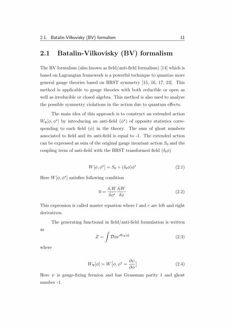
The main idea of this approach is to construct an extended action
WΨ[φ, φ?] by introducing an anti-field (φ?) of opposite statistics corre-
sponding to each field (φ) in the theory. The sum of ghost numbers
associated to field and its anti-field is equal to -1. The extended action
can be expressed as sum of the original gauge invariant action S0 and the
coupling term of anti-field with the BRST transformed field (δbφ)
W [φ, φ?] = S0 + (δbφ)φ? (2.1)
Here W [φ, φ?] satisfies following condition
0 =δrW
δφ?δlW
δφ(2.2)
This expression is called master equation where l and r are left and right
derivatives.
The generating functional in field/anti-field formulation is written
as
Z =
∫DφeiWΨ[φ] (2.3)
where
WΨ[φ] = W[φ, φ? =
∂ψ
∂φ
](2.4)
Here ψ is gauge-fixing fermion and has Grassman parity 1 and ghost
number -1.
2.1. Batalin-Vilkovisky (BV) formalism 12
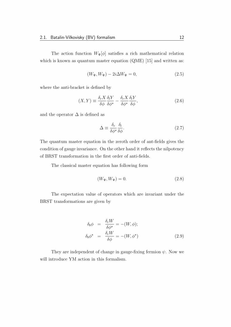
The action function WΨ[φ] satisfies a rich mathematical relation
which is known as quantum master equation (QME) [15] and written as:
(WΨ,WΨ)− 2i∆WΨ = 0, (2.5)
where the anti-bracket is defined by
(X, Y ) ≡ δrX
δφ
δlY
δφ?− δrX
δφ?δlY
δφ, (2.6)
and the operator ∆ is defined as
∆ ≡ δrδφ?
δlδφ. (2.7)
The quantum master equation in the zeroth order of ant-fields gives the
condition of gauge invariance. On the other hand it reflects the nilpotency
of BRST transformation in the first order of anti-fields.
The classical master equation has following form
(WΨ,WΨ) = 0. (2.8)
The expectation value of operators which are invariant under the
BRST transformations are given by
δbφ =δrW
δφ?= −(W,φ);
δbφ? =
δrW
δφ= −(W,φ?) (2.9)
They are independent of change in gauge-fixing fermion ψ. Now we
will introduce YM action in this formalism.
2.2. Hamiltonian BRST Formalism 13
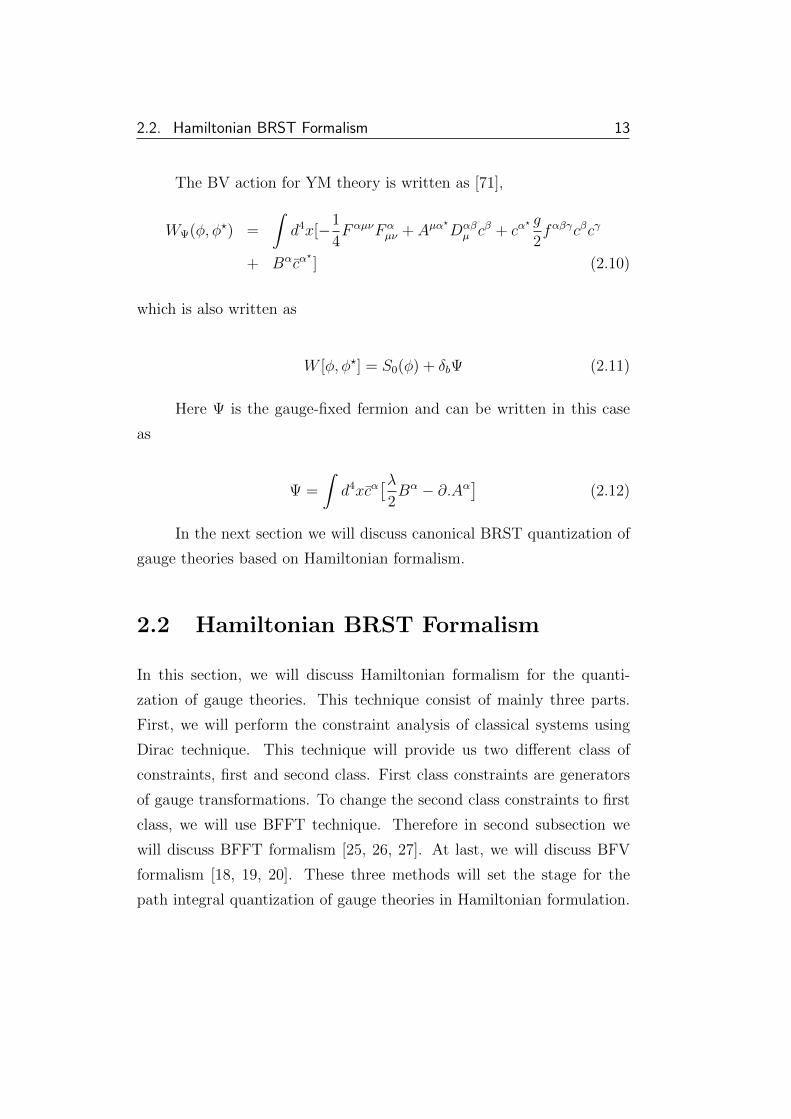
The BV action for YM theory is written as [71],
WΨ(φ, φ?) =
∫d4x[−1
4FαµνFα
µν + Aµα?
Dαβµ cβ + cα
? g
2fαβγcβcγ
+ Bαcα?
] (2.10)
which is also written as
W [φ, φ?] = S0(φ) + δbΨ (2.11)
Here Ψ is the gauge-fixed fermion and can be written in this case
as
Ψ =
∫d4xcα
[λ2Bα − ∂.Aα
](2.12)
In the next section we will discuss canonical BRST quantization of
gauge theories based on Hamiltonian formalism.
2.2 Hamiltonian BRST Formalism
In this section, we will discuss Hamiltonian formalism for the quanti-
zation of gauge theories. This technique consist of mainly three parts.
First, we will perform the constraint analysis of classical systems using
Dirac technique. This technique will provide us two different class of
constraints, first and second class. First class constraints are generators
of gauge transformations. To change the second class constraints to first
class, we will use BFFT technique. Therefore in second subsection we
will discuss BFFT formalism [25, 26, 27]. At last, we will discuss BFV
formalism [18, 19, 20]. These three methods will set the stage for the
path integral quantization of gauge theories in Hamiltonian formulation.
2.2. Hamiltonian BRST Formalism 14
2.2.1 Dirac Constraints Analysis
In this subsection, we will discuss briefly a very useful technique of quan-
tization of the systems with first and second class constraints developed
by Dirac [22]. In various field theory models, the dynamical phase space
variables are not all independent. They satisfy some constraints emerg-
ing from the structure of models. In such situations usual procedure for
obtaining Hamiltonian from Lagrangian doesn’t work. For such models
Dirac’s technique is used to systematically develop Hamiltonian from La-
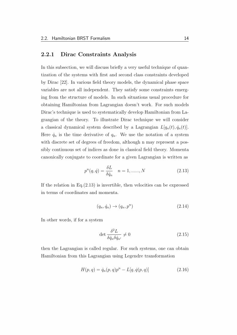
grangian of the theory. To illustrate Dirac technique we will consider
a classical dynamical system described by a Lagrangian L[qn(t), qn(t)].
Here qn is the time derivative of qn. We use the notation of a system
with discrete set of degrees of freedom, although n may represent a pos-
sibly continuous set of indices as done in classical field theory. Momenta
canonically conjugate to coordinate for a given Lagrangian is written as
pn(q, q) =δL
δqnn = 1, ......, N (2.13)
If the relation in Eq.(2.13) is invertible, then velocities can be expressed
in terms of coordinates and momenta.
(qn, qn)→ (qn, pn) (2.14)
In other words, if for a system
detδ2L
δqnδqn′6= 0 (2.15)
then the Lagrangian is called regular. For such systems, one can obtain
Hamiltonian from this Lagrangian using Legendre transformation
H(p, q) = qn(p, q)pn − L[q, q(p, q)] (2.16)
2.2. Hamiltonian BRST Formalism 15
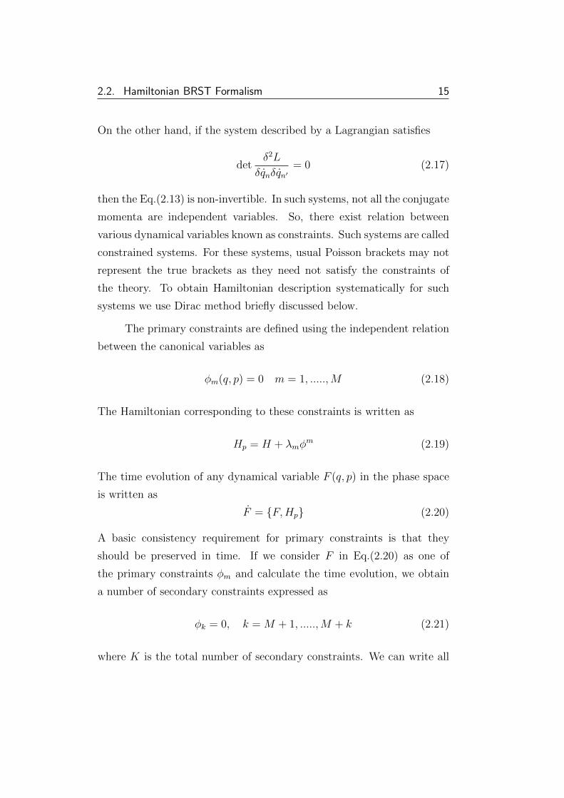
On the other hand, if the system described by a Lagrangian satisfies
detδ2L
δqnδqn′= 0 (2.17)
then the Eq.(2.13) is non-invertible. In such systems, not all the conjugate
momenta are independent variables. So, there exist relation between
various dynamical variables known as constraints. Such systems are called
constrained systems. For these systems, usual Poisson brackets may not
represent the true brackets as they need not satisfy the constraints of
the theory. To obtain Hamiltonian description systematically for such
systems we use Dirac method briefly discussed below.
The primary constraints are defined using the independent relation
between the canonical variables as
φm(q, p) = 0 m = 1, .....,M (2.18)
The Hamiltonian corresponding to these constraints is written as
Hp = H + λmφm (2.19)
The time evolution of any dynamical variable F (q, p) in the phase space
is written as
F = F,Hp (2.20)
A basic consistency requirement for primary constraints is that they
should be preserved in time. If we consider F in Eq.(2.20) as one of
the primary constraints φm and calculate the time evolution, we obtain
a number of secondary constraints expressed as
φk = 0, k = M + 1, .....,M + k (2.21)
where K is the total number of secondary constraints. We can write all
2.2. Hamiltonian BRST Formalism 16
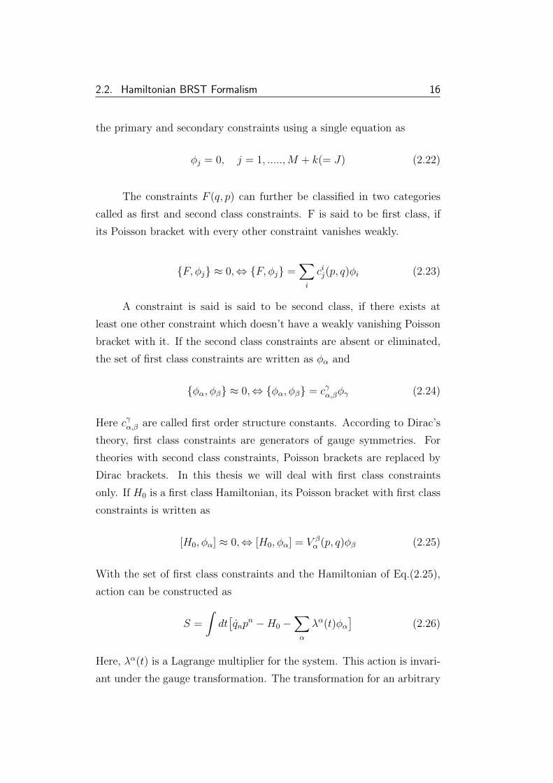
the primary and secondary constraints using a single equation as
φj = 0, j = 1, .....,M + k(= J) (2.22)
The constraints F (q, p) can further be classified in two categories
called as first and second class constraints. F is said to be first class, if
its Poisson bracket with every other constraint vanishes weakly.
F, φj ≈ 0,⇔ F, φj =∑i
cij(p, q)φi (2.23)
A constraint is said is said to be second class, if there exists at
least one other constraint which doesn’t have a weakly vanishing Poisson
bracket with it. If the second class constraints are absent or eliminated,
the set of first class constraints are written as φα and
φα, φβ ≈ 0,⇔ φα, φβ = cγα,βφγ (2.24)
Here cγα,β are called first order structure constants. According to Dirac’s
theory, first class constraints are generators of gauge symmetries. For
theories with second class constraints, Poisson brackets are replaced by
Dirac brackets. In this thesis we will deal with first class constraints
only. If H0 is a first class Hamiltonian, its Poisson bracket with first class
constraints is written as
[H0, φα] ≈ 0,⇔ [H0, φα] = V βα (p, q)φβ (2.25)
With the set of first class constraints and the Hamiltonian of Eq.(2.25),
action can be constructed as
S =
∫dt[qnp
n −H0 −∑α
λα(t)φα]
(2.26)
Here, λα(t) is a Lagrange multiplier for the system. This action is invari-
ant under the gauge transformation. The transformation for an arbitrary
2.2. Hamiltonian BRST Formalism 17
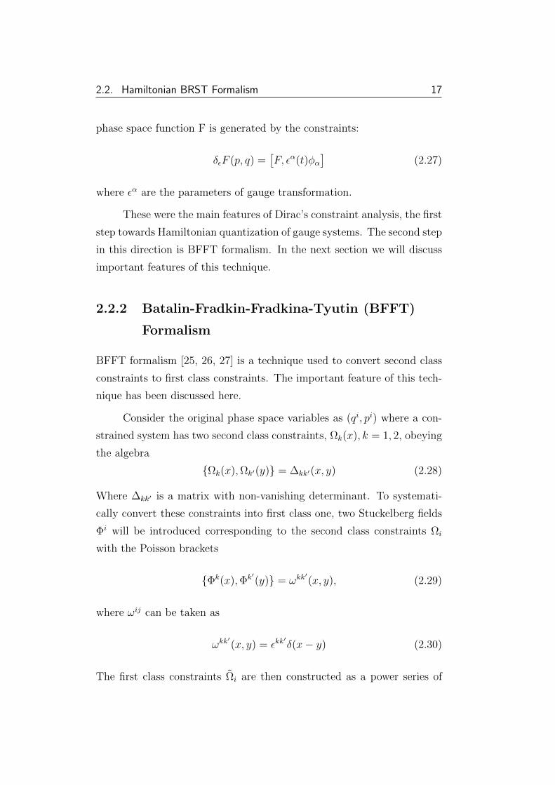
phase space function F is generated by the constraints:
δεF (p, q) =[F, εα(t)φα
](2.27)
where εα are the parameters of gauge transformation.
These were the main features of Dirac’s constraint analysis, the first
step towards Hamiltonian quantization of gauge systems. The second step
in this direction is BFFT formalism. In the next section we will discuss
important features of this technique.
2.2.2 Batalin-Fradkin-Fradkina-Tyutin (BFFT)
Formalism
BFFT formalism [25, 26, 27] is a technique used to convert second class
constraints to first class constraints. The important feature of this tech-
nique has been discussed here.
Consider the original phase space variables as (qi, pi) where a con-
strained system has two second class constraints, Ωk(x), k = 1, 2, obeying
the algebra
Ωk(x),Ωk′(y) = ∆kk′(x, y) (2.28)
Where ∆kk′ is a matrix with non-vanishing determinant. To systemati-
cally convert these constraints into first class one, two Stuckelberg fields
Φi will be introduced corresponding to the second class constraints Ωi
with the Poisson brackets
Φk(x),Φk′(y) = ωkk′(x, y), (2.29)
where ωij can be taken as
ωkk′(x, y) = εkk
′δ(x− y) (2.30)
The first class constraints Ωi are then constructed as a power series of
2.2. Hamiltonian BRST Formalism 18
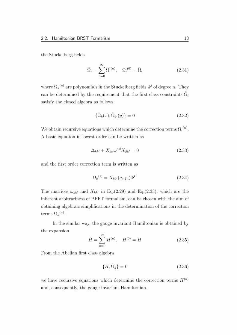
the Stuckelberg fields
Ωi =∞∑n=0
Ωi(n), Ωi
(0) = Ωi (2.31)
where Ωk(n) are polynomials in the Stuckelberg fields Φi of degree n. They
can be determined by the requirement that the first class constraints Ωi
satisfy the closed algebra as follows
Ωk(x), Ωk′(y) = 0 (2.32)
We obtain recursive equations which determine the correction terms Ωi(n).
A basic equation in lowest order can be written as
∆kk′ +XkαωαβXβk′ = 0 (2.33)
and the first order correction term is written as
Ωk(1) = Xkk′(qi, pi)Φ
k′ (2.34)
The matrices ωkk′ and Xkk′ in Eq.(2.29) and Eq.(2.33), which are the
inherent arbitrariness of BFFT formalism, can be chosen with the aim of
obtaining algebraic simplifications in the determination of the correction
terms Ωk(n).
In the similar way, the gauge invariant Hamiltonian is obtained by
the expansion
H =∞∑n=0
H(n), H(0) = H (2.35)
From the Abelian first class algebra
H, Ωk = 0 (2.36)
we have recursive equations which determine the correction terms H(n)
and, consequently, the gauge invariant Hamiltonian.
2.2. Hamiltonian BRST Formalism 19
2.2.3 Batalin-Fradkin-Vilkovisky (BFV) Formalism
We will briefly discuss the BFV formalism [18, 19, 20] which is applicable
for the theories with first-class constraints. This method uses an extended
phase space where the Lagrange multiplier and the ghosts are treated as
dynamical variables. The main features of this approach are as follows:
i) it does not require off-shell closure of the gauge algebra and there-
fore does not require an auxiliary field ii) It heavily depends on BRST
transformation which is independent of the gauge condition and iii) it is
even applicable to Lagrangian which are not quadratic in velocities and
hence is more general than the Lagrangian BRST formalism. First of
all, consider a phase space of canonical variables (qi, pi)(i = 1, 2...., n) in
terms of which the canonical Hamiltonian H0(qi, pi) and the constraints
(Ωa ≈ 0)(a = 1, 2, ...,m) are given. These constraints satisfy following
algebra
Ωa,Ωb = iΩcUcab
H0,Ωa = iΩbVba (2.37)
where the structure coefficients U cab and V b
a are generally functions
of the canonical variables. We also assume that the constraints are irre-
ducible. In order to single out the physical variables, we introduce the
additional conditions Φa(qi, pi) ≈ 0. Here the Φa play the role of gauge-
fixing function. The action, in terms of canonical Hamiltonian densityH0,
first class constraints, Ωa and gauge-fixing function Φa can be written in
this formalism as
S =
∫d4x(piqi −H0 − λaΩa + πaΦ
a), (2.38)
where (qi, pi) are the canonical variables. Lagrange multiplier fields λa
and πa are canonically conjugate variables.
In order to make the theory in extended phase space to be consistent
with the initial theory, two sets of canonically conjugate anti-commuting
2.2. Hamiltonian BRST Formalism 20
ghost coordinate and momenta (Ca, Pa) and (P a, Ca) are introduced for
each constraint. These canonically conjugate ghost and momenta satisfy
the following anti-commutation relation:
[Ca, Pb] = [P a, Cb] = iδab (2.39)
where Cα and Pα have ghost number 1 and −1, respectively. The gener-
ating functional for this extended theory is then defined as
ZΨ =
∫[Dφ]eiSeff [φ], (2.40)
where [Dφ] is the path integral measure and the effective action Seff is
Seff =
∫dt(piq
i + πaλa + PaCa + CaP a −Hm + iQ,Ψ). (2.41)
Here Hm is the BRST invariant Hamiltonian which one calls the minimal
Hamiltonian,
Hm = H0 + PaVab C
b (2.42)
where Ψ is the gauge-fixing fermion and Qb is the nilpotent BRST charge.
They have following general form:
Qb = CaΩa −1
2CbCcUa
cbPa + P aπa,
Ψ = Caχa + Paλ
a (2.43)
Here χa are gauge-fixing functions that neither depends on the
ghosts, anti-ghosts nor on the momenta of both Ca and Ca. This con-
cludes our brief outline of BFV technique based on Hamiltonian formalism
for gauge theories with constraints.
2.3. Finite Field BRST Transformation 21
2.3 Finite Field BRST Transformation
The usual BRST transformation for the generic fields φ of an effective
theory is defined compactly as
δbφ = sbφΛ, (2.44)
where sbφ is the BRST variation of the fields with infinitesimal, anti-
commuting and global parameter Λ. Such transformations are on-shell
nilpotent, i.e. s2b = 0, with the use of some equations of motion for fields
and leaves the Fadeev-Popov (FP) effective action invariant. Joglekar
and Mandal [41] observed that Λ needs neither to be infinitesimal, nor
to be field-independent to maintain the symmetry of the FP effective
action of the theory as long as it is anti-commuting and does not depend
explicitly on space and time. This observation enabled them to propose
finite field-dependent BRST transformation which can be written as
δbφ = sbφΘb[φ], (2.45)
where Θb[φ] is an x-independent functional of fields φ. These transfor-
mations are also symmetry of FP effective action. Even though FFBRST
transformations are symmetry of the effective action, the path integral
measure and hence the generating functional are not invariant under such
finite transformations. We briefly mention the important steps to con-
struct FFBRST transformation. We start with the field, φ(x, κ), which
is made to depend on some parameter, κ : 0 ≤ κ ≤ 1, in such a manner
that φ(x, κ = 0) = φ(x) is the initial field and φ(x, κ = 1) = φ′(x) is the
transformed field. The infinitesimal parameter Λ in the BRST transfor-
mation is made field dependent and hence the BRST transformation can
be written as
d
dκφ(x, κ) = sbφ(x, κ)Θ′b[φ(x, κ)], (2.46)
2.3. Finite Field BRST Transformation 22
where Θ′b is an infinitesimal field dependent parameter. By integrating
these equations from κ = 0 to κ = 1, it has been shown [41] that the
φ′(x) are related to φ(x) by the FFBRST transformation as
φ′(x) = φ(x) + sbφ(x)Θb[φ(x)], (2.47)
where Θb[φ(x)] is obtained from Θ′b[φ(x)] through the relation [41]
Θb[φ(x, κ)] = Θ′b[φ(x, 0)]exp f [φ(x, 0)]− 1
f [φ(x, 0)], (2.48)
where f [φ] is written as
f [φ] =∑i
δΘ′b(x)
δφi(x)sbφi(x) (2.49)
This transformation is nilpotent and symmetry of the effective action.
The Jacobian for finite BRST transformations can be evaluated for
some specific value of Θ′[φ] using the fact that the Jacobian can be written
as a succession of infinitesimal transformations of Eq.(2.47).
Now, the path integral measure is defined as
Dφ = J(κ)Dφ(κ) = J(κ+ dκ)Dφ(κ+ dκ) (2.50)
Since the transformation φ(κ) to φ(κ + dκ) is an infinitesimal one, then
the equation reduces to
J(κ)
J(κ+ dκ)=
∫d4x
∑φ
±δφ(x, κ+ dκ)
δφ(x, κ), (2.51)
where∑
φ sums over all fields in the measure and ± refers to whether φ
is bosonic or fermionic field. Using the Taylor’s expansion in the above
equation, the expression for infinitesimal change in Jacobian is obtained
2.3. Finite Field BRST Transformation 23
as follows:
1
J(κ)
dJ(κ)
dκ= −
∫d4x
∑φ
[±sbφ
δΘ′b[φ(x, κ)]
δφ(x, κ)
](2.52)
The nontrivial Jacobian is the source of new results in the FFBRST
formulation.
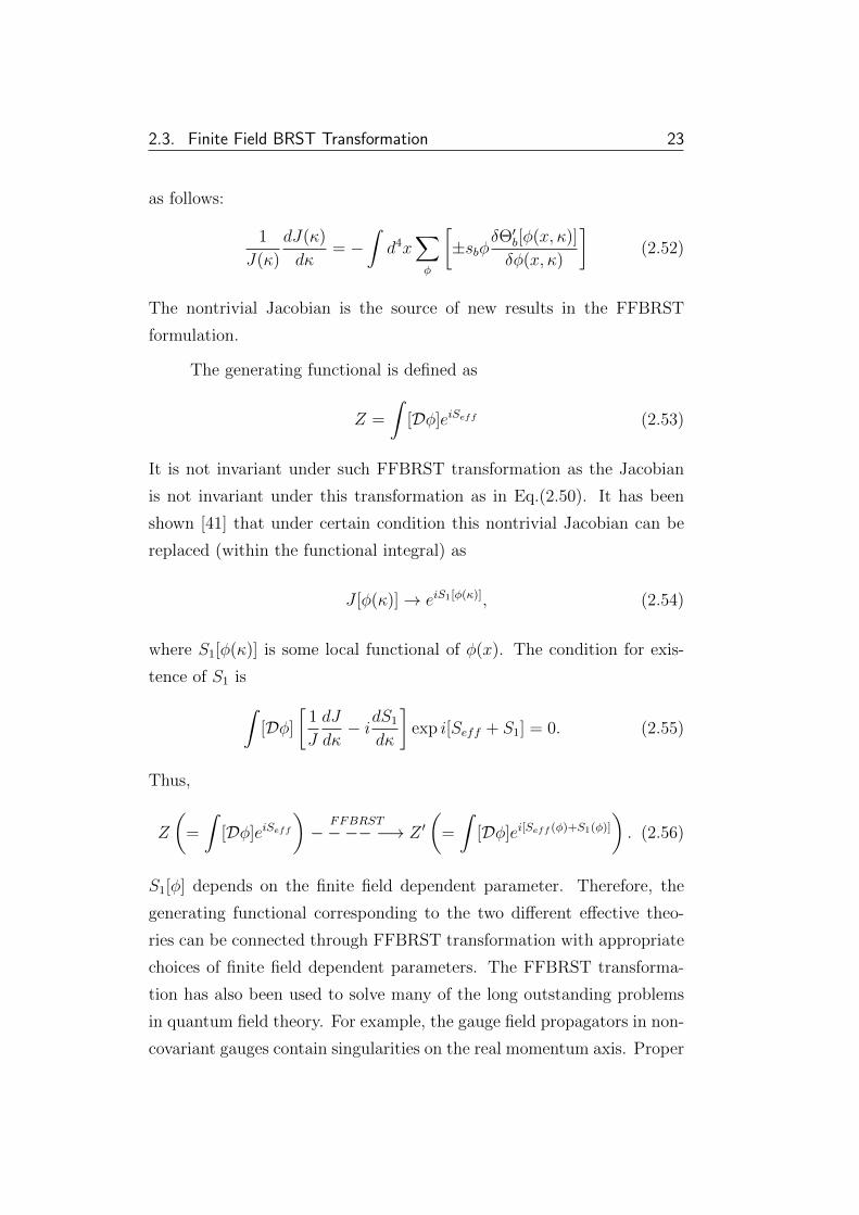
The generating functional is defined as
Z =
∫[Dφ]eiSeff (2.53)
It is not invariant under such FFBRST transformation as the Jacobian
is not invariant under this transformation as in Eq.(2.50). It has been
shown [41] that under certain condition this nontrivial Jacobian can be
replaced (within the functional integral) as
J [φ(κ)]→ eiS1[φ(κ)], (2.54)
where S1[φ(κ)] is some local functional of φ(x). The condition for exis-
tence of S1 is∫[Dφ]
[1
J
dJ
dκ− idS1
dκ
]exp i[Seff + S1] = 0. (2.55)
Thus,
Z
(=
∫[Dφ]eiSeff
)FFBRST
−−−− −→ Z ′(
=
∫[Dφ]ei[Seff (φ)+S1(φ)]
). (2.56)
S1[φ] depends on the finite field dependent parameter. Therefore, the
generating functional corresponding to the two different effective theo-
ries can be connected through FFBRST transformation with appropriate
choices of finite field dependent parameters. The FFBRST transforma-
tion has also been used to solve many of the long outstanding problems
in quantum field theory. For example, the gauge field propagators in non-
covariant gauges contain singularities on the real momentum axis. Proper
2.3. Finite Field BRST Transformation 24
prescriptions for these singularities in gauge field propagators have been
found by using FFBRST transformation [42, 43]. These transformations
have been used to establish relation between first class constraint theories
to second class constraint theories [69]. These symmetries has been ex-
plicitly constructed for pure gauge theories [70]. These symmetries have
been studied in both Lagrangian and Hamiltonian formalisms [71, 79].
These symmetry transformations have found applications in many other
theories like Chern-Simons theory, BLG theory, ABJM theory, QCD, gen-
eralized QED etc. [72, 73, 74, 75, 76, 77, 78, 194, 195].
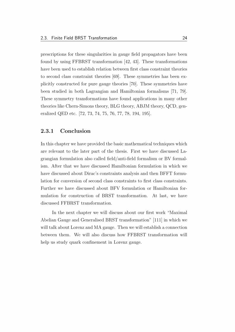
2.3.1 Conclusion
In this chapter we have provided the basic mathematical techniques which
are relevant to the later part of the thesis. First we have discussed La-
grangian formulation also called field/anti-field formalism or BV formal-
ism. After that we have discussed Hamiltonian formulation in which we
have discussed about Dirac’s constraints analysis and then BFFT formu-
lation for conversion of second class constraints to first class constraints.
Further we have discussed about BFV formulation or Hamiltonian for-
mulation for construction of BRST transformation. At last, we have
discussed FFBRST transformation.
In the next chapter we will discuss about our first work “Maximal
Abelian Gauge and Generalised BRST transformation” [111] in which we
will talk about Lorenz and MA gauge. Then we will establish a connection
between them. We will also discuss how FFBRST transformation will
help us study quark confinement in Lorenz gauge.

Chapter 3
Abelian Projection in Lorenz
Gauge and FFBRST
transformations
3.1 Introduction
In the previous two chapters we have discussed the introduction and ba-
sic mathematical preliminaries. Now we are in position to present the
research work carried out in this thesis. The first problem we will dis-
cuss about is Maximal Abelian (MA) gauge in Yang-Mills theory and
its connection with Lorenz gauge through generalized BRST transforma-
tion. It is shown that the generating functional corresponding to the
Faddeev-Popov (FP) effective action in the MA gauge can be obtained
from that in the Lorenz gauge by carrying out an appropriate finite and
field-dependent BRST (FFBRST) transformation. The present FFBRST
formulation might be useful to see how Abelian dominance in the MA
gauge is realized in the Lorenz gauge.
3.1.1 Maximal Abelian Gauge
In SU(N) YM theory, the MA gauge has been exploited to investigate its
non-perturbative features, such as quark confinement [95]. The MA gauge
is a nonlinear gauge for a partial gauge fixing, imposed to maintain only
25
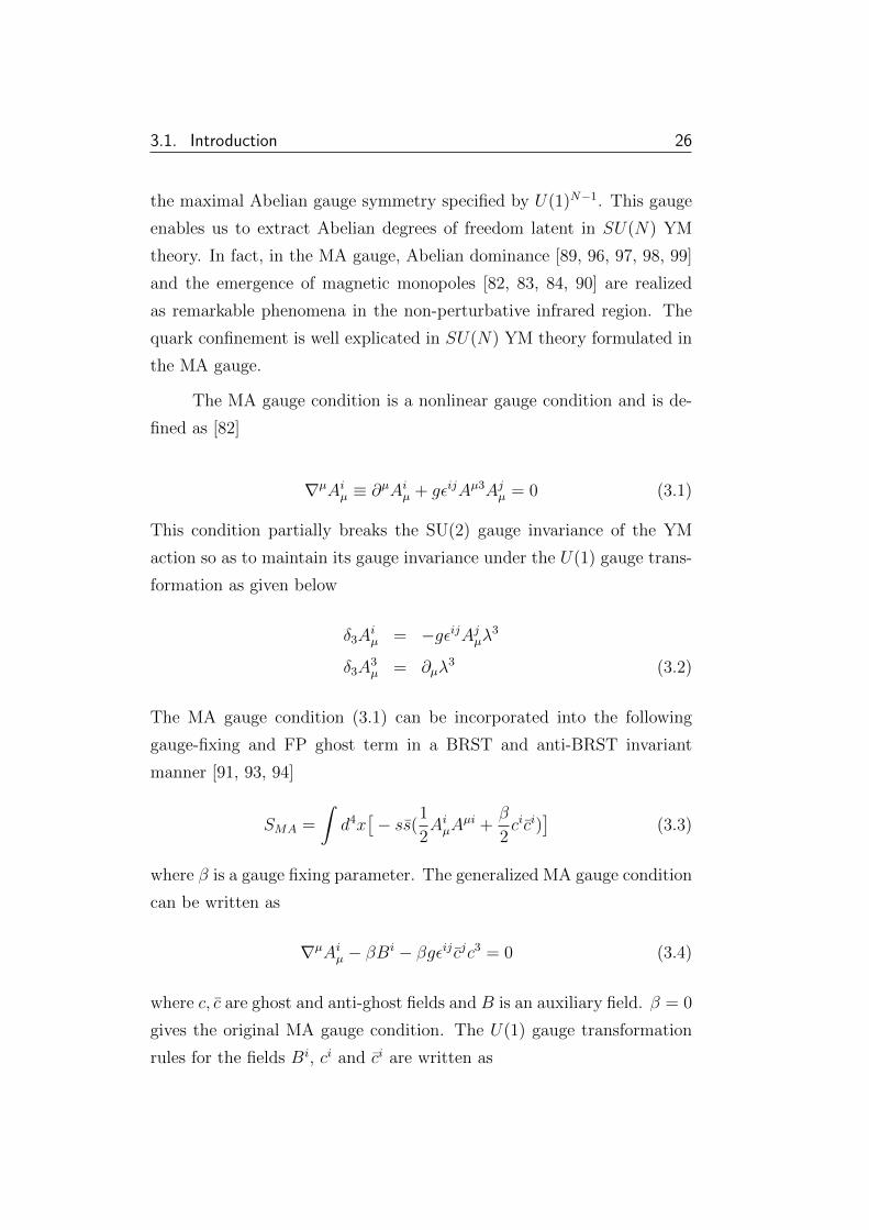
3.1. Introduction 26
the maximal Abelian gauge symmetry specified by U(1)N−1. This gauge
enables us to extract Abelian degrees of freedom latent in SU(N) YM
theory. In fact, in the MA gauge, Abelian dominance [89, 96, 97, 98, 99]
and the emergence of magnetic monopoles [82, 83, 84, 90] are realized
as remarkable phenomena in the non-perturbative infrared region. The
quark confinement is well explicated in SU(N) YM theory formulated in
the MA gauge.
The MA gauge condition is a nonlinear gauge condition and is de-
fined as [82]
∇µAiµ ≡ ∂µAiµ + gεijAµ3Ajµ = 0 (3.1)
This condition partially breaks the SU(2) gauge invariance of the YM
action so as to maintain its gauge invariance under the U(1) gauge trans-
formation as given below
δ3Aiµ = −gεijAjµλ3
δ3A3µ = ∂µλ
3 (3.2)
The MA gauge condition (3.1) can be incorporated into the following
gauge-fixing and FP ghost term in a BRST and anti-BRST invariant
manner [91, 93, 94]
SMA =
∫d4x[− ss(1
2AiµA
µi +β
2cici)
](3.3)
where β is a gauge fixing parameter. The generalized MA gauge condition
can be written as
∇µAiµ − βBi − βgεij cjc3 = 0 (3.4)
where c, c are ghost and anti-ghost fields and B is an auxiliary field. β = 0
gives the original MA gauge condition. The U(1) gauge transformation
rules for the fields Bi, ci and ci are written as

3.1. Introduction 27
δ3Bi = −gεijBjλ3
δ3ci = −gεijcjλ3
δ3ci = −gεij cjλ3 (3.5)
3.1.2 Lorenz Gauge
The Lorenz gauge condition ∂µAaµ = 0 [106] can be used to completely
break the SU(2) gauge invariance of the YM action. This gauge condition
can be incorporated into the following gauge-fixing and FP ghost term in
a BRST and anti-BRST invariant manner [12, 107, 108]
SL =
∫d4x[− ss(1
2AaµA
µa +α
2caca)
](3.6)
where α is a gauge fixing parameter. The generalized Lorenz gauge con-
dition can be written as
∇µAaµ − αBa − α
2gεabccbcc = 0 (3.7)
When α = 0, the gauge condition (3.7) reduces to the (original) Lorenz
gauge condition.
3.1.3 BRST Symmetry
The total action is defined as
ST =
∫d2x(L0 + Lgf + Lgh) (3.8)
where L0 is the kinetic part of the total Lagrangian density.
3.1. Introduction 28
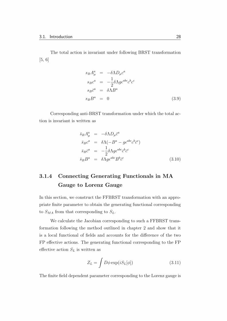
The total action is invariant under following BRST transformation
[5, 6]
sBAaµ = −δΛDµc
a
sBca = −1
2δΛgεabccbcc
sB ca = δΛBa
sBBa = 0 (3.9)
Corresponding anti-BRST transformation under which the total ac-
tion is invariant is written as
sBAaµ = −δΛDµc
a
sBca = δΛ(−Ba − gεabccbcc)
sB ca = −1
2δΛgεabccbcc
sBBa = δΛgεabcBbcc (3.10)
3.1.4 Connecting Generating Functionals in MA
Gauge to Lorenz Gauge
In this section, we construct the FFBRST transformation with an appro-
priate finite parameter to obtain the generating functional corresponding
to SMA from that corresponding to SL.
We calculate the Jacobian corresponding to such a FFBRST trans-
formation following the method outlined in chapter 2 and show that it
is a local functional of fields and accounts for the difference of the two
FP effective actions. The generating functional corresponding to the FP
effective action SL is written as
ZL =
∫Dφ exp(iSL[φ]) (3.11)
The finite field dependent parameter corresponding to the Lorenz gauge is
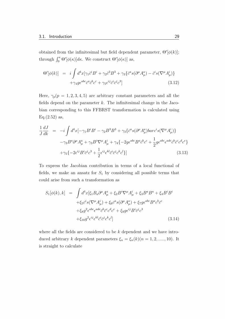
3.1. Introduction 29
obtained from the infinitesimal but field dependent parameter, Θ′[φ(k)];
through∫ κ
0Θ′[φ(κ)]dκ. We construct Θ′[φ(κ)] as,
Θ′[φ(k)] = i
∫d4x[γ1c
iBi + γ2c3B3 + γ3cas(∂µAaµ)− cis(∇µAiµ)
+γ4gεabccacbcc + γ5ε
ij cicjc3] (3.12)
Here, γp(p = 1, 2, 3, 4, 5) are arbitrary constant parameters and all the
fields depend on the parameter k. The infinitesimal change in the Jaco-
bian corresponding to this FFBRST transformation is calculated using
Eq.(2.52) as,
1
J
dJ
dk= −i
∫d4x[−γ1B
iBi − γ2B3B3 + γ3cas(∂µAaµ)barcis(∇µAiµ)
−γ3Ba∂µAaµ + γ3B
i∇µAiµ + γ4−2gεabcBacbcc +1
2gεabcεadecbcccdce
+γ5−2εijBicjc3 +1
2εijεklcicjckcl] (3.13)
To express the Jacobian contribution in terms of a local functional of
fields, we make an ansatz for S1 by considering all possible terms that
could arise from such a transformation as
S1[φ(k), k] =
∫d4x[ξ1Ba∂
µAaµ + ξ2Bi∇µAiµ + ξ3B
aBa + ξ4BiBi
+ξ5cis(∇µAiµ) + ξ6c
as(∂µAaµ) + ξ7gεabcBacbcc
+ξ8g2εabcεadecbcccdce + ξ9gε
ijBicjc3
+ξ10g2εijεklcicjckcl] (3.14)
where all the fields are considered to be k dependent and we have intro-
duced arbitrary k dependent parameters ξn = ξn(k)(n = 1, 2, ....., 10). It
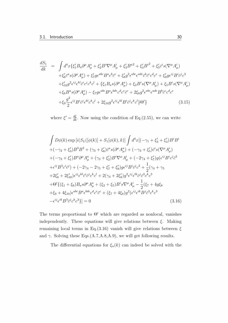
is straight to calculate
3.1. Introduction 30
dS1
dk=
∫d4xξ′1Ba∂
µAaµ + ξ′2Bi∇µAiµ + ξ′3B
a2 + ξ′4Bi2 + ξ′5c
is(∇µAiµ)
+ξ′6cas(∂µAaµ) + ξ′7gε
abcBacbcc + ξ′8g2εabcεadecbcccdce + ξ′9gε
ijBicjc3
+ξ′10g2εijεklcicjckcl + ξ1Bas(∂
µAaµ) + ξ2Bis(∇µAiµ) + ξ5B
is(∇µAiµ)
+ξ6Bas(∂µAaµ)− ξ7gε
abcBaεbdecdcecc + 2ξ8g2εabcεadeBbcccdce
+ξ9g2
2εijBicjεklckcl + 2ξ10g
2εijεklBicjckclΘ′ (3.15)
where ξ′ = dξdk
. Now using the condition of Eq.(2.55), we can write
∫Dφ(k) exp [i(SL([φ(k)] + S1[φ(k), k)]
∫d4x[(−γ1 + ξ′3 + ξ′4)BiBi
+(−γ2 + ξ′3)B3B3 + (γ3 + ξ′6)cas(∂µAaµ) + (−γ3 + ξ′5)cis(∇µAiµ)
+(−γ3 + ξ′1)Ba∂µAaµ + (γ3 + ξ′2)Bi∇µAiµ + (−2γ4 + ξ′7)g(εijBicj c3
+εijB3cicj) + (−2γ4 − 2γ5 + ξ′7 + ξ′9)gεijBicjc3 +1
2(γ4 + γ5
+2ξ′8 + 2ξ′10)εijεklcicjckcl + 2(γ4 + 2ξ′8)g2εijεlkcj c3ckc3
+Θ′(ξ1 + ξ6)Bas∂µAaµ + (ξ2 + ξ5)Bis∇µAiµ −
1
2(ξ7 + 4gξ8
+ξ9 + 4ξ10)εabcBaεbdecdcecc + (ξ7 + 4ξ8)g2(εijεikBj c3ckc3
−εijεikB3cjckc3] = 0 (3.16)
The terms proportional to Θ′ which are regarded as nonlocal, vanishes
independently. These equations will give relations between ξ. Making
remaining local terms in Eq.(3.16) vanish will give relations between ξ
and γ. Solving these Eqs.(A.7,A.8,A.9), we will get following results.
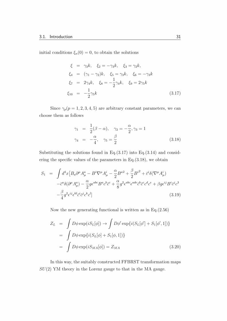
The differential equations for ξn(k) can indeed be solved with the
3.1. Introduction 31
initial conditions ξn(0) = 0, to obtain the solutions
ξ = γ3k, ξ2 = −γ3k, ξ3 = γ2k,
ξ4 = (γ1 − γ2)k, ξ5 = γ3k, ξ6 = −γ3k
ξ7 = 2γ4k, ξ8 = −1
2γ4k, ξ9 = 2γ5k
ξ10 = −1
2γ5k (3.17)
Since γp(p = 1, 2, 3, 4, 5) are arbitrary constant parameters, we can
choose them as follows
γ1 =1
2(β − α), γ2 = −α
2, γ3 = 1
γ4 = −α4, γ5 =
β
2(3.18)
Substituting the solutions found in Eq.(3.17) into Eq.(3.14) and consid-
ering the specific values of the parameters in Eq.(3.18), we obtain
S1 =
∫d4x[Ba∂
µAaµ −Bi∇µAiµ −α
2Ba2 +
β
2Bi2 + ciδ(∇µAiµ)
−caδ(∂µAaµ)− α
2gεabcBacbcc +
α
8g2εabcεadecbcccdce + βgεijBicjc3
−β4g2εijεklcicjckcl] (3.19)
Now the new generating functional is written as in Eq.(2.56)
ZL =
∫Dφ exp(iSL[φ])→
∫Dφ′ expi(SL[φ′] + S1[φ′, 1])
=
∫Dφ expi(SL[φ] + S1[φ, 1])
=
∫Dφ exp(iSMA[φ]) = ZMA (3.20)
In this way, the suitably constructed FFBRST transformation maps
SU(2) YM theory in the Lorenz gauge to that in the MA gauge.
3.1. Introduction 32
3.1.5 Conclusion
We have applied the FFBRST formulation discussed in chapter 2 to clar-
ify the connection between the gauge fixed SU(2) YM theory formulated
in the Lorenz and MA gauges. We have explicitly shown that the gen-
erating functional corresponding to the FP effective action in the MA
gauge can be obtained from that in the Lorenz gauge by carrying out a
suitably constructed FFBRST transformation. In this procedure, the FP
effective action in the MA gauge is found from that in the Lorenz gauge
by taking into account the non-trivial Jacobian arising from the FFBRST
transformation in the path integral measure.
In the next chapter we will discuss about various nilpotent sym-
metries for particle on torus [137]. We will show that these symmetries
follow the Hodge algebra and the system follows double Hodge theory.
We will also show connection between various gauge conditions for torus
system using FFBRST transformation. Then we will discuss BRST and
anti-BRST symmetries for particle on a torus knot [147]. We will also
show connection between various gauges for torus knot system through
FFBRST transformation. At last we will construct BRST and anti-BRST
symmetries for particle on torus knot [149] using the technique discussed
in ref. [148].
Chapter 4
Torus and Torus Knot:
Various Nilpotent Symmetries
In the previous chapter we have observed that YM action in MA gauge
can be connected to that in Lorenz gauge through FFBRST transfor-
mation. Now in this chapter we are going to extend BRST symmetry
and formulate FFBRST symmetry for torus and torus knot system. We
investigate all possible nilpotent symmetries for a particle on torus. We
explicitly construct four independent nilpotent BRST symmetries for such
systems and derive the algebra between the generators of such symme-
tries. We develop BRST symmetry for the first time for a particle on
the surface of a torus knot by analyzing the constraints of the system.
The theory contains second class constraints and has been extended by
introducing the Wess-Zumino term to convert it into a theory with first-
class constraints. BFV analysis of the extended theory is performed to
construct BRST/anti-BRST symmetries for the particle on a torus knot.
We further construct the FFBRST transformation for such systems by
integrating the infinitesimal BRST transformation systematically.
4.1 Double Hodge Theory for a Particle
on Torus
Toric geometry which is generalization of the projective identification that
defines CP n corresponding to the most general linear sigma model pro-
33
4.1. Double Hodge Theory for a Particle on Torus 34
vides a scheme for constructing Calabi-Yau manifolds and their mirrors
[113]. Recently, on the basis of boundary string field theory [114], the
brane-antibrane system was exploited [115] in the toroidal background
to investigate its thermodynamic properties associated with the Hage-
dorn temperature [116, 117]. The Nahm transform and moduli spaces
of CP n models were also studied on the toric geometry [118]. In a
four-dimensional, toroidally compactified heterotic string, the electrically
charged BPS-saturated states were shown to become massless along the
hyper surfaces of enhanced gauge symmetry of a two-torus moduli sub-
space [119].
In the present work we investigate various possible nilpotent sym-
metries for a particle on torus. Usual BRST symmetry for a particle
on torus has already been constructed [120]. In this work we construct
four different nilpotent symmetries associated with this system, namely,
BRST symmetry, anti-BRST symmetry, dual BRST (also known as co-
BRST) symmetry and anti-dual BRST (also known as anti-co-BRST)
symmetry [36, 39]. We further construct two different bosonic symme-
tries using these nilpotent BRST symmetries. Some discrete symmetries
associated with ghost number are also written for such systems. Com-
plete algebra satisfied by charges, which generate these symmetries, is
derived. Deep mathematical connections of such system with Hodge the-
ory [121, 122, 123, 124] has been established in this work. We found
that the system of particle on a torus is realized as Hodge theory with
respect to two different sets of operators. The generators for BRST, dual
BRST symmetries, and generator for corresponding bosonic symmetries
constructed out of BRST and dual BRST symmetries are analogous to
exterior derivative, coexterior derivative, and Laplace operator in Hodge
theory [64, 125, 126, 127, 128, 129, 130, 131, 132]. On the other hand the
charges corresponding to anti-BRST symmetry, anti-dual BRST symme-
try and bosonic symmetry constructed out of these two BRST symmetries
also form set of de-Rham cohomological operators.
4.1. Double Hodge Theory for a Particle on Torus 35
4.1.1 Free Particle on Surface of Torus
A particle moving freely on the surface of a torus is described by La-
grangian [120]:
L0 =1
2mr2 +
1
2mr2θ2 +
1
2m(b+ r sin θ)2φ2 (4.1)
where (r, θ, φ) are toroidal coordinates related to Cartesian coordinates
as
x = (b+ r sin θ) cosφ, y = (b+ r sin θ) sinφ, z = r cos θ (4.2)
Here we have considered a torus with axial circle in the x − y plane
centered at the origin, of radius b, having a circular cross section of radius
r. The angle θ ranges from −π to π and the angle φ from 0 to 2π. Since
the particle moves on the surface of torus of radius r, it is constrained to
satisfy
Ω1 = r − a ≈ 0 (4.3)
The canonical Hamiltonian corresponding to the Lagrangian in Eq.(4.1)
with the above constraint is then written as
H0 =p2r
2m+
p2θ
2mr2+
p2φ
2m(b+ r sin θ)2+ λ(r − a) (4.4)
where pr, pθ and pφ are the canonical momenta conjugate to the coordi-
nate r, θ and φ, respectively, given by
pr = mr, pθ = mr2θ, pφ = m(b+ r sin θ)2φ (4.5)
From Eq.(2.20), the time evolution of the constraint Ω1 yields the sec-
ondary constraint as
Ω2 = pr ≈ 0 (4.6)

4.1. Double Hodge Theory for a Particle on Torus 36
4.1.2 Wess-Zumino term and Hamiltonian
formation
To construct a gauge invariant theory corresponding to the gauge non-
invariant model in Eq.(4.4), we introduce the Wess-Zumino (WZ) term
[132] in the Lagrangian density L. For this purpose we enlarge the Hilbert
space of the theory by introducing a new quantum field η, called as WZ
field, through the redefinition of fields r and λ in the original Lagrangian
density L as follows
r → r − η; λ→ λ+ η (4.7)
With this redefinition of the fields, the modified Lagrangian density be-
comes
LI =1
2m(r − η)2 +
1
2m(r − η)2θ2 +
1
2m(b+ (r − η) sin θ)2φ2
− (λ+ η)(r − a− η) (4.8)
Canonical momenta corresponding to this modified Lagrangian density
are then given by
pr = m(r − η), pη = −(m(r − η) + (r − a− η)), pλ = 0
pθ = m(r − η)2θ, pφ = m(b+ (r − η) sin θ)2φ (4.9)
The primary constraints for this extended theory is
ψ1 ≡ pλ ≈ 0 (4.10)
The Hamiltonian density corresponding to LI is written as,
HI = prr + pηη + pθθ + pφφ+ pλλ− LI (4.11)
The total Hamiltonian density after the introduction of a Lagrange mul-
tiplier field u corresponding to the primary constraint ψ1 is then obtained
4.1. Double Hodge Theory for a Particle on Torus 37
as
HIT =
p2r
2m+
p2θ
2m(r − η)2+
p2φ
2m(b+ (r − η) sin θ)2+λ(pr+pη)+upλ (4.12)
Following the Dirac’s method of constraint analysis [22], we obtain sec-
ondary constraint as in Eq.(2.20),
ψ2 ≡ (pη + pr) ≈ 0 (4.13)
4.1.3 BFV Formulation for free Particle on the
Surface of Torus
To discuss all possible nilpotent symmetries we further extend the theory
using BFV formalism [18, 19, 20, 79, 134, 135]. In the BFV formulation
associated with this system, we introduce a pair of canonically conjugate
ghost fields (c,p) with ghost number 1 and -1 respectively, for the primary
constraint pλ ≈ 0 and another pair of ghost fields (c, p) with ghost number
-1 and 1 respectively, for the secondary constraint, (pη + pr) ≈ 0. The
effective action for a particle on the surface of torus in extended phase
space is then written as in Eq.(2.41)
Seff =
∫d4x[prr + pηη + pθθ + pφφ− pλλ−
p2r
2m− p2
θ
2m(r − η)2
−p2φ
2m(b+ (r − η) sin θ)2+ cp+ ˙cp− Qb, ψ
](4.14)
where Qb is the BRST charge and ψ is the gauge-fixed fermion. This
effective action is invariant under BRST transformation generated by Qb
which is constructed using constraints in the theory as in Eq.(2.43),
Qb = ic(pr + pη)− ippλ (4.15)
4.1. Double Hodge Theory for a Particle on Torus 38
The canonical brackets for all dynamical variables are written as
[r, pr] = [θ, pθ] = [φ, pφ] = [η, pη] = [λ, pλ] = c, c = i, c, ˙c = −i(4.16)
Rest of the brackets are zero. Now, the nilpotent BRST transformation,
using the relation sbφ = [φ,Qb]± (± sign represents the fermionic and
bosonic nature of the fields φ), are explicitly written as
sbr = −c, sbλ = p, sbp = 0, sbθ = −c
sbpφ = 0, sbpθ = 0, sbp = (pr + pη)
sbc = pλ, sbpλ = 0, sbc = 0 (4.17)
In BFV formulation the generating functional is independent of gauge-
fixed fermion [18, 19, 20, 79, 134, 135], hence we have liberty to choose it
in the convenient form as in Eq.(2.43)
ψ = pλ+ c(r + η +pλ2
) (4.18)
Putting the value of ψ in Eq.(4.14) and using Eq.(4.15) and Eq.(4.16),
we obtain
Seff =
∫d4x[prr + pηη + pθθ + pφφ− pλλ−
p2r
2m− p2
θ
2m(r − η)2
−p2φ
2m(b+ (r − η) sin θ)2+ cp+ ˙cp+ λ(pr + pη) + 2cc − pp
+pλ(r + η +pλ2
)]
(4.19)
and the generating functional for this effective theory is represented as
Zψ =
∫Dφ exp
[iSeff
](4.20)
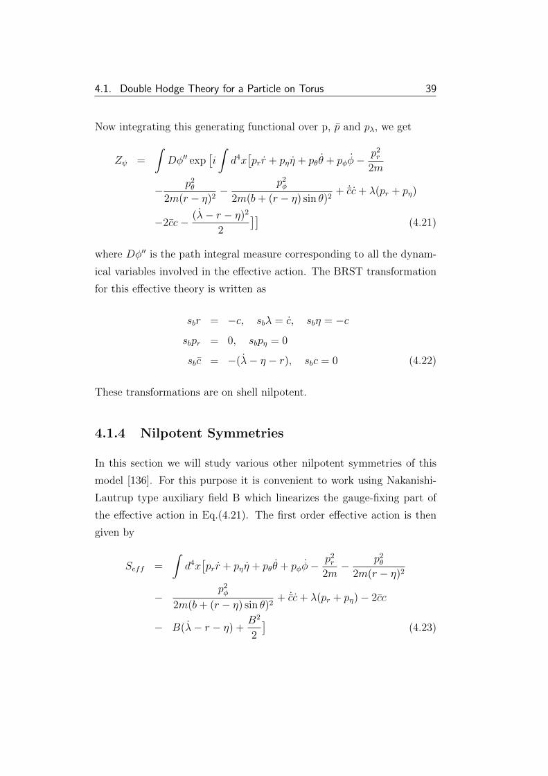
4.1. Double Hodge Theory for a Particle on Torus 39
Now integrating this generating functional over p, p and pλ, we get
Zψ =
∫Dφ′′ exp
[i
∫d4x[prr + pηη + pθθ + pφφ−
p2r
2m
− p2θ
2m(r − η)2−
p2φ
2m(b+ (r − η) sin θ)2+ ˙cc+ λ(pr + pη)
−2cc− (λ− r − η)2
2
]](4.21)
where Dφ′′ is the path integral measure corresponding to all the dynam-
ical variables involved in the effective action. The BRST transformation
for this effective theory is written as
sbr = −c, sbλ = c, sbη = −c
sbpr = 0, sbpη = 0
sbc = −(λ− η − r), sbc = 0 (4.22)
These transformations are on shell nilpotent.
4.1.4 Nilpotent Symmetries
In this section we will study various other nilpotent symmetries of this
model [136]. For this purpose it is convenient to work using Nakanishi-
Lautrup type auxiliary field B which linearizes the gauge-fixing part of
the effective action in Eq.(4.21). The first order effective action is then
given by
Seff =
∫d4x[prr + pηη + pθθ + pφφ−
p2r
2m− p2
θ
2m(r − η)2
−p2φ
2m(b+ (r − η) sin θ)2+ ˙cc+ λ(pr + pη)− 2cc
− B(λ− r − η) +B2
2
](4.23)
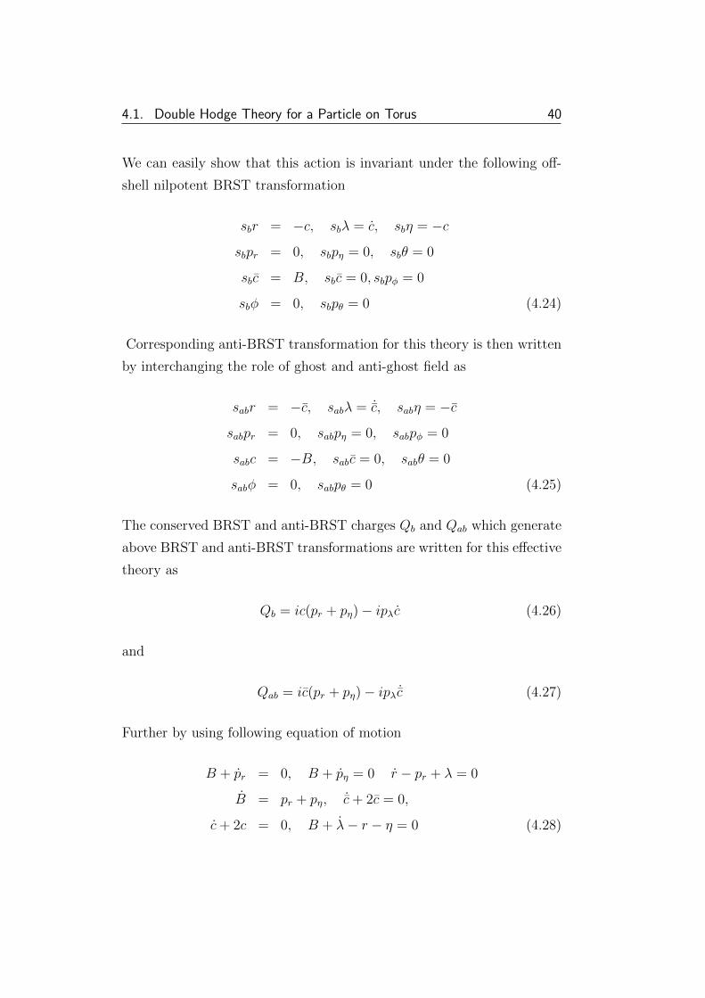
4.1. Double Hodge Theory for a Particle on Torus 40
We can easily show that this action is invariant under the following off-
shell nilpotent BRST transformation
sbr = −c, sbλ = c, sbη = −c
sbpr = 0, sbpη = 0, sbθ = 0
sbc = B, sbc = 0, sbpφ = 0
sbφ = 0, sbpθ = 0 (4.24)
Corresponding anti-BRST transformation for this theory is then written
by interchanging the role of ghost and anti-ghost field as
sabr = −c, sabλ = ˙c, sabη = −c
sabpr = 0, sabpη = 0, sabpφ = 0
sabc = −B, sabc = 0, sabθ = 0
sabφ = 0, sabpθ = 0 (4.25)
The conserved BRST and anti-BRST charges Qb and Qab which generate
above BRST and anti-BRST transformations are written for this effective
theory as
Qb = ic(pr + pη)− ipλc (4.26)
and
Qab = ic(pr + pη)− ipλ ˙c (4.27)
Further by using following equation of motion
B + pr = 0, B + pη = 0 r − pr + λ = 0
B = pr + pη, ˙c+ 2c = 0,
c+ 2c = 0, B + λ− r − η = 0 (4.28)
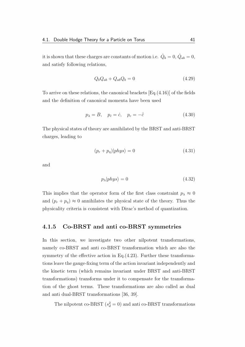
4.1. Double Hodge Theory for a Particle on Torus 41
it is shown that these charges are constants of motion i.e. Qb = 0, Qab = 0,
and satisfy following relations,
QbQab +QabQb = 0 (4.29)
To arrive on these relations, the canonical brackets [Eq.(4.16)] of the fields
and the definition of canonical momenta have been used
pλ = B, pc = c, pc = − ˙c (4.30)
The physical states of theory are annihilated by the BRST and anti-BRST
charges, leading to
(pr + pη)|phys〉 = 0 (4.31)
and
pλ|phys〉 = 0 (4.32)
This implies that the operator form of the first class constraint pλ ≈ 0
and (pr + pη) ≈ 0 annihilates the physical state of the theory. Thus the
physicality criteria is consistent with Dirac’s method of quantization.
4.1.5 Co-BRST and anti co-BRST symmetries
In this section, we investigate two other nilpotent transformations,
namely co-BRST and anti co-BRST transformation which are also the
symmetry of the effective action in Eq.(4.23). Further these transforma-
tions leave the gauge-fixing term of the action invariant independently and
the kinetic term (which remains invariant under BRST and anti-BRST
transformations) transforms under it to compensate for the transforma-
tion of the ghost terms. These transformations are also called as dual
and anti dual-BRST transformations [36, 39].
The nilpotent co-BRST (s2d = 0) and anti co-BRST transformations
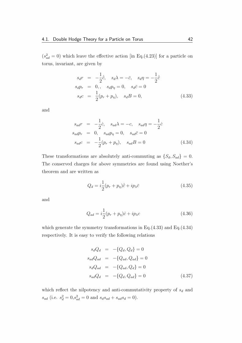
4.1. Double Hodge Theory for a Particle on Torus 42
(s2ad = 0) which leave the effective action [in Eq.(4.23)] for a particle on
torus, invariant, are given by
sdr = −1
2˙c, sdλ = −c, sdη = −1
2˙c
sdpr = 0, , sdpη = 0, sdc = 0
sdc =1
2(pr + pη), sdB = 0, (4.33)
and
sadr = −1
2c, sadλ = −c, sadη = −1
2c
sadpr = 0, sadpη = 0, sadc = 0
sadc = −1
2(pr + pη), sadB = 0 (4.34)
These transformations are absolutely anti-commuting as Sd, Sad = 0.
The conserved charges for above symmetries are found using Noether’s
theorem and are written as
Qd = i1
2(pr + pη) ˙c+ ipλc (4.35)
and
Qad = i1
2(pr + pη)c+ ipλc (4.36)
which generate the symmetry transformations in Eq.(4.33) and Eq.(4.34)
respectively. It is easy to verify the following relations
sdQd = −Qd, Qd = 0
sadQad = −Qad, Qad = 0
sdQad = −Qad, Qd = 0
sadQd = −Qd, Qad = 0 (4.37)
which reflect the nilpotency and anti-commutativity property of sd and
sad (i.e. s2d = 0,s2
ad = 0 and sdsad + sadsd = 0).

4.1. Double Hodge Theory for a Particle on Torus 43
4.1.6 Other Symmetries
In this section, we construct other symmetries related to this system. Two
different bosonic symmetries are constructed out of four nilpotent sym-
metries. Discrete symmetry related to ghost number is also constructed.
4.1.7 Bosonic Symmetry
In this part we construct the bosonic symmetry out of these nilpotent
BRST symmetries of the theory using ref. [134, 135]. The BRST (sb),
anti-BRST (sab), co-BRST (sd), and anti co-BRST(sad) symmetry oper-
ators satisfy the following algebra
sd, sad = 0, sb, sab = 0
sb, sad = 0, sd, sab = 0 (4.38)
and we define bosonic symmetries, sw and sw as,
sw ≡ sb, sd, sw ≡ sab, sad (4.39)
The fields variables transform under bosonic symmetry sw as,
swr = −1
2(B + pr + pη), swλ = −1
2(2B − pr − pη)
swη = −1
2(B + pr + pη), swpr = 0, swpη = 0
swc = 0, swB = 0, swc = 0 (4.40)
On the other hand transformation generated by sw are,
swr = −1
2(B + pr + pη), swλ =
1
2(2B − pr − pη)
swη = −1
2(B + pr + pη), swpr = 0, swpη = 0
swc = 0, swB = 0, swc = 0 (4.41)
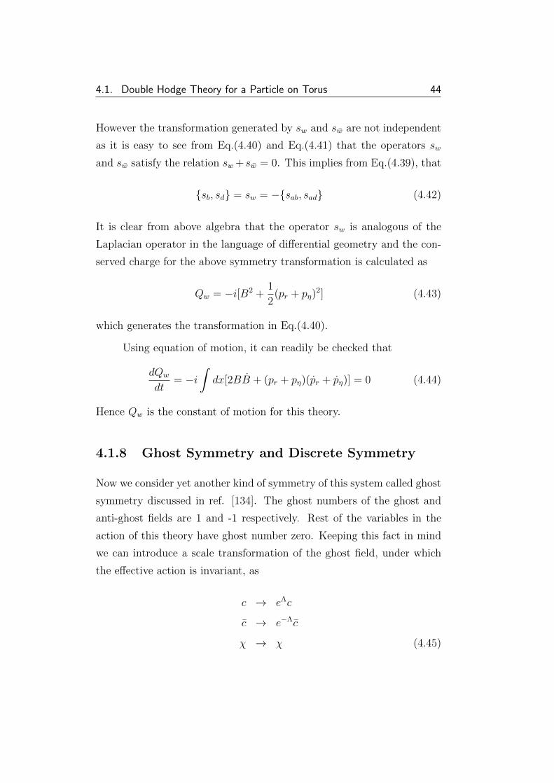
4.1. Double Hodge Theory for a Particle on Torus 44
However the transformation generated by sw and sw are not independent
as it is easy to see from Eq.(4.40) and Eq.(4.41) that the operators sw
and sw satisfy the relation sw +sw = 0. This implies from Eq.(4.39), that
sb, sd = sw = −sab, sad (4.42)
It is clear from above algebra that the operator sw is analogous of the
Laplacian operator in the language of differential geometry and the con-
served charge for the above symmetry transformation is calculated as
Qw = −i[B2 +1
2(pr + pη)
2] (4.43)
which generates the transformation in Eq.(4.40).
Using equation of motion, it can readily be checked that
dQw
dt= −i
∫dx[2BB + (pr + pη)(pr + pη)] = 0 (4.44)
Hence Qw is the constant of motion for this theory.
4.1.8 Ghost Symmetry and Discrete Symmetry
Now we consider yet another kind of symmetry of this system called ghost
symmetry discussed in ref. [134]. The ghost numbers of the ghost and
anti-ghost fields are 1 and -1 respectively. Rest of the variables in the
action of this theory have ghost number zero. Keeping this fact in mind
we can introduce a scale transformation of the ghost field, under which
the effective action is invariant, as
c → eΛc
c → e−Λc
χ → χ (4.45)
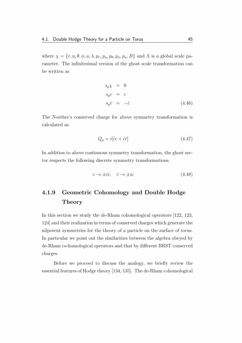
4.1. Double Hodge Theory for a Particle on Torus 45
where χ = r, η, θ, φ, u, λ, pr, pη, pθ, pφ, pu, B and Λ is a global scale pa-
rameter. The infinitesimal version of the ghost scale transformation can
be written as
sgχ = 0
sgc = c
sg c = −c (4.46)
The Noether’s conserved charge for above symmetry transformation is
calculated as
Qg = i[ ˙cc+ cc] (4.47)
In addition to above continuous symmetry transformation, the ghost sec-
tor respects the following discrete symmetry transformations.
c→ ±ic, c→ ±ic (4.48)
4.1.9 Geometric Cohomology and Double Hodge
Theory
In this section we study the de-Rham cohomological operators [122, 123,
124] and their realization in terms of conserved charges which generate the
nilpotent symmetries for the theory of a particle on the surface of torus.
In particular we point out the similarities between the algebra obeyed by
de-Rham co-homological operators and that by different BRST conserved
charges.
Before we proceed to discuss the analogy, we briefly review the
essential features of Hodge theory [134, 135]. The de-Rham cohomological
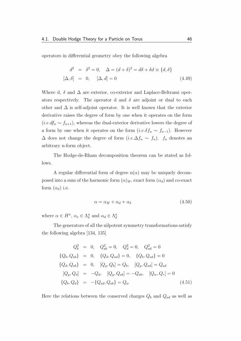
4.1. Double Hodge Theory for a Particle on Torus 46
operators in differential geometry obey the following algebra
d2 = δ2 = 0, ∆ = (d+ δ)2 = dδ + δd ≡ d, δ
[∆, δ] = 0, [∆, d] = 0 (4.49)
Where d, δ and ∆ are exterior, co-exterior and Laplace-Beltrami oper-
ators respectively. The operator d and δ are adjoint or dual to each
other and ∆ is self-adjoint operator. It is well known that the exterior
derivative raises the degree of form by one when it operates on the form
(i.e.dfn ∼ fn+1), whereas the dual-exterior derivative lowers the degree of
a form by one when it operates on the form (i.e.δfn ∼ fn−1). However
∆ does not change the degree of form (i.e.∆fn ∼ fn). fn denotes an
arbitrary n-form object.
The Hodge-de-Rham decomposition theorem can be stated as fol-
lows.
A regular differential form of degree n(α) may be uniquely decom-
posed into a sum of the harmonic form (α)H , exact form (αd) and co-exact
form (αδ) i.e.
α = αH + αd + αδ (4.50)
where α ∈ Hn, αs ∈ Λnδ and αd ∈ Λn
d
The generators of all the nilpotent symmetry transformations satisfy
the following algebra [134, 135]
Q2b = 0, Q2
ab = 0, Q2d = 0, Q2
ad = 0
Qb, Qab = 0, Qd, Qad = 0, Qb, Qad = 0
Qd, Qab = 0, [Qg, Qb] = Qb, [Qg, Qad] = Qad
[Qg, Qd] = −Qd, [Qg, Qab] = −Qab, [Qw, Qr] = 0
Qb, Qd = −Qad, Qab = Qw (4.51)
Here the relations between the conserved charges Qb and Qad as well as
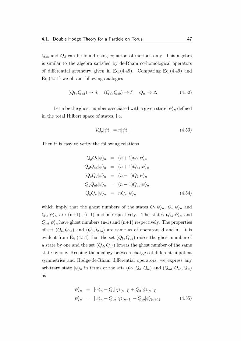
4.1. Double Hodge Theory for a Particle on Torus 47
Qab and Qd can be found using equation of motions only. This algebra
is similar to the algebra satisfied by de-Rham co-homological operators
of differential geometry given in Eq.(4.49). Comparing Eq.(4.49) and
Eq.(4.51) we obtain following analogies
(Qb, Qad)→ d, (Qd, Qab)→ δ, Qw → ∆ (4.52)
Let n be the ghost number associated with a given state |ψ〉n defined
in the total Hilbert space of states, i.e.
iQg|ψ〉n = n|ψ〉n (4.53)
Then it is easy to verify the following relations
QgQb|ψ〉n = (n+ 1)Qb|ψ〉nQgQad|ψ〉n = (n+ 1)Qad|ψ〉nQgQd|ψ〉n = (n− 1)Qb|ψ〉nQgQab|ψ〉n = (n− 1)Qad|ψ〉nQgQw|ψ〉n = nQw|ψ〉n (4.54)
which imply that the ghost numbers of the states Qb|ψ〉n, Qd|ψ〉n and
Qw|ψ〉n are (n+1), (n-1) and n respectively. The states Qab|ψ〉n and
Qad|ψ〉n have ghost numbers (n-1) and (n+1) respectively. The properties
of set (Qb, Qad) and (Qd, Qab) are same as of operators d and δ. It is
evident from Eq.(4.54) that the set (Qb, Qad) raises the ghost number of
a state by one and the set (Qd, Qab) lowers the ghost number of the same
state by one. Keeping the analogy between charges of different nilpotent
symmetries and Hodge-de-Rham differential operators, we express any
arbitrary state |ψ〉n in terms of the sets (Qb, Qd, Qw) and (Qad, Qab, Qw)
as
|ψ〉n = |w〉n +Qb|χ〉(n−1) +Qd|φ〉(n+1)
|ψ〉n = |w〉n +Qad|χ〉(n−1) +Qab|φ〉(n+1) (4.55)

4.1. Double Hodge Theory for a Particle on Torus 48
where the most symmetric state is the harmonic state |w〉n that satisfies
Qw|w〉n = 0, Qb|w〉n = 0, Qd|w〉n = 0
Qab|w〉n = 0, Qad|w〉n = 0 (4.56)
analogous to the Eq.(4.49). Therefore the BRST charges for a particle
on a torus forms two separate set of de-Rham co-homological operators,
namely Qb, Qab, Qw and Qd, Qad, Qw. Thus we call the theory of a
particle on torus as double Hodge theory. Fermionic charges Qb, Qab, Qd
and Qad follow physicality criteria given below,
Qb|phys〉 = 0, Qab|phys〉 = 0
Qd|phys〉 = 0, Qad|phys〉 = 0 (4.57)
which lead to
pλ|phys〉 = 0
(Pr + Pη)|phys〉 = 0 (4.58)
This is the operator form of the first class constraint which annihilates
the physical state as a consequence of physicality criteria, which further
is consistent with the Dirac’s method of quantization of a system with
first class constraints.
4.1.10 FFBRST for free particle on surface of torus
The effective action for the free particle on surface of torus using BFV
formulation is written in Eq.(4.19) and its BRST transformation is given
by Eq.(4.22). In BRST transformation given by Eq.(4.22), δΛ is global,
infinitesimal and anti-commuting parameter. FFBRST transformation
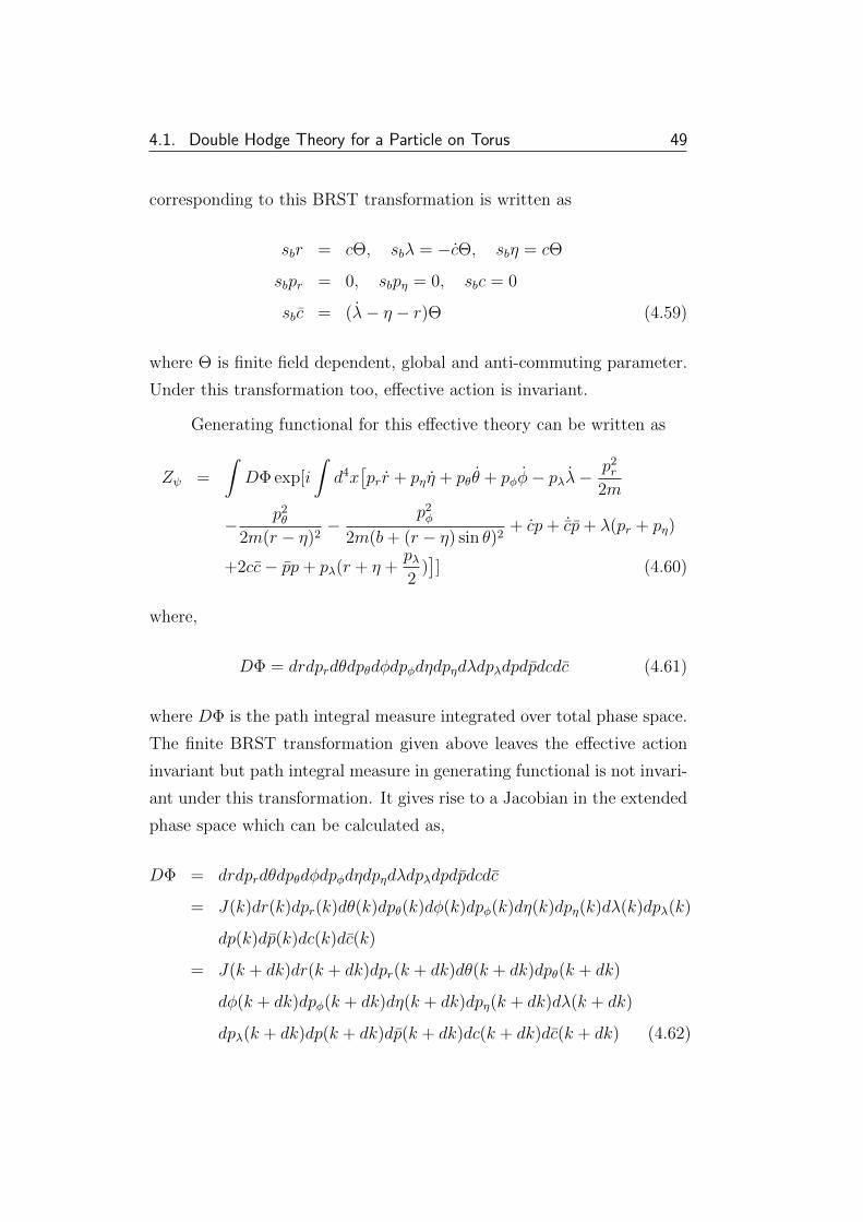
4.1. Double Hodge Theory for a Particle on Torus 49
corresponding to this BRST transformation is written as
sbr = cΘ, sbλ = −cΘ, sbη = cΘ
sbpr = 0, sbpη = 0, sbc = 0
sbc = (λ− η − r)Θ (4.59)
where Θ is finite field dependent, global and anti-commuting parameter.
Under this transformation too, effective action is invariant.
Generating functional for this effective theory can be written as
Zψ =
∫DΦ exp[i
∫d4x[prr + pηη + pθθ + pφφ− pλλ−
p2r
2m
− p2θ
2m(r − η)2−
p2φ
2m(b+ (r − η) sin θ)2+ cp+ ˙cp+ λ(pr + pη)
+2cc− pp+ pλ(r + η +pλ2
)]] (4.60)
where,
DΦ = drdprdθdpθdφdpφdηdpηdλdpλdpdpdcdc (4.61)
where DΦ is the path integral measure integrated over total phase space.
The finite BRST transformation given above leaves the effective action
invariant but path integral measure in generating functional is not invari-
ant under this transformation. It gives rise to a Jacobian in the extended
phase space which can be calculated as,
DΦ = drdprdθdpθdφdpφdηdpηdλdpλdpdpdcdc
= J(k)dr(k)dpr(k)dθ(k)dpθ(k)dφ(k)dpφ(k)dη(k)dpη(k)dλ(k)dpλ(k)
dp(k)dp(k)dc(k)dc(k)
= J(k + dk)dr(k + dk)dpr(k + dk)dθ(k + dk)dpθ(k + dk)
dφ(k + dk)dpφ(k + dk)dη(k + dk)dpη(k + dk)dλ(k + dk)
dpλ(k + dk)dp(k + dk)dp(k + dk)dc(k + dk)dc(k + dk) (4.62)
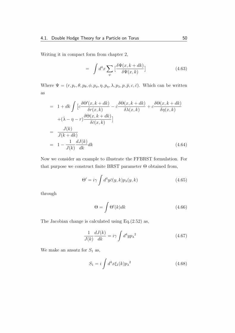
4.1. Double Hodge Theory for a Particle on Torus 50
Writing it in compact form from chapter 2,
=
∫d4x
∑ψ
[δΨ(x, k + dk)
δΨ(x, k)
](4.63)
Where Ψ = (r, pr, θ, pθ, φ, pφ, η, pη, λ, pλ, p, p, c, c). Which can be written
as
= 1 + dk
∫ [cδΘ′(x, k + dk)
δr(x, k)− c δΘ(x, k + dk)
δλ(x, k)+ c
δΘ(x, k + dk)
δη(x, k)
+(λ− η − r)δΘ(x, k + dk)
δc(x, k)
]=
J(k)
J(k + dk)
= 1− 1
J(k)
dJ(k)
dkdk (4.64)
Now we consider an example to illustrate the FFBRST formulation. For
that purpose we construct finite BRST parameter Θ obtained from,
Θ′ = iγ
∫d4yc(y, k)pλ(y, k) (4.65)
through
Θ =
∫Θ′(k)dk (4.66)
The Jacobian change is calculated using Eq.(2.52) as,
1
J(k)
dJ(k)
dk= iγ
∫d4ypλ
2 (4.67)
We make an ansatz for S1 as,
S1 = i
∫d4xξ1(k)pλ
2 (4.68)
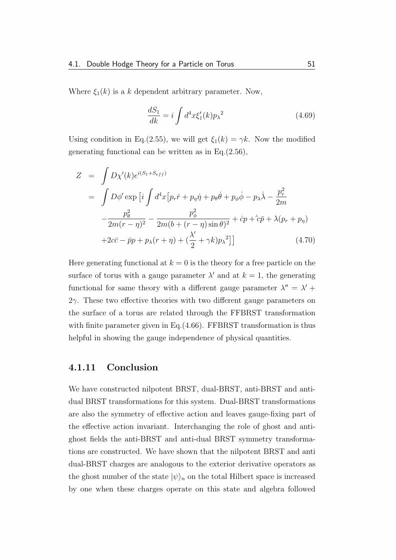
4.1. Double Hodge Theory for a Particle on Torus 51
Where ξ1(k) is a k dependent arbitrary parameter. Now,
dS1
dk= i
∫d4xξ′1(k)pλ
2 (4.69)
Using condition in Eq.(2.55), we will get ξ1(k) = γk. Now the modified
generating functional can be written as in Eq.(2.56),
Z =
∫Dχ′(k)ei(S1+Seff )
=
∫Dφ′ exp
[i
∫d4x[prr + pηη + pθθ + pφφ− pλλ−
p2r
2m
− p2θ
2m(r − η)2−
p2φ
2m(b+ (r − η) sin θ)2+ cp+˙cp+ λ(pr + pη)
+2cc− pp+ pλ(r + η) + (λ′
2+ γk)pλ
2]]
(4.70)
Here generating functional at k = 0 is the theory for a free particle on the
surface of torus with a gauge parameter λ′ and at k = 1, the generating
functional for same theory with a different gauge parameter λ′′ = λ′ +
2γ. These two effective theories with two different gauge parameters on
the surface of a torus are related through the FFBRST transformation
with finite parameter given in Eq.(4.66). FFBRST transformation is thus
helpful in showing the gauge independence of physical quantities.
4.1.11 Conclusion
We have constructed nilpotent BRST, dual-BRST, anti-BRST and anti-
dual BRST transformations for this system. Dual-BRST transformations
are also the symmetry of effective action and leaves gauge-fixing part of
the effective action invariant. Interchanging the role of ghost and anti-
ghost fields the anti-BRST and anti-dual BRST symmetry transforma-
tions are constructed. We have shown that the nilpotent BRST and anti
dual-BRST charges are analogous to the exterior derivative operators as
the ghost number of the state |ψ〉n on the total Hilbert space is increased
by one when these charges operate on this state and algebra followed
4.2. BRST Symmetry for a Torus Knot 52
by these operators is same as the algebra obeyed by the de-Rham co-
homological operators. Similarly the dual-BRST and anti-BRST charges
are analogous to co-exterior derivative. The anti-commutators of BRST
and dual-BRST and anti-BRST and anti dual-BRST charges lead to
bosonic symmetry. The corresponding charges are analogous to Lapla-
cian operator. Further, this theory has another nilpotent symmetry called
ghost symmetry under which the ghost term of the effective action is in-
variant. We further have shown that this theory behaves as double Hodge
theory as the charges for BRST (Qb), dual BRST (Qd) and the charges
for the bosonic symmetry generated out of these two symmetries (Qw)
form the algebra for Hodge theory. On the other hand charges for anti-
BRST (Qab), anti-dual BRST (Qad) and Qw, charge for bosonic symmetry
generalized out of these nilpotent symmetries also satisfy the Hodge al-
gebra. Thus particle on the surface of torus has very rich mathematical
structure.
We further constructed the FFBRST transformation for this sys-
tem. By constructing appropriate field dependent parameter we have ex-
plicitly shown that such generalized BRST transformations are capable of
connecting different theories on torus. It will be interesting to construct
finite version of dual BRST transformation and study its consequences
on the system with constraints.
4.2 BRST Symmetry for a Torus Knot
Knot [138, 139] theory, based on mathematical concepts has found im-
mense applications in various branches of frontier physics. Knot invari-
ants in physical systems were introduced long ago and have got consid-
erable impact during last one and half decades [138, 139, 140, 141, 142,
143, 144, 145, 146], especially when interpreted as Wilson loop observable
in Chern-Simons(CS) theory [144]. The discussion on topological string
approach to the torus knot invariants are presented in ref. [144]. In the
context of gauge theory, knot invariant theories relate 3d symmetry on
4.2. BRST Symmetry for a Torus Knot 53
the CS sub-manifold and 3d SUSY gauge theory. It also plays important
role in various other problems like, inequivalent quantization problem
[141], in the role of topology in defining vacuum state in gauge theories
[142], in understanding band theory of solids [143]. We will discuss here
the BRST symmetry for particle on a torus knot. We will also discuss
FFBRST symmetry for this system.
4.2.1 Particle on a Torus Knot
In knot theory, a torus knot is a special kind of knot that lies on the
surface of un-knotted torus in R3. It is specified by a set of co-prime
integers p and q. A torus knot of type (p, q) winds p times around the
rotational symmetry axis of the torus and q times around a circle in the
interior of the torus. The toroidal co-ordinate system is a suitable choice
to study this system. Toroidal co-ordinates are related to Cartesian co-
ordinates (x1, x2, x3) in following ways,
x1 =a sinh η cosφ
cosh η − cos θ, x2 =
a sinh η sinφ
cosh η − cos θ, x3 =
a sin θ
cosh η − cos θ(4.71)
where, 0 ≤ η ≤ ∞, −π ≤ θ ≤ π and 0 ≤ φ ≤ 2π. A toroidal surface is
represented by some specific value of η (say η0). Parameters a and η0 are
written as a2 = R2 − d2 and cosh η0 = RD
, where R and D are major and
minor radius of torus respectively.
Similarly, toroidal coordinates can be represented in the form of
Cartesian co-ordinates as,
η = lnd1
d2
, cos θ =r2 − a2
((r2 − a2)2 + 4a2x32)
12
, φ = tan−1 x2
x1
(4.72)
where
d21 = (
√x2
1 + x22 + a)2 + x2
3, d22 = (
√x2
1 + x22 − a)2 + x2
3
r2 = x21 + x2
2 (4.73)
4.2. BRST Symmetry for a Torus Knot 54
r is cylindrical radius.
Lagrangian for a particle residing on the surface of torus knot is
given by [140, 146]
L =1
2ma2 η
2 + θ2 + sinh η2φ2
(cosh η − cos θ)2− λ(pθ + qφ) (4.74)
where (η, θ, φ) are the toroidal coordinates for toric geometry.
Constraint that forces the particle to move in knot is imposed as
Ω1 = (pθ + qφ) ≈ 0 (4.75)
The Hamiltonian corresponding to this Lagrangian is then written as,‘
H =(cosh η − cos θ)2
ma2[p2η + p2
θ +p2φ
sinh2 η] + λ(pθ + qφ) (4.76)
Here pη, pθ and pφ are canonical momenta corresponding to the co-
ordinates η, θ and φ.
Using Eq.(2.20), the time evolution of the constraint Ω1 gives addi-
tional secondary constraint
Ω2 =(cosh η − cos θ)2
ma2[ppθ +
qpφ
sinh2 η] ≈ 0 (4.77)
Constraints Ω1 and Ω2 form second-class constraint algebra [22]
∆kk′(x, y) = Ωk(x),Ωk′(y)
= εkk′ (cosh η − cos θ)2
ma2[p2 +
q2
sinh2 η]δ(x− y) (4.78)
with ε12 = −ε21 = 1. In the next section we will convert this gauge variant
theory to the gauge invariant theory in an extended Hilbert space.
4.2. BRST Symmetry for a Torus Knot 55
4.2.2 Wess-Zumino term and Hamiltonian
Formation
To construct a gauge invariant theory corresponding to a gauge non-
invariant model of particle on a torus knot, we introduce Wess-Zumino
(WZ) term in Lagrangian in Eq.(4.74). For this purpose we enlarge the
Hilbert space of the theory by introducing a new co-ordinate α, called
as WZ term, through the redefinition of co-ordinates θ, φ and λ in the
Lagrangian L as follows
θ → θ − α
2p, φ→ φ− α
2q, λ→ λ+ α (4.79)
With this redefinition of co-ordinates, modified Lagrangian is writ-
ten as
LI =1
2
ma2
(cosh η − cos(θ − α2p
))2[η2 + θ2 + sinh2 ηφ2 +
α2
4(
1
p2+
sinh2 η
q2)
−α(θ
p+ sinh2 η
φ
q)]− (λ+ α)(pθ + qφ− α) (4.80)
which is invariant under following time-dependent gauge transformations
δλ = f(t), δθ = −f(t)
2p, δφ = −f(t)
2q, δα = −f(t)
δpη = δpθ = δpφ = 0, δb = δΠα = δη = δΠλ = 0 (4.81)
where f(t) is an arbitrary function of time. To construct the Hamilto-
nian for this gauge invariant theory we construct the canonical momenta
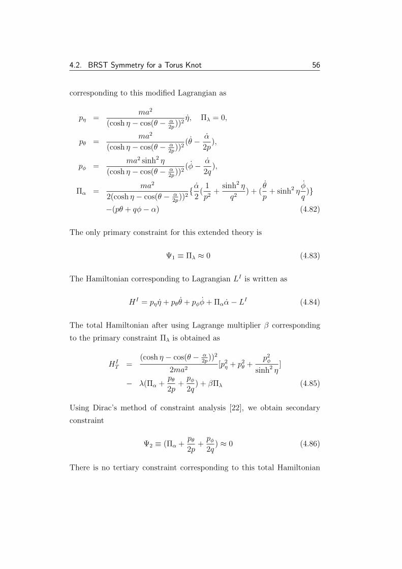
4.2. BRST Symmetry for a Torus Knot 56
corresponding to this modified Lagrangian as
pη =ma2
(cosh η − cos(θ − α2p
))2η, Πλ = 0,
pθ =ma2
(cosh η − cos(θ − α2p
))2(θ − α
2p),
pφ =ma2 sinh2 η
(cosh η − cos(θ − α2p
))2(φ− α
2q),
Πα =ma2
2(cosh η − cos(θ − α2p
))2 α
2(
1
p2+
sinh2 η
q2) + (
θ
p+ sinh2 η
φ
q)
−(pθ + qφ− α) (4.82)
The only primary constraint for this extended theory is
Ψ1 ≡ Πλ ≈ 0 (4.83)
The Hamiltonian corresponding to Lagrangian LI is written as
HI = pηη + pθθ + pφφ+ Παα− LI (4.84)
The total Hamiltonian after using Lagrange multiplier β corresponding
to the primary constraint Πλ is obtained as
HIT =
(cosh η − cos(θ − α2p
))2
2ma2[p2η + p2
θ +p2φ
sinh2 η]
− λ(Πα +pθ2p
+pφ2q
) + βΠλ (4.85)
Using Dirac’s method of constraint analysis [22], we obtain secondary
constraint
Ψ2 ≡ (Πα +pθ2p
+pφ2q
) ≈ 0 (4.86)
There is no tertiary constraint corresponding to this total Hamiltonian
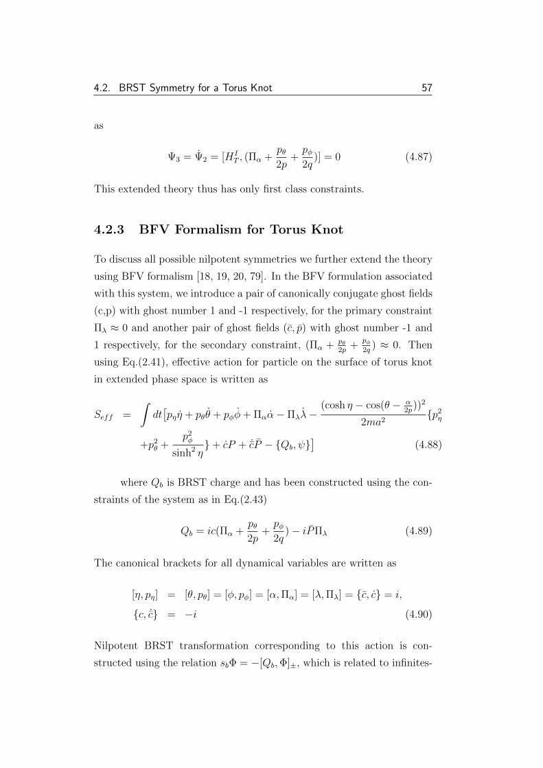
4.2. BRST Symmetry for a Torus Knot 57
as
Ψ3 = Ψ2 = [HIT , (Πα +
pθ2p
+pφ2q
)] = 0 (4.87)
This extended theory thus has only first class constraints.
4.2.3 BFV Formalism for Torus Knot
To discuss all possible nilpotent symmetries we further extend the theory
using BFV formalism [18, 19, 20, 79]. In the BFV formulation associated
with this system, we introduce a pair of canonically conjugate ghost fields
(c,p) with ghost number 1 and -1 respectively, for the primary constraint
Πλ ≈ 0 and another pair of ghost fields (c, p) with ghost number -1 and
1 respectively, for the secondary constraint, (Πα + pθ2p
+pφ2q
) ≈ 0. Then
using Eq.(2.41), effective action for particle on the surface of torus knot
in extended phase space is written as
Seff =
∫dt[pηη + pθθ + pφφ+ Παα− Πλλ−
(cosh η − cos(θ − α2p
))2
2ma2p2
η
+p2θ +
p2φ
sinh2 η+ cP + ˙cP − Qb, ψ
](4.88)
where Qb is BRST charge and has been constructed using the con-
straints of the system as in Eq.(2.43)
Qb = ic(Πα +pθ2p
+pφ2q
)− iPΠλ (4.89)
The canonical brackets for all dynamical variables are written as
[η, pη] = [θ, pθ] = [φ, pφ] = [α,Πα] = [λ,Πλ] = c, c = i,
c, ˙c = −i (4.90)
Nilpotent BRST transformation corresponding to this action is con-
structed using the relation sbΦ = −[Qb,Φ]±, which is related to infinites-
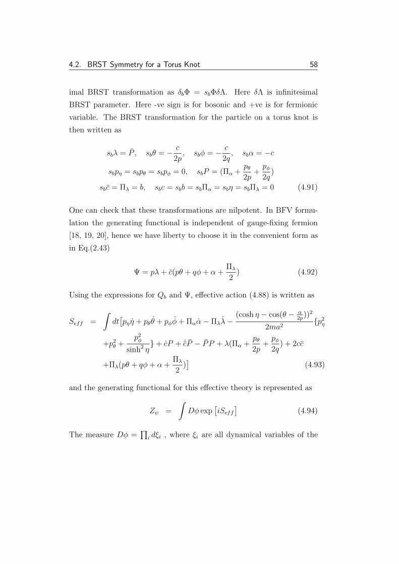
4.2. BRST Symmetry for a Torus Knot 58
imal BRST transformation as δbΦ = sbΦδΛ. Here δΛ is infinitesimal
BRST parameter. Here -ve sign is for bosonic and +ve is for fermionic
variable. The BRST transformation for the particle on a torus knot is
then written as
sbλ = P , sbθ = − c
2p, sbφ = − c
2q, sbα = −c
sbpη = sbpθ = sbpφ = 0, sbP = (Πα +pθ2p
+pφ2q
)
sbc = Πλ = b, sbc = sbb = sbΠα = sbη = sbΠλ = 0 (4.91)
One can check that these transformations are nilpotent. In BFV formu-
lation the generating functional is independent of gauge-fixing fermion
[18, 19, 20], hence we have liberty to choose it in the convenient form as
in Eq.(2.43)
Ψ = pλ+ c(pθ + qφ+ α +Πλ
2) (4.92)
Using the expressions for Qb and Ψ, effective action (4.88) is written as
Seff =
∫dt[pηη + pθθ + pφφ+ Παα− Πλλ−
(cosh η − cos(θ − α2p
))2
2ma2p2
η
+p2θ +
p2φ
sinh2 η+ cP + ˙cP − PP + λ(Πα +
pθ2p
+pφ2q
) + 2cc
+Πλ(pθ + qφ+ α +Πλ
2)]
(4.93)
and the generating functional for this effective theory is represented as
Zψ =
∫Dφ exp
[iSeff
](4.94)
The measure Dφ =∏
i dξi , where ξi are all dynamical variables of the
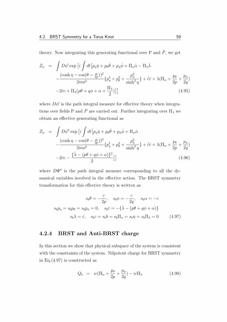
4.2. BRST Symmetry for a Torus Knot 59
theory. Now integrating this generating functional over P and P , we get
Zψ =
∫Dφ′ exp
[i
∫dt[pηη + pθθ + pφφ+ Παα− Πλλ
−(cosh η − cos(θ − α
2p))2
2ma2p2
η + p2θ +
p2φ
sinh2 η+ ˙cc+ λ(Πα +
pθ2p
+pφ2q
)
−2cc+ Πλ(pθ + qφ+ α +Πλ
2)]]
(4.95)
where Dφ′ is the path integral measure for effective theory when integra-
tions over fields P and P are carried out. Further integrating over Πλ we
obtain an effective generating functional as
Zψ =
∫Dφ′′ exp
[i
∫dt[pηη + pθθ + pφφ+ Παα
−(cosh η − cos(θ − α
2p))2
2ma2p2
η + p2θ +
p2φ
sinh2 η+ ˙cc+ λ(Πα +
pθ2p
+pφ2q
)
−2cc− λ− (pθ + qφ+ α)2
2
]](4.96)
where DΦ′′ is the path integral measure corresponding to all the dy-
namical variables involved in the effective action. The BRST symmetry
transformation for this effective theory is written as
sbθ = − c
2p, sbφ = − c
2q, sbα = −c
sbpη = sbpθ = sbpφ = 0, sbc = −λ− (pθ + qφ+ α)
sbλ = c, sbc = sbb = sbΠα = sbη = sbΠλ = 0 (4.97)
4.2.4 BRST and Anti-BRST charge
In this section we show that physical subspace of the system is consistent
with the constraints of the system. Nilpotent charge for BRST symmetry
in Eq.(4.97) is constructed as
Qb = ic(Πα +pθ2p
+pφ2q
)− icΠλ (4.98)
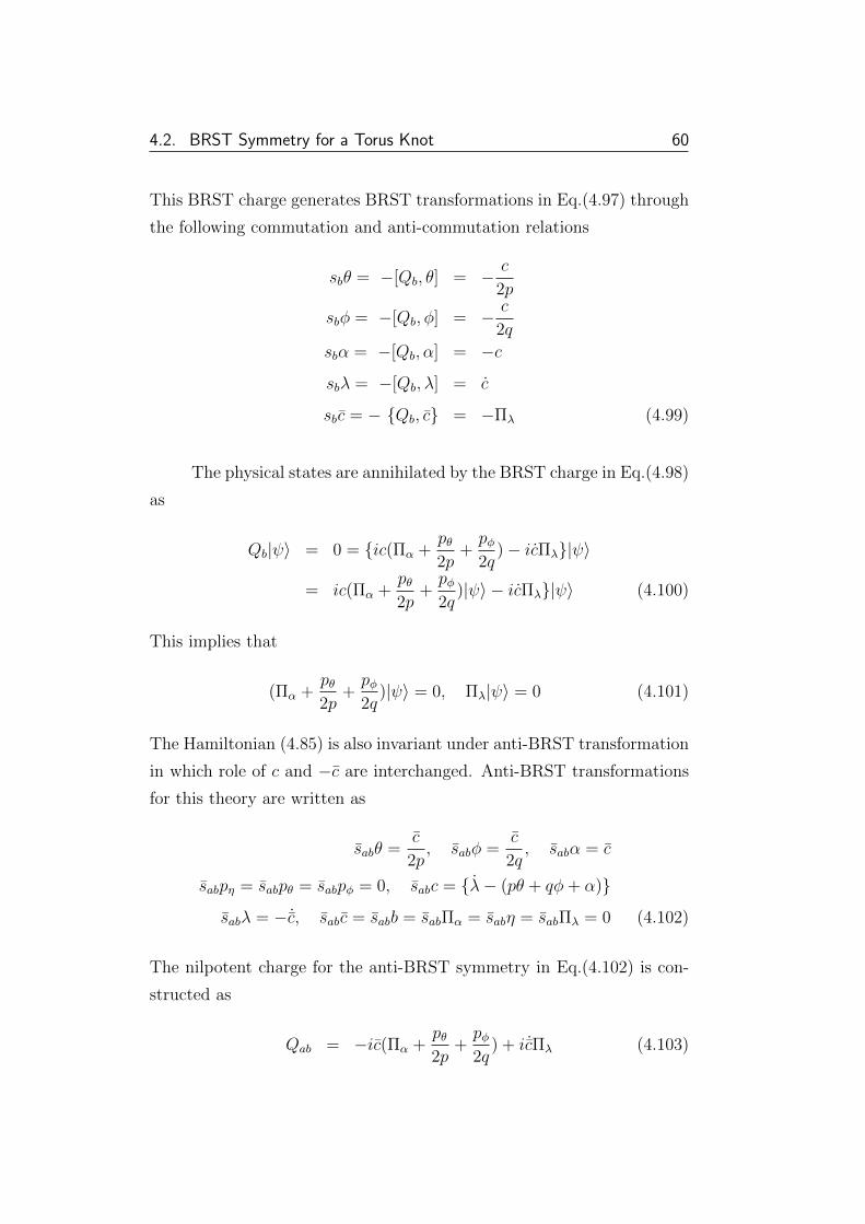
4.2. BRST Symmetry for a Torus Knot 60
This BRST charge generates BRST transformations in Eq.(4.97) through
the following commutation and anti-commutation relations
sbθ = −[Qb, θ] = − c
2p
sbφ = −[Qb, φ] = − c
2q
sbα = −[Qb, α] = −c
sbλ = −[Qb, λ] = c
sbc = − Qb, c = −Πλ (4.99)
The physical states are annihilated by the BRST charge in Eq.(4.98)
as
Qb|ψ〉 = 0 = ic(Πα +pθ2p
+pφ2q
)− icΠλ|ψ〉
= ic(Πα +pθ2p
+pφ2q
)|ψ〉 − icΠλ|ψ〉 (4.100)
This implies that
(Πα +pθ2p
+pφ2q
)|ψ〉 = 0, Πλ|ψ〉 = 0 (4.101)
The Hamiltonian (4.85) is also invariant under anti-BRST transformation
in which role of c and −c are interchanged. Anti-BRST transformations
for this theory are written as
sabθ =c
2p, sabφ =
c
2q, sabα = c
sabpη = sabpθ = sabpφ = 0, sabc = λ− (pθ + qφ+ α)
sabλ = − ˙c, sabc = sabb = sabΠα = sabη = sabΠλ = 0 (4.102)
The nilpotent charge for the anti-BRST symmetry in Eq.(4.102) is con-
structed as
Qab = −ic(Πα +pθ2p
+pφ2q
) + i ˙cΠλ (4.103)
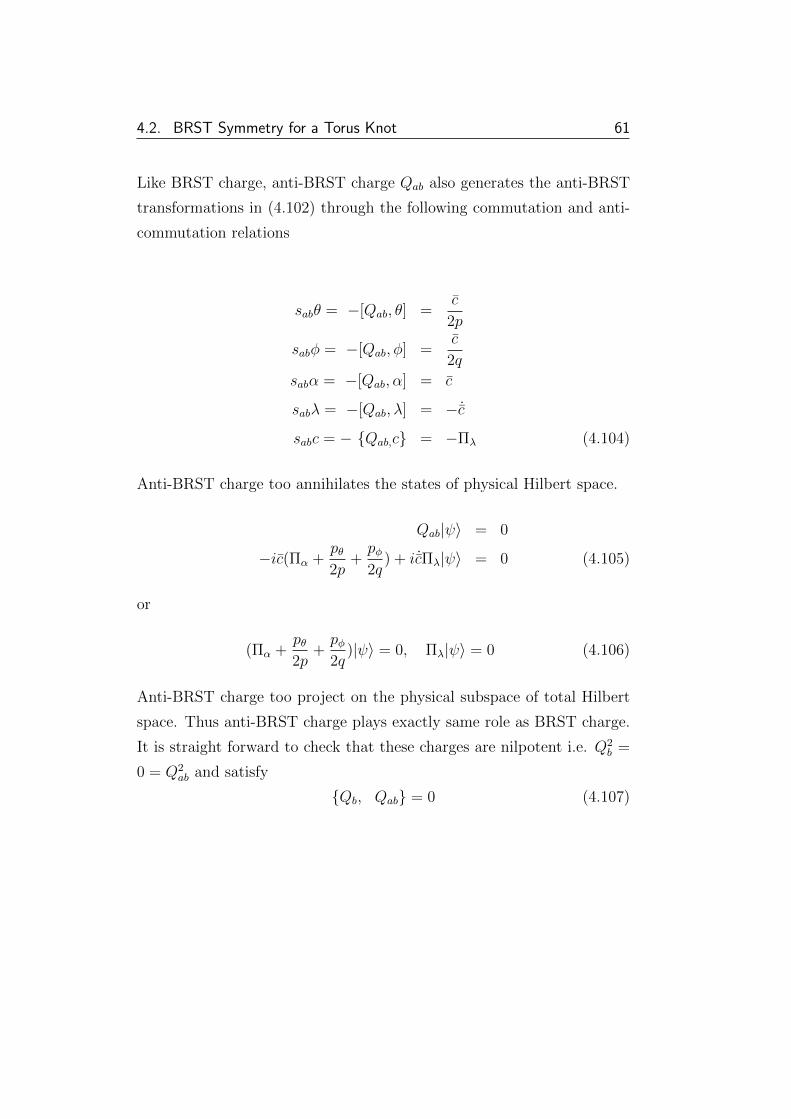
4.2. BRST Symmetry for a Torus Knot 61
Like BRST charge, anti-BRST charge Qab also generates the anti-BRST
transformations in (4.102) through the following commutation and anti-
commutation relations
sabθ = −[Qab, θ] =c
2p
sabφ = −[Qab, φ] =c
2q
sabα = −[Qab, α] = c
sabλ = −[Qab, λ] = − ˙c
sabc = − Qab,c = −Πλ (4.104)
Anti-BRST charge too annihilates the states of physical Hilbert space.
Qab|ψ〉 = 0
−ic(Πα +pθ2p
+pφ2q
) + i ˙cΠλ|ψ〉 = 0 (4.105)
or
(Πα +pθ2p
+pφ2q
)|ψ〉 = 0, Πλ|ψ〉 = 0 (4.106)
Anti-BRST charge too project on the physical subspace of total Hilbert
space. Thus anti-BRST charge plays exactly same role as BRST charge.
It is straight forward to check that these charges are nilpotent i.e. Q2b =
0 = Q2ab and satisfy
Qb, Qab = 0 (4.107)
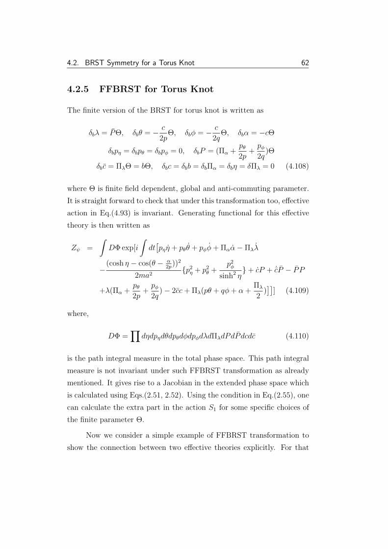
4.2. BRST Symmetry for a Torus Knot 62
4.2.5 FFBRST for Torus Knot
The finite version of the BRST for torus knot is written as
δbλ = PΘ, δbθ = − c
2pΘ, δbφ = − c
2qΘ, δbα = −cΘ
δbpη = δbpθ = δbpφ = 0, δbP = (Πα +pθ2p
+pφ2q
)Θ
δbc = ΠλΘ = bΘ, δbc = δbb = δbΠα = δbη = δΠλ = 0 (4.108)
where Θ is finite field dependent, global and anti-commuting parameter.
It is straight forward to check that under this transformation too, effective
action in Eq.(4.93) is invariant. Generating functional for this effective
theory is then written as
Zψ =
∫DΦ exp[i
∫dt[pηη + pθθ + pφφ+ Παα− Πλλ
−(cosh η − cos(θ − α
2p))2
2ma2p2
η + p2θ +
p2φ
sinh2 η+ cP + ˙cP − PP
+λ(Πα +pθ2p
+pφ2q
)− 2cc+ Πλ(pθ + qφ+ α +Πλ
2)]]
] (4.109)
where,
DΦ =∏
dηdpηdθdpθdφdpφdλdΠλdPdPdcdc (4.110)
is the path integral measure in the total phase space. This path integral
measure is not invariant under such FFBRST transformation as already
mentioned. It gives rise to a Jacobian in the extended phase space which
is calculated using Eqs.(2.51, 2.52). Using the condition in Eq.(2.55), one
can calculate the extra part in the action S1 for some specific choices of
the finite parameter Θ.
Now we consider a simple example of FFBRST transformation to
show the connection between two effective theories explicitly. For that
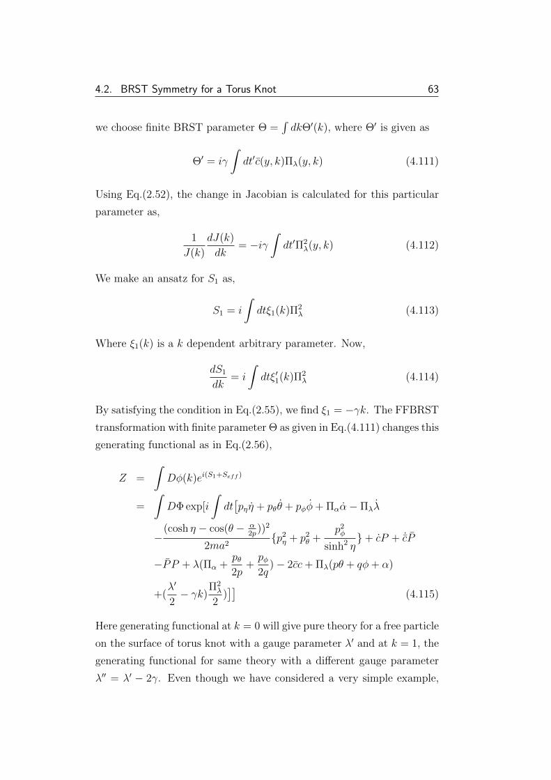
4.2. BRST Symmetry for a Torus Knot 63
we choose finite BRST parameter Θ =∫dkΘ′(k), where Θ′ is given as
Θ′ = iγ
∫dt′c(y, k)Πλ(y, k) (4.111)
Using Eq.(2.52), the change in Jacobian is calculated for this particular
parameter as,
1
J(k)
dJ(k)
dk= −iγ
∫dt′Π2
λ(y, k) (4.112)
We make an ansatz for S1 as,
S1 = i
∫dtξ1(k)Π2
λ (4.113)
Where ξ1(k) is a k dependent arbitrary parameter. Now,
dS1
dk= i
∫dtξ′1(k)Π2
λ (4.114)
By satisfying the condition in Eq.(2.55), we find ξ1 = −γk. The FFBRST
transformation with finite parameter Θ as given in Eq.(4.111) changes this
generating functional as in Eq.(2.56),
Z =
∫Dφ(k)ei(S1+Seff )
=
∫DΦ exp[i
∫dt[pηη + pθθ + pφφ+ Παα− Πλλ
−(cosh η − cos(θ − α
2p))2
2ma2p2
η + p2θ +
p2φ
sinh2 η+ cP + ˙cP
−PP + λ(Πα +pθ2p
+pφ2q
)− 2cc+ Πλ(pθ + qφ+ α)
+(λ′
2− γk)
Π2λ
2)]]
(4.115)
Here generating functional at k = 0 will give pure theory for a free particle
on the surface of torus knot with a gauge parameter λ′ and at k = 1, the
generating functional for same theory with a different gauge parameter
λ′′ = λ′ − 2γ. Even though we have considered a very simple example,
4.2. BRST Symmetry for a Torus Knot 64
our formulation is valid to connect any two generating functionals corre-
sponding to different effective actions on the surface of torus knot using
FFBRST transformation with suitable parameter.
4.2.6 Conclusion
Mathematical concept of knot theory is very useful in describing various
physical systems and it has been extensively used to study many differ-
ent phenomena in physics. However there was no BRST formulation for
particle on the surface of torus knot. In this work we systematically de-
veloped the BRST/anti-BRST formulation for the first time for a particle
moving on a torus knot. Using Dirac’s constraint analysis we found all
the constraints of this system. Further we have extended this theory to
include WZ term to recast this theory as gauge theory. Using BFV formu-
lation BRST/anti-BRST invariant effective action for a particle moving
on a torus knot has been developed. Nilpotent charges which generate
these symmetries have been calculated explicitly. The physical states
which are annihilated by these nilpotent charges are consistent with the
constraints of the system. Our formulation is independent of particular
choice of a torus knot. We further have extended the BRST formulation
by considering the transformation parameter finite and field dependent.
We indicate how different effective theories on the surface of torus knot
are related through such a finite transformation through the non-trivial
Jacobian factor. In support of our result we explicitly relate the gen-
erating functionals of two effective theories with different gauge-fixing
parameters. Using FFBRST with suitable finite parameter the connec-
tion between any two effective theories can be made in a straight forward
manner following the prescriptions outlined in this work.
4.3. BRST Qantization on Torus Knot 65
4.3 BRST Qantization on Torus Knot
4.3.1 Particle on a Torus Knot
Particle on surface of torus knot is given by [140, 146]. This model is
analogous to the rigid rotor model discussed in ref. [148].
To quantize the system and realize the physics, we have to diago-
nalize the system in presence of the constraints Φ = (pθ + qφ) ≈ 0. To
execute this, we will discard the [148] terms proportional to p2θ and p2
φ as
they don’t commute with the constraint equation. The effective Hamilto-
nian for this system keeping the essential physical content of the theory
intact is then written as
Hc =(cosh η − cos θ)2
ma2p2η + λ(pθ + qφ) (4.116)
4.3.2 Particle on torus knot as gauge theory
The constraint which doesn’t commute with unphysical operators is to
be identified with the generator of gauge transformations. In this case
the gauge transformation is an unitary operator of the form [148]
Uf = e−if(t)Φ (4.117)
where f(t) is an arbitrary c number and function of t. Under this trans-
formation only pθ and pφ transform non-trivially. First order Lagrangian
for torus knot is written as
Lc = pηη + pθθ + pφφ−(cosh η − cos θ)2
ma2p2η − λ(pθ + qφ) (4.118)
Here we have enlarged the dynamical degrees of freedom to include the
Lagrange multiplier λ and its canonically conjugate momentum pλ. This
Lagrangian is invariant under following time dependent gauge transfor-
4.3. BRST Qantization on Torus Knot 66
mation [148]
δλ = f(t), δpθ = pf(t), δpφ = qf(t)
δpη = δη = δθ = δφ = δpλ = 0 (4.119)
as under this gauge transformation the Lagrangian corresponding to
canonical Hamiltonian Hc changes only by a total time derivative,ddt
[f(t)(pθ + qφ)]. Hence the action is invariant under gauge transfor-
mation in Eq.(4.119).
4.3.3 Gauge fixing and BRST transformation
To construct the BRST and anti-BRST symmetry for the particle on the
surface of a torus knot we consider the gauge invariant Lagrangian of the
torus knot obtained in last section and replace the gauge transformation
in Eq.(4.119) by introducing new anti-commuting variables c and c and
a commuting variable b such that the BRST transformations
δλ = −c, δpθ = pc, δpφ = qc, δc = −pλ = b
δpη = δη = δθ = δφ = δpλ = δc = δb = 0 (4.120)
are nilpotent in nature. The gauge fixed effective Lagrangian which is
invariant under this kind of BRST transformation is then constructed as
Leff = pηη + pθθ + pφφ−(cosh η − cos θ)2
ma2p2η − λ(pθ + qφ)
− b(λ− pθ2p− pφ
2q)− b2
2+ ˙cc− cc (4.121)
The BRST charge which generates the transformation in (4.120) is
written as
Qb = −ic(pθ + qφ)− icpλ. (4.122)
4.3. BRST Qantization on Torus Knot 67
The Lagrangian (4.121) is also invariant under anti-BRST transfor-
mation in which role of c and −c are interchanged.
The nilpotent charge for the anti-BRST symmetry is written as
Qab = ic(pθ + qφ) + i ˙cpλ (4.123)
It is straight forward to check that these charges are nilpotent i.e.
Q2b = 0 = Q2
ab and satisfy
Qb, Qab = 0 (4.124)
4.3.4 Conclusion
We for the first time constructed BRST/anti-BRST transformations for
particle moving on torus knot. The nilpotent BRST/anti-BRST charges
are constructed which produce such nilpotent transformations. Our for-
mulation will be helpful in characterizing various field theoretic models
defined on torus knot manifold.
In the next chapter we will discuss about “Weyl Degree of freedom
in Nambu-Goto string through field Transformation” [163]. We will show
how Weyl degrees of freedom can be introduced in the Nambu-Goto string
in the path-integral formulation using the re-parametrization invariant
measure. First, we will identify Weyl degrees of freedom in conformal
gauge using BFV formulation. Further we will change the NG string
action to the Polyakov action. The generating functional in light-cone
gauge will then be obtained from the generating functional corresponding
to the Polyakov action in conformal gauge by using suitably constructed
FFBRST transformation.
Chapter 5
Nambu-Goto String and Weyl
Symmetry
5.1 Weyl Degree of Freedom in
Nambu-Goto String through Field
Transformaion
In this chapter we will study, how Weyl degree of freedom can be incor-
porated in Nambu-Goto (NG) string in light-cone gauge. Bosonic strings
are formulated using two alternative actions namely the NG action [150]
and the Polyakov action [151]. In the Polyakov formulation, one uses
the metric of the string world-sheet, gαβ, to manifest the Weyl and re-
parametrization symmetries at the classical level. These symmetries are
useful to eliminate the degrees of freedom of gαβ. On the other hand,
in the NG string only string coordinates Xµ(µ = 0, ..., D − 1) are used
as dynamical variables and hence no Weyl freedom is present from the
beginning. We consider the NG string theory in BFV formulation at
the sub-critical dimensions, where the BF fields appear as the conformal
degrees of freedom [155, 156]. Using FFBRST transformations we will
connect the action in conformal gauge to light cone gauge. In this way
we will be able to incorporate Weyl degrees of freedom in NG string.
68
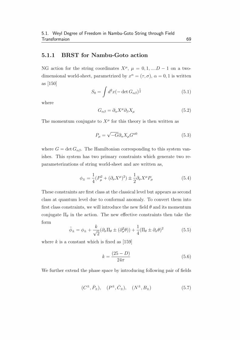
5.1. Weyl Degree of Freedom in Nambu-Goto String through FieldTransformaion 69
5.1.1 BRST for Nambu-Goto action
NG action for the string coordinates Xµ, µ = 0, 1, ....D − 1 on a two-
dimensional world-sheet, parametrized by xα = (τ, σ), α = 0, 1 is written
as [150]
S0 =
∫d2x(− detGαβ)
12 (5.1)
where
Gαβ = ∂αXµ∂βXµ (5.2)
The momentum conjugate to Xµ for this theory is then written as
Pµ =√−G∂αXµG
α0 (5.3)
where G = detGαβ. The Hamiltonian corresponding to this system van-
ishes. This system has two primary constraints which generate two re-
parameterizations of string world-sheet and are written as,
φ± =1
4(P 2
µ + (∂σXµ)2)± 1
2∂σX
µPµ (5.4)
These constraints are first class at the classical level but appears as second
class at quantum level due to conformal anomaly. To convert them into
first class constraints, we will introduce the new field θ and its momentum
conjugate Πθ in the action. The new effective constraints then take the
form
φ± = φ± +k√2
(∂σΠθ ± (∂2σθ)) +
1
4(Πθ ± ∂σθ)2 (5.5)
where k is a constant which is fixed as [159]
k =(25−D)
24π(5.6)
We further extend the phase space by introducing following pair of fields
(C±, P±), (P±, C±), (N±, B±) (5.7)
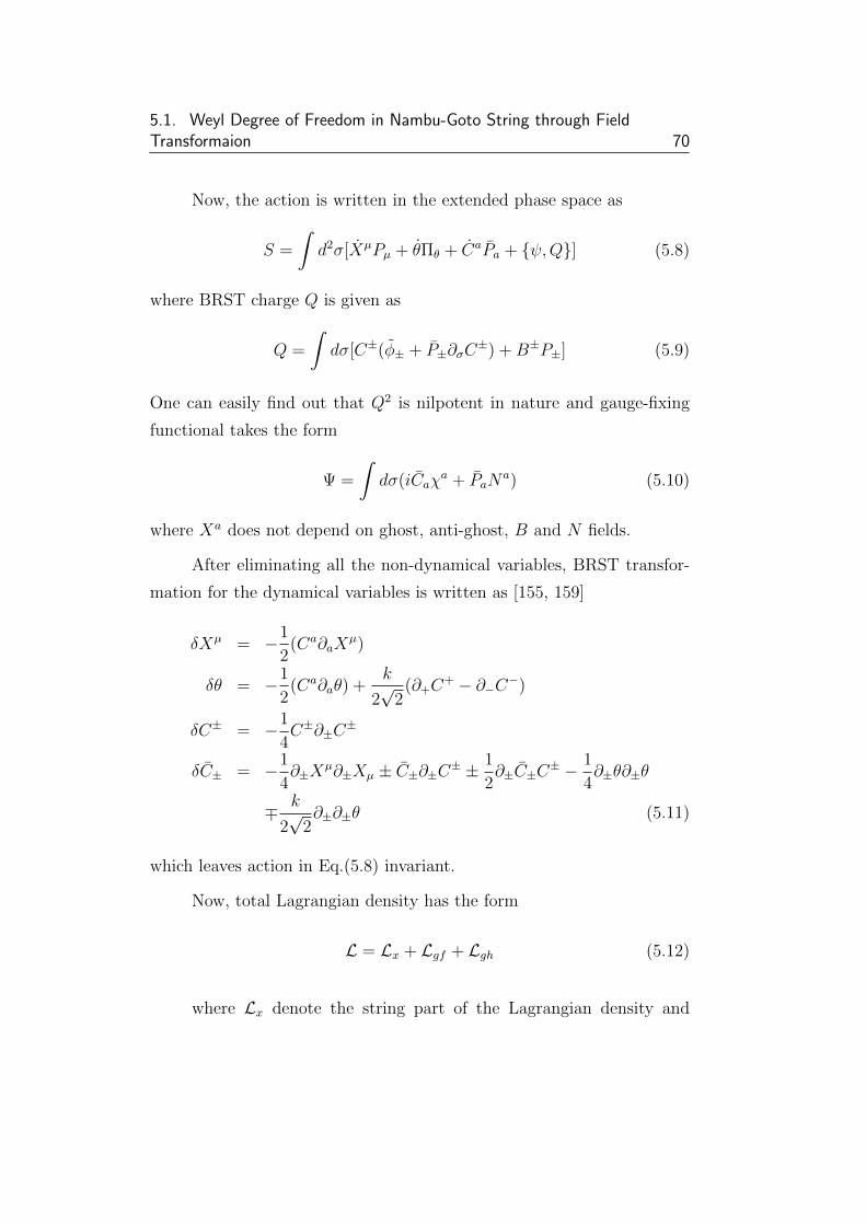
5.1. Weyl Degree of Freedom in Nambu-Goto String through FieldTransformaion 70
Now, the action is written in the extended phase space as
S =
∫d2σ[XµPµ + θΠθ + CaPa + ψ,Q] (5.8)
where BRST charge Q is given as
Q =
∫dσ[C±(φ± + P±∂σC
±) +B±P±] (5.9)
One can easily find out that Q2 is nilpotent in nature and gauge-fixing
functional takes the form
Ψ =
∫dσ(iCaχ
a + PaNa) (5.10)
where Xa does not depend on ghost, anti-ghost, B and N fields.
After eliminating all the non-dynamical variables, BRST transfor-
mation for the dynamical variables is written as [155, 159]
δXµ = −1
2(Ca∂aX
µ)
δθ = −1
2(Ca∂aθ) +
k
2√
2(∂+C
+ − ∂−C−)
δC± = −1
4C±∂±C
±
δC± = −1
4∂±X
µ∂±Xµ ± C±∂±C± ±1
2∂±C±C
± − 1
4∂±θ∂±θ
∓ k
2√
2∂±∂±θ (5.11)
which leaves action in Eq.(5.8) invariant.
Now, total Lagrangian density has the form
L = Lx + Lgf + Lgh (5.12)
where Lx denote the string part of the Lagrangian density and
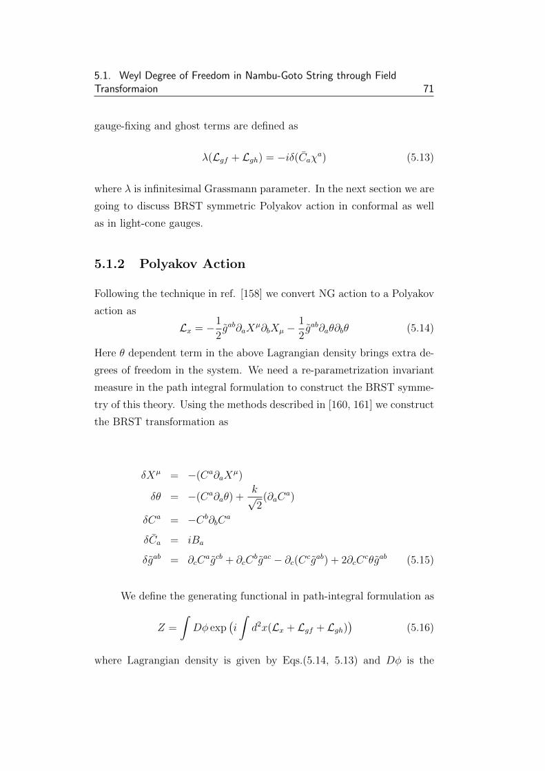
5.1. Weyl Degree of Freedom in Nambu-Goto String through FieldTransformaion 71
gauge-fixing and ghost terms are defined as
λ(Lgf + Lgh) = −iδ(Caχa) (5.13)
where λ is infinitesimal Grassmann parameter. In the next section we are
going to discuss BRST symmetric Polyakov action in conformal as well
as in light-cone gauges.
5.1.2 Polyakov Action
Following the technique in ref. [158] we convert NG action to a Polyakov
action as
Lx = −1
2gab∂aX
µ∂bXµ −1
2gab∂aθ∂bθ (5.14)
Here θ dependent term in the above Lagrangian density brings extra de-
grees of freedom in the system. We need a re-parametrization invariant
measure in the path integral formulation to construct the BRST symme-
try of this theory. Using the methods described in [160, 161] we construct
the BRST transformation as
δXµ = −(Ca∂aXµ)
δθ = −(Ca∂aθ) +k√2
(∂aCa)
δCa = −Cb∂bCa
δCa = iBa
δgab = ∂cCagcb + ∂cC
bgac − ∂c(Ccgab) + 2∂cCcθgab (5.15)
We define the generating functional in path-integral formulation as
Z =
∫Dφ exp
(i
∫d2x(Lx + Lgf + Lgh)
)(5.16)
where Lagrangian density is given by Eqs.(5.14, 5.13) and Dφ is the
5.1. Weyl Degree of Freedom in Nambu-Goto String through FieldTransformaion 72
generic notation for path integral measure. Transformation in Eq.(5.15)
leaves the effective action invariant. Now we fix the gauge more specifi-
cally and discuss BRST invariant effective theories in conformal as well
as light cone gauges.
5.1.3 Conformal Gauge
Conformal gauge has been used extensively in the discussion of various
problems. It has been used to study strings, gravity etc in path-integral
and covariant operator formalism. This gauge is very useful to remove
conformal anomaly, to introduce Weyl symmetry and in renormalizing
the theory [157, 159, 160].
The conformal gauge condition is expressed as gab = ηab [156, 160]
and is incorporated into the following gauge-fixing and FP ghost term in
a BRST invariant manner,
Lcf = λ(Lgf + Lgh) = −iδB(C0g++ + C1g−−) (5.17)
Here C0 and C1 are anti-ghost fields.
5.1.4 Light-cone Gauge
On the other hand, light cone gauge is used to eliminate unphysical de-
grees of freedom and also in decoupling of ghost fields. Light-cone gauge
has also been used in Kaku-Kikkawa string field theory, in showing the
ultraviolet finiteness of N = 4 supersymmetric YM theory, in dimensional
regularization, in gravity, supergravity, string and superstrings theories
[162].
The light-cone gauge condition, (X+ = f(σ), g++ = 0) [156, 161] is
incorporated into the following gauge-fixing and ghost term in a BRST
5.1. Weyl Degree of Freedom in Nambu-Goto String through FieldTransformaion 73
invariant manner,
Llc = λ(Lgf + Lgh) = −iδB(C0g++ + C1(X+ − f(σ))). (5.18)
Here f(σ) is an arbitrary function of σ0 and σ1.
Now we proceed to use FFBRST to address the Weyl degree of
freedom in NG string formulation.
5.1.5 Connection between generating functionals
in conformal and light-cone gauges
In this subsection, we construct the FFBRST transformation with an
appropriate finite parameter to obtain the generating functional corre-
sponding to Lcf from that of corresponding to Llc. We calculate the
Jacobian corresponding to such a FFBRST transformation following the
method outlined in chapter 2 and show that it is a local functional of
fields and accounts for the difference of the two FP effective actions.
The generating functional corresponding to the FP effective action
Scf is written as
Zcf =
∫Dφ exp(iScf [φ]) (5.19)
where Scf is given by
Scf =
∫d2x(Lx + Lcf ) (5.20)
Now, to obtain the generating functional corresponding to Slc, we ap-
ply the FFBRST transformation with a finite parameter Θ[φ], which is
obtained from the infinitesimal but field dependent parameter, Θ′[φ(k)];
through∫ κ
0Θ′[φ(κ)]dκ. We construct Θ′[φ(κ)] as,
Θ′[φ] = i
∫d2x[γC1(X+ − f(σ))− g−−] (5.21)
5.1. Weyl Degree of Freedom in Nambu-Goto String through FieldTransformaion 74
Here γ is arbitrary constant parameter and all the fields depend on the
parameter k. The infinitesimal change in the Jacobian corresponding to
this FFBRST transformation is calculated using Eq.(2.52)
1
J(k)
dJ(k)
dk= −i
∫d2xγ[−iB1(X+ − f(σ))− g−− − (Ca∂aX
+)C1
−δg−−C1] (5.22)
To express the Jacobian contribution in terms of a local functional of
fields, we make an ansatz for S1 by considering all possible terms that
could arise from such a transformation as
S1[φ(k), k] =
∫d2x[ξ1iB
1(X+ − f(σ)) + ξ2iB1g−− + ξ3(Ca∂aX
+)C1
+ξ4δg−−C1 + ξ5iB
0g++ + ξ6C0δg++] (5.23)
where all the fields are considered to be k dependent and we have intro-
duced arbitrary k dependent parameters ξn = ξn(k)(n = 1, 2, .., 6) with
initial condition ξn(k = 0) = 0. It is straight forward to calculate
dS1
dk=
∫d2x[ξ′1iB
1(X+ − f(σ)) + ξ′2iB1g−− + ξ′3(Ca∂aX
+)C1
+ξ′4δg−−C1 + ξ′5iB
0g++ + ξ′6C0δg++ + Θ′−ξ1C
a∂aX+iB1
+ξ2δg−−iB1 + ξ3(iB1)Ca∂aX
+ + ξ3(Cb∂bCa)∂aX
+C1
+ξ3Ca∂a(−Cb∂bX
+)C1 − ξ4iB1δg−− + ξ5δg
++iB0
−ξ6iB0δg++] (5.24)
where ξ′n = dξndk
. Now we will use the condition of Eq.(2.55).∫Dφ exp[i(Scf [φ(k)] + S1[φ(k), k])]
∫d2x[(−γ + ξ′1)iB1(X+ − f(σ))
+(γ + ξ′2)iB1g−− + (−γ + ξ′3)(Ca∂aX+)C1 + (−γ + ξ′4)δg−−C1
+ξ′5iB0g++ + ξ′6C
0δg++ + Θ′(−ξ1 + ξ3)Ca∂aX+iB1
+(ξ2 + ξ4)δg−−iB1 + (ξ5 − ξ6)δg++iB0] = 0 (5.25)
5.1. Weyl Degree of Freedom in Nambu-Goto String through FieldTransformaion 75
The terms proportional to Θ′ which are regarded as nonlocal, van-
ishes independently. These will give relations between ξ. Making remain-
ing local terms in Eq.(5.25) vanish will give relations between ξ and γ.
Solving these Eqs.(A.18, A.19), we will get following results.
The differential equations for ξn(k) can be solved with the initial
conditions ξn(0) = 0, to obtain the solutions
ξ1 = γk, ξ2 = −γk, ξ3 = γk, ξ4 = γk, ξ5 = ξ6 = 0 (5.26)
Putting values of these parameters in expression of S1, and choosing
arbitrary parameter γ = −1, we obtain,
S1[φ(1), 1] =
∫d2x[−iB1(X+ − f(σ)) + iB1g−− − (Ca∂aX
+)C1
−δg−−C1] (5.27)
Thus the FFBRST transformation with the finite parameter Θ that is
defined by Eq.(5.21) changes the generating functional Zcf as in Eq.(2.56)
Zcf =
∫Dφ exp(iScf [φ])
=
∫Dφ′ exp[i(Scf [φ
′] + S1[φ′, 1])]
=
∫Dφ exp[i(Scf [φ] + S1[φ, 1])]
=
∫Dφ exp(iSlc[φ]) ≡ Zlc (5.28)
Here Slc is defined as
Slc =
∫d2x(Lx + Llc) (5.29)
In this way FFBRST transformation with the finite field dependent pa-
rameter in Eq.(5.21) connects generating functional for the Polyakov ac-
tion in conformal gauge to that of in the light-cone gauge.
5.1. Weyl Degree of Freedom in Nambu-Goto String through FieldTransformaion 76
5.1.6 Conclusion
In this present work we have demonstrated how Weyl degrees of freedom
are incorporated in the formulation of NG string through certain field
transformation. Weyl degrees of freedom are first identified in conformal
gauge using BFV formulation. Then we have established the connection
between conformal gauge to light-cone in Polyakov type action for NG
string using the technique of FFBRST transformation, which connects
various theories through the non-trivial Jacobian of path integral mea-
sure. The non-local BRST transformation by Igarashi etal in [158] is
nothing but a particular type of FFBRST transformation. The parame-
ter λ in the non-local transformation in [158] is identified with FFBRST
parameter Θ′.
In the next chapter we will discuss about issue of ghost number cur-
rent anomaly in bosonic string in conformal gauge and its removal using
FFBRST transformation [196]. We consider Polyakov theory of Bosonic
strings in conformal gauge which are used to study conformal anomaly.
However it exhibits ghost number anomaly. We show how this anomaly
can be avoided by connecting this theory to that of in background co-
variant harmonic gauge which is known to be free from conformal and
ghost number current anomaly, by using suitably constructed finite field
dependent BRST transformation.
Chapter 6
Harmonic Gauge in Bosonic
String and FFBRST
Transformation
6.1 Background Covariant Harmonic
Gauge and Finite Field Dependent
BRST Transformation
Bosonic string in path integral formulation [151, 164, 165] has been stud-
ied in many gauges. The simplest choice of gauge is conformal gauge
[151, 157, 160, 165]. Renormalizing effective action in this gauge gives
conformal anomaly [166]. The effective action is defined as whole by one
loop Feynman diagram. Besides the conformal anomaly, there is another
important anomaly associated with conformal gauge is the ghost number
current anomaly on curved world-sheet [157]. Bosonic string has been
investigated in harmonic gauge [167] (a choice similar to Lorentz gauge
in QED). In harmonic gauge standard (D − 26) answer [151] has been
produced. It has been also found that ghost number current anomaly
in curved world-sheet is absent in background covariant harmonic gauge
[168] but the absence of a ghost number anomaly is achieved at the ex-
pense of a new anomaly in the sector involving the Nakanishi-Lautrup
field [169]. The BRST analysis of the bosonic string in this perspective
77
6.1. Background Covariant Harmonic Gauge and Finite Field DependentBRST Transformation 78
have been discussed in [170].
6.1.1 Bosonic String Action
In the path integral formalism bosonic string action is written as [151]
S0 =
∫d2x
1
2
√−ggab∂aXµ∂bXµ (6.1)
where Xµ, µ = 0, 1, 2....D− 1 is string co-ordinate and gab, (a, b = 0, 1) is
world-sheet metric. This action is invariant under both diffeomorphisms
and Weyl transformations in following ways
gab → g′ab = gab +∇aξb +∇bξa, gab → g′ab = (1 + 2σ)gab (6.2)
To factor out the infinite factors in the functional integral associated with
these transformations, usually we choose the conformal gauge condition
and introduce the Jacobian for the change of the gauge condition under
the infinitesimal diffeomorphisms (ξa) and Weyl transformations (σ).
6.1.2 Conformal Gauge
Conformal gauge has been used extensively in the discussion of various
problems. It has been used to study strings, gravity etc in path-integral
and covariant operator formalism. This gauge is very useful to remove
conformal anomaly, to introduce Weyl symmetry and in re-normalizing
the theory [151, 157, 160, 165].
The conformal gauge condition is expressed as hab(≡ gab − gab = 0)
and is incorporated into the following gauge-fixing and FP ghost term in
a BRST invariant manner [160],
Lcf = λ(Lgf + Lgh) = −iδB[Ca(1
2hab)] = −iδB[Ca(
1
2Aa)] (6.3)
6.1. Background Covariant Harmonic Gauge and Finite Field DependentBRST Transformation 79
Total Lagrangian density in conformal gauge in extended form is written
as
Ltcf =1
2
√−ggab∂aXµ∂bXµ −
1
2
√−gbahab −
1
2
√−gδB(Aa)Ca(6.4)
6.1.3 Harmonic Gauge
The harmonic gauge condition for bosonic string action is written as
[167, 168, 169]
∇a(√−ggab) = 0 (6.5)
where the Christoffel connection in ∇ is calculated for an arbitrary back-
ground metric gab.
In order to calculate gauge-fixing and ghost part of the action we
split the metric gab into a classical background field gab and a (quantum)
metric perturbation hab :
gab = gab + hab (6.6)
We need to fix the gauge invariance only for the quantum field hab
δhab = ∇aξb + ∇bξa + hbc∇aξc + hac∇bξ
c + ξc∇chab
δhab = 2σ(gab + hab) (6.7)
Here the classical field gab is invariant under general coordinate invariance
together with standard tensor transformation rules for the other fields.
The linearized form of gauge-fixing condition in harmonic gauge is
1
2∇ah− ∇bhab = 0 (6.8)
where h = gabhab. The gauge condition in Eq.(6.8) as well as in Eq.(6.5)
are not quantum Weyl covariant. To make them Weyl covariant we need
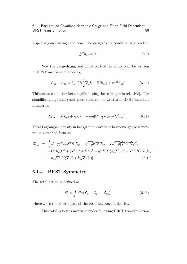
6.1. Background Covariant Harmonic Gauge and Finite Field DependentBRST Transformation 80
a special gauge fixing condition. The gauge-fixing condition is given by
gabhab = 0 (6.9)
Now the gauge-fixing and ghost part of the action can be written
in BRST invariant manner as,
Lgf + Lfp = δB[Ca(1
2∇ah− ∇bhab) + τ gabhab] (6.10)
This action can be further simplified using the technique in ref. [168]. The
simplified gauge-fixing and ghost term can be written in BRST invariant
manner as
Lhm = λ(Lgf + Lfp) = −iδB[Ca(1
2∇ah− ∇bhab)] (6.11)
Total Lagrangian density in background covariant harmonic gauge is writ-
ten in extended form as
Lthm =1
2
√−ggab∂aXµ∂bXµ −
√−gba∇bhab − i
√−g[∇bCa∇bCa
−CaRabCb + (∇bCa + ∇aCb − gab∇.C)hbc∇aC
c + ∇bCaCc∇chab
−hab∇aCb(∇.C + hij∇iCj)] (6.12)
6.1.4 BRST Symmetry
The total action is defined as
St0 =
∫d2x(L0 + Lgf + Lgh) (6.13)
where L0 is the kinetic part of the total Lagrangian density.
This total action is invariant under following BRST transformation
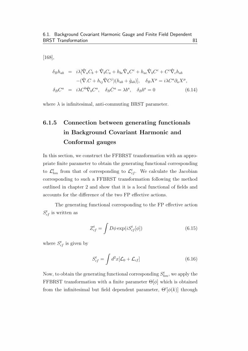
6.1. Background Covariant Harmonic Gauge and Finite Field DependentBRST Transformation 81
[168],
δBhab = iλ[∇aCb + ∇bCa + hbc∇aCc + hac∇bC
c + Cc∇chab
−(∇.C + hij∇Cj)(hab + gab)], δBXµ = iλCa∂aX
µ,
δBCa = iλCb∇bC
a, δBCa = λba, δBb
a = 0 (6.14)
where λ is infinitesimal, anti-commuting BRST parameter.
6.1.5 Connection between generating functionals
in Background Covariant Harmonic and
Conformal gauges
In this section, we construct the FFBRST transformation with an appro-
priate finite parameter to obtain the generating functional corresponding
to Lthm from that of corresponding to Ltcf . We calculate the Jacobian
corresponding to such a FFBRST transformation following the method
outlined in chapter 2 and show that it is a local functional of fields and
accounts for the difference of the two FP effective actions.
The generating functional corresponding to the FP effective action
Stcf is written as
Ztcf =
∫Dφ exp(iStcf [φ]) (6.15)
where Stcf is given by
Stcf =
∫d2x[L0 + Lcf ] (6.16)
Now, to obtain the generating functional corresponding Sthm, we apply the
FFBRST transformation with a finite parameter Θ[φ] which is obtained
from the infinitesimal but field dependent parameter, Θ′[φ(k)] through
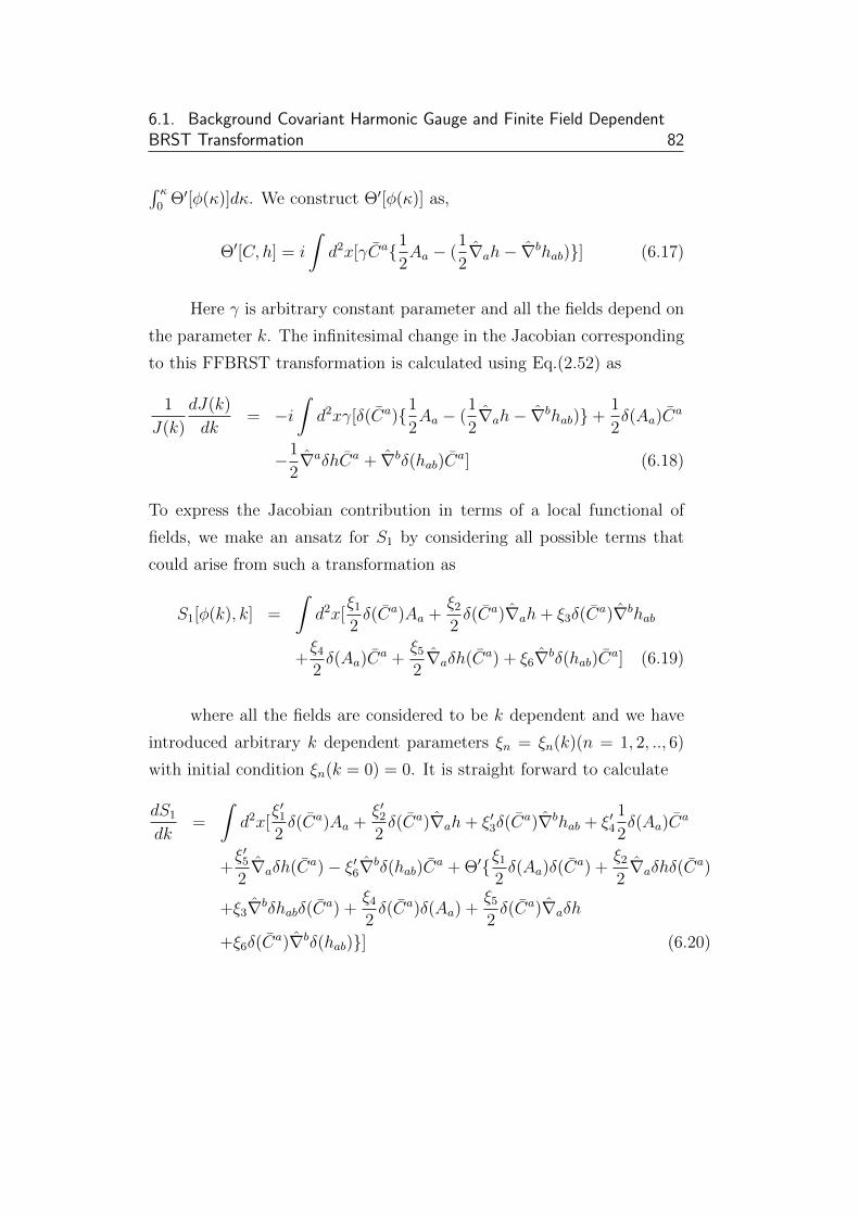
6.1. Background Covariant Harmonic Gauge and Finite Field DependentBRST Transformation 82
∫ κ0
Θ′[φ(κ)]dκ. We construct Θ′[φ(κ)] as,
Θ′[C, h] = i
∫d2x[γCa1
2Aa − (
1
2∇ah− ∇bhab)] (6.17)
Here γ is arbitrary constant parameter and all the fields depend on
the parameter k. The infinitesimal change in the Jacobian corresponding
to this FFBRST transformation is calculated using Eq.(2.52) as
1
J(k)
dJ(k)
dk= −i
∫d2xγ[δ(Ca)1
2Aa − (
1
2∇ah− ∇bhab)+
1
2δ(Aa)C
a
−1
2∇aδhCa + ∇bδ(hab)C
a] (6.18)
To express the Jacobian contribution in terms of a local functional of
fields, we make an ansatz for S1 by considering all possible terms that
could arise from such a transformation as
S1[φ(k), k] =
∫d2x[
ξ1
2δ(Ca)Aa +
ξ2
2δ(Ca)∇ah+ ξ3δ(C
a)∇bhab
+ξ4
2δ(Aa)C
a +ξ5
2∇aδh(Ca) + ξ6∇bδ(hab)C
a] (6.19)
where all the fields are considered to be k dependent and we have
introduced arbitrary k dependent parameters ξn = ξn(k)(n = 1, 2, .., 6)
with initial condition ξn(k = 0) = 0. It is straight forward to calculate
dS1
dk=
∫d2x[
ξ′12δ(Ca)Aa +
ξ′22δ(Ca)∇ah+ ξ′3δ(C
a)∇bhab + ξ′41
2δ(Aa)C
a
+ξ′52∇aδh(Ca)− ξ′6∇bδ(hab)C
a + Θ′ξ1
2δ(Aa)δ(C
a) +ξ2
2∇aδhδ(C
a)
+ξ3∇bδhabδ(Ca) +
ξ4
2δ(Ca)δ(Aa) +
ξ5
2δ(Ca)∇aδh
+ξ6δ(Ca)∇bδ(hab)] (6.20)
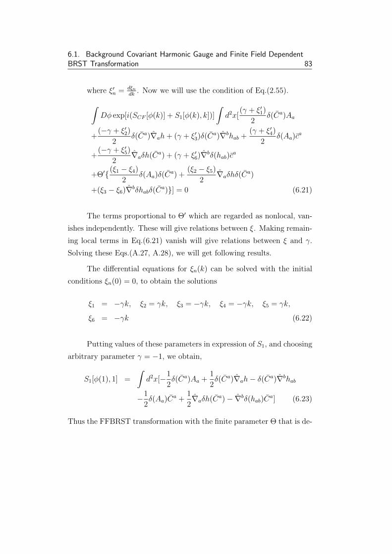
6.1. Background Covariant Harmonic Gauge and Finite Field DependentBRST Transformation 83
where ξ′n = dξndk
. Now we will use the condition of Eq.(2.55).∫Dφ exp[i(SCF [φ(k)] + S1[φ(k), k])]
∫d2x[
(γ + ξ′1)
2δ(Ca)Aa
+(−γ + ξ′2)
2δ(Ca)∇ah+ (γ + ξ′3)δ(Ca)∇bhab +
(γ + ξ′4)
2δ(Aa)c
a
+(−γ + ξ′5)
2∇aδh(Ca) + (γ + ξ′6)∇bδ(hab)c
a
+Θ′(ξ1 − ξ4)
2δ(Aa)δ(C
a) +(ξ2 − ξ5)
2∇aδhδ(C
a)
+(ξ3 − ξ6)∇bδhabδ(Ca)] = 0 (6.21)
The terms proportional to Θ′ which are regarded as nonlocal, van-
ishes independently. These will give relations between ξ. Making remain-
ing local terms in Eq.(6.21) vanish will give relations between ξ and γ.
Solving these Eqs.(A.27, A.28), we will get following results.
The differential equations for ξn(k) can be solved with the initial
conditions ξn(0) = 0, to obtain the solutions
ξ1 = −γk, ξ2 = γk, ξ3 = −γk, ξ4 = −γk, ξ5 = γk,
ξ6 = −γk (6.22)
Putting values of these parameters in expression of S1, and choosing
arbitrary parameter γ = −1, we obtain,
S1[φ(1), 1] =
∫d2x[−1
2δ(Ca)Aa +
1
2δ(Ca)∇ah− δ(Ca)∇bhab
−1
2δ(Aa)C
a +1
2∇aδh(Ca)− ∇bδ(hab)C
a] (6.23)
Thus the FFBRST transformation with the finite parameter Θ that is de-

6.1. Background Covariant Harmonic Gauge and Finite Field DependentBRST Transformation 84
fined by Eq.(6.17) changes the generating functional ZCF as in Eq.(2.56).
Ztcf =
∫Dφ exp(iStcf [φ])
=
∫Dφ′ exp[i(Stcf [φ
′] + S1[φ′, 1])]
=
∫Dφ exp[i(Stcf [φ] + S1[φ, 1])]
=
∫Dφ exp(iSthm[φ]) ≡ Zt
hm (6.24)
Here Sthm is defined as
Sthm =
∫d2x(Lx + Lhm) (6.25)
In this way FFBRST transformation with the finite field dependent pa-
rameter in Eq.(6.17) connects generating functional for the Polyakov ac-
tion in the conformal gauge to that of in background covariant harmonic
gauge.
6.1.6 Conclusion
In this chapter we have shown how ghost number current anomaly can be
removed in conformal gauge in curved world-sheet. Ghost number current
anomaly is absent in bosonic string in background covariant harmonic
gauge. Using the finite field dependent BRST transformation we have
obtained action in background covariant harmonic gauge from action in
conformal gauge. In this way we have avoided ghost number current
anomaly in conformal gauge.
In the next chapter we will present overall summary of this thesis.

Chapter 7
Concluding Remarks
This thesis is based on the construction of various generalizations of
BRST transformations and their applications in different type of gauge
field theories and string theories. We have started with the techniques of
BRST quantization in both Lagrangian and Hamiltonian formalism. In
Lagrangian formulation we have discussed field/anti-field formalism ap-
plicable to gauge theories with irreducible/reducible or closed/open gauge
algebra. In Hamiltonian formalism first we have discussed Dirac’s con-
straints analysis. Then we have discussed the (BFFT) formalism, which is
used to convert second class constraints to first class constraints. Finally
we have discussed (BFV) formalism, to construct BRST transformation.
In this thesis, BRST symmetry has been generalized in various ways and
some applications of such generalizations have been discussed. The usual
BRST transformation under which the FP effective action remains in-
variant, is characterized by an infinitesimal, global and anti-commuting
parameter. One of the important generalizations of BRST transforma-
tions is FFBRST transformation in which infinitesimal BRST parame-
ter is generalized to be finite field dependent. Various implications of
FFBRST transformations have been discussed. Under the generalized
BRST transformation with a finite field dependent parameter, the effec-
tive action remains invariant but the path integral measure gives rise to
a nontrivial Jacobian which under certain condition can be written as
exponential of some local functional of fields. In the usual BRST trans-
formation, the variation of kinetic part independently vanishes whereas
the variation of gauge fixing part cancels with the variation of ghost part
85
86
of the effective action. Another important generalization of BRST trans-
formation which is local and covariant is dual-BRST transformation. It
has been discussed in the context of particle on a torus. Under dual-
BRST transformations, the variation of gauge fixing part independently
vanishes whereas the variation of kinetic part cancels with the variation
of ghost part of the effective action. In the Lagrangian framework, dual
BRST symmetry is generally considered to be an independent symme-
try because of its analogy with co-exterior derivative in the language
of differential geometry. The absolute anti-commutativity of BRST and
anti-BRST symmetry as well as dual-BRST and anti-dual BRST sym-
metry is essential for these symmetries to be independent. Independency
of these symmetries can be insured through application of Curci-Ferrari
condition. In the Lagrangian framework of BRST formalism, it is not
clear why it is important to impose CF condition. It also doesn’t answer
the question “What kind of constraint CF condition is” in the Dirac’s
classification of constraints.
In the chapter I, we have discussed about introductory idea of BRST
quantization in the gauge theory. BRST transformation is a very powerful
technique since its origin in non-Abelian gauge theories. We have also
given various methods of BRST quantization. We have also discussed
various types of BRST transformations. Later we have given introductory
idea of our work.
In the II chapter we have discussed various techniques of BRST
quantization. First we have discussed Lagrangian formalism also called
field/anti-field formalism or BV formalism. Then we have discussed
Hamiltonian formalism also called BFV formalism. This formalism is
mainly based on Dirac’s method of constraints analysis. Then we have
discussed about BFFT formalism which is a technique of converting sec-
ond class constraints to first class constraints. At last we have discussed
generalized BRST transformation also called FFBRST transformation.
In the III chapter we have discussed about MA gauge and gener-
alized BRST transformation [111]. The main idea of this chapter is to
87
show how quark confinement can be realized in Lorenz gauge. In SU(N)
YM theory, the MA gauge has been used to study its non-perturbative
features, such as quark confinement. The MA gauge is a nonlinear partial
gauge. It partially fixes the the system to maintain only the MA gauge
symmetry specified by U(1)N−1. This gauge helps us to extract Abelian
degrees of freedom latent in SU(N) YM theory. In MA gauge, Abelian
dominance and the emergence of magnetic monopoles are realized as re-
markable phenomena in the non-perturbative infrared region. We have
applied the FFBRST formulation discussed in chapter 2, to connect the
action in the gauge-fixed SU(2) YM theories formulated in the Lorenz
and MA gauges. We have clearly shown, how the generating functional
corresponding to the FP effective action in the MA gauge can be obtained
from that in the Lorenz gauge by carrying out a suitably constructed FF-
BRST transformation.
In the IV chapter we have discussed about various nilpotent sym-
metries for a particle on torus [137]. We have also discussed about BRST
and anti-BRST symmetries for a particle on torus knot. For particle on
torus, we have used BFV technique to study all the symmetries. We
have constructed nilpotent BRST, dual BRST, anti-BRST, and anti-dual
BRST transformations for this system. Dual BRST transformations are
also the symmetry of effective action and leave gauge fixing part of the
effective action invariant. Interchanging the role of ghost and anti-ghost
fields the anti-BRST and anti-dual BRST symmetry transformations are
constructed. We have shown that the nilpotent BRST and anti-dual
BRST charges are analogous to the exterior derivative operators as the
ghost number of the state |ψ〉 on the total Hilbert space is increased by
one when these charges operate on these states and algebra followed by
these operators is the same as the algebra obeyed by the de-Rham coho-
mological operators. Similarly the dual BRST and anti-BRST charges are
analogous to coexterior derivative. The anti-commutators of BRST and
dual BRST and anti-BRST and anti-dual BRST charges lead to bosonic
symmetry. The corresponding charges are analogous to Laplacian oper-
88
ator. Further, this theory has another nilpotent symmetry called ghost
symmetry under which the ghost term of the effective action is invariant.
We further have shown that this theory behaves as double Hodge theory
as the charges for BRST Qb and dual BRST Qd and the charges for the
bosonic symmetry Qw generated out of these two symmetries, form the
algebra for Hodge theory. On the other hand charges for anti-BRST,
Qab anti-dual BRST Qad, and Qw, charge for bosonic symmetry gener-
ated out of these nilpotent symmetries, also satisfy the Hodge algebra.
Thus a particle on the surface of the torus has very rich mathematical
structure. We further constructed the FFBRST transformation for this
system. By constructing appropriate field dependent parameter we have
explicitly shown that such generalized BRST transformations are capable
of connecting different theories on torus.
For a particle on the surface of torus knot we have systematically
developed the BRST/anti-BRST formulation for the first time [147]. Us-
ing Diracs constraint analysis we found all the constraints of this sys-
tem. Further, we have extended this theory to include the Wess-Zumino
term to recast this theory as gauge theory. Using BFV formulation, the
BRST/anti-BRST invariant effective action for a particle moving on a
torus knot has been developed. Nilpotent charges which generate these
symmetries have been calculated explicitly. The physical states which
are annihilated by these nilpotent charges are consistent with the con-
straints of the system. Our formulation is independent of a particular
choice of a torus knot. We have further extended the BRST formulation
by considering the transformation parameter finite and field dependent.
We indicate how different effective theories on the surface of the torus
knot are related through such a finite transformation through the non-
trivial Jacobian factor. In support of our result we explicitly relate the
generating functionals of two effective theories with different gauge fixing
parameters. Using FFBRST with a suitable finite parameter the connec-
tion between any two effective theories can be made in a straightforward
manner following the prescriptions outlined in this work.
89
We have also developed BRST and anti-BRST symmetries for a
particle on torus knot [149] using the technique used in ref. [148].
In chapter V we have discussed Weyl degree of freedom in NG string
in light-cone gauge through field transformation [163]. In this work we
have demonstrated how Weyl degrees of freedom are incorporated in the
formulation of NG string through a certain field transformation. Weyl
degrees of freedom are first identified in conformal gauge using BFV for-
mulation. Then we have established the connection between conformal
gauge to light-cone gauge in a Polyakov-type action for NG string using
the technique of FFBRST transformation, which connects various theo-
ries through the nontrivial Jacobian of the path-integral measure. The
nonlocal BRST transformation by Igarashi et al. in [158] is nothing but a
particular type of FFBRST transformation. The parameter λ in the non-
local transformation in [158] is identified with the FFBRST parameter
Θ′.
In the chapter VI we have discussed connection between confor-
mal and harmonic gauges for Bosonic Strings [196]. In this present work
we have shown how ghost number current anomaly present in conformal
gauge in curved world-sheet is avoided using field transformation. By con-
structing appropriate FFBRST transformation we obtain the generating
functional in harmonic gauge from that of conformal gauge. This provides
a convenient way to go from a theory with ghost number anomaly to the
theory where there is no ghost number current anomaly. Further har-
monic gauge which is a complicated gauge is directly connected through
the suitably constructed field transformation to conformal gauge theory
which is simpler to use.
In the chapter VII we have presented conclusion of the whole thesis.
We have specifically discussed about work done in each chapter.
In future we will try to work on more mathematical models similar
to torus and knot, which have some implications on physical phenomena.
It will be interesting to generalize the FFBRST formulation for other

90
theories like superstring, supergravity etc. It will also be interesting to
construct finite version of dual BRST transformation and study its impact
on the system with constraints.
Bibliography
[1] C. N. Yang and R. L. Mills, Conservation of isotopic spin and iso-
topic gauge invariance, Phys. Rev. 96 (1954) 191.
[2] L. D. Faddeev and V. N. Popov, Feynman diagrams for the Yang-
Mills field, Phys. Lett. B 25 (1967) 29.
[3] C. Becchi, A. Rouet and R. Stora, The Abelian Higgs Kibble model,
unitarity of the S-operator, Phys. Lett. B 52 (1974) 344.
[4] C. Becchi, A. Rouet and R. Stora, Renormalization of the Abelian
Higgs Kibble model, Commun. Math. Phys. 42 (1975) 127.
[5] C. Becchi, A. Rouet and R. Stora, Renormalization of gauge theo-
ries, Ann. Phys. 98 (1976) 287.
[6] I. V. Tyutin, Gauge invariance in field theory and statistical physics
in operator formalism, Leb. Phys. Ins. prep. fian 39 (1975).
[7] T. Kugo and I. Ojima, Local Covariant operator formalism of
non-Abelian gauge theories and quark confinement problem, Suppl.
Progr. Theor. Phys. 66 (1979) 14.
[8] A. A. Slanov, Ward identities in gauge theories, Theor. Math. Phys.
10 (1972) 99; J. C. Taylor, Ward identities and charge renormal-
ization of the Yang-Mills field, Nucl. Phys. B 33 (1971) 436.
[9] G. Curci and R. Ferrari, Slanov transformations and supersymme-
try, Phys. Lett. B 63 (1976) 91.
99
Bibliography 100
[10] I. Ojima, Another BRS transformation, Prog. Theor. Phys. 64 625
(1980).
[11] L. Baulieu, Perturbative gauge theories, Phys. Rep. 129 (1985) 1.
[12] L. Bonora and M. Tonin, Superfield formulation of extended BRS
symmetry, Phys. Lett. B 98 (1981) 48.
[13] R. E. Kallosh, Modified Feynman Rules in Supergravity, Nucl. Phys.
B 141 (1978) 141.
[14] I. A. Batalin and G. A. Vilkovisky, Gauge algebra and quantization,
Phys. Lett. B 102 (1981) 27; I. A. Batalin and G. A. Vilkovisky,
Quantization of gauge theories with linearly dependent generators,
Phys. Rev. D 28 (1983) 2567; Erratum ibid D 30 (1984) 508; I.
A. Batalin and G. A. Vilkovisky, Feynman rules for reducible gauge
theories, Phys. Lett. B 120 (1983) 166.
[15] S. Weinberg, The quantum theory of fields, Vol-II: Modern Appli-
cations, Cambridge Univ. Press, Cambridge, UK (1996).
[16] M. Henneaux, Lectures on the antifield - BRST formalism for gauge
theories, Nucl. Phys. Suppl. B 18 (1990) 47.
[17] G. Barnich, F. Brandt and M. Henneaux, Local BRST cohomology
in gauge theories, Phys. Rep. 338 (2000) 439.
[18] E. S. Fradkin and G. A. Vilkovisky, Quantization of relativistic
systems with constraints, Phys. Lett. B 55 (1975) 224.
[19] I. A. Batalin and G. A. Vilkovisky, Relativistic S-matrix of dynam-
ical systems with boson and fermion constraints, Phys. Lett. B 69
(1977) 309.
[20] I. A. Batalin and E. S. Fradkin, A generalised canonical formalism
and quantization of reducible gauge theories, Phys. Lett. B 122
(1983) 157.
Bibliography 101
[21] K. Sundermeyer, Constrained Dynamics, 169 Lec. Not. Phys.,
Springer, Berlin, Germany, (1982).
[22] P. A. M. Dirac, Proc. R. Soc. London, Ser. A 246 (1958) 326; Lec-
tures on Quantum Mechanics, Bel. Grad. Sch. Sci., Yeshiva Univ.
Press, New York, NY, USA, (1964).
[23] M. Henneaux and C. Teitelboim, Quantization of Gauge Systems,
Princeton Univ. Press, (1992).
[24] M. Henneaux, Hamiltonian form of the path integral for theories
with a gauge freedom, Phys. Rep. 126 (1985) 1.
[25] I. A. Batalin and E. S. Fradkin, Operator quantization of dynami-
cal systems with irreducible first and second class constraints, Phys.
Lett. B 180 (1986) 157; ibid. Operational quantization of dynami-
cal systems subject to second class constraints, Nucl. Phys. B 279
(1987) 514.
[26] I. A. Batalin, E. S. Fradkin and T. E. Fradkina, Another version
for operatorial quantization of dynamical systems with irreducible
constraints, Nucl. Phys. B 314 (1989) 158; ibid. (Erratum) B 323
(1989) 734.
[27] I. A. Batalin and I. V. Tyutin, Existence theorem for the effective
gauge algebra in the generalized canonical formalism with Abelian
conversion of second class constraints, Int. J. Mod. Phys. A 6
(1991) 3255.
[28] R. Amorim and J. Barcelos-Neto, BFT quantization of the FJ
chiral-boson, Phys. Lett. B 333 (1994) 413; ibid. Phys. Rev. D
53 (1996) 7129.
[29] R. Banerjee and J. Barcelos-Neto, Hamiltonian embedding of the
massive Yang-Mills theory and the generalized Stuckelberg formal-
ism, Nucl. Phys. B 499 (1997) 453.
Bibliography 102
[30] Y. W. Kim and K. D. Rothe, BFT Hamiltonian embedding of non-
Abelian self-dual model, Nucl. Phys. B 511 (1998) 510.
[31] N. Banerjee, R. Banerjee and S. Ghosh, Batalin-Tyutin quantization
of the CPN−1 model, Phys. Rev. D 49 (1994) 1996.
[32] J. Barcelos-Neto and W. Oliveira, Gauging the nonlinear σ model
through a non-Abelian algebra, Phys. Rev. D 56 (1997) 2257.
[33] W. T. Kim, Y.-W. Kim, M.-I. Park, Y.-J. Park and S. J. Yoon,
The quantization of the chiral Schwinger model based on the BFT -
BFV formalism, J. Phys. G 23 (1997) 325.
[34] M. I. Park, Y. J. Park and S. Yoon, The quantization of the chiral
Schwinger model based on the BFT-BFV formalism II, J. Phys. G
24 (1998) 2179.
[35] C. P. Natividade and H. Boschi-Filho, BFFT quantization and dy-
namical solutions of a fluid field theory, Phys. Rev. D 62 (2000)
025016.
[36] M. Lavelle and D. McMullan, Nonlocal Symmetry for QED, Phys.
Rev. Lett. 71 (1993) 3758; Lavelle and McMullan reply 1, Phys.
Rev. Lett. 75 (1995) 4151.
[37] D. Evens, J. W. Moffat, G. Kleppe and B. P. Woodard, Nonlocal
regularizations of gauge theories, Phys. Rev. D 43 (1991) 499.
[38] N. J. Cornish, Quantum nonlocal field theory: Physics Without in-
finities, Int. J. Mod. Phys. A 7 (1992) 6121.
[39] Z. Tang and D. Finkelstein, Relativistically Covariant Symmetry in
QED, Phys. Rev. Lett. 73 (1994) 3055.
[40] H. S. Yang and B. H. Lee, Noncovariant Local Symmetry in Abelian
Gauge Theories, J. Kor. Phys. Soc. 28 (1995) 572.
Bibliography 103
[41] S. D. Joglekar and B. P. Mandal, Finite field-dependent BRS trans-
formations, Phys. Rev. D 51 (1995) 1919.
[42] S. D. Joglekar and A. Misra, Relating Greens functions in axial and
Lorentz gauges using finite field-dependent BRS transformations, J.
Math. Phys. 41 (2000) 1755; Correct treatment of 1/(η·κ)p singular-
ities in the axial gauge propagator, Int. J. Mod. Phys. A 15 (2000)
1453; A Derivation of the correct treatment of 1/(η · κ)p singular-
ities in axial gauges, Mod. Phys. Lett. A 14 (1999) 2083; Wilson
loop and the treatment of axial gauge poles, Mod. Phys. Lett. A 15
(2000) 541.
[43] S. D. Joglekar, Green’s functions in Axial and Lorentz type gauges
and BRS transformations, Mod. Phys. Lett A 15 (2000) 245.
[44] S. D. Joglekar and B. P. Mandal, Application of finite field-
dependent BRS transformations to problems of the Coulomb gauge,
Int. J. Mod. Phys. A 17 (2002) 1279.
[45] R. Banerjee and B. P. Mandal, Quantum gauge symmetry from
finite field dependent BRST transformations, Phys. Lett. B 488 27
(2000).
[46] S. D. Joglekar, Additional considerations in the definition and
renormalization of non-covariant gauges, Mod. Phys. lett. A 18
843 (2003).
[47] S. D. Joglekar, Connecting Green functions in an arbitrary pair of
gauges and an application to planar gauges, Int. J. Mod. Phys A
16 5043 (2000).
[48] R. S. Bandhu and S. D. Joglekar, Finite field-dependent BRS trans-
formation and axial gauges, J. Phys. A 31 4217 (1998).
[49] I. A. Batalin, P. M. Lavrov and I. V. Tyutin, A systematic study
of finite BRST-BFV transformations in generalized Hamiltonian
formalism, Int. J. Mod. Phys. A 29 (2014) 1450127.

Bibliography 104
[50] I. A. Batalin, P. M. Lavrov and I. V. Tyutin, A systematic study of
finite BRST-BV transformations in field-antifield formalism, Int. J.
Mod. Phys. A 29 (2014) 1450166.
[51] I. A. Batalin, P. M. Lavrov and I. V. Tyutin, A systematic study
of finite BRST-BFV transformations in Sp(2)-extended generalized
Hamiltonian formalism, Int. J. Mod. Phys. A 29 (2014) 1450128.
[52] I. A. Batalin, P. M. Lavrov and I. V. Tyutin, Finite anticanonical
transformations in field-antifield formalism, Euro. Phys. J. C 75
(2015) 270.
[53] I. A. Batalin, P. M. Lavrov and I. V. Tyutin, Finite BRST-
BFV transformations for dynamical systems with second-class con-
straints, Mod. Phys. Lett. A 30 (2015) 1550108.
[54] P. Y. Moshin and A. A. Reshetnyak, Field-dependent BRST-
antiBRST transformations in generalized Hamiltonian formalism,
Int. J. Mod. Phys. A 29 (2014) 1450159.
[55] P. Y. Moshin and A. A. Reshetnyak, Finite BRST-antiBRST trans-
formations in Lagrangian formalism, Phys. Lett. B 739 (2014) 110.
[56] P. Y. Moshin and A. A. Reshetnyak, Finite BRST-antiBRST Trans-
formations for the Theories with Gauge Group, TSPU Bull., 12
(2014) 189.
[57] P. Y. Moshin and A. A. Reshetnyak, Finite Field-Dependent BRST-
antiBRST Transformations: Jacobians and Application to the Stan-
dard Model, Int. J. Mod. Phys. A 31 (2016) 1650111.
[58] P. Y. Moshin and A. A. Reshetnyak, Comparative analysis of finite
field-dependent BRST transformations, Phys. Part. Nucl. Lett. 14
(2017) 411.
[59] P. Y. Moshin and A. A. Reshetnyak, Field-dependent BRST-
antiBRST transformations in Yang-Mills and Gribov Zwanziger
theories, Nucl. Phys. B 888 (2014) 92.
Bibliography 105
[60] D. Francia, S. L. Lyakhovich and A. A. Sharapov, On the gauge
symmetries of Maxwell-like higher-spin Lagrangians, Nucl. Phys. B
881 (2014) 248.
[61] D. M. Gitman, P. Y. Moshin and A. A. Reshetnyak, Local superfield
Lagrangian BRST quantization, J. Math. Phys. 46 (2005) 072302;
An Embedding of the BV Quantization into an N=1 Local Superfield
Formalism, Phys. Lett. B 621 (2005) 295.
[62] D. S. Kaparulin, S. L. Lyakhovich and A. A. Sharapov, BRST anal-
ysis of general mechanical systems, J. Differ. Geom. 74 (2013) 164.
[63] R. P. Malik, Dual-BRST for QED, Mod. Phys. Lett. A 16 (2001)
477.
[64] E. Harikumar, R. P. Malik and M. Sivakumar, Hodge decomposition
theorem for Abelian two form gauge theory, J. Phys. A 33 (2000)
7149.
[65] R. P. Malik, Abelian two form gauge theory: special features, J.
Phys. A 36 (2003) 5095.
[66] L. Bonora and R. P. Malik, BRST, anti-BRST and gerbs, Phys.
Lett. B 655 (2007) 75.
[67] S. D. Joglekar and B. P. Mandal, Local BRS transformations and
OSp(3, 1|2) symmetry of Yang-Mills theories, Z. Phys. C 74 (1997)
179.
[68] B. P. Mandal and S. D. Joglekar, A superspace formulation of an
asymptotic OSp(3, 1|2) invariance in Yang-Mills theories, J. Math.
Phys. 41 (2000) 4464.
[69] S. Upadhyay and B. P. Mandal, Finite BRST transformation and
constrained systems, Ann. Phys. 327 (2012) 2885.
[70] S. Upadhyay and B. P. Mandal, Field dependent nilpotent symmetry
for gauge theories, Eur. Phys. J. C 72 (2012) 2065.
Bibliography 106
[71] B. P. Mandal, S. K. Rai and S. Upadhyay, Finite nilpotent symmetry
in Batalin-Vilkovisky formalism, Euro phys. Lett. 92 (2010) 21001.
[72] M. Faizal, B. P. Mandal and S. Upadhyay, Finite BRST Transfor-
mations for the Bagger-Lambert-Gustavasson Theory, Phys. Lett.
B 721 (2013) 159.
[73] S. Upadhyay, Field-dependent quantum gauge transformation, Euro
phys. Lett. 105 (2014) 21001; S. Upadhyay, N = 1 super-Chern-
Simons theory in Batalin-Vilkovisky formulation, Euro phys. Lett.
104 (2013) 61001; Finite field dependent BRST transformations
and its applications to gauge field theories, arXiv:1308.0982 [hep-
th].
[74] S. Upadhyay, Aspects of finite field-dependent symmetry in SU(2)
Cho-Faddeev-Niemi decomposition, Phys. Lett. B 727 (2013) 293.
[75] M. Faizal, S. Upadhyay and B. P. Mandal, Finite field-dependent
BRST symmetry for ABJM theory in N = 1 superspace, Phys. Lett.
B 738 (2014) 201.
[76] M. Faizal, S. Upadhyay and B. P. Mandal, Anti-FFBRST trans-
formations for the BLG Theory in presence of a boundary, Int. J.
Mod. Phys. A 30 (2015) 1550032.
[77] S. Upadhyay, S. K. Rai and B. P. Mandal, Off-shell nilpotent finite
Becchi-Rouet-StoraTyutin (BRST)/anti-BRST transformations, J.
Math. Phys. 52 (2011) 022301.
[78] S. Upadhyay, A. Reshetnyak, and B. P. Mandal, Comments on
interactions in the SUSY models, Euro. Phys. J. C 76 (2016) 391.
[79] S. K. Rai and B. P. Mandal, Finite nilpotent BRST transformations
in Hamiltonian formulation, I. J. Theor. Phys. 52 (2013) 3512.
[80] D. J. Gross and F. Wilczek, Ultraviolet behavior of non-Abelian
gauge theories, Phys. Rev. Lett. 30 (1973) 1343.
Bibliography 107
[81] H. D. Politzer, Reliable perturbative results for strong interactions?,
Phys. Rev. Lett. 30 (1973) 1346.
[82] G. t Hooft, Topology of the gauge condition and new confinement
phases in non-Abelian gauge theories, Nucl. Phys. B 190 (1981)
[FS3] 455.
[83] A. Kronfeld, G. Schierholz and U. -J. Wiese, Topology and dynamics
of the confinement mechanism, Nucl. Phys. B 293 (1987) 461.
[84] A. S. Kronfeld, M. L. Laursen, G. Schierholz and U. -J. Wiese,
Monopole condensation and color confinement, Phys. Lett. B 198
(1987) 516.
[85] K. -I. Kondo, Abelian-projected effective gauge theory of QCD with
asymptotic freedom and quark confinement, Phys. Rev. D 57 (1998)
7467.
[86] M. Quandt and H. Reinhardt, Field strength formulation of SU(2)
Yang-Mills theory in the maximal Abelian gauge: Perturbation the-
ory, Int. J. Mod. Phys. A 13 (1998) 4049.
[87] K. -I. Kondo and T. Shinohara, Renormalizable Abelian-projected
effective gauge theory derived from Quantum Chromodynamics,
Prog. Theor. Phys. 105 (2001) 649.
[88] F. Freire, Abelian projected SU(2) Yang-Mills action for renormal-
isation group flows, Phys. Lett. B 526 (2002) 405.
[89] H. Ichie and H. Suganuma, Abelian dominance for confinement
and random phase property of off-diagonal gluons in the maximally
Abelian gauge, Nucl. Phys. B 548 (1999) 365.
[90] H. Ichie and H. Suganuma, Monopoles and gluon fields in QCD in
the maximally Abelian gauge, Nucl. Phys. B 574 (2000) 70.
[91] K. -I. Kondo, S. Kato, A. Shibata and T. Shinohara, Quark confine-
ment: Dual superconductor picture based on a non-Abelian Stokes
Bibliography 108
theorem and reformulations of Yang–Mills theory, Phys. Rep. 579
(2015) 1.
[92] A. R. Fazio, V. E. R. Lemes, M. S. Sarandy, S. P. Sorella, Diagonal
ghost equation Ward identity for Yang-Mills theories in the maximal
Abelian gauge, Phys. Rev. D 64 (2001) 085003.
[93] K. -I. Kondo, Yang-Mills theory as a deformation of topological field
theory, dimensional reduction, and quark confinement, Phys. Rev.
D 58 (1998) 105019.
[94] T. Shinohara, T. Imai and K. -I. Kondo, The Most General and
Renormalizable Maximal Abelian Gauge, Int. J. Mod. Phys. A 18
(2003) 5733.
[95] K. G. Wilson, Confinement of quarks, Phys. Rev. D 10 (1974) 2445.
[96] Z. F. Ezawa and A. Iwazaki, Abelian dominance and quark confine-
ment in Yang-Mills theories, Phys. Rev. D 25 (1982) 2681; Z. F.
Ezawa and A. Iwazaki, Abelian dominance and quark confinement
in Yang-Mills theories. II. Oblique confinement and η′ mass, Phys.
Rev. D 26 (1982) 631.
[97] K. Amemiya and H. Suganuma, Off-diagonal gluon mass generation
and infrared Abelian dominance in the maximally Abelian gauge in
lattice QCD, Phys. Rev. D 60 (1999) 114509.
[98] S. Gongyo, T. Iritani and H. Suganuma, Off-diagonal gluon mass
generation and infrared Abelian dominance in maximally Abelian
gauge in SU(3) lattice QCD, Phys. Rev. D 86 (2012) 094018.
[99] H. Suganuma and N. Sakumichi, Perfect Abelian dominance of
confinement in quark-antiquark potential in SU(3) lattice QCD,
arXiv:1412.8489 [hep-lat].
[100] S. Deguchi and Y. Kokubo, Abelian Projection of Massive SU(2)
Yang-Mills Theory, Mod. Phys. Lett. A 18 (2003) 2051.
Bibliography 109
[101] Y. Nambu, Strings, monopoles and gauge fields, Phys. Rev. D 10
(1974) 4262.
[102] G. t Hooft, In High Energy Physics, Editorice Compositori,
Bologna, 1975.
[103] S. Mandelstam, II. Vortices and quark confinement in non-Abelian
gauge theories, Phys. Rep. 23 (1976) 245.
[104] D. Antonov and D. Ebert, String representation of field correlators
in the Dual Abelian Higgs Model, Euro. Phys. J. C 8 (1999) 343.
[105] S. Deguchi and Y. Kokubo, Quantization of massive Abelian anti-
symmetric tensor field and linear potential, Mod. Phys. Lett. A 17
(2002) 503.
[106] L. Lorenz, On the identity of the vibrations of light with electrical
currents, Philos. Mag. 34 (1867) 287.
[107] L. Baulieu and J. Thierry-Mieg, The Principal of BRST symmetry:
An alternative approach to Yang-Mills Theories, Nucl. Phys. B 197
(1982) 477.
[108] R. Delbourgo and P.D. Jarvis, Extended BRS invariance and OSp
(4/2) supersymmetry, J. Phys. A (Math. Gen.) 15 (1982) 611.
[109] G. Curci and R. Ferrari, On a class of Lagrangian models for mas-
sive and massless Yang-mills fields, Nuovo Cimento A 32 (1976)
151; G. Curci, R. Ferrari, The unitarity problem and the zero-mass
limit for a model of massive Yang-Mills theory, Nuovo Cimento A
35 (1976) 1; G. Curci, R. Ferrari, The unitarity problem and the
zero-mass limit for a model of massive Yang-Mills theory, Nuovo
Cimento A 47 (1978) 555 (Erratum).
[110] R. Banerjee and S. Deguchi, A superspace formulation of Yang–
Mills theory on sphere, J. Math. Phys. 51 (2010) 052301.
Bibliography 110
[111] S. Deguchi, V. K. Pandey, and B. P. Mandal, Maximal Abelian
gauge and generalized BRST transformation, Phys. Lett. B 756
(2016) 394.
[112] M. Chaichian and N. F. Nelipa, Introduction to gauge field theories,
Texts and Monographs in Physics, Springer-Verlag, Berlin, (1984).
[113] J. Polchinski, Superstring Theory and Beyond String Theory, vol.2
Cambridge University Press, Cambridge, UK (1998).
[114] E. Witten, On background-independent open-string field theory,
Phys. Rev. D 46 (1992) 5467.
[115] K. Hotta, Finite temperature systems of brane-antibrane on a torus,
J. High Ener. Phys. 0309 (2003) 002.
[116] J. J. Atick and E. Witten, The Hagedorn transition and the number
of degrees of freedom of string theory, Nucl. Phys. B 310 (1988) 291.
[117] S. S. Gubser, S. Gukov, I. R. Klebanov, M. Rangamani and E.
Witten, The Hagedorn transition in noncommutative open string
theory, J. Math. Phys. 42 (2001) 2749.
[118] M. Aguado, M. Asorey, and A. Wipf, Nahm transform and moduli
spaces of N-models on the torus, Ann. Phys. 298 (2002) 2.
[119] K. -L. Chan and M. Cvetic, Massless BPS-saturated states on the
two-torus moduli sub-space of heterotic string, Phys. Let. B 375
(1996) 98.
[120] S. -T. Hong, BRST symmetry in free particle system on toric ge-
ometry, Mod. Phys. Lett. A 20 (2005) 1577.
[121] P. Bracken, The Hodge-de Rham decomposition theorem and an ap-
plication to a partial differential equation, Acta Math. Hung. 133
(2011) 332.
Bibliography 111
[122] S. I. Goldberg, Curvature and Homology, Dover Publications, Inc.,
Mineola, NY, USA, (1970).
[123] S. Morita, Geometry of Differential Forms, 209 of Trans. Math.
Mono., Amer. Math. Soc., Prov., RI, (2001).
[124] F. W. Warner, Foundations of differentiable manifolds and Lie
groups, 94 Grad. Tex. in Math., Springer-Verlag, New York-Berlin,
(1983).
[125] T. Eguchi, P. B. Gilkey, and A. J. Hanson, Gravitation, gauge the-
ories and differential geometry, Phys. Rep. 66 (1980) 213.
[126] K. Nishijima, The Casimir operator in the representations of BRS
algebra, Prog. Theor. Exp. Phys. 80 (1988) 897.
[127] K. Nishijima, Observable states in the representations of BRS alge-
bra, Prog. Theor. Exp. Phys. 80 (1988) 905.
[128] W. Kalau and J. W. van Holten, BRST cohomology and BRST
gauge fixing, Nuc. Phys. B 361 (1991) 233.
[129] J. W. van Holten, Becchi-Rouet-Stora-Tyutin cohomology of com-
pact gauge algebras, Phys. Rev. Lett. 64 (1990) 2863.
[130] J. W. van Holten, The BRST complex and the cohomology of com-
pact Lie algebras, Nucl. Phys. B 339 (1990) 158.
[131] H. Aratyn, BRS cohomology in string theory: geometry of abeliza-
tion and the quartet mechanism, J. Math. Phys. 31 (1990) 1240.
[132] J. Wess and B. Zumino, Consequences of anomalous ward identities,
Phys. Lett. B 37 (1971) 95.
[133] M. Plyushchay, Hidden nonlinear supersymmetries in pure para-
bosonic systems, Int. J. Mod. Phys. A 15 (2000) 3679.
[134] S. Upadhyay and B. P. Mandal, The model for self-dual chiral
bosons as a Hodge theory, Euro. Phys. J. C 71 (2011) 1759.
Bibliography 112
[135] S. Upadhyay and B. P. Mandal, Noncommutative gauge theories:
model for Hodge theory, Int. J. Mod. Phys. A 28 (2013) 1350122.
[136] R. Kumar, Off-shell nilpotent (anti-)BRST symmetries for a free
particle system on a toric geometry: superfield formalism, Euro
Phys. Lett. 106 (2014) 51001.
[137] V. K. Pandey and B. P. Mandal, Double Hodge Theory for a Particle
on Torus, Adv. High Ener. Phys. 10 (2017) 1155.
[138] L. Faddeev and A. J. Niemi, Stable knot-like structures in classical
field theory, Nature 387 (1997) 58.
[139] P. M. Morse and H. Feshbach, Methods of Theoretical Physics (Mc-
Graw Hill Publication) (1953).
[140] V. V. Sreedhar, The classical and quantum mechanics of a particle
on a knot, Ann. Phys. 359 (2015) 20.
[141] Y. Ohnuki and S. Kitakado, Quantum mechanics on compact space,
Mod. Phys. Lett. A 7 (1992) 2477.
[142] S. Coleman, Aspects of Symmetry (Cambridge University Press)
(1988).
[143] F. Wilczek, Fractional Statistics and Anyon Superconductivity
(World Sci. Pub. Com. Pvt. Ltd.) (1990).
[144] A. Gorsky and A. Milekhin, Condensates and instanton-torus knot
duality. Hidden Physics at UV scale, arXiv:1412.8455.
[145] S. A. Nejad, M. Dehghani and M. Monemzadeh, Lagrange multiplier
and Wess-Zumino variable as large extra dimensions in the torus
universe, J. High Ener. Phys. 01 (2018) 17.
[146] P. Das and S. Ghosh, Particle on a torus knot: a Hamiltonian
analysis, Found. Phys. 46 (2016) 1649.
Bibliography 113
[147] V. K. Pandey and B. P. Mandal, BRST Symmetry for a torus knot,
Euro Phys. Lett. 119 (2017) 31003.
[148] D. Nemeschansky, C. Preitschopf and M. Weinstein, A BRST
Primer, Ann. Phys. 183 (1988) 226268.
[149] V. K. Pandey and B. P. Mandal, BRST quantization on torus knot,
Spr. Proc. Phys. 203 (2018) 513.
[150] Y. Nambu, Lectures at the Copenhagen Symposium (1970); T.
Goto, Relativistic quantum mechanics of one-Dimensional mechan-
ical continuum and subsidiary condition of dual resonance model,
Prog. Theor. Phys. 46 (1971) 1560.
[151] A. M. Polyakov, Quantum geometry of bosonic strings, Phys. Lett.
B 103 (1981) 207.
[152] P. Goddard, C. Rebbi and C. B. Thorn, Lorentz covariance and
the physical states in dual-resonance models, Nuovo Cimento A 12
(1972) 425; A. Patrascioiu, Quantum dynamics of a massless rela-
tivistic string (II), Nucl. Phys. B 81 (1974) 525; W. A. Bardeen, I.
Bars, A. J. Hanson and R. D. Peccei, Study of the longitudinal kink
modes of the string, Phys. Rev. D 13 (1976) 2364.
[153] E. S. Fradkin and A. A. Tseytin, Quantized string models, Ann.
Phys. 143 (1982) 413.
[154] L. D. Faddeev, The Feynman integral for singular Lagrangians,
Theor. Math. Phys. 1 (1970) 1.
[155] T. Fujiwara, Y. Igarashi and J. Kubo, Anomalous gauge theo-
ries and subcritical strings based on the Batalin-Fradkin formalism,
Nucl. Phys. B 341 (1990) 695.
[156] T. Fujiwara, Y. Igarashi, J. Kubo and T. Tabei, Gauge equivalence
in two-dimensional gravity, Phys. Rev. D 48 (1993) 1736.
Bibliography 114
[157] K. Fujikawa, Path integral of relativistic strings, Phys. Rev. D 25
(1982) 2584; Weyl gauge fixing and BRS symmetry in string theory,
Nucl. Phys. B 291 (1987) 583.
[158] Y. Igarashi and J. Kubo, Weyl degree of freedom in the Nambu-Goto
string, Phys. Lett. B 217 (1989) 55.
[159] S. Hwang, Covariant quantization of the string in dimensions D ≤26 using a Becchi-Rouet-Stora formulation, Phys. Rev. D 28 (1983)
2614; K. Fujikawa, T. Inagaki and H. Suzuki, BRS anomaly and the
weyl freedom in string theory, Phys. Lett. B 213 (1988) 279.
[160] M. Kato and K. Ogawa, Covariant quantization of string based on
BRS invariance, Nucl. Phys. B 212 (1983) 443.
[161] R. Tzani, BRST light-cone quantization of the bosonic string La-
grangian, Phys. Rev. D 43 (1991) 1254.
[162] M. Kaku and K. Kikkawa, Field theory of relativistic strings. I.
Trees, Phys. Rev. D 10 (1974) 1110; G. Leibbrandt, Introduction
to noncovariant gauges, Rev. Mod. Phys. 59 (1987) 4.
[163] V. K. Pandey and B. P Mandal, Weyl degree of freedom in the
Nambu-Goto string through field transformation, Euro. Phys Lett.
122 (2018) 21002.
[164] L. Brink, P. DiVecchia and P. Howe, A locally supersymmetric and
reparametrization invariant action for the spinning string, Phys.
Lett. B 65 (1976) 471; S. Deser and B. Zumino, A Complete Action
for the Spinning String, Phys. Lett. B 65 (1976) 369.
[165] O. Alvarez, Theory of strings with boundaries: Fluctuations, topol-
ogy and quantum geometry, Nucl. Phys. B 216 (1983) 125.; D. Z.
Freedman and N. P. Warner, Locally supersymmetric string Jaco-
bian, Phys. Rev. D 34 (1986) 3084.

Bibliography 115
[166] S. Deser, M. J. Duff and C. J. Isham, Nonlocal conformal anoma-
lies, Nucl. Phys. B 111 (1976) 45; M. J. Duff, Observations on
conformal anomalies, Nucl. Phys. B 125 (1977) 334; N. D. Birell
and P. C. W. Davies, Quantum fields on curved space, (Cambridge
U. P., Cambridge) (1982) and references therein.
[167] L. Baulieu, W. Siegel and B. Zwiebach, New coordinates for string
fields, Nucl. Phys. B 287 (1987) 93; W. Siegel and B. Zwiebach,
OSp(1, 1|2) string field theory with the world-sheet metric, Nucl.
Phys. B 288 (1987) 332.
[168] D. W. Diisedau, Strings in the harmonic gauge, Phys.Lett. B 188
(1987) 51.
[169] A. Rebhan and U. Kraemmer, On the harmonic gauge in the quan-
tization of strings, Phys. Lett. B 196 (1987) 477; U. Kraemmer and
A. Rebhan, String world-sheet anomalies in non-conformal gauges,
Nucl. Phys. B 315 (1989) 717.
[170] W. Kummer, World sheet anomalies, symmetry-extended BRS tech-
nique and gauge-independence, Phys. Lett. B 231 (1989) 53; O.
Piguet, D. Schwarz and M. Schweda, Extended global symmetries
of the bosonic string. Their current algebra and anomalies, Phys.
Lett. B 245 (1990) 393.
[171] Y. Baba, N. Ishibashi and K. Murakami, Light-cone gauge super-
string field theory and dimensional regularization II, J. High Ener.
Phys. 08 (2010) 102.
[172] M. B. Halpern, The orbifold-string theories of permutation-type: I.
One twisted BRST per cycle per sector, J. High Ener. Phys. 11
(2010) 031.
[173] D. Polyakov, Interactions of massless higher spin fields from string
theory, Phys. Rev. D 82 (2010) 066005.
Bibliography 116
[174] N. Ishibashi and K. Murakami, Light-cone gauge NSR strings in
non-critical dimensions II - Ramond Sector, J. High Ener. Phys.
01 (2011) 008.
[175] C. R. Mafra, O. Schlotterer, S. Stieberger and D. Tsimpis, Six open
string disk amplitude in pure spinor superspace, Nucl. Phys. B 846
(2011) 359.
[176] T. Erler and Carlo Maccaferri, Connecting solutions in open string
field theory with singular gauge transformations, J. High Ener. Phys.
04 (2012) 107.
[177] R. L. Jusinskas, Notes on the pure spinor b ghost, J. High Ener.
Phys. 07 (2013) 142.
[178] K. Murase, Quantum 3D tensionless string in light cone gauge, J.
High Ener. Phys. 02 (2014) 038.
[179] C. R. Mafra and O. Schlotterer, Multiparticle SYM equations of
motion and pure spinor BRST blocks, J. High Ener. Phys. 07 (2014)
153.
[180] C. R. Mafra and O. Schlotterer, The structure of n point one-loop
open supersting amplitudes, J. High Ener. Phys. 08 (2014) 099.
[181] R. L. Jusinskas, On the field-antifield (a) symmetry of the pure
spinor superstring, J. High Ener. Phys. 12 (2015)136.
[182] B. Schroer, Peculiarities of massive vector mesons and their zero
mass limits, Euro. Phys. J. C 75 (2015) 365.
[183] C. R. Mafra and O. Schlotterer, One-loop superstring six-point am-
plitudes and anomalies in pure spinor superspace, J. High Ener.
Phys. 04 (2016) 148.
[184] T. Azevedoa and R. L. Jusinskas, Background constraints in the
infinite tension limit of the heterotic string, J. High Ener. Phys. 08
(2016) 133.
Bibliography 117
[185] M. B. Cantcheff and R. J. S. Santos, Thermofield dynamics exten-
sion of the open string field theory, Phys. Rev. D 93 (2016) 065015.
[186] M. Faizal, M theory in deformed superspace, Phys. Rev. D 84 (2011)
106011.
[187] M. Faizal and D. J. Smith, Supersymmetric Chern-Simons theory
in presence of a boundary, Phys. Rev. D 85 (2012) 105007.
[188] M. Faizal, M theory in the gaugeon formalism, Comm. Theor. Phys.
57.4 (2012) 637.
[189] M. Faizal, Harmonic superspace gaugeon formalism for the ABJM
theory, Mod. Phys. Lett. A 27 (2012) 1250147.
[190] M. Faizal, The BV formalization of Chern-Simons theory on de-
formed superspace, Comm. Theor. Phys. 58 (2012) 704.
[191] M. Faizal, Aspects of ABJ theory, J. High Ener. Phys. 01 (2013)
156.
[192] M. Faizal, Chern-Simons matter theory, Int. J. Mod. Phys. A 28
(2013) 1350012.
[193] M. Faizal, S. Upadhyay, Spontaneous breaking of the BRST sym-
metry in the ABJM theory, Phys. Lett. B 736 (2014) 288.
[194] H. Raval and B. P. Mandal, Non-perturbative to perturbative QCD
via the FFBRST, Euro. Phys. J C 78 (2018) 416.
[195] K. K. Mishra and B. P. Mandal, Generalized quantum electrody-
namics in the framework of generalized BRST transformation, Euro
Phys Lett. 123 (2018) 41002.
[196] V. K. Pandey and B. P. Mandal, Conformal to harmonic gauge for
bosonic strings, arXiv:1810.11364 (to appear in EPL).
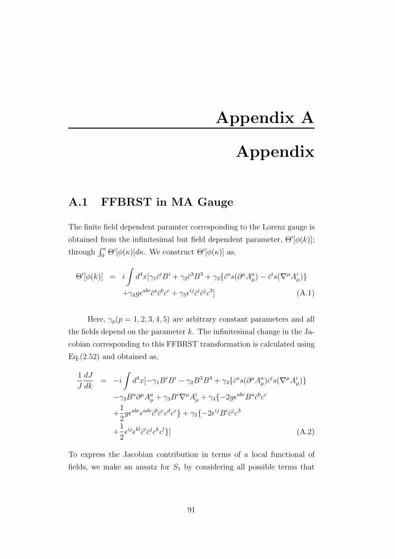
Appendix A
Appendix
A.1 FFBRST in MA Gauge
The finite field dependent paramter corresponding to the Lorenz gauge is
obtained from the infinitesimal but field dependent parameter, Θ′[φ(k)];
through∫ κ
0Θ′[φ(κ)]dκ. We construct Θ′[φ(κ)] as,
Θ′[φ(k)] = i
∫d4x[γ1c
iBi + γ2c3B3 + γ3cas(∂µAaµ)− cis(∇µAiµ)
+γ4gεabccacbcc + γ5ε
ij cicjc3] (A.1)
Here, γp(p = 1, 2, 3, 4, 5) are arbitrary constant parameters and all
the fields depend on the parameter k. The infinitesimal change in the Ja-
cobian corresponding to this FFBRST transformation is calculated using
Eq.(2.52) and obtained as,
1
J
dJ
dk= −i
∫d4x[−γ1B
iBi − γ2B3B3 + γ3cas(∂µAaµ)cis(∇µAiµ)
−γ3Ba∂µAaµ + γ3B
i∇µAiµ + γ4−2gεabcBacbcc
+1
2gεabcεadecbcccdce+ γ5−2εijBicjc3
+1
2εijεklcicjckcl] (A.2)
To express the Jacobian contribution in terms of a local functional of
fields, we make an ansatz for S1 by considering all possible terms that
91
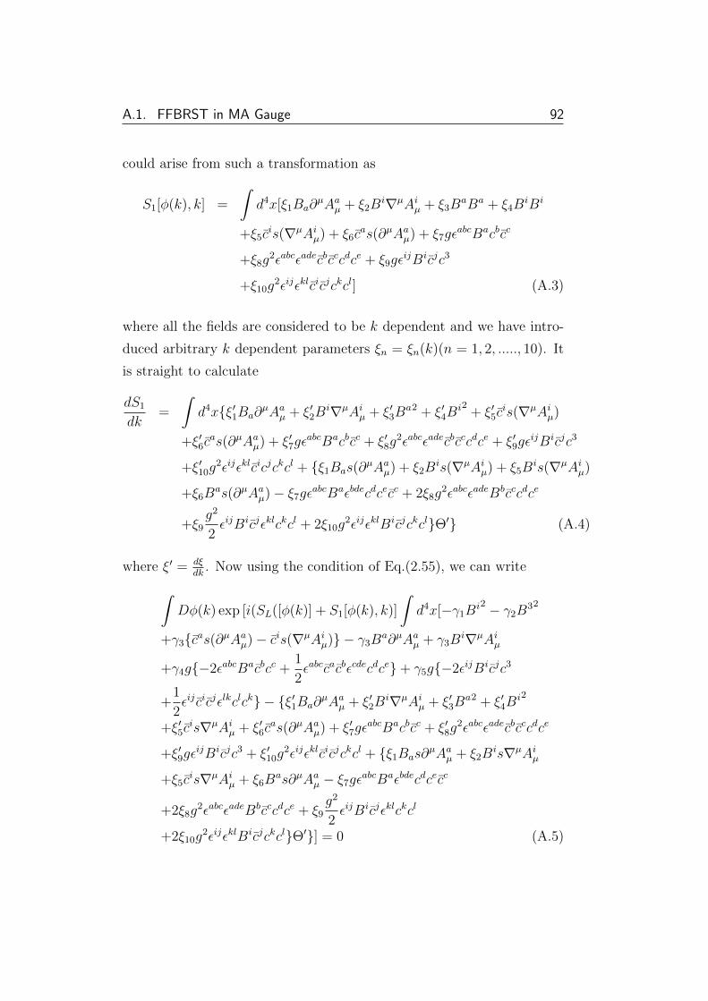
A.1. FFBRST in MA Gauge 92
could arise from such a transformation as
S1[φ(k), k] =
∫d4x[ξ1Ba∂
µAaµ + ξ2Bi∇µAiµ + ξ3B
aBa + ξ4BiBi
+ξ5cis(∇µAiµ) + ξ6c
as(∂µAaµ) + ξ7gεabcBacbcc
+ξ8g2εabcεadecbcccdce + ξ9gε
ijBicjc3
+ξ10g2εijεklcicjckcl] (A.3)
where all the fields are considered to be k dependent and we have intro-
duced arbitrary k dependent parameters ξn = ξn(k)(n = 1, 2, ....., 10). It
is straight to calculate
dS1
dk=
∫d4xξ′1Ba∂
µAaµ + ξ′2Bi∇µAiµ + ξ′3B
a2 + ξ′4Bi2 + ξ′5c
is(∇µAiµ)
+ξ′6cas(∂µAaµ) + ξ′7gε
abcBacbcc + ξ′8g2εabcεadecbcccdce + ξ′9gε
ijBicjc3
+ξ′10g2εijεklcicjckcl + ξ1Bas(∂
µAaµ) + ξ2Bis(∇µAiµ) + ξ5B
is(∇µAiµ)
+ξ6Bas(∂µAaµ)− ξ7gε
abcBaεbdecdcecc + 2ξ8g2εabcεadeBbcccdce
+ξ9g2
2εijBicjεklckcl + 2ξ10g
2εijεklBicjckclΘ′ (A.4)
where ξ′ = dξdk
. Now using the condition of Eq.(2.55), we can write∫Dφ(k) exp [i(SL([φ(k)] + S1[φ(k), k)]
∫d4x[−γ1B
i2 − γ2B32
+γ3cas(∂µAaµ)− cis(∇µAiµ) − γ3Ba∂µAaµ + γ3B
i∇µAiµ
+γ4g−2εabcBacbcc +1
2εabccacbεcdecdce+ γ5g−2εijBicjc3
+1
2εij cicjεlkclck − ξ′1Ba∂
µAaµ + ξ′2Bi∇µAiµ + ξ′3B
a2 + ξ′4Bi2
+ξ′5cis∇µAiµ + ξ′6c
as(∂µAaµ) + ξ′7gεabcBacbcc + ξ′8g
2εabcεadecbcccdce
+ξ′9gεijBicjc3 + ξ′10g
2εijεklcicjckcl + ξ1Bas∂µAaµ + ξ2B
is∇µAiµ
+ξ5cis∇µAiµ + ξ6B
as∂µAaµ − ξ7gεabcBaεbdecdcecc
+2ξ8g2εabcεadeBbcccdce + ξ9
g2
2εijBicjεklckcl
+2ξ10g2εijεklBicjckclΘ′] = 0 (A.5)
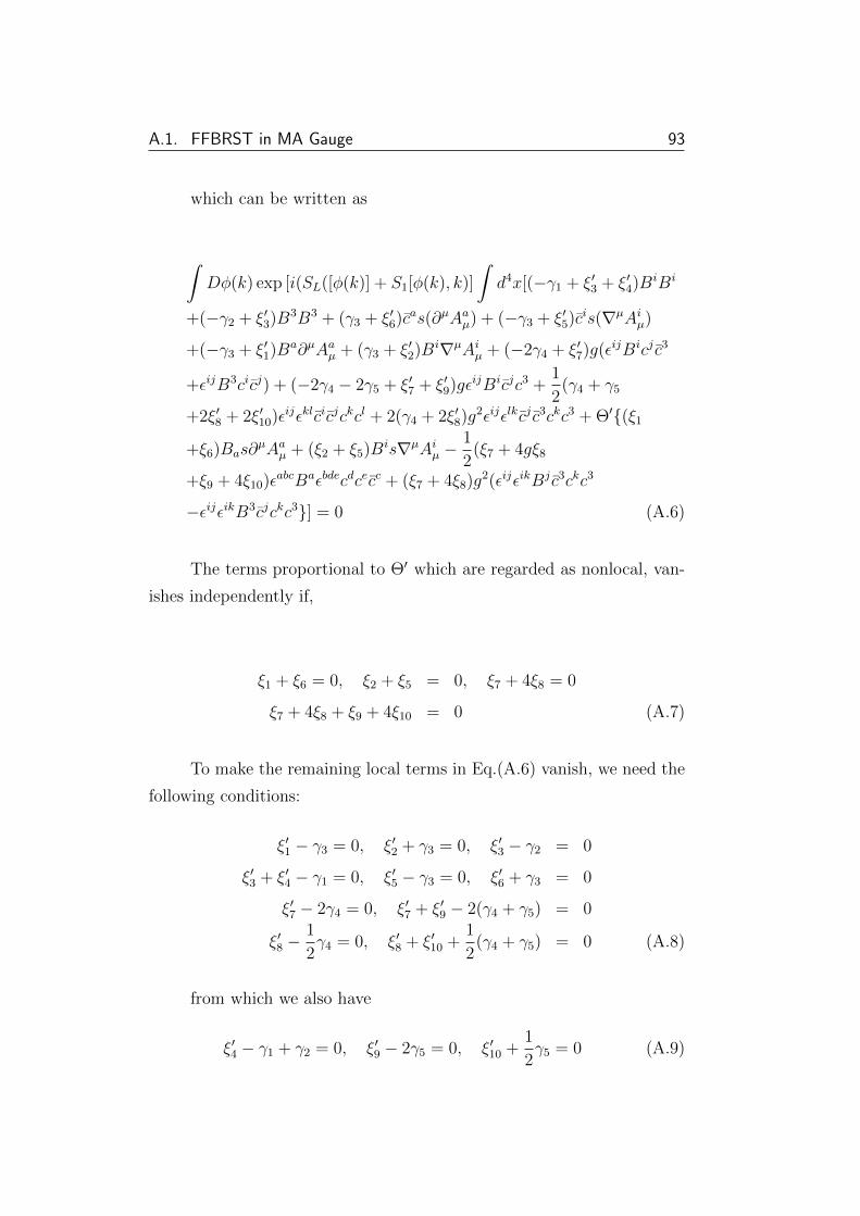
A.1. FFBRST in MA Gauge 93
which can be written as
∫Dφ(k) exp [i(SL([φ(k)] + S1[φ(k), k)]
∫d4x[(−γ1 + ξ′3 + ξ′4)BiBi
+(−γ2 + ξ′3)B3B3 + (γ3 + ξ′6)cas(∂µAaµ) + (−γ3 + ξ′5)cis(∇µAiµ)
+(−γ3 + ξ′1)Ba∂µAaµ + (γ3 + ξ′2)Bi∇µAiµ + (−2γ4 + ξ′7)g(εijBicj c3
+εijB3cicj) + (−2γ4 − 2γ5 + ξ′7 + ξ′9)gεijBicjc3 +1
2(γ4 + γ5
+2ξ′8 + 2ξ′10)εijεklcicjckcl + 2(γ4 + 2ξ′8)g2εijεlkcj c3ckc3 + Θ′(ξ1
+ξ6)Bas∂µAaµ + (ξ2 + ξ5)Bis∇µAiµ −
1
2(ξ7 + 4gξ8
+ξ9 + 4ξ10)εabcBaεbdecdcecc + (ξ7 + 4ξ8)g2(εijεikBj c3ckc3
−εijεikB3cjckc3] = 0 (A.6)
The terms proportional to Θ′ which are regarded as nonlocal, van-
ishes independently if,
ξ1 + ξ6 = 0, ξ2 + ξ5 = 0, ξ7 + 4ξ8 = 0
ξ7 + 4ξ8 + ξ9 + 4ξ10 = 0 (A.7)
To make the remaining local terms in Eq.(A.6) vanish, we need the
following conditions:
ξ′1 − γ3 = 0, ξ′2 + γ3 = 0, ξ′3 − γ2 = 0
ξ′3 + ξ′4 − γ1 = 0, ξ′5 − γ3 = 0, ξ′6 + γ3 = 0
ξ′7 − 2γ4 = 0, ξ′7 + ξ′9 − 2(γ4 + γ5) = 0
ξ′8 −1
2γ4 = 0, ξ′8 + ξ′10 +
1
2(γ4 + γ5) = 0 (A.8)
from which we also have
ξ′4 − γ1 + γ2 = 0, ξ′9 − 2γ5 = 0, ξ′10 +1
2γ5 = 0 (A.9)
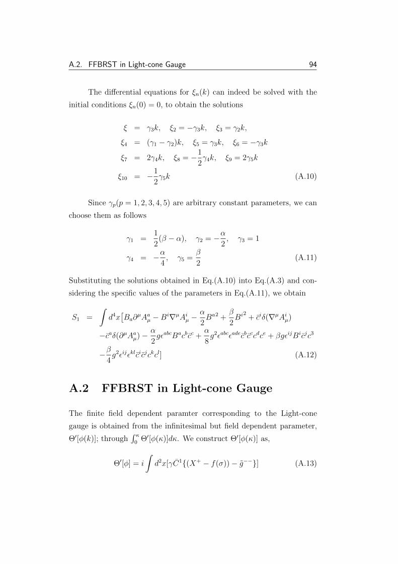
A.2. FFBRST in Light-cone Gauge 94
The differential equations for ξn(k) can indeed be solved with the
initial conditions ξn(0) = 0, to obtain the solutions
ξ = γ3k, ξ2 = −γ3k, ξ3 = γ2k,
ξ4 = (γ1 − γ2)k, ξ5 = γ3k, ξ6 = −γ3k
ξ7 = 2γ4k, ξ8 = −1
2γ4k, ξ9 = 2γ5k
ξ10 = −1
2γ5k (A.10)
Since γp(p = 1, 2, 3, 4, 5) are arbitrary constant parameters, we can
choose them as follows
γ1 =1
2(β − α), γ2 = −α
2, γ3 = 1
γ4 = −α4, γ5 =
β
2(A.11)
Substituting the solutions obtained in Eq.(A.10) into Eq.(A.3) and con-
sidering the specific values of the parameters in Eq.(A.11), we obtain
S1 =
∫d4x[Ba∂
µAaµ −Bi∇µAiµ −α
2Ba2 +
β
2Bi2 + ciδ(∇µAiµ)
−caδ(∂µAaµ)− α
2gεabcBacbcc +
α
8g2εabcεadecbcccdce + βgεijBicjc3
−β4g2εijεklcicjckcl] (A.12)
A.2 FFBRST in Light-cone Gauge
The finite field dependent paramter corresponding to the Light-cone
gauge is obtained from the infinitesimal but field dependent parameter,
Θ′[φ(k)]; through∫ κ
0Θ′[φ(κ)]dκ. We construct Θ′[φ(κ)] as,
Θ′[φ] = i
∫d2x[γC1(X+ − f(σ))− g−−] (A.13)
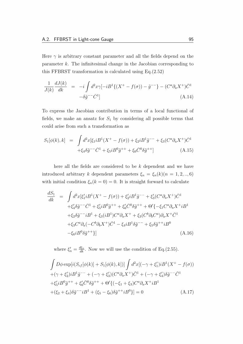
A.2. FFBRST in Light-cone Gauge 95
Here γ is arbitrary constant parameter and all the fields depend on the
parameter k. The infinitesimal change in the Jacobian corresponding to
this FFBRST transformation is calculated using Eq.(2.52)
1
J(k)
dJ(k)
dk= −i
∫d2xγ[−iB1(X+ − f(σ))− g−− − (Ca∂aX
+)C1
−δg−−C1] (A.14)
To express the Jacobian contribution in terms of a local functional of
fields, we make an ansatz for S1 by considering all possible terms that
could arise from such a transformation as
S1[φ(k), k] =
∫d2x[ξ1iB
1(X+ − f(σ)) + ξ2iB1g−− + ξ3(Ca∂aX
+)C1
+ξ4δg−−C1 + ξ5iB
0g++ + ξ6C0δg++] (A.15)
here all the fields are considered to be k dependent and we have
introduced arbitrary k dependent parameters ξn = ξn(k)(n = 1, 2, .., 6)
with initial condition ξn(k = 0) = 0. It is straight forward to calculate
dS1
dk=
∫d2x[ξ′1iB
1(X+ − f(σ)) + ξ′2iB1g−− + ξ′3(Ca∂aX
+)C1
+ξ′4δg−−C1 + ξ′5iB
0g++ + ξ′6C0δg++ + Θ′−ξ1C
a∂aX+iB1
+ξ2δg−−iB1 + ξ3(iB1)Ca∂aX
+ + ξ3(Cb∂bCa)∂aX
+C1
+ξ3Ca∂a(−Cb∂bX
+)C1 − ξ4iB1δg−− + ξ5δg
++iB0
−ξ6iB0δg++] (A.16)
where ξ′n = dξndk
. Now we will use the condition of Eq.(2.55).∫Dφ exp[i(Scf [φ(k)] + S1[φ(k), k])]
∫d2x[(−γ + ξ′1)iB1(X+ − f(σ))
+(γ + ξ′2)iB1g−− + (−γ + ξ′3)(Ca∂aX+)C1 + (−γ + ξ′4)δg−−C1
+ξ′5iB0g++ + ξ′6C
0δg++ + Θ′(−ξ1 + ξ3)Ca∂aX+iB1
+(ξ2 + ξ4)δg−−iB1 + (ξ5 − ξ6)δg++iB0] = 0 (A.17)
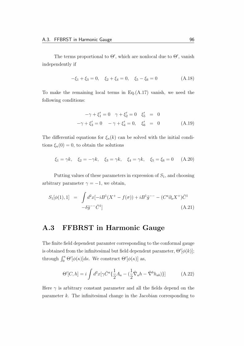
A.3. FFBRST in Harmonic Gauge 96
The terms proportional to Θ′, which are nonlocal due to Θ′, vanish
independently if
−ξ1 + ξ3 = 0, ξ2 + ξ4 = 0, ξ5 − ξ6 = 0 (A.18)
To make the remaining local terms in Eq.(A.17) vanish, we need the
following conditions:
−γ + ξ′1 = 0 γ + ξ′2 = 0 ξ′5 = 0
−γ + ξ′3 = 0 − γ + ξ′4 = 0, ξ′6 = 0 (A.19)
The differential equations for ξn(k) can be solved with the initial condi-
tions ξn(0) = 0, to obtain the solutions
ξ1 = γk, ξ2 = −γk, ξ3 = γk, ξ4 = γk, ξ5 = ξ6 = 0 (A.20)
Putting values of these parameters in expression of S1, and choosing
arbitrary parameter γ = −1, we obtain,
S1[φ(1), 1] =
∫d2x[−iB1(X+ − f(σ)) + iB1g−− − (Ca∂aX
+)C1
−δg−−C1] (A.21)
A.3 FFBRST in Harmonic Gauge
The finite field dependent paramter corresponding to the conformal gauge
is obtained from the infinitesimal but field dependent parameter, Θ′[φ(k)];
through∫ κ
0Θ′[φ(κ)]dκ. We construct Θ′[φ(κ)] as,
Θ′[C, h] = i
∫d2x[γCa1
2Aa − (
1
2∇ah− ∇bhab)] (A.22)
Here γ is arbitrary constant parameter and all the fields depend on the
parameter k. The infinitesimal change in the Jacobian corresponding to
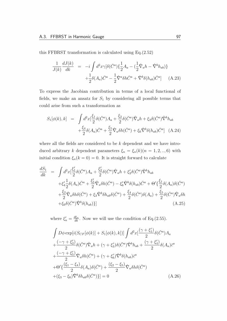
A.3. FFBRST in Harmonic Gauge 97
this FFBRST transformation is calculated using Eq.(2.52)
1
J(k)
dJ(k)
dk= −i
∫d2xγ[δ(Ca)1
2Aa − (
1
2∇ah− ∇bhab)
+1
2δ(Aa)C
a − 1
2∇aδhCa + ∇bδ(hab)C
a] (A.23)
To express the Jacobian contribution in terms of a local functional of
fields, we make an ansatz for S1 by considering all possible terms that
could arise from such a transformation as
S1[φ(k), k] =
∫d2x[
ξ1
2δ(Ca)Aa +
ξ2
2δ(Ca)∇ah+ ξ3δ(C
a)∇bhab
+ξ4
2δ(Aa)C
a +ξ5
2∇aδh(Ca) + ξ6∇bδ(hab)C
a] (A.24)
where all the fields are considered to be k dependent and we have intro-
duced arbitrary k dependent parameters ξn = ξn(k)(n = 1, 2, .., 6) with
initial condition ξn(k = 0) = 0. It is straight forward to calculate
dS1
dk=
∫d2x[
ξ′12δ(Ca)Aa +
ξ′22δ(Ca)∇ah+ ξ′3δ(C
a)∇bhab
+ξ′41
2δ(Aa)C
a +ξ′52∇aδh(Ca)− ξ′6∇bδ(hab)C
a + Θ′ξ1
2δ(Aa)δ(C
a)
+ξ2
2∇aδhδ(C
a) + ξ3∇bδhabδ(Ca) +
ξ4
2δ(Ca)δ(Aa) +
ξ5
2δ(Ca)∇aδh
+ξ6δ(Ca)∇bδ(hab)] (A.25)
where ξ′n = dξndk
. Now we will use the condition of Eq.(2.55).∫Dφ exp[i(SCF [φ(k)] + S1[φ(k), k])]
∫d2x[
(γ + ξ′1)
2δ(Ca)Aa
+(−γ + ξ′2)
2δ(Ca)∇ah+ (γ + ξ′3)δ(Ca)∇bhab +
(γ + ξ′4)
2δ(Aa)c
a
+(−γ + ξ′5)
2∇aδh(Ca) + (γ + ξ′6)∇bδ(hab)c
a
+Θ′(ξ1 − ξ4)
2δ(Aa)δ(C
a) +(ξ2 − ξ5)
2∇aδhδ(C
a)
+(ξ3 − ξ6)∇bδhabδ(Ca)] = 0 (A.26)
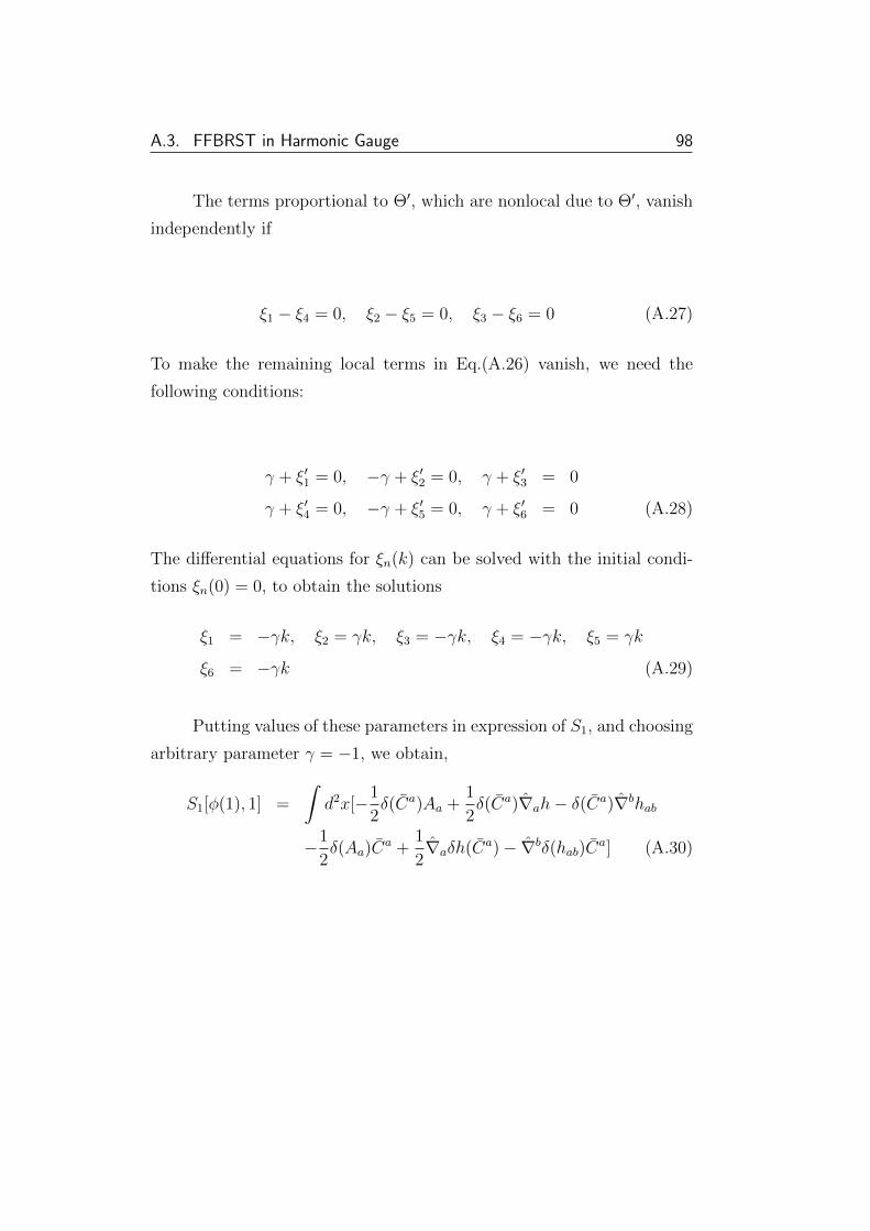
A.3. FFBRST in Harmonic Gauge 98
The terms proportional to Θ′, which are nonlocal due to Θ′, vanish
independently if
ξ1 − ξ4 = 0, ξ2 − ξ5 = 0, ξ3 − ξ6 = 0 (A.27)
To make the remaining local terms in Eq.(A.26) vanish, we need the
following conditions:
γ + ξ′1 = 0, −γ + ξ′2 = 0, γ + ξ′3 = 0
γ + ξ′4 = 0, −γ + ξ′5 = 0, γ + ξ′6 = 0 (A.28)
The differential equations for ξn(k) can be solved with the initial condi-
tions ξn(0) = 0, to obtain the solutions
ξ1 = −γk, ξ2 = γk, ξ3 = −γk, ξ4 = −γk, ξ5 = γk
ξ6 = −γk (A.29)
Putting values of these parameters in expression of S1, and choosing
arbitrary parameter γ = −1, we obtain,
S1[φ(1), 1] =
∫d2x[−1
2δ(Ca)Aa +
1
2δ(Ca)∇ah− δ(Ca)∇bhab
−1
2δ(Aa)C
a +1
2∇aδh(Ca)− ∇bδ(hab)C
a] (A.30)