Holographic Quantum Liquids

Nikolaos Kaplis

Magdalen College

University of Oxford

A thesis submitted for the degree of

Doctor of Philosophy

Trinity 2013

Abstract

In this thesis, applications of Holography in the context of Condensed

Matter Physics and in particular hydrodynamics, will be studied. Holog-

raphy or gauge/gravity duality has been an enormously useful tool in

studying strongly-coupled Field Theories with particular success in their

low-frequency and large-wavelength fluctuation regime, i.e the hydrody-

namical regime. Here, following a phenomenological approach, gravita-

tional systems, simple enough to be properly examined, will be studied in

order to derive as much information as possible about their dual theories,

given that their exact form is not accessible in this way. After a review

of the most important elements of standard Condensed Matter Theory,

the gauge/gravity duality itself will be presented, along with some of its

most important achievements. Having established the framework of this

work, the main results of this thesis will be presented. Initially the sound

channel of the theory dual to the anti-de Sitter Reissner–Nordstrom black

hole space-time will be studied, at finite temperature and finite chemical

potential. Hydrodynamical properties of the boundary theory will be of

major interest. Following that, focus will be shifted towards another grav-

itational system, namely the Electron Star. There, the shear channel of

the dual theory will be mainly examined. The goal will be, as before, to

extract information about the hydrodynamical properties of the boundary

theory.

To my parents.

Γράφω γιὰ κείνους ποὺ δὲν ξέρουν νὰ διαβάσουν

γιὰ τοὺς ἐργάτες ποὺ γυρίζουνε τὸ βράδι μὲ τὰ μάτια κόκκινα ἀπv τὸν ἄμμο

γιὰ σᾶς, χωριάτες, ποὺ ἤπιαμε μαζὶ στὰ χάνια τὶς χειμωνιάτικες νύχτες τοῦ ἀγώνα

ἐνῶ μακριὰ ἀκουγότανε τὸ ντουφεκίδι τῶν συντρόφων μας.

Γράφω νὰ μὲ διαβάζουν αὐτοὶ ποὺ μαζεύουν τὰ χαρτιὰ ἀπv τοὺς δρόμους

καὶ σκορπίζουνε τοὺς σπόρους ὅλων τῶν αὐριανῶν μας τραγουδιῶν

γράφω γιὰ τοὺς καρβουνιάρηδες, γιὰ τοὺς γυρολόγους καὶ τὶς πλύστρες.

Γράφω γιὰ σᾶς

ἀδέρφια μου στὸ θάνατο

συντρόφοι μου στὴν ἐλπίδα

ποὺ σᾶς ἀγάπησα βαθειὰ κι ἀπέραντα

ὅπως ἑνώνεται κανεὶς μὲ μιὰ γυναίκα.

Κι ὅταν πεθάνω καὶ δὲ θἆμαι οὔτε λίγη σκόνη πιὰ μέσα στοὺς δρόμους σας

τὰ βιβλία μου, στέρεα κι ἁπλά

θὰ βρίσκουν πάντοτε μιὰ θέση πάνω στὰ ξύλινα τραπέζια

ἀνάμεσα στὸ ψωμὶ

καὶ τὰ ἐργαλεῖα τοῦ λαοῦ.

Ποιητικὴ, Τάσος Λειβαδίτης

Acknowledgements

I would like to thank my supervisor, Andrei Starinets, for his guidance

and support over the course of my studies. I would also like to thank

my colleagues, Richard Davison and Saso Grozdanov, for a very fruitful

and enjoyable cooperation. Furthermore I would like to acknowledge the

Greek State Scholarship Foundation (IKY), without the financial support

of which I would not have been able to pursuit my degree. Similarly I

would like to thank my college, Magdalen, for their assistance - financial

and otherwise - that made my studies a pleasant and untroubled experi-

ence. Finally I would like to thank my family and friends for their for-

bearance throughout this rather demanding part of my life. Their support

allowed me to overcome the more arduous parts of the last few years.

Contents

1 Introduction 1

2 Elements of Condensed Matter Physics 6

2.1 Hydrodynamics . . . . . . . . . . . . . . . . . . . . . . . . . . . . . . 6

2.2 Quantum Hydrodynamics . . . . . . . . . . . . . . . . . . . . . . . . 17

3 Aspects of Holography 39

3.1 History . . . . . . . . . . . . . . . . . . . . . . . . . . . . . . . . . . . 39

3.2 Background . . . . . . . . . . . . . . . . . . . . . . . . . . . . . . . . 42

3.3 Holographic toolbox . . . . . . . . . . . . . . . . . . . . . . . . . . . 54

3.4 AdS-CMT . . . . . . . . . . . . . . . . . . . . . . . . . . . . . . . . . 63

4 Anti-de Sitter Reissner-Nordstrom 72

4.1 Introduction . . . . . . . . . . . . . . . . . . . . . . . . . . . . . . . . 72

4.2 The RN-AdS4 background and fluctuations . . . . . . . . . . . . . . . 77

4.3 Temperature dependence of the sound mode . . . . . . . . . . . . . . 85

4.4 Further temperature-dependent properties of the theory when q < 1 . 90

4.5 Dispersion relations at fixed temperature T < µ . . . . . . . . . . . . 96

4.6 An effective hydrodynamic scale . . . . . . . . . . . . . . . . . . . . . 102

5 Electron Star 108

5.1 Background . . . . . . . . . . . . . . . . . . . . . . . . . . . . . . . . 109

5.2 Thermo/Hydro-dynamics . . . . . . . . . . . . . . . . . . . . . . . . . 119

5.3 Shear channel . . . . . . . . . . . . . . . . . . . . . . . . . . . . . . . 126

5.4 Sound channel . . . . . . . . . . . . . . . . . . . . . . . . . . . . . . . 147

6 Conclusions and discussion 153

6.1 AdS4 . . . . . . . . . . . . . . . . . . . . . . . . . . . . . . . . . . . . 153

6.2 Electron Star . . . . . . . . . . . . . . . . . . . . . . . . . . . . . . . 155

i

Bibliography 157

ii

List of Figures

2.1 Integration contour in the complex ω plane. . . . . . . . . . . . . . . 20

2.2 Momenta defined relative to the Fermi surfaces. . . . . . . . . . . . . 26

2.3 Feynman diagrams corresponding to Γ4 up to one loop. . . . . . . . . 33

3.1 The relation between the coupling coefficients between the two dual

theories in Krammers-Wannier system. . . . . . . . . . . . . . . . . . 40

3.2 The objects of String Theory. . . . . . . . . . . . . . . . . . . . . . . 42

3.3 The world-sheet of a closed string. . . . . . . . . . . . . . . . . . . . . 42

3.4 Perturbation series of String Theory - sum over topologies. . . . . . . 43

3.5 As ls → 0 the String Theory perturbation series reduces to the standard

Feynman perturbation series. . . . . . . . . . . . . . . . . . . . . . . 43

3.6 Closed string vertex. . . . . . . . . . . . . . . . . . . . . . . . . . . . 44

3.7 Schematic of interactions between strings and branes. . . . . . . . . . 45

3.8 Possible configurations of open string between two branes. . . . . . . 48

3.9 A stack of Nc D3−branes. . . . . . . . . . . . . . . . . . . . . . . . . 49

3.10 Ten-dimensional space-time from the closed-string or gravitational per-

spective for gsNc 1 and Nc 1. There are two distinct regimes -

the near-horizon “throat” and the asymptotic boundary. . . . . . . . 51

3.11 The Holographic parameter space. Figure taken from [1]. . . . . . . . 52

4.1 The sound attenuation Γ in an LFL as a function of temperature,

at fixed ω and µ. A is the collisionless quantum regime, B is the

collisionless thermal regime and C is the hydrodynamic regime. . . . 73

4.2 Variation of the real part of the sound mode as the temperature is

increased. The crosses mark the T = 0 numerical results, the dots

are the numerical results for T > 0, and the solid lines are the µ = 0

analytic result (4.26). . . . . . . . . . . . . . . . . . . . . . . . . . . . 86

iii

4.3 Variation of the imaginary part of the sound mode as the temperature

is increased. The crosses marks the T = 0 numerical results, the dots

are the numerical results for T > 0, and the solid lines are the µ = 0

analytic result (4.26). . . . . . . . . . . . . . . . . . . . . . . . . . . . 87

4.4 Variation of the imaginary part of the sound mode as the temperature

is increased, in the regime T < µ. The dots are the numerical results

for T > 0, and the two dashed lines on each plot denote T/µ = q/µ

and T/µ =√q/µ as one moves to the right along the plot. . . . . . . 88

4.5 A superposition of the plots of the temperature dependence of the nor-

malised imaginary part of the sound mode when q/µ = 0.2 for both

the D3/D7 theory and the RN-AdS4 theory. Crosses denote the D3/D7

numerical results [2] and circles denote the RN-AdS4 results. Moving

from left to right, the dotted lines mark the transition points between

the quantum and thermal collisionless regimes, and the thermal col-

lisionless regime and the hydrodynamic regime, in the D3/D7 theory.

These occur when ω ∼ T and ω ∼ T 2/µ respectively. There are no

results for the D3/D7 sound mode in the hydrodynamic regime since

the hydrodynamic sound mode is suppressed in the probe brane limit.

We refer the reader to [2] for a more detailed discussion of these features. 89

4.6 Variation of the imaginary part of the longitudinal diffusion mode as

the temperature is increased. The dots are the numerical results for

T > 0, and the solid line is the µ = 0 analytic result (4.27). . . . . . . 91

4.7 Movement of the sound and diffusion poles in the complex frequency

plane as the temperature is increased at fixed q = 0.5. . . . . . . . . . 92

4.8 The energy density spectral function for q = 0.5 as the temperature is

increased, in units of 2µ2r0/κ24. The peak due to sound propagation

dominates at all temperatures. . . . . . . . . . . . . . . . . . . . . . . 94

4.9 The charge density spectral function for q = 0.5 as the temperature

is increased, in units of 2r0/κ24. There is a crossover between sound

domination and diffusion domination at high temperature. . . . . . . 95

4.10 The dependence of the crossover value of µ/T upon q/µ. The best fit

straight-line to these results has intercept ≈ 0.003 and gradient ≈ 0.34. 96

iv

4.11 The temperature dependence of the quadratic term Γ in the imaginary

part of the sound dispersion relation (4.4). Circles show our numerical

results, the solid line shows the µ = 0 analytic result (4.26), the ‘+’

shows the T = 0 numerical result of [3] and the ‘×’ shows the prediction

of ‘T = 0 hydrodynamics’. . . . . . . . . . . . . . . . . . . . . . . . . 97

4.12 The dispersion relation of the sound mode at T = 0.0219µ for 0.01 ≤q ≤ 0.5. The circles show the numerical results and the solid line is

the best fit ω ≈ q/√

2− i0.075q2 +O(q3). . . . . . . . . . . . . . . . . 98

4.13 The dispersion relation of the sound mode at two different tempera-

tures: T = 0 (circles) and T = 0.159µ (crosses). The dashed line is the

line Re (ω) = q. . . . . . . . . . . . . . . . . . . . . . . . . . . . . . . 98

4.14 The dispersion relation of the diffusion mode at two different tem-

peratures: T = 0.0219µ (circles) and T = 0.159µ (crosses) with the

polynomial best fit at T = 0.0219µ shown also (solid line). We cannot

track the T = 0.0219µ mode for as high momenta as the T = 0.159µ

mode. . . . . . . . . . . . . . . . . . . . . . . . . . . . . . . . . . . . 99

4.15 The temperature dependence of the quadratic coefficient D in the dis-

persion relation of the diffusion mode (4.5). The circles show the nu-

merical results and the solid line is the analytic µ = 0 result (4.27). . 100

4.16 The dispersion relation of the second stablest propagating mode at two

different temperatures: T = 0 (circles) and T = 0.159µ (crosses). The

dashed line is the line Re (ω) = q. . . . . . . . . . . . . . . . . . . . . 101

4.17 The dispersion relation of the second-stablest purely imaginary mode

at two different temperatures: T = 0.0219µ (circles) and T = 0.159µ

(crosses). . . . . . . . . . . . . . . . . . . . . . . . . . . . . . . . . . . 101

4.18 Movement of the six longest-lived modes in the complex frequency

plane as a function of momentum, for fixed T = 0.159µ. The crosses

denote the sound and diffusion modes, and the circles denote the sec-

ondary propagating and imaginary modes. . . . . . . . . . . . . . . . 103

4.19 The energy density spectral function for T = 0.159µ as the momentum

is increased, in units of 2µ2r0/κ24. As the momentum is increased, the

peak due to sound propagation becomes less dominant. . . . . . . . . 104

4.20 The charge density spectral function for T = 0.159µ as the momentum

is increased, in units of 2r0/κ24. As the momentum is increased, the

peak due to sound propagation becomes less dominant. . . . . . . . . 105

v

4.21 Contour plot showing |Im (ω) |/Re (ω) for the sound mode as a function

of q/µ and q/T and the best fit to these results: a0 = 10.1 and a1 =

8.3. Darker colours correspond to smaller values (i.e. more stable

propagation) and the contours show the values 0.02, 0.04, 0.06, and 0.08.106

5.1 The Electron Star’s development as a function of T/µ. The top curves

correspond to T/µ = 0.00003 and the bottom ones to T/µ = 0.13.

Here m = 0.36, β = 19.951. . . . . . . . . . . . . . . . . . . . . . . . 112

5.2 Dependence of the Electron Star background on the parameters m, β

for T/µ = 0.007. . . . . . . . . . . . . . . . . . . . . . . . . . . . . . . 113

5.3 The surface defined by eq. (5.22). . . . . . . . . . . . . . . . . . . . . 114

5.4 (z, β) section of fig. 5.3, giving the critical exponent as a function of β. 115

5.5 (z, m) section of fig. 5.3, giving the critical exponent as a function of m.116

5.6 The pressure, energy and charge density for z = 3, m = 0.36. In these

coordinates r →∞ corresponds to the IR (Lifshitz). . . . . . . . . . . 118

5.7 Free energy of the Electron Star system for three electron masses m.

The RN result is overlaid for comparison. . . . . . . . . . . . . . . . . 121

5.8 Free energy of the Electron Star system for four critical exponents z.

The RN result is overlaid for comparison. . . . . . . . . . . . . . . . . 122

5.9 The entropy density of the Electron Star for three electron masses (m).

The RN result is overlaid for comparison. . . . . . . . . . . . . . . . . 123

5.10 The entropy density for the Electron Star for four critical exponents

(z). The RN result is overlaid for comparison. . . . . . . . . . . . . . 124

5.11 Verification of the conformality condition (5.48). . . . . . . . . . . . . 125

5.12 ηs

for two critical exponents. The solid line corresponds to the value 14π

. 126

5.13 Diffusion coefficient for three electron masses as well as RN. . . . . . 127

5.14 Diffusion coefficient for four critical exponents as well as RN. . . . . . 128

5.15 QNMs in the complex frequency (ω) plane for kµ

= 0.1 and Tµ'

0.11, 0.09, 0.07, 0.05, 0.03. . . . . . . . . . . . . . . . . . . . . . . . . . 141

5.16 QNMs on the imaginary axis for kµ

= 0.1 and Tµ' 0.11, 0.09, 0.07, 0.05, 0.03.141

5.17 D(T ) for z = 2 and m ∈ 0.1, 0.36, 0.5. . . . . . . . . . . . . . . . . . 142

5.18 D(T ) for m = 0.36 and z ∈ 3, 5, 10, 100. . . . . . . . . . . . . . . . 143

5.19 Fraction of Electron Star charge vs. z and Tµ

. . . . . . . . . . . . . . . 145

5.20 Fraction of Electron Star charge vs. m and Tµ

. . . . . . . . . . . . . . 146

5.21 Dispersion relations. . . . . . . . . . . . . . . . . . . . . . . . . . . . 152

vi

List of Tables

2.1 Shear viscosity values for various fluids at T = 298K [4] . . . . . . . . 11

3.1 Low-energy spectrum of Type-IIB String Theory. . . . . . . . . . . . 44

3.2 The symmetries of the theories on the two sides of the Holographic

duality. . . . . . . . . . . . . . . . . . . . . . . . . . . . . . . . . . . . 53

3.3 Operator-field mapping within the Holographic dictionary. . . . . . . 55

5.1 Dispersion relation for the lowest QNM, for various ES parameters and

temperatures. . . . . . . . . . . . . . . . . . . . . . . . . . . . . . . . 147

vii

Chapter 1

Introduction

Over the past fifteen years an amazing development coming from String Theory, has

created a novel and fast growing sector in the field of Theoretical Physics. This

development is Holography or what was originally named AdS/CFT correspondence

or later gauge/gravity duality [5–8]. Holography has had a twofold effect - on the

one hand it has significantly revitalized String Theory releasing it from the singular

pursuit of a Theory of Everything, posing new problems for investigation and pointing

at new directions to be explored. On the other hand it has proven to be a stupendously

useful computational tool (which also provides unique insights) that can be applied to

a vast variety of problems seemingly unrelated to String Theory. One may call it a tool

instead of an actual physical theory, because it maps physically interesting systems

to artificial (though not necessarily) configurations that fall under the purview of

String Theory, where they can be solved or at the very least be addressed in an

unprecedented and almost always useful way. Though the specifics of Holography

will be developed in a following chapter, it should be noted from this point that this

aspect of Holography, i.e. the practical one, that is going to be explored in this thesis.

Temporarily postponing any technical description, Holography in its very essence

provides a map (and the tools to implement it) between strongly interacting theories

of some kind and weakly coupled ones of a completely different kind. In particular

Quantum Field Theories (QFTs) at strong coupling are mapped to weakly coupled

gravitational theories in higher dimensions. It is hard to over-emphasize the impor-

tance of this statement, given that strongly coupled problems have forever plagued

Theoretical Physics, limiting one to perturbative descriptions of most phenomena.

Holography offers a path around this restriction, since for each intractable problem

it substitutes a solvable one or at least one that can be systematically studied. This

feature was immediately appreciated and from the very early stages Holographic ap-

plications were sought in almost every strongly coupled system of interest. The most

1

noticeable examples of application fields include Heavy Ion Physics (and in particular

the study of Quark Gluon Plasma) [9] and Condensed Matter Physics [10]. The latter

will be the most pertinent to this thesis.

In Condensed Matter Physics one studies systems consisting of large number of

components, or said in a better way, degrees of freedom. Systems like that include

gases, liquids, metals, plasmas as well as more exotic configurations. Despite the long

and successful history of this field there are still a lot of outstanding problems, e.g.

high-temperature superconductivity, strange metals, non-Fermi liquids and others.

The difficulties are primarily focused on developing a deeper understanding of the

mechanisms that lead to the emergence of these phenomena. These difficulties are

attributed, to a great extent, to the strongly-coupled nature of those systems, because

of which standard perturbation theory breaks down and one is left without reliable,

systematic tools to use. The break-through brought about by Holography is what one

could colloquially call “transmutation” of degrees of freedom. That is the realization

that the fundamental degrees of freedom (dof), appropriate to describe a system,

and consequently the appropriate perturbative scheme, in its weak regime are not

necessarily suitable to describe the same system in its strongly-coupled phase. In fact

in going from the former to the latter the dof can change so dramatically that the

resulting system may be difficult to identify with or even relate to the original.

Even after more than a decade of intensive study the single most examined and

better understood system is that of the N = 4 Super Yang-Mills (SYM) non-Abelian

Quantum Field Theory, with SU(Nc) Nc →∞ gauge group at four dimensions (d =

4). This system is dual to a String Theory (Type-IIB) in a particular background,

namely AdS5 × S5. It should be noted at this point that Holography takes its name

from the fact that the dimensionality of the dual theories differ by one, and in fact

one is defined on the boundary of the other, hence the holographic interpretation.

The innovative part is that difficult, i.e. strongly-coupled, problems in the Field

Theory side can be translated into weakly-coupled ones on the String Theory (actually

gravity) side where the perturbative arsenal is still available, solved and then the

solution can be translated back, or at the very least some useful intuition can be

gained.

However, what can a highly super-symmetric, non-Abelian theory at Nc →∞ tell

one about regular Condensed Matter? The first and easy answer is that even though

N = 4 SYM is not a realistic theory, it provides a very well-controlled toy model,

in the strongly-coupled regime, that can be used to extract new insights into how to

address such systems. The most interesting answer though came as people started

2

understanding better the nature and mechanics of the duality, realizing that one

can engineer Holographic duals, i.e. stringy/gravitational, systems (backgrounds),

suitable for the Condensed Matter problem in question, overcoming the limitation

posed by excessive and often exotic symmetries. Thus began what is commonly known

as “bottom-up” approaches to Holography. That is one first decides the essential

ingredients of the boundary theory and then “tailors” the (minimal) appropriate

gravitational dual, respecting of course the Holographic principles, which is then used

to compute interesting and previously inaccessible properties of the boundary theory.

Examples of this method will be examined in this thesis. This approach has become

so wide-spread that it nowadays goes by its own name, that is AdS-CMT [10–18].

Besides being a computational tool, Holography has provided some amazing in-

sights too. One of the most interesting ones is the emergence of universalities in

strongly-coupled systems. By allowing the treatment of system in that regime, in-

accessible by conventional perturbative methods, it has shown that quite distinct

weakly-coupled theories flow, in the RG1 sense, to similar duals on the other end of

the coupling scale. As an illustration it is worth mentioning that most Holographic

models have a common gravitational sector, the Einstein-Hilbert action, that seems to

provide a basic set of characteristics for all these strongly (in fact infinitely) coupled

theories. The emergence of common behaviour is more apparent in a regime where

Holography is particularly powerful - that is hydrodynamics or in other words the

regime of low-frequency and large-wavelength fluctuations. Hydrodynamics emerge

for almost every theory as a low-energy effective theory. Through Holography they

are mapped, to the low-frequency regime of gravity. Exactly because the Holographic

dual is essentially horizon dynamics within classical gravity, for which quite a lot is

known, Holography has had such a remarkable success in hydrodynamics [19].

In particular, the thermodynamic and near-equilibrium properties of such strongly-

coupled field theories can be obtained relatively easily from their dual gravitational

descriptions. Initial studies of these properties concentrated on field theories at non-

zero temperature T (most notablyN = 4 SU(Nc) super-symmetric Yang-Mills theory

with Nc → ∞) and were motivated by experimentally-observed properties of ther-

mal field theories [9]. For perturbations whose frequency ω and momentum q are

much less than T , these field theories were found to obey the laws of hydrodynamics

and their transport coefficients, such as shear viscosity, charge diffusion constant etc.

were calculated (see [20–22] and subsequent work). More recently, there has been

a lot of interest in studying field theories at zero temperature but with a non-zero

1Renormalization Group.

3

density of a conserved global U(1) charge - these are analogues of strongly-coupled

condensed matter systems with a non-zero density of particles (see [10, 18, 23, 24] for

some introductions to the field).

This thesis will be structured as follows. In the chapter following this introduction,

aspects of Condensed Matter Physics will be reviewed. This will familiarize one with

the field into which Holographic applications will be later attempted. This review will

also provide the framework into which any Holographic results concerning Condensed

Matter systems should belong, as well as a baseline against which the novelty and

sensibility of any Holographic result will be measured.

In the next chapter more detailed aspects of Holography itself will be presented.

The technical details that have been avoided in this introduction, to the detriment of

specificity, will be provided. The String Theory/gravity framework in which Holog-

raphy “lives” will also be addressed. Towards the end of this section some celebrated

Holographic results, particularly of hydrodynamic/CM nature, will be reviewed, in

order to demonstrate the power of the Duality.

In the fourth chapter the AdS4−RN system will be studied. This system consists,

on the gravity side, of a Reissner–Nordstrom black hole in a four-dimensional anti-de

Sitter space-time. The properties of the dual theory, i.e. a 2 + 1-dimensional theory,

will be examined. Even though the exact nature of the theory on the boundary is not

known, as this system does not come directly from some UV-complete configuration,

very interesting information can still be extracted. In particular the long-lived modes

of the charge density and energy density correlators will be studied, in the strongly-

coupled, finite density and temperature phase of the theory dual to this gravitational

system.

In the fifth chapter the properties of a different gravitational system, namely the

Electron Star, will be investigated. This system consists of a four-dimensional RN-

AdS background, as before, in which fermions are introduced. More specifically the

fermions are assumed to populate the available states to form a star-like object, i.e.

a system of charged fermions at gravitational equilibrium, that has not however gone

through collapse. In other words the fermionic matter does not introduce a horizon.

For simplicity the fermions2 are assumed to behave like an ideal fermionic liquid.

The total system has therefore two kinds of charge available - that which comes from

behind the horizon and that coming directly from the bulk. The relation between

these two will be of particular interest. The shear channel of this system will be

2In this context the terms fermions and electrons will be used interchangeably.

4

primarily examined while only some preliminary results on the longitudinal one will

be presented.

Finally this thesis will be concluded by a summary of the most important findings

and some discussion regarding the prospects of this work.

5

Chapter 2

Elements of Condensed MatterPhysics

In this chapter, which is of auxiliary nature, a set of fundamental ideas and results

from Condensed Matter Theory, will be reviewed. The purpose of this presentation

is twofold. Firstly it will provide context for some of the most important results

of Holography, which are related to strongly coupled hydrodynamics. Secondly it

will guide one’s physical intuition through the unfamiliar regime of strongly coupled

dynamics and provide the contrast, given that it typically refers to weakly interacting

systems, necessary to appreciate the novelty of Holographic calculations.

The structure of this chapter is the following. In the first section the standard

approach to both ideal and viscous hydrodynamics, will be presented. Following

that the relativistic approach to hydrodynamics will be reviewed, which is the most

relevant in the Holographic context. Next quantum aspects of Hydrodynamics will

be addressed, which formally fall into the purview of finite-temperature and finite-

density Field Theory. Finally the most characteristic example of a quantum liquid in

the context of Condensed Matter Physics (Fermi liquid), will be examined in some

detail. This example will prove to be particularly useful as it will act as the yardstick

against which the Holographic results, can be compared.

2.1 Hydrodynamics

One might wonder why Hydrodynamics are relevant to our discussion. On the face

of it, they seem to describe rather trivial and exhausted systems. However if viewed

as the dynamics of long-wavelength fluctuations of any given system they acquire a

highly universal and modern character [25, 26]. Essentially any theory describing a

physical system (i.e. a Quantum Field Theory) at the limit of long wavelengths and

6

small frequencies admits a hydrodynamic description. This universality is particu-

larly useful in the case of Holography as in many cases the exact microscopic theory

describing the relevant system is not known. Nonetheless the hydrodynamic limit

of such a theory can still be studied and important properties can be revealed. A

spectacular example of this phenomenon is the case of Heavy Ion Collisions and stud-

ies of Quark Gluon Plasma [27]. In that system the specific microscopic dynamics

are extremely difficult to track, given that QCD is still in its strongly-coupled phase.

However one can still study the hydrodynamical properties of the system, which turn

out to be the primary route of access to that regime.

Perfect fluids

Let us start this presentation with the simplest system - that of an ideal fluid. The

current presentation follows very closely the standard textbook [28]. An ideal fluid

is a classical multi-particle system treated as a continuum with the following scale

restriction - the unit volume of this fluid, even if considered infinitesimal around a

point, has to be much larger than the characteristic inter-particle distances or in

other words even infinitesimal fluid volumes must contain a very large number of

constituent particles. Additionally an ideal fluid is characterized by the absence of

heat exchange and dissipation, or equivalently there is no thermal conductivity or

viscosity. Consequently the motion of such fluid is adiabatic, i.e. dsdt

= 0, where s is

the entropy density. In order to describe the dynamics of ideal fluids one uses the

velocity v(t, r), energy density (ρ(t, r)) and pressure p(t, r) fields, which are functions

of space-time, with the aforementioned caveat regarding scales. The dynamics are

governed by the continuity and Euler equations. The continuity equation

∂tρ+ ∇(ρv) = 0 (2.1)

is just a representation of the conservation of matter (i.e the rate of change of the

amount of fluid within some volume is equal to the amount crossing the boundary of

said volume). Defining the flux vector j := ρv this equation can be written as

∂tρ+ ρ∇v + v ·∇ρ = 0 (2.2)

Similarly by considering the force that is exerted on a unit volume due to pressure,

−∮pdS = −

∫dV∇p (where dS is the infinitesimal surface bounding the infinitesi-

mal volume dV ), and essentially writing Newton’s law one gets Euler’s equation

ρdv

dt= −∇p (2.3)

7

Taking into account that the time derivative is a total one, i.e. it contains the implicit

dependence through the fluid’s flow, one arrives at the familiar form

∂tv + (v ·∇)v = −1

ρ∇p (2.4)

Specifying v, ρ,p along with the appropriate boundary conditions, fully determines

the system.

Given that such fluids are adiabatic one can make use of the constancy of entropy

in order to re-write Euler’s equation (2.4) with respect to macroscopic quantities.

Starting from the definition of enthalpy dw = Tds+V dp (where T is the temperature

and V = 1/ρ is the specific volume) which for adiabatic systems becomes dw = V dp,

one gets 1ρ∇p = ∇w. Equation (2.4) therefore becomes

∂tv + (v ·∇)v = −∇w (2.5)

By applying some trivial vector calculus one can recast this in the following form

∂tv − v ×∇× v = −∇(w +1

2v2)⇒ ∂t(∇× v) = ∇× (v ×∇× v) (2.6)

This particular form is special because it only involves the velocity field.

In anticipation of the viscous fluids results, as well as the Holographic results,

let us define the quantities of energy and momentum flux. Starting from the energy

contained in a unit volume 12ρv2 + ρε one has

∂t(1

2ρv2) = −1

2v2∇(ρv)− v ·∇p− ρv · (v ·∇)v (2.7)

for the first term. Using, as before, thermodynamic quantities, this equations becomes

∂t(1

2ρv2) = −1

2v2∇(ρv)− ρv ·∇(

1

2v2 + w) + ρTv ·∇s (2.8)

Moving now to the second term of the energy

∂t(ρε) = w∂tρ+ ρT∂ts = −w∇(ρv)− ρTv ·∇s (2.9)

where the first law of thermodynamics dε = Tds−pdV = Tds+( pρ2 )dρ has been used.

By adding the two terms up and integrating over the relevant volume one immediately

sees that

∂t

∫dV (

1

2ρv2 + ρε) = −

∫dV∇(ρv(

1

2v2 + w))

⇒ ∂t

∫dV (

1

2ρv2 + ρε) = −

∮ρv(

1

2v2 + w) · dS (2.10)

8

It therefore becomes obvious that the quantity ρv(12v2 +w) is the energy flux density

vector, i.e. the energy that flows through a surface that bounds a volume in which

the energy changes in time.

One can repeat the same process with respect to the momentum contained in a

unit volume ρv

∂t(ρvi) = − ∂p∂xi− ∂(ρvivj)

∂xj= −∂Πij

∂xj(2.11)

with the definition of the symmetric tensor Πij = pδij + ρvivj, where both the conti-

nuity (2.1)and Euler’s (2.4) equations have been used. In order to make the physical

content of this tensor clear, one can integrate over a certain volume

∂t

∫dV ρvi = −

∮ΠijdSj (2.12)

where dS is the vector perpendicular to the surface surrounding the integration vol-

ume. It is now obvious that Πij represents the ith component of momentum flowing

through an infinitesimal surface element oriented along the jth direction (encoded

in the normal vector). In the next section it will be seen how this is related to the

stress-energy tensor, which is central in interpreting the Holographic results.

Viscous fluids

Departing from the perfect fluid, towards a more realistic system, viscous fluids will

now be examined, by allowing energy dissipation. Dissipation is tightly related to

thermodynamic irreversibility. Formally this can be treated through the study of

Liouville equation for an N−particle system [29]

∂tfN = H, fN (2.13)

where fN is the N−particle probability function. For statistical systems N → ∞,

hence in order to make the system manageable one would like to reduce the previous

equation down to one for the single-particle probability function, by integrating out

higher-particle contributions

f1 = N

∫ N∏i=2

fi (2.14)

In this way the BBGKY 1 hierarchy of equations emerges

∂tfi = Hi, fi+i∑

j=1

∫∂U

∂xj· ∂fi+1

∂pj(2.15)

1The acronym stands for Bogoliubov, Born, Green, Kirkwood and Yuan

9

where Hi is the effective Hamiltonian

Hn =n∑j=1

(p2i

2m+ V (ri)

)+∑i<j<n

U(ri − rj) (2.16)

for an overall potential V and inter-particle interaction potential U . BBGKY is par-

ticularly convenient as an approximation scheme, provided that reliable assumptions

can be made about the magnitude of the i−th-particle function.

In a more intuitive way one can attribute irreversibility and therefore dissipation,

to internal friction (encoded in the viscosity of the fluid) and thermal conduction.

How does one incorporate this into the fluid dynamics description, without changing

the degrees of freedom (d.o.f.), i.e. the velocity, density, pressure etc. fields? Another

element that one cannot change is the continuity equation, since it is just a mani-

festation of the conservation of mass which should not be altered by the existence of

dissipation. Hence Euler’s equation (2.4) must be modified in such a way that it does

not represent the reversible mechanical interaction of constituent particles. Equipped

with the momentum flux tensor that was previously defined, one can write (2.4) as

∂t(ρvi) = −∂Πij

∂xj(2.17)

and modify Πij so that transfer of energy from high to low velocity regions of the

fluid, is achieved. This can be accomplished by writing

Πij = pδij + ρvivj − σij (2.18)

where σij is the viscous stress tensor which along with pδij form the stress-energy

tensor σij = −pδij + σij. The particular form of the viscous stress tensor is

σij = η

(∂ui∂xj

+∂uj∂xi− 2

3δij∂uk∂xk

)+ ζδij

∂vk∂xk

(2.19)

where η, ζ are constants (know as first order transport coefficients, which however still

depend on temperature and pressure), namely the shear and bulk viscosity. The form

of the viscous stress tensor requires some explanation. As mentioned before one would

like σij to encode transfer of energy from high velocity areas to low velocity ones. It

should therefore depend on spatial derivatives of velocities. Generically σij can be

written as a gradient expansion of velocities and to first order (which is sufficient

for small gradients) it only depends linearly on velocity derivatives. However rigid

rotation of a fluid cannot result in dissipation. It therefore follows that this linear

dependence must not contain the antisymmetric combinations (which correspond to

10

Fluid η(10−3kgm−1s−1)

Water 0.891Ethanol 1.06Mercury 1.55

Sulphuric acid 27

Table 2.1: Shear viscosity values for various fluids at T = 298K [4]

rotations), so that it vanishes when in uniform rotation. Under these conditions (2.19)

is the most general rank-2 tensor that one can write. Having determined the viscous

stress tensor one has fully determined, to first order in the gradient expansion, the

equations of motion for a viscous fluid.

If one assumes, furthermore, that shear and bulk viscosities remain constant

throughout the fluid, Euler’s equation (2.17) becomes

ρ (∂tv + (v ·∇)v) = −∇p+ η4v + (ζ +1

3η)∇∇ · v (2.20)

which is the Navier-Stokes equation. Expecting the results from Holography, it is

worth writing down this equation for the case of incompressible fluids, i.e. ∇ · v = 0

∂tv + (v ·∇)v = −1

ρ∇p+

η

ρ4v (2.21)

In terms of the stress-energy tensor this means that

σij = −pδij + η

(∂vi∂xj

+∂vj∂xi

)(2.22)

Let this section end by presenting a table of typical values for the shear viscosity

for a selection of fluids, as seen in table 2.1. This is particularly interesting since

Holography makes a prediction for a related quantity (namely ηs), and it would be

helpful to develop some intuition.

Sound

A highly interesting property of these systems (i.e. compressible fluids) is that they

can support sound-wave propagation. Such waves correspond to fluctuations of pres-

sure / density. In order to study these fluctuations the pressure and density fields are

written as

p = p0 + δp

ρ = ρ0 + δρ (2.23)

11

where p0, ρ0 are the unperturbed / equilibrium values of pressure and density. The

continuity and Euler’s equations, therefore become

∂tδρ+ ρ0∇v = 0

∂tv +

(1

ρ0

)∇δp = 0 (2.24)

In the previous set of equations the term (v · ∇)v from (2.4) has been dismissed

because of the small-velocity approximation and only fist-order terms have been con-

sistently kept. An extra condition that needs to be satisfied in order for this approx-

imation to be valid is that the velocity of the constituents particles must be much

smaller that the speed of sound (which will henceforth be denoted by c),i.e. v c,

which is equivalent to demanding that the density perturbations are much smaller

than the unperturbed value, i.e. δρ ρ0.

Equations (2.24) can be simplified if one can reliably assume that the process (of

the travelling wave inside the fluid) is adiabatic, as is the case for ideal fluids, because

δp =

(∂p

∂ρ0

)δρ

which makes the first of (2.24)

∂tδp+ ρ0

(p

ρ0

)s

∇v = 0 (2.25)

Although the second of equations (2.24) along with (2.25) fully describe the (adia-

batic) propagation of waves, they do not look like the regular wave equation. This can

be rectified by introducing the velocity potential φ : v = ∇φ so that δp = −ρ0∂tφ.

Hence

∂2t φ− c24φ = 0 (2.26)

with c2 =(∂p∂ρ

)s

the speed of sound. This is the familiar form of the wave equation

(admitting the expected solutions). The individual equations for v, p, ρ can be then

derived from (2.26).

What happens though if one takes into account phenomena of dissipation, due to

viscosity or thermal conductivity? For this purpose it is necessary to compute the

rate of loss of energy E = −(∂E∂S

)S, where S is the entropy. At this point one can

lift the results from thermal conduction in fluids, from which one knows that

S =

∫dV

κ

T 2(∇T )2 +

∫dV

η

2T

(∂vi∂xj

+∂vj∂xi− 2

3δij∂vi∂xi

)2

+

∫dV

ζ

T(∇v)2 (2.27)

12

from which one gets

E = − κT

∫dV (∇T )2 − 1

2η

∫dV

(∂vi∂xj

+∂vj∂xi− 2

3δij∂vi∂xi

)− ζ

∫dV (∇v)2 (2.28)

where κ is the thermal conductivity. For simplicity and without loss of generality one

can choose a particular configuration, namely a wave travelling along the x axis of

the form vx = v0 cos(kx− ωt), vy = vz = 0. Taking the time average one has

〈E〉 = −1

2k2v2

0V0

((4

3η + ζ) + κ(

1

cV− 1

cp)

)(2.29)

where V0 is the volume of the fluid and cV , cp are the heat capacities under constant

volume and pressure respectively. Furthermore the total energy of the sound wave is

〈Et〉 = 12ρv2

0V0. There are enough ingredients now to compute the damping coefficient

v0 ∝ exp[−γx]

γ =〈E〉

2c〈Et〉=

ω2

2ρc3

(4

3η + ζ) + κ

(1

cV− 1

cp

):= αω2 (2.30)

Finally in the presence of damping the wave-vector will become complex and in par-

ticular

k =ω

c+ ıαω2 (2.31)

Relativistic Hydrodynamics

So far the fluid dynamics treatment presented has been non-relativistic. However

most results coming from Holography are of relativistic nature, since they refer to the

hydrodynamic limit of Quantum Field Theories (QFTs). It is worth noting though

that this is not exclusively the case, as a lot of studies have been focused on various

departures from relativistic dynamics. In this section the most noteworthy elements

of relativistic hydrodynamics will be reviewed [30,31].

The first thing that needs to be reconsidered is the degrees of freedom, with which

the fluid dynamics will be described. This is quite obvious since the 3-velocity, scalar

density and 3-vector pressure, are not well-defined objects in a four-dimensional space-

time. The fields appropriate for relativistic hydrodynamics are the 4-velocity uµ and

the energy-momentum tensor Tµν . Another detail to be taken under consideration is

that the mass density ρ, used so far, is not a good degree of freedom since it cannot

account for the kinetic energy, of the system, that can now become comparable to the

mass. In its place one should use the total energy, which will be denote by ε(xµ). As

expected lim vc→0 ε = ρ. It should be noted that although the 4-velocity has apparently

13

four degrees of freedom corresponding to the four components, this is not the case

since there is also a constraint, namely u2 = −1 2

In order to determine the dynamics, one needs first to determine the energy-

momentum tensor form. Starting from the case of ideal fluids3, one notices that

the energy-momentum tensor has to be built out of ε, p, uµ and the metric tensor

gµν . Tµν must also be a symmetric rank - 2 tensor (i.e. have a well-defined Lorentz

transformation). The most general such tensor can be written as

T µν(0) = ε (αgµν + βuµuν) + p (γgµν + δuµuν) (2.32)

In the fluid’s rest frame T 00(0) should reduce to the total energy ε. Additionally in

the rest frame T 0i(0) = 0, ∀i ∈ 1, 2, 3 and T ij(0) = pδij, i, j ∈ 1, 2, 3. Applying these

constraints on the general form of the energy-momentum tensor one gets the following

system of equations

(α + β)ε+ (γ + δ)p = ε

−αε− γp = p

which result in α = 0, β = 1, γ = −1, δ = 1, or

T µν(0) = εuµuν − p(gµν − uµuν) (2.33)

The form of the energy-momentum tensor suggests the definition of the projection

tensor ∆µν = gµν − uµuν which projects on the space orthogonal to the fluid velocity

uµ. It is obvious that ∆µνuµ = ∆µνuν = 0 and ∆ρν = ∆µρ. Using the projection

tensor the energy-momentum tensors can be written as

T µν(0) = εuµuν − p∆µν (2.34)

In the absence of external sources, conservation of the energy-momentum tensor reads

∂µTµν(0) = 0 (2.35)

which encodes the equations of motion for the fluid dynamics. One can use the

projection tensor to split these equations into directions parallel (i.e. uν∂µTµν(0)) and

perpendicular (i.e. ∆σν∂µT

µν(0)) to the fluid velocity. One therefore has

uν∂µTµν(0) = uµ∂µε+ε(∂µu

µ)+εuνuµ∂µu

ν−puν∂µ∆µν = (ε+p)∂µuµ+uµ∂µε = 0 (2.36)

2There is a sign ambiguity in this expression, which depends on the metric signature used.3When ideal fluids are considered, this will be denoted by a 0 index

14

and

∆σν∂µT

µν(0) = εuµ∆σ

ν∂µuν −∆µσ(∂µp) + puµ∆σ

ν∂µuν = (ε+ p)uµ∂µu

σ −∆µσ∂µp = 0

(2.37)

Introducing, for conciseness, the operators D := uµ∂µ and ∇σ := ∆µσ∂µ, one can

rewrite the equations of motion in a compact form

Dε+ (ε+ p)∂µuµ = 0 (2.38)

(ε+ p)Duσ −∇σp = 0 (2.39)

One can now make a connection to the non-relativistic case by taking the small

velocity limit |v|c→ 0

D = uµ∂µ → ∂t + v ·∇ +O(v2) (2.40)

∇i = ∆iµ∂µ → ∂i +O(v) (2.41)

In other words D and ∇i reduce to the time and space derivatives, respectively. If one

further demands that the energy is primarily that corresponding to the mass density,

i.e. ε ' ρ and that p ε (in the appropriate units), one retrieves the non-relativistic

continuity and Euler’s equations.

So far only ideal relativistic fluids have been considered. Introducing dissipation

effects, as is the case when one does not neglect viscosity, the energy-momentum

tensor has to be modified, in the same spirit as in the non-relativistic case

T µν = T µν(0) + Πµν (2.42)

where T µν(0) is the previously defined energy-momentum tensor for ideal fluids, while

Πµν is the viscous stress tensor. The equations of motion get modified to

uν∂µTµν = Dε+ (ε+ p)∂νu

µ + uν∂µΠµν = 0 (2.43)

∆σν∂µT

µν = (ε+ p)Duσ −∇σp+ ∆σν∂µΠµν = 0 (2.44)

Note now that uν∂µΠµν = ∂µ(uνΠµν)− Πµν∂(µuν) (where parentheses around indices

imply symmetrization) and ∂µ = uµD + ∇µ. Putting all this together one gets the

final version of the equations of motion

Dε+ (ε+ p)∂µuµ − Πµν∇(µ)uν) = 0 (2.45)

(ε+ p)Duσ −∇σp+ ∆σν∂µΠµν = 0 (2.46)

15

It is necessary at this point to emphasize that the viscous stress tensor still needs to be

determined. One way of achieving that is to assume local thermodynamic equilibrium

in which case the local version of the Second Law of Thermodynamics is ∂µsµ ≥ 0,

where sµ is the entropy 4-current, which in local equilibrium is sµ = suµ. Using the

basic thermodynamic relations (in the absence of conserved charges)

ε+ p = Ts

Tds = dε

the divergence of the entropy current becomes

∂µsµ = Ds+ s∂µu

µ =1

TDε+

ε+ p

T∂µu

µ =1

TΠµν∇(µuν) ≥ 0 (2.47)

Conventionally one writes Πµν = πµν +∆µνΠ, which is a splitting into a traceless part

and the remainder. It is also convenient to define the traceless part of ∇(µuν)

∇〈µuν〉 := 2∇(µ)uν) −2

3∆µν∇σu

σ (2.48)

The entropy current divergence is hence rewritten as

∂µsµ =

1

2Tπµν∇〈µuν〉 +

1

TΠ∇σu

σ ≥ 0 (2.49)

This is satisfied if πµν = η∇〈µuν〉 and Π = ζ∇σuσ, with η ≥ 0 and ζ ≥ 0. In the

non-relativistic limit η and ζ reduce to the shear and bulk viscosity, respectively.

There is an interesting caveat in the presentation so far. That is, the fluids

considered have been uncharged, or more precisely there have been no conserved

charges. This is important because the existence of conserved charges implies the

existence of a charge current Jµ, which can be used to define the fluid velocity. This

allows one to consider two different frames choices. In one of them (Landau) one

defines the local rest frame as the frame where energy density is at rest, while in the

other (Eckart) the local rest frame is identified with the frame in which the charge

density is at rest. This choice is a redundancy of the description and physical content

should not depend on it. The result of this freedom of choice is that what is interpreted

as charge diffusion in one frame is thermal conduction in the other.

Having cleared this intricacy, the relativistic hydrodynamics of charged fluids will

now be presented [32]. In addition to the conservation of energy-momentum tensor

∂µTµν = 0, one now has the conservation of current density ∂µJ

µ = 0. Moreover the

constitutive equations are

T µν = (ε+ p)uµuν + pgµν + Πµν (2.50)

Jµ = ρuµ + νµ (2.51)

16

where ε is the local energy density, p the local pressure density, Πµν the dissipative

part of the energy-momentum tensor and νµ the dissipative part of the charge current.

The choice one can make at this point is uµΠµν = uµνµ = 0. As before one can derive

the form of the dissipative parts, from the Second Law. The thermodynamic relations

for a charged fluid are

ε+ p = Ts+ µρ (2.52)

dε = Tds+ µdρ (2.53)

where µ is the chemical potential. One can now compute the divergence of the entropy

current, using in addition the fact that uν∂µTµν = 0

∂µ(sµ) =µ

T∂µν

µ − Πµν

T∂µuν ⇒

∂µ

(suµ − µ

Tνµ)

= −νµ∂µµ

T− Πµν

T∂µν

µ (2.54)

Defining the left-hand side of (2.54) as the entropy current, one has to demand that

the right-hand side is positive. Hence it follows that

νµ = −κ(∂µµ

T+ uµuν∂ν

µ

T

)(2.55)

Πµν = −η (∂µuν + ∂νuµ + uµuσ∂σuν + uνuσ∂σu

µ)−(ζ − 2

3η

)(gµν + uµuν)∂σu

σ

(2.56)

where η, ζ are the shear and bulk viscosity respectively and κ is the thermal conduc-

tivity.

2.2 Quantum Hydrodynamics

One of the most celebrated achievements of Holography is the ability to describe

strongly interacting systems, away but very close to equilibrium. For weakly inter-

acting systems this is the purview of Linear Response. In this section Linear Response

of a generic quantum system will be presented, so as to lay the foundation and set

the context for the Holographic results. This will also serve as an introduction to the

presentation of purely quantum systems (with no classical analogue) such as Fermi

liquids, which are of high interest from a Holographic point of view.

Linear Response treats a system under an external stimulus, like an electromag-

netic field, a temperature or pressure fluctuation. In the framework of Quantum

Mechanics the dynamics of a system are encoded in its Hamiltonian, H. Similarly an

17

observable is mapped into an operator, say O. The goal is to study the system under

some perturbation. Such a perturbation is described by the addition of a term in the

Hamiltonian

H → H + Hpert

where

Hpert := φO

The coefficient field corresponding to an observable O is referred to as the source of

said observable and plays the role of the external stimulus. The introduction of Hpert

deforms the original theory, modifying the equations of motion, in which one now

finds the field φ in addition to the original degrees of freedom.

Generically this problem is difficult to address, hence the first step is to assume

that the response of the system under the external perturbation, remains linear. In

other words the change in the expectation value of an operator (corresponding to an

observable) is a linear function of the external source4

δ〈O(t)〉 =

∫dt′χ(t, t′)φ(t′) (2.57)

This is the case for sources that are small in comparison with the relative scales.

The function χ(t, t′) is called the response function. It is obvious from the above

definitions that the response function is nothing more than the Green’s function, of

the system and the terms will be henceforth used interchangeably. If the system is

endowed with space-time symmetries, like time reversal (and similarly translational

invariance) one can simplify things significantly by writing the linear response relation

(2.57) in Fourier space

δ〈O(ω)〉 =

∫dt′dteıωtχ(t− t′)φ(t′) = χ(ω)φ(ω) (2.58)

where χ(ω) and φ(ω) are the Fourier transformations of the response function and

the source respectively. Moreover the product is to be understood as the convolution

of the two functions. The simplification in working in Fourier space, lies in the fact

that what is a bi-local function (χ(t − t′)) in coordinate space is a local function in

frequency space (χ(ω)).

Writing it in frequency space, allows one to easily uncover further properties of

the response function. Note first that since O correspond to an observable, it has to

be Hermitian as an operator and hence its expectation value has to be real. Assuming

4Here the Heisenberg picture is adopted, in which time dependence is included in the operators.

18

that the external source is also real one concludes that the response function is real

in coordinate space (χ(t, t′) ∈ R). In Fourier space though χ(ω) ∈ C, with its real

(<χ(ω)) and imaginary (=χ(ω)) parts having distinct interpretations. The imaginary

part can be written

=χ(ω) ≡ − ı2

(χ(ω)− χ(ω)) = − ı2

∫dtχ(t)

(eıωt − e−ıωt

)(2.59)

= − ı2

∫dteıωt (χ(t)− χ(−t)) (2.60)

Similarly for the real part

<χ(ω) ≡ 1

2(χ(ω) + χ(ω)) =

1

2

∫dteıωt (χ(t) + χ(−t)) (2.61)

It becomes clear from the above expressions that the imaginary part of the response

function is not symmetric under time reversal, while the real part is. Given that on

a microscopic level, dynamics are assumed to be time reversible, the imaginary part

must originate from dissipative effects. =χ is therefore called the dissipative part of

the response function and is also referred to as the spectral function.

Another interesting aspect of the response function is its detailed relation to the

Green’s function. In real-time Quantum dynamics (as opposed to Euclidean time)

there are more than one Green’s functions (i.e. retarded (GR), advanced (GA), Feyn-

man (GF )). By demanding causality, i.e. no response prior to the appearance of the

external source, assuming that at t = 0 the source is turned on, one has χ(t < 0) = 0.

This relates the response function to the retarded Green’s function. Borrowing from

the analytic properties of Green’s functions one can translate this requirement into

a requirement about the analytic structure of χ(ω) for complex frequencies (ω ∈ C).

For t < 0 the Fourier integral

χ(t) =

∫dω

2πe−ıωtχ(ω)

has to follow a contour that closes in the upper complex plane (Fig.2.1). In order for

χ to vanish, it is therefore required that it has no poles for =ω > 0. The requirement

that χ(ω) is analytic in the upper ω-plane induces a relation between its real and

imaginary part, known as the Krammers-Kronig relation. In particular by making

use of the Principal Value one can write the Krammers-Kronig relations

<χ(ω) = P∫dω′

π

=χ(ω′)

ω′ − ω(2.62)

=χ(ω) = −P∫dω′

π

<χ(ω′)

ω′ − ω(2.63)

19

RΩ

IΩ

C

Figure 2.1: Integration contour in the complex ω plane.

At this point two comments are in order. Firstly these relations are derived purely

from causality, without any extra assumption and details about the dynamics. How-

ever the cost for such a broad result is that one needs the full analytic structure of

the imaginary part of the response function in order to reconstruct the real part and

vice versa. A rephrasing of this result is that one can write the full response func-

tion, knowing only its imaginary or dissipative part. To see this one needs to write

the principal value as a deformation of the integration contour. In particular if one

defines g(ω) := (1/ıπ)∫dω′χ(ω)/(ω′ − ω), then

P∫dω′

χ(ω)

ω′ − ω:=

ıπ

2(g(ω + ıε) + g(ω − ıε)) (2.64)

By Cauchy’s theorem one also has that χ(ω) = (1/2) (g(ω + ıε)− g(ω − ıε)) and

hence one writes∫dω′

ıπ

=χ(ω′)

ω′ − ω − ıε= =χ(ω) + P

∫dω′

ıπ

=χ(ω′)

ω′ − ω − ıε= =χ(ω)− ı<χ(ω) (2.65)

which then leads to

χ(ω) =

∫dω′

π

=χ(ω′)

ω′ − ω − ıε(2.66)

It is then apparent that the imaginary (or dissipative) part of the response function

(i.e. the spectral function) contains the full information about the system studied

and this is why it will play a very important role in what follows. This fact also

highlights the importance of being able to compute the spectral function of strongly

interacting systems by Holographic means.

20

A quantity that can immediately be computed from the response function is sus-

ceptibility (χ). For an external source φ corresponding to the observable O, causing

a change of the expectation value δ〈O〉 susceptibility is

χ :=∂δ〈O〉∂φ

∣∣∣∣ω=0

(2.67)

which by the definition of the response function means that

χ = limω→0

χ(ω) (2.68)

or in integral form

χ =

∫dω′

π

=χ(ω′)

ω′ − ıε(2.69)

It is appropriate at this point to make an aside to established a connection with

what was presented before, with respect to classical hydrodynamics. To achieve this

a simple dissipative hydrodynamics model will be examined, in which one adds a

diffusive current on top of an ideal fluid, along with and external driving force

J = −D∇ρ+ f (2.70)

where D is the diffusion constant and f is the driving force. From the continuity

equation (2.1) one has

∂tρ−D∇2ρ = −∇ · f (2.71)

Treating f as the external source here, the observables would be the density ρ and

the current J and it is the response to these that one wants to study. Using (2.57)

one writes

ρ(t, x) =

∫dt′dx′χρJ(t′, x′; t′x)f(t′, x′) (2.72)

J(t, x) =

∫dt′dx′χJJ(t′, x′; t′x)f(t′, x′) (2.73)

where the indices in the response function appear now because there are two correlated

responses to the external source. Hence there is a current-density response, i.e. the

external source drives the current which in turn perturbs the density, and a current-

current response, i.e. the immediate response of the current to the external force.

Assuming full space-time translational symmetry and Fourier transforming, as before,

the responses become

ρ(ω, k) = χρJ(ω, k)f(ω, k) (2.74)

J(ω, k) = χJJ(ω, k)f(ω, k) (2.75)

21

Plugging into (2.71) the Fourier transformations for ρ, J and the linear response

relations (2.74,2.75) the density-current response function is

χρJ =−ık

ıω −Dk2(2.76)

Then from the definition of the current J one also gets the current-current response

function

χJJ =ıω

ıω −Dk2(2.77)

From (2.76,2.77) it is obvious that both response functions have a pole at ω = −ıDk2.

This is the well-known diffusion pole that governs the diffusive behaviour of the sys-

tem. This pole will re-appear in the Holographic context demonstrating the persis-

tence of hydrodynamics even in strongly interacting systems.

One of the last pieces necessary to have a relatively complete picture of hydrody-

namics and linear response on the quantum level, is the celebrated Kubo formulae.

These are relations, derived in the context of quantum statistical mechanics, which

relate the response of a system under perturbation, to the two-point function of the

relevant observable. In order to arrive at the Kubo formula, one needs to do first-order

perturbation of a quantum system, described by a density matrix ρ.5 As before the

perturbation is encoded in the Hamiltonian, through Hpert := φiOj, where the index

indicates that there can be more than one sources, for more than one observables. 6

Following standard perturbation theory one defines the time evolution operator

U(t, t′) = T exp

(−ı∫ t

t′dt′Hpert

)(2.78)

which satisfies Schrodinger’s equation

ı∂tU = HpertU (2.79)

and governs the time evolution of the wave-functions

|ψ(t)〉 = U(t, t0)|ψ(t0)〉 (2.80)

Similarly the density matrix evolves as

ρ(t) = U(t, t0)ρ0U−1(t, t0) (2.81)

5Not to be confused with the energy density for which this symbol has been used previously.6Here Einstein’s index summation convention is adopted.

22

where ρ0 is the density matrix at a distant enough time (t0 → −∞) that the pertur-

bation has died off. One is in position now to compute the expectation value of an

operator, for a non-vanishing external source φ

〈O(t)〉|φ ≡ Trρ(t)O(t) = Trρ0U−1OU (2.82)

= Trρ0

(O + ı

∫ t

−∞dt′ [Hpert, O] + . . .

)= 〈O〉|φ=0 + ı

∫ t

−∞dt′〈[Hpert, O]〉+ . . .

(2.83)

The change in the expectation value δ〈O〉 := 〈O〉φ − 〈O〉φ=0 can be written, taking

into account the explicit form of the perturbation, as

δ〈O〉 = ı

∫ t

−∞dt′〈[O(t′), O(t)]〉φ(t′) (2.84)

or in order to make the integration interval symmetric, one can introduce a step

function, resulting in

δ〈O〉 = ı

∫ +∞

−∞dt′θ(t− t′)〈[O(t′), O(t)]〉φ(t′) (2.85)

A simple comparison of the last equation with (2.57) reveals that the response function

is

χ(t− t′) = −ıθ(t− t′)〈[O(t), O(t′)]〉 (2.86)

which is the well-known Kubo formula. From this point it is straightforward to gen-

eralize to Quantum Field Theory, which is more relevant to Holography, by allowing

the operators as well as the response function to depend in space in addition to time.

The Kubo formula becomes then

χij(t′,x′; t,x) = −ıθ(t− t′)〈[Oi(t,x), Oj(t

′,x′)]〉 (2.87)

where the indices account for multiple operators.

The usefulness of Kubo’s formula is most easily demonstrated by straightforwardly

calculating two quantities that come up almost constantly in Holographic calculations,

and which sparked interest in using Holography as a computational tool. The first

quantity is conductivity. Assume a system that possesses a global U(1) symmetry.

For this symmetry there is a corresponding conserved current Jµ. This current plays

the role of the operator in the previous discussion. The external source is the elec-

tromagnetic field Aµ and the perturbation Hamiltonian reads

Hpert =

∫ddxAµJ

µ (2.88)

23

where d is the number of spatial dimensions. By restricting the electromagnetic field

to a purely electric one, the (electrical) conductivity is defined as the response function

relative to the electric field

〈Ji(ω,k)〉 = σij(ω,k)Ej(ω,k) (2.89)

Applying Kubo’s formula for this perturbation gives

δ〈Jµ〉 ≡ 〈Jµ〉 − 〈Jµ〉0 = −ı∫d4x′〈[Jµ(x′), Jν(x)]〉0Aµ(x′) (2.90)

Now by working in a gauge where A0 = 0, the U(1) field in Fourier space is just

Ei(ω) = ıωAi(ω) and hence the change in the current’s expectation value can be put

into the Ohm’s law form (2.89) by setting the conductivity tensor to be

σij =α

ıωδij +

χij(ω,k)

ıω(2.91)

The second term in the above sum, which is the relevant one for this discussion, comes

directly from the current-current Green’s function

χij(ω,k) = −ı∫d4xθ(t)eıkx〈[Ji(x), Jj(0)]〉 (2.92)

It should be noted here that the first term in (2.91) derives from the background,

〈Ji〉0 = e2Aiρ, where ρ, allowing for some abuse of the notation, is the charge density.

Hence α = −eρ in (2.91).

The second, even more celebrated in the Holographic context, quantity that can

be computed using Kubo’s formula, is the shear viscosity. In this case the operator

involved is the energy-momentum tensor Tµν and the response function has a tensor

structure because of the different configurations possible. For this example a situa-

tion where momentum injected in x1 direction gets diffused into x2, is picked. This

scenario involves the T12 components of the energy-momentum tensor. The relevant

components of the response function are therefore

χ12,12(ω,k) = −ı∫d4xθ(t)eıkx〈[T12(x), T12(0)]〉 (2.93)

Compared to the case of conductivity there is no background contribution, since in

the unperturbed state there is no net momentum diffusion. Finally to get the actual

viscosity one needs to apply the zero frequency limit

η = limω→0

1

ıωχ12,12(ω, 0) (2.94)

given that viscosity is related to constant external force (source).

24

Fermi Liquids

In this final section of the present chapter the theory of Fermi liquids will be re-

viewed [33–37]. Fermi liquids are quintessentially quantum mechanical in nature,

and as it will soon become apparent, possess characteristics that survive into the

strongly interacting regime, making them a very interesting test-bed for Holographic

calculations. In particular the systematic Holographic reconstruction of one of their

most important feature, i.e. the existence of a Fermi surface, is a constant goal

of Holographic models. The starting point will be the standard phenomenological

approach, followed by a quick microscopical justification. Towards the end of this

section, the Renormalization Group analysis of Fermi surfaces, will be presented as

the background necessary to justify the discussion of Fermi surfaces in the context of

strongly interacting theories and Holography.

The term Fermi Liquid is used to generically describe a multi-particle state of

fermions at non-vanishing density. One of the most striking characteristics of Fermi

liquids is that, even in the non-zero interaction regime, they retain properties of

the free Fermion gas system. Free multi-particle fermion states are organized based

on Pauli’s exclusion principle, into shells, resulting in the Fermi surface, defined

as the last occupied shell. It should be noted that this surface lives in momentum

space. Low-energy excitations around this ground states involve quasi-particles, which

resemble particles, above and holes below the Fermi surface. Examples of Fermi

liquids include He4 and the electron gas of metals.

The free action of a spin-1/2 fermion ψs(k), of spin s and momentum k (in d

spatial dimensions) is

Sfree =

∫dτ

∫ddk

(2π)dψ†s(k) (∂τ + ε(k))ψs(k) (2.95)

The corresponding Green’s function is therefore

G0(ωn, k) =1

−ıωn + ε(k)(2.96)

Analytically continuing to real frequencies, reveals that (2.96) has a simple pole at

energy E = ε(k) with residue 1. This pole corresponds to quasi-particle excitations,

which can have either positive (particle-like) or negative (hole-like) energies. The

locus of points in the phase space where the energy flips sign, is exactly the Fermi

surface, i.e. it is the surface that divides particle-like from hole-like excitations. 7

7It should be noted here that the appearance of negative energies should not be interpreted asthe emergence of an instability. This is just a result of artificially combining particles and holes inthe same propagator, through identifying hole-like excitations with the negative-energy counterpartof the particle-like ones.

25

In studying further the quasi-particle excitations it is important to take into ac-

count the complications imposed by the fact that these do not occur in some empty,

uniform space, but rather around the Fermi surface. This means that there could be

excitations travelling tangentially to the Fermi surface, with ε(k) = 0. In order to

accommodate for this particularity, it is convenient assign kF (n) to the actual Fermi

surface and then define momenta with respect to that as

k = kF (n) + k⊥n (2.97)

where n is the unit vector perpendicular to the Fermi surface, pointing outwards

kÞ

kÞ

kÞ

kÞ

kF

Figure 2.2: Momenta defined relative to the Fermi surfaces.

(n := kF|kF |

) (Fig.2.2). Now any momenta expansion is considered around the Fermi

surface, i.e. with respect to k⊥. One can now rescale the original fermion fields as

ψs(k)→ 1

VFψs,n(k⊥) (2.98)

where VF is the area of the Fermi surface. Another, more intuitive, way of under-

standing this reformulation is that because motion tangentially to the Fermi surface

corresponds to ε(k) = 0, one needs to expand around every point of the surface.

Taking this into account the effective action becomes

SFL =

∫dΩn

∫dk⊥ψ

†s,n(k⊥) (∂τ − ıvF (n∂k⊥))ψs,n(k⊥) (2.99)

where vF is the Fermi velocity which corresponds to the energy gradient on the Fermi

surface, i.e. vF (n) = |∇kεkF |. Intuitively this effective action describes the Fermi

26

surface as an infinite collection of (one for each point of the surface) fermions, moving

in a transverse to the surface direction. The effective action (2.99), does not take

into account excitations moving along the surface. To address this issue one can work

with fermions living in the full d-dimensional space, instead of just on the surface.

Then one splits the coordinates into k⊥ which is perpendicular to the Fermi surface

and k// normal to the k⊥ direction. With that in mind the effective action can be

recast in the form

S =

∫dτ

∫dk⊥

∫dk//ψ

†s

(∂τ − ıvF∂k⊥ −

κ

2∇2//

)ψs (2.100)

where κ encodes the curvature of the Fermi surface. The benefit of using this action

now becomes apparent, as one can immediately extract the dispersion relation

vFk⊥ + κk2//

2= 0 (2.101)

Having given a very brief, definitional overview of Fermi liquids, one can now

approach them from a more phenomenological (statistical) point of view. Temporarily

ignoring interactions, the energy of a system consisting of N free fermions (i.e. a free

Fermi gas) is

E =∑k

k2

2mn(k) (2.102)

where n(k = 2θ(kF − |k|) is the occupation number for a state of momentum k. If

one applies an external stimulus on the system the energy will get shifted implicitly,

through the change in the occupation number

δE =∑k

=k2

2mδn(k) (2.103)

To the extent that the external field applied remains small, the occupation number

will be a distribution concentrated around the Fermi surface.

The next step is to allow for inter-particle interactions. A critical point in doing so,

is that interactions need to be turned on adiabatically, so that one retains a one-to-one

correspondence between the free and interacting states. In other words one does not

want bound states created as one introduces interactions, which would drastically

change the true degrees of freedom. As a results the picture of Fermi surface and

particle or hole-like excitations around it, coming from the free system, remains valid.

Since interactions are now present, apart from the quasi-particle’s energy ε(k) (while

ε0(k) will be the unperturbed energy) there is also the interaction energy, denoted

by f(k, k′), where k, k′ are the momenta of the quasi-particles involved. Applying a

27

weak external field on the interacting system, the induced change of energy for the

system is

δE =∑k

ε0(k)δn(k) +1

2V

∑k,k′

f(k,k′)δn(k)δn(k′) (2.104)

where V is the volume occupied by the system. From (2.104) one can now compute

the “dressed” (i.e. the perturbed) energy of each quasi-particle

ε(k) =δE

δn(k)= ε0(k) +

1

V

∑k′

f(k,k′)δn(k′) (2.105)

while the interaction energy is given by

f(k,k′) = Vδ2E

δn(k)δn(k′)(2.106)

Here one can make use, again, of the adiabaticity to note that interacting quasi-

particles, stemming from fermions, will obey Fermi-Dirac statistics and hence the

occupation number is

n(k) =1

eε(k)T−µ + 1

(2.107)

where µ is the system’s chemical potential.

With this description at hand one can calculate various observable / phenomeno-

logical properties of Fermi liquids, which will be very useful to compare with Holo-

graphic results, testing whether the latter constitute or not true Fermi liquids. One

such quantity of particular interest is specific heat. By definition

cV =1

V

∂E

∂T

∣∣∣∣V

(2.108)

The change of temperature affects the energy indirectly through the change of the

occupation number, hence

cV =1

V

∑k

∂E

∂n(k)

∂n(k)

∂T(2.109)

which by using (2.104) becomes

cV =1

V

∑k

ε(k)∂n(k)

∂ε(k)

(µ− ε(k)

T+∂(ε(k)− µ)

∂T

)(2.110)

At this point one needs to notice that at low temperatures (β →∞) the interaction

part of (2.104) goes like β−2 or T 2 which means that it can be ignored compared to

28

ε0(k) and therefore one can just use the latter. An immediate result of this approxi-

mation is that the sum over momenta can be substituted by a sum over energies. At

low temperatures, the sum can then be computed giving

cV =1

3m∗kFkBT (2.111)

where kB is the Boltzmann constant and m∗ the effective mass. The effective mass

comes as the modification of the dispersion relation, by the self energy and can be

extracted from

ε0(k) = µ+ (k − kF )kFm∗

(2.112)

m∗ =kFvF

(2.113)

where vF = ∂ε0(k)∂k

. The linear temperature dependence of the specific heat is one of

the most commonly used tests, in Holography, to verify whether the system studied

is dominated by fermions.

Another interesting quantity is the speed of sound, also referred to as first sound to

contrast it with zero-sound which will be presented momentarily. The thermodynamic

speed of sound is defined as

c21 =

1

m

∂P

∂ρ=

1

mρχ(2.114)

where m is the bare fermion mass, ρ = NV

the density and χ the compressibility which

is defined as

χ−1 = −V ∂P∂V

= ρ∂P

∂ρ(2.115)

In order to relate the speed of sound to the, by now familiar, interaction function

f(k,k′), one needs to first employ the Free Energy to write the compressibility in

term of the chemical potential, which is then related to the energy on the Fermi

surface. Then using (2.104) one write c1 in terms of f(k,k′) and more specifically

in terms of spatial averages of the first two multi-pole components of the interaction

function, known as Landau parameters. In particular, one starts from the pressure

P = −∂F∂V

= f − ρ ∂f

∂ρ(2.116)

where F is the Free Energy and f = F/V the Free Energy per unity volume. Hence

χ−1 = ρ2 ∂2f

∂ρ2(2.117)

29

By definition of the chemical potential

µ =∂F

∂N=∂f

∂ρ(2.118)

and therefore χ−1 = ρ2 ∂µ∂ρ

. Then noting that µ = ε(kF , n) one can use (2.104) to write

∂µ

∂ρ=∂ε0(kF )

∂kF

∂kF∂ρ

+∑∫

d3k′

(2π)3f(kF ,k

′)∂n(k′)

∂kF

∂kF∂ρ

(2.119)

The remaining sum in the previous expression is over the spin degrees of freedom.

Employing the following properties of Fermi liquids

ρ =k3F

3π2(2.120)

∂ε0∂kF

=kFm∗

(2.121)

∂n(k′)

∂kF= δ(k′ − kF ) (2.122)

(2.119) can be rewritten as

ρ∂µ

∂ρ= ρ

kF∂ρ

(kFm∗

+k2F

(2π)3

∑∫dΩf

)=

k2F

3m∗(1 + F0) (2.123)

Here F0 is just the spherically symmetric average of the interaction function, or in

other words the first term in its multi-pole expansion. By borrowing the expression

for the effective mass from [34] in terms of Landau parameters one writes

χ−1 =ρk2

F

m

1 + F0

3 + F1

(2.124)

where F1 is the next term in the multi-pole expansion of f . Consequently

c21 =

k2F

m2

1 + F0

3 + F1

(2.125)

First, or regular thermodynamic, sound dies off as T → 0. In particular for a

sound wave of frequency ν its life-time goes like τ ∼ (ε − εF )−2 and its energy like

(ε(k) − εF ) ∼ kBT and therefore in order to have sound, temperature has to be

T 2 ν. Intuitively in the T 2 ν limit, inter-particle collisions cease to exists and

liquid perturbations cannot propagate. However in this collision-less regime another

collective mode emerges out of the Boltzmann equation. In particular, Boltzmann’s

equation is

∂tn+ ∂rn∂kε− ∂kn∂rε = I(n) (2.126)

30

where I(n) encodes quasi-particle collisions. Hence one can look for propagating

solution to (2.126) in its collision-less regime, where I(n) = 0. Since one looks for

wave-like solutions, one writes

δn(k, r, t) = exp[ı(q · r − ωt)]φk (2.127)

and then the linearised version of Boltzmann’s equations becomes

(q · vk − ω)φk + q · vkδ(µ− ε(k))1

V

∑k′

f(k,k′)φk′ = 0 (2.128)

where vk = k/m∗. Rescaling the solution like

φk := δ(ε(k)− µ)vFu(k) (2.129)

so that u(k) measure the displacement of the Fermi surface, one gets

(q · vk − ω)u(k) + q · vk1

V

∑k′

f(k,k′)δ(εk′ − µ)u(k′) = 0 (2.130)

Since the momentum is restricted on the Fermi surface, the remaining dependence is

on the angles (θ, φ =: Ω) defining the direction of k and of course spin. Writing all

the parameters of (2.128) in terms of the Fermi momentum kF , one eventually gets

(s− cos θ)u(Ω, s) = cos θ∑s′

∫d3k′

(2π)3δ(kFm∗

(k − kF ))f(k, k′; s, s′)u(Ω, s′) (2.131)

where s = ωqvF

.

From the discussion so far it has become abundantly clear that the key object

in the Fermi liquid description is the interaction function f(k,k′). It is therefore

important to see how it is related to the microscopic degrees of freedom of the theory.

In this part of the section, it will be presented how this can be achieved. In fact it will

be shown that f(k,k′) is related to a particular limit of the four-point Green’s function

(or to be more precise the vertex function, i.e. the sum of the one-particle irreducible

amputated Feynman diagrams). In order to keep the discussion concise and given

that the details of these calculations are not the purpose of this section, elements

of finite-temperature perturbation theory will be borrowed from standard textbooks

treatments [34–36]. For purposes of simplicity of the notation the convention of [34]

will be adopted, so that all the degrees of freedom associated with a particle will be

encoded in a number representing said particle (e.g. x1, s1, . . . → 1).

The first object needed is the two-point Green’s function (or propagator)

G(1, 2) = −ı〈ψ0|Tψ(1), ψ†(2)

|ψ0〉 (2.132)

31

where |ψ0〉 is the ground state and T . . . represents the time-ordered product. In

momentum space the propagator can be written

G2(p) =1

ω − p2

2m− Σ(ω,p)

(2.133)

where Σ(ω,p) is the standard self-energy. Rewriting this around the Fermi surface

one gets

G2(p) =a

ω − εF − vF (p− kF ) + ıζsgn(ω − εF )(2.134)

where a = (1− ∂εΣ)−1 is the residue of the quasi-particle pole, εF the Fermi energy,

vF = kF/m∗ and ζ just a positive infinitesimal constant.

The next object one needs, is the four-point Green’s function

G4(1, 2; 3, 4) = 〈ψ0|Tψ(1)ψ(2)ψ†(3)ψ†(4)

|ψ0〉 (2.135)

which following standard perturbation procedures is split into disconnected and 1PI

parts

G4(1, 2; 3, 4) = G2(1, 3)G2(2, 4)−G2(1, 4)G2(2, 3)

+ ı

∫d1′d2′d3′d4′G2(1, 1′)G2(2, 2′)G2(3, 3′)G2(4, 4′)Γ4(1′, 2′; 3′, 4′)

(2.136)

or in momentum space

G4(p1,p2;p3,p4) = (2π)8G2(p1)G2(p2) (δ(p1 − p3)δ(p2 − p4)− δ(p1 − p4)δ(p2 − p3))

+ ı(2π)4G2(p1)G2(p2)G2(p3)G2(p4)δ(p1 + p2 − p3 − p4)Γ4(p1,p2;p3,p4)(2.137)

The analytic structure of Γ4 is then of prime interest, since its poles correspond to

different states of the system. In particular the specific time ordering determines this

state. Since here the Fermi liquids dynamics are of interest, the relevant ordering is

ψ(1)ψ(3)†ψ(2)ψ(4)†, which in turn means that poles should be found in the ω(3)−ω(1)

channel, i.e. the particle-hole channel. In order to remain within the regime of

validity of Fermi liquid description both energy and momentum should remain small

and close to the Fermi surface. It is then convenient to write p3 = p1 + k and

p4 = p2 − k, where k = (ω,k) is a small four-vector. Putting all these together one

can now write down the Feynman diagrams involved in computing Γ4. In Fig.2.3

the first two orders of perturbation series are presented. Given that the momentum

with respect to which the poles should be studied is k, it is convenient to write

Γ(p1, p2; k) = Γ4(p1, p2; p3, p4).

32

p1 + k

p2 − k

p1

p2

(a)

p1 + p2 − q

qp1 + k

p2 − k

p1

p2

(b)

p1 − p2 + k + q

qp1 + k

p2

p1

p2 − k

(c)

k + q q

p1 + k

p2

p1

p2 − k

(d)

Figure 2.3: Feynman diagrams corresponding to Γ4 up to one loop.

Out of the one-loop graphs in Fig.2.3 the first two behave nicely in the limit

k → 0, so one can just set k = 0 for them. On the other hand in the last graph as

k → 0 the two propagators G2(q) and G2(k + q) come together, making the graph

apparently divergent. Defining Γ(p1, p2) := Γ(p1, p2; k = 0) as the finite part of the

vertex function one can write the integral equation that governs Γ4

Γ4(p1, p2; k) = Γ(p1, p2)− ı∫

d4q

(2π)4Γ(p1, q)G2(q)G2(q + k)Γ4(q, p2; k) (2.138)

Now one uses expression (2.134) to explicitly write the product of the two propagators

as

G2(q)G2(q + k) =a

ε− εF − vF (q − kF ) + ıζsgn(ε− εF )

· a

ω + ε− εF − vF ((k + q)− kF ) + ıζsgn(ω + ε− εF )(2.139)

The regime of interest is the Hydrodynamic one, meaning long wavelengths and small

frequencies, i.e. k → 0 and ω → 0. In this limit one can split the product of the

propagators into divergent and regular part

G2(q)G2(q + k) =k→0

Res(θ)δ(ε− εF )δ(q − kF ) +Reg(q) (2.140)

33

where Reg(q) is the regular part and Res(θ) is the residue (θ = cos−1( q·k|k||q|)). Fol-

lowing standard procedures the residue can be computed by carefully taking the

integration over the complex plane, resulting in

Res(θ) =k→0

2ıa2k cos θ

ω − vFk cos θ(2.141)

making the product of propagators

G2(q)G2(q + k) =k→0

2ıa2q · kω − vF cos θ

δ(ε− εF )δ(q − kF ) +Reg(q) (2.142)

where the following identity has been used: k cos θ = q · k. Putting all the pieces

together the four-point function (to first order) becomes

Γ4(p1, p2; k) = Γ(p1, p2)− ı∫

d4q

(2π)4Γ(p1, θ)Reg(q)Γ4(q, p2; k)

+a2kF(2π)3

∫dΩΓ(p1, q)

q · kω − vF q · k

Γ4(q, p2; k) (2.143)

where d4q = q2dqdεdΩ and dΩ is the solid angle. At this point one encounters a

crucial detail - the way the Hydrodynamic limit is taken. In other words the two

limits involved, i.e. k → 0 and ω → 0 are not commuting. For the present purposes

the one that will be used is limω→0 limk→0. 8 Consequently

limω→0

limk→0

(q · k

ω − vF q · k

)= 0 (2.144)

and the vertex function, which in this limit will be denoted as Γω becomes

Γω(p1, p2) = Γ(p1, p2)− ı∫

d4q

(2π)4Γ(p1, q)Reg(q)Γω(q, p2) (2.145)

and eliminating Reg(q)

Γ4(p1, p2; k) = Γω(p1, p2) +a2k2

F

(2π)3

∫dΩΓω(p, q)

q · kω − vF q · k

Γ4(q, p2; k) (2.146)

Now all the components are in place to take the Hydrodynamic limit

Γ4(p1, p2; k) =k→0

a2k2F

(2π)3

∫dΩΓω(p1, q)

q · kω − vF q · k

Γ4(q, p2; k) (2.147)

where the fact that energy and momentum is very close to the Fermi values, i.e. p1 =

(εF , kF p1) and p2 = (εF , kF p2), where p1 and p2 are unit vectors and limk→0 Γω = 0,

8The other limit, i.e. limk→0 limω→0, results in a Γ4 that corresponds to physical forward scat-tering of quasi-particles off the the Fermi surface, while the limit used in the text, corresponds tovirtual excitations.

34

has been used. In the last equation the only real variable is p1 and hence is can be

manipulated into a familiar form so that the connection with the interaction function

f(k, k′) can be made. Namely one writes it as(ω

kvF− cos θ

)u(p) = cos θ

m∗kF2π2

∫dΩ

4πa2Γω(p, q)u(q) (2.148)

where

u(q) =q · k

ω − vF q · kΓ4(q) (2.149)

Comparing the last equation with (2.131) one immediately sees that the sought after

relation between f(k, k′) and the vertex function is

f(p, q) = a2Γω(p, q) (2.150)

The significance of this result needs to be stressed, since it relates a phenomenologi-

cally introduced function that encodes the interaction energy between quasi-particles,

with a microscopic quantity, the vertex function, that is well grounded on Quantum

Field Theory and can be perturbatively calculated in a systematic way. It is also

important to explicitly state the physical content of this statement. It describes the

scattering of a particle-hole pair from one point of the Fermi surface to another.

To conclude this presentation of Fermi liquids, the resilience of their description by

Landau’s theory and of the presence of a Fermi surface, will be reviewed. Landau’s

theory is in essence an effective theory and as such it can be examined using the

standard toolbox of effective field theories. Here [33, 37] will be followed. What will

be shown is that interaction terms of this theory, can be effectively integrated out

resulting in a theory with almost no relevant or marginal operators.

The starting point will be the non-interacting action encountered before∫dtd3p

ıψs(p)

†∂tψs(p)− (ε(p)− εF )ψs(p)†ψs(p)

(2.151)

with the ground state corresponding to the Fermi sea, with filled states for ε < εF and

empty ones for ε > εF . In order to make the presence of the Fermi surface explicit

one writes, as done previously, the momentum as p = k + l, where k is vector on the

Fermi surface and l is orthogonal to it. The single-particle energy therefore becomes

ε(p)− εF = lvF +O(l2).

In order to study the effects of adding interactions to this theory, one does what

is usually done with effective theories, that is write down all the terms allowed by

the symmetries of the system and study their scaling behaviour. Assuming that an

35

effective theory is studied at a scale Λ the interaction terms at this scale can be

written as a series of operators

SΛ =

∫ddx

∑i

giOi (2.152)

with the i-th term scaling as∫ddxOi ∼ Eδi−d or written in terms of a dimensionless

parameter λi (E/Λ)δi−d. If δi > d, Oi is irrelevant, i.e. it becomes less important

as energy becomes lower (E → 0). If δi < d, Oi is relevant, i.e. it becomes more

important as energy becomes lower. If δi = d, Oi is marginal and it is equally

important at all energy scales. Marginal operators can turn relevant or irrelevant

depending or higher interaction terms. This is determined by the beta-function

E∂Eg = bg2 +O(g3) (2.153)

If b > 0 then the corresponding operator is marginally irrelevant, while if b < 0 it is

marginally relevant. In the case where b = 0 for all higher orders then the operator

is truly marginal.

The symmetries of this theory include number of particle and space-time sym-

metries, which for the case of realistic scenarios break down to lattice symmetries.

Additionally in the non-relativistic limit (c→∞), where spin and rotational symme-

tries get decoupled, one gets an additional SU(2) internal spin symmetry.

If energies get rescaled as E → λE, where λ < 1, then k → k, l→ λl, dt→ λ−1dt,

dk → dk, dl → λdl and ∂t → λ∂t. The action then scales as λ× (scaling of ψ†ψ),

which means the ψ ∼ λ−1/2. The scaling of possible interaction terms will now be

examined. A quadratic term∫dtd2kdlµ(k)ψs(p)

†ψs(p) ∼ λ−1 (2.154)

This looks like a mass term and it is relevant but it can be absorbed into the definition

of ε(p). Next a quartic term will be examined∫dtd2k1dl1d

2k2dl2d2k3dl3d

2k4dl4V (k1, k2, k3, k4)

ψs(p1)†ψs(p3)ψs′(p2)†ψs′(p4)δ(3)(p1 + p+ 2− p3 − p4) ∼ λ1 × λδ (2.155)

where λδ is the scaling of the delta-function. If one naively assumes that the scaling

of the delta-function goes like λ0 because

δ(3)(p1 +p2−p3−p4) = δ(3)(k1 +k2−k3−k4 + l1 + l2− l3− l4) ' δ(3)(k1 +k2−k3−k4)

(2.156)

36

since l scales to 0, then the overall scaling of the quartic operator is λ1, which makes

it irrelevant. It therefore seems that quadratic and quartic terms are irrelevant indi-

cating that at low energies the theory becomes “freer” - almost like a free electron

gas.

However there are two caveats that require further examination. The first one

involves phonon interactions, while the second one stems from the delta-function

scaling. Starting from the phonon interactions, one notices that the presence of a

crystal lattice breaks space-time symmetries giving rise to Goldstone bosons. This

bosons must be included in the low-energy theory and therefore one introduces a

phonon field D(r) which is proportional the displacement of the ions from their

equilibrium position times their mass (M1/2). The kinetic plus restoring force part of

the action describing the phonon field is

1

2

∫dtd3q

(∂tDi(q)∂tDi(−q)−M−1∆ij(q)Di(q)Dj(−q)

)(2.157)

The scaling of the phonon field can be determined by the free action and then used

to derive the scaling of the phonon-fermion interaction term. In particular close

to the Fermi surface the particles’ momenta scale as q ∼ λ0 while the integration

variables and the derivatives of the kinetic term contribute another λ1. Overall then

the phonon field’s scaling is λ−1/2. If one now examines the first of possible phonon-

particle interaction terms∫dtd3qd2l1dl1d

2l2dl2M−1/2gi(q,k1,k2)Di(q)ψs(p1)†ψs(p2)δ(3)(p1−p2− q) (2.158)

scales as λ−1/2 assuming that one treats the delta-function as before, i.e. scaling as

λ0. That makes the term relevant. However the term gets suppressed by a factor

of (m/M)1/4. Note here that below the Debye energy (m/M)1/2E0, where E0 is the

characteristic energy scale, the restoring force is larger than the kinetic term and it is

therefore what should be used to determine the scaling of D. In that case D ∼ λ1/2

and similarly (2.158)∼ λ1/2, making the interaction term irrelevant below E1.

Finally one needs to address the issue of the scaling of the delta-function. So far

it has been assumed that it scales as λ0. This is a valid assumption when particles

scattered with generic initial momenta. Assume that two particles of momenta p1

and p2 scatter into p3 and p4. One can then write

p3 = p1 + δk3 + δl3 (2.159)

p4 = p2 + δk4 + δl4 (2.160)

37

and the corresponding delta-function becomes δ(d)(δk3 + δk4 + δl3 + δl4). Recall that,

as before, l− momenta are perpendicular to the Fermi surface and k−momenta tan-

gential. Now for generic momenta, δki are linearly independent, hence the argument

of the delta-function is dominated by those and neglecting the δli parts is reasonable,

leading to the scaling λ0. However in the special case where the initial momenta add

up to zero, i.e. p1 = −p2, then δ(d)(δk3 + δk4) becomes degenerate and one needs

to take into account the perpendicular momenta li. This leads to a λ−1 scaling for

the delta-function which in turn makes the quartic interaction term scale as λ0, i.e.

marginal. The rest of the interaction terms remain irrelevant. As for the phonon-

particle interactions one can integrate out the phonons leading back to the quartic

interaction term. The effect of the presence of a marginal operator is that the one-

loop (and higher) correction to a diagram involving external momenta, restricted to

sum up to zero, is not suppressed and need to be explicitly calculated and taken into

account. These corrections can be summed up into a geometric series and their effect

is a modification of the expectation values of currents, compared to the free case.

38

Chapter 3

Aspects of Holography

Following the review of some fundamental aspects of Condensed Matter, a detour will

be attempted in order to provide an overview of Holography itself. In this chapter

some of its most important elements will be presented, starting from its origins in

String Theory and ending at its application to strongly coupled Condensed Matter

systems. The structure of this chapter is the following. Firstly a brief history of

Holography and strong-weak dualities will be presented. Then the practical tools

of Holography (which is usually refereed to as the Holographic dictionary) will be

reviewed. Finally those tools, will be used in practical applications and contact with

Condensed Matter Theory will be attempted.

3.1 History

Holography can be considered as the most successful and most influential example

of a strong-weak duality. It is highly interesting to note though that it is neither

the only nor the first one. As early as the forties it was noticed that in the context

of Lattice Field Theory one encounters such dualities. In particular Krammers and

Wannier [38,39] noticed that for d = 2 Ising model on a square lattice, with nearest-

neighbour interactions, where the partition function is

Z[J ] =∑s=±1

exp

J∑〈ij〉

sisj

(3.1)

one can do the following transformation J → J∗ = −12

ln tanh J resulting in the

transformed partition function Z[J ]→ Z[J ] = C(J)Z∗[J∗] or explicitly

Z[J ] =1

2(cosh J sinh J)N

∑s∗=±1

exp

J∗∑〈ij〉

s∗i s∗j

(3.2)

39

where N is number of sites of the lattice. It is then obvious that in the starred

coordinates one gets an identical (self-dual) system with a new coupling constant

J∗. What gives rise to the strong-weak duality, is the relation between the two

coupling constants J and J∗. As shown in fig. 3.1 when the system in its strongly-

coupled regime in the starred coordinates, it is in its weak regime in the un-starred

coordinates and vice-versa. It should be noted here, that the emergence of a self-dual

Weak coupling in J coordinates

Weak coupling in J* coordinates

0.0 0.5 1.0 1.5 2.0

0.0

0.5

1.0

1.5

2.0

J

J*

Figure 3.1: The relation between the coupling coefficients between the two dual theories inKrammers-Wannier system.

system under this transformation is specific to the d = 2 case. In higher dimensions

the system is not necessarily self-dual. This system contains a phase transition at JC

such that sinh2 2JC = 1 [40]. It is important to note that the simplicity of this model

is predicated on the symmetry group (which for the d = 2 Ising model is Z2) being

Abelian. If this is not the case the treatment is much more involved and leads to what

is referred to as Tannaka-Krein duality [41]. Further information on this subject can

be found in the excellent review of R.Savit [42].

Another such system, that develops strong-weak duality is the Sin-Gordon model

[43]. The standard action is

SSG =

∫d2x

1

2∂µφ∂

µφ+α

β2(cos βφ− 1)

(3.3)

In this theory there are two types of excitations: meson (Mmes =√α) and solitons

(Msol = 8√α

β2 ). The perturbative regime of this theory is β2 1 where Msol Mmes,

40

where β2 is the relevant coupling constant. It turns out that this model is dual

(through bosonization) to the Thirring model, described by the action

ST =

∫d2x

ψıγµ∂

µψ +mψψ − g

2ψγµψψγµψ

(3.4)

The excitations of this theory consist of fundamental fermions (dual to solitons in

the Sin-Gordon model) and fermion-anti-fermion bound states (dual to meson in the

Sin-Gordon model). The duality relates the coupling constants of the two models as

β2

4π=

1

1 + gπ

(3.5)

which makes it clear that when on side of the duality pair is at its weakly-coupled

regime, then the other is at its strongly-coupled regime and vice-versa. It should be

noted here that in this case the dual degrees of freedom are fundamental quanta on

the on side and solitons on the other, while Noether charges are interchanged with

topological charges.

Strong-weak dualities are not restricted to low-dimensional models. There are nu-

merous higher-dimensional cases, which however are usually super-symmetric. Such

examples include the Montonen-Olive duality [44] as well as the Seiberg-Witten du-

ality [45].

Having established that weak-strong dualities are not a rare and exotic phe-

nomenon but rather abundant one can now turn two Holography. As it will be

argued momentarily Holography is based on a similar duality but involving gravita-

tional degrees of freedom. What is even more striking is that the dual degrees of

freedom are not gravitational. There are many reviews on this subject, of which a

few are used and cited here [8, 46–52].

The historic context within which Holography emerged was that of attempting to

describe in a microscopic way (within String Theory most commonly), Black Holes

and their thermodynamic properties in particular (e.g. see [53]). This properties are

nicely reviewed in [54] and more recent progress presented in [55]. These attempts

brought into the foreground the extended objects which naturally occur in String The-

ory, i.e. branes and emphasized their importance in extending one’s understanding

of String Theory. The origins of Holography itself can be traced back to the sem-

inal work of Maldacena [5], Witten [7] and Gubser, Klebanov, Polyakov [6]. These

constitute the foundational works of Holography, that sparked an enormous interest

on the subject and motivated a huge body of work, that extends from fundamental,

mathematical aspects of Holography, all the way to applications to “real-life” systems

(e.g. Heavy Ion physics [27] and high-TC superconductivity [12]).

41

3.2 Background

The framework of Holography is String Theory [56–59], which started as the quantum

theory describing interacting strings but it became quickly apparent that it quite

naturally includes other extended objects, i.e. branes [60–62].

(a) Open string (b) Closed string (c) Brane

Figure 3.2: The objects of String Theory.

In the full quantum theory apart from the open-closed string interaction, there

are interactions between open-closed strings and branes, as schematically depicted in

fig. 3.7. The dynamics of the string is governed by the action

S = −T∫d2σ√−g (3.6)

where

gαβ = Gµν∂Xµ

∂σα∂Xν

∂σβ, Xµ = Xµ(σ) (3.7)

and T is the string tension. This is the fundamental parameter of String Theory and

(σ1, σ2

)

Xµ

Figure 3.3: The world-sheet of a closed string.

is often written as T = 14πα′

, with α′ = l2s where ls is the fundamental string length.

Strings are quantized in the first quantization formalism and once super-symmetric

42

extensions are included one gets a finite number of massless states along with an

infinite number of massive modes, the mass of which is M ∼ msl−1s . Depending

on the boundary conditions imposed, one finds five self-consistent string theories.

Namely Type-IIA, Type-IIB, Type-I, Heterotic SO(32) and Heterotic E8×E8, all of

which are considered as limits of an eleven-dimensional theory, i.e. M-theory [63]. The

requirement of no negative-norm states fixes the dimensionality to D = 10. When

weak string interactions are included one gets a scheme similar to the perturbation

theory in QFTs (i.e. Feynman diagrams) where the summation is over distinct world-

sheet topologies (fig. 3.4). The string length or equivalently α′ controls the departure

+ + . . .

Figure 3.4: Perturbation series of String Theory - sum over topologies.

of string amplitudes from the corresponding point-like particle amplitudes, so that at

ls → 0 one recovers the standard perturbative series (fig. 3.5). Similarly the string

+ + . . .

Figure 3.5: As ls → 0 the String Theory perturbation series reduces to the standard Feyn-man perturbation series.

coupling gs which is related to the string length and the ten-dimensional Newton’s

constant through 16πG = (2π)7g2s l

8s and is attached to each vertex (as depicted in

fig. 3.6), controls the convergence of the topological series (fig. 3.4). For each diagram

in this series one gets a factor of g2h+1s , where h is the number of holes of the world-

sheet surface. It should be noted here that gs is not a free parameter (as is the case in

QFTs) but rather is related to the dilaton (φ) through gs = exp[〈φ〉]. In the context

of Holography the gauge-string duality is often approximated by the gauge-gravity

duality, which involves the following limits: L ls and gs 1, where L is the

43

∼ gs

Figure 3.6: Closed string vertex.

characteristic length scale. The former guarantees that the string-length effects can

be safely neglected, while the latter, which is equivalent to the requirement that the

dilaton remains small, allows the use of only the first term in the perturbative series

(fig. 3.4), i.e allows one to neglect quantum corrections.

Before proceeding further towards the presentation of the Holographic duality,

one needs to introduce branes and in particular D-branes. Within String Theory

branes enter as non-perturbative (with respect to gs) higher-dimensional objects with

tension (i.e. energy per unit volume) Ts ∼ 1gs

. Dp− branes are topological defects

in the D−dimensional space-time, with (p+ 1)−dimensional world-volume, on which

open strings can end (hence the name D from the Dirichlet boundary conditions

imposed) [61]. It should be noted here that Dp−branes are by no means the only

type of extended objects “living” within String Theory, but they are the most relevant

to Holography, at least as it was originally formulated. Apart from having open strings

ending on them, Dp−branes can emit and absorb closed strings, as they carry tension,

i.e. energy and therefore they gravitate (with gravity belonging to the closed string

spectrum) (fig. 3.7). At low energies, i.e. for E ms ∼ 1ls

, only the lowest states

are relevant. Taking Type-IIB String Theory as a working example (which is also the

most relevant for Holography), the low-energy spectrum includes the fields listed in

table 3.1, which constitutes a N = 2 ten-dimensional Super-gravity (SUGRA) [64].

gµν Graviton

φ, C Dilaton and Axion

Bµν , Aµν Rank-2 anti-symmetric tensors

A†µνρσ Rank-4, anti-symmetric, self-dual tensor

ψI=1,2µ,α Majorana-Weyl gravitini

λI=1,2α Dilatini

Table 3.1: Low-energy spectrum of Type-IIB String Theory.

44

Figure 3.7: Schematic of interactions between strings and branes.

Next one writes down the Polyakov action

SP = − 1

4πα′

∫dx√−hhαβ∂αXµ∂βX

νgµν (3.8)

where gµν is the ten-dimensional metric, Xµ the embedding functions, hαβ the world-

sheet metric and h its determinant. Demanding the preservation of the symmetries

(like conformal symmetry) of the Polyakov action on the quantum level one gets a

set of restrictions which appear as the beta functionals of the theory [65]

βµν(X) = Rµν +1

4Hλσ

µHνλσ − 2DµDνφ+O(α′)!

= 0 (3.9)

where Hµνρ := ∂µBνρ + ∂νBµρ + ∂ρBµν is a generalization of the Faraday tensor

Fµν = ∂µAν − ∂νAµ. Similarly there are more beta functionals

Rµν =1

2∂µφ∂νφ+

1

4exp[−φ]

HµαβH

αβν − 1

2gµνH

2

+ exp[2φ]

1

2∂µC∂νC

+ exp[φ]1

4

Fµλσ F

λσν − 1

2gµνF

2(3)

+

1

96FµλρσκF

λρσκν (3.10)

∇2φ = exp[2φ]∂µC∂µC − 1

12exp[−φ]H2

3 +1

12exp[φ]F 2

(3) (3.11)

∂µ√−ggµν exp[2φ]∂νC

= −1

6exp[φ]Hµνσ F

µνσ (3.12)

d ? F5 = H3 ∧ F3 (3.13)

45

d ?(

exp[φ]F3

)= F5 ∧H3 (3.14)

d ?(CF3 exp[φ]−H3 exp[−φ]

)= F3 ∧ F3 (3.15)

F5 = ?F5 (3.16)

where F3 = F3 − CH3, F3 = dA2 (noting that A2 ↔ Aµν), H3 = dB2 (noting that

B2 ↔ Bµν). On top of the beta functionals there are a couple of Bianchi identities

dF3 = −dC ∧H3 , dF5 = H3 ∧ F3 (3.17)

This set of equations constitute the equations of motion of the low energy theory, and

can be derived from and action

Slow energyIIB = SNS + SR + SCS + fermions (3.18)

with

SNS =1

2κ210

∫d10√−gR− 1

2∂µφ∂

µφ− 1

2exp[−φ]|H3|2

(3.19)

SR =1

4κ210

∫d10√−g

exp[2φ]|F1|2 + exp[φ]|F3|2 +1

2|F5|2

(3.20)

SCS =1

4κ210

∫A4 ∧H3 ∧ F3 (3.21)

where F1 = dC. A word of caution is appropriate here - these equations of mo-

tion receive string-length corrections (i.e. α′ 6= 0), which signify a departure from

Super-gravity towards String Theory. For example the action contains corrections

like γ exp[−32φ]W with

W = ChmnkCpmnq crsph Cq

rsk + . . . (3.22)

where Chmnk is the Weyl tensor1 and γ = 18ζ(3)α

′3.

Most solutions to the Type-IIB equations of motion receive α′ corrections with

some exceptions the most striking of which is Minkowski and AdS5×S5 space-times,

which are highly relevant to Holography. Generically if one has a classical solution to

the Super-gravity equations of motion, characterized by some length scale L (as is the

case for the Schwarzschild black hole solution where L = rS) then this solution will

receive string corrections (α′ 6= 0) and quantum corrections (gs 6= 0) unless L ls

and L lp (where lp is the Planck length) respectively. The equations of motion

(eqs. (3.9) to (3.16)) have an extremely rich structure resulting in numerous solutions.

1Cabcd = Rabcd − 2d−2

(ga[cRb]d − gb[cRd]a

)+ 2

(d−1)(d−2)Rga[cga]b

46

However, there is also a sub-sector of the fields that can be isolated and excited

separately so that one can consistently eliminate the rest. One such example studied

in [32] among other places, involves keeping only gravitational degrees of freedom gµν

and the five-form field F5 (also keeping the dilaton (φ) constant). Setting all other

fields to zero, one gets a much simpler set of equations of motion

Rµν =1

96FµabcdF

abcdν (3.23)

F5 = ?F5 (3.24)

which can be solved by

ds210 = H−

12 (r)

(−f(r)dt+ dx2 + dy2 + dz2

)+H

12

(1

f(r)dr2 + r2dΩ2

5

)(3.25)

F5 = − 4L2

H2r5

√r4

0 + L4 (1 + ?) dt ∧ dx ∧ dy ∧ dz ∧ dr (3.26)

where f(r) = 1 − r40

r4 , H(r) = 1 + L4

r4 . This solution corresponds to a black 3−brane

with r0 being the horizon’s radial position. An interesting limit emerges when this

solution is examined near its horizon. In particular in the limit where r L one

can bring the metric solution (3.25) in the following form (changing coordinates to

u :=r20

r2 )

ds210 =

(πTL)2

u

(−f(u)dt2 + dx2 + dy2 + dz2

)+

L2

4u2f(u)du2 + L2dΩ2

5 (3.27)

where T = r0πL2 is the temperature corresponding to the solution’s horizon. If fur-

thermore, one takes the zero-temperature limit T → 0 and going to the original

coordinates, the metric becomes

ds210 =

r2

L2

(−dt2 + dx2 + dy2 + dz2

)+L2

r2

(dr2 + r2dΩ2

5

)(3.28)

It is then clear that the space-time described by this metric is AdS5 × S5 2, which

will be crucial in what follows.

Reviewing the ingredients of this restricted theory, one sees that on a perturbative

level, i.e. where the relevant degrees of freedom are (potentially interacting) open and

closed strings, there are gravitons gµ and a gauge field A†µνλρ. On the non-perturbative

level there is a variety of higher-dimensional objects appearing like the Dp−branes.

As mentioned before these are dynamical hyper-surfaces, with (p + 1)−dimensional

world-volumes, on which open strings can end. They are charged objects (under the

2In particular this is the Poincare patch of AdS5

47

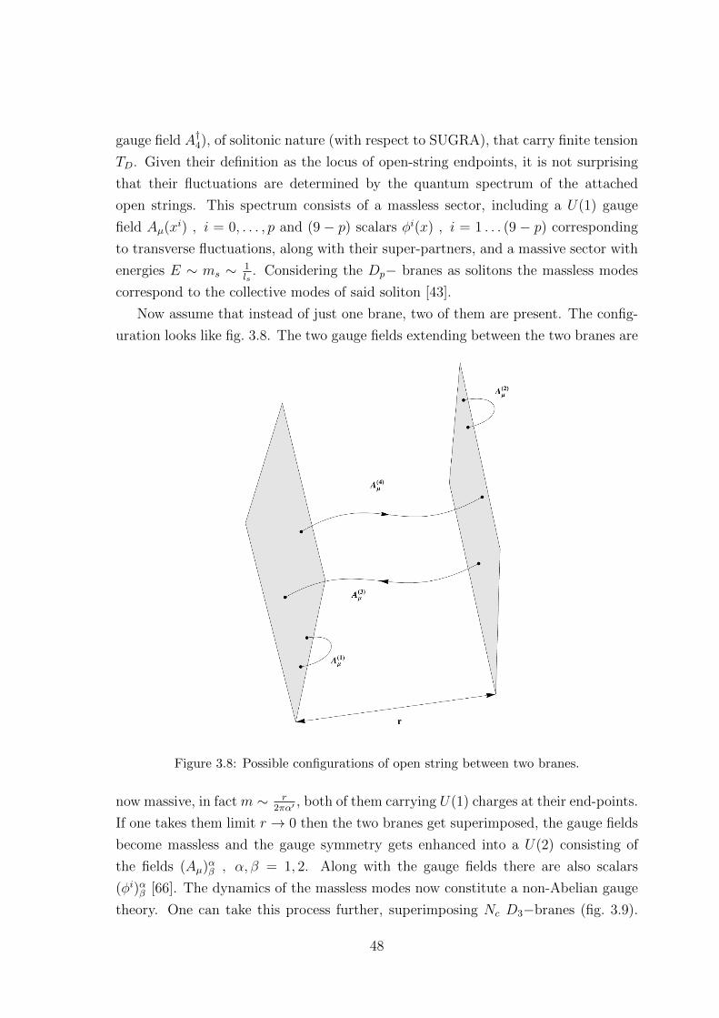
gauge field A†4), of solitonic nature (with respect to SUGRA), that carry finite tension

TD. Given their definition as the locus of open-string endpoints, it is not surprising

that their fluctuations are determined by the quantum spectrum of the attached

open strings. This spectrum consists of a massless sector, including a U(1) gauge

field Aµ(xi) , i = 0, . . . , p and (9 − p) scalars φi(x) , i = 1 . . . (9 − p) corresponding

to transverse fluctuations, along with their super-partners, and a massive sector with

energies E ∼ ms ∼ 1ls

. Considering the Dp− branes as solitons the massless modes

correspond to the collective modes of said soliton [43].

Now assume that instead of just one brane, two of them are present. The config-

uration looks like fig. 3.8. The two gauge fields extending between the two branes are

Figure 3.8: Possible configurations of open string between two branes.

now massive, in fact m ∼ r2πα′

, both of them carrying U(1) charges at their end-points.

If one takes them limit r → 0 then the two branes get superimposed, the gauge fields

become massless and the gauge symmetry gets enhanced into a U(2) consisting of

the fields (Aµ)αβ , α, β = 1, 2. Along with the gauge fields there are also scalars

(φi)αβ [66]. The dynamics of the massless modes now constitute a non-Abelian gauge

theory. One can take this process further, superimposing Nc D3−branes (fig. 3.9).

48

The massless spectrum of this system consists of Aµ , φi , i = 1, . . . , 6 along with the

Figure 3.9: A stack of Nc D3−branes.

super-partners - four Weyl fermions in the adjoint of U(Nc). The low-energy effective

action describing this system would then be

L = − 1

g2YM

Tr

1

4FµνF

µν +1

2Dµφ

iDµφi +[φi, φj

]2+ fermions

(3.29)

where g2YM = 4πgs

3. In other words the low-energy effective action of a stack of

D3−branes correspond to an N = 4, U(Nc)4 Super-Yang-Mills theory in four dimen-

sions (d = 4). This is a rather special and particularly interesting theory. For example

it has an identically vanishing beta-function, i.e. it is scale invariant and its coupling

constant does not run (can be set to an arbitrary value and it will remain there).

This is a striking difference with ordinary, less symmetric Quantum Field Theories

where the beta-functions are either positive or negative, but certainly non-zero.

The effective super-symmetric theory is governed by two parameters - Nc and gYM .

It is however convenient to combine them into the ’tHooft coupling λ = g2YMNc, as

in the large-Nc limit the perturbative expansion of any amplitude A(gYM , Nc) can be

3This can be derived from DBI action, describing a single Dp−brane with constant (or slowlyvarying) world-volume fields, re-summing the α′ corrections [61].

4The U(Nc) group is decomposed into SU(Nc) ⊗ U(1) with the U(1) component describing themotion of the centre of mass of the brane system, essentially resulting in the more familiar SU(Nc),N = 4 SYM.

49

written as

A(gYM , Nc) =∞∑g=0

N2−2gfg(λ) (3.30)

where g is the genus of the diagram [67].

The content and the symmetries of this theory are highly relevant to the AdS/CFT

conjecture as the constitute the first tests one can perform on it. As mentioned earlier

the field content consists of Aµ, φi and λaα, i.e. gauge field, scalars and fermions. The

theory’s symmetries are

• Conformal symmetry SO(2, 4), with generators Pµ, Lµν , D, Kµ

• R-Symmetry SO(6) ∼ SU(4)R

• Poincare SUSY, with generators Qaα, Qa,α, a = 1, . . . , 4

• Conformal SUSY, with generators sα,a, Saα, a = 1, . . . , 4

It should not be overlooked that the action (3.29) is an effective one and therefore

receives corrections, which take the form of higher derivative terms. This corrections

however are suppressed by factors of E2α′, where E is the energy scale. The brane-

system also includes closed strings which interact with a strength G10 ∼ g2s l

8s meaning

that interaction terms will come with factors of E8G10 and can be neglected for small

enough energies, i.e. for E 1ls

. At this energy regime closed string do not interact

(i.e. one is in the classical gravity regime) and they decouple from the open string

sector which in this limit reduces to the N = 4 SYM in d = 4. More formally the

system’s action is

S = Sbrane + Sbulk + Sinteraction (3.31)

At the low energy regime Sinteraction can be neglected (∼ O(E8G10)), Sbrane is the

N = 4, SU(Nc) SYM in d = 3 + 1 dimensions (plus corrections O(E2l2s)) and Sbulk

corresponds to d = 10 Minkowski gravity (plus corrections O(E8G10)). More specifi-

cally as the number of branes grows the gravitational field they induce increases, since

each one carries a finite tension. The resulting gravitational system, at low energies,

is one that has been encountered before (3.25), i.e the p = 3 black p−brane solution

of Type-IIB super-gravity. Noticing that∫S8−p ?F5 = Q ⇒ L4 = 4πgsNcl

4s which is

the relevant scale. Therefore the gravitational system at r L (near-horizon limit)

simplifies to AdS5 × S5.

Given that it has been established that the brane-system gravitates, it is interest-

ing to estimate at which point of the parameter space, the gravitational effects are

50

significant. In general an extended p−dimensional object will produce a gravitation

field ∼ G10Mtot

rd−p−3 . Specifically for a D3−brane this field is ∼ G10NcT(3)

r4 or written in

terms of the theory’s parameters

gravity field for D3 − brane ∼gsNcl

4s

r4(3.32)

This now allows one to estimate the regime of validity for each picture, i.e. that of

the stack of branes embedded in flat space-time (fig. 3.9) or that of the black brane

space-time (fig. 3.10). In particular one has

Figure 3.10: Ten-dimensional space-time from the closed-string or gravitational perspectivefor gsNc 1 and Nc 1. There are two distinct regimes - the near-horizon “throat” andthe asymptotic boundary.

• for gsNc 1 gravity corrections are of order O(1) for r ls

• for gsNc 1 gravity corrections are of order O(1) for r ls

Beyond these limits there is another, more subtle one that needs to be examined,

particularly if one intends to ignore quantum gravity corrections. Suppression of

quantum effects occurs when L lp ⇔ L4

l4p 1. Recalling that (l

(10)p )8 = ~G10

c3and

G10 ∼ g2s l

8s one sees that

L4

l4p∼ gsNcl

4s

G1/210

∼ Nc (3.33)

51

It is then apparent that in order for quantum gravity effects to be negligible Nc 1,

independently of any other limits.

To summarize, the system consisting of a stack of Nc D3−branes admits the

following two descriptions

• at gsNc 1 or equivalently λ 1, the open-string picture prevails, giving rise

to the effective action corresponding to a N = 4 SU(Nc) SYM

• at gsNc 1 or equivalently λ 1 and Nc 1, the closed-string picture

prevails, giving rise to the geometric black brane description

In principle both these descriptions should be valid for any value of the parameters

λ, Nc and it is only a matter of one’s ability to track the theory at each limit that

these convenient effective theories emerge. In other words each of them is limited

to a particular area of the parameter space (fig. 3.11), only because of the difficulty

(and potentially inability) to compute the higher corrections necessary to extend the

regime of validity.

genusexpansion

loopexpansion

λ00 ∞

g str

1/N

chandles

handles

worldsheet loopsgauge loops

classicalga

ugetheory

perturbativegauge

theory

interacting

classicalstrings

freeclassicalstrings

freequantumstringsplanar limit

hardinteracting quantum strings

quantum gauge theory

c© 2010 Niklas Beisert~

Figure 3.11: The Holographic parameter space. Figure taken from [1].

Having established the relation of this two regimes and the corresponding theories,

as limits of a common starting point, one is now in a position to explicitly state the

AdS/CFT conjecture:

The AdS/CFT Conjecture.

N = 4 , SU(Nc) SYM @d = 3 + 1 = TypeIIB superstring theory on AdS5 × S5

(3.34)

52

This is a weak-strong duality, in which the relevant degrees of freedom are very

different - on the one side they are gauge ones and on the other side they are gravita-

tional. The characterization of this duality as Holographic, stems from the fact that

the gravity side lives on a five (in fact 5 + 5) dimensional space-time while the gauge

side lives on the boundary of this space-time, in one dimension less, i.e. d = 3 + 1. In

a more formal way one can write down the duality using the partition functions on

each side

Zd=3+1,N=4SYM [J ] = ZTypeIIB@AdS5×S5 [J ] (3.35)

The very first test one performs on this duality, as mentioned earlier, is to check

if the symmetries on the two sides match. As seen in table 3.2 that appears to be the

case.

N = 4 SYM d = 3 + 1 AdS5 × S5

SO(4, 2) (conformal) × SO(6)R (R-symmetry) SO(4, 2)× SO(6) (isometries)

SL(2,Z) SL(2,Z)

Table 3.2: The symmetries of the theories on the two sides of the Holographic duality.

Another revealing comparison that can be made, is that of the entropy density

(s) on the two sides. As seen in [68] using Holographic techniques one gets

sH =π2

2N2c T

3 (3.36)

This should match the entropy density for N = 4 SYM at the λ → ∞, Nc → ∞limit. From standard perturbative approaches [35,36] (i.e. λ 1) it is known that

sYM |λ→0 =4π2

90T 3

(NB +

7

8NF

)(3.37)

where NB and NF are the number of bosons and fermions respectively. For the

particular field content of N = 4 SYM this reduces to

s(λ→ 0) =2π2

3N2c T

3 (3.38)

This expression though receives λ correction, which one necessarily needs to include

in order to depart from the strict λ→ 0 limit. In fact as seen in [69,70] for λ > 0

s(λ) =2π2

3N2c T

3f(λ) (3.39)

53

where

f(λ) = 1− 3

2π2λ+

3 +√

2

π3λ

32 + . . . (3.40)

Similarly in order to depart from the strict λ→∞ limit, on the other side, one needs

to include 1λ

corrections. This is done in [68], resulting in

f(λ) =3

4+

45

32ζ(3)λ−

32 + . . . (3.41)

It is therefore presumed that f(λ) interpolates between the two limiting values f(0) =

1 and f(∞) = 34.

3.3 Holographic toolbox

Having stated the AdS/CFT conjecture, established its connections to String Theory

and glossed over its derivation, the next step is to examine how one can make practical

use out of it. To do that one notices that on the right-hand-side of eq. (3.35) saddle

point approximation can be used to give

ZIIB ST@AdS5×S5

saddle'point

exp [−SIIB SUGRA] +O(1

N2c

, λ−32 ) (3.42)

where O( 1N2c) corresponds to quantum corrections and O(λ−

32 ) to higher-derivative

terms. This is a much more tractable theory and can even be consistently truncated

down to regular gravity. Given this approximation one can then compute expectation

values of operators 〈O(x1) . . . O(xn)〉YM in the dual theory since

〈exp

[∫d4xJO

]〉YM = exp [−Sgrav[J ]] (3.43)

The question then becomes what plays the role of J on the gravity side. For this

purpose it is instructive to recall that the string coupling constant gs = 4πg2YM

is related to the expectation value of the dilaton at the AdS boundary, i.e. gs =

exp [〈φ∞〉]. Deforming the gauge theory (on the boundary), meaning that one changes

the coupling constant is equivalent to changing the boundary value of a bulk field,

namely the dilaton. This can be extended so that generically a deformation of the

YM theory is of the form

SYM → SYM +

∫d4xφ(x)O(x) (3.44)

where O(x) is a local, gauge-invariant operator (e.g. O = TrF 2) and φ(x) is a source.

Then

φ(x) = Φbulk|∂AdS (x) = limr→∞

Φbulk(r, x) (3.45)

54

This process leads quite naturally to the field-operator correspondence. That is for

every boundary operator O(x) there is a bulk field, the boundary value of which

acts as a source for that operator. In some cases where both gravity and boundary

theories are well-controlled and fully understood this field-operator matching comes

directly (e.g. DBI action can help in these identifications). This however is not always

possible in which case a more phenomenological approach is needed. For example one

looks for fields such that the quantum numbers of the global symmetries in both

sides match. For conserved currents such as Oµ(x) = Jµ(x) or Oµν(x) = T µν(x) the

appropriate terms are easy to identify, namely∫d4xAµ(x)Jµ → Aµ(x, r) @d = 5 (3.46)∫

d4xgµν(x)T µν(x)→ gµν(x, r) @d = 5 (3.47)∫d4xφ(x)O(x)→ φ(x, r) @d = 5 (3.48)

Out of these considerations a Holographic “dictionary” emerges

O (boundary operator) δφ (bulk field)Tµν δgµν

Jµ Aµ

TrF 2 φ

Table 3.3: Operator-field mapping within the Holographic dictionary.

One therefore is equipped with a tool to compute strongly-coupled (in fact infinitely-

coupled) correlators of the boundary theory, the most important of which is the

two-point (Green’s) function (or propagator). This is achieved by taking functional

derivatives of the (on-shell) gravitational action with respect to the boundary val-

ues of the field corresponding to the operator, the correlator of which one wants to

compute. Since in most Holographic calculations the goal (at least initially) is the

computation of some theory’s propagators, the discussion about a subtlety is in order.

When working in Euclidean signature the propagator GE is uniquely defined, without

any ambiguity.

GE(kE) =

∫d4xE exp [ıkExE] 〈TEO(xE)O(0)〉T (3.49)

For finite temperature this becomes the Matsubara propagator defined at ωE = 2πTn

for boson and ωE = 2πT (n + 1/2) for fermions [35]. In fact the first Holographic

calculations were done in Euclidean signature [7].

55

It was soon realized though that this poses some difficulties particularly if one

tries to compute non-zero temperature and chemical potential correlators as well

as real-time dynamics (small deviations from equilibrium). In principal one would

expect that this could be achieved through an analytic continuation, however this

poses problems since there is not a unique way to do this continuation. Additionally

in many cases of practical interest propagators can only be calculated numerically, in

which case it is not clear how one could analytically continue a numerical function.

These limitations were realized and addressed in [71, 72] which laid the foundations

for real-time Holography. Moreover this opened the way for a more phenomenological

approach to Holography.

From ordinary Quantum Field Theory (at finite temperature) it is already known

that [35,36] there are four distinct propagators in Minkowski signature, namely

GR(k) = ı

∫d4x exp[−ıkx]Θ(t)〈

[O(x), O(0)

]〉T (3.50)

GA(k) = ı

∫d4x exp[−ıkx]Θ(−t)〈

[O(x), O(0)

]〉T (3.51)

G(k) =1

2

∫d4x exp[−ıkx]〈O(x)O(0) + O(0)O(x)〉T (3.52)

GF (k) = −ı∫d4x exp[−ıkx]〈TO(x)O(0)〉T (3.53)

where the expectation values are 〈A〉 := TrρA, with ρ = exp[−βH + µAQA] and

T (. . .) is the time-ordering. In the order that they appear these are the Retarded,

Advanced, Wightman and Feynman propagators, respectively. It is important to note

that these are not all independent. In fact using the spectral representation of the

propagators one can write

GF =1

2

(GR +GA

)− ıG (3.54)

G(k) = − cothω

2T=GR (3.55)

GF (k) = <GR + ı cothω

2T=GR (3.56)

GA(k) = GR(−k) = (GR)∗ (3.57)

and moreover at the zero-temperature limit T → 0, GF (k) = ReGR + ısgnωImGR.

Out of this set of Green’s functions causality picks out the retarded one, because,

as seen in the Linear Response section, one does not want a response prior to the

appearance of the external stimulus.

All the elements are in place now to write down the “recipe” for Holographic

calculation of correlation functions

56

• identify the bulk field δφ corresponding to the operator O of interest

• solve the equations of motion (to linear order if one is interested in Linear

Response) for δφ with the boundary condition that φ(boundary) = J

• compute the on-shell action Sgrav[J ]

• compute correlators by taking functional derivatives δδJ

exp [−Sgrav[J ]]

This concludes the recipe for the cases of Euclidean signature. In order to compute

real-time Green’s functions this recipe needs to be amended to

• Fourier decompose the bulk field δφ(r, x)∫ddk exp[ık · x]fk(r)φ0(k)

• solve equations of motion with boundary conditions fk(r → ∂) = 1 and impose

incoming wave conditions at the horizon

• write the on-shell action in the form S =∫ dkφ0(−k) F(k, r)φ0(k)|r=rHr→∂

• extract the retarded Green’s function GR(k) = −2F(k, r)|r→∂

This section will end by presenting a simple example of such a Holographic cal-

culation, which will smoothly transition to one of the most celebrated results of

Holography, namely the calculation of the ratio of shear viscosity over the entropy

density ηs.

The background will be an AdS space-time,

ds2 =r2

L2

(−dt2 + dx2

1 + dx22dx

23

)+L2

r4dr2 + L2dΩ2

5 (3.58)

or making the radial coordinate transformation r → z = L2

r5

ds2 =L2

z2

(dz2 + dx2

1 + dx23 + dx2

4

)(3.59)

where the sphere part is left out. Now consider in this background a massive scalar

field describe by the action

SE =π2L8

4κ210

∫d4xdz

z3

[(∂zφ)2 + (∂iφ)2 +

m2L2

z2φ2

](3.60)

Following the procedure described previously, one first Fourier decomposes the field

in

φ(z, k) =

∫d4k

(2π)4exp[ıkx]fk(z)φ0(k) (3.61)

5Note that in these coordinates the AdS boundary r →∞ is now at z = 0.

57

The equations of motion are then

f ′′k (z)− 3

zf ′k(z)− (k2

E +m2L2

z2)fk(z) = 0 (3.62)

with the boundary condition fk(z → 0) = 1 as well as the demand for regularity. The

on-shell action then becomes

SE =π3L8

4κ210

∫ ∞ε

∫d4k

(2π)4d4k′

1

zδ(k+k′)

[∂zfk∂zfk′ + kk′fkfk′ +

m2L2

z2fkfk′

]φ0(k)φ0(k′)

(3.63)

where ε is a small number setting the lower end of the integral close to but not on the

AdS boundary. This is because divergences emerge as one approaches the boundary

that need to be carefully renormalized, giving rise to additional terms in the action

(i.e. Holographic counter-terms). This is the subject of Holographic Renormalization

discussed in [73,74], but will not be pursued here as it doesn’t affect the results. The

solutions of eq. (3.62) are of the form

fk(z) = AzνIν(kz) +BzνKν(kz) (3.64)

where k = |kE|, ν = (4 + m2L2)1/2 and I, K are the modified Bessel functions

of the first and second kind (following the standard Frobenious theory for Ordinary

Differential Equations (ODE) [75]). The asymptotic behaviour of the Bessel functions,

i.e. Kν(x → ∞) ∼ exp[−x] while Iν(x → ∞) ∼ exp[x], allows one, by demanding

finiteness to exclude the latter. Hence the solution is (for the massless case, which

means ν = 2)

fk(z) =z2K2(kz)

ε2K2(kε)(3.65)

such that fk(ε) = 1. Plugging this back into the on-shell action, it can be written as

SE =π3L8

4κ210

∫d4kd4k′

(2π)4δ(k+k′)φ0(k)φ0(k′)

fk′∂zfk(z)

z3

∣∣∣∣∞ε

=

∫d4kd4k′

(2π)8φ0(k)φ0(k′) F|∞ε

(3.66)

which allows one to compute the two-point function

〈O(k)O(k′)〉 =1

Zδ2Z[φ0]

δφ0(k)δφ0(k′)

∣∣∣∣φ0=0

= −2F(z, k, k′)|∞ε

= −(2π)4δ(k + k′)π3L8

2κ210

fk′∂zfkz3

∣∣∣∣∞ε

(3.67)

or recalling that κ10 = 2π5/2 L4

Nc, the Euclidean propagator becomes

〈O(k)O(k′)〉E =N2c

8π2δ(k + k′)

f ′(ε)

ε3(3.68)

58

in the limit ε → 0. In this limit, properly treating the Holographic counter-terms,

and neglecting contact ones (non singular terms), one finds that

limε→0

f ′

ε3= −k

4

8ln k2 (3.69)

Hence

〈O(k)O(k′)〉E = − N2c

64π2(2π)4δ(k + k′)k2

E ln k2E (3.70)

There is an interesting observation to be made at this point. From perturbative

calculations one knows that

〈O(x)O(y)〉pert ∼1

|x− y|8=:

1

|x− y|2∆0(3.71)

resulting in ∆0 = 4. By Fourier transforming the Holographic result back into coor-

dinate space one

〈O(k)O(k′)〉 ∼ N2c

|x− y|8(3.72)

yielding ∆(λ = 0) = ∆(λ =∞) = 4. This is consistent with what is known for N = 4

SYM (non-renormalization theorems), which is scale invariant. However not allN = 4

operators are protected against running so generically one expects ∆ = ∆(λ) to be a

non-trivial function.

The calculation presented so far has been in Euclidean signature. The Minkowski

version will now be presented. The background metric is now

ds2 =L2

z2

[dz2 + ηµνdx

µdxν]

(3.73)

where ηµν = diag[−+ . . .+]. The Fourier decomposition is

φ(z, x) =

∫d4k

(2π)4exp[−ıωt+ ıkx]fk(z)φ0(k) (3.74)

the action

S = −π3L8

4κ210

∫d4x

∫ ∞ε

dz

z3

(∂zφ)2 + ηµν∂µφ∂νφ+

m2L2

z2φ2

(3.75)

the equations of motion

f ′′k (z)− 3

zf ′k(z)−

(k2 +

m2L2

z2

)fk = 0 (3.76)

but note that here k2 can be either positive or negative. The on-shell action becomes

S =

∫d4k

(2π)4(F(k,∞)−F(k, ε))φ0(−k)φ0(k) (3.77)

59

where F(k, z) = −π3L8

4κ210

f−l∂zfkz3 . It should be mentioned here that for space-like mo-

menta k2 > 0, the situation is similar to the Euclidean case. For time-like momenta

k2 < 0 requiring non-diverging solutions, results in usual instead of modified Bessel

functions. In particular setting q =√−k2

fk(z) =z2H

(1)ν (qz)

ε2H(1)ν (qε)

, ω > 0 (3.78)

fk(z) =z2H

(2)ν (qz)

ε2H(2)ν (qε)

, ω < 0 (3.79)

with Hν being the Hankel function H(1,2)ν = Jν ± ıYν . Incoming wave conditions need

to be imposed now. To do this notice first that the asymptotic behaviour of Hankel

functions is

limz→∞

H(1,2)ν (z) =

√2

πzexp

[±ı(z − νπ

2− π

4

)](3.80)

and therefore imposing incoming conditions at z → ∞ means that for ω > 0 picks

out H(1)ν and for ω < 0, H

(1)ν . The incoming conditions also pick out the retarded

Green’s function GR. Putting all these together one gets

GR(k) =Nck

4

64π2

(ln |k2| − ıπΘ(−k2)sgnω

)(3.81)

which a posteriori can be easily checked to be the proper analytic continuation of the

Euclidean propagator GE.

The above calculation can be easily extended to higher dimensions, where the

metric is

ds2d+1 =

L2

z2

(dz2 + ηµνdx

µdxν)

(3.82)

and the equations of motion

zd+1∂z(z1−d∂zφ

)− k2z2φ−m2L2φ = 0 (3.83)

The solution near the boundary ∂AdS (z → 0) can be written as 6

φ(z, k) = A(k)zd−∆ + . . .+ B(k)z∆ + . . . (3.84)

where ∆ = d2

+ ν, with ν =(d2

4+m2L2

)1/2

. This “anomalous” dimension, that

controls whether a mode is normalizable or non-normalizable 7, raises an interesting

6This comes again from Frobenious theory [30].7Normalizability is determined with respect to the AdS inner product that is defined, according

to [76], as (φ1, φ2) = −ı∫

Σtdtddx

√−ggtt(φ∗1∂tφ2 − φ2∂tφ

∗1).

60

issue. It has to be real and that can be achieved when m2L2 ≥ −d2

4, i.e there is a

small negative window of mass that is allowed. This is the well-known Breitenlohner-

Freedman bound [77]. The modes with masses above the BF bound are split into two

categories

• −d2

4≤ m2L2 ≤ −d2

4+ 1

• −d2

4+ 1 ≤ m2L2

In the first case both zd−∆ and z∆ are normalizable. In the case where the mass is

unbounded from above, i.e . m2L2 ≥ −d2

4+1, the term φ ∼ zd−∆ is non-normalizable

while the term φ2 ∼ z∆ is normalizable. The non-normalizable term (at the bound-

ary) plays the role of the source for the boundary operator operator O whereas the

normalizable mode correspond to the its expectation value 〈O〉. In particular on the

boundary

S∂AdS → S∂AdS +

∫ddxJ(x)O(x) (3.85)

with

J(x) = φ|∂AdS = limz→0

z∆−dφ(z, x) (3.86)

In other words if the bulk field φ correspond to the boundary operator O, using

eq. (3.84), J ↔ A and 〈O〉 ↔ B.

This section will end with the presentation of the Holographic hydrodynamical

limit, that will allow a smooth transition to the Condensed Matter applications of

Holography (as it actually happened historically). For this purpose the prototypical

example of N = 4 SYM at finite temperature, will be used. The dual background to

this theory, as seen above, is the black brane configuration

d25 =

(πTL)2

u

(−f(u)dt2 + dx2

)+

L2

4f(u)u2du2 (3.87)

with u =r20

r2 and T = r0πL2 . In order to study the hydrodynamical limit, one needs

to perturb the system (remaining close to equilibrium. For this purpose one expands

the gravity field as gµν = g(0)µν + δgµν(t,x, u). It is then straightforward to write the

linearised version of Einstein’s equation

Rµν = R(0)µν +R(1)

µν + . . . =2Λ

3

(g(0)µν + δgµν + . . .

)(3.88)

Using the symmetries of the system one can pick, without loss of generality, the di-

rection into which the metric perturbation propagates, the presence of which breaks

rotational symmetry. Fortunately the resulting system still possesses enough symme-

try to split the metric perturbations into three families

61

• δgxy, called tensor channel

• δgxt, δgxt, δgty, δgyz, called vector (or shear) channel

• δgtz, δgii, called scalar (or sound) channel

assuming that the perturbation travels along the z direction. Since the elements of

each channel cannot mix with any other, Einstein’s equations also split along these

channels, significantly simplifying treatment of the system. Focusing, for now, on the

shear channel, the relevant Einstein’s equations are

H ′t +q

ωfH ′z =0 (3.89)

H ′′t −1

uH ′t −

ωq

uf 2Hz −

q2

ufHt =0 (3.90)

H ′′z −1 + u2

ufH ′z +

ω2

uf 2Hz +

ωq

uf 2Ht =0 (3.91)

where Ht := uδgtx(πTL)2 , Hz := uδgzx

(πTL)2 , ω = ω2πT

and q = q2πT

. Considering that one

wants to compute correlation functions of gauge invariant operators and given that

individual metric components are not invariant under diffeomorphism transforma-

tions (which are the gauge transformations of gravity) it is necessary to combine the

fundamental degrees of freedom into gauge invariant ones. For this case one defines

Z1 := qHt + ωHz (3.92)

Taking the Lie derivative of Z1 one sees that LξZ1 = 0 8. The shear Einstein’s

equations can be combined into a single equation for this gauge invariant degree of

freedom, namely

Z ′′1 +

(ω2 − q2f)f − uω2f ′

uf(q2f − ω2)

Z ′1 +

ω2 − q2f

uf 2

Z1 = 0 (3.93)

Near the boundary (u = 0) the solution of this equation can be expanded as Z1 =

A1(1 + . . .) +B1(u2 + . . .). As seen before, once one has this expansion extracting the

Green’s functions is straightforward, i.e.

G1(ω, q) = −π2N2c T

4 B1(ω, q)

A1(ω, q)(3.94)

At this stage one can impose the hydrodynamical limit, by looking for solutions G

perturbatively in ω, q. In other words the hydrodynamic limit is valid for small ω

8Recall that Lξgµν = ∇µξν +∇νξµ.

62

and q. To see why this is the case, first notice that for finite-temperature N = 4

SYM there is only one scale, that of the temperature T . Therefore the free mean

path scales like lmfp ∼ 1T

. In terms of the free mean path the hydrodynamic limit

is lmfp l L. It is then apparent that this limit is equivalent to qlmfp 1 orq

2πT 1 and similarly ω

T 1. One then writes Z1 as a series over ω and q

Z1(u) = C1f(u)−ıω/2(

1 +ıq2f

2ω+O(ω2, q2, ωq)

)(3.95)

Imposing Dirichlet boundary conditions on the boundary, i.e. Z1(0) = 0, yields the

dispersion relation

ω = − ı

4πTq2 +O(q4) (3.96)

This is the Holographic result for N = 4 SYM at λ → ∞ and Nc → ∞. From

general dissipative hydrodynamics it is known that from the dispersion relation one

can extract the diffusion coefficient D, since ω = ıDq2 + . . .. Hence the Holographic

prediction is that D = 14πT

. It is also the case that D = ηε+p

, where η is the shear

viscosity, ε the energy density and p the pressure. For a system where the chemical

potential vanishes, i.e.µ = 0, thermodynamic relations dictate that ε+p = sT , where

s is the entropy density. Therefore D = ηsT

. Combining this with the Holographic

result one gets the famous result [71,78].

η

s=

1

4π(3.97)

This has been a very impactful result and it has been conjectured that it constitutes

a lower bound for a certain class of Holographic theories. Its corrections have also

been studied quite extensively and it is known that to first λ correction it is

η

s=

~4πkB

(1 +

15ζ(3)

λ3/2

)(3.98)

where all the units have been put back in explicitly. In general it is expected that at

Nc →∞ viscosity itself (that is extracting s = π2

2N2c T

3) is η(λ) = f(λ)N2c T

3, where

f(λ) is a function interpolating between π/8 at λ 1 and λ−2 ln−1 1λ

at λ 1, i.e.

between the strongly-coupled and the perturbative results.

3.4 AdS-CMT

In the final section of this chapter further Holographic calculations pertaining to

Condensed Matter systems will be presented.

63

Sound

The starting point will be sound propagation. This is a natural point to begin, since

it is closely related to the calculation of shear viscosity. In particular the underlying

system is the same and one only changes the channel studied [21]. The background

metric is again

ds2 =(πTL)2

u

(−f(u)dt2 + dx2 + dy2 + dz2

)+

L2

4u2f(u)du2 (3.99)

As expected by the listing of the fundamental components δgµν in the sound

channel above, the linearised Einstein’s equation are more numerous and less simple.

In particular (using radial gauge where δguµ = 0) and reducing to the independent

set one has

H ′′tt −3u

fH ′t −H ′′ii +

u

fH ′ii = 0 (3.100)

ω

(H ′ii +

u

fHii

)+ q

(H ′tz +

2u

fHtz

)= 0 (3.101)

q (fH ′tt − uHtt) + ωH ′tz − qH ′aa = 0 (3.102)

H ′ii −3fH ′tt3− u2

− 2

f(3− u2)

(ω2Hii + 2ωqHtz + q2f(Htt −Haa)

)= 0 (3.103)

where Htt := uf(πTL)2 δgtt, Htz := u

(πTL)2 δgtz, Hij := u(πTL)2 δgij, Haa : Hxx + Hyy and

Hii := Haa +Hzz. The equations of motion still have some residual gauge symmetry,

thus one can construct solution to them by acting on the trivial solution Hµν = 0

with the generating transformations of said symmetry. This are by construction pure

gauge solutions and are linear combinations of the terms

HItz = ω (3.104)

HIzz = −2q (3.105)

HIItt = −2ω (3.106)

HIItz = qf (3.107)

HIIItt =

1 + u2 + 2ω2u√f

(3.108)

HIIItz = −qω arcsinu− qωu

√f (3.109)

HIIIaa = −2

√f (3.110)

HIIIzz = 2q2 arcsin i−

√f (3.111)

as found in [21]. Proceeding further one employs the standard Frobenius procedure,

on top of which the small frequency and long wavelength (ω 1 and q 1) limit is

64

taken, along with the incoming boundary conditions, one gets (to second order in ω

and q)

Htt =q2

3(1− u) (3.112)

Hii = q2(1− u) (3.113)

Htz = −ı q2

(1− u2) +ωq

2u(1− u)− ωq

4(1− u2) ln

2(1− u)

1 + u(3.114)

Haa = 1− ı ω2

ln1− u2

2− ω2

8ln2(1− u)− ω2

4ln(1− u) ln

1 + u

2

+2

3q2(1− u) +

3ω2 + q2

3ln

1 + u

2+ω2

8ln2 1 + u

2− ω2

2Li2

1− u2

(3.115)

To these solutions the pure gauge one can be added, yielding another solution. The

general solution can then be deduced and given that the on-shell action can be com-

puted. The action of the system, including the appropriate counter-terms [73], is

S =π3L5

2κ210

∫ 1

0

dud4x√−g (R− 2Λ) + 2

∫d4x√−hK − 6

L

∫d4x√−h (3.116)

where hµν is the induced metric (and h its determinant) and K the extrinsic curvature.

On shell this reduces to

SOS(ε) =π2N2

c T4

8

∫d4x

(−1 +

1

2(3Htt +Hii)

+1

8(3H2

tt − 12H2tz + 2HttHii + 2HzzHaa −H2

zz)

− 1

2ε(H2

tz +1

4H2aa −HttHii +HzzHaa)

′)

(3.117)

for some infinitesimal ε > 0. Plugging in the solutions, to linear order in ω and q the

action becomes

SOS =π2N2

c T4

8

(V4 +

1

3(3H0

tt +H0ii) +

1

2(q2 − 3ω2)

[(2qH0

tz + ωH0ii)

2

+ H0tt(3q

2H0tt + 12qωH0

tz + (3ω2 + q2)H0ii)]

+1

8

[3(H0

tt)2 − 12(H0

tz)2 + 2H0

ttH0ii + 2H0

zzH0aa − (H0

zz)2])

(3.118)

where V4 is the four-dimensional volume, making the first term in the action the free

energy F = −π2

8N2c T

4V4. The zero index indicates non-dependence on ω and q. It is

now possible to extract some useful information about the dual theory. Namely the

65

expectation values of the stress-energy tensor can be computed

ε = 〈T tt〉 = 2δSOSδH0

tt

=3π2

8N2c T

4 (3.119)

2p = 〈T aa〉 = 4δSOSδH0

aa

=π2

4N2c T

4 (3.120)

p = 〈T zz〉 = 2δSOSδH0

zz

=π2

8N2c T

4 (3.121)

Combining the above one sees that ε = 3P . This is exactly what one would expect

from a conformal theory, like the boundary one (N = 4 SYM), which constitutes

another test for the AdS/CFT correspondence. Beyond one-point function one can

get the two-point function as well

Gtttt(ω, q) = −4δ2SOSδ(H0

tt)2

=3N2

c π2T 4q2

2(3ω2 − q2)− 3π2

8N2c T

4 = 3p5q2 − 3ω2

3ω2 − q2(3.122)

More information can be derived from this Green’s function. In particular it has a

pole at ω = 1√3k. This pole corresponds to sound propagation (density fluctuations)

and its velocity is exactly vs = 1√3

(see relative section of previous chapter), which

once again is exactly what is expected of a conformal boundary theory (in which the

stress-energy tensor has to be trace-less). It should be noted that it is not just the

position of the pole that matches but the full two-point function is identical to the

one computed by field-theoretical tools (for N = 4 SYM).

Zero sound

It has been seen that there is sound propagation in Holographic models and it is of

the exact form expected for the relative field theory. One can then ask if it is possible

to reconstruct Holographically zero-sound, which as seen in the previous chapter is

a feature of quantum liquids (Fermi liquids in particular). This has actually been

studied in [2, 79]. On the gravity side (IIB string theory) the system consists of

intersecting Nc D3−branes and Nf D7−branes with the following configuration in

the ten-dimensional space

x0 x1 x2 x3 x4 x5 x6 x7 x8 x9

D3 × × × ×D7 × × × × × × × ×

(3.123)

In the usual Holographic limits Nc →∞ and λ→∞ the D3-branes reduce, as usual,

to gravity in AdS5×S2, whereas the D7−branes can be made into probes (that do not

disturb the gravitational background) provided that Nf Nc. The Holographic dual

66

of this system is N = 4 SU(Nc) SYM with Nf massless N = 2 hyper-multiplet fields

(flavours) at zero temperature. The gravitational background, in the near-horizon

limit, is as seen previously

ds2 =r2

L2ηνµdx

µdxν +L2

r2

(dr2 + r2dΩ

)(3.124)

In this background the action describing the dynamics of the D7−branes is the DBI9

action

SDBI = −NfTD7

∫d8ξ√−det (gab + 2πα′Fab) (3.125)

where ξa are the brane’s world-volume coordinates, gab is the induced metric and Fab

the world-volume U(1) gauge field. In order to induce a non-vanishing baryon density

on the boundary one needs to turn on the zeroth component of the bulk gauge field

A0. This results in 〈J0〉 6= 0, where Jµ is the flavour current, that belongs to the

baryon number subgroup (U(1)B) of the U(Nf ) global symmetry, characterizing the

N = 2 hyper-multiplet. This significantly simplifies the DBI action (3.125)

SDBI = −λNfNc

(2π)4V3

∫drr3

√1− A′20 (3.126)

where a factor of 2πα′ has been absorbed by rescaling A0 and V3 is the volume of the

boundary theory. In order to study the existence of zero-sound one needs to compute

the current-density two-point (retarded) correlation function and check whether this

has a pole at zero temperature. Following the standard Holographic recipe the system

needs to be slightly perturbed, i.e.

Aµ → Aµ + δAµ (3.127)

Substituting this into the DBI action and expanding to first order with respect to the

gauge field, leads to

S2 =N

2

∫d4xdrr3

δA′2t

(1− A′2t )3/2+

(∂tAz − ∂zAt)2

r4√

1− A′2t− A

′2z√

1− A′2t

(3.128)

where N = λNfNc/(2π)4. Continuing with the Holographic dictionary, the fluctua-

tions are Fourier decomposed as

δAµ =

∫dωdq

(2π)2exp[−ıωt+ ıqx]δAµ (3.129)

9Dirac-Born-Infeld.

67

and the equations of motion are[r3δA′t

(1− A′2t )3/2

]′− 1

r√

1− A′2t

(ωqδAz + q2δAt

)= 0 (3.130)[

r3δA′z√1− A′2t

]′+

1

r√

1− A′2t

(ωqδAt + ω2δAz

)= 0 (3.131)

ωδA′t + (1− A′2t )qδA′z = 0 (3.132)

where eq. (3.132) is just a constraint equation, resulting from the residual gauge

symmetry. As seen before given that the goal is to calculate correlators of gauge-

invariant operators on the boundary, it is very useful to construct a gauge invariant

bulk field, out of the variables δAt and δAz. The gauge invariant variable is Z =

ωδAz + qδAt and the equations of motion are combined into

Z ′′ +

(f ′(3q2 − ω2f 2)

f(q2 − ω2f 2)− 1

u

)Z ′ +

ω2f 2 − q2

f 2Z = 0 (3.133)

where variables have been switched r → u = 1/r and f(u) =√

1 + d2u6 where

d = (2πα′N)−1ρ, with ρ being the baryon density. Imposing incoming boundary

conditions close to the horizon at u→∞ the solution asymptotes to E(u) ∼ exp[ıωu]u

.

Assuming that ωu 1, qu 1 with ω/q fixed, the equation of motion reduces to

Z ′′ +

[f ′(3q2 − ω2f 2)

f(q2 − ω2f 2)− 1

u

]E ′ = 0 (3.134)

the solution of which is

Z = C1 + C2u2

(q2

3f+q2 − 3ω2

6F2 1 (

1

2,1

3;4

3;−d2u6)

)(3.135)

where F2 1 is the Hyper-geometric function. Using the asymptotic behaviour of F2 1

one then finds

Z = C1 + C2

(au

+ b)

+O(1/u2) (3.136)

where a = ω2/d and b = (q2 − 3ω2)d2/3Γ(1/3)Γ(1/6)(18Γ(1/2))−1. In order to deter-

mine the integration constants C1 and C2 this solution needs to be matched with the

asymptotic behavior when ωz 1. In that case

Z =C

u+ ıωC (3.137)

The matching of the two asymptotic expansions leads to C1 = (ıω − b/a)C and

C2 = C/a. There is enough information in place to examine the existence of zero-

sound. This is because zero-sound would appear as a pole of the two-point retarded

68

function, which from the gravity point of view would emerge as a quasi-normal mode

of the field Z [80]. More precisely given that the hydrodynamic limit is of interest

here, one needs to extract the lowest quasi-normal pole (i.e. the one with the smallest

|ω|). Seeing as an analytic solution is available for this case, it is easy to extract the

lowest quasi-normal mode by just imposting the Dirichlet boundary conditions on the

field Z, on the AdS boundary, i.e. Z(0) = 0⇔ C1 = 0. This in turn yields

ıω =

(q2

ω2− 3

)d1/3Γ(1/3)Γ(1/6)

18Γ(1/6)(3.138)

In the hydrodynamic regime, i.e. for small ω and q this simplifies to

ω = ± q√3− ıΓ(1/2)q2

d1/3Γ(1/3)Γ(1/6)+O(q3) (3.139)

or in a more convenient form

ω = ± q√3− ıq2

6µ0

+O(q3) (3.140)

where the zero-temperature chemical potential has been used

µ0 = Γ(1/3)Γ(1/6)(6Γ(1/2))−1d1/3 (3.141)

In summary what has been shown in [79] is that the system of D3/D7 branes, in the

probe limit, has a propagating mode at zero temperature. The identification of this

mode as zero-sound, comes firstly from the dependence of its imaginary part on q,

i.e. q2. This is compatible with zero-sound. Moreover this dependence excludes the

possibility of this mode corresponding to a super-fluid phonon. In fact this could not

have been the case since the background preserves the particle number symmetry,

meaning that the ground state cannot be a super-fluid. However, this particular

zero-sound is not exactly the zero-sound of Fermi liquids. This is because its speed

is the same at finite temperatures (first sound), whereas in the case of Fermi liquids

zero and first sound differ by a factor of√

3.

Fermi Liquids

It has just been reviewed how one can construct gravitational systems, that can re-

produce Condensed Matter phenomena (like normal and zero-sound). Is it possible

in a Holographic context to actually reconstruct Fermi liquids? The answer seems to

be affirmative. Following [15,16] a quick review of this answer, will be demonstrated

69

here. Once again the starting point is the Holographic ingredients. The system con-

sists of a four-dimensional10 gravitational background (AdS4), a bulk gauge field (AM)

and a bulk, charged fermionic field (Ψ). It should be stressed here, that this is the

phenomenological or bottom-up way of approaching the problem, i.e. including the

minimum set of necessary ingredients without looking for a String Theory embedding.

This may cause some worries and in general it needs to be addressed, however none

of the relevant results are affected by this subtlety. Thus one can begin this analysis

from the action

S =1

κ10

∫d4x√−gR +

6

L2+ L2

[−1

4F 2 − ΨeMA ΓADMΨ−mΨΨ

](3.142)

containing all the aforementioned fields. In eq. (3.142) ΓA are just the Dirac matrices

(ΓA = γa, γ4) and eMA is the inverse vielbein. Moreover the covariant derivative,

acting on the spinors is

DMΨ =

(∂M +

1

8ωABM [ΓA,ΓB] + ıgAM

)Ψ (3.143)

A solution to the equations of motion coming from this action contains and AdS4

black-hole background

ds2 =L2α2

z2

(−fdt2 + dx2 + dy2

)+

L2

z2fdz2 (3.144)

a gauge field

A0 = 2qα(z − 1) (3.145)

where f(z) = (1− z)(z2 + z+ 1− q2z2). For book-keeping reasons it should be noted

that, in these coordinates, the horizon is located at z = 1 and the AdS boundary at

z = 0. Temperature and chemical potential for this system are T = α4π

(3 − q2) and

µ = −2qα respectively. Treatment of the fermions becomes more involved because of

their action is first-order and hence on the boundary it vanishes identically, making

it more tricky to set up the variational problem and use the boundary action as the

generating functional for the boundary theory. This phenomenon is a side-effect of

the fact that not all the components of the Dirac spinor are independent. However

one can project out half of the spinor and use that to define the boundary action [81].

Following the careful analysis in [15] one can eventually derive the retarded fermionic

Green’s function and then from that the spectral function. Studying the behaviour

10This choice is made so that the dual theory is 2 + 1 dimensional, which is the case for manyrelevant experimental configurations.

70

of the spectral function, the authors of [15] have established that in fact there is a

parameter regime, within this model, that describes a Fermi liquid.

The examples presented here are in no way an exhaustive list. In fact over the

last several years a lot of effort has been invested in understanding strongly coupled

systems from Condensed Matter, using the tools of Holography. The systems studied

include high-TC superconductivity [12, 17], strange metals [82, 83], non-Fermi liquids

[14], Josephson junctions [84], Mott insulators [85] and almost every other system of

Condensed Matter interest. Here, just for completeness, the major references for each

system are provided.

71

Chapter 4

Anti-de Sitter Reissner-Nordstrom

4.1 Introduction

In this chapter a Holographic study of the Anti-de Sitter Reissner-Nordstrom (RN-

AdS) system will be presented [86]. As it may already be known the RN-AdS system

is an extremely useful one, particularly from the phenomenological or bottom-up,

approach to Holography, since it contains the necessary ingredients, that is gravity

and a U(1) gauge field, necessary to address a lot of interesting Condensed Matter

problems. It is also very popular because it constitutes a realistic truncation of

top-down models, presenting a quite universal character. It therefore provides an

excellent toy model / laboratory to explore Holography. This system has been rather

well-examined so this study comes as an addition to the existing body of work which

most notably includes [3, 87,88].

Over the years, the excitations present when T = 0 and ω, q µ in specific

strongly-coupled field theories have attracted a lot of interest and a significant amount

of scrutiny, and one common feature amongst many examples is a propagating longi-

tudinal mode with the dispersion relation

ω = ±vsq − iΓ0q2 +O

(q3), (4.1)

where

ω =ω

µ, and q =

q

µ. (4.2)

One can detect this feature in probe brane theories in different dimensions and with

different UV symmetries (where the conserved charge is a density of fundamental

matter - at least in the case where the background is derived from string theory)

[79,89–96] as well as in 4D bulk Einstein-Maxwell theory with a cosmological constant

(where the conserved charge is an R-charge density) [3].

72

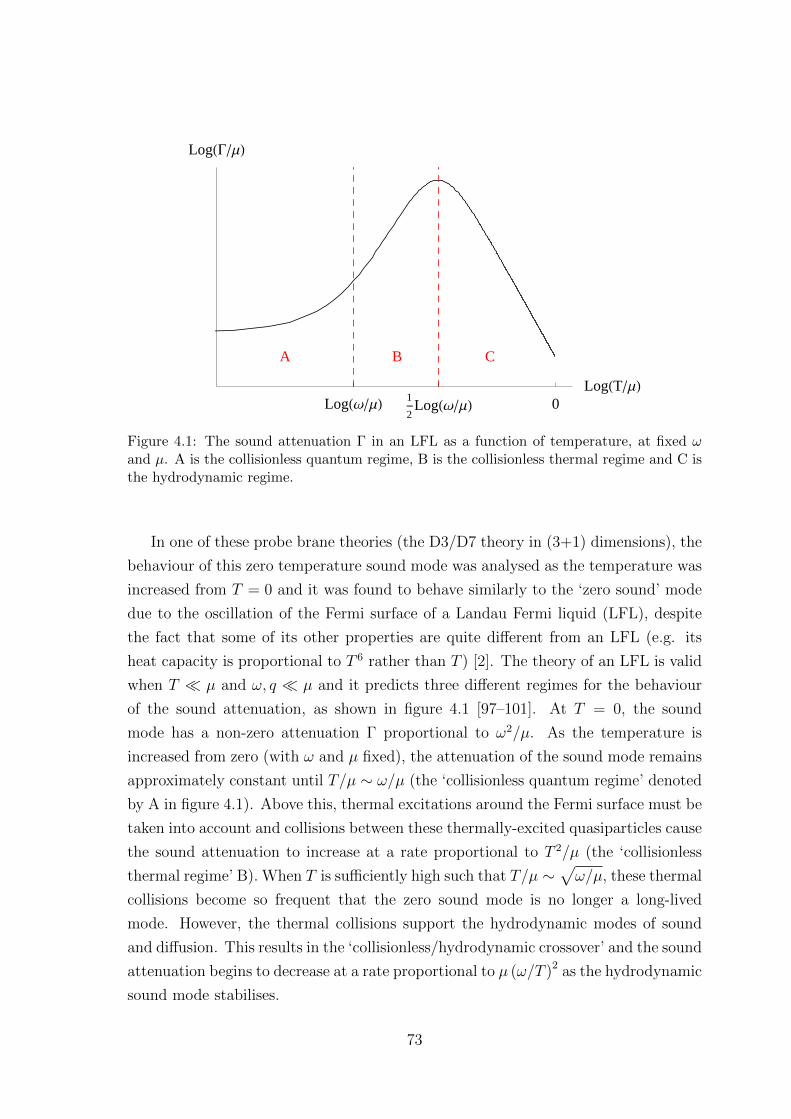
A B C

1

2LogHΩΜLLogHΩΜL 0

LogHTΜL

LogHGΜL

Figure 4.1: The sound attenuation Γ in an LFL as a function of temperature, at fixed ωand µ. A is the collisionless quantum regime, B is the collisionless thermal regime and C isthe hydrodynamic regime.

In one of these probe brane theories (the D3/D7 theory in (3+1) dimensions), the

behaviour of this zero temperature sound mode was analysed as the temperature was

increased from T = 0 and it was found to behave similarly to the ‘zero sound’ mode

due to the oscillation of the Fermi surface of a Landau Fermi liquid (LFL), despite

the fact that some of its other properties are quite different from an LFL (e.g. its

heat capacity is proportional to T 6 rather than T ) [2]. The theory of an LFL is valid

when T µ and ω, q µ and it predicts three different regimes for the behaviour

of the sound attenuation, as shown in figure 4.1 [97–101]. At T = 0, the sound

mode has a non-zero attenuation Γ proportional to ω2/µ. As the temperature is

increased from zero (with ω and µ fixed), the attenuation of the sound mode remains

approximately constant until T/µ ∼ ω/µ (the ‘collisionless quantum regime’ denoted

by A in figure 4.1). Above this, thermal excitations around the Fermi surface must be

taken into account and collisions between these thermally-excited quasiparticles cause

the sound attenuation to increase at a rate proportional to T 2/µ (the ‘collisionless

thermal regime’ B). When T is sufficiently high such that T/µ ∼√ω/µ, these thermal

collisions become so frequent that the zero sound mode is no longer a long-lived

mode. However, the thermal collisions support the hydrodynamic modes of sound

and diffusion. This results in the ‘collisionless/hydrodynamic crossover’ and the sound

attenuation begins to decrease at a rate proportional to µ (ω/T )2 as the hydrodynamic

sound mode stabilises.

73

These features were reproduced precisely in the strongly-coupled D3/D7 field the-

ory except that there was no sound propagation in the hydrodynamic regime - this

can be explained by the fact that the fluctuations of the bulk metric, which generate

the hydrodynamic sound mode of the dual field theory, were explicitly suppressed for

consistency with the probe limit. The collisionless/hydrodynamic crossover is most

clearly exhibited in the D3/D7 theory via the poles of the charge density Green’s

function in the complex frequency plane [2]. As the temperature is raised, the low

temperature poles corresponding to sound propagation approach the imaginary axis

and collide to form two purely imaginary poles, one of which becomes the hydrody-

namic diffusion mode as the temperature is raised further. The crossover can also be

seen by examining the charge density spectral function - the tall, narrow peak cor-

responding to the sound mode becomes smaller and moves towards the origin as the

temperature is raised, eventually forming a diffusive peak around ω = 0. A natural

question to ask is whether similar behaviour is observed in the low temperature sound

modes of other holographic theories at large chemical potential and hence whether

they can all be characterised in this way as LFL-like ‘zero sound’ modes or not.

Here, the strongly-coupled field theory dual to the RN-AdS4 black hole solution

of 4D Einstein-Maxwell theory with a cosmological constant, will be studied. Many

properties of this theory have been investigated in recent years as it is relatively

simple and yet has very interesting behaviour. In particular when T = 0, the low

energy behaviour of the field theory is governed by a CFT1 dual to the AdS2 factor

of the black hole’s AdS2 × R2 near-horizon geometry [16]. If one considers a probe

Dirac action for fermions in this background, the field theory operators dual to these

fermions exhibit Fermi surfaces of a non-Fermi liquid type [14–16]. If instead one

considers a fermionic action which is the super-symmetric completion of the Einstein-

Maxwell action, no such Fermi surfaces are observed [102–104].

The quasi-normal modes of the bulk bosonic fields, which correspond to the poles of

the retarded Green’s functions of the field theory energy-momentum tensor T µν and

U(1) current Jµ, have also been studied at zero temperature. At T = 0 the transverse

sector (i.e. transport perpendicular to the direction of the momentum flow) contains a

branch cut along the negative imaginary frequency axis, and no long-lived modes (by

which we mean no modes satisfying ω → 0 as q → 0). At very small temperatures

T µ, this branch cut becomes a series of poles, one of which has a dispersion

relation of the form ω = −iDq2 + O (q3) [88, 105, 106]. This is an analogue of the

74

well-known hydrodynamic shear diffusive mode of the energy-momentum tensor [20].

At T = 0, the longitudinal sector (i.e. transport parallel to the direction of the

momentum flow) also contains a branch cut along the negative imaginary frequency

axis. Additionally, it has two propagating modes with dispersion relations of the

form (4.1) with vs =√

(∂P/∂ε)|T=0 and Γ0 ≈ µη0/2(ε + P ), where η0 is the ‘zero

temperature viscosity’ derived via the ‘Kubo formula’

η0 = − limω→0

1

ωIm[GRTxyTxy (ω, 0)

] ∣∣∣∣T=0

, (4.3)

ε and P are the field theory’s energy density and pressure respectively, and the ‘≈’

signifies that these are equal to within about 10% [3,87].1 A priori, this result is not

obvious. It suggests that when T = 0, µ acts as an ‘effective hydrodynamic scale’, at

least as far as sound propagation is concerned.

In this work, a numerical study of the behaviour of the longitudinal poles for a

fixed momentum q < 1 as the temperature is increased from T = 0 to T µ, will

be presented. Of particular interest is the behaviour of the sound mode and whether

there is a collisionless/hydrodynamic crossover as in the D3/D7 theory and Landau’s

theory of Fermi liquids. What is discovered is that the attenuation of the sound mode

shows no significant temperature dependence over the range T . µ where we may

have expected to find LFL-like behaviour and above this it approaches the µ = 0

hydrodynamic result [107,108] where the attenuation decreases like T−1. Its speed is

approximately 1/√

2 at all temperatures. This is in complete contrast to the results

for an LFL (as shown in figure 4.1). Such an outcome is not particularly surprising

since all available evidence suggests that this field theory is not an LFL. However, this

is also true of the D3/D7 theory and yet it possesses an LFL-like zero sound mode.

The present results show that this kind of mode is not generic to all strongly-coupled

field theories at large chemical potential which have a gravitational dual.

The other long-lived, longitudinal mode of the theory corresponds to a purely imag-

inary pole that forms when the branch cut along the negative imaginary frequency

axis dissolves at non-zero temperatures. This mode becomes more stable as the tem-

perature increases and when T µ its dispersion relation is that of the µ = 0

hydrodynamic charge diffusion mode [108,109].

1The sound attenuation Γ0 is only known numerically and thus an exact comparison cannot bemade.

75

In addition to the poles of the Green’s functions, the spectral functions of energy

density and charge density, is also computed, as the temperature is increased at fixed

q < 1. The energy density spectral function is dominated by the peak corresponding

to sound propagation at all temperatures. In contrast to this, the charge density

spectral function undergoes a crossover from being dominated by the sound peak

at low temperatures to being dominated by the diffusion peak at high temperatures

T µ2/q. Note that this mechanism is quite different than in the D3/D7 theory

where the sound poles collide to form the diffusion pole. Here, the sound and diffusion

poles coexist at all non-zero temperatures (that we can access numerically) but their

residues change and this results in the crossover. In the D3/D7 theory this crossover

was reminiscent of that in an LFL, but here we know of no such comparison - in

particular, the RN-AdS4 crossover occurs outside of the ‘quantum liquid’ range T µ

where we may expect an LFL-like theory to apply.

As well as the previous results regarding the temperature dependence of the poles

and spectral functions at fixed momentum, their momentum dependence at various

fixed temperatures has also been calculated. The results show that the sound and

purely imaginary modes exist at all non-zero temperatures that can be accessed nu-

merically (T ≥ 0.0219µ) with the dispersion relations

ω =q√2− iΓ(T/µ)q2 +O(q3), (4.4)

and

ω = −iD(T/µ)q2 +O(q3), (4.5)

where the functions D(T/µ) and Γ(T/µ) are computed numerically. For this reason,

and the fact that it becomes the µ = 0 hydrodynamic charge diffusion mode in the

T µ limit, this purely imaginary mode will be labelled the diffusion mode. When

q 1, these modes no longer dominate the low-energy properties of the theory and

one must consider additional poles of the Green’s functions also.

Finally, the properties of sound propagation in the theory, at some fixed momentum

q, over the (T, µ) plane, are investigated. As discussed above, it is known that when

µ = 0, T is the hydrodynamic scale and sound will propagate provided its momentum

satisfies q T . It is also known that when T = 0, there is an effective hydrodynamic

scale µ in that there is a long-lived sound mode provided that q µ. It is found

that when both of these scales are non-zero, there will be a long-lived sound mode

provided that any one of them is much larger than the momentum. In other words,

76

sound will propagate for any value of µ/T , provided that one considers small enough

momenta.

The structure of the rest of this chapter is as follows. In section 4.2 the RN-

AdS4 solution of the four dimensional Einstein-Maxwell theory with a cosmological

constant is presented, as well as the gauge-invariant fluctuations of the bulk fields

that are used to compute the poles of the retarded Green’s functions and the spectral

functions. Section 4.3 contains the numerical results showing how the properties of

the sound mode change as we increase the temperature at fixed q < 1. In particular,

it is demonstrated that these properties are significantly different from those of an

LFL and of the D3/D7 theory. In section 4.4, the behaviour of the other long-lived

mode of the system - the diffusion mode - as T is increased for q < 1, is explored.

The dependence of the energy and charge density spectral functions on T for q < 1,

is also examined. Section 4.5 contains results for the poles and spectral functions as a

function of q at fixed temperature T < µ. The existence of an effective hydrodynamic

scale in section 4.6, is then studied, by examining the properties of the sound mode

as a function of both q/µ and q/T .

4.2 The RN-AdS4 background and fluctuations

The action and background solution

The gravitational theory under investigation is the four dimensional Einstein-Maxwell

theory with a cosmological constant, described by the action

S =1

2κ24

[∫Md4x√−g(R− 2Λ− L2FµνF

µν)

+ 2

∫∂M

d3x√|h| (K + counterterms)

],

(4.6)

where Λ = −3/L2, h is the induced metric on the boundary of the space-time, K is

the extrinsic curvature on this boundary and Fµν is the field strength of a U(1) gauge

field Aµ. This is a consistent truncation of D = 11 super-gravity [110,111].

77

This theory has a charged, asymptotically-AdS black hole solution with a planar

horizon: the planar AdS4 Reissner-Nordstrom black hole (RN-AdS4)

ds24 = −r

2f(r)

L2dt2 +

r2

L2dx2 +

r2

L2dy2 +

L2

r2f(r)dr2,

f(r) = 1− (1 +Q2)(r0

r

)3

+Q2(r0

r

)4

,

At =Qr0

L2

(1− r0

r

),

(4.7)

where r is the bulk radial co-ordinate, r0 is the position of the horizon and Q deter-

mines the U(1) charge of the black hole. In the full D = 11 supergravity theory, it

is the decoupling limit of the geometry created by a stack of M2-branes which are

rotating (in a specific way) in the directions transverse to their world-volume [111].

The bulk U(1) gauge field is dual to a U(1) R-current in the field theory on this

world-volume.

This solution has one tunable dimensionless parameter Q which determines the

ratio of the chemical potential in the field theory to the temperature

µ

T=

4πQ

3−Q2. (4.8)

It takes values between 0 (the zero chemical potential limit) and√

3 (the zero tem-

perature limit). The thermodynamics of the dual field theory are well-known [110]. It

is important to note that the entropy density has the unusual property of being non-

zero when T = 0, which will naturally lead to the next system that will be studied,

that of the Electron Star.

Fluctuations around equilibrium

Of interest is the response of the field theory to small perturbations around the

equilibrium state - this is encoded holographically in the linear response of the black

hole to perturbations around the background solution (4.7):

gµν → gµν + hµν ,

Aµ → Aµ + aµ.(4.9)

The residual rotational invariance in the (x, y)-plane is used to choose the momentum

to flow only in the x-direction of the field theory, without loss of generality. One may

then classify fluctuations according to their parity under y → −y. The fluctuations

which are even under this operation (hxx, hyy, hrr, htt, hrt, hrx, hxt, ar, at and ax)

78

decouple from those which are odd (hyr, hyx, hyt and ay) at linear order [109]. The

indices are raised and lowered with the background metric. In the following of interest

are only the even fluctuations which will be referred to as ‘longitudinal’ henceforth,

as they encode the response of the fields parallel to the direction of momentum flow.

The metric and gauge field fluctuations are coupled within this longitudinal sector

which means that the retarded Green’s functions of the longitudinal components of

the field theory energy-momentum tensor T µν and U(1) conserved current Jµ are not

independent.

Two properties of the retarded Green’s functions GROAOB will be particularly inter-

esting. The first is the poles of the Green’s functions in the complex frequency plane.

These poles correspond to the field theory excitations - the real part of each pole is

its propagating frequency and the imaginary part is its decay rate. One is primarily

interested in the long-lived excitations - those with the smallest imaginary part. Note

that if any excited bulk fields are coupled, their dual field theory operators share a

common set of Green’s function poles.

The second object of interest is the matrix of spectral functions

χAB (ω, q) ≡ i(GROAOB (ω, q)−GR

OBOA (ω, q)∗), (4.10)

which contains information about the rate of work done on the system by small ex-

ternal sources for OA and OB with frequency ω (see, for example, [10]). Modes which

couple strongly to external sources in this way are visible in the spectral functions

as tall, narrow peaks centred on the propagating frequency and with a width pro-

portional to their decay rate. Such a peak will be produced by a pole of the Green’s

function with small imaginary part provided that the residue of the Green’s function

is large enough at this pole and that there are no other poles near it in the complex

frequency plane. Unlike the existence of a pole, the residue at a pole differs between

the Green’s functions of a set of coupled operators and hence despite the fact that

they have a shared set of Green’s function poles, the spectral functions of coupled op-

erators can be very different. The focus of interest will be the energy density spectral

function χT ttT tt ≡ χεε and the charge density spectral function χJtJt ≡ χQQ, which

are real quantities, and dictate which modes couple strongly to external sources of

energy density and charge density respectively.

79

Gauge-invariant variables and Ward identities

The retarded Green’s functions can be computed from the on-shell action of the

gravitational theory which generically has the form

Son-shell =

∫r→∞,ω>0

dωd2q

(2π)3

[φI(r,−ω,−q)GIJ∂rφJ(r, ω, q)+φI(r,−ω,−q)CIJφJ(r, ω, q)

],

(4.11)

where φI label the perturbations of bulk fields which are dual to field theory operators

OI . To obtain the retarded Green’s function of two operators GROAOB (ω, q), one must

find solutions to the bulk field equations which satisfy ingoing conditions at the black

hole horizon and asymptote to

φI (r →∞,−ω,−q)→

1, I = A

0, I 6= Aand φJ (r →∞, ω, q)→

1, J = B

0, J 6= B,

(4.12)

near the boundary. GROAOB (ω, q) is then given by the integrand of the on-shell action

evaluated on these solutions [71,112].

The longitudinal sector of the theory contains ten fields whose excitations are cou-

pled. The equations of motion and on-shell action for the excited longitudinal fields

can be simplified considerably by noting that the theory has a U(1) gauge symmetry

which acts on the gauge field fluctuations as

aµ → aµ − ∂µΛ, (4.13)

and a diffeomorphism symmetry which acts as

hµν → hµν −∇µξν −∇νξµ,

aµ → aµ − ξα∇αAµ − Aα∇µξα,

(4.14)

to linear order, where ∇ is the covariant derivative with respect to the background

metric [113]. One can form two linearly-independent variables which are invariant

under these transformations

Z1(r, ω, q) = ωax(r, ω, q) + qat(r, ω, q)−qL2A′t(r)

2rhyy,

Z2(r, ω, q) =2ωq

r2hxt +

ω2

r2hxx +

q2

r2htt +

q2f(r)

r2hyy

(1 +

rf ′(r)

2f(r)− ω2

q2f(r)

),

(4.15)

and to linear order in the fluctuations, one can write the theory in terms of these

variables. In particular, this reduces the set of ten coupled equations to a set of two.

80

It also allows one to write the on-shell action in the form

Son-shell =

∫r→∞,ω>0

dωd2q

(2π)3

[Zi (r,−ω,−q)Gij∂rZj (r, ω, q)+φI (r,−ω,−q) CIJφJ (r, ω, q)

],

(4.16)

where i = 1, 2 and φI denote the fundamental fluctuations htt, hxx, hyy, htx, at, ax.The CIJ terms are analytic in ω, q and hence contribute only contact terms to the

retarded Green’s functions (i.e. terms analytic in ω, q). These Zi variables are a

generalisation of those of [114] to non-zero chemical potential (and in 3+1, rather

than 4+1, dimensions).

Written in this way it is seen explicitly that, neglecting contact terms, the on-shell

action for a solution that has the form at (r →∞,±ω,±q)→ 1 (with all others fields

zero in this limit) differs from that for a solution with ax (r →∞,±ω,±q)→ 1 (with

all other fields zero in this limit) only by the factor q2/ω2 in the definition of the

variables Zi, and similarly for the other fields.

This property of bulk gauge-invariance thus generates a number of relationships

between the retarded Green’s functions of the corresponding field theory operators:

GRJxJt =

ω

qGRJtJt , GR

JxJx =ω2

q2GRJtJt , (4.17)

GRTxxJt =

ω2

q2GRT ttJt , GR

T txJt =ω

qGRT ttJt , GR

T yyJt =

(1− ω2

q2

)GRT ttJt , . . . ,

(4.18)

GRTxxT tt =

ω2

q2GRT ttT tt , GR

T txT tt =ω

qGRT ttT tt , . . . , (4.19)

where the ‘. . .’ represents other similar relations, and these equations should be un-

derstood to hold up to contact terms. These are precisely the Ward identities of the

field theory.

Thus not only do these gauge-invariant variables simplify the equations of mo-

tion for the bulk fluctuations, they also explicitly encode the Ward identities of the

field theory. The contribution of the contact terms to the diagonal retarded Green’s

functions is purely real, and thus they don’t affect our results for the spectral func-

tions χεε and χQQ. Note that the contact terms cannot be written in terms of these

gauge-invariant variables - it is believed that this is because the linear diffeomor-

phism transformations (4.14) are not the correct ones to apply to the action which is

quadratic in fluctuations.

81

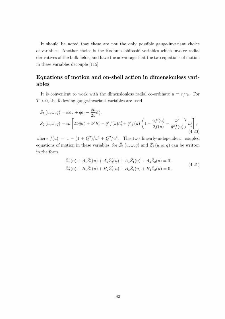
It should be noted that these are not the only possible gauge-invariant choice

of variables. Another choice is the Kodama-Ishibashi variables which involve radial

derivatives of the bulk fields, and have the advantage that the two equations of motion

in these variables decouple [115].

Equations of motion and on-shell action in dimensionless vari-ables

It is convenient to work with the dimensionless radial co-ordinate u ≡ r/r0. For

T > 0, the following gauge-invariant variables are used

Z1 (u, ω, q) = ωax + qat −qµ

2uhyy,

Z2 (u, ω, q) = iµ

[2ωqhxt + ω2hxx − q2f(u)htt + q2f(u)

(1 +

uf ′(u)

2f(u)− ω2

q2f(u)

)hyy

],

(4.20)

where f(u) = 1 − (1 + Q2)/u3 + Q2/u4. The two linearly-independent, coupled

equations of motion in these variables, for Z1 (u, ω, q) and Z2 (u, ω, q) can be written

in the form

Z ′′1 (u) + A1Z′1(u) + A2Z

′2(u) + A3Z1(u) + A4Z2(u) = 0,

Z ′′2 (u) +B1Z′1(u) +B2Z

′2(u) +B3Z1(u) +B4Z2(u) = 0,

(4.21)

82

where the dependence of Z1,2 on ω and q has been suppressed, and the coefficients

are

A1 =u5f ′(u)ω2 + 2f(u) [Q2q2 + u4 (ω2 − f(u)q2)]

u5f(u) (ω2 − f(u)q2),

A2 = −iq u5f ′(u)q2 + 2 [Q2q2 − u4 (ω2 − f(u)q2)]

u6 (ω2 − f(u)q2) [uf ′(u)q2 − 4 (ω2 − f(u)q2)],

A3 =Q2 [u2 (ω2 − f(u)q2)− 4f(u)]

u6f(u)2+

4Q2q2

u6 (ω2 − f(u)q2)

+8Q2q2 [u4 (ω2 − f(u)q2) +Q2q2]

u10 (ω2 − f(u)q2) [uf ′(u)q2 − 4 (ω2 − f(u)q2)],

A4 = iq4Q2 + u5f ′(u)

u7f(u) [uf ′(u)q2 − 4 (ω2 − f(u)q2)],

B1 = −iq2Q2 [uf ′(u)q2 − 4 (ω2 − f(u)q2)]

u4 (ω2 − f(u)q2),

B2 =1

u5f(u) (ω2 − f(u)q2) [uf ′(u)q2 − 4 (ω2 − f(u)q2)]

−16u4f(u)3q4

+ 2f(u)2q2[−4Q2q2 + 16u4ω2 + u5 (f ′(u) + uf ′′(u)) q2

]− f(u)

[−8Q2q2ω2 + 16u4ω4 + uq2

f ′(u)

(2Q2q2 − 2u4ω2 + u5f ′(u)q2

)+ 2u5f ′′(u)ω2

]+ u5f ′(u)ω2

[uf ′(u)q2 − 4ω2

],

B3 =8iQ2q

u9f(u) (ω2 − f(u)q2) [uf ′(u)q2 − 4 (ω2 − f(u)q2)]

u5f ′(u)ω2[uf ′(u)q2 − 4ω2]

− f(u)q2[−4Q2ω2 + uf ′(u)

(Q2q2 − 3u4ω2 + u5f ′(u)q2

)+ u6f ′′(u)ω2

]+ f(u)2q4

[−4Q2 + u5 (f ′(u) + uf ′′(u))

],

B4 =1

u4f(u)2 [uf ′(u)q2 − 4 (ω2 − f(u)q2)]

−4Q2f(u)2q4 +Q2ω2

[uf ′(u)q2 − 4ω2

]+ f(u)q2

[8Q2ω2 + uf ′(u)

(u4f ′′(u) + 5u3f ′(u)−Q2q2

)].

(4.22)

In these variables, the off-shell action to quadratic order in the fluctuations is of

83

the form

S =r0

2κ24

∫ ∞1

dudωd2q

(2π)3

[G11∂uZ1(u,−ω,−q)∂uZ1(u, ω, q) + G12∂uZ1(u,−ω,−q)∂uZ2(u, ω, q)

+ G21∂uZ2(u,−ω,−q)∂uZ1(u, ω, q) + G22∂uZ2(u,−ω,−q)∂uZ2(u, ω, q) + . . .],

(4.23)

where the coefficients are

G11 =2u2f(u)

ω2 − f(u)q2,

G12 = − 2iquf(u)

(ω2 − f(u)q2) [−4 (ω2 − f(u)q2) + uf ′(u)q2],

G21 = −G12,

G22 =2u4f(u)

[(ω2 − f(u)q2) + q2Q2

u4

]Q2 (ω2 − f(u)q2) [−4 (ω2 − f(u)q2) + q2uf ′(u)]2

,

(4.24)

and the ‘. . .’ represents terms with less than two u derivatives (which cannot gener-

ically be written in terms of these gauge-invariant variables). These coefficients,

combined with the equations of motion listed previously, allow one to compute the

Green’s function’s poles and spectral functions χεε, χQQ by following the method

of [112]. Note that the counter-terms in (4.6) (listed, for example, in [3]) do not affect

these quantities.

To compute the poles and spectral functions, the numerical procedure described

in [112] is used. This procedure involves a numerical check which relies on the co-

efficients of the one-derivative terms in the action in addition to the two-derivative

terms. Hence to obtain a numerical check in the present gauge-invariant formalism, a

boundary ‘counter-term’ has been added (distinct from those mentioned previously)

to the off-shell action of the form

Sc.t. =r0

2κ24

∫dudωd2q

(2π)3

d

du

[φI (u,−ω,−q)Dc.t.

IJ (u, ω, q)φJ (u, ω, q)], (4.25)

where Dc.t.IJ (u, ω, q) was chosen such that the full off-shell action could then be written

in terms of the gauge-invariant variables Z1,2. This boundary term does not alter the

equations of motion and as the coefficients Dc.t.IJ are purely real, it does not have any

effect upon the poles of the Green’s functions or the diagonal spectral functions χεε

and χQQ.

At T = 0, on the other hand, the Kodama-Ishibashi variables are used following

the methods described in [3]. The equations of motion in these variables are given in

84

appendix A of [3]. Accurate numerics at T = 0 are only expected above q & 0.1, and

hence only T = 0 results in this range are presented.

4.3 Temperature dependence of the sound mode

The primary motivation for studying this theory is that it supports stable, propa-

gating excitations of energy and charge density at zero temperature and large chemical

potential q 1. These sound modes at zero temperature have a dispersion relation

of the form (4.1) where the speed is vs = 1/√

2 [3]. One would want to know what

effect the increase of temperature has upon this mode - in particular one is interested

to see if it shares the characteristics of the ‘zero sound’ mode of a Landau Fermi liq-

uid. This comparison can be made by studying the sound attenuation as a function

of temperature for T µ and looking for the three different regimes shown in figure

4.1.

Note that when µ = 0 and ω, q T , there are sound modes with the dispersion

relation

ω = ± 1√2q − i 1

8πTq2 +O(q3). (4.26)

At non-zero µ, we would expect to recover these results when µ ω, q T , which

is outside of the ‘quantum liquid’ regime T µ where any LFL-like behaviour would

be present.

The temperature dependence of the real and imaginary parts of the sound mode

are shown in figures 4.2 and 4.3 for various q < 1. The finite temperature numerical

results are shown along with T = 0 numerical results (for q ≥ 0.1 where accurate

results can be obtained) and the µ = 0 analytic result (4.26).

The plots show that both the real and imaginary parts of the mode have a non-

trivial temperature dependence. As the temperature is increased from zero, finite

temperature corrections cause small changes to the real part of the sound mode whose

sign depends upon the value of q. At sufficiently high temperature, T/µ & 1, the real

part quickly asymptotes to the µ = 0 hydrodynamic result (4.26). The imaginary part

of the sound mode shows similar behaviour. This is slightly surprising - it indicates

that the µ = 0 result (4.26) is valid when q µ T . This will be reviewed in

section 4.6.

85

0.0 0.5 1.0 1.5 2.0 2.50.00700

0.00702

0.00704

0.00706

0.00708

0.00710

TΜ

ReH

ΩL

Sound mode, q=0.01

(a)

´

0.0 0.5 1.0 1.5 2.0 2.50.0700

0.0702

0.0704

0.0706

0.0708

0.0710

TΜ

ReH

ΩL

Sound mode, q=0.1

(b)

´

0.0 0.5 1.0 1.5 2.0 2.50.206

0.208

0.210

0.212

0.214

0.216

TΜ

ReH

ΩL

Sound mode, q=0.3

(c)

´

0.0 0.5 1.0 1.5 2.0 2.50.348

0.350

0.352

0.354

0.356

0.358

TΜ

ReH

ΩL

Sound mode, q=0.5

(d)

Figure 4.2: Variation of the real part of the sound mode as the temperature is increased.The crosses mark the T = 0 numerical results, the dots are the numerical results for T > 0,and the solid lines are the µ = 0 analytic result (4.26).

To make an easier comparison with Landau Fermi liquid theory, the temperature

dependence of the imaginary part of the sound mode is plotted on a logarithmic scale

in figure 4.4. These plots show only the region T < µ where one may expect such a

theory to apply, and the imaginary part of the sound mode is normalised by ω0, its

value at the lowest non-zero temperature that can be accessed.

There is a stark contrast between these plots and the results expected for an LFL

zero sound mode, shown in figure 4.1.2 Landau’s theory predicts that as the tem-

2The magnitude of the frequency of the sound mode in the RN-AdS4 theory is of the same orderas its momentum for the results shown, and thus comparisons are made to the LFL results withω → q.

86

0.0 0.5 1.0 1.5 2.0 2.5-0.00001

-8. ´ 10-6

-6. ´ 10-6

-4. ´ 10-6

-2. ´ 10-6

0

TΜ

ImHΩ

L

Sound mode, q=0.01

(a)

´

0.0 0.5 1.0 1.5 2.0 2.5-0.0010

-0.0008

-0.0006

-0.0004

-0.0002

0.0000

TΜ

ImHΩ

L

Sound mode, q=0.1

(b)

´

0.0 0.5 1.0 1.5 2.0 2.5-0.010

-0.008

-0.006

-0.004

-0.002

0.000

TΜ

ImHΩ

L

Sound mode, q=0.3

(c)

´

0.0 0.5 1.0 1.5 2.0 2.5-0.030

-0.025

-0.020

-0.015

-0.010

-0.005

0.000

TΜ

ImHΩ

L

Sound mode, q=0.5

(d)

Figure 4.3: Variation of the imaginary part of the sound mode as the temperature is in-creased. The crosses marks the T = 0 numerical results, the dots are the numerical resultsfor T > 0, and the solid lines are the µ = 0 analytic result (4.26).

87

(a) (b)

(c) (d)

Figure 4.4: Variation of the imaginary part of the sound mode as the temperature is in-creased, in the regime T < µ. The dots are the numerical results for T > 0, and the twodashed lines on each plot denote T/µ = q/µ and T/µ =

√q/µ as one moves to the right

along the plot.

88

+ + + + +++

++

++

++

+

++

+crossover to diffusion

-5 -4 -3 -2 -1 0-1

0

1

2

3

4

5

Log@TΜD

Log

@ImΩ

HTLI

mΩ

H0LD

Figure 4.5: A superposition of the plots of the temperature dependence of the normalisedimaginary part of the sound mode when q/µ = 0.2 for both the D3/D7 theory and theRN-AdS4 theory. Crosses denote the D3/D7 numerical results [2] and circles denote theRN-AdS4 results. Moving from left to right, the dotted lines mark the transition pointsbetween the quantum and thermal collisionless regimes, and the thermal collisionless regimeand the hydrodynamic regime, in the D3/D7 theory. These occur when ω ∼ T and ω ∼ T 2/µrespectively. There are no results for the D3/D7 sound mode in the hydrodynamic regimesince the hydrodynamic sound mode is suppressed in the probe brane limit. We refer thereader to [2] for a more detailed discussion of these features.

perature is increased at fixed q and µ, the imaginary part of the zero sound mode

should be approximately constant up until T/µ ∼ q/µ. Between T/µ ∼ q/µ and

T/µ ∼√q/µ, it should increase like T 2. Above T/µ ∼

√q/µ and below T/µ ∼ 1, it

should decrease like T 2. None of these features are present in our results. The mag-

nitude of the imaginary part of the sound mode in our theory shows no significant

temperature dependence until T ∼ µ. Above this, it begins to approach the µ = 0,

ω, q T result (4.26) where it decreases as 1/T .

An explicit comparison between these RN-AdS4 results and the corresponding

D3/D7 results is shown in figure 4.5. This highlights the fact that the D3/D7 sound

mode behaves like the LFL zero sound mode, whereas the RN-AdS4 sound mode does

not.

89

4.4 Further temperature-dependent properties of

the theory when q < 1

In addition to the sound modes at T = 0, there are other propagating modes lying

deeper in the complex frequency plane as well as a branch cut along the negative

imaginary frequency axis [3]. In this section, changes in this configuration are studied

as T/µ is increased at a fixed momentum q < 1. In particular, attention is focused

on the longest-lived purely imaginary mode - this exists at non-zero temperatures as

the branch cut mentioned above dissolves into a series of poles when T 6= 0. We note

here that when µ = 0 and ω, q T , the longest-lived purely imaginary mode has the

dispersion relation

ω = −i 3

4πTq2 +O(q3), (4.27)

corresponding to hydrodynamic charge diffusion [109]. One expects to recover this

behaviour at non-zero µ in the limit µ ω, q T .

It is also shown in this section how the energy density and charge density spec-

tral functions of the theory change with the temperature, and in particular how the

residues of the long-lived modes play an important role in the transition from sound

domination of the charge density spectral function to diffusion domination.

Temperature dependence of the diffusion mode

The study begins with the longitudinal diffusion mode of the theory. At T = 0, the

negative imaginary frequency axis is a branch cut [3]. At non-zero temperatures, this

branch cut dissolves into a series of poles along the axis and generically these become

less stable (they recede into the complex plane) as the temperature is increased.

However, one of the modes is special in that it becomes more stable as the temperature

is increased, and at very high temperatures it becomes the µ = 0 hydrodynamic charge

diffusion mode (4.27). Figure 4.6 shows how the imaginary part of this mode changes

with the temperature. Its real part is always zero. Unlike for the sound mode, this

plot has the same shape for all values of 0.01 ≤ q ≤ 0.5 and so we show only one for

brevity. The decay rate of this mode decreases monotonically as the temperature is

increased, and is described well by the µ = 0 result (4.27) when T & µ. Again, it is

non-trivial that the µ = 0 result holds in the regime q µ T . Note that there is

no T = 0 point on this plot because it does not make sense to ask where the pole is

in that case - the whole negative imaginary frequency axis forms a branch cut.

90

0.0 0.5 1.0 1.5 2.0 2.5-0.25

-0.20

-0.15

-0.10

-0.05

0.00

TΜ

ImHΩ

L

Diffusion mode, q=0.5

Figure 4.6: Variation of the imaginary part of the longitudinal diffusion mode as the tem-perature is increased. The dots are the numerical results for T > 0, and the solid line is theµ = 0 analytic result (4.27).

Movement of the poles in the complex frequency plane withtemperature

It is instructive to view the simultaneous movement of the Green’s function poles

described previously in the complex frequency plane as the temperature is increased

- this is shown in figure 4.7. As described previously, the sound and diffusion modes

both become more stable, approaching the real axis as the temperature is increased.

Note that the sound mode is closer to the real axis than the diffusion mode for all

values of the temperature and thus it is always the longest-lived mode of the theory.

However this does not mean that it always dominates the low-energy properties of the

theory, as it will be shown in the following subsection. Finally, it must be noted that

both the sound and diffusion poles coexist for all non-zero values of the temperature

that we can access numerically (T & 0.02µ). This is in contrast to the strongly-

coupled D3/D7 field theory in which the low temperature sound poles collide to form

the high temperature diffusion pole [2].

In addition to the sound and diffusion poles, there are ‘secondary’ modes corre-

sponding to poles lying deeper in the complex frequency plane. These are much

shorter-lived than the sound and diffusion poles when q < 1 and become less stable

91

´ ´

´

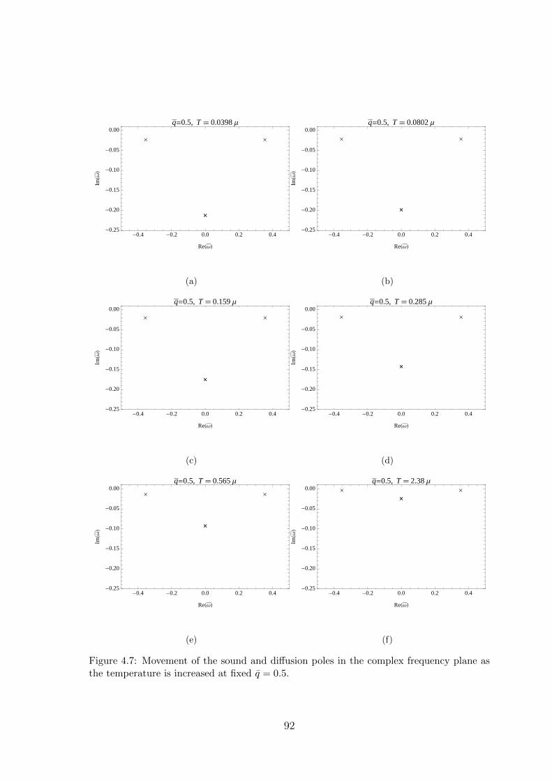
-0.4 -0.2 0.0 0.2 0.4-0.25

-0.20

-0.15

-0.10

-0.05

0.00

ReHΩL

ImHΩ

L

q=0.5, T 0.0398 Μ

(a)

´ ´

´

-0.4 -0.2 0.0 0.2 0.4-0.25

-0.20

-0.15

-0.10

-0.05

0.00

ReHΩL

ImHΩ

L

q=0.5, T 0.0802 Μ

(b)

´ ´

´

-0.4 -0.2 0.0 0.2 0.4-0.25

-0.20

-0.15

-0.10

-0.05

0.00

ReHΩL

ImHΩ

L

q=0.5, T 0.159 Μ

(c)

´ ´

´

-0.4 -0.2 0.0 0.2 0.4-0.25

-0.20

-0.15

-0.10

-0.05

0.00

ReHΩL

ImHΩ

L

q=0.5, T 0.285 Μ

(d)

´ ´

´

-0.4 -0.2 0.0 0.2 0.4-0.25

-0.20

-0.15

-0.10

-0.05

0.00

ReHΩL

ImHΩ

L

q=0.5, T 0.565 Μ

(e)

´ ´

´

-0.4 -0.2 0.0 0.2 0.4-0.25

-0.20

-0.15

-0.10

-0.05

0.00

ReHΩL

ImHΩ

L

q=0.5, T 2.38 Μ

(f)

Figure 4.7: Movement of the sound and diffusion poles in the complex frequency plane asthe temperature is increased at fixed q = 0.5.

92

as the temperature is increased. They do not have a significant effect on the low

energy properties of the theory when q < 1 and hence their temperature dependence

is not shown.

Variation of the spectral functions with temperature

Up to this point, attention has been exclusively focused on the positions of the poles

of the retarded Green’s functions in the complex frequency plane. While these are

interesting, they do not tell the full story of how charge and energy are transported

in the theory. To investigate this, one needs to turn one’s attention to the spectral

functions of the energy density and charge density. These determine the average work

done on the system when an external source of some frequency is applied to either the

energy density or the charge density respectively. Despite the fact that the retarded

Green’s functions of both of these operators have the same set of poles, their spectral

functions are quite different as shown in figures 4.8 and 4.9.

At very low temperatures, both spectral functions are dominated by the peak corre-

sponding to sound propagation. As the temperature is increased, the spectral function

of the energy density undergoes a fairly unremarkable change - the sound peak be-

comes narrower and taller (corresponding to a longer-lived excitation) but completely

dominates at all temperatures. In contrast to this, the sound peak of the charge den-

sity spectral function becomes smaller (and narrower) as the temperature increases.

At a sufficiently high temperature it becomes so small that the peak around ω = 0,

corresponding to the high temperature diffusion mode, dominates the spectral func-

tion. At what temperature does this crossover occur? In figure 4.10, it is shown how

the crossover value of µ/T (i.e. the value where the sound and diffusion peaks are of

the same height) varies with q/µ. There is a clear linear relationship, signifying that

the crossover occurs when

Tcross. ∼ µ2/q, (4.28)

and that diffusion dominates when T µ2/q. Note that since we are studying the

range q < 1, this condition automatically implies that T µ. This crossover is

reminiscent of the µ→ 0 limit. In that limit, the fluctuations of T µν and Jµ decouple

resulting in a hydrodynamic sound pole in the T µν correlators and a hydrodynamic

diffusion pole in the Jµ correlators. The charge density spectral function in this limit

is shown in [116]. However, it is not possible to interpret the crossover shown above

to be due to approaching this limit, since it corresponds to the limit µ q, T of the

results, whereas the regime studied here is q µ T .

93

0.0 0.2 0.4 0.6 0.8 1.00

2.0 ´ 100

4.0 ´ 100

6.0 ´ 100

8.0 ´ 100

Ω

ΧΕΕ

q 0.5 , T 0.0219 Μ

(a)

0.0 0.2 0.4 0.6 0.8 1.00

1.0 ´ 101

2.0 ´ 101

3.0 ´ 101

4.0 ´ 101

5.0 ´ 101

6.0 ´ 101

7.0 ´ 101

Ω

ΧΕΕ

q 0.5 , T 0.565 Μ

(b)

0.0 0.2 0.4 0.6 0.8 1.00

1.0 ´ 102

2.0 ´ 102

3.0 ´ 102

4.0 ´ 102

Ω

ΧΕΕ

q 0.5 , T 1.18 Μ

(c)

0.0 0.2 0.4 0.6 0.8 1.00

2.0 ´ 103

4.0 ´ 103

6.0 ´ 103

8.0 ´ 103

1.0 ´ 104

Ω

ΧΕΕ

q 0.5 , T 3.4 Μ

(d)

0.0 0.2 0.4 0.6 0.8 1.00

2.0 ´ 104

4.0 ´ 104

6.0 ´ 104

8.0 ´ 104

1.0 ´ 105

1.2 ´ 105

Ω

ΧΕΕ

q 0.5 , T 7.96 Μ

(e)

0.0 0.2 0.4 0.6 0.8 1.00

5.0 ´ 108

1.0 ´ 109

1.5 ´ 109

2.0 ´ 109

2.5 ´ 109

3.0 ´ 109

Ω

ΧΕΕ

q 0.5 , T 239. Μ

(f)

Figure 4.8: The energy density spectral function for q = 0.5 as the temperature is increased,in units of 2µ2r0/κ

24. The peak due to sound propagation dominates at all temperatures.

94

0.0 0.2 0.4 0.6 0.8 1.00

5.0 ´ 100

1.0 ´ 101

1.5 ´ 101

2.0 ´ 101

2.5 ´ 101

Ω

ΧQ

Q

q 0.5 , T 0.0219 Μ

(a)

0.0 0.2 0.4 0.6 0.8 1.00

2.0 ´ 100

4.0 ´ 100

6.0 ´ 100

8.0 ´ 100

1.0 ´ 101

Ω

ΧQ

Q

q 0.5 , T 0.565 Μ

(b)

0.0 0.2 0.4 0.6 0.8 1.00

1.0 ´ 100

2.0 ´ 100

3.0 ´ 100

4.0 ´ 100

5.0 ´ 100

Ω

ΧQ

Q

q 0.5 , T 1.18 Μ

(c)

0.0 0.2 0.4 0.6 0.8 1.00

2.5 ´ 10-1

5.0 ´ 10-1

7.5 ´ 10-1

1.0 ´ 100

1.2 ´ 100

1.5 ´ 100

1.8 ´ 100

Ω

ΧQ

Qq 0.5 , T 3.4 Μ

(d)

0.0 0.2 0.4 0.6 0.8 1.00

2.0 ´ 10-1

4.0 ´ 10-1

6.0 ´ 10-1

8.0 ´ 10-1

1.0 ´ 100

Ω

ΧQ

Q

q 0.5 , T 7.96 Μ

(e)

0.0 0.2 0.4 0.6 0.8 1.00

2.0 ´ 10-1

4.0 ´ 10-1

6.0 ´ 10-1

8.0 ´ 10-1

1.0 ´ 100

Ω

ΧQ

Q

q 0.5 , T 239. Μ

(f)

Figure 4.9: The charge density spectral function for q = 0.5 as the temperature is increased,in units of 2r0/κ

24. There is a crossover between sound domination and diffusion domination

at high temperature.

95

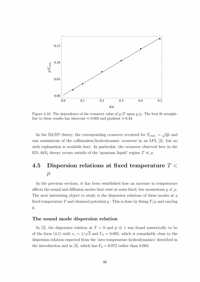
0.0 0.1 0.2 0.3 0.4 0.50.00

0.05

0.10

0.15

qΜ

ΜT

cros

s.

Figure 4.10: The dependence of the crossover value of µ/T upon q/µ. The best fit straight-line to these results has intercept ≈ 0.003 and gradient ≈ 0.34.

In the D3/D7 theory, the corresponding crossover occurred for Tcross. ∼√qµ and

was reminiscent of the collisionless/hydrodynamic crossover in an LFL [2], but no

such explanation is available here. In particular, the crossover observed here in the

RN-AdS4 theory occurs outside of the ‘quantum liquid’ regime T µ.

4.5 Dispersion relations at fixed temperature T <

µ

In the previous sections, it has been established how an increase in temperature

affects the sound and diffusion modes that exist at some fixed, low momentum q µ.

The next interesting object to study is the dispersion relations of these modes at a

fixed temperature T and chemical potential µ. This is done by fixing T/µ and varying

q.

The sound mode dispersion relation

In [3], the dispersion relation at T = 0 and q 1 was found numerically to be

of the form (4.1) with vs = 1/√

2 and Γ0 = 0.083, which is remarkably close to the

dispersion relation expected from the ‘zero temperature hydrodynamics’ described in

the introduction and in [3], which has Γ0 = 0.072 rather than 0.083.

96

++

´

0.0 0.5 1.0 1.5 2.0 2.50.00

0.02

0.04

0.06

0.08

TΜ

G

Figure 4.11: The temperature dependence of the quadratic term Γ in the imaginary part ofthe sound dispersion relation (4.4). Circles show our numerical results, the solid line showsthe µ = 0 analytic result (4.26), the ‘+’ shows the T = 0 numerical result of [3] and the ‘×’shows the prediction of ‘T = 0 hydrodynamics’.

Here a dispersion relation of the form (4.4) was found to be valid for non-zero

temperatures also. The quadratic coefficient of the attenuation Γ as a function of

temperature is shown in figure 4.11. These results were obtained by fitting over the

range 0.01 ≤ q ≤ 0.5, and an example of the fit for T = 0.0219µ is shown in figure

4.12. At high temperatures T µ, it agrees with the µ = 0 result (4.26), and at low

temperatures T µ it approaches a similar value to the T = 0 result of [3]. Although

the results at very low T do not match smoothly onto the T = 0 numerical result

of [3], they differ only by around 10% and it is believed that this is most likely caused

by numerical inaccuracies, which grow as the temperature is lowered. The proximity

of the numerical results to the prediction of ‘T = 0 hydrodynamics’ is surprising -

ultimately, an analytic calculation will be needed to determine whether these small

discrepancies are due to inaccurate numerics, or whether this proximity is in fact a

coincidence. The general trend of the results is clear however - as the temperature

increases, the sound mode becomes more stable, as was observed in section 4.3.

When q & 1, this series form of the dispersion relation is useless. Figure 4.13

shows the dispersion relation of the sound mode when q > µ > T , at two different

temperatures: T = 0 and T = 0.159µ. The dispersion relations have the same shape

97

0.0 0.1 0.2 0.3 0.4 0.50.00

0.05

0.10

0.15

0.20

0.25

0.30

0.35

q

ReH

ΩL

T=0.0219Μ sound mode

(a)

0.0 0.1 0.2 0.3 0.4 0.5-0.025

-0.020

-0.015

-0.010

-0.005

0.000

q

ImHΩ

L

T=0.0219Μ sound mode

(b)

Figure 4.12: The dispersion relation of the sound mode at T = 0.0219µ for 0.01 ≤ q ≤ 0.5.The circles show the numerical results and the solid line is the best fit ω ≈ q/

√2−i0.075q2+

O(q3).

´ ´ ´ ´ ´ ´´

´´

´

´

´

´

´

´

´

´

´

´

´

0 1 2 3 4 5 6 70

1

2

3

4

5

6

7

q

ReH

ΩL

Sound mode dispersion relation

(a)

´ ´ ´´

´´

´´

´´

´´

´´

´´

´

´

´´ ´ ´ ´ ´ ´ ´

0 1 2 3 4 5 6 7-0.6

-0.5

-0.4

-0.3

-0.2

-0.1

0.0

q

ImHΩ

L

Sound mode dispersion relation

(b)

Figure 4.13: The dispersion relation of the sound mode at two different temperatures: T = 0(circles) and T = 0.159µ (crosses). The dashed line is the line Re (ω) = q.

98

´ ´ ´ ´ ´´

´´

´´

´

´

´

´

´

´

´

0.0 0.5 1.0 1.5

-2.5

-2.0

-1.5

-1.0

-0.5

0.0

q

ImHΩ

L

Diffusion mode dispersion relation

(a) Numerical results

0.0 0.1 0.2 0.3 0.4 0.5

-0.20

-0.15

-0.10

-0.05

0.00

q

ImHΩ

L

Fit to diffusion mode dispersion relation, T=0.0219Μ

(b) Best fit

Figure 4.14: The dispersion relation of the diffusion mode at two different temperatures:T = 0.0219µ (circles) and T = 0.159µ (crosses) with the polynomial best fit at T = 0.0219µshown also (solid line). We cannot track the T = 0.0219µ mode for as high momenta as theT = 0.159µ mode.

at both temperatures - the real part asymptotes to ω = q, and the imaginary part

tends to a constant, in the region q µ > T .

The diffusion mode dispersion relation

Recall that at non-zero temperatures, the branch cut along the negative imaginary

frequency axis becomes a series of poles and that the most stable of these becomes

the µ = 0 diffusion mode at high temperatures. Figure 4.14a shows the imaginary

part of the dispersion relation of this pole at two fixed, low temperatures T = 0.0219µ

and T = 0.159µ (its real part is always zero). At both temperatures, the pole recedes

quickly into the complex plane as the momentum is increased. Performing a polyno-

mial fit to the imaginary part in the range 0.01 ≤ q ≤ 0.5 at the very low temperature

T = 0.0219µ, a dispersion relation of the form (4.5) is found, with D ≈ 0.83. The fit is

shown in figure 4.14b. This therefore is an analogue, at low temperatures T < q < µ,

of the µ = 0, q T hydrodynamic charge diffusion mode.

In fact, this quadratic form of the dispersion relation (4.5) is valid for all non-

zero temperatures that could be accessed - the dependence of D upon T is shown in

figure 4.15. D was extracted from a fit over the range 0.01 ≤ q ≤ 0.5. It decreases

monotonically as the temperature is raised, in agreement with the results of section

99

0.0 0.5 1.0 1.5 2.0 2.50.0

0.2

0.4

0.6

0.8

TΜ

D

Figure 4.15: The temperature dependence of the quadratic coefficient D in the dispersionrelation of the diffusion mode (4.5). The circles show the numerical results and the solidline is the analytic µ = 0 result (4.27).

4.4, and approaches the µ = 0 result (4.27) in the limit T µ. Again, it should be

noted that this is despite the fact that the regime µ q is studied.

It has not been possible to obtain the numerical accuracy required to access non-

zero temperatures lower than T = 0.0219µ and hence it is impossible to say whether

the mode exists with a quadratic dispersion relation for arbitrarily low non-zero tem-

peratures. It is emphasized again that this mode does not exist at T = 0 itself (unlike

the T = 0 ‘R-spin diffusion’ mode of [91]), as there is a branch cut in that case.

Dispersion relations of the secondary modes

Figures 4.16 and 4.17 show the dispersion relations of the second stablest (‘sec-

ondary’) propagating and purely imaginary modes at two different temperatures.

These differ qualitatively from the sound and diffusion modes described above in that

ω 6= 0 when q = 0. At high momenta q µ > T , the propagating secondary modes

have the same form as the sound modes - their real parts asymptote to Re (ω) = q

and their imaginary parts tend to a constant. The purely imaginary secondary mode

recedes into the complex plane as the momentum is increased, and the rate at which

this happens increases with the temperature.

100

´ ´ ´ ´ ´ ´ ´ ´ ´ ´

´

´

´

´

´

´

´

´

´

´

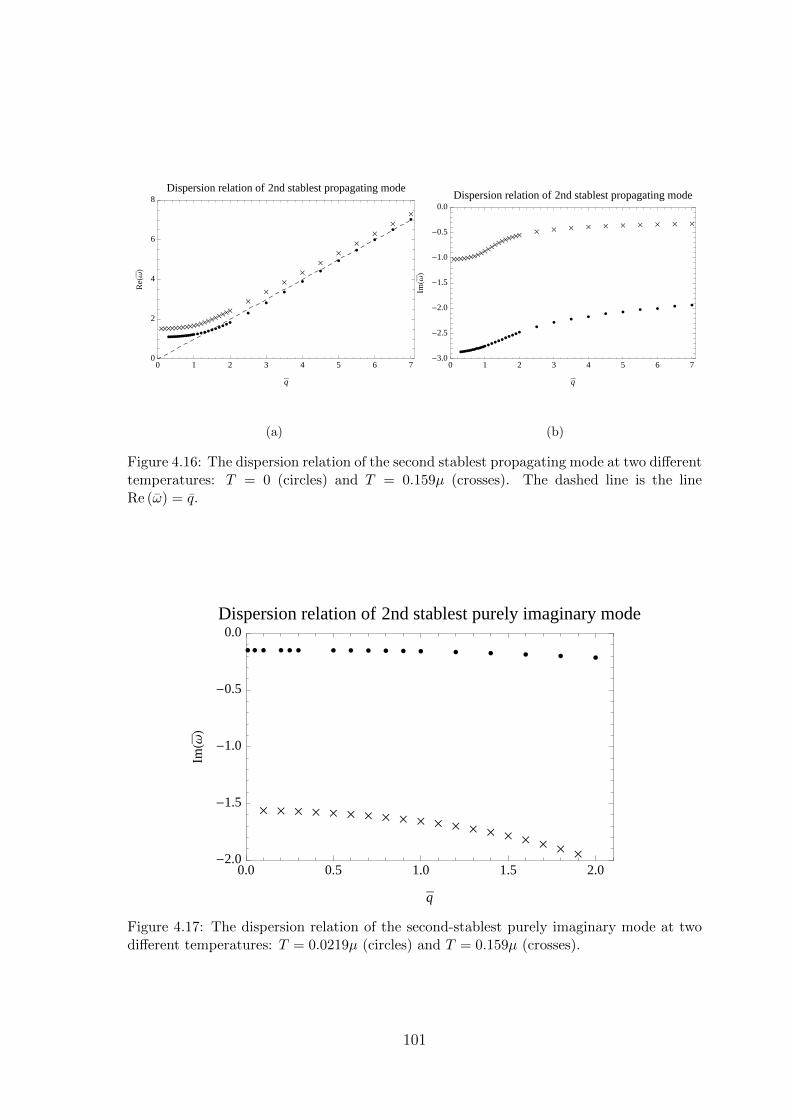
0 1 2 3 4 5 6 70

2

4

6

8

q

ReH

ΩL

Dispersion relation of 2nd stablest propagating mode

(a)

´ ´ ´ ´ ´´

´ ´ ´ ´´ ´ ´ ´ ´ ´ ´ ´ ´ ´

0 1 2 3 4 5 6 7-3.0

-2.5

-2.0

-1.5

-1.0

-0.5

0.0

q

ImHΩ

L

Dispersion relation of 2nd stablest propagating mode

(b)

Figure 4.16: The dispersion relation of the second stablest propagating mode at two differenttemperatures: T = 0 (circles) and T = 0.159µ (crosses). The dashed line is the lineRe (ω) = q.

´ ´ ´ ´ ´ ´ ´ ´ ´ ´ ´ ´ ´ ´ ´ ´ ´ ´ ´

0.0 0.5 1.0 1.5 2.0-2.0

-1.5

-1.0

-0.5

0.0

q

ImHΩ

L

Dispersion relation of 2nd stablest purely imaginary mode

Figure 4.17: The dispersion relation of the second-stablest purely imaginary mode at twodifferent temperatures: T = 0.0219µ (circles) and T = 0.159µ (crosses).

101

Movement of the poles in the complex frequency plane withmomentum

It is instructive to view the simultaneous movements of these poles in the complex

frequency plane as the momentum is increased. This is shown in figure 4.18 for

T = 0.159µ. It is apparent that as q is increased, the purely imaginary modes both

become less stable as described previously. This figure shows that the diffusion mode

destabilises much quicker than the secondary imaginary mode. The propagating

modes show a different behaviour - their speeds both increase but their imaginary

parts move in opposite directions and begin to approach each other in the complex

plane as q increases. They eventually cross, before moving off horizontally together

along the relativistic trajectory Re (ω) = q. At these high values of q it is clear

that our original separation of modes into the stablest (sound and diffusion), second

stablest etc. is of no value.

Variation of the spectral functions with momentum

Finally, attention is turned towards the spectral functions of the theory at low

temperatures and as a function of the momentum q. These are shown in figures 4.19

and 4.20 for T = 0.159µ. At q = 0.5, the lowest momentum shown, both spectral

functions are completely dominated by the peak due to sound propagation. As the

momentum is increased, this peak becomes smaller and wider and when q & µ, it

no longer dominates the spectral function - a peak due to the secondary propagating

mode also becomes visible. As the momentum is increased further, these two peaks

merge into one peak which moves with speed Re (ω) = q and constant width. This is

a direct reflection of the two corresponding Green’s function poles approaching each

other in the complex plane. At high momenta, the value of the spectral function is

very small at low frequencies ω . q and it only becomes significant when ω & q. Note

that there is no significant difference between the charge density and energy density

spectral functions in this regime.

4.6 An effective hydrodynamic scale

As discussed previously, when µ = 0 there is a long-lived sound mode with mo-

mentum q provided that q T , and when T = 0 there is a long-lived sound mode

provided that q µ. In the first instance, this is the regime of applicability of hydro-

102

´´

´

-10 -5 0 5 10-2.0

-1.5

-1.0

-0.5

0.0

ReHΩL

ImHΩ

L

T=0.159Μ, q 0.5

(a)

´´

´

-10 -5 0 5 10-2.0

-1.5

-1.0

-0.5

0.0

ReHΩL

ImHΩ

L

T=0.159Μ, q 1.

(b)

´´

´-10 -5 0 5 10

-2.0

-1.5

-1.0

-0.5

0.0

ReHΩL

ImHΩ

L

T=0.159Μ, q 1.5

(c)

´´

-10 -5 0 5 10-2.0

-1.5

-1.0

-0.5

0.0

ReHΩL

ImHΩ

LT=0.159Μ, q 2.

(d)

´´

-10 -5 0 5 10-2.0

-1.5

-1.0

-0.5

0.0

ReHΩL

ImHΩ

L

T=0.159Μ, q 4.5

(e)

´´

-10 -5 0 5 10-2.0

-1.5

-1.0

-0.5

0.0

ReHΩL

ImHΩ

L

T=0.159Μ, q 7.

(f)

Figure 4.18: Movement of the six longest-lived modes in the complex frequency plane as afunction of momentum, for fixed T = 0.159µ. The crosses denote the sound and diffusionmodes, and the circles denote the secondary propagating and imaginary modes.

103

0 2 4 6 8 100

2.0 ´ 100

4.0 ´ 100

6.0 ´ 100

8.0 ´ 100

1.0 ´ 101

1.2 ´ 101

Ω

ΧΕΕ

T=0.159Μ, q=0.5

(a)

0 2 4 6 8 100

1.0 ´ 100

2.0 ´ 100

3.0 ´ 100

4.0 ´ 100

5.0 ´ 100

6.0 ´ 100

7.0 ´ 100

Ω

ΧΕΕ

T=0.159Μ, q=1.0

(b)

0 2 4 6 8 100

1.0 ´ 100

2.0 ´ 100

3.0 ´ 100

4.0 ´ 100

5.0 ´ 100

6.0 ´ 100

Ω

ΧΕΕ

T=0.159Μ, q=2.0

(c)

0 2 4 6 8 100

1.0 ´ 100

2.0 ´ 100

3.0 ´ 100

4.0 ´ 100

5.0 ´ 100

6.0 ´ 100

7.0 ´ 100

Ω

ΧΕΕ

T=0.159Μ, q=2.5

(d)

0 2 4 6 8 100

2.0 ´ 100

4.0 ´ 100

6.0 ´ 100

8.0 ´ 100

1.0 ´ 101

1.2 ´ 101

1.4 ´ 101

Ω

ΧΕΕ

T=0.159Μ, q=3.5

(e)

0 2 4 6 8 100

2.0 ´ 101

4.0 ´ 101

6.0 ´ 101

8.0 ´ 101

1.0 ´ 102

1.2 ´ 102

Ω

ΧΕΕ

T=0.159Μ, q=6.5

(f)

Figure 4.19: The energy density spectral function for T = 0.159µ as the momentum isincreased, in units of 2µ2r0/κ

24. As the momentum is increased, the peak due to sound

propagation becomes less dominant.

104

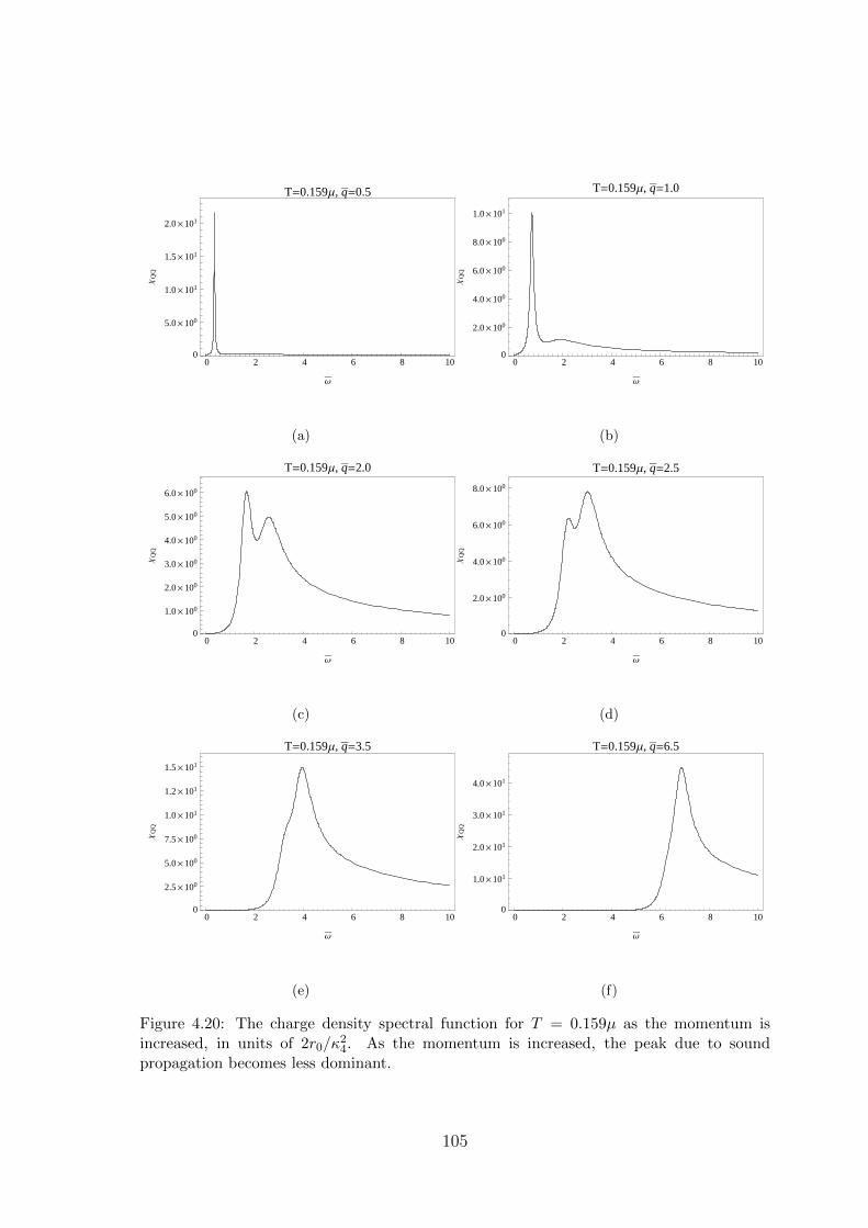
0 2 4 6 8 100

5.0 ´ 100

1.0 ´ 101

1.5 ´ 101

2.0 ´ 101

Ω

ΧQ

Q

T=0.159Μ, q=0.5

(a)

0 2 4 6 8 100

2.0 ´ 100

4.0 ´ 100

6.0 ´ 100

8.0 ´ 100

1.0 ´ 101

Ω

ΧQ

Q

T=0.159Μ, q=1.0

(b)

0 2 4 6 8 100

1.0 ´ 100

2.0 ´ 100

3.0 ´ 100

4.0 ´ 100

5.0 ´ 100

6.0 ´ 100

Ω

ΧQ

Q

T=0.159Μ, q=2.0

(c)

0 2 4 6 8 100

2.0 ´ 100

4.0 ´ 100

6.0 ´ 100

8.0 ´ 100

Ω

ΧQ

Q

T=0.159Μ, q=2.5

(d)

0 2 4 6 8 100

2.5 ´ 100

5.0 ´ 100

7.5 ´ 100

1.0 ´ 101

1.2 ´ 101

1.5 ´ 101

Ω

ΧQ

Q

T=0.159Μ, q=3.5

(e)

0 2 4 6 8 100

1.0 ´ 101

2.0 ´ 101

3.0 ´ 101

4.0 ´ 101

Ω

ΧQ

Q

T=0.159Μ, q=6.5

(f)

Figure 4.20: The charge density spectral function for T = 0.159µ as the momentum isincreased, in units of 2r0/κ

24. As the momentum is increased, the peak due to sound

propagation becomes less dominant.

105

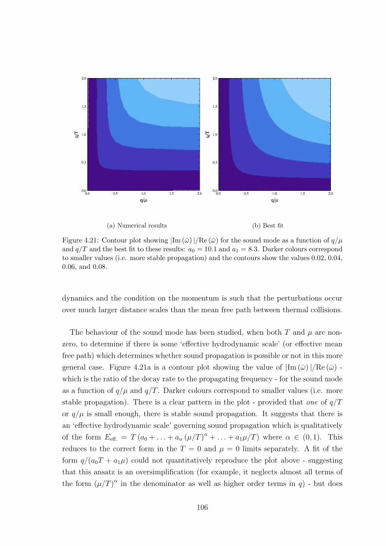
(a) Numerical results (b) Best fit

Figure 4.21: Contour plot showing |Im (ω) |/Re (ω) for the sound mode as a function of q/µand q/T and the best fit to these results: a0 = 10.1 and a1 = 8.3. Darker colours correspondto smaller values (i.e. more stable propagation) and the contours show the values 0.02, 0.04,0.06, and 0.08.

dynamics and the condition on the momentum is such that the perturbations occur

over much larger distance scales than the mean free path between thermal collisions.

The behaviour of the sound mode has been studied, when both T and µ are non-

zero, to determine if there is some ‘effective hydrodynamic scale’ (or effective mean

free path) which determines whether sound propagation is possible or not in this more

general case. Figure 4.21a is a contour plot showing the value of |Im (ω) |/Re (ω) -

which is the ratio of the decay rate to the propagating frequency - for the sound mode

as a function of q/µ and q/T . Darker colours correspond to smaller values (i.e. more

stable propagation). There is a clear pattern in the plot - provided that one of q/T

or q/µ is small enough, there is stable sound propagation. It suggests that there is

an ‘effective hydrodynamic scale’ governing sound propagation which is qualitatively

of the form Eeff. = T (a0 + . . .+ aα (µ/T )α + . . .+ a1µ/T ) where α ∈ (0, 1). This

reduces to the correct form in the T = 0 and µ = 0 limits separately. A fit of the

form q/(a0T + a1µ) could not quantitatively reproduce the plot above - suggesting

that this ansatz is an oversimplification (for example, it neglects almost all terms of

the form (µ/T )α in the denominator as well as higher order terms in q) - but does

106

give qualitatively the correct features for the sound propagation properties. Figure

4.21b shows the best fit to this form.

An effective hydrodynamic scale of this form is also consistent with the fact that

the region q µ T reproduces the µ = 0, q T results, as seen in section 4.3.

107

Chapter 5

Electron Star

Useful as it is, the Reissner-Nordstrom (RN) system exhibits a major complication,

when using it in comparison with Condensed Matter systems. This comes from the

peculiarity of Reissner-Nordstrom horizon. In particular it is well known (e.g. [113])

that at zero-temperature, i.e. at extremality, the area of the horizon does not van-

ish and given that the black hole’s entropy is proportional to the horizon area, the

system has non-zero entropy at zero temperature. This contradicts standard intu-

ition from Condensed Matter. Many attempts have been made to construct systems

that would have the necessary Holographic ingredients, the RN system provides, but

circumventing the finite entropy limitation. One such system is the Electron Star.

The system consists of an ideal fluid of bulk (in 3 + 1 dimensions) fermions which is

set-up in a similar way that the Neutron Star was constructed as a solution of Ein-

stein’s equations, resulting in the Tolman-Oppenheimer-Volkoff equations [117, 118].

In the infra-red regime and at zero temperature, the system asymptotes to a Lifshitz

background geometry. The absence of a horizon resolves the finite entropy problem.

Similarly at finite temperature, the system is a composite, consisting of an AdS-RN,

that provides the temperature to the system, followed by the electron cloud and finally

another AdS-RN up to the ultraviolet regime.

Another indication that extensions to the standard AdS-RN system need to be

considered is that in many cases, RN black holes have been found to be thermody-

namically unstable, transitioning to different systems. This transition involves the

discharge of the black hole via various mechanisms, resulting in some bulk field carry-

ing the charge that was “hiding” behind the horizon. Such mechanisms have been ex-

tensively explored and some indicative examples include, charged scalar field conden-

sation [11], fermion Cooper pairing [119], D-branes emission [82, 120, 121], fermionic

back-reaction [82], confinement [122–124] and lattice emergences [125]. Moreover

108

in [126] the more general issue of whether any finite-size-horizon black brane remains

stable at zero temperature, has been addressed.

5.1 Background

As introduced in [127–129] the Electron Star emerges as a solution to the Einstein-

Maxwell system with non-trivial stress-energy tensor. Namely, the Einstein equations

are

Rµν −1

2gµνR−

3

L2gµν = κ2

[1

e2

(FµσF

σν −

1

4gµνFρτF

ρτ

)+ Tµν

](5.1)

while the Maxwell equations are

∇αFβα = e2Jβ (5.2)

Here the crucial difference to the AdS-RN system is the non-trivial energy-momentum

tensor on the right-hand side of eq. (5.1), which given that one is dealing with a perfect

fluid, is

Tµν = (p+ ρ)uµuν + pgµν , Jµ = σuµ (5.3)

Where p, ρ, σ are the pressure, energy and charge density respectively. Moreover uµ is

the velocity field which is normalized so that u2 = −1, L is the characteristic length

scale of the AdS, e is the electromagnetic coupling, κ Newton’s constant (in d = 3+1).

As is usual the case one makes the black-brane ansatz in search for solutions to this

problem. Namely

ds2 = L2

[−f(r)dt2 +

1

r2(dx2 + dy2) + g(r)dr2

](5.4)

for the metric, while for the gauge field

A =eL

κh(r)dt (5.5)

In order to unclutter the formalism, as well as in anticipation of numerical calcula-

tions, it makes sense to rescale the fields in order to absorb the various constants. To

achieve this one rescales

p→ p =1

L2κ2p , ρ→ ρ =

1

L2κ2ρ , σ → σ =

1

eL2κσ (5.6)

and works with the hatted variables. Introducing the ansatz (5.4, 5.5, 5.3) into the

Einstein-Maxwell system, one gets the following system of equations for the fields to

109

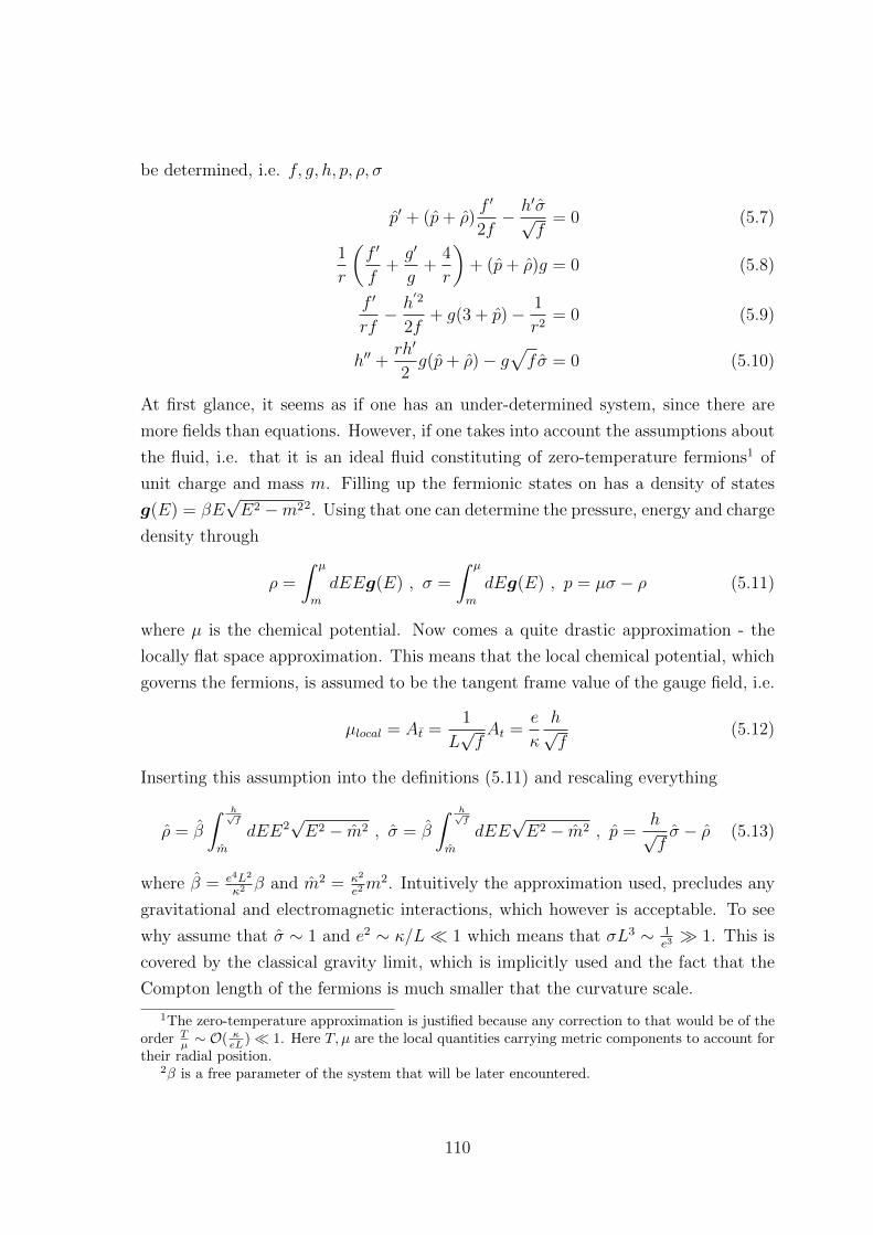
be determined, i.e. f, g, h, p, ρ, σ

p′ + (p+ ρ)f ′

2f− h′σ√

f= 0 (5.7)

1

r

(f ′

f+g′

g+

4

r

)+ (p+ ρ)g = 0 (5.8)

f ′

rf− h

′2

2f+ g(3 + p)− 1

r2= 0 (5.9)

h′′ +rh′

2g(p+ ρ)− g

√fσ = 0 (5.10)

At first glance, it seems as if one has an under-determined system, since there are

more fields than equations. However, if one takes into account the assumptions about

the fluid, i.e. that it is an ideal fluid constituting of zero-temperature fermions1 of

unit charge and mass m. Filling up the fermionic states on has a density of states

g(E) = βE√E2 −m22. Using that one can determine the pressure, energy and charge

density through

ρ =

∫ µ

m

dEEg(E) , σ =

∫ µ

m

dEg(E) , p = µσ − ρ (5.11)

where µ is the chemical potential. Now comes a quite drastic approximation - the

locally flat space approximation. This means that the local chemical potential, which

governs the fermions, is assumed to be the tangent frame value of the gauge field, i.e.

µlocal = At =1

L√fAt =

e

κ

h√f

(5.12)

Inserting this assumption into the definitions (5.11) and rescaling everything

ρ = β

∫ h√f

m

dEE2√E2 − m2 , σ = β

∫ h√f

m

dEE√E2 − m2 , p =

h√fσ − ρ (5.13)

where β = e4L2

κ2 β and m2 = κ2

e2m2. Intuitively the approximation used, precludes any

gravitational and electromagnetic interactions, which however is acceptable. To see

why assume that σ ∼ 1 and e2 ∼ κ/L 1 which means that σL3 ∼ 1e3 1. This is

covered by the classical gravity limit, which is implicitly used and the fact that the

Compton length of the fermions is much smaller that the curvature scale.

1The zero-temperature approximation is justified because any correction to that would be of theorder T

µ ∼ O( κeL ) 1. Here T, µ are the local quantities carrying metric components to account for

their radial position.2β is a free parameter of the system that will be later encountered.

110

Equations (5.13) eliminate three of the unknown fields, in the equations of motion,

reducing them down to three, involving only f, g, h as dynamic fields

1

r

(f ′

f+g′

g+

4

r

)+ghσ√f

=0 (5.14)

f ′

rf− h

′2

2f+ g(3 + p)− 1

r2=0 (5.15)

h′′ +gσ√f

(rhh′

2− f

)=0 (5.16)

For finite temperature, as discussed before, at the deep IR the space-time is that

of AdS-RN. In particular using the forms (5.4,5.5), AdS-RN corresponds to

f =1

r2−(

1

r2+

+µ2

2

)r

r+

+µ2

2

r2

r2+

g =1

r4f

h = µ

(1− r

r+

)(5.17)

where r+ is the location of the event horizon and µ the chemical potential. It is clear

from the above, and expressions (5.13) that the star cannot be supported for any

temperature of the black hole. That is for a given mass m the star appears only when

the AdS-RN parameters f, g, h, that are governed by the temperature as the only

physical parameter of the black hole, become such that

m =h√f,d

dr

h√f

= 0 (5.18)

All the information is in place now, to compute the background solutions for T > 0.

This is done by taking the AdS-RN at lower and lower temperatures and solving the

background equations (5.14,5.15,5.16) numerically in the exterior. In order to do so

the coordinates have been switched (r → u) so that the horizon is at u = 1 and

the AdS boundary at u = 0. This allows for a better depiction of the full range of

features. Moreover the controlling parameter used, is the dimensionless T/µ instead

of just T . The results for T/µ = 0.00003, 0.007, 0.027, 0.05, 0.07, 0.09, 0.12, 0.13 are

presented in fig. 5.1. What becomes immediately obvious is that there is a critical

temperature, determined by eq. (5.18), over which the Electron Star background

equations have no non-trivial solutions, or in other words a finite star cannot be

sustained. Once the critical temperature is crossed the star emerges and as one

continues to lower the temperature, it eventually dominates the full space-time. It

111

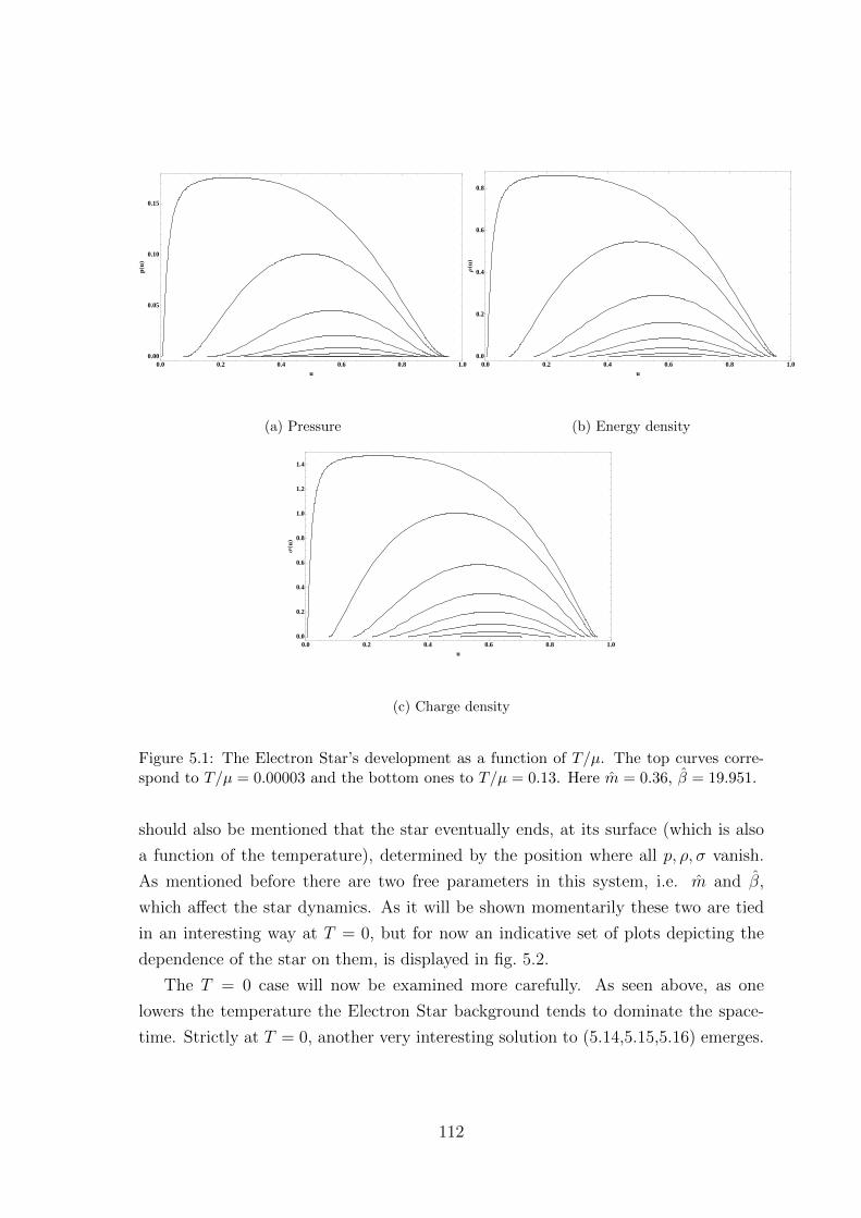
0.0 0.2 0.4 0.6 0.8 1.0

0.00

0.05

0.10

0.15

u

pHu

L

(a) Pressure

0.0 0.2 0.4 0.6 0.8 1.0

0.0

0.2

0.4

0.6

0.8

u

ΡHu

L

(b) Energy density

0.0 0.2 0.4 0.6 0.8 1.0

0.0

0.2

0.4

0.6

0.8

1.0

1.2

1.4

u

ΣHu

L

(c) Charge density

Figure 5.1: The Electron Star’s development as a function of T/µ. The top curves corre-spond to T/µ = 0.00003 and the bottom ones to T/µ = 0.13. Here m = 0.36, β = 19.951.

should also be mentioned that the star eventually ends, at its surface (which is also

a function of the temperature), determined by the position where all p, ρ, σ vanish.

As mentioned before there are two free parameters in this system, i.e. m and β,

which affect the star dynamics. As it will be shown momentarily these two are tied

in an interesting way at T = 0, but for now an indicative set of plots depicting the

dependence of the star on them, is displayed in fig. 5.2.

The T = 0 case will now be examined more carefully. As seen above, as one

lowers the temperature the Electron Star background tends to dominate the space-

time. Strictly at T = 0, another very interesting solution to (5.14,5.15,5.16) emerges.

112

p

Ρ

Σ

0.0 0.2 0.4 0.6 0.8 1.00.00

0.05

0.10

0.15

u

p,Ρ

,Σ

Β`

= 19.951 , m`

=0.5

(a) m = 0.5, β = 19.051

p

Ρ

Σ

0.0 0.2 0.4 0.6 0.8 1.00.00

0.02

0.04

0.06

0.08

0.10

0.12

0.14

u

p,Ρ

,Σ

Β`

= 4.05036 , m`

=0.36

(b) m = 0.36, β = 4.05036

p

Ρ

Σ

0.0 0.2 0.4 0.6 0.8 1.00.00

0.05

0.10

0.15

0.20

0.25

u

p,Ρ

,Σ

Β`

= 4.05036 , m`

=0.1

(c) m = 0.1, β = 4.05036

Figure 5.2: Dependence of the Electron Star background on the parameters m, β for T/µ =0.007.

That is the Lifshitz solution, i.e.

f =1

r2z, g =

g∞r2

, h =h∞rz

(5.19)

where z is dynamical critical exponent. By plugging the Lifshitz solution into the

background equations, the parameters g∞ and h∞ are determined. In particular

eliminating β from (eq. (5.14)) and (eq. (5.16)) yields

h2∞ =

z − 1

z(5.20)

113

and substituting this in (eq. (5.14)) results in

g2∞ =

36(z − 1)z4

((1− m2)z − 1)β2(5.21)

Using the last two equations in (eq. (5.15)), one gets a rather complicated relation

between z, β, m, namely

1

4

√− (z − 1)z4

β2 ((m2 − 1) z + 1)3

β√z − 1√−m2 − 1

z+ 1 ((2− 5m2) z − 2)

z3/2+ 72

−3βm4

√− (z − 1)z4

β2 ((m2 − 1) z + 1)3 log

m√−m2 − 1

z+ 1 +

√z−1z

− 2(z + 1)(z + 2)

= 0

(5.22)

which albeit analytically intractable, can be numerically solved (fig. 5.3), meaning

that out of z, β, m, only two are really independent. Taking sections of fig. 5.3 one

Figure 5.3: The surface defined by eq. (5.22).

gets z = z(β) (fig. 5.4) and z = z(m) (fig. 5.5).

114

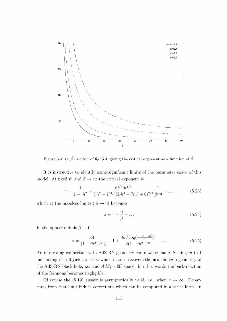
m`

=0.1

m`

=0.4

m`

=0.6

m`

=0.7

5 10 15 20 25 30 35 40

5

10

15

20

Β`

z

Figure 5.4: (z, β) section of fig. 5.3, giving the critical exponent as a function of β.

It is instructive to identify some significant limits of the parameter space of this

model. At fixed m and β →∞ the critical exponent is

z =1

1− m2+

64/3m2/3

(m2 − 1)4/3(2m4 − 7m2 + 6)2/3

1

β2/3+ . . . (5.23)

which at the massless limits (m→ 0) becomes

z = 1 +6

β+ . . . (5.24)

In the opposite limit β → 0

z =36

(1− m2)3/2

1

β− 1 +

3m4 log(1+√

1−m2

m)

2(1− m2)3/2+ . . . (5.25)

An interesting connection with AdS-RN geometry can now be made. Setting m to 1

and taking β → 0 yields z →∞ which in turn recovers the near-horizon geometry of

the AdS-RN black hole, i.e. and AdS2 ×R2 space. In other words the back-reaction

of the fermions becomes negligible.

Of course the (5.19) ansatz is asymptotically valid, i.e. when r → ∞. Depar-

tures from that limit induce corrections which can be computed in a series form. In

115

Β`

=1

Β`

=2

Β`

=3

Β`

=4

0.0 0.2 0.4 0.6 0.8

5

10

15

20

m`

z

Figure 5.5: (z, m) section of fig. 5.3, giving the critical exponent as a function of m.

fact these corrections are necessary to define accurate boundary conditions for the

perturbation fields, that will be encountered later on. Generically one writes

f =1

r2z(1 + f1r

α1 + f2rα2 + . . .) (5.26)

g =g∞r2

(1 + g1rα1 + g2r

α2 + . . .) (5.27)

h =h∞rz

(1 + h1rα1 + h2r

α2 + . . .) (5.28)

which can be inserted into the equations of motion and recursively determine the

coefficients fi, gi, hi, αi. In fact solving for α1 yields three solutions

α01 = 2 + z (5.29)

α±1 =2 + z

2±√

9z3 − 21z2 + 40z − 28− m2z(4− 3z)2

2√

(1− m2)z − 1(5.30)

Out of the three solutions α01 corresponds to a relevant deformation, which generates

the finite temperature solution, α−1 is negative and corresponds to the coupling of an

irrelevant operator and α+1 is positive and corresponds to the expectation value of

116

that operator. The expressions for g1 and h1 are significantly more complicated

g1 = −36α31 + 18α2

1

(βg∞h

3∞

√(h∞ − m) (h∞ + m) + 2

)+ βα1g∞h∞

((4h2∞ − m2

) (βg∞h∞

(h2∞ − m2

)2 − 6

√(h∞ − m) (h∞ + m)

)+36

√(h∞ − m) (h∞ + m)

)− 6z2

(6α1 + βg∞h∞

√(h∞ − m) (h∞ + m)

(m2 − 4h2

∞))

+ z(

72α21 − 18α1

(βg∞h

3∞

√(h∞ − m) (h∞ + m) + 2

)−βg∞h∞

(4h2∞ − m2

) (βg∞h∞

(h2∞ − m2

)2 − 6

√(h∞ − m) (h∞ + m)

))− 2β2g2

∞(h2∞ − m2

)2/

2(

18α31 + 9α2

1

(βg∞h∞ ((h∞ − m) (h∞ + m)) 3/2 − 2

)+βα1g∞h∞

((h∞ − m) (h∞ + m)

(βg∞h∞

(h2∞ − m2

)2 − 6

√(h∞ − m) (h∞ + m)

)−18

√(h∞ − m) (h∞ + m)

)+ 6z2

(3α1 + βg∞h∞ ((h∞ − m) (h∞ + m)) 3/2

)+z(−36α2

1 + 9α1

(βg∞h∞

√(h∞ − m) (h∞ + m)

(2m2 − 3h2

∞)

+ 2)

−β2g2∞h

2∞(h2∞ − m2

)3 + 6βg∞h∞ ((h∞ − m) (h∞ + m)) 3/2

)+ 2β2g2

∞(h2∞ − m2

)3)

(5.31)

h1 = βg∞√

(h∞ − m) (h∞ + m)(3α1

(h2∞(3m2z − 8

)− 6zh4

∞ + 2m2)

+4βg∞h5∞

√(h∞ − m) (h∞ + m)− 8βm2g∞h

3∞

√(h∞ − m) (h∞ + m)

+4βm4g∞h∞√

(h∞ − m) (h∞ + m))/

2h∞

(18α3

1 + 9α21

(βg∞h∞ ((h∞ − m) (h∞ + m)) 3/2 − 2

)+βα1g∞h∞

((h∞ − m) (h∞ + m)

(βg∞h∞

(h2∞ − m2

)2

−6√

(h∞ − m) (h∞ + m))− 18

√(h∞ − m) (h∞ + m)

)+6z2

(3α1 + βg∞h∞ ((h∞ − m) (h∞ + m)) 3/2

)+z(−36α2

1 + 9α1

(βg∞h∞

√(h∞ − m) (h∞ + m)

(2m2 − 3h2

∞)

+ 2)

−β2g2∞h

2∞(h2∞ − m2

)3 + 6βg∞h∞ ((h∞ − m) (h∞ + m)) 3/2

)+ 2β2g2

∞(h2∞ − m2

)3)

(5.32)

In general f1 is unconstrained and has been set to unity in the previous expressions.

Despite the complexity of the expressions, they can be iteratively solved to give as

many terms as necessary.

It is interesting to notice that in the pure Lifshitz background the chemical poten-

tial µ = h/√f takes a constant value. This can be seen by the fact that the pressure,

117

energy and charge density of the Electron Star background are asymptotically con-

stant (fig. 5.6).

p

Ρ

Σ

0 10 20 30 40 50

0.0

0.5

1.0

1.5

r

Figure 5.6: The pressure, energy and charge density for z = 3, m = 0.36. In these coordi-nates r →∞ corresponds to the IR (Lifshitz).

Before carrying forward any further, another point about Lifshitz backgrounds

needs to be stressed. It has been noticed (e.g. in [130]) that even though all the

curvature scalars of this background, i.e. Ricci (R = R µµ ), Kretschmann (K =

RµνρσRµνρσ), are all finite at r → ∞, at that limit the tidal forces on a test string

diverge. This would indicate that there is a true, naked singularity at r →∞ which

cannot be lifted by String Theory. This however is slightly misleading. Lishitz back-

grounds are not solutions of vacuum Einstein’s equations. In other words there needs

to be matter contained in the space-time in order to support Lishitz backgrounds.

This means that when one studies the nature of this space-time at r → ∞, one

has to take into account interactions with the relevant matter. Apparently, carefully

incorporating these interactions resolves the singularity [131].

Concluding the discussion about the Electron Star background the space-time

outside the Electron Star needs to be described. That exterior corresponds to an

AdS-RN, but with modified parameters (compared to interior RN-AdS when T > 0).

Those parameters are determined by matching the functions f, g, h across the star’s

surface when T = 0 or across the surface and across the interface between the star

and the interior RN-AdS when T > 0. More explicitly one writes down the generic

118

RN-AdS functions as

fRN−AdS = c2

(1

r2− Mr +

r2

2Q2

), gRN−AdS =

c2

r4f, hRN−AdS = c

(µ− rQ

)(5.33)

where c is the speed of light which is now not necessarily equal to one. The rest of

the parameters are the standard RN-AdS ones. Then by writing

fRN−AdS|r=rs = fES|r=rs (5.34)

gRN−AdS|r=rs = gES|r=rs (5.35)

gRN−AdS|r=rs = gES|r=rs (5.36)

one gets a system of equations that can be solved to compute Q, M and c.

5.2 Thermo/Hydro-dynamics

Having reviewed the nature of the Electron-Star background, and before endeavouring

to study the linear response of the this system, it is useful to examine its thermo-

dynamic properties. This will provide a deeper understanding of the system and its

usefulness. From the Holographic dictionary it is known that the on-shell Euclidean

bulk action corresponds to the Free energy of the dual theory (Ω). In terms of the

other thermodynamic parameters the free energy is

Ω = M − µQ− sT (5.37)

where s is the Bekenstein-Hawking entropy, M the mass parameter of the AdS-RN

black hole, µ the chemical potential and Q the charge parameter of the AdS-RN black

hole. From standard thermodynamics it is also known that

Ω = −pV (5.38)

where p is the pressure and V the system’s volume. The bulk action reads

SE =

∫d4x√g

[1

2κ2

(R +

6

L2

)− 1

4e2F 2 + p

]+ SGH + Sc.t. (5.39)

where SGH is the Gibbons-Hawking term, necessary to make the variational problem

well-defined and Sc.t. is the counter-term prescribed by Holographic Renormalization,

necessary to cancel the infinity that emerges at r → ∂AdS [73, 88]. In particular

SGH = − 1

2κ2

∫∂AdS

d3x√γ2K (5.40)

119

and

Sc.t. = − 1

2κ2

∫∂AdS

d3x4

L

√γ + L

√γ R(3) (5.41)

where γ is the determinant of the induced metric, K the extrinsic curvature and R(3)

the three-dimensional Ricci scalar which in this case vanishes. Written out explicitly

the action is

SE = L2√f(r)g(r)

(r2g(r)f ′(r)2 + rf(r) (rf ′(r)g′(r) + 2g(r) (−rf ′′(r) + 2f ′(r)

+rh′(r)2))

+ 4f(r)2(g(r)

(r2g(r) (p(r) + 3)− 5

)− rg′(r)

))/(4κ2r4f(r)2g(r)2

)(5.42)

and after applying the background equations of motion one gets

SE =L2

κ2

d

dr

f ′(r)− 2h(r)h′(r)

2r2√f(r)g(r)

(5.43)

Similarly

SGH + Sc.t. =L2(εf ′(ε) + 4f(ε)

(ε√g(ε)− 1

))2ε3κ2

√f(ε)

√g(ε)

(5.44)

where ε is an infinitesimal positive number, i.e. ε → 0. Given that the background

can be numerically computed, so can the action and consequently the free energy.

The results are presented in fig. 5.7 and fig. 5.8. What one sees is that as the electron

mass m decreases so does the free energy, at low temperatures3. Moreover as the

temperature is increased, a transition to the pure AdS-RN appears (for each m there

is a different transition temperature Tt) as the free energies of different Electron Star

systems converge onto the AdS-RN free energy. Said differently for every electron

mass there is a temperature over which the RN black hole becomes big enough that

the Electron System ceases being supported and the black hole dominates the space-

time. Furthermore by varying the critical exponent (z) one sees that the higher z is,

the closer to the RN results one gets. This is in accordance with expectations, as at

the limit where z → ∞ one expects to recover the RN-AdS system. It should also

be noted that the AdS-RN free energy is always larger that the Electron Star one, in

the regime where the two systems can co-exist. This means that the Electron Star

configuration is thermodynamically preferred to the pure AdS-RN.

Having numerically computed the background, more thermodynamical quantities

can be computed. The entropy density4 for example, which in the coordinate system

3Here temperature is measured with respect to the chemical potential through the dimensionlessparameter T

µ4As in the case of temperature and Free Energy, entropy density is measure in units of chemical

potential, which is the relevant scale. Seen in another way one computes the dimensionless entropydensity.

120

æ æ æ æ æ æ ææ

ææ

æ

æ

æ

æ

æ

æ

à àà

à

à

à

à

ì ìì

ì

ì

ì

ì

ìì

òò

ò

ò

ò

ò

ò

ò

ò

ò

ò

ò

æ m`

=0.10

à m`

=0.36

ì m`

=0.50

ò RN

0.00 0.02 0.04 0.06 0.08 0.10 0.12-0.5

-0.4

-0.3

-0.2

-0.1

0.0

T

Μ

W Μ3

Figure 5.7: Free energy of the Electron Star system for three electron masses m. The RNresult is overlaid for comparison.

where the horizon is placed at r = r+ = 1 is

s

µ2=

2π

r2+µ

2=

2π

µ2(5.45)

Extracting the chemical potential from the outer (i.e. the one on the boundary side of

space-time) RN one finds fig. 5.9, where the electron mass is varied and fig. 5.10 where

the critical exponent dependence is examined. The striking characteristic compared

to the RN case, is that the dimensionless entropy density vanishes as the temperature

(also dimensionless) goes to zero. This seems to be circumventing one of the major

issues encountered when studying the thermodynamics of theories dual to a pure RN-

AdS system, since in those cases, as seen by the RN curve in fig. 5.9, the entropy

density remains finite even at zero temperature, which is a bizarre result from the

Condensed Matter point of view. With respect to the Electron Star parameters,

one again sees that higher electron mass and higher critical exponent leads to faster

convergence to RN.

Having the Free Energy and entropy of the system available, one can proceed to

compute every thermodynamical quantity. What is more pertinent however is that

one can compute at least one hydrodynamical quantity, namely the diffusion constant

D, for viscous fluids. It is known from standard liquid hydrodynamics (e.g. [28]) that

the diffusion constant is related to the shear viscosity, the energy density and pressure,

121

æ æ

æ

æ

æ

æ

æ

à à àà

àà

à

à

à

à

à

à

à

à

à

à

ì ì ì ì ìì

ìì

ì

ì

ì

ì

ì

ì

ì

ì

ì

ì

ì

ò ò ò òò

òò

òò

ò

ò

ò

ò

ò

ò

ò

ò

ò

ò

ò

ò

ô

ô

ô

ô

ô

ô

ô

ô

ô

ô

ô

ô

æ z=2

à z=3

ì z=5

ò z=10

ô RN

0.00 0.02 0.04 0.06 0.08 0.10 0.12

-0.4

-0.3

-0.2

-0.1

0.0

T

Μ

W Μ3

Figure 5.8: Free energy of the Electron Star system for four critical exponents z. The RNresult is overlaid for comparison.

through

D =η

ε+ p(5.46)

The standard practice in Holography literature is to use the KSS5 relation [132]

η

s=

~4πkB

=1

4π(5.47)

where in the last step natural units (kB = ~ = 1) have been used. Moreover, asymp-

totic symmetries indicate that the boundary theory should be conformal, imposing

the relation

ε− 2p = 0 (5.48)

on energy density and pressure. Since the Electron Star system has not been examined

in this way before and mainly out of caution concerning the potential numerical errors

stemming from the fact that the background itself is only known numerically, both

these statements will now be verified. The first to be examined is the conformality

condition. The pressure can be extracted from the on-shell action through eq. (5.38)

and the energy corresponds to the mass parameter of the outer RN part of the space-

time. It should be noted that since in the outer region c 6= 1 it has to be properly

re-inserted in the calculation. From the numerical solution one indeed sees in fig. 5.11

that the condition holds.

5Kovtun-Son-Starinets

122

æ ææ

æ

æ

æ

æ

æ

æ

æ

æ

æ

æ

æ

æ

æ

æ

æ

à

à

à

à

à

à

à

à

à

ì

ì

ì

ì

ì

ì

ì

ìì

ò

ò

ò

ò

ò

ò

ò

ò

ò

ò

ò

ò

æ m`

=0.10

à m`

=0.36

ì m`

=0.50

ò RN

0.00 0.02 0.04 0.06 0.08 0.10 0.12 0.140

1

2

3

4

T

Μ

s Μ2

Figure 5.9: The entropy density of the Electron Star for three electron masses (m). TheRN result is overlaid for comparison.

The next one, i.e. the KSS relation is a bit more involved to verify. Since the

entropy for this system is already known (5.45) one needs to calculate the shear

viscosity in an independent way. To do that one makes use of the Kubo formula that

relates the shear viscosity with the Green’s function of the shear part (in this case

xy) of the stress-energy tensor which, in turn, is computed, in standard Holographic

practice, by calculating the solution of the perturbation to the gravity mode of the

same symmetries [32,109]. In particular

η = limω→0

1

2ω

∫dtdxeıωt〈[Txy(x), Txy(0)]〉 = − lim

ω→0

1

ωG(ω,0) (5.49)

where in the last part 0 stands for zero momentum. To complete this calculation one

needs the equation of motion for the xy component of the metric. The setup is similar

to that described by eq. (4.6) and eq. (4.9) with the caveat that the background is a

modified RN-AdS. The equations of motion are similarly

Rµν −1

2gµνR−

3

L2gµν = κ2

[1

e2

(FµσF

σν −

1

4gµνFρτF

ρτ

)](5.50)

perturbed at linear order. Fortunately at zero momentum, which is the case for this

calculation, the Einstein’s equation involving this mode, decouple giving

h yx′′(r) +

f ′out(r)

fout(r)h yx′(r) + ω

gout(r)

fout(r)h yx (r) = 0 (5.51)

123

æ

æ

æ

æ

æ

æ

æ

æ

æ

æ

à

à

à

à

à

à

à

à

à

à

à

à

à

à

à

à

à

ì

ì

ì

ì

ì

ì

ì

ì

ì

ì

ì

ì

ì

ì

ì

ì

ì

ì

ì

ì

ò

ò

ò

ò

ò

ò

ò

ò

ò

ò

ò

ò

ò

ò

ò

ò

ò

ò

ò

ò

ò

ò

ô

ô

ô

ô

ô

ô

ô

ô

ô

ô

ô

ô

æ z=2

à z=3

ì z=5

ò z=10

ô RN

0.00 0.02 0.04 0.06 0.08 0.10 0.12 0.140

1

2

3

4

T

Μ

s Μ2

Figure 5.10: The entropy density for the Electron Star for four critical exponents (z). TheRN result is overlaid for comparison.

where fout, gout, hout are the RN parameters for the outer RN part of the space-time

determined by eq. (5.36). By expanding this equation near the boundary one sees

that its solution admits a series expansion of the form

h yx = a0 + a1r + a2r

2 + a3r3 + a4r

4 + . . . (5.52)

The indices of the equation (determined by setting h yx = rνf(r) and solving the

resulting equation so that f is regular) for the regular singular point 0, are ν = 0, 36,

which indicates that the leading and sub-leading terms in the expansion are ∼ r0 and

∼ r3 and the rest of the coefficients are determined in terms of a0, a3. In fact

a1 = 0 ; a2 = a0ω2

2c2; a4 =

9a3c2M − a0Q

2ω2

ω2(5.53)

where c,M,Q are the RN parameters for the outer region. These relations will be

used as checks of our numerical solution. In order to proceed, eq. (5.51) will be solved

numerically setting in-going boundary conditions on the horizon. Once the solution is

found the checks mentioned above are performed to verify the numerical stability of

the solution. Once the tests are passed the solution is fitted to the series expression,

in order to determine the free parameters a0 and a3. Having determined these then

6This means that the solution can be written in the form h yx ∼ r0(1 + . . .) + r3(1 + . . .).

124

ææææ æ æ æ æ æ æ æ æ æ æ æ æ æ æ æ æ

0.00 0.02 0.04 0.06 0.08 0.10 0.12

1.6

1.8

2.0

2.2

2.4

T

Μ

¶ p

Figure 5.11: Verification of the conformality condition (5.48).

one can immediately determine the relative Green’s function through the standard

Holographic procedure (see e.g. [18])

G(ω,k) = (2∆− d)a3(ω,k)

a0(ω,k)(5.54)

where d is the dimensionality of the boundary (here d = 3) and ∆ the scaling dimen-

sion of the involved operator. The latter can either be computed by the indices of

the governing equation of motion, at the boundary or through the standard formula

∆± =d

2±

√(d

2

)2

+m2 (5.55)

which in this case (m = 0) yields 0, 3. Hence the ∆ = 3. Combining eq. (5.49) and

eq. (5.54) the results of fig. 5.12 are obtained, verifying that KSS does indeed hold.

Now all the components are in place to compute the diffusion coefficient D through

eq. (5.46). The results are presented in fig. 5.13 where the electron mass (m) is varied

and fig. 5.14 where the critical exponent (z) is varied.

It should be stressed here that this is the prediction of standard hydrodynamics,

for this particular system. In the next section it will be compared and found to

conditionally disagree with the full linear perturbation analysis of the system. For the

time being, though one sees that at low temperature the diffusion coefficient vanishes

as expected from standard Condensed Matter intuition. Moreover in accordance

125

* * * * * * * * * * * *

z=2 ; m-0.36

* z=100 ; m-0.36

0.00 0.02 0.04 0.06 0.08 0.10 0.120.00

0.02

0.04

0.06

0.08

0.10

T

Μ

Η s

Figure 5.12: ηs for two critical exponents. The solid line corresponds to the value 1

4π .

with the already established fact that the Electron Star disappears at high enough

temperatures, one sees that D converges to the RN values above a certain temperature

(distinct for each electron mass). What can also be determined from these results

is that the more massive the constituent electrons are the “quicker” (in terms of

temperature) D converges to RN. Similarly the higher the critical exponent is the

“quicker” the convergence to RN occurs. This is to be expected however, since it is

known that at the infinite critical exponent limit (z → ∞) one recovers the AdS2

near horizon geometry corresponding to the RN black hole.

5.3 Shear channel

Now that all the necessary information is extracted from the background one can

proceed to the full linear perturbation of the Electron Star system. What is going to

be presented next, is a study of the low-lying poles of the correlators of the boundary

theory, dual to the Electron Star system. The standard Holographic dictionary will

be followed, according to which one needs to perturb the system and then examine

the equation of motions of the fluctuations of all relevant bulk fields, as was done in

the previous chapter for the Reissner-Nordstrom black hole. At first, attention will

be focused on the shear channel (defined below).

126

æææ æ ææ

ææ

æ

æ

æ

æ

æ

æ

æ

æ

æ

æ

æ

æ

æ

æ

æ

æ

æ

æ

æ

æ

àà

à

à

à

à

à

àà

ì

ì

ì

ì

ì

ì

ì

ìì

òò

ò

ò

ò

ò

ò

ò

ò

ò

ò

ò

ò

ò

ò

ò

ò

ò

ò

ò

æ m`

=0.10

à m`

=0.36

ì m`

=0.50

ò RN

0.0 0.1 0.2 0.3 0.4

0.00

0.05

0.10

0.15

0.20

0.25

0.30

T

Μ

D

Figure 5.13: Diffusion coefficient for three electron masses as well as RN.

The starting point will be the action

S =

∫dx√−g[

1

2κ2

(R +

6

L2

)− 1

4e2FµνF

µν − ρ(σ) + σuµ(∂µφ+ Aµ)

+ λ(uµuµ + 1)]

+ SGH + counterterms (5.56)

The non-Einstein-Maxwell terms in this action comprise the so-called Schutz action

at zero temperature [133]. This action should be varied with respect to the metric

gµν , the U(1) gauge field Aµ, the four-velocity of the fluid uµ, the charge density of

the fluid σ, the Clebsch potential φ and the Lagrange multiplier λ, which imposes

the requirement for a relativistic fluid that u2 = −1. For simplicity, the fields will be

rescaled so that the full action is proportional to L2

κ2

Aµ →eL

κAµ , φ→

eL

κφ , uµ → Luµ , σ →

1

eL2κσ , λ→ 1

L2κ2λ (5.57)

Note that when fluctuations of these fields will be considered shortly, they will inherit

this rescaling also.

If one now makes the definitions

µ(σ) ≡ ρ′(σ) = uµ(∂µφ+ Aµ) , p(σ) ≡ −ρ(σ) + σµ(σ) (5.58)

127

æ

æ

æ

æ

æ

æ

æ

ææ

æ

à

à

à

à

à

à

à

à

à

à

à

à

à

à

à

à

à

ì

ì

ì

ì

ì

ì

ì

ì

ì

ì

ì

ì

ì

ì

ì

ì

ì

ì

ì

ì

ò

ò

ò

ò

ò

ò

ò

ò

ò

ò

ò

ò

ò

ò

ò

ò

ò

ò

ò

ò

ò

ò

ô

ô

ô

ô

ô

ô

ô

ô

ô

ô

ô

ô

ô

æ z=2

à z=3

ì z=5

ò z=10

ô RN

0.00 0.05 0.10 0.150.00

0.05

0.10

0.15

0.20

T

Μ

D

Figure 5.14: Diffusion coefficient for four critical exponents as well as RN.

then the energy-momentum tensor associated to the Schutz action is simply that of

a perfect fluid

T µνSchults = (p+ ρ)uµuν + pgµν (5.59)

with pressure p, energy density ρ, charge density σ and chemical potential µ.

In order to get the equations of motion for the perturbations, one has to excite

all the involved fields as

gµν(r)→ gµν(r) + hµν(r, t,x)

Aµ(r)→ Aµ(r) + aµ(r, t,x)

uµ(r)→ uµ(r) + δuµ(r, t,x)

φ(r)→ φ(r) + δφ(r, t,x)

σ(r)→ σ(r) + δσ(r, t,x)

λ(r)→ λ(r) + δλ(r, t,x) (5.60)

The equations then come from varying the action. Furthermore, the non-radial spatial

dependence for every field takes, without loss of generality, the trivial form

φ(r, t,x) = exp[−ıωt+ ıkx]φ(r, ω, k) (5.61)

128

where φ stands for each field. This procedure results in twenty one equations. These

split naturally into two decoupled sets of equations - the shear equations of motion,

involving fields that are odd under y → −y, and the longitudinal equations of motion,

involving fields that are even under y → −y. This decoupling is guaranteed at linear

order in the fluctuations as the theory is invariant under y → −y.

The shear degrees of freedom include hxy, hty, hry, ay, δuy. By varying the action

with respect to these one gets the equations

h xy′′ − ıkr2gh r

y′ +

(f ′

2f− g′

2g− 2

r

)h xy′ − 2ıkr2g

(f ′

4f+g′

4g

)h ry

+ ω2 g

fh xy − ωkr2gh t

t = 0 (5.62)

h ty′′ − ıω g

fh ry′ +

(3f ′

2f− g′

2g

)h ty′ − 2h′

fa′y − 2ıω

g

f

(g′

4g− f ′

4f− 1

r

)h ry

+ ωkg

fh xy − k2r2gh t

y + 2g√f

(p+ ρ)δuy + 2

(h′2

f+ g(p+ ρ)

)h ty = 0 (5.63)

(ω2 − k2r2f

)h ry + ıω

f

gh ty′ − ıkf

gh xy′ +

ıω

g

(2f

r+ f ′

)h ty − 2ıω

h′

gay = 0 (5.64)

a′′y +1

2

(f ′

f− g′

g

)a′y +

g

f(ω2 − k2r2f)ay − h′h t

y′ + ıω

g

fh′h r

y + gσδuy

+h′

2

(rg(p+ ρ)− f ′

f+g′

g

)h ty = 0 (5.65)

δay + µδuy = 0 (5.66)

where indices of the metric fluctuations hµν are raised and lowered using the back-

ground metric, a prime denotes a derivative with respect to r, and the dependence

of the field fluctuations upon r, ω and k, and of the background fields upon r, have

been suppressed for conciseness. Now the equations in this form are unmanageable.

Thankfully, they may be considerably simplified. This is done by solving a subset

of the equations of motion algebraically. In the shear sector one can solve equations

(5.64) and (5.66) for h ry and δuy. Substituting the solutions for these fields into the

remaining equations, one finds that there are only two linearly-independent equations

of motion in the shear sector. These equations are naturally written in terms of the

following gauge-invariant combinations of the fluctuations

Z1(r, ω, k) = ωh xy − kr2f(r)h t

y (r, ω, k) (5.67)

Z2(r, ω, k) = ay(r, ω, k) (5.68)

These are invariant under both the bulk U(1) gauge symmetry, which acts as

aµ(r, ω, k)→ aµ(r, ω, k)− ∂µΛ(r, ω, k) (5.69)

129

and the bulk diffeomorphism symmetry which acts as

hµν(r, x, t)→ hµν(r, x, t)−∇µξν(r, x, t)−∇νξµ(r, x, t)

aµ(r, x, t)→ aµ(r, x, t)− ξα(r, x, t)∇αAµ(r)− Aα∇µξα(r, x, t)

δσ(r, x, t)→ δσ(r, x, t)− ξα(r, x, t)∇ασ(r) (5.70)

to linear order in the fluctuations, where ∇µ is the covariant derivative with respect

to the background metric. These particular combinations are natural in the language

of the dual field theory operators as they guarantee that the relevant field theory

Ward identities are satisfied (as seen above).

In terms of these fluctuations the the two linearly-independent equations of motion

are

Z ′′1 + 2kr2h′Z ′2 +

(rgσµ

2+ω2f ′ + 2k2rf 2

f(ω2 − k2r2f)

)Z ′1 +

g

f(ω2 − k2r2f)Z1

+ 2kr2√fµ

(2ω2h

′2

f(ω2 − k2r2f)+gσ

µ

)Z2 = 0 (5.71)

Z ′′2 +1

2

(f ′

f− g′

g

)Z ′2 −

kh′

ω2 − k2r2fZ ′1 +

g

f(ω2 − k2r2f)Z2

−(

2ω2h′2

f(ω2 − k2r2f)+gσ

µ

)Z2 = 0 (5.72)

These are the equations that need to be solved numerically. In order however to

compute physical quantities, like spectral functions, one needs the on-shell action,

which from standard Holographic dictionary, correspond to the generating functional

for the boundary theory. By perturbing the action to quadratic order in fluctuations

(O(h2)), and imposing the equations of motion one gets, in terms of the original

130

degrees of freedom

S(2)on−shell =

∫r→0

dωdk

(2π)2

L2

κ2

[1

4r4√fgh xt h

xt′ +

ıω√g

4r2√f

(h xt h

rx − h x

x hrt − h y

y hrt )

+

√f

8r2√g

(h tt h

xx′ + h x

x htt′ + h y

y htt′ + h t

t hyy′ + h x

x hyy′ + h y

y hxx′)

− ık√fg

4(h t

t hrx + h y

y hrx )−

ık√g

4r2√fh xt h

rt −

1

r5√fgh xt

2

+(rf ′ − 2f)

16r3√fg

(h tt h

xx + h t

t hyy + h x

x hyy + h y

y hxx − h r

r hxx − h r

r hyy − h 2

x2 − h y

y2)

√f

4r3√g

(h tt

2 + h tt h

rr − h t

t hxx − h t

t hyy ) +

1

2r2√fgat(a

′t + ıωar)

−√f

2√gax(a

′x − ıkar)−

h′

4r2√fgat(h

rr + h t

t − h xx − h y

y )− h′

2r2√fgaxh

xT

−√gσ

2r2h rt δφ+

√fσ

2r2√gδurφ

−√f

4r2√gh xy h

xy′ +

f 3/2

4√gh ty h

ty′ − ıω

√fg

4h ty h

ry +

ık√fg

4h xy h

ry −

√f

2√gaya

′y

+

√f(rf ′ − 2f)

4r√g

h ty

2 − (rf ′ − 2f)

4r3√fg

h xx

2 +

√fh′

2√gh ty ay ]

+ counterterms (5.73)

where the first fluctuation written in each term has argument (r,−ω,−k), the second

has argument (r, ω, k), and a prime denotes a derivative with respect to r.

As we will work with the equations of motion for the gauge-invariant variables

(5.68), we require the action to be written in terms of these variables also. It is

not possible to write the full on-shell action in terms of these variables. This does

not mean that any of the bulk gauge symmetries are broken but simply reflects the

fact that the variables (5.68) are valid to linear order in fluctuations, whereas the

action is quadratic in fluctuations. However, the derivative terms in the on-shell

action can be written purely in terms of the gauge-invariant variables - this ensures

that the relevant Ward identities of the field theory are satisfied. In terms of the

gauge-invariant variables the on-shell action can be recast in the following form

S(2)on−shell =

∫r→0

dωdk

(2π)2

L2

κ2

[Zi(r,−ω,−k)AijZ ′j(r, ω, k)

]+ non− derivative terms

(5.74)

where the coefficients, though lengthy, are presented here for completeness:

131

A11 =

√f

4r2√g(ω2 − k2r2f)

(5.75)

A22 = −√f

2√g

(5.76)

A12 = A21 = 0 (5.77)

A33 =[−4k2r2f 3µ4σ + r2ω2(k2r2µ+ σ − 2µ2σ + µ4σ)f′2 + 4f 2(k2r2ω2µ− 2k2r2ω2µ3

+ ω2σ4µσ(ω2 + k2r3f ′)) + f(8ω4µ3 + 4k2r3ω2µf ′ + 4rω2σf ′

− rµ4σf ′(4ω2 + k2r3f ′))]/[8r2ω2√f(−ω2 + k2r2f)

√gµ2(µ(4ω2 − 2k2r2f+

+ k2r3f ′)2 + 2µ2σ(−4k2r2f 2 + 4f(ω2 + k2r3f ′)− rf ′(4ω2 + k2r3f ′))

+ rσ(4k2rf 2 − 4k2r2ff ′ + f ′(8ω2 + k2r3f ′)))] (5.78)

A44 = [√f(ω2µ(4ω2 − 2k2r2f + k2r3f ′)2 + 2ω2µ2σ(−4k2r2f 2 + 4f(ω2 + k2r3f ′)

+−rf ′(4ω2 + k2r3f ′)) + rσ(−4k4r3f 3 + 2ω2f ′(4ω2 + k2r3f ′)

− k2r2ff ′(8ω2 + k2r3f ′) + 4f 2(2k2rω2 + k4r4f ′)))]/

[2ω2(ω2 − k2r2f)√g(µ(4ω2 − 2k2r2f + k2r3f ′)2 + 2µ2σ(−4k2r2f 2

+ 4f(ω2 + k2r3f ′)− rf ′(4ω2 + k2r3f ′)) + rσ(4k2rf 2 − 4k2r2ff ′

+ f ′(8ω2 + k2r3f ′)))] (5.79)

A55 = −[f 3/2σ(4ω2 − 2k2r2f + k2r3f ′)2µ′2]/[2r2ω2√g(µ(4ω2 − 2k2r2f + k2r3f ′)2

+ 2µ2σ(−4k2r2f 2 + 4f(ω2 + k2r3f ′)− rf ′(4ω2 + k2r4f ′)) + rσ(4k2rf 2

− 4k2r2ff ′ + f ′(8ω2 + k2r3f ′)))σ′2] (5.80)

A34 = −[k(−4k2r2f 3µ2σ + 4f 2(−k2r2ω2µ+ ω2σ + µ2σ(ω2 + k2r3f ′)) + rω2f ′(rσf ′

− rµ2σf ′ + µ(4ω2 + k2r3f ′)) + f(8ω4µ+ 4rω2σf ′ − rµ2σf ′(4ω2 + k2r3f ′)))]/

[4ω2(ω2 − k2r2f)√gµ(µ(4ω2 − 2k2r2f + k2r3f ′)2 + 2µ2σ(−4k2r2f 2

+ 4f(ω2 + k2r3f ′)− rf ′(4ω2 + k2r3f ′)) + rσ(4k2rf 2 − 4k2r2ff ′)

+ f ′(8ω2 + k2r3f ′)))] (5.81)

132

A35 = [√fσ(4k2r2f 2µ2 − 4f(2ω2 + k2r3µ2f ′) + rf ′(−4ω2 + µ2(4ω2 + k2r3f ′)))µ′]/

[4r2ω2√gµ(µ(4ω2 − 2k2r2f + k2r3f ′)2 + 2µ2σ(−4k2r2f 2 + 4f(ω2 + k2r3f ′)

− rf ′(4ω2 + k2r3f ′)) + rσ(4k2rf 2 − 4k2r2ff ′ + f ′(8ω2 + k2r3f ′)))σ′] (5.82)

A45 = −[kfσ(2f − rf ′)(−4ω2 + 2k2r2f − k2r3f ′)µ′]/[2ω2√g(µ(4ω2 − 2k2r2f

+ k2r3f ′)2 + 2µ2σ(−4k2r2f 2 + 4f(ω2 + k2r3f ′)− rf ′(4ω2 + k2r3f ′))

+ rσ(4k2rf 2 − 4k2r2ff ′ + f ′(8ω2 + k2r3f ′)))σ′] (5.83)

A43 = −A34 (5.84)

A53 = A34 (5.85)

A54 = −A45 (5.86)

(5.87)

where a prime denotes a derivative with respect to r.

It is also of interest to determine the off-shell action to quadratic order in the

fluctuations in the gauge-invariant variables. This action has a Noether current cor-

responding to a global symmetry of the form

φ(r, ω, k)→ exp[ıα]φ(r, ω, k)

φ(r,−ω,−k)→ exp[−ıα]φ(r,−ω,−k) (5.88)

where φ represents the fluctuation of a generic field. This results in the existence

of a quantity which is invariant under translations in the radial direction and this

invariance can be used as a check on the numerical results obtained. As explained

previously, the full quadratic action cannot be written in the variables (5.68). In fact,

only the first-derivative squared terms in the action may be written in these variables.

The conserved quantity depends on these terms, and also the single-derivative terms.

This problem can be circumvented by adding purely real boundary counter-terms

(different from the counter-terms the action) such that the single-derivative terms

may be written in terms of the variables (5.68). These do not affect the equations

of motion of the theory (and hence the Green’s function poles), nor the spectral

133

functions (as they are purely real) but only the contact terms in the real part of the

Green’s function. Having done this, the off-shell action takes the form

S(2)off−shel =

∫drdωdl

(2π)2

L2

κ2

[Z ′i(r,−ω,−k)AijZ

′j(r, ω, k) + Zi(r,−ω,−k)BijZ

′j(r, ω, k)

+non− derivativeterms] (5.89)

where a prime denotes a derivative with respect to r. The coefficients are

A11 =

√f

4r2√g(ω2 − k2r2f)

(5.90)

A12 = A21 = 0 (5.91)

A22 = −√f

2√g

(5.92)

B11 =rf ′ − 2f

2ω2r3√fg

(5.93)

B12 = 0 (5.94)

B21 = − k(rf ′ + 2f)

2rµ√g(ω2 − k2r2d)

(5.95)

B22 = 0 (5.96)

(5.97)

Note that Aij = Aij in the shear sector.

In order to proceed one needs to determine the boundary conditions, in order to

numerically solve the equations of motion, and set up the numerical framework. The

framework followed here will be the one prescribed in [112]. In particular it needs

to be noted that the system consists of a coupled system of differential equation and

hence it is not well-defined to talk about one-to-one solution-operator correspondence

anywhere but strictly on the boundary. In other words it is only strictly on the

boundary that the solution of each equation of motion provides information about a

single, specific operator of the boundary theory. Given though that numerically one

is never strictly on the boundary, but rather on a radial slice close to it, which defines

a cut-off scale (rΛ), one must take into account operator mixing effects. In essence the

recipe in [112] consists of (numerically) finding a set of linearly independent solutions

to the equations of motion, out of which, one forms a solution matrix which at the

boundary reduces to a diagonal one. Out of this matrix one can extract all the

relevant information about the boundary system. This process will now be briefly

reviewed. The starting point is a system consisting of N fields ΦI , I ∈ 1, · · · , N

134

governed by the bilinear action

S =

∫ddx

∫dr[∂mΦIAIJ(x, r)∂nΦJgmn + ΦIBm

IJ(x, r)∂mΦJ + ΦICIJ(x, r)ΦJ]

(5.98)

where m,n span the Minkowski and radial coordinates (x ∼ xµ, z). For the specific

case in which this machinery will be implemented here, N = 2 and the two fields are

the two gauge-invariant variables defined above. As usual, the non-radial directions

are separated through a Fourier decomposition

ΦI(xµ, r) =

∫ddk

(2π)dΦIk(r) exp[−ıkx] (5.99)

which transforms the action into

S =

∫ddk

(2π)d

∫dr[Φ′

I−kAIJ(k, r)Φ′

Jk + ΦI

−kBIJ(k, r)Φ′Jk + ΦI

−kCIJ(k, r)ΦJk

](5.100)

where k ≡ kµ, AIJ(−k, r) = AIJ(k, r)∗, and similarly for B and C. Now the small

issue of double counting arises, but is easily fixed by splitting the momentum in-

tegration into (k> = (ω > 0,k)) and (k< = (ω < 0,k)) and re-writing the action

as

S =

∫dk>

∫dr[2AHIJΦ′

I−kΦ

′Jk +BIJΦI

−kΦ′Jk +B†IJΦ′I−kΦ

Jk + 2CH

IJΦI−kΦ

Jk

](5.101)

where∫dk> ≡ 1

(2π)d

∫∞0dω∫ d−1

Rdd−1k. One can now disregard the positive-negative

momenta issue and just use the momentum variable k = k>. The equations of motion

can be recovered by varying ΦI−k, holding ΦI

k fixed,

− 2(AHIJΦ′Jk )′ + 2BAIJΦ′Jk + (2CH −B†′)IJΦJ

k = 0 (5.102)

where MH,A now stands for the (anti-)hermitian part MH,A = 12(M ±M †), for some

matrix M . This is precisely how eq. (5.71) and eq. (5.72) where derived. In solving

the equations of motion, one finds that near the boundary, the components of the

vector Φ asymptote to ΦI(r → 0) ∼ r∆I−φI0 + ... + r∆I

+φI1 + .... ∆I− is the smallest

exponent at the boundary r = 0. In order to compute the Green’s functions of the

dual quantum operators one needs to consider conveniently normalized fields Φk(r) =

r∆I−ΦI

k(z) that close to the boundary have an expansion ΦI(r → 0) = φI0+O(r∆I+−∆I

−),

meaning that φI0 can be interpreted as the source of the dual operator. The new fields

can be treated collectively in the same formalism by defining the rescaling matrix

DIJ = δIJz

∆J− = D† IJ . Replacing Φ by DΦ inside (eq. (5.101)) yields

S =

∫dk>

∫dz[2AHIJΦ′

I−kΦ

′Jk + BIJΦI

−kΦ′Jk + B†IJΦ′I−kΦ

Jk + 2CH

IJΦI−kΦ

Jk

], (5.103)

135

where

AH = D†AHD , (5.104)

B = D†BD + 2D′†AHD , (5.105)

CH = D†CHD +D′†AHD′ +1

2D†BD′ +

1

2D′†B†D (5.106)

One can now assume that the fields are indeed normalized this way and avoid the

clutter caused by the barred symbols. Now consider a solution ΦIk of the coupled

system. The boundary value of it acts as the source for the boundary theory oper-

ator OI . Conversely the source of a particular operator, will be given by a vector

(Φ1k(r),Φ

2k(r), ...) that, approaching the UV cut-off rΛ, asymptotes, by construction,

to a single component vector, (Φ1k(r),Φ

2k(r), ...)

r→rΛ→ (ϕ1k, 0, 0, ...). Similarly for ev-

ery boundary operator. Therefore the bulk solution dual to a source OI0(k) is given

by a set ΦIk(r) that solves the equations of motion in the bulk and asymptote to

ΦJ(rΛ) = δJ I0φI00 (k), J = 1, ..., N , where φI00 (k) ≡ ϕI0k is the source of the corre-

sponding operator OI0(k). Since the system of equations of motion is coupled, at any

other scale r > rΛ this set, ΦIk(z), will generically source a linear combination of all

the operators. Hence, this set can be expressed in terms of the arbitrary boundary

values, ϕJk , as

ΦIk(r) = F I

J(k, r)ϕJk (5.107)

ΦI−k(r) = F I

J(−k, r)ϕJ−k = ϕJ−kF†JI(k, r) (5.108)

The interesting dynamics of the fields are in this formalism contained in the solution

matrix F (k, z)I J = F (−k, z)∗IJ , which is constructed to be normalized at the UV

cut-off rΛ as

F (k, rΛ)I J = δIJ (5.109)

i.e. it reduces to a diagonal matrix, with each element corresponding to a specific

boundary operator. Immediately two question arise - how does one construct this

solution matrix and how can one extract the Green’s function out of it. The latter

is easier to address and therefore it will be treated first. Assuming that in some way

one has constructed the solution matrix, the on-shell action can be rewritten in the

form

S =

∫dk

∫dr

[ΦI−k[e.o.m.(ΦI

k)]

+d

dr[2AIJΦI

−kΦ′Jk +B†IJΦI

−kΦJk ]

]=

∫dk ϕI−k FIJ(k, z)ϕJk

∣∣rhrb, (5.110)

136

where

F(k, r) = 2F †AHF ′ + F †B†F . (5.111)

rh is the position of the horizon and rb the position of the boundary. In the present

case those values are 1 and 0 respectively. It is now straightforward to generalize the

standard Holographic approach [71] and write the Green’s functions as

GRIJ(k) = − lim

rΛ→0FIJ(k, rΛ) (5.112)

One immediate property of these Green’s functions can be derived by the conjugation

properties of A,B, F defined above, i.e .

GRIJ(−k) = GR

IJ(k)∗ (5.113)

It is important to notice at this point that the Green’s function constructed in this

fashion are not finite at the boundary. As prescribed by the Holographic Renor-

malization program [73], specific counter-terms need to be include in the action to

compensate for the boundary infinities. These terms induce a change

FIJ(k, rΛ)→ FIJ(k, rΛ)−Fct,IJ(k, rΛ) (5.114)

These terms, presented in eq. (5.40) and eq. (5.41), have been appropriately intro-

duced in the action used in this work.

Now the actual process of constructing the solution matrix will be considered, in

particular in the context of numerical solutions. In order to construct these solutions

a “shooting” method will be implemented. This means that a point close to the

horizon will be picked, from which the integration will start, and on which boundary

conditions (values and derivatives) will be set. The integration will be carried through

the three parts of the space-time, i.e. first AdS-RN, Electron Star and finally the outer

AdS-RN, all the way to a cut-off very close to the boundary, where the solutions will

be checked using various numerical checks for stability and consistency. This checks

include conservation of the current derived through the off-shell action, as well as the

near-boundary solution of the equations of motion (what was defined before as a0, a2).

In the presence of the horizon one imposes, as usual, in-going boundary conditions,

which mirror the computation of the retarded Green’s function. Hence, formally the

solutions can be written as

ΦI(a) = (r − rh)−

iω2T

(eI(a) +O(r − rH)

)(5.115)

realizing the IR boundary conditions. Here T is the Hawking temperature of the

black hole in the inner region. The vectors e(a) should be used so as to provide

137

linearly independent solutions. In the present case, where two fields are involved,

they are chosen to be

eI(1) = (1, 1) (5.116)

eI(2) = (1,−1) (5.117)

By performing the numerical integration for each boundary condition one obtains 2

independent solutions that extend in the range r ∈ (rΛ, rh). These IR-normalized

solutions can be arranged in a matrix, H(k, r), in such a way that the J th solution

(Φ1(J),Φ

2(J), ...,Φ

N(J)) appears as the J th column, i.e.

HIJ(k, r) = ΦI

(J)(k, r) (5.118)

In the present case this is going to be a 2 × 2 matrix. Any in-going solution,

can be written as a linear combination of the 2 independent solutions stemming

from these boundary conditions. Consequently the matrix F (k, r), consisting of the

UV-normalized solutions must be related to H(k, r). Given that by construction

F (k, rΛ) = 1 this relation must be

F (k, r) = H(k, r) ·H(k, rΛ)−1 (5.119)

Then the Green’s functions is

GR(k) = − limrΛ→0

F(k, rΛ) = − limrΛ→0

(2AH(k, rΛ)F ′(k, rΛ) +B†(k, rΛ)

)(5.120)

where Holographic counter-terms have not been explicitly included. The near-boundary

numerical check, i.e. the near-boundary behaviour of the fields, can be translated in

this matrix language as

HIJ(k, r → 0) ∼ A(k)IJ + z∆I

+−∆I−B(k)IJ + ... (5.121)

in the standard Holographic practice. Here A(k) and B(k) are equivalent to the

connection coefficient found for example in [134], modified into matrices in order to

fit this case. Inserting this expression into the Green’s function one gets

GR(k)IJ = − limrΛ→0

[2(∆I

+ −∆I−)r

∆I+−∆I

−−1

Λ

(AH(k, rΛ)B(k)A(k)−1

)+B†(k, rΛ)

]IJ

(5.122)

As is the case in many Holographic studies, of particular importance are the

Quasi-Normal modes (QNMs) related to these Green’s functions. Those correspond

to poles of said Green’s functions and even though the contain less information than

138

the full function, since they do not include the residue of each pole, they are easier to

compute, particularly in cases where only numerical approaches are available like the

present one, and contain enough information to calculate many interesting properties

of the dual theory. In this coupled systems one can define a very useful operational

criterion to locate QNMs. In particular one notices from eq. (5.122) that GR(k) is

ill-defined whenever detA(k) = 0, hence the Green’s function has poles whenever the

inverse matrix H(k, rΛ)−1 does not exist. This is equivalent to demanding that the

determinant of H vanishes at the cut-off, i.e.

det[H(kn, rΛ)] = 0 (5.123)

This is going to be the quantity computed in what follows to determine the position

of a QNM.

Before presenting the main results it is useful, for completeness, to present the

actual near-horizon boundary conditions determined after imposing in-going condition

on the two coupled equations eq. (5.71) and eq. (5.72). By expanding the equations

of motion close to the horizon and demanding that the regular part of the solution is

expressed as a series, one has

Zreg1 (u) = a0 + a1(1− u) + . . . (5.124)

Zreg2 (u) = b0 + b1(1− u) + . . . (5.125)

Here the first two coefficients will be presented due to space limitations. However in

the actual calculation the series has been continued up to sixth order, which provide

enhanced numerical accuracy. Plugging in this ansatz into the equations of motion

and iteratively solving, one finds that every coefficient can be computed in terms of

a0 and b0. Those two parameters will provide the two linearly independent solutions

by setting (a0, b0) = (1, 1) for one of them and (a0, b0) = (1,−1) for the other.

Indicatively the first order coefficients for each field are presented here

a1 =a0

(ε− ı(ε− 1)k2

ω− (ε− 1) (2k2 +Q2 − 6)

Q2 + 4ıω − 6− 8ı(ε− 1)Q2ω

(Q2 − 6)2

)+

2b0(ε− 1)kQ (Q2 + 2ıω − 6)

Q2 + 4ıω − 6(5.126)

b1 = − 2ıa0(ε− 1)kQ

ω (Q2 + 4ıω − 6)+

2b0(ε− 1) (k2 + 2Q2)

Q2 + 4ıω − 6− 8ıb0(ε− 1)Q2ω

(Q2 − 6)2 + b0 (5.127)

139

Here ε is taken to be a very small (0 < ε 1) number determining how close to

the horizon the integration starts. Its appearance in these expressions highlights the

point that one cannot just set the boundary conditions to either 1 or −1 since de-

parture from the exact position of the horizon, which is numerically unavoidable,

induces extra corrections. Having this series expansion, and the capacity to itera-

tively compute all terms up to what is required for numerical reasons, allows one to

fully set boundary conditions for the gauge-invariant variables and their derivatives

on the horizon. Therefore one has a well-defined differential problem that can be

systematically studied.

The free parameters of the studied system are the temperature (in its dimen-

sionless form) Tµ

, the injected (dimensionless) momentum kµ, the critical exponent z

and the electron mass m. The main target is to isolate the QNM corresponding to

diffusion, in other words the lowest lying pole on the imaginary axis in the complex

frequency plane 7. The interest will be focused on extracting the diffusion coeffi-

cient of the dual theory and studying its dependence on temperature, momentum

(dispersion relation) and then z and m.

Putting all the ingredients together the complex frequency plane looks like fig. 5.15.

In this plot the first three (in the sense that they are the lowest ones, or said dif-

ferently they have the smallest (absolute) imaginary part) poles are presented, for a

series of temperatures. The blob near the origin represents the lowest lying poles,

which because they have the smallest imaginary part they are the longest-living ones

(i.e. they attenuate with the slowest rate). The scaling imposed by the simultaneous

plotting of the poles with non-vanishing real part, obscures these poles, which are

the ones corresponding to diffusion and are the most interesting. Zooming into the

origin, the diffusion mode, for various temperatures, looks like fig. 5.16. Since the

purely imaginary pole is of maximum interest, from now on plots will be presented

in one-dimensional form, only depicting the imaginary axis.

The first numerical study will attempt to extract the diffusion coefficient. It is

expected that the diffusion mode behaves like

ω = −ıD(T )k2 + . . . (5.128)

or in the proper dimensionless form

ω

cµ= −ıD(T )

(k

µ

)2

+ . . . (5.129)

7By definition the frequencies of QNMs are complex [114].

140

æ0.111983

æ0.111983

æ0.0913462

æ0.0913462

æ0.0700566

æ0.0700566

æ0.0484253

æ0.0484253

æ0.0269957

æ0.0269957

-3 -2 -1 0 1 2 3-2.0

-1.5

-1.0

-0.5

0.0

ReHΩ

ΜL

ImHΩ Μ

Lz=2 ; m

`=0.36

Figure 5.15: QNMs in the complex frequency (ω) plane for kµ = 0.1 and T

µ '0.11, 0.09, 0.07, 0.05, 0.03.

-1.0 -0.5 0.0 0.5 1.0

-0.005

-0.004

-0.003

-0.002

-0.001

0.000

ReHΩ

ΜL

ImHΩ Μ

L

z=2 ; m`

=0.36

Figure 5.16: QNMs on the imaginary axis for kµ = 0.1 and T

µ ' 0.11, 0.09, 0.07, 0.05, 0.03.

141

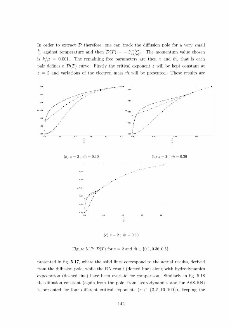
In order to extract D therefore, one can track the diffusion pole for a very smallkµ, against temperature and then D(T ) = −= ω/µc

(k/µ)2 . The momentum value chosen

is k/µ = 0.001. The remaining free parameters are then z and m, that is each

pair defines a D(T ) curve. Firstly the critical exponent z will be kept constant at

z = 2 and variations of the electron mass m will be presented. These results are

ææææ ææ

ææ

æ

æ

æ

æ

æ

æ

æ

æ

æ

æ

æ

æ

æ

æ

æ

æ

æ

æ

æ

æ

æ

æ

æ

æ

æ

æ

æ

æ

æ

æ

æ

æ

æ

æ

æ

æ

æ

æ

æ

æ

æ

æ

æ

æ

æ

æ

æ

æ

æ

æ

æ

æ

æ

æ

æ

æ

æ

æ

æ

æ

æ

æ

æ

æ

æ

æ

æ

æ

æ

æ

0.0 0.1 0.2 0.3 0.4 0.5

0.00

0.05

0.10

0.15

0.20

0.25

0.30

T

Μ

D

(a) z = 2 ; m = 0.10

æææææææ

æ

æ

æ

æ

æ

æ

æ

æ

æ

æ

æ

ææ

æ

æ

æ

æ

æ

æ

æ

æ

æ

æ

æ

æ

æ

æ

æ

æ

æ

æ

æ

æ

æ

æ

æ

æ

æ

æ

æ

æ

æ

æ

æ

æ

æ

æ

0.00 0.05 0.10 0.15

0.00

0.05

0.10

0.15

0.20

T

Μ

D

(b) z = 2 ; m = 0.36

æ

æ

æ

æ

æ

æ

æ

ææ

æ

æ

æ

æ

æ

æ

æ

æ

æ

æ

æ

æ

æ

æ

æ

æ

æ

æ

æ

æ

æ

æ

æ

æ

ææ

æææ

0.0 0.1 0.2 0.3 0.4

0.00

0.05

0.10

0.15

0.20

0.25

T

Μ

D

(c) z = 2 ; m = 0.50

Figure 5.17: D(T ) for z = 2 and m ∈ 0.1, 0.36, 0.5.

presented in fig. 5.17, where the solid lines correspond to the actual results, derived

from the diffusion pole, while the RN result (dotted line) along with hydrodynamics

expectation (dashed line) have been overlaid for comparison. Similarly in fig. 5.18

the diffusion constant (again from the pole, from hydrodynamics and for AdS-RN)

is presented for four different critical exponents (z ∈ 3, 5, 10, 100), keeping the

142

electron mass constant at m = 0.36.

æ

æ

æ

æ

æ

æ

æ

æ

æ

æ

æ

æ

æ

æ

æ

æ

æ

æ

æ

æ

æ

æ

æ

æ

æ

æ

æ

æ

æ

æ

æ

æ

æ

æ

æ

æ

æ

æ

æ

æ

æ

æ

æ

æ

æ

ææ

ææ

æ

æ

æ

æ

æ

0.0 0.1 0.2 0.3 0.4

0.00

0.05

0.10

0.15

0.20

0.25

T

Μ

D

(a) z = 3 ; m = 0.36

æ

æ

æ

æ

æ

æ

æ

æ

æ

æ

æ

æ

æ

æ

æ

æ

æ

æ

æ

æ

æ

æ

æ

æ

æ

æ

æ

æ

æ

æ

æ

æ

æ

æ

æ

æ

æ

æ

æ

æ

æ

æ

æ

æ

æ

æ

æ

æ

æ

ææ

ææ

ææ

æ

æ

æ

æ

æ

0.0 0.1 0.2 0.3 0.4

0.00

0.05

0.10

0.15

0.20

0.25

T

Μ

D

(b) z = 5 ; m = 0.36

æ

æ

æ

æ

æ

æ

æ

æ

æ

æ

æ

æ

æ

æ

æ

æ

æ

æ

æ

æ

æ

æ

æ

æ

æ

æ

æ

æ

æ

æ

æ

æ

æ

æ

æ

æ

æ

æ

æ

æ

æ

æ

æ

æ

æ

æ

æ

æ

æ

ææ

ææ

ææ

ææ

æ

æ

æ

æ

æ

æ

æ

0.0 0.1 0.2 0.3 0.4

0.00

0.05

0.10

0.15

0.20

0.25

T

Μ

D

(c) z = 10 ; m = 0.36

æ

æ

ææ

ææ

ææ

ææ

ææ

ææ

æ

æ

æ

æ

æ

æ

æ

æ

æ

æ

æ

æ

æ

æ

æ

æ

æ

æ

æ

æ

æ

æ

æ

æ

æ

æ

æ

æ

æ

æ

æ

ææ

ææ

ææ

ææ

ææ

ææ

ææ

æ

æ

æ

æ

æ

æ

æ

æ

æ

0.0 0.1 0.2 0.3 0.4

0.00

0.05

0.10

0.15

0.20

0.25

T

Μ

D

(d) z = 100 ; m = 0.36

Figure 5.18: D(T ) for m = 0.36 and z ∈ 3, 5, 10, 100.

Let’s summarize these results. The first, and easiest to describe, feature of the

plots presented in this sections, is that for every pair of the parameters z, m there

is a transition temperature above which the diffusion coefficient converges to the

prediction for the pure AdS-RN system, i.e. when the Electron Star is absent. This is

trivially expected since, as it has been noticed when studying the background, there is

a finite range of temperatures within which the Electron Star is supported. Once the

temperature exceeds the upper bound the black hole is hot/large enough to dominate

the space-time, leaving no room for the star. The transition temperature appears to

depend on the mass of the electron (m). In particular the larger the mass the lower

143

the transition temperature. On the other hand the transition temperature seems to

be very weakly correlated (if at all) with the critical exponent (z).

The more interesting and challenging part of these results is however related with

the low-temperature behaviour of the diffusion constant. The striking characteristic

is that it does not match the purely hydrodynamical prediction. The discrepancy

seems not to be affected primarily by the electron mass, however the fact that an

increase in m makes the transition towards the RN prediction quicker, suppresses the

phenomenon. On the other hand this discrepancy seems to depend more strongly on

the critical exponent. In particular the higher the critical exponent the closer the

results are to both the hydrodynamics prediction and the RN. This should not be

surprising since, as already noticed before, it is expected that at the limit z → ∞one should recover the AdS2 near-horizon geometry. In other words the purely RN

result.

What is striking and unexpected is that away from the limits when one recovers

known systems, the system does not agree with hydrodynamical expectations. In

order to understand this phenomenon one needs to consider the physical attributes of

the system. What one has here is a system with two types of bulk charges - one that

is behind the horizon (corresponding to the black hole) and one that is outside the

horizon (corresponding to the electron star). Each of these charge sources, induces

an electric flux through the boundary corresponding to boundary states. Depending

on the source of the flux the phases are described as mesonic (Electron Star), fully

fractionalised (RN) and partially fractionalised (ES and RN together) [135]. At low

temperatures where ES and RN coexist the system is in the partially fractionlized

phase, while above the transition temperature where there is only RN the system is in

the fully fractionalised phase. Although this system has been studied at zero temper-

ature in [135], here the system is heated up by taking the RN black hole away from

extremality without however allowing the mesonic degrees of freedom to exchange

heat with the fractionalised ones. This is because the Electron Star is assumed to

remain at zero temperature (as explained above) no matter what the Hawking tem-

perature of the black hole is. In other words on the boundary the systems consists of

a set of two degrees of freedom that do not “communicate” thermodynamically and

therefore the system is not in equilibrium. When the temperature is lowered enough,

i.e the black hole is nearly extremal, eventually the phenomenon becomes irrelevant

and diffusion ceases as expected by standard hydrodynamics, since the degrees of

freedom “freeze” out, leading to D(T → 0) = 0.

144

æ

æ

æ

æ

æ

æ

æ

æ

æ

æ

æ

æ

ææ

à

à

à

à

à

à

à

à

à

à

à

à

à

à

àà

à

ì

ì

ì

ì

ì

ì

ì

ì

ì

ì

ì

ì

ì

ì

ì

ìì

ìì ì

ò

ò

ò

ò

ò

ò

ò

ò

ò

ò

ò

ò

ò

ò

òò

òò

ò ò ò ò

ô

ô

ôô

ôô ô ô ô ô ô ô ô ô ô ô ô ô ô ô ô ô ô ô

æ z=2

à z=3

ì z=5

ò z=10

ô z=100

0.00 0.02 0.04 0.06 0.08 0.10 0.12

0.0

0.2

0.4

0.6

0.8

1.0

T

Μ

Qes

Qto

tal

Figure 5.19: Fraction of Electron Star charge vs. z and Tµ .

How can one quantify this phenomenon? A useful parameter is the ratio of the

charge of the Electron Star over the total charge of the system [129]. This quantity

measures how much of the boundary flux comes from the “frozen” mesonic degrees

of freedom. Varying the critical exponent the ratio against temperature is presented

in fig. 5.19, while the results varying the electron mass in fig. 5.20. What one sees

from these is that the higher the critical exponent, the faster the transition from a

partially to a fully fractionalised phase is. The more the system approaches the latter

the more the diffusion constant agrees with both the hydrodynamical prediction and

the pure RN, which corresponds to the fully fractionalised phase. Said differently

for a fixed temperature (and electron mass) the charge ratio QesQtotal

→ 0 as z →∞, i.e the boundary flux is essentially sourced from behind the horizon, restoring

the known hydrodynamical properties of the AdS-RN system. Similarly if one fixes

the temperature and the critical exponent and varies the electron mass, it becomes

apparent that as the mass grows the ratio goes to 0 again asymptoting to the AdS-RN

system.

Trying to explain further this phenomenon the following was attempted. Assuming

the form 5.46 for the diffusion coefficient what would happen if one had included more

145

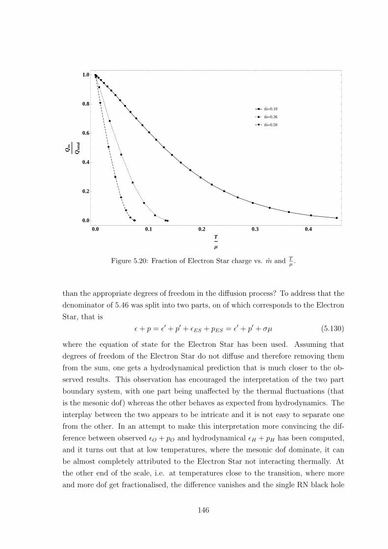
æææ

æ

æ

æ

æ

æ

æ

æ

æ

æ

æ

æ

æ

æ

æ

æ

æ

æ

æ

æ

æ

æ

æ

æ

æ

æ

à

à

à

à

à

à

à

àà

ì

ì

ì

ì

ì

ì

ììì

æ m`

=0.10

à m`

=0.36

ì m`

=0.50

0.0 0.1 0.2 0.3 0.4

0.0

0.2

0.4

0.6

0.8

1.0

T

Μ

Qes

Qto

tal

Figure 5.20: Fraction of Electron Star charge vs. m and Tµ .

than the appropriate degrees of freedom in the diffusion process? To address that the

denominator of 5.46 was split into two parts, on of which corresponds to the Electron

Star, that is

ε+ p = ε′ + p′ + εES + pES = ε′ + p′ + σµ (5.130)

where the equation of state for the Electron Star has been used. Assuming that

degrees of freedom of the Electron Star do not diffuse and therefore removing them

from the sum, one gets a hydrodynamical prediction that is much closer to the ob-

served results. This observation has encouraged the interpretation of the two part

boundary system, with one part being unaffected by the thermal fluctuations (that

is the mesonic dof) whereas the other behaves as expected from hydrodynamics. The

interplay between the two appears to be intricate and it is not easy to separate one

from the other. In an attempt to make this interpretation more convincing the dif-

ference between observed εO + pO and hydrodynamical εH + pH has been computed,

and it turns out that at low temperatures, where the mesonic dof dominate, it can

be almost completely attributed to the Electron Star not interacting thermally. At

the other end of the scale, i.e. at temperatures close to the transition, where more

and more dof get fractionalised, the difference vanishes and the single RN black hole

146

High Tµ

Low Tµ

z=2 ∼ (k/µ)2.06 ∼ (k/µ)2.003

z=3 ∼ (k/µ)2.03 ∼ (k/µ)2.08

z=10 ∼ (k/µ)2.08 ∼ (k/µ)2.08

Table 5.1: Dispersion relation for the lowest QNM, for various ES parameters and temper-atures.

appears to account quite well for the observed diffusion coefficient.

In extracting the diffusion coefficient an important assumption has been made -

that the imaginary part of the corresponding pole should behave quadratically (at

least to first approximation) with momentum. This is an assumption that can and

needs to be tested. In this last part of the current section the dispersion relation of the

lowest lying pole will be examined. Of particular interest is its dependence (if any) on

temperature and the two Electron Star parameters, i.e. the critical exponent and the

electron mass. The way these results will be presented is the following - for each set

of (z, m) the position of the pole against the injected momentum kµ

will be plotted for

the lowest and highest available temperatures 8. The results are presented in fig. 5.21.

The plots are made to be log-log so that a power law will be immediately identified

as straight line. Inset in every plot is the estimate for the exponent of power-law

relation fitting to the small-momentum data 9. Since the presentation of the plots

is quite compact, the actual results are summarized in table 5.1. What becomes

apparent from fig. 5.21 and table 5.1 is that the imaginary part of the lowest lying

QNM does in fact behave quadratically (to a very satisfactory numerical accuracy),

independently of temperature, critical exponent and electron mass. It is also clear

that there are corrections to the quadratic relation, as for higher momenta there is a

deviation from the quadratic curve.

5.4 Sound channel

In this final section, preliminary work on the other channel, i.e sound, will be pre-

sented. What will be included is essentially the necessary analytic preparatory work,

8This form is chosen due to space limitation even though intermediate temperature have beenexamined and found to agree with what is presented here.

9In the inset the symbol k is used for the fitted relation. This is in fact kµ but the symbol k was

chosen for presentation reasons.

147

whereas the actual full numerical analysis will not be done here, due to space-time

limitations. The sound channel consists of the following perturbation components:

hxy, hxx, htt, hyy, hrt, hrx, hrr, ax, at, ar, δφ, δux, δut, δur, δσ, δλ. By perturbing the ac-

tion with respect to these components, one can extract the relevant equations of

motion, which as mentioned before form a closed set and do not couple to the shear

sector due to their symmetry properties (parity under y → −y). The equations of

motion are:

h xt′′ −

(f ′

2f+g′

2g+

4

r

)h xt′ + ıωr2gh r

x′ − ıkr2gh r

t′ − ık

2r2g

(f ′

f+g′

g

)h rt

+ıω

2r2g

(g′

g− f ′

f− 4

r

)h rx + r2gωk

(h yy + h r

r

)+ 2r2h′ (a′x − ıkar)

+ 2r2√fgσ(ax + ıkδφ) = 0 (5.131)

h tt′′ + h y

y′′ +

(f ′

f− g′

2g− 1

r

)h tt′ +

(f ′

2f− g′

2g− 2

r

)h yy′ − 2ıω

g

fh rt′

+

(1

r− f ′

2f

)h rr′ + ıω

(2g

rf− g′

f

)h rt + ω2 g

f(h y

y + h rr )− 2h′

f(a′t + ıωar)

+

(2f ′

rf− h

′2

f− 2

r2

)h rr +

(h′2

f+ g(p+ ρ)

)h tt − 2

gσ√f

(at − ıωδφ) = 0 (5.132)

h xx′′ + h y

y′′ − 2ıkr2gh r

x′ +

2

rh rr′ −(g′

2g+

3

r

)(h x

x′ + h y

y′) + ık(2rg − r2g′)h r

x

− k2r2g(h rr + h y

y ) +

(2f ′

rf− h

′2

f− 2

r2+ 2g(p+ ρ)

)h rr −

(h′2

f+ g(p+ ρ)

)h tt

+2h′

f(a′t + ıωar) + 2

gσ√f

(at − ıωδφ) + 4gµδσ − 4gδλ = 0 (5.133)

h xx′′ + h t

t′′ − 2ıkr2gh r

x′ − 2ıω

g

fh rt′ +

(f ′

f− g′

g− 1

g

)h tt′ +

(1

r− f ′

2f

)h rr′

+

(f ′

2f− g′

2g− 2

r

)h xx′ − ıω

(g′

f− 2g

rf

)h rt − ık

(r2g′ +

r2gf ′

f

)h rx + 2ωk

g

fh xt

+ ω2 g

fh xx − k2r2gh t

t +g

f(ω2 − k2r2f)h r

r +

(h′2

f+ g(p+ ρ)

)h tt

+

(2f ′

rf− h

′2

f− 2

r2

)h rr −

2h′

f(a′t + ıωar)− 2

gσ√f

(at − ıωδφ) = 0 (5.134)

148

ıω

2(h x

x′ + h y

y′) +

ık

2h xt′ +

1

2k2r2gh r

t +1

2ωkr2gh r

x +ıω

rh rr − g(p+ ρ)h r

t

− ıω(f ′

4f+

1

2r

)(h x

x + h yy )− ık

(f ′

2f+

1

r

)h xt −

√fσ(ar + δφ′) = 0

(5.135)

ık

2(h t

t′ + h y

y′)− ıω

2r2fh xt′ +

g

2fωkh r

t +g

2fω2h r

x + ık

(f ′

4f+

1

2r

)h tt

− ık(f ′

4f− 1

2r

)h rr − ı

h′

f(ωax + kat) = 0 (5.136)

(f ′

4f− 1

2r

)(h x

x′ + h y

y′)− 1

rh tt′ + 2ıω

g

rfh rt −

ıkrg

2f(rf ′ − 2f)h r

x

−(h′2

2f− g

2(p+ ρ)

)h tt −

1

2r2f

(r2h

′2 − 2rf ′ + 2f)h rr +

g

2fω2h x

x −k2r2g

2h tt

+g

2f(ω2 − k2r2f)h y

y +g

fωkh x

t +h′

f(a′t + ıωar)−

gσ√f

(at − ıωδφ) = 0 (5.137)

a′′x − ıka′r +1

2

(f ′

f− g′

g

)(a′x − ıkar) +

g

fω(ωax + kat) +

h′2

r2fh xt′

+ ıωgh′

fh rx + gσδux = 0 (5.138)

a′′t + ıωa′r +rg

2(p+ ρ)(a′t + ıωar)− kr2g(kat + ωax)− ıkr2gh′h r

x

+h′

2(h x

x′ + h y

y′ − h t

t′ − h r

r′)− g

√fσh r

r + gσδut − g√fδσ = 0 (5.139)

ıωa′t + ıkr2fa′x − ar(ω2 − k2r2f) +ıω

2h′(h x

x + h yy − h t

t − h rr ) + ıkh′h x

t

+√fgσh r

t − fσδur = 0 (5.140)

h rt′ −√f

gδu′r +

(g′

2g− σ′

σ− 2

r

)h rt +

ıω

2(h r

r + h xx + h y

y − h tt ) + ıkh x

t

+

√f

g

(g′

2g− f ′

2f− σ′

σ+

2

r

)δur −

ıω√fδut +

ıω

σδσ − ıkr2

√fδux = 0 (5.141)

149

ax + ıkδφ+ µδux = 0 (5.142)

2δλ− µδσ − σ√f

(at − ıωδφ+ µδut) = 0 (5.143)

ar + δφ′ + µδur = 0 (5.144)

µ′

σ′δσ + µh t

t −1√f

(at − ıωδφ− µδut) (5.145)

h tt +

2√fδut = 0 (5.146)

where again indices of the metric fluctuations hµν are raised and lowered using the

background metric, a prime denotes a derivative with respect to r, and the depen-

dence of the field fluctuations upon r, ω and k, and of the background fields upon r,

have been suppressed. It should be noted that one may also choose to parametrise

deviations from equilibrium in terms of the variables hµν , aµ, δuµ, δσ, δp and δρ.

This is convenient if one works directly at the level of equations of motion without

invoking an action (as in section 2 of [127]). The bulk fluctuations of pressure and

energy density are related to fluctuations of the Schutz variables via

δp =σµ′

σ′δσ , δρ = µδσ (5.147)

This set of equations is even more unmanageable than the shear sector. Again

though they organize themselves in a much more convenient way, if one introduces

the gauge-invariant variables

Z3(r, ω, l) =ω2h xx (r, ω, k) + 2ωkh x

t (r, ω, k)− k2r2fh tt (r, ω, k) (5.148)

−(ω2 +

k2r3f ′

2

)h yy (r, ω, k)

Z4(r, ω, l) =ωax(r, ω, k) + kat(r, ω, k) +k

2rh′h y

y (r, ω, k)

Z5(r, ω, l) =δσ(r, ω, k) +rσ′

2h yy (5.149)

These are invariant under, as were their shear counterparts, both U(1) (5.69), as

well as diffeomorphism transformations (5.70). Again not all of these equations are

dynamic. Some of them, corresponding to constraint equations, can be solved al-

gebraically and used to simplify the rest. In particular one can solve (5.134-5.136)

150

and (5.139-5.144) for the constraint fields h rr , h r

t , h rt , ar, δut, δux, δur, δφ and δλ.

Substituting the solutions for these fields into the remaining equations, one finds that

there are only three linearly independent equations in the sound (longitudinal) sector.

These linearly-independent equations of motion may be written in the form

Z ′′3 (r) + C31Z′3(r) + C32Z

′4(r) + C33Z

′5(r) + C34Z3(r) + C35Z4(r) + C36Z5(r) = 0

(5.150)

Z ′′4 (r) + C41Z′3(r) + C42Z

′4(r) + C43Z

′5(r) + C44Z3(r) + C45Z4(r) + C46Z5(r) = 0

(5.151)

Z ′′3 (r) + C51Z′3(r) + C52Z

′4(r) + C53Z

′5(r) + C54Z3(r) + C55Z4(r) + C56Z5(r) = 0

(5.152)

The coefficients of these equations are too lengthy and complicated to be put into

print, which would anyway be of limited value. In fact they are computed through

computer algebra software (in particular Mathematica) and are planned to accompany

the upcoming publication of this work, in electronic form. Similarly unprintable is

the on-shell action, which has also been computed in this way. Now, as was the case

for the shear sector, all the necessary ingredients are available in order to proceed

in a systematic numerical analysis of this system. Of particular interest will be the

quest for zero-sound. For this extensive study one is referred to upcoming work.

151

æ

æ

æ

æ

æ

æ

æ

æ

æ

æ

æ

æ

æ

æ

æ

æ

æ

æ

æ

æ

æ

æ

æ

0.26 × k2.06

0.02 0.05 0.10 0.20 0.50 1.00 2.00

0.001

0.01

0.1

1

k

Μ

-Im

@Ω Μc

D

T

Μ=0.131732

(a) z = 2, high

æ

æ

æ

æ

æ

æ

æ

æ

æ

æ

æ

ææ

ææ

æ

0.51 × k2.003

0.02 0.05 0.10 0.20 0.50 1.00

5 ´ 10-4

0.001

0.005

0.010

0.050

0.100

k

Μ

-Im

@Ω ΜcD

T

Μ=0.00711821

(b) z = 2, low

æ

æ

æ

æ

æ

æ

æ

æ

æ

æ

æ

æ

æ

æ

æ

æ

æ

æ

æ

æ

æ

æ

æ

0.26×k2.03

0.02 0.05 0.10 0.20 0.50 1.00 2.00

10-4

0.001

0.01

0.1

1

k

Μ

-Im

@Ω Μc

D

T

Μ=0.131804

(c) z = 3, high

æ

æ

æ

æ

æ

æ

æ

æ

æ

æ

æ

ææ

ææ

ææ

ææ

æ æ æ æ æ

0.38 × k2.08

0.02 0.05 0.10 0.20 0.50 1.00 2.00

0.001

0.01

0.1

k

Μ

-Im

@Ω Μc

DT

Μ=0.026438

(d) z = 3, low

æ

æ

æ

æ

æ

æ

æ

æ

æ

æ

æ

æ

æ

æ

æ

æ

æ

æ

æ

æ

æ

æ

0.27 × k2.08

0.02 0.05 0.10 0.20 0.50 1.00 2.00

10-4

0.001

0.01

0.1

1

k

Μ

-Im

@Ω Μc

D

T

Μ=0.131878

(e) z = 10, high

æ

æ

æ

æ

æ

æ

æ

æ

æ

æ

æ

æ

æ

ææ

ææ

æ æ æ æ æ æ æ

0.29×k2.08

0.02 0.05 0.10 0.20 0.50 1.00 2.00

10-4

0.001

0.01

0.1

k

Μ

-Im

@Ω Μc

D

T

Μ=0.042794

(f) z = 10, low

Figure 5.21: Dispersion relations.

152

Chapter 6

Conclusions and discussion

In the concluding chapter of this thesis the main results presented so far will be

summarized. First the AdS4 case will be reviewed, followed by the Electron Star.

6.1 AdS4

In the studying the Anti-de Sitter Reissner–Nordstrom system the main results, in

summary, are as follows:

i) When momentum q µ, the long-lived modes of the charge density and en-

ergy density Green’s functions are the sound and diffusion-like modes with dispersion

relations (4.4) and (4.5) respectively.

ii) When momentum q µ and temperature T µ, the attenuation of the

sound mode shows no significant temperature dependence, unlike in the strongly-

coupled D3/D7 field theory and in Landau’s theory of Fermi liquids. When q µ

and T µ, the sound and diffusion dispersion relations are well-approximated by

the µ = 0 results of [107,109].

iii) When q µ, the energy density spectral function is dominated by the sound

peak at all temperatures, whereas the charge density spectral function undergoes a

crossover from sound domination at low temperatures to diffusion domination at high

temperatures. This crossover is due to the changing residue at each pole, and occurs

at a temperature Tcross ∼ µ2/q µ.

iv) When q µ and T µ, the sound and diffusion modes no longer dominate

the energy density and charge density spectral functions, and the effects of other

modes become important.

v) When both µ and T are non-zero, a long-lived sound mode will propagate

provided that its momentum q is much less than either µ or T .

153

These results show that although many strongly-coupled field theories at large

chemical potential (which have a gravitational dual) possess a T = 0 sound mode,

these are not all LFL-like ‘zero sound’ modes (by which one means that they don’t

have the properties shown in figure 4.1) as was the case in the D3/D7 theory. However,

there is still the possibility that there could be universal behaviour of the sound mode

within subsets of strongly-coupled field theories with a gravitational dual. It is noted

that the density-dependent physics in the D3/D7 and RN-AdS4 theories arise through

different holographic mechanisms (see [82, 136] for further discussion of this). In the

D3/D7 theory, the background metric is fixed and it is the gauge field action - the DBI

action - which alters the equation of motion of the gauge field from the µ = 0 Maxwell

equation (whose only long-lived mode is the high temperature charge diffusion mode).

In contrast to this, the gauge field equation of motion in the RN-AdS4 theory departs

from the µ = 0 Maxwell equation via couplings to the bulk metric fluctuations.

The other major difference between these two field theories is the number of spatial

dimensions, but it not expected that this will have a significant effect on the acoustic

properties of the theory (provided that the number of field theory spatial dimensions

is greater than one).

It would be very interesting to check whether the low temperature sound modes in

other probe brane theories [92–96] share the LFL-like properties of the D3/D7 theory.

This would help to establish whether it is the form of the DBI action, which implies

that the non-zero density in the field theory is a density of fundamental matter

(at least in the cases where the background geometry can be derived from string

theory) rather than, for example, the R-charge density in the RN-AdS4 theory, that

generates these interesting properties or not. The effects of metric back-reaction (i.e.

coupling between the field theory’s charge density and energy density) are also yet to

be computed for these probe brane theories. These may complete the LFL-like picture

of acoustic propagation (by reproducing the full LFL sound attenuation curve - figure

4.1 - including the hydrodynamic regime), or they may result in deviations from it. No

more insight can be gained into this from our back-reacted RN-AdS4 results because

of the difference in gauge field actions described previously. Although an expansion

of the DBI action in powers of Fµν yields the Maxwell action at lowest order, in field

theory quantities this is an expansion in powers of µ/T which is the opposite limit

from that in which any LFL-like properties of a theory would be exhibited.

In addition to those mentioned above, there are numerous other field theories with

a gravitational dual which may possess interesting sound modes when T µ. Among

the most interesting of these are dilatonic black holes [136–138] and geometries where

154

the bulk charge density is sourced by fermions [127, 129, 139–141]. It would also

be worthwhile to determine the acoustic properties of more general truncations of

super-gravity which admit more complicated solutions than RN-AdS4 (for example,

those of [111, 137, 142]), to determine whether the specific truncation chosen has a

significant effect on these properties.

It has become clear that even this relatively simple holographic theory has many

non-trivial features in its bosonic excitations. Among the most intriguing are the

accuracy of the ‘zero temperature hydrodynamics’, and the crossover temperature

Tcross. ∼ µ2/q between the charge density spectral function being dominated by the

sound mode and the diffusion mode. It would be useful to have a clearer physical

understanding of these properties, and also to determine if they are present in other

field theories at non-zero chemical potential.

6.2 Electron Star

In studying the Electron Star system, in a non-zero temperature RN-AdS background,

and in particular in the shear channel, the main results, in summary, are as follows:

i)The system possesses a QNM structure similar to many other gravitational sys-

tems, studied within Holography. In particular there is a long-lived or stable (i.e.

very close to the origin of the complex frequency plane) pole on the imaginary axis

(i.e. purely dissipative), which corresponds to diffusion in the system.

ii)The system is essentially composed of two kinds of degrees of freedom on the

boundary - those related to the black-hole charge, i.e. the charge coming from behind

the horizon and those related to the bulk fermionic charge of the Electron Star. The

two sets of degrees of freedom are not in equilibrium, as one of them (the mesonic

part) is constantly kept at zero temperature, while the other is heated up. This

is reflected in the non-hydrodynamical low-temperature behaviour of the diffusion

coefficient.

iii)The mixture of the two kinds of degrees of freedom is measure by the Electron

Star to total charge ratio, which has been shown to depend on the system’s tem-

perature as well as the critical exponent and the electron mass. This ratio can be

used as an order parameter to distinguish between the partially fractionalised and

the fully fractionalised phases. Furthermore, as seen from the results presented here,

it measures the departure from the hydrodynamical behaviour.

iv)A feature that has been observed in this analysis but was not elaborated on,

since it is a negative result, is the absence of a real pole in the frequency plane. Such

155

a pole would correspond to a Fermi Surface in the boundary theory. This absence

cannot be reliably accounted for and further study along with more robust numerical

methods, appears to be required.

Moving forward in the exploration of the properties of this system, two directions

should be pursued. Firstly and most importantly the bulk fermions must be allowed

to thermally interact with the rest of the system so that it can relax and reach a

proper equilibrium state. This entails the explicit treatment of the bulk fermions in

the RN-AdS background, in place of the current approximation. This work is already

under way.

Finally, the sound channel of the system has to be finalized. The existence of a

zero-sound, as is the case in so many Holographic systems, should be examined. This

work is almost completed and will be soon published.

156

Bibliography

[1] N. Beisert, C. Ahn, L. F. Alday, Z. Bajnok, J. M. Drummond, et al., Review

of AdS/CFT Integrability: An Overview, Lett.Math.Phys. 99 (2012) 3–32,

[arXiv:1012.3982].

[2] R. A. Davison and A. O. Starinets, Holographic zero sound at finite

temperature, Phys.Rev. D85 (2012) 026004, [arXiv:1109.6343].

[3] M. Edalati, J. I. Jottar, and R. G. Leigh, Holography and the sound of

criticality, JHEP 1010 (2010) 058, [arXiv:1005.4075].

[4] P. Atkins and J. de Paula, Atkins’ Physical Chemistry. OUP Oxford, 2010.

[5] J. M. Maldacena, The Large N limit of superconformal field theories and

supergravity, Adv.Theor.Math.Phys. 2 (1998) 231–252, [hep-th/9711200].

[6] S. Gubser, I. R. Klebanov, and A. M. Polyakov, Gauge theory correlators from

noncritical string theory, Phys.Lett. B428 (1998) 105–114, [hep-th/9802109].

[7] E. Witten, Anti-de Sitter space and holography, Adv.Theor.Math.Phys. 2

(1998) 253–291, [hep-th/9802150].

[8] O. Aharony, S. S. Gubser, J. M. Maldacena, H. Ooguri, and Y. Oz, Large N

field theories, string theory and gravity, Phys.Rept. 323 (2000) 183–386,

[hep-th/9905111].

[9] J. Casalderrey-Solana, H. Liu, D. Mateos, K. Rajagopal, and U. A.

Wiedemann, Gauge/String Duality, Hot QCD and Heavy Ion Collisions,

arXiv:1101.0618.

[10] S. A. Hartnoll, Lectures on holographic methods for condensed matter physics,

Class.Quant.Grav. 26 (2009) 224002, [arXiv:0903.3246].

157

[11] S. S. Gubser, Breaking an Abelian gauge symmetry near a black hole horizon,

Phys.Rev. D78 (2008) 065034, [arXiv:0801.2977].

[12] S. A. Hartnoll, C. P. Herzog, and G. T. Horowitz, Building a Holographic

Superconductor, Phys.Rev.Lett. 101 (2008) 031601, [arXiv:0803.3295].

[13] S. A. Hartnoll, C. P. Herzog, and G. T. Horowitz, Holographic

Superconductors, JHEP 0812 (2008) 015, [arXiv:0810.1563].

[14] H. Liu, J. McGreevy, and D. Vegh, Non-Fermi liquids from holography,

Phys.Rev. D83 (2011) 065029, [arXiv:0903.2477].

[15] M. Cubrovic, J. Zaanen, and K. Schalm, String Theory, Quantum Phase

Transitions and the Emergent Fermi-Liquid, Science 325 (2009) 439–444,

[arXiv:0904.1993].

[16] T. Faulkner, H. Liu, J. McGreevy, and D. Vegh, Emergent quantum criticality,

Fermi surfaces, and AdS(2), Phys.Rev. D83 (2011) 125002,

[arXiv:0907.2694].

[17] G. T. Horowitz, Theory of Superconductivity, Lect.Notes Phys. 828 (2011)

313–347, [arXiv:1002.1722].

[18] J. McGreevy, Holographic duality with a view toward many-body physics,

Adv.High Energy Phys. 2010 (2010) 723105, [arXiv:0909.0518].

[19] M. Rangamani, Gravity and Hydrodynamics: Lectures on the fluid-gravity

correspondence, Class.Quant.Grav. 26 (2009) 224003, [arXiv:0905.4352].

[20] G. Policastro, D. T. Son, and A. O. Starinets, From AdS / CFT

correspondence to hydrodynamics, JHEP 0209 (2002) 043, [hep-th/0205052].

[21] G. Policastro, D. T. Son, and A. O. Starinets, From AdS / CFT

correspondence to hydrodynamics. 2. Sound waves, JHEP 0212 (2002) 054,

[hep-th/0210220].

[22] S. Bhattacharyya, V. E. Hubeny, S. Minwalla, and M. Rangamani, Nonlinear

Fluid Dynamics from Gravity, JHEP 0802 (2008) 045, [arXiv:0712.2456].

[23] C. P. Herzog, Lectures on Holographic Superfluidity and Superconductivity,

J.Phys. A42 (2009) 343001, [arXiv:0904.1975].

158

[24] S. A. Hartnoll, Horizons, holography and condensed matter, arXiv:1106.4324.

[25] V. E. Hubeny, S. Minwalla, and M. Rangamani, The fluid/gravity

correspondence, arXiv:1107.5780.

[26] V. E. Hubeny, The Fluid/Gravity Correspondence: a new perspective on the

Membrane Paradigm, Class.Quant.Grav. 28 (2011) 114007,

[arXiv:1011.4948].

[27] M. P. Heller, R. A. Janik, and P. Witaszczyk, The characteristics of

thermalization of boost-invariant plasma from holography, Phys.Rev.Lett. 108

(2012) 201602, [arXiv:1103.3452].

[28] L. Landau and E. Lifshitz, Fluid Mechnics. Pergamon, 1966.

[29] R. Liboff, Kinetic Theory: Classical, Quantum, and Relativistic Descriptions.

Graduate Texts in Contemporary Physics. Springer, 2003.

[30] P. Romatschke, New Developments in Relativistic Viscous Hydrodynamics,

Int.J.Mod.Phys. E19 (2010) 1–53, [arXiv:0902.3663].

[31] P. Kovtun, Lectures on hydrodynamic fluctuations in relativistic theories,

J.Phys. A45 (2012) 473001, [arXiv:1205.5040].

[32] D. T. Son and A. O. Starinets, Hydrodynamics of r-charged black holes, JHEP

0603 (2006) 052, [hep-th/0601157].

[33] S. Sachdev, Quantum Phase Transitions. Cambridge University Press, 2001.

[34] J. Negele and H. Orland, Quantum Many-particle Systems. Westview Press,

2008.

[35] M. Bellac, Thermal Field Theory. Cambridge Monographs on Mathematical

Physics. Cambridge University Press, 2000.

[36] J. Kapusta and C. Gale, Finite-Temperature Field Theory: Principles and

Applications. Cambridge Monographs on Mathematical Physics. Cambridge

University Press, 2006.

[37] J. Polchinski, Effective field theory and the Fermi surface, hep-th/9210046.

[38] H. A. Kramers and G. H. Wannier, Statistics of the two-dimensional

ferromagnet. part i, Phys. Rev. 60 (Aug, 1941) 252–262.

159

[39] H. A. Kramers and G. H. Wannier, Statistics of the two-dimensional

ferromagnet. part ii, Phys. Rev. 60 (Aug, 1941) 263–276.

[40] L. Onsager, Crystal statistics. i. a two-dimensional model with an

order-disorder transition, Phys. Rev. 65 (Feb, 1944) 117–149.

[41] A. Joyal and R. Street, An introduction to tannaka duality and quantum

groups, in Category theory, pp. 413–492, Springer, 1991.

[42] R. Savit, Duality in field theory and statistical systems, Rev. Mod. Phys. 52

(Apr, 1980) 453–487.

[43] R. Rajaraman, Solitons and Instantons: An Introduction to Solitons and

Instantons in Quantum Field Theory. North-Holland personal library.

North-Holland Publishing Company, 1982.

[44] C. Vafa, Geometric origin of Montonen-Olive duality, Adv.Theor.Math.Phys. 1

(1998) 158–166, [hep-th/9707131].

[45] N. Seiberg and E. Witten, Electric - magnetic duality, monopole condensation,

and confinement in N=2 supersymmetric Yang-Mills theory, Nucl.Phys. B426

(1994) 19–52, [hep-th/9407087].

[46] J. de Boer, L. Maoz, and A. Naqvi, Some aspects of the AdS / CFT

correspondence, hep-th/0407212.

[47] K.-H. Rehren, QFT lectures on AdS-CFT, hep-th/0411086.

[48] G. T. Horowitz and J. Polchinski, Gauge/gravity duality, gr-qc/0602037.

[49] H. Nastase, Introduction to AdS-CFT, arXiv:0712.0689.

[50] M. K. Benna and I. R. Klebanov, Gauge-String Dualities and Some

Applications, arXiv:0803.1315.

[51] J. Soda, AdS/CFT on the brane, Lect.Notes Phys. 828 (2011) 235–270,

[arXiv:1001.1011].

[52] J. Polchinski, Introduction to Gauge/Gravity Duality, arXiv:1010.6134.

[53] A. Strominger and C. Vafa, Microscopic origin of the Bekenstein-Hawking

entropy, Phys.Lett. B379 (1996) 99–104, [hep-th/9601029].

160

[54] S. Carlip, Black Hole Thermodynamics and Statistical Mechanics, Lect.Notes

Phys. 769 (2009) 89–123, [arXiv:0807.4520].

[55] A. Sen, Black Hole Entropy Function, Attractors and Precision Counting of

Microstates, Gen.Rel.Grav. 40 (2008) 2249–2431, [arXiv:0708.1270].

[56] M. Green, J. Schwarz, and E. Witten, Superstring Theory: Volume 1,

Introduction. Cambridge Monographs on Mathematical Physics. Cambridge

University Press, 1988.

[57] M. Green, J. Schwarz, and E. Witten, Superstring Theory: Volume 2, Loop

Amplitudes, Anomalies and Phenomenology. Cambridge Monographs on

Mathematical Physics. Cambridge University Press, 1987.

[58] E. Kiritsis, String Theory in a Nutshell. In a Nutshell. Princeton University

Press, 2011.

[59] J. Polchinski, String Theory. Cambridge Monographs on Mathematical

Physics. Cambridge University Press, 2005.

[60] J. Polchinski, Tasi lectures on D-branes, hep-th/9611050.

[61] C. Johnson, D-Branes. Cambridge Monographs on Mathematical Physics.

Cambridge University Press, 2006.

[62] P. West, Introduction to Strings and Branes. Cambridge University Press,

2012.

[63] K. Becker, M. Becker, and J. Schwarz, String Theory and M-Theory: A

Modern Introduction. Cambridge University Press, 2007.

[64] D. Freedman and A. Van Proeyen, Supergravity. Cambridge University Press,

2012.

[65] D. Tong, String Theory, arXiv:0908.0333.

[66] E. Witten, Bound states of strings and p-branes, Nucl.Phys. B460 (1996)

335–350, [hep-th/9510135].

[67] Y. Makeenko, Methods of Contemporary Gauge Theory. Cambridge

Monographs on Mathematical Physics. Cambridge University Press, 2002.

161

[68] S. S. Gubser, I. R. Klebanov, and A. A. Tseytlin, Coupling constant

dependence in the thermodynamics of N=4 supersymmetric Yang-Mills theory,

Nucl.Phys. B534 (1998) 202–222, [hep-th/9805156].

[69] A. Fotopoulos and T. Taylor, Comment on two loop free energy in N=4

supersymmetric Yang-Mills theory at finite temperature, Phys.Rev. D59

(1999) 061701, [hep-th/9811224].

[70] J.-P. Blaizot, E. Iancu, U. Kraemmer, and A. Rebhan, Hard thermal loops and

the entropy of supersymmetric Yang-Mills theories, JHEP 0706 (2007) 035,

[hep-ph/0611393].

[71] D. T. Son and A. O. Starinets, Minkowski space correlators in AdS / CFT

correspondence: Recipe and applications, JHEP 0209 (2002) 042,

[hep-th/0205051].

[72] C. Herzog and D. Son, Schwinger-Keldysh propagators from AdS/CFT

correspondence, JHEP 0303 (2003) 046, [hep-th/0212072].

[73] K. Skenderis, Lecture notes on holographic renormalization, Class.Quant.Grav.

19 (2002) 5849–5876, [hep-th/0209067].

[74] M. Bianchi, D. Z. Freedman, and K. Skenderis, Holographic renormalization,

Nucl.Phys. B631 (2002) 159–194, [hep-th/0112119].

[75] P. Morse and H. Feshbach, Methods of Theoretical Physics. Philip M.

Morse,... Herman Feshbach,... Mc Graw-Hill book Co, 1953.

[76] N. Birrell and P. Davies, Quantum Fields in Curved Space. Cambridge

Monographs on Mathematical Physics. Cambridge University Press, 1984.

[77] P. Breitenlohner and D. Z. Freedman, Stability in Gauged Extended

Supergravity, Annals Phys. 144 (1982) 249.

[78] G. Policastro, D. Son, and A. Starinets, The Shear viscosity of strongly

coupled N=4 supersymmetric Yang-Mills plasma, Phys.Rev.Lett. 87 (2001)

081601, [hep-th/0104066].

[79] A. Karch, D. Son, and A. Starinets, Zero Sound from Holography,

arXiv:0806.3796.

162

[80] A. Nunez and A. O. Starinets, AdS / CFT correspondence, quasinormal

modes, and thermal correlators in N=4 SYM, Phys.Rev. D67 (2003) 124013,

[hep-th/0302026].

[81] K. Sfetsos and K. Skenderis, Microscopic derivation of the

Bekenstein-Hawking entropy formula for nonextremal black holes, Nucl.Phys.

B517 (1998) 179–204, [hep-th/9711138].

[82] S. A. Hartnoll, J. Polchinski, E. Silverstein, and D. Tong, Towards strange

metallic holography, JHEP 1004 (2010) 120, [arXiv:0912.1061].

[83] T. Faulkner, N. Iqbal, H. Liu, J. McGreevy, and D. Vegh, From Black Holes to

Strange Metals, arXiv:1003.1728.

[84] G. T. Horowitz, J. E. Santos, and B. Way, A Holographic Josephson Junction,

Phys.Rev.Lett. 106 (2011) 221601, [arXiv:1101.3326].

[85] M. Edalati, R. G. Leigh, and P. W. Phillips, Dynamically Generated Mott Gap

from Holography, Phys.Rev.Lett. 106 (2011) 091602, [arXiv:1010.3238].

[86] R. A. Davison and N. K. Kaplis, Bosonic excitations of the AdS4

Reissner-Nordstrom black hole, JHEP 1112 (2011) 037, [arXiv:1111.0660].

[87] M. Edalati, J. I. Jottar, and R. G. Leigh, Transport Coefficients at Zero

Temperature from Extremal Black Holes, JHEP 1001 (2010) 018,

[arXiv:0910.0645].

[88] M. Edalati, J. I. Jottar, and R. G. Leigh, Shear Modes, Criticality and

Extremal Black Holes, JHEP 1004 (2010) 075, [arXiv:1001.0779].

[89] D. Nickel and D. T. Son, Deconstructing holographic liquids, New J.Phys. 13

(2011) 075010, [arXiv:1009.3094].

[90] M. Kulaxizi and A. Parnachev, Comments on Fermi Liquid from Holography,

Phys.Rev. D78 (2008) 086004, [arXiv:0808.3953].

[91] M. Ammon, J. Erdmenger, S. Lin, S. Muller, A. O’Bannon, et al., On Stability

and Transport of Cold Holographic Matter, JHEP 1109 (2011) 030,

[arXiv:1108.1798].

[92] M. Kulaxizi and A. Parnachev, Holographic Responses of Fermion Matter,

Nucl.Phys. B815 (2009) 125–141, [arXiv:0811.2262].

163

[93] L.-Y. Hung and A. Sinha, Holographic quantum liquids in 1+1 dimensions,

JHEP 1001 (2010) 114, [arXiv:0909.3526].

[94] C. Hoyos-Badajoz, A. O’Bannon, and J. M. Wu, Zero Sound in Strange

Metallic Holography, JHEP 1009 (2010) 086, [arXiv:1007.0590].

[95] B.-H. Lee, D.-W. Pang, and C. Park, Zero Sound in Effective Holographic

Theories, JHEP 1011 (2010) 120, [arXiv:1009.3966].

[96] O. Bergman, N. Jokela, G. Lifschytz, and M. Lippert, Striped instability of a

holographic Fermi-like liquid, JHEP 1110 (2011) 034, [arXiv:1106.3883].

[97] L. Landau, E. Lifshitz, and L. Pitaevskii, Statistical Physics. No. pt. 2 in

Course of Theoretical Physics. Butterworth-Heinemann, 1980.

[98] L. Pitaevskii and E. Lifshitz, Physical Kinetics. No. v. 10. Elsevier Science,

1981.

[99] A. Abrikosov, L. Gorkov, I. Dzalosinskij, and I. Dzialoshinskii, Methods of

Quantum Field Theory in Statistical Physics. Dover books on advanced

mathematics. Dover Publications, Incorporated, 1975.

[100] P. Nozieres and D. Pines, Theory Of Quantum Liquids. Advanced Books

Classics. Westview Press, 1999.

[101] A. Abrikosov and I. Khalatnikov, The theory of a fermi liquid (the properties

of liquid 3he at low temperatures), Reports on Progress in Physics 22 (1959),

no. 1 329.

[102] R. Belliard, S. S. Gubser, and A. Yarom, Absence of a Fermi surface in

classical minimal four-dimensional gauged supergravity, JHEP 1110 (2011)

055, [arXiv:1106.6030].

[103] J. P. Gauntlett, J. Sonner, and D. Waldram, Universal fermionic spectral

functions from string theory, Phys.Rev.Lett. 107 (2011) 241601,

[arXiv:1106.4694].

[104] J. P. Gauntlett, J. Sonner, and D. Waldram, Spectral function of the

supersymmetry current, JHEP 1111 (2011) 153, [arXiv:1108.1205].

[105] D. K. Brattan and S. A. Gentle, Shear channel correlators from hot charged

black holes, JHEP 1104 (2011) 082, [arXiv:1012.1280].

164

[106] X.-H. Ge, K. Jo, and S.-J. Sin, Hydrodynamics of RN AdS4 black hole and

Holographic Optics, JHEP 1103 (2011) 104, [arXiv:1012.2515].

[107] C. P. Herzog, The Sound of M theory, Phys.Rev. D68 (2003) 024013,

[hep-th/0302086].

[108] A. S. Miranda, J. Morgan, and V. T. Zanchin, Quasinormal modes of

plane-symmetric black holes according to the AdS/CFT correspondence, JHEP

0811 (2008) 030, [arXiv:0809.0297].

[109] C. P. Herzog, The Hydrodynamics of M theory, JHEP 0212 (2002) 026,

[hep-th/0210126].

[110] A. Chamblin, R. Emparan, C. V. Johnson, and R. C. Myers, Charged AdS

black holes and catastrophic holography, Phys.Rev. D60 (1999) 064018,

[hep-th/9902170].

[111] M. Cvetic, M. Duff, P. Hoxha, J. T. Liu, H. Lu, et al., Embedding AdS black

holes in ten-dimensions and eleven-dimensions, Nucl.Phys. B558 (1999)

96–126, [hep-th/9903214].

[112] M. Kaminski, K. Landsteiner, J. Mas, J. P. Shock, and J. Tarrio, Holographic

Operator Mixing and Quasinormal Modes on the Brane, JHEP 1002 (2010)

021, [arXiv:0911.3610].

[113] R. Wald, General Relativity. University of Chicago Press, 2010.

[114] P. K. Kovtun and A. O. Starinets, Quasinormal modes and holography,

Phys.Rev. D72 (2005) 086009, [hep-th/0506184].

[115] H. Kodama and A. Ishibashi, Master equations for perturbations of generalized

static black holes with charge in higher dimensions, Prog.Theor.Phys. 111

(2004) 29–73, [hep-th/0308128].

[116] C. P. Herzog, P. Kovtun, S. Sachdev, and D. T. Son, Quantum critical

transport, duality, and M-theory, Phys.Rev. D75 (2007) 085020,

[hep-th/0701036].

[117] J. Oppenheimer and G. Volkoff, On Massive neutron cores, Phys.Rev. 55

(1939) 374–381.

165

[118] R. C. Tolman, Static solutions of Einstein’s field equations for spheres of fluid,

Phys.Rev. 55 (1939) 364–373.

[119] T. Hartman and S. A. Hartnoll, Cooper pairing near charged black holes,

JHEP 1006 (2010) 005, [arXiv:1003.1918].

[120] D. Yamada, Fragmentation of Spinning Branes, Class.Quant.Grav. 25 (2008)

145006, [arXiv:0802.3508].

[121] B. McInnes, Bounding the Temperatures of Black Holes Dual to Strongly

Coupled Field Theories on Flat Spacetime, JHEP 0909 (2009) 048,

[arXiv:0905.1180].

[122] E. Witten, Anti-de Sitter space, thermal phase transition, and confinement in

gauge theories, Adv.Theor.Math.Phys. 2 (1998) 505–532, [hep-th/9803131].

[123] T. Nishioka, S. Ryu, and T. Takayanagi, Holographic Superconductor/Insulator

Transition at Zero Temperature, JHEP 1003 (2010) 131, [arXiv:0911.0962].

[124] G. T. Horowitz and B. Way, Complete Phase Diagrams for a Holographic

Superconductor/Insulator System, JHEP 1011 (2010) 011,

[arXiv:1007.3714].

[125] S. Sachdev, Holographic metals and the fractionalized Fermi liquid,

Phys.Rev.Lett. 105 (2010) 151602, [arXiv:1006.3794].

[126] F. Denef and S. A. Hartnoll, Landscape of superconducting membranes,

Phys.Rev. D79 (2009) 126008, [arXiv:0901.1160].

[127] S. A. Hartnoll and A. Tavanfar, Electron stars for holographic metallic

criticality, Phys.Rev. D83 (2011) 046003, [arXiv:1008.2828].

[128] S. A. Hartnoll, D. M. Hofman, and A. Tavanfar, Holographically smeared

Fermi surface: Quantum oscillations and Luttinger count in electron stars,

Europhys.Lett. 95 (2011) 31002, [arXiv:1011.2502].

[129] S. A. Hartnoll and P. Petrov, Electron star birth: A continuous phase

transition at nonzero density, Phys.Rev.Lett. 106 (2011) 121601,

[arXiv:1011.6469].

[130] G. T. Horowitz and B. Way, Lifshitz Singularities, Phys.Rev. D85 (2012)

046008, [arXiv:1111.1243].

166

[131] N. Bao, X. Dong, S. Harrison, and E. Silverstein, The Benefits of Stress:

Resolution of the Lifshitz Singularity, Phys.Rev. D86 (2012) 106008,

[arXiv:1207.0171].

[132] P. Kovtun, D. T. Son, and A. O. Starinets, Holography and hydrodynamics:

Diffusion on stretched horizons, JHEP 0310 (2003) 064, [hep-th/0309213].

[133] B. F. Schutz, Perfect Fluids in General Relativity: Velocity Potentials and a

Variational Principle, Phys.Rev. D2 (1970) 2762–2773.

[134] P. Benincasa, A. Buchel, and A. O. Starinets, Sound waves in strongly coupled

non-conformal gauge theory plasma, Nucl.Phys. B733 (2006) 160–187,

[hep-th/0507026].

[135] S. A. Hartnoll and L. Huijse, Fractionalization of holographic Fermi surfaces,

Class.Quant.Grav. 29 (2012) 194001, [arXiv:1111.2606].

[136] C. Charmousis, B. Gouteraux, B. Kim, E. Kiritsis, and R. Meyer, Effective

Holographic Theories for low-temperature condensed matter systems, JHEP

1011 (2010) 151, [arXiv:1005.4690].

[137] S. S. Gubser and F. D. Rocha, Peculiar properties of a charged dilatonic black

hole in AdS5, Phys.Rev. D81 (2010) 046001, [arXiv:0911.2898].

[138] K. Goldstein, S. Kachru, S. Prakash, and S. P. Trivedi, Holography of Charged

Dilaton Black Holes, JHEP 1008 (2010) 078, [arXiv:0911.3586].

[139] V. G. M. Puletti, S. Nowling, L. Thorlacius, and T. Zingg, Holographic metals

at finite temperature, JHEP 1101 (2011) 117, [arXiv:1011.6261].

[140] N. Iqbal, H. Liu, and M. Mezei, Semi-local quantum liquids, JHEP 1204

(2012) 086, [arXiv:1105.4621].

[141] S. Sachdev, A model of a Fermi liquid using gauge-gravity duality, Phys.Rev.

D84 (2011) 066009, [arXiv:1107.5321].

[142] M. Duff and J. T. Liu, Anti-de Sitter black holes in gauged N = 8 supergravity,

Nucl.Phys. B554 (1999) 237–253, [hep-th/9901149].

167