ERRATA FOR SLAC-PUB-932 Yung-Su Tsai, “Decay Correlations of Heavy Leptons in et.;+ e- 4+ +Q-," Phys. Rev., D 4, 2821 (1971).

1. A term, -M3(M2 Q p - 4M$/wl 2 was left out of the square bracket of Eq.

(2.20); the complete expression for the square bracket of Eq. (2.20)

should read

2. The right-hand side of Eq. (4.11) must be divided by 4; hence 16 in the

denominator should be replaced by 64. Similarly, 8 in the denominator

of Eq. (40 12) should be replaced by 32.

3. The right-hand side of Eqs.(4.26) and (4.33) must be multiplied by 4. Also,

I in the sentence following Eq, (4.33), “because C is equal to. 0 -. ” should be

replaced by ‘%&cause 4C is equal to. 0 0 ., ”

4. The two mistakes of factor 4 shown above cancel each other in the three

examples of decay correlations given on pp. 2834 and 2835 if we ignore the

corrections. However, after the corrections made in 2 and 3 above we

must also multiply by 4 the left-hand side of Eqs. (40 34), (4.35), (4.37),

(4. 38), (4.41), and (4.42).

The author wishes to thank Dr. John Liu, Dr. T. Sanda, and Dr. S. Y 0

Tsai for pointing out the mistakes.

SLAC-PUB-932 July 1971 (TH) and (EXP)

DECAY CORRELATIONS OF HEAVY LEPTONS IN e+ + e-+ Q+ + Q- *

Yung-Su Tsai

Stanford Linear Accelerator Center Stanford University., Stanford, California 94305

ABSTRACT

Assuming leptons heavier than muons exist in nature we consider their

decay modes and the correlations between the decay products of Q+ and Q- in

the colliding beam experiment: e+ + e- --f Q’ + Q-. Far above the threshold, the

helicities of Q+ and I- tend to be opposite to each other and near the threshold / * . the directions of spins of Q+ and Q- like to be parallel to each other and the sum

. of the two spins likes to be either parallel or antiparallel to the direction of the

incident electron. Because the parity conservation is violated maximally in the

decays of Q+ and Q-, the angular distributions of decay products depend strongly

on the spin orientation of the heavy leptons. Since the spins of Q’ and I- are

strongly correlated in the production we found a strong correlation between

the energy-angle distributions of the decay products of Q+ and Q-. The decay

widths of Q- into channels v r e-, v,V p-, v r-, v k-, v p-, v de P Q Q Q Q k*, v A Ql’ ’

vQQ and vQ+ hadron continuum as functions of the mass of Q- are estimated.

(Submitted to Phys. Rev. and also to the 5th International Symposium on Electron and Photon Interactions at High Energies, Cornell University, Ithaca, New York, August 23-27, 1971)

* Work supported by the U. S. Atomic Energy Commission.

I

I. INTRODUCTION

Since muons exist in nature for no apparent reason, it is possible that other

heavy leptons may also exist in nature. If one discovers heavy leptons, one may

be able to understand why muons exist and obtain some clue as to why the ratio

of the muon mass to the electron mass is roughly mP/me z 210. Searches for these

leptons have been attempted in the past 132 and no doubt people will be looking for

these particles in the e+ -t- e- colliding beam experiments:! (e’ + e--+ Q++ Q-) ,

photo pair production experiments3 ( y + z-+Q+ + Q- + z*) and neutrino experiments

from the electron machine4 ( vQ + z ---+I- + 2”). We have made extensive calcula-

tions for these cross sections. This paper dealsmainly with the decay correla-

-I- - tions in the reaction, e f e + --+I + Q-.

We assume that if heavy lepton exists the leptonic current in the usual

current-current effective Lagrangian5 of the weak interaction is given by

h Jlept = Tp +(l- r5) p+ Ue +(l- r5) e + V Q y*P- r,)Q

and the electromagnetic interaction of the heavy lepton is exactly like that of an

electron or a muon. The major difference between the heavy lepton and the

muon is that whereas the muon is lighter than any strongly interacting particle,

the heavy lepton, if it exists, is expected to be heavier than the k meson; and

hence the heavy lepton decays’ into hadrons in addition to electron and muon.

In the electromagnetic scattering of an electron, it is well known that at

high energies (m/E-O) the helicity of the electron remains the same during the

scattering, whereas at low energies (m/E -1) the direction of the spin with re-

spect to a fixed coordinate system in space is preserved during the scattering. 7

-2-

In Section IV we show that analogous things happen in the reaction e+ + e-+ Q++Q-.

Far above the threshold @4,/E--+ 0)) the helicities of Q+ and Q- like to be opposite

to each other, whereas near the threshold (MQ/E --+ I) the directions of spins of

Q’ and Q- like to be parallel to each other and their total spin likes to be either

parallel or antiparallel to the direction of the incident electron. To the lowest

order in Q, $ and Q- are not polarized if only one of them is analyzed and if neither

the incident electron nor positron is polarized. This is very similar8 to the ep

scattering where in the lowest order in Q the differential cross section is independent

of the spin orientation of the target proton if the incident electron is unpolarized. Since

Q’ and Q- decay via weak interaction where parity conservation is violated maxi-

mally, the angular distribution of decay products depends strongly on the spin

orientation of the heavy lepton. Since the spins of Q+ and I- are strongly cor-

related in the production, we expect the angular distributions of decay products

of Q’ to be strongly correlated to those of Q-. In Section II, we discuss the decay c

widths and energy-angle distribution of the charged decay products from an

arbitrarily polarized Q- into vQ -t Fe + e-, vQ -I- r + ,u-, vQ + r-, vQ + k- and c1

VQ +p-. The invariance under CP is then used to relate the energy-angle distri-

bution of the decay products of Q’ to that of Q-. In Section III, the hadronic decay

width of Q’ is written in terms of an integration over the spectral

functions of weak hadronic currents. Weinbergis stun rule is used to evaluate

the decay width of Q -, vQ + A1 (1070). Das, Mathur and Okubo sum rules are

used to evaluate the decay widths of Q+v,+k*(892) and I-+ vQ f Q (-1300). CVC

and the result of the e’ + e- colliding beam experiment from Frascati are used

to evaluate the width of Q when its mass is large. If weak vector bosons exist and

their mass is less than MQ, Q will first decay into W + vQ semiweakly rather than

decay directly into hadrons and leptons. Subsequently W decays into ey , pv and

-3-

hadrons semiweakly. The total hadronic decay width of W is expected’ to be

about the same as its leptonic decay width. In Section IV we first obtain the

spin correlation function for the reaction es + e-- Q + + Q-, then we fold the

results of Section II to obtain the correlation of the decay products of Q+ and Q-.

In Section V we summarize the general aspects of searching for the existence

of&.

II. DECAY OF POLARIZED Q*

In this section we give the energy and angular distribution of the decay products

of heavy leptons. We assume the heavy leptons to have an arbitrary polarization

denoted by $ in the rest frame of the heavy lepton. The three components of

w” = (Wx,Wy, Wz) have the usual meaning, for example:

w = no. of Q with spin along -k x direction - no. of Q with spin along -x direction X no. of Q with spin along + x direction -t no. of Q with spin along -x direction .

We assume the existence of a neutrino vQ (and yQ) which has a helicity -

(+ for FQ) and the same leptonic quantum number as Q- (Q* for FQ) in exact

zk analogy with the properties of p , v and v . P I-1

A. Leptonic Decay Modes

Similar to the decay p-4 e- + < + v P, heavy leptons decay leptonically via

Q -t/i-+u,+; and IJ

Q-e-+v +ve. Q

For antileptons we have + Q + FQ+ upSp+ and

-I- Q -+FQ+ue+e+ .

-4-

As is well known from the muon decay, the energy and angular distribution

of the electron from an arbitrarily polarized heavy lepton can be written in the

rest frame of Q as 10

r Q---+uQ+Ve+ e-

= + Q-+v+ue+e +

;2l4 Jd4-Ie 1: x2 [3 - 2x + @. 9 (2x-l)]

Q 0 (2-l)

where G= 1. O2XlO-5/Mi , x is E/Emax of the electron with Emax = MQ/2, G is the

polarization vector of the heavy lepton and fj, is the unit vector along the direction

of the electron. We have ignored the mass of the electron in Eq. (2.1). The

polarization dependent term w’. $, is due to the parity nonconservation. The

relative magnitude of the parity violating term is maximum when the electron

is at the maximum possible energy (x = 1). Near x = 1, an electron likes to be

emitted opposite to the direction of the spin of Q-, whereas the positron likes to

be emitted parallel to the direction of the spin of Q+. Near the lower end of the

energy spectrum (x + 0) exactly the opposite holds. The easiest way to understand

these qualitative features is to draw some pictures. Figure 1 shows why the de-

cay of I+ can be obtained from that of Q- by changing the sign of the polarization

vector in Eq. (2.1). Since we have ignored the mass of the electron, e-, vQ and .

ve have negative helicities, and e+, FQ and Fe have positive helicities. Let us

first consider a charge conjugate state, shown in Fig. lb, of an arbitrary angular

distribution of the I- decay shown in Fig. la. Figure lb is unrealizable physically

because e’, vQ and FQ have wrong helicities. The mirror image of Fig. lb shown

in Fig. lc, is physically realizable because the spins of all particles in Fig. lb

are flipped by taking the mirror image.

-5-

Since (c) is obtainable from (a) by the combined operation of CP, the

probability of (a) must be equal to the probability of (c) if the decay is invariant

under CP. This explains why the decay of Q+ can be obtained from that of Q- by

changing the sign of the polarization vector in Eq. (2.1). In order to understand

which sign belongs to which decay, we consider the case x = 1 as shown in Fig. 2.

At x = 1 kinematics require that I/ and r are both emitted in the opposite direction

to the direction of the electron. Since the component of the orbital angular

momentum is zero along the direction the electron (z axis) and the z components

of two neutrino spins add up to zero, the z component of the spin of the electron

must be parallel to the spin of the heavy lepton. Since the electron has a negative

helicity and the positron has a positive helicity, the positron likes to be emitted

along the spin of Q’ whereas the electron likes to be emitted opposite to the spin

of Q- when x N 1. .<When x 4 0, the kinematics require that v and v come out in

the opposite direction to each other, hence their net spin is equal to unity and is

pointing toward the direction of r . In order to conserve angular momentum, e- has

to move in the direction of v and the spin of I- has to point in the direction of r.

Hence, near x = 0, e- likes to come out along the direction of the spin of Q- which

is exactly the opposite to the case for x = 1.

Integrating Eq. (2.1) with respect to the solid angle and x, we obtain

G2M5 I-- (Q-e, + Ge + e-) = f(Q’+,+ vet- e”, = ’

3~2%~ ’

It is convenient to write

f(Q--,~~-t~~+e)/ji =2.66x10 10 set-’ M$Mi ,

(2.2)

where MQ and Mp are inunits of GeV.

-6-

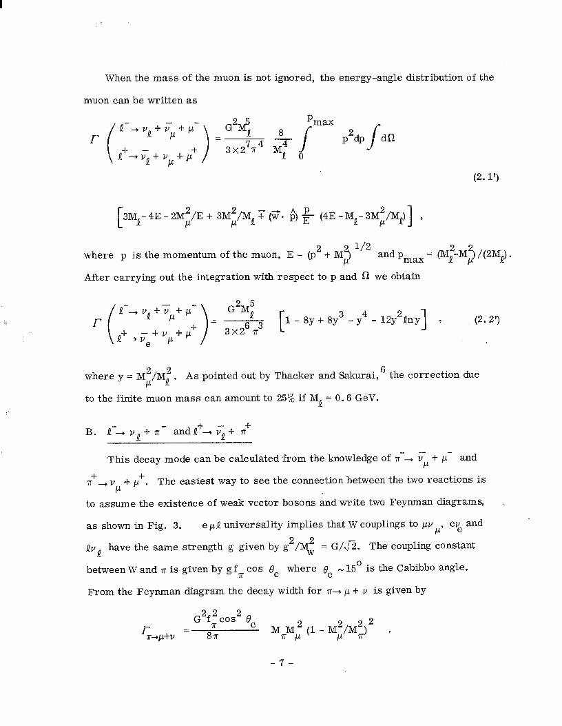
When the mass of the muon is not ignored, the energy-angle distribution of the

muon can be written as

(2.1’)

3MQ- 4E - 2M;/E + 3M;/MQ + (??a j$) $ (4E - MQ- 3$/MQ)] 3

where p is the momentum of the muon, E = (p2 + M2J l/2 and pmax = t$-M> /(2MQ) -

After carrying out the integration with respect to p and fi we obtain

r (~~~~~~~I:-)- 3TzT3 [1-8y+8y3-y4-12y2Qny] , (2.;

where y = Mg/M: . As pointed out by Thacker and Sakurai, ’ the correction due

to the finite muon mass can amount to 25% if MQ = 0.6 GeV.

B. Q-r vQ+ r- 4 andQ + “p-t 7r’

This decay mode can be calculated from the knowledge of 7r-. v + p- and P +

Tr ,vp+p+. The easiest way to see the connection between the two reactions is

to assume the existence of weak vector bosons and write two Feynman diagrams, .

as shown in Fig. 3. e 1-1 Q universality implies that W couplings to pv P’

eze and

QvQ have the same strength g given by g’/Mz = G/a. The coupling constant

between W and 7r is given by g fn cos 8 c where 0, hl 15’ is the Cabibbo angle.

From the Feynman diagram the decay width for 7r-+ p + v is given by

G2f2cos2 e

1” 7r C 22 T++V = 87r MrM; (1 - ME/MS) .

-7-

I

Hence from the experimental lifetime of 7 = h/T= 2.6 x 10e8 set we

obtain

fr= 0.137 M . P (2.4)

The angular distribution of $ from the decay of a polarized Q’ can be computed

from the Feynrnan diagram. We have

I- G2f; cos2 19~

= 167r (2.5)

where $71 is the unit vector in the direction of motion of the pion. Again the in-

variance underCP says that the decay angular distribution of Q+-+ TQ + ? can be

obtained from that of Q + v Q + 7r- by changing the sign of $. (Proof similar to

Fig. 1.) Comparing Eq. (2.5) with Eq. (2.1) we notice that the x integration is

missing from the latter because in the two-body decay the energy of each particle

is fixed in the rest frame of 8: En = (Mf + M2J /(2MQ) and EV = (Mi- M2J/(2MQ).

We also notice that the sign in front of G* 8, is opposite to that of ??a iQ when x-1.

The 5 sign in Eq. (2.5) can be understood easily if we draw pictures similar to

Fig. 2. Consider Q -, vQ -I- r-. Since vQ and 7r- come out back to back, the com-

ponent of the orbital angular momentum along the direction of vQ is zero. NOW

vQ has helicity - hence, it likes to be emitted opposite to the direction of the spin

of Q-. Therefore, r- likes to be emitted in the direction of the spin of Q-.

Integrating Eq. (2.5) with respect to the solid angle, the spin dependent part

vanishes. From Eq. (2.2) and (2.5)) we obtain the ratio

2 5-4 4-V +e-

2 MQ

2 v

Q e MQ 1 fQ-

!z - -bTr 4-V 6~2f2cos28 = M2 1.04 *

7r C P

(2.6)

-8-

This equation shows that when the lepton mass is equal to the proton mass, the

width for the pionic decay mode is roughly equal to the sum of the widths of the

electronic and muonic decay modes of I. If M < M Q P’

then the pionic decay mode is

more important than the total leptonic decay mode (e plus 1-1).

C. Q- -ck- + vQ

We can calculate this decay rate from the known rate of k-+ /.L- + $, or

equivalently we may obtain this by simply replacing cos2 SC and MT in Eq. (2.6) by

sin’ oc and Mk respectively. fr is equal to fk because this is how Cabibbo 11

obtained ec from comparison of the decay rates of r-+ /J+ v and k -+ p + v .

Hence we obtain

r Q-+ktu = (2-V

where tan2 Oc 1 Ts- ’

D. Q -+ p- + vQ

This decay mode can be calculated from the cross sectionof e’+e--- p using CVC.

CVC is equivalent to the statement that the coupling of W to p is obtainable from

the yo coupling by replacing e in the latter by &g cos ec, where

g2/M; = G/c .

The width for this decay can be calculated easily and we obtain (neglecting the

p width)

r(Q-- p- + v) =

where &g2cos ec gpQv = M2 g

PY W

and

(2.8)

P-9)

(2.10)

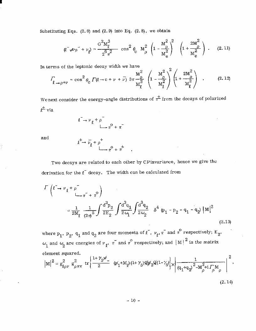
Substituting Eqs. (2.8) and (2.9) into Eq. (2.8)) we obtain

(Q-+p- + vQ) = G”M;

26T2 cos2 6” M2 p (dg ti+$) . (2.11)

In terms of the leptonic decay width we have

r Q -+p+v

= cos2 (lc f(Q -re+v +v>

Wenext consider the energy-angle distributions of &from the decays of polarized

8 via

Q + vQ + p-

LoTo + 7r-

and + Q+rQ+p

+

17r"+** .

Two decays are related to each other by CPinvariance, hence we give the

derivation for the I- decay. The width can be calculated from

r Q-+ VQ+p-

I*-- + 7r”

(2.13)

where ply p2, q1 and q2 are four momenta of Q-, vQ, r- and no respectively; E2, ’

w1 and w2 are energies of v Q, 7r- and r” respectively; and 1 M ) 2 is the matrix

element squared.

tr l+ y#- 1 1 2

2 (I3i+MQ)(l+y5)~~2~('-'y5) x 1 (q1+q2) 2-J'$+icMp '

(2.14)

- 10 -

where g pQv is given by Eq. (2.9), gp ~~ is given by Eq. (2. lo), Q = qI-q2,

w is the four vector which reduces to the three dimensional polarization vector

?? in the rest frame of Q-, and

2

c=& M P

(2.15)

For simplicity, let us make a narrow width approximation, i. e., we replace

the Breit Wigner factor by a 6 function:

1

tq1+q2) 2- Mp” + i 5Mp

After taking the trace we have

- M; (2.16)

2@1aQ)(~2’Q) - @I’P2)Q2-Ma ~~(~*Q)(P;Q~ - (W_-P,)&~

6 (qI+q2)2 - M; .

In the rest frame of Q-, we have

and

p2*Q = p1.Q = MQ(ul-‘Jz),

Q2 = 4M;-M; ,

pl’p2 = MQtMQ-“l-u2),

w-’ p2 = G.q+G*~2,

w/Q = - (%-$-F*q2) .

Since we are interested in the energy and angle distribution of qI, we have

to integrate Eq. (2.13) with respect to p2 and q2. We first integrate with respect

to d3p2 with the help of the 84(pl-p2-q,-q2) and obtain

J- 2 84(pl-P2-ql-q2) = 6” j(Pl-ql-q2)2 j = 6 jM;+M;-2MQ(u1+w2)) . (2.18)

- 11 -

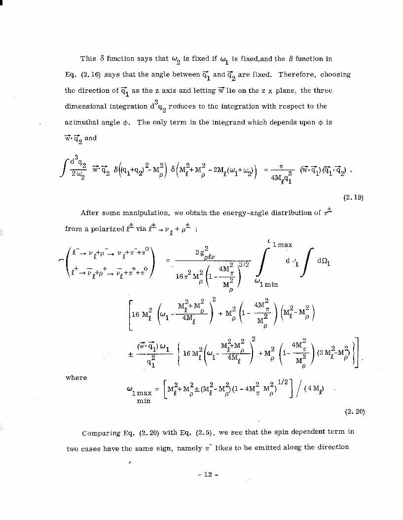
This 8 function says that o2 is fixed if ol is fixed,and the 6 function in

Eq. (2.16) says that the angle between cl and T2 are fixed, Therefore, choosing

the direction of Tl as the z axis and letting w’lie on the z x plane, the three

dimensional integration d3q2 reduces to the integration with respect to the

azimuthal angle $. The only term in the integrand which depends upon $I is

L’?.T2 and

- 2MQ ( wl+ w2) = T 3 ($0 $) @;*z2) .

4MQql

(2.19)

After some manipulation, we obtain the energy-angle distribution of 2

from a polarized Q’ via Q’ -+ vQ + p’ :

Q--, v +p Q +

Q++: Q +p+-,

3 g;Qv

‘lmax

ds2,

9 min

where 0

2 l/2

lmax = M;+M;k(M,2-M2J(l-4Mi MP) Ii t4MQ) min

(2.20)

Comparing Eq. (2.20) with Eq. (2.5)) we see that the spin dependent term in

two cases have the same sign, namely 7r- likes to be emitted along the direction

d

- 12 -

of polarization of Q-, whereas $ likes to be emitted opposite to the direction of

polarization of Q+. Since the terms inside the curly bracket are positive definite,

this is true independent of the energy WI. Equation (2.20) reduces to Eq. (2.8)

after integrations with respect to energy and angle as it should.

III. WIDTH OF Q AND SPECTRAL FUNCTIONS OF CURRENTS

In the previous section we considered in detail the energy-angle distributions

of simple decay products from a polarized $. If the mass of $ is less than

1 GeV, the consideration given so far is sufficient (except Q-, v + k* (890) to be

considered in this section). When the mass of &is greater than 1 GeV, Q’

decays into v + AI (1070)) v + Q ( 1300) and v + hadron continuum in addition

to simple discrete states considered in the previous section. If weak vector

bosons (d exist and if MQ > Mw, then Qf- will first decay into v + vc;t semi-

weakly rather than decay directly (weakly) into leptons and hadrons. In this

section we consider the width of Q’ from a more systematic point of view which

enables us to deal with these new problems and put the special cases discussed

in the previous section in better perspective.

The width of Q ---, hadrons + vQ can be written as

G2 $--, hadrons+v = !&- - d3p2 - - - Q Q2 ’ i trvl+MQ) (

2E2 (2743 1-r Ys> Y/f2P- Ys> * .

c <O ) J: (0) 1 f ><f 1 e (0) \ 0 >(2nj4 e4 (P1-P2-Pf) f

(3.1)

- 13 -

where JE is the Cabibbo current 11,5 :

5P 5P P The four types of currents, Fy + i Fg, F1 + i F2, F4 + i Fg and FtP+ iFz ,

do not interfere with each other because the final states associated with each cur-

rent have different quantum numbers,as shown in Table I.

TABLE I

S Q G JP I3 Examples

Fy+ iF;

F5P + F5P 1 2

Fz+ iFE

F5p+ i F5P 4 5

0 -1

0 -1

-1 -1

-1 -1

-l-

-

1-

o-,1+

0+,1-

o-,1+

-1

-1

-;

-f

p-, 2T, 4n, k-i-k0

6, 37r, A;

k’(892)

k-, Q- (1300)

Since Ft + i Fg is conserved (CVC), the final state ( f 7 cannot be a J = 0

state with nonzero mass for this current.

- 14 -

I

Let us define the spectral functions:

Vl(9

= (qPqV- q2gkV) al(q2)

i

7 \

+s 3

,s(S2) I

(3.3)

The spectral functions vl, al, VT and a: come from the final states with

J = 1, whereas ao’ v: and ai come from the final states with J = 0. v. r- 0 is

due to CVC. All these spectral functions are positive semidefinite ( LO) as can

be verified by going to the rest frame of the final state, qP = (q’, 0, 0,O) , and let

,u=v=Oandp=v=l. This form of decomposition shows explicitly that the

final states with J = 1 is always conserved and if the current is not conserved

it must decay into J = 0 states at some q2 in addition to J = 1 states. Let us

show that J = 1 final states contribute only to vl, a1 vs and a; and J = 0 final

states contribute only to ao, v: and a: . Since we sum over everything in If > ,

we may simulate 1 f 7 by a particle specified by its momentum and spin. Let US

consider a matrix element of a current J P’

which may or may not be conserved,

between a vacuum and a spin 1 particle with a polarization vector E and a

momentum q .

- 15 -

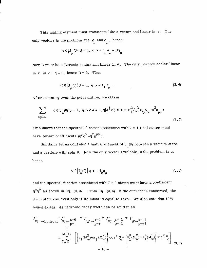
This matrix element must transform like a vector and linear in E . The

only vectors in the problem are E and q hence P P’

<OlJ,(O)IJ=l, q>=fleP+Bq P

Now B must be a Lorentz scalar and linear in E . The only Lorentz scalar linear

inC is Em q = 0, hence B = 0. Thus

<O(JP(0)lJ= 1, q>=f E . 1 P

(3.4)

After summing over the polarization, we obtain

c < O\JP(0)IJ = 1, q >< J = l,qlJ;(o)[o 7 = (f2,/s2,(qp9, -q2gpv) spin

P-5)

This shows that the spectral function associated with J = 1 final states must

have tensor coefficients (qPqv -q g 2 PV ).

Similarly let us consider a matrix element of JP(0) between a vacuum state

and a particle with spin 0. Now the only vector available in the problem is q,

hence

< 0 (J&O) 1 q 7 = fogcl (3.6)

and the spectral function associated with J = 0 states must have a coefficient

q’q” as shown in Eq (3 3) . . . From Eq. (3.6), if the current is conserved, the

J = 0 state can exist only if its mass is equal to zero. We also note that if W

boson exists, its hadronic decay width can be written as

r W-+hadrons

=r W +

vl(M$+al (Mt) cos2 6”f \vT(Ma+as(M$ 1

I (

(3.7) - 16 -

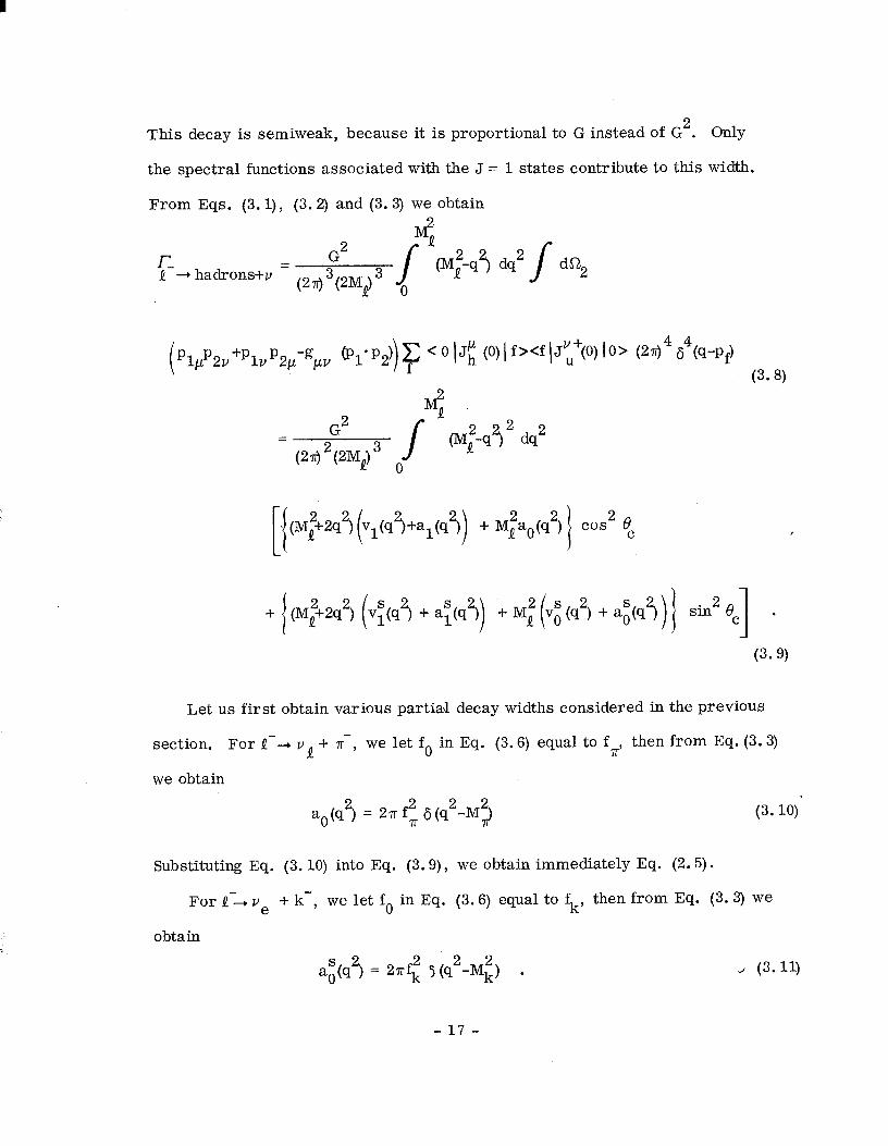
This decay is semiweak, because it is proportional to G instead of G2. Only

the spectral functions associated with the J = 1 states contribute to this width.

From Eqs. (3. l), (3.2) and (3.3) we obtain

lh!?

‘(M2-qz) dq2 Q

pl~p2v +p1v p2$& (P1*p2) F < 6 1 Jt (0) 1 f><f 1 Jvt(O) 107 (W4 s4Wpf) (3.8)

G2 Y

= t2@ 2(2MQ) 3 /

Wf-d2 ds2 o

2 2 + MQao(q ) c”s i

Let us first obtain various partia\l decay widths considered in the previous

section. For Q ---) v + 7r-, Q we let f. in Eq. (3.6) equal to f*, then from Eq. (3.3)

we obtain

a()(9 2, = 27r f”, 6 (q2-Mj (3.10)‘

Substituting Eq. (3.10) into Eq. (3.9)) we obtain immediately Eq. (2.5).

ForQ-rv +k, e we let f. in Eq. (3.6) equal to fk, then from Eq. (3. 3) we

obtain

a:(q2) = 27rfz 3 (q2-Mi) . J (3.11)

- 17 -

Substituting Eq. (3.11) into Eq. (3.9) and remembering f?,= fk by definition

of the Cabibbo angle, we obtain Eq. (2..7,.

ForQ-+ v,+p , - we let fl in Eq. (3.5) equal to Lg M2 , then from PY P

Eq. (3.3) we obtain

Vl(9 2, = 4n gtYM; 6 (q2-M;) . (3.12)

Substituting Eq. (3.12) into Eq. (3.9)) we obtain immediately Eq. (2.11). The

fact that the constant f; in Eq. (3.5) is equal to fi gpyMi comes from CVC.

In general CVC relates vl(q 2, to the isovector part of the total cross section

for ef- + e-4 hadrons. From

2 c c 0 @i(O) 1 f%f’lFg (0) 10 > (2f14 54(q-pfl) f

= c < 0 1 F:(O) + i FE(O) If ,<f (F$O)-iFl(O) 10 > (2734 $(q-pf) f’

(3.13)

we obtain

v102 = 3 q2q$+e-c12)

47r2 a2 l

The total cross section for e’ + e-4 p” --$ n+ + rTT- is given by

where

and

2 a(e++ e-4p) =y

3q

312

- 18 -

(3.14)

(3-W _

(3.16)

(3.17)

Replacing the Breit Wigner factor by a 6 function (see Eq. (2.16))) we obtain

a(e++e-+ p”) (3.18)

Subsituting Eq. (3.18) into Eq. (3.14), we obtain Eq. (3.12).

A. Weinberg Sum Rules andQ+Al+vQ13

If SU 3 X SU 3 were an exact symmetry, then vl(q 2,

and v. (q5 = a0 ts? = v$c.?j = a$s? = 0. In this case p and A1 would have the

same mass and the width of Q -+vQ + p would be identical to that of Q-, vQ + Al.

In order to do better we have to know how the symmetry is broken. Weinberg’s

sum rules can be used to relate these two widths. Weinberg’s /3t,, pA and Fn

are related to our vl, a1 and FT by

and FT=fT .

In our notation Weinberg’s two sum rules can be written as

and

and

Co J[ v1tq2) - al(q2) dq2 = 2~ f”,

0 I

v1tq 5 - qq dq2=0 ,

If v1 and al are dominated by p and A1 respectively, we have

vltq 2, = 2$/M;) S(q2 - M;)

a,(s2) = 2+f$Mi ) 6 (q2-Mi ) , 1 1

(3.19)

(3.20).

(3.21)

(3.22)

- 19 -

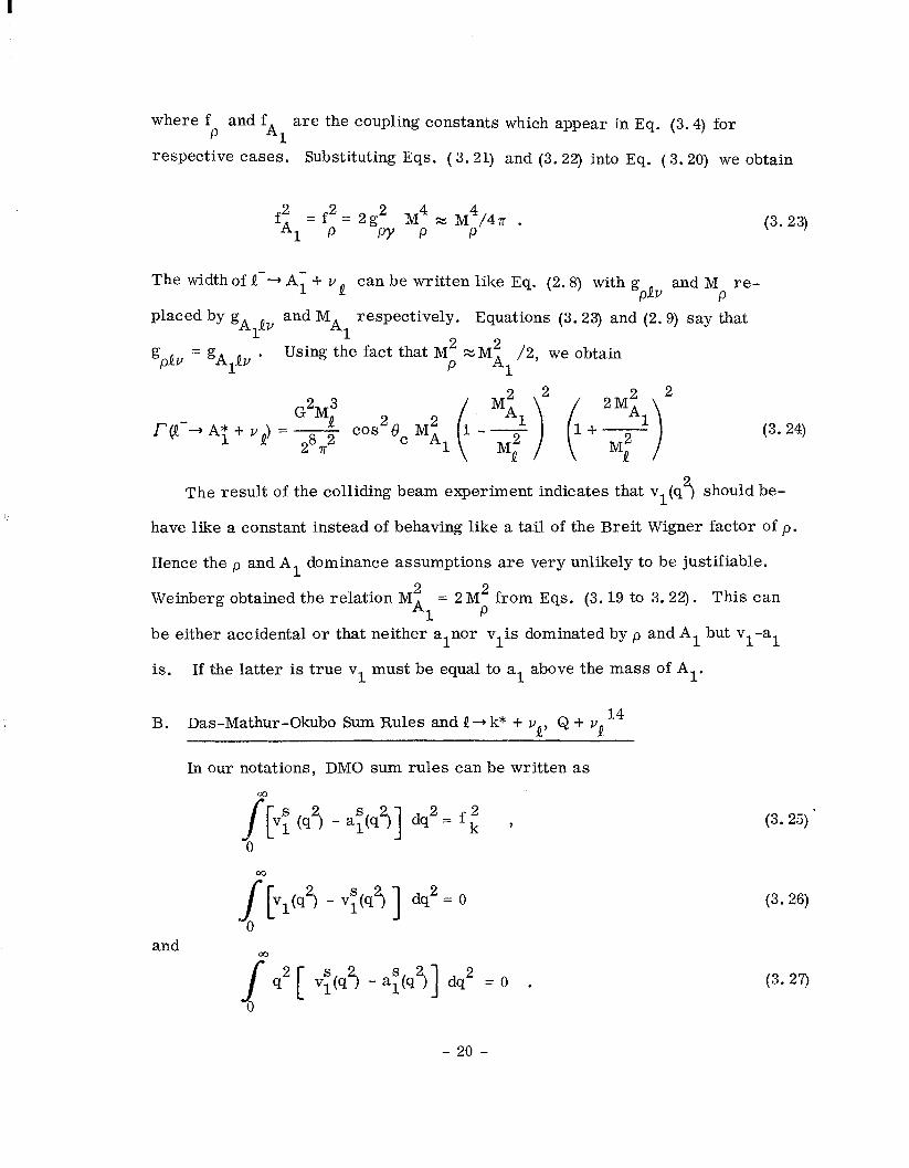
where f and f P Al

are the coupling constants which appear in Eq. (3.4) for

respective cases. Substituting Eqs. (3.21) and (3.22) into Eq. (3.20) we obtain

f2 =f2=2g2 M4zM;/4n . A1 p PY p

The width of I--, A- + v 1 Q can be written like Eq. (2.8) with g PQV

and M re- P

placed by gA Qv and MA respectively. Equations (3.23) and (2.9) say that ? -l I

g pdv = gAIQ~ ’ Using the fact that M2 p z Mi /2, we obtain 1

r(Q-+ AT + vQ) = G2M3 Q 287r2

cos2e M2 c A1

(3.23)

(3.24)

The result of the colliding beam experiment indicates that vl(q 3 should be-

have like a constant instead of behaving like a tail of the Breit Wigner factor of p.

Hence the p and A1 dominance assumptions are very unlikely to be justifiable.

Weinberg obtained the relation M2 A1

= 2Mi from Eqs. (3.19 to 3.22). This can

be either accidental or that neither alnor vlis dominated by p and A1 but vl-al

is. If the latter is true v1 must be equal to al above the mass of Al.

B. Das-Mathur-Okubo Sum Rules and Q-k* + vQ, Q + vQ 14

In our notations, DMO sum rules can be written as

and

co

/[ VT (q2) - a:&?) ds2 = fi -il 1 ,

ccl 2, - vpl dq2 = 0

a, v;tq 2, - +.I dq2 = 0 .

(3.25)'

(3. 26)

(3.29

- 20 -

Let us assume that VT - a; is dominated by k*(890) in vs and Q(1313) in a; ,

and that vl-vs is dominated by ~(760) in v1 and k*(890) in vs . These as-

sumptions mean that when using the sum rules we may let

+J. 2, = 2~&b’$*) 6 ts2-M;,) (3.28)

a$ 2, = 27r(f;/Ma 6(q2-Ma (3.29)

Vl(4 2, = 27r(fd”/M> s(q2-M;) (3.30)

From Eqs. (3.26) and (3.27) we obtain

f;/ M; = f;*/Mp = f;/M;* . (3.31)

From (3.31) and the known value of f2, we can calculate the widths for the decays P

Q +v + k*(890) andQ-+ v + Q(1313):

G2M3 sin 8 r(Q +vQ+ ky = 26;2 ’ M;$ -+I (i+?) . (3.32)

~(Q+v, + Q) = G”Mi sin2 ec

26 7r2

C. Q+W+v,

If weak vector bosons exist and if Mw < Ma, then Q will first decay into

W + vQ rather than decay directly into hadrons and leptons. The width of

Q- +W- + vQ can be obtained from the width of Q-+ p- + VQ given in Eq. (2.8)

by making substitutions: M 4 Mw and g + g. P PQV

.

f(Q---W-+v) = Q --& M+-$l+~j. (3.34)

- 21 -

This decay is proportional to G instead of G2, hence numerically it is much

larger than the decay mechanisms we have considered so far, unless Mw and MQ

are almost degenerate to each other. W decays also semiweakly into leptons

and hadrons. The hadronic decay modes of W can be written as Eq. (3.7) and

the leptonic decay modes (W-, 5 I- Q-, W-+ v i-4

t- p-, or W-4 5 + Q- if

MQ < Mw) can be written as

D. Q --, v n + Hadron Continuum

(3.35)

Let us assume that either $ do not exist or MQ < Mw. The decay width

f. of Q + v Q + hadron continuum can be estimated from the results of e++ e--r hadrons

using Eq. (3.14). In order to do this let us make the following reasonable as-

sumptions :

1. When q2 is large, say q2 > 1 GeV2, the magnitudes of vl(q 3, a,(s3>

+I. 3 and as (q 2, corresponding to the decay Q + vQ -t hadron continuum are

roughly equal to each other. This can be regarded as the basic assumption

about the symmetry of currents.

2. The spectral functions for J = 0 states ao(q 3 , vi(q2) and a:(q2) in

Eq. (3.9) are negligible compared with the spectral functions for J = 1 states .

when q2 is large. This is true if we accept the notion that the symmetry of cur-

rents becomes exact in the limit q2d 03 .

3. The isoscalar part of the cross sections for e++ e-+ hadrons is small

compared with the isovector part. For production of p, $I and o, the ratios of

these cross sections are given experimentally by

4r g2 2 : YP 4llg$

Jng2 1. yw=z.

1 .L z. 11.5 *

- 22 -

Hence the isovector cross section is three times as large as the isoscalar cross

section. Whether this is true for large q2 is an interesting open question. SU3

gives the ratio of 3 to 1 for the isovector to the isoscalar cross sections. If

we accept this, then Eq. (3.14) becomes

lim v1tq 2, = g 92~e++e-(qy .

2 cl-03 47r2cz2

(3.36)

These assumptions say that for estimating the partial width of Q-.-B vQ + hadron

continuum we may let ec = 0, a0 = 0 and v1 = al in Eq. (3.9)) hence

r- Q -+ vQ f hadron continuum

2

G2 MQ

I-

2 e++e-

dq2 (M;-q2) 2 (I$ 2q2) + (20 cl21 = .

(2f12(2MQ) 3 ri2 47r2a2 (3.37)

The e+ + e- colliding beam experiment of Frascat?shows that in the energy

range 1.6 GeVs, q2< 2.0 GeV, the cross section for e r + + e-+ hadrons is

(3f0.3) 1o-32 2 + cm compared with the cross section for e + e-+ p’ + p- of

2.5 x 1o-32 cm2 at 1.8 GeV. However it is not clear whether the observed cross

section really represents the process e+ + e-+ hadrons. For example some of

the events may be due to the production of heavy leptons as considered in Section

IV of this paper, or some may be due to the two photon process. 15 It is in-

teresting to note that in the quark parton model, the cross section for

e+ + e-+ hadron is less than that of e+ + e---r p’ + pt- by a factor of 2/3. Let

us denote the cross section for e’ + e-+ hadron given by the quark parton model

as

- Oquark (e’ + e---r hadron) = f o(e+ + e-* ,u* 2 47r cY2 +/-O=Tj3 q2 ’ (3. 38)

- 23 -

.16 and the quoted cross section from Frascati as

0 Frascati(e+ + e-+ hadron) M 5 o (e+ + e-+ p’ + p-) . (3. 39)

Substituting Eq. (3. 38) into Eq. (3.36) we obtain 1

r(Q-+ hadron continuum) = (l-x)2 (1+2x)dxrR r(Q-4 e- + vQ + <)

(3.40)

This result corresponds to using the quark model. If we use Eq. (3.39)) the

right-hand side of Eq. (3.40) would be multiplied by 2. A should be taken to be

w 1 GeV. We notice that as A2/Mf+ 0, the ratio R becomes unity if quark model

were used and the ratio becomes two if the experimental result of Frascati is

taken at its face value.

+ - IV. e + e -+Q+ + Q- AND DECAY CORRELATIONS

The cross section for this reaction is well known. Ignoring the mass of the

electron we have in the center-of-mass system, 17

%= 16”Ea -A[ i+ ,0s2e+- sin20

Y2 3 (4.1)

where E is the energy of Q+ or Q-, p = (E2-M$1’2/E and y= E/MQ. Integrating

Eq. (4.1) with respect to the solid angle we obtain the total cross section

47(e+ + e- -Q++Q-)=[Y2" 3E2

. F-2)

- 24 -

Since heavy leptons are unstable particles and their decay angular distribu-

tions depend upon their spin orientations, we have to know the probabilities of

the heavy leptons coming out at different spin orientations. In order to do this

let us calculate the probability of the reaction ef + e-4 If + Q- with the spin of

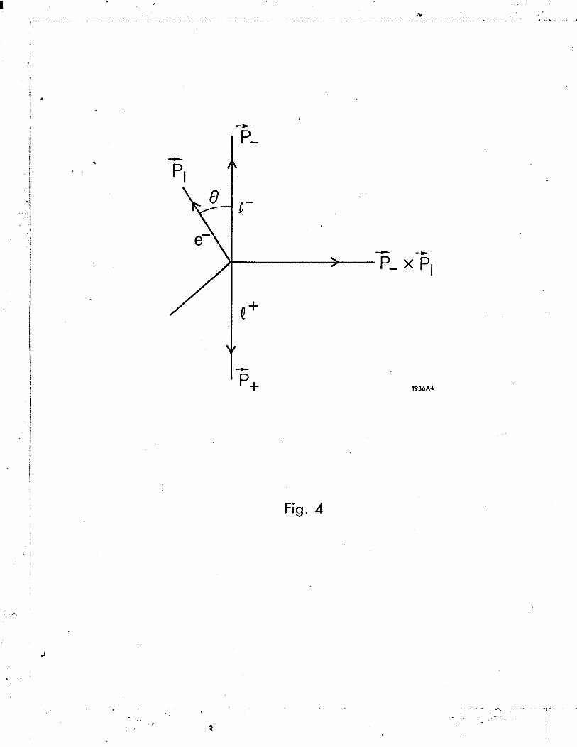
Q- in the direction g and the spin of Q’ in the directionT1. X andz! are unit vectors

defined in the rest frames of I- and Q+ respectively. In order to calculate the spin

effect covariantly, let us define two four-vectors (axial) s- and ss. which reduce to

the three vectors s’andT7, respectively, in the rest frames of Q- and Q+. Let us

choose a coordinate system where the direction of p in the center-of-mass

system is the z axis and the direction;-x Fl is the y axis, as shown in Fig. 4.

In this frame the components of s- and s+ can be written in terms of the components

of s and s’ as

(4.3)

(4.4)

Let us denote the four momenta of e-, et, Q- and Q’ by pl, p2, p- and p+ , re-

spectively. We have then

P- = (E,O,O,PE)

P, = (E,O,O,-PE)

p E (pl-p,)/2 = (0,E sinO,o,E cos 0).

(4.5) .

The projection operator for Q- with momentum p and spin in the direction

x is then

1 + Y5$ P’-+MQ 2 2MQ ’ (4.6)

- 25 -

and for Q’ with momentum p, and spin ?? is

1 + Y,$+ -P++ MQ

2 2MQ ’ (4.7)

We use the following representation for y matrices:

Let us show that Eq. (4.7) indeed is the required projection operator for Qf with

spin 3. In the rest frame of Q’ we have

1+ CT-$ 2 0

I’Y5i’l = 2 [ 1 -‘7i’.-$

0 2

and -p! + MQ

2MQ =

hence

1 + Y5$+ -d+MQ ’ ’

= 2 2MQ

0

l-

z.xt 2 1

1 .

(4.8)

(4.9)

In our representation a positron with spin in 2 direction is represented by a

negative energy state with spin in zT direction, hence the projection operator is

(1 - z* ;I) /2. (Notice the negative sign in front of 3 for positrons and positive

sign for electrons.)

- 26 -

The desired cross section can be calculated in the standard way:

e4 g (T,??) = -

1 (2nj2 4(PI l P2)

4 6 @I+P2-P+-P-)

t1 + Y5 d-) e’-+“Q) ?$ (95 $+) @+ -“Q) y,

(4.10)

cx2 =- 16E2

p [ i 4- c0s2e +-

sin20

Y2 +s s’ z z (

i + cos2e - sin20

Y2

-l-s s’ x x J+ +- sin28 - sys$ p2 ( 1

sin2 8 + (sxs;+ s;sz) -$- sin 2e . Y 1

(4.11)

We notice that gand s’! occur only bilinearly. This means that if only one

particle is analyzed,then no effect of polarization can be observed, but if two

particles are analyzed simultaneously, their spins are correlated. The correla-

tion is such that if sz = +_ 1, then the cross section is maximum when sk = 3~ 1.

In other words the helicities of a” and Q- like to be opposite to each other. We

also notice that the coefficients of sxsk and s y y do not approach zero as y -,03. s’

For a massless lepton pair the terms sxsJc and s s’ need not be considered and YY

hence we have always s Z = + 1 and s; = f. 1. In this case Q+ and Q- always have the

opposite helicity. When the leptons have finite mass, the spin correlation is not

complete even in the limit of y-+ 00. For example, the probability for sz = 1 and

and s; = --$ is not zero even if we let y-+ co . Another interesting

feature is the behavior near threshold. Near the threshold we have p -+ 0 and

y-+1. Hence Eq. (4.11) gives

(4.12)

- 27 -

where ^p is the unit vector along the direction of the incident electron. Equation

(4.12) shows that g and z1 like to be both parallel or both antiparallel to the

direction of the incident electron beam.

Let us try to understand Eqs. (4.11) and (4.12) using a more illuminating

but clumsy method. Let us denote the electron-positron current by

- jp = W2hp @,I . (4.13)

Current conservation gives 2E j, = 0, therefore j, = 0. If the mass of the electron

is ignored, we have

hence jz

Writing

and

P; jP = 7 il u(pl) = 0 = E jo-pljz= -pljz9

q 0. Instead of jx and j Y’

it is more convenient to consider

jx+ijx jrt=2 .

=

=

1

(E+M)1’2 ! 1 X zq E+M 2.72 (E + w l/2 E+M w [ 1 1

(4.14)

(4.15)

(4.16)

where X is the two component spinor representing the spin state of the electron

in its rest frame andwis the two component spinor representing the spin state

of the hole: For example X = 1 o represents a state with spin up for the

electron but ?N= 1 [I

[I o represents a hole state with spin up hence it represents

a positron with spin down. A positron with helicity + and momentum r2 satisfies

0. j2 ,pv= -9/ .

- 28 -

From Eqs. (4.13 to 4.16) we have

k * =2EdcJ&x, (4.17)

where a+ = 0 1 [ 1 0 0 and 0 0 o = -[ 1 1 0 , and the axis of quantization is along

the direction of pl. Taking the spin average, we notice that j+ is nonvanishing

only when the electron has negative helicity and the positron has a positive

helicity, whereas j- is nonvanishing only when the electron has a positive helicity,

and the positron has a negative helicity. The numerical value of each matrix

element is 2E. Equation (4.1’7) shows also that the total angular momentum of

the electron positron system is unity and the direction of the angular momentum

is parallel to the total spin -“cl + 2 2 which is either parallel or antiparallel to the

direction of the incident electron.

Let us denote the current of the final lepton pair by

Jp = c (P-) yp v(p+) .

Then J jp =-j J -j J = -2j J _ 2j J

CL xx YY +- -+

because j, = jz = 0. Now for discussion of the matrix element of JP it is more

convenient to quantize the angular momentum along the direction of motion of

F than along the direction of the incident electron. Using the coordinate system

shown in Fig. 4 and denoting it by a prime, we obtain

Jk3 i(JxiiJy) =f (J&cos8- J; sin 8 +iJ’ y’

= i (COS 0 + 1) J; + i (COS 8 7 1) J1 - i sin 8 J; ,

hence J j”=j

P + - (1 + cose)J; + sin 8 J; 1

+j _ -(I + ~0~8) J:, + (1 - c0se) J; + sin 8 J:, I .

- 29 -

(4.18)

In terms of two components spinors, J; and J; can be written as:

Jk= 2EX+ $94 and J; = 2 MI X+ oz G-V . (4.19)

In our representation the states of P- with spin pointing in x’, y1 and z1

directions are given respectively by

xx, =A 1 [I &1 ’

x ,A 1 [I y$ i

and xz, =

(4.20)

Similarly the states of Q’ with spin pointing in x1, y1 and z1 directions are

given respectively by

and OUzr = (4. 2.1)

The cross section is proportional to the square of Eq. (4.18). Since the helicity

states contributing to j+ are different from those contributing to j-, the two

square bracket terms do not interfere with each other. Averaging over the spin

of the incident particles, we obtain

da dS2

a2 (2,3) = - 16E2P

[I pcO~e) 1 2 xs a+-(l+cOse) 0 + y sin 8 I “z( s’ “96

t-x s ~-(~+cose~ a+ +(i-c0se) 4 + y o~/w~,

2

13 . (4.22)

- 30 -

With the aid of Eqs. (4.20) and (4.21) we can verify Eq. (4.11) from Eq. (4.22).

The latter derivation of the spin correlation is clumsy, but it brings out many subtle

points of the problem.

Let us discuss qualitatively the experimental consequences of spin correla-

tion. In Section It, we calculated the decay angular distribution of arbitrary

polarized Q- and Q+. In general we may write symbolically:

f(Q- --Pw= /

l+Ys‘ll_ da tr 2 . . . =

s (A+BFq dR (4.23)

and

r(Q++ X’) /

l+%v/, = da1 tr 2 . . . = (A’+B’ T.3) d&?’ , (4. 24)

where q and q1 are momenta of the decay products to be detected. Let us write

symbolically the spin correlation in the production, Eq. (4.11)) as

dR - =C+Dijsis! . d?2 J

(4.25)

The combined angular distribution of the decay products Q--* X and Q’+ X’

for a fixed production angle, can be written as

do dQQdaa’ =

CM’ -I- Dij qiq; BB’ 2 , (4. 26)

r total

where r total is the total width of m”, dflQ is the solid angle for I- (or Q’) in the

center-of-mass system, da and do ’ are solid angles for the decay products of

Q- and Q+ in the rest frames of Q- and Q+, respectively. Equation (4.26) can be

derived in the following way: ?? represents the polarization vector of Q, and

by definition each component of $= (w,, wy, wz) represents

number of Q- polarized along Gi - number of Q- polarized along -gi wi =

number of Q- polarized along gi + number of Q- polarized along -gi .

- 31 -

,

Now the number of Q - having spin along the direction ci with the polarization of

I’ in a certain direction s* is proportional to C + D..s’ 1~ j)

whereas the correspond-

ing number of Q - having spin along the direction -gi is C - D. .s! . 1J J Hence D.. s!

w.= 2L.L 1 C (4.27)

and the angular distribution of the decay product of Q - is proportional to

CA + Dijs; qiB . (4. 28)

For a fixed angular distribution of the decay product of I- given by Eq. (4.28),

the components of the spin of Q+ are given by D. .q. B

w!=dX’ . .l

(4.29)

Substituting Eq. (4.29) into Eq. (4.24) we obtain the combined angular dis-

tribution of the decay products of Q’ and Q- at a fixed production angle:

CAA’ + Dijqiq; BB’ .

In order to obtain the proper normalization factor, we notice that the partial

decay width r(Q- -+ X) is independent of the polarization, hence

r(Q-+ X) =/-,,Q and fiFz dn = 0 . (4.30) .

Similarly r(Q-4 Xl) =

J A’ dlR * and

/ B*?. G* dn* = 0 . (4.31)

This implies

/ DijBiB;dQ=

f DijBiB;dR’=O , (4.32)

- 32 -

and therefore integrating Eq. (4.26) we obtain

i-+X’ dR - (e++e-+ Q++Q- )=C r(Q++ X’) l-Q-* 2Q .

mQ 2 (4.33) LX r total

This shows that Eq. (4.26) is indeed properly normalized because C is equal to

dQ/daQ summed over the polarizations of Q+ and Q-. Equation (4.32) shows ex-

plicitly that if the decay angular distribution of only Q+ or only Q- is observed,

then the effects of the spin correlation vanish. This is as mentioned earlier due

to the absence of the terms linear in zaand? in Eq. (4.11). The absence of

linear terms in Eq. (4.11) is due to the approximation of one photon exchange.

In the absence of spin correlation we have only the CAA* term in Eq. (4.26).

It is very important to notice that the existence of B and B* in Eqs. (4.24) and

(4.25) is due to parity nonconservation in the decay of heavy leptons. Since the

spin correlation term Dij qiq; BB* in Eq. (4.26) is proportional to BB’, we con-

clude that if we detect in coincidence one particle from the decay products of I-

and one particle from those of Q’, the effects of spin correlation exist only if

parity conservation is violated in the decays of both Q and Q-. This is due to the

fact that the polarization vector for a spin f particle is an axial vector. (This

would not be true if Q+ and Q- were spin 1 particles. In this case the correlation

exists even if parity is conserved.)

In order to see the effects of the spin correlation let us compare the magnitudes

of the isotropic term CAA* and the spin correlation term Dij qi q; BB’ in Eq. (4.26)

corresponding to various combinations of decay channels.

Example 1 I--+ vQ -!- Fp -!- p-,

+ Q -+r+ve+e

-!-

Q and

p- and e are detected in coincidence.

-33 -

From Eqs. (2.1) and (4.11) we have (we have ignored the mass of muon for

simplicity)

CAA’ = F +)fx2ti(3-2x) { xr2dx’ (3-2x’)

0 0

and

Dijqiq; BB’ = -F x’2dx’ (1-2x) (1-2x’)

0 0

X 1 gq’ [ (

q,q; l+cos20 - p) + qxq$l+--+) sin20

- yy4;P2 sin20 + (qxq;+q;qz) $ sin20 , I

(4.34)

(4. 35)

where

ax ’

X’ = q’/qrmax and qmax =qtmax = MQ/2 .

We observe the following:

1. Correlation is maximum when x and x’ are both near 1.

2. Ln the limit ydco, and both x and x* are near 1, e+ and ,LL- like to come

out either both along the directions of motion of parent particles, or both

opposite to the directions of motion of parent particles.

3. Near the threshold (y -+l), we may write

CAA’+Dijqiq; BB’ X (3-2x) (3-2x’) -(1-2x) (1-2x’) & 4 6. 4’) (4. 36)

where b is the unit vector along the direction of the incident electron.

This shows that the correlation is maximum when both x and x1 are

- 34 -

I

near 1. The effect of correlation vanishes when either $ or 4’ is

perpendicular to 8; and the maximum correlation occurs when both 4

and h* are in the direction of the incident beam. e+ and p- like to come

out in the opposite direction from each other if both x and x1 are near 1

and both qaand? are in the incident beam direction.

Example 2 Q-tv +T-, Q + Q -+;;+T+

+ Q and r and 7rS are detected in coincidence.

From Eqs. (2.5) and (4.11) we have

CAA’ = F2 (

1 I- cos2Q (4. 37)

and

Dijqiq; BB’ = F 1 qzq; id- c0s2e - * + s,s; 1++ sin28 Y Y

where

3%

F =?,(Q+ TW) a2 p 2

w-J2 16E2 *

Near the threshold we have

sin 2Q I

, (4. 38)

(4. 39)

CAA’ + Dij qiq; BB’ = 2F2 (4.40)

Comparison with the results of Example 1, we see that the two cases are very

similar except that in the present case 7f- have a definite momentum in the rest

frames of Q’. As far as the ratio Dijqiq;BB’/CAA’ is concerned, the present

case is identical to x = x’ = 1 of the previous example.

- 35 -

Example 3 Q--, vQ -!- r-, Q’-, 5 + v + ,u’ and 7r- and p’ are detected P

in coincidence. From Eqs. (2.1)) (2.5) and (4.11) we obtain

(4.41)

and 1

Dijqiq; BB’ = -F3 s

(1-2x’) x12dx’ Sill29 -- Y2

0

+ s,s; l+ -+ ( ) Y

sin20 - qygsr p2 sin28 + (qxq;+q;qz)$ sin 26 1 where G2M5 F = I-(Q+r+v) Q

3 47r 3~2~~~ 7

x’ = q*/q’max and qtmax = MQ/2.

In this case the effect of spin correlation is again maximum at x1 = 1. How-

ever, near x’ = 1, the relative sign between CAA* and Dijq.qjBB1 is opposite to

the previous two examples. Hence, if 7r- is emitted along the direction of motion

of Q-, then p’ likes to be emitted opposite to the direction of motion of Q+ when

y is large and x* is near 1. Near the threshold T- and p’ like to be emitted in

the same direction and along the incident beams (e+ or e-) when x’ is near 1. ,

V. SUMMARY AND CONCLUSIONS

In Table II, we give the partial and total decay rates of Q for various values

of M Q. The formulas used to calculate them are given in Sections II and III. We

- 36 -

collect them here for easy reference. (All masses are in units of GeV.)

r(Q -G~+v~+/A) = 3.47 x 10 lo M5 set-’ Q .

r(Q -+v 4v Q c1

+p) = 3.47 x lOlo Mi (l-8y+8y3-y4-12y2Qny) set-l, (J-;/M;) .

T(Q--+Q+v~) = 0.614 x lOlo M:

lo Me” ( 2 6 r(Q-, v Q+hadron continuum) = 3.47 x 10 A8 I-&& ++ _ - -1

8 set .

MQ lvIQ MQ

For construction of Table II, we have used the following numerical values:

G = 1.02 x lo-j/M; , Mp=.938, MP=.106, Mx=.14, Mk=.495, Mo=.765, ’

Mk* = . 892 , MA =1.070, MQ=1.3, 1

A= 1, sin2Bc= .068, cos2,6c= .932,

and tan2 ec = .073 . We have also computed the decay lengths in the vacuum

corresponding to EQ = 5 GeV and En = 50 GeV. We make the following comments

and observations:

1. In the photo pair production y + z -PQ’ + Q- + z*, if the decay length is

greater than 1 cm, then Q’ and Q- can be identified visually in a streamer chamber. 18

- 37 -

Hence, at SLAC energy (EQ< 5 GeV) we see from Table II that the identification

of Qup to Mm = 1 GeV is possible. Another scheme, suggested by M. Davier, 19

is to aim a spectrometer in the decay region and detect the decay products. If

the production region and the decay region is well separated ( > 1 cm), & can be

identified. At NAL energies, one can identify the production of Q’ if MQ < 1.3 GeV

using these two methods.

2. In Table II, the first four decay modes (e, ,u, 7r and k) depend only on the

validity of the current-current interaction hypothesis of weak interaction. The

decay Q-, p+v depends on CVC besides the current-current hypothesis. Since we

have made a narrow width approximation for the p decay the numerical value near

p threshold is not reliable. This can be improved easily if we use the experimental

cross section for e+ + e- -+o’-+ r’ + 7r- in Eqs. (3.14) and Eq. (3.9). The last

three modes of decay depend upon the assumptions of SU3 symmetry and the as-

ymptotic behavior of the spectral functions. They are probably correct to within

a factor of two except near the threshold where again the assumption of narrow

widths was used. If the mass Ma happens to be near one of these resonances, one

should restore the Breit Wigner factor in the spectral function Eq. (3.9) instead of

approximating it by a 6 function (see Eq. (2.16)).

3. For the partial width r(Q -+ v + hadron continuum) we have used the ex-

pression obtained from the quark model,Eq. (3.38), instead of the quoted experi-

mental value of the Frascati experiment, Eq. (3.39).

If both heavy leptons and weak vector bosons exist and Ma > Mw, then the

decay mode Q-+W+ VQ will completely dominate the widths given in Table II. For

example, if Mw = 2 GeV and Ma = 3 GeV, then from Eq. (3.34)) we obtain

r(Q--+W- +,2/t, = 2.6 XIO1’ see-’ which is much larger than the total weak

decay rate of 3.4 X 1013 set-’ given in Table II.

- 38 -

W bosons decay rapidly into v e + e, v P

+ ~1 and hadrons. The leptonic decay

widths can be calculated by using Eq. (3. 35). The hadronic decay width can be

2 2 s estimated by using Eq. (3.7). Assuming vl(Mw = al(Mw) = v: (Mw) = al (Mt) 2,

and using Eqs. (3.7)) (3.36) and (3.38) we obtain

M;G r(W-, hadrons) = l-(W- e+ ve) = - .

6 $9~

This is the result of the quark model. If the experimental result from Frascati

is taken at its face value, we obtain

I‘(W -, hadrons) = 2 r(W-, e + v e) .

In the experiment e+ + em-, Q+ + Q-, the first thing to try is to look for ~7r

coincidence. The energy and angle of 7~ and ,u are correlated,as shown in

Eqs. (4.41) and (4.42). The effects of correlations, together with the branching

ratios into various channels, can be used to confirm the existence of fi. The

work,as presented in this paper, is not complete because in the colliding beam

experiment one probably detects only the decay products, hence the production

angle of QL has to be integrated out. Also, the energy-angle distributions of the

decay products have to be given in the overall center-of-mass system instead of

the rest frames of Q+ and Q-. Both of these can be done easily by a computer

using the technique similar to the one used in the calculation of e++e--, W++W=+ ’

p’+v P+e-+ Fe by A. C. Hearn and the author 20 many years ago.

In the experiment vQ+z -Q + z*, the heavy lepton is polarized, and we expect

the angular distribution of the decay product to be quite different from that of an

unpolarized Q. The calculation of this process is being performed.

In the experiment y + z+Q’+Q-+ z*, the polarizations of Q+ and Q- have

similar correlations to the process e’ f e--, Q’+Q-. The detail of these correla-

tions have never been investigated.

- 39 -

VI. ACKNOWLEDGEMENTS

The author’wishes to thank Drs. J. D. Bjorken, M. Davier, A. Odian,

F. Villa and D. R. Yennie for useful conversations. He also wishes to thank

Dr. J. J. Sakurai for a preprint of his work which partially overlaps with the

contents of our sections II and III.

- 40 -

FOOTNOTES AND REFERENCES

1.

2.

3.

4.

5.

6.

7.

8.

9.

10.

11.

12.

13.

14.

15.

16.

17.

A. Barna et al., Phys. Rev. 173, 1391 (1968). Earlier attempts for

searching the heavy leptons can be traced from this paper.

V . Alles-Borelli et al. , Nuovo Cimento Letters 4, 1156 (1970). A. K. Mann,

Nuovo Cimento Letters &, 486 (1971).

W. Y. Lee et al., NAL Proposal No. 81. --

M. Schwartz et al., SLAC Experiment E56a.

See for example, S. L. Adler and R. F. Dashen, Current Algebra (W. A.

Benjamin, Inc., New York, 1968), p. 14.

Ya B. Zel’dovich, Soviet Phys. Uspekhi 2, 931 (1963). E. M. Lipmanov,

JETP 19, 1291 (1964). K. W. Roth and A. M. Wolsky, Nucl. Phys. E,

241 (1969). J. J. Sakurai, Nuovo Cimento Letters (to be published).

H. B. Thacker and J. J. Sakurai, UCLA preprint (1971).

C. K. Iddings, G. L. Shaw and Y. S. Tsai, Phys. Rev. 135, B1388 (1964).

N. Christ and T. D. Lee, Phys. Rev. 143, 1310 (1966). R. N. Cahn and

Y. S. Tsai, Phys. Rev. g, 870 (1970).

L. F. Li and E. A. Paschos, Phys. Rev. z, 1178 (1971).

T. Kinoshita and A. Sirlin, Phys. Rev. 107, 593 (1957).

N. Cabibbo, Phys. Rev. Letters lo, 531 (1963).

J. E. Augustine et al., Phys. Letters 28B, 508 (1969).

S. Weinberg, Phys. Rev. Letters 18, 507 (1967).

T. Das, V. S. Mathur, and S. Okubo, Phys. Rev. Letters 2, 761 (1967).

N. Arteaga-Romeo et al. , Phys. Rev. a, 1569 (1971).

B ’ Bartoli et al. , Frascati preprint (1970).

Y. S. Tsai, Phys. Rev. 120, 269 (1960); Eq. (57).

- 41 -

18. A. Odian and F. Villa, private conversation.

19. M. Davier , private conversation.

20. Y. S. Tsai and A. C. Hearn, Phys. Rev. 140, B721 (1965).

- 42 -

TABLE11

Decay rate (10 10 set-l) =(I%) =1/T

M,, WV) 0.6 0.8 0.938 i.2 1.8 3.0 6.0

Decay Mode

Q vQ+ve+e

vl+ vp+c”

r+v P

k+vl

P+vQ

k*cvl

A1+VP

Q+vp

v+hadron

I continuum

0.266 1.12 2.46 8.5 64.6 831 26600

0.2 0.96 2.21 7.97 63 823

1.02 2.57 4.17 9.0 30 143

0.0092 0.09 0.2 0.55 2.3 11.7

0 0.21 3.8 19 96 486

0 0 0.03 0.96 6.3 33

0 0 0 0.6 33.7 364

0 0 0 0 0.17 15.2

26533

1145

98

3900

280

1550

133

0 0 0 0.5 27 737 25900

v +hadrons 1.03 2.87 8.2 29.6 195 1790 33006

Total Rate 1.5 3.95 12.9 46.1 323 3444 85539

Decay length incmat 16.5 4.7 1.2 0.26 0.024 -- El= 5 GeV

Decay length in cm at 167 48 12.2 2.7 0.257 0.0145 -- El= 50 GeV

- 43 -

FIGURE CAPTIONS

1. (a) is a.n arbitrary energy-angle distribution of decay products of a polarized

Q-. (b) is a charge conjugate of (a) and is physically unrealizable because +

e , ve and sa have wrong helicities. (c) is a mirror image of (b) and is

physically realizable. Since the decay is invariant under CP, the probability

of (c) is equal to the probability of (a). These figures show that the decay

energy angle distribution of a polarized 1’ can be obtained from that of a

polarized I- by changing the sign of the polarization vector.

2. Both neutrinos must come out in the opposite direction to the direction of

the electron when the electron has the maximum allowed energy. Neutrino

and antineutrino have opposite helicities, therefore the z component of their

total angular momentum must be zero. es‘ has a positive helicity and e- has

a negative helicity when their mass can be ignored. Thus e+ likes to be

emitted in the direction of the spin of 1 whereas e- likes to be emitted

opposite to the direction of the spin of P- when x is near 1.

3. These two diagrams show why the decay P- - r-v1 can be calculated from the

knowledge of the decay r---, P-P . CL

4. Coordinate system and notations used in the calculation of the cross section

of e++e---, 1++Q-.

- 44 -

. . .’

I

,. ,!

e-u-

- _-

__

._---

----.-

-_--

~.~.

__..

. __

,. _.

._

.~.~

-..

.

- CT

-

IT1

-. (cz .

- 0

c

.

P

, i

.

e+

c: If\ Q +

5 ue

X=l

favored

e+

cr + Q +

?! % X=1

forbidden

Fig. 2

. . . . . . . . .

favored

_

w -. * ‘A-

forbidden 1936A2

1 -. - . _- ~-1

I

..,

-

gf, cos 8, #&-- - - -- - ; L 7T- w- g p-

1936A3

Fig. 3

._:

. .’

1 \ ‘..

. P

1936A4

Fig. 4

.,I_ ‘, - - _ !

I