CEMA 7th ed. Belt Book ERRATA-FEBRUARY 1, 2015 ...

CEMA 7th e

d. Belt

Boo

k ERRATA-F

EBRUARY 1, 20

15-C

OPYRIGHTED

THE VOICE OF THE CONVEYOR INDUSTRY OF THE AMERICAS

5672 Strand Ct., Suite 2, Naples, Florida 34110 Tel: (239) - 514-3441 • Fax: (239) - 514-3470

Web Site: http://www.cemanet.org

ERRATA BELT CONVEYORS FOR BULK MATERIALS, 7th edition

As of February 1, 2015

New Errata Items are listed below in 'Red'. The pages following the listed Errata will reflect the 'error' in red on the left hand side and then the corrected page will be on the right hand side.

CHAPTER 4

Page 69

‐ Move close parentheses in equation 4.15

‐ Change of equation reference in “A” meaning (Equation 4.12 should read “Equation 4.5”)

Page 72

‐ Change of figure reference in figure 4.21 (Figure 4.24 should read “Figure 4.11 or 4.13”)

Page 74

‐ Change of equation reference in equation 4.25 (Equation 4.26 should read “Equation 4.15”)

‐ Change in elements of equation 4.26 (bc should read “ws“ in denominator)

‐ Change in elements of equation 4.28 as follow:

Page 75

‐ Change of figure reference in figure 4.29 (Figure 4.25 should read “Figure 4.23 or Figure 4.21 with A=As“)

‐ After value of As , add “ws = 0.667”

‐ Change in elements of ds formula as follow:

Page 76

‐ Lacks a Square function (It should read “ ”) in equation 4.32

Page 78

‐ Change of equation reference in figure 4.37 (Figure 4.28 should read “Equation 4.11 and 4.13”)

‐ Remove one of sub w’s (should read “ ”) in the formula of Af.

Conveyor Equipment Manufacturers Association

CEMA 7th e

d. Belt

Boo

k ERRATA-F

EBRUARY 1, 20

15-C

OPYRIGHTED

• Page 80

- Change table reference in figure 4.38 (Table 4.44 should read “Table 4.43”)

CHAPTER 5

• Page 109

- Change in figure 5.31. (It should read K3A ≈ 500 (rpm)/n (rpm))

CHAPTER 6

• Page 148

- Change in elements of formula in figure 6.15 as follow:

• Page 151

- Change Css = 2 x m ss to 2 x μ ss in nomenclature table.

• Page 153

- Change Ris to Rris in equation 6.25

• Page 154

- Add “ft(m)” at the end of Sin meaning (It should read “n” ft (m))

• Page 160

- Change in elements of formulas in figure 6.40 as follow:

• Page 161

- Change in the KbiR-L meaning (Equation 6.60 should read “Equation 6.57”)

• Page 163

- With: Dm Equation 6.70… should read “dm from Equation 4.17 for Dm using A from Equation 4.5 for As, = bulk density, Si = idler spacing”

• Pages 164

- Corrections in table 6.47 to Type 2 Rubber values from constant a1 to the end.

• Page 165

- Type 1 table should be labeled Type 3 and Type 3 table should be labeled Type 1 in table 6.48.


CEMA 7th e

d. Belt

Boo

k ERRATA-F

EBRUARY 1, 20

15-C

OPYRIGHTED

• Page 167

- In figure 6.50, Typos (9.4o C) should read (-9.4o C) in operating temperature.

• Page 169

- Pj2 should to be added in KbiR-S formula

- T0 = 9.4°C should read T = - 9.4°C

- Move the 3 lines starting at “From table 6.47…” up to ahead of “s = …”

- Replace (15°F - 32°F)/1.8 with -9.4°C; 9.4°C in the numerator should read -9.4°C

- The value of “s” should read 0.754 in xF formula

• Page 170

- Pj2 should to be added in KbiR-S formula

- Move “From F calculation: ...” down to directly above "Since the value wiW…”

- Move the finish xP calculation below of “From Table 6.47…”

- 9.4°C should read - 9.4°C in xP formula (2 Places)

- Eliminate “-0.756” from xp calculations

• Page 171

- Remove Pj2 in Tbi2 formula

- Add formula for KbiR-S including Pj2 below “Calculate KbiR-S …“

- Delete entire line "BW = 48 in ...."

- Move the line "Xld =..." to below "Use Rbi = 1.0” line

- Add x Pj2; x 0.0792 and change the result to =0.02064 in KbiR-S formula and move it up to under “For fabric belts: csd =...”

- Remove x Pj2 in the Note and 0.25 should read 0.0206

• Page 173

- Change in wRRIR and wRL meanings (lbf/im should read “lbf/in”).

CHAPTER 8

• 28

- In Equation 8.33, 2 in superscript should be added in D formula as follow:

CHAPTER 12

• Page 538

- In Figure 12.73, ɸ in the drawing should be ɸ i


CEMA 7th e

d. Belt

Boo

k ERRATA-F

EBRUARY 1, 20

15-C

OPYRIGHTED

• Page 552 - In Figure 12.95, Replace: 'Vs=Tangential Velocity, fps, of the cross-sectional area center

of gravity of the load shape' with: “Vs=Velocity of the load cross section used for plotting the trajectory”

• Page 559 - In Figure 12.109, Greek letters are incorrect, there is a font error for “phi” describing the

angle of incline of the conveyor. It is showing the 'capital phi' not in lower case as it should be. (ϕ should be φ (2 places) and γ should be ϒ (1 place)).

• Page 560 - In the paragraph between Equation 12.111 and Equation 12.112; the reference to Table 4.4,

should read “Table 4.6”. - In the Figure 12.110, this should read: Vs = Velocity of the load cross section used for plotting

the trajectory: 1. Belt velocity, V, is used as the velocity of the material at its center of mass if the

discharge point is at the tangency of the belt-to-discharge pulley (Vs = V) 2. Velocity of the material at its center of mass, Vcg, is used as the velocity of the material

for all other conditions of discharge after the point of belt-to-discharge pulley tangency. (Vs= Vcg)

APPENDIX B • Page 780

- Change definition of Vs to be consistent with changes in Chapter 12 – Trajectories. Vcg also added


CEMA 7th e

d. Belt

Boo

k ERRATA-F

EBRUARY 1, 20

15-C

OPYRIGHTED

69

CAPACITIES, BELT WIDTHS AND SPEEDS 4CEMA Standard Cross Sectional Area, A

s

�� s , for standard CEMA three equal roll troughing idlers based on the average CEMA center roll length circular surcharge surface and the CEMA standard belt edge.

��wmc calculated from bw and with bwe set to the standard dimensions:

Equation 4.15As, CEMA standard cross sectional area

��

Equation 4.16� � ��

with standard cross sectional area As

��

Equation 4.17dm�� standard cross sectional area, As

As = 2 � BW2 � r2sch �

�s

2 �

sin �s( ) � cos �s( )2

�

��

�

�

�

�

�� +

bc

2� bwmc � sin �( )

�

�

�

�� + bwmc

2 � sin �( ) � cos �( )

2

w = bc +2 � bwmc � cos �( )

A = Standard material cross sectional area based on design criteria [ft2(m2 )] (Equation 4.12)�� As = CEMA Standard Cross Sectional Area, bulk material cross sectional area based on three equal roll CEMA

troughing idler, the surcharge angle with circular top surface, and standard edge distance [ft2(m2 )]

BW = Belt width, [in (mm)]

bc = Dimensionless ratio of the effective upper surface of the belt above the center roll to the belt width, BW

bd = Dimensionless ratio of maximum depth of material above the belt at the center roll to the belt width, BW

bwe = Dimensionless ratio of the standard edge distance to the belt width, BW

bwmc = Dimensionless ratio of the length of material on the wing roll to the belt width, BW

dm = Dimensionless ratio of depth of the material above the belt at the center roll to the belt width, BW

w = Dimensionless ratio of the widest part of the load to the belt width, BW

� = Idler trough angle, (degrees when used with a trig function, otherwise radians)

�s = Material surcharge angle, (degrees when used with a trig function, otherwise radians)

rsch = Dimensionless ratio of the radius tangent to the surcharge angle at the belt edge to the belt width, BW

dm= bwmc � sin �( ) +bc

2sin �s( )

+cos �( ) � bwmc

sin �s( )

�

�

��

�

�

� 1�cos �s( )( )

��

move close parenthesis to the end

��

CEMA 7th e

d. Belt

Boo

k ERRATA-F

EBRUARY 1, 20

15-C

OPYRIGHTED

69

CAPACITIES, BELT WIDTHS AND SPEEDS 4CEMA Standard Cross Sectional Area, A

s

�� s , for standard CEMA three equal roll troughing idlers based on the average CEMA center roll length circular surcharge surface and the CEMA standard belt edge.

��wmc calculated from bw and with bwe set to the standard dimensions:

Equation 4.15As, CEMA standard cross sectional area

��

Equation 4.16� � �� with standard cross sectional area As

��

Equation 4.17 dm�� standard cross sectional area, As

As = 2 � BW2 � r2� �s

2��

��

sin �s( ) � cos �s( )2

�

��

�

� +

bc

2 � bwmc � sin �( )

�

��

�

�� + bwmc

2 � sin �( ) � cos �( )

2

�

��

�

��

w = bc +2 � bwmc � cos �( )

A = Standard material cross sectional area based on design criteria [ft2(m2 )] (Equation 4.5)

As = CEMA Standard Cross Sectional Area, bulk material cross sectional area based on three equal roll CEMA

troughing idler, the surcharge angle with circular top surface, and standard edge distance [ft2(m2 )]

BW = Belt width, [in (mm)]

bc = Dimensionless ratio of the effective upper surface of the belt above the center roll to the belt width, BW

bd = Dimensionless ratio of maximum depth of material above the belt at the center roll to the belt width, BW

bwe = Dimensionless ratio of the standard edge distance to the belt width, BW

bwmc = Dimensionless ratio of the length of material on the wing roll to the belt width, BW

dm = Dimensionless ratio of depth of the material above the belt at the center roll to the belt width, BW

w = Dimensionless ratio of the widest part of the load to the belt width, BW

� = Idler trough angle, (degrees when used with a trig function, otherwise radians)

�s = Material surcharge angle, (degrees when used with a trig function, otherwise radians)

rsch = Dimensionless ratio of the radius tangent to the surcharge angle at the belt edge to the belt width, BW

dm= bwmc � sin �( ) +

bc

2sin �s( )

+ cos �( ) � bwmc

sin �s( )

�

�

��

��

� 1�cos �s( )( )

CEMA 7th e

d. Belt

Boo

k ERRATA-F

EBRUARY 1, 20

15-C

OPYRIGHTED

72

CAPACITIES, BELT WIDTHS AND SPEEDS4Example: Non-standard Edge Distance

Figure 4.21 Example of calculating non standard belt edge distance from known idler, belt width and cross sectional area, A

Assume: CEMA standard three equal roll troughing idler,

Q = 1800 tph, V = 500 fpm, �m = 60 lbf/ft3

Given: BW = 48.0 inches, � = 35 degrees, �s= 20 degrees

From Figure 4.24: bc = 0.3762 and bw= 0.3119

A = Q

V � �m

= 1800

th

� 2000lbft

500ft

min� 60

minh

60lbfft3

= 3,600,000

lbfh

1,800,000 lbf

h� ft2

= 2.0 ft2

a ' = cos(�)2

sin(�s )2 � �s�sin �s( ) � cos �s( )( ) + cos �( ) � sin �( )

= 0.8192( )2

(0.3420)2� 0.3491�0.3420( ) � 0.9397( )+0.8192 � 0.5736

= 5.7359 � 0.02774+0.4699= 0.6290

b ' = bc � sin �( ) + bc � cos �( )

sin �s( )2 � �s�sin �s( ) � cos �s( )( )

= 0.3762 � 0.5736+0.3762 � 0.8192

0.3420( )2 � 0.3491�.3420 � 0.9397( )

= 0.2158+2.6349 � 0.02774 = 0.2889

c ' = � A

BW2 + 14

� b2

c

sin �s( )2 � �s�sin �s( ) � cos �s( )( )

= -2.0 � 144

in2

ft2

48.0( )2+0.25 �

0.37622

0.34202 � 0.02774

= -0.125 + 0.3024 � 0.02774 = - 0.1166

bwmc =-b' + b'( )2 - 4 � a' � c'

2 � a'=�0.2889+ 0.2889( )2�4 � 0.6290 � (�0.1166)

2 � 0.6290

=�0.2889+ 0.3769

1.2580 = 0.2583

bwe = bw- bwmc= 0.3119�0.2583 = 0.05360

Bwe = bwe � BW = 0.05340 � 48.0 in = 2.6 in (65 mm)

Figure 4.11 or 4.13Figure 4.11 or 4.13

CEMA 7th e

d. Belt

Boo

k ERRATA-F

EBRUARY 1, 20

15-C

OPYRIGHTED

72

CAPACITIES, BELT WIDTHS AND SPEEDS4Example: Non-standard Edge Distance

Figure 4.21 Example of calculating non standard belt edge distance from known idler, belt width and cross sectional area, A

Assume: CEMA standard three equal roll troughing idler,

Q = 1800 tph, V = 500 fpm, �m = 60 lbf/ft3


From Figure 4.11 or 4.13: bc = 0.3762 and bw= 0.3119

A = Q

V � �m

= 1800

th

� 2000lbft

500ft

min� 60

minh

60lbfft3

= 3,600,000

lbfh

1,800,000 lbf

h� ft2

= 2.0 ft2

a ' = cos(�)2

sin(�s )2 � �s�sin �s( ) � cos �s( )( ) + cos �( ) � sin �( )

= 0.8192( )2

(0.3420)2� 0.3491�0.3420( ) � 0.9397( )+0.8192 � 0.5736

= 5.7359 � 0.02774+0.4699= 0.6290

b ' = bc � sin �( ) + bc � cos �( )

sin �s( )2 � �s�sin �s( ) � cos �s( )( )

= 0.3762 � 0.5736+0.3762 � 0.8192

0.3420( )2 � 0.3491�.3420 � 0.9397( )

= 0.2158+2.6349 � 0.02774 = 0.2889

c ' = � A

BW2 + 14

� b2

c

sin �s( )2 � �s�sin �s( ) � cos �s( )( )

= -2.0 � 144

in2

ft2

48.0( )2+0.25 �

0.37622

0.34202 � 0.02774

= -0.125 + 0.3024 � 0.02774 = - 0.1166

bwmc =-b' + b'( )2 - 4 � a' � c'

2 � a'=�0.2889+ 0.2889( )2�4 � 0.6290 � (�0.1166)

2 � 0.6290

=�0.2889+ 0.3769

1.2580 = 0.2583

bwe = bw- bwmc= 0.3119�0.2583 = 0.05360

Bwe = bwe � BW = 0.05340 � 48.0 in = 2.6 in (65 mm)

CEMA 7th e

d. Belt

Boo

k ERRATA-F

EBRUARY 1, 20

15-C

OPYRIGHTED

74

CAPACITIES, BELT WIDTHS AND SPEEDS4�� s, is greater than the standard center roll effective width, bc��


Equation 4.26dms��

Equation 4.27 Dms��

Equation 4.28ds��

If ws > bc recalculate As (Equation 4.26) using: bwmc = bs�bc

2 �cos �( )

dms =

ABW2 -

14

� bs2 �

�s

sin �s( )2 - cot �s( )

�

��

�

-

sin �( )4�

bc2 - bs

2( )cos �( )

�

�

�

�

��

bs

Dms= dms � BW

ds = bs�bc

2�tan �( )+bms +

bs

2 �

1sin �s( )

� 1tan �s( )

�

��

��

4.15

Ws

d w

4.15

d wWs

Ws

CEMA 7th e

d. Belt

Boo

k ERRATA-F

EBRUARY 1, 20

15-C

OPYRIGHTED

74

CAPACITIES, BELT WIDTHS AND SPEEDS4�� s, is greater than the standard center roll effective width, bc��


Equation 4.26 dms��

Equation 4.27 Dms��

Equation 4.28 ds��

If ws > bc recalculate As (Equation 4.15) using: bwmc = ws�bc

2 �cos �( )

dms =

ABW2 -

14

� ws2 �

�s

sin �s( )2 - cot �s( )

�

��

�

�� -

sin �( )4

�bc

2 - ws2( )

cos �( )

�

�

��

�

�

��

ws

Dms= dms � BW

ds = ws�bc

2 �tan �( )+dms +

ws

2 �

1sin �s( )

� 1tan �s( )

�

��

�

��

CEMA 7th e

d. Belt

Boo

k ERRATA-F

EBRUARY 1, 20

15-C

OPYRIGHTED

75

CAPACITIES, BELT WIDTHS AND SPEEDS 4Example: Height of Bulk Material between Skirtboards, D

s

and Dms

Figure 4.29��

�� make experience based choices to modify the recommended measurements. The width of the skirtboards �� as, samplers or dust collection, or anticipated mistracking. Multiple loading points on a belt require either skirting the multiple load points as one continuous skirtboard, or making successive skirtboards wider in the direction of belt travel. The lump size discussion in this chapter governs the belt width and therefore �� skirtboard should be generous enough to handle the lump sizes, and to allow for the material volume in the turbulent loading area having a loose bulk density. The height and length of the skirtboard is often �� !�� aid in controlling dust exiting the skirtboarded area.


From Figure 4.25 bc = 0.3762 bs= 0.6667 As =1.8 ft2

Calculate the heigth of material rubbing on the skirtboards:

dms =

As

BW2 - 14� bs

2 � �s

sin �s( )2 - cot �s( )�

��

�

-

sin �( )4

� bc

2- bs2( )

cos �( )

�

�

�

�

��

bs

1.8 � 144in2

ft2

(48.0)2 - 14

� 0.4445 � 0.3491

(0.3420)2 - 2.7475( )��

� -

0.57364

� 0.3762( )2 - 0.6667( )2( )

0.8192

�

�

�

�

��

0.6667

0.1125� 0.1111 � (.2272)�(0.1434 � -0.3699[ ]0.6667

=(0.1125�0.07828)

0.6667= 0.05133

Dms = dms � BW = 0.05133 � 48.0 = 2.5 in (62.5 mm)

Calculate the maximum depth of material between the skirboards:

ds = bs �bc

2�tan �( )+bms +

bs

2 � 1

sin �s( )� 1

tan �s( )�

��

�

= 0.6667�0.3762

2 � 0.7002+0.05133+ 0.6667

2x

10.3420

� 10.3640

��

�

= 0.1017 + 0.05133 + 0.05890 = 0.2119

Ds = ds � BW = 0.2119 x 48.0 = 10.2 in (232 mm)

Figure 4.23 or Figure 4.21 with A =As

Ws = 0.6667

WsWs d

=

=

Naylu

Cross-Out

Naylu

Line

CEMA 7th e

d. Belt

Boo

k ERRATA-F

EBRUARY 1, 20

15-C

OPYRIGHTED

75

CAPACITIES, BELT WIDTHS AND SPEEDS 4Example: Height of Bulk Material between Skirtboards, D

s

and Dms

Figure 4.29��

�� make experience based choices to modify the recommended measurements. The width of the skirtboards �� as, samplers or dust collection, or anticipated mistracking. Multiple loading points on a belt require either skirting the multiple load points as one continuous skirtboard, or making successive skirtboards wider in the direction of belt travel. The lump size discussion in this chapter governs the belt width and therefore �� skirtboard should be generous enough to handle the lump sizes, and to allow for the material volume in the turbulent loading area having a loose bulk density. The height and length of the skirtboard is often �� !�� aid in controlling dust exiting the skirtboarded area.


From Figure 4.23 (or Figure 4.21 with A = As ) bc = 0.3762 ws= 0.6667 As =1.8 ft2

Calculate the height of material rubbing on the skirtboards:

dms =

As

BW2 - 14� bs

2 � �s

sin �s( )2 - cot �s( )

�

��

�

�� -

sin �( )4

� bc

2- bs2( )

cos �( )

�

�

��

�

�

��

bs

1.8 � 144in2

ft2

(48.0)2 - 14

� 0.4445 � 0.3491

(0.3420)2 - 2.7475( )��

�� -

0.57364

� 0.3762( )2 - 0.6667( )2( )

0.8192

�

�

��

�

��

0.6667

0.1125� 0.1111 � (.2272)�(0.1434 � -0.3699[ ]0.6667

=(0.1125�0.07828)

0.6667= 0.05133

Dms = dms � BW = 0.05133 � 48.0 = 2.5 in (62.5 mm)

Calculate the maximum depth of material between the skirtboards:

ds = ws�bc

2�tan �( )+bms +

ws

2 �

1sin �s( )

� 1tan �s( )

�

��

�

��

= 0.66670.3762

2 � 0.7002+0.05133+ 0.6667

2x

10.3420

10.3640

��

��

= 0.1017 + 0.05133 + 0.05890 = 0.2119

Ds = ds � BW = 0.2119 x 48.0 = 10.2 in (232 mm)

=

dms

=

CEMA 7th e

d. Belt

Boo

k ERRATA-F

EBRUARY 1, 20

15-C

OPYRIGHTED

76

CAPACITIES, BELT WIDTHS AND SPEEDS4100% Full, Edge To Edge, Cross Sectional Area, A

f�� -porting the conveyor system should be designed for the dead loads plus the live material load as if the belt �� f , df and rschf are introduced for calculations for a ��we�!��wmc!��w and bw is used to calculate Af and df. The �� "��#s with bwe set to zero.

Figure 4.30 Af, Cross sectional area dimensionless nomenclature for 100% full, edge to edge,

��

Equation 4.31rschf ��

� � � � ��

Equation 4.32 Af ��

Equation 4.33df ��

��

ß

bw

bc

A f

df

rschf

�s

wf

rschf = 1-cos �( )( ) � bc +cos �( )

2 � sin(�s )

Af = 2 � BW2 � rschf2 �

�s

2-sin �s( ) � cos �s( )

2

�

��

�

+

bc

2� bw xsin �( )

�

�

�

��+bw �

sin �( )�cos �( )2

�

�

�

��

df = bw � sin �( )+ bc

2+bw � cos �( )

��

��

1sin �s( )

-1

tan �s( )�

��

�

��

2

Naylu

Line

CEMA 7th e

d. Belt

Boo

k ERRATA-F

EBRUARY 1, 20

15-C

OPYRIGHTED

76

CAPACITIES, BELT WIDTHS AND SPEEDS4100% Full, Edge To Edge, Cross Sectional Area, A

f�� -porting the conveyor system should be designed for the dead loads plus the live material load as if the belt �� f , df and rschf are introduced for calculations for a ��we�!��wmc!��w and bw is used to calculate Af and df. The �� "��#s with bwe set to zero.

Figure 4.30 Af, Cross sectional area dimensionless nomenclature for 100% full, edge to edge,

��

Equation 4.31rschf ��

� � � � ��

Equation 4.32 Af ��

Equation 4.33df ��

��

ß

bw

bc

A f

df

rschf

�s

wf

rschf = 1-cos �( )( ) � bc +cos �( )

2 � sin(�s )

Af = 2 � BW2 � rschf2 �

�s

2-sin �s( ) � cos �s( )

2

�

��

�

+

bc

2� bw xsin �( )

�

�

�

��+b

w

2 �sin �( )�cos �( )

2

�

�

�

��


2+bw � cos �( )

��

��

1sin �s( )

-1

tan �s( )�

��

�

��

2

CEMA 7th e

d. Belt

Boo

k ERRATA-F

EBRUARY 1, 20

15-C

OPYRIGHTED

78

CAPACITIES, BELT WIDTHS AND SPEEDS4Example: 100% Full, Edge to Edge, Belt Cross Sectional Area, A

f

Figure 4.37��

Given: BW = 48.0 inches, �=35 degrees, �s= 20 degrees

From Figure 4.28 bc = 0.3762 bw = 0.3119

rschf = 1 -cos �( )( )� bc +cos �( )

2 � sin(�s )

= 1 - 0.8192( ) � 0.3762 + 0.8192

2 � 0.3420 =

0.06802+0.81920.6840

=1.2971

Af = 2 � BW2 � rschf2 �

�s

2 -

sin �s( ) � cos �s( )2

�

��

�

+

bc

2� bw �sin �( )

�

�

�

��+bw

2w x

sin �( ) � cos �( )2

�

�

�

��

= 4608

144in2

ft2

� 1.6825 � 0.34912

� 0.3420 � 0.93972

��

�+ 0.1881 � 0.3119 � 0.5736[ ]+0.09728 � 0.2349

�

�

�

��

= 32.0 � 1.6825 � 0.01391+0.03365+0.02285[ ]= 32 � 0.07990= 2.6 ft2 (0.24 m2 )


2+bw � cos �( )

��

� �

1sin �s( )

-1

tan �s( )�

��

�

= 0.3119 � 0.5736 + 0.3762

2+0.3119 � 0.8192

��

� �

10.3420

� 10.3640

��

�

= 0.1789 + 0.4436 � 0.1767 = 0.2573

Df = df � BW = 0.2573 � 48.0 = 12.4 in (314 mm)

Equation 4-11 and 4-13

CEMA 7th e

d. Belt

Boo

k ERRATA-F

EBRUARY 1, 20

15-C

OPYRIGHTED

78

CAPACITIES, BELT WIDTHS AND SPEEDS4Example: 100% Full, Edge to Edge, Belt Cross Sectional Area, A

f

Figure 4.37��

Given: BW = 48.0 inches, �=35 degrees, �s= 20 degrees

From Equations 4.11 and 4.13 bc = 0.3762 bw = 0.3119

rschf = 1 -cos �( )( )� bc +cos �( )

2 � sin(�s )

= 1 - 0.8192( ) � 0.3762 + 0.8192

2 � 0.3420 =

0.06802+0.81920.6840

=1.2971

Af = 2 � BW2 � rschf2 �

�s

2 -

sin �s( ) � cos �s( )2

�

��

�

�+

bc

2� bw �sin �( )

�

��

�

��+bw

2 xsin �( ) � cos �( )

2

�

��

��

= 4608

144in2

ft2

� 1.6825 � 0.34912� 0.3420 � 0.9397

2

��

��+ 0.1881 � 0.3119 � 0.5736[ ]+0.09728 � 0.2349

�

��

�

��

= 32.0 � 1.6825 � 0.01391+0.03365+0.02285[ ]= 32 � 0.07990= 2.6 ft2 (0.24 m2 )


2+bw � cos �( )

��

��

1sin �s( )

- 1

tan �s( )�

��

�

�

= 0.3119 � 0.5736 + 0.3762

2+0.3119 � 0.8192

��

��

10.3420

� 10.3640

��

��

= 0.1789 + 0.4436 � 0.1767 = 0.2573

Df = df � BW = 0.2573 � 48.0 = 12.4 in (314 mm)

CEMA 7th e

d. Belt

Boo

k ERRATA-F

EBRUARY 1, 20

15-C

OPYRIGHTED

80

CAPACITIES, BELT WIDTHS AND SPEEDS4General Applications: Capacity Derating�� !�� one conveyor to a common cause of transfer point spillage and plugging is the time it takes for the dis-charged load to settle down and reach the receiving belt speed and direction. It is common practice, in � �� #�� $%�� &�'&(�� )�� and bulk material degradation.

Coal Fired Power Generating Plant: Capacity Derating * +��#�� /�� +��plants and handling other bulk materials subject to degradation and the hazards associated with spillage, leakage and dust generation. It is common practice not to load conveyors handling these bulk materials to their capacity in order to reduce degradation, accommodate surge loads and to reduce spillage and �� $%�� 0(�'&�� )�� #��#��

Example: Capacity Derating

Figure 4.38 Capacity derating example

Required capacity: Q = 2400 tph Bulk Material Properties: �m= 90lbfft3 �s= 20deg

Initial design choices: BW = 48 in � = 35 deg V = 600 ft

min Angle of incline, � = 0 deg

Calculate conveyed cross sectional area, A (Ref. Equation 4.5)

A = Q

V��m

= 2400

th� 1 h

60 min�2000

lbft

600ft

min�90

lbfft3

= 80,000

lbfmin

54,000lbf

min� ft2

= 1.48 ft2

Derate loading of cross section to 85%, DF = 1.18

Minimum As = A � DF = 1.48 ft2 � 1.18 = 1.75 ft2 (0.16 m2 )

From Table 4.44 at � = 35 and �s= 20 deg: 48-inch belt, As= 1.804 ft2 (0.168 m2 )

The initial design choice (BW = 48 in and V = 600 fpm) appears appropriate from a capacity standpoint

4.43

CEMA 7th e

d. Belt

Boo

k ERRATA-F

EBRUARY 1, 20

15-C

OPYRIGHTED

80

CAPACITIES, BELT WIDTHS AND SPEEDS4General Applications: Capacity Derating�� !�� one conveyor to a common cause of transfer point spillage and plugging is the time it takes for the dis-charged load to settle down and reach the receiving belt speed and direction. It is common practice, in � �� #�� $%�� &�'&(�� )�� and bulk material degradation.

Coal Fired Power Generating Plant: Capacity Derating * +��#�� /�� +��plants and handling other bulk materials subject to degradation and the hazards associated with spillage, leakage and dust generation. It is common practice not to load conveyors handling these bulk materials to their capacity in order to reduce degradation, accommodate surge loads and to reduce spillage and �� $%�� 0(�'&�� )�� #��#��

Example: Capacity Derating

Figure 4.38 Capacity derating example

Required capacity: Q = 2400 tph Bulk Material Properties: �m= 90lbfft3 �s= 20deg

Initial design choices: BW = 48 in � = 35 deg V = 600 ft

min Angle of incline, � = 0 deg

Calculate conveyed cross sectional area, A (Ref. Equation 4.5)

A = Q

V��m

= 2400

th� 1 h

60 min�2000

lbft

600ft

min�90

lbfft3

= 80,000

lbfmin

54,000lbf

min� ft2

= 1.48 ft2

Derate loading of cross section to 85%, DF = 1.18

Minimum As = A � DF = 1.48 ft2 � 1.18 = 1.75 ft2 (0.16 m2 )

From Table 4.4� at � = 35 and �s= 20 deg: 48-inch belt, As= 1.804 ft2 (0.168 m2 )

The initial design choice (BW = 48 in and V = 600 fpm) appears appropriate from a capacity standpoint

CEMA 7th e

d. Belt

Boo

k ERRATA-F

EBRUARY 1, 20

15-C

OPYRIGHTED

5

109

BELT CONVEYOR IDLERS

Step No. 3: K2 Effect Of Load On Predicted Bearing L

10 Life

R) is less than the CEMA load rating of the class of idler selected the earing L life will increase.

Figure 5.30K L

Step No. 4: K3A

Effect Of Belt Speed On Predicted Bearing L

10 Life

CEMA L life ratings are ased on r . lower s eeds increase life and faster s eeds decrease life. ig re . shows this relationshi .

10.0

8.0

6.0

4.0

2.0

0.050 100 200 300 400 500 600 700 800 900 1000

0.5

K3A

Fac

tor L10

500 (rpm)n (rpm)

Roll Speed= Belt SpeedRoll Circumference

(rpm)

Figure 5.31 K3A ct o t o r ct ar L10 o

K 2 Fac

tor

0.0

2.0

4.0

6.0

8.0

10.0

0.5 0.8 0.9 1.00.6 0.7

CIL (Calulated Idler Load) ILR (Idler Load Rating)

K2 =1

CILILR

3.0 (Ball Bearings)

K2 =1

CILILR

3.3 (Roller Bearings)

1.0

K3A

Naylu

Cross-Out

Naylu

Line

CEMA 7th e

d. Belt

Boo

k ERRATA-F

EBRUARY 1, 20

15-C

OPYRIGHTED

5

109

BELT CONVEYOR IDLERS

Step No. 3: K2 Effect Of Load On Predicted Bearing L

10 Life

R) is less than the CEMA load rating of the class of idler selected the earing L life will increase.

Figure 5.30K L

Step No. 4: K3A

Effect Of Belt Speed On Predicted Bearing L

10 Life

CEMA L life ratings are ased on r . lower s eeds increase life and faster s eeds decrease life. ig re . shows this relationshi .

10.0

8.0

6.0

4.0

2.0

0.050 100 200 300 400 500 600 700 800 900 1000

0.5

K3A

Fac

tor K3A

500 (rpm)n (rpm)

Roll Speed= Belt SpeedRoll Circumference

(rpm)

Figure 5.31 K3A ct o t o r ct ar L10 o

K 2 Fac

tor

0.0

2.0

4.0

6.0

8.0

10.0

0.5 0.8 0.9 1.00.6 0.7

CIL (Calulated Idler Load) ILR (Idler Load Rating)

K2 =1

CILILR

3.0 (Ball Bearings)

K2 =1

CILILR

3.3 (Roller Bearings)

1.0

CEMA 7th e

d. Belt

Boo

k ERRATA-F

EBRUARY 1, 20

15-C

OPYRIGHTED

148

BELT TENSION AND POWER ENGINEERING 6�� T

nEnergyGravity�� paths due to the potential energy change in the bulk material and belt for a height change Hn. The tension is sensitive to the direction of travel so that with uphill movement the tension increases and a downhill or negative slope angle causes reduction in this component of tension along the conveyance direction as gravity pulls the conveyor down the slope.

Gravity or potential energy is considered to have a continuous effect on tension along the length of any �� side belt cancel each other out from the perspective of total conveyor Te but need to be included in circuit calculations to identify the local tension at any point.

�THn = Hn � Wb+ Wm( )

Equation 6.14 � � � � ��, Flight tension change due to elevate�� n), the belt and the load

Where:

TH5= H5 � Wb+ Wm( ) = 44.0 ft � (26.3lbfft

+ 138.9lbfft

) = 7,268.8 lbf (3,304 kgf)

Figure 6.15 Example calculation of tension needed to elevate material in flight 5

� ��!��"#��$��%&��'n as the net change in elevation � ��!��

Bulk Material AccelerationWork or kinetic energy must be provided to the bulk material to accelerate it to match the speed of the belt. The accelerating force is provided by the belt through an increase in tension at the loading point(s) in the direction of belt movement. Using the amount of Kinetic Energy added to the bulk material allows the calculation of belt tension effects without concern for the acceleration rate or the dynamics involved with impact, although these can be important issues for belt and chute wear and material degradation.

�THn = Tension change in fligh "n" due to lift

Hn = Elevation change in flight "n"

Wb = Weight of the belt per unit length from manufacturer

Wm = Weight of the bulk material on the belt per unit length

Add

52.9 8,738.4 3,958

Naylu

Line

CEMA 7th e

d. Belt

Boo

k ERRATA-F

EBRUARY 1, 20

15-C

OPYRIGHTED

148

BELT TENSION AND POWER ENGINEERING 6�� T

nEnergyGravity�� paths due to the potential energy change in the bulk material and belt for a height change Hn. The tension is sensitive to the direction of travel so that with uphill movement the tension increases and a downhill or negative slope angle causes reduction in this component of tension along the conveyance direction as gravity pulls the conveyor down the slope.

Gravity or potential energy is considered to have a continuous effect on tension along the length of any �� side belt cancel each other out from the perspective of total conveyor Te but need to be included in circuit calculations to identify the local tension at any point.

�THn = Hn � Wb+ Wm( )

Equation 6.14 � � � � ��, Flight tension change due to elevate�� n), the belt and the load Where:

�TH5= H5 � Wb+ Wm( ) = 52.9 ft � (26.3lbfft

+ 138.9lbfft

) = 8,738.4 lbf (3,958 kgf)

Figure 6.15 Example calculation of tension needed to elevate material in flight 5

� ��!��"#��$��%&��'n as the net change in elevation � ��!��

Bulk Material AccelerationWork or kinetic energy must be provided to the bulk material to accelerate it to match the speed of the belt. The accelerating force is provided by the belt through an increase in tension at the loading point(s) in the direction of belt movement. Using the amount of Kinetic Energy added to the bulk material allows the calculation of belt tension effects without concern for the acceleration rate or the dynamics involved with impact, although these can be important issues for belt and chute wear and material degradation.

�THn = Tension change in flight "n" due to lift

Hn = Elevation change in flight "n"

Wb = Weight of the belt per unit length from manufacturer

Wm = Weight of the bulk material on the belt per unit length

CEMA 7th e

d. Belt

Boo

k ERRATA-F

EBRUARY 1, 20

15-C

OPYRIGHTED

151

BELT TENSION AND POWER ENGINEERING 6Skirtboard Seal Friction A skirt seal which rides on the belt is commonly used to contain dust and small particles. The calculation predicts the resistance as the product of a friction factor and the unit normal force between the moving belt and the seal without in uence from the material loading. The values are provided below apply to a generic rubber edge seal as shown in igure . for ight n that is sealed along it s full length on both sides.

Fss Fss Ln

Figure 6.20 Skirtboard seal drag on conveyor belt

Equation 6.21 Tssn, Calculation of skirtboard seal drag

Where:

Tssn = Tension change due to belt sliding on skirtboard sealed flight, "n"

Css = 2 mss Fss Rrss Frictional resistance to the belt movement

μss = Sliding friction coefficient between belt and seal rubber (dimensionless)

Fss = Effective normal force between belt and seal

Rrss = Modifying Factor (dimensionless)

L1 = 15.0 ft μss= 1.0 Fss= 3.0 lbf / ft Rrss= 1.0

Css = 2 1.0 3.0 lbfft

x 1.0 = 6.0 lbf/ft

Tss1 = Css L1 Rrss = 6.0 lbfft

15.0 ft 1.0 = 90.0 lbf (40.9 kgf)

Figure 6.22Tss1, Skirtboard seal example calculation

arious specialty sealing products are available to perform this function with varying performance life and drag. Typical values for design are μss . and ss = 3.0 lbf ft . kgf/m) of skirt seal for conven-tional slab rubber skirt board seals shown in igure . 0. ss is calculated by multiplying by a factor of because it is assumed that both sides of the belt have a skirt seal. Therefore an estimate of .0 lbf/ft .0

Tssn = Css Ln Rrss

μ

Naylu

Cross-Out

Naylu

Line

CEMA 7th e

d. Belt

Boo

k ERRATA-F

EBRUARY 1, 20

15-C

OPYRIGHTED

151

BELT TENSION AND POWER ENGINEERING 6Skirtboard Seal Friction A skirt seal which rides on the belt is commonly used to contain dust and small particles. The calculation predicts the resistance as the product of a friction factor and the unit normal force between the moving belt and the seal without in uence from the material loading. The values are provided below apply to a generic rubber edge seal as shown in igure . for ight n that is sealed along it s full length on both sides.

Fss Fss Ln

Figure 6.20 Skirtboard seal drag on conveyor belt

Equation 6.21 Tssn, Calculation of skirtboard seal drag

Where:

Tssn = Tension change due to belt sliding on skirtboard sealed flight, "n"

Css = 2 µss Fss Rrss Frictional resistance to the belt movement

μss = Sliding friction coefficient between belt and seal rubber (dimensionless) Fss = Effective normal force between belt and seal

Rrss = Modifying Factor (dimensionless)

L1 = 15.0 ft μss= 1.0 Fss= 3.0 lbf / ft Rrss= 1.0

Css = 2 1.0 3.0 lbfft

x 1.0 = 6.0 lbf/ft

Tss1 = Css L1 Rrss = 6.0 lbfft

15.0 ft 1.0 = 90.0 lbf (40.9 kgf)

Figure 6.22Tss1, Skirtboard seal example calculation

arious specialty sealing products are available to perform this function with varying performance life and drag. Typical values for design are μss . and ss = 3.0 lbf ft . kgf/m) of skirt seal for conven-tional slab rubber skirt board seals shown in igure . 0. ss is calculated by multiplying by a factor of because it is assumed that both sides of the belt have a skirt seal. Therefore an estimate of .0 lbf/ft .0

Tssn = Css Ln Rrss

CEMA 7th e

d. Belt

Boo

k ERRATA-F

EBRUARY 1, 20

15-C

OPYRIGHTED

153

BELT TENSION AND POWER ENGINEERING 6

Figure 6.24 Drag from a single idler roll

Equation 6.25 ir, Drag from a single idler roll

Equation 6.26 Tisn, Idler seal friction

00

100 200 300 400 500 600 700 800rpm

Dra

g fo

r One

Rol

l lb

f-in

(N-m

)

1.0 (0.11)

2.0 (0.23)

3.0 (0.34)

4.0 (0.45)

5.0 (0.57)

6.0 (0.68)

Kiv= Slope

Tir = Kiv Rriv Ni- 500 rpm( )+ Kis Ris 2Dr

Tisn = KiT Tir nr

Sin

Ln

ris

Naylu

Cross-Out

Naylu

Line

CEMA 7th e

d. Belt

Boo

k ERRATA-F

EBRUARY 1, 20

15-C

OPYRIGHTED

153


Figure 6.24 Drag from a single idler roll

Equation 6.25 ir, Drag from a single idler roll

Equation 6.26 Tisn, Idler seal friction

00

100 200 300 400 500 600 700 800rpm

Dra

g fo

r One

Rol

l lb

f-in

(N-m

)

1.0 (0.11)

2.0 (0.23)

3.0 (0.34)

4.0 (0.45)

5.0 (0.57)

6.0 (0.68)

Kiv= Slope

Tir = Kiv Rriv Ni- 500 rpm( )+ Kis Ris 2Dr

Tisn = KiT Tir nr

Sin

Ln

r

CEMA 7th e

d. Belt

Boo

k ERRATA-F

EBRUARY 1, 20

15-C

OPYRIGHTED

154

BELT TENSION AND POWER ENGINEERING 6Where:

Figure 6.27KiT Te er re rre i r r e r i er r

idler seal drag and it is accounted for by the multiplying factor, Kit ember products ha e been independently tested and the e uations published re ect seal drag change with temperature. This comparison of results with the CEMA Historical correction is graphically shown in igure . . CEMA published Kit values should only be used with published Kis and Kiv values. Testing shows designs can vary widely and using design speci c Kis or Kiv values with the Kit calculated by e uations in igure . can misrepresent true performance.

Tir = Change in tension for single roll from idler seal resistance lbf (N)

Tisn = Change in tension in flight "n" from idler seal resistance lbf (N)

Dr = Idler roll diameter in (mm)

KiV = Slope of torsional speed curve per roll lbf-inrpm

N-mrpm

Table 6.29

Kis = Seal torsional resistance per roll at 500 rpm lbf-in (N-m) Table 6.29

KiT = Temperature correction factor (dimensionless) Figure 6.27

KiTb = Curve fit constants for temperature correction [R 1(K 1)]

Note: R = Rankine, K = Kelvin [TR= °F + 459.67 (TK = °C + 273.15 °K)]

Ln = Length of flight "n" ft (m)

nr = Number of rolls per idler set

Ni = Actual rpm of idler based on diameter and belt speed rpm

Rris = Modifying Factor for seal torsional resistance (dimensionless)

RriV = Modifying Factor for torsional speed effect (dimensionless)

Sin = Carrying or return idler spacing in flight "n" ft(m)

0.0

0.5

1.0

1.5

2.0

2.5

3.0

3.5

-40 -20 0 20 40 60 80 100 120(-40) (-28) (-18) (-4) (4) (16) (27) (38) (49)

KIT

Temperature °F (°C)

CEMA C&D

CEMA E

CEMA Historical

CEMA 7th e

d. Belt

Boo

k ERRATA-F

EBRUARY 1, 20

15-C

OPYRIGHTED

160

BELT TENSION AND POWER ENGINEERING 6There are no generally available tabulated indentation values for various belt constructions for either the small or large sample methods. CEMA does not endorse any particular method so long as it accurately predicts the indentation resistance on a single idler for different temperatures and loads and can be used to determine Tbin for speci c belt constructions being considered in the conveyor design.

ndentation loss is usually a ma or factor on long overland conveyors. The magnitude of the indentation loss for short hori ontal or inclined conveyors is usually not a signi cant loss component in the total tension requirement. While the indentation qualities of the belt covers are an important consideration for energy consumption, it is important to balance other requirements for the cover design such as abrasion resistance or ame retardancy hen considering rubber compounds including a lo rolling resistance (LRR) conveyor belt cover.

Equation 6.37 Tbin, Tension increase from viscoelastic indentation reaction

between roller and belt

Figure 6.38ivalent load distrib tion from t ree roll idler cross sectional area

Two methods for KbiR are provided for the small sample (Kbir-S) and large sample (Kbir-L) methods. To arrive at Tbin it is necessary to adjust for the uneven loading ( igure . ) on the rollers to arrive at an average pressure between the belt and roller. The equation for cwd is derived from the geometry of the cross sectional area based on the load area, A and represents a correction to the average line load, wiw.

Equation 6.39cwd, Load distribution factor

Equation 6.40Xld, Loading pressure adjustment factor

Tbin = KbiR cwd (Wb+ Wm) Ln Rrbi

BW

wiw

Equivalent Load Distribution

Area Distribution

ßA

s

Dm

cwd = 1.239 + 0.10866 Xld+ 0.00500 0.00476 BW 0.00263 s

Xld = m Si Xldref

Xldref = 5.22lbfin2 36,000

Nmm2

Division sign

Naylu

Cross-Out

Naylu

Cross-Out

Naylu

Line

CEMA 7th e

d. Belt

Boo

k ERRATA-F

EBRUARY 1, 20

15-C

OPYRIGHTED

160

BELT TENSION AND POWER ENGINEERING 6There are no generally available tabulated indentation values for various belt constructions for either the small or large sample methods. CEMA does not endorse any particular method so long as it accurately predicts the indentation resistance on a single idler for different temperatures and loads and can be used to determine Tbin for speci c belt constructions being considered in the conveyor design.

ndentation loss is usually a ma or factor on long overland conveyors. The magnitude of the indentation loss for short hori ontal or inclined conveyors is usually not a signi cant loss component in the total tension requirement. While the indentation qualities of the belt covers are an important consideration for energy consumption, it is important to balance other requirements for the cover design such as abrasion resistance or ame retardancy hen considering rubber compounds including a lo rolling resistance (LRR) conveyor belt cover.

Equation 6.37 Tbin, Tension increase from viscoelastic indentation reaction

between roller and belt

Figure 6.38ivalent load distrib tion from t ree roll idler cross sectional area

Two methods for KbiR are provided for the small sample (Kbir-S) and large sample (Kbir-L) methods. To arrive at Tbin it is necessary to adjust for the uneven loading ( igure . ) on the rollers to arrive at an average pressure between the belt and roller. The equation for cwd is derived from the geometry of the cross sectional area based on the load area, A and represents a correction to the average line load, wiw.

Equation 6.39cwd, Load distribution factor

Equation 6.40Xld, Loading pressure adjustment factor

Tbin = KbiR cwd (Wb+ Wm) Ln Rrbi

BW

wiw

Equivalent Load Distribution

Area Distribution

ßA

s

Dm

cwd = 1.239 + 0.10866 Xld+ 0.00500 0.00476 BW 0.00263 s

CEMA 7th e

d. Belt

Boo

k ERRATA-F

EBRUARY 1, 20

15-C

OPYRIGHTED

161


Small Sample Indentation Loss Method Rubber indentation energy loss aries ith the idler roll s indentation into the belt o er thi ness and with the nominal deformation work as affected by the idler roll radius and the normal load. Just as important is the degree to which the rubber reacts elastically to return the energy of deformation to the system. This is affected by the rubber composition, the amount of deformation or strain, the rubber temperature and, to a lesser degree, the belt speed. The rubber composition is a design variable through the viscoelastic concepts of Storage Modulus and Loss Modulus with their ratio, known as tan delta, as an index of the rubbers loss characteristic. These properties are best obtained from harmonic testing and vary with frequency, temperature and strain, paralleling the idler indentation of interest. The loss may be then considered to be the area within the steady cycles of stress and strain along the transient path of the indentation.

The contribution of the rubber material is incorporated into the indentation prediction with KbiR-S. n effect, it sets the width of the ellipse in igure . . or a particular rubber, the applicable value varies with the temperature, belt speed and loading. This requires a series of calculations with application details and a set of numerical values for the particular rubber. Constants for several example rubber cover compounds are provided for evaluation and consideration. Belt manufacturer should be contacted for selection, application and speci cation of compounds for speci c applications.

Figure 6.41

Tbin = Tension increase from viscoelastic deformation of belt cover rubber

KbiR S = Viscoelastic characteristic of belt cover rubber from the small sample method Equation 6.42

KbiR-L = Viscoelastic characteristic of belt cover rubber from the large sample method Equation 6.60

cwd = Load distribution factor (dimensionless)

Rrbi = Modifying factor (dimensionless)

Si = Idler spacing [ft (m)]

Xld = Loading pressure adjustment factor (dimensionless)

= Troughing angle (deg)

s = Surcharge angle (deg)

m = Bulk density of conveyed material

Strain

Str

ess

0

Steady Cycle

Transient Cycle

Indentation Loss

Com

pres

sion

Tens

ion

Negative Positive

6.57

Naylu

Cross-Out

Naylu

Cross-Out

Naylu

Line

CEMA 7th e

d. Belt

Boo

k ERRATA-F

EBRUARY 1, 20

15-C

OPYRIGHTED

161


Small Sample Indentation Loss Method Rubber indentation energy loss aries ith the idler roll s indentation into the belt o er thi ness and with the nominal deformation work as affected by the idler roll radius and the normal load. Just as important is the degree to which the rubber reacts elastically to return the energy of deformation to the system. This is affected by the rubber composition, the amount of deformation or strain, the rubber temperature and, to a lesser degree, the belt speed. The rubber composition is a design variable through the viscoelastic concepts of Storage Modulus and Loss Modulus with their ratio, known as tan delta, as an index of the rubbers loss characteristic. These properties are best obtained from harmonic testing and vary with frequency, temperature and strain, paralleling the idler indentation of interest. The loss may be then considered to be the area within the steady cycles of stress and strain along the transient path of the indentation.

The contribution of the rubber material is incorporated into the indentation prediction with KbiR-S. n effect, it sets the width of the ellipse in igure . . or a particular rubber, the applicable value varies with the temperature, belt speed and loading. This requires a series of calculations with application details and a set of numerical values for the particular rubber. Constants for several example rubber cover compounds are provided for evaluation and consideration. Belt manufacturer should be contacted for selection, application and speci cation of compounds for speci c applications.

Figure 6.41

Tbin = Tension increase from viscoelastic deformation of belt cover rubber

KbiR S = Viscoelastic characteristic of belt cover rubber from the small sample method Equation 6.42 KbiR-L = Viscoelastic characteristic of belt cover rubber from the large sample method Equation 6.57cwd = Load distribution factor (dimensionless)

Rrbi = Modifying factor (dimensionless)

Si = Idler spacing [ft (m)]

Xld = Loading pressure adjustment factor (dimensionless)

= Troughing angle (deg)

s = Surcharge angle (deg)

m = Bulk density of conveyed material

Strain

Str

ess

0

Steady Cycle

Transient Cycle

Indentation Loss

Com

pres

sion

Tens

ion

Negative Positive

CEMA 7th e

d. Belt

Boo

k ERRATA-F

EBRUARY 1, 20

15-C

OPYRIGHTED

163

BELT TENSION AND POWER ENGINEERING 6The contribution of the rubber material is incorporated into the indentation prediction with KbiR-S��-�� the temperature, belt speed and loading. This requires a series of calculations with application details and a set of constant values for the particular rubber. Constants for several example rubber cover compounds are provided for evaluation and consideration. Belt manufacturer should be contacted for selection, ap-��

Equation 6.44F, Normalized indentation factor

Where:

Equation 6.45wiw��

Where:

F = b1 + [b2 � (xF )] + [b3 � (xF

2 )] + [b4 � (xF3 )]

b5 + [b6 � (xF )] + xF2 (dimensionless)

xF = - C1 � T�T0( )

C2 + T�T0( )+ log vu( )- s (dimensionless)

s = a1 + [a2 � (xs )] + [a3 � (xs2 )] + [a4 � (xs

3 )] (dimensionless)

T = Operating temperature (oC)

vu = Belt speed ms

�� Note: vumust be in

ms

units in xF equation

��

��

xS = wiW

wmax

�

��

�

�

1/3

(dimensionless)

With: Dm Equation 6.70, �m = bulk density, Si = idler spacing

wmax = 285.5lbfin

50,000Nm

��

��

Note :

For constants ai, bi, C1, C2 and T0 see Table 6.47

wiW = Dm � �m + Wb

BW

�

��

�

�� Si

BW = Belt width in (mm)

Dm = Maximum depth of material on three roll idler in (mm)

�m = Bulk density lbfft3

kgfm3

��

Si = Idler spacing ft (m)

Wb = Belt weight per unit length lbfft

Nm

��

dm from Equation 4.17 for Dm using A from Equation 4.5 for As

CEMA 7th e

d. Belt

Boo

k ERRATA-F

EBRUARY 1, 20

15-C

OPYRIGHTED

163

BELT TENSION AND POWER ENGINEERING 6The contribution of the rubber material is incorporated into the indentation prediction with KbiR-S��-�� the temperature, belt speed and loading. This requires a series of calculations with application details and a set of constant values for the particular rubber. Constants for several example rubber cover compounds are provided for evaluation and consideration. Belt manufacturer should be contacted for selection, ap-��

Equation 6.44 F, Normalized indentation factor

Where:

Equation 6.45 wiw��

Where:

F = b1 + [b2 � (xF )] + [b3 � (xF

2 )] + [b4 � (xF3 )]

b5 + [b6 � (xF )] + xF2 (dimensionless)

xF = - C1 � T�T0( )

C2 + T�T0( )+ log vu( )- s (dimensionless)

s = a1 + [a2 � (xs )] + [a3 � (xs2 )] + [a4 � (xs

3 )] (dimensionless)


vu = Belt speed ms

�� Note: vumust be in

ms


��

��

xS = wiW

wmax

�

��

�

�

1/3

(dimensionless)

With: dmfrom Equation 4.17 for Dm using A from Equation 4.5 for As,

�m = bulk density, Si = idler spacing

wmax = 285.5lbfin

50,000Nm

��

��

Note :

For constants ai, bi, C1, C2 and T0 see Table 6.47

wiW = Dm � �m + Wb

BW

�

��

�

�� Si

BW = Belt width in (mm)

Dm = Maximum depth of material on three roll idler in (mm)

�m = Bulk density lbfft3

kgfm3

��

Si = Idler spacing ft (m)

Wb = Belt weight per unit length lbfft

Nm

��

CEMA 7th e

d. Belt

Boo

k ERRATA-F

EBRUARY 1, 20

15-C

OPYRIGHTED

164

BELT TENSION AND POWER ENGINEERING6

Equation 6.46P, Rubber strain level adjustment

Where:

-tual loading strain which is commonly in the range of nonlinear stress strain behavior.

classes of conveyor belt rubber covers.

Constant Default Rubber Type 1 Rubber Type 2 Rubber Type 3 Rubber

T0 (°C) -3.024038 -3.979867 -0.030701 0.005

E0 (N/m2) 9945456 9757293 11035707 12468384

C1 17.45185 23.24667 29.37737 25.41034C2 177.2557 169.8751 214.4231 179.3597a1 -0.35429 -0.421415 -0.35429 -0.336227a2 4.06002 4.865202 4.06002 3.859253a3 -4.54043 -5.748855 -4.54043 -4.195092a4 1.92861 2.47541 1.92861 1.826561b1 1.053392 1.542234 1.053392 0.458954b2 -0.182956 -0.365242 -0.182956 -0.140241b3 0.026214 0.023831 0.026214 0.031505b4 -0.002687 0.000351 -0.002687 -0.002599b5 13.072109 43.361026 13.072109 8.698437b6 -4.58769 -12.840972 -4.58769 -4.674162

Table 6.47

biR-S F factor

P = c1 + [c2 (xP)] + [c3 (xP2 )] + [c4 (xP

3 )]c5 + [c6 (xP)] + xP

2 (dimensionless)

xP = - C1 T T0( )

C2 + T T0( )+ log vu( ) (dimensionless)

Notes :For constants ci see Table 6.48 For constants C1, C2 and T0 see Table 6.47


vu = Belt speed ms

Note: vu must be inms


-0.354294.06002-4.540431.92861

1.053392-0.1829560.026214-0.00268713.072109-4.58769

These values are incorrect

CEMA 7th e

d. Belt

Boo

k ERRATA-F

EBRUARY 1, 20

15-C

OPYRIGHTED

164

BELT TENSION AND POWER ENGINEERING6

Equation 6.46 P, Rubber strain level adjustment

Where:

-tual loading strain which is commonly in the range of nonlinear stress strain behavior.

classes of conveyor belt rubber covers.

Constant Default Rubber Type 1 Rubber Type 2 Rubber Type 3 Rubber

T0 (°C) -3.024038 -3.979867 -0.03070089 0.005

E0 (N/m2) 9945456 9757293 11035707 12468384

C1 17.45185 23.24667 29.37737 25.41034C2 177.2557 169.8751 214.4231 179.3597a1 -0.35429 -0.421415 -0.323058087 -0.336227a2 4.06002 4.865202 3.644338997 3.859253a3 -4.54043 -5.748855 -3.392291798 -4.195092a4 1.92861 2.47541 1.302375425 1.826561b1 1.053392 1.542234 0.909008774 0.458954b2 -0.182956 -0.365242 -0.310274815 -0.140241b3 0.026214 0.023831 0.048174509 0.031505b4 -0.002687 0.000351 -0.002253177 -0.002599b5 13.072109 43.361026 22.77865292 8.698437b6 -4.58769 -12.840972 -8.787259779 -4.674162

Table 6.47

biR-S F factor

P = c1 + [c2 (xP)] + [c3 (xP2 )] + [c4 (xP

3 )]c5 + [c6 (xP)] + xP

2 (dimensionless)

xP = - C1 T T0( )

C2 + T T0( )+ log vu( ) (dimensionless)

Notes :For constants ci see Table 6.48 For constants C1, C2 and T0 see Table 6.47


vu = Belt speed ms

Note: vu must be inms


CEMA 7th e

d. Belt

Boo

k ERRATA-F

EBRUARY 1, 20

15-C

OPYRIGHTED

165

BELT TENSION AND POWER ENGINEERING 6ci Intervals:

Each ci constant is linearly interpolated for wiW, relative to the seven levels of wrefand extrapolated past the last row.

CoverCompound wref (N/m)

c1 c2 c3 c4 c5 c6

(dimensionless)

Default

50 72.823586 -15.993227 0.894994 0.007674 73.5406 -16.469735781.25 13.087349 -4.081407 0.830437 0.00727 15.609762 -5.2299463200 19.795824 -7.047877 0.795608 0.00313 24.954568 -8.9795288318.75 26.085887 -8.612814 0.78762 0.000988 33.157742 -10.98570417150 29.569802 -9.281963 0.785585 0.000441 37.667941 -11.84094330706.25 30.8115 -9.507821 0.784687 0.000214 39.279478 -12.12920450000 31.060747 -9.566614 0.784278 0.000107 39.609968 -12.20428

Type 1

50 62.280015 -13.991099 0.97748 0.001444 62.329346 -14.093358781.25 51.782128 -12.13993 0.789242 0.011081 54.496084 -13.4604093200 21.497594 -6.276245 0.680523 0.017448 25.471233 -8.2087258318.75 16.297514 -4.612051 0.662879 0.01501 22.26054 -7.02835717150 15.572718 -4.783286 0.641214 0.013201 23.3893 -7.66650430706.25 16.859875 -5.246605 0.622723 0.011397 26.642278 -8.59548650000 18.89338 -5.728367 0.61003 0.009562 30.701501 -9.513217

Type 2

50 86.630235 19.841426 1.043307 0.001827 86.856992 19.667252781.25 6.981862 2.617528 0.91964 0.020614 8.071031 2.8472653200 42.614702 -8.338799 0.488742 0.009067 63.550218 -14.4057838318.75 31.356054 -7.555346 0.508052 0.00654 53.74788 -13.7893317150 31.878233 -7.827432 0.506974 0.003897 57.807009 -14.6806130706.25 33.469375 -8.099311 0.508384 0.002248 62.334433 -15.41111550000 34.66393 -8.270816 0.509878 0.001406 65.494103 -15.858405

Type 3

50 46.59902 -11.887443 0.973644 0.001456 47.051467 -12.06724781.25 79.313111 -17.095325 0.793363 0.003555 87.687893 -19.5646913200 57.756984 -13.68793 0.778352 0.001127 69.433854 -16.8473798318.75 49.891924 -12.581414 0.779045 0.000612 62.053068 -15.83112217150 48.322668 -12.34657 0.779138 0.000361 60.944828 -15.67238230706.25 48.73659 -12.384495 0.779231 0.000218 61.875574 -15.78616350000 47.488014 -12.238979 0.779342 0.000142 60.504443 -15.634258

Table 6.48

biR-S P factor at several wref values

compounds for common covers for more conservative designs that operate at lower temperatures. Type 1 constants are for a low rolling resistance rubber cover compound considered for applications where

50 62.280015 -13.991099 0.97748 0.001444 62.329346 -14.093358781.25 51.782128 -12.13993 0.789242 0.011081 54.496084 -13.4604093200 21.497594 -6.276245 0.680523 0.017448 25.471233 -8.2087258318.75 16.297514 -4.612051 0.662879 0.01501 22.26054 -7.02835717150 15.572718 -4.783286 0.641214 0.013201 23.3893 -7.66650430706.25 16.859875 -5.246605 0.622723 0.011397 26.642278 -8.59548650000 18.89338 -5.728367 0.61003 0.009562 30.701501 -9.513217

50 46.59902 -11.887443 0.973644 0.001456 47.051467 -12.06724781.25 79.313111 -17.095325 0.793363 0.003555 87.687893 -19.5646913200 57.756984 -13.68793 0.778352 0.001127 69.433854 -16.8473798318.75 49.891924 -12.581414 0.779045 0.000612 62.053068 -15.83112217150 48.322668 -12.34657 0.779138 0.000361 60.944828 -15.67238230706.25 48.73659 -12.384495 0.779231 0.000218 61.875574 -15.78616350000 47.488014 -12.238979 0.779342 0.000142 60.504443 -15.634258

Data for Type 1 andType 3 was transposed

CEMA 7th e

d. Belt

Boo

k ERRATA-F

EBRUARY 1, 20

15-C

OPYRIGHTED

165

BELT TENSION AND POWER ENGINEERING 6ci Intervals:

Each ci constant is linearly interpolated for wiW, relative to the seven levels of wrefand extrapolated past the last row.

CoverCompound wref (N/m)

c1 c2 c3 c4 c5 c6

(dimensionless)

Default

50 72.823586 -15.993227 0.894994 0.007674 73.5406 -16.469735781.25 13.087349 -4.081407 0.830437 0.00727 15.609762 -5.2299463200 19.795824 -7.047877 0.795608 0.00313 24.954568 -8.9795288318.75 26.085887 -8.612814 0.78762 0.000988 33.157742 -10.98570417150 29.569802 -9.281963 0.785585 0.000441 37.667941 -11.84094330706.25 30.8115 -9.507821 0.784687 0.000214 39.279478 -12.12920450000 31.060747 -9.566614 0.784278 0.000107 39.609968 -12.20428

Type 1

50 46.59902 -11.887443 0.973644 0.001456 47.051467 -12.06724781.25 79.313111 -17.095325 0.793363 0.003555 87.687893 -19.5646913200 57.756984 -13.68793 0.778352 0.001127 69.433854 -16.8473798318.75 49.891924 -12.581414 0.779045 0.000612 62.053068 -15.83112217150 48.322668 -12.34657 0.779138 0.000361 60.944828 -15.67238230706.25 48.73659 -12.384495 0.779231 0.000218 61.875574 -15.78616350000 47.488014 -12.238979 0.779342 0.000142 60.504443 -15.634258

Type 2

50 86.630235 19.841426 1.043307 0.001827 86.856992 19.667252781.25 6.981862 2.617528 0.91964 0.020614 8.071031 2.8472653200 42.614702 -8.338799 0.488742 0.009067 63.550218 -14.4057838318.75 31.356054 -7.555346 0.508052 0.00654 53.74788 -13.7893317150 31.878233 -7.827432 0.506974 0.003897 57.807009 -14.6806130706.25 33.469375 -8.099311 0.508384 0.002248 62.334433 -15.41111550000 34.66393 -8.270816 0.509878 0.001406 65.494103 -15.858405

Type 3

50 62.280015 -13.991099 0.97748 0.001444 62.329346 -14.093358781.25 51.782128 -12.13993 0.789242 0.011081 54.496084 -13.4604093200 21.497594 -6.276245 0.680523 0.017448 25.471233 -8.2087258318.75 16.297514 -4.612051 0.662879 0.01501 22.26054 -7.02835717150 15.572718 -4.783286 0.641214 0.013201 23.3893 -7.66650430706.25 16.859875 -5.246605 0.622723 0.011397 26.642278 -8.59548650000 18.89338 -5.728367 0.61003 0.009562 30.701501 -9.513217

Table 6.48

biR-S P factor at several wref values

compounds for common covers for more conservative designs that operate at lower temperatures. Type 1 constants are for a low rolling resistance rubber cover compound considered for applications where

CEMA 7th e

d. Belt

Boo

k ERRATA-F

EBRUARY 1, 20

15-C

OPYRIGHTED

167

BELT TENSION AND POWER ENGINEERING 6Small Sample Indentation Loss ExampleThe following example of the small sample method for belt cover indentation loss is divided into several �� ! ��"��# �� $��

Figure 6.50��bi2 ��

Belt Cover Indentation Loss Example Assumptions

Design capacity: Q = 2,500 tph

Belt width: BW = 48 in

Cover thickness in contact with the rollers: hb= 0.375 in

Unit weight of the belt, Wb = 26.3 lbfft

, fabric belt

Default rubber cover compound, E0= 9,945,456N

m2 = 207,715 lbfft2

Belt speed: V = 600ft

min, vu = 3.05

ms

Three equal roll troughing idler angle: � = 35deg.

Idler roll diameter: Dr = 6.0 in

Idler spacing Si2 = 5.0 ft

Bulk material surcharge angle: �s = 20deg.

Material bulk density: �m = 90lbfft3

Operating temperature: TF = 15 oF ( - 9.4 oC)

Length of the flight: L2 = 500 ft

Constants used in �Tbin calculation: wmax= 285.5lbfin

, Xldref = 5.22 psi

Typo - should havebeen -9.4

CEMA 7th e

d. Belt

Boo

k ERRATA-F

EBRUARY 1, 20

15-C

OPYRIGHTED

167

BELT TENSION AND POWER ENGINEERING 6Small Sample Indentation Loss ExampleThe following example of the small sample method for belt cover indentation loss is divided into several steps for clarity. The example calculation is for the carrying run of ight 2 for the conveyor described in Tables 6.11 and 6.13 and, Figure 6.12. As with other example calculations rounding of intermediate results can have a minor affect on the nal results.

Figure 6.50 ΔTbi2 , Example small sample method cover indentation loss assumptions for fl ight 2

Belt Cover Identation Loss Example AssumptionsDesign capacity: Q = 2,500 tphBelt width: BW = 48 inCover thickness in contact with the rollers: h 0.375 in

Unit weight of the belt, W 26.3 , fabric

b

blbfft

0 2 2

2

belt

Default rubber cover compound, E 9,945,456 207,715

Belt speed: 600 , 3.05min

Three equal roll troughing idler angle: 35deg.Idler roll diameter: D 6.0 inIdler spacing S 5.0 ftB

u

r

i

N lbfm ft

ft mV Vs

3

2

max

ulk material surcharge angle: 20deg.

Material bulk density: 90

Operating temperature: T 15 F (-9.4°C)Length of the flight: L 500 ft

Constants used in T calculation: W 285.5 , X

s

m

F

bin Id

lbfft

lbfin

5.22 psiref

CEMA 7th e

d. Belt

Boo

k ERRATA-F

EBRUARY 1, 20

15-C

OPYRIGHTED

169


Figure 6.52��bi2, Example F calculation

KbiR-S =F

P� csd � cbc

Calculate F:

F = b1 +b2 � (xF ) + b3 � (xF

2 ) + b4 � (xF

3 )

b5 + b6 � (xF ) + xF

2

xF = �C1 � T�T0( )

C2 + T�T0( )+ log vu( )- s T0 = - 9.4 °C and V = 600

ft

min or 3.05

ms

� vu= 3.05��

�

s = a1 +a2 � (xs )+a3 � (xs

2 )+a4 � (xs

3 )

wiW = Dm � �m +Wb

BW

� ��

�� Si = 8.8 in �

90lbf

ft3

1728in3

ft3

+26.3

lbf

ft�

1

12

ft

in48 in

�

��

�

�

��

� 5 ft � 12in

ft= 0.504

lbf

in2 � 60 in = 30.24

lbf

in

xs = wiW

Wmax

�

��

�

��

1/3

= 30.24

285.5

� ��

��

1/3

= 0.473

s = a1 +a2 � (xs )+a3 � (xs

2 )+a4 � (xs

3 ) = - 0.35429 + 4.06002 � 0.475( )- 4.54043 � 0.473( )2 +1.92861 � 0.473( )3 =

= - 0.35429 + 1.92039 - 1.01583 + 0.20409 = 0.754

From Table 6.47 for Default Rubber: C1 = 17.45185, C2 = 177.2557, T0 = -3.024038 �C

b1 = 1.053392, b2 = -0.182956, b3 = 0.026214, b4 = -0.002687, b5 = 13.072109, b6 = -4.58769

a1 = - 0.35429, a2 = 4.06002, a3 = -4.54043, a4 = 1.92861

xF = - C1 � T-T0( )

C2 + T-T0( )+ log vu( ) - s =

- 17.45185 � 9.4oC - (-3.024038 oC) ( )

177.2557 + 15oF - 32oF( )

1.8 - (-3.024038 oC)

�

��

�

��

+ log 3.05( )- s =

= 112.047

170.835+ log(3.048) - 0.756 = 0.656 + 0.484 - 0.754 = 0.386

F = b1 +b2 � (xF ) + b3 � (xF

2 ) + b4 � (xF

3 )

b5 + b6 � (xF ) + xF

2=

1.053392 - 0.182956 � (0.386) + 0.026214 � (0.386)2 - 0.002687 � (0.386)3

13.072109 - 4.58769 � (0.386) + (0.386)2=

1.053392 - 070621 + 0.003906 - 0.000155

13.072109 - 1.770848 + 0.148996 =

0.98652

11.4503 = 0.0862

s

X Pj2

Typo - should have been -9.4

T

Typo - should have been -9.4

-9.4

0.754

=

=

Naylu

Line

Naylu

Line

Naylu

Cross-Out

Naylu

Line

Naylu

Rectangle

Naylu

Polygonal Line

Naylu

Polygonal Line

Naylu

Line

Naylu

Line

Naylu

Line

Naylu

Line

Naylu

Line

Naylu

Cross-Out

Naylu

Line

Naylu

Line

Naylu

Line

Naylu

Line

CEMA 7th e

d. Belt

Boo

k ERRATA-F

EBRUARY 1, 20

15-C

OPYRIGHTED

169


Figure 6.52

bi2, Example F calculation

KbiR-S =F

P csd cbc

Calculate F:

F = b1+b2 (xF ) + b3 (xF

2 ) + b4 (xF

3 )

b5 + b6 (xF ) + xF

2

xF = C1 T T0( )

+ log vu( )- s T = -9.4 °C and V = 600 ft

min or 3.05

ms

vu= 3.05C2 + T T0( )

s = a1 + a2 (xs ) + a3 (xs

2 ) + a4 (xs

3 )

wiW = Dm m +Wb

BW Si = 8.8 in

90lbf

ft3

1728in3

ft3

+26.3

lbf

ft

1

12

ft

in48 in

5 ft 12in

ft= 0.504

lbf

in2 60 in = 30.24

lbf

in

xs = wiW

Wmax

1/3

= 30.24

285.5

1/3

= 0.473

From Table 6.47 for Default Rubber: C1 = 17.45185, C2 = 177.2557, T0 = -3.024038 C

b1 = 1.053392, b2 = -0.182956, b3 = 0.026214, b4 = -0.002687, b5 = 13.072109, b6 = -4.58769

a1 = - 0.35429, a2 = 4.06002, a3 = -4.54043, a4 = 1.92861

F = b1+b2 (xF ) + b3 (xF

2 ) + b4 (xF

3 )

b5 + b6 (xF ) + xF

2

1.053392 - 0.182956 (0.386) + 0.026214 (0.386)2 - 0.002687 (0.386)3

13.072109 - 4.58769 (0.386) + (0.386)2

= 1.053392 - 070621 + 0.003906 - 0.000155

13.072109 - 1.770848 + 0.148996 =

0.98652

11.4503 = 0.0862

X Pj2

=

CEMA 7th e

d. Belt

Boo

k ERRATA-F

EBRUARY 1, 20

15-C

OPYRIGHTED

170


Figure 6.53��bi2, Example P calculation

KbiR-S = FP� csd � cbc

Calculate P:

P = c1+c2 � (xP) + c3 � (xP

2 ) + c4 � (xP3 )

c5 + c6 � (xP) + xP2

xp = �C1 � T - T0( )

C2 + T - T0( )+ log vu( )

From F calculation: wiW = 30.28lbfin

= 5303Nm

From Table 6.47 for Default Rubber: C1=17.45185, C2 =177.2557, T0 = -3.024038

From Table 6.48 for Default Rubber:

wref = 3200: c1= 19.795824, c2= -7.047877, c3= 0.795608, c4= 0.00313, c5= 24.954568, c6= -8.979528

wref = 8318.75: c1= 26.085887, c2= -8.612814, c3= 0.78762, c4= 0.000988, c5= 33.157742, c6= -10.985704

Since the value wiW is not in Table 6.48, the P-Constants must be interpolated:

Interpolation Factor =5303 - 3200

8318.75 - 3200= 0.4095 use 0.411

c1 = 19.795824 + 26.085887 - 19.795824( ) � 0.411 = 22.38

Similarly: c2 = -7.69, c3= 0.792, c4= 0.00225, c5= 28.33, c6= -9.8

xP = - C1 � T�T0( )

C2 + T�T0( )+ log vu( ) =

-17.45185 � 9.4 oC - (-3.024038 oC) ( )177.2557 + 9.4 oC - (-3.024038 oC) ( )

+ log 3.05( )=

112.047170.835

+ log(3.048) - 0.756 = 0.656 + 0.484 = 1.14

P = c1+ c2 � (xP) + c3 � (xP

2 ) + c4 � (xP3 )

c5+ c6 � (xP) + xP2 =

22.38 - 7.69 � (1.14) + 0.792 � (1.14)2+ 0.00225 � (1.14)3

28.32 - 9.8 � (1.14) + (1.14)2 =

P = 22.38 - 8.77 + 1.03 + 0.003

28.32 - 11.17 + 1.30 =

14.6418.45

= 0.794

Typo - should read -9.4

X Pj2

Typo - should read -9.4 =

Naylu

Rectangle

Naylu

Polygonal Line

Naylu

Rectangle

Naylu

Polygonal Line

Naylu

Polygonal Line

Naylu

Line

Naylu

Line

Naylu

Line

CEMA 7th e

d. Belt

Boo

k ERRATA-F

EBRUARY 1, 20

15-C

OPYRIGHTED

170


Figure 6.53

bi2, Example P calculation

KbiR-S = FP

csd cbc

Calculate P:

P = c1+c2 (xP) + c3 (xP

2 ) + c4 (xP3 )

c5 + c6 (xP) + xP2

xp = C1 T - T0( )C2 + T - T0( )

+ log vu( )

From F calculation: wiW = 30.28lbfin

= 5303Nm

From Table 6.47 for Default Rubber: C1=17.45185, C2 =177.2557, T0 = -3.024038

From Table 6.48 for Default Rubber:

wref = 3200: c1= 19.795824, c2= -7.047877, c3= 0.795608, c4= 0.00313, c5= 24.954568, c6= -8.979528

wref = 8318.75: c1= 26.085887, c2= -8.612814, c3= 0.78762, c4= 0.000988, c5= 33.157742, c6= -10.985704

Since the value wiW is not in Table 6.48, the P-Constants must be interpolated:

Interpolation Factor =5303 - 3200

8318.75 - 3200= 0.4095 use 0.411

c1 = 19.795824 + 26.085887 - 19.795824( ) 0.411 = 22.38

Similarly: c2 = -7.69, c3= 0.792, c4= 0.00225, c5= 28.33, c6= -9.8

P = c1+ c2 (xP) + c3 (xP

2 ) + c4 (xP3 )

c5+ c6 (xP) + xP2 =

22.38 - 7.69 (1.14) + 0.792 (1.14)2+ 0.00225 (1.14)3

28.32 - 9.8 (1.14) + (1.14)2

= 22.38 - 8.77 + 1.03 + 0.003

28.32 - 11.17 + 1.30 =

14.6418.45

= 0.794

X Pj2

CEMA 7th e

d. Belt

Boo

k ERRATA-F

EBRUARY 1, 20

15-C

OPYRIGHTED

171


Figure 6.54

bi2, Example Pj2 al la i a al bi2 small sample method result

Tbi2 = KbiR S Pj2 Wb +Wm( ) cwd L2 Rrbi

Calculate Pj2:

Wm = QV

= 2500

th

2000lbft

600ft

min 60

minh

= 138.9lbfft

Pj2 = Wb +Wm( ) Sin hb

Eo Dr

2

2

BW

1/3

=

26.3lbfft

+ 138.9lbfft

5 ft 0.375 in

12inft

207,715lbfft2

6.0in

2 12inft

2

48 in

12inft

1/3

= 25.81 lbf-ft

51,928.75 lbf-ft

1/3

= 0.0792

Calculate KbiR S :

For fabric belts: csd= 2.0, cbc = 1.2

BW = 48 in, and s units= degrees

Xld = m Si

5.22 psi =

90lbfft3 5 ft

5.22 lbfin2

144in2

ft2

= 0.599

Calculate Tbi2:

Use Rrbi = 1.0

cwd = 1.239 + 0.10866 Xld+ 0.005 ( )- 0.00476 BW( )- 0.00263 s( ) =

= 1.239 + 0.10866 0.599 + 0.005 35( )- 0.00476 48( )- 0.00263 20( ) =

= 1.239 + 0.0651 + 0.1750 - 0.2285 - 0.0526 = 1.198

KbiR-S = FP

csd cbc = 0.08620.794

2.0 1.2 = 0.026

Tbi2 = KbiR-S Pj2 Wb +Wm( ) cwd L2 Rrbi= 0.026 0.0792 26.3lbfft

+ 138.9lbfft

1.198 500 ft 1.0 = 2,041 lbf

Tbi2 = 2041 lbf (927 kgf) or 4.08 lbfft

for flight 2

Note:

KbiR-S Pj2= 0.025 can be considered an equivalent indentation loss friction factor for the carrying run of flight 2

with the default rubber.

Copy here KbiR-S formula only

Add X Pj2

0.0206

2042

0.0206

Naylu

Line

Naylu

Line

Naylu

Line

Naylu

Line

Naylu

Rectangle

Naylu

Polygonal Line

Naylu

Rectangle

Naylu

Polygonal Line

Naylu

Line

Naylu

Cross-Out

Naylu

Line

Naylu

Line

Naylu

Line

Naylu

Sticky Note

Unmarked set by Naylu

Naylu

Line

Naylu

Line

Naylu

Line

Naylu

Line

Naylu

Cross-Out

Naylu

Line

Naylu

Cross-Out

Naylu

Line

Naylu

Line

Naylu

Cross-Out

Naylu

Line

CEMA 7th e

d. Belt

Boo

k ERRATA-F

EBRUARY 1, 20

15-C

OPYRIGHTED

171


Figure 6.54ΔTbi2, Example Pj2 calculation and fi nal ΔTbi2 small sample method result

2 2

2

1/3

2 2

2

Calculate P :

2500 2000138.9

min600 60min

0.37526.3 138.9 512

62 207,715

bi biR S b m wd rbi

j

m

b m in bj

ro

T K W W c L R

t lbfQ lbfh tw

ftV fth

lbf lbf inft inft ftW W S h ftP

DE BW lbfft

1/3

1/3

2

2

25.81 lbf-ft 0.079251,928.75 lbf-ft

.0 48

2 12 12

Calculate :

c c

For fabric belts: c 2.0, c 1.2

c c

biR S

biR S sd bc j

sd bc

biR S sd bc

in inin inft ft

KFK PP

FKP 2

2

3

2

2 2

0.0862 2.0 1.2 0.0792 0.020640.794

Calculate :Use 1.0

90 5 ft0.599

5.22 psi 5.22 144

1.239 0.10866

j

bi

rbi

m ild

wd l

P

TR

lbfS ftX

lbf inin ft

c X

2 2

0.005 0.00476 0.00263

1.239 0.10866 0.599 0.005 35 0.00476 48 0.00263 20

1.239 0.0651 0.1750 0.2285 0.0526 1.198

0.0206 26.3 138.9

d s

bi biR S b m wd rbi

BW

lbf lbfT K W W c L Rft ft

2

1.198 500 ft 1.0 2,042 lbf

2,042 lbf (926 kgf) or 4.08 for flight 2

Note:0.0206 can be considered an equivalent indentation loss friction factor for the carrying run of flight 2

with

bi

biR S

lbfTft

Kthe default rubber.

CEMA 7th e

d. Belt

Boo

k ERRATA-F

EBRUARY 1, 20

15-C

OPYRIGHTED

173


wRL used in the large sample method is the average line load on the belt as applied by the test roll and seen on the operating idler.

Measured values of w��, and wRL�� !�"� ��#�� $ibT �� %�� "��methods results are comparable but note that the large and small sample examples provided are for differ-ent rubbers and meant to be illustrative of the indentation phenomenon for typical rubber compounds. (Note: the data sets used in the large and small sample method examples are not for the same rubbers.) !� �&�� "��'��

The width related load in the conveyor a designer is analyzing is computed using the following expression:

Equation 6.59 WRL, Width related load factor

Where:

�� "� ��&��$biT in the table that corresponds to the temperature, and computed the width related load on a particular section of conveyor.

�� %�� *�+��/��*�� 0��1�*/�� -eters and belt cover thicknesses that are different from those tested, the designer can multiply KbiT by a constant, chr'��&��2

Equation 6.60 chr��

KbiT�L = Large sample method friction factor (dimensionless)

wRRIR = Indentation loss from a single idler roll [lbf/im (N/mm)]

wRL = Width related load [lbf/im (N/mm)]

wRL = Wb + Wm( ) � Si

BW

BW = Belt Width of the conveyor being evaluated

Si = Idler spacing in the flight being evaluated

Wb = Weight of the belt per unit length

Wm = Weight of the bulk mateiral per unit length

chr =

hb

Htest

�

��

�

��

0.25

Dr

Dtest

�

��

�

��

0.7

Typos

CEMA 7th e

d. Belt

Boo

k ERRATA-F

EBRUARY 1, 20

15-C

OPYRIGHTED

173


wRL used in the large sample method is the average line load on the belt as applied by the test roll and seen on the operating idler.

Measured values of w��, and wRL�� !�"� ��#�� $ibT �� %�� "��methods results are comparable but note that the large and small sample examples provided are for differ-ent rubbers and meant to be illustrative of the indentation phenomenon for typical rubber compounds. (Note: the data sets used in the large and small sample method examples are not for the same rubbers.) !� �&�� "��'��

The width related load in the conveyor a designer is analyzing is computed using the following expression:

Equation 6.59WRL, Width related load factor

Where:

�� "� ��&��$biT in the table that corresponds to the temperature, and computed the width related load on a particular section of conveyor.

�� %�� *�+��/��*�� 0��1�*/�� -eters and belt cover thicknesses that are different from those tested, the designer can multiply KbiT by a constant, chr'��&��2

Equation 6.60chr��

KbiT�L = Large sample method friction factor (dimensionless) wRRIR = Indentation loss from a single idler roll [lbf/in (N/mm)] wRL = Width related load [lbf/in (N/mm)]

wRL = Wb + Wm( ) � Si

BW

BW = Belt Width of the conveyor being evaluated

Si = Idler spacing in the flight being evaluated

Wb = Weight of the belt per unit length

Wm = Weight of the bulk mateiral per unit length

chr =

hb

Htest

�

��

�

��

0.25

Dr

Dtest

�

��

�

��

0.7

CEMA 7th e

d. Belt

Boo

k ERRATA-F

EBRUARY 1, 20

15-C

OPYRIGHTED

328

PULLEYS, SHAFTS AND BEARINGS8Shaft Sizing

limit. Then whichever gives the larger shaft size governs. The diameter is then increased to the next standard shaft size.

Shaft Sizing By Stress Limit Equation 8.33 is given in CEMA B105.1 for the diameter of a pulley shaft loaded in bending and torsion (drive pulley with no overhung load) is:

D = 32 x F.S.

MSf

+ 34

TSy

2

3

Equation 8.33D, Shaft size based on stress

Where:

Fatigue Stress Concentration Factor, kf (dimensionless)

Steel ro led e a Sled unner e a

Annealed <200 BHN 0.63 0.77

Quenched and drawn >200 BHN 0.50 0.63

Table 8.34kf, ati e stress on entration fa tors for t i a e ke a on rations

50% of Tabulated Ultimate Tensile Strength, Sf*

Steel Sf* psi (MPa)

SAE 1018 < 200 BHN 29,000 (200)

SAE 1045 < 200 BHN 41,000 (283)

SAE 4140 , 200 BHN annealed 47,500 (328)

Table 8.35Sf* 50% of ultimate tensile strengths for typical pulley shaft materials

D = Shaft Diameter [in (mm)]

F.S. = Factor of Safety = 1.5 (dimensionless)

Sf = Corrected shaft fatigue limit = ka kb kc kd ke kf kg Sf*

ka = Surface factor = 0.8 for machined shaft (dimensionless)

kb = Size factor = (D)-0.19 for D in inches or 1.85 x (D) 0.19 for D in mm (used as dimensionless)

kc = Reliability factor = 0.897 (dimensionless)

kd = Temperature factor = 1.0 for -70 °F ( -57 °C) to + 400 °F ( +204 °C) (dimensionless)

ke = Duty cycle factor = 1.0 provided cyclic stresses do not exceed Sf* (dimensionless)

kf = Fatigue stress concentration factor due to keyway (dimensionless)

kg = Miscellaneous factor =1.0 for normal service (dimensionless)

M = Bending moment [lbf-in (N-mm)]

T = Torsional moment [lbf-in (N-mm)]

2

Naylu

Line

CEMA 7th e

d. Belt

Boo

k ERRATA-F

EBRUARY 1, 20

15-C

OPYRIGHTED

328

PULLEYS, SHAFTS AND BEARINGS8Shaft Sizing

limit. Then whichever gives the larger shaft size governs. The diameter is then increased to the next standard shaft size.

Shaft Sizing By Stress Limit Equation 8.33 is given in CEMA B105.1 for the diameter of a pulley shaft loaded in bending and torsion (drive pulley with no overhung load) is:

D = 32 x F.S.

MSf

+ 34

TSy

2

3

Equation 8.33D, Shaft size based on stress

Where:

Fatigue Stress Concentration Factor, kf (dimensionless)

Steel ro led e a Sled unner e a

Annealed <200 BHN 0.63 0.77

Quenched and drawn >200 BHN 0.50 0.63

Table 8.34kf, ati e stress on entration fa tors for t i a e ke a on rations

50% of Tabulated Ultimate Tensile Strength, Sf*

Steel Sf* psi (MPa)

SAE 1018 < 200 BHN 29,000 (200)

SAE 1045 < 200 BHN 41,000 (283)

SAE 4140 , 200 BHN annealed 47,500 (328)

Table 8.35Sf* 50% of ultimate tensile strengths for typical pulley shaft materials

D = Shaft Diameter [in (mm)]

F.S. = Factor of Safety = 1.5 (dimensionless)

Sf = Corrected shaft fatigue limit = ka kb kc kd ke kf kg Sf*

ka = Surface factor = 0.8 for machined shaft (dimensionless)

kb = Size factor = (D)-0.19 for D in inches or 1.85 x (D) 0.19 for D in mm (used as dimensionless)

kc = Reliability factor = 0.897 (dimensionless)

kd = Temperature factor = 1.0 for -70 °F ( -57 °C) to + 400 °F ( +204 °C) (dimensionless)

ke = Duty cycle factor = 1.0 provided cyclic stresses do not exceed Sf* (dimensionless)

kf = Fatigue stress concentration factor due to keyway (dimensionless)

kg = Miscellaneous factor =1.0 for normal service (dimensionless)

M = Bending moment [lbf-in (N-mm)]

T = Torsional moment [lbf-in (N-mm)]

2

CEMA 7th e

d. Belt

Boo

k ERRATA-F

EBRUARY 1, 20

15-C

OPYRIGHTED

538

TRANSFER POINTS 12�� i for free ��!��"�� -��#�� $�� %��&'(�' ��

Figure 12.73 Simple belt feeder

Figure 12.74 Simple belt feeder pressure volumes

$�� )

Equation 12.75� � � ��*fs��

Equation 12.76 Qi��

Pressure Volume (see text)

b2

b1

Lh

y2 y1 �hh1h2

b2

b1h2

h1

Lh

b2

Lh

b1

h

�i

Consolidated Load Volume Based on Internal Angle of Friction, �i

Unconsolidated Hydrostatic Load Volume

Vfs = 12

� b1+b2

2

��

��

h1+h2

2

��

�� Lh

Qi = Vfs � �m

�

This should be phi sub i

CEMA 7th e

d. Belt

Boo

k ERRATA-F

EBRUARY 1, 20

15-C

OPYRIGHTED

538

TRANSFER POINTS12i for free

-

Figure 12.73 Simple belt feeder

Figure 12.74 Simple belt feeder pressure volumes

Equation 12.75

fs

Equation 12.76 Qi

Pressure Volume (see text)

b2b1

Lh

y2 y1i

hh1h2

b2

b1h2

h1

Lh

b2

Lh

b1

h

i

Consolidated Load Volume Based on Internal Angle of Friction, i

Unconsolidated HydrostaticLoad Volume

Vfs = 12

b1+b2

2h1+h2

2 Lh

Qi = Vfs m

CEMA 7th e

d. Belt

Boo

k ERRATA-F

EBRUARY 1, 20

15-C

OPYRIGHTED

552

TRANSFER POINTS12Fundamental Force-Velocity Relationships

s

Equation 12.92

Equation 12.93

t

Figure 12.94

s

Belt Trajectory Nomenclature

Figure 12.95

Centrifugal Force = W Vs2

g rs

Centrifugal ForceW

= Vs2

g rs

If Vbelt2

g rs>1.0 then Vs =V, If no then : If

Vcg2

g rs<1.0 then: Vs =Vcg, If no then: Vs = g rs

a1 = Distance from the belt to the center of gravity of the load shape cg = Center of gravity of the cross section of the load shapeet = Point where the material leaves the beltg = Acceleration due to gravity h = Distance from the belt to the top of the load shape rp = Radius of the pulleyrs = Radius from the center of pulley to the cross-sectional center of gravity of the load shapet = Thickness of the belt V = Belt speedVs = Tangential velocity, fps, of the cross-sectional area center of gravity of the load shapeW = Weight of bulk material acting at center of gravity

= Angle between pulley vertical centerline and point et (degrees) = Angle of incline of the belt conveyor to the horizontal (degrees)

Tangential velocity, fps, of the cross-sectional area center of gravity of the load shape

This definition has been revised to eliminate fps and correct the definition as used in the rest of the Trajectory Section

Naylu

Line

CEMA 7th e

d. Belt

Boo

k ERRATA-F

EBRUARY 1, 20

15-C

OPYRIGHTED

552

TRANSFER POINTS12Fundamental Force-Velocity Relationships

s

Equation 12.92

Equation 12.93

t

Figure 12.94

s

Belt Trajectory Nomenclature

Figure 12.95

Centrifugal Force = W Vs2

g rs

Centrifugal ForceW

= Vs2

g rs

If Vbelt2

g rs>1.0 then Vs =V, If no then : If

Vcg2

g rs<1.0 then: Vs =Vcg, If no then: Vs = g rs

a1 = Distance from the belt to the center of gravity of the load shape cg = Center of gravity of the cross section of the load shapeet = Point where the material leaves the beltg = Acceleration due to gravity h = Distance from the belt to the top of the load shape rp = Radius of the pulleyrs = Radius from the center of pulley to the cross-sectional center of gravity of the load shapet = Thickness of the belt V = Belt speedVs = Velocity of the load cross section used for plotting the trajectoryW = Weight of bulk material acting at center of gravity

= Angle between pulley vertical centerline and point et (degrees) = Angle of incline of the belt conveyor to the horizontal (degrees)

CEMA 7th e

d. Belt

Boo

k ERRATA-F

EBRUARY 1, 20

15-C

OPYRIGHTED

559

TRANSFER POINTS 12Declined Belt Conveyor Discharge Case 7

s

Equation 12.108

Figure 12.109

Vs2

g rs>1.0

Vs

a1v

h

et

cg

rs

rp

t

φ

φ

γφ

γ

φ

These symbols should be lower case

Naylu

Line

Naylu

Line

CEMA 7th e

d. Belt

Boo

k ERRATA-F

EBRUARY 1, 20

15-C

OPYRIGHTED

559

TRANSFER POINTS 12Declined Belt Conveyor Discharge Case 7

s

Equation 12.108

Figure 12.109

Vs2

g rs>1.0

Vs

a1v

h

et

cg

rs

rp

t

CEMA 7th e

d. Belt

Boo

k ERRATA-F

EBRUARY 1, 20

15-C

OPYRIGHTED

560

TRANSFER POINTS12PLOTTING THE TRAJECTORY

s -

Figure 12.110

Equation 12.111 rs

The values of a×

from the relation:

Equation 12.112 V

a1 = Distance above the belt surface of the center of gravity of the cross-section shape of the load, at the point where the pulley is tangent to the belth = Distance above the belt surface of the top of the load, at the point where the belt is tangent to the pulleyrp = Radius of the outer surface of the pulley and lagging

rs = Radius from the center of the pulley to the center of gravity of the circular segment load cross sectiont = Thickness of the beltVs = Velocity at the center of gravity of the load cross section used for plotting the trajectory:

1. Belt velocity is used as the velocity of the material at its center of mass if dischargepoint is at the tangency of the belt-to-discharge pulley (V)

2. Velocity of the material at its center of mass is used as the velocity of the material for all other conditions of discharge after the point of belt-to-discharge pulley tangency. (Vcg)

rs = a1 + t + rp

V = 2 (rp + t) rpm of discharge pulley

60

Vcg = 2 rs rpm of discharge pulley60

1. Belt velocity is used as the velocity of the material at its center of mass if dischargepoint is at the tangency of the belt-to-discharge pulley (V)

2. Velocity of the material at its center of mass is used as the velocity of the material for all other conditions of discharge after the point of belt-to-discharge pulley tangency. (VcgVV )

Should be Table 4.6

These definitions are unclear and confusing when used with the Trajectory Section

Naylu

Line

Naylu

Line

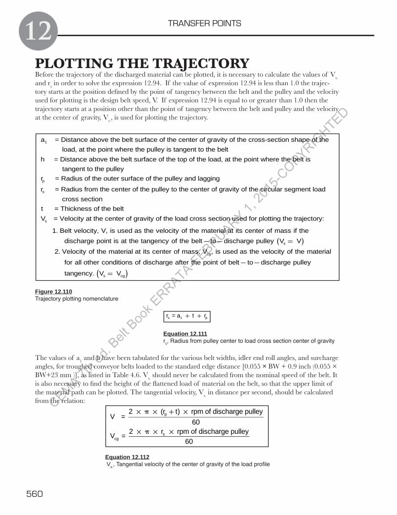
CEMA 7th e

d. Belt

Boo

k ERRATA-F

EBRUARY 1, 20

15-C

OPYRIGHTED

560

TRANSFER POINTS12PLOTTING THE TRAJECTORY

s -

Figure 12.110

Equation 12.111 rs

The values of a×

from the relation:

Equation 12.112 V

a1 = Distance above the belt surface of the center of gravity of the cross-section shape of the load, at the point where the pulley is tangent to the belth = Distance above the belt surface of the top of the load, at the point where the belt is tangent to the pulleyrp = Radius of the outer surface of the pulley and lagging

rs = Radius from the center of the pulley to the center of gravity of the circular segment load cross sectiont = Thickness of the beltVs = Velocity at the center of gravity of the load cross section used for plotting the trajectory:

1. Belt velocity, V, is used as the velocity of the material at its center of mass if thedischarge point is at the tangency of the belt to discharge pulley Vs = V( )

2. Velocity of the material at its center of mass, Vcg, is used as the velocity of the material

for all other conditions of discharge after the point of belt to discharge pulley

tangency. Vs = Vcg( )

rs = a1 + t + rp

V = 2 (rp + t) rpm of discharge pulley

60

Vcg = 2 rs rpm of discharge pulley60

CEMA 7th e

d. Belt

Boo

k ERRATA-F

EBRUARY 1, 20

15-C

OPYRIGHTED

780

Chapter Twelve Continued

Ts Belt Tension required to remove material from feeder due the bulk material

TQ The resistance (belt tension) to shear the bulk material for a simple feeder

s Surcharge angleAngle of incline of the belt conveyor

i Angle of internal friction of bulk solid on shear planeVeb Vertical velocity of bulk material as it leaves the discharging chuteVfs Consolidated pressure volumeVsc The volume of the surcharge material Vy Falling bulk material stream vertical velocity W Weight of the bulk material acting at the center of gravity of the discharging

loadWs Width between skirtboards y1 Vertical height of skirtboard at the rear of feeder hoppery2 Vertical height of skirtboard at front of feeder hopper V Belt speedVfs Consolidated pressure volumeVs Tangential speed of the discharging load center of gravity

Chapter ThirteenSymbol DescriptionCF Conversion ConstantNn Backstop pulley rotational speed Pdn Total power at drive location rpm Motor shaft revolutions per minute rpmAC-Motor AC motor shaft speed SF Back stop service factorTaccel Prime mover torque - required load torque Tbn Minimum torque rating of the backstop Timeaccel Acceleration time in seconds of the motorWK2 Moment of inertia of rotating parts

NOMENCLATUREB

fs

Vs Tangential speed of the discharging load center of gravity

The definition of Vs was changed to be consistent with the other changes in the Trajectory Section. Definition of Vcg needs to be added.

Naylu

Line

CEMA 7th e

d. Belt

Boo

k ERRATA-F

EBRUARY 1, 20

15-C

OPYRIGHTED

780

Chapter Twelve Continued

Ts Belt Tension required to remove material from feeder due the bulk material

TQ The resistance (belt tension) to shear the bulk material for a simple feeder

�s Surcharge angle

� Angle of incline of the belt conveyor

�i Angle of internal friction of bulk solid on shear planeVeb Vertical velocity of bulk material as it leaves the discharging chute

Vfs Consolidated pressure volumeVsc The volume of the surcharge material

Vy Falling bulk material stream vertical velocity

W Weight of the bulk material acting at the center of gravity of the discharging load

Ws Width between skirtboards

y1 Vertical height of skirtboard at the rear of feeder hopper

y2 Vertical height of skirtboard at front of feeder hopper

V Belt speedVfs Consolidated pressure volumeVcg Tangential speed of the load at the center of gravity. Vcg is used when

the material discharges at other than the tangency of the belt and pulley. Vs = Vcg

VsVs = Velocity of the load cross section used for plotting the trajectory when the material diacharges at the tangency of the belt and pulley. Vs = V (belt speed)

Chapter ThirteenSymbol DescriptionCF Conversion Constant

Nn Backstop pulley rotational speed

Pdn Total power at drive location

rpm Motor shaft revolutions per minute

rpmAC-Motor AC motor shaft speed

SF Back stop service factor

Taccel Prime mover torque - required load torque

Tbn Minimum torque rating of the backstop

Timeaccel Acceleration time in seconds of the motor

WK2 Moment of inertia of rotating parts

NOMENCLATUREB

CEMA 7th ed. Belt Book ERRATA-FEBRUARY 1, 2015 ...

Documents

Transcript of CEMA 7th ed. Belt Book ERRATA-FEBRUARY 1, 2015 ...