STUDY OF FOUR-LEPTON FINAL STATES IN ... - SLAC

SLAC-347 UC-34D

w

STUDY OF FOUR-LEPTON FINAL STATES IN

ELECTRON-POSITRON INTERACTIONS AT 29 GeV

Assimina Petradza

Stanford Linear Accelerator Center

Stanford University

Stanford, California 94309 -.

August 1989

Prepared for the Department of Energy

under contract number DE-AC03-76SF00515

Printed in the United States of America. Available from the National Techni- cal Information Service, U.S. Department of Commerce, 5285 Port Royal Road, Springfield, Virginia 22161. Price: -Printed Copy A07, Microfiche AOl.

+ partial fulfillment for Ph. D. thesis

-

ITHAKA

As you set out for Ithaka hope your road is a long one,

Constantine Cavajy

jull of adventure, full of discovery.

Laistrygonians, Cyclops, angry Poseidon-don? be afraid of them:

you’ll never find things like that on your way

as long as you keep your thoughts raised high,

as long as a rare excitement stirs your spirit and your body,

Laistrygonians, Cyclops, wild Poseidon-you won’t encounter them

unless you bring them along inside your soul --. unless your soul sets them up in front of-you.

Hope your road is a long one. _

May there be many summer mornings when,

with what pleasure, what joy,

you enter harbors you are seeing for the first time;

may you stop at Phoenician trading stations to buy fine things,

mother of pearl and coral, amber and ebony,

sensual perfume of every kind- as many sensual perfumes as you can;

and may you visit many Egyptian cities

to learn and go on learning from their scholars.

Keep Ithaka always in your mind. Arriving there is what you’re destined for.

But don’t hurry the journey at all. Better if it lasts for years,

so you’re old by the time you reach the island,

wealthy with all you’ve gained on the way,

not expecting Ithaka to make you rich.

Ithaka gave you the marvelous journey.

Without her you wouldn’t have set out.

She has nothing left to give you now. -

And if you find her poor, Ithaka won’t have fooled you.

Wise as you will have become, so full of experience,

you’ll have understood by then what these Ithakas mean.

ABSTRACT

This thesis presents a study of electron-positron scattering to four light leptons.

The motivations behind it are twofold. Firstly, the study is a test of the theory of

electron-positron interactions to 4th order in the fine structure constant cr. A devia-

tion from the theory could indicate the existence of a heavy new particle. Secondly,

a measurement of these-processes may prove useful in the understanding of other

QED-type reactions. The method for simulating the four-lepton processes by the -.

Monte Carlo event generator of Berends, Daverveldt and Kleiss is described. Theo-

retical predictions are compared to data from the Mark II and HRS experiments at

the PEP storage ring. The observed events consist of four leptons at large angles.

Data for all three eSe-e+e- , e+e-p+p- and ~+P-P+,u- processes are well de-

scribed by the QED Monte Carlo calculation. The various kinematical distributions

are in good agreement with QED to order 04.

ACKNOWLEDGMENTS

-

Six years in graduate school has been an interesting experience. Rudi Thun

made it particularly educa-tional, not only with the variety of projects that he

assigned me, but also with his dedication as an advisor. It was he who suggested

the subject of this thesis after discussions we had with Martin Perl. --

The members of the Mark II and-HRS collaborations provided me with fine

sets of data to work with, and valuable help when needed. I would like to express

my special thanks to David Stoker from Mark II and David Blockus from HRS for

the very many useful discussions during the course of this thesis. Chris Hawkins

introduced me to the four-lepton Monte Carlo and Francois Le Diberder helped me

understand its finer details. The SLAC theory group, and in particular Michael

Peskin, often provided enlightening comments. The friendly help of Charlotte Hee

made problem-solving easier, especially where the Mark II software was concerned.

Finally, the shape of this thesis owes a lot to Ray Cowan’s expertise in Y&X.

To my friends and family : thanks for sharing the journey !

. . . 111

TABLE OF CONTENTS

-.

ABSTRACT . . . . .

ACKNOWLEDGMENTS

LIST OF TABLES . . .

LIST OF FIGURES . . .

LIST OF APPENDICES .

CHAPTER

.*.--.................. ii

. . . . . . . . . . . . . . . . . . . . . . . . . . 111

....................... vii

....................... ix

. . . . . . . . . . . . . . . . . . . . . . . xii

1 INTRODUCTION .................... 1

2 THE MARK II DETECTOR AT PEP .......... 5 .

2.1

2.2

2.3

2.4

2.5

2.6

2.7

The PEP storage ring ................ 7

Vertex and main drift chambers ............ 8

Time-of-flight connters ................ 10

Magnet ....................... 11

Liquid argon calorimeter ............... 11

Muon chambers ................... 14

End cap shower counters ............... 15

iv

2.8 Trigger . . . . . . . . . . . . . . . . . . . . . . . 16

3 THE HRS DETECTOR AT PEP . . . . . . . . . . . . . 18

3.1 Superconducting magnet . . . . . . . . . . . . . . . 18

3.2 Vertex chamber . . . . . . . . . . . . . . . . . . . . 20

3.3 Central and outer drift chambers . . . . . . . . . . . . 20

3.4 Electromagnetic calorimetry . . . . . . . . . . . . . . . 21

3.5 Trigger . . . . . . . . . . . . . . . . . . . . . . . 24

4 MONTE CARLO GENERATOR OF FOUR-LEPTON PR&ESSES . . . . . . . . . . . . . 27

4.1 Theoretical description of four-lepton processes . . . . . 28

4.2 Monte Carlo technique for event generation . . . . . . . 33

5 MONTE CARLO SIGNAL GENERATION AND ANALYSIS . . . . . . . . . . . . . . . . . . . . . . . 36

5.1 Event generation of four-lepton final states . . . . . . . 36

5.1.1 e+e-e+e- . . . . . . . . . . . . . . . . . 38

5.1.2 e+e-p+p- . . . . . . . . . . . . . . . . . 41

5.1.3 /..L+p-p+p- . . . . . . . . . . . . . . . . . 44

5.2 Monte Carlo results . . . . . . . . . . . . . . . . . 44

5.2.1 Mark II analysis of Monte Carlo signal events . . . . . . . . . . . . . . . . . . 44

5.2.2 HRS analysis of Monte Carlo signal events . . . . . . . . . . . . . . . , . . 47

6 MONTE CARLO BACKGROUND GENERATION AND ANALYSIS . . . . . . . . . . . . 50

7 MARK II DATA ANALYSIS . . . . . . . . . . . . . . . 57

7.1 Event selection and analysis . . . . . . . . . . . . . . 57

7.2 Monte Carlo event selection and comparison with

data ........................ .66

7.3 Detection efficiencies ................... 81

8 HRS DATA-ANALYSIS ................. 83 -

8.1 Selection criteria . . . . . . . . . . . . . . . . . . . 83

8.2 Comparison with Monte Carlo ............. 89

8.3 Detection efficiencies ................ -101

9 CONCLUSIONS . . . . . . . . . . . . . . . . . . . . 103

APPENDICES . . . . . . . . . . . . . . . . . . . . . . . . . 106

REFERENCES . . . . . . . . . . . . . . . . . . _ . . . . . . . 127

vi

LIST OFTABLES -

-- .

4.1 Number of contributing diagrams in each of the final states . . . . . 32

5.1 Summary of MC event statistics and luminosities for Mark II . . . . 37

5.2 Summary of MC event statistics and luminosities for HRS , . . . . 47

7.1 Effect of kinematical cuts on Mark II data in case (A) . . . . . . . 61

7.2 Effect of kinematical cuts on Mark II data in case (B) . . . . . . . 62

7.3 Effect of analysis cuts on MC signal and background-events in case (A) 67

7.4 Effect of analysis cuts on MC signal and background events in case (B) 68

7.5 Summary of Mark II results in case (A) , . . . . . . . . . . . . 71

7.6 Summary of Mark II results in case (B) . . . . . . . . . . . . . 72

7.7 Breakdown of MC identified events for case (A) . . . . . . . . . . 73

7.8 Breakdown of MC identified events for case (B) . . . . . . . . . . 74

7.9 Summary of Mark II cross sections and MC event statistics for case (A) 82

7.10 Summary of Mark II cross sections and MC event statistics for case (B) 82

8.1 Effect of the analysis cuts on HRS data . . . . . . . . . . . . . 85

8.2 Effect of HRS analysis cuts on MC signal and background events . . 90

8.3 Summary of HRS results . . . . . . . . . . . . . . . . . . . . 92

8.4 Summary of HRS cross sections and MC event statistics . . . . . 102

9.1 Summary of e+e-e+e- results from various experiments . . . . . 104

9.2 Summary of e+e-p+p- results from various experiments . . . . . 105

A.1 List of the generation parameters for e+e-e+e- MC events . . . . 110

vii

A.2 Summary of MC cross sections for e+e-e+e- events ....... 112

A.3 Summary of MC efficiencies for e+e-e+e- events ........ 113

C.l Mark II four-lepton candidate events .............. 120

D.l HRS four-lepton candidate events ............... 123

. . . Vlll

_LIST OF FIGURES -

The Mark II detector at PEP . . . . . . . . . . . . . . . . . . 6

The PEP storage ring ..................... 7

The Mark II/PEP5 drift chamber geometry ............ 10

Mark II liquid argon calorimeter module ............. 13

Mark II liquid argon calorimeter layer ganging scheme ....... 14

The Mark II muon system proportional chamber geometry ..... 15

The HRS detector at PEP ................... 19

The HRS central drift chamber ................. 22

Momentum resolution of the HRS ................ 23

HRS barrel shower counter module ............... 25

The bremsstrahlung group of diagrams for e+e-e+e- ....... 30

The annihilation group of diagrams for e+e-e+e- ......... 31

The conversion group of diagrams for e+e-e+e- ......... 31

The multiperipheral group of diagrams for e+e-e+e- ....... 32

Momentum and angular distributions in e+e-eSe- MC events ... 39

Angular distributions in e+e-e+e- MC events .......... 39

Invariant mass distributions in e+e-e+e- MC events ....... 40

Momentum and angular distributions in e+e-p+p- MC events ... 41

Angular distributions in e+e-p+p- MC events .......... 42

Invariant mass distributions in e+e-p+p- MC events ........ 42

.

2.1

2.2

2.3

2.4

2.5

2.6

3.1

3.2

3.3

3.4

4.1

4.2

4.3

4.4

5.1

5.2

5.3

5.4

5.5

5.6

ix

5.7

5.8

5.9

5110

5.11

5.12

5.13

6.1 -

6.2

6.3 -. . 6.4

6.5

7.1

7.2

7.3

7.4

7.5

7.6

7.7

7.8

. 7.9

7.10

7.11

7.12

7.13

7.14

8.1

8.2

8.3

MC lowest mass distributions .................. 43

Mark II MC e+e-e+e- track and energy distributions ....... 45

Mark II MC e+e-p+p- track and energy distributions ....... 46

Mark II MC p+p-p+p- track and energy distributions ...... 46

HRS MC e+e-e+e- track and energy distributions ........ 48

HRS MC e+e-p+p- track and energy distributions ........ 49

HRS MC ~t~-~s~- track and energy distributions ........ 49

MC e+e-r+r- k ac multiplicity and energy distributions k ..... 54

MC e+e-h+h- track multiplicity and energy distributions ..... 54

MC T+T- track multiplicity and energy distributions ....... 55

MC hadronic track multiplicity and energy distributions ...... 55

MC e+e-+yr track multiplicity and energy distributions ...... 56

Energy distribution of Mark II data before cut (3) ......... 60

Pair mass distribution of Mark II data before cut (4) ....... 60

Mass distribution of Mark II data before cut (5) ......... 62

E/P distribution of Mark II four-lepton candidates ......... 64

Distributions of e* in Mark II e+e-e+e- events ......... 75

Distributions of e* in Mark II e+e-p+p- events ......... 76

Distributions of p* in Mark II e+e-p+p- events ......... 76

Lowest mass distributions in Mark II e+e-e+e-, e+e-p+p- .... 77

Energy distributions in Mark II e+e-e+e-, e+e-p+p- ...... 77

Invariant mass distributions in Mark II e+e-e+e- events ...... 78

Invariant mass distributions in Mark II e+e-p+p- events ..... 79

Mark II e+e-e+e- event picture ................ 79

Mark II e+e-p+p- event picture ................ 80

Mark II /.L+~-P+P- event picture ................ 80

Energy distribution of HRS data before cut (2) .......... 86

Pair mass distribution of HRS data before cut (3) ......... 87

E/P distribution in HRS data .................. 88

X

8.4 Energy distribution of tracks in HRS data . . . . . . . . . . . . 88

8.5 Energy distribution of tracks with E/P<0.55 in HRS data . . . . . 89

8.6 HRS CX’ candidate event . . . . . . . . . . . . . . . . . . . . 91

8.7 E/P distribution in HRS data and MC events ........... 94

8.8 HRS data and MC energy distributions of tracks with E/Ps0.55 . . 94

8.9 Distributions of e* in HRS e+e-e+e- events ........... 96

8.10 Distributions of e* in HRS e+e-p+p- events , .......... 96

8.11 Distributions of p* in HRS e+.e-#p- events .......... 97

8.12 Lowest mass distributions in HRS e+e-e+e-, e+e-p+p- ..... 97

-. . 8.13 Energy distributions in HRS eSe-e+e-, e+e-p+p- ........ 98

8.14 Invariant mass distributions in HRS eSe-e+e- events ....... 98 _

8.15 Invariant mass distributions in HRS e+e-#p- events ....... 99

8.16 HRS e+e-e+e- event picture .................. 99

8.17 HRS e+e-/l+p- event picture ................ 100

8.18 HRS ~L+~-~f~- event picture ................ 100

A.1 The center-of-mass energy distribution of MC events- ....... 108

A.2 The distribution of MC generated cross section ......... 109

A.3 The distribution of MC observed cross section ......... 111

A.4 The distribution of MC efficiency ............... 114

B.1 E/P and energy distributions of Mark II end cap ........ 116

xi

LIST OF APPENDICES

Appendix

-- . A RADIATIVE CORRECTCONS . . . . . . . . . : . t 106

B STUDY OF THE MARki END CAP SHOWER COUNTER . . . . . . . . . . . . . . . . . . . . 115

C MARK II EVENT LIST . . . . . . . . . . . . . . . 118

D HRS EVENT LIST . . . . . . . . . . . . . . . . . 122

xii

CHAPTER 1

INTRODUCTION

This thesis is a study of the production of four-lepton final states in e+e- inter-

actions, using the Mark II and the HRS detectors at the Stanford Linear Accelerator

Center. These detectors recorded data from events produced by the PEP storage

ring, operating at a center-of-mass (c.m.) energy of 29 GeV. -

During the last twenty years, e+e- experiments have led to many interesting and

important discoveries. Although the main focus has been on processes like e+e- +

p+p-, e+e- 4 e+e-, e+e- + hadrons, where the interaction is mediated by a single,

virtual photon, the interest in higher order processes, such as e+e- --+ e+e-e+e-,

e+e- + e+e-p+p- or e+e- + e+e’hadrons, has been increasing. In these processes,

the dominant contribution to the total cross section comes from Feynman diagrams

with two spacelike virtual photons which are emitted along the beam direction and

are almost real. These diagrams are called multiperipheral, or t-channel diagrams.

These processes are also known as two-photon processes, since the reactions are

quasi-two body interactions of two almost-real photons. There is also a subclass of

O(a4) diagrams, namely those with two timelike virtual photons which, in addition

1

2

to e+e’ ---, e+e-e+e-, e+e- 4 e+e-p+p- and e+e- --$ e+e’hadrons, can also yield final

states consisting of e+e- 4 ~+p-r+r-, e+e- 4 ,u+J.J-~+~- or e+e- --* p+p-qij. When

the timelike photons are massive, these non-multiperipheral processes are expected

to have very small cross sections, since they probe higher order interactions at small

distances. They offer an opportunity to make sensitive tests for unexpected physics.

It is the objective of this thesis to test QED to 4th order in the coupling constant

cr by studying those interactions of electrons and positrons which yield final states -- .

containing four observed light leptons :

e+e’ 4 e+e-e+e-

e+e- 4 e+e-p+p-

e+e- 4 p+p-p+p-

The cross section for these reactions is very small, of the order of a tenth of

a picobarn (pb), in the region of large pair masses and large scattering angles. In

this region, the background to four-lepton final states is small, making them easily

distinguishable despite the smallness of the cross section.

By using data from two PEP detectors, Mark II and HRS, we are making

two independent measurements of the production of four-lepton final states in e+e-

interactions. These experiments accumulated large integrated luminosities. They

also had different detector components, such as the muon detection system present

only in the Mark II, thus allowing two independent tests of the theory.

The motivation of this analysis is the following : QED is the physical theory

best established experimentally. It serves as the prototype of more evolved theories

. .

3

such as the electroweak theory and &CD. The degree of precision attained in the

measurements and predictions of g-2 for the electron (I) and the muon c2) severely

constrain the existence of new physics c3) such as composite leptons, excited leptons,

and supersymmetric particles. The non-observation of significant deviations from

the theory in measurements of the differential cross sections of Bhabha scattering

and muon-pair production establish QED to order o2 and a3 at small distances.

_. . The results reported here extend tests of QED to order cy4 at large LJ2, where &” is

the four-momentum squared of the-photon propagators appearing in the Feynman

diagrams of the four-lepton final states. By requiring all leptons to be detected, one

accomplishes two things. First, at large angles, virtual bremsstrahlung processes are

expected to dominate and the production of two virtual photons becomes measur-

able. Second, if massive new particles decaying into leptons are produced, an excess

of events would appear above the QED prediction.

The proliferation of Feynman diagrams with increasing order make the calcu-

. lations of QED contributions to order (Y’ quite difficult. For example, while the

Bhabha reaction e+e- + e+e- involves just 2 Feynman diagrams, final states with

4 electrons from e+e- interactions involve 36 ! A Monte Carlo program, where all

Feynman diagrams contributing to order cy4 are taken into account, was written by

Berends, Daverveldt and Kleiss t4-‘) to generate the four body final states. This is

the one used in this analysis for comparison with the data.

In the past, other collaborations c8) have done similar studies at c.m. energies

ranging from 14 to 47 GeV and found good agreement between data and QED

4

predictions to cy4. One group (‘1 initially found some disagreement but recently

reported agreement (lo) between their data and the Monte Carlo program of Berends,

Daverveldt and Kleiss.

The further outline of this thesis is as follows. In the next ttio chapters we

briefly describe the parts of the Mark II and HRS detectors which are relevant

- to this analysis. In chapter 4 we present the theoretical description of the Monte

Carlo (MC) event generator used in the analysis. In chapter 5 we discuss the MC -- .

generation and simulation of signal processes. Expected backgrounds are discussed

in the next chapter. Comparisons between theory and data from the Mark II and

HRS experiments are then presented in chapters 7 and 8, respectively. Finally, in

chapter 9 we summarize the results from Mark II and HRS and those reported by

other experiments.

CHAPTER 2

THE-MARK II DETECTOR AT PEP

The Mark II/PEP5 detector (r’-)-, shown in fig. 2.1, was a device built for study-

ing the physics of e+e- interactions. After having been used initially at the SPEAR

storage ring in 1978, it was placed at the PEP storage ring from 1980 through 1985.

It was characterized by good charged particle tracking, electromagnetic calorimetry,

and muon detection systems. An upgraded version of the detector is presently at

the interaction region of the SLC for studying 2’ physics.

.

After a brief description of the PEP storage ring, we present in this chapter

a description of the components of the Mark II detector that are relevant to this

analysis. Further details can be found in refs. 12 and 13.

A MUON DETECTORS

FLUX RETURN

-

Window (0.012’ Slainless SInI)

=/ I Sol Shower Counlrr

Figure 2.1. The Mark II detector at PEP; a) isometric view; b) side view.

2.1 The PEP storage ring

The PEP (Positron Electron Project) storage ring guides positrons and elec-

trons around a ring with a diameter of 700 m. The location of the PEP ring and

the HRS and the Mark II detectors at the SLAC site is presented ia fig. 2.2. Three

positron and three electron bunches collided at six interaction regions, while circu-

- lating in opposite direct&s. The ring .was run at 29 GeV, but it had been originally

designed for collision energies of up to 36 GeV. (14) This lower energy allowed op- -. .

eration at a higher luminosity. At each interaction region collisions occurred every

2.4,~. The maximum luminosity reached was 3 x 1031cm2 see-r.

SAND HILL ROAD

SHOPS II

LINES

(0 Scale -

0 50 100 200 Y “IaP

Figure 2.2. Overview of the PEP storage ring and the SLAC site.

8

2.2 Vertex and main drift chambers

The inner part of the Mark II detector was the vertex chamber (is), a high

precision cylindrical drift chamber, 126 cm long, with an outer radius of 35 cm. It

was used to measure the distance of closest approach of particles to the event origin,

thereby improving momentum and lifetime measurements. It was built as close as

possible to the 1.4 mm thick beryllium beam pipe, which formed the inner wall of

_._ the chamber.

The wires of this vertex chamber were organized in seven concentric layers.

Four inner layers were at an average radius of 11.4 cm from the beam pipe, while

the outer three were at a radius of 31.2 cm. All wires were strung axially, no attempt

being made to measure the z coordinate. This arrangement allowed the accurate

projection of tracks back to the origin. There were 270 drift cells in the inner layers

and 555 in the outer layers, with a radius of 0.53 cm. Each cell was parallel to

the axis and had a single sense wire. Apart from the sense wires that collected the

ionization electrons, there were also field wires that carried high voltage and guard

wires that ensured electrostatic stability. Field wires placed exactly between the

sense wires minimized cell-to-cell cross talk. The chamber operated with a 50%-

50% mixture of argon and ethane- at 15.5 psi.

.

The position resolution of the individual wires jn the vertex chamber ranged

from 85 pm at the center of the drift cell up to 100 pm at the edges. This excellent

spatial resolution was due to :

1. the precise location of the wires

2. the minimization of Coulomb scattering due to the beryllium beam pipe,

9

which was only 0.6% radiation length thick

3. the fact that the precision tracking in the vertex chamber was decoupled from

that in the main drift chamber

4. an excellent timing resolution of 250 ps of the electronics

5. the full efficiencysf the chamber at the voltages used

6. the fact that the gas, kept at a stable pressure, maintained a constant drift

-. . velocity over the cell. _

The 2.7 m long main drift chamber, (16) shown in fig. 2.3, measured the sign of

the charge and the momentum of charged particles. Its sense wires were arranged

in 16 concentric layers, located at various radii from the beam axis, ranging from

41.4 cm up to 144.8 cm. The first six layers were located in a conical inner piece,

made out of solid aluminum. The other ten were located on the outer flat endplates,

which were made out of aluminum honeycomb. The drift cells in the conical piece

were small, while the cells in the honeycomb portion were larger. All wires were

made of silver plated beryllium-copper. Each cell had a single sense wire, surrounded

by six field wires. The wires, strung in a O”, +3’, -3’ pattern with respect to the

axis of the detector, allowed the measurement of the polar and azimuthal angles of

the tracks. There were 3204 cells in the chamber, the large ones operating below

the drift velocity saturation point, while the small ones operated just above it. The

timing resolution of the electronics was 350 ps and the average spatial resolution was

200 pm. The main drift chamber was operated with a 50%-50% mixture of argon

and ethane, at atmospheric pressure.

10

.-I I ’ 142.00 4

Figure 2.3. The Mark II/PEP5 drift chamber geometry; the angles 6 and C$ are defined.

The vertex and main drift chambers had a combined momentum resolution for

charged tracks given by &p/p = d(O.OIOp)z + (0.025)2, where p is in GeV/c. The

first term comes from the intrinsic resolution, the second from multiple scattering.

The resolution was determined from Bhabha electron and cosmic ray studies.

2.3 Time-of-flight counters

The time-of-flight system, located around the main drift chamber and inside

the solenoidal magnet, consisted of an array of 48 plastic scintillators, at a radius of

1.5 m from the beam pipe, each one 0.20 m wide and 3.4 m long. They covered 70%

of the 4n solid angle. Each counter was oriented along the beam axis. The light of

the scintillator was brought to each end by a lucite light guide, and was collected

there by a phototube. The output from these phototubes was fed into electronics

that measured the charge integral signal and pulse arrival times.

The purpose of the time-of-flight system was the precise measurement of flight

times of charged particles, to be used in the determination of the mass of slow

11

particles. It was also used to eliminate cosmic ray backgrounds and to form an

integral part of the charged-particle trigger. The timing resolution was about 350

ps, and the efficiency of having a time-of-flight counter fired by a charged track was

99%.

2.4 Magnet -

The magnet, a conventional room temperature solenoid at a radius of 1.6 m

from the beam axis, consisted of two water-cooled aluminum conductors separated

by an insulating layer. It was external to the vertex and main drift chambers, as

well as to the time-of-flight system. The conductors were 1.4 radiation lenghts thick

and produced a uniform axial solenoidal magnetic field. The momentum of charged

particles was determined from the curvature of their tracks-in the magnetic field.

Initially operated at 4.5 kG, it eventually developed a short between the inner and

outer layers, due to corrosion caused by the cooling water. Only the outer conductor

was powered from then on, yielding a 2.35 kG field. Thus the momentum resolution

was degraded, while the tracking of lower momentum particles became possible.

The magnetic field was known to within 1%.

2.5 Liquid argon calorimeter

An electromagnetic calorimeter, 0’) located outside the magnet coil at 1.8 m

from the axis, (see fig. 2.1) measured the energies of showering particles and thereby

distinguished electrons from other charged particles. It consisted of eight modules

arrayed octagonally which covered 65% of the 47r solid angle. The front portion of

each module consisted of two aluminum planes, 1.6 mm thick, separated by 8 mm

12

of liquid argon. These axial planes were known as the trigger gap and were 0.1%

radjatjon lengths thjck. They sampled the showers that started in the magnet coil.

The rest of the module was a sandwich of 3 mm liquid argon gaps and 2 mm-thick

layers of lead, 37 layers in total, the whole. assembly being cooled down to 88’ K.

The odd numbered layefs were made of solid lead, while the even numbered layers

were formed of lead strips and collected the ionization produced in the liquid argon.

-s- A potential difference of 3.5 kV across the 3 mm liquid argon gaps provided a drift

field for the released electrons. In order to determine the position of the shower,

the layers of lead at high potential were segmented into strips in various directions

(see fig. 2.4). Nine of these 18 readout strip layers, each of which corresponded

to 0.8 radiation lengths, had their 3.8 cm wide strips oriented axially, and gave

information about the azimuthal angle of the shower. Six of them had their 3.8 cm

wide strips perpendicular to the beam direction, and determined the polar angle.

The remaining three planes had 5.4 cm strips oriented along the diagonal direction,

and they helped resolve ambiguities concerning multiple showering tracks. There

were 1152 lead strips all together in each module, and shower sampling occurred

every 0.4% of a radiation length, the complete module being 14.4 radiation lengths

thick.

The fine segmentation of the liquid argon made possible the precise determina-

tion of the shower position and led to a large number of electronic channels. The

reduction of this number down to a more manageable number of the order of 3000

required the ganging of some strip planes, shown in fig. 2.5, and the wiring together

13

orgon

Figure 2.4. Cutaway view of a liquid argon calorimeter module. The insert shows the liquid argon gap and the segmentation of the lead strips.

of pairs of neighboring channels in the back of the calorimeter. Out of the 37 layers

of lead, 18 were read out and ganged into six measurements, leaving a net number

of 362 channels per module.

Due to the above described segmentation, both in depth and angle, the dif-

ferentiation of electrons from hadrons became possible, since the electrons would

shower quickly, depositing all their energy in the calorimeter, while most hadrons

would pass through with little energy loss. The hadrons that did deposit energy

in the calorimeter did so over a-larger area than electrons. Furthermore, a very

good energy resolution of 14.5%/a was achieved (E in GeV), while the entering

position of a Bhabha electron could be measured to within 8 mm. The polar angle

covered corresponded to 1 cos 01 50.7. The azimuthal angle covered was the 88% of

-LA t Trigger gap

F3

TZ

F2

U Tl Fl

Figure 2.5. Liquid argon calorimeter ganging scheme. Particles enter from the trigger gap and the ionization is measured along the azimuthal (F), polar (T), and diagonal (U) directions.

2.6 Muon chambers

The muon detection system, located outside the electromagnetic calorimeter,

consisted of four walls placed at the top, bottom, right and left of the beam pipe,

235 cm away from the interaction point (see fig. 2.1). Each wall consisted of four

layers of hadron absorber alternating with four layers of proportional tubes. The

proportional tubes were made from extruded aluminum modules, each module hav-

ing eight proportional wire chambers (see fig. 2.6). Each tube contained one 45 ,um

wire, 2.5 cm away from the wire of the nearest proportional tube. There were 408

modules, 3264 channels, in total. The proportional wire chambers were triangular

in shape, and operated at 2 kV with a gas mixture of 95% argon and 5% carbon

15

dioxide. The tubes in the first layer were perpendicular to the beam axis in order to

measure the polar angle, while those in the outer three layers were oriented axially

in order to measure the azimuthal angle. Particles had to traverse at least 7.4 in-

teraction lengths of material in order to cross all the layers. This thickness ensured

the reduction of the contamination from hadronic punchthrough, while accepting

muons with a momentum as low as 1 -GeV/c. The complete system covered about

55% of the entire solid angle. -.

2.5 cm

Figure 2.6. Muon system cross sectional view. A single module is shown.

2.7 End cap shower counters

Placed at each end of the drift chamber, the end cap shower counters covered

the forward and backward regions of Mark II. They consisted of two sheets of lead,

each one 2.3 radiation lenghts thick, alternating with two layers of proportional

wire chambers. They measured electromagnetic showers between the polar angles

of 15’ and 40°, over most of the azimuthal range. The system attained an energy

resolution of 50%/o, for photons and electrons, where E is in GeV. Its poor energy

resolution, combined with the 2.5% probability of photon non-conversion, prevented

16

its use in many Mark II/PEP analyses. In this analysis though, the system proved

useful as a tool for discriminating electrons from muons as shown in appendix B.

2.8 Tbigger

A two-level programmable trigger of considerable flexibility was used. It had

very little dead time and-could be reprogrammed for various event topologies. The

primary trigger would decide if an event was interesting enough to be processed by -. _

the secondary trigger. It used simple-selection criteria in the drift chambers, liquid

argon and small angle shower counters. The primary trigger relevant to this anal-

ysis was generated by either charged tracking or calorimetry. The charged primary

trigger was produced when a beam crossing signal coincided with a drift cham-

ber majority signal (DCM). A DCM signal was present only if all of the following

conditions were satisfied :

1. at least 3 vertex chamber layers hit

2. at least 6 drift chamber layers hit

3. at least 1 time-of-flight counter hit

The calorimetric primary trigger was generated by the presence of energy de-

posited in at least two Liquid Argon (LA) or End Cap (EC) modules. The energy

threshold was 1 GeV for LA and 2.5 GeV for EC.

The secondary trigger was intended to find track patterns in the vertex and drift

chambers and the time-of-flight system. A special pattern recognition processor,

consisting of twenty-four curvature modules, was used to find tracks. A track. was

defined for the purposes of this trigger as a signal in two of the inner four vertex

17

chamber layers, four inner and two outer main drift chamber layers, and a time-

of-flight counter aligned in a momentum band. The generation of a secondary

calorimetric trigger followed automatically if calorimetry had set the primary trigger.

The secondary trigger requirement relevant to this analysis was that either the

number of charged tracks or the number of calorimeter modules with total energy

above a certain threshold be two or more.

CHAPTER 3

THE HRS DETECTOR AT PEP

-. _ The High Resolution Spectrometer (HRS),(“) shown in fig. .3.1, was a general

purpose solenoidal detector. It was-characterized by the strong uniform magnetic

field (1.6 Tesla) of its superconducting magnet, a good spatial resolution of the drift

chambers, a long tracking radius of 2 m, and consequently an excellent momentum

resolution for charged particles. The detector covered over 90% of the solid angle.

This chapter describes briefly the elements of the HRS detector which are rele-

vant to this analysis, as they existed during the years 1982 through 1986, when data

were taken at the PEP storage ring. Detailed descriptions of the HRS detector can

. . be found in refs. 19 and 20.

3.1 Superconducting magnet

The unique characteristic of the HRS detector was its large superconducting

magnet, with a cylindrical volume 4.8 m in diameter and 3.1 m in length. The

solenoidal coil consisted of 15120 turns of niobium-titanium strands and was sur-

rounded by an iron yoke of 1600 tons of low carbon steel. The magnet was operated

at 1.6 Tesla during the collection of the data and was characterized by a uniform

18

19

CCIITRAL DRlfT CPAYt OUTU I

-- ; . .--Is.w.. “I .“I+

Figure 3.1. The HRS detector at PEP; a) isometric view; b) side view.

20

field which varied less than 3% over the detector volume.

3.2 Vertex chamber

A small, high-precision drift chamber was installed between the central drift

chamber and the beam pipe after the first two years of running. It was made of two

double layers of aluminized mylar tubes,(2’) and used a 75% argon - 25% ethane

mixture at atmospheric-pressure. As .it was inside the main tracking system, it

was constructed with a total material thickness of just 0.004 radiation lengths to -. _

reduce multiple scattering. Its operation improved the track fitting, enhanced the

momentum resolution, and made possible the accurate measurement of lifetimes of

leptons and hadrons. Since all the tracks had to pass through this chamber, it was

also able to play the role of a cosmic ray veto, reducing the trigger rate by a factor

of three. Its spatial resolution was 120 pm.

3.3 Central and outer drift chambers

Most of the tracking information was gathered by the central drift chamber,(“)

. a large cylindrical chamber with 2448 drift cells distributed among fifteen concentric

layers, as shown in fig. 3.2. The seven even-numbered layers had their wires placed

parallel to the beam direction (z), while the rest made a stereo angle of &60 mr

with respect to the beam axis. The cells in each layer numbered from 80 in the

innermost layer at a radius of 21 cm to 256 in the outermost at a radius of 103 cm.

Each of these cells had a central sense wire carrying positive voltage, surrounded by

six field shaping wires that carried negative voltage, yielding potential differences of

about 2500 Volts. The drift cell efficiency exceeded 99% at 1.6 Tesla. A beryllium

21

inner chamber wall and an aluminum honeycomb outer chamber wall reduced the

multiple scattering. The total thickness of material traversed by particles was 0.02

radiation lengths. Charged particles were tracked over 90% of the entire solid angle.

The spatial resolution was 200pm. The gas used was a mixture of 89% argon, 10%

carbon dioxide, and 1% methane (HRS gas). More details about the central drift

- chamber are described in Ref. 22.

The outer drift chamber,(23) located 1.9 m away from the beams, was a cylin-

-~. drical shell consisting of 896 thin stainless steel tubes, arranged ,in two layers. The

tubes were 350 cm long and had a 2.5 cm diameter. The layers were staggered by

half a tube width with respect to each other, to eliminate inefficiencies and resolve

ambiguities. This chamber operated with HRS gas at 2150 Volts and had a spa-

tial resolution of 200 pm. Because the radius of the outer drift chamber was twice

that of the inner drift chamber, the momentum resolution of large-angle tracks was

improved by a factor of four as shown in fig. 3.3.

3.4 Electromagnetic calorimetry

Two sets of calorimeters were used to measure the energy and position of elec-

tromagnetic showers, as well as the time-of-flight of charged particles. The barrel

shower counter system, with a time-of-flight resolution of f 360 ps and an energy

resolution of 16%/G (E in GeV), covered 60% of the entire solid angle, while the

end cap shower counter system, with a time-of-flight resolution of f 1000 ps and an

energy resolution of 20%/a (E in GeV), covered 27% of the total solid angle.

The barrel shower counter system,(24), shown in fig. 3.4, consisted of 40 modules

... : T(.~.I.l.i.i.:.,.,:“.’

WRS DRlff WA8ER END VIEW i

Figure 3.2. The HRS central drift chamber; a) side view; b) end view.

23

CENTRAL DRIFT CHAMBER ONLY / (NO OUTER D.C.) /

//

CENTRAL AND OUTER DRIFT CHAMBERS

4002 - _

*

0.001 ’ ’ ’ ’ ’ ’ I I I1 III,1 t 0.5 I 2 5 IO 20

YOYENTUY, p (6tV/cl

Figure 3.3. Momentum resolution of the HRS

.-

of lead-scintillator sandwiches. These surrounded the outer drift chamber system,

just inside the magnet coil, and formed a cylindrical shell coaxial with the beam

line. Two sections, between which a layer of fourteen proportional wire chambers

was placed, composed each module. Scintillation light from both the three radiation

lengths thick front section and the eight radiation lengths thick back section was

collected at the ends by two-inch diameter phototubes which provided energy infor-

mation on the traversing particles. There were thus four phototubes per module,

160 in all. Processing the signals from these phototubes also provided time-of-flight

information. The front section of each module consisted of two radiator plates of

two and one radiation lengths, and two layers of scintillators. The outer section of

24

the module had eight radiator plates, one radiation lengths thick, and eight layers of

scintillators. All scintillators were 305 cm long, and were oriented axially. Segmen-

tation along the azimuthal direction was provided by a total of 560 proportional wire

cells. These cells were read out at both ends and provided z information by means

of current division. Further details about the barrel shower counters are given in

Ref. 24.

The end cap shower counter system was composed of four C-shaped units

-- . mounted on the magnet return yoke at each end of the solenoid. Each unit contained

1.5 radiation lengths of lead, 76 proportional wire chambers oriented.verticaIly, and

10 pie-shaped lead-scintillator sandwiches, arrayed in that order. These latter sand-

wiches consisted of eight layers of one radiation length thick lead sheets and 9.5 mm

thick scintillators. They were viewed at their outer edge by one two-inch diameter

phototube each. All proportional wire chambers used the HRS gas.

3.5 Trigger

The HRS trigger consisted of a two-level system similar to that of the Mark II.

The primary trigger used the wire hit information from the central drift chambers

to produce a charged trigger, and the phototube pulse height information from the

shower counters to produce a neutral trigger. Within 1.5 ps after a collision, the

primary trigger decided whether an event should proceed to the secondary trigger

or not.

If any of the following criteria was satisfied, the event was accepted by the

primary trigger :

25

.

- WALL -

/

SE-!!

Figure 3.4. HRS barrel shower counter module; a) end view; b) side view.

26

l NTl: total energy deposited in the end cap and barrel shower counters

> 4.8 GeV

-0 NT2: total energy deposited in the end cap and barrel shower counters

> 2.4 GeV

l CTl: > 12 layers of the central drift- chamber hit

l CT2: > 7 of the inner 8 layers of the central drift chamber plus a hit in the

corresponding quadrant in the end cap shower counter

l SP5: back to back hits in opposite end cap modules

l SP6: a phototube signal in the shower counters within an 80 ns gate

SP5 and SP6 were not used after the installation of the vertex chamber.

If the event was rejected by the primary trigger, the detector would get ready for

the next collision. Otherwise the secondary trigger was activated. A 24-module track

finding system, the curvature processor, was then used to search for drift chamber

.

hits forming track segments, and to determine their approximate momenta.

The secondary trigger, after completing the track finding within 39 ps, accepted

the event provided any of the following requirements was satisfied :

l NT1

l NT2 plus at least one track found

l 2 tracks found in the vertex chamber

l 3 to 6 tracks found without the requirement of the vertex chamber.

Accepted events were written onto tapes within several ms, producing a typical

dead time of about 6% for the detector.

CHAPTER 4

MONTE CARLO GENERATOR OF FOUR-LEPTON PROCESSES

_. The classical linear equations of electrodynamics do not allow electromagnetic

waves to be scattered, because the superposition principle requires that the ‘rays tra-

verse one another without hindrance’.cz5) Quantum Electrodynamics (QED), how-

ever, predicts that electromagnetic waves interact nonlinearly through the creation

and absorption of virtual fermion pairs. (26-2g)

It was Euler(27) who first calculated elastic photon-photon scattering, while

Landau and Lifshitzc2’) computed the cross section for the production of e+e- pairs

from collisions of charged particles fifty-five years ago. It was only recently that

cross sections for four-lepton final states were calculated by Vermaseren@‘) and by

Berends, Daverveldt and Kleiss. (‘-‘) Vermaseren wrote a Monte Carlo integration

program which only included diagrams of the type of the e+e-,u+p- final states

shown in figs. 4.1-4.4. The four-electron final state actually requires a total of

thirty-six diagrams !

.

The full leading-order calculation, taking all the diagrams into account, has

been done by Berends, Daverveldt and Kleiss. The comparison of data with theory

in this thesis are based on the Monte Carlo programs by Berends et al., which are

27

28

especially designed to generate four-lepton final states where all four leptons are

emitted at large angles. In these programs, Berends et al. have taken into account

both photon and Z” exchanges to order cy4. At cm. energies of 29 GeV, the Z”

contribution to the cross sections is very small because of the presence of the Iarge

Z” mass in the progagators.

4.1 Theoretical description of four-lepton process&s

-- Quantum electrodynamics is a field theory where the interacting part of the

Lagrangian has a small coupling constant. This particularly fortunate feature of

the theory is the one that enables us to calculate the cross sections for various

processes, and compare them to experiment, in contrast with QCD. The reason

is that we can use perturbation theory. In the context of quantum field theory,

perturbation theory is best expressed in terms of Feynman diagrams, the sum of

which gives the transition amplitudes for the various processes. The sums of these

Feynman diagrams can be expected to converge only if the coupling constant is

small enough. Even in the case of QED, where the series is asymptotic, we can use

such perturbation techniques due to the smallness of the coupling constant.

In this and subsequent sections we concentrate on four-lepton final states where

only photon exchanges are considered. The object of this thesis is the comparison

of data with the calculation of the cross section for processes of the type e+e- +

1+1-L+L-, where I, L are electrons or muons. This calculation involves a large

number of diagrams. Furthermore, the computation of each amplitude involves

complicated combinations of Dirac matrices. The complexity of these calculations

.

29

necessitates the use of numerical algorithms. These algorithms have been presented

in the series of papers by Berends, Daverveldt and Kleiss that were mentioned

above. The differential cross section for these processes can be evaluated using the

corresponding amplitudes since

da = a4 12&r4 Eb=

The amplitude M of the process is equal to the sum of the amplitudes of all the

--- relevant diagrams, where each amplitude can be evaluated using the standard Feyn-

man rules. Here p+ and p- are the incoming momenta, and q+, q-, k+ , k- are

the outgoing momenta. These transition amplitudes have to be calculated numer-

ically before squaring and summing over the spins. Such numerical calculations

necessitate the systematic classification of the 36 diagrams describing the process

e+e- -5 e+e-e+e-, or of the 12 diagrams describing e+e- + e+e-p+p-, or of the

12 diagrams describing e+e- + ~‘~-~‘,u-. This classification is made necessary

because of the extreme variations of the differential cross section. Indeed, in the

e+e-e+e- case there are 657 different poles of the differential cross section in a

phase-space with seven dimensions ! As each peak must be describable by a set of

integration variables, and as there is no single set of integration variables that can

do the job for all the diagrams, Berends et al. (4-5) divided the 36 diagrams of the

e+e-e+e- case into 4 groups.

Group (I) is the ‘bremsstrahlung group, shown in fig. 4.1 for e+e-e+e- final

. .

states, where one of the photons has a four-momentum squared &’ >O, and the

other &” <O. They are most important in the reactions examined in this thesis.

30

0. P,

q. 2 k*-

0. k. *=G- P. z: .

Q.

p.

-LF

k. 0, -z-

9:

. .

Figure 4.1. The bremsstrahlung group of diagrams for e+e-e+e’. The diagrams in the last row may also be e+e’p+p-.

Groups (II) and (III) are the ‘annihilation’ and ‘conversion’ groups, respec-

tively, and are shown in fig. 4.2 and fig. 4.3 for e+e-e+e- final states. Both photons

satisfy Q’ >O. They can be neglected as soon as one of the electrons is emitted

at small angles. However, for the large-angle reactions studied in this thesis they

represent a significant effect.

Group (IV) is the ‘multiperipheral group, shown in fig. 4.4 for e+e-e+e- final

states. Both photons satisfy Q” ~0. This group of diagrams becomes dominant as

soon as one of the electrons is emitted at small angles. Of the four classes, the

multiperipheral group contributes the least to the four-lepton final states in this

study.

31

Figure 4.2. The annihilation group- of diagrams for e+e’e+e-. The diagrams in the last row may also be e+e-p+p-.

Figure 4.3. The conversion group of diagrams for e+e’e+e-. The first two diagrams may also be e+e’p+p-.

The number of diagrams that contribute in each of the final states, where only

photon exchanges are accounted for, is shown in table 4.1. When, in addition, the

Z” exchanges are taken into acco&t, the number of contributing diagrams increases

by a factor of four.

P.

- x

0. 0,

h.

P. . c-

p. k.

x

q.

IL P, 0,

32

h. a,

a. k,

p.

1_

@b 9.

a, 0, k,

Figure 4.4. The multiperipheral group of diagrams for e+e’e+e’. The last two diagrams may also be e+e-/r+p-.

Table 4.1. Number of contributing diagrams in each of the final states.

Group (I) Group (II) Group (III) Group (IV) total

e+e-e+e- 16 8 4 8 36

e+e-pip- 4 4 2 2 12

P+P-P+P- 0 8 4 0 12 . .

33

4.2 Monte Carlo technique for event generation

Theoretical predictions and experimental results are usually compared at the

cross section level. In the past, the relative simplicity of the detectors and the low

order of the examined processes made possible theoretical predictions consisting of

just a number, such as the value of the cross section. Modern detectors, however,

are composed of complic&ed subsystems with diverse responses. Furthermore, when

going to higher orders, the cross section formulae become complex functions of

--- many variables and the calculations -are not straightforward. The replacement of a

single predicted number by an event-generator is thus vital for two reasons. Firstly,

it is necessary to apply different selection criteria on the various subsystems of a

particular detector, in order to make reliable measurements. Secondly, it is essential

to be able to simulate any experimental setup in order to allow for cross checks of

the theory.

The presence of a very large number of poles in the differential cross section

of four-lepton final states calls for a special Monte Carlo technique. Berends et al.

used ’ importance sampling ‘. This method is unique for removing singularities in

the expression for a differential cross section, a task achieved through the use of a

sampling function. This function must be analytically integrable and must moreover

exhibit the same peaking structufe as the exact expression da. At this point, the

seemingly artificial division of the total number of diagrams into 4 groups is justi-

fied, since every group has its own characteristic peaking behaviour. For each group

(bremsstrahlung, annihilation, conversion, or multiperipheral), a separate subgen-

erator is designed. The exact differential cross section dai of a particular group i is

34

calculated.

-

Within a group there are sets of diagrams which form gauge invariant combina-

tioxis and are denoted as subgroups. For each subgroup j, a suitable approximation

dfj describing the same peaking behaviour as the exact differential cross section, as

well as a set of appropriate integration variables, are specified. Interferences between

subgroups j within a group k are also calculated. The approximate cross section fi

can be thus calculated for each of the four groups.

-- . An event is generated according to a subgenerator i which is selected at random,

and an approximate dZi is calculated. A weight which equals the ratio of the exact

over the approximate differential cross section, Wi = 2, corresponding to the

particular subgenerator i used, is initially assigned to the event.

At this stage, the decision about keeping or rejecting an event is based on the

following algorithm : if Rx W max < Wi, where R is a random number between zero

and one and IV,,, = maxi,~,~{Wmazi}, th e event is accepted as an unweighted

event. The cross section calculated up to this point is simply given by Ci=1,‘L dai.

The choice of Wmazi is dictated by efficiency requirements. Berends et al. have set

all of them equal, but the user is free to give them arbitrary values. In our work

we have kept their assignments. If RX W,,, > Wi, the event is rejected and the

process for the generation of a new event is repeated.

Next, interferences between the four groups are accounted for, The ratio

I Ci=l,‘) d”i C&l,4 I”i12 =

da = I C&1,2 Mi12

is formed, where Mi is the complete matrix element corresponding to the subgener-

35

ator i. We use the symbol Jmaz for a predetermined maximum value that the ratio

I is allowed to take. If r xJmaz < I, where r is a random number between zero and

one’, then the calculation of the total exact cross section may proceed.

The event n is assigned a new weight Wn = maz(1, I,,.,,,). Finally, the average

of the weights (W)i f or all those events n that are generated according to the

subgenerator i is calculated. The multiplication of Z, the total approximate cross

section given by Ci=1,* Si, by the average of the weights for all the generated events

-. gives the total exact cross section u,- which has the simple form

Q= c $(w)p i=l,..4

Here i runs over the four subgenerators, while lV is the total number of generated

events and Ni is the number of events generated according to the subgenerator i.

In principle, the Monte Carlo event generator described above can simulate

any experimental set-up. In the version we used, the scattering angles of the beam

particles were chosen as integration variables, thus ensuring that not too many

.

events were thrown away after the imposition of appropriate cuts.

In the next chapter we present a list of the parameters used for the event gen-

eration and the kinematical cuts applied after the event generation, as well as event

statistics for the three examined processes e+e-e+e-, e+e-p+p- and ~+P-P+/.L-.

Comparisons of the theoretical predictions to the experimental data from two PEP

experiments, Mark II and HRS, are presented in chapters 7 and 8, respectively.

CHAPTER 5

-

MONTE CARLO SIGNAL GENERATION AND ANALYSIS

-. A precise comparison of a theoretical cross section with the data requires a pro-

gram to simulate the detector response. It is therefore necessary that the generated

particles, the momenta of which are distributed according to the theoretical cross

section, be passed through a detector simulation program, so that the limitations

of the detector can be taken into account. In this chapter we outline a study of

Monte Carlo generated signal events for the purpose of choosing appropriate selec-

tion criteria. Results of event statistics and comparisons to Mark II and HRS data

are presented in chapters 7 and 8, respectively.

.

5.1 Event generation of four-lepton final states

Particle momenta for all three processes e+e-e+e-, e+e-@p- and ~+~-~+~L-

were generated by using the Berends, Daverveldt and Kleiss(4) event generator de-

signed for four-lepton processes, when all four leptons are emitted at large angles, as

discussed earlier in chapter 4. All Feynman diagrams contributing to lowest order

were taken into account. All possible virtual photon and all possible Z” exchanges

were included to order a4. The kinematic range of the generated particles extended

36

37

-

a few standard deviations beyond the final acceptance criteria. The kinematical

requirements on the generated events were applied in two steps. The first step de-

manded the scattering angle of the final-state particles to be within the angular

interval 20’ < 0 2 160’ with respect to the electron beam direction. The second

step imposed the following two conditions :-

l All particles wereJequired to have a momentum P of at least 0.1 GeV/c.

l All opposite-charge particle pair combinations were required to have an in-

-- . variant mass Mpa+ of at least 0.5 GeV/c2.

The event statistics and integra%ed luminosities of the MC generated events for

each of the processes e+e-e+e-, e+e-p+p- and ,Q+,!L-~+P- are summarized in

table 5.1 . The distributions presented in this section have been normalized to

205 pb-‘, the Mark II detector’s integrated luminosity.

Table 5.1. Summary of MC event statistics and integrated luminosities for Mark II.

e+e-e+e-

j- Ldt

(Pb--‘>

6005

Events Events satisfying

satisfying PLO.1 GeV/c

20’ 5 8 5 160’ M pair 20.5 GeV/c2

5284 2686

e+e-p+p- 3682 4160 1853

PP-PP- 28343 1171 688

51.1 e+e-e+e-

38

It is interesting to examine the kinematical distributions of Monte Carlo gen-

erated e+e-e+e- final states, before any detector simulation is done. In this and

subsequent subsections we shall use the term ‘electrons’ to denote both e+ and e-,

and the term ‘muons’ to refer to both p+ and p-. The momentum distribution of

the final-state electrons-is displayed in fig. 5.3 (a), while fig. 5.1 (b) shows the an-

gular distribution. The distributions peak at low and high momenta, and at angles

corresponding to the beam direction.

We now present the relative angular position of the four tracks in correlation

to the magnitude of their momenta. Fig. 5.2 (a) shows the distribution of the

angle 0(1,2) b e ween those two tracks that have zero net charge and the highest t

momenta in the event. This is to be compared with the distribution of the angle

8(3,4) between the other two tracks in the event, shown in fig. 5.2 (b). We see that

the two most energetic electrons in the event are almost back to back, as expected

from momentum conservation. The two least energetic electrons are generally close

to each other in angle. This is an indication that bremsstrahlung is an important

process. The conversion and annihilation diagrams can also give similar results,

.

depending on the value of the four-momentum squared Q’ of the photons.

39

-

-.

P 8 < % E

100

80

00

40

20 -

0 ,.,.‘....‘.... 0 5 10 15 Momentum (CcV/c) _

120

100

s 80 4 +fj 60

b 40

20

Figure 5.1. Distribution of electrons (e*) in e+e-e+e’ MC events in momentum (a) and co8 6 (b).

80 II e+e-e+e-

cu

Ii-

(b) P 40 3 B h 20

ff(l.2) (red)

Figure 5.2. Angular distribution of electrons (e*) in e+e-e+e- MC events : (a) e(l, 2)

and (b) 8(3,4) (see text).

40

The distributions of invariant masses of the four e+e- pairs in each event are

shown in fig. 5.3 (a)-(d) in increasing mass order. Fig. 5.3 (a) shows the invariant

mass distribution of the e+e- pair with the smallest mass among the four pairs,

-

whereas fig. 5.3 (d) h s ows the distribution of e+e- pairs with the l&rgest invariant

mass. Momentum conservation requires that a pair with large invariant mass appear

(fig. 5.3 (d)) h w enever apair with small invariant mass appears (fig. 5.3 (a)).

When all four electrons are emitted in the angular interval 20’ 5 0 5 160’ -- _

with respect to the electron beam direction, the total e+e-e+e- exact cross section

is (0.88 f O.Ol)pb before momentum and pair mass cuts. More than about 85% of

the total cross section comes from bremsstrahlung type events.

125 -0 2 100 $ 75 - 3 50 25 -.

(4

!b5 o;*--- I . , Yin mtL (e’e-) (GZ/c*)

Invariant mass (GeV/c*)

t (4

10 20 30 Max mase (e+e-) @V/c’)

Figure 5.3. Invariant mass distribution in e+e-eSe- events for all e+e- pairs in increasing mass order (a)-(d).

41

5.1.2 e+e- p+p-

The momentum and angular distributions before detector simulation of all four

final-state particles in e+e-,u+p- are shown in fig. 5.4 . These distributions are

similar to those seen in e+e- e+e- processes. We also present the distributions of

the opening angles of the e+e- pair and of the /.L+P- pair in fig. 5.5 (a)-(b).

P 6

150

100

50

150

100

50

01’.“1.‘.““‘.1 0 5 10 15

Momentum (C&/c)

. Figure 5.4. Distribution of tracks (e*, pi) in e+e-p+p- MC events in momentum (a) and cos8 (b).

The invariant mass distributions of the e+e- and the p+p- pairs are shown

in fig. 5.6 (a) and (b), respectively. The masses of the electrons and muons have

been set to zero in the calculations of invariant masses. This approximation has a

negligible impact on the analysis.

Finally, we compare the minimum invariant mass distribution of two leptons in

both cases : e+e-e+e- events and e+e-@p- events. The lowest invariant mass

of all four possible combinations e+e- in e+e-e+e- events is shown in fig. 5.7 (a) ,

whereas fig. 5.7 (b) p resents the lower of the invariant masses of the e+e- or @,x-

42

,y&~,l 0 1 2 3

B(e+,s-) (red) eb+ BP-) bad)

t 00 - e+e’p+p-

o! (b) Qro - 3 -8 A 20 -

r- 0 ....'..‘.'..‘, 0 1 2 3

Figure 5.5. Angular distribution of tracks (e*,p*) in e+e’,u+p- MC events :

00

30 - Y(e+e-) " 5

(4

CT 2o ri j 10 -

G fl-".."..".."

_ wP+cc-) (b)

-0 10 20 30 0 10 20 30 rmmrlnnt Mars (GoV/c') Invariant Mass (GeV/c*)

(a) 6(e+,e-) and (b) B(#,p-) (see text).

Figure 5.6. Invariant mass distributions of the e+e- pair (a) and of the p+p- pair (b) in e+e’j.4+p- events.

pairs in e+e-p+p- events. The distributions are very similar.

When all four final-state particles are emitted in the angular interval

20° 5 8 5160” with respect to the electron beam direction, the total exact cross

section of generation of the e+e-p+p- final state is (1.14 f O.Ol)pb before mo-

mentum and pair mass cuts. In this final state, the bremsstrahIung contribution is

125 .

au 100 2 8 75

4 50 % % 25

(4

7, I I

I (b)

1

-.

0 2 4 6 8 10 12 0 2 4 6 6 10 12 yin mass (e’e-) (GeV/c*) yin mass (e*c-,p+p-) (GeV/c*)

Figure 5.7. Lowest invariant mass distributions in eie-e+e- events (a) and e+e-/z+p- events (b) .

about 65% of the total cross section, but now the contribution from annihilation

and conversion type of events is quite substantial, about 15% each.

.

It is interesting to note that the process e+e-p+p-, described by only 12 Feyn-

man diagrams, has a cross section Iarger than that of e+e-e+e-, which is described

by 36 Feynman diagrams. The reason is that for the e+e-e+e- set of diagrams,

there are destructive interferences which contribute to a smaller cross section. To

understand this point more clearly, we reran the MC generator for the e+e-p+p-

process after replacing the muon mass with that of the electron. This way, we

calculated an e+e-e+e- cross section which corresponds only to the 12 diagrams

of e+e-p+p-. We obtained a cross section of (1.23 f O.Ol)pb in contrast to the

cross section of (0.88 f O.Ol)pb that was obtained when all 36 e+e-e+e- diagrams

were taken into account. This demonstrates the important role of the destructive

interferences among these diagrams. Furthermore, this artificial 1Zdiagram cross

section is slightly bigger than the e+e-p+p- cross section of (1.14 f O.Ol)pb. This

44

result is not surprising, since it is easier for these processes to occur when the mass

of the two leptons that come from the same photon is small.

5.1.3 /.iQi-p+p-

Again, in this process, the angular and momentum distributions are similar to

those observed for e+e-e+e- and e+e-p+p- final states.

When all four final-state muons are emitted in the angular interval

-. . 20” 5 0 5160” with respect to the-electron beam direction, the total ~+/L-P+/.L-

cross section of generation is (0.042-=t O.OOl)pb. The two-photon couversion contri-

bution is about 70% of the total cross section. The rest of the cross section is made

up from the annihilation cross section, and the interference between the two-photon

conversion and the annihilation diagrams.

5.2 Monte Carlo results

5.2.1 Mark II analysis of Monte Carlo signal events

In this section, we show the characteristics of the MC generated signal events .

after they have passed through a detector simulation program. Comparisons be-

tween Mark II data and MC predictions are shown in chapter 7. The generated

events were passed through a full detector simulation, which included the effects

of photon conversions, multiple Coulomb scattering, electromagnetic interactions in

the calorimeters, dead wires and cell inefficiencies in the drift chamber, tube in-

efficiencies and hadron punchthrough in the muon system. The simulated events

were passed through the same analysis code used for the real data analysis, and

comparisons were made between theory and experiment (see chapter 7). All the

45

distributions presented in this section have been normalized to 205 pb-‘, the

Mark II detector’s integrated luminosity.

The effect of the detector simulation on the track multiplicity distribution in

the case of e+e-e+e-, e+e-p*p- and /J+~~-P+/L- events is shown in fig. 5.11 (a),

fig. 5.12 (a) and fig. 5.13_(a), respectively. The kinematic range of the generated

-- . after simulation.

events is larger than the detector coverage, resulting in a significant loss of tracks

40 m %

E

20

0 IL!! 0 4 2

e+e-c+c-

MC

04

-

% 10 D

5 t3 5 rf;

MC

(b)

6 6 10 12 15 20 25 30 35 Number of charged track8 Energy (GeV)

. Figure 5.8. ‘Track multiplicity (a) and energy (b) in Mark II e+e-e+e- MC events (see text). Events scaled to 205 pb-’ integrated luminosity.

From now on, whenever we refer to the energy of an event we mean the total

scalar momentum of the charged tracks times c, Ci=l,rl clFi[, except when stated

otherwise. The energy distributions of events with 4 charged tracks with zero net,

charge, are shown in fig. 5.8 (b), 5.9 (b) and 5.10 (b), for e+e-e+e-, e+e-p+p-

and p+p-p+p- events, respectively.

60

m 40 2 &

20

0

’ I ’

- r

I

46

I I

e+e-p+p-

MC

(4 1: 0 2 4 6 6 10 12 15 20 25 30 35

Number of charged tracks Energy (Cd)

Figure 5.9. Track multiplicity (a) andenergy (b) in Mark II e+e-p+p: MC events (see text). Events scaled to 205 pb-’ integrated luminosity.

~-

The spread of the distributions around 29 GeV has several sources. They

include the effect of the drift chamber resolution and inefficiency, which alter the

values of the generated momenta, as well as interactions, stich as bremsstrahlung,

which degrade the momenta of the scattered particles.

0 2 4 6 6 10 12 15 20 25 30 35 Number of charged track8 Energy (CeV)

Figure 5.10. Track multiplicity (a) and energy (b) in Mark II p+p-p+p- MC events (see text). Events scaled to 205 pb-’ integrated luminosity.

- in table 5.1, was used LHRS. We summarize the MC integrated luminosities and

47

5.2.2 HRS analysis of Monte Cado signal events

’ The HRS detector simulation gives results that are qualitatively similar to those

observed in the Mark II. Again, the generated events were passed through a full

detector simulation. A subset* of the MC-generated events, previously presented

event statistics for the three processes e+e-e+e-, e+e-p+,cl- and ,u+p-p+p- used

--- in HRS in table 5.2 . The simulated-events were passed through the same analysis

code used for the real data analysis, and comparisons were made between theory and

experiment. These comparisons will be discussed in chapter 8, All the distributions

presented in this section have been normalized to 291 pb-r , the HRS detector’s

integrated luminosity.

Table 5.2. Summary of MC event statistics and integrated luminosities for HRS.

e+e-e+e-

e+e-p+p-

P+P-P+P-

$ Ldt

W-l 1

1598

1590

2059

Events Events satisfying

satisfying Pro.1 GeV/c

20’ < 8 5 160’ M pair 20.5 GeV/c’

1406 700

1796 800

- 85 50

* The reason for only using a subset is twofold : a) the MC integrated luminosities used are

still large compared to the HRS luminosity of 291 pb -‘; b) Detector simulation is a very computer

intensive procedure.

48

The effect of the detector simulation on the track multiplicity distribution .in

each of the final states e+e-e+e-, e+e-p+p- and ~+,u-P+,u- is shown in fig-

ure 5.11 (a), figure 5.12 (a) and figure 5.13 (a), respectively.

The energy distributions of events with 4 charged tracks with zero net charge

are shown in fig. 5.11 (b), 5.12 (b) and 5.-13 (b), for e+e-e+e-, e+e-p+p- and

P+P-PP- events, res+ctively. These distributions are narrower than in the

Mark II because of the better momentum resolution of HRS. -.

80 e+e-c+6-

50 - MC

(4

5 40 -

rl 20 -

I . , , 0 2 4 6 B 10 12

Number of charged tracks

30

HRS . e+e-e+e-

20 - YC

(b)

10 -

0’ ’ ‘ --’ 20 25 30 35

Energy (GeV)

Figure 5.11. Track multiplicity (a) and energy (b) in HFtS e+e-e+e- MC events (see text). Events scaled to 291pb-’ integrated luminosity.

49

-

I”““. “ ‘. I 75

t n

e+e-p+p- MC

- Ln (A)

2:: 0 2 4 6 I3 10 12

L,“‘,““,.“‘, L,“‘,““,.“‘,

30 - HRS f- . e+e-p+p-

MC 20 - (b)

10 I- 10 -

O- 20 20 25 25 30 30 35 35

Number of charged tracks - Energy, (CeV)

Figure 5.12. Track multiplicity (a) and energy (b) in HRS e+e-@p- MC events (see text). Events scaled to 291pb-’ integrated luminosity.

P+P-P+P- 4- YC

z (A)

f2-

0. . I I . 0 2 4 6 0 10 12

Number of charged tracka

P+cc-F+P-

Energy (GeV)

Figure 5.13. 73ack multiplicity (a) and energy (b) in HRS ~+/A-~+~- MC events (see

text). Events scaled to 291pb” integrated luminosity.

CHAPTER 6

MONTE CARLO BACKGROUND GENERATION AND ANALYSIS

Two characteristic features of the four-lepton final states studied in this thesis

e+e-e+e- , e+e-p+p-, p+p-p+p-, are :

0 the events are composed of four charged tracks (electrons or muons) at

large angles.

l the energy (total scalar momentum) distribution peaks at 29 GeV.

It is therefore useful to examine the multiplicity and energy distributions in

processes which can fake the signal.

.- Reactions which can a priori contribute as background to the examined four-

lepton processes are the following :

e+e- 4 e+e-r+r-

e+e’ + e+e-h+h-

e+e- + r+r-

e+e- + qq + hadrons

e+e- --+ e+e-77

50

51

The most important source of background is e+e- + e+e-r+r-, since both 7’s

may decay into a charged lepton (an electron or a muon) plus neutrinos. Events from

this reaction were simulated using the Monte Carlo programs of Berends et al. (‘-‘)

The kinematic cuts used for the generation of these e+e-r+r- MC events -were

exactly the same as the ones used for the generation of e+e-e+e-, e+e-p+p- and

p+p-#p- MC events. We simply recall them here :

-- . l The scattering angle of the final-state particles was required to be within the

angular interval 20’ 5 8 5 160” with respect to the electron beam direction.

l All particles were required to have a momentum of at least 0.1 GeV/c.

l All opposite-charge particle pair combinations were required to have an in-

variant mass of at least 0.5 GeV/c2.

.

The generated events corresponded to an integrated luminosity of 10055 pb-‘.

The background from e+e- + e+e- h+ h-, where h is a hadron, was determined

from simulated events,(31) using the same Monte Carlo programs of Berends et al.

for the generation of e+e- + e+e -- qq events. The kinematic cuts used for the

generation of these e+e-qq MC events were the following :

l The scattering angle of the final-state positron was required to be within the

angular interval 40’ 5 6 ,<- 140° with respect to the electron beam direction.

l The scattering angle of the final-state electron was required to be within the

angular interval 0’ 2 0 < 40’ with respect to the electron beam direction.

These angular requirements are not unduly restrictive given the selection crite-

ria on four-lepton final states discussed in chapter 7.

-

52

0 The final-state quarks (q, g) could scatter at any angle with respect to the

electron beam.

The Lund Monte Carlo code(32) was used to fragment the quarks into hadrons.

The events corresponded to an integrated luminosity of 5156 pb-‘.

The contribution of e+e- --+ ~$7~ as background comes when one 7 decays into

an electron or muon plus neutrinos and the other r decays into charged and neutral

_. pions plus a neutrino, where the pions simulate electrons or muons. The generated

events (33) corresponded to an integrated luminosity of 512 pb-‘.

The process e+e- + qq + hadrons may contribute either through the decay

of a hadron to an electron or muon, or through the misidentification of a hadron

as an electron or muon. The Lund Monte Carlo program with Lund and Peter-

son 13*) fragmentation methods was used c3’) to generate events corresponding to an

integrated luminosity of 627 pb-‘.

Higher-order radiative Bhabha events, e+e- + e+e-yy, can fake e+e-e+e-

events if the radiated photons are converted in the beam pipe, producing electrons.

Due to the smallness of its cross section, this process is expected to contribute min-

imally to the background, at the high &” regions examined in this study. A Monte

Carlo generator (36) was used to-reproduce events corresponding to an integrated

luminosity of 655 pb-‘.

For illustration, we present the behaviour of the MC generated background

processes in the Mark II detector. The track multiplicity and energy (total scalar

momentum) distributions of the simulated events for each of the background pro-

53

cesses mentioned earlier, before any analysis cuts are applied, are shown in figures

6.1: 6.5. In each of these figures, fig. (a) shows the number of tracks per event after

detector simulation and fig. (b) presents the energy (total scalar momentum) dis-

tribution of events with four tracks only. Considering these distributions, as well as

the corresponding ones for e+e-ese-, e+e-p+p-, ~+/J-JL+~- events (fig. 5.8 (b)-

5.10 (b)), it is clear that the requirement of having only four charged tracks with an

-- energy (total scalar momentum) above 20 GeV will not only reject a large part of the

background, but will also keep most of the signal. Other selection criteria, designed

to reject specific types of background processes, have also been used. At this point,

we would like to emphasize that these additional cuts, such as the zero-charge pair

mass cut, greatly suppress the backgrounds remaining after the track multiplicity

and energy cuts.

. .

The background processes mentioned earlier, show similar general behaviour

in the HRS detector. We comment now on the MC generated background event

samples used in the HRS analysis.

The Monte Carlo generated e+e-r+r- events used in the HRS analysis are a

subset of the sample used in Mark II. They correspond to a luminosity of 2530 pb-’ ,

which is substantially larger than-the 291 pb-’ of HRS.

To study the contribution of e+e- -+ e+e-h+h- we generated a new set of

e+e-qq MC events since the four-momenta files of the e+e-qq MC events from

Mark II were not available.

54

. 20 , 1

9

e+e-‘T+r-

(4

“‘I k 1 01

0 6 10 Number of charged tracks -

e+c-r+r-

z -c) (b)

‘:L: ‘:L: 0 0 10 10 20 20 30 30

Energy’ (GtV)

Figure 6.1. Track multiplicity distribution (a) and energy distribution (b) in e+e-r+s- MC events. Events scaled to 205 pb-l integrated luminosity.

150

Ill

-I

t+t-h+h-

100 3

(4 c(

1 50

0 0

Number of charged tracks Energy (CtV)

e+t-hch'

(b)

Figure 6.2. Track multiplicity distribution (a) and energy distribution (b) in e+e-h+h- MC events. Events scaled to 205 pb-’ integrated luminosity.

55

15

lo- - r+r- _

(4

5-

0 . . I ," . .

._ 0 5 10

Number of charged tracks - Energy, (GtV)

Figure 6.3. Track multiplicity distribution (a) and energy distribution (b) in T+T- MC events. Events scaled to 205 pb-’ integrated luminosity.

Number of charged track6 Energy (GtV)

Figure 6.4. Track multiplicity distribution (a) and energy distribution (b) in MC hadronic events. Events scaled to 205 pb-’ integrated luminosity.

56

=O I . r

-

e+e’yy

(4 - 20 - 5 -5 -

f lo-

o I-. x’-+*” ’ . 0 2 4 6 8 10

Number of charged tracks

5

4- 8+8-n

(b)

0 ,’ I. ..I..,. 15 20 25 30

Energy (GeV)

Figure 6.5. Track multiplicity distribution (a) and energy distribution (b) in e+e-77 MC events. Events scaled to 205 pb-.‘_ integrated luminosity.

The kinematic cuts used for the generation of the e+e-qij MC events for

HRS were identical to the ones used for the generation of e+e-e+e-, e+e-p+p-,

~+~-~+~- and e+e-r + - final states. The Lund Monte Carlo code was used to r

fragment the quarks into hadrons. The generated events corresponded to an in-

tegrated luminosity of 933 pb-‘. _ The contribution of e+e- + r+r- was studied

by using T+T- MC generated events,(37) corresponding to an integrated luminos-

ity of 294 pb-‘. Finally, the sample of events of the type e+e- + q?j + hadrons

corresponded to the integrated luminosity of 185 pb-‘.

In the next two chapters we shall present the complete list of the selection

criteria for four-lepton final states, in the Mark II and HRS experiments.

CHAPTER ‘7

MARK II DATA ANALYSIS -

In this chapter, the experimental data from the Mark II detector are compared

with the QED calculations from chapters 4, 5 and 6. The first section presents

the event selection and the analysis of high Q” data events. A comparison of these

candidate four-lepton events with the MC data and background processes follows.

Finally, we briefly discuss the detection efficiencies for the three processes e+e-e+e-,

e+e-p+p-, p+p-p+p-. For the sake of brevity, we shall denote electrons and

positrons by the collective term ‘electrons’, and similarly for muons.

7.1 Event selection and analysis

The four-lepton event selection proceeded in two stages. The original data

sample (205 pb-‘) was reduced to 6532 events by a first program filter. The filter

selected events with loose enough criteria so as to be efficient for four-body QED

final states. The selection criteria used were the following :

All events must have at least 4 ‘good’ charged tracks. In events with only 4

‘go08 charged tracks, the net total charge should be zero. A ‘go08 track satisfies

the following criteria :

57

58

1. momentum P > 0.1 GeV/c

2: pass close to the interaction point (~50.1 m, rL0.05 m)

3. hit at least a total of 5 layers in the drift chamber

4. have a x2 per degree of freedom 2 20.

The 6532 events which survived the above cuts were passed through the sec-

ond and final analysis filter. The second filter applied stricter acceptance criteria,

___ designed to select four-lepton final states while eliminating background events.

The event selection and event identification requirements were crystallized after

a study of the background processes was completed. We found that, for the high

Q” (large pair mass) final states that interest us, background problems are minimal.

Lepton identification and pair mass cuts proved to be powerful tools for eliminating

backgrounds.

We present two analyses, (A) and (B), which d ff i er in the requirements placed

on the invariant mass of any zero-charge pair of tracks. Both cases were examined

in view of our goal of testing QED at small distances (or high Q”).

In case (A), each event was required to satisfy the following criteria :

1. Four good charged tracks with zero net total charge. A good track has a

momentum of at least 0.5 GeV/c, passes sufficiently close to the interaction

point (r<O.O5m, z<O.lm), through at least 6 drift chamber and 3 vertex

chamber layers, and has a x2 per degree of freedom of at most 10.

2. At least two tracks should be in the barrel of the detector, 1 cos 61 < cos 45’.

This condition was imposed because the Mark II trigger required at least two

59

tracks in this angular region in the absence of a significant calorimeter signal.

. The other tracks could be at any other large angle above 28” with respect to

the beam direction.

3. The energy of an event, which was defined as the scalar sum of the charged

particle momenta-times c, Xi=1 ,4 clPij, should be at least 20 and not more

than 40 GeV. Four-lepton final state processes may have a Ci=l,r c/Pi] dif-

ferent from 29 GeV, the c.m. energy, due to initial or final-state radiation.

Collinear initial-state radiation is not visible in the detector, but affects the

observed cross section. Final-state radiation is in principle visible in the de-

tector. In appendix A we present the method used to estimate the effect of

collinear initial-state radiation on the measured cross sections, and the re-

sults obtained. The energy distribution of the data before this cut is applied

is shown in fig. 7.1. Note that the tail above 29 GeV arises from imprecise

momentum measurements of tracks, due to resolution effects.

4. All pairs of tracks with zero net charge must have an invariant mass of at

least 1 GeV/c’. This cut helps reduce the background coming from hadronic

resonance production, as well as the background from single-photon conver-

sion to an e+e- pair. The effect of this cut on the data sample is shown in

fig. 7.2, where the invariant mass distribution of the data is presented in the

form it had before this cut was applied. The invariant masses shown range

from 0 to 2 GeV/c2. From a physical point of view, it also ensures that this

analysis is a test of QED at small distances (or high Q’).

60

-- .

Figure

300

* 200 s s “a $ 100

W

0 0 10 20 30

Energy (GeV) 7.1. Mark II data energy distribution before cut (3) is applied

150

0 0.5 1 1.5 2

Pair Mass (GeV/c’)

Figure 7.2. Mark II data invariant mass distribution before cut (4) is applied

61

In case (A), th e effect of each cut on the original data sample is given in

table 7.1 .

Table 7.1. Effect of kinematical cuts on Mark II data in case (A).

cut 1 cut 2 cut 3 cut 4

# of Events 1726 1699 395 38 -

Case (B) was basically a check of the stability of our results under kinematical -- .

cuts less severe than the pair mass --cut of 1 GeV/c2. The cuts used in case (B)

were identical to those of case (A), except for cut 4, which in case (B) required that

all pairs of tracks have an invariant mass of at least 0.6 GeV/c’. An additional

kinematical cut, used in case (B) to reduce background coming from r decays, did

not affect at all the results of case (A). This additional cut demanded that the

invariant mass of any three tracks be at least 1.6 GeV/c2. The effect of this cut

on the data sample is shown in fig. 7.3. We present there the distribution of the

. smallest mass that can be obtained from combinations of any three tracks in an

event, in the form it had before the application of the cut on the data. The masses

shown range from 0 to 4 GeV/c2.

In case (B), the effect of each cut on the original data sample is given in

table 7.2 . In this table, cut 5 is the requirement that the effective mass of any three

charged tracks be equal to at least 1.6 GeV/c’.

We identify electrons and muons by examining the momentum P measured by

the drift chambers, the energy E deposited in the calorimeters and the signal from

the muon chambers. This energy E of a particle should not be confused with the

62

Mark II data

I I I I?--!-- 0 1 -- 2 3 4

Mass (GeV/c’) Figure 7.3. Distribution of the smallest among the masses obtained from any 3 tracks, as it was before the application of cut (5) on the Mark II data, in case (B).

Table 7.2. Effect of kinematical cuts on Mark II data in case (B). _

cut 1 cut 2 cut 3 cut 4 cut 5

# of Events 1726 1699 395 104 65

energy of an event, defined earlier in this section. We remind the reader about the

parts of the Mark II detector, previously described in chapter 2, which were used

for lepton identification. The Mark II detector had a central drift chamber which

provided us with momentum measurement of tracks emerging at angles above 28’.

In the central region there was a liquid argon electromagnetic calorimeter (LA) that

measured the energies deposited by particles with 1 cos 61 < 0.7 with respect to the

electron beam direction. The energies of particles with 0.76 5 1 co6 6’1 5 0.85 were

measured by two end cap shower counters (EC) located symmetrically on either side

63

of the interaction point. In addition to the calorimeter and shower counters, there

was a dedicated muon system covering about 55% of the solid angle.

In general, the ratio E/P gives a reliable tool for identifying electrons and

muons. In a perfect detector with excellent resolution and without cracks, -E/P

must equal one for electrons, whereas for muons, which are non-showering parti-

cles, E/P must be very-small. In real detectors though, tracks with E/P > 0.5

are usually identified as electrons, while tracks with E/P < 0.5 are identified as --

muons. Additional requirements on the shower shapes of the particles traversing -

an electromagnetic calorimeter differentiate electrons from hadrons with E/P > -0.5.

In the Mark II detector, the presence of a system of hadron absorber/proportional

wire chamber allows a fairly strict muon identification by eliminating hadrons which

could be passed off as muons.

Having all the above comments in mind, we imposed the following identification

requirements :

There must be at least 3 identified leptons in an event, or 2 identified lep-

tons of the same charge sign. An identified lepton must have a momentum of at

least 1 GeV/c in order to minimize hadronic misidentification. The presence of low

backgrounds allowed us to use rather loose identification criteria for leptons. The

identification criteria for leptons are the following:

1. An electron candidate in the LA calorimeter must satisfy the shower develop-

ment criteria that are characteristic of an electromagnetic shower. Also the

energy E measured in the LA calorimeter and the momentum P measured

64

with the drift chamber must be compatible. c3’) This requirement is essentially

equivalent to E/P>0.6 . In the EC shower counter, a candidate electron must

have a momentum of at least 3 GeV/c and E/P>0.5 (see appendix B).

2. A muon candidate is required to leave hits in the layers of the muon system,

in accordance with its expected range and track extrapolation error. A real

muon would have to scatter in .position or momentum by more than three

standard deviations to avoid being detected, when we use this criterion.(38)

When only 3 leptons are identified in an event, the fourth is assumed to conserve ~-

lepton flavor. In events with 2 identified leptons of the same sign, the identities of

the two other tracks are fixed by the assumption of lepton flavor conservation.

The E/P distribution of the data events which passed all kinematical require-

ments is shown in fig. 7.4.

60, 50 I

,

40

$30

3

~I

& 20

10

Mark II data

Figure 7.4. E/P distribution of the Mark II four-lepton candidate events.

65

Of the 38 events which passed all kinematical cuts of case (A), 21 events

were identified. Ten were identified as e+e-e+e-, ten as e+e-p+p- and one as

p+c”-p/L-. Of the 10 e+e-e+e- events, 4 had all four leptons identified as elec-

trons, 5 had three, and 1 event had two leptons of the same charge sign identified as

electrons. Of the 10 e+e-p+p- events, 4 had all four leptons identified, 5 had three,

and 1 event had two leptons of the same charge sign identified, The p+p-/~+p-

event had three leptons identified as muons. In case a lepton is identified by the as-

sumption of lepton number conservation, we make sure that the event identification

is appropriate , by looking at the event display and available tracking information.

In other words, we check that the assignment inferred from the assumption of lepton

number conservation is consistent with that made by our identification algorithm

for those tracks that are not explicitly identified as leptons, There were no such

discrepancies in the Mark II data.

-. .

Events which could not be identified as containing four leptons had tracks

which :

i) were outside the calorimeters’ fiducial volume, so that their energy deposition

could not be tested; or

ii) were in the calorimeters’ fiducial volume but failed the lepton identification

criteria; or

iii) missed the muon system, thus not giving any information about candidate

muon tracks.

The list of the 38 events which passed all kinematical requirements in case

66

(A), some of their properties and their identification assignments are given in

appendix C.

Of the 65 events which passed all kinematical cuts of case (B), 28 events were

identified : 14 as e+e-e+e-, 13 as e+e-/L+p- and 1 as p+p-p+p-. Of the 14

e+e-e+e- events, 5 had all four leptons identified as electrons, 8 had three, and

1 event had two leptons-of the same charge sign identified as electrons. Of the 13

e+e-p+p- events, 4 had all four leptons identified, 8 had three, and 1 event had --

two leptons of the same charge sign identified. The ,z+~-,x+P- event had three

leptons identified as muons. Thirty-seven events did not satisfy the identification

criteria. In this case, the greater proportion of events failing the lepton identification

requirements is consistent with an increase in four-prong events from sources other

than four-lepton production when the pair mass cut is relaxed to 0.6 GeV/c2.

7.2 Monte Carlo event selection and comparison with data

The QED predictions were obtained by analyzing the Monte Carlo generated

and detector simulated signal and background events, presented in chapters 5 and 6,

with the same programs used for the analysis of the real data events. As mentioned

in chapter 5, all generation limits in angle, energy and invariant mass extended a

few standard deviations beyond the final acceptance criteria.

We now present the results of Monte Carlo event selection and background

rejection in both cases (A) and (B). Table 7.3 for case (A), and table 7.4 for case (B),

list the effect of the analysis requirements imposed on the Monte Carlo generated

signal and background processes. For each process, the number of events surviving

67

each cut are listed under the corresponding column, while the initial number of

events is given in the second column. The luminosity of the Monte Carlo event

samples greatly exceeded the actual Mark II luminosity of 205 pb-‘, as can be seen

in tables 7.3 and 7.4.

The number of expected signal events from Monte Carlo, when scaled to a lumi- -

- nosity of 205 pb-‘, was 10.9f0.7, 9.6f0.8 and 0.76zlzO.07 for efe-e+e-, efe-p+p-

and ~+P-/.L+/.L- respectively, while 10, 10 and 1 events were observed in case (A). -- _

In case (B), th e expected number of signal events was 14.0f0.8, 12.0f0.9 and _

1.03f0.09 for e+e-e+e-, ese-p+p- and P+/.L-~+~L- respectively, while 14, 13 and

1 events were observed. The errors attached to the predicted values are statistical

only.

Table 7.3. Effect of analysis cuts on Monte Carlo signal and background events in cme (A). The integrated luminosity corresponding to each process is given in pb-I.

case (A) J Ldt # Events Cut 1 Cut 2 Cut 3 Cut 4 ID

e+e- * e+e-e+e- 6005 2686 890 743 726 460 360

e+e- 4 e+e-p+p- 3682 1853 638 517 506 319 194

e+e- 4 p+p-pip- 28343 688 378 338 337 205 118

e+e- 4 e+e-7+7- 10055 1196 204 177 73 50 14

e’e- 4 e+e-h+h- 5156 7940 68 44 11 6 0

e+e- 4 e+e-77 655 12736 31 29 26 0 0

e+e- + t hadrons qij 627 250875 697 573 22 5 0

e+e- 3 r+T- 512 70885 5000 4544 605 3 0

68

Table 7.4. Effect of analysis cuts on Monte Carlo signal and background events in case (B). The integrated luminosity corresponding to each process is given in pb-‘.

e+e- 4 e+e-pip-

e+e- + p+p-pip-

e+e- 4 e+e-r+r- -IO055 1 1196 1 204 ~- -

e+e- + e+e-h+h-

e”e- 4 r+r-

s Ldt I# Events 1 Cut 1 cut PICut 3

6005 2686 890

-t-t-

3682 1853 638

28343 688 -378

512 1 70885 1 5000 4544 1 605

743 726

517 506

338 1 337

177 73

-t 44 11

29 1 26

573 1 22

646 638 463

44i 442 243

284 281 160

64 64 15

10 10 0

0 0 0

9- 9 0

197 9 0

Among the observed identified events we searched for photons with an energy

greater than 1 GeV, and with an angle greater than 10’ from the nearest track.

There was only one e+e-p+p- event with such a photon. It had 1.5 GeV of energy

and made an angle of 14.6’ with the nearest track. This event cannot be com- .

pared separately with theory, since there is no complete QED calculation (3g) for

the radiative corrections to order 04.

The emission of a real or virtual photon from the electron or positron before

they annihilate can affect the observed cross section. We therefore attempted to

estimate the correction to the four-lepton cross section for initial-state radiation. In

our estimate we made use of the factorization of the infrared contributions, and of

the strong peaking of the photon cross section in directions parallel to the motion

of the charged particles. We used the probability function of Kuraev and Fadin (“J)

69

to describe the emission of photons. We generated four-electron events, which we

simulated and passed through the same analysis programs as the real data, at various

center-of-mass energies below 29 GeV. All appropriate kinematical transformations

between the center of mass and the laboratory’frames were taken into account; We

found that the ratio of the cross section of e+e- + e+e-e+e-, corrected for initial

state radiation, over the observed e’e’ 4 e+e-e+e- cross section is 0.98f0.08, -

where the error is due to limited MC statistics (see appendix A). -.

The predicted numbers of signal and background events that would pass all

cuts at an integrated luminosity of 205 pb-l are shown in table 7.5 and table 7.6 for

cases (A) and (B), respectively. The 95% CL upper limits are given in background

processes where zero events passed the identification cuts.

The number of data events is presented without background subtraction. The

expected numbers of signal and background events have been corrected track by

track for lepton identification efficiency of 0.97f0.02 for electrons and muons, c4i)

and for initial-state radiation. In particular, the number of identified events with n

tracks identified as leptons is multiplied by 0.97n. So, for events with 4, 3 and

2 identified leptons, the lepton identification correction factor is 0.88, 0.91 and

0.94, respectively. The breakdown of Monte Carlo events in categories with 4, 3

and 2 identified leptons is shown in table 7.7 and table 7.8 for cases (A) and (B),

respectively. The following numerical example shows how these factors are used

to calculate the final numbers of expected events shown in tables 7.5 and 7.6. In

order to obtain the total number of expected e+e-e+e- events for case (A), we first

.

70

multiply the numbers 125, 208 and 27 corresponding to the categories 1111, ZZZx, llxx

(see table 7.7), with the appropriate factors 0.88, 0.91, and 0.94, respectively. We

then multiply by 0.98 to correct for initial state radiation, and we scale down the

result from 6005 pb-l to 205 pb-‘, obtaining the final answer shown in table 7.5 :

10.9 = $&x0.98x(125x0.88 + 208x0.91 + 27x0.94)

- The errors attached30 the predicted values (signal and background) are statis-

tical, whereas the errors in the total number of expected events are statistical (first

error) and systematic (second error): The systematic error consists of the error of

the relative particle identification efficiencies in the data and the Monte Carlo sim-

ulations (2%), and the systematic uncertainty in the integrated luminosity of the

data (1.5%), added in quadrature.

--.

We tested the sensitivity of our results to the identification cuts used. We define

&Jht (Rloose > as the ratio of the number of observed data from all three processes

.

( e+e-e+e- Ye e P P + - + -, p+p-p+p-) over the number of corresponding predicted

events, when tight(loose) identification cuts and the kinematical cuts of case (B)

have been used. We define as loose identification cuts the ones used in the analyses

presented previously, whereas tight identification cuts are defined as follows:

l An electron candidate in the LA calorimeter is tested with more restrictive

criteria. This time, the electron identification requirement is essentially equiv-

alent to E/P>0.8. Energy information from the EC shower counter is not

used.

71

Table 7.5. Number of observed (no background subtraction) and expected signal and background events for e+e-e+e’ e+e-p+p- and p+p-p+/.r in case (A) (pair masses > 1 GeV/c2). &own upper limits are at 95% CL.

. events failing

e+e-e+e- e+e-p+p- P+P-P+P- lepton

ID cut

Data events 10 10 1 17

Expected signal

e+e- + e+e-e+e- 10.9 3.4 f 0.7 f 0.3

e+e- 3 e+e-p+p- 9.6 7.0 f 0.8 .f 0.6

e+e- -+ p+p-p+p- 0.76 0.6 f 0.07 f 0.07

Expected background

e+e- 4 e+e-r+r- 0.16 0.09 < 0.06 0.7 f 0.06 f 0.04 f 0.1

e+e- + e+e-h+h- < 0.1 < 0.1 < 0.1 0.2 f 0.1

e+e- -b e+e-77 < 0.9 < 0.9

e+e- -+ r+r- < 1.2 < 1.2 < 1.2 1.2 f 0.7

e+e- -+ Q?7 <l Cl <1 1.6 f 0.7

Total 11.1 - 9.7 0.76 14.7

expected events f 0.7 f 0.8 f 0.07 f 1.2

f 0.03 f 0.03 f 0.03 f 0.03

72

Table 7.6. Number of observed (no background subtraction) and expected signal and background events for e+e’e+e-, e+e’p+p- and cI+P-P+P- in case (B) (pair masses 2 0.6 GeV/c2). Shown upper limits are at 95% CL.

events failing

e+e-e+e- e+e-p+p- P+P-P+P- lepton.

ID cut

Data events

Expected signal

e+ e- + e+e-e+e-

e+e- 4 e+e-p+p-

e+e- 3 p+p-p+p-

Expected background

e+e- 3 e+e-7+7-

e+e- + e+e-h+h-

e+e- 4 e+e-77

14 13 1 37

14.0 6.0 f 0.8 f 0.5

12.0 11.1 _ f 0.9 f 0.8

1.03 0.88 f 0.09 31 0.08

0.18 0.09 < 0.06 1.0 f 0.06 f 0.04 f 0.1

< 0.1 < 0.1 < 0.1 0.4 f 0.1

< 0.9 < 0.9

e+e- 4 7+7-

e+e- ---) aq

Total

expected events

< 1.2 < 1.2 < 1.2 3.6 f 1.2

<l <l <l 2.9 f 1.0

14.2 - 12.1 1.03 25.9

f 0.8 f 0.9 f 0.09 f 1.8

f 0.03 f 0.03 f 0.03 f 0.03

73

l A muon candidate is required to leave hits in either the first three or all

four layers of the muon system, consistent with its expected range and track

extrapolation error.

We observed a total of 28 events from the three processes when loose identifi-

- cation cuts were used, and found Rloose = 1.04 f 0.20. When tight identification

cuts were used, we observed a total of 18 events from the three processes and found

_._ &W = 0.96 f 0.23. Their difference is &loose - &ight = 0.08 f 0.14, where the

errors are statistical only. Therefore, within errors, the results of the analysis do

not depend on the details of the particle identification criteria.

Table 7.7. Breakdown of Monte Carlo events in categories with 4, 3 and 2 identified leptons for case (A); 1 d enotes an electron and/or muon.

w

$ Ldt # Events 1111 111x llxx

case (A) (pb-l> identified

e+e- 4 e+e-e+e- 1 6005 1 360 I 125 I 208 27

e+e- 4 e+e-p+p- 3682 194 56 86 eepx 25 epxx

27 ppex

e+e- + pip-p+p- 1 28343 1 118 1 25 1 67 26

6 eeex 3 eexx

e+e- + e+e-r+r- 10055 - 14 -

5 eepx - -

Various distributions are shown for the final samples, and compared with QED

calculations for case (A). These distributions include all four tracks of an identified

event, even when only three tracks, or two tracks of the same charge sign, have been

--

74

Table 7.8. Breakdown of Monte Carlo events in categories with 4, 3 and 2 identified leptons for case (B); I denotes an electron and/or muon.

j Ldt # Events 1111 111X llxx

case (B) (Pb-? identified

e+e- t e+e-e+e- 6005 463‘ 155 261 47

e+e- -P e+e-p;+p- .- 3682 243 67 106 eepx 35 epxx

35 ppex

e+e- + p+p-p+p- 28343 160 46 82 32

5 eeex 5 eexx

e+e- + e+e-7+7- 10055 15 -

4 eepx 1 efixx

individually identified. In such cases, the assumption of lepton number conservation

determines the identity of the remaining tracks in the event. The energy and angular

distribution bf electrons (e*) in e+e-e+e- and e+e-#p- events are shown in

fig. 7.5 and fig. 7.6, whereas fig. 7.7 shows the momentum and angular distribution

of muons (p*) in e+e-p+p- events. In fig. 7.8 we present the minimum mass

distribution of two leptons. Here, we took the lowest invariant mass of all four

possible combinations (e+e-) in e+e-e+e- events, and the lower invariant mass of

the e+e- or /.LU+~- combinations in e+e-p+p- events. The energy (total scalar

momentum) distributions in (a) e+e-e+e- and (b) e+e-p+p- events are shown

in fig. 7.9. The distributions of the invariant masses of the four e+e- pairs in

e+e-e+e- events are shown in fig. 7.10 (a)-(d) in increasing mass order. Fig. 7.10 (a)

shows the invariant mass distribution of the e+e- pair that has the smallest mass

-

75

among the four pairs, whereas fig. 7.10 (d) shows the distribution of e+e- pairs

with the largest invariant mass in an event. The invariant mass distributions of the

e+e- and the P+/J- pairs in e+e-p+p- events are shown in fig. 7.11 (a) and (b),

respectively. They all agree well with the QED predictions.

Figure 7.5. Distribution of electrons (e*) in ese-e+e- events : (a) electron energy; (b) cos0. The histogram is the QED prediction to CY~ (Mark II data).

Finally, fig. 7.12, fig. 7.13 and fig. 7.14 show 3 characteristic event pictures for

each of the 3 processes e+e-e+e-, e+e-p+p- and p+p-p+/~~.

76

-

5 10 15 20 Electron energy (GeV) -

@! % 0

4 4 &

2

0 -1 -0.5 0 0.5 1

Cos(8)

Figure 7.6. Distribution of electrons (e*) in e+e-p+p- events : (a) electron energy; (b) cosB. The histogram is the QED prediction to a4 (Mark II data).

12 [ 1 L

10 - (4

$B- 1: X- Data P - Node Carlo

s e- I e . J 4- 2: IL IL s g 2-

0’ ’ * ’ . . ’ ’ ’ 0 5 10

Muon momentum (GeV/c)

b) 5 e+e-k+p-

Figure 7.7. Distribution of muons (pi) in e+e-p+p’- events: (a) muon momentum; (b) cos(0). The histogram is the QED prediction to order cr4 (Mark II data).

77

10 .

lOI I I

n-l (4 X- Data

I I I 1 ‘- Monte Carlo I

2 4 6 0 10 12 Min mass (e+e-) (CeV/c’) -

8 I p 8 $

4

$2 t

0

0’)

I I . I . II. 0 2 4 6 8 10 12

yin mass (e+e-&‘fi-) (GeV/c’)

Figure 7.8. Lowest invariant mass distribution in (a) e+e-e+e- events; (b) e+e’p+p- events. The histogram is the QED prediction to order o4 (Mark II data).

12C (a)

e+e-e+e-

,t I f

1 I 1 -,

20 25 30 35

12 I I 10 - lb)

8- e+e-p+p- I(

6-

4-

2-

0 I t 1 15 20 25 30 35

Energy (GeV) Energy (GeV)

Figure 7.9. Energy distribution in (a) e+e-e+e- events; (b) e+e-p+p- events. The histogram is the QED prediction t6 order cx4 (Mark II data).

78

l” rzi=-- I B

-v 56 ti I I X- Data I i if / ,I, ! ,i,rT:‘yIl

0 2 4 6 8 10 12 Min mass (e’s-) (GeV/c*)

Inv. mass (e’a-) (CeV/ce)

61 I

. ’ .T. ’ . ImPmass (e+>y (CeV/c’)

15

6 4 $6

10 15 20 25 30 Max mass (e+e-) (GeV/c”)

Figure 7.10. Invariant mass distribution in e+e-e+e- events for all e+e- pairs in increasing mass order (a)-(d) (Mark II data).

79

I)

$6

s

(4 X - Data

A”

I 04

Inv. mass (a+e-) (G~V/G*) Inv. mars (p+jb-) (CeV/c’)

Figure 7.11. Invariant mass distributions of the e+e- pair (a) and of the p+p- pair (b) in e+e’#p- events (Mark II data).

RUN 11794 REC 9896 _

6

Figure 7.12. Characteristic e+e-e+e’ event picture, observed in the Mark II data.

80

RUN 12937 REC 3891

I@ s 1 1 T , 1 c

Figure 7.13. Characteristic e+e-#p- event picture, obmrved in the Mark II data.

RUN 10943 REC 3194

6

Figure 7.14. Picture of #‘IJ-~+P - event observed in the Mark II data.

7.3 Detection efficiencies

81

We applied kinematical cuts before detector simulation on the MC generated

four:momenta files, for each of the three processes e+e-e+e-, e+e-p+p- and

P+P-P+P-- These cuts were identical to those used in section 7.1. for cases~ (A)

and (B). In detail, each event should satisfy-the following criteria :

1.

2.

-. 3.

4.

5. all opposite-charge pairs of leptons should have an invariant mass > 1 GeV/c2

there should be 4 charged leptons, with zero net total charge, (true by default)

each lepton should have a momentum P > 0.5 GeV/c and 1 cos 81 5 0.88

at least two leptons should have 1 cos 81 5 cos 45O

the sum of the scalar momenta-of all four leptons should be 2 20 GeV/c, but

5 40 GeV/c

Table 7.9 lists the numbers of expected signal events that were obtained by

applying the above requirements, both before and after detector simulation, scaled

down to the Mark II luminosity L of 205 pb-‘. Note that Nafter refers to the final

results obtained after event identification, shown already in table 7.5 for e+e-e+e-,

e+e-p+p- and ~+P-,u+P-. The errors attached are due to limited Monte Carlo

statistics. The numbers corresponding to the MC generation luminosities, 6005

pb-1 of e+e-e+e- 3682 pb-’ of e+e-p+p- and 28343 pb-1 of ~+~-,cL+~-, are 9 ,

given in parentheses. The detection efficiencies, determined from Monte Carlo,

e = E, for e+e-e+e-, e+e-@p- and /~+P-P+P-, are 0.66 f 0.02,

0.52 f 0.03 and 0.54 f 0.03, respectively.

In the same table, we present the cross sections gMC (in fb, 1 fb = 10m3pb) cor-

responding to the number of expected signal events for each of the 3 processes. The

82

cross section bMMc is derived from the formula aMC = e, where

L MC is the generation luminosity of the process, and Nbefore is given in paren-

theses in table 7.9.

Table 7.9. Summary of Mark II cross sections b,, and Monte Carlo event statistics for caSe (A) (see text).

case (A) QMC Nbefore N after

(fb) WC) WC) -. e+e-e+e- 91 18.6 f 0.8 (545) 10.9 zk 0.7 (360)

e+e-p+p- 101 ib.8 f 1.1 (373) 9.6 f 0.8 (194).

P+P-P-+P-- 8 1.6 f 0.1 (219) 0.76 f 0.07 (118)

Table 7.10 has similar information, but in this case the requirement on the in-

variant mass of opposite-charge pairs of leptons is 0.6 GeV/c2. An additional require-

ment demands that the mass of any three leptons be at least 1.6 GeV/c2. In this case,

the detection efficiencies that are expected from Monte Carlo,

for e+e-e+e-, e+e-p+p- and $p-p+p-, are 0.62 f 0.02, 0.48 k 0.02 and

0.53 f 0.03, respectively.

Table 7.10. Summary of Mark II cross sections u,, and Monte Carlo event statistics for case (B) (see text).

case (B) uMC Nbefore

w (MC)

e+e-e+e- 125 25.6 f 0.9 (750)

e+e-p+p- 137 28.2 f 1.2 (506)

P+P-P+P- 11 2.2 f 0.1 (302)

N after

(MC)

14.0 f 0.8 (463)

12.0 f 0.9 (243)

1.03 f 0.09 (160)

CHAPTER 8

HRS DATA ANALYSIS

In this chapter, the experimental data from the HRS detector are compared

with the QED calculations from chapters 4, 5 and 6. The first section presents the

event selection of high Q” four-lepton candidate events. Comparisons between data

and Monte Carlo expectations are presented next. Finally, we present a brief discus-

sion of the detection efficiencies for all 3 signal processes, e+e-e+e-, e+e-p+p-,

P+P-P+P-* The general scheme of this analysis is similar to the one previously

presented for the Mark II detector.

.

8.1 Selection criteria

In the region of phase space that interests us (large angles, 8 > 25’, high Q’),

the presence of low backgrounds and the distinct signature of the four-lepton events

allow us to use a combination of hard kinematical and rather loose identification

criteria.

The analysis proceeded in two stages. First, an initial program filter (**I selected

events with 4 good charged tracks and zero net total charge.

From the original HRS sample of (290.7f12.7) pb-’ 23203 events survived.

83

84

These events passed through a second and final analysis filter. This time, each

event was required to satisfy the following criteria :

1. Four good charged tracks with zero net total charge. Each track was required

to have a momentum of at least 0.6 GeV/c, 1 cos el.50.9 , and to pass close to

the interaction point (r_<O.O5m, z<O.lm), through at least 6 drift chamber

(DC) layers. All tracks, depending on their angle with respect to the beam -

-- axis, were required to have a corresponding minimum number of DC hits

(NDC). Specifically, we asked that tracks satisfy the following conditions :

0 for 0.866 < 1 codl 5 0.9, NDC 2 6

l for 0.766 < I cos8) 5 0.866, NDC L 7

l for I cos01 5 0.766, NDC 2 9

2. The energy of an event, defined as the scalar sum of the momenta of the

charged tracks times c, CI=1,4 cIP,l, should be at least 20, but not more

than 40 GeV. This is an appropriate cut for reducing a large part of the

background shown in fig. 6.1-6.5 (b). It al so allows for radiation of photons

from the initial or final states. The energy distribution of the data is shown

in fig. 8.1, in the form it had before this cut was applied.

3. All opposite-charge pairs must have an invariant mass of at least 1 GeV/c*.

This cut not only ensures that we are testing QED at small distances, but it

also helps reduce background coming from hadronic resonance production and

single-photon conversion. Figure 8.2 shows the invariant mass distribution of

the data, in the form it had before this cut was applied. The invariant m.asses

85

shown range from 0 to 1.5 GeV/c*.

4. In each event, there should be at least 3 identified leptons, or 2 identified

leptons of the same charge sign. The identity of the remaining tracks in an

event is determined by assuming lepton flavor conservation. In this case, we

explicitly demand that the identification assignment of the tracks is consis-

tent with that made from the assumption of lepton flavor conservation. For

example, if there are two tracks identified as electrons and one as a muon, the

event is a candidate e+e-p+C4- as long as the fourth track’s identification

-. .

assignment does not contradict the muon identity. In order to be identified,

lepton-candidates must have a momentum of at least 1 GeV/c. The electron .

and muon candidates were selected on the basis of information obtained from

the drift chambers and the shower counters.

The effect of each cut on the original data sample is given in table 8.1 .

Table 8.1. Effect of the analysis cuts on HRS data.

;j

Tracks were identified by examining the ratio E/P of the energy E deposited

in the shower counters over the momentum P measured by the drift chamber. This

energy E of a particle should not be confused with the energy of an event, defined

earlier in this section. Figure 8.3 shows the E/P distribution of tracks for all events

which survived the kinematical cuts l-3.

-

86

For an electron, which may lose all its energy when passing through material

of several radiation lengths thick, this ratio should be about one. For a minimum

ionizing particle with momentum above 1 GeV/c, this ratio should be at most, 0.2,

taking into account that a non-showering particle typically deposits an energy of

0.2 GeV in the shower counters.(24)

loo0 I L

800 -

5 600 -

Y 3 400 - $ w

200

HRS data

0” * I I I 0 10 20 30 40

Energy (GeV) Figure 8.1. Energy distribution before cut (2) is applied on HRS data:

Tracks extrapolated into the end cap or barrel shower counters were assigned the

energy (if any) deposited in the module they hit. A candidate lepton was required

to have 0.55 <E/P< 1.45 in order to be identified as an electron. So, for electrons

with a momentum of at least 1 GeV/ c, we ask that their E/P be f3a away from

E/P=l. A track with E/PLO.55 was identified as a muon, as long as it deposited

less than 0.5 GeV in the acceptance region of either shower counter. The latt,er

condition was imposed in order to ensure a reliable measurement of the deposited

8’7

600

500

cu^ 400

s $j 300

g g 200 2 1 100 I?;

O- 0

HRS data

0.5 1 Pair Mass (GeV/c2)

Figure 8.2. Distribution of the invariant mass of a11 opposite-charge pairs in HRS data, before cut (3) is applied.

energy. The barrel shower counter covers the angular region.1 cos 61 50.6. A track

hitting a barrel module was required to be at least 0.5’ from the edge at the radial

distance of 2.03 m. In addition we required that the distance in z between the track

that was extrapolated into a barrel module and the center-of-gravity of the energy

deposited in the module be not more than 0.5 m. The end cap shower counter covers

the angular region of 0.7 5 1 cos 01 20.9. A track hitting an end cap module was

required to be at least 0.5 cm away from the edge.

The energy distribution of tracks from all events surviving cut 3 is shown in

fig. 8.4, while the energy deposited in the shower counters by tracks with E/PLO.55

is presented in the range O-2 GeV, in fig. 8.5.

The list of the 73 events which passed all kinematical requirements, some of

their properties, and their identification assignments are given in appendix D.

88

00 I I I

60 -

70 - HRS data

60 -

2 50 - \ 3 40 -

d 30 -

20 -

10 -

0 ,

- 0 0.5 1 1.5 2’

~- E/P Figure 8.3. E/P distribution of tracks from all events observed in the HRS data after cut (3).

0 5 10 15 20

Track energy (GeV)

Figure 8.4. Energy distribution of individual tracks in HR!3 four-lepton candidates.

HRS data

Of the 73 events, 43 events were identified by our identification algorithm. Seventeen

were identified as e+e-e+e-, twenty-four as e+e-p+p- and two as p+p-@p-. Of

the 17 e+e-e+e- events, 3 had all four leptons identified as electrons, 11 had three,

and 3 events had two leptons of the same charge sign identified as electrons. Of the

89

40

o- 0 0.5 1 1.5 2 :

Track energy (GeV)

HRS data

E/P d 0.55

Figure 8.5. Energy distribution of individual tracks with E/PLO.55 in HIS four-lepton. candidates.

24 e+e-p+p- events, 3 had all four leptons identified, 20 had three, and 1 event had

two leptons of the same charge sign identified. Ofthe two ~+P-P+/.L- candidates,

one was rejected upon further examination. It was Run 3953, Record 8637, which

had one track with a mismeasured momentum of 27.7 GeV/c. All four tracks hit two

neighboring modules in the west end cap shower counter. The event also contained

. a 17.3 GeV measured energy deposit in the east end cap not correlated with any of

the charged tracks. This topology is typical of annihilation processes into hadrons

which are preceded by initial-state radiation of a large-angle photon. The other

~+~-~+~- event had all four leptons identified as muons.

8.2 Comparison with Monte Carlo

As mentioned in earlier chapters, the Monte Carlo programs(‘-‘1 of Berends

et al. were used to generate e+e-e+e-, e+e-,u+p- and p+p-p+p- events. Not

only did the kinematic cuts used for the generation of the four-lepton final states

90

extend a few standard deviations beyond the final acceptance criteria (see chapters

4, 5. and 6), but also the luminosities of the Monte Carlo event samples sufficiently

exceeded the actual HRS luminosity of 291 pb-’ . We present the effect of the analysis

cuts on Monte Carlo generated signal and background events in table 8.2. For each

process, the number of events surviving each cut are listed under the corresponding

column, while the initial number of events is given in the second column. One other

-- source of background, e+e-yy, is estimated to be negligible, not only on the basis

of the Mark II analysis, but also because of the application of a 1 GeV/c2 invariant

mass cut on any opposite-charge pair of tracks,

Table 8.2. Effect of HRS analysis cuts on MC signa and background events. The integrated luminosity corresponding to each process is given in pb-‘.

s Ldt # Events Cut 1 . Cut 2 Cut 3 ID

e+e- -+ e+e-e+e- 1598 700 308 307 189 132

e+e- + e+e-p+p- 1590 800 363 362 225 176

e+e- -b p+p-p+p- 2059 50 31 31 22 21 .

e+e- -+ e+e-r+r- 2530 306 5 0 0 0

e+e- + e+e-h+h- 933 597 3 1 1 0

e+e- + 4 hadrons qlj 185 74005 360 41 0 0

e+e- -b r+r- 294 39984 4339 514 2 1 _

The number of predicted events from Monte Carlo was 23.5f2.2, 31.5f2.5 and

2.9f0.7 for e+e-e+e-, e+e-p+p- and p+p-p+p-, respectively, while 17, 24 and

1 events were observed. The errors attached to the predicted values are statistical

only.

91

A summary of the HRS results for the four-lepton signal and background re-

actions is shown in table 8.3. The number of data events are presented without

background subtraction. The numbers of expected signal events have been cor-

rected for initial-state radiation (see appendix A). The errors in .the total -Monte

Car10 events are statistical (first error) and systematic (second error). The system-

atic error comes from the uncertainty in the luminosity measurement (4%).

-. Among the observed identified events we searched for photons with an energy

greater than 1 GeV and an angle greater than 10’ with the nearest track. There was _

one event which radiated such a photon. It was an e+e-p+p- candidate event with

a photon of 4.6 GeV of energy that made an angle of 31’ with the nearest track.

This event cannot be compared separately with theory, since there is no complete

QED calculation ~‘1 for the radiative corrections to order cr’: It is shown in fig. 8.6.

HRS RUN=4560

EVENT= 10292 OCHITS = 75 NPRNG = SH SUM= 0.: l 24.5

TRACK MOHENTLIM THETA 5.4 45.0

-3.0 46.4 3 7.0 35.5 4 -7.7 149.5

Figure 8.6. HRS CY’ e+e’~+p’ candidate event.

-

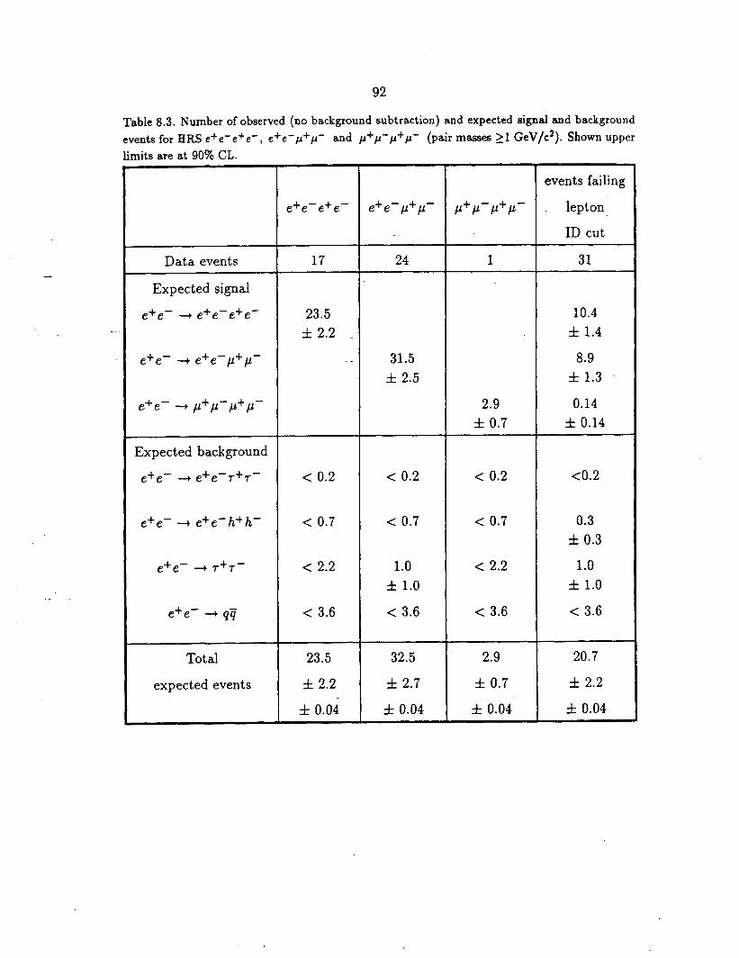
92

Table 8.3. Number of observed (no background subtraction) and expected signal and background events for HRS eSe-e+e-, e+e-l.r+Cc- and ~+P-/.J*/J- (pair masses 21 GeV/c2). Shown upper limits are at 90% CL.

events failing

e+e-e+e- e+e-p+p- P+P-P+P- lepton

ID cut

Data events 17 24 1 31

Expected signal

e+e- 3 e+e-e+e- 23.5 10.4 f 2.2 f 1.4 _

e+e- 3 e+e-p+p- _ 31.5 8.9 f 2.5 f 1.3

e+e- 3 p+p-p+p- 2.9 0.14 f 0.7 f 0.14

Expected background

e+e- 4 e+e-7+7- < 0.2 < 0.2 < 0.2 co.2

e+e- + e+e-h+h- < 0.7 < 0.7 < 0.7 0.3 f 0.3

e+e- 4 7+7- < 2.2 1.0 < 2.2 1.0 f 1.0 f 1.0

e+e- + (IT7 < 3.6 < 3.6 < 3.6 < 3.6

Total 23.5 32.5 2.9 20.7

expected events f 2.2 f 2.7 f 0.7 f 2.2

f 0.04 f 0.04 f 0.04 f 0.04

93

The total number of Monte Carlo signal and background events, taking into

account those events which failed the lepton identification criteria, is

N- MC = 79.6 = 23.5 + 32.5 + 2.9 + 20.7 (from table 8.3). The corresponding total

number of data events is N, = 73 = 17 + 24 + 1 + 31. Since the expected con-

tribution from background processes is small (about 3%), a direct comparison of

- N MC and N, represenTs a sensitive test of QED. We see that there is agreement

within one standard deviation between data and Monte Carlo results, before lepton . . .

identification.

.

After lepton identification, the agreement between the data and the Monte

Carlo results is not quite as good, the data falling below expectation in all chan-

nels. Even though this is not highly significant, it was studied further by comparing

the data and Monte Carlo distributions for E/P and deposited energy. These dis-

tributions were used for the identification of electrons and muons. Figure 8.7 (b)

shows the E/P distribution of tracks from Monte Carlo e+e-e+e-, e+e-p+p- and

~+~-~+~- events, scaled down to 291pb-‘ , before lepton identification. This is to

be compared with the E/P distribution of data tracks shown in fig. 8.7 (a), which

is identical to fig. 8.3, and is presented here once again for the sake of comparison.

Figure 8.8 (b) h s ows the energy distribution of tracks with E/PLO.55 from Monte

Carlo e+e-e+e-, e+e-p+p- and /.L+~-/J+P- events, scaled down to 291pbm1, be-

fore lepton identification. For the sake of comparison again, we present fig. 8.8 (a),

the corresponding distribution of data tracks, which is identical to fig. 8.5, shown

earlier. These distributions are qualitatively similar but both Monte Carlo distribu-

94

tions show slightly narrower peaks than those present in the data. The somewhat

weaker agreement between the number of data and Monte Carlo events after lepton .

identification, may be caused, in part, by small imperfections in the simulation of

the HRS calorimeter response to electrons and muons. However, We reiterate that

the general agreement is good and that the relatively small data sample does not

allow a deeper investigation of this point.

-- . 90 1 1 90 ,

HRS Monte Carlo

(b)

80 1

70 - HRS data -

00 - (4 2 so - \ J? 40 - 8 30 - t 20 -

10 - 0 0 0.5 1 1.5 2 0 0.5 - 1 1.5 2

E/P E/P

Figure 8.7. E/P distribution of tracks before lepton identification in HRS data four-lepton candidates (a) and in Monte Carlo four-lepton events (b).

40/ HRS data

E/P s 0.55

(4

‘hack energy (GeV)

-7

40

30 - HRS Monte Carlo

% L5 E/P s 0.55

? 20 - (b) e 4 3 10 - &

-0 0.5 1 1.5 2 Track energy (GeV)

Figure 8.8. Energy distribution of individual tracks with E/P<0.55 in HRS data four-lepton candidates (a) and in Monte Carlo four-lepton events (b).

95

Various distributions are shown for the final HRS samples, and compared with

QED calculations. All four tracks of an identified event are included in these dis-

tributions, even when only three or two of the same charge sign tracks have been

identified. In such events, the identity of the remaining tracks is de&mined by the

assumption of lepton number conservation. The energy and angular distributions

of electrons (e*) in ese-e+e- and e+e-p+p- events are’ shown in fig. 8.9 and

_._ fig. 8.10, respectively. The momentum and angular distribution of muons (cl*) in

e+e-p+p- events is shown in fig. 8:ll. In fig. 8.12 we present the minimum mass

distribution of two leptons. We took the lowest invariant mass of all four possible

combinations (e+e-) in e+e-e+e- events, and the lower invariant mass of the e+e-

or p+p- combinations in e+e-p+p- events. The energy (total scalar momentum)

distributions in (a) e+e-e+e- and (b) e+e-p+p- events are shown in fig. 8.13. The

distributions of the invariant masses of the four e+e- pairs in e+e-e+e- events are

shown in fig. 8.14 (a)-(d) in increasing mass order. Fig. 8.14 (a) shows the invariant

. mass distribution of the e+e- pair with the smallest mass among the four pairs,

whereas fig. 8.14 (d) h s ows the distribution of e+e- pairs with the largest invari-

ant mass in an event. The invariant mass distributions of the e+e- and the p+p-

pairs in e+e-p+p- events are shpwn in fig. 8.15 (a) and (b), respectively. They

all agree reasonably well with the QED predictions. Finally, fig. 8.16, fig. 8.17 and

fig. 8.18 show 3 characteristic event pictures for each of the 3 processes e+e-e+e-,

e+e-#p- and p+pL-pip-.

96

-

X- Data I-- Monte Carlo

I+7 L_, (al I 2ot’ T

lf....,.,,. I 1

“@J-j 0 5 10 15 -20

Electron energy (Gev)

20 “‘-,,‘.‘,‘-“,‘.‘.

(b) 15

Y e 10 Ii

b,

0

e+e-e+e- -I

-1 -0.5 0 0.5 1 Cor( ‘9)

Figure 8.9. Distribution of electrons (e*) in e+e-e+e- events : (a) electron energy;(b) cos8. The histogram is the QED prediction to a4 (HRS data).

so; l-h

(4 X-Data

20 o- Monte Carlo

(4 X-Data

20 o- Monte Carlo ,c

t ’ )( IC I( I( 10 - 10 -

0 0 *.*.‘*...‘..*. t, *.*.‘*...‘..*. t, .‘A ..3 ..- ..l

0 0 5 10 15 5 10 15 20 20 Electron energy (GeV) COB(B)

20 ““,““,““,‘“’

(b) 15 - e+a-p+p-

o! e B 10 -

2 5r It _

lTTjy i ,I . +. ! ” 0 ....I

-1 -0.5 0 0.5 1

Figure 8.10. Distribution of electrons (e*) in e+e‘p+p’ events : (a) electron energy; (b) cos8. The histogram is the QED prediction to a4 (HFLS data).

97

(4 20 -

r X- Data p- Monte Carlo I1

10 - 4:

t I .

OL”““““..’ 7.

0 5 10 - l5 Muon momentum (GeV/c)

_

(b)

005 -1 -0.5 0. . 1

Cos( 6)

Figure 8.11. Distribution of muons (pi) in e+e-/.?p- events: (a) muon momentum; (b) cos(6). The histogram is the QED prediction to order cx4 (HRS data).

(4 I X- Data 1 P- Monte Carlo

t ,:

I

I I 2 4 6 6 10 12

Yin mass (e+e-) (GeV/c’)

20 , 1

15 - 11 b) I)

V

1 Y lo-

s ii 5- I

% 0 I “pii I . 4i

0 2 4 0 B 10 12 Min mass (e’e-,p+p-) (GeV/c*)

Figure 8.12. Lowest invariant mass distribution in (a) e+e-e+e- events; (b) e+e’p+p’- events. The histogram is the QED prediction to order cr4 (HRS data).

(4

e+e-e+e-

98

(b)

e+e-p+p-

-15 20 25 30 35 ~15 20 25 30 35 Energy (GeV) Energy (GeV)

-. . Figure 8.13. Energy distribution in (a) e+e-e+e- events; (b) e+e-p+p- events. The histogram is the QED prediction to .qrder a4 (HM data).

ijij~p--~,,1 0 2 4 6 8 10 12

Yin mass (e’e-) (GsV/c*)

% h

Oo I . I ,

2 4 6 8 10 12 Yin mass (e’e-) (GsV/c*)

. . 10 ) 10 ) 1 1

20 (4

mv 15 - X- Data r- Monte Ckrlo

0 10 20 lnv. mam (e’e-) (GeV/c’)

12

10

lnv.5masm (e+e’y (GeV/c’) 15

10 15 20 25 3i Max masm (e’e-) (GeV/c’)

Figure 8.14. Invariant mass distribution in e+e-e+e’ events for all e+e- pairs in increasing mass order (a)-(d) (HIS data).

99

-0 10 20 30

Inv. mass (e+e-) (&V/c’)

25

20

” p 15

8 ho 10 a

$5 t I-L-

(b) x - Data p - Monte Carlo

I

0 I I 0 10 20 30

Inv. mai* (p+p-) (Cd/c*)

Figure 8.15. Invariant mass distributions of the e+e- pair (a) and of the /1+~- pair (b) in e+e-p+p- events (HRS data).

HRS RUN-4 173

EVENT- 2809 DCHITS - 66 NPRNG - SH SW- 6.: l 23.5

TRACK IlDtIENTUfl THETA

: -5.7 8.1 81.4 40.9 3 3.0 43.4 4 - 12.2 143.1

Figure 8.16. Characteristic e+e-e+e’ event picture observed in the HFtS data.

HRS RUN-4735 :

EVENT- :QQ28 DCHITS - 74 NPRNG - SH SUM- 0.: l 27.6

TRACK MDMENTUfl T-HETA 1 12.6 43.1 2 -11.5 137.5 3 -3.8 108.5 4 1.1 86.2

Figure 8.17. Characteristic e+e’p+p- event picture observed in the HRS data.

HRS RUN-7463

EVENT- 12190 DCHITS - 109 NPRNG - 5 SH SUM- 0,8 l

TRACK MOMENTUM 2 5.4 3 -2.3

9.3 - 12.2

0.0

THETA 73.5

103.3 125.8

68.9

Figure 8.18. Picture of p+p-@p- event observed in the HRS data.

101

8.3 Detection efficiencies

We applied kinematical cuts, before the detector simulation, on the Monte Carlo

generated four-momenta files, for each of the three processes e+e-e+e-, e+e-p+p-

and ~+P-,!L+P-. These cuts were identical to those used in section 8.1. In detail,

each event should satisfy the following criteria : -

1. there should be 4 charged leptons with zero net total charge, (true by default)

2. each lepton should have a momentum P _> 0.6 GeV/c and 1 cos 01 5 0.9

3. the energy (Ci=l,d cIPjj> of-all f our leptons should be 2, 20 GeV, but

< 40 GeV

4. all opposite-charge pairs of leptons should have an invariant mass 2 1 GeV/c’

Table 8.4 lists the numbers of expected signal events that were obtained by

applying the above requirements, both before and after detector simulation, scaled

down to the HRS integrated luminosity L of 291 pb-‘. Note that Nafier refers

to the final results obtained after event identification, shown already in table 8.3

for e+e-e+e-, e+e-p+p- and ~+~-~+~-. The errors attached are due to lim- .

ited Monte Carlo statistics. Th e numbers corresponding to the MC generation

luminosities, 1598 pb-’ of e+e-e+e-, 1590 pb-’ of e+e-p+p-, and 2059 pb-*

of P+P-P+P-, are given in parentheses. The detection efficiencies, determined

from Monte Carlo, E = Nafler for e+e-e+e-, e+e-p+p- and p+p-p+p-, are Nbefore ’

0.65 f 0.03, 0.77 f 0.03 and 0.95 f 0.04, respectively.

In the same table, we present the cross sections uMMc (in fb, 1 fb = 10D3pb) cor-

responding to the number of expected signal events for each of the 3 processes. The

cross section trMc is derived from the formula crMMc = e, where

102

L MC is the generation luminosity of the process, and Nbeforc is given in paren-

theges in table 8.4.

Table 8.4. Summary of HRS cross sections uMc and Monte Carlo event statistics (see text).

e+e-e+e-

e+e-p+p-

P+P-PP-

aMC %efore N after

w WC) WC)

126 36.8 f 2.6 (202) 23.5 f 2.2 (132)

143 41.7 f 2.8 (228) 31.5 f 2.5 (176)

11 3.1 f 0.7 (22) 2.9 f 0.7 (21)

-

CHAPTER 9

CONCLUSIONS

The theoretical predictions and -measurements presented in this- thesis for the

production of four-lepton final states (e+e-e+e-, e+e-#p-, ~+~-~+~-) are in

good agreement. For this analysis the leptons were all required to be at large

angles. The effective mass of the lepton pairs was also required to exceed 1 GeV/c2.

For an integrated luminosity of 205 pb-’ in the Mark II experiment, we observed

10 e+e-e+e-, 10 e+e-p+p- and 1 #p-p+p- events with opposite-charge pair

masses greater than 1 GeV/c2, while 10.9f0.7, 9.6f0.8 and 0.76f0.07 events were

expected, respectively. In the HRS experiment, for an integrated luminosity of

291 pb-‘, we observed 17 e+e-e+e-, 24 e+e-p+p- and 1 p+p-p+p- events with

opposite-charge pair masses greater than 1 GeV/c2, while 23.5f2.2, 31.5f2.5 and

2.9f0.7 events were expected, respectively. The various kinematical distributions

also show good overall agreement. QED, calculated to fourth order, gives a good

description of the data within the overall statistical uncertainty of about 20%. It is

interesting to note that the cross sections tested in this thesis are at the 0.1 pb level

compared to the total annihilation cross section of the order of 100 pb.

For completeness, we summarize the basic selection criteria and results for

103

104

large-angle e+e-e+e- and e+e-@p- events from the CELLO, JADE, Mark J,

ASP, HRS and Mark II experiments (from refs. 8, 10 and this thesis), in tables 9.1

and 9.2, respectively. The tiny e+e- ---) P+P-P+P- cross section has been observed

only in the CELLO, Mark II and HRS detectors. This is not surprising since these

experiments have accumulated the highest integrated luminosities in e+e- storage

rings in a range of c.m. energies 14-47 GeV.

Table 9.1. Summary of basic selection cuts and number of large angle e+e-e+e- events from JADE, ASP, CELLO, Matk II and FIRS. Pe is the electron momentum, M(I+I-) is the invariant mass of any opposite-charge pair of tracks.

JADE ASP CELLO Mark II HRS

e+e-e+e- 13 15 16 10 17

J Jut (pb-1) 95 109.6 130 205 291

1 COS ee 1 < 0.955 < 0.94 < 0.85 < 0.88 <0.9

Pe > Ebeam/3 > 0.3 GeV > 0.05 * Ebea,.,, > 1 GeV > 1 GeV

, hqz+z-) , - , > 0.5 GeV , > 0.01 GeV , >lGeV, >lGeV ,

105

Table 9.2. Summary of basic selection cuts and number of large angle e+e-p+p- events from JADE, Mark J, CELLO, Mark II and HRS. Pe is the electron momentum,

e M(I+I-) is the invariant mass of any opposite-charge pair of tracks, P,, ia the muon momentum

e+e-p+p-

s Ldt (pb-* )

I COSde 1

Pe

I cos eu I

M(Z+Z-)

JADE 1 Mark J 1 CELLO 1 Mark.11 1 HFiS

,I 10 I 24

1 205 1 291

< 0.955 1 < 0.94 I < 0.85 1 < 0.88 1 <0.9

> Ebeam/3 > 0.2 * gbeam > 0.05 * Ebeon > 1 GeV > 1 GeV I

< 0.966 < O-87 < 0.92 < 0.55 <0.9

> 1 GeV > 1.5 GeV > 0.1 * Ebeam > 1 GeV > 1 G6V .~

- I > 1 GeV I > 0.01 GeV (>lGeVI >lGeV

.

APPENDIX A

FADIATIVE CORRECTIONS

A number of papers have been devoted to the problem of radiative corrections

to processes of the type e+e- + e+e-e+e-, e+e-#p-, but unfortunately not in our

domain of interest, where the leptons are emitted at large angles. They all consider

the case where both of the outgoing electrons are either not detected, or detected

at small angles. (43-45) Even Berends et al., whose MC programs were used to

generate fourth order QED events, have only treated the radiative corrections for

multiperipheral four-lepton production,(3g) which peaks at small angles.

The emission of a real or virtual photon from the electron or positron before

they annihilate is called initial-state radiation. It is known from QED that a fast,

interacting particle can emit radiation (bremsstrahlung) into a narrow cone in the

direction of its motion. Scattering cross sections are proportional to l/S, where

S is the center-of-mass (c.m.) energy squared of the incoming particles. Since the

c.m. energy of the incoming particles may decrease due to bremsstrahlung, the cross

section may change. This change due to initial-state radiation needs to be taken into

account in measurements of cross sections. Final-state radiation, emitted after the

annihilation process, does not have a similar impact on the measured cross sections.

106

-

107

We now present an estimate of the magnitude and sign of the correction for

initial-state radiation. We need only consider collinear radiation, since photon emis-

sion peaks in directions parallel to the motion of the charged particles.

The state of the art in radiative corrections using renormalization group meth-

ods is found in the paper by Kuraev and Fadin. (“1 They consider the radiative

corrections to single-photon annihilatidn of an e+e- pair that are only associated

with the initial-state. These radiative corrections are part of the corrections to all -- .

processes with an arbitrary final state. We make use of their probability function

F(x,S) to emit photons which carry away a fraction x of the beam energy. The

proper definition of x is l-S’/S, where S is the nominal and S’ the observed c.m.

energy squared.

The aspect of initial-state radiation that is most important for the four-lepton

study is the nongaussian cm. energy distribution of the incoming leptons, and in

particular the long tail to lower energies shown in fig. A.l. The cutoff at 16 GeV is

well below the cut applied on the energy (total scalar momentum) of the data sets

(see sections 7.1, 8.1).

We now present our methodology:

1. We generate MC e+e-e+e- events at various energies E’ below the nominal

E= 29 GeV, with enough statistics to keep the statistical error arising from

MC limited statistics small. We assume a photon of energy E, is emitted

from one of the beam electrons along z, thus reducing the c.m. energy from

E to E’ = E - E-,. Figure A.2 shows the generated cross section before any

0.4 b -

0.2

I

L-T I - I I I ~0”‘~““~““““““““““”

15 17.6 20. _ 22.6 26 27.6 SC0 Eoal (cd)

Figure A.l. The center-of-mass energy distribution of Monte Carlo events after initial- state radiation of a beam with nominal center-of-mass energy equal to 29 GeV and sigmaequal to 17 MeV.

cuts are applied. The procedure followed in the generation of e+e-e+e- is

presented here : we first transform all quantities relevant to the generation

@beam, @rnin, ema8 of electrons) from the laboratory frame after radiation

(E’, 18.5’, 161.5’ electron angles) to a new c.m. frame, where we let the

MC generator produce four-momenta of the four-lepton events. Then we

transform back to the lab, where we apply a crude set of kinematical cuts

on the generated four-momenta, identical to the ones described in chapter 5.

The’ parameters used to generate the data are listed in table A.1 .

2. Then we pass those four-momenta through the Mark II detector simulation

Monte Carlo programs and through our analysis cuts, previously described

in section 7.1. This way, for every energy E’ we get a corresponding observed

cross section. We then fit the points (cross section, E’) to an empirically

found smooth function of the form (l+tanh(crEP))(c+dE) where cx, p, c, d

109

Figure A.2. The distribution of MC generated cross section at various lab energies.

t b

7

60-- -I

.+a- .+a- -@ l *~-~+o- -@ l *~-~+o- 40- 40-

30- 30-

20 - I 10 -

I o-‘t”““““““““‘l”“‘fi-

16 17.6 -20 22.6 26 27.6 30 Ok

16 17.6 -20 22.6 26 27.6

are parameters determined from the fit. Figure A.3 shows the observed cross

section and the empirical function which fits the points.

3. Using Simpson’s rule over small enough energy intervals (0.1 GeV), we in-

tegrate numerically the cross sectional function we found, weighted by the

Kuraev-Fadin probability function F(x,S).

The result of the numerical integration is our radiatively corrected cross section.

To determine the uncertainty of the corrected cross section :

1. We varied every parameter (one at a time) of the cross sectional function by

one standard deviation of the parameter value, and found the corresponding

variance of the result of the integration.

2. The variance of the corrected cross section is simply the sum of the corre-

sponding variances.

We find that the cross section of e+e- -+ e+e-e+e- , corrected for initial-state

radiation, is (0.058 f 0.004) pb, w h ereas the observed is (0.059 f 0.003) pb. There-

110

Table A.l. List of the parameters used to generate Monte Carlo e+e’e+e’ events at . . various lab energies E’.

E’ @cm/lab Ebearn emin

CM CM

GeV Get

24 1 -5/24 1 11.7 1 15.1°

23.5 I-5.5/23.5 1 11.42 114.6’

22 1 -7/22 1 10.43 113.5’

18 1 -11/18 1 ‘7.12 1 9.2’

’ enaz CM

163’

160’

157.8’

156.6’

152’

143.3O

137O

126’

fore we estimate that an approximate overall correction, defined as the ratio of the

corrected e+e- -+ e+e-e+e- cross section over the observed e+e’ -+ e+e-e+e-

cross section, is 0.98f0.08. The set of points used in the fit to the empirically found

function are presented in table A.2 , whereas table A.3 shows the MC rates and

efficiencies at various lab energies E’. We define the efficiency R at each E’ (shown

in fig. A.4) as the ratio of the number of MC simulated events which survive the

s 0.04 - 4

J b

0.02 -

0.00 - ' ' ' ' ' ' ' ' ' 16 17.6 20 22.6 26 27.6 30

Lb WJ) Figure A.3. The distribution of MC observed cross section at various lab energies.

analysis cuts over the number of the corresponding MC generated events at the

specific E’.

The vanishing of the observed cross section below 21 GeV is the result of the

combination of mainly two effects. First, the applied boost from the laboratory

after radiation to the MC c.m. frame, where we generated our data at every E’,

causes a shrinking of the effective cone in which the four leptons are produced.

The magnitude of the emitted photon momentum determines the relative speed

P cm/lab between the lab frame and the cm. frame of the theoretical MC. Note that

the lab frame had initially zero momentum before the emission of the photon. The

higher this relative speed is, the more pronounced the relativistic ‘headlight’ effect

becomes. In other words, large angles in the MC frame become substantially smaller

after their transformation to the lab frame, for large relative speeds. The steep fall

at around 24 GeV of the visible cross section curve comes from a drastic reduction

of events with four good tracks. The second effect (weaker than the first) comes

112

Table A.2. Generated and visible cross sections (in picobarns) at various lab energies E’ of Monte Carlo e+e-e+e- events.

.

from applying a 1 GeV/c2 invariant mass cut on all zero charge pairs of two tracks.

The lower the c.m. energy, the harder the above mass cut becomes,

In conclusion, we have seen that initial-state radiation, collinear to the incom-

ing electrons, does not affect significantly the Born level cross section of e+c- --+

e+e-e+e-, or any other four lepton process in which the four leptons are detected

at large angles, high Q’.

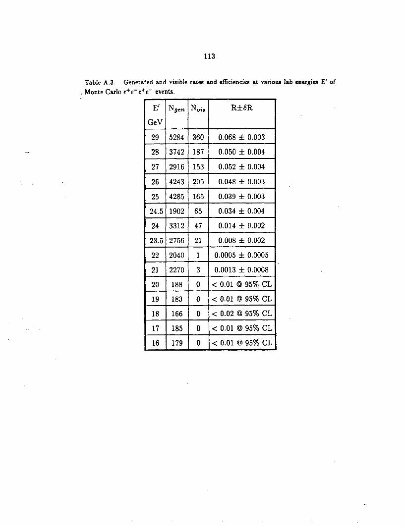
113

Table A.3. Generated and visible rates and efficiencies at various lab energies I? of . Monte Carlo e+e-e c- events.

0.0013 f 0.0008

20 188 0 < 0.01 @ 95% CL

19 183 0 < 0.01 @ 95% CL

18 166 0 c 0.02 @ 95% CL

17 185 0 < 0.01 @ 95% CL

16 179 0 < 0.01 @ 95% CL

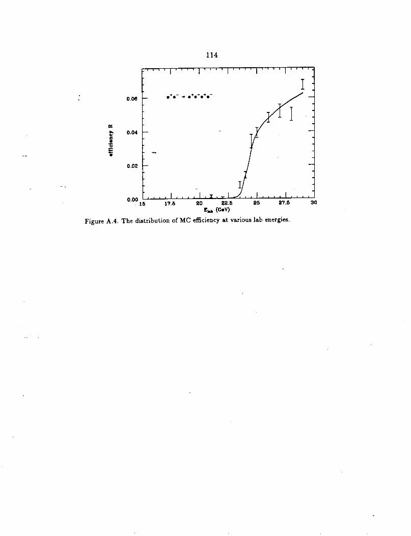
L

0.06 -

a 6 0.04 -

1 0 T F

0.02 -

0.00 ” ” ” ” ” ’ ~r~-‘J~ ” ” I I 16 17.6 a0 22.6 26 27.6

Eu t-v) Figure A.4. The distribution of MC efficiency at various lab energies.

115

APPENDIX B

STUDY OF THE MARK II END CAP SHOWER COUNTER

We have investigated the use of the Mark II/PEP end cap shower counter

(EC) in order to differentiate electrons (e*) from muons (p*) in four-lepton can-

didate events. We do not worry about other interacting particles, such as pions,

since we found that the background to the four-lepton processes that interest us

( e+e- 4 e+e-e+e-, e+e-p+p-, #/~-p+p-) is very small (see tables 7.5 and 7.6).

We used radiative Bhabhas, hadronic and cosmic ray data, in order to study

the EC performance when it is hit by electrons and minimum ionizing particles.

Electrons hitting the EC were selected among e+e--y events (46) that came from the

total sample of Mark II/PEP data, in accordance with the following requirements:

1.

2.

3.

4.

2 charged tracks.

one neutral energy cluster with energy of at least 1 GeV, at least 20 cm away

from a charged track at the liquid argon calorimeter (LA) entrance.

the sum of the scalar momenta of the 2 charged tracks and of the photon

energy should be at least 24 GeV.

at least one good electron. An electron is good if it has momentum greater

116

than 1 GeV/c and if the ratio E/P of the energy E deposited in the LA over

- . its momentum P measured by the drift chamber is greater than 0.7.

Forty-two e+e-+y were selected for our study. In these events, one of the elec-

trons had an equivalent E/P>0.6, while the photon hit the LA. The other electron

was going into the fiducial volume of the EC, avoiding the azimuthal region where

lies a keyway cut : 4.21 4 55.2. We explicitly demanded that the angular range

--‘of those EC electrons be 0.762 1 cos 01 50.85, as measured by the drift chamber, in _

order to ensure a good momentum measurement.

Based on these 42 e+e-y events, we present fig. B.l to show the EC response

to electrons. The energy deposited by the electrons in the EC is shown in fig. (a).

The distribution of E/P is shown in fig. (b).

2c

6 10

EC energy (CeV)

EC clcctron~

(b)

Figure B.l. Energy deposited in the end cap from (a) electrons and (c) minimum ionizing particles; the ratio E/P for electrons is shown in (b) (see text).

117

For hadronic events with at least 4 charged tracks, and with momenta of at least

3 GeV/c, we present the distribution of minimum ionizing particles hitting the EC

in the inset fig. (c).

-

Cosmic ray data taken at PEP have -also shown that, for EC tracks with

0.765 1 cos 61 50.85, th-e average pulse height in the EC, multiplied by cos6, is

105 MeV. _.

After taking into consideration the above presented distributions, we decided to

use the EC information to distinguish electrons from muons in four-lepton candidate

events. Tracks with 0.761 1 cos81 SO.85 and momenta of at least 3 GeV/c are

identified as electrons, as long as they have E/P>0.5 . If they have E/PLO.S, they

are considered to be muons or hadrons.

118

APPENDIX C

- MARK II EVENT LIST

-- .

Table C.l contains the list of the38 four-lepton candidate events observed in.the

Mark II data, where all four tracks are detected at large angles, and have opposite-

charge pair masses 2 1 GeV/c 2. The energy of an event is defined as the sum of the

scalar momenta times c, Ci=l,‘l @iI. The smallest mass of an opposite-charge pair

of tracks in an event is denoted by Mmin. The identities of tracks with momentum

P 1 1 GeV/c are categorized as follows :

0 2= ‘electron’ : tracks in the fiducial volume of the liquid argon calorimeter

and E/P>0.6 ( w h ere E is the energy measured in the calorimeter); or tracks

in the fiducial volume of the end cap shower counter with Pz3 GeV/c and

E/P>0.5.

0 3 = ‘muon’ : tracks identified by muon system.

l 4= ‘hadron’ (=‘not electron’ and ‘not muon’) : tracks pointing into the

fiducial volume of the calorimeters and the muon system, but which are not

identified as either electrons or muons.

l 5 = ambiguous (‘electron or hadron’) : tracks pointing into the muon. sys-

tem and not identified as muons, but for which the information from the

-

119

calorimeters is insufficient for allowing electron identification.

6 6= ambiguous (‘muon or hadron’) : tracks pointing into the calorimeters

and not identified as electrons, but for which the muon system information

is insufficient for allowing muon identification.

0 7 = ambiguous (%lectron or muon or hadron’) : all tracks with P>l GeV/c

which are not in the above categories. -.

l 8 = tracks with P<l GeV/ c - f or which no identification is attempted. -

Note that in the codes 5-7, the particle identity is ambiguous because the track

enters regions not well covered by the calorimeters or by the muon system.

120

Table C.l. Mark II four-lepton candidate events with pair masses 2 1 GeV/c’.

-

%un# Rec# Energy M min Track ID Event ID

GeV GeV/c2

8282 3319 35.2 1.03 - 7787

8862 5656 27.9 5.41 2737

9502 3048 23.5 i.68 8222 e+e-e+e-

9699 1311 21.7 4.42 2277

- 9835 6825 28.6 2.98 7733

-- 9902 5972 29.3 8.17 5272 e+e-e+e-

9928 7987 ~~~ I 28.7 I 3.96 I 2328 1 e+e-p+p-

9995 12751 23.2 1.69 6627

10044 4441 29.5 4.22 3227 e+e-p+p-

10129 10891 30.7 5.93 2222 - e+e-e+e-

10282 2028 24.6 4.57 7226

10408 3884 26.9 1.18 8223 e+e-p+p-

10408 11257 32.4 3.57 2277

10445 1369 23.2 1.48 8778

10491 8818 27.2 3.74 7227

10561 4044 34.8 2.49 8222 e+e-e+e-

10588 4966 28.3 2.44 5737

10591 6637 30.8 _ 1.33 2673 e+e-p+p-

10943 3194 24.5 4.78 3336 P+P-P+P-

11102 7798 1 29.5 I 1.18 I 2222 I e+e-e+e-

121

.

: Table C.1. Mark II four-lepton candidate events with pair masses 2 1 GeV/Z (cont.)

Run# Rec# Energy M min Track ID Event ID

GeV GeV/c’

11167 881 26.1 1.72 2233 e+e-p+p-

11215 785 28.9 ‘2.76 3232 e+e-p+p-

11220 2848 30.1 6.27 2227 e+e-e+e- -.

- 11243 4233 26.8 4.92

122

APPENDIX D

HRS EVENT LIST

-- .

Table D.l contains the list of the 73 four-lepton candidate events observed in

the HRS data, where all four tracks are detected at large angles, and have opposite-

charge pair masses 2 1 GeV/c 2. The energy of an event is defined as the sum of the

scalar momenta times c, Cj=l,l @I. The smallest mass of an opposite-charge pair

of tracks in an event is denoted by Mmin- The identities of tracks with momentum

Pzl GeV/c are categorized as follows :

0 2= ‘electron’ : tracks with 0.55<E/P<1.45, where E is the energy measured

in the calorimeters.

l 3 = ‘muon’ : tracks in the fiducial volume of calorimeters and O<E<0.5 GeV.

0 4= ‘hadron’ (=‘not electron’ and ‘not muon’) : tracks in the fiducial volume

of calorimeters with E/PLO.-55 and Ez0.5 GeV.

0 5 = ambiguous (‘electron or hadron’) : tracks with E/PLO.55 and

Ez0.5 GeV, but which are not in the fiducial volume of the calorimeters.

l 7 = ambiguous (‘electron or muon or hadron’) : tracks with E/PLO.55 and

O<E<0.5 GeV which are not in the fiducial volume of the calorimeters..

l 8 = tracks with P<l GeV/c for which no identification is attempted.

123

0 9 = tracks with E/P>1.45.

!, 0 = no energy deposit was associated with the tracks (tracks miss calorime-

ters).

Table D.l. HRS four-lzpton candidate events with pair m888es > 1 GeV/c2.

Run# Rec#

1157 20210

1239 18757

1239 22262

1239 25671

2648 5063

3820 6537

3951 4717

3953 8637

4000 16596

4048 12168

4077 18840

4078 16596

4106 19452

4173 2809

4249 1228

4272 41056

4376 6575

4394 2556

Energy

GeV

27.4

20.5

29.1

26.6

21.3

29.7

28.3

34.3

31.3

21.9

27.4

26.7

28.9

29.1

21.1

29.1

20.6

27.1

M min Track ID Event ID

GeV/c2

- 2.47 8000

1.05 2200

2.16 2270

1.28 0732

1.46 0000

- 1.44 2230 e+e-p+p-

9.50 3702

1.04 3333

1.20 2732 e+e-p+p-

1.28 8222 e+e-e+e-

4.15 3302 e+e-p+p-

4.96 2022 e+e-e+e-

7.83 0502

- 4.33 2222 e+e-e+e-

1.86 8330

1.78 2072 e+e-e+e-

1.32 4322

3.47 3003

124

.- Table D.l. ERS four-lepton candidate events with pair masses 2 1 GeV/c2 (cont.)

-

5594 11956 24.6 1.38 2082

5648 5024 29.7 t 5.75 3022 e+e-p+p-

125

’ . Table D.l. HRS four-Iepton candidate events with pair masses > 1 &V/c2 (cont.)

Run# Rec# Energy M min

GeV GeV/c2

Track ID

-

Event ID

5716 1650 27.9 4.55 2272 e+e-e+e-

5738 7052 27.5 .3.16 0302

5845 10576 29.6 2.23 3282 e+e-p+p-

- 5919 6519 20.6 1.47 2283 e+e-p+p-

126

* . Table D.l. HF4.S four-lepton candidate events with pair masses 2 1 GeV/c2 (cont.)

.

Run# Rec# Energy M min Track ID . Event ID.

GeV GeV/c2

6976 8982 20.0 2.26 3300

‘1.61 7125 5214 29.1 2279

7199 743 29.3 1.11 2230 e+e-p+p- -- .

- 7294 6904 25.5 6.43 2234

-- 7311 10910 21.8 4.37 2224

7382 6790 27.9 3.00 2222 e+e-e+e-

7396 1752 21.5 1.58 2800

7409 3263 21.2 1.43 4344

7437 893 27.3 1.04 2094 -

7463 12190 29.1 2.35 3333 P+P-P+P-

7596 14149 29.9 1.66 2202 e+e-e+e-

7641 1298 33.1 1.38 0200

8164 3338 27.7 1.23 0277

8213 4672 30.7 1.03 2924

8302 3723 26.1 2.09 3274

8456 8514 24.3 1.12 8302 e+e-p+p-

8524 6170 25.8 _ 1.34 5225 e+e-e+e-

8612 1591 27.1 1.26 2823 e+e-p+p-

8625 2975 25.0 3.09 3239 e+e-p+p- *

REFERENCES

1. T. Kinoshita, CERN-TH-5097j88, July 1988.

2. A.S. Elkovskii, Novosibirsk Inst. Nucl. Phys. Acad. Sci.-88-050, June 1988.

3. A. Davies, S. Brodsky, SLAC-PUB-4498, Dec. 1987; J. Grifols, A. Mendez, Phys. Rev. D26, 1809 (1982); A. Mendez, F. Orteu, Phys. Lett. 163B, 167 (1985) and references therein. A general review of recent studies beyond the standard model can be found in Proceedings of the 1987 International Sympo- sium on Lepton and Photon Interactions at High Energies, DESY, Hamburg.

4. F. A. Berends, P. A. Daverveldt and R. Kleiss, Comp. Phys. Comm. 40 (1986) 285.

5. F. A. Berends, P. A. Daverveldt and R. Kleiss, Nucl. Phys. B253 (1985) 441. .

6. F. A. Berends, P. A. Daverveldt and R. Kleiss, Comp. Phys. Comm. 40 (1986) 309.

7. R. Kleiss, Nucl. Phys. B241 (1984) 61.

8. MARK J Collaboration, DESY-85-073 (1985); JADE Collaboration, Z Phys. C30, 545 (1986); ASP Co11 a b oration, SLAC-Report-337 (1989).

9. CELLO Collaboration, DESY-84-103 (1984).

10. CELLO Collaboration, Z Phys. C43, 1 (1989).

11. M. Alam, et al., SLAC-Proposal-PEP-005, December, 1976.

12. B. W. LeClaire, Ph.D. thesis, Stanford University, SLAGReport-321, 1987.

127

128

13. R. H. Schindler, et al., Phys. Rev. D24 (1981) 78.

14. J. Rees, et al., Particle Accelerator Conference, Chicago, 1977, p. 1836.

15. J. A.Jaros,in Proceedingsof theInternational conferenceon Instrumentation for Colliding Beam Physics, edited by W. Ash (Stanford Linear Accelerator Center, Stanford, CA, 1982), pp. 29-33.

- 16. W. Davies-Whiteyet al., Nucl. Instr. and Meth. 160 (1979) 227.

17. G. Abrams, et al., IEEE Trans. Nucl. Sci. NS-25 (1978) 309; NS-27, 59 -- (1980).

18. M. Derrick, et al., SLAC-Proposal-PEP-12, October, 1977.

19. D. Bender, et al., Phys. Rev. D30 (1984) 151.

20. R. Ng, Ph.D. thesis, Purdue University, 1987.

21. P. Baringer, et al., Nucl. Instr. and Meth. A254 (1987) 542.

.

22. D. Rubin, et al., Nucl. Instr. and Meth. 203 (1982) 119.

23. G. Baranko, et al., Nucl. Instr. and Meth. 169 (1980) 413.

24. J. Loos, et aZ., Nucl. Instr. and Meth. A249 (1986) 185.

25. Christiaan Huygens, Traitd de la Lumiere, Leiden, 1690.

26. H. Euler and B. Kockel, Naturwissenschaften 23 (1935) 246.

27. H. Euler, Ann. Phys. 26 (1936) 398.

28. A. Akhiezer, Phys. 2s. Soviet Union 11 (1937) 263.

29. L. Landau and E. Lifshitz, Phys. Zs. Soviet Union 6 (1934) 244.

30. J. Smith, J. A. M. Vermaseren and G. Grammer, Phys. Rev. Dl5 (1977) 3280.

31. courtesy of T. Barklow.

32. T. Sjostrand, Comp. Phys. Comm. 39 (1986) 347.

129

33. courtesy of P. Burchat.

34. C. Peterson et al. , Phys. Rev. D27 (1983) 105.

35. courtesy of A. Petersen, P. Sheldon and A. Weir.

36. F.A. Berends, et al. (CALCUL Coliaboration), Nucl. Phys. B239 (1984) 395, calculation of the matrix elements of the process; Monte Carlo program

- by C.Hawkins (ASP collaboration), Ph.D. thesis, Stanford University, SLAC- Report-337, 1989.

_-_ 37. courtesy of J. Repond.

38. M. E. Nelson, Ph.D. thesis, Lawrence Berkeley Laboratory Report No. LBL- 16724, 1983.

39. F.A. Berends, P. Daverveldt, and R. Kleiss, Nucl. Phys. B253, 421 (1985); Comp. Phys. Comm. 40, 271 (1986). They h ave only treated the radiative corrections of multiperipheral four-lepton production which peaks at small angles.

40. E. A. Kuraev and V. S. Fadin, Sov. J. Nucl. Phys. 41 (1985) 466.

41. P. R. Burchat, Ph.D. thesis, Stanford University, SLAC-Report-292, 1986.

42. courtesy of R. Tschirhart.

43. G. Cochard, S. Ong, Phys. Rev. D19 (1979) 810.

44. M. Defrise, Z. Phys. C9 (1981) 41.

45. W. L. Van Neerven and J. A. M. Vermaseren, Nucl. Phys. B238 (1984) 73.

46. P. Burchat’s tapes SC2882 and SC2172 h’ h w rc contain 9278 e+e-7 and p+p-“y events.

STUDY OF FOUR-LEPTON FINAL STATES IN ... - SLAC

Documents

Transcript of STUDY OF FOUR-LEPTON FINAL STATES IN ... - SLAC