Black Holes and Revelations - Inspire HEP
288
Investigating Black Holes using String Theory, SYK-Models and Quark-Gluon Plasmas Black Holes and Revelations Eric Marcus
-
Upload
khangminh22 -
Category
Documents
-
view
0 -
download
0
Transcript of Black Holes and Revelations - Inspire HEP

Black H
oles and Revelations
Eric Marcus
Investigating Black Holes using String Theory,
SYK-Models and Quark-Gluon Plasmas
Black Holes and Revelations
Eric Marcus
INVITATIONto the public defence
of my PhD thesis
Black Holes and Revelations
Wednesday 22 September 2021 at 12:15 PM
Details for attendance can be found at
sites.google.com/view/ericmarcus
Eric [email protected]


Black Holes and RevelationsInvestigating Black Holes using String Theory,
SYK-Models and Quark-Gluon Plasmas
Eric Marcus

PhD thesis, Utrecht University, September 2021ISBN: 978-90-393-7394-1About the cover: it depicts a supermassive black hole slowly ‘eating’ a nearbystar. The image was created by the author using neural network techniques; in thiscase the style is based on Starry Night by Van Gogh.
Black Holes and RevelationsInvestigating Black Holes using String Theory,
SYK-Models and Quark-Gluon Plasmas
Zwarte Gaten en OpenbaringenZwarte Gaten bestudeerd met Snaartheorie,SYK-Modellen en Quark-Gluon Plasma’s
(met een samenvatting in het Nederlands)
Proefschrift
ter verkrijging van de graad van doctor aan de Universiteit Utrecht opgezag van de rector magnificus, prof. dr. H.R.B.M. Kummeling,
ingevolge het besluit van het college voor promoties in het openbaar teverdedigen op woensdag 22 september 2021 des middags te 12:15 uur
door
Eric Jeffrey Marcus
geboren op 13 mei 1994te Meppel

Promotor: Prof. dr. S.J.G. VandorenCopromotor: Dr. U. Gürsoy

To my parents


Publications
Part I of this thesis is centred around black holes in string theory and M-theory.It is based on the following publications:
[1] C. Hull, E. Marcus, K. Stemerdink and S. Vandoren, Black holes in stringtheory with duality twists, JHEP 07 (2020) 086,
[2] C. Couzens, E. Marcus, K. Stemerdink and D. van de Heisteeg, The Near-Horizon Geometry of Supersymmetric Rotating AdS4 Black Holes in M-theory,accepted for publication in JHEP.
Part II of this thesis concerns new class of Sachdev-Ye-Kitaev models. The secondpart is based upon the publication:
[3] E. Marcus and S. Vandoren, A new class of SYK-like models with maximalchaos, JHEP 01 (2019) 166,
Part III of the thesis concerns the study of magnetohydrodynamics during heavyion collisions, and is based upon the publications:
[4] U. Gürsoy, D. Kharzeev, E. Marcus and K. Rajagopal, Magnetohydrodynamicsand charged flow in heavy ion collisions, Nucl phys. A 956 (2016) 389,
[5] Proceedings paper: U. Gürsoy, D. Kharzeev, E. Marcus, K. Rajagopal andC. Shen, Charge-dependent Flow Induced by Magnetic and Electric Fields inHeavy Ion Collisions, Phys. Rev. C 98 (2018) 055201,
[6] Proceedings paper: U. Gürsoy, D. Kharzeev, E. Marcus, K. Rajagopal andC. Shen, Charge-dependent flow induced by electromagnetic in heavy ioncollisions, Nucl. Phys. A 1005 (2021) 121837.
i

Before moving on, we comment on the overlap of the first part of this thesis withthe upcoming theses of K. Stemerdink and D. van de Heisteeg.
[1] Sections 2 and 3 were computed together by K. Stemerdink and the author,section 4 was mostly computed by K. Stemerdink and section 5 mostly bythe author.
[2] Most of the computations in section 2 were performed by D. van de Heisteeg,section 3 was mostly calculated by K. Stemerdink and the author performedmost computations in section 4.
ii

Contents1 Introduction 1
1.1 Black Holes and Revelations . . . . . . . . . . . . . . . . . . . . . . 21.2 String Theory and Black Holes . . . . . . . . . . . . . . . . . . . . 7
1.2.1 Supersymmetry and Our Universe . . . . . . . . . . . . . . 101.2.2 Different Types of String Theories . . . . . . . . . . . . . . 111.2.3 Low Energy Limits . . . . . . . . . . . . . . . . . . . . . . . 151.2.4 The Dual Pictures . . . . . . . . . . . . . . . . . . . . . . . 201.2.5 Branes . . . . . . . . . . . . . . . . . . . . . . . . . . . . . . 221.2.6 Building Black Holes . . . . . . . . . . . . . . . . . . . . . . 251.2.7 Holograms . . . . . . . . . . . . . . . . . . . . . . . . . . . . 28
1.3 SYK Models . . . . . . . . . . . . . . . . . . . . . . . . . . . . . . 311.4 Heavy-Ion Collisions . . . . . . . . . . . . . . . . . . . . . . . . . . 441.5 This thesis . . . . . . . . . . . . . . . . . . . . . . . . . . . . . . . . 53
I Black Holes in String Theory 55
2 Black Holes in String Theory with Duality Twists 572.1 Duality invariant formulation of IIB supergravity on a four-torus . 622.2 Scherk-Schwarz reduction to five dimensions . . . . . . . . . . . . . 702.3 Five-dimensional black hole solutions . . . . . . . . . . . . . . . . . 922.4 Quantum corrections . . . . . . . . . . . . . . . . . . . . . . . . . . 1022.5 Embedding in string theory . . . . . . . . . . . . . . . . . . . . . . 1122.6 Conclusion . . . . . . . . . . . . . . . . . . . . . . . . . . . . . . . 1152.A Conventions and notation . . . . . . . . . . . . . . . . . . . . . . . 1172.B Group theory . . . . . . . . . . . . . . . . . . . . . . . . . . . . . . 1182.C Scalar and tensor masses after Scherk-Schwarz reduction . . . . . . 123
iii

Contents
3 Rotating black holes in M-theory 1273.1 Setup . . . . . . . . . . . . . . . . . . . . . . . . . . . . . . . . . . 1293.2 Action for the theory . . . . . . . . . . . . . . . . . . . . . . . . . . 1413.3 Embedding of the AdS4 Kerr–Newman black hole . . . . . . . . . . 1473.4 Black strings in Type IIB . . . . . . . . . . . . . . . . . . . . . . . 1543.5 Conclusions and future directions . . . . . . . . . . . . . . . . . . . 1593.A Complex Geometry . . . . . . . . . . . . . . . . . . . . . . . . . . . 1603.B Black hole near-horizons and observables . . . . . . . . . . . . . . . 163
II Sachdev-Ye-Kitaev Models 171
4 A new class of SYK-models 1734.1 Bosons and Fermions . . . . . . . . . . . . . . . . . . . . . . . . . . 1744.2 Effective action and conformal dimensions . . . . . . . . . . . . . . 1764.3 Dominant saddle . . . . . . . . . . . . . . . . . . . . . . . . . . . . 1824.4 Chaos . . . . . . . . . . . . . . . . . . . . . . . . . . . . . . . . . . 1904.5 Discussion . . . . . . . . . . . . . . . . . . . . . . . . . . . . . . . . 1984.A The model for a q-point interaction . . . . . . . . . . . . . . . . . . 198
III Quark-Gluon Plasmas 201
5 Magnetohydrodynamics at Heavy Ion Collisions 2035.1 Introduction . . . . . . . . . . . . . . . . . . . . . . . . . . . . . . . 2045.2 Model Setup . . . . . . . . . . . . . . . . . . . . . . . . . . . . . . 2095.3 Electromagnetic fields . . . . . . . . . . . . . . . . . . . . . . . . . 2135.4 Results . . . . . . . . . . . . . . . . . . . . . . . . . . . . . . . . . . 2225.5 Discussion and Outlook . . . . . . . . . . . . . . . . . . . . . . . . 236
Summary and Outlook 241
Samenvatting en Vooruitzicht 247
Acknowledgements 253
About the author 257
Bibliography 259
iv

Chapter 1
Introduction
While differing widely in the various little bits we know, in our infiniteignorance we are all equal.
– Karl Popper, Conjectures and Refutations
In this work, I will discuss some of the various little bits of research that I havebeen part of in the last few years. Although all subjects in this work are in someway related to black hole physics, they are all independent of one another. I havefound that constantly working on new, unrelated subjects is both challenging andrewarding. Although it requires much effort to work yourself to the necessary levelof understanding, there is something enjoyable about learning new ways of lookingat things.There are, besides this introduction, four chapters that each contain a differentsubject of research. Before we get to those, we will, in this preliminary chapter,first introduce the topics and provide some context. Then, the first chapterconsiders black holes in the presence of supersymmetry breaking of the backgroundtheory. Secondly, we will discuss the embedding of near-horizons of rotating blackholes into M-theory. The third chapter concerns a one-dimensional model ofMajorana fermions, the Sachdev-Ye-Kitaev model. Lastly, we concern ourselveswith magnetohydrodynamics at heavy-ion collisions.Remarkably, all of these subjects are related to black holes. The first two chaptersturn the spotlight onto black holes themselves, while the last two are related toblack holes by so-called AdS/CFT and AdS/QCD dualities (which we will explainbelow). Since parts of this chapter might be read by non-experts, I have writtena small section for some of the topics that should be accessible for the layman.I would recommend the first following section on black holes and perhaps the
1

1 Introduction
introduction to string theory and heavy-ion collisions. For each of these sectionsthere is, however, a progressive line of complexity.
1.1 Black Holes and Revelations
What are black holes? What is string theory? How do black holes arise in stringtheory? It is these questions, plus perhaps some more that we will attempt to answerin the coming sections. We will start by discussing black holes in the classical,general relativistic sense in this section, and in the next section, we introduce stringtheory to find out how black holes are created using strings.
1.1.1 Dark Stars
The first picture of a black hole was captured only relatively recently, in 2019 [7], itis shown in Figure 1.1. This particular supermassive black hole lies at the center ofa galaxy called M87. The picture quickly teaches us why blacks holes are calledblack; the black center of the image is where the black hole is located. The accretiondisk of matter surrounding the black hole causes the glowing ring around the blackhole. The glowing ring around it is caused by emissions from the accretion disk ofmatter that surrounds the black hole. An example closer to home is Sagittarius A∗,a supermassive black hole located in the center of our galaxy. Such supermassiveblack holes can be found in most, if not all, spiral and elliptical galaxies.The more ordinary, stellar-mass, black holes come into existence after heavy starshave burned through all their fuel. At this point, provided the star is massiveenough, the star will collapse into itself due to gravity, and the extreme densitiesthat build up in the center irreversibly collapse into a black hole.1
The existence of these black holes is a critical consequence of Einstein’s theory ofGeneral Relativity (GR). Gravitational objects are called black holes as soon aslight can no longer escape its gravitational potential anymore; no emitted lightmeans they become black, hence the name. Before he published GR, Einsteinalready figured out that light always travels at the same speed and nothing movesfaster than light. Coming back to black holes, when light cannot escape something,nothing can. This point beyond which nothing can escape is usually called theevent horizon.
1The formation of supermassive black holes remains an active field of research, with manyhypotheses on the origin of progenitors for the supermassive black holes.
2

1.1 Black Holes and Revelations
Figure 1.1: The first picture of a black hole, captured by the Event HorizonTelescope Collaboration [7]. The glowing ’ring’ is caused by the accretion diskthat spirals around the rotating black hole. The varying brightness is caused bythe relativistic beaming of the emission from the rotating plasma.
The first hints of black holes were already found far before GR was developedin the 18th century. At that time, Michell and Laplace considered objects withgravitational fields that were strong enough to prevent light from escaping [8]. Itis because of this fundamental property that Michell named them dark stars, thenomenclature of black holes was only introduced in the 60s by Wheeler. Withoutthe full force of general relativity, however, they could not make much progress inunderstanding these objects. This lack of understanding changed when the firstgenuine black hole solution, within general relativity, was written down in 1916 bySchwarzschild2 and independently by Droste four months later, the metric is givenby
ds2 = −(
1 − rsr
)dt2 +
(1 − rs
r
)−1dr2 + r2dΩ2 , (1.1)
with rs = 2GM , the Schwarzschild radius and dΩ2 is the metric on a two-sphere.
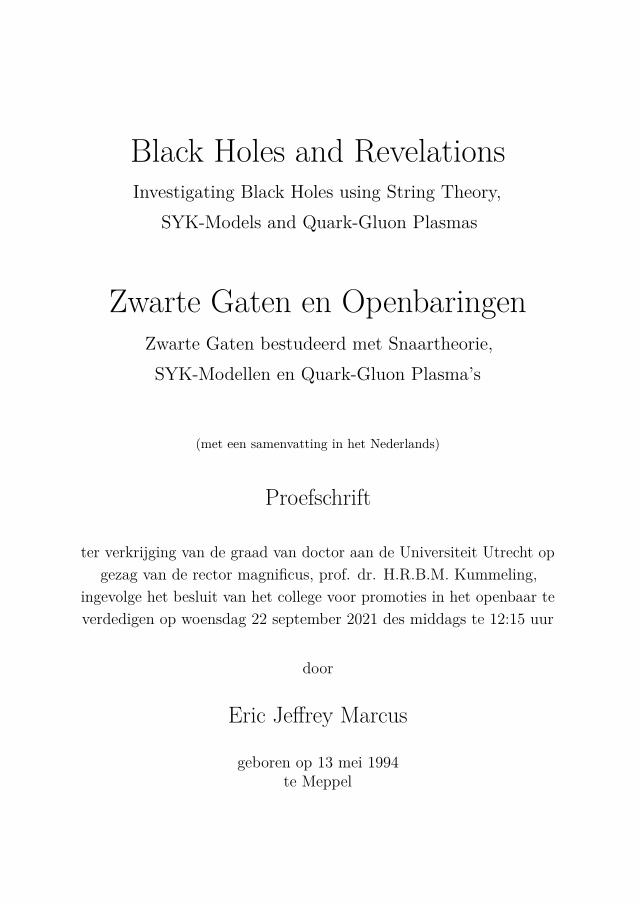
One way to illustrate the black hole spacetimes more intuitively is with a so-calledPenrose diagram. The Penrose diagram corresponding to the Schwarzschild black
2Although Schwarzschild wrote it down in 1916, the interpretation as a part of spacetime fromwhich nothing can escape, was only realized by Finkelstein in 1958.
3
1 Introduction
Figure 1.2: The Penrose diagram for a Schwarzschild black hole. The timeand spatial coordinates are shown in the bottom left, along with the yellow linesindicating how light rays move. The horizon is drawn as a dashed line; note thatit is also at a 45 angle, meaning light can never escape once it is beyond thehorizon. In the diagram, there is also a worldline of an observer that falls intothe black hole and ends up in the singularity (which is unavoidable once you crossthe horizon, as you may convince yourself from this diagram). Fig. from [10].
hole is shown in Figure 1.2.3 In these diagrams, the whole spacetime is put into acompact form, and light always moves on straight lines at angles of 45.Since massive objects (such as observers) always move slower than light, they areconfined to move within the cone defined by two oppositely moving light rays. Theevent horizon is shown in the diagram as a line of 45, such that when light raysmove past it, they can never return.
Singularities
Perhaps the most curious feature of black hole solutions in GR arises when wecompute their curvature. As we move closer and closer to the center of the blackhole, the curvature gets stronger and stronger. In the middle of the black hole, thecurvature diverges, a gravitational singularity. At this point, Einstein’s theory tellsus that the curvature is infinite. Needless to say, you would not want to be at this
3As a historical note: it is precisely this diagram that Stephen Hawking used at a conferenceorganized by Jack Rosenberg to introduce the so-called information paradox of black holes.Hawking believed to have found that information that fell into the black hole was irretrievablylost. A discussion of this fascinating problem is beyond the scope of this thesis, but I wouldhighly recommend the popular scientific book by Susskind [9].
4

1.1 Black Holes and Revelations
singularity; from Figure 1.2 it becomes clear that it is, however, impossible to avoidonce you move beyond the event horizon.
Usually, singularities signal that the theory is not complete in its explanations.For example, in quantum field theory, we are very used to singularities showingup in the computations and have even thought of a scheme to get rid of themconsistently. After doing so, we can match the computations with good agreementto the experiments. That does not mean that quantum field theory is thereby fixed,a better theory would not need such an ad hoc procedure in the first place, andit signals flaws in the theory. However, the gravitational singularities inside theblack holes can not be gotten rid of in a similar manner. To make matters worse, ifthe black hole is rotating, there are also closed timelike curves near the singularity,meaning you could wave to your past self. It is usually thought that a theory ofquantum gravity will provide better explanations of what happens inside a blackhole and possibly resolve the infinities.
But can they spin?
So far we have discussed only Schwarzschild black holes, which are static non-rotating black holes. In this thesis we will also be interested in certain classes ofblack holes that rotate. Whereas the Schwarzschild black hole was only characterisedby its mass M , the rotating black hole will also have angular momentum J . In fourdimensions, the asymptotically flat rotating black holes were discovered by Kerr,and the metric is given by4
ds2 = −(
1 − rsr
Σ
)dt2 + Σ
∆dr2 + Σdθ2 +(r2 + a2 + rsra
2
Σ sin2 θ
)sin2 θ dφ2
− 2rsra sin2 θ
Σ dt dφ , (1.2)
where, as before, rs = 2GM is the Schwarzschild radius, and we have defined
a = J
M,
Σ = r2 + a2 cos2 θ ,
∆ = r2 − rsr + a2 .
(1.3)
4The metric is written in Boyer-Lindquist coordinates, which conforms with conventions we willuse later in the thesis.
5

1 Introduction
The rotation of the black hole can be seen from the dt dφ term, which shows thereis a coupling between the time and one of the angular coordinates. Furthermore, aswe take the angular momentum to zero, this term disappears, as we would expect.The event horizons can be found by considering ∆ = 0, which has real solutionsprovided that a2 ≤ M2 (we took G = 1 here). The case in which we take a = M iscalled extremal, which will be an important limit in some of our later chapters. Ifwe were to take the near-horizon limit for the extremal Kerr black hole we wouldget an AdS2 term from the time and radial coordinates, along with still the mixingbetween the time and angular coordinate. Due to this last ‘mixing’, we often saythat the AdS2 is fibered; in this case over the angular coordinate φ.
Apart from rotation, there is one more property we could have given the black hole,an electric charge Q. A static but charged asymptotically flat four-dimensionalblack hole is known as a Reissner-Nordström black hole, and is given by
ds2 = −
(1 − rs
r+r2Q
r2
)dt2 +
1 −rs + r2
Q
r2
r
−1
dr2 + r2dΩ2 , (1.4)
where we have defined a length scale
r2Q = Q2 G
4πε0. (1.5)
A natural generalization would be to combine all the above discussed propertiesand obtain a black hole solution that is both charged and rotating. This is called aKerr-Newman solution and we will discuss a variant of this later in chapter 3.
What if I throw my wallet in?
Suppose you are near a black hole and throw your wallet into the black hole. Willyou still know how much money was in there? What happens with information ingeneral as we throw it into the black hole has a long, interesting history with manyviewpoints. It is beyond the scope of this thesis to go into the problem in-depth, andI would happily refer to the book black hole war by Susskind [9] for an accessiblehistory. To summarize, the consensus is that information of infalling objects seemsto be conserved and is later radiated away by Hawking radiation. So, regardingyour wallet: you definitely lose your money, but you can figure out how much itwas (by analyzing the Hawking radiation). The presence of radiation already showsus that black holes are thermodynamic objects, and they have their own black hole
6

1.2 String Theory and Black Holes
thermodynamic laws. The most important for us is the analog of the second law,which states that the entropy of isolated systems never decreases. The entropy of ablack hole can be computed by the Bekenstein-Hawking entropy [11]
SBH = A
4 , (1.6)
where A is the area of the horizon. This formula shows us that the second law of blackhole thermodynamics gets translated to ‘the area of a black hole never decreases’,i.e. dA ≥ 0. Now, if we combine the above entropy along with Boltzmann’sunderstanding that entropy ‘measures’ the number of microstates, we can wonder,what are the microstates of black holes? Strominger and Vafa gave an answerto this question in [12] for certain five-dimensional black holes. They reproducedthe entropy using string theory by considering the distribution of momentum onso-called D1 and D5 branes. In the next section, we will discuss more string theoryand how to make black holes within the theory.
1.2 String Theory and Black Holes
The next element in our physics toolbox is string theory, the leading candidatefor a theory of quantum gravity. The basic idea of string theory is perfectly wellencompassed in its name: instead of considering zero-dimensional point particles,we study one-dimensional objects called strings. Other fields, such as gauge fields,will be made from certain strings and excitations that live on these strings. Withinstring theory, there are two types of strings: open and closed strings. In Figure 1.3we show two kinds of strings along with another curious feature of string theories,the existence of so-called branes (short for membranes). As it turns out, openstrings always have their endpoints confined to higher-dimensional surfaces calledD-branes. These D-branes will be extremely vital for our purposes later on; spoileralert: most of our black holes are made from such D-branes. We will discuss whattypes of branes exist in which string theories later on in subsection 1.2.5.
So how exactly does this make a theory of quantum gravity? To answer this, welook at the spectrum of string theory. After we have quantized the theory, wecan find out what objects exist in the excitations of the strings. As it turns out,the closed string spectrum always has a graviton, which is the force carrier for
7

1 Introduction
Figure 1.3: String theories consist of two types of strings, open and closedstrings. The closed ones are colored in green, while the open strings are red.A crucial observation in string theories is the existence of D-branes, which aredepicted as the black squares here. The open strings always have their endpointsfixed to such branes. Figure from [13].
gravity.5 This signals that our quantum theory of strings contains gravity. Apartfrom the graviton, we can also find gauge fields and others, indicating that wecan also describe gauge theories. The presence of gauge fields provided even moreenthusiasm for string theory since the current best-corroborated theory of particlesin our universe, the standard model, is also a gauge theory. The standard modelhas a gauge group SU(3)×SU(2)×U(1), corresponding to the strong interaction,weak interaction, and electromagnetic interaction, respectively.One curious feature of string theory6 is that it requires ten dimensions for consistency.Clearly, we only encounter four of these in our daily lives, so the question arises:where did the others go? The best explanation is in terms of compactification,whereby the ‘extra’ dimensions are rolled up to become very small and thus
5In quantum field theories, such as the standard model, an indicative feature is the presence offorce carriers. These particles, such as the photon for the electromagnetic force, are the fieldsthat mediate interactions. So the presence of the graviton is a good indicator that we are dealingwith quantum gravity.
6I am assuming here that we are considering superstring theory, we will show in the next sectionwhy purely bosonic string theory is not enough to describe anything remotely related to ouruniverse.
8

1.2 String Theory and Black Holes
Figure 1.4: To go from ten dimensions to four, we compactify the extra dimen-sions. This means we ’roll up’ the additional dimensions such that they seempoint-like from our four-dimensional point of view. If we were to zoom in closely,we could still find the hidden structure of these additional dimensions. Figurefrom [13].
not visible in our seemingly four-dimensional world. An illustration is shownin Figure 1.4. It might help to imagine the drawn line as a power cable seenfrom far away; it then appears as a one-dimensional object. Suppose now anant is living on the cable, at his (much smaller) length scales, the wire is notone-dimensional, but the ant can move around the cable in another direction. Thisanalogy encompasses the idea of compactification; at large length scales, the extradimensions are practically point-like, but they are present on microscopic lengthscales.
A very reasonable question at this stage would be, are there different ways ofcompactifying? The answer is yes; in fact, at this stage, it seems appropriate togive the usual estimate of 10500 compactifications7 different possibilities. So, at firstsight, it seems that there is an extraordinary amount of freedom to choose here. Ifwe, however, take a closer look at how we can reproduce all aspects of our universe,it seems there is a problem: how can we create de-Sitter spacetimes from stringtheory. Instead of too much freedom, it seems in this area there is too little. To myknowledge, there exists only one – widely criticized – way to achieve it [14]. Theswampland program (see, e.g. [15]) aims to investigate this and other importantquestions but is beyond the scope of this thesis.Let me now briefly summarise what we will discuss in the rest of this section. We
7This number is more correctly given as an estimate of the possible metastable vacua that can becreated in string theory.
9

1 Introduction
will begin with an overview of which types of string theories exist and which we willuse in our research later on. Afterward, we will move on to supergravity, which isthe low-energy limit of string theory, followed by a short discussion of dualities thatexist in string theory. Then we turn to the elusive branes, both from supergravityand string theory points of view. In the penultimate part we discuss how blackholes are made in string theory. The last part will shortly discuss holography andthe AdS/CFT correspondence since it lies in the motivation of many questionsaddressed in this thesis.
1.2.1 Supersymmetry and Our Universe
Before we consider the string theories in more detail, we have a short discussion onsupersymmetry. The symmetry relates two types of particles: bosons with integerspin and fermions with half-integer spin. Depending on the degree (or amount) ofsupersymmetry, we can form so-called supermultiplets of different sizes by actingwith the different supersymmetries.For example, consider 4D with N = 1 supersymmetry; in this scenario with onespinor, we can act on, e.g., a spin 0 particle to obtain a spin 1/2, which togetherform a chiral multiplet. We can build a vector multiplet is built by working onthe spin 1/2 particle to get a spin one particle. Similar considerations apply todifferent dimensions and more extensive amounts of supersymmetry, in which casewe can build larger multiplets.Supersymmetry is also a vital ingredient of superstring theory, and the types ofstring theories we consider in this thesis will start with the maximal amount ofsupersymmetry8. The question then remains, how much supersymmetry exists in‘our’ universe? To answer this question, experiments (including B-physics at LHC,XENON, WIMP, and many more) have sought for the superpartner particles forquite some years; the Particle Data group gives a good overview of experimentalresults in [16]. Up to now, no superpartners have been found experimentally, andthere are strong constraints on the existence of supersymmetry up to the energyscales reached by the LHC.Due to such results, it has become essential to find ways of ending up in fourdimensions with as little or no supersymmetry as possible. These considerations haveled to much research into compactifications on manifolds that break supersymmetry.
8There is a maximal amount because we only want the multiplets to go up to spin 2 (the graviton);for higher spins, we can’t consistently write down renormalizable and interacting actions.
10

1.2 String Theory and Black Holes
It is also one of the motivations for our work in chapter 2, whereby we constructblack hole solutions in supersymmetry breaking backgrounds. Such approachesallow us to use the tools of superstring theory and still try to make contact withour seemingly supersymmetry-less world.
1.2.2 Different Types of String Theories
In this section we will discuss the different types of string theories. To do so, let’smake our previous discussion on strings a bit more precise, the action for a pointparticle in D dimensions is given by
S = −m∫
ds = −m∫
dτ√ηµν ∂τXµ∂τXν , (1.7)
where η is the spacetime metric, m is the mass of the particle, µ runs over0, 1, . . . ,D − 1 and ds is the line element. The coordinate τ describes the timeevolution of the worldline of the particle. This expression can now be generalized tohigher dimensional objects, in particular one-dimensional strings, where it is calledthe Nambu-Goto action
S = −T∫
d2σ
√(X)2(X ′)2 − (X ·X ′)2 , (1.8)
where T is now the string tension and since strings are one-dimensional we haveintroduced a new coordinate σ for the extended spatial direction. Due to the squareroot in (1.8) it is hard to quantise, but luckily there is another way to write theaction, it is the (classically) equivalent Polyakov action
S = −T
2
∫d2σ
√ggαβ∂αX
µ∂βXνηµν , (1.9)
where we have now introduced the auxiliary field g, the metric on the worldsheet.This action is equivalent to the Nambu-Goto one upon substituting the equation ofmotion for g back into the action. The equation of motion for X reduces to thefree wave equation,9 for which the most general solution is a sum of a left-movingand right-moving wave.We can complete the quantization for which there are many methods, excellentlydocumented in any string textbook. If we only consider (1.9), however, we will runinto a couple of problems. The first problem arises because we only incorporated9Before it takes the form of the free wave equation, we first have to use the reparametrization andWeyl symmetries to fix the worldsheet metric gαβ = ηαβ .
11

1 Introduction
bosonic fields in the Polyakov action so far. After the quantization, we will onlyfind bosonic fields; in our universe, all matter is built from fermions, meaning thatany remotely realistic theory should reproduce them. Secondly, in the spectrum, wefind a tachyon, a particle with a negative mass that usually indicates that we aredoing perturbation theory in an unstable vacuum. The problem is that we don’tknow in bosonic string theory what this vacuum is or what we decay into.
Thankfully both problems can be solved by superstring theory, where we willexplicitly introduce fermions and supersymmetry into the Polyakov action. Thefermions can be included by simply adding the Dirac action for free masslessfermions to the Polyakov action:
S = −T
2
∫d2σ
(∂αX
µ∂αXµ + ψµρα∂αψµ), (1.10)
with ψ the worldsheet fermion field and ρ are two-dimensional Dirac matricessatisfying the algebra
ρα, ρβ = 2ηαβ . (1.11)
In addition to the action itself, we also need to specify boundary conditions forthe fields in order for it to be well defined. We let the σ integral run from 0 to l,where usually l is chosen to be 2π. We then distinguish between closed and openstrings.
Closed strings. The boundary points should be identified for the closed stringssince it is a closed topology. For the bosonic fields X this means
Xµ(τ, σ + 2π) = Xµ(τ, σ) . (1.12)
For the fermions, there are two options, which computationally arises because thefermion action has only one derivative. In practice, this means we can choose
(R) : ψµ(τ, σ + 2π) = ψµ(τ, σ) , (1.13)
(NS) : ψµ(τ, σ + 2π) = −ψµ(τ, σ) , (1.14)
where we call the periodic boundary conditions the Ramond (R) sector and theanti-periodic sector is called the Neveu-Schwarz (NS) sector. Recalling that themost general solutions to the equations of motion were separate for left and rightmoving waves, we can get four sectors: R-R, R-NS, NS-R, and NS-NS. As a lastnote, we have to choose the same boundary conditions for all the µ directions, topreserve the spacetime Poincaré invariance.
12

1.2 String Theory and Black Holes
Open strings. In the open string sector, we have boundary conditions for bothendpoints separately since they no longer coincide. The one extra ingredient, whichwe have mentioned shortly before, is the presence of D-branes. The endpoints ofopen strings end on these branes, and the presence of them allows us to breakthe Poincaré invariance in the spacetime, meaning we can have different boundaryconditions for different values of the µ index. In Figure 1.3 we can see open strings(drawn in red) that both start and end on the same D-brane, as well as open stringsthat start and end on different stacks of D-branes (of different dimensions).Let us consider the bosonic fields Xµ. There are then two different boundaryconditions that we can impose at the endpoints σ∗ ∈ 0, l, Neumann (N) andDirichlet (D)10
(N) : ∂σXµ|σ=σ∗ = 0 , (1.15)
(D) : δXµ|σ=σ∗ = 0 , (1.16)
where δXµ indicates the variation of the field X. The Neumann condition isassociated with directions in which the open string can move on the D-brane, whilstthe Dirichlet condition tells us that the string is fixed in these directions. As anexample, if we had open strings ending on a D5-brane, they would have Neumannboundary conditions in the 0, 1, . . . , 5 directions (where the brane is located), whilsthaving Dirichlet in the remaining 6, . . . , 9 directions of spacetime.Similar to the closed strings, the fermions have an R and NS sector, depending onthe sign difference we choose at the endpoint of the string. The result for the openstrings thus consists of the four possibilities: NN, ND, DN, and DD, within each ofwhich the fermions have the choice between Ramond and Neveu-Schwarz.
Ten Dimensions
The Polyakov action (1.10) has supersymmetry on the two-dimensional worldsheetof the string. We can wonder whether supersymmetry also shows up in the ten-dimensional spacetime that it describes. Before diving into the types of stringtheories that arise in 10D, we first mention the orientation of strings. This orien-tation of a string is flipped when sending σ → 2π − σ. Strings that are invariantunder this operation are called unoriented. These properties allows us to classifythe first three types of string theories:10The equivalence in the last line follows by realizing that demanding that the variation is zero
for all τ is equivalent to saying that X is independent of τ , i.e., the derivative is zero.
13
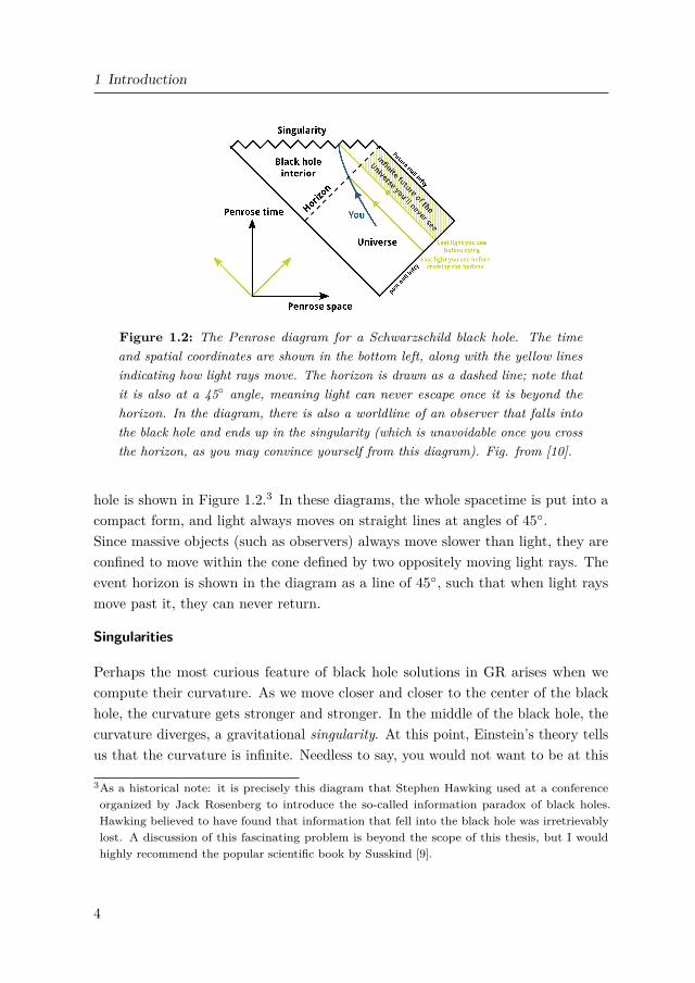
1 Introduction
Type I Type IIA Type IIBStrings Open + Closed Closed Closed
Orientation Unoriented Oriented OrientedSupercharges 16 32 32
All of these theories have supersymmetric spectra. The two Type II theoriesare distinguished by the particular GSO11 projections that are performed on thespectrum; we will have more to say about GSO projections in chapter 2. The TypeI theory can be constructed from the IIB theory by orientifolding12 the theoryand adding several branes (which break half of the supersymmetry) to cancelanomalies [18].
In the remainder of this work, we will mostly be interested in the Type II theories,so let’s shortly discuss their massless spectrum. In the NS-NS sector, both theoriescontain the same fields: a dilaton Φ, the Kalb-Ramond two-form Bµν and themetric gµν . The dilaton plays an important role in string theory, as the vacuumexpectation value determines the coupling strength as
gs = e〈Φ〉 . (1.17)
In the R-R sector, the theories differ, IIA has a one-form C1 and a three-formC3, while the spectrum of IIB contains a zero-form (also known as the axion) a13,two-form C2 and a self-dual four-form C4. In the fermionic sectors NS-R and R-NS,both have two gravitini (corresponding to 32 supercharges) and dilatini; however,they are of different chiralities. Type IIA is a non-chiral N = (1, 1) theory, and IIBa chiral N = (2, 0) theory. Before moving on, it is important to notice that thesetheories fix the problems we had with bosonic string theory. There are no tachyonsin the spectrum, and we have also found the fermions we were looking for.
So far, we have assumed that we make both the left and right moving sectors ofthe Polyakov action supersymmetric. If we relax this condition and make only oneof these sectors supersymmetric, while leaving the other purely bosonic, we obtaintwo new theories, called heterotic string theories:
11Named after the inventors Gliozzi, Scherk and Olive [17].12An orientifold is a generalization of an orbifold, whereby the orbifold group includes the
orientation reversing operator σ → 2π − σ.13Here, I use the notation conventions we will use later on, in the literature it is usually written
as C0
14

1.2 String Theory and Black Holes
• E8 × E8 heterotic string theory
• SO(32) heterotic string theory
The two theories differ in their gauge groups, under which the massless vectorstransform. Together all the approaches we have considered make up the fiveconsistent superstring theories.Apart from these string theories, there is one other player left: M-theory. EdwardWitten introduced the name14 at the strings conference in 1995 [19]. The theoryis not completely formulated yet, but its low-energy limit is known to be 11Dsupergravity, which we will discuss in the upcoming section. M-theory is not astring theory in the sense that its constituents are not strings. It is perhaps moreaccurately described as a membrane theory since it contains two kinds of branes: M2and M5-branes. In subsection 1.2.4 we will see how M-theory and 11d supergravityare related to the other string theories. Before that, we will discuss supergravitytheories.
1.2.3 Low Energy Limits
It is now time to consider the low-energy limit of string theory: supergravity. Thesupergravities form a correct description when E l−1
s , with ls the string lengthscale.15 The supergravities will be of particular importance to us in several places,as we will use the Type IIB supergravity in our Scherk-Schwarz reductions inchapter 2, and 11d supergravity plays a big role in chapter 3. Supergravity hashad different roles in its history. Originally, it was envisioned as a fundamentaltheory, unifying the forces and describing underlying degrees of freedom and free ofultraviolet divergences. It was soon discovered that it could not fulfill these roles.Its modern-day interpretation is better described as an effective field theory of amore fundamental, underlying theory: superstring theory and M-theory.
Local supersymmetry
The fundamental idea of supergravity is to combine the ideas of gravity andsupersymmetry. The supersymmetry is promoted to a local gauge symmetry.14Usually said to mean ‘mysterious’ or ‘membrane’ of even ‘mother’, perhaps you can think of a
better one even.15The energy E is to be interpreted as the center of mass-energy in a particle experiment. Massive
particles can be made from oscillations on strings and have masses M ≈ l−1s , when our energy
scale is lower than this; we can effectively consider the massless spectrum instead.
15

1 Introduction
A natural question to ask is then: what is the gauge field associated with thissymmetry? It is called the gravitino, the superpartner of the graviton, and it carriesboth a spinor and a vector index. The presence of two indices was expected since,unlike ‘normal’ gauge symmetries, the underlying algebra of supersymmetry is asuperalgebra, also containing fermionic generators, the supercharges. Consider nowthe Lagrangian for a D ≤ 11 dimensional supergravity; we know that it should atleast contain the Einstein-Hilbert term for gravity, but also a description of thegravitino field. As it turns out, these fields are described by the Rarita-SchwingerLagrangian, supposing we have a single gravitino it is given by
L = 12e ψµΓµνρDνψρ + . . . , (1.18)
with e the determinant of the vielbein, ψ is the gravitino field, and Γµ form aClifford algebra16 by
Γµ,Γν = 2ηµν . (1.19)
The a, b, . . . in the Lagrangian denote the tangent space indices needed to describethe spinors, while µν, . . . are the curved indices; both types run from 0, . . . D − 1.The covariant derivative D is given by
Dµψ =(∂µ − 1
4ωabµ Γab
)ψ , (1.20)
where ω abµ is the spin connection associated with the vielbeins.
The degree of supersymmetry differs among the possible supergravity theories,and we can denote them according to the amounts of supercharges in the theory.The maximum number that we consider is 32, as theories with more superchargesautomatically get massless fields with a spin larger than two, for which we can’tconsistently write down interactions.How these supersymmetries are distributed over the spinors depends on the space-time dimension. The minimum number of components of the spinors relies onthe type of spinors we can define; we can always make a Dirac spinor that has2bD/2c complex components. In even dimensions, we can, furthermore, define Weylspinors, and in D = 2 mod 4 we can combine the Weyl condition with the Majoranacondition to obtain Majorana-Weyl spinors. Both of the constraints place addi-tional limitations on the spinor, halving its number of degrees of freedom. Spinors16The Γµν indicate asymmetric combinations of gamma matrices, e.g. Γµν = 1
2 [Γµ,Γν ].
16

1.2 String Theory and Black Holes
Dimension Spinor Components2 MW 13 M 24 M 45 S 86 SW 87 S 168 M 169 M 1610 MW 1611 M 32
Table 1.1: This table shows the minimal real components spinors have in variousdimensions. M stands for Majorana, W for Weyl, and S for symplectic. Thesymplectic condition leaves the number of independent components invariant, butboth Majorana and Weyl conditions halve the degrees of freedom of a Dirac spinor.It is also possible to define Weyl spinors in 4D and 8D, but we omitted this fromthe table.
can also be symplectic, but this does not yield any restriction on their degreesof freedom. In Table 1.1 we show the different possibilities for the spinors in thevarious dimensions.
As an example, we can consider the Type II theories in ten dimensions. From thetable, we can see that in ten dimensions, we have Majorana-Weyl (MW) spinors,meaning that the 32 complex components of a Dirac spinor get reduced to 16 realcomponents. The Type II theories are maximally supersymmetric, so there will betwo of these MW spinors. We can make two choices for the chiralities, one yieldinga chiral theory, IIB, and the other a non-chiral theory, IIA. We denote this bywriting that IIA is an N = (1, 1) theory whilst Type IIB is an N = (2, 0) theory.Apart from the ten- and eleven-dimensional theories, we will also often make use ofthe six- and five-dimensional spinors in chapter 2.
What does it look like?
Now that we have discussed supersymmetry and spinors, it is time to study someexamples of supergravities. As mentioned, the IIB and eleven-dimensional su-
17
1 Introduction
pergravities will play important roles for us. So let us begin with discussing theeleven-dimensional supergravity.
11-dimensional supergravity. The unique, eleven-dimensional supergravity wasfirst written down in [20]; it is maximally supersymmetric, and by consideringTable 1.1 we find that there will be one gravitino, whose spinor structures is a 32-component Majorana spinor. The fermionic part of the action will at least containthe Rarita-Schwinger Lagrangian (1.18). In fact, the actions are usually used tomake classical solutions, in which the fermions always vanish, so the fermionic partof the actions are often omitted. The bosonic action is given by
S = 12κ2
11
∫R ∗ 1 − 1
2F4 ∧ ∗F4 − 16 A3 ∧ F4 ∧ F4 , (1.21)
where the last term is known as a Chern-Simons term, R denotes the Ricci-scalar,A3 a three-form, F4 = dA3 is its field strength and κ11 denotes the gravitationalcoupling through
2κ211 = 16πG11 . (1.22)
The Bianchi-identity and equation of motion for the three-form are given by
dF4 = 0 , (1.23)
d ∗ F4 = 12F4 ∧ F4 . (1.24)
Apart from these equations it is often useful to consider the supersymmetry trans-formations on the action. In particular the variation of the gravitino is considered,since the solutions that set these variations to zero characterise Killing spinors. TheKilling spinors indicate conserved supersymmetries. The variation, with parameterε, for the gravitino is given by
δεψµ = Dµε+ 1288(Γνρσλµ − 8δνµ Γρσλ)Fνρσλε = 0 , (1.25)
Dµε =(∂µ + 1
4ωβγµ Γβγ
)ε . (1.26)
Another supergravity theory can be found by reducing the 11d supergravity ona circle. As it turns out this yields exactly the Type IIA supergravity. Thisremarkable relation is due to the duality of M-theory on a circle to Type IIA stringtheory, about which we say some more in the next section.
18

1.2 String Theory and Black Holes
Type IIB. Unlike the IIA theory, IIB cannot be found by reducing the eleven-dimensional theory on a circle. The action for the IIB supergravity schematicallylooks as
SIIB = SNS + SR + Sf , (1.27)
where the first two terms denote the bosonic actions, arising from NS-NS and R-Rsectors of the string theories (see subsection 1.2.2), and the last term denotes thefermions. As mentioned before, the fermionic part will not be of importance forclassical solutions, so we focus on the bosonic part. The NS part of the action isgiven by
SNS = 12κ2
10
∫e−2Φ
(R10 ∗ 1 − 1
2H3 ∧ ∗H3 + 4dΦ ∧ ∗dΦ), (1.28)
where Φ is the dilaton and H3 = dB2 is the field strength of the Kalb-Ramond fieldB2. The other bosonic part of the action is found to be
SR = − 14κ2
10
∫F1 ∧ ∗F1 + F3 ∧ ∗F3 + 1
2F5 ∧ ∗F5 + C4 ∧H3 ∧ F3 , (1.29)
where the field strengths are defined as
F1 = da , (1.30)
F3 = dC2 − adB2 , (1.31)
F5 = dC4 − 12C2 ∧ dB2 + 1
2B2 ∧ dC2 . (1.32)
The IIB action, as written above, gives rise to all the equations of motion, but weare still missing one more ingredient. As we have mentioned before the five-formfield strength is self dual and we need to still manually implement this afterward17
by demanding alongside the equations of motion
F5 = ∗F5 . (1.33)
The Type IIB supergravity has an important symmetry that is not currentlymanifest. To find it we change from the string frame to the Einstein frame by aredefinition of the metric, and define two new fields as
gEµν = e−Φ/2gµν , (1.34)
τ = a+ ie−Φ , (1.35)
F ′3 = dC2 − τH3 , (1.36)
17If it is imposed within the action we find the term∫F5 ∧ F5 = −
∫F5 ∧ F5 = 0.
19

1 Introduction
The scalar τ is often referred to as the axion-dilaton. Using the above definitionswe can rewrite the bosonic IIB action to
SIIB = 12κ2
10
∫ (RE ∗ 1 − 1
4F5 ∧ ∗F5 − 12(Imτ)F
′3 ∧ ∗F ′
3
− 12(Imτ)2 dτ ∧ ∗dτ − i
14 Imτ C4 ∧ F ′
3 ∧ F ′3
),
(1.37)
where we wrote RE to indicate that it is now computed in the Einstein frame. Inthis form there is an SL(2,R) symmetry present, that acts non-trivially two-formsand τ . The two 2-forms transform as a vector18(
B2
C2
)=(d c
b a
)(B2
C2
), (1.38)
while the scalar τ transforms as
τ → aτ + b
cτ + dτ . (1.39)
Within this group there is the transformation with b = 1, c = −1 and the otherparameters zero; it sends τ → −1/τ . Using the fact that the exponent of thedilaton is the string coupling (1.17), we can see that this maps gs → 1/gs. Thistransformation is better known as S-duality, which we will have more to say aboutin the next section. This concludes for now the discussion on the, for us relevant,supergravities. Later on, in subsection 1.2.5, we will come back to brane solutionsof string theory and supergravity. First we turn back to string theory and discusssome important dualities.
1.2.4 The Dual Pictures
This section will have a brief look at some essential dualities for string theory andM-theory. We will not exhaustively discuss all examples of them, but instead, weshow the possible dualities and pick a few relevant examples for our purposes.
S-duality The first to consider is called S-duality, which is short for strong-weakduality. This duality is thus concerned with the coupling strength of the theory. Itis not only known and used within string theory, but also shows up in quantumfield theories. For our purposes, however, let’s first consider the Type IIB theory;as it turns out the S-duality here is part of a larger symmetry group SL(2,Z), which18Note that the matrix has to be invertible, real and ad− bc = 1.
20

1.2 String Theory and Black Holes
is the discrete version of the SL(2,R) symmetry of the previous section. The dualitysends the string coupling gs → 1
gs, and in this case, it will map the IIB theory to
itself.For the Type IIA theory, something more intriguing happens. As it turns out,M-theory, when compactified on a circle, is dual to the IIA theory. In the low-energylimit, we already mentioned this, but the duality runs a bit further than this. Theradius of the circle is given by
R11 = `s gs ,
with `s the string length and, more importantly, gs the string coupling. For theperturbative regime of small gs, the radius will tend to zero, and we have ‘ordinary’ten-dimensional string theory. When we now send gs → 1
gswe find that the circle
radius goes to infinity; it decompactifies. So the S-duality relates the IIA theoryto the eleven-dimensional M-theory. There exist other S-dualities between stringtheories, for example, between Type I and the SO(32) heterotic string theory, butsince we will not be using these, we will not go into detail.
T-duality The name is short for target-space duality. This duality arises when weconsider theories that are compactified on circles or tori. If we were to considerpurely bosonic, closed, string theories, one compactified on a circle with radius Rand the other with R = α′/R, then T-duality maps these to one another by
XR → −XR XL → XL , (1.40)
where XL,R denote the left and right-movers, respectively. A similar story holds forthe Type II string theories when compactified on a circle. When we compactify oneof them, say IIA, on a circle with radius R, it turns that T-duality maps it to TypeIIB theory compactified on a circle with radius α′
R . We already saw that M-theoryon a circle was dual to IIA, so combining these facts teaches us that M-theory on atwo-torus is dual to IIB.
For compactifications on tori, we usually talk about the T-duality group: this groupis, in some sense, the generalization of the R → 1
R symmetry for circles we justmentioned. It acts upon the coordinates, background fluxes and also includes shiftssymmetries. When compactifying on a Tn, the resulting T-duality group for TypeII theories will be SO(n,n,Z). If we were to consider the O(n,n,Z) group, we canalso interchange the Type IIA and Type IIB theories.
21

1 Introduction
Figure 1.5: This diagram shows the various dualities and relations betweenstring theories, 11D supergravity, and M-theory. The star indicates that all othertheories are certain limits of M-theory. Figure from [21].
Apart from the Type II theories, there is also a T-duality between the two heteroticstring theories. An overview of the different dualities is shown in Figure 1.5.
U-duality The last duality we will shortly mention is the so-called U-duality [22],which unites the previous two dualities into a larger symmetry group. This particularsymmetry group is vital for us since we will use it for Scherk-Schwarz reductions inchapter 2. In the specific example that we will consider, we will first be compactifyingType IIB supergravity on a T 4 which has an SO(4,4) T-duality group. The totalsymmetry (or duality) group for the supergravity is SO(5,5,R), which contains theT-duality group. The U-duality group for string theory is then the discrete version,i.e. SO(5,5,Z).
1.2.5 Branes
String theories describe more than just strings; they also contain non-perturbative,extended objects called D-branes or Dp-branes (with p the spatial dimension).These branes are objects upon which open strings can end. The Dirichlet boundaryconditions, which we saw in subsection 1.2.2, indicate that the endpoints of anopen string are fixed in those spacetime directions; this is the origin of their name:Dirichlet-branes. If we have an open string that has Dirichlet boundary conditions
22

1.2 String Theory and Black Holes
in p directions and Neumann boundary conditions in the rest, we find that the openstring endpoint is confined to a Dp-brane. A major leap in understanding D-braneswas made by Polchinski [23], when he realized that the branes carry charge underthe RR-fields in string theory. This allowed the identification of the Dp-branes withthe supergravity analog called p-branes. A p-brane couples to a (p+1)-form field byan interaction as
Sint = µp
∫Ap+1 , (1.41)
which can be seen as a generalization of the coupling of a charged particle to agauge field. We can also consider the worldvolume theory of the brane, which isknown as the Dirac-Born-Infeld (DBI) action. The massless bosonic part19 of thisaction is given by
S = −Tp∫
dp+1σe−Φ√
−det(G+B2 + 2πα′F ) , (1.42)
where F = dA is the field strength of a gauge field, B2 is the pullback of theKalb-Ramond form to the brane and G is given as
Gab = ηµν∂aXµ∂bX
ν , (1.43)
with the a, b indices on the worldvolume and µ, ν in the ten-dimensional spacetime.Before we consider how these branes look in supergravity, we consider what happenswith the D-branes under T-duality. The duality acts on the open string boundaryconditions in the circle direction by interchanging the Neumann and Dirichletconditions. We can then distinguish two situations: the D-brane is wrapped on thecircle or it lies in directions orthogonal to the circle. This results in
Wrapped : Dp-brane → D(p− 1)-brane ,
Unwrapped : Dp-brane → D(p+ 1)-brane ,
where the last line follows from the fact that the Dirichlet conditions change toNeumann. To summarize: D-branes that wrap the circle are mapped to those thatdon’t and vice-versa.
From the supergravity point of view
To find the p-branes in supergravity, we can solve the equations of motion that followfrom the supergravity actions. First, we will consider the ten-dimensional Type II19There also exist Chern-Simons terms, but they will not be important for us.
23

1 Introduction
theories. Let us consider the spacetime symmetries that exist in the presence ofthese branes. Before we add the branes, there is an SO(1,9); when introducing ap-dimensional brane, we find
SO(1,9) → SO(1, p) × SO(9 - p) . (1.44)
The brane breaks the Lorentz-symmetry to its spacetime direction, and the rightmostgroup arises due to rotations around the directions orthogonal to the brane. Wewill place one extra demand upon the brane solutions: they are extremal, whichwe require for the preservation of supersymmetry.20 In particular, the branes willsatisfy the Bogomol’ny-Prasad-Sommerfield, or BPS, bound, which relates the mass(or mass density) to the charge of the brane. The extremal branes are 1/2 BPSstates, meaning that they preserve half of the supersymmetry. The p-brane solution,in string frame, is found to be21
ds2 = H−1/2p [−dx2
0 + dx21 + · · · + dx2
p] +H1/2p [dr2 + r2dΩ2
8−p] , (1.45)
eΦ = H3−p
4p , (1.46)
Cp+1 = (H−1p − 1)dx0 ∧ · · · ∧ dxp , (1.47)
and all other fields are set to zero. The Hp is a harmonic function given by
Hp = 1 + Qpr7−p , (1.48)
and Qp is the charge of the p-brane. When there are multiple branes present, wecan write Qp = cpNp, where Np is the number of branes, and cp is the chargeof a single brane, which we will say more about in chapter 2. So far, we haveconsidered branes charged under RR-fields; what if the brane is charged underthe Kalb-Ramond field? When electrically charged, this turns out to be nothingbut the fundamental string, and the magnetically charged brane is the so-calledNS5-brane.
Looking at M-theory
So far, we have been discussing the ten-dimensional theories, but let’s switch over toM-theory for a bit. We saw before, subsection 1.2.2, that the low-energy description20This ensures that the solutions are stable. Also, the solutions are truly ‘black’, the temperature
of the extremal solutions is zero.21When Cp+1 is one of the form fields present in, say, the IIB theory, the brane is said to be
electrically charged. If Cp+1 is, however, the Hodge dual of one of the IIB forms, the brane issaid to be magnetically charged.
24

1.2 String Theory and Black Holes
of M-theory, eleven-dimensional supergravity, contains a three-form field A3. Byour previous discussion, we can then conclude there exist two kinds of branes inthe theory: M2-branes, which are charged by A3 electrically, and M5-branes thatare charged by the Hodge-star of A3, hence charged magnetically. The M2-branesolution in the 11d supergravity is
ds2 = H−2/3dxµdxνηµν +H1/3dxmdxnδmn , (1.49)
A3 = H−1dt ∧ dx1dx2 , (1.50)
where H is again a harmonic function, dependent on the radial coordinate in thetransverse space:
H(r) = 1 + q
r6 . (1.51)
A similar solution can be written down for the M5-brane. Before we move on, wecan consider what happens with the M-theory branes when we reduce M-theory ona circle, which yields the IIA theory. The results depend on whether the branes lieon the circle. If the M2-brane is wrapped on the circle, we obtain the fundamentalstring in IIA, and if it is orthogonal to the circle, we get a D2-brane. The M5-braneon the circle similarly yields a D4-brane, but when it is orthogonal to the circle, weobtain an NS5-brane.
1.2.6 Building Black Holes
The branes we have discussed so far are in some sense ‘black’; as we take thelimit of r → 0 we find that the solutions have a horizon.22 There are more thingswe demand of our black hole solutions, most importantly that they will have afinite, non-zero entropy. By the Bekenstein-Hawking entropy formula, (1.6), ablack hole has non-zero entropy if its event-horizon has a non-zero area. Thisabsence of a horizon furthermore implies that black holes with an area of zero havea naked singularity, which are conjectured to not exist in the cosmic censorshipconjectures.
So let us use some of the techniques of previous sections to create a physicallyacceptable black hole. In particular we will consider a five-dimensional black hole,since it will play a role later in chapter 2. One way to construct them is to start with
22That the horizon is located at r = 0 is a feature of the isotropic coordinates that we have usedso far.
25

1 Introduction
M-theory on a six-torus and place three orthogonal M2-branes together to obtain aM2⊥M2⊥M2 solution. We can then apply dualities in the following manner
M-theory R10−−→ IIA T567−−−→ IIB (1.52)
where R10 denotes reduction of the tenth spatial dimension, and T567 indicatesT-dualities in the 5,6 and 7 directions. Note that we end up with Type IIB theoryon T 4 × S1, where we take the circle to be denoted by the x5 and the torus by ymwith m = 1, 2, 3, 4. Denoting an M2-brane that is extended in the (i, j) directionsby M2(i, j), the dualities act as follows
M2(8, 9) R10−−→ D2(8, 9) T567−−−→ D5(5, 6, 7, 8, 9)
M2(6, 7) R10−−→ D2(6, 7) T567−−−→ D1(5) (1.53)
M2(5, 10) R10−−→ NS1(5) T567−−−→ P(5)
In the last transformation we end up with a gravitational wave in the 5-direction,meaning there is a non-zero amount of momentum present in the resulting D1-D5-Psystem. The solution in the Type IIB theory is given as
ds2 = H−1/21 H
−1/25 [−dt2 + dx2
5 +K(dt− dx5)2] +H1/21 H
1/25 [dr2 + r2dΩ2
3]
+H1/21 H
−1/25 [dy2
1 + · · · + dy24 ] ,
e−2φ = H−11 H5 (1.54)
C05 = H−11 − 1 ,
(∗C)056789 = H−15 − 1 ,
where we see that, as expected, the D1-brane is charged under C2 and the D5-braneunder the Hodge-dual of C2. The harmonic functions are given by
H1 = 1 + Q1
r2 , H5 = 1 + Q5
r2 , HK = 1 +K = 1 + QKr2 . (1.55)
As we mentioned before the branes are BPS objects, and we can wonder how manysupercharges are conserved by this combined configuration. To investigate this, wecan investigate the Killing spinors, and how many independent components theyhave. By considering the starting point with M2-branes (1.53), and realizing thatevery orthogonal M2-brane breaks half of the supersymmetry, we could alreadyguess that it preserves 1/8. Nevertheless, let us look a bit more formally: Type IIBtheory is a chiral (2, 0) theory and contains two spinors of the same 10D chirality,
26

1.2 String Theory and Black Holes
which we denote by εL and εR.23 The D1 and D5-branes impose the followingconstraints on the spinors (see e.g. [24])
Γ0Γ5εL = εR , (1.56)
Γ0Γ5Γ6Γ7Γ8Γ9εL = εR . (1.57)
The momentum in the x5 direction imposes the following additional independentconstraint
Γ0Γ5εL = εL , (1.58)
which, when combined with the other constraints, implies the same constraint onthe εR spinor. So, in total, we can see that the independent components in thespinors are halved three times, meaning that the D1-D5-P system is 1/8 BPS.
Down by Five Dimensions
The five-dimensional black hole solution can be found by compactifying over theT 4 × S1, using the ansatz
ds210 = e2χdymdym + e2ψ(dx2
5 +Aµdxµ)2 + e−(8χ+2ψ+φ)/3ds25 , (1.59)
where χ, φ and ψ are scalar fields, the index µ runs over 1, 2, 3, 4 and Aµ denotegauge fields in the five-dimensional theory. The prefactor of the five-dimensionalmetric is found by demanding that it becomes the metric in the Einstein-frame.The 5D-metric is found to be
ds25 = −H−2/3(r)dt2 +H1/3(r)(dr2 + r2dΩ2
3) ,
H(r) = H1(r)H5(r)HK(r) .(1.60)
This is the metric of a five-dimensional black hole, and we can now investigate theentropy. To do so we first compute the area of the horizon as r → 0, which gives
A = 2π2√Q1Q5QK . (1.61)
As we have mentioned before the charges can be written as Qi = ciNi, where ciare the charges of an individual brane, and Ni integers, indicating the number of
23The conventional notation for the spinors seems confusing since they have the same chirality inten dimensions. The L/R denote, however, the two-dimensional worldsheet chirality.
27

1 Introduction
branes or units of momentum. A derivation of the individual charges is found in,for example, [24], the product of the three charges yields
√c1c5cK = 4G(5)
N
π. (1.62)
Using these results we can find that the entropy of the black hole, computed by theBekenstein-Hawking entropy (1.6), is given by
SBH = 2π√N1N5NK . (1.63)
The black hole has a non-zero entropy, for which it is vitally important that allNi are non-zero. This last observation shows us that if we had omitted one of theingredients, be it one of the D-brane species or the momentum; then the blackhole would have been a naked singularity. This particular solution has had quitesome attention in the past, as it was also used in [12] to re-derive this entropy fromthe microscopic string-theory side. This work by Strominger and Vafa providedfor the first time a microscopic origin of the black hole entropy. In chapter 2 wewill investigate solutions like the D1-D5-P whilst breaking part of the backgroundsupersymmetry and then study how this affects the entropy. Let us now turn toanother exciting topic: holography.
1.2.7 Holograms
the three-dimensional world of ordinary experience —the universe filledwith galaxies, stars, planets, houses, boulders, and people— is a hologram,an image of reality coded on a distant two-dimensional surface. This newlaw of physics, known as the Holographic Principle, asserts that everythinginside a region of space can be described by bits of information restrictedto the boundary.
– Leonard Susskind, The Black Hole War
The physics world was shocked in 1997 when Maldacena published his paper on theAnti-de Sitter / Conformal Field Theory duality (AdS/CFT) [25]. This proposalwas the first string theory-based example of holography: the phenomenon wherebya higher-dimensional theory is equivalently described by a lower-dimensional one,thought of by ’t Hooft [26] and popularized by Susskind [27].
28

1.2 String Theory and Black Holes
The AdS/CFT duality was discovered by looking at stacks of N D3-branes fromdifferent perspectives. First, we can consider the D3-branes from a microscopicpoint of view, where there exist closed strings in the vacuum and open strings thatend on the stack of D3-branes. We can consider only the massless excitations ifwe take the low energy limit, meaning we obtain Type IIB supergravity in 10DMinkowski space in the bulk from the closed strings. For the open string sector wecan consider the DBI-action (1.42) which, when expanded in α′, yields a maximallysupersymmetric Yang-Mills theory. From the first point of view, we thus have twodecoupled systems: free IIB supergravity in the bulk, and for the D3-branes, wefind an N = 4, D = 4 SYM theory.Now, we also know that D-branes are objects that source fields in the supergrav-ity theory. When considering this perspective at low energies, we get a similardecoupling. The excitations that exist close to the brane, r R := Q
1/43 , will
be decoupling from those that exist far away, r R.24 In other words, therewill be excitations that have such long wavelengths that they will not ‘feel’ thebrane anymore, while the others can’t escape the gravity well of the brane. Thelong-range excitations constitute, once again, IIB supergravity in 10D Minkowskiand the short-range ones constitute the near-horizon physics of the branes. Thelatter consists of an AdS5× S5 geometry. We find an equal IIB supergravity in thebulk for both perspectives, so we are now led to identifying the N = 4, D = 4 SYMtheory with the IIB supergravity in AdS5× S5. Since the five-sphere is compact,we usually say that the CFT4 is dual to AdS5, and in general that an AdS in D+ 1dimensions is dual to a D-dimensional CFT.
AdS / CFT Dictionary
Let us be a bit more precise in the couplings and limits that we take. The stringcoupling constant is gs, the Yang-Mills coupling is denoted by gYM , L representsthe AdS radius. The two theories are then related by
g2YM = 2πgs , 2λ = 2g2
YMN = L4
α′2 , (1.64)
where we introduced the ’t Hooft coupling λ = g2YMN . As for the limits: in the
weakest form of the AdS/CFT duality, we take limits on the string theory side to
24The specific power of Q3 arises due to the harmonic functions f = 1 + Q3r4 .
29

1 Introduction
end up in supergravity. The limits consist of first taking the limit N → ∞ andsubsequently taking λ → ∞, making sure that gs is small. By (1.64), these limitsimply that the string length is much smaller than the AdS radius, meaning we takethe point particle limit of string theory and hence obtain supergravity. So this formof the AdS/CFT duality states that N = 4, D = 4 Yang-Mills with gauge groupSU(N) is dual to Type IIB supergravity with a radius of curvature L along withN units of flux (due to the brane charges). This duality is a strong/weak dualitybecause the gauge theory is strongly coupled, and the supergravity is weakly curved.Stronger forms of the duality are less stringent than the weak form on the limits ofN and λ.
Let us now consider the (bosonic) symmetries on both sides. The SYM theory isconformal in four dimensions, and the four-dimensional conformal group is SO(2,4).Furthermore, the R-symmetry in the theory is given by SU(4) ∼= SO(6). For AdS5,the isometry group is SO(2,4) and the isometry group of S5 is SO(6); the symmetriesthus coincide on both ends.The next important step is to realize how the bulk fields φ are related to theoperators in the CFT, O. The one-to-one correspondence between these two isrealized as25 ∫
φ0
Dφ e−Sstring =⟨
e∫
d4xφ0 O⟩
CFT, (1.65)
where the subscript φ0 means that the paths of φ are on-shell and at the boundaryof the AdS-space take the value φ0. The partition function of the string theoryis thus identified with the generating functional for correlation functions. Theidentification of objects between the two theories is usually called the dictionary.For example, we identify the energy-momentum tensor in the CFT with the metricin the bulk. In this case, the boundary value is the metric on the boundary.26 Amore elaborate introduction to the duality can be found in, for example, [28].Although we don’t explicitly use the correspondence in this thesis often, it motivatesmuch research. The research described in chapter 2 is from the supergravity side ofthings; an explanation using the AdS/CFT duality would (hopefully) teach us themicroscopics of the story. In chapter 3 we discuss the embedding of near horizonlimits of rotating black holes into M-theory, which provides the first step towards agravitational dual of c and I-extremization applicable to rotating geometries. The25Note that we have switched to a Euclidean signature, if26To be precise, it is defined up to a conformal rescaling, so φ0 would correspond to the boundary
value of the conformal class of the metric.
30

1.3 SYK Models
models in chapter 5 and chapter 4 can be viewed as duals of black hole physics insome limits, the one-dimensional SYK-model (in certain limits) is thought to bedual to the two-dimensional Jackiw-Teitelboim gravity [29,30]. The quark-gluonplasma created in heavy-ion collisions can be linked to five-dimensional black holephysics via the AdS/QCD correspondence [31].
1.3 SYK Models
So far, our discussion has concerned string theory and how to build black holeswithin string theory. We now turn our attention to the Sachdev-Ye-Kitaev (SYK)model [32,33]. Instead of the ten dimensions of string theory, this model has only one:time. In the context of studying black holes, the one-dimensional model is thoughtto be dual to a two-dimensional gravity model that can contain black holes. Thereare two reasons why we expect this duality, the first being that there is emergentconformal symmetry in the IR limit. So by the AdS/CFT correspondence, we couldlearn about the two-dimensional black holes by studying the one-dimensional model.A second relevant property is that the SYK model is maximally chaotic. Before weturn to the SYK model, let’s shortly review what chaos means and what it has todo with black holes.
Chaos and Scrambling
Black holes are fast scramblers , meaning they quickly scramble any informationthrown into the black hole. More technically, we can consider a complex, chaoticquantum system with many degrees of freedom N (for example, a black hole)that we initially place into a pure state. After some time, the system evolves inthe following sense: if we consider a subsystem of size m N , we find that thedensity matrix approaches a maximally mixed state. Computing the entropy ofthis mixed state tells us how much entanglement exists between m and mc (sinceit is effectively computing the entanglement entropy between the two). In otherwords, the scrambling tends to send the entanglement entropy of the subsystem toits maximal value. Now, if this last statement is true for any subsystem with sizem < N/2, we call the system scrambled. In practical terms, we need to considerhalf of the total system to extract information since the data is scrambled over thesystem. Consider now adding one bit of information to the system. Initially, thesystem is then no longer scrambled since we can find information by looking only
31

1 Introduction
at one bit. The scrambling time is then defined as the time scale until the bit ofinformation is scrambled over the system. What does it have to do with chaos? Thechaos, or also called the butterfly effect, is thought to be the underlying mechanismby which black holes achieve the scrambling of information. This quantum chaosturns out to be subject to a bound [34], and black holes exactly satisfy this bound,i.e., they are the fastest possible scramblers. So if there is any theory dual to theblack hole, we expect it to show this maximal chaos, which the SYK model indeeddoes.
What does the SYK model look like?
In chapter 4 we will be studying a generalization of the SYK model. We willintroduce the ‘original’ SYK model and its supersymmetric variant here to providesome context for the generalized model. We will introduce the Hamiltonian of themodel, the disorder average and afterward, we discuss the two-point function forboth free Majorana fermions and the complete interacting theory. When we takethe large N limit (’t Hooft limit) alongside the IR limit, we can obtain an expressionfor this full two-point function. Afterward, we will focus on the four-point function,which has a unique role in computing the chaos exponent or Lyapunov exponent. Inthe next section we discuss the effective action to rewrite the theory in terms of abilocal action. The last section shortly discusses the supersymmetric SYK model.
The SYK model [35] is a simplified version of the Sachdev-Ye model [32]. Themodel contains N Majorana fermions that randomly interact with q ∈ 2Z otherMajorana fermions. In particular, we will first discuss the case q = 4 where fourfermions interact with each other. The Hamiltonian is then given by:
H = 14!∑ijkl
Jijkl χi χj χk χl , (1.66)
where χ denote the Majorana fermions, which obey the commutation relations
χi, χj = δij . (1.67)
The coupling Jijkl is completely antisymmetric in all its indices (which followsfrom H being Hermitian and the anti commutation of the χ fields). From the
32

1.3 SYK Models
Hamiltonian we can also obtain the Lagrangian:
L = 12 χj
d
dτχj −H . (1.68)
From the Lagrangian we can find that the fermions χ have dimension 0 and thecoupling in the Hamiltonian (for any q) has dimension 1, the dimension of an energyscale. The Euler-Lagrange equation for the fermion yields
χi = 13! Jiklmχ
k χl χm . (1.69)
Lastly, the model has quenched disorder where the couplings Jijkl are randomlydrawn from a normal distribution [35]
P (Jijkl) =√
N3
12πJ2 exp(
−N3 J2ijkl
12J2
). (1.70)
Where J is the dimension 1 (energy) parameter that characterizes the distribution.To find the average 〈Jn
ijkl〉 (n ∈ Z+) we simply integrate over the probabilitydistribution (note that there is no sum in the expression below)
〈Jnijkl〉 =
∫d(Jijkl) Jn
ijkl P ( Jijkl ) , (1.71)
which yields us the two results:
〈Jijkl〉 = 0 , (1.72)
〈J2ijkl〉 = 3!J2
N3 . (1.73)
We will also use X, for some X dependent on Jijkl, to denote the averaging overthe distribution.
One of the nice things about the SYK model is that we can write down explicitresults for the n point functions under a large N and strong coupling limit. Let us,as an example, show the results for the two-point function.
1.3.1 Two-Point Functions
The combination of large N and strong coupling limits will severely limit thediagrams that can show up in the loop corrections, and in fact all will be of a typecalled ‘melons’. Let us first see the influence of the large N limit. Consider for
33

1 Introduction
i i
j
k
l
m
n
o
i i
l
k
m
n
oj j
Figure 1.6: These diagrams will contribute to leading order in N. The dotted line indicatesthe disorder average, which forces the indices to be equal. Note that the indices in theloops are summed over.
example the diagram in Figure 1.6 which will contribute to the leading order inN ; the dotted line indicates the disorder average. The expression for the leftmostdiagram is:
C
(4!)2
∑jklmno
〈Jijkl Jimno〉G0,jmG0,knG0,lo = J2G0(τ1, τ2)3 , (1.74)
where we made use of (1.73) and the combinatorial factor C =(4
3)(4
3)
3!. There are,however, also diagrams that don’t contribute at this order. For example take thediagrams in Figure 1.7 which can be checked to contribute as 1
Ndwith d > 0.
We can now generalize the expression for the self energy by realizing that the onlykinds of diagrams that contribute are those similar to (1.74). The diagrams needin general to have a disorder average over their incoming and outgoing lines andthe lines must not cross any other lines in the diagram. We can thus constructthe full two-point function as shown in (1.8). It then becomes clear that the totalexpression for the self energy becomes [36,37]
Σ(τ1, τ2) = J2G(τ1, τ2)3 , (1.75)
where G now denotes the full two-point function. Besides the above expression,we can also express the full two-point function as a sum of all the one particleirreducible (1PI) diagrams by
1G(ω) = −iω − Σ(ω) . (1.76)
34

1.3 SYK Models
Figure 1.7: Here we show two diagrams that do not contribute at leading order in N theleft diagram will contribute at N−5 and the right diagram as N−1.
= + + . . . + + . . .
Figure 1.8: The full two-point function is denoted by the line with the box. On the rightside, we omitted the dotted lines indicating the disorder averages. They are, however, allimplemented in the same manner as shown in Figure 1.6.
When we take (1.75) and (1.76) together, they completely determine the full two-point function. We can solve these equations in the strong coupling (or low energy)limit: ω J .
Cranking the Coupling
In the strong coupling limit we may ignore the first term that appears in (1.76)such that we can obtain the following equation:∫
dτ ′G(τ, τ ′) Σ(τ ′, τ ′′) = −δ(τ − τ ′′) , (1.77)
which, by using (1.75), becomes (notice the familiarity with the Schwinger-Dysonequations)
J2∫dτ ′G(τ, τ ′)G(τ ′, τ ′′)3 = −δ(τ − τ ′′) . (1.78)
35

1 Introduction
We can now make an ansatz for G by using the conformal symmetry and anticom-mutativity of fermions
Gc(τ) = Asgn(τ)|τ |2∆ , (1.79)
where A and ∆ are constants and the subscript c denotes the conformal limit. Indeed,it can be checked that the expression is invariant under SL(2,R) transformations.Plugging this into (1.78), we can find that the full two-point function is given by
G(τ) =(
14π J2
) 14 sgn(τ)√
|τ |. (1.80)
Similarly, there are techniques for computing four point functions using ladderdiagrams, and there are also results for n-point functions [38].
Conformal symmetries and heating up
There is an interesting consequence of taking the IR limit for the equations definingthe full two-point function: emergent conformal symmetry. We can see that (1.78)has Conf(R1) ∼= Diff(R1) symmetry as follows27 Suppose that G(σ, σ′′) solves theequation:
J2∫dσ′G(σ, σ′)G(σ′, σ′′)3 = −δ(σ − σ′′) .
We now let σ = f(τ) such that we obtain
J2∫ ∣∣∣∣ dfdτ ′
∣∣∣∣ dτ ′G(f(τ), f(τ ′))G(f(τ ′), f(τ ′′))3 = − 1|f ′(τ ′′)|δ(τ − τ ′′) , (1.81)
where we used that δ(f(x) − f(x0)) = 1|f ′(x0)|δ(x− x0). It now becomes clear that
this is equal to (1.78) if we have
G(τ, τ ′) = |f ′(τ) f ′(τ ′)|∆ G(f(τ), f(τ ′)) , (1.82)
where, in our current case, ∆ = 14 . So we find that (1.78) is invariant under
the reparametrisation group Diff(R). The symmetry is, however, spontaneouslybroken by the explicit solution for G in (1.80). This solution no longer has the fullsymmetry group but instead is only invariant under the subgroup SL(2,R). Wecan use the conformal symmetry to change the domain to a compact manifold, for
27Conf(R1) ∼= Diff(R1) follows because there is no notion of an angle in one-dimension, so allsmooth transformations are conformal.
36

1.3 SYK Models
example S1. We pick f(τ) = e2πit/β such that we map the line into the circle, andwith this we can obtain a result for finite temperature:
Gβ(τ) = − π14
√2β J
1√sin(πτβ )
sgn(τ) . (1.83)
1.3.2 Lyapunov and Chaos
As mentioned in the introduction, the SYK model saturates the chaos bound.This chaos bound, introduced in [34], can be found using an Out of Time OrderCorrelation (OTOC) function. In particular one can consider two Hermitianoperators V and W separated by a time distance t. The chaos can then beinvestigated by the OTOC
F (t) = tr [yW (t) y V (0) yW (t) y V (0)] , (1.84)
where y = ρ(β)1/4. So the thermal density matrix ρ is split into the four factorsof y. One may then furthermore show that for a large N CFT, holographicallydescribed by Einstein gravity [34], that
F (t) = f0 − f1
N2 exp(
2πβt
)+ O(N−4) . (1.85)
The conjecture about the bound on chaos then reads: chaos in thermal quan-tum systems (with many degrees of freedom) can never develop faster than theabove holographic result. In chaotic systems the correlators are expected to growexponentially
Fd − F (t) ∝ exp (λL t) , (1.86)
where λL the Lyapunov exponent and Fd is the product of the disconnectedcorrelators. Furthermore, at some time between the scrambling time, mentionedin the introduction of the SYK section, and the dissipation time, the exponentialdecay time of two-point functions, we have that F (t) ≈ Fd. The conjecture is thenstated as:
d
dt(Fd − F (t)) ≤ 2π
β(Fd − F (t)) . (1.87)
Or in terms of the Lyapunov exponent:
λL ≤ 2πβ. (1.88)
37

1 Introduction
As it turns out the SYK saturates this bound. To derive this explicitly requiresconsidering the non-conformal contribution to the four point function in exhaustivedetail. In particular we would consider:
Tr [y χi(t) y χj(0) y χi(t) y χj(0)] . (1.89)
Then, as derived in [37], the non-conformal contribution will yield a factor in thefour point function as:
C β J
(1 − π
2 cosh 2πtβ
), (1.90)
where C is a constant. This indeed shows the exponential behaviour with a Lyapunovexponent λL = 2π
β , such that SYK saturates the chaos bound. In chapter 4 we willuse a different, easier, method to find the maximally chaotic behaviour.
1.3.3 Effective Action
Another useful way to understand the model is by a path integral representationover bilocal fields. This can be used to find the free energy, the entropy and mightbe a good starting point for a holographic interpretation of the theory. We note thatthe results we discuss below also have a generalization including certain ’flavours’of χ’s, see [39]. Now, in order to find the free energy (or action) we would usenaively −β F = logZ. Due to the disorder averaging, however, we have to considerZ, and for the free energy F = logZ. The problem with our naive assumption isthat logZ 6= log(Z) in general. The solution to this problem is the so-called replicatrick (see [40] for an introduction). This is most intuitively stated as
logZ = limn→0
Zn − 1n
. (1.91)
The main idea of this equality is that we now have to calculate the disorder averageover n copies of Z instead of the logarithm. This means the disorder average willboil down to doing Gaussian integrals. The replica trick can also be written in amore useful way as
logZ = limn→0
1n
log(Zn). (1.92)
38

1.3 SYK Models
Following the replica idea we will now compute the disorder average of M copies ofthe partition function.
ZM =∫
Dχαi DJijkl exp
−a∑ijkl
J2ijkl
(1.93)
× exp
−M∑α=1
∫dτ
12∑i
χαid
dτχαi − 1
4!∑ijkl
Jijkl χαi χ
αj χ
αk χ
αl
,
where the bar denotes the disorder average, α denotes the replica index and a isthe prefactor in the exponential as in (1.70). We won’t show all the details here,but the straightforward computation consists out of first computing the Gaussianintegral over Jijkl and afterward introducing, by means of Lagrangian multipliers,bilocal fields
Gαβ(τ1, τ2) = 1N
N∑i=1
χαi (τ1)χβi (τ2) . (1.94)
As a last step we can integrate out the fermions and the resulting partition functionbecomes
ZM =∫
DGDΣ exp −M Seff , (1.95)
where Seff is given by
Seff = −N
2 log det(∂τ − Σ
)+ 1
2
∫dτ1 dτ2
(N Σ(τ1, τ2) G(τ1, τ2) − J2N
4
(G(τ1, τ2)
)4),
(1.96)
where the G denotes the bilocal field, and Σ arose as the Lagrangian multiplier.Note that if we vary Σ or G we obtain (1.76) or (1.75) respectively. This showsus that we have found an exact rewriting of our theory in terms of path integralsover bilocal fields. The computation for a general q-pt interaction is completelyanalogous to above and yields as a result
ZM =∫
DGDΣ expM
N
2 log det(∂τ − Σ
)× exp
−M
2
∫dτ1 dτ2
(N Σ(τ1, τ2) G(τ1, τ2)−
J2N
q
(G(τ1, τ2)
)q).
(1.97)
39
1 Introduction
Lastly, we can now compute the leading order contribution to the free energy byevaluating at the saddle point and using our starting point (1.92) (which exactlydivides away the M):
−β FN
= 12 log det (∂τ − Σ) − 1
2
∫dτ1 dτ2 [Σ(τ1, τ2)G(τ1, τ2)
− J2
qG(τ1, τ2)q
].
(1.98)
Schwarzian
A widely discussed action in relation to the SYK model is the so-called Schwarzianaction. It arises when we consider the action at its saddle point, and subsequentlyconsider fluctuations around these saddle points, and want an action describingsuch fluctuations. When we consider the low energy limit, this action has zeromodes, exactly the same zero modes as we mentioned during the four point functioncomputations. These zero modes are the fluctuations which are exactly equal toreparametrisations τ → f(τ). The Schwarzian action arises when we consider thenon-conformal corrections in the four point function, yielding a finite action forthe reparametrisations. The full derivation is involved, but described in [37]. Theaction is given by
S
N= −αs
J
∫dτ f, τ , (1.99)
f, τ = f ′′′
f ′ − 32
(f ′′
f ′
)2, (1.100)
where f, τ is called the Schwarzian derivative.
1.3.4 The Supersymmetric SYK Model
In this section, we will shortly discuss the supersymmetric N = 1 SYK model, firstintroduced in [41]. The model we will discuss in chapter 4 will be equivalent to thismodel at some choice of parameters. We will shortly discuss the Hamiltonian andLagrangian formulation, followed by the effective action.To construct the Hamiltonian we start by considering the supercharge
Q = i
3!
N∑ijk=1
Cijk χi χj χk . (1.101)
40

1.3 SYK Models
Following the standard procedures of supersymmetry for quantum mechanics wenote that
H = 12 Q,Q† .
Of course, in our case, with Majorana fermions, we simply find that Q† = Q andthus H = Q2. Since H must be Hermitian it follows that also Q must be andCijk must be an N ×N ×N antisymmetric tensor with fixed real entries. In someanalogy with the standard SYK model (see (1.73)) we now take Cijk to be a randomGaussian variables with:
〈Cijk〉 = 0 , (1.102)
〈C2ijk〉 = 2! J
N2 . (1.103)
After some manipulations we can then write the Hamiltonian as
H = E0 + 14!
N∑ijkl=1
Jijkl χi χj χk χl , (1.104)
where we have defined the constant E0 and a coupling Jijkl as
E0 = 18
13!
N∑ijk=1
C2ijk = 1
8∑
1≤i<j<k≤N
C2ijk , (1.105)
Jijkl = −18∑a
Ca[ij Ckl]a . (1.106)
It is important to note that in this case Jijkl are not the independent Gaussianvariables, which constitutes an important difference between the supersymmetricmodel and the ordinary one.
Superspace and Lagrangian
Now we will obtain the Lagrangian for this supersymmetric model. In particular,we will start by deriving it in the superspace representation following [41], for whichwe will denote the supercharge with Q. The superspace representation arises byintroducing an anticommuting coordinate for each supercharge in the model. So inour case we essentially map (for each t in the domain):
t 7→ (t, θ) ,
41

1 Introduction
where now θ is the anticommuting coordinate. In a model where Q† 6= Q (sono Majorana fermions) one would also have the θ∗ coordinate. Furthermore, weintroduce the superfield
Ψi = χi + θ bi , (1.107)
with b a non-dynamical auxiliary field, that will linearise the supersymmetrytransformations. To see this we start by considering the supercharge in thisrepresentation
Q = ∂θ − θ ∂τ . (1.108)
Note that this supercharge satisfies the expected anticommutation relation 12 Q,Q =
−∂τ = i∂t, yielding the generator of time translations. Related to the superchargeby t 7→ −t (or taking right derivatives instead of left ones) is the covariant derivative:
Dθ = ∂θ + θ ∂τ . (1.109)
Now we can determine how the superfield (and its components) change undersupersymmetry transformations, which we will denote by δε. For a general superfieldΦ we have
δεΦ = (ε∗Q + εQ†) Φ ,
where ε and ε∗ are (infinitesimal) anticommuting constant parameters. So in ourcase we have only the supercharge Q and the above reduces to
δε Ψi = εQ Ψi = εbi + θ ε ∂τχi . (1.110)
So we find that the χ and b fields transform as follows
δεχi = εbi , (1.111)
δεbi = ε ∂τ χ
i . (1.112)
The manifestly supersymmetric Lagrangian is then given by
L =∫dθ
(−1
2 ΨiDθ Ψi + i
3! Cijk Ψi Ψj Ψk
), (1.113)
where Dθ = ∂θ + θ ∂τ , the covariant derivative, is obtained by taking t 7→ −t in thesupercharge. Instead of writing it in this manifestly symmetric way we can alsofirst fill in the above expressions:
L =∫dθ
[−1
2(χi + θ bi
)(∂θ + θ ∂τ )
(χi + θ bi
)+ i
3! Cijk(χi + θ bi
) (χj + θ bj
) (χk + θ bk
)].
(1.114)
42

1.3 SYK Models
Then we can complete the Grassmann integral to obtain
L = 12 χ
i ∂τ χi − 1
2 bi bi + i
2 Cijk bi χj χk . (1.115)
We see that, as expected, the equation of motion for bi is algebraic:
bi = i
2Cijk χj χk . (1.116)
And since the Lagrangian is quadratic in this non-dynamical field b we can substitutethe equation of motion back into the action. When we plug (1.116) into theLagrangian, (1.115), we see indeed that the second and third term yield the fourfermion interaction as seen in (1.104). The dynamics described by this Lagrangianthus indeed reproduce those of the found Hamiltonian.
Effective actions and symmetries
In an analogous process as we followed in subsection 1.3.3 one can integrate out thedisorder and derive an effective action for the supersymmetric SYK model [41]
Z =∫
DGψψDΣψψDGbbDΣbb e−Seff ,
Seff
N= −1
2 log det [∂τ − Σψψ] + 12 log det [−1 − Σbb]
+ 12
∫dτ1 dτ2 [Σψψ(τ1, τ2)Gψψ(τ1, τ2) + Σbb(τ1, τ2)Gbb(τ1, τ2)
−J Gbb(τ1, τ2)Gψψ(τ1, τ2)2] .(1.117)
Here, just as in the non-supersymmetric SYK, (1.96), the Σ and G are introducedby Lagrange multipliers. In this case there are two types of fields due to theappearance of both a bosonic b and a fermionic ψ. Note also the similar kineticterms, the lack of a ∂τ term for b is due to it’s lack of dynamics.The model has a symmetry-breaking pattern analogous to the non-supersymmetricSYK model. However, apart from the Diff(R) there is now also supersymmetry.The transformations hence include also the above introduced θ:
τ 7→ τ ′(τ, θ) , (1.118)
θ 7→ θ′(τ, θ) . (1.119)
43

1 Introduction
Together, these make up the so-called SDiff group. The bosonic part of thesetransformations is simply the group Diff(R):
τ 7→ τ ′ = f(τ) , (1.120)
θ 7→ θ′ =√∂τθ . (1.121)
The first line is the symmetry as we had it in the original SYK model, the secondline shows its action on θ. There are many more results in supersymmetric SYKmodels; here, we mention a few, although our list is incomplete. In [42], the notionsabove are extended to two dimensions, and it discusses the of problems whendoing so. The article [43] discusses a bi-local collective superfield theory for bothN = 1, 2 supersymmetric SYK models. In [44] the four-point function in N = 2supersymmetric SYK is computed. This concludes our introduction to the SYKmodels, and we will continue with the topic in chapter 4.
1.4 Heavy-Ion Collisions
It is now time, once again, to make a complete switch of subjects; this time, wewill focus our attention mainly on the depths below Geneva in Switzerland: CERN.About 175 meters below the ground, there is the (at the time of writing) mostgiant machine in the world, the Large Hadron Collider (LHC). One month a year,two beams of heavy-ions, usually lead, are accelerated to speeds very close to thespeed of light, after which they are sent to collide with each other. Understandably,there is loads of energy packed into these collisions, and the resulting plasma hasan extremely high temperature (billions of degrees in Kelvin). In this introductionwe will shortly introduce quantum chromodynamics and point out some relationsto the AdS/CFT correspondence. Afterward we expand on heavy-ion collisions anddiscuss the quark-gluon plasma.
1.4.1 Quantum Chromodynamics
In order to understand what happens at the extreme temperatures of heavy-ioncollisions we will need a theory of strong interactions, which govern this regime.The best known explanations are formed by QCD, which is a gauge theory basedupon the group SU(3). Its main constituents are the quarks and gluons, which existin three so-called colors (hence the name). The Lagrangian for this gauge theory is
44

1.4 Heavy-Ion Collisions
written as
LQCD = −14 tr [Gµν Gµν ] +
Nf∑i=1
qi(i /D −mi) qi , (1.122)
where we have defined
Gµν = ∂[µAν] + g[Aµ, Aν ] , /D = γµ (i∂µ + gAµ) . (1.123)
The trace over the field strengths G concerns the Nc = 3 color indices, and thesummation goes over the quark flavours Nf . In the standard model there are sixflavours of quarks, denoted by q in the above Lagrangian. Sometimes, for examplein holographic applications, the number of colors and flavours are left unspecified;for example in the Veneziano limit both Nf and Nc are assumed to be large, buttheir ratio is kept fixed.
A remarkable property of QCD concerns the coupling constant g, which we caninvestigate with the beta function. It turns out that the beta function is negativeto the first order in perturbation theory under some reasonable condition on Nc
and Nf [45, 46]. This negative beta function leads to the phenomenon known asasymptotic freedom, meaning that at high energies, the coupling constant decreases,and the particles become free. This behavior of the coupling constant is also seenin experiment, as shown in Figure 1.9. From the figure we can also see that around1 GeV the coupling constant is of order one, i.e., we can no longer use perturbationtheory.
At the low energy scales, we can thus no longer use the standard, perturbativetechniques for understanding the behavior of particles. We won’t be very interestedin the low energy limit for our purposes, but let us mention one exciting feature:confinement. At low energies, it appears that all quarks confine themselves ingroups such that the total color charge is zero. One way this low energy limit ofQCD is still studied is using LatticeQCD, whereby the equations of QCD are solvednumerically on a small lattice of points.
One last, important aspect of QCD concerns the phase diagram; the expecteddiagram is shown in Figure 1.10. The phase diagram is plotted with temperatureand baryon chemical potential µB . The latter quantifies the abundance of quarksover anti-quarks. We can study highly energetic heavy-ion collisions to goodapproximation with zero chemical potential. In the figure also the accessible partsto LHC and RHIC experiments are shown, along with the beam energies. Note
45

1 Introduction
Figure 1.9: This figure shows the QCD coupling constant, denoted here by αs, asa function of the energy scale Q. As the energy scale increases, we see indeed thatthe coupling drops, indicating asymptotic freedom. The figure is taken from [47].
46

1.4 Heavy-Ion Collisions
Figure 1.10: Here, we show the expected phase diagram that follows from quan-tum chromodynamics; it plots temperature versus chemical potential. At highenough temperatures, a quark-gluon plasma forms. The lines show the regions thatare accessible in heavy-ion collisions, along with their beam energies. Note that forincreasing beam energy, a baryon chemical of zero becomes a better approximation.The figure was taken from [48].
that indeed the highly energetic collisions at LHC can be approximated very wellwith zero chemical potential. The most important takeaway is that there is a phasetransition to a Quark-Gluon Plasma (QGP) at high enough temperatures, whichwe will discuss more below.
One of the main motivations for studying the quark-gluon plasma comes fromcosmology. In particular, it has been known since early in the 70’s [49, 50] thatthe early universe was too hot for hadrons, like protons and neutrons, to exist.At these extreme temperatures, microseconds after the big bang, the universeconsisted of quark-gluon plasma. The studies of the QGP thus provide us with apeek back at the very early universe. Another interesting situation arises from theAdS/QCD correspondence, which aims to understand (aspects of) QCD by usingthe AdS/CFT duality from subsection 1.2.7. In [31] it was shown that some aspectsof the quark-gluon plasma could be understood by studying five-dimensional blackholes.28 In particular, the ratio of the shear viscosity over the volume density of
28And perhaps we can understand aspects of black holes by studying the quark-gluon plasma.
47

1 Introduction
entropy was calculated asη
s= 1
4π . (1.124)
Recent Bayesian analyses [51, 52] show that the experimentally observed values areconsistent with this predicted value.
1.4.2 Quark-Gluon Soup
The question then arises, how can we create the quark-gluon plasma? This iswhere heavy-ion collisions come in; the collisions produce the right conditions for aquark-gluon plasma to be produced. For the remainder of this section, I will discussthe situation for the ALICE detector at the LHC, although the same principlesapply to the Relativistic Heavy Ion Collider (RHIC), albeit with slightly differentnumbers.
For one month a year, heavy-ions are accelerated in the LHC to tremendous speeds,close to the speed of light. As a result, there are two ‘blobs’ of heavy-ions, acceleratedin opposite directions; when the blobs reach the desired speed, they collide withone another. In Figure 1.11 we show an example of a heavy-ion collision. In thisparticular example, we can see before the collision the two blobs of heavy-ions.Their shape is elongated due to Lorentz contraction (I usually describe them aspancakes), which is quite extreme at the relativistic velocities of the heavy-ions.
The diameter of the disks of heavy-ions is about 14 fm (femtometer), and theirwidth is Lorentz contracted to 14/γ fm, where γ is approximately 2500 for theLHC [53]. The energy density just after the collision is roughly 12 GeV/fm3, whichis close to twenty times the energy density of a hadron. At such energy densities, aquark-gluon plasma is created, see also Figure 1.10. As the name suggests, it is aplasma that consists out of quarks and gluons. Normally, under lower temperatures,all the quarks are bound to hadrons, such as protons and neutrons.As the plasma cools down and expands, we get to a phase called hadronization,whereby the energy densities have dropped enough for hadrons to form again.Understanding this process of hadronization is yet another motivation for performingheavy-ion collisions.
The example collision shown in Figure 1.11 is a central one. In heavy-ion collisions,centrality measures how aligned the two beams of heavy-ions are, with 0% being themost central and 100% being the most peripheral collisions. A related variable is
48

1.4 Heavy-Ion Collisions
Figure 1.11: Time snapshots of an animated PbPb heavy-ion collision, as viewedfrom the side. The situation before, during and after the collision is shown; redcolor indicates the presence of the quark-gluon plasma. The last time snapshotshows the hadronization taking place. Figure taken from [53], which adapted itfrom [54].
the impact parameter b, which is defined as the distance between the two centers ofthe heavy-ion disks. The ions that participate in the collision are called participantsand those that don’t are called spectators, since they only ‘spectate’ the collision;the latter will turn out to be very important for us. The situation is illustratedin Figure 1.12, where the dotted circles indicate spectators and the solid lines theparticipants.
Coordinate systems
In the field of particle physics, there are some conventions for coordinates, whichwe briefly review. Due to the detector layouts, it is useful to measure not ‘ordinary’momentum but transverse momentum. This transverse momentum thus lies inthe plane orthogonal to the beam direction (z), so it lies in the xy-plane. Moreimportantly, however, the transverse momentum is caused completely by the collisionand contains all the important information. The azimuthal angle φ is defined asthe angle in the transverse plane. Next up, the pseudorapidity, η, which is a spatialcoordinate describing the angle of the particle relative to the beam-axis (not to be
49
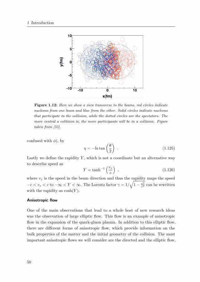
1 Introduction
Figure 1.12: Here we show a view transverse to the beams, red circles indicatenucleons from one beam and blue from the other. Solid circles indicate nucleonsthat participate in the collision, while the dotted circles are the spectators. Themore central a collision is, the more participants will be in a collision. Figuretaken from [55].
confused with φ), by
η = −ln tan(θ
2
). (1.125)
Lastly we define the rapidity Y , which is not a coordinate but an alternative wayto describe speed as
Y = tanh−1(vzc
), (1.126)
where vz is the speed in the beam direction and thus the rapidity maps the speed−c < vz < c to −∞ < Y < ∞. The Lorentz factor γ = 1/
√1 − v2
c2 can be rewrittenwith the rapidity as cosh(Y ).
Anisotropic flow
One of the main observations that lead to a whole host of new research ideaswas the observation of large elliptic flow. This flow is an example of anisotropicflow in the expansion of the quark-gluon plasma. In addition to this elliptic flow,there are different forms of anisotropic flow, which provide information on thebulk properties of the matter and the initial geometry of the collision. The mostimportant anisotropic flows we will consider are the directed and the elliptic flow,
50

1.4 Heavy-Ion Collisions
Figure 1.13: Shown here is the elliptic flow and its time dependence. One can see thecharacteristic elliptic shape of the expansion, which defines elliptic flow. Note that thez-direction is the beam direction, and here the x-axis is defined by the impact parameter.Figure from Ref. [23].
denoted by v1 and v2 respectively. These flow components can be found from aFourier expansion of the differential azimuthal distribution of the particles, givenby
Ed3N
dp3 = 12π
d2N
dpT dY
(1 + 2
∞∑n=1
vn cos[n(φ− ψRP)]), (1.127)
where E is the energy of the particle, p the momentum, pT the transverse momentum,Y the rapidity, φ the azimuthal angle, ψRP the angle with the reaction plane29 andvn are the Fourier coefficients or flow components, defined by
vn = 〈cos[n(φ− ψRP)]〉 , (1.128)
where the brackets define an average over all particles and all events (for a certain(pT ,Y ) bin). As mentioned before, we will look mostly at the first few Fouriercoefficients, called the directed flow, v1, the elliptic flow, v2 and the triangular flowv3. The directed flow is the flow directed along transverse axes with respect to thebeam axis. The elliptic/triangular flow is the elliptic/triangular expansion of theplasma in the transverse plane, the elliptic flow is shown in Figure 1.13.
1.4.3 Electromagnetic fields
In this thesis, we shall be looking at the quark-gluon plasma in the presence of vastelectromagnetic fields. These fields have various origins, which we will study in
29The reaction plane is the plane formed by the collision geometry, and lies in the x and z
directions if we follow the conventions of Figure 1.13
51

1 Introduction
chapter 5. The magnitude of these fields, at LHC, has been estimated to be of ordere| ~B|/m2
π ≈ 10−15 [56]. 30 Our goal is to obtain the influence of the electromagneticfields on the expansion of the QGP and, in particular, the influence on the firstfew flow coefficients. We will approach this by first using a numerical realistichydrodynamic background for the quark-gluon expansion without electromagneticfields. After obtaining the background velocity u, we want to get the velocity ~vcaused by the electromagnetic field. To get this, however, we will need to boost tothe local fluid rest frame where we have ~u′ = 0. In this primed frame (with ~v′), allthe components of ~E′ and ~B′ are non-zero. To compute the velocity ~v′ we will solvethe equation of motion with the Lorentz force law and using stationary currents
md~v′
dt= q ~E′ + q~v′ × ~B′ − µm~v′ = 0 , (1.129)
where m denotes the mass, q the charge, µ is the drag coefficient, and the lastterm denotes the drag force on a fluid element with mass m. Note that the aboveLorentz equation is a non-relativistic equation, which is only applicable in the casethat |~v| << |~u|. We shall see later, chapter 5, that this is a good assumption. Thecalculation of µm for light quarks is not trivial, and it is not exactly analyticallyknown at this moment. We use holographic results from [57]; currently, there areonly precise results known for heavy quarks in the N = 4 SYM theory (which wealso mentioned in subsection 1.2.7)
µm = 12 π
√λT 2 , (1.130)
where λ = g2YM Nc is the t’ Hooft coupling. Here g is the gauge coupling and Nc
the number of colors, see also [58, 59]. We will pick, just as in [56], λ = 6π andfurther assume µm to be constant. Having obtained our four-velocity in the fluidrest frame, we shall boost back to the center of mass frame and obtain V ±µ, thetotal four-velocity. This four-velocity then incorporates the expansion as found bythe hydrodynamic model and the effects due to the electromagnetic field. Withthe four-velocity at hand, we can get the spectra of particles (protons and pions inour case), and by using (1.127) we can compute the different flow components, thedetails of which we will show in the later chapters.
30In units of Tesla, this estimate is of order 1015 T.
52

1.5 This thesis
1.5 This thesis
Although we have mentioned various bits throughout the introduction, let us brieflydiscuss the topics in this thesis. In the first chapter, chapter 2 we will discussblack holes in string theory with duality twists. In particular, we start off using asupergravity setup and then perform Scherk-Schwarz twists (of which the stringcounterpart is called a duality twist). The starting point is Type IIB supergravity,which we then compactify on T 4 × S1, where the compactification on the circleis a Scherk-Schwarz twist. The Scherk-Schwarz twist can, as we will see, breakthe supersymmetry of the supergravity theory. This breaking provides one of theprimary motivations for this research: to study black holes from string theory underthe breaking of supersymmetry. The relevance of this study is clear since thereappears to be no supersymmetry in our universe (at currently accessible energyscales). Thus, we will use black holes, like the ones we created in subsection 1.2.6,and investigate them under the Scherk-Schwarz twists. We will describe the TypeIIB action in an SO(5,5) covariant manner, introduce the relevant Scherk-Schwarztwists, discuss the implications for the black hole solutions, and, finally, describehow the twists can be uplifted to string theory. Certain classes of duality twistscan be alternatively described as orbifolds, which provide a more complete pictureof the duality twists, including all the possible string states.
In the second chapter, chapter 3, we investigate the near-horizons of rotatingsupersymmetric black holes, in particular how we can uplift these to the eleven-dimensional M-theory. The rotating black holes always have some fibered AdS2
structure in the near-horizon, which we also saw in our discussion of the Kerr blackhole in (1.2). We will allow for the most general fibration over the AdS2 and keepa flux configuration that allows for rotating M2-branes. As an example, we willprovide the uplift of the asymptotically AdS4 Kerr-Newman black hole into theclassification. The last part of the chapter concerns the conditions of rotating blackstrings in Type IIB using dualities with the aforementioned eleven-dimensionaltheory.
The third chapter, chapter 4, concerns a generalization of the ‘standard’ SYKmodel that we discussed in section 1.3. Apart from the N Majorana fermions,we also add in M auxiliary bosons; when M = N the model coincides with thesupersymmetric SYK model. The disorder average gets changed in this model,which results in different dynamics. When solving the model with assumptions that
53

1 Introduction
the two-point functions are conformal, similar to what we did in (1.79), we findtwo solutions. Based on their behavior when M/N = 1, we name them ‘rational’and ‘irrational’. Afterward we determine numerically which of these appears to bethe dominant saddle, and lastly, we investigate the chaos of the model using theOTOC correlators.
Finally, in the last chapter, chapter 5, we will study heavy-ion collisions and thequark-gluon plasma, which we introduced in section 1.4. In particular, we willexamine the electromagnetic fields that are present in the heavy-ion collisions andwhat influence they have on the charge-dependent expansion of the quark-gluonplasma, beside its ‘normal’ thermodynamic growth. First, we first numerically modelthe evolution of a cooling droplet in the strongly coupled plasma and subsequentlyadd in the electromagnetic fields. We find that there are charge-odd, parity-odd,contributions to the directed flow v1 and the triangular flow v3, arising due toa combination of Lorentz, Faraday, and Coulomb forces. Furthermore, we finda parity even contribution to the elliptic flow v2, which arises from the plasma’scharged participants. We conclude by analyzing of the influence of parameters usedin the computations.
Conventions
In this thesis we will always use natural units with ~ = c = kb = G = 1 unlessotherwise stated. For metrics we work in the mostly plus convention such thatη = diag(−1, 1, 1, . . . , 1).
54

Part I
Black Holes in String Theory
In this first part there are two chapters, each with a specific focus on black holesolutions. The first chapter, black holes in string theory with duality twists, focusseson black hole solutions in string theory whereby part of the spacetime supersymme-try is broken. We will investigate whether several ten-dimensional brane solutionsare preserved under the supersymmetry breaking compactifications. In the secondchapter we discuss how the near-horizon geometries of rotating black holes can beembedded into M-theory. We will allow for a general AdS2 fibration structure, withfluxes allowing rotating M2-brane setups. As an example, we show how the AdS4
Kerr-Newman black hole fits into the classification.
55


Chapter 2
Black Holes in String Theory with DualityTwists
Of all the conceptions of the human mind from unicorns to gargoyles tothe hydrogen bomb perhaps the most fantastic is the black hole: a hole inspace with a definite edge over which anything can fall and nothing canescape; a hole with a gravitational field so strong that even light is caughtand held in its grip; a hole that curves space and warps time.
– Kip Thorne, Cosmology + 1
In this first chapter we will discuss black holes in the presence of supersymmetrybreaking backgrounds. From a phenomenological point of view this has interest sincethere appears to be no supersymmetry present in our universe at our energy scales.The method we use can in principle be used to break all of the supersymmetry,which could provide insights into creating black hole objects from string theorywhilst simultaneously breaking the supersymmetry. In this work we will mostlyconsider cases where only part of the supersymmetry is broken, as to maintain thevarious advantages of the symmetry, e.g. the stability of the vacuum that we endup in. The set-up we consider will be Type IIB theory on T 4 × S1, whereby thereduction on the circle will be a so-called Scherk-Schwarz reduction, which we willintroduce in section 2.2.1 Since Type IIB is ten-dimensional, our resulting blackholes will live in five dimensions.
In order to study such BPS black holes in five dimensions both macroscopicallyand microscopically, we can use a set-up of the D1-D5-P system in Type IIB string
1We could also have used K3 instead of T 4.
57

2 Black Holes in String Theory with Duality Twists
theory. The black hole can be described as an asymptotically flat three-charge1/8 BPS black hole solution of 5D N = 8 supergravity (or 1/4 BPS in N = 4supergravity). The entropy can be computed microscopically from a 2D (4, 4)CFT dual to the near horizon geometry of the black hole [12]. This system hasU-dual formulations in terms of F1 and NS5-branes, and in terms of intersectingD3-branes.
Black holes in compactifications preserving eight supersymmetries in five dimensionscan be constructed in M-theory on CY3 [60] or in F-theory on CY3 × S1 [61,62]. Inthese cases, the microscopic field theory dual to the black hole horizon geometry is a2D (0, 4) CFT. These CFTs are considerably more complicated than the (4, 4) CFTson the symmetric product of T 4 (or K3) as they have less supersymmetry [12].
In this chapter, we consider a different way to reduce supersymmetry, namelystring compactifications with a duality twist [63], which are the lifts to stringtheory of Scherk-Schwarz reductions in supergravity [64,65]. Such compactificationsallow for partial supersymmetry breaking and include string vacua preserving nosupersymmetry at all (though this won’t be the focus in this work). This gives riseto 5D Minkowski vacua preserving N = 6, 4, 2, 0 supersymmetry. We investigate 5Dsupersymmetric black holes in these theories that lift to 10D systems of branes inthe string theory picture. An important point is that we choose the twist inducingthe supersymmetry breaking to be a duality transformation that leaves the originalsystem of branes invariant, and so the 5D black hole solution of the untwistedtheory remains a solution of the twisted theory. The fields sourcing the system ofbranes are invariant under the twist, so that the fields appearing in the solutionremain massless and the same solution remains as a solution of the twisted theory.This makes it possible to consider the effect of the twist on the corresponding CFTand so to investigate the microscopic aspects of these black holes.
This work is a follow-up to the ideas proposed earlier in [66] in an M-theory settingin which supersymmetry is completely broken. Completely broken supersymmetryis not a well controlled situation, and for that reason we will focus on the twistspreserving some supersymmetry. The current work studies string vacua with partialsupersymmetry breaking and the macroscopic supergravity description of blackholes in such vacua. The microscopic description of the dual CFTs is left for futurestudy.
58

Scherk-Schwarz reduction of supergravity theories has been extensively studiedin the literature; see e.g. [63–65, 67–75] and references therein. IIB supergravitycompactified on T 4 gives maximal N = (2, 2) supergravity in six dimensions whichhas a Spin(5, 5) duality symmetry. The maximal compact subgroup of this globalsymmetry is Spin(5)×Spin(5); we shall refer to this as the R-symmetry group. (Notethat this global R-symmetry should not be confused with the Spin(5)×Spin(5) localsymmetry that is introduced in some formulations of the theory.) The 6D scalarfields take values in the coset Spin(5, 5)/Spin(5) × Spin(5). We will be interestedin the Scherk-Schwarz reduction of this theory to five dimensions, which has beenconsidered previously in [69,70]. This uses ansätze of the type ψ(xµ, z) = g(z)ψ(xµ)where z is the S1 coordinate and g(z) is a local element of Spin(5, 5). On going roundthe circle z → z + 2πR, the fields pick up a monodromy M = g(2πR) ∈ Spin(5, 5).Such a reduction gives a consistent truncation to a 5D gauged supergravity theoryfor the fields ψ(xµ), in which there is a Scherk-Schwarz potential for the scalarfields and mass terms are generated for all fields charged under the monodromy.
If the twist g(z) is compact, i.e. it is an element of the R-symmetry group, thenthe potential is non-negative and has stable five-dimensional Minkowski vacua [63].Such a twist can be specified by four parameters m1,m2,m3,m4 which becomemass parameters in the reduced theory. The amount of supersymmetry that ispreserved in the vacuum depends on the number of parameters mi that are equal tozero: if r of the parameters mi are zero, then N = 2r supersymmetry is preserved.This yields 5D supergravities with N = 8, 6, 4, 2, 0 Minkowski vacua [70] (wherethe case r = 4 is the untwisted reduction to 5D N = 8 supergravity, and the caser = 0 is the twisted reduction that breaks all supersymmetry). This reductionis a straightforward generalization of the Scherk-Schwarz reduction of 5D N = 8supergravity to 4D with four mass parameters and N = 8, 6, 4, 2, 0 vacua [67].
The lift of these supergravity reductions to full compactifications of string theoryinvolves a number of subtle features [63]. These have been worked out in detail forcompactifications of IIA string theory on K3 or the heterotic string on T 4 followedby a reduction on a circle with a duality twist in [74,75]. Here we draw on these andthe results of [63] for our construction, which is IIB string theory compactified onT 4 × S1 with a U-duality twist around the circle. Type IIB on T 4 has a Spin(5, 5)supergravity duality symmetry that, on the level of the full string theory, isbroken to the discrete U-duality subgroup Spin(5, 5;Z) by quantum corrections [22].The moduli space is the scalar coset space Spin(5, 5)/[(Spin(5) × Spin(5))/Z2]
59

2 Black Holes in String Theory with Duality Twists
identified under the action of Spin(5, 5;Z). A key requirement for there to be alift to string theory is that the Scherk-Schwarz monodromy lies in the U-dualitygroup Spin(5, 5;Z), imposing a ‘quantization’ condition on the twist parametersmi [63, 76].
There is still an action of the continuous group Spin(5, 5) on the theory, but onlythe subgroup Spin(5, 5;Z) is a symmetry. Reduction of the theory on a circle witha duality twist introduces a monodromy M which is required to be an element ofSpin(5, 5;Z). If the monodromy acts as a diffeomorphism of T 4, which requires thatit is in a GL(4;Z) subgroup of Spin(5, 5;Z), then this corresponds to compactificationof the IIB string on a T 4 bundle over S1. If the monodromy acts as a T-duality ofT 4, which requires that it is in an SO(4, 4;Z) subgroup of Spin(5, 5;Z), then thisconstructs a T-fold background, while for general U-duality monodromies this is aU-fold [77].
A point in the scalar coset will be a minimum of the scalar potential giving astable Minkowski vacuum if and only if it is a fixed point under the action ofthe monodromy M ∈ Spin(5, 5;Z) [63]. The monodromy will then generate a Zpsubgroup of Spin(5, 5;Z) for some integer p. Furthermore, at this critical point theconstruction becomes a Zp generalized orbifold of IIB string theory on T 5, wherethe theory is quotiented by the Zp generated by M acting on the IIB string on T 4
combined with a shift by 2πR/p on the circle. When the monodromy is a T-duality,this is a Zp asymmetric orbifold.
Regarded as an element of Spin(5, 5), the monodromy is conjugate to an R-symmetrytransformation: M = kRk−1 for some R ∈ Spin(5)×Spin(5) and k ∈ Spin(5, 5) [63].The rotation R conjugate to a given monodromy is specified by four angles, whichare given by the four parameters mi. For N = 2 supersymmetry to be preserved,one of the parameters must be zero so that R in fact lies in an SU(2) × Spin(5)subgroup. For N = 4 supersymmetry to be preserved, two of the parameters mustbe zero so that R lies either in a Spin(5) subgroup or a SU(2) × SU(2) subgroup(with one SU(2) factor in each Spin(5)). These two options lead to theories thathave the same massless sector, but differ in their massive sectors. We use thenotation (0, 2) and (1, 1) to distinguish these two N = 4 theories, reflecting whetherthe massive states are in (0, 2) or (1, 1) BPS supermultiplets, using the terminologyof [78]. Lastly, for N = 6 supersymmetry to be preserved, three of the parametersmust be zero so that R lies in an SU(2) subgroup of the R-symmetry.
60

As mentioned above, if M is a perturbative symmetry (i.e. a T-duality) inSpin(4, 4;Z), the theory in the Minkowski vacuum is an asymmetric orbifold. Ingeneral this will not be modular invariant, and further modifications are neededto achieve modular invariance. For perturbative monodromies, the shift in thecircle coordinate z must be accompanied by a shift in the coordinate of the T-dualcircle [75, 79, 80]. Put differently, the quotient introduces phases dependent onboth the momentum and the winding number on the circle, and on the chargesof the state under the action of M [75]. For non-perturbative monodromies, thearguments of [75,81] lead to phases dependent on other brane wrapping numbers.
Quantum effects can lead to corrections to the coefficients of the five-dimensionalChern-Simons terms A ∧ F ∧ F at the two-derivative level and A ∧R ∧R at thefour-derivative level. There have been indications in the literature (see e.g. [82])that the A ∧ R ∧ R term can be supersymmetrized in the N = 4 (0, 2) theorybut not in the N = 4 (1, 1) theory, nor in the N = 6 theory. In the N = 2theory the supersymmetrization is known [83]. Our results are in agreement withthese claims. That is, we find corrections only in the cases where supersymmetricChern-Simons terms are expected. The corrections to the Chern-Simons coefficientsmodify the black hole solutions in supergravity [84, 85] and therefore also theentropy. We compute the quantum corrections to the Chern-Simons coefficients andthe resulting modifications to the black hole entropies from supergravity and theKaluza-Klein modes from the circle compactification, using results in the literaturefor 5D N = 2 supergravity [84,85]. Similar calculations have been done in differentsetups, see [86,87].
As a by-product of our analysis, we present in detail the supergravity reductionof type IIB on T 4. While the general techniques and results are known in theliterature [88], the explicit relation between the 10D and 6D fields has not beengiven, to the best of our knowledge. We present this calculation in section 2.1;the results are relevant for understanding which black holes survive which twist insubsequent sections.
In section 2.2, we perform the Scherk-Schwarz reduction to five dimensions, startingfrom the maximally supersymmetric 6D (2, 2) supergravity. We construct massmatrices and decompose the 5D field content into massless and massive multiplets.By simply truncating to the massless sector, we can embed known BPS black holesin these five dimensional theories. In section 2.3, we work out which choices of
61

2 Black Holes in String Theory with Duality Twists
Scherk-Schwarz twist preserve the D1-D5-P black hole, the F1-NS5-P black holeand the D3-D3-P black hole. By tuning the mass parameters, we can find twiststhat preserve more than one black hole solution (e.g. we find the twists thatpreserve both the D1-D5-P and the F1-NS5-P black holes). In section 2.4, we studyone-loop effects by integrating out the massive fields. We compute the correctionsto the Chern-Simons terms and to the entropy of 5D BPS black holes. Finally, insection 2.5, we discuss how to embed our supergravity model in string theory anddiscuss the quantization conditions on the parameters mi of the twist.
2.1 Duality invariant formulation of IIB supergravity on afour-torus
Reducing type IIB supergravity on a four-torus gives six-dimensional maximalsupergravity. This theory has N = (2, 2) supersymmetry and a Spin(5, 5) dualitysymmetry group. The goal of this section is to write this supergravity theory ina form in which both the type IIB origin of the six-dimensional fields and theSpin(5, 5) symmetry are manifest. We do this explicitly for the scalar and tensorfields.
2.1.1 Ansätze for reduction to 6D
We start from type IIB supergravity. Written in Einstein frame, the bosonic termsin the Lagrangian read
LIIB =(R(10) − 1
2 |dΦ|2 − 12 e
−Φ ∣∣H(10)3∣∣2 − 1
2 e2Φ |da|2 − 1
2 eΦ ∣∣F (10)
3∣∣2
−14∣∣F (10)
5∣∣2) ∗ 1 − 1
2 C(10)4 ∧H
(10)3 ∧ F
(10)3 ,
(2.1)
where the field strengths are given by
H(10)3 = dB(10)
2 ,
F(10)3 = dC(10)
2 − adB(10)2 ,
F(10)5 = dC(10)
4 − 12C
(10)2 ∧ dB(10)
2 + 12B
(10)2 ∧ dC(10)
2 .
(2.2)
62

2.1 Duality invariant formulation of IIB supergravity on a four-torus
The superscripts (10) indicate that the fields live in 10 dimensions. The fieldequations are supplemented by the self-duality constraint
F(10)5 = ∗F (10)
5 . (2.3)
In our compactification to six dimensions, the coordinates split up as XM = (xµ, ym)with M = 0, . . . , 9, µ = 0, . . . , 5 and m = 1, . . . , 4. We now present the ansätze thatwe use in our reduction. In order to arrive in Einstein frame in 6D, we decomposethe ten-dimensional metric as
gMN =
g−1/44 gµν + gmn Am
µ Anν gmn Am
µ
gmn Anν gmn
, (2.4)
where g4 = det(gmn). The compact part of the metric, gmn, we parametrize interms of scalar fields φi (i = 1, . . . , 4) and Amn (m < n) by
gmn =
e~bm·~φ +
∑k<m
e~bk·~φ (Akm)2 for m = n
e~bm·~φAmn +
∑k<m
e~bk·~φAkmAkn for m < n
gnm for m > n .
(2.5)
Here ~φ = (φ1, φ2, φ3, φ4) and the vectors ~bm are given by
~b1 = (− 1√2 ,−
1√2 ,−
1√2 ,
12 ) ,
~b2 = (− 1√2 ,
1√2 ,
1√2 ,
12 ) ,
~b3 = ( 1√2 ,
1√2 ,−
1√2 ,
12 ) ,
~b4 = ( 1√2 ,−
1√2 ,
1√2 ,
12 ) .
(2.6)
From this, it can be computed that g4 = e2φ4 , so the scalar φ4 parametrizes thevolume of the T 4.
We reduce the 10D form-valued fields by simply splitting into components withdifferent numbers of indices on the torus. For example, the Kalb-Ramond field
63

2 Black Holes in String Theory with Duality Twists
B(10)2 decomposes as
B(10)2 = 1
2 BMN dXM ∧ dXN
= 12 Bµν dxµ ∧ dxν +Bµm dxµ ∧ dym + 1
2 Bmn dym ∧ dyn
= B(6)2 +B
(6)1,m ∧ dym + 1
2 Bmn dym ∧ dyn ,
(2.7)
where B(6)2 , B(6)
1,m and Bmn are 2, 1 and 0-forms defined on the six-dimensionalnon-compact space. The ten-dimensional scalars are simply equal to their six-dimensional descendants, e.g. Φ(10) = Φ(6) = Φ. For this reason, we usually dropthe superscript (D) for scalar fields.
Reduction of the self-dual five-form field strength
To find the fields that descend from the RR four-form C(10)4 we need to be a bit
careful, since it has a self-dual field strength: ∗F (10)5 = F
(10)5 . Because of this
self-duality, the action (2.1) does not properly describe the dynamics of the RRfour-form. So instead of reducing the action, we should reduce the correspondingfield equations along with the self-duality constraint. The action (2.1) with fieldstrengths (2.2) yields the following equation of motion and Bianchi identity
d(∗ F (10)
5)
= dB(10)2 ∧ dC(10)
2 , (2.8)
dF (10)5 = dB(10)
2 ∧ dC(10)2 . (2.9)
We see that, because of the self-duality of F (10)5 , these two equations are identical,
so we only have to reduce one of them. In what follows, we choose to reduce theBianchi identity (2.9). Subsequently, we reduce the self-duality equation and use itto rewrite the six-dimensional Bianchi identities to a system of Bianchi identitiesand equations of motion. By integrating this system of equations to an action, wefind the proper result of the reduction of C(10)
4 . Below, we work out this reductionin detail for the scalars and the two-forms.
First, we consider the scalars. In 6D, massless four-forms can be dualized to scalars,so we need to consider the components of F (10)
5 that have either zero or four legs onthe torus. The Bianchi identities for these components following from (2.9) read
dP (6)1 = 1
2! 2! εmnpq dBmn ∧ dCpq ,
dP (6)5 = dB(6)
2 ∧ dC(6)2 .
(2.10)
64

2.1 Duality invariant formulation of IIB supergravity on a four-torus
Here we have introduced the notation P(6)1 = 1
4! εmnpq F
(6)1,mnpq and P
(6)5 = F
(6)5 .
Next, we write down the relevant components that follow from the reduction of theself-duality constraint. By using the metric ansatz (2.4), and ignoring interactionswith the graviphotons Am
µ , we find
P(6)5 = 1
g4∗ P (6)
1 . (2.11)
We now use this constraint to eliminate P (6)5 from (2.10). In this way, we find the
following Bianchi identity and equation of motion for the one-form field strengthP
(6)1
dP (6)1 = 1
2! 2! εmnpq dBmn ∧ dCpq ,
d(e−2φ4 ∗ P (6)
1)
= dB(6)2 ∧ dC(6)
2 .
(2.12)
From the first equation, we can find an expression for P (6)1 in terms of the corre-
sponding scalar field that we denote by b. The second equation can be integrated toan action that contains both the kinetic term for b and interaction terms betweenb and other scalar and two-forms fields. These expressions can be found in (2.16)and (2.17).
Next, we look at the two-forms coming from C(10)4 . We are interested in the action
for the six-dimensional two-form fields and their interactions with scalar fields. Wewill ignore interactions with six-dimensional one-forms. The relevant componentsthat follow from the reduction of (2.9) read
dF (6)3,mn = dBmn ∧ dC(6)
2 + dB(6)2 ∧ dCmn
= d(Bmn dC(6)
2 − Cmn dB(6)2).
(2.13)
These are Bianchi identities for six tensors in six dimensions. We want to eliminatehalf of these fields in exchange for equations of motion for the residual ones. Wechoose to retain the components F (6)
3,mn for mn = 12, 13, 14 and to eliminate theones with indices mn = 23, 24, 34. For this, we again use the reduced self-dualityconstraint. The relevant components are
F(6)3,mn = 1
2√g4 εmnpq g
prgqs ∗ F (6)3,rs . (2.14)
Due to the summations over the r and s indices, each component of this equationcontains a linear combination of all the dual field strengths ∗F (6)
3,rs (recall that the
65

2 Black Holes in String Theory with Duality Twists
metric on T 4 is given by (2.5)). Consequently, solving (2.14) for three of the sixfield strengths results in unwieldy expressions. We choose not to write down theseexpressions here, but instead to give a step-by-step outline of the way we use themto find an action for the 6D tensors.
First, we introduce a new notation for the field strengths that we plan on retaining:P
(6)3; 1 = F
(6)3,12, P (6)
3; 2 = F(6)3,14 and P
(6)3; 3 = F
(6)3,13. Here the first subscript indicates
that these are three-forms, and the second subscript labels the three distinct fieldstrengths (we will sometimes drop this label when we are talking about all threeof them). The expressions for these field strengths in terms of the correspondingtwo-form fields can be deduced from (2.13). For example,
P(6)3; 1 = dR(6)
2; 1 +B12 dC(6)2 − C12 dB(6)
2 , (2.15)
where R(6)2; 1 is then one of the two-forms that arise from compactifying the ten-
dimensional 4-form. Similar expressions can be found for P (6)3; 2 and P (6)
3; 3 in terms offields that we call R(6)
2; 2 and R(6)2; 3 respectively.
Next, we solve the six equations in (2.14) for F (6)3,mn and ∗F (6)
3,mn (for mn = 23, 24, 34)in terms of the field strengths P (6)
3 and their duals ∗P (6)3 . By substituting these
expressions in the components of (2.13) for mn = 23, 24, 34, we find the equationsof motion for the tensor fields R(6)
2 purely in terms of the (dual) field strengthsP
(6)3 and ∗P (6)
3 , and fields that don’t descend from the RR four-form C(10)4 . These
field equations are quite unwieldy, but with some careful bookkeeping they canbe integrated to an action. We will not write down this awkward version ofthe action here. Instead, we write down a more elegant version of the actionfor the six-dimensional tensor fields and their interactions with scalar fields insubsection 2.1.3.
2.1.2 6D scalars
The field content of maximal six-dimensional supergravity contains 25 scalars. Interms of their origin in type IIB, these are Φ, φi, Amn, Bmn, Cmn, a and b. Wefind the action for these scalar fields by using the methods and ansätze describedin the previous section. This yields
e−1(6) Ls = − 1
2 |dΦ|2 − 14 |dφ4|2 − 1
2 |dgmn|2 − 12 e
−Φ ∣∣H(6)1,mn
∣∣2− 1
2 e2Φ |da|2 − 1
2 eΦ ∣∣F (6)
1,mn∣∣2 − 1
2 e−2φ4
∣∣P (6)1∣∣2 . (2.16)
66

2.1 Duality invariant formulation of IIB supergravity on a four-torus
Note that the absolute values apply both to the 6D Lorentz indices and to the indiceson the torus. For example, |H(6)
1,mn|2 = 12! HµmnH
µmn = 12! Hµmn g
mpH µpq g
pn. Thefield strengths in (2.16) are given by
H(6)1,mn = dBmn ,
F(6)1,mn = dCmn − adBmn , (2.17)
P(6)1 = db+ 1
8 εmnpq (Bmn dCpq − Cmn dBpq) .
These 25 scalar fields together parametrize the coset Spin(5, 5)/(Spin(5) × Spin(5))[88]. The action above has a global Spin(5, 5) and a local Spin(5)×Spin(5) symmetry.In its current form, these symmetries are not visible, so we will now write thisaction in a form that makes both symmetries manifest.
In order to do this, we construct a generalized vielbein (or coset representative) Vfrom the scalar fields. This vielbein is an element of Spin(5, 5) and it transforms asV → U V W (x), with U ∈ Spin(5, 5) and W (x) ∈ Spin(5) × Spin(5). We now definethe Spin(5) × Spin(5) invariant field H = V VT , that transforms as H → U HUT
under global Spin(5, 5) transformations2. We can now write the scalar Lagrangianin terms of H as
e−1(6) Ls = 1
8 Tr[∂µH−1∂µH
]. (2.18)
In this formulation, the Lagrangian is manifestly invariant under the U-dualitygroup Spin(5, 5).
We now specify the way we build V from the 25 scalar fields so that the twoLagrangians (2.16) and (2.18) are equal to one another. We choose to buildV ∈ Spin(5, 5) in τ -frame, i.e. it satisfies VT τ V = τ (for the definition of τ , seeAppendix 2.B.1). The exact construction is as follows:
V = exp[b T b
]× exp
[ ∑1≤m<n≤4
(Bmn T
Bmn + Cmn T
Cmn
)]× exp
[aT a
]×( ∏
1≤m<n≤4exp
[Amn T
Amn
])× exp
[ΦH0 +
4∑i=1
φiHi
].
(2.19)
2In this section we suppress Spin(5, 5) indices, but we will need them later on. With indices, H iswritten as HAB and it transforms as HAB → U C
A HCD
(UT)D
B. The inverse of H is written
with upper indices: H−1 = HAB .
67

2 Black Holes in String Theory with Duality Twists
Here the T ’s and the H’s are generators of so(5, 5) that span the subspace of so(5, 5)that generates the coset Spin(5, 5)/(Spin(5) × Spin(5)). The precise expressions forthese generators are given in Appendix 2.B.1. All the scalar fields appear underthe same name as in (2.16).
Because we construct our vielbein (2.19) in τ -frame3, the transformation matricesU and W are also written in τ -frame. Henceforth, we use this frame wheneverSpin(5, 5) and Spin(5) × Spin(5) groups appear (unless mentioned otherwise).
2.1.3 6D tensors
The field content of maximal supergravity in six dimensions contains five 2-formtensor gauge fields. Collectively, we denote these fields by A(6)
2,a (a = 1, . . . , 5), andtheir field strengths by G(6)
3,a = dA(6)2,a. The Lagrangian for these fields reads [88, 89]
Lt = −12 K
abG(6)3,a ∧ ∗G(6)
3,b − 12 L
abG(6)3,a ∧G
(6)3,b . (2.20)
Here Kab and Lab are functions of the scalar fields. We define a set of dual fieldstrengths G(6)a
3 = Kab ∗G(6)3,b +LabG
(6)3,b so that we can write the Lagrangian in the
more compact formLt = −1
2 G(6)3,a ∧ G
(6)a3 . (2.21)
In this notation, we write the Bianchi identities and the equations of motion asdG(6)
3,a = 0 and dG(6)a3 = 0. We can combine these in the more compact notation
dG(6)3,A = 0, where G(6)
3,A is defined as
G(6)3,A =
(G
(6)3,a
G(6)a3
). (2.22)
The Spin(5, 5) duality symmetry acts on this ten-component vector as
G(6)3,A → U B
A G(6)3,B , U B
A ∈ Spin(5, 5) . (2.23)
Only the subgroup GL(5) ⊂ Spin(5, 5) is a symmetry of the action. The fullsymmetry group is only manifest on the level of the field equations.
3For the convenience of the reader, it might be useful to mention how this convention is relatedto those of other authors. The following relations hold: V = X U[Tanii]X where U[Tanii] is thevielbein that is used in [88], and V = V[BSS]X where V[BSS] is the vielbein that is used in [89].The matrix X is a conjugation matrix that is defined in Appendix 2.B.1.
68

2.1 Duality invariant formulation of IIB supergravity on a four-torus
When we decompose our coset representative in 5 × 5 blocks as V =(a bc d
), we can
write the matrices Kab and Lab as
K = 12 ((c+ d)(a+ b)−1 − (c− d)(a− b)−1) ,
L = 12 ((c+ d)(a+ b)−1 + (c− d)(a− b)−1) .
(2.24)
Now, by making the identification
A(6)2,a =
(R
(6)2; 1 , R
(6)2; 2 , R
(6)2; 3 , C
(6)2 , −B(6)
2), (2.25)
the Lagrangian (2.21) is exactly equal to the one that we find by explicit reductionfrom type IIB supergravity using the ansätze given in subsection 2.1.1. Theadvantage of (2.21) is that we have made the duality symmetry manifest.
Doubled formalism
It is a common feature of supergravity actions in even dimensions that only asubgroup of the duality group is a symmetry of the action. In such cases, onecan use the so-called doubled formalism [90] to construct an action that realizesthe full symmetry group. In order to do this, one needs to introduce twice theoriginal amount of form-valued fields as well as a constraint that makes sure thatthe doubled theory does not contain more degrees of freedom than the originaltheory.
We apply this formalism to our 6D tensor fields. We promote the G(6)a3 to field
strengths that correspond to the doubled fields, i.e. we write them as G(6)a3 = dA(6)a
2 .These doubled fields A(6)a
2 are now treated as independent fields. We write downthe doubled Lagrangian as
L(doubled)t = −1
4 HAB G(6)3,A ∧ ∗G(6)
3,B . (2.26)
In this formulation we have ten field strengths G(6)3,A that satisfy the Bianchi identities
dG(6)3,A = 0 and the equations of motion d
(HAB ∗ G(6)
3,B)
= 0. Furthermore, thesefields are subject to the self-duality constraint
G(6)3,A = τAB HBC ∗G(6)
3,C . (2.27)
By imposing this constraint on the field equations, we see that they reduce tothe ones that correspond to the undoubled action. Thus we have found a proper
69

2 Black Holes in String Theory with Duality Twists
doubled version of (2.21). Both the action (2.26) and the constraint (2.27) areinvariant under the full Spin(5, 5) duality group. This can be seen directly fromthe way that these transformations work on the fields:
HAB →(U−T )A
CHCD
(U−1) B
D, G
(6)3,A → U B
A G(6)3,B , (2.28)
where U BA ∈ Spin(5, 5) and we use the notation U−T = (U−1)T .
2.2 Scherk-Schwarz reduction to five dimensions
In a Scherk-Schwarz reduction, one considers a (D + 1)-dimensional supergravitytheory with a global symmetry given by a Lie group G that is compactified to Ddimensions. The difference between ‘ordinary’ Kaluza-Klein and Scherk-Schwarzreduction lies in the compactification ansatz. Consider a field ψ in the (D + 1)-dimensional theory that transforms as ψ → gψ with g ∈ G (for scalars, this istypically a non-linear realization, while some fields such as the metric in Einsteinframe will be invariant). The Scherk-Schwarz ansatz then gives ψ a dependence onthe coordinate z on the circle, which has periodicity z ' z + 2πR, given by
ψ(xµ, z) = exp(Mz
2πR
)ψ(xµ) , (2.29)
where M lies in the Lie algebra of G. This ansatz is not periodic around the circle,but picks up a monodromy M = eM ∈ G. The Lie algebra element M is sometimescalled the mass matrix because it appears in mass terms in the D-dimensionaltheory. For more details, see [63–65,67–75,91] and references therein. A conjugatemass matrix
M ′ = gMg−1 , (2.30)
with g ∈ G, gives a conjugate monodromy
M′ = gMg−1 . (2.31)
This conjugated monodromy gives a massive theory that is related to the one forthe monodromy M by a field redefinition, so that it defines an equivalent theory.Thus the possible Scherk-Schwarz reductions are classified by the conjugacy classesof the duality group [63].
In our case, we reduce from 6D to 5D on a circle with a Scherk-Schwarz twist. Wedenote the coordinates on the five-dimensional Minkowski space by xµ and the
70

2.2 Scherk-Schwarz reduction to five dimensions
coordinate on the circle by z. The compact coordinate is periodic with periodicityz ' z + 2πR. The metric (in Einstein frame) is inert under the duality group, sowe choose the conventional Kaluza-Klein metric ansatz:
gµν =
e−√
1/6φ5 gµν + e√
3/2φ5 A5µA5
ν e√
3/2φ5 A5µ
e√
3/2φ5 A5ν e
√3/2φ5
. (2.32)
The factors in the exponents are chosen so that we arrive in Einstein frame in fivedimensions and the scalar field φ5 is canonically normalized [92].
The result of our reduction is a gauged N = 8 supergravity theory in five dimensionsin which a non-semi-simple subgroup of Spin(5, 5) is gauged. The gauge groupcontains an important U(1) subgroup for which A5
µ is the corresponding gauge field.For each twist, the theory has a vacuum (partially) breaking the supersymmetrywhere it can be described by an N < 8 effective field theory. This reduction from6D to 5D has been considered previously in [69,70]. An important feature is thatreducing self-dual 2-form gauge fields in 6D can result in massive self-dual 2-formfields in 5D [69]. See [72,91] for further details.
2.2.1 Monodromies and masses
In six dimensions the global symmetry is G = Spin(5, 5), so in principle we canchoose the mass matrix to be any element of the Lie algebra of G. However, ourgoal is to obtain a Minkowski vacuum with partially broken supersymmetry, so, asdiscussed in the introduction, we restrict our twist to be conjugate to an element ofthe R-symmetry group
USp(4)L × USp(4)R = Spin(5)L × Spin(5)R , (2.33)
that preserves the identity in Spin(5, 5). We take then a monodromy
M = gMg−1 , g ∈ Spin(5, 5) , M ∈ USp(4)L × USp(4)R ⊂ Spin(5, 5) . (2.34)
By a further conjugation, we can bring M to an element M of a maximal torusT = U(1)4 of the R-symmetry group USp(4)L × USp(4)R
M = hMh−1 , h ∈ USp(4)L × USp(4)R , M ∈ T ⊂ USp(4)L × USp(4)R . (2.35)
The element M of a maximal torus T = U(1)4 is then specified by four angles,which we denote m1,m2,m3,m4; we take 0 ≤ mi < 2π. Writing
M = (Musp(4)L ,Musp(4)
R ) , Musp(4)L/R ∈ USp(4)L/R , (2.36)
71

2 Black Holes in String Theory with Duality Twists
we can take the monodromies to be in the SU(2) × SU(2) subgroup of USp(4) forboth the left and right factors (note that SU(2) ∼= USp(2)):
SU(2)L1× SU(2)L2
× SU(2)R1× SU(2)R2
⊂ USp(4)L × USp(4)R . (2.37)
We can then take, for example,
Musp(4)L = em1σ3 ⊗ em2σ3 , Musp(4)
R = em3σ3 ⊗ em4σ3 , (2.38)
where σ3 is the usual Pauli matrix. Other choices of the monodromy are related tothis by USp(4)L × USp(4)R conjugation.
The six-dimensional supergravity fields fit into the following representations underthe R-symmetry group (see e.g. [70,88]):
scalars : (5,5) ,
vectors : (4,4) ,
tensors : (5,1) + (1,5) ,
gravitini : (4,1) + (1,4) ,
dilatini : (5,4) + (4,5) .
(2.39)
We have an equal number of self-dual and anti-self-dual 2-form tensor fields, andan equal number of fermions of positive and negative chirality. In terms of theR-symmetry representations above, the self-dual tensors B+
2 transform in the (5,1)and the anti-self-dual tensors B−
2 transform in the (1,5). The positive chiralgravitini ψ+
µ and dilatini χ+ transform in the (4,1) and (5,4) respectively, and thenegative chiral gravitini ψ−
µ and dilatini χ− transform in the (1,4) and (4,5).
These representations determine the charges (e1, e2, e3, e4) of each field underU(1)4 ⊂ USp(4)L × USp(4)R. A field with charges (e1, e2, e3, e4) will then be aneigenvector of the mass matrix with eigenvalue iµ and will have z-dependenceeiµz/2πR where
µ =4∑i=1
eimi . (2.40)
The resulting mass for the field will turn out to be |µ|/2πR.
72
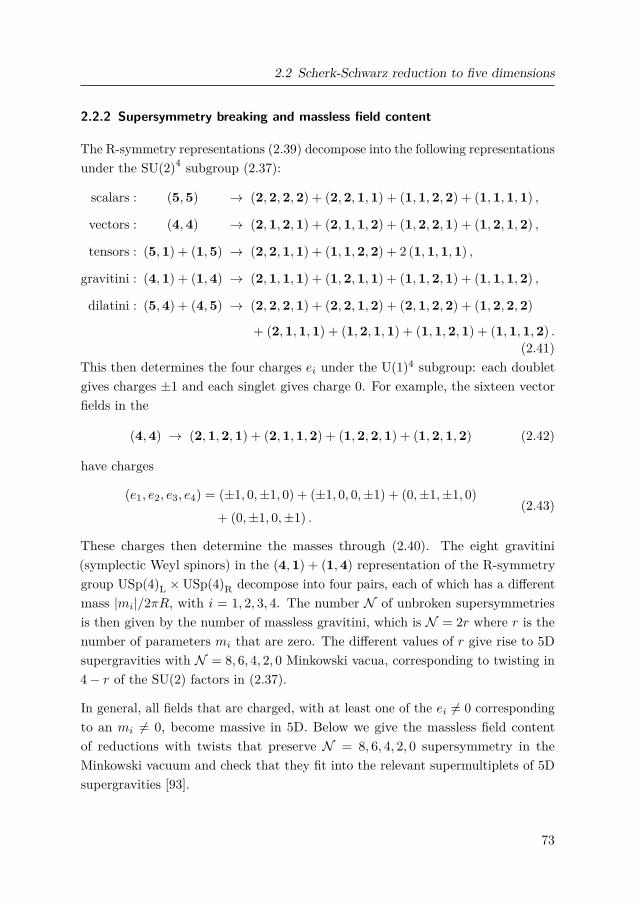
2.2 Scherk-Schwarz reduction to five dimensions
2.2.2 Supersymmetry breaking and massless field content
The R-symmetry representations (2.39) decompose into the following representationsunder the SU(2)4 subgroup (2.37):
scalars : (5,5) → (2,2,2,2) + (2,2,1,1) + (1,1,2,2) + (1,1,1,1) ,
vectors : (4,4) → (2,1,2,1) + (2,1,1,2) + (1,2,2,1) + (1,2,1,2) ,
tensors : (5,1) + (1,5) → (2,2,1,1) + (1,1,2,2) + 2 (1,1,1,1) ,
gravitini : (4,1) + (1,4) → (2,1,1,1) + (1,2,1,1) + (1,1,2,1) + (1,1,1,2) ,
dilatini : (5,4) + (4,5) → (2,2,2,1) + (2,2,1,2) + (2,1,2,2) + (1,2,2,2)
+ (2,1,1,1) + (1,2,1,1) + (1,1,2,1) + (1,1,1,2) .(2.41)
This then determines the four charges ei under the U(1)4 subgroup: each doubletgives charges ±1 and each singlet gives charge 0. For example, the sixteen vectorfields in the
(4,4) → (2,1,2,1) + (2,1,1,2) + (1,2,2,1) + (1,2,1,2) (2.42)
have charges
(e1, e2, e3, e4) = (±1, 0,±1, 0) + (±1, 0, 0,±1) + (0,±1,±1, 0)
+ (0,±1, 0,±1) .(2.43)
These charges then determine the masses through (2.40). The eight gravitini(symplectic Weyl spinors) in the (4,1) + (1,4) representation of the R-symmetrygroup USp(4)L × USp(4)R decompose into four pairs, each of which has a differentmass |mi|/2πR, with i = 1, 2, 3, 4. The number N of unbroken supersymmetriesis then given by the number of massless gravitini, which is N = 2r where r is thenumber of parameters mi that are zero. The different values of r give rise to 5Dsupergravities with N = 8, 6, 4, 2, 0 Minkowski vacua, corresponding to twisting in4 − r of the SU(2) factors in (2.37).
In general, all fields that are charged, with at least one of the ei 6= 0 correspondingto an mi 6= 0, become massive in 5D. Below we give the massless field contentof reductions with twists that preserve N = 8, 6, 4, 2, 0 supersymmetry in theMinkowski vacuum and check that they fit into the relevant supermultiplets of 5Dsupergravities [93].
73

2 Black Holes in String Theory with Duality Twists
• N = 8
We start with the untwisted case, mi = 0, where all fields remain massless.Apart from the 5D graviton, the spectrum contains 8 gravitini, 27 vectors,48 dilatini and 42 scalars (all massless). As expected, these fields make up asingle gravity multiplet of maximal 5D supergravity.
• N = 6
In order to end up with N = 6 supergravity, we take only one of the fourmass parameters to be non-zero so that we twist in only one of the four SU(2)subgroups. The massless spectrum from such a reduction contains a graviton,6 gravitini, 15 vectors, 20 dilatini and 14 scalars. These fields form the gravitymultiplet of the N = 6 theory.
• N = 4
We obtain N = 4 supergravity by twisting in two SU(2) groups, with two massparameters zero. This can be done in two qualitatively different ways: eitherwith a chiral twist, say in SU(2)R1
and SU(2)R2with m1 = m2 = 0, or with
a non-chiral twist, for example in SU(2)L2and SU(2)R2
with m1 = m3 = 0.Both types of twists result in the same massless spectrum: the graviton, 4gravitini, 7 vectors, 8 dilatini and 6 scalars, although as we shall see, theyresult in different massive spectra.
In the N = 4 theory, the gravity multiplet contains the graviton, 4 gravitini,6 vectors, 4 dilatini and a single scalar field, and the vector multiplet contains1 vector, 4 dilatini and 5 scalars [94]. We see that our massless spectrumconsists of the gravity multiplet coupled to one vector multiplet.
• N = 2
We end up with minimal 5D supergravity by twisting in three of the fourSU(2) subgroups, with just one of the mass parameters zero. The masslessfield content after such a twist contains the graviton, 2 gravitini, 3 vectors, 4dilatini and 2 scalars.
For N = 2 supersymmetry, the gravity multiplet contains the graviton, 2gravitini, and 1 vector field, and the vector multiplet contains 1 vector, 2
74

2.2 Scherk-Schwarz reduction to five dimensions
dilatini and 1 scalar field. Thus, the field content that we find from thisreduction forms a gravity multiplet coupled to two vector multiplets.
• N = 0
By twisting in all four SU(2) groups, with all four mass parameters non-zero,we break all supersymmetry. The only fields that are not charged under sucha twist are the graviton and the singlets which are completely uncharged, withall ei = 0. As a result, the massless spectrum in 5D consists of the graviton,3 vectors and 2 scalars. Note that all fermions become massive.
2.2.3 Massive field content
The charges (e1, e2, e3, e4) following from (2.41) determine the massive spectrum forthe reduced theory in five dimensions. This spectrum is summarized in Table 2.1.The spectrum of Table 2.1 has been previously derived from Scherk-Schwarz reduc-tion in [70] and corresponds to a gauging of N = 8 five-dimensional supergravity.
We now give the supermultiplet structure of the massive spectra that follow from thevarious twists preserving different amounts of supersymmetry. All fields that acquiremass also become charged under the graviphoton A5
1 with covariant derivatives ofthe form
Dµ = ∂µ − iq gA5µ . (2.44)
Here the gauge coupling is g = 1/R, and the charge q of each 5D field is equalto 1/g = R times its mass. Because the massive fields are charged, the real fieldsthat follow from the reduction have to combine into complex fields. In the spectrathat we give below, we list the number of complex fields (unless stated otherwise).Furthermore, when we give the mass of a field or collection of fields we only writedown |µ|. In order to find the actual mass, this needs to be divided by 2πR.
The massive multiplets we find are all BPS multiplets in five dimensions; thesemultiplets were analyzed and classified in [78] and are labeled by two integers(p, q). For N supersymmetries in five dimensions (with N even), the R-symmetryis USp(N ). For a (p, q) massive multiplet, the choice of central charge breaksthe R-symmetry to a subgroup USp(2p) × USp(2q), i.e. the subgroup of USp(N )preserving the central charge, where 2p+ 2q = N . The nomenclature was chosensuch that a massless supermultiplet of (p, q) supersymmetry in six-dimensionshas, after reducing on a circle, Kaluza-Klein modes that fit into (p, q) massive
75

2 Black Holes in String Theory with Duality Twists
Fields Representation |µ| = Mass (multiplied by 2πR)
Scalars (5,5)∣∣±m1 ±m2 ±m3 ±m4
∣∣∣∣±m1 ±m2∣∣∣∣±m3 ±m4∣∣
0
Vectors (4,4)∣∣±m1,2 ±m3,4
∣∣Tensors (5,1)
∣∣±m1 ±m2∣∣ , 0
(1,5)∣∣±m3 ±m4
∣∣ , 0
Gravitini (4,1)∣∣±m1,2
∣∣(1,4)
∣∣±m3,4∣∣
Dilatini (5,4)∣∣±m1 ±m2 ±m3,4
∣∣∣∣±m3,4∣∣
(4,5)∣∣±m1,2 ±m3 ±m4
∣∣∣∣±m1,2∣∣
Table 2.1: This table gives the value of |µ(mi)| for the 5D fields coming fromthe different types of 6D fields. The mass of the field is then |µ(mi)|/2πR. Thenotation mi,j indicates that both mi and mj occur. There is no correlationbetween the ± signs and the ij indices, so that e.g. (±m1 ± m2) denotes 4different combinations of mass parameters, and (±m1,2 ± m3,4) denotes 16different combinations. For example, the 5 tensors in the (5,1) representationconsist of two with mass |m1 +m2| , two with mass |m1 −m2| and one with mass0.
supermultiplets in five dimensions. The physical states of a (p, q) massive multipletin five dimensions then fit into representations of
SU(2) × SU(2) × USp(2p) × USp(2q) , (2.45)
where SU(2) × SU(2) ∼ SO(4) is the little group for massive representations infive dimensions. The representations of the little group SU(2) × SU(2) that ariseinclude (3, 2) and (2, 3) for massive gravitini and (2, 2) for massive vector fields.
76

2.2 Scherk-Schwarz reduction to five dimensions
The representation (3, 1) corresponds to a massive self-dual two-form field satisfyingthe five-dimensional duality condition
dB2 = −im ∗B2 , (2.46)
while the (1, 3) representation corresponds to the anti-self dual case with dB2 =im ∗ B2. In the following, we consider the cases in which the Scherk-Schwarzreduction breaks the supersymmetry to N = 6, 4, 2. The massless states are in theN supersymmetry representations given in the previous subsection, and we nowgive the N supersymmetry representations of the massive fields. It was alreadypointed out in subsection 2.2.2 that there are two qualitatively different twists thatresult in a theory with N = 4 supersymmetry: a chiral one and a non-chiral one.Both theories have the same massless spectrum (see subsection 2.2.2), but theirmassive spectra are different. The non-chiral twist gives massive fields fitting into(1, 1) multiplets and we will refer to this as the (1, 1) theory. The chiral twist leadsto (0, 2) supermultiplets and we will refer to this as the (0, 2) (or (2, 0)) theory.
• N = 6
In order to break to N = 6, we twist with just one of the four mass parametersnon-zero. Without loss of generality, we take m1 6= 0 and the other threeparameters equal to zero. The physical states will then fall into representationsof
SU(2) × SU(2) × USp(2) × USp(4) . (2.47)
The massive field content from such a twist contains 1 gravitino, 2 self-dualtensors, 4 vectors, 13 dilatini and 10 scalars. All these fields are complex,and their mass is equal to |m1|. This is a (1, 2) BPS supermultiplet with therepresentations
(3, 2; 1, 1)+(3, 1; 2, 1)+(2, 2; 1, 4)+(1, 2; 1, 5)+(2, 1; 2, 4)+(1, 1; 2, 5) . (2.48)
• N = 4 (0, 2)
We obtain the (0, 2) theory by taking chiral twist with m1,m2 6= 0 andm3,m4 = 0. The physical states will then fall in representations of
SU(2) × SU(2) × USp(4) . (2.49)
77

2 Black Holes in String Theory with Duality Twists
From the reduction we find two massive (0, 2) spin- 32 multiplets, one with
mass |m1|, and the other with mass |m2|. Each consists of 1 gravitino, 4vectors and 5 dilatini, which are in the representations
(3, 2; 1) + (2, 2; 4) + (1, 2; 5) . (2.50)
Furthermore, we find two massive (0, 2) tensor multiplets with masses |m1 +m2| and |m1 − m2|. Each of these contains one self-dual 2-form satisfying(2.46), 4 dilatini and 5 scalars [78], fitting in the representations
(3, 1; 1) + (2, 1; 4) + (1, 1; 5) . (2.51)
We note at this point that a part of the massive spectrum above can be mademassless by tuning the mass parameters. That is, if we choose m1 = ±m2,one of the two (complex) tensor multiplets becomes massless. This gives twoadditional real vector multiplets in the massless sector of the N = 4 theory(see subsection 2.2.2).
• N = 4 (1, 1)
For the non-chiral twist, we choose m1,m3 6= 0 and m2,m4 = 0 in orderobtain the (1, 1) theory. There are two massive (1, 1) vector multiplets, onewith mass |m1 +m3| and one with mass |m1 −m3|. Each consists of 1 vector,4 dilatini and 4 scalars [78] corresponding to a representation of
SU(2) × SU(2) × USp(2) × USp(2) , (2.52)
given by(2, 2; 1, 1) + (2, 1; 2, 1) + (1, 2; 1, 2) + (1, 1; 2, 2) . (2.53)
In addition, there are two massive (1, 1) spin- 32 multiplets, one with mass
|m1|, and one with mass |m3|. Each consists of 1 gravitino, 2 (anti-)self-dualtensors, 2 vectors, 5 dilatini and 2 scalars. The one with mass |m1| is in therepresentation
(3, 2; 1, 1)+(3, 1; 2, 1)+(2, 2; 1, 2)+(1, 2; 1, 1)+(2, 1; 2, 2)+(1, 1; 2, 1) , (2.54)
and the one with mass |m3| is in the representation
(2, 3; 1, 1)+(1, 3; 1, 2)+(2, 2; 2, 1)+(2, 1; 1, 1)+(1, 2; 2, 2)+(1, 1; 1, 2) . (2.55)
78

2.2 Scherk-Schwarz reduction to five dimensions
As in the (0, 2) theory, we can tune the mass parameters in such a way that apart of this spectrum becomes massless. For m1 = ±m3, one of the massivevector multiplets becomes massless, and so we get two more real vectormultiplets in the massless sector of the theory (again see subsection 2.2.2).Note that, even though the massive tensor multiplet of the (0, 2) theory andthe massive vector multiplet of the (1, 1) theory contain different fields, theygive the same field content in the massless limit.
• N = 2
We choose m1,m2,m3 6= 0 and m4 = 0 to obtain the N = 2 case with massive(0, 1) multiplets in representations of
SU(2) × SU(2) × USp(2) . (2.56)
There are four massive hypermultiplets with masses |m1 ±m2 ±m3| consistingof 1 complex dilatino and 2 complex scalars in the
(2, 1; 1) + (1, 1; 2) (2.57)
representation. The four vector multiplets with masses |m1,2 ±m3| consist of1 vector and 2 dilatini in the
(2, 2; 1) + (1, 2; 2) (2.58)
representation. Furthermore, we find two tensor multiplets (1 self-dual tensor,2 dilatini, 1 scalar) with masses |m1 ±m2| in the following representation of(2.56):
(3, 1; 1) + (2, 1; 2) + (1, 1; 1) . (2.59)
There are also two spin- 32 multiplets, one with mass |m1| and one with mass
|m2|, containing 1 gravitino, 2 vectors and 1 dilatino in the
(3, 2; 1) + (2, 2; 2) + (1, 2; 1) (2.60)
representation. We also find another multiplet containing a spin- 32 field: 1
gravitino, 2 anti-self-dual tensors, 1 dilatino and 2 scalars with mass |m3|.This is reducible, giving one massive hypermultiplet consisting of 1 dilatinoand 2 scalars with the representation (2.57) and one multiplet consisting of 1gravitino and 2 anti-self-dual tensors in the representation:
(2, 3; 1) + (1, 3; 2) . (2.61)
79

2 Black Holes in String Theory with Duality Twists
As for the N = 4 theories, we can tune the mass parameters in order toobtain extra massless fields. Choosing m1 = ±m2 or m1,2 = ±m3 wouldmake either a tensor multiplet or a vector multiplet massless. Both of thesewould give two real massless vector multiplets. Another choice would be toset m1 = ±m2 ± m3 so that one of the massive hypermultiplets becomesmassless.
2.2.4 Mass matrices
The monodromies Musp(4)L ∈ USp(4)L and Musp(4)
R ∈ USp(4)R in (2.36) are theexponentials of mass matrices in the Lie algebra of USp(4):
Musp(4)L = exp(Musp(4)
L ) , Musp(4)R = exp(Musp(4)
R ) . (2.62)
For the monodromies (2.38), the mass matrices are given by
Musp(4)L = m1σ3 ⊕m2σ3 , M
usp(4)R = m3σ3 ⊕m4σ3 . (2.63)
By conjugating, as in (2.35), by an element h of the SU(2)4 subgroup (2.37), wecan bring this to the form
Musp(4)L = m1(n1 · σ) ⊕m2(n2 · σ) ,
Musp(4)R = m3(n3 · σ) ⊕m4(n4 · σ) ,
(2.64)
for any four unit 3-vectors ni. Here σ is the 3-vector of Pauli matrices.
The Lie algebra of USp(4) consists of anti-hermitian 4×4 matrices MAB (M† = −M)
such that MAB = ΩACMCB is symmetric (MAB = MBA), where ΩAB = −ΩBA is
the symplectic invariant; see Appendix 2.B.2 for more details. In a basis in whichΩ = σ2 ⊕ σ2 and the subgroup (2.37) is block diagonal, we have the 4 × 4 matrixrepresentation
Musp(4)L =
(m1(n1 · σ) 0
0 m2(n2 · σ)
), ΩAB =
(σ2 00 σ2
). (2.65)
However, for our purposes, it will be useful to have mass matrices in a basis inwhich
ΩAB =(
0 12
−12 0
). (2.66)
80

2.2 Scherk-Schwarz reduction to five dimensions
In this basis, we can take for example
Musp(4)L =
0 0 −m1 00 0 0 −m2
m1 0 0 00 m2 0 0
, (2.67)
and a similar expression for Musp(4)R that can be found by replacing m1 → m3 and
m2 → m4. The monodromy for the above mass matrix is given by
Musp(4)L =
cos(m1) 0 − sin(m1) 0
0 cos(m2) 0 − sin(m2)sin(m1) 0 cos(m1) 0
0 sin(m2) 0 cos(m2)
, (2.68)
and there is a similar expression for Musp(4)R . We can use the isomorphism usp(4) ∼=
so(5) to map (2.67) to the corresponding generator in the Lie algebra of SO(5).This yields
ML =
0 −(m1 +m2) 0 0 0
m1 +m2 0 0 0 00 0 0 0 −(m1 −m2)0 0 0 0 00 0 m1 −m2 0 0
, (2.69)
and a similar expression for MR where we replace m1 → m3 and m2 → m4 (seeAppendix 2.B.2 for more information on the isomorphism usp(4) ∼= so(5)). Thecorresponding SO(5) monodromy is given by
ML =
cos(m1 +m2) − sin(m1 +m2) 0 0 0sin(m1 +m2) cos(m1 +m2) 0 0 0
0 0 cos(m1 −m2) 0 − sin(m1 −m2)0 0 0 1 00 0 sin(m1 −m2) 0 cos(m1 −m2)
.
The USp(4) monodromy is of course a double cover of the SO(5) monodromy:taking e.g. m1 = m2 = π gives ML = 1 but Musp(4)
L = −1.
We can use the mass matrices ML and MR in the algebras of SO(5)L and SO(5)Rto create an so(5, 5) mass matrix. In the basis in which the SO(5, 5) metric takes
81

2 Black Holes in String Theory with Duality Twists
the form
τAB =(
0 15
15 0
), (2.70)
(see Appendix 2.B.1) this so(5, 5) mass matrix is given by
MB
A = 12
((ML +MR) b
a (ML −MR)ab(ML −MR)ab (ML +MR)a b
)∈ so(5, 5) . (2.71)
It is this matrix that appears explicitly in the bosonic action, as we shall see in thefollowing subsections.
In section 2.3, we consider various brane configurations that result in five-dimensionalblack holes. For each of these systems, we choose ML and MR in such a way that thefields that charge the black hole remain massless in 5D. All of these are conjugateto the ones given here. In particular, they all have the same eigenvalues and so givethe same mass spectrum.
2.2.5 5D scalars
In this section, we go through the reduction of the 6D scalar fields in detail. Thegoal is to compute the mass that each of the 25 scalar fields obtains in 5D. Fornotational convenience, we set R = 1
2π here and in the next subsection where wereduce the 6D tensors. Consequently, the masses that we compute here carry an‘invisible’ factor 1
2πR that can be reinstated by checking the mass dimensions.
The scalar Lagrangian in six dimensions reads (see subsection 2.1.2)
e−1(6) Ls = 1
8 Tr[∂µH−1∂µH
]. (2.72)
The global Spin(5, 5) transformations act as H → U HUT with U ∈ Spin(5, 5).This leads us to the following Scherk-Schwarz ansatz:
H(xµ) = eMz H(xµ) eMT z , (2.73)
where M is the mass matrix defined in (2.71). By substituting this ansatz in (2.72),we find the five-dimensional Lagrangian
e−1(5) Ls = 1
8 Tr[DµH−1DµH
]− V (H) . (2.74)
82

2.2 Scherk-Schwarz reduction to five dimensions
Matter that is charged under the monodromy becomes charged under the U(1)symmetry corresponding to the graviphoton A5
1 in 5D. The covariant derivative onH is given by
DµH = ∂µH − A5µ
(MH + HMT
). (2.75)
The potential in (2.74) is given by
V (H) = 14 e
−√
8/3φ5 Tr[M
2 +MTH−1MH
]. (2.76)
For an R-symmetry twist, such potentials must be non-negative [63]; consequently,a global minimum can be found by solving V = 0. We find such a minimum byputting all 25 scalar fields to zero, so that H = 1. By realizing that our massmatrix is anti-symmetric, MT = −M, we immediately see that this gives V = 0.
We now compute the masses of the scalar fields in this minimum. We denote thecollection of all 25 scalar fields by σi, with i = 1, . . . , 25, and compute the massmatrix as4
mij = ∂2V
∂σi∂σj
∣∣∣∣σk=0
. (2.77)
We diagonalize this mass matrix as mij = Q ki mdiag
kl Ql j , where mdiag is a diagonalmatrix and Q is a conjugation matrix built from an orthonormal basis of eigenvectors.In this way, we find the mass that corresponds to each of the redefined fieldsσi = Qijσ
j .
We have computed these masses explicitly for the mass matrices that preserve thevarious 6D black string configurations that we consider in section 2.3. Tables areprovided in section 2.C.
2.2.6 5D tensors
In this section we work out the reduction of the six-dimensional tensor fields indetail, following [69,91]. Just like in the previous subsection, we set R = 1
2π andneglect the Kaluza-Klein towers for notational convenience.
The Lagrangian for the six-dimensional tensor fields reads
L(doubled)t = −1
4 HAB G(6)3,A ∧ ∗G(6)
3,B . (2.78)
4The kinetic term of the sigma model is diagonal at the minimum of the potential, i.e. it takesthe form − 1
2gij(σk) ∂µσi∂µσj with gij(0) = δij .
83

2 Black Holes in String Theory with Duality Twists
The ten three-form field strengths G(6)3,A transform as in (2.28), so we choose our
Scherk-Schwarz ansatz to be
G(6)3,A(xµ) =
(eMz
) B
A
(G
(5)3,B(xµ) + G
(5)2,B(xµ) ∧
(dz + A5
1)), (2.79)
where G(5)3,A and G
(5)2,A are five-dimensional field strengths that are independent of
the circle coordinate z. As usual for self-dual tensor fields, we don’t compactify theLagrangian of the theory but rather its field equations. We start by reducing thesix-dimensional Bianchi identities dG(6)
3,A = 0. We find
dG(5)3,A + d
(G
(5)2,A ∧ A5
1)
= 0 ,
dG(5)2,A −M B
A
(G
(5)3,B +G
(5)2,B ∧ A5
1)
= 0 .(2.80)
From these we deduce expressions for the five-dimensional field strengths in termsof the corresponding two-form and one-form potentials:
G(5)3,A = dA(5)
2,A −G(5)2,A ∧ A5
1 ,
G(5)2,A = dA(5)
1,A +M BA A
(5)2,B .
(2.81)
Normally at this point, we would like to shift A(5)2,A → A
(5)2,A − (M−1) B
A dA(5)1,B so
that the field strengths in (2.81) would lose their dependence on A(5)1,A. This is not
possible, however, because our mass matrix M BA is not invertible. We therefore
need to diagonalize M BA and split the indices that correspond to zero and non-zero
eigenvalues. In the most general case where the combinations m1 ±m2 and m3 ±m4
are non-zero, this splitting goes like A → (α, α) with α ∈ i, i + 5, where i isthe index that corresponds to the row and column that we set to zero in ML andMR. For example, for the reduction of the D1-D5 system (see (2.112)) we haveα ∈ 4, 9. The index α takes the other eight values of the original index A. Thesecond equation in (2.81) now separates into
G(5)2,α = dA(5)
1,α +M βα A
(5)2,β ,
G(5)2,α = dA(5)
1,α .(2.82)
The matrix M βα is invertible, so now we can shift A(5)
2,α → A(5)2,α − (M−1) β
α dA(5)1,β .
After this shift, the five-dimensional field strengths read
G(5)3,α = dA(5)
2,α −G(5)2,α ∧ A5
1 , G(5)3,α = dA(5)
2,α −G(5)2,α ∧ A5
1 ,
G(5)2,α = M β
α A(5)2,β , G
(5)2,α = dA(5)
1,α .(2.83)
84

2.2 Scherk-Schwarz reduction to five dimensions
The six-dimensional field strengths are subject to the self-duality constraint
G(6)3,A = τAB HBC ∗G(6)
3,C . (2.84)
We now compactify this constraint. First, we need to reduce the six-dimensionalHodge star to five dimensions. By using the metric decomposition (2.32), we find
∗(6)G(6)3,A =
(eMz
) B
A∗(6)(G(5)
3,B + G(5)2,B ∧
(dz + A5
1))
(2.85)
=(eMz
) B
A
(e√
2/3φ5 ∗(5)G(5)3,B ∧
(dz + A5
1)
− e−√
2/3φ5 ∗(5)G(5)2,B).
This result allows us to write down the 5D self-duality constraint that follows from(2.84) as
G(5)3,A = − e−
√2/3φ5 τAB HBC ∗G(5)
2,C . (2.86)
Recall for the derivation of this result that HAB with raised indices is the inverseof the matrix H as defined in subsection 2.1.2. Consequently, we use the inverse of(2.73) as Scherk-Schwarz ansatz.
Mass spectrum
In order to find the mass spectrum of the fields that descend from G(6)3,A, we put all
other fields in (2.86) to zero. In particular, this means that HAB = δAB . We find
dA(5)2,α = − τ β
α Mγ
β ∗A(5)2,γ , dA(5)
2,α = − τ βα ∗ dA(5)
1,β , (2.87)
where we use the notation τ βα = ταγ δ
γβ and an analogous expression for the dottedindices. These are massive and massless five-dimensional self-duality conditions.From these, we can deduce the equations of motion for the corresponding fields(following [95]). They read
d(∗ dA(5)
2,α)
= −(τMτM
) β
α∗A(5)
2,β , d(∗ dA(5)
1,α)
= 0 . (2.88)
So in 5D, we end up with eight massive tensors and two massless vectors (again,this is for the case where m1 ± m2 and m3 ± m4 are non-zero). The self-dualityconstraint (2.86) eliminates the massless tensors A(5)
2,α and makes sure that themassive tensors A(5)
2,α carry only half their usual degrees of freedom. The masses ofthe fields A(5)
2,α are determined by the mass matrix −(τMτM
) β
α. By diagonalizing
this matrix, we find the mass corresponding to each field.
85

2 Black Holes in String Theory with Duality Twists
Just as for the scalar fields, we have computed these masses explicitly for the massmatrices that we use for the reduction of the D1-D5 system and the dual braneconfigurations in section 2.3. These masses can be found in section 2.C.
Graviphoton interactions
We now pay some extra attention to the interactions between the graviphoton andthe vector and tensor fields that we find in this subsection. They will prove to bevery important in section 2.4. As it turns out, there is a difference in the resultthat we find for the reduction of a self-dual 6D tensor and an anti-self-dual 6Dtensor. We illustrate this difference with two simple examples.
Consider a six-dimensional (anti-)self-dual tensor field B2 with field strength H3 =dB2 (here hats denote 6D quantities). The field equations and self-duality constraintfor this field read
dH3 = 0 , ∗ H3 = ± H3 . (2.89)
By decomposing this field (strength) as H3 = H3 +H2 ∧ (dz + A1), and by usingstraightforward reduction techniques and the conventions of this chapter, we findthe following 5D Lagrangian:
L = − 12 H2 ∧ ∗H2 ± 1
2 A1 ∧H2 ∧H2 , (2.90)
with H2 = dB1. We see that a self-dual and an anti-self-dual tensor give a Chern-Simons interaction term with the graviphoton with an opposite sign.
Now take a real doublet of (anti-)self-dual tensor fields, that we Scherk-Schwarzreduce from 6D to 5D with the ansatz
H3 = exp[(
0 −mm 0
)z
] (H3 +H2 ∧ (dz + A1)
), (2.91)
(apart from the ansatz and the fact that we are considering a doublet this set-up issimilar to the previous one). Going through this reduction gives a complex massivetensor B2 in five dimensions subject to the self-duality equation
dB2 − imA1 ∧B2 ± im ∗B2 = 0 . (2.92)
Again, the ± sign indicates the difference between the result for the reduction of aself-dual and an anti-self-dual tensor from six dimensions. Now, this sign is not in
86

2.2 Scherk-Schwarz reduction to five dimensions
front of the interaction with the graviphoton, but we can still flip it by redefiningA1 → −A1. To see this, recall that the field B2 is complex so that we also have thecomplex conjugate of (2.92). By flipping the sign of the graviphoton, we effectivelyswitch the particle and the anti-particle B2 ↔ B2 in order to protect the sign inthe covariant derivative. The ± sign in the mass term of the equation for B2 isflipped with respect to (2.92), and so we see that redefining A1 → −A1 effectivelyinterchanges the result for a self-dual and an anti-self-dual tensor.
2.2.7 Conjugate monodromies
We have so far considered monodromies in the R-symmetry group Spin(5)L ×Spin(5)R preserving the identity in the coset Spin(5, 5)/Spin(5)L × Spin(5)R, whichis the point in the moduli space at which all scalar fields vanish. Then this pointin moduli space is a fixed point under the action of the Spin(5, 5) transformationψ → Mψ given by the monodromy, and as we have seen this point is a minimumof the Scherk-Schwarz potential giving a Minkowski vacuum. Conjugating by anelement of the R-symmetry group
M → hMh−1 , h ∈ USp(4)L × USp(4)R (2.93)
will then preserve the fixed point in the moduli space and the minimum will remainat the origin.
However, for the embedding in string theory (see subsection 2.5.1), we will needto consider monodromies that are related to an R-symmetry transformation byconjugation by an element of Spin(5, 5)
M = gMg−1 , g ∈ Spin(5, 5) , M ∈ USp(4)L × USp(4)R ⊂ Spin(5, 5) . (2.94)
This change of monodromy can be thought of as the result of acting on the theorytwisted with monodromy M by a transformation ψ → gψ. For the supergravitytheory, this is just a field redefinition giving an equivalent theory, but as we shallsee later this has consequences for the embedding in string theory. The fixed pointis now at the coset containing g, [g] = gh | h ∈ Spin(5)L × Spin(5)R, and this isnow the location of the minimum of the potential [63]. At this point, the kineticterms of the various fields are not conventionally normalized. On bringing these tostandard form, the masses become precisely the ones given earlier for the theorywith monodromy M. This was of course to be expected: a field redefinition cannotchange physical parameters such as masses.
87

2 Black Holes in String Theory with Duality Twists
2.2.8 Gauged supergravity and gauge group
The result of the Scherk-Schwarz reduction is a gauged N = 8 supergravity theory inwhich a subgroup of the E6 duality symmetry of the ungauged 5D theory is promotedto a gauge symmetry. In this subsection we discuss this gauged supergravity andits gauge group.
We start with the case in which the twist is a T-duality transformation in theT-duality subgroup Spin(4, 4) of Spin(5, 5). Consider first the bosonic NS-NS sectorof the ten-dimensional supergravity theory, consisting of the metric, B-field anddilaton. Compactifying on T 4 gives a 6D theory with SO(4, 4) symmetry. There is a6D metric, B-field and dilaton, together with 8 vector fields AAµ in the 8 of SO(4, 4)(with A = 1, . . . , 8 labelling the vector representation of SO(4, 4)) and scalars in thecoset space SO(4, 4)/SO(4) × SO(4). The Scherk-Schwarz compactification of thison a circle with an SO(4, 4) twist with mass matrix NAB was given in detail in [72].In 5D, there are then 10 gauge fields: eight AAµ arising from the 6D vector fields, thegraviphoton vector field A5
µ from the metric and a vector field B5µ from the reduction
of the 6D B-field. Then (AAµ ,A5µ,B5
µ) are the gauge fields for a gauge group with10 generators TA, Tz, Tz respectively. After the field redefinitions given in [72] toobtain tensorial fields transforming covariantly under duality transformations, thegauge algebra is [72]
[Tz, TA] = NAB TB , [TA, TB ] = NAB Tz , (2.95)
with all other commutators vanishing. Here NAB = NACηCB where ηAB is the
SO(4, 4)-invariant metric, so that NAB = −NBA as the mass matrix is in the Liealgebra of SO(4, 4). This then represents a gauging of a 10-dimensional subgroupof SO(4, 4), which has a U(1)2 subgroup generated by Tz, Tz. A further U(1) factorcan be obtained by dualising the 2-form bµν to give an extra gauge field and thegenerator t of this U(1) factor commutes with all other generators.
Next, consider reintroducing the R-R sector. In six dimensions, there are a further 8one-form gauge fields Cαµ transforming as a Weyl spinor of Spin(4, 4) (α = 1, . . . , 8),which combine with the 8 NS-NS one-form gauge fields to form the 16 of Spin(5, 5).There are also a further 4 two-form gauge fields, which split into four self-dual onesand four anti-self dual ones that transform as an 8 of SO(4, 4). These combinewith the degrees of freedom of the NS-NS 2-form to form the 10 of Spin(5, 5). Themass matrix acts on the spinor representation through Nαβ which is given as usual
88

2.2 Scherk-Schwarz reduction to five dimensions
by Nαβ = 14NAB(γAB)αβ where Nαβ = Nα
γηγβ and ηαβ is the symmetric chargeconjugation matrix. The structure in the spinor representation is related to thatin the vector representation by SO(4, 4) triality. The gauge algebra then gains theterms
[Tz, Tα] = Nαβ Tβ , [Tα, Tβ ] = Nαβ Tz , (2.96)
to give an 18-dimensional gauge group. This corresponds to gauging an 18-dimensional subgroup of E6. For generic values of the parameters mi, the two-formgauge fields in the 8 of SO(4, 4) become massive, while the 5D NS-NS two-formremains massless and can again be dualized to give a further U(1) factor withgenerator t. For special values of the parameters, some of the two-forms in the 8of SO(4, 4) can become invariant under the twist and so become massless as well.These can be dualized to give further U(1) factors.
The gauge algebra can now be written
[Tz, Ta] = Mab Tb , [Ta, Tb] = Mab Tz , (2.97)
with all other commutators vanishing, where Ta = (TA, Tα) and
Mab =
(NA
B 00 Nα
β
). (2.98)
There is a U(1)3 subgroup generated by t (if the NS-NS two-form is dualized)with possible further U(1) factors coming in if some of the R-R two-forms remainmassless.
In the generic case in which Mab has no zero eigenvalues, then the vector fields
Aa corresponding to the generators Ta all become massive, while the gauge fieldscorresponding to the generators Tz, Tz, t remain massless. Then the gauge groupis spontaneously broken to the U(1)3 subgroup generated by Tz, Tz, t. For specialvalues of the parameters mi such that Ma
b has some zero eigenvalues, there will bemore massless gauge fields and the unbroken gauge group will be larger.
In subsection 2.3.2, we will consider a twist of this kind in the compact Spin(4) ×Spin(4) subgroup of the Spin(4, 4) T-duality group. The other twists we willconsider are all related to this one by conjugation (see subsection 2.2.7 and 2.3.2)and will give isomorphic gauge groups.
89

2 Black Holes in String Theory with Duality Twists
One can argue what part of the matter content is charged under each of thesegenerators of the gauge group by Scherk-Schwarz reducing the 6D gauge transforma-tions and seeing how the 5D fields transform under these reduced transformations.The 6D gauge transformations can be found in [88, 89]. The generators Ta comefrom the gauge transformations corresponding to the 16 vector fields in 6D. Thesetransform the 6D vectors and the 6D tensors, so the 5D descendants of these fieldscan become charged under generators Ta. The generators Tz and t come from thegauge transformation that correspond to the 6D tensor field that is a singlet underthe twist. This transformation acts only on this tensor field, so after reduction nomatter becomes charged under the resulting 5D transformations Tz and t. Thegenerator Tz (corresponding to the graviphoton A5
1) comes from 6D diffeomorphismsin the circle direction. By explicit reduction of these diffeomorphisms, we find thatall fields that become massive in 5D carry U(1) charge under Tz.
2.2.9 Kaluza-Klein towers
In the previous subsections, we have constructed 5D theories with both masslessand massive fields from Scherk-Schwarz reduction. However, this is not the wholestory: if we consider a compactification on S1, then each field picks up an infiniteKaluza-Klein tower5. We choose Scherk-Schwarz ansätze including Kaluza-Kleintowers on the S1 of the form
ψ(xµ, z) = exp(Mz
2πR
) ∑n∈Z
einz/R ψn(xµ) , (2.99)
where we use ψ as a schematic notation for any field in the theory that transformsin some representation of the R-symmetry group. Then if ψ has charges ei, it is aneigenvector of M with eigenvalue iµ given by (2.40), Mψ = iµψ, so that
ψ(xµ, z) =∑n∈Z
exp(i( µ
2π + n) z
R
)ψn(xµ) . (2.100)
Clearly, shifting µ2π by an integer r can be absorbed into a shift n → n− r and so
corresponds to changing the n’th Kaluza-Klein mode to the (n− r)’th one whileleaving the sum unchanged. From Table 2.1, we see that shifting the mi by 2πri for
5Of course, even this is not the whole story. There are also Kaluza-Klein modes that come fromthe reduction from 10D to 6D on the four-torus, plus stringy degrees of freedom. We will returnto these in section 2.5, where we discuss the full string theory.
90

2.2 Scherk-Schwarz reduction to five dimensions
any integers ri shifts all the µ2π by an integer and so leaves the above sum (2.100)
unchanged. For this reason, there is no loss of generality in taking mi ∈ [0, 2π).
Without loss of generality, we can restrict the mi’s further by realizing that alleigenvalues iµ appear with a ± sign in front of them. By taking into account twotowers of the form (2.100), one of them with a minus sign in front of µ, we see thatthe combination of these towers is unchanged under µ
2π → 1 − µ2π . Consequently,
we can take mi ∈ [0, π] without loss of generality.
The Scherk-Schwarz ansatz is a truncation of (2.100) to the n = 0 mode. This givesa consistent truncation to a gauged five-dimensional supergravity theory, which issufficient for e.g. determining which twists preserve which brane configuration insection 2.3. The full string theory requires keeping all these modes, together withstringy modes and degrees of freedom from branes wrapping the internal space.
The mass of the n’th KK-mode is given by∣∣∣ µ
2πR + n
R
∣∣∣ , n ∈ Z , (2.101)
and the value of µ(mi) for each field can be read off from Table 2.1. As an example,we check this for the reduction of the 6D tensors. If the whole tower is taken intoaccount, the Scherk-Schwarz ansatz (2.79) is extended to
G(6)3 (xµ) = exp
(Mz
2πR
) ∑n∈Z
einz/R(G
(5)3,n(xµ) + G
(5)2,n(xµ) ∧
(dz + A5
1)). (2.102)
Note that we have restored the circle radius R in this ansatz; from now on, wewill keep it manifest in all our equations. Furthermore, in (2.102) the Spin(5, 5)indices are suppressed for clarity. It can be seen directly that this extended ansatzessentially changes the mass matrix M as we used it in subsection 2.2.6 to(
M
2πR + in1
R
), n ∈ Z . (2.103)
We can now use that the eigenvalue of M is iµ with µ given by (2.40) to see thatthe masses of the Kaluza-Klein modes are given by (2.101).
Note that the modes with n = 0 that are kept in the Scherk-Schwarz reduction arenot necessarily the lightest modes in the tower. In particular, if the parameters mi
91

2 Black Holes in String Theory with Duality Twists
are chosen so that µ(mi)2π is an integer, µ(mi)
2π = N , then the mode with n = −Nwill be massless. As an example of this, we can choose
m1 = m2 = π2 , m3 = π , m4 = 0 . (2.104)
By using Table 2.1, we can see which additional massless fields arise. In this case,there are four scalars and two spin- 1
2 fermions that become massless, which forma hypermultiplet of N = 2 supergravity. For further discussion of such accidentalmassless modes, see [63,74].
2.3 Five-dimensional black hole solutions
In this section, we consider several 10D brane configurations that we compactifyto give black holes in 5D. We do this in two steps. First, we reduce the braneconfiguration to a black string solution of (2, 2) supergravity in six dimensions.This solution will not be invariant under the whole Spin(5, 5) duality group, butwill be preserved by a stabilizing subgroup. If we then do a standard (untwisted)compactification of this on a circle with the black string wrapped along the circle,we obtain a BPS black hole solution of N = 8 supergravity in five dimensions. Thisreduction can be modified by including a duality twist on the circle. If the dualitytwist is in the stabilizing subgroup, the same black hole solution will remain asolution of the gauged supergravity resulting from the Scherk-Schwarz reduction,and of its truncation to an effective N < 8 supergravity describing the masslesssector. This is because the only fields that become massive as a result of theScherk-Schwarz twist are the ones that are trivial (zero) in the black hole solution.As a consequence, the black hole will also be BPS and preserving (at least) foursupercharges. Indeed, it descends from a BPS black string solution in six dimensions,and the duality twist preserves the supercharges and Killing spinors of the truncatedtheory that has the black hole as a solution.
Primarily, we focus on the D1-D5 system, but later in this section we also considerthe dual F1-NS5 and D3-D3 systems.
2.3.1 The D1-D5-P system
The D1-D5 system, sometimes more accurately called the D1-D5-P system, consistsof D1-branes, D5-branes and waves carrying momentum. The ten-dimensionalconfiguration is as follows:
92

2.3 Five-dimensional black hole solutions
R1,4 S1 T 4︷ ︸︸ ︷ ︷︸︸︷ ︷ ︸︸ ︷t r θ ϕ1 ϕ2 z y1 y2 y3 y4
D1 − · · · · − · · · · · · · · · · · ·D5 − · · · · − − − − −P − · · · · − · · · · · · · · · · · ·
Here a line (−) denotes an extended direction, a dot ( · ) denotes a pointlike direction,and multiple dots (· · · ) denote a direction in which the brane or wave is smeared.
We start from the ten-dimensional solution and reduce it to 5D with the ansätzethat are given in previous sections. The D1-D5 solution of type IIB supergravity inEinstein frame reads
ds2(10) = H
− 34
1 H− 1
45[− dt2 + dz2 +K(dt− dz)2]+H
14
1 H34
5[dr2 + r2dΩ2
3]
+H14
1 H− 1
45[dy2
1 + dy22 + dy2
3 + dy24]
eΦ = H12
1 H− 1
25
C(10)2 = (H−1
1 − 1) dt ∧ dz +Q5 cos2θ dϕ1 ∧ dϕ2 ,
(2.105)
where dΩ23 = dθ2 + sin2θ dϕ2
1 + cos2θ dϕ22 is the metric on the three-sphere written
in Hopf coordinates. The harmonic functions corresponding to the D1-branes, theD5-branes and the momentum modes can be written in terms of their total chargesas
H1 = 1 + Q1
r2 , H5 = 1 + Q5
r2 , HK = 1 +K = 1 + QKr2 . (2.106)
Reduction to six dimensions
We compactify the metric in (2.105) to 6D using the ansatz (2.4). The metric onthe torus, gmn, is diagonal in (2.105) so we find that
e~bm·~φ = H
14
1 H− 1
45 , m = 1, . . . , 4 . (2.107)
By using the expressions for the vectors ~bm given in (2.6), we can solve for theindividual scalar fields φi. We find that only one of them is non-zero in the 6Dsolution:
eφ4 = H12
1 H− 1
25 , φ1 = φ2 = φ3 = 0 . (2.108)
93

2 Black Holes in String Theory with Duality Twists
The rest of the reduction is straightforward. The six-dimensional Einstein framemetric is related to the ten-dimensional one by a Weyl rescaling with g1/4
4 = H14
1 H− 1
45 ,
which is incorporated in the ansatz (2.4). The dilaton Φ and the R-R two-formC
(10)2 have no non-zero components on the torus, so they reduce trivially. The
result readsds2
(6) = H− 1
21 H
− 12
5[− dt2 + dz2 +K(dt− dz)2]+H
12
1 H12
5[dr2 + r2dΩ2
3]
eφ+ = H
√12
1 H−
√12
5
C(6)2 = (H−1
1 − 1) dt ∧ dz +Q5 cos2θ dϕ1 ∧ dϕ2 .
(2.109)
Here, we have defined the scalar field φ+ = 1√2 (φ4 + Φ). This solution describes a
black string in six dimensions.
When we use the doubled formalism (see subsection 2.1.3) we can rewrite thesolution above in terms of the doubled tensor fields. To derive the contributions ofthese doubled fields to the black string solution, recall that the dual field strengthsare defined as G(6)a
3 = Kab ∗ G(6)3,b + LabG
(6)3,b . By putting all scalar fields except
φ+ to zero, this reduces to G(6)a3 = Kab ∗G(6)
3,b with Kab = diag (1, 1, 1, e√
2φ+ , 1).Hence, we find that the doubled tensors to which the black string solution couplesare given by
C(6)2 = (H−1
1 − 1) dt ∧ dz +Q5 cos2θ dϕ1 ∧ dϕ2 ,
C(6)2 = (H−1
5 − 1) dt ∧ dz +Q1 cos2θ dϕ1 ∧ dϕ2 .(2.110)
In the doubled formalism, the degrees of freedom of both these fields are halved bythe self-duality constraint (2.27) so the total number of degrees of freedom of thefields that the black string couples to remain unchanged.
Scherk-Schwarz reduction to five dimensions
The last step is to Scherk-Schwarz reduce the six-dimensional black string solution,which results in a black hole in five dimensions. We choose the twist matricesto be in the stabilizing subgroup of the R-symmetry group, i.e. the subgroup ofthe R-symmetry that preserves the solution. As a result, all the fields that arenon-constant in the black hole remain massless.
94

2.3 Five-dimensional black hole solutions
For the D1-D5 system, we choose the following usp(4) mass matrices:
Musp(4)L =
0 0 −m1 00 0 0 −m2
m1 0 0 00 m2 0 0
,
Musp(4)R =
0 0 −m3 00 0 0 −m4
m3 0 0 00 m4 0 0
.
(2.111)
Here m1, m2, m3 and m4 are real mass parameters, each corresponding to oneSU(2) in the R-symmetry subgroup (2.37). The isomorphism usp(4) ∼= so(5) ofAppendix 2.B.2 maps these to so(5) mass matrices. We find
ML =
0 −(m1 +m2) 0 0 0
m1 +m2 0 0 0 00 0 0 0 −(m1 −m2)0 0 0 0 00 0 m1 −m2 0 0
,
MR =
0 −(m3 +m4) 0 0 0
m3 +m4 0 0 0 00 0 0 0 −(m3 −m4)0 0 0 0 00 0 m3 −m4 0 0
.
(2.112)
The embedding of these so(5) matrices in the so(5, 5) mass matrix M BA is given in
(2.71).
We can now follow the techniques of subsection 2.2.5 and 2.2.6 to determine themasses that each of the scalar and tensor fields acquires due to this twist. Theresults of these calculations for the mass matrices (2.112) are presented in Appendix2.C. In particular, we find that the fields that appear in the six-dimensional blackstring solution (φ+, C(6)
2 and C(6)2 ) do not become massive in this Scherk-Schwarz
reduction, as required. This means that the reduction of the solution (2.109) to a5D black hole is the same as in the untwisted case.
95

2 Black Holes in String Theory with Duality Twists
The two self-dual tensors that charge the black string solution, C(6)2 and C(6)
2 , yieldtwo tensors and two vector fields in 5D. We denote these by C(5)
2 , C(5)1 , C(5)
2 , C(5)1 .
We now consider the self-duality conditions for these fields from (2.86), where weonly take along fields that are non-zero in the 5D black hole solution. We find thatthey are pairwise dual by the relations
dC(5)1 = e
√2/3φ5 e−
√2φ+ ∗ dC(5)
2 ,
dC(5)1 = e
√2/3φ5 e
√2φ+ ∗ dC(5)
2 .(2.113)
We use these to write the contributions of C(5)2 and C(5)
2 to the black hole solutionin terms of the dual one-forms. In doing so, we move to an undoubled formalism.The full five-dimensional black hole solution is then given by
ds2(5) = − (H1H5HK)− 2
3 dt2 + (H1H5HK) 13[dr2 + r2dΩ2
3]
eφ+ = H
√12
1 H−
√12
5
eφ5 = H−
√16
1 H−
√16
5 H
√23
K
C(5)1 = (H−1
1 − 1) dt
C(5)1 = (H−1
5 − 1) dt
A51 = (H−1
K − 1) dt .
(2.114)
Here C(5)1 and C
(5)1 are full vector fields, meaning that they are not subject to a
self-duality constraint and carry the usual number of degrees of freedom. Note thatthis compactification can be generalized by adding angular momentum in directionstransverse to the 10D branes to give a rotating black hole in five dimensions.
This three-charge black hole has been well studied in the literature. Its charges arequantized as Qi = ciNi, where Ni are integers and the the basic charges are givenby [24]
c1 = 4G(5)N R
πα′gs, c5 = α′gs , cK = 4G(5)
N
πR. (2.115)
The entropy of this black hole can be computed with the Bekenstein-Hawkingformula, which yields
SBH = A
4G(5)N
= π2
2G(5)N
√Q1Q5QK = 2π
√N1N5NK . (2.116)
96

2.3 Five-dimensional black hole solutions
2.3.2 Dual brane configurations
The F1-NS5-P system
We now study the F1-NS5-P system, which consists of F1 and NS5-branes arrangedas follows:
t r θ ϕ1 ϕ2 z y1 y2 y3 y4
F1 − · · · · − · · · · · · · · · · · ·NS5 − · · · · − − − − −
Again there are waves with momentum in the z-direction. This system is related tothe D1-D5 system via S-duality. As in the previous case, we start by consideringthe supergravity solution in ten dimensions. It can be written in Einstein frame as
ds2(10) = H
− 34
F H− 1
4N
[− dt2 + dz2 +K(dt− dz)2]+H
14FH
34N
[dr2 + r2dΩ2
3]
+H14FH
− 14
N
[dy2
1 + dy22 + dy2
3 + dy24]
eΦ = H− 1
2F H
12N
B(10)2 = (H−1
F − 1) dt ∧ dz +QN cos2θ dϕ1 ∧ dϕ2 ,
(2.117)
where we have the harmonic functions
HF = 1 + QFr2 , HN = 1 + QN
r2 , (2.118)
andHK is as before. Note that this solution can be obtained from the D1-D5 solution(2.105) by an S-duality transformation, which sends Φ → − Φ and C
(10)2 → B
(10)2 .
After reduction on T 4, we obtain a very similar six-dimensional solution, given by(2.109) with the replacements φ+ → φ− = 1√
2 (φ4 − Φ) and C(6)2 → B
(6)2 . In the
doubled formalism, the black string couples to the two-forms
B(6)2 = (H−1
F − 1) dt ∧ dz +QN cos2θ dϕ1 ∧ dϕ2 ,
B(6)2 = (H−1
N − 1) dt ∧ dz +QF cos2θ dϕ1 ∧ dϕ2 .(2.119)
Again these fields carry only half their usual degrees of freedom due to the self-dualityconstraint (2.27).
97

2 Black Holes in String Theory with Duality Twists
To reduce to five dimensions, we need to specify the mass matrices. We choose theScherk-Schwarz twist to be in the stabilizing subgroup of the R-symmetry group.Since the F1-NS5 system couples to B2 instead of C2, the twist is chosen to preserveB2. We choose the so(5) matrices
ML =
0 −(m1 +m2) 0 0 0
m1 +m2 0 0 0 00 0 0 −(m1 −m2) 00 0 m1 −m2 0 00 0 0 0 0
, (2.120)
and MR similar with m1 → m3 and m2 → m4. By using the isomorphism inAppendix 2.B.2, these map to usp(4) generators of the form
Musp(4)L =
0 0 −m1+m2
2m1−m2
20 0 m1−m2
2 −m1+m22
m1+m22
−m1+m22 0 0
−m1+m22
m1+m22 0 0
. (2.121)
The masses of the scalar and tensor fields that follow from the reduction with thesemass matrices are given in Appendix 2.C.
The resulting five-dimensional black hole is given by (2.114) with the field redef-initions φ+ → φ−, C(5)
2 → B(5)2 and C
(5)2 → B
(5)2 . It is not surprising that these
black holes are related by field redefinitions. After all, the D1-D5 and F1-NS5systems are related by U-duality, and the corresponding mass matrices are relatedby conjugation
MF1-NS5 = CMD1-D5 C−1 , C ∈ Spin(5, 5) . (2.122)
This conjugation matrix C is given by
C =(c 00 c
), c =
1 0 0 0 00 1 0 0 00 0 1 0 00 0 0 0 10 0 0 1 0
. (2.123)
Essentially this conjugation matrix interchanges the fourth and fifth row and columnand the ninth and tenth row and column in the mass matrix (and monodromy).
98

2.3 Five-dimensional black hole solutions
The D3-D3-P systems
Finally, we consider the reduction of the D3-D3-P system of branes. We specifythe brane configuration:
t r θ ϕ1 ϕ2 z y1 y2 y3 y4
D3 − · · · · − − − · · · · · ·D3′ − · · · · − · · · · · · − −
As before, we also have momentum in the z-direction. We start with the supergravitysolution in ten dimensions, in Einstein frame it can be written as
ds2(10) = H
− 12
3 H− 1
23′
[− dt2 + dz2 +K(dt− dz)2]+H
12
3 H12
3′
[dr2 + r2dΩ2
3]
+H− 1
23 H
12
3′
[dy2
1 + dy22]
+H12
3 H− 1
23′
[dy2
3 + dy24]
C(10)4 = (H−1
3 − 1) dt ∧ dz ∧ dy1 ∧ dy2 + (H−13′ − 1) dt ∧ dz ∧ dy3 ∧ dy4 ,
(2.124)
where the harmonic functions are given by
H3 = 1 + Q3
r2 , H3′ = 1 + Q3′
r2 . (2.125)
On compactifying to six dimensions on T 4 by taking the coordinates y1, . . . , y4
periodic, this brane configuration is related to the D1-D5 system by T-duality. Thismeans that the black string solution for the D3-D3 system can be obtained from thatfor the D1-D5 system (2.109) by a field redefinition. We find this field redefinitionas C(6)
2 → R(6)2; 1 and φ+ → φ1. In the doubled formalism, the six-dimensional black
string arising from the D3-D3 system couples to the two-forms
R(6)2; 1 = (H−1
3 − 1) dt ∧ dz +Q3′ cos2θ dϕ1 ∧ dϕ2 ,
R(6)2; 1 = (H−1
3′ − 1) dt ∧ dz +Q3 cos2θ dϕ1 ∧ dϕ2 .(2.126)
Different D3-D3 systems can be constructed by arranging the D3-branes differentlyon the torus. These would be charged under the two-forms coming from thereduction of C(10)
4 in such systems. All of these systems are related by T-duality.
In the last step of the reduction we need to ensure the fields that are non-trivial inthe black hole solution remain massless in 5D. For this twisted reduction we choose
99

2 Black Holes in String Theory with Duality Twists
so(5) mass matrices of the form
ML =
0 0 0 0 00 0 0 −(m1 +m2) 00 0 0 0 −(m1 −m2)0 m1 +m2 0 0 00 0 m1 −m2 0 0
, (2.127)
which results in R(6)2; 1 remaining massless. In usp(4) this mass matrix reads
Musp(4)L =
0 0 −m1−m2
2i(m1+m2)
20 0 i(m1+m2)
2m1−m2
2m1−m2
2i(m1+m2)
2 0 0i(m1+m2)
2 −m1−m22 0 0
. (2.128)
The scalar and tensor masses that follow from the reduction with these massmatrices are given in Appendix 2.C. The resulting five-dimensional black hole isgiven by making the field redefinitions φ+ → φ1, C(5)
2 → R(5)2; 1 and C
(5)2 → R
(5)2; 1
in the solution (2.114). The mass matrices are again conjugate to those of thedual D1-D5 and F1-NS5 solutions. The relation is similar to the F1-NS5 result in(2.122), except now the matrix C switches the first and fourth rows and columnsinstead of the fourth and fifth ones.
2.3.3 Preserving further black holes by tuning mass parameters
In the previous subsection, we chose twist matrices with four arbitrary real pa-rameters mi. For each black hole solution (D1-D5, F1-NS5, D3-D3), we chose thismatrix in such a way that the fields that source the black hole are left unchangedby the Scherk-Schwarz twist. Consequently, the black hole remains a valid solutionof the 5D theory for all values of the mass parameters.
Here, we treat the special cases in which the mass parameters can be tuned in sucha way that, in addition to the original black hole, other black hole solutions arealso preserved by the same twist. For example, we consider twists that preserveboth the D1-D5 and F1-NS5 black holes. As it turns out, this can only be done inthe N = 4 (0, 2) theory and in the N = 0 theory. Since we are interested mostly inpartial supersymmetry breaking, we treat an example of the N = 4 (0, 2) case indetail below.
100

2.3 Five-dimensional black hole solutions
Preserving D1-D5 with T-duality twist in N = 4(0, 2)
For this example, we consider mass matrices of the form given in (2.120) thatpreserve the F1-NS5 black hole solution. In order to twist to the N = 4 (0, 2)theory, we choose m1,m2 6= 0 and m3,m4 = 0.
Suppose that, in addition to the F1-NS5 solution, we also want to preserve theD1-D5 solution with this twist. Then the fields
φ+ = 1√2 (φ4 + Φ) , C(5)
2 , C(5)2
(2.129)
have to remain massless as well. The masses of these fields for this twist matrixcan be found in Appendix 2.C. By setting m3,m4 = 0, we see that each fieldeither becomes massive with mass |m1 −m2| or remains massless. It is thereforestraightforward to tune the mass parameters in such a way that all of these fieldsremain massless by taking m1 = m2.
We thus see that the D1-D5 solution can be preserved in a reduction to N = 4 (0, 2)with the twist matrix that was originally proposed to preserve the F1-NS5 solution,simply by taking the two mass parameters to be equal. This particular exampleoffers some interesting possibilities. On the one hand, we note that the twist thatpreserves the F1-NS5 solution lies in the perturbative SO(4, 4) subgroup of theduality group. From the perspective of the full string theory this is a T-dualitytwist. Since T-duality is a perturbative symmetry, we can in principle work out thecorresponding orbifold compactification of the perturbative string theory explicitly.On the other hand, the microscopic description of the D1-D5 black hole, the D1-D5CFT, is understood reasonably well. Therefore, it should be possible to study thisparticular reduction thoroughly both from the perspective of the full string theory,and from the perspective of the black hole microscopics. We will return to thiselsewhere.
Other possibilities in N = 4 (0, 2)
By taking m1 = m2 in the example above, we managed to keep the fields thatcouple to the D1-D5 black hole massless, and so we could preserve this particularsolution. It turns out, however, that this choice kept more fields massless than justthe ones that charge the D1-D5 solution. In particular, the fields
φ3 , R(5)2;3 , R
(5)2;3
(2.130)
101

2 Black Holes in String Theory with Duality Twists
also remain massless (as can be checked from the tables in Appendix 2.C). Theseare exactly the fields that are non-trivial in one of the three possible D3-D3 blackholes. So not only the D1-D5 and F1-NS5 black holes, but also one of the D3-D3black holes is preserved in this reduction.
Suppose now that, instead of m1 = m2, we choose m1 = −m2 in this reductionto N = 4 (0, 2). This choice does not preserve the D1-D5 solution and the D3-D3solution charged under R(5)
2;3, but instead other solutions are preserved. Now thefields coupling to the two other D3-D3 black holes remain massless:
φ1 , R(5)2;1 , R
(5)2;1
andφ2 , R
(5)2;2 , R
(5)2;2. (2.131)
These are all the possibilities for preserving multiple black hole solutions with aT-duality twist to the N = 4 (0, 2) theory. The same game can be played, however,with the other twist matrices given in subsection 2.3.1 and 2.3.2. For each case,we find that taking either m1 = m2 or m1 = −m2 in the reduction to N = 4 (0, 2)results in the preservation of two additional black hole solutions.
Preserving further black holes in N = 0
The only other theory in which we can preserve several black hole solutions bytuning mass parameters is the one in which we break all supersymmetry: the N = 0case. Now all four mass parameters are non-zero. As an example, let’s consider thegeometric F1-NS5 twist (2.120) again. If we take m1 = m2 and m3 = m4 in thisreduction, all fields (2.129) that are non-trivial in the D1-D5 black hole solutionremain massless. Consequently, the D1-D5 solution is preserved. Other examplescan be worked out for similar reductions to N = 0.
2.4 Quantum corrections
So far, we have considered five-dimensional supergravity theories with both masslessand massive fields. For the purpose of finding black hole solutions in these theories,we truncated (consistently) to the n = 0 modes of the Kaluza-Klein towers andidentified black hole solutions in the massless sector after this truncation.
Under certain conditions, which we discuss in the next section, the black holesolutions we have been considering lift to solutions of the full string theory. In thestring theory, the effective supergravity theory receives quantum corrections. In
102

2.4 Quantum corrections
particular, there are quantum corrections to the coefficients of the 5D Chern-Simonsterms which in turn lead to modifications of the black hole solutions and hence toquantum corrections to their entropy.
In this section, we consider corrections to the coefficients of the 5D Chern-Simonsterms that result from integrating out the massive spectrum. It is a little unusualthat it is massive fields that contribute to these parity-violating terms. This isbecause in five dimensions massive fields can be in chiral representations of thelittle group SU(2) × SU(2) and so can contribute to the parity-violating Chern-Simons terms. First, we consider these quantum corrections in a general settingand then discuss their origins and consequences for the entropy of the black holessolutions of section 2.3. Subsequently, we compute the quantum corrections to theChern-Simons terms from integrating out massive supergravity fields. This is ofcourse not the full story: there are in principle further corrections from stringymodes; these will be considered elsewhere.
2.4.1 Corrections to Chern-Simons terms
In five dimensions massive fields can be chiral as they are in representations (s, s′)of the little group SU(2) × SU(2), and we will refer to them as chiral if s 6= s′. Inthe supergravity theory we have been discussing, the chiral massive field contentconsists of the gravitino in the (3, 2) representation, the self-dual two-form fieldin the (3, 1) representation and the spin-half dilatino in the (2, 1) representation(together with their anti-chiral counterparts (2, 3), (1, 3) and (1, 2)). As we haveseen in subsection 2.2.3, these massive fields fit into (p, q) BPS supermultiplets. Byintegrating out this chiral matter, we can obtain corrections to the 5D Chern-Simonsterms [96]. In principle, one would need to integrate out the entire chiral massivespectrum; the fields that we found in our supergravity calculation, as well as massivestringy modes. We focus on the supergravity fields here.
From the fields that we obtain in our duality-twisted compactification of 6Dsupergravity, only the self-dual tensors, gravitini (spin- 3
2 fermions) and dilatini(spin- 1
2 fermions) contribute to the Chern-Simons terms. Integrating out othertypes of massive fields does not yield Chern-Simons couplings [96]. The origin ofthis lies in parity: since the Chern-Simons terms violate parity, they can only begenerated by integrating out parity-violating fields.
103

2 Black Holes in String Theory with Duality Twists
The non-abelian gauge symmetry of the 5-dimensional gauged supergravity isspontaneously broken to an abelian subgroup with massless abelian gauge fieldone-forms AI with field strengths F I = dAI , with the index I running over thenumber of massless vector fields in the theory. The pure gauge and the mixedgauge-gravitational Chern-Simons terms involving these fields are of the form
SAFF = − g3
48π2
∫kIJKA
I ∧ F J ∧ FK ,
SARR = − g
48π2
∫kIA
I ∧ tr (R ∧R) ,(2.132)
for some coefficients kIJK , kI . Here g denotes the gauge coupling and R denotesthe curvature two-form. Integrating out the chiral massive fields yields quantumcorrections to the coefficients kIJK , kI .
Consider first the Chern-Simons terms in the classical 5D supergravity obtained byScherk-Schwarz reduction from maximal 6D supergravity. By explicit reduction, wefind that there are no A∧R∧R terms. There are A∧F ∧F terms present however.For example, in the reduction with the Scherk-Schwarz twist that preserves theD1-D5 black hole, we find the term
12κ2
(5)
∫A5
1 ∧ dC(5)1 ∧ dC(5)
1 , (2.133)
so that we have kIJK = − 4π2
κ2(5)g
3 for the indices I, J,K corresponding to the threegauge fields in (2.133). This Chern-Simons term (and other similar terms) can befound from the reduction of the 6D tensor fields (following subsection 2.2.6). Thereare also Chern-Simons terms coming from the reduction of the 6D vectors.
Quantum corrections to the Chern-Simons terms are only allowed for certainamounts of unbroken supersymmetry. The coefficients of the A ∧ F ∧ F term arefixed for N > 2 supersymmetry, so corrections to this terms are only allowed inthe N = 2 (and 0) theories. For N = 2, the supersymmetric completion of theA ∧R ∧R term exists and is known [83], but this is not the case for theories withmore supersymmetry. However, in the chiral N = 4 (0, 2) theory a A∧R∧R term isgenerated by quantum corrections, leading to the conjecture that a supersymmetriccompletion of this term should exist [82]. There is no such quantum A ∧ R ∧ R
term for the non-chiral N = 4 (1, 1) theory, nor for the N = 8, 6 theories. Wewill see in subsection 2.4.3 that the corrections that we find from integrating
104

2.4 Quantum corrections
out the massive fields that come from our duality-twisted compactification of 6Dsupergravity (including the Kaluza-Klein towers from the circle compactification)are in agreement with the above: we find corrections to the A∧F ∧F term only forN = 2 supersymmetry and a quantum A ∧R ∧R term is induced only for N = 2and the chiral N = 4 (0, 2) theory.
For our purposes, we will focus on the Chern-Simons terms A5 ∧ dA5 ∧ dA5 andA5 ∧ R ∧ R that involve the graviphoton A5. This is because the black holesthat we consider couple only to the graviphoton and to vectors descending fromthe 6D tensors (see section 2.3). The chiral massive field content that we findfrom duality-twisted compactification is not charged under the gauge symmetriescorresponding to the vectors that descend from 6D tensors, so for the purposes ofstudying corrections to the black hole solutions we only need to consider couplingsof this chiral matter to the graviphoton; these then lead to corrections to thecoefficients of the A5 ∧ dA5 ∧ dA5 and A5 ∧R ∧R terms.
We introduce the notation kAFF for the coefficient of the A5 ∧ dA5 ∧ dA5 term andkARR for the coefficient of the A5 ∧R ∧R term. Neither of these terms are presentin the classical theory – there is no A5 ∧ dA5 ∧ dA5 term for the graviphoton. As aresult, both kAFF and kARR have no classical contributions and arise only fromquantum corrections.
2.4.2 Corrections to black hole entropy
We now study the effect that the corrections to the Chern-Simons terms have onthe black holes that we studied in section 2.3. As it turns out, both the coefficientskAFF and kARR affect the black hole solutions. In particular, the entropy of theseblack holes is modified by the corrections to these coefficients.
In [84,85] general BPS black hole solutions were found for N = 2 supergravity withboth pure gauge and gauge-gravitational Chern-Simons terms (2.132). These generalresults then give BPS black hole solutions for our N = 2 supergravity models, withthe specific values of the Chern-Simons coefficients obtained in the next subsection.In particular, these BPS black holes are preserved by four supersymmetries, andthese are the black holes for which we compute the entropy.
We can also apply this to the black holes in the N = 4 (0, 2) theory. As discussedin the previous subsection, the N = 2 and N = 4 (0, 2) theories are the only ones
105
2 Black Holes in String Theory with Duality Twists
for which corrections to the Chern-Simons coefficients are allowed, and so these arethe only theories in which we find corrected black hole solutions.
Consider the N = 4 (0, 2) theory. By integrating out the massive field content weobtain a non-zero coefficient kARR for the gauge-gravitational Chern-Simons term.In order to compute corrected BPS black hole solutions in this theory, we use theframework of [84, 85] for N = 2 supergravity. We can consistently truncate thisN = 4 theory to an N = 2 theory by decomposing fields into representations ofan USp(2) × USp(2) subgroup of the R-symmetry group and removing all fieldsthat transform non-trivially under one of these USp(2)’s. For each of the black holesolutions we have considered, we make a corresponding choice of the embeddingof the USp(2) × USp(2) subgroup so that all the fields that are non-trivial in theblack hole solution survive the truncation. As a result, the black hole solutions ofthe effective theory with an A∧R∧R term given in [84,85] will also be solutions ofthe quantum-corrected N = 4 (0, 2) theory that we have been considering here.
We now briefly review the procedure to compute the entropy of BPS black holes inthese quantum corrected theories. It is given by the formula [84,85]
S = π
6 kIJK XIXJXK , (2.134)
where XI are the (rescaled) moduli corresponding to the three gauge fields AI
that couple to the black hole charges and kIJK are the Chern-Simons coefficientsfrom (2.132). The values of these moduli in the solution are found by solving theattractor equation, which in the near-horizon limit is
−12 kIJK X
JXK = π
2g G(5)N
QI + 2 kI , (2.135)
More comprehensive studies of these solutions can be found in [84,85].
We now apply this to our setup. When we solve (2.135) and compute (2.134) forgeneral coefficients kAFF and kARR (to the Chern-Simons terms that contain thegraviphoton A5), we find the entropy of the corrected D1-D5-P black hole solutionin terms of its three charges to be
SBH = 2π2
4G(5)N
√√√√√√√√Q1Q5QK
2(
1 +√
1 + kAFF4G(5)
N
πR3Q1Q5Q2K
+ kAFF4G(5)
N
3πR3Q1Q5Q2K
)2
(1 +
√1 + kAFF
4G(5)N
πR3Q1Q5Q2K
)3 .
(2.136)
106

2.4 Quantum corrections
Here the charge arising from momentum in the z direction is shifted
QK = QK + 4G(5)N
πRkARR . (2.137)
It can easily be checked that for kAFF = kARR = 0 this expression for the blackhole entropy reduces to the uncorrected result
SBH = π2
2G(5)N
√Q1Q5QK . (2.138)
Just as was done for the uncorrected expression for the entropy, we can express thethree charges in terms of integers Ni times the basic charges as Qi = ciNi with thebasic charges ci as given in (2.115). This yields
SBH = 2π
√√√√√√√√N1N5NK
2(
1 +√
1 + kAFFN1N5N2K
+ 13 kAFF
N1N5N2K
)2
(1 +
√1 + kAFF
N1N5N2K
)3 , (2.139)
where the shifted momentum charge number is given by
NK = NK + kARR . (2.140)
The expression (2.139) can be expanded for small kAFF as
SBH = 2π√N1N5NK + π
12 kAFF(N1N5
NK
) 32
+ O(k2AFF
). (2.141)
The first term is equal to the uncorrected black hole entropy (2.116) and the secondterm is the correction to first order in kAFF .
2.4.3 One-loop calculation of the Chern-Simons coefficients
In this section we compute the contributions to kAFF and kARR that come fromintegrating out chiral massive fields arising from the duality-twisted compactificationof 6D supergravity. While this is a well-defined calculation, some caution is neededsince there will also be contributions from the chiral spectrum of stringy modes tothe Chern-Simons coefficients. The coefficients that we compute here come purelyfrom the supergravity modes.
Contributions are only obtained from integrating out massive self-dual tensors,gravitini (spin- 3
2 fermions) and dilatini (spin- 12 fermions). The relevant diagrams
107

2 Black Holes in String Theory with Duality Twists
k
A51(p1) A5
1(p2)
A51(p3)
Figure 2.1: This diagram generates corrections to the A∧F ∧F Chern-Simonscoupling. The external lines represent the graviphoton whilst the solid internallines represent a massive self-dual tensor, gravitino or dilatino running in theloop.
for corrections to the couplings (2.132) have been computed in [96]. As an example,we show the diagram that contributes to the A ∧ F ∧ F term in Figure 2.1. Thediagrams that contribute to the A ∧R ∧R term can be found in [96]. The resultsof these computations are shown in the table below.
self-dual tensor B2 gravitino ψµ dilatino χ
kAFF −4 cB q3 5 cψ q3 cχ q3
kARR cB q − 198 cψ q
18 cχ q
We see that the contribution of a massive field to each of the Chern-Simons couplingsconsists of three parts: a prefactor that depends on the field type, a constant cfield
(equal to ±1) that depends on the field’s representation under the massive littlegroup, and the field’s U(1) charge q under the graviphoton A5
1.
In order to find the corrections to the Chern-Simons terms that are induced by themassive spectra of our 5D theories, we need to know two things about each of themassive fields: the sign of cfield and the charge q. We always take q ≥ 0 and absorbany minus signs into the corresponding cfield.
The conventions in this work are such that 5D tensors that descend from 6D self-dual tensors and 5D fermions that descend from 6D positive chiral fermions havecfield = −1, while tensors descending from 6D anti-self-dual tensors and fermionsdescending from 6D negative chiral fermions have cfield = +1. In terms of the
108

2.4 Quantum corrections
six-dimensional R-symmetry representations, the signs of cfield of the correspondingfive-dimensional massive fields are
(5,1) : cB = −1 , (1,5) : cB = +1 ,
(4,1) : cψ = −1 , (1,4) : cψ = +1 , (2.142)
(5,4) : cχ = −1 , (4,5) : cχ = +1 .
We know from subsection 2.2.9 that each 6D field produces a Kaluza-Klein towerof 5D fields for which the sum of the charges is given by
∞∑n=−∞
∣∣∣∣µ(mi)2π + n
∣∣∣∣ . (2.143)
We need to regularize such sums (and similar sums in which we take the sum ofthe cube of the charges). Following [97], the regularized expressions are
s1[m] =∞∑
n=−∞
∣∣∣m2π + n
∣∣∣ =∣∣∣m2π ∣∣∣ (2k + 1) − k(k + 1) − 1
6 , (2.144)
s3[m] =∞∑
n=−∞
∣∣∣m2π + n
∣∣∣3 =∣∣∣m2π ∣∣∣3 (2k + 1) − 3
(m
2π
)2 (k(k + 1) + 1
6
)(2.145)
+ 3∣∣∣m2π ∣∣∣
(k(k + 1)(2k + 1)
3
)− k2(k + 1)2
2 + 160 .
Here we use the notationk ≡
⌊∣∣m2π∣∣⌋ ,
where bxc is the integer part of x.
We now have all the information that we need to compute the corrections to theChern-Simons terms (2.132) that are generated by integrating out our massivefive-dimensional spectra. Now, for a general twist (i.e. all twist parameters are
109

2 Black Holes in String Theory with Duality Twists
turned on) we find the correction to the pure gauge term
kAFF = 4(− s3[m1] − s3[m2] + s3[m3] + s3[m4]
+ s3[m1 +m2] + s3[m1 −m2] − s3[m3 +m4] − s3[m3 −m4])
− s3[m1 +m2 +m3] − s3[m1 +m2 −m3] − s3[m1 −m2 +m3]
− s3[m1 −m2 −m3] − s3[m1 +m2 +m4] − s3[m1 +m2 −m4]
− s3[m1 −m2 +m4] − s3[m1 −m2 −m4] + s3[m1 +m3 +m4]
+ s3[m1 +m3 −m4] + s3[m1 −m3 +m4] + s3[m1 −m3 −m4]
+ s3[m2 +m3 +m4] + s3[m2 +m3 −m4] + s3[m2 −m3 +m4]
+ s3[m2 −m3 −m4] ,
(2.146)
and the correction to the mixed gauge-gravitational term
kARR = 52(s1[m1] + s1[m2] − s1[m3] − s1[m4]
)− s1[m1 +m2] − s1[m1 −m2] + s1[m3 +m4] + s1[m3 −m4]
+ 18(
− s1[m1 +m2 +m3] − s1[m1 +m2 −m3] − s1[m1 −m2 +m3]
− s1[m1 −m2 −m3] − s1[m1 +m2 +m4] − s1[m1 +m2 −m4]
− s1[m1 −m2 +m4] − s1[m1 −m2 −m4] + s1[m1 +m3 +m4]
+ s1[m1 +m3 −m4] + s1[m1 −m3 +m4] + s1[m1 −m3 −m4]
+ s1[m2 +m3 +m4] + s1[m2 +m3 −m4] + s1[m2 −m3 +m4]
+ s1[m2 −m3 −m4]).
(2.147)
The above formulae give the contributions from summing over all Kaluza Kleinmodes arising from the reduction from 6D to 5D. The Scherk-Schwarz reduction to5D supergravity keeps only the n = 0 modes and not the whole KK-towers, and onrestricting to the n = 0 modes the functions s1 and s3 reduce to
s1[m] =∣∣m
2π∣∣ , s3[m] =
∣∣m2π∣∣3 . (2.148)
Then the quantum corrections to the Chern-Simons coefficients kAFF and kARR
from integrating out only the massive modes of the 5D supergravity that arisesfrom Scherk-Schwarz reduction are given by (2.146) and (2.147) with the simplerexpressions (2.148) for s1, s3.
The expressions (2.146) and (2.147) are the quantum corrections for general valuesof the mass parameters. The results for twists that preserve supersymmetry can befound by taking certain parameters in (2.146) and (2.147) equal to zero. We workout some interesting cases below.
110

2.4 Quantum corrections
• N = 8, N = 6 and N = 4 (1, 1)
By twisting to any of these cases we find that kAFF = 0 and kARR = 0, ascan be checked straightforwardly by setting the appropriate mass parametersequal to zero in (2.146) and (2.147). This is consistent with expectationsbased on supersymmetry and chirality, as was explained earlier in this section.
• N = 4 (0, 2)
For the case where we choose a chiral twist to the N = 4 theory, say withm1,m2 6= 0 and m3 = m4 = 0, we find that kAFF vanishes but kARR doesnot. For such a twist, we find the correction from the n = 0 modes to be
kARR = 12π(3 |m1| + 3 |m2| − 3
2 |m1 +m2| − 32 |m1 −m2|
), (2.149)
and by taking into account the Kaluza-Klein towers as well we find
kARR = 12 + 3 s1[m1] + 3 s1[m2] − 3
2 s1[m1 +m2] − 32 s1[m1 −m2] . (2.150)
• N = 2 (0, 1)
In the minimal N = 2 theory corrections to both the Chern-Simons coefficientsare allowed, and the supersymmetric extension of the A ∧ R ∧ R term isknown [83]. The coefficients kAFF and kARR can be computed from the generalformulas (2.146) and (2.147) by taking m4 = 0 and the other parametersnon-zero. The general expressions are quite unwieldy, but if we take m1 =m2 = m3 = m they simplify substantially. For this choice of mass parametersthe corrections due to the n = 0 modes are
kAFF = 36∣∣∣m2π ∣∣∣3 , kARR = 9
4
∣∣∣m2π ∣∣∣ , (2.151)
and the corrections due to both the n = 0 modes and the Kaluza-Klein towersread
kAFF = 16 − 15 s3[m] + 6 s3[2m] − s3[3m] , (2.152)
kARR = 1324 + 33
8 s1[m] − 34 s1[2m] − 1
8 s1[3m] . (2.153)
The expressions for the coefficients kAFF and kARR that we found in this subsectionare computed from the supergravity fields that come from the duality-twisted
111

2 Black Holes in String Theory with Duality Twists
compactification. A more thorough calculation would be needed to include allthe stringy modes as well. The embedding into string theory is discussed in thenext section. The full string theory calculation of the coefficients kAFF and kARR,however, is beyond the scope of this research and left for future study.
2.5 Embedding in string theory
So far we have considered a supergravity setup in which we studied BPS black holesin a Scherk-Schwarz reduced theory. In some cases, Scherk-Schwarz reductions canbe lifted to string theory as compactifications with a duality twist. We study suchlifts in this section.
2.5.1 Quantization of the twist parameters
The Scherk-Schwarz reductions we have been considering have lifts to string theory(or M-theory) only for special values of the parameters mi. We now investigate thelifts of Scherk-Schwarz reductions to full string theory constructions. The supergrav-ity duality symmetry is broken to the discrete U-duality symmetry Spin(5, 5;Z) [22],and the Scherk-Schwarz monodromy has to be restricted to be in this discretesubgroup [63,76].
We then have three conditions on the monodromy, similar to the three conditionsin [74,75].
1. The monodromy is a U-duality
M ∈ Spin(5, 5;Z) . (2.154)
2. The monodromy is conjugate to an R-symmetry
M = gMg−1, g ∈ Spin(5, 5), M ∈ USp(4)L × USp(4)R . (2.155)
This ensures that there is a Minkowski vacuum and implies that the mon-odromy is in fact conjugate to an element of a maximal torus (2.35) parame-terised by four angles mi. Note that the conjugation is by an element g ofthe continuous group Spin(5, 5).
112

2.5 Embedding in string theory
3. At least one of the parameters mi is zero, so that the monodromy is conjugateto a subgroup of the R-symmetry
M ∈ SU(2) × USp(4) ∈ USp(4) × USp(4) . (2.156)
This condition ensures that some supersymmetry is preserved.
Conditions (1) and (2) imply that M satisfies Mp = 1 for some integer p, so thatM generates a cyclic group Zp [63]. As a a result, the phases eimi are all p’th rootsof unity, so that
mi = 2πnip
, i = 1, . . . , 4 , (2.157)
for some integers ni. This can be thought of as a quantization of the parametersmi.
The point in the moduli space given by the coset [g] of the group element g ∈Spin(5, 5) in (2.155) is a fixed point under the action of the Zp generated by M,and this is the point at which the scalar potential has its minimum [63]. The corre-sponding low energy supergravity description is as described in subsection 2.2.7.
The general solution to these three requirements is not known. Consider, however,the special case in which
M ∈ SL(2;Z) × SL(2;Z) × SL(2;Z) × SL(2;Z) ⊂ Spin(5, 5;Z) . (2.158)
This subgroup arises from considering
Spin(2, 2) × Spin(2, 2) ⊂ Spin(4, 4) ⊂ Spin(5, 5) , (2.159)
and the isomorphism
Spin(2, 2) ∼= SL(2;R) × SL(2;R) . (2.160)
Then taking
M = M1 ×M2 ×M3 ×M4 ∈ SL(2;Z) × SL(2;Z) × SL(2;Z) × SL(2;Z) , (2.161)
there are solutions in which each Mi ∈ SL(2;Z) is an element of an elliptic conjugacyclass of SL(2;Z) [63]. Each Mi is then conjugate to a rotation:
Mi = kiR(mi) k−1i , (2.162)
113

2 Black Holes in String Theory with Duality Twists
where
ki ∈ SL(2;R) , R(mi) =(
cosmi − sinmi
sinmi cosmi
). (2.163)
The angles mi must each take one of the values
mi ∈
0, π3 ,π2 ,
2π3 , π
, (2.164)
and each Mi generates a Zni subgroup of SL(2;Z) with each ni being one of1, 2, 3, 4, 6 (the lowest number such that R(mi)ni = 1). The monodromy M thengenerates a Zp where p is the least common multiple of the ni (i = 1, . . . , 4) and sois equal to 2, 3, 4, 6 or 12 (excluding the trivial case M = 1).
The quantization condition on the parameters mi then provides a condition on thecorrections to the coefficients of the Chern-Simons terms. We have checked thatfor the values of the mi given by (2.164), the corrections to the coefficients of theChern-Simons terms satisfy the appropriate quantization conditions.
2.5.2 Orbifold picture and modular invariance
The point in moduli space at which there is a minimum of the scalar potential is afixed point under the action of the Zp generated by the U-duality transformationM. At this point, the construction can be realized as a generalized orbifold of IIBstring theory compactified on T 4 × S1 [63]. The full string construction is then IIBstring theory on T 4 × S1 quotiented by the Zp generated by the monodromy Mcombined with a shift on the S1 given by z → z + 2πR/p.
The T-duality subgroup of the U-duality group is a particular embedding ofSpin(4, 4;Z) ⊂ Spin(5, 5;Z), and when the monodromy is a T-duality, this orbifoldconstruction becomes a conventional asymmetric orbifold [79, 80]. However, thisasymmetric orbifold is not modular invariant in general. The remedy is straight-forward [75, 79, 80]: modular invariance can be achieved if the shift in the circlecoordinate z is accompanied by a shift in the coordinate of the T-dual circle. The T-dual circle has radius α′/R, and its coordinate z undergoes a shift z → z+2πnα′/pR
for a particular integer n which is determined as in [75,80]. This can also be under-stood in momentum space. The quotient introduces phases dependent on both themomentum and the winding number on the circle, and dependent on the chargesei under the action of M; see [75] for further discussion. This then gives an exact
114

2.6 Conclusion
conformal field theory formulation of the duality twisted theory in its Minkowskivacuum [63].
Acting on this asymmetric orbifold with a U-duality transformation will take themonodromy to a conjugate U-duality monodromy that will in general not be aT-duality. It will then take the phase depending on the winding number to a phasedepending on brane wrapping numbers, giving a non-perturbative constructionsimilar to the ones given in [75,81].
2.6 Conclusion
In this chapter we have studied duality twists and their effect on black holes instring theory. Our set-up was type IIB string theory compactified on T 4 and thenfurther compactified on S1 with a duality twist along the circle. If the twist is witha diffeomorphism of T 4, this gives T 4 bundle over S1, but for a U-duality twist thisgives a U-fold, which is a non-geometric generalization of this bundle [77].
We have given the relations between the 6D fields of the duality-invariant formulationof 6D N = 8 supergravity and the 10D fields of type IIB supergravity on a four-torus explicitly. We then reduced this six-dimensional theory on a circle with aduality twist. For this reduction we have chosen a monodromy in the R-symmetry,depending on four independent twist parameters. This reduction yields gauged 5DN = 8 supergravity, with Minkowski vacua preserving N = 6, 4, 2, 0 supersymmetry.The amount of supersymmetry that is preserved depends on the number of thetwist parameters that are equal to zero.
This Scherk-Schwarz reduction in supergravity can be embedded in string theoryas a compactification with a duality twist. For such an embedding to exist, themonodromy must be an element of the discrete U-duality group Spin(5, 5;Z). Asa consequence, the twist parameters were constrained to take certain discretevalues, and could hence be thought of as being quantized. The minimum of theScherk-Schwarz potential in such compactifications is a fixed point under the actionof the monodromy. When the duality twist is a T-duality, the theory arising atthe minimum of the potential is an asymmetric orbifold of the type IIB stringtheory and so has an exact CFT description. In this case, the stringy quantumcorrections can be calculated exactly. For more general twists in which the twist is
115

2 Black Holes in String Theory with Duality Twists
a non-perturbative symmetry, the result is a generalized orbifold of the type IIBstring theory in which it is quotiented by a U-duality symmetry.
One of our main objectives was to study black holes in this set-up with partiallybroken supersymmetry. Here we considered several brane configurations – D1-D5,F1-NS5 and D3-D3 – that result in five-dimensional black holes after standard(untwisted) dimensional reduction. In each case, we compactified on T 4 to a 6Dsolution and then chose the twist in such a way that all the fields that source the 6Dsolution remain massless in 5D. This ensures that the original black hole solutionremains a solution of the twisted theory with partially broken supersymmetry.
Our reduction scheme yielded a rich spectrum of massive modes. In 5D, massiveBPS multiplets can be chiral. For twists that yield chiral BPS multiplets, integratingout the chiral fields gives quantum corrections to the coefficients of the pure gaugeand mixed gauge-gravitational Chern-Simons terms. This gives an EFT with bothpure gauge and mixed gauge-gravitational Chern-Simons terms and these termsled to modifications of the BPS black hole solutions and in particular modifies theexpression for the black hole entropy.
Several interesting directions for follow-up research remain. One is to investigate themicroscopic side of the macroscopic story laid out in this work. This would involvestudying the effects of the duality twist on the CFT dual of the black holes in ourset-up. Of these, the D1-D5 CFT has been studied the most in the literature andtherefore seems to be the most practical option for this. In general, one might expectthat similar supersymmetry breaking patterns arise in the dual superconformal CFT,from (4,4) supersymmetry to e.g. (4,2), (2,2) or (4,0) supersymmetry. D-branesand their world-volume theories in backgrounds with a duality twist have beendiscussed in [98] and it will be interesting to apply the results found there to theconfigurations discussed here.
Another open question is the computation of the Chern-Simons coefficients in thefull string theory. That is, including modes that we don’t see from the supergravitypoint of view (such as winding modes). For twists that lie in the T-duality group,this can be worked out in detail as an asymmetric orbifold compactification ofperturbative string theory. As we have seen in this work, it is possible to choose aT-duality twist that preserves the D1-D5-P black hole in reductions to the N = 4(0, 2) theory. In this reduction it may be possible to combine the detailed study ofthe full string theory with the microscopic calculation.
116

2.A Conventions and notation
Finally, it would be interesting to extend this work to the study of four-dimensionalblack holes in string compactifications with duality twists. For this, one could takefor example the four-charge D2-D6-NS5-P black hole of type IIA string theory or adual brane configuration.
Appendices
2.A Conventions and notation
Throughout this work, we set c = ~ = kB = 1, and we work in the ‘mostly plus’convention for the metric, i.e. ηµν = diag(−,+, . . . ,+). The notations that we usefor the coordinates and indices in various dimensions are summarized in the tablebelow.
Space Coordinate Indices
D = 10 XM =(xµ, ym
)M,N, . . . = 0, 1, . . . , 9
D = 6 xµ = (xµ, z) µ, ν, . . . = 0, 1, . . . , 5
D = 5 xµ µ, ν, . . . = 0, 1, . . . , 4
T 4 ym m,n, . . . = 1, . . . , 4
In general, we denote form-values fields as A(d)p , where p is the rank of the form and
d is the dimension in which it lives. We define the Hodge star operator on forms as
∗A(d)p = 1
p!(d− p)!√g(d) εµ1...µpν1...νd−p A
µ1...µp dxν1 ∧ . . . ∧ dxνd−p . (2.165)
We use the subscript or superscript (d) more often to indicate the number ofspacetime dimensions where necessary, e.g. R(d), e(d), etc. In all dimensions, wenormalize Lagrangians such that the corresponding actions are given by
S(d) = 12κ2
(d)
∫L (d) , (2.166)
where κ2(d) = 8πG(d)
N is the d-dimensional Newton’s constant.
We use A,B, . . . = 1, . . . , 10 to denote Spin(5, 5) indices that transform in τ -frame (as explained in Appendix 2.B.1), and we use a, b, . . . = 1, . . . , 5 for indices
117

2 Black Holes in String Theory with Duality Twists
transforming under the subgroup GL(5) ⊂ Spin(5, 5). For example, in 6D we haveten tensor fields (subject to a self-duality constraint), whose field strengths we writeas
G(6)3,A =
(G
(6)3,a
G(6)a3
). (2.167)
The GL(5) subgroup works on the index a of the (dual) field strengths G(6)3,a and
G(6)a3 . For more information on how this subgroup works, see Appendix 2.B.1.
2.B Group theory
2.B.1 The group SO(5, 5) and its algebra
In this appendix we discuss some details and our conventions concerning thegroup SO(5, 5) and its algebra so(5, 5). In particular, we construct two bases inwhich SO(5, 5) can be written down; we call these the η-frame and the τ -frame.Furthermore, we build an explicit basis for the algebra that we use to construct avielbein V ∈ SO(5, 5) in the main text.
Canonically, an element g ∈ SO(5, 5) is represented by a 10 × 10 matrix, satisfyingthe conditions
gT η g = η , η =(15 00 −15
), (2.168)
and det(g) = 1. Henceforth, we refer to group elements satisfying these conditionsas being written in the η-frame of SO(5, 5). In the η-frame, a generator of the Liealgebra M ∈ so(5, 5) can be written in 5 × 5 blocks as
M =(a b
bT c
), (2.169)
where a and c are antisymmetric and b is unconstrained.
There is another (isomorphic) way of writing down the group SO(5, 5). We constructthis other basis by conjugating the group elements as g = X−1gX, where X is thematrix
X = 1√2
(15 15
15 −15
). (2.170)
118

2.B Group theory
Note that X = X−1 = XT . We can now rewrite (2.168) in terms of g, which yieldsthe following conditions on the conjugated group elements:
gT τ g = τ , τ =(
0 15
15 0
). (2.171)
We see that the conjugated matrices g preserve the matrix τ (instead of η), andtherefore we refer to these matrices as being written in the τ -frame of SO(5, 5). It isclear from the conjugation relation g = X−1gX that the two frames are isomorphic.The general block structure for generators of the Lie algebra so(5, 5) in the τ -frameis of the form
M =(A B
C −AT
). (2.172)
Here A is unconstrained and B and C are antisymmetric.
There is a subgroup GL(5) ⊂ SO(5, 5) that is embedded diagonally in the τ -framematrices g. Generators of GL(5) can be represented by unconstrained 5×5 matrices,and these can be embedded diagonally in the block structure (2.172) by takingB = C = 0 and A equal to the gl(5) generator. By exponentiating, we find thecorresponding group element to be of the form(
P 00 (PT )−1
)∈ GL(5) ⊂ SO(5, 5) , (2.173)
where P is an invertible five by five matrix. The embedding in the η-frame can befound by conjugating (2.173) with the matrix X given in (2.170).
A basis for the algebra so(5, 5)
Using the general form of M , we build a basis of generators. Since so(5, 5) has rankfive, we have five Cartan generators, denoted by Hn (n = 0, . . . , 4). We choose theCartan subalgebra to be block-diagonal in the τ -frame, so that when written in theform (2.172), they all have B = C = 0. Furthermore, for convenience we choose
119

2 Black Holes in String Theory with Duality Twists
the following form for the A matrices for the Hn:
AH0 = 12 diag (0, 0, 0,−1, 1)
AH1 = 1√2
diag (−1, 0, 0, 0, 0) ,
AH2 = 1√2
diag (0,−1, 0, 0, 0) ,
AH3 = 1√2
diag (0, 0,−1, 0, 0) ,
AH4 = 12 diag (0, 0, 0,−1,−1) .
Apart from these Cartan generators, there are 20 root generators with B = C = 0.We denote them by EA,+nm and EA,−nm (n,m = 1, . . . , 5 and n < m). The EA,+nm
together fill the upper triangular part of A and the EA,−nm fill the lower-triangularpart. They do so in such a way that
(EA,+nm
)T = EA,−nm . For example, we have
AEA,+12=
0 −1 0 0 00 0 0 0 00 0 0 0 00 0 0 0 00 0 0 0 0
and AEA,−12=
0 0 0 0 0
−1 0 0 0 00 0 0 0 00 0 0 0 00 0 0 0 0
.(2.174)
Finally, there are ten root generators EBnm with A = C = 0, and ten root generatorsECnm with A = B = 0. The generators EBnm have
BEB12=
0 1 0 0 0
−1 0 0 0 00 0 0 0 00 0 0 0 00 0 0 0 0
, BEB13=
0 0 1 0 00 0 0 0 0
−1 0 0 0 00 0 0 0 00 0 0 0 0
, etc. (2.175)
The generators ECnm are constructed in the same way as EBnm, but now we haveB = 0 and C 6= 0. The matrix C that corresponds to ECnm is equal to thematrix B that defined EBnm in the construction above. Note that this implies that(EBnm
)T = −ECnm.
The set of matrices defined aboveHn, E
A,+nm , EA,−nm , EBnm, E
Cnm
gives a complete
basis of generators of so(5,5). When we mention EAmn below we always meanEA,+mn .
120

2.B Group theory
Let us now discuss the notation TFij used in the text. These matrices T arecertain generators of the so(5,5) algebra described above. In particular if we let~TFij := (TF12, T
F13, . . . , T
F34), then we have the following definitions for T :
~TAij =(EC23, E
C12, −EC13, −(EA13)T , −(EA12)T , −EA23
)~TBij =
(EA14, E
A34, E
A24, −EC24, E
C34, −EC14
)~TCij =
(EA15, E
A35, E
A25, −EC25, E
C35, −EC15
)(2.176)
T a = EA45
T b = EC45
2.B.2 The isomorphism usp(4) ∼= so(5)
The group USp(4) is the group of 4 × 4 matrices g satisfying
g† = g−1 , Ω gΩ−1 =(g−1)T (2.177)
where Ω is the symplectic metric, given by the block matrix
ΩAB =(
02×2 12×2
−12×2 02×2
). (2.178)
The Lie algebra usp(4) is represented by 4 × 4 matrices M BA satisfying
M† = −M, ΩM Ω−1 = −MT , (2.179)
The isomorphism USp(4) ∼= Spin(5) can be made explicit by introducing five 4 × 4gamma matrices, that satisfy the Euclidean Clifford algebra
Γa,Γb BA = 2 δab δBA . (2.180)
Here a, b = 1, . . . , 5 are the indices corresponding to Spin(5), and A,B = 1, . . . , 4 arethe indices corresponding to USp(4). An explicit basis of (Hermitian and traceless)gamma matrices, that satisfies (2.180), is given by
Γ1 =
0 i 0 0
−i 0 0 00 0 0 −i0 0 i 0
, Γ2 =
0 0 0 i
0 0 −i 00 i 0 0
−i 0 0 0
, Γ3 =
0 0 0 10 0 −1 00 −1 0 01 0 0 0
,
121

2 Black Holes in String Theory with Duality Twists
Γ4 =
1 0 0 00 −1 0 00 0 1 00 0 0 −1
, Γ5 =
0 1 0 01 0 0 00 0 0 10 0 1 0
. (2.181)
It can easily be checked that the gamma matrices with upper indices, defined as(Γa)AB = ΩAC(Γa) B
C , are antisymmetric6, i.e. (Γa)T = −Γa. Using this, wededuce that
(Γa)T = (Ω−1Γa)T = −Γa (Ω−1)T = Ω Γa Ω−1. (2.182)
Hence, the symplectic metric Ω acts on the gamma matrices as a charge conjugationmatrix. We now define Γab = 1
2 [Γa,Γb]. From (2.182) and the Hermitian propertyof the Dirac matrices, it follows directly that Γab satisfies the conditions (2.179).Furthermore, using the Clifford algebra, it is straightforward to check that thecommutator of Γab reads[
Γab,Γcd]
= −2 δacΓbd + 2 δadΓbc + 2 δbcΓad − 2 δbdΓac. (2.183)
This is exactly the commutator of the basis elements of the so(5) algebra. Weconclude that the ten matrices Γab form a set of generators of USp(4) ∼= Spin(5).Using these gamma matrices the explicit form of the isomorphism between thealgebras can be derived [99]
Mab = −12 tr
[M BA (Γab) C
B
]. (2.184)
The special orthogonal Lie algebra so(5) consists of real antisymmetric matrices.We can check these properties for the found generators (2.184). The antisymmetryfollows immediately from the antisymmetry in the gamma matrices Γab = −Γba.To prove the reality condition we use that both M B
A and (Γab) BA satisfy the
conditions (2.179). Using these constraints we find
(Mab)∗ = −12 tr
[M ∗(Γab)∗]
= −12 tr
[ΩM Ω−1 Ω Γab Ω−1]
= −12 tr
[M Γab
]= Mab.
(2.185)
6This property is used in what follows, but it is not generally true for other choices of Ω andΓa.
122

2.C Scalar and tensor masses after Scherk-Schwarz reduction
Thus we find that Mab, as given in (2.184), is a real antisymmetric matrix, andtherefore a suitable generator of SO(5). For completeness we also mention theinverse of the isomorphism (2.184) which maps so(5) to usp(4):
MAB = 1
4 Mab (Γab)AB . (2.186)
2.C Scalar and tensor masses after Scherk-Schwarz reduction
In this appendix we show the masses of the fields for the various set-ups wediscussed. In particular, we show the scalar and tensor masses for the D1-D5 systemdiscussed in subsection 2.3.1, and the dual NS5-F1 and D3-D3 systems discussed insubsection 2.3.2.
Field σi Mass1√2 (φ4 + Φ) 0
12 (φ4 − Φ +
√2φ3) |m1 −m2 −m3 +m4|
12 (φ4 − Φ −
√2φ3) |m1 −m2 +m3 −m4|
1√2 (φ1 + φ2) |m1 +m2 −m3 −m4|
1√2 (φ1 − φ2) |m1 +m2 +m3 +m4|
12 (A12 +A34 + C12 + C34) |m1 +m2 −m3 +m4|12 (A12 +A34 − C12 − C34) |m1 +m2 +m3 −m4|12 (A12 −A34 + C12 − C34) |m1 −m2 +m3 +m4|12 (A12 −A34 − C12 + C34) |m1 −m2 −m3 −m4|12 (A14 +A23 + C14 − C23) |m1 −m2 +m3 +m4|12 (A14 +A23 − C14 + C23) |m1 −m2 −m3 −m4|12 (A14 −A23 + C14 + C23) |m1 +m2 −m3 +m4|
12 (−A14 +A23 + C14 + C23) |m1 +m2 +m3 −m4|
A13 |m1 +m2 −m3 −m4|A24 |m1 +m2 +m3 +m4|C13 |m1 −m2 +m3 −m4|C24 |m1 −m2 −m3 +m4|
1√2 (B12 +B34) |m1 +m2|
1√2 (B12 −B34) |m3 +m4|
1√2 (B13 +B24) |m3 −m4|
1√2 (B13 −B24) |m1 −m2|
1√2 (B14 +B23) |m1 +m2|
1√2 (B14 −B23) |m3 +m4|
1√2 (a+ b) |m1 −m2|
1√2 (a− b) |m3 −m4|
Table 2.2: The D1-D5 scalar masses.
123

2 Black Holes in String Theory with Duality Twists
Field A(5)2,A Mass
C(5)2 0
C(5)2 0
1√2
(B
(5)2 + B
(5)2)
|m1 −m2|1√2
(B
(5)2 − B
(5)2)
|m3 −m4|1√2
(R
(5)2; 1 + R
(5)2; 1)
|m1 +m2|1√2
(R
(5)2; 1 − R
(5)2; 1)
|m3 +m4|1√2
(R
(5)2; 2 + R
(5)2; 2)
|m1 +m2|1√2
(R
(5)2; 2 − R
(5)2; 2)
|m3 +m4|1√2
(R
(5)2; 3 + R
(5)2; 3)
|m1 −m2|1√2
(R
(5)2; 3 − R
(5)2; 3)
|m3 −m4|
Table 2.3: The D1-D5 tensor masses.
Field σi Mass1√2 (φ4 − Φ) 0
12 (φ4 + Φ +
√2φ3) |m1 −m2 −m3 +m4|
12 (φ4 + Φ −
√2φ3) |m1 −m2 +m3 −m4|
1√2 (φ1 + φ2) |m1 +m2 −m3 −m4|
1√2 (φ1 − φ2) |m1 +m2 +m3 +m4|
12 (A12 +A34 +B12 +B34) |m1 +m2 −m3 +m4|12 (A12 +A34 −B12 −B34) |m1 +m2 +m3 −m4|12 (A12 −A34 +B12 −B34) |m1 −m2 +m3 +m4|12 (A12 −A34 −B12 +B34) |m1 −m2 −m3 −m4|12 (A14 +A23 +B14 −B23) |m1 −m2 +m3 +m4|12 (A14 +A23 −B14 +B23) |m1 −m2 −m3 −m4|12 (A14 −A23 +B14 +B23) |m1 +m2 −m3 +m4|
12 (−A14 +A23 +B14 +B23) |m1 +m2 +m3 −m4|
A13 |m1 +m2 −m3 −m4|A24 |m1 +m2 +m3 +m4|B13 |m1 −m2 +m3 −m4|B24 |m1 −m2 −m3 +m4|
1√2 (C12 + C34) |m1 +m2|
1√2 (C12 − C34) |m3 +m4|
1√2 (C13 + C24) |m3 −m4|
1√2 (C13 − C24) |m1 −m2|
1√2 (C14 + C23) |m1 +m2|
1√2 (C14 − C23) |m3 +m4|
1√2 (a+ b) |m3 −m4|
1√2 (a− b) |m1 −m2|
Table 2.4: The NS5-F1 scalar masses.
124

2.C Scalar and tensor masses after Scherk-Schwarz reduction
Field A(5)2,A Mass
B(5)2 0
B(5)2 0
1√2
(C
(5)2 + C
(5)2)
|m1 −m2|1√2
(C
(5)2 − C
(5)2)
|m3 −m4|1√2
(R
(5)2; 1 + R
(5)2; 1)
|m1 +m2|1√2
(R
(5)2; 1 − R
(5)2; 1)
|m3 +m4|1√2
(R
(5)2; 2 + R
(5)2; 2)
|m1 +m2|1√2
(R
(5)2; 2 − R
(5)2; 2)
|m3 +m4|1√2
(R
(5)2; 3 + R
(5)2; 3)
|m1 −m2|1√2
(R
(5)2; 3 − R
(5)2; 3)
|m3 −m4|
Table 2.5: The NS5-F1 tensor masses.
Field σi Massφ1 0
12 (Φ +
√2φ2 + φ4) |m1 +m2 −m3 −m4|
12 (Φ +
√2φ3 − φ4) |m1 −m2 +m3 −m4|
12 (Φ −
√2φ3 − φ4) |m1 −m2 −m3 +m4|
12 (Φ −
√2φ2 + φ4) |m1 +m2 +m3 +m4|
12 (b+ a+A12 −A34) |m1 −m2 −m3 −m4|12 (b− a−A12 −A34) |m1 +m2 +m3 −m4|12 (b− a+A12 +A34) |m1 +m2 −m3 +m4|12 (b+ a−A12 +A34) |m1 −m2 +m3 +m4|
12 (C23 − C14 −B24 +B13) |m1 −m2 −m3 −m4|12 (C23 + C14 +B24 +B13) |m1 +m2 +m3 −m4|12 (C23 + C14 −B24 −B13) |m1 +m2 −m3 +m4|12 (C23 − C14 +B24 −B13) |m1 −m2 +m3 +m4|
B14 |m1 +m2 +m3 +m4|B23 |m1 +m2 −m3 −m4|C13 |m1 −m2 +m3 −m4|C24 |m1 −m2 −m3 +m4|
1√2 (C12 + C34) |m3 −m4|
1√2 (C12 − C34) |m1 −m2|
1√2 (A13 +A24) |m3 +m4|
1√2 (A13 −A24) |m1 +m2|
1√2 (A14 +A23) |m1 −m2|
1√2 (A14 −A23) |m3 −m4|
1√2 (B12 +B34) |m3 +m4|
1√2 (B12 −B34) |m1 +m2|
Table 2.6: The D3-D3 scalar masses.
125

2 Black Holes in String Theory with Duality Twists
Field A(5)2,A Mass
R(5)2; 1 0
R(5)2; 1 0
1√2
(C
(5)2 + C
(5)2)
|m1 +m2|1√2
(C
(5)2 − C
(5)2)
|m3 +m4|1√2
(B
(5)2 + B
(5)2)
|m1 −m2|1√2
(B
(5)2 − B
(5)2)
|m3 −m4|1√2
(R
(5)2; 2 + R
(5)2; 2)
|m1 +m2|1√2
(R
(5)2; 2 − R
(5)2; 2)
|m3 +m4|1√2
(R
(5)2; 3 + R
(5)2; 3)
|m1 −m2|1√2
(R
(5)2; 3 − R
(5)2; 3)
|m3 −m4|
Table 2.7: The D3-D3 tensor masses.
126
Chapter 3
Rotating black holes in M-theory
There are more things in heaven and earth, Horatio, than are dreamt of inyour philosophy.
– William Shakespeare, Hamlet
In the previous chapter we investigated black hole solutions, in particular theD1-D5-P solution, in the presence of supersymmetry-breaking backgrounds. Wenow turn our attention to rotating black holes. This chapter will focus on thenear-horizons of rotating black holes and how to uplift them into M-theory. Beforewe dive into the story, we will use several principles of complex geometry in thischapter, and we have given a very short review in section 3.A.
One of the motivations for the project is related to a gravitational extremizationprinciple. The idea of extremizationd principles playing a fundamental role inphysics has a long history since the advent of the Lagrangian and the principleof least action. More recently extremal problems have also been shown to play arole in both quantum field theory and supergravity. On the field theory side theso-called a-maximization [100], F -maximization [101], c-extremization [102, 103]and I-extremization [104] have been successfully used to compute observables inSCFTs in 4, 3, 2 and 1 dimension(s) respectively. Via AdS/CFT it is natural toconjecture that there are dual extremization principles on the gravity side. Indeed,such geometric extremization principles have been found for all of the field theoryprinciples mentioned above. In [105,106] a geometric dual to a-maximization andF -maximization was given whilst in [107] an analogous proposal for c-extremizationand I-extremization was given for certain classes of theories. The classes of solutionstackled in [107] and in the later works [108–114] are AdS3 solutions in Type IIB and
127

3 Rotating black holes in M-theory
AdS2 solutions in 11d supergravity. Subclasses of these arise as the near-horizon ofstatic black strings and black holes embedded in the respective theories.1
For example, the near-horizon limit of a static asymptotically AdS4 extremal blackhole in 4d gauged supergravity contains an AdS2 factor, see the review [116] andreferences therein. The staticity of the black hole requires that the transversedirections of the geometry are not fibered over AdS2 but merely form a warpedproduct. If one further restricts to magnetically charged black holes and uplifts thenear-horizon solution to 11d supergravity, one obtains a supersymmetric solutionwith an AdS2 factor and electric four-form charge. Solutions of this form wereclassified in [117] and later extended in [118,119] to include additional magneticflux. The geometries are a warped product of AdS2 with a nine-dimensional internalmanifold which is locally a U(1) bundle over a conformally Kähler space. Toconstruct these geometries one places M2-branes in an asymptotic geometry ofR × CY5 and wraps them on a curve inside the Calabi–Yau five-fold. The near-horizon of this setup then gives rise to the AdS2 geometry which in turn is seen tobe the near-horizon of a black hole.
In order to obtain an AdS2 solution it was important that the 4d black hole wasboth static and only magnetically charged. Adding rotation to the four-dimensionalblack hole leads to the internal space being fibered over the AdS2 in the near-horizon, which will clearly persist in the uplift. Though not as obvious, if the 4dblack hole has electric charges which are identified as arising from gauged flavoursymmetries, this will also lead to a fibered AdS2 in the 11d uplift. A gauge fieldin the truncation can have two sources, either it comes from gauging an isometryof the compactification manifold, or from the expansion of a p-form potential on(p− 1)-cycles of the compactification manifold. The former gauge fields are dualto flavour symmetries whilst the latter are dual to baryonic symmetries. For theflavour symmetries the uplift will lead to the isometries being fibered over AdS2
in the 11d solution. In summary, in order to incorporate more general black holeswhich rotate and have electric charges, one must relax the product structure ofthe 11d solution and allow for the internal manifold to be fibered over AdS2. Incontrast, one of the essential ingredients used in the works [117, 119], and moregenerally in AdS classifications, is that the AdS factor is a direct product in themetric.
1See also [115] for an extremization principle for N = (0, 4) AdS2 solutions in Type IIB.
128

3.1 Setup
In this chapter we will lay the groundwork for extending the geometric dual ofI-extremization and c-extremization to theories arising from the near-horizon ofrotating black holes and black strings respectively. Concretely we will classify alarge class of supersymmetric solutions of 11d supergravity containing an internalmanifold arbitrarily fibered over AdS2. With such a general ansatz we cover theblack holes considered in [120–124]. We find that the 9d internal manifold isa U(1) fibration over an 8d space admitting a balanced metric. The balancedmetric satisfies a master equation which is the analogue of the one found in thenon-rotating case [117, 125], see also [118, 126–128] for further generalizations ofthese master equations. Through dualities we also classify a class of rotating blackstring near-horizons in Type IIB.
The outline of this chapter is as follows. In section 3.1 we study the necessaryand sufficient conditions for a supersymmetric solution with time fibered over thetransverse directions and consistent with preserving an SO(2, 1) symmetry. Insection 3.2 we give an action from which the equations of motion found in section3.1 may be derived. In particular we show that when supersymmetry is imposedon the action it reduces to a simple form which computes the entropy of theblack hole/string. In section 3.3 we exemplify how the electrically charged AdS4
Kerr-Newman black hole is embedded in the classification. Section 3.4 discussesthe conditions on the geometry of rotating black strings in Type IIB by usingdualities with the 11d geometry. We conclude in section 3.5. A discussion ongeneral black hole near-horizons and computing observables of the solutions ispresented in appendix 3.B.
3.1 Setup
In this section we will explain the general procedure for obtaining the conditionsfor preserving supersymmetry of near-horizon solutions of rotating black holes. Ingeneral the conditions we find are necessary and sufficient conditions that mustbe satisfied by the near-horizon of any rotating black hole in 11d supergravityarising from rotating M2-branes. We will determine these conditions by usingthe results in [129] which classified all 11d supergravity backgrounds preservingsupersymmetry and admitting a timelike Killing vector. Using [129] we can reducethe 11d supersymmetry conditions into differential conditions on a 10d base space.This base space must be non-compact and upon imposing the natural condition
129

3 Rotating black holes in M-theory
that the 10d space is a cone we can reduce the conditions further to a compact9d base, Y9. This 9d base is a U(1) fibration over an 8d base, B. In general the8d base is not conformally Kähler, which is true for the non-rotating AdS2 casestudied in [117], but instead is a conformally balanced space.
One of the guiding principles that we will use is to impose that the near-horizonsolution possesses an SO(2, 1) symmetry dual to the conformal group in the 1dsuperconformal quantum mechanical theory. Generally the ansatz that we will usewhen reducing the supersymmetry conditions does not possess this full symmetrybut only a subset of it. However, from the point of view of imposing supersymmetryit is more convenient to work with this more general setup and then further constrainthe geometry to preserve the full conformal group later. We will find that theadditional constraints that we need to impose for the existence of an SO(2, 1)symmetry are specified by giving a constant vector with entries correspondingto each of the Killing vectors of the metric. These constants are related to thenear-horizon angular velocities of the black hole along the Killing directions.
We begin this section by reviewing the conditions for a supersymmetric geometryin 11d supergravity to admit a timelike Killing vector following [129]. We discuss indetail the ansatz we will use in performing the reduction and subsequently reducethe conditions to an 8d base space. Up until this point we have not imposed theexistence of an SO(2, 1) symmetry and in the final part of this section we discussthe additional constraints one must impose for such a symmetry using the resultsin appendix 3.B.
3.1.1 Timelike structures in 11d supergravity
In [129] the conditions for a solution of 11d supergravity to admit a timelike Killingspinor were derived. Here we summarize the most important results for our purposes.The metric takes the general form
ds211 = −∆2(dt+ a)2 + ∆−1e2φds2
10 (3.1)
where ∆ and e2φ are functions defined on the 10d base. Note that we use a rescalinge2φ of the 10d metric compared to [129]. The 10d base admits a canonical SU(5)
130

3.1 Setup
structure which we denote by (j, ω)2. We normalize this structure such that
ω ∧ ω = (−2i)5 j5
5! . (3.2)
The exterior derivatives of the structure forms satisfy
dj = 18w1y Im[ω] + w3 + 1
4w4 ∧ j , (3.3)
d Re[ω] = 13w1 ∧ j2
2! + w2 ∧ j − 18w5 ∧ Re[ω] . (3.4)
Here the wi are the torsion modules of the SU(5) structure: w1 is a real (2, 0)+(0, 2)-form, w2 a real primitive (3, 1)+(1, 3)-form, w3 a real primitive (2, 1)+(1, 2)-formand w4 and w5 are real one-forms. The 11d four-form flux is decomposed into 10dfluxes as
G4 = (dt+ a) ∧ f3 + h4 . (3.5)
Following the results of [129], imposing supersymmetry yields the following condi-tions relating the fluxes to the structure forms
d(e2φj) = f3 , (3.6)
d(∆−3/2e5φ Re[ω]
)= e2φ ?10 h4 − e2φ h4 ∧ j − e4φ da ∧ j2
2 . (3.7)
Moreover it follows that the 11d flux takes the form
G4 = (dt+ a) ∧ d(e2φj) −[3
4 da(0)j + da(2,0) + da(0,2) + 13 da(1,1)
0
]∧ e2φj
+ 12e−2φ ?10 d
(∆−3/2e5φ Re[ω]
)− 1
2e−2φ ?10
[j ∧ d
(∆−3/2e5φ Re[ω]
)]∧ j
− 116∆−3/2e3φ ?10 ([w5 + 4w4 − 8dφ] ∧ Re[ω]) + h
(2,2)0 ,
(3.8)
where da decomposes as da = da(0)j + da(1,1)0 + da(2,0) + da(0,2), and h
(2,2)0 is the
primitive (2, 2) part of h4 and is unconstrained by supersymmetry. Additionallythe torsion module w5 is fixed by supersymmetry to be
w5 = −12 d log ∆ + 40 dφ . (3.9)
2In comparison to [129] one should identify (a, e2φj, e5φω, e5φ Re[ω])here ↔ (ω,Ω, θ, χ)there. In par-ticular this transforms the torsion modules as (eφw1, e3φw2, e2φw3, w4 + 8 dφ,w5 − 40 dφ)here ↔(w1, w2, w3, w4, w5)there.
131

3 Rotating black holes in M-theory
For a supersymmetric solution to exist these conditions must be supplemented bythe Bianchi identity and Maxwell equation
dh4 = −da ∧ d(e2φj) , (3.10)
d(∆−3e4φ ?10 d(e2φj)
)= e2φ da ∧ ?10 h4 + 1
2h4 ∧ h4 . (3.11)
The set of equations as given above are both necessary and sufficient for a solutionto admit a timelike Killing spinor.
Our main motivation is to obtain the near-horizon geometries of rotating M2-braneswrapped on Riemann surfaces, which may give rise to the near-horizon of rotatingblack holes. It is also possible to engineer black holes using M5-branes, see forexample [124, 130–133] however we will not consider this possibility in this workand restrict exclusively to solutions without M5 branes. This implies that we mustmake some assumptions about the form of the solution. It would be interesting inthe future to relax these assumptions. To engineer such solutions one should placethe rotating M2-branes in an asymptotic geometry of the form Rt n CY5 and thenwrap the M2-brane on a Riemann surface inside the Calabi–Yau five-fold. Note thatthe rotation of the M2-brane leads to the non-trivial fibration of the 11d spacetime,with the time direction fibered over the five-fold. Since the asymptotic geometryis Calabi–Yau it is natural to expect that our 10d base space is complex, whichrequires that w1 = w2 = 0. This is indeed how the rotating M2-brane solution isembedded in the classification of [129] however we have not been able to prove thatrestricting to just M2-branes implies the complex condition. We will be satisfiedwith using the complex condition as a well-motivated ansatz in the following thoughit would certainly be interesting to lift this restriction. In addition to requiringthe complex condition we also want to eliminate the possibility of having fluxsourcing M5-branes. For this reason we will remove any terms appearing in the fluxwhich are of Hodge type (4, 0)+(0, 4), since these would not come from M2-braneswrapped on a Riemann surface.3 From (3.8) and (3.9) we see that this assumptionimplies w4 = 3 d log ∆ − 8 dφ.
3Lifting this assumption would open up the possibility of studying the near-horizon of rotatingasymptotically AdS7 black holes [130] arising from wrapping M5-branes on SLAG five-cyclesin the Calabi–Yau five-fold. This would give the 11d geometric setting for the computationsperformed in [124,131–133].
132

3.1 Setup
Under these assumptions the 10d torsion conditions are
d(e2φ j) = f3 ,
d(∆−3e8φ j4) = 0 ,
d(∆−3/2e5φ ω) = 0 .
(3.12)
The last unspecified torsion module is given by the primitive part of the three-formflux: w3 = e−2φ f3,0. The 11d flux can now be succinctly written as
G4 = (dt+ a) ∧ d(e2φj) −[3
4 da(0)j + da(2,0) + da(0,2) + 13 da(1,1)
0
]∧ e2φj + h
(2,2)0
= − d[(dt+ a) ∧ e2φj
]+ h(2,2) , (3.13)
where we define the shifted four-form flux
h(2,2) = h4 + da ∧ e2φj ,
= h(2,2)0 + 1
2 e2φ da(0) j2
2! + 23 e2φ da(1,1)
0 ∧ j . (3.14)
The Bianchi identity (3.10) and Maxwell equation (3.11) can now be rewritten interms of h(2,2) as
dh(2,2) = 0 , (3.15)
d(∆−3e4φ ?10 d(e2φj)
)= 1
2 h(2,2) ∧ h(2,2) . (3.16)
For future reference, we give a few useful identities containing h(2,2):
?10 h(2,2) = h(2,2) ∧ j − e2φ da(0) j
3
3! − 2 e2φ da(1,1)0 ∧ j2
2! , (3.17)
jy h(2,2) = 2e2φ da(1,1) . (3.18)
Here da(1,1) = da(0)j + da(1,1)0 , i.e. we omit the (0, 2) and (2, 0) contributions.
3.1.2 Ansatz
To proceed we must now insert an ansatz for the 10d base space. It was shown in [129]that the base is necessarily non-compact (the argument uses some smoothnessconditions but these should hold in the present setting), and so we impose that thebase is conformally a cone. The metric we take is
ds211 = −∆2(dt+ a)2 + ∆−1e2φ(dr2 + r2ds2
9). (3.19)
133

3 Rotating black holes in M-theory
Next we need to specify how the scalar fields ∆, φ, connection one-form a andfluxes scale with respect to the radial coordinate. Ultimately we want to be able torecover a warped AdS2 factor and an r-independent 9d space. This fixes the scalingof ∆ and φ to be
∆ = eB+C
r, e2φ = e3B+C
r3 , (3.20)
where we have introduced two new scalars B and C which are independent of theradial coordinate. For general scalar C this will not lead to a geometry admittingan SO(2, 1) isometry generating the conformal group in 1d. As discussed earlierone must impose additional constraints. Rather than imposing them now it ismore convenient to impose them later and leave the scalar C unconstrained for themoment.
The conical geometry naturally gives rise to an R-symmetry vector ξ defined by
ξ = j · (r∂r) . (3.21)
As can be easily checked by explicit computation the norm squared of the vector isr2. On the link of the cone at r = 1 this translates to the existence of a unit-normvector generating a holomorphic foliation over an 8d base admitting an SU(4)structure inherited from the parent SU(5) structure. We denote this 8d base by B.Introducing coordinates for this vector
ξ = ∂z , (3.22)
we can write the dual one-form as
η = dz + P , (3.23)
where P is a one-form on B. We may now decompose the SU(5) structure (j, ω) interms of the SU(4) structure, which we denote by (J,Ω), as
j = rη ∧ dr + r2 e−3B−C/3 J ,
ω = r4 e−6B−2C/3 eiz(dr − irη) ∧ Ω .(3.24)
Here we include a scaling e−3B−C/3 of the 8d base, and a phase along the z-direction.The choice of scaling has been chosen so that the two form is balanced rather thanconformally balanced as will become clear in the following section. While the phaseis required by supersymmetry and implies that the holomorphic volume form hasunit charge under the vector ξ.
134

3.1 Setup
The scaling of the connection one-form appearing in the time-fibration is fixed tobe
a = r(αη +A) , (3.25)
where α and A denote an 8d scalar and one-form respectively. Note that we did notinclude a term with a leg on dr in this decomposition because such a term couldbe absorbed by redefinitions and coordinate changes for a near-horizon geometry.It will turn out that imposing the SO(2, 1) symmetry will further constrain theone-form a and scalar C however we postpone this discussion to later. The fieldstrength da is
da = α dr ∧ η + dr ∧A− r η ∧ dα+ r (α dη + dA) . (3.26)
With these ansätze the 11d metric becomes
ds211 = e2B
[− e2C
(dtr
+ αη +A)2
+ dr2
r2 + η2 + e−3B−C/3 ds28
]. (3.27)
We recover the non-rotating case by setting α = 0, A = 0 and e2C = 1.4
Finally we must fix the r-scaling of the flux. The scaling is fixed by regularity asr → 0 and preserving the SO(2, 1) symmetry which requires the radial dependenceto only appear in the one-forms
dtr
and drr. (3.28)
It follows that the 10d fluxes f3 and h(2,2) decompose in terms of 8d fluxes as
f3 = r−1[drr
∧ η ∧ F1 + drr
∧ F2 + F3
], (3.29)
h(2,2) = H(2,2) + drr
∧ (H(2,1) +H(1,2)) + η ∧ i(H(2,1) −H(1,2))
+ drr
∧ η ∧H(1,1) . (3.30)
In principle one could include a piece of f3 with one leg on η and two legs on B,but we omit it here because it will be put to zero by supersymmetry. Note that wekeep track of the Hodge type of the components of h(2,2), where the holomorphicand anti-holomorphic one-form associated with dr and η are given by e1 = dr− irηand its conjugate respectively.4In comparison to [117] we identify Bhere ↔ Athere, and comparing with [134] we identifyBhere ↔ −Bthere/3.
135

3 Rotating black holes in M-theory
3.1.3 8d supersymmetry conditions
We can now derive the 8d conditions by reducing their 10d counterparts usingthe ansätze presented in the previous section. Let us begin by reducing the SU(5)structure torsion conditions to SU(4) structure conditions. From decomposing(3.12) we find
F1 = − de3B+C , (3.31)
F2 = e3B+C dη − e2C/3 J , (3.32)
F3 = d(e2C/3 J) , (3.33)
dJ3 = 0 , (3.34)
dη ∧ J3
3! = e−3B−C/3 J4
4! , (3.35)
de−3B−C/3 ∧ J4 = 0 , (3.36)
dΩ = i(P + 1
3 dcC)
∧ Ω . (3.37)
Recall that Ω has unit charge under the vector ∂z which is evident from (3.24).From these equations we can deduce the SU(4) torsion modules Wi. From (3.37)we immediately see that the 8d base is complex: W1 = W2 = 0. Furthermore,from (3.34) we see that W4 = 0, i.e. the base is balanced. Fixing the two-formto be balanced as opposed to conformally balanced fixed the choice of scalingof the 8d base in (3.24). In particular the base is not Kähler: the third torsionmodule is related to the primitive part of F3 as W3 = e−2C/3 F3,0. However, forthe Kerr–Newman electrically charged black hole that we consider in section 3.3this part of the flux vanishes, and the 8d base is therefore Kähler. From (3.37) wefind W5 = −4J · P − 4
3 dC and this fixes the Ricci-form of the base in terms of theconnection P and the scalar C as we show below. Before proceeding it is useful torewrite the three-form flux f3 as
f3 = r−1[drr
∧ F − dF], where F = −e2C/3J + d(e3B+Cη) (3.38)
which puts it into a form more reminiscent of the non-rotating case [117].
Let us turn our attention to the other identities following from (3.31)-(3.37). Firstly,from (3.36) we find
Lξe−3B−C/3 = 0 . (3.39)
136

3.1 Setup
In fact, we will take ξ to be a symmetry of each of the scalars B,C individually,though supersymmetry does not require this. This assumption is natural sincewe want ξ to play the role of the R-symmetry vector of the solution. Note thatthese conditions imply that it is a Killing vector of the 10d space and by imposingLξα = 0, it is in fact a Killing vector for the full 11d metric. Taking the exteriorderivative of (3.37) implies
dη ∧ Ω = 0 , (3.40)
hence dη is a (1, 1)-form on the base. Moreover from (3.35) we find that
Jydη = e−3B−C/3 . (3.41)
Finally from (3.37) we can read off the Ricci form ρ on the 8d space to be
ρ = dη + 13 ddcC . (3.42)
Note that the second term is exact since we require the scalar C to be globallywell-defined.This in turn allows us to compute the Chern–Ricci scalar5
RC ≡ 2Jy ρ = 2e−3B−C/3 − 23C . (3.43)
The Chern–Ricci scalar is related to the more common 8d Ricci scalar via6
R8 = RC − 12 |dJ |2 . (3.44)
It is clear from the above relation that the two scalars coincide when the manifoldis Kähler.
So far we have only imposed supersymmetry and not the equations of motion.Integrability of the Killing spinor equations implies that the Einstein equationsare satisfied so long as the Bianchi identity (3.15) and Maxwell equation (3.16) areimposed. Imposing these gives us additional constraints on the geometry and fluxes.
5Here we find the d’Alembertian operator through the short computation:
Jy ddcC = ∗(ddcC ∧ ∗J) = ∗ d (dcC ∧ ∗J) = ∗ d ∗ (dcCy J) = − ∗ d ∗ dC = −C ,
where we use that 13! dJ3 = d ∗ J = 0.
6Note that this is equivalent to the identity R8 = RC − 12 |dcJ |2 that is also used in the literature.
137

3 Rotating black holes in M-theory
From reducing the Bianchi identity we find
dH(2,2) = −idη ∧ (H(2,1) −H(1,2)) ,
∂H(2,1) = ∂H(1,2) = 0 ,
∂H(2,1) = ∂H(1,2) = − 12 dη ∧H(1,1) ,
dH(1,1) = 0 .
(3.45)
From this decomposition it is simple to show that the R-symmetry vector ξ is notjust a symmetry of the metric, but also for the 10d flux h(2,2), i.e.
Lξh(2,2) = 0 . (3.46)
In fact, we find that ξ is a symmetry for the full 11d flux G4 as well, since by using(3.26) and that the scalar α has vanishing Lie-derivative along ξ one can show that
LξG4 = 0 . (3.47)
This is then consistent with our interpretation of ξ as being the Killing vector dualto the R-symmetry of a putative dual field theory.From the 10d Maxwell equation we find the set of equations
−d ∗8 de−3B−C + e−2C/3 dη ∧ dη ∧ J2
2! = 12H
(2,2) ∧H(2,2) , (3.48)
e−4C/3 dη ∧ ∗8 d(e2C/3J) = H(2,2) ∧ (H(2,1) +H(1,2)) , (3.49)
−dη ∧ d(
e−2C/3 J2
2!
)= H(2,2) ∧ i(H(2,1) −H(1,2)) , (3.50)
−ddc(
e−2C/3 J2
2!
)= H(2,2) ∧H(1,1) + 2iH(2,1) ∧H(1,2) . (3.51)
It can be shown that the second and third equation are equivalent by acting withthe operator J · which acts by contracting the complex structure into each index ofthe form. For a (p, q)-form this acts by multiplying the form by ip−q. By applyingthe 8d Hodge star to (3.48), and by inserting (3.42) and (3.43), we can rewrite itas
e2C/3 ∗8 (H(2,2) ∧H(2,2)) = −e2C/3(e−2C/3(RC + 2
3C))
+ 12(RC + 2
3C)2 − 2
∣∣ρ− 13 ddcC
∣∣2 (3.52)
This is the rotating version of the master equation [117, 125]. It reduces to thefamiliar non-rotating master equation of [117] by setting e2C = 1, H(2,2) = 0 anddJ = 0 (so that RC = R8).
138

3.1 Setup
One can be slightly more explicit with the form of the flux terms and determinethem up to primitive pieces. From (3.26) and by decomposing da in term of itsHodge type we find
da(0) = 45 r
−1e3B+C/3 dA(0) ,
da(2,0) = 12e
1 ∧ (A(1,0) − i∂α) + r dA(2,0) ,
da(0,2) = 12 e
1 ∧ (A(0,1) + i∂α) + r dA(0,2) ,
da(1,1)0 = dr ∧ η
(α+ 4
5 e3B+C/3 dA(0))+ r(α dη + 1
5 dA(0)J + dA(1,1)0
)+ 1
2 dr ∧ (A− dcα) + 12rη ∧ (J ·A− dα) .
(3.53)
We can use these decompositions to reduce (3.18) which implies:
e−2C/3 JyH(1,1) = 2α ,
e−2C/3 JyH(2,1) = i∂α+A(1,0) ,
e−2C/3 JyH(2,2) − e−3B−C H(1,1) = 2dA(1,1) + 2αdη .
(3.54)
Therefore we may rewrite the fluxes as
H(1,1) = 12e
2C/3αJ +H(1,1)0 ,
H(2,1) = 13e
2C/3J ∧ (i∂α+A(1,0)) +H(2,1)0 ,
H(2,2) = 12J ∧
(e−3B−C/3H(1,1) + 2e2C/3(dA(1,1) + αdη)
)− 1
3 (2e2C/3dA(0) + e−3B+C/3α)J2 +H(2,2)0 ,
(3.55)
where H(p,q)0 denotes the primitive piece. In principle one could now substitute
these expressions into the Bianchi identities and Maxwell equations however this isnot particularly enlightening and so we refrain from presenting them here. Notethat the primitive pieces are essential for satisfying the Bianchi identities.
3.1.4 Imposing the SO(2,1) isometry
So far our analysis has been for general scalars C, α and one-form A. However, inorder to construct the near-horizon of a black hole we need to impose that thereis an SO(2, 1) isometry, which leads to constraints on these fields. In appendix3.B we have given the general metric for the near-horizon of a rotating black holewith a manifest AdS2 factor over which the internal manifold is fibered and seenthe constraints that this imposes on the geometry. In particular the fibration isgoverned by a vector of constants ki associated to each Killing vector of the internal
139
3 Rotating black holes in M-theory
manifold fibered over AdS2. As we reviewed in the appendix the necessity for theseparameters to be constant arises in order that there is an SO(2, 1) isometry. Fromthe analysis of appendix 3.B we find that the scalar and one-form take the form7
αη +A = −kig(∂φi , ·) , e−2C = 1 + |αη +A|29 , (3.56)
where ∂φi are the Killing vectors of the internal manifold and the metric gij is themetric on ds2
9, as defined in (3.19), restricted to the angular coordinates. Denotingby
ηi ≡ g(∂φi , ·) , (3.57)
the dual one-form of the Killing vector ∂φi using the metric on ds29. Then the
one-form a is simplya ≡ r(αη +A) = −rkiηi . (3.58)
In the remainder of this section let us assume that the 8d base is Kähler since thiswill allow for more explicit expressions. In addition we will assume that the base istoric, with the 9d space Y9 admitting a U(1)5 action with Killing vectors ∂φi .8 Wemay write the one form η as9
η = 2∑i
widφi , (3.59)
where the wi are the moment map coordinates of the cone restricted to Y9. Moreoverthe Kähler two-form on the base may be expanded as
J =∑i
dxi ∧ dφi , (3.60)
where xi are global functions on Y9 since b1(Y9) = 0 for a toric contact structure.Note that
∂φiy J = −dxi . (3.61)
7We use the math literature notation such that g(∂φi , ·) is a one-form.8We need not require the full space to be toric for our arguments to hold, we merely doso for simplicity of exposition. An interesting case to consider, which requires a minorgeneralization, is to consider a Riemann surface embedded into Y9 as Y9 ≡ O(~n)Σg ×U(1)4 Y7
with ~n a four-vector of constant twist parameters which are the Chern numbers of the U(1)bundle over the Riemann surface [108].
9We follow the toric geometry notational conventions of [108].
140

3.2 Action for the theory
With this short (and very incomplete) review of toric geometry we may proceedwith writing the scalars and one-form in terms of the global functions of the toricgeometry defined above. It follows that
α = −ki∂φiy η = −2kiwi . (3.62)
Next consider A, we find the simple result
A = −e−3B−C/3kidcxi . (3.63)
Finally we may evaluate (3.56) which implies
e−2C = 1 + (2kiwi)2 + e−3B−C/3|kidcxi|28 , (3.64)
where | · |28 is the norm with respect to the Kähler metric. In principle one couldtry to solve this for the scalar C, however this is a sextic equation to solve. Onecould use (3.64) as defining the combination e−3B−C/3 which appears ubiquitouslyin the geometry.
Note that this last comment only applies when the gauge field A is non-zero. Whenit vanishes and the fibration is only along the R-symmetry direction, it turns outthat C is constant. To see this it is more insightful to use the parametrizationemployed in appendix 3.B where the z-coordinate is assigned its own constant kz,i.e. we do not use the basis ∂φi used previously in this section. In this basis theKilling vectors are the four U(1) isometries of the base and the R-symmetry vector∂z. It is then clear that for A to vanish each of the four constants associated tothe U(1)’s of the base must be zero. It follows from (3.176) that α is precisely theconstant −kz. Moreover e−2C takes the constant value,
e−2C = 1 + (kz)2 . (3.65)
The natural interpretation of this subcase is that of the near-horizon of a non-rotating black hole equipped with an electric component for the graviphoton andpossibly including magnetic charges for each of the gauge fields in the 4d theory.
3.2 Action for the theory
One of the essential ingredients for performing the extremization in [107] was theexistence of an action which gave rise to the equations of motion of the theory. This
141

3 Rotating black holes in M-theory
action was derived in [134] for the near-horizon geometry of static black holes andstrings in M-theory and Type IIB respectively. As a first step towards performingthe extremization in the rotating case we will construct the analogous rotatingaction. Thereafter we impose the supersymmetry constraints on this action andshow that it reduces to a simple and familiar form. The action computes the entropyof these black holes.
3.2.1 Non-supersymmetric action
The simplest method for constructing an action for the 9d geometry is to reducethe 11d action using our ansätze. By construction the equations of motion of theresulting 9d action will match the ones obtained in the section 3.1.3. We start fromthe action of eleven-dimensional supergravity
S11 = 12κ2
11
∫R11 ∗111 − 1
2 G4 ∧ ∗11 G4 − 16 C3 ∧ G4 ∧ G4 . (3.66)
Here C3 is the three-form potential and G4 = dC3 is its field strength. Using theansätze
ds211 = −∆2(dt+ a)2 + ∆−1e2φ ds2
10 ,
G4 = ∆−1e0 ∧ f3 + h4 ,(3.67)
we reduce this action to 10d. The Bianchi identity dG4 = 0 implies that
df3 = 0 , dh4 + da ∧ f3 = 0 . (3.68)
We write these field strengths in terms of their potentials as
f3 = dc2 , h4 = dc3 − da ∧ c2 . (3.69)
Now we can write G4 into the convenient form
G4 = − d[(dt+ a) ∧ c2
]+ h(2,2) , (3.70)
where we introduce the shifted four-form field strength
h(2,2) = h4 + da ∧ c2 = dc3 . (3.71)
Note that although we add a superscript to indicate that upon imposing super-symmetry this field strength is a (2, 2)-form, at the moment we have not imposed
142

3.2 Action for the theory
supersymmetry yet so we have to treat h(2,2) as a general four-form. The 11dpotential C3 can now be expressed in terms of the 10d potentials as
C3 = −(dt+ a) ∧ c2 + c3 . (3.72)
By using these ansätze and definitions, we find the 10d Lagrangian
L10 = ∆−3e8φ(R10 − 72(∂µφ)2 − 18 ∇2φ
− 12(∂µ log ∆)2 + 7 ∇2 log ∆ + 56 ∂µφ∂µ log ∆)
∗10 1
+ 12 e
6φ da ∧ ∗10 da+ 12 ∆−3e4φ f3 ∧ ∗10 f3 − 1
2 e2φ h(2,2) ∧ ∗10 h
(2,2)
+ e2φ c2 ∧ da ∧ ∗10 h(2,2) − 1
2 e2φ c2 ∧ da ∧ ∗10 (c2 ∧ da)
+ 12 c2 ∧ h(2,2) ∧ h(2,2) − 1
2 (c2)2 ∧ da ∧ h(2,2) + 16 (c2)3 ∧ (da)2 .
(3.73)
Next we want to consider the reduction of this Lagrangian to 9d, by using thecone ansatz presented in (3.1.2). In addition, we want to split off the η-directionfrom the 8d space B so that we end up with a 9d Lagrangian density of the formL9 = η ∧ (. . .) where the dots represent an expression in terms of fields defined onB. The relevant ansätze for this reduction are10
ds210 = dr2 + r2η2 + r2 e−3B−C/3 ds2
8 ,
e2φ = r−3 e3B+C ,
∆ = r−1 eB+C ,
da = r (α dη + dA) + dr ∧A− r η ∧ dα+ α dr ∧ η , (3.74)
c2 = r−1 C2 + r−1 η ∧ C1 + r−2 C0 dr ∧ η ,
f3 = r−1 F3 + r−2 dr ∧ F2 + r−1 η ∧ F2 + r−2 dr ∧ η ∧ F1 ,
h(2,2) = H(2,2) + r−1dr ∧ (H(2,1) +H(1,2)) + iη ∧ (H(2,1) −H(1,2)) ,
+ r−1dr ∧ η ∧H(1,1) .
10Note that we omitted the part of c2 that has one leg on dr and one leg on B only. Thereason for this is that such a term can be absorbed in C2 by a gauge transformation.
143

3 Rotating black holes in M-theory
Performing this reduction is a lengthy but in principle straightforward calculation.We find the 9d Lagrangian11
L9 = η ∧[(R8 − 9
2 (∂µB)2 − 76 (∂µC)2 − 3 ∂µB ∂µC − 2 e−3B−C/3) ∗8 1 − 1
2 e3B+C/3 dη ∧ ∗8dη
+ 12 e
−3B+5C/3α2 ∗8 1 + 12 e
2CA ∧ ∗8A+ 12 e
2Cdα ∧ ∗8dα+ 12 e
3B+7C/3(α dη + dA) ∧ ∗8(α dη + dA)
+ 12 e
−6B−2CF1 ∧ ∗8F1 + 12 e
−3B−5C/3F2 ∧ ∗8F2 + 12 e
−3B−5C/3F2 ∧ ∗8F2 + 12 e
−4C/3F3 ∧ ∗8F3
− 12 e
3B+C H(2,2) ∧ ∗8H(2,2) − 2e2C/3H(2,1) ∧ ∗8H
(1,2) − 12 e
−3B+C/3H(1,1) ∧ ∗8H(1,1)
+ e3B+C C2 ∧ (α dη + dA) ∧ ∗8H(2,2) + ie2C/3(C1 ∧ (α dη + dA) − C2 ∧ dα
)∧ ∗8(H(2,1) −H(1,2))
+ e2C/3C2 ∧A ∧ ∗8(H(2,1) +H(1,2)) + e−3B+C/3(αC2 + C1 ∧A+ C0 (α dη + dA))
∧ ∗8H(1,1)
− 12 e
3B+C C2 ∧ (α dη + dA) ∧ ∗8(C2 ∧ (α dη + dA)) − 12 e
2C/3C2 ∧A ∧ ∗8(C2 ∧A)
− 12 e
2C/3(C1 ∧ (α dη + dA) − C2 ∧ dα)
∧ ∗8(C1 ∧ (α dη + dA) − C2 ∧ dα
)− 1
2 e−3B+C/3(αC2 + C1 ∧A+ C0 (α dη + dA)
)∧ ∗8
(αC2 + C1 ∧A+ C0 (α dη + dA)
)− C2 ∧H(2,2) ∧H(1,1) − 2iC2 ∧H(2,1) ∧H(1,2) − 1
2 C0 H(2,2) ∧H(2,2) − C1 ∧H(2,2) ∧ (H(2,1) +H(1,2))
+ 12 (C2)2 ∧ αH(2,2) − 1
2 (C2)2 ∧ dα ∧ (H(2,1) +H(1,2)) − 12 i(C2)2 ∧A ∧ (H(2,1) −H(1,2))
+ 12 (C2)2 ∧ (α dη + dA) ∧H(1,1) + C0 C2 ∧ (α dη + dA) ∧H(2,2) + C2 ∧ C1 ∧A ∧H(2,2)
+ C2 ∧ C1 ∧ (α dη + dA) ∧ (H(2,1) +H(1,2)) − (C2)2 ∧ C1 ∧A ∧ (α dη + dA)
− 13 (C2)3 ∧ α (α dη + dA) − 1
3 (C2)3 ∧A ∧ dα− 12 C0 (C2)2 ∧ (α dη + dA)2
].
(3.75)
From this action one can derive the equation of motions that define the solutionsdiscussed in the previous section 3.1.3. Note that we have not imposed anysupersymmetry in deriving this action.
3.2.2 Supersymmetric action
Here we consider the restriction of the Lagrangian obtained above to off-shellsupersymmetric geometries. We say these 9d geometries are off-shell because we donot impose the equations of motion such as (3.52), and supersymmetric since wedo impose the supersymmetry constraints discussed in section 3.1. We will see thatthe Lagrangian (3.75) becomes quite simple once supersymmetry has been imposed.The simplest method is to impose supersymmetry in 10d and subsequently reduceto 9d, instead of starting from the 9d Lagrangian (3.75). We begin with the 10dnon-supersymmetric Lagrangian in (3.73). There we can readily plug in the susyconditions
c2 = e2φ j , f3 = d(e2φ j) . (3.76)
11We split off the r-coordinate as L10 = L9 ∧ r−2dr. Splitting off dr on the left side wouldgive an overall minus sign.
144

3.2 Action for the theory
Furthermore, we use the decompositions
da = da(0) j + da(1,1)0 + da(2,0) + da(0,2) , (3.77)
h(2,2) = h(2,2)0 + 1
2 e2φ da(0) j2
2! + 23 e2φ da(1,1)
0 ∧ j , (3.78)
to write out the Hodge stars
∗10 da = da(0) j4
4! − da(1,1)0 ∧ j3
3! +(da(2,0) + da(0,2)) ∧ j3
3! , (3.79)
∗10 (j ∧ da) = 2 da(0) j3
3! − da(1,1)0 ∧ j2
2! +(da(2,0) + da(0,2)) ∧ j2
2! , (3.80)
∗10 h(2,2) = h(2,2) ∧ j − e2φ da(0) j
3
3! − 2 e2φ da(1,1)0 ∧ j2
2! . (3.81)
By combining all these results, we find the 10d supersymmetric Lagrangian
L SUSY10 = ∆−3e8φ(R10 − 80(∂µφ)2 − 12(∂µ log ∆)2 + 62 ∂µφ∂µ log ∆
− ∇2(18φ− 7 log ∆))
∗10 1 + 12 ∆−3e8φ dj ∧ ∗10 dj .
(3.82)
Here we also used that w4 = jydj = 3 d log ∆ − 8 dφ.
We reduce this Lagrangian to 9d using the ansätze
ds210 = dr2 + r2η2 + r2 e−3B−C/3 ds2
8 ,
e2φ = r−3 e3B+C ,
∆ = r−1 eB+C ,
j = r η ∧ dr + r2 e−3B−C/3 J ,
(3.83)
and find (again using L10 = L9 ∧ r−2dr)
L SUSY9 = η ∧
[(R8 − 3
2 (∂µ(3B + 13C))2 − 11 e−3B−C/3) ∗8 1 + 2 J ∧ ∗8 dη
+ 2 e−3B−C/3 J ∧ ∗8 J + 12 e6B+2C/3 d(e−3B−C/3 J) ∧ ∗8 d(e−3B−C/3 J)
].
(3.84)
We simplify this expression using the supersymmetry conditions
Jydη = e−3B−C/3 ,
W4 = JydJ = 0 ,
RC = 2 e−3B−C/3 − 23 C ,
(3.85)
145

3 Rotating black holes in M-theory
as well as the relation between the Ricci and the Chern–Ricci scalar
RC = R8 + 12 |dJ |2 . (3.86)
This yields the surprisingly simple result
L SUSY9 = η ∧ e−3B−C/3 ∗8 1
= η ∧ dη ∧ J3
3! .(3.87)
Note that this is the same expression for the 9d supersymmetric action as wasobtained in the non-rotating case in [107]. A subtle difference is that dη 6= ρ here,but rather ρ = dη + 1
3ddcC. However since the forms ρ and dη are in the samecohomology class this distinction does not matter. Observe that∫
Y9
η ∧ ddcC ∧ J3
3! =∫Y9
η ∧
(d(
dcC ∧ J3
3!
)+ dcC ∧ dJ3
3!
)= 0 , (3.88)
where the first term equality uses the fact that J,dJ and dcC are basic12 withrespect to to the R-symmetry vector ξ, and the second equality follows since thefirst term is a total derivative and the second vanishes because J is balanced. Weconclude that we may replace dη by ρ in expression (3.87) and therefore the integralsfor computing the supersymmetric action, and therefore the entropy
SBH = 14G11
∫Y9
L SUSY9 , (3.89)
in both the rotating and non-rotating cases are exactly the same.
Later in section 3.4 we will discuss how one can obtain near-horizon geometriesof rotating black strings in Type IIB from the 11d setup considered so far. Inanticipation of this, let us reduce the 9d action for geometries on the M-theoryside to a 7d action for geometries on the Type IIB side. These 7d geometries canbe obtained from the 9d geometries by requiring that the 9d geometry admits atwo-torus. By using the ansatz (3.132) we find the supersymmetric Lagrangian forthe 7d geometry to be
L SUSY7 = η ∧ dη ∧
J2(6)
2! . (3.90)
Let us point out that one can replace dη by ρ(6) in the 7d Lagrangian only when τis constant. Namely, for a non-trivial axio-dilaton profile the term dQ appearing in12A form β is basic with respect to ξ if it satisfies both ξyβ = 0 and Lξβ = 0.
146

3.3 Embedding of the AdS4 Kerr–Newman black hole
(3.136) is only locally exact, and therefore cannot be interpreted as a total derivativeterm as was the case for the ddcC term. As studied in [114] it is more convenientto view these near-horizon geometries from an 11d perspective rather than a 10done. The central charge of the dual 2d SCFT is given by
c = 3(2π)6g2
s`8s
∫Y7
η ∧ dη ∧J2
(6)
2! . (3.91)
3.3 Embedding of the AdS4 Kerr–Newman black hole
Here we study the embedding of the supersymmetric limit of the AdS4 Kerr–Newman(KN) black hole solution found in [135] and further studied in [136,137] into ourclassification by using the uplift of minimal gauged supergravity on an arbitrary7d Sasaki–Einstein manifold. Note that we could have taken one out of the zooof supersymmetric rotating AdS4 solutions, e.g. [130,138–140]. We choose the KNsolution since it is the simplest yet contains all the necessary ingredients. Notethat the Kerr–Newman black hole is one of two classes of possible black holes [141],the other being the magnetic black holes. We have checked that an example ofthe second class also fits into the classification however we will not present theresults here.13 In future work we will investigate how the 11d solution differentiatesbetween the two classes of solution in 4d.
3.3.1 Kerr–Newman solution
We begin by first considering the black hole in four dimensions before studying thefull eleven-dimensional solution. The four-dimensional black hole is given by
ds2 = −∆r
W
(dt− γ sin2 θ
Ξ dφ)2
+W
(dr2
∆r+ dθ2
∆θ
)+ ∆θ sin2 θ
W
(γdt− r2 + γ2
Ξ dφ)2
,
A = 2mr sinh2 δ
W
(dt− γ sin2 θ
Ξ dφ)
+ αgaugedt , (3.92)
13We thank K. Hristov and S. Hosseini for discussions on this point.
147

3 Rotating black holes in M-theory
where
r = r + 2m sinh2 δ ,
∆r = r2 + γ2 − 2mr + r2(r2 + γ2) ,
∆θ = 1 − γ2 cos2 θ , (3.93)
W = r2 + γ2 cos2 θ ,
Ξ = 1 − γ2 .
The solution is characterised by three constants (γ, δ,m) whilst the parameterαgauge is related to a pure gauge transformation and is therefore not a parameter ofthe solution. The solution describes a non-extremal black hole provided that γ2 < 1and m is bounded from below. The exact value of the bound is not importantfor our purposes, but it is derived in [142]. Without loss of generality we havem, δ, γ > 0. The black hole is characterized by its energy E, electric charge Q andmomentum J :
E = m
G(4)Ξ2 cosh 2δ , Q = m
G(4)Ξsinh 2δ , J = mγ
G(4)Ξ2 cosh 2δ . (3.94)
The Bekenstein-Hawking entropy of the black hole can be found by computing thearea of the outer horizon, resulting in
S = π(r2 + γ2)G(4)Ξ
∣∣∣∣r=r+
, (3.95)
where r+ denotes the largest positive root of ∆r = 0, and therefore describes thelocation of the outer horizon. For arbitrary values of the parameters (γ, δ,m), theblack hole is neither extremal nor supersymmetric. The BPS limit is defined by firstimposing supersymmetry and then extremality. The supersymmetry is attained byimposing
e4δ = 1 + 2γ. (3.96)
The solution is now supersymmetric but not extremal, in fact it has timelike closedcurves and a naked singularity. To remedy this and obtain an extremal black holewe further identify
m = γ(1 + γ)√
2 + γ . (3.97)
There is now only a single parameter left in the theory, namely γ. With theseidentifications the function ∆r acquires a double root at
r∗ = γ√
2 + γ(
1 + γ −√γ(2 + γ)
), (3.98)
with the other two roots becoming complex.
148

3.3 Embedding of the AdS4 Kerr–Newman black hole
3.3.2 Near-horizon limit
We now want to take the near-horizon limit of the solution. It is convenient througha change of coordinates to shift the double root location in ∆r to 0 and to rewritethe function as
∆r = ρ2f(ρ) , f(ρ) = (ρ+ r∗ − r−)(ρ+ r∗ − r+) , (3.99)
whereρ = r − r∗ . (3.100)
Since we will need to evaluate the function f at the horizon often, we note that
f(0) = 1 + γ (6 + γ) . (3.101)
In the metric, the change of the r to ρ coordinate results only in changes inthe functions (3.93), since the dr term is invariant. To simplify notation we willtherefore shift the functions such that an argument of 0 means we evaluate at thehorizon. In particular we now take
r(ρ) = ρ+ r∗ + 2m sinh2 δ , (3.102)
such that r(0) is evaluating the function r at the horizon. Similarly W (0, θ)evaluates W at the horizon; for notational convenience we denote the functionsW (0, θ) = W (θ) and f(0) = f0. Furthermore, in the BPS limit one can derive thatr(0) = √
γ. To take the near-horizon limit we perform the change of coordinates
ρ → ερ , t → t
ε, φ → φ+ βt
ε, (3.103)
where β is a constant that we will determine shortly an then send ε → 0. The near-horizon limit is now obtained by taking ε → 0 after making the above substitutions.The dθ2 term will clearly be sent to W (θ)/∆θ, and we can ignore this term for timebeing. We find
∆r
W (r, θ)
(dt− γ sin2 θ
Ξ dφ)2
→ ρ2f0
W (θ)
(1 − βγ sin2 θ
Ξ
)2
dt2 ,
W (r, θ)∆r
dr2 → W (θ)f0
dρ2
ρ2 , (3.104)
∆θ sin2 θ
W (r, θ)
(γdt− r2 + γ2
Ξ dφ)2
→ ∆θ sin2 θ
W (θ)
[dtε
(γ − r(ερ)2 + γ2
Ξ β)
− γ + γ2
Ξ dφ]2
.
149

3 Rotating black holes in M-theory
In the last line we can expand r(ερ) ∼ √γ + ερr′(0) + O(ε2), resulting in a term
which diverges as ε−1, proportional to the constant
1 − 1 + γ
Ξ β . (3.105)
The existence of this term is the reason we introduced the shift in the φ coordinate,and it can be set to zero by fixing the constant β in the shift as
β = Ξ1 + γ
. (3.106)
Including this factor of β we can combine the results from above and write downthe final result for the near-horizon solution
ds2|NH = W (θ)f0
(− ρ2dt2 + dρ2
ρ2
)+ W (θ)
∆θdθ2 + sin2 θ∆θ
W (θ)
(γ + γ2
Ξ
)2(
dφ+2√
γ Ξ(1 + γ)f0
ρdt)2
,
(3.107)
where, in order to make the AdS2 factor manifest, we rescaled the time-coordinate
t → γ(1 + γ)f0
t . (3.108)
Consider now the gauge field. Performing the same near-horizon limit and imposingthe BPS limit, we find a divergent term in the gauge field, proportional to
dt
ε(αgauge − 2) . (3.109)
This term is purely gauge and we can remove it without problem by making asuitable choice for the gauge parameter. The resulting near-horizon vector field is
A|NH =2 √
γ (1 + γ)W (θ)
(2γ −W (θ)
f0ρdt+
γ√γ sin2 θ
Ξ dφ), (3.110)
where of course the time coordinate has been rescaled with the same factor (3.108)as in the metric.
3.3.3 Uplift to 11d
Now that we have derived the near-horizon metric and gauge field of the AdS4 KNsolution in minimal supergravity we can consider the uplift to 11d supergravity.
150

3.3 Embedding of the AdS4 Kerr–Newman black hole
The uplift of the metric and flux to eleven dimensions are given by
ds211 = ds2
4 +(η + 1
4A)2 + ds2
6 ,
G4 = 38 dvol(AdS4) − 1
4 ?4 F ∧ J ,(3.111)
where F = dA is the field strength of A, ds24 is the near-horizon metric we just
derived in (3.107) and ds26 is the base of the Sasaki-Einstein manifold with η = dz+σ
dual to the Reeb-vector ∂z. The conventions are chosen such that dη = 2J , whereJ is the Kähler form on ds2
6.
We now want to rewrite the metric and flux appearing in (3.111) in the form of ourclassification as presented in section 3.1.3. To recover this form, we write the metricin (3.111) such that it becomes a time-fibration over a base. It is also necessary toperform some coordinate redefinitions
z → γ (3 + γ)2 f0
z ,
φ → φ− Ξf0z .
(3.112)
After completing the straightforward but tedious rotations of the vielbeins andshifting the coordinates, the metric we find is of the following form
ds211 = e2B
[− e2C
r2 (dt+a)2 + dr2
r2 + η2 +Y (θ) Dφ2 + f0
∆θdθ2 + e−2Bds2
6
]. (3.113)
We will now clarify the several notational conventions used in this metric. Firstly,we have renamed the coordinate ρ to r, in order to conform with the conventions ofthe classification. We have also introduced the function Y , Dφ and redefined η as
Y (θ) = γ2 (3 + γ)2 f0 (1 − γ2 cos2 θ) sin2 θ
Ξ2 cos2 θ (2γ +W (θ))2 ,
Dφ = dφ+ 2 Ξγ (3 + γ) σ ,
η = dz + 2 f0
γ (3 + γ) σ + f0 (γ sin θ)2
Ξ (2γ +W (θ)) Dφ .
(3.114)
Note that the coordinate shift we made in (3.112) was necessary to ensure thatthe metric ends up with dz2, with its coefficient being exactly equal to one. The
151

3 Rotating black holes in M-theory
scalars eC and eB are found to be
eC = γ(1 + γ) cos θ (W (θ) + 2γ)W (θ)
√f0 W (θ)
, (3.115)
eB =
√W (θ)4 f0
. (3.116)
Recall that these scalars can also be used to compute ∆ in (3.20). The last remainingpuzzle-piece in the metric is the fibration a, which is given by
a = √γ r
(2 γ2 cos2 θ − γ2 − 1
(1 + γ) (W (θ) + 2γ) η + γ (3 + γ) tan2 θ (γ2 cos2 θ − 1)f0
(1 + γ) Ξ (W (θ) + 2γ)2 Dφ). (3.117)
The fibration is of the expected form a = r(αη + A), and this specification of acompletes the endeavour of writing the metric in the classification form. Now wecan move on to consider the flux; recall that in the classification we wrote it as
G4 = −d((dt+ a) ∧ e2φj
)+ h(2,2) ,
h(2,2) = dc3 .(3.118)
We have already found the fibration a in (3.117) and e2φ is given in terms of thescalars eB and eC , by making use of (3.20). The ten-dimensional complex structureform j can be found from the vielbeins of the metric we found in (3.113). Ourremaining tasks thus consists of finding an expression for h(2,2), which in its turnis determined by the potential c3. The only form we have thus not yet specifiedis the potential c3. After carefully rewriting the flux we obtain from (3.111), theresulting potential is given by
c3 =γ2√
γ (3 + γ)8 Ξ (2γ +W (θ))
(sin θ dθ ∧ η ∧ Dφ+ (3 + γ)(2γ −W (θ))
γ Ξ cos θ Dφ ∧ d(Dφ)
+sin2 θ (2γ −W (θ))r f0 γ cos θ dr ∧ Dφ ∧ η
).
(3.119)
From the above expression we can immediately determine that all components ofthe flux in (3.29) are turned on. Having obtained the potential, and thus its fieldstrength, we have completed our mission of embedding the AdS4 black hole solutioninto the classification. We have checked that the solution satisfies all the conditionsof our classification, which is a non-trivial check of the correctness of our results.
Another useful way to write the metric consists of explicitly showing the AdS2
factor we also obtained in (3.107), which will allow us to read off the values of the
152

3.3 Embedding of the AdS4 Kerr–Newman black hole
near-horizon angular velocities, denoted by ki. These ki are needed to define thekilling vectors, over which we should integrate to find the angular momentum ofthe black hole. To obtain the particular form of the metric, we undo the rotationof the vielbeins (or simply do not rotate them in the first place). Instead of thetime-fibration we then find a metric reminiscent of the one written in (3.162)
ds2 = e2B(
−r2dt2 + dr2
r2
)+ γθθ dθ2 + ds2
6
+ γµν (dψµ +Mµ(θ)σ + kµrdt) (dψν +Mν(θ)σ + kνrdt) ,(3.120)
where the AdS2 is now clearly visible. As before, ds6 denotes the base of the Sasaki-Einstein manifold and the one-form σ is still defined on the Kähler-Einstein spaceds6 such that dσ = 2J . Apart from these already familiar notions we establishedseveral new notational conventions; first of all we have introduced γθθ and Mµ(θ)as
γθθ = W (θ)4 ∆θ
, (3.121)
Mz = 2 f0
γ (3 + γ) , (3.122)
Mφ = 2 Ξγ (3 + γ) . (3.123)
Besides these coefficients we introduced indices µ, ν ∈ z, φ, along with a metricγµν we will specify below and, finally, defined dψ as
dψµ = (dz, dφ) . (3.124)
The metric (3.120) shows that only the φ and z coordinates are gauged over theAdS2 space. We could have expected this, since the original AdS4 black hole hadrotation only in the φ direction, and in (3.111) we have gauged the Reeb-vectorwith respect to the four-dimensional gauge vector. The metric, γµν , we introducedfor these two coordinates has the following components
γzz = κ2 − γ2 (1 + γ) sin2 θ
f0 W (θ)
(κ− γ (1 + γ)N(θ)
4 f0 W (θ)
), (3.125)
γzφ = γ2 (1 + γ) sin2 θ
2 ΞW (θ)
(κ− γ (1 + γ)N(θ)
2 f0 W (θ)
), (3.126)
γφφ = γ3 (1 + γ)2 sin2 θ N(θ)4 Ξ2 W (θ)2 , (3.127)
153

3 Rotating black holes in M-theory
where, to alleviate the notational clutter, we have introduced the constant κ andthe function N(θ) as
κ = γ (3 + γ)2 f0
,
N(θ) = 1 + γ − γ2 cos2 θ − γ3 cos4 θ .
(3.128)
Now that we have specified the γµν in (3.120), the description of the metric isalmost complete. The last remaining unknowns are the constants ki which specifythe gauging over the AdS2. We find
kz = kφ = 1 − γ√γ (3 + γ) . (3.129)
Note that the precise value of kφ depends on how we scale the φ coordinate; thefact that both ki are equal arises due to our conventions for the coordinates. Sincethe above ki are the only non-zero ones, it follows that the AdS4 black hole rotatesonly in the z and φ directions. We can now check the identifications (3.62) and(3.63). In order to do this we need to compute the scalars wi and xi appearing in(3.59) and (3.60) for our solution. For simplicity we use the basis of Killing vectorsz, φ, ψ1, ψ2, ψ3, with the ψ1,2,3 the Killing vectors of the 6d Kähler-Einstein baseof the Sasaki–Einstein space. In the following we need only compute the scalars forz and φ since the solution only rotates in the z and φ directions. We find
xφ = −γ5/3(3 + γ)(1 + γ)1/3(3 + γ cos2 θ)1/3
8Ξf2/30
, xz = 0 ,
wφ = γf0 sin2 θ
2Ξ(3 + γ cos2 θ) , wz = 12 .
(3.130)
It is then a simple matter of substituting these and the constants ki found in(3.129) to see that both (3.62) and (3.63) are satisfied. Moreover using the resultsof section 3.2.2 and appendix 3.B we can compute the entropy. With a little carein the definitions of the periods it follows that the integral (3.89) is the same as(3.95) and therefore this serves as another consistency check of our identification ofthe entropy and the supersymmetric action in (3.89).
3.4 Black strings in Type IIB
Having studied our 11d setup we now turn our attention to rotating black stringsolutions in Type IIB supergravity. We take our 11d setup and require that the
154

3.4 Black strings in Type IIB
internal space admits a two-torus, T 2. The 8d balanced manifold then breaks up asa semidirect product of this torus and a 6d manifold. Wherever 8d quantities splitup in components on the torus and the 6d manifold, we simply denote this with thesubscripts (2) and (6). Under this assumption of a torus in the internal space wecan apply dualities to arrive in Type IIB, where we find a classification of rotatingblack string solutions that can be interpreted as rotating D3-branes wrapped on aRiemann surface.
If we add a warp factor acting homogeneously on the torus, the balanced conditionof the 8d manifold implies that the 6d manifold is conformally balanced. Forsimplicity we do not take into account such a warping which gives a balanced 6dmanifold. As such we take the metric ansatz
ds211 = e2B
[− e2C
(dtr
+ αη +A(6) +A(2)
)2+ dr2
r2 + η2
+ e−3B−C/3(
ds26 + 1
τ2(dx+ τ1dy)2 + τ2dy2
)],
(3.131)
where τ1 and τ2 are scalars valued on the 6d base and the complex combinationτ = τ1 + iτ2 is a holomorphic function (∂τ = 0). In principle we can take the twoU(1)’s of the two-torus to be fibered over AdS2, i.e. in the language of appendix3.B we can introduce constants kx, ky which are related to the angular momentain these directions. However, introducing these parameters leads to the systembecoming unreasonably complicated14 once we arrive in Type IIB, and therefore weshall just proceed with these parameters set to zero, which in (3.131) implies thatA(2) = 0. In addition, we also assume that η has no dependence on the T 2. Thefinal piece of the solution we need to specify is the dependence of the flux on thetorus: we take h(2,2) to have no legs along the torus directions.15 Note that this isconsistent with setting the rotation of the solution along the torus directions tozero, through the condition (3.18). In addition to this, we assume that the scalars
14In Type IIB these extra parameters will lead to a further warping of the metric. In particular,the dilaton will not be simply the dilaton one would get from the F-theory picture, i.e. τ−1
2 .In addition, since we must satisfy (3.18) it is clear that turning these on will lead to turningon additional fluxes other than the self-dual five-form in Type IIB. It would be interestingto fully work out the details of this more general case, but it deserves more than this smallsection in this chapter and a full treatment of the most general construction.
15The primitive piece of this part of flux (with legs on the torus) will give rise to a transgressionterm like in [118,143]. Again for our purposes such a term is an unnecessary complication,and so we set it to zero here, although it is certainly interesting to consider.
155
3 Rotating black holes in M-theory
B,C are independent of the torus coordinates, and are hence defined on the 6dbase.
We now reduce the 8d conditions from section 3.1.3 with this assumption of a torusin the internal space onto a set of conditions on the inherited 6d base space thathas an SU(3) structure. We decompose the two-form as
J = J(6) + J(2) , J(2) = dx ∧ dy , (3.132)
which (using (3.34)) implies that J(6) is a balanced two-form: dJ2(6) = 0. Further-
more from (3.35) we find that
dη ∧J2
(6)
2! = e−3B−C/3 J3(6)
3! , (3.133)
which implies J(6)ydη = e−3B−C/3. We write the holomorphic four-form as
Ω = Ω(6) ∧ Ω(2) , Ω(2) = 1√τ2
(dx+ τdy
). (3.134)
From (3.37) it now follows that
dΩ(6) = i(P + 1
3 dcC −Q)
∧ Ω(6) , (3.135)
where Q = − 12τ2
dτ1 and we have used the holomorphicity of τ . This gives us theRicci form on the 6d space as
ρ(6) = dη + 13 ddcC − dQ , (3.136)
which is the generalization of equation (2.57) of [126] to the rotating case. Theadditional term changes the expression for the Chern–Ricci scalar to
RC(6) = 2e−3B−C/3 − 236C + 1
2τ22
|dτ |2 . (3.137)
With our ansatz the 8d Bianchi identities (3.45) for the fluxes H(p,q) remain thesame but should be understood as 6d conditions. The expansions of these fluxes asin (3.55) require slight modifications in the numerical coefficients but are otherwisethe same after the replacement J → J(6). From reducing the Maxwell equations(3.48 – 3.51) we find
−d ?6 de−3B−C + e−2C/3dη ∧ dη ∧ J(6) = 0 ,
dη ∧ d(e−2C/3J(6)) = 0 ,
ddc(e−2C/3J(6)) = 0 ,
d ?6 de−2C/3 = H(2,2) ∧H(1,1) + 2iH(2,1) ∧H(1,2) .
(3.138)
156

3.4 Black strings in Type IIB
We can now proceed by reducing along the A-cycle (dx+ τ1dy) of the torus to TypeIIA supergravity. Note that the Ricci form is independent of the T 2-coordinatesand therefore so is the one-form η. This leads to a standard reduction of 11dsupergravity to massless Type IIA. One finds that the metric in string frame isgiven by
ds2IIA = e2B+2φIIA/3
[− e2C
(dtr
+ αη +A(6)
)2+ dr2
r2 + η2
+ e−3B−C/3(ds26 + τ2dy2)] , (3.139)
and is supplemented by
e4φIIA/3 = 1τ2
e−B−C/3 , (3.140)
CIIA1 = τ1dy , (3.141)
CIIA3 = c3 − e3B+C
(dtr
+ αη +A(6)
)∧(η ∧ dr
r+ e−3B−C/3J(6)
), (3.142)
BIIA2 = e2C/3
(dtr
+ αη +A(6)
)∧ dy . (3.143)
Recall that we can decompose the 11d gauge potential as (3.72), where c3 is thepotential corresponding to h(2,2), and c2 = e2φj is fixed by supersymmetry.
By performing a T-duality along the y-direction we land in Type IIB. The metricin Einstein frame reads
ds2IIB = e3B/2−C/6
[− e2C
(dtr
+ αη +A(6)
)2+ e2C/3
(dy + e2C/3
(dtr
+ αη +A(6)
))2
+ 1r2
(dr2 + r2(η2 + e−3B−C/3 ds2
6))]
. (3.144)
Here we have made explicit a cone in the geometry. It is useful to redefine thescalar B in the form B = −B/3 + C/9 which puts the metric in the form
ds2IIB = e−B/2
[− e2C
(dtr
+ αη +A(6)
)2+ e2C/3
(dy + e2C/3
(dtr
+ αη +A(6)
))2
+ dr2
r2 + η2 + eB−2C/3 ds26
]. (3.145)
If we take C = α = A(6) = 0, the first line gives precisely the metric for AdS3
written as a U(1) fibration over AdS2. The effect of a non-trivial scalar C andconnection pieces α,A(6) is to make the black string rotate. Note that this isprecisely the form of the near-horizon of the black string found in [123] uplifted to
157

3 Rotating black holes in M-theory
a 10d solution of Type IIB. The fluxes consist of an axio-dilaton and five-form fluxgiven by
CIIB0 + ie−φIIB = τ1 + iτ2 ,
F IIB5 = (1 + ?10) d
[c3 ∧
(dy + e2C/3
(dtr
+ αη +A(6)
))(3.146)
− e−B+4C/3(dtr
+ αη +A(6)
)∧(η ∧ dr
r+ eB−2C/3J(6)
)∧ dy
].
Having given the metric and fluxes we now specify the supersymmetry conditionsthat the geometry must satisfy. These can be derived from the 11d supergravityones by reducing them on the torus. Note that the cone appearing in the metricin (3.144) has an SU(4) structure which is inherited from the SU(5) structure ofour 11d solutions. We denote the corresponding two-form by j(8), and we candecompose it as
j(8) = rη ∧ dr + r2eB−2C/3 J(6) , (3.147)
where J(6) is the two-form that we found in the decomposition (3.132). This two-form corresponds to the balanced SU(3) structure of the 6d space. On this SU(3)structure, we previously found the conditions:
dJ2(6) = 0 , (3.148)
dΩ(6) = i(P + 1
3 dcC −Q)
∧ Ω(6) . (3.149)
The geometry must in addition satisfy the Bianchi identities and Maxwell equationsthat we discussed earlier in this section subject to the potential c3 satisfying
j(8)ydc3 = 2r−3e−B+4C/3da(1,1) . (3.150)
The first of the Maxwell equations (3.138) is the master equation, which can berewritten as
e2C/3 6(e−2C/3(RC(6) + 2
36C − 12τ2
2|dτ |2
))+ 2∣∣ρ(6) − 1
3 ddcC + dQ∣∣2
− 12(RC(6) + 2
36C − 12τ2
2|dτ |2
)2 = 0 .(3.151)
Note that the master equation is independent of the fluxes here. Further, noticethat the conditions reduce to those of [125] if one sets C = α = A(6) = c3 = 0.
The solutions in this classification may be interpreted as the near-horizon geometriesof rotating black strings. When one inserts a Riemann surface into the balanced 6d
158

3.5 Conclusions and future directions
base it is natural to interpret these as arising from the compactification of rotatingD3-branes on the Riemann surface. Moreover, this is not the most general setupthat can be considered and it would be interesting to further investigate extensions.A possible method for doing this is to reduce the 11d setup studied here on a toruswhich is also fibered over the AdS2, as we alluded to at the beginning of this section.This will necessarily lead to two free constants in the Type IIB solution and also tomore general fluxes. However, such solutions are far more involved than the onespresented in this section.
3.5 Conclusions and future directions
In this chapter we studied the geometry of supersymmetric solutions which maybe interpreted as the near-horizon of rotating black holes and strings embedded in11d supergravity and Type IIB respectively. This generalizes the results of [117]and [125]. Due to the generality of our ansatz the black holes covered by ourclassification can include both electric and magnetic flavour fluxes and angularmomentum when viewed from 4d. Note that this does not translate into magneticfluxes in 11d but rather into fibrations of the manifold.16 Similar statements applyfor the 5d black strings in Type IIB that we considered.
One natural extension of our work is to consider a more general classification of theblack strings in Type IIB. In performing the duality chain we aimed for a simplifiedsolution consisting of only five-form flux and axio-dilaton. One could in fact includea complex three-form flux in the setup. This may be achieved from 11d by allowingthe flux components of h(2,2) to have legs along the torus directions. The minimalextension would be adding in a transgression term of the form discussed in [118],however we expect that one can be more general by also allowing for rotation alongthe T 2-directions. A preliminary analysis showed that this case is rather involvedwith all fluxes turned on and a non-holomorphic axio-dilaton. For the sake ofpresentation we have given only the simpler case.
It would be interesting to formulate an extremization principle for these geometriesalong the lines of [107]. This seems quite challenging though there are glimpses ofhope. The entropy of the black hole and string can be seen to be given by the same
16The role of baryonic symmetries is slightly more mysterious but we believe that these shouldalso be covered by our work.
159

3 Rotating black holes in M-theory
formula as in the non-rotating case. In particular the actions presented in section3.2.2 reduce to simple integrals (3.89) and (3.91) which can easily be computedin the toric case. The difficulty arises in evaluating the integrals which imposeflux quantisation. One should be able to compare with the field theory resultsin [122, 123] for rotating black holes and black strings. We have preliminary resultson this extremization problem and plan to present these in the future.
Some alternative and intriguing avenues are to attempt to perform a similar analysisfor Euclidean black saddles [144], for other rotating black hole solutions and toinclude higher derivative corrections [145–147]. There are many results with whichone could compare for black holes in other theories, for example [148–155]. It wouldalso be desirable to understand the connection with Sen’s entropy function [156–158]and whether one can perform a similar classification for near extremal blackholes [159–161].
Appendices
3.A Complex Geometry
But in my opinion, all things in nature occur mathematically.
– Rene Descartes, Correspondence with Mersenne
In this chapter we have described the embedding of near horizons of rotating blackholes into M-theory. In order to describe the geometries that arise when consideringsuch rotating black holes, we made frequent use of complex geometry. In this sectionwe give a lighting-review of a few tools from complex geometry that we have used.If this overview is not enough, a more elaborate review can be found in [162].
The first and foremost consideration about complex geometry is that it is complex,which in formal terms means that there exists a complex structure. The complexstructure, usually denoted by J , can act upon vectors. Due to the complexcoordinates, the tangent spaces (where vectors reside) are split up into holomorphic(L) and anti-holomorphic (L) parts. The complex structure can locally be writtenin complex coordinates za as
J = i∂
∂za⊗ dza − i
∂
∂za⊗ dza . (3.152)
160

3.A Complex Geometry
If we were to act upon vectors of the (anti) holomorphic sector with J , it wouldyield an eigenvalue of (-)i. Let us describe this story for the dual tangent spacesmore formally: the complex structure splits the cotangent bundle of rank d intotwo subbundles of rank d/2 as
Λ1T ∗M ⊗ C = Λ(1,0)T ∗M ⊕ Λ(0,1)T ∗M , (3.153)
where now θ ∈ Λ(1,0)T ∗M if and only if θ(X) = 0 for all X ∈ L.17 The differentialoperator also splits, into Dolbeault operators
d = ∂ + ∂ , (3.154)
where the operators thus work on sections of the bundles by
∂ : Γ(Λ(p,q)T ∗M) → Γ(Λ(p+1,q)T ∗M) ,
∂ : Γ(Λ(p,q)T ∗M) → Γ(Λ(p,q+1)T ∗M) .(3.155)
If we have a manifold M along with a complex structure J , we call (M,J) a complexmanifold. Now let us introduce the metric, g, into the playing-field. We will requirethe metric to be Hermitic with respect to the complex structure which, in localcoordinates, means
gµν = J ρµ J
σν gρσ . (3.156)
Using the metric and the complex structure we can define another two-form which,by following our conventions of chapter 3, we call j:
jµν = J ρµ gρν . (3.157)
By using the Hermiticity of the metric along with (3.152) it can be checked thatj is a (1,1) form. This (1,1) form is usually called the fundamental two-form orthe Kähler form, although the latter name is best reserved for the case in whichour manifold is actually Kähler. When is the manifold Kähler? This depends onproperties of the fundamental form; suppose we have a complex manifold of complexdimension n along with a Hermitian metric, we then call the manifold
• Kähler if dj = 0 ,
• Balanced if djn−1 = 0 .17Similar decompositions hold for higher-rank forms, e.g. a 2-form decomposes to (2,0) +
(0,2) + (1,1).
161

3 Rotating black holes in M-theory
The mathematical structures we will use in chapter 3 to describe the geometriesare called G-structures, where the G stands for a Lie group. In our scenarios wewill always consider SU(5) or SU(4) structures; in this introductory section we willdiscuss the SU(5) structure, but the principles also hold for other groups. Followingthe conventions we use later on, the SU(5) structure can be described by twostructure forms: a (1,1)-form denoted by j and a (5,0)-form denoted by ω.18 Thestructure has a normalisation that we choose to be
ω ∧ ω = (−2i)5 j5
5! , (3.158)
where the prefactors allow us to write the structure forms in terms of a local basisof (1,0)-forms θa by
j = − i
2∑a
θa ∧ θa , ω = θ1 ∧ · · · ∧ θd/2 . (3.159)
The SU(5) structure can be used to investigate the geometry by considering theexterior derivatives on its structure forms. In general these exterior derivativeshave the following form:
dj = 18w1y Im[ω] + w3 + 1
4w4 ∧ j , (3.160)
d Re[ω] = 13w1 ∧ j2
2! + w2 ∧ j − 18w5 ∧ Re[ω] , (3.161)
where the wi are called the torsion modules, w1 is a real (2,0) + (0,2) form, w2 areal primitive (3,1) + (1,3) form, w3 a real primitive (2,1) + (1,2) form, w4 andw5 are real one-forms. These torsion modules prove their worth by specifying thegeometry as seen in the table below. In the chapter we dealt mostly with balanced
Torsion Classes Geometryw1 = w2 = 0 Complex
w1 = w3 = w4 = 0 Symplecticw1 = w2 = w4 = 0 Balanced
w1 = w2 = w3 = w4 = 0 Kählerw1 = w2 = w3 = w4 = w5 = 0 Calabi-Yau
manifolds.18 For an SU(n) structure, ω is a (n,0) form.
162

3.B Black hole near-horizons and observables
3.B Black hole near-horizons and observables
In this appendix we will study the general form of the near-horizon of a black hole.This analysis serves two purposes. Firstly it will motivate the ansatz we take insection 3.1.2 for the 11d supergravity solution, in particular the warping of themetric and the temporal fibration. Despite this, in the main text we will use a moregeneral ansatz to the one motivated here purely for convenience of the notation.It is understood that one must impose an additional constraint on the geometryin order for it to be the near-horizon of a black hole as we will show later in thissection.
The second purpose for this analysis is to determine how to evaluate the physicalobservables for our solution. The parametrization of the metric which is most usefulfor obtaining the conditions arising from supersymmetry is not the one that is mostuseful for defining the observables such as the entropy and angular momentum ofthe black hole where an explicit AdS2 factor is used. The analysis of this sectionwill allow us to translate between the two view-points and compute observableseasily from the form of the metric obtained from supersymmetry.
3.B.1 General near-horizon metric
Following [163, 164] (see also [116] and references therein) consider a spacetimecontaining a smooth degenerate Killing horizon, with future directed Killing fieldK. Let the cross section of the Killing field be H and let the unique past-directedvector field be U . The vector field U is tangent to the null geodesics orthogonalto the horizon cross section and can be normalised so that K · U = 1. We willconsider rotating black holes which imply that the solution must admit at least onerotational U(1) symmetry, i.e. it is axisymmetric. If, in addition, the spacetimehas a U(1)m isometry group which acts transitively on the horizon the black holenear-horizon takes the form19
ds2 = Γ(y)[
− r2dt2 + dr2
r2 +GMN (y)dyMdyN + γµν(y)(dφµ + kµrdt)(dφν + kνrdt)]. (3.162)
Here φ are periodic coordinates and kµ are constants related to the near-horizonvalue of the chemical potentials of the angular momentum of the black hole. The
19We have made some trivial redefinitions to the form of the metric appearing in [164], inparticular we have changed coordinates on AdS2 from Gaussian Null coordinates to Poincarécoordinates and extracted an overall factor from each of the sub metrics.
163

3 Rotating black holes in M-theory
functions of the metric all depend on the y coordinates and are independent of theφ’s. We do not need to specify the ranges of the indices M and µ for the argumentbut let the range of µ ∈ 1, . . . ,m20. Note that the first two entries of the metricare precisely the metric on AdS2 with unit radius. Moreover it is clear from thisform that there is an SO(2, 1) × U(1)m isometry.21
The metric in this form is useful for computing the observables of the black holehowever it is not as useful when trying to impose supersymmetry. Due to thegauging over AdS2 it is finicky to try to implement SUSY preservation in this form.It is known that supersymmetry in 11d supergravity imposes that a metric admitseither a timelike or null Killing vector [129,165]. Since the form of the metric weare considering above has a timelike Killing vector we will focus on this case22. Itis then useful to rewrite the metric so that the timelike Killing vector is manifest.This will lead to the time-direction being fibered over the remaining directions. Asmall rearrangement puts the metric into the form
ds2 =Γ(y)[
− (1 − γτκkτkκ)
(rdt− kµγµνdφν
1 − γσρkσkρ
)2+ dr2
r2 +Gmn(y)dymdyn
+(γµν + kσγσµk
ργρν1 − γκτkτkκ
)dφµdφν
]. (3.163)
The metric now exhibits the timelike Killing vector in a simple form. It is then
20Note that n cannot be zero otherwise the black hole is not rotating and we fall into theclass of solutions given in [117].
21The SO(2, 1) algebra of the metric in these coordinates is realised by the three Killingvectors
H = ∂t , D = t∂t + r∂r , K = (t2 + r−2)∂t − 2tr∂r − 2r−1ki∂ψi ,
where the ψi denote the U(1) symmetries of the internal manifold. Note that the generatorsare twisted with respect to the U(1) symmetries of the internal manifold which are gaugedover the AdS2. It is important that the twisting parameters, the ki’s are constant otherwisethe SO(2, 1) algebra is broken. The Killing vectors satisfy the algebra
[H,D] = H , [K,D] = −K , [H,K] = 2D
which is precisely the algebra of the conformal group in 1d and commutes with the isometriesof the internal manifold.
22One could also have attacked the problem using the null Killing vector of AdS2. The benefitof using the timelike Killing vector is that it is transferable to the case of black strings inType IIB and so we pursue this choice here.
164

3.B Black hole near-horizons and observables
natural to take as ansatz23
ds2 = e2B[
− e2C(dtr
+ A)2
+ dr2
r2 + ds29
](3.164)
for the near-horizon, with A an r-independent one-form on the 9d base. In thisrotated form the AdS2 factor is obscured, however as we mentioned previously thisform is far more amenable to imposing supersymmetry. However this ansatz doescome with some downsides. Firstly computing observables, such as the horizonarea are not nearly as clear as in the form given in the ansatz (3.162). Moreover itis not clear which solutions can be identified with the near-horizon of a rotatingblack hole from the form in (3.164), in particular the scalar C is arbitrary in ouransatz whilst its analogue in (3.163) is constrained. We shall study this constraintshortly however in the main text we shall refrain from imposing it for as long aspossible. We will see that we can proceed unabated in the classification withoutneeding to impose such a condition.
3.B.2 Constraints from the near-horizon
In this section we shall look at the additional constraints imposed on the metricansatz used in the main text which follow from it being the near-horizon of a blackhole. We shall compare our ansatz with the general form of the near-horizon givenin the previous section, rewriting the expressions in terms of quantities adaptedto the metric in the form of the classification. The classification implies that themetric takes the form
ds2 = e2B[
− e2C(dtr
+αη+A)2
+ dr2
r2 +Gmn(y)dymdyn + gµνdφµdφν]
(3.165)
where we have written the metric with the same splitting as earlier. We can thenidentify
e2B = Γ(y) ,
e2C = 1 − |k|2γ ,
−e−2Ckµγµνdφν = αη +A ,
gµν = γµν + kσγσµkργρν
1 − γκτkτkκ.
(3.166)
23We change the radial coordinate as r → r−1 in order to write the transverse directions tothe timelike foliation as a cone in the main text.
165

3 Rotating black holes in M-theory
Note that we have defined | · |γ to be the norm with respect to the metric γ,similarly we let | · |g denote the norm with respect to g. Simple manipulations ofthese definitions gives
gµνkν = e−2Cγµνk
ν , |k|2g = e−2C |k|2γ , e2C = (1 + |k|2g)−1 . (3.167)
Note that this implies we can constrain the scalar C in terms of data of the fibration,in particular
e−2C = 1 + |αη +A|29 . (3.168)
Finally rewriting this in terms of the full metric of the classification we find thecondition
e−2C = 1 + α2 + e3B+C/3|A|2 (3.169)
where the final norm is with respect to the metric on the balanced manifold. Letus further analyse the condition on the fibration in the time-direction. We have
αη +A = −kµgµνdφν . (3.170)
Therefore in order to specify α and A we should specify η, the metric gµν and a setof constants kµ. These constants kµ are related to the near-horizon values of thechemical potentials of the angular momentum of the black hole (when viewed from11d). As a final step let us rewrite the metric used in the arguments above so thatthe R-symmetry vector is manifest. We want to identify
Gmndymdyn + gµνdφµdφν ≡ (dz + P )2 + eDds28 . (3.171)
Clearly the Gmn part fits in trivially after extracting out the required warp factor.The angular part can be written as
gµνdφµdφν = gzzdz2 + 2gzµdzdφµ + gµνdzµdzν (3.172)
= (dz + gzµdφµ)2 + (gµν − gzµgzν)dφµdφν (3.173)
where we have used that gzz = 1 and we should identify gzµdφµ = P . Therefore wehave
ds2 = (dz+P )2+eDds28 = (dz+P )2+Gmndymdyn+(gµν−PµPν)dφµdφν . (3.174)
Inserting the decomposition into the connection piece of the timelike fibration wehave
kµgµνdφν = kzdz + kµgµzdz + kµgµνdφν + kzgzµdφµ (3.175)
166

3.B Black hole near-horizons and observables
from which we find
−α(dz+P )−A = kµgµνdφν = (kz+kµPµ)(dz+P )+(gµν−PµPν)kµdφν . (3.176)
Therefore given a vector of constants parametrising the rotation and the internalmetric one can construct αη+A. In fact if one imposes that the internal manifold istoric one may write the gauge field in a simple way as we have explained in section3.1.4.
3.B.3 Observables
Let us now use the near-horizon solution to study what observables we can compute.The three main observables are the entropy of the black hole, the angular momentumand its electric/magnetic charges, all of which can be computed in the near-horizon.One may also ask if it is possible to compute the electrostatic potential and angularvelocity, however these observables require some knowledge of the UV data sincethey are defined as
OBH = ONH − O∞ . (3.177)
In this section we will focus on rephrasing the computation of the entropy, electriccharges and angular momentum in terms of integrals over various cycles of theinternal manifold.
Entropy
First consider the entropy of the black hole. The entropy is given up to normalizationby the area of the horizon of the black hole. In order to compute the horizon areaone should write the metric so that a bona-fide AdS2 factor appears in the metricand the internal manifold is fibered over this. Clearly in order to compute theentropy in this way the metric of use to us is the one given in (3.162) and not theone that naturally comes out from supersymmetry. With this rewriting the horizonis manifest and the entropy is given simply the surface area of the horizon whichimplies
SBH = 14G2
, (3.178)
where the Newton’s constant is that of a 2d theory admitting the AdS2 near-horizonas a vacuum solution. In order to compute the Newton’s constant (at leading order,we will not make any comments about subleading corrections though these are
167

3 Rotating black holes in M-theory
certainly very interesting) we should look at reducing the 11d Einstein-Hilbert termof 11d supergravity on the AdS2 background in (3.162). We have24
1G11
∫M11
RdvolM11 = 1G11
∫M2
R2dvol2∫Y9
Γ(y)92√
det(G)√
det(γ)dy ∧ dφ
≡ 1G2
∫M2
R2dvol2 , (3.179)
from which we identify
1G2
= 1G11
∫Y9
Γ(y)92√
det(G)√
det(γ)dy ∧ dφ
= 1G11
∫Y9
Γ(y)92 dvol9 .
(3.180)
Let us now translate this result into the notation of the metric arising fromsupersymmetry, namely (3.163). We expect that the difference is precisely awarping of the volume form which indeed turns out to be the case. To this end letus compute the volume of the internal manifold. We distinguish between the twovolume forms by writing dvolSUSY for the volume form in the form natural fromsupersymmetry. We have
dvolSUSY = Γ(y)92√
det(G)
√det(γµν + kσγσµkργρν
1 − γκτkτkκ
)dy ∧ dφ . (3.181)
We can expand the determinant second determinant. Using the fact that for aninvertible matrix A and vectors v, w one has
det(A+ vwT ) = det(A)(1 + wTA−1v) , (3.182)
we have
det(γµν + kσγσµk
ργρν1 − γκτkτkκ
)= det(γµν)
(1 + 1
1 − γκτkτkκkσγσµγ
µνkργρν
)= det(γµν)
1 − γκτkτkκ. (3.183)
It follows that
dvolSUSY =Γ(y)
92√
det(G)√
det(γ)√1 − γκγτγκτ
dy ∧ dφ , (3.184)
24To save cluttering the notation we let dy ∧ dφ denote∧
dym ∧∧
dφµ.
168

3.B Black hole near-horizons and observables
and therefore1G2
=∫Y9
Γ(y)92√
1 − γκτkκkτdvolSUSY . (3.185)
Our proposal for computing the entropy is therefore
SBH = 14G11
∫Y9
e−3B−C/3η ∧ J4
4!
= 14G11
∫Y9
η ∧ dη ∧ J3
3! ,(3.186)
where we used (3.41) in the final equality. As discussed in section 3.2.2 this isprecisely the same formula as the entropy in the non-rotating case. One shouldview this section as a proof that the quantity computed in section 3.2.2 really isthe entropy of the black hole.
Electric charges
Next let us consider the quantization of the four-form flux which will give rise tothe electric charges of the theory. In the presence of a Chern–Simons term thereis more than one definition of a charge. One can consider the gauge-invariant butnon-conserved charge
Q = 1(2π`p)6
∫Σ7
∗11G4 , (3.187)
where we integrate over all compact seven-cycles of the geometry. Alternatively thePage charge
Q = 1(2π`p)6
∫Σ7
(∗11 G4 + 1
2C3 ∧G4
), (3.188)
is conserved by application of the Maxwell equation but is not gauge invariant dueto the bare potential appearing in the definition. In the following we will consideronly the Page charge since it defines a conserved charge. In order to be able towrite this charge we must be able to at least locally write the four-form flux interms of a potential three-form. This is equivalent to the requirement that h(2,2) asdefined in (3.14) can be written (at least locally) in terms of a potential. In fact, ifwe demand that it is exact, i.e. that the potential is a globally defined three-form,it follows that there is no M5-brane charge. Substituting our ansatz into the Page
169

3 Rotating black holes in M-theory
charge we find
Q = 1(2π`p)6
∫Σ7
η ∧[e−2C/3dη ∧ J2
2 − 12
(C(2) ∧H(2,2) + C(3) ∧ dC(2)
+ e2C/3J ∧(C(3) ∧ dα− C(2) ∧ (αdη + dA)
))], (3.189)
where we have introduced the potentials
H(1,1) = dC(1) ,
i(H(2,1) −H(1,2)) = dC(2) , (3.190)
H(2,2) = dC(3) = dη ∧ C(2) .
Angular momentum
We now want to find a similar formulation for computing the angular momentumof the black hole. To such an end we may use the results of [166], (see also [167]for the analogous computation for 5d black rings), which gives the formula forcomputing the Komar integral for the Noether current of a Killing vector, ξ in 11dsupergravity. By an abuse of notation we will also call the dual one-form ξ. Theangular momentum is then given by
Jξ = 1§SUSY
∫Y9
[∗11 dξ + (ξ · C3) ∧ ∗11G4 + 1
3(ξ · C3) ∧ C3 ∧G4
](3.191)
where the three-form potential C3 should be chosen so that it has vanishing Liederivative along the given isometry. Since this formula is dependent on the choiceof Killing vector we will refrain from writing this more explicitly and just include itfor completeness.
170

Part II
Sachdev-Ye-Kitaev Models
The second part of the thesis concerns a new class of the Sachdev-Ye-Kitaev (SYK)models. We will investigate a model where instead of only fermions, we also addauxiliary bosonic fields. We investigate the various properties of the model as afunction of the ratio of bosons to fermions. We will discuss the relation of thisclass of models to the N = 1 supersymmetric SYK model and the original SYKmodel. Furthermore, we derive the effective action for the model and compute theLyapunov exponent for the model.
171


Chapter 4
A new class of SYK-models
In this chapter we will discuss a generalisation of the SYK model. In the previouschapter we have focussed on specific black hole solutions in string theories; herewe will take a different approach. By virtue of the AdS/CFT duality, we canlearn things about gravitational objects (e.g. black holes) by studying the dualconformal field theory. The dual of SYK is though to be the two-dimensionalJackiw-Teitelboim gravity. In this chapter we will, however, focus completely on thefield theory side, and we refer to e.g. [168] for an overview of the two-dimensionalmodels.
The SYK model was introduced by Kitaev [33], based on the original Sachdev-Yemodel [32, 169, 170]. We discussed this SYK model at length in section 1.3. Wesaw that one of the characterizing features of the model is the appearance ofmaximal chaos, which strongly suggests a relation to black holes, which also showthis chaotic behaviour [34,171–174]. The SYK model is a (nearly) conformal fieldtheory (CFT) in the infrared, and as we mentioned before it is expected to havea nearly anti de sitter (AdS) dual in this regime [175, 176]. For low energies theSYK model can be described by a Schwarzian [177], which also appears on thebulk side in the AdS2 dilaton gravity. There exist many generalisations of SYKincluding higher dimensions [42, 178–181], flavours [39, 43], tunable chaos [182],supersymmetry [41,42] and many more.
In this chapter we consider a particular model closely related to the N = 1supersymmetric extension of SYK. Instead of having an equal number, N , offermions and bosons we consider the case where we have M bosons and N fermionsand study its behaviour as a function of the ratio M/N . In section 4.1 we willintroduce the model and discuss in more detail the relation to the (supersymmetric)
173

4 A new class of SYK-models
SYK model. Afterwards, in section 4.2, we consider the effective action. We derivethe equations of motion and consider the solutions at strong coupling. We find twofamilies of solutions that we label by their conformal dimensions at M = N , whichwe call rational and irrational. Afterwards we elaborate on the behaviour of theconformal dimensions at different regimes, e.g. as M/N → ∞ we obtain the samebehaviour as in the original SYK model. In section 4.3 we compare the entropy ofboth solutions and perform some numerical investigations to figure out which is thedominant saddle for all M/N . In section 4.4 we compute the Lyapunov exponentand find that is independent of M/N due to a subtle cancellation.
4.1 Bosons and Fermions
The model consists out of N Majorana fermions obeying ψi, ψj = δij and M
(auxiliary) bosons. We will use indices a, b to denote the bosons and i, j, k for thefermions (no ambiguity will arise). The Lagrangian is given as follows:
L = 12
N∑i=1
ψi∂τψi − 1
2
M∑a=1
φa φa + i
M∑a=1
N∑i<j=1
Caijφa ψi ψj , (4.1)
where ψ denote the Majorana fermions and φ the bosons. The coupling Caij isdefined to be antisymmetric in the last two indices, which are contracted with theMajorana fermions. In [183] a similar term was studied as a perturbation upon theordinary SYK model. The fermions are dimensionless, whereas the bosons φ andcouplings C have dimension of E1/2.Notice that we have two parameters M and N . We are interested in taking thelimits of both M and N going to infinity but keeping M/N fixed. In other wordswe have that M = αN for some fixed α. From now on we will always assume thattwo a indices are summed up to M whilst the other i, j, k, .. are summed up to N .We let the coupling be disordered averaged by the following distribution:
〈Caij〉 = 0 , (4.2)
〈C2aij〉 = 2J
N3/2M1/2 . (4.3)
Here J has the dimension of energy and is larger than zero. We can now computesome basic one-loop diagrams for both the fermions and the bosons. We show theone-loop corrections to the two point functions in Figure 4.1, which are proportionalto some power of M/N (that can easily be checked). In fact one can check thatany boson loop adds a factor of
√MN and each fermion loop
√NM .
174

4.1 Bosons and Fermions
(a) Proportional to√
NM
. (b) Proportional to√
MN
.
Figure 4.1: In this figure we show the two one-loop corrections to the two pointfunctions. The solid lines indicate fermions, the wiggly lines the bosons and thedotted line shows the disorder average. Below the diagrams we show the power ofM/N to which they are proportional.
4.1.1 Relation to SYK
Let us first examine the relation to the original SYK model [33,37] with Hamilto-nian
HSYK = − 14!Jijkl ψ
i ψj ψk ψl . (4.4)
To check the similarity we start by plugging in the algebraic equation of motion forφa back into the Lagrangian. The equation of motion is found to be φa = i
2Caij ψ
i ψj .After plugging it into (4.1) we obtain the Hamiltonian:
H = 18 Caij Cakl ψ
i ψj ψk ψl. (4.5)
This is also the presentation that one can see in [183]. We can then use theantisymmetry in the last two indices of Caij and the commutation relations of theMajorana fermions to rewrite this to:
H = 14!
18 Ca[ij C|a|kl] ψ
i ψj ψk ψl + E0 , (4.6)
where we defined the constant E0 = − 116C
2aij (recall that a is summed to M and
i, j up to N). Comparing now to the standard SYK Hamiltonian, (4.4), we find:
Jijkl = −M∑a=1
18Ca[ij C|a|kl] . (4.7)
The notation indicates that the asymmetry on the right hand side is only in i, j, k
and l, which in turn of course means that Jijkl is completely asymmetric. Theabove expression for the J coupling shows us that the model is essentially obtainedby performing a Hubbard-Stratonovich (HS) transformation on SYK. Of course
175

4 A new class of SYK-models
apart from this HS transformation we have also chosen a different distribution(see (4.2)) compared to SYK. This means that Jijkl are no longer the independentGaussian variables and this is the cause of the differences between the models.
4.1.2 Relation to supersymmetric SYK
The N = 1 supersymmetric SYK model was introduced in [41], the Lagrangiandensity is given by:
L =N∑i=1
12ψ
i∂τψi − 1
2φiφi + i
∑1≤j<k≤N
Cijkφiψjψk
. (4.8)
There are two important differences compared to the model described in (4.1). Thefirst important aspect is that there are N bosons, which is the same as the numberof fermions (which has to be true for supersymmetry). Secondly the coupling Cijkin the supersymmetric case has to be completely antisymmetric. Note that theequal number of bosons and fermions is also necessary for the antisymmetry in thecoupling.
In other words, starting from (4.1) we can obtain the supersymmetric model bysetting M = N and making the coupling completely antisymmetric. It is preciselywhen the coupling is completely antisymmetric (and hence M = N) that theLagrangian is invariant under supersymmetry transformations.
4.2 Effective action and conformal dimensions
To find the effective action we will follow the standard procedure of averaging overthe disorder in Caij by using the replica trick (see appendices in [39,184]). As in theusual SYK case we will assume replica diagonal matrices. To justify this we haveto compare logZ and logZ since assuming replica diagonal matrices correspondsto evaluating the latter instead of the former. The usual argument (see [184])is to consider diagrams that are in logZ but not in logZ. The leading diagrambelonging to the former but not the latter is shown in Figure 4.2 and as can beverified it is suppressed by 1
N M . Thus in the large N limit these contributionswill be subdominant. Using replica symmetry, the result of the disorder average
176

4.2 Effective action and conformal dimensions
Figure 4.2: This is the leading diagram that contributes to interactions betweenreplicas. In the figure the top three lines would be associated with a differentreplica index than the other three below. One can check that this figure is pro-portional to 1/N .
becomes:
Seff = 12
∫dτ
(N∑i=1
ψi ∂τ ψi −
M∑a=1
φa φa
)(4.9)
−√N
M
J
2N2
∫dτ1dτ2
∑a,(j,k)
(φa(τ1)φa(τ2))(ψj(τ1)ψj(τ2)
) (ψk(τ1)ψk(τ2)
).
For the last term we introduced brackets below the sum to indicate that j, k sumup to N whilst a sums up to M . We now introduce bilocal fields for both thefermions and bosons as follows:
δ
(Gψ(τ1, τ2) − 1
N
N∑i=1
ψi(τ1)ψi(τ2)
)=
=∫dΣψ(τ1, τ2) exp
−N
2 Σψ(τ1, τ2)
(Gψ(τ1, τ2) − 1
N
N∑i=1
ψi(τ1)ψi(τ2)
),
δ
(Gφ(τ1, τ2) − 1
M
M∑a=1
φa(τ1)φa(τ2)
)=
=∫dΣφ(τ1, τ2) exp
−M
2 Σφ(τ1, τ2)
(Gφ(τ1, τ2) − 1
M
M∑i=1
φi(τ1)φi(τ2)
).
(4.10)
We insert them into the partition function by Lagrange multipliers. Afterwards weare only left with Gaussian integrals for both the fermions and bosons. Completing
177

4 A new class of SYK-models
these leads to:
Seff
N= − log pf (∂τ − Σψ(τ)) + M
2N log det (−1 − Σφ(τ))
+ 12
∫dτ1dτ2
[Σψ(τ1, τ2)Gψ(τ1, τ2) + M
NΣφ(τ1, τ2)Gφ(τ1, τ2)
−J√M
NGφ(τ1, τ2)G2
ψ(τ1, τ2)].
(4.11)
On the left hand side we divided out a factor of N , but could just as well havetaken out M , since M/N is fixed. Let us now vary with respect to Gφ and Gψ toobtain the self energies:
Σψ = J
√M
NGφGψ , (4.12)
Σφ = J
√N
MG2ψ . (4.13)
These equations can also be obtained using the melonic structure of the Feynmandiagrams at large N and M , just as in ordinary SYK. The Schwinger-Dysonequations are obtained by varying with respect to the Σ (we assume time translationsymmetry and go to Fourier space):
G−1ψ (iω) = −iω − Σψ(iω) , (4.14)
G−1φ (iω) = −1 − Σφ(iω) . (4.15)
4.2.1 Two saddle points
In order to solve the above equations we have to assume the strong coupling limitβJ 1. This implies that in (4.14) we can ignore the first terms on the right handside. Hence we can write the equations as follows (we have Fourier transformedback to time):
2J√M
N
∫dτ ′Gψ(τ, τ ′)Gφ(τ ′, τ ′′)Gψ(τ ′, τ ′′) = −δ(τ − τ ′′) ,
J
√N
M
∫dτ ′Gφ(τ, τ ′)G2
ψ(τ ′, τ ′′) = −δ(τ − τ ′′) .(4.16)
178

4.2 Effective action and conformal dimensions
We then use the following (conformal) form for the two point functions:
Gψ(τ) = Asgn(τ)|τ |2∆ψ
, (4.17)
Gφ(τ) = B1
|τ |2∆φ. (4.18)
To obtain conditions on the conformal dimensions we plug these into the saddlepoint equations above (4.16). Afterwards we Fourier transform using∫
dτei ω τsgn(τ)|τ |2∆ = 2i cos(π∆) Γ(1 − 2∆) sgn(ω) |ω|2∆−1, (4.19)∫
dτei ω τ1
|τ |2∆ = 2 sin(π∆) Γ(1 − 2∆) |ω|2∆−1. (4.20)
Some other useful relations for Γ functions are
Γ(1 − 2∆) = 2−2∆ √π
cos(π∆)Γ(1 − ∆)Γ( 1
2 + ∆) , (4.21)
Γ(1 − ∆) Γ(∆)Γ( 1
2 + ∆)
Γ( 3
2 − ∆) = 2
1 − 2∆cos(π∆)sin(π∆) . (4.22)
After plugging this all in we obtain the following relations:
A2B
√M
N
4π J1 − 2∆ψ
cos(π∆ψ)sin(π∆ψ) |ω|2(2∆ψ+∆φ)−2 = 1 , (4.23)
A2B
√N
M
2π J1 − 4∆ψ
tan(2π∆ψ)|ω|2(2∆ψ+∆φ)−2 = 1 . (4.24)
By comparing the frequency dependent parts we obtain the first condition on theconformal dimensions:
2∆ψ + ∆φ = 1 . (4.25)
As a side note, under this condition the saddle point equations have the conformalsymmetry, very analogous to the original SYK model:
Gψ(τ, τ ′) = |f ′(τ) f ′(τ ′)|∆ψ Gψ (f(τ), f(τ ′)) , (4.26)
Gφ(τ, τ ′) = |f ′(τ) f ′(τ ′)|∆φ Gφ (f(τ), f(τ ′)) ,
where f(τ) a smooth function (in one dimension Conf(R) ∼= Diff(R)). To obtainresults for finite temperature we use this symmetry with f being the exponentialmap for example.
179

4 A new class of SYK-models
Coming back to (4.23), we can obtain another constraint by taking the quotient,which yields the (transcendental) equation:
N
Mtan(π∆ψ) tan(2π∆ψ) = 2(1 − 4 ∆ψ)
1 − 2∆ψ. (4.27)
This result, for M = N , is also obtained in [41]. In [183] it is also shown for M 6= N ,albeit in a different form. The second condition, (4.27), can also be recast to anequation for ∆φ using (4.25):
−4 + 2∆φ
− N
M
tan(π∆φ)tan( 1
2π∆φ)= 0 . (4.28)
4.2.1.1 The case M = N
First we solve (4.27) for M being equal to N . This case overlaps with supersymmet-ric SYK (as commented upon in the introduction) and we find the same solutionsas in [41]. The first solution is given by:
∆ψ = 16 ,
∆φ = 23 , (4.29)
A2B = 16π J
√3.
We label this solution as the ‘rational’ solution. In the supersymmetric model thissolution is the one that preserves supersymmetry. In that case, the supersymmetricWard identity Gφ = ∂τGψ, together with (4.17) implies ∆φ = ∆ψ+ 1
2 [41], obviouslyobeyed by (4.29).There is another solution with positive conformal dimensions, it is however irra-tional:
∆ψ = 0.350585... ,
∆φ = 0.29883... , (4.30)
A2B = 0.589161...4πJ .
As one can easily check this does not satisfy ∆φ = ∆ψ + 12 and hence would break
supersymmetry. A similar situation arises in [185] where there are also two solutions,one preserving and one breaking the supersymmetry.
180

4.2 Effective action and conformal dimensions
[/]
ΔψΔϕ
/
Δϕ -
Δϕ -
Δψ -
Δψ -
Figure 4.3: This figure shows the conformal dimensions as a function of M/N .The two solutions are labelled by their (ir)rational behaviour at M = N (whichmay differ for other values), see (4.29) and (4.30). The green line representsthis point where M/N = 1.
4.2.1.2 Arbitrary M and N
Let us now vary the ratio M/N and find the conformal dimensions as a function ofthis ratio. We solve (4.27) numerically and show the results in Figure 4.3. Thereare two branches (or families) of solutions, labelled by their behaviour at M = N .The rational solution was also found in [183].
When M/N becomes large the rational and irrational flow to the same point. Thiscan be understood by considering the defining equations (4.27) and (4.28). Whenone takes the limit of M/N going to infinity there is only one solution left:
∆ψ = 14 ,
∆φ = 12 .
(4.31)
This is an interesting point, since we find that the conformal dimension of thefermion is exactly that which one finds in the original SYK model [37]. In particularthey find that the conformal dimension for an arbitrary number of interactionsqSYK is given by 1
qSYK. Let us consider our model with q interactions as described
in appendix 4.A. We derive there the relation (q − 1) = 12qSYK and furthermore
181

4 A new class of SYK-models
that the solution for ∆ψ in the general q case (4.90):
∆ψ = 12(q − 1) = 1
qSYK. (4.32)
We find thus in the M/N → ∞ limit that we obtain the same behaviour as SYK,and conclude that the two models have the same infrared fixed point.
The behaviour for small M/N can be understood by taking the small M/N limitsin the defining equations. This is equivalent to considering the limit N/M going toinfinity in (4.28). Consider the following two limits:
lim∆φ→ 1
tan (π∆φ)tan
(π2 ∆φ
) = 0 , lim∆φ→ 0
tan (π∆φ)tan
(π2 ∆φ
) = 2 . (4.33)
Applying these in (4.28) shows us that for small M/N we either need to consider thecase where ∆φ is very small or the case where it goes to one. The latter correspondsto the rational family. For the irrational ∆φ 1 case we find from (4.28) that forsmall M/N it behaves as:
∆φ = M
N. (4.34)
The corresponding dimensions for the fermion can be found by (4.25). Lastly let usinvestigate the rational ∆ψ for small M/N . Observing Figure 4.3, we assume that∆ψ is small and consider (4.23) and (4.27). We can then solve as follows:
A2B = 14πJ , ∆ψ = 1
π
√M
N. (4.35)
The solution corresponding with ∆ψ going to zero might be understood fromFigure 4.1, since in this limit the right diagram corresponding with the self energycorrections to the fermion vanishes. We then expect the fermion to reduce to itsfree propagator, i.e. with ∆ψ = 0. Such an argument can however not be made forthe case where instead ∆φ goes to zero.
4.3 Dominant saddle
In this section we will investigate the dominant saddle by comparing the entropiesof both solutions for arbitrary M/N . For the case M/N = 1 in the rational branch,we can do the computation analytically. For the computation we will follow [41]and use the model for a q-interaction (meaning a vertex with one boson and q − 1
182

4.3 Dominant saddle
fermions, with q odd), see appendix 4.A for an overview of the changes. The freeenergy becomes
log(Z)N
= log pf (∂τ − Σψψ(τ)) − M
2N log det (−1 − Σφφ(τ))
− 12
∫dτ1dτ2
[Σψψ(τ1, τ2)Gψψ(τ1, τ2) + M
NΣφφ(τ1, τ2)Gφφ(τ1, τ2)
−J√M
NGφφ(τ1, τ2)Gq−1
ψψ (τ1, τ2)
].
(4.36)
Now we derive with respect to q (we continue the values of q to the reals) suchthat we don’t have to evaluate the first terms. We take the fields to be on-shellsuch that we only need to explicitly take the partial derivative of the last term
∂qlog(Z)N
= J
2
√M
N
∫dτ dτ ′Gφ(τ − τ ′) log (Gψ(τ − τ ′)) Gq−1
ψ (τ − τ ′) , (4.37)
where we take the Gs to be the finite temperature versions that we obtained in(4.26):
Gψ(τ) = A sgn(τ) ,
π
β sin(πτβ
)2∆ψ
, Gφ(τ) = B
π
β sin(πτβ
)2∆φ
.
(4.38)The integral can then be computed straightforwardly (using the periodicity in theτ variables):
∂qlog(Z)N
=√M
N
J
2Aq−1 B π2 [2∆ψ + β C] , (4.39)
where C is a constant independent of β. The constant C is a diverging quantityindependent of q contributing to the ground state energy, but will not contributeto the zero temperature entropy, similar to the scenario in [41]. It is importantto note that apart from the overall factor, the M/N dependence is also in Aq−1B
((4.88)) and the conformal dimension ∆ψ (Figure 4.3).
The zero temperature entropies SR and SI are labelled by their rational or irrationalorigin, see (4.29) and (4.30) respectively, and given by:
Si
N= J π2
√M
N
∫dq Aq−1 B∆i
ψ , (4.40)
183

4 A new class of SYK-models
where then i ∈ I,R, depending on the branch we consider. We will call theintegrands (including the constants) also i(q) and r(q). The expression for Aq−1B
is shown in (4.88) and is also dependent on the conformal dimensions. Since wedon’t know the analytical expressions for ∆ψ at arbitrary M/N we will solve thisproblem numerically and afterwards fit these as a function of q. In particular weproceed as follows:
• Fix a value for M/N
• Solve ∆Rψ and ∆I
ψ numerically
• Fit these conformal dimensions as a power series in 1q
• Find the irrational integrand i(q) and the rational integrand r(q)
After we have the integrands we can compare both the entropies by integration.There are a couple remarks regarding the power series for the ∆ψ. First of all, wealready obtain good fits for the numerical solution when going up to order 1/q4.Secondly, the leading power of all the numerically computed ∆ψ behave as 1
2q . Inorder to illustrate the described process we will first work it out for a particularvalue M/N ≈ 10−1. As it turns out the other values of M/N follow qualitativelythe same behaviour. Afterwards we have a short discussion for M/N = 1, in whichcase there is some more analytical control for the rational case.
4.3.1 An example: M/N ≈ 10−1
We have done the above procedure for a range of values of M/N , in particular atM/N being of order 10−2, 10−1, 1, 101 and 102. As it turns out the behaviour isvery similar at all of these values, so let us just describe one of them, 10−1.
Having fixed the value of M/N and proceed with the next step, to solve the equationfor ∆ψ as a function of q (see (4.90)):
N
Mtan(π∆ψ) tan(π(q − 1)∆ψ) = (q − 1)1 − 2(q − 1)∆ψ
1 − 2∆ψ. (4.41)
184

4.3 Dominant saddle
Δψ
(/ ≃ -)
Figure 4.4: This plot shows the conformal dimension ∆ψ for both the irrationaland the rational case as a function of q. The points indicate the numericalvalues, whilst the lines are the fits found in (4.42). We only show a smallamount of these points such that the fits can be clearly distinguished. As can beseen, the power series up to 1/q4 describes the results with high accuracy.
This equation is first solved numerically for both branches. Afterwards we fittedthe data with the following power series:
∆Rψ = 0.500 . . .
q− 0.507 . . .
q2 + 0.127 . . .q3 + 0.163 . . .
q4 + O(
1q5
), (4.42)
∆Iψ = 0.500 . . .
q+ 1.477 . . .
q2 + 3.723 . . .q3 − 3.936 . . .
q4 + O(
1q5
). (4.43)
The results can be seen in Figure 4.4. Note that we plotted only a small region of qfor clarity, we solved all the cases from q = 3 at least up to q = 300; in the plot weonly show some of these data points for clarity.
As mentioned before, we can see that both the ∆ψ have a leading order term equal(to our numerical precision) to 1
2q . Motivated by this numerical result and the exactanalytical result for M/N = 1 (which we discuss in the next section) we take theleading coefficient to be 1
2q for both the rational and irrational cases. It means thatin the strict q → ∞ limit the two branches coincide, and we can already expecttheir entropies to be the same in that limit. This might have been expected, sincethe large q limit in (supersymmetric) SYK is a limit in which the models become
185

4 A new class of SYK-models
solvable with self energies proportional to 1/q [41]. In the strict q → ∞ limit, themodel becomes a free theory in which it is exactly solvable, and there should clearlynot be any difference between the branches.
Let us now compute the integrands from (4.40), which we first do numerically andthen compare those with the obtained fits. We show the results in Figure 4.5. Forclarity we show again only a subset of the computed q values. It becomes clearthat i(q) > r(q) (which also holds outside the plotted range of q), i.e. the slope ofthe irrational entropy is always larger than the rational one. We can then expandthe integrands for large q to find also the leading behaviour of the actual entropies.This yields (we plugged in the expression for Aq−1B):
i(q) = π
2
(1 − 2 ∆I
ψ
)tan
(π∆I
ψ
)q − 1 ∆I
ψ ≈ 1.233 . . .q3 + 7.388 . . .
q4 + O(
1q5
), (4.44)
r(q) = π
2
(1 − 2 ∆R
ψ
)tan
(π∆R
ψ
)q − 1 ∆R
ψ ≈ 1.233 . . .q3 − 2.456 . . .
q4 + O(
1q5
).
(4.45)
The fact that the first terms are the same is no coincidence, it arises from the equalityof the leading order terms in (4.42). Now we can find the entropies behaviour atlarge q:
1N
(SR − SI
) q1≈ 3.281 . . .
q3 + O(
1q4
). (4.46)
The first thing to notice is that we find in the strict q → ∞ that the entropiescoincide. Apart from this we see that for q 1 (where the above approximation isvalid) the entropy of the rational branch dominates the one of the irrational branch.But we can extend this now to arbitrary q, using the behaviour of the derivatives ofthe entropies (i(q) and r(q)). The numerical results shown in Figure 4.5 show thati(q) > r(q). This means that the slope of the rational entropy is always smallerthan the irrational one and hence we have SR > SI for all (finite) q, indicatingthat the rational branch is the dominant saddle.
4.3.2 Other M/N values
The procedure outlined in the previous section we have followed also for the othervalues of M/N around 10−2, 101 and 102. As it turns out the behaviour is always(qualitatively) similar. We indeed find that the rational branch is the dominant
186

4.3 Dominant saddle
(/ ≃ -)
Figure 4.5: Here we show the integrands from (4.40) for both branches. Thedots indicate the numerical evaluation of these quantities, whilst the solid linesindicate the integrands with the fitted ∆ψ behaviour of q. We only plot a subsetof the computed q values for clarity.
saddle for all the M/N values. The larger the value of M/N the smaller thedifference between the entropies becomes. This can be deduced from Figure 4.3,where the branches flow to the same point as we increase M/N . Let us in thissection mention the M/N = 1 case, where we have more analytical control for therational branch.
Let us first consider this rational branch: in this case we can always solve the exactdependence of the conformal dimension on q (see appendix 4.A):
∆Rψ = 1
2q , (4.47)
which coincides with the leading order behaviour that we found for other M/N
values. Plugging this expression for the conformal dimension into the integrandr(q), see (4.40), yields
r(q) = π
4q2 tan(π
2q
), (4.48)
and hence we can compute the zero temperature entropy for the rational case:
SR
N= 1
2 log(
cos(π
2q
))+ C . (4.49)
187

4 A new class of SYK-models
To fix the integration constant C we will consider the limit q → ∞. We can followexactly [41], section II.C. There the results in a large q expansion are obtained:
Gψ = 12 sgn(τ) + 1
2q gψ(τ) , (4.50)
Gφ = −δ(τ) + 12q gφ(τ) , (4.51)
logZN
= 12 log 2 + 1
4q2
(−v2
4 + v tan v2
). (4.52)
Note that v is an integration constant related to βJ [41]. The q → ∞ limit reducesthe model to free fermions. It also allows us to fix the constant C since:
limq→∞
12 log
(cos(π
2q
))= 0 , (4.53)
which, in combination with (4.49), yields
limq→∞
SR
N= C = 1
2 log 2 , (4.54)
where we used the above observation that it should reduce to a free fermion entropyin this limit. We will see that the irrational entropy also behaves similarly asC2 + f
(1q
)and hence for q → ∞ we find that it has the same integration constant,
i.e. C2 = C.
Just as in the M/N 6= 1 cases, we can’t solve analytically the q dependence ofthe irrational solution. We did manage to find a good fit by ∆I
ψ = − 12q + 1
q−1 ,which matches the numerical results well. Note it also reduces to 1
2q for large q. InFigure 4.6 we plot the numerical results for both the rational and irrational cases.To conclude which of the entropies is bigger (i.e. which is the dominant saddle) wewill investigate again the integrands as a function of q, see Figure 4.7. From thisplot we can see that the irrational integrand is (as in all the M/N cases) biggerthan the rational one and as q increases their difference decreases.
We now investigate the behaviour for large q. By using the approximate solution(see Figure 4.6) we can obtain an expression for i(q) at large q. This is done byusing the approximate solution in the integrand and expanding:
i(q) q1=π(q + 1)((q − 2)q − 1) tan
(π(q+1)2(q−1)q
)4(q − 1)3q2 = π2
8q3 + π2
2q4 + O(
1q5
). (4.55)
188

4.3 Dominant saddle
Δψ
(/=)
Figure 4.6: Here we plot the dependence of the conformal dimensions on thenumber of interactions q. Although we do not have the exact results for theirrational case, it is well approximated by the guessed solution in green. it canbe seen that for large enough q the solutions approach one another.
(/=)
Figure 4.7 This plot shows the dependence of the integrands at M/N = 1 on thenumber of interactions q. We can see that the irrational integrand (i(q)) islarger than the rational one (r(q)).
189

4 A new class of SYK-models
From this we can find the leading order behaviour in the difference between theentropies:
1N
(SR − SI
) q1≈ π2
6q3 + O(
1q4
), (4.56)
where the integration constants cancelled each other, such that only q dependentterms remain (recall that as q → ∞ we should obtain the free fermion entropy).We also used the rational entropy behaviour for large q, which can be obtainedfrom (4.49):
12 log
(cos(π
2q
))= − π2
16q2 − π4
384q4 + O(
1q5
). (4.57)
We can then conclude that for large q: SI < SR. Further more since the slope ofSR is always smaller than that of SI (since i(q) > r(q)) we find that this conclusionholds for any q. So, as for the other values of M/N , we find that the rationalbranch is the dominant saddle.
4.4 Chaos
In this section we will investigate the chaos or Lyapunov exponent of the modelas a function of the ratio M/N . We will first review shortly the basics of sucha computation and then move on to our model. The main tool for quantifyingquantum chaos are so called Out of Time Order Correlators (OTOC) [171,186–189].For a more elaborate review of chaos and calculating these correlators see chapter8 in [42], the first section of [34] and a discussion in [184].
From a quantum mechanical point of view we can take two arbitrary Hermitianoperators V and W and consider the commutator [W (it), V (0)] (with real timet ∈ R). The argument of the operator is imaginary since we consider it to beEuclidean time, as will be the case for our operators later on. The commutatordescribes the influence of small changes of V on later measurements of W (or theother way around). One particular indicator of these effects of chaos, which we willalso use, puts the operators on the thermal circle [34]:
〈 [V (0),W (it)] [V (β/2) ,W (β/2 + it)] 〉 , (4.58)
where the brackets 〈〉 denote the thermal trace, the precise factors of β will not beimportant for us. For late enough times t (to be precise, between the dissipation
190

4.4 Chaos
and scrambling time [34]), quantum chaos dictates that this correlator will growexponentially. By considering all the terms that arise in the above correlator one canshow [34] that the exponential growth of the correlator arises due to the exponentialbehaviour of the related correlator:
F (t) = 〈V (0)W (β/4 + it)V (β/2)W (3β/4 + it) 〉 . (4.59)
These out of time order correlators F (t) are usually studied in the context ofquantum chaos, and we will use these as well. Schematically the OTOC (4.59)behaves as [34,42,188]:
F (t) = 1 − 1NeλLt + . . . (4.60)
The exponent λL is called the Lyapunov exponent and it quantifies the chaos of thesystem. In the coming section our goal is to extract this Lyapunov exponent fromthe OTOCs. In general one can follow two approaches. The most obvious one is tocompute the full four point function and continue these Euclidean correlators toreal time. An easier option, however, is to consider the so called retarded kernel andits eigenfunctions [33,37,188]. In the context of ladder diagrams, kernels are theoperators that add one more ladder to the diagram. For the OTOCs it has to be theretarded kernel due to the complex time contours specified by OTOCs similar to(4.58). For a review of this procedure including the complex time contours, ladderdiagrams and the application to ordinary SYK see [42].
The key idea of this procedure is to consider an exponentially growing OTOC onwhich the kernel(s) are acting. Under the assumption of this exponential growthone can find that it is precisely the eigenfunctions of the kernel with eigenvalue onethat govern the chaotic behaviour. More intuitively, the growth rate of OTOC isdetermined by the demand that adding another ladder should not change the totalsum. In the rest of this section we explain this procedure in more detail.
4.4.1 Retarded kernels
Let us now turn to our model and consider the four point functions (or OTOCs)that we want to compute. We will consider the four point functions 〈ψ ψ ψ ψ 〉,〈ψ ψ φφ 〉, 〈φφψ ψ 〉 and 〈φφφφ 〉. This is because acting with kernels on these
191

4 A new class of SYK-models
t1 t3
t2 t4
(a) K11 kernel
t1 t3
t2 t4
(b) K21 kernel
t1 t3
t2 t4
(c) K12 kernel
Figure 4.8: Here we show the relevant kernels for the chaos computation. Thesubscripts of the kernels denote that they are elements of a matrix. The totalmatrix acts on a vector consisting of diagrams which starts with either two ψ
or two φ lines.
diagrams will result in mixing between them and hence we can not consider themseparately. The explicit OTOCs we will consider are of the form:
Fψψ(t1, t2) = Tr [y ψ(t1) y ψ(0) y ψ(t2) y ψ(0)] , (4.61)
where y is defined as y4 = ρ(β). Diagrammatically these OTOCs are four pointfunctions (ladder diagrams) with an arbitrary large amount of rungs. The othercombinations of ψ and φ listed above have similar expressions and are denoted byFψφ, Fφψ and Fφφ. The two subscripts of Fij denote the two incoming and twooutgoing species, respectively.
Let us now consider all the (retarded) kernels necessary for our model, which wedraw in Figure 4.8. Note that there is no kernel K22 since there is no such interactionin the Lagrangian. It then becomes clear that acting with the K12 and K21 kernelscauses mixing between the four point functions. To get expressions for them weneed first the necessary propagators in the diagrams. For the horizontal propagatorswe need the retarded ones (due to the complex time contours, see [42]):
GψR(t) =(〈ψi(it)ψi(0)〉 + 〈ψi(0)ψi(it)〉
)θ(t) , (4.62)
GφR(t) = (〈φa(it)φa(0)〉 − 〈φa(0)φa(it)〉) θ(t) .
Recall that the arguments are imaginary since we consider complex Euclidean time.We can then use the finite temperature two point functions from (4.38) (at τ > 0)to find:
GψR(t) = 2A cos(π∆ψ)π2∆ψ(β sinh
(πtβ
))2∆ψθ(t) . (4.63)
192

4.4 Chaos
And similarly for φ:
GφR(t) = −2i B sin(π∆φ)π2∆φ(β sinh
(πtβ
))2∆φθ(t) . (4.64)
Lastly we need the ladder rung (lr) propagator,1 which is obtained by simplycontinuing the Euclidean propagator τ 7→ it+ β
2 :
Gxlr(t) = bxπ2∆x(
β cosh(πtβ
))2∆x. (4.65)
Here x denotes ψ or φ and bx denotes A or B respectively. The form of thispropagator is the same for fermions and scalars since we only need to considerτ > 0 here.We can then write down the expressions for the kernels. Note that each vertex getsa factor i from inserting it on a Lorentzian time fold in the contour and apart fromthis we also give K11 and K21 an additional minus sign due to the ordering of thecontour (see also [44,190]). The resulting form of the kernels is:
K11 = 2√M
NJ GψR(t13)GψR(t24)Gφlr(t34) ,
K12 = −2√M
NJ GψR(t13)GψR(t24)Gψlr(t34) , (4.66)
K21 = 2√N
MJ GφR(t13)GφR(t24)Gψlr(t34) .
The times tij = ti − tj are shown in Figure 4.8.
4.4.2 Integral matrix equation
Now that we have obtained the retarded kernels we go back to our four out of timeorder correlators. All together they obey an integral matrix equation as shownin Figure 4.9, this is a generalization of the one particle version seen for examplein [42]. In the figure we have put all the OTOCs in a four component vector seenon the very left (and right) side. These are exactly the OTOCs we named Fψψ,Fψφ, Fφψ and Fφφ before. Our (drawing) conventions are such that for the very
1These are also called left-right propagators since often the ladder diagrams are drawn verti-cally instead of horizontally, in which case the ladder rung propagates from left to right.
193

4 A new class of SYK-models
0
0= +
0
0
0
0 0
0
0 0
0 0
Figure 4.9: Here we show the matrix integral equation that the OTOCs obey.The black boxes indicate the arbitrary large amount of rungs in the ladder dia-grams. The very left vector consists out of all the OTOCs, the first vector onthe right hand side denotes the zeroth order contributions to these and the lastterm is the kernel acting upon the vector of the four point functions. The matrixproduct also includes a convolution between the kernels and the OTOCs. Noticethat the 4 × 4 kernel matrix has a 2 × 2 block diagonal structure.
left vector the times t1 and t2 are on the top left and bottom left of each four pointfunction, respectively.
The first vector on the right hand side denotes the free contributions to the fourpoint functions. Clearly Fψφ and Fφψ don’t have these since there is no such freepropagator. The matrix consists out of the retarded kernels discussed above anddepicted in Figure 4.8. Note that the matrix product in the last term also has animplicit convolution (which we will explicitly compute later on).
Quantum chaos implies that for late enough times these OTOCs will show expo-nentially growing behaviour, as discussed shortly in the introduction of this section.So let us make the following exponential growth ansatz:
Fij(t1, t2) = fij(t1 − t2) eλL
2 (t1+t2) , (4.67)
where i, j can denote ψ or φ and fij denote functions of the time difference. Underthe assumption of exponential growth the matrix equation Figure 4.9 will simplifydue to suppression of the zeroth order contributions. In fact, as one can easilycheck, the free diagrams will exponentially vanish compared to the exponentialgrowth of the other terms. We are then left with the following equation:
Fψψ
Fφψ
Fψφ
Fφφ
=
K11 K12 0 0K21 0 0 0
0 0 K11 K12
0 0 K21 0
Fψψ
Fφψ
Fψφ
Fφφ
. (4.68)
194

4.4 Chaos
The F s now obey the ansatz (4.67) and the matrix multiplication still involves theconvolutions. However, we see that the problem can in fact be reduced to twoidentical problems because of the block diagonal structure. Hence we don’t haveto refer to the outgoing lines of the OTOCs (the second subscript of the Fij) andconsider simply: (
Fψ
Fφ
)=(K11 K12
K21 0
)(Fψ
Fφ
). (4.69)
This leads to the following equations:
Fψ(t1, t2) =t1∫
−∞
dt3
t2∫−∞
dt4[K11(t1, t2; t3, t4)Fψ(t3, t4) (4.70)
+K12(t1, t2; t3, t4)Fφ(t3, t4)] ,
Fφ(t1, t2) =t1∫
−∞
dt3
t2∫−∞
dt4 K21(t1, t2; t3, t4)Fψ(t3, t4) , (4.71)
where we have now explicitly written out the convolutions. The two equations aremixed and can be combined to give:
Fψ(t1, t2) = (K11 ∗ Fψ)(t1, t2) + (K12 ∗ (K21 ∗ Fψ))(t1, t2) . (4.72)
4.4.3 Lyapunov exponents
To actually solve the integrals we need to find the functions fi(t12) in (4.67)such that (4.69) is satisfied. We take the following form of the functions, similarto [37,42,44,190]:
Fψ(t1, t2) = Cψe−πh
β (t1+t2)(βπ cosh
(πt12β
))2∆ψ−h , (4.73)
Fφ(t1, t2) = Cφe−πh
β (t1+t2)(βπ cosh
(πt12β
))2∆φ−h .
Here the Ci denote non-zero real constants, and we have h as the free exponentialgrowth parameter. The Lyapunov exponent can be found by λL = − 2πh
β .
195
4 A new class of SYK-models
The crucial integral for the computations is as follows2
t1∫−∞
dt3
t2∫−∞
dt4 (fs(t13) fs(t24)) 2d fc(t34)2− 2
d−h e−πhβ (t3+t4) =
=Γ(d−2d
)2 Γ( 2d − h
)Γ(−h− 2
d + 2) fc(t12) 2
d−h e−πhβ (t1+t2) ,
(4.74)
where d is, for now, variable and we have defined
fs(tij) = π
β sinh(πtijβ
) , fc(tij) = π
β cosh(πtijβ
) . (4.75)
Using the above integral identity we can then calculate the following integrals,reminiscent of eigenvalue equations:∫
dt3 dt4 K11(t1, t2; t3, t4)Fψ(t3, t4) = k11 Fψ(t1, t2) ,∫
dt3 dt4 K12(t1, t2; t3, t4)Fφ(t3, t4) = CφCψ
k12 Fψ(t1, t2) ,∫
dt3 dt4 K21(t1, t2; t3, t4)Fψ(t3, t4) = CψCφ
k21 Fφ(t1, t2) .
(4.76)
The eigenvalues kij are found to be
k11 = 8√M
NJ A2B cos2
(πd
) Γ(d−2d
)2 Γ( 2d − h
)Γ(−h− 2
d + 2) ,
k12 = −8√M
NJ A3 cos2
(πd
) Γ(d−2d
)2 Γ( 2d − h
)Γ(−h− 2
d + 2) ,
k21 = −8√N
MJ AB2 sin2
(π
(1 − 2
d
)) Γ( 4d − 1
)2 Γ(
2 (d−2)d − h
)Γ( 4d − h
) .
(4.77)
where, importantly, d is now fixed by virtue of our expressions for F and G as
d = 1∆ψ
(4.78)
We can now use the above kij along with (4.76) in the integral equation (4.72), toget:
Fψ(t1, t2) = (k11 + k21 k12)Fψ(t1, t2) . (4.79)2As a side note, one could use substitutions of the form z = eiτ to simplify the integrals,making it easier to solve them. This is done in e.g. [37, 42].
196

4.4 Chaos
Of course, one could also have used the eigenfunctions ((4.76)) first in (4.70) andafterwards solved the mixing. Either way the equation resulting from the chaosregime is:
k11 + k21 k12 = 1 . (4.80)
We pick then some fixed M/N (which fixes ∆ψ and A2B) and numerically solvethis equation for the Lyapunov exponent λL = − 2π h
β , which yields the solutionh = −1. As it turns out, for h = −1 all the M/N dependence drops out and wefind in fact maximal chaos for all values of M/N :
λL = 2πβ
. (4.81)
Motivated by these numerical results we analytically checked whether k11+k21 k12 =1 for h = −1. To do so we use the identities from (4.21) and also the following:
sin(πz) = π
Γ(z) Γ(1 − z) . (4.82)
Using these identities and the expressions for A2B, we obtain the following simplifiedexpressions, valid at h = −1:
k11 = ∆ψ
1 − ∆ψ, (4.83)
k12 k21 = 1 − ∆ψ
1 − ∆ψ. (4.84)
Hence even though k11 and k12 k21 individually depend on M/N (since ∆ψ does),the combined result exactly cancels.
Lastly let us shortly mention another method of obtaining the chaos, outlinedin [44,190]. In these articles the approach is to take the matrix of kernel eigenvalues,the kij , and diagonalize it. Afterwards one of the eigenvalues is set to one. Let usconsider this matrix: (
k11 k12
k21 0
), (4.85)
for which the resulting eigenvalues are k± = 12
(k11 ±
√k2
11 + 4 k21 k12
). The
growing behaviour is found when k+ = 1, which amounts to k11 + k21k12 = 1,consistent with our method.
197

4 A new class of SYK-models
4.5 Discussion
In this article we have investigated new SYK-like models with M bosons and N
fermions. The parameter M/N determines the behaviour of the model and forM = N our model is related to the supersymmetric SYK model. We have found thatthere are two families of solutions in the model, distinguished by their conformaldimensions which we plotted as a function of M/N in Figure 3. For M = N therational solution coincides with the supersymmetric solution found in [41]. Anotherinteresting regime is the M/N → ∞ limit. We have shown that the solution of thefermionic conformal dimension in this limit is given by:
∆ψ = 1qSYK
.
This shows us that in this limit our model and SYK have the same behaviour, i.e.they have the same infrared fixed point.We have shown that the rational branch is the dominant saddle for arbitrary valuesof M/N (and arbitrary q) . For the generic values of M/N we have shown thisby first solving the problem numerically and then fitting it (with high accuracy).When M = N it can be done in a more analytical manner.
Apart from this we investigated the Lyapunov exponent and found it to be λL = 2πT ,independent of M/N . This is due to some non trivial cancellations in the M/N
dependences. Due to the maximal chaos the model has a holographic interpretationas a black hole. It would be interesting to understand the role of M/N in thisholographic description. Concretely it would be interesting to find the Schwarzianfor this model, in particular the coefficient in front of the Schwarzian action, relatedto the heat capacity, and its dependence on M/N .
Appendices
4.A The model for a q-point interaction
In this appendix we will shortly show how the model and some results change whenwe consider an interaction vertex of degree q, so an interaction with one boson andq − 1 fermions. The integer q is supposed to be odd, but later we will continue itto arbitrary real values. The model we consider in the main text has q = 3. Whenwe apply this, the coupling i
2Caijφaψiψj goes to i
(q−1)!Cai1i2...iq−1φaψi1 ...ψiq−1 .
198

4.A The model for a q-point interaction
Integrating out the bosons would lead to a Hamiltonian with a vertex containing2(q−1) fermions. One can thus relate this to the interaction parameter qSYK in [37]by (q − 1) = 1
2qSYK. The disorder average is now chosen as follows:
〈C2〉 = (q − 1)!JN−3/2+qM1/2 . (4.86)
Once again we can take the conformal form (see (4.17)) for the two point functions.By following the computations done for the q = 3 case we find that the conformalsymmetry is present under the condition that (compare to (4.25)):
∆φ + (q − 1)∆ψ = 1 . (4.87)
The equations for the constants in the two point functions, Aq−1B, yield (comparedto (4.23)):
Aq−1B =√N
M
(1 − 2∆ψ) tan(π∆ψ)2π(q − 1)J , (4.88)
Aq−1B =√M
N
(1 − 2(q − 1)∆ψ)2πJ tan(π(q − 1)∆ψ) . (4.89)
The resulting transcendental equation for the conformal dimensions reads:
N
Mtan(π∆ψ) tan(π(q − 1)∆ψ) = (q − 1)1 − 2(q − 1)∆ψ
1 − 2∆ψ. (4.90)
One may check that the rational value ∆ψ = 12q is a solution atM = N . Furthermore
as we take the limit M/N → ∞ we see that we find the solution:
∆ψ = 12(q − 1) . (4.91)
Using the above found relation (q−1) = 12qSYK we see that this is equal to 1
qSYK.
199


Part III
Quark-Gluon Plasmas
The third part of the thesis concerns magnetohydrodynamics at heavy ion collisions.In particular, we discuss heavy ion collisions in the presence of strong electromagneticfields. During the heavy ion collisions a quark-gluon plasma is formed, and we studyhow its expansion is affected by the electromagnetic fields by investigating flow coef-ficients. This is done using a combination of semi analytical and numerical methods.
201


Chapter 5
Magnetohydrodynamics at Heavy Ion Col-lisions
In the beginning the Universe was created. This has made many peoplevery angry and has been widely regarded as a bad move.
– Douglas Adams, The Restaurant at the End of the Universe
Shortly after the big bang, up to a few microseconds afterwards to be more precise,the universe is thought to have been in a quark gluon plasma state. It is no surprisethen, that such plasmas are widely studied, mostly in order to investigate the earlynature of the universe.1 In this chapter we will discuss such quark gluon plasmas,which also arise in heavy-ion collisions. In particular, we will investigate them inthe presence of large electromagentic fields, which are present during the heavy-ioncollisions. We will be studying very practical aspects of the quark gluon plasma(QGP) and its expansion. This also means that we will have a more vague linkto black hole physics, which we have so far been discussing in the thesis. Thereis, however, a relation by the AdS/QCD correspondence. Similar to the SYKmodel of the previous chapter, it is expected that the field theory (in this caseQCD) has a gravitational dual. This was also the point of study in [31], where theauthors managed to compute quantities relevant for the QGP using five-dimensionalblack hole physics. Furthermore, there is a correspondence between fluids andgravity [191]. In essence this correspondence tells us that the holographic descriptionof fluids can be recast to the hydrodynamic gradient expansion.
A quick overview of this chapter: we will start by a long introduction, in whichwe explain the different kinds of electromagnetic fields are present in non-central1The quark gluon plasma might also exist in other places, such as the interior of neutron stars.
203

5 Magnetohydrodynamics at Heavy Ion Collisions
heavy-ion collisions. In the second section we discuss the numerical model setup, thecomputation of the electromagnetic fields and the different hydrodynamic flows wewill compute. In the result section, we show the different flows and their dependenceon parameters used in the model.
5.1 Introduction
In fact, large magnetic fields ~B are produced in all non-central heavy-ion collisions(those with nonzero impact parameter) by the moving and positively chargedspectator nucleons that “miss”, flying past each other rather than colliding, aswell as by the nucleons that participate in the collision. Estimates obtained byapplying the Biot-Savart law to collisions with an impact parameter b = 4 fm yielde| ~B|/m2
π ≈ 1-3 about 0.1-0.2 fm/c after a RHIC collision with√s = 200 AGeV
and e| ~B|/m2π ≈ 10-15 at some even earlier time after an LHC collision with
√s = 2.76 ATeV [56, 192–198]. The interplay between these magnetic fields and
quantum anomalies has been of much interest in recent years, as it has been predictedto lead to interesting phenomena including the chiral magnetic effect [192, 199] andthe chiral magnetic wave [200,201]. This makes it imperative to establish that thepresence of an early-time magnetic field can, via Faraday’s Law and the Lorentzforce, have observable consequences on the motion of the final-state charged particlesseen in the detectors [56]. Since the plasma produced in collisions of positivelycharged nuclei has a (small) net positive charge, electric effects – which is to say theCoulomb force – can also yield observable consequences to the motion of chargedparticles in the final state. These electric effects are distinct from the consequencesof a magnetic field first studied in Ref. [56], but comparable in magnitude. Our goalin this chapter will be a qualitative, perhaps semi-quantitative, assessment of theobservable effects of both magnetic and electric fields, arising just via the Maxwellequations and the Lorentz force law, so that experimental measurements can beused to constrain the strength of the fields and to establish baseline expectationsagainst which to compare any other, possibly anomalous, experimental consequencesof ~B.
In previous work [56] three of the authors noted that the magnetic field produced ina heavy-ion collision could result in a measurable effect in the form of a charge-oddcontribution to the directed flow coefficient ∆v1. This contribution has the oppositesign for positively vs. negatively charged hadrons in the final state and is odd
204

5.1 Introduction
in rapidity. However, the authors of [56] neglected to observe that a part of thischarge-odd, parity-odd effect originates from the Coulomb interaction. In particularit originates from the interaction between the positively charged spectators thathave passed by the collision and the plasma produced in the collision, as will beexplained in detail below.
The study in Ref. [56] was simplified in many ways, including in particular bybeing built upon the azimuthally symmetric solution to the equations of relativisticviscous hydrodynamics constructed by Gubser in Ref. [202]. Because this solutionis analytic, various practical simplifications in the calculations of Ref. [56] followed.In reality magnetic fields do not arise in azimuthally symmetric collisions. Thecalculations of Ref. [56] were intended to provide an initial order of magnitudeestimate of the ~B-driven, charge-odd, rapidity-odd contribution to ∆v1 in heavy-ioncollisions with a nonzero impact parameter, but the authors perturbed aroundan azimuthally symmetric hydrodynamic solution for simplicity. Also, the radialprofile of the energy density in Gubser’s solution to hydrodynamics is not realistic.Here, we shall repeat and extend the calculation of Ref. [56], this time buildingthe perturbative calculation of the electromagnetic fields and the resulting currentsupon numerical solutions to the equations of relativistic viscous hydrodynamicssimulated within the iEBE-VISHNU framework [203] that provide a good descriptionof azimuthally anisotropic heavy-ion collisions with a nonzero impact parameter.
The idea of Ref. [56] is to calculate the electromagnetic fields, and then theincremental contribution to the velocity fields of the positively and negativelycharged components of the hydrodynamic fluid (aka the electric currents) causedby the electromagnetic forces, in a perturbative manner. A similar conclusion havebeen reached in [204] and [205]. One first computes the electric and magnetic fields~E and ~B using the Maxwell equations as we describe further below. Then, at eachpoint in the fluid, one transforms to the local fluid rest frame by boosting with thelocal background velocity field ~vflow. Afterwards one computes the incremental driftvelocity ~vdrift caused by the electromagnetic forces in this frame by demanding thatthe electromagnetic force acting on a fluid unit cell with charge q is balanced bythe drag force. One then boosts back to the lab frame to obtain the total velocityfield that now includes both ~vflow and ~vdrift, with ~vdrift taking opposite signs forthe positively and negatively charged components of the fluid. The authors ofRef. [56] then use a standard Cooper-Frye freeze out analysis to show that theelectromagnetic forces acting within the hydrodynamic fluid result in a contribution
205

5 Magnetohydrodynamics at Heavy Ion Collisions
to the charge-odd directed flow parameter ∆v1 ≡ v1(h+)−v1(h−). We shall providethe (standard) definition of the directed flow v1 in Section 5.2. The charge-oddcontribution ∆v1 is small but distinctive: in addition to being anti-symmetric underthe flip of charge, it is also antisymmetric under flipping the rapidity. That thecontribution has opposite sign for oppositely charged hadrons is easy to understand:it results from an electric current in the plasma. The fact that it has opposite signat positive and negative rapidity can also easily be understood, as we explain inFigure 5.1 and below.
As illustrated in Figure 5.1, there are three distinct origins for a sideways push oncharged components of the fluid, resulting in a sideways current:
1. Faraday: as the magnetic field decreases in time (see the bottom panel ofFigure 5.3 below), Faraday’s law dictates the induction of an electric field and,since the plasma includes mobile charges, an electric current. We denote thiselectric field by ~EF . Since ~EF curls around the (decreasing) ~B that points inthe y-direction, the sideways component of EF points in opposite directionsat opposite rapidity, see Figure 5.1.
2. Lorentz: since the hydrodynamic fluid exhibits a strong longitudinal flowvelocity ~vflow denoted by ~u in Figure 5.1, which points along the beamdirection (hence perpendicular to ~B), the Lorentz force exerts a sideways pushon charged particles in opposite directions at opposite rapidity. Equivalently,upon boosting to the local fluid rest frame in which the fluid is not moving, thelab frame ~B yields a fluid frame ~E whose effects on the charged componentsof the fluid are equivalent to the effects of the Lorentz force in the lab frame.We denote this electric field by ~EL. Both ~EF and ~EL are of magnetic origin.
3. Coulomb: The positively charged spectators that have passed the collisionzone exert an electric force on the charged plasma produced in the collision,which again points in opposite directions at opposite rapidity. We denotethis electric field by ~EC . As we noted above, the authors of Ref. [56] didnot identify this contribution, even though it was correctly included in theirnumerical results.
As is clear from their physical origins, all three of these electric fields — and theconsequent electric currents — have opposite directions at positive and negativerapidity. It is also clear from Figure 5.1 that ~EF and ~EC have the same sign, while
206

5.1 Introduction
x
zB
s s
Figure 5.1: Schematic illustration of how the magnetic field ~B in a heavy-ioncollision results in a directed flow of electric charge, ∆v1. The collision occursin the z-direction, meaning that the longitudinal expansion velocity ~u of theconducting QGP produced in the collision points in the +z (−z) direction atpositive (negative) z. We take the impact parameter vector to point in the +xdirection, choosing the nucleus moving toward positive (negative) z to be located atnegative (positive) x. The trajectories of the spectators that “miss” the collisionbecause of the nonzero impact parameter are indicated by the red and blue arrows.This configuration generates a magnetic field ~B in the +y direction, as shown.The directions of the electric fields (and hence currents) due to the Faraday,Lorentz and Coulomb effects are shown. The two different Coulomb contributionsare indicated, one due to the force exerted by the spectators and the other comingfrom Coulomb forces within the plasma. The dashed arrows indicate the directionof the directed flow of positive charge in the case where the Faraday + spectatorCoulomb effects are on balance stronger than the Lorentz effect. Hence, the totaldirected flow in this example corresponds to v1 < 0 (v1 > 0) for positive chargesat spacetime rapidity ηs > 0 (ηs < 0), and opposite for negative charges.
207

5 Magnetohydrodynamics at Heavy Ion Collisions
~EL opposes them. Hence, the sign of the total rapidity-odd, charge-odd, ∆v1 thatresults from the electric current driven by these electric fields depends on whether~EF + ~EC or ~EL is dominant.
In this chapter we make three significant advances relative to the exploratory studyof Ref. [56]. First, as already noted we build our calculation upon a realistichydrodynamic description of the expansion dynamics of the droplet of matterproduced in a heavy-ion collision with a nonzero impact parameter.
Second, we find that the same mechanism that produces the charge-odd ∆v1 alsoproduces a similar charge-odd contribution to all the odd flow coefficients. Theazimuthal asymmetry of the almond-shaped collision zone in a collision with nonzeroimpact parameter, its remaining symmetries under x ↔ −x and y ↔ −y, and theorientation of the magnetic field ~B perpendicular to the beam and impact parameterdirections together mean that the currents induced by the Faraday and Lorentzeffects (illustrated in Figure 5.1) make a charge-odd and rapidity-odd contributionto all the odd flow harmonics, not only to ∆v1. We compute the charge-oddcontribution to ∆v3 in addition to ∆v1 in this chapter.
Last but not least, we identify a new electromagnetic mechanism that generatesanother type of sideways current which generates a charge-odd, rapidity-even,contribution to the elliptical flow coefficient ∆v2. Although it differs in its symmetryfrom the three sources of sideways electric field above, it should be added to ourlist:
4. Plasma: As is apparent from the left panel of Figure 5.2 in Section 5.3 and aswe show explicitly in that Section, there is a non-vanishing outward-pointingcomponent of the electric field already in the lab frame, because the plasma(and the spectators) have a net positive charge. We denote this component ofthe electric field by ~EP , since its origin includes Coulomb forces within theplasma.
At the collision energies that we consider, ~EP receives contributions both from thespectator nucleons and from the charge density deposited in the plasma by thenucleons participating in the collision. As illustrated below by the results in the leftpanel of Figure 5.2, the electric field will push an outward-directed current. As thisfield configuration is even in rapidity and odd under x ↔ −x (which means thatthe radial component of the field is even under x ↔ −x), the current that it drives
208

5.2 Model Setup
will yield a rapidity-even, charge-odd, contribution to the even flow harmonics,see Figure 5.1. We shall demonstrate this by calculating the charge-dependentcontribution to the radial flow, ∆〈pT 〉 (which can be thought of as ∆v0) and tothe elliptic flow, ∆v2, that result from the electric field ~EP . Furthermore, wediscover that these observables also receive a contribution from a component ofthe spectator-induced contribution to the electric field ~EF + ~EL + ~EC that is oddunder x ↔ −x and even in rapidity.
In the next Section we set up our model. In particular, we explain the densities ofthe nucleons, the computation of the drift velocity, and the freezeout procedurefrom which we read off the charge-dependent contributions to the radial 〈pT 〉 andto the anisotropic flow parameters v1, v2 and v3. In Section 5.3 we start by solvingthe Maxwell equations as analytically as possible. Afterward, we present numericalresults for the (integrated) electromagnetic fields. Then in Section 5.4 we move onto the calculation of the flow coefficients, for collisions with both RHIC and LHCenergies, for pions and for protons, for varying centralities and ranges of pT , and forseveral values of the electrical conductivity σ of the plasma and the drag coefficientµm. The latter two being the properties of the plasma to which the effects that weanalyse are sensitive. Finally in Section 5.5 we discuss the validity of the variousapproximations used in our calculations, discuss other related work, and present anoutlook.
5.2 Model Setup
We simulate the dynamical evolution of the medium produced in heavy-ion collisionsusing the iEBE-VISHNU framework described in full in Ref. [203]. We take event-averaged initial conditions from a Monte-Carlo-Glauber model, obtaining the initialenergy density profiles by first aligning individual bumpy events with respect totheir second-order participant plane angles (the appropriate proxy for the reactionplane in a bumpy event) and then averaging over 10,000 events. The second orderparticipant plane of the averaged initial condition, ΨPP
2 , is rotated to align withthe x-axis, which is to say we choose coordinates such that the averaged initialcondition has ΨPP
2 = 0 and an impact parameter vector that points in the +xdirection. The hydrodynamic calculation that follows assumes longitudinal boost-invariance and starts at τ0 = 0.4 fm/c.2 We then evolve the relativistic viscous2Starting hydrodynamics at a different thermalization time, between 0.2 and 0.6 fm/c, onlychanges the hadronic observables by few percent. [206]
209

5 Magnetohydrodynamics at Heavy Ion Collisions
hydrodynamic equations for a fluid with an equation of state based upon latticeQCD calculations, choosing the s95p-v1-PCE equation of state from Ref. [207]which implements partial chemical equilibrium at Tchem = 150 MeV. The kineticfreeze-out temperature is fixed to be 105 MeV to reproduce the mean pT of theidentified hadrons in the final state. Specifying the equations of relativistic viscoushydrodynamics requires specifying the temperature dependent ratio of the shearviscosity to the entropy density, η/s(T ), in addition to specifying the equation ofstate. Following Ref. [208], we choose
η
s(T ) =
(ηs
)min + 0.288
(TTtr
− 1)
+ 0.0818((
TTtr
)2 − 1)
for T > Ttr(ηs
)min + 0.0594
(1 − T
Ttr
)+ 0.544
(1 −
(TTtr
)2)
for T < Ttr. (5.1)
We choose (η/s)min = 0.08 at Ttr = 180 MeV. These choices result in hydrodynamicsimulations that yield reasonable agreement with the experimental measurementsover all centrality and collision energies, see for example Figure 5.5 in Section 5.4below.
The electromagnetic fields are generated by both the spectators and participantcharged nucleons. The transverse distribution of the right-going (+) and left-going (−) charge density profiles ρ±
spectator(~x⊥) and ρ±participant(~x⊥) are generated
by averaging over 10,000 events using the same Monte-Carlo-Glauber model usedto initialize the hydrodynamic calculation. The external charge and current sourcesfor the electromagnetic fields are then given by
ρext(~x⊥, ηs) = ρ+ext(~x⊥, ηs) + ρ−
ext(~x⊥, ηs) , ~Jext(~x⊥, ηs) = ~J+ext(~x⊥, ηs) + ~J−
ext(~x⊥, ηs)(5.2)
with
ρ±ext(~x⊥, ηs) = ρ±
spectator(~x⊥)δ(ηs ∓ ybeam) + ρ±participant(~x⊥)f±(ηs) (5.3)
~J±ext(~x⊥, ηs) = ~β±(ηs)ρ±
ext(~x⊥, ηs) with ~β± = (0, 0,± tanh(ηs)). (5.4)
Here we are making the Bjorken approximation: the space-time rapidities ηs ofthe external charges are assumed equal to their rapidity. The spectators fly withthe beam rapidity ybeam and the participant nucleons lose some rapidity in thecollisions; their rapidity distribution in Eq. (5.3) is assumed to be [56,192,209]
f±(y) = 14 sinh(ybeam/2)e
±y/2 for − ybeam < y < ybeam. (5.5)
210

5.2 Model Setup
The electromagnetic fields generated by the charges and currents evolve accordingto the Maxwell equations
(∇2 − ∂2t − σ∂t) ~B = −~∇ × ~Jext (5.6)
(∇2 − ∂2t − σ∂t) ~E = 1
ε~∇ρext + ∂t ~Jext , (5.7)
which we will discuss in more detail in the next section. Here σ is the electricalconductivity of the QGP plasma. As in Ref. [56], we shall make the significantsimplifying assumption of treating σ as if it were a constant. We make thisassumption only because it permits us to use a semi-analytic form for the evolutionof the electromagnetic fields rather than having to solve Eqs. (5.6) and (5.7) fullynumerically. This simplification therefore significantly speeds up our calculations.In reality, σ is certainly temperature dependent: just on dimensional grounds it isexpected to be proportional to the temperature of the plasma, meaning that σ shouldbe a function of space and time as the plasma expands and flows hydrodynamically,with σ decreasing as the plasma cools. Furthermore, during the pre-equilibriumepoch σ should rapidly increase from zero to its equilibrium value. Taking all ofthis into consideration would require a full, numerical, magnetohydrodynamicalanalysis, something that we leave for the future. Throughout most of this chapter,we shall follow Ref. [56] and set the electrical conductivity to the constant valueσ = 0.023 fm−1 which, according to the lattice QCD calculations in Refs. [210–214],corresponds to σ in three-flavor quark-gluon plasma at T ∼ 250 MeV.
With the evolution of the electromagnetic fields in hand, the next step is to computethe drift velocity ~v drift that the electromagnetic field induces at each point on thefreeze-out surface. Because this drift velocity is only a small perturbation comparedto the background hydrodynamic flow velocity, |~vdrift| |~vflow|, we can obtain~v drift by solving the force-balance equation [56]
md~v lrf
driftdt
= q~v lrfdrift × ~B lrf + q ~E lrf − µm~v lrf
drift = 0 (5.8)
in its non-relativistic form in the local rest frame of the fluid cell of interest. Thelast term in (5.8) describes the drag force on a fluid element with mass m on whichsome external (in this case electromagnetic) force is being exerted, with µ the dragcoefficient. The calculation of µm for quark-gluon plasma in QCD remains an openquestion. In the N = 4 supersymmetric Yang-Mills (SYM) theory plasma it shouldbe accessible via a holographic calculation. At present its value is known precisely
211

5 Magnetohydrodynamics at Heavy Ion Collisions
only for heavy quarks in N = 4 SYM theory, in which [57–59],
µm = π√λ
2 T 2 (5.9)
with λ ≡ g2Nc the ’t-Hooft coupling, g being the gauge coupling and Nc thenumber of colors. For our purposes, throughout most of this chapter we shall followRef. [56] and use (5.8) with λ = 6π. We investigate the consequences of varying thischoice in Section 5.4.2. Finally, the drift velocity ~v lrf
drift in every fluid cell along thefreeze-out surface is boosted by the flow velocity to bring it back to the lab frame,V µ = (Λflow)µ ν(ulrf
drift)ν , where (Λflow)µ ν is the Lorentz boost matrix associatedwith the hydrodynamic flow velocity uµflow.
With the full, charge-dependent, fluid velocity V µ — including the sum of the flowvelocity and the charge-dependent drift velocity induced by the electromagneticfields — in hand, we now use the Cooper-Frye formula [215],
dN
dypT dpT dφ= g
(2π)3
∫Σpµdσµ
[f0 + f0(1 ∓ f0) pµpνπµν
2T 2(e+ P )
](5.10)
to integrate over the freezeout surface (the spacetime surface at which the matterproduced in the collision cools to the freezeout temperature that we take to be 105MeV) and obtain the momentum distribution for hadrons with different charges.Here, g is the hadron’s spin degeneracy factor and the equilibrium distributionfunction is given by
f0 = 1exp((p · V )/T ) ± 1 . (5.11)
With the momentum distribution for hadrons with different charge in hand, thefinal step in the calculation is the evaluation of the anisotropic flow coefficients asfunction of rapidity:
vn(y) ≡∫dpT dφ pT
dNdypT dpT dφ
cos [n(φ− Ψn)]∫dpT dφ pT
dNdypT dpT dφ
(5.12)
where Ψn = 0 is the event-plane angle in the numerical simulations. In orderto define the sign of the rapidity-odd directed flow v1, we choose the spectatorsat positive x to fly toward negative z, as illustrated in Figure 5.1. We can thencompute the odd component of v1(y) according to
vodd1 = 1
2(v1(Ψ+) − v1(Ψ−)), (5.13)
212

5.3 Electromagnetic fields
Experimentally, the rapidity-odd directed flow vodd1 is measured [216] by correlating
the directed flow vector of particles of interest, QPOI1 =
∑MPOI
j=1 eiφj , with the flowvectors from the energy deposition of spectators in the zero-degree calorimeter(ZDC), QZDC
± =∑j E
±j rje
iφj . The directed flow is defined using the scalar-productmethod:
v1(Ψ±) = 1〈MPOI〉ev
〈 QPOI1 · ( QZDC
± )∗〉ev√〈| QZDC
+ · ( QZDC− )∗|〉ev
. (5.14)
In the definition of QZDC± , the index j runs over all the segments in the ZDC and
Ej denotes the energy deposition at xj = rjeiφj . In our notation, the flow vector
angle Ψ+ = π in the forward (+z direction) ZDC and Ψ− = 0 in the backward (−z)direction ZDC. The odd component of v1(y) that we compute according to Eqs.(5.12) and (5.13) can be directly compared to v odd
1 defined from the experimentaldefinition of v1(Ψ±) in (5.14).
In order to isolate the small contribution to the various flow observables that wasinduced by the electromagnetic fields, separating it from the much larger backgroundhydrodynamic flow, we compute the difference between the value of a given flowobservable for positively and negatively charged hadrons:
∆〈pT 〉 ≡ 〈pT 〉(h+) − 〈pT 〉(h−) (5.15)
and∆vn ≡ vn(h+) − vn(h−), (5.16)
are the quantities of interest.
5.3 Electromagnetic fields
In this Section we will first investigate the Maxwell equations for our heavy-ioncollision using analytical methods as much as possible. We will see that the finalintegrations of the electromagnetic fields have to be done numerically; we will showthe results of these numerical integrations along with the time-evolution in the lastpart of the Section.
5.3.1 Analytical Computations
The story’s starting point is the Maxwell equations for a single charge; later onwe will integrate over the different particles producing such fields. First, we will
213
5 Magnetohydrodynamics at Heavy Ion Collisions
write down the Maxwell equations, including the conductivity σ, discussed in theprevious section. To model the moving charge density, we use Dirac delta functions.One delta function for the z direction, in which the particle is moving, and onefor the location in the transverse plane, denoted with ~x⊥ and ~x′
⊥; these last twovectors denote the location where we calculate the ~B and the location of the particle,respectively. The electromagnetic fields are thus functions of the variables ~x⊥, ~x′
⊥,z and t. Besides the charge density we incorporate the conductivity by Ohm’s lawJ = σ ~E, resulting in
~∇ · ~B = 0 ,
~∇ × ~E = −∂ ~B
∂t,
~∇ · ~E = eδ(z − vt)δ(~x⊥ − ~x′⊥) ,
~∇ × ~B = ∂ ~E
∂t+ σ ~E + e v zδ(z − vt)δ(~x⊥ − ~x′
⊥) .
(5.17)
We can rewrite these equations to a second order equation for the ~B field by takingthe cross product of the last equation for ~B again to obtain
~∇ × (~∇ × ~B) = ~∇(~∇ · ~B) − ~∇2 ~B , (5.18)
which can be further simplified using the expressions of (5.17) to
∇2 ~B − ∂2t~B − σ∂t ~B = −e v ~∇ × (zδ(z − vt)δ(~x⊥ − ~x′
⊥)) . (5.19)
In a similar manner we can obtain an equation for the electric field:
∇2 ~E − ∂2t~E − σ∂t ~E = −e ~∇(δ(z − vt)δ(~x⊥ − ~x′
⊥))
+ evz∂t(δ(z − vt)δ(~x⊥ − ~x′⊥)) .
(5.20)
To solve such equations we can use Green’s functions; here we will demonstratethe computation for the magnetic field. Using such a Green’s function we get asolution for ~B as
~B(z,~b, t) =∫d4x′ G(z − z′,~b−~b′, t− t′) e v ~∇ ×
((zδ(z′ − vt′)δ(~b′)
), (5.21)
where our Green’s function G must now satisfy our linear differential operator fromEquation 5.19:
~∇2 ~G− ∂2 ~G
∂t2− σ
∂ ~G
∂t= −δ(z − z′)δ(~b−~b′)δ(t− t′) . (5.22)
214

5.3 Electromagnetic fields
This equation can be solved by Fourier transforming the coordinates such thatthe derivatives become less of a nuisance. The resulting solution in the Fouriertransformed space reads
Gf (kz,~k⊥, ω) = e−ikzz′e−i~k⊥·~b′
eiωt′
k2z + k2
⊥ − ω2 − iσω, (5.23)
where kz,~k⊥, ω are the Fourier transforms of z,~b, t, respectively. We can thenFourier transform back to plug the result back into (5.21). This procedure resultsin
~B(z,~b, t)2πev =
∫d2k⊥
(2π)2 ei~b·~k⊥
∫dkz2π e
ikzz
∫dω
2π e−iωt (i~k × z)δ(ω − kzv)
k2z + k2
⊥ − ω2 − iσω. (5.24)
From this point on, we will focus on the y-component of the ~B field; the othercomponents can be calculated similarly. To get this y component, we take the innerproduct with y:
(~k⊥ × z) · y = −k⊥ cos(φ) . (5.25)
When we complete the integral over kz in (5.24) we find
~Bye
= y
(2π)2
∫d2k⊥dω
−ik⊥ cos(φ)(ω/v)2 + k2
⊥ − ω2 − iσωe−ibk⊥ cos(φ) eiω( zv−t) , (5.26)
where d2k⊥ = k⊥dk⊥dφ. We can solve the φ integral by∫ 2π
0dφ− ik⊥ cos(φ)e−ibk⊥ cos(φ) = (2π)2k⊥J1(bk⊥) , (5.27)
where J1 denotes a Bessel function; applying this to our expression for By yields
e ~By = αemπ
y
∫ ∞
0dk⊥
∫ ∞
−∞dω
J1(bk⊥) k2⊥
ω2
v2 + k2⊥ − ω2 − iσω
eiω( zv−t) , (5.28)
where we introduced the electromagnetic coupling strength αem = e2
4π . The nextintegral we will solve is the ω integral. To solve it we use a contour integral, andsee that we have poles at
ω± = i σ γ2 v2
2
(1 ±
(1 + 4 k2
⊥σ2 γ2 v2
) 12), (5.29)
215
5 Magnetohydrodynamics at Heavy Ion Collisions
where γ = 1√1−v2 . We close the contour in the lower half of the complex plane, and
we pick up ω−. Using the residue theorem we complete the integral over ω and getthe following expression for the integral
I :=∫ ∞
0dk⊥
∫ ∞
−∞dω
J1(bk⊥) k2⊥
ω2
v2 + k2⊥ − ω2 − iσω
eiω( zv−t) (5.30)
= 2π∫ ∞
0
dk⊥ J1(bk⊥) k2⊥ e−|ω−|(t− z
v )
σ(
1 + 4k2⊥
σ2 γ2 v2
) 12
(5.31)
= 2π (γ2 σ2 v2)4
γ v
2 e(t− zv ) σ γ2 v2
2
√2πβ(α2 + β2)− 3
4 K 32(√α2 + β2) , (5.32)
where, in the second step, we completed the contour integral, and in the last stepwe used an integral identity. We have defined α = (t− z
v ) σ γ2 v2
2 and β = b σ γ v2 .
Furthermore, K 32
is a modified Bessel function and has an exact form:
K 32(z) =
√2πe−z (1 + 1
z) . (5.33)
At this point we reintroduce ~b = (~x⊥ − ~x′⊥) and we shall also make the coordinate
transformations
t = cosh(ηs) τ ,
z = sinh(ηs) τ , (5.34)
v = sinh(Y )cosh(Y ) ,
where ηs is the pseudorapidity and Y is the rapidity. In principle we have solvedthe integrals for the B-field; we can however place it in a more aesthetically pleasingform. We take x⊥ = |~x⊥|, which means we can express ~x⊥ = x⊥ cos(φ) with φ
the azimuthal angle (the same applies for ~x′⊥). After some manipulations with the
above expressions and coordinate transformations we reach the following expressionfor the B-field:
e ~B+y (τ, η, x⊥, φ) = αem y sinh(Y ) (x⊥ cos(φ) − x′
⊥ cos(φ′))
×
(σ | sinh(Y )|
2
√∆ + 1
)∆ 3
2eA ,
(5.35)
216

5.3 Electromagnetic fields
where the + indicates the fact that it is a positively moving (+z) particle. We havedefined A and ∆ as follows
A = σ
2 (sinh(Y ) sinh(Y − η) − | sinh(Y )|√
∆) , (5.36)
∆ = τ2 sinh2(Y − η) + (x⊥)2 + (x′⊥)2 − 2x⊥ x
′⊥ cos(φ− φ′) . (5.37)
With this result, we conclude the computation of the single-particle magnetic field(in the y-direction). The last task that thus remains is the integration over thedifferent particles. To get the complete contribution in either case, we need to addup the fields created by particles moving in both + and − z direction. So, the totalB-field would look like ~Btot = ~B+
s + ~B−s + ~B+
p + ~B−p . Here ~B+
s , e.g., denotes the Bfield due to a spectator moving in the + direction; the ~Bp denote the participants.Considering only the spectators for the moment, we can write down the expressionfor the total magnetic field in the y-direction as
eBy,s(τ, η, x⊥, φ) = −Z∫dφ′ dx′
⊥ x′⊥ (5.38)
× (ρ+(x′⊥) eB+
y (τ, η, x⊥, π − φ) + ρ−(x′⊥) eB+
y (τ,−η, x⊥, φ)) ,
where Z is the charge of the nucleus; for LHC, the used nuclei are lead such thatZ = 82. The densities ρ± are, in this case, the numerically modelled spectatordensities that we discussed last section. When doing the computations for theparticipants, we replace them by the respective distributions for the participatingparticles.Similar calculations can be done for the other components of the electromagneticfields, and for the participants. As we mentioned in the previous section, for theparticipants we should also include a distribution for the change in rapidity due tothe collisions; it is given in (5.5).
5.3.2 Numerical Integration
The integrations over the different particles in (5.38) have to be done numerically.The numerical code that we have used to compute these, and the evolution ofthe electromagnetic fields can be found at https://github.com/chunshen1987/Heavy-ion_EM_fields. In the remainder of this Section we will analyze the spatialdistribution and evolution of the electromagnetic fields. Figure 5.2 presents ourcalculation of the magnitude and direction of the electromagnetic fields, bothelectric and magnetic, in the lab frame across the z = 0 transverse plane at a proper
217

5 Magnetohydrodynamics at Heavy Ion Collisions
10 5 0 5 10x (fm)
10
5
0
5
10
y (f
m)
0.0
0.02
0.04
0.06
0.08
0.1
0.12
|E|/m
2 π
−10 −5 0 5 10x (fm)
−10.0
−7.5
−5.0
−2.5
0.0
2.5
5.0
7.5
10.0
y(f
m)
0.0
0.01
0.02
0.03
0.04
0.05
0.06
0.07
e|B|/m
2 π
Figure 5.2: The electric (left) and magnetic (right) fields in the transverseplane at z = 0 in the lab frame at a proper time τ = 1 fm/c after a Pb+Pb col-lision with 20-30% centrality (corresponding to impact parameters in the range6.24 fm < b < 9.05 fm) and with a collision energy
√s = 2.76 ATeV. The fields
are produced by the spectator ions moving in the +z (−z) direction for x < 0(x > 0) as well as by the ions that participate in the collision. In both panels, thecontribution from the spectators is larger, however. We see that the magneticfield is strongest at the center of the plasma, where it points in the +y directionas anticipated in Figure 5.1. The electric field points in a generally outwarddirection and is strongest on the periphery of the plasma. Its magnitude is notazimuthally symmetric: the field is on average stronger where it is pointing inthe ±y directions than where it is pointing in the ±x directions.
218

5.3 Electromagnetic fields
time τ = 1fm/c after a Pb+Pb collision with 20-30% centrality and a collisionenergy of
√s = 2.76 ATeV. These electric and magnetic fields are produced by
both spectator and participant ions in the two incoming nuclei. We outlined thecalculation in Section 5.2; it follows Ref. [56]. The spectator nucleons give thedominant contributions to the ~B field. The beam directions for the ions at x > 0(x < 0) are chosen as −z (+z), as in Figure 5.1.
The left panel in Figure 5.2 includes three of the four different components ofthe electric field that we discussed in the Introduction, namely the electric fieldgenerated by Faraday’s law ~EF , the Coulomb field sourced by the spectators ~EC ,and the Coulomb field sourced by the net charge in the plasma ~EP . Their sumgives the total electric field in the lab frame, which is what is plotted. When wetransform to the local rest frame of a moving fluid cell, namely the frame in whichwe calculate the electromagnetically induced drift velocity of positive and negativecharges in that fluid cell, there is an additional component originating from theLorentz force law, ~EL, as explained in the Introduction. The total electric field inthe rest frame, which now also includes the EL component, is shown below in theleft panel of Figure 5.4 as a function of time.
The magnetic field in the right panel of Figure 5.2 indeed decays as a function oftime as shown in the bottom panel of Figure 5.3. Via Faraday’s law this induces acurrent in the same direction as the current pushed by the Coulomb electric fieldcoming from the spectators, and it opposes the current caused by the Lorentz forceon fluid elements moving in the longitudinal direction, as sketched in Figure 5.1and seen in Figure 5.4.
When solving the force-balance equation, Eq. (5.8), we find that the drift velocityis mainly determined by the electric field in the local local fluid rest frame. Tounderstand how the Coulomb, Lorentz and Faraday effects contribute to the driftvelocity on the freeze-out surface it is instructive to study how the different effectscontribute to the electric field in the local fluid rest frame. We do so at ηs = 0 inthe top panel of Figure 5.3. At ηs = 0, only the Coulomb effect contributes. Thismeans that when in Section 5.4 we compute the charge-odd contribution to theeven flow harmonics at ηs = 0 this will provide an estimate of the magnitude ofthe Coulomb contribution to the flow coefficients. In Figure 5.4 we look at thedifferent contributions to the electric field in the local fluid rest frame at ηs = 1 andηs = 3. We see that the Coulomb + Faraday and Lorentz effects point in opposite
219

5 Magnetohydrodynamics at Heavy Ion Collisions
0.0 2.5 5.0 7.5 10.0 12.5
τ (fm)
−0.0010
−0.0005
0.0000
0.0005
0.0010
Elr
fx
(GeV
2 /e)
ηs = 0
Coulomb
0.0 2.5 5.0 7.5 10.0 12.5
τ (fm)
0.0000
0.0005
0.0010
0.0015
0.0020
0.0025
By
(GeV
2 /e)
ηs = 0
Figure 5.3: Top: The x-component of the electric field in the local fluid restframe at points on the freezeout surface at spacetime rapidity ηs = 0, as afunction of proper time. Each cross corresponds to a single fluid cell on thefreezeout surface, with the vertical line of crosses at any single τ correspondingto different points on the freezeout surface at that τ . Only the Coulomb electricfield generated by the net charge in the plasma contributes at ηs = 0, and bysymmetry there for every point where E lrf
x > 0 there is a point where E lrfx < 0.
Bottom: Time dependence of the y-component of the magnetic field in the labframe at ηs = 0. Again, each cross corresponds to a single point on the freeze-out surface. We see that By > 0 as diagrammed in Figure 5.1 and shown inFigure 5.2, and here we can see how By decreases with time.
220

5.3 Electromagnetic fields
0.0 2.5 5.0 7.5 10.0 12.5τ (fm)
−0.003
−0.002
−0.001
0.000
0.001
0.002
0.003
Elr
fx
(GeV
2/e
)
ηs = 1
Coulomb + Faraday
Lorentz
full
0.0 2.5 5.0 7.5 10.0 12.5
τ (fm)
−0.04
−0.02
0.00
0.02
0.04
Elr
fx
(GeV
2 /e)
ηs = 3
Coulomb + Faraday
Lorentz
full
Figure 5.4: Contributions to the electric field in the local rest frame of a unitcell in the fluid on the freezeout surface at a specified, non-vanishing, spacetimerapidity ηs: ηs = 1 in the left panel and ηs = 3 in the right panel. Each unit cellis represented in the figure by a black cross, a red cross, and a green cross. Blackcrosses denote the contribution to the electric field at a given fluid cell in its localrest frame coming from the Coulomb and Faraday effects. Red crosses denotethe contribution from the Lorentz force. And, green crosses represent the totalelectric field at the fluid cell, namely the sum of a black cross and a red cross.We observe that the Coulomb+Faraday and Lorentz contributions to the electricfield point in opposite directions, as sketched in Figure 5.1, and furthermoresee that the two contributions almost cancel at large ηs, as we shall discuss inSection 5.4.1. We shall see there that the Coulomb+Faraday contribution isslightly larger in magnitude than the Lorentz contribution.
221

5 Magnetohydrodynamics at Heavy Ion Collisions
0 10 20 30 40 50 60 70 80Centrality (%)
0
500
1000
1500
2000
dN
ch/dη
PHENIX Au+Au@200 GeV
ALICE Pb+Pb@2760 GeV
ALICE Pb+Pb@5020 GeV
0 10 20 30 40 50 60 70 80Centrality (%)
0.00
0.02
0.04
0.06
0.08
0.10
v 2
STAR v2
EP Au+Au@200 GeV
STAR v2
4 Au+Au@200 GeV
ALICE v2
4 Pb+Pb@2760 GeV
ALICE v2
4 Pb+Pb@5020 GeV
Figure 5.5: To get a sense of how well the solution to relativistic viscoushydrodynamics upon which we build our calculation of electromagnetic fieldsand currents describes heavy-ion collisions, we compare our results for chargedhadron multiplicities (left) and elliptic flow coefficients (right) to experimentalmeasurements at the top RHIC and LHC energies from Refs. [217–219] andRefs. [220–222], respectively.
directions, and almost cancel at large spacetime rapidity. We discuss the origin andconsequences of this cancellation in Section 5.4.1 below.
5.4 Results
In this Section we present our results for the charge-dependent contributions to theanisotropic flow induced by the electromagnetic effects introduced in Section 5.1. Aswe have described in Section 5.2, to obtain the anisotropic flow coefficients we inputthe electromagnetic fields in the local rest frame of the fluid, calculated in Section 5.3,into the force-balance equation (5.8) which then yields the electromagneticallyinduced component of the velocity field of the fluid. This velocity field is then inputinto the Cooper-Frye freezout procedure [215] to obtain the distribution of particlesin the final state and, in particular, the anisotropic flow coefficients [56].
To provide a realistic dynamical background on top of which to compute theelectromagnetic fields and consequent currents, we have calibrated the solutions torelativistic viscous hydrodynamics that we use by comparing them to experimentalmeasurements of hadronic observables. To give a sense of the agreement that wehave obtained, in Figure 5.5 we show our results for the centrality dependences of
222

5.4 Results
charged hadron multiplicity and elliptic flow coefficients are shown for heavy-ioncollisions at three collision energies as well as data from STAR, PHENIX andALICE Collaborations [217–222]. Since we do not have event-by-event fluctuationsin our calculations, we compare our results for the elliptic flow coefficent v2 toexperimental measurements of v2 from the 4-particle cumulant, v24 [223]. Withthe choice of the specific shear viscosity η/s(T ) that we have made in Eq. (5.1), ourmodel provides a reasonable agreement with charged hadron v24 for heavy-ioncollisions with centralities up to the 40-50% bin.
To isolate the effect of electromagnetic fields on charged hadron flow observables,we study the difference between the vn of positively charged particles and the vn ofnegatively charged particles as defined in Eq. (5.16). We also study the differencebetween the mean transverse momentum 〈pT 〉 of positively charged hadrons andthat of negatively charged hadrons. This provides us with information about themodification in the hydrodynamic radial flow induced by the electromagnetic fields.The difference between the charge-dependent flow of light pions and heavy protonsis also compared. Hadrons with different masses have different sensitivities to theunderlying hydrodynamic flow and to the electromagnetic fields.
We should distinguish the charge-odd contributions to the odd flow moments, ∆v1,∆v3, . . ., from the charge-dependent contributions to the even ones, ∆v2, ∆v4,. . ., as they have qualitatively different origins. The charge-odd contributions tothe odd flow coefficients induced by electromagnetic fields, ∆v2n−1, are rapidity-odd: ∆v2n−1(ηs) = −∆v2n−1(−ηs). This can easily be understood by inspectingFigure 5.1, where we describe different effects that contribute to the total theelectric field in the plasma. This can also be proven analytically by studying thetransformation property of ∆vn under η → −η. As we have seen in Section 5.1,there are three basic effects that contribute. First, there is the electric field produceddirectly by the positively charged spectator ions. They generate electric fields inopposite directions in the z > 0 and z < 0 regions. We call this the Coulombelectric field ~EC , as the resulting electric current in the plasma is a direct result ofthe Coulomb force between the spectators and charges in the plasma. Then thereare the two separate magnetically induced electric fields, as discussed in Ref. [56].The Faraday electric field ~EF results from the rapidly decreasing magnitude of themagnetic field perpendicular to the reaction plane, see Figure 5.1, as a consequenceof Faraday’s law. Note that ~EF and ~EC point in the same directions. Finally, thereis another magnetically induced electric field, the Lorentz electric field ~EL that
223

5 Magnetohydrodynamics at Heavy Ion Collisions
can be described in the lab frame as the Lorentz force on charges that are movingbecause of the longitudinal expansion of the plasma and that are in a magneticfield. Upon transforming to the local fluid rest frame, the lab-frame magnetic fieldbecomes an electric field that we denote ~EL.3 As shown in Figure 5.1, ~EL points inthe opposite direction to ~EF and ~EC .
On the other hand, the charge-dependent contributions to the even order anisotropicflow coefficients v2n are even under ηs → −ηs. Obviously this cannot arise fromthe rapidity-odd electric fields described above. Instead, we find that although theelectromagnetic contribution to the v2n receives some contribution from componentsof the electric fields above that are rapidity-even and that are odd under x → −x,it also receives an important contribution from the Coulomb force between the netpositive electric charge in the plasma. This arises as a result of the Coulomb forceexerted on the charges in the plasma by each other — as opposed to the Coulombforce exerted on charges in the plasma by the spectator ions. This electric field isnon-trivial even at z = 0 as shown in Figure 5.2 (left). We call this field the plasmaelectric field and denote it by ~EP . This contributes to the net ∆v2 and it is clearfrom the geometry that it makes no contribution to the odd flow harmonics.
In Figure 5.6, we begin the presentation of our principal results. This figure shows∆vn, the charge-odd contribution to the anisotropic flow harmonics induced byelectromagnetic fields, for pions in 20-30% Au+Au collisions at 200 GeV. It alsoshows the difference in the mean-pT of particles with positive and negative charge,which shows how the electromagnetic fields modify the hydrodynamic radial flow.The radial outward pointing electric fields in Figure 5.2 increase the radial flow forpositively charged hadrons while reducing the flow for negative particles. We seethat the effect is even in rapidity. Figure 5.6 shows that these fields also make acharge-odd, rapidity-even contribution to v2.
We compare the red dashed curves, arising from electromagnetic effects by spectatorsonly, with the solid black curves that show the full calculation including theparticipants. Noting that the lines are significantly different it follows that theCoulomb force exerted on charges in the plasma by charges in the plasma makes alarge contribution to ∆〈pT 〉 and ∆v2. The induced ∆〈pT 〉 is larger at forward andbackward rapidities, because the electric fields from the spectators and from the
3This electric field was called the Hall electric field in Ref. [56].
224

5.4 Results
0.0
0.5
1.0
1.5
2.0
∆〈pT〉(
10−
3G
eV)
0 < pT < 3 GeV(a)
20-30% Au+Au@200 GeV
-8.0
-4.0
0.0
4.0
8.0
103∆v 1
(b) pT ∈ [1, 2] GeV
spectators+ participants
spectators only
-2.0 -1.0 0.0 1.0 2.0y
-4.0
-3.0
-2.0
-1.0
0.0
103∆v 2
(c) pT ∈ [1, 2] GeV
-2.0 -1.0 0.0 1.0 2.0y
-2.0
-1.0
0.0
1.0
2.0
103∆v 3
(d) pT ∈ [1, 2] GeV
Figure 5.6: The solid black curves display the principal results of our calcu-lations for 20-30% centrality Au+Au collisions at 200 GeV, as at RHIC. Weshow the contribution to the mean-pT of charged pions and the first three vn
coefficients induced by the electromagnetic fields that we have calculated, isolat-ing the electromagnetically induced effects by taking the difference between thecalculated value of each observable for π+ and π− mesons, namely the charge-odd or charge-dependent contributions that we denote ∆〈pT 〉 and ∆vn. We seerapidity-odd contributions ∆v1 and ∆v3 and rapidity-even contributions ∆〈pT 〉and ∆v2. The red dashed curves show the results we obtain when we calculatethe same observables in the presence of the electromagnetic fields produced bythe spectators only. We see that the dominant contribution to the odd vn’s isgenerated by these spectator-induced fields, whereas the even vn’s also receive asignificant contribution from the Coulomb force exerted on charges in the plasmaby other charges in the plasma, originating from the participant nucleons.
charge density in the plasma deposited according to the distribution (5.5) are bothstronger there.
The electromagnetically induced elliptic flow ∆v2 originates from the Coulombelectric field in the transverse plane, depicted in Figure 5.2. We see there that theCoulomb field is stronger along the y-direction than in the x-direction. This reduces
225

5 Magnetohydrodynamics at Heavy Ion Collisions
the elliptic flow v2 for positively charged hadrons and increases it for negativelycharged hadrons. Hence, ∆v2 is negative.
Note that ∆〈pT 〉 and ∆v2 are much smaller than 〈pT 〉 and v2; in the calculationof Figure 5.6, 〈pT 〉 ≈ 0.47 GeV and v2 ≈ 0.048 for both the π+ and π−. Thedifferences between these observables for π+ and π− that we plot are much smaller,with ∆〈pT 〉 smaller than 〈pT 〉 by a factor of O(10−3) and ∆v2 smaller than v2 by afactor of O(10−2) in Au+Au collisions at 200 GeV. This reflects, and is consistentwith, the fact that the drift velocity induced by the electromagnetic fields is asmall perturbation compared to the overall hydrodynamic flow on the freeze-outsurface.
The electromagnetically induced contributions to the odd flow harmonics ∆v1 and∆v3 are odd in rapidity. In our calculation, which neglects fluctuations, v1 andv3 both vanish in the absence of electromagnetic effects. We see from Figure 5.6that the magnitudes of ∆v1 and ∆v3 are controlled by the electromagnetic fieldsdue to the spectators, namely ~EF , ~EC and ~EL. By comparing the sign of therapidity-odd ∆v1 that we have calculated in Fig. 5.6 to the illustration in Figure 5.1,we see that the rapidity-odd electric current flows in the direction of ~EF and ~EC ,opposite to the direction of ~EL, meaning that | ~EF + ~EC | is greater than | ~EL|. Ourresults for ∆v1 are qualitatively similar to those found in Ref. [56], although theydiffer quantitatively because of the differences between our realistic hydrodynamicbackground and the simplified hydrodynamic solution used in Ref. [56]. Here, wefind a nonzero ∆v3 in addition, also odd in rapidity, and with the same sign as ∆v1
and a similar magnitude. This is natural since ∆v3 receives a contribution from themode coupling between the electromagnetically induced ∆v1 and the backgroundelliptic flow v2.
In Figure 5.7 we see that the heavier protons have a larger electromagneticallyinduced shift in their mean pT compared to that for the lighter pions. Because aproton has a larger mass than a pion, its velocity is slower than that of a pion withthe same transverse momentum, pT . Thus, when we compare pions and protons withthe same pT , the hydrodynamic radial flow generates a stronger blue shift effect forthe less relativistic proton spectra, which is to say that the proton spectra are moresensitive to the hydrodynamic radial flow [224]. Similarly, when the electromagneticfields that we compute induce a small difference between the radial flow velocityof positively charged particles relative to that of negatively charged particles, the
226

5.4 Results
0.0
2.0
4.0
6.0
∆〈pT〉(
10−
3G
eV)
0 < pT < 3 GeV(a)
π+ − π−p− p
-6.0
-3.0
0.0
3.0
6.0
103∆v 1
(b)
pT ∈ [0, 1] GeV
-2.0 -1.0 0.0 1.0 2.0y
-6.0
-4.0
-2.0
0.0
103∆v 2
(c)
-2.0 -1.0 0.0 1.0 2.0y
-4.0
-2.0
0.0
2.0
4.0
103∆v 3
(d)
20-30%Au+Au@200 GeV
pT ∈ [1, 2] GeV
pT ∈ [2, 3] GeV
Figure 5.7: The electromagnetically induced difference between the mean pT
and vn coefficients of π+ and π− mesons (solid lines) and between protons andantiprotons (dashed lines) as a function of particle rapidity for 20-30% Au+Aucollisions at 200 GeV. Three different pT integration ranges are shown for eachof the ∆vn as a function of particle rapidity.
resulting difference between the mean pT of protons and antiprotons is greater thanthe difference between the mean pT of positive and negative pions. Turning tothe ∆vn’s, we see in Figure 5.7 that the difference between the electromagneticallyinduced ∆vn’s for protons and those for pions are much smaller in magnitude. Weshall also see below that these differences are modified somewhat by contributionsfrom pions and protons produced after freezeout by the decay of resonances. Forboth these reasons, these differences cannot be interpreted via a simple blue shiftargument. Figure 5.7 also shows the charge-odd electromagnetically induced flowcoefficients ∆vn computed from charged pions and protons+antiprotons in threedifferent pT ranges. The ∆v1, ∆v2 and ∆v3 all increase as the pT range increases,in much the same way that the background v2 does. In the case of ∆v1, this agreeswith what was found in Ref. [56].
In Figure 5.8 we study the centrality dependence of the electromagnetically induced
227

5 Magnetohydrodynamics at Heavy Ion Collisions
0.0
0.5
1.0
1.5
2.0
∆〈pT〉(
10−
3G
eV)
0 < pT < 3 GeV(a)
Au+Au @ 200 GeV
-8.0
-4.0
0.0
4.0
8.0
103∆v 1
(b)pT ∈ [1, 2] GeV
0-5
10-20
-2.0 -1.0 0.0 1.0 2.0y
-6.0
-4.0
-2.0
0.0
103∆v 2
(c)
pT ∈ [1, 2] GeV
-2.0 -1.0 0.0 1.0 2.0y
-4.0
-2.0
0.0
2.0
4.0
103∆v 3
(d)
pT ∈ [1, 2] GeV
30-40
40-50
Figure 5.8: The centrality dependence of the electromagnetically induced flowdifference in π+ vs π− as a function of particle rapidity in Au+Au collisions at200 GeV.
flow in Au+Au collisions at 200 GeV. The difference between the flow of positive andnegative pions, both the radial flow and the flow anisotropy coefficients, increases asone goes from central toward peripheral heavy-ion collisions. However, the increasein ∆〈pT 〉 and ∆v2 is smaller than the increase in the odd ∆vn’s. This furtherconfirms that the odd ∆vn’s are induced by the electromagnetic fields producedby the spectator nucleons only – since the more peripheral a collision is the morespectators there are.
Compared to any of the anisotropic flow coefficients ∆vn, the ∆〈pT 〉 shows theleast centrality dependence because, as we saw in Figure 5.6, ∆〈pT 〉 originateslargely from the Coulomb field of the plasma, coming from the charge of theparticipants, with only a small contribution from the spectators. The increase of∆v2 with centrality is intermediate in magnitude, since it originates both from theparticipants and from the spectators, as seen in Figure 5.6. Another origin for theincrease in electromagnetically induced effects in more peripheral collisions is thatthe typical lifetime of the fireball in these collisions is shorter compared to that in
228

5.4 Results
0.0
2.0
4.0
6.0
8.0
∆〈pT〉(
10−
3G
eV)
pT ∈ [0, 3] GeV, y = −1(a)
Au+Au @ 200 GeV
π+ − π−p− p
0.0
4.0
8.0
12.0
16.0
103∆v 1
(b)pT ∈ [1, 2] GeV
y = −1
-8.0
-6.0
-4.0
-2.0
103∆v 2
(c)
pT ∈ [1, 2] GeV
y = −1
0 10 20 30 40 50 60 70 80Centrality (%)
0.0
2.0
4.0
6.0
103∆v 3
(d)pT ∈ [1, 2] GeV
y = −1
Figure 5.9: The centrality dependence of the electromagnetically induced dif-ferences in the radial flow and anisotropic flow coefficients for positively andnegatively charged hadrons, here at a fixed rapidity y = −1.
central collisions. This gives less time for the electromagnetic fields to decay bythe time of peak particle production in more peripheral collisions. In the case of∆〈pT 〉, which is dominantly controlled by the plasma Coulomb field which is less inmore peripheral collisions where there is less plasma, this effect partially cancelsthe effect of the reduction in the fireball lifetime, and results in ∆〈pT 〉 being almostcentrality independent.
Figure 5.9 further shows the centrality dependence of the electromagneticallyinduced difference between flow observables for positive and negative particles at afixed rapidity. We observe that ∆〈pT 〉 does not vanish in central collisions. Thisfurther confirms that it is largely driven by the Coulomb field created by a netpositive charge density in the plasma itself, as this Coulomb field is present in
229

5 Magnetohydrodynamics at Heavy Ion Collisions
0.0
0.5
1.0
1.5
2.0
∆〈pT〉(
10−
3G
eV)
0 < pT < 3 GeV(a)
20-30%
-4.0
-2.0
0.0
2.0
4.0
103∆v 1
(b)
pT ∈ [1, 2] GeV
AuAu@200 GeV
-2.0 -1.0 0.0 1.0 2.0y
-4.0
-3.0
-2.0
-1.0
0.0
103∆v 2
(c)pT ∈ [1, 2] GeV
-2.0 -1.0 0.0 1.0 2.0y
-2.0
-1.0
0.0
1.0
2.0
103∆v 3
(d)
pT ∈ [1, 2] GeV
PbPb@2760 GeV
PbPb@5020 GeV
Figure 5.10: The collision energy dependence of the electromagnetically in-duced charge-odd contributions to flow observables. The difference of particlemean pT and vn between π+ and π− are plotted as a function of particle rapid-ity for collisions at the top RHIC energy of 200 GeV and at two LHC collisionenergies.
collisions with zero impact parameter whereas all spectator-induced effects vanishwhen there are no spectators. This charge density creates an outward electric fieldthat generates an outward flux of positive charge in the plasma and leads to anon-vanishing charge-identified radial flow.
In Figure 5.10, we study the collision energy dependence of the effects of electro-magnetic fields on charged hadron flow. The electromagnetically induced effectson the differences between flow observables for positive and negative particles arelarger at the top RHIC energy than at LHC energies. This can be understood asarising from the fact that because the spectators pass by more quickly in higherenergy collisions the spectator-induced electromagnetic fields decrease more rapidlywith time in LHC collisions than in RHIC collisions. Furthermore, in higher energycollisions at the LHC the fireball lives longer, further reducing the magnitude ofthe electromagnetic fields on the freeze-out surface. The results illustrated in Fig-
230

5.4 Results
0.0
2.0
4.0
6.0
∆〈pT〉(
10−
3G
eV)
0 < pT < 3 GeV(a)-6.0
-3.0
0.0
3.0
6.0
103∆v 1
(b)
pT ∈ [1, 2] GeV
w. feed down
thermal only
-2.0 -1.0 0.0 1.0 2.0y
-4.0
-3.0
-2.0
-1.0
0.0
103∆v 2
(c)
20-30%Au+Au @ 200 GeV
pT ∈ [1, 2] GeV
-2.0 -1.0 0.0 1.0 2.0y
-2.0
-1.0
0.0
1.0
2.0
103∆v 3
(d)
pT ∈ [1, 2] GeV
π+ − π−p− p
Figure 5.11: The solid curves include the contributions to the electromagneti-cally induced charge-dependent flow observables of pions and protons producedafter freeze-out by resonance decay, often referred to as resonance feed-downcontributions. In the dashed curves, pions and protons produced from resonancefeed-down are left out.
ure 5.10 motivate repeating our analysis for the lower energy collisions being donein the RHIC Beam Energy Scan, although doing so will require more sophisticatedunderlying hydrodynamic calculations and we also note that in such collisions thereare other physical effects that contribute significantly to ∆〈pT 〉 and ∆v2 [225–231],in the case of ∆v2 for protons making a contribution with opposite sign to the onethat we have calculated. For both these reasons, we leave such investigations tofuture work.
Finally, in Figure 5.11, we investigate the contribution of resonance decays to theelectromagnetically induced charge-dependent contributions to flow observablesthat we have computed. These contributions are included in all our calculationswith the exception of those shown as the dashed lines in Figure 5.11, where weinclude only the hadrons produced directly at freezeout, leaving out those producedlater as resonances decay. We see that the feed-down contribution from resonance
231

5 Magnetohydrodynamics at Heavy Ion Collisions
decays does not significantly dilute the effects we are interested in. To the contrary,the magnitudes of the ∆vn for protons are slightly increased by feed-down effects,in particular the significant contribution to the final proton yield coming from thedecay of the ∆++ [232]. Because the ∆++ resonance carries 2 units of the charge,its electromagnetically induced drift velocity is larger than those of protons.
This concludes the presentation of our central results. In the remainder of thisSection, in two subsections we shall present a qualitative argument for why ∆v1 isas small as it is, and then take a brief look at how our results depend on the valueof two important material properties of the plasma, namely the drag coefficient andthe electrical conductivity.
5.4.1 A qualitative argument for the smallness of ∆v1
As we have seen, the net effect on ∆v1 of the various contributions to the electricfield turns out to be rather small in magnitude. This is because even though thecontributions ~EC + ~EF and ~EL with opposite sign, shown separately in Figure 5.4,are each relatively large in magnitude they cancel each other almost precisely. Thisleaves only a small net contribution that generates the charge-odd contributionsto the odd flow harmonics that we have computed, ∆v1 and ∆v3. We see inFigure 5.4 that this cancellation becomes more and more complete at larger ηs. Inthis subsection we provide a qualitative argument for this near-cancellation andexplain why the cancellation becomes more complete at larger ηs.
One can find an expression for the total Faraday+Coulomb electric field ~EF+C ≡~EF + ~EC by solving the Maxwell equations sourced by the spectator (and partici-pant4) charges. In general this determines both the electric and the magnetic fieldsin terms of the sources. However, we only need to express ~EF+C in terms of ~B forthe argument. In particular, we are interested in the x component of this field asshown in Figure 5.1. This is given by solving Faraday’s law ∇× ~EF+C = −∂ ~B/∂t toobtain EF+C,x = By coth(Y0−ηs), where Y0 is the rapidity of the beam and ηs is thespacetime rapidity. Since for both RHIC and LHC we have Y0 ηs, one can safelyignore the ηs-dependence everywhere in the plasma, finding EF+C,x ≈ By coth(Y0).For the same reason, as Y0 1, one can further approximate EF+C,x ≈ By every-where in the plasma. The effect of this electric field on the drift velocity of theplasma charges is found by solving the null-force equation (5.8) by boosting it to the
4To a very good approximation, one can in fact ignore the participant contribution [56].
232

5.4 Results
local fluid rest frame in a given unit cell in the plasma. This gives the contributionE lrfF+C,x ≈ γ(u)By where γ(u) is the Lorentz gamma factor of the plasma moving
with velocity u. On the other hand, the x-component of the Lorentz contributionto the force in the local fluid rest frame is to a very good approximation givenby E lrf
L,x = −γ(u)uzBy, where uz = tanh ηs is the z-component of the backgroundflow velocity. As is clear from Figure 5.1, the directed flow coefficient v1 receivesits largest contribution from sufficiently large ηs where uz ≈ 1. We now see thatin the regime 2 . ηs Y0 there is an almost perfect cancellation between E lrf
L,x
and E lrfF+C,x, with E lrf
L,x slightly smaller on account of the fact that uz is slightlysmaller than 1. This means that the main contribution to ∆v1 should come from themid-rapidity region where the cancellation is only partial as illustrated in Figure 5.4,meaning that ∆v1 is bound to be small in magnitude.
5.4.2 Parameter dependence of the results
Throughout this chapter, we have chosen fixed values for the two important materialparameters that govern the magnitude of the electromagnetically induced contri-butions to flow observables, namely the drag coefficient µm defined in Eq. (5.9)and the electrical conductivity σ. Here we explore the consequences of choosingdifferent values for these two parameters.
In Figure 5.12, we study the effect of varying the drag coefficient µm on the themagnitude of the electromagnetically induced differences between the flow of protonsand antiprotons. We change the value of the drag coefficient in Eq. (5.9) by choosingdifferent values of the ’t Hooft coupling λ. (The consequences of varying µm forthe differences between the flow of π+ and π− are similar, although the magnitudeof the ∆vn’s is less for pions than for protons.) We see in Figure 5.12 that all ofthe charge-dependent contributions to the flow that are induced by electromagneticfields become larger when the drag coefficient µm becomes smaller, as at weakercoupling. This is because the induced drift velocity v lrf
drift in equation (5.8) is largerwhen the drag coefficient µm is smaller. Since throughout the chapter we haveused a value of µm that is motivated by analyses of drag forces in strongly coupledplasma, meaning that we may have overestimated µm, it is possible that in sodoing we have underestimated the magnitude of the charge-odd electromagneticallyinduced contributions to flow observables.
In Figure 5.13, we study the effect of varying the electrical conductivity σ on
233

5 Magnetohydrodynamics at Heavy Ion Collisions
0.0
2.0
4.0
6.0
8.0∆〈pT〉(
10−
3G
eV)
0 < pT < 3 GeV(a)-4.0
-2.0
0.0
2.0
4.0
103∆v 1
(b)pT ∈ [1, 2] GeV
λ = 3π
-2.0 -1.0 0.0 1.0 2.0y
-6.0
-4.0
-2.0
0.0
103∆v 2
(c)pT ∈ [1, 2] GeV
-2.0 -1.0 0.0 1.0 2.0y
-1.5
-1.0
-0.5
0.0
0.5
1.0
1.5
103∆v 3
(d)
20-30%
AuAu@200 GeVpT ∈ [1, 2] GeV
λ = 6π
λ = 12π
Figure 5.12: The dependence of the electromagnetically induced differencesbetween the flow of protons and antiprotons on the choice of the drag coefficientµm defined in Eq. (5.9). Elsewhere in this chapter, we fix µm by choosing the’t-Hooft coupling in Eq. (5.9) to be 6π. Here we explore the consequences ofvarying this parameter by factors of 2 and 1/2, thus varying µm by factors of√
2 and 1/√
2.
the magnitude of the electromagnetically induced differences between the flow ofprotons and antiprotons. Note that, throughout, we are treating µm and σ asconstants, neglecting their temperature dependence. This is appropriate for µm,since what matters in our analysis is the value of µm at the freezeout temperature.However, σ matters throughout our analysis since it governs how fast the magneticfields sourced initially by the spectator nucleons decay away. The value of σ thatwe have used throughout the rest of this chapter is reasonable for quark-gluonplasma with a temperature T ∼ 250 MeV, as we discussed in Section 5.2. In a morecomplete analysis, σ should depend on the plasma temperature and hence shouldvary in space and time. We leave a full-fledged magnetohydrodynamic study likethis to the future. Here, in order to get a sense of the sensitivity of our results tothe choice that we have made for σ we explore the consequences for our results ofdoubling σ, and of setting σ = 0.
234

5.4 Results
0.0
2.0
4.0
6.0
∆〈pT〉(
10−
3G
eV)
0 < pT < 3 GeV(a)-5.0
-2.5
0.0
2.5
5.0
103∆v 1
(b)pT ∈ [1, 2] GeV
σ = 0 fm−1
σ = 0.023 fm−1
-2.0 -1.0 0.0 1.0 2.0y
-6.0
-4.0
-2.0
0.0
103∆v 2
(c)pT ∈ [1, 2] GeV
-2.0 -1.0 0.0 1.0 2.0y
-2.0
-1.0
0.0
1.0
2.0
103∆v 3
(d)
20-30%AuAu@200 GeV
pT ∈ [1, 2] GeV
σ = 0.046 fm−1
Figure 5.13: The dependence of the electromagnetically induced differencesbetween the flow of protons and antiprotons on the choice the electrical conduc-tivity σ in the Maxwell equations (5.6) and (5.7).
The electromagnetically induced charge-odd contributions to the flow observables∆〈pT 〉 and ∆v2 increase in magnitude if the value of σ is increased. This is becausethe magnetic fields in the plasma decay more slowly when σ is large [56]. And, alarger electromagnetic field in the local fluid rest frame at the freezeout surfacesinduces a larger drift velocity which drives the opposite contribution to proton andantiproton flow observables. We see, however, that the increase in the charge-odd,rapidity-odd, odd ∆vn’s with increasing σ is very small, suggesting a robustnessin our calculation of their magnitudes. This would need to be confirmed via a fullmagnetohydrodynamical calculation in future. Since ∆〈pT 〉 and the even ∆vn’sare to a significant degree driven by Coulomb fields, it makes sense that they arecloser to proportional to σ: increasing σ means that a given Coulomb field pushesa larger current, and it is the current in the plasma that leads to the charge-oddcontributions to flow observables. Although not physically relevant, it is alsointeresting to check the consequences of setting σ = 0. What remains are small butnonzero contributions to ∆〈pT 〉 and the ∆vn. With σ = 0 the electric fields do nothave any effects during the Maxwell evolution; the small remnant fields at freezeout
235

5 Magnetohydrodynamics at Heavy Ion Collisions
are responsible for these effects.
5.5 Discussion and Outlook
We have described the effects of electric and magnetic fields on the flow of chargedhadrons in non-central heavy-ion collisions by using a realistic hydrodynamic evolu-tion within the iEBE-VISHNU framework. The electromagnetic fields are generatedmostly by the spectator ions. These fields induce a rapidity-odd contribution to∆v1 and ∆v3 of charged particles, namely the difference between v1 (and v3) forpositively and negatively charged particles. Three different effects contribute: theCoulomb field of the spectator ions, the Lorentz force due to the magnetic fieldsourced by the spectator ions, and the electromotive force induced by Faraday’s lawas that magnetic field decreases. The ∆v1 and ∆v3 in sum arise from a competitionbetween the Faraday and Coulomb effects, which point in the same direction, andthe Lorentz force, which points in the opposite direction. These effects also induce arapidity-even contribution to ∆〈pT 〉 and ∆v2, as does the Coulomb field sourced bythe charge within the plasma itself, deposited therein by the participant ions. Wehave estimated the magnitude of all of these effects for pions and protons producedin heavy-ion collisions with varying centrality at RHIC and LHC energies. Ourresults motivate the experimental measurement of these quantities with the goal ofseeing observable consequences of the strong early time magnetic and electric fieldsexpected in ultrarelativistic heavy-ion collisions.
In our calculations, we have treated the electrodynamics of the charged matterin the plasma in a perturbative fashion, added on top of the background flow,rather than attempting a full-fledged magnetohydrodynamical calculation. Thesmallness of the effects that we find supports this approach. However, we cautionthat we have made various important assumptions that simplify our calculations:(i) we treat the two key properties of the medium that enter our calculation, theelectrical conductivity σ and the drag coefficient µm, as if they are both constantseven though we know that both are temperature-dependent and hence in realitymust vary in both space and time within the droplet of plasma produced in aheavy-ion collision; (ii) we neglect event-by-event fluctuations in the shape of thecollision zone; (iii) rather than full-fledged magnetohydrodynamics, we follow aperturbative calculation where we neglect backreaction of various types, includingthe rearrangement of the net charge in response to the electromagnetic fields; (iv)
236

5.5 Discussion and Outlook
we assume that the force-balance equation (5.8) holds at any time and at any pointon the plasma, meaning that we assume that the plasma equilibrates immediatelyby balancing the electromagnetic forces against drag. As we shall discuss in turn,relaxing these assumptions could have interesting consequences, and is worthy offuture investigation. But, relaxing any of these assumptions would result in asubstantially more challenging calculation.
Relaxing (i) necessitates solving the Maxwell equations on a medium with time-and space-dependent parameters, which would result in a more complicated profilefor the electromagnetic fields. We expect that this would modify our results ina quantitative manner without altering main qualitative findings. We have triedto choose a value for σ corresponding roughly to a time average over the lifetimeof the plasma and a value of µm corresponding roughly to its value at freezeout,which is where it is relevant to our analysis. The values of each could be revisited,of course, but our investigation in Section 5.4.2 indicates that this would not affectany qualitative results.
Relaxing (ii), which is to say adding event-by-event fluctuations in the initialconditions for the hydrodynamic evolution of the matter produced in the collisionzone, as well as for the distribution of spectator charges, would have quite significanteffects on the values of the charge-averaged 〈pT 〉 and vn’s, for example introducingnonzero v1 and v3. Solving the Maxwell equations on such a medium would ofcourse be much more complicated. Furthermore we expect that consequences wouldappear in all four of the electromagnetic effects that we have analysed (the Faraday~EF , the Lorentz ~EL, the Coulomb field of the spectators ~EC and the Coulombfield of the plasma ~EP ) resulting in each contributing at some level to each of thefour observables that we have analysed (∆〈pT 〉, ∆v1, ∆v2 and ∆v3). However, weexpect that the electromagnetically induced contributions that we have found usinga smooth hydrodynamic background without fluctuations, and whose magnitudeswe have estimated, will remain the largest contributions.
Relaxing assumption (iii) may bring new effects and, as we shall explain, couldpotentially flip the sign of the odd flow coefficients ∆v1 and ∆v3. One particularphysical effect that we neglect is the shorting, or partial shorting, of the Coulombelectric fields in the plasma, both the ~EC sourced by the spectators and the ~EP
sourced by the plasma itself. These Coulomb fields will push charges in the plasma torearrange in a way that reduces the electric field within the conducting plasma. We
237

5 Magnetohydrodynamics at Heavy Ion Collisions
have neglected this, and all, back reaction in our calculation. However, although itwould require a fully dynamical calculation of the currents and electric and magneticfields to estimate its extent, some degree of shorting must occur. There may, in fact,be experimental evidence of this effect: ∆v2 for pions has been measured in RHICcollisions with 30-40% centrality and collision energy
√s = 200 AGeV by the STAR
collaboration [233], and although it turns out to be negative as our calculationspredict it is substantially smaller in magnitude than what we find. Because thereare other effects (unrelated to Coulomb fields) that can contribute to ∆v2 and thatare known to contribute significantly to ∆v2 in lower energy collisions [225–231], itwould take substantially more analysis than we have done to use the experimentallymeasured results for ∆v2 to constrain the magnitude of ~EC and ~EP quantitatively.However, it does seem likely that, due to back reaction, they have been at leastpartially shorted, making them weaker in reality than in our calculation.
The likely reduction in the magnitude of ~EC , in turn, has implications for the odd∆vn’s. Recall that they arise from the sum of three effects, in which there is a nearcancellation between ~EF + ~EC and ~EL, which point in opposite directions. The signof the rapidity-odd ∆v1 and ∆v3 that we have found in our calculation correspondsto | ~EF + ~EC | being slightly greater than | ~EL|. If | ~EC | is in reality smaller thanin our calculation, this could easily flip the sign of ∆v1 and ∆v3. In this context,it is quite interesting that a preliminary analysis of ALICE data [216] indicatesa measured value of ∆v1 for charged particles in LHC heavy-ion collisions with5%-40% centrality and collision energy
√s = 5.02 ATeV that is indeed rapidity-odd
and is comparable in magnitude to the pion ∆v1 for collisions with this energy thatwe have found in Fig.10, but is opposite in sign.
Finally, let us consider relaxing our assumption (iv). This corresponds to consideringa more general version of (5.8) with a non-vanishing acceleration on the right-handside. The drift velocity that would be obtained in such a calculation would decay tothe one that we have found by solving the force-balance equation (5.8) exponentially,with an exponent controlled by the drag coefficient µ. Thus, for very large µ wedo not expect any significant deviation from our results. However, at a conceptuallevel relaxing assumption (iv) would change our calculation significantly, since it isonly by making assumption (iv) that we are able to do a calculation in which µ
enters only through the value of µm at freezeout. If we relax assumption (iv), theactual drift velocity would always be lagging behind the value obtained by solving(5.8), and determining the drift velocity at freezeout would, in principle, retain a
238
5.5 Discussion and Outlook
memory of the history of the time evolution of µ. If we use the estimate (5.9) forµ and focus only on light quarks, and hence pions and protons, as we have donewe do not expect that relaxing assumption (iv) would have a qualitative effect onour results. However, µ may in reality not be as large as that in (5.9) at freezeout.And, furthermore, it is also very interesting to extend our considerations to considerheavy charm quarks, as in Ref. [234]. The charm quarks receive a substantial initialkick from the strong early time magnetic [234] and electric fields, and becausethey are heavy µ may not be large enough to slow them down and bring theminto alignment with the small drift velocity that (5.8) predicts for heavy quarks.Hence, consideration of heavy quarks requires relaxing our assumption (iv) in away that alters our conclusions significantly, and indeed the authors of Ref. [234]find a substantially larger ∆v1 for mesons containing charm quarks than the ∆v1
that we find for pions and protons. These considerations motivate the (challenging)experimental measurement of ∆v1 for D mesons. In [235] there is a discussion onthe (mis)match between the theory and experiment.
239


Summary and Outlook
In this thesis, we have discussed a wide array of topics, split up into three parts.In the first part of the thesis, we focussed explicitly on black hole solutions withinstring theory and M-theory. In chapter 2 we focussed on black holes in string theorywith duality twists. One motivation for the project was to study black holes insupersymmetry-breaking background theories. To break the supersymmetry, wemade use of Scherk-Schwarz reductions on a circle. These reductions introduce amonodromy on the fields as they move around the circle, and the monodromies, intheir turn, result in mass terms in the lower dimensional theory. When (some of)the gravitini get a mass in this manner, the supersymmetry is broken.The chapter started by discussing the Type IIB supergravity theory in ten di-mensions, subsequently reduced on T 4 to obtain a six-dimensional theory withN = (2, 2) supersymmetry and a Spin(5,5) duality group. Our first goal was towrite this six-dimensional theory in an explicitly Spin(5,5)-covariant manner, suchthat we can let the monodromies act on the fields. We could then reduce on theScherk-Schwarz circle; the monodromies were chosen to lie in the maximal torusU(1)4 of the R-symmetry subgroup of the total Spin(5,5) duality group. This choicemeant that there are four mass parameters mi that can be tuned to our preference;depending on which of the mi we choose non-zero, we can end up in five-dimensionswith N ∈ 8, 6, 4, 2, 0 supersymmetry.The subsequent ingredients were the black holes themselves; we presented first the10D solutions of the D1-D5-P, F1-NS5-P, and the D3-D3-P systems. Reducing theseto six dimensions followed the straightforward procedure, but for the reduction onthe Scherk-Schwarz circle, we had to pay close attention to the choice of monodromy.This is because each of the brane configurations is charged by different fields, andto preserve the solution, these fields must remain massless. The case where themonodromy lies within the T-duality subgroup SO(4,4) received particular attentionsince, in these scenarios, the theory could also be described by orbifold constructions.In particular, the case where we end up with N = 4 (2, 0) supersymmetry, achievedby m1 = m2, is of interest since it lies in the T-duality subgroup and simultaneously
241

Summary and Outlook
preserves both the F1-NS5 and D1-D5 systems.After completing the reductions, we considered the theories as effective theoriesand integrated out the massive fields in the theory. This procedure generatescorrections to the Chern-Simons terms of the theory, and we subsequently studiedthe effects the integrating has on the black hole entropy, which changes due to boththe gravitational and mixed Chern-Simons terms. Lastly, we discussed the uplift ofthe procedure to string theory and showed that when the mi are suitably quantized,the procedure can be embedded into string theory.
In chapter 3 we studied the geometry of supersymmetric solutions that can beinterpreted as the near-horizons of rotating black holes and black strings. Thenear-horizon of rotating black holes is characterized by the presence of a fibrationover an AdS2 space. From the eleven-dimensional viewpoint, this means we want toconsider rotating M2-branes wrapped on a Riemann surface since such geometriesmay give rise to near horizons of black holes. To find the geometries, we started bydiscussing the conditions for an 11D geometry admitting a timelike Killing vector.Preservation of supersymmetry imposes conditions on the allowed terms in thefour-form flux and the SU(5) structure present on the 10D space.The next step was to specify the ten-dimensional space conformally as a cone,under the conditions that we to recover a warped AdS2 space along with a 9Dspace that is independent of the radial coordinate. The conical geometry naturallyyields an R-symmetry vector, which in its turn allows us to create a holomorphicfoliation of an 8D space that admits an SU(4) structure, which it inherits fromthe 10D SU(5) structure. We reduced the SU(5) structure to the 8D base andfound that the 8D space is, in general, a balanced manifold, not necessarily Kähler.Furthermore, we reduced the fluxes to eight dimensions and derived their Bianchiidentities and Maxwell equations. The first Maxwell equation is also known as the‘master equation’, which we thus generalized to the rotating case.We also give a (non-supersymmetric) Lagrangian description, from which theequations of motion can be derived. Afterward, we applied supersymmetry to theLagrangian and showed to what extent it coincides with the non-rotating case. Asan example of the classification, we embedded the asymptotically AdS4, electricallycharged, Kerr-Newman black hole in 4D N = 2 into the classification. Lastly,assuming that the internal space admits a two-torus, we used dualities to end up inType IIB theory and discussed the near-horizon geometries of rotating black stringssimilar to the black holes preceding them.
242
In the second part of the thesis, we switched our focus away from explicit blackhole solutions and their implementations in string theory and supergravity. Instead,we focussed first on a one-dimensional conformal field theory, whose dual theorydescribes black holes. In this second part, we considered a generalization tothe Sachdev-Ye-Kitaev model, a one-dimensional field theory. Instead of onlyconsidering N Majorana fermions, as is the case in the original SYK model, we alsointroduced M auxiliary bosons. We considered the model while taking both thelarge N and the large M limits but keeping the ratio M/N fixed. If we were to takeM = N , we find that the model essentially reduces to the N = 1 supersymmetricSYK model. In order to properly investigate the dynamics of the model, wederived the effective action and the corresponding equations of motion for thebilocal fields in the effective action. For general M/N , the equations of motionyield two solutions; we label them by their behavior for M = N as ‘rational’ and‘irrational’. The rational branch has, for M = N , the same conformal dimensions asthe supersymmetric SYK model. As we take the limit M/N → ∞, we find thatthe branches coincide, and only one solution remains. In this limit, the conformaldimension of the fermions coincides with that of vanilla SYK, and we can considerthem to have the same infrared fixed points.To figure out which of the branches is the dominant saddle one, we performeda numerical analysis on the entropies and found that for general M/N that therational branch dominates. Finally, we concluded the chapter by investigating thechaos in the model and found that the model is still maximally chaotic for all M/N ,necessary for a possible dual interpretation as black holes.
The last part of the thesis considered heavy-ion collisions, quark-gluon plasmas,and electromagnetic fields. The relation between these three is as follows: theheavy-ion collisions, at large enough speeds (for example, at the LHC), produce thequark-gluon plasma. Not all ions collide with one another, however, and when thesecharged particles fly by the collision, they result in powerful electromagnetic fields.This chapter aimed to investigate the effects of the electromagnetic fields on thehydrodynamic expansion of the quark-gluon plasma. The first part of the chapterfocussed on explaining the different electromagnetic fields and their origins. Firstly,the ‘spectating’ particles that fly by the collision cause a diminishing magnetic fieldin the y direction, from the plasma’s point of view. Faraday’s law causes an electricfield EF that curls around the decreasing magnetic field. The Lorentz force causesa second effect, also caused by the magnetic field. Lastly, there are Coulomb forces,
243

Summary and Outlook
both from the spectators and the participants of the collision.The setup we used consisted of a combination of numerical models. The electro-magnetic fields could be solved semi-analytically by assuming that the conductivityis constant and independent of temperature. The hydrodynamic evolution was sim-ulated using iEBE-VISHNU framework, where the initial conditions were determinedby averaging over Monte-Carlo-Glauber events.The effects of the electromagnetic fields were investigated using flow coefficients vn.Specifically we considered the directed flow v1, the elliptic flow v2 and the triangularflow v3. The odd flow coefficients receive an odd contribution in rapidity, whilethe even flow coefficients are even in rapidity. The effects of the electromagneticfields are several orders of magnitudes smaller than the overall hydrodynamic flowof the plasma, which is consistent with the expectation that electromagnetic effectsshould yield a small perturbation on the expansion. In the last part of the chapter,we considered the influence of parameters on the resulting flow. We investigatedthe effects of centrality, the drag coefficient µm, and the conductivity σ on theresulting flow coefficients.
Outlook
Let me now discuss my broad outlook on the field and what I see as exciting andpromising future directions. All of my projects were, in some way, related to blackholes. Even more so than when I started my Ph.D., I believe that black holes makefor a fascinating challenge in physics research; our understanding is genuinely testedunder such extreme circumstances. For that reason, I think that research focussedon black holes is bound to bring us further in our knowledge. More concretely, theduality between quark-gluon plasmas and black hole physics remains one of the onlyways to examine our theories experimentally. Due to the tremendous importance ofexperimental falsification, I sincerely hope that research will continue to blossom inthis direction, both theoretically and experimentally.1 A more in-depth study of themagnetically induced transport in the plasma can have far-reaching consequences.One of these consequences is, for example, a better understanding of the baryonasymmetry in the early universe using CP-violation. The relation between the twophenomena was made by Sakharov in 1967 [236] when he listed C- and CP-violationas one of the necessary ingredients of baryogenesis. These violations occur due
1Fortunately, my co-promoter has, at the time of writing, just received a Vici grant for pursuingexactly such interests.
244

to quantum effects in the topologically non-trivial vacuum of the standard model.Heavy-ion collisions reproduce the early universe several microseconds after thebig bang; however, they cannot directly probe the topological vacuum transitionsresponsible for baryogenesis. Fortunately, QCD allows for a similar situation withdifferent topological vacuum sectors when considering the chirality in heavy-ioncollisions. In these chirally asymmetric situations, an imbalance between the left-and right-handed quarks exists. Since the left- and right-handed quarks are relatedby parity P, the vacuum transitions violate a combination of C and CP-symmetries;analogous to the baryogenesis before, we now get a ‘chirogenesis’ effect.
As for the string theoretical research into black holes presented, there are a fewobvious and exciting follow-up directions. First, a field theory dual to the dualitycompactifications is bound to shed light on the microscopic details of the remainingbrane systems and thus black holes. It would be fascinating to see if the blackhole entropies could be reproduced in the microscopic setting. Secondly, regardingthe rotating black holes: a complete understanding of the extremization for ourclassification would extend the current framework to a large class of rotating blackholes. This extension would allow us, for example, to calculate the entropies of suchblack holes using only topological properties. Let me now make some more generalcomments about encouraging directions in the black hole physics field. Although Ihave not actively researched it as much as I wanted, quantum information and blackholes remains, to me, a captivating subject. At the interplay between those two,we should probably learn more about both; perhaps we can even make progressin understanding the foundations of quantum mechanics. In particular, a betterunderstanding of the information paradox seems vital for improving our under-standing of black holes; the recent ‘island’ proposals seem to make good progressin this direction. Finally, the study of quantum information principles in stringtheory and holography also seems a significant field of interest. Significant stepshere have already been made with, for example, holographic entanglement entropyor holographic complexity, which allow for another construction of fundamentalinformation principles.
245


Samenvatting en Vooruitzicht
In dit proefschrift hebben we een breed scala aan onderwerpen besproken, opgesplitstin drie delen. In het eerste deel van het proefschrift hebben we ons expliciet gefocustop zwarte gat oplossingen binnen snaartheorie en M-theorie. In hoodstuk tweehebben we ons gericht op zwarte gaten in snaartheorie met dualiteits-draaiingen. Eenmotivatie voor het project was het bestuderen van zwarte gaten in supersymmetrie-brekende achtergrondtheorieën. Om de supersymmetrie te breken hebben wegebruik gemaakt van Scherk-Schwarz reducties op een cirkel. Deze reductiesintroduceren een monodromie op de velden terwijl ze rond de cirkel bewegen, endeze monodromieën resulteren in massa termen in de lager-dimensionale theorie.Wanneer (een deel van) de gravitini op deze manier een massa krijgen, wordt desupersymmetrie broken.Het hoofdstuk begon met een bespreking van de Type IIB supergravitatie-theorie intien dimensies, welke vervolgens gereduceerd werd op T 4 om een zes-dimensionaletheorie te verkrijgen met N = (2, 2) supersymmetrie en een Spin(5,5) dualiteitsgroep.Ons eerste doel was om deze zes-dimensionale theorie expliciet Spin(5,5)-invariantte schrijven, zodat we de monodromieën op de velden konden laten werken. Daarnakunnen we reduceren op de Scherk-Schwarz cirkel: de mondoromieën zijn gekozenom te liggen in de maximale torus U(1)4 van de R-symmetrie subgroep van de totaleSpin(5,5) dualiteitsgroep. Deze keuze betekende dat er vier massa parameters mi
zijn die kunnen worden afgestemd op onze voorkeur; afhankelijk van welke van demi we niet-nul kiezen, kunnen we eindigen in vijf dimensies met N ∈ 8, 6, 4, 2, 0supersymmetrie.De volgende ingrediënten waren de zwarte gaten zelf; we presenteerden eerst de 10D-oplossingen van de D1-D5-P, F1-NS5-P en de D3-D3-P systemen. Het terugbrengenvan deze oplossingen tot zes dimensies volgde de standaard procedure, maar voorde reductie op de Scherk-Schwarz-cirkel moesten we goed letten op de keuze voormonodromie. Elk van de braan configuraties wordt geladen door verschillendevelden en om de oplossing te behouden, moeten deze velden massavrij blijven.Het geval waarin de monodromie binnen de T-dualiteit subgroep SO(4,4) ligt
247

Samenvatting en Vooruitzicht
kreeg speciale aandacht, aangezien in deze scenario’s de theorie ook door orbifoldconstructies beschreven kan worden. In het bijzonder het geval waarin we eindigenmet N = 4 (2, 0) supersymmetrie, bereikt door m1 = m2, is interessant omdat hetin de T-dualiteit-subgroep ligt en tegelijkertijd het zowel de F1-NS5 als de D1-D5systemen behoudt.Na het voltooien van de reducties beschouwden we de theorieën als effectievetheorieën en integreerden we de massieve velden uit de theorie. Deze proceduregenereert correcties op de Chern-Simons-termen van de theorie, en we hebbenvervolgens de effecten bestudeerd die de integratie heeft op de entropieën van dezwarte gaten, die veranderen als gevolg van zowel de zwaartekracht- als de gemengde-Chern-Simons termen. Ten slotte hebben we de ophijsing van de procedure naar desnaartheorie besproken en laten zien dat een juiste kwantisatie van de mi ervoorzorgt dat de procedure kan worden ingebed in snaartheorie.
In het derde hoofdstuk hebben we de meetkunde van supersymmetrische oplossingenbestudeerd die kunnen worden geïnterpreteerd als de nabije horizon van roterendezwarte gaten en zwarte snaren. De nabije horizon van roterende zwarte gaten wordtgekenmerkt door de aanwezigheid van een fibratie over een AdS2 ruimte. Vanuithet elf-dimensionale gezichtspunt betekent dit dat we roterende M2-branen willenplaatsen, gewikkeld op een Riemann-oppervlak, aangezien dergelijke geometrieënaanleiding kunnen geven tot nabije horizons van zwarte gaten. Om de geometrieënte vinden, zijn we begonnen met het bespreken van de voorwaarden voor een 11D-geometrie die een tijdachtige Killing-vector toelaat. Behoud van supersymmetriestelt voorwaarden aan de toegestane termen in de vier-vorm flux en de SU(5)-structuur die aanwezig is op de 10D-ruimte.De volgende stap was om de tien-dimensionale ruimte conform te specificeren alseen kegel, onder de voorwaarden dat we een kromgetrokken AdS2 ruimte willenherkennen, samen met een 9D-ruimte die onafhankelijk is van de radiale coördinaat.De conische meetkunde levert een R-symmetrievector op, die ons in staat stelt eenholomorfe foliatie te creëren van een 8D-ruimte die een SU(4)-structuur toelaat, diehij erft van de 10D SU(5)-structuur. We hebben de SU(5)-structuur teruggebrachttot de 8D-basis en ontdekten dat de 8D-ruimte in het algemeen een gebalanceerdevariëteit is, niet noodzakelijk Kähler. Verder hebben we de fluxen teruggebrachttot acht dimensies en hun Bianchi-identiteiten en Maxwell-vergelijkingen afgeleid.De eerste Maxwell-vergelijking staat ook bekend als de ‘hoofdvergelijking’, die wedus gegeneraliseerd hebben naar het roterende geval.
248

We geven ook een (niet-supersymmetrische) Lagrangiaanse beschrijving, waaruit debewegingsvergelijkingen kunnen worden afgeleid. Daarna hebben we supersymmetrietoegepast op de Lagrangiaan en laten zien in hoeverre deze samenvalt met hetniet-roterende geval. Als voorbeeld van de classificatie hebben we het asymptotischAdS4, elektrisch geladen, Kerr-Newman zwarte gat in 4D N = 2 in de classificatiegeplaatst. Ten slotte, ervan uitgaande dat de interne ruimte een twee-torus toelaat,gebruikten we dualiteiten om in Type IIB theorie terecht te komen en besprakenwe de nabije horizon geometrieën van roterende zwarte snaren op een gelijkaardigemanier als de zwarte gaten die eraan voorafgingen.
In het tweede deel van het proefschrift hebben we onze focus verlegd van de explicietezwart-gatoplossingen en hun relaties tot snaartheorie en superzwaartekracht toteen één-dimensionale conforme veldentheorie. In het bijzonder hebben we eengeneralisatie naar het Sachdev-Ye-Kitaev-model beschouwd, een één-dimensionaleveldtheorie. In plaats van alleen N Majorana-fermionen te beschouwen, zoals hetgeval is in het originele SYK-model, hebben we ook M hulp-bosonen geïntroduceerd.We hebben het model bekeken terwijl we zowel de grote N als de grote M limietennamen, maar de verhouding M/N vast hielden. Als we M = N zouden nemen, zienwe dat het model in wezen reduceert tot het N = 1 supersymmetrische SYK-model.Om de dynamiek van het model goed te onderzoeken hebben we de effectieveactie en de bijbehorende bewegingsvergelijkingen afgeleid voor de bilocale veldenin de effectieve actie. De bewegingsvergelijkingen leveren voor algemene M/N
twee oplossingen op; we bestempelen ze op basis van hun gedrag voor M = N als‘rationeel’ en ‘irrationeel’. De rationele tak heeft voor M = N dezelfde conformedimensies als het supersymmetrische SYK-model. Als we de limiet M/N → ∞nemen, zien we dat de vertakkingen samenvallen en dat er maar een enkele oplossingoverblijft. In deze limiet valt de conforme dimensie van de fermionen samen met dievan ‘normale’ SYK, en we kunnen ervan uitgaan dat ze hetzelfde infrarood vastepunt hebben.Om erachter te komen welke van de takken het dominante zadel is, hebben we eennumerieke analyse van de entropieën uitgevoerd en vastgesteld dat voor algemeneM/N de rationele tak domineert. We sloten het hoofdstuk af met een onderzoeknaar de chaos in het model en ontdekten dat het model nog steeds maximaalchaotisch is voor alle M/N , wat ook nodig is voor een mogelijke duale interpretatieals zwarte gaten.
Het laatste deel van het proefschrift behandelde zware ionen botsingen, quark-gluon-
249

Samenvatting en Vooruitzicht
plasma’s en elektromagnetische velden. De relatie tussen deze drie is als volgt: dezware ionen botsingen, bij voldoende hoge snelheden (bijvoorbeeld bij de LHC),produceren het quark-gluon plasma. Niet alle ionen komen echter met elkaar inbotsing, en wanneer deze geladen deeltjes door de botsing vliegen, resulteren zein zeer sterke elektromagnetische velden. Het doel van dit hoofdstuk was om deeffecten van de elektromagnetische velden op de hydrodynamische expansie vanhet quark-gluon plasma te onderzoeken. Het eerste deel van het hoofdstuk wasgericht op het uitleggen van de verschillende elektromagnetische velden en hunoorsprong. Ten eerste veroorzaken de ‘toekijkende’ deeltjes die de botsing voorbijvliegen, een afnemend magnetisch veld in de y richting, vanuit het oogpunt van hetplasma. Volgens de wet van Faraday veroorzaakt dit een elektrisch veld EF datrond het afnemende magnetische veld krult. Een tweede effect wordt veroorzaaktdoor de Lorentz-kracht, ook veroorzaakt door het magnetische veld. Ten slottezijn er Coulomb-krachten, zowel van de toeschouwers als van de deelnemers aan debotsing.De opstelling die we gebruikten, bestond uit een combinatie van numerieke modellen.De elektromagnetische velden zouden semi-analytisch kunnen worden opgelost dooraan te nemen dat de geleidbaarheid constant en temperatuur onafhankelijk is.De hydrodynamische evolutie werd gesimuleerd met behulp van het iEBE-VISHNU-raamwerk, waarbij de initiële condities werden bepaald door middeling over Monte-Carlo-Glauber events.De effecten van de elektromagnetische velden zijn onderzocht met behulp vanstroomcoëfficiënten vn. We hebben specifiek gekeken naar de gerichte stroom v1, deelliptische stroom v2 en de driehoekige stroom v3. De oneven stroomcoëfficiëntenontvangen een bijdrage die in de rapiditeit oneven is, terwijl de even stroomcoëfficiën-ten ook een even contributie geven. De effecten van de elektromagnetische veldenzijn enkele ordes van grootte kleiner dan de algehele hydrodynamische stroming vanhet plasma, wat consistent is met de verwachting dat elektromagnetische effecteneen kleine verstoring van de expansie zouden opleveren. In het laatste deel van hethoofdstuk hebben we gekeken naar de invloed van parameters op de resulterendestroming. We onderzochten de effecten van centraliteit, de weerstandscoëfficiëntµm en de geleidbaarheid σ op de resulterende stromingscoëfficiënten.
250

Vooruitzicht
Laat me nu mijn brede kijk op het veld bespreken en mijn visie op uitdagendeen veelbelovende toekomstige richtingen. Al mijn projecten waren, op de een ofandere manier, gerelateerd aan zwarte gaten. Nog meer dan toen ik aan mijndoctoraat begon, geloof ik dat zwarte gaten een fascinerende uitdaging vormen voornatuurkundig onderzoek; ons begrip wordt echt op de proef gesteld onder zulkeextreme omstandigheden. Om die reden denk ik dat onderzoek gericht op zwartegaten ons zeker verder zal brengen in onze kennis. Concreet blijft de dualiteit tussenquark-gluon plasma’s en de fysica van zwarte gaten één van de weinige manierenom onze theorieën experimenteel te onderzoeken. Vanwege het enorme belang vanexperimentele falsificatie hoop ik dat het onderzoek in deze richting zal blijvenbloeien, zowel theoretisch als experimenteel.1 Een meer diepgaande studie vanhet magnetisch geïnduceerde transport in het plasma kan verstrekkende gevolgenhebben. Één van deze gevolgen is, bijvoorbeeld, een beter begrip van de baryon-asymmetrie in het vroege heelal, met behulp van CP-symmetrie schending. Derelatie tussen de twee fenomenen werd gelegd door Sacharov in 1967 [236] toen hij C-en CP-schending noemde als één van de noodzakelijke ingrediënten van baryogenese.Deze schendingen treden op vanwege kwantumeffecten in het topologisch niet-triviale vacuüm van het standaardmodel. Botsingen met zware ionen reproducerenhet vroege heelal enkele microseconden na de oerknal; ze kunnen echter niet directde topologische vacuümovergangen onderzoeken die verantwoordelijk zijn voorbaryogenese. Gelukkig zorgt QCD voor een vergelijkbare situatie met verschillendetopologische vacuümsectoren als we kijken naar de chiraliteit bij botsingen metzware ionen. In deze chiraal asymmetrische situaties bestaat er een onbalans tussende links- en rechtshandige quarks. Aangezien de links- en rechtshandige quarksverwant zijn door pariteit P, schenden de vacuümovergangen een combinatie vanC- en CP-symmetrieën; analoog aan de baryogenese voorheen, krijgen we nu een‘chirogenesis’-effect.
Wat betreft het gepresenteerde snaartheoretisch onderzoek naar zwarte gaten, zijner een paar voor de hand liggende en uitnodigende vervolgrichtingen. Ten eerste,zal een veldtheorie die duaal is aan de dualiteits-compactificaties ongetwijfeldlicht werpen op de microscopische details van de resterende braansystemen en
1Gelukkig heeft mijn copromotor, op het moment van schrijven, zojuist een Vici-beurs ontvangenvoor precies zulke interesses.
251

Samenvatting en Vooruitzicht
dus zwarte gaten. Het zou fascinerend zijn om te zien of de entropieën vanhet zwarte gat kunnen worden gereproduceerd in de microscopische omgeving.Ten tweede, met betrekking tot de roterende zwarte gaten: een volledig begripvan de extremisering voor onze classificatie zou het huidige raamwerk uitbreidentot een grote klasse van roterende zwarte gaten. Met deze uitbreiding zoudenwe bijvoorbeeld de entropie van dergelijke zwarte gaten kunnen berekenen metalleen topologische eigenschappen. Laat me nu wat meer algemene opmerkingenmaken over bemoedigende richtingen op het gebied van de fysica van zwarte gaten.Hoewel ik het niet zoveel heb onderzocht als ik wilde, blijft kwantuminformatiein relatie tot zwarte gaten een erg boeiend onderwerp. Bij de wisselwerkingtussen die twee zouden we waarschijnlijk meer over beide moeten leren; misschienkunnen we zelfs vooruitgang boeken in het begrijpen van de fundamenten van dekwantummechanica. Met name een beter begrip van de informatieparadox lijktessentieel voor het verbeteren van ons begrip van zwarte gaten; de recente ’eiland’-voorstellen lijken in deze richting goede vooruitgang te boeken. Ten slotte lijkt destudie van kwantuminformatie-principes in de snaartheorie en holografie ook eenbelangrijk aandachtsgebied. Hier zijn al belangrijke stappen gezet met bijvoorbeeldholografische verstrengelingsentropie of holografische complexiteit, welke een andereconstructie van fundamentele informatieprincipes mogelijk maken.
252

Acknowledgements
The last four years have marked an exhilarating, inspiring and, of course, at somepoints, challenging time; here I want to thank the people that have made theseyears such a pleasant experience. First up, I want to thank my supervisors. Stefan,bedankt voor alle vragen, inzichten, commentaren en (natuurkundige) discussiesover de jaren. Het was me een waar genoegen om deze jaren met je samen te werken,en ook bedankt de vrijheid die je me hebt gegeven om vooral aan de onderwerpente werken die me op dat moment het meest intereseerden. Umut, it has been apleasure doing research with you over the past years. We first met in 2015, andstarted working on projects that retained our interest all the way into my PhD; itwas always very engaging and a lot of fun to work with you.Then on to my fellow Tori Legend and one of my paranymphs: Koen. We haveworked together on almost all our projects in the last few years, and it has continu-ously been a very fruitful and enjoyable experience; wow. Perhaps most of all, Ienjoyed our endless discussions on any topic we could find ourselves to disagree on;I hope we will continue to have them!Damian, thanks for all the good times; you have always impressed me with yourquick thinking; I’d have loved to do another five or six projects with you! Similarly,Chris, you are a very motivated, curious, and hardworking physicist. I’ve learnedmany things from you, and I feel that the physics world will be quite all right ifpeople as determined as you continue to be its inhabitants.I would like to thank Huibert (or Herbert) and Kilian for discussions, and also forall the fun nights out, where Herbert never missed an opportunity to shoot anotherembarrassing video of me. I also would like to thank Kilian for teaching me Germanaccents. Markus, Miguel and John, thanks so much for all the (good) jokes anddiscussions, all of you inspired me on several fronts.To the Amsterdam people: Antonio, Carlos, Dora and more, thanks for making theholography meetings and DRSTP schools so much more fun! Beatrix, thanks for allthe company to our concerts in the past years! Greg, thanks for all the hangouts,nice pictures from Switzerland, gossip, concerts, and good friendship through the
253

Acknowledgements
years; I’m looking forward to our beers in NY.Let me acknowledge Govert, Domingo, Natale and Juan for collaborations on holo-graphic entanglement entropy and matrix quantum mechanics, which, unfortunately,we did not manage to solve in the end. Similarly, I want to thank Frits, Natale andRonnie for collaboration on tensor models.Joren, thank you for enlightening me on how valuable triangles can be for under-standing practically anything. Also, many thanks for all the discussions on booksand other things we have had throughout the years.Thanks to my previous office mates Aron and Matti. I want to thank the people inthe institute for the nice company and discussions during lunch and coffee times:Adriana, Anna, Brice, Camilo, Chongchuo, Erik, Guido, Henk, Irene, Nava, Niccolo,Pierre, Raffaele, Rembert, Ronnie, Sander & Sander, Taka, Tomislav, Tycho, Watseand many more.Merel, thanks for being one of my paranymphs and for all the opportunities to chill,complain, drink beers and climb huge mountains. Also, many thanks for your keensense of humor, and I hope we can make all our planned trips very soon! Similarly,thanks to Danny (or Donny) for all the forms of (digital) entertainment, humour,and friendship throughout the years. Sjors, Mark, Kelley (Kelsey), I am delightedto have you as my friends and have loved all of our evenings of gaming, our tripsand holidays; I hope there will be many more! Mirte, you have been a great friendand sister-in-law; thanks for all the times where you listened to my complaining,and the many fun evenings with wine, games, and cats! Also, thanks to Pim forproviding ample distractions throughout the years! Robbin, it is always a pleasureto discuss practically any topic with you; thanks for all the ideas, creativity, andfun times!Thanks to Domingo, Danna, Natale and, since recently, Centli for all the fun boardgame evenings; I’m looking forward to meeting Centli real soon!I would like to thank the people of the Oxford Karl Popper Society for introducingme to the fantastic world of epistemology and good explanations. Sam, thanks alot for the numerous (digital) conversations. We never seem to have enough timeto discuss everything we want; I look forward to visiting you in Oxford!Baayla, thank you for all the tea sessions and the introduction to your work onAlzheimer’s; I hope our collaboration on combining your work with artificial intelli-gence will bear its fruits soon!Charlotte, thanks a lot for giving a very positive spin to 2020! It has been greatto have you by my side during the writing of this thesis and your comments on
254

my intro; I will gladly return the favor! Last but certainly not least, my parents:thanks for all the support throughout the years; you have always let me follow myown path, which is part of the reason that this thesis exists in the first place.
255


About the author
Eric Marcus was born on the 13th ofMay 1994 in Meppel. In 2012 he startedhis bachelor’s in physics at Utrecht Uni-versity, which he completed cum laudein 2015. During this time, he also par-ticipated in the honors program, partof which requires an extended bache-lor research project, which was super-vised by Umut Gürsoy. This researchconcerned magnetohydrodynamics atheavy-ion collisions and was awardedseveral national prizes. After the bachelor program, Eric started a master’s intheoretical physics, which he completed cum laude in 2017. The research subjectof his master thesis was about Sachdev-Ye-Kitaev models and Jackiw-Teitelboimgravity, supervised by Stefan Vandoren.In that same year, he started his Ph.D. under the NWO ‘scanning new horizons’grant at the Institute of Theoretical Physics in Utrecht. During his Ph.D. heinvestigated a wide array of topics with several collaborators, concerning black holesin string theory, and follow-up projects of the research performed in his bachelorand master years. Part of this research resulted in this thesis. Apart from research,Eric also played a role in supervising students, teaching classes, and presenting theresearch (internationally).More recently, Eric has also taken an interest in artificial intelligence, and inparticular deep learning. He is currently engaged in an internship at the UMCAmsterdam, whereby deep learning methods are applied to Alzheimer’s diseasescans to determine the disease’s subtypes automatically, thereby removing thistime-consuming burden from the pathologists.
257


Bibliography
[1] C. Hull, E. Marcus, K. Stemerdink and S. Vandoren, Black holes in stringtheory with duality twists, JHEP 07 (2020) 86 [2003.11034].
[2] C. Couzens, E. Marcus, K. Stemerdink and D. van de Heisteeg, TheNear-Horizon Geometry of Supersymmetric Rotating AdS4 Black Holes inM-theory, 2011.07071.
[3] E. Marcus and S. Vandoren, A new class of SYK-like models with maximalchaos, JHEP 01 (2019) 166 [1808.01190].
[4] U. Gürsoy, D. Kharzeev, E. Marcus and K. Rajagopal,Magnetohydrodynamics and charged flow in heavy ion collisions, Nucl. Phys.A 956 (2016) 389.
[5] U. Gürsoy, D. Kharzeev, E. Marcus, K. Rajagopal and C. Shen,Charge-dependent Flow Induced by Magnetic and Electric Fields in Heavy IonCollisions, Phys. Rev. C 98 (2018) 55201 [1806.05288].
[6] U. Gürsoy, D. E. Kharzeev, E. Marcus, K. Rajagopal and C. Shen,Charge-dependent flow induced by electromagnetic fields in heavy ioncollisions, Nucl. Phys. A 1005 (2021) 121837 [2002.12818].
[7] K. Akiyama, A. Alberdi, W. Alef, K. Asada, R. Azulay, A. K. Baczko et al.,First M87 event horizon telescope results. I. The shadow of the supermassiveblack hole, 2019. 10.3847/2041-8213/ab0ec7.
[8] C. Montgomery, W. Orchiston and I. Whittingham, MICHELL, LAPLACEAND THE ORIGIN OF THE BLACK HOLE CONCEPT, Journal ofAstronomical History and Heritage (2009) .
[9] L. Susskind, The black hole war.
[10] RantonelsOnline Graphic .
[11] S. W. Hawking, Particle creation by black holes, Communications inMathematical Physics (1975) .
259

Bibliography
[12] A. Strominger and C. Vafa, Microscopic origin of the Bekenstein-Hawkingentropy, Phys. Lett. B379 (1996) 99 [hep-th/9601029].
[13] H. het Lam, Black hole entropy in string theory, Ph.D. thesis, 2020.
[14] S. Kachru, R. Kallosh, A. Linde and S. P. Trivedi, De Sitter vacua in stringtheory, Physical Review D (2003) [0301240].
[15] E. Palti, The Swampland: Introduction and Review, Fortschritte der Physik(2019) [1903.06239].
[16] Particle Data Group, Supersymmetric Particle Searches, .
[17] F. Gliozzi, J. Scherk and D. Olive, Supersymmetry, supergravity theories andthe dual spinor model, Nuclear Physics, Section B (1977) .
[18] A. Sagnotti, Open Strings and their Symmetry Groups, (1988), 0208020,DOI.
[19] E. Witten, String theory dynamics in various dimensions, Nuclear Physics,Section B (1995) [9503124].
[20] E. Cremmer, B. Julia and J. Scherk, Supergravity in theory in 11 dimensions,Physics Letters B (1978) .
[21] K. Mayer, On quantum corrections in string compactifications, Ph.D. thesis,2020.
[22] C. M. Hull and P. K. Townsend, Unity of superstring dualities, Nucl. Phys.B438 (1995) 109 [hep-th/9410167].
[23] J. Polchinski, Dirichlet branes and Ramond-Ramond charges, PhysicalReview Letters (1995) [9510017].
[24] J. M. Maldacena, Black holes in string theory, Ph.D. thesis, Princeton U.,1996. hep-th/9607235.
[25] J. M. Maldacena, The Large N limit of superconformal field theories andsupergravity, Int. J. Theor. Phys. 38 (1999) 1113 [hep-th/9711200].
[26] G. t. Hooft, Dimensional Reduction in Quantum Gravity, 9310026.
[27] L. Susskind, The world as a hologram, Journal of Mathematical Physics(1995) [9409089].
[28] O. Aharony, S. S. Gubser, J. Maldacena, H. Ooguri and Y. Oz, Large N fieldtheories, string theory and gravity, 2000. 10.1016/S0370-1573(99)00083-6.
[29] R. Jackiw, Lower dimensional gravity, Nuclear Physics, Section B (1985) .
260

Bibliography
[30] C. Teitelboim, Gravitation and hamiltonian structure in two spacetimedimensions, Physics Letters B (1983) .
[31] P. K. Kovtun, D. T. Son and A. O. Starinets, Viscosity in stronglyinteracting quantum field theories from black hole physics, Phys.Rev.Lett. 94(2005) 111601 [hep-th/0405231].
[32] S. Sachdev and J. Ye, Gapless spin fluid ground state in a random, quantumHeisenberg magnet, Phys. Rev. Lett. 70 (1993) 3339 [9212030].
[33] A. Kitaev, A simple model of quantum holography., Talks at KITP, April 7,2015 and May 27, 2015 .
[34] J. Maldacena, S. H. Shenker and D. Stanford, A bound on chaos, Journal ofHigh Energy Physics (2016) [1503.01409].
[35] A. Kitaev, “A simple model of quantum holography, Talks at KITP.”http://online.kitp.ucsb.edu/online/entangled15/kitaev/, 2015.
[36] J. Polchinski and V. Rosenhaus, The spectrum in the Sachdev-Ye-Kitaevmodel, Journal of High Energy Physics (2016) [1601.06768].
[37] J. Maldacena and D. Stanford, Remarks on the Sachdev-Ye-Kitaev model,Physical Review D (2016) .
[38] D. J. Gross and V. Rosenhaus, All point correlation functions in SYK,Journal of High Energy Physics (2017) [1710.08113].
[39] D. J. Gross and V. Rosenhaus, A generalization of Sachdev-Ye-Kitaev,Journal of High Energy Physics (2017) [1610.01569].
[40] M. Mezard, G. Parisi, M. A. Virasoro and D. J. Thouless, Spin GlassTheory and Beyond , Physics Today (1988) .
[41] W. Fu, D. Gaiotto, J. Maldacena and S. Sachdev, SupersymmetricSachdev-Ye-Kitaev models, Physical Review D (2017) .
[42] J. Murugan, D. Stanford and E. Witten, More on supersymmetric and 2danalogs of the SYK model, Journal of High Energy Physics (2017)[1706.05362].
[43] J. Yoon, Supersymmetric SYK Model:Bi-local CollectiveSuperfield/Supermatrix Formulation, 2017.
[44] C. Peng, M. Spradlin and A. Volovich, Correlators in the N= 2supersymmetric SYK model, Journal of High Energy Physics (2017) .
261
Bibliography
[45] H. D. Politzer, Reliable perturbative results for strong interactions?, PhysicalReview Letters (1973) .
[46] D. J. Gross and F. Wilczek, Ultraviolet behavior of non-abelian gaugetheories, Physical Review Letters (1973) .
[47] S. Bethke, Determination of the QCD coupling αs, 2000.10.1088/0954-3899/26/7/201.
[48] A. Aprahamian, et al., Reaching for the horizon: The 2015 long range planfor nuclear science, .
[49] A. D. Linde, Phase transitions in gauge theories and cosmology, Reports onProgress in Physics (1979) .
[50] J. C. Collins and M. J. Perry, Superdense matter: Neutrons or asymptoticallyfree quarks?, Physical Review Letters (1975) .
[51] JETSCAPE, Multi-system Bayesian constraints on the transport coefficientsof QCD matter, .
[52] G. Nijs, W. Van Der Schee, U. Gursoy and R. Snellings, A Bayesian analysisof Heavy Ion Collisions with Trajectum, .
[53] W. Busza, K. Rajagopal and W. Van Der Schee, Heavy ion collisions: Thebig picture and the big questions, 2018. 10.1146/annurev-nucl-101917-020852.
[54] Y.-J. Lee, A. S. Yoon and W. Busza,“http://web.mit.edu/mithig/movies/LHCanmation.mov.”
[55] B. Alver, M. Baker, C. Loizides and P. Steinberg, The PHOBOS GlauberMonte Carlo, 0805.4411.
[56] U. Gursoy, D. Kharzeev and K. Rajagopal, Magnetohydrodynamics, chargedcurrents and directed flow in heavy ion collisions, Phys. Rev. C89 (2014)54905 [1401.3805].
[57] C. P. Herzog, A. Karch, P. Kovtun, C. Kozcaz and L. G. Yaffe, Energy lossof a heavy quark moving through N=4 supersymmetric Yang-Mills plasma,JHEP 07 (2006) 13 [hep-th/0605158].
[58] J. Casalderrey-Solana and D. Teaney, Heavy quark diffusion in stronglycoupled N=4 Yang-Mills, Phys. Rev. D74 (2006) 85012 [hep-ph/0605199].
[59] S. S. Gubser, Drag force in AdS/CFT, Phys. Rev. D74 (2006) 126005[hep-th/0605182].
262

Bibliography
[60] J. M. Maldacena, A. Strominger and E. Witten, Black hole entropy in Mtheory, JHEP 12 (1997) 2 [hep-th/9711053].
[61] C. Vafa, Black holes and Calabi-Yau threefolds, Adv. Theor. Math. Phys. 2(1998) 207 [hep-th/9711067].
[62] B. Haghighat, S. Murthy, C. Vafa and S. Vandoren, F-Theory, SpinningBlack Holes and Multi-string Branches, JHEP 01 (2016) 9 [1509.00455].
[63] A. Dabholkar and C. Hull, Duality twists, orbifolds, and fluxes, JHEP 09(2003) 54 [hep-th/0210209].
[64] J. Scherk and J. H. Schwarz, Spontaneous Breaking of SupersymmetryThrough Dimensional Reduction, Phys. Lett. 82B (1979) 60.
[65] J. Scherk and J. H. Schwarz, How to Get Masses from Extra Dimensions,Nucl. Phys. B153 (1979) 61.
[66] N. Gaddam, A. Gnecchi, S. Vandoren and O. Varela, Rholography, BlackHoles and Scherk-Schwarz, JHEP 06 (2015) 58 [1412.7325].
[67] E. Cremmer, J. Scherk and J. H. Schwarz, Spontaneously Broken N=8Supergravity, Phys. Lett. 84B (1979) 83.
[68] N. Kaloper and R. C. Myers, The Odd story of massive supergravity, JHEP05 (1999) 10 [hep-th/9901045].
[69] C. M. Hull and A. Çatal-Özer, Compactifications with S duality twists, JHEP10 (2003) 34 [hep-th/0308133].
[70] L. Andrianopoli, S. Ferrara and M. A. Lledo, No-scale D=5 supergravityfrom Scherk-Schwarz reduction of D=6 theories, JHEP 06 (2004) 18[hep-th/0406018].
[71] C. M. Hull and R. A. Reid-Edwards, Flux compactifications of string theoryon twisted tori, Fortsch. Phys. 57 (2009) 862 [hep-th/0503114].
[72] C. M. Hull and R. A. Reid-Edwards, Gauge symmetry, T-duality and doubledgeometry, JHEP 08 (2008) 43 [0711.4818].
[73] C. M. Hull and R. A. Reid-Edwards, Non-geometric backgrounds, doubledgeometry and generalised T-duality, JHEP 09 (2009) 14 [0902.4032].
[74] C. M. Hull, D. Israël and A. Sarti, Non-geometric Calabi-Yau Backgroundsand K3 automorphisms, JHEP 11 (2017) 84 [1710.00853].
[75] Y. Gautier, C. M. Hull and D. Israël, Heterotic/type II Duality and
263

Bibliography
Non-Geometric Compactifications, JHEP 10 (2019) 214 [1906.02165].
[76] C. M. Hull, Massive string theories from M theory and F theory, JHEP 11(1998) 27 [hep-th/9811021].
[77] C. M. Hull, A Geometry for non-geometric string backgrounds, JHEP 10(2005) 65 [hep-th/0406102].
[78] C. M. Hull, BPS supermultiplets in five-dimensions, JHEP 06 (2000) 19[hep-th/0004086].
[79] K. S. Narain, M. H. Sarmadi and C. Vafa, Asymmetric Orbifolds, Nucl. Phys.B288 (1987) 551.
[80] K. S. Narain, M. H. Sarmadi and C. Vafa, Asymmetric orbifolds: Pathintegral and operator formulations, Nucl. Phys. B356 (1991) 163.
[81] S. Ferrara, J. A. Harvey, A. Strominger and C. Vafa, Second quantizedmirror symmetry, Phys. Lett. B361 (1995) 59 [hep-th/9505162].
[82] F. Bonetti, T. W. Grimm and S. Hohenegger, Exploring 6D origins of 5Dsupergravities with Chern-Simons terms, JHEP 05 (2013) 124 [1303.2661].
[83] K. Hanaki, K. Ohashi and Y. Tachikawa, Supersymmetric Completion of anR**2 term in Five-dimensional Supergravity, Prog. Theor. Phys. 117 (2007)533 [hep-th/0611329].
[84] A. Castro, J. L. Davis, P. Kraus and F. Larsen, 5D Black Holes and Stringswith Higher Derivatives, JHEP 06 (2007) 7 [hep-th/0703087].
[85] B. de Wit and S. Katmadas, Near-Horizon Analysis of D=5 BPS BlackHoles and Rings, JHEP 02 (2010) 56 [0910.4907].
[86] T. W. Grimm, H. het Lam, K. Mayer and S. Vandoren, Four-dimensionalblack hole entropy from F-theory, JHEP 01 (2019) 37 [1808.05228].
[87] C. Couzens, H. het Lam, K. Mayer and S. Vandoren, Black Holes and (0,4)SCFTs from Type IIB on K3, JHEP 08 (2019) 43 [1904.05361].
[88] Y. Tanii, N = 8 Supergravity in Six-dimensions, Phys. Lett. 145B (1984)197.
[89] E. Bergshoeff, H. Samtleben and E. Sezgin, The Gaugings of Maximal D=6Supergravity, JHEP 03 (2008) 68 [0712.4277].
[90] E. Cremmer, B. Julia, H. Lu and C. N. Pope, Dualization of dualities. 1.,Nucl. Phys. B523 (1998) 73 [hep-th/9710119].
264

Bibliography
[91] A. Çatal-Özer, Scherk-Schwarz Reductions of Effective String Theories inEven Dimensions, Ph.D. thesis, Middle East Technical U.
[92] C. N. Pope, Kaluza-Klein Theory. Centre Emile Borel, Institut HenriPoincaré.
[93] E. Cremmer, Supergravities in 5 Dimensions, in In *Salam, A. (ed.), Sezgin,E. (ed.): Supergravities in diverse dimensions, vol. 1* 422-437. (In*Cambridge 1980, Proceedings, Superspace and supergravity* 267-282) andParis Ec. Norm. Sup. - LPTENS 80-17 (80,rec.Sep.) 17 p. (see Book Index),1980.
[94] M. Awada and P. K. Townsend, N=4 Maxwell-Einstein Supergravity inFive-dimensions and Its SU(2) Gauging, Nucl. Phys. B255 (1985) 617.
[95] P. K. Townsend, K. Pilch and P. van Nieuwenhuizen, Selfduality in OddDimensions, Phys. Lett. 136B (1984) 38.
[96] F. Bonetti, T. W. Grimm and S. Hohenegger, One-loop Chern-Simons termsin five dimensions, JHEP 07 (2013) 43 [1302.2918].
[97] T. W. Grimm, A. Kapfer and J. Keitel, Effective action of 6D F-Theory withU(1) factors: Rational sections make Chern-Simons terms jump, JHEP 07(2013) 115 [1305.1929].
[98] C. Hull and R. J. Szabo, Noncommutative gauge theories on D-branes innon-geometric backgrounds, JHEP 09 (2019) 51 [1903.04947].
[99] G. Villadoro and F. Zwirner, The Minimal N=4 no-scale model fromgeneralized dimensional reduction, JHEP 07 (2004) 55 [hep-th/0406185].
[100] K. A. Intriligator and B. Wecht, The Exact superconformal R symmetrymaximizes a, Nucl. Phys. B667 (2003) 183 [hep-th/0304128].
[101] D. L. Jafferis, The Exact Superconformal R-Symmetry Extremizes Z, JHEP05 (2012) 159 [1012.3210].
[102] F. Benini and N. Bobev, Exact two-dimensional superconformal R-symmetryand c-extremization, Phys. Rev. Lett. 110 (2013) 61601 [1211.4030].
[103] F. Benini and N. Bobev, Two-dimensional SCFTs from wrapped branes andc-extremization, JHEP 06 (2013) 5 [1302.4451].
[104] F. Benini, K. Hristov and A. Zaffaroni, Black hole microstates in AdS4 fromsupersymmetric localization, JHEP 05 (2016) 54 [1511.04085].
[105] D. Martelli, J. Sparks and S.-T. Yau, The Geometric dual of a-maximisation
265

Bibliography
for Toric Sasaki-Einstein manifolds, Commun. Math. Phys. 268 (2006) 39[hep-th/0503183].
[106] D. Martelli, J. Sparks and S.-T. Yau, Sasaki-Einstein manifolds and volumeminimisation, Commun. Math. Phys. 280 (2008) 611 [hep-th/0603021].
[107] C. Couzens, J. P. Gauntlett, D. Martelli and J. Sparks, A geometric dual ofc-extremization, JHEP 01 (2019) 212 [1810.11026].
[108] J. P. Gauntlett, D. Martelli and J. Sparks, Toric geometry and the dual ofc-extremization, JHEP 01 (2019) 204 [1812.05597].
[109] S. M. Hosseini and A. Zaffaroni, Proving the equivalence of c-extremizationand its gravitational dual for all toric quivers, JHEP 03 (2019) 108[1901.05977].
[110] J. P. Gauntlett, D. Martelli and J. Sparks, Toric geometry and the dual ofI-extremization, JHEP 06 (2019) 140 [1904.04282].
[111] S. M. Hosseini and A. Zaffaroni, Geometry of I-extremization and black holesmicrostates, JHEP 07 (2019) 174 [1904.04269].
[112] H. Kim and N. Kim, Black holes with baryonic charge and I-extremization,1904.05344.
[113] J. P. Gauntlett, D. Martelli and J. Sparks, Fibred GK geometry andsupersymmetric AdS solutions, JHEP 11 (2019) 176 [1910.08078].
[114] M. van Beest, S. Cizel, S. Schafer-Nameki and J. Sparks, I/c-Extremizationin M/F-Duality, SciPost Phys. 9 (2020) 29 [2004.04020].
[115] Y. Lozano, C. Nunez, A. Ramirez and S. Speziali, New AdS2 backgroundsand N = 4 Conformal Quantum Mechanics, 2011.00005.
[116] H. K. Kunduri and J. Lucietti, Classification of near-horizon geometries ofextremal black holes, Living Rev. Rel. 16 (2013) 8 [1306.2517].
[117] N. Kim and J.-D. Park, Comments on AdS(2) solutions of D=11supergravity, JHEP 09 (2006) 41 [hep-th/0607093].
[118] A. Donos, J. P. Gauntlett and N. Kim, AdS Solutions Through Transgression,JHEP 09 (2008) 21 [0807.4375].
[119] J. Hong, N. T. Macpherson and L. A. Pando Zayas, Aspects of AdS2
classification in M-theory: solutions with mesonic and baryonic charges,JHEP 11 (2019) 127 [1908.08518].
266

Bibliography
[120] J. Nian and L. A. Pando Zayas, Microscopic entropy of rotating electricallycharged AdS4 black holes from field theory localization, JHEP 03 (2020) 81[1909.07943].
[121] S. Choi, C. Hwang, S. Kim and J. Nahmgoong, Entropy Functions of BPSBlack Holes in AdS4 and AdS6, J. Korean Phys. Soc. 76 (2020) 101[1811.02158].
[122] S. M. Hosseini, K. Hristov and A. Zaffaroni, Gluing gravitational blocks forAdS black holes, JHEP 12 (2019) 168 [1909.10550].
[123] S. M. Hosseini, K. Hristov and A. Zaffaroni, Microstates of rotating AdS5
strings, JHEP 11 (2019) 90 [1909.08000].
[124] N. Bobev and P. M. Crichigno, Universal spinning black holes and theoriesof class R, JHEP 12 (2019) 54 [1909.05873].
[125] N. Kim, AdS3 solutions of IIB supergravity from D3-branes, JHEP 01 (2006)94 [hep-th/0511029].
[126] C. Couzens, D. Martelli and S. Schafer-Nameki, F-theory and AdS3/CFT2 (2,0), JHEP 06 (2018) 8 [1712.07631].
[127] A. Passias and D. Prins, On N = 1 AdS3 solutions of Type IIB, 1910.06326.
[128] C. Couzens, N = (0, 2) AdS3 Solutions of Type IIB and F-theory withGeneric Fluxes, 1911.04439.
[129] J. P. Gauntlett and S. Pakis, The Geometry of D = 11 killing spinors, JHEP04 (2003) 39 [hep-th/0212008].
[130] M. Cvetic, G. W. Gibbons, H. Lu and C. N. Pope, Rotating black holes ingauged supergravities: Thermodynamics, supersymmetric limits, topologicalsolitons and time machines, 0504080.
[131] S. M. Hosseini, K. Hristov and A. Zaffaroni, A note on the entropy ofrotating BPS AdS7 × S4 black holes, JHEP 05 (2018) 121 [1803.07568].
[132] G. Kántor, C. Papageorgakis and P. Richmond, AdS7 black-hole entropy and5D N = 2 Yang-Mills, JHEP 01 (2020) 17 [1907.02923].
[133] F. Benini, D. Gang and L. A. Pando Zayas, Rotating Black Hole Entropyfrom M5 Branes, JHEP 03 (2020) 57 [1909.11612].
[134] J. P. Gauntlett and N. Kim, Geometries with Killing Spinors andSupersymmetric AdS Solutions, Commun. Math. Phys. 284 (2008) 897[0710.2590].
267

Bibliography
[135] B. Carter, Global Structure of the Kerr Family of Gravitational Fields, Phys.Rev. 174 (1968) 1559.
[136] V. Kostelecky and M. J. Perry, Solitonic black holes in gauged N=2supergravity, Phys. Lett. B 371 (1996) 191 [9512222].
[137] M. M. Caldarelli and D. Klemm, Supersymmetry of Anti-de Sitter blackholes, Nucl. Phys. B545 (1999) 434 [hep-th/9808097].
[138] K. Hristov, S. Katmadas and C. Toldo, Matter-coupled supersymmetricKerr-Newman-AdS4 black holes, Phys. Rev. D 100 (2019) 66016[1907.05192].
[139] S. M. Hosseini and A. Zaffaroni, Universal AdS black holes in theories withsixteen supercharges and their microstates, 2011.01249.
[140] D. D. K. Chow and G. Compère, Dyonic AdS black holes in maximal gaugedsupergravity, Phys. Rev. D 89 (2014) 65003 [1311.1204].
[141] K. Hristov and S. Vandoren, Static supersymmetric black holes in AdS4 withspherical symmetry, JHEP 1104 (2011) 47 [1012.4314].
[142] M. M. Caldarelli, G. Cognola and D. Klemm, Thermodynamics ofKerr-Newman-AdS black holes and conformal field theories, Class. Quant.Grav. 17 (2000) 399 [9908022].
[143] C. Couzens, to appear, .
[144] N. Bobev, A. M. Charles and V. S. Min, Euclidean black saddles and AdS4
black holes, JHEP 10 (2020) 73 [2006.01148].
[145] N. Bobev, A. M. Charles, K. Hristov and V. Reys, The UnreasonableEffectiveness of Higher-Derivative Supergravity in AdS4 Holography, Phys.Rev. Lett. 125 (2020) 131601 [2006.09390].
[146] N. Bobev, A. M. Charles, D. Gang, K. Hristov and V. Reys,Higher-Derivative Supergravity, Wrapped M5-branes, and Theories of ClassR, 2011.05971.
[147] L. A. Pando Zayas and Y. Xin, Universal Logarithmic Behavior in MicrostateCounting and the Dual One-loop Entropy of AdS4 Black Holes, 2008.03239.
[148] A. Lanir, A. Nedelin and O. Sela, Black hole entropy function for torictheories via Bethe Ansatz, JHEP 04 (2020) 91 [1908.01737].
[149] A. Cabo-Bizet, D. Cassani, D. Martelli and S. Murthy, Microscopic origin ofthe Bekenstein-Hawking entropy of supersymmetric AdS5 black holes, JHEP
268

Bibliography
10 (2019) 62 [1810.11442].
[150] A. Cabo-Bizet, D. Cassani, D. Martelli and S. Murthy, The large-N limit ofthe 4d N = 1 superconformal index, 2005.10654.
[151] F. Benini, E. Colombo, S. Soltani, A. Zaffaroni and Z. Zhang,Superconformal indices at large N and the entropy of AdS5 × SE5 blackholes, Class. Quant. Grav. 37 (2020) 215021 [2005.12308].
[152] A. González Lezcano and L. A. Pando Zayas, Microstate counting via BetheAnsätze in the 4d N = 1 superconformal index, JHEP 03 (2020) 88[1907.12841].
[153] D. Cassani and L. Papini, The BPS limit of rotating AdS black holethermodynamics, JHEP 09 (2019) 79 [1906.10148].
[154] S. M. Hosseini, K. Hristov and A. Passias, Holographic microstate countingfor AdS4 black holes in massive IIA supergravity, JHEP 10 (2017) 190[1707.06884].
[155] S. M. Hosseini, K. Hristov and A. Zaffaroni, An extremization principle forthe entropy of rotating BPS black holes in AdS5, JHEP 07 (2017) 106[1705.05383].
[156] A. Sen, Black hole entropy function and the attractor mechanism in higherderivative gravity, JHEP 09 (2005) 38 [0506177].
[157] J. F. Morales and H. Samtleben, Entropy function and attractors for AdSblack holes, JHEP 10 (2006) 74 [0608044].
[158] J. K. Ghosh and L. A. Pando Zayas, Comments on Sen’s Classical EntropyFunction for Static and Rotating AdS4 Black Holes, 2009.11147.
[159] M. David and J. Nian, Universal Entropy and Hawking Radiation ofNear-Extremal AdS4 Black Holes, 2009.12370.
[160] F. Larsen and S. Paranjape, Thermodynamics of Near BPS Black Holes inAdS4 and AdS7, 2010.04359.
[161] F. Larsen, J. Nian and Y. Zeng, AdS5 black hole entropy near the BPS limit,JHEP 06 (2020) 1 [1907.02505].
[162] P. Koerber, Lectures on Generalized Complex Geometry for Physicists,Fortsch. Phys. 59 (2011) 169 [1006.1536].
[163] H. K. Kunduri and J. Lucietti, Uniqueness of near-horizon geometries ofrotating extremal AdS(4) black holes, Class. Quant. Grav. 26 (2009) 55019
269

Bibliography
[0812.1576].
[164] J. Lucietti, Two remarks on near-horizon geometries, Class. Quant. Grav. 29(2012) 235014 [1209.4042].
[165] J. P. Gauntlett, J. B. Gutowski and S. Pakis, The Geometry of D = 11 nullKilling spinors, JHEP 12 (2003) 49 [0311112].
[166] S. Katmadas and A. Tomasiello, AdS4 black holes from M-theory, JHEP 12(2015) 111 [1509.00474].
[167] K. Hanaki, K. Ohashi and Y. Tachikawa, Comments on charges andnear-horizon data of black rings, JHEP 12 (2007) 57 [0704.1819].
[168] A. Almheiri and J. Polchinski, Models of AdS2 backreaction and holography,Journal of High Energy Physics (2015) [1402.6334].
[169] O. Parcollet and A. Georges, Non-fermi-liquid regime of a doped mottinsulator, Physical Review B - Condensed Matter and Materials Physics(1999) [9806119].
[170] A. Georges, O. Parcollet and S. Sachdev, Mean field theory of a quantumHeisenberg spin glass, Physical Review Letters (2000) [9909239].
[171] S. H. Shenker and D. Stanford, Black holes and the butterfly effect, Journalof High Energy Physics (2014) [1306.0622].
[172] S. H. Shenker and D. Stanford, Stringy effects in scrambling, Journal of HighEnergy Physics (2015) [1412.6087].
[173] S. Sachdev, Holographic metals and the fractionalized fermi liquid, PhysicalReview Letters (2010) [1006.3794].
[174] S. Sachdev, Bekenstein-hawking entropy and strange metals, Physical ReviewX (2015) [1506.05111].
[175] J. Engelsy, T. G. Mertens and H. Verlinde, An investigation of AdS2
backreaction and holography, JHEP 07 (2016) 139 [1606.03438].
[176] J. Maldacena, D. Stanford and Z. Yang, Conformal symmetry and itsbreaking in two-dimensional nearly anti-de Sitter space, Progress ofTheoretical and Experimental Physics (2016) [1606.01857].
[177] K. Jensen, Chaos in AdS2 Holography, Physical Review Letters (2016)[1605.06098].
[178] M. Berkooz, P. Narayan, M. Rozali and J. Simón, Higher dimensional
270

Bibliography
generalizations of the SYK model, Journal of High Energy Physics (2017)[1610.02422].
[179] Y. Gu, X. L. Qi and D. Stanford, Local criticality, diffusion and chaos ingeneralized Sachdev-Ye-Kitaev models, Journal of High Energy Physics (2017)[1609.07832].
[180] S. K. Jian and H. Yao, Solvable Sachdev-Ye-Kitaev Models in HigherDimensions: From Diffusion to Many-Body Localization, Physical ReviewLetters (2017) [1703.02051].
[181] G. J. Turiaci and H. Verlinde, Towards a 2d QFT analog of the SYK model,Journal of High Energy Physics (2017) [1701.00528].
[182] Y. Chen, H. Zhai and P. Zhang, Tunable Quantum Chaos in theSachdev-Ye-Kitaev Model Coupled to a Thermal Bath, JHEP 07 (2017) 150[1705.09818].
[183] Z. Bi, C. M. Jian, Y. Z. You, K. A. Pawlak and C. Xu, Instability of thenon-Fermi-liquid state of the Sachdev-Ye-Kitaev model, Physical Review B(2017) [1701.07081].
[184] A. Kitaev and S. J. Suh, The soft mode in the Sachdev-Ye-Kitaev model andits gravity dual, Journal of High Energy Physics (2017) [1711.08467].
[185] D. Anninos, T. Anous and F. Denef, Disordered quivers and cold horizons,Journal of High Energy Physics (2016) [1603.00453].
[186] A. Larkin and Y. Ovchinnikov, Quasiclassical Method in the Theory ofSuperconductivity, Soviet Journal of Experimental and Theoretical Physics 28(1969) 1200.
[187] A. Almheiri, D. Marolf, J. Polchinski, D. Stanford and J. Sully, An apologiafor firewalls, Journal of High Energy Physics (2013) [1304.6483].
[188] A. Kitaev, Hidden correlations in the Hawking radiation and thermal noise.,Talks at KITP, February 12, 2015 .
[189] D. A. Roberts and D. Stanford, Two-dimensional conformal field theory andthe butterfly effect, Phys. Rev. Lett. 115 (2015) 131603 [1412.5123].
[190] C. Peng, M. Spradlin and A. Volovich, Correlators in the N = 2Supersymmetric SYK Model, JHEP 10 (2017) 202 [1706.06078].
[191] S. Bhattacharyya, S. Minwalla, V. E. Hubeny and M. Rangamani, Nonlinearfluid dynamics from gravity, Journal of High Energy Physics (2008)
271

Bibliography
[0712.2456].
[192] D. E. Kharzeev, L. D. McLerran and H. J. Warringa, The Effects oftopological charge change in heavy ion collisions: ’Event by event P and CPviolation’, Nucl. Phys. A803 (2008) 227 [0711.0950].
[193] V. Skokov, A. r. Y. Illarionov and V. Toneev, Estimate of the magnetic fieldstrength in heavy-ion collisions, Int. J. Mod. Phys. A24 (2009) 5925[0907.1396].
[194] K. Tuchin, Synchrotron radiation by fast fermions in heavy-ion collisions,Phys. Rev. C82 (2010) 34904 [1006.3051].
[195] V. Voronyuk, V. D. Toneev, W. Cassing, E. L. Bratkovskaya, V. P.Konchakovski and S. A. Voloshin, (Electro-)Magnetic field evolution inrelativistic heavy-ion collisions, Phys. Rev. C83 (2011) 54911 [1103.4239].
[196] W.-T. Deng and X.-G. Huang, Event-by-event generation of electromagneticfields in heavy-ion collisions, Phys. Rev. C85 (2012) 44907 [1201.5108].
[197] K. Tuchin, Particle production in strong electromagnetic fields in relativisticheavy-ion collisions, Adv. High Energy Phys. 2013 (2013) 490495[1301.0099].
[198] L. McLerran and V. Skokov, Comments About the Electromagnetic Field inHeavy-Ion Collisions, Nucl. Phys. A929 (2014) 184 [1305.0774].
[199] K. Fukushima, D. E. Kharzeev and H. J. Warringa, The Chiral MagneticEffect, Phys. Rev. D78 (2008) 74033 [0808.3382].
[200] D. E. Kharzeev and H.-U. Yee, Chiral Magnetic Wave, Phys. Rev. D83(2011) 85007 [1012.6026].
[201] Y. Burnier, D. E. Kharzeev, J. Liao and H.-U. Yee, Chiral magnetic wave atfinite baryon density and the electric quadrupole moment of quark-gluonplasma in heavy ion collisions, Phys. Rev. Lett. 107 (2011) 52303[1103.1307].
[202] S. S. Gubser, Symmetry constraints on generalizations of Bjorken flow, Phys.Rev. D82 (2010) 85027 [1006.0006].
[203] C. Shen, Z. Qiu, H. Song, J. Bernhard, S. Bass and U. Heinz, TheiEBE-VISHNU code package for relativistic heavy-ion collisions, Comput.Phys. Commun. 199 (2016) 61 [1409.8164].
[204] V. Roy, S. Pu, L. Rezzolla and D. H. Rischke, Effect of intense magnetic
272

Bibliography
fields on reduced-MHD evolution in √sNN = 200 GeV Au+Au collisions,
Phys. Rev. C96 (2017) 54909 [1706.05326].
[205] E. Stewart and K. Tuchin, Magnetic field in expanding quark-gluon plasma,Phys. Rev. C97 (2018) 44906 [1710.08793].
[206] C. Shen, U. Heinz, P. Huovinen and H. Song, Systematic parameter study ofhadron spectra and elliptic flow from viscous hydrodynamic simulations ofAu+Au collisions at √
sNN = 200 GeV, Phys. Rev. C82 (2010) 54904[1010.1856].
[207] P. Huovinen and P. Petreczky, QCD Equation of State and HadronResonance Gas, Nucl. Phys. A837 (2010) 26 [0912.2541].
[208] H. Niemi, G. S. Denicol, P. Huovinen, E. Molnar and D. H. Rischke,Influence of the shear viscosity of the quark-gluon plasma on elliptic flow inultrarelativistic heavy-ion collisions, Phys. Rev. Lett. 106 (2011) 212302[1101.2442].
[209] D. Kharzeev, Can gluons trace baryon number?, Phys. Lett. B378 (1996) 238[nucl-th/9602027].
[210] H. T. Ding, A. Francis, O. Kaczmarek, F. Karsch, E. Laermann andW. Soeldner, Thermal dilepton rate and electrical conductivity: An analysisof vector current correlation functions in quenched lattice QCD, Phys. Rev.D83 (2011) 34504 [1012.4963].
[211] A. Francis and O. Kaczmarek, On the temperature dependence of theelectrical conductivity in hot quenched lattice QCD, Prog. Part. Nucl. Phys.67 (2012) 212 [1112.4802].
[212] B. B. Brandt, A. Francis, H. B. Meyer and H. Wittig, Thermal Correlatorsin the ρ channel of two-flavor QCD, JHEP 03 (2013) 100 [1212.4200].
[213] A. Amato, G. Aarts, C. Allton, P. Giudice, S. Hands and J.-I. Skullerud,Electrical conductivity of the quark-gluon plasma across the deconfinementtransition, Phys. Rev. Lett. 111 (2013) 172001 [1307.6763].
[214] O. Kaczmarek and M. Muller, Temperature dependence of electricalconductivity and dilepton rates from hot quenched lattice QCD, PoSLATTICE201 (2014) 175 [1312.5609].
[215] F. Cooper and G. Frye, Comment on the Single Particle Distribution in theHydrodynamic and Statistical Thermodynamic Models of Multiparticle
273

Bibliography
Production, Phys. Rev. D10 (1974) 186.
[216] J. Margutti, The search for magnetic-induced charged currents in Pb–Pbcollisions with ALICE, in 12th Workshop on Particle Correlations andFemtoscopy (WPCF 2017) Amsterdam, Netherdands, June 12-16, 2017, 2017,http://inspirehep.net/record/1624208/files/arXiv:1709.05618.pdf[1709.05618].
[217] S. S. Adler and Others, Systematic studies of the centrality and s(NN)**(1/2)dependence of the d E(T) / d eta and d (N(ch) / d eta in heavy ion collisionsat mid-rapidity, Phys. Rev. C71 (2005) 34908 [nucl-ex/0409015].
[218] K. Aamodt and Others, Centrality dependence of the charged-particlemultiplicity density at mid-rapidity in Pb-Pb collisions at √
sNN = 2.76 TeV,Phys. Rev. Lett. 106 (2011) 32301 [1012.1657].
[219] J. Adam and Others, Centrality dependence of the charged-particlemultiplicity density at midrapidity in Pb-Pb collisions at √
sNN = 5.02 TeV,Phys. Rev. Lett. 116 (2016) 222302 [1512.06104].
[220] J. Adams and Others, Azimuthal anisotropy in Au+Au collisions ats(NN)**(1/2) = 200-GeV, Phys. Rev. C72 (2005) 14904 [nucl-ex/0409033].
[221] K. Aamodt and Others, Elliptic flow of charged particles in Pb-Pb collisionsat 2.76 TeV, Phys. Rev. Lett. 105 (2010) 252302 [1011.3914].
[222] J. Adam and Others, Anisotropic flow of charged particles in Pb-Pb collisionsat √
sNN = 5.02 TeV, Phys. Rev. Lett. 116 (2016) 132302 [1602.01119].
[223] Z. Qiu and U. W. Heinz, Event-by-event shape and flow fluctuations ofrelativistic heavy-ion collision fireballs, Phys. Rev. C84 (2011) 24911[1104.0650].
[224] U. W. Heinz, Concepts of heavy ion physics, in 2002 European School ofhigh-energy physics, Pylos, Greece, 25 Aug-7 Sep 2002: Proceedings,pp. 165–238, 2004, http://doc.cern.ch/yellowrep/CERN-2004-001[hep-ph/0407360].
[225] J. Xu, L.-W. Chen, C. M. Ko and Z.-W. Lin, Effects of hadronic potentialson elliptic flows in relativistic heavy ion collisions, Phys. Rev. C85 (2012)41901 [1201.3391].
[226] J. Steinheimer, V. Koch and M. Bleicher, Hydrodynamics at large baryondensities: Understanding proton vs. anti-proton v2 and other puzzles, Phys.
274

Bibliography
Rev. C86 (2012) 44903 [1207.2791].
[227] C. M. Ko, T. Song, F. Li, V. Greco and S. Plumari, Partonic mean-fieldeffects on matter and antimatter elliptic flows, Nucl. Phys. A928 (2014) 234[1211.5511].
[228] L. Adamczyk and Others, Observation of an Energy-Dependent Difference inElliptic Flow between Particles and Antiparticles in Relativistic Heavy IonCollisions, Phys. Rev. Lett. 110 (2013) 142301 [1301.2347].
[229] J. Xu, T. Song, C. M. Ko and F. Li, Elliptic flow splitting as a probe of theQCD phase structure at finite baryon chemical potential, Phys. Rev. Lett. 112(2014) 12301 [1308.1753].
[230] L. Adamczyk and Others, Centrality dependence of identified particle ellipticflow in relativistic heavy ion collisions at √
sNN=7.762.4 GeV, Phys. Rev.C93 (2016) 14907 [1509.08397].
[231] J. Xu and C. M. Ko, Collision energy dependence of elliptic flow splittingbetween particles and their antiparticles from an extended multiphasetransport model, Phys. Rev. C94 (2016) 54909 [1610.03202].
[232] Z. Qiu, C. Shen and U. W. Heinz, Resonance Decay Contributions toHigher-Order Anisotropic Flow Coefficients, Phys. Rev. C86 (2012) 64906[1210.7010].
[233] L. Adamczyk and Others, Observation of charge asymmetry dependence ofpion elliptic flow and the possible chiral magnetic wave in heavy-ioncollisions, Phys. Rev. Lett. 114 (2015) 252302 [1504.02175].
[234] S. K. Das, S. Plumari, S. Chatterjee, J. Alam, F. Scardina and V. Greco,Directed Flow of Charm Quarks as a Witness of the Initial Strong MagneticField in Ultra-Relativistic Heavy Ion Collisions, Phys. Lett. B768 (2017) 260[1608.02231].
[235] A. Dubla, U. Gursoy and R. Snellings, Charge-dependent flow as evidence ofstrong electromagnetic fields in heavy-ion collisions, 2020.10.1142/S0217732320503241.
[236] A. D. SAKHAROV, VIOLATION OF CP-INVARIANCE, C-ASYMMETRY,AND BARYON ASYMMETRY OF THE UNIVERSE, in Sov. Phys. Usp. 34,no.5, 392-393 (1991), (1998), DOI.
275

Black H
oles and Revelations
Eric Marcus
Investigating Black Holes using String Theory,
SYK-Models and Quark-Gluon Plasmas
Black Holes and Revelations
Eric Marcus
INVITATIONto the public defence
of my PhD thesis
Black Holes and Revelations
Wednesday 22 September 2021 at 12:15 PM
Details for attendance can be found at
sites.google.com/view/ericmarcus
Eric [email protected]