JHEP06(2021)126 - Inspire HEP

JHEP06(2021)126

Published for SISSA by Springer

Received: February 15, 2021Accepted: June 9, 2021

Published: June 21, 2021

The Bethe-Ansatz approach to the N = 4superconformal index at finite rank

Alfredo González Lezcano,a,b,c Junho Hong,d James T. Liudand Leopoldo A. Pando Zayasa,daThe Abdus Salam International Centre for Theoretical Physics,34014 Trieste, ItalybSISSA International School for Advanced Studies and INFN, sezione di Trieste,Via Bonomea 265, 34136 Trieste, ItalycDepartamento de Física, Universidad de Pinar del Río,Avenida José Martí No. 270, CP 20100, Pinar del Río, CubadLeinweber Center for Theoretical Physics, University of Michigan,Ann Arbor, MI 48109, U.S.A.E-mail: [email protected], [email protected], [email protected],[email protected]

Abstract: We investigate the Bethe-Ansatz approach to the superconformal index ofN = 4 supersymmetric Yang-Mills with SU(N) gauge group in the context of finite rank, N .We explicitly explore the role of the various types of solutions to the Bethe-Ansatz Equa-tions in recovering the exact index for N = 2, 3. We classify the Bethe-Ansatz Equationssolutions as standard (corresponding to a freely acting orbifold T 2/Zm × Zn) and non-standard. For N = 2, we find that the index is fully recovered by standard solutions anddisplays an interesting pattern of cancellations. However, for N ≥ 3, the standard solutionsalone do not suffice to reconstruct the index. We present quantitative arguments in variousregimes of fugacities that highlight the challenging role played by the continuous familiesof non-standard solutions.

Keywords: Supersymmetric Gauge Theory, AdS-CFT Correspondence, Black Holes inString Theory

ArXiv ePrint: 2101.12233

Open Access, c© The Authors.Article funded by SCOAP3. https://doi.org/10.1007/JHEP06(2021)126

mailto:[email protected]




https://arxiv.org/abs/2101.12233

https://doi.org/10.1007/JHEP06(2021)126

JHEP06(2021)126

Contents

1 Introduction 1

2 Review of the Bethe-Ansatz approach 3

3 The SU(2) index 53.1 Asymptotic behavior 7

3.1.1 The low-temperature limit 83.1.2 The Cardy-like limit 9

3.2 Numerical investigation 12

4 The SU(3) index 134.1 Asymptotic behaviors 15

4.1.1 The low-temperature limit 164.1.2 The Cardy-like limit 17

4.2 Numerical investigation 19

5 Discussion 21

A Elliptic functions 23A.1 Definitions 23A.2 Basic properties 23A.3 Asymptotic behaviors 24

B Series expansion of the SU(2) index 25

C Cardy-like expansions of the standard contributions 31C.1 SU(2) case 31C.2 SU(3) case 33

1 Introduction

An insightful analysis of the superconformal index of N = 4 maximally supersymmetricYang-Mills theory with gauge group SU(N) has recently provided a microscopic foundationfor the entropy of electrically charged, rotating, asymptotically AdS5 black holes [1–3]. Theresults are an important improvement on the understanding of the superconformal indexpreviously introduced in [4, 5] and provide an explicit realization of a conjecture put forwardin [6] regarding the entropy of AdS5 black holes. These developments motivated variousstudies into the superconformal index of large classes of 4d N = 1 theories [7–14].

– 1 –

JHEP06(2021)126

The problem of microscopic counting of the entropy has thus descended into a technicalplane. Two main technical approaches have emerged, one rooted in saddle point approxima-tions [1, 2], and one in a Bethe-Ansatz (BA) formula of the index [3]; a systematic discussioncomparing both approaches including sub-leading contributions and extending the resultsto include 4d N = 1 theories was presented in [15]. Other approaches to the evaluation ofthe index, include, for example, those rooted in doubly-periodic extensions [16, 17], directnumerical evaluation [18, 19]; a partial list of results includes [20–23].

In the context of the AdS/CFT correspondence the superconformal index (SCI) rep-resents the full quantum entropy of the dual black holes. The drive to have an exact inN expression for the index is motivated by nothing less than to have the exact quantumentropy of the dual black holes. One expects such object will have powerful lessons to teachus about the nature of quantum gravity. Indeed, studies of the superconformal index havealready yielded important insight into aspects of quantum gravity in asymptotically AdSspacetimes. The analysis of [15] and more recently [23], have established the robustness ofthe ultraviolet prediction for the logarithmic corrections to the entropy; a study reportedin [24] has provided some insight into the structure of certain non-perturbative terms inthe index. More ambitiously, one can expect that the BA structure of the index, whereby itis rewritten as the contributions of solutions to the Bethe-Ansatz Equations (BAE), mightgive us some clues about the path integral on the gravity side. Similarly, in the saddlepoint approach to the index one might expect that the hierarchy of saddle point solutionsis related to the contributions to the gravitational path integral. With that motivation inmind, we explore the extent to which the exact superconformal index can be reconstructedfrom the BAE solutions.

In this manuscript we explore, within the BA approach to the SCI, the ingredientsnecessary to reconstruct the full exact index. Most of the recent work devoted to the SCIhas been analytic in nature. There have been, however, two recent studies exploiting adirect numerical approach to the index with the main goal of better understanding finiteN aspects [18, 19]. In part inspired by these developments we study the SCI at finite Nfocusing on N = 2, 3. We take advantage of the relative simplicity of these cases to shedlight on general aspects of the BA approach to recovering the full index.

The BA approach to the superconformal index has the advantage of providing, inprinciple, an exact formula for the index. The devil, as we know, is in the details and thedetails in this context are the set of BAE solutions that need to be included to computethe index. Roughly speaking, following the classification of [14, 25], all the BAE solutionsinclude standard (corresponding to a freely acting orbifold T 2/Zm×Zn) and non-standardones. One concrete result of this manuscript is to clarify the role that these two types ofsolutions play in reconstructing the full SCI. The large N picture is by now fairly clear,the dominant contribution coming from the so-called basic solutions and perhaps a smallset of other solutions depending on the fugacities [14, 15]. In this manuscript we focus onthe more subtle finite N issues, in particular, we study how each type contributes to thecomputation of the full SCI. In particular, we will demonstrate the important role played,for N ≥ 3, by non-standard solutions.

– 2 –

JHEP06(2021)126

The rest of the manuscript is organized as follows. We start in section 2 by brieflyreviewing the BA approach to the superconformal index. We discuss the SU(2) case insection 3 and SU(3) in section 4. We discuss our results in section 5 and relegate a numberof technical details to a series of appendices.

2 Review of the Bethe-Ansatz approach

The superconformal index (SCI) of 4d N = 4 SU(N) supersymmetric-Yang-Mills (SYM)theory [4, 5] is given as (following the convention of [3]1):

I(ya, p, q) = Tr(−1)F e−β{Q,Q†}pJ1qJ2yQ11 yQ2

2 yQ33 . (2.1)

The SCI (2.1) above receives contributions from the 116 -BPS states of the radially quan-

tized theory on R × S3 that preserve a complex supercharge Q. These BPS states arecharacterized by the charges J1,2 and Q1,2,3. Here J1,2 = JL ± JR are angular momentaassociated with SU(2)L×SO(2)R ∼= SO(4) acting on S3 and Q1,2,3 are three R-charges forU(1)3 ⊂ SO(6)R. The fugacities p, q, y1,2,3 are associated with the quantum numbers J1,2and Q1,2,3 respectively, and constrained as pq = y1y2y3. The SCI (2.1) is well defined for|p|, |q| < 1.

One can rewrite the expression (2.1) more explicitly in terms of elliptic hypergeometricintegrals as [26, 27]

I(ya,p,q) = ((p;p)∞(q;q)∞)N−1

N !

3∏a=1

Γ(ya;p,q)N−1∮ N−1∏

i=1

dzi2πizi

N∏i,j=1(i 6=j)

∏3a=1 Γ( zizj ya;p,q)

Γ( zizj ;p,q) ,

(2.2)where the zi-integration is over a unit circle with the SU(N) constraint ∏N

i=1 zi = 1. Theintegral (2.2) can be evaluated using a saddle point approximation [1, 2] (see also [7, 8, 14]).It has recently been computed beyond the saddle point approximation and shown to begiven, up to exponentially suppressed contributions, in terms of the exact S3 partitionfunction of a Chern-Simons theory [15] (see also [23] for more general classical groups).

One can also compute the SCI (2.2) following the Bethe-Ansatz (BA) approach. TheBA approach has been introduced for a generic 4d N = 1 supersymmetric gauge theoriesin [28] based on insightful observations made in [29, 30]. It was then applied to the N = 4SU(N) SYM theory with p = q in [3] and, more recently, to the same theory with p = ha

and q = hb where a, b ∈ N and gcd(a, b) = 1 [31]. Some discussion of the BA approach tothe SCI of a large class of 4d N = 1 supersymmetric quiver gauge theories was presented toleading order in [12, 13] and a systematic sub-leading study was presented recently in [15].In this manuscript we focus on the BA approach to the index of N = 4 SU(N) SYMwith emphasis on aspects of the finite rank, N . Our starting point is the correspondingpresentation of the index following the BA formula for the SCI of the N = 4 SU(N) SYMtheory as (see appendix A for the definitions of elliptic functions)

I(ya, p, q) = κ(ya, p, q)∑

{ui}∈MBAE

Ztot({ui}; ∆, σ, τ)H({ui}; ∆, ω)−1, (2.3)

1We have used Qherea = 1

2 Rtherea (a = 1, 2, 3).

– 3 –

JHEP06(2021)126

where zi = e2πiui , ya = e2πi∆a , p = ha = e2πiσ, q = hb = e2πiτ , h = e2πiω, and

κ(ya, p, q) = 1N !

((p; p)∞(q; q)∞

3∏a=1

Γ(ya, p, q))N−1

, (2.4a)

Ztot({ui}; ∆, σ, τ) =ab∑

m1=1· · ·

ab∑mN−1=1

Z({ul −mlω}; ∆, σ, τ) (2.4b)

Z({ui}; ∆, σ, τ) =N∏i 6=j

(Γ(uij ;σ, τ)−1

3∏a=1

Γ(uij + ∆a;σ, τ)), (2.4c)

H({ui}; ∆, ω) = det[ 1

2πi∂(Q1, . . . , QN )

∂(u1, . . . , uN−1, λ)

]. (2.4d)

Here uij ≡ ui − uj and {ui} is a shorthand notation for N holonomies {ui| i = 1, · · · , N}.The SU(N) constraint is given as∑N

i=1 ui ∈ Z. In (2.4b), theN -th integermN is determinedthrough the constraint

N∑l=1

ml = 0. (2.5)

The BA operator used in (2.4d) is defined as

Qi({uj}; ∆, ω) ≡ e2πi(λ+3∑N

j=1 uij)∏∆

N∏j=1

θ0(uji + ∆;ω)θ0(uij + ∆;ω)

= e2πiλ∏∆

N∏j=1

θ1(uji + ∆;ω)θ1(uij + ∆;ω) ,

(2.6)

where ∆ take values in ∆ ∈ {∆1,∆2,−∆1 − ∆2} and λ is a free parameter that will bedetermined next. The Bethe-Ansatz Equations (BAE) used in the BA formula (2.3) is thengiven as a system of transcendental equations as

Qi({uj}; ∆, ω) = 1, (2.7)

which fixes the parameter e2πiλ to a N -th root of unity. MBAE in (2.3) denotes a set ofBAE solutions whose first N − 1 holonomies are within the fundamental domain, namely

{ui} ∈ MBAE iffi) Qi({uj}; ∆, ω) = 1 (i = 1, · · · , N)ii) ui = xi + yiω with 0 ≤ yi < 1 (i = 1, · · · , N − 1)

. (2.8)

For later purpose, here we summarize the key properties of the BA operator (2.6) andthe building blocks (2.4). Let us begin with the BA operator (2.6) which is doubly periodicwith respect to holonomies and invariant under a constant shift as follows

Qi({uj +mj + njω}; ∆, ω) = Qi({uj}; ∆, ω) (nj ,mj ∈ Z), (2.9a)Qi({uj + c}; ∆, ω) = Qi({uj}; ∆, ω). (2.9b)

– 4 –

JHEP06(2021)126

One of the building blocks Z({ui}; ∆, aω, bω) (2.4c) in the BA formula (2.3) is quasi-periodic with respect to holonomies and invariant under a constant shift as

Z({uj − δjkabω}; ∆, σ, τ) = (−1)N−1e−2πiλQk({uj}; ∆, ω)Z({uj}; ∆, σ, τ), (2.10a)Z({uj + c}; ∆, σ, τ) = Z({uj}; ∆, σ, τ). (2.10b)

The quasi-periodicity can be proved using (A.6a), (A.7), and (A.10). Another buildingblock H({ui}; ∆, ω) (2.4d) in the BA formula (2.3) satisfies similar properties explicitlygiven as:

H({uj − δjkω}; ∆, σ, τ) = H({uj}; ∆, σ, τ), (2.11a)H({uj + c}; ∆, σ, τ) = H({uj}; ∆, σ, τ), (2.11b)

which follows from its definition in (2.4d) and the properties (2.9). Note that, accordingto (2.11a), the determinant H({ui}; ∆, ω) is invariant under the ω-shift of the k-th holon-omy with an arbitrary k = 1, · · · , N . Hence it is periodic with respect to holonomies,which is distinguished from the quasi-periodicity of a building block Z({ui}; ∆, aω, bω)given in (2.10a). For SU(N), the determinant (2.4d) reduces to that of an (N−1)×(N−1)matrix H [15, 25]

H({ui}; ∆, ω) = N det[Hij ] ≡ N det[ 1

2πi∂(Q1, . . . , QN−1)∂(u1, . . . , uN−1)

]. (2.12)

Evaluating ∂Qi/∂uj with the BA operator (2.6) at BAE solutions satisfying (2.7), weobtain the elements of the matrix H explicitly as

Hii = −N−1∑k 6=i

g(uki;ω)− 2g(uNi;ω),

Hij = g(uij ;ω)− g(uNj ;ω) (i 6= j),(2.13)

whereg(u;ω) ≡ 1

2πi∑∆

∂

∂∆ [log θ1(u+ ∆;ω) + log θ1(−u+ ∆;ω)] . (2.14)

3 The SU(2) index

In this section, we specialize to the case of SU(2) with the goal of achieving a clear pictureof how the full SCI arises from the BA formula (2.3) and the explicit role of the Bethevacua (2.8). We will further directly compare the results of the BA approach with otherapproaches such as the series expansion by counting states [18, 19] and direct numericalintegration of (2.2).

For N = 2, the BAE (2.7) reduces to a single transcendental equation as

± 1 = e−2πiλ =∏∆

θ1(∆ + u21;ω)θ1(∆− u21;ω) ⇔ 1 =

∏∆

θ1(∆ + u21;ω)2

θ1(∆− u21;ω)2 , (3.1)

– 5 –

JHEP06(2021)126

where ∆ take values in ∆ ∈ {∆1,∆2,−∆1 −∆2}. Note that the double-periodicity of theBA operator (2.9a) implies that given a solution u21, we can generate countably many BAEsolutions u21 +m+ nω (m,n ∈ Z). For the SU(2) case at hand, if we identify solutions indifferent lattices as u21 ∼ u21 +Z+Zω, there are only 6 distinct BAE solutions [14]. Theyare given as

u21 ∈{

0, 12 ,ω

2 ,1 + ω

2 , u∆,−u∆

}. (3.2)

Let us now introduce a classification of the solutions. We will roughly group the solutoinsto the BAE as standard and non-standard as follows (except the trivial one):

• Standard solutions: the BAE solutions that correspond to a freely acting orbifoldT 2/Zm × Zn.These solutions can be associated to an SL(2,Z) action and are generi-cally ∆-indepent.

• Non-standard solutions: all the other solutions, they have the generic property ofbeing ∆-dependent.

Applied to the set of solutions in (3.2), the first solution is the trivial one and the nextthree are standard solutions denoted by three integers as {2, 1, 0}, {1, 2, 0}, and {1, 2, 1}respectively in the convention of [25]. The last two are called non-standard solutions thatdepend on chemical potentials [14]. The explicit form of a non-standard solution is knownonly for real ∆1,2 in the asymptotic regions: for example, in the ‘low-temperature’ limit|ω| → ∞ with fixed argω, u∆ is given for real ∆1,2 as [14]

u∆(|ω| → ∞) = 12πi log

−(1−∑∆ cos 2π∆2

)+

√(1−∑∆ cos 2π∆2

)2− 1

. (3.3)

It is also convenient to characterize the solutions based on the value of e−2πiλ in equa-tion (3.1). In this case we can split the 6 solutions (3.2) into two groups as

e−2πiλ = −1 : u21 ∈{1

2 ,ω

2 ,1 + ω

2

}, (3.4a)

e−2πiλ = 1 : u21 ∈ {0, u∆,−u∆} . (3.4b)

It is noteworthy that, in the SU(2) case, the characterization by the value of e−2πiλ (3.4)distinguishes standard solutions (3.4a) from a trivial one and non-standard ones (3.4b).We will see that such grouping will play an important role in computing the SU(2) indexthrough the BA formula (2.3) below.

Observe that the low-temperature asymptotic form (3.3) is enough to evaluate thevalue of e−2πiλ for a non-standard solution u21 = ±u∆. This is because the value of e−2πiλ

cannot jump between ±1 under continuous deformation of ω: once the value of e−2πiλ isdetermined in the low-temperature limit |ω| → ∞, it has to be the same for arbitrary ω.

Now we consider the contribution from a BAE solution u21 = u?, which is an arbitraryelement of the 6 solutions listed in (3.2), to the SCI through the BA formula (2.3). Usingthe double-periodicity of the BA operator (2.9a), we set

u? = x? + y?ω with − 1 < y? ≤ 0 (3.5)

– 6 –

JHEP06(2021)126

without loss of generality. From this BAE solution u21 = u?, we can generate a total of 4 in-equivalent elements {u1, u2} ofMBAE (2.8) using the properties of the BA operator (2.9) as

MBAE 3{−u

?

2 + r + s1ω

2 ,u?

2 + r + s2ω

2

}, (3.6)

wherer ∈ {0, 1}, {s1, s2} ∈ {{0, 0}, {1,−1}}. (3.7)

Substituting these 4 elements into the BA formula (2.3) and using (2.10b), we obtain thecontribution from a BAE solution u21 = u? to the SCI

I{u21=u?}(ya, p, q) = 2κ(ya, p, q)2ab∑m1=1

Z({−u?+m1ω2 , u

?+m1ω2 }; ∆, aω, bω)

H({−u?+m1ω2 , u

?+m1ω2 }; ∆, ω)

. (3.8)

Using the properties of Z({ui}; ∆, aω, bω) (2.10) and H({ui}; ∆, ω) (2.11), we can sim-plify (3.8) further as

I{u21=u?}(ya, p, q) =

4κ(ya, p, q)∑ab

m1=1 Z({−u?+m1ω

2 ,u?+m1ω

2 };∆,aω,bω)

H({−u?2 ,u?

2 };∆,ω)(e−2πiλ = −1)

0 (e−2πiλ = 1),

(3.9)where the value of e−2πiλ follows from (3.4) for a given u21 = u?.

Finally, the SU(2) index is given as the sum of (3.9) over all BAE solutions u21 = u?

listed in (3.2). The result can be written strictly in terms of the standard solutions as

I(ya, p, q) = 4(I{2,1,0} + I{1,2,0} + I{1,2,1}

), (3.10)

where we have defined

κ−1I{2,1,0} =∑abm1=1Z({−1/2+m1ω

2 , 1/2+m1ω2 }; ∆, aω, bω)

H({−14 ,

14}; ∆, ω)

, (3.11a)

κ−1I{1,2,0} =∑abm1=1Z({− (m1−1/2)ω

2 , (m1−1/2)ω2 }; ∆, aω, bω)

H({−ω4 ,

ω4 }; ∆, ω) , (3.11b)

κ−1I{1,2,1} =∑abm1=1Z({−1/2+(m1−1/2)ω

2 , 1/2+(m1−1/2)ω2 }; ∆, aω, bω)

H({−1+ω4 , 1+ω

4 }; ∆, ω). (3.11c)

We remark that the non-standard solutions in the SU(2) case evaluate to zero but thisis an accident of SU(2). The non-standard solutions will play a more prominent, albeitpuzzling, role in generic cases of SU(N).

3.1 Asymptotic behavior

The SU(2) index (3.10) is exact but each contribution from standard solutions listedin (3.11) is a complicated combination of elliptic Gamma functions. Hence, in this subsec-tion, we investigate the SU(2) index (3.10) in the asymptotic regions where the exact BAformula (3.10) can be written in terms of elementary functions. This will allow us to un-derstand the behavior of the SU(2) index more intuitively and also compare it with resultsfrom other approaches including the series expansion by counting states [18, 19] and a nu-merical integration of (2.2). The asymptotic regions we consider are the low-temperaturelimit (|ω| → ∞ or |h| → 0) and the Cardy-like limit (|ω| → 0 or |h| → 1) with fixed argω.

– 7 –

JHEP06(2021)126

3.1.1 The low-temperature limit

When |h| < 1, we can expand the SU(2) index (3.10) as a series in h, which gives areasonable approximation under |ω| → ∞ or |h| → 0. Specializing to the case p = q =h = y

3/2a , corresponding to (a, b) = (1, 1), and using the product representations of the

Pochhammer symbol and the elliptic Gamma function, the contributions from the threestandard solutions (3.11) can be expanded as

I{2,1,0} = −12 − 3x− 21

2 x2 − 31x3 − 87x4 − 225x5 − 1071

2 x6 − 1215x7 − 2661x8

− 5598x9 − 227552 x10 +O

(x11), (3.12a)

I{1,2,0} = − 116x3/2 −

316x1/2 + 3

8 −34x

1/2 + 32x−

4316x

3/2 + 214 x

2 − 15316 x

5/2

+ 312 x

3 − 1054 x7/2 + 177

4 x4 − 113116 x9/2 + 447

4 x5 − 277516 x11/2 + 2135

8 x6

− 16354 x13/2 + 2439

4 x7 − 72118 x15/2 + 5325

4 x8 − 3099916 x17/2 + 5589

2 x9

− 160234 x19/2 + 11379

2 x10 − 643278 x21/2 +O

(x11), (3.12b)

I{1,2,1} = 116x3/2 + 3

16x1/2 + 38 + 3

4x1/2 + 3

2x+ 4316x

3/2 + 214 x

2 + 15316 x

5/2

+ 312 x

3 + 1054 x7/2 + 177

4 x4 + 113116 x9/2 + 447

4 x5 + 277516 x11/2 + 2135x6

8+ 1635

4 x13/2 + 24394 x7 + 7211

8 x15/2 + 53254 x8 + 30999

16 x17/2 + 55892 x9

+ 160234 x19/2 + 11379

2 x10 + 643278 x21/2 +O

(x11). (3.12c)

Here we follow the notation of [18, 19], where x is defined by the relations p = q = x3

and ya = x2. Combining these three standard solutions according to (3.10) then gives theSU(2) index

I(ya =x2,p=x3, q=x3) = 1+6x4−6x5−7x6+18x7+6x8−36x9+6x10+O(x11), (3.13)

which agrees with the generalized series expansion of the SU(2) index (B.10) derived inappendix B based on [18, 19]. Although these expressions are presented here only up toO(x10), the Pochhammer symbol and elliptic Gamma function can easily be expanded toconsiderably higher order if desired.

We also investigated the more generic case p = h3, q = h2, and ya = h5/3 correspondingto (a, b) = (3, 2). In this case, the three standard solutions, (3.11), admit the expansions

I{2,1,0}=− 34x3−

3x2−

454x−33− 381

4 x− 4952 x2− 2457

4 x3−1434x4− 128794 x5

− 277474 x6− 57867

4 x7− 585092 x8− 230523

4 x9− 4432714 x10− 834345

4 x11

− 15398614 x12+· · ·− 36607515

2 x19+O(x20), (3.14a)

– 8 –

JHEP06(2021)126

I{1,2,0}=− 18x9/2−

38x7/2 + 3

8x3−9

8x5/2 + 32x2−

134x3/2 + 45

8x−39

4x1/2 + 1338

− 572 x

1/2+ 3818 x−77x3/2+· · ·+ 73215039

8 x19−11782924x39/2+O(x20), (3.14b)

I{1,2,1}= 18x9/2 + 3

8x7/2 + 38x3 + 9

8x5/2 + 32x2 + 13

4x3/2 + 458x+ 39

4x1/2 + 1338

+ 572 x

1/2+ 3818 x+77x3/2+· · ·+ 73215039

8 x19+11782924x39/2+O(x20), (3.14c)

where we have taken p = x9, q = x6 and ya = x5. Adding these contributions then givesthe SU(2) index

I(ya = x5, p = x9, q = x6) = 1 + 6x10 − 3x11 − 3x14 − 7x15 + 9x16 − 3x17 + 9x19 +O(x20).(3.15)

This agrees with the generalized series expansion of the SU(2) index, (B.10), when rear-ranged according to the scaling p = h3, q = h2, and ya = h5/3.

The above observation confirms that the BA formula (2.3) is consistent with the seriesexpansion (B.10) based on [18, 19] in the low-temperature regime where |h| < 1. Thisstrongly supports that the N = 2 BA formula (3.10) gives the exact SU(2) index, in partic-ular that the three contributions from standard solutions (3.11) are the only contributionsto the SCI and each one has a degeneracy of 4.

It is noteworthy that, both in (3.12) and (3.14), the series for I{2,1,0} is a Taylor seriesin integer powers of x, but the other two series for I{1,2,0} and I{1,2,1} include half-integerpowers of x. Moreover, they start at order x−3/2. Remarkably, the half-integer powers ofx cancel in the sum I{1,2,0} + I{1,2,1}. From this observation in the SU(2) case, we expectI{m,n,r}, namely the contribution from a BAE solution to the SCI denoted by three integers{m,n, r} following [25], to be a series in powers of x1/n and that fractional powers of xare removed in the sum ∑n−1

r=0 I{m,n,r} in general. Nevertheless, inverse integer powers ofx can remain in this sum. If would be interesting to investigate whether this tantalizingcancellations offer a bridge to the bootstrap ideas for the superconformal index based onmodularity advanced by Gadde [32].

3.1.2 The Cardy-like limitNext we investigate the Cardy-like limit (|ω| → 0 or |h| → 1) of the SU(2) indexthrough (3.10). For simplicity, we identify p = q with (a, b) = (1, 1). Standard contri-butions to the SU(2) index (3.11) are then written explicitly as

I{2,1,0}= (q;q)2∞∏3a=1 Γ(∆a;τ)

4iπ

∑∆∂∆ log[θ1(1

2 +∆;τ)θ1(−12 +∆;τ)]

∏3a=1 Γ(1

2 +∆a;τ)Γ(−12 +∆a;τ)

Γ(12 ;τ)Γ(−1

2 ;τ),

(3.16a)

I{1,2,0}= (q;q)2∞∏3a=1 Γ(∆a;τ)

4iπ

∑∆∂∆ log[θ1( τ2 +∆;τ)θ1(− τ

2 +∆;τ)]

∏3a=1 Γ( τ2 +∆a;τ)Γ(− τ

2 +∆a;τ)Γ( τ2 ;τ)Γ(− τ

2 ;τ),

(3.16b)

I{1,2,1}= (q;q)2∞∏3a=1 Γ(∆a;τ)

4iπ

∑∆∂∆ log[θ1( τ+1

2 +∆;τ)θ1(− τ+12 +∆;τ)]

∏3a=1 Γ( τ+1

2 +∆a;τ)Γ(− τ+12 +∆a;τ)

Γ( τ+12 ;τ)Γ(− τ+1

2 ;τ).

(3.16c)

– 9 –

JHEP06(2021)126

From here on, we use q and τ instead of h and ω since they are the same under theidentification p = q = h with (a, b) = (1, 1). We will also use the “∼” symbol for equationsvalid up to exponentially suppressed terms of the form O(e−1/|τ |).

To begin with, substituting the asymptotic behaviors of θ1(u; τ) (A.18) andΓ(u; τ) (A.19) into (3.16b) gives the Cardy-like limit of the contribution from the basic{1, 2, 0} BAE solution as

log I{1,2,0} ∼ −3πiτ2

3∏a=1

({∆a}τ −

1 + η12

)− log 2. (3.17)

Here the τ -modded value {·}τ is defined in (A.12) and we have introduced ηC ∈ {±1} as

3∑a=1{C∆a}τ = 2Cτ + 3 + ηC

2 ⇔3∑

a=1{C∆a} = 3 + ηC

2 , (3.18)

assuming ∆a 6∈ Z. Refer to (A.14) and (A.15) for the definitions of the ‘tilde’ componentof chemical potentials ∆a and a real modded value {·} respectively.

For the other two BA contributions (3.16a) and (3.16c), we keep track of the leadingexponentially suppressed terms since otherwise they diverge for the η1 = η2 case. Substi-tuting the asymptotic behaviors (A.18) and (A.19) into (3.16a) and (3.16c) then gives

logI{2,1,0}

∼− πi

2τ2

3∏a=1

({2∆a}τ−

1+η22

)+ πi

τ2

3∏a=1

({∆a}τ−

1+η12

)−log16

+3∑

a=1

(2log

ψ({1/2+∆a}ττ −1)

ψ(1−{1/2+∆a}ττ +1)

+logψ({∆a}τ

τ −1)ψ(1−{∆a}τ

τ +1)

)+4log

(1−e−

πiτ

)

+

3η1πi

4 (η1 =−η2)πi(6−5η1)

12 −log∑∆

(e−

2πiτ (1−{ 1

2 +∆}τ )

1−e−2πiτ (1−{ 1

2 +∆}τ )− e−

2πiτ {

12 +∆}τ

1−e−2πiτ {

12 +∆}τ

)(η1 = η2)

,

(3.19)

logI{1,2,1}

∼− πi

2τ2

3∏a=1

({2∆a}τ−

1+η22

)+ πi

τ2

3∏a=1

({∆a}τ−

1+η12

)−log16

+3∑

a=1

(log

ψ({1/2+∆a}ττ − 1

2)ψ(1−{1/2+∆a}τ

τ + 12)

+logψ({1/2+∆a}τ

τ − 32)

ψ(1−{1/2+∆a}ττ + 3

2)+log

ψ({∆a}ττ −1)

ψ(1−{∆a}ττ +1)

)

+4log(1+e

πiτ

)+

5η1πi

4 (η1 =−η2)πi(6−5η1)

12 −log∑∆

(−e−

2πiτ (1−{ 1

2 +∆}τ )

1+e−2πiτ (1−{ 1

2 +∆}τ )− −e

− 2πiτ {

12 +∆}τ

1+e−2πiτ {

12 +∆}τ

)(η1 = η2)

.

(3.20)

Refer to appendix C.1 for details. Note that the BA contributions (3.19) and (3.20) havethe same 1

τ2 -leading order terms. The sub-leading terms are different, however, and this

– 10 –

JHEP06(2021)126

difference will play an important role in estimating the Cardy-like asymptotics of the SU(2)index in the region of chemical potentials dubbed as “W -wing” defined below in (3.21).

Now, substituting (3.17), (3.19), and (3.20) into (3.10) gives the Cardy-like limit of theSU(2) index. Following the classification of [14], we investigate the resulting SU(2) indexin the “M -wing” and in the “W -wing,” respectively. The M -wing is the region of chemicalpotentials where the contribution from the basic {1, N, 0} BAE solution, namely (3.17) forN = 2, is dominant. In theW -wing the contribution from the basic solution is exponentiallysuppressed. These two regimes of chemical potentials are explicitly determined as

M -wing: Re[− i

τ2

3∏a=1

({∆a}τ −

1 + η12

)]> 0,

W -wing: Re[− i

τ2

3∏a=1

({∆a}τ −

1 + η12

)]< 0.

(3.21)

The Cardy-like limit in the M-wing. In the M -wing, we can simplify (3.10) withp = q as

I(ya, q, q) = 4I{1,2,0}

(1 +I{2,1,0} + I{1,2,1}

I{1,2,0}

)∼ 4I{1,2,0}. (3.22)

The SU(2) index is then given from (3.17) as

I(ya, q, q) ∼ 2e−3πiτ2∏3a=1

({∆a}τ− 1+η1

2

)(M -wing). (3.23)

This is consistent with (1.2) of [15], including the factor of 2.

The Cardy-like limit in the W -wing. In the W -wing, we can simplify (3.10) withp = q as

I(ya, q, q) = 4(I{2,1,0} + I{1,2,1}

)(1 +

I{1,2,0}I{2,1,0} + I{1,2,1}

)∼ 4

(I{2,1,0} + I{1,2,1}

).

(3.24)

Since I{2,1,0} and I{1,2,1} have the same exponential leading order in the Cardy-like limit,we must keep track of both contributions to evaluate the SU(2) index. We compute theirsum in two different cases: η1 = −η2 and η1 = η2. Recall that ηC ∈ {±1} from (3.18) sothese are the only options.

First, when η1 = −η2, substituting (3.19) and (3.20) into (3.24) simply gives

I(ya, q, q) ∼ −1

2√

2e−

πi2τ2∏3a=1

({2∆a}τ− 1+η2

2

)+ πiτ2∏3a=1

({∆a}τ− 1+η1

2

)(W -wing, η1 = −η2).

(3.25)

For η1 = η2, substituting (3.19) and (3.20) into (3.24) gives

I(ya, q) ∼XSU(2)

4 e−πi

2τ2∏3a=1

({2∆a}τ− 1+η2

2

)+ πiτ2∏3a=1

({∆a}τ− 1+η1

2

)+ (6−5η1)πi

12

×3∏

a=1

ψ({∆a}ττ − 1

)ψ(

1−{∆a}ττ + 1

) (W -wing, η1 = η2),(3.26)

– 11 –

JHEP06(2021)126

where XSU(2) is a complicated function of chemical potentials defined in (C.5). Followingappendix C.1, we can approximate XSU(2) as

XSU(2) ∼ 4∆SU(2)

τ+ 2η1 −

2iπ, (3.27)

where we have introduced ∆SU(2) as

∆SU(2) =

{1/2 + ∆3}τ (η1 = η2 = −1)1− {1/2 + ∆1}τ (η1 = η2 = 1)

, (3.28)

under the ordering (without loss of generality)

0 < {∆1} < {∆2} < {∆3} < 1. (3.29)

Refer to (A.14) for the definition of ∆a. Substituting (3.27) back into (3.26) then gives

I(ya, q, q)

∼(∆SU(2)

τ+ η1

2 −i

2π

)e−

πi2τ2∏3a=1

({2∆a}τ− 1+η2

2

)+ πiτ2∏3a=1

({∆a}τ− 1+η1

2

)+ (6−5η1)πi

12

(W -wing, η1 = η2).

(3.30)

As we have explained, for the configuration of chemical potentials satisfying η1 = η2 withinthe W-wing, the Jacobian of the 2-center BAE solutions vanishes in the leading Cardy-like limit. This situation forces us to keep track of the first exponentially suppressedterm in the Cardy-like expansion. For the configuration of chemical potentials satisfyingη1 = −η2 within the W-wing, however, the Jacobian of the 2-center BAE solutions doesnot vanish in the leading Cardy-like limit and affords us the possibility of neglecting thefirst exponentially suppressed terms.

3.2 Numerical investigation

Thus far we have discussed the treatment of the SU(2) SCI using the BA approach. Inthis subsection we want to confront our analysis with the full index which can be obtainedby direct integration in the case of small rank N . The integral expression of the N = 4SU(N) SCI (2.2) reduces to a one-dimensional integral for the N = 2 case as

I(ya,p,q) = (p;p)∞(q;q)∞2

3∏a=1

Γ(ya;p,q)∮

dz12πiz1

∏3a=1 Γ(z2

1ya;p,q)Γ(z−21 ya;p,q)

Γ(z21 ;p,q)Γ(z−2

1 ;p,q). (3.31)

We can obtain the SU(2) index directly by evaluating the integral (3.31) numerically.Taking the numerical answer as reference, we will confirm in several examples that thenumerical integral matches the analytic result for I(ya, p, q) from the BA formula (3.10)in both asymptotic regions discussed in the two previous subsections. The comparisonwith the numerical evaluation of the index has the added bonus of showing us where eachapproximation breaks down.

– 12 –

JHEP06(2021)126

��

��

��

�

��

��

��

��

��

��

�

��

��

��

��

��

��

�

��

Figure 1. Plots of Re log I(ya, q, q) versus |τ | for q = e2πiτ where τ has the phase τ = |τ |e 2πi3 . From

the left to the right, we have chosen ∆a = 13 + 2τ

3 , ∆a = 23 + 2τ

3 , and ∆a = { 45 + 2τ

3 ,45 + 2τ

3 ,25 + 2τ

3 }respectively. The black dots are from numerical evaluation of the integral (3.31) and the dotted redlines are from the low-temperature expansion (B.10) up to order x30. The blue lines correspondsto the Cardy-like expansions (3.23), (3.25), and (3.30) respectively. The above plots show thatthe low-temperature (Cardy-like) expansions are consistent with the numerical integral where |τ | islarge (small).

Our results are illustrated in figure 1, where the black dots represent the direct numeri-cal evaluation of (3.31). We compare the numerical results with two asymptotic expansions:(i) The low temperature (i.e. large |τ |) expansion represented by a red dotted line and dis-cussed in subsection 3.1.1; (ii) The Cardy-like (i.e. small |τ |) expansion represented byan solid blue line and discussed in subsection 3.1.2. Here we identify p = q (= h) witha = b = 1 and thereby σ = τ (= ω). Recall that the SCI is defined for |p|, |q| < 1 so0 < arg τ < π. Let us summarize our findings in three main points:

• The results displayed in figure 1 support the efficacy of the BA approach and ex-plicitly validate that the BA formula (2.3) gives the exact SCI for the SU(2) case.In particular, only the standard BAE solutions (3.4a) contribute to the SU(2) index.Non-standard BAE solutions (3.4b) do not contribute to the SU(2) index.

• The low temperature expansion is expected to have the radius of convergence |q| = 1.Hence (B.10) is supposed to match the numerical results for any τ with Im τ > 0,provided one keeps track of as many terms as necessary. Figure 1 shows that theexpansion up to order x30 is only valid for |τ | & 0.2. This result can be improved ifone adds more terms in the series expansion. See appendix B for some examples.

• The Cardy-like expansions (3.23), (3.25), and (3.30) are valid up to exponentiallysuppressed terms of the form O(e−1/|τ |). Hence they match the numerical results inthe small |τ | region only.

4 The SU(3) index

In this section, we investigate the extent to which the BA formula (2.3) yields the fullSU(3) index following a path parallel to that followed in the SU(2) case. For N = 3, theBAE (2.7) reduces to two transcendental equations as

e−2πiλ =∏∆

θ1(∆ + u21;ω)θ1(∆− u21;ω)

θ1(∆ + u31;ω)θ1(∆− u31;ω) =

∏∆

θ1(∆− u21;ω)θ1(∆ + u21;ω)

θ1(∆ + u32;ω)θ1(∆− u32;ω)

∈ {1, w, w2},(4.1)

– 13 –

JHEP06(2021)126

where w = e2πi3 is a primitive cube root of unity and ∆ take values in ∆ ∈ {∆1,∆2,−∆1−

∆2}. Since each transcendental equation is a multi-variable function of u21 and u31 andthe two transcendental equations are coupled, it is difficult to classify all possible BAEsolutions under the identification (u21, u31) ∼ (u21 +Z+Zω, u31 +Z+Zω) as in the SU(2)case. The known standard BAE solutions are given as

(u21, u31) ∈{(1

3 ,23

),

(ω

3 ,2ω3

),

(1 + ω

3 ,2(1 + ω)

3

),

(2 + ω

3 ,2(2 + ω)

3

)}∪{(2

3 ,13

),

(2ω3 ,

ω

3

),

(2(1 + ω)3 ,

1 + ω

3

),

(2(2 + ω)3 ,

2 + ω

3

)},

(4.2)

where they are denoted by triples of integers {3, 1, 0}, {1, 3, 0}, {1, 3, 1}, and {1, 3, 2}respectively in the conventions of [25].2 Note that above, the second line is a permutationof the first one. A complex 1-dimensional continuous family of non-standard BAE solutionswas also found in [14]. Even though its full analytic expression is not yet known, a specialpoint within the family of solution is known explicitly as

(u21, u31) ∈{(1

2 ,ω

2

),

(ω

2 ,12

)}. (4.3)

For all the known N = 3 BAE solutions (4.2) and (4.3), the value of λ is given as e−2πiλ = 1.Hence, in the SU(3) case, the value of e−2πiλ is not a good criteria to distinguish standardsolutions and non-standard ones.

We now consider the contribution from a standard BAE solution (u21, u31) = (u?, v?),representing an arbitrary element of the 8 solutions listed in (4.2), to the SCI through theBA formula (2.3). Using the double-periodicity of the BA operator (2.9a), we set

(u?, v?) = (x? + y?ω,w? + z?ω) with − 1 < y? + z? ≤ 0, 0 ≤ 2y? − z? < 3, (4.4)

without loss of generality. From this BAE solution (u21, u31) = (u?, v?), we can generatetotal 9 inequivalent elements {u1, u2, u3} within MBAE (2.8) using the properties of theBA operator (2.9) as

MBAE 3{−u

? + v?

3 + r + s1ω

3 ,2u? − v?

3 + r + s2ω

3 ,−u? + 2v?

3 + r + s3ω

3

}, (4.5)

where

r ∈ {0, 1, 2},

{s1, s2, s3} ∈

{{0, 0, 0}, {1, 1,−2}, {2, 2,−4}} (0 ≤ 2y? − z? < 1){{0, 0, 0}, {1, 1,−2}, {2,−1,−1}} (1 ≤ 2y? − z? < 2){{0, 0, 0}, {1,−2, 1}, {2,−1,−1}} (2 ≤ 2y? − z? < 3)

.(4.6)

Substituting these 9 elements into the BA formula (2.3), we obtain the contribution froma standard BAE solution (u21, u31) = (u?, v?) to the SCI. The resulting expression can be

2The solutions in the second line of (4.2) have the same three-integer notation as the ones in the firstline: switching u21 ↔ u31 does not change the three-integer notation.

– 14 –

JHEP06(2021)126

simplified further by using the properties of the building blocks (2.10) and (2.11) as

I{(u21,u31)=(u?,v?)}(yq,p,q)

= 9κ(ya,p,q)∑abm1=1

∑abm2=1Z({−u?+v?+(m1+m2)ω

3 , 2u?−v?+(2m1−m2)ω3 , −u

?+2v?+(−m1+2m2)ω3 };∆,aω,bω)

H({−u?+v?3 , 2u?−v?

3 , −u?+2v?3 };∆,ω)

.

(4.7)Finally, the standard contribution to the SU(3) index Istandard(ya, p, q) is given as the

sum of (4.7) over all standard BAE solutions (u21, u31) = (u?, v?) listed in (4.2). The resultcan be written as

I(ya, p, q) = 18(I{3,1,0} + I{1,3,0} + I{1,3,1} + I{1,3,2}

)︸︷︷︸

= Istandard(ya,p,q)

+Inon-standard(ya, p, q), (4.8)


κ−1I{3,1,0} =∑abm1=1

∑abm2=1Z({−1+(m1+m2)ω

3 , (2m1−m2)ω3 , 1+(−m1+2m2)ω

3 }; ∆, aω, bω)H({−u?+v?

3 , 2u?−v?3 , −u

?+2v?3 }; ∆, ω)

,

(4.9a)

κ−1I{1,3,0} =∑abm1=1

∑abm2=1Z({− (m1+m2+1)ω

3 , (2m1−m2)ω3 , (−m1+2m2+1)ω

3 }; ∆, aω, bω)H({−u?+v?

3 , 2u?−v?3 , −u

?+2v?3 }; ∆, ω)

,

(4.9b)

κ−1I{1,3,1} =∑abm1=1

∑abm2=1Z({−1+(m1+m2+1)ω

3 , (2m1−m2)ω3 , 1+(−m1+2m2+1)ω

3 }; ∆, aω, bω)H({−u?+v?

3 , 2u?−v?3 , −u

?+2v?3 }; ∆, ω)

,

(4.9c)

κ−1I{1,3,2} =∑abm1=1

∑abm2=1Z({−2+(m1+m2+1)ω

3 , (2m1−m2)ω3 , 2+(−m1+2m2+1)ω

3 }; ∆, aω, bω)H({−u?+v?

3 , 2u?−v?3 , −u

?+2v?3 }; ∆, ω)

.

(4.9d)

Note that we do not have an explicit expression for Inon-standard(ya, p, q). The issues withthis non-standard contribution will determine our ability to recover the full index usingthe BA approach.

4.1 Asymptotic behaviors

As in the SU(2) case, the SU(3) index (4.8) with standard contribution (4.9) is written interms of elliptic functions in a complicated way. Hence, in this subsection, we investigatethe SU(3) index (4.8) in the asymptotic regions where we have more control of the expres-sion (4.8). Going to these limiting regions and comparison with direct numerical evaluationhelps us identify quantitatively how close we are able to reconstruct the full index from thegiven BAE solutions. In this subsection, therefore, we investigate the SU(3) index (4.8) intwo asymptotic regions. Namely, in the low-temperature limit (|ω| → ∞ or |h| → 0) and inthe Cardy-like limit (|ω| → 0 or |h| → 1) with fixed argω. For simplicity, here we identifyp = q = h with (a, b) = (1, 1).

– 15 –

JHEP06(2021)126

4.1.1 The low-temperature limit

When |p| = |q| = |h| < 1, we can expand the SU(3) index (4.8) as a series in h. Specializingto the case p = q = x3 with ya = Yax

2 following the convention of [18, 19], we find that (4.9)are expanded as series in x as

I{3,1,0} = 16 + 1

3

( 1Y1

+ 1Y2

+ 1Y3

)x+O(x2), (4.10a)

I{1,3,0} = − (1− Y1)(1− Y2)(1− Y3)162(3− Y1 − Y2 − Y3)2x4 +O(x−3), (4.10b)

I{1,3,1} = − (1− wY1)(1− wY2)(1− wY3)162w(3− wY1 − wY2 − wY3)2x4 +O(x−3), (4.10c)

I{1,3,2} = − (1− w2Y1)(1− w2Y2)(1− w2Y3)162w2(3− w2Y1 − w2Y2 − w2Y3)2x4 +O(x−3), (4.10d)

where w = e2πi3 is a primitive cube root of unity. The above expressions might be quite

involved but it is easy to note that the sum of all standard contributions (4.10) still has anon-vanishing x−4 order. We can compare this result with the series expansion of the SU(3)index obtained from explicitly performing the holonomy integrals in the representation (2.2)whose result is

I(ya = Yax2, p = x3, q = x3) = 1 + (Y 2

1 + Y 22 + Y 2

3 + Y1Y2 + Y2Y3 + Y3Y1)x4

− 2(Y1 + Y2 + Y3)x5 +O(x6).(4.11)

This expansion of the exact index does not have inverse powers of x. Substituting (4.10)and (4.11) into (4.8) then implies

I(ya, p, q) 6= Istandard(ya, p, q). (4.12)

We have found similar results for N = 4, 5 cases. We conclude that the BA formula (2.3)does not yield the complete SCI for N ≥ 3 if we take only the standard BAE solutionsdenoted by three integers {m,n, r} into account.

The above finding is one of the main results of this manuscript as it highlights thecrucial role of non-standard solutions. In particular, our result shows that the continuousfamily of BAE solution in N ≥ 3 cases found in [14], should be seriously considered inattempts of reproducing the full exact superconformal index. When N = 3, in particular,we mentioned that there is a complex 1-dimensional continuous family of BAE solutionsincluding a special point (4.3). At the moment it is not obvious how to modify the BA for-mula (2.3) to incorporate this continuous family of BAE solutions.3 The main obstructionto applying the BA formula is a zero mode of the determinant H({ui}; ∆, ω). The aboveanalysis demonstrates the importance of this issue when computing the SCI through theBA formula (2.3) in the regime where the SCI allows for a series expansion with respect tofugacities.

3We are grateful to A. Cabo-Bizet for discussions on this and related topics addressed in [22] and, inparticular, for his suggestion of considering equivariant integration à la Atiyah-Bott-Berline-Vergne as aguiding principle.

– 16 –

JHEP06(2021)126

4.1.2 The Cardy-like limitNext we investigate the Cardy-like limit (|ω| → 0 or |h| → 1) of the SU(3) indexthrough (4.8). From here on, we use q and τ instead of h and ω since they are thesame under the identification p = q = h with (a, b) = (1, 1). We will also use the “∼”symbol for equations valid up to exponentially suppressed terms of the form O(e−1/|τ |).

Let us start by discussing the basic solution which has proven to be central in theCardy-like limit. Substituting the asymptotic behavior of θ1(u; τ) (A.18) and Γ(u; τ) (A.19)into (4.9b) gives the Cardy-like limit of the contribution from the basic {1, 3, 0} BAEsolution as

log I{1,3,0} ∼ −8πiτ2

3∏a=1

({∆a}τ −

1 + η12

)− log 6. (4.13)

Refer to (A.12) and (3.18) for the definitions of the τ -modded value {·}τ and ηC ∈ {±1}.For the other three BA contributions (4.9a), (4.9c), and (4.9d), we keep track of the

leading exponentially suppressed terms for the same reason in the SU(2) case: the deter-minant H({ui}; ∆, τ) diverges for the η1 = η3 case without the leading exponentially sup-pressed terms. Substituting the asymptotic behaviors (A.18) and (A.19) into (4.9a), (4.9c),and (4.9d) then gives

logI{3,1,0}

∼− πi

3τ2

3∏a=1

({3∆a}τ−

1+η32

)+ πi

τ2

3∏a=1

({∆a}τ−

1+η12

)−log

(33×3!

)

+3∑

a=1

(3log

ψ({1/3+∆a}ττ −1)

ψ(1−{1/3+∆a}ττ +1)

+3logψ({2/3+∆a}τ

τ −1)ψ(1−{2/3+∆a}τ

τ +1)+2log

ψ({∆a}ττ −1)

ψ(1−{∆a}ττ +1)

)

+6log(1−e−

2πi3τ)

+6log(1−e−

4πi3τ)

+

2η1πi

3 (η1 =−η3)πi(6−5η1)

6 −2log∑2J=1

∑∆

(e−

2πiτ (1−{J3 +∆}τ )

1−e−2πiτ (1−{J3 +∆}τ )

− e−2πiτ {

J3 +∆}τ

1−e−2πiτ {

J3 +∆}τ

)(η1 = η3)

,

(4.14)

logI{1,3,1}

∼− πi

3τ2

3∏a=1

({3∆a}τ−

1+η32

)+ πi

τ2

3∏a=1

({∆a}τ−

1+η12

)−log

(33×3!

)

+3∑

a=1

(2log

ψ({1/3+∆a}ττ − 2

3)ψ(1−{1/3+∆a}τ

τ + 23)

+2logψ({2/3+∆a}τ

τ − 43)

ψ(1−{2/3+∆a}ττ + 4

3)

+logψ({2/3+∆a}τ

τ − 13)

ψ(1−{2/3+∆a}ττ + 1

3)+log

ψ({1/3+∆a}ττ − 5

3)ψ(1−{1/3+∆a}τ

τ + 53)

+2logψ({∆a}τ

τ −1)ψ(1−{∆a}τ

τ +1)

)

+6log(1−e−2πi( 1

3τ−23 ))

+6log(1−e−2πi( 2

3τ−13 ))

+

4η1πi

3 (η1 =−η3)πi(6−5η1)

6 −2log∑2J=1

∑∆

(e−

2πiτ (1−{J3 +∆}τ−Jτ3 )

1−e−2πiτ (1−{J3 +∆}τ−Jτ3 )

− e−2πiτ ({J3 +∆}τ+Jτ

3 )

1−e−2πiτ ({J3 +∆}τ+Jτ

3 )

)(η1 = η3)

,

(4.15)

– 17 –

JHEP06(2021)126

logI{1,3,2}

∼− πi

3τ2

3∏a=1

({3∆a}τ−

1+η32

)+ πi

τ2

3∏a=1

({∆a}τ−

1+η12

)−log

(33×3!

)

+3∑

a=1

(2log

ψ({2/3+∆a}ττ − 2

3)ψ(1−{2/3+∆a}τ

τ + 23)

+2logψ({1/3+∆a}τ

τ − 43)

ψ(1−{1/3+∆a}ττ + 4

3)

+logψ({1/3+∆a}τ

τ − 13)

ψ(1−{1/3+∆a}ττ + 1

3)+log

ψ({2/3+∆a}ττ − 5

3)ψ(1−{2/3+∆a}τ

τ + 53)

+2logψ({∆a}τ

τ −1)ψ(1−{∆a}τ

τ +1)

)

+6log(1−e−2πi( 2

3τ−23 ))

+6log(1−e−2πi( 1

3τ−13 ))

+

4η1πi

3 (η1 =−η3)πi(6−5η1)

6 −2log∑2J=1

∑∆

(e−

2πiτ (1−{J3 +∆}τ+Jτ

3 )

1−e−2πiτ (1−{J3 +∆}τ+Jτ

3 )− e−

2πiτ ({J3 +∆}τ−Jτ3 )

1−e−2πiτ ({J3 +∆}τ−Jτ3 )

)(η1 = η3)

.

(4.16)

Refer to appendix C.2 for details. As in the SU(2) case, the BA contributions (4.14), (4.15),and (4.16) have the same 1

τ2 -leading order but their sub-leading terms are different. Thisdifference will play an important role in estimating the Cardy-like asymptotics of the SU(3)index in the W -wing (3.21).

Now, substituting (4.13), (4.14), (4.15), and (4.16) into (4.8), we obtain the Cardy-like limit of the standard contribution Istandard(ya, q, q) to the SU(3) index. Note thatthis contribution may not match the Cardy-like limit of the SU(3) index because the non-standard contribution Inon-standard(yq, q, q) may affect the result: we have already seen thatthis is truly the case in the low-temperature (|τ | → ∞) regime. For now, we focus on theCardy-like limit of the standard contribution Istandard(ya, q, q) in the M -wing and in theW -wing classified as (3.21).

The Cardy-like limit in the M-wing. In theM -wing, we can simplify Istandard(ya, p, q)in (4.8) with p = q as

Istandard(ya, q, q) = 18I{1,3,0}

(1 +I{3,1,0} + I{1,3,1} + I{1,3,2}

I{1,3,0}

)∼ 18I{1,3,0}. (4.17)

The standard contribution is then given from (4.13) as

Istandard(ya, q, q) ∼ 3e−8πiτ2∏3a=1

({∆a}τ− 1+η1

2

)(M -wing). (4.18)

This is consistent with (1.2) of [15], whose logarithm matches the entropy function of thedual supersymmetric, rotating, electrically charged black hole upon the Legendre transfor-mation with respect to chemical potentials [2, 3].

The Cardy-like limit in the W -wing. In theW -wing, we can simplify Istandard(ya, p, q)in (4.8) with p = q as

Istandard(ya, q,q) = 18(I{3,1,0}+I{1,3,1}+I{1,3,2})(

1+I{1,3,0}

I{3,1,0}+I{1,3,1}+I{1,3,2}

)∼ 18(I{3,1,0}+I{1,3,1}+I{1,3,2}).

(4.19)

– 18 –

JHEP06(2021)126

Since I{3,1,0}, I{1,3,1}, and I{1,3,2} have the same exponential leading order in the Cardy-like limit, we must keep track of all of them to evaluate the SU(3) index. We computetheir sum in two different cases: η1 = −η3 and η1 = η3. Recall that ηC ∈ {±1} from (3.18)so these are the only options.

First, when η1 = −η3, substituting (4.14), (4.15), and (4.16) into (4.19) simply gives

Istandard(ya, q, q) ∼e

2η1πi3 + 2e

4η1πi3

9 e−πi

3τ2∏3a=1

({3∆a}τ− 1+η3

2

)+ πiτ2∏3a=1

({∆a}τ− 1+η1

2

)(W -wing, η1 = −η3).

(4.20)

For η1 = η3, substituting (4.14), (4.15), and (4.16) into (4.19) gives

Istandard(ya, q, q) ∼XSU(3)

9 e−πi

3τ2∏3a=1

({3∆a}τ− 1+η3

2

)+ πiτ2∏3a=1

({∆a}τ− 1+η1

2

)+πi(6−5η1)

6

×( 3∏a=1

ψ({∆a}ττ − 1)

ψ(1−{∆a}ττ + 1)

)2

(W -wing, η1 = η3)(4.21)

where XSU(3) is a complicated function of chemical potentials defined in (C.15). Followingappendix C.2, one can approximate XSU(3) as

XSU(3) ∼ 27(∆SU(3))2

2τ2 + 27∆SU(3)(η1π − i)2πτ + 3(8π2 − 15η1πi− 9)

8π2 , (4.22)

where we have introduced ∆SU(3) as

∆SU(3) =

{1/3 + ∆3}τ (η1 = η3 = −1, {∆3} > 2/3){2/3 + ∆2}τ (η1 = η3 = −1, {∆3} < 2/3)1− {2/3 + ∆1}τ (η1 = η3 = 1, {∆1} < 1/3)1− {1/3 + ∆2}τ (η1 = η3 = 1, {∆1} > 1/3)

, (4.23)


0 < {∆1} < {∆2} < {∆3} < 1. (4.24)

Refer to (A.14) for the definition of ∆a. Substituting (4.22) back into (4.21) then gives

Istandard(ya, q, q) ∼(

3(∆SU(3))2

2τ2 + 3∆SU(3)(η1π − i)2πτ + 8π2 − 15η1πi− 9

24π2

)

× e−πi

3τ2∏3a=1

({3∆a}τ− 1+η3

2

)+ πiτ2∏3a=1

({∆a}τ− 1+η1

2

)+πi(6−5η1)

6

(W -wing, η1 = η3).

(4.25)

4.2 Numerical investigation

The integral expression of the N = 4 SU(N) SCI (2.2) reduces to a two-dimensional integralfor the N = 3 case as

I(ya, p, q) = (p; p)2∞(q; q)2

∞3!

3∏a=1

Γ(ya; p, q)∮

dz12πiz1

dz22πiz2

3∏i,j=1 (i 6=j)

∏3a=1 Γ( zizj ya; p, q)

Γ( zizj ; p, q) ,

(4.26)

– 19 –

JHEP06(2021)126

0.05 0.06 0.07 0.08|τ|

50

100

150

200

Re [Logℐ]

M-wing

0.05 0.10 0.15 0.20|τ|

10

20

30

40

50

Re [Logℐ]

W-wing (η1=-η3 )

0.05 0.10 0.15 0.20|τ|

-2.5

-2.0

-1.5

-1.0

-0.5

0.0

Re [Logℐ]

W-wing (η1=η3 )

Figure 2. Plots of Re log I(ya, q, q) and Re log Istandard(ya, q, q) versus |τ | for q = e2πiτ . From theleft to the right, we have chosen ∆a = { 13

48 + 2τ3 ,

2848 + 2τ

3 ,7

48 + 2τ3 }, ∆a = { 5

12 + 2τ3 ,

912 + 2τ

3 ,1012 +

2τ3 }, and ∆a = { 3

12 + 2τ3 ,

1012 + 2τ

3 ,1112 + 2τ

3 } respectively with τ = |τ |e 2πi3 . Blue dots are from

the numerical integral (4.26) and orange lines are from the Cardy-like expansions (4.18), (4.20),and (4.25) respectively. Red dashed line in the last plot, which matches the numerical integralbetter, is obtained by using XSU(3) in (C.15) without approximation. The above plots show thatthe Cardy-like expansion of the standard contribution Istandard(ya, q, q) matches the numerical indexI(ya, q, q) where |τ | is small.

where z3 = 1/(z1z2). We can obtain the SU(3) index directly by evaluating the inte-gral (4.26) numerically. We confirmed in several examples that the numerical integralmatches the analytic result for Istandard(yq, p, q) from the BA formula (4.8) in the Cardy-like limit. See figure 2. This means that the non-standard contribution Inon-standard(yq, p, q)in (4.8), which plays an important role in the low-temperature limit as we have ob-served in (4.12), is suppressed in the Cardy-like limit compared to the standard oneIstandard(yq, p, q). In short, we have

I(ya, q, q) ∼ Istandard(ya, q, q) =∑n|N

n−1∑r=0I{N/n,n,r} (4.27)

for the N = 3 case. This Cardy-like asymptotics (4.27) has already been anticipated forN ≤ 4 in [14] by investigating a dominant holonomy configuration among various C-centersaddles and comparing its contribution to the Cardy-like asymptotics of the SCI withnumerical results: in the context of BA approach, C-center saddles correspond to standardBAE solutions. However, it has been shown that the Cardy-like asymptotics (4.27) is notvalid for N = 5, 6 in [14]. Hence for a general N , we expect non-standard BAE solutionsaffect the Cardy-like asymptotics of the SCI beyond the exponentially suppressed level.Refer to section 4.2.2 of [14] for some examples of such non-standard BAE solutions.

Let us conclude this section with a numerical exploration of one non-standard solutionto highlight some of its puzzling properties. We have already observed in (4.12) thatthe standard contribution does not give the complete SU(3) index beyond the Cardy-likelimit. We also pointed to the culprit — a complex 1-dimensional continuous family of BAEsolutions including a special point (4.3). Such solution cannot be taken into account in theconventional BA formula (2.3) because the formula implicitly assumes that all the BAEsolutions are isolated. We explore this issue with a numerical example more explicitly.Recall that the BA formula of the index (2.3) is derived from integration over the first

– 20 –

JHEP06(2021)126

●●●●●●●●●●●●●●●●●●●●●●●●●●

●●

●●

●

●●

-3 -2 -1 1 2 3Re[z1]

-4

-2

2

Im [z1]

●●●●●●●●●●●●●●●●●●●●●●●●●●●●●●●

●●

-3 -2 -1 1 2 3Re[z2]

-3

-2

-1

1

2

3

Im [z2]

Figure 3. Numerical BAE solutions {z1, z2, z3 = 1/z1z2} of the BAE (4.1) with ∆a = { 15 +

τ4 ,

13 + τ

2 ,−8

15 + 5τ4 } and τ = 1 + i

5 . Recall zi = e2πiui . Blue dots denote the exact BAE solution(u21, u32) = ( 1

2 ,τ2 ) given in (4.3) under the SU(N) constraint

∑3i=1 ui ∈ Z and orange dots are

numerical BAE solutions with u21 = 12 + i k

100 (k = 1, 2, · · · , 30). Dashed lines represent theintegration contour. You may obtain different flat directions by choosing different values of u21 andsolve (4.1) numerically for u31.

N − 1 holonomies along the annulus [28]

ui : {0→ 1} ∪ {−τ + 1→ −τ} (4.28)

for i = 1, · · · , N − 1. In figure 3, we plot the exponentiated numerical values of thefirst N − 1 holonomies zi = e2πiui (i = 1, · · · , N − 1) corresponding to the continuousfamily of BAE solutions in the N = 3 case. It is evident that the solution is not isolatedand, moreover, intersects the integration contour. These two properties clearly invalidatethe conventional BA formula (2.3) derived from the contour integral over the first N − 1holonomies along the annulus, and require a modification that incorporates the effect ofsuch continuous family of BAE solutions.

5 Discussion

The BA approach to the SCI has the technical advantage of providing an exact answerfor the index expressed as a sum over the solutions of the corresponding BAE. In thismanuscript we have studied the details of such construction with the ultimate goal ofunderstanding the extent to which the full index can be reconstructed from different classesof BAE solutions. Our first step was, naturally, to group the solutions following a particularclassification into standard (corresponding to a freely acting orbifold T 2/Zm×Zn) and non-standard. Since our goal is on finite N aspects we focused explicitly on N = 2 in section 3and N = 3 in section 4; for these and other values of N one can alternatively compute theindex using direct numerical integration in the expression (2.2).

In section 3, for SU(2), we showed explicitly that the standard solutions (3.4a) weresufficient to reproduce full SCI. The non-standard solutions, presented in (3.3), turn out,accidentally, to not contribute to the SCI.

– 21 –

JHEP06(2021)126

In the SU(3) case, by going to a particular regime (low temperature regime in sec-tion 4.1.1) in the SCI, we showed that the standard solutions are not enough to reproducethe index. This is the general state of affairs for N ≥ 3. In the Cardy-like limit, wehave shown that non-standard BAE solutions including dreaded family of continuous onescontribute exponentially suppressed terms to the SU(3) index at most. This supports theprevious numerical investigation of [14], which implies that for N ≤ 4 the standard so-lutions determine the Cardy-like asymptotics of the SCI up to exponentially suppressedterms. But for N ≥ 5, the non-standard solutions may also contribute to the Cardy-likeasymptotics of the SCI beyond the exponentially suppressed level. Furthermore, we alsoverified, in more details than the recent analysis of [15], that when restricted to theM -wingregion of fugacities, the basic solution is sufficient to reproduce the index in the Cardy-likelimit up to exponentially suppressed contributions of the form O(e−1/|τ |).

One important aspect that we leave for future investigation is how to incorporate thecontinuous families of solutions into the expression for the BA approach to the SCI. Onenatural challenge is that the BA formula, as currently formulated, assumes that the solu-tions to the BAE are isolated; this is clearly not the case as shown in this manuscript. An-other important generalization that needs to be considered is the fact that the holonomiesare not all contained within a particular annulus. Indeed, in section 4.1.1 we showed explic-itly that the continuous family of solutions in that case intersects the integration contour,bringing in extra difficulties. There is, nevertheless, some guidance on how to generalizethe BA approach to the SCI coming from equivariant integration à la Atiyah-Bott-Berline-Vergne, as recently discussed in [22]. We hope to address this issue in the future.

One might question the need for an exact in N expression for the SCI when we havedemonstrated control over the leading order and, in this very manuscript, demonstratedthat the non-standard solutions are exponentially suppressed in the Cardy-like limit. Ourmotivation is two-fold. First, we expect that such an exact in N expression will help inunderstanding modular properties of the full index in more details. Second, the gravita-tional dual of the SCI is the exact quantum entropy of the dual black holes. Namely, theexact answer in all powers of Newton’s constant which will undoubtedly teach us muchabout quantum gravity. There are the obvious lessons from corrections to the Bekenstein-Hawking entropy recently discussed in [33–38] in the context of AdS4 balck holes. Moreambitiously, is the hope that the structure of the index might guide into elucidating aspectsof the putative quantum gravity path integral. For example, it would be quite interest-ing if there was a one-to-one correspondence between BAE solutions in field theory andgravitational configurations contributing to the path integral.

Acknowledgments

We gratefully acknowledge useful discussions with Arash Arabi Ardehali, Alejandro Cabo-Bizet and Abhijit Gadde. This work was supported in part by the U.S. Department ofEnergy under grant DE-SC0007859. JH is supported in part by a Grant for DoctoralStudy from the Korea Foundation for Advanced Studies.

– 22 –

JHEP06(2021)126

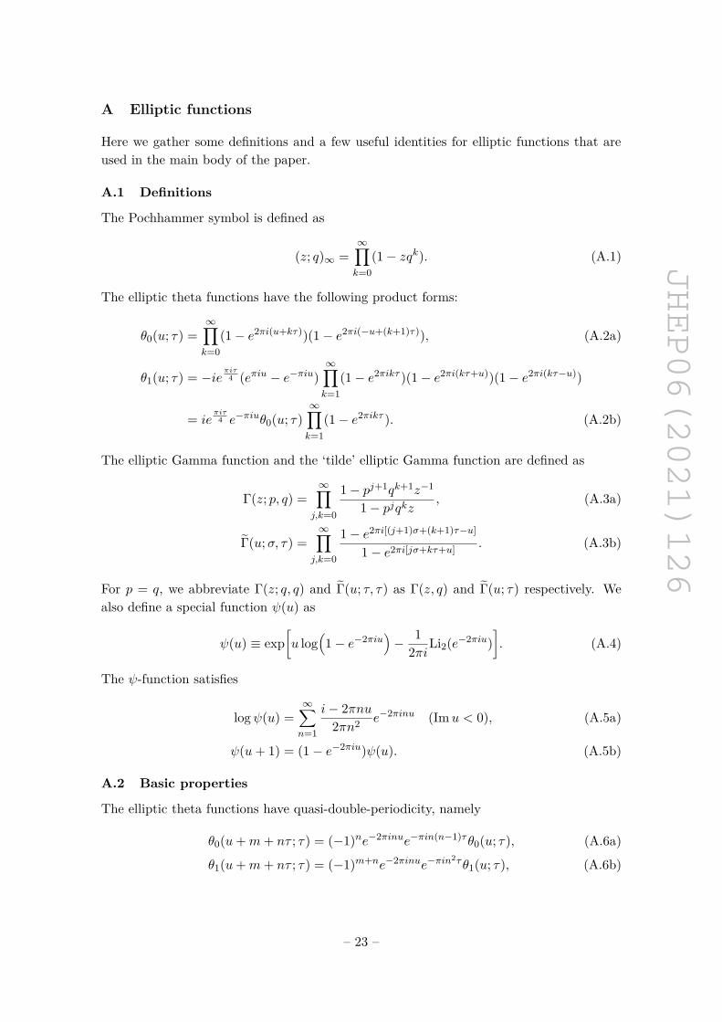
A Elliptic functions

Here we gather some definitions and a few useful identities for elliptic functions that areused in the main body of the paper.

A.1 Definitions

The Pochhammer symbol is defined as

(z; q)∞ =∞∏k=0

(1− zqk). (A.1)

The elliptic theta functions have the following product forms:

θ0(u; τ) =∞∏k=0

(1− e2πi(u+kτ))(1− e2πi(−u+(k+1)τ)), (A.2a)

θ1(u; τ) = −ieπiτ4 (eπiu − e−πiu)

∞∏k=1

(1− e2πikτ )(1− e2πi(kτ+u))(1− e2πi(kτ−u))

= ieπiτ4 e−πiuθ0(u; τ)

∞∏k=1

(1− e2πikτ ). (A.2b)

The elliptic Gamma function and the ‘tilde’ elliptic Gamma function are defined as

Γ(z; p, q) =∞∏

j,k=0

1− pj+1qk+1z−1

1− pjqkz , (A.3a)

Γ(u;σ, τ) =∞∏

j,k=0

1− e2πi[(j+1)σ+(k+1)τ−u]

1− e2πi[jσ+kτ+u] . (A.3b)

For p = q, we abbreviate Γ(z; q, q) and Γ(u; τ, τ) as Γ(z, q) and Γ(u; τ) respectively. Wealso define a special function ψ(u) as

ψ(u) ≡ exp[u log

(1− e−2πiu

)− 1

2πiLi2(e−2πiu)]. (A.4)

The ψ-function satisfies

logψ(u) =∞∑n=1

i− 2πnu2πn2 e−2πinu (Im u < 0), (A.5a)

ψ(u+ 1) = (1− e−2πiu)ψ(u). (A.5b)

A.2 Basic properties

The elliptic theta functions have quasi-double-periodicity, namely

θ0(u+m+ nτ ; τ) = (−1)ne−2πinue−πin(n−1)τθ0(u; τ), (A.6a)

θ1(u+m+ nτ ; τ) = (−1)m+ne−2πinue−πin2τθ1(u; τ), (A.6b)

– 23 –

JHEP06(2021)126

for m,n ∈ Z. The inversion formula of θ0(u; τ) can be written simply as

θ0(−u; τ) = −e−2πiuθ0(u; τ). (A.7)

The elliptic Gamma function also has quasi-double-periodicity, namely

Γ(u;σ, τ) = Γ(u+ 1;σ, τ) = θ0(u; τ)−1Γ(u+ σ;σ, τ) = θ0(u;σ)−1Γ(u+ τ ;σ, τ). (A.8)

It also satisfies the inversion formula

Γ(u;σ, τ) = Γ(σ + τ − u;σ, τ)−1. (A.9)

The following identity in [28] is also useful:

Γ(u+mabω; aω, bω) = (−e2πiu)−abm2

2 +m(a+b−1)2 (e2πiω)−

abm36 +ab(a+b)m2

4 − (a2+b2+3ab−1)m12

× θ0(u;ω)mΓ(u; aω, bω). (A.10)

A.3 Asymptotic behaviors

For small |τ | with fixed 0 < arg τ < π, the Pochhammer symbol can be approximated as

log(q; q)∞ = −πi12

(τ + 1

τ

)− 1

2 log(−iτ) +O(e− 2π sin(arg τ)

|τ |

). (A.11)

To study asymptotic behaviors of elliptic functions, first we introduce a τ -moddedvalue of a complex number u, namely {u}τ , as

{u}τ ≡ u− bReu− cot(arg τ) Im uc (u ∈ C). (A.12)

By definition, the τ -modded value satisfies

{u}τ = {u}τ + uτ, {−u}τ =

1− {u}τ (u /∈ Z)−{u}τ (u ∈ Z),

(A.13)

where we have defined u, u ∈ R asu = u+ uτ. (A.14)

Note that, for a real number x, a τ -modded value {x}τ reduces to a normal modded value{x} defined as

{x} ≡ x− bxc (x ∈ R). (A.15)

Bernoulli functions Bn(·) satisfy the following useful identity written in terms of the τ -modded value:

C−1∑J=0

Bn

({J

C+ u

}τ

)= 1Cn−1Bn({Cu}τ ). (A.16)

– 24 –

JHEP06(2021)126

Now, the asymptotic behavior of elliptic functions for a small |τ | with fixed 0 < arg τ <π are given as follows:

logθ0(u;τ) = πi

τ{u}τ (1−{u}τ )+πi{u}τ−

πi

6τ (1+3τ+τ2)

+log(1−e−

2πiτ

(1−{u}τ ))(

1−e−2πiτ{u}τ

)+O

(e− 2π sin(argτ)

|τ |

),

(A.17)

logθ1(u;τ) = πi

τ{u}τ (1−{u}τ )− πi4τ (1−τ)+πibReu−cot(argτ)Imuc− 1

2 logτ

+log(1−e−

2πiτ

(1−{u}τ ))(

1−e−2πiτ{u}τ

)+O


|τ |

),

(A.18)

log Γ(u;τ) = 2πiQ({u}τ ;τ)−logψ({u}τ

τ−1)−logψ

(1−{u}ττ

+1)

+O(e− 2π sin(argτ)

|τ |

),

Q(u;τ)≡−B3(u)6τ2 +B2(u)

2τ − 512B1(u)+ τ

12 . (A.19)

B Series expansion of the SU(2) index

For finite N , the elliptic hypergeometric integral representation, (2.2), leads to a directevaluation of the index by explicit integration. While the elliptic Gamma function is notelementary, its product representation, (A.3a), allows for a series expansion of the finite-Nindex. This was explicitly realized in [18, 19], where the series expansion of the N = 4 U(N)index was investigated for finite N with the simplest possible configuration of fugacities,namely p = q = y

3/2a .

For even moderately large values of N & 10, the (N − 1)-dimensional integral soonbecomes computationally expensive. However, the N = 2 case can readily be pushed tofairly high order in the series expansion. Here we have explicitly

ISU(2)(ya,p,q) = (p;p)∞(q;q)∞ΠΓ(ya;p,q)2

∫ 1

0duW (z;p;q)ΠΓ(zya;p,q)ΠΓ(z−1ya;p,q),

IU(2)(ya,p,q) = ((p;p)∞(q;q)∞ΠΓ(ya;p,q))2

2

∫ 1

0duW (z;p;q)ΠΓ(zya;p,q)ΠΓ(z−1ya;p,q),

(B.1)

where z = e2πiu and we have defined

W (z; p; q) ≡ 1Γ(z; p, q)Γ(z−1; pq) = (z; p)∞(z−1p; p)∞(z; q)∞(z−1q; q)∞,

ΠΓ(ya; p, q) ≡3∏

a=1Γ(ya; p, q). (B.2)

– 25 –

JHEP06(2021)126

Using the product form of the elliptic Gamma function, (A.3a), we can obtain the productrepresentation

ΠΓ(ζya; p; q) =∞∏

j,k=0

1− ζ−1Wpj+1qk+1 + ζ−2Y p2j+1q2k+1 − ζ−3p3j+2q3k+2

1− ζY pjqk + ζ2Wp2j+1q2j+1 − ζ3p3j+1lq3k+1 , (B.3)


Y ≡3∑

a=1ya, W ≡

3∑a=1

y−1a . (B.4)

Note that we have used the constraint y1y2y3 = pq in deriving this expression.We now consider the evaluation of the integral for the index, (B.1). One approach is

to evaluate the integral over the holonomy as a contour integral

∫ 1

0du →

∮dz

2πiz , (B.5)

where the contour is the unit circle surrounding z = 0 taken in the conventional direction.This picks up the residues inside the unit circle, which can be identified from the productrepresentation of the integrand, with the poles coming from the denominator of (B.3) asworked out in [21]. Alternatively, by truncating the infinite product at some finite order,the index becomes the integral of a rational function of the form

I(Y,W, p, q) ∼∫ 1

0du f(z = e2πiu), (B.6)

which just picks out the zero-mode f0 in the series expansion of

f(z) =∑n

fnzn (B.7)

(where negative powers of z are allowed).There is still some subtlety in truncating the product representation (B.3), and that is

that the series expansion in ζ (which corresponds to either z or z−1) will still have an infinitenumber of contributions at each order. To avoid this issue, we must simultaneously expandin powers of p and q. This can be made explicit by introducing an expansion parameter xalong with a particular set of scalings of the fugacities. The most straightforward scalingis to take

p→ px3, q → qx3, ya → yax2, (B.8)

to keep track of the orders of the series expansion with respect to x. Note that this scalingis consistent with the constraint y1y2y3 = pq.

After expanding as a series in x, we then pick out the zero-mode of the integrand andmultiply by the appropriate U(2) or SU(2) prefactor in (B.1). The result for the U(2)

– 26 –

JHEP06(2021)126

index is

IU(2)(Y x2,Wx−2, px3, qx3)= 1 + Y x2 − (p+ q)x3 + (−3pqW + 2Y 2)x4 − (p+ q)Y x5

+ (−p2 + 4pq − q2 − 5pqWY + 2Y 3)x6 + (p+ q)(2pqW − Y 2)x7

+ (5p2q2W 2 + (−p2 + 8pq − q2)Y − 11pqWY 2 + 3Y 4)x8

+ (p+ q)(−2pq + 4pqWY − Y 3)x9

+ ((2p3q − 11p2q2 + 2pq3)W + 13p2q2W 2Y

+ (−2p2 + 10pq − 2q2)Y 2 − 14pqWY 3 + 3Y 5)x10 +O(x11),

(B.9)

while the result for the SU(2) index is

ISU(2)(Y x2,Wx−2, px3, qx3)= 1 + (−pqW + Y 2)x4 − (p+ q)Y x5 + pq(2−WY )x6 + (p+ q)Y 2x7

+ (p2q2W 2 + (−p2 + pq − q2)Y − 3pqWY 2 + Y 4)x8

+ (p+ q)Y (pqW − Y 2)x9

+ (−p2q2W + 2p2q2W 2Y + (p+ q)2Y 2 − pqWY 3)x10 +O(x11).

(B.10)

Here we recall the definitions

Y = y1 + y2 + y3, W = 1y1

+ 1y2

+ 1y3 = y1y2 + y2y3 + y3y1

pq. (B.11)

The U(2) index reduces to the result of [18, 19] in the equal fugacity case

Y = 3q2/3, W = 3q−2/3, p = q. (B.12)

(Alternatively, we can just set Y = W = 3 and p = q = 1 and retain x as the expansionparameter used in [18, 19].) The first 30 terms in the expansion of the SU(2) index arepresented in table 1. While the expansion gets unwieldy at high order for general yafugacities, it simplifies considerably in special cases such as the equal fugacity case.

When p and q are related according to p = ha and q = hb, expansion of the BAresult (3.10) is the most computationally efficient method for obtaining the series repre-sentation. However, the advantage of the series expansion of the elliptic hypergeometricintegral is that it applies in general even when p and q are unrelated. In particular, whilewe assumed the scaling (B.8), the expansion can also be rearranged as a double series in pand q with some corresponding scaling of the ya fugacities.

The series expansion can be viewed as an explicit realization of the Hamiltonian formu-lation of the index, (2.1), with integer coefficients corresponding to the degeneracies at eachorder in powers of the fugacities. As such, the series is expected to converge with fugacitiesinside the unit circle, namely |p| < 1, |q| < 1 and |ya| < 1. However, this convergence canbe extremely slow, so the series expansion is not particularly useful as one approaches theCardy-like regime. As a demonstration, we compare the numerically evaluated index withthe series expansion obtained from (3.10) truncated to different orders in figure 4.

– 27 –

JHEP06(2021)126

��

��

��

�

��

��

Figure 4. The series evaluation of Re log I(ya, q, q) compared with its numerical evaluation. Theparameters ∆a = 1

3 + 2τ3 and τ = |τ |e 2πi

3 correspond to the left panel of figure 1. The series istruncated at order xn where q = x3 with n = 30, 100 and 500 as indicated.

n d2(n)0 11 02 03 04 Y 2−pqW

5 Y (−p−q)6 2pq−pqW Y

7 Y 2(p+q)8 p2q2W 2+Y

(−p2+pq−q2)−3pqW Y 2+Y 4

9 pqW Y (p+q)+Y 3(−p−q)10 2p2q2W 2Y −p2q2W−pqW Y 3+Y 2(p+q)2

11 Y(−p3−q3)−p2q2W 2(p+q)−pqW Y 2(p+q)+Y 4(p+q)

12 −p3q3W 3+6p2q2W 2Y 2+pqW Y(2p2−7pq+2q2)+Y 3 (−2p2+3pq−2q2)+p2q2

−5pqW Y 4+Y 6

13 −pqW(p3+q3)+2Y 2 (p3+q3)+2pqW Y 3(p+q)+Y 5(−p−q)

14 2p3q3W 2+4p2q2W 2Y 3−2pqW Y 2 (p2+3pq+q2)+Y 4 (2p2+3pq+2q2)+Y(−p4−3p3q3W 3−p3q+2p2q2−pq3−q4)−pqW Y 5

15 2pqW Y(p3+q3)+p2q2W 2Y 2(p+q)+Y 3 (−3p3−p2q−pq2−3q3)−3pqW Y 4(p+q)

+Y 6(p+q)16 p4q4W 4+15p2q2W 2Y 4−p2q2W 2Y

(p2−16pq+q2)+2pqW Y 3 (2p2−11pq+2q2)

+p2q2W(p2−5pq+q2)+Y 5 (−2p2+5pq−2q2)+Y 2 (2p4−10p3q3W 3+9p2q2+2q4)

−7pqW Y 6+Y 8

17 −3p2q2W 2Y 3(p+q)−p2q2W 2 (p3+2p2q+2pq2+q3)+pqW Y 2 (−2p3+7p2q+7pq2−2q3)+Y 4 (3p3−p2q−pq2+3q3)+Y

(−p5−3p3q2−3p2q3−q5)+4pqW Y 5(p+q)+Y 7(−p−q)

18 14p3q3W 2Y 2+p3q3+6p2q2W 2Y 5−pqW Y 4 (5p2+13pq+5q2)+Y 6 (2p2+3pq+2q2)+Y(4p4q4W 4+pqW (p+q)2 (2p2−5pq+2q2))+p3q3W 3 (p2−3pq+q2)

Table 1. Continued on next page.

– 28 –

JHEP06(2021)126

n d2(n)+Y 3 (−4p4−10p3q3W 3−p3q+2p2q2−pq3−4q4)−pqW Y 7

19 6p2q2W 2Y 4(p+q)−pqW (p+q)(p2−pq+q2)2+p2q2W 2Y

(−2p3+p2q+pq2−2q3)

+pqW Y 3 (8p3−5p2q−5pq2+8q3)+Y 5 (−4p3+p2q+pq2−4q3)+Y 2 (3p5−p4q−p3q3W 3(p+q)+5p3q2+5p2q3−pq4+3q5)−5pqW Y 6(p+q)+Y 8(p+q)

20 −p5q5W 5+28p2q2W 2Y 6+p2q2W 2Y 3 (−4p2+71pq−4q2)+pqW Y 5 (7p2−43pq+7q2)+Y 7 (−2p2+7pq−2q2)+Y 2 (15p4q4W 4+pqW

(−5p4+6p3q−42p2q2+6pq3−5q4))

+Y 4 (5p4−35p3q3W 3−p3q+20p2q2−pq3+5q4)+Y(−24p4q4W 3−(p−q)2(p4+2p3q+4p2q2+2pq3+q4))

+p2q2W 2 (p4−p3q+10p2q2−pq3+q4)−9pqW Y 8+Y 10

21 −10p2q2W 2Y 5(p+q)+p3q3W 3 (p3+p2q+pq2+q3)+2p2q2W 2Y 2 (p3−7p2q−7pq2+q3)−2pqW Y 4 (5p3−6p2q−6pq2+5q3)+Y 6 (4p3−2p2q−2pq2+4q3)+2p2q2 (p3+q3)+Y 3 (−5p5+2p4q+4p3q3W 3(p+q)−9p3q2−9p2q3+2pq4−5q5)+pqW Y

(2p5−7p4q+6p3q2+6p2q3−7pq4+2q5)+6pqW Y 7(p+q)+Y 9(−p−q)

22 5p5q5W 4+8p2q2W 2Y 7+p2q2W 2Y 4 (9p2+47pq+9q2)−3pqW Y 6 (3p2+7pq+3q2)+Y 8 (2p2+3pq+2q2)+Y 3 (20p4q4W 4+pqW

(10p4−5p3q−24p2q2−5pq3+10q4))

+Y 5 (−6p4−21p3q3W 3+p3q+5p2q2+pq3−6q4)+Y 2((p+q)2(3p4−7p3q+12p2q2−7pq3+3q4)−p3q3W 3 (p2+37pq+q2))+p2q2W

(p4+2p3q−3p2q2+2pq3+q4)

+Y(−5p5q5W 5−p2q2W 2 (p4−3p3q−18p2q2−3pq3+q4))−pqW Y 9

23 −4p3q3W 2 (p3+q3)+15p2q2W 2Y 6(p+q)+p2q2W 2Y 3 (−10p3+21p2q+21pq2−10q3)+pqW Y 5 (14p3−17p2q−17pq2+14q3)+Y 7 (−4p3+3p2q+3pq2−4q3)+Y 2 (p4q4W 4(p+q)−pqW

(6p5−15p4q+14p3q2+14p2q3−15pq4+6q5))

+Y 4 (7p5−5p4q−10p3q3W 3(p+q)+11p3q2+11p2q3−5pq4+7q5)+Y(−p7−3p5q2+2p4q3+2p3q4+2p3q3W 3 (p3+q3)−3p2q5−q7)−7pqW Y 8(p+q)

+Y 10(p+q)24 p6q6W 6+45p2q2W 2Y 8−2p2q2W 2Y 5 (8p2−91pq+8q2)+pqW Y 7 (11p2−71pq+11q2)

+Y 9 (−2p2+9pq−2q2)−pq(p6+p3q3+q6)

+Y 4(70p4q4W 4+pqW(−12p4+22p3q−125p2q2+22pq3−12q4))

+Y 6 (6p4−84p3q3W 3−4p3q+33p2q2−4pq3+6q4)+p3q3W 3 (p4+2p3q−14p2q2+2pq3+q4)+Y 2(−21p5q5W 5−p2q2W 2(p4+24p3q−111p2q2+24pq3+q4))+Y(36p5q5W 4+pqW

(4p6−2p5q+7p4q2−23p3q3+7p2q4−2pq5+4q6))

+Y 3(−7p6+p5q−10p4q2+16p3q3−10p2q4+p3q3W 3 (5p2−164pq+5q2)+pq5−7q6)−11pqW Y 10+Y 12

25 −21p2q2W 2Y 7(p+q)+p2q2W 2Y 4 (15p3−44p2q−44pq2+15q3)+p3q3W 2Y

(8p3−11p2q−11pq2+8q3)+pqW Y 6 (−17p3+25p2q+25pq2−17q3)

−p4q4W 4 (p3+p2q+pq2+q3)+Y 3 (pqW

(13p5−18p4q+39p3q2+39p2q3−18pq4+13q5)−5p4q4W 4(p+q)

)+Y 5 (−9p5+5p4q+20p3q3W 3(p+q)−18p3q2−18p2q3+5pq4−9q5)+Y 2(4p7+8p5q2−3p4q3−3p3q4+8p2q5+p3q3W 3 (p3+18p2q+18pq2+q3)+4q7)−pqW

(p7+p6q+3p5q2−2p4q3−2p3q4+3p2q5+pq6+q7)+8pqW Y 9(p+q)+Y 11(−p−q)

+4Y 8(p−q)2(p+q)26 −6p6q6W 5+10p2q2W 2Y 9+p2q2W 2Y 6 (25p2+98pq+25q2)−pqW Y 8 (13p2+29pq+13q2)


– 29 –

JHEP06(2021)126

n d2(n)+Y 10 (2p2+3pq+2q2)+Y 5 (56p4q4W 4+pqW

(23p4−25p3q−71p2q2−25pq3+23q4))

+Y 7 (−7p4−36p3q3W 3+5p3q+11p2q2+5pq3−7q4)+Y 3(p2q2W 2(−15p4+25p3q+111p2q2+25pq3−15q4)−35p5q5W 5)+Y 2(p4q4W 4 (p2+71pq+q2)−pqW

(9p6−16p5q+11p4q2+43p3q3+11p2q4−16pq5+9q6))

+Y 4(10p6−7p5q+13p4q2+29p3q3+13p2q4−2p3q3W 3 (7p2+69pq+7q2)−7pq5+10q6)+p2q2W 2(p6−2p5q+p4q2+3p3q3+p2q4−2pq5+q6)+Y(−p8+6p6q6W 6−3p6q2−4p5q3+7p4q4−4p3q5−3p2q6

+p3q3W 3 (2p4+p3q−36p2q2+pq3+2q4)−q8)−pqW Y 11

27 −p3q3 (p3+q3)+28p2q2W 2Y 8(p+q)−p4q4W 3 (p3+q3)+p2q2W 2Y 5(−29p3+70p2q+70pq2−29q3)+pqW Y 7 (21p3−34p2q−34pq2+21q3)+Y 9 (−4p3+5p2q+5pq2−4q3)+Y 4 (15p4q4W 4(p+q)−pqW

(21p5−41p4q+45p3q2+45p2q3−41pq4+21q5))

+Y 6 (10p5−9p4q−35p3q3W 3(p+q)+19p3q2+19p2q3−9pq4+10q5)+Y 2(2p2q2W 2(2p5−17p4q+8p3q2+8p2q3−17pq4+2q5)−p5q5W 5(p+q)

)+Y 3(−8p7+5p6q−17p5q2+2p4q3+2p3q4−17p2q5+3p3q3W 3 (3p3−13p2q−13pq2+3q3)

+5pq6−8q7)+pqW Y(3p7−7p6q+15p5q2−6p4q3−6p3q4+15p2q5−7pq6+3q7)

−9pqW Y 10(p+q)+Y 12(p+q)28 −p7q7W 7+19p6q6W 4+66p2q2W 2Y 10+p2q2W 2Y 7 (−36p2+373pq−36q2)

+pqW Y 9(15p2−107pq+15q2)+Y 11 (−2p2+11pq−2q2)+Y 6(210p4q4W 4+pqW

(−28p4+41p3q−287p2q2+41pq3−28q4))

+Y 8 (7(p4−p3q+7p2q2−pq3+q4)−165p3q3W 3)+Y 4 (p2q2W 2 (23p4−67p3q+506p2q2−67pq3+23q4)−126p5q5W 5)+W

(2p8q2−2p6q4−5p5q5−2p4q6+2p2q8)

+Y 3(p4q4W 4 (−6p2+323pq−6q2)+pqW

(18p6−29p5q+44p4q2−173p3q3+44p2q4−29pq5+18q6))

+Y 5(−13p6+9p5q−25p4q2+53p3q3−25p2q4+15p3q3W 3 (2p2−37pq+2q2)+9pq5−13q6)+Y(−49p6q6W 5−p2q2W 2(p6−12p5q+10p4q2−102p3q3+10p2q4−12pq5+q6))

+Y 2(4p8−3p7q+28p6q6W 6+8p6q2+2p5q3+13p4q4+2p3q5+8p2q6

+p4q4W 3 (25p2−272pq+25q2)−3pq7+4q8)−13pqW Y 12+Y 14

29 −36p2q2W 2Y 9(p+q)+2p2q2W 2Y 6 (23p3−55p2q−55pq2+23q3)−5pqW Y 8(5p3−9p2q−9pq2+5q3)+Y 10 (4p3−6p2q−6pq2+4q3)+Y 5(pqW

(33p5−51p4q+95p3q2+95p2q3−51pq4+33q5)−35p4q4W 4(p+q)

)+Y 7(−11p5+11p4q+56p3q3W 3(p+q)−25p3q2−25p2q3+11pq4−11q5)−4p3q3W 2 (p5−p4q+2p3q2+2p2q3−pq4+q5)+Y 3(6p5q5W 5(p+q)−p2q2W 2 (17p5−50p4q+97p3q2+97p2q3−50pq4+17q5))+Y 2(2p4q4W 4(p3−8p2q−8pq2+q3)

+2pqW(−5p7+10p6q−17p5q2+17p4q3+17p3q4−17p2q5+10pq6−5q7))

+Y 4(13p7−10p6q+27p5q2−10p4q3−10p3q4+27p2q5

+p3q3W 3(−25p3+92p2q+92pq2−25q3)−10pq6+13q7)+Y(−p9−2p7q2+p6q3−2p5q4−2p4q5+p3q6−2p2q7

+p4q4W 3 (−2p3+21p2q+21pq2−2q3)−q9)+10pqW Y 11(p+q)+Y 13(−p−q)30 −pqW Y 13+

(2p2+3qp+2q2)Y 12+12p2q2W 2Y 11−pq

(17p2+37qp+17q2)W Y 10


– 30 –

JHEP06(2021)126

n d2(n)+(−7p4−55q3W 3p3+9qp3+17q2p2+9q3p−7q4)Y 9+p2q2 (49p2+169qp+49q2)W 2Y 8

+(120p4q4W 4+pq

(35p4−57qp3−141q2p2−57q3p+35q4)W

)Y 7

+(15p6−16qp5+28q2p4+51q3p3−5q3 (11p2+71qp+11q2)W 3p3+28q4p2−16q5p+15q6)Y 6

+(p2q2(−46p4+106qp3+367q2p2+106q3p−46q4)W 2−126p5q5W 5)Y 5

+(20p4q4 (p2+17qp+q2)W 4

−pq(30p6−65qp5+59q2p4+159q3p3+59q4p2−65q5p+30q6)W

)Y 4

+(−10p8+8qp7+56q6W 6p6−23q2p6−6q3p5+29q4p4−6q5p3

+q3(16p4−47qp3−325q2p2−47q3p+16q4)W 3p3−23q6p2+8q7p−10q8)Y 3

+(2p2q2(3p6−24qp5+11q2p4+57q3p3+11q4p2−24q5p+3q6)W 2

−p5q5 (p2+121qp+q2)W 5)Y 2

+(−7p7q7W 7−p4q4(3p4+4qp3−74q2p2+4q3p+3q4)W 4

+pq(4p8−11qp7+15q2p6+4q3p5−37q4p4+4q5p3+15q6p2−11q7p+4q8)W)Y

+3p2q8+7p7q7W 6+5p5q5+p3q3(p6+4qp5−2q2p4−11q3p3−2q4p2+4q5p+q6)W 3+3p8q2

Table 1. The coefficients d2(n) in the expansion of the SU(2) index ISU(2)(Y x2,Wx−2,px3, qx3) =∑n d2(n)xn up to O(x30) where Y and W are defined in (B.12).

C Cardy-like expansions of the standard contributions

In this appendix, we investigate the Cardy-like limit of the standard contributions to theN = 4 SU(N) SCI through the BA formula (2.3) for N = 2 and N = 3 cases respectively.In particular, since the contribution from the basic {1, N, 0} BAE solution have alreadybeen computed in the literature and given explicitly as (3.17) and (4.13) for N = 2 andN = 3 respectively, we focus on the other standard BAE solutions. As mentioned in themain text, we identify p = q for simplicity.

C.1 SU(2) case

For the SU(2) case, there are two remaining standard BAE solutions: {2, 1, 0} and {1, 2, 1}.Their contributions to the SCI are given in (3.16a) and (3.16c) respectively.

First, the building blocks of (3.16a), or equivalently those of (3.11a) with a = b = 1,can be computed using the asymptotic expansions (A.18) and (A.19) as

log κZ{2,1,0} = − πi

2τ2

3∏a=1

({2∆a}τ −

1 + η22

)+ πi

τ2

3∏a=1

({∆a}τ −

1 + η12

)

+ πi(6 + 5η1 − 10η2)12 − log τ − log 2!

+3∑

a=1

(2 log

ψ({1/2+∆a}ττ − 1)

ψ(1−{1/2+∆a}ττ + 1)

+ logψ({∆a}τ

τ − 1)ψ(1−{∆a}τ

τ + 1)

)

+ 4 log(1− e−

πiτ

)+O

(e− 2π sin(arg τ)

|τ |

)(C.1)

– 31 –

JHEP06(2021)126

and

− logH{2,1,0}=− log4−log(η2−η1τ

+ 2τ

∑∆

(e−

2πiτ

(1−{ 12 +∆}τ )

1−e− 2πiτ

(1−{ 12 +∆}τ )

− e−2πiτ{ 1

2 +∆}τ

1−e− 2πiτ{ 1

2 +∆}τ

))


|τ |

). (C.2)

Here we have also used the identity (A.16). The determinant contribution (C.2) nowexplains why we should keep track of the leading exponentially suppressed terms. If η1 = η2,we get a divergent logarithmic contribution “log 0” without those terms. The Cardy-likelimit of the contribution (3.16a) is then given as the sum of (C.1) and (C.2), which resultsin (3.19).

Similarly the building blocks of (3.16c), or equivalently those of (3.11c) with a = b = 1,are given as

logκZ{1,2,1}=− πi

2τ2

3∏a=1

({2∆a}τ−

1+η22

)+ πi

τ2

3∏a=1

({∆a}τ−

1+η12

)

+πi(6+8η1−13η2)12 −logτ−log2!

+3∑

a=1

(log

ψ({1/2+∆a}ττ − 1

2)ψ(1−{1/2+∆a}τ

τ + 12)

+logψ({1/2+∆a}τ

τ − 32)

ψ(1−{1/2+∆a}ττ + 3

2)+log

ψ({∆a}ττ −1)

ψ(1−{∆a}ττ +1)

)

+4log(1+e

πiτ

)+O


|τ |

)(C.3)

and

− logH{1,2,1}=− log4−log(η2−η1τ

+ 2τ

∑∆

(−e−

2πiτ

(1−{ 12 +∆}τ )

1+e− 2πiτ

(1−{ 12 +∆}τ )

− −e− 2πi

τ{ 1

2 +∆}τ

1+e− 2πiτ{ 1

2 +∆}τ

))


|τ |

). (C.4)

The Cardy-like limit of the contribution (3.16c) is then given as the sum of (C.3) and (C.4),which leads to (3.20).

Sum of the two contributions (3.19) and (3.20) also involves complicated calculations.The resulting sum (3.26) is therefore written in terms of XSU(2), which is defined as

XSU(2) =(1− e−πiτ )4∏3

a=1ψ( {1/2+∆a}τ

τ−1)2

ψ( 1−{1/2+∆a}ττ

+1)2∑∆

(e−

2πiτ (1−{ 1

2 +∆}τ )

1−e−2πiτ (1−{ 1

2 +∆}τ )− e−

2πiτ {

12 +∆}τ

1−e−2πiτ {

12 +∆}τ

)

+(1 + e−

πiτ )4∏3

a=1ψ( {1/2+∆a}τ

τ− 1

2 )ψ( 1−{1/2+∆a}τ

τ+ 1

2 )ψ( {1/2+∆a}τ

τ− 3

2 )ψ( 1−{1/2+∆a}τ

τ+ 3

2 )∑∆

(−e−

2πiτ (1−{ 1

2 +∆}τ )

1+e−2πiτ (1−{ 1

2 +∆}τ )− −e−

2πiτ {

12 +∆}τ

1+e−2πiτ {

12 +∆}τ

) .

(C.5)

– 32 –

JHEP06(2021)126

To simplify this expression in the Cardy-like limit, first note that

max∆

{|e−

2πiτ

(1−{ 12 +∆}τ )|, |e−

2πiτ{ 1

2 +∆}τ |}

= |e−2πiτ

∆SU(2) |

=

|e− 2πi

τ{ 1

2 +∆3}τ | (η1 = η2 = −1)|e−

2πiτ

(1−{ 12 +∆1}τ )| (η1 = η2 = 1)

,(C.6)


0 < {∆1} < {∆2} < {∆3} < 1. (C.7)

This explains the origin of the definition of ∆SU(2) given in (3.28). For this ∆SU(2), onecan prove the following asymptotic expansions

ψ(∆SU(2)

τ − 1)2

− e−2πiτ ∆SU(2))

1−e−2πiτ ∆SU(2))

+ψ(∆SU(2)

τ − 12)ψ(∆SU(2)

τ − 32)

− −e− 2πi

τ ∆SU(2))

1+e−2πiτ ∆SU(2))

∼ 4∆SU(2)

τ− 2− 2i

π,

ψ(∆SU(2)

τ + 1)−2

e−2πiτ ∆SU(2))

1−e−2πiτ ∆SU(2))

+ψ(∆SU(2)

τ + 12)−1ψ(∆SU(2)

τ + 32)−1

−e−2πiτ ∆SU(2))

1+e−2πiτ ∆SU(2))

∼ 4∆SU(2)

τ+ 2− 2i

π,

(C.8)

using the expansion of the ψ-function (A.5a). Applying the above results (C.8) to thedefinition of XSU(2) (C.5) along with (C.6) and (3.28), we obtain the asymptotic expansionof XSU(2) (3.27).

C.2 SU(3) case

For the SU(3) case, there are three remaining standard BAE solutions: {3, 1, 0} and{1, 3, 1}, and {1, 3, 2}. Their contributions to the SCI are given in (4.9a), (4.9c), and (4.9d)with p = q (a = b = 1) respectively.

First, the building blocks of (4.9a) with a = b = 1 can be computed using the asymp-totic expansions (A.18) and (A.19) as

log κZ{3,1,0}

= − πi

3τ2

3∏a=1

({3∆a}τ −

1 + η32

)+ πi

τ2

3∏a=1

({∆a}τ −

1 + η12

)

+ πi(12 + 5η1 − 15η3)12 − 2 log τ − log 3!

+3∑

a=1

(3 log

ψ({1/3+∆a}ττ − 1)

ψ(1−{1/3+∆a}ττ + 1)

+ 3 logψ({2/3+∆a}τ

τ − 1)ψ(1−{2/3+∆a}τ

τ + 1)+ 2 log

ψ({∆a}ττ − 1)

ψ(1−{∆a}ττ + 1)

)

+ 6 log(1− e−

2πi3τ)

+ 6 log(1− e−

4πi3τ)

+O(e− 2π sin(arg τ)

|τ |

)(C.9)

and− logH{3,1,0}

= −3 log 3− 2 log(η3 − η1

2τ + 1τ

2∑J=1

∑∆

(e−

2πiτ

(1−{J3 +∆}τ )

1− e− 2πiτ

(1−{J3 +∆}τ )− e−

2πiτ{J3 +∆}τ

1− e− 2πiτ{J3 +∆}τ

)).

(C.10)

– 33 –

JHEP06(2021)126

Here we have also used the identity (A.16). The determinant contribution (C.10) nowexplains why we should keep track of the leading exponentially suppressed terms. If η1 = η3,we get a logarithmically divergent contribution “log 0” without those terms. The Cardy-like limit of the contribution (4.9a) with a = b = 1 is then given as the sum of (C.9)and (C.10), which gives (4.14).

Similarly the building blocks of (4.9c) with a = b = 1 are given as

log κZ{1,3,1}

= − πi

3τ2

3∏a=1

({3∆a}τ −

1 + η32

)+ πi

τ2

3∏a=1

({∆a}τ −

1 + η12

)

+ πi(12 + 9η1 − 19η3)12 − 2 log τ − log 3!

+3∑

a=1

(2 log

ψ({1/3+∆a}ττ − 2

3)ψ(1−{1/3+∆a}τ

τ + 23)

+ 2 logψ({2/3+∆a}τ

τ − 43)

ψ(1−{2/3+∆a}ττ + 4

3)

+ logψ({2/3+∆a}τ

τ − 13)

ψ(1−{2/3+∆a}ττ + 1

3)+ log

ψ({1/3+∆a}ττ − 5

3)ψ(1−{1/3+∆a}τ

τ + 53)

+ 2 logψ({∆a}τ

τ − 1)ψ(1−{∆a}τ

τ + 1)

)

+ 6 log(1− e−2πi( 1

3τ−23 ))

+ 6 log(1− e−2πi( 2

3τ−13 ))


|τ |

)(C.11)

and

−logH{1,3,1}

=−3log3−2log(η3−η1

2τ + 1τ

2∑J=1

∑∆

(e−

2πiτ

(1−{J3 +∆}τ−Jτ3 )

1−e− 2πiτ

(1−{J3 +∆}τ−Jτ3 )− e−

2πiτ

({J3 +∆}τ+Jτ3 )

1−e− 2πiτ

({J3 +∆}τ+Jτ3 )

)).

(C.12)

The Cardy-like limit of the contribution (4.9c) with a = b = 1 is then given as the sumof (C.11) and (C.12), which gives (4.15).

Finally the building blocks of (4.9d) with a = b = 1 are given as

log κZ{1,3,2}

= − πi

3τ2

3∏a=1

({3∆a}τ −

1 + η32

)+ πi

τ2

3∏a=1

({∆a}τ −

1 + η12

)

+ πi(12 + 9η1 − 19η3)12 − 2 log τ − log 3!

+3∑

a=1

(2 log

ψ({2/3+∆a}ττ − 2

3)ψ(1−{2/3+∆a}τ

τ + 23)

+ 2 logψ({1/3+∆a}τ

τ − 43)

ψ(1−{1/3+∆a}ττ + 4

3)

+ logψ({1/3+∆a}τ

τ − 13)

ψ(1−{1/3+∆a}ττ + 1

3)+ log

ψ({2/3+∆a}ττ − 5

3)ψ(1−{2/3+∆a}τ

τ + 53)

+ 2 logψ({∆a}τ

τ − 1)ψ(1−{∆a}τ

τ + 1)

)

+ 6 log(1− e−2πi( 2

3τ−23 ))

+ 6 log(1− e−2πi( 1

3τ−13 ))


|τ |

), (C.13)

– 34 –

JHEP06(2021)126

and

−logH{1,3,2}

=−3log3−2log(η3−η1

2τ + 1τ

2∑J=1

∑∆

(e−

2πiτ

(1−{J3 +∆}τ+Jτ3 )

1−e− 2πiτ

(1−{J3 +∆}τ+Jτ3 )− e−

2πiτ

({J3 +∆}τ−Jτ3 )

1−e− 2πiτ

({J3 +∆}τ−Jτ3 )

)).

(C.14)

The Cardy-like limit of the contribution (4.9d) with a = b = 1 is then given as the sumof (C.13) and (C.14), which gives (4.16).

Sum of the three contributions (4.14), (4.15), and (4.16) also involves complicatedcalculations. The resulting sum (4.21) is therefore written in terms of XSU(3), which isdefined as

XSU(3)

=(1−e− 2πi

3τ )6(1−e− 4πi3τ )6∏3

a=1ψ( {1/3+∆a}τ

τ−1)3

ψ( 1−{1/3+∆a}ττ

+1)3

ψ( {2/3+∆a}ττ

−1)3

ψ( 1−{2/3+∆a}ττ

+1)3(∑2J=1

∑∆( e−

2πiτ (1−{J/3+∆}τ )

1−e−2πiτ (1−{J/3+∆}τ )

− e−2πiτ {J/3+∆}τ

1−e−2πiτ {J/3+∆}τ

))2

+ (1−e−2πi( 13τ−

23 ))6(1−e−2πi( 2

3τ−13 ))6(∑2

J=1( e−2πiτ (1−{J/3+∆}τ−Jτ/3)

1−e−2πiτ (1−{J/3+∆}τ−Jτ/3)

− e−2πiτ ({J/3+∆}τ+Jτ/3)

1−e−2πiτ ({J/3+∆}τ+Jτ/3)

))2

×3∏

a=1

ψ({1/3+∆a}ττ − 2

3)2

ψ(1−{1/3+∆a}ττ + 2

3)2

ψ({2/3+∆a}ττ − 4

3)2

ψ(1−{2/3+∆a}ττ + 4

3)2

ψ({2/3+∆a}ττ − 1

3)ψ(1−{2/3+∆a}τ

τ + 13)

ψ({1/3+∆a}ττ − 5

3)ψ(1−{1/3+∆a}τ

τ + 53)

+ (1−e−2πi( 23τ−

23 ))6(1−e−2πi( 1

3τ−13 ))6(∑2

J=1( e−2πiτ (1−{J/3+∆}τ+Jτ/3)

1−e−2πiτ (1−{J/3+∆}τ+Jτ/3)

− e−2πiτ ({J/3+∆}τ−Jτ/3)

1−e−2πiτ ({J/3+∆}τ−Jτ/3)

))2

×3∏

a=1

ψ({2/3+∆a}ττ − 2

3)2

ψ(1−{2/3+∆a}ττ + 2

3)2

ψ({1/3+∆a}ττ − 4

3)2

ψ(1−{1/3+∆a}ττ + 4

3)2

ψ({1/3+∆a}ττ − 1

3)ψ(1−{1/3+∆a}τ

τ + 13)

ψ({2/3+∆a}ττ − 5

3)ψ(1−{2/3+∆a}τ

τ + 53).

(C.15)

To simplify this expression in the Cardy-like limit, first note that

max∆

{|e−

2πiτ

(1−{ 13 +∆}τ )|, |e−

2πiτ

(1−{ 23 +∆}τ )|, |e−

2πiτ{ 1

3 +∆}τ |, |e−2πiτ{ 2

3 +∆}τ |}

= |e−2πiτ

∆SU(3) | =

|e−2πiτ{ 1

3 +∆3}τ | (η1 = η3 = −1, {∆3} > 2/3)|e−

2πiτ{ 2

3 +∆2}τ | (η1 = η3 = −1, {∆3} < 2/3)|e−

2πiτ

(1−{ 23 +∆1}τ )| (η1 = η3 = 1, {∆1} < 1/3)

|e−2πiτ

(1−{ 13 +∆2}τ )| (η1 = η3 = 1, {∆1} > 1/3)

,(C.16)


0 < {∆1} < {∆2} < {∆3} < 1. (C.17)

– 35 –

JHEP06(2021)126

This explains the origin of the definition of ∆SU(3) given in (4.23). For this ∆SU(3), onecan prove the following asymptotic expansions

ψ(∆SU(3)

τ − 1)3(− e−

2πiτ ∆SU(3))

1−e−2πiτ ∆SU(3))

)2 +ψ(∆SU(3)

τ − 23)2ψ(∆SU(3)

τ − 53)(

− w2e−2πiτ ∆SU(3))

1−w2e−2πiτ ∆SU(3))

)2 +ψ(∆SU(3)

τ − 43)2ψ(∆SU(3)

τ − 13)(

− we−2πiτ ∆SU(3))

1−we−2πiτ ∆SU(3))

)2

∼ 27(∆SU(3))2

2τ2 + 27∆SU(3)(−π − i)2πτ + 3(8π2 + 15πi− 9)

8π2 ,

ψ(∆SU(3)

τ + 1)−3(e−

2πiτ ∆SU(3))

1−e−2πiτ ∆SU(3))

)2 +ψ(∆SU(3)

τ + 23)−2ψ(∆SU(3)

τ + 53)−1(

we−2πiτ ∆SU(3))

1−we−2πiτ ∆SU(3))

)2 +ψ(∆SU(3)

τ + 43)−2ψ(∆SU(3)

τ + 13)−1(

w2e−2πiτ ∆SU(3))

1−w2e−2πiτ ∆SU(3))

)2

∼ 27(∆SU(3))2

2τ2 + 27∆SU(3)(π − i)2πτ + 3(8π2 − 15πi− 9)

8π2 , (C.18)

using the expansion of the ψ-function (A.5a). Here w = e2πi/3 is a primitive cube root ofunity. Applying the above results (C.18) to the definition ofXSU(3) (C.15) along with (C.16)and (4.23), we obtain the asymptotic expansion of XSU(3) (4.22).

Open Access. This article is distributed under the terms of the Creative CommonsAttribution License (CC-BY 4.0), which permits any use, distribution and reproduction inany medium, provided the original author(s) and source are credited.

References

[1] A. Cabo-Bizet, D. Cassani, D. Martelli and S. Murthy, Microscopic origin of theBekenstein-Hawking entropy of supersymmetric AdS5 black holes, JHEP 10 (2019) 062[arXiv:1810.11442] [INSPIRE].

[2] S. Choi, J. Kim, S. Kim and J. Nahmgoong, Large AdS black holes from QFT,arXiv:1810.12067 [INSPIRE].

[3] F. Benini and P. Milan, Black Holes in 4D N = 4 Super-Yang-Mills Field Theory, Phys.Rev. X 10 (2020) 021037 [arXiv:1812.09613] [INSPIRE].

[4] C. Romelsberger, Counting chiral primaries in N = 1, d = 4 superconformal field theories,Nucl. Phys. B 747 (2006) 329 [hep-th/0510060] [INSPIRE].

[5] J. Kinney, J.M. Maldacena, S. Minwalla and S. Raju, An Index for 4 dimensional superconformal theories, Commun. Math. Phys. 275 (2007) 209 [hep-th/0510251] [INSPIRE].

[6] S.M. Hosseini, K. Hristov and A. Zaffaroni, An extremization principle for the entropy ofrotating BPS black holes in AdS5, JHEP 07 (2017) 106 [arXiv:1705.05383] [INSPIRE].

[7] M. Honda, Quantum Black Hole Entropy from 4d Supersymmetric Cardy formula, Phys. Rev.D 100 (2019) 026008 [arXiv:1901.08091] [INSPIRE].

[8] A. Arabi Ardehali, Cardy-like asymptotics of the 4d N = 4 index and AdS5 blackholes, JHEP06 (2019) 134 [arXiv:1902.06619] [INSPIRE].

[9] J. Kim, S. Kim and J. Song, A 4d N = 1 Cardy Formula, JHEP 01 (2021) 025[arXiv:1904.03455] [INSPIRE].

– 36 –

https://creativecommons.org/licenses/by/4.0/



https://inspirehep.net/search?p=find+EPRINT%2BarXiv%3A1810.11442



https://doi.org/10.1103/PhysRevX.10.021037

https://doi.org/10.1103/PhysRevX.10.021037



https://doi.org/10.1016/j.nuclphysb.2006.03.037

https://arxiv.org/abs/hep-th/0510060

https://inspirehep.net/search?p=find+EPRINT%2Bhep-th%2F0510060

https://doi.org/10.1007/s00220-007-0258-7

https://arxiv.org/abs/hep-th/0510251

https://inspirehep.net/search?p=find+EPRINT%2Bhep-th%2F0510251




https://doi.org/10.1103/PhysRevD.100.026008











JHEP06(2021)126

[10] A. Cabo-Bizet, D. Cassani, D. Martelli and S. Murthy, The asymptotic growth of states ofthe 4d N = 1 superconformal index, JHEP 08 (2019) 120 [arXiv:1904.05865] [INSPIRE].

[11] A. Amariti, I. Garozzo and G. Lo Monaco, Entropy function from toric geometry,arXiv:1904.10009 [INSPIRE].

[12] A. González Lezcano and L.A. Pando Zayas, Microstate counting via Bethe Ansätze in the 4dN = 1 superconformal index, JHEP 03 (2020) 088 [arXiv:1907.12841] [INSPIRE].

[13] A. Lanir, A. Nedelin and O. Sela, Black hole entropy function for toric theories via BetheAnsatz, JHEP 04 (2020) 091 [arXiv:1908.01737] [INSPIRE].

[14] A. Arabi Ardehali, J. Hong and J.T. Liu, Asymptotic growth of the 4d N = 4 index andpartially deconfined phases, JHEP 07 (2020) 073 [arXiv:1912.04169] [INSPIRE].

[15] A. González Lezcano, J. Hong, J.T. Liu and L.A. Pando Zayas, Sub-leading Structures inSuperconformal Indices: Subdominant Saddles and Logarithmic Contributions, JHEP 01(2021) 001 [arXiv:2007.12604] [INSPIRE].

[16] A. Cabo-Bizet, D. Cassani, D. Martelli and S. Murthy, The large-N limit of the 4d N = 1superconformal index, JHEP 11 (2020) 150 [arXiv:2005.10654] [INSPIRE].

[17] A. Cabo-Bizet and S. Murthy, Supersymmetric phases of 4d N = 4 SYM at large N , JHEP09 (2020) 184 [arXiv:1909.09597] [INSPIRE].

[18] S. Murthy, The growth of the 116 -BPS index in 4d N = 4 SYM, arXiv:2005.10843 [INSPIRE].

[19] P. Agarwal, S. Choi, J. Kim, S. Kim and J. Nahmgoong, AdS black holes and finite Nindices, Phys. Rev. D 103 (2021) 126006 [arXiv:2005.11240] [INSPIRE].

[20] C. Copetti, A. Grassi, Z. Komargodski and L. Tizzano, Delayed Deconfinement and theHawking-Page Transition, arXiv:2008.04950 [INSPIRE].

[21] K. Goldstein, V. Jejjala, Y. Lei, S. van Leuven and W. Li, Residues, modularity, and theCardy limit of the 4d N = 4 superconformal index, JHEP 04 (2021) 216 [arXiv:2011.06605][INSPIRE].

[22] A. Cabo-Bizet, From multi-gravitons to Black holes: The role of complex saddles,arXiv:2012.04815 [INSPIRE].

[23] A. Amariti, M. Fazzi and A. Segati, The superconformal index of N = 4 USp(2Nc) andSO(Nc) SYM as a matrix integral, arXiv:2012.15208 [INSPIRE].

[24] O. Aharony, A gravity interpretation for the Bethe ansatz expansion of the N = 4 SYMindex, talk at SCGP workshop (2020).

[25] J. Hong and J.T. Liu, The topologically twisted index of N = 4 super-Yang-Mills on T2 × S2

and the elliptic genus, JHEP 07 (2018) 018 [arXiv:1804.04592] [INSPIRE].

[26] F.A. Dolan and H. Osborn, Applications of the Superconformal Index for Protected Operatorsand q-Hypergeometric Identities to N = 1 Dual Theories, Nucl. Phys. B 818 (2009) 137[arXiv:0801.4947] [INSPIRE].

[27] V.P. Spiridonov and G.S. Vartanov, Superconformal indices of N = 4 SYM field theories,Lett. Math. Phys. 100 (2012) 97 [arXiv:1005.4196] [INSPIRE].

[28] F. Benini and P. Milan, A Bethe Ansatz type formula for the superconformal index,Commun. Math. Phys. 376 (2020) 1413 [arXiv:1811.04107] [INSPIRE].

– 37 –











































https://doi.org/10.1016/j.nuclphysb.2009.01.028



https://doi.org/10.1007/s11005-011-0537-2



https://doi.org/10.1007/s00220-019-03679-y



JHEP06(2021)126

[29] C. Closset, H. Kim and B. Willett, N = 1 supersymmetric indices and the four-dimensionalA-model, JHEP 08 (2017) 090 [arXiv:1707.05774] [INSPIRE].

[30] C. Closset, H. Kim and B. Willett, Supersymmetric partition functions and thethree-dimensional A-twist, JHEP 03 (2017) 074 [arXiv:1701.03171] [INSPIRE].

[31] F. Benini, E. Colombo, S. Soltani, A. Zaffaroni and Z. Zhang, Superconformal indices atlarge N and the entropy of AdS5 × SE5 black holes, Class. Quant. Grav. 37 (2020) 215021[arXiv:2005.12308] [INSPIRE].

[32] A. Gadde, Modularity of supersymmetric partition functions, arXiv:2004.13490 [INSPIRE].

[33] J.T. Liu, L.A. Pando Zayas, V. Rathee and W. Zhao, Toward Microstate Counting BeyondLarge N in Localization and the Dual One-loop Quantum Supergravity, JHEP 01 (2018) 026[arXiv:1707.04197] [INSPIRE].

[34] J.T. Liu, L.A. Pando Zayas, V. Rathee and W. Zhao, One-Loop Test of Quantum Black Holesin anti-de Sitter Space, Phys. Rev. Lett. 120 (2018) 221602 [arXiv:1711.01076] [INSPIRE].

[35] D. Gang, N. Kim and L.A. Pando Zayas, Precision Microstate Counting for the Entropy ofWrapped M5-branes, JHEP 03 (2020) 164 [arXiv:1905.01559] [INSPIRE].

[36] F. Benini, D. Gang and L.A. Pando Zayas, Rotating Black Hole Entropy from M5 Branes,JHEP 03 (2020) 057 [arXiv:1909.11612] [INSPIRE].

[37] N. Bobev, A.M. Charles, K. Hristov and V. Reys, The Unreasonable Effectiveness ofHigher-Derivative Supergravity in AdS4 Holography, Phys. Rev. Lett. 125 (2020) 131601[arXiv:2006.09390] [INSPIRE].

[38] L.A. Pando Zayas and Y. Xin, Universal logarithmic behavior in microstate counting and thedual one-loop entropy of AdS4 black holes, Phys. Rev. D 103 (2021) 026003[arXiv:2008.03239] [INSPIRE].

– 38 –







https://doi.org/10.1088/1361-6382/abb39b








https://doi.org/10.1103/PhysRevLett.120.221602









https://doi.org/10.1103/PhysRevLett.125.131601






JHEP06(2021)126 - Inspire HEP

Documents

Transcript of JHEP06(2021)126 - Inspire HEP