
Phase transitions in lattice gauge theories - Inspire HEP
144
-
Upload
khangminh22 -
Category
Documents
-
view
0 -
download
0
Transcript of Phase transitions in lattice gauge theories - Inspire HEP

Dissertation
submitted to the
Combined Faculties of the Natural Sciences and Mathematicsof the Ruperto-Carola-University of Heidelberg, Germany
for the degree of
Doctor of Natural Sciences
Put forward by
Manuel Scherzer
born in: Marburg-Wehrda, GermanyOral examination: June 4th, 2019

Phase transitions in lattice gauge theories:From the numerical sign problem to machine
learning
Referees: Prof. Dr. Ion-Olimpiu Stamatescu
Prof. Dr. Tilman Plehn
Phasenübergänge in Gittereichtheorien: Vom numerischen Vorzeichen-
problem zu maschinellem Lernen
Gittersimulationen der Quantenchromodynamik (QCD) sind ein wichtiges
Werkzeug der modernen Quantenfeldtheorie. Derartige Simulationen der grundle-
genden Theorie ergeben höchst präzise Ergebnisse und ermöglichen somit den
Vergleich von Theorie und Experiment. Bei endlicher baryonischer Dichte sind
solche Simulationen nicht mehr möglich. Dies liegt am sogenannten numerischen
Vorzeichenproblem, welches auftritt, wenn die Wirkung der Theorie komplexwer-
tig wird und somit zu Integralen über stark oszillierenden Funktionen führt. Wir
untersuchen zwei Ansätze dieses Problem zu lösen. Zunächst verwenden wir die
komplexe Langevin Methode, ein komplexizierter stochastischer Prozess, und
untersuchen ihre Eigenschaften. Wir wenden diese Methode auf QCD an und
simulieren eine Parameterregion in der andere Methoden unzuverlässig sind, wir
simulieren Parameter bis µ/Tc ≈ 5. Wir untersuchen schlussendlich die Anwend-
barkeit der Methode für SU(2) Realzeitsimulationen. Weiterhin untersuchen wir
die Methode der sogenannten Lefschetz Thimbles, welche das Vorzeichenproblem
durch eine Deformierung der Integrationsmannigfaltigkeit löst, sodass keine Oszil-
lationen mehr auftreten. Wir diskutieren Aspekte der Methode anhand einfacher
Modelle und entwickeln Algorithmen für höhere Dimensionen.
Zum Abschluss wenden wir neuronale Netze auf Daten aus Gittersimulationen
and und benutzen diese um den Ordnungsparameter des Phasenübergangs im
Ising Modell und in SU(2) Eichtheorie zu nden. Wir entschlüsseln somit die
Grösse, die das neuronale Netz lernt.
Phase transitions in lattice gauge theories: From the numerical sign
problem to machine learning
Lattice simulations of Quantum chromodynamics (QCD) are an important tool
of modern quantum eld theory. They provide high precision results from rst
principle computations and as such allow for comparison between experiment and
theory. At nite baryon density, such simulations are no longer possible due to
the numerical sign problem which occurs when the action of the theory becomes
complex, leading to integrals over highly oscillatory functions. We investigate two
approaches to solve this problem. We employ complex Langevin method, which
is a complexied stochastic process and investigate its properties. We apply it to
QCD in a region where other methods are unreliable, we go up to µ/Tc ≈ 5. We
nally investigate its applicability for SU(2) real-time simulations. We also inves-
tigate the Lefschetz Thimble method, which solves the sign problem by deforming
the manifold of integration, such that there is no more oscillatory behavior. We
discuss aspects of the method in simple models and develop algorithms for higher
dimensions.
Finally, we apply neural networks to lattice simulation data and use them to ex-
tract the order parameter for the phase transition in the Ising model and SU(2)
gauge theory. Thus, we uncover what the neural network learns.

4
Contents
1 Introduction 61.1 Motivation . . . . . . . . . . . . . . . . . . . . . . . . . . . . . . . . . 61.2 Publications . . . . . . . . . . . . . . . . . . . . . . . . . . . . . . . . 81.3 Outline . . . . . . . . . . . . . . . . . . . . . . . . . . . . . . . . . . . 9
2 QCD, the lattice, and the sign problem 102.1 The phase diagram of QCD . . . . . . . . . . . . . . . . . . . . . . . 112.2 Equilibrium quantum eld theory in real time . . . . . . . . . . . . . 152.3 Lattice discretization of QCD . . . . . . . . . . . . . . . . . . . . . . 162.4 The sign problem in QCD . . . . . . . . . . . . . . . . . . . . . . . . 23
3 Complex Langevin 263.1 Convergence requirements of Complex Langevin . . . . . . . . . . . . 28
3.1.1 Convergence of complex Langevin and boundary terms . . . . 303.1.2 A more practical way to compute boundary terms . . . . . . . 393.1.3 Conclusion on boundary terms . . . . . . . . . . . . . . . . . . 44
3.2 Application to QCD . . . . . . . . . . . . . . . . . . . . . . . . . . . 443.2.1 HDQCD and hopping expansion . . . . . . . . . . . . . . . . . 453.2.2 Full QCD at low temperature . . . . . . . . . . . . . . . . . . 493.2.3 Curvature of the transition line from full QCD . . . . . . . . . 533.2.4 Conclusion on complex Langevin for QCD . . . . . . . . . . . 60
3.3 Applicability of complex Langevin in SU(2) real-time simulations . . 633.3.1 Conclusion of SU(2) real-time simulations . . . . . . . . . . . 68
3.4 Summary, Outlook, and lessons for complex Langevin . . . . . . . . . 69
4 Lefschetz Thimbles 714.1 Introduction to Lefschetz Thimbles . . . . . . . . . . . . . . . . . . . 724.2 Monte Carlo simulations on Lefschetz Thimbles in simple models . . . 73
4.2.1 Applications . . . . . . . . . . . . . . . . . . . . . . . . . . . . 754.3 Thimbles and complex Langevin . . . . . . . . . . . . . . . . . . . . . 764.4 Towards higher dimensions . . . . . . . . . . . . . . . . . . . . . . . . 78
4.4.1 U(1) gauge theory . . . . . . . . . . . . . . . . . . . . . . . . 784.4.2 Scalar theory on two lattice points . . . . . . . . . . . . . . . 83
4.5 Summary and conclusions on Lefschetz thimbles . . . . . . . . . . . . 85
5 Finding order parameters with Neural Networks 865.1 Brief introduction to feed-forward neural networks . . . . . . . . . . . 86

Contents 5
5.2 Machine Learning of Explicit Order Parameters . . . . . . . . . . . . 895.2.1 The Correlation Probing Neural Network . . . . . . . . . . . . 89
5.3 Conclusion on neural networks . . . . . . . . . . . . . . . . . . . . . . 98
6 Summary and outlook 100
A Complex Langevin simulation details 102A.1 Detailed derivation of the convergence criterion and boundary terms
for complex Langevin . . . . . . . . . . . . . . . . . . . . . . . . . . . 102A.2 Details on the solution of the Fokker-Planck equation . . . . . . . . . 105A.3 The correct evolution . . . . . . . . . . . . . . . . . . . . . . . . . . . 106A.4 Polyakov chain . . . . . . . . . . . . . . . . . . . . . . . . . . . . . . 106A.5 Updating prescription for SU(N) and QCD . . . . . . . . . . . . . . . 107A.6 Lattice spacings and pion masses for QCD simulations . . . . . . . . 108A.7 Gauge cooling and dynamical stabilization . . . . . . . . . . . . . . . 109
A.7.1 Gauge cooling . . . . . . . . . . . . . . . . . . . . . . . . . . . 109A.7.2 Dynamical stabilization . . . . . . . . . . . . . . . . . . . . . 109
B Appendix to Lefschetz Thimbles 111B.1 Some simple ideas to nd stationary points and thimbles . . . . . . . 111B.2 Combining Complex Langevin and Lefschetz Thimbles . . . . . . . . 112B.3 Local updating algorithm U(1) . . . . . . . . . . . . . . . . . . . . . . 114B.4 Tangent space and Takagi vector basis . . . . . . . . . . . . . . . . . 117
C Appendix to neural networks 119C.1 Network architecture and training . . . . . . . . . . . . . . . . . . . . 119
Acknowledgments 121
Lists 122
Bibliography 124

6
1 Introduction
Knowledge of the fundamental interactions between the constituents of matter is im-perative to our understanding of how nature works. Those interactions are largelydescribed by the standard model of particle physics, which is a staggering success ofmodern high energy physics. It describes the fundamental interactions of particlesvia the electroweak and strong force and has been able to explain many phenom-ena in very precise agreement to experimental results. The most prominent recentsuccess is the discovery of the Higgs boson [1, 2]. In this thesis, we are interestedin the strong sector of the standard model, which is described by quantum chro-modynamics (QCD). While QCD at high energies is well described by perturbativecalculations, it is strongly coupled at low energies and thus requires non-perturbativemethods. QCD at T ≥ 0 can be simulated with high-performance lattice simulationsto yield high precision results, which are in very good agreement with experimentaldata [3]. Hence, nowadays lattice QCD (LQCD) is the go-to method for precisioncomputations of QCD, it will be the method of choice in this thesis as well.
1.1 Motivation
QCD describes the dynamics of quarks which are interacting via gluons, both carrya charge called color. Its vacuum physics is well understood in the high energyregime via perturbative calculations and in the low energy regime via lattice QCDsimulations. In nature only color neutral objects exist, thus quarks and gluonsare strongly coupled and form bound states called hadrons. On the other hand,we know that scattering processes of QCD at high energy collider experiments areweakly coupled in the so-called quark-gluon plasma. It is thus described very wellby perturbation theory. This weak coupling tends to zero for high energies, which isknown as asymptotic freedom [4, 5]. Its discovery led to the physics Nobel prize in2004. The transition from the quark-gluon plasma to hadronic matter is describedby two phenomena. In Yang-Mills theory this transition is a proper phase transition,which goes from a deconned phase at high temperature into a conned phase atlow temperatures. Similarly, QCD with massless quarks exhibits chiral symmetrybreaking from high temperatures where quarks are massless to low temperatureswhere the constituents of hadrons have acquired mass. In practice both of thosetransitions turn into a crossover, i.e. the transition is continuous and smooth sinceneither pure Yang-Mills theory nor massless quarks are realized in nature. Thiscrossover is known as the QCD crossover transition. It is generally accepted thatthe transition is a crossover and that deconnement and chiral symmetry breakinghappen simultaneously [6]. At vanishing chemical potential, the crossover is acces-

Chapter 1. Introduction 7
sible to high precision from rst principle lattice QCD simulations [6]. Alternativerst principle approaches are functional methods such as the functional renormal-ization group (FRG) [710] and Dyson-Schwinger equations, for a review, see [11].The situation changes for nite baryon density or baryochemical potential µ1. Herelattice simulations are no longer applicable due to the so-called sign problem [12] the Boltzmann factor is no longer real and positive and thus loses its interpretationas a probability distribution. However, model computations show that there areinteresting phenomena at nite µ. For instance models of QCD specically focusingon chiral symmetry and deconnement show a critical endpoint of the transitionwhere the crossover turns into a rst-order transition, see e.g. [13, 14]. The same isseen in computations via the Dyson-Schwinger equations. Thus, it is important toconrm or dispute the existence of the critical endpoint of QCD from rst principlemethods. Despite the sign problem for lattice simulations at nite µ it is, possi-ble to use expansion or extrapolation techniques to obtain results at small niteµ anyway. Hence, there is a strong focus of several collaborations on investigatingthe phase diagram with large success at µ/T < 1, for recent works see [6, 1519].For an overview addressing the QCD phase diagram in general and other phases see[2022].Experimentally the phase diagram can be probed via heavy-ion collisions, whichis done at the Large Hadron Collider (LHC) [23] and the Relativistic Heavy IonCollider (RHIC) [24]. Here the transition cannot be directly observed, instead so-called chemical freeze-out the region where hadron content no longer changes isinvestigated and the corresponding freeze-out temperature and chemical potentialare extracted, see [25] for a recent article.Nowadays results from lattice computations and experiment agree well at µ/T < 1.Hence, it is highly desirable to directly simulate at nite chemical potential in orderto go to higher µ/T to determine the precise location critical endpoint. In this thesiswill investigate two of the approaches to the sign problem, the complex Langevinmethod and the Lefschetz Thimble method with the goal of simulating rst princi-ple QCD at nite T and µ. We are able to use the complex Langevin method tosimulate regions of the phase diagram which so far have been inaccessible in latticesimulations.
Lattice simulations typically require large statistics to yield high precision results.Hence it is natural to apply techniques designed for big data. Recently there hasbeen a lot of progress in applying machine learning and in particular neural net-works to physics problems, see [26] for a review. Oftentimes these techniques aretreated as black boxes. I.e. there is no general understanding of what exactly theylearn. As such they are unsuitable for purely theoretical predictions. However, anunderstanding of the learning process and structure of machine learning algorithmscould make them suitable for such tasks. An application could be the sign problem
1Chemical potential is the energy that is related to a change in particle number. Baryochemicalpotential refers specically to baryons.

8 1.2. Publications
e.g. by nding coordinate transformations or manifolds of integration where the signproblem is weaker [27, 28]. We will take a dierent approach here and apply neuralnetworks to data from Monte Carlo simulations in order to detect phase transitionsand understand what the neural network learns in the process thus partly decodingthe black box.
1.2 Publications
While the compilation of this thesis was done solely by the author, the vast major-ity of the work presented here was done together with my collaborators. The yetunpublished parts of this work are based on collaborations with
• E. Seiler, D. Séxty and I.-O. Stamatescu for the improved method for boundaryterms in complex Langevin.
• D. Séxty and I.-O. Stamatescu for everything related to complex Langevin andQCD.
• J.M. Pawlowski, C. Schmidt, I.-O. Stamatescu, F.P.G. Ziegler and F. Zieschéfor the local thimble algorithm.
All results from published works were obtained with the corresponding co-authors.Results and gures from these published works are not marked explicitly. Thecorresponding publications are:
• [29] Complex Langevin and boundary termsManuel Scherzer, Erhard Seiler, Dénes Sexty and Ion-Olimpiu StamatescuPublished in Phys.Rev. D99 (2019) no.1, 014512.Eprint: arXiv:1808.05187Comment: The contents of this work are contained in section 3.1.1.
• [30] Reweighting Lefschetz ThimblesStefan Bluecher, Jan M. Pawlowski, Manuel Scherzer, Mike Schlosser, Ion-Olimpiu Stamatescu, Sebastian Syrkowski and Felix P.G. ZieglerPublished in SciPost Phys. 5 (2018) no.5, 044.Eprint: arXiv:1803.08418Comment: The contents of this work are contained in section 4.2.
• [31] Machine Learning of Explicit Order Parameters: From the IsingModel to SU(2) Lattice Gauge TheorySebastian Johann Wetzel and Manuel ScherzerPublished in Phys.Rev. B96 (2017) no.18, 184410.Eprint: arXiv:1705.05582Comment: The contents of this work are contained in section 5.2.1.
There are also some proceedings from the annual lattice conference, which presentsome of the results discussed in this thesis.

Chapter 1. Introduction 9
• [32] Getting even with CLEGert Aarts, Kirill Boguslavski, Manuel Scherzer, Erhard Seiler, Dénes Sexty,Ion-Olimpiu StamatescuPublished in EPJ Web Conf. 175 (2018) 14007.Eprint: arXiv:1710.05699Comment: Parts of the contents of this work are contained in sections 3.2.1and 3.3.
There is another proceeding from the 2018 lattice conference [33] which containsparts of 3.2.3, however, the review process of those proceedings is not yet nished,hence the work is not ocially published.I am currently also working on a project within Prof. Dr. Jan M. Pawlowskis groupon the application of neural networks to extract spectral functions from propagatordata, which is an ill-posed inverse problem. The progress of this project is notcontained in this thesis.
1.3 Outline
This thesis is organized as follows. Chapter 2 introduces the basics of the phasediagram of quantum chromodynamics (QCD), lattice QCD and the sign problem.The purpose of this chapter is mainly to set the stage and establish notation, thecontent does not contain new research and may thus be skipped by a reader familiarwith those topics.In chapter 3 we introduce the complex Langevin method as an approach to the signproblem, discuss its convergence properties and apply it to QCD and SU(2) latticegauge theory on a real-time contour.Chapter 4 introduces another approach to the sign problem, namely Lefschetz thim-bles. We investigate aspects of the method in simple models and discuss its appli-cability in higher dimensional theories.In Chapter 5 we briey introduce feed-forward neural networks and show how theycan be used to nd order parameters from lattice congurations while also ndingout what the neural network learns, thus decoding the black box for specic cases.We summarize our ndings and give an outlook in chapter 6.Finally, the appendices A-C contain more technical information on chapters 3-5.

10
2 QCD, the lattice, and the sign problem
In this part, we briey introduce the relevant physics and basic methods that arenecessary throughout this thesis.
A brief reminder of continuum QCD
The QCD Lagrangian describes the coupling of quarks and gluons. With the inclu-sion of nite baryochemical potential it reads
LQCD =1
4F aµνF
aµν +
∑α
ψα (γµDµ +mα + iµγ0)ψα . (2.1)
We work in Euclidean space, hence the metric is just δµν . We also use c = kB = ~ = 1throughout this thesis. In equation (2.1) as well as throughout this thesis the sub-script Greek letters refer to space-time indices, i.e. µ ∈ 0 . . . d− 1 with d being thenumber of dimensions, superscript Latin letters represent the adjoint color indexa = 1 . . . N2 − 1, where N refers to the gauge group SU(N). The superscript αstands for avors, i.e. α ∈ u, d, s, c, b, t. F a
µν = ∂µAaν − ∂νA
aµ + gfabcAbµA
cν is
the eld strength tensor with fabc being the structure constants of SU(3). Dµ =(∂µ + igAaµt
a)is the covariant derivative with ta being the generators of SU(3). For a
detailed derivation of those quantities we refer to standard textbooks such as [34, 35].QCD in contrast to Quantum electrodynamics (QED), which describes the interac-tion between particles with electric charge, is a nonabelian gauge theory, meaningthat the elements of the gauge group SU(3) do not commute. A consequence of thisis the term gfabcAbµA
cν in the eld strength tensor. Since the action is quadratic in
the eld strength there are self-interactions between the gluons. This is in contrastto QED with the abelian gauge group U(1). There this term does not occur andhence there is no interaction between photons. Possible interactions from the QCDLagrangian in equation (2.1) are between three gluons, four gluons, and two quarksand a gluon. Those interactions are described by vertex terms and together withthe gluon and quark propagators they make up the essential quantities needed todescribe QCD in the continuum.
There is one property of QCD that is of particular importance for its latticediscretization, namely the invariance under local gauge transformations
ψ → UψAµ → UAµU† − i
gU(∂µU
†) , (2.2)
where U(x) ∈ SU(3). There are many intricate details related to gauge symmetrysuch as the need for gauge xing in continuum calculations, see e.g. [34, 35]. On

Chapter 2. QCD, the lattice, and the sign problem 11
the lattice, gauge xing is not necessary since lattice QCD is formulated inherentlygauge invariant, see section 2.3. Thus, we will not discuss gauge xing.In this thesis, we are interested in QCD at nite chemical potential µ and nitetemperature T . We will thus briey introduce the important phenomena occurringin the corresponding phase diagram.
2.1 The phase diagram of QCD
One of the best-known property of QCD is asymptotic freedom [4, 5] whose discov-ery lead to the physics Nobel prize in 2004. Asymptotic freedom is the property ofQCD that at large energies the coupling strength between particle becomes small,such that they eectively behave like free particles. It is the reason that perturbativecalculations for QCD at arbitrarily high energies are possible. The state of QCDmatter at high energies is called the quark-gluon plasma. In contrast, at low ener-gies the coupling strength becomes large. Hence, perturbation theory is no longerapplicable and particles are strongly interacting. Due to this strong interaction con-nement occurs. Connement is the phenomenon that at low energies quarks andgluons can exist only in color-neutral bound states, such as protons and neutrons.Hence, it is an interesting question to ask for the properties of the transition betweenthose regions.
The deconnement transition
Connement is usually dened via the potential between a static quark-antiquarkpair. To be more precise, at large distances the potential rises linearly,
limr→∞
Vqq(r) = σr . (2.3)
Thus an innite amount of energy is required to separate two static quarks. Innature another quark-antiquark pair will be created at suciently large energiesintroducing a screening eect for the potential, this is referred to as string breaking.In the deconned phase the potential is Coulomb-like
limr→0
V (r) =a
r. (2.4)
The behavior of the potential can be shown best in certain limits in the latticediscretization of Yang-Mills theories, see e.g. [36, 37] for a derivation. Lattice simu-lations have conrmed that this behavior holds also outside those limits, see e.g. [3840] for some examples. The deconnement transition is a phase transition only inpure Yang-Mills theory since it relies on quarks being static. This is not the case innature such that the transition becomes a crossover. In pure Yang-Mills the orderparameter for the transition is the so-called Polyakov loop 〈L〉. Physically, it isrelated to the free energy of a static quark-antiquark pair
e−βFqq(~n−~m) =⟨L(~n)L†(~m)
⟩. (2.5)

12 2.1. The phase diagram of QCD
If the Polyakov loops decouple for large distances |~n− ~m| → ∞ we have⟨L(~n)L†(~m)
⟩= |〈L〉|2 . (2.6)
If 〈L〉 = 0 this means that Fqq →∞ as the distance increases. On the other hand if〈L〉 > 0, we have Fqq = const < ∞, in which case the energy becomes constant forinnite distances. This can be interpreted as the deconnement transition, since inthe conned phase it takes innitely much energy to separate a bound state, whilein the deconned phase a nite amount of energy suces. To conclude
〈L〉 = 0⇒ connement
〈L〉 6= 0⇒ deconnement .
In the strong coupling limit of lattice QCD one can compute the potential of aquark antiquark pair directly and show that in what we called the conned phase itrises linearly with distance, while it has a Coulomb like behavior in the deconnedphase, see e.g. [36]. With the inclusion of fermions the deconnement transitionbecomes a crossover, however the Polyakov loop can still be used to give a transitiontemperature. Due to the inherent noisiness of the Polyakov loop it is often simplerto look at its absolute value, i.e. 〈|L|〉.There is a symmetry connected to the deconnement transition, the so-called centersymmetry [41]. The center of a group is given by elements which commute with allelements of the group. Pure Yang-Mills theory is invariant under center symmetrytransformations
U = zU , (2.7)
where U ∈ SU(N) is the exponential of the gluon eld Aµ and z an element ofthe center of SU(N) center. The Polyakov loop is not invariant under the sametransformation L → zL, such that center symmetry holds only when 〈L〉 = 0. Inthat sense center symmetry breaking signals deconnement.
Chiral symmetry breaking
Another transition related to the QCD crossover is the chiral phase transition. TheQCD Lagrangian from equation 2.1 in the limit of vanishing masses the chirallimit exhibits chiral symmetry. The quark eld can be decomposed as q = qR + qLwith projectors
qL/R = P±q =1
2(1± γ5) . (2.8)
Under this decomposition the Lagrangian is invariant under
qL → eiαqL
qL → qLe−iα
qR → eiβqR
qR → qRe−iβ , (2.9)

Chapter 2. QCD, the lattice, and the sign problem 13
where α, β ∈ R are constants. This symmetry is spontaneously broken at low temper-atures, an order parameter is given by the chiral condensate 〈qq〉, which correspondsto the mass term in equation (2.1) The symmetry breaking pattern is the following
U(Nf )L(Nf )R = SU(Nf )V × U(1)V × SU(Nf )A × U(1)Aanomalous−−−−−−→ U(Nf )V × U(1)V × SU(Nf )Achiral−−−→ U(Nf )V × U(1)V . (2.10)
The anomalous breaking of U(1)A is related to the axial anomaly [4245], whichleads to the mass splitting of the η and η′ mesons [46]. Chiral symmetry breakingis described by the breaking of SU(Nf )A. In the chiral limit, it leads to masslesspions, the Goldstone bosons of chiral symmetry. In nature the mass of the up- anddown quarks are only approximately zero, hence the pions have a small mass as well.
The QCD phase transition and chemical freeze-out
The above transitions are very well studied in the limit of vanishing chemical po-tential by means of lattice QCD and by now it is accepted that the transitionis a crossover [6] and that the deconnement and chiral phase crossovers happenat the same point. The transition temperature in full QCD with Nf = 2 + 1 isTc ≈ 155 MeV [16, 47] and about 25 MeV lower in the chiral limit [48].The situation is dierent at nite chemical potential µ. Due to the sign problem,which will be discussed below in section 2.4, lattice QCD is not easily applicableat nite µ. Standard lattice simulations are restricted to either extrapolation fromimaginary chemical potential, see e.g. [18, 19, 49] or Taylor expansion around µ = 0,see e.g. [15, 16, 19]. The results from those suggest that the transition temperatureTc(µ) is well described by a quadratic behavior with curvature κ2 ≈ 0.014. Thereare many results from continuum computations from Dyson-Schwinger equations,see [11] for a review or from model computations, see e.g. [13, 14]. The phase diagramin those computations typically shows a critical endpoint. The critical endpoint ofQCD is the point where the crossover turns into a rst order transition. Unfortu-nately, the prediction of the position of the critical point between those methodsvaries wildly. It remains to be seen whether standard lattice computations can proveor disprove the existence of a critical point since extrapolations and expansions typ-ically have a radius of convergence and thus may not be able to reach it, so far theyyield reliable results up to µ/T < 1. Hence, it is important to look for alternativeswhich allow for direct simulation at nite µ, such as the complex Langevin methodwhich we will discuss in chapter 3 or the Lefschetz thimble method which we discussin chapter 4.Experimentally there is no way to directly probe the phase transition. Instead,the so-called chemical freeze-out parameters can be measured. Chemical freeze-out describes the region in the phase diagram at which the hadron content in aheavy-ion collision no longer changes, a comparison for criteria of chemical freeze-out can be found in [50]. It is clear that this transition has to be below the QCD

14 2.1. The phase diagram of QCD
phase transition since hadrons do not exist above the transition. Unfortunately inheavy-ion collisions, one cannot just tune µ and T since the center-of-mass energyof a nucleon-nucleon pair
√sNN is the only adjustable parameter. What is typically
done to extract the transition parameters is a t of the so-called hadron resonancegas model to experimental quantities such as hadron yields [25]. The hadron reso-nance model is motivated from statistical physics, it is a mixed gas of baryons andmesons, i.e.
log Z(T, V, µB, µQ, µS) ≈∑
i∈mesons
log Zmi(T, V, µQ, µS)
+∑
i∈baryons
log Zmi(T, V, µB, µQ, µS) , (2.11)
where mi is the mass of the hadron. The sum over mesons and baryons incorporatesall stable particles and resonances listed in the Particle Data Booklet [51]. Those tsthen yield µB and T . Note however that they can only be trusted below the phasetransition, where hadrons exist. The chemical freeze-out temperature at µB ≈ 0agrees within errors with the phase transition temperature, suggesting that thephenomenon occurs close to the QCD transition [25]. The freeze-out temperatureand chemical potential are usually described by rather simple parametrizations ofµB(√sNN) and T (
√sNN), e.g. from [25]
TCF =158.4 MeV
1 + e2.60 − log√sNN
0.45
(2.12)
µB =1307.5 MeV
1 + 0.288√sNN
, (2.13)
which describes the experimental data remarkably well in the measured region downto TCF ≈ 60 MeV and up to µB = 800 MeV. There are also recent eorts to extractthe temperature by comparing lattice simulations to experiment [52].Concerning the critical endpoint, so far there has been no experimental evidence forits existence.
Nuclear liquid-gas transition
Another better-understood transition is the nuclear liquid-gas transition. At van-ishing temperature T = 0, a baryon can only be created if there is enough energy,i.e. when µB = mB. While this is physically intuitive, it is not simple to deducethis from the Dirac operator. This phenomenon has been coined the Silver-Blazeproblem [53]. At T = 0 the sudden creation of a particle corresponds to a rst orderphase transition, where the density is the order parameter. At suciently smallT > 0, the transition is still rst order by continuity and shows a critical endpoint.There is no rst principle computation for the location of the critical endpoint ofthis transition, however models and experiment largely agree, see e.g. [54, 55]. It isfound at T ≈ 10−20 MeV. It is also desirable to have a rst principle determination

Chapter 2. QCD, the lattice, and the sign problem 15
of the equation of state at T = 0 as a function of µ, since this is an important inpute.g. for the mass-radius relation of neutron stars, for a review see [56].
There are other phases in the QCD phase diagram such as a color-superconductingphase, see e.g. [20] for a review. Such exotic phases are not the topic of this thesis.
2.2 Equilibrium quantum eld theory in real time
Since we are interested in doing lattice QCD simulations, we typically work in Eu-clidean space, i.e. imaginary time, such that the Boltzmann factor is exp(−SE).There are many quantities such as spectral functions or transport coecients, whichare inaccessible in imaginary time and require continuation to real time.In the case of imaginary time, the time variable is traded for inverse temperature dueto the analogy to statistical physics. Bosonic (fermionic) elds are (anti-)periodicin inverse temperature, see e.g. [57, 58] for a derivation of the corresponding pathintegral. Correlation functions can be taken along the imaginary time or tempera-ture axis, i.e. along a path from 0 to − i/T . If real-time t comes into play, this pathhas to be deformed. The common way to do this is the closed time path formalism,i.e. the integration path along which the action is integrated is deformed accordingto
∫ β
0
dτ
∫d~xLE →
∫ −iβ0
dt
∫d~xLM →
∫Cdt
∫d~xLM (2.14)
where in the rst step we rephrased the imaginary time action in terms of real timeto visualize that the contour of integration in the imaginary time formalism goesalong the negative imaginary axis. In the second step we changed the integrationpath according to
∫C
=
∫ ∞−∞
dt+ +
∫ −∞∞
dt− +
∫ −∞−iβ−∞
. (2.15)
Physically the situation is the following: the eld starts in its asymptotic past att = −∞, we measure correlation functions at some intermediate time t, let the eldevolve to the asymptotic future at ∞, The contour in equation (2.15) is called theSchwinger-Keldysh contour. back to −∞ and nally to −iβ. Thus we have includedall nite time and nite temperature eects. For the purpose of this thesis detailsof the formalism are not important, see [58] for Greens functions and a proper pathintegral denition along the path. It is important to note that deformations of thepath are also possible [59], which we will make use of in section 3.3 when setting upreal-time lattice simulations along such paths.

16 2.3. Lattice discretization of QCD
2.3 Lattice discretization of QCD
Lattice gauge theory was originally introduced by Wegner [60] for Z2 gauge theoryand by Wilson [61] for SU(N). It quickly gained popularity and nowadays is thego-to method for high precision computations in high energy physics and especiallyQCD, where applicable. Due to this popularity, there exist many good textbooks onthe matter. Some of the more recent ones are [36, 37, 6264]. Since our introductionin this section will be rather brief, we refer to those textbooks for details.
We start the lattice discretization by introducing a four-dimensional lattice Λ withindex n = t, x, y, z and periodic boundary conditions. For now, we work withoutchemical potential. On each lattice site there is a fermion, which we demand totransform under local gauge transformations, which we now call Ω as
ψ(n)→ Ω(n)ψ(n) and ψ(n)→ ψ(n)Ω†(n) . (2.16)
There is an apparent problem when looking at the discretization of parts of thederivative term
ψ∂µψ → ψ(n)1
2a(ψ(n+ µ)− ψ(n− µ))) , (2.17)
where µ is the unit vector in direction µ, i.e. it refers to the neighboring point indirection µ. This term is not invariant under gauge transformations
ψ(n)ψ(n+ µ)→ ψ(n)Ω†(n)Ω(n+ µ)ψ(n+ µ) , (2.18)
unless an additional eld Uµ(n) which transforms as
Uµ(n)→ Ω(n)Uµ(n)Ω†(n+ µ) , (2.19)
is introduced to connect the fermions. The fermionic derivative term is replacedaccording to
ψ(n)ψ(n+ µ)→ ψ(n)Uµ(n)ψ(n+ µ) , (2.20)
which again is gauge invariant. Note that the eld Uµ(n), which is called the gaugelink has a direction. It points from n to n + µ, this will be important when goingback to the continuum. The naive fermion action on the lattice then reads
SF = a4∑n∈Λ
ψ(n)
(4∑
µ=1
γµUµ(n)ψ(n+ µ)− U−µ(n)ψ(n− µ)
2a+mψ(n)
). (2.21)
To get the continuum action back, we dene
Uµ(n) = eiaAµ(n) = 1 + iaAµ(n) +O(a2) . (2.22)

Chapter 2. QCD, the lattice, and the sign problem 17
By plugging this into the fermionic lattice action it is straight forward to see thatup to O(a) this yields the continuum action.The gauge part of the action is represented by
SG = −β∑Up
(1
2Nc
(Tr(Up) + Tr(U−1
p ))− 1
)(2.23)
with the plaquette Up dened via
Up = Uµν(n) = Uµ(n)Uν(x+ µ)U−1µ (n+ ν)U−1
ν (n) , (2.24)
which is the smallest possible closed loop on the lattice. This action is called theWilson gauge action. Without providing much detail, we note that one can regainthe continuum gauge action by inserting Uµ(n) = eiaAµ(n) as in the fermionic case,see e.g. [37]. Note that in the standard lattice literature the link variables are inSU(N) and hence further simplications due to U−1 = U † can be made. Since ina large part of this thesis we are interested in the group SL(N,C) we cannot makethose simplications.
Fermion doubling and Wilson fermions
Unfortunately the naive fermion action in equation (2.21) has a problem. We startby dening the lattice Dirac operator, which we will callM , to avoid confusion later
M(n,m)αβab∑µ
(γµ)αβUµ(n)abδn+µ,m − U−µ(n)abδn−µ,m
2a+mδabδ
αβδnm , (2.25)
with Dirac indices α, β, color indices a, b and space-time positions n,m. In Fourierspace it becomes
M(p, q) = δ(p− q)
(m1 +
i
a
4∑µ=1
γµsin(pµa)
). (2.26)
Its inverse can be shown to be
M(p)−1 =m1− ia−1
∑µ γµsin(pµa)
m2 + a−2∑
µ sin(pµa)2. (2.27)
When Fourier transforming back into real space, this is the lattice equivalent ofthe quark propagator. Looking at the massless limit, we observe that we havesin(pµa) = 0 for pµ = 0 as well as pµ = π/a and its periodic images. Hence, we donot only get the physical mass pole at pµ = 0 but 15 additional poles 2. There are
2There are 16 poles in total since the momentum p is a four-vector and each of the entries can beeither π/a or zero.
18 2.3. Lattice discretization of QCD
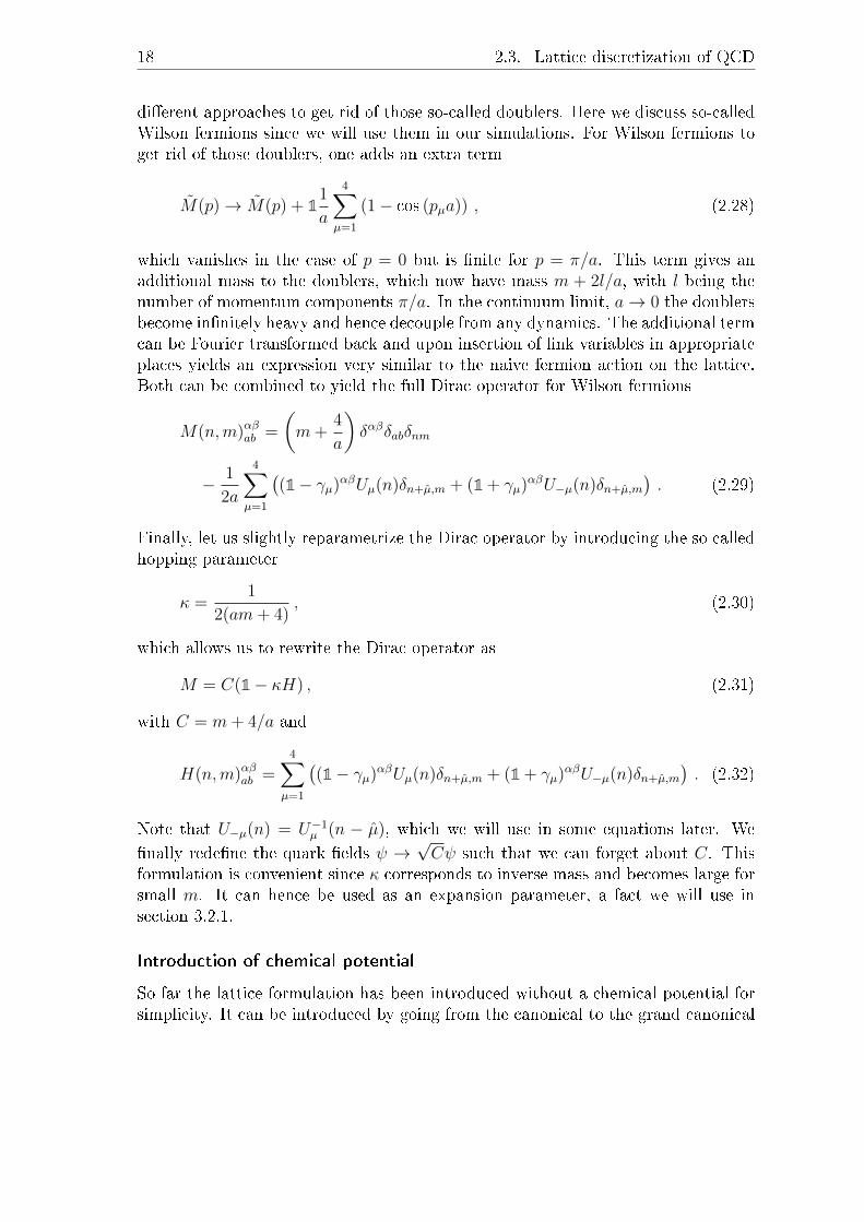
dierent approaches to get rid of those so-called doublers. Here we discuss so-calledWilson fermions since we will use them in our simulations. For Wilson fermions toget rid of those doublers, one adds an extra term
M(p)→ M(p) + 11
a
4∑µ=1
(1− cos (pµa)) , (2.28)
which vanishes in the case of p = 0 but is nite for p = π/a. This term gives anadditional mass to the doublers, which now have mass m + 2l/a, with l being thenumber of momentum components π/a. In the continuum limit, a→ 0 the doublersbecome innitely heavy and hence decouple from any dynamics. The additional termcan be Fourier transformed back and upon insertion of link variables in appropriateplaces yields an expression very similar to the naive fermion action on the lattice.Both can be combined to yield the full Dirac operator for Wilson fermions
M(n,m)αβab =
(m+
4
a
)δαβδabδnm
− 1
2a
4∑µ=1
((1− γµ)αβUµ(n)δn+µ,m + (1 + γµ)αβU−µ(n)δn+µ,m
). (2.29)
Finally, let us slightly reparametrize the Dirac operator by introducing the so calledhopping parameter
κ =1
2(am+ 4), (2.30)
which allows us to rewrite the Dirac operator as
M = C(1− κH) , (2.31)
with C = m+ 4/a and
H(n,m)αβab =4∑
µ=1
((1− γµ)αβUµ(n)δn+µ,m + (1 + γµ)αβU−µ(n)δn+µ,m
). (2.32)
Note that U−µ(n) = U−1µ (n − µ), which we will use in some equations later. We
nally redene the quark elds ψ →√Cψ such that we can forget about C. This
formulation is convenient since κ corresponds to inverse mass and becomes large forsmall m. It can hence be used as an expansion parameter, a fact we will use insection 3.2.1.
Introduction of chemical potential
So far the lattice formulation has been introduced without a chemical potential forsimplicity. It can be introduced by going from the canonical to the grand canonical

Chapter 2. QCD, the lattice, and the sign problem 19
ensemble. As seen in equation (2.1), only the temporal direction relates to chemicalpotential. Then H in the Dirac operator from equation (2.32) is replaced by
H(n,m)αβab =4∑
ν=1
(eδν,4µ(1− γν)αβUν(n)δn+ν,m + e−δν,4µ(1 + γν)
αβU−ν(n)δn+ν,m
).
(2.33)
Introducing chemical potential µ in this way ensures that the correct continuumlimit is reached, see e.g. [37] for details.Given a lattice conguration from a simulation of QCD discretized as explainedabove, we can compute physical observables on the conguration.
Observables on the lattice
The fact that observables generally should be gauge invariant limits our freedom toconstruct them. The simplest observables are traces of closed loops made up of linkvariables.
PlaquettesThe simplest of those is the plaquette, which already occurred in the denition ofthe Wilson gauge action. It is the trace of the smallest possible closed loop startingon a given site, which is the product of four links. It is sometimes convenient to lookat the spatial and temporal plaquette separately. The temporal plaquette is denedas the average over all plaquettes on a given lattice conguration which contain atemporal link. The spatial plaquette only consists of spatial links.
Polyakov loopAnother useful observable is the Polyakov loop, which we already introduced in 2.1.On the lattice, it is the product of all temporal link variables at a spatial point
L =1
Nc
TrNt−1∏t=0
U(t, ~n) . (2.34)
Similarly, one can dene the inverse Polyakov loop
L−1 =1
Nc
Tr0∏
t=Nt−1
U−1(t, ~n) . (2.35)
Chiral condensateThere are several fermionic observables that are useful. One of them is the chiralcondensate, which is given by⟨
ψψ⟩
=1
N3sNt
∂lnZ∂m
= −2κNf
N3sNt
Tr(D−1(D − 1)) = −2κNf
N3sNt
Tr(D−1) (2.36)

20 2.3. Lattice discretization of QCD
in the last equality we dropped a constant, which we can do since the chiral conden-sate renormalizes additively [65]. It is the order parameter for the chiral transitionin the limit of vanishing quark masses, which turns into a crossover at nite quarkmasses.
Quark number densityDerivatives of the quark number density
n =1
N3sNt
∂lnZ∂µ
=Nf
N3sNt
⟨Tr
(M−1 ∂
∂µM
)⟩, (2.37)
e.g. the susceptibility
χn =1
N3sNt
∂2lnZ∂2µ
=N2f
N3sNt
⟨Tr
(M−1∂M
∂µ
)2⟩
− Nf
N3sNt
⟨Tr
(M−1∂M
∂µM−1∂M
∂µ
)2⟩
+Nf
N3sNt
⟨Tr
(M−1∂
2M
∂µ2M−1
)⟩−N3
sNtn2 . (2.38)
also signal the phase transition.
We will discuss the usefulness of those observables when we discuss the phase dia-gram in the context of complex Langevin.
Representation of SU(2) and SU(3) matrices and their complexgeneralizations
The Lie algebra su(n) which corresponds to the group SU(N) has N2− 1 generatorsλa/2, with λa the Gell-Mann matrices. Thus, in principle, it is enough to store N2−1real numbers per matrix. Since exponentiation is needed to get from the algebrainto the group this is expensive. Instead, we save the rst two rows u and v of thematrix, which allows us to reconstruct the third row via the cross product w = u× v,this is convenient on GPUs, where a memory operation is much more expensive thana few oating point operations, we will do this for QCD. CPU simulations typicallyare not limited by memory bandwidth and we can just save the full matrix, i.e. 9complex or 18 real numbers we will do this for HDQCD and the Polyakov chain.Both representations are also useful since in the case of complexication of themanifold i.e. when we consider SL(3,C) as we will do in chapter 3 nothing needsto be changed, even though the coecients of the generators become complex.For SU(2) there is a real representation, it can be written in terms of Pauli matricesσi as
U = x01 + i
3∑i=1
xiσi , (2.39)

Chapter 2. QCD, the lattice, and the sign problem 21
with xi ∈ R and detU =∑x2i = 1. After complexication the coecient xi can be
a complex number, the rest stays the same.
From the lattice to physics
On the lattice, all quantities are formulated in a dimensionless way. To get backto physical units one has to multiply by appropriate powers of the lattice spacing,which has the dimension of length. E.g. temperature, which is given by the temporallattice extent as 1/Nt in physical units reads 1/(aNt). The appropriate power of acan be obtained by dimensional analysis of the quantity at hand.Getting to physical values also requires an actual value for the lattice spacing. Thiscan be done in several ways, e.g. by measuring some observables with good precisionand xing them to the corresponding physical value. However, a particularly conve-nient and cheap way is the gradient ow [66]. The gradient ow is a method whichsmoothes a given lattice conguration. If too much smoothing is applied, it drivesthe lattice towards the classical theory. It is a way to get rid of strong UV uctu-ations, for an alternative way to do this see [67]. For the gradient ow observablestypically monotonously tend towards their classical values as ow time increases.This is used for scale setting by monitoring the ow of 1/4F µνF µν . When it reachesa certain value which has to be predetermined by other scale xing methods, thecorresponding ow time can be used as a scale. The advantage of this approach isthat it is precise and cheap to do. We have used a high precision value from [68]to measure the scale in our QCD simulations. Since this value is for Nf = 2 + 1at physical pion masses, our physical values are just approximate, since we haveNf = 2 avors and heavy pions. The details of the procedure can be found in thecorresponding references, they are not the focus of this thesis.
Whether a lattice simulation is close to the physical point or not is typically deter-mined by the pion rest-mass, since it is the lightest particle of the theory. Therefore,we briey explain how hadron masses can be obtained from the lattice, see [37] formore details. In this thesis we are mainly interested in the pion, hence we use it asan example. The idea is to nd an observable which has the same quantum numbersas the pion. We then measure the correlation function of the creation operator andannihilation operator between dierent lattice points. Intuitively this means thatwe create a pion at some lattice site, let it propagate to another point and annihilateit there. The Euclidean correlator of such observables is given by⟨O(t)O(0)
⟩∼⟨0|e−(T−t)HO(t)e−tHO(0)|0
⟩ T→∞−−−→∑n
〈0|O|n〉⟨n|O|0
⟩e−tEn , (2.40)
where we inserted 1 =∑
n |n〉 〈n| and let the Hamiltonian act on the states. Thusfor large temporal lattice extent, we can extract the lowest lying energies, which aregiven by the rest mass of the observable, via an exponential t. For the pion, welook at the pion interpolator given by
π = q1γ5q2 , (2.41)

22 2.3. Lattice discretization of QCD
with q1 = u and q2 = d for the π+, vice versa for π− and we have a sum of twoterms with q1 = u, q2 = u and q1 = d, q2 = d for the π0. Note that for degeneratequark masses which we have since we do not take into account the U(1) charge the quarks and pions are not distinguishable. Therefore all three choices give thesame result. One can show that this interpolator transforms just like the pion underparity and charge conjugation, see e.g. [37] for details. The correlator for a pioncreated at position m and annihilated at n is given by⟨
O(n)O(m)⟩
=⟨d(n)γ5u(n)u(m)γ4d(m)
⟩= −Tr
[γ5M
−1u (n,m)γ4M
−1d (m,n)
],
(2.42)
where we contracted the quarks according to Wicks theorem. This correlator canbe measured on the lattice. As a nal step, we project the correlators to zeromomentum. This is done by observing that the hadron interpolator can be Fouriertransformed with respect to spatial momentum
O(~p, nt) ∼∑~n
O(~n, nt)e−ia~n·~p , (2.43)
such that for ~p = 0 we only need to sum over all points in a given time-slice.
Monte Carlo simulations and importance sampling
In statistical physics the partition function is given over a sum of all possible energystates via
Z =∑i
e−1TEi . (2.44)
Many interesting quantities can be directly derived from it. If there is a small niteamount of states this sum can often be evaluated analytically. However, typicallythose sums are too large and need to be computed by simulations. In lattice QCDwe deal with innite integrals instead of nite sums, which have to be approximatedby a nite simulation. This is done by setting up a simulation which produces eldcongurations distributed according to the Boltzmann factor e−S. Observables canbe computed from a nite number N of those congurations as
〈O〉 =1
N
∑i
Oi ≈1
Z
∫dφOe−S(φ) . (2.45)
This goes under the name of importance sampling. There are many dierent al-gorithms to produce such congurations, the simplest one being the Metropolisalgorithm [69]Since we will need variations of the Metropolis algorithm in chapter 4, we brieydescribe it here. Given the Euclidean action S in terms of elds φ, the elds areupdated sequentially or in parallel if allowed by symmetry. The updating of asingle site goes as follows

Chapter 2. QCD, the lattice, and the sign problem 23
-1
-0.8
-0.6
-0.4
-0.2
0
0.2
0.4
0.6
0.8
1
-3 -2 -1 0 1 2 3
λ=0λ=50
0
Figure 2.1: Illustration of the sign problem in a simple model from [71]. See text foran explanation.
1. Propose a new value for the eld φ. This is typically done by adding a smallrandom number from a symmetric probability distribution to the current valueof a eld.
2. Compute the dierence in the action ∆S = S(φnew)− S(φold).
3. Draw a uniform random number u from [0, 1]. If u ≤ e−∆S accept the updateand set the eld to its new value. Otherwise, reject and keep the old value.
This algorithm is repeated for all elds. The last step of the algorithm is called anaccept-reject step and we will make use of it in our algorithms in chapter 4.We will use the Metropolis algorithm for simulations of the Ising model and theheat bath algorithm [70] for SU(2) Yang-Mills simulations. For everything relatedto complex actions, we will use a complexied Langevin process, which will bediscussed in much more detail in section 3. In the case of Lefschetz thimbles, as willbe described in the corresponding section, we will use specialized algorithms to doimportance sampling.
2.4 The sign problem in QCD
Consider the simple integral [71]
Z(λ) =
∫ ∞−∞
e−x2+iλxdx =
√πe−
λ2
4 , (2.46)
which is entirely real. Here Z has the form of a simple partition function. The realpart of the integrand is plotted in gure 2.1, it is a smooth positive function for λ = 0and the partition function takes the value
√π while it wildly oscillates for λ = 50
and the partition function evaluates to Z(50) = 6.5 × 10−272. Hence, when MonteCarlo sampling is applied contributions of the order O(1) have to be added up toyield a nal result of almost 300 orders of magnitude lower. Getting a reliable valuewhich can be distinguished from zero would require too many Monte Carlo samples.The numerical sign problem, therefore, is the problem of the precise evaluation

24 2.4. The sign problem in QCD
of highly oscillatory functions by sampling methods. In many theories also inQCD at nite chemical potential, see equation (2.1) oscillatory integrands arecomplex, prohibiting the usual probability interpretation of the measure in which theBoltzmann factor is positive. Thus the usual simulation algorithms no longer work.Both problems, oscillations and complex integrands mathematically speaking arenot an issue since in principle one can shift parts of the measure into the observableby taking averages only with respect to some smooth and real ρR(x) of the measureaccording to
〈O(x)〉 =
∫O(x)ρ(x)dx∫ρ(x)dx
=
∫O(x) ρ(x)
ρR(x)ρR(x)dx∫ ρ(x)
ρR(x)ρR(x)dx
=
⟨O(x) ρ(x)
ρR(x)
⟩R⟨
ρ(x)ρR(x)
⟩R
. (2.47)
This technique goes by the name of reweighting, see e.g. [37]. The denominator istypically referred to as the average sign. The standard choice is ρR = |ρ|. Since weare discussing a statistical physics system, we can rewrite the average sign accordingto ⟨
ρ(x)
ρR(x)
⟩R
=
∫ρ(x)dx∫ρR(x)dx
=Z
ZR= e−
VT
∆f(T ) (2.48)
where we used that in statistical physics Z = e−V/Tf(T ) with the free energy densityf(T ). Thus the average sign approaches zero exponentially fast with increasing vol-ume V for xed temperature. This is a problem since we are usually interested inthe innite volume limit to get rid of nite size eects. If the average sign is closeto zero the cancellation of large contributions is again an issue. Hence, to have aconstant numerical accuracy the computation cost grows exponentially with volume.
For specic instances the sign problem has been shown to be NP hard3 [72], itis hence not to be taken lightly. There exist a variety of approaches to solving thesign problem. Here we list just a few of those that are applicable to QCD or QCDlike theories.
• Reweighting (see above) and its variation multi-parameter reweighting [73].
• Dual formulations make use of the fact that the sign problem is representationdependent. Hence, one can nd model specic coordinate transformationssuch that the action is real or at least such that the sign problem is weaker.Recent examples include QCD in the strong coupling limit [74, 75] and severalother lattice eld theories [7679].
• The density of states method consists of rst simulating the theory with (typ-ically) the energy xed and then numerically integrating over the resultingdistribution. This method relies on very precise simulations in the rst step.For a recent review see [80], for applications to gauge theories see [81, 82].
3NP hardness of an algorithm means that it does scale worse than polynomially with system size,i.e. the complexity of the algorithm cannot be reduced to O(Np) with p ∈ N.

Chapter 2. QCD, the lattice, and the sign problem 25
• In the complex Langevin method a complex stochastic process is simulated.The equilibrium distribution of this process mimics the Boltzmann factor e−S
under certain conditions. It has been successfully applied to dierent param-eter regions of QCD [83, 84]. It is, however, dicult to quantify convergenceof the method. We will investigate complex Langevin in much more detail inchapter 3.
• The Lefschetz Thimble method and its generalizations consist of deformingthe real manifold in such a way that the integrand of the path integral staysreal [85] or imaginary uctuations are minimal [86, 87]. Due to its complexityso far there has been no application to QCD. We will investigate this methodin more detail in chapter 4.
• Much progress exists for the Taylor expansion around µ = 0. This methodhas brought forward many high precision calculations at the physical point forrecent examples see [15, 16, 19]. The Taylor expansion is limited by its radiusof convergence. It is expected to break down at the critical point. Currently,it is not reliable beyond µ/T = 1.
• Analytic continuation from imaginary chemical potential also allows for highprecision computations at the physical point. With iµ ∈ R, the action onceagain is real and simulations can be performed. One can then use analyticityarguments at µ = 0 to extrapolate from µ2 ≤ 0 to µ2 > 0. For recent progresssee [18, 19, 49]. This method so far is also only reliable in the region µ/T < 1.
Despite this multitude of approaches, there is no general solution to the signproblem. The general consensus amongst the community is that each sign problemhas its own solution. One can only hope to nd solutions for classes of theories. Theaim of this thesis is to investigate dierent aspects of the sign problem.
26
3 Complex Langevin
One popular approach to the sign problem is the complex Langevin method. Histor-ically, it was introduced by Klauder [8890] and Parisi [91]. However, problems ofwrong convergence as will be investigated further below showed up rather soon[9295]. Despite some initial success (see e.g. [96]) and some analysis on the failureof complex Langevin in specic situations [97101] its popularity stayed limited fora long time. The main issue was the lack of a criterion to identify convergence tothe wrong distribution. It has since regained popularity and has successfully beenapplied to some real time problems [59, 102, 103], models of QCD at nite chemi-cal potential [83, 104110], the complex Bose gas [111, 112], some fermionic theories[113117] and ultimately some parameter regions of QCD at nite chemical potential[84, 118, 119]. Simultaneously proofs of convergence and resulting criteria have beendeveloped [29, 120123]. However, there are some cases in which complex Langevinsimply does not work. Popular cases are the 3d XY-model at small chemical poten-tials [124] as well as QCD at low lattice couplings β [125127]. While it is usuallyclear if it does not work, there is no general recipe to make it work. The failureof complex Langevin is related either to poles in the action or to insucient decayof the distribution of observables, see section 3.1 for a thorough discussion. Somemethods circumventing those problems have been developed for QCD [105, 128] andnon-relativistic fermionic theories [115].
In this section, we will give a brief and simple introduction to complex Langevin.In section 3.1 we discuss convergence properties of the Complex Langevin method.Section 3.2 contains results and discussions for the application of Complex Langevinto QCD. Finally, in section 3.3 we briey discuss the applicability of the method toreal-time simulations of SU(2) lattice eld theory.
Stochastic quantization
The complex Langevin method is the complex generalization of stochastic quan-tization which was introduced in [129], for an overview, see [130, 131]. The ideabehind stochastic quantization is to obtain the Euclidean Boltzmann factor as anequilibrium distribution of a stochastic process. This will be briey introduced here.First, a fth coordinate t called Langevin time in addition to the four Euclideancoordinates x = (x0, x1, x2, x3) is introduced. The quantum eld then depends onall ve variables φ(x, t). One can dene a stochastic process in form of a Langevin

Chapter 3. Complex Langevin 27
equation as
∂φ(x, t)
∂t= − δS
δφ(x, t)+ η(x, t) = Kφ + η(x, t) , (3.1)
whereKφ is called a drift term, η is Gaussian noise with 〈η(x, t)〉 = 0 and 〈η(x, t)η(x′, t′)〉 =2δ(x−x′)δ(t− t′). By stochastic calculus4 one can derive the corresponding Fokker-Planck equation, which is a dierential equation for the probability distributioncorresponding to a stochastic process. It is easy to see that in this case it has astationary solution of the form
limt→∞
P (φ, t) =e−S(φ)∫Dφe−S(φ)
, (3.2)
i.e. the Euclidean Boltzmann factor as long as the action is well behaved. Hence,stochastic quantization is an alternative way of quantization. Here we focus onlattice simulations of quantum eld theory, a general discussion of stochastic quan-tization/Langevin dynamics for lattice eld theories can be found in [132, 133].So far everything in this chapter has been discussed for the case of real variables, inthe remainder of this chapter, we will refer to this as real Langevin.
Complex Langevin dynamics
In contrast, complex Langevin is obtained by complexifying the eld variable. Wewill demonstrate this for a simple system with only one variable x. In the real case,the integral
〈O〉 =1
Z
∫O(x)e−S(x)dx (3.3)
can be simulated using stochastic quantization as described above. The Langevinequation simply reads
x =∂x(t)
∂t= −∂S
∂x+ η(t) = Kx + η(t) . (3.4)
This stochastic process gives an estimate of the integral in 3.3 after averaging theobservable O over the whole process after equilibration. Note that x ∈ R, hence thisprocess is not properly dened if the action S(x) can take complex values. When thishappens, the whole space needs to be complexied, i.e. x ∈ R→ z ∈ C. The complexLangevin equation is the same as (3.4) but with the replacement x → z = x + iy.By splitting into real- and imaginary part it reads
x =− Re∂S
∂z+ η = Kx + η
y =− Im∂S
∂z= Ky , (3.5)
4In this work everything is formulated via Itô-calculus.

28 3.1. Convergence requirements of Complex Langevin
where we chose a purely real noise, since complex noise usually introduces stabilityissues [121]. This is a coupled system of stochastic dierential equations, which hasan equilibrium distribution of P (x, y). The question that remains to be answeredis whether this leads to the same expectation values as the desired path integralmeasure with the Euclidean action.
A note on discretization and step size
When discretizing the Langevin equation (3.5), a discretization parameter ε, whichrepresents the step size in t direction must be introduced. We will typically performthe easiest discretization, i.e. Euler-Maruyama discretization. Only in full QCDwill we make use of an improved scheme, since it will speed up the simulations.In principle, this parameter then needs to be extrapolated to ε = 0 by performingsimulations at dierent values of ε and observing some converging behavior. Mostlywe will not be concerned with this limit since there are enough issues to be discussedalready before this extrapolation.A pressing issue in complex Langevin are runaway trajectories. They occur in manymodels no matter how simple or complex they are when the simulation escapes intoan unstable direction. The natural way to circumvent those is to make the stepsize ε very small, however, this drastically increases simulation time and can lead toergodicity issues if bottleneck regions exist. A better way to tackle this problem isadaptive step size [104, 134], which makes the step size small if a runaway trajectoryoccurs and forbids the process to go large steps in such directions. We will makeuse of adaptive step size when necessary, especially in the case of QCD.
3.1 Convergence requirements of Complex
Langevin
Let us rst give a denition of what correct convergence of Complex Langevin means.There are two probability distributions which are of importance. On the one handthere is the complex path integral measure ρ(x, t)dx = e−S(x)dx with S ∈ C, whichgives rise to the correct evolution for the expectation value
〈O(t)〉ρ(t) =1
Z
∫O(x)ρ(x; t) dx . (3.6)
On the other hand there is the equilibrium distribution of the process after com-plexication P (x, y; t), which gives rise to
〈O(t)〉P (t) =1
Z
∫O(x+ iy)P (x, y; t) dx dy . (3.7)
Correctness now means that
〈O〉P (t) = 〈O〉ρ(t) ∀t , (3.8)

Chapter 3. Complex Langevin 29
i.e. the expectation value of any observable agrees under both distributions, providedthe initial conditions agree. We choose initial conditions according to equation (A.4).More specically we choose
P (x, y; 0) =1
2πδ(y) (3.9)
There are a few requirements which if not fullled can spoil this equivalence.Those requirements can be split into two groups. The rst group are requirements,which if not fullled do not lead to a Langevin time independent equilibrium distri-bution. While this can be a problem it is also easy to detect. In lattice simulations,we want to simulate in thermal equilibrium and hence, if this is not fullled it isclear that some condition was not met. In the real case, those requirements areusually fullled and they are established by theorems, see e.g. [131]. In the complexcase, it is usually not clear. This has been discussed in [121, 135]. We will not beconcerned with those criteria here since it is easy to see a posteriori if the simulationdoes not converge at all. The other group of requirements covers those, which if notfullled lead to convergence to a wrong limit. It is not so easy to detect this andhence will be discussed in more detail. Those requirements are
1. The process must be ergodic.
2. The distribution, observable, drift and action must be holomorphic. If instead,they are meromorphic poles can spoil the convergence.
3. The distribution, observable and drift must decay fast enough far away fromthe real manifold. We will see below what fast enough means.
The rst point is a problem not only in complex Langevin but also for realLangevin and similar simulation methods such as the more commonly used HybridMonte Carlo algorithm [136]. See [100, 137139] for some discussions on ergodicityin real as well as complex Langevin simulations. We will not go into further detailhere.The second point is one of the current issues still plaguing complex Langevin sim-ulations. The occurrence of poles has received lots of attention in recent years[106, 107, 110, 137, 140143] and it has been suggested that the problem with polesis similar to the problem of slow decay, i.e. if all quantities decay fast enough towardsthe pole, they are no issues [144]. If such fast decay is not observed, poles typicallylead to separated regions in the manifold, spoiling ergodicity. Some possible solu-tions such as the deformation technique [118, 145] have been proposed. However sofar there are not enough results to make a nal judgment on a general procedurefor dealing with poles.The approach we take here is to carefully monitor our simulations for the occurrenceof poles and avoid parameter sets where the poles aect the simulation. Hence, poleswill not be an issue for us, see section 3.2.3.The third point has been discussed mainly in [120, 121]. There a criterion for cor-rectness was based on so-called consistency conditions, which are a measure for

30 3.1. Convergence requirements of Complex Langevin
convergence of complex Langevin. However, neither this condition nor the relatedSchwinger-Dyson equations [120, 146], which are a slightly stronger condition [147]are enough to guarantee convergence without further control. See [59] for a casewhere the Schwinger-Dyson equations are fullled but the evolution converges tothe wrong measure. This can only happen if the solution of the Fokker-Plank equa-tion is not unique.Below we will take a more practical approach. Namely, we will focus on nding a
criterion which can be measured without much additional eort in a realistic latticesimulation.
3.1.1 Convergence of complex Langevin and boundary terms
We start by briey sketching the proof of convergence for the complex Langevinmethod from [120, 121]. The idea of the proof is to introduce an interpolating quan-tity FO(t, τ) between the two sides of equation (3.8) and to show that its derivativevanishes, here τ ∈ [0, t]. To that end we dene
FO(t, τ) =
∫P (x, y; t− τ)O(x+ iy; τ)dxdy , (3.10)
which gives 〈O〉P (t) at τ = 0 and 〈O〉ρ(t) at t = τ , see appendix A.1 for a proof.Hence, if FO(t, τ) is constant for all t and τ equation (3.8) is clearly fullled. Inother words, we require that
∂
∂τFO(t, τ) =
∫(∂τP (x, y; t− τ))O(x+ iy; τ)dxdy
+
∫P (x, y; t− τ)∂τO(x+ iy; τ)dxdy = 0 . (3.11)
In appendix A.1 we show via integration by parts of equation (3.11) that this boilsdown to the vanishing of a boundary term
∂
∂τFO(t, τ) = lim
Y→∞BO(Y ; t, τ) , (3.12)
where
BO(Y ; t, τ) ≡∫[Ky(x, Y )P (x, Y ; t− τ)O(x+ iY ; τ)−KyP (x,−Y ; t− τ)O(x− iY ; τ)]dx .
(3.13)
A simple model
In order to gain a deeper understanding of this boundary term we investigate themodel
ρ(x) =1
Zeiβ cos(x) , (3.14)

Chapter 3. Complex Langevin 31
1x10⁻⁹
1x10⁻⁸
1x10⁻⁷
1x10⁻⁶
1x10⁻⁵
0.0001
0.001
0.01
0.1
-8 -6 -4 -2 0 2 4 6 8
Py(
y;t
)
y
CLEstationary solution
0
0.5
1
1.5
2
2.5
3
3.5
-2 -1.5 -1 -0.5 0 0.5 1 1.5 2
Py(
y;t
)
y
t=1t=5
t=10t=20t=30t=50
t=200stationary solution
Figure 3.1: Left: Comparison of the equilibrium distribution for the model in equa-tion (3.14) with β = 1 from complex Langevin simulations (black) withthe known solution from equation (3.14) (red). Right: Marginal dis-tribution Py(y; t) from solving the Fokker-Planck equation for dierenttimes t (solid lines) compared with the known solution from equation(3.14) (dashed line).
with β ∈ R. This model has been studied with complex Langevin in [103, 148] anddoes give wrong results under complex Langevin evolution. The correct expectationvalues for exponential modes can be obtained in terms of Bessel functions of therst kind∫
eikxρ(x)dx = (−i)kJk(β)
J0(β)6= 0 . (3.15)
For this model the equilibrium distribution P (x, y) is known [149]
P (x, y) =1
4π
1
cosh(y)2. (3.16)
It is remarkable that this solution does neither depend on the coupling β nor on x.By comparison to equation (3.15) it is immediately clear that P cannot give correctresults. Furthermore P decays like e−2|y| for large |y| and hence, the integral for allmodes with k > 1 is not absolutely convergent.We study this model in two ways: By simulating the complex Langevin equationand by solving the Fokker-Planck equation for P (x, y; t) on a grid. Details on thelatter can be found in appendix A.2. The drifts of the complex Langevin equationfor the measure (3.14) read
Kx =− β cos(x) sinh(y)
Ky =β sin(x) cosh(y) , (3.17)
the simulation is then done using Newton discretization for equation (3.5). In gure3.1 left we show that the equilibrium marginal distribution Py(y; t→∞) for β = 1.0obtained by complex Langevin agrees with the exact distribution from equation(3.14) over several orders of magnitude.

32 3.1. Convergence requirements of Complex Langevin
O eix e−ix e2ix e−2ix
CL 0.004(3) 0.002(3) 1.027(22) 1.001(20)correct -0.575081i -0.575081i -0.150162 -0.150162
Table 3.1: Complex Langevin (real part, imaginary part negligible) and correct re-sults for the model in equation (3.14) with β = 1.
To show that the simulation gives wrong results, we list expectation values for therst few modes in table 3.1. The expectation values are measured from 100 dierentruns with randomly chosen starting points and Langevin time up to t ≈ 2500 andstep size dt ≈ 5× 10⁻⁶. For |k| > 2 we nd that expectation values are dominatedby noise, but already for |k| = 2 the result depends on how the averages are com-puted, taking measurements only every 0.01 Langevin time also leads to a resultdominated by noise, while measuring every dt yields the results in table 3.1. This isbecause the integral for the higher modes is not absolutely convergent as mentionedabove. Hence, in principle we would expect a correct result only from the rst mode.However we see that this is also wrong.
Investigation of boundary terms
Since the initial conditions in the complex Langevin and Fokker-Planck simulationswere chosen such that equation (3.8) is fullled (see (A.4) and equation (3.9)), thequestion is where both evolutions start do deviate. The right plot in gure 3.1 showsthe marginal distribution Py(y; t) of the real process for dierent times for β = 0.1.The distribution starts out as a δ-peak at t = 0, which is correct by denition. Itthen broadens over time and nally converges to the wrong distribution in equation(3.14). Looking at the other marginal distribution Px(x; t) in gure 3.2 we see thatP (x, y) does have a small x-dependence at intermediate times, which vanishes forlarger times.
In order to see at which time the correct distribution transitions to the wrong onewe need to see when the boundary term in equation (3.13) becomes non-negligible,which in this simple model we can see by either looking at the time evolution of〈exp(ix)〉 or at the boundary terms directly. Figure 3.3 left shows Fokker-Planckevolution of the rst mode 〈exp(ix)〉 (solid black line) compared to the correct evo-lution (solid black line) 5 (dashed black line). The expectation values from correct-and Fokker-Planck evolution agree up to t ≈ 20, which suggests that up to thattime the deviation of the probability distributions is minor. The boundary term ishard to properly visualize since it depends on three variables already in this simplemodel. Hence, we make the simplication that we only look at τ = 0. We will
5See appendix A.3 for how the correct evolution is obtained.

Chapter 3. Complex Langevin 33
0.1587
0.1588
0.1589
0.159
0.1591
0.1592
0.1593
0.1594
0.1595
0.1596
-3 -2 -1 0 1 2 3
Px(
x;t
)
x
t=1t=10t=20t=50
t=100t=150t=200
stationary solution
Figure 3.2: Marginal distribution Px(x; t) for β = 0.1 at dierent times t. By choiceof the initial condition the distribution starts out constant. It thendevelops a nontrivial structure and in the limit of large times t becomesconstant again.
justify this below. The boundary term at τ = 0 for the rst mode is shown in theright plot of gure 3.3 for β = 0.1 and Y = 5. It starts to deviate from 0 at aroundt ≈ 20 and hence conrms the suspicion that up to this point the evolution seems toagree. Note that the time at which the evolution starts to deviate depends on thechoice of coupling. A larger coupling seems to lead to an earlier deviation, see [29].For the wrong equilibrium distribution in equation (3.14) the boundary term canbe evaluated explicitly. Using equations (3.14) and (3.17) we obtain the boundaryterm from equation (3.12) at τ = 0 in the limit t→∞
Bk(Y ;∞, 0) = −2β
∫ π
−πdx
sin(x) cosh(Y )eikx sinh(Y )
4π cosh2(Y ). (3.18)
Which does converge only for |k| = 1
B∓1(Y ;∞, 0) = ∓iβ2
tanh(Y ) , (3.19)
and is also plotted in gure 3.3, where one can see that the Fokker-Planck evolutionagain converges to the stationary solution.In the end, the limit Y → ∞ has to be taken, see equation (3.12). To this endwe repeat the analysis of the boundary term for dierent values of Y to look forconvergence. This is demonstrated in the left plot of gure 3.4. We see that thedeviation between Y = 5 and Y = 6 is rather small, and hence our earlier choice ofY = 5 can be regarded as already being in the limit Y →∞. This can also be seenby looking at equation (3.19) which is very close to its asymptotic value for Y = 5.The right plot of gure 3.4 shows that the Langevin simulation actually yields theboundary terms following equation (3.19). This can be obtained by looking at thehistogram of KyO, since the histogram already encodes the distribution.
To justify only looking at the boundary term for τ = 0, we need to look at FO(t, τ)directly as shown in gure 3.5. First of all, as expected FO(t, τ) is approximately

34 3.1. Convergence requirements of Complex Langevin
-0.055
-0.05
-0.045
-0.04
-0.035
-0.03
-0.025
-0.02
-0.015
-0.01
-0.005
0
0 50 100 150 200 250
<exp(i
x)>
t
from P(x,y)correct value
from P(x,y) with sreg=0.1
-0.01
0
0.01
0.02
0.03
0.04
0.05
0.06
0 50 100 150 200
β=0.1
-Im
[B1(Y
;t,0
)]
t
from P(x,y)stationary solution
Figure 3.3: Left: Comparison of Im [〈exp(ix)〉] using the Fokker-Planck evolution ofP (solid black line) equation (3.7) with the Lc evolution of the observ-ables (dashed black line equation (3.6) for β = 0.1. For small timest < 20 both evolutions are practically indistinguishable. The red lineshows a regularized version of the action. Right: Boundary term forβ = 0.1 and Y = 5 directly computed from the Fokker-Planck evolution(solid line) and the asymptotic value for t → ∞ from equation (3.19)(dashed line).
constant for times t < 20. Secondly we see that its slope i.e. the boundary term is always maximal at τ = 0. This observation is the reason why we are allowed tochoose τ = 0 in equations (3.18) and (3.19). Note that the evaluation of FO(t, τ) fromequation (3.10) requires knowledge of O(z; t) from the exact evolution as describedin appendix A.3. This evolution reaches it asymptotic limit 〈O〉c approximately atτ > 7. Hence, for large τ it is just a constant that can be pulled out under theintegral and for large τ we arrive at
FO(t, τ) ≈ 〈O〉c∫P (x, y)dxdy = 〈O〉c , (3.20)
which is 〈O〉c = 0.500626i for the rst mode at β = 0.1.
Relation to tails in the distribution
Some works stated that wrong convergence can be identied by looking for largetails in the distribution of the observable [120, 121]. This can be related to theboundary terms in the following way: We can regard equation (3.18) in the limit oflarge Y as the probability density of
v(Y ) ≡ Im∫dxKy(x, Y )O1(x− iY ) ∼ e2Y . (3.21)
Then the statement
limY→∞
v(Y )Py(Y ) 6= 0 , (3.22)
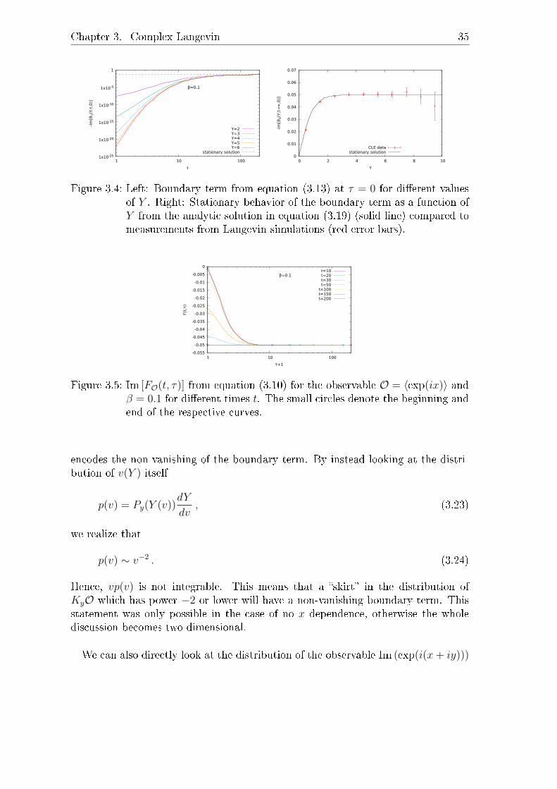
Chapter 3. Complex Langevin 35
1x10-25
1x10-20
1x10-15
1x10⁻¹⁰
1x10⁻⁵
1
1 10 100
β=0.1-I
m[B
1(Y
;t,0
)]
t
Y=2Y=3Y=4Y=5Y=6
stationary solution 0
0.01
0.02
0.03
0.04
0.05
0.06
0.07
0 2 4 6 8 10
-Im
[B1(Y
;t→∞
,0)]
Y
CLE datastationary solution
Figure 3.4: Left: Boundary term from equation (3.13) at τ = 0 for dierent valuesof Y . Right: Stationary behavior of the boundary term as a function ofY from the analytic solution in equation (3.19) (solid line) compared tomeasurements from Langevin simulations (red error bars).
-0.055
-0.05
-0.045
-0.04
-0.035
-0.03
-0.025
-0.02
-0.015
-0.01
-0.005
0
1 10 100
β=0.1
F(t,τ)
τ+1
t=10t=20t=30t=50
t=100t=150t=200
Figure 3.5: Im [FO(t, τ)] from equation (3.10) for the observable O = 〈exp(ix)〉 andβ = 0.1 for dierent times t. The small circles denote the beginning andend of the respective curves.
encodes the non-vanishing of the boundary term. By instead looking at the distri-bution of v(Y ) itself
p(v) = Py(Y (v))dY
dv, (3.23)
we realize that
p(v) ∼ v−2 . (3.24)
Hence, vp(v) is not integrable. This means that a skirt in the distribution ofKyO which has power −2 or lower will have a non-vanishing boundary term. Thisstatement was only possible in the case of no x dependence, otherwise the wholediscussion becomes two dimensional.
We can also directly look at the distribution of the observable Im (exp(i(x+ iy)))

36 3.1. Convergence requirements of Complex Langevin
0
0.1
0.2
0.3
0.4
0.5
0.6
-3 -2 -1 0 1 2 3
σ(u
) (fi
rst
mode)
u
t=1t=5
t=10t=20t=30t=75
t=200 stationary
solution
0.001
0.01
0.1
1
-4 -2 0 2 4
σ(u
) (fi
rst
mode)
u
t=50t=75
t=100t=200
stationary solution
Figure 3.6: Evolution of the distribution of the rst mode σ(u) for dierent timest. Left: Linear scale. Right: Log-scale, the approach to the stationarysolution is more visible here.
for our model by looking at its histogram
σ(u; t) ≡∫dxdyP (x, y; t)δ(sin(x)e−y − u) , (3.25)
which can be evaluated for equation (3.16)
σ(u;∞) =1
2(1 + u2)3/2. (3.26)
It can also be computed from the Fokker-Planck evolution by introducing a binningin the observable, i.e. we sum over all P (x, y) that correspond to a certain valueu = O(x, y). The result for the rst mode is shown in gure 3.6. Initially, theobservable has a double peak structure and decays exponentially, however for largert the double peak structure disappears and tails develop. Hence, we conclude thatthe occurrence of boundary terms and tails in the distribution of observables areintimately linked.
Comparison the drift distribution
Another criterion that has been derived directly in the discretized formulation in[122] is concerned with the distribution of the drift term Ky. It states that thedistribution of the drift term has to decay at least exponentially strong. Since thiscriterion is quite simple, we can easily check it from the Fokker-Planck evolutionas well as from complex Langevin simulations directly using the same methodologythat was used to compute the histogram of the observable. The result is shown ingure 3.7, where it is clear that the drift decays with a power law for all times t andhence violates the criterion from [122]. It is interesting though that initially, thedrift decays with a large power which corresponds to the small boundary termsin that region. Hence, it seems that both criteria the decay of the drift and theboundary term signal a lack of correct convergence in this model.

Chapter 3. Complex Langevin 37
1x10-20
1x10-15
1x10⁻¹⁰
1x10⁻⁵
1
0.01 0.1 1
σ(u
) (|
dri
ft t
erm
|)
u
t=1t=10t=50
t=200
Figure 3.7: Histogram of the Langevin drift for dierent times at β = 0.1. See textfor a discussion.
3 2 1 0 1 2 3x
4
2
0
2
4
y
3 2 1 0 1 2 3x
4
2
0
2
4
y
Figure 3.8: Visualization of the Langevin ow (stream lines), the xed points (reddots) and the actual Langevin evolution (black dots) for β = 0.1. Left:Without regularization. Right: With regularization parameter sz = 0.1.
Restoring convergence in the simple model
It is known quite well that failure of convergence is usually related to large devi-ations or runaways in the complex direction of complex Langevin simulations, seee.g. [121]. Those deviations occur if there are repulsive direction close to the realmanifold. In some cases this can be resolved by using adaptive step size [104, 134],such that the drift force adapts itself if a strong repulsion exists. In gure 3.8 left wevisualize the trajectory the Langevin process takes. The blue ow lines represent theclassical ow without noise. There are no attractive xed points near the real axisbut some repulsive directions. The xed points (red dots) are also not attractive,but circular. This means that the process has no incentive to stay near the realmanifold and will make excursions further from it. In this model the excursions canbe circumvented by adding a regularizing term to the action [29, 115], which is sim-ilar in spirit to dynamical stabilization [128] which will be discussed further in thecontext of gauge theories below. One can regularize here in dierent ways. AddingKRy = −syy to the drift in the imaginary direction introduces an attractive force

38 3.1. Convergence requirements of Complex Langevin
-0.06
-0.05
-0.04
-0.03
-0.02
-0.01
0
0.01
0.02
0 20 40 60 80 100
t
beta=0.1, O1 vs t; CLE s=0.0
CLE s=0.1
FPE s=0.0
-0.05006
-0.05
-0.04
-0.03
-0.02
-0.01
0
0 0.1 0.2 0.3 0.4 0.5 0.6 0.7 0.8
s
beta = 0.1, O1 vs s; CLE data
-0.05006exact integral
Figure 3.9: Left: Comparison of the complex Langevin evolution of Im(exp(ix)) with(purple) and without (orange) regularization (sz = 0.1) for β = 0.1 as afunction of time. The red line shows the Fokker-Planck solution withoutregularization, the purple line shows the correct result for the regular-ized model. Here the regularization leads to correct convergence. Right:Longtime expectation value of Im(exp(ix)) for β = 0.1 for dierent reg-ularization strengths.
towards the real manifold. This term also leaves the periodicity of the real manifoldintact but cannot be expressed as part of a holomorphic action with −∂zS = K.We did solve the Fokker-Planck equation with such regularization for β = 0.1 andsy = 0.1, see the red curve in gure 3.3 left. This regularization term makes thedynamics stable but introduces a large deviation from the original theory. Anotherway of regularizing is to add a term SR = −szz. This leaves the action holomorphicbut destroys the periodicity of the real manifold. We illustrate the eect of sucha term in the right plot of gure 3.8. As one can see such regularization removesthe repulsive directions from the real manifold and makes the xed points attractiveand as a result, the evolution is conned to a much thinner strip around the realmanifold. Depending on the choice of parameters this can make the expectationvalues correct. In the left plot of gure 3.9 we show the Langevin evolution of theregularized and the unregularized model from many dierent Langevin trajectories.The evolution of the regularized model at β = 0.1 closely follows the correct expec-tation value in the case of s = 0.1. However, at larger regularization parametersthis is no longer the case. The evolution still is stable, but the expectation valuesdeviate, see the right plot of gure 3.9.For larger couplings β, the plateau region in the unregularized model becomes muchsmaller or vanishes at all. In this case, the regularization does also stabilize but theexpectation values of the regularized model no longer agree with the original modelfor any choice of regularization parameter [29].
The comparison of the regularized and unregularized model is a good test-bed forthe boundary term and drift criterion. Figure 3.10 shows both criteria and compares

Chapter 3. Complex Langevin 39
-0.01
0
0.01
0.02
0.03
0.04
0.05
0.06
0 0.5 1 1.5 2 2.5 3 3.5 4 4.5 5
-Im
[B1(Y
;t→∞
,0)]
Y
sz=0sz=0.1
0.1
1
10
100
1000
10000
0.5 1 1.5 2 2.5
S= iβcos(x)+s x2/2
β=0.1
His
togra
m o
f th
e d
rift
term
t=15, s=0.1t=100, s=0.1
t=15, s=0 t=30, s=0
t=100, s=0
Figure 3.10: Left: Boundary term for β = 0.1 at t→∞, while there is a boundaryterm for sz = 0 it vanishes for sz = 0.1. Right: Histogram of the drift atdierent times t for sz = 0, where the decay is slower than exponentialand sz = 0.1 where the decay is stronger than exponential.
the regularized case sz = 0.1 with the unregularized case sz = 0 for β = 0.1. Inboth cases, the boundary term goes to a plateau and hence the limit Y → ∞can be taken easily. It becomes clear that the regularization removes boundaryterms completely. Similarly, the drift term decays weaker than exponential for theunregularized case suggesting the failure of complex Langevin. For t = 15 this isnot so clear, however comparing with the drift histogram from the Fokker-Planckevolution (gure 3.7) shows that the decay should be with a high power polynomial.In case of regularization, the decay of the drift decays stronger than exponentialsuggesting that complex Langevin works.The conclusion here is that both criteria perform equally well.
3.1.2 A more practical way to compute boundary terms
Computing boundary terms according to equation (3.13) is practically impossible inhigh dimensional models. This can, however, be simplied. In a practical simulation,we are always interested in expectation values after thermalization, essentially t→∞. Hence, to compute the boundary terms according to equation (3.12) we have totake an additional limit. However, one may wonder about the order, i.e. whether thelimit Y →∞ or t→∞ has to be taken rst. The boundary term (equation (3.12)with (3.11)) without the limit Y →∞ can be rewritten as (cf. equation (A.12))
∂
∂τFO(t, τ) =
−∫ Y
−Y
(∂
∂tP (x, y; t− τ)
)O(x+ iy; τ)dxdy
+
∫ Y
−YP (x, y; t− τ)LcO(x+ iy; τ)dxdy = 0 . (3.27)
Where as before we will take τ = 0, since there the boundary term, i.e. the slope ingure 3.5, is maximal. The rst term vanishes if a stationary solution of the Fokker-

40 3.1. Convergence requirements of Complex Langevin
0
0.05
0.1
0.15
0.2
0.25
0 2 4 6 8 10
-Im
[B1(Y
;t→∞
,0)]
Y
Figure 3.11: Boundary term of the U(1) model computed via 〈Lceix〉.
Planck equation does exist. The second term is just the average of LcO constrainedto the interval [−Y, Y ] such that
BO(Y ; t→∞, τ = 0) = 〈LcO〉Y , (3.28)
with Lc dened in equation (A.7). In the limit Y →∞ this is just the consistencycondition from [120]. A careful look at the Y dependence shows that in the limitthe observable becomes very noisy to the extent that it is almost always consistentto zero within large error bars. Figure 3.11 shows the boundary term for the U(1)model and the observable eix for β = 0.1 without regularization. The equation ofthe observable for the boundary term is
Lceiz = (1 + iβ sin(z))eiz . (3.29)
The boundary term computed this way agrees with gure 3.10. However, for largeY the boundary term becomes very noisy such that it is approximately consistentwith zero. Hence, by the criterion from [120] one could conclude proper convergencewithout further control. This shows that not only the limit Y → ∞ is importantbut also how the limit is approached. From this simple case, we conclude thatthe development of a plateau before large error bars kick in gives the value of theboundary term. If this is nonzero complex Langevin does not converge to the correctresult.
Higher dimensions
So far everything was focused on a simple integral with one variable. Here we willcompute the boundary terms in an exactly solvable higher dimensional model, theSU(3) Polyakov chain. The model consists of a chain of length Nt where points areconnected with SU(3) matrices. Its action reads [105]
−S = c+TrU1 . . . UNt + c−TrU−1Nt. . . U−1
1 , (3.30)
with c± = β+κe±µ. When µ 6= 0 or any of the parameters are chosen to be complex,this will not stay in SU(3), hence for complex Langevin simulations one complexies

Chapter 3. Complex Langevin 41
to SL(3,C), which are all 3 × 3 matrices with detU = 1. This model can be gaugexed such that only one link remains. This one link can then be diagonalized, andonly two variables remain6. In this case the remaining link has the form
U = diag(eiω1 , eiω2 , e−i(ω1+ω2)
), (3.31)
and the action reads
−S = c+
(eiω1 + eiω2 + e−i(ω1+ω2)
)+ c−
(e−iω1 + e−iω2 + ei(ω1+ω2)
). (3.32)
Since this is a variable transformation from SL(3,C) → C2 one has to explicitlycompute the Haar-measure and include it in the action. The additional term is
−S → −S + ln
[sin2
(−2ω1 + ω2
2
)sin2
(ω1 − ω2
2
)sin2
(ω1 + 2ω2
2
)]. (3.33)
Details on the Langevin simulation in both prescriptions can be found in appendixA.4.For the gauge-xed, diagonalized model it is still possible to compute the boundaryterms in both ways. I.e. following equation (3.13) or (3.28). For the explicit com-putation equation (3.13) needs to be generalized. Dropping t and τ dependence fornow the boundary term reads∫ ∫
~∇y
(~KyP (~x, ~y)O(~x+ i~y)
)d~xd~y , (3.34)
where ~x and ~y are vectors containing the real- and imaginary part of the variablesωi. This can be further simplied by using Gauss theorem∫ ∫ [(
~KyP (~x, ~y)O(~x+ i~y))· ~ny]d~xdSy . (3.35)
We choose the surface Sy to be a square with side length 2Y around the origin withY = max(|y1|, |y2|). Hence, the boundary term becomes∫ ∫
Ky1PO|y1=+Y d~xdy2 −∫ ∫
Ky1PO|y1=−Y d~xdy2
+
∫ ∫Ky2PO|y2=+Y d~xdy1 −
∫ ∫Ky2PO|y2=−Y d~xdy1 . (3.36)
In practice this is done by looking at the histogram of Y , which encodes P (Y ),the x-dependence is dropped here. For a given interval [Y − dY/2, Y + dY/2] onecomputes the probability of this interval, i.e. the ratio of the number of Y in thisinterval compared to the total number Nbin/(NtotaldY ). Then one averages PKyOover the bin, i.e.∫
KY PO =1
Nbin
∑bin
PbinKYO =1
NtotaldY
∑bin
KYO , (3.37)
6There are three diagonal entries, but the condition for U ∈ SU(3) that detU = 1 reduces thenumber of variables such that two remain.

42 3.1. Convergence requirements of Complex Langevin
0
0.2
0.4
0.6
0.8
1
1.2
0 0.5 1 1.5 2 2.5 3
Boundary
term
max(|y1|,|y2|)
Real part, from <Lc>YImaginary part, from <Lc>Y
Real part from Gauss theoremImaginary part from Gauss theorem
-1.8
-1.6
-1.4
-1.2
-1
-0.8
-0.6
-0.4
-0.2
0
0.2
0 0.02 0.04 0.06 0.08 0.1
<L c
TrU
>U
N c
utoff
UN
Real part, from <Lc>YImaginary part, from <Lc>Y
Real part from Gauss theoremImaginary part from Gauss theorem
zero
-0.04
-0.02
0
0.02
0.08 0.1
Figure 3.12: Boundary term for the gauge-xed, diagonalized Polyakov Chain. Left:β = i, κ = 0 = µ, complex Langevin does not work. Right: β = 2,κ = 0.1, µ = 1. In both cases the discussed methods to compute theboundary terms agree.
The only subtlety is that there are terms with y1 and y2 in the boundary terms.This is solved by choosing a surface, we always choose KO belonging to the currentY = max(|y1|, |y2|). Having thus computed
∫(KPO)(Y ) = F (Y ) the only thing
that remains is to compute F (Y )−F (−Y ) due to the dierence in equation (3.36).The computation according to equation (3.28) is much easier. Choosing O = TrU =eiω1 + eiω2 + e−i(ω1+ω2) one has to average has to average
〈LcTrU〉 =(~∇+ ~K
)~∇TrU
= −(eiω1 + 2e−i(ω1+ω2) + eiω2
)+ iKω1
(eiω1 − e−i(ω1+ω2)
)+ iKω2
(eiω2 − e−i(ω1+ω2)
), (3.38)
with the drifts Kωi given in appendix A.4. For this model one can easily checkif complex Langevin yields correct results, since the two-dimensional integral canbe done numerically. Choosing β = 2, κ = 0.1 and µ = 1.0 The correct result is〈TrU〉 = 2.0957. The simulation yields 〈TrU〉 = 2.0955(13). Hence, for that setof parameters complex Langevin yields correct results. Accordingly, the boundaryterms plateau to zero up to step size artifacts due to step size of 10−4.If instead we choose β = i, κ = 0 = µ, the correct result is 〈TrU〉 = −0.664 + 0.793iwhereas the simulation yields 〈TrU〉 = −0.4809(6) + 0.5968(5)i. Here complexLangevin clearly fails to converge properly. This is also reected in the boundaryterms in gure 3.12. While the real part goes to zero, the imaginary part saturatesat a nonzero value. The comparison between both methods for computing boundaryterms shows that they agree, however, the computation via 〈LcO〉 becomes noisyfaster at larger Y .
Next, we generalize the boundary terms according to equation (3.28) to the fullPolyakov chain, which is a rst test in a eld theoretical setting and thus an im-portant test in a more realistic case. Since the real manifold is SU(3) with the

Chapter 3. Complex Langevin 43
-5000
-4000
-3000
-2000
-1000
0
1000
2000
0 500 1000 1500 2000 2500
<L c
TrU
>U
N c
utoff
UN
Real partImaginary part
-16
-14
-12
-10
-8
-6
-4
-2
0
2
0 0.0002 0.0004 0.0006 0.0008 0.001
<L c
TrU
>U
N c
utoff
UN
zeroReal part
Imaginary part
-0.3
-0.2
-0.1
0
0.1
0.2
0.0008 0.0009 0.001
Figure 3.13: Boundary term for the full Polyakov-chain for β = 2, κ = 0.1 and µ = 1.Left is without gauge cooling, where boundary terms are expected, rightis with gauge cooling, where they should vanish.
property that for U ∈ SU(3) U †U = 1 but we lose this property when complexifyingto SL(3,C), it makes sense to dene the distance via the so called unitarity norm,which for SU(N) reads
dU = TrU †U −N , (3.39)
and becomes zero for SU(N) matrices. Choosing the unitary norm for Y we canapply equation (3.28). As an observable we choose the Polyakov loop P , which isjust the trace of the product of all the links in order, yielding
LcTrP =Nt−1∑j=0
(Dja +Kj
a
)DjaTrP
= −2NtN2 − 1
NTrP + i
Nt∑j=1
KjaTr (U1 . . . λaUj . . . UNt) , (3.40)
Remember that for β = 2, κ = 0.1 and µ = 1.0 the correct result for the Polyakovloop P is 〈TrP 〉 = 2.0957. The simulation at a constant step size ε = 10−5 yields〈TrP 〉 = 6.09(2) − 0.04(1)i. During the simulation the unitarity norm took valuesup to dU = 3e3, so this deviation is to be expected. The left plot of gure 3.13shows the resulting boundary terms which clearly signals wrong convergence.For the Polyakov chain, it is hard to nd a set of parameters which give correctresults unless they are chosen such that the simulation stays on the real manifold.Hence, we resort to gauge cooling [105]. This procedure is described in A.7. Theidea of the method is to do gauge transformations in the opposite direction of thegradient of the unitarity norm such that the rise of the unitarity norm is sloweddown or stopped. With gauge cooling and a step size of 10−6 the expectation valueof the Polyakov loop becomes 〈TrP 〉 = 2.0961(9) suggesting that convergence hasbeen restored. This is also reected in the boundary terms in the right plot of gure3.13, which is consistent with zero.

44 3.2. Application to QCD
-0.5
0
0.5
1
1.5
2
2.5
3
3.5
1e-6 1e-5 1e-4 1e-3
<L c
TrU
>
stepsize ε
Figure 3.14: Step size dependence of the boundary term in a case where it shouldbe identically zero.
Step size dependence of the boundary terms
In Langevin simulations of lattice eld theories, in principle one has to extrapolatethe step size to zero. Here we are not interested in the ε → 0 limit since oursimulations have strong systematic errors due to a nite volume. Hence we simplyuse small step sizes. In the case of the boundary terms, this can be a problem, sinceat least in the Polyakov chain they are really noisy and uctuate around zero up toO(102). This means that a deviation from a small step size artifact can be inatedconsiderably. We demonstrate this in gure 3.14 for β = 2, κ = 0, µ = 0 wherewe regularly reunitarize the SU(3) matrices. This case is a real Langevin simulationand should not show boundary terms. The gure only shows the average over thefull range, since Y is zero for all values, due to reunitarization. As one can see atlarge step size the boundary term has a large deviation from zero which vanishes forsmall enough step sizes. This needs to be taken into account when judging whethera boundary term is there or not.
3.1.3 Conclusion on boundary terms
We have given a detailed explanation of what happens when complex Langevinfails to converge due to the occurrence of boundary terms. To that end, we havethoroughly investigated a simple model and computed its boundary terms usingcomplex Langevin as well as the Fokker-Planck formulation. We were also able toformulate an observable which can be measured on the lattice and signals wrongconvergence, see equation (3.28). We related the boundary terms to skirts of thedistribution which is typically used to check for convergence and found that anon-vanishing boundary term leads to skirts.
3.2 Application to QCD
Initially, lack of convergence prohibited the application of complex Langevin to QCDat nite chemical potential µ. However, since its revival, some methods to improve

Chapter 3. Complex Langevin 45
convergence have been introduced. Notable methods are the use of adaptive stepsize [104, 134], gauge cooling [105] and dynamical stabilization7 [128], see appendixA.7 for a brief explanation of the last two. In our simulations for QCD, we make useof adaptive step size and gauge cooling, which respects gauge symmetry and doesnot alter the theory. So far we have not used dynamical stabilization, which altersthe dynamics similar to regularization in the U(1) model in the previous section.This section is split into two parts. The rst one is the use of an expansion scheme,which allows for fast simulations. The second part is concerned with the simulationof full QCD with Nf = 2 degenerate fermion avors.Note that for our simulations of gauge theories using complex Langevin we alwaysmonitor the unitarity norm given in equation (3.39) and discard all lattice congu-rations after it grows too large, i.e. after dU = 0.1 is reached for the rst time. Wewill explain why this suces in the context of QCD in section 3.2.3.For the simulations in this section in the expansion and full QCD, we used a GPUcode provided by Dénes Sexty for the production of the lattice congurations. Forthe HDQCD simulations, we used a CPU code by the author.
3.2.1 HDQCD and hopping expansion
The simulation of full QCD is a numerically expensive endeavor. The bottleneckof lattice simulations with fermions is the inversion of the fermion matrix. Sim-ulations may be sped up by using the hopping parameter expansion (see e.g. [62]for a textbook). There have been several works employing dierent version of suchexpansions with aim to study the phase diagram of QCD [83, 108, 150156]. Herewe will further investigate the systematic approach brought forward in [108]. Giventhe full action
S = SYM + Sferm = SYM − log detM , (3.41)
the fermion matrix M from equation (2.31) and below can be rewritten as
M = 1− κsS −R , (3.42)
with the spatial part
S(n,m) = 23∑i=1
(Γ−iUi(n)δm,n+i + Γ+iU
−1i (m)δm,n−i
), (3.43)
and the temporal part
R(n,m) = 2κt(eµΓ−4U4(n)δm,n+4 + e−µΓ+4U
−14 (m)δm,n−4
), (3.44)
7Dynamical stabilization is a modication of the Langevin process. A term is added to the drift,which makes the SU(N) manifold attractive. The only issue with dynamical stabilization isthat the proof of convergence for complex Langevin no longer goes through since the drift ismodied in a non-holomorphic fashion. However, rst tests show a strong improvement in thestability of the simulations upon the use of this method.

46 3.2. Application to QCD
where we introduced the projectors
Γ±ν = (1± γν) . (3.45)
A further rewriting
M = (1−R)
(1− 1
1−RκsS
)(3.46)
allows for factorization of the determinant
detM = det(1−R)exp
(∞∑n=1
−κns
nTr
(1
1−RS
)n), (3.47)
where the spatial part was exponentiated, log det A = Tr logA was used and the log-arithm was expanded. The rst determinant can be computed analytically [104, 150].Both, the fermionic part as well as the terms in the expansion of the spatial deter-minant now only depends on Wilson lines and Wilson loops8 and no longer requireexpensive matrix inversions. To zeroth order, this expansion is known as heavy denseQCD (HDQCD) which is the limit of heavy mass such that fermions cannot movein spatial directions on the lattice but temporal movement is allowed. In HDQCDcomplex Langevin in combination with gauge cooling allows for simulation of thefull phase diagram [83].
Brief analysis of the failure of complex Langevin at low β
It is however known that at lattice coupling β < 5.7 complex Langevin no longergives correct results even in HDQCD as was determined [105] by comparing toreweighting.In gure 3.15 we show the evolution of the spatial part of the plaquette, the simplestobservable on the lattice. Parameters are β = 5.4, κ = 0.12, µ = 0.85 on a 64 latticeas in [105] where complex Langevin was shown to fail even with gauge cooling.The gure shows the long term complex Langevin average (green), the long termreweighting average (blue line) which is expected to be correct in this case andthe evolution of the observable during the simulation. One can see that initially,the simulation approaches the correct value. However, as soon as the correct valueis reached the process goes to another value and stays there. This behavior is verysimilar to the left plot in gure 3.3 for the simple U(1) model. Hence, in analogy,we conclude that even with gauge cooling the real manifold is not attractive enoughand excursions in the complex direction lead to wrong convergence.Note that in HDQCD this is generally not an issue since one can just simulate at
larger β, where correct convergence is observed. We will, however, take this lessonto full QCD as well as higher orders in the expansion and stay at larger β.
8A Wilson line is the product of link variables that form a path. A Wilson loop is a closed Wilsonline.

Chapter 3. Complex Langevin 47
0.46
0.48
0.5
0.52
0.54
0 2 4 6 8 10
CLE evolutionCLE resultRW result
Figure 3.15: Langevin time evolution of the spatial plaquette at β = 5.4, κ = 0.12,µ = 0.85 on a 64 lattice. The green line represents the long term com-plex Langevin result, the blue line shows the same but for reweighting,which in this parameter region is expected to give correct results.
-0.02
0
0.02
0.04
0.06
0.08
0.1
0.12
0.14
1 1.05 1.1 1.15 1.2 1.25 1.3
µ
Polyakov loop, HDQCDPolyakov loop, expansion order 4
Polyakov loop, expansion order 10inv. Polyakov loop, HDQCD
inv. Polyakov loop, expansion order 4inv. Polyakov loop, expansion order 10
-2
0
2
4
6
8
10
12
14
0 0.5 1 1.5 2
densi
ty
µ
Nt=4Nt=8
Nt=16Nt=32Nt=64
Figure 3.16: Left: Polyakov loop at β = 6.0, κs = 0.12 = κt, µ = 0.85 on a 103 × 32lattice for dierent orders of the expansion. The onset of the transitionmoves to the left for higher orders. Right: Density for same parametersall at order N = 10 for dierent inverse temperatures Nt. A non-resolvable region occurs at lower temperatures (see text for details).
Higher orders
We aim to simulate at low temperature to resolve the nuclear transition. In [108] ithas been shown that the expansion for sensible parameters converges around orderN = 10, which we will assume to be the case in general and investigate furtherbelow. To see the eect of the higher orders we simulate κs = 0.12 = κt, β = 6.0,spatial volume N3
s = 103 and temporal extend Nt = 32 for orders N = 0, 4, 10. Theleft plot of gure 3.16 shows the resulting Polyakov loops. One can see that there isa signicant dierence in the onset of the phase transition depending on the order.As a next step, we try to map out the phase diagram of κs expanded QCD at orderN = 10 by varying Nt for dierent temperatures. Choosing the same parameters asabove, we show the resulting density in the right plot of 3.16. Unfortunately for µin the phase transition region, the simulation becomes very slow and it is practicallyunfeasible to get any results for those points.Hence, we conclude that the κs expansion is not a good way to investigate the

48 3.2. Application to QCD
0.594
0.596
0.598
0.6
0.602
0.604
0.606
0.608
0.61
6 8 10 12 14 16 18 20
expansion order
spatial plaquette µ=0.0temporal plaquette µ=0.0
spatial plaquette µ=0.9temporal plaquette µ=0.9
0
0.5
1
1.5
2
2.5
3
3.5
4 6 8 10 12 14 16 18 20
Nt
expansion, µ=0.90expansion, µ=0.95expansion, µ=1.00expansion, µ=1.05expansion, µ=1.10
full QCD, µ=0.90full QCD, µ=0.95full QCD, µ=1.00full QCD, µ=1.05full QCD, µ=1.10
Figure 3.17: Lack of convergence of the κs expansion, see text for details. Left:Convergence of the κs expansion at β = 6.0, κs = 0.12 = κt on a 104
lattice Right: Comparison of 10th order κs expansion to full QCD.
phase diagram of QCD. To see why, we take a look at how well the expansionconverges. This is investigated in gure 3.17. The left plot shows the dependenceof the plaquette on the order of the expansion. While for µ = 0 it is practicallyconverged for N = 10 in agreement to [108], for µ = 0.9 convergence has not beenreached at even N = 20. This suggests that one needs to go even higher or thatconvergence is not possible at all. The right plot shows a comparison of full QCDwith 10th order κs expansion close to the non-resolvable region. One can see thatthe expansion describes QCD less and less while approaching the border. We willsee later in the case of full QCD that the eigenvalues of the fermion matrix becomerather small and it even becomes dicult to invert the fermion matrix in somecases. The breakdown of the expansion seems to be aected by that as well, justmuch earlier 9.
Complex Langevin at µ = 0
Before we turn to full QCD it is instructive to compare the complex Langevinmethod at µ = 0 to the real Langevin method, where the only dierence is reg-ular reunitarization of the SU(3) matrices in the case of real Langevin. We makethis comparison due to repeated claims in the recent years, that complex Langevindoes not even yield correct results at µ = 0, where no complex values should occur[119, 126, 157]. The reason why the process even starts to deviate from the realmanifold is numerical instability. In standard lattice simulations, regular reunita-rization is a necessary feature to avoid this. In complex Langevin however, we arenot allowed to reunitarize but only to use gauge cooling, which has a similar butweaker eect. As we have already established above, complex Langevin does notperform well at lattice coupling β < 5.7 in the case of HDQCD. The reason for theapparent failure of complex Langevin at µ = 0 in other works is the fact that the
9Here the full theory is not holomorphic, but the expansion is. If there is a pole in the full theory,the convergence radius of the expansion is expected to not include that point. Hence, here thebreakdown of the expansion signals the occurrence of the pole in the full theory.

Chapter 3. Complex Langevin 49
-0.0004
-0.0002
0
0.0002
0.0004
0.0006
0.0008
0.001
0.0012
0 10 20 30 40 50 60 70
pla
quett
eunit-p
laquett
enonunit
Nt
spatial plaquettetemporal plaquette
Figure 3.18: Comparison of complex Langevin and real Langevin for β = 6.0,κs = 0.12 = κt in the κs expansion to 10th order. The plot showsthe dierence in the plaquettes between both methods at µ = 0.
simulations have been done close to or below that boundary region10. Assumingthat one can generalize from HDQCD which is suggested by [125], where complexLangevin fails at low β in full QCD as well this explains the failure and suggeststhat larger β is necessary. Hence, to show that complex Langevin and real Langevinagree for large enough coupling we simulate QCD in the κs expansion to 10th orderwith the same parameters as above. The dierence in the plaquette between thesimulations with and without reunitarization is shown in gure 3.18, where one cansee that there is a good agreement with zero. Note that the range of the y-axis inthis plot is rather small, hence everything is consistent with zero11.
Since the κs expansion did not converge to full QCD, we now directly simulatefull QCD.
3.2.2 Full QCD at low temperature
First, we continue to pursue low-temperature simulations. This is achieved by mak-ing Nt large, keeping β xed and varying µ to nd the nuclear liquid-gas transition.So far this has not been achieved in lattice QCD due to the sign problem, however,there are studies for gauge groups without a sign problem, see e.g. [158] for thegroup G2. The transition should be at mN/3, the quark mass from the nucleon.We start by simulating full QCD at the same parameters we used in the expan-sion, i.e. spatial volume N3
s = 103, β = 6.0, κ = 0.12. For those parameters, thesimulation is well behaved and there are no issues for any value of µ. The densityfor Nt = 10 (T ≈ 237MeV) and Nt = 16 (T ≈ 135MeV) is shown in gure 3.19.First we note that the temperature is still rather high, however at T ≈ 135 MeVat least a signal of the transition should be visible. We do only see the lattice go
10Of course this value depends on the choice of discretization for fermions, so in this context, it isto be taken as a rough guideline.
11At small Nt uctuations are usually stronger, hence the larger errors.

50 3.2. Application to QCD
0.0001
0.001
0.01
0.1
1
10
0 0.5 1 1.5 2 2.5
densi
ty
µ
Nt=10Nt=16
Figure 3.19: Density for full QCD at two dierent temperatures. Nt = 10 corre-sponds to T ≈ 237MeV, Nt = 16 to T ≈ 135MeV. This is at a pionmass above mπ > 4.5GeV.
0.0001
0.001
0.01
0.1
1
10
0 0.5 1 1.5 2 2.5
0.0001
0.001
0.01
0.1
0 0.1 0.2 0.3 0.4 0.5
densi
ty
µ
Figure 3.20: Density for full QCD for two dierent parameter sets. The simulationsare at much lower masses than in gure 3.19 and show an onset whichmay be interpreted as the nuclear transition. Note that the onset is notat the correct position, see text for details.
into saturation, but no distinct plateaus as in the case of G2 [158] occur. Thisis to be expected here since the pion mass is12 mπ > 4.5GeV, see appendix A.6.Hence, the quark mass for the onset from the nucleon mN/3 will be at least mπ/2 oreven larger. In lattice units, this means that the earliest point where we expect thetransition is at µ ≈ 0.9, which is already far into the rise to saturation. Hence, wecannot see the transition even if it is there. Therefore we need to go to lower masses.
Figure 3.20 shows the resulting density at smaller masses. The left plot is forβ = 5.9 and κ = 0.148 on a 83×20 lattice. We list the lattice spacing and masses inappendix A.6. The corresponding pion mass is amπ = 0.834(25) or mπ ≈ 3.1GeV.We expect the onset of the transition to be at mN/3, which is above mπ/2. How-ever, even mπ/2 is already on the plateau, this means that the onset happens toearly. In the right plot we zoom in on the plateau region. The data are for β = 6.0,κ = 0.15 on a 83 × 24 lattice. Here amπ/2 = 0.370(9) (mπ/2 ≈ 1.3GeV) and againthe onset is already before that. A possible reason for this discrepancy is that the
12Here we only measured the pion mass on a rather large lattice. Finite size eects will make themass even larger.

Chapter 3. Complex Langevin 51
0.0001
0.001
0.01
0.1
0 0.1 0.2 0.3 0.4 0.5 0.6
densi
ty
µ (phase quenched)
λ2=0.0001λ2=0.00003λ2=0.00001
-0.08
-0.06
-0.04
-0.02
0
0.02
0.04
0.06
0.08
0.1
0.12
0 2000 4000 6000 8000 10000 12000 14000 16000
densi
ty
update number
Figure 3.21: Left: Density for a phase quenched simulation with on a 83× 24 latticewith κ = 0.15 and β = 6.0. Lower λ2 is closer to the actual physics.Right: Evolution of the density for µ = 0.31 and λ2 = 0.00001. Seetext for a discussion.
temperature in those simulations is already moderately high. In physical units, theright plot of gure 3.20 has temperature T ≈ 141MeV. In the left plot this valuesimilar T ≈ 140MeV. Physically the critical endpoint of this transition is found atT ≈ 10MeV. Hence, at our high temperatures, this can only be a remnant of thetransition. We are however not in the continuum limit, where things might change.
The more pressing concern, however, is a problem in the simulation itself, whichwe observe in phase quenched simulations.
Phase quenched simulations
Phase quenched QCD is full QCD but with the phase factor left out, it does notagree with full QCD and we only use it for diagnostic purposes. Its partition functionreads
Zpq =
∫DU
(detM(µ)M †(µ) + λ2
)Nf/2 e−Sg (3.48)
and the determinant is real. Here λ acts as a regularization parameter to preventtoo small eigenvalues in the fermion matrix M and hence speeds up the simulation,it has to be extrapolated to zero. Physically this is equivalent to the introductionof isospin chemical potential, which parametrizes the dierence in dierent quarkspecies. For lattice studies of phase quenched QCD or QCD at nite isospin chem-ical potential see e.g. [159161]. In phase quenched simulations the onset of thetransition is expected at mπ/2. The left plot of gure 3.21 shows the onset transi-tion in from a phase quenched simulation at nite λ. Here the extrapolation λ→ 0would move the onset of the plateau even further to the left. The onset should beat half the pion mass amπ/2 = 0.371(9) (mπ/2 ≈ 1.31GeV), however it happenstoo early again, just as in full QCD. Thus we conclude that this is not an issue ofcomplex Langevin. Instead, the reason is a problem with the thermalization of thesimulation. The right plot of the same gure shows the HMC trajectory at µ = 0.31

52 3.2. Application to QCD
0.6
0.7
0.8
0.9
1
1.1
1.2
0.14 0.145 0.15 0.155 0.16 0.165 0.17
mπ o
n 8
3
κ
beta=6.0beta=5.9
0.4
0.5
0.6
0.7
0.8
0.9
1
1.1
1.2
1.3
1.4
1.5
0.13 0.135 0.14 0.145 0.15 0.155 0.16
mπ o
n 1
23
κ
beta=5.9
Figure 3.22: Pion mass at spatial volume 83 and 123. It was measured with Nt = 32.
for the smallest value of λ2. After a long simulation time, the density goes to a dif-ferent value, which should not happen for purely real simulations unless the systemis not yet thermalized properly.
Assuming we have the same issue in complex Langevin simulations, this explains theoccurrence of the transition at wrong values. The need for long runs is in conictwith the fast rise of the unitarity norm. Dynamical stabilization [128] may makelong simulations and a proper investigation of this issue possible. Additionally forcontinuum extrapolated simulations, one needs to go to a much lower temperature,hence making lattices much larger. Such simulations are out of reach with our re-sources for now.
Let us briey mention that in our simulations we see a clear dierence betweenphase quenched and full QCD simulations. This can be seen e.g. for the Polyakovloop. In a phase quenched simulation the Polyakov loop and the inverse Polyakovloop are equal. In our full QCD simulations only observe this at µ = 0, where phasequenched and full QCD agree either way.
Volume dependence of the mass
In the previous section, the pion mass was always above 2GeV. We want to get farbelow that, however, at small spatial volumes such as ours, the mass has a lowerbound [162]. We measured the mass at a volume of N3
s × 32 with Ns = 8, 12. Theresult is shown in gure 3.22. This conrms that our simulations have been doneat approximately the lowest possible mass at this volume. Below we will performsimulations at β = 5.9 and κ = 0.15. The pion mass for Ns = 8 is mπ > 2.1 GeV,we did not measure mN . For Ns = 12 mπ ≈ 1.55 GeV and mN ≈ 2.8 GeV. Seeappendix A.6. Hence, mπ/2 < mN/3 such that we are not in the limit of very heavyquarks. Hence, we see nontrivial eects from the quarks and the dynamics are notpurely dominated by the Yang-Mills sector.
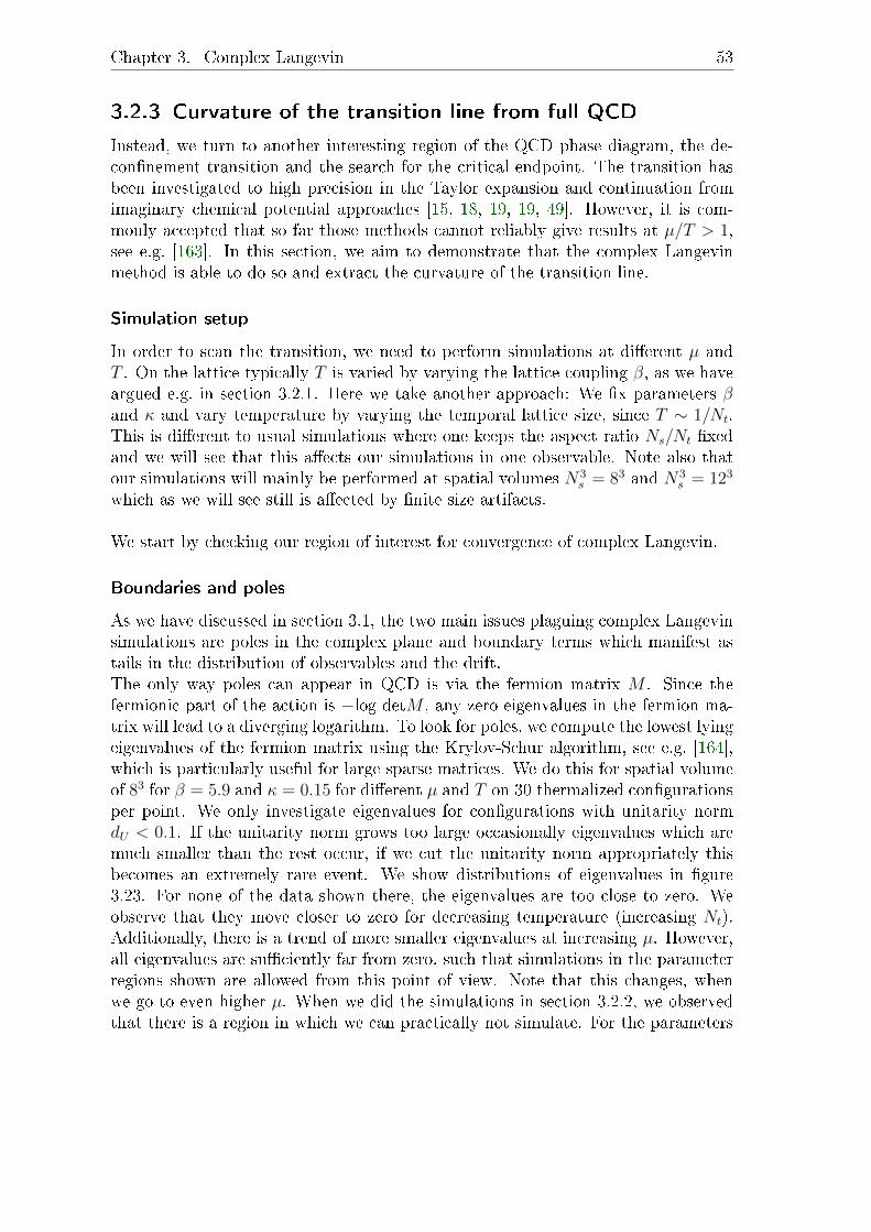
Chapter 3. Complex Langevin 53
3.2.3 Curvature of the transition line from full QCD
Instead, we turn to another interesting region of the QCD phase diagram, the de-connement transition and the search for the critical endpoint. The transition hasbeen investigated to high precision in the Taylor expansion and continuation fromimaginary chemical potential approaches [15, 18, 19, 19, 49]. However, it is com-monly accepted that so far those methods cannot reliably give results at µ/T > 1,see e.g. [163]. In this section, we aim to demonstrate that the complex Langevinmethod is able to do so and extract the curvature of the transition line.
Simulation setup
In order to scan the transition, we need to perform simulations at dierent µ andT . On the lattice typically T is varied by varying the lattice coupling β, as we haveargued e.g. in section 3.2.1. Here we take another approach: We x parameters βand κ and vary temperature by varying the temporal lattice size, since T ∼ 1/Nt.This is dierent to usual simulations where one keeps the aspect ratio Ns/Nt xedand we will see that this aects our simulations in one observable. Note also thatour simulations will mainly be performed at spatial volumes N3
s = 83 and N3s = 123
which as we will see still is aected by nite size artifacts.
We start by checking our region of interest for convergence of complex Langevin.
Boundaries and poles
As we have discussed in section 3.1, the two main issues plaguing complex Langevinsimulations are poles in the complex plane and boundary terms which manifest astails in the distribution of observables and the drift.The only way poles can appear in QCD is via the fermion matrix M . Since thefermionic part of the action is −log detM , any zero eigenvalues in the fermion ma-trix will lead to a diverging logarithm. To look for poles, we compute the lowest lyingeigenvalues of the fermion matrix using the Krylov-Schur algorithm, see e.g. [164],which is particularly useful for large sparse matrices. We do this for spatial volumeof 83 for β = 5.9 and κ = 0.15 for dierent µ and T on 30 thermalized congurationsper point. We only investigate eigenvalues for congurations with unitarity normdU < 0.1. If the unitarity norm grows too large occasionally eigenvalues which aremuch smaller than the rest occur, if we cut the unitarity norm appropriately thisbecomes an extremely rare event. We show distributions of eigenvalues in gure3.23. For none of the data shown there, the eigenvalues are too close to zero. Weobserve that they move closer to zero for decreasing temperature (increasing Nt).Additionally, there is a trend of more smaller eigenvalues at increasing µ. However,all eigenvalues are suciently far from zero, such that simulations in the parameterregions shown are allowed from this point of view. Note that this changes, whenwe go to even higher µ. When we did the simulations in section 3.2.2, we observedthat there is a region in which we can practically not simulate. For the parameters

54 3.2. Application to QCD
0.0001
0.001
0.01
0.1
0.001 0.01 0.1 1
Nt=4Nt=8
Nt=12Nt=16Nt=20
0.0001
0.001
0.01
0.1
0.001 0.01 0.1 1
Nt=4Nt=8
Nt=12Nt=16Nt=20
0.0001
0.001
0.01
0.1
0.001 0.01 0.1 1
Nt=4Nt=8
Nt=12Nt=16Nt=20
0.0001
0.001
0.01
0.1
0.001 0.01 0.1 1
Nt=4Nt=8
Nt=12Nt=16Nt=20
Figure 3.23: Normalized histogram of the absolute value of the lowest lying eigen-values. The dierent plots are at µ = 0.0, 0.3, 0.9, 1.2 from top left tobottom right.
investigated here, we also observe that the simulation slows down signicantly whenapproaching the region of µ = 1. This can be interpreted by an increasing numberof low lying eigenvalues, since the conjugate gradient which we use to invert thefermion matrix is known to slow down signicantly for too low eigenvalues. Fornow we stay away from too large µ and too low T , we have a maximal value ofµ/Tc(0) ≈ 5 and our simulations do not hit any poles.
We investigate the boundary terms by looking at histograms of observables andcheck for tails in the distribution. If we observe exponential decay, we trust thatthere are no signicant boundary terms. Figure 3.24 shows the histogram of Labs =√LL−1 for two dierent Nt at µ = 0.3. The histograms decay exponentially and no
change in behavior is seen when cutting the unitarity norm earlier than dU = 0.1.We also show the expectation values of the Polyakov loop as we will use it, seeequation (3.49) in the next section. This is shown in table 3.2, where no trend ofmore accuracy or deviations towards lower cuto is visible. Here we focused on thePolyakov loop, since for the location of the phase transition we are mainly interestedin this observable. Other observables such as the plaquette, the density, and thechiral condensate are equally well behaved, but not shown here. We conclude, thatour simulations are not plagued by boundary terms.

Chapter 3. Complex Langevin 55
0.0001
0.001
0.01
0.1
0.04 0.06 0.08 0.1 0.12 0.14 0.16 0.18
norm
aliz
ed c
ount
Re[Labs]
0.0001
0.001
0.01
0.1
0 0.005 0.01 0.015 0.02 0.025 0.03 0.035 0.04 0.045
norm
aliz
ed c
ount
Re[Labs]
Figure 3.24: Normalized histogram of Labs for µ = 0.3 and Nt = 7 (left) and Nt = 15(right). It is well behaved.
µ Nt Labs cut at 0.1 Labs cut at 0.010.0 7 0.081(1) 0.083(1)0.0 15 0.0138(1) 0.0139(2)0.3 7 0.0108(5) 0.1111(14)0.3 15 0.0138(1) 0.0140(2)0.5 7 0.1364(5) 0.1354(6)0.5 15 0.0148(1) 0.0146(2)
Table 3.2: Comparing Labs expectation values for dierent unitarity norm cutos.
A note on the drift criterion
For completeness, we also had a brief look at the criterion on the decay of the driftfrom [122]. This criterion states that the drift term has to decay at least exponen-tially fast for complex Langevin to be convergent. We show the drift histogram fortwo dierent µ and Nt
13 in gure 3.25. One can see that according to this criterion,complex Langevin results should not be trusted at much lower unitarity norm.Since expectation values and histograms of the observables are well behaved as shownin the previous section, we do not cut earlier despite the drift histogram decayingpolynomially in some cases. This can be viewed in analogy to the simple model, seegures 3.4, 3.7 and 3.3. There the drift histogram shows polynomial decay all thetime, but the boundary terms initially are small enough such that the expectationvalues still are correct.
We conclude that we simulate in a region without boundary terms or poles. Aslong as we cut the unitarity norm early enough complex Langevin can be trusted.
13Note that there is no particular reason why those µ and Nt values are dierent from those inthe previous section, we just did not measure the histogram in all cases, so here we chose runswhich had large enough unitarity norm to show something. Many runs stay at low enoughunitarity norm to never develop issues.

56 3.2. Application to QCD
10-9
10-8
10-7
10-6
10-5
10-4
10-3
10-2
10-1
100
0 50 100 150 200 250
norm
aliz
ed c
ount
|Drift|2
cut at UN=0.09cut at UN=0.056
cut at UN=0.03
10-9
10-8
10-7
10-6
10-5
10-4
10-3
10-2
10-1
100
0 50 100 150 200 250
norm
aliz
ed c
ount
|Drift|2
cut at UN=0.06cut at UN=0.029cut at UN=0.014cut at UN=0.007cut at UN=0.003
Figure 3.25: Histogram of the drift for µ = 0.15 and Nt = 10 (left) and µ = 0.05and Nt = 20, see text for a discussion.
Observables for the transition
The typical observable that is chosen to probe the QCD crossover transition at phys-ical pion mass is the susceptibility of the chiral condensate. Since our simulationsare at heavier pion masses, it can be hard to get a signal for the crossover transition,see e.g. [165] for the mass dependence of the chiral susceptibility. The chiral conden-sate also needs to be renormalized, which requires additional expensive simulationsat zero temperature. Hence, we discard the chiral condensate as an observable forthis work.Instead, we turn to the Polyakov loop, which at our masses gives a much better sig-nal for the crossover. However, the Polyakov loop needs to be renormalized as well.Since it renormalizes purely multiplicatively [166], we can use ratios of Polyakovloops and not renormalize at all. Also, since the Polyakov loop itself is very noisy,we work with
Labs =√LL−1 (3.49)
instead. One could also use the sum of L and L−1, but we nd that within oursetup the signal for the transition becomes much less clear in this case. We use thefollowing observables to determine the phase transition
C3(Labs) =〈L3
abs〉〈L2
abs〉1.5 (3.50)
C3(Labs − 〈Labs〉) =
⟨(Labs − 〈Labs〉)3⟩⟨
(Labs − 〈Labs〉)2⟩1.5 (3.51)
C4(Labs) =〈L4
abs〉〈L2
abs〉2 . (3.52)
The quantity C3(Labs−〈Labs〉) measures the dierence of uctuations in both phases.Commonly one extracts the phase transition temperature from such quantities astheir intersection point from dierent volumes, see e.g. [167]. The Binder cumulantC4(Labs−〈Labs〉) is a more common observable for that, however within our setup it

Chapter 3. Complex Langevin 57
-1
-0.8
-0.6
-0.4
-0.2
0
0.2
0.4
0.6
0.8
5.2 5.3 5.4 5.5 5.6 5.7 5.8 5.9 6
subtr
act
ed t
hir
d o
rder
cum
ula
nt
β
Ns=12Ns=16Ns=24
0 1
1.5
2
2.5
3
3.5
5.2 5.3 5.4 5.5 5.6 5.7 5.8 5.9 6
unsu
btr
act
ed f
ourt
h o
rder
cum
ula
nt
β
Ns=12Ns=16Ns=24Ns=32
1
1.5
2
2.5
3
3.5
4 6 8 10 12 14 16 18 20
unsu
btr
act
ed f
ourt
h o
rder
cum
ula
nt
Nt
N=8N=12N=20N=32
Figure 3.26: Top left: Subtracted third order cumulant C3(Labs−〈Labs〉) as a functionof β. Top right: Unsubtracted fourth order cumulant C4(Labs). In bothcases κ = 0.15, Nt = 6. Bottom: Unsubtracted fourth order cumulantas a function of Nt for dierent volumes. Here β = 5.9 and κ = 0.15.See text for a discussion.
does not show a strong enough signal, so we do not use it. Taking the same quanti-ties but only with Labs instead of Labs− 〈Labs〉 also shows a crossover between bothphases. However, here it is not clear how to extract a phase transition temperature.We will argue how to get a transition temperature using a dierent method than forC3(Labs − 〈Labs〉), see below.Before going to chemical potential, we look at the behavior of the third order cumu-lant from (3.51) at µ = 0 and when varying T via β instead of Nt. We only performthis analysis to identify Tc, we will not use it further since complex Langevin doesnot work for low β. The result is shown in gure 3.26. One can see that the curvesfor dierent volumes meet at their zero crossing. Thus we dene the transition tem-perature as the temperature at which C3(Labs − 〈Labs〉) = 0. Figure 3.26 also showsthe unsubtracted fourth order cumulant C4(Labs) which does not show any distinctpoints which could be used to identify the phase transition, the same holds for theunsubtracted third order cumulant. Finally, 3.26 also shows the volume dependenceof the unsubtracted fourth order cumulant. It shows strong nite size eects in thevolumes we work with, hence strong eects in the results are expected.
The subtracted third order cumulant for β = 5.9, κ = 0.15 as a function ofNt for dierent µ is shown in gure 3.27 (top). From this gure, we see that largerµ tend to be less noisy. We extract the transition temperatures for C3(Labs−〈Labs〉)

58 3.2. Application to QCD
-0.6
-0.4
-0.2
0
0.2
0.4
0.6
0.8
1
0.05 0.1 0.15 0.2 0.25
3rd
ord
er
cum
ula
nt
subtr
act
ed
1/Nt
mu=0.0mu=0.1mu=0.2mu=0.3mu=0.4mu=0.5
-0.4
-0.2
0
0.2
0.4
0.6
0.8
1
0.05 0.1 0.15 0.2 0.25
3rd
ord
er
cum
ula
nt
subtr
act
ed
1/Nt
mu=0.0mu=0.1mu=0.2mu=0.3mu=0.4mu=0.5
1
1.05
1.1
1.15
1.2
1.25
1.3
1.35
1.4
0.05 0.1 0.15 0.2 0.25
3rd
ord
er
cum
ula
nt
unsu
btr
act
ed
1/Nt
mu=0.0mu=0.1mu=0.2mu=0.3mu=0.4mu=0.5
1
1.05
1.1
1.15
1.2
1.25
1.3
1.35
1.4
0.05 0.1 0.15 0.2 0.25
3rd
ord
er
cum
ula
nt
unsu
btr
act
ed
1/Nt
mu=0.0mu=0.1mu=0.2mu=0.3mu=0.4mu=0.5
1
1.2
1.4
1.6
1.8
2
2.2
2.4
0.05 0.1 0.15 0.2 0.25
4th
ord
er
cum
ula
nt
unsu
btr
act
ed
1/Nt
mu=0.0mu=0.1mu=0.2mu=0.3mu=0.4mu=0.5
1
1.2
1.4
1.6
1.8
2
2.2
2.4
0.05 0.1 0.15 0.2 0.25
4th
ord
er
cum
ula
nt
unsu
btr
act
ed
1/Nt
mu=0.0mu=0.1mu=0.2mu=0.3mu=0.4mu=0.5
Figure 3.27: Observables as a function of 1/Nt for dierent µ. Parameters are β =5.9, κ = 0.15 and N3
s = 83 (left) or N3s = 123 (right). Top: Subtracted
third order cumulant C3(Labs − 〈Labs〉). Middle: Third order cumulantC3(Labs). Bottom: Fourth order cumulant C4(Labs). See text for adiscussion.
from two dierent ts such that we can have an estimate for the systematic error.
1. A linear t to the region close to the zero crossing.
2. A t of
s− (s− b)e−kNt , (3.53)
which is performed with Nt and not 1/Nt on the x axis. This t takes intoaccount all points with Nt larger than the rst point where the cumulant islarger than 0.15.
Errors are estimated using the statistical bootstrap. I.e. given the original data setof size N , we draw N random samples from it, such that samples can occur multiple

Chapter 3. Complex Langevin 59
-0.01
0
0.01
0.02
0.03
0.04
0.05
0.06
0.07
0.08
5.2 5.3 5.4 5.5 5.6 5.7
densi
ty s
usc
epti
bili
ty
β
Ns=12Ns=16Ns=24Ns=32
-0.2
0
0.2
0.4
0.6
0.8
1
1.2
1.4
1.6
1.8
0.08 0.1 0.12 0.14 0.16 0.18 0.2 0.22 0.24 0.26
densi
ty s
usc
epti
bili
ty
1/Nt
mu=0.0, Nt=12mu=0.1, Nt=12mu=0.2, Nt=12mu=0.3, Nt=12mu=0.4, Nt=12mu=0.5, Nt=12mu=0.0, Nt=16mu=0.1, Nt=16mu=0.2, Nt=16mu=0.3, Nt=16mu=0.4, Nt=16
Figure 3.28: Density susceptibility. Left: From β-scan. Right: From Nt-scan. Theirbehavior diers, see text.
times. We then perform the t on this random set. Averaging over many of thosesets yields an estimate for the statistical error, see e.g. [37].
For the other two observables, there is no clear feature that can be used to identifya transition temperature, see gure 3.27. Instead, we use the method from [168],which was also applied and shown to agree with other denitions in the continuumin [19]. The idea is to obtain the transition temperature at nite µ from the one atµ = 0 by shifting the observables. To be more precise, given an observable Ons thatdoes not show any identiable behaviors in the transition region, we take the valueof Tc(0) from another observable Os, which gives a clear signal. We then extractthe value of temperature at µ = 0 at which Ocrit
ns = Tc(0). Next, we look at Ons athigher µ and check for the temperature Tc(µ) at which Ons = Ocrit
ns . This denesthe critical temperature at higher µ. This denes the critical temperature and doesnot require any distinct features in the observable, as long as we have a good de-termination at µ = 0. We use the µ = 0 value from the analysis of the subtractedthird-order cumulant. In our simulations, we use a smoothing cubic spline t to geta continuous function from our data before applying the shifting method. We tunedthe number of supports in the cubic spline t such that a smooth behavior withoutany bumps was observed in the transition region. Errors again are estimated usingbootstrap analysis.
Another observable that does not need to be renormalized is the density and itsderivatives. We show the density susceptibility see equation (2.38) from a βscan and from our Nt scan in gure 3.28. While for the β scan a transition is clearlyvisible, this is not the case for the Nt scan. This is probably due to the fact thatthe aspect ratio of the lattice is not held constant. The advantage of this observableis that it does not depend on volume. Hence, we could use any value of N3
s andextract a transition temperature. Since we are unable to extract a distinct featurefrom our data and the dierence between both plots in gure 3.28 is so large wediscard this observable for now.

60 3.2. Application to QCD
Curvature of the transition line for µ/Tc(0) < 5.
Finally, we are interested in the curvature of the transition line, which is a commonlymeasured quantity from lattice simulations, see e.g. [19, 49] for recent values. UsingµB = 3µ, the transition temperature is commonly parametrized as
Tc(µB) = Tc(0)− κ2µ2B
Tc(0)+O(µ4
B) . (3.54)
We t this function to our data and normalize afterwards to
Tc(µB)
Tc(0)= 1− κ2
(µBTc(0)
)2
+O(µ4B) . (3.55)
We report the resulting parameters in table 3.3. Tc(0) is the t parameter fromthe above t, errors are from a bootstrap analysis by performing the t on dierentbootstrap samples and averaging over those. Hence, even though we used the sameTc at µ = 0 from the subtracted third-order cumulant for all other observables aswell, the actual quoted value of Tc(0) diers from that, since it comes from the tand hence incorporates the eect of the other data points as well.
The resulting value for κ2 is consistent for all observables from the Polyakov loopratios we looked at.Comparing to the values from [19, 49] which is approximately κ2 ≈ 0.014, the
curvature from our data is much smaller. This is not surprising since in HDQCD where quarks are heavy and cannot move in spatial directions the transition line atsmall temperatures is at [83]. Hence, our results nicely interpolate between heavyquarks and those with physical mass. Note, however, that there are a few othersystematic sources of error which may have an eect. This is also reected in thetransition temperature which for physical quark masses should be Tc ≈ 155 MeV,while in pure Yang-Mills or innite masses it is at Tc ≈ 270 MeV. Our simulationsyield values above the Yang-Mills temperature due to nite size eects. This is alsoreected in the fact that the curvature slightly diers between volumes, see table3.3. We are also not in the continuum limit, while curvature values given in [19, 49]are properly continuum extrapolated.
3.2.4 Conclusion on complex Langevin for QCD
In this section, we found that complex Langevin seems to be applicable throughoutthe most part of the phase diagram. We found that the hopping expansion does notwork well close to poles and thus should not be used to scan the phase diagram.Using the hopping expansion in a region where it behaves nicely, we showed that

Chapter 3. Complex Langevin 61
0.7
0.75
0.8
0.85
0.9
0.95
1
1.05
1.1
1.15
0 0.5 1 1.5 2 2.5 3 3.5 4 4.5
Tc(
µ)/
Tc(
0)
µ/Tc(0)
data from exp fitdata from lin fit
fit to data from exp fit of 1-κ x2
fit to data from lin fit of 1-κ x2
0.6
0.65
0.7
0.75
0.8
0.85
0.9
0.95
1
1.05
1.1
1.15
0 1 2 3 4 5T
c(µ
)/T
c(0
)
µ/Tc(0)
quadratic fit to exp fit dataquadratic fit to lin fit data
data from exp fitdata from lin fit
0.7
0.75
0.8
0.85
0.9
0.95
1
1.05
1.1
0 0.5 1 1.5 2 2.5 3 3.5 4 4.5
Tc(
µ)/
Tc(
0)
µ/Tc(0)
data from exp fitdata from lin fit
fit to data from exp fit of 1-κ x2
fit to data from lin fit of 1-κ x2
0.6
0.65
0.7
0.75
0.8
0.85
0.9
0.95
1
1.05
1.1
0 1 2 3 4 5
Tc(
µ)/
Tc(
0)
µ/Tc(0)
quadratic fit to exp fit dataquadratic fit to lin fit data
data from exp fitdata from lin fit
0.7
0.75
0.8
0.85
0.9
0.95
1
1.05
1.1
0 0.5 1 1.5 2 2.5 3 3.5 4 4.5
Tc(
µ)/
Tc(
0)
µ/Tc(0)
data from exp fitdata from lin fit
fit to data from exp fit of 1-κ x2
fit to data from lin fit of 1-κ x2
0.65
0.7
0.75
0.8
0.85
0.9
0.95
1
1.05
1.1
0 1 2 3 4 5
Tc(
µ)/
Tc(
0)
µ/Tc(0)
quadratic fit to exp fit dataquadratic fit to lin fit data
data from exp fitdata from lin fit
Figure 3.29: Curvature of the transition line. Parameters are as in gure 3.27.
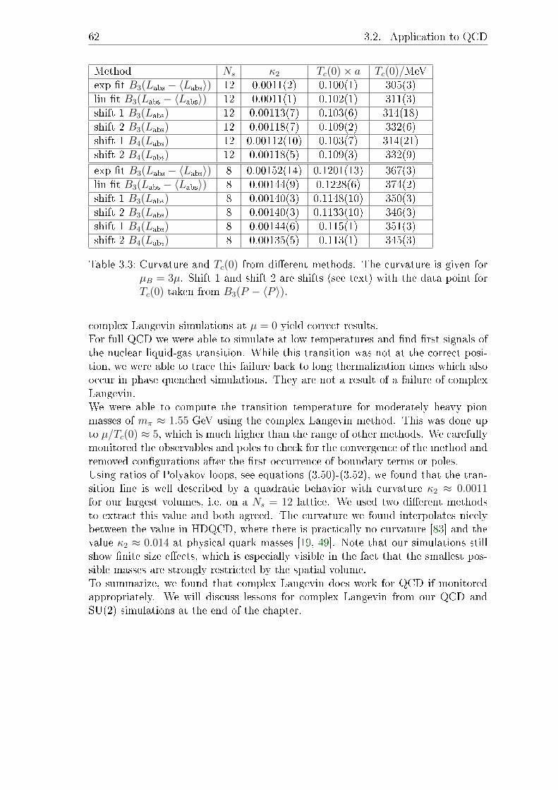
62 3.2. Application to QCD
Method Ns κ2 Tc(0)× a Tc(0)/MeVexp t B3(Labs − 〈Labs〉) 12 0.0011(2) 0.100(1) 305(3)lin t B3(Labs − 〈Labs〉) 12 0.0011(1) 0.102(1) 311(3)shift 1 B3(Labs) 12 0.00113(7) 0.103(6) 314(18)shift 2 B3(Labs) 12 0.00118(7) 0.109(2) 332(6)shift 1 B4(Labs) 12 0.00112(10) 0.103(7) 314(21)shift 2 B4(Labs) 12 0.00118(5) 0.109(3) 332(9)
exp t B3(Labs − 〈Labs〉) 8 0.00152(14) 0.1201(13) 367(3)lin t B3(Labs − 〈Labs〉) 8 0.00144(9) 0.1228(6) 374(2)shift 1 B3(Labs) 8 0.00140(3) 0.1148(10) 350(3)shift 2 B3(Labs) 8 0.00140(3) 0.1133(10) 346(3)shift 1 B4(Labs) 8 0.00144(6) 0.115(1) 351(3)shift 2 B4(Labs) 8 0.00135(5) 0.113(1) 345(3)
Table 3.3: Curvature and Tc(0) from dierent methods. The curvature is given forµB = 3µ. Shift 1 and shift 2 are shifts (see text) with the data point forTc(0) taken from B3(P − 〈P 〉).
complex Langevin simulations at µ = 0 yield correct results.For full QCD we were able to simulate at low temperatures and nd rst signals ofthe nuclear liquid-gas transition. While this transition was not at the correct posi-tion, we were able to trace this failure back to long thermalization times which alsooccur in phase quenched simulations. They are not a result of a failure of complexLangevin.We were able to compute the transition temperature for moderately heavy pionmasses of mπ ≈ 1.55 GeV using the complex Langevin method. This was done upto µ/Tc(0) ≈ 5, which is much higher than the range of other methods. We carefullymonitored the observables and poles to check for the convergence of the method andremoved congurations after the rst occurrence of boundary terms or poles.Using ratios of Polyakov loops, see equations (3.50)-(3.52), we found that the tran-sition line is well described by a quadratic behavior with curvature κ2 ≈ 0.0011for our largest volumes, i.e. on a Ns = 12 lattice. We used two dierent methodsto extract this value and both agreed. The curvature we found interpolates nicelybetween the value in HDQCD, where there is practically no curvature [83] and thevalue κ2 ≈ 0.014 at physical quark masses [19, 49]. Note that our simulations stillshow nite size eects, which is especially visible in the fact that the smallest pos-sible masses are strongly restricted by the spatial volume.To summarize, we found that complex Langevin does work for QCD if monitoredappropriately. We will discuss lessons for complex Langevin from our QCD andSU(2) simulations at the end of the chapter.

Chapter 3. Complex Langevin 63
3.3 Applicability of complex Langevin in SU(2)
real-time simulations
Apart from simulations at nite chemical potential, the sign problem also prohibitssimulations in Minkowski space directly, since there the Boltzmann factor is a purephase. The application of complex Langevin to real-time problems was investi-gated in [59, 102, 103]. The focus there was put on real-time simulations at nitetemperature. This is done by simulating on the Schwinger-Keldysh contour or ondeformations thereof. For SU(2) gauge theory, it turned out that Langevin dynam-ics are very unstable and do not yield correct convergence unless rather unpracticalparameters were chosen.We aim to investigate the applicability of the complex Langevin method to SU(2)pure gauge theory by using gauge cooling [105] and dynamical stabilization [128]and investigate dierent choices of contours. For the simulations in this section, weused a CPU code written by the author.
The Wilson gauge action on a contour
We wish to investigate dierent contours, so a general expression for the latticeaction on a contour is needed. Since the contour does only change the temporalpart of the lattice gauge action, we have to split the action into two parts
S =− βγt∑n
∑i
[1
4
(TrU0i(n) + TrU−1
0i (n))− 1
]+β
γt
∑n
∑ij, i<j
[1
4
(TrUij(n) + TrU−1
ij (n))− 1
], (3.56)
the rst term contains loops containing temporal links, the second part containsonly spatial loops. The anisotropy parameter γt = as/at is the ratio of the spatialand temporal lattice spacing. When speaking of at in this part of the thesis, wewill refer to the lattice spacing corresponding to the real-time formulation unlessspecied otherwise. It is necessary to yield the correct continuum limit. Fromequation (3.56), one can regain the usual Euclidean action in the usual way
iSMinkowski(at,Minkowski = −iat,Euclidean) = −SEuclidean . (3.57)
In equation (3.56) this is done by replacing at → −iat in the anisotropy factor γt,yielding the usual Euclidean Wilson gauge action. Additionally, one has to takecare when formulating Langevin dynamics, since in the Minkowski formulation theprefactor of the action changes. Hence, the Langevin drift changes accordingly
Ka(n) = −Da(n)S → Ka(n) = iDa(n)S . (3.58)

64 3.3. Applicability of complex Langevin in SU(2) real-time simulations
0
0.2
0.4
0.6
0.8
1
1.2
0 100 200 300 400 500 600 700 800 900
Langevin time
spatial plaquetteunitarity norm/2
correct spatial plaquette value
1x10⁻⁶
1x10⁻⁵
0.0001
0.001
0.01
0.6 0.65 0.7 0.75 0.8 0.85 0.9 0.95 1
spatial plaquette
full histogramhistogram with unitarity norm < 0.07
Figure 3.30: Left: Langevin evolution of the spatial plaquette and the unitaritynorm. Note that the deviation of the Euclidean result from the ap-parent average of the complex Langevin trajectory is due to discretiza-tion artifacts. Right: Histogram of the spatial plaquette. See text fordetails.
Any given contour can be implemented via the anisotropy parameter. The contoursare dened using the parameters τ which is the extent of the contour in the Eu-clidean direction and represents inverse temperature and t0 which is the extent inMinkowski direction. All contours are deformations of the one described in section2.2, they start at 0 and end at −iτ and both points are identied with periodicboundary conditions.For a lattice with temporal extent Nt, in general, the anisotropy parameter is dif-ferent for each pair of points. For example, given a lattice with Nt points in thetemporal direction and using the action of equation (3.56), one regains the usualEuclidean simulation by putting γ = Nt/(−iτ) for all anisotropies.
Running the simulation
A good choice of the contour is a symmetric triangle [59, 103], we will investigateother choices below. We begin by simulating on a 43 × 8 lattice on a symmetrictriangle with real-time extent t0 = 1 and Euclidean extent τ = 1. Following [103],we simulate at lattice coupling β = 16.0. Note that this value is extraordinarilylarge. The deconnement transition in a standard Euclidean simulation happensat around β ≈ 2.5 (for Nt around the values chosen in this part of the thesis).Instead of gauge xing as in [103], we employ gauge cooling [105] to stabilize thesimulation. We will compare dierent stabilization methods below. We employadaptive step size [104, 134] for all simulations with a typical value for the time stepof ε ≈ 10−4 to 5× 10⁻⁴ or lower. For some of the simulations we use the improvedLangevin algorithm from [169].As was discussed in section 3.1, in order for complex Langevin to converge, there
must be no boundary terms in the observables or drift. An easy way to quantifythis is to look at histograms of observables. Another way to check for correctnesswithin this simulation setup is to compare it to Euclidean simulations. Fortunately,observables that depend only on spatial quantities do not have any dependence

Chapter 3. Complex Langevin 65
0.6
0.65
0.7
0.75
0.8
0.85
0 10 20 30 40 50 60 70
spati
al pla
quett
e
Nt
euclidean contourtriangle contour
Figure 3.31: Visualization of discretization artifacts. We compare the spatial pla-quette for the symmetric triangle contour with standard Euclidean sim-ulations. Larger Nt means smaller steps. See text for details.
on the contour (except discretization artifacts) and can be used as a correctnessmeasure. One such observable is the spatial plaquette. In gure 3.30 we showthe evolution of the spatial plaquette and the unitarity norm (see equation (3.39)),which is a measure for the distance to SU(2). We also show the histogram of thespatial plaquette. One can see that the evolution seems to stay close to the correctvalue, however, occasionally there are spikes in the unitarity norm and plaquetteevolution. Looking at the full histogram one can clearly observe a weaker thanexponential decay when taking into account the full simulation, hinting at the failureof complex Langevin. This is xed by leaving out all data points that are abovedU = 0.07. In this case, the histogram decays nicely and expectation values becomecorrect. Typically instead of leaving out the parts of the simulation where theunitarity norm is small one would only take the initial part of the simulation beforeany spikes start to occur and do many of those simulations to average over. Thisrequires the simulation to thermalize before the spikes set in. In general, this mustbe carefully monitored. In our case it is sucient to compare to the spatial plaquettefrom Euclidean simulations.
A brief note on discretization artifacts
In gure 3.30 it looks like the spatial plaquette from complex Langevin and standardEuclidean simulations do not agree. This is due to discretization artifacts from thecontour. In gure 3.31 we compare both simulations on a 83 ×Nt for β = 3.0. Thetriangle contour in this case has real time extent t0 = 3 and inverse temperatureτ = 16. This triangle is really at and hence should yield results close to theEuclidean ones. In the gure, one can see that by increasing the number of pointson the contour in both triangle and Euclidean contour simulations leads to betteragreement.

66 3.3. Applicability of complex Langevin in SU(2) real-time simulations
Comparison of contours
In principle, the interesting contour for real-time simulations is the Keldysh-Schwingercontour. However, on this contour complex Langevin does not converge at all. In-stead, we take variations of the Keldysh-Schwinger contour on which the anisotropyparameter always has a real and imaginary part. In this case, one still has to donumerical analytic continuation to the pure Minkowski case via Bayesian methods[170173]. These problems are typically numerically ill-posed due to statistical er-rors in the data. The hope when choosing a contour which is in between the pureEuclidean and Minkowski contour is that the problem becomes less ill-posed sincethe distance to Minkowski space is lower.The contours we will compare are
• a triangle (symmetric and asymmetric), which we parametrize by splitting theinverse temperature into τ = τ+ + τ−. The + part lies above the edge of thetriangle and the − part below. We split the number of points in temporaldirection Nt equally between the upper and lower branch of the triangle. Thetemporal lattice spacing at point n on the contour reads
at,up(n) = n(t0 − iτ+)
Nt/2
at,lw(n) = n(−t0 − iτ−)
Nt/2. (3.59)
We assume periodic boundary conditions.
• an ellipse with points equidistant on the contour. This is parametrized by
at(n) = t0 sin
(π
Nt
n
)+ i
τ
2
(−1 + cos
(nπ
Nt
))(3.60)
• an ellipse with points equidistant in Euclidean direction. Since the ellipse as inthe previous point does not have equidistant points and hence in the Euclideanlimit (t0 → 0) does not give the correct result unless Nt is really large. Theequation in this case reads
at(n) = ite(n) + 2t0
√te(n)(te(n) + τ)
τ 2, (3.61)
where te(n) = −nτ/N corresponds to an equidistant partitioning of the Eu-clidean contour.
Triangles have already been investigated in [59, 103], and it has been found that inthe case of SU(2) the symmetric triangle performed best. To compare the contourswe perform simulations on 83 × 16 lattices with inverse temperature τ = 16. Forthe asymmetric triangle we choose τ+ = 1 and τ− = 15. This choice is close to the

Chapter 3. Complex Langevin 67
0
1
2
3
4
5
6
7
8
9
2.4 2.6 2.8 3 3.2 3.4 3.6 3.8 4
Maxim
um
poss
ible
t0
β
symmetric triangleasymmetric triangle
naive ellipseequidistant ellipse
0
0.5
1
1.5
2
2.5
2 4 6 8 10 12 14 16
Maxim
um
poss
ible
t0/τ
β
τ=0.5, gauge coolingτ=1.0, gauge coolingτ=2.0, gauge coolingτ=16, gauge fixing
τ=16, gauge coolingτ=16 dynamical stabilization
Figure 3.32: Left: Comparison of dierent contour choices for SU(2) real time sim-ulations. Right: Investigation of the parameter range of the symmetrictriangle contour. See text for a discussion.
real-time contour and if feasible will yield results close to Minkowski space physicsas was shown for quantum mechanics in [59]. We vary β and t0 to see how farin real time one can go. The criterion we choose for this is the following: Thesimulations are typically well thermalized after a Langevin time t ≈ 10. To takeaverages one has to have enough data after thermalization to take averages, in thiscase, multiple runs can be done to produce higher statistics. We choose to say thatthe simulation works if the histogram of the simulation looks ne up to t ≈ 25. Notethat this is not an exact criterion since depending on the random numbers producedby the computer, deviations can occur earlier or later. In this case, we only did onerun for each set of parameters and hence, the results for the possible range are aguideline and might dier slightly. Note also that while in gure 3.30 the simulationseems to be going on indenitely, for some parameters the step size becomes verysmall and the simulation comes to a halt. The left plot in gure 3.32 shows thepossible extent of the dierent contours using gauge cooling. All contours exceptthe symmetric triangle seem to prohibit a larger real-time extent. In the case ofthe symmetric triangle, the range seems to increase with increasing β. We concludethat the symmetric triangle contour performs best.Therefore we investigate the possible parameter range of this contour for the sameparameters as before, the result is shown in the right plot of gure 3.32. There aretwo observations to be made. (i) for smaller lattice coupling β the possible real-timeextent for given inverse temperature τ is rather limited. Especially in the interestingregion around the critical beta of β ≈ 2.5 barely any real time extent is possible.(ii) smaller τ allows for larger ratios t0/τ . However, given that the ratio is plotted,the actual value of t0 that is possible is larger for τ = 16. In this gure, we alsocompare stabilization methods, which will be discussed below.
Comparison of stabilization methods
In [103] it was found that it is necessary to employ some method to keep the evolutionclose to the real manifold. The method that was chosen there was to use maximaltree gauge, i.e. the maximum possible number of gauge links is xed to one, and

68 3.3. Applicability of complex Langevin in SU(2) real-time simulations
0
1
2
3
4
5
6
7
8
9
2 2.5 3 3.5 4
Maxim
um
poss
ible
t0
β
gauge fixinggauge cooling
dynamical stabilizationdyn. stab. + gauge cool
Figure 3.33: Comparison of dierent stabilization methods for SU(2) real-timesimulations.
hence keeps the simulation somewhat close to the real manifold. Since then gaugecooling [105] and dynamical stabilization [128] have been shown to help with QCDsimulations. Gauge cooling keeps the simulation close to the real manifold by gaugetransformations while dynamical stabilization adds an attractive drift force towardsthe real manifold to the dynamics. For more details on both methods see appendixA.7. Here we compare four dierent methods
• maximal tree gauge xing as in [103]
• gauge cooling where we found that a cooling parameter αgc = 1 with vecooling sweeps is typically enough
• dynamical stabilization with αds = 10
• dynamical stabilization with one gauge cooling sweep.
Note that in the case of dynamical stabilization one usually compares dierent valuesof αds to nd a region in which the additional drift does not change the physicaloutcome. Since in our simulations we have the additional advantage that we knowthe value of the spatial plaquette, we can x a value for αds by simply choosing avalue which makes the real manifold attractive enough and simultaneously keeps thespatial plaquette at its correct value. The comparison of those methods is shownin gure 3.33. We observe that in the investigated β region gauge xing is not avalid option. The parameters chosen in [103] are such that they require currentlyunreachable lattice sizes to give a large enough physical lattice volume since largerβ correspond to a smaller lattice spacing. The use of gauge cooling and dynamicalstabilization opens up the possibility to simulate in a physically more interestingregion. We also observe that dynamical stabilization outperforms gauge coolingthough the dierence is not too large.
3.3.1 Conclusion of SU(2) real-time simulations
We have shown that complex Langevin simulations employing gauge cooling anddynamical stabilization vastly improve the stability of complex Langevin simulation

Chapter 3. Complex Langevin 69
compared to gauge xing. We found that the best contour is a symmetric triangle.Unfortunately, the symmetric triangle is far enough away from the real-time contourthat some kind of analytic continuation still has to be performed. The parameterrange of the contour is also limited to short real-time extents t0.
3.4 Summary, Outlook, and lessons for complex
Langevin
The complex Langevin method has proved to be a powerful tool to attack thesign problem. Especially in SU(N) simulations and for QCD there has been muchprogress. It enabled us to systematically investigate the phase transition of fullQCD for a large range of µ/T , which was not possible before. In particular, we wereable to compute the curvature of the transition line for up to µ/Tc(0) ≈ 5, whichis out of the reach of other approaches so far. We nd values of the curvature ofκ2 ≈ 0.0011 to 0.0015 depending on volume and observable. Since our pion massesare between 1 to 2 GeV this ts nicely between the results of HDQCD [83], wherethere appears to be no curvature and simulations at physical pion masses, whereκ2 ≈ 0.014 [19, 49]. We were also able to see rst signals of the liquid-gas transitionat low temperature, though there were some systematic errors that prohibited aprecise evaluation of the data. This should be improvable by applying dynamicalstabilization. The next step should be simulations closer to the physical point tosee if complex Langevin still performs well or if poles start to appear.For SU(2) Yang-Mills on a contour, we were able to improve upon previous simula-tions and to simulate in physically more interesting regions than before. However,simulations directly on a real-time contour were not possible as well and there stillare restrictions to the types of contours that are possible.
Lessons from QCD and SU(2): How to use complex Langevin
In addition to all systematics that have to be controlled in standard lattice simula-tions, complex Langevin adds a few points that have to be taken care of. Here wegive a brief summary of those.
• Avoid regions of wrong convergence. They are rather simple to identify bylooking at histograms, boundary terms or the unitarity norm, or in the case ofour SU(2) simulations by comparing to the spatial plaquette. Many complexLangevin simulations have been done in inaccessible parameter regions withthe conclusion that complex Langevin is not a valid method. In QCD we wereable to go below the phase transition anyway by varying Nt instead of β asis usually done. Hence, unconventional ideas may be able to help in makingcomplex Langevin work better.

70 3.4. Summary, Outlook, and lessons for complex Langevin
• Avoid long runs. Even with gauge cooling, the unitarity norm tends to growlarge after some time due to the accumulation of numerical errors. It is best totake measurements only as long as the unitarity norm stays small. Typicallyruns are already rather long before the rise of the unitarity norm. Longer runsmay be possible using dynamical stabilization. It is best to nd out at whichvalue the unitarity norm is too large, i.e. signals boundary terms, and discardall congurations after that value was reached.
When those points are taken into account the complex Langevin method can beapplied. Unfortunately, in some cases the interesting regions are inaccessible and itis not clear how to modify the simulation to make them accessible such as QCDbefore gauge cooling existed. Hence, there is no set it and forget it recipe to applycomplex Langevin to any theory. When complex Langevin works it is rather reliableand can solve many interesting physical phenomena.

71
4 Lefschetz Thimbles
An alternative approach to the sign problem is that of Lefschetz thimbles and gen-eralized complex manifolds. It is related to the complex Langevin method since italso starts with complexication of the original integration space. The idea of theLefschetz thimble method is to nd paths in the complexied space on which thereis no sign problem such that Monte Carlo methods can be applied. The method wasintroduced in a dierent context in [174] and was rst applied to lattice simulationsin [85]. It has since been applied to the complex Bose gas [175] and mainly to sim-ple models [30, 176183]. Some more algorithms also appeared in [184187]. Therehave also been some eorts to combine the Lefschetz Thimble method with complexLangevin [30, 188]. One of the problems with Lefschetz thimbles is that a theoryusually has many of them and that simulations are only possible on one at a time.This is circumvented in the generalized Lefschetz Thimble method [87] or path opti-mization method [189]. Both of these methods try to nd manifolds which lie closeto Lefschetz thimbles but are continuous deformations of the original integrationdomain such that they are homotopy equivalent to it. There are several approachesto nd those manifolds. The most straight forward one is to use the steepest as-cent ow which asymptotes towards the thimble. With this method models of QCD[190], real time quantum mechanics [191, 192] and actual eld theories in low vol-umes [193195] have been investigated. For algorithmic improvements see [196198].Another way to nd such manifolds is a physical ansatz, which of course is modeldependent, see [86, 199] for an application in the Thirring model. Finally, there aresome works parametrizing such manifolds using neural networks [27, 28, 200202]by either directly nding a manifold or by optimizing the parameters of a physicalansatz. The problem with those generalized approaches to Lefschetz thimbles isthat they only ameliorate the sign problem such that reweighting (see section 2.4)is still necessary, hence they are not easily scalable to high volumes. They are alsooftentimes rather expensive. Hence, so far simulations have been possible only inlow volumes.
In this chapter, we will focus on Lefschetz thimbles and not their generalizations.We will briey introduce the method in section 4.1. We then discuss its issues andgive some ideas for solutions which we demonstrate in simple models in section 4.2.We briey discuss the relation of complex Langevin and Lefschetz thimbles in section4.3. Finally, we investigate the diculties that arise when applying the method toeld theories in section 4.4.

72 4.1. Introduction to Lefschetz Thimbles
4.1 Introduction to Lefschetz Thimbles
The mathematics behind Lefschetz thimbles is described by Picard-Lefschetz theory,a complexication of Morse theory. We are interested in the application to oscillatoryintegrals [203]. Here we only state the important equations and do not go intomathematical details.Consider an action S(x) ∈ C with x ∈ R. As in complex Langevin, our rst step isto complexify, i.e. S(z) ∈ C with z ∈ C. We then compute the stationary points zσ,which are the solution to
∂S
∂z
∣∣∣∣z=zσ
= 0 . (4.1)
Note that for the method to be applicable the zσ need to be non-degenerate. TheLefschetz (anti-/unstable) thimbles are then the paths Dσ in the complex plainwhich follow the steepest (ascent/)descent equation
∂z
∂τ= ±∂S
∂z. (4.2)
and end in the stationary points. The plus/minus sign is for the steepest as-cent/descent equation. Integrals of the form of the partition function can thenbe decomposed according to
Z =
∫Re−S =
∑σ
nσ
∫Dσ
e−S , (4.3)
where the sum goes over all stationary points. The number nσ is the orientedintersection number of the corresponding anti-thimble with the original manifold.One can see the advantage of this formulation by dierentiating the imaginary partof the action
2i∂
∂τIm S(z) = ∂τ
(S(z)− S(z)
)=S(z)
∂z
∂z
∂τ− S(z)
∂z
∂z
∂τ
=S(z)
∂z
S(z)
∂z− S(z)
∂z
S(z)
∂z= 0 , (4.4)
where we inserted equation (4.2). Thus the imaginary part of the action along thethimbles and anti-thimbles is a constant and can be pulled out of the integral. Thepartition function becomes
Z =∑σ
nσe−iIm S(zσ)
∫Dσ
e−Re S(z) ≡∑σ
nσe−iIm S(zσ)Zσ , (4.5)
which denes the partition function Zσ on the thimble. The Boltzmann factoralong the thimble now has the nice property that it is no longer oscillatory sinceit is purely real. Furthermore, it is maximal at the stationary point and decays

Chapter 4. Lefschetz Thimbles 73
exponentially. Thus we have a well-dened integral which we can sample usingMonte Carlo techniques. Observables on one thimble are computed via
〈O〉 =1
Z
∑σ
nσe−iIm S(zσ)
∫Dσ
dzOe−Re S(z) =1
Z
∑σ
nσe−iIm S(zσ) 〈O〉σ
=
∑σ nσe
−iIm S(zσ)Zσ 〈O〉σ∑σ nσe
−iIm S(zσ)Zσ. (4.6)
While this method leads to an integration over a well dened probability measure,it has its own drawbacks
• There is a residual sign problem from the Jacobian for the transformation ofthe integral.
• In a general eld theory it can be hard to nd all stationary points and deter-mine which of the thimbles contribute.
• In the case of multiple thimbles we need to know the partition function on thethimble, which cannot be computed via Monte Carlo methods.
For most applications the rst point usually does not pose a problem, it seemsthat the sign problem from the Jacobian is much weaker than the sign problem ofthe original theory. The last two problems are challenging and there is no generalsolution. Some ideas on how to nd stationary points and thimbles are describedin appendix B.1. For now, we deal only with simple models, where nding thexed points is simple and the partition functions can be computed by numericalintegration such that we can focus on conceptual problems.
4.2 Monte Carlo simulations on Lefschetz
Thimbles in simple models
We nd the (anti-)thimble by starting arbitrarily close the the xed point and nu-merically solving the normalized steepest (descent/)ascent equation
∂z
∂τ= ±∂S
∂z
/∣∣∣∣∂S∂z∣∣∣∣ , (4.7)
where the normalization has been done for convenience. Having a parametrizationof the thimble in terms of the parameter τ the partition function on the thimblebecomes
Zσ =
∫Dσ
dz e−ReS(z) =
∫ b
a
dτ e−ReSσ(τ)Jσ(z(τ)) , (4.8)

74 4.2. Monte Carlo simulations on Lefschetz Thimbles in simple models
where the Jacobian now introduces the residual sign problem mentioned above. Weperform standard Monte Carlo simulations on the thimble sampling from exp(−ReS(τ))and deal with the Jacobian via reweighting, i.e.
〈O〉 =〈O Jσ〉〈Jσ〉
. (4.9)
For multiple thimbles this equation becomes
〈O〉 =
∑σ nσe
−iImS(zσ)Zrσ 〈O Jσ〉
rσ∑
σ nσe−iImS(zσ)Zr
σ 〈Jσ〉rσ
, (4.10)
with
〈O〉rσ =1
Zrσ
∫ b
a
dτ e−ReSσ(τ)O
Zrσ =
∫ b
a
dτ e−ReSσ(τ) . (4.11)
The evaluation of the full partition function requires knowledge about the partitionfunctions on all contributing thimbles, which is a priori not known. In [177] it hasbeen solved by normalizing the partition functions at a point where simulations arepossible without a sign problem, which is not always possible. Instead we solve thisproblem by rewriting the ratio of the partition functions of two dierent thimbles
Zr1
Zr2
=
∫ badτ e−Re[S1(τ)]∫ b
adτ e−Re[S2(τ)]
=
∫ badτ e−Re[S1(τ)+S2(τ)−S2(τ)]∫ b
adτ e−Re[S2(τ)]
=
∫ badτ e−Re[S2(τ)]eRe[S2(τ)−S1(τ)]∫ b
adτ e−Re[S2(τ)]
=⟨eRe[S2(τ)−S1(τ)]
⟩r2. (4.12)
This means that we can compute the ratio of partition functions on thimbles bycomputing a simple observable on one of the thimbles. There are some subtletiesthat have to be taken care of here. First, we implicitly assumed that the parametersτ on both thimbles can be identied. In our case this is automatically fullled sincewe normalized equation (4.7), otherwise, an additional Jacobian would occur. Thesecond is that there has to be sucient overlap of the distributions on the thimble.To some extent, this is fullled since in all cases the distribution on the thimble hasits maximum at the xed point. If one thimble ends at some nite value there maybe no overlap in some region such that the ratio from equation (4.12) cannot becomputed.This can be solved by simply mapping the boundaries of all thimbles into the sameinterval, e.g. τ ∈ [0, 1]. If the thimble originally is dened on a nite intervalτ ∈ [a, b] this can be done by a linear transformation. If τ ∈ [−∞, a] a possibletransformation is
x→ x′ = 1 + tanh (ξ (x− a)) , (4.13)

Chapter 4. Lefschetz Thimbles 75
and accordingly for τ ∈ [a,∞]
x→ x′ = tanh (ξ (x− a)) , (4.14)
for τ ∈ [−∞,∞] the mapping becomes
x→ x′ =1 + tanh (ξx)
2, (4.15)
where ξ is a tunable parameter which can be used to maximize the overlap of thedistributions.
4.2.1 Applications
We test our procedure to compute equation (4.10) in three simple models
1. A quartic action with a symmetry breaking term such that there is no z → −zsymmetry
S(z) =σ
2z2 +
λ
4z4 + hz , (4.16)
with σ = 1, λ = 1/3 and h = 1 + i, here only one thimble contributes.
2. The same action with σ = 1, λ = 1 and h = 1 + i, where two thimblescontribute
3. A U(1) one link model, somewhat modeling the occurrence of a fermion de-terminant via the logarithm
S(x) = −βcos(x)− log (1 + κcos(x− iµ)) , (4.17)
where κ = 2, β = 1 and µ = 2. This model is particularly interesting, sincecomplex Langevin fails to give correct results due to the occurrence of poles[204].
Figure 4.1 shows the thimble structures of all models. The ow lines in the back-ground are the negative gradient of the action −∂zS. This is the ow that describescomplex Langevin, we will discuss the connection further below. (Anti-)thimbles aregiven by (dashed)solid lines. One can see that in the rst model only one thimblecontributes since only one anti-thimble has an intersection with the real axis. In thesecond model, two thimbles contribute. The third model is periodic in the real partsuch that the green thimbles should be identied. Here three thimbles contribute.We apply our algorithm to those models. For the rst model only one thimble con-tributes. We show the result for the observable 〈z2〉 in table 4.1, everything agreesnicely.For the second model we map the distributions to the interval τ ∈ [0, 1] according toequation (4.15) with ξ = 0.25, since both thimbles end at innity in both directions.

76 4.3. Thimbles and complex Langevin
-3 0 3
-3
0
3
-3 0 3
-3
0
3
-3 0 3
0
3
Figure 4.1: Complex plane with thimble structure and drift of the three models inorder from left to right. See text for details.
We show the corresponding distributions in the left plot of gure 4.2. They havesucient overlap and we can compute the ratio of partition functions. Results areshown in table 4.1, where again all observables agree with the analytical solutions.The third model is the most interesting case. Here the thimbles end in poles, suchthat we need to apply equations (4.13), (4.14) with ξ = 1.5 for the outer thimblesand a linear transformation for the middle thimble. The distributions resulting fromthe mappings are shown in the right plot of gure 4.2, the overlap is still sucientfor simulations. Observables are zero dimensional versions of the Polyakov loop andits inverse, the plaquette and the number density
〈U〉 =⟨eix⟩,⟨
U−1⟩
=⟨e−ix
⟩,
〈P 〉 = 〈cos(x)〉 ,
〈n〉 =
⟨iκsin(x− iµ)
1 + κcos(x− iµ)
⟩. (4.18)
The results are shown in table 4.1, again everything agrees. We conclude that ouralgorithm for combining thimbles works, at least in simple models. In principle, thisis applicable also in higher dimensions as long as the variables of the parametrizationsoverlap. A similar idea has appeared in [177, 178].
4.3 Thimbles and complex Langevin
Intuitively the Lefschetz Thimble and complex Langevin method are related. Bothstart with the complexication of the integration space and in both methods thexed points are important, in complex Langevin by driving the dynamics of thesimulation and for Lefschetz thimbles by being their anchors. It has been shown[204] that the complex Langevin evolution typically clusters around contributing
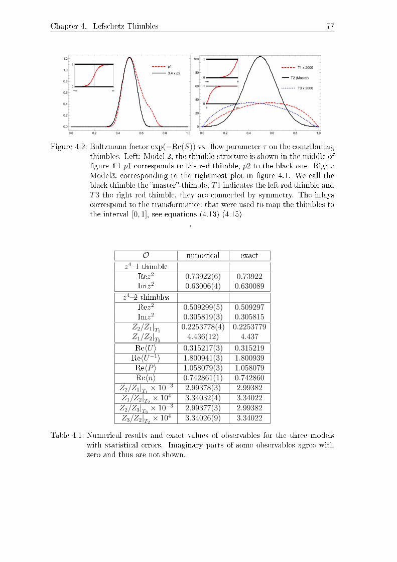
Chapter 4. Lefschetz Thimbles 77
p1
3.4 x p2
0.0 0.2 0.4 0.6 0.8 1.0
0.0
0.2
0.4
0.6
0.8
1.0
1.2
-∞ ∞
0
1T1 x 2000
T2 (Master)
T3 x 2000
0.0 0.2 0.4 0.6 0.8 1.0
0
20
40
60
80
100
-∞ a
0
1
∞a
0
1
Figure 4.2: Boltzmann factor exp(−Re(S)) vs. ow parameter τ on the contributingthimbles. Left: Model 2, the thimble structure is shown in the middle ofgure 4.1 p1 corresponds to the red thimble, p2 to the black one. Right:Model3, corresponding to the rightmost plot in gure 4.1. We call theblack thimble the master-thimble, T1 indicates the left red thimble andT3 the right red thimble, they are connected by symmetry. The inlayscorrespond to the transformation that were used to map the thimbles tothe interval [0, 1], see equations (4.13)-(4.15)
.
O numerical exact
z41 thimbleRez2 0.73922(6) 0.73922Imz2 0.63006(4) 0.630089
z42 thimblesRez2 0.509299(5) 0.509297Imz2 0.305819(3) 0.305815
Z2/Z1|T10.2253778(4) 0.2253779
Z1/Z2|T24.436(12) 4.437
Re〈U〉 0.315217(3) 0.315219Re〈U−1〉 1.800941(3) 1.800939Re〈P 〉 1.058079(3) 1.058079Re〈n〉 0.742861(1) 0.742860
Z2/Z1|T1× 10−3 2.99378(3) 2.99382
Z1/Z2|T2× 104 3.34032(4) 3.34022
Z2/Z3|T3× 10−3 2.99377(3) 2.99382
Z3/Z2|T2× 104 3.34026(9) 3.34022
Table 4.1: Numerical results and exact values of observables for the three modelswith statistical errors. Imaginary parts of some observables agree withzero and thus are not shown.

78 4.4. Towards higher dimensions
thimbles. Hence, the natural question is if one can combine both methods. Com-plex Langevin has been combined with the generalized Lefschetz thimble method in[188] in a simple model.We briey discuss our insights from trying to combine both methods, details can befound in appendix B.2. It is well known that complex Langevin can be improvedby appropriate coordinate transformations [205], which is e.g. also the case for thePolyakov chain from 3.1.2, where the gauge xed and diagonalized version is muchmore stable than the full- or only gauge xed chain.Hence we tried to use coordinate transformations to keep the complex Langevinevolution close to thimbles. I.e. we introduce a transformation z → z(u, θ), where uis the new variable and θ is a parameter which is updated every Langevin step suchthat the transformation is always able to get close to thimbles.In practice, this is done by introducing a constraint into the complex Langevin evolu-tion. This constraint should be derived from some quantity which measures the dis-tance of the complex Langevin evolution to the thimbles, which is not a well-denedquantity. We found that some measures for the distance can signicantly destabilizethe evolution by introducing poles, which is a problem for complex Langevin as wehave seen in chapter 3. However, even without poles, it is hard to nd a criterionto measure the distance to all thimbles, which also allows jumps between thimbles.While we found a way to push the distribution of the elds close to the thimbles andkeep the simulation stable by trial and error see appendix B.2 we were unable toget correct values for observables. Thus we conclude that much more mathematicalinsight is needed to combine both methods, this is work in progress.
4.4 Towards higher dimensions
So far we simulated on the thimbles by explicitly nding a parametrization. Inhigher dimensions, this will become numerically unfeasible. Unfortunately, globalsimulation algorithms are also expensive. Hence, we would like to nd local updatingalgorithms similar to the Metropolis algorithm to make simulations of interestingtheories possible. We do this by using the fact that the imaginary part of the actiondoes not change along the thimble, i.e.
∆SI = 0 . (4.19)
Instead of writing down a global algorithm, which requires nding the thimble ofthe whole lattice, we would like to nd an algorithm which allows local updates. Wewill explain this idea in more detail using an example.
4.4.1 U(1) gauge theory
Here we are interested in U(1) gauge theory on a 1 + 1d lattice with the action
S = −β∑Up
(1
2
(Up + U−1
p
)− 1
), (4.20)

Chapter 4. Lefschetz Thimbles 79
where we chose β ∈ C to introduce a sign problem. Note that this is just the Wilsongauge action from equation (2.23). In the thermodynamic limit, the expectationvalue of the plaquette for this theory is known analytically, see e.g. [36], as
〈Up〉 =I1(β)
I0(β), (4.21)
where In(β) are the modied Bessel functions of the rst kind.In order to describe the full theory we now need to nd all stationary points andthimbles. For a lattice theory, the stationary points are given by whole latticecongurations. For now, we will concentrate on the thimble corresponding to theclassical xed point, where S = 0. Hence, we proceed to describe how to do updateson a global thimble using local updates by keeping the imaginary part of the actionconstant. By writing the action as
S = βΣ = (βRΣR − βIΣI) + i(βIΣR + βRΣI) , (4.22)
we see that this is equivalent to demanding
SI = βIΣR + βRΣI = const . (4.23)
The local action of a single link is given by
S(Uk(n))
β= 2− 1
2
(Uki(n) + U−1
kj (n− i) + Ukj(n− i) + U−1ki (n)
)= 2− 1
2
[Uk(n)
(Vi(n) + V −1
j (n− i))
+ U−1k (n)
(Vj(n− i) + V −1
i (n))]
≡ 2−(Uk(n)Vij(n) + U−1
k Vji(n− i)), (4.24)
since each link appears in two dierent plaquettes. We split the link from the so-called staples Vi and Vj and introduced the sum of two staples Vij. We drop thedependence on the site n from now on since it is unambiguously clear which to usefor Uk and U
−1k . In case of an update U → U ′ the dierence will be
S(U ′k(n))
β− S(Uk(n))
β= Vij(Uk − U ′k) + Vji(U
−1k − U
′−1k ) ≡ δ
β. (4.25)
If we parametrize the link as Uk = eiφk this leads to U ′k = eiφkei∆φk = Uk∆Uk. WithPij ≡ UkVij the dierence thus becomes
δ
β= Pij(1−∆Uk) + Pji
(1−∆U−1
k
), (4.26)
if we now split ∆U = |∆U | ei∆φR , we see that
Im δ = Im (β(Pij+Pji))−|∆Uk|Im (βPijei∆φRk )−|∆Uk|−1Im (βPjie
−i∆φRk ) , (4.27)
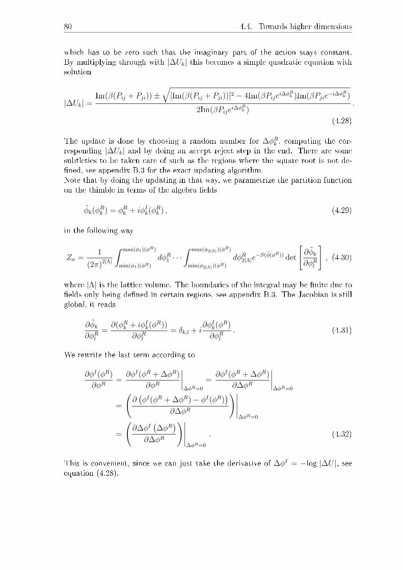
80 4.4. Towards higher dimensions
which has to be zero such that the imaginary part of the action stays constant.By multiplying through with |∆Uk| this becomes a simple quadratic equation withsolution
|∆Uk| =Im(β(Pij + Pji))±
√[Im(β(Pij + Pji))]2 − 4Im(βPijei∆φ
Rk )Im(βPjie−i∆φ
Rk )
2Im(βPijei∆φRk )
.
(4.28)
The update is done by choosing a random number for ∆φRk , computing the cor-responding |∆Uk| and by doing an accept reject step in the end. There are somesubtleties to be taken care of such as the regions where the square root is not de-ned, see appendix B.3 for the exact updating algorithm.Note that by doing the updating in that way, we parametrize the partition functionon the thimble in terms of the algebra elds
φk(φRk ) = φRk + iφIk(φ
Rk ) , (4.29)
in the following way
Zσ =1
(2π)2|Λ|
∫ max(φ1)(φR)
min(φ1)(φR)
dφR1 · · ·∫ max(φ2|Λ|)(φ
R)
min(φ2|Λ|)(φR)
dφR2|Λ|e−S(φ(φR)) det
[∂φk∂φRl
], (4.30)
where |Λ| is the lattice volume. The boundaries of the integral may be nite due toelds only being dened in certain regions, see appendix B.3. The Jacobian is stillglobal, it reads
∂φk∂φRl
=∂(φRk + iφIk(φ
R))
∂φRl= δk,l + i
∂φIk(φR)
∂φRl. (4.31)
We rewrite the last term according to
∂φI(φR)
∂φR=∂φI(φR + ∆φR)
∂φR
∣∣∣∣∆φR=0
=∂φI(φR + ∆φR)
∂∆φR
∣∣∣∣∆φR=0
=
(∂(φI(φR + ∆φR)− φI(φR)
)∂∆φR
)∣∣∣∣∣∆φR=0
=
(∂∆φI
(∆φR
)∂∆φR
)∣∣∣∣∣∆φR=0
. (4.32)
This is convenient, since we can just take the derivative of ∆φI = −log |∆U |, seeequation (4.28).

Chapter 4. Lefschetz Thimbles 81
-3 -2 -1 0 1 2 3-6
-4
-2
0
2
4
6
-3 -2 -1 0 1 2 3-6
-4
-2
0
2
4
6
-3 -2 -1 0 1 2 3-6
-4
-2
0
2
4
6
Figure 4.3: Complex plane with thimble for the model in equation (4.33) for β =1 + 0.1i, β = 1 + i and β = i from left to right. Full black lines are thethimbles, red dashed lines the anti-thimbles. See text for a discussion.
Application to one link
We rst test this procedure on one link, i.e. we set the staples to one. The actionthen reads
S = β
(1− 1
2
(U + U−1
))= β
(1− 1
2
(eiφ + e−iφ
))= β(1− cos(φ)) , (4.33)
where the constant part will drop out in the simulation, thus we ignore it. Note thatfor purely imaginary β this is the same action we used to investigate the boundaryterms in section 3.1.1, see equation (3.14). We show the thimbles structure fordierent β in gure 4.3. For small imaginary part of β the thimble is close to the realaxis, ultimately becoming the real axis at Im β = 0. For Re β = 0 both thimbleslook the same just shifted by π. In this case, they both are equally important,i.e. they contribute equally to the partition function. We tested our algorithm inthis model. Here the Jacobian is given by
J =1 + i−dlog |∆U |d∆φR
= 1 + iIm iβU + Im iβU−1
Im βU − Im βU−1, (4.34)
see equation (4.32). We can compute observables according to the reweighting pre-scription in equation (4.9). On the main thimble the simulation yields
⟨eiφ⟩
=0.840(5) + 0.060(15)i for β = 3 + i, while numerical integration along the thimbleyields
⟨eiφ⟩
= 0.839 + 0.064i. The algorithm yields correct results within error barsin the simple model.Before we apply the algorithm to higher dimensions, we look at the relative im-portance of the thimbles in the one link model. Figure 4.4 shows the situation fordierent β. The left and center plot show that for xed βI the thimble correspondingto the stationary point at zero will yield the main contribution if βR is large enough,i.e. when βR > βI . However, for small βR there is no convergence in βI . This meansthat in the most interesting case β = i, which corresponds to a real-time simulation,

82 4.4. Towards higher dimensions
-1
-0.5
0
0.5
1
0 1 2 3 4 5
<1
/2(P
+P
-1)>
βR
Re(P) MainRe(P) All
Im(P) MainIm(P) All
0
0.2
0.4
0.6
0.8
1
1.2
0 1 2 3 4 5
<1
/2(P
+P
-1)>
βR
Re(P) MainRe(P) All
Im(P) MainIm(P) All
-1
-0.5
0
0.5
1
1.5
2
2 4 6 8 10 12
<1
/2(P
+P
-1)>
βI
Re(P) MainIm(P) Main
Re(P) AllIm(P) All
Figure 4.4: Expectation value of the plaquette for xed βI with βI = 0.5 (left) andβI = 3 (center) as a function of βR. The same for xed βR = 0.5 as afunction of βI (right). The relevance of the main thimble is discussed inthe text.
all thimbles contribute equally. This is interesting since here complex Langevin failsto yield correct results, see section 3.1.1.
U(1) in 1+1 dimensions
The same algorithm can straightforwardly be applied to higher dimensions. Un-fortunately, the algorithm no longer is stable in 1+1 dimensions. First of all, eventhough initially the imaginary part stays constant, the simulation is driven awayfrom the unitary manifold very fast. This can be seen by monitoring the unitaritynorm, see equation (3.39). Since the imaginary part of the action stays constant,this is a priori not a problem. For gauge theories, the simulation can stay on thecomplexied gauge orbit of the thimble and still yield correct results. In practice,this introduces large dierences in orders of magnitude of the variables thus desta-bilizing the simulation. This problem can be dealt with by means of gauge cooling[105] see appendix A.7, which slows down this rise of the unitarity norm consider-ably.Even then the simulation is unstable, especially at small Reβ. We found that af-ter some time congurations with S = 0 can no longer be gauge transformed backto the xed point, suggesting that the simulation was able to jump on a dierentmanifold with the same SI at some point during the simulation. However, for sucha complicated theory, we lack insight into the underlying structure of the manifold.Hence, we look at a simpler lattice theory to nd out how to improve our algorithm.

Chapter 4. Lefschetz Thimbles 83
4.4.2 Scalar theory on two lattice points
The action for a free scalar eld on a lattice with two points and periodic boundaryconditions reads
S = −i[(φ1 − φ2)2 − m2
2(φ2
1 + φ22)
], (4.35)
where the elds φi live on the sites i with i = 1, 2 and the factor −i mimics a signproblem from real time simulations. In this theory, one can show that the tangentspace at the critical point is identical to the thimble, which allows for a convenientparametrization of the action. See appendix B.4 for a detailed computation. In theend we nd an analytical expression for an observable, namely⟨
φ2⟩
=
⟨φ2
1 + φ22
2
⟩= − i
2
(1
m2+
1
m2 − 4
), (4.36)
which is useful to compare to results from our simulations
Application of our algorithm
We apply the same algorithm as for U(1), i.e. we demand that ∆SI = 0 and vary theelds along that constraint. We parametrize the elds as φk = φRk + iφIk and proposean update according to φRk → φRk +∆φRk . We use the condition Im[S(φ′)−S(φ)] = 0to compute ∆φIk. In this theory this turns out much simpler than the algorithmin the U(1) model14, which is described in appendix B.3. Here we only have onestationary point, hence the corresponding thimble gives results for the full theory.Since the action is quadratic, the equation for ∆φIk(∆φ
Rk ) still contains a square root
∆φIk =−µφIk − 2φIj ±
√µ2∆φRk +
(µφIk + 2φIj
)2+ 2µ∆φRk
(µφRk + 2φRj
)µ
(4.37)
where k 6= j and we introduced the abbreviation µ = (m2 − 2). This equationstill has undened regions due to the square root. The boundaries can simply befound by numerically nding the root in ∆φRk for the term under the square root.The algorithm is then similar to the U(1) case. Here we nd that the solution witha plus corresponds to the thimble when ∆φRk < 0 and the solution with a minuscorresponds to the thimble when ∆φRk > 0. Note, however, that the algorithm worksonly for m > 2, see appendix B.4 for details. We update a single site according to
1. Draw a Gaussian random number with mean zero and standard deviation one.If it is smaller than zero, choose the plus solution, otherwise choose the minussolution in (4.37).
14The reasons are twofold: First, here we do not have an absolute value and thus do not get aconstraint from a quantity being positive. Second, the theory is not periodic and hence thespace of possible values extends to innity. Thus there are fewer constraints on the proposablevalues for δφ.

84 4.4. Towards higher dimensions
-2.5-2-1.5-1-0.5 0 0.5 1 1.5 2 2.5-2.5 -2 -1.5 -1 -0.5 0 0.5 1 1.5 2 2.5
-2.5-2
-1.5-1
-0.5 0
0.5 1
1.5 2
2.5
ThimbleAntithimble
simulation data
Re[φ1] Re[φ2]
Im[φ2]
-4000
-2000
0
2000
4000
6000
8000
10000
12000
0 10000 20000 30000 40000 50000 60000 70000 80000 90000 100000
J 12
Monte Carlo time
Figure 4.5: Left: Projection of the thimble structure with simulation data. Right:Evolution of part of the Jacobian. See text for details.
2. Find the boundary where the square root becomes real.
3. Add the random number to the position of the boundary ∆φRk = boundary +random number, this gives the proposal for the eld.
4. Do a Metropolis accept-reject step.
We simulated this for m2 = 6. The left plot of gure 4.5 shows a projection ofthe thimble structure, the simulation lies on the thimble and is stable. To getexpectation values we also need the Jacobian, which is computed according to (4.31)and below, i.e. it is just the derivative of equation (4.37) with respect to ∆φR. Weshow the Monte Carlo evolution of one of the entries of the Jacobian in the rightplot of gure 4.5. The equation for that entry of the Jacobian is
J12(φ) =4φ2,R√
(4φ1,I − 4φ2,I + 2m2φ2,I)2. (4.38)
The enormous spikes in gure 4.5 occur when numerator and denominator havelargely dierent orders of magnitude and often even lead to numerical divergences,i.e. NaN.Alternatively we can use the Takagi vectors vi see appendix B.4 as a basis. I.e. weupdate a generic eld conguration as(
φ1
φ2
)→(φ1 + ∆φ1
φ2 + ∆φ2
)=
(φ1
φ2
)+ ξ1v1 + ξ2v2 (4.39)
where the ξi are just Gaussian random numbers. We nalize the update with aMetropolis accept-reject step. In this basis, the Jacobian is just a constant and thusdrops out of the reweighting, see equation (4.9). Results from this procedure areshown in gure 4.6. They agree with the analytical result.
Note that the scalar model is much simpler than U(1) theory in 1+1d. It isjust a free Gaussian theory, which is usually highly symmetric and easier to solve.However, our original algorithm turned out to be unstable in both theories. In the

Chapter 4. Lefschetz Thimbles 85
-2
-1.5
-1
-0.5
0
0.5
1
1.5
2
0 1 2 3 4 5
Im(<
φ2>
)
m
analyticsimulation result
Figure 4.6: Results from simulating in the space spanned by the Takagi vectors, theyagree with the analytical results.
scalar case, we were able to recover correct results by choosing the correct basis.Hence, nding a good basis for U(1) on the lattice may enable local updating in thefuture.
4.5 Summary and conclusions on Lefschetz
thimbles
In this chapter, we have investigated so-called Lefschetz thimbles which are inte-gration paths in the complexied space of a given theory. Integrands which areoscillatory in the original manifold are Gaussian-like along the thimbles and thusenable normal Monte Carlo simulations. We have examined some simple integralsand found a way to compute the ratio of the partition functions on dierent thim-bles, which trivially generalizes to higher dimensions. This is highly desirable sinceso far there is no way to nd the relative weights for contributing thimbles.Finally, we have investigated higher dimensional theories and found a way to performlocal updates which sample the global thimble. While this algorithm does samplethe thimble in a simple scalar theory, it does not yield correct expectation valuesdue to numerical deviations. The same algorithm is not stable in a complexiedU(1) gauge theory. In the scalar theory, we were able to nd a better basis for thesimulation manifold, which yields correct results.
We conclude that except for simple models, a thorough understanding of the under-lying manifolds is required to properly sample Lefschetz thimbles.

86
5 Finding order parameters with Neural
Networks
In the last decade, there has been a huge increase in the use of machine learning.This is mainly due to the increase in computing power, which enabled the now pop-ular deep learning using neural networks.The rst instance where deep learning decidedly outperformed other methods wasAlexNet [206], a neural network which was entered into ImageNet Large Scale Vi-sual Recognition Challenge [207], where the machine learning algorithm is taskedto correctly classify pictures into hundreds of categories. By now most machinelearning applications use neural networks since they are the best machine learningtechnique for hierarchical and nonlinear learning tasks. They are being used in im-age classication [206, 208], Language processing [209], beating humans in complexgames [210] and medical diagnosis [211, 212] to give just a few examples.In high energy physics standard neural networks are used e.g. to nd signals indetector data [213215]. By now there are many other applications of machinelearning in physics including quantum many-body systems [216218], simulatingstatistical physics systems [219, 220], solving inverse problems relevant to physics[221223], detecting and investigating phase transitions [31, 224237], improvingMonte Carlo simulations [238243] and more. There have even been attempts tosolve the sign problem using neural networks [244]. So far applications in latticeQCD are [31, 245, 246] For a review on applications in physics see [26].Despite their wide usage, there is no generic way to nd out what neural networkslearn. In theoretical physics, however, it is crucial to understand the underlyingmechanisms of the tools at hand in order to gain a deeper understanding of physics.In this chapter, we will set neural networks on physical grounds by explicitly show-ing that they learn order parameters when they are trained on phase transitions.We thus open the black box for a specic case.
We give a brief introduction to feed-forward neural networks in 5.1 show how tond order parameters with neural networks in section 5.2.
5.1 Brief introduction to feed-forward neural
networks
By now there is a huge variety of many dierent neural network architectures. Hence,for a complete understanding of neural networks, we refer to books such as [247, 248].Machine learning tasks are often classied via the learning method.
Chapter 5. Finding order parameters with Neural Networks 87
• Supervised learning relies on labeled data sets. A data point corresponds to acertain class and the algorithm is tasked to correctly classify the data set.
• Unsupervised learning is used for unlabeled data sets. Here the algorithm istasked to nd structures in a large data set without further input.
• Reinforcement learning is used to let an agent nd a strategy to solve a task.Typically the agent does not get any information a priori but is punished orrewarded based on its actions.
Here we will focus on supervised learning and introduce a simple neural networkarchitecture known as a feed-forward network.The use of neural networks is motivated by the architecture of the brain, wheremany rather simple neurons work together to perform complex tasks. As the namesuggests, neural networks are formed by a network of neurons. A neuron is a functionf(x) which takes an input vector x and maps it to a an output z
f(~x) = a(~w · ~x+ b) . (5.1)
The weights ~w represent the relative importance of each input to the neuron, thebias b introduces a minimum threshold the input has to reach and the activationfunction a(x) produces the scalar output of the neuron depending on the input.Popular activation functions include the sigmoid function
a(x) = σ(x) =1
1 + e−x(5.2)
and the rectied linear unit (ReLU)
a(x) = max(0, x) . (5.3)
Typically neural networks perform well with a whole range of activation functions.A single neuron by itself is not very powerful. Thus they are typically grouped intolayers. A layer F (~x) consists of many neurons, which are not interconnected in afeed-forward network. Those layers are then connected, i.e. the output of the neuralnetwork is
y = FM(FM−1(. . . (F1(F0(~x))))) , (5.4)
where F0 is the input layer and FM is the output layer. In a binary classicationtask, for example, the input could be a picture and the input layer would have asmany neurons as there are pixels and the output layer would be a single neuronoutputting 0 or 1. This setup typically has several hundred to several millions ofparameters, i.e. the weights and biases. Given a data point as input, it is fed throughthe network and produces an output. If the weights and biases are chosen correctly,the data point will be classied correctly. Since choosing millions of parameters byhand is a near impossible task, this is done in an automatic way as described below.It has been shown that such a simple network is able to approximate any continuousfunction arbitrarily close [249, 250]. Thus a correctly trained neural network is apowerful tool for regression and classication tasks.

88 5.1. Brief introduction to feed-forward neural networks
Training the feed-forward network
In the case of supervised learning, we can use a so called loss-function to determinehow far the output of the network was from the correct classication, we will usethe binary cross-entropy
C(Y, P ) = − 1
N
∑i
(yi log pi + (1− yi) log(1− pi)) , (5.5)
where yi ∈ Y are the correct labels of the data point, and pi ∈ P are the predictionsof the network and the sum now goes over N data points. Note that the label herecan be only 0 or 1 such that log(pi) (or log(1 − pi)) is added to the sum if yi = 1(or yi = 0). The logarithm is maximal if pi = 1, since pi ∈ [0, 1] is a probability.A similar argument holds for the second term. The global minus sign then turnsmaxima into minima such that the binary cross-entropy needs to be minimized.This minimization is done by some variant of gradient descent, which is a simplealgorithm to nd the minimum of a function. It does so by making small steps inthe direction of steepest descent. Thus it requires a step size, which in the context ofneural networks is referred to as the learning rate η. Each of those steps is then usedto adjust the parameters of the neural network using backpropagation. In gradientdescent, we take the derivative of the loss function with respect to the parameters ofthe network. Since the network has a hierarchical structure, the derivative in earlierlayers depends on the parameters in later layers by the chain rule. The derivativefor the output layer can be computed directly. The derivative for the second to lastlayer then depends on the derivative of the output layer via the chain rule, and soon. Thus, the change in parameters is propagated back through the network. Afull description of the algorithm can be found in any standard textbook on neuralnetworks, see e.g. [247, 248]. State-of-the-art algorithms use adaptive learning rates,compute the gradient just in a random subset of all directions (stochastic gradientdescent) in order to decrease the chance of ending up in bad local minima, and haveways to not get stuck in shallow minima, e.g. momentum terms.Training is then done by feeding the training set through the network multiple times,each of which is called a training epoch. Usually, in order to avoid over-tting, i.e. toprevent the neural network from just memorizing the training data, regularizationis used. Popular regularization schemes include dropout, where only part of thenetwork is updated in each learning epoch or to add regularization terms to theloss function. Widely used are L1 and L2 regularization, where the Ln norm of theweights is added to the loss function in order to keep their values low. We now intro-duced everything needed to train a simple neural network. We will not need muchmore in the application to lattice congurations and thus will introduce additionaltechniques when they are needed.

Chapter 5. Finding order parameters with Neural Networks 89
5.2 Machine Learning of Explicit Order Parameters
Binary classication tasks as introduced above can give very precise predictions.Hence, they are a wonderful tool to look for phase transitions and are able to ndthe position of the transition to high accuracy see [224]. A neural network in abinary classication task can be viewed as an approximation of the so-called decisionfunction D, which assigns a probability pi ∈ [0, 1] to each sample S to be in classone. The decision boundary is a hyperplane in the hyperspace of congurationswith D(S) = 0.5, i.e. the boundary where the neural network is unsure aboutits prediction. Thus, if the neural network learns a single function Q(S) whichdistinguished between phases, we expect that ∇Q||∇D near the decision boundary.In our networks we will use the sigmoid activation function see equation (5.2) tomap the latent prediction ξ(S) (the output of the last ReLU layer) to a probability15.Hence, we can write D(S) = σ(ξ(S)) and ∇Q||∇ξ which allows us to write downan approximate linear relation
ξ(S) = wQ(S) + b , (5.6)
in the vicinity of the decision boundary. In the following sections we will explicitlydetermine ξ and hence D as functions of the lattice congurations S and thus ulti-mately nd the quantity Q, which turns out to be the order parameter or energy ofthe theory.
5.2.1 The Correlation Probing Neural Network
Neural networks encode their decision function in highly elusive non-linear ways.Since we are interested in applications to Monte Carlo samples, we would like tond out if the leading contributions to the decision function can be expressed bycombining just a few lattice points. Typically many interesting observables in latticetheories can be expressed by local combinations of variables. Motivated by thisobservation, we construct a neural network which only gets to see a subset of thefull lattice. If we successively lower the number of variables the network gets tosee we can nd the minimum amount of variable the neural network requires to stillcorrectly predict the phase transition. This is the idea behind the correlation probingneural network which is depicted in gure 5.1. The lattice conguration is fed intothe localization network, which simply is a fully connected convolutional neuralnetwork. A convolutional neural network consists of receptive elds which can onlysee a part of the conguration. This is typically used in image recognition, wherea receptive eld is only allowed to see parts of a picture, which is useful to extractinformation in a hierarchical way. Many convolutional layers are used to successively
15We will use the ReLU activation function everywhere else, hence the output of the last ReLUlayer ξ(S), which in our case just consists of one neuron, is generally not in [0, 1] and thuscannot be interpreted as a probability. The only reason for the use of σ(x) is this mapping to[0, 1].

90 5.2. Machine Learning of Explicit Order Parameters
SampleConfiguration
LocalizationNetwork
AveragingLayer
PredictionNetwork
Figure 5.1: Schematic depiction of the correlation probing neural network. It con-sists of three dierent neural networks stacked on top of each other. Thelocalization network is a fully connected convolutional neural networkwhich allows connections only in within the receptive elds. The av-eraging layer averages over all receptive elds. Finally, the predictionnetwork transforms the output of the averaging layer into a predictionprobability.
combine the receptive elds. In our case, We do not combine the receptive eldsand keep them separate all the time. The output of the convolutional network isfed into an averaging layer, which averages over all receptive elds. Finally, a fullyconnected prediction network is used to map the output of the averaging layer to aprediction.We train the network with dierent receptive eld sizes to nd the minimum requiredsize such that the phase transition is still found. In the following, we will describethe application of the correlation probing neural network to the Ising model andSU(2) lattice gauge theory. Technical details on the network setup and training canbe found in appendix C.1.
Application to the Ising model
We rst do this for the Ising model in two dimensions. The Ising model is given bythe Hamiltonian
H(S) = −∑〈i,j〉nn
sisj + h∑i
si . (5.7)
The spin si ∈ −1, 1 variables are aligned on a regular lattice. The rst sum runsover nearest neighbors of spins. For simplicity we set h = 0 in the following. One spinconguration is given by S = (s1, . . . , sn). It is a simple model for ferromagnetism,its partition function is
Z =∑i
e−βH(Si) , (5.8)
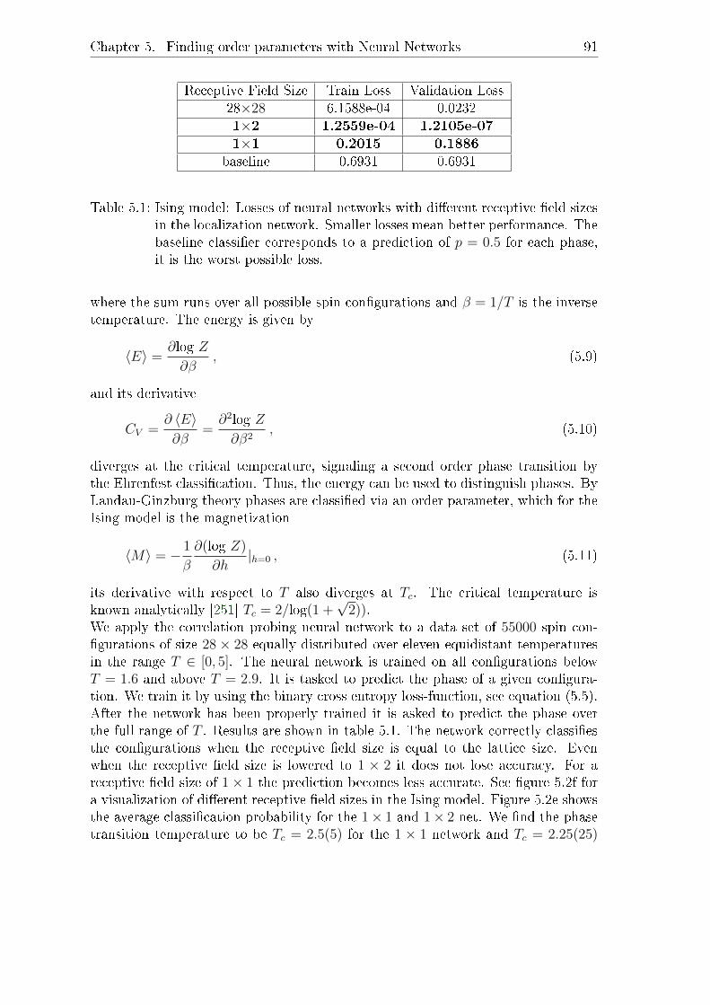
Chapter 5. Finding order parameters with Neural Networks 91
Receptive Field Size Train Loss Validation Loss28×28 6.1588e-04 0.02321×2 1.2559e-04 1.2105e-071×1 0.2015 0.1886
baseline 0.6931 0.6931
Table 5.1: Ising model: Losses of neural networks with dierent receptive eld sizesin the localization network. Smaller losses mean better performance. Thebaseline classier corresponds to a prediction of p = 0.5 for each phase,it is the worst possible loss.
where the sum runs over all possible spin congurations and β = 1/T is the inversetemperature. The energy is given by
〈E〉 =∂log Z∂β
, (5.9)
and its derivative
CV =∂ 〈E〉∂β
=∂2log Z∂β2
, (5.10)
diverges at the critical temperature, signaling a second order phase transition bythe Ehrenfest classication. Thus, the energy can be used to distinguish phases. ByLandau-Ginzburg theory phases are classied via an order parameter, which for theIsing model is the magnetization
〈M〉 = − 1
β
∂(log Z)
∂h|h=0 , (5.11)
its derivative with respect to T also diverges at Tc. The critical temperature isknown analytically [251] Tc = 2/log(1 +
√2)).
We apply the correlation probing neural network to a data set of 55000 spin con-gurations of size 28× 28 equally distributed over eleven equidistant temperaturesin the range T ∈ [0, 5]. The neural network is trained on all congurations belowT = 1.6 and above T = 2.9. It is tasked to predict the phase of a given congura-tion. We train it by using the binary cross entropy loss-function, see equation (5.5).After the network has been properly trained it is asked to predict the phase overthe full range of T . Results are shown in table 5.1. The network correctly classiesthe congurations when the receptive eld size is equal to the lattice size. Evenwhen the receptive eld size is lowered to 1 × 2 it does not lose accuracy. For areceptive eld size of 1× 1 the prediction becomes less accurate. See gure 5.2f fora visualization of dierent receptive eld sizes in the Ising model. Figure 5.2e showsthe average classication probability for the 1× 1 and 1× 2 net. We nd the phasetransition temperature to be Tc = 2.5(5) for the 1 × 1 network and Tc = 2.25(25)

92 5.2. Machine Learning of Explicit Order Parameters
Figure 5.2: Results of the correlation probing neural network for the Ising Model.The latent prediction ξ is the argument of the sigmoid σ function, whichwe use as the activation function for the last layer of the predictionnetwork. a: Correlation of the latent prediction with the absolute valueof the average spins, i.e. the magnetization in the 1×1 network. b: Sameas (a), but with the average product of neighboring spins, i.e. the energyinstead of the magnetization. c: Correlation of the latent predictionwith the magnetization for the 1 × 2 network. d: Same as (c), butwith the energy instead of the magnetization. e: Average classicationprobability as a function of temperature. f : Visualization of receptiveelds 1×1, 1×2 and 28×28 of the localization network output neurons.

Chapter 5. Finding order parameters with Neural Networks 93
for the 1 × 2 network. Both agree with the correct value within error bars whichsuces for our task, see [224] for more accurate results for Tc from neural networks.In our task to nd an analytical expression for the decision function, we rst turnto the 1× 1 net. By construction its decision function can be expressed as
D(S) = F
(1
N
∑i
f(si)
)= σ
(ξ
(1
N
∑i
f(si)
)), (5.12)
where f is the output of the localization network and F is the output of the predic-tion network. Due to the small receptive eld size, we can expand the function f interms of a single spin variable
f(si) = f0 + f1 si + f2 s2i︸︷︷︸
1
+f3 s3i︸︷︷︸si
+... , (5.13)
where higher powers of spins can be absorbed into the lowest two orders due to s2i =
1. The constants f0 and f1 can be absorbed into weights and biases of the predictionnetwork approximating F . This signicantly simplies the decision function to
D(S) = F
(1
N
∑i
si
). (5.14)
Now we need to nd an expression for F , which we do by comparing the latentprediction ξ with the argument of F . Figure 5.2a suggests a linear relation
ξ(S) ≈ w
∣∣∣∣∣1/N∑i
si
∣∣∣∣∣+ b . (5.15)
Thus employing equation (5.12), the decision function becomes
D(S) ≈ σ
(w
∣∣∣∣∣ 1
N
∑i
si
∣∣∣∣∣+ b
), (5.16)
where w and b are weight and bias of the prediction neuron. Since we used nophysical information except Monte Carlo congurations, we can conclude that thenetwork learns the quantity
Q(S) =
∣∣∣∣∣ 1
N
∑i
si
∣∣∣∣∣ , (5.17)
the magnetization.We can give similar arguments for the 1× 2 network. Here, by construction
D(S) = F
(1
N
∑<i,j>T
f(si, sj)
), (5.18)

94 5.2. Machine Learning of Explicit Order Parameters
where the sum goes only over transversal neighbors. The expansion of f
f(si, sj) =f0,0 + f1,0 si + f0,1 sj + f2,0 s2i + f1,1 si sj + f0,2 s
2j + ... , (5.19)
contains only three notable terms, again since s2i = 1. Terms linear in one spin si
represent the magnetization, which according to the drop in performance seen intable 5.1 contain less information than what we are looking for. Hence, the leadingterm must be f1,1sisj, reducing the decision function to
D(S) ≈ F
(1
N
∑<i,j>T
sisj
). (5.20)
Figure 5.2d shows a perfect correlation between the latent prediction ξ and the sumover transversal nearest neighbors 1/N
∑<i,j>T
sisj. Here, the nal expression forthe decision function is
D(S) ≈ σ
(w
(1
N
∑<i,j>T
sisj
)+ b
). (5.21)
Note that the sum over transversal nearest neighbors was sucient. It can begeneralized to all nearest neighbors by rotational and translational symmetry. Thus,the neural network learns
Q(S) =1
N
∑<i,j>nn
sisj , (5.22)
which corresponds to the energy per site.We nd that the energy works better in our context, see table 5.1. Figure 5.2also shows the correlation of the latent predictions of both the 1 × 1 and 1 × 2network with the energy and magnetization respectively. No correlation is foundsuggesting that the network really learns the order parameters that are dominantfor the corresponding eld size.
Application to SU(2) lattice gauge theory
Motivated by the success of the method in the Ising model, we apply it to SU(2)gauge theory on the lattice. We already introduced lattice gauge theory for SU(N)in section 2.3, however here we will change notation slightly to be more clear. Givena four dimensional lattice with Nτ × N3
s points, where in the following we chooseNs = 8 and Nτ = 2, the gauge elds are parametrized via the link variables, whichconnect the lattice sites. For the site x = (τ, x, y, z) the SU(2) link pointing indirection µ ∈ t, x, y, z reads
Uxµ = axµ1 + i
(bxµσ1 + cxµσ2 + dxµσ3
), (5.23)
Chapter 5. Finding order parameters with Neural Networks 95
where the σi are the Pauli matrices and the coecients obey (axµ)2 + (bxµ)2 + (cxµ)2 +(dxµ)2 = 1. Since the Pauli matrices are traceless. TrUx
µ = 2axµ. We write one latticeconguration as the collection of all link variables
S = (Uxµ |x ∈ Nτ ×Ns ×Ns ×Ns, µ ∈ τ, x, y, z) . (5.24)
Since we hope that our neural network nds the order parameter, the Polyakov loop,we write it in the current notation as
L(~x) = tr
(Nτ−1∏x0=0
Uxτ
)Nτ=2
= tr(U0,~xτ U1,~x
τ
)= 2
(a0,~xτ a1,~x
τ − b0,~xτ b1,~x
τ − c0,~xτ c1,~x
τ − d0,~xτ d1,~x
τ
). (5.25)
For the following analysis we produced a total of 15600 decorrelated congurationsusing the Wilson gauge action (2.23). The congurations are equally distributedover 26 values of β = 4/g2 ∈ [1, 3.5]. It is important that the congurations aredecorrelated, see e.g. [246] for a case where correlations between the samples con-taminated the learning task.Since our aim is to have a completely blind method, we do not assume any knowledgeexcept the gauge congurations themselves. I.e. we do not assume any knowledgeabout where the phase transition is. Thus, as a rst step, we employ an unsuper-vised learning algorithm to nd a rough approximation for the transition. Notethat due to the gauge freedom in lattice QCD, networks like autoencoders [230] arenot a good match for this task, since the reconstruction of the conguration fromthe latent variables is not unique if the latent variables represent a gauge invariantquantity such as the Polyakov loop. Instead, we use principal component analysis,which is an orthogonal linear transformation to a set of variables which are orderedby their variance. The rst few principal components contain the most information.This algorithm is perfect in our case, since in the ordered phase there should notbe many uctuations and hence much lower variance than in the disordered phaseif a phase transition exists. Note, however, that PCA is a linear transformation andas such can only nd linear approximations. In the Ising model PCA was able tocorrectly predict the transition temperature [229]. Figure 5.3 shows that with twoprincipal components there is a signal for a phase transition around β ≈ 2.0. How-ever, no clear correlation between the Polyakov loop and the principal componentsis found, which was expected, since the Polyakov loop is a nonlinear function.PCA suggest a phase transition at β ≈ 2. Hence, we train the correlation probingneural network with dierent receptive eld sizes to predict the phase transition.To that end we train the neural network at β ∈ [1, 1.2] and β ∈ [3.3, 3.5]. It is ableto predict the phase transition with the receptive eld size incorporating the wholelattice, i.e. 2× 8× 8× 8 and nds a critical value of βc = 1.97(1). For a 2× 1× 1× 1network we nd βc = 1.99(1), this is depicted in gure 5.4c. A direct lattice com-putation of the critical temperature yields βc = 1.880(25). The small deviation is

96 5.2. Machine Learning of Explicit Order Parameters
Figure 5.3: a: The average mean squared error reconstruction loss of PCA as a func-tion of temperature signals a phase transition. It was calculated in 100independent PCA runs with two principal components (PC), measuredin units of ×10−5 and shifted by the value at β = 3.5. The average normof the PC also indicates a phase transition. b: Correlation between thePolyakov loop and the principal components.
most likely due to a systematic error. When producing the gauge congurations,we always initialized at the same point, all links were set to one. In that case, it ishard for the simulation to cross over to having all links equal to minus one. Thisbiases the network, hence the dierence. We are however not interested in gettingan exact value for the critical coupling and are satised with the given precision.Since we want to nd the order parameter, we look at dierent receptive eld sizes intable 5.2. The minimal receptive eld size is 2×1×1×1. Allowing only 1×1×1×1is as bad as the network just guessing, i.e. the baseline classier. Thus, the decision
Receptive Field Size Train Loss Validation Loss2×8× 8× 8 1.0004e-04 2.6266e-042×8× 8× 1 8.8104e-08 1.3486e-072×8× 1× 1 7.7671e-05 2.0394e-042×1× 1× 1 8.8104e-08 6.8276e-082× 1× 1× 1
no hidden layersin prediction net
2.2292e-07 4.2958e-07
1×1× 1× 1 0.6620 0.9482baseline 0.6931 0.6931
Table 5.2: SU(2): Losses of neural networks with dierent receptive elds of theneurons in the localization network.

Chapter 5. Finding order parameters with Neural Networks 97
Figure 5.4: Results from the correlation probing neural network for SU(2). a,b:Correlation of the latent prediction with the Polyakov loop in both the2 × 8 × 8 × 8 network and the 2 × 1 × 1 × 1 network. c: The averageprediction probability of the two networks.
function must be constructed from two lattice points with four links each
D(S) = F
(2
N
∑~x
f(U0,~xτ , U0,~x
x , U0,~xy , U0,~x
z , U1,~xτ , U1,~x
x , U1,~xy , U1,~x
z )
). (5.26)
Now f is a function of 32 variables, 2 lattice points times 4 links times 4 real variablesper link and F is a function of a single variable as before.We see in table 5.2, that it is enough for the prediction network to contain a singlesigmoid neuron and no hidden layers, thus D(S) = σ(wQ(S) + b). We also split thelattice congurations in patches of size 2 × 1 × 1 × 1. I.e. we view each of thosepatches as a single conguration, eectively enhancing our statistics by a factor of512. Thus,
Q(S) =2
N
∑~x
f(U0,~xτ , U0,~x
x , U0,~xy , U0,~x
z , U1,~xτ , U1,~x
x , U1,~xy , U1,~x
z ) . (5.27)
In order to nd an expression for f , we train a network only on the local patches.We then perform a polynomial regression on the latent prediction of the localizationnetwork on 1% of the data set, using another 1% for validation. To be more precise,the t-function is given by all possible combinations of the 32 variables per patch upto the order of the polynomial. We nd that a second-order polynomial t suces,it is a t with 561 dierent terms. The results are shown in table 5.3. We nd the

98 5.3. Conclusion on neural networks
Order of Regression Train Score Validation ScorePolynomial Regression
1 0.00128 -0.000422 0.72025 0.723953 0.75675 0.69129
Table 5.3: Scores of dierent regression algorithms. Higher is better.
coecients with the larges absolute value from the t
f(Ux0µ ) =f(U0
τ , U0x , U
0y , U
0z , U
1τ , U
1x , U
1y , U
1z )
=f((a0τ , b
0τ , ..., d
1z))
≈+ 7.3816 a0τa
1τ + 0.2529 a1
τb1τ
+ ...
− 0.2869 d0τc
1τ − 7.2279 b0
τb1τ
− 7.3005 c0τc
1τ − 7.4642 d0
τd1τ , (5.28)
where the dierences between the leading contributions are of the same order as thesize of the sub-leading coecient, and as such most likely originate from approxi-mation errors in the network. Overall factors and constants can be absorbed intoweights and biases and we are allowed to rescale the t result. We conclude that
f((a0τ , b
0τ , ..., d
1z)) ≈ a0
τa1τ − b0
τb1τ − c0
τc1τ − d0
τd1τ
=(U0τU
1τ
). (5.29)
Which is just the Polyakov loop (5.25) on the 2 × 1 × 1 × 1 patch as suspected.Due translation symmetry, we are allowed to generalize this to the whole latticef(Ux0
µ )→ f(Ux0,~xµ ) . The decision function of the full network thus becomes
D(S) ≈ σ
(w
(2
N
∑~x
f(Ux0,~xµ )
)+ b
). (5.30)
with the argument of σ begin Q(S) = 2N
∑~x f(Ux0,~x
µ ), i.e. the Polyakov loop onthe full lattice. This is conrmed by the perfect correlation between the Polyakovloop and the latent prediction in gure 5.4a,b.
5.3 Conclusion on neural networks
We have applied neural networks to SU(2) gauge theory and the Ising model. Byshowing that the neural network explicitly learns the order parameter, we decodedthe black box of neural networks, at least in this specic case. By doing so we alsofound a method which allows nding order parameters of systems of many variables.

Chapter 5. Finding order parameters with Neural Networks 99
This is in principle applicable anywhere but limited by computational power. In ourcase, all order parameters were local to some degree. While the Polyakov loop is aglobal observable, we chose the lattice size such that it was eectively local. We triedthe same analysis on a 4 × 83 lattice and found that much higher statistics wouldbe required to get equally good results. Hence, if the order parameter is completelyglobal, as is the case e.g. for the chiral condensate, the amount of data requiredfor our method grows quickly. Note that in principle this is not a problem. Earlylattice simulations from the 70s and 80s have shown that qualitative features can becaptured very well on even small lattices. Thus, one should try to nd the minimallattice size which shows the transition and perform the analysis on this lattice size.In the case of SU(2) gauge theory and the Ising model, the generalization of theorder parameter to larger lattices is trivial. There would be no gain in performingthe analysis on larger lattices.In principle, this method can be used to nd any somewhat local structure fromlattice congurations, not only order parameters. Given any quantity we want topredict, we can use the correlation probing neural network and nd out which quan-tity it learns.Neural networks could also be useful for solving sign problems. A simple case hasbeen investigated in [244]. One has to be careful however not to rely on extrapola-tions over phase transitions or similarly singular phenomena, since the structure maychange signicantly and if the network is not properly trained, the results will beunphysical since the network never would have seen such structures during training.

100
6 Summary and outlook
We have investigated the phase diagram of QCD by means of the complex Langevinmethod, investigated various aspects of the Lefschetz thimble method and nallyshowed that neural networks learn the order parameter when trained on latticecongurations.
Complex Langevin
Starting with the complex Langevin method, we gave a systematic way to check forits convergence, namely by looking for eects of poles and boundary terms. We werethus able to investigate several aspects of QCD with complex Langevin. We rstinvestigated QCD using a hopping expansion and found that it does not convergeproperly in some interesting regions. In full QCD we found rst signals of the nuclearliquid-gas transition from lattice QCD, though thermalization issues prohibited usfrom a thorough study of the transition. Finally, we focused on the QCD transitionbetween hadronic matter and the quark-gluon plasma by simulating in the transitionregion up to µ/Tc(µ = 0) ≈ 5, which is a much larger region than other methods cancurrently investigate. In our simulations transition temperature is a quadratic func-tion of chemical potential µ in accordance with other simulations. Our simulationswere still plagued by large nite size eects, which most prominently shows in ourmoderately heavy pion mass, which in our largest volume had a minimum possiblevalue of mπ ≈ 1.55 GeV. We have found that a value of κ2 ≈ 0.0011 − 0.0015 forthe curvature of the transition line, see table 3.3. This value interpolates betweena curvature of κ2 ≈ 0.014 from [19, 49] and QCD with heavy static quarks wherethere is basically no curvature [83]. All in all, we found that complex Langevin isapplicable to a large portion of the QCD phase diagram if all convergence criteriaare carefully monitored.Finally, we investigated SU(2) gauge theory on a real-time contour and found thatwith the inclusion of recent improvements to complex Langevin, i.e. gauge coolingand dynamical stabilization, it is now applicable in a physically interesting region.In terms of the QCD phase diagram, future research is straightforward. Simulationsat smaller quark masses and larger volumes, as well as continuum extrapolated re-sults, are highly desirable, especially to locate the critical endpoint. Here one has tobe particularly careful with poles since low lying eigenvalues in the Dirac operatortend to occur for simulations at small masses.In SU(2) gauge theory, the next step should be to compute any physical quantity onthe contour, e.g. the shear viscosity, to see whether analytical continuation methodsreally perform better, when starting from a real-time contour instead of in Euclideanspace.

Chapter 6. Summary and outlook 101
In terms of the complex Langevin method, it is highly desirable to nd a simplerway to look for poles, e.g. by computing boundary terms close to the poles.
Lefschetz Thimbles
We have thoroughly investigated the Lefschetz thimble method and discussed itsissues in the case of simple models. There we have found a way to compute therelative weights of the separate thimbles, which is a crucial ingredient. This methodis also applicable in higher dimensional theories. We formulated an algorithm toperform local updates in U(1) and scalar eld theory. While being stable in simplemodels, the algorithm showed issues in higher dimensions, which we were able totrace back to a bad choice of basis. In a simplied scalar eld theory, this insightallowed us to simulate the theory using Takagi vectors as a basis.Current algorithms on Lefschetz thimbles become prohibitively expensive in higherdimensions. A large portion of current research seems to be focused on ndingalternative manifolds, however here most algorithms are also expensive and onlyameliorate the sign problem. Hence, there should be a focus to nd better ways tosimulate on Lefschetz thimbles or similar manifolds, e.g. by making local updatespossible. Such algorithms are an important step towards solving the sign problem inQCD since there an application of Lefschetz thimbles or related methods is currentlyunfeasible.
Neural networks in Monte Carlo simulations
We applied a simple neural network architecture to lattice congurations from theIsing model and SU(2) gauge theory. This allowed us to explicitly show, that theneural network learns the order parameter of the theory. We thus also decoded theneural network black box in this particular application and simultaneously gave away to nd the order parameter from no prior knowledge except the Hamiltonianor action.Decoding the neural network black box is an important step towards the integrationof neural networks in the toolkit of lattice simulations. Theoretical predictionsrely on a thorough understanding of the underlying theory, i.e. the neural networkin this context. Applications of neural networks in the context of Monte Carlosimulation should be applied to help improve current algorithms, such as in the pathoptimization method [27], where they are used to nd a better simulation manifoldclose to Lefschetz thimbles. Applications like the one in this work, in particular,prohibit the use of deep learning, since there is not much understanding of thelearned quantities deep networks, due to their multilayered nature and complexity.Instead, the focus should be on simple neural networks for simple systems, wherethey can be understood.

102
A Complex Langevin simulation details
A.1 Detailed derivation of the convergence
criterion and boundary terms for complex
Langevin
Here we give a more detailed derivation of the criterion of correctness providedin chapter 3.1.1. The proof with full mathematical rigor can be found in [120,121]. Before we investigate the interpolating quantity FO(t, τ) as dened in equation(3.10), we give some important denitions and equations, which follow from thesedenitions by Itô calculus, see e.g. [252]. The evolution equation for the distributionfunction ρ(x) corresponding to the Langevin equation (3.4) is the Fokker-Planckequation
∂
∂tρ(x; t) = ∂x [∂x + S ′(x)] ρ(x; t) = LTc ρ(x; t) . (A.1)
We will refer to it as the complex Fokker-Planck equation in the case of a complexaction. Similarly, when splitting the Langevin equation into real- and imaginarypart (3.5) we get the real Fokker-Planck equation
∂
∂tP (x, y; t) = (∂x [∂x + ReS ′(x+ iy)] + ∂yImS
′(x+ iy))P (x, y; t) = LTP (x, y; t) .
(A.2)
The operators LTc and LT are called the real and complex Fokker-Planck operatorsrespectively. As is stated in the main text in equation (3.8) we want to show thatboth evolution agree, i.e.∫
dxO(x)ρ(x; t) =
∫dxdyO(x+ iy)P (x, y; t) , (A.3)
provided
P (x, y; 0) = ρ(x; 0)δ(y) ≥ 0∫ρ(x; 0)dx = 1 . (A.4)
For the complex Fokker-Planck equation we know that if it has a spectrum in theleft half plane with 0 a non-degenerate eigenvalue, see e.g. [131], that it has a uniqueequilibrium distribution e−S(z). Hence, if we can prove (A.3) we immediately know

Appendix A. Complex Langevin simulation details 103
that complex Langevin simulates the right physics in equilibrium.With those prerequisites, we can start the proof for convergence from the interpo-lating quantity
FO(t, τ) =
∫P (x, y; t− τ)O(x+ iy; τ)dxdy . (A.5)
This quantity interpolates between the real- and complex measures, which is trivialto see for τ = 0
FO(t, 0) =
∫P (x, y; t)O(x+ iy)dxdy = 〈O〉P (t) , (A.6)
For τ = t rst note that an observable O follows the equation
∂tO(z; t) = (∂z − S ′(z)) ∂zO(z; t) = LcO(z) (A.7)
with formal solution
O(z; t) = etLO(z) , (A.8)
where the initial condition is O(z; 0) = O(z). In a slight abuse of notation we usedthe same name for this operator as for the one in (A.2), since
(∂zS′(z)) ∂zO(z) = ([∂x + ReS ′(x+ iy)] ∂x + ImS ′(x+ iy)∂y)O(x+ iy) , (A.9)
if O is holomorphic. Using the evolution of an observable (A.8) as well as the initialcondition (A.4), we obtain
FO(t, t) =
∫P (x, y; 0)O(x+ iy; t)dxdy
=
∫P (x, y; 0)
[etLO
](x+ iy)dxdy
=
∫ρ(x; 0)etLcO(x)dx
=
∫O(x)etL
Tc ρ(x; 0)dx
= 〈O〉ρ(t) . (A.10)
Here we also made the assumption that integration by parts in x is possible. This iscorrect if the action and observables are periodic in x, which is true for all theorieswe investigate in this thesis. Otherwise, locality of the integral is another require-ment.From this interpolating quantity, we can formulate a criterion for convergence,namely
∂
∂τFO(t, τ) = 0 . (A.11)

104A.1. Detailed derivation of the convergence criterion and boundary terms for
complex Langevin
If this holds for all τ , then (A.3) is fullled and complex Langevin must converge tothe correct probability distribution, provided all assumptions made in this derivationare correct. The derivative reads
∂
∂τFO(t, τ) =
−∫ (
LTP (x, y; t− τ))O(x+ iy; τ)dxdy
+
∫P (x, y; t− τ)LcO(x+ iy; τ)dxdy = 0 (A.12)
and can be rewritten further by writing out the Fokker-Planck operators. All termscontaining only derivatives in x vanish via integration by parts since by assumptionthere are no boundary terms for x. This leaves
∂
∂τFO(t, τ) =∫O(x+ iy; τ)(∂xKx + ∂yKy)P (x, y; t− τ)dxdy
−∫P (x, y; t− τ)S ′(x+ iy)∂xO(x+ iy; τ)dxdy . (A.13)
Since the observable is holomorphic for any τ [121], we can rewrite −S ′∂x = Kx∂x+Ky∂y and cancel the term with ∂x. The remaining terms
∂
∂τFO(t, τ) =∫(∂yKyP (x, y; t− τ))O(x+ iy; τ)dxdy
+
∫P (x, y; t− τ)Ky∂yO(x+ iy; τ)dxdy , (A.14)
can be interpreted as a total derivative in y, which by fundamental theorem ofcalculus can be integrated as
∂
∂τFO(t, τ) = lim
Y→∞BO(Y ; t, τ) (A.15)
with
BO(Y ; t, τ) ≡∫[Ky(x, Y )P (x, Y ; t− τ)O(x+ iY ; τ)−KyP (x,−Y ; t− τ)O(x− iY ; τ)]dx ,
(A.16)
which is the boundary term that has to vanish for proper convergence of complexLangevin.

Appendix A. Complex Langevin simulation details 105
A.2 Details on the solution of the Fokker-Planck
equation
The real Fokker-Planck equation for the model in equation 3.14 is
∂P (x, y; t)
∂t= [∂x (∂x −Kx)− ∂yKy]P (x, y; t)
=[∂2x + β(−2 sinx sinh y + cosx sinh y∂x
− sinx cosh y∂y)]P (x, y; t) . (A.17)
By discretizing (A.17) in x and y with symmetric derivatives we obtain
P (x, y; t+ dt) =
1
dx2(P (x+, y; t)− 2P (x, y; t) + P (x−, y; t))
−2β sinx sinh yP (x, y; t)
+β
2dxcosx sinh y (P (x+, y; t)− P (x−, y; t))
− β
2dysinx cosh y (P (x, y+; t)− P (x, y−; t)) , (A.18)
with x± = x± dx and y± = y ± dy.With a regularization term in the y-drift Ky → Ky − syy, additional terms occur
P (x, y; t+ dt)→ P (x, y; t+ dt) + syP (x, y; t)
+ syy
2dy(P (x, y+; t)− P (x, y−; t)) . (A.19)
We have solved the Fokker-Planck equation on an x-y-grid with parameters dt =10−6, dx = 0.005 = dy. A value of Y = 5 is sucient for the cuto in y-direction(see equation (3.18). In x-direction we cut o at X = 3.14, which is due to the 2πperiodicity of the problem. Boundary conditions are periodic in both directions. Ini-tial conditions are given by (A.4), with a smeared out δ-function to avoid numericalissues,
P (x, y; 0) =1
2π√
2πσ2y
e− y2
2σ2y , (A.20)
with σy = 0.1. In this discretization, it is dicult to resolve higher modes. This iseasier in Fourier space, where the discretized evolution equation for P is given by
P (k, y; t+ dt) = −k2P (k, y; t)
− iβ
2sinh(y) (k−P (k+, y; t) + k+P (k−, y; t))
+iβ
4dycosh(y) (P (k+, y+; t)− P (k−, y+; t))
+iβ
4dycosh(y) (−P (k+, y−; t) + P (k−, y−; t)) , (A.21)

106 A.3. The correct evolution
where k± = k ± 1 and similarly for y. Here we chose dt = 0.5 × 10⁻⁵, k ∈−19, . . . , 20, dy =
√dt, Y ≈ 2.8 with anti-periodic boundary conditions in k
for the imaginary part of P (k, y; t) and periodic boundary conditions for the realpart in k as well as for y. After a time of t ∼ 30 the result strongly depends onthe choice of discretization. We thus use the k-y discretization to resolve the highermodes and the x-y-discretization for the rest.
A.3 The correct evolution
In order to compute the boundary term in equation (3.13) we require knowledge ofO(x + iy; τ) for τ > 0 as described by equation (A.7). This can be done by goinginto Fourier space. For a general observable
O(x) =∑k
ak exp(ikx) , (A.22)
the Fokker-Planck operator acts like
(Lca)k = −k2ak −iβ
2(k − 1)ak−1 +
iβ
2(k + 1)ak+1 , (A.23)
which gives the matrix form of the operator Lc
(Lc)kl = −k2δkl −iβ
2(k − 1)δk−1,l +
iβ
2(k + 1)δk+1,l . (A.24)
One can compute the action of the exponential of the matrix as in equation (A.8)numerically by cutting the modes of at large K = |k| which was chosen as K = 50.This solution gives correct expectation values for all modes as expected.
A.4 Polyakov chain
The action for the Polyakov chain with SL(3,C) links reads
−S = c+TrU1 . . . UNt + c−TrU−1Nt. . . U−1
1 , (A.25)
where c± = β + κe±µ. Using the derivative
Daf(U) =∂
∂αf(eiαU)|α=0 , (A.26)
the Langevin at position n for generator a becomes
Ka,n = −DaS =
ic+Tr (U1 . . . Un−1λaUn . . . UNt)− ic−Tr(U−1Nt. . . U−1
n λaU−1n−1 . . . U
−11
). (A.27)

Appendix A. Complex Langevin simulation details 107
The prescription for making updates in the algebra at position n is then
U → exp
[8∑
a=1
iλaεKa,n +√εη
]U , (A.28)
where a rst order discretization scheme was used for the Langevin equation, ε isthe step size and η is the usual Gaussian noise.
After gauge xing and diagonalization the action depends on two complex variablesω1 and ω2. The action including the Haar-measure reads
−S =c+
(eiω1 + eiω2 + e−i(ω1+ω2)
)+ c−
(e−iω1 + e−iω2 + ei(ω1+ω2)
)+ ln
[sin2
(−2ω1 + ω2
2
)sin2
(ω1 − ω2
2
)sin2
(ω1 + 2ω2
2
)]. (A.29)
The drift is
Kω1 = −∂ω1S = ic+(eiω1 − e−i(ω1+ω2)) + ic−(−e−iω1 + ei(ω1+ω2))
+ tan
((π
2− (w1− w2)
2
)+ 2tan
(π2− (ω1 +
ω2
2))
+ tan(π
2− (
ω1
2+ ω2)
)Kω2 = −∂ω2S = ic+(eiω2 − e−i(ω1+ω2)) + ic−(−e−iω2 + ei(ω1+ω2))
− tan
((π
2− (w1− w2)
2
)+ tan
(π2− (ω1 +
ω2
2))
+ 2tan(π
2− (
ω1
2+ ω2)
),
(A.30)
and the update prescription becomes
ωi → ωi + εKi +√εη , (A.31)
with ε and η the step size and Gaussian noise.
A.5 Updating prescription for SU(N) and QCD
In the case of SU(N) and its complexications, the update prescription for a singlelink following a Langevin process reads
U(n)→ eiλa(εKa,n,ν+√εη)U(n) , (A.32)
with the driftKa,n,ν = −Da,n,νS begin the derivative of the action with the derivativedened as in equation (A.26). For the Wilson gauge action (see equation (2.23)),the drift term reads
Kbosona,n,ν = i
1
2Nc
∑µ6=ν
Tr[λaUµ(n)Cµν(n)− Cµν(n)U−1
µ (n)], (A.33)

108 A.6. Lattice spacings and pion masses for QCD simulations
with
Cµν(n) =Uν(n+ µ)U−1µ (n+ ν)U−1
ν (n)
+U−1ν (n+ µ− ν)U−1
µ (n− ν)Uν(n− ν)
Cµν(n) =Uν(n)Uµ(n+ ν)U−1ν (n+ µ)
+U−1ν (n− ν)Uµ(n− ν)Uν(n+ µ− ν) . (A.34)
The fermionic part of the action is given by
Sf = −Tr logM , (A.35)
with the Dirac matrix M as dened in equation (2.31) and below. In the caseof HDQCD and the hopping expansion the fermionic part can be simplied, see[83, 104, 108] for the drift terms. In full QCD the fermionic part of the drift termbecomes
K fermiona,n,ν = NfTr
(M−1Da,n,νM
). (A.36)
An exact evaluation of the trace is numerically too expensive, since the inversion ofa matrix of size (volume × d × Nc × 4) is required16. Instead we use a stochasticestimator as was used in [84]. We write the drift as
η†M−1Da,n,νMη = ψ†Da,n,νMη , (A.37)
with ψ† = η†M−1 is the solution of the linear equation M †ψ = η and η is a noisevector with Gaussian noise with zero mean and variance one. If we have a way tocompute this solution, we can just use one noise vector per update, since we averageover long trajectories anyway. In the limit of Langevin step size ε→ 0 there will bemany noise vectors per time interval. The bottleneck of any lattice QCD simulationis the inversion of the Dirac matrix. We do so by using the standard conjugategradient (CG) algorithm. It is particularly useful for sparse matrices, where it istoo expensive to save the full matrix. Thus we do not need to save the full fermionmatrix but only need to know how it multiplies a vector. The CG is dened forhermitian matrices, hence we invert MM † to get ψ = M−1
(M †)−1
η. A simplemultiplication by M then yields ψ.In practice we use the bilinear noise scheme from [132, 253] for the fermionic driftforce.
A.6 Lattice spacings and pion masses for QCD
simulations
The lattice spacings and pion masses for our simulation parameters are given intable A.1. Everything was measured at µ = 0. The lattice spacings were measuredon 24348 lattices. The |Λ| columns refers to the lattice sizes on which the masseswere measured.16The four comes from the Dirac gamma matrix per site.

Appendix A. Complex Langevin simulation details 109
κ β a/fm |Λ| for am amπ mπ/GeV amN mN/GeV0.12 6.0 0.09146(78) 163 × 16 1.869(39) 4.53(19) - -
0.148 5.9 0.0534(6) 83 × 32 0.834(25) 3.08(9) - -0.15 6.0 0.0555(6) 83 × 32 0.741(16) 2.63(6) - -
0.15 5.9 0.0655(10) 123 × 32 0.5104(18) 1.537(5) 0.9345(58) 2.88(2)
Table A.1: Lattice spacings and pion mass for QCD simulations with CLE.
A.7 Gauge cooling and dynamical stabilization
A.7.1 Gauge cooling
Gauge cooling was introduced in [105], we will briey introduce it here. It is amethod to keep the Langevin evolution close to the real SU(N) manifold in SL(N,C)simulations. This is done by using gauge symmetry to move the evolution towardsthe unitary manifold. We use a more symmetric denition of the unitarity norm
dU =∑n
Tr[U †ν(n)Uν(n) +
(U †ν(n)
)−1(Uν(n))−1 − 21
]. (A.38)
A gauge transformation in the opposite direction of the gradient of dU is
Uν(n)→e−∑a εαgcλaGa(n)Uν(n)
Uν(n− ν)→Uν(n− ν)e∑a εαgcλaGa(n) (A.39)
with the cooling strength αgc, the Langevin step size ε and
Ga(m) =2Tr λa[Uν(m)U †ν(m)− U †ν(m− ν)Uν(m− ν)]
+2Tr λa[−(U †ν(m)
)−1(Uν(m))−1 −
(U †ν(m− ν)
)−1(Uν(m− ν))−1]
(A.40)
The particular value of αgc and the number of cooling sweeps depend on the theoryat hand. In QCD we typically use αgc ≈ 1 to 5 and between 10 and 20 sweeps. InSU(2) real-time simulations αgc = 1 and just a few sweeps turned out to be sucient.There are also adaptive ways to use gauge cooling [254].
A.7.2 Dynamical stabilization
Dynamical stabilization was investigated in [128]. Here no symmetry is used, butthe drift is deformed to make the unitary manifold SU(N) attractive to the process.This is done via the substitution
Kaν (n)→ Ka
ν (n) + iαdsiba(n)
(∑c
bc(n)bc(n)
)3
, (A.41)

110 A.7. Gauge cooling and dynamical stabilization
where b quanties the distance to the unitary manifold
ba(n) = Tr
[λa∑ν
Uν(n)U †ν(n)
]. (A.42)
This deformation was found heuristically. In principle, one has to be careful withdynamical stabilization since a non-holomorphic term is added to the drift. Thisdeforms the original theory and in addition, the proof of convergence for complexLangevin does not go through without modication. In practice, it is useful tostabilize the simulation and the added term seems to vanish towards the continuumlimit [128] thus restoring the applicability of the proof. The drawback of dynamicalstabilization is that one has to study many values of αDS and look for a stable region.

111
B Appendix to Lefschetz Thimbles
B.1 Some simple ideas to nd stationary points
and thimbles
Finding stationary points by scanning the real manifold
All contributing thimbles have a corresponding anti-thimble which intersects theoriginal manifold. Hence if we start on the anti-thimble and solve the steepestascent equation, we end up in the stationary point. One idea to nd the xed pointis hence to discretize the real axis and ow from each point along the steepest ascentpath [255]. We can measure the distance to a stationary point by looking at thederivative of the action, if it is very small we are close. We can then reach the xedpoint by continuing the evolution with
z =
−∂S
∂zFP attractive under − ∂zS
+∂S∂z
FP repulsive under − ∂zS
±eiπ/2 ∂S∂z
FP circular under − ∂zS
. (B.1)
This is visualized in the left plot of B.1.
Finding thimbles by random initialization in the whole space
Once we have found a xed point we know the imaginary part of the action alongthe whole thimble. Hence we can nd the thimble (and corresponding anti-thimble)
0
-2 0 2
-2
0
0.75
-2 0 2
-2
0
0.75
Figure B.1: Left: Visualization of the xed point search. Center and right: Visual-ization of the Thimble search. See text for details.

112 B.2. Combining Complex Langevin and Lefschetz Thimbles
by drawing random points close to the thimble (e.g. by successively going fartherfrom the xed point) or in the whole space and then minimizing the distance to thethimble using Mσ(x, y) = |ImS(x + iy)− ImS(zσ)|2 as a metric. The minimizationis done using gradient descent
x = −∂Mσ(x, y)
∂x,
y = −∂Mσ(x, y)
∂y. (B.2)
We visualize the method for the z4 model with parameters σ = 1, λ = 1, h = 1 + iin gure B.1.
Note that both of those algorithms will become unfeasible in higher dimensions.The rst method, because scanning a full high dimensional manifold is numericallyunfeasible and the second one because typically thimbles are not the only manifoldshaving this particular imaginary part of the action. There are other curves with thesame imaginary part, see gure B.1 which are typically dense in higher dimensions.The second algorithm can also be used to correct for numerical errors, i.e. drivethe numerical evolution back onto the thimble if it is driven away by numericaluncertainties.
B.2 Combining Complex Langevin and Lefschetz
Thimbles
Here we will discuss our insights from trying to combine Thimbles and complexLangevin [30].We try to combine both methods by using coordinate transformations to restrictthe complex Langevin evolution in a region close to thimbles. We formulate thecomplex Langevin equation in the transformed variables. We choose the transfor-mation z(u) = exp(iθ)u, which will be used to rotate points onto the thimble. Hereθ depends on Langevin time, it will be updated during the simulation. More gen-eral transformations are possible, but we found that more freedom leads to moreinstabilities. The transformed action reads
Su := S(z(u))− log(z′(u)) . (B.3)
We are now free to formulate any condition which keeps us close to the thimble inorder to get an equation for θ. Since the imaginary part is constant along thimbles,one possibility is to choose ImSu = const for the transformed action or ImS = constfor the original action. It turns out that both of those prescriptions lead to polesand cuts in the complex plane such that the dynamics of the process is severelyrestricted, see [30] for details.

Appendix B. Appendix to Lefschetz Thimbles 113
Instead we combine the complex Langevin and steepest descent equations
∂u
∂τ= −∂Su
∂u+ η
∂u
∂τ= −∂Su
∂u, (B.4)
by demanding that on average their dierence is zero
0 =∂Su∂u− ∂Su
∂u⇒ ∂τ Im(u) = 0 , (B.5)
where we used the fact that the noise averages out. The idea is that complexLangevin already samples all relevant xed points and that steepest descent keepsthe evolution close to thimbles. Using equation (B.3), this leads to
∂τReu = −Re∂Su∂u
+ η
∂τ Imu = −Im ∂Su∂u
= −Im
(∂S
∂zz′ − z′′
z′
)= 0 , (B.6)
and we will use the second equation as a constraint to compute ∂τθ. In the Gaussianmodel with S = σz2/2 one can immediately see why a rotation is a good choice forthe coordinate transformation, there z′ = ei θ, z′′ = 0 leads to the constraint
Im(σ z z′) = Im(σ e2iθu) = 0 . (B.7)
With u ∈ R and with σ = σr eiθσ this leads to the solution for equation (B.7)
θ∗ = −1
2θσ . (B.8)
This is just a rotation of the thimble in the original theory onto the real axis in thetransformed theory. We take the derivative of the lower equation in (B.6), leadingto
θ =
Im
(∂2Su∂u2
∂Su∂u
)Im
(∂2Su∂u ∂θ
) . (B.9)
Examining this in the Gaussian model, it turns out that this drives the evolutiontowards the anti-thimble instead of the thimble. Motivated by this heuristic ndingwe switch the prefactor in the equation for θ, leading to
θ = −Im
(∂2Su∂u2
∂Su∂u
)Im
(∂2Su∂u ∂θ
) . (B.10)

114 B.3. Local updating algorithm U(1)
-2 -1 0 1 2 3
-2
-1
0
1
2
-4 -2 0 2 4
-1
0
1
2
3
Figure B.2: Density plot of the evolution of the combination of complex Langevinwith Lefschetz thimbles. Left: z4 model. Right: U(1) model. A discus-sion can be found in the text.
.
Due to its heuristic nature, there is no mathematical reason why this equation shouldkeep the evolution close to thimbles. However, simulations in the model from equa-tion (4.16) with σ = 1, λ = 1 and h = 1 + i, i.e. the model 2 from section 4.2 showthat the numerical evolution stays close to the thimbles and respects their hierarchy,i.e. it samples the thimble with the strongest contribution the most, see left plotof gure B.2. Unfortunately, observables come out wrong, also for dierent models[256]. Similarly, when applying the method to the U(1) model from equation (4.17),the evolution gets caught on a non-contributing thimble, see right plot of gure B.2.The reason is that the thimble is a straight line and hence no rotation is necessaryonce the process is caught on the thimble.
B.3 Local updating algorithm U(1)
Here we give the simulation algorithm for the U(1) part of section 4.4. We rewriteequation (4.28) as
|∆Uk| =−b±
√b2 − 4ac
2a, (B.11)
with a = Im βPijei∆φRk , b = −Im β(Pij + Pji), c = Im βPije
−i∆φRk . Note that thereare two solutions, one with a plus sign and one with a minus sign in front of the squareroot. If we start on the xed point and go into positive ∆φR direction, we nd thatthe action becomes larger for the solution with the plus sign and thus corresponds

Appendix B. Appendix to Lefschetz Thimbles 115
0
2
4
6
8
10
-2.5 -2 -1.5 -1 -0.5 0 0.5 1 1.5 2 2.5 3
Re(S
)
ΔΦR
Figure B.3: Real part of the action in the dened region (red dashed line), verticalblack lines are the boundaries of the range where |∆U | is dened, thevertical green line gives the switching point.
to the thimble17. Similarly in negative ∆φR direction the minus sign corresponds tothe thimble. Both other combinations correspond to the anti-thimbles. In general,we do not start on the xed point since we x the local theory to the thimble, notthe global one. Instead, we start at the switching angle which is the point wherethe plus and minus solution from the quadratic formula cross, i.e. the position ofthe minimum of the term under the square root, it can be written as
φRsw =arg(Pj)− arg(Pi)
2. (B.12)
In general the square root in equation (B.11) can be undened, since |∆U | ∈ R.Hence, we need to choose the update proposals from a region where the term underthe square root is larger or equal to zero. Additionally, |∆U | > 0, since it is anabsolute value. This gives us additional constraints depending on the values of a,band c. We will not explain this in detail here and instead give the algorithm tond the boundaries for the region where the solutions are dened, the intervals are[φ−L , φ
−R] for the solution with the minus sign and [φ+
L , φ+R] for the solution with the
plus sign. Figure B.3 shows a typical situation. Here the real part of the actionis plotted in the region where |∆U | is dened and the boundaries, as well as theswitching angle, are shown.Note that the problem is 2π periodic and reection symmetric about the switching
angle, i.e. if we nd solutions in [φRsw, φRsw + π] we can reconstruct everything else
from this. The algorithm for the boundaries reads
1. Find the switching angle φRsw (see (B.12)).
2. Find a zero φ+L of (b2 − 4ac) in the interval [φRSw, φ
RSw + π/2]. If there is none,
set φ+L = φRSw.
3. Set φ+R = 2φRSw + π − φ+
L (this is the left boundary mirrored at φRSw + π/2).
17Remember that e−S has its maximum at the xed point on the thimble, hence away from thexed point the action has to become larger.

116 B.3. Local updating algorithm U(1)
4. If b < 0:
a) Calculate
φa = arctan2(−Im(βPij),Re(βPij)),
and translate it into our interval by
φa = φa − bφa − φRSw
πcπ.
b) If φa ∈ [φ+L , φ
+R] then calculate
Im(βPijei(φa−π/2)).
If it is smaller than zero, set φ+L = φa, otherwise set φ
+R = φa.
5. If b > 0:
a) Calculate
φc = arctan 2(Im(βPji),Re(βPji)),
and translate it into our interval by
φc = φc − bφc − φRSw
πcπ.
b) If φc ∈ [φ+L , φ
+R] then calculate
Im(βPjie−i(φc−π/2)).
If it is smaller than zero, set φ+R = φc, otherwise set φ
+L = φc.
6. Mirror the boundaries on the right side of the switching angle to the left sideby
φ−L = 2φRSw − φ+R
φ−R = 2φRSw − φ+L
Having found the boundaries, the update prescription for a given link is rathersimple
1. Choose with equal probability whether the update shall be done for the plusor minus solution of the quadratic equation (B.11).
2. Compute the boundaries [φmin, φmax] for the corresponding branch.
3. Draw a uniform random number from the interval [φmin, φmax] as a proposalfor ∆φR.
4. Do a Metropolis accept/reject step with the real part of the action.

Appendix B. Appendix to Lefschetz Thimbles 117
B.4 Tangent space and Takagi vector basis
In scalar theory on a two-point lattice given by equation (4.35), we can show thatthe thimble is the tangent space around the xed point, which is convenient forchoosing a good basis for the simulations and analytical integrals. Consider theHessian matrix
H = −iM = −i ∂S
∂φkφl= −i
((2−m2) −2−2 (2−m2)
). (B.13)
The tangent space at the critical point is spanned by the Takagi vectors v, denedvia
Hv = λv , (B.14)
where λ ∈ R and the bar stands for complex conjugation. λ > 0 corresponds to thethimble and λ < 0 to the anti-thimble. We can bring this in the form of a normaleigenproblem, by writing v = cv, where c is a complex phase,
Hv = icM ¯v = icαv = icαv
c(B.15)
where we used thatM is a real symmetric matrix and thus v are real vectors. Thus,dividing both sides of equation (B.14) by ic we have
Mv = αv , (B.16)
where α now are the eigenvalue of M . For the eigenvectors and eigenvalues we nd
v1 =
(11
)with α1 = −m2 and v2 =
(1−1
)with α2 = 4−m2 . (B.17)
We can regain the Takagi vectors by multiplying with ic. Since c is just a phase,λ = ±α. Thus we nd
c =√±sign(α)i , (B.18)
where again the positive sign corresponds to the thimble. We nd
c1 = e−iπ/4 and c2 = eisign(4−m2)π/4 =
eiπ/4, m < 2
e−iπ/4, m > 2 .(B.19)
Note that when the phases are not equal c12, i.e. for m<2, we cannot write downour local algorithm around equation (4.37). This is because this algorithm updatesboth lattice sites separately, i.e. the update is suggested according to(
∆φR1 + i∆φI10
)and
(0
∆φR2 + i∆φI2
), (B.20)

118 B.4. Tangent space and Takagi vector basis
which is not possible if the phases are unequal.We can also use this parametrization and insert the elds in tangent space(
φ1
φ2
)= x1c1v1 + x2c2v2 , (B.21)
such that the action becomes
S =− i(
(φ1 − φ2)2 − m2
2(φ2
1 + φ22)
)=− i
(4sign(4−m2)ix2
2 −m2
2(−2ix2
1 + 2sign(4−m2)ix22)
)=m2x2
1 + |4−m2|x22 , (B.22)
where the xi are real variables. This action is completely real and positive andhence the tangent space and the thimble are equivalent. It is also simple enough tocompute observables analytically by writing the partition function in terms of thexi instead of φi. Since the action is quadratic and the Jacobian is just a constantmatrix those are just simple Gaussian integrals. We nd
⟨φ2⟩
=
⟨φ2
1 + φ22
2
⟩= − i
2
(1
m2+
1
m2 − 4
), (B.23)

119
C Appendix to neural networks
C.1 Network architecture and training
We used a combination of the keras [257] and scikit-learn [258] packages for pythonto set up our machine learning pipeline.The architecture of both networks is shown in tables C.1 and C.2. We chained
one-dimensional convolutional layers to produce the correct receptive elds. For ex-ample in the SU(2) case with the 2×1×1×1 network, the rst layer outputs patchesof size 2 × 8 × 8 × 1. The second layer then outputs patches of 2 × 8 × 1 × 1 andthe third layer has has C = 1 and outputs 2× 1× 1× 1. Thus together they makeup the receptive eld. The average pooling layer just averages over all receptiveelds, thus outputting a single averaged 2 × 1 × 1 × 1 patch. The attening layeris just there for technical reasons and the dense layers correspond to the predictionnetwork. A,B,C and nA, nB, nC are the sizes and numbers of lters respectively,we always used nC = 1.We used ReLU activation functions, see equation (5.3) everywhere except for thelast layer, where we used the sigmoid function, see equation (5.2). We chose thebinary cross-entropy as in equation (5.5) as our loss function and employed RM-Sprop gradient descent as implemented in keras for the minimization of the loss andtraining. The networks were trained with a maximum of 300 epochs. We used 20%as a validation set in all cases.
Layer Output Shape Kernel SizeInputLayer (784, 1)
Convolution1D (784/(A), nA) AConvolution1D (784/(A×B), nB) BConvolution1D (784/(A×B × C), nC) CAverage Pooling (1, nC)
Flatten (nC)Dense (nD)Dense (1)
Table C.1: Architecture of the Ising model neural network, see text for details

120 C.1. Network architecture and training
Layer Output Shape Kernel SizeInputLayer ( 1024, 16)
Convolution1D (1024/(A), nA) AConvolution1D ( 1024/(A×B), nB) BConvolution1D ( 1024/(A×B × C), nC) CAverage Pooling ( 1, nC)
Flatten ( nC)Dense (nD)Dense ( 1)
Table C.2: Architecture of SU(2) neural network, see text for details.

121
Acknowledgments
I am grateful to many people who supported me professionally and personally dur-ing my work on this thesis.
First and foremost I thank my supervisor, Prof. Dr. Ion-Olimpiu Stamatescu for theenjoyable and excellent supervision. While he always provided me with interestingtopics to work on, he also let me pursue my own interests, which I nd particularlyimportant. I am also grateful for the many discussions in a pleasant atmosphere.
I am grateful to Prof. Dr. Tilman Plehn for being my second referee.
My special thanks go to all my collaborators. In particular, I would like to thankDr. Dénes Sexty for providing me with his GPU code and for helping me with hislattice expertise. I thank Prof. Dr. Jan M. Pawlowski, Dr. Erhard Seiler, Dr. Chris-tian Schmidt, Felix P.G. Ziegler and Felix Ziesché for the enjoyable collaborationand insightful discussions. I thank Dr. Sebastian Johann Wetzel for letting me joinhis work on neural networks and the many interesting discussions that arose fromour collaboration.
I am also grateful many members of the extended group around Prof. Pawlowskiand many other friends and colleagues at the Institute for making my time thereenjoyable.
I thank my collaborators as well as Aaron Held for proofreading parts of this thesis.
On a personal level, I would like to thank my friends, family and my ancee forthe support in all respects during my time as a Ph.D. student.
I acknowledge support by the DFG from the project QCD und andere Modellebei endlicher Dichte, stochastische Quantisierung, Nichtgleichgewichtsphänomenein der Quantenfeldtheorie with number STA 283/16-2.I acknowledge support by the High Performance and Cloud Computing Group atthe Zentrum für Datenverarbeitung of the University of Tübingen, the state ofBaden-Württemberg through bwHPC and the German Research Foundation (DFG)through grant no INST 37/935-1 FUGG.

122
Lists
List of Figures
2.1 Illustration of the sign problem . . . . . . . . . . . . . . . . . . . . . 23
3.1 Marginal y distribution for the simple U(1) model . . . . . . . . . . . 313.2 Marginal x distribution in the simple U(1) model . . . . . . . . . . . 333.3 Evolution of the rst mode in the simple U(1) model and relation to
boundary terms . . . . . . . . . . . . . . . . . . . . . . . . . . . . . . 343.4 Boundary terms for the simple U(1) model for dierent cutos and
from CLE . . . . . . . . . . . . . . . . . . . . . . . . . . . . . . . . . 353.5 The interpolating function F (t, τ) for the simple U(1) model . . . . . 353.6 Histogram of the rst mode in the simple U(1) model . . . . . . . . . 363.7 Histogram of the Langevin drift in the simple model . . . . . . . . . . 373.8 Visualization of the ow for the simple model . . . . . . . . . . . . . 373.9 Regularized observables for the simple U(1) . . . . . . . . . . . . . . 383.10 Boundary term with regularization for the simple U(1) model . . . . 393.11 Boundary term in the simple U(1) model computed via the simpler
method . . . . . . . . . . . . . . . . . . . . . . . . . . . . . . . . . . 403.12 Boundary terms from two methods for the gauge xed Polyakov chain 423.13 Boundary term in the Polyakov chain . . . . . . . . . . . . . . . . . . 433.14 Step size dependence of the boundary terms . . . . . . . . . . . . . . 443.15 Failure of CLE in HDQCD at small β . . . . . . . . . . . . . . . . . . 473.16 Comparing dierent orders in the hopping expansion . . . . . . . . . 473.17 κs convergence an comparison to full QCD . . . . . . . . . . . . . . . 483.18 Complex Langevin at µ = 0 . . . . . . . . . . . . . . . . . . . . . . . 493.19 Density for heavy quarks in full QCD . . . . . . . . . . . . . . . . . . 503.20 Density for moderately heavy quarks for full QCD . . . . . . . . . . . 503.21 Issues in the phase quenched simulation . . . . . . . . . . . . . . . . . 513.22 Pion mass at spatial volume 83 and 123 . . . . . . . . . . . . . . . . . 523.23 Lowest lying eigenvalues of the fermion matrix for dierent points in
the phase diagram . . . . . . . . . . . . . . . . . . . . . . . . . . . . 543.24 Histogram of the Polyakov loop in QCD . . . . . . . . . . . . . . . . 553.25 Histogram of the drift in QCD . . . . . . . . . . . . . . . . . . . . . . 563.26 Observables for the phase transition as a function of β and volume
dependence in Nt . . . . . . . . . . . . . . . . . . . . . . . . . . . . . 573.27 Observables for the phase transition as functions of 1/Nt . . . . . . . 583.28 Density susceptibility . . . . . . . . . . . . . . . . . . . . . . . . . . . 59

Appendix C. Appendix to neural networks 123
3.29 QCD transition and quadratic t . . . . . . . . . . . . . . . . . . . . 613.30 Evolution and histogram of spatial plaquette in SU(2) . . . . . . . . . 643.31 Discretization artifacts in SU(2) . . . . . . . . . . . . . . . . . . . . . 653.32 Comparison of contours and range of the best contour . . . . . . . . . 673.33 Comparison of stabilization methods for SU(2) . . . . . . . . . . . . . 68
4.1 Thimble structure of three models . . . . . . . . . . . . . . . . . . . . 764.2 Boltzmann factor on the thimbles . . . . . . . . . . . . . . . . . . . . 774.3 Thimble structure of the one link U(1) model with complex β . . . . 814.4 Contributions of the thimbles in the U(1) model for dierent complex β 824.5 Simulation results in the two-point scalar simulation with thimbles . . 844.6 Simulation results in Takagi basis . . . . . . . . . . . . . . . . . . . . 85
5.1 Correlation probing neural network . . . . . . . . . . . . . . . . . . . 905.2 Results of the correlation probing neural network for the Ising model 925.3 PCA for SU(2) gauge theory . . . . . . . . . . . . . . . . . . . . . . . 965.4 Results of the correlation probing network applied to SU(2) lattice
gauge theory . . . . . . . . . . . . . . . . . . . . . . . . . . . . . . . . 97
B.1 Fixed point and thimble search . . . . . . . . . . . . . . . . . . . . . 111B.2 Evolution of the CL+thimble method . . . . . . . . . . . . . . . . . . 114B.3 Dened region in the updating algorithm . . . . . . . . . . . . . . . . 115
List of Tables
3.1 Results for the simple U(1) model from CL . . . . . . . . . . . . . . . 323.2 No visible unitarity norm cuto dependence in QCD . . . . . . . . . 553.3 Results for the curvature of the QCD transition line over the whole
range and critical temperature at µ = 0 . . . . . . . . . . . . . . . . . 62
4.1 Simulation results on the thimbles for the simple models . . . . . . . 77
5.1 Training losses of the correlation probing neural network for the Isingmodel . . . . . . . . . . . . . . . . . . . . . . . . . . . . . . . . . . . 91
5.2 Losses of the neural network for SU(2) for dierent receptive eld sizes 975.3 Scores of dierent regression algorithms. Higher is better. . . . . . . . 98
A.1 Lattice spacings and pion mass for QCD simulations with CLE . . . . 109
C.1 Architecture of Ising model neural network . . . . . . . . . . . . . . . 119C.2 Architecture of SU(2) neural network . . . . . . . . . . . . . . . . . . 120
124
Bibliography
[1] G. Aad et al. (ATLAS), Observation of a new particle in the search for theStandard Model Higgs boson with the ATLAS detector at the LHC, Phys.Lett. B716, 129 (2012), arXiv:1207.7214 .
[2] S. Chatrchyan et al. (CMS), Observation of a new boson at a mass of 125GeV with the CMS experiment at the LHC, Phys. Lett. B716, 3061 (2012),arXiv:1207.7235 .
[3] S. Aoki et al. (Flavour Lattice Averaging Group), FLAG Review 2019,arXiv:1902.08191 .
[4] D. J. Gross and F. Wilczek, Ultraviolet Behavior of Nonabelian Gauge The-ories, Phys. Rev. Lett. 30, 13431346 (1973).
[5] H. D. Politzer, Reliable Perturbative Results for Strong Interactions? Phys.Rev. Lett. 30, 13461349 (1973).
[6] Y. Aoki, G. Endrodi, Z. Fodor, S. D. Katz, and K. K. Szabo, The Order ofthe quantum chromodynamics transition predicted by the standard model ofparticle physics, Nature 443, 675678 (2006), arXiv:hep-lat/0611014 .
[7] A. K. Cyrol, M. Mitter, J. M. Pawlowski, and N. Strodtho, Nonperturba-tive nite-temperature Yang-Mills theory, Phys. Rev. D97, 054015 (2018),arXiv:1708.03482 .
[8] M. Mitter, J. M. Pawlowski, and N. Strodtho, Chiral symmetry breakingin continuum QCD, Phys. Rev. D91, 054035 (2015), arXiv:1411.7978 .
[9] A. K. Cyrol, L. Fister, M. Mitter, J. M. Pawlowski, and N. Strodtho, Lan-dau gauge Yang-Mills correlation functions, Phys. Rev. D94, 054005 (2016),arXiv:1605.01856 .
[10] A. K. Cyrol, M. Mitter, J. M. Pawlowski, and N. Strodtho, Nonperturbativequark, gluon, and meson correlators of unquenched QCD, Phys. Rev. D97,054006 (2018), arXiv:1706.06326 .
[11] C. S. Fischer, QCD at nite temperature and chemical potential from Dyson-Schwinger equations, (2018), arXiv:1810.12938 .

Bibliography 125
[12] G. Aarts, Introductory lectures on lattice QCD at nonzero baryon number,Proceedings, 13th International Workshop on Hadron Physics: Angra dos Reis,Rio de Janeiro, Brazil, March 22-27, 2015, J. Phys. Conf. Ser. 706, 022004(2016), arXiv:1512.05145 .
[13] B.-J. Schaefer, J. M. Pawlowski, and J. Wambach, The Phase Struc-ture of the PolyakovQuark-Meson Model, Phys. Rev. D76, 074023 (2007),arXiv:0704.3234 .
[14] R.-A. Tripolt, N. Strodtho, L. von Smekal, and J. Wambach, SpectralFunctions for the Quark-Meson Model Phase Diagram from the FunctionalRenormalization Group, Phys. Rev. D89, 034010 (2014), arXiv:1311.0630 .
[15] A. Bazavov et al., Chiral crossover in QCD at zero and non-zero chemicalpotentials, (2018), arXiv:1812.08235 .
[16] A. Bazavov et al., The QCD Equation of State to O(µ6B) from Lattice QCD,
Phys. Rev. D95, 054504 (2017), arXiv:1701.04325 .
[17] S. Borsanyi, Z. Fodor, C. Hoelbling, S. D. Katz, S. Krieg, and K. K. Szabo,Full result for the QCD equation of state with 2+1 avors, Phys. Lett.B730,99104 (2014), arXiv:1309.5258 .
[18] S. Borsanyi, Z. Fodor, J. N. Guenther, S. K. Katz, K. K. Szabo, A. Pasztor,I. Portillo, and C. Ratti, Higher order uctuations and correlations of con-served charges from lattice QCD, JHEP 10, 205 (2018), arXiv:1805.04445.
[19] C. Bonati, M. D'Elia, F. Negro, F. Sanlippo, and K. Zambello, Curvatureof the pseudocritical line in QCD: Taylor expansion matches analytic contin-uation, Phys. Rev. D98, 054510 (2018), arXiv:1805.02960 .
[20] K. Fukushima and T. Hatsuda, The phase diagram of dense QCD, Rept.Prog. Phys. 74, 014001 (2011), arXiv:1005.4814 .
[21] J. B. Kogut and M. A. Stephanov, The phases of quantum chromodynam-ics: From connement to extreme environments, Camb. Monogr. Part. Phys.Nucl. Phys. Cosmol. 21, 1364 (2004).
[22] B. Friman, C. Hohne, J. Knoll, S. Leupold, J. Randrup, R. Rapp, and P. Sen-ger, The CBM physics book: Compressed baryonic matter in laboratory ex-periments, Lect. Notes Phys. 814, pp.1980 (2011).
[23] Large hadron collider (lhc), https://home.cern/.
[24] Relativistic heavy ion collider (rhic), https://www.bnl.gov/rhic/.

126 Bibliography
[25] A. Andronic, P. Braun-Munzinger, K. Redlich, and J. Stachel, Decoding thephase structure of QCD via particle production at high energy, Nature 561,321330 (2018), arXiv:1710.09425 .
[26] P. Mehta, M. Bukov, C.-H. Wang, A. r. G. R. Day, C. Richardson, C. K.Fisher, and D. J. Schwab, A high-bias, low-variance introduction to MachineLearning for physicists, (2018), arXiv:1803.08823 .
[27] Y. Mori, K. Kashiwa, and A. Ohnishi, Application of a neural network tothe sign problem via the path optimization method, PTEP 2018, 023B04(2018), arXiv:1709.03208 .
[28] F. Bursa and M. Kroyter, A simple approach towards the sign problem usingpath optimisation, JHEP 12, 054 (2018), arXiv:1805.04941 .
[29] M. Scherzer, E. Seiler, D. Sexty, and I.-O. Stamatescu, Complex Langevinand boundary terms, Phys. Rev. D99, 014512 (2019), arXiv:1808.05187 .
[30] S. Bluecher, J. M. Pawlowski, M. Scherzer, M. Schlosser, I.-O. Stamatescu,S. Syrkowski, and F. P. G. Ziegler, Reweighting Lefschetz Thimbles, SciPostPhys. 5, 044 (2018), arXiv:1803.08418 .
[31] S. J. Wetzel and M. Scherzer, Machine Learning of Explicit Order Parameters:From the Ising Model to SU(2) Lattice Gauge Theory, Phys. Rev. B96,184410 (2017), arXiv:1705.05582 .
[32] G. Aarts, K. Boguslavski, M. Scherzer, E. Seiler, D. Sexty, and I.-O. Sta-matescu, Getting even with CLE, Proceedings, 35th International Sympo-sium on Lattice Field Theory (Lattice 2017): Granada, Spain, June 18-24,2017, EPJ Web Conf. 175, 14007 (2018), arXiv:1710.05699 [hep-lat] .
[33] M. Scherzer, E. Seiler, D. Sexty, and I.-O. Stamatescu, Complex Langevin:Boundary terms and application to QCD, in 36th International Symposiumon Lattice Field Theory (Lattice 2018) East Lansing, MI, United States, July22-28, 2018 (2018) arXiv:1810.09713 [hep-lat] .
[34] M. E. Peskin and D. V. Schroeder, An Introduction to quantum eld theory(Addison-Wesley, Reading, USA, 1995).
[35] S. Weinberg, The quantum theory of elds. Vol. 2: Modern applications (Cam-bridge University Press, 2013).
[36] H. J. Rothe, Lattice Gauge Theories , 4th ed. (World Scientic, 2012).
[37] C. Gattringer and C. B. Lang, Quantum chromodynamics on the lattice,Lect. Notes Phys. 788, 1343 (2010).

Bibliography 127
[38] S. W. Otto and J. D. Stack, The SU(3) Heavy Quark Potential with HighStatistics, Phys. Rev. Lett. 52, 2328 (1984).
[39] P. de Forcrand, QCD from Chippewa Falls, in Conference on Frontiers ofQuantum Monte Carlo Los Alamos, New Mexico, September 3-6, 1985 (1985)pp. 10771094.
[40] H. Q. Ding, Improved determination of the heavy quark potential in latticeQCD, Phys. Rev. D44, 22002202 (1991).
[41] G. 't Hooft, On the Phase Transition Towards Permanent Quark Conne-ment, Nucl. Phys. B138, 125 (1978).
[42] J. S. Bell and R. Jackiw, A PCAC puzzle: π0 → γγ in the σ model, NuovoCim. A60, 4761 (1969).
[43] S. L. Adler, Axial vector vertex in spinor electrodynamics, Phys. Rev. 177,24262438 (1969).
[44] S. L. Adler and W. A. Bardeen, Absence of higher order corrections inthe anomalous axial vector divergence equation, Phys. Rev. 182, 15171536(1969).
[45] K. Fujikawa, Path Integral Measure for Gauge Invariant Fermion Theories,Phys. Rev. Lett. 42, 11951198 (1979).
[46] G. 't Hooft, Symmetry Breaking Through Bell-Jackiw Anomalies, Phys. Rev.Lett. 37, 811 (1976).
[47] S. Borsanyi, Z. Fodor, C. Hoelbling, S. D. Katz, S. Krieg, C. Ratti, andK. K. Szabo (Wuppertal-Budapest), Is there still any Tc mystery in latticeQCD? Results with physical masses in the continuum limit III, JHEP 09,073 (2010), arXiv:1005.3508 .
[48] H. T. Ding et al., The chiral phase transition temperature in (2+1)-avorQCD, (2019), arXiv:1903.04801 .
[49] R. Bellwied, S. Borsanyi, Z. Fodor, J. Günther, S. D. Katz, C. Ratti, andK. K. Szabo, The QCD phase diagram from analytic continuation, Phys.Lett. B751, 559564 (2015), arXiv:1507.07510 .
[50] J. Cleymans, H. Oeschler, K. Redlich, and S. Wheaton, Comparison of chem-ical freeze-out criteria in heavy-ion collisions, Phys. Rev. C73, 034905 (2006),arXiv:hep-ph/0511094 .
[51] M. Tanabashi et al. (Particle Data Group), Review of Particle Physics, Phys.Rev. D98, 030001 (2018).
128 Bibliography
[52] S. Borsanyi, Z. Fodor, S. D. Katz, S. Krieg, C. Ratti, and K. K. Szabo,Freeze-out parameters from electric charge and baryon number uctuations:is there consistency? Phys. Rev. Lett. 113, 052301 (2014), arXiv:1403.4576 .
[53] T. D. . Cohen, Functional integrals for QCD at nonzero chemical potentialand zero density, Phys. Rev. Lett. 91, 222001 (2003), arXiv:hep-ph/0307089.
[54] P. Chomaz, M. Colonna, and J. Randrup, Nuclear spinodal fragmentation,Phys. Rept. 389, 263440 (2004).
[55] M. D'Agostino, M. Bruno, F. Gulminelli, F. Cannata, P. Chomaz, G. Casini,E. Geraci, F. Gramegna, A. Moroni, and G. Vannini, Nuclear liquid-gasphase transition: Experimental signals, Proceedings, 18th Nuclear PhysicsDivision Conference of the EPS: Phase Transitions in Strongly InteractingMatter (NPDC 18): Prague, Czech Republic, August 23-29, 2004, Nucl. Phys.A749, 5564 (2005).
[56] F. Özel and P. Freire, Masses, Radii, and the Equation of State of NeutronStars, Ann. Rev. Astron. Astrophys. 54, 401440 (2016), arXiv:1603.02698[astro-ph.HE] .
[57] J. I. Kapusta and C. Gale, Finite-temperature eld theory: Principles andapplications , Cambridge Monographs on Mathematical Physics (CambridgeUniversity Press, 2011).
[58] A. K. Das, Finite Temperature Field Theory (World Scientic, New York,1997).
[59] J. Berges, S. Borsanyi, D. Sexty, and I. O. Stamatescu, Lattice simula-tions of real-time quantum elds, Phys. Rev. D75, 045007 (2007), arXiv:hep-lat/0609058 .
[60] F. J. Wegner, Duality in generalized ising models and phase transitions with-out local order parameters, Journal of Mathematical Physics 12, 22592272(1971).
[61] K. G. Wilson, Connement of Quarks, Phys. Rev. D10, 24452459 (1974).
[62] I. Montvay and G. Münster, Quantum Fields on a Lattice, Cambridge Mono-graphs on Mathematical Physics (Cambridge University Press, 1994).
[63] T. DeGrand and C. DeTar, Lattice Methods for Quantum Chromodynamics(World Scientic, 2006).
[64] F. Knechtli, M. Günther, and M. Peardon, Lattice Quantum Chromodynamics:Practical Essentials , SpringerBriefs in Physics (Springer, 2017).

Bibliography 129
[65] L. Giusti, F. Rapuano, M. Talevi, and A. Vladikas, The QCD chiral con-densate from the lattice, Nucl. Phys. B538, 249277 (1999), arXiv:hep-lat/9807014 [hep-lat] .
[66] M. Lüscher, Properties and uses of the Wilson ow in lattice QCD, JHEP08, 071 (2010), [Erratum: JHEP03,092(2014)], arXiv:1006.4518 .
[67] J. M. Pawlowski, I.-O. Stamatescu, and F. P. G. Ziegler, Cooling Stochas-tic Quantization with colored noise, Phys. Rev. D96, 114505 (2017),arXiv:1705.06231 [hep-lat] .
[68] S. Borsanyi et al., High-precision scale setting in lattice QCD, JHEP 09,010 (2012), arXiv:1203.4469 .
[69] N. Metropolis, A. W. Rosenbluth, M. N. Rosenbluth, A. H. Teller, andE. Teller, Equation of state calculations by fast computing machines, J.Chem. Phys. 21, 10871092 (1953).
[70] M. Creutz, Monte Carlo Study of Quantized SU(2) Gauge Theory, Phys.Rev. D21, 23082315 (1980).
[71] P. de Forcrand, Simulating QCD at nite density, Proceedings, 27th Interna-tional Symposium on Lattice eld theory (Lattice 2009): Beijing, P.R. China,July 26-31, 2009, PoS LAT2009, 010 (2009), arXiv:1005.0539 .
[72] M. Troyer and U.-J. Wiese, Computational complexity and fundamental lim-itations to fermionic quantum Monte Carlo simulations, Phys. Rev. Lett. 94,170201 (2005), arXiv:cond-mat/0408370 .
[73] Z. Fodor and S. D. Katz, A New method to study lattice QCD at nite tem-perature and chemical potential, Phys. Lett. B534, 8792 (2002), arXiv:hep-lat/0104001 .
[74] P. de Forcrand, J. Langelage, O. Philipsen, and W. Unger, Lattice QCDPhase Diagram In and Away from the Strong Coupling Limit, Phys. Rev.Lett. 113, 152002 (2014), arXiv:1406.4397 .
[75] G. Gagliardi and W. Unger, Towards a Dual Representation of Lattice QCD,in 36th International Symposium on Lattice Field Theory (Lattice 2018) EastLansing, MI, United States, July 22-28, 2018 (2018) arXiv:1811.02817 .
[76] C. Gattringer, New developments for dual methods in lattice eld theoryat non-zero density, Proceedings, 31st International Symposium on LatticeField Theory (Lattice 2013): Mainz, Germany, July 29-August 3, 2013, PoSLATTICE2013, 002 (2014), arXiv:1401.7788 .

130 Bibliography
[77] Y. Delgado Mercado, C. Gattringer, and A. Schmidt, Dual Lattice Simulationof the Abelian Gauge-Higgs Model at Finite Density: An Exploratory Proofof Concept Study, Phys. Rev. Lett. 111, 141601 (2013), arXiv:1307.6120 .
[78] F. Bruckmann, C. Gattringer, T. Kloiber, and T. Sulejmanpasic, Dual lat-tice representations for O(N) and CP(N1) models with a chemical potential,Phys. Lett. B749, 495501 (2015), [Erratum: Phys. Lett.B751,595(2015)],arXiv:1507.04253 .
[79] C. Gattringer, D. Göschl, and T. Sulejmanpasic, Dual simulation of the2d U(1) gauge Higgs model at topological angle θ = π : Critical endpointbehavior, Nucl. Phys. B935, 344364 (2018), arXiv:1807.07793 .
[80] K. Langfeld, Density-of-states, Proceedings, 34th International Symposiumon Lattice Field Theory (Lattice 2016): Southampton, UK, July 24-30, 2016,PoS LATTICE2016, 010 (2017), arXiv:1610.09856 .
[81] K. Langfeld, B. Lucini, and A. Rago, The density of states in gauge theories,Phys. Rev. Lett. 109, 111601 (2012), arXiv:1204.3243 .
[82] N. Garron and K. Langfeld, Tackling the sign problem with a moment expan-sion and application to Heavy dense QCD, Proceedings, 34th InternationalSymposium on Lattice Field Theory (Lattice 2016): Southampton, UK, July24-30, 2016, PoS LATTICE2016, 084 (2016), arXiv:1611.01378 .
[83] G. Aarts, F. Attanasio, B. Jäger, and D. Sexty, The QCD phase diagram inthe limit of heavy quarks using complex Langevin dynamics, JHEP 09, 087(2016), arXiv:1606.05561 .
[84] D. Sexty, Simulating full QCD at nonzero density using the complex Langevinequation, Phys. Lett. B729, 108111 (2014), arXiv:1307.7748 .
[85] M. Cristoforetti, F. Di Renzo, and L. Scorzato (AuroraScience), New ap-proach to the sign problem in quantum eld theories: High density QCD ona Lefschetz thimble, Phys. Rev. D86, 074506 (2012), arXiv:1205.3996 .
[86] A. Alexandru, P. F. Bedaque, H. Lamm, S. Lawrence, and N. C. Warrington,Fermions at Finite Density in 2+1 Dimensions with Sign-Optimized Mani-folds, Phys. Rev. Lett. 121, 191602 (2018), arXiv:1808.09799 .
[87] A. Alexandru, G. Basar, P. F. Bedaque, G. W. Ridgway, and N. C. Warring-ton, Sign problem and Monte Carlo calculations beyond Lefschetz thimbles,JHEP 05, 053 (2016), arXiv:1512.08764 .
[88] J. R. Klauder, Stochastic quantization, Recent developments in high-energyphysics. Proceedings, 22. Internationale Universitätswochen für Kernphysik:Schladming, Austria, February 23 - March 5, 1983, Acta Phys. AustriacaSuppl. 25, 251281 (1983).

Bibliography 131
[89] J. R. Klauder, A Langevin Approach to Fermion and Quantum Spin Corre-lation Functions, J. Phys. A16, L317 (1983).
[90] J. R. Klauder, Coherent State Langevin Equations for Canonical QuantumSystems With Applications to the Quantized Hall Eect, Phys. Rev. A29,20362047 (1984).
[91] G. Parisi, On complex probabilities, Phys. Lett. 131B, 393395 (1983).
[92] J. Ambjorn and S. K. Yang, Numerical Problems in Applying the LangevinEquation to Complex Eective Actions, Phys. Lett. 165B, 140 (1985).
[93] J. R. Klauder and W. P. Petersen, Spectrum of certain nonselfad-joint operators and solutions of Langevin equations with complex drift,10.1007/BF01007974.
[94] H. Q. Lin and J. E. Hirsch, Monte carlo versus langevin methods for nonpos-itive denite weights, Phys. Rev. B 34, 19641967 (1986).
[95] J. Ambjorn, M. Flensburg, and C. Peterson, The Complex Langevin Equa-tion and Monte Carlo Simulations of Actions With Static Charges, Nucl.Phys. B275, 375397 (1986).
[96] F. Karsch and H. W. Wyld, Complex Langevin Simulation of the SU(3) SpinModel With Nonzero Chemical Potential, Phys. Rev. Lett. 55, 2242 (1985).
[97] H. Okamoto, K. Okano, L. Schulke, and S. Tanaka, The Role of a Kernel inComplex Langevin Systems, Nucl. Phys. B324, 684714 (1989).
[98] K. Okano, L. Schulke, and B. Zheng, Kernel controlled complex Langevinsimulation: Field dependent kernel, Phys. Lett. B258, 421426 (1991).
[99] K. Okano, L. Schulke, and B. Zheng, Complex Langevin simulation, Prog.Theor. Phys. Suppl. 111, 313347 (1993).
[100] K. Fujimura, K. Okano, L. Schulke, K. Yamagishi, and B. Zheng, On thesegregation phenomenon in complex Langevin simulation, Nucl. Phys. B424,675689 (1994), arXiv:hep-th/9311174 .
[101] L. L. Salcedo, Spurious solutions of the complex Langevin equation, Phys.Lett. B305, 125130 (1993).
[102] J. Berges and I. O. Stamatescu, Simulating nonequilibrium quantum eldswith stochastic quantization techniques, Phys. Rev. Lett. 95, 202003 (2005),arXiv:hep-lat/0508030 .
[103] J. Berges and D. Sexty, Real-time gauge theory simulations from stochasticquantization with optimized updating, Nucl. Phys. B799, 306329 (2008),arXiv:0708.0779 .

132 Bibliography
[104] G. Aarts and I.-O. Stamatescu, Stochastic quantization at nite chemicalpotential, JHEP 09, 018 (2008), arXiv:0807.1597 .
[105] E. Seiler, D. Sexty, and I.-O. Stamatescu, Gauge cooling in complexLangevin for QCD with heavy quarks, Phys. Lett. B723, 213216 (2013),arXiv:1211.3709 .
[106] A. Mollgaard and K. Splittor, Complex Langevin Dynamics for chiral Ran-dom Matrix Theory, Phys. Rev. D88, 116007 (2013), arXiv:1309.4335 .
[107] J. Bloch, J. Glesaaen, J. J. M. Verbaarschot, and S. Zafeiropoulos, Com-plex Langevin Simulation of a Random Matrix Model at Nonzero ChemicalPotential, JHEP 03, 015 (2018), arXiv:1712.07514 .
[108] G. Aarts, E. Seiler, D. Sexty, and I.-O. Stamatescu, Simulating QCD atnonzero baryon density to all orders in the hopping parameter expansion,Phys. Rev. D90, 114505 (2014), arXiv:1408.3770 .
[109] K. Nagata, J. Nishimura, and S. Shimasaki, Testing the criterion for cor-rect convergence in the complex Langevin method, JHEP 05, 004 (2018),arXiv:1802.01876 .
[110] K. Nagata, J. Nishimura, and S. Shimasaki, Gauge cooling for the singular-drift problem in the complex Langevin method - a test in Random MatrixTheory for nite density QCD, JHEP 07, 073 (2016), arXiv:1604.07717 .
[111] G. Aarts, Can stochastic quantization evade the sign problem? The relativis-tic Bose gas at nite chemical potential, Phys. Rev. Lett. 102, 131601 (2009),arXiv:0810.2089 .
[112] G. Aarts, Complex Langevin dynamics at nite chemical potential:Mean eld analysis in the relativistic Bose gas, JHEP 05, 052 (2009),arXiv:0902.4686 .
[113] J. M. Pawlowski and C. Zielinski, Thirring model at nite density in 0+1dimensions with stochastic quantization: Crosscheck with an exact solution,Phys. Rev. D87, 094503 (2013), arXiv:1302.1622 .
[114] J. M. Pawlowski and C. Zielinski, Thirring model at nite density in 2+1dimensions with stochastic quantization, Phys. Rev. D87, 094509 (2013),arXiv:1302.2249 .
[115] A. C. Loheac and J. E. Drut, Third-order perturbative lattice and complexLangevin analyses of the nite-temperature equation of state of nonrelativisticfermions in one dimension, Phys. Rev. D95, 094502 (2017), arXiv:1702.04666.

Bibliography 133
[116] A. C. Loheac, J. Braun, and J. E. Drut, Polarized fermions in one dimen-sion: density and polarization from complex Langevin calculations, pertur-bation theory, and the virial expansion, Phys. Rev. D98, 054507 (2018),arXiv:1804.10257 .
[117] L. Rammelmüller, W. J. Porter, J. E. Drut, and J. Braun, Surmountingthe sign problem in non-relativistic calculations: a case study with mass-imbalanced fermions, Phys. Rev. D96, 094506 (2017), arXiv:1708.03149 .
[118] K. Nagata, J. Nishimura, and S. Shimasaki, Complex Langevin calculationsin nite density QCD at large µ/T with the deformation technique, Phys.Rev. D98, 114513 (2018), arXiv:1805.03964 .
[119] J. B. Kogut and D. K. Sinclair, Applying Complex Langevin Simulations toLattice QCD at Finite Density, (2019), arXiv:1903.02622 .
[120] G. Aarts, F. A. James, E. Seiler, and I.-O. Stamatescu, Complex Langevin:Etiology and Diagnostics of its Main Problem, Eur. Phys. J. C71, 1756(2011), arXiv:1101.3270 .
[121] G. Aarts, E. Seiler, and I.-O. Stamatescu, The Complex Langevin method:When can it be trusted? Phys. Rev. D81, 054508 (2010), arXiv:0912.3360 .
[122] K. Nagata, J. Nishimura, and S. Shimasaki, Argument for justication of thecomplex Langevin method and the condition for correct convergence, Phys.Rev. D94, 114515 (2016), arXiv:1606.07627 .
[123] K. Nagata, J. Nishimura, and S. Shimasaki, Justication of the complexLangevin method with the gauge cooling procedure, PTEP 2016, 013B01(2016), arXiv:1508.02377 .
[124] G. Aarts and F. A. James, On the convergence of complex Langevin dynamics:The Three-dimensional XY model at nite chemical potential, JHEP 08, 020(2010), arXiv:1005.3468 .
[125] Z. Fodor, S. D. Katz, D. Sexty, and C. Török, Complex Langevin dynamicsfor dynamical QCD at nonzero chemical potential: A comparison with mul-tiparameter reweighting, Phys. Rev. D92, 094516 (2015), arXiv:1508.05260.
[126] J. Bloch and O. Schenk, Selected inversion as key to a stable Langevin evolu-tion across the QCD phase boundary, Proceedings, 35th International Sym-posium on Lattice Field Theory (Lattice 2017): Granada, Spain, June 18-24,2017, EPJ Web Conf. 175, 07003 (2018), arXiv:1707.08874 .
[127] D. K. Sinclair and J. B. Kogut, Complex Langevin Simulations of QCD atFinite Density Progress Report, Proceedings, 35th International Symposium

134 Bibliography
on Lattice Field Theory (Lattice 2017): Granada, Spain, June 18-24, 2017,EPJ Web Conf. 175, 07031 (2018), arXiv:1710.08465 .
[128] F. Attanasio and B. Jäger, Dynamical stabilisation of complex Langevin sim-ulations of QCD, Eur. Phys. J. C79, 16 (2019), arXiv:1808.04400 .
[129] G. Parisi and Y.-s. Wu, Perturbation Theory Without Gauge Fixing, Sci.Sin. 24, 483 (1981).
[130] P. H. Damgaard and H. Hüel, Stochastic Quantization, Phys. Rept. 152,227 (1987).
[131] M. Namiki, I. Ohba, K. Okano, Y. Yamanaka, A. K. Kapoor, H. Nakazato,and S. Tanaka, Stochastic quantization, Lect. Notes Phys. Monogr. 9, 1217(1992).
[132] G. G. Batrouni, G. R. Katz, A. S. Kronfeld, G. P. Lepage, B. Svetitsky, andK. G. Wilson, Langevin Simulations of Lattice Field Theories, Phys. Rev.D32, 2736 (1985).
[133] A. Ukawa and M. Fukugita, Langevin simulation including dynamical quarkloops, Phys. Rev. Lett. 55, 1854 (1985).
[134] G. Aarts, F. A. James, E. Seiler, and I.-O. Stamatescu, Adaptive stepsizeand instabilities in complex Langevin dynamics, Phys. Lett. B687, 154159(2010), arXiv:0912.0617 .
[135] E. Seiler, Status of Complex Langevin, Proceedings, 35th International Sym-posium on Lattice Field Theory (Lattice 2017): Granada, Spain, June 18-24,2017, EPJ Web Conf. 175, 01019 (2018), arXiv:1708.08254 .
[136] S. Duane, A. D. Kennedy, B. J. Pendleton, and D. Roweth, Hybrid MonteCarlo, Phys. Lett. B195, 216222 (1987).
[137] G. Aarts, E. Seiler, D. Sexty, and I.-O. Stamatescu, Complex Langevindynamics and zeroes of the fermion determinant, JHEP 05, 044 (2017), [Er-ratum: JHEP01,128(2018)], arXiv:1701.02322 .
[138] M. Nagasawa, Segregation of a population in an environment, Journal ofMathematical Biology 9, 213235 (1980).
[139] J. Flower, S. W. Otto, and S. Callahan, Complex Langevin Equations andLattice Gauge Theory, Phys. Rev. D34, 598 (1986).
[140] A. Mollgaard and K. Splittor, Full simulation of chiral random matrix theoryat nonzero chemical potential by complex Langevin, Phys. Rev. D91, 036007(2015), arXiv:1412.2729 .

Bibliography 135
[141] J. Greensite, Comparison of complex Langevin and mean eld methods ap-plied to eective Polyakov line models, Phys. Rev. D90, 114507 (2014),arXiv:1406.4558 .
[142] K. Splittor, Dirac spectrum in complex Langevin simulations of QCD,Phys. Rev. D91, 034507 (2015), arXiv:1412.0502 .
[143] T. Ichihara, K. Nagata, and K. Kashiwa, Test for a universal behavior ofDirac eigenvalues in the complex Langevin method, Phys. Rev. D93, 094511(2016), arXiv:1603.09554 .
[144] J. Nishimura and S. Shimasaki, New Insights into the Problem with a Sin-gular Drift Term in the Complex Langevin Method, Phys. Rev. D92, 011501(2015), arXiv:1504.08359 .
[145] Y. Ito and J. Nishimura, The complex Langevin analysis of spontaneoussymmetry breaking induced by complex fermion determinant, JHEP 12, 009(2016), arXiv:1609.04501 .
[146] C. Pehlevan and G. Guralnik, Complex Langevin Equations and Schwinger-Dyson Equations, Nucl. Phys. B811, 519536 (2009), arXiv:0710.3756 .
[147] L. L. Salcedo and E. Seiler, SchwingerDyson equations and line integrals,J. Phys. A52, 035201 (2019), arXiv:1809.06888 .
[148] I.-O. Stamatescu, unpublished notes (2007), .
[149] L. L. Salcedo, Does the complex Langevin method give unbiased results?Phys. Rev. D94, 114505 (2016), arXiv:1611.06390 .
[150] R. De Pietri, A. Feo, E. Seiler, and I.-O. Stamatescu, A Model for QCDat high density and large quark mass, Phys. Rev. D76, 114501 (2007),arXiv:0705.3420 .
[151] M. Fromm, J. Langelage, S. Lottini, and O. Philipsen, The QCD deconne-ment transition for heavy quarks and all baryon chemical potentials, JHEP01, 042 (2012), arXiv:1111.4953 .
[152] M. Fromm, J. Langelage, S. Lottini, M. Neuman, and O. Philipsen, OnsetTransition to Cold Nuclear Matter from Lattice QCD with Heavy Quarks,Phys. Rev. Lett. 110, 122001 (2013), arXiv:1207.3005 .
[153] J. Langelage, M. Neuman, and O. Philipsen, Heavy dense QCD and nuclearmatter from an eective lattice theory, JHEP 09, 131 (2014), arXiv:1403.4162.
[154] T. C. Blum, J. E. Hetrick, and D. Toussaint, High density QCD with staticquarks, Phys. Rev. Lett. 76, 10191022 (1996), arXiv:hep-lat/9509002 .

136 Bibliography
[155] G. Aarts, O. Kaczmarek, F. Karsch, and I.-O. Stamatescu, 1 / M correctionto quenched QCD with nonzero baryon density, Lattice eld theory. Pro-ceedings, 19th International Symposium, Lattice 2001, Berlin, Germany, Au-gust 19-24, 2001, Nucl. Phys. Proc. Suppl. 106, 456458 (2002), arXiv:hep-lat/0110145 .
[156] I. Bender, T. Hashimoto, F. Karsch, V. Linke, A. Nakamura, M. Plewnia,I. O. Stamatescu, and W. Wetzel, Full QCD and QED at nite temperatureand chemical potential, LATTICE 91: International Symposium on LatticeField Theory Tsukuba, Japan, November 5-9, 1991, Nucl. Phys. Proc. Suppl.26, 323325 (1992).
[157] D. K. Sinclair and J. B. Kogut, Complex Langevin for Lattice QCD atT = 0 and µ ≥ 0, Proceedings, 34th International Symposium on LatticeField Theory (Lattice 2016): Southampton, UK, July 24-30, 2016, PoS LAT-TICE2016, 026 (2016), arXiv:1611.02312 .
[158] B. H. Wellegehausen, A. Maas, A. Wipf, and L. von Smekal, Hadron massesand baryonic scales in G2-QCD at nite density, Phys. Rev. D89, 056007(2014), arXiv:1312.5579 .
[159] J. B. Kogut and D. K. Sinclair, Lattice QCD at nite isospin density atzero and nite temperature, Phys. Rev. D66, 034505 (2002), arXiv:hep-lat/0202028 .
[160] J. B. Kogut and D. K. Sinclair, Lattice QCD at nite temperature and den-sity in the phase-quenched approximation, Phys. Rev. D77, 114503 (2008),arXiv:0712.2625 .
[161] B. B. Brandt, G. Endrodi, and S. Schmalzbauer, QCD phase dia-gram for nonzero isospin-asymmetry, Phys. Rev. D97, 054514 (2018),arXiv:1712.08190 .
[162] F. Butler, H. Chen, J. Sexton, A. Vaccarino, and D. Weingarten, Volumedependence of the valence Wilson fermion mass spectrum, LATTICE 91:International Symposium on Lattice Field Theory Tsukuba, Japan, November5-9, 1991, Nucl. Phys. Proc. Suppl. 26, 287289 (1992).
[163] S. Kratochvila and P. de Forcrand, The Canonical approach to nite den-sity QCD, Proceedings, 23rd International Symposium on Lattice eld theory(Lattice 2005): Dublin, Ireland, Jul 25-30, 2005, PoS LAT2005, 167 (2006),arXiv:hep-lat/0509143 .
[164] D. Kressner, Numerical Methods for General and Structured Eigenvalue Prob-lems , Lecture Notes in Computational Science and Engineering (Springer-Verlag Berlin Heidelberg, 2005).

Bibliography 137
[165] H. T. Ding, P. Hegde, F. Karsch, A. Lahiri, S. T. Li, S. Mukherjee, and P. Pe-treczky, Chiral phase transition of (2+1)-avor QCD, Proceedings, 27th In-ternational Conference on Ultrarelativistic Nucleus-Nucleus Collisions (QuarkMatter 2018): Venice, Italy, May 14-19, 2018, Nucl. Phys. A982, 211214(2019), arXiv:1807.05727 .
[166] A. M. Polyakov, Gauge Fields as Rings of Glue, Nucl. Phys. B164, 171188(1980).
[167] K. Binder, D. Heermann, L. Roelofs, A. J. Mallinckrodt, and S. McKay,Monte carlo simulation in statistical physics, Computers in Physics 7, 156157 (1993).
[168] G. Endrodi, Z. Fodor, S. D. Katz, and K. K. Szabo, The QCD phase diagramat nonzero quark density, JHEP 04, 001 (2011), arXiv:1102.1356 .
[169] A. S. Kronfeld, Dynamics of Langevin simulations, Prog. Theor. Phys. Suppl.111, 293312 (1993), arXiv:hep-lat/9205008 .
[170] M. Jarrell and J. E. Gubernatis, Bayesian inference and the analytic con-tinuation of imaginary-time quantum Monte Carlo data, Phys. Rept. 269,133195 (1996).
[171] M. Asakawa, T. Hatsuda, and Y. Nakahara, Maximum entropy analysis ofthe spectral functions in lattice QCD, Prog. Part. Nucl. Phys. 46, 459508(2001), arXiv:hep-lat/0011040 .
[172] Y. Burnier and A. Rothkopf, Bayesian Approach to Spectral Function Re-construction for Euclidean Quantum Field Theories, Phys. Rev. Lett. 111,182003 (2013), arXiv:1307.6106 .
[173] A. K. Cyrol, J. M. Pawlowski, A. Rothkopf, and N. Wink, Reconstructingthe gluon, SciPost Phys. 5, 065 (2018), arXiv:1804.00945 .
[174] E. Witten, Analytic Continuation Of Chern-Simons Theory, AMS/IP Stud.Adv. Math. 50, 347446 (2011), arXiv:1001.2933 .
[175] M. Cristoforetti, F. Di Renzo, A. Mukherjee, and L. Scorzato, Monte Carlosimulations on the Lefschetz thimble: Taming the sign problem, Phys. Rev.D88, 051501 (2013), arXiv:1303.7204 .
[176] F. Di Renzo and G. Eruzzi, Thimble regularization at work: from toymodels to chiral random matrix theories, Phys. Rev. D92, 085030 (2015),arXiv:1507.03858 .
[177] F. Di Renzo and G. Eruzzi, One-dimensional QCD in thimble regularization,Phys. Rev. D97, 014503 (2018), arXiv:1709.10468 .

138 Bibliography
[178] K. Zambello and F. Di Renzo, Towards Lefschetz thimbles regularization ofheavy-dense QCD, in 36th International Symposium on Lattice Field The-ory (Lattice 2018) East Lansing, MI, United States, July 22-28, 2018 (2018)arXiv:1811.03605 .
[179] Y. Tanizaki and M. Tachibana, Multi-avor massless QED2 at nite densitiesvia Lefschetz thimbles, JHEP 02, 081 (2017), arXiv:1612.06529 .
[180] Y. Tanizaki, Y. Hidaka, and T. Hayata, Lefschetz-thimble analysis of thesign problem in one-site fermion model, New J. Phys. 18, 033002 (2016),arXiv:1509.07146 .
[181] K. Fukushima and Y. Tanizaki, Hamilton dynamics for Lefschetz-thimble in-tegration akin to the complex Langevin method, PTEP 2015, 111A01 (2015),arXiv:1507.07351 .
[182] Y. Tanizaki, H. Nishimura, and K. Kashiwa, Evading the sign problem inthe mean-eld approximation through Lefschetz-thimble path integral, Phys.Rev. D91, 101701 (2015), arXiv:1504.02979 .
[183] T. Kanazawa and Y. Tanizaki, Structure of Lefschetz thimbles in simplefermionic systems, JHEP 03, 044 (2015), arXiv:1412.2802 .
[184] H. Fujii, D. Honda, M. Kato, Y. Kikukawa, S. Komatsu, and T. Sano, HybridMonte Carlo on Lefschetz thimbles - A study of the residual sign problem,JHEP 10, 147 (2013), arXiv:1309.4371 .
[185] M. Cristoforetti, F. Di Renzo, G. Eruzzi, A. Mukherjee, C. Schmidt,L. Scorzato, and C. Torrero, An ecient method to compute theresidual phase on a Lefschetz thimble, Phys. Rev. D89, 114505 (2014),arXiv:1403.5637 .
[186] Y. Tanizaki, H. Nishimura, and J. J. M. Verbaarschot, Gradient ows withoutblow-up for Lefschetz thimbles, JHEP 10, 100 (2017), arXiv:1706.03822 .
[187] A. Alexandru, G. Basar, and P. Bedaque, Monte Carlo algorithm for sim-ulating fermions on Lefschetz thimbles, Phys. Rev. D93, 014504 (2016),arXiv:1510.03258 .
[188] J. Nishimura and S. Shimasaki, Combining the complex Langevin methodand the generalized Lefschetz-thimble method, JHEP 06, 023 (2017),arXiv:1703.09409 .
[189] Y. Mori, K. Kashiwa, and A. Ohnishi, Toward solving the sign problem withpath optimization method, Phys. Rev.D96, 111501 (2017), arXiv:1705.05605.

Bibliography 139
[190] C. Schmidt and F. Ziesché, Simulating low dimensional QCD with Lefschetzthimbles, Proceedings, 34th International Symposium on Lattice Field Theory(Lattice 2016): Southampton, UK, July 24-30, 2016, PoS LATTICE2016,076 (2017), arXiv:1701.08959 .
[191] A. Alexandru, G. Basar, P. F. Bedaque, S. Vartak, and N. C. Warrington,Monte Carlo Study of Real Time Dynamics on the Lattice, Phys. Rev. Lett.117, 081602 (2016), arXiv:1605.08040 .
[192] A. Alexandru, G. Basar, P. F. Bedaque, and G. W. Ridgway, Schwinger-Keldysh formalism on the lattice: A faster algorithm and its application toeld theory, Phys. Rev. D95, 114501 (2017), arXiv:1704.06404 .
[193] A. Alexandru, G. Basar, P. Bedaque, G. W. Ridgway, and N. C. Warrington,Study of symmetry breaking in a relativistic Bose gas using the contractionalgorithm, Phys. Rev. D94, 045017 (2016), arXiv:1606.02742 .
[194] A. Alexandru, G. Basar, P. F. Bedaque, G. W. Ridgway, and N. C. Warring-ton, Monte Carlo calculations of the nite density Thirring model, Phys.Rev. D95, 014502 (2017), arXiv:1609.01730 .
[195] A. Alexandru, G. Ba³ar, P. F. Bedaque, H. Lamm, and S. Lawrence, FiniteDensity QED1+1 Near Lefschetz Thimbles, Phys. Rev. D98, 034506 (2018),arXiv:1807.02027 .
[196] M. Fukuma and N. Umeda, Parallel tempering algorithm for integration overLefschetz thimbles, PTEP 2017, 073B01 (2017), arXiv:1703.00861 .
[197] A. Alexandru, G. Basar, P. F. Bedaque, G. W. Ridgway, and N. C. Warring-ton, Fast estimator of Jacobians in the Monte Carlo integration on Lefschetzthimbles, Phys. Rev. D93, 094514 (2016), arXiv:1604.00956 .
[198] A. Alexandru, G. Basar, P. F. Bedaque, and N. C. Warrington, Tem-pered transitions between thimbles, Phys. Rev. D96, 034513 (2017),arXiv:1703.02414 .
[199] A. Alexandru, P. F. Bedaque, H. Lamm, and S. Lawrence, Finite-DensityMonte Carlo Calculations on Sign-Optimized Manifolds, Phys. Rev. D97,094510 (2018), arXiv:1804.00697 .
[200] A. Alexandru, P. F. Bedaque, H. Lamm, and S. Lawrence, Deep Learning Be-yond Lefschetz Thimbles, Phys. Rev. D96, 094505 (2017), arXiv:1709.01971.
[201] K. Kashiwa, Y. Mori, and A. Ohnishi, Application of path optimizationmethod to the model sign problem in QCD eective model with repulsivevector-type interaction, (2019), arXiv:1903.03679 .

140 Bibliography
[202] K. Kashiwa, Y. Mori, and A. Ohnishi, Controlling the model sign problemvia the path optimization method: Monte Carlo approach to a QCD eectivemodel with Polyakov loop, Phys. Rev. D99, 014033 (2019), arXiv:1805.08940.
[203] F. Pham, Vanishing homologies and the n variable saddlepoint method,Proc.Symp.Pure Math 40, 319 (1983).
[204] G. Aarts, L. Bongiovanni, E. Seiler, and D. Sexty, Some remarks on Lef-schetz thimbles and complex Langevin dynamics, JHEP 10, 159 (2014),arXiv:1407.2090 .
[205] G. Aarts, F. A. James, J. M. Pawlowski, E. Seiler, D. Sexty, and I.-O. Sta-matescu, Stability of complex Langevin dynamics in eective models, JHEP03, 073 (2013), arXiv:1212.5231 .
[206] A. Krizhevsky, I. Sutskever, and G. E. Hinton, Imagenet classication withdeep convolutional neural networks, in Advances in Neural Information Pro-cessing Systems 25 , edited by F. Pereira, C. J. C. Burges, L. Bottou, andK. Q. Weinberger (Curran Associates, Inc., 2012) pp. 10971105.
[207] O. Russakovsky, J. Deng, H. Su, J. Krause, S. Satheesh, S. Ma, Z. Huang,A. Karpathy, A. Khosla, M. Bernstein, A. C. Berg, and L. Fei-Fei, Imagenetlarge scale visual recognition challenge, International Journal of ComputerVision (IJCV) 115, 211252 (2015), arXiv:1409.0575 .
[208] J. Hu, L. Shen, and G. Sun, Squeeze-and-excitation networks, in The IEEEConference on Computer Vision and Pattern Recognition (CVPR) (2018)arXiv:1709.01507 .
[209] G. Hinton, L. Deng, D. Yu, G. E. Dahl, A. Mohamed, N. Jaitly, A. Senior,V. Vanhoucke, P. Nguyen, T. N. Sainath, and B. Kingsbury, Deep neuralnetworks for acoustic modeling in speech recognition: The shared views of fourresearch groups, IEEE Signal Processing Magazine 29, 8297 (2012).
[210] D. Silver, A. Huang, C. J. Maddison, A. Guez, L. Sifre, G. van den Driessche,J. Schrittwieser, I. Antonoglou, V. Panneershelvam, M. Lanctot, S. Dieleman,D. Grewe, J. Nham, N. Kalchbrenner, I. Sutskever, T. Lillicrap, M. Leach,K. Kavukcuoglu, T. Graepel, and D. Hassabis, Mastering the game of Gowith deep neural networks and tree search, Nature 529, 484489 (2016).
[211] N. Strodtho and C. Strodtho, Detecting and interpreting myocardial in-farction using fully convolutional neural networks, Physiological Measurement40, 015001 (2019), arXiv:1806.07385 .
[212] A. Esteva, B. Kuprel, R. A. Novoa, J. Ko, S. M. Swetter, H. M. Blau, andS. Thrun, Dermatologist-level classication of skin cancer with deep neuralnetworks, Nature 542, 115 (2017).
http://papers.nips.cc/paper/4824-imagenet-classification-with-deep-convolutional-neural-networks.pdf

Bibliography 141
[213] P. Baldi, P. Sadowski, and D. Whiteson, Enhanced Higgs Boson toτ+τ− Search with Deep Learning, Phys. Rev. Lett. 114, 111801 (2015),arXiv:1410.3469 .
[214] D. Guest, J. Collado, P. Baldi, S.-C. Hsu, G. Urban, and D. Whiteson, JetFlavor Classication in High-Energy Physics with Deep Neural Networks,Phys. Rev. D94, 112002 (2016), arXiv:1607.08633 .
[215] G. Kasieczka, T. Plehn, M. Russell, and T. Schell, Deep-learning Top Taggersor The End of QCD? JHEP 05, 006 (2017), arXiv:1701.08784 .
[216] G. Carleo and M. Troyer, Solving the quantum many-body problem witharticial neural networks, Science 355, 602606 (2017), arXiv:1606.02318 .
[217] X. Gao and L.-M. Duan, Ecient representation of quantum many-bodystates with deep neural networks, Nature Communications 8, 662 (2017),arXiv:1701.05039 .
[218] G. Torlai, G. Mazzola, J. Carrasquilla, M. Troyer, R. Melko, and G. Car-leo, Neural-network quantum state tomography, Nature Physics 14, 447450(2018), arXiv:1703.05334 .
[219] G. Torlai and R. G. Melko, Learning thermodynamics with boltzmann ma-chines, Phys. Rev. B 94, 165134 (2016), arXiv:1606.02718 .
[220] K.-I. Aoki and T. Kobayashi, Restricted boltzmann machines for thelong range ising models, Modern Physics Letters B 30, 1650401 (2016),arXiv:1701.00246 .
[221] J. Karpie, K. Orginos, A. Rothkopf, and S. Zafeiropoulos, Reconstructingparton distribution functions from Ioe time data: from Bayesian methods toNeural Networks, (2019), arXiv:1901.05408 .
[222] R. Fournier, L. Wang, O. V. Yazyev, and Q. Wu, An Articial Neu-ral Network Approach to the Analytic Continuation Problem, (2018),arXiv:1810.00913 .
[223] H. Yoon, J.-H. Sim, and M. J. Han, Analytic continuation via domain knowl-edge free machine learning, Phys. Rev. B 98, 245101 (2018), arXiv:1806.03841.
[224] J. Carrasquilla and R. G. Melko, Machine learning phases of matter, NaturePhysics 13 (2017), arXiv:1605.01735 .
[225] L. Li, T. E. Baker, S. R. White, and K. Burke, Pure density functional forstrong correlation and the thermodynamic limit from machine learning, Phys.Rev. B 94, 245129 (2016), arXiv:1609.03705 .

142 Bibliography
[226] K. Ch'ng, J. Carrasquilla, R. G. Melko, and E. Khatami, Machine learn-ing phases of strongly correlated fermions, Phys. Rev. X 7, 031038 (2017),arXiv:1609.02552 .
[227] Y. Zhang and E.-A. Kim, Quantum loop topography for machine learning,Phys. Rev. Lett. 118, 216401 (2017), arXiv:1611.01518 .
[228] F. Schindler, N. Regnault, and T. Neupert, Probing many-body localizationwith neural networks, Phys. Rev. B 95, 245134 (2017), arXiv:1704.01578 .
[229] L. Wang, Discovering phase transitions with unsupervised learning, Phys.Rev. B 94, 195105 (2016), arXiv:1606.00318 .
[230] S. J. Wetzel, Unsupervised learning of phase transitions: From principal com-ponent analysis to variational autoencoders, Phys. Rev. E 96, 022140 (2017),arXiv:1703.02435 .
[231] E. L. van Nieuwenburg, Y.-H. Liu, and S. Huber, Learning phase transitionsby confusion, Nature Physics 13, 435 EP (2017), arXiv:1610.02048 .
[232] W. Hu, R. R. P. Singh, and R. T. Scalettar, Discovering phases, phasetransitions, and crossovers through unsupervised machine learning: A criticalexamination, Phys. Rev. E 95, 062122 (2017), arXiv:1704.00080 .
[233] C. Casert, T. Vieijra, J. Nys, and J. Ryckebusch, Interpretable machinelearning for inferring the phase boundaries in a nonequilibrium system, Phys.Rev. E 99, 023304 (2019), arXiv:1807.02 .
[234] M. Matty, Y. Zhang, Z. Papic, and E.-A. Kim, Multi-faceted machinelearning of competing orders in disordered interacting systems, (2019),arXiv:1902.04079 .
[235] J. Greitemann, K. Liu, and L. Pollet, Probing hidden spin order with inter-pretable machine learning, Phys. Rev. B 99, 060404 (2019), arXiv:1804.08557.
[236] P. Ponte and R. G. Melko, Kernel methods for interpretable machine learningof order parameters, Phys. Rev. B 96, 205146 (2017), arXiv:1704.05848 .
[237] D. Kim and D.-H. Kim, Smallest neural network to learn the ising criticality,Phys. Rev. E 98, 022138 (2018), arXiv:1804.02171 .
[238] J. Liu, Y. Qi, Z. Y. Meng, and L. Fu, Self-learning monte carlo method,Phys. Rev. B 95, 041101 (2017), arXiv:1610.03137 .
[239] H. Shen, J. Liu, and L. Fu, Self-learning monte carlo with deep neural net-works, Phys. Rev. B 97, 205140 (2018), arXiv:1801.01127 .
Bibliography 143
[240] J. M. Urban and J. M. Pawlowski, Reducing Autocorrelation Times in LatticeSimulations with Generative Adversarial Networks, (2018), arXiv:1811.03533.
[241] K. Zhou, G. Endr®di, L.-G. Pang, and H. Stöcker, Regressive and generativeneural networks for scalar eld theory, (2018), arXiv:1810.12879 .
[242] L. Huang and L. Wang, Accelerated monte carlo simulations with restrictedboltzmann machines, Phys. Rev. B 95, 035105 (2017), arXiv:1610.02746 .
[243] N. Portman and I. Tamblyn, Sampling algorithms for validation of supervisedlearning models for ising-like systems, Journal of Computational Physics 350,871 890 (2017), arXiv:1611.05891 .
[244] P. Broecker, J. Carrasquilla, R. G. Melko, and S. Trebst, Machine learn-ing quantum phases of matter beyond the fermion sign problem, ScienticReports 7, 8823 (2017), arXiv:1608.07848 .
[245] B. Yoon, T. Bhattacharya, and R. Gupta, Machine Learning Estimators forLattice QCD Observables, (2018), arXiv:1807.05971 .
[246] P. E. Shanahan, D. Trewartha, and W. Detmold, Machine learning actionparameters in lattice quantum chromodynamics, Phys. Rev. D97, 094506(2018), arXiv:1801.05784 .
[247] M. A. Nielsen, Neural networks and deep learning, (2018).
[248] I. Goodfellow, Y. Bengio, and A. Courville, Deep Learning (MIT Press, 2016)http://www.deeplearningbook.org.
[249] G. Cybenko, Approximation by superpositions of a sigmoidal function,Mathematics of Control, Signals and Systems 2, 303314 (1989).
[250] K. Hornik, Approximation capabilities of multilayer feedforward networks,Neural Networks 4, 251 257 (1991).
[251] L. Onsager, Crystal statistics. i. a two-dimensional model with an order-disorder transition, Phys. Rev. 65, 117149 (1944).
[252] K. Jacobs, Stochastic Processes for Physicists: Understanding Noisy Systems(Cambridge University Press, 2010).
[253] M. Fukugita, Y. Oyanagi, and A. Ukawa, Langevin Simulation of the FullQCD Hadron Mass Spectrum on a Lattice, Phys. Rev. D36, 824 (1987).
[254] L. Bongiovanni, G. Aarts, E. Seiler, D. Sexty, and I.-O. Stamatescu, Adaptivegauge cooling for complex Langevin dynamics, Proceedings, 31st InternationalSymposium on Lattice Field Theory (Lattice 2013): Mainz, Germany, July 29-August 3, 2013, PoS LATTICE2013, 449 (2014), arXiv:1311.1056 .

144 Bibliography
[255] M. Schlosser, Langevin Dynamics on Lefschetz thimbles (Bachelor thesis,2017).
[256] S. Syrkowski, Lefschetz cooled Stochastic Quantization (Bachelor thesis, 2017).
[257] F. Chollet et al., Keras, https://keras.io (2015).
[258] F. Pedregosa, G. Varoquaux, A. Gramfort, V. Michel, B. Thirion, O. Grisel,M. Blondel, P. Prettenhofer, R. Weiss, V. Dubourg, J. Vanderplas, A. Passos,D. Cournapeau, M. Brucher, M. Perrot, and E. Duchesnay, Scikit-learn:Machine learning in Python, Journal of Machine Learning Research 12, 28252830 (2011).