UCLAUCLA Electronic Theses and Dissertations

TitleUV Behavior of Nonlocal Field Theories

Permalinkhttps://escholarship.org/uc/item/1b29437v

AuthorEmmel, Steven

Publication Date2021 Peer reviewed|Thesis/dissertation

eScholarship.org Powered by the California Digital LibraryUniversity of California

UNIVERSITY OF CALIFORNIA

Los Angeles

UV Behavior of Nonlocal Field Theories

A dissertation submitted in partial satisfaction

of the requirements for the degree

Doctor of Philosophy in Physics

by

Steven C. Emmel

2021

© Copyright by

Steven C. Emmel

2021

ABSTRACT OF THE DISSERTATION

UV Behavior of Nonlocal Field Theories

by

Steven C. Emmel

Doctor of Philosophy in Physics

University of California, Los Angeles, 2021

Professor E.T. Tomboulis, Chair

Accommodating scalar fields in local QFT, without BSM physics, has been a persistent

problem. The quantum triviality problem means that no matter the initial choice of coupling

constants, after renormalization, the theory becomes the free one. The lack of evidence for

BSM physics, specifically supersymmetry or compositeness, that may address such issues

has led us to consider other possible options. Here we consider one such solution to this

problem: nonlocal fields. After choosing a suitable nonlocal kernel that satisfies constraints

including Lorentz invariance, unitarity, and UV finiteness, the delocalization is applied to

a pure φ4 theory. We show that the beta function mimics a UV FP near the scale of

locality, defined as M in momentum space. Then an additional interaction vertex is added

to understand how the presence of higher-order interactions affects this result. More matter

content is also investigated, in a theory involving a Dirac fermion coupled to a scalar field

via a Yukawa interaction. Finally, an Abelian gauge theory is discussed, which have thusfar

eluded delocalization due to the difficulty of preserving the gauge symmetry and avoiding

the introduction of singularities from the nonlocal kernel. In all cases, we find that above

the locality scale, the beta functions are exponentially suppressed, mimicking the presence

of a UV FP.

ii

The dissertation of Steven C. Emmel is approved.

Zvi Bern

Graciela Gelmini

Per Kraus

E.T. Tomboulis, Committee Chair

University of California, Los Angeles

2021

iii

To Katie,

Thank you for your seemingly unending patience and support during the past several years.

To my parents, Brian and Julie,

Thank you for giving me the skills I needed to make it this far.

iv

TABLE OF CONTENTS

List of Figures . . . . . . . . . . . . . . . . . . . . . . . . . . . . . . . . . . . . . . vi

List of Tables . . . . . . . . . . . . . . . . . . . . . . . . . . . . . . . . . . . . . . . vii

Acknowledgments . . . . . . . . . . . . . . . . . . . . . . . . . . . . . . . . . . . . viii

Vita . . . . . . . . . . . . . . . . . . . . . . . . . . . . . . . . . . . . . . . . . . . . . ix

1 Introduction . . . . . . . . . . . . . . . . . . . . . . . . . . . . . . . . . . . . . . 1

2 Form of Nonlocality . . . . . . . . . . . . . . . . . . . . . . . . . . . . . . . . . 6

3 Nonlocal φ4 . . . . . . . . . . . . . . . . . . . . . . . . . . . . . . . . . . . . . . 9

3.1 Calculation of Diagrams Contributing to the Pure φ4 Beta Function . 14

3.2 Running of the Coupling . . . . . . . . . . . . . . . . . . . . . . . . . 19

4 Higher-Order Scalar Interactions . . . . . . . . . . . . . . . . . . . . . . . . . 23

5 Fermions . . . . . . . . . . . . . . . . . . . . . . . . . . . . . . . . . . . . . . . . 29

6 Abelian Higgs Model . . . . . . . . . . . . . . . . . . . . . . . . . . . . . . . . 33

6.1 Calculation of Beta Functions . . . . . . . . . . . . . . . . . . . . . . 38

7 Conclusion . . . . . . . . . . . . . . . . . . . . . . . . . . . . . . . . . . . . . . . 41

8 Appendix . . . . . . . . . . . . . . . . . . . . . . . . . . . . . . . . . . . . . . . 44

8.1 Calculation of −µ δλ(1)

∂µin Nonlocal φ4 Theory . . . . . . . . . . . . . 44

8.2 Expansion of φ4 Beta Function around Λ ≈M . . . . . . . . . . . . . 45

8.3 Selected Amplitudes Contributing to Abelian Gauge Theory Beta Func-

tion . . . . . . . . . . . . . . . . . . . . . . . . . . . . . . . . . . . . 46

References . . . . . . . . . . . . . . . . . . . . . . . . . . . . . . . . . . . . . . . . . 52

v

LIST OF FIGURES

3.1 D4, the only one-loop contribution to G(4) . . . . . . . . . . . . . . . . . . . . . 14

3.2 Integration region of (3.29) after the change of variables (3.30) . . . . . . . . . . 16

3.3 Running of scalar coupling λ (Λ) in the limit µ�M . . . . . . . . . . . . . . . 21

3.4 Running of scalar coupling λ (µ) in the limit M � Λ . . . . . . . . . . . . . . . 22

4.1 F4 . . . . . . . . . . . . . . . . . . . . . . . . . . . . . . . . . . . . . . . . . . . 25

4.2 D6 . . . . . . . . . . . . . . . . . . . . . . . . . . . . . . . . . . . . . . . . . . . 25

5.1 Scalar self-energy diagram . . . . . . . . . . . . . . . . . . . . . . . . . . . . . . 30

5.2 Box diagram for four external scalars . . . . . . . . . . . . . . . . . . . . . . . . 31

8.1 Σ2 . . . . . . . . . . . . . . . . . . . . . . . . . . . . . . . . . . . . . . . . . . . 46

vi

ACKNOWLEDGMENTS

I would like to first and foremost thank my adviser, Terry Tomboulis, for guiding me through

the arduous years of research that culminated in this work, and for helping me correct the

countless drafts of this thesis. Thanks to the remainder of my committee, Zvi Bern, Graciela

Gelmini, and Per Kraus, for dedicating their time to sitting in on my candidacy exam and

thesis defense, providing valuable feedback on my work. I am indebted to David Saltzberg,

who gave me my first job as a first-year grad student and allowed me to become involved

in an exciting project before even arriving at UCLA. His guidance and support throughout

my time at UCLA has been greatly appreciated. Many thanks to Michael Gutperle, Eric

D’Hoker, Zvi Bern, and Per Kraus, as well as others who contributed to the TEP journal

clubs, a resource I found particularly useful the last few years. Lastly, I would be remiss

to not thank Stephanie Krilov for always being available and having the answers to my

questions about the department.

viii

VITA

2010–2014 Bachelor of Science (Physics, Mathematics) and Bachelor of Arts (Clas-

sical Languages), University of Nebraska

2014–2016 Master of Science (Physics), UCLA

2012–2014 Research Assistant, University of Nebraska. Designed an analog-to-digital

converter for the read-out chips on the pixel detector at CMS. Also tested

various parameters of the read-out chips themselves.

2014 Lab Assistant, UCLA. Assembled and tested components of the ANITA

III Balloon Experiment.

2014–2021 Teaching Assistant, UCLA. Led discussion sections and graded student

submissions for graduate and undergraduate classes.

2017–2021 Research Assistant, UCLA. Investigated the UV behavior of nonlocal field

theories.

ix

CHAPTER 1

Introduction

Within the framework of local QFT, at least in the absence of supersymmetry, incorporating

fundamental scalar fields has long been known to be problematic.

This is the well-known triviality problem in four (and higher) spacetime dimensions: non-

perturbatively, all interaction couplings vanish upon removal of the UV cutoff independently

of the manner in which it is removed. This has been rigorously proven (modulo some mild

assumptions) for the φ4 theory [1]; and a large body of nonperturbative studies, mainly on

the lattice, indicate that this is the case for rather more general theories with fundamental

scalar fields [2], [3], [4] . This means that the Standard Model of particle physics, though

renormalizable, is UV incomplete. The well known problems arising in the Higgs sector of

the SM, i.e., the hierarchy/fine-tuning problem and the question of the stability of the Higgs

vacuum are symptomatic of this underlying triviality.

An enormous amount of work has been done over the last several decades in developing

and exploring the two main general ideas that have been proposed to alleviate these SM

problems: one is the introduction of supersymmetry; the other is compositeness of the Higgs

sector, thus doing away with elementary scalar fields. Since the discovery of the Higgs,

however, the accumulating LHC data, of steadily increasing volume and accuracy, extending

into the Tev range has so far given no evidence of either supersymmetry or compositeness.

In fact all experimental evidence up to this point is in complete agreement with the minimal

SM.

This absence of any indication of beyond the SM (BSM) physics has provided some motiva-

1

tion for exploring ideas beyond those in common currency over the past few decades.

An obvious idea is to ensure UV completeness by the presence of a non-trivial (non-gaussian)

UV fixed point (FP) with a finite number of relevant directions. The problem here is that

one would normally expect such a FP, if it exists in some BSM theory, to be in a non-

perturbative regime and thus not accessible by any perturbative means. No attempts have

been made at the large scale simulations that would be required to explore this question.1

Still, one may entertain the possibility that such UV FP do occur within the perturbative

regime in models with the appropriate BSM matter fields. There have indeed been a number

of studies, which indicate that such UV FP can be located by choosing (vector-like) fermion

and scalar fields of appropriate flavor and color content, e.g., [6]. An extensive study of the

general class of models of vector-like fermion charged under the SM gauge group in different

representations and coupled via Yukawa interactions to scalar sectors singlet under the SM

group was carried out in [7]. This analysis of the beta functions to next and next-to-next to

leading orders with respect to the stability of the perturbation series, however, shows that

all candidate UV FP are either perturbative artifacts (unstable) or, if potentially viable, do

not correspond to SM low energy physics [7].

A variety of other ideas are being explored in view of the absence of any experimental evidence

of new physics at the ELW scale. As examples, we may mention here two such proposals

for generating a wide hierarchy of scales. One is the so-called clockwork models (cite).

This interesting idea, however, does not appear to readily generalize to non-Abelian groups.

Another idea that has been studied over a long period is that of non-commutative field

theory [8], [9], [10], [11], [12]. It exhibits potential IR/UV mixing which has been proposed

as a possible model of a natural mechanism for generating a mass hierarchy [13]. Non-

commutative field theory, however, suffers from basic problems of lack of Lorentz invariance

1The challenge of convincingly locating non-trivial FP in a large space of matter fields is illustrated bythe great efforts that have been devoted over the last two decade towards locating IR FP, and the associatedconformal windows, in BSM models as a means of obtaining a light composite Higgs. This has involvedenormous, state of the art simulations of gauge theories with a variety of fermion content (see, e.g., [5]).This, despite the fact, that by several analytic arguments, more is known about the expected occurrence ofsuch IR FP than in the UV case.

2

and unitarity so that, at the moment, it can only serve as an incomplete model of such a

mechanism.

Another approach is based on giving up the assumption of locality of interactions down to

arbitrarily short scales. Attempts to introduce nonlocality (a fundamental length) in QFT

have a long, albeit spotty, history. They were a prominent subject in the late forties and

fifties as a way to address the UV problem.2 Recent interest in nonlocal field theories comes

from a variety of motivations. Nonlocal interaction vertices occur in string field theory and

various nonlocal field theory models of quantum gravity. Appropriate classes of models with

nonlocal interactions have recently been studied with regard to the unitarity and analyticity

properties of their amplitudes both for string field theory in a simplified context as well as

in their own right [15], [16], [17]. In this paper we consider how nonlocality of interactions

modifies the triviality problem with elementary scalar fields and, upon coupling to gauge

fields, the Higgs mechanism.

A general way to delocalize interaction vertices is to simply replace the fields in a local

interaction Lagrangian by delocalized fields obtained by smearing over a spacetime region

of linear extent `, where ` is some fundamental length characterizing the nonlocality scale.

To obtain a sensible theory a number of requirements must be satisfied by the kernels im-

plementing this smearing [18], [15], [17]. The requirements must be such as to ensure UV

finiteness, Lorentz (Euclidean) invariance and unitarity. UV finiteness requires that such

kernels must be of sufficiently fast decay along the Euclidean axis in momentum space; in

particular, one may assume rapid (exponential) decay. Unitarity requires that the kernels

be entire functions of each of their arguments in complex momentum space. This implies

that closing contours at infinity and the usual Wick rotation is no longer possible. This is

a general, hallmark feature of nonlocal theories. These matters are discussed in chapter 2

below.

Given such a nonlocal theory the basic idea investigated in this work is the following. Well

2Concise reviews and references to that body of work are interspersed in [14].

3

below the delocalization mass scale M = 1/`, the theory would be indistinguishable from

a local theory. In the local theory one would proceed to regulate by introducing a UV

cutoff Λ and let the bare couplings depend on the cutoff in a manner such that renormalized

couplings stay finite when the cutoff is removed. The renormalized couplings depend on the

renormalization scale µ at which they were defined. One may then define the appropriate

beta functions and characterize the theory by the running of the renormalized couplings with

µ, or, equivalently, that of the bare couplings with Λ as the cutoff is moved. Now, as long as

the cutoff Λ remains well below M , this running of couplings would look as in a local theory

(with a large finite cutoff). At some point, however, as Λ approaches and eventually exceeds

M , the effect of nonlocality must become visible. In particular, for Λ > M all interactions

become rapidly decaying and rapidly insensitive to further variations in Λ. Correspondingly,

the beta functions appear to go to zero around and above M . Such behavior mimics that

of an UV FP: the running couplings defined at lower scales appear to freeze at the values

attained around M .

In chapter 3, the scalar theory with φ4 delocalized interactions is considered as the prototype

model for investigating this UV behavior. The relevant machinery in terms of beta functions

for the running w.r.t. Λ and that with w.r.t. µ is set up and used to exhibit this phenomenon

induced by nonlocality, i.e., behavior analogous to that in the presence of a UV FP, by explicit

computation.

At a generic UV FP one of course expects an infinite number of irrelevant couplings fixed at

values determined by the FP. A nonlocal theory of the general type considered in chapter

2 is UV finite for general φn interactions. It, therefore, can be expected to exhibit this UV

behavior mimicking a generic UV FP in the space of general scalar interactions. This is

demonstrated explicitly in chapter 4 by the addition of φ6 interactions.

In chapter 5 the addition of fermions coupled to the scalar field by Yukawa couplings is

considered. As expected, and verified by the explicit one-loop computations, the inclusion

of fermions affects only quantitatively the running of couplings but does not qualitatively

alter the overall UV behavior mimicking a FP.

4

Though only the case of a single scalar and one Dirac fermion field is explicitly considered

here, the generalization to the case of several flavors and presence of global symmetries

is straightforward. Delocalizing interactions in the presence of local symmetries, however,

presents a new challenge. This is because gauge symmetries relate the quadratic (free ki-

netic) part with the interaction part of the Lagrangian, so that straight delocalization of the

interactions would violate gauge invariance and cannot work.

A relatively straightforward idea that has been considered repeatedly in the past is to insert

appropriate delocalizing kernels in front of covariant derivatives. Though this can maintain

gauge invariance, it does not result in UV finiteness and presents other problems, especially

with regard to implementing the Higgs mechanism, rendering such models wholly untenable.

This is briefly reviewed in chapter 6, where the Abelian Higgs model is considered. In this

section a way to delocalize the model is proposed based on the polar decomposition of the

complex scalar field. In the Higgs phase this leads to a form of the Lagrangian consist-

ing of ordinary propagators and delocalized interaction vertices, the Goldstone field (phase

field) acting as a Stuckelberg field maintaining gauge invariance. The same phenomenon

of mimicking the presence of a UV FP is then explicitly demonstrated at one-loop level

computations in the unitary gauge.

It is, unfortunately, not immediately clear how to couple fermions to this Abelian Higgs

model by delocalized interactions so that a UV finite theory is obtained while the fermions

get mass. Nor does it admit a straightforward generalization to the non-Abelian case. This

is discussed in the final chapter (7) summarizing our conclusions.

5

CHAPTER 2

Form of Nonlocality

How exactly to incorporate nonlocal interactions into field theories is a question that must

be addressed first. Consider a scalar field theory with general polynomial interactions with

Lagrangian

L =1

2(∂µφ)2 − 1

2m2φ2 − V (φ) , (2.1)

where V (φ) =∑∞

n=2 λ2nφ2n. One way of obtaining a nonlocal field φ from the local one is

by

φ (x) =

∫ddyF (x, y)φ (y) , (2.2)

which we will refer to in later sections as the result of the operator F acting upon the

local fields. Given this definition of the nonlocal fields, the delocalization of (2.1) is defined

as

L =1

2(∂µφ)2 − 1

2m2φ2 − V

(φ). (2.3)

Note that perhaps the most obvious choice to make in order to obtain a nonlocal Lagrangian

is to take (2.1) and replace the fields in all terms with their nonlocal counterparts. This

6

doesn’t work because the locality is easily removed by a field redefinition (the nonlocality

is “fake”) as long as F is invertible. More general ways of delocalizing (2.1) exist, but

(2.3) is the simplest, while retaining the basic features of more general delocalizations. For

this reason, it is the form of nonlocal Lagrangian that appears most often in the literature.

Interactions of the form given by (2.2) occur in String Field Theory as well [19].

As mentioned in the introduction (section 1), the nonlocal vertices, and therefore the kernel F

are constrained by requirements of Lorentz invariance, UV finiteness, and unitarity. Lorentz

invariance implies that the Fourier transform of F (x, y) depends on the Lorentz invariant

quantity k2.

F (x, y) =1

(2π)d

∫ddkF

(k2)e−ik(x−y) (2.4)

Next, to ensure unitarity, we require that the kernel F introduce no singularities in ampli-

tudes in complex momentum space. This implies that F (k2) must be an entire function of

each of its arguments kµ, µ = 1, · · · , d. From the theory of entire functions, it is known that

F (k2) will diverge along certain directions in complex momentum space.1 This precludes

taking a contour to infinity, and thus the usual Wick rotation is no longer possible. In-

stead, the theory is defined in Euclidean space. Physical amplitudes are defined by analytic

continuation in the external momenta invariants to Minkowski values.

UV finiteness, the final requirement we place on the nonlocal kernel, requires that F (k2) be

a function of sufficiently rapid decay along the Euclidean axis. This is possible to achieve

in a wide range of interactions with a kernel that decays polynomially with sufficiently high

degree. However, to ensure UV finiteness of theories involving φn interactions of arbitrarily

high degree n, F (k2) must be a function of rapid decay. A canonical choice is

1The number of sectors of such diverging directions depends on the order of F

7

F(k2)

= exp

{−1

2`2P

(k2)}, (2.5)

where P (k2) is a polynomial of finite degree. (2.5) may be multiplied by polynomial terms

and still statisfy the conditions enumerated above. Such models will be ignored here, as they

fail to qualitatively affect the results, i.e., the convergence of loop integrals. The simplest

choice is thus

F(k2)

= exp

{−1

2`2k2

}, (2.6)

which is the nonlocal kernel utilized throughout this work. Taking only the lowest-order

term of P (k2), or in general, a polynomial with odd highest degree in k2, all diagrams

diverge for timelike Minkowski momenta. This is easily rectified by requiring P (k2) have

even degree.

An alternative resolution to this problem in more complicated theories with different inter-

actions may be that the contributions from different odd degree polynomial vertices cancel,

destroying the divergences for large timelike Minkowski momenta.2

Here (2.6) suits our purposes, since an additional quartic term doesn’t have a significant

qualtitative difference on the computations of the beta functions. As outlined in section 1,

we will be mainly concerned with the momenta in the vicinity of the locality scale ∼ 1`2

,

approaching from below, where the quadratic terms are either bigger than or comparable

to the quartic. The length scale `2 is taken to be 1M2 , where M is a momentum defining

the locality scale. In the limit M → ∞, the local case is recovered, as will be periodically

checked.

2This is expected to occur, for example, in String Field Theory amplitudes, but has not been verifiedeven to low order.

8

CHAPTER 3

Nonlocal φ4

Now that the form of the nonlocal interactions has been described, it will be applied to the

simplest possible toy model first, before approaching theories with additional fields. In a

process similar to local renormalization, the nonlocal case is now undertaken.

Beginning with the Lagrangian

L =1

2(∂µφ)2 − 1

2m2φ2 − λ

4!

(Fφ)4

, (3.1)

the Euclidean Feynman rules are found to be

Propagator:−i

p2 +m2(3.2)

Vertex: − iλe−p2

2M2 , (3.3)

and the loops imply integration over the loop momenta in Euclidean space, along with an

additional factor of i.

The Wick rotation no longer makes sense because of the form of the nonlocal kernel. Since

e−k2

has a pole where Im (k)→∞, the integration in the time component can’t be deformed

to lie along the imaginary axis via the usual Wick rotation employed in Feynman integrals.

9

In fact, the pole is actually an essential singularity, so it is unlikely that it could be eas-

ily removed. Because of this difficulty, as mentioned above, all momenta are taken to be

Euclidean from the outset, then analytically continued to Minkowski space.

To derive the beta function, one must consider the counterterm Lagrangian and apply the

renormalization conditions. The counterterm Lagrangian has the form

Lct =1

2(∂µφ)2 − 1

2m2φ2 − λ

4!

(Fφ)4

+1

2δφ (∂µ)2 − 1

2δm2φ2 − λ

4!

(Fφ)4

. (3.4)

Each parameter (φ, m, and λ) has its own counterterm, allowing for the cancellation of

divergences. In order to know how exactly how this should happen, the renormalization

scheme must be defined. To make this absolutely explicit, the renormalization terms are

listed in (3.5). These resemble a scheme that might be used in local renormalization with

a small adjustment: the exponential in the four-point Green’s function. The idea behind

these renormalization conditions is to set the propagator and the four-point function exactly

equal to their lowest-order (tree-level) contributions.

Γ(2)(p2 = 0

)= m2

d

dp2Γ2

∣∣∣∣p2=µ2

= 1

G(4)∣∣SP

= λe−3µ2

2M2

(3.5)

Here Γ(2) represents the inverse exact propagator and G(4) represents the four-point Green’s

function. SP refers to the symmetry point, where

pi · pj =µ2

4(4δij − 1) . (3.6)

The choices made in (3.5) are arbitrary, and the theory won’t be affected by a different choice,

as long as they depend on µ (thus defining µ as the renormalization scale). Notice that

10

there are three renormalization conditions and three counterterms (corresponding to three

parameters in the original Lagrangian). Any additional conditions risk over-constraining the

system. These conditions imply that certain terms in the expansion for these functions are

cancelled out by the counterterms. Then finding the counterterms amounts to calculating

the contribution from these diagrams, since these conditions imply that the exact propagator

and the four-point function will be exactly equal to their tree-level contributions. The exact

value of each counterterm will then be an infinite sum of Feynman diagrams. Here the one-

loop order terms will be the focus (those of lowest order in ~), especially those which are

locally divergent (of highest order in Λ). From these conditions, the relationship between

the counterterms and the amplitudes may be derived by explicitly writing out the inverse

exact propagator given by the counterterm Lagrangian.

Γ(2)(p2 = 0

)=[Zφp

2 +m2 + δm2 + Σ(p2)]p2=0

(3.7)

m2 = m2 + δm2 + Σ(p2 = 0

)(3.8)

δm2 = −Σ(p2 = 0

)(3.9)

While (3.5) includes a mass m, the analysis of this nonlocal theory will be done on the

massless case. Including mass introduces an unnecessary additional counterterm without

qualitatively affecting the outcome of the computed amplitudes. For this reason, several

of the theories to be discussed in the following sections will also be considered massless,

and thus (3.9) will not be utilized. Expressing Γ(2) using counterterms and applying the

second renormalization condition it becomes clear that a calculation of the self-energy Σ is

needed.

11

d

dp2Γ(2)

∣∣∣∣p2=µ2

=d

dp2

[Zφp

2 +m2 + δm2 + Σ(p2)]p2=0

(3.10)

1 = Zφ +d

dp2Σ(p2)∣∣∣∣p2=µ2

(3.11)

Zφ = 1− d

dp2Σ(p2)∣∣∣∣p2=µ2

(3.12)

The self-energy may be expressed diagramatically in φ4 theory as a perturbative expansion

in the number of loops in the corresponding Feynman diagrams.

Σ = + + + . . . (3.13)

Here only one particle irreducible (or 1PI) diagrams are considered in the expansion; di-

agrams that aren’t 1PI are already accounted for in the geometric series summation that

causes Σ to appear in the propagator. The one-loop order term, the first in (3.13), is the

one that will be examined in the calculation of the beta function. However, given that this

amplitude has no dependence upon the external momentum, dΣ(1)

dp2 vanishes, making Z ≈ 1

to first order.

The four-point Green’s function may be similarly expressed.

G(4) = + + + + . . . (3.14)

12

Algebraically, the counterterm δλ may be expressed to first-order as in (3.16), where D4 is

the second diagram in (3.14).

λ = λ+ δλ(1) + D4|SP (3.15)

δλ(1) = − D4|SP (3.16)

Now that these expansions have been detailed, the beta function itself may be derived.

Comparing the counterterm Lagrangian (3.4) with the following redefinition of fields involv-

ing the bare fields, an expression for the beta function emerges.1 By convention, this field

redefinition is given by φ→ Z1/2φ.

L =1

2Z (∂µφ)2 − 1

2Zm2

0φ2 − λ0

4!Z2φ4 (3.17)

By setting the interaction terms in the two Lagrangians equal, a relationship between the

bare and renormalized couplings is obtained.

Z2λ0 = λ+ δλ (3.18)

Demanding that the renormalized coupling be independent of the UV cutoff, an expression

for the beta function of the coupling λ0 emerges.

Λ∂λ

∂Λ= Λ

∂

∂Λ

[Z2λ0 + δλ

](3.19)

0 = 2λ0ΛZ∂Z

∂Λ+ Z2Λ

∂λ0

∂Λ− Λ

∂δλ

∂Λ(3.20)

βΛ = Λ∂λ0

∂Λ= Z−2Λ

∂δλ

∂Λ− 2λ0Z

−1Λ∂Z

∂Λ(3.21)

1Here the bare parameters are denoted by a subscript zero. This doesn’t necessarily conform to whatmay be found elsewhere in the literature.

13

An alternative formulation of the beta function may be found by instead working with the

renormalization scale rather than the UV cutoff. In this case, the bare parameter is taken

to be independent of the renormalization scale. This approach is essentially the opposite as

was taken with the UV cutoff, when it was the renormalized quantity taken independent of

the cutoff. As expected, the beta function dependence on the counterterm δλ is the negative

of what was found above.

µ∂λ0

∂µ= µ

∂

∂µZ−2 [λ+ δλ] (3.22)

0 = −2µZ−3 [λ+ δλ]∂Z

∂µ+ µZ−2

[∂λ

∂µ+∂δλ

∂µ

](3.23)

βµ = µ∂λ

∂µ= 2µZ−1 [λ+ δλ]

∂Z

∂µ− µ∂δλ

∂µ(3.24)

3.1 Calculation of Diagrams Contributing to the Pure φ4 Beta Function

Figure 3.1: D4, the only one-loop contribution to G(4)

With these expressions for the beta function in hand, the locally divergent diagrams con-

tributing to the one-loop counterterm must be calculated. The only one-loop correction

contributing to the four-point interaction, seen in figure 3.1, has an amplitude given by

δλ(1) =3

2λ2

∫ Λ d4k

(2π)4

e−1M2 [k2+(k+p1+p2)2]

k2 (k + p1 + p2)2

∣∣∣∣∣SP

. (3.25)

Using Schwinger parametrization, which will be used repeatedly in the sections that follow,

one can transfer the denominator to the exponential.

n∏i=1

1

Ai=

∫ n∏i=1

exp {−αiAi}dαi (3.26)

14

This integral, as well as many encountered later, is greatly simplified after applying this

identity.

δλ(1) =3λ2

32π4

∫ Λ

d4k

∫ ∞0

dα1dα2 exp

{−(

2

M2+ α1 + α2

)k2

}× exp

{−2

(1

M2+ α2

)k · (p1 + p2)−

(1

M2+ α2

)(p1 + p2)2

}∣∣∣∣SP

(3.27)

To simplify things a bit, the shift αi → αi − 1M2 is applied, so that now the parameter M

(the locality scale) only appears in the bounds of the αi integrals. In order to remove the

dependence on terms involving the dot product of two different momenta (e.g. k · p1), now

complete the square in the exponent and shift the momentum k.

δλ(1) =3λ2

32π4

∫ Λ

d4k

∫ ∞1M2

exp

{− (α1 + α2)

[k +

α2

α1 + α2

(p1 + p2)

]2}

× exp

{−α2 (p1 + p2)2 +

α22

α1 + α2

(p1 + p2)2

} (3.28)

=3λ2

32π4

∫ Λ

d4k

∫ ∞1M2

dα1dα2 exp

{− (α1 + α2) k2 − α1α2

α1 + α2

(p1 + p2)2

}(3.29)

In analogy with the local theory (and similar to the approach in [20]), a change of variables

is now applied to simplify the integration. This particular choice is made because of its sim-

plicity and ability to be easily extended to integrals involving more than just two Schwinger

parameters (αi). The variables used henceforth are

s = α1 + α2

u =α1

α1 + α2

.(3.30)

The Jacobian provides a factor of s. How exactly the bounds of the integrals change under

these transformations is a more complicated question. The integration region after the

change of variables is shown below (Figure 3.2).

15

Figure 3.2: Integration region of (3.29) after the change of variables (3.30)

Here the local limit is far simpler. Since there is no 1M2 term in the bounds, the change

of variables is straightforward. This minor alteration of the lower bounds of αi makes the

integral much more difficult, as the integration region is no longer a simple rectangle in the

s-u plane. Again, this change of variables will be utilized repeatedly in the sections that

follow.

Now the angular portion of the momentum integration can be performed. Since the only

dependence on the momentum is on k2, this integration merely results in replacing d4k with

π2k2dk2.

δλ(1) =3λ2

16π2

∫ Λ2

0

k2dk2

∫ 1/2

0

du

∫ ∞1

uM2

sds exp{−sk2 − sµ2u (1− u)

}(3.31)

Taking the derivative in Λ according to (3.21), the remaining momentum integration may

be avoided altogether.

16

Λ∂λ(1)

∂Λ=

3λ2

8π2

∫ 1/2

0

du

∫ ∞1

uM2

dsΛ4s exp{−sΛ2 − sµ2u (1− u)

}(3.32)

=3λ2

8π2

∫ 1/2

0

duΛ4

{ 1uM2

Λ2 + µ2u (1− u)+

1

[Λ2 + µ2u (1− u)]2

}× exp

{− Λ2

uM2− µ2

M2(1− u)

} (3.33)

At this point, the integral obtained lacks a closed-form solution. In various limits, however,

the integral may be approximated. There are three limits that will be considered throughout

this document. These involve three parameters that appear in the integrand: µ, Λ, and M .

The limits are µ� Λ�M , µ�M � Λ, and M � µ� Λ. It is important to realize that

the first of these limits includes the local limit, so the comparison will be made to assure

that the results here converge to the local case when M →∞. The latter two limits can be

interpreted as the situation in which the parameters µ and Λ are allowed to become greater

than the local scale, where one should start to see the effects of nonlocal fields taking over.

Not that µ can never be greater than Λ, however, because the cutoff defines the highest

allowable momentum. The following calculations detail the behavior of the beta function in

these limits.

µ� Λ�M

Λ∂δλ(1)

∂Λ≈ 3λ2

16π2

[1− µ2

3Λ2− 2Λ2

M2

](3.34)

µ�M � Λ

Λ∂δλ(1)

∂Λ≈ 3λ2

16π2

[1− µ2

2M2

]e−

2Λ2

M2 (3.35)

M � µ� Λ

17

Λ∂δλ(1)

∂Λ≈ 3λ2

16π2

[1− µ2

2Λ2

]e−

2Λ2

M2 −µ2

2M2 (3.36)

In the alternative formulation of the beta function, involving the µ derivative, the momentum

integration cannot be avoided as above because the integrand depends on µ.

−µ∂δλ(1)

∂µ= −3λ2

8π2

{M2

µ2

(e−

µ2

M2 − e−µ2

2M2

)

+

∫ 1/2

0

du

µ2 (1− u)

(1M2 + u

Λ2

)1 + µ2

Λ2u (1− u)+

µ2

Λ2u (1− u)[1 + µ2

Λ2u (1− u)]2

e−Λ2

uM2−µ2

M2 (1−u)

(3.37)

After the derivative is applied, the first portion of the integral (that which has no dependence

on Λ) is performed before the change of variables. The details of this integration are spelled

out in Appendix 8.1.

Again, a closed-form solution is not possible, but the limiting cases are examined.

µ� Λ�M

−µ∂δλ(1)

∂µ≈ 3λ2

16π2

[1− µ2

3Λ2

](3.38)

µ�M � Λ

−µ∂δλ(1)

∂µ≈ 3λ2

16π2

[1− 3µ2

4M2− µ2

4Λ2e−

2Λ2

M2

](3.39)

M � µ� Λ

18

−µ∂δλ(1)

∂µ≈ 3λ2

16π2

[2M2

µ2

(e−

µ2

2M2 − e−µ2

M2

)− µ2

4Λ2e−

2Λ2

M2 −µ2

2M2

](3.40)

There is a great amount of agreement between the two formulations of the beta function. In

both, when the momentum scale rises above M , the beta function begins to be exponentially

supressed, mimicking a UV fixed point. In 3.2, the scalar coupling λ is shown to stop running

near the scale of M , confirming this idea. Both beta functions coincide with the local limit

when M → ∞, and beyond the local scale M , there is an exponential suppression of all

terms.2

3.2 Running of the Coupling

The strength of the coupling λ as a function of the energy scale may be found by solving the

(separable) differential equations (3.34) - (3.40). For a differential equation of the form

Λ∂λ

∂Λ= λ2f (Λ) , (3.41)

the solution is given by

λ (Λ) =λ(0)

1− λ(0)∫ Λ

µf(Λ′)dΛ′

Λ′

, (3.42)

where λ(0) is defined at the renormalization scale, λ (µ) = λ(0). Using this expression for

λ (Λ), in the three regimes discussed previously, the coupling evolves according to the fol-

lowing three functions.

2While βµ only exhibits the exponential suppression in the limit M � µ � Λ, this is to be expected,since µ is defining the energy scale in this formulation.

19

µ� Λ�M

λ (Λ) ≈ λ(0)

1− 3λ(0)

32π2

[log(

Λ2

µ2

)− 1

3+ µ2

3Λ2 − Λ2

2M2 + µ2

2M2

] (3.43)

µ�M � Λ

λ (Λ) ≈ λ(0)

1− 3λ(0)

32π2

[1− µ2

2M2

] [Γ(

0, 2µ2

M2

)− Γ

(0, 2Λ2

M2

)] (3.44)

≈ λ(0)

1− 3λ(0)

32π2

[1− µ2

2M2

] [log(M2

2µ2

)− γE + 2µ2

M2 − M2

2Λ2 e− 2Λ2

M2

] (3.45)

M � µ� Λ

λ (Λ) ≈ λ(0)

1− 3λ(0)

32π2 e− µ2

2M2

{Γ(

0, 2µ2

M2

)− Γ

(0, 2Λ2

M2

)− µ2

M2

[Γ(−1, 2µ2

M2

)− Γ

(−1, 2Λ2

M2

)]} (3.46)

≈ λ(0)

1− 3λ(0)

32π2

[(M2

4µ2 − M6

8µ6

)e−

5µ2

2M2 −(M2

2Λ2 − µ2M2

4Λ4

)e−

2Λ2

M2 −µ2

2M2

] (3.47)

To visualize how the coupling evolves in a realistic sense, one may take the local scale M to

be much higher than the scale at which the renormalization is defined. Then allowing the

coupling to run up to and beyond the local regime, one may obtain a function that showcases

how the running is halted when it enters the nonlocal regime. The expansion of the coupling

around M is described in Appendix 8.2. Figure 3.3 shows λ as a function of Λ near M . In

this example, λ(0) is taken to be .1, µ is 20 GeV and M is 1015 GeV.

The same procedure may be followed for the µ beta function. Of course, this time the inte-

gration variable is µ and the bounds of the integration are now adjusted to be [µ0, µ].

λ (µ) =λ(0)

1− λ(0)∫ µµ0

f(µ′)dµ′

µ′

(3.48)

µ� Λ�M

20

1013

1014

1015

1016

Λ(GeV)

0.1056

0.1058

0.1060

0.1062

λ

Figure 3.3: Running of scalar coupling λ (Λ) in the limit µ�M

λ (µ) ≈ λ(0)

1− 3λ(0)

32π2

[log(µ2

µ20

)− µ2

3Λ2 +µ2

0

3Λ2

] (3.49)

µ�M � Λ

λ (µ) ≈ λ(0)

1− 3λ(0)

32π2

[log(µ2

µ20

)− 3µ2

4M2 +3µ2

0

4M2

] (3.50)

M � µ� Λ

λ (µ) ≈ λ(0)

1− 3λ(0)

32π2

[Γ(−1,

µ20

2M2

)− Γ

(−1, µ2

2M2

)− 2Γ

(−1,

µ20

M2

)+ 2Γ

(−1, µ

2

M2

)] (3.51)

≈ λ(0)

1− 3λ(0)

32π2

[(4M4

µ40− 16M6

µ60

)e−

µ20

2M2 −(

2M4

µ4 − 4M6

µ6

)e−

µ2

2M2

] (3.52)

21

2×1014 5×1014 1×1015 2×1015 5×1015 1×1016μ(GeV)

0.1060

0.1061

0.1062

0.1063

λ

Figure 3.4: Running of scalar coupling λ (µ) in the limit M � Λ

22

CHAPTER 4

Higher-Order Scalar Interactions

Expanding our outlook beyond pure φ4 interactions, we now consider the addition of a higher-

order scalar interaction. We are motivated to consider such a model because, while locally

non-renormalizable, the delocalization of the interaction terms causes all loop integrals to

become UV convergent. Thus, we set out to demonstrate that the nonlocal interactions

cause the same FP-like behavior in the UV, even in the presence of higher-order terms which

make the theory non-renormalizable.

To this end, consider a theory with both a φ4 interaction and φ6 interaction term, the lowest-

order extension of section 3 that remains stable. Only even powers of the field may appear

in the potential terms to preserve stability. Here the φ4 coupling is denoted by λ4 and the

φ6 coupling by λ6. The Lagrangian for such a theory resembles the previous φ4 Lagrangian

with one additional term.

L =1

2(∂µφ)2 − 1

2m2φ2 − λ4

4!

(Fφ)4

− λ6

6!

(Fφ)6

(4.1)

Using the appropriate renormalization conditions, the beta functions may be found in much

the same way as earlier.

23

Γ(2)(p2 = 0

)= m2 (4.2)

d

dp2Γ(2)

∣∣∣∣p2=µ2

= 1 (4.3)

Γ(4)∣∣SP4

= λ4e− 3µ2

2M2 (4.4)

Γ(6)∣∣SP6

= λ6e− 5µ2

3M2 , (4.5)

The conditions, equations (4.2) - (4.5), are the φ4 conditions with one added to define the

renormalized value of λ6. Here two separate symmetry points are used for the two couplings,

which are defined as follows.

SP4 : pi · pj =µ2

4(4δij − 1) (4.6)

SP6 : pi · pj =µ2

9(6δij − 1) (4.7)

Notice that now the λ6 coupling has a mass dimension not equal to zero in d = 4. Define

this coupling to be (in general dimension d)1

λ6 = Λ6−2dλ6,

where λ6 is a dimensionless quantity. Then the beta function for λ6 becomes

β6 = Λ∂λ6

∂Λ= (6− 2d)λ6 + Λ6−2d∂λ6

∂Λ.

The relevant counterterms are found to be

1Though here the coupling is related to its dimensionless part with a general dimension for illustration,this is outside the scope of the discussion here.

24

δZ(1) =dΣ(1)

dp2

∣∣∣∣p2=µ2

(4.8)

δλ(1)4 = − D4|SP4

− F4|SP4(4.9)

δλ(1)6 = − D6|SP6

. (4.10)

Figure 4.1: F4Figure 4.2: D6

Here D4 is exactly as it was earlier (figure 3.1), D6 represents the diagram in figure 4.2, and

F4 is shown in figure 4.1. Of course, because these two diagrams have the same internal

structure, the two terms appearing in the beta functions will look the same besides the

dependence on the coupling constants and the momentum taken at the symmetry points.

F4 denotes the diagram with four external lines meeting a loop at a φ6 vertex. Notice that,

as before, to first order, Z = 1, so the beta functions are simply

β4 = Λ∂δλ

(1)4

∂Λ

β6 = Λ∂δλ

(1)6

∂Λ.

Now, evaluating the integrals which appear in the counterterms, one obtains

− F4|SP =λ6M

2

16π2

(1− e−

Λ2

M2

)− D6|SP =

5λ4λ6

16π2

∫ Λ2

0

k2dk2

∫ 1/2

0

du

∫ ∞1

uM2

sds exp

{−sk2 − 8µ2

9su (1− u)

}.

Using these in addition to what has been found earlier, the beta functions are

25

β4 =3λ2

4Λ4

8π2

∫ 1/2

0

du

∫ ∞1

uM2

sds exp{−sΛ2 − µ2su (1− u)

}+λ6Λ2

8π2e−

Λ2

M2

β6 =5λ4λ6Λ4

8π2

∫ 1/2

0

du

∫ ∞1

uM2

sds exp

{−sΛ2 − 8µ2

9su (1− u)

}+ (6− 2d)λ6.

Although it is difficult to solve this series of differential equations as they are, by taking

limits as above, they will simplify immensely. In the limit µ� Λ,

I = Λ4

∫ 1/2

0

du

∫ ∞1

uM2

sds exp{−sΛ2 − aµ2su (1− u)

}

=

∫ 1/2

0

du

Λ2

uM2

1 + a µ2

Λ2u (1− u)+

1[1 + a µ

2

Λ2u (1− u)]2

e−Λ2

uM2−aµ2

M2 (1−u)

≈∫ 1/2

0

du

{Λ2

uM2+ 1− aµ2

M2(1− u)− 2aµ2

Λ2u (1− u) +

a2µ4

M2Λ2u (1− u)− a2µ4

M2Λ2u2 (1− u)2

}× exp

{−2Λ2

M2− 2aµ2

M2

(1− u2

)}

Using this fact, the beta functions may be obtained in the various limits.

µ� Λ�M

βΛ4 =

3λ24

16π2

(1− µ2

3Λ2− 2Λ2

M2

)+λ6Λ2

8π2

(1− Λ2

M2

)(4.11a)

βΛ6 =

5λ4λ6

16π2

(1− 8µ2

27Λ2− 2Λ2

M2

)− 2λ6 (4.11b)

Here using only the highest-order terms in the couplings, the solutions are

26

λ4 =λ

(0)4

1− 3λ(0)4

16π2 log ΛΛ0

λ6 = λR6Λ2

0

Λ2

1

1− 3λR416π2 log Λ

Λ0

5/3 (4.12)

This solution doesn’t have much meaning, since in the local limit this theory is actually

non-renormalizable. The one-loop expressions don’t fully capture the divergences of all

diagrams.

µ�M � Λ

βΛ4 =

3λ24

16π2

(1− µ2

2M2− µ2

2Λ2

)e−

2Λ2

M2 +λ6Λ2

8π2e−

Λ2

M2 (4.13a)

βΛ6 =

5λ4λ6

16π2

(1− 4µ2

9M2− 4µ2

9Λ2

)e−

2Λ2

M2 − 2λ6 (4.13b)

Solving this system of equations analytically is difficult, but a solution may be approximated

iteratively without too much trouble. Using only the lowest order term in the expression for

βΛ6 , i.e., βΛ

6 = −2λ6, the solution is

λ6 = λ(0)6

Λ20

Λ2. (4.14)

Using this in equation (4.13a) and ignoring all terms smaller than e−Λ2

M2 , we obtain

λ4 = λ(0)4 +

λ(0)6 Λ2

0

16π2

[Γ

(0,

Λ20

M2

)− Γ

(0,

Λ2

M2

)]. (4.15)

Finally, using this expression in equation (4.13b) and the lowest order expansion of Γ(

0, Λ2

M2

),

27

λ6 = λ(0)6

Λ20

Λ2exp

{[5λ

(0)4

32π2+

5λ(0)6 Λ2

0

512π4Γ

(0,

Λ20

M2

)][Γ

(0,

2Λ20

M2

)− Γ

(0,

2Λ2

M2

)]}

× exp

{−15λ

(0)6 Λ2

0

512π4

[Γ

(−1,

3Λ20

M2

)− Γ

(−1,

3Λ2

M2

)]} (4.16)

M � µ� Λ

βΛ4 =

3λ24

16π2

(1− µ2

2Λ2

)e−

2Λ2

M2 −µ2

2M2 +λ6Λ2

8π2e−

Λ2

M2

βΛ6 =

5λ4λ6

16π2

(1− 4µ2

9Λ2

)e−

2Λ2

M2 −4µ2

9M2 − 2λ6

(4.17)

In a manner identical to the procedure in the previous section, these equations may be solved

iteratively.

λ4 = λ(0)4 +

λ(0)6 Λ2

0

16π2

[Γ

(0,

Λ20

M2

)− Γ

(0,

Λ2

M2

)]λ6 = λ

(0)6

Λ20

Λ2exp

{[5λ

(0)4

32π2+

5λ(0)6 Λ2

0

512π4Γ

(0,

Λ20

M2

)][Γ

(0,

2Λ20

M2

)− Γ

(0,

2Λ2

M2

)]e−

4µ2

9M2

}

× exp

{15λ

(0)6 Λ2

0

512π4

[Γ

(−1,

3Λ20

M2

)− Γ

(−1,

3Λ2

M2

)]e−

4µ2

9M2

}(4.18)

28

CHAPTER 5

Fermions

So far only scalar particles have been considered. To extend the application of our approach,

we now consider a Lagrangian with a Dirac fermion and a Yukawa coupling. We are interested

in how the addition of matter content might affect the beta functions.

In creating the nonlocal Lagrangian, each field is separately delocalized in exactly the same

way as before, i.e., the fields appearing in interaction terms are replaced according to φ→ Fφ

and ψ → Fψ.

L =1

2(∂µφ)2 − 1

2m2φφ

2 + ψ(/∂ −mψ

)ψ − λ

4!

(Fφ)4

− y(Fφ)(F ψ)(Fψ)

+ c.t.

(5.1)

The renormalization conditions are chosen as the natural extension of what has been used

previously. Again the masses will be taken as zero for simplicity.

29

Γ(2,0)(p2 = 0

)= m2 (5.2)

d

dp2Γ(2,0)

∣∣∣∣p2=µ2

= 1 (5.3)

Γ(4,0)∣∣SP

= λe−3µ2

2M2 (5.4)

Γ(0,2)(/p = µ

)= µ (5.5)

d

d/pΓ(0,2)

∣∣p2=µ2 = 1 (5.6)

Γ(1,2)∣∣SP

= ye−3µ2

2M2 (5.7)

With the addition of the fermionic field, the expression for the beta function is determined by

again applying the renormalization conditions and enforcing that the renormalized coupling

be independent of the cutoff (or the bare coupling be independent of the renormalization

scale).

βΛ = ΛZ−2φ

∂δλ

∂Λ− 2ΛZ−1

φ λ0∂Zφ∂Λ

. (5.8)

In the previous calculations, the wave function renormalization, Z, was ignored, since it was

one to first order. This is no longer the case due to the contribution from the self-energy

diagram given in figure 5.1.

Figure 5.1: Scalar self-energy diagram

Three diagrams must be computed in the calculation of the β-function. They are the dia-

grams shown in figures 5.1, 5.2, and 3.1.

The contribution from the diagram shown in figure 3.1 has already been calculated, so we

won’t repeat it. The contribution from the self-energy is straightforward.

30

Figure 5.2: Box diagram for four external scalars

Σφ = −2y2

∫d4k

(2π)4 Tr

[/k(/k + /p

)k2 (k + p)2

]exp

{− 1

M2

[k2 + (k + p)2]}

(dΣφ

dp2

)SP

= − y2

8π2

{e−

µ2

M2

(M2

µ2+M4

µ4

)− e−

µ2

2M2

(M2

2µ2+M4

µ4

)+

1

2Γ

(0,

µ2

2M2

)− Γ

(0,µ2

M2

)+ 2

∫ 12

0

du

[Λ4

M2 (1− u)− µ2Λ2

M2 u (1− u)2 − 3µ2u2 (1− u)2

Λ2 + µ2u (1− u)+

2Λ4u (1− u)

[Λ2 + µ2u (1− u)]2

]e−

Λ2

M2u− µ2

M2 (1−u)

+ 2

∫ 12

0

du

[2u (1− u) e−

Λ2

uM2−µ2

M2 (1−u) + 3u (1− u) Γ

(0,

Λ2

M2u+

µ2

M2(1− u)

)]}(5.9)

The calculation involved in the box diagram shown in figure 5.2 is more involved.

B = −6y4

∫d4k

(2π)4 Tr

/k(/k + /p1

)(/k + /p1

+ /p2

)(/k + /p1

+ /p2+ /p3

)k2 (k + p1)2 (k + p1 + p2)2 (k + p1 + p2 + p3)2

× exp

{− 1

M2

[k2 + (k + p1)2 + (k + p1 + p2)2 + (k + p1 + p2 + p3)2]}

BLO ≈ −3y4

π2e−

4Λ2

M2

(5.10)

Only the leading order, k4 term, will be treated. Of course, there are only a very few terms,

all of which are smaller than the k4 term, so this shouldn’t qualitatively change the results.

Again, we present the results in various regimes.

µ� Λ�M

31

βΛ ≈{

1− y2

2π2

[1

5− 7µ2

30Λ2+

3Λ2

8M2

]}{3λ2

16π2

[1− µ2

3Λ2− 2Λ2

M2

]− 3y4

π2

[1− 4Λ2

M2

]}− 2λ

{1− y2

4π2

[1

5− 7µ2

30Λ2+

3Λ2

8M2

]}{y2

4π2

[−1 +

7µ2

15Λ2

]} (5.11)

µ�M � Λ

βΛ ≈{

1− y2

2π2

[3

8− γE

2− 1

2log 2 +

11µ2

24M2

]}{3λ2

16π2

[1− µ2

2Λ2

]e−

2Λ2

M2 − 3y4

π2e−

4Λ2

M2

}− 2λ

{1− y2

4π2

[3

8− γE

2− 1

2log 2 +

11µ2

24M2

]}{y2

2π2

[−2− M2

Λ2

]e−

2Λ2

M2

}(5.12)

M � µ� Λ

βΛ ≈{

1− y2

2π2

[−M

2

2µ2+

3M4

µ4

]e−

µ2

2M2

}{3λ2

16π2

[1− µ2

2Λ2

]e−

2Λ2

M2 −µ2

2M2 − 3y4

π2e−

4Λ2

M2

}− 2λ

{1− y2

4π2

[−M

2

2µ2+

3M4

µ4

]e−

µ2

2M2

}{−3y2

8π2

[M2

Λ2+M4

Λ4

]e−

2Λ2

M2

} (5.13)

The main takeaway is that the β-function is once again exponentially supressed when Λ�

M , while mimicking local behavior in the limit Λ�M . To orders λ2, λy2, and y4, the local

limit agrees with established results [21].

32

CHAPTER 6

Abelian Higgs Model

Introducing nonlocality in the presence of gauge fields proves to be particularly difficult

because the methods utilized in earlier sections fail to preserve the gauge invariance. Delo-

calizing the fields in the obvious fashion

L = −1

4Fµνe

−`2�F µν + (Dµφ)∗ e`2D2

(Dµφ) (6.1)

is unsuccessful because the nonlocality exists in both the kinetic and interaction terms (sim-

ilar to that seen in section 2). In the presence of delocalized interaction terms, (6.1) has

the effect of removing divergences at two- and higher-loop orders, but the local one-loop

divergences remain; the theory isn’t UV finite. Furthermore, the model (6.1), in the broken

(Higgs) phase acquires unphysical poles (ghosts/tachyons) already at tree level, as shown

in [22]. Actually, the situation is even worse, since the authors in [22] looked only for real

poles. The presence of entire functions implies that there are in fact an infinite number of

complex poles, so the model is physically untenable.

To protect the gauge invariance after delocalization requires some sort of auxiliary field,

similar to the way in which the Stuckelberg field protects the gauge invariance in a massive

Abelian gauge theory. The scalar fields may be represented as φ (x) = ρ (x)G (x), where ρ (x)

is the modulus of φ and G (x) an element of the gauge group. ρ (x) is gauge-invariant, while

G (x) contains the additional degrees of freedom provided by the gauge symmetry.

Here we espouse the novel approach of only inserting the nonlocality after decomposing the

33

scalar field into its modulus and phase, thereby introducing the Stuckelberg-like field to

preserve the gauge invariance.

First consider the Abelian Higgs Lagrangian.

L = −1

4F 2 + |Dφ|2 − λ

2

(φ∗φ− v2

)2(6.2)

Here the covariant derivative Dµ = ∂µ + ieAµ and v is the vacuum expectation value of the

scalar field φ. Now the scalar field is parametrized using

φ =

(v +

h√2

)eiω, (6.3)

and the Stuckelberg field is rescaled ω → ωv√

2, so that the Lagrangian becomes

L = −1

4F 2 +

1

2m2A

(A+

1

mA

∂ω

)2

+1

2(∂h)2 − 1

2m2hh

2

+ emAh

(A+

1

mA

∂ω

)2

+1

2e2h2

(A+

1

mA

∂ω

)2

−√λ

2mhh

3 − λ

8h4.

(6.4)

Here the masses mA and mh are defined in terms of the parameters in (6.2) according to

m2A = 2e2v2, m2

h = 2λv2. (6.5)

Notice that by treating these masses as independent, we are introducing another parameter

into the Lagrangian. However, one of the parameters doesn’t represent a real freedom, since

the non-perturbative relations (6.5) constrain the renormalized values. So far this Lagrangian

is completely local one. It is left invariant under the U(1) symmetry transformation, in this

representation given by

34

A′µ (x) = Aµ (x)− ∂µα (x) (6.6a)

ω′ (x) = ω (x) +mAα (x) (6.6b)

h′ (x) = h (x) . (6.6c)

The first and second lines of (6.4), which are the kinetic and interaction terms, respec-

tively, are separately manifestly invariant under (6.6). This is the key to preserving the

gauge invariance in the nonlocal Lagrangian, as an overall factor of F won’t affect gauge

invariance. This quality is unique to the representation used here. Other, more standard

methods of decomposing the scalar fields do not work. Now the interaction terms will be

delocalized.

L = −1

4F 2 +

1

2m2A

(A+

1

mA

∂ω

)2

+1

2(∂h)2 − 1

2m2hh

2

+ emA

(Fh)F2

(A+

1

mA

∂ω

)2

+1

2e2(Fh2

)F2

(A+

1

mA

∂ω

)2

−√λ

2mh

(Fh)3

− λ

8

(Fh)4

.

(6.7)

Adding the gauge-fixing term for Rξ gauges

Lgf = − 1

2ξ(∂µA

µ − ξmAω)2 , (6.8)

the mixing of the A and ω fields in the free part of the Lagrangian is cancelled. The gauge

will be defined by what ξ is chosen.1 In the calculations of amplitudes in this theory, the

unitary gauge (ξrightarrow∞) will be used, thus causing the ω propagator to become zero.

In this gauge, there exists a gauge field with mass mA and a scalar field with mass mh.

1E.g., the Landau gauge corresponds to ξ → 0, and the Feynman-t’Hooft gauge to ξ = 1.

35

L = −1

4F 2 − 1

2ξ(∂A)2 +

1

2m2AA

2 +1

2(∂ω)2 − 1

2ξm2

Aω2 +

1

2(∂h)2 − 1

2m2hh

2 (6.9)

+ emA

(Fh)F2

(A+

1

mA

∂ω

)2

+1

2e2(Fh2

)F2

(A+

1

mA

∂ω

)2

−√λ

2mh

(Fh)3

− λ

8

(Fh)4

.

(6.10)

To make precise the renormalization process, the conditions applied to Green’s functions

involving both external scalar and gauge fields are now specified. The choices made here

again coincide with the usual local procedure; the renormalized quantities are taken to have

exactly the kind of behavior one would expect from the Lagrangian to lowest order.

Γ(0,2)(p2 = 0

)= m2

h (6.11)

d

dp2Γ(0,2)

∣∣∣∣p2=µ2

= 1 (6.12)

Γ(2,0)(p2 = 0

)= m4

A (6.13)

d

dp2Γ(2,0)

∣∣∣∣p2=µ2

= 1 (6.14)

G(0,4)∣∣SP4

= λe−3µ2

2M2 (6.15)

G(2,1)∣∣SP3

= emAe− 3µ2

2M2 (6.16)

Here Γ(0,2) refers to the inverse of the scalar propagator, while Γ(2,0) = 1k2 (gµν∆µν). G

(m,n)

represents the Green function with m external gauge fields and n external scalar fields. From

these conditions, the counterterms are derived.

36

Γ(0,2) = (1 + δZφ) p2 +m2h + δm2

h + Σh

(p2)

(6.17a)

= (1 + δZφ) p2 +m2h + δm2

h + Σh

(p2 = µ2

)+(p2 − µ2

) dΣh

dp2

∣∣∣∣p2=µ2

+ Σfh

(p2)

(6.17b)

= p2

(1 + δZφ +

dΣh

dp2

∣∣∣∣p2=µ2

)+m2

h + δm2h + Σh

(p2 = µ2

)− µ2 dΣh

dp2

∣∣∣∣p2=µ2

+ Σfh

(p2)

(6.17c)

⇒ δZφ = − dΣh

dp2

∣∣∣∣p2=µ2

(6.17d)

⇒ δm2h = −Σh

(p2 = µ2

)+ µ2 dΣh

dp2

∣∣∣∣p2=µ2

− Σfh

(p2)

(6.17e)

One can carry out the same process to find the expressions for the counterterms δm2A and

δZA.

δZA = − d (gµνΣµνA )

dp2

∣∣∣∣p2=µ2

(6.18a)

δm2A = −gµνΣµν

A

(p2 = 0

)(6.18b)

The beta functions themselves may be found in the same way as in previous sections, taking

the bare couplings to be independent of the cutoff.

Λ∂λ

∂Λ= 2ΛZ−1

h

∂Zh∂Λ

(λ+ δλ)− Λ∂δh

∂Λ(6.19)

Λ∂e

∂Λ=e

2Z−1φ Λ

∂Zφ∂Λ

+e

2Z−1A Λ

∂ZA∂Λ− 1

mA

Λ∂

∂Λ(eδmA +mAδe)−

e

mA

Λ∂δmA

∂Λ(6.20)

Note that e and mA both appear in the h−A−A vertex term as well as the renormalization

condition in (6.16). The counterterms of the two are computed together in the calculation of

G(2,1) as eδmA + mAδe. The counterterm δmA is separately calculated from the gauge field

self-energy.

37

Now what remains to be done is to calculate the counterterms that appear in the expressions

for the beta functions. As mentioned previously, the unitary gauge (i.e. ξ → ∞) will be

used. In this gauge, the Feynman rules reduce and make the integrals a bit easier to deal

with.

The Feynman rules for this theory are given by

Scalar propagator, amplitude mode:−i

p2 +m2h

(6.21)

Scalar propagator, Goldstone mode:−i

p2 + ξm2A

(6.22)

Gauge propagator: igµν − (1− ξ) pµpν/ (p2 + ξm2

A)

p2 +m2A

(6.23)

h− A− A Vertex: iemAgµνe− p

21+p22+p23

2M2 (6.24)

h− h− A− A Vertex: ie2

2gµνe

− p21+p22+p23+p24

2M2 (6.25)

h− h− h Vertex: − i√λ

2e−

p21+p22+p232M2 (6.26)

h− h− h− h Vertex: − iλ8e−

p21+p22+p23+p242M2 , (6.27)

where once again any loops acquire a Euclidean integration over the loop momentum and a

factor of i.

This actually isn’t the complete set of rules; interactions involving ω have been omitted.

In the unitary gauge, the propagator 1p2+ξm2

Abecomes zero, killing any diagrams involving

ghosts. This has the effect of saving us from computing dozens of additional diagrams.

6.1 Calculation of Beta Functions

Some of the amplitudes central to this calculation are detailed in Appendix 8.3. With the

nonlocal kernel given in section 2, all loop integrals are UV convergent. The beta functions

for both λ and e are shown below in the usual limits.

µ� Λ�M

38

Λ∂λ

∂Λ≈ 2λ

[1 +

12m2A

7Λ2

(µ2

2m2A

+3

2

)log

(Λ2

m2A

)− 16π2

e2· 12m2

A

7Λ2

] [2− 12m2

A

7Λ2

(µ2

m2A

+ 3

)log

(Λ2

m2A

)]+

e4

16π2

[5µ4

512m4A

+3µ2

32m2A

+1

4

](6.28)

Λ∂e

∂Λ≈ e

2

[1 +

12m2A

7Λ2

(µ2

2m2A

+3

2

)log

(Λ2

m2A

)− 16π2

e2· 12m2

A

7Λ2

] [2− 12m2

A

7Λ2

(µ2

m2A

+ 3

)log

(Λ2

m2A

)]+e

2

{1− e2

16π2

[1

6− µ2

60Λ2+m2A

3Λ2

]}e2

16π2

[µ2

30Λ2− 2m2

A

3Λ2

]+

e3

8π2

[Λ2

2m2A

+13µ2

18m2A

− m2h

2m2A

]− eλ

16π2

[1

4− µ2

12Λ2− m2

h

2Λ2− m2

A

2Λ2

]+

e3

32π2

[m2h

m2A −m2

h

log

(Λ2 +m2

h

m2h

)− m2

A

m2A −m2

h

log

(Λ2 +m2

A

m2A

)](6.29)

µ�M � Λ

Λ∂λ

∂Λ≈ 2λ

[1 +

µ2

M2log

(M2

2m2A

)− 16π2

e2· 4m2

A

M2

]×[

2Λ4

M4− µ2Λ4

M6− Λ2

M2

]e−

2Λ2

M2 +e4

32π2

[Λ4

2m4A

− µ2Λ4

4m4AM

2− µ2Λ2

2m4A

− Λ2

2m2A

]e−

2Λ2

M2

(6.30)

Λ∂e

∂Λ≈ e

2

[1 +

µ2

M2log

(M2

2m2A

)− 16π2

e2· 4m2

A

M2

]×[

2Λ4

M4− µ2Λ4

M6− Λ2

M2

]e−

2Λ2

M2

+e

2

{1− e2

16π2

[1

3+

19m2h

12µ2− 7m2

A

12µ2+m2h

µ2log

(m2h

µ2

)]}e2

16π2

[µ2

10M2+

µ2

10Λ2

]e−

Λ2

M2

+e3

8π2

[Λ2

m2A

+Λ2

M2− m2

hΛ2

m2AM

2− 1

]e−

2Λ2

M2 +eλ

32π2

[1

2− µ2

4M2− m2

h

M2

]e−

2Λ2

M2

+e3

32π2

[M2

m2A

− m2hM

2

m2AΛ2

]e−

Λ2

M2−m2h

M2

(6.31)

39

M � µ� Λ

Λ∂λ

∂Λ≈ 2λ

[1− e2

16π2

(M2

16m2A

+M4

4m2Aµ

2

)e−

µ2

2M2

]× e2

16π2

[Λ4

2m2AM

2− Λ4

4m2A

− µ2Λ2

2m2AM

2

]e−

2Λ2

M2 −µ2

2M2

+e4

32π2

[Λ4

2m4A

− µ2Λ2

4m4A

− Λ2

2m2A

]e−

2Λ2

M2 −µ2

2M2

(6.32)

Λ∂e

∂Λ≈ e

2

[1− e2

16π2

(M2

16m2A

+M4

4m2Aµ

2

)e−

µ2

2M2

]× e2

16π2

[Λ4

2m2AM

2− Λ4

4m2A

− µ2Λ2

2m2AM

2

]e−

2Λ2

M2 −µ2

2M2

+e

2· e2

16π2

[M2Λ2

µ4− 2Λ4

µ4

] [e− 2Λ2

M2 −2m2

AM2 −

m4h

2µ2M2−m4A

2µ2M2 − e−2Λ2

M2 −2m2

hM2 −

m4h

2µ2M2−m4A

2µ2M2

]+

e3

8π2

[Λ2

m2A

− 1− m2h

m2A

− µ2

2m2A

]e−

2Λ2

M2 −m2A

M2 −m2h

M2−µ2

2M2 +eλ

32π2

[1

2− m2

h

Λ2− µ2

Λ2

]e−

2Λ2

M2 −2m2

hM2 −

µ2

2M2

+e3

32π2

[M2

m2A

− m2hM

2

m2AΛ2

]e−

Λ2

M2−m2h

M2

(6.33)

Once again, we see that in the nonlocal limits, all terms in the beta functions of λ and e are

exponentially suppressed, thus behaving as a UV fixed point.

40

CHAPTER 7

Conclusion

In this work, we set out to demonstrate that certain nonlocal field theories exhibit behavior

mimicking a nontrivial UV FP. We first justified our choice of nonlocal kernel to be one

that satisfied constraints of Lorentz invariance, unitarity, and UV finiteness, then set out to

apply this to various theories. A momentum scale, M , was introduced, defining the energy

at which the nonlocal behavior becomes apparent. Beginning with the pure φ4 model, and

following it with the addition of a φ6 vertex term, we found that the beta functions for λ4

were suppressed exponentially beyond the scale M . This was also the case with the beta

function for λ6. The specific behaviors of the couplings were derived from these differential

equations to confirm that the delocalization caused these models to be UV complete. In

the presence of fermions, when delocalizing all fields in the same way as before, a similar

behavior of the beta function for the scalar coupling is observed. It coincides with the local

limit when the energy scale is below M , but above, the beta function rapidly decays like

e−Λ2

M2 .

Finally, an Abelian gauge theory was considered. Delocalizing in this model was a particular

challenge, given that traditional methods failed to preserve the gauge invariance. A certain

representation of the scalar field was chosen so as to protect this gauge invariance using an

auxiliary field. With this method, it was shown to be possible to delocalize without affecting

the U(1) symmetry in the local Lagrangian. Then the beta functions for the scalar and

gauge coulings were derived, showing the same suppression beyond the local scale.

Here we have considered a few basic theories involving elementary scalar fields, with the goal

41

of demonstrating that by delocalizing the fields in an appropriate manner, a situation resem-

bling asymptotic safety may be achieved. In each of these theories, the beta functions have

been seen to behave in a similar way beyond the local scale, M , i.e., they are exponentially

suppressed. While these do not imply a true UV FP, wherein couplings cease to run alto-

gether, they mimic this behavior by sufficiently slowing the evolution of the couplings. This

is especially well-illustrated by the figures in section 3.2, where we see the coupling growing

rapidly until an abrupt change near M , whence the coupling becomes nearly constant.

While this doesn’t imply that the SM Lagrangian may be delocalized in the same manner

in order to obtain UV completeness, it does suggest that more research should be done to

explore the possibility. Future work in this area may involve the inclusion of fermions in

the Abelian Higgs model, as it is not immediately clear how to bring this about without

destroying the gauge invariance. In section 6, a method of preserving the gauge invariance

was presented, but this is not generally applicable to theories with additional matter content.

Specifically, complications arise in the presence of additional kinetic and potential terms

which aren’t separately gauge invariant. Non-Abelian theories are another avenue of research

on the horizon, but again, this theory is plagued by the additional gauge field couplings that

make the gauge invariance difficult to maintain after delocalization.

Accommodating scalar fields in QFT may be resolved (at least in the theories considered

here) by the presence of nonlocal interactions. Longstanding problems such as quantum triv-

iality and Higgs stability are overcome in simple models via the introduction of nonlocality.

Though nonlocality is not the only way to overcome these problems, it provides an allur-

ing approach in the absence of evidence from any BSM models proposed thusfar. Nonlocal

models are by no means a panacea, however; the hierarchy problem, to take one example,

remains unresolved by this technique.

In conclusion, the findings presented here are consistent with the idea that nonlocal inter-

actions may coincide with local results while mimicking a UV FP. Much more research is

needed into theories with enhanced matter content before one can say anything definitive

about applications to the SM, but the outlook is positive. The challenges of applying non-

42

locality consistent with gauge symmetries is a serious barrier to studying more complicated

nonlocal models. However, if this obstacle may be overcome, nonlocal QFT presents an

exciting possibility for physics beyond the Standard Model.

43

CHAPTER 8

Appendix

8.1 Calculation of −µ δλ(1)

∂µin Nonlocal φ4 Theory

From (3.29), the counterterm δλ is given to first-order as

δλ(1)∣∣SP

=3λ2

32π4

∫ Λ

d4k

∫ ∞1M2

dα1dα2 exp

{− (α1 + α2) k2 − µ2 α1α2

α1 + α2

}. (8.1)

Now taking the derivative is not quite as easy, since µ appears in the integrand, unlike Λ.

The momentum integration is performed first.

δλ(1) =3λ2

16π2

∫ ∞1M2

[1

(α1 + α2)2 −(

Λ2

α1 + α2

+1

(α1 + α2)2

)]× exp

{−µ2 α1α2

α1 + α2

} (8.2)

The first term in the integrand is done first, before any change of variables.

δλ(1) =3λ2

32π2

[2M2

µ2

(e−

µ2

2M2 − e−µ2

M2

)+ 2Γ

(0,µ2

M2

)− Γ

(0,

µ2

2M2

)−∫ ∞

1M2

dα1dα2

(Λ2

α1 + α2

+1

(α1 + α2)2

)exp

{− (α1 + α2) Λ2 − µ2 α1α2

α1 + α2

}](8.3)

The remaining integral is done after changing variables in the same way as before.

44

s = α1 + α2

u =α2

α1 + α2

(8.4)

δλ(1) =3λ2

32π2

{2M2

µ2

(e−

µ2

2M2 − e−µ2

M2

)+ 2Γ

(0,µ2

M2

)− Γ

(0,

µ2

2M2

)

−2

∫ 1/2

0

du

Λ2e−Λ2

uM2−µ2

M2 (1−u)

Λ2 + µ2u (1− u)+ Γ

(0,

Λ2

uM2+

µ2

M2(1− u)

)(8.5)

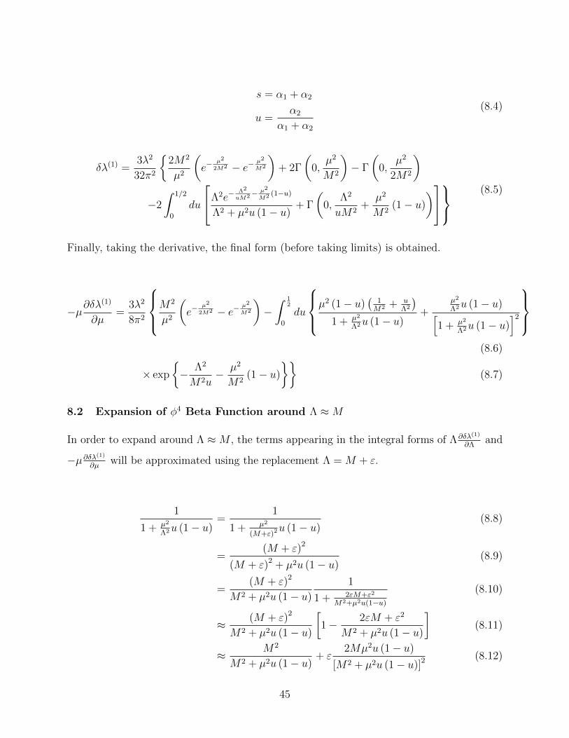
Finally, taking the derivative, the final form (before taking limits) is obtained.

−µ∂δλ(1)

∂µ=

3λ2

8π2

M2

µ2

(e−

µ2

2M2 − e−µ2

M2

)−∫ 1

2

0

du

µ2 (1− u)

(1M2 + u

Λ2

)1 + µ2

Λ2u (1− u)+

µ2

Λ2u (1− u)[1 + µ2

Λ2u (1− u)]2

(8.6)

× exp

{− Λ2

M2u− µ2

M2(1− u)

}}(8.7)

8.2 Expansion of φ4 Beta Function around Λ ≈M

In order to expand around Λ ≈M , the terms appearing in the integral forms of Λ∂δλ(1)

∂Λand

−µ∂δλ(1)

∂µwill be approximated using the replacement Λ = M + ε.

1

1 + µ2

Λ2u (1− u)=

1

1 + µ2

(M+ε)2u (1− u)(8.8)

=(M + ε)2

(M + ε)2 + µ2u (1− u)(8.9)

=(M + ε)2

M2 + µ2u (1− u)

1

1 + 2εM+ε2

M2+µ2u(1−u)

(8.10)

≈ (M + ε)2

M2 + µ2u (1− u)

[1− 2εM + ε2

M2 + µ2u (1− u)

](8.11)

≈ M2

M2 + µ2u (1− u)+ ε

2Mµ2u (1− u)

[M2 + µ2u (1− u)]2(8.12)

45

µ2

Λ2u (1− u)[1 + µ2

Λ2u (1− u)]2 =

µ2

(M+ε)2u (1− u)[1 + µ2

(M+ε)2u (1− u)]2 (8.13)

=(M + ε)2 µ2u (1− u)[

(M + ε)2 + µ2u (1− u)]2 (8.14)

=(M + ε)2 µ2u (1− u)

[M2 + µ2u (1− u)]21[

1 + 2εM+ε2

M2+µ2u(1−u)

]2 (8.15)

≈ (M + ε)2 µ2u (1− u)

[M2 + µ2u (1− u)]2

[1− 2

2εM + ε2

M2 + µ2u (1− u)

](8.16)

≈ µ2M2u (1− u)

[M2 + µ2u (1− u)]2+ ε

[2µ2Mu (1− u)

[M2 + µ2u (1− u)]2− 4µ2M3u (1− u)

[M2 + µ2u (1− u)]3

](8.17)

8.3 Selected Amplitudes Contributing to Abelian Gauge Theory Beta Func-

tion

The self-energy of the scalar field has two diagrams which contribute to one-loop order. The

leading-order term corresponds to the diagram below, which is called Σ2.

Figure 8.1: Σ2

46

Σ2 =1

2

e2

m2A

∫d4k

(2π)4

(k2 + k · p)2exp

{− 1M2

[k2 +m2

A + (k + p)2 +m2A

]}[k2 +m2

A][(k + p)2 +m2

A

]=

1

2

e2

m2A

∫d4k

(2π)4

∫ ∞1M2

dα1

∫ ∞1M2

dα2

[k4 − 2α1α2

(α1 + α2)2p2k2 +

(α1 − α2)2

(α1 + α2)2 (k · p)2 +α2

1α22

(α1 + α2)4p4

]

× exp

{− (α1 + α2)

(k2 +m2

A

)− α1α2

α1 + α2

p2

}=

e2

32π2m2A

∫ ∞1M2

dα1

∫ ∞1M2

dα2

{[− Λ6

α1 + α2

− 3Λ4

(α1 + α2)2 −6Λ2

(α1 + α2)3 −6

(α1 + α2)4

+2p2Λ4α1α2

(α1 + α2)3 +4p2Λ2α1α2

(α1 + α2)4 +4p2α1α2

(α1 + α2)5 −p2Λ4 (α1 − α2)2

4 (α1 + α2)3

− p2Λ2 (α1 − α2)2

2 (α1 + α2)4 − p2 (α1 − α2)2

2 (α1 + α2)5 −p4Λ2α2

1α22

(α1 + α2)5 −p4α2

1α22

(α1 + α2)6

]

× exp

{− (α1 + α2)

(Λ2 +m2

A

)− α1α2

α1 + α2

p2

}+

[6

(α1 + α2)4 −4p2α1α2

(α1 + α2)5 +p2 (α1 − α2)2

2 (α1 + α2)5 +p4α2

1α22

(α1 + α2)6

]

× exp

{− (α1 + α2)m2

A −α1α2

α1 + α2

p2

}}=

e2

16π2m2A

∫ 1/2

0

du

∫ ∞1

uM2

ds

{[−Λ6 − 3Λ4

s− 6Λ2

s2− 6

s3+ 2p2Λ4u (1− u) +

4p2Λ2u (1− u)

s

+4p2u (1− u)

s2− p2Λ4 (1− 2u)2 − p2Λ2 (1− 2u)2

s− p2 (1− 2u)2

s2

−p4Λ2u2 (1− u)2 − p4u2 (1− u)2

s

]× exp

{−s(Λ2 +m2

A

)− sp2u (1− u)

}}In the various limits,

µ� Λ�M

− dΣ2

dp2

∣∣∣∣p2=µ2

≈ e2

16π2

[7Λ2

12m2A

+µ2 + 3m2

A

2m2A

log

(m2A

Λ2

)]

µ�M � Λ

47

− dΣ2

dp2

∣∣∣∣p2=µ2

≈ e2

16π2

[M2

4m2A

+µ2

4m2A

log

(2m2

A

M2

)+

(− Λ2

8m2A

+µ2Λ2

16m2AM

2− µ4Λ2

64m2AM

4

)e−

2Λ2

M2

]

M � µ� Λ

− dΣ2

dp2

∣∣∣∣p2=µ2

≈ e2

16π2

[(M2

16m2A

+M4

4m2Aµ

2

)e−

µ2

2M2 +

(− Λ2

8m2A

+µ2

8m2A

− 5M2

16m2A

+1

4

)e−

2Λ2

M2 −µ2

2M2

]

The four-point function has several diagrams which contribute to one-loop order. One ex-

ample of such a diagram is below, called T2.

First, we calculate the term that will appear in the numerator of the integrand.

C = k6 + 4k4 (k · p1) + 2k4 (k · p2) + p21k

4 + (p1 · p2) k4 + 2p21k

2 (k · p1) + 5k2 (k · p1)2 + k2 (k · p2)2

+ 5k2 (k · p1) (k · p2) + 2 (p1 · p2) k2 (k · p1) + p21k

2 (k · p2) + (p1 · p2) k2 (k · p2) + 2 (k · p1)3

+ 3 (k · p1)2 (k · p2) + p21 (k · p1)2 + (p1 · p2) (k · p1)2 + (k · p1) (k · p2)2 + p2

1 (k · p1) (k · p2)

+ (p1 · p2) (k · p1) (k · p2)

After the momentum shift k → k − ap1 − bp2, taking the external momenta to be at the

symmetry point, and integrating out the angular part, the coefficient becomes

C = 2π2

[k6 + k4

(21µ2

16+

9µ2

2a2 +

9µ2

2b2 − 5µ2a− µ2b− 3µ2ab

)+ k2

(27a4µ4

8− 9

2a3bµ4 − 15a3µ4

2+

33

4a2b2µ4 +

7

2a2bµ4 +

359a2µ4

64− 9

2ab3µ4 − 13

2ab2µ4

+19

32abµ4 − 49aµ4

32+

27b4µ4

8− 3b3µ4

2+

103b2µ4

64− 9bµ4

32+µ4

16

)+O

(k0)]

48

For this integral, a = α2+α3

α1+α2+α3and b = α3

α1+α2+α3. The integral becomes (keeping terms down

to order Λ0)

T2|SP ≈e4

32π4m4A

∫ Λ

0

dk

∫ ∞1M2

dα1dα2dα3C (k) k3

× exp

{− (α1 + α2 + α3)

(k2 +m2

A

)− µ2

4

3α1α2 + 4α1α3 + 3α2α3

α1 + α2 + α3

}Λ∂T2

∂Λ

∣∣∣∣SP

≈ e4

32π4m4A

∫ ∞1M2

dα1dα2dα3Λ4C (Λ)

× exp

{− (α1 + α2 + α3)

(Λ2 +m2

A

)− µ2

4

3α1α2 + 4α1α3 + 3α2α3

α1 + α2 + α3

}Λ∂T2

∂Λ

∣∣∣∣SP

<e4

32π4m4A

∫ 1

0

du

∫ 1−u

0

dv

∫ ∞3M2

s2dsΛ4C (Λ)

× exp

{−s(Λ2 +m2

A

)− sµ

2

4[4u (1− u− v) + 3v (1− v)]

}Λ∂T2

∂Λ

∣∣∣∣SP

<e4

32π4m4A

∫ 1

0

du

∫ 1−u

0

dvΛ4C (Λ)

×

[9M4

Λ2 +m2A + µ2

4[4u (1− u− v) + 3v (1− v)]

+6M2(

Λ2 +m2A + µ2

4[4u (1− u− v) + 3v (1− v)]

)2

+2(

Λ2 +m2A + µ2

4[4u (1− u− v) + 3v (1− v)]

)3

× exp

{−3Λ2

M2− 3m2

A

M2− 3µ2

4M2[4u (1− u− v) + 3v (1− v)]

}Λ∂T2

∂Λ

∣∣∣∣SP

>e4

32π4m4A

∫ ∞1M2

dα1dα2dα32π2Λ10 exp

{− (α1 + α2 + α3)

(Λ2 +m2

A +µ2

2

)}

An upper and lower limit have been found for this integral so that there is no doubt about

the accuracy of these approximations. Now in the various regimes,

µ� Λ�M

49

Λ∂T2

∂Λ

∣∣∣∣SP

<e4

16π2

[Λ4

m4A

− 35Λ2µ2

48m4A

− 3Λ2

m2A

+45µ2

16m2A

+25µ4

64m4A

+ 6

]Λ∂T2

∂Λ

∣∣∣∣SP

>e4

16π2

[Λ4

m4A

− 3µ2Λ2

2m4A

− 3Λ2

m2A

]

µ�M � Λ

Λ∂T2

∂Λ

∣∣∣∣SP

<e2

16π2

[9Λ8

2m4AM

4− 45µ2Λ8

16m4AM

6+

603µ4Λ8

640m4AM

8

]e−

3Λ2

M2

Λ∂T2

∂Λ

∣∣∣∣SP

>e2

32π2

[Λ4

m4A

− 3µ2Λ4

2m4AM

2− 3Λ4

m2AM

2− 3µ2Λ2

2m4A

− 3Λ2

m2A

]e−

3Λ2

M2

M � µ� Λ

Λ∂T2

∂Λ

∣∣∣∣SP

<e2

16π2

[(73Λ6

18m4Aµ

2+

3Λ4

32m4A

− 14Λ4

m2Aµ

2

)e−

3Λ2

M2 +

(9Λ8

3200m4AM

4+

54Λ8

625m4AM

2µ2

)e−

3Λ2

M2 −µ2

16M2

]Λ∂T2

∂Λ

∣∣∣∣SP

>e2

32π2

[9µ4Λ4

8m4AM

4+

9µ2Λ4

2m2AM

4+

9Λ4

2M4

]e−

3Λ2

M2 −3m2

AM2 −

3µ2

2M2 .

50

REFERENCES

[1] Michael Aizenman. Geometric Analysis of ϕ4 Fields and Ising Models (Parts 1 & 2).Commun. Math. Phys., 86:1, 1982.

[2] M. Luscher and P. Weisz. Scaling Laws and Triviality Bounds in the Lattice φ4 Theory.III. N Component Model. Nucl. Phys. B, 318:705–741, 1989.

[3] David J. E. Callaway. Triviality Pursuit: Can Elementary Scalar Particles Exist? Phys.Rept., 167:241, 1988.

[4] J. Frohlich. On the Triviality of λφ4 in D-Dimensions Theories and the Approach tothe Critical Point in D ≥ Four-Dimensions. Nucl. Phys. B, 200:281–296, 1982.

[5] Luigi Del Debbio. The conformal window on the lattice. PoS, Lattice2010:004, 2014.

[6] Daniel F. Litim and Francesco Sannino. Asymptotic safety guaranteed. JHEP, 12:178,2014.

[7] Daniele Barducci, Marco Fabbrichesi, Carlos M. Nieto, Roberto Percacci, and VedranSkrinjar. In search of a UV completion of the standard model — 378,000 models thatdon’t work. JHEP, 11:057, 2018.

[8] Richard J. Szabo. Quantum field theory on noncommutative spaces. Phys. Rept.,378:207–299, 2003.

[9] Michael R. Douglas and Nikita A. Nekrasov. Noncommutative field theory. Rev. Mod.Phys., 73:977–1029, 2001.

[10] Jaume Gomis and Thomas Mehen. Space-time noncommutative field theories and uni-tarity. Nucl. Phys. B, 591:265–276, 2000.

[11] A. Bassetto, L. Griguolo, G. Nardelli, and F. Vian. On the unitarity of quantum gaugetheories on noncommutative spaces. JHEP, 07:008, 2001.

[12] Luis Alvarez-Gaume, J. L. F. Barbon, and Roman Zwicky. Remarks on time spacenoncommutative field theories. JHEP, 05:057, 2001.

[13] Nathaniel Craig and Seth Koren. IR Dynamics from UV Divergences: UV/IR Mixing,NCFT, and the Hierarchy Problem. JHEP, 03:037, 2020.

[14] Silvan S. Schweber, Hans A. Bethe, and Frederic de Hoffmann. Mesons and fields.Volume 1: Fields. Peterson and Comp., 1955.

[15] Roji Pius and Ashoke Sen. Unitarity of the Box Diagram. JHEP, 11:094, 2018.

51

[16] Roji Pius and Ashoke Sen. Cutkosky rules for superstring field theory. JHEP, 10:024,2016. [Erratum: JHEP 09, 122 (2018)].

[17] Paokuan Chin and E. T. Tomboulis. Nonlocal vertices and analyticity: Landau equa-tions and general Cutkosky rule. JHEP, 06:014, 2018.

[18] E. T. Tomboulis. Nonlocal and quasilocal field theories. Phys. Rev. D, 92(12):125037,2015.

[19] Neil Barnaby and Niky Kamran. Dynamics with infinitely many derivatives: The Initialvalue problem. JHEP, 02:008, 2008.

[20] Anish Ghoshal, Anupam Mazumdar, Nobuchika Okada, and Desmond Villalba. Stabilityof infinite derivative Abelian Higgs models. Phys. Rev. D, 97(7):076011, 2018.

[21] M. Srednicki. Quantum field theory. Cambridge University Press, 1 2007.

[22] Manami Noumi Hashi, Hiroshi Isono, Toshifumi Noumi, Gary Shiu, and Pablo Soler.Higgs Mechanism in Nonlocal Field Theories. JHEP, 08:064, 2018.

52