CENTRO PER LA RICERCA

SCIENTIFICA E TECNOLOGICA

38050 Povo (Trento), ItalyTel.: +39 0461 314312Fax: +39 0461 302040e−mail: prdoc@itc.it − url: http://www.itc.it

WEAK, STRONG, AND STRONG CYCLIC PLANNINGVIA SYMBOLIC MODEL CHECKING

Cimatti A., Pistore M.,Roveri M., Traverso P.

April 2001

Technical Report # 0104−11

Istituto Trentino di Cultura, 2001

LIMITED DISTRIBUTION NOTICE

This report has been submitted forpublication outside of ITC and will probably be copyrighted if accepted for publication. It has beenissued as a Technical Report forearly dissemination of its contents. In view of the transfert of copy right tothe outside publisher, itsdistribution outside of ITC priorto publication should be limited to peer communications and specificrequests. After outside publication,material will be available only inthe form authorized by the copyright owner.

Weak, Strong, and Strong Cy li Planningvia Symboli Model Che kingAlessandro Cimatti1, Mar o Pistore1, Mar o Roveri1;2, Paolo Traverso11 ITC-IRST, Via Sommarive 18, 38055 Povo, Trento, Italyf imatti,pistore,roveri,traversog�irst.it .it2 DSI, University of Milano, Via Comeli o 39, 20135 Milano, ItalyAbstra tPlanning in non-deterministi domains yields both on eptual and pra ti al diÆ ulties. Fromthe on eptual point of view, di�erent notions of planning problems an be devised: for instan e,a plan might either guarantee goal a hievement, or just have some han es of su ess. From thepra ti al point of view, the problem is to devise for algorithms that an deal e�e tively withlarge state spa es. In this paper, we ta kle planning in non-deterministi domains by address-ing on eptual and pra ti al problems. We formally hara terize di�erent planning problems,where solutions have a han e of su ess (\weak planning"), are guaranteed to a hieve the goal(\strong planning"), or a hieve the goal with iterative trial-and-error strategies (\strong y li planning"). In strong y li planning, all the exe utions asso iated with the solution plan alwayshave a possibility of terminating and, when they do, they are guaranteed to a hieve the goal.We present planning algorithms for these problem lasses, and prove that they are orre t and omplete. We implement the algorithms in the mbp planner, by using symboli model he kingte hniques. We show that our approa h is pra ti al with an extensive experimental evaluation:mbp ompares positively with state-of-the-art planners, both in terms of expressiveness and interms of performan e.Keywords: Planning in Non-Deterministi Domains, Conditional Planning, Symboli Model-Che king, Binary De ision Diagrams.

1

Contents1 Introdu tion 22 Domains, Plans, and Planning Problems 32.1 Non-deterministi Domains . . . . . . . . . . . . . . . . . . . . . . . . . . . . . . . . 32.2 Plans as State-a tion Tables . . . . . . . . . . . . . . . . . . . . . . . . . . . . . . . . 52.3 Planning Problems and Solutions . . . . . . . . . . . . . . . . . . . . . . . . . . . . . 83 Algorithms for Weak and Strong Planning 103.1 Formal Properties of the Weak Planning Algorithm . . . . . . . . . . . . . . . . . . . 133.2 Formal Properties of the Strong Planning Algorithm . . . . . . . . . . . . . . . . . . 144 Algorithms for Strong Cy li Planning 154.1 The Global Algorithm . . . . . . . . . . . . . . . . . . . . . . . . . . . . . . . . . . . 154.2 Formal Properties of the Global Algorithm . . . . . . . . . . . . . . . . . . . . . . . 184.3 The Lo al Algorithm . . . . . . . . . . . . . . . . . . . . . . . . . . . . . . . . . . . . 204.4 Formal Properties of the Lo al Algorithm . . . . . . . . . . . . . . . . . . . . . . . . 225 Planning via Symboli Model Che king 245.1 Symboli Representation of Planning Domains . . . . . . . . . . . . . . . . . . . . . 245.2 Symboli Representation of the Planning Algorithms . . . . . . . . . . . . . . . . . . 276 The MBP Planner 286.1 Fun tionalities . . . . . . . . . . . . . . . . . . . . . . . . . . . . . . . . . . . . . . . 286.2 Implementation with Binary De ision Diagrams . . . . . . . . . . . . . . . . . . . . . 287 Experimental Evaluation 307.1 State-of-the-art Planners for Nondeterministi Domains . . . . . . . . . . . . . . . . 307.2 Experimental evaluation setup . . . . . . . . . . . . . . . . . . . . . . . . . . . . . . 317.3 Problems and results . . . . . . . . . . . . . . . . . . . . . . . . . . . . . . . . . . . . 327.4 Analysis of the results . . . . . . . . . . . . . . . . . . . . . . . . . . . . . . . . . . . 408 Related work 419 Con luding Remarks and Future Work 43A Proofs of the Theorems 49A.1 Proofs for the Weak Planning Algorithm . . . . . . . . . . . . . . . . . . . . . . . . . 49A.2 Proofs for the Strong Cy li Algorithms . . . . . . . . . . . . . . . . . . . . . . . . . 51

1

1 Introdu tionResear h in planning is more and more fo using on the problem of planning in nondeterministi domains and with in omplete information, see for instan e [Pryor&Collins, 1996; Kabanza et al.,1997; Weld et al., 1998; Cimatti et al., 1998a; Rintanen, 1999a; Bonet&Ge�ner, 2000℄. Mostreal world appli ation domains are indeed intrinsi ally \non-deterministi ". For instan e, mobilerobots may en ounter unexpe ted obsta les during navigation, the value of variables in input to ontrollers annot be predi ted before ontrol takes pla e, and exogenous events and failures ano ur in spa e missions at exe ution time. Approa hes that do not take into a ount the intrinsi non-determinism of the domain are often very hard, if not impossible, to be used in pra ti e.Non-deterministi planning domains an be modeled with a tions that lead from one state tomany possibly di�erent states, rather than ne essarily to a single state, like in lassi al planning(see, e.g., [Fikes&Nilsson, 1971; Penberthy&Weld, 1992℄). For instan e, \pi k-up a blo k from thetable" may either su eed, and lead to a state where the \blo k is at hand", or fail, and leave the\blo k on the table". This apparently simple extension to the lassi al planning paradigm yieldssigni� ant diÆ ulties, both on eptual and pra ti al, related to the fa t that the exe ution of agiven plan depends on the non-determinism of the domain and may result, in general, in more thanone sequen e of states.A on eptual diÆ ulty is the de�nition of the notion of \solution to a planning problem":di�erent kinds of solutions an be devised. For instan e, we might a ept plans that have at leasta han e of su ess, i.e., at least one of the many possible di�erent exe ution paths a hieves thegoal. Most often, however, we would like to have plans that are guaranteed to a hieve the goalin all the exe ution paths, in spite of non-determinism. In order to satisfy this requirement, non-determinism an be ta kled with onditional plans that sense the a tual a tion out ome, among themany possible ones, and a t a ording to the information gathered at exe ution time. An exampleof onditional plan is \pi k up the blo k; if the blo k is at hand, then move the blo k, else pi k upthe blo k again". In several domains, however, there might be no plan that is guaranteed to a hievea given goal. For instan e, if the a tion \pi k-up a blo k from the table" may fail by leaving theblo k on the table (i.e., in the same state), an in�nite sequen e of failures an in prin iple o ur.In these ases, the planner should generate iterative trial-and-error strategies, like \pi k up a blo kuntil su eed", whi h repeat the exe ution of some a tions until the iteration terminates. A planlike \pi k up a blo k until su eed" might in prin iple loop forever, under an in�nite sequen e offailures. However, this is a ase of \in�nite" bad lu k. In many pra ti al ases, we might onsider asa eptable an iterative trial-and error strategy that is guaranteed to su eed in any ase of \�nite"bad lu k.From the pra ti al point of view, there is a need for algorithms that an deal e�e tively withlarge state spa es. In order to guarantee goal a hievement, planning algorithms need eÆ ientways to analyze all the exe ution paths asso iated with andidate plans. Furthermore, in the aseof planning for iterative trial-and-error strategies, there is the additional diÆ ulty that in�niteexe ution paths must be analyzed.In this paper we address the problem of planning in non-deterministi domains. We fo us ona rather simple but general model of non-determinism, where a tions are modeled as transitionsfrom states to sets of states, without information on osts or probabilities. We hoose a \quali-tative" formulation of the planning problem in non deterministi domains that is independent of osts and probability distributions, and we provide sound and pra ti al planning algorithms. Our ontributions are the following:- We formally hara terize di�erent kinds of solutions to the planning problem in non-deterministi 2

domains. We distinguish between plans that have at least a han e to a hieve the goal (weaksolutions), plans that are guaranteed to a hieve the goal (strong solutions), and iterative plansthat formalize the notion of \a eptable" trial-and-error strategies (strong y li solutions).- We present planning algorithms for �nding weak, strong, and strong y li solutions. Thealgorithms generate iterative and onditional plans that repeatedly sense the world, sele tan appropriate a tion, exe ute it, and iterate until the goal is rea hed. We prove that thealgorithms are orre t and omplete, i.e. they �nd a solution if it exists and, if no solutionexists, they terminate with failure.- We show that the algorithms an be formulated by using symboli model he king te h-niques [M Millan, 1993℄. In parti ular, sets of states are represented as propositional formu-lae, and sear h through the state spa e is performed as a set of logi al transformations overpropositional formulas. We implement the algorithms in the Model Based Planner (mbp), aplanner built on top of a state of the art symboli model he ker NuSMV [Cimatti et al.,2000℄. mbp is based on Binary De ision Diagrams (bdds) [Bryant, 1992℄, that allow for the ompa t representation and e�e tive manipulation of propositional formulae.- We provide an extensive experimental evaluation of our approa h. We show that mbp om-pares positively with the existing planners that an deal with non-deterministi domains,both in terms of expressiveness and in terms of performan e. Most of the other planners annot deal with all the planning problems the mbp algorithms have been designed for, e.g.,strong y li solutions.The paper is stru tured as follows. In Se tion 2, we de�ne non-deterministi planning domains, onditional and iterative plans, and the di�erent notions of planning solutions. In Se tion 3 weprovide algorithms for strong and weak planning, whi h share a ommon stru ture and are similarin spirit: the resulting plans, if any, a hieve the goal in a �nite number of steps. In Se tion 4 wepresent the algorithms for generating strong y li plans, whi h generate iterative trial-and-errorstrategies. In Se tion 5 we present the formulate the algorithms using the te hniques of symboli model he king. In Se tion 6 we des ribe mbp, our planner based on symboli model he kingte hniques. In Se tion 7 we des ribe the experimental evaluation of our approa h. We omparembp with state-of-the-art planners that deal with non-deterministi domains. In Se tion 8 wepresent some related work. In Se tion 9 we draw some on lusions and present the lines of futureresear h. In Appendix we report in detail the formal proofs of the theorems.2 Domains, Plans, and Planning ProblemsThe aim of this se tion is to provide a pre ise notion of planning problems in non-deterministi domains. We �rst de�ne non-deterministi planning domains (Se tion 2.1), then the plan stru turethat we hoose to represent onditional and iterative behaviors, and the notion of exe ution of aplan in a planning domain (Se tion 2.2). Finally, we de�ne the notion of planning problem withdi�erent forms of solutions: weak, strong, and strong y li solutions (Se tion 2.3).2.1 Non-deterministi DomainsA (non-deterministi ) planning domain an be des ribed in terms of propositions, whi h may as-sume di�erent values in di�erent states, of a tions and of a transition relation des ribing how (theexe ution of) an a tion leads from one state to possibly many di�erent states.3

De�nition 2.1 (Planning Domain) A Planning Domain D is a 4-tuple hP;S;A;Ri where- P is the �nite set of propositions,- S � 2P is the set of states,- A is the �nite set of a tions, and- R � S �A� S is the transition relation.Intuitively, a state is a olle tion of the propositions holding in it. The transition relation des ribesthe e�e ts of a tion exe ution. An a tion a is exe utable in a state s i� there exists at least onestate s0 su h that R(s; a; s0). An a tion a is deterministi (non-deterministi ) in a state s i� thereexists exa tly one (more than one) state s0 su h that R(s; a; s0). We denote with A t(s) the set ofa tions that are exe utable in state s:A t(s) = fa : 9s0:R(s; a; s0)gWe all exe ution of a in s (denoted by Exe (s; a)) the set of the states that an be rea hed froms performing a tion a 2 A t(s): Exe (s; a) = fs0 : R(s; a; s0)gbad

bad

#eggs=0 #eggs=1 #eggs=2

break

break

break

good

open

open

open

discard

1

2

3

4

5

6

7

8

unbroken

good

good

good

goodunbroken

unbroken

discard

discard

discard

discard

discard

discard

bad

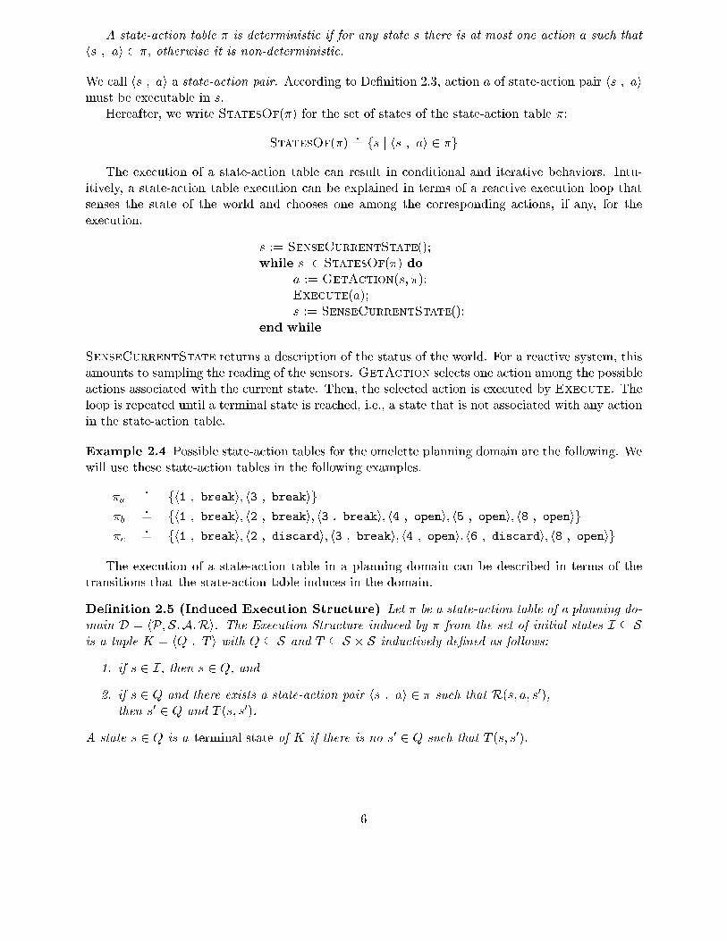
Figure 1: The \Omelette" example4

Example 2.2 As an example, we use a simpli�ed version of the \Omelette" non-deterministi domain [Levesque, 1996℄, depi ted in Figure 1. We have a bowl, whi h an ontain up to 2 eggs.The eggs an be broken into a bowl. The intended goal is to have two eggs into the bowl, so thatan omelette an be prepared. Eggs an be unpredi tably good or bad. A rotten egg in the bowlhas the e�e t of spoiling the bowl. It is possible to determine whether the egg is good or bad onlyafter the egg is into the bowl. However, breaking an egg into a bowl may fail to open the egg anddropping its ontent into the bowl. In this ase it is still impossible to determine whether an egg isgood or bad. If we for e the egg to open, we assure that its ontent is in the bowl. After this we andetermine whether the egg is good or bad. A bowl an always be leaned by dis arding its ontent.We assume to have an in�nite number of eggs that an be grabbed and broken into the bowl. In thisdomain, the propositions in P are f#eggs=0, #eggs=1, #eggs=2, bad, good, unbrokeng. #eggs=iindi ates the number of eggs that have been broken into a bowl, in luding the egg that we mighthave failed to break. bad holds in a state where at least one of the eggs in the bowl is bad, goodis true in states where all eggs in the bowl are good. unbroken holds when we have failed to breakan egg.Possible states are sets of propositions. Ea h state may ontain exa tly one of the #eggs=i, andexa tly one between good and bad. In the following, we asso iate ea h state with a numeri al label.For instan e, state 1 ontains the propositions good and #eggs=0; state 5 ontains the propositions#eggs=2, bad and unbroken; state 8 ontains the propositions #eggs=2, good and unbroken.The set of a tions A is fbreak, open, dis ardg. The transition relation R represents thepre ondition of ea h a tion, and the e�e ts of an a tion in a given state. For instan e, we havethat R(1; break; 2), R(1; break; 3), and R(1; break; 4). This means that the a tion break anbe exe uted in the state where #eggs=0 holds, leads to a state where #eggs=1 holds, and wherenon-deterministi ally either the egg is unbroken and good holds, or unbroken does not hold andthe bowl an be unpredi tably good or bad.Planning domains, as given in De�nition 2.1, are independent of the language that we useto des ribe them. Di�erent languages for des ribing non-deterministi domains have been pro-posed so far, a notable example being the family of high level a tion des ription languages, e.g.AR [Giun higlia et al., 1997℄ and C [Giun higlia&Lifs hitz, 1998℄. strips-like [Fikes&Nilsson,1971℄ or adl-like [Penberthy&Weld, 1992℄ languages (e.g., pddl [Ghallab et al., 1998℄) are notexpressive enough, and they should be extended with disjun tive post onditions to deal with non-deterministi domains. All the work presented in this paper, in luding the planning algorithmsdes ribed in Se tions 3 and 4, is independent of the language for des ribing planning domains,sin e they work at the level of the (semanti ) model of the planning domain. The problem of map-ping the des ription of a domain given in one of these languages into the orresponding semanti model is addressed, for instan e, in [Cimatti et al., 1997℄.2.2 Plans as State-a tion TablesWe need to express onditional and iterative plans that, when exe uted, sense the world at run-time and, depending on the state of the world, an exe ute di�erent a tions. These plans anbe des ribed by asso iating to a state the a tion that has to be exe uted in su h state. We allthem State-A tion Tables. They resemble universal plans [S hoppers, 1987℄ and poli ies [Bonet&Ge�ner, 2000℄.De�nition 2.3 (State-A tion Table) A state-a tion table � for a planning domain D = hP;S;A;Riis a set of pairs fhs ; ai j s 2 S; a 2 A t(s)g. 5

A state-a tion table � is deterministi if for any state s there is at most one a tion a su h thaths ; ai 2 �, otherwise it is non-deterministi .We all hs ; ai a state-a tion pair. A ording to De�nition 2.3, a tion a of state-a tion pair hs ; aimust be exe utable in s.Hereafter, we write StatesOf(�) for the set of states of the state-a tion table �:StatesOf(�) _= fs j hs ; ai 2 �gThe exe ution of a state-a tion table an result in onditional and iterative behaviors. Intu-itively, a state-a tion table exe ution an be explained in terms of a rea tive exe ution loop thatsenses the state of the world and hooses one among the orresponding a tions, if any, for theexe ution. s := SenseCurrentState();while s 2 StatesOf(�) doa := GetA tion(s; �);Exe ute(a);s := SenseCurrentState();end whileSenseCurrentState returns a des ription of the status of the world. For a rea tive system, thisamounts to sampling the reading of the sensors. GetA tion sele ts one a tion among the possiblea tions asso iated with the urrent state. Then, the sele ted a tion is exe uted by Exe ute. Theloop is repeated until a terminal state is rea hed, i.e., a state that is not asso iated with any a tionin the state-a tion table.Example 2.4 Possible state-a tion tables for the omelette planning domain are the following. Wewill use these state-a tion tables in the following examples.�a _= fh1 ; breaki; h3 ; breakig�b _= fh1 ; breaki; h2 ; breaki; h3 ; breaki; h4 ; openi; h5 ; openi; h8 ; openig� _= fh1 ; breaki; h2 ; dis ardi; h3 ; breaki; h4 ; openi; h6 ; dis ardi; h8 ; openigThe exe ution of a state-a tion table in a planning domain an be des ribed in terms of thetransitions that the state-a tion table indu es in the domain.De�nition 2.5 (Indu ed Exe ution Stru ture) Let � be a state-a tion table of a planning do-main D = hP;S;A;Ri. The Exe ution Stru ture indu ed by � from the set of initial states I � Sis a tuple K = hQ ; T i with Q � S and T � S � S indu tively de�ned as follows:1. if s 2 I, then s 2 Q, and2. if s 2 Q and there exists a state-a tion pair hs ; ai 2 � su h that R(s; a; s0),then s0 2 Q and T (s; s0).A state s 2 Q is a terminal state of K if there is no s0 2 Q su h that T (s; s0).6

An exe ution stru ture is a dire ted graph, where the nodes are all the states whi h an be rea hedby exe uting a tions in the state-a tion table, and the ar s represent a possible a tion exe ution.Indu ed exe ution stru tures resemble Kripke Stru tures [Emerson, 1990℄. Intuitively, an indu edexe ution stru ture ontains all the states (transitions) that an be rea hed (�red) when exe utingthe state a tion table � from the initial set of states I. An indu ed exe ution stru ture is notrequired to be total, i.e. it may ontain states with no out oming ar s. Intuitively, terminal statesrepresent states at whi h the exe ution stops.Example 2.6 The exe ution stru tures indu ed by the state-a tion tables �a, �b and � in Example2.4 on the omelette domain from state 1 an be depi ted as the graphs in Figures 2, 3, and 4.bad

good

bad

#eggs=0 #eggs=1 #eggs=2

good

unbroken

1

2

3

4

6

7

8good

good

goodunbroken

Figure 2: The exe ution stru ture indu ed by state a tion table �aAn exe ution stru ture is a �nite presentation of all the possible exe utions of a given plan in agiven planning domain. An exe ution path of an exe ution stru ture is one of the possible sequen esof states in the exe ution stru ture. It an be either a �nite path ending in a terminal state, or anin�nite path.De�nition 2.7 (Exe ution Path) Let K = hQ ; T i be the exe ution stru ture indu ed by astate-a tion table � from I. An exe ution path of K from s0 2 I is a possibly in�nite sequen es0; s1; s2; : : : of states in Q su h that, for all states si in the sequen e:- either si is the last state of the sequen e, in whi h ase si is a terminal state of K;- or T (si; si+1) .We say that a state s0 is rea hable from a state s if there is a path from s to s0.K is an a y li exe ution stru ture i� all its exe ution paths are �nite.7

bad

good

bad

#eggs=0 #eggs=1 #eggs=2

good

unbroken

1

2

3

4

5

6

7

8 good

good

good

badunbroken

unbroken

Figure 3: The exe ution stru ture indu ed by state a tion table �bExample 2.8 Some of the in�nitely many exe ution paths for the exe ution stru ture indu ed bythe state-a tion table � in Example 2.4 from state 1 are the following.1, 3, 71, 4, 3, 8, 71, 2, 1, 3, 71, 2, 1, 2, 1, 3, 71, 2, 1, 2, : : :1, 3, 6, 1, 3, 71, 3, 6, 1, 3, 6 : : :All these sequen es of states are paths of the exe ution stru ture represented in Figure 4. Allthe �nite paths end in state 7, that is the only terminal state of the exe ution stru ture.2.3 Planning Problems and SolutionsA planning problem is de�ned by a planning domain D, a set of initial states I, and a set of goalstates G.De�nition 2.9 (Planning Problem) Let D = hP;S;A;Ri be a planning domain. A planningproblem for D is a triple fD;I;Gg, where I � S and G � S.The above de�nition takes into a ount two forms of non-determinism. First, we have a set of initialstates, and not a single initial state. This allows for expressing partially spe i�ed initial onditions.Se ond, the exe ution of an a tion from a state results in a set of states, and not ne essarily in asingle state (see R in de�nition 2.1). This allows for expressing non-deterministi a tion exe utions.Intuitively, solutions to a planning problem satisfy a rea hability requirement: a solution is astate a tion table whose aim is, when exe uted from any state in the set of initial states I, to rea hstates in a set of �nal desired states G. In order to make this requirement pre ise, we need to spe ify\how" the set of �nal desired states should be rea hed, i.e., the \strength" of this requirement.We formalize the notion of weak, strong and strong y li solutions as follows.8

bad

good

bad

#eggs=0 #eggs=1 #eggs=2

good

unbroken

1

2

3

4

6

7

8 good

good

good

unbroken

Figure 4: The exe ution stru ture indu ed by state a tion table � De�nition 2.10 (Solutions to a planning problem) Let D = hP;S;A;Ri be a planning do-main. Let P = fD;I;Gg be a planning problem. Let � be a deterministi state-a tion table for D.Let K = hQ ; T i be the exe ution stru ture indu ed by � from I.1. � is a weak solution to P i� for any state in I some terminal state is rea hable that is alsoin G.2. � is a strong solution to P i� K is a y li and all the terminal states of K are in G.3. � is a strong y li solution to P i� from any state in Q some terminal state is rea hable andall the terminal states of K are in G.Weak solutions are plans that may a hieve the goal, but are not guaranteed to do so. Thisamounts to saying that at least one of the many possible exe ution paths of the state a tiontable should result in a terminal state that is a goal state. Strong solutions are plans that areguaranteed to a hieve the goal in spite of non-determinism, i.e. all the exe ution paths shouldresult in a terminal state that is a goal state. Strong y li solutions formalize the intuitive notionof \a eptable" iterative trial-and-error strategies: all their possible exe ution paths have always apossibility of terminating and, when they do, they are guaranteed to a hieve the goal.In the general ase of non-deterministi state-a tion tables, we say that � is a strong (weak,strong y li ) solution to a planning problem if all the determinizations of � are, a ording toDe�nition 2.10. Formally, a determinization of � is any deterministi state-a tion table �d � �su h that StatesOf(�d) = StatesOf(�). In this way, we model the fa t that the exe utor an hoose any a tion arbitrarily when building the deterministi state-a tion table, i.e., there areno ompatibility onstraints among the a tion in di�erent states. This guarantees that the planis orre t also in the general ase where the exe utor sele ts at run-time one a tion among thepossible a tions asso iated to the urrent state by the state-a tion table.9

De�nition 2.11 (Solutions to a planning problem (2)) Let D = hP;S;A;Ri be a planningdomain. Let P = fD;I;Gg be a planning problem. Let � be a (non-deterministi ) state-a tiontable for D.� is a weak (resp. strong, strong y li ) solution to P if all the determinizations �d of � areweak (resp. strong, strong y li ) solutions of P a ording to De�nition 2.10.As �nal remark, noti e that the strong solutions to a planning problem are a subset of thestrong y li solutions, whi h are in turn a subset of the weak solutions. Indeed, any state-a tiontable � that is a strong solution to a planning problem P is also a strong y li solution to P : ifthe exe ution stru ture K indu ed by � is a y li , then all the exe ution paths are �nite. Hen e,from any state in K, a terminal state is rea hed following any path. Also, any state-a tion table� that is a strong y li solution to a planning problem P is also a weak solution to P . Indeed,a ording to the de�nition of strong y li solution, a terminal state that is also a goal is rea hablefrom any state of the exe ution stru ture, so this is true in parti ular for all the initial states.Example 2.12 In Example 2.4, state-a tion table �a is a weak solution to the planning problemwhere the initial state is state 1 and the goal state is 7. It is a plan that may a hieve the goal ofhaving two good eggs in the bowl.State-a tion table �b is a strong solution to the planning problem where the initial state is state1 and the goal states are 6 and 7. It is a safe plan that guarantees that two eggs (either bad orgood) are broken in the bowl.State-a tion table �b is also a weak solution to the planning problem where the initial state isstate 1 and the goal state is 7, even if it is not a strong solution for this planning problem.State-a tion table � is a strong y li solution to the planning problem where the initial stateis 1 and the goal state is 7. It is an iterative trial-and-error strategy that, every time a bad eggis broken into the bowl, leans the bowl by dis arding the egg(s). It iteratively tries to get to thepoint where two good eggs are in the bowl, so that an omelette an be prepared.The latter planning problem admits no strong solutions: in prin iple, it is always possible toen ounter an in�nite sequen e of rotten eggs whi h will prevent us from making our omelette. Thisis, however, a ase of extreme bad lu k. A strong y li solution guarantees that, for any ase of\�nite" bad lu k, the goal is rea hed with a �nite exe ution.3 Algorithms for Weak and Strong PlanningIn this se tion we des ribe the algorithms for weak and strong planning. These two algorithms sharea similar ontrol stru ture, based on a breadth-�rst sear h pro eeding ba kwards from the goal,towards the initial states. They operate on the planning problem: the sets of the initial states Iand of the goal states G are expli itly given as input parameters, while the domain D = hP;S;A;Riis assumed to be globally available to the invoked subroutines. Both algorithms either return asolution state-a tion table, or a distinguished value for state-a tion tables, alled Fail, used torepresent sear h failure. In parti ular, we assume that Fail is di�erent from the empty state-a tiontable, that we will denote with ;.Fun tion WeakPlan, presented in Figure 5, works by in rementally building a state-a tiontable in variable SA. At ea h iteration step, the set of states for whi h a solution has been alreadyfound is used as a target for the expansion preimage routineWeakPreImage, that returns a new\sli e" to be added to the state-a tion table under onstru tion. Fun tion WeakPreImage is10

1 fun tion WeakPlan(I;G);2 OldSA := Fail;3 SA := ;;4 while (OldSA 6= SA ^ I 6� (G [ StatesOf(SA))) do5 PreImage :=WeakPreImage(G [ StatesOf(SA));6 NewSA := PruneStates(PreImage; G [ StatesOf(SA));7 OldSA := SA;8 SA := SA [NewSA;9 done;10 if (I � (G [ StatesOf(SA))) then11 return SA;12 else13 return Fail;14 �;15 end;1 fun tion StrongPlan(I;G);2 OldSA := Fail;3 SA := ;;4 while (OldSA 6= SA ^ I 6� (G [ StatesOf(SA))) do5 PreImage := StrongPreImage(G [ StatesOf(SA));6 NewSA := PruneStates(PreImage; G [ StatesOf(SA));7 OldSA := SA;8 SA := SA [NewSA;9 done;10 if (I � (G [ StatesOf(SA))) then11 return SA;12 else13 return Fail;14 �;15 end; Figure 5: The Algorithms for Weak and Strong Planning.11

de�ned as follows: WeakPreImage(S) _= fhs ; ai : Exe (s; a) \ S 6= ;g:Intuitively,WeakPreImage(S) returns the set of pairs state-a tion hs ; ai su h that the exe utionof a in s may lead inside S.In the algorithm, fun tion WeakPreImage is alled using as target the goal states G and thestates that are already in the state-a tion table SA: these are the states for whi h a solution isalready known. The returned weak preimage PreImage is then passed to fun tion PruneStates,de�ned as follows: PruneStates(�; S) _= fhs ; ai 2 � : s 62 Sg:This fun tion removes from the preimage table all the pairs hs ; ai su h that a solution is alreadyknown for s. This pruning is important to guarantee that only the shortest solution from any stateappears in the state-a tion table. The termination test requires that the initial states are in ludedin the set of a umulated states (i.e. G [ StatesOf(SA)), or that a �xed point has been rea hedand no more states an be added to state-a tion table SA. In the �rst ase, the state-a tion tablereturned by the algorithm is a weak solution to the planning problem. In the se ond ase, no weaksolution exists: indeed, there is some initial state from whi h it is not possible to rea h any goalstate.The planning pro edure StrongPlan, presented in Figure 5, solves the strong planning prob-lem. It is identi al to WeakPlan, ex ept that a strong preimage, rather than a weak preimage, is omputed at ea h iteration of the algorithm. The StrongPreImage fun tion is de�ned asStrongPreImage(S) _= fhs ; ai : ; 6= Exe (s; a) � Sg:Intuitively, StrongPreImage(S) returns the set of pairs state-a tion hs ; ai su h that the exe u-tion of a in s is guaranteed to lead to states inside S. Namely, StrongPreImage(S) ontains allthe states-a tion pairs from whi h S is guaranteed to be rea hed regardless of non-determinism.Example 3.1 Let us onsider the omelette domain and the planning problem of rea hing state 7from state 1.The weak planning algorithm su eeds to build a weak solution for the planning problem.Indeed, the value of variable SA in the algorithm after i iterations of the while loop oin ides withstate-a tion table �i, where:�0 = ;�1 = fh3 ; breaki; h8 ; openig�2 = fh3 ; breaki; h8 ; openi; h1 ; breaki; h4 ; openigAfter the se ond iteration of the while loop, the algorithm terminates, as the state-a tion table isde�ned on the initial state 1.The strong planning algorithm, instead, fails to build a strong solution for the planning problem.The algorithm starts with variable SA set to ; and, sin e StrongPreImage(f7g) = ;, no newstate-a tion pair is added to variable SA in the �rst iteration of the while loop: the �x point isimmediately rea hed. The omputed state-a tion table ; does not over the initial state 1, thereforethe strong planning algorithm returns with a failure. This result is orre t, as there is no strongsolution for this planning problem. In general, it is possible to show that, if the �x point is rea hed,the omputed state-a tion table overs all the states that admit a strong solution: in this ase, theonly state that admits a (trivial) strong solution is the goal state 7.12

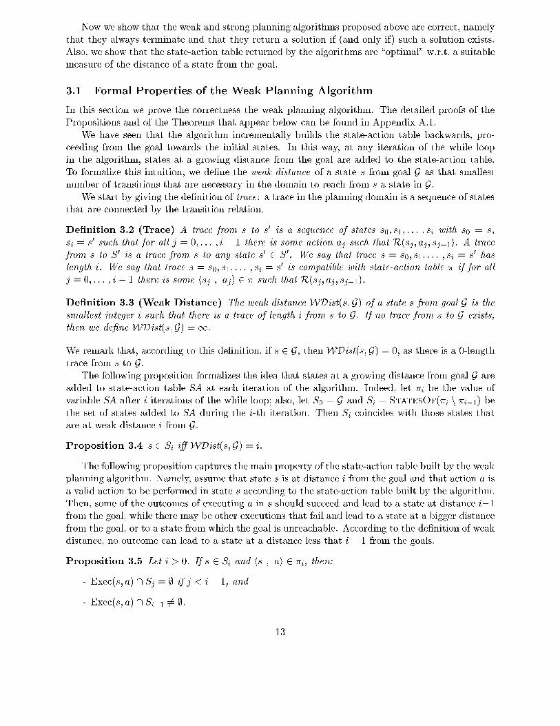
Now we show that the weak and strong planning algorithms proposed above are orre t, namelythat they always terminate and that they return a solution if (and only if) su h a solution exists.Also, we show that the state-a tion table returned by the algorithms are \optimal" w.r.t. a suitablemeasure of the distan e of a state from the goal.3.1 Formal Properties of the Weak Planning AlgorithmIn this se tion we prove the orre tness the weak planning algorithm. The detailed proofs of thePropositions and of the Theorems that appear below an be found in Appendix A.1.We have seen that the algorithm in rementally builds the state-a tion table ba kwards, pro- eeding from the goal towards the initial states. In this way, at any iteration of the while loopin the algorithm, states at a growing distan e from the goal are added to the state-a tion table.To formalize this intuition, we de�ne the weak distan e of a state s from goal G as that smallestnumber of transitions that are ne essary in the domain to rea h from s a state in G.We start by giving the de�nition of tra e: a tra e in the planning domain is a sequen e of statesthat are onne ted by the transition relation.De�nition 3.2 (Tra e) A tra e from s to s0 is a sequen e of states s0; s1; : : : ; si with s0 = s,si = s0 su h that for all j = 0; : : : ; i � 1 there is some a tion aj su h that R(sj ; aj ; sj+1). A tra efrom s to S0 is a tra e from s to any state s0 2 S0. We say that tra e s = s0; s1; : : : ; si = s0 haslength i. We say that tra e s = s0; s1; : : : ; si = s0 is ompatible with state-a tion table � if for allj = 0; : : : ; i� 1 there is some hsj ; aji 2 � su h that R(sj; aj ; sj+1).De�nition 3.3 (Weak Distan e) The weak distan e WDist(s;G) of a state s from goal G is thesmallest integer i su h that there is a tra e of length i from s to G. If no tra e from s to G exists,then we de�ne WDist(s;G) =1.We remark that, a ording to this de�nition, if s 2 G, then WDist(s;G) = 0, as there is a 0-lengthtra e from s to G.The following proposition formalizes the idea that states at a growing distan e from goal G areadded to state-a tion table SA at ea h iteration of the algorithm. Indeed, let �i be the value ofvariable SA after i iterations of the while loop; also, let S0 = G and Si = StatesOf(�i n �i�1) bethe set of states added to SA during the i-th iteration. Then Si oin ides with those states thatare at weak distan e i from G.Proposition 3.4 s 2 Si i� WDist(s;G) = i.The following proposition aptures the main property of the state-a tion table built by the weakplanning algorithm. Namely, assume that state s is at distan e i from the goal and that a tion a isa valid a tion to be performed in state s a ording to the state-a tion table built by the algorithm.Then, some of the out omes of exe uting a in s should su eed and lead to a state at distan e i�1from the goal, while there may be other exe utions that fail and lead to a state at a bigger distan efrom the goal, or to a state from whi h the goal is unrea hable. A ording to the de�nition of weakdistan e, no out ome an lead to a state at a distan e less that i� 1 from the goals.Proposition 3.5 Let i > 0. If s 2 Si and hs ; ai 2 �i, then:- Exe (s; a) \ Sj = ; if j < i� 1, and- Exe (s; a) \ Si�1 6= ;. 13

Propositions 3.4 and 3.5 are the basi ingredients to prove the orre tness of fun tionWeakPlan.The orre tness depends on the fa t that all the states from whi h the goal may be rea hed have a�nite weak distan e from the goal, and hen e are eventually added to the state-a tion table builtby the algorithm (Proposition 3.4); and on the fa t that any a tion that appears in the state-a tiontable has some out omes that lead to a shorter distan e from the goal (Proposition 3.5), so that apath to the goal an be obtained by following there progressing out omes.Theorem 3.6 (Corre tness) Let � _= WeakPlan(I;G) 6= Fail. Then � is a weak solution ofthe planning problem P = fD;I;Gg. If WeakPlan(I;G) = Fail, instead, then there is no weaksolution for planning problem P .AlgorithmWeakPlan always terminates: indeed, at any iteration of the while loop, either theset SA stri tly grows, or the loop ends due to ondition \OldSA 6= SA" in the guard of the while.Also, SA annot grow unboundedly, as there are only �nitely many valid state-a tion pairs.Theorem 3.7 (Termination) Fun tion WeakPlan always terminates.The ba kward onstru tion performed by the algorithm guarantees the optimality of the om-puted solution with respe t to the weak distan e of the initial states from the goal.Theorem 3.8 (Optimality) Let � _= WeakPlan(I;G) 6= Fail. Then plan � is optimal withrespe t to the weak distan e: namely, for ea h s 2 I, in the exe ution stru ture for � there existsan exe ution path from s to G of length WDist(s;G).We remark that, by de�nition of weak distan e, there an be no exe ution path shorter thatWDist(s;G) in the exe ution stru ture orresponding to a weak solution. This guarantees theoptimality of plan �.3.2 Formal Properties of the Strong Planning AlgorithmThe formal results for the strong planning algorithm an be easily obtained by adapting those forthe weak planning algorithm presented in Se tion 3.1 and detailed in Appendix A.1. Here we onlydis uss the most relevant di�eren es.The strong planning algorithm di�ers from the weak one only for the preimages omputed inthe while loop: the former omputes strong preimages, while the latter omputes weak preimages.The onsequen e is that, during the iterations of the strong planning algorithm, states are addedto state-a tion tables SA a ording to a di�erent distan e from the goal states. The strong distan eof a state from a goal takes into a ount that a strong solution must guarantee to rea h the goalin spite of the possible non-deterministi out omes of the exe uted a tions. To de�ne the strongdistan e, we �rst introdu e the notion of a omplete set T of tra es from state s to G. It is a set oftra es that overs all the possible non-deterministi out omes of a tions: if a parti ular out ome is onsidered in any tra e of T , then all the other non-deterministi out omes must be onsidered insome other tra es of T .De�nition 3.9 (Complete Set of Tra es) A omplete set of tra es from s to G is a set T oftra es from s to states in G su h that, whenever s = s0; s1; : : : ; si is in the set T and j = 0; : : : ; i�1,then there is some a tion a su h that R(sj; a; sj+1) and, whenever R(sj; a; s0j+1), then there is sometra e in T that extends s = s0; s1; : : : ; sj; s0j+1 : : : .The strong distan e of a state s from G orresponds to the longest tra e in the shortest ompleteset of tra es from s to G, where the length of a omplete set of tra es is the length of its longesttra e. 14

De�nition 3.10 (Strong Distan e) The strong distan e SDist(s;G) of a state s from a goal Gis the smallest integer i su h that there is some omplete set of tra es T from s to G and i is thelength of the longest tra e in T . If no omplete set of tra es from s to G exists, then we de�neSDist(s;G) =1.Let �i be the value of variable SA after i iterations of the while loop and let Si be the set ofstates for whi h a solution is found at the i-th iteration. Similarly to what happens in the weak ase, Si are exa tly the states at strong distan e i from G.Proposition 3.11 s 2 Si i� SDist(s;G) = i.Proposition 3.5 has also to be adapted to take into a ount the fa t that StrongPreImagerepla es WeakPreImage in the algorithm.Proposition 3.12 Let i > 0. If s 2 Si and hs ; ai 2 �i, then:- Exe (s; a) � Sj<i Sj, and- Exe (s; a) \ Si�1 6= ;.The main results on the strong planning algorithm follow.Theorem 3.13 (Corre tness) Let � _= StrongPlan(I;G) 6= Fail. Then � is a strong solutionof the planning problem P = fD;I;Gg. If StrongPlan(I;G) = Fail, instead, then there is nostrong solution for planning problem P .Theorem 3.14 (Termination) Fun tion StrongPlan always terminates.Theorem 3.15 (Optimality) Let � _= StrongPlan(I;G) 6= Fail. Then plan � is optimal withrespe t to the strong distan e: namely, for ea h s 2 I, in the exe ution stru ture for � all theexe ution paths from s to G have a length smaller of equal to SDist(s;G).4 Algorithms for Strong Cy li PlanningIn this se tion we ta kle the problem of strong y li planning. The main di�eren e with thealgorithms presented in previous se tion is that here the resulting plans allow for in�nite behaviors:loops must no longer be eliminated, but rather ontrolled, i.e. only ertain, \good" loops must bekept. In parti ular, we eliminate those loops that, on e entered, have no han e to rea h the goal.We present two di�erent approa hes to strong y li planning, whi h an be applied in di�erentsituations. The �rst algorithm is based on a global approa h, whi h requires the analysis of thewhole state spa e in one shot. The se ond, based on a lo al approa h, tries to onstru t thestate-a tion table in rementally from the goal, building on the strong planning algorithm.4.1 The Global AlgorithmThe global version of the strong y li planning algorithm is presented in Figure 6. The main fun -tion is StrongCy li PlanGlobal, but most of the work is done by StrongCy li PlanAux.The latter fun tion re eives in input a starting state-a tion table and a set of goal states, re�nes thestate-a tion table as des ribed below, and returns a andidate solution for the planning problem.Fun tion StrongCy li PlanGlobal, then, he ks whether the returned state-a tion table SA15

1 fun tion StrongCy li PlanGlobal(I;G);2 SA := StrongCy li PlanAux(UnivSA; G);3 if (I � (G [ StatesOf(SA))) then4 return SA;5 else6 return Fail;7 �;8 end;1 fun tion StrongCy li PlanAux(StartSA; G);2 OldSA := ;;3 SA := StartSA;4 while (OldSA 6= SA) do5 OldSA := SA;6 SA := PruneUn onne ted(PruneOutgoing(SA; G); G);7 done;8 return RemoveNonProgress(SA; G);9 end; Figure 6: The Global Algorithm for Strong Cy li Planning.de�nes a plan for all the initial states, i.e., whether I � (G [ StatesOf(SA)). If this is the ase,SA is a strong y li solution for the planning problem. Otherwise, a failure is returned.The starting state-a tion table passed to fun tion StrongCy li PlanAux is the universalstate-a tion table UnivSA. It ontains all state-a tion pairs that satisfy the appli ability onditions:UnivSA _= fhs ; ai j a 2 A t(s)g:The algorithm starts to analyze the universal state-a tion table with respe t to the problem beingsolved, and eliminates all those state-a tion pairs whi h are dis overed to be sour e of potential\bad" loops, or to lead to states whi h have been dis overed not to allow for a solution. Withrespe t to the algorithms presented in previous se tion, here the \envelope" of possible solutions isredu ed rather than being extended: this approa h amounts to omputing a greatest �x point.This \elimination" phase, where unsafe state-a tion pairs are dis arded, orresponds to the whileloop of fun tion StrongCy li PlanAux. It is based on the repeated appli ation of the fun tionsPruneOutgoing and PruneUn onne ted. The role of PruneOutgoing is to remove all thosestate-a tion pairs whi h may lead out of G [ StatesOf(SA), whi h is the urrent set of potentialsolutions. Be ause of the elimination of these a tions, from ertain states it may be ome impossibleto rea h the set of goal states. The role of PruneUn onne ted is to identify and remove su hstates. Due to this removal, the need may arise to eliminate further outgoing transitions, and soon. When onvergen e is rea hed, the elimination loop is quit. The resulting state-a tion table isguaranteed to generate exe utions whi h either terminate in the goal or loop forever on states fromwhi h it is possible to rea h the goal.As the following example shows, the state-a tion table obtained after the elimination loop isnot ne essarily a valid solution for the planning problem. Indeed, it may ontain state-a tion pairsthat, while preserving the rea hability of the goal, still do not perform any progress against it.16

1 fun tion PruneUn onne ted(SA; G);2 OldSA := Fail;3 NewSA := ;;4 while (OldSA 6= NewSA) do5 OldSA := NewSA;6 NewSA := SA \WeakPreImage(G [ StatesOf(NewSA));7 done;8 return NewSA;9 end;1 fun tion PruneOutgoing(SA; G);2 NewSA := SA nComputeOutgoing(SA; G [ StatesOf(SA));3 return NewSA;4 end;1 fun tion RemoveNonProgress(SA; G);2 OldSA := Fail;3 NewSA := ;;4 while (OldSA 6= NewSA) do5 PreImage := SA \WeakPreImage(G [ StatesOf(NewSA));6 OldSA := NewSA;7 NewSA := NewSA [PruneStates(PreImage; G [ StatesOf(NewSA));8 done;9 return NewSA;10 end; Figure 7: The Primitives for Strong Cy li Planning.17

Example 4.1 Consider the omelette domain, and the planning problem of rea hing state 7 fromstate 1. A tion dis ard in state 3 is \safe": if exe uted, it leads in state 1, where the goal is stillrea hable. However, this a tion does not ontribute to rea h the goal. On the ontrary, it leadsba k to the initial state and, to rea h the goal from 1, it is ne essary to move again to state 3.Moreover, if a tion dis ard is performed whenever the exe ution is in state 3, then the goal isnever rea hed.In the strong y li planning algorithm, fun tionRemoveNonProgress takes are of removingall those a tions from a state whose out omes do not lead to any progress against the goal. Thisfun tion is very similar to the weak planning algorithm: it iteratively extends the state-a tion tableby onsidering states at an in reasing distan e from the goal. In this ase, however, the weakpreimage omputed at any iteration step is restri ted to the state-a tion pairs that appear in theinput state-a tion table, and hen e that are \safe" a ording to the elimination phase.Fun tions PruneOutgoing, PruneUn onne ted, and RemoveNonProgress are pre-sented in Figure 7. They are based on the primitivesWeakPreImage and PruneStates alreadyde�ned in Se tion 3, and on the primitive ComputeOutgoing, that takes in input a state-a tiontable SA and a set of states S, and returns those state-a tion pairs whi h are not guaranteed toresult in states in S, therefore possibly outgoing from S:ComputeOutgoing(SA; S) _= fhs ; ai 2 SA j Exe (s; a) 6� Sg:Example 4.2 Let us onsider the omelette domain and the planning problem of rea hing goalstate 7 from the initial state 1. The \elimination" phase of the algorithm does not remove anystate-a tion pair from UnivSA. Indeed, the goal state is rea hable from any state of the domain,and, as a onsequen e, there are no outgoing a tions. Fun tion RemoveNonProgress, hen e,re eives in input the universal state-a tion table, and re�nes it taking only those a tions thatmay lead to a progress against the goal. The sequen e �i of state-a tion tables built by fun tionRemoveNonProgress is the following:�0 = ;�1 = fh3 ; breaki; h8 ; openig�2 = fh3 ; breaki; h8 ; openi; h1 ; breaki; h4 ; openig�3 = fh3 ; breaki; h8 ; openi; h1 ; breaki; h4 ; openi; h2 ; dis ardi; h5 ; dis ardi; h6 ; dis ardig�4 = �3Sin e in this parti ular ase the state-a tion table passed to RemoveNonProgress is UnivSA,the initial iterations of the fun tion are identi al to the ones of algorithm WeakPlan des ribedin Example 3.1. Here, however, the omputation stops only after four iterations, when a �x pointis rea hed. The �nal state-a tion table is a stri t subset of UnivSA. For instan e, a tion dis ardis not allowed in states 3, 4, 7, and 8. Indeed, in these states we have made some progress againstthe goal, and there is no reason to go ba k to the initial state.4.2 Formal Properties of the Global AlgorithmNow we prove the orre tness of the global version of the strong y li planning algorithm. Thedetailed proofs of the Propositions and of the Theorems that appear in this se tion an be foundin Appendix A.2. 18

We begin with some general on epts and with some properties of fun tion StrongCy li PlanAuxthat will be useful also for proving the orre tness of the lo al version of the strong y li planningalgorithm. We start by de�ning when a state-a tion table � is SC-valid (or strong- y li al valid)for a set of states G. Intuitively, if a state-a tion table SA is SC-valid for G, then it is a strong y li solution of the planning problem of rea hing G from any of the states in SA. Informally,a SC-valid state-a tion table should guarantee that the exe ution stops on e the goal is rea hed:there is no reason to ontinue the exe ution in a goal state. Also, the exe ution of a SC-valid planshould never lead to states where the plan is unde�ned (with the ex eption of the goal states).Finally, we require that any a tion in the plan may lead to some progress in rea hing the goal.De�nition 4.3 (SC-valid state-a tion table) State-a tion table � is SC-valid for G if:- StatesOf(�) \G = ;;- if hs ; ai 2 � and s0 2 Exe (s; a) then s0 2 StatesOf(�) [G;- given any determinization �d of � and any state s 2 StatesOf(�) there is some tra e froms to G that is ompatible with �d.We remark that, in the last item, it is important to require that a tra e from s to G exists for anydeterminization of �. Indeed, in this way we require that there are no state-a tion pairs that donot ontribute in rea hing the goal.A SC-valid state-a tion table is almost what is needed to have a strong y li solution for aplanning problem. The only other property that we need to enfor e on the state-a tion table isthat the plan is de�ned for all the initial states.Proposition 4.4 Let � be a SC-valid plan for G and let I � G[StatesOf(�). Then � is a strong y li solution for the planning problem P = fD;I;Gg.The main result that guarantees the orre tness of algorithm StrongCy li PlanGlobal isthe fa t that StrongCy li PlanAux returns only SC-valid state-a tion tables.Proposition 4.5 Let � = StrongCy li PlanAux(�0; G), where �0 is a generi state-a tiontable. Then � is a SC-valid state-a tion table for G.By ombining Propositions 4.4 and 4.5 it is easy to prove that, if fun tion StrongCy li PlanGlobalreturns a state-a tion table � 6= Fail, then � is a strong y li solution. The onverse proof, namelythat a state-a tion table is returned whenever a strong y li solution exists, relies on the fa tthat fun tion StrongCy li PlanAux is alled on the universal state-a tion table: starting fromUnivSA, it is impossible to prune away states for whi h the goal is rea hable in a strong y li way.Theorem 4.6 (Corre tness) Let � _= StrongCy li PlanGlobal(I;G) 6= Fail. Then � is astrong y li solution of the planning problem P = fD;I;Gg. If StrongCy li PlanGlobal(I;G) =Fail, instead, then there is no strong y li solution for planning problem P .The global strong y li planning algorithm terminates: this is a onsequen e of the fa t thatfun tion StrongCy li PlanAux always terminates.Theorem 4.7 (Termination) Fun tion StrongCy li PlanGlobal always terminates.19

4.3 The Lo al AlgorithmThe main feature of the global algorithm presented above is that it ta kles the whole state spa ein one shot. Also, whenever more than one strategies are possible to rea h the goal from a givenstate, the global algorithm enfor es the one that may lead to the goal in the smallest number ofsteps. Indeed, fun tion RemoveNonProgress sele ts and adds states to the state-a tion tablea ording to their weak distan e from the goal. Therefore it is possible that many potentially\long" loops are present in the returned state-a tion table. In ertain situations, stronger solutionsmay exist, that ontain a small number of potential loops. Even if there is a strong solution forthe planning problem, however, the global algorithm builds a solution that is not strong, if it maylead to shorter tra es to the goal.Often, a plan that may lead to longer exe utions, but that is \stronger" is preferable to a\weaker" plan that, in the optimisti ase, may rea h the goal earlier. Therefore, we would liketo be able to limit y li behaviors to the situations where a strong solution does not exist. Thealgorithm StrongCy li PlanLo al approa hes this problem by extending the StrongPlanalgorithm. In the lo al algorithm, the state-a tion table is built ba kwards, from to goal towardthe initial states. Moreover, strong extensions to the state-a tion table are given priority over theintrodu tion of potential y les. Only when a �x point is rea hed in the strong extension, a y li behavior is planned for.The lo al strong y li planning algorithm is presented in Figure 8. It builds a state-a tiontable SA by performing, alternatively, a \strong" extension and a \ y li " extension. The \strong"extension of the state-a tion table is performed at lines 5-15. This phase of the algorithm isvery similar to the strong planning algorithm presented in Figure 5. The only di�eren e is thatNewG = G [ StatesOf(SA) is used as the set of goal states: indeed, a plan for StatesOf(SA)has already been built in the previous iterations of the main loop of the algorithm.The \ y li " extension phase (lines 19-30) starts only when a �x point is rea hed in the strongextension phase and a plan is not yet de�ned for all the initial states. The y li behavior isbuilt by exploiting fun tion StrongCy li PlanAux, whi h guarantees that the extension of thestate-a tion table preserves the properties required by a strong y li solution. To limit as mu has possible the number of loops introdu ed by this phase, fun tion StrongCy li PlanAux isnot alled on UnivSA. Rather, a state-a tion table WeakSA is used, that is iteratively extendedto onsider states at a growing distan e from the urrent set of goal states NewG. At the i-thiteration of the while loop at lines 24-28, WeakSA ontains all the state-a tion pairs up to a weakdistan e i from NewG. As soon as a non-empty strong y li extension is returned by fun tionStrongCy li PlanAux, the y li extension phase ends, and the algorithm starts sear hing forstrong extensions of the new plan.There are two termination onditions for the global planning algorithm. The �rst ondition(lines 16-18) o urs when the initial states are in luded in the set of states for whi h a plan hasbeen found (namely, G [ StatesOf(SA)). In this ase, SA is a strong y li solution for theplanning problem, and the algorithm terminates su essfully. The se ond termination ondition(the guard of the while at line 4) o urs when the \ y li " extension step is not able to �nd anyextension to the urrent state-a tion table. In this ase, the algorithm reports a failure. Indeed, atthat moment G[StatesOf(SA) ontains all the states from whi h a strong y li solution exists,and the initial states are not in luded in G [ StatesOf(SA).20

1 fun tion StrongCy li PlanLo al(I;G);2 OldSA := Fail;3 SA := ;;4 while (OldSA 6= SA) do5 =� Phase 1: strong extension �=6 NewG := G [ StatesOf(SA);7 OldStrongSA := Fail;8 StrongSA := ;;9 while (OldStrongSA 6= StrongSA ^ I 6� (NewG [ StatesOf(StrongSA))) do10 PreImage := StrongPreImage(G [ StatesOf(StrongSA));11 NewStrongSA := PruneStates(PreImage;NewG [ StatesOf(StrongSA));12 OldStrongSA := StrongSA;13 StrongSA := StrongSA [NewStrongSA;14 done;15 SA := SA [ StrongSA;16 if (I � (G [ StatesOf(SA))) then17 return SA;18 �;19 =� Phase 2: y li extension �=20 NewG = G [ StatesOf(SA);21 OldWeakSA := Fail;22 WeakSA := ;;23 StrongCy li SA := ;;24 while (StrongCy li SA = ; ^OldWeakSA 6=WeakSA) do25 OldWeakSA :=WeakSA;26 WeakSA :=WeakPreImage(NewG [ StatesOf(WeakSA));27 StrongCy li SA := StrongCy li PlanAux(WeakSA;NewG);28 done;29 OldSA := SA;30 SA := SA [ StrongCy li SA;31 done;32 return Fail;33 end; Figure 8: The Lo al Algorithm for Strong Cy li Planning21

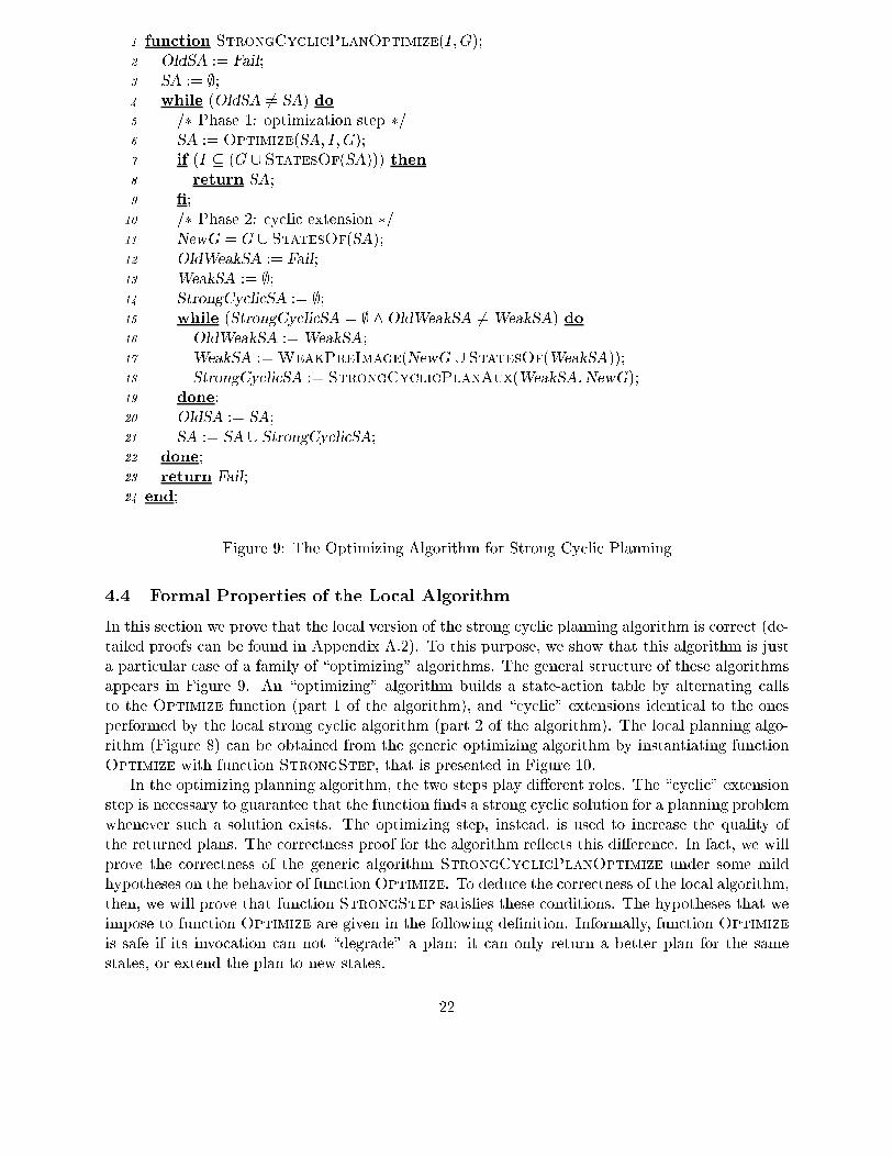
1 fun tion StrongCy li PlanOptimize(I;G);2 OldSA := Fail;3 SA := ;;4 while (OldSA 6= SA) do5 =� Phase 1: optimization step �=6 SA := Optimize(SA; I; G);7 if (I � (G [ StatesOf(SA))) then8 return SA;9 �;10 =� Phase 2: y li extension �=11 NewG = G [ StatesOf(SA);12 OldWeakSA := Fail;13 WeakSA := ;;14 StrongCy li SA := ;;15 while (StrongCy li SA = ; ^OldWeakSA 6=WeakSA) do16 OldWeakSA :=WeakSA;17 WeakSA :=WeakPreImage(NewG [ StatesOf(WeakSA));18 StrongCy li SA := StrongCy li PlanAux(WeakSA;NewG);19 done;20 OldSA := SA;21 SA := SA [ StrongCy li SA;22 done;23 return Fail;24 end; Figure 9: The Optimizing Algorithm for Strong Cy li Planning4.4 Formal Properties of the Lo al AlgorithmIn this se tion we prove that the lo al version of the strong y li planning algorithm is orre t (de-tailed proofs an be found in Appendix A.2). To this purpose, we show that this algorithm is justa parti ular ase of a family of \optimizing" algorithms. The general stru ture of these algorithmsappears in Figure 9. An \optimizing" algorithm builds a state-a tion table by alternating allsto the Optimize fun tion (part 1 of the algorithm), and \ y li " extensions identi al to the onesperformed by the lo al strong y li algorithm (part 2 of the algorithm). The lo al planning algo-rithm (Figure 8) an be obtained from the generi optimizing algorithm by instantiating fun tionOptimize with fun tion StrongStep, that is presented in Figure 10.In the optimizing planning algorithm, the two steps play di�erent roles. The \ y li " extensionstep is ne essary to guarantee that the fun tion �nds a strong y li solution for a planning problemwhenever su h a solution exists. The optimizing step, instead, is used to in rease the quality ofthe returned plans. The orre tness proof for the algorithm re e ts this di�eren e. In fa t, we willprove the orre tness of the generi algorithm StrongCy li PlanOptimize under some mildhypotheses on the behavior of fun tionOptimize. To dedu e the orre tness of the lo al algorithm,then, we will prove that fun tion StrongStep satis�es these onditions. The hypotheses that weimpose to fun tion Optimize are given in the following de�nition. Informally, fun tion Optimizeis safe if its invo ation an not \degrade" a plan: it an only return a better plan for the samestates, or extend the plan to new states. 22

1 fun tion StrongStep(SA; I; G);2 NewG := G [ StatesOf(SA);3 OldStrongSA := Fail;4 StrongSA := ;;5 while (OldStrongSA 6= StrongSA ^ I 6� (NewG [ StatesOf(StrongSA))) do6 PreImage := StrongPreImage(G [ StatesOf(StrongSA));7 NewStrongSA := PruneStates(PreImage;NewG [ StatesOf(StrongSA));8 OldStrongSA := StrongSA;9 StrongSA := StrongSA [NewStrongSA;10 done;11 return SA [ StrongSA;12 end;Figure 10: The Strong Optimizing Step in the Lo al Algorithm for Strong Cy li PlanningDe�nition 4.8 (Safe optimizing fun tion) Fun tion Optimize is safe if it always terminatesand if, whenever � is SC-valid for G and �0 = Optimize(�; I;G) then:- �0 is also SC-valid for G (i.e., the plan is still valid), and- StatesOf(�) � StatesOf(�0) (i.e., no states are lost).The y li extension step is built on the top of fun tion StrongCy li PlanAux, and we knowthat this fun tion returns only SC-valid state-a tion tables. If fun tion Optimize is safe, then itpreserves the SC-validity of a state-a tion table. The orre tness of the optimizing algorithm, then,relies on the following Proposition, that guarantees that the SC-valid state-a tion tables omputedin the di�erent parts of the algorithm an be safely ombined.Proposition 4.9 If � is SC-valid for G and �0 is SC-valid for G [ StatesOf(�), then � [ �0 isSC-valid for G.Theorem 4.10 (Corre tness) Let Optimize be a safe fun tion.If � _= StrongCy li PlanOptimize(I;G) 6= Fail then � is a strong y li solution of the plan-ning problem P = fD;I;Gg. If StrongCy li PlanOptimize(I;G) = Fail, instead, then there isno strong y li solution for planning problem P .The optimizing algorithm always terminates if fun tion Optimize is safe. Indeed, in this asethe \optimization" step annot redu e the set of states in the urrent state-a tion table, while the\ y li " extension step either stri tly in reases this set or leads to a termination of the outer whileloop. Sin e the possible states that an appear in the state-a tion table are �nite, the algorithmterminates after a �nite number of iterations of the while loop.Theorem 4.11 (Termination) Let Optimize be a safe fun tion.Then fun tion StrongCy li PlanOptimize always terminates.To on lude that the lo al version of the strong y li plan algorithm is orre t it is suÆ ientto prove that fun tion StrongStep is safe. This is true, as any strong plan is also a strong y li plan.Proposition 4.12 Fun tion StrongStep is safe.23

Another example of safe optimizing fun tion is the identity fun tion, whi h returns the state-a tiontable that re eives in input.The following Corollaries are a trivial appli ation of the orre tness results for the generi optimizing algorithm.Corollary 4.13 If � _= StrongCy li PlanLo al(I;G) 6= Fail then � is a strong y li solutionof the planning problem P = fD;I;Gg. If StrongCy li PlanLo al(I;G) = Fail, instead, thenthere is no strong y li solution for planning problem P .Corollary 4.14 Fun tion StrongCy li PlanLo al always terminates.In this paper we onsider only one optimizing fun tion, namely StrongStep. The generi stru -ture of the optimizing algorithm, however, an be seen as a �rst step towards a modular library forthe de�nition of planning algorithms: di�erent styles of solutions an be obtained by ombining and\tuning" di�erent primitive building blo ks, similar to StrongStep or StrongCy li PlanAux.The hoi e of the most appropriate algorithm may depend on the spe i� domain, and an be de-termined by the fa t that a ertain style of solution may be more appropriate to the appli ationbeing ta kled, or may be found more eÆ iently than another.5 Planning via Symboli Model Che kingModel Che king is a formal veri� ation te hnique based on the exhaustive exploration of �nite stateautomata [Clarke et al., 1999℄. Symboli Model Che king [M Millan, 1993℄ is a parti ular form ofmodel he king, where propositional formulae are used for the ompa t representation of �nite stateautomata, and transformations over propositional formulae provide a basis for eÆ ient exploration.The use of symboli te hniques allows for the analysis of extremely large systems [Bur h et al.,1992℄. As a result, symboli model he king is routinely applied in in industrial hardware design,and is taking up in other appli ation domains (see [Clarke&Wing, 1996℄ for a survey). In thisse tion we des ribe how the algorithms presented in the previous se tions an be des ribed withthe on eptual representation me hanisms of Symboli Model Che king, leaving to the next se tionthe issue of the eÆ ient implementation.5.1 Symboli Representation of Planning DomainsA planning domain hP;S;A;Ri an be symboli ally represented by the standard ma hinery devel-oped for symboli model he king, as follows. A ve tor of (distin t) propositional variables xxx, alledstate variables is devoted to the representation of the states of the domain. Ea h of these variableshas a dire t asso iation with a proposition of the domain in P used in the des ription of the domain.Therefore, in the rest of this se tion we will not distinguish a proposition and the orrespondingpropositional variable. For instan e, for the omelette domain, xxx is f#eggs=0, #eggs=1, #eggs=2,bad, good, unbrokeng. A state is the set of propositions of P that are intended to hold in it. Forea h state s, there is a orresponding assignment to the state variables in xxx, i.e. the assignmentwhere ea h variable in s is assigned to True, and ea h other variable is assigned to False. Werepresent s with a propositional formula �(s), having su h an assignment as its unique satisfyingassignment. For instan e, the formulae representing state 2 and 8 in the omelette example are:�(2) _= :#eggs=0 ^ #eggs=1 ^ :#eggs=2 ^ :good ^ bad ^ :unbroken�(8) _= :#eggs=0 ^ :#eggs=1 ^ #eggs=2 ^ good ^ :bad ^ unbroken24

This representation naturally extends to any set of states Q � S as follows:�(Q) _= _s2Q �(s):That is, we asso iate a set of states with the generalized disjun tion of the formulae representingea h of the states. The satisfying assignments of �(Q) are exa tly the assignments representing anystate in Q. We an use su h a formula to represent the set S of all the states of the domain. In the ase of the omelette example, the formula �(S) would be (equivalent to) the following formula:0�( #eggs=0^:#eggs=1^:#eggs=2)_(:#eggs=0^ #eggs=1^:#eggs=2)_(:#eggs=0^:#eggs=1^ #eggs=2) 1A^�( good^:bad)_(:good^ bad) �^�(#eggs=0!:bad^:unbroken)_(#eggs=1!:bad_:unbroken) �We use a propositional formula as representative for the set of assignments that satisfy it (and hen efor the orresponding set of states), so we abstra t away from the a tual syntax of the formula used:we do not distinguish among equivalent formulas as they represent the same sets of assignments.1The main eÆ ien y of the symboli representation is in that the ardinality of the represented setis not dire tly related to the size of the formula. For instan e, in the limit ases, �(2P ) and �(;), arethe True and False formulae, independently of the ardinality of P. As a further advantage, thesymboli representation an deal quite e�e tively with irrelevant information. For instan e, noti ethat the variables good, bad and unbroken need not to appear in the formula �(f5; 6; 7; 8g) =:#eggs=2. For this reason, a symboli representation an have a dramati improvement over anexpli it, enumerative representation. This is what allows symboli model he kers to handle �nitestate automata with a very large number of states (see for instan e [Bur h et al., 1992℄).Another advantage of the symboli representation is the natural en oding of set theoreti trans-formations (e.g. union, interse tion, omplementation) into propositional operations, as follows:�(Q1 [Q2) _= �(Q1) _ �(Q2)�(Q1 \Q2) _= �(Q1) ^ �(Q2)�(SnQ) _= �(S) ^ :�(Q)Also the predi ates over sets of states have a symboli ounterpart: for instan e, testing Q1 = Q2amounts to he king the validity of the formula �(Q1)$ �(Q2), while testing Q1 � Q2 orrespondsto he king the validity of �(Q1)! �(Q2).In order to represent a tions, we use another set of propositional variables, alled a tion vari-ables, written���. One approa h is to use one a tion variable for ea h possible a tion inA. Intuitively,an a tion variable is true if and only if the orresponding a tion is being exe uted. In prin iplethis allows for the representation of on urrent a tions. If a sequential en oding is used, i.e. no on urrent a tions are allowed, a mutual ex lusion onstraint stating that exa tly one of the a tionvariables must be true at ea h time must imposed. In the following, we all SeqA(���) the formula,in the state variables, expressing the mutual ex lusion onstraint over A. In the ase of the omeletteexample, SeqA(���) _= 0�( break^:open^:dis ard)_(:break^ open^:dis ard)_(:break^:open^ dis ard) 1AIn the spe i� ase of sequential en oding, it is possible to use only dlog kAke a tion variables, whereea h assignment to the a tion variables denotes a spe i� a tion to be exe uted. Furthermore, being1Although the a tual syntax of the formula may have a omputational impa t, in the next se tion we show thatthe use formulae as representatives of sets of models is indeed pra ti al.25

two assignments mutually ex lusive, the onstraint Seq(���) needs not to be represented. When the ardinality ofA is not a power of two, the standard solution is to asso iate more than one assignmentto ertain values. For instan e, in the omelette domain two variables �0 and �1 are suÆ ient torepresent a tions break, open and dis ard. A possible en oding is the following:�(break) _= :�0 �(open) _= �0 ^ :�1 �(dis ard) _= �0 ^ �1:A transition is a 3-tuple omposed of a state (the initial state of the transition), an a tion (thea tion being exe uted), and a state (the resulting state of the transition). To represent transitions,another ve tor xxx0 of propositional variables, alled next state variables, is used. We require that xxxand xxx0 have the same number of variables, and that the variables in similar positions in xxx and in xxx0 orrespond. We write �0(s) for the representation of the state s in the next state variables. With�0(Q) we denote the formula orresponding to the set of states Q, using ea h variable in the nextstate ve tor xxx0 instead of ea h urrent state variables xxx. In the following, we indi ate with �[v=℄the formula resulting from the substitution of v with in �, where v is a variable, and � and are formulae. If v1 and v2 are ve tors of (the same number of) distin t variables, we indi atewith �[v1=v2℄ the parallel substitution in � of the variables in ve tor v1 with the ( orresponding)variables in v2. We de�ne the representation of a set of states in the next variables as follows:�0(s) _= �(s)[xxx=xxx0℄:We all the operation �[xxx=xxx0℄ \forward shifting", be ause it transforms the representation of a setof \ urrent" states in the representation of a set of \next" states. The dual operation �[xxx0=xxx℄ is alled \ba kward shifting". In the following, we all xxx urrent state variables to distinguish themfrom next state variables.A transition is represented as an assignment to xxx, ��� and xxx0. For the omelette example, thesingle transition orresponding to the appli ation of a tion break in state 1 and resulting exa tlyin state 2 is represented by the formula�(h1; break; 2i) _= �(1) ^ break^ �0(2)The transition relation R of the automaton orresponding to a planning domain is simply aset of transitions, and is thus represented by a formula in the variables xxx, ��� and xxx0, where ea hsatisfying assignment represents a possible transition.�(R) _= Seq(���) ^ _t2R �(t)In the rest of this paper, we assume that the symboli representation of a planning domainand of a planning problem are given. In parti ular, we assume as given the ve tors of variablesxxx, ��� and xxx0, the en oding fun tions � and �0, and we simply all S(xxx), R(xxx;���;xxx0), I(xxx) and G(xxx)the formulae representing the states of the domain, the transition relation, the initial states andthe goal states, respe tively. Also, we will represent the formula �(Q), orresponding to the set ofstates Q � S, with Q(xxx), and �0(Q) as Q(xxx0).In order to operate over relations, we use quanti� ation in the style of qbf (the logi of Quanti-�ed Boolean Formulae), a de�nitional extension to propositional logi , where propositional variables an be universally and existentially quanti�ed. If � is a formula, and vi is one of its variables, the ex-istential quanti� ation of vi in �, written 9vi:�(v1; : : : ; vn), is equivalent to �(v1; : : : ; vn)[vi=False℄_�(v1; : : : ; vn)[vi=True℄. Analogously, the universal quanti� ation 8vi:�(v1; : : : ; vn) is equivalent to26

�(v1; : : : ; vn)[vi=False℄ ^ �(v1; : : : ; vn)[vi=True℄. qbf formulae allow for an exponentially more ompa t representation than propositional formulae.As an example of the appli ation of qbf formulae, the symboli al representation of the imageof a set of states Q, i.e. the set of states rea hable from any state in Q by applying any a tion, isthe following: (9xxx���:(R(xxx;���;xxx0) ^ Q(xxx)))[xxx0=xxx℄:Noti e that, with this single operation, we symboli ally simulate the e�e t of the appli ation of anyappli able a tion in A to any of the states in Q. The dual ba kward image is des ribed as follows:(9xxx0���:(R(xxx;���;xxx0) ^ Q(xxx0))):5.2 Symboli Representation of the Planning AlgorithmsThe ma hinery for the symboli representation of planning domains just presented an be adaptedto represent and manipulate symboli ally also the other stru tures of the planning algorithms.A state-a tion table SA is a relations between states and a tions, and an be representedsymboli ally as a formula in the xxx and ��� variables. In the following, we write SA(xxx;���) for theformula orresponding to state-a tion table SA: ea h satisfying assignment to SA(xxx;���) representsa state-a tion pair in SA. This view inherits all the properties seen above for sets of states. Forinstan e, the symboli representation of the union of two state-a tion tables SA1[SA2 is representedby the disjun tion of their symboli representations SA1(xxx;���) _ SA2(xxx;���). The set of states ofa state-a tion table StatesOf(SA(xxx;���)) is represented symboli ally as 9���:SA(xxx;���): The set ofa tions asso iated in SA with a given state s is given by 9xxx:(SA(xxx;���) ^ �(s)) Any element of therepresented set is a possible result from the GetA tion primitive. The symboli representationof the universal state a tion table UnivSA is 9xxx0:R(xxx;���;xxx0), that also represents the appli abilityrelation of a tions in states.We now des ribe how the planning algorithms an be seen in terms of transformations overpropositional formulae. The basi steps of the algorithms are the generalizations of the preimage op-erations, that rather than returning sets of states, onstru t state-a tion tables. WeakPreImage(Q) orresponds to 9xxx0:(R(xxx;���;xxx0) ^Q(xxx0))while StrongPreImage(Q) orresponds to8xxx0:(R(xxx;���;xxx0)! Q(xxx0)) ^ Appli able(xxx;���)where the appli ability relation Appli able(xxx;���) is9xxx0:R(xxx;���;xxx0)In both ases, the resulting formula is obtained as a one-step omputation, and may ompa tlydes ribe an extremely large set. The other basi ingredients in the planning algorithms are fun tionsPruneStates(SA; Q), that an be omputed asSA(xxx;���) ^ :Q(xxx)and fun tion ComputeOutgoing, that orresponds toSA(xxx;���) ^ 9xxx0(R(xxx;���;xxx0) ^ :Q(xxx0)):Given the basi building blo ks just de�ned, the algorithms presented in previous se tions an besymboli ally implemented by repla ing, within the same ontrol stru ture, ea h fun tion all withthe symboli ounterpart, and by asting the operations on sets into the orresponding operationson propositional formulae. 27

6 The MBP PlannerIn this se tion, we give an overview of the fun tionalities of mbp, and des ribe its implementationin terms of bdds.6.1 Fun tionalitiesmbp is a general system for planning in nondeterministi domains based on symboli model he kingte hniques. It implements the data stru tures and the algorithms presented in this paper, and otherforms of planning.mbp is a two-stage system. In the �rst stage, an internal bdd-based representation of the domainis built, while in se ond stage planning problems an be solved. Planning domains are urrentlydes ribed by means of the high-level a tion language AR [Giun higlia et al., 1997℄. AR allowsto spe ify onditional e�e ts and un ertain e�e ts of a tions by means of high level assertions.Non-boolean propositions are allowed. The semanti s of AR yields a serial en oding, i.e. exa tlyone a tion is assumed to be exe uted at ea h time. The automaton orresponding to an ARdes ription is obtained by means of the minimization pro edure des ribed in [Giun higlia et al.,1997℄. This pro edure solves the frame problem and the rami� ation problem, and is implementedas des ribed in [Cimatti et al., 1997℄. Be ause of the separation between the domain onstru tionand the planning phases, mbp is not bound to AR. Standard deterministi domains spe i�ed inpddl an also be given to mbp by means of a (prototype) ompiler. Parallel en odings have beeninvestigated in [Cimatti et al., 2001℄, where planning te hniques are applied to hardware ir uitsdes ribed in SMV language. The use of the C a tion language [Giun higlia&Lifs hitz, 1998℄, whi hallows to represent planning domains with parallel a tions, is also under investigation.In the se ond stage, di�erent planning algorithms an be applied to the spe i�ed planning prob-lems. They operate solely on the automaton representation, and are ompletely independent of theparti ular language used to spe ify the domain. In this paper we on entrate on the automati on-stru tion of onditional plans under full observability. Other fun tionalities of mbp, out of the s opeof this paper, are onformant planning [Cimatti&Roveri, 1999; Cimatti&Roveri, 2000; Bertoli etal., 2001a℄, onditional planning under partial observability [Bertoli et al., 2001b℄, and planningfor temporally extended goals [Pistore&Traverso, 2001℄. mbp is urrently being reengineered anddo umented, and will be publi ly available in June 2001 at http://sra.it .it/tools/mbp/.6.2 Implementation with Binary De ision Diagramsmbp is built on top of the symboli model he ker NuSMV [Cimatti et al., 2000℄. mbp relieson the powerful ma hinery of Redu ed Ordered Binary De ision Diagrams [Bryant, 1992; Bryant,1986℄ (in the following simply alled bdds), the �rst and most popular implementation devi e ofsymboli model he king (see e.g. [Biere et al., 1999; Abdulla et al., 2000℄ for alternative symboli representation me hanisms). bdds provide a general interfa e that allows for a dire t map ofthe symboli representation me hanisms presented in previous se tion (e.g. tautology he king,quanti� ation, shifting). In the rest of this se tion we present an overview of bdds.A bdd is a dire ted a y li graph (DAG). The terminal nodes are either True or False. Ea hnon-terminal node is asso iated with a boolean variable, and two bdds, alled left and rightbran hes. Figure 11 (a) depi ts a bdd for (a1 $ b1) ^ (a2 $ b2) ^ (a3 $ b3). At ea h non-terminal node, the right [left, respe tively℄ bran h is depi ted as a solid [dashed, resp.℄ line, andrepresents the assignment of the value True [False, resp.℄ to the orresponding variable. bddsprovide a anoni al representation of boolean fun tion. Given a bdd, the value of the fun tion28

True False

a1

b1

a2

b2 b2

a3

b3 b3

b1

(a)b1b1b1b1b1b1b1b1

a3 a3 a3 a3

a2a2

a1

b3 b3

b2b2b2b2

FalseTrue (b)Figure 11: Two bdd for the formula (a1 $ b1) ^ (a2 $ b2) ^ (a3 $ b3). orresponding to a given truth assignment to the variables, is determined by traversing the graphfrom the root to the leaves, following ea h bran h indi ated by the value assigned to the variables.(A path from the root to a leaf an visit nodes asso iated with a subset of all the variables of thebdd. See for instan e the path asso iated with a1;:b1 in Figure 11(a).) The rea hed leaf node islabeled with the resulting truth value. If v is a bdd, its size kvk is the number of its nodes. If n isa node, var(n) indi ates the variable indexing node n.The anoni ity of bdds follows by imposing a total order < over the set of variables used tolabel nodes, su h that for any node n and respe tive non-terminal hild m, their variables must beordered, i.e. var(n) < var(m), and requiring that the bdd ontains no isomorphi subgraphs.bdds an be ombined with the usual boolean transformations (e.g. negation, onjun tion,disjun tion). Given two bdds, for instan e, the onjun tion operator builds and returns the bdd orresponding to the onjun tion of its arguments. Substitution and quanti� ation an also beeÆ iently represented as bdd transformations. In terms of bdd omputations, a quanti� ation orresponds to a tranformation mapping the bdd of � and the variable vi being quanti�ed into thebdd of the resulting (propositional) formula. The time omplexity of the algorithm for omputinga truth-fun tional boolean transformation f1<op>f2 is O(kf1k �kf2k). As far as quanti� ations are on erned, the time omplexity is quadrati in the size of the bdd being quanti�ed, and linear inthe number of variables being quanti�ed, i.e. O(kvk � kfk2) [Bryant, 1992; Bryant, 1986℄.bdd pa kages are eÆ ient implementations of su h data stru tures and algorithms (see [Bra eet al., 1990℄). mbp, as NuSMV, uses one of the best bdd pa kages available, the CUDD [Somenzi,1997℄. A bdd pa kage deals with a single multi-rooted DAG, where ea h node represents a booleanfun tion. Memory eÆ ien y is obtained by using a \unique table", and by sharing ommon sub-graphs between bdds. The unique table is used to guarantee that at ea h time there are noisomorphi subgraphs and no redundant nodes in the multi-rooted DAG. Before reating a new29

node, the unique table is he ked to see if the node is already present, and only if this is not the ase a new node is reated and stored in the unique table. The unique table allows to perform theequivalen e he k between two bdds in onstant time (sin e two equivalent fun tions always sharethe same subgraph) [Bra e et al., 1990; Somenzi, 1997℄. Time eÆ ien y is obtained by maintaininga \ omputed table", whi h keeps tra ks of the results of re ently omputed transformations, thusavoiding the re omputation.A riti al omputational fa tor with bdds is the order of the variables used. (Figure 11 showsan example of the impa t of a hange in the variable ordering on the size of a bdd.) For a ertain lass of boolean fun tions, the size of the orresponding bdd is exponential in the numberof variables for any possible variable ordering. In many pra ti al ases, however, �nding a goodvariable ordering is rather easy. Beside a�e ting the memory used to represent a boolean fun tion,�nding a good variable ordering an have a big impa t on omputation times, sin e the omplexityof the transformation algorithms depends on the size of the operands. Most bdd pa kages provideheuristi algorithms for �nding good variable orderings, whi h an be alled to try to redu e theoverall size of the stored bdds. The reordering algorithms an also be a tivated dynami ally bythe pa kage, during a bdd omputation, when the total amount of nodes in the pa kage rea hes aprede�ned threshold (dynami reoredering).7 Experimental EvaluationIn this se tion we experimentally evaluate the strength of our approa h. We des ribe the state of theart relevant planners (sgp [Weld et al., 1998℄, gpt [Bonet&Ge�ner, 2000℄, QbfPlan [Rintanen,1999a℄, and simplan [Kabanza et al., 1997℄), we present the working hypotheses of the experimentalevaluation, des ribe the sele ted problems and analyze the results.7.1 State-of-the-art Planners for Nondeterministi Domains7.1.1 SGPsgp [Weld et al., 1998℄ implements an observation-based approa h to planning. It is able to plan inpartially observable domains, where run-time information an be gathered by observation a tions.sgp is based on the GraphPlan approa h, from whi h it inherits a remarkable strength in theanalysis of parallelizable problems. sgp was the �rst onditional planner able to solve non-trivialproblem. In [Weld et al., 1998℄, sgp is shown to outperform the existing planners obtained asextensions to lassi al planners (e.g., [Warren, 1976; Peot&Smith, 1992; Pryor&Collins, 1996℄).The approa h underlying sgp is of enumerative nature: for ea h sour e of un ertainty, eitherin the possible initial states, or multiple a tion e�e ts, a planning graph is built, and then themutual relations among them are analyzed. The a tual sgp system is limited to the ase ofdeterministi domains, where un ertainty is only in the initial ondition. Domains are expressedin a generalization of pddl. Observations are expressed as e�e ts of operators by means of thespe ial Observes predi ate. With respe t to the problems in this paper, sgp is able to ta kle strong(but not strong y li ) planning problems, produ ing a onditional, non-iterative plan. sgp is notable to dete t when the problem does not admit a solution.7.1.2 GPTgpt [Bonet&Ge�ner, 2000℄ is an integrated planning environment, able to ta kle onformantplanning problems, and problems formulated in terms of Markov De ision Pro esses (MDPs) and30

Partially-Observable MDP. In this paper we fo us on the MDP algorithms of gpt. (See [Cimatti&Roveri, 1999; Cimatti&Roveri, 2000; Bertoli et al., 2001a℄ for a omparison of gpt with the sym-boli model he king approa h on onformant planning and [Bertoli et al., 2001b℄ for a omparisonon partially observable planning.) gpt an deal with probabilisti distributions: in parti ular, it an take into a ount probability distributions of a tion transitions, sin e it makes use of MDPte hniques to sear h through a sto hasti automaton. gpt requires training examples to tend tooptimal solutions. This pro ess an be quite onsuming, and he king the rea hed onvergen e isnot obvious. Compared to mbp, gpt an not be for ed to return an a y li poli y (or even he kingfor its existen e), and is unable to distinguish between y li and a y li solutions.7.1.3 QbfPlanQbfPlan [Rintanen, 1999a℄ is a generalization of the satplan approa h [Kautz et al., 1996℄ tothe ase of planning in nondeterministi domains. In QbfPlan, the planning problem is reformu-lated in qbf, rather than in propositional logi . The problem is then solved by an eÆ ient qbfsolver [Rintanen, 1999b℄. QbfPlan is able to ta kle a wide variety of onditional planning prob-lems. The user must provide the stru ture of the plan to be generated (e.g. the length in the aseof onformant planning, the number of ontrol points and observations in the plan in the ase of onditional planning). This an provide a signi� ant limitation of the sear h spa e. In QbfPlan,the points of nondeterminism are expli itly odi�ed in terms of \environment variables", with a onstru tion known as determinization of the transition relation. Compared to mbp, QbfPlan isunable to de ide whether the given problem admits a solution.7.1.4 Simplansimplan [Kabanza et al., 1997℄ implements di�erent approa hes to planning in nondeterministi domains. In this paper we fo us on the logi -based planning omponent, where temporally extendedgoals an be expressed in (an extension of) Linear Temporal Logi (LTL) [Pnueli, 1977℄, and theasso iated plans are onstru ted under the hypothesis of full observability. simplan is very similarin spirit to mbp, sin e it is based on model he king te hniques. A major di�eren e is that simplanrelies on the expli it-statemodel he king paradigm, where individual states are manipulated (ratherthan sets of states). Therefore, the algorithms of simplan are of enumerative nature | this anbe a major drawba k in large domains. In simplan, LTL formulae are also used to des ribe user-de�ned ontrol strategies, that an provide aggressive pruning of the sear h spa e. The lassesof problems solved by mbp and simplan are in omparable. LTL allows for the spe i� ation oftemporally extended goals. This in ludes strong planning, but not strong y li planning. In orderto express strong y li planning, properties of bran hing omputation stru tures are needed. Theseare expressible, for instan e, in CTL [Clarke&Emerson, 1981℄. In [Pistore&Traverso, 2001℄ ourplanning paradigm is extended to deal with goals expressed in full CTL. See also [Vardi, 2001℄ fora omparison of linear time and bran hing time temporal logi s.7.2 Experimental evaluation setupWe performed an extensive experimental evaluation of mbp. We ompared mbp with the plannersdes ribed in previous se tion, fo using on test problems taken from the distribution of the othersystems. We also test the di�erent algorithms for strong y li planning on di�erent planningdomains. We analyze the behavior of the di�erent planners on parameterized problems, reportingperforman e on di�erent parameter values. In the following we write P (i) for the i-th instan e31

of the problem lass P . The testing platform used is an Intel 300MHz Pentium-II, 512MB RAM,running Linux. CPU time was limited to 7200 se onds (two hours) for ea h test, while memory waslimited to 500MB. In the following, we write \T.O." or \M.O." for a test that did not ompletewithin the above time and memory limits, respe tively.Rather than the total run time of the systems, we onsider as \performan e" the sear h time,i.e. the time needed to solve the planning problem on e the respe tive internal representation hasbeen built. This ex ludes the time needed by QbfPlan to generate the en odings, the time neededby gpt to generate the sour e ode of its internal representation and to ompile it, the time neededby simplan to ompile the domain des riptions, and the time needed by mbp to onstru t thesymboli automaton representation. There are several reasons for this hoi e. First, our fo us ison the properties of the planning algorithms. Se ond, the prepro essing time is sometimes veryhard to measure. Third, the prepro essing time is of diÆ ult interpretation, sin e its meaning andepend on the system being run. For instan e, for mbp and simplan the prepro essing time isrelated to the domain (the internal representation resulting from the prepro essing an be reusedfor several planning problems) while for gpt and QbfPlan the overhead is problem spe i� , andshould be taken into a ount for ea h problem. In the experimental evaluation, in addition to thesear h time, we expli itly plot the prepro essing time for mbp, as it appears to be a signi� antfa tor (see Se tion 7.3.3 for a dis ussion).In the tables, times are reported in se onds. We use Str, SCLo and SCGlob for the sear htimes of the strong, lo al strong y li and global strong y li algorithms, and Prep as prepro- essing time for mbp. For mbp, all the tests were run with a �xed variable ordering, where a tionsvariables pre ede state variables (with urrent and next state variables interleaved). Dynami vari-able reordering was disabled. The ordering within a tion variables and within state variables is a onsequen e of the model variable de larations in the input �le. For the other planners, we triedto maximize their performan e to the best of our knowledge.mbp gptOMELETTE(i) Prep Str SCLo SCGlob 1k LT SR 10k LT SR 100k LT SROMELETTE(2) 0.030 0.000 0.020 0.010 0.525 0.994 4.752 0.9994 50.664 0.99994OMELETTE(4) 0.040 0.000 0.080 0.020 1.642 0.978 10.242 0.9978 99.903 0.99977OMELETTE(6) 0.030 0.000 0.170 0.050 5.219 0.877 19.745 0.9880 168.729 0.99878OMELETTE(8) 0.040 0.010 0.290 0.080 12.356 0.537 38.946 0.9413 249.133 0.99414OMELETTE(10) 0.070 0.020 0.450 0.120 18.737 0.227 75.750 0.8093 370.196 0.98012OMELETTE(12) 0.080 0.020 0.590 0.180 23.761 0.038 138.107 0.5255 534.824 0.94887OMELETTE(14) 0.090 0.020 0.800 0.240 27.758 0.003 196.810 0.2323 756.499 0.88869OMELETTE(16) 0.120 0.020 1.080 0.300 31.539 0.003 237.688 0.1073 1055.966 0.78541OMELETTE(18) 0.140 0.030 1.390 0.410 37.045 0.000 268.552 0.0376 1480.801 0.62727OMELETTE(20) 0.130 0.030 1.790 0.480 39.324 0.000 291.644 0.0052 2038.822 0.40691OMELETTE(50) 0.600 0.120 12.000 5.500 73.471 0.000 M.O.OMELETTE(100) 2.620 0.340 60.960 34.990OMELETTE(250) 16.820 1.920 609.22 379.21Table 1: Results for the OMELETTE problems.7.3 Problems and results7.3.1 OmeletteWe �rst onsider the lassi al OMELETTE(i) problem [Levesque, 1996℄. The goal is to have igood eggs and no bad ones in one of two bowls of apa ity i. There is an unlimited number ofeggs, ea h of whi h an be unpredi tably good or bad. The eggs an be grabbed and broken into32

MBPOMELETTE-B(20, b) Prep Str SCLo SCGlobOMELETTE-B(20, 1) 0.180 0.680 0.690 0.440OMELETTE-B(20, 2) 0.140 0.880 0.890 0.430OMELETTE-B(20, 3) 0.190 1.030 1.130 0.430OMELETTE-B(20, 4) 0.180 1.360 1.480 0.460OMELETTE-B(20, 5) 0.170 1.490 1.630 0.440OMELETTE-B(20, 6) 0.190 1.350 1.760 0.430OMELETTE-B(20, 7) 0.190 1.680 1.830 0.440OMELETTE-B(20, 8) 0.210 1.720 1.930 0.440OMELETTE-B(20, 9) 0.190 1.560 2.050 0.450OMELETTE-B(20, 10) 0.190 1.910 2.110 0.450OMELETTE-B(20, 20) 0.200 2.510 2.940 0.449OMELETTE-B(20, 50) 0.270 4.230 5.280 0.440OMELETTE-B(20, 100) 0.360 7.170 9.310 0.460Table 2: Results for the bounded OMELETTE problems.a bowl. The ontent of a bowl an be dis arded, or poured to the other bowl. Breaking a rottenegg in a bowl has the e�e t of spoiling the bowl. A bowl an always be leaned by dis ardingits ontent. In the problem as formulated in the distribution of gpt, an expli it sensing a tion isrequired to dis over whether the ontent of the bowl is spoiled. The problem is modeled in mbpas a fully observable problem, without the need of an expli it sensing a tion, by onsidering thatthe result of the a tion (e.g. the status of the bowl) be omes observable as soon as the a tion hasbeen exe uted. The results are reported in Table 1. The problem does not admit a strong solution,but only a strong y li solution. Column Str reports the time required by the strong algorithmto dis over that the problem admits no strong solution. mbp is able to perform this task quiteeÆ iently (e.g. less than 2 se onds for the OMELETTE(250)). Both strong y li algorithms �nda solution. The global algorithm perform better than the lo al one. This is intuitively due to thefa t that there are no useful \strong" steps in the domain, and the lo al algorithm ends up doinguseless omputations. On the same set of problems, we ran the MDP module of gpt. The sear his based on the repeated generation of learning trials (LTs), starting from randomly sele ted initialstate. The poli y tends to improve as the number of learning trials grows. However, gpt an notguarantee that the returned poli ies do not implement y li ourses of a tion. In table 1 we reporttime needed to perform 1000, 10000 and 100000 learning trials, and the su ess rate (SR) of the orresponding poli y ( omputed on a basis of 1000, 10000 and 100000 ontrol trials). As shownin [Bonet&Ge�ner, 2000℄, the qualitative pattern is that the ontroller tends to improve with agrowing number of learning trials. However, gpt appears to su�er from the enumerative nature ofthe algorithm, and for in reasing problem size the learning time tends to grow while the qualityof the ontroller degrades. In the ase of 50 omelettes, the memory is exhausted during the 10000learning trials.In order to stress the mbp algorithms for strong planning, we onsider the OMELETTE-B(i,r)variation, where the number of rotten eggs is bounded to r. For su h problem, a strong solutionexists. Table 2 depi ts the results for in reasing number of rotten eggs when the size of the bowlsis �xed to 20. The performan e of the strong and the lo al strong y li are similar, both sensitiveto the number of rotten eggs (although the latter appears to be slightly slower, possibly be ause of33

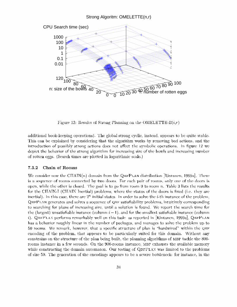
Strong Algoritm: OMELETTE(n,r)

0 10 20 30 40 50 60 70 80 90 100

r: number of rotten eggs0

2040

6080

100120

n: size of the bowls

0.010.1

110

1001000

CPU Search time (sec)

Figure 12: Results of Strong Planning on the OMELETTE-B(i,r)additional book-keeping operations). The global strong y li , instead, appears to be quite stable.This an be explained by onsidering that the algorithm works by removing bad a tions, and theintrodu tion of possibly strong a tions does not a�e t the symboli operations. In �gure 12 wedepi t the behavior of the strong algorithm for in reasing size of the bowls and in reasing numberof rotten eggs. (Sear h times are plotted in logarithmi s ale.)7.3.2 Chain of RoomsWe onsider now the CHAIN(n) domain from the QbfPlan distribution [Rintanen, 1999a℄. Thereis a sequen e of rooms onne ted by two doors. For ea h pair of rooms, only one of the doors isopen, while the other is losed. The goal is to go from room 0 to room n. Table 3 lists the resultsfor the CHAIN-I (CHAIN Inertial) problems, where the status of the doors is �xed (i.e. they areinertial). In this ase, there are 2n initial states. In order to solve the i-th instan e of the problem,QbfPlan generates and solves a sequen e of qbf satis�ability problems, intuitively orrespondingto sear hing for plans of in reasing size, until a solution is found. We report the sear h time forthe (largest) unsatis�able instan e ( olumn i� 1), and for the smallest satis�able instan e ( olumni). QbfPlan performs remarkably well on this task: as reported in [Rintanen, 1999a℄, QbfPlanhas a behavior roughly linear in the number of pa kages, and manages to solve the problem up to50 rooms. We remark, however, that a spe i� stru ture of plan is \hardwired" within the qbfen oding of the problem, that appears to be parti ularly suited for this domain. Without any onstrains on the stru ture of the plan being built, the planning algorithms of mbp ta kle the 800-rooms instan e in a few se onds. On the 900-rooms instan e, mbp exhausts the available memorywhile onstru ting the domain automaton. Our testing of QbfPlan was limited to the problemsof size 50. The generation of the en odings appears to be a severe bottlene k: for instan e, in the34

mbp QbfPlanCHAIN-I(n) Prep Str SCLo SCGlob i� 1 iCHAIN-I(6) 0.020 0.000 0.000 0.000 0.02 0.04CHAIN-I(10) 0.020 0.000 0.000 0.010 0.05 0.10CHAIN-I(24) 0.100 0.010 0.010 0.010 0.89 2.35CHAIN-I(30) 0.130 0.010 0.020 0.020 1.00 2.91CHAIN-I(50) 0.330 0.020 0.030 0.040 0.84 13.97CHAIN-I(100) 1.560 0.060 0.060 0.100CHAIN-I(200) 6.890 0.180 0.200 0.260CHAIN-I(300) 15.840 0.340 0.370 0.450CHAIN-I(400) 29.170 0.530 0.640 0.720CHAIN-I(500) 47.790 0.740 0.900 0.950CHAIN-I(600) 68.770 1.040 1.260 1.260CHAIN-I(700) 135.900 1.490 1.780 1.750CHAIN-I(800) 176.380 1.930 2.360 2.250CHAIN-I(900) M.O.Table 3: Results for the CHAIN-I problems. ase of CHAIN-I(50), the en oding generation for i� 1 and i required, respe tively, about 70 and110 minutes. We also ran mbp on the CHAIN-NI problems, NI standing for Non-Inertial doors,i.e. the variation of the CHAIN where the status of doors an hange nondeterministi ally at ea htime instant. This example gives a lear example of the non-enumerative nature of the symboli approa h. The bran hing fa tor of the sear h spa e is extremely high: at ea h a tion exe ution orrespond 2p possible su essor states. However, the symboli representation allows to ontain theresour es needed to represent the orresponding automaton. Therefore, the automaton onstru tiondoes not blow up, and it is possible ta kle on�gurations with 4000 rooms in a ouple of minutes ofsear h time. The problem admits a strong solution, and the strong algorithm is the most e�e tive.The lo al strong y li algorithm seems to be able to exploit the existen e of a strong solution, andtherefore performs slightly better than the global algorithm. QbfPlan was not run on this domain,be ause the en oding s hema was not available from the QbfPlan distribution. QbfPlan is basedon a low level input language (problem des riptions must be spe i�ed as ML ode, whi h generatesthe qbf en odings), and writing new en odings turns out to be a very diÆ ult and error-pronetask.7.3.3 An aside on Automaton Constru tion in MBPIn this se tion we dis uss the overhead given by the automaton onstru tion time in mbp. Inseveral domains, this step turns out to be higher than the sear h time, and in the CHAIN-I(900)problem, mbp goes out of memory while building the automaton. However, we do not onsiderthis a serious limiting fa tor. We on entrated on the planning algorithms, without optimizing theautomaton onstru tion part, and we believe that there is substantial room for improvement. First,we urrently express problems in the AR a tion language, that requires a omplex minimizationpro edure (with an additional set of state variables) in order to ompute the automaton [Cimattiet al., 1997℄. In many ases, AR appears to be too powerful for the en oding of planning problems,and with a di�erent input language (either a generalization of pddl or a di�erent a tion language,35

mbpCHAIN-NI(n) Prep Str SCLo SCGlobCHAIN-NI(6) 0.010 0.000 0.000 0.000CHAIN-NI(10) 0.000 0.000 0.000 0.010CHAIN-NI(50) 0.040 0.020 0.030 0.030CHAIN-NI(100) 0.140 0.060 0.070 0.090CHAIN-NI(200) 0.460 0.170 0.190 0.250CHAIN-NI(300) 1.030 0.320 0.360 0.440CHAIN-NI(400) 1.790 0.510 0.620 0.760CHAIN-NI(500) 2.870 0.720 0.850 1.080CHAIN-NI(600) 4.190 1.060 1.280 1.480CHAIN-NI(700) 5.870 1.450 1.760 2.050CHAIN-NI(800) 7.580 1.910 2.280 2.830CHAIN-NI(900) 9.620 2.230 2.770 3.510CHAIN-NI(1000) 12.340 2.680 3.140 4.320CHAIN-NI(1500) 31.200 6.270 7.640 9.430CHAIN-NI(2000) 56.760 21.050 23.660 28.760CHAIN-NI(3000) 145.560 47.030 54.830 60.320CHAIN-NI(4000) 279.740 79.290 93.610 106.970Table 4: Results for the non-inertial CHAIN problems.e.g. C), the automaton onstru tion ould be greatly simpli�ed. Furthermore, the internal repre-sentation of the domain ould greatly bene�t from the use of standard simpli� ation te hniquesdeveloped in symboli model he king. For instan e, with \partitioning" te hniques [Geist&Beer,1994℄, the transition relation is impli itly represented as a list of bdds. This avoids the onstru tionof unique, \monolithi " bdd representing the transition relation of the automaton.To substantiate these laims, we odi�ed the CHAIN-I dire tly into the input language ofNuSMV, the symboli model he ker on top of whi h mbp is built. The input language of NuSMVis a simple, low level language, that allows to des ribe expli itly the law of inertia, and does notrequire the minimization pro edure used to ompile AR domain des riptions. In Table 5, onCHAIN-I(800) Prep bdd sizembp 176.380 1926446NuSMV (mono) 33.130 1926446NuSMV (th=1000) 8.510 [515;999;999;1602;1603℄NuSMV (th=2000) 9.610 [512;2001;1613℄NuSMV (th=5000) 12.160 [2498;7200℄ mbp (NuSMV)CHAIN-I(n) Prep Str SCLo SCGlobCHAIN-I(800) 33.130 2.210 2.620 2.580CHAIN-I(900) 42.500 3.010 3.550 3.450CHAIN-I(1000) 56.120 2.430 3.010 3.850CHAIN-I(1500) 154.120 7.930 9.390 8.650CHAIN-I(2000) M.O.Table 5: Automaton onstru tion for the CHAIN-I(800) domain.the left, we report the prepro essing time and the size of the transition relation for mbp and forNuSMV on the CHAIN-I(800) problem. With NuSMV (mono) we indi ate the \monolithi " modein the representation of the transition relation inNuSMV. This is similar to the onstru tion that is arried out in mbp starting from the AR domain des ription. Given the same variable ordering, theresult of the two domain onstru tions is identi al, but with a signi� ant di�eren e in onstru tiontime. In the other rows, we report the onstru tion times and sizes of a partitioned domain36

representation, obtained with a simple partitioning me hanisms. The size of the bdd partitions ofthe transition relation, listed in square bra kets, are mu h smaller that the monolithi transitionrelation. In Table 5, on the right, we report the sear h time on the domain automaton des ribedin the NuSMV language. We see that in this way it is possible to ta kle larger on�gurations, upto 1500 rooms.7.3.4 Robot DeliveryThe Robot Delivery domain, introdu ed by Kabanza in [Kabanza et al., 1997℄, des ribes an 8-roombuilding, where a mobile robot an move from room to room, pi king up and putting down pa kages.Nondeterminism in the domain is due to \produ er" and \ onsumer" rooms: an obje t of a ertaintype an disappear if positioned in a onsumer room, and an then reappear in one of the produ errooms. Furthermore, it is possible to have external pro esses that an hange the position of thedoors. We onsidered three di�erent problems for this domain from the simplan distribution, withdi�erent initial onditions (e.g. robot and pa kage positions), and with di�erent goals. In the �rst,simple problem, ROBOT(p1), the robot has to rea h a room ontiguous to the room where it isinitially positioned. A plan of length one exists. The se ond problem, ROBOT(p2), requires therobot to go to a given obje t, move it in a di�erent lo ation, and then rea h a third lo ation.The last problem, ROBOT(p3) is an extension of the ROBOT(p1), with one of the doors that anopen and lose nondeterministi ally. We odi�ed two sets of problems. In the �rst set, only onepa kage is assumed to be present in the domain. In the se ond set, the domain ontains �ve obje ts(although only one is relevant for the problems being onsidered). The results of the omparisonare depi ted in Table 6. simplan appears to be very sensitive to nondeterminism. For instan e,the di�eren e between p1 and p3 is only in the nondeterministi behavior of a door that the robotneeds not to traverse. simplan relies on the use of domain spe i� , user de�ned ontrol rules toprune the sear h spa e. The reported run times, obtained with and without ontrol rules, showthat the eÆ ien y of simplan is very dependent on the quality of the ontrol rule. When a solutiondoes not exist, as in the ase of p3, the sear h spa e must be exhausted. simplan, being basedon expli it-state model he king te hniques, appears to su�er when it has to handle large statespa es. mbp appears to be more stable with respe t to nondeterminism. However, the introdu tionof additional irrelevant pa kages has an impa t both on prepro essing and sear h.mbp simplanPrep Str SCLo SCGlob CtrlRule w/o CtrlRuleROBOT(p1) 0.450 0.010 0.010 0.100 0.01 0.00ROBOT(p2) 0.410 0.080 0.060 0.250 0.23 0.41ROBOT(p3) 0.450 0.010 0.000 0.070 T.O. T.O.ROBOT(p1+) 150.870 0.050 0.050 12.210 0.01 0.02ROBOT(p2+) 150.760 11.730 11.660 15.580 0.35 T.O.ROBOT(p3+) 235.330 0.060 0.050 21.290 T.O. T.O.Table 6: Results for the ROBOT Delivery Problems.37

HUNTER(p) Prep Str SCLo SCGlobHUNTER(6) 0.000 0.000 0.000 0.010HUNTER(10) 0.030 0.000 0.010 0.000HUNTER(50) 0.090 0.080 0.090 0.110HUNTER(100) 0.200 0.250 0.310 0.510HUNTER(200) 0.590 0.940 1.190 2.650HUNTER(300) 1.120 1.900 2.490 5.980HUNTER(400) 2.030 2.780 3.920 10.320HUNTER(500) 3.050 4.480 6.130 17.190HUNTER(600) 4.200 6.370 9.060 23.540HUNTER(700) 5.640 8.760 12.530 34.540HUNTER(800) 7.220 10.620 15.790 41.220HUNTER(900) 9.340 13.900 20.080 56.970HUNTER(1000) 11.510 16.940 24.410 68.000HUNTER(1500) 24.950 39.940 59.850 168.170HUNTER(2000) 44.170 67.250 105.480 287.550HUNTER(3000) 96.220 164.050 262.520 697.870HUNTER(4000) 179.830 290.630 475.730 1264.460Table 7: Results for the Hunter and Prey problems.7.3.5 Hunter and PreyThe \Hunter-Prey" problem was presented in [Koenig&Simmons, 1995℄ as an explanatory asestudy, where a hunter has to rea h a prey. In the �rst ase we onsider, un ertainty is limited tothe initial situation: the hunter and the prey an be initially in any position, but the prey does notmove. The results for the HUNTER(p) problem, where p is the number of possible lo ations of thehunter and the prey, are reported in Table 7. Noti e that the number of initial on�gurations isp2. The problem admits strong solutions, and the strong planning algorithm performs signi� antlybetter than the global strong y li algorithms.We ran sgp on a simpli�ed version of the Hunter-Prey domain, alled HUNTER-S(p,i), wherepossible positions are range from 0 to p � 1, and there is no prey, and the hunter has the goal ofsimply rea hing position 0 from any of i initial positions. For ea h position there is an observationa tion, he k-hunter-p, that allows to dete t if the hunter is in position p. We onsidered di�erentproblems, with di�erent number of initial states (parameter i). The results are the reported inTable 8. sgp is designed for partial observability, and therefore the results on problems underthe hypothesis of full observability must be arefully interpreted. The degrade in performan e,however, appears to be related to the enumerative nature of the sear h algorithms, that expand aplanning graph for ea h initial situation. In parti ular, limiting fa tors appear to be the numberof initial states and the number of levels that need to be expanded.To stress the strong y li algorithms of mbp, we also onsidered the CHUNTER variationwhere, in order to rea h the goal, the hunter must \grab" the prey on e they are in the samelo ation. The prey may nondeterministi ally es ape from a grab attempt, and this results in y les. As shown in Table 9, the strong algorithm dete ts the absen e of a strong solution almostimmediately. The lo al algorithm, in the new version of the problem, is outperformed by the globalalgorithm. This appears to be aused by the new stru ture of the problem, that has a number of38

HUNTER-S(p,i) sgp Levels sgp SCLo HUNTER-S(4,1) 2 0.010HUNTER-S(4,2) 2 0.020HUNTER-S(4,3) 3 0.250HUNTER-S(4,4) 3 9.880HUNTER-S(5,1) 1 0.000HUNTER-S(5,2) 3 0.060HUNTER-S(5,3) 3 0.550HUNTER-S(5,4) 3 206.390HUNTER-S(5,5) 3 T.O.HUNTER-S(6,1) 2 0.020HUNTER-S(6,2) 4 0.100HUNTER-S(6,3) 4 9.120HUNTER-S(6,4) 4 6118.310HUNTER-S(6,5) 3 T.O.Table 8: Results of sgp on the simpli�ed Hunter problems.additional, \short" loops, resulting from the possibility of the prey to es ape from the grab attempt.7.3.6 BeamThe Beam domain, introdu ed in [Cimatti et al., 1998a℄, was designed to stress the strong y li algorithms. It models an agent whose purpose is to walk to the end of a beam. The walk a tion isun ertain, and an move non-deterministi ally from position UPi-1 to UPi, when su essful, or toposition DOWNi, when the agent falls down. In order to go up, the agent has go ba k to the startingposition (DOWN0), where a \go-up" a tion is appli able and takes it to UP0. There, it is possible toretry from the beginning. The goal onsists in rea hing UPn starting from DOWN0. The results arereported in Table 10.In order to stress the algorithms, we introdu e the JBEAM problem, where the agent anperform jumps, as follows:0 1 2 3 4 5 7 8Up

Down

Dead

9 106

The jump moves the agent towards the goal. Depending on the position, jumping an be fatal, i.e.take the agent into a \dead" state, from whi h it is not possible to re over. The results for this lass of problems are listed in Table 10 on the right. The strong algorithm keeps dis overing veryeÆ iently that the problem admits no strong solution. Interestingly, while there is a redu tion inthe sear h time of the lo al algorithm (due to the fa t that the distan e from the goal is redu edthanks to the jumps), the global algorithm be omes slower (due to the further work needed toeliminate the possibly fatal jumps). Finally, we onsider the generalization where two beams (with39

mbpCHUNTER(p) Prep Str SCLo SCGlobCHUNTER(6) 0.000 0.000 0.010 0.010CHUNTER(10) 0.040 0.000 0.020 0.010CHUNTER(50) 0.350 0.120 0.320 0.220CHUNTER(100) 1.070 0.020 0.780 0.440CHUNTER(200) 3.730 0.030 3.010 1.760CHUNTER(300) 8.590 0.040 7.340 4.240CHUNTER(400) 14.380 0.060 14.330 7.490CHUNTER(500) 22.140 0.080 21.280 12.770CHUNTER(600) 32.780 0.090 32.610 17.310CHUNTER(700) 44.730 0.140 42.900 24.870CHUNTER(800) 57.520 0.120 55.010 34.070CHUNTER(900) 73.620 0.140 82.530 41.260CHUNTER(1000) 90.170 0.140 88.480 56.430CHUNTER(1500) 208.310 0.210 242.800 146.180CHUNTER(2000) 365.340 0.280 372.210 229.700CHUNTER(3000) 858.080 0.420 924.690 527.340CHUNTER(4000) 1544.670 0.600 1670.800 966.980Table 9: Results on the Cy li Hunter and Prey problems.jumps) are omposed together in a bidimensional grid. The position of the agent is hara terized bya pair hx ; yi. The agent an perform a movement, as in the JBEAM, in one of the two dire tions.The goal is rea hing the end of the two beams starting from h0 ; 0i. The results of the experimentsare listed in Table 11. Although the problems are more ompli ated, mbp is still able to ta klesigni� antly large on�gurations.7.4 Analysis of the resultsCare must be taken when drawing on lusions from the results of the experimental omparison.First, the systems solve di�erent problems, formulated in di�erent languages. Furthermore, thea tual problem en oding an have an impa t on the performan e, although we tried to be asfair as possible. Given these premises, mbp appears to behave very e�e tively on a wide lass ofproblems taken from the distributions of the other systems. Some of the strengths of mbp arethe ability to des ribe general nondeterministi domains, to distinguish between strong and strong y li solutions, and to determine when a problem admits no solution. Depending on the problem,better performan e an be obtained by the either of the strong y li algorithms. The use of bddsprovides for extremely e�e tive ways of dealing with irrelevant information, and of avoiding theexpli it enumeration of the state spa e. The major limitation of mbp is urrently in the weaknessof the model onstru tion module.The other systems, besides the limitations in expressiveness, tend to have di�erent forms ofbottlene ks. gpt appears to require high amounts of memory and omputation time to rea h on-vergen e. The performan e of simplan is subje t to the availability of a suitable, domain dependent ontrol fun tion. QbfPlan shares with mbp a symboli approa h and performs remarkably wellon the analyzed example. While mbp is based on a domain independent algorithm, the eÆ ien y of40

mbpBEAM(i) Prep Str SCLo SCGlobBEAM(6) 0.000 0.000 0.020 0.010BEAM(10) 0.010 0.000 0.030 0.010BEAM(50) 0.030 0.000 0.150 0.040BEAM(100) 0.050 0.000 0.320 0.080BEAM(200) 0.180 0.000 0.700 0.160BEAM(300) 0.370 0.000 1.090 0.270BEAM(400) 0.670 0.000 1.560 0.380BEAM(500) 1.060 0.000 1.830 0.430BEAM(600) 1.560 0.000 2.370 0.580BEAM(700) 2.260 0.000 2.700 0.650BEAM(800) 2.950 0.000 3.330 0.800BEAM(900) 3.960 0.000 3.430 0.850BEAM(1000) 5.210 0.000 3.910 0.950BEAM(1500) 13.160 0.000 6.280 1.490BEAM(2000) 23.010 0.000 8.650 2.030BEAM(3000) 51.960 0.000 13.820 3.600BEAM(4000) 92.590 0.010 18.580 4.800

mbpJBEAM(i) Prep Str SCLo SCGlobJBEAM(6) 0.000 0.000 0.010 0.010JBEAM(10) 0.010 0.000 0.030 0.010JBEAM(50) 0.030 0.000 0.140 0.070JBEAM(100) 0.050 0.000 0.280 0.120JBEAM(200) 0.180 0.000 0.580 0.260JBEAM(300) 0.410 0.000 0.910 0.400JBEAM(400) 0.690 0.000 1.230 0.550JBEAM(500) 1.140 0.000 1.550 0.660JBEAM(600) 1.730 0.010 1.880 0.840JBEAM(700) 2.380 0.000 2.220 0.970JBEAM(800) 3.190 0.000 2.780 1.140JBEAM(900) 4.370 0.000 3.090 1.260JBEAM(1000) 6.060 0.000 3.310 1.360JBEAM(1500) 15.760 0.000 5.310 2.360JBEAM(2000) 28.380 0.000 7.130 2.890JBEAM(3000) 64.780 0.000 10.990 5.290JBEAM(4000) 114.110 0.010 15.240 7.200Table 10: Results for the BEAM and JBEAM problems.QbfPlan appears to depend on the spe i� ation of the plan stru ture in the en oding (in [Rinta-nen, 1999a℄ a similar sensitivity is reported). sgp tends to su�er from the enumeration of the initialstates. Noti e however that the omparison of mbp with the observation-based approa h of sgp israther unfair. While in mbp the assumption of full observability is built-in and expli itly exploited,for sgp the number of observations is a tually a fa tor in the bran hing rate of the sear h spa e.8 Related workThe work presented in this paper is based on a simple but general model of non-deterministi domains. The model en ompasses both un ertainty on the initial situation and on the a tione�e ts: the former is modeled as a set of initial states, the latter as a tions that may lead from onestate to a set of states. We do not model domains with information about osts and/or probabilitiesof a tion transitions, like in all the work on planning based on MDP (e.g., [Bonet&Ge�ner, 2000;Dean et al., 1995; Cassandra et al., 1994; Poupart&Boutilier, 2000℄). While osts and probabilities an provide useful information in some domains, there are domains where modeling transitionswith osts and/or probabilities is rather diÆ ult and unnatural in pra ti e, e.g., sin e not enoughstatisti al data are available. In MDP-based planning, planning is performed by the onstru tionof optimal poli ies w.r.t. rewards and probability distributions. As a onsequen e, it is not possibleto for e a planner based on probabilisti models to generate a solution within a spe i� lass. Forinstan e, if both a strong and a strong y li solution do exist, an MDP-based planner annot befor ed to �nd a strong solution that is guaranteed to avoid possible loops at exe ution time.Several works in planning in non-deterministi domains (e.g., [Warren, 1976; Peot&Smith, 1992;Pryor&Collins, 1996; Weld et al., 1998℄) do not address the problem of dealing with in�nite pathsand of generating iterative trial-and-error strategies. simplan [Kabanza et al., 1997℄ an deal withtemporally extended goals but annot generate strong y li solutions.Our work is based on the hypothesis known as \full observability" (see, e.g., [Kabanza et al.,1997; Bonet&Ge�ner, 2000℄), where the generated plans are exe uted by a rea tive ontroller,that repeatedly, at ea h step, sense the world, determine the urrent state, sele t an appropriatea tion and exe ute it. Di�erent approa hes onsider models that distinguish on how informa-41

mbpMJBEAM(i) Prep Str SCLo SCGlobMJBEAM(6) 0.030 0.000 0.050 0.020MJBEAM(10) 0.020 0.000 0.100 0.060MJBEAM(50) 0.050 0.000 1.050 0.620MJBEAM(100) 0.130 0.000 3.630 2.680MJBEAM(200) 0.360 0.000 15.860 12.240MJBEAM(300) 0.820 0.010 37.120 25.960MJBEAM(400) 1.410 0.010 62.200 44.500MJBEAM(500) 2.290 0.000 91.370 70.390MJBEAM(600) 3.660 0.000 140.700 100.650MJBEAM(700) 5.660 0.010 191.840 138.190MJBEAM(800) 8.860 0.000 243.090 177.250MJBEAM(900) 11.450 0.000 311.310 224.560MJBEAM(1000) 14.250 0.000 376.820 271.120MJBEAM(1500) 32.720 0.010 889.110 642.870MJBEAM(2000) 57.100 0.000 1576.110 1124.730MJBEAM(3000) 128.500 0.020 3671.480 2772.690MJBEAM(4000) 236.050 0.020 6488.450 5005.720Table 11: Results for the multiple JBEAM problems.tion is assumed to be available to the ontroller at run-time, e.g., just some variables an beobserved in di�erent situations. Under this hypothesis, known as \partial observability", plan-ning in deterministi domain is addressed by di�erent te hniques, see, e.g., [Pryor&Collins, 1996;Weld et al., 1998; Bonet&Ge�ner, 2000; Rintanen, 1999a; Koenig&Simmons, 1998; Tovey&Koenig, 2000℄. A limit ase of planning under partial observability is onformant planning, wherethe assumption is that no information is available at run time, see, e.g., [Smith&Weld, 1998;Bonet&Ge�ner, 2000℄.The idea of Planning via (Symboli ) Model Che king has been �rst introdu ed in [Cimatti et al.,1997℄ (see also [Giun higlia&Traverso, 1999℄ for an introdu tion). Some of the ideas presented inthis paper have been presented in preliminary form in [Cimatti et al., 1998b; Cimatti et al., 1998a;Daniele et al., 1999℄. In this paper, we make the following ontributions. We provide a formal hara terization of the di�erent notions, give a new, ompositional presentation of the planningalgorithms, prove their formal properties, and arry out an extensive experimental evaluation ofthe approa h. The idea of Planning via Symboli Model Che king te hniques has also been ap-plied to deal with onformant planning [Cimatti&Roveri, 2000; Bertoli et al., 2001a℄, with partialobservability [Bertoli et al., 2001b℄, and with temporally extended goals [Pistore&Traverso, 2001℄.Other planners are based on Symboli Model Che king te hniques. [Traverso et al., 2000℄ reportsabout bdd-based planners for lassi al planning in deterministi domains. The work in [Jensen&Veloso, 2000℄ exploits the ideas presented in [Cimatti et al., 1998b; Cimatti et al., 1998a℄ as a start-ing point for their work on the UMOP planner. [Hoey et al., 1999℄ makes use of Algebrai De isionDiagrams, data stru tures similar to bdds, to do MDP-based planning. Other approa hes arebased on di�erent model he king te hniques. simplan [Kabanza et al., 1997℄ implements an ap-proa h to planning in nondeterministi domains based on expli it-state model he king. [Ba hus&42

Kabanza, 1998℄ uses expli it-state model he king to embed ontrol strategies expressed in LTL ina deterministi planner based on forward sear h. [De Gia omo&Vardi, 1999℄ presents an automatabased approa h to formalize planning in deterministi domains. The work in [Goldman et al., 1998;Goldman et al., 1999; Goldman et al., 2000℄ presents a method where model he king with timedautomata is used to verify that generated plans meet timing onstraints.Our work shares some ideas with work on the automata-based synthesis of ontrollers (see,e.g., [Pnueli&Rosner, 1989; Vardi, 1995; Asarin et al., 1995; Maler et al., 1995; Kupferman&Vardi, 1997℄). However, most of the work in this area fo uses on the theoreti al foundations,without providing pra ti al implementations. Moreover, it is based on rather di�erent te hni alassumptions on a tions and on the intera tion with the environment.Several rea tive planners (e.g., [Beetz&M Dermott., 1994; Firby, 1987; George�&Lansky,1986; Simmons, 1990℄) have been designed to deal with non-determinism at exe ution time. Theyare able to exe ute rea tive plans en oding onditional and iterative trial-and-error strategies. How-ever, none of these systems an generate automati ally rea tive plans as we do in the work presentedin this paper.In the area of dedu tive planning, very expressive formalisms have been proposed (see, e.g.,[Steel, 1994; Stephan&Biundo, 1993℄). They allow, for instan e, to ta kle in�nite domains. Nev-ertheless, the automati generation of plans is still an open problem.9 Con luding Remarks and Future WorkThe work presented in this paper provides both on eptual and pra ti al ontributions to the openproblem of planning in non-deterministi domains. First, we provide a formal a ount for theproblem of lassifying solutions of di�erent strength in non-deterministi domains. We identifyweak solutions, that may a hieve the goal but are not guaranteed to, strong solutions, that areguaranteed to a hieve the goal in spite of non-determinism, and strong y li solutions, whoseexe utions always have a possibility of terminating and, when they do, they are guaranteed toa hieve the goal. Se ond, we present a family of algorithms for solving the above mentionedproblems. The algorithm are proven to terminate, and to be sound and omplete. Third, weimplement these algorithms in the mbp planner, by means of symboli model he king te hniquesbased on bdds, and we show that the approa h is pra ti al. The experimental results show thatmbp is able to ta kle signi� ant problems, and ompares positively with the existing planners thatdeal with non-determinism.Future resear h obje tives are the following. As far as mbp is on erned, we plan to push itsexpressiveness by means of an extended input language, and to improve its eÆ ien y with a moreaggressive use of domain prepro essing te hniques and advan ed symboli model he king te h-niques. Our approa h will be extended to the general ase of planning under partial observabilityfor temporally extended goals. The work des ribed in [Bertoli et al., 2001b; Pistore&Traverso,2001℄ goes in this dire tion. Finally, we will investigate the integration, within our framework, ofte hniques based on heuristi sear h and POMDP planning. The idea is to use the \qualitative"approa h of mbp to drive the MDP approa h: the former an guarantee that some returned planssatisfy some properties (e.g., they are strong solutions), and the latter ould then be used to sele t,among all the returned plans, those that are optimal w.r.t. rewards and probability distributions.43

Referen es[Abdulla et al., 2000℄ P. A. Abdulla, P. Bjesse, and N. E�en. Symboli rea hability analysis based onSAT-solvers. In S. Graf and M. S hwartzba h, editors, Pro . Tools and Algorithms for the Con-stru tion and Analysis of Systems TACAS, Berlin, Germany, volume 1785 of LNCS. Springer-Verlag, 2000.[Asarin et al., 1995℄ E. Asarin, O. Maler, and A. Pnueli. Symboli ontroller synthesis for dis reteand timed systems. In Hybrid System II, volume 999 of LNCS. Springer Verlag, 1995.[Ba hus&Kabanza, 1998℄ F. Ba hus and F. Kabanza. Using temporal logi to express sear h ontrol knowledge for planning. J. of Arti� ial Intelligen e, 1998. Submitted for pubbli ation.[Beetz&M Dermott., 1994℄ M. Beetz and D. M Dermott. Improving Robot Plans During TheirExe ution. In Pro eedings 2nd International Conferen e on AI Planning Systems (AIPS-94),1994.[Bertoli et al., 2001a℄ P. Bertoli, A. Cimatti, and M. Roveri. Heuristi Sear h + Symboli ModelChe king = EÆ ient Conformant Planning. In Pro . 7th International Joint Conferen e onArti� ial Intelligen e (IJCAI-01). AAAI Press, August 2001.[Bertoli et al., 2001b℄ P. Bertoli, A. Cimatti, M. Roveri, and P. Traverso. Planning in Nonde-terministi Domains under Partial Observability via Symboli Model Che king. In Pro . 7thInternational Joint Conferen e on Arti� ial Intelligen e (IJCAI-01). AAAI Press, August 2001.[Biere et al., 1999℄ A. Biere, A. Cimatti, E. Clarke, and Y. Zhu. Symboli model he king withoutBDDs. In Pro eedings of the Fifth International Conferen e on Tools and Algorithms for theConstru tion and Analysis of Systems (TACAS '99), 1999.[Bonet&Ge�ner, 2000℄ B. Bonet and H. Ge�ner. Planning with In omplete Information as Heuris-ti Se ar h in Belief Spa e. In S. Chien, S. Kambhampati, and C. Knoblo k, editors, 5th Interna-tional Conferen e on Arti� ial Intelligen e Planning and S heduling, pages 52{61. AAAI-Press,April 2000.[Bra e et al., 1990℄ K. Bra e, R. Rudell, and R. Bryant. EÆ ient Implementation of a BDD Pa k-age. In 27th ACM/IEEE Design Automation Conferen e, pages 40{45, Orlando, Florida, June1990. ACM/IEEE, IEEE Computer So iety Press.[Bryant, 1986℄ R. E. Bryant. Graph-Based Algorithms for Boolean Fun tion Manipulation. IEEETransa tions on Computers, C-35(8):677{691, August 1986.[Bryant, 1992℄ R. E. Bryant. Symboli Boolean manipulation with ordered binary-de ision dia-grams. ACM Computing Surveys, 24(3):293{318, September 1992.[Bur h et al., 1992℄ J. R. Bur h, E. M. Clarke, K. L. M Millan, D. L. Dill, and L. J. Hwang.Symboli Model Che king: 1020 States and Beyond. Information and Computation, 98(2):142{170, June 1992.[Cassandra et al., 1994℄ A. Cassandra, L. Kaelbling, and M. Littman. A ting optimally in partiallyobservable sto hasti domains. In Pro . of AAAI-94. AAAI-Press, 1994.44

[Cimatti et al., 1997℄ A. Cimatti, E. Giun higlia, F. Giun higlia, and P. Traverso. Planning viaModel Che king: A De ision Pro edure for AR. In S. Steel and R. Alami, editors, Pro eedingof the Fourth European Conferen e on Planning, number 1348 in Le ture Notes in Arti� ialIntelligen e, pages 130{142, Toulouse, Fran e, September 1997. Springer-Verlag. Also ITC-IRSTTe hni al Report 9705-02, ITC-IRST Trento, Italy.[Cimatti et al., 1998a℄ A. Cimatti, M. Roveri, and P. Traverso. Automati OBDD-based Genera-tion of Universal Plans in Non-Deterministi Domains. In Pro eeding of the Fifteenth NationalConferen e on Arti� ial Intelligen e (AAAI-98), Madison, Wis onsin, 1998. AAAI-Press. AlsoIRST-Te hni al Report 9801-10, Trento, Italy.[Cimatti et al., 1998b℄ A. Cimatti, M. Roveri, and P. Traverso. Strong Planning in Non-Deterministi Domains via Model Che king. In Pro eeding of the Fourth International Conferen eon Arti� ial Intelligen e Planning Systems (AIPS-98), Carnegie Mellon University, Pittsburgh,USA, June 1998. AAAI-Press.[Cimatti et al., 2000℄ A. Cimatti, E. Clarke, F. Giun higlia, and M. Roveri. NuSMV : a new sym-boli model he ker. International Journal on Software Tools for Te hnology Transfer (STTT),2(4), Mar h 2000.[Cimatti et al., 2001℄ A. Cimatti, M. Roveri, and P. Bertoli. Sear hing Powerset Automata byCombining Expli it-State and Symboli Model Che king. In Pro eedings of the 7th InternationalConferen e on Tools and Algorithms for the Constru tion of Systems, pages 313{327. Springer,April 2001.[Cimatti&Roveri, 1999℄ A. Cimatti and M. Roveri. Conformant Planning via Model Che king. InS. Biundo, editor, Pro eeding of the Fifth European Conferen e on Planning, Le ture Notes inArti� ial Intelligen e, Durham, United Kingdom, September 1999. Springer-Verlag. Also ITC-IRST Te hni al Report 9908-01, ITC-IRST Trento, Italy.[Cimatti&Roveri, 2000℄ A. Cimatti and M. Roveri. Conformant Planning via Symboli ModelChe king. Journal of Arti� ial Intelligen e Resear h (JAIR), 13:305{338, 2000.[Clarke et al., 1999℄ E. M. Clarke, O. Grumberg, and D. A. Peled. Model Che king. The MITPress, Cambridge, Massa husetts, 1999.[Clarke&Emerson, 1981℄ E. M. Clarke and E. A. Emerson. Synthesis of syn hronization skeletonsfor bran hing time temporal logi . In Logi of Programs: Workshop. Springer Verlag, May 1981.Le ture Notes in Computer S ien e No. 131.[Clarke&Wing, 1996℄ E. M. Clarke and J. M. Wing. Formal methods: State of the art and futuredire tions. ACM Computing Surveys, 28(4):626{643, De ember 1996.[Daniele et al., 1999℄ M. Daniele, P. Traverso, and M. Y. Vardi. Strong Cy li Planning Revisited.In S. Biundo, editor, Pro eeding of the Fifth European Conferen e on Planning, Le ture Notesin Arti� ial Intelligen e, Durham, United Kingdom, September 1999. Springer-Verlag.[De Gia omo&Vardi, 1999℄ G. De Gia omo and M. Vardi. Automata-Theoreti Approa h to Plan-ning for Temporally Extended Goals. In S. Biundo, editor, Pro eeding of the Fifth EuropeanConferen e on Planning, Le ture Notes in Arti� ial Intelligen e, Durham, United Kingdom,September 1999. Springer-Verlag. 45

[Dean et al., 1995℄ T. Dean, L. Kaelbling, J. Kirman, and A. Ni holson. Planning Under TimeConstraints in Sto hasti Domains. Arti� ial Intelligen e, 76(1-2):35{74, 1995.[Emerson, 1990℄ E. A. Emerson. Temporal and modal logi . In J. van Leeuwen, editor, Handbookof Theoreti al Computer S ien e, Volume B: Formal Models and Semanti s, hapter 16, pages995{1072. Elsevier, 1990.[Fikes&Nilsson, 1971℄ R. E. Fikes and N. J. Nilsson. STRIPS: A new approa h to the appli ationof Theorem Proving to Problem Solving. Arti� ial Intelligen e, 2(3-4):189{208, 1971.[Firby, 1987℄ R. J. Firby. An Investigation into Rea tive Planning in Complex Domains. In Pro .of the 6th National Conferen e on Arti� ial Intelligen e, pages 202{206, Seattle, WA, USA, 1987.[Geist&Beer, 1994℄ D. Geist and I. Beer. EÆ ient model he king by automated ordering oftransition relation partitions. In D. L. Dill, editor, Pro . Computer Aided Veri� ation (CAV'94),number 818 in LNCS, Stanford, California, USA, June 1994. Springer-Verlag.[George�&Lansky, 1986℄ M. George� and A. L. Lansky. Pro edural knowledge. Pro . of IEEE,74(10):1383{1398, 1986.[Ghallab et al., 1998℄ M. Ghallab, A. Howe, C. Knoblo k, D. M Dermott, A. Ram, D. Weld, andD. Wilkins. PDDL | The Planning Domain De�nition Language. Te hni al Report CVC TR-98-003/DCS TR-1165, Yale Center for Computational Vision and Control, O tober 1998.[Giun higlia et al., 1997℄ E. Giun higlia, G. N. Kartha, and V. Lifs hitz. Representing a tion:Indetermina y and rami� ations. Arti� ial Intelligen e, 95(2):409{438, 1997.[Giun higlia&Lifs hitz, 1998℄ E. Giun higlia and V. Lifs hitz. An a tion language based on ausalexplanation: Preliminary report. In Pro eedings of the 15th National Conferen e on Arti� ialIntelligen e (AAAI-98) and of the 10th Conferen e on Innovative Appli ations of Arti� ial In-telligen e (IAAI-98), pages 623{630, Menlo Park, July 26{30 1998. AAAI Press.[Giun higlia&Traverso, 1999℄ F. Giun higlia and P. Traverso. Planning as Model Che king. InS. Biundo, editor, Pro eeding of the Fifth European Conferen e on Planning, Le ture Notes inArti� ial Intelligen e, Durham, United Kingdom, September 1999. Springer-Verlag.[Goldman et al., 1998℄ R. Goldman, D. Musliner, K. Krebsba h, and M. Boddy. Dynami Abstra -tion Planning. In Pro . of AAAI97, 1998.[Goldman et al., 1999℄ R. Goldman, M. Peli an, and D. Musliner. Hard Real-time Mode Logi Synthesis for Hybrid Control: A CIRCA-based approa h, mar 1999. Working notes of the 1999AAAI Spring Symposium on Hybrid Control.[Goldman et al., 2000℄ R. P. Goldman, D. J. Musliner, and M. J. Peli an. Using Model Che kingto Plan Hard Real-Time Controllers. In Pro eeding of the AIPS2k Workshop on Model-Theoreti Approa hes to Planning, Bre keridge, Colorado, April 2000.[Hoey et al., 1999℄ J. Hoey, R. St-Aubin, A. Hu, and C. Boutilier. SPUDD: Sto hasti Planning us-ing De ision Diagrams. In Fifteenth Conferen e on Un ertainty in Arti� ial Intelligen e (UAI99),1999. 46

[Jensen&Veloso, 2000℄ R. Jensen and M. Veloso. OBDD-based Universal Planning for Syn hro-nized Agents in Non-Deterministi Domains. Journal of Arti� ial Intelligen e Resear h, 13:189{226, 2000.[Kabanza et al., 1997℄ F. Kabanza, M. Barbeau, and R. St-Denis. Planning ontrol rules for rea -tive agents. Arti� ial Intelligen e, 95(1):67{113, 1997.[Kautz et al., 1996℄ H. A. Kautz, D. M Allester, and B. Selman. En oding Plans in PropositionalLogi . In Pro . KR-96, 1996.[Koenig&Simmons, 1995℄ S. Koenig and R. Simmons. Real-Time Sear h in Non-Deterministi Domains. In Pro . of IJCAI-95, pages 1660{1667, 1995.[Koenig&Simmons, 1998℄ S. Koenig and R. Simmons. Solving robot navigation problems withinitial pose un ertainty using real-time heuristi sear h. In Pro eedings 2nd International Con-feren e on AI Planning Systems (AIPS-98), 1998.[Kupferman&Vardi, 1997℄ O. Kupferman and M. Vardi. Synthesis with in omplete information.In Pro . of 2nd International Conferen e on Temporal Logi , pages 91{106, 1997.[Levesque, 1996℄ H. J. Levesque. What is planning in the presen e of sensing? In Pro eedings of theThirteenth National Conferen e on Arti� ial Intelligen e and the Eighth Innovative Appli ationsof Arti� ial Intelligen e Conferen e, pages 1139{1146, Menlo Park, August 4{8 1996. AAAIPress/MIT Press.[Maler et al., 1995℄ O. Maler, A. Pnueli, and J. Sifakis. On the Synthesis of Dis rete Controllers.In Pro . of STACS-95, volume 900 of LNCS, pages 229{242, 1995.[M Millan, 1993℄ K. M Millan. Symboli Model Che king. Kluwer A ademi Publ., 1993.[Penberthy&Weld, 1992℄ J. S. Penberthy and D. S. Weld. UCPOP: A sound, omplete, partialorder planner for ADL. In W. Nebel, Bernhard; Ri h, Charles; Swartout, editor, Pro eedingsof the 3rd International Conferen e on Prin iples of Knowledge Representation and Reasoning,pages 103{114, Cambridge, MA, O tober 1992. Morgan Kaufmann.[Peot&Smith, 1992℄ M. Peot and D. Smith. Conditional nonlinear planning. In J. Hendler, edi-tor, Pro eedings of the First International Conferen e on AI Planning Systems, pages 189{197,College Park, Maryland, June 15{17 1992. Morgan Kaufmann.[Pistore&Traverso, 2001℄ M. Pistore and P. Traverso. Planning as Model Che king for ExtendedGoals in Non-deterministi Domains. In Pro . 7th International Joint Conferen e on Arti� ialIntelligen e (IJCAI-01). AAAI Press, August 2001.[Pnueli, 1977℄ A. Pnueli. The temporal logi of programs. In Pro eedings of the 18th IEEE Sym-posium on the Foundations of Computer S ien e (FOCS-77), pages 46{57, Providen e, RhodeIsland, 31{ 2 1977. IEEE Computer So iety Press.[Pnueli&Rosner, 1989℄ A. Pnueli and R. Rosner. On the synthesis of a rea tive module. In Pro .16th ACM Symposium on Prin iples of Programming Languages, 1989.[Poupart&Boutilier, 2000℄ P. Poupart and C. Boutilier. Value-dire ted belief state approximationfor POMDPS. In Pro eedings of UAI 2000), 2000.47

[Pryor&Collins, 1996℄ L. Pryor and G. Collins. Planning for Contingen y: a De ision Based Ap-proa h. J. of Arti� ial Intelligen e Resear h, 4:81{120, 1996.[Rintanen, 1999a℄ J. Rintanen. Constru ting onditional plans by a theorem-prover. Journal ofArti� ial Intellegen e Resear h, 10:323{352, 1999.[Rintanen, 1999b℄ J. Rintanen. Improvements to the Evaluation of Quanti�ed Boolean Formulae.In T. Dean, editor, 16th Iinternational Joint Conferen e on Arti� ial Intelligen e, pages 1192{1197. Morgan Kaufmann Publishers, August 1999.[S hoppers, 1987℄ M. J. S hoppers. Universal plans for Rea tive Robots in Unpredi table Envi-ronments. In Pro . of the 10th International Joint Conferen e on Arti� ial Intelligen e, pages1039{1046, 1987.[Simmons, 1990℄ R. Simmons. An Ar hite ture for Coordinating Planning, Sensing and A tion.In Pro eedings of the Workshop on Innovative Approa hes to Planning, S heduling and Control,pages 292{297, 1990.[Smith&Weld, 1998℄ D. E. Smith and D. S. Weld. Conformant graphplan. In Pro eedings of the15th National Conferen e on Arti� ial Intelligen e (AAAI-98) and of the 10th Conferen e onInnovative Appli ations of Arti� ial Intelligen e (IAAI-98), pages 889{896, Menlo Park, July 26{30 1998. AAAI Press.[Somenzi, 1997℄ F. Somenzi. CUDD: CU De ision Diagram pa kage | release 2.1.2. Departmentof Ele tri al and Computer Engineering | University of Colorado at Boulder, April 1997.[Steel, 1994℄ S. Steel. A tion under Un ertainty. J. of Logi and Computation, Spe ial Issue onA tion and Pro esses, 4(5):777{795, 1994.[Stephan&Biundo, 1993℄ W. Stephan and S. Biundo. A New Logi al Framework for Dedu tivePlanning. In Pro . of IJCAI93, pages 32{38, 1993.[Tovey&Koenig, 2000℄ C. Tovey and S. Koenig. Gridworlds as testbeds for planning with in om-plete information. In Pro eedings AAAI, 2000.[Traverso et al., 2000℄ P. Traverso, M. Veloso, and F. Giun higlia, editors. AIPS2000 Workshopon Model-Theoreti Approa hes to Planning, Bre keridge, Colorado, April 2000.[Vardi, 1995℄ M. Y. Vardi. An automata-theoreti approa h to fair realizability and synthesis. In P.Wolper, editor, Pro eedings of the 7th International Conferen e On Computer Aided Veri� ation,volume 939 of Le ture Notes in Computer S ien e, pages 267{278, Liege, Belgium, July 1995.Springer Verlag.[Vardi, 2001℄ M. Vardi. Bran hing vs. Linear Time: Final Showdown. In Pro eedings of the 7thInternational Conferen e on Tools and Algorithms for the Constru tion of Systems. Springer,April 2001.[Warren, 1976℄ D. Warren. Generating Conditional Plans and Programs. In Pro . of AISB-76,1976.[Weld et al., 1998℄ D. S. Weld, C. R. Anderson, and D. E. Smith. Extending graphplan to handleun ertainty and sensing a tions. In Pro eedings of the 15th National Conferen e on Arti� ialIntelligen e (AAAI-98) and of the 10th Conferen e on Innovative Appli ations of Arti� ial In-telligen e (IAAI-98), pages 897{904, Menlo Park, July 26{30 1998. AAAI Press.48

A Proofs of the TheoremsA.1 Proofs for the Weak Planning AlgorithmLet �i be the value of variable SA after i iterations of the while loop at lines 4-9 of theWeakPlanalgorithm. More pre isely, let �0 = ; and�i+1 = �i [PruneStates(WeakPreImage(G [ StatesOf(�i));G [ StatesOf(�i)):Also, let Si be the set of the states for whi h a solution is found at the i-th iteration of the whileloop, namely S0 = G and Si+1 = StatesOf(�i+1 n �i).Lemma A.1 StatesOf(�i) = Sj=1::i Sj and G [ StatesOf(�i) = Sj=0::i Sj.Proof: This Lemma is a dire t onsequen e of the de�nitions of �i and Si.Proposition 3.4 s 2 Si i� WDist(s;G) = i.Proof: By indu tion on i.Case i = 0. By de�nition of S0, s 2 S0 i� s 2 G. Also, by de�nition of weak distan e,WDist(s;G) =0 i� s 2 G. So s 2 S0 i� WDist(s;G) = 0.Case i > 0. By the indu tive hypothesis, for all j < i we have s0 2 Sj i� WDist(s0;G) = j. So, byLemma A.1, s0 2 G [ StatesOf(�i�1) i� s 2 Sj=0::i�1 Sj i� WDist(s;G) < i.Assume s 2 Si. Then, by de�nition of Si and of �i, it holds thats 2 StatesOf(WeakPreImage(G [ StatesOf(�i�1)) and s 62 G [ StatesOf(�i�1):By de�nition of WeakPreImage, there is some a tion a and some s0 2 Exe (s; a) su h thats0 2 G [ StatesOf(�i�1). Hen e WDist(s;G) � WDist(s0;G) + 1 � i, as WDist(s0;G) � i� 1 forall s0 2 G[StatesOf(�i�1). So, we have proved thatWDist(s;G) � i. To on ludeWDist(s;G) = iwe observe that WDist(s;G) � i� 1 is impossible, as s 62 G [ StatesOf(�i�1).Assume now WDist(s;G) = i. Then, by de�nition of weak distan e, there is some a and somes0 2 Exe (s; a) su h that WDist(s0;G) = i � 1. Then hs ; ai 2WeakPreImage(Si�1) and, sin eSi�1 � G [ StatesOf(�i�1) by Lemma A.1, we obtainhs ; ai 2WeakPreImage(G [ StatesOf(�i�1)):Moreover, s 62 G [StatesOf(�i�1): otherwise s 2 Sj for some j < i and hen e WDist(s;G) < i bythe indu tive hypothesis, and this ontradi ts the hypothesis the WDist(s;G) = i. So,hs ; ai 2 �i = PruneStates(WeakPreImage(G [ StatesOf(�i�1));G [ StatesOf(�i�1)):We on lude that s 2 Si by de�nition of Si.We observe that the sets of states Si are disjoint, i.e., a state is added at most at one iterationof the loop.Lemma A.2 Si \ Sj = ; if i 6= j.Proof: The all of fun tion PruneStates at line 7 of the algorithm guarantees this property.49

Proposition 3.5 Let i > 0. If s 2 Si and hs ; ai 2 �i, then:- Exe (s; a) \ Sj = ; if j < i� 1, and- Exe (s; a) \ Si�1 6= ;.Proof: By de�nition of Si and of �i, we know that hs ; ai 2WeakPreImage(G[StatesOf(�i�1))and that s 62 G [ StatesOf(�i�1).We start proving the �rst item. Assume Exe (s; a) \ Sj 6= ; for some j < i. Then hs ; ai 2WeakPreImage(Sj) by de�nition of weak preimage, and sin e Sj � G [ StatesOf(�j) thenhs ; ai 2 WeakPreImage(G [ StatesOf(�j)). Moreover, s 62 G [ StatesOf(�i�1) and j < iimply s 62 G [ StatesOf(�j). Summing up, we have proved thaths ; ai 2 PruneStates(WeakPreImage(G [ StatesOf(�j));G [ StatesOf(�j));that is hs ; ai 2 �j+1. This implies s 2 Sj+1 and, sin e s 2 Si by hypothesis, Lemma A.2 for esi = j + 1. This on ludes the proof of the �rst item.For the se ond item, assume by ontradi tion Exe (s; a) \ Si�1 = ;. We have just proved thatExe (s; a)\Sj = ; for j < i�1, so, by Lemma A.1 we on lude Exe (s; a)\(G[StatesOf(�i�1)) =;. Therefore, hs ; ai 62WeakPreImage(G [StatesOf(�i�1)) and hen e hs ; ai 62 �i, whi h is anabsurd. By ontradi tion, we on lude that Exe (s; a) \ Si�1 6= ;.Theorem 3.7 Fun tion WeakPlan always terminates.Proof: The only possible ause of non-termination is the while loop at lines 4-9. We an see (line8) that during an iteration of the loop the value of variable SA annot redu e. Moreover, if the ontent of variable SA does not hange during an iteration, then the loop terminates ( onditionOldSA 6= SA in the guard of the loop). Sin e set SA � S �A and S �A is �nite, it is not possiblefor SA to stri tly grow inde�nitely, so the loop will eventually terminate.It is easy to observe that also StatesOf(SA) grows stri tly at all iterations of the loop ex ept thelast one: due to the usage of PruneStates, if StatesOf(�i+1) = StatesOf(�i), then �i+1 = �i.So, the loop is exe uted at most jSj+ 1 times.Theorem 3.6 Let � _= WeakPlan(I;G) 6= Fail. Then � is a weak solution of the planningproblem P = fD;I;Gg. If WeakPlan(I;G) = Fail, instead, then there is no weak solution forplanning problem P .Proof: Assume � 6= Fail and let �d be any deterministi plan in �. We show that �d is a weaksolution for planning problem P .Sin e � 6= Fail, there must be some i � 0 su h that � = �i and I � G [ StatesOf(�i). Let s 2 I:we have to show that there exists some path in the exe ution stru ture from s to G. We know,by Lemma A.1, that s 2 G [ StatesOf(�i) implies s 2 Sj for some j � i. If s 2 S0 = G thenwe have on luded: there is the trivial path. Otherwise, s 2 StatesOf(�i) and, by de�nition ofdeterminization, there is some hs ; ai 2 �d su h that hs ; ai 2 �i. Sin e s 2 Sj, we also havehs ; ai 2 �j. By Proposition 3.5 we on lude that there is some s0 2 Exe (s; a) su h that s0 2 Sj�1;hen e, (s; s0) is a transition of the exe ution stru ture. By indu tion on j, it is easy to on ludethat there is an exe ution path of length j from s to G.Assume now � = Fail. Then there is some i su h that �i = �j for any j > i, and there exists somes 2 I su h that s 62 StatesOf(�i)[G. Now, assume by ontradi tion that there is a deterministi 50

state-a tion table �d and a �nite exe ution path from s to G in the exe ution stru ture for �d.Then, learly, there is some tra e in the domain that orresponds to that exe ution path, andhen e WDist(s;G) is �nite. Let k = WDist(s;G): then s 2 Sk. If k � i then we would haves 2 G [ StatesOf(�i) by Lemma A.1, and this ontradi ts the hypotheses. If k > i, then s 2 Sk;this is absurd as whi h is absurd sin e �k = �i = �k�1 and hen e Sk = ;. So, we on lude that noweak solution �d an exist if � = Fail.Theorem 3.8 Let � _= WeakPlan(I;G) 6= Fail. Then plan � is optimal with respe t to the weakdistan e: namely, for ea h s 2 I, in the exe ution stru ture for � there exists an exe ution pathfrom s to G of length WDist(s;G).Proof: In the proof of the orre tness theorem we have already proved that if s 2 I and s 2 Sj thenthere is a path of length j in the exe ution stru ture for �. By Proposition 3.4, j =WDist(s;G).A.2 Proofs for the Strong Cy li AlgorithmsA.2.1 Proofs for the Global AlgorithmProposition 4.4 Let � be a SC-valid plan for G and let I � G[StatesOf(�). Then � is a strong y li solution for the planning problem P = fD;I;Gg.Proof: Let �d be any deterministi plan in � and let K = hQ ; T i be the exe ution stru ture orresponding to �d. We have to show that (1) all the terminal states of K are in G and that (2)all the states in K have a path to a state in G.To prove (1) we show, by indu tion on the de�nition ofK, that s 2 Q implies s 2 G[StatesOf(�d):then, if s 2 Q and s 62 G, we must have s 2 StatesOf(�d), so s in not terminal in K. For thebase step, if s 2 I, then s 2 StatesOf(�d) [ G, as I � G [ StatesOf(�) by hypothesis. For theindu tive step, if s0 2 Exe (s; a) with s 2 Q and hs ; ai 2 �d � �, then s0 2 G [ StatesOf(�)by de�nition of SC-valid state-a tion table. Sin e StatesOf(�d) = StatesOf(�), this impliess0 2 G [ StatesOf(�).To prove (2) we exploit the fa t that from any state s 2 StatesOf(�d) there is a tra e from s to Gthat is ompatible with �d. Indeed, it is easy to he k that this tra e orresponds to an exe utionpath in K. Sin e Q = G [ StatesOf(�d), and sin e a trivial exe ution exists in K from s 2 G toG, we on lude that an exe ution in K exists for any s 2 Q to G.Lemma A.3 Let �0 be a generi state-a tion table and let � be the value of variable SA in fun tionStrongCy li PlanAux(�0; G) after the while loop at lines 4-7.1. If hs ; ai 2 � and s0 2 Exe (s; a), then s0 2 G [ StatesOf(�).2. If s 2 StatesOf(�) then there is a tra e from s to G that is ompatible with �.Proof: It is easy to see that � = PruneOutgoing(�;G) and that � = PruneUn onne ted(�;G):indeed, both fun tions return a subset of the state-a tion table that they re eive as a parameter,and the while loop at lines 4{7 ends only when a �xed point is rea hed.To prove the �rst property, assume by ontradi tion that hs ; ai 2 � and s0 2 Exe (s; a), but s0 62 G[StatesOf(�). By de�nition of ComputeOutgoing, we have hs ; ai 2 ComputeOutgoing(�).Hen e hs ; ai 62 PruneOutgoing(�) = �, whi h is absurd.51

For the se ond item, it is suÆ ient to observe that G[StatesOf(PruneUn onne ted(�;G)) isexa tly the set of states from whi h there is a tra e ompatible with � that leads to a state in G:this property is guaranteed by the all to fun tion WeakPreImage in any iteration of the whileloop at lines 4-7 of fun tion PruneUn onne ted.Lemma A.4 Let � be a generi state-a tion table and let �0 = RemoveNonProgress(�;G).Then:1. �0 � �;2. StatesOf(�0) \G = ;;3. given any determinization �0d of �0 and any state s 2 StatesOf(�0) there is some tra e froms to G that is ompatible with �0d.Proof: By inspe tion of the ode of fun tion RemoveNonProgress, it is possible to he k thatonly pairs hs ; ai 2 � are added to the state-a tion table NewSA. Hen e, �0 � � must hold.Now we prove the other two properties.Let �i be the value of variable NewSA after i iterations of the while loop at lines 4-8 of fun tionRemoveNonProgress. Also, let Si be the set of that are added to NewSA during the i-thiteration (and S0 = G).By following arguments similar to the ones used in the proofs for the weak planning algorithm, itis possible to prove, by indu tion on i, that:(a) s 2 Si i� the shortest tra e from s to G that is ompatible with � has length i: this isanalogous to Proposition 3.4.(b) If i 6= j, then Si \ Sj = ;: this is analogous to Lemma A.2.( ) If s 2 Si and hs ; ai 2 �i then there is some s0 2 Exe (s; a) su h that s0 2 Si�1 and there isno s0 2 Exe (s; a) su h that s0 2 Sj for j < i� 1: this is analogous to Proposition 3.5.The fa t that StatesOf(�0) \ G = ; is a onsequen e of property (b), sin e G = S0 andStatesOf(�0) = Si>0 Si.Let �0d be any determinization of �0 and let s 2 StatesOf(�0). By indu tion on i it is possibleto show that if s 2 Si then there is some tra e from s to G that is ompatible with �0d. Thisis a onsequen e of properties ( ): indeed, the tra e from s to G visits, in turn, states in Sj forj = i; i�1; : : : ; 1; 0.Sin e StatesOf(�0d) = StatesOf(�0) = Si>0 Si, we on lude that for any s 2 StatesOf(�0)there is some tra e from s to G that is ompatible with �0d.Lemma A.5 Let �0 be a generi state-a tion table. Also, let � be the value of variable SA infun tion StrongCy li PlanAux(�0; G) after the while loop at lines 4-7. Finally, let �0 =RemoveNonProgress(�;G). Then StatesOf(�0) = StatesOf(�) nG.Proof: By Lemma A.3(2), if s 2 StatesOf(�) then there is a tra e from s to G that is ompatiblewith �. Let i be the length of the shortest tra e from s to G that is ompatible with �. By usingthe notations introdu ed in the proof of Lemma A.4, and by exploiting property (a) in that prove,we dedu e that s 2 Si. Now, if i = 0 then s 2 S0 = G; otherwise s 2 Si>0 Si = StatesOf(�0).Therefore StatesOf(�) � StatesOf(�0) [G, and hen e StatesOf(�) nG � StatesOf(�0).The onverse in lusion, namely StatesOf(�0) � StatesOf(�) nG, is a onsequen e of �0 � � andof StatesOf(�0) \G = ;. 52

Proposition 4.5 Let � = StrongCy li PlanAux(�0; G), where �0 is a generi state-a tiontable. Then � is a SC-valid state-a tion table for G.Proof: By Lemma A.4(2), StatesOf(�) \G = ;.Let hs ; ai 2 � and s0 2 Exe (s; a). We prove that s0 2 G [ StatesOf(�). Let �p be thestate-a tion table obtained after the prune phase in fun tion StrongCy li PlanAux(�0; G).By Lemma A.4(1), hs ; ai 2 �p. Then, by Lemma A.3(1) s0 2 G [ StatesOf(�p). Hen es0 2 G [ StatesOf(�) by Lemma A.5.Finally, by Lemma A.4(3), for any determinization �d of � and for any state s 2 StatesOf(�)there is a tra e from s to G ompatible with �d.This on ludes the proof that � is a SC-valid state-a tion table for G.Lemma A.6 Fun tion StrongCy li PlanAux always terminates.Proof: The fa t that the while loop at lines 4-7 of fun tion StrongCy li PlanAux alwaysterminates derives from the following observations:- fun tion PruneOutgoing always terminates: it does not ontain loops;- fun tion PruneUn onne ted always terminates: the proof is similar to the one of Theo-rem 3.7;- at any iteration, either the value of variable SA stri tly de reases, or the loop terminates:indeed, fun tions PruneOutgoing and PruneUn onne ted return a subset of the state-a tion table that re eive as parameter.To prove that fun tion StrongCy li PlanAux terminates is then suÆ ient to show that fun tionRemoveNonProgress always terminates. The proof of this property is similar to the proof ofTheorem 3.7.Lemma A.7 Let � be a state-a tion table that SC-valid for G su h that � � �0. Then StatesOf(�) �StatesOf(StrongCy li PlanAux(�0; G)).Proof: Let �p be the value of variable SA in fun tion StrongCy li PlanAux(�0; G) at the endof the while loop at lines 4-7. Below we prove that � � �p. Then, StatesOf(�) � StatesOf(�p) �G[StatesOf(StrongCy li PlanAux(�0; G)) by Lemma A.5. Sin e StatesOf(�)\G = ; byde�nition of SC-valid state-a tion table, we dedu eStatesOf(�) � StatesOf(StrongCy li PlanAux(�0; G)):To prove that � � �p we show, by indu tion on i, that � � �i, where �i is the value of variable SAin fun tion StrongCy li PlanAux(�0; G) after i iterations of the while loop.Case i = 0. By hypothesis, � � �0.Case i = i0 + 1. We observe that, sin e � is a SC-valid state-a tion table for G, then � =PruneOutgoing(�;G) and � = PruneUn onne ted(�;G): indeed, by de�nition SC-valid statea tion tables annot ontain outgoing a tions, not states from whi h the goal is unrea hable.Now we prove that � � PruneOutgoing(�i0 ; G). By the indu tive hypothesis, � � �i0 . Then,� = PruneOutgoing(�;G) � PruneOutgoing(�i0 ; G): indeed, by inspe tion it is easy to he kthat fun tion PruneOutgoing is monotoni in its �rst parameter.53

Similarly, by the monotoni ity of fun tion PruneUn onne ted we dedu e� � PruneUn onne ted(PruneOutgoing(�i0 ; G); G)from � � PruneOutgoing(�i0 ; G).Sin e, by de�nition, �i = �i0+1 = PruneUn onne ted(PruneOutgoing(�i0 ; G); G), this on- ludes the proof of the indu tive step.Theorem 4.7 Fun tion StrongCy li PlanGlobal always terminates.Proof: It is a onsequen e of Lemma A.6.Theorem 4.6 Let � _= StrongCy li PlanGlobal(I;G) 6= Fail. Then � is a strong y li solution of the planning problem P = fD;I;Gg. If StrongCy li PlanGlobal(I;G) = Fail,instead, then there is no strong y li solution for planning problem P .Proof: Assume � 6= Fail; we show that � is a strong y li solution for P . First of all, I �G [ StatesOf(�), otherwise fun tion StrongCy li PlanGlobal returns Fail. Also, � =StrongCy li PlanAux(UnivSA;G), so, by Proposition 4.5, state-a tion table � is SC-valid forG. Then, by Proposition 4.4, � is a strong y li solution. This on ludes the proof that anydeterministi plan in � 6= Fail is a strong y li solution for planning problem P .Now we show that, if � = Fail then there is no plan that is a strong y li solution for the planningproblem. By ontradi tion, assume � is a solution. We an assume, without loss of generality, thatall the states in StatesOf(�) are rea hable from I, and that no states in G appear in �. Indeed,if we restri t any solution � to these states we still have a valid solution. It is easy to he k that� is a SC-valid state-a tion table for G. Also, � � UnivSA. So, by Lemma A.7, StatesOf(�) �StatesOf(StrongCy li PlanAux(UnivSA;G)). Also I � G[StatesOf(�), otherwise � wouldnot be a solution for P . Summing up, I � G [StatesOf(StrongCy li PlanAux(UnivSA;G)).Then, fun tion StrongCy li PlanGlobal(I;G) does not return Fail, whi h ontradi ts ourhypothesis.A.2.2 Proofs for the Lo al AlgorithmProposition 4.9 If � is SC-valid for G and �0 is SC-valid for G [ StatesOf(�), then � [ �0 isSC-valid for G.Proof: Clearly StatesOf(� [ �0) \G = ;, as neither � nor �0 have states in G by hypothesis.Now we show that, if hs ; ai 2 �[�0 all s0 2 Exe (s; a), then s0 2 StatesOf(�0)[StatesOf(�)[G.If hs ; ai 2 � then s0 2 StatesOf(�) [ G as � is SC-valid for G. If hs ; ai 2 �0 then s0 2StatesOf(�0) [ StatesOf(�) [G as �0 is SC-valid for StatesOf(�) [G.Finally, we show that, give any determinization �00d of �[�0 and any state in s 2 StatesOf(�[�0),there is some tra e from s to G ompatible with �00d .Sin e �0 is ompatible with StatesOf(�) [ G, then StatesOf(�) \ StatesOf(�0) = ;. Hen e�00d = �d [ �0d, where �d and �0d are determinizations of � and �0 respe tively.Now, let s 2 StatesOf(�0) ( ase s 2 StatesOf(�) is easier). As �0 is SC-valid for G [StatesOf(�), there is a tra e ompatible with pi0d from s to some state s0 2 G[StatesOf(�). Ifs0 2 G then this is also a tra e from s to G ompatible with �00d . If s0 2 StatesOf(�), sin e � isSC-valid for G, then there is some tra e from s0 to G ompatible with �0d. Then, the on atenationsof the tra es from s to s0 and from s0 to G is ompatible with �00d = �d [ �0d.54

Lemma A.8 If � is SC-valid for G and G0 � G, then � _= fhs ; ai 2 � : s 62 G0g is SC-valid forG0.Proof: Clearly StatesOf(�0) \G0 = ;, by de�nition.If hs ; ai 2 �0 � �0 and s0 2 Exe (s; a), then s0 2 StatesOf(�) [G = StatesOf(�0) [G0.Finally, let �0d be a determinization of �0. We show that, if s 2 StatesOf(�0), then there is sometra e from s to G0 ompatible with �0d. It is easy to he k that �0d = fhs ; ai 2 �d : s 62 G0g forsome determinization �d of �. Sin e � is SC-valid for G, then there is a tra e from s to G that is ompatible with �d. By taking the initial part of this tra e, up to a state in G0, we obtain a tra efrom s to G0. Sin e only the last state of this tra e is in G, and sin e �0d = fhs ; ai 2 �d : s 62 G0g,the tra e is ompatible with �0d.Lemma A.9 Let fun tion Optimize be safe. Let � _= StrongCy li PlanOptimize(I;G) 6=Fail. Then � is a SC-valid state-a tion table for G.Proof: The proof is by indu tion on the number of iterations of the outer while loop of fun tionStrongCy li PlanOptimize. Initially, SA ontains the empty state-a tion table, whi h is triv-ially SC-valid for G. During the loop, variable SA is assigned twi e, on e at line 6 and on e atline 21. The assignment at line 6 preserves the SC-validity of the value of variable SA sin e, byhypothesis, fun tion Optimize is safe. Before the assignment at line 21, by Proposition 4.5 thevalue of variable StrongCy li SA is SC-valid for NewG = G [ StatesOf(SA). So, the value ofvariable SA after the assignment is SC-valid for G by Proposition 4.9. Also this assignment, then,preserves the SC-validity of SA. By indu tion on the number of iterations of the outer while loop,then, the state-a tion table returned by fun tion StrongCy li PlanOptimize is SC-valid forG, if it is di�erent from Fail.Theorem 4.11 Let Optimize be a safe fun tion.Then fun tion StrongCy li PlanOptimize always terminates.Proof: Sin e fun tionOptimize always terminates by hypothesis and fun tion StrongCy li PlanAuxterminates by Lemma A.6, the only two possible auses of non-termination are the two while loopsat lines 4-22 and at lines 15-19.To prove that the inner while loop at lines 15-19 terminates it is suÆ ient to observe that, at anyiteration of the y le, either WeakSA stri tly grows, or the while loop terminates. As WeakSA is asubset of the �nite set S �A, the exe ution must terminate after a �nite number of iterations.To prove that the outer while loop at lines 4-22 terminates it is suÆ ient to prove that StatesOf(SA)grows stri tly at ea h iteration, or the while loop terminates. Indeed, both the assignmentsto variable SA annot remove any state from StatesOf(SA). Also, sin e by onstru tion vari-able StrongCy li SA annot ontain states that are already in G [ StatesOf(SA), then: eitherStrongCy li SA = ;, OldSA = SA, and the loop terminates; or StatesOf(SA) stri tly grows.Theorem 4.10 Let Optimize be a safe fun tion.If � _= StrongCy li PlanOptimize(I;G) 6= Fail then then � is a strong y li solution of theplanning problem P = fD;I;Gg. If StrongCy li PlanOptimize(I;G) = Fail, instead, thenthere is no strong y li solution for planning problem P .55

Proof: Assume � 6= Fail. Lemma A.9 proves that � is SC-valid for G. By Lemma 4.4 it is suÆ ientto prove that I � G [ StatesOf(�), and this is true, as otherwise the algorithm returns Fail.Assume now � = Fail and, by ontradi tion, assume that �d is a deterministi plan that is a strong y li solution. Without loss of generality, we an assume that all the states that are in �d arerea hable from I and that no states in G appear in �d. Then, �d is SC-valid for G.Let us onsider the last iteration of the outer while loop of algorithm StrongCy li PlanOptimize.Sin e the algorithm returns Fail, in the last iteration we must have OldSA = SA.Let �f be the �nal value of variable SA and let �0d _= fhs ; ai 2 �d : s 62 StatesOf(�d)g. ByLemma A.9, state-a tion table �0d is SC-valid for G [ StatesOf(�f ), that is, for the value ofvariable NewG.We remark that from any state in StatesOf(�0d) there is some tra e to G [ StatesOf(�0f ). So,eventually, all the state-a tion pairs in �0d will be added to variable WeakSA in the omputation ofthe weak preimages in the while loop at lines 15-19.Now, �0d is a SC-valid state-a tion table for NewG = G[StatesOf(�0f ) and �0d �WeakSA at someiteration of the inner while loop. So, by Lemma A.7StatesOf(�0) � StatesOf(StrongCy li PlanAux(WeakSA;NewG):So, however, StrongCy li SA will not be empty at the end of that iteration. The loop will end,and the value of SA will be extended to OldSA [ StrongCy li SA. However, this ontradi ts thehypothesis that SA 6= OldSA. So we are for ed to on lude that there an be no strong y li solution to planning problem P if StrongCy li PlanOptimize(I;G) = Fail.Proposition 4.12 Fun tion StrongStep is safe.Proof: The proof that fun tion StrongStep always terminates is similar to the one that thestrong planning algorithm always terminates: namely, the set StrongSA � S �A grows stri tly atany iteration of the while loop, so the number of iterations is ne essarily �nite.Let � be a SC-valid state a tion table and let �0 _= StrongStep(�; I;G).Sin e � � �0 (see line 11 of the StrongStep fun tion), learly StatesOf(�) � StatesOf(�0).It remains to show that �0 is SC-valid for G. To this purpose, let �s be the value of variableStrongSA after the while loop at lines 5-10. Then �s is SC-valid for G0 _= G [ StatesOf(�) andhen e we an on lude that �0 = � [ �s is SC-valid for G by Proposition 4.9.To prove that �s is SC-valid for G0, we remark that StatesOf(�s) \G0 = ; by onstru tion, andthat �s is a strong solution for the planning problem of going from StatesOf(�s) to G0. Then, byde�nition of strong solution, any out ome of an a tion in the plan is either a goal state or a statewhere the state-a tion table is still de�ned. Also, all the tra es ompatible with �s will eventuallylead to a state in G0, and the same property holds for any determinimization of �s.This on ludes the proof that �0 is SC-valid for G.

56