Software Model Checking with Explicit Scheduler and Symbolic Threads

Logical Methods in Computer ScienceVol. 8 (2:18) 2012, pp. 1–42www.lmcs-online.org

Submitted Oct. 19, 2011Published Jun. 28, 2012

SOFTWARE MODEL CHECKING WITH EXPLICIT SCHEDULER AND

SYMBOLIC THREADS

ALESSANDRO CIMATTI, IMAN NARASAMDYA, AND MARCO ROVERI

Fondazione Bruno Kesslere-mail address: {cimatti,narasamdya,roveri}@fbk.eu

Abstract. In many practical application domains, the software is organized into a set ofthreads, whose activation is exclusive and controlled by a cooperative scheduling policy:threads execute, without any interruption, until they either terminate or yield the controlexplicitly to the scheduler.

The formal verification of such software poses significant challenges. On the one side,each thread may have infinite state space, and might call for abstraction. On the otherside, the scheduling policy is often important for correctness, and an approach based onabstracting the scheduler may result in loss of precision and false positives. Unfortunately,the translation of the problem into a purely sequential software model checking problemturns out to be highly inefficient for the available technologies.

We propose a software model checking technique that exploits the intrinsic structure ofthese programs. Each thread is translated into a separate sequential program and exploredsymbolically with lazy abstraction, while the overall verification is orchestrated by thedirect execution of the scheduler. The approach is optimized by filtering the explorationof the scheduler with the integration of partial-order reduction.

The technique, called ESST (Explicit Scheduler, Symbolic Threads) has been imple-mented and experimentally evaluated on a significant set of benchmarks. The resultsdemonstrate that ESST technique is way more effective than software model checking ap-plied to the sequentialized programs, and that partial-order reduction can lead to furtherperformance improvements.

1. Introduction

In many practical application domains, the software is organized into a set of threads thatare activated by a scheduler implementing a set of domain-specific rules. Particularly rele-vant is the case of multi-threaded programs with cooperative scheduling, shared-variables andwith mutually-exclusive thread execution. With cooperative scheduling, there is no preemp-tion: a thread executes, without interruption, until it either terminates or explicitly yieldsthe control to the scheduler. This programming model, simply called cooperative threads

1998 ACM Subject Classification: D.2.4.Key words and phrases: Software Model Checking, Counter-Example Guided Abstraction Refinement,

Lazy Predicate Abstraction, Multi-threaded program, Partial-Order Reduction.

LOGICAL METHODSl IN COMPUTER SCIENCE DOI:10.2168/LMCS-8 (2:18) 2012

c© A. Cimatti, I. Narasamdya, and M. RoveriCC© Creative Commons

http://creativecommons.org/about/licenses

2 A. CIMATTI, I. NARASAMDYA, AND M. ROVERI

in the following, is used in several software paradigms for embedded systems (e.g., Sys-temC [Ope05], FairThreads [Bou06], OSEK/VDX [OSE05], SpecC [GDPG01]), and alsoin other domains (e.g., [CGM+98]).

Such applications are often critical, and it is thus important to provide highly effectiveverification techniques. In this paper, we consider the use of formal techniques for theverification of cooperative threads. We face two key difficulties: on the one side, we mustdeal with the potentially infinite state space of the threads, which often requires the use ofabstractions; on the other side, the overall correctness often depends on the details of thescheduling policy, and thus the use of abstractions in the verification process may result infalse positives.

Unfortunately, the state of the art in verification is unable to deal with such chal-lenges. Previous attempts to apply various software model checking techniques to co-operative threads (in specific domains) have demonstrated limited effectiveness. For ex-ample, techinques like [KS05, TCMM07, CJK07] abstract away significant aspects of thescheduler and synchronization primitives, and thus they may report too many false posi-tives, due to loss of precision, and their applicability is also limited. Symbolic techniques,like [MMMC05, HFG08], show poor scalability because too many details of the scheduler areincluded in the model. Explicit-state techniques, like [CCNR11], are effective in handlingthe details of the scheduler and in exploring possible thread interleavings, but are unableto counter the infinite nature of the state space of the threads [GV04]. Unfortunately, forexplicit-state techniques, a finite-state abstraction is not easily available in general.

Another approach could be to reduce the verification of cooperative threads to theverification of sequential programs. This approach relies on a translation from (or se-quentialization of) the cooperative threads to the (possibly non-deterministic) sequentialprograms that contain both the mapping of the threads in the form of functions and theencoding of the scheduler. The sequentialized program can be analyzed by means of “off-the-shelf” software model checking techniques, such as [CKSY05, McM06, BHJM07], thatare based on the counter-example guided abstraction refinement (CEGAR) [CGJ+03] par-adigm. However, this approach turns out to be problematic. General purpose analysistechniques are unable to exploit the intrinsic structures of the combination of scheduler andthreads, hidden by the translation into a single program. For instance, abstraction-basedtechniques are inefficient because the abstraction of the scheduler is often too aggressive,and many refinements are needed to re-introduce necessary details.

In this paper we propose a verification technique which is tailored to the verificationof cooperative threads. The technique translates each thread into a separate sequentialprogram; each thread is analyzed, as if it were a sequential program, with the lazy predicateabstraction approach [HJMS02, BHJM07]. The overall verification is orchestrated by thedirect execution of the scheduler, with techniques similar to explicit-state model checking.This technique, in the following referred to as Explicit-Scheduler/Symbolic Threads (ESST)model checking, lifts the lazy predicate abstraction for sequential software to the moregeneral case of multi-threaded software with cooperative scheduling.

Furthermore, we enhance ESST with partial-order reduction [God96, Pel93, Val91]. Infact, despite its relative effectiveness, ESST often requires the exploration of a large numberof thread interleavings, many of which are redundant, with subsequent degradations in therun time performance and high memory consumption [CMNR10]. POR essentially exploitsthe commutativity of concurrent transitions that result in the same state when they are ex-ecuted in different orders. We integrate within ESST two complementary POR techniques,

EXPLICIT-SCHEDULER SYMBOLIC-THREAD 3

persistent sets and sleep sets. The POR techniques in ESST limit the expansion of thetransitions in the explicit scheduler, while leave the nature of the symbolic analysis of thethreads unchanged. The integration of POR in ESST algorithm is only seemingly trivial,because POR could in principle interact negatively with the lazy predicate abstraction usedfor analyzing the threads.

The ESST algorithm has been implemented within the Kratos software model checker[CGM+11]. Kratos has a generic structure, encompassing the cooperative threads frame-work, and has been specialized for the verification of SystemC programs [Ope05] and ofFairThreads programs [Bou06]. Both SystemC and FairThreads fall within the paradigmof cooperative threads, but they have significant differences. This indicates that the ESSTapproach is highly general, and can be adapted to specific frameworks with moderate effort.We carried out an extensive experimental evaluation over a significant set of benchmarkstaken and adapted from the literature. We first compare ESST with the verification ofsequentialized benchmarks, and then analyze the impact of partial-order reduction. Theresults clearly show that ESST dramatically outperforms the approach based on sequen-tialization, and that both POR techniques are very effective in further boosting the per-formance of ESST.

This paper presents in a general and coherent manner material from [CMNR10] andfrom [CNR11]. While in [CMNR10] and in [CNR11] the focus is on SystemC, the frame-work presented in this paper deals with the general case of cooperative threads, withoutfocussing on a specific programming framework. In order to emphasize the generality of theapproach, the experimental evaluation in this paper has been carried out in a completelydifferent setting than the one used in [CMNR10] and in [CNR11], namely the FairThreadsprogramming framework. We also considered a set of new benchmarks from [Bou06] andfrom [WH08], in addition to adapting some of the benchmarks used in [CNR11] to theFairThreads scheduling policy. We also provide proofs of correctness of the proposed tech-niques in Appendix A.

The structure of this paper is as follows. Section 2 provides some background in softwaremodel checking via the lazy predicate abstraction. Section 3 introduces the programmingmodel to which ESST can be applied. Section 4 presents the ESST algorithm. Section 5explains how to extend ESST with POR techniques. Section 6 shows the experimentalevaluation. Section 7 discusses some related work. Finally, Section 8 draws conclusions andoutlines some future work.

2. Background

In this section we provide some background on software model checking via the lazy predi-cate abstraction for sequential programs.

2.1. Sequential Programs. We consider sequential programs written in a simple impera-tive programming language over a finite set Var of integer variables, with basic control-flowconstructs (e.g., sequence, if-then-else, iterative loops) where each operation is either anassignment or an assumption. An assignment is of the form x := exp, where x is a variableand exp is either a variable, an integer constant, an explicit nondeterministic construct ∗,or an arithmetic operation. To simplify the presentation, we assume that the consideredprograms do not contain function calls. Function calls can be removed by inlining, under


l0

l1

l2l8

l3

l4 l5

l6

le l7

[true][false]

x := *

[x < 0] [x >= 0]

y := -x y := x

[y >= 0][y < 0]

Figure 1: An example of acontrol-flow graph.

the assumption that there are no recursive calls (a typical assumption in embedded soft-ware). An assumption is of the form [bexp], where bexp is a Boolean expression that canbe a relational operation or an operation involving Boolean operators. Subsequently, wedenote by Ops the set of program operations.

Without loss of generality, we represent a program P by a control-flow graph (CFG).

Definition 2.1 (Control-Flow Graph). A control-flow graph G for a program P is a tuple(L,E, l0, Lerr) where

(1) L is the set of program locations,(2) E ⊆ L×Ops×L is the set of directed edges labelled by a program operation from the

set Ops,(3) l0 ∈ L is the unique entry location such that, for any location l ∈ L and any operation

op ∈ Ops, the set E does not contain any edge (l, op, l0), and(4) Lerr ⊆ L of is the set of error locations such that, for each le ∈ Lerr, we have (le, op, l) 6∈

E for all op ∈ Ops and for all l ∈ L.

In this paper we are interested in verifying safety properties by reducing the verificationproblem to the reachability of error locations.

Example 2.2. Figure 1 depicts an example of a CFG. Typical program assertions can berepresented by branches going to error locations. For example, the branches going out of l6can be the representation of assert(y >= 0).

A state s of a program is a mapping from variables to their values (in this case integers).Let State be the set of states, we have s ∈ State = Var → Z. We denote by Dom(s) thedomain of a state s. We also denote by s[x1 7→ v1, . . . , xn 7→ vn] the state obtained froms by substituting the image of xi in s by vi for all i = 1, . . . , n. Let G = (L,E, l0, Lerr)be the CFG for a program P . A configuration γ of P is a pair (l, s), where l ∈ L and sis a state. We assume some first-order language in which one can represent a set of statessymbolically. We write s |= ϕ to mean the formula ϕ is true in the state s, and also saythat s satisfies ϕ, or that ϕ holds at s. A data region r ⊆ State is a set of states. A dataregion r can be represented symbolically by a first-order formula ϕr, with free variablesfrom Var , such that all states in r satisfy ϕr; that is, r = {s | s |= ϕr}. When the context isclear, we also call the formula ϕr data region as well. An atomic region, or simply a region,


is a pair (l, ϕ), where l ∈ L and ϕ is a data region, such that the pair represents the set{(l, s) | s |= ϕ} of program configurations. When the context is clear, we often refer to theboth kinds of region as simply region.

The semantics of an operation op ∈ Ops can be defined by the strongest post-operatorSPop. For a formula ϕ representing a region, the strongest post-condition SPop(ϕ) representsthe set of states that are reachable from any of the states in the region represented by ϕ afterthe execution of the operation op. The semantics of assignment and assumption operationsare as follows:

SPx:=exp(ϕ) = ∃x′.ϕ[x/x′] ∧ (x = exp[x/x′]), for exp 6= ∗,SPx:=∗(ϕ) = ∃x′.ϕ[x/x′] ∧ (x = a), where a is a fresh variable, andSP [bexp](ϕ) = ϕ ∧ bexp,

where ϕ[x/x′] and exp[x/x′], respectively, denote the formula obtained from ϕ and theexpression obtained from exp by replacing the variable x′ for x. We define the applicationof the strongest post-operator to a finite sequence σ = op1, . . . , opn of operations as thesuccessive application of the strongest post-operator to each operator as follows: SPσ(ϕ) =SPopn(. . . SPop1(ϕ) . . .).

2.2. Predicate Abstraction. A program can be viewed as a transition system with tran-sitions between configurations. The set of configurations can potentially be infinite becausethe states can be infinite. Predicate abstraction [GS97] is a technique for extracting a finitetransition system from a potentially infinite one by approximating possibly infinite sets ofstates of the latter system by Boolean combinations of some predicates.

Let Π be a set of predicates over program variables in some quantifier-free theory T . Aprecision π is a finite subset of Π. A predicate abstraction ϕπ of a formula ϕ over a precisionπ is a Boolean formula over π that is entailed by ϕ in T , that is, the formula ϕ ⇒ ϕπ isvalid in T . To avoid losing precision, we are interested in the strongest Boolean combinationϕπ, which is called Boolean predicate abstraction [LNO06]. As described in [LNO06], for aformula ϕ, the more predicates we have in the precision π, the more expensive the computa-tion of Boolean predicate abstraction. We refer the reader to [LNO06, CCF+07, CDJR09]for the descriptions of advanced techniques for computing predicate abstractions based onSatisfiability Modulo Theory (SMT) [BSST09].

Given a precision π, we can define the abstract strongest post-operator SPπop for an oper-

ation op. That is, the abstract strongest post-condition SPπop(ϕ) is the formula (SPop(ϕ))

π .

2.3. Predicate-Abstraction based Software Model Checking. One prominent soft-ware model checking technique is the lazy predicate abstraction [BHJM07] technique. Thistechnique is a counter-example guided abstraction refinement (CEGAR) [CGJ+03] tech-nique based on on-the-fly construction of an abstract reachability tree (ART). An ARTdescribes the reachable abstract states of the program: a node in an ART is a region (l, ϕ)describing an abstract state. Children of an ART node (or abstract successors) are obtainedby unwinding the CFG and by computing the abstract post-conditions of the node’s dataregion with respect to the unwound CFG edge and some precision π. That is, the abstractsuccessors of a node (l, ϕ) is the set {(l1, ϕ1), . . . , (ln, ϕn)}, where, for i = 1, . . . , n, we have(l, opi, li) is a CFG edge, and ϕi = SPπi

opi(ϕ) for some precision πi. The precision πi can be

associated with the location li or can be associated globally with the CFG itself. The ARTedge connecting a node (l, ϕ) with its child (l′, ϕ′) is labelled by the operation op of the


CFG edge (l, op, l′). In this paper computing abstract successors of an ART node is alsocalled node expansion. An ART node (l, ϕ) is covered by another ART node (l′, ϕ′) if l = l′

and ϕ entails ϕ′. A node (l, ϕ) can be expanded if it is not covered by another node and itsdata region ϕ is satisfiable. An ART is complete if no further node expansion is possible.An ART node (l, ϕ) is an error node if ϕ is satisfiable and l is an error location. An ARTis safe if it is complete and does not contain any error node. Obtaining a safe ART impliesthat the program is safe.

The construction of an ART for a the CFG G = (L,E, l0, Lerr) for a program P startsfrom its root (l0,⊤). During the construction, when an error node is reached, we check ifthe path from the root to the error node is feasible. An ART path ρ is a finite sequenceε1, . . . , εn of edges in the ART such that, for every i = 1, . . . , n − 1, the target node of εiis the source node of εi+1. Note that, the ART path ρ corresponds to a path in the CFG.We denote by σρ the sequence of operations labelling the edges of the ART path ρ. Acounter-example path is an ART path ε1, . . . , εn such that the source node of ε1 is the rootof the ART and the target node of εn is an error node. A counter-example path ρ is feasibleif and only if SPσρ(true) is satisfiable. An infeasible counter-example path is also calledspurious counter-example. A feasible counter-example path witnesses that the program Pis unsafe.

An alternative way of checking feasibility of a counter-example path ρ is to create apath formula that corresponds to the path. This is achieved by first transforming the se-quence σρ = op1, . . . , opn of operations labelling ρ into its single-static assignment (SSA)form [CFR+91], where there is only one single assignment to each variable. Next, a con-straint for each operation is generated by rewriting each assignment x := exp into theequality x = exp, with nondeterministic construct ∗ being translated into a fresh variable,and turning each assumption [bexp] into the constraint bexp. The path formula is the con-junction of the constraint generated by each operation. A counter-example path ρ is feasibleif and only if its corresponding path formula is satisfiable.

Example 2.3. Suppose that the operations labelling a counter-example path are

x := y, [x > 0], x := x+ 1, y := x, [y < 0],

then, to check the feasibility of the path, we check the satisfiability of the following formula:

x1 = y0 ∧ x1 > 0 ∧ x2 = x1 + 1 ∧ y1 = x2 ∧ y1 < 0.

If the counter-example path is infeasible, then it has to be removed from the constructedART by refining the precisions. Such a refinement amounts to analyzing the path andextracting new predicates from it. One successful method for extracting relevant predicatesat certain locations of the CFG is based on the computation of Craig interpolants [Cra57], asshown in [HJMM04]. Given a pair of formulas (ϕ−, ϕ+) such that ϕ− ∧ϕ+ is unsatisfiable,a Craig interpolant of (ϕ−, ϕ+) is a formula ψ such that ϕ− ⇒ ψ is valid, ψ ∧ ϕ+ isunsatisfiable, and ψ contains only variables that are common to both ϕ− and ϕ+. Givenan infeasible counter-example ρ, the predicates can be extracted from interpolants in thefollowing way:

(1) Let σρ = op1, . . . , opn, and let the sub-path σi,jρ such that i ≤ j denote the sub-sequenceopi, opi+1, . . . , opj of σρ.

(2) For every k = 1, . . . , n − 1, let ϕ1,k be the path formula for the sub-path σ1,kρ and

ϕk+1,n be the path formula for the sub-path σk+1,nρ , we generate an interpolant ψk of

(ϕ1,k, ϕk+1,n).


Scheduler

PrimitiveFunctions

update/queryscheduler state

Thread Threadquery result get state

set state

pass control

.......

Threaded sequentialprogram

T1 TN

Figure 2: Programming model.

(3) The predicates are the (un-SSA) atoms in the interpolant ψk for k = 1, . . . , n.

The discovered predicates are then added to the precisions that are associated with somelocations in the CFG. Let p be a predicate extracted from the interpolant ψk of (ϕ1,k, ϕk+1,n)for 1 ≤ k < n. Let ε1, . . . , εn be the sequence of edges labelled by the operations op1, . . . , opn,that is, for i = 1, . . . , n, the edge εi is labelled by opi. Let the nodes (l, ϕ) and (l′, ϕ′) bethe source and target nodes of the edge εk. The predicate p can be added to the precisionassociated with the location l′.

Once the precisions have been refined, the constructed ART is analyzed to remove thesub part containing the infeasible counter-example path, and then the ART is reconstructedusing the refined precisions.

Lazy predicate abstraction has been implemented in several software model checkers,including Blast [BHJM07], CpaChecker [BK11], and Kratos [CGM+11]. For detailsand in-depth illustrations of ART constructions, we refer the reader to [BHJM07].

3. Programming Model

In this paper we analyze shared-variable multi-threaded programs with exclusive thread(there is at most one running thread at a time) and cooperative scheduling policy (thescheduler never preempts the running thread, but waits until the running thread coopera-tively yields the control back to the scheduler). At the moment we do not deal with dynamicthread creations. This restriction is not severe because typically multi-threaded programsfor embedded system designs are such that all threads are known and created a priori, andthere are no dynamic thread creations.

Our programming model is depicted in Figure 2. It consists of three components: a so-called threaded sequential program, a scheduler, and a set of primitive functions. A threadedsequential program (or threaded program) P is a multi-threaded program consisting of a setof sequential programs T1, . . . , TN such that each sequential program Ti represent a thread.From now on, we will refer to the sequential programs in the threaded programs as threads.We assume that the threaded program has a main thread, denoted by main, from whichthe execution starts. The main thread is responsible for initializing the shared variables.

Let P be a threaded program, we denote by GVar the set of shared (or global) variablesof P and by LVarT the set of local variables of the thread T in P . We assume thatLVarT ∩ GVar = ∅ for every thread T and LVarTi

∩ LVarTj= ∅ for each two threads Ti

and Tj such that i 6= j. We denote by GT the CFG for the thread T . All operations in GT

only access variables in LVarT ∪GVar .The scheduler governs the executions of threads. It employs a cooperative scheduling

policy that only allows at most one running thread at a time. The scheduler keeps track of aset of variables that are necessary to orchestrate the thread executions and synchronizations.We denote such a set by SVar . For example, the scheduler can keep track of the states


of threads and events, and also the time delays of event notifications. The mapping fromvariables in SVar to their values form a scheduler state. Passing the control to a thread canbe done, for example, by simply setting the state of the thread to running. Such a controlpassing is represented by the dashed line in Figure 2.

Primitive functions are special functions used by the threads to communicate with thescheduler by querying or updating the scheduler state. To allow threads to call primitivefunctions, we simply extend the form of assignment described in Section 2.1 as follows: theexpression exp of an assignment x := exp can also be a call to a primitive function. Weassume that such a function call is the top-level expression exp and not nested in anotherexpression. Calls to primitive functions do not modify the values of variables occurring inthe threaded program. Note that, as primitive function calls only occur on the right-handside of assignment, we implicitly assume that every primitive function has a return value.

The primitive functions can be thought of as a programming interface between thethreads and the scheduler. For example, for event-based synchronizations, one can have aprimitive function wait event(e) that is parametrized by an event name e. This functionsuspends the calling thread by telling the scheduler that it is now waiting for the notificationof event e. Another example is the function notify event(e) that triggers the notificationof event e by updating the event’s state, which is tracked by the scheduler, to a valueindicating that it has been notified. In turn, the scheduler can wake up the threads thatare waiting for the notification of e by making them runnable.

We now provide a formal semantics for our programming model. Evaluating expressionsin program operations involves three kinds of state:

(1) The state si of local variables of some thread Ti (Dom(si) = LVarTi).

(2) The state gs of global variables (Dom(gs) = GVar).(3) The scheduler state S (Dom(S) = SVar ).

The evaluation of the right-hand side expression of an assignment requires a scheduler statebecause the expression can be a call to a primitive function whose evaluation depends onand can update the scheduler state.

We require, for each thread T , there is a variable stT ∈ Dom(S) that indicates the stateof T . We consider the set {Running ,Runnable ,Waiting} as the domain of stT , where eachelement in the set has an obvious meaning. The elements Running , Runnable, and Waitingcan be thought of as enumerations that denote different integers. We say that the threadT is running, runnable, or waiting in a scheduler state S if S(stT ) is, respectively, Running ,Runnable, orWaiting . We denote by SState the set of all scheduler states. Given a threadedprogram with N threads T1, . . . , TN , by the exclusive running thread property, we have, forevery state S ∈ SState, if, for some i, we have S(stTi

) = Running , then S(stTj) 6= Running

for all j 6= i, where 1 ≤ i, j ≤ N .The semantics of expressions in program operations are given by the following two

evaluation functions

[[·]]E : exp→ ((State × State × SState) → (Z× SState))[[·]]B : bexp→ ((State × State × SState) → {true, false}).

The function [[·]]E takes as arguments an expression occurring on the right-hand side ofan assignment and the above three kinds of state, and returns the value of evaluating theexpression over the states along with the possible updated scheduler state. The function[[·]]B takes as arguments a boolean expression and the local and global states, and returnsthe valuation of the boolean expression. Figure 3 shows the semantics of expressions in


Variable [[x]]E(s, gs, S) = (v, S), where v = s(x) if x ∈ Dom(s) or v = gs(x) ifx ∈ Dom(gs).

Integer constant [[c]]E(s, gs, S) = (c, S).

Nondeterministicconstruct

[[∗]]E (s, gs,S) = (v,S), for some v ∈ Z.

Binary arithmeticoperation

[[exp1⊗exp2]]E(s, gs, S) = (v1⊗v2, S), where v1 = proj1([[exp1]]E(s, gs, S))and v2 = proj1([[exp2]]E(s, gs, S)).

Primitivefunction call

[[f(exp1, . . . , expn)]](s, gs, S) = (v, S′), where (v, S′) = f ′(v1, . . . , vn, S)and vi = proj1[[expi]]E(s, gs, S), for i = 1, . . . , n.

Relational opera-tion

[[exp1 ⊙ exp2]]B(s, gs, S) = v1 ⊙ v2, where v1 = proj1([[exp1]]E(s, gs, S))and v2 = proj1([[exp2]]E(s, gs, S)).

Binary booleanoperation

[[bexp1 ⋆ bexp2]]B(s, gs, S) = v1 ⋆ v2, where v1 = [[bexp1]]B(s, gs, S) andv2 = [[bexp2]]B(s, gs, S).

Figure 3: Semantics of expressions in program operations.

program operations given by the evaluation functions [[·]]E and [[·]]B. To extract the resultof evaluation function, we use the standard projection function proji to get the i-th valueof a tuple. The rules for unary arithmetic operations and unary boolean operations canbe defined similarly to their binary counterparts. For primitive functions, we assume thatevery n-ary primitive function f is associated with an (n+1)-ary function f ′ such that thefirst n arguments of f ′ are the values resulting from the evaluations of the arguments of f ,and the (n + 1)-th argument of f ′ is a scheduler state. The function f ′ returns a pair ofvalue and updated scheduler state.

Next, we define the meaning of a threaded program by using the operational semanticsin terms of the CFGs of the threads. The main ingredient of the semantics is the notionof run-time configuration. Let GT = (L,E, l0, Lerr) be the CFG for a thread T . A threadconfiguration γT of T is a pair (l, s), where l ∈ L and s is a state such that Dom(s) = LVarT .

Definition 3.1 (Configuration). A configuration γ of a threaded program P with N threadsT1, . . . , TN is a tuple 〈γT1 , . . . , γTN

, gs,S〉 where

• each γTiis a thread configuration of thread Ti,

• gs is the state of global variables, and• S is the scheduler state.

For succinctness, we often refer the thread configuration γTi= (l, s) of the thread Ti as

the indexed pair (l, s)i. A configuration 〈γT1 , . . . , γTN, gs,S〉, is an initial configuration for

a threaded program if for each i = 1, . . . , N , the location l of γTi= (l, s) is the entry of the

CFG GTiof Ti, and S(stmain) = Running and S(stTi

) 6= Running for all Ti 6= main.Let SStateNo ⊂ SState be the set of scheduler states such that every state in SStateNo

has no running thread, and SStateOne ⊂ SState be the set of scheduler states such thatevery state in SStateOne has exactly one running thread. A scheduler with a cooperativescheduling policy can simply be defined as a function Sched : SStateNo → P(SStateOne).

The transitions of the semantics are of the form

Edge transition: γop→ γ′

Scheduler transition: γ·→ γ′

where γ, γ′ are configurations and op is the operation labelling an edge. Figure 4 shows thesemantics of threaded programs. The first three rules show that transitions over edges of the


GTi= (L,E, l0, Lerr) (l, [bexp], l′) ∈ E S(stTi

) = Running [[[bexp]]]B(s, gs, S) = true

〈γT1, . . . , (l, s)i, . . . , γTN

, gs, S〉[bexp]→ 〈γT1

, . . . , (l′, s)i, . . . , γTN, gs, S〉

(1)

GTi= (L,E, l0, Lerr)

[[x := exp]]E(s, gs, S) = (v, S′)(l, x := exp, l′) ∈ Es′ = s[x 7→ v]

S(stTi) = Running

x ∈ LVarTi

〈γT1, . . . , (l, s)i, . . . , γTN

, gs, S〉x:=exp→ 〈γT1

, . . . , (l′, s′)i, . . . , γTN, gs, S′〉

(2)

GTi= (L,E, l0, Lerr)

[[x := exp]]E(s, gs, S) = (v, S′)(l, x := exp, l′) ∈ Egs′ = gs[x 7→ v]

S(stTi) = Running

x ∈ GVar

〈γT1, . . . , (l, s)i, . . . , γTN

, gs, S〉x:=exp→ 〈γT1

, . . . , (l′, s)i, . . . , γTN, gs′, S′〉

(3)

∀i.S(stTi) 6= Running S

′ ∈ Sched(S)

〈γT1, . . . , γTN

, gs, S〉·→ 〈γT1

, . . . , γTN, gs, S′〉

(4)

Figure 4: Operational semantics of threaded sequential programs.

CFG GT of a thread T are defined if and only if T is running, as indicated by the schedulerstate. The first rule shows that a transition over an edge labelled by an assumption isdefined if the boolean expression of the assumption evaluates to true. The second and thirdrules show the updates of the states caused by the assignment. Finally, the fourth ruledescribes the running of the scheduler.

Definition 3.2 (Computation Sequence, Run, Reachable Configuration). A computationsequence γ0, γ1, . . . of a threaded program P is either a finite or an infinite sequence of

configurations of P such that, for all i, either γiop→ γi+1 for some operation op or γi

·→ γi+1.

A run of a threaded program P is a computation sequence γ0, γ1, . . . such that γ0 is aninitial configuration. A configuration γ of P is reachable from a configuration γ′ if thereis a computation sequence γ0, . . . , γn such that γ0 = γ′ and γn = γ. A configuration γ isreachable in P if it is reachable from an initial configuration.

A configuration 〈γT1 , . . . , (l, s)i, . . . , γTN, gs,S〉 of a threaded program P is an error

configuration if CFG GTi= (L,E, l0, Lerr) and l ∈ Lerr. We say a threaded program P is

safe iff no error configuration is reachable in P ; otherwise, P is unsafe.

4. Explicit-Scheduler Symbolic-Thread (ESST)

In this section we present our novel technique for verifying threaded programs. We callour technique Explicit-Scheduler Symbolic-Thread (ESST) [CMNR10]. This technique is aCEGAR based technique that combines explicit-state techniques with the lazy predicateabstraction described in Section 2.3. In the same way as the lazy predicate abstraction,ESST analyzes the data path of the threads by means of predicate abstraction and ana-lyzes the flow of control of each thread with explicit-state techniques. Additionally, ESSTincludes the scheduler as part of its model checking algorithm and analyzes the state of thescheduler with explicit-state techniques.


4.1. Abstract Reachability Forest (ARF). The ESST technique is based on the on-the-fly construction and analysis of an abstract reachability forest (ARF). An ARF de-scribes the reachable abstract states of the threaded program. It consists of connectedabstract reachability trees (ARTs), each describing the reachable abstract states of the run-ning thread. The connections between one ART with the others in an ARF describe possiblethread interleavings from the currently running thread to the next running thread.

Let P be a threaded program with N threads T1, . . . , TN . A thread region for the threadTi, for 1 ≤ i ≤ N , is a set of thread configurations such that the domain of the states of theconfigurations is LVarTi

∪GVar . A global region for a threaded program P is a set of stateswhose domain is

⋃

i=1,...,N LVarTi∪GVar .

Definition 4.1 (ARF Node). An ARF node for a threaded program P with N threadsT1, . . . , TN is a tuple

(〈l1, ϕ1〉, . . . , 〈lN , ϕN 〉, ϕ,S),

where (li, ϕi), for i = 1, . . . , N , is a thread region for Ti, ϕ is a global region, and S is thescheduler state.

Note that, by definition, the global region, along with the program locations and thescheduler state, is sufficient for representing the abstract state of a threaded program.However, such a representation will incur some inefficiencies in computing the predicateabstraction. That is, without any thread regions, the precision is only associated withthe global region. Such a precision will undoubtedly contains a lot of predicates about thevariables occurring in the threaded program. However, when we are interested in computingan abstraction of a thread region, we often do not need the predicates consisting only ofvariables that are local to some other threads.

In ESST we can associate a precision with a location li of the CFG GT for thread T ,denoted by πli , with a thread T , denoted by πT , or the global region ϕ, denoted by π. For aprecision πT and for every location l of GT , we have πT ⊆ πl for the precision πl associatedwith the location l. Given a predicate ψ and a location l of the CFG GTi

, and let fvar(ψ)be the set of free variables of ψ, we can add ψ into the following precisions:

• If fvar(ψ) ⊆ LVarTi, then ψ can be added into π, πTi

, or πl.• If fvar(ψ) ⊆ LVarTi

∪GVar , then ψ can be added into π, πTi, or πl.

• If fvar(ψ) ⊆⋃

j=1,...,N LVarTj∪GVar , then ψ can be added into π.

4.2. Primitive Executor and Scheduler. As indicated by the operational semantics ofthreaded programs, besides computing abstract post-conditions, we need to execute callsto primitive functions and to explore all possible schedules (or interleavings) during theconstruction of an ARF. For the calls to primitive functions, we assume that the valuespassed as arguments to the primitive functions are known statically. This is a limitation ofthe current ESST algorithm, and we will address this limitation in our future work.

Recall that, SState denotes the set of scheduler states, and let PrimitiveCall be the setof calls to primitive functions. To implement the semantic function [[exp]]E , where exp is aprimitive function call, we introduce the function

Sexec : (SState × PrimitiveCall) → (Z× SState).

This function takes as inputs a scheduler state, a call f(~x) to a primitive function f , andreturns a value and an updated scheduler state resulting from the execution of f on the


arguments ~x. That is, Sexec(S, f(~x)) essentially computes [[f(~x)]]E (·, ·,S). Since we assumethat the values of ~x are known statically, we deliberately ignore, by ·, the states of localand global variables.

Example 4.2. Let us consider a primitive function call wait event(e) that suspends arunning thread T and makes the thread wait for a notification of an event e. Let evT bethe variable in the scheduler state that keeps track of the event whose notification is waitedfor by T . The state S

′ of (·,S′) = Sexec(S, wait event(e)) is obtained from the state S bychanging the status of running thread to Waiting , and noting that the thread is waiting forevent e, that is, S′ = S[sT 7→ Waiting , evT 7→ e].

Finally, to implement the scheduler function Sched in the operational semantics, andto explore all possible schedules, we introduce the function

Sched : SStateNo → P(SStateOne).

This function takes as an input a scheduler state and returns a set of scheduler states thatrepresent all possible schedules.

4.3. ARF Construction. We expand an ARF node by unwinding the CFG of the runningthread and by running the scheduler. Given an ARF node

(〈l1, ϕ1〉, . . . , 〈lN , ϕN 〉, ϕ,S),

we expand the node by the following rules [CMNR10]:

E1. If there is a running thread Ti in S such that the thread performs an operation op and(li, op, l

′i) is an edge of the CFG GTi

of thread Ti, then we have two cases:• If op is not a call to primitive function, then the successor node is

(〈l1, ϕ′1〉, . . . , 〈l

′i, ϕ

′i〉, . . . , 〈lN , ϕ

′N 〉, ϕ′,S),

where

(i) ϕ′i = SP

πl′i

op (ϕi ∧ ϕ) and πl′i is the precision associated with l′i,

(ii) ϕ′j = SP

πlj

havoc(op)(ϕj ∧ ϕ) for j 6= i and πlj is the precision associated with lj ,

if op possibly updates global variables, otherwise ϕ′j = ϕj , and

(iii) ϕ′ = SPπop(ϕ) and π is the precision associated with the global region.

The function havoc collects all global variables possibly updated by op, and buildsa new operation where these variables are assigned with fresh variables. The edgeconnecting the original node and the resulting successor node is labelled by theoperation op.

• If op is a primitive function call x := f(~y), then the successor node is

(〈l1, ϕ′1〉, . . . , 〈l

′i, ϕ

′i〉, . . . , 〈lN , ϕ

′N 〉, ϕ′,S′),

where(i) (v,S′) = Sexec(S, f(~y)),(ii) op′ is the assignment x := v,

(iii) ϕ′i = SP

πl′i

op′(ϕi ∧ ϕ) and πl′i is the precision associated with l′i,

(iv) ϕ′j = SP

πlj

havoc(op′)(ϕj ∧ ϕ) for j 6= i and πlj is the precision associated with lj

if op possibly updates global variables, otherwise ϕ′j = ϕj , and

(v) ϕ′ = SPπop′(ϕ) and π is the precision associated with the global region.


The edge connecting the original node and the resulting successor node is labelledby the operation op′.

E2. If there is no running thread in S, then, for each S′ ∈ Sched(S), we create a successor

node(〈l1, ϕ1〉, . . . , 〈lN , ϕN 〉, ϕ,S′).

We call such a connection between two nodes an ARF connector.

Note that, the rule E1 constructs the ART that belongs to the running thread, while theconnections between the ARTs that are established by ARF connectors in the rule E2represent possible thread interleavings or context switches.

An ARF node (〈l1, ϕ1〉, . . . , 〈lN , ϕN 〉, ϕ,S) is the initial node if for all i = 1, . . . , N , thelocation li is the entry location of the CFG GTi

of thread Ti and ϕi is true, ϕ is true, andS(smain) = Running and S(sTi

) 6= Running for all Ti 6= main.We construct an ARF by applying the rules E1 and E2 starting from the initial node.

A node can be expanded if the node is not covered by other nodes and if the conjunctionof all its thread regions and the global region is satisfiable.

Definition 4.3 (Node Coverage). An ARF node (〈l1, ϕ1〉, . . . , 〈lN , ϕN 〉, ϕ,S) is covered byanother ARF node (〈l′1, ϕ

′1〉, . . . , 〈l

′N , ϕ

′N 〉, ϕ′,S′) if li = l′i for i = 1, . . . , N , S = S

′, andϕ⇒ ϕ′ and

∧

i=1,...,N (ϕi ⇒ ϕ′i) are valid.

An ARF is complete if it is closed under the expansion of rules E1 and E2. An ARFnode (〈l1, ϕ1〉, . . . , 〈lN , ϕN 〉, ϕ,S) is an error node if ϕ ∧

∧

i=1,...,N ϕi is satisfiable, and atleast one of the locations l1, . . . , lN is an error location. An ARF is safe if it is completeand does not contain any error node.

4.4. Counter-example Analysis. Similar to the lazy predicate abstraction for sequentialprograms, during the construction of an ARF, when we reach an error node, we check ifthe path in the ARF from the initial node to the error node is feasible.

Definition 4.4 (ARF Path). An ARF path ρ = ρ1, κ1, ρ2, . . . , κn−1, ρn is a finite sequenceof ART paths ρi connected by ARF connectors κj , such that

(1) ρi, for i = 1, . . . , n, is an ART path,(2) κj , for j = 1, . . . , n− 1, is an ARF connector, and

(3) for every j = 1, . . . , n − 1, such that ρj = εj1, . . . , εjm and ρj+1 = εj+1

1 , . . . , εj+1l , the

target node of εjm is the source node of κj and the source node of εj+11 is the target

node of κj .

A suppressed ARF path sup(ρ) of ρ is the sequence ρ1, . . . , ρn.

A counter-example path ρ is an ARF path such that the source node of ε1 of ρ1 =ε1, . . . , εm is the initial node, and the target node of ε′k of ρn = ε′1, . . . , ε

′k is an error node.

Let σsup(ρ) denote the sequence of operations labelling the edges in sup(ρ). We say that acounter-example path ρ is feasible if and only if SPσsup(ρ)

(true) is satisfiable. Similar to thecase of sequential programs, one can check the feasibility of ρ by checking the satisfiabilityof the path formula corresponding to the SSA form of σsup(ρ).

Example 4.5. Suppose that the top path in Figure 5 is a counter-example path (the targetnode of the last edge is an error node). The bottom path is the suppressed version of thetop one. The dashed edge is an ARF connector. To check feasibility of the path by means of


x := x+y y := 7 x := z [x < y+z]

x := x+y y := 7 x := z [x < y+z]

Suppressed

Figure 5: An example of a counter-example path.

satisfiability of the corresponding path formula, we check the satisfiability of the followingformula:

x1 = x0+ y0 ∧ y1 = 7 ∧ x2 = z0 ∧ x2 < y1+ z0.

4.5. ARF Refinement. When the counter-example path ρ is infeasible, we need to ruleout such a path by refining the precision of nodes in the ARF. ARF refinement amounts tofinding additional predicates to refine the precisions. Similar to the case of sequential pro-grams, these additional predicates can be extracted from the path formula corresponding tosequence σsup(ρ) by using the Craig interpolant refinement method described in Section 2.3.

As described in Section 4.1 newly discovered predicates can be added to precisionsassociated to locations, threads, or the global region. Consider again the Craig interpolantmethod in Section 2.3. Let ε1, . . . , εn be the sequence of edges labelled by the operationsop1, . . . , opn of σsup(ρ), that is, for i = 1, . . . , n, the edge εi is labelled by opi. Let p be a

predicate extracted from the interpolant ψk of (ϕ1,k, ϕk+1,n) for 1 ≤ k < n, and let thenodes

(〈l1, ϕ1〉, . . . , 〈li, ϕi〉, . . . , 〈lN , ϕN 〉, ϕ,S)

and(〈l1, ϕ

′1〉, . . . , 〈l

′i, ϕ

′i〉, . . . , 〈lN , ϕ

′N 〉, ϕ′,S′)

be, respectively, the source and target nodes of the edge εk such that the running threadin the source node’s scheduler state is the thread Ti. If p contains only variables local toTi, then we can add p to the precision associated with the location l′i, to the the precisionassociated with Ti, or to the precision associated with the global region. Other precisionsrefinement strategies are applicable. For example, one might add a predicate into theprecision associated with the global region if and only if the predicate contains variableslocal to several threads.

Similar to the ART refinement in the case of sequential programs, once the precisionsare refined, we refine the ARF by removing the infeasible counter-example path or byremoving part of the ARF that contains the infeasible path, and then reconstruct again theARF using the refined precisions.

4.6. Havocked Operations. Computing the abstract strongest post-conditions with re-spect to the havocked operation in the rule E1 is necessary, not only to keep the regions ofthe ARF node consistent, but, more importantly, to maintain soundness: never reports safefor an unsafe case. Suppose that the region of a non-running thread T is the formula x = g,where x is a variable local to T and g is a shared global variable. Suppose further that theglobal region is true. If the running thread T ′ updates the value of g with, for example,the assignment g := w, for some variable w local to T ′, then the region x = g of T might


no longer hold, and has to be invalidated. Otherwise, when T resumes, and, for example,checks for an assertion assert(x = g), then no assertion violation can occur. One way tokeep the region of T consistent is to update the region using the havoc(g := w) operation,as shown in the rule E1. That is, we compute the successor region of T as SPπl

g:=a(x = g),where a is a fresh variable and l is the current location of T . The fresh variable a essentiallydenotes an arbitrary value that is assigned to g.

Note that, by using a havoc(op) operation, we do not leak variables local to the runningthread when we update the regions of non-running threads. Unfortunately, the use ofhavoc(op) can cause loss of precision. One way to address this issue is to add predicatescontaining local and global variables to the precision associated with the global region. Analternative approach, as described in [DKKW11], is to simply use the operation op (leakingthe local variables) when updating the regions of non-running threads.

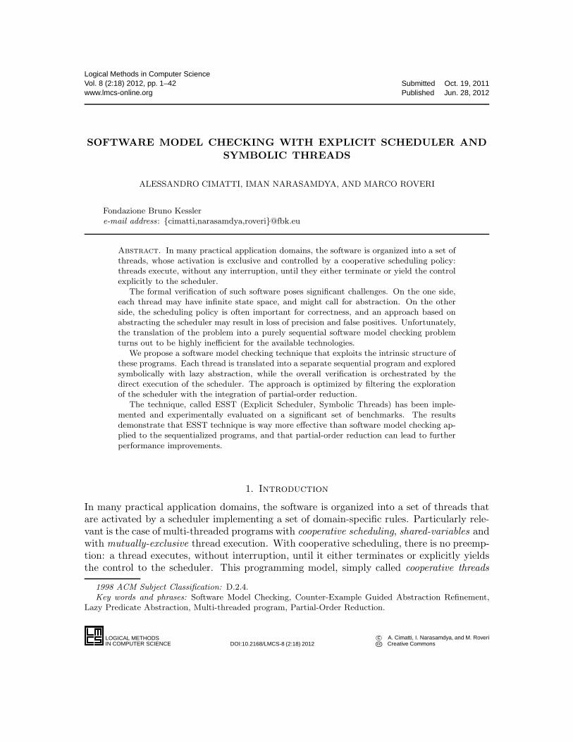
4.7. Summary of ESST. The ESST algorithm takes a threaded program P as an inputand, when its execution terminates, returns either a feasible counter-example path andreports that P is unsafe, or a safe ARF and reports that P is safe. The execution ofESST(P ) can be illustrated in Figure 6:

(1) Start with an ARF consisting only of the initial node, as shown in Figure 6(a).(2) Pick an ARF node that can be expanded and apply the rules E1 or E2 to grow the ARF,

as shown in Figures 6(b) and 6(c). The different colors denote the different threads towhich the ARTs belong.

(3) If we reach an error node, as shown by the red line in Figure 6(d), we analyze thecounter-example path.(a) If the path is feasible, then report that P is unsafe.(b) If the path is spurious, then refine the ARF:

(i) Discover new predicates to refine abstractions.(ii) Undo part of the ARF, as shown in Figure 6(e).(iii) Goto (2) to reconstruct the ARF.

(4) If the ARF is safe, as shown in Figure 6(f), then report that P is safe.

4.8. Correctness of ESST. To prove the correctness of ESST, we need to introduceseveral notions and notations that relate the ESST algorithm with the operational semanticsin Section 3. Given two states s1 and s2 whose domains are disjoint, we denote by s1 ∪ s2the union of two states such that Dom(s1 ∪ s2) is Dom(s1) ∪ Dom(s2), and, for everyx ∈ Dom(s1 ∪ s2), we have

(s1 ∪ s2)(x) =

{

s1(x) if x ∈ Dom(s1);s2(x) otherwise.

Let P be a threaded program with N threads, and γ be a configuration

〈(l1, s1), . . . , (lN , sN ), gs,S〉,

of P . Let η be an ARF node

(〈l′1, ϕ1〉, . . . , 〈l′N , ϕN 〉, ϕ,S′),

for P . We say that the configuration γ satisfies the ARF node η, denoted by γ |= η if andonly if for all i = 1, . . . , N , we have li = l′i and si ∪ gs |= ϕi,

⋃

i=1,...,N si ∪ gs |= ϕ, and

S = S′.


main

(a) (b)

main main

(c) (d)

main main

(e) (f)

Figure 6: ARF construction in ESST.

By the above definition, it is easy to see that, for any initial configuration γ0 of P , wehave γ0 |= η0 for the initial ARF node η0. In the sequel we refer to the configurations ofP and the ARF nodes (or connectors) for P when we speak about configurations and ARFnodes (or connectors), respectively.

We now show that the node expansion rules E1 and E2 create successor nodes that areover-approximations of the configurations reachable by performing operations considered inthe rules.

Lemma 4.6. Let η and η′ be ARF nodes for a threaded program P such that η′ is a successornode of η. Let γ be a configuration of P such that γ |= η. The following properties hold:

(1) If η′ is obtained from η by the rule E1 with the performed operation op, then, for any

configuration γ′ of P such that γop→ γ′, we have γ′ |= η′.


(2) If η′ is obtained from η by the rule E2, then, for any configuration γ′ of P such that

γ·→ γ′ and the scheduler states of η′ and γ′ coincide, we have γ′ |= η′.

Let ε be an ART edge with source node

η = (〈l1, ϕ1〉, . . . , 〈li, ϕi〉, . . . 〈lN , ϕN 〉, ϕ,S)

and target nodeη′ = (〈l1, ϕ

′1〉, . . . , 〈l

′i, ϕ

′i〉, . . . 〈lN , ϕ

′N 〉, ϕ′,S′),

such that S(sTi) = Running and for all j 6= i, we have S(sTj

) 6= Running . Let GTi=

(L,E, l0, Lerr) be the CFG for Ti such that (li, op, l′i) ∈ E. Let γ and γ′ be configurations.

We denote by γε→ γ′ if γ |= η, γ′ |= η′, and γ

op→ γ′. Note that, the operation op is the

operation labelling the edge of CFG, not the one labelling the ART edge ε. Similarly, we

denote by γκ→ γ′ for an ARF connector κ if γ |= η, γ′ |= η′, and γ

·→ γ′. Let ρ = ξ1, . . . , ξm

be an ARF path. That is, for each i = 1, . . . ,m, the element ξi is either an ART edge or an

ARF connector. We denote by γρ→ γ′ if there exists a computation sequence γ1, . . . , γm+1

such that γiξi→ γi+1 for all i = 1, . . . ,m, and γ = γ1 and γ′ = γm+1.

In Section 3 the notion of strongest post-condition is defined as a set of reachable statesafter executing some operation. We now try to relate the notion of configuration with thenotion of strongest post-condition. Let γ be a configuration

γ = 〈(l1, s1), . . . , (li, si), . . . , (lN , sN ), gs,S〉,

and ϕ be a formula whose free variables range over⋃

k=1,...,N Dom(sk) ∪Dom(gs). We say

that the configuration satisfies the formula ϕ, denoted by γ |= ϕ if⋃

k=1,...,N sk ∪ gs |= ϕ.

Suppose that in the above configuration γ we have S(sTi) = Running and S(sTj

) 6= Runningfor all j 6= i. Let GTi

= (L,E, l0, Lerr) be the CFG for Ti such that (li, op, l′i) ∈ E. Let op

be op if op does not contain any primitive function call, otherwise op be op′ as in the secondcase of the expansion rule E1. Then, for any configuration

γ′ = 〈(l1, s1), . . . , (l′i, s

′i), . . . , (lN , sN ), gs′,S′〉,

such that γop→ γ′, we have γ′ |= SP op(ϕ). Note that, the scheduler states S and S

′ are notconstrained by, respectively, ϕ and SP op(ϕ), and so they can be different.

When ESST(P ) terminates and reports that P is safe, we require that, for everyconfiguration γ reachable in P , there is a node in F such that the configuration satisfies thenode. We denote by Reach(P ) the set of configurations reachable in P , and by Nodes(F)the set of nodes in F .

Theorem 4.7 (Correctness). Let P be a threaded program. For every terminating executionof ESST(P ), we have the following properties:

(1) If ESST(P ) returns a feasible counter-example path ρ, then we have γρ→ γ′ for an

initial configuration γ and an error configuration γ′ of P .(2) If ESST(P ) returns a safe ARF F , then for every configuration γ ∈ Reach(P ), there

is an ARF node η ∈ Nodes(F) such that γ |= η.


5. ESST + Partial-Order Reduction

The ESST algorithm often has to explore a large number of possible thread interleavings.However, some of them might be redundant because the order of interleavings of somethreads is irrelevant. Given N threads such that each of them accesses a disjoint set ofvariables, there are N ! possible interleavings that ESST has to explore. The constructedARF will consists of 2N abstract states (or nodes). Unfortunately, the more abstract statesto explore, the more computations of abstract strongest post-conditions are needed, andthe more coverage checks are involved. Moreover, the more interleavings to explore, themore possible spurious counter-example paths to rule out, and thus the more refinements areneeded. As refinements result in keeping track of additional predicates, the computations ofabstract strongest post-conditions become expensive. Consequently, exploring all possibleinterleavings degrades the performance of ESST and leads to state explosion.

Partial-order reduction techniques (POR) [God96, Pel93, Val91] have been successfullyapplied in explicit-state software model checkers like SPIN [Hol05] and VeriSoft [God05]to avoid exploring redundant interleavings. POR has also been applied to symbolic modelchecking techniques as shown in [KGS06, WYKG08, ABH+01]. In this section we will extendthe ESST algorithm with POR techniques. However, as we will see, such an integrationis not trivial because we need to ensure that in the construction of the ARF the PORtechniques do not make ESST unsound.

5.1. Partial-Order Reduction (POR). Partial-order reduction (POR) is a model check-ing technique that is aimed at combating the state explosion by exploring only represen-tative subset of all possible interleavings. POR exploits the commutativity of concurrenttransitions that result in the same state when they are executed in different orders.

We present POR using the standard notions and notations used in [God96, CGP99].We model a concurrent program as a transition systemM = (S, S0, T ), where S is the finiteset of states, S0 ⊂ S is the set of initial states, and T is a set of transitions such that for

each α ∈ T , we have α ⊂ S × S. We say that α(s, s′) holds and often write it as sα→ s′

if (s, s′) ∈ α. A state s′ is a successor of a state s if sα→ s′ for some transition α ∈ T . In

the following we will only consider deterministic transitions, and often write s′ = α(s) forα(s, s′). A transition α is enabled in a state s if there is a state s′ such that α(s, s′) holds.The set of transitions enabled in a state s is denoted by enabled(s). A path from a state s

in a transition system is a finite or infinite sequence s0α0→ s1

α1→ · · · such that s = s0 and

siαi→ si+1 for all i. A path is empty if the sequence consists only of a single state. The

length of a finite path is the number of transitions in the path.Let M = (S, S0, T ) be a transition system, we denote by Reach(S0, T ) ⊆ S the set of

states reachable from the states in S0 by the transitions in T : for a state s ∈ Reach(S0, T ),

there is a finite path s0α0→ . . .

αn−1→ sn system such that s0 ∈ S0 and s = sn. In this work we

are interested in verifying safety properties in the form of program assertion. To this end,we assume that there is a set Terr ⊆ T of error transitions such that the set

EM,Terr= {s ∈ S | ∃s′ ∈ S.∃α ∈ Terr . α(s

′, s) holds }

is the set of error states of M with respect to Terr . A transition system M = (S, S0, T ) issafe with respect to the set Terr ⊆ T of error transitions iff Reach(S0, T ) ∩ EM,Terr

= ∅.


Selective search in POR exploits the commutativity of concurrent transitions. Theconcept of commutativity of concurrent transitions can be formulated by defining an inde-pendence relation on pairs of transitions.

Definition 5.1 (Independence Relation, Independent Transitions). An independence rela-tion I ⊆ T ×T is a symmetric, anti-reflexive relation such that for each state s ∈ S and foreach (α, β) ∈ I the following conditions are satisfied:

Enabledness: If α is in enabled(s), then β is in enabled(s) iff β is in enabled(α(s)).Commutativity: If α and β are in enabled(s), then α(β(s)) = β(α(s)).

We say that two transitions α and β are independent of each other if for every state s theysatisfy the enabledness and commutativity conditions. We also say that two transitionsα and β are independent in a state s of each other if they satisfy the enabledness andcommutativity conditions in s.

In the sequel we will use the notion of valid dependence relation to select a representativesubset of transitions that need to be explored.

Definition 5.2 (Valid Dependence Relation). A valid dependence relation D ⊆ T × T isa symmetric, reflexive relation such that for every (α, β) 6∈ D, the transitions α and β areindependent of each other.

5.1.1. The Persistent Set Approach. To reduce the number of possible interleavings, in everystate visited during the state space exploration one only explores a representative subsetof transitions that are enabled in that state. However, to select such a subset we have toavoid possible dependencies that can happen in the future. To this end, we appeal to thenotion of persistent set [God96].

Definition 5.3 (Persistent Set). A set P ⊆ T of enabled transitions in a state s is persistent

in s if for every finite non-empty path s = s0α0→ s1

α1→ · · ·αn−1→ sn

αn→ sn+1 such that αi 6∈ Pfor all i = 0, . . . , n, we have αn independent of any transition in P in sn.

Note that the persistent set in a state is not unique. To guarantee the existence ofsuccessor state, we impose the successor-state condition on the persistent set: the persistentset in s is empty iff so is enabled(s). In the sequel we assume persistent sets satisfy thesuccessor-state condition. We say that a state s is fully expanded if the persistent set in sequals enabled(s). It is easy to see that, for any transition α not in the persistent set P ina state s, the transition α is disabled in s or independent of any transition in P .

We denote by Reachred(S0, T ) ⊆ S the set of states reachable from the states in S0by the transitions in T such that, during the state space exploration, in every visited statewe only explore the transitions in the persistent set in that state. That is, for a state

s ∈ Reachred(S0, T ), there is a finite path s0α0→ . . .

αn−1→ sn in the transition system such

that s0 ∈ S0 and s = sn, and αi is in the persistent set of si, for i = 0, . . . , n− 1. It is easyto see that Reachred(S0, T ) ⊆ Reach(S0, T ).

To preserve safety properties of a transition system, we need to guarantee that thereduction by means of persistent sets does not remove all interleavings that lead to anerror state. To this end, we impose the cycle condition on Reachred(S0, T ) [CGP99, Pel93]:a cycle is not allowed if it contains a state in which a transition α is enabled, but α isnever included in the persistent set of any state s on the cycle. That is, if there is a cycle


s0α0→ . . .

αn−1→ sn = s0 induced by the states s0, . . . , sn−1 in Reachred(S0, T ) such that αi is

persistent in si, for i = 0, . . . , n − 1 and α ∈ enabled(sj) for some 0 ≤ j < n, then α mustbe in the persistent set of any of s0, . . . , sn−1.

Theorem 5.4. A transition system M = (S, S0, T ) is safe w.r.t. a set Terr ⊆ T of errortransitions iff Reachred(S0, T ) that satisfies the cycle condition does not contain any errorstate from EM,Terr

.

5.1.2. The Sleep Set Approach. The sleep set POR technique exploits independencies ofenabled transitions in the current state. For example, suppose that in some state s thereare two enabled transitions α and β, and they are independent of each other. Supposefurther that the search explores α first from s. Then, when the search explores β from

s such that sβ→ s′ for some state s′, we associate with s′ a sleep set containing only α.

From s′ the search only explores transitions that are not in the sleep set of s′. That is,although the transition α is still enabled in s′, it will not be explored. Both persistentset and sleep set techniques are orthogonal and complementary, and thus can be appliedsimultaneously. Note that the sleep set technique only removes transitions, and not states.Thus, Theorem 5.4 still holds when the sleep set technique is applied.

5.2. Applying POR to ESST. The key idea of applying POR to ESST is to select arepresentative subset of scheduler states output by the scheduler in ESST. That is, insteadof creating successor nodes with all scheduler states from {S1, . . . ,Sn} = Sched(S), for somestate S, we create successor nodes with the representative subset of {S1, . . . ,Sn}. However,such an application is non-trivial. The ESST algorithm is based on the construction ofan ARF that describes the reachable abstract states, while the exposition of POR beforeis based on the analysis of reachable concrete states. As we will see later, some PORproperties that hold in the concrete state space do not hold in the abstract state space.Nevertheless, in applying POR to ESST one needs to guarantee that the original ARF issafe if and only if the reduced ARF, obtained by the restriction on the scheduler’s output,is safe. In particular, the construction of reduced ARF has to check if the cycle conditionis satisfied in its concretization.

To integrate POR techniques into the ESST algorithm, we first need to identify frag-ments in the threaded program that count as transitions in the transition system. In theprevious description of POR the execution of a transition is atomic, that is, its executioncannot be interleaved by the executions of other transitions. We introduce the notion ofatomic block as the notion of transition in the threaded program. Intuitively, an atomicblock is a block of operations between calls to primitive functions that can suspend thethread. Let us call such primitive functions blocking functions.

An atomic block of a thread is a rooted subgraph of the CFG such that the subgraphsatisfies the following conditions:

(1) its unique entry is the entry of the CFG or the location that immediately follows a callto a blocking function;

(2) its exit is the exit of the CFG or the location that immediately follows a call to ablocking function; and

(3) there is no call to a blocking function in any CFG path from the entry to an exit exceptthe one that precedes the exit.


l0

l1

l2 l3

l4

l5

l6l7

. . . . . .

x:=wait(. . .)

l0

l1

l2 l3

l4

l5

l6l7

. . . . . .

x:=wait(. . .)

l0

l1

l2 l3

l4

l5

l6l7

. . . . . .

x:=wait(. . .)

(a) (b) (c)

Figure 7: Identifying atomic blocks.

Note that an atomic block has a unique entry, but can have multiple exits. We often identifyan atomic block by its entry. Furthermore, we denote by ABlock the set of atomic blocks.

Example 5.5. Consider a thread whose CFG is depicted in Figure 7(a). Let wait(. . .) bethe only call to a blocking function in the CFG. Figures 7(b) and (c) depicts the atomicblocks of the thread. The atomic block in Figure 7(b) starts from l0 and exits at l5 and l7,while the one in Figure 7(c) starts from l5 and exits at l5 and l7.

Note that, an atomic block can span over multiple basic blocks or even multiple largeblocks in the basic block or large block encoding [BCG+09]. In the sequel we will use theterms transition and atomic block interchangeably.

Prior to computing persistent sets, we need to compute valid dependence relations.The criteria for two transitions being dependent are different from one application domainto the other. Cooperative threads in many embedded system domains employ event-basedsynchronizations through event waits and notifications. Different domains can have differenttypes of event notification. For generality, we anticipate two kinds of notification: immediateand delayed notifications. An immediate notification is materialized immediately at thecurrent time or at the current cycle (for cycle-based semantics). Threads that are waitingfor the notified events are made runnable upon the notification. A delayed notification isscheduled to be materialized at some future time or at the end of the current cycle. In somedomains delayed notifications can be cancelled before they are triggered.

For example, in a system design language that supports event-based synchronization, apair (α, β) of atomic blocks are in a valid dependence relation if one of the following criteriais satisfied: (1) the atomic block α contains a write to a shared (or global) variable g, andthe atomic block β contains a write or a read to g; (2) the atomic block α contains animmediate notification of an event e, and the atomic block β contains a wait for e; (3) theatomic block α contains a delayed notification of an event e, and the atomic block β containsa cancellation of a notification of e. Note that the first criterion is a standard criterion fortwo blocks to become dependent on each other. That is, the order of executions of thetwo blocks is relevant because different orders yield different values assigned to variables.The second and the third criteria are specific to event-based synchronization language. Anevent notification can make runnable a thread that is waiting for a notification of the event.A waiting thread misses an event notification if the thread waited for such a notification


Algorithm 1 Persistent sets.

Input: a set Ben of enabled atomic blocks.Output: a persistent set P .

(1) Let B := {α}, where α ∈ Ben.(2) For each atomic block α ∈ B:

(a) If α ∈ Ben (α is enabled):• Add into B every atomic block β such that (α, β) ∈ D.

(b) If α 6∈ Ben (α is disabled):• Add into B a necessary enabling set for α with Ben.

(3) Repeat step 2 until no more atomic blocks can be added into B.(4) P := B ∩Ben.

after another thread had made the notification. Thus, the order of executions of atomicblocks containing event waits and event notifications is relevant. Similarly for the delayednotification in the third criterion. Given criteria for being dependent, one can use staticanalysis techniques to compute a valid dependence relation.

To have small persistent sets, we need to know whether a disabled transition that hasa dependence relation with the currently enabled ones can be made enabled in the future.To this end, we use the notion of necessary enabling set introduced in [God96].

Definition 5.6 (Necessary Enabling Set). Let M = (S, S0, T ) be a transition system suchthat a transition α ∈ T is diabled in a state s ∈ S. A set Tα,s ⊆ T is a necessary enabling

set for α in s if for every finite path s = s0α0→ · · ·

αn−1→ sn in M such that α is disabled in

si, for all 0 ≤ i < n, but is enabled in sn, a transition tj, for some 0 ≤ j ≤ n − 1, is inTα,s. A set Tα,Ten ⊆ T , for Ten ⊆ T , is a necessary enabling set for α with Ten if Tα,Ten is anecessary enabling set for α in every state s such that Ten is the set of enabled transitionsin s.

Intuitively, a necessary enabling set Tα,s for a transition α in a state s is a set of transitionssuch that α cannot become enabled in the future before at least a transition in Tα,s isexecuted.

Algorithm 1 computes persistent sets using a valid dependence relation D. It is easy tosee that the persistent set computed by the algorithm satisfies the successor-state condition.The algorithm is also a variant of the stubborn set algorithm presented in [God96], that is,we use a valid dependence relation as the interference relation used in the latter algorithm.

We apply POR to the ESST algorithm by modifying the ARF node expansion rule E2,described in Section 4 in two steps. First we compute a persistent set from a set of schedulerstates output by the function Sched. Second, we ensure that the cycle condition is satisfiedby the concretization of the constructed ARF.

We introduce the function Persistent that computes a persistent set of a set of sched-uler states. Persistent takes as inputs an ARF node and a set S of scheduler states, andoutputs a subset S ′ of S. The input ARF node keeps track of the thread locations, whichare used to identify atomic blocks, while the input scheduler states keep track of the statusof the threads. From the ARF node and the set S, the function Persistent extracts theset Ben of enabled atomic blocks. Persistent then computes a persistent set P from Ben

using Algorithm 1. Finally, Persistent constructs back a subset S ′ of the input set S ofscheduler states from the persistent set P .


Algorithm 2 ARF expansion algorithm for non-running node.

Input: a non-running ARF node η that contains no error locations.(1) Let NonRunning(ARFPath(η,F)) be η0, . . . , ηm such that η = ηm(2) If there exists i < m such that ηi covers η:

(a) Let ηm−1 = (〈l′1, ϕ′1〉, . . . , 〈l

′N , ϕ

′N 〉, ϕ′,S′).

(b) If Persistent(ηm−1,Sched(S′)) ⊂ Sched(S′):

• For all S′′ ∈ Sched(S′) \ Persistent(ηm−1,Sched(S′)):

− Create a new ART with root node (〈l′1, ϕ′1〉, . . . , 〈l

′N , ϕ

′N 〉, ϕ′,S′′).

(3) If η is covered: Mark η as covered.(4) If η is not covered: Expand η by rule E2’.

Let η = (〈l1, ϕ1〉, . . . , 〈lN , ϕN 〉, ϕ,S) be an ARF node that is going to be expanded. Wereplace the rule E2 in the following way: instead of creating a new ART for each stateS′ ∈ Sched(S), we create a new ART whose root is the node (〈l1, ϕ1〉, . . . , 〈lN , ϕN 〉, ϕ,S′)

for each state S′ ∈ Persistent(η,Sched(S)) (rule E2’).

To guarantee the preservation of safety properties, we have to check that the cyclecondition is satisfied. Following [CGP99], we check a stronger condition: at least one statealong the cycle is fully expanded. In the ESST algorithm a potential cycle occurs if an ARFnode is covered by one of its predecessors in the ARF. Let η = (〈l1, ϕ1〉, . . . , 〈lN , ϕN 〉, ϕ,S)be an ARF node. We say that the scheduler state S is running if there is a running threadin S. We also say that the node η is running if its scheduler state S is. Note that duringARF expansion the input of Sched is always a non-running scheduler state. A path in anARF can be represented as a sequence η0, . . . , ηm of ARF nodes such that for all i, we haveηi+1 is a successor of ηi in the same ART or there is an ARF connector from ηi to ηi+1.Given an ARF node η of ARF F , we denote by ARFPath(η,F) the ARF path η0, . . . , ηmsuch that η0 has neither a predecessor ARF node nor an incoming ARF connector, andηm = η. Let ρ be an ARF path, we denote by NonRunning(ρ) the maximal subsequence ofnon-running node in ρ.

Algorithm 2 shows how a non-running ARF node η is expanded in the presence ofPOR. We assume that η is not an error node. The algorithm fully expands the immediatenon-running predecessor node of η when a potential cycle is detected. Otherwise the nodeis expanded as usual.

Our POR technique slightly differs from that of [CGP99]. On computing the successorstates of a state s, the technique in [CGP99] tries to compute a persistent set P in s thatdoes not create a cycle. That is, particularly for the depth-first search (DFS) exploration,for every α in P , the successor state α(s) is not in the DFS stack. If it does not succeed, thenit fully expands the state. Because the technique in [CGP99] is applied to the explicit-statemodel checking, computing the successor state α(s) is cheap.

In our context, to detect a cycle, one has to expand an ARF node by a transition (oran atomic block) that can span over multiple operations in the CFG, and thus may requiremultiple applications of the rule E1. As the rule involves expensive computations of abstractstrongest post-conditions, detecting a cycle using the technique in [CGP99] is bound to beexpensive.

In addition to coverage check, in the above algorithm one can also check if the detectedcycle is spurious. We only fully expand a node iff the detected cycle is not spurious. When


Algorithm 3 Sleep sets.

Input:• a set Ben of enabled atomic blocks.• a sleep set Z.

Output:• a reduced set Bred ⊆ Ben of enabled atomic blocks.• a mapping MZ : Bred → P(ABlock )

(1) Bred := Ben \ Z.(2) For all α ∈ Bred:

(a) For all β ∈ Z:• If (α, β) 6∈ D (α and β are independent): MZ [α] := MZ [α] ∪ {β}.

(b) Z := Z ∪ {α}.

cycles are rare, the benefit of POR can be defeated by the price of generating and solvingthe constraints representing the cycle.

POR based on sleep sets can also be applied to ESST. First, we extend the node ofARF to include a sleep set. That is, an ARF node is a tuple (〈l1, ϕ1〉, . . . , 〈lN , ϕN 〉, ϕ,S, Z),where the sleep set Z is a set of atomic blocks. The sleep set is ignored during coveragecheck. Second, from the set of enabled atomic blocks and the sleep set of the current node,we compute a subset of enabled atomic blocks and a mapping from every atomic block inthe former subset to a successor sleep set.

Let D be a valid dependence relation, Algorithm 3 shows how to compute a reduced setof enabled transitions Bred and a mapping MZ to successor sleep sets using D. The inputof the algorithm is a set Ben of enabled atomic blocks and the sleep set Z of the currentnode. Note that the set Ben can be a persistent set obtained by Algorithm 1.

Similar to the persistent set technique, we introduce the function Sleep that takes asinputs an ARF node η and a set of scheduler states S, and outputs a subset S ′ of S alongwith the above mappingMZ . From the ARF node and the scheduler states, Sleep extractsthe set Ben of enabled atomic blocks and the current sleep set. Sleep then computesa subset Bred of Ben of enabled atomic blocks and the mapping MZ using Algorithm 3.Finally, Sleep constructs back a subset S ′ of the input set S of scheduler states from theset Bred of enabled atomic blocks.

Let η = (〈l1, ϕ1〉, . . . , 〈lN , ϕN 〉, ϕ,S, Z) be an ARF node that is going to be expanded.We replace the rule E2 in the following way: let (S ′,MZ) = Sleep(η,Sched(S)), create anew ART whose root is the node (〈l1, ϕ1〉, . . . , 〈lN , ϕN 〉, ϕ,S′,MZ [l

′]) for each S′ ∈ S ′ such

that l′ is the atomic block of the running thread in S′ (rule E2”).

One can easily combine persistent and sleep sets by replacing the above computation(S ′,MZ) = Sleep(η,Sched(S)) by (S ′,MZ) = Sleep(η,Persistent(η,Sched(S))).

5.3. Correctness of ESST + POR. The correctness of POR with respect to verifyingprogram assertions in transition systems has been shown in Theorem 5.4. The correctnessproof relies on the enabledness and commutativity of independent transitions. However,the proof is applied in the concrete state space of the transition system, while the ESSTalgorithm works in the abstract state space represented by the ARF. The following obser-vation shows that two transitions that are independent in the concrete state space may notcommute in the abstract state space.


η2 (p)

η3 (p ∨ q)

β

α β

α

η4 (p ∨ q)

η5 (p)

η1 (p)

Figure 8: Independent transitionsdo not commute inabstract state space.

For simplicity of presentation, we represent an abstract state by a formula representinga region. Let g1, g2 be global variables, and p, q be predicates such that p⇔ (g1 < g2) andq ⇔ (g1 = g2). Let α be the transition g1 := g1 - 1 and β be the transition g2 := g2 - 1.It is obvious that α and β are independent of each other. However, Figure 8 shows that thetwo transitions do no commute when we start from an abstract state η1 such that η1 ⇔ p.The edges in the figure represent the computation of abstract strongest post-condition ofthe corresponding abstract states and transitions.

Even though two independent transitions do not commute in the abstract state space,they still commute in the concrete state space overapproximated by the abstract state space,as shown by the lemma below.

Lemma 5.7. Let α and β be transitions that are independent of each other such thatfor concrete states s1, s2, s3 and abstract state η we have s1 |= η, and both α(s1, s2) andβ(s2, s3) hold. Let η′ be the abstract successor state of η by applying the abstract strongestpost-operator to η and β, and η′′ be the abstract successor state of η′ by applying the abstractstrongest post-operator to η′ and α. Then, there are concrete states s4 and s5 such that:β(s1, s4) holds, s4 |= η′, β(s4, s5) holds, s5 |= η′′, and s3 = s5.

The above lemma shows that POR can be applied in the abstract state space. LetESSTPOR be the ESST algorithm with POR. The correctness of POR in ESST is statedby the following theorem:

Theorem 5.8. Let P be a threaded sequential program. For every terminating executions ofESST(P ) and ESSTPOR(P ), we have that ESST(P ) reports safe iff so does ESSTPOR(P ).

6. Experimental Evaluation

In this section we show an experimental evaluation of the ESST algorithm in the verificationof multi-threaded programs in the FairThreads [Bou06] programming framework. The aimof this evaluation is to show the effectiveness of ESST and of the partial-order reductionapplied to ESST. By following the same methodology, the ESST algorithm can be adaptedto other programming frameworks, like SpecC [GDPG01] and OSEK/VDX [OSE05], withmoderate effort.

6.1. Verifying FairThreads. FairThreads is a framework for programming multi-threadedsoftware that allows for mixing both cooperative and preemptive threads. As we want toapply ESST, we only deal with the cooperative threads. FairThreads includes a schedulerthat executes threads according to a simple round-robin policy. FairThreads also providesa programming interface that allows threads to synchronize and communicate with eachothers. Examples of synchronization primitives of FairThreads are as follows: await(e) for


selectthreadthread

runof−instant

end−

no runnablethread

await/join/cooperate

runnable thread

start

no runnable threadinstant

end

Figure 9: The scheduler of FairThreads.

waiting for the notification of event e if such a notification does not exist, generate(e) forgenerating a notification of event e, cooperate for yielding the control back to the scheduler,and join(t) for waiting for the termination of thread t.

The scheduler of FairThreads is shown in Figure 9. At the beginning all threads areset to be runnable. The executions of threads consist of a series of instants in which thescheduler runs all runnable threads, in a deterministic round-robin fashion, until there areno more runnable threads.

A running thread can yield the control back to the scheduler either by waiting for anevent notification (await), by cooperating (cooperate), or by waiting for another thread toterminate (join). A thread that executes the primitive await(e) can observe the notificationof e even though the notification occurs long before the execution of the primitive, so longas the execution of await(e) is still in the same instant of the notification of e. Thus, theexecution of await does not necessarily yields the control back to the scheduler.

When there are no more runnable threads, the scheduler enters the end-of-instant phase.In this phase the scheduler wakes up all threads that had cooperated during the last instant,and also clears all event notifications. The scheduler then starts a new instant if there arerunnable threads; otherwise the execution ends.

The operational semantics of cooperative FairThreads has been described in [Bou02].However, it is not clear from the semantics whether the round-robin order of the threadexecutions remains the same from one instant to the other. Here, we assume that the orderis the same from one instant to the other. The operational semantics does not specifyeither the initial round-robin order of the thread executions. Thus, for the verification, oneneeds to explore all possible round-robin orders. This situation could easily degrade theperformance of ESST and possibly lead to state explosion. The POR techniques describedin Section 5 could in principle address this problem.

In this section we evaluate two software model checking approaches for the verificationof FairThreads programs. In the first approach we rely on a translation from FairThreadsinto sequential programs (or sequentialization), such that the resulting sequential programscontain both the mapping of the cooperative threads in the form of functions and theencoding of the FairThreads scheduler. The thread activations are encoded as functioncalls from the scheduler function to the functions that correspond to the threads. Theprogram can be thought of as jumping back and forth between the “control level” imposedby the scheduler, and the “logical level” implemented by the threads. Having the sequentialprogram, we then use off-the-shelf software model checkers to verify the programs.

In the second approach we apply the ESST algorithm to verify FairThreads programs.In this approach we define a set of primitive functions that implement FairThreads synchro-nization functions, and instantiate the scheduler of ESST with the FairThreads scheduler.We then translate the FairThreads program into a threaded program such that there isa one-to-one correspondence between the threads in the FairThreads program and in the


resulting threaded program. Furthermore, each call to a FairThreads synchronization func-tion is translated into a call to the corresponding primitive function. The ESST algorithmis then applied to the resulting threaded program.

6.2. Experimental evaluation setup. The ESST algorithm has been implemented in theKratos software model checker [CGM+11]. In this work we have extended Kratos withthe FairThreads scheduler and the primitive functions that correspond to the FairThreadssynchronization functions.

We have carried out a significant experimental evaluation on a set of benchmarks takenand adapted from the literature on verification of cooperative threads. For example, thefact* benchmarks are extracted from [JBGT10], which describes a synchronous approach toverifying the absence of deadlocks in FairThreads programs. We adapted the benchmarksby recoding the bad synchronization, that can cause deadlocks, as an unreachable falseassertion. The gear-box benchmark is taken from the case study in [WH08]. This casestudy is about an automated gearbox control system that consists of a five-speed gearboxand a dry clutch. Our adaptation of this benchmark does not model the timing behavior ofthe components and gives the same priority to all tasks (or threads) of the control system.In our case we considered the verification of safety properties that do not depend on thetiming behavior. Ignoring the timing behavior in this case results in more non-determinismthan that of the original case study. The ft-pc-sfifo* and ft-token-ring* benchmarksare taken and adapted from, respectively, the pc-sfifo* and token-ring* benchmarks usedin [CMNR10, CNR11]. All considered benchmarks satisfy the restriction of ESST: thearguments passed to every call to a primitive function are constants.

For the sequentialized version of FairThreads programs, we experimented with severalstate-of-the-art predicate-abstraction based software model checkers, including SatAbs-3.0 [CKSY05], CpaChecker [BK11], and the sequential analysis of Kratos [CGM+11].We also experimented with CBMC-4.0 [CKL04] for bug hunting with bounded model check-ing (BMC) [BCCZ99]. For the BMC experiment, we set the size of loop unwindings to 5and consider only the unsafe benchmarks. All benchmarks and tools’ setup are available athttp://es.fbk.eu/people/roveri/tests/jlmcs-esst.

We ran the experiments on a Linux machine with Intel-Xeon DC 3GHz processor and4GB of RAM. We fixed the time limit to 1000 seconds, and the memory limit to 4GB.

6.3. Results of Experiments. The results of experiments are shown in Table 1, for therun times, and in Table 2, for the numbers of explored abstract states by ESST. Thecolumn V indicates the status of the benchmarks: S for safe and U for unsafe. In theexperiments we also enable the POR techniques in ESST. The column No-POR indicatesthat during the experiments POR is not enabled. The column P-POR indicates that onlythe persistent set technique is enabled, while the column S-POR indicates that only thesleep set technique is enabled. The column PS-POR indicates that both the persistent setand the sleep set techniques are enabled. We mark the best results with bold letters, anddenote the out-of-time results by T.O.

The results clearly show that ESST outperforms the predicate abstraction based se-quentialization approach. The main bottleneck in the latter approach is the number ofpredicates that the model checkers need to keep track of to model details of the scheduler.For example, on the ft-pc-sfifo1.c benchmark SatAbs, CpaChecker, and the sequential

http://es.fbk.eu/people/roveri/tests/jlmcs-esst


Sequentialization ESST

Name V SatAbs CpaChecker Kratos CBMC No-POR P-POR S-POR PS-POR

fact1 S 9.07 14.26 2.90 - 0.01 0.01 0.01 0.01

fact1-bug U 22.18 8.06 0.39 15.09 0.01 0.01 0.01 0.03

fact1-mod S 4.41 8.18 0.50 - 0.40 0.40 0.39 0.39

fact2 S 69.05 17.25 15.40 - 0.01 0.01 0.01 0.01

gear-box S T.O T.O T.O - T.O 473.55 44.89 44.19

ft-pc-sfifo1 S 57.08 56.56 44.49 - 0.30 0.30 0.29 0.29

ft-pc-sfifo2 S 715.31 T.O T.O - 0.39 0.39 0.30 0.39

ft-token-ring.3 S 115.66 T.O T.O - 0.48 0.29 0.20 0.20

ft-token-ring.4 S 448.86 T.O T.O - 5.20 1.10 0.29 0.29

ft-token-ring.5 S T.O T.O T.O - 213.37 6.20 0.50 0.40

ft-token-ring.6 S T.O T.O T.O - T.O 92.39 0.69 0.49

ft-token-ring.7 S T.O T.O T.O - T.O T.O 0.99 0.80




ft-token-ring-bug.3 U 111.10 T.O T.O 158.76 0.10 0.10 0.10 0.10

ft-token-ring-bug.4 U 306.41 T.O T.O *407.36 1.70 0.30 0.10 0.10

ft-token-ring-bug.5 U 860.29 T.O T.O *751.44 66.09 1.80 0.10 0.10

ft-token-ring-bug.6 U T.O T.O T.O T.O T.O 26.29 0.20 0.10

ft-token-ring-bug.7 U T.O T.O T.O T.O T.O T.O 0.30 0.20




Table 1: Run time results of the experimental evaluation (in seconds).

analysis of Kratos needs to keep track of, respectively, 71, 37, and 45 predicates. On theother hand, ESST only needs to keep track of 8 predicates on the same benchmark.

Regarding the refinement steps, ESST needs less abstraction-refinement iterations thanother techniques. For example, starting with the empty precision, the sequential analysisof Kratos needs 8 abstraction-refinement iterations to verify fact2, and 35 abstraction-refinement iterations to verify ft-pc-sfifo1. ESST, on the other hand, verifies fact2

without performing any refinements at all, and verifies ft-pc-sfifo1with only 3 abstraction-refinement iterations.

The BMC approach, represented by CBMC, is ineffective on our benchmarks. First,the breadth-first nature of the BMC approach creates big formulas on which the satisfiabilityproblems are hard. In particular, CBMC employs bit-precise semantics, which contributesto the hardness of the problems. Second, for our benchmarks, it is not feasible to identify thesize of loop unwindings that is sufficient for finding the bug. For example, due to insufficientloop unwindings, CBMC reports safe for the unsafe benchmarks ft-token-ring-bug.4 andft-token-ring-bug.5 (marked with “*”). Increasing the size of loop unwindings only resultsin time out.

Table 1 also shows that the POR techniques boost the performance of ESST and allowus to verify benchmarks that could not be verified given the resource limits. In particularwe get the best results when the persistent set and sleep set techniques are applied together.Additionally, Table 2 shows that the POR techniques reduce the number of abstract statesexplored by ESST. This reduction also implies the reductions on the number of abstractpost computations and on the number of coverage checks.


Name No-POR P-POR S-POR PS-POR

fact1 66 66 66 66

fact1-bug 49 49 49 49

fact1-mod 269 269 269 269

fact2 49 49 29 29

gear-box - 204178 60823 58846

ft-pc-sfifo1 180 180 180 180

ft-pc-sfifo2 540 287 310 287

ft-token-ring.3 1304 575 228 180

ft-token-ring.4 7464 2483 375 266

ft-token-ring.5 50364 7880 699 395

ft-token-ring.6 - 32578 1239 518

ft-token-ring.7 - - 2195 963

ft-token-ring.8 - - 4290 1088

ft-token-ring.9 - - 8863 2628

ft-token-ring.10 - - 16109 3292

ft-token-ring-bug.3 496 223 113 89

ft-token-ring-bug.4 2698 914 179 125

ft-token-ring-bug.5 17428 2801 328 181

ft-token-ring-bug.6 - 11302 611 251

ft-token-ring-bug.7 - - 1064 457




Table 2: Numbers of explored abstract states.

Despite the effectiveness showed by the obtained results, the following remarks arein order. POR, in principle, could interact negatively with the ESST algorithm. Theconstruction of ARF in ESST is sensitive to the explored scheduler states and to thetracked predicates. POR prunes some scheduler states that ESST has to explore. However,exploring such scheduler states can yield a smaller ARF than if they are omitted. Inparticular, for an unsafe benchmark, exploring omitted scheduler states can lead to theshortest counter-example path. Furthermore, exploring the omitted scheduler states couldlead to spurious counter-example ARF paths that yield predicates that allow ESST toperform less refinements and construct a smaller ARF.

6.4. Verifying SystemC. SystemC is a C++ library that has widely been used to writeexecutable models of systems-on-chips. The library consists of a language to model thecomponent architecture of the system and also to model the parallel behavior of the systemby means of sequential threads. Similar to FairThreads, the SystemC scheduler employs acooperative scheduling, and the execution of the scheduler is divided into a series of so-calleddelta cycles, which correspond to the notion of instant.

Despite their similarities, the scheduling policy and the behavior of synchronizationprimitives of SystemC and FairThreads have significant differences. For example, theFairThreads scheduler employs a round-robin scheduling, while the SystemC scheduler canexecute any runnable thread. Also, in FairThreads a notification of an event performed bysome thread can later still be observed by another thread, as long as the execution of theother thread is still in the same instant as the notification. In SystemC the latter threadwill simply miss the notification.


In [CMNR10, CNR11], we report on the application of ESST to the verification of Sys-temC models. We follow a similar approach, comparing ESST and the sequentializationapproach, and also experimenting with POR in ESST. The results of those experimentsshow the same patterns as the results reported here for FairThreads: the ESST approachoutperforms the sequentialization approach, and the POR techniques improve further theperformance of ESST in terms of run time and the the number of visited abstract states.These results allow us to conclude that the ESST algorithm, along with the POR tech-niques, is a very effective and general technique for the verification of cooperative threads.

7. Related Work

There have been a plethora of works on developing techniques for the verification of multi-threaded programs, both for general ones and for those with specific scheduling policies.Similar to the work in this paper, many of these existing techniques are concerned withverifying safety properties. In this section we review some of these techniques and describehow they are related to our work.

7.1. Verification of Cooperative Threads. Techniques for verifying multi-threaded pro-grams with cooperative scheduling policy have been considered in different applicationdomains: [MMMC05, GD05, KS05, TCMM07, HFG08, BK08, CMNR10] for SystemC,[JBGT10] for FairThreads, [WH08] for OSEK/VDX, and [CJK07] for SpecC. Most ofthese techniques either embed details of the scheduler in the programs under verificationor simply abstract away those details. As shown in [CMNR10], verification techniques thatembed details of the scheduler show poor scalability. On the other hand, abstracting awaythe scheduler not only makes the techniques report too many false positives, but also lim-its their applicability. The techniques described in [MMMC05, TCMM07, HFG08] onlyemploys explicit-state model checking techniques, and thus they cannot handle effectivelyinfinite-domain inputs for threads. ESST addresses these issues by analyzing the threadssymbolically and by orchestrating the overall verification by direct execution of the schedulerthat can be modeled faithfully.

7.2. Thread-modular Model Checking. In the traditional verification methods, suchas the one described in [OG76], safety properties are proved with the help of assertionsthat annotate program statements. These annotations form the pre- and post-conditionsfor the statements. The correctness of the assertions is then proved by proof rules that aresimilar to the Floyd-Hoare proof rules [Flo67, Hoa83] for sequential programs. The methodin [OG76] requires a so-called interference freedom test to ensure that no assertions used inthe proof of one thread are invalidated by the execution of another thread. Such a freedomtest makes this method non-modular (each thread cannot be verified in isolation from otherthreads).

Jones [Jon83] introduces thread-modular reasoning that verifies each thread separatelyusing assumption about the other threads. In this work the interference information is in-corporated into the specifications as environment assumptions and guarantee relations. Theenvironment assumptions model the interleaved transitions of other threads by describingtheir possible updates of shared variables. The guarantee relations describe the global stateupdates of the whole program. However, the formulation of the environment assumptionsin [Jon83] and [OG76] incurs a significant verification cost.


Flanagan and Qadeer [FQ03] describe a thread-modular model checking technique thatautomatically infers environment assumptions. First, a guarantee relation for each of thethread is inferred. The assumption relation for a thread is then the disjunction of all theguarantee relations of the other threads. Similar to ESST, this technique computes an over-approximation of the reachable concrete states of the multi-threaded program by abstractionusing the environment assumptions. However, unlike ESST, the thread-modular modelchecking technique is incomplete since it can report false positives.

Similar to ESST, the work in [HJMQ03] describes a CEGAR-based thread-modularmodel checking technique, that analyzes the data-flow of each thread symbolically usingpredicate abstraction, starting from a very coarse over-approximation of the thread’s datastates and successively refining the approximation using predicates discovered during theCEGAR loop. Unlike ESST, the thread-modular algorithm also analyzes the environmentassumption symbolically starting with an empty environment assumption and subsequentlyweakening it using the refined abstractions of threads’ data states.

Chaki et. al. [COYC03] describe another CEGAR-based model checking technique.Like ESST, the programs considered by this technique have a fixed number of threads.But, unlike other previous techniques that deal with shared-variable multi-threaded pro-grams, the threads considered by this technique use message passing as the synchronizationmechanism. This technique uses two levels of abstractions over each individual thread.The first abstraction level is predicate abstraction. The second one, which is applied tothe result of the first abstraction, is action-guided abstraction. The parallel compositionof the threads is performed after the second abstraction has been applied. Compositionalreasoning is used during the check for spuriousness of a counter-example by projecting andexamining the counter-example on each individual thread separately.

Recently, Gupta et. al. [GPR11] have proposed a new predicate abstraction and re-finement technique for verifying multi-threaded programs Similar to ESST, the techniqueconstructs an ART for each thread. But unlike ESST, branches in the constructed ARTmight not correspond to a CFG unwinding but correspond to transitions of the environment.The technique uses a declarative formulation of the refinement to describe constraints onthe desired predicates for thread reachability and environment transition. Depending onthe declarative formulation, the technique can generate a non-modular proof as in [OG76]or a modular proof as in [FQ03].

7.3. Bounded Model Checking. Another approach to verifying multi-threaded programsis by bounded model checking (BMC) [BCCZ99]. For multi-threaded programs, the boundis concerned, not only with the length (or depth) of CFG unwinding, as in the case ofsequential programs, but also with the number of scheduler invocations or the number ofcontext switches. This approach is sound and complete, but only up to the given bound.

Prominent techniques that exploit the BMC approach include [God05] and [QR05].The work in [God05] limits the number of scheduler invocations. While the work in [QR05]bounds the number of context switches. That is, given a bound k, the technique verifiesif a multi-threaded program can fail an assertion through an execution with at most kcontext switches. This technique relies on regular push-down systems [Sch00] for a finiterepresentation of the unbounded number of stack configurations. The ESST algorithm caneasily be made depth bounded or context-switch bounded by not expanding the constructedARF node when the number of ARF connectors leading to the node has reached the bound.


The above depth bounded and context-switch bounded model checking techniques areineffective in finding errors that appear only after each thread has a chance to completeits execution. To overcome this limitation, Musuvathi and Qadeer [MQ07] have proposeda BMC technique that bounds the number of context switches caused only by schedulerpreemptions. Such a bound gives the opportunity for each thread to complete its execution.

The state-space complexity imposed by the previously described BMC techniques growswith the number of threads. Thus, those techniques are ineffective for verifying multi-threaded programs that allow for dynamic creations of threads. Recently a technique calleddelay bounded scheduling has been proposed in [EQR11]. Given a bound k, a deterministicscheduler is made non-deterministic by allowing the scheduler to delay its next executedthread at most k times. The bound k is chosen independently of the number of threads.This technique has been used for the analysis and testing of concurrent programs [MQ06].

SAT/SMT-based BMC has also been applied to the verification of multi-threaded pro-grams. In [RG05] a SAT-based BMC that bounds the number of context switches has beendescribed. In this work, for each thread, a set of constraints describing the thread is gener-ated using BMC techniques for sequential programs [CKL04]. Constraints for concurrencydescribing both the number of context switches and the reading or writing of global variablesare then added to the previous sets of constraints. The work in [GG08] is also concernedwith efficient modeling of multi-threaded programs using SMT-based BMC. Unlike [RG05],in this work the constraints for concurrency are added lazily during the BMC unrolling.

7.4. Verification via Sequentialization. Yet another approach used for verifying multi-threaded programs is by reducing bounded concurrent analysis to sequential analysis. Inthis approach the multi-threaded program is translated into a sequential program suchthat the latter over-approximates the bounded reachability of the former. The resultingsequential program can then be analyzed using any existing model checker for sequentialprograms.

This approach has been pioneered by the work in [QW04]. In this work a multi-threadedprogram is converted to a sequential one that simulates all the interleavings generated bymultiple stacks of the multi-threaded program using its single stack. The simulation itselfis bounded by the size of a multiset that holds existing runnable threads at any time duringthe execution of a thread.

Lal and Reps [LR09] propose a translation from multi-threaded programs to sequentialprograms that reduces the context-bounded reachability of the former to the reachability ofthe latter for any context bound. Given a bound k, the translation constructs a sequentialprogram that tracks, at any point, only the local state of one thread, the global state,and k copies of the global state. In the translation each thread is processed separatelyfrom the others, and updates of global states caused by context switches in the processedthread are modeled by guessing future states using prophecy variables and constrainingthese variables at an appropriate control point in the execution. Due to the prophecyvariables, the resulting sequential program explores more reachable states than that of theoriginal multi-threaded program. A similar translation has been proposed in [TMP09]. Butthis translation requires the sequential program to call the individual thread multiple timesfrom scratch to recompute the local states at context switches.

As shown in Section 6, and also in [CMNR10], the verification of multi-threaded pro-grams via sequentialization and abstraction-based software model checking techniques turns


out to suffer from several inefficiencies. First, the encoding of the scheduler makes the se-quential program more complex and harder to verify. Second, details of the scheduler areoften needed to verify the properties, and thus abstraction-based technique requires manyabstraction-refinement iterations to re-introduce the abstracted details.

7.5. Partial-Order Reduction. POR is an effective technique for reducing the searchspace by avoiding visiting redundant executions. It has been mostly adopted in explicit-statemodel checkers, like SPIN [Hol05, HP95, Pel96], VeriSoft [God05], and Zing [AQR+04].Despite their inability to handle infinite-domain inputs, the maturity of these model check-ers, in particular the support for POR, has attracted research on encodings of multi-threaded programs into the language that the model checkers accept. In [CCNR11] weverify SystemC models by encoding them in Promela, the language accepted by the SPINmodel checker. The work shows that the resulting encodings lose the intrinsic structures ofthe multi-threaded programs that are important to enable optimizations like POR.

There have been several attempts at applying POR to symbolic model checking tech-niques [ABH+01, KGS06, WYKG08]. In these applications POR is achieved by staticallyadding constraints describing the reduction technique into the encoding of the program.The work in [ABH+01] apply POR technique to symbolic BDD-based invariant checking.While the work in [WYKG08] describes an approach that can be considered as a symbolicsleep-set based technique. They introduce the notion of guarded independence relation,where a pair of transitions are independent of each other if certain conditions specified inthe pair’s guards are satisfied. The POR techniques applied into ESST can be extendedto use guarded independence relation by exploiting the thread and global regions. Finally,the work in [KGS06] uses patterns of lock acquisition to refine the notion of independencetransition, which subsequently yields better reductions.

8. Conclusions and Future Work

In this paper we have presented a new technique, called ESST, for the verification of shared-variable multi-threaded programs with cooperative scheduling. The ESST algorithm usesexplicit-state model checking techniques to handle the scheduler, while analyzes the threadsusing symbolic techniques based on lazy predicate abstraction. Such a combination allowsthe ESST algorithm to have a precise model of the scheduler, to handle it efficiently, andalso to benefit from the effectiveness of explicit-state techniques in systematic explorationof thread interleavings. At the same time, the use of symbolic techniques allows the ESSTalgorithm to deal with threads that potentially have infinite state space. ESST is futherenhanced with POR techniques, that prevents the exploration of redundant thread in-terleavings. The results of experiments carried out on a general class of benchmarks forSystemC and FairThreads cooperative threads clearly shows that ESST outperforms theverification approach based on sequentialization, and that POR can effectively improve theperformance.

As future work, we will proceed along different directions. We will experiment with lazyabstraction with interpolants [McM06], to improve the performance of predicate abstractionwhen there are too many predicates to keep track of. We will also investigate the possibilityof applying symmetry reduction [DKKW11] to deal with cases where there are multiplethreads of the same type, and possibly with parametrized configurations.


We will extend the ESST algorithm to deal with primitive function calls whose argu-ments cannot be inferred statically. This requires a generalization of the scheduler explo-ration with a hybrid (explicit-symbolic or semi-symbolic) approach, and the use of SMTtechniques to enumerate all possible next states of the scheduler. Finally, we will look intothe possibility of applying the ESST algorithm to the verification of general multi-threadedprograms. This work amounts to identifying important program locations in threads wherethe control must be returned to the scheduler.

References

[ABH+01] R. Alur, R. K. Brayton, T. A. Henzinger, S. Qadeer, and S. K. Rajamani. Partial-order reductionin symbolic state-space exploration. Formal Methods in System Design, 18(2):97–116, 2001.

[AQR+04] T. Andrews, S. Qadeer, S. K. Rajamani, J. Rehof, and Y. Xie. Zing: A model checker forconcurrent software. In R. Alur and D. A. Peled, editors, CAV, volume 3114 of LNCS, pages484–487. Springer, 2004.

[BCCZ99] A. Biere, A. Cimatti, E. M. Clarke, and Y. Zhu. Symbolic Model Checking without BDDs. InR. Cleaveland, editor, TACAS, volume 1579 of LNCS, pages 193–207. Springer, 1999.

[BCG+09] D. Beyer, A. Cimatti, A. Griggio, M. E. Keremoglu, and R. Sebastiani. Software model checkingvia large-block encoding. In FMCAD, pages 25–32. IEEE, 2009.

[BHJM07] D. Beyer, T. A. Henzinger, R. Jhala, and R. Majumdar. The software model checker Blast.STTT, 9(5-6):505–525, 2007.

[BK08] N. Blanc and D. Kroening. Race analysis for SystemC using model checking. In S. R. Nassifand J. S. Roychowdhury, editors, ICCAD, pages 356–363. IEEE, 2008.

[BK11] D. Beyer and M. E. Keremoglu. CPAchecker: A Tool for Configurable Software Verification.In G. Gopalakrishnan and S. Qadeer, editors, CAV, volume 6806 of LNCS, pages 184–190.Springer, 2011.

[Bou02] F. Boussinot. Operational Semantics of Cooperative Fair Threads, 2002. http://www-sop.inria.fr/meije/rp/FairThreads/FTC/documentation/semantics.pdf.

[Bou06] F. Boussinot. FairThreads: mixing cooperative and preemptive threads in C. Concurrency andComputation: Practice and Experience, 18(5):445–469, 2006.

[BSST09] C. W. Barrett, R. Sebastiani, S. A. Seshia, and C. Tinelli. Satisfiability modulo theories. InA. Biere, M. Heule, H. van Maaren, and T. Walsh, editors, Handbook of Satisfiability, volume185 of Frontiers in Art. Int. and Applications, pages 825–885. IOS Press, 2009.

[CCF+07] R. Cavada, A. Cimatti, A. Franzen, K. Kalyanasundaram, M. Roveri, and R. K. Shyamasundar.Computing Predicate Abstractions by Integrating BDDs and SMT Solvers. In FMCAD, pages69–76. IEEE, 2007.

[CCNR11] D. Campana, A. Cimatti, I. Narasamdya, and M. Roveri. An analytic evaluation of SystemCencodings in promela. In A. Groce and M. Musuvathi, editors, SPIN, volume 6823 of LNCS,pages 90–107. Springer, 2011.

[CDJR09] A. Cimatti, J. Dubrovin, T. Junttila, and M. Roveri. Structure-aware computation of predicateabstraction. In FMCAD, pages 9–16. IEEE, 2009.

[CFR+91] R. Cytron, J. Ferrante, B. K. Rosen, M. N. Wegman, and F. K Zadeck. Efficiently computingstatic single assignment form and the control dependence graph. ACM Trans. Program. Lang.Syst., 13(4):451–490, 1991.

[CGJ+03] E. M. Clarke, O. Grumberg, S. Jha, Y. Lu, and H. Veith. Counterexample-guided abstractionrefinement for symbolic model checking. J. ACM, 50(5):752–794, 2003.

[CGM+98] A. Cimatti, F. Giunchiglia, G. Mongardi, D. Romano, F. Torielli, and P. Traverso. Formal verifi-cation of a railway interlocking system using model checking. Formal Asp. Comput., 10(4):361–380, 1998.

[CGM+11] A. Cimatti, A. Griggio, A. Micheli, I. Narasamdya, and M. Roveri. Kratos - a software modelchecker for SystemC. In G. Gopalakrishnan and S. Qadeer, editors, CAV, volume 6806 of LNCS,pages 310–316. Springer, 2011.

[CGP99] E. M. Clarke, O. Grumberg, and D. A. Peled. Model Checking. The MIT Press, 1999.


[CJK07] E. M. Clarke, H. Jain, and D. Kroening. Verification of SpecC using predicate abstraction.Formal Methods in System Design, 30(1):5–28, 2007.

[CKL04] E. M. Clarke, D. Kroening, and F. Lerda. A Tool for Checking ANSI-C Programs. In K. Jensenand A. Podelski, editors, TACAS, volume 2988 of LNCS, pages 168–176. Springer, 2004.

[CKSY05] E. M. Clarke, D. Kroening, N. Sharygina, and K. Yorav. SATABS: SAT-Based Predicate Ab-straction for ANSI-C. In N. Halbwachs and L. D. Zuck, editors, TACAS, volume 3440 of LNCS,pages 570–574. Springer, 2005.

[CMNR10] A. Cimatti, A. Micheli, I. Narasamdya, and M. Roveri. Verifying systemc: A software modelchecking approach. In R. Bloem and N. Sharygina, editors, FMCAD, pages 51–59. IEEE, 2010.

[CNR11] A. Cimatti, I. Narasamdya, and M. Roveri. Boosting lazy abstraction for systemc with partialorder reduction. In P. A. Abdulla and K. R. M. Leino, editors, TACAS, volume 6605 of LNCS,pages 341–356. Springer, 2011.

[COYC03] S. Chaki, J. Ouaknine, K. Yorav, and E. M. Clarke. Automated compositional abstractionrefinement for concurrent c programs: A two-level approach. ENTCS, 89(3):417–432, 2003.

[Cra57] W. Craig. Linear reasoning. a new form of the herbrand-gentzen theorem. Journal of SymbolicLogic, 22:250–268, 1957.

[DKKW11] A. F. Donaldson, A. Kaiser, D. Kroening, and T. Wahl. Symmetry-aware predicate abstractionfor shared-variable concurrent programs. In G. Gopalakrishnan and S. Qadeer, editors, CAV,volume 6806 of Lecture Notes in Computer Science, pages 356–371. Springer, 2011.

[EQR11] M. Emmi, S. Qadeer, and Z. Rakamaric. Delay-bounded scheduling. In T. Ball and M. Sagiv,editors, POPL, pages 411–422. ACM, 2011.

[Flo67] R. W. Floyd. Assigning meaning to programs. In J. T. Schwartz, editor, Proceedings of Sympo-sium in Applied Mathematics, pages 19–32, 1967.

[FQ03] C. Flanagan and S. Qadeer. Thread-modular model checking. In T. Ball and S. K. Rajamani,editors, SPIN, volume 2648 of LNCS, pages 213–224. Springer, 2003.

[GD05] D. Große and R. Drechsler. CheckSyC: an efficient property checker for RTL SystemC designs.In ISCAS (4), pages 4167–4170. IEEE, 2005.

[GDPG01] A. Gerstlauer, R. Doemer, J. Peng, and D. D. Gajski. System Design: A Practical Guide withSpecC. Kluwer Academic Publishers, Boston, MA, USA, June 2001.

[GG08] M. K. Ganai and A. Gupta. Efficient modeling of concurrent systems in BMC. In K. Havelund,R. Majumdar, and J. Palsberg, editors, SPIN, volume 5156 of LNCS, pages 114–133. Springer,2008.

[God96] P. Godefroid. Partial-Order Methods for the Verification of Concurrent Systems - An Approachto the State-Explosion Problem, volume 1032 of LNCS. Springer, 1996.

[God05] P. Godefroid. Software Model Checking: The VeriSoft Approach. F. M. in Sys. Des., 26(2):77–101, 2005.

[GPR11] A. Gupta, C. Popeea, and A. Rybalchenko. Predicate abstraction and refinement for verifyingmulti-threaded programs. In T. Ball and M. Sagiv, editors, POPL, pages 331–344. ACM, 2011.

[GS97] Susanne Graf and Hassen Saıdi. Construction of abstract state graphs with pvs. In Orna Grum-berg, editor, CAV, volume 1254 of LNCS, pages 72–83. Springer, 1997.

[GV04] A. Groce and W. Visser. Heuristics for model checking Java programs. STTT, 6(4):260–276,2004.

[HFG08] P. Herber, J. Fellmuth, and S. Glesner. Model checking SystemC designs using timed automata.In C. H. Gebotys and G. Martin, editors, CODES+ISSS, pages 131–136. ACM, 2008.

[HJMM04] T. A. Henzinger, R. Jhala, R. Majumdar, and K. L. McMillan. Abstractions from proofs. InN. D. Jones and X. Leroy, editors, POPL, pages 232–244. ACM, 2004.

[HJMQ03] T. A. Henzinger, R. Jhala, R. Majumdar, and S. Qadeer. Thread-modular abstraction refine-ment. In W. A. Hunt Jr. and F. Somenzi, editors, CAV, volume 2725 of LNCS, pages 262–274.Springer, 2003.

[HJMS02] T. A. Henzinger, R. Jhala, R. Majumdar, and G. Sutre. Lazy abstraction. In POPL, pages58–70. ACM, 2002.

[Hoa83] C. A. R. Hoare. An axiomatic basis for computer programming (reprint). Commun. ACM,26(1):53–56, 1983.

[Hol05] G. J. Holzmann. Software model checking with SPIN. Advances in Computers, 65:78–109, 2005.


[HP95] G. J. Holzmann and D. A. Peled. An improvement in formal verification. In 7th IFIP WG6.1Int. Conf. on Formal Description Techniques VII, pages 197–211, London, UK, UK, 1995.

[JBGT10] K. Johnson, L. Besnard, T. Gautier, and J. P. Talpin. A synchronous approach to threadedprogram verification. In Proc. of the 10th International Workshop on Automated Verification ofCritical Systems, 2010.

[Jon83] C. B. Jones. Tentative steps toward a development method for interfering programs. ACMTrans. Program. Lang. Syst., 5(4):596–619, 1983.

[KGS06] V. Kahlon, A. Gupta, and N. Sinha. Symbolic model checking of concurrent programs usingpartial orders and on-the-fly transactions. In T. Ball and R. B. Jones, editors, CAV, volume4144 of LNCS, pages 286–299. Springer, 2006.

[KS05] D. Kroening and N. Sharygina. Formal verification of SystemC by automatic hardware/softwarepartitioning. In MEMOCODE, pages 101–110. IEEE, 2005.

[LNO06] S. K. Lahiri, R. Nieuwenhuis, and A. Oliveras. SMT techniques for fast predicate abstraction.In T. Ball and R. B. Jones, editors, CAV, volume 4144 of LNCS, pages 424–437. Springer, 2006.

[LR09] A. Lal and T. W. Reps. Reducing concurrent analysis under a context bound to sequentialanalysis. Formal Methods in System Design, 35(1):73–97, 2009.

[McM06] K. L. McMillan. Lazy abstraction with interpolants. In T. Ball and R. B. Jones, editors, CAV,volume 4144 of LNCS, pages 123–136. Springer, 2006.

[MMMC05] M. Moy, F. Maraninchi, and L. Maillet-Contoz. Lussy: A toolbox for the analysis of systems-on-a-chip at the transactional level. In ACSD, pages 26–35. IEEE, 2005.

[MQ06] M. Musuvathi and S. Qadeer. Chess: Systematic stress testing of concurrent software. InG. Puebla, editor, LOPSTR, volume 4407 of LNCS, pages 15–16. Springer, 2006.

[MQ07] M. Musuvathi and S. Qadeer. Iterative context bounding for systematic testing of multithreadedprograms. In J. Ferrante and K. S. McKinley, editors, PLDI, pages 446–455. ACM, 2007.

[OG76] S. S. Owicki and D. Gries. An axiomatic proof technique for parallel programs. Acta Inf., 6:319–340, 1976.

[Ope05] IEEE 1666: SystemC language Reference Manual, 2005.[OSE05] OSEK. OSEK/VDX Operating System Specification 2.2.3, 2005. http://www.osek-vdx.org.[Pel93] D. A. Peled. All from one, one for all: on model checking using representatives. In CAV, volume

697 of LNCS, pages 409–423. Springer, 1993.[Pel96] D. A. Peled. Combining partial order reductions with on-the-fly model-checking. Formal Meth-

ods in System Design, 8(1):39–64, 1996.[QR05] S. Qadeer and J. Rehof. Context-bounded model checking of concurrent software. In N. Halb-

wachs and L. D. Zuck, editors, TACAS, volume 3440 of LNCS, pages 93–107. Springer, 2005.[QW04] S. Qadeer and D. Wu. Kiss: keep it simple and sequential. In W. Pugh and C. Chambers,

editors, PLDI, pages 14–24. ACM, 2004.[RG05] I. Rabinovitz and O. Grumberg. Bounded model checking of concurrent programs. In K. Etes-

sami and S. K. Rajamani, editors, CAV, volume 3576 of LNCS, pages 82–97. Springer, 2005.[Sch00] S. Schwoon. Model-Checking Pushdown Systems. PhD thesis, Lehrstuhl fur informatik VII der

Technischen Universitat Munchen, 2000.[TCMM07] C. Traulsen, J. Cornet, M. Moy, and F. Maraninchi. A SystemC/TLM Semantics in Promela

and Its Possible Applications. In D. Bosnacki and S. Edelkamp, editors, SPIN, volume 4595 ofLNCS, pages 204–222. Springer, 2007.

[TMP09] S. L. Torre, P. Madhusudan, and G. Parlato. Reducing context-bounded concurrent reachabilityto sequential reachability. In A. Bouajjani and O. Maler, editors, CAV, volume 5643 of LNCS,pages 477–492. Springer, 2009.

[Val91] A. Valmari. Stubborn sets for reduced state generation. In APN 90: Proceedings on Advancesin Petri nets 1990, pages 491–515, New York, NY, USA, 1991. Springer-Verlag.

[WH08] L. Waszniowski and Z. Hanzalek. Formal verification of multitasking applications based ontimed automata model. Real-Time Systems, 38(1):39–65, 2008.

[WYKG08] C. Wang, Z. Yang, V. Kahlon, and A. Gupta. Peephole partial order reduction. In C. Ra-makrishnan and J. Rehof, editors, TACAS, volume 4963 of LNCS, pages 382–396. Springer,2008.


Appendix A. Proofs of Lemmas and Theorems.

Lemma (4.6). Let η and η′ be ARF nodes for a threaded program P such that η′ is asuccessor node of η. Let γ be a configuration of P such that γ |= η. The following propertieshold:

(1) If η′ is obtained from η by the rule E1 with the performed operation op, then, for any

configuration γ′ of P such that γop→ γ′, we have γ′ |= η′.

(2) If η′ is obtained from η by the rule E2, then, for any configuration γ′ of P such that

γ·→ γ′ and the scheduler states of η′ and γ′ coincide, we have γ′ |= η′.

Proof. We first prove property (1). Let η and η′ be as follows:

η = (〈l1, ϕ1〉, . . . , 〈li, ϕi〉, . . . 〈lN , ϕN 〉, ϕ,S)η′ = (〈l1, ϕ

′1〉, . . . , 〈l

′i, ϕ

′i〉, . . . 〈lN , ϕ

′N 〉, ϕ′,S′),

such that S(sTi) = Running and for all j 6= i, we have S(sTj

) 6= Running . Let GTi=

(L,E, l0, Lerr) be the CFG for Ti such that (li, op, l′i) ∈ E. Let γ and γ′ be as follows:

γ = 〈(l1, s1), . . . , (li, si), . . . , (lN , sN ), gs,S〉γ′ = 〈(l1, s1), . . . , (l

′i, s

′i), . . . , (lN , sN ), gs′,S′′〉,

such that γop→ γ′. We need to prove that γ′ |= η′. Let op be op if op contains no primitive

function call, or be op′ as in the second case of the rule E1. First, from γ |= η, we havesi∪gs |= ϕi. By the definition of operational semantics of op and the definition of SP op(ϕi),it follows that s′i∪gs

′ |= SP op(ϕi). Since SP op(ϕi) implies SPπop(ϕi) for any precision π, and

ϕ′i is SP

πl′i

op (ϕi) for some precision πl′i associated with l′i, it follows that s′i∪gs

′ |= ϕ′i. A similar

reasoning can be applied to prove that s′j ∪ gs′ |= ϕ′

j for j 6= i and⋃

i=1,...,N s′i ∪ gs

′ |= ϕ′.

We remark that the havoc(op) operation only makes the values of global variables possiblyassigned in op unconstrained. To prove that γ′ |= η′, it remains to show that S

′ and S′′

coincide. Now, consider the case where op does not contain any call to primitive function. Itis then trivial that S′ = S

′′. Otherwise, if op contains a call to primitive function, then, sincethe primitive executor follows the operational semantics, that is, Sexec(S, f(~x)) computes[[f(~x)]](·, ·,S), we have S

′ = S′′. Hence, we have proven that γ′ |= η′.

For property (2), let η and η′ be as follows:

η = (〈l1, ϕ1〉, . . . , 〈lN , ϕN 〉, ϕ,S)η′ = (〈l1, ϕ1〉, . . . , 〈lN , ϕN 〉, ϕ,S′),

such that S(sTi) 6= Running for all i = 1, . . . , N . Let γ and γ′ be as follows:

γ = 〈(l1, s1), . . . , (lN , sN ), gs,S〉γ′ = 〈(l1, s

′1), . . . , (lN , s

′N ), gs′,S′′〉,

By the operational semantics, we have si = s′i for all i = 1, . . . , N , and gs = gs′. SinceS′ = S

′′, it follows from γ |= η that γ′ |= η′.

Theorem (4.7). Let P be a threaded program. For every terminating execution of ESST(P ),we have the following properties:

(1) If ESST(P ) returns a feasible counter-example path ρ, then we have γρ→ γ′ for an

initial configuration γ and an error configuration γ′ of P .(2) If ESST(P ) returns a safe ARF F , then for every configuration γ ∈ Reach(P ), there

is an ARF node η ∈ Nodes(F) such that γ |= η.


Proof. We first prove property (1). Let the counter-example path ρ be the sequenceξ1, . . . , ξm, such that, for each i = 1, . . . ,m, the element ξi is either an ART edge or anARF connector. We need to show the existence of a computation sequence γ1, . . . , γm+1

such that γiξi→ γi+1 for all i = 1, . . . ,m, and γ = γ1 and γ′ = γm+1. Let ρ

j , for 0 ≤ j ≤ m,denote the prefix ξ1, . . . , ξj of ρ. Let ψ

j be the strongest post-condition after performing theoperations in the suppressed version of ρj. That is, ψj is SPσ

sup(ρj )(true). For k = 1, . . . ,m,

we need to show that, for any configuration γk satisfying ψk−1 and the source node of ξk,there is a configuration γk+1 such that γk+1 satisfies ψk and the target node of ξk.

First, any configuration satisfies true, and thus γ |= true. By definition of counter-example path, the source node of ξ1 is an initial node η0. Any initial configuration satisfiesthe initial node, and thus γ |= η0. Second, take any 1 ≤ k ≤ m, and assume that we havea configuration γk satisfying ψk−1 and the source node of ξk. Consider the case where ξkis an ART edge obtained by unwinding CFG edge labelled by an operation op. Let op bethe label of the ART edge. That is, op = op if op has no primitive function call; otherwiseop = op′ where op′ is defined in the second case of rule E1. Since ψm is satisfiable, then so

is ψk. It means that there is a configuration γ′ such that γkop→ γ′ and γ′ |= ψk. Recall that

the scheduler state of γk+1 is not constrained by ψk and primitive function calls can onlymodify scheduler states. Thus, there is a configuration γk+1 that differs from γ′ only in the

scheduler state, such that γkop→ γk+1 and γk+1 |= ψk. When op has no primitive function

call, then we simply take γ′ as γk+1. By Lemma 4.6, it follows that γk+1 satisfies the target

node of ξk, and hence we have γkξk→ γk+1, as required.

Consider now the case where ξk is an ARF connector. The connector ξk is suppressedin the computation of the strongest post-condition, that is ψk is ψk−1. We obtain γk+1

from γk by replacing γk’s scheduler state with the scheduler state in the target node of ξk.Since free variables of ψk do not range over variables tracked by the scheduler state andγk |= ψk−1, we have γk+1 |= ψk. By the construction of γk+1 and by Lemma 4.6, it follows

that γk+1 satisfies the target node of ξk, and hence we have γkξk→ γk+1, as required.

We now prove property (2). We prove that, for any run γ0, γ1, . . . of P and for anyconfiguration γi in the run, there is a node η ∈ Nodes(F) such that γi |= η. We prove theproperty by induction on the length l of the run:

Case l = 1: This case is trivial because the initial configuration γ0 satisfies the initial node,and the construction of an ARF starts with the initial node.

Case l > 1: Let η ∈ Nodes(F) be an ARF node such that the configuration γn |= η. If ηis covered by another node η′ ∈ Nodes(F), then, by Definition 4.3 of node coverage, wehave γl |= η′. Thus, we pick such an ARF node η such that it is not covered by othernodes.

Consider the transition γlop→ γl+1 from γl to γl+1. By the rule E1, the node η has

a successor node η′ obtained by performing the operation op. By Lemma 4.6, we haveγl+1 |= η′, as required.

Now, consider the transition γl·→ γl+1. Because the scheduler Sched implements

the function Sched in the operational semantics, then, by the rule E2, the node η hasa successor node η′ whose scheduler state coincide with γl+1. By Lemma 4.6, we haveγl+1 |= η′, as required.


Theorem (5.4). A transition system M = (S, S0, T ) is safe w.r.t. a set Terr ⊆ T of errortransitions iff Reachred(S0, T ) that satisfies the cycle condition does not contain any errorstate from EM,Terr

.

Proof. If the transition system M is safe w.r.t. Terr , then Reachred(S0, T ) ∩ EM,Terr= ∅

follows obviously because Reach(S0, T ) ∩ EM,Terr= ∅ and Reachred(S0, T ) ⊆ Reach(S0, T ).

For the other direction, let us assume the transition system M being unsafe w.r.t. Terr .Without loss of generality we also assume that Terr = {α}. We prove that for every states0 ∈ S such that there is a path of length n > 0 leading to an error state se, then thereis a path from s0 to an error state s′e such that the path consists only of transitions in thepersistent sets of visited states. When the state s0 is in S0, then the states visited by thelatter path are only states in Reachred(S0, T ). We first show the proof for n = 1 and n = 2,and then we generalize it for arbitrary n > 1.

Case n = 1: Let s0 ∈ S be such that s0α→ se holds for an error state se. By the successor-

state condition, the persistent set in s0 is non-empty. If the only persistent set in s0 is

the singleton set {α}, then the path s0α→ se is the path leading to an error state and the

path consists only of transitions in the persistent sets of visited states. Suppose that thetransition α is not in the persistent set in s0. Take the greatest m > 0 such that there isa path

s0γ0→ s1

γ1→ · · ·

γm−1→ sm,

where for all i = 0, . . . ,m − 1, the set Pi is the persistent set in state si, the transitionγi is in Pi, and the transition α in not in Pi (see Figure 10). First, the above path existsbecause of the successor-state condition and it must be finite because the set S of statesis finite. The path cannot form a cycle, otherwise by the cycle condition the transitionα will have been in the persistent set in one of the states that form the cycle. Thatis, by the above path, we delay the exploration of α as long as possible. Second, sincethe transition α is enabled in s0 and is independent in si of any transition in Pi for alli = 0, . . . ,m− 1 (otherwise Pi is not a persistent set), then α remains enabled in sj forj = 1, . . . ,m. Third, since m is the greatest number, we have α in the persistent set in

the state sm, and furthermore smα→ s′e holds for an error state s′e. Thus, the path

s0γ0→ · · ·

γm−1→ sm

α→ s′e

is the path from s0 leading to an error state s′e involving only transitions in the persistentsets of visited states.

Case n = 2: Let s0 ∈ S be such that there is a path

s0β0→ s′1

β1=α→ se

for some state s′1 and an error state se. By the successor-state condition, the persistentset in s0 is non-empty. If the only persistent set in s0 is the singleton set {β0}, then the

path s0β0→ s′1 consists only of transition in the persistent set. By the case n = 1, it is

guaranteed that there is a path from s′1 leading to an error state s′e such that the pathconsists only of transitions in the persistent sets of visited states. Thus, there is a pathfrom s0 leading to an error state s′e such that the path consists only of transitions in thepersistent sets of visited states.


Suppose that the transition β0 is not in the persistent set in s0. Take the greatestm > 0 such that there is a path

s0γ0→ s1

γ1→ · · ·

γm−1→ sm,

where for all i = 0, . . . ,m− 1, the set Pi is the persistent set in state si, the transition γiis in Pi, and the transition β0 in not in Pi (see Figure 10). With the same reasoning asin the case of n = 1, the above path exists, and is finite and acyclic. That is, we delaythe exploration of β0 as long as possible.

Consider now the path

s0γ0→ s1

γ1→ · · ·

γm−1→ sm

β0→ s′m+1.

We show that an error state is reachable from the state s′m+1. First, since the transitionsγ0 and β0 are independent in s0, the transitions γ0 and β0 are enabled, respectively,in the states s′1 and s1, and they commute in the state s′2. The transition γ0 is alsoindependent of the transition α in s′1, otherwise P0 is not a persistent set in s0. Thus,the transition α is enabled in s′2. Second, since the transitions γ1 and β0 are independentin s1, the transitions γ1 and β0 are enabled, respectively, in the states s′2 and s2, andthey commute in the state s′3. The transition γ1 is independent of the transition α in s′2,otherwise P1 is not a persistent set in s1. Thus, the transition α is enabled in s′3.

By repeatedly applying the above reasoning, it follows that the transition α is enabledin the state s′m+1. If the singleton set {α} is the only persistent set in s′m+1, then we aredone. That is, the path

s0γ0→ s1

γ1→ · · ·

γm−1→ sm

β0→ s′m+1

α→ s′e

is the path from s0 leading to an error state s′e such that it consists only of transitionsin the persistent sets of visited states.

In the same way as in the case of n = 1, if the transition α is not in the persistent setin s′m+1, then we can delay α as long as possible by taking the greatest k > 0 such thatthere is a path

s′m+1γm→ s′m+2

γm+1→ · · ·

γm+k−1→ s′m+k+1,

where for all l = 1, . . . , k+1, the set Pm+l is the persistent set in state s′m+l, the transitionγm+l−1 is in Pm+l, and the transition α in not in Pm+l. Thus, the path

s0γ0→ s1

γ1→ · · ·

γm−1→ sm

β0→ s′m+1 · · ·

γm+k−1→ s′m+k+1

α→ s′e

is the path from s0 leading to an error state s′e such that it consists only of transitionsin the persistent sets of visited states.

Case n > 1: Let s0 ∈ S be such that there is a path

s0β0→ s′1

β1→ · · ·

βn−1=α→ se

for some state s′1 and an error state se. By the successor-state condition, the persistentset in s0 is non-empty. If the only persistent set in s0 is the singleton set {β0}, then the

path s0β0→ s′1 consists only of transition in the persistent set. By the case n − 1, it is

guaranteed that there is a path from s′1 leading to an error state s′e such that the pathconsists only of transitions in the persistent sets of visited states. Thus, there is a pathfrom s0 leading to an error state s′e such that the path consists only of transitions in thepersistent sets of visited states.


se

s′

e

s0

s1

s2

sm−1

γm−1

γ1

γ0

α

α

α

α

sm

α

s0

s1

s2

sm−1

γm−1

γ1

γ0

sm

se

α

α

α

β0

β0

β0

β0

β0

β1 = αs′1

s′2

s′3

s′m

s′m+1

γm−1

γ1

γ0

α

α

α

α

s′e

s′m+2

γm

s′m+k+1

γm+k−1

s′m+k

s0

s1

s2

sm−1

γm−1

γ1

γ0

sm

α

β0

β0

β0

β0

β0

s′1

s′2

s′3

s′m

s′m+1

γm−1

γ1

γ0β1

β1

β1

β1

se

βn−1 = α

α

α

α

α

γ0

γ0γ1

γ1

γm−1

γm−1

n = 1 n = 2 n > 1

Figure 10: Cases of the proof of Theorem 5.4.

Suppose that the transition β0 is not in the persistent set in s0. Take the greatestm > 0 such that there is a path

s0γ0→ s1

γ1→ · · ·

γm−1→ sm,

where for all i = 0, . . . ,m − 1, the set Pi is the persistent set in state si, the transitionγi is in Pi, and the transition β0 in not in Pi (see Figure 10). That is, we delay theexploration of β0 as long as possible.

Consider now the path

s0γ0→ s1

γ1→ · · ·

γm−1→ sm

β0→ s′m+1.

With the same reasoning as in the case of n = 2, we have the transition β1 enabled inthe state s′m+1, and we can postpone the exploration of β1 as long as possible. When β1gets explored, the transition β2 is enabled in the successor state. By repeatedly applyingthe same reasoning for transitions βk for k = 2, . . . , n − 1, the path formed in a similarway to that of the case of n = 2 is the path from s0 leading to an error state s′e such thatthe path consists only of transitions in the persistent sets of visited states.

Lemma (5.7). Let α and β be transitions that are independent of each other such thatfor concreate states s1, s2, s3 and abstract state η we have s1 |= η, and both α(s1, s2) andβ(s2, s3) hold. Let η′ be the abstract successor state of η by applying the abstract strongestpost-operator to η and β, and η′′ be the abstract successor state of η′ by applying the abstractstrongest post-operator to η′ and α. Then, there are concrete states s4 and s5 such that:β(s1, s4) holds, s4 |= η′, β(s4, s5) holds, s5 |= η′′, and s3 = s5.

Proof. By the independence of α and β, we have β(s1, s4) holds. By the abstract strongestpost-operator, we have s4 |= η′. By the independence of α and β, we have β(s4, s5) holds.By the abstract strongest post-operator and the fact that s4 |= η′, we have s5 |= η′′. Finallyby the independence of α and β, we have s3 = s5.

Theorem (5.8). Let P be a threaded sequential program. For every terminating execu-tions of ESST(P ) and ESSTPOR(P ), we have that ESST(P ) reports safe iff so doesESSTPOR(P ).


Proof. First, we first prove the left-to-right direction of iff and then prove the other direction.(=⇒) : Assume that ESST(P ) returns a safe ARF F . Assume to the contrary that

ESSTPOR reports unsafe and returns a counter-example path ρ. By Theorem 4.7, we have

γρ→ γ′ for an initial configuration γ and an error configuration γ′ of P . That is, the error

configuration is in Reach(P ). Again, by Theorem 4.7, there is an ARF node η ∈ Nodes(F)such that γ′ |= η. But then the node η is an error node, and F is not safe, which contradictsour assumption that F is safe.

(⇐=) : We lift Theorem 5.4 and its proof to the case of abstract transition systemor abstract state space with the help of Lemma 5.7. The lifting amounts to establishingcorrespondences between the transition systemM = (S, S0, T ) in Theorem 5.4 and the ARFconstructed by ESST and ESSTPOR. First, since the executions are terminating, the set ofreachable scheduler states is finite. Now let the set of ARF nodes reachable by the rules E1and E2 correspond to the set S. That is, the set S is now the set of ARF nodes. The setS0 contains only the initial node. A transition in T represents either an ART path ρ thatstarts from the root of the ART and ends with a leaf of the ART, or an ARF connector.The error transitions Terr contains every transition in T such that the transition representsan ART path ρ with an error node as the end node. The set EM,Terr consists of error nodes.

Every path s0α0→ s1

α1→ · · ·αn−1→ sn, corresponds the the following path in the ARF:

(1) for i = 0, . . . , n, the node si is a node in the ARF,(2) for i = 0, . . . , n − 1, there is an ARF path from si to si+1 that is represented by the

transition αi, and(3) for i = 0, . . . , n − 1, if the transition αi leads to a node s covered by another node s′,

then si+1 is s′.

We now exemplify how we address the issue of commutativity in the proof of Theorem 5.4.Consider the case n = 2 where transitions γ0, β0 and β0, γ0 commute in s′2. In the caseof abstract state space, they might not commute. However, by Lemma 5.7, they commutein the concrete state space. Thus, the transition α is still enabled after performing thetransitions γ0, β0.

This work is licensed under the Creative Commons Attribution-NoDerivs License. To viewa copy of this license, visit http://creativecommons.org/licenses/by-nd/2.0/ or send aletter to Creative Commons, 171 Second St, Suite 300, San Francisco, CA 94105, USA, orEisenacher Strasse 2, 10777 Berlin, Germany

Software Model Checking with Explicit Scheduler and Symbolic Threads

Documents

Transcript of Software Model Checking with Explicit Scheduler and Symbolic Threads