FinancialInstitutionsCenter

Checking Accounts and Bank Monitoring

byLoretta J. MesterLeonard I. NakamuraMicheline Renault

99-02-C

The Wharton Financial Institutions Center

The Wharton Financial Institutions Center provides a multi-disciplinary research approach tothe problems and opportunities facing the financial services industry in its search forcompetitive excellence. The Center's research focuses on the issues related to managing riskat the firm level as well as ways to improve productivity and performance.

The Center fosters the development of a community of faculty, visiting scholars and Ph.D.candidates whose research interests complement and support the mission of the Center. TheCenter works closely with industry executives and practitioners to ensure that its research isinformed by the operating realities and competitive demands facing industry participants asthey pursue competitive excellence.

Copies of the working papers summarized here are available from the Center. If you wouldlike to learn more about the Center or become a member of our research community, pleaselet us know of your interest.

Franklin Allen Richard J. HerringCo-Director Co-Director

The Working Paper Series is made possible by a generousgrant from the Alfred P. Sloan Foundation

CHECKING ACCOUNTS AND BANK MONITORING

Loretta J. MesterFederal Reserve Bank of Philadelphia

andThe Wharton School, University of Pennsylvania

Leonard I. NakamuraFederal Reserve Bank of Philadelphia

Micheline RenaultUniversité du Québec à Montréal

July 2002

We thank Mitchell Berlin, Martine Durez-Demal, Mark Flannery, Sherrill Shaffer, Joanna Stavins andseminar participants at Temple University, American University, the Federal Reserve Bank ofPhiladelphia, North Carolina State University, and the Office of the Comptroller of the Currency, and themeeting of the Financial Structure and Regulation System Committee of the Federal Reserve System forhelpful comments. We thank Denise Duffy and Victoria Geyfman for excellent research assistance. Andwe thank the management of the bank under study for their help.

This paper supersedes Working Paper No. 98-25.

The views expressed here are those of the authors and do not necessarily reflect those of the FederalReserve Bank of Philadelphia or of the Federal Reserve System.

Correspondence to Mester at Research Department, Federal Reserve Bank of Philadelphia, TenIndependence Mall, Philadelphia, PA 19106-1574; phone: (215) 574-3807; fax: (215) 574-4364; E-mail: Loretta.Mester@PHIL.frb.org. To Nakamura at Research Department, Federal Reserve Bank ofPhiladelphia, Ten Independence Mall, Philadelphia, PA 19106-1574; phone: (215) 574-3804; fax: (215)574-4364; E-mail: Leonard.Nakamura@PHIL.frb.org. To Renault at Départment des SciencesComptables, École des Sciences de la Gestion, Université du Québec à Montréal; Case Postale 8888;Montréal, Québec, H3C 3P8, Canada; phone: (514) 987-6508; fax: (514) 987-6629; E-mail:renault.micheline@uqam.ca

CHECKING ACCOUNTS AND BANK MONITORING

Abstract

Do checking accounts help banks monitor borrowers? A borrower’s checking account provides a

bank with exclusive access to a continuous stream of borrower data, namely, the borrower’s checking

account balances at the bank. Using a unique set of data that includes monthly and annual information on

small-business borrowers at an anonymous Canadian bank, we provide empirical evidence that checking

account information helps the bank to monitor commercial borrowers. We show the direct mechanism

through which banks can use this information in monitoring. Our results provide empirical support for the

notion of Black (Jrl of Fin Econ, 1975) and Fama (Jrl of Mon Econ, 1985) that, because of their role in the

payments system, banks are “special” monitors.

CHECKING ACCOUNTS AND BANK MONITORING

1. Introduction

Do checking accounts help banks monitor borrowers? If so, as Black (1975) and Fama (1985)

have argued, banks are “special” monitors of borrowers because of their role in the payments mechanism.

While several papers have presented striking evidence that banks are indeed special lenders, none that we

know of shows the direct mechanism by which banks use their role in payments to monitor loans. In this

paper we show how one bank uses information from checking accounts to ascertain whether operating

loans are being used to finance normal operations — inventory and accounts receivable — rather than

unanticipated cash shortfalls.

Some of the information in a checking account is clearly of use to a lender. For example, a

borrower’s canceled checks and banking statements allow a lender to verify the usual information

accompanying a loan application; these are particularly useful in the absence of an independent auditor’s

report. However, a bank does not have a monopoly over this kind of evidence — the borrower can provide

it to any lender.

On the other hand, a bank can have exclusive access to a continuous stream of borrower data on

the most timely basis possible, provided the borrower uses the bank as its exclusive depository. These data

are the flows into and out of the borrower’s checking account at the bank. This timely access is useful in

monitoring an existing loan to detect and control moral hazard problems associated with a rising

probability of bankruptcy.

We analyze a unique set of data that includes monthly and annual information on bank balances,

accounts receivable, and inventories for small-business borrowers at a Canadian bank that wishes to remain

anonymous. In particular, we test the hypothesis that the lender uses information from borrower checking

accounts to ascertain that operating loans are being used for normal operating purposes rather than to

finance abnormal losses.

2

We establish that the bank account provides useful information to the lender and characterize how the

lender responds to the information. Specifically, we find first that monthly changes in accounts receivable

are quite transparently perceivable in movements in the checking account, when the borrower has an

exclusive banking relationship with the lender. This transparency diminishes for borrowers who have

relationships with more than one bank. Our second finding is that borrowings not accounted for by

inventory and accounts receivable are clear predictors of credit downgrades and loan writedowns, and the

bank uses such information promptly. Our third finding is that the bank intensifies monitoring as loans

deteriorate — loan reviews become lengthier and are more frequent.

Taken together, these findings establish a set of links showing that banks can, and do, use

checking accounts to monitor accounts receivable and inventories; and we show exactly how this one bank

does so. Our finding on the transparency of changes in accounts receivable and banking accounts cover

more than 1200 firm-months of data. Even though our data come from a particular bank, the bank does

not control these cash flow movements (most obviously for healthy borrowers). Thus, we consider the

results based on this data set as broadly representative of bank monitoring of small-business borrowers in

general.

To our knowledge, this paper is the first direct empirical test of the usefulness of checking account

information in monitoring commercial borrowers. Previous empirical research has documented the value

of lending relationships to firms by examining loan rates (e.g., Petersen and Rajan, 1994; Berger and

Udell, 1995; and Berlin and Mester, 1998). Other studies have documented a positive abnormal stock-

price reaction to announcements of new or continuing bank loan agreements or loan commitments (e.g.,

Lummer and McConnell, 1989; Billet, Flannery, and Garfinkel, 1995; and Preece and Mullineaux, 1996).

Berlin and Mester (1999) present empirical evidence for an explicit link between banks’ liability structure

and their distinctive lending behavior. Yet none of these previous papers directly examines the mechanism

through which a bank is able to gain an information advantage over other types of lenders. And this is the

3

focus of our paper.

Recent papers by Kashyap, Rajan, and Stein (2002) and Diamond and Rajan (2001) offer

alternative, complementary theoretical rationales for combining deposits and lending under a single roof.

Kashyap, Rajan, and Stein argue that taking deposits and offering lines of credit are forms of liquidity

provision that are optimally bundled together as long as they are not perfectly correlated. With such

bundling, a bank is better able to hedge the risk of withdrawal. Diamond and Rajan argue that by taking

deposits, banks commit themselves to bearing withdrawal risk. This commitment is beneficial, since it

commits the bank to using its skill to collect from borrowers to repay depositors. (If a lender did not try to

collect payment from borrowers, a run would be precipitated and the bank would fail.) This commitment

means that deposits that are withdrawn from the bank to meet unforeseen liquidity needs can be replaced

by new deposits, since new depositors are confident the bank will work to collect from borrowers to repay

depositors. At the same time, borrowers are insulated from unforeseen liquidity needs of direct investors.

In this paper, we explore detailed micro data that show checking account information at banks is

indeed relatively transparent for monitoring borrowers’ collateral and that such monitoring is useful in

detecting problems with loans.

2. The Mechanics of Bank Loan Monitoring

When a borrower suffers unexpected losses, its probability of bankruptcy rises and, by a familiar

moral hazard mechanism, its incentives to invest optimally fall (Myers and Majluf, 1984). A lender who

monitors the borrower’s account and is able to detect such losses may be able to create incentives for the

borrower to take actions that improve expected return (Nakamura, 1993a). In particular, the lender may

strive to ensure that the operating loan extended by the bank finances operations and does not finance

unexpected equity losses. It is thus an important advantage to a lender to be able to detect changes in

normal seasonal borrowing needs, i.e., flows of inventory and accounts receivable.

4

Although much of the literature cites a bank’s ability to monitor borrowers as one of its special

talents, the literature rarely describes what gives the bank its monitoring advantage over other types of

lenders. We argue that a bank loan officer has access to fine-grained information about a borrower’s

activities through its operating account, as he or she can observe checks on an item-by-item basis and

compare them to the borrower’s pro forma business plan. The continuing operation of a business demands

that the business be able to meet its financial requirements, which means that the business must have

enough cash to pay its employees, suppliers, and others. The cash flows of the business are recorded in its

bank account. The bank account information is likely to be one of the timeliest sources of information

available to the bank and will not be as readily available to other lenders. Moreover, as Nakamura

(1993a,b) has argued, checking account information is relatively more transparent and complete for a

small-business borrower whose banking relationship is exclusive to a single lender.

The flow of information about accounts receivable and inventory at our bank is provided for

contractually. A representative loan contract for the bank we study included the following language:

“Total outstandings are not to exceed 75% of good accounts receivable, excluding

accounts over 90 days and inter-company accounts plus 50% of inventory, up to a

maximum of $5 million dollars, including raw material, work in process and finished

products, less priority claims.”

“The Borrower will deliver to the Banks such financial information as the Bank may reasonably

request including but not limited to the following:

a) audited annual financial statements of the Borrower, within 90 days after the fiscal

year end;

b) in house monthly financial statements of the Borrower within 20 days after the end of

the month;

c) monthly aged listing of accounts receivable and inventory reports within 20 days after

the end of month.”

5

This loan contract restricts the amount of the loan to a certain percentage of accounts receivable

and inventory. It also requires the borrower to report shipments to customers that constitute new accounts

receivable, as well as customer payments on accounts receivable. A borrower whose business is

floundering may be tempted to submit false statements, particularly if these reports lie within the bounds of

plausible error. For example, an account that has already been paid may be included among receivables.

Or an order that has not yet been shipped may be called a receivable. However, by observing the detailed

flow of checks received, the bank loan officer can verify that each receivable is followed, within 90 days,

by a payment. In fact, every month, the loan officer can do an item-by-item reconciliation of the account

receivables: beginning of month receivables + sales (operating revenues) � cash inflows (checks) = end of

month receivables. This is a check not just on the veracity of the borrower but on how careful the business

is in managing accounts receivables, itself a telling sign.

A nonbank lender — or a bank lender who did not have the borrower’s checking account business

— would not have the same timely access to this verification. While it is true that a nonbank financial

institution can arrange to become the receiver of the accounts receivable, this adds additional cost, and may

restrict the borrower’s flexibility. There are two other reasons this might be a costly solution. First, the

borrower may not wish to reveal to buyers that it is having financial difficulties. Second, the borrower is

likely to be in a better position than the bank to judge how best to collect receivables, and the borrower

will be deprived of information on the timeliness of payments, which helps it conduct its business. As a

result, a nonbank lender is usually not able to easily discern that a troubled borrower is continuing to post

accounts receivable after they have been collected. While any information possessed by the borrower may

be in principle transmitted to any lender, such forward transmission may come at a cost, including loss of

privacy and loss of timeliness and detail, as well as any direct cost of sending and receiving. The bank

lender’s access to this information is, by contrast, a necessary byproduct of the checking account

6

The importance of proprietary information and banking, using the example of R&D contests, is1

explored in Bhattacharya and Chiesa (1995).

technology. 1

Before continuing, it may be worthwhile mentioning that in the Canadian bank being studied, an

operating loan is supplied as a negative-balance checking account, a typical practice in English banking.

In the U.S., by contrast, the operating loan and the checking account are separated, with the checking

account balance, at least in principle, required to be positive. Thus, the operating loan balance plus the

checking account balance in the U.S. would be equal to the operating loan balance in this Canadian bank.

U.S.-style Bank Account English-style Bank Account(used by our Canadian bank)

Assets Liabilities Assets LiabilitiesChecking Balance = C Loan = L Bank Account = Bt t t

A nonbank lender in either the U.S. or Canada would observe only the loan balance. This would

consist of a series of debits and credits between the firm’s checking account at the firm’s bank and the loan

account at the firm’s nonbank lender. In general, the nonbank lender does not see the individual checks

the firm writes on its bank checking account that pay suppliers, workers, and other creditors, nor those that

are paid into the account by clients. A bank lender, on the other hand, using the English-style account,

observes B , the checks between the borrower and the rest of the world, but there is no separate loant

account. In contrast, a bank lender using the system prevalent in the U.S. observes C and L . Thus, thet t

U.S.-style bank lender observes both the checks between the borrower and the rest of the world, and

between the loan account and the checking account. The U.S. bank accounting system provides somewhat

more information than this Canadian bank’s system, and it is possible that drawdowns of the operating

loan may represent signals the bank can interpret. Thus, if anything, the results found using our Canadian

data should indicate the lower bound on the information available in U.S.-style banking systems. On the

7

other hand, the gross liability of the bank to the borrower and vice versa are greater under the U.S.-style

banking practice, because the checking account and loan account are not netted.

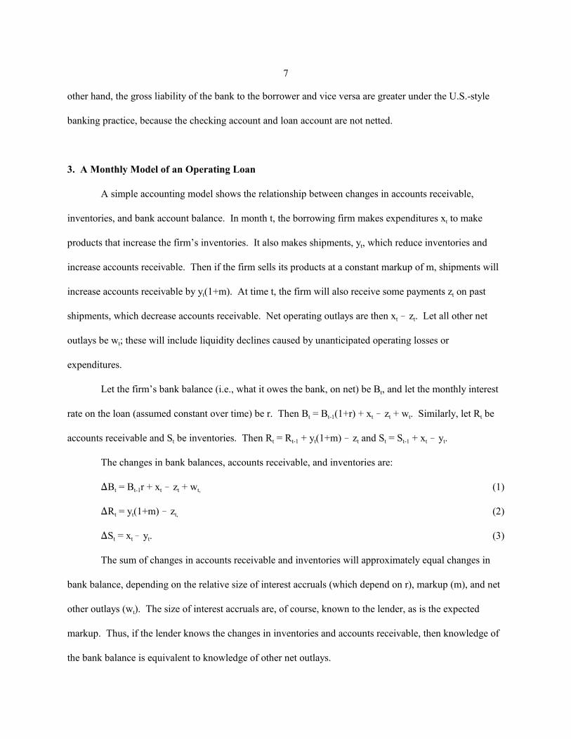
3. A Monthly Model of an Operating Loan

A simple accounting model shows the relationship between changes in accounts receivable,

inventories, and bank account balance. In month t, the borrowing firm makes expenditures x to maket

products that increase the firm’s inventories. It also makes shipments, y , which reduce inventories andt

increase accounts receivable. Then if the firm sells its products at a constant markup of m, shipments will

increase accounts receivable by y (1+m). At time t, the firm will also receive some payments z on pastt t

shipments, which decrease accounts receivable. Net operating outlays are then x � z . Let all other nett t

outlays be w ; these will include liquidity declines caused by unanticipated operating losses ort

expenditures.

Let the firm’s bank balance (i.e., what it owes the bank, on net) be B , and let the monthly interestt

rate on the loan (assumed constant over time) be r. Then B = B (1+r) + x � z + w . Similarly, let R bet t-1 t t t t

accounts receivable and S be inventories. Then R = R + y (1+m) � z and S = S + x � y .t t t-1 t t t t-1 t t

The changes in bank balances, accounts receivable, and inventories are:

�B = B r + x � z + w (1)t t-1 t t t,

�R = y (1+m) � z (2)t t t,

�S = x � y . (3)t t t

The sum of changes in accounts receivable and inventories will approximately equal changes in

bank balance, depending on the relative size of interest accruals (which depend on r), markup (m), and net

other outlays (w ). The size of interest accruals are, of course, known to the lender, as is the expectedt

markup. Thus, if the lender knows the changes in inventories and accounts receivable, then knowledge of

the bank balance is equivalent to knowledge of other net outlays.

8

The reverse is true too. If movements in w are infrequent, the bank balance can generally be usedt

to monitor changes in inventory and accounts receivable.

The individual payments a borrower makes would be available to the borrower’s bank lender.

However, our data set does not include checking account or accounts receivable information detailed

enough to verify individual payments in this manner. But it does allow us to demonstrate that the account

balance provides a relatively transparent window on accounts receivable and inventory. In the empirical

work described below, we use correlations between inventory, accounts receivable, and bank balance to

judge how easily the bank balance can be used to monitor operations. We then show how this bank uses

unexpected movements in the operating loan relative to inventory and accounts receivable to determine

credit risk, intensify monitoring, and declare a loan troubled. We now describe our data set more fully and

then turn to our empirical implementation and results.

4. The Data Set

The data contain information on 100 small-business borrowers who are customers of the Canadian

bank. A small business is defined as one with authorized credit between C$500,000 and C$10,000,000

and whose shareholders are managers of the firm. The average sum actually borrowed on the credit in our

sample is about C$1,500,000. The selected firms have been active for at least three years; public utilities,

management firms, and financial companies are excluded. Fifty of these loans were declared troubled by

the bank and the rest were healthy loans over the period studied. Declaring a loan troubled is a highly

consequential act for the lender, as it is the point when the bank acknowledges a high probability of loss on

the loans.

Table 1 shows the outcomes for the troubled loans. For the vast majority (72 percent) of these

9

A private liquidation is a cooperative sell-off of assets without a court settlement. When the2

owner has signed a personal guarantee as a part of the loan agreement, such a private liquidation is likelyto be efficient, as the owner is strongly motivated to maximize liquidation value of the firm and minimizehis personal liability. Of course, if there are other claimants liquidation may be complicated andbankruptcy entered into.

Because the reference dates for a matched troubled loan and healthy loan differ, the data on two3

matched loans could potentially cover substantially different time periods, with significantly differentmacroeconomic conditions. But this does not seem to pose a large problem here, since the difference inreference dates was under two years in all but four cases, and the maximum difference was three and a halfyears for one loan pair.

loans, the borrowing firms ended up going into bankruptcy or were privately liquidated. Of the other2

loans, nine remained troubled, four were repaid, and one was upgraded.

The troubled loans here are substantially all the troubled loans during this period that meet our

criterion. Then for each troubled loan, we found a loan that remained healthy over the period studied and

matched the troubled loan by industry, level of annual sales, credit rating at the start of the three year

period, and loan amount.

Most of these troubled loans were so classified between 1990 and 1992 (only three loans were

classified as troubled before 1990); healthy loans were last reviewed by the bank at some date in 1991 or

1992. Six industrial sectors are represented in the data (see Table 2).

For each loan, we have both annual and monthly data. For a troubled loan, the annual data pertain

to the firm’s three fiscal years prior to the loan’s being declared troubled, and the monthly data pertain to

the three calendar years prior to the firm’s being declared troubled. (The data are not necessarily complete

for each loan.) For the matched healthy loan, we have comparable information, with the reference date

being the last time the firm’s credit file was reviewed by the bank. For example, consider a firm whose

loan was declared troubled in April 1991 and whose fiscal year runs from October to September. Our

annual data on this firm would cover the firm’s fiscal years FY1988, FY1989, and FY1990, and the

monthly data would run from January 1988 through December 1990.3

10/1/87 10/1/88 10/1/89 10/1/90

FY88 FY89 FY90

1/1/88 1/1/89 1/1/90 1/1/91

4/15/91Monthly Data

Annual Data

Loan Declared Troubled

10

An important variable included in our data set is whether the firm has an exclusive banking

arrangement with the bank. This variable allows us to segment the loans into “exclusive” and

“nonexclusive” categories, providing a metric against which we can measure certain effects. If a borrower

has a nonexclusive relationship with our bank, it is not clear whose customer the borrower really is. In

some cases, the borrower will have a primary customer relationship with the bank we are studying, in

which case the borrower’s operating balance is likely to remain quite informative. In other cases, the

borrower’s primary relationship will be with another bank, and the bank we are studying is partially

dependent on the other bank for information on the borrower’s creditworthiness. Thus, if checking

account information is valuable, we would expect it to be more valuable for exclusive loans, since the

bank’s account balance data on the firm would reflect its entire checking account activity. However, in our

empirical tests that use accounts receivable and inventories, almost all the “nonexclusive” borrowers have

primary customer relationships with the bank under study. To that extent, the differences between

exclusive and nonexclusive borrowers may be attenuated.

In our data, of the 50 troubled loans, 33 of the borrowers have an exclusive relationship with the

bank; of the 50 healthy loans, 26 have an exclusive relationship. There appears to be a definite correlation

between the completeness of our data and whether the bank serves as the firm’s exclusive bank. Of the 59

firms with exclusive relationships, we have complete data on 19, i.e., 32 percent, while of the 41 firms

with nonexclusive relationships, we have complete data on only four, i.e., less than 10 percent.

11

One such borrower with unusually large sales of over $300 million distorts the data on4

“nonexclusive-troubled” borrowers. When that borrower is omitted, average sales for all three years fallsto $14.5 million for troubled loans, to $18.8 million for nonexclusive loans, and to $24.5 million fornonexclusive-troubled loans. This borrower’s data, fortunately, does not materially affect any of our otherresults. Indeed, when this borrower is omitted, the results of our statistical tests, are, on average, slightlymore favorable to our hypotheses.

4.1 Annual data

The annual data contain information typically found on a firm’s financial statement, e.g., balance-

sheet data, such as the book value of accounts receivable and inventories; income-statement data; some

items from the statement of changes in financial position; and information in the firm’s credit file. Our

data set also contains some information from the outside auditor’s report on the firm, e.g., whether there

were any qualifications in the auditor’s report and the date of the audit. These data would be available to

any lender the firm approached for a loan. Nonexclusive borrowers generally tend to have larger sales and

often represent borrowers who are being accommodated by our bank because they have a plant or

subsidiary outside their primary bank’s territory.4

The credit file contains annual information about the firm’s sales, the level of authorized credit the

firm has gotten from the bank for an operating loan, additional credit for seasonal loans, and other

temporary loans. In addition, there is information on whether the loan has covenants. A crucial datum in

each annual credit review is the credit rating assigned to the loan by the bank’s credit department upon

completion of the review. This credit rating is arranged on a scale of one through eight, with one being the

best, and six through eight being different degrees of “trouble.”

Tables 3A, 3B, and 4 show some of the annual data on our borrowers. The first three columns in

the top panel of Table 3A show the average loan sizes (measured by the average amount actually

borrowed) for all the loans and for the healthy and troubled loan subsamples over the entire three-year

period covered by the data and over each year individually, where the years are measured relative to the

reference date (i.e., for a troubled loan, the three fiscal years prior to the loan being declared troubled; and

12

for a healthy loan, the three fiscal years prior to the firm’s last credit review by the bank). It is evident that

the bank does not use its information about troubled borrowers to substantially reduce its exposure to loss;

rather, if anything, troubled loans rise in average size. The top panel of Table 3B shows the average

annual business sales for all firms and for the healthy and troubled loan subsamples. Note that troubled

borrowers do not generally have obviously declining average sales compared to healthy ones.

The bottom panels of Tables 3A and 3B show the average loan amounts and average annual

business sales, respectively, over time for exclusive and nonexclusive loans, and for these categories

separated into healthy and troubled loan subcategories. As might be expected, firms that are larger, as

measured by sales, tend to deal with more than one bank and so do not have an exclusive relationship with

the bank under study.

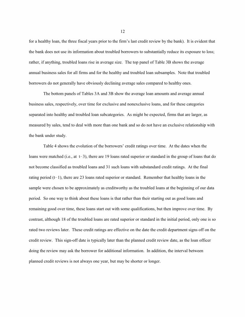
Table 4 shows the evolution of the borrowers’ credit ratings over time. At the dates when the

loans were matched (i.e., at t�3), there are 19 loans rated superior or standard in the group of loans that do

not become classified as troubled loans and 31 such loans with substandard credit ratings. At the final

rating period (t�1), there are 23 loans rated superior or standard. Remember that healthy loans in the

sample were chosen to be approximately as creditworthy as the troubled loans at the beginning of our data

period. So one way to think about these loans is that rather than their starting out as good loans and

remaining good over time, these loans start out with some qualifications, but then improve over time. By

contrast, although 18 of the troubled loans are rated superior or standard in the initial period, only one is so

rated two reviews later. These credit ratings are effective on the date the credit department signs off on the

credit review. This sign-off date is typically later than the planned credit review date, as the loan officer

doing the review may ask the borrower for additional information. In addition, the interval between

planned credit reviews is not always one year, but may be shorter or longer.

13

The mean haircut on accounts receivable was 0.29 for borrowers rated superior or standard and5

0.36 for borrowers rated as troubled (with one of the three worst credit ratings). The mean haircut oninventories was 0.62 for borrowers rated superior or standard and 0.66 for borrowers rated as troubled.

4.2 Monthly data

The monthly data contain information on the value that the bank assigns to the firm’s accounts

receivable and inventories, as well as the end-of-month balance in the firm’s bank account, as well as the

minimum, maximum, and average balance over the month. The bank’s valuation of accounts receivable

and inventories are important ingredients in determining how much the bank is willing to lend to a

commercial borrower. To restrict the use of the operating loan to purely operational ends and to ensure

that the borrower has adequate collateral for the loan, the bank verifies on a monthly basis that the amount

borrowed does not exceed the estimated value of the firm’s operating assets that serve as collateral.

The bank’s valuations include subjective discounts (haircuts) from book value (note, we do not

have monthly information on these book values). These haircuts provide a comfort level for the lender;

they also reflect the liquidity and quality of accounts receivable and inventories. For example, as accounts

receivable remain uncollected, their quality (i.e., the probability they will ultimately be collected) may

deteriorate. Also, the state to which the inventory is processed reflects its liquidity — works-in-progress

inventory is the least valuable, since it is the most difficult to convert to other uses and, therefore, to sell to

other producers. In general, our data indicate that this bank values accounts receivable at two-thirds to

three-quarters of book value, while it values inventories at between one-quarter and two-fifths of book

value. Credit rating does not seem to have much impact on the size of haircut, although borrowers with a

credit rating in the “troubled” range may receive a bigger haircut on their accounts receivable than do other

borrowers. This presumably reflects the aging of some proportion of the accounts receivable.5

14

5. Feasibility of Using Bank Account Information for Monitoring Borrowers: The RelationshipBetween Loan Balances and the Bank’s Valuation of Accounts Receivable

Next, we turn to the transparency of the bank balance in providing information on accounts

receivable. If we had complete data on loan balances, accounts receivable, and inventories, then, under

the hypothesis of transparency, almost all the movements in bank balances would be accounted for by

movements in accounts receivable and inventories. However, in our data, it appears that there is a limit on

the amount the bank is willing to lend against inventory. That is, there is a binding ceiling on the bank’s

inventory valuation, so that changes in inventory are typically not reflected in our inventory valuations

data. For this reason, we focus on the relationship between loan balances and accounts receivable. As

indicated in section 3, to the extent that there is a high correlation between bank account balances and

changes in accounts receivable and inventories, changes in the firm’s bank account balance can be used to

monitor a firm’s operations. But how high can we expect this correlation to be? Obviously, this will

depend on the distribution of the underlying variables defined in section 3, x , y , z , and w , i.e.,t t t t

expenditures, shipments, payments on past shipments, and other net outlays, respectively. When

inventory is shipped, the borrower writes down its finished goods inventory but the loan balance is

unaffected. Loan balances change only in response to payments, which represent only half of the changes

in accounts receivable. This suggests that the correlation between accounts receivable and loan balances

should be negative, and roughly one-half. In the appendix, we formalize this conjecture. Note that a

similar calculation can be performed for the correlation between the change in bank account balance and

the change in inventories.

To see whether bank account balance gives the bank useful information for monitoring the firm’s

operations, we examined the correlations between changes from the beginning to the end of each month in

the firm’s checking account balance, and the bank’s valuations of the firm’s accounts receivable and

inventories. As discussed in section 3, we hypothesize that the correlation would be stronger for firms that

15

To normalize, we use the earliest annual sales figure available for each firm. For troubled loans,6

this is sales in the fiscal year three years prior to the loans’ being declared troubled, and for healthy loans,this is sales in the fiscal year three years prior to the last credit file review.

Not only would the bank have less data on nonexclusive firms, but the value of any information it7

had might be lower, since the firm would be less under the bank’s control.

Note that we also find a stronger correlation for healthy loans than for troubled loans, holding8

exclusivity constant. This may reflect the fact that when loans become troubled, the bank may lower itsvaluations and the loan limits may become binding on the firm. (It also suggests that the bank’s control isnot perfect.) This would disrupt the normal relationship between checking account balances and bankvaluations of accounts receivable.

have an exclusive relationship with the bank than for firms that do not. So we repeat the correlation

analysis for the exclusive and nonexclusive subsamples, and we also divide these subsamples into their

healthy and troubled loan subgroups, to control for any loan performance effect. Thus, we perform the

analysis for seven groups: all loans, exclusive, nonexclusive, exclusive-healthy, nonexclusive-healthy,

exclusive-troubled, nonexclusive-troubled. In this analysis we normalize the variables by the firm’s annual

sales to control for heteroscedasticity.6

As shown in the first row of Table 5, the correlation between changes in bank balances and

changes in accounts receivable is 0.45 for all loans, and is higher for exclusive loans than for nonexclusive

loans. Thus, our data are showing about as high a level of correlation as one should expect. We also see

that the correlations are stronger for firms that deal exclusively with the bank than for firms that have

multiple banking relationships, even when we control for loan performance. This suggests there is more

information to be gleaned about a firm’s operations from the account balances for firms that deal

exclusively with the bank than for those that have other banking relationships. It appears that simply7

having a continuous record of the borrower’s operating balance in an exclusive client relationship provides

the lender with a substantial amount of information. Of course, the loan officer has access to even better

information, as the loan officer can examine individual checks and deposits.8

The correlations between changes in inventories and changes in either bank balances or accounts

16

receivable are much smaller than the correlations between changes in bank balances and accounts

receivable. This is because there is generally much less variation in changes in inventory valuations than

in the other variables, as shown in the bottom panel of Table 5. Indeed, roughly 20 percent of the monthly

observations of the bank’s valuation of inventories appear to be at an upper limit. These are cases where

there are more than two observations of the same valuation and that valuation is greater than others for that

borrower.

This analysis suggests that changes in accounts receivable potentially contain useful information

about firm operations, while changes in inventories are likely to contain less information. The empirical

analysis in the next sections attempts to determine whether indeed there is useful information and how the

bank uses such information.

6. Information Available from the Monthly Valuations: The Relationship Between Signals of FirmTrouble, Credit Downgrades, and Troubled Firms

The monthly data allow the lender to detect two signals of potential trouble at the firm. The first

signal is when the bank’s loan balance exceeds the bank’s valuation of collateral, i.e., valuations of

account receivables and inventory. The second signal is whether the borrower is consistently borrowing

an amount close to or exceeding the credit line authorized at the beginning of the credit year. These two

signals differ sharply on what kinds of lenders can use them. The first type of signal is available only to

bank lenders, since only a bank lender can track the high frequency movements in collateral valuations and

thus can create a reliable signal based on them. Monthly monitoring and valuation of accounts receivable

and inventories are likely to be very difficult for a nonbank lender who does not have access to the

checking account data we have documented as providing useful information. On the other hand, a signal

based just on information on the firm’s account balance would be available to both bank and nonbank

lenders. Presumably any lender will know the extent to which the borrower is using or even exceeding the

17

Months for which our data are incomplete do not count as positive or negative exceed and,9

therefore, do not increase either violations or nonviolations. To the extent that data are missing and to theextent that the firm is just borrowing an amount equal to the bank’s valuation of its collateral, the sum ofviolations and nonviolations will differ from 36.

authorized credit line. We compare the informativeness of these two types of signals and are specifically

interested in what additional information is provided by the bank’s valuations of collateral.

Our measures of these two types of signals are exceed and utilization. Exceed is the amount the

firm has borrowed less the firm’s collateral (as measured by the bank’s valuation of the firm’s accounts

receivable and inventories and other guarantees posted by the firm), as a percent of the firm’s authorized

credit line. Utilization is the firm’s borrowing as a percent of its authorized credit line. Exceed is a signal

of trouble available to only a bank lender, while utilization is available to any lender. Troubled firms are

likely to have higher, and possibly positive, values of exceed and higher values of utilization, since they are

likely to have borrowed more, had the bank lower its valuations of accounts receivable and inventory, and

had the bank also lower the firm’s credit line.

Both exceed and utilization are computed using the monthly data on the firm, and thus, they are

likely to be better signs of trouble for exclusive borrowers than for nonexclusive borrowers, since the bank

has more accurate monthly data on exclusive borrowers. As expected, we found higher mean values of

exceed and utilization for exclusive-troubled firms than for exclusive-healthy firms.

When exceed turns positive, the bank is at risk, in that the borrower’s ability to relatively quickly

pay off the loan has become stretched. This is a warning signal to the loan officer and to the bank. How

useful is this signal? We define a variable, violations, which equals the number of months for which

exceed is positive over the three years prior to our reference date (either the date when a loan was declared

troubled or the date of a healthy loan’s last credit review). We also define violations_i, i=1,2,3, which is

the number of months exceed is positive in the i year before the reference date. Similarly, we define th

nonviolations and nonviolations_i, i=1,2,3, which are the number of months for which exceed is negative.9

18

The logit results are qualitatively the same and are available upon request from the authors.10

We are interested in two nested types of outcomes: downgrades of a loan’s credit rating and,

among these, downgrades to “troubled.” The declaration that a borrower is troubled requires an immediate

write down of the loan and is also tantamount to failure of the borrower; in almost all cases, the ultimate

outcome is bankruptcy (see Table 1). Failure of the borrower is a more clearly objective event than a credit

downgrade, which is explicitly subjective, and need not have immediate consequences. Thus we expect

that signals of trouble will have quick and full impacts on credit downgrades — and that is what we find.

6.1 Usefulness of the bank balance data for monitoring borrowers

We ran OLS regressions and logit regressions of whether a loan was eventually declared troubled

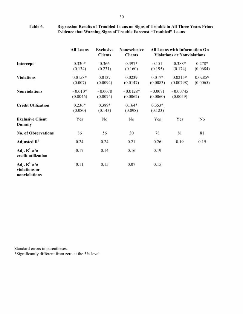
on violations, nonviolations, and utilization. The OLS results are shown in Table 6. First note that the10

coefficients have the expected signs: the coefficients on violations and utilization are significantly positive

and that on nonviolations is significantly negative. Taking all loans, including those on which we have no

information on violations or nonviolations, we find that the additional information on violations and

nonviolations adds 13 percentage points to the ability to separate troubled loans from untroubled loans.

(While the level of the adjusted R suggests there is still much to be explained, the adjusted R increases2 2

from 0.11 to 0.24 when violations and nonviolations are included in the OLS regression equation.) Note

that this information is useful for both exclusive clients and nonexclusive clients — it seems generally true

that the nonexclusive clients about which the bank collects this type of information are clients with whom

the bank has a strong relationship. On the other hand, the results are little changed if we exclude those

borrowers for which the bank lacks information about violations.

6.2 Speed with which the lender acts on signals from the bank balance

How quickly is this information used? Two pieces of evidence suggest that the information is

used relatively soon after it is available. Most of the information that determines whether a loan is

19

Since the results for downgrades at the final review date are virtually identical to the results for11

declarations of “trouble,” we omit them here for brevity; they are available upon request from the authors.

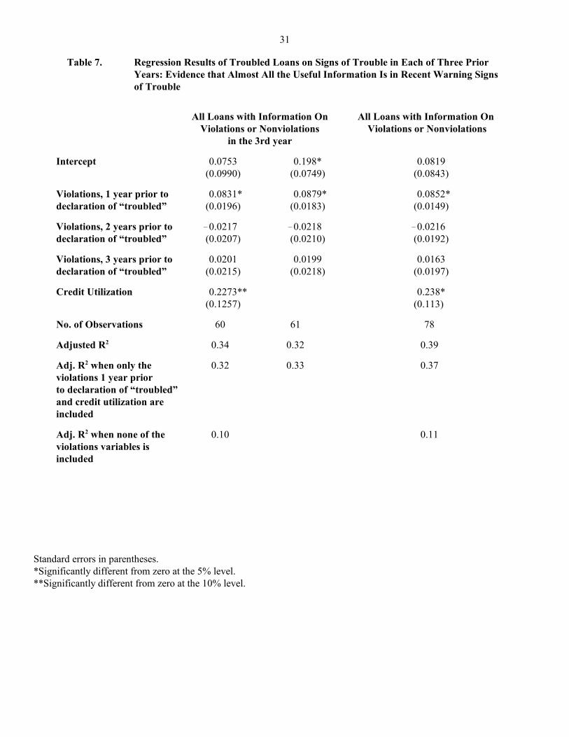
declared troubled is in violations in the most recent fiscal year before a declaration of trouble, as shown in

Table 7. Here we use our disaggregated measures of violations, violations_1, violations_2, and

violations_3, which give separate counts of the number of violations according to how far in advance they

took place before the loan was declared troubled (or before the final fiscal year for healthy borrowers).

The first column of Table 7 shows the regression results for the sample of loans excluding those for which

there was no information on violations during the third year prior to declaration. The third column

excludes loans where there is no information on violations in any of the three years. In both cases, the bulk

of the information is derived from the latest year: there is little difference in the adjusted R when only the2

number of violations in the year prior to declaration is included in the regression compared to when

violations in each of the three years prior are included.

Now consider downgrades of loans at the second review date, i.e., at least a year prior to when the

loan was declared troubled. Here we would expect that the most important information would be11

violations that occurred in the second year prior to the declaration that the loan is troubled, i.e., in the year

prior to downgrade. Table 8 shows that is indeed the case. Almost all the information provided by

violations in explaining downgrades in the second year is contained in violations that occurred in the year

prior to the downgrade. The adjusted R increases from 0.12 to 0.19 when the second-year violations are2

included. Here the information content of the second-year violations is somewhat lower when only

information on violations in the second year is included, but the information remains significant both

statistically and economically.

20

7. Information Available from the Monthly Valuations: How the Lender Reacts to Signs ofTrouble Gleaned from Checking Account Information

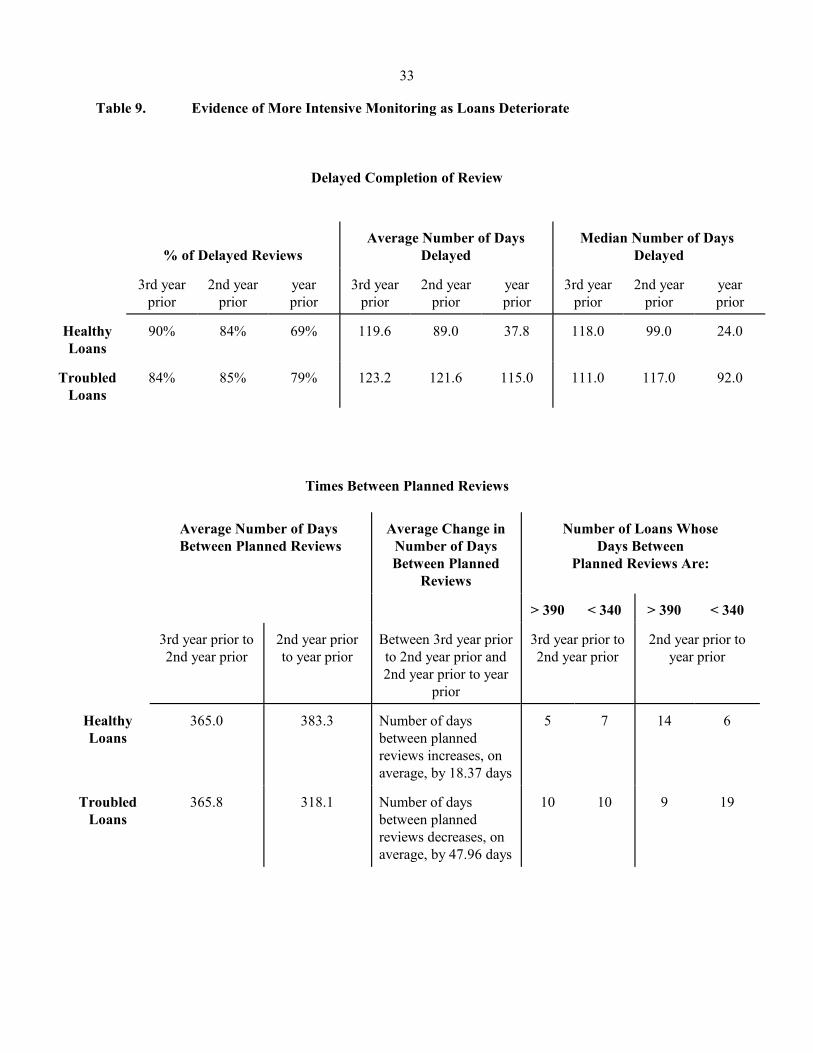
The last two tables show that the lender intensifies its monitoring of risky loans by spending more

time in loan review and by reducing the time between loan reviews. We examined the date on which a

credit review was completed relative to the date the review was planned to be completed and changes in

the frequency of planned reviews.

We expect that for loans that remain healthy, the completion of the credit review should be closer

to the planned completion date than for loans that have deteriorated in quality, since for healthy loans the

reviewer is less likely to find troublesome information that takes longer to evaluate. A credit review is

typically prolonged by the bank’s requests for additional information, such as more complete financial

statements and more detail about projected future disbursements from the bank account. Higher ranking

and presumably more experienced credit officers may become involved in the review, as the bank puts

more resources into monitoring. The bank may negotiate changes in the terms of the loan (for example,

asking for personal guarantees, such as the pledge of property), and such negotiations may take time. Thus

a lengthy delay between the expected loan review date and the sign-off by the loan officer is a strong sign

that monitoring has been intensified. Similarly, we expect that as a loan’s quality deteriorates, a bank

would want to examine the loan more frequently. Clearly, more frequent loan reviews are signs of more

intensive monitoring, as they require more data collection and analysis per unit of time.

7.1 Delayed completion of loan reviews

At the beginning of our data (t�3), healthy loans were chosen to be approximately as creditworthy

as the troubled loans. Over time, the healthy loans, on average, improve in apparent quality, while the

troubled loans, by definition, deteriorate. Table 9 shows that among healthy loans, delays in loan reviews

decrease compared to planned dates. This suggests that for loans that improve in quality, loan officers are

able to sign off on them closer to the review date, while for troubled loans, a delay remains. For example,

21

The modal number of days between planned reviews is about 365, a year. The 340- and 390-day12

cutoffs were chosen to represent periods significantly less and significantly more than a year.

in the third year prior to our reference date, 90 percent of healthy loans have a delayed review while in the

first year prior, only 69 percent do. Moreover the length of delay is cut by three-fourths — from about 120

days to 38 days, on average. In contrast, for loans that remain troubled, there is little lessening in the

number of delayed reviews or average length of delay.

7.2 Frequency of loan reviews

The lower part of Table 9 shows that over time, as the troubled loans worsen, the time planned

between credit reviews shortens on average, while for loans that improve in health, the time between

reviews increases. For example, for troubled loans, on average, the time between planned reviews

decreases by about 48 days over the three years, whereas for healthy loans, on average, planned reviews

become less frequent by about 18 days. Similarly, the number of troubled loans with fewer than 340 days

between planned reviews increases from 10 to 19 over the three years, while the number of healthy loans

with more than 390 days between planned reviews increases from 5 to 14.12

Table 10 replicates Table 9, but rather than sort the loans by whether they eventually are declared

troubled or not, we sort them on the number of violations they eventually have — in particular, we divide

the loans into two groups, those with violations less than or equal to the median level of violations over the

sample of loans and those with violations greater than the median level. (The median level is 2.5

violations.) This is information that the bank can discern from a firm’s checking account. In general, we

see results similar to those shown in Table 9, albeit a bit weaker. First, loans with greater numbers of

violations do have their credit reviews delayed relative to loans that have fewer violations: for example, in

the third year prior to our reference date, 90 percent of loans with fewer violations have a delayed review

while in the first year prior, only 69 percent do; the length of delay declines from 118 days, on average, to

48 days. For loans with a greater number of violations, there is little decline in the number of delayed

22

The right side of the bottom panel of Table 10 indicates there is little change over the three years13

in the number of high-violation loans whose planned reviews are significantly more than a year apart andthere is little change in those whose planned reviews are less than a year apart. However, over the threeyears, the number of low-violation loans whose reviews are significantly more than a year apart increases. This increase is about the same as the increase in the number of low-violation loans whose reviews aresignificantly less than a year apart.

Similar results are obtained if instead of dividing the loans into two groups, we divide them into14

three groups: violations = 0; 1 � violations � 10; and violations � 10.

reviews and a much smaller decline in the average length of delay, compared to loans with fewer

violations. The bottom panel shows that all loans have an increase in the frequency of their planned

reviews over the three years, but loans with a greater number of violations have a larger decline in the

number of days between planned reviews than do loans with a lower number of violations (approximately

17 days vs. 10 days).13,14

Overall, we see that borrowers whose borrowing needs exceed the bank’s valuations of accounts

receivable and inventories have their credit ratings downgraded at the next credit review. We have also

shown that, together with downgrading of credit, scrutiny appears to become stronger, with the credit

review itself dragging on and the time between reviews sometimes becoming shorter.

8. Conclusion

How are banks special? This paper has described the efforts of one Canadian bank to use

information in checking accounts to scrutinize the activities of small business borrowers. It is clear from

the evidence that the bank does use instances where borrowings exceed the bank’s own valuation of a

firm’s accounts receivable and inventories as a signal of deterioration in credit. Moreover, movements in

checking account balances are closely related to movements in the bank’s valuation of accounts receivable

and inventories, suggesting strongly that the checking account provides a relatively transparent window on

these aspects of a firm’s activity. Although our results pertain to only one bank, we believe that these

results taken together provide detailed micro-level evidence that banks’ handling of business transactions

23

enables them to be special lenders to firms.

24

Table 1. Outcomes of the Troubled Loans

Number of loans Percent of Loans

Bankruptcy of the firm 10 20%

Private liquidation of the firm 26 52%

Loan remained troubled 9 18%

Loan repaid 4 8%

Loan upgraded to healthy 1 2%

25

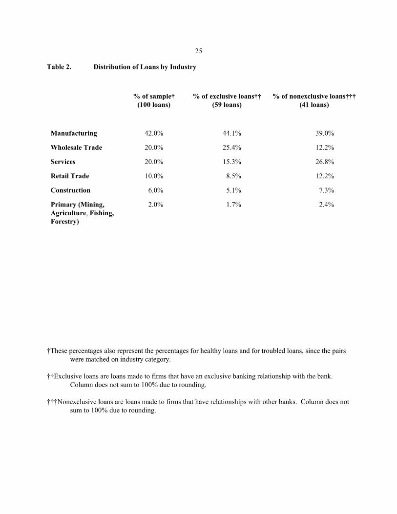
Table 2. Distribution of Loans by Industry

% of sample† % of exclusive loans†† % of nonexclusive loans†††(100 loans) (59 loans) (41 loans)

Manufacturing 42.0% 44.1% 39.0%

Wholesale Trade 20.0% 25.4% 12.2%

Services 20.0% 15.3% 26.8%

Retail Trade 10.0% 8.5% 12.2%

Construction 6.0% 5.1% 7.3%

Primary (Mining, 2.0% 1.7% 2.4%Agriculture, Fishing,Forestry)

†These percentages also represent the percentages for healthy loans and for troubled loans, since the pairswere matched on industry category.

††Exclusive loans are loans made to firms that have an exclusive banking relationship with the bank. Column does not sum to 100% due to rounding.

†††Nonexclusive loans are loans made to firms that have relationships with other banks. Column does notsum to 100% due to rounding.

26

Table 3A. Average Loan Size (in thousands C$)†

All Loans Healthy TroubledLoans Loans

All three years $1496.3 $1269.9 $1741.1(2485.8) (2828.8) (2024.3)

Three years prior to 1250.8 1126.4 1400.8reference date (2216.9) (2546.4) (1730.1)

Two years prior to 1500.9 1231.5 1783.7reference date (2388.7) (2608.3) (2099.8)

One year prior to 1679.4 1426.2 1938.5reference date (2745.7) (3229.3) (2113.2)

Exclusive Nonexclusive Exclusive, Nonexclusive, Exclusive, Nonexclusive,Loans Loans Healthy Healthy Troubled Troubled

Loans Loans Loans Loans

All three years $1365.8 $1745.3 $883.4 $1849.9 $1802.5 $1585.9(1994.6) (3207.9) (1612.5) (3945.6) (2197.5) (1491.1)

Three years prior to 1088.5 1593.0 797.3 1705.7 1396.6 1412.2reference date (1682.3) (3028.2) (1494.6) (3674.8) (1813.2) (1495.1)

Two years prior to 1364.9 1762.3 836.7 1843.7 1839.7 1646.6reference date (2096.2) (2853.8) (1686.6) (3516.8) (2307.0) (1472.2)

One year prior to 1592.1 1832.9 1014.2 1953.8 2056.4 1642.8reference date (2095.8) (3613.7) (1635.3) (4462.9) (2302.1) (1508.6)

†Loan size in thousands of Canadian dollars averaged over months and firms and standard deviation ofloan size in parentheses. For healthy loans, the reference date is the last time the firm’s credit file wasreviewed by the bank. For troubled loans, the reference date is the date when the loan was declaredtroubled.

27

Table 3B. Average Business Sales (in thousands C$)†

All Loans Healthy TroubledLoans Loans

All three years $16,898.0 $12,805.2 $20,990.8(36,811.3) (16,445.5) (49,327.0)

Three years prior to 15,885.3 10,846.5 20,924.0reference date (38,803.3) (10,836.6) (53,599.2)

Two years prior to 18,112.0 14,028.5 22,195.4reference date (42,688.4) (23,514.0) (55,631.4)

One year prior to 16,696.9 13,540.6 19,853.1reference date (30,621.6) (17,004.6) (39,812.2)

Exclusive Nonexclusive Exclusive, Nonexclusive, Exclusive, Nonexclusive,Loans Loans Healthy Healthy Troubled Troubled

Loans Loans Loans Loans

All three years $10,108.8 $26,667.9 $10,742.0 $15,040.4 $9,609.8 $43,083.4(9,379.2) (55,321.0) (10,363.2) (21,199.6) (8,657.9) (80,721.0)

Three years prior to 9,746.7 24,718.8 10,405.2 11,324.6 9,227.8 43,628.2reference date (10,120.9) (58,672.9) (10,448.1) (11,448.5) (9,987.4) (88,141.0)

Two years prior to 9,934.8 29,879.1 10,855.6 17,465.9 9,209.3 47,403.6reference date (9,497.2) (64,333.9) (10,958.3) (31,995.2) (8,272.5) (91,203.8)

One year prior to 10,644.8 25,406.0 10,965.2 16,330.6 10,392.3 38,218.2reference date (10,173.4) (45,154.4) (9,796.3) (22,273.3) (10,605.1) (63,923.3)

†Annual business sales in thousands of Canadian dollars averaged over firms and standard deviation ofbusiness sales in parentheses. For healthy loans, the reference date is the last time the firm’s credit file wasreviewed by the bank. For troubled loans, the reference date is the date when the loan was declaredtroubled.

28

Table 4. Number of Loans with a Given Credit Rating Over Time

Credit Ratings for Loans Not Declared Troubled within Sample

Time

ReservationsSuperior Standard Mild Average Strong

1 2 3 4 5

No. of Loans at t�3 4 15 23 0 8

No. of Loans at t�2 3 17 23 0 7

No. of Loans at t�1 4 19 18 0 9

Credit Ratings for Loans Declared Troubled at Time tReservations Troubled

Superior Standard Mild Average Strong Standard Severe Very SevereTime 1 2 3 4 5 6 7 8

No. of Loans at t�3 3 15 28 0 4 0 0 0

No. of Loans at t�2 1 2 14 1 31 0 0 0

No. of Loans at t�1 0 1 2 1 6 29 5 6

29

Table 5. Correlations and Variances of Monthly Changes in Bank Account Balances, Bank’sValuation of Accounts Receivable and Inventories†

Correlations Loans Loans Loans Loansbetweenchanges in:

Total Exclusive Nonexclusive Exclusive, Nonexclusive, Exclusive, Nonexclusive,Loans Loans Healthy Healthy Troubled Troubled

Bank Account 0.44* 0.49* 0.31* 0.54* 0.34* 0.44* 0.28*Balances andAccountsReceivable

Bank Account 0.19* 0.13* 0.28* 0.18* 0.36* 0.11* 0.19*Balances andInventories

Inventories �0.08* �0.10* �0.06 �0.10* 0.07 �0.10* �0.20*and AccountsReceivable

No. of 1327 1024 303 514 142 510 161Observations

Variances Loans Loans Loans Loansof changesin:

Total Exclusive Nonexclusive Exclusive, Nonexclusive, Exclusive, Nonexclusive,Loans Loans Healthy Healthy Troubled Troubled

Bank 0.00233 0.00209 0.00315 0.00207 0.00367 0.00211 0.00270AccountBalances

Accounts 0.00200 0.00204 0.00178 0.00226 0.00202 0.00182 0.00180Receivable

Inventories 0.00053 0.00040 0.00098 0.00023 0.00112 0.00057 0.00085

†Here, a positive bank account balance corresponds to a firm’s borrowings exceeding its deposits; a negative bank accountbalance corresponds to a firm’s deposits exceeding its borrowings. Thus, positive bank account balances indicate the firmis borrowing, on net. All data are monthly changes, scaled by dividing by annual sales. For troubled loans, this is sales inthe fiscal year three years prior to the loans’ being declared troubled, and for healthy loans, this is sales in the fiscal yearthree years prior to the last credit file review.

*Significantly different from zero at the 5% level.

30

Table 6. Regression Results of Troubled Loans on Signs of Trouble in All Three Years Prior:Evidence that Warning Signs of Trouble Forecast “Troubled” Loans

All Loans Exclusive Nonexclusive All Loans with Information OnClients Clients Violations or Nonviolations

Intercept 0.330* 0.366 0.397* 0.151 0.388* 0.278*(0.134) (0.231) (0.160) (0.195) (0.174) (0.0684)

Violations 0.0158* 0.0137 0.0239 0.017* 0.0215* 0.0285*(0.007) (0.0094) (0.0147) (0.0083) (0.00798) (0.0065)

Nonviolations �0.010* �0.0078 �0.0128* �0.0071 �0.00745(0.0046) (0.0074) (0.0062) (0.0060) (0.0059)

Credit Utilization 0.236* 0.389* 0.164* 0.353*(0.080) (0.143) (0.098) (0.123)

Exclusive Client Yes No No Yes Yes NoDummy

No. of Observations 86 56 30 78 81 81

Adjusted R 0.24 0.24 0.21 0.26 0.19 0.192

Adj. R w/o 0.17 0.14 0.16 0.192

credit utilization

Adj. R w/o 0.11 0.15 0.07 0.152

violations ornonviolations

Standard errors in parentheses.*Significantly different from zero at the 5% level.

31

Table 7. Regression Results of Troubled Loans on Signs of Trouble in Each of Three PriorYears: Evidence that Almost All the Useful Information Is in Recent Warning Signsof Trouble

All Loans with Information On All Loans with Information On Violations or Nonviolations Violations or Nonviolations

in the 3rd year

Intercept 0.0753 0.198* 0.0819(0.0990) (0.0749) (0.0843)

Violations, 1 year prior to 0.0831* 0.0879* 0.0852*declaration of “troubled” (0.0196) (0.0183) (0.0149)

Violations, 2 years prior to �0.0217 �0.0218 �0.0216declaration of “troubled” (0.0207) (0.0210) (0.0192)

Violations, 3 years prior to 0.0201 0.0199 0.0163declaration of “troubled” (0.0215) (0.0218) (0.0197)

Credit Utilization 0.2273** 0.238*(0.1257) (0.113)

No. of Observations 60 61 78

Adjusted R 0.34 0.32 0.392

Adj. R when only the 0.32 0.33 0.372

violations 1 year priorto declaration of “troubled”and credit utilization areincluded

Adj. R when none of the 0.10 0.112

violations variables isincluded

Standard errors in parentheses.*Significantly different from zero at the 5% level.**Significantly different from zero at the 10% level.

32

Table 8. Regression Results of Credit Downgrades in the 2nd Year Before Classification onSigns of Trouble in Each of the Three Prior Years: Evidence that Warning Signs ofTrouble Are Used Immediately

All Loans with Information on All Loans with Information onViolations or Nonviolations Violations or Nonviolations

in the 3rd Year in the 2nd Year

Intercept 0.1109 0.2561*(0.0751) (0.0665)

Violations, 1 year prior to 0.0375*classification (0.0184)

Violations, 2 years prior 0.051* 0.0386*to classification (0.021) (0.0167)

Violations, 3 years prior �0.0293to classification (0.0219)

No. of Observations 61 75

Adjusted R 0.19 0.062

Adj. R when violations 0.152

1 year prior toclassification is excluded

Adj. R when violations 2 0.122

years prior toclassification is excluded

Standard errors in parentheses.*Significantly different from zero at the 5% level.

33

Table 9. Evidence of More Intensive Monitoring as Loans Deteriorate

Delayed Completion of Review

% of Delayed Reviews Delayed DelayedAverage Number of Days Median Number of Days

3rd year 2nd year year 3rd year 2nd year year 3rd year 2nd year yearprior prior prior prior prior prior prior prior prior

Healthy 90% 84% 69% 119.6 89.0 37.8 118.0 99.0 24.0Loans

Troubled 84% 85% 79% 123.2 121.6 115.0 111.0 117.0 92.0Loans

Times Between Planned Reviews

Average Number of Days Average Change in Number of Loans WhoseBetween Planned Reviews Number of Days Days Between

Between Planned Planned Reviews Are:Reviews

> 390 < 340 > 390 < 340

3rd year prior to 2nd year prior Between 3rd year prior 3rd year prior to 2nd year prior to2nd year prior to year prior to 2nd year prior and 2nd year prior year prior

2nd year prior to yearprior

Healthy 365.0 383.3 Number of days 5 7 14 6Loans between planned

reviews increases, onaverage, by 18.37 days

Troubled 365.8 318.1 Number of days 10 10 9 19Loans between planned

reviews decreases, onaverage, by 47.96 days

34

Table 10. Evidence of More Intensive Monitoring in Response to Violations Based on theMonthly Bank Account Information†

Delayed Completion of Review

% of Delayed Reviews Delayed DelayedAverage Number of Days Median Number of Days

3rd year 2nd year year 3rd year 2nd year year 3rd year 2nd year yearprior prior prior prior prior prior prior prior prior

Loans with � 90% 80% 69% 118.1 98.9 48.1 118.0 99.0 51.0Median No.of Violations

Loans with > 85% 90% 79% 124.7 111.5 104.5 111.0 105.0 83.0Median No.of Violations

Times Between Planned Reviews

Average Number of Days Average Change in Number of Loans WhoseBetween Planned Reviews Number of Days Days Between

Between Planned Planned Reviews Are:Reviews

> 390 < 340 >390 < 340

3rd year prior to 2nd year prior Between 3rd year prior 3rd year prior to 2nd year prior to2nd year prior to year prior to 2nd year prior and 2nd year prior year prior

2nd year prior to yearprior

Loans with � 367.1 354.6 Number of days 5 6 10 12Median No. between plannedof Violations reviews decreases, on

average, by 9.94 days

Loans with > 363.6 347.7 Number of days 10 11 13 13Median No. between plannedof Violations reviews decreases, on

average, by 16.98 days

†The median number of violations is 2.5.

35

Appendix. The correlation between changes in the loan balance and the bank’s valuation ofaccounts receivable

To the extent that there is a high correlation between bank account balances and changes in

accounts receivable and inventories, changes in the firm’s bank account balance can be used to monitor a

firm’s operations.

We can derive approximate values of the correlations under certain simplifying assumptions. For

example, suppose the bank values the collateral represented by the accounts receivable at vR. (It applies a

haircut, since there is some chance the accounts receivable will not be collected.) Then, using equation (2)

in the text, the change in the bank’s valuation of accounts receivable is �vR � vR � vR = v[y (1+m) �t t t�1 t

z ]. If m is small, thent

�vR � v(y� z ). (A.1)t t t

The correlation between the change in the firm’s bank account balance and the change in the

bank’s valuation of the firm’s accounts receivable is

corr(�B , �vR ) = covariance(�B ,�vR ) / [variance(�B ) variance(�vR ) ].t t t t t t½ ½

Using equations (1) in the text and (A.1), and assuming r is small, then

corr(�B , �vR )t t

� cov(x � z + w , v(y � z )) / [var(x � z + w ) var(v(y� z )) ]t t t t t t t t t t½ ½

= [v cov(x ,y ) � v cov(x ,z ) � v cov(z ,y ) + v var(z ) + v cov(w ,y ) � v cov(w ,z )]/t t t t t t t t t t t

[var(x ) + var(z ) + var(w ) � 2cov(x ,z ) � 2cov(z ,w ) + 2cov(x ,w )] ×t t t t t t t t t½

[v var(y ) + v var(z ) � 2 v cov(y ,z )] .2 2 2t t t t

½

As an approximation, assume x , y , z , w are independent. Then,t t t t

corr(�B , �vR ) � [var(z )] / [var(x ) + var(z ) + var(w )] [var(y ) + var(z )] .t t t t t t t t½ ½

If other payments are not variable, i.e., var(w ) = 0 and the variance in goods purchased, goods sold, andt

payments received are similar, i.e., var(x ) = var(y ) = var(z ), thent t t

36

corr(�B , �vR ) � [var(z )] / [2var(z )] [2var(z )] = 1/2.t t t t t½ ½

A similar calculation can be performed for the correlation between the change in bank account balance and

the change in inventories.

Obviously, this is a rough approximation, based on a number of simplifying assumptions. But it

gives an idea of the magnitude of the correlation we would need to find to anticipate that the bank account

balance might be a useful indicator of firm operations.

37

References

Berger, Allen N. and Gregory F. Udell, 1995. “Relationship Lending and Lines of Credit in Small Firm

Finance,” Journal of Business, 68, 351-81.

Berlin, Mitchell and Loretta J. Mester, 1998. “On the Profitability and Cost of Relationship Lending,”

Journal of Banking and Finance, 22, 873-897.

Berlin, Mitchell and Loretta J. Mester, 1999. “Deposits and Relationship Lending,” Review of Financial

Studies, 12, 579-607.

Bhattacharya, Sudipto, and Gabriella Chiesa, 1995. “Proprietary Information, Financial Intermediation,

and Research Incentives,” Journal of Financial Intermediation, 4, 328-357.

Billet, Matthew T., and Mark J. Flannery and Jon A. Garfinkel, 1995. “The Effect of Lender Identity on a

Borrowing Firm’s Equity Return,” Journal of Finance, 2, 699-718.

Black, Fischer, 1975. “Bank Funds Management in an Efficient Market,” Journal of Financial Economics,

2, 323-339.

Diamond, Douglas and Raghuram Rajan, "Liquidity Risk, Liquidity Creation and Financial Fragility: A

Theory of Banking," Journal of Political Economy, 109, 287-327.

Fama, Eugene F. 1985. “What’s Different About Banks?” Journal of Monetary Economics, 15, 29-40.

Kashyap, Anil K., Raghuram Rajan, and Jeremy C. Stein, “Banks as Liquidity Providers: An Explanation

for the Coexistence of Lending and Deposit-Taking,” Journal of Finance, 57, February 2002, 33-

73.

Lummer, Scott L. and John J. McConnell, 1989. “Further Evidence on the Bank Lending Process and the

Capital Market Response to Bank Loan Announcements,” Journal of Financial Economics, 25,

99-122.

Merton, Robert C., 1977. “An Analytic Derivation of the Cost of Deposit Insurance and Loan Guarantees:

An Application of Modern Option Pricing Theory,” Journal of Banking and Finance, 1, 3-11.

38

Myers, Stuart C. and Nicholas S. Majluf, 1984. "Corporate Financing and Investment Decisions When

Firms Have Information that Investors Do Not Have," Journal of Financial Economics 13, 187-

221.

Nakamura, Leonard I., 1993a. “Commercial Bank Information: Implications for the Structure of Banking,”

pp. 131-160 in Michael Klausner and Lawrence J. White, ed., Structural Change in Banking,

Business One/Irwin, Homewood, IL.

Nakamura, Leonard I., 1993b. “Recent Research in Commercial Banking: Information and Lending,”

Financial Markets, Institutions, and Instruments, 2, 73-88.

Petersen, Mitchell A. and Raghuram G. Rajan, 1994. “The Benefits of Lending Relationships: Evidence

from Small Business Data,” Journal of Finance, 49, 3-37.

Preece, Diana and Donald J. Mullineaux, 1996. “Monitoring, Loan Renegotiability, and Firm Value: The

Role of Lending Syndicates,” Journal of Banking and Finance, 20, 577-94.