ANALYZING THREADS FOR SHARED

MEMORY CONSISTENCY

BY

ZEHRA NOMAN SURA

B.E., Nagpur University, 1998M.S., University of Illinois at Urbana-Champaign, 2001

DISSERTATION

Submitted in partial fulfillment of the requirementsfor the degree of Doctor of Philosophy in Computer Science

in the Graduate College of theUniversity of Illinois at Urbana-Champaign, 2004

Urbana, Illinois

c© Copyright by Zehra Noman Sura, 2004

Abstract

Languages allowing explicitly parallel, multithreaded programming (e.g. Java and

C#) need to specify a memory consistency model to define program behavior. The

memory consistency model defines constraints on the order of memory accesses in systems

with shared memory. The design of a memory consistency model affects ease of parallel

programming as well as system performance. Compiler analysis can be used to mitigate

the performance impact of a memory consistency model that imposes strong constraints

on shared memory access orders. In this work, we explore the capability of a compiler to

analyze what restrictions are imposed by a memory consistency model for the program

being compiled.

Our compiler analysis targets Java bytecodes. It focuses on two components: delay

set analysis and synchronization analysis. Delay set analysis determines the order of

shared memory accesses that must be respected within each individual thread of execu-

tion in the source program. We describe a simplified analysis algorithm that is applicable

to programs with general thread structure (MIMD programs), and has polynomial time

worst-case complexity. This algorithm uses synchronization analysis to improve the ac-

curacy of the results. Synchronization analysis determines the order of shared memory

accesses already enforced by synchronization in the source program. We describe a

dataflow analysis algorithm for synchronization analysis that is efficient to compute, and

that improves precision over previously known methods.

The analysis techniques described are used in the implementation of a virtual machine

that guarantees sequentially consistent execution of Java bytecodes. This implementa-

tion is used to show the effectiveness of our analysis algorithms. On many benchmark

programs, the performance of programs on our system is close to 100% of the perfor-

mance of the same programs executing under a relaxed memory model. Specifically, we

iii

observe an average slowdown of 10% on an Intel Xeon platform, with slowdowns of 7%

or less for 7 out of 10 benchmarks. On an IBM Power3 platform, we observe an average

slowdown of 26%, with slowdowns of 7% or less for 8 out of 10 benchmarks.

iv

This work is dedicated to my family.

v

Acknowledgments

This work owes its existence in part to all members of the Pensieve Compiler group:

Prof. David Padua, Prof. Sam Midkiff, Jaejin Lee, David Wong, and Xing Fang.

Prof. David Padua and Prof. Sam Midkiff have inspired, guided, encouraged, sup-

ported, scrutinized, and corrected this work. But most of all, I am grateful to them for

the things I have learnt over the past few years.

The many discussions with David Wong have been very helpful, both in developing

the techniques presented here, as well as implementing them. I am thankful for his

critiques, and for his support throughout this work.

Special thanks are due to Xing Fang for implementing the memory barrier insertion

phase and accomodating my feature requests.

Prof. David Padua has provided the opportunities for my work, and the freedom to

experiment. I appreciate his patience and support, and I am glad for his influence in

shaping the way I think.

I thank Prof. Marc Snir, Prof. Sarita Adve, and Prof. Laxmikant Kale for their

interest, encouragement, insights, and guidance. Their involvement has improved the

quality of this work.

I would also like to acknowledge Peng Wu. It was working with her that I first realized

the joys of research.

vi

Table of Contents

List of Tables . . . . . . . . . . . . . . . . . . . . . . . . . . . . . . . . . . . . . xi

List of Figures . . . . . . . . . . . . . . . . . . . . . . . . . . . . . . . . . . . . xii

1 Introduction . . . . . . . . . . . . . . . . . . . . . . . . . . . . . . . . . . . . 1

1.1 Memory Consistency Models . . . . . . . . . . . . . . . . . . . . . . . . . 2

1.1.1 Sequential Consistency Model . . . . . . . . . . . . . . . . . . . . 3

1.1.2 Relaxed Consistency Models . . . . . . . . . . . . . . . . . . . . . 4

1.1.3 Choosing a Consistency Model . . . . . . . . . . . . . . . . . . . . 5

1.2 Objectives and Strategy . . . . . . . . . . . . . . . . . . . . . . . . . . . 6

1.2.1 Compiling for a Memory Consistency Model . . . . . . . . . . . . 7

1.2.2 Our Compiler System . . . . . . . . . . . . . . . . . . . . . . . . . 9

1.2.3 Assumptions . . . . . . . . . . . . . . . . . . . . . . . . . . . . . . 12

1.3 Presentation Outline . . . . . . . . . . . . . . . . . . . . . . . . . . . . . 13

2 Delay Set Analysis . . . . . . . . . . . . . . . . . . . . . . . . . . . . . . . . 14

2.1 Problem Statement . . . . . . . . . . . . . . . . . . . . . . . . . . . . . . 14

2.2 Background . . . . . . . . . . . . . . . . . . . . . . . . . . . . . . . . . . 15

2.3 Simplified Delay Set Analysis Applied to Real Programs . . . . . . . . . 19

2.4 Illustrative Examples . . . . . . . . . . . . . . . . . . . . . . . . . . . . . 23

2.5 Implementation . . . . . . . . . . . . . . . . . . . . . . . . . . . . . . . . 25

2.5.1 Nodes in the Access Order Graph . . . . . . . . . . . . . . . . . . 25

2.5.2 Edges in the Access Order Graph . . . . . . . . . . . . . . . . . . 25

vii

2.5.3 Algorithm . . . . . . . . . . . . . . . . . . . . . . . . . . . . . . . 26

2.5.4 Complexity . . . . . . . . . . . . . . . . . . . . . . . . . . . . . . 28

2.5.5 Type Resolution . . . . . . . . . . . . . . . . . . . . . . . . . . . 28

2.6 Optimizing for Object Constructors . . . . . . . . . . . . . . . . . . . . . 29

2.7 Related Work . . . . . . . . . . . . . . . . . . . . . . . . . . . . . . . . . 32

3 Synchronization Analysis . . . . . . . . . . . . . . . . . . . . . . . . . . . . 34

3.1 Problem Statement . . . . . . . . . . . . . . . . . . . . . . . . . . . . . . 34

3.2 Thread Structure Analysis . . . . . . . . . . . . . . . . . . . . . . . . . . 36

3.2.1 Matching Thread Start and Join Calls . . . . . . . . . . . . . . . 37

3.2.2 Algorithm . . . . . . . . . . . . . . . . . . . . . . . . . . . . . . . 39

3.2.3 Using Thread Structure Information in Delay Set Analysis . . . . 45

3.2.3.1 Eliminating Conflict Edges . . . . . . . . . . . . . . . . 45

3.2.3.2 Ordering Program Accesses . . . . . . . . . . . . . . . . 46

3.2.3.3 An Example . . . . . . . . . . . . . . . . . . . . . . . . 49

3.3 Event-based Synchronization . . . . . . . . . . . . . . . . . . . . . . . . . 50

3.3.1 Algorithm . . . . . . . . . . . . . . . . . . . . . . . . . . . . . . . 51

3.3.2 Using Event-based Synchronization in Delay Set Analysis . . . . . 54

3.3.2.1 Limited Use in Java Programs . . . . . . . . . . . . . . . 55

3.4 Lock-based Synchronization . . . . . . . . . . . . . . . . . . . . . . . . . 56

3.4.1 Algorithm . . . . . . . . . . . . . . . . . . . . . . . . . . . . . . . 57

3.4.2 Using Lock Information in Delay Set Analysis . . . . . . . . . . . 60

3.5 Implementation . . . . . . . . . . . . . . . . . . . . . . . . . . . . . . . . 61

3.5.1 Exceptions . . . . . . . . . . . . . . . . . . . . . . . . . . . . . . . 63

3.5.2 Space Complexity . . . . . . . . . . . . . . . . . . . . . . . . . . . 65

3.6 Related Work . . . . . . . . . . . . . . . . . . . . . . . . . . . . . . . . . 66

4 Compiler Framework . . . . . . . . . . . . . . . . . . . . . . . . . . . . . . 68

4.1 Java Terminology . . . . . . . . . . . . . . . . . . . . . . . . . . . . . . . 68

4.2 The Jikes Research Virtual Machine and Compiler . . . . . . . . . . . . . 69

viii

4.3 Our Memory-model Aware Compiler . . . . . . . . . . . . . . . . . . . . 71

4.3.1 Thread Escape Analysis . . . . . . . . . . . . . . . . . . . . . . . 72

4.3.1.1 Algorithm . . . . . . . . . . . . . . . . . . . . . . . . . . 72

4.3.1.2 Optimization for Fast Analysis . . . . . . . . . . . . . . 77

4.3.2 Alias Analysis . . . . . . . . . . . . . . . . . . . . . . . . . . . . . 81

4.3.3 Inhibiting Code Transformations . . . . . . . . . . . . . . . . . . 82

4.3.4 Memory Barrier Insertion . . . . . . . . . . . . . . . . . . . . . . 85

4.3.5 Specialization of the Jikes RVM Code . . . . . . . . . . . . . . . . 87

4.3.6 Dynamic Class Loading . . . . . . . . . . . . . . . . . . . . . . . 89

4.3.6.1 Incremental Analysis . . . . . . . . . . . . . . . . . . . . 89

4.3.6.2 Method Invalidation . . . . . . . . . . . . . . . . . . . . 93

4.4 Related Work . . . . . . . . . . . . . . . . . . . . . . . . . . . . . . . . . 95

5 Experimental Evaluation . . . . . . . . . . . . . . . . . . . . . . . . . . . . 97

5.1 Benchmark Programs . . . . . . . . . . . . . . . . . . . . . . . . . . . . . 97

5.2 Performance Impact . . . . . . . . . . . . . . . . . . . . . . . . . . . . . 101

5.2.1 Execution Times . . . . . . . . . . . . . . . . . . . . . . . . . . . 102

5.2.2 Effect of Escape Analysis . . . . . . . . . . . . . . . . . . . . . . . 107

5.2.3 Accuracy of Delay Set Analysis . . . . . . . . . . . . . . . . . . . 109

5.2.4 Memory Barrier Instruction Counts . . . . . . . . . . . . . . . . . 111

5.2.5 Optimizations and Memory Usage . . . . . . . . . . . . . . . . . . 113

5.2.6 Effect of Synchronization Analysis . . . . . . . . . . . . . . . . . . 116

5.3 Analysis Times . . . . . . . . . . . . . . . . . . . . . . . . . . . . . . . . 117

5.3.1 Effect of Adaptive Re-compilation for Optimization . . . . . . . . 120

6 Conclusion . . . . . . . . . . . . . . . . . . . . . . . . . . . . . . . . . . . . . 123

6.1 Contributions . . . . . . . . . . . . . . . . . . . . . . . . . . . . . . . . . 123

6.2 Open Problems . . . . . . . . . . . . . . . . . . . . . . . . . . . . . . . . 125

ix

Bibliography . . . . . . . . . . . . . . . . . . . . . . . . . . . . . . . . . . . . . 127

Vita . . . . . . . . . . . . . . . . . . . . . . . . . . . . . . . . . . . . . . . . . . . 139

x

List of Tables

5.1 Benchmark Characteristics . . . . . . . . . . . . . . . . . . . . . . . . . . 101

5.2 Slowdowns for the Intel Xeon Platform . . . . . . . . . . . . . . . . . . . 104

5.3 Slowdowns for the IBM Power3 Platform . . . . . . . . . . . . . . . . . . 106

5.4 Delay Edge Counts for the Intel Xeon Platform . . . . . . . . . . . . . . 109

5.5 Delay Edge Counts for the Power3 Platform . . . . . . . . . . . . . . . . 110

5.6 Memory Fences Inserted and Executed on the Intel Xeon Platform . . . . 111

5.7 Sync Instructions Inserted and Executed on the Power3 Platform . . . . 112

5.8 Optimizations Inhibited and Memory Overhead . . . . . . . . . . . . . . 113

5.9 Analysis Times in Seconds for the Intel Xeon Platform . . . . . . . . . . 118

5.10 Analysis Times in Seconds for the Power3 Platform . . . . . . . . . . . . 120

5.11 Number of Methods Re-compiled for Adaptive Optimization . . . . . . . 121

5.12 Analysis Times in Seconds With No Re-compilation for Optimization . . 121

xi

List of Figures

1.1 Unordered Shared Memory Accesses . . . . . . . . . . . . . . . . . . . . . 2

1.2 Busy-wait Synchronization Example . . . . . . . . . . . . . . . . . . . . . 6

1.3 Memory Barrier Example . . . . . . . . . . . . . . . . . . . . . . . . . . 9

1.4 Components of Our Memory-Model Aware Compiler . . . . . . . . . . . 10

2.1 Access Order Graphs for a Multithreaded Program . . . . . . . . . . . . 17

2.2 Re-orderings Allowed Under Sequential Consistency . . . . . . . . . . . . 17

2.3 Simplified Cycle Detection . . . . . . . . . . . . . . . . . . . . . . . . . . 22

2.4 Example to Illustrate Cumulative Ordering . . . . . . . . . . . . . . . . . 23

2.5 Example to Illustrate a Non-minimal Cycle . . . . . . . . . . . . . . . . . 24

2.6 Example to Illustrate Conservatism of Our Simplified Approach . . . . . 24

2.7 Algorithm for Simplified Delay Set Analysis . . . . . . . . . . . . . . . . 27

2.8 Delay Edges Related to the Point an Object Escapes . . . . . . . . . . . 29

2.9 Effect of Delay Set Analysis Optimization for Constructor Methods . . . 31

3.1 Use of Synchronization to Break Delay Cycles . . . . . . . . . . . . . . . 35

3.2 Orders Implied by Program Thread Structure . . . . . . . . . . . . . . . 37

3.3 Matching join() for a start() in a Loop . . . . . . . . . . . . . . . . . 38

3.4 Effect of Thread Start and Join Calls . . . . . . . . . . . . . . . . . . . . 41

3.5 Gen and Kill Functions for Thread Structure Analysis . . . . . . . . . . 42

3.6 Algorithm to Compute Orders for Thread Starts and Joins . . . . . . . . 43

3.7 Orders Inferred From Thread Structure Analysis . . . . . . . . . . . . . . 48

3.8 Example to Infer Orders From Thread Structure Synchronization . . . . 50

xii

3.9 Algorithm to Compute Orders for Event-based Synchronization . . . . . 53

3.10 Algorithm to Compute Sets of Acquired Locks . . . . . . . . . . . . . . . 57

3.11 Possible Cycles for a Conflict Edge Between Synchronized Accesses . . . 60

3.12 Flow Graph With Normal Control Flow and Exception Control Flow . . 64

3.13 Factored Control Flow Graph in the Jikes RVM . . . . . . . . . . . . . . 64

4.1 Performance of the Jikes RVM and Commercial JVMs . . . . . . . . . . 70

4.2 Different Calling Contexts of Methods for Escape Analysis . . . . . . . . 77

4.3 Escape Analysis Algorithm . . . . . . . . . . . . . . . . . . . . . . . . . . 78

4.4 Effect of Statements in Escape Analysis Algorithm . . . . . . . . . . . . 79

4.5 Optimizing Escape Analysis for Fast Convergence . . . . . . . . . . . . . 80

4.6 Loop Invariant Code Motion Example . . . . . . . . . . . . . . . . . . . . 83

4.7 Loop Unrolling Example . . . . . . . . . . . . . . . . . . . . . . . . . . . 84

4.8 Common Subexpression and Load Elimination Example . . . . . . . . . . 84

4.9 Example for Memory Barrier Insertion . . . . . . . . . . . . . . . . . . . 87

4.10 Determining the Set of Methods to Invalidate . . . . . . . . . . . . . . . 94

5.1 Slowdowns for Sequential Consistency on Intel Xeon . . . . . . . . . . . . 103

5.2 Slowdowns for Sequential Consistency on IBM Power3 . . . . . . . . . . 106

5.3 Slowdowns for SC Using the Jikes RVM Escape Analysis . . . . . . . . . 108

5.4 Example for Loop Invariant Code Motion . . . . . . . . . . . . . . . . . . 114

5.5 Example for Load Elimination . . . . . . . . . . . . . . . . . . . . . . . . 115

5.6 Effect of Thread Structure Analysis and Locking Synchronization . . . . 116

xiii

Chapter 1

Introduction

In shared memory multiprocessing systems, multiple threads of execution can communi-

cate with one another by reading and writing common memory locations. When explicit

synchronization does not define a total order for all shared memory accesses in a pro-

gram, the result of an execution can vary depending on the actual order in which shared

memory accesses are performed by different threads. For example, consider the system

in Figure 1.1. Processors 1 and 2 both access the same memory locations X and Y, and

issue memory access requests independent of one another. Memory locations X and Y

initially contain zero. Since there are no dependences between the instructions executed

by each individual processor, the instructions A, B, C, and D may be completed in

memory in any order. Depending on what this order is, the variables t1 and t2 may

contain any combination of 0 and 1 values when both threads terminate.

A memory consistency model defines the order of shared memory accesses that dif-

ferent threads must appear to observe. In this work, we are interested in a compiler

that takes the memory consistency model into account and generates code that ensures

required shared memory access orders are maintained during execution.

1

C

UnorderedMemory Accesses

D

SHAREDMEMORY

Read

X

Read

YWrite X

Write Y

Memory Controller

Location X: 0Location Y: 0

B

A

PROCESSOR 1 PROCESSOR 2t1 = Y

t2 = XY = 1

X = 1

Thread 2Thread 1

Figure 1.1: Unordered Shared Memory Accesses

1.1 Memory Consistency Models

A memory consistency model constrains the order of execution of shared memory accesses

in a multithreaded program, and helps determine what constitutes a correct execution.

A memory access is an instruction that reads from or writes into some memory lo-

cation(s). The value contained in a memory location may change when an instruction

writes to that location. Throughout the execution of a program, each memory location

will assume a sequence of values, one after another. Each value in this sequence is the

result of the execution of an instruction that writes to the memory location. We refer to

the sequence of values corresponding to a memory location L as Sequence(L).

Definition 1.1.1 Given a memory location L and a value V contained in Sequence (L),

we say V is available to a processor when all subsequent reads of L by the processor

return a value that does not precede V in Sequence (L).

2

Definition 1.1.2 Given a memory location L, an access to L is complete if the value

that it reads from or writes into L is available to all processors in the system.

Two memory accesses may be re-ordered if the second access is issued by a processor

before the first access is complete. In a shared memory system, system software can cause

shared memory accesses to be re-ordered when it compiles programs into machine code.

Also, hardware can re-order shared memory accesses when it executes machine code.

Definition 1.1.3 A hardware memory model defines shared memory access orders

that are guaranteed to be preserved when the hardware executes a program.

Definition 1.1.4 A programming language memory model defines shared memory

access orders that are guaranteed to be preserved on any system that executes a program

written in that language.

1.1.1 Sequential Consistency Model

Sequential consistency [Lam79] is a memory consistency model that is considered to be

the simplest and most intuitive. It imposes both atomicity and ordering constraints on

shared memory accesses.

Definition 1.1.5 An access A is atomic if, while it is in progress, other accesses that

concurrently execute with A cannot modify or observe intermediate states of the memory

location accessed by A. [Sin96]

As defined in [SS88], a program segment is the code executed by a single thread of a

multithreaded program. Sequential consistency requires that:

“The outcome of an execution of a parallel code is as if all the instructions were exe-

cuted sequentially and atomically. Instructions in the same program segment are executed

in the sequential order specified by this segment; the order of execution of instructions

belonging to distinct segments is arbitrary” [SS88].

3

Sequential consistency is a strong memory consistency model since it imposes strong con-

traints on re-ordering shared memory accesses within a program segment. If the system

in Figure 1.1 is sequentially consistent, then all orders for shared memory instructions

A, B, C, and D are no longer allowed. Specifically, any order in which both B occurs

before C, and D occurs before A is prohibited, since it results in t1=1 and t2=0, which

is not a seqentially consistent outcome.

1.1.2 Relaxed Consistency Models

Relaxed memory consistency models relax the requirement that all instructions in a pro-

gram segment appear to execute in the sequential order in which they are specified. These

models allow some instructions within a program segment to complete out of order.

An example of a relaxed consistency model is weak consistency [DSB88]. Weak con-

sistency distinguishes each access as a regular data access or a special synchronization

access. It requires that [Sin96]:

1. All synchronization accesses must obey sequential consistency semantics.

2. All write accesses that occur in the program code before a synchronization access

must be completed before the synchronization access is allowed.

3. All synchronization accesses that occur in the program code before a non-synchronization

access must be completed before the non-synchronization access is allowed.

4. All orders due to data dependences within a thread are enforced. Thus, two accesses

in a thread must appear to complete in the sequential order specified by the program

source if they both access the same memory location, and at least one of them is a

write.

The IBM Power3 architecture supports weak consistency and, as a result, allows any

order of shared memory instructions A, B, C, and D from the example in Figure 1.1.

4

1.1.3 Choosing a Consistency Model

Relaxed consistency models impose fewer constraints than sequential consistency on the

order of shared memory accesses. This allows more instruction re-ordering, increasing

the potential for instruction level parallelism and better performance. However, it is

usually easier to understand the sequence of events in program code when using sequential

consistency, since it allows fewer valid re-orderings of shared memory accesses. Thus, it

seems likely that using sequential consistency will improve productivity over relaxed

consistency models, both in development and maintenance of multithreaded program

code.

Until the last decade, memory consistency models were mostly studied in the context

of hardware architectures. They were of concern only to system programmers and de-

signers, and architects. They had to cater to performance more than programmability.

Most multiprocessor systems implement some relaxed memory consistency model [AG96]

as the hardware memory model.

With the popularity of languages like Java and C# that incorporate explicit seman-

tics of memory consistency models, programming language memory models have become

an issue for a large part of the programmer community, and for language and compiler

designers. The issues facing programmers with different memory consistency models are

illustrated by the busy-wait construct which is used to synchronize accesses to Data in

Figure 1.2. The code fragment in Figure 1.2 provides busy-wait synchronization in a

sequentially consistent system. However, for most relaxed memory consistency systems,

this busy-wait synchronization will not work as expected. For a language that supports

a relaxed memory consistency model, the compiler can move Flag = 1 prior to “Data =

...”, breaking the desired synchronization. Even if the compiler does not break the syn-

chronization with an optimization, the target architecture may break the synchronization

if it implements a relaxed consistency model that re-orders the two write instructions.

5

...Data = ...;Flag = 1;

...while (Flag==0) wait;

... = Data;

Figure 1.2: Busy-wait Synchronization Example

With widespread use of multithreaded programming, the trade-offs between produc-

tivity and performance have taken on increased importance. In [Hil98], Hill addresses

these concerns, and advocates sacrificing some performance for ease-of-use. Sequential

consistency may be the ideal choice for a programming language memory model because

of its ease-of-use. However, we do not know how this choice impacts performance. This

is because sequential consistency does not explicitly prohibit re-ordering of shared mem-

ory accesses in a thread; it only requires that an execution maintain the illusion that

no shared memory accesses in a thread have been re-ordered. A compiler can analyze

the program to determine re-orderings that do not break the illusion of sequential con-

sistency. Then, the performance of program execution will depend on the accuracy with

which these allowed re-orderings are determined, and how they compare with the number

of re-orderings allowed under a relaxed consistency model.

1.2 Objectives and Strategy

Our aim in this thesis is to minimize the loss of performance when sequential consistency

is the programming language memory model. We develop analysis techniques for this

purpose and apply them in a just-in-time compiler for Java bytecodes. We target Java

since it is a general-purpose programming language in widespread use, that also allows

multithreaded programming.

For a system that implements a given programming language memory model in soft-

ware, performance of the generated code tends to degrade with an increase in the number

6

of shared memory access orders that must be enforced. This is because there is a po-

tential decrease in the amount of instruction-level parallelism when a greater number of

accesses are ordered. Also, the memory barrier instructions that are used to enforce these

orders have an intrinsic cost. The results presented in Section 5.2.1 and Section 5.2.3

support this. On an Intel Xeon-based system, a 90% reduction in the number of orders

to enforce results in a performance improvement of 26 times on average. On an IBM

Power3-based system, a 42% reduction in the number of orders to enforce results in a

performance improvement of 84% on average. It is therefore desirable to minimize the

number of orders that must be enforced. The best method known to identify orders

that must be enforced is delay set analysis [SS88]. Delay set analysis considers thread

interactions through shared memory, and determines the minimum number of orders of

shared memory accesses that must be respected within each individual thread in the

source program.

Precise delay set analysis was first described by Shasha and Snir in [SS88]. Their

analysis assumes straight-line code where the location in memory corresponding to each

access is unambiguous, and accesses performed by each thread in the program are individ-

ually accounted for. However, as discussed in Section 2.3, a Java compiler that performs

delay set analysis must be able to handle branching control flow, imperfect memory

disambiguation, and an unknown or very large number of program threads. Moreover,

Krishnamurthy and Yelick [KY96] prove that Shasha and Snir’s precise delay set analysis

is NP-complete, and the execution time is exponential in the number of threads.

Our strategy is to use a simplified delay set analysis that takes into account explicit

synchronization programmed by the user.

1.2.1 Compiling for a Memory Consistency Model

Well-synchronized programs include explicit synchronization such that the set of valid

shared memory access orders is the same for sequential consistency and relaxed con-

7

sistency models. In practice, most programs are written to be well-synchronized. This

means that a compiler with perfect analysis capability should be able to produce code for

a system that uses sequential consistency as the programming language memory model,

such that the performance of this code is close to that of code generated for a system that

uses a relaxed consistency model. However, analyses are not perfect. So, performance

depends on the precision with which a compiler can determine the shared memory access

orders that must be enforced to honor the programming language memory model.

The example in Figure 1.2 illustrates the challenges faced by a memory model aware

compiler. To generate correct code, it must:

1. Inhibit itself from performing some code optimizations: These are optimizations

that affect the values a processor reads from or writes into shared memory, and

cause the resulting execution to be invalid according to the programming language

memory model. Examples of such optimizations are dead code elimination, common

subexpression elimination, register allocation, loop invariant code motion, and loop

unrolling [MP90]. In Figure 1.2, allocating Flag to a register will cause the while

loop to never terminate when the value of Flag assigned to the register is zero.

2. Enforce the programming language memory model on the target architecture: To

generate correct code efficiently, the compiler must determine which accesses in each

thread are to memory locations also accessed in another thread, and which of those

accesses must be completed in the same order specified by the program code. These

orders can be enforced by appropriately inserting synchronization instructions in

the machine code generated.

Languages and hardware provide constructs that the user, or compiler, may use to

prevent re-ordering of shared memory accesses – such as synchronized in Java [GJS96]

and machine instructions like fences on the Intel Xeon architecture [IA3], or syncs on

the IBM Power3 architecture [PPCb]. In this thesis, we refer to hardware instructions

for memory synchronization as memory barriers.

8

...Data = ...;syncFlag = 1;

...while (Flag==0) wait;

sync...= Data;

Figure 1.3: Memory Barrier Example

Definition 1.2.1 A memory barrier is a hardware instruction used to synchronize

shared memory accesses. It defines two sets of memory accesses:

1. A set of accesses that are issued by a processor before it issues the memory barrier.

2. A set of accesses that will be issued by a processor after it has issued the memory

barrier.

The memory barrier instruction guarantees that all accesses in the first set complete

before any access in the second set begins execution.

Figure 1.3 shows the code in Figure 1.2 with sync instructions inserted to enforce

sequential consistency. These instructions guarantee that the set of all memory accesses

performed in a thread before the sync are complete before the thread executes any

memory access after the sync.

1.2.2 Our Compiler System

In Figure 1.4, we give an overview of the components in our compiler system. We im-

plement it using the Jikes Research Virtual Machine from IBM, described in Section 4.2.

The components in the figure are the analyses and transformations that we add to sup-

port sequential consistency. Given a source program, the program analysis component

determines shared memory access orders that must be enforced so that sequential con-

sistency is not violated. The code transformations component uses the analysis results

9

Ordering Constraintsto Enforce

Alias Analysis

Synchronization Analysis

Delay Set Analysis

Thread Escape Analysis

SourceProgram

HardwareMemory Model

TargetMachine Code

Elimination Transformations

ProgramAnalysis

Code Re−ordering and Code

Memory Barrier Insertion

Jikes RVM

SC ModelCompiler for

Figure 1.4: Components of Our Memory-Model Aware Compiler

10

to judiciously optimize the program without changing any of the required access orders.

In particular, we examine each optimization and augment it so that when compiling for

sequential consistency, an optimization instance is not performed if it violates an access

order that needs to be enforced. The memory barrier insertion component also uses the

analysis results, along with knowledge of the hardware memory model, to generate code

that enforces the required access orders. It does this by emitting memory barriers for

access orders that are not enforced by the hardware memory model but are required by

sequential consistency [FLM03].

Program Analyses

Delay set analysis determines orders within a thread that must be enforced to honor the

semantics of the memory consistency model. We describe our delay set analysis algorithm

in Chapter 2. To perform delay set analysis, we require several other supporting analyses:

synchronization analysis, thread escape analysis, and alias analysis.

Synchronization analysis determines orders that are enforced by explicit synchro-

nization in the program. This helps improve the precision of delay set analysis. Our

synchronization analysis is decribed in detail in Chapter 3.

Thread escape analysis identifies shared memory accesses that reference an object that

may be accessed by more than one thread. Only these accesses need to be considered when

performing delay set analysis. We describe our thread escape analysis in Section 4.3.1.

Alias analysis determines if two accesses may refer to the same memory location. This

information is required by delay set analysis. We describe our approach to alias analysis

in Section 4.3.2.

11

1.2.3 Assumptions

In our work, we focus on the high-level analysis that determines pairs of accesses that

must not be re-ordered to enforce memory consistency. In previous work [FLM03], the

back-end memory barrier insertion phase (Section 4.3.4) was implemented in the Jikes

Research Virtual Machine. We re-use this implementation in our experiments to enforce

the orders determined by our high-level analysis.

Besides ordering constraints, sequential consistency requires atomic execution of shared

memory accesses (Section 1.1.1). We assume the following in our implementation:

1. The hardware architecture supports atomic access of multiple locations in memory

that are read or written by a single instruction. Java bytecodes are specified such

that each instruction reads or writes a single primitive or reference value. All such

values are either 8-bit, 16-bit, 32-bit, or 64-bit wide. The IBM Power3 system and

the Intel Xeon system that we use in our experiments by default provide atomic

access for 8-bit, 16-bit, 32-bit and 64-bit wide locations that are correctly aligned on

8-bit, 16-bit, 32-bit and 64-bit address boundaries, respectively [PPCb, IA3]. This

covers atomic access for all instructions in Java bytecodes that access memory.

2. The hardware architecture makes available memory barrier instructions that can

be used to:

(a) order two accesses within a processor: a memory barrier between two accesses

prevents the second access from being issued by the processor until it has

finished executing the first access.

(b) provide total ordering of an access across multiple processors: a memory bar-

rier inserted between two accesses ensures that the first access completes with

respect to all processors in the system before the second access is issued. This

is used to honor the property of sequential consistency that specifies a total

ordering over all instructions in the program.

12

This requirement is satisfied for the systems we use in our experiments: by sync

instructions on the IBM Power3 system [PPCa], and mfence, lfence, and sfence

instructions on the Intel Xeon system [IA3].

1.3 Presentation Outline

This thesis is structured as follows:

• In Chapter 2, we describe delay set analysis and our simplified algorithm for it.

• In Chapter 3, we discuss how we perform synchronization analysis, and how we use

the analysis results in delay set analysis.

• In Chapter 4, we present the components required in our memory-model aware

compiler system, and describe their implementation.

• In Chapter 5, we report on the performance of our system when sequential con-

sistency is used as the programming language memory model, as opposed to weak

consistency.

• Finally, in Chapter 6, we present our conclusions.

13

Chapter 2

Delay Set Analysis

2.1 Problem Statement

If shared memory accesses are re-ordered, the resulting program computation may not

be equivalent to the program computation without the re-ordering.

Definition 2.1.1 “Two computations are equivalent if, on the same inputs, they pro-

duce identical values for output variables at the time output statements are executed and

the output statements are executed in the same order.”[AK02]

A memory consistency model defines constraints on the order of shared memory

accesses. Delay set analysis determines those orders that must be respected within each

individual thread in the source program, to ensure that the result of a program execution

is always valid according to the memory consistency model. The analysis results in a

delay set, i.e. a set of ordered pairs of shared memory accesses such that the second access

in each pair must be delayed until the first access has completed.

14

2.2 Background

In [SS88], Shasha and Snir show how to find the minimal delay set that gives orders that

must be enforced to guarantee all executions are valid for sequential consistency. Their

analysis is precise since they assume:

• straight-line code with no branching control flow,

• the target location in memory for each access is unambiguously known when the

analysis is performed, and

• the number of threads in the program is known when the analysis is performed.

In this section, we explain how this precise delay set analysis is performed.

Sequential consistency requires atomic execution of multiple accesses corresponding to

the same program instruction. The analysis described in [SS88] explicitly determines the

minimal set of orders that need to be enforced for atomicity requirements to be satisfied.

In our work, we aim to provide sequential consistency for a Java virtual machine. As

discussed in Section 1.2.3, each instruction (or bytecode) executed by a Java virtual

machine accesses at most one location in memory 1. We assume the hardware architecture

supports atomic access of locations accessed by any single Java instruction. Thus, we

do not need the portion of the analysis in [SS88] that determines orders that guarantee

atomicity of multiple accesses corresponding to a single instruction.

Shasha and Snir’s precise analysis uses a graph that we call the access order graph.

Definition 2.2.1 An access order graph is a graph G = (V, P, C), where:

1The synchronized keyword in Java provides programmers the facility to specify that some set ofinstructions must execute atomically with respect to some other set of instructions. By default, ourcompiler explicitly enforces all orders that are specified in the program using this synchronized keyword.As described in Section 3.4, our analysis exploits these orders to reduce the number of orders in thedelay set that it computes.

15

• V is the set of nodes in the graph. There is one node for each shared memory access

performed by each thread in the program.

• P is the set of all program edges in the graph.

• C is the set of all conflict edges in the graph.

Definition 2.2.2 A program edge is a directed edge from node A to node B, where

A and B represent shared memory accesses performed by the same thread, and program

semantics require A to appear to complete before B.

Definition 2.2.3 A conflict edge is an edge between two nodes that access the same

memory location, and at least one of them writes to the location being accessed.

Program edges capture the ordering requirements specified by the programming lan-

guage memory model, as well as those specified by the control flow semantics of a

program2. When sequential consistency is the memory model, program edges exist be-

tween an access and all other accesses that follow it in sequential program order.

Conflict edges represent points where instructions in the program may communicate

through shared memory, and the execution of one instruction may affect another. Con-

flict edges within the same thread of execution are directed data dependences, whose

order is determined by traditional dependence analysis. These orders are enforced by

default during execution on the platforms that we use for our experiments. In general,

conflict edges between accesses in different threads are not directed. Threads execute

concurrently, and either one of two accesses related by a conflict edge may be executed

first. The outcome of an execution may differ depending on which of these two accesses

executes first.

Figure 2.1 shows a multithreaded program represented as an access order graph. Solid

edges are program edges and dashed edges are conflict edges. Part (a) of the figure shows

2The precise exception model in Java also contributes to its control flow semantics.

16

the access order graph for a program assuming sequential consistency, so that all accesses

within a thread are ordered. Part (b) of the figure shows the access order graph for the

same program assuming weak consistency, so that only accesses to the same memory

location are related by edges in the graph.

A

B A’

B’X = ...

Y = 1 ... = X

while (Y==0) wait;

Thread 1 Thread 2

A’

B’A

B ... = X

while (Y==0) wait;X = ...

Y = 1

Thread 1 Thread 2

(a) Sequential Consistency (b) Weak Consistency

Figure 2.1: Access Order Graphs for a Multithreaded Program

Consider a program edge from an access A to an access B. This program edge says

that A must appear to complete before B in a valid program execution. However, during

execution, the thread performing accesses A and B may re-order them if this change is

not observable, i.e. the program computation with the re-ordering is equivalent to the

program computation without the re-ordering. Thus, assuming sequential consistency

for both programs shown in Figure 2.2, the two accesses A and B in the code in part (a)

may be re-ordered, but this is not the case for the code in part (b).

A’

B’B

A

Y = 1

X = 1

t2 = Y

t1 = X

Thread 1 Thread 2

B’

A’B

A

Y = 1

X = 1

t2 = X

t1 = Y

Thread 1 Thread 2

(a) A and B May Be Re-ordered (b) A and B May Not Be Re-ordered

Figure 2.2: Re-orderings Allowed Under Sequential Consistency

Theorem 2.2.1 For a program edge from A to B, re-ordering A and B may affect the

program computation only if the access order graph contains a path from B to A that

begins and ends with a conflict edge.

17

Suppose there are no intra-thread dependences between A and B, and B executes

first. If no other instruction accesses memory location A or B, then this re-ordering has

no effect on program execution. The only way the execution of B may be noticed by

another instruction and affect program execution is if there is a conflict edge between B

and some access, say B’, that accesses the same location as B. Similarly, the execution

of A may be noticed by another instruction only if there is some other conflicting access

A’. Thus, for the re-ordering of A and B to be evident, there must be an execution of the

program in which access B occurs before access B’, B’ occurs before A’, and A’ occurs

before A. In terms of the access order graph, this translates to a path from B to A, such

that this path begins and ends with a conflict edge. Therefore, if the access order graph

contains a program edge from A to B, as well as a path from B to A that begins and

ends with a conflict edge (as in Figure 2.2(b) but not in Figure 2.2(a)), then re-ordering

the two accesses A and B may affect the program computation.

Note that the delay edge A to B and the path from B to A form a cycle in the access

order graph. Shasha and Snir’s algorithm to find delay pairs looks for such cycles in the

access order graph. Theorem 3.9 of [SS88] shows that it is sufficient to consider only

“critical” cycles that satisfy the following properties:

1. The cycle contains at most two accesses from any thread; these accesses occur at

successive locations in the cycle.

2. The cycle contains either zero, two, or three accesses to any given memory location;

these accesses occur in consecutive locations in the cycle.

Each program edge in a “critical” cycle is a delay edge, and the ordered pair of accesses

corresponding to this program edge is a delay pair. Delay pairs represent the orders

within a thread that must be enforced for any program execution to honor the semantics

of the programming language memory consistency model.

From the first property of critical cycles, we can infer that conflict edges that begin

and end the path from B to A in Theorem 2.2.1 must be edges between accesses in

18

different threads. This is because there is a program edge between A and B which means

A and B are in the same thread. They are successive accesses in the cycle from A to

B and back to A. So, for the cycle to be critical, all other accesses in the path from B

back to A must be in a thread different from the thread that contains accesses A and B.

Based on this, we can refine Theorem 2.2.1:

Theorem 2.2.2 For a program edge from A to B, re-ordering A and B may affect the

program computation only if the access order graph contains a path from B to A that

begins and ends with a conflict edge, and these conflict edges are between accesses in

different threads.

Corollary For a program edge from A to B, if no path exists from B to A that begins and

ends with a conflict edge such that these conflict edges are between accesses in different

threads, then the program edge from A to B is not a delay edge.

2.3 Simplified Delay Set Analysis Applied to Real

Programs

Precise delay set analysis finds the minimal set of delay edges that need to be enforced

in a program, but it is not possible in a compiler for a general-purpose language. In real

applications, the access order graph cannot always be accurately constructed. There are

several reasons for this:

• The number of dynamic threads spawned during execution may be indeterminate

at analysis time, or simply too large to individually account for each thread in the

access order graph. Therefore, a single graph node may represent an access in the

program when it is performed by multiple threads, instead of an individual node

corresponding to each thread that performs the access.

19

• Most real programs include branching control flow such as loops and if-then con-

structs. Due to this, a graph node may represent multiple instances of shared

memory accesses that may be performed during a program execution.

• For a language such as Java that includes references, a variable may contain a

reference to different memory locations at different points in the execution. Two

accesses using the same reference variable may not access the same memory loca-

tion. Conversely, two accesses using different reference variables may in fact access

the same memory location. Pointer analysis is needed to disambiguate memory

locations accessed. Also, array dependence analysis is needed to determine if two

array accesses refer to the element at the same array index. Perfect memory dis-

ambiguation is not possible for all programs at compile time because the location

accessed at some point may depend on the specific execution path that a program

follows, or it may depend on external inputs, or the subscript expression for an

array access may be too complex to analyze. In such cases, the analysis must

conservatively assume that an access may refer to any memory location in a set

of possible locations. So a graph node may represent accesses to multiple shared

memory locations.

Thus, nodes in the access order graph constructed by our compiler may represent multiple

accesses in the program execution.

Definition 2.3.1 Given a node N in the access order graph, an instance of N is a

dynamic access that may be performed in some program execution, and this access is

represented by N in the access order graph.

Our access order graph conservatively includes a program edge (or a conflict edge) be-

tween nodes A and B if there exists a program edge (or a conflict edge) between some

instance of A and some instance of B.

Even if the access order graph can be accurately constructed, precise delay set analysis

is expensive to apply in practical systems if the number of threads in a program is large.

20

In [KY96], Krishnamurthy and Yelick show that Shasha and Snir’s precise delay set

analysis is NP-complete by reducing the Hamiltonian path problem to the problem of

finding the minimal delay set. They prove the following theorem:

Theorem 2.3.1 “Given a directed graph G with n vertices, we can construct a parallel

program P for n processors such that there exists a Hamiltonian path in G if and only if

there exists a simple cycle in (the access order graph for) P.”

Note that all critical cycles are simple cycles since they contain at most two consecutive

accesses from a single thread. Thus, the execution time for precise delay set analysis is

exponential in the number of threads in the program.

Our goal is to perform delay set analysis that is approximate and fast, but precise

enough to generate code that performs well for sequential consistency. In our simplified

analysis, we do not find cycles in the access order graph to determine the set of all

possible delay edges. Instead, we consider each program edge one at a time, and apply

a simple, conservative test to determine if it cannot be a delay edge. This test checks to

see if the end-points of a potential cycle exist. If they do, we conservatively assume that

the complete cycle exists, without verifying if it actually does exist in the access order

graph.

We say a node M may occur before (or after) a node N if some instance of M may

occur before (or after) some instance of N in a program execution. To test if a program

edge from node A to node B cannot be a delay edge (see Figure 2.3), we determine if

there exist two other nodes X and Y such that:

1. a conflict edge exists between A and X, and

2. a conflict edge exists between B and Y, and

3. some instance of A and some instance of X may occur in different threads, and

4. some instance of B and some instance of Y may occur in different threads, and

21

5. A may occur after X and Y, and

6. B may occur before X and Y, and

7. Y may occur before X.

If X and Y exist, then we conservatively assume that a path from B to A exists that

completes a cycle in the access order graph, and so the program edge from A to B is

a delay edge. If no such nodes X and Y exist, then it follows from the Corollary to

Theorem 2.2.2 that the program edge from A to B cannot be a delay edge.

Some path thatcompletes cycle

A

B

Y

X

Del

ay to

test

Conflict edge Conflict edge

Figure 2.3: Simplified Cycle Detection

Note that if A may occur after X, and Y may occur before X, this does not necessarily

mean that A may occur after Y. This is because our analysis is conservative. It may be

the case that A always occurs only before X and only before Y, but our imprecise analysis

can only determine that A always occurs before Y, and it cannot determine the relative

order of A and X. Therefore, we test each of the orders enumerated above, including

whether A may occur after Y, and whether B may occur before X.

Without synchronization analysis, the check for a delay edge is not very effective

since it only tests for the first two conditions enumerated above. We use synchronization

analysis, described in Chapter 3, to refine delay set analysis. Synchronization analysis

determines threads that may concurrently execute in the program, and orders that are

guaranteed between accesses in the program due to explicit synchronization programmed

by the user. This information is used to test all the conditions for a delay edge enumerated

above.

22

2.4 Illustrative Examples

Example 1

Figure 2.4 shows an example similar to one presented in [AG96]. This example illustrates

transitive ordering required by sequential consistency, which assumes a total order over

all accesses in a program execution. If access B of Thread 2 observes the value 1 written

by A, and D in Thread 3 observes the value 1 written by C in Thread 2, then the value

observed by E in Thread 3 must be the one written by A, or an access to X that executes

after A. That is, the orders A to B, B to C, C to D, and D to E together imply the

order A to E.

D

E

A

C

BX = 1

Y = 1

t1 = X

t3 = X

t2 = Y

Thread 1 Thread 2 Thread 3

Figure 2.4: Example to Illustrate Cumulative Ordering

There is a cycle (A, B, C, D, E, A) in the access order graph. The program edges in

this cycle from B to C and from D to E, are the delay pairs that need to be ordered

for sequential consistency. Enforcing these delay pairs must also enforce the transitive

order A to E in an execution where A executes before B and C executes before D. For

this, enforcing the delay pair from B to C must ensure that C is delayed until the value

returned by B is available to all processors, not just the processor that executes Thread

2.

Example 2

The access order graph in Figure 2.5 has two cycles: (D, A, B, C, E, F, D) and (D, A, B, C, D).

The nodes in the smaller cycle form a subsequence of the nodes in the bigger cycle. As

23

shown in [SS88], only the program edges in the smaller cycle are delay edges that need to

be enforced. Thus, the program edge from E to F is not a delay edge. In our simplified

delay set analysis, we check only for potential cycles, and do not determine any cycle in

its entirety. Thus, our analysis will conservatively include the program edge from E to

F as a delay edge.

A

B

E

FD

C

X = 1

Y = 1

t2 = Y

t1 = X

t4 = X

t3 = Y

Thread 1 Thread 2 Thread 3

Figure 2.5: Example to Illustrate a Non-minimal Cycle

Example 3

The access order graph in Figure 2.6 further illustrates the conservatism of our simplified

analysis. This graph has no cycles but, assuming all threads execute concurrently, our

analysis will determine the program edge from A to B to be a delay edge. This is because

of the conflict edges between A and D, and B and E.

A

B

C

D

E

F

W = 1t1 = X Y = 1

X = 1t2 = Y Z = 1

Thread 1 Thread 2 Thread 3

Figure 2.6: Example to Illustrate Conservatism of Our Simplified Approach

24

2.5 Implementation

2.5.1 Nodes in the Access Order Graph

There are two kinds of nodes in our access order graph: shared memory accesses and

method calls. Thread escape analysis, described in Section 4.3.1, is used to determine

instructions that refer to memory locations accessible by multiple threads in the program.

Method call nodes represent all accesses to shared memory that may be performed as a

result of the method invocation, i.e. directly in the method called, or indirectly in other

methods invoked by the method called. When determining conflict edges for a method

call node, we consider conflict edges due to any such access.

2.5.2 Edges in the Access Order Graph

When compiling a method, the control flow graph determines the program edges in that

method. These program edges are between nodes that correspond to call instructions

and shared memory access instructions in the method. Exceptions in Java affect the

flow of control. In our implementation, the control flow graph includes edges to capture

control flow for exceptions in the program 3. Thus, program edges also include ordering

requirements due to exceptions. We assume program edges exist between an instruction

and all its successors in the control flow graph for the method. Each intra-procedural

program edge is tested to check if it is a delay edge that must be enforced in the code

generated.

A conflict edge exists between two nodes if both nodes may access the same memory

location. We take advantage of user-defined types in Java to partition shared memory

such that if two accesses refer to objects of the same type, then we assume they may

access the same location in memory. Since Java is a strongly typed language, two accesses

3Refer to Section 3.5.1 for a discussion of how exceptions are handled in our analysis implementation.

25

to objects of different types cannot be to the same memory location. This strategy is

effective because it groups together memory locations that are likely to have similar

access properties, and it avoids the need to perform expensive alias analysis.

2.5.3 Algorithm

We implement our delay set analysis as part of the compiler described in Chapter 4. We

analyze the program source and record a summary of information for each method. This

information implicitly determines the access order graph needed for delay set analysis.

Figure 2.7 shows how we compute this summary information for each method, and how we

use this information to test for delay edges. When compiling a method, we individually

test each program edge that is determined from the control flow graph of the method to

check if it is a delay edge.

When we test for a delay edge from a node A to a node B, we explicitly determine

conflict edges that involve at least one of A or B. We do not search for individual nodes

that conflict with A or B, but look for methods that may contain accesses corresponding

to conflicting nodes. Thus, there are at most m candidates in the set ConflictMethods in

Figure 2.7, where m is the number of methods in the program. The method information

we compute has a single entry to summarize all shared memory accesses in the method

that read from an object of a specific type. Similarly, there is a single entry to summarize

all shared memory accesses in the method that write to an object of a specific type.

The delay set analysis algorithm presented here is very simple. In Section 3.2.3, 3.3.2,

and 3.4.2, we show how information about program synchronization can be used to make

this analysis more accurate.

26

To Determine Method Summary Information:

1. Compute ∀ method M , DirectWrites(M) to be the set of all types Tsuch that some access in M writes to a location of type T.

2. Compute ∀ method M , DirectReads(M) to be the set of all types Tsuch that some access in M reads a location of type T.

3. Compute ∀ method M , sets AllWrites(M) and AllReads(M) as follows:(a) ∀ method M , AllWrites(M) = DirectWrites(M)(b)∀ method M , AllReads(M) = DirectReads(M)(c) Repeat while any set AllWrites(M) or AllReads(M) changes:

∀ method M ,∀ method N such that M calls N ,

i) AllWrites(M) ∪= AllWrites(N)ii) AllReads(M) ∪= AllReads(N)

To Test For A Delay Edge From Node A to Node B:

Define, for an instruction S that corresponds to a node in the access order graph,ConflictMethods(S)

= {M | T ∈ DirectWrites(M)};S is a read access to a location of type T.

= {M | T ∈ DirectWrites(M) or T ∈ DirectReads(M)};S is a write access to a location of type T.

= {M | ∃ T, (T ∈ AllReads(N) and T ∈ DirectWrites(M)) or(T ∈ AllWrites(N) and

(T ∈ DirectWrites(M) or T ∈ DirectReads(M)))};S is a method call that invokes method N .

If either ConflictMethods(A) or ConflictMethods(B) is an empty set,then the edge from A to B is not a delay edge. Else, it is a delay edge.

Figure 2.7: Algorithm for Simplified Delay Set Analysis

27

2.5.4 Complexity

The worst case time complexity of our simplified delay set analysis is bounded by O(n),

where n is the maximum number of access order graph nodes in the program. We test

each intra-procedural program edge in the access order graph to check if it is a delay

edge. Since Java is a structured language, and the maximum outdegree of each node due

to control flow is a fixed constant, the number of edges we need to test is O(n). A delay

test between two nodes A and B searches for a pair of accesses X and Y that conflict

with A and B respectively, and are possible end-points of a cycle. By itself, delay set

analysis checks only to see if some conflicting access exists for both A and B, and it

does not perform any further tests. Information for all accesses of a specific type can be

summarized together. Since the type for A and B is known, it takes constant time to

check if a conflicting access exists. Thus, the complexity is O(n): O(1) for each delay

test, times O(n) number of delay tests.

However, if synchronization analysis is used to refine the delay test, then all conflicting

accesses may need to be determined. Our analysis summarizes access information for each

method based on the types of accesses contained in the method. Instead of individual

accesses X and Y, we search for methods that may contain conflicting accesses. Suppose

there are m methods in the program. Then there are m2 possible choices for a pair X

and Y that may need to be tested for orders enforced by program synchronization. In

this case, the complexity is O(n∗m2 ∗s), where s is the time taken to determine ordering

between two accesses based on synchronization information.

2.5.5 Type Resolution

We summarize method information based on the type of objects referenced by each access

in the method. It is possible that the type of objects referenced by a particular access

is concretely known only when the access actually executes. Our analysis conservatively

assumes that such an access references objects that may be one of several types. To

28

determine a set of possible types for a reference, we consider all classes loaded in the

system and check each one to see if it is compatible with the declared type of the reference

(Section 4.3.2). If the type corresponding to a class is compatible with the reference type,

then the reference may access an object of that type.

References to objects may be used to invoke a method call as well as to access shared

memory. The type of the object accessed through the reference determines the method

that is invoked by the call. As before, if we cannot concretely resolve the type of the

object referenced, we conservatively assume that any of a set of possible types may be

accessed, and thus any of a set of possible methods may be invoked by the call.

2.6 Optimizing for Object Constructors

Figure 2.8 shows the access order graph for an example program. Assume that the

memory location X is initially accessible only by Thread 1. At point C, Thread 1 writes

the reference to X into a shared memory location. Thread 2 reads this reference at

point D, and then it can also access location X. The access order graph has three critical

cycles: (B, C, D, E, B), (A, B, E, F, A), and (A, C, D, F, A). Thus, all the program edges

are delay edges to be enforced.

F

E

D

P

B

A

C

X = 1

Z = 1

t3 = Z

t2 = X

t1 = Y

Barrier

Y = Ref to X

Thread 1 Thread 2

Figure 2.8: Delay Edges Related to the Point an Object Escapes

29

If B and E conflict, they must access the same location. B accesses location X, and

the reference to X is not available outside of Thread 1 until C executes. Therefore, either

C must execute before E, or there is no conflict edge between B and E. In the latter

case, there is only one cycle in the program graph (A, C, D, F, A), and the program edges

in this cycle, from A to C and from D to F , need to be enforced.

Suppose B and E conflict, and C executes before E. Assume there is a memory

barrier at point P in Thread 1 that ensures access B completes execution before C. The

orders from B to C and from C to E transitively induce the order B to E on the conflict

edge between B and E. As a result, the cycle (B, C, D, E, B) is no longer possible, and

the delay edge from D to E need not be enforced.

The memory barrier at point P in Thread 1 also enforces the delay edge from A to C.

This obviates the need to enforce the order from A to B. The orders A to C (due to the

memory barrier) and C to E (due to the accessibility of location X) transitively result

in the order A to E. This makes it impossible for an execution to have a shared memory

access order of B → E → F → A, where A occurs after E. Thus, the re-ordering of A

and B is not visible to Thread 2 in any execution, and the delay edge from A to B need

not be enforced.

In summary, if location X can be accessed only by Thread 1 until it makes the reference

to X available to other threads at point C, and there is a memory barrier just before

point C, we need not enforce the delay edges from A to B, and from D to E. This result

can be used to reduce the number of delay edges.

It is common in Java programs for a new object to be created and initialized by

one thread before it is made accessible to other threads. When a new object is cre-

ated, memory is allocated for the object, and a special constructor method is invoked

to initialize the object. If we determine that the reference to the newly created object

(X in the previous example) is not shared by multiple threads at the point just before

the constructor method returns (point P in the previous example), and we generate a

30

memory barrier at the return point of the constructor method, then we can apply the

optimization illustrated by the example in Figure 2.8.

We do this in our implementation by using thread escape analysis (Section 4.3.1)

to check, for each constructor method, if the reference to the object that is being con-

structed may escape at some point in the constructor method. We consider only those

constructor methods for which the reference to the object being constructed does not

escape in the constructor method. For each of these constructor methods, we insert a

memory barrier instruction at the return points of the method. When performing delay

set analysis, we can safely assume that delay edges do not involve any nodes within these

constructor methods that access the object being constructed. Also, we disregard con-

flict edges directed into nodes within these constructor methods that access the object

being constructed. Thus, the edge from D to E is determined not to be a delay edge.

This optimization is useful in our implementation because our type-based alias analysis

is conservative, and it is unable to eliminate conflict edges between accesses to different

instances of objects of the same type. Figure 2.9 shows the effect this optimization has

when compiling the benchmarks in Section 5.1.

1.54 1.5

0.95

1

1.05

1.1

1.15

1.2

1.25

1.3

1.35

Hash

map

Gene

ticAl

go

Boun

dedB

uf

Siev

e

Disk

Sche

d

Rayt

race

Mont

ecar

lo

MolD

yn

SPEC

mtrt

SPEC

jbb0

0

Exec

utio

ntim

eno

rmal

ized

toBa

seRe

laxe

dtim

e

NoOpt WthOpt

Figure 2.9: Effect of Delay Set Analysis Optimization for Constructor Methods

31

The figure shows execution times for sequential consistency, normalized to the time

taken by the base Jikes RVM implementation that uses weak consistency, for:

1. NoOpt: the case when our delay set analysis does not use the optimization for

object constructors.

2. WithOpt: the case when our delay set analysis uses the optimization for object

constructors.

We observe that the optimization improves performance for 5 out of 10 programs, and

this improvement is 8.1% on average, ranging from 4% to 11.8%.

2.7 Related Work

Delay set analysis was first described by Shasha and Snir in [SS88]. Their algorithm

is precise, but is shown to be NP-complete in the number of threads [KY96]. Krishna-

murthy and Yelick [KY94, KY96] give a delay set analysis algorithm for SPMD programs.

Their algorithm incorporates synchronization information, and uses the property that all

threads execute the same code to achieve polynomial time complexity. Midkiff, Padua,

and Cytron [MPC90] refine delay set analysis by considering array accesses and building

a statement instance level flow graph. In this graph, edges between array accesses are

labeled with a symbolic relation between the indices of the two accesses connected by the

edge, and this information is used to reduce the set of shared memory access orders that

need to be enforced. In [Mid95], Midkiff applies Kirchoff’s Laws of Flow to the parallel

program graph, and represents the path from a statement S back to itself as a system

of equations. A linear system solver can then be used to check if the path may violate

consistency requirements and the program edges along the path need to be enforced.

This technique allows cycle detection in graphs considering all program accesses, includ-

ing array accesses. In [CKY03], Chen, Krishnamurthy, and Yelick further present four

polynomial time algorithms to perform delay set analysis for SPMD programs. One of

32

these algorithms uses strongly connected components to achieve an analysis complexity

of O(n2), where n is the number of shared memory accesses in the program. The other

three algorithms target precision for programs that access array elements, and in the

graph constructed for the analysis, edges between array accesses are labelled with some

information that relates the indices of the two accesses. In [vP04], von Praun uses an

object-based approach to simplify delay set analysis. In this approach, the analysis checks

to see if there is an absolute order on all accesses to a memory location relative to all

shared memory accesses, or a relative order between all accesses to two memory locations.

The delay set analysis algorithm we present in this work has polynomial complexity and

is applicable to MIMD programs.

33

Chapter 3

Synchronization Analysis

3.1 Problem Statement

In our synchronization analysis we aim to determine, for each shared memory access and

each use of a synchronization primitive in the program code, constraints on the order in

which they may be executed relative to one another. Then, by applying the semantics

of the synchronization primitives, we can determine the order of execution of any two

shared memory accesses.

This ordering information helps to restrict the conflict edges in the access order graph,

and improve the precision of delay set analysis [KY96]. For example, the access order

graph in Figure 3.1(a) has a cycle (A, B, E, F, A), where A to B and E to F are delay

edges. Thread 2 is spawned by Thread 1 at point C. Spawning of a thread implicitly

synchronizes the creator thread and the new thread. So, point D which is the start

of Thread 2 must execute after C. Java semantics ensure that all memory instructions

in the program source that occur in the creator thread before the thread spawn point

complete before the new thread starts. Thus, the values stored by A and B are visible

before the new thread starts. Since E and F happen after D, and C executes before D,

by transitivity E and F both happen after A and B. This enables us to direct the conflict

34

edges from A to F and from B to E, as shown in Figure 3.1(b). The cycle no longer

exists, and no delay edges need to be enforced. Thus, synchronization helps reduce the

number of orders that must be respected, which can improve the performance of program

execution.

A

C

B

D

E

F

X = 1

t2 = X

Y = 1 t1 = Y

Spawn Thd 2

Start of Thd 2

Thread 1 Thread 2

A

C

B

D

E

F

X = 1

t2 = X

Y = 1 t1 = Y

Spawn Thd 2

Start of Thd 2

Thread 1 Thread 2

(a) Access Order Graph With Cycle (b) Directed Conflict Edges Break Cycle

Figure 3.1: Use of Synchronization to Break Delay Cycles

Since we compile Java programs, we consider the following synchronization primitives

that are part of the Java language:

• thread start() and join() calls, used to determine the program thread structure.

• wait(), notify(), and notifyAll() calls, used for event-based synchronization.

• synchronized blocks, used for lock-based synchronization.

When our compiler for sequential consistency generates machine code for these synchro-

nization primitives, it ensures that a memory barrier is inserted before each start(),

notify(), and notifyAll() call, after each join() and wait() call, and before and

after each synchronized block.

In the next three sections, we describe our thread structure analysis, event-based syn-

chronization analysis, and lock-based synchronization analysis respectively, and explain

how we use the results of these analyses to determine delay edges. At the end of this

chapter, we discuss some implementation issues for our analysis algorithms.

35

3.2 Thread Structure Analysis

Thread structure analysis determines orders enforced by thread spawning and thread

termination. Java language semantics guarantee that when a thread is spawned via a

thread start() call, all memory accesses of the creator thread that occur in the program

source before the thread spawn point complete before the new thread starts. Also, if a

thread T invokes a join() call to wait for another thread to terminate, then all memory

accesses performed by the thread that terminates complete before T continues execution

after the join().

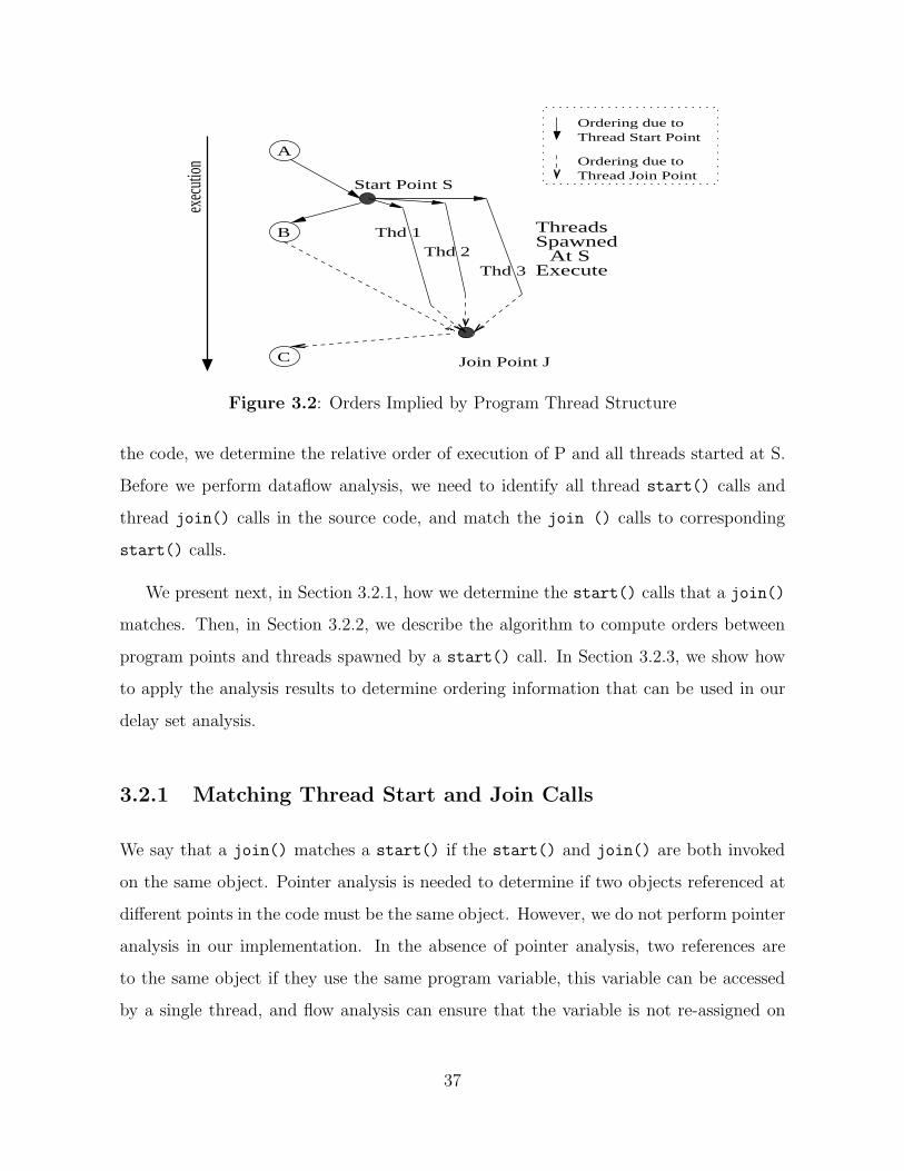
Figure 3.2 shows the execution timeline for an example program in which threads

are spawned by a start() call S. The points A, B, and C represent static points in the

program code. During an execution, a static instruction may be executed multiple times

due to program control flow.

Definition 3.2.1 For a static program statement S, an instance of S is some dynamic

execution of S.

Suppose we know from program control flow that:

• all instances of A must execute before any thread is spawned by S,

• all instances of B must execute after all instances of S, and before any join() point

in the program that waits for all threads spawned at S to terminate, and

• all instances of C must execute after a join() point in the program that waits for

all threads spawned at S to terminate.

Since shared memory accesses are not re-ordered across thread start and join points, we

can infer the execution orders from A to B, from B to C, and from A to C.

We use dataflow analysis to determine orderings due to the thread structure of the

program. For each pair (S, P), where S is a thread start() call, and P is any point in

36

A

B

C

SpawnedAt S

Execute

ThreadsThd 1

Thd 3

Thd 2

exec

ution

Start Point S

Thread Start PointOrdering due to

Ordering due toThread Join Point

Join Point J

Figure 3.2: Orders Implied by Program Thread Structure

the code, we determine the relative order of execution of P and all threads started at S.

Before we perform dataflow analysis, we need to identify all thread start() calls and

thread join() calls in the source code, and match the join () calls to corresponding

start() calls.

We present next, in Section 3.2.1, how we determine the start() calls that a join()

matches. Then, in Section 3.2.2, we describe the algorithm to compute orders between

program points and threads spawned by a start() call. In Section 3.2.3, we show how

to apply the analysis results to determine ordering information that can be used in our

delay set analysis.

3.2.1 Matching Thread Start and Join Calls

We say that a join() matches a start() if the start() and join() are both invoked

on the same object. Pointer analysis is needed to determine if two objects referenced at

different points in the code must be the same object. However, we do not perform pointer

analysis in our implementation. In the absence of pointer analysis, two references are

to the same object if they use the same program variable, this variable can be accessed

by a single thread, and flow analysis can ensure that the variable is not re-assigned on

37

any path from the first reference to the second reference. We use thread escape analysis

and a conservative intra-procedural flow analysis, and attempt to match a join() with a

start() only if both occur in the same method. Note that a join() may match multiple

start() calls that occur on different control flow paths reaching the join().

If a start() is in a loop, then it must be invoked on a distinct object for each

iteration of the loop 1. So, a set of threads is associated with the start(). We say that

a join() matches this start() if it is invoked on exactly the same set of objects as the

start() is invoked on. A matching join() may be in the same loop as the start(), as

in Figure 3.3(a), or in a different loop, as in Figure 3.3(b).

for ( ... ) { for (int i = LB; i < UB; i++) {x.start(); thd[i].start();

... }x.join(); for (int i = LB; i < UB; i++) {

} thd[i].join();

}(a) (b)

Figure 3.3: Matching join() for a start() in a Loop

In the case of Figure 3.3(b), if we know that the array thd can be accessed by a single

thread, we can determine that the set of objects on which the start() and join() are

invoked is exactly the same by observing that for both loops, the bounds and increments

for the loop index variable i are same, and the array index expression used to access the

array thd is also the same. In our implementation, we use simple pattern matching to

detect this case.

When doing the analysis, we consider only those join() calls that are matched with

some start(). It is safe to leave some join() unmatched because in that case, we

consider fewer synchronizations, and this leads to a conservative, but correct, analysis.

1Java semantics do not allow the thread corresponding to a specific object to be started multipletimes.

38

3.2.2 Algorithm

We use an inter-procedural inter-thread analysis to compute, for each program point P ,

the sets StartsAfter(P ), JoinsBefore(P ), and Concurrent(P ).

Definition 3.2.2 For a program point P , the set StartsAfter (P ) is defined to be the

set of all thread start() calls S such that some instance of S may execute after some

instance of P .

Definition 3.2.3 For a program point P , the set JoinsBefore (P ) is defined to be the

set of all thread start() calls with a matching join() such that some instance of the

join() may execute before some instance of P .

Definition 3.2.4 For a program point P , the set Concurrent (P ) is defined to be the

set of all thread start() calls S such that some instance of S starts a thread that may

concurrently execute with some instance of P .

In our analysis, we compute supersets that contain the sets defined above:

• For a thread start() S and any program point P , S ∈ StartsAfter(P ) if S does

not dominate P .

• For a thread start() S and any program point P , S ∈ JoinsBefore(P ) if a thread

join() that matches with S executes on some path from the program entry point

to P .

• For a thread start() S and any program point P , S ∈ Concurrent(P ) if S executes

on some path from the program entry point to P , and a join() that matches with

S does not execute on that same path after S and before P .

Note that these are may sets, not must sets. It is conservative, but correct, to include

any start() in any of these sets.

39

Initially, at the entry point of the application, say E, there is a single application

thread and no program statements have executed. So StartsAfter(E) is the set of all

start calls in the program, and JoinsBefore(E) and Concurrent(E) are empty sets.

We define Gen and Kill functions that determine how a program statement trans-

forms each of the three sets we compute. For a statement S, these functions help compute

the corresponding StartsAfter(), JoinsBefore(), and Concurrent() sets, for successors

of S in the control flow graph.

Definition 3.2.5 For a program statement S, the function Gen Concurrent (S) de-

fines the set of start() calls that should be included in set Concurrent(P ) for any point

P that is a successor of S in the control flow graph.

Definition 3.2.6 For a program statement S, the function Kill Concurrent (S) de-

fines the set of start() calls that should be removed from set Concurrent(P ) for any

point P that is a successor of S in the control flow graph.

Definition 3.2.7 For a program statement S, the function Gen JoinsBefore (S) de-

fines the set of start() calls that should be included in set JoinsBefore(P ) for any

point P that is a successor of S in the control flow graph.

Definition 3.2.8 For a program statement S, the function Kill StartsAfter (S) de-

fines the set of start() calls that should be removed from set StartsAfter(P ) for any

point P that is a successor of S in the control flow graph.

Consider the program control flow graph in Figure 3.4. Point E is the program entry

point, point S is a thread start() call, and point J is a join() call that is matched

with S. For point Q that occurs after the thread start() S, S should be removed from

the set StartsAfter(Q), and should be added to the set Concurrent(Q). For point R

that occurs after the thread join() J , S should be added to the set JoinsBefore(R),

and should be removed from the set Concurrent(R). Thus, we get the definitions for

Gen and Kill as shown in Figure 3.5.

40

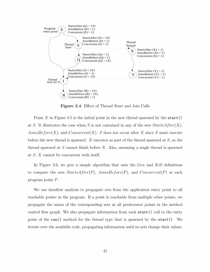
E

S

J

R

X

Y

ThreadStart

ThreadJoin for S

Programentry point

Q

JoinsBefore (E) = {}Concurrent (E) = {}

StartsAfter (E) = {S}

JoinsBefore (S) = {}Concurrent (S) = {}

StartsAfter (S) = {S}

JoinsBefore (Q) = {}Concurrent (Q) = {S}

StartsAfter (Q) = {}

JoinsBefore (R) = {S}Concurrent (R) = {}

StartsAfter (R) = {S}

JoinsBefore (Y) = {}Concurrent (Y) = {}

StartsAfter (Y) = {}JoinsBefore (J) = {}Concurrent (J) = {S}

StartsAfter (J) = {S}

JoinsBefore (X) = {}Concurrent (X) = {}

StartsAfter (X) = {}

ThreadStarted

Figure 3.4: Effect of Thread Start and Join Calls

Point X in Figure 3.5 is the initial point in the new thread spawned by the start()

at S. It illustrates the case when S is not contained in any of the sets StartsAfter(X),

JoinsBefore(X), and Concurrent(X). S does not occur after X since S must execute

before the new thread is spawned. X executes as part of the thread spawned at S, so the

thread spawned at S cannot finish before X. Also, assuming a single thread is spawned

at S, X cannot be concurrent with itself.

In Figure 3.6, we give a simple algorithm that uses the Gen and Kill definitions

to compute the sets StartsAfter(P ), JoinsBefore(P ), and Concurrent(P ) at each

program point P .

We use dataflow analysis to propagate sets from the application entry point to all

reachable points in the program. If a point is reachable from multiple other points, we

propagate the union of the corresponding sets at all predecessor points in the method

control flow graph. We also propagate information from each start() call to the entry

point of the run() method for the thread type that is spawned by the start(). We

iterate over the available code, propagating information until no sets change their values.

41

StartsInMethod(M) is the set of all start() calls that may execute whenmethod M is invoked, either directly in M , or indirectly in a method called in M .

JoinsInMethod(M) is the set of all start() calls such that a matched join()

must execute when method M is invoked, either directly in M , or indirectly ina method called in M .

Kill StartsAfter (x) = {x} , x is a thread start() call= StartsInMethod(M) , x is a call to method M= φ , otherwise.

Gen JoinsBefore (x) = {y} , x is a matching join()

for thread start() call y= JoinsInMethod(M) , x is a call to method M= φ , otherwise.

Gen Concurrent (x) = {x} , x is a thread start() call= StartsInMethod(M) , x is a call to method M= φ , otherwise.

Kill Concurrent (x) = {y} , x is a matching join()

for thread start() call y= JoinsInMethod(M) , x is a call to method M= φ , otherwise.

Figure 3.5: Gen and Kill Functions for Thread Structure Analysis

42

1. ∀ method M , compute StartsInMethod(M) and JoinsInMethod(M) asdefined in Figure 3.5.

2. For each program point P , initialize the sets StartsAfter(P ), JoinsBefore(P ),and Concurrent(P ) to be empty.

3. For the application entry point E, include all start() calls in StartsAfter(E).

4. Repeat the following while there is a change in the sets for any program point:∀ statement S in the program code

(a) StartsAfter(S) ∪=⋃

p∈Predecessor(S) ( StartsAfter(p) - Kill StartsAfter (p) )

(b) JoinsBefore(S) ∪=⋃

p∈Predecessor(S) ( JoinsBefore(p) ∪ Gen JoinsBefore (p) )

(c) Concurrent(S) ∪=⋃

p∈Predecessor(S) ( ( Concurrent(p) - Kill Concurrent (p) ) ∪Gen Concurrent (p) )

(d) If S is a start(), and R is the entry point of the run() methodfor the thread spawned by S, then

(i) StartsAfter(R) ∪= (StartsAfter(S)− {S})(ii) JoinsBefore(R) ∪= JoinsBefore(S)(iii) Concurrent(R) ∪= Concurrent(S)

Figure 3.6: Algorithm to Compute Orders for Thread Starts and Joins

43

The analysis converges because there are a fixed number of start() calls in the code,

and once a start() is added to a set due to propagation, it is never removed from it.

Predecessor Relation

The predecessor relation used in the analysis depends on the programming language

memory model. For sequential consistency, it is defined as follows:

• The predecessor set of the first statement in a method includes the set of call sites

that invoke the method.

• The predecessor set of the first statement of a basic block B includes the last

statement of each basic block that is a predecessor of B in the method control flow

graph.

• The predecessor set of all other statements includes the single statement that pre-

cedes it in its basic block.

However, in the general case, we need to construct a partial order graph for statements

within each basic block using knowledge of the program edges that are implied by the

programming language memory model.

Complexity

The worst case time complexity of our thread structure analysis is bounded by O(n2 ∗ s),

where n is the number of program points and s is the number of thread start calls in

the program source. The analysis iterates until none of the sets being computed change.

Each iteration does a pass over the program source and takes O(n) time. The dataflow

analysis is monotonic and a set can change only when an element is added to it. There

are three sets computed for each program point n, and the s thread start calls in the

program form the universe of elements that can be added to these sets. In the worst

44

case, a single element will be added to a single set in each iteration. Thus, the analysis

needs at most O(n ∗ s) iterations, and the overall complexity is O(n2 ∗ s).

3.2.3 Using Thread Structure Information in Delay Set Analy-

sis

The results of thread structure analysis are used to refine our delay set analysis. In

Section 3.2.3.1, we describe how these results can be applied to eliminate conflict edges. In

Section 3.2.3.2, we describe how these results are used to determine an order between two

accesses in the program. We illustrate these use cases with an example in Section 3.2.3.3.

3.2.3.1 Eliminating Conflict Edges

To help in determining if conflict edges can be eliminated, we determine for each thread

type whether it satisfies the single thread constraint. We say that a thread type satisfies

the single thread constraint if at most one thread of that type can execute at any given

time. In Java, when a new thread is spawned, it begins execution by invoking a specific

run() method that corresponds to the type of the thread spawned. A thread type T

satisfies the single thread constraint if the run() method for T is not concurrent with

any thread start() call that may directly or indirectly spawn a thread of type T. This

information is readily available in the summary set Concurrent(R), where R is any

point that executes when the run() method corresponding to T is invoked. Section 3.5

describes summary sets and how they are computed.

The special thread type that distinguishes the main thread started at the program

entry point will trivially satisfy the single thread constraint, since there are no thread

start() calls corresponding to it.

We can eliminate conflict edges between two shared memory accesses that both exe-

cute as part of a single thread type, and where that thread type satisfies the single thread

45

constraint. This is because the single thread constraint implies that the two accesses are

performed by the same thread, and in our delay set analysis, we search for conflict edges

that occur between accesses performed in different threads.

3.2.3.2 Ordering Program Accesses

Definition 3.2.9 For a thread type T, Code (T) is the set of all program statements

such that an instance of the statement may be executed by a thread of type T in some

program execution.

Definition 3.2.10 For a thread type T, ThreadsSpawnedBy (T) is the set of all

thread types T’ such that a thread of type T’ may be spawned when a thread of type

T executes. This includes threads spawned directly by a start() in Code (T), as well as

threads spawned indirectly by a start() in any other thread that may be spawned as a

result of the execution of a thread of type T.

Consider two accesses X and Y. We cannot determine an order between these two

accesses if:

• one of the accesses (say X) may be concurrent with a thread of type T, and

• the other access (say Y) is part of the code that may execute when a thread of

type T is spawned, i.e. Y ∈ Code(T ) or ∃T ′, T ′ ∈ ThreadsSpawnedBy(T ) and

Y ∈ Code(T ′).

Otherwise, we may be able to order the two accesses if all instances of X or Y execute

before some start(), or all of them execute after a join() that matches some start().

If an instance of X in thread T1 and an instance of Y in another thread T2 are

ordered by the thread structure of the program, then this order must be evident either

from the ordering information for X and Y with respect to the start() that spawns T1,

or from the ordering information for X and Y with respect to the start() that spawns

46

T2. To determine if there is an order between all instances of X and all instances of Y ,

we need only consider ordering information for X and Y with respect to start() calls

S such that S may spawn a thread of type T , and either X ∈ Code(T ) or Y ∈ Code(T ).

We can order X → Y (or Y → X) if the same order is determined with respect to each

of these start() calls S.

In Figure 3.7, we list all the possible orderings that may be inferred for two program

accesses X and Y using their ordering information with respect to one particular start(),

say S. The first row in the figure corresponds to the case when S is not contained in any

of the sets StartsAfter(X), JoinsBefore(X) or Concurrent(X). This implies that X is

part of the code that may execute when a thread is spawned by S (refer to the discussion

for the example in Figure 3.4). The third column in the figure corresponds to the case

when S is contained in JoinsBefore(Y ), but not in StartsAfter(Y ) or Concurrent(Y ).

Thus, the entry in the figure for the first row and third column determines the order

X → Y , since it corresponds to the case when X is part of the code executed by a

thread spawned at S, and when all instances of Y execute after all threads spawned at

S have finished execution. The other entries in the table in Figure 3.7 can be similarly

interpreted.

We can infer some of the orders in Figure 3.7 only for conflict edges in our simplified

delay set analysis. To infer these orders, we apply the extra check that is described next.

Refined Check to Order Conflict Edges

Consider a conflict edge between two accesses X and Y. In cases where all instances of

one access (say X) occur before a start(), and instances of the other access (say Y)

occur before the start() or concurrent with a thread spawned by the start(), we can

apply an extra test to improve the precision of the orders determined. Let the type of the

thread spawned by the start() be T. Then we check to see if all the following conditions

hold:

47

=> => =>A (Y) StartsAfter (Y) JoinsBefore (Y) Concurrent (Y)B (Y) C (Y)

X −> Y

X −> Y

Y −> X

Y −> X

X −> Y X −> Y X −> Y X −> Y (X −> Y)***see below

Y −> XY −> X Y −> X***see below(Y −> X) Y −> X

X −> Y (Y −> X)***see below

(X −> Y)***see below

Y −> X

Access X

Access Y

C(X)={S}A(X)={S} B(X)={S}

C(X)={}A(X)={S} B(X)={S}

C(X)={S}A(X)={S} B(X)={}

C(X)={}A(X)={S} B(X)={}

C(Y)={S}A(X)={} B(X)={S}

C(X)={}A(X)={} B(X)={S}

C(X)={S}A(X)={} B(X)={}

C(X)={}A(X)={} B(X)={}

A(Y) = {}

C(Y) = {}

B(Y) = {}

A(Y) = {}

C(Y) = {S}

A(Y) = {}

C(Y) = {}

B(Y) = {S}

A(Y) = {}

C(Y) = {S}

B(Y) = {S}

A(Y) = {S}

C(Y) = {}

B(Y) = {}

A(Y) = {S}

C(Y) = {S}

B(Y) = {}

A(Y) = {S}

C(Y) = {}

B(Y) = {S}

A(Y) = {S}

C(Y) = {S}

B(Y) = {S}B(Y) = {}

***These orders are contingent upon the refined check described in the text.***

Figure 3.7: Orders Inferred From Thread Structure Analysis

1. all instances of X may execute as part of a single thread type, say T’.

2. all instances of Y may execute as part of at most two thread types, T and T’.

3. T’ satisfies the single thread constraint.

4. The order X → R can be inferred, where R is the entry point of the run() method

that corresponds to thread type T.

If all of the above conditions are satisfied, then X → Y .

In the example code that follows, the access to x at S2 occurs before the start() at

S4. The access to x at S6 in method foo() can occur at points S1, S5, and T1. Thus, S6

may occur before S4, concurrent with the thread started at S4, and as part of the thread

started at S4. However, only the access S6 from point T1 is a candidate for a conflict

edge between S2 and S6. This is because in our delay set analysis, we only consider

conflict edges that exist between accesses in different threads, and S1 and S5 occur in

the same thread as S2. Conditions 1-4 of the check above ensure that S1 and S5 are in

the same thread as S2, and that T1 happens after S2. Thus, S2 → S6.

48

main () { class T extends Thread { foo () {S1: foo (); void run () { S6: access to x;

S2: access to x; T1: foo (); }S3: T t = new T (); ...;

S4: t.start (); }S5: foo (); }

}

A similar reasoning applies for the case when all instances of one access occur after

a join() that matches a start() S, and instances of the other access occur concurrent

with the threads spawned by S, or after the join().

3.2.3.3 An Example

The example in Figure 3.8 shows the control flow graph of a program where the main

thread spawns several threads at point D which is in a loop. The main thread and the

spawned threads both make calls to method Z and execute point F in the code. The

figure also shows the results of our thread structure analysis for each point in the graph.

Note that D is propagated to the Concurrent() sets for all points in the loop, and then

to point E and F . This captures the case when multiple threads spawned at a point are

concurrent with one another.

We cannot infer any orders among points C, E, and F . This is because the Concurrent()

sets at these points all include D, and E and F are part of the code executed by a

thread spawned at D. Thus, the first condition to order conflict edges, described in

Section 3.2.3.2, is not satisfied.

At point B, we observe that only the set StartsAfter(B) contains D, so we can

deduce that B must execute before any thread is spawned at D. Also, at point E, only

the set Concurrent(E) contains D, so we can deduce that E must execute concurrent

with or as part of a thread spawned at D. Thus, B → E is an order imposed by thread

start synchronization, and we can infer this using the table in Figure 3.7.

49

JoinsBefore (A) = {}StartsAfter (A) = {D}

Concurrent (A) = {}

JoinsBefore (B) = {}StartsAfter (B) = {D}

Concurrent (B) = {}

JoinsBefore (D) = {}StartsAfter (D) = {D}

Concurrent (D) = {D}

JoinsBefore (C) = {}Concurrent (C) = {D}

StartsAfter (C) = {D}

A

B: Call Z

C

D: Start Y

F

ProgramEntry Point

E: Call Z

Entry Point for Thread Y

JoinsBefore (E) = {}StartsAfter (E) = {}

Concurrent (E) = {D}

JoinsBefore (F) = {}Concurrent (F) = {D}

StartsAfter (F) = {D}Method Z

Method Call and Return

Met

hod

Cal

l and

Ret

urn

Thread Spawn

Figure 3.8: Example to Infer Orders From Thread Structure Synchronization

The points A, B, C, and D execute as part of the main thread that satisfies the single

thread constraint (Section 3.2.3.1). We do not consider any conflict edges among them,

since in our delay set analysis, we only consider conflict edges that occur between points

that execute in different threads.

We can use the refined check described in Section 3.2.3.2 to determine the order

B → F . B only executes as part of the single main thread. F executes as part of two

thread types: the single main thread, and the threads spawned at point D. E is the

entry point of the threads spawned at D, and we previously inferred the order B → E.

Thus, all the conditions for the refined check are satisfied, and we infer B → F .

3.3 Event-based Synchronization

In Java, event-based synchronization is provided by wait(), notify(), and notifyAll()

calls.A thread that needs to wait for an event invokes the wait() call on the corresponding

Java object. A thread that needs to signal a particular event invokes the notify() or

notifyAll() call on the corresponding Java object. The notify() unblocks a single

50

thread that is waiting on that particular object, and the notifyAll() unblocks all threads

that are waiting on that particular object.

Java language semantics prevent re-ordering of shared memory accesses across wait(),

notify(), and notifyAll() calls. They guarantee that when a notify() or notifyAll()

call executes, all shared memory accesses that occur in the notifying thread before the

call complete before a thread is unblocked by the call. Also, shared memory accesses that

occur in the waiting thread after the wait() call do not execute before the notify()

or notifyAll() call that unblocks the waiting thread. This implies that if all instances

of an access X in the program source execute before a notify() or notifyAll() call,

and this call must unblock a particular wait(), and all instances of an access Y in the

program source execute after the wait(), then X → Y is an order.

We use dataflow analysis to determine orderings due to event-based synchronization.

For each pair (S, P), where S is a wait(), notify(), or notifyAll() call, and P is any

point in the code, we determine the relative order of execution of P and S.

3.3.1 Algorithm

The analysis first identifies all wait(), notify(), and notifyAll() calls in the program

source.

Definition 3.3.1 For a program point P , the set SyncsAfter (P ) is defined to be the

set of all wait(), notify(), and notifyAll() calls such that some instance of the call

may execute after some instance of P .

Definition 3.3.2 For a program point P , the set SyncsBefore (P ) is defined to be the

set of all wait(), notify(), and notifyAll() calls such that some instance of the call

may execute before some instance of P .

For each program point P , we compute the sets SyncsAfter(P ) and SyncsBefore(P )

to be supersets that contain the sets defined above:

51

• For a wait(), notify(), or notifyAll() call S and any program point P , S ∈SyncsAfter(P ) if S does not dominate P with respect to the entry point of a

thread that executes both S and P .

• For a wait(), notify(), or notifyAll() call S and any program point P , S ∈SyncsBefore(P ) if S executes on some path from the thread entry point to P , for

a thread that executes both S and P .

Note that these are may sets, not must sets. It is conservative, but correct, to include

any wait(), notify(), or notifyAll() call in any of these sets.

We determine the SyncsAfter(P ) sets at each program point P by computing for

each thread type T in the program, the dominators for the flowgraph rooted at the

entry point of T. Since we are interested only in wait(), notify(), and notifyAll()

statements, we need to only consider these statements to include in the dominator sets

computed. For a program point P and a wait(), notify(), or notifyAll() call S, if

S is not a dominator of P in the dominator sets computed for some thread type T that

may execute P , then we include S in the set SyncsAfter(P ).

We compute the SyncsBefore(P ) sets at each program point P using a dataflow

analysis that is analogous to the one used in Section 3.2.2 to compute the JoinsBefore()

sets. The event-based synchronization analysis iterates over the code for each thread type

in the program, one at a time.

MaySyncsInMethod(M) is the set of all wait(), notify(), and notifyAll() calls

that may execute when method M is invoked, either directly in M , or indirectly in a

method called when M executes. We define the function Gen SyncsBefore(P ) that

determines, for any program statement P , how the execution of P transforms the sets

we compute:

Gen SyncsBefore (x)

= {x} , x is a wait(), notify(), or notifyAll() call

52

= MaySyncsInMethod(M) , x is a call to method M

= φ , otherwise.

Figure 3.9 outlines an algorithm that uses this definition to compute sets SyncsBefore(P )

at each program point P . The predecessor relation used in the algorithm is the same as

that described in Section 3.2.2.

1. ∀ method M , compute MaySyncsInMethod(M).

2. ∀ program point P , initialize the set SyncsBefore(P ) to be empty.

3. ∀ thread type T in the program:Repeat while there is a change in the sets for any program point ∈ Code(T ):∀ statement S ∈ Code(T ):

SyncsBefore(S) ∪=⋃

p∈Predecessor(S) ( SyncsBefore(p) ∪ Gen SyncsBefore (p) )

Figure 3.9: Algorithm to Compute Orders for Event-based Synchronization

For a thread of type T that cannot execute any instance of a particular wait(),

notify(), or notifyAll() call S, we conservatively include S in sets SyncsAfter(P )

and SyncsBefore(P ), at each point P ∈ Code(T ). Due to this, information from one

thread type does not affect the results for program points in other thread types. Thus,

our event-synchronization analysis need not propagate information at thread start sites to

the entry point of the newly started thread type. This does not affect precision because

thread structure analysis already accounts for orders implied by thread spawning and

termination.

Complexity

The worst case time complexity of our event-based synchronization analysis is O(t∗n2∗s)

where t is the number of thread types in the program, n is the maximum number of

53

program points in the code for any thread type, and s is the number of wait(), notify(),

and notifyAll() calls in the program. The analysis iterates until convergence over the

code for each thread type individually. Each iteration does a pass over the code for

a thread type and takes O(n) time. The dataflow analysis is monotonic, and the sets

SyncsBefore(P ) computed at each point P can change only when an element is added

to them. There can be at most s elements in any of these sets. Thus, in the worst case

when a single element is added to a single set in an iteration, we require O(t ∗ n ∗ s)

iterations, and the overall complexity is O(t ∗ n2 ∗ s).

3.3.2 Using Event-based Synchronization in Delay Set Analysis

For a program point P and a wait(), notify(), or notifyAll() call S, P occurs in the

program only before S (P → S) if S ∈ SyncsAfter(P ) and S /∈ SyncsBefore(P ).

For a program point P and a wait(), notify(), or notifyAll() call S, P occurs in

the program only after S (S → P ) if S /∈ SyncsAfter(P ) and S ∈ SyncsBefore(P ).

For any two shared memory accesses X and Y , we can use event-based synchronization

to infer the order X → Y if:

• X occurs in the program source only before a notify() or notifyAll(), say N ,

• Y occurs in the program source only after a wait(), say W , and

• N definitely is the synchronization operation that causes W to exit its wait.

N can cause W to exit its wait if both of them may occur concurrently, and are invoked

on the same Java object. In general, there can be multiple points in the code where

a wait() (or a notify() or notifyAll()) call are invoked on the same Java object.

Also, we need alias analysis to determine if two references may in fact refer to the same

Java object. Thus, during analysis we conservatively determine a set of wait() calls

54

that correspond to each notify() and notifyAll() call, and a set of notify() and

notifyAll() calls that correspond to each wait() call.

Definition 3.3.3 For a notify() or notifyAll() call N, WaitSet (N) is the set of

all wait() calls W such that N and W may be invoked on the same object, and thread

structure analysis does not determine an order N → W or W → N.

Definition 3.3.4 For a wait() call W, NotifySet (W) is the set of all notify() and

notifyAll() calls N such that W and N may be invoked on the same object, and thread

structure analysis does not determine an order N → W or W → N.

For accesses X and Y , we can determine an order X → Y if either of the following is

valid:

• there exists a wait() call W such that W → Y , and for each call N in the set

NotifySet (W), X → N , or

• there exists a notify() or notifyAll() call N such that X → N , and for each

call W in WaitSet (N), W → Y .

3.3.2.1 Limited Use in Java Programs

In practice, our event synchronization analysis is conservative when applied to Java

programs. This is due to several reasons:

• The common usage for a wait() call is in a while loop, with some condition that

determines if the loop will iterate and the wait() will be invoked. In these cases, it

is possible that the loop performs zero iterations and the wait() is never invoked.

So, there is no possibility of determining synchronization orders based on such

conditional wait() calls.

55

• Java provides a timed version of the wait() call that is used more often in code

than the untimed version. This timed wait() unblocks by default when a spec-

ified amount of time has elapsed. We cannot use it to determine orders due to

synchronization.

• We use alias analysis to determine the sets WaitSet(N) and NotifySet(W ) that

are needed to apply the results of the analysis. The precision of the alias anal-

ysis impacts the utility of event-based synchronization analysis. Alias analysis is

expensive to compute with high precision.

3.4 Lock-based Synchronization

Lock-based synchronization analysis uses properties of synchronized blocks in Java to

eliminate some delay edges. A synchronized block in Java has a lock associated with it.

This lock is acquired before the block begins execution, and is released when the block

finishes execution. Synchronized blocks enforce the following properties:

1. They provide mutual exclusion for code blocks that are synchronized using the

same lock.

2. They guarantee that all memory accesses in the source program prior to the end

of the synchronized block happen before the lock for the synchronized block is

released.

3. They guarantee that no memory access in the source program after the beginning

of the synchronized block happens before the lock for the synchronized block has

been acquired.

In our analysis, we compute a locking set at each program point that includes lock

objects, corresponding to synchronized blocks, that have been acquired and not yet

released when any instance of that program point executes. In the next section, we

56

describe our algorithm to compute these locking sets. Then, in Section 3.4.2, we show

how these sets can be used to eliminate some conflict edges in our delay set analysis.

3.4.1 Algorithm

Figure 3.10 shows how to compute the sets of locks acquired due to synchronized blocks

at each program point. For each statement in a synchronized block that uses the lock

associated with an object L, we add L to the set of acquired locks for that statement.

If the statement is a method call, then L is recursively propagated using set intersection

to all statements reachable from the called method. The predecessor relation used in the

algorithm is defined by the control flow graph of each method. The predecessors of the

entry point of a method are all call sites for that method.

1. Initialize the sets of acquired locks as follows:(a) For the main() method that is the application entry point: empty set.(b) For each run() method that is the entry point of a thread: empty set.(c) For all other methods: universe of all possible locks.

2. Repeat the following while there is a change in the set of acquired locks forany program point:

∀ statement S in the program code, with set of acquired locks LS(S),LS(S) ∩=

⋂p∈Predecessor(S) (set of acquired locks for p)

If S is the first statement in a synchronized block that uses lock X,add X to LS(S).

If S is the first statement after a synchronized block that uses lock X,remove X from LS(S).

3. For each statement, add the “container” lock to its set of acquired locks if thestatement only accesses fields of objects included in its set of acquired locks.

Figure 3.10: Algorithm to Compute Sets of Acquired Locks

Note that in our implementation, we conservatively initialize the sets of acquired

locks at the entry point of a thread to be empty. We can improve the accuracy of locking

analysis if we combine it with thread structure analysis. In this case, we would initialize

57

only the set of acquired locks at the program entry point to be empty, and initialize all

other sets to be the universe of all possible locks. Then, in the algorithm in Figure 3.10,

we would consider a thread start() point S to be the predecessor of entry points of

threads that may be started at S.

Locks are regular Java objects. So we need pointer analysis to determine if a lock

object is the same as one of the objects in a locking set. Since we do not have pointer

analysis in the implementation, we take advantage of user-defined types to determine if

two lock objects must be aliased. A lock object must be the same as another if both

are of the same user-defined type, and we are guaranteed that a single instance of that

type is instantiated. Thus, we consider a synchronized block only if its lock object is a

write-once static field in Java.

We can circumvent the need for pointer analysis in the case when a synchronized

block is used to protect accesses to fields of the same object whose associated lock is used

by the synchronized block. We identify the lock in these cases by a special type that we

call “container” lock. In the example code below, we include the “container” lock in

the set of acquired locks for statements X2 and Y2.

Thread X Thread Y

X1:synchronized (ObjectOne) { Y1:synchronized (ObjectTwo) {X2: ObjectOne.fld = . . . ; Y2: ObjectTwo.fld = . . . ;

X3:} Y3 }

We use locking information in our delay set analysis to check if some conflict edges

may be eliminated when searching for the end-points of a potential cycle. As shown in

Section 3.4.2, if two accesses occur in synchronized blocks in the code, and the lock object

used for both these blocks must be the same, then we can ignore a conflict edge between

the two accesses in our simplified delay set analysis.

58

Consider accesses in synchronized blocks that access a field of the same object whose

associated lock is used to synchronize the block. It is safe to discard any conflict edge

between two such accesses in our delay set analysis. To see why this is the case, consider

a conflict edge between accesses X2 and Y2 in the example above. There will be no

conflict edge between X2 and Y2 because:

• either ObjectOne and ObjectTwo both refer to the same object, so both accesses

are synchronized using the same lock, and we can eliminate conflict edges between

them based on the discussion in Section 3.4.2, or

• ObjectOne and ObjectTwo refer to different objects, which implies that the two

accesses are to different memory locations and therefore they do not conflict.

The special “container” lock is used to capture this case. We include this lock in the

locking set corresponding to each access that refers to a field of object L, and the lock

associated with L is used to synchronize the block that the access is contained in.

Complexity

The worst case time complexity of our locking analysis is bounded by O(n2 ∗ s), where n

is the number of program points and s is the number of locks used in sychronized blocks

in the program. Each iteration does a pass over the program source and takes O(n) time.

The analysis iterates until there is no change in the locking sets being computed at each

of the n program points. A locking set can only change monotonically. It can initially

contain s elements, and it may have all of these elements removed from it. In the worst

case, a single element will be removed from a single set in each iteration. Thus, the

analysis needs at most O(n ∗ s) iterations, and the overall complexity is O(n2 ∗ s).

59

3.4.2 Using Lock Information in Delay Set Analysis

In our approximate delay set analysis, when we search for initial conflict edges that form

the end-points of a potential cycle, we can ignore conflict edges that occur between two

accesses that execute as part of synchronized blocks with the same lock object.

Consider two conflicting memory accesses, say A and B, that execute as part of

synchronized blocks with the same lock object. The mutual exclusion property of syn-

chronized blocks implies that one access must finish before the other can start. Suppose

that A happens before B in an execution of the program. For this case, Figure 3.11 shows

the two possible ways in which a cycle may exist in the access order graph for delay set

analysis, considering that only cycles with at most two consecutive conflict edges con-

tribute to the delay set [SS88]. In the figure, thick lines denote program edges, thin lines

denote conflict edges, and dashed lines denote some path that exists in the access order

graph for delay set analysis.

D

Release Lock

Acquire Lock

C

Release Lock

Acquire Lock

( b )( a )

A B A B

Figure 3.11: Possible Cycles for a Conflict Edge Between Synchronized Accesses

The cycle in Figure 3.11 (a) requires a program edge from some access C to A, and

a path from B to C, i.e. the possibility that B happens before C. However, the second

property listed above implies that since C is a memory access before the end of the

synchronized block for A in the program source, C must happen before the lock for this

synchronized block is released. From our assumption that A happens before B, we know

B cannot happen before synchronization enforces ordering from the release of the lock

after A to the acquire of the lock before B. So, it is not possible for B to happen before C.

60

Thus, when checking for a delay from C to A, we can safely ignore the cycle in Figure 3.11

(a), and the conflict edge between A and B can be eliminated.

The cycle in Figure 3.11 (b) requires a program edge from B to some access D, and

a path from D to A. The last property listed above implies that since D is a memory

access after the beginning of the synchronized block for B in the program source, it

cannot happen before the lock for this synchronized block has been acquired. We know

A happens before this lock is acquired, so it is not possible for D to happen before A.

Thus, when checking for a delay from B to D, we can safely ignore the cycle in Figure 3.11

(b), and the conflict edge between A and B can be eliminated.

A similar reasoning applies to the case when B happens before A in a program execu-

tion. Thus, when checking if the program edge between two accesses X and Y is a delay

edge, we can ignore conflict edges between X and another access if both of them have a

common lock object in their locking sets. Likewise, we can ignore conflict edges between

Y and another access if both of them have a common lock object in their locking sets.

3.5 Implementation

We efficiently implement dataflow analysis using a topological traversal of the strongly

connected components of each method control flow graph. Also, we use a bitset im-

plementation for our thread structure analysis algorithm. We have not implemented

event-based synchronization analysis since it does not impact the benchmark programs

we use. After the analysis, we preserve only the sets corresponding to method entry

points. The sets for each program point can be computed intra-procedurally on demand.

Even though our synchronization analysis is inter-procedural and flow-sensitive, it

is efficient in practice (Section 5.3). This is because the time it takes for the analysis

to converge depends on the number of synchronization constructs used in the program.

Typically, the number of points in the code where threads are spawned, or locks are

61

acquired or released, is small compared to the total number of program points. Also,

for locking analysis, we need not perform a flow-sensitive analysis of methods that do

not contain any synchronized blocks. For these methods, the locking information at

each point in the method will be the same as the locking information at the method

entry point. Likewise, for thread structure analysis, we need not perform a flow-sensitive

analysis of methods that do not start or join any threads, either directly or indirectly

through another call invoked when the method executes.

We use the results of synchronization analysis to perform delay set analysis. When

searching for conflict edges, delay set analysis aggregates shared memory accesses within

each method, instead of considering each individual access separately (Section 2.5.3).

Also, nodes in the access order graph that correspond to method calls are treated as a

collection of accesses performed either directly in the method called, or indirectly through

a call invoked when the method executes. To efficiently handle method calls in delay

checks, we compute for each method a summary of the synchronization information:

• over all read accesses of a given type that may execute when the method is called,

• over all write accesses of a given type that may execute when the method is called,

and

• over all possible accesses that may execute when the method is called.

Thus, we store at most 2 ∗ t + 1 summaries for each method, where t is the number of

types in the program.

For thread structure analysis, we can compute this summary by performing a union

over the corresponding StartsAfter(P ), JoinsBefore(P ), and Concurrent(P ) sets for

each point P that is included in the summary information. Similarly, for event-based

synchronization analysis, we can compute this summary by performing a union over

the corresponding SyncsAfter(P ) and SyncsBefore(P ) sets for each point P that is

included in the summary information. For locking analysis, we can compute this sum-

62

mary by intersecting the locking sets for each point P that is included in the summary

information.

3.5.1 Exceptions

Exceptions in Java affect the flow of control in a program. Many instructions in Java are

defined such that they either complete normally, or they throw an exception to indicate

that something out of the ordinary happened. The program execution may proceed

along different control flow paths depending on whether an instruction execution throws

an exception or not. Programmers can define execption handlers that specify the code to

be executed when a particular exception is thrown. Also, programmers can define new

types of exceptions2 and explicitly incorporate exception control flow in their programs

due to these new exceptions.

Figure 3.12 shows an example where the execution of instructions I1 and I2 may throw

some exception. If I1 executes normally, the next instruction to execute is I2. However, if

an exception is thrown when I1 executes, the program continues execution at instruction

I4 in the first exception handler block B5. Likewise, if an exception is thrown when I2

executes, the program continues execution at the second exception handler block B6.

Traditionally, a control flow graph is constructed so that the branching flow of control

due to each instruction that may throw an exception terminates the basic block that the

instruction is contained in. A majority of instructions in Java codes may throw excep-

tions. Due to this, there may be a large number of basic blocks, and this may increase

the time for dataflow analysis in the compiler. Also, some optimization opportunities

may be missed due to few instructions within each individual basic block. To alleviate

these problems, the Jikes Research Virtual Machine compiler builds a factored control

flow graph [CGHS99]. In a factored control flow graph, a basic block is not terminated

2Note that exceptions are encapsulated as Java objects, and each exception has a specific type asso-ciated with it.

63

...

I1

I3

I2

...

I4

NormalControl Flow

ExceptionControl Flow

Handler OneException

Handler TwoException ...

I0

B1

B2

B3

B4

B5

B6

...B0

Figure 3.12: Flow Graph With Normal Control Flow and Exception Control Flow

at an instruction if exceptions are the only reason for a branch in control flow after the

instruction executes. An edge exists between two basic blocks in a factored control flow

graph if an exception due to any instruction in the first block may transfer flow of control

to the second block. Figure 3.13 shows the factored control flow graph for the example

in Figure 3.12.

...

Handler TwoException ...

I0

I1

I2

I3

B1

Handler OneException B5

between I1 and I4, ifneeded, inserted here

Memory barrier

B4

B6

...

B0

...

I4

Figure 3.13: Factored Control Flow Graph in the Jikes RVM

For our synchronization analysis, we use dataflow analysis that traverses the control

flow graph in a forward direction. The information propagated to exception handlers

may be different for a traditional control flow graph and a factored control flow graph.

In Figure 3.13, the information propagated to B5 and B6 is the information at instruction

I3, instead of the information at I1 and I2 respectively. Only synchronization instruc-

64

tions change the sets that are propagated within a basic block. Thus, we can ensure

correct analysis using a factored control flow graph if each synchronization instruction

(start(), join(), wait(), notify(), and notifyAll() calls, and locks and unlocks

corresponding to synchronized blocks) is the only instruction in its basic block. Since

programs typically contain few synchronization instructions relative to the total number

of program instructions, this change does not significantly impact the performance of

program analysis.

Our delay set analysis considers each edge between an instruction and its successors in

the control flow graph to be a program edge (Section 2.5.2). Successors of an instruction

I contained in a basic block B include all instructions in basic blocks that are successors

of B, as well as instructions within B that follow I in sequential order. In the example

of Figure 3.13, delay edges that we test (among the instructions labelled in the figure)

include edges from I1 to I2, I1 to I3, I1 to I4, I2 to I3, I2 to I4, and I3 to I4. Comparing this

with Figure 3.12, we conservatively test the edges from I2 to I4, and I3 to I4. However,

all successor edges determined from the flow graph in Figure 3.12 are also determined

from the flow graph in Figure 3.13.

All paths in the original graph are contained in the factored control flow graph. This

means that if our simplified delay set analysis determines an edge to be a delay edge in

the original control flow graph, it will also determine that edge to be a delay edge in the

corresponding factored control flow graph.

The design of a factored control flow graph ensures successors of an instruction include

successors due to exception control flow. Thus, our delay set analysis correctly handles

exception semantics in Java.

3.5.2 Space Complexity

As previously described, we store the results of synchronization analysis in terms of

summaries for each method in the program. We have at most 2 ∗ t + 1 summaries for

65

each method, where t is the number of object types in the program. Each instance

of synchronization information is proportional to the total number of synchronization

constructs in the program: 3 bits for each thread start() call, 2 bits for each wait(),

notify(), and notifyAll(), and 1 bit for each write-once static lock object associated

with a synchronized block. Suppose the program contains s of these synchronization

constructs. Then the space required to store the results of the analysis is O(m ∗ t ∗ s),

where m is the number of methods in the program.

During delay set analysis, we check program edges within each method to determine

if they are delay edges. For this, we perform an intra-procedural flow-sensitive analysis

to compute the synchronization information at each point in the method. This analysis

considers one method at a time, and requires space proportional to i ∗ s where i is the

maximum number of program points within any single method in the program.

Thus, the total space requirement for our analysis is O((m ∗ t ∗ s) + (i ∗ s)).

3.6 Related Work

Synchronization enforces orders between different events in a program execution. In

[NM90], Netzer and Miller prove that in general it is NP-hard to determine if two events

in a program may be ordered, and it is co-NP-hard to determine if two events must

be ordered. Past work has considered synchronization analysis in the context of race

detection, deadlock detection, and synchronization removal. Early work in [YT88, HM91]

describes how to perform an exhaustive search of all possible states that may occur in

a parallel execution. This information is represented as concurrency history graphs, and

takes exponential time to compute. Other research [EGP89, KY96, RM94] has focused

on constructing a task graph for control flow amongst parallel threads of execution, and

computing dominance relations on this graph to determine orders. This takes polynomial

time, but is not as precise as the dataflow analysis methods described in [CS89, DS91],

which also take polynomial time.

66

Callahan and Subhlok [CS89] give dataflow equations to compute synchronization

orders, but their method cannot be generalized to handle recursion. Duesterwald and

Soffa [DS91] use dataflow analysis to compute synchronization orders for a program that

may use recursion, and whose code comprises of multiple methods. Their approach de-

termines when one event must happen before and/or after another event. It cannot

determine when two events may/must happen concurrently, and it is unable to differ-

entiate between contexts specific to different call sites for the same method. Masticola

and Ryder [MR93] build on previous work and describe a framework to determine events

that may happen in parallel by successively refining the analysis results using various

techniques. Recent work [NAC99] applies dataflow analysis to compute events that may

happen in parallel for programs that use synchronization constructs defined in the Java

language, but it does not attempt to compute any happens-before or happens-after or-

ders. The synchronization analysis we present in this work also uses dataflow analysis.

It computes happens-before, happens-after, and happens-in-parallel relations. It is more

precise than previous methods based on dataflow analysis, and can distinguish informa-

tion at different call sites for the same method.

There is substantial research on dynamic data race detection that attempts to de-

termine orders based on a particular program execution. This work is related to our

synchronization analysis, but the most advanced techniques [NG92, CLL+02] take ad-

vantage of dynamic properties of a particular execution. These techniques cannot be

applied to a software implementation of memory consistency that must determine the

delay set to honor the memory consistency model for any execution of the program.

In [KY96], Krishnamurthy and Yelick perform delay set analysis and incorporate

synchronization information to improve the precision of their results. Their work aims

to optimize the communication backend when compiling Titanium programs [YSP+98].

They target SPMD programs that do not include synchronization due to thread spawning

or termination. Also, their use of locking synchronization to refine the access order graph

differs from our approach.

67

Chapter 4

Compiler Framework

4.1 Java Terminology

Our analysis algorithms target the Java programming language. We explain some terms

that refer to semantics of Java, and are used in the description of our algorithms.

Java programs manipulate data values. Each value in Java has a specific type asso-

ciated with it. There are two basic types in Java: primitive and reference. A primitive

type denotes an integer, floating point, or boolean value, as defined in the Java Language

Specification[GJS96]. The value of a reference type denotes a collection of memory loca-

tions. A reference type may be any array, class, or interface declared in the code.

An object is an aggregation of primitive and/or reference values in memory that are

collectively identified by a single reference value. A field is an identifier for a specific

member of an object. A class or interface defines an aggregation by specifying fields,

the types of values stored in fields, and methods to manipulate values in a program. An

object is an instance of a class C,and the reference that identifies the object is said to be

of type C. We say user-defined types are classes or interfaces that are defined in the user

program.

68

A memory access is any instruction that reads a value from, or writes a value to,

a location in memory. A single memory access can only read or write one primitive

value, or one reference value. A memory access has an associated reference value that

determines what object is accessed, and an associated field that specifies what member

within the object is accessed.

A variable is a container for a primitive or reference value. It is declared to be of a

specific type. Java is strongly typed, which means that a container can only be assigned

values that are of a type compatible with the type of the container. Section 4.3.2 defines

when one type is compatible with another.

4.2 The Jikes Research Virtual Machine and Com-

piler

We implemented the algorithms described in Chapters 2 and 3 in the Jikes Research

Virtual Machine (Jikes RVM) from IBM [AAB+00]. The Jikes RVM is an open-source

virtual machine that executes bytecodes contained in Java classes. It uses a dynamic just-

in-time compiler to generate machine code for each Java method before it is executed.

Except for some basic functionality, the source code for the Jikes RVM is written in

Java. This enables the compiler to seamlessly integrate the virtual machine code and the

application code when performing certain optimizations, such as code inlining.

The Jikes RVM has the ability to perform online adaptive feedback-directed optimiza-

tion [AFG+00]. The virtual machine includes a monitor that profiles code executions

to determine hot methods that take up a significant percentage of execution time. The

monitor provides this information to the optimizing compiler. The compiler can then

optimize hot methods in the code to improve performance. Mechanisms used to imple-

ment this adaptive optimization are method invalidation and re-compilation. Multiple

instances of machine code for the same Java method may exist at the same time, and

69

outdated versions of code can be marked as invalid to indicate that they must no longer

be used. We use this facility in our compiler system to make our analysis effective when

dealing with partial program evaluation (Section 4.3.6).

Since compilation occurs dynamically in the Jikes RVM, compile time counts as part

of an application’s execution time. So it is essential that our analysis be fast. However,

there are significant advantages of using dynamic compilation and a runtime system:

• We can dynamically detect when an application spawns a new thread during exe-

cution. Since our analysis is only applied to multithreaded programs, we need not

analyze code until a thread is spawned. Therefore we can execute single-threaded

applications with no overhead.

• Suppose a particular execution instance of an application never loads some class

nor invokes some method present in the code for the application. A dynamic

compiler can exclude such classes and methods when performing analysis, but a

static compiler, in general, cannot. Thus, the analysis performed by a dynamic

compiler can be more precise.

6.525.52

5.516.07

0

0.2

0.4

0.6

0.8

1

1.2

1.4

1.6

1.8

2

Hash

map

Gene

ticAl

go

Boun

dedB

uf

Siev

e

Disk

Sche

d

Raytr

ace

Monte

carlo

MolD

yn

SPEC

mtrt

SPEC

jbb00Ex

ecuti

ontim

enor

maliz

edto

Jikes

RVM

time

JikesRVM

Sun / JikesRVM

IBM / JikesRVM

Figure 4.1: Performance of the Jikes RVM and Commercial JVMs

70

Figure 4.1 shows the performance of the Jikes RVM with respect to two commercial

Java Virtual Machines: the Sun JDK 1.4.2 and the IBM JDK2-1.4.2. All measurements

were obtained on a Dell PowerEdge 6600 SMP with 4 Intel hyperthreaded 1.5GHz Xeon

processors running Linux. For each of the benchmark programs described in Section 5.1,

the figure shows two ratios: the Sun JDK execution time over the Jikes RVM execution

time, and the IBM JDK execution time over the Jikes RVM execution time1. We observe

that on average the performance of the Jikes RVM is comparable with that of commercial

Java virtual machines. Thus, we believe our results are comparable to those that would

have been obtained using one of the commercial Java Virtual Machines.

4.3 Our Memory-model Aware Compiler

In Section 1.2.2, Figure 1.4, we gave an overview of the components in our compiler sys-

tem. We implement our system using the Jikes RVM, and extend its optimizing compiler

with our analyses and transformations. Currently the programming language memory

model is fixed to be sequential consistency, but in the long term this is expected to be

a programmable feature and the system will automatically adapt to different memory

consistency models.

The delay set analysis and synchronization analysis components of Figure 1.4 were

discussed in Chapter 2 and 3 respectively. In this section, we discuss the thread escape

analysis, alias analysis, and memory barrier insertion components of our compiler imple-

mentation. We describe the code re-ordering optimizations in the Jikes RVM that need

to be augmented for sequential consistency. We also describe how our algorithms adapt

to perform partial program analysis in the presence of dynamic classloading.

1SPEC JBB 2000 [Cor00] is a server benchmark and its performance is measured in terms of through-put, i.e. number of transactions completed per second. Thus, the ratios for SPEC JBB 2000 are computedas the Jikes RVM throughput over the Sun JDK throughput, and the Jikes RVM throughput over theIBM JDK throughput.

71

4.3.1 Thread Escape Analysis

Definition 4.3.1 A reference to a memory location escapes if that location is accessible

by multiple threads in the program.

Thread escape analysis identifies shared memory accesses in the program that may

use references that escape. In our system, we use a flow-insensitive, partially context-

sensitive, iterative algorithm for thread escape analysis. It differs from previous algo-

rithms in that it considers individual fields of Java Thread objects, and checks if they do

indeed escape. Also, it makes use of user-defined types to speed up convergence of the

iterative analysis.

We tested our implementation of sequential consistency using different escape analysis

algorithms to determine the effect escape analysis has on delay set analysis (Section 5.2.2).

The different escape analysis algorithms varied in the accuracy of their analysis results.

Not surprisingly, we found that delay set analysis is very sensitive to the precision of

escape analysis. For some of the benchmark programs described in Section 5.1, we

observed slowdowns in execution time that were an order of magnitude greater when

using an escape analysis that is less precise than the one described in Section 4.3.1.2.

4.3.1.1 Algorithm

In Java, there are three causes for a reference to escape a thread:

1. A reference to a static field may be accessed by multiple threads in the program,

causing it to escape.

2. When a new thread T1 is created by a thread T2, the reference to T1 may be

accessed by T1 itself as well as its creator T2. So, the reference to T1 escapes.

3. If a reference R1 escapes, then any reference R2 read from or written into a memory

location accessed through reference R1 also escapes.

72

When a type may escape, all accesses to all objects that are instances of that type may

escape. Similarly, when a field may escape, all accesses to that field may escape.

When a new thread object T1 is created, its creator thread may use the reference to

T1 to access fields of T1. If these fields are of a reference type, the values they contain

escape because they are accessible both by the creator thread, and by the execution

of T1. The second and third conditions enumerated above together identify that these

references escape. However, the second condition is conservative because it causes all

references contained in fields of T1 to escape. In reality, only some fields of T1 will be

accessed by the creator. That the reference to T1 is available to its creator thread will

cause only those references to escape that are read from or written into fields of T1 by

its creator thread.

We use this in our analysis to refine the second condition enumerated above. We

do not assume that the reference to a new thread T1 escapes by default. Instead, each

reference that is a field of T1 that may be accessed in the creator thread escapes. To

determine these fields, we need to analyze all code that may be executed by the creator

thread. In our implementation, we use a conservative test that only examines the code

for two methods: the method that contains the thread start() call for T1, say M, and

the constructor for T1, say C. This test determines if the reference to T1 is available for

use only within these two methods:

1. T1 is newly allocated in M, and

2. the reference to T1 is not stored to memory in M or C, and

3. the reference to T1 is not passed as a parameter for a method called from M or C,

and

4. the reference to T1 is not returned from M.

73

If so, then only fields of T1 accessed in M or C escape. Otherwise, our analysis con-

servatively assumes that the thread type for T1 escapes, and that all fields of T1 also

escape.

Thus, the root causes for a reference to escape in our analysis are:

1. Any reference to a static field escapes.

2. For a new thread T1 that is spawned by a thread T2, the thread type that corre-

sponds to T1 escapes, unless our conservative intra-procedural analysis determines

that the reference to T1 is not available for use outside the method that spawns

the thread T1, and the constructor for T1.

3. For a thread type T1 that does not escape according to the above condition, a field

F of T1 escapes if:

• F is of reference type, and

• a statement S, in the method that spawns T1 or in the constructor method

for T1, accesses a value in F, except when:

(a) the value accessed by S is null, or

(b) S is a write access that stores a reference to an object newly allocated in

the constructor for T1, and this reference is not found to be escaping.

There are four categories of statements in our intermediate representation that cause

a reference to escape because of another escaping reference: load or store to an object

field in memory, read or write access to an array element, statements that use register

operands to perform a unary or binary operation, and method calls. We describe each

of these below. In our discussion, F identifies a field type, and R, R0, R1, . . . identify

temporary registers in the intermediate code.

Loads and Stores of an Object Field A load of an object field, R2 = R1.F , loads

into R2 the value from field F in the object referenced by R1. A store of an object field,

74

R1.F = R2 stores the value from R2 into the field F in the object referenced by R1. In

both cases, escape properties are affected only if the value loaded or stored is of reference

type. If R1 escapes, then everything accessible through it also escapes, and so R2 escapes.

If F is a field of a thread type that escapes (the second root cause enumerated above),

then we conservatively assume that both R1 and R2 escape. If F is an escaping field

type (the third root cause enumerated above), then the value read from or written into

F may be accessible by multiple threads, and so R2 escapes.

Array Element Accesses A read access of an array element, R2 = R1[i], reads

into R2 the value that is at index i of the array referenced by R1. A write access of an

array element, R1[i] = R2, stores the value from R2 into the element at index i in the

array referenced by R1. We treat array accesses very conservatively since we do not use

subscript analysis to determine when two array accesses may refer to the same location

in memory. If an element of an array escapes, we assume the entire array escapes. Thus,

if R2 escapes, then R1 escapes. Also, if R1 escapes, then each element in the array also

becomes accessible by multiple threads, and so R2 escapes.

Register-to-register Operations A unary operation, R1 op = R2, performs some

operation on the value in R2, and stores the result in R1. If R2 escapes, we conservatively

assume R1 also escapes. Note that a move instruction also counts as a unary operation

that simply tranfers the value from R2 to R1. A binary operation, R1 = R2 op R3,

performs some operation on the values in R2 and R3 and stores the result in R1. If R2

or R3 escape, we conservatively assume R1 also escapes.

Method Calls For each method M we compute two sets during the iterative analysis:

EscapeParamsOnEntry(M) and EscapeParamsOnExit(M).

Definition 4.3.2 For a method M , i ∈ EscapeParamsOnEntry(M) if some call to

M in the program may be invoked with an escaping reference as the argument for the ith

parameter.

75

Definition 4.3.3 For a method M , i ∈ EscapeParamsOnExit(M) if execution of M

may cause the reference contained in the ith parameter to escape.

Consider a method call, R0 = foo(R1 . . . Rn), where foo is the method invoked. foo

takes n parameters whose values are passed in registers R1 through Rn. It returns a

value that is stored in register R0. This return value can be treated as an out parameter

that is available only on return from the method. Thus, we consider it to be the zero’th

parameter when computing the set EscapeParamsOnExit(M).

For parameter i of method M , 0 ≤ i ≤ n, if i ∈ EscapeParamsOnExit(M),

then Ri escapes. Conversely, for 1 ≤ i ≤ n if Ri escapes, then we add i to the set

EscapeParamsOnEntry(M).

To compute EscapeParamsOnExit(M) for a method M , we determine all registers

in M that escape when initially no parameter passed into the method escapes. If regis-

ter Ri corresponding to parameter i is found to be escaping, then we know the actions

of the method cause the reference passed in parameter i to escape. So we add i to

EscapeParamsOnExit(M). It is also possible that a parameter that does not initially

escape on method entry later escapes during method execution only because of an escap-

ing reference that is passed in through some other parameter. Due to this, we individually

consider the effect of each parameter that may be escaping on method entry. In each

case, we determine what other parameters may escape due to actions of the method, and

add them to the set EscapeParamsOnExit(M). We only need to consider the effects

of parameters that escape on method entry one at a time, since the sets of escaping

references determined in each case are independent of one another.

Figure 4.2 illustrates how our analysis is partially context-sensitive. Method M takes

two parameters u and v, and the actions of M are such that it causes v to escape only

when the reference passed in u escapes. Method M is called from three points in the

program:

1. Method A calls M with neither parameter initially escaping.

76

/* X escapes, Y does not*/call M (X, Y);/* X, Y escape */

/* X, Y escape */call M (X, Y);/* X, Y escape */

/* X, Y do not escape */call M (X, Y);/* Y escapes */

EscapeParamsOnEntry (M) = {1, 2}EscapeParamsOnExit (M) = {2}/* M causes v to escape only

if u escapes on entry */

void M (u, v) {

}

A ( ) {

}

B ( ) {

}

C ( ) {

}

Figure 4.2: Different Calling Contexts of Methods for Escape Analysis

2. Method B calls M with u initially escaping but v not escaping.

3. Method C calls M with both parameters initially escaping.

The figure also shows sets EscapeParamsOnEntry(M) and EscapeParamsOnExit(M)

that our analysis computes. Based on this, we correctly determine that Y escapes after

the call to M in B returns, and that X does not escape after the call to M in A returns.

However, we conservatively determine that Y escapes after the call to M in A returns.

Figure 4.3 gives an algorithm to perform our iterative thread escape analysis. It

uses the rules in Figure 4.4 that describe how to process statements in a method during

analysis.

At the end of the iterative analysis, we save sets EscapeParamsOnEntry(M) and

EscapeParamsOnExit(M), and discard escape information for registers in the interme-

diate code. This information can later be computed intra-procedurally on demand, using

the saved sets.

4.3.1.2 Optimization for Fast Analysis

We take advantage of user-defined types in Java to speed up the convergence of our

iterative analysis. We conservatively assume that if an access to an object field escapes,

then all accesses to the same field also escape. To incorporate this change, we need only

77

I Initialize the following sets to be empty:1) EscapingThreads: set of all thread types found to be escaping.2) EscapingThreadF ields: set of all fields that are part of thread objects

and that are found to be escaping.

II For each method M , initialize the sets EscapeParamsOnEntry(M) andEscapeParamsOnExit(M) to be empty.

III Repeat the following until there is no change in the escape property of anyparameter, thread type, or field:

For each method M in the program with parameters contained in registersR1 . . . Rn, and the return value contained in register R0:

1) Process M to determine escaping references as described in Fig 4.4.

2) ∀i, 0 ≤ i ≤ n, if Ri escapes ⇒ add i to EscapeParamsOnExit(M).

3) ∀i ∈ EscapeParamsOnEntry(M):a) Set Ri to be escaping.b) Process M to determine escaping references as in Figure 4.4.c) ∀j, 0 ≤ j ≤ n,

if i 6= j and Rj escapes ⇒ add j to EscapeParamsOnExit(M).d) Reset all registers in M to be not escaping.

Figure 4.3: Escape Analysis Algorithm

78

Repeat the following until there is no change in the escape property of anyregister, parameter, thread type, or field:

∀ statement S in method M:1) If S is an access to a static field F : R = F or F = R,

R is of reference type ⇒ R escapes.

2) If S is a thread start call invoked on object R of thread type T : R.start(),R escapes ⇒ add T to set EscapingThreads.R accessed in a method other than M or the constructor method for R

⇒ R escapes, and add T to set EscapingThreads.

3) If S accesses a field in a thread of reference type: R1.F = R2 or R2 = R1.F ,Thread type of R1 ∈ EscapingThreads

⇒ add F to set EscapingThreadF ields.S is a read in constructor for R1 or in method that starts thread R1

⇒ add F to set EscapingThreadF ields.S is a write in constructor for R1 or in method that starts thread R1, andR2 is not null, and R2 is not a thread-local object newly allocated in theconstructor for R1

⇒ add F to set EscapingThreadF ields.

4) If S is an access to field F of object type T : R1.F = R2 or R2 = R1.F ,R2 is a reference and T ∈ EscapingThreads ⇒ R1 and R2 escape.R2 is a reference and F ∈ EscapingThreadF ields ⇒ R2 escapes.R2 is a reference and R1 escapes ⇒ R2 escapes.

5) If S is an access to an element of array R1: R1[ ] = R2 or R2 = R1[ ],R1 escapes ⇒ R2 escapes.R2 escapes ⇒ R1 escapes.

6) If S is a unary or binary operation: R1 op = R2 or R1 = R2 op R3,R2 escapes or R3 escapes ⇒ R1 escapes.

7) If S is a method call: R0 = foo(R1 . . . Rn),For each i, 0 ≤ i ≤ n, i ∈ EscapeParamsOnExit(foo) ⇒ Ri escapes.For each i, 1 ≤ i ≤ n, Ri escapes ⇒ add i to EscapeParamsOnEntry(foo).

Figure 4.4: Effect of Statements in Escape Analysis Algorithm

79

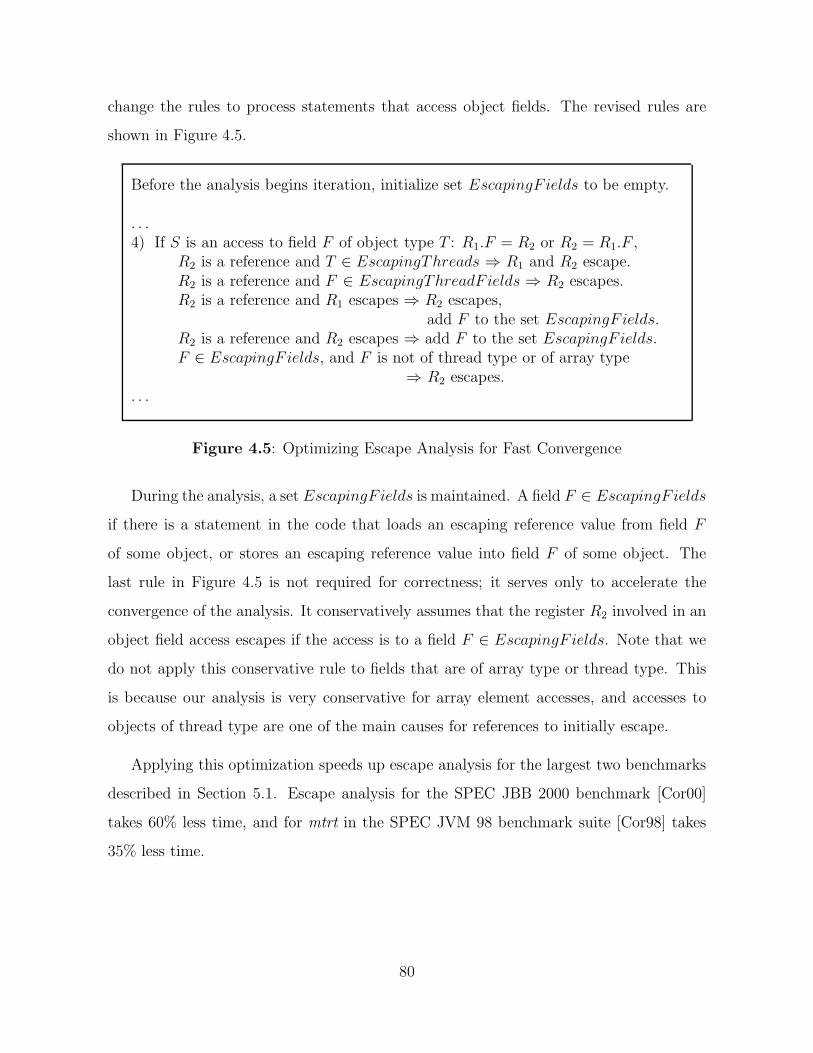
change the rules to process statements that access object fields. The revised rules are

shown in Figure 4.5.

Before the analysis begins iteration, initialize set EscapingF ields to be empty.

. . .4) If S is an access to field F of object type T : R1.F = R2 or R2 = R1.F ,

R2 is a reference and T ∈ EscapingThreads ⇒ R1 and R2 escape.R2 is a reference and F ∈ EscapingThreadF ields ⇒ R2 escapes.R2 is a reference and R1 escapes ⇒ R2 escapes,

add F to the set EscapingF ields.R2 is a reference and R2 escapes ⇒ add F to the set EscapingF ields.F ∈ EscapingF ields, and F is not of thread type or of array type

⇒ R2 escapes.. . .

Figure 4.5: Optimizing Escape Analysis for Fast Convergence

During the analysis, a set EscapingF ields is maintained. A field F ∈ EscapingF ields

if there is a statement in the code that loads an escaping reference value from field F

of some object, or stores an escaping reference value into field F of some object. The

last rule in Figure 4.5 is not required for correctness; it serves only to accelerate the

convergence of the analysis. It conservatively assumes that the register R2 involved in an

object field access escapes if the access is to a field F ∈ EscapingF ields. Note that we

do not apply this conservative rule to fields that are of array type or thread type. This

is because our analysis is very conservative for array element accesses, and accesses to

objects of thread type are one of the main causes for references to initially escape.

Applying this optimization speeds up escape analysis for the largest two benchmarks

described in Section 5.1. Escape analysis for the SPEC JBB 2000 benchmark [Cor00]

takes 60% less time, and for mtrt in the SPEC JVM 98 benchmark suite [Cor98] takes

35% less time.

80

4.3.2 Alias Analysis

Given two references, alias analysis determines if they may be aliased, i.e. if they may

refer to the same memory location. This information is used to test for conflict edges

during delay set analysis. A conflict edge can only exist between two accesses that may

be aliased. Precision of alias analysis affects the number of conflict edges found, and so

it affects the accuracy of delay set analysis. Ideally, we want to perform pointer analysis

and trace when specific accesses in the program may refer to the same memory location.

However, precise pointer analysis is expensive. Since compilation occurs during runtime

in our dynamic compiler, we choose not to use pointer analysis in our implementation.

Instead, we take advantage of strong typing in Java, and use a type-based alias analysis.

Definition 4.3.4 We say type A is compatible with type B in Java if:

1. A is the same type as B, or

2. A is a subclass of B, or

3. A is a class that implements interface B.

Each variable in the program is declared to be of a specific type. A reference variable

can only refer to objects that are of a type compatible with the declared type of the

reference. For two references of type A and B, if A is compatile with B, or B is compatible

with A, then our alias analysis assumes they may refer to the same memory location,

and so they may be aliased.

If the class corresponding to some type has not yet been loaded, then the Java virtual

machine has no knowledge of its superclass, subclasses, or interfaces implemented by it.

In the absence of such information, our alias analysis optimistically assumes that the

unknown type is not compatible with any other type in the application2. Later, if a new

class is loaded, we need to re-analyze the code, as described in Section 4.3.6.

2The exception is that all classes are by default subclasses of the Object type in Java.

81

For accesses to array elements, we need array dependence analysis to process sub-

script expressions, and determine if two accesses may refer to elements at the same array

index. In our implementation, we do not perform array dependence analysis. Instead,

we conservatively assume that all accesses to elements of a given array may access the

same element.

4.3.3 Inhibiting Code Transformations

Subset correctness is the correctness criterion for our memory-model aware compiler. It

requires that the set of outcomes possible from execution of a transformed program be a

subset of outcomes possible from the original program execution. Transformations that

preserve orders determined by delay set analysis (and normal intra-thread dependences)

preserve subset correctness [LPM99].

To preserve orders determined by delay set analysis, we need to prevent transforma-

tions in the compiler that re-order or eliminate accesses related by delay edges. Specifi-

cally, for each delay edge from access A to B, the order of A and B must not be changed,

and neither A nor B must be eliminated.

In the Jikes RVM optimizing compiler, there are four optimization phases that may

re-order or eliminate shared memory accesses:

1. loop invariant code motion,

2. loop unrolling,

3. common subexpression elimination, and

4. redundant load elimination.

Figure 4.6 shows an example of a loop invariant code motion transformation that

is valid in a single-threaded application. However, for multithreaded execution, this

optimization cannot be applied when there is another thread that writes the value 1

82

while (R2 == 0) { R2 = R1.F;}

while (R2 == 0) {R2 = R1.F;

}

R2 = R1.F

R2 = R1.F

R2 = R1.F

R1.F = 1

conflictedges

Thread 1 Thread 2

Initially, all values are zero.

...Figure 4.6: Loop Invariant Code Motion Example

into the memory location referred by R1.F . In this case, a possible outcome for the

transformed code is that the loop repeats forever. However, this is not possible in the

original code as it must eventually observe the value written by the other thread. The

access order graph for sequential consistency has a delay edge from access R1.F in one

loop iteration to access R1.F in subsequent loop iterations. The transformation amounts

to eliminating all accesses to R1.F except the one in the first loop iteration. Thus,

the transformation does not preserve delay edges intact, and the transformed program

violates subset correctness.

Figure 4.7 shows an example of loop unrolling that is valid in a single-threaded appli-

cation when R2 is a loop constant, and the number of loop iterations can be symbolically

computed. However, in a multithreaded context, R2 is not a constant if concurrent

threads write to the memory location referred by R3.F . In this case, the number of loop

iterations executed by the transformed code may differ, thus violating subset correctness.

The access order graph for sequential consistency has delay edges between access R3.F

in one iteration and access R3.F in subsequent loop iterations in the original code. The

transformation either results in some of the accesses to R3.F being eliminated or some

83

for (R1 = 0; R1 < R2; R1++) { STMT BLOCK R2 = R3.F;}

R2 = R3.F

R2 = R3.F

R2 = R3.F

conflictedges

R3.F = ......

Thread 1 Thread 2

R1 = 0;for (j = 0; j < R2/2; j++) { STMT BLOCK R2 = R3.F; R1++; STMT BLOCK R2 = R3.F; R1++;}if (R1 < R2) { STMT BLOCK R2 = R3.F; R1++;}

Figure 4.7: Loop Unrolling Example

new accesses to R3.F being introduced 3. The transformed code does not preserve delay

edges intact, and the transformation is invalid.

R2 = R1.FR3 = R2 + 2R5 = R4.FR6 = R1.FR7 = R6 + 2

R2 = R1.FR3 = R2 + 2R5 = R4.FR7 = R3

R5 = R4.F

R6 = R1.F

R2 = R1.F

R4.F = 2

R1.F = 1

conflictedges

Thread 1 Thread 2

Initially, all values are zero.

Figure 4.8: Common Subexpression and Load Elimination Example

Figure 4.8 shows an example of common subexpression elimination and load elimina-

tion that is valid in a single-threaded aplication. However, this transformation cannot be

3Note that transformations typically do not introduce extra shared memory accesses when optimizingcode. However, in general, it is not correct to insert extra shared memory accesses.

84

applied when another thread writes to the memory locations accessed by R1.F and R4.F ,

and sequential consistency is assumed. The access order graph in the figure illustrates

such an execution. For the original code, if R5 = 2, then the value for R6 must be 1 and

R7 must be 3. However, in the transformed code, it is possible to observe R5 = 2 and

R7 = 2, which is not a possible behavior in the original code. Thus, subset correctness

does not hold. The transformation eliminates the second load of R1.F and this violates

the delay edges shown in the access order graph.

In our implementation, we observe no significant impact on performance due to in-

hibiting code re-ordering and code elimination transformations. This is despite the fact

that we use a conservative test to determine when to inhibit transformations. To check if

accesses A and B may be re-ordered, we ensure that neither A nor B is thread-escaping.

Likewise, to check if an access A may be eliminated, we ensure A is not thread-escaping.

We do not test for a delay edge from A to B to preclude re-ordering them, and we do

not search for some delay edge that involves A to determine if A can be eliminated. This

is because when a method is compiled, we test for delay edges after optimizations have

been applied and we are ready to generate machine code for it. We could test for delay

edges earlier in the compilation process and store the results. Then, as the method code

is transformed, we will need to either update or re-compute the set of delay edges found.

However, by using the conservative test based only on results of thread escape analysis,

we save the overhead of doing this without sacrificing performance in practice.

4.3.4 Memory Barrier Insertion

Memory barrier insertion occurs when machine code is being generated for a method. It

ensures that the access orders required by the programming language memory model are

not violated by the processor executing the machine code.

On the IBM Power3 architecture, memory barrier insertion inserts sync instructions

between access pairs whose order needs to be enforced. A sync instruction ensures that all

85

data memory accesses4 issued by the processor before the sync instruction are complete

and available to all processors before any data memory access after the sync is issued.

On the Intel Xeon architecture, there are three types of memory barrier instructions that

are used to enforce access orders:

1. An mfence ensures all memory accesses that occur in code order before the mfence

are complete before any access after it is issued.

2. An lfence ensures all load accesses that occur in code order before the lfence are

complete before any load access after it is issued.

3. An sfence ensures all store accesses that occur in code order before the sfence are

complete before any store access after it is issued.

Note that lfences and sfences cost less than mfences in terms of execution time.

Our system uses the local-optimized version of memory barrier insertion described

in [FLM03]. After code optimization and transformation, the compiler determines the

sequence of machine instructions to be generated for a method being compiled. Mem-

ory barrier insertion searches this sequence and constructs the set of all memory access

instructions and method call instructions. For each pair of instructions (I, J) such that

I and J are in this set, and I is a predecessor of J in the method control flow graph, it

queries delay set analysis to determine if a delay edge exists from I to J . For each delay

edge (I, J), a memory barrier instruction is inserted on every path from I to J in the

control flow graph: if I and J are in different basic blocks of the control flow graph, the

memory barrier is inserted at the beginning of the basic block for J , else the memory

barrier is inserted just before J .

Memory barrier insertion is optimized to coalesce consecutive memory barrier in-

structions in the code into a single instruction. In the example control flow graph in

4To order accesses to program instructions, the IBM Power3 architecture provides a separate isyncinstruction.

86

Figure 4.9, if there is a delay edge from A to C, and from B to C, then a single memory

barrier before C enforces both these delay edges.

A B

C

...

... ...

MemoryBarrier

Figure 4.9: Example for Memory Barrier Insertion

Also, on the Intel Xeon system, the analysis is optimized to use cost-effective lfences

and sfences instead of mfences wherever possible. Note that there is further scope for

optimizing memory barrier insertion that is not currently part of our system implemen-

tation. In particular, we can take into account loop structure and branch probabilities

in the control flow graph when deciding where to insert a memory barrier instruction.

4.3.5 Specialization of the Jikes RVM Code

The Jikes RVM is mostly written in Java, and the compiler can integrate the virtual

machine (VM) code with the application code. Thus, some methods may execute both

as part of the VM and the application. Ideally, for an implementation of sequential

consistency, we want to analyze all methods to determine delay edges, including methods

shared by the VM itself. Note that this would not be an issue if the Jikes RVM was

written in C/C++, as are commercial Java virtual machines. If our analysis includes

VM methods, it results in high overhead:

• If VM methods are included in the analysis, their number tends to be much greater

than the number of application methods. As a result, the analysis time increases,

and the majority of it is spent analyzing VM code. Moreover, this is done each

time an application executes.

87

• The VM code is large and complex, and it uses several concurrent thread types, as

well as static variables. As a result, our analysis is not precise for VM code, and

this conservativeness infiltrates the application code as well. Thus, overall accuracy

and performance are affected.

• The VM and the application may share some library methods. The application

may pass an escaping reference to the shared method while the VM does not. The

method will need memory barriers in the context of the application, but not in the

context of the VM. Thus, an application can potentially slow down the execution

of the entire VM.

In our implementation, we want to ensure sequential consistency for all code executed

by an application without having to analyze VM code each time an application runs. We

identify VM methods that may execute as part of application code. To do this, we use

manual inspection of the VM code that is guided by execution traces from our benchmark

programs. Methods identified include:

• methods to clone an object,

• methods to efficiently copy arrays,

• methods to query the execution state of a thread, and

• methods in the implementation of the java.lang.Throwable class that access the

state of an exception5.

For all such methods identified, we provide two specialized versions of the method in the

system: one version has memory barriers conservatively inserted for each shared memory

access in it, and the other version does not have any memory barriers inserted. The

VM always uses the version with no memory barriers6. For the application, the compiler

5All exceptions in Java are derived from the type java.lang.Throwable.6We assume the VM is well-synchronized.

88

decides which version to invoke at each call site depending on whether escaping references

are passed as parameters to the method.

Thus, the number of memory barriers inserted is similar to the number that would

be inserted if the VM was written in C/C++.

4.3.6 Dynamic Class Loading

Java allows dynamic classloading, so the entire code for a program may not be avail-

able when it begins execution. During our inter-procedural analysis, we may need to

consider the effect of some methods whose code is not accessible when the analysis is

performed. In such cases, we can be conservative and ensure that the analysis results are

valid irrespective of what the method does. However, this will cause delay set analysis

and synchronization analysis to be ineffective, since they will have to assume that the

unknown method reads and writes all user-defined types that are accessible from it, and

it starts threads of all types accessible from it. Instead, our analysis optimistically as-

sumes that the unknown method does not spawn any new threads, and that it contains

no shared memory accesses that conflict with an access in another method. Later, when

code for the method becomes available, these properties must be verified to determine if

the analysis results are valid. If an assumption is found to be wrong, we must perform the

analysis again, invalidate previously compiled methods that may now need extra memory

barriers inserted, and recompile all these methods to generate correct code.

4.3.6.1 Incremental Analysis

We modify the runtime system of the Jikes RVM to detect the first time the applica-

tion spawns a new thread. Until a thread is spawned, we assume the application is

single-threaded, and delay set analysis trivially finds no delay edges. When the runtime

system is first invoked by the application to spawn a new thread, it passes control to

the optimizing compiler. At that point, synchronization analysis is performed for the

89

first time, and the check for delay edges is no longer trivial. The analysis is performed

inter-procedurally over code for all methods possibly executed by the application and

available at the point of the analysis. We do not repeat the inter-procedural analysis if

the just-in-time compiler later compiles a method whose code was available during the

inter-procedural analysis phase.

Due to classloading, code for a method that was previously unavailable may become

available. When the just-in-time compiler attempts to compile this method, our analysis

must perform an inter-procedural phase to account for the effect of the new method.

Instead of repeating the entire analysis from scratch, we design it to build upon previous

results.

Since each inter-procedural phase is potentially expensive, we want to minimize the

number of times it occurs. For this, we want to perform each analysis phase over all

application code that is available. Therefore, we use aggressive classloading for class

types seen in the application code that is already available to the analysis. We attempt

to load such classes before they are actually needed by the execution, so we can analyze

them as part of the current inter-procedural analysis phase. Java semantics allow this as

long as no exception is thrown if the class being aggressively loaded does not exist, and

if the class initializer is not executed till the point when the class is actually used.

Call Graph

For our analysis, we maintain an explicit call graph. A call site may invoke one of several

possible methods, depending on the type of the object on which the call is invoked (Sec-

tion 2.5.5). When a new method triggers our inter-procedural analysis, it is possible that

a new class has been loaded and is used in the application. If a class C is newly loaded,

we determine the set of all types T such that C is compatible with T (Section 4.3.2). For

each call to a method (say M) invoked through a reference of type T , we check if class C

defines a method (say N) that is a candidate for that call. If so, we update our call graph

to include this new method N in the set of possible methods that the call to M resolves to.

90

Also, we set the synchronization information at the entry point of method N 7 to be the

conservative summary of the synchronization information at the entry points of method

M and method N. Section 3.5 describes how synchronization information is summarized

over multiple points.

Thread Structure Analysis

We check the code for any new methods that have become available and look for thread

start() calls and matching thread join() calls. If no such calls are found, the incremen-

tal analysis traverses the call graph rooted at each new method to propagate thread struc-

ture information across all methods called directly or indirectly from the new method.

Note that we only need to iterate over individual statements of the new methods, since

we can use the call graph along with the summarized synchronization information stored

for each method that was previously analyzed, to reconstruct its inter-procedural effect.

If any thread start() call is identified in the new methods, then the iterative analysis

outlined in Figure 3.6 is performed with respect to the newly identified start() calls. In

this case, we need to iterate over individual statements of all the new methods, as well

as any method that may invoke a newly identified start() or join() indirectly through

another method that it calls. With reference to Figure 3.6, we iterate over statements of

a method M if either StartsInMethod(M) or JoinsInMethod(M) contains one of the

newly identified start() calls. For all other previously analyzed methods, we only need

to propagate information from that method to all other methods that it may call. We

maintain an explicit call graph that can be used for this purpose.

Locking Analysis

Incremental locking analysis traverses the call graph rooted at each new method to prop-

agate locking information across all methods called directly or indirectly from the new

method. With reference to Figure 3.10, we perform step 2 of the algorithm, iterating

over individual statements only in the new methods and using the call graph to propa-

7Recall from Section 3.5 that we preserve the synchronization information for the entry point of eachmethod.

91

gate information across entry points of methods previously analyzed. Also, step 3 of the

algorithm in Figure 3.10 is performed for each new method.

Delay Set Analysis

For each new method whose code has become available since the last inter-procedural

analysis phase, we compute synchronization information summaries over read and write

accesses of a specific type in the method, and over all possible accesses that result from

the method execution, as described in Section 3.5. The summary information over all

possible accesses in a method M takes into account accesses in methods that may be

called directly or indirectly by M. So, we need to re-compute this summary over all

accesses for any method that may directly or indirectly call one of the new methods.

For a newly loaded class C, we determine the set of all types T such that C is

compatible with T (Section 4.3.2). Then, for each method in the application, and each

type T in the set, we update information on types accessed by the method (Section 3.5)

as follows:

• If the method may read accesses of type C as well as type T , then we conservatively

incorporate the summarized synchronization information for T into C.

• If the method may read accesses of type T but not of type C, we add an entry in

the summarized synchronization information for read accesses to type C, and this

entry has the same summary information as that for type T .

• If the method may write accesses of type C as well as type T , then we conservatively

incorporate the summarized synchronization information for T into C.

• If the method may write accesses of type T but not of type C, we add an entry in

the summarized synchronization information for write accesses to type C, and this

entry has the same summary information as that for type T .

We choose to store all possible types in the method summary information instead of

dynamically checking for compatible types each time the summary information is used.

92

This makes it easy to check for methods that must be invalidated because of a change in

the analysis results (Section 4.3.6.2).

4.3.6.2 Method Invalidation

If the entire program source is not available the first time we perform our inter-procedural

analysis, we make optimistic assumptions about parts of the code that are not available.

Later, when more code becomes available, we may determine that some of our optimistic

assumptions are not valid. At this point, we re-analyze the program, determine methods

that may now need more memory barriers inserted in them, and re-compile these meth-

ods. We need to ensure that the program execution henceforth uses the new versions

of re-compiled methods, so we invalidate the old code that was previously generated for

these methods.

We consider the analysis results for a method to have changed in the last inter-

procedural analysis phase if any of the following is valid:

1. The analysis determines a new type that some shared memory access in the method

may refer to. This may happen either because the code for a method is available

for the first time, or due to type resolution that takes into account newly loaded

classes.

2. The analysis causes some StartsAfter(), JoinsBefore(), or Concurrent() set in

any of the synchronization information summaries for the method to include a new

element not previously contained in the set.

3. The analysis causes some locking set in any of the synchronization information

summaries for the method to exclude some element previously contained in the set.

4. The analysis determines that the method may execute as part of additional thread

types, or that the single thread type that executes the method no longer satisfies

the single thread constraint (Section 3.2.3.1).

93

Figure 4.10 shows how we compute the set of methods that need to be invalidated.

Recall that our delay set analysis checks for a delay edge between two accesses A and B

in the same method by searching for conflict edges that involve A or B (Section 2.3). So

when the analysis information for a method M changes, it may affect delay edges within

all methods N such that a conflict edge exists between some access in M and some access

in N .

1) Compute ChangedMethods as the set of all methods whose analysis resultshave changed in the last inter-procedural analysis.

2) Compute set MethodsToInvalidate as follows:∀ method M :a) If M ∈ ChangedMethods, add M to the set MethodsToInvalidate.b) If a conflict edge may exist between some access in M and some access

in method N ∈ ChangedMethods, add M to MethodsToInvalidate.3) ∀M ∈ MethodsToInvalidate,

a) If machine code for method M has not yet been generated,remove M from set MethodsToInvalidate.

b) If all accesses in M occur in single-threaded regions of the program,remove M from set MethodsToInvalidate.

An access point P occurs in a single-threaded region of the program if:1) P definitely occurs before any thread is spawned in the program, i.e.

∀S, S is a thread start() call:S ∈ StartsAfter(P ), and S /∈ JoinsBefore(P ), and S /∈ Concurrent(P ),

or,2) P definitely occurs after all threads spawned in the program are known to

have finished execution, i.e. ∀S, S is a thread start() call:S /∈ StartsAfter(P ), and S ∈ JoinsBefore(P ), and S /∈ Concurrent(P ).

Figure 4.10: Determining the Set of Methods to Invalidate

We use the method invalidation mechanism provided in the Jikes RVM to invalidate

the code generated for these methods. This ensures that any subsequent calls to the

method will use newly generated code. However, this mechanism does not handle the

case when a method call has already been invoked by a thread and is currently active

on its execution stack. In this case, we would need to interrupt the thread execution

94

and modify its stack. For each stack frame that corresponds to a method that has been

invalidated and re-compiled, we would need to re-write the frame to conform to the newly

generated code. Also, before the thread is allowed to resume execution, we would need

to ensure that all previous memory accesses issued by it are complete. Moreover, we

would need to do this stack re-writing before any method that was analyzed for the first

time in the last inter-procedural analysis begins its execution. In our implementation, we

do not handle stack re-writing to invalidate methods that are currently executing. This

is not an issue for the experiments we perform, as no methods on the stack need to be

invalidated during execution of our benchmark programs.

4.4 Related Work

In [AG96], Adve and Gharachorloo review the different memory consistency models pro-

posed in literature and implemented in commercial processors.

It has been widely conjectured that a system that supports sequential consistency is

bound to degrade performance so much as to make it an impractical option. Research has

been done to gauge the performance impact of implementing sequential consistency in

hardware [GFV99, RPA97]. Experiments with some benchmark programs have shown

that speculative techniques can be used to build sequentially consistent architectures

with a performance degradation of about 20% on average [Hil98].

In our work, we determine the performance impact of implementing sequential con-

sistency in software. We are aware of two publications that quantitatively compare the

performance of a relaxed consistency model and sequential consistency implemented in

software. In [LAY03], Liblit, Aiken, and Yelick develop a type system that identifies

shared data accesses between multiple threads in SPMD Titanium programs [YSP+98].

They insert a memory barrier at each shared data access identified by the type infer-

ence system to show the performance difference between sequential consistency and the

Titanium memory model (a relaxed memory model). However, it is difficult to gauge

95

the impact of their technique. This is because the specific benchmarks that they use

show no significant performance benefit of using a relaxed consistency model over se-

quential consistency on the system used in their experiments. In [vP04], von Praun uses

an object-based approach to help the compiler analyse what constraints to enforce for

sequential consistency. Our approach is different because it uses inter-procedural anal-

ysis and considers control flow in the program, and this makes it more accurate. For

the common benchmarks used, the work in [vP04] gives 98.6% performance degradation,

whereas the techniques we use give a degradation of 11.5%. This comparison shows that

compiler techniques can have a significant impact on performance.

It is encouraging to note that all these techniques are complementary, and a combi-

nation of them can potentially yield a generally applicable, low-overhead, sequentially

consistent system.

Shen, Arvind, and Rudolph have proposed the Commit-Reconcile & Fences (CRF)

notation and algebra for manipulating consistency models and cache protocols [SAR99].

This may be useful to specify the memory model in our memory-model aware com-

piler. Pugh has described problems with the semantics of the original memory model

for the Java programming language[Pug99], and has led efforts to revise this memory

model[Jav03].

Thread escape analysis identifies memory locations that may be accessed by mul-

tiple threads of execution. These are the memory locations that are of interest when

performing synchronization and delay set analysis. Several researchers have studied

thread escape analysis [VR01, Ruf00, BH99, CGS+99, Bla98]. In [vPG03], Praun and

Gross use object use graphs that augment the prior escape analyses with the happened-

before relation for object accesses to improve the precision of escape analysis. Recently,

there has been research on using specialized programming language features, such as

keywords, user annotations, or a restrictive type system to limit shared memory ac-

cesses [YSP+98, FF00, LAY03, BLR02].

96

Chapter 5

Experimental Evaluation

In our experiments, we determine the impact that our compiler techniques have on per-

formance of benchmark programs compiled for sequential consistency. We measure the

performance penalty incurred when sequential consistency is used as the programming

language memory model, instead of the default consistency model implemented in the

Jikes RVM. The Jikes RVM model is weak consistency, that allows shared memory ac-

cesses to be freely re-ordered except when:

• the re-ordering violates single-threaded data dependences, or

• the re-ordering is across an explicit synchronization point in the code. This in-

cludes thread structure, event-based, and lock-based synchronization described in

Chapter 3. This does not include accesses to Java volatile variables.

5.1 Benchmark Programs

We use the following benchmark programs in our experiments to gauge the utility of

synchronization analysis and delay set analysis:

97

1. Hashmap: A program based on [Lea99b], designed to test the performance of Con-

currentHashMap from the implementation of JSR 166 [Lea]. This implementation

allows reads and writes to access the hashmap concurrently, and uses Java volatile

variables to synchronize these accesses. Each thread in the program continuously

looks for an object in the hashmap. If the object is found, it deletes the object with

0.05 probability, else it adds the object with 0.1 probability.The program tries to

mimic typical usage patterns where reads dominate all accesses.

2. GeneticAlgo: A parallel genetic algorithm based on the sequential version found

in [Har98]. The implementation allows the selection, crossing-over, and mutation

phases to proceed concurrently. It uses the WaitFreeQueue class from Doug Lea’s

concurrency utilities package, which is a precursor to the JSR 166 [Lea] implemen-

tation. The WaitFreeQueue class implementation includes volatile variables for

synchronization.

3. BoundedBuf: A producer-consumer application that uses the BoundedBuffer class

from Doug Lea’s concurrency utilities package, which is a precursor to the JSR

166 [Lea] implementation. Threads mutate from being producers to consumers,

and back again, depending on whether the buffer is full or empty.

4. Sieve: An implementation of sieve of Erastothenes to generate the first “n” prime

numbers. This is an example program in [Har98]. It is modified to use a bounded

number of threads instead of “n” threads, to prevent out of memory errors due to

excessive thread spawning.

5. DiskSched: A disk scheduler that uses an elevator algorithm to schedule concurrent

read and write requests to different disk locations. This is based on an example

program in Doug Lea’s book [Lea99a]. The program includes busy-wait synchro-

nization implemented using Java volatile variables.

6. Raytrace: A ray tracing application that is part of the Java Grande Forum multi-

threaded benchmarks suite [jgf].

98

7. Montecarlo: A Monte Carlo simulation that is part of the Java Grande Forum

multithreaded benchmarks suite [jgf].

8. MolDyn: A molecular dynamics aplication that is part of the Java Grande Forum

multithreaded benchmarks suite [jgf].

9. SPECmtrt: A ray tracing application from the SPECJVM98 benchmark suite [Cor98].

This program is the only multithreaded application in the suite, and it uses dynamic

class loading.

10. SPECjbb00: A server side application that is a standard SPEC benchmark [Cor00].

It focuses on the middle layer in business servers that is responsible for imple-

menting business logic and manipulating objects. This program uses dynamic class

loading.

The benchmarks we use include many standard multithreaded Java benchmarks, as

well as applications that use concurrent implementations of data structures such as

hashmaps and queues. These data structures are widely used in general applications,

and the concurrent implementations are to be incorporated in the Java standard li-

braries. However, there are programs with characteristics that are not reflected in our

set of benchmarks:

• Applications that are trivial to analyze: These include programs that have no data

shared between threads, and a very simple escape analysis can detect this (e.g. the

n-Queens problem, and some game codes). These also include programs that are

computationally intensive (e.g. integration and interpolation functions). The com-

putationally intensive programs perform just as well using a naive implementation

for sequential consistency without any of our analysis, and using an implementation

for relaxed consistency.

• Applications that need powerful alias analysis or shape analysis: None of the mul-

tithreaded Java benchmarks that we collected require powerful alias analysis or

99

shape analysis. For our analysis requirements on these benchmarks, a simple type-

based alias analysis is sufficient. However, in general, there exist programs that

use a recursive data structure such as a tree, and different threads work on data in

distinct parts of the data structure (e.g. some programs in the Olden C++ bench-

mark suite have this property). Our type-based alias analysis cannot detect that

individual portions of the data structure are not shared between threads, and so

our speculation is that we would have significant performance degradation on these

programs when sequential consistency is used.

• Applications that primarily need array dependence analysis: Many numerical pro-

grams analyze large amounts of data stored in arrays. These programs use data

partitioning parallelism, and each thread accesses its own region in a shared array.

In such cases, array dependence analysis is needed to determine that individual

array elements do not escape 1. The programs in Section 2 of the Java Grande Fo-

rum multithreaded benchmark suite [jgf] exhibit this property. We have previously

experimented with a simple dependence analysis, and we obtained perfect results

for 3 out of 5 Java Grande Forum Section 2 benchmarks. The two benchmarks that

showed performance degradation either used subscripts of subscripts, or different

array elements to synchronize different iterations of a loop. Our system lacks array

dependence analysis. Since this analysis is expensive in general, there is a need

to develop a sophisticated technique for it that takes advantage of the adaptive

system. Such a technique would initially perform a simple analysis over all code,

and then progressively refine the results for hot methods that take up a significant

amount of execution time.

1In our set of benchmark programs, MolDyn includes some arrays that are partitioned across threads,and we observe performance degradation for MolDyn due to the lack of array dependence analysis in oursystem.

100

Benchmark Bytecodes Methods Thread Types IP Analyses Invalidates

Hashmap 24,989 108 1 8 0

GeneticAlgo 30,147 230 6 20 25

BoundedBuf 12,050 79 1 4 0

Sieve 10,811 976 2 3 0

DiskSched 21,186 1,220 2 14 18

Raytrace 33,198 113 1 16 0

Montecarlo 63,452 100 1 26 0

MolDyn 26,913 51 1 9 0

SPECmtrt 290,260 51 2 25 67

SPECjbb00 521,021 98 1 357 626

Table 5.1: Benchmark Characteristics

For each of the benchmarks we use, Table 5.1 shows the number of bytecodes that need

to be analyzed, the number of methods in the call graph used for analysis, the number

of thread types in the application, the number of inter-procedural analysis phases that

are performed (Section 4.3.6), and the number of methods that need to be invalidated

(Section 4.3.6.2).

5.2 Performance Impact

For our experiments, we used the memory-model aware compiler infrastructure described

in Chapter 4. For the benchmark programs in Section 5.1, we obtained execution times

for the following configurations:

1. Base RelaxedConsistency: This is the default Jikes RVM execution without any of

our changes. It uses weak consistency, and freely performs re-ordering optimizations

like loop invariant code motion, load elimination, and dead store elimination.

101

2. Escape SequentialConsistency: This is an implementation of sequential consistency

that uses only the results of our escape analysis to determine the memory barriers

that need to be inserted. It assumes there is a delay edge between a pair of shared

memory accesses if both accesses may refer to escaping objects.

3. Delay SequentialConsistency: This is an implementation of sequential consistency

that uses escape analysis, type-based alias analysis, synchronization analysis, and

delay set analysis to determine the memory barriers that need to be inserted.

We ran our experiments using a FastAdaptiveSemiSpace configuration for the Jikes

RVM version 2.3.1. In this configuration, adaptive optimization is enabled, a copying

garbage collector is used, and much of the Java code used to implement the virtual

machine is pre-compiled and optimized. We set options so that each method is compiled

using the optimizing compiler modified by us.

We obtain performance numbers for two architectures with different memory consis-

tency models:

• Intel Xeon: We use a Dell PowerEdge 6600 SMP with 4 Intel hyperthreaded 1.5GHz

Xeon processors (each having 1MB cache), and 6GB of system memory, running

the Linux operating system. This platform provides a stronger hardware memory

model than the Power3-based one.

• IBM Power3: We use an IBM SP 9076-550 with 8 375MHz processors, and 8GB

of system memory, running the AIX operating system. This platform provides a

more relaxed hardware memory model than the Xeon-based one.

5.2.1 Execution Times

For each benchmark program listed in Section 5.1, we obtain performance data by aver-

aging over five executions of the program.

102

Intel Xeon Platform

Figure 5.1 and Table 5.2 show the execution times on the Intel Xeon platform for each of

the three configurations, normalized to the Base RelaxedConsistency configuration. We

observe that our implementation of sequential consistency shows a slowdown of 10% on

average over the default weak consistency model implemented by the Jikes RVM. Delay

set analysis and synchronization analysis have a high impact on performance, since the

average slowdown is 26.5 times when these two analyses are not used.

77.25138.0613.347.76 18.56

0

0.5

1

1.5

2

2.5

3

3.5

4

Hash

map

Gen

etic

Algo

Boun

dedB

uf

Siev

e

Disk

Sche

d

Rayt

race

Mon

teca

rlo

Mol

Dyn

SPEC

mtr

t

SPEC

jbb0

0

Exec

utio

nti

me

norm

aliz

edto

Base

Rela

xed

tim

e

Base_Relaxed Escape_SC Delay_SC

Figure 5.1: Slowdowns for Sequential Consistency on Intel Xeon

103

Benchmark Slowdowns with respect to Base RelaxedConsistency

Escape SequentialConsistency Delay SequentialConsistency

Hashmap 7.76 1.01

GeneticAlgo 18.56 1.00

BoundedBuf 2.49 1.02

Sieve 3.54 1.01

DiskSched 13.34 1.50

Raytrace 138.06 1.01

Montecarlo 0.99 0.98

MolDyn 77.25 1.24

SPECmtrt 1.35 1.21

SPECjbb00 1.30 1.06

Table 5.2: Slowdowns for the Intel Xeon Platform

For 7 out of 10 benchmarks, the slowdowns were 6% or less. The three benchmarks

that did not perform as well are:

• DiskSched: This application uses busy-wait synchronization that is implemented

with the help of a volatile variable. A thread, say T1, tests the value of a volatile

variable in each iteration of its busy-wait loop, and exits the loop only when the

variable contains a specific value. This value is written by another thread in the

program, say T2. Synchronization through the volatile variable ensures shared

memory accesses that occur in T2 before the write, are completed before accesses

that occur in T1 after the busy-wait loop. This ordering is not captured by our

synchronization analysis, and delay set analysis detects delay edges in the code for

T1 and T2 that do not have to be enforced for sequential consistency. This results

in superfluous memory barriers being inserted, and a loss in performance.

• MolDyn: This application uses several shared arrays that are accessed by all

threads. However, some of these arrays are such that each thread accesses one

specific element of the array. Our analysis does not capture this. In previous

104

work [WFPS02], we developed a technique to perform array dependence analysis

in Java. Note that in Java, array dependence analysis is complicated by the fact

that all arrays are one-dimensional objects. Multi-dimensional arrays are consid-

ered to be arrays of array objects. Individual arrays in each dimension need not

be distinct and they may have a differing number of elements. The analysis in

[WFPS02] can handle the semantics of Java arrays, but it is too expensive to apply

in the context of our just-in-time compiler system. In the absence of array de-

pendence analysis, accesses to some arrays in the application are considered to be

escaping, even though in reality each individual element of the array is accessed by

a single thread. Thus, our analysis conservatively finds delay edges between these

array accesses and inserts memory barriers to enforce them. This slows down the

application in the case of sequential consistency.

• SPECmtrt: Threads in this application all read data from the same input file. As

a result of this shared file reference, our conservative escape analysis determines

several fields in the Java standard I/O library classes to be escaping. Delay set

analysis detects delay edges between accesses to these fields, and memory barriers

are inserted to enforce them. This contributes to some of the performance slow-

down observed. However, as described in Section 5.3.1, a significant amount of the

slowdown for SPECmtrt is due to adaptive re-compilation for optimization that

overlaps with the application execution.

Power3 Platform

Figure 5.2 and Table 5.3 show the execution times for the Power3 platform for each of

the three configurations, normalized to the Base RelaxedConsistency configuration. We

observe that our implementation of sequential consistency shows a slowdown of 26% on

average over the default relaxed memory model implemented by the Jikes RVM. Again,

delay set analysis and synchronization analysis have a significant impact on performance,

and the average slowdown is 8.21 times when these two analyses are not used.

105

23.9331.24.1 11.25

0

0.5

1

1.5

2

2.5

3

3.5

4

Hash

map

Gen

etic

Algo

Boun

dedB

uf

Siev

e

Disk

Sche

d

Rayt

race

Mon

teca

rlo

Mol

Dyn

SPEC

mtr

t

SPEC

jbb0

0

Exec

utio

nti

me

norm

aliz

edto

Base

Rela

xed

tim

e

Base_Relaxed Escape_SC Delay_SC

Figure 5.2: Slowdowns for Sequential Consistency on IBM Power3

Benchmark Slowdowns with respect to Base RelaxedConsistency

Escape SequentialConsistency Delay SequentialConsistency

Hashmap 4.10 1.01

GeneticAlgo 11.25 1.06

BoundedBuf 1.27 1.03

Sieve 2.43 1.06

DiskSched 3.20 3.00

Raytrace 31.20 1.05

Montecarlo 1.67 1.00

MolDyn 23.93 1.25

SPECmtrt 1.15 1.06

SPECjbb00 1.94 1.07

Table 5.3: Slowdowns for the IBM Power3 Platform

106

For 8 out of 10 benchmarks, the slowdowns were 7% or less. The 2 benchmarks that

did not perform as well are DiskSched and MolDyn, that did not perform well on the

Intel Xeon platform either.

5.2.2 Effect of Escape Analysis

Escape analysis determines nodes in the access order graph for delay set analysis. The

accuracy of escape analysis affects the accuracy of delay set analysis. Figure 5.3 shows

the performance impact when our memory-model aware compiler uses the escape anal-

ysis implemented in the Jikes RVM distribution. The Jikes RVM escape analysis is a

very conservative, simple, flow-insensitive analysis. It initially assumes that no variables

escape. Then, each time a method is analyzed, a reference variable is considered to be

escaping if:

1. it contains a reference used in a load or store operation, or

2. it is the destination of a load from a memory location, or

3. it is the source of a store to a memory location, or

4. it is the operand of a statement that returns a value from the method, or

5. it is the operand of a reference move statement.

Just like Figure 5.1, Figure 5.3 shows execution times on an Intel Xeon platform for

each of the three configurations we test. The difference between the two is that we obtain

the data in Figure 5.3 by replacing the escape analysis described in Section 4.3.1.1 with

the default Jikes RVM escape analysis. In this case, delay set analysis is not very effective.

We observe an average slowdown of 32.2 times without delay set analysis, and an average

slowdown of 22.9 times with delay set analysis. In contrast, when our escape analysis is

used, the performance improves from an average slowdown of 26.5 times without delay set

107

28.94

90.49139.21 28.09

26.76130.24

0

2

4

6

8

10

12

14

16

18

20

Hash

map

Gen

etic

Algo

Boun

dedB

uf

Siev

e

Disk

Sche

d

Rayt

race

Mon

teca

rlo

Mol

Dyn

SPEC

mtr

t

SPEC

jbb0

0

Exec

utio

nti

me

norm

aliz

edto

Base

Rela

xed

tim

e

Base_Relaxed Escape_SC Delay_SC

Figure 5.3: Slowdowns for Sequential Consistency Using the Jikes RVM Escape Analysis

analysis, to an average slowdown of 10% with it. Thus, the effect of our delay set analysis

on execution time performance is highly sensitive to the accuracy of escape analysis.

108

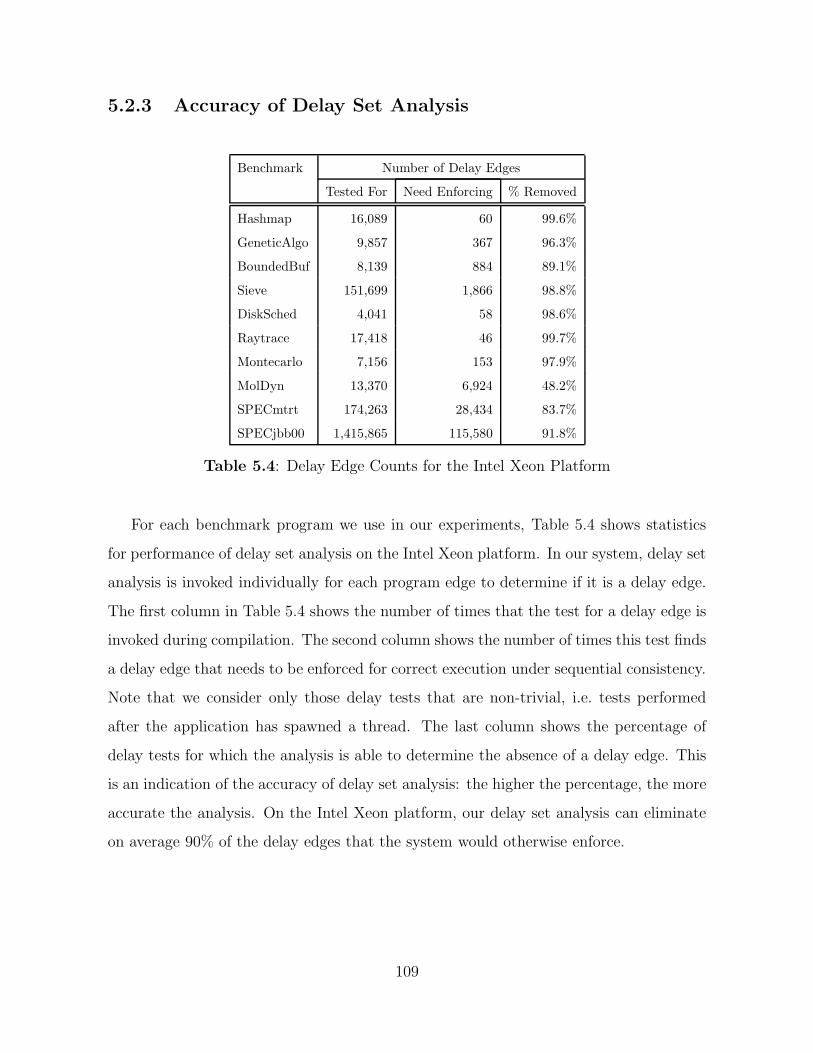
5.2.3 Accuracy of Delay Set Analysis

Benchmark Number of Delay Edges

Tested For Need Enforcing % Removed

Hashmap 16,089 60 99.6%

GeneticAlgo 9,857 367 96.3%

BoundedBuf 8,139 884 89.1%

Sieve 151,699 1,866 98.8%

DiskSched 4,041 58 98.6%

Raytrace 17,418 46 99.7%

Montecarlo 7,156 153 97.9%

MolDyn 13,370 6,924 48.2%

SPECmtrt 174,263 28,434 83.7%

SPECjbb00 1,415,865 115,580 91.8%

Table 5.4: Delay Edge Counts for the Intel Xeon Platform

For each benchmark program we use in our experiments, Table 5.4 shows statistics

for performance of delay set analysis on the Intel Xeon platform. In our system, delay set

analysis is invoked individually for each program edge to determine if it is a delay edge.

The first column in Table 5.4 shows the number of times that the test for a delay edge is

invoked during compilation. The second column shows the number of times this test finds

a delay edge that needs to be enforced for correct execution under sequential consistency.

Note that we consider only those delay tests that are non-trivial, i.e. tests performed

after the application has spawned a thread. The last column shows the percentage of

delay tests for which the analysis is able to determine the absence of a delay edge. This

is an indication of the accuracy of delay set analysis: the higher the percentage, the more

accurate the analysis. On the Intel Xeon platform, our delay set analysis can eliminate

on average 90% of the delay edges that the system would otherwise enforce.

109

Benchmark Number of Delay Edges

Tested For Need Enforcing % Removed

Hashmap 17,265 347 98.0%

GeneticAlgo 17,664 750 95.8%

BoundedBuf 3,890 824 78.8%

Sieve 5,256 1,121 78.7%

DiskSched 3,296 202 93.9%

Raytrace 78,786 47 99.9%

Montecarlo 16,568 314 98.1%

MolDyn 13,938 6,583 52.8%

SPECmtrt 150,501 19,861 86.8%

SPECjbb00 1,162,591 88,309 92.4%

Table 5.5: Delay Edge Counts for the Power3 Platform

Table 5.5 shows statistics for performance of delay set analysis on the Power3 platform

(analogous to Table 5.4 for the Intel Xeon platform). In this case, we eliminate on average

87.5% of the delay edges that the system would otherwise enforce.

Note that execution time performance is not proportional to the number of delay

edges found. This is because one memory barrier instruction may enforce multiple delay

edges [FLM03]. The number of memory barriers inserted depends on the number of delay

edges found, the specific pairs of accesses in the code that these delay edges are between,

as well as the placement of barriers in the code that is determined by the memory barrier

insertion algorithm.

110

5.2.4 Memory Barrier Instruction Counts

Benchmark Static Memory Barriers Dynamic Memory Barriers

Escape Delay % of Escape Escape Delay % of Escape

Hashmap 1,459 6 0.4% 857,291 K 62 0.0%

GeneticAlgo 1,427 56 3.9% 898,186 K 4,066 K 0.5%

BoundedBuf 1,265 20 1.6% 3,918,543 K 263,951 K 6.7%

Sieve 9,860 394 4.0% 1,955,615 K 4,538 K 0.2%

DiskSched 1,217 9 0.7% 528,132 K 50,129 K 9.5%

Raytrace 1,235 11 0.9% 3,562,060 K 6 K 0.0%

Montecarlo 1,556 18 1.2% 5,925 K 40 K 0.7%

MolDyn 1,096 78 7.1% 1,710,646 K 26,057 K 1.5%

SPECmtrt 4,175 970 23.2% 9,354 K 3,700 K 39.6%

SPECjbb00 19,613 2,344 12.0% 1,245,037 K 238,103 K 19.1%

Table 5.6: Memory Fences Inserted and Executed on the Intel Xeon Platform

Table 5.6 shows memory barrier instruction counts for each of the benchmark pro-

grams we test on the Intel Xeon platform. For all these applications, no lfences or sfences

are inserted (Section 4.3.4). Thus, all counts are for the number of mfence instructions.

The table shows two sets of data:

1. Static Memory Barriers: the number of memory barrier instructions inserted by

our compiler to enforce the set of delay edges determined.

2. Dynamic Memory Barriers: the number of memory barrier instructions dynamically

executed when an application runs.

The first column in each set is the number of memory barrier instructions for the

Escape SequentialConsistency configuration that uses only escape analysis to enforce se-

quential consistency. The second column in each set is the number of memory bar-

rier instructions for the Delay SequentialConsistency configuration that uses all our

111

analyses to enforce sequential consistency. The last column in each set is the num-

ber of memory barrier instructions for the Delay SequentialConsistency configuration

expressed as a percentage of the number of memory barrier instructions for the Es-

cape SequentialConsistency configuration. The number of fences inserted and executed

is much higher when our delay set analysis is not used.

Benchmark Static Memory Barriers Dynamic Memory Barriers

Escape Delay % of Escape Escape Delay % of Escape

Hashmap 1,217 23 1.9% 446,031 K 129 0.0%

GeneticAlgo 1,414 76 5.4% 446,131 K 2,514 K 0.6%

BoundedBuf 1,134 25 2.2% 142,456 K 13,373 K 9.4%

Sieve 1,091 94 8.6% 215,313 K 4,964 K 2.3%

DiskSched 1,068 12 1.1% 13,696 K 15 K 0.1%

Raytrace 1,755 4 0.2% 12,609 K 1 K 0.0%

Montecarlo 1,461 56 3.8% 73,948 K 106 K 0.1%

MolDyn 960 79 8.2% 290,997 K 12,998 K 4.5%

SPECmtrt 3,735 914 24.5% 28,992 K 8,339 K 28.8%

SPECjbb00 17,039 2,657 15.6% 1,337,196 K 173,385 K 13.0%

Table 5.7: Sync Instructions Inserted and Executed on the Power3 Platform

For the Power3 platform, Table 5.7 shows memory barrier instruction (i.e. sync)

counts for each of the benchmark programs we test (analogous to Table 5.6 for the Intel

Xeon platform).

112

5.2.5 Optimizations and Memory Usage

Benchmark Optimizations Performance Cost With Memory

Inhibited Performance Cost All Optimizations Inhibited Overhead

Hashmap 509 (75%) 0.0% 3.1% 44 M ( 62.3%)

GeneticAlgo 578 (63%) 0.0% 0.0% 13 M ( 12.1%)

BoundedBuf 491 (78%) 0.0% 0.0% 48 M ( 32.6%)

Sieve 803 (64%) 0.0% 0.0% 18 M ( 26.4%)

DiskSched 525 (75%) 0.0% 0.0% 71 M ( 97.2%)

Raytrace 864 (57%) 0.05% 0.05% 36 M ( 37.5%)

Montecarlo 718 (45%) 0.0% 4.0% 41 M ( 14.4%)

MolDyn 782 (66%) 0.0% 0.0% 36 M ( 46.7%)

SPECmtrt 1,141 (41%) 0.0% 0.0% 254 M (164.9%)

SPECjbb00 7,304 (59%) 0.1% 4.7% 517 M (106.9%)

Table 5.8: Optimizations Inhibited and Memory Overhead

In this section, we consider only code re-ordering and code elimination optimizations

that depend on the memory consistency model. The first column of Table 5.8 shows

the number of instances of these optimizations that are inhibited in our compiler to

honor sequential consistency (Section 4.3.3). The majority of the inhibited optimization

instances correspond to common subexpression elimination. We count the number of

optimization instances performed for two cases: when a benchmark is executed with all

optimizations enabled, and when a benchmark is executed with optimizations inhibited

based on sequential consistency requirements. The difference of these two counts is the

absolute number of optimizations inhibited, shown in the first column of the table. This

column also shows the optimizations inhibited as a percentage of the total number of

optimizations performed when all of them are enabled.

The second column in Table 5.8 shows the percentage slowdown in execution time

when using sequential consistency over a relaxed model, that is due to inhibiting op-

timizations. We observe that even though a significant percentage of code re-ordering

113

Thread 1

for (i=0; i<108; i++)Y.field += X.field;

print (X.field, Y.field);

Thread 2

X.field = 10;Y.field = 3;

Figure 5.4: Example for Loop Invariant Code Motion

optimizations are inhibited, there is a negligible effect on execution time performance.

The third column in Table 5.8 shows the percentage slowdown in execution time when

using sequential consistency, that is due to inhibiting all code re-ordering and code elim-

ination optimizations in the Jikes RVM. We find that these optimizations are not very

effective for our set of benchmark programs, and only 3 benchmarks show any significant

performance degradation when these optimizations are disabled: Hashmap, Montecarlo,

and SPECjbb00. Thus, for our benchmarks, inhibiting optimizations for sequential con-

sistency does not impact performance.

The last column in Table 5.8 shows the memory overhead of our compiler analysis,

i.e. the heap space required by the analysis during program execution. It also gives the

amount of this extra space as a percentage of the maximum heap space used by a program

when it executes without our analysis.

To further study the effect of optimizations in our system, we use the microbench-

marks illustrated in Figure 5.4 and Figure 5.5. In these examples, X and Y refer to

shared memory locations that are accessed by both threads in the example programs.

For the example in Figure 5.4, a traditional compiler may attempt to perform loop in-

variant code motion, and move the reference to X.field outside the for loop in Thread 1.

In our sequentially consistent system, we inhibit this optimization if the compiler at-

tempts to perform it (Section 4.3.3). When bytecode is generated by javac 2 for the Java

2We use the Sun javac compiler to translate Java source code to bytecodes. From Sun Java 2SDK onwards, javac does not perform common optimizations such as loop invariant code motion, loopunrolling, algebraic simplification, or strength reduction [Hag01].

114

Thread 1

for (i=0; i<108; i++) {T1 = X.field;T2 = T1 + 10;T3 = Y.field;T4 = X.field;T5 = T4 + 10;

}print (T2, T3, T5);

Thread 2

X.field = 7;Y.field = 3;

Figure 5.5: Example for Load Elimination

source code corresponding to this example, loop invariant code motion is not performed.

Also, we inspect the final machine code generated by the default Jikes RVM system, and

determine that it does not perform loop invariant code motion for this example. Thus,

in this case, inhibiting optimizations for sequential consistency has no effect, as the op-

timization is not performed at all in the default Jikes RVM system that we use to build

our compiler.

For the example in Figure 5.5, a traditional compiler may attempt to eliminate the

load of X.field into T4, since X.field has previously been loaded into T1. Also, the

compiler may attempt to re-use the common subexpression computed in T2 for uses of

T5. In our sequentially consistent system, we inhibit these optimizations if the compiler

attempts to perform them (Section 4.3.3). When bytecode is generated by javac for the

Java source code corresponding to this example, neither the load elimination for T4,

nor the common subexpression elimination for T5 is performed. When we inspect the

final machine code generated by the default Jikes RVM system, we determine that it

eliminates the load into T4, and uses the value loaded in T2 instead. However, it does

not perform common subexpression elimination for T5.

For this second microbenchmark, we obtained the following execution times:

1. Base RelaxedConsistency configuration: 1.35 seconds.

115

2. Base RelaxedConsistency configuration with all load eliminations disabled: 1.35

seconds.

3. Delay SequentialConsistency configuration: 66.7 seconds.

4. Delay SequentialConsistency configuration with no load eliminations disabled: 56.7

seconds.

From these results, we observe that inhibiting optimizations may impact performance.

The slowdown for sequential consistency over the default Jikes RVM memory model is 49

times. However, if load elimination is not disabled and only memory barriers are inserted,

the slowdown is 42 times. The example also illustrates the importance of reducing the

number of memory barriers inserted in hot methods, since this can lead to large slowdowns

otherwise.

5.2.6 Effect of Synchronization Analysis

7.222.7 2.38

0

0.2

0.4

0.6

0.8

1

1.2

1.4

1.6

Hash

map

Gen

etic

Algo

Boun

dedB

uf

Siev

e

Disk

Sche

d

Rayt

race

Mon

teca

rlo

Mol

Dyn

SPEC

mtr

t

SPEC

jbb0

0

Exec

utio

nti

me

norm

aliz

edto

Base

Rela

xed

tim

e

DelayWithoutSynch DelayWithoutLocks Delay

Figure 5.6: Effect of Thread Structure Analysis and Locking Synchronization

116

Figure 5.6 shows the effect of synchronization analysis on execution time performance.

The figure shows the execution times, normalized to the Base RelaxedConsistency con-

figuration, for the following three cases:

1. DelayWithoutSynch: This is an implementation of sequential consistency that uses

escape analysis, type-based alias analysis, and delay set analysis to determine the

memory barriers that need to be inserted. It does not use synchronization analysis.

2. DelayWithoutLocks: This is an implementation of sequential consistency that uses

escape analysis, type-based alias analysis, thread structure analysis, and delay set

analysis to determine the memory barriers that need to be inserted. It does not

use locking information based on synchronized blocks in Java.

3. Delay: This is the same as the Delay SequentialConsistency configuration described

earlier, that uses escape analysis, type-based alias analysis, synchronization anal-

ysis, and delay set analysis to determine the memory barriers that need to be

inserted.

The effect of synchronization analysis depends on the particular characteristics of a

specific program. For our benchmarks, synchronization analysis has a significant impact

on the performance of 5 out of 10 programs. Performance of Hashmap improves by

169% over the Base RelaxedConsistency configuration, DiskSched by 572%, Montecarlo

by 10%, SPECmtrt by 8%, and SPECjbb00 by 24%. The locking analysis component of

synchronization analysis improves the performance of DiskSched by 88%, SPECmtrt by

5%, and SPECjbb00 by 9%.

5.3 Analysis Times

The performance numbers in Figure 5.1 do not include the compile time for an applica-

tion, except for re-compilation due to adaptive optimization. On the Intel Xeon platform,

117

the compile time is significantly large for three benchmarks MolDyn, SPECmtrt, and

SPECjbb00. SPECjbb00 is a server application that runs for long periods of time in

practice. We expect the compilation overhead to be amortized over this long running

time. A similar argument applies to MolDyn and SPECmtrt if they are used to process

large data sets, and take a long time to finish execution. Note that a significant por-

tion of the compilation overhead for these benchmarks is due to adaptive optimization

of methods (Section 5.3.1). On the Power3 platform, compile time is significantly large

enough to impact performance numbers for most of our benchmarks. In this case, the

applications will have to run for longer periods of time if the compilation cost is to be

amortized.

Benchmark Delay Synch Escape Barrier TotalSC TotalRC

Hashmap 0.1 ( 7.7) 0.6 ( 46.2) 1.2 ( 92.3) 0.9 ( 69.2) 4.7 ( 361.5) 1.3

GeneticAlgo 0.1 ( 5.6) 0.8 ( 44.4) 1.0 ( 55.6) 0.7 ( 38.9) 4.8 ( 266.7) 1.8

BoundedBuf 0.02 ( 1.2) 0.3 ( 17.6) 0.5 ( 29.4) 0.7 ( 41.2) 2.9 ( 170.6) 1.7

Sieve 0.6 ( 10.5) 0.2 ( 3.5) 0.3 ( 5.3) 2.1 ( 36.8) 8.9 ( 156.1) 5.7

DiskSched 0.1 ( 8.3) 0.5 ( 41.7) 1.9 (158.3) 0.7 ( 58.3) 4.9 ( 408.3) 1.2

Raytrace 0.1 ( 3.8) 0.7 ( 26.9) 1.5 ( 57.7) 1.4 ( 53.8) 6.6 ( 253.8) 2.6

Montecarlo 0.1 ( 4.8) 1.1 ( 52.4) 2.0 ( 95.2) 0.8 ( 38.1) 7.2 ( 342.9) 2.1

MolDyn 0.7 ( 38.9) 0.6 ( 33.3) 1.4 ( 77.8) 14.2 (788.9) 22.6 (1255.6) 1.8

SPECmtrt 5.5 ( 83.3) 9.1 (137.9) 57.9 (877.3) 3.2 ( 48.5) 89.1 (1350.0) 6.6

SPECjbb00 60.1 (140.4) 33.0 ( 77.1) 340.1 (794.6) 125.1 (292.3) 716.5 (1674.1) 42.8

Table 5.9: Analysis Times in Seconds for the Intel Xeon Platform

Table 5.9 shows the total analysis times (including all re-compilations) in seconds for

each benchmark executing on the Intel Xeon platform. The first five columns also show

in brackets the time for their respective analysis components expressed as a percentage

of the total Jikes RVM base compile time, shown in the column titled TotalRC.

• Delay: This column shows the time taken by delay set analysis.

118

• Synch: This column shows the time taken by synchronization analysis.

• Escape: This column shows the time taken by escape analysis.

• Barrier: This column shows the time taken by memory barrier insertion.

• TotalSC: This column shows the total compilation time in the De-

lay SequentialConsistency configuration when all analyses are enabled.

• TotalRC: This column shows the total compilation

time in the Base RelaxedConsistency configuration when none of our analysis is

performed.

We observe that delay set analysis and synchronization analysis take at most 1.1 sec-

onds each for 8 out of 10 programs. Also, for 7 out of 10 programs, the difference between

the total compile time for our implementation of sequential consistency, and the total

compile time for the default Jikes RVM system is at most 5 seconds. The 3 programs that

have higher overheads are MolDyn, SPECmtrt, and SPECjbb00. Most of the overhead

for MolDyn comes from memory barrier insertion. SPECmtrt and SPECjbb00 both make

use of dynamic class loading, which leads to many non-trivial inter-procedural analysis

phases and re-compilations (Section 4.3.6). These contribute to increase the analysis

time.

119

Benchmark Delay Synch Escape Barrier TotalSC TotalRC

Hashmap 0.2 ( 4.8) 2.0 ( 47.6) 7.9 (188.1) 2.3 ( 54.8) 18.2 ( 433.3) 4.2

GeneticAlgo 0.3 ( 6.3) 2.5 ( 52.1) 5.7 (118.8) 2.3 ( 47.9) 16.6 ( 345.8) 4.8

BoundedBuf 0.03 ( 0.7) 0.9 ( 22.0) 1.9 ( 46.3) 1.9 ( 46.3) 9.1 ( 222.0) 4.1

Sieve 0.1 ( 2.9) 0.8 ( 23.5) 1.1 ( 32.4) 1.9 ( 55.9) 7.9 ( 232.4) 3.4

DiskSched 0.1 ( 3.1) 1.7 ( 53.1) 6.1 (190.6) 1.9 ( 59.4) 13.9 ( 434.4) 3.2

Raytrace 0.3 ( 3.8) 2.3 ( 28.8) 7.5 ( 93.8) 4.9 ( 61.3) 24.3 ( 303.8) 8.0

Montecarlo 0.3 ( 3.6) 4.7 ( 60.0) 9.7 (115.5) 2.7 ( 32.1) 25.7 ( 306.0) 8.4

MolDyn 0.4 ( 8.3) 1.8 ( 37.5) 5.0 (104.2) 2.6 ( 54.2) 17.5 ( 364.6) 4.8

SPECmtrt 12.0 (82.2) 19.4 (132.9) 93.1 (637.7) 11.7 ( 80.1) 179.7 (1230.8) 14.6

SPECjbb00 45.0 (94.3) 31.1 ( 65.2) 361.2 (757.2) 118.5 (248.4) 716.7 (1502.5) 47.7

Table 5.10: Analysis Times in Seconds for the Power3 Platform

Table 5.10 shows the total analysis times (including all re-compilations) in seconds for

each benchmark executing on the Power3 platform (analogous to Table 5.9). For most

benchmarks, the absolute compile times are higher than the times on the Intel Xeon

platform. The base compile time for the Base RelaxedConsistency configuration is also

higher in general.

5.3.1 Effect of Adaptive Re-compilation for Optimization

We base our compiler on the adaptive configuration of the Jikes RVM that profiles an

application as it executes, and attempts to dynamically optimize methods that take a

significant percentage of the execution time. The re-compilation of methods for opti-

mization purposes can be switched off using a command-line option. We experimented

with this option to determine the effect of adaptive re-compilations on analysis times and

execution time performance.

120

Benchmark Base Delay

BoundedBuf 1 3

Sieve 1 6

DiskSched 1 6

MolDyn 1 5

SPECmtrt 4 23

SPECjbb00 6 23

Table 5.11: Number of Methods Re-compiled for Adaptive Optimization

Benchmark Delay Synch Escape Barrier TotalSC TotalRC

BoundedBuf 0.02 ( 2.0) 0.2 ( 20.0) 0.5 ( 50.0) 0.5 ( 50.0) 2.4 ( 240.0) 1.0

Sieve 0.02 ( 2.0) 0.2 ( 20.0) 0.4 ( 40.0) 0.6 ( 60.0) 2.3 ( 230.0) 1.0

DiskSched 0.1 ( 9.1) 0.5 ( 45.5) 1.6 (145.5) 0.6 ( 54.5) 3.9 ( 354.5) 1.1

MolDyn 0.2 (12.5) 0.6 ( 37.5) 1.7 (106.3) 0.9 ( 56.3) 6.6 ( 412.5) 1.6

SPECmtrt 3.6 (69.2) 9.1 (175.0) 39.4 (757.7) 2.7 ( 51.9) 65.0 (1250.0) 5.2

SPECjbb00 9.9 (34.9) 24.6 ( 86.6) 63.2 (222.5) 62.0 (218.3) 212.3 ( 747.5) 28.4

Table 5.12: Analysis Times in Seconds With No Re-compilation for Optimization

Table 5.11 shows the number of methods that are re-compiled for adap-

tive optimization in the Base RelaxedConsistency configuration (Base) and the

Delay SequentialConsistency configuration (Delay). Table 5.12 shows the analysis

times analogous to Table 5.9 (Intel Xeon platform) for the case when re-compilations

for adaptive optimization are disabled. The table includes only those benchmarks that

show a difference in compile times for this case. We observe a significant reduction in the

compile time for the 3 programs that have the highest compile time overheads. The total

compile time for MolDyn reduced by 70.8%, for SPECmtrt by 27%, and for SPECjbb00 by

70.4%. Moreover, the performance of SPECmtrt and SPECjbb00 improved in this case.

SPECmtrt shows a slowdown of 8.8%, and SPECjbb00 shows a slowdown of 2% over

the Base RelaxedConsistency configuration. However, 3 programs show a performance

121

degradation when re-compilations are disabled. For the Delay SequentialConsistency

configuration, MolDyn, Montecarlo, and Raytrace respectively perform 10%, 15%, and

20% worse when re-compilations are turned off. Thus, adaptive re-compilation is impor-

tant in general, and disabling it is not a solution. We believe it is worth exploring how to

fine-tune the use of adaptive re-compilation in the context of a compiler like ours, that

performs expensive inter-procedural analysis.

122

Chapter 6

Conclusion

6.1 Contributions

This thesis makes the following contributions:

• It describes a fast and effective algorithm for delay set analysis that is applicable to

MIMD programs. The algorithm has polynomial time complexity in the number of

shared memory accesses. Program synchronization information is used to improve

the accuracy of the results.

• It describes a dataflow analysis algorithm to determine orders enforced by explicit

synchronization in the program. The algorithm computes ordering information

that includes happens-before, happens-after, and happens-in-parallel relations, and

represents the results in a compact form. The algorithm places no restraints on

recursion or dynamic thread creation, and is more precise than previous methods

based on dataflow analysis.

• It describes our memory-model aware compiler and the range of analysis techniques

needed to account for the effect of inter-thread memory accesses.

123

• It evaluates performance of our proposed algorithms in the framework of a Java just-

in-time compiler. It reports data to compare the performance of two programming

language memory models: sequential consistency and weak consistency.

The synchronization and delay set analysis algorithms are designed to be fast. Ex-

perience with the implementation indicates that the analysis times required are within

15% of the total compile time in most cases. On the Intel Xeon platform, the absolute

analysis times are in the order of a few seconds for all applications except SPECjbb00.

Thus, these algorithms may be implemented in a just-in-time compiler where the compile

time contributes to the application execution time. Several factors contribute to make

our analysis fast:

• We use a conservative and simple algorithm for delay set analysis. This algorithm

is effective because for the most part applications communicate through shared

memory in a disciplined manner using specific sharing patterns.

• Our synchronization analysis is efficient since only orders involving a synchroniza-

tion construct are determined. Applications typically include relatively few syn-

chronization constructs.

• We summarize the analysis results for each method. This makes the inter-procedural

analysis fast since the effect of a method call can be easily incorporated when testing

for shared memory access orders to enforce.

• We take advantage of user-defined types in the programming language to determine

if two shared memory locations may be the same. In most cases, user-defined types

naturally group together locations with similar access properties. This enables the

system to perform delay set analysis with a high level of accuracy without having

to use an expensive alias analysis phase.

Experiments on a set of benchmark programs show that our techniques are effective

in reducing the number of delays that need to be enforced when implementing sequential

124

consistency in software. This results in low performance overheads for a sequentially

consistent system over a system that uses weak consistency. In our experiments, we

observe a slowdown of 10% on average for our benchmarks executing on an architecture

based on the Intel Xeon processor, and 26% on average for an architecture based on the

IBM Power3. Moreover, 7 out of 10 applications on the Intel Xeon platform, and 8 out

of 10 applications on the Power3 platform, show a performance loss of 7% or less.

This is important because sequential consistency is the memory consistency model

that enforces the most constraints on an implementation. We show the possibility of

achieving reasonable performance with sequential consistency. This opens up a wide

space for the design of programming language memory models since performance need

no longer be a prohibitive factor. We can consider using models that are more stringent

than the relaxed consistency models popular today. Use of such strong models may help

make parallel programming more efficient.

6.2 Open Problems

In this work, we use the analysis techniques described to reduce the number of fences that

need to be inserted when implementing memory consistency in software. These analysis

results can also be applied to optimize programs by:

• Removing redundant synchronization: We can use our analyses to determine delay

edges without taking into account some synchronization constructs in the program.

Then we can match these delay edges with orders enforced by the synchronizations

constructs, and determine if some of the synchronizations are unnecessary.

• Improving thread scheduling: We can apply our analysis results to infer knowledge

about code sections that may execute independently of each other. This knowledge

can be used to determine when or where to schedule threads so that the overall

execution is efficient.

125

• Applying code specialization: Our analysis results retain information about the

source of concurrency in terms of the start() calls that spawn threads that may

be concurrent with a program point. This information can be used by a code

specialization phase to optimize code sections that are common to multiple thread

types, and may be executed by a thread of any of these types. Code specialization

generates multiple versions of a piece of code, each optimized for use in different

contexts.

The analysis can also be used to aid program development and debugging by:

• Statically detecting possible races and deadlocks in the program code.

• Reducing the overhead of dynamic data race detection by eliminating the need to

track some shared memory accesses in the program.

• Efficiently inserting fences to automatically enforce orders on a subset of shared

memory accesses specified by the programmer. This can reduce the complexity of

reasoning about different permutations of shared memory accesses when developing

a program.

126

Bibliography

[AAB+00] B. Alpern, C. R. Attanasio, J. J. Barton, M. G. Burke, P.Cheng, J.-D.

Choi, A. Cocchi, S. J. Fink, D. Grove, M. Hind, S. F. Hummel, D. Lieber,

V. Litvinov, M. F. Mergen, T. Ngo, J. R. Russell, V. Sarkar, M. J. Serrano,

J. C. Shepherd, S. E. Smith, V. C. Sreedhar, H. Srinivasan, and J. Whaley.

The Jalapeno Virtual Machine. IBM System Journal, 39(1), February 2000.

[AFG+00] Matthew Arnold, Stephen Fink, David Grove, Michael Hind, and Peter F.

Sweeney. Adaptive Optimization in the Jalapeno JVM. Third ACM Work-

shop on Feedback-Directed and Dynamic Optimization, December 2000.

[AG96] Sarita V. Adve and Kourosh Gharachorloo. Shared Memory Consistency

Models: A Tutorial. IEEE Computer, pages 66–76, December 1996.

[AH90] Sarita V. Adve and Mark D. Hill. Weak Ordering - A New Definition.

In Proceedings of The 17th Annual International Symposium on Computer

Architecture (ISCA), pages 2–14, May 1990.

[AK02] Randy Allen and Ken Kennedy. Optimizing Compilers for Modern Archi-

tectures. Morgan Kaufmann Publishers, 2002.

[BH99] Jeff Bogda and Urs Holzle. Removing Unnecessary Synchronization in Java.

In Proceedings of the 14th ACM SIGPLAN Conference on Object-oriented

Programming, Systems, Languages, and Applications, pages 35–46. ACM

Press, 1999.

127

[BHJ+03] Konstantin Berlin, Jun Huan, Mary Jacob, Garima Kochhar, Jan Prins,

Bill Pugh, P. Sadayappan, Jaime Spacco, and Chau-Wen Tseng. Evaluat-

ing the Impact of Programming Language Features on the Performance of

Parallel Applications on Cluster Architectures. In 16th Annual Workshop

on Languages and Compilers for Parallel Computing, October 2003.

[BK89] Vasanth Balasundaram and Ken Kennedy. Compile-time Detection of Race

Conditions in a Parallel Program. In Proceedings of the 3rd international

conference on Supercomputing, pages 175–185. ACM Press, 1989.

[Bla98] Bruno Blanchet. Escape Analysis: Correctness Proof, Implementation and

Experimental Results. In Proceedings of the 25th ACM SIGPLAN-SIGACT

Symposium on Principles of Programming Languages, pages 25–37. ACM

Press, 1998.

[BLR02] Chandrasekhar Boyapati, Robert Lee, and Martin Rinard. Ownership Types

for Safe Programming: Preventing Data Races and Deadlocks. In Object-

oriented Programming, Systems, Languages, and Applications (OOPSLA),

November 2002.

[CADG+93] David E. Culler, Andrea C. Arpaci-Dusseau, Seth Copen Goldstein, Arvind

Krishnamurthy, Steven Lumetta, Thorsten von Eicken, and Katherine A.

Yelick. Parallel programming in Split-C. In Supercomputing, pages 262–273,

1993.

[CGHS99] Jong-Deok Choi, David Grove, Michael Hind, and Vivek Sarkar. Efficient

and Precise Modeling of Exceptions for the Analysis of Java Programs.

ACM SIGPLAN-SIGSOFT Workshop on Program Analysis for Software

Tools and Engineering (PASTE), September 1999.

128

[CGS+99] Jong-Deok Choi, Manish Gupta, Mauricio Serrano, Vugranam C. Sreedhar,

and Samuel P. Midkiff. Escape Analysis for Java. In Proceedings of the

ACM SIGPLAN 1999 Conference on Object-oriented Programming Systems,

Languages, and Applications (OOPSLA), pages 1–19, November 1999.

[CKS90] David Callahan, Ken Kennedy, and Jaspal Subhlok. Analysis of Event

Synchronization in a Parallel Programming Tool. In Proceedings of the

Second ACM SIGPLAN Symposium on Principles and Practice of Parallel

Programming, pages 21–30, Seattle WA, 1990.

[CKY03] Wei-Yu Chen, Arvind Krishnamurthy, and Katherine Yelick. Polynomial-

Time Algorithms for Enforcing Sequential Consistency in SPMD Programs

with Arrays. In Sixteenth Annual Workshop on Languages and Compilers

for Parallel Computing, October 2003.

[CL97] M. Cierniak and W. Li. Just-in-time Optimization for High-performance

Java Programs. Concurrency: Practice and Experience, 9(11):1063–73,

November 1997.

[CLL+02] J.-D. Choi, K. Lee, A. Loginov, R. O’Callahan, V. Sarkar, and M. Sridharan.

Efficient and Precise Datarace Detection for Multithreaded Object-oriented

Programs. In Proceedings of the ACM SIGPLAN 2002 Conference on Pro-

gramming Language Design and Implementation (PLDI), pages 258–269,

June 2002.

[Cor98] The Standard Performance Evaluation Corporation. SPEC JVM Client98

Suite. 1998. URL: http://www.specbench.org/jvm98/jvm98.

[Cor00] The Standard Performance Evaluation Corporation. SPEC JBB 2000

Benchmark. 2000. URL: http://www.specbench.org/jbb2000.

129

[CS89] D. Callahan and J. Subhlok. Static Analysis of Low-level Synchronization.

In Proceedings of the ACM SIGPLAN and SIGOPS Workshop on Parallel

and Distributed Debugging, pages 100–111, January 1989.

[DS91] Evelyn Duesterwald and Mary Lou Soffa. Concurrency Analysis in the

Presence of Procedures Using a Data-flow Framework. In Proceedings of

the Symposium on Testing, Analysis, and Verification, pages 36–48. ACM

Press, 1991.

[DSB88] M. Dubois, C. Scheurich, and F.A. Briggs. Synchronization, Coherence, and

Event Ordering in Multiprocessors. 21(2):9–21, 1988.

[EGP89] Perry A. Emrath, Sanjoy Ghosh, and David A. Padua. Event Synchroniza-

tion Analysis for Debugging Parallel Programs. In Proceedings of Supercom-

puting ’89, pages 580–588, 1989.

[FF00] Cormac Flanagan and Stephen N. Freund. Type-based race detection for

Java. ACM SIGPLAN Notices, 35(5):219–232, 2000.

[FLM03] Xing Fang, Jaejin Lee, and Samuel P. Midkiff. Automatic Fence Insertion

for Shared Memory Processing. In 2003 ACM International Conference on

Supercomputing, June 2003.

[FLR98] Matteo Frigo, Charles E. Leiserson, and Keith H. Randall. The Implemen-

tation of the Cilk-5 Multithreaded Language. In SIGPLAN Conference on

Programming Language Design and Implementation, pages 212–223, 1998.

[GFV99] K. Gniady, B. Falsafi, and T. Vijaykumar. Is SC + ILP = RC? In Proc.

of the 26th Annual International Symposium on Computer Architecture

(ISCA’99), 1999.

[GJS96] James Gosling, Bill Joy, and Guy Steele. The Java Language Specification,

Second Edition. Addison-Wesley, 1996.

130

[GLL+90] Kourosh Gharachorloo, Daniel Lenoski, James Laudon, Phillip Gibbons,

Anoop Gupta, and John Hennessy. Memory Consistency and Event Order-

ing in Scalable Shared-Memory Multiprocessors. In Proceedings of The 17th

Annual International Symposium on Computer Architecture (ISCA), pages

15–26, May 1990.

[GS93] D. Grunwald and H. Srinivasan. Data Flow Equations for Explicitly Parallel

Programs. In Proceedings of the Fourth ACM SIGPLAN Symposium on

Principles and Practice of Parallel Programming, San Diego, CA, 1993.

[Hag01] Peter Haggar. Understanding Bytecode Makes You a Better Program-

mer. July 2001. URL: www-106.ibm.com/developerworks/ibm/library/it-

haggar bytecode.

[Har98] Stephen Hartley. Concurrent Programming: the Java Programming Lan-

guage. Oxford University Press, 1998.

[Hil98] Mark D. Hill. Multiprocessors Should Support Simple Memory-Consistency

Models. IEEE Computer, August 1998.

[HM91] David P. Helmbold and Charles E. McDowell. Computing Reachable States

of Parallel Programs. Proceedings of the ACM/ONR Workshop on Par-

allel and Distributed Debugging, published in ACM SIGPLAN Notices,

26(12):76–84, 1991.

[IA3] IA-32 Intel Architecture Software Developer’s Manual, Volume 2 and 3.

URL: developer.intel.com/design/pentium4/manuals/index new.htm.

[Jav03] JavaMemoryModel. Java Memory Model Mailing List. In Archive at

http://www.cs.umd.edu/ pugh/java/memoryModel/arc hive/, 2003.

[jgf] The Java Grande Forum Multi-threaded Benchmarks. URL:

http://www.epcc.ed.ac.uk/javagrande/threads/contents.html.

131

[KJCS99] Sanjeev Kumar, Dongming Jiang, Rohit Chandra, and Jaswinder Pal

Singh. Evaluating Synchronization on Shared Address Space Multipro-

cessors: Methodology and Performance. In Proceedings of the 1999 ACM

SIGMETRICS International Conference on Measurement and Modeling of

Computer Systems, pages 23–34. ACM Press, 1999.

[KSV96] Jens Knoop, Bernhard Steffen, and Jurgen Vollmer. Parallelism for Free: Ef-

ficient and Optimal Bitvector Analyses for Parallel Programs. ACM Trans-

actions on Programming Languages and Systems, 18(3):268–299, May 1996.

[KY94] Arvind Krishnamurthy and Katherine Yelick. Optimizing Parallel SPMD

Programs. In Seventh Annual Workshop on Languages and Compilers for

Parallel Computing, August 1994.

[KY96] Arvind Krishnamurthy and Katherine Yelick. Analyses and Optimizations

for Shared Address Space Programs. Journal of Parallel and Distributed

Computing, 38:139–144, 1996.

[Lam79] Leslie Lamport. How to Make a Multiprocessor Computer That Correctly

Executes Multiprocess Programs. IEEE Transactions on Computers, C-

28(9):690–691, September 1979.

[LAY03] Ben Liblit, Alex Aiken, and Katherine Yelick. Type Systems for Distributed

Data Sharing. In Proceedings of the Tenth International Static Analysis

Symposium, 2003.

[Lea] Doug Lea. Java Specification Request (JSR) 166: Concurrency Utilities. In

http://gee.cs.oswego.edu/dl/concurrency-interest/index.html .

[Lea99a] Doug Lea. Concurrent Programming in Java. Addison Wesley, 1999. URL:

http://gee.cs.oswego.edu/dl/cpj.

[Lea99b] Doug Lea. JavaMemoryModel: recap: concurrent reads. December 1999.

URL: www.cs.umd.edu/ pugh/java/memoryModel/archive/0358.html.

132

[LMP97] Jaejin Lee, Samuel P. Midkiff, and David A. Padua. Concurrent Static

Single Assignment Form and Constant Propagation for Explicitly Parallel

Programs. In Z. Li, P.-C. Yew, S. Chatterjee, C.-H. Huang, P. Sadayappan,

and D. Sehr, editors, Proceedings of The 10th International Workshop on

Languages and Compilers for Parallel Computing, number 1366 in Lecture

Notes in Computer Science, pages 114–130. Springer, August 1997.

[LP00] Jaejin Lee and David A. Padua. Hiding Relaxed Memory Consistency with

Compilers. In Proceedings of the IEEE International Conference on Parallel

Architectures and Compilation Techniques (PACT), pages 111–122, October

2000.

[LPM99] Jaejin Lee, David A. Padua, and Samuel P. Midkiff. Basic Compiler Al-

gorithms for Parallel Programs. In Proceedings of the 7th ACM SIGPLAN

Symposium on Principles and Practice of Parallel Programming (PPoPP),

pages 1–12, May 1999.

[MC93] John M. Mellor-Crummey. Compile-Time Support for Efficient Data Race

Detection in Shared-Memory Parallel Programs. In Workshop on Parallel

and Distributed Debugging, pages 129–139, 1993.

[Mid95] S. Midkiff. Dependence Analysis in Parallel Loops with i+/-k Subscripts. In

1995 Workshop on Languages and Compilers for Parallel Computing, 1995.

available as Springer Lecture Notes in Computer Science Vol. N. 1033.

[MP87] Samuel P. Midkiff and David A. Padua. Compiler Algorithms for Synchro-

nization. IEEE Transactions on Computers, C-36(12):1485–1495, December

1987.

[MP90] S. Midkiff and D. Padua. Issues in the Compile-Time Optimization of Par-

allel Programs. In Proceedings of the 1990 International Conference on

Parallel Processing, Vol. II, pages 105–113, August 1990.

133

[MP01] J. Manson and W. Pugh. Core Semantics of Multithreaded Java. In Pro-

ceedings of the ACM SIGPLAN 2001 ISCOPE/Java Grande Conference,

pages 29–38, 2001.

[MPC90] Samuel P. Midkiff, David A. Padua, and Ron Cytron. Compiling Programs

with User Parallelism. In Languages and Compilers for Parallel Computing,

pages 402–422, 1990.

[MR93] Stephen P. Masticola and Barbara G. Ryder. Non-concurrency Analysis.

In Proceedings of the Fourth ACM SIGPLAN Symposium on Principles and

Practice of Parallel Programming, pages 129–138. ACM Press, 1993.

[NAC99] Gleb Naumovich, George S. Avruninand, and Lori A. Clarke. An Efficient

Algorithm for Computing MHP Information for Concurrent Java Programs.

In Proceedings of Seventh European Software Engineering Conference and

Seventh ACM SIGSOFT Symposium on the Foundations of Software Engi-

neering, Sept. 1999.

[NG92] Robert H. B. Netzer and Sanjoy Ghosh. Efficient Race Condition Detection

for Shared-Memory Programs with Post/Wait Synchronization. In Proceed-

ings of the 1992 International Conference on Parallel Processing, volume II,

Software, pages II:242–246, Boca Raton, Florida, 1992. CRC Press.

[NM90] Robert H. B. Netzer and Barton P. Miller. On the Complexity of Event

Ordering for Shared-Memory Parallel Program Executions. In Proceedings

of 1990 International Conference on Parallel Processing, pages II.93–II.97,

University Park PA, 1990.

[NM91] Robert H. B. Netzer and Barton P. Miller. Improving the Accuracy of

Data Race Detection. Proceedings of the ACM SIGPLAN Symposium on

Principles and Practice of Parallel Programming PPOPP, published in ACM

SIGPLAN NOTICES, 26(7):133–144, 1991.

134

[NM92] Robert H. B. Netzer and Barton P. Miller. What are Race Conditions?

Some Issues and Formalizations. ACM Letters on Programming Languages

and Systems, 1(1), March 1992.

[PPCa] Book II: PowerPC Virtual Environment Architecture. URL: www-

106.ibm.com/developerworks/eserver/articles/archguide.html.

[PPCb] PowerPC Microprocessor Family: Programming Environments Man-

ual. URL: www-3.ibm.com/chips/techlib/techlib.nsf/products/PowerPC

970 and 970FX Microprocessors.

[Pug99] William Pugh. Fixing the Java Memory Model. In Proceedings of the ACM

1999 Java Grande Conference, June 1999.

[Rin01] Martin Rinard. Analysis of Multithreaded Programs. Lecture Notes in

Computer Science, 2126, 2001.

[RL98] Martin C. Rinard and Monica S. Lam. The Design, Implementation, and

Evaluation of Jade. ACM Transactions on Programming Languages and

Systems, 20(3):483–545, 1 May 1998.

[RM94] J. Ramanujam and A. Mathew. Analysis of Event Synchronization in Par-

allel Programs. In Languages and Compilers for Parallel Computing, pages

300–315, 1994.

[RPA97] Parthasarathy Ranganathan, Vijay S. Pai, and Sarita V. Adve. Using Spec-

ulative Retirement and Larger Instruction Windows to Narrow the Perfor-

mance Gap between Memory Consistency Models. In Proceedings of The 9th

ACM Symposium on Parallel Algorithms and Architectures (SPAA), pages

199–210, June 1997.

[Ruf00] Erik Ruf. Effective synchronization Removal for Java. In Conference on

Programming Languages, Design, and Implementation (PLDI), 2000.

135

[SAR99] Xiaowei Shen, Arvind, and Larry Rudolph. Commit-Reconcile & Fences

(CRF): A New Memory Model for Architects and Compiler Writers. In

Proceedings of The 26th Annual International Symposium on Computer Ar-

chitecture (ISCA), pages 150–161, May 1999.

[SBN+97] Stefan Savage, Michael Burrows, Greg Nelson, Patrick Sobalvarro, and

Thomas Anderson. Eraser: A Dynamic Data Race Detector for Multi-

threaded Programs. ACM Transactions on Computer Systems, 15(4):391–

411, 1997.

[Sch89] Edmond Schonberg. On-the-fly Detection of Access Anomalies. In Pro-

ceedings of the ACM SIGPLAN ’89 Conference on Programming Language

Design and Implementation, volume 24, pages 285–297, Portland, OR, June

1989.

[Sin96] Pradeep K. Sinha. Distributed Operating Systems, Concepts and Design.

IEEE Press, 1996.

[SL94] Daniel J. Scales and Monica S. Lam. The Design and Evaluation of a Shared

Object System for Distributed Memory Machines. In Operating Systems

Design and Implementation, pages 101–114, 1994.

[SS88] Dennis Shasha and Marc Snir. Efficient and Correct Execution of Parallel

Programs that Share Memory. ACM Transactions on Programming Lan-

guages and Systems, 10(2):282–312, April 1988.

[Ste90] Guy L. Steele, Jr. Making Asynchronous Parallelism Safe for the World. In

Proceedings of the 17th ACM SIGPLAN-SIGACT Symposium on Principles

of Programming Languages, pages 218–231. ACM Press, 1990.

136

[SWF+02] Z. Sura, C.-L. Wong, X. Fang, J. Lee, S.P. Midkiff, and D. Padua. Auto-

matic Implementation of Programming Language Consistency Models. In

15th Annual Workshop on Languages and Compilers for Parallel Comput-

ing, July 2002.

[Tay83] Richard N. Taylor. A General-purpose Algorithm for Analyzing Concurrent

Programs. Commun. ACM, 26(5):361–376, 1983.

[vP04] Christoph von Praun. Efficient Computation of Communicator Variables for

Programs with Unstructured Parallelism. In Seventeenth Annual Workshop

on Languages and Compilers for Parallel Computing, September 2004.

[vPG03] Christoph von Praun and Thomas R. Gross. Static Conflict Analysis for

Multi-threaded Object-oriented Programs. In Proceedings of the ACM SIG-

PLAN 2003 Conference on Programming Language Design and Implemen-

tation (PLDI), June 2003.

[VR01] Frederic Vivien and Martin Rinard. Incremental Pointer and Escape Anal-

ysis. In Proceedings of the ACM SIGPLAN Conference on Programming

Language Design and Implementation (PLDI), 2001.

[WFPS02] Peng Wu, Paul Feautrier, David Padua, and Zehra Sura. Instance-wise

Points-to Analysis for Loop-based Dependence Testing. In ACM Interna-

tional Conference on Supercomputing, June 2002.

[WR99] John Whaley and Martin Rinard. Compositional Pointer and Escape Anal-

ysis for Java Programs. In Proceedings of the ACM SIGPLAN 1999 Confer-

ence on Object-oriented Programming Systems, Languages, and Applications

(OOPSLA), pages 187–206, November 1999.

[WSF+02] C.-L. Wong, Z. Sura, X. Fang, S.P. Midkiff, J. Lee, and D. Padua. The Pen-

sieve Project: A Compiler Infrastructure for Memory Models. International

Symposium on Parallel Architectures, Algorithms, and Networks, May 2002.

137

[YSP+98] K. Yelick, L. Semenzato, G. Pike, C. Miyamoto, B. Liblit, A. Krishna-

murthy, P. Hilfinger, S. Graham, D. Gay, P. Col ella, and A. Aiken. Tita-

nium: A High-Performance Java Dialect. In ACM 1998 Workshop on Java

for High-Performance Network Computing. ACM SIGPLAN, 1998. URL:

http://www.cs.ucsb.edu/conferences/java98.

[YT88] M. Young and R. M. Taylor. Combining Static Concurrency Analysis

with Symbolic Execution. IEEE Transactions on Software Engineering,

14(10):1499–1511, 1988.

138

Vita

Zehra Sura was born on April 12, 1976 in Dubai, U.A.E. She earned a Bachelor of En-

gineering degree in computer science from Visvesvaraya College of Engineering, Nagpur,

India in 1998. Immediately after that, she began her graduate study in computer science

at the University of Illinois, Urbana-Champaign (UIUC). In Fall 1998, she worked as a

research assistant in the Parallel Programming Laboratory, UIUC under the guidance

of Professor Laxmikant Kale. In Spring 1999, she was a teaching assistant for an intro-

ductory course in parallel programming in the department of computer science, UIUC.

Since the summer of 1999, she has worked as a research assistant under the guidance of

Professor David Padua. She did an internship at Intel KAI Lab, Champaign, Illinois in

the summer of 2001, and at IBM T.J. Watson Research Center, Yorktown Heights, New

York in the summer of 2003. In 2004, she completed her Doctor of Philosophy degree in

computer science. After graduation, she will join the IBM T.J. Watson Research Center

in Yorktown Heights, New York. Her research interests include analysis and transforma-

tion of programs for parallel processing, and the use of runtime techniques to improve

compiler optiizations.

139