Using Excel for AnalyzingSurvey Questionnaires

You have created, tested, and implemented a survey, and now you would like to see the results of your work. Thereare five steps in analyzing your survey data using Excel.

1. Create an Excel database2. Code and Standardize data3. Input data4. Clean & Categorize data5. Analyze data

CREATE AN EXCEL DATABASE When you open up Microsoft Excel, you will see a blank worksheet. This worksheet is part of a workbook. A workbook holds all of your worksheets, and is simply another name for an Excel file. A blank Excel worksheet is composed of a series of vertical columns, horizontal rows, and individual cells. You can select different worksheets by clicking on the tabs at the bottom of your workbook.

• Columns are alphabetized — A, B, C, D … — fromleft to right across the top.

• Rows are numbered — 1, 2, 3, 4 … — from top tobottom down the left of the worksheet.

• Cells are individual boxes within the work-sheet.

•

Designing a list or table

An Excel database may consist of several list/tables thatcan be linked using a common field/label such as respondent number.

Although Excel is quite accommodating when it comes to the information that is stored in a list, you should givesome initial thought to how you want to organize your information. The following are some guidelines to keep inmind when designing lists/tables:

✦ Insert descriptive labels (one for each column) in the first row of the list.This is the header row. Column labels should be well associated with the question.

✦ Each column should contain the same type of information. For example, don’t mix dates and text in asingle column.

✦ Don’t use any empty rows within the list. For list operations, Excel determines the list boundaries

automatically, and an empty row signals the end of the list.

✦ For best results, try to keep the list on a worksheet by itself.

✦ Design the list in its “Normal Form”

CODE & STANDARDIZE DATA

Survey questions are coded/labeled and act as headers of our lists/tables.

Excel has two features that facilitates coding our data:

✦ AutoComplete: When you begin to type in a cell, Excel scans up and down the column to see whether it recognizes what you’re typing. If it finds a match, Excel fills in the rest of the text automatically. Press Enter to make the entry. You can turn this feature on or off in the Edit panel of the Options dialog box.

✦ Pick Lists: You can right-click on a cell and select Pick from List from the shortcut menu .Excel displays alist box that shows all entries in the column. Click onthe one that you want, and it is then entered into the cell. (No typing is required.)

An unanswered question is usually coded as blank or “no response”, however, if the required response is quantitative then we must qualify it if it is “0” or blank.Narrative text are usual responses to open-ended questions and are coded as answered.

Standardize values of measurements, date/time and other quantitative type of answers. Write the standardized values strategically and consistently placed in the questionnaire to clearly associate it with the answer andavoid overwriting the original answer.

INPUT DATA

While entering your data, you may encounter some unexpected problems. Here are tips for preventing problems and dealing with common situations that come up while entering data:

✦ Gather and input the same pages of the accomplished questionnaires sorted by respondent number

✦ Select the upper-left data cell and choose Window➪Freeze Panes to make sure that the headings arevisible when the list is scrolled.

✦ Preformat entire columns to ensure that the data has the same format. For example, if a column contains dates, format the entire column with the desired date format.

✦ Make backup copies

✦ Remember to SAVE, SAVE, SAVE!!! Save your file after each record using the keyboard command <ctrl-s>.

✦ After all your data are entered: Create at least one backup copy of your file. This will be helpful during the analysis process

✦ To check data integrity, sample 5% randomly for each page and compare inputted data

CLEAN & CATEGORIZE DATA

Filtering a List

Filtering a list is the process of hiding all rows in thelist except those that meet some criteria that you specify. For example, if you have a list of customers, you can filter the list to show only those who live in Seattle. Filtering is a common (and very useful) technique. Excel provides two ways to filter a list:✦ AutoFilter for simple filtering criteria✦ Advance Filter for more-complex filtering

Using autofilteringTo autofilter a list, start by moving the cell pointer anywhere within the list. Then choose Data➪Filter➪AutoFilter. Excel analyzes your list and adds drop-down arrows to the field names in the header row. When you click the arrow in one of these dropdown lists, the list expands to show the unique items in that column. Select an item, and Excel hides all rows except those that include the selected item. In other words, thelist is filtered by the item that you selected.

After you filter the list, the status bar displays a message that tells you how many rows qualified. In addition, the drop-down arrow changes color to remind youthat the list is filtered by a value in that column. Autofiltering has a limit. Only the first 1,000 unique items in the column appear in the drop-down list. If yourlist exceeds this limit, you can use advanced filtering.

Besides showing every item in the column, the drop-down list includes other items:✦ All: Displays all items in the column. Use this to

remove filtering for a column.✦ Top 10: Filters to display the “top 10” items in the

list; I discuss this later in this chapter.✦ Custom: Lets you filter the list by multiple items; I

discuss this in the “Custom autofiltering” section, later in this chapter.

✦ Blanks: Filters the list by showing rows that contain blanks in this column. This item appears at the bottom of the drop-down list and only if the column contains one or more blank cells..

✦ NonBlanks: Filters the list by showing rows that contain nonblanks in this column. This item appears at the bottom of the drop-down list and only if the column contains one or more blank cells.

To display the entire list again, click the arrow and choose All—the first item in the drop-down list. Or you can select Data➪Filter➪Show All.

To move out of AutoFilter mode and remove the drop-down arrows from the field names, choose Data➪Filter➪AutoFilter again. This removes the check mark from the AutoFilter menu item and restores the list to its normal state.

Custom autofilteringUsually, autofiltering involves selecting a single value for one or more columns. If you choose the Custom option in a drop-down list, you gain a bit more flexibility in filtering the list. Selecting the Custom option displays

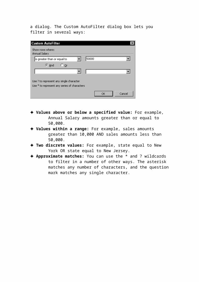
a dialog. The Custom AutoFilter dialog box lets you filter in several ways:

✦ Values above or below a specified value: For example, Annual Salary amounts greater than or equal to 50,000.

✦ Values within a range: For example, sales amounts greater than 10,000 AND sales amounts less than 50,000.

✦ Two discrete values: For example, state equal to New York OR state equal to New Jersey.

✦ Approximate matches: You can use the * and ? wildcards to filter in a number of other ways. The asterisk matches any number of characters, and the questionmark matches any single character.

JOINING LISTS/TABLES USING MSQUERYBegin with an empty worksheet. Select Data➪Import External Data➪New Database Query, which displays the Choose Data Source dialog box. This dialog box contains three tabs:

✦ Databases: Lists the data sources that are known to Query—this tab may be empty, depending on which data sources are defined on your system.

✦ Queries: Contains a list of stored queries. Again, thismay or may not be empty.✦ OLAP Cubes: Lists OLAP databases that are available forquery.

Using Query without the WizardWhen you select Data➪Import External Data➪New Database Query, the Choose Data Source dialog box gives you the option of whether to use Query Wizard. If you choose not to use Query Wizard, Microsoft Query is launched with a Select Database window

and subsequent Add tables window prompt.

You may have to click on Options... and check System Tables for all the lists/tables to be displayed.

To establish link between two tables, click and drag fromone common field to the other.

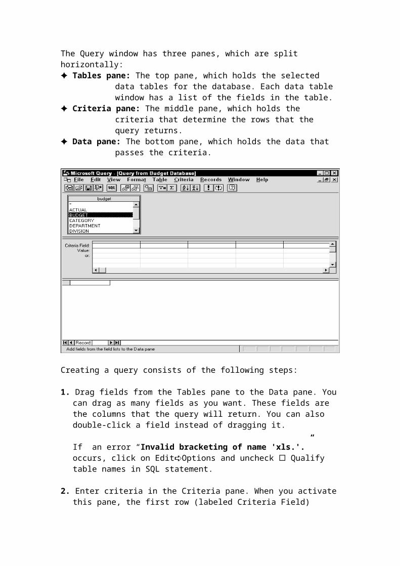
The Query window has three panes, which are split horizontally:✦ Tables pane: The top pane, which holds the selected

data tables for the database. Each data table window has a list of the fields in the table.

✦ Criteria pane: The middle pane, which holds the criteria that determine the rows that the query returns.

✦ Data pane: The bottom pane, which holds the data that passes the criteria.

Creating a query consists of the following steps:

1. Drag fields from the Tables pane to the Data pane. Youcan drag as many fields as you want. These fields are the columns that the query will return. You can also double-click a field instead of dragging it.

If an error “Invalid bracketing of name 'xls.'.” occurs, click on Edit Options and uncheck ➪ Qualify table names in SQL statement.

2. Enter criteria in the Criteria pane. When you activatethis pane, the first row (labeled Criteria Field)

displays a drop-down list that contains all the field names. Select a field and enter the criteria below it. Query updates the Data pane automatically, treating each row like an OR operator.

3. Choose File➪Return Data to Microsoft Excel to execute the query and place the data in a worksheet or pivot table.

ANALYZE DATA

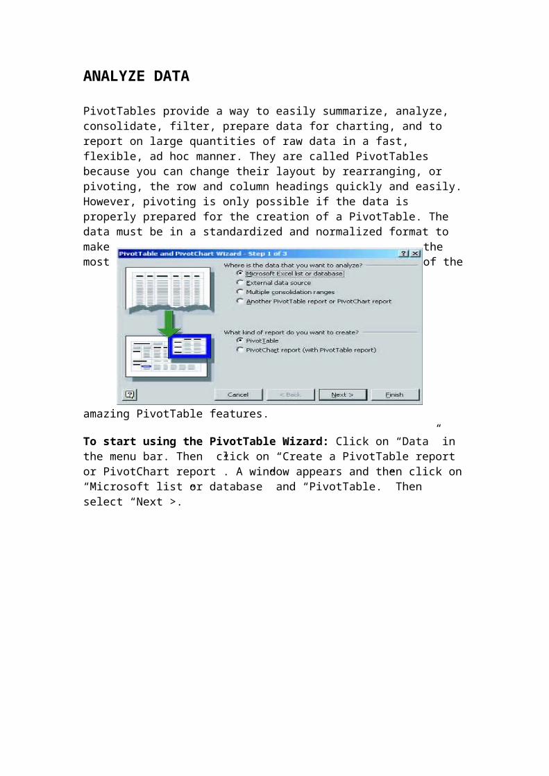
PivotTables provide a way to easily summarize, analyze, consolidate, filter, prepare data for charting, and to report on large quantities of raw data in a fast, flexible, ad hoc manner. They are called PivotTables because you can change their layout by rearranging, or pivoting, the row and column headings quickly and easily.However, pivoting is only possible if the data is properly prepared for the creation of a PivotTable. The data must be in a standardized and normalized format to make the most of the

amazing PivotTable features.

To start using the PivotTable Wizard: Click on “Data” in the menu bar. Then click on “Create a PivotTable report or PivotChart report”. A window appears and then click on“Microsoft list or database” and “PivotTable.” Then select “Next >.”

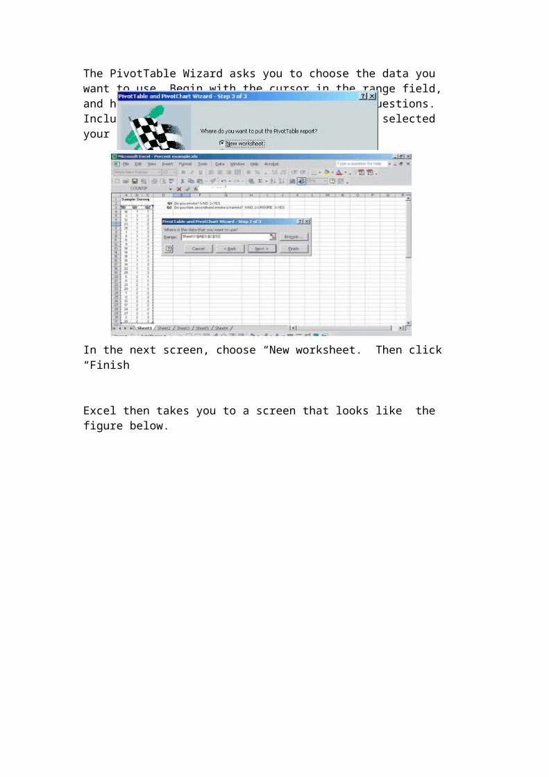
The PivotTable Wizard asks you to choose the data you want to use. Begin with the cursor in the range field, and highlight all of your data or selected questions. Include the question headers. After you have selected your data, click “Next”.

In the next screen, choose “New worksheet.” Then click “Finish

Excel then takes you to a screen that looks like the figure below.

Choose the question for which you want to create frequencies in the “PivotTable Field List.” Drag the question header from the “PivotTable Field List” to the

“Drop Row Fields Here” box in the PivotTable. After you have dragged the question header to the “DropRow Fields Here” box, the response items will appear inthe PivotTable.

To make data appear in the PivotTable: Select your question from the “PivotTable Field List” again. This time, drag the question into the field that says “Drop Data Items Here”.

Refreshing a PivotTablePivotTables are not updated each time a change occurs in their source data. To update a table, select any cell in the table and choose Data, Refresh External Data, or click the red exclamation point on the PivotTable toolbar.

Refreshing on File Open

If you want Excel to refresh your PivotTable every time you open the workbook in which it resides, choose PivotTable, Table Options. (The PivotTable menu is on thePivotTable toolbar.) Then select the Refresh On Open check box in the PivotTable Options dialog box. If you want to prevent Excel from updating the table each time

you open the workbook (for example, if the table is basedon a time-consuming query of external data), be sure thischeck box is cleared.

Selecting Elements of a PivotTableTo select a single cell in a PivotTable, click it the normal way—that is, while the mouse pointer is a fat white cross. To select a field item in such a way that all identical items and all associated data are also selected, position your mouse on the edge of the item so that the mouse pointer turns into a small black arrow, and then click.

Changing the Numeric Format for the Data AreaTo change the format of numbers in the data area, select any cell in the data area. Then click the Field Settings tool on the PivotTable toolbar (or choose PivotTable, Field Settings). In the PivotTable Field dialog box , click Number, and then select the format you want. If your data area includes more than one field, you need to format each field separately.

Changing a PivotTable’s CalculationsBy default, Excel populates the data area of your PivotTable by applying the Sum function to any numeric field you put in the data area or the Count function to any nonnumeric field. But you can choose from many alternative forms of calculation, and you can add your own calculated fields to the table.

Using a Different Summary FunctionTo switch to a different summary function, select any cell in the data area of your PivotTable. Then click the Field Settings button on the PivotTable toolbar (or choose PivotTable, Field Settings). Excel displays the PivotTable Field dialog box. Select the function you wantto use, and then click OK.

Using Multiple Data FieldsTo use a second or subsequent field, drag another field from the PivotTable Field List into the data area of the table If you add a second field to the data area of your table, Excel displays subtotals for each field.

Notice that the table now includes a new field heading called Data.

Applying Multiple Summary Functions to the Same FieldYou can apply as many summary functions as you want to a field. To use a second or subsequent function with a field that’s already in the data area of your PivotTable,drag another copy of the field from the PivotTable Field List into the data area of the table. Then select a data cell, choose PivotTable, Field Settings, choose the function you want to use, and click OK. The available summary functions are Sum, Count, Average, Max, Min, Product, Count Nums, StdDev, StdDevp, Var, and Varp.

Sorting ItemsIf you sort field items using the standard Sort command, Excel will sort all instances of your field items and preserve the sort order when you pivot the table.

You can also sort field items using an AutoSort feature. Like the standard Sort command, autoSort rearranges tablematerial across all instances and preserves the order youwant even hen you move fields from axis to axis. However,the AutoSort feature gives you the additional option of sorting field items on the basis of their data values.

Using AutoSortTo use AutoSort for a field, follow these steps:1 Select an item in the field or the field’s heading.2 Click the Field Settings button on the PivotTable toolbar (or choose PivotTable, Field Settings).

3 Click the Advanced button.4 In the PivotTable Field Advanced Options dialog box, choose the Ascending or Descending option, and then select the field you want to sort from the Using Field drop-down list. For example, to sort Channel items from those with highest sales to those with lowest, you wouldselect the Descending option and Sum Of Sales. To turn AutoSort off, return to the PivotTable Field Advanced Options dialog box. Under AutoSort Options, choose Manual.