Symbolic Model Checking without BDDs

Armin Biere1 Alessandro Cimatti2 Edmund Clarke1

Yunshan Zhu1

January 4, 1999

CMU-CS-99-101

School of Computer ScienceCarnegie Mellon University

Pittsburgh, PA 15213

Submitted for TACAS’99

1Computer Science Department, Carnegie Mellon University5000 Forbes Avenue, Pittsburgh, PA 15213, U.S.A�Armin.Biere,Edmund.Clarke,Yunshan.Zhu � @cs.cmu.edu

2Istituto per la Ricerca Scientifica e Tecnologica (IRST)via Sommarive 18, 38055 Povo (TN), Italycimatti@irst.itc.it

This research is sponsored by the Semiconductor Research Corporation (SRC) under ContractNo. 97-DJ-294 and the National Science Foundation (NSF) under Grant No. CCR-9505472.Any opinions, findings and conclusions or recommendations expressed in this material arethose of the authors and do not necessarily reflect the views of SRC, NSF, or the United StatesGovernment.The U. S. Government is authorized to reproduce and distribute reprints for Government pur-poses notwithstanding any copyright notation thereon. This manuscript is submitted for pub-lication with the understanding that the U. S. Government is authorized to reproduce and dis-tribute reprints for Governmental purposes.

Keywords: out-of-order execution, automatic verification, temporal logic, symbolicmodel checking, boolean satisfiability

Abstract

Symbolic Model Checking [3, 14] has proven to be a powerful technique for the verification ofreactive systems. BDDs [2] have traditionally been used as a symbolic representation of the sys-tem. In this paper we show how boolean decision procedures, like Stalmarck’s Method [16] or theDavis & Putnam Procedure [7], can replace BDDs. This new technique avoids the space blow upof BDDs, generates counterexamples much faster, and sometimes speeds up the verification. Inaddition, it produces counterexamples of minimal length. We introduce a bounded model check-ing procedure for LTL which reduces model checking to propositional satisfiability. We show thatbounded LTL model checking can be done without a tableau construction. We have implementeda model checker BMC, based on bounded model checking, and preliminary results are presented.

1 Introduction

Model checking [4] is a powerful technique for verifying reactive systems. Able to findsubtle errors in real commercial designs, it is gaining wide industrial acceptance. Com-pared to other formal verification techniques (e.g. theorem proving) model checking islargely automatic.

In model checking, the specification is expressed in temporal logic and the sys-tem is modeled as a finite state machine. For realistic designs, the number of states ofthe system can be very large and the explicit traversal of the state space becomes in-feasible. Symbolic model checking [3, 14], with boolean encoding of the finite statemachine, can handle more than 1020 states. BDDs [2], a canonical form for booleanexpressions, have traditionally been used as the underlying representation for symbolicmodel checkers [14]. Model checkers based on BDDs are usually able to handle sys-tems with hundreds of state variables. However, for larger systems the BDDs generatedduring model checking become too large for currently available computers. In addition,selecting the right ordering of BDD variables is very important. The generation of avariable ordering that results in small BDDs is often time consuming or needs manualintervention. For many examples no space efficient variable ordering exists.

Propositional decision procedures (SAT) [7] also operate on boolean expressionsbut do not use canonical forms. They do not suffer from the potential space explosionof BDDs and can handle propositional satisfiability problems with thousands of vari-ables. SAT based techniques have been successfully applied in various domains, suchas hardware verification [17], modal logics [9], formal verification of railway controlsystems [1], and AI planning systems [11]. A number of efficient implementations areavailable. Some notable examples are the PROVE tool [1] based on Stalmarck’s Method[16], and SATO [18] based on the Davis & Putnam Procedure [7].

In this paper we present a symbolic model checking technique based on SAT pro-cedures. The basic idea is to consider counterexamples of a particular length k andgenerate a propositional formula that is satisfiable iff such a counterexample exists. Inparticular, we introduce the notion of bounded model checking, where the bound is themaximal length of a counterexample. We show that bounded model checking for lin-ear temporal logic (LTL) can be reduced to propositional satisfiability in polynomialtime. To prove the correctness and completeness of our technique, we establish a cor-respondence between bounded model checking and model checking in general. Unlikeprevious approaches to LTL model checking, our method does not require a tableau orautomaton construction.

The main advantages of our technique are the following. First, bounded modelchecking finds counterexamples very fast. This is due to the depth first nature of SATsearch procedures. Finding counterexamples is arguably the most important feature ofmodel checking. Second, it finds counterexamples of minimal length. This feature helpsthe user to understand a counterexample more easily. Third, bounded model check-ing uses much less space than BDD based approaches. Finally, unlike BDD based ap-proaches, bounded model checking does not need a manually selected variable order ortime consuming dynamic reordering. Default splitting heuristics are usually sufficient.

To evaluate our ideas we have implemented a tool BMC based on bounded modelchecking. We give examples in which SAT based model checking significantly out-

performs BDD based model checking. In some cases bounded model checking detectserrors instantly, while the BDDs for the initial state cannot be built.

The paper is organized as follows. In the following section we explain the basicidea of bounded model checking with an example. In Section 3 we give the semanticsfor bounded model checking. Section 4 explains the translation of a bounded modelchecking problem into a propositional satisfiability problem. In Section 5 we discussbounds on the length of counterexamples. In Section 6 our experimental results arepresented, and Section 7 describes some directions for future research.

2 Example

Consider the following simple state machine M that consists of a three bit shift registerx with the individual bits denoted by x

�0��� x � 1� , and x

�2� . The predicate T � x � x ��� denotes

the transition relation between current state values x and next state values x � and isequivalent to:

� x � � 0 �� x�1 ���� � x � � 1 �� x

�2����� � x � � 2�� 1 �

In the initial state the content of the register x can be arbitrary. The predicate I � x � thatdenotes the set of initial states is ������� .

This shift register is meant to be empty (all bits set to zero) after three consecu-tive shifts. But we introduced an error in the transition relation for the next state valueof x

�2� , where an incorrect value 1 is used instead of 0. Therefore, the property, that

eventually the register will be empty (written as x � 0) after a sufficiently large numberof steps is not valid. This property can be formulated as the LTL formula F � x � 0 � .We translate the “universal” model checking problem AF � x � 0 � into the “existential”model checking problem EG � x �� 0 � by negating the formula. Then, we check if thereis an execution sequence that fulfills G � x �� 0 � . Instead of searching for an arbitrarypath, we restrict ourselves to paths that have at most k � 1 states, for instance we choosek � 2. Call the first three states of this path x0 , x1 and x2 and let x0 be the initial state (seeFigure 1). Since the initial content of x can be arbitrary, we do not have any restriction

x0

x

x

x0

0

0

[0]

[1]

[2]

x

x

x

x [0]

[1]

[2]

1

1

1

1x

x

x

x [0]

[1]

[2]

2

2

2

2

L0L1

L2

Fig. 1. Unrolling the transition relation twice and adding a back loop.

on x0 . We unroll the transition relation twice and derive the propositional formula fm

defined as I � x0 ��� T � x0 � x1 ��� T � x1 � x2 � . We expand the definition of T and I, and get the

following formula.

� x1�0�� x0

�1 �� � � x1

�1�� x0

�2��� � � x1

�2�� 1 � � 1st step

� x2�0�� x1

�1 �� � � x2

�1�� x1

�2��� � � x2

�2�� 1 � 2nd step

Any path with three states that is a “witness” for G � x �� 0 � must contain a loop. Thus,we require that there is a transition from x2 back to the initial state, to the second state,or to itself (see also Figure 1). We represent this transition as Li defined as T � x2 � xi �which is equivalent to the following formula.

� xi�0�� x2

�1��� � � xi

�1 �� x2

�2 �� � � xi

�2 �� 1 �

Finally, we have to make sure that this path will fulfill the constraints imposed by theformula G � x �� 0 � . In this case the property Si defined as xi �� 0 has to hold at each state.Si is equivalent to the following formula.

� xi�0�� 1 � � � xi

�1 �� 1 � � � xi

�2�� 1 �

Putting this all together we derive the following propositional formula.

fM �2�

i � 0

Li �2�

i � 0

Si (1)

This formula is satisfiable iff there is a counterexample of length 2 for the originalformula F � x � 0 � . In our example we find a satisfying assignment for � 1 � by settingxi�j � : � 1 for all i � j � 0 � 1 � 2.

3 Semantics

ACTL* is defined as the subset of formulas of CTL* [8] that are in negation normalform and contain only universal path quantifiers. A formula is in negation normalform (NNF) if negations only occur in front of atomic propositions. ECTL* is de-fined in the same way, but only existential path quantifiers are allowed. We considerthe next time operator ‘X’, the eventuality operator ‘F’, the globally operator ‘G’, andthe until operator ‘U’. We assume that formulas are in NNF. We can always transforma formula in NNF without increasing its size by including the release operator ‘R’( f R g iff � ��� f U � g � ). In an LTL formula no path quantifiers (E or A) are allowed. Inthis paper we concentrate on LTL model checking. Our technique can be extended tohandle full ACTL* (resp. ECTL*).

Definition 1. A Kripke structure is a tuple M � � S � I � T ��� � with a finite set of states S,the set of initial states I � S, a transition relation between states T � S S, and thelabeling of the states � :S P � A � with atomic propositions A .

We use Kripke structures as models in order to give the semantics of the logic. Forthe rest of the paper we consider only Kripke structures for which we have a boolean en-coding. We require that S ��� 0 � 1 n, and that each state can be represented by a vector of

state variables s � � s � 1 � � ����� � s � n ��� where s � i � for i � 1 � ����� � n are propositional variables.We define propositional formulas fI � s � , fT � s � t � and fp � s � as: fI � s � iff s

�I, fT � s � t � iff

� s � t � � T , and fp � s � iff p� � � s � . For the rest of the paper we simply use T � s � t � instead

of fT � s � t � etc. In addition, we require that every state has a successor state. That is, forall s

�S there is a t

�S with � s � t � � T . For � s � t � � T we also write s t. For an infinite

sequence of states π � � s0 � s1 � ����� � we define π � i � � si and πi � � si � si � 1 � ����� � for i�

IN.An infinite sequence of states π is a path if π � i � π � i � 1 � for all i

�IN.

Definition 2 (Semantics). Let M be a Kripke structure, π be a path in M and f be anLTL formula. Then π � � f ( f is valid along π) is defined as follows.

π � � p iff p� ��� π � 0 ��� π � � � p iff p �� � � π � 0 ���

π � � f � g iff π � � f and π � � g π � � f�

g iff π � � f or π � � g

π � � G f iff � i � πi � � f π � � F f iff � i � πi � � f

π � � X f iff π1 � � f

π � � f U g iff � i�πi � � g and � j � j � i � π j � � f �

π � � f R g iff � i�πi � � g or � j � j � i � π j � � f �

Definition 3 (Validity). An LTL formula f is universally valid in a Kripke structure M(in symbols M � � A f ) iff π � � f for all paths π in M with π � 0 � �

I. An LTL formula f isexistentially valid in a Kripke structure M (in symbols M � � E f ) iff there exists a pathπ in M with π � � f and π � 0 � �

I.

Determining whether an LTL formula f is existentially (resp. universally) valid in agiven Kripke structure is called an existential (resp. universal) model checking problem.

In conformance to the semantics of CTL* [8], it is clear that an LTL formula f isuniversally valid in a Kripke structure M iff � f is not existentially valid. In order tosolve the universal model checking problem, we negate the formula and show that theexistential model checking problem for the negated formula has no solution. Intuitively,we are trying to find a counterexample, and if we do not succeed then the formulais universally valid. Therefore, in the theory part of the paper we only consider theexistential model checking problem.

The basic idea of bounded model checking is to consider only a finite prefix of a paththat may be a solution to an existential model checking problem. We restrict the lengthof the prefix by a certain bound k. In practice we progressively increase the bound,looking for longer and longer possible counterexamples.

A crucial observation is that, though the prefix of a path is finite, it still might repre-sent an infinite path if there is a back loop from the last state of the prefix to any of theprevious states (see Figure 2(b)). If there is no such back loop (see Figure 2(a)), thenthe prefix does not say anything about the infinite behavior of the path. For instance,only a prefix with a back loop can represent a witness for Gp. Even if p holds along allthe states from s0 to sk , but there is no back loop from sk to a previous state, then wecannot conclude that we have found a witness for Gp, since p might not hold at sk � 1.

Definition 4. For l k we call a path π a � k � l � -loop if π � k � π � l � and π � u vω withu � � π � 0 � � ����� � π � l � 1 � � and v � � π � l � � ����� � π � k ��� . We call π simply a k-loop if there isan l

� IN with l k for which π is a � k � l � -loop.

SkSi SkSiSl

(a) no loop (b)�k � l � -loop

Fig. 2. The two cases for a bounded path.

We give a bounded semantics that is an approximation to the unbounded semanticsof Definition 2. It allows us to define the bounded model checking problem and in thenext section we will give a translation of a bounded model checking problem into asatisfiability problem.

In the bounded semantics we only consider a finite prefix of a path. In particular,we only use the first k � 1 states (s0 � ����� � sk) of a path to determine the validity of aformula along that path. If a path is a k-loop then we simply maintain the original LTLsemantics, since all the information about this (infinite) path is contained in the prefixof length k.

Definition 5 (Bounded Semantics for a Loop). Let k�

IN and π be a k-loop. Then anLTL formula f is valid along the path π with bound k (in symbols π � � k f ) iff π � � f .

Assume that π is not a k-loop. Then the formula f : � Fp is valid along π in theunbounded semantics if we can find an index i

�IN such that p is valid along the suffix

πi of π. In the bounded semantics the � k � 1 � -th state π � k � does not have a successor.Therefore, we cannot define the bounded semantics recursively over suffixes (e.g. πi) ofπ. We keep the original π instead but add a parameter i in the definition of the boundedsemantics and use the notation � � i

k. The parameter i is the current position in the prefixof π. In Lemma 7 we will show that π � � i

k f implies πi � � f .

Definition 6 (Bounded Semantics without a Loop). Let k�

IN, and let π be a paththat is not a k-loop. Then an LTL formula f is valid along π with bound k (in symbolsπ � � k f ) iff π � � 0

k f where

π � � ik p iff p

� � � π � i ��� π � � ik � p iff p �� � � π � i ���

π � � ik f � g iff π � � i

k f and π � � ik g π � � i

k f�

g iff π � � ik f or π � � i

k g

π � � ik G f is always false π � � i

k F f iff � j � i j k � π � � jk f

π � � ik X f iff i � k and π � � i � 1

k f

π � � ik f U g iff � j � i j k

�π � � j

k g and � n � i n � j � π � � nk f �

π � � ik f R g iff � j � i j k

�π � � j

k f and � n � i n j � π � � nk g �

Note that if π is not a k-loop, then we say that G f is not valid along π in the boundedsemantics with bound k since f might not hold along πk � 1. Similarly, the case for f R gwhere g always holds and f is never fulfilled has to be excluded. These constraints

imply that for the bounded semantics the duality of G and F ( � F f � G � f ) and theduality of R and U ( � � f U g � � � � f � R ��� g � ) no longer hold.

The existential and universal bounded model checking problems are defined in thesame manner as in Definition 3. Now we describe how the existential model checkingproblem (M � � E f ) can be reduced to a bounded existential model checking problem(M � � k E f ).

Lemma 7. Let h be an LTL formula and π a path, then π � � k h � π � � h

Proof. If π is a k-loop then the conclusion follows by definition. In the other case weassume that π is not a loop. Then we prove by induction over the structure of f andi k the stronger property π � � i

k h � πi � � h. We only consider the most complicatedcase h � f R g.

π � � ik f R g � � j � i j k

�π � � j

k f and � n � i n j � π � � nk g �

� � j � i j k�π j � � f and � n � i n j � πn � � g �

� � j � i j�π j � � f and � n � i n j � πn � � g �

Let j ��� j � i and n ��� n � i

� � j � � πi � j � � � f and � n ��� n � j � � πi � n � � � g �� � j

� � πi � j � � f and � n � n j � � πi � n � � g �� � n

� � πi � n � � g or � j � j � n � � πi � j � � f �� πi � � f R g

In the next-to-last step we used the following fact:

� m�πm � � f and � l � l m � πl � � g � � � n

�πn � � g or � j � j � n � π j � � f �

Assume that m is the smallest number such that πm � � f and πl � � g for all l with l m.In the first case we consider n � m. Based on the assumption, there exists j � n suchthat π j � � f (choose j � m). The second case is n m. Because πl � � g for all l m wehave πn � � g for all n m. Thus, for all n we have proven that the disjunction on theright hand side is fulfilled. ��

Lemma 8. Let f be an LTL formula f and M a Kripke structure. If M � � E f then thereexists k

�IN with M � � k E f

Proof. In [3, 5, 12] it is shown that an existential model checking problem for an LTLformula f can be reduced to FairCTL model checking of the formula EG ����� � in acertain product Kripke structure. This Kripke structure is the product of the originalKripke structure and a “tableau” that is exponential in the size of the formula f in theworst case. If the LTL formula f is existentially valid in M then there exists a pathin the product structure that starts with an initial state and ends with a cycle in thestrongly connected component of fair states. This path can be chosen to be a k-loopwith k bounded by � S �� 2

�f

�which is the size of the product structure. If we project this

path onto its first component, the original Kripke structure, then we get a path π that isa k-loop and in addition fulfills π � � f . By definition of the bounded semantics this alsoimplies π � � k f . ��

The main theorem of this section states that, if we take all possible bounds intoaccount, then the bounded and unbounded semantics are equivalent.

Theorem 9. Let f be an LTL formula, M a Kripke structure. Then M � � E f iff thereexists k

�IN with M � � k E f .

4 Translation

In the previous section, we defined the semantics for bounded model checking. We nowreduce bounded model checking to propositional satisfiability. This reduction enablesus to use efficient propositional decision procedures to perform model checking.

Given a Kripke structure M, an LTL formula f and a bound k, we will construct apropositional formula

� �M � f � � k. The variables s0 � ����� � sk in

� �M � f � � k denote a finite se-

quence of states on a path π. Each si is a vector of state variables. The formula� �

M � f � � kessentially represents constraints on s0 � ����� � sk such that

� �M � f � � k is satisfiable iff f is

valid along π.The size of

� �M � f � � k is polynomial in the size of f if common subformulas are

shared (as in our tool BMC). It is quadratic in k and linear in the size of the propositionalformulas for T , I and the p

� A . Thus, existential bounded model checking can bereduced in polynomial time to propositional satisfiability.

To construct� �

M � f � � k, we first define a propositional formula� �

M � � k that constrainss0 � ����� � sk to be on a valid path π in M. Second, we give the translation of an LTL formulaf to a propositional formula that constrains π to satisfy f .

Definition 10 (Unfolding the Transition Relation). For a Kripke structure M, k�

IN

� �M � � k : � I � s0 ���

k � 1�i � 0

T � si � si � 1 �

Depending on whether a path is a k-loop or not (see Figure 2), we have two differenttranslations of the temporal formula f . In Definition 11 we describe the translation ifthe path is not a loop (“

� � � � ik”). The more technical translation where the path is a loop(“l

� � � � ik”) is given in Definition 13.Consider the formula h : � p U q and a path π that is not a k-loop for a given k

� IN(see Figure 2(a)). Starting at πi for i

� IN with i k the formula h is valid along πi withrespect to the bounded semantics iff there is a position j with i j k and q holdsat π � j � . In addition, for all states π � n � with n

� IN starting at π � i � up to π � j � 1 � theproposition p has to be fulfilled. Therefore the translation is simply a disjunction overall possible positions j at which q eventually might hold. For each of these positionsa conjunction is added that ensures that p holds along the path from π � i � to π � j � 1 � .Similar reasoning leads to the translation of the other temporal operators.

The translation “� � � � ik” maps an LTL formula into a propositional formula. The

parameter k is the length of the prefix of the path that we consider and i is the currentposition in this prefix (see Figure 2(a)). When we recursively process subformulas, ichanges but k stays the same. Note that we define the translation of any formula G f as����� � � . This translation is consistent with the bounded semantics.

Definition 11 (Translation of an LTL Formula without a Loop). For an LTL formulaf and k � i � IN, with i k

� �p � � ik : � p � si �

� � � p � � ik : � � p � si �� �f � g � � ik : � � �

f � � ik �� �

g � � ik� �

f�

g � � ik : � � �f � � ik

� � �g � � ik� �

G f � � ik : � ����� � � � �F f � � ik : � � k

j � i� �

f � � jk� �

X f � � ik : � if i � k then� �

f � � i � 1k else

����� � �� �

f U g � � ik : � � kj � i

� � �g � � j

k ��� j � 1n � i

� �f � � nk �

� �f R g � � ik : � � k

j � i

� � �f � � j

k � � jn � i

� �g � � nk �

Now we consider the case where the path is a k-loop. The translation “ l

� � � � ik” of anLTL formula depends on the current position i and on the length of the prefix k. It alsodepends on the position where the loop starts (see Figure 2(b)). This position is denotedby l for loop.

Definition 12 (Successor in a Loop). Let k � l � i � IN, with l � i k. Define the successorsucc � i � of i in a � k � l � -loop as succ � i � : � i � 1 for i � k and succ � i � : � l for i � k.

Definition 13 (Translation of an LTL Formula for a Loop). Let f be an LTL formula,k � l � i � IN, with l � i k.

l

� �p � � ik : � p � si � l

� � � p � � ik : � � p � si �l� �

f � g � � ik : � l� �

f � � ik � l� �

g � � ik l� �

f�

g � � ik : � l� �

f � � ik �l� �

g � � ikl

� �G f � � ik : � � k

j � min� i � l � l

� �f � � j

k l

� �F f � � ik : � � k

j � min� i � l � l

� �f � � j

k

l

� �X f � � ik : � l

� �f � � succ � i �

k

l

� �f U g � � ik : � � k

j � i

�l

� �g � � j

k � � j � 1n � i l

� �f � � nk � �� i � 1

j � l

�l

� �g � � j

k � � kn � i l

� �f � � nk � � j � 1

n � l l

� �f � � nk �

l

� �f R g � � ik : � � k

j � min� i � l � l

� �g � � j

k�� k

j � i

�l

� �f � � j

k � � jn � i l

� �g � � nk � �� i � 1

j � l

�l

� �f � � j

k � � kn � i l

� �g � � nk � � j

n � l l

� �g � � nk �

The translation of the formula depends on the shape of the path (whether it is a loopor not). We now define a loop condition to distinguish these cases.

Definition 14 (Loop Condition). For k � l �IN, let lLk : � T � sk � sl � � Lk : � � k

l � 0 lLk

Definition 15 (General Translation). Let f be an LTL formula, M a Kripke structureand k

�IN

� �M � f � � k : � � �

M � � k ��� � � Lk �� �

f � � 0k � � k�l � 0

�lLk � l

� �f � � 0k �

The left side of the disjunction is the case where there is no back loop and thetranslation without a loop is used. On the right side all possible starts l of a loop aretried and the translation for a � k � l � -loop is conjuncted with the corresponding lLk loopcondition.

Theorem 16.� �

M � f � � k is satisfiable iff M � � k E f .

Corollary 17. M � � A � f iff� �

M � f � � k is unsatisfiable for all k� IN.

5 Determining the bound

In Section 3 we have shown that the unbounded semantics is equivalent to the boundedsemantics if we consider all possible bounds. This equivalence leads to a straightfor-ward LTL model checking procedure. To check whether M � � E f , the procedure checksM � � k E f for k � 0 � 1 � 2 � � � � . If M � � k E f , then the procedure proves that M � � E f andproduces a witness of length k. If M �� � E f , we have to increment the value of k indefi-nitely, and the procedure does not terminate. In this section we establish several boundson k. If M �� � k E f for all k within the bound, we conclude that M �� � E f .

5.1 ECTL

ECTL is a subset of ECTL* where each temporal operator is preceded by one existentialpath quantifier. We have extended bounded model checking to handle ECTL formulas.Semantics and translation for ECTL formulas can be found in the full version of thispaper. In general, better bounds can be derived for ECTL formulas than for LTL formu-las. The intersection of the two sets of formulas includes many temporal properties ofpractical interest (e.g. EFp and EGp). Therefore, we include the discussion of boundsfor ECTL formulas in this section.

Theorem 18. Given an ECTL formula f and a Kripke structure M. Let � M � be thenumber of states in M, then M � � E f iff there exists k � M � with M � � k E f .

In symbolic model checking, the number of states in a Kripke structure is boundedby 2n, where n is the number of boolean variables to encode the Kripke structure.Typical model checking problems involve Kripke structures with tens or hundreds ofboolean variables. The bound given in Theorem 18 is often too large for practical prob-lems.

Definition 19 (Diameter). Given a Kripke structure M, the diameter of M is the mini-mal number d

� IN with the following property. For every sequence of states s0 � ����� � sd � 1with � si � si � 1 � �

T for i d, there exists a sequence of states t0 � ����� � tl where l d suchthat t0 � s0, tl � sd � 1 and � t j � t j � 1 � � T for j � l. In other words, if a state v is reachablefrom a state u, then v is reachable from u via a path of length d or less.

Theorem 20. Given an ECTL formula f : � EFp and a Kripke structure M with diam-eter d, M � � EFp iff there exists k d with M � � k EFp.

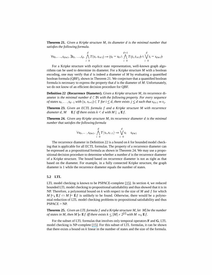
Theorem 21. Given a Kripke structure M, its diameter d is the minimal number thatsatisfies the following formula.

� s0 � ����� � sd � 1 � � t0 � ����� � td �d�

i � 0

T � si � si � 1 � � t0 � s0 �d � 1�i � 0

T � ti � ti � 1 ���d�

i � 0

ti � sd � 1 �

For a Kripke structure with explicit state representation, well-known graph algo-rithms can be used to determine its diameter. For a Kripke structure M with a booleanencoding, one may verify that d is indeed a diameter of M by evaluating a quantifiedboolean formula (QBF), shown in Theorem 21. We conjecture that a quantified booleanformula is necessary to express the property that d is the diameter of M. Unfortunately,we do not know of an efficient decision procedure for QBF.

Definition 22 (Recurrence Diameter). Given a Kripke structure M, its recurrence di-ameter is the minimal number d

�IN with the following property. For every sequence

of states s0 � ����� � sd � 1 with � si � si � 1 � � T for i d, there exists j d such that sd � 1 � s j.

Theorem 23. Given an ECTL formula f and a Kripke structure M with recurrencediameter d, M � � E f iff there exists k d with M � � k E f .

Theorem 24. Given any Kripke structure M, its recurrence diameter d is the minimalnumber that satisfies the following formula

� s0 � ����� � sd � 1 �d�

i � 0

T � si � si � 1 � d�

i � 0

si � sd � 1

The recurrence diameter in Definition 22 is a bound on k for bounded model check-ing that is applicable for all ECTL formulas. The property of a recurrence diameter canbe expressed as a propositional formula as shown in Theorem 24. We may use a propo-sitional decision procedure to determine whether a number d is the recurrence diameterof a Kripke structure. The bound based on recurrence diameter is not as tight as thatbased on the diameter. For example, in a fully connected Kripke structure, the graphdiameter is 1 while the recurrence diameter equals the number of states.

5.2 LTL

LTL model checking is known to be PSPACE-complete [15]. In section 4, we reducedbounded LTL model checking to propositional satisfiability and thus showed that it is inNP. Therefore, a polynomial bound on k with respect to the size of M and f for whichM � � k E f � M � � E f is unlikely to be found. Otherwise, there would be a polyno-mial reduction of LTL model checking problems to propositional satisfiability and thusPSPACE = NP.

Theorem 25. Given an LTL formula f and a Kripke structure M, let � M � be the numberof states in M, then M � � E f iff there exists k � M � 2

�f

�with M � � k E f .

For the subset of LTL formulas that involves only temporal operators F and G, LTLmodel checking is NP-complete [15]. For this subset of LTL formulas, it can be shownthat there exists a bound on k linear in the number of states and the size of the formula.

Definition 26 (Loop Diameter). We say a Kripke structure M is lasso shaped if everypath p starting from an initial state is of the form upvω

p , where up and vp are finitesequences of length less or equal to u and v, respectively. We define the loop diameterof M as � u � v � .

Theorem 27. Given an LTL formula f and a lasso-shaped Kripke structure M, let theloop diameter of M be � u � v � , then M � � E f iff there exists k u � v with M � � k E f .

Theorem 27 shows that for a restricted class of Kripke structures, small bounds onk exist. In particular, if a Kripke structure is lasso shaped, k is bounded by u � v, where� u � v � is the loop diameter of M.

6 Experimental Results

We have implemented a model checker BMC based on bounded model checking. Itsinput language is a subset of the SMV language [14]. It outputs a SMV program ora propositional formula. For the propositional output mode, two different formats aresupported. The first format is the DIMACS format [10] for satisfiability problems. TheSATO tool [18] is a very efficient implementation of the Davis & Putnam Procedure [7]and it uses the DIMACS format. We also support the input format of the PROVE Tool[1] which is based on Stalmarck’s Method [16].

As benchmarks we chose examples where BDDs are known to behave badly. Firstwe investigated a sequential multiplier, the sequential shift and add multiplier of [6].We formulated as model checking problem the following property: when the sequentialmultiplier is finished its output is the same as the output of a combinational multiplier(the C6288 circuit from the ISCAS’85 benchmarks) applied to the same input words.These multipliers are 16x16 bit multipliers but we only allowed 16 output bits as in [6]together with an overflow bit. We proved the property for each output bit individuallyand the results are shown in Table 1. For SATO we conducted two experiments to studythe effect of the ‘-g’ parameter that controls the maximal size of cached clauses. Wepicked a very small value (‘-g 5’) and a very large value (‘-g 50’). Note that the overflowbit depends on all the bits of the sequential multiplier and occurs in the specification.Thus, cone of influence reduction could not remove anything.

In the column SMV1 of Table 1 the official version of the CMU model checkerSMV was used. SMV2 is a version by Bwolen Yang from CMU with improved supportfor conjunctive partitioning. We used a manually chosen variable ordering where thebits of registers are interleaved. Dynamic reordering failed to find a considerably betterordering in a reasonable amount of time.

We used a barrel shifter as another example. It rotates the contents of a register fileb with each step by one position. The model also contains another register file r that isrelated to b in the following way. If a register in r and one in b have the same contentsthen their neighbors also have the same contents. This property holds in the initial stateof the model, and we proved that it is valid in all successor states. The results of thisexperiment can be found in Table 2. The width of the registers is chosen to be

�log2 � r � �

where � r � is the number of registers in the register file r. In this case we were also able

SMV1 SMV2 SATO -g5 SATO -g50 PROVEbit sec MB sec MB sec MB sec MB sec MB0 919 13 25 79 0 0 0 1 0 11 1978 13 25 79 0 0 0 1 0 12 2916 13 26 80 0 0 0 2 0 13 4744 13 27 82 0 0 0 3 1 24 6580 15 33 92 2 0 3 4 1 25 10803 25 67 102 12 0 36 7 1 26 43983 73 258 172 55 0 208 10 2 27

�17h 1741 492 209 0 642 13 7 3

8�

1GB 473 0 1198 16 29 39 856 1 2413 20 58 310 1837 1 2055 20 91 311 2367 1 1667 19 125 312 3830 1 976 17 156 413 5128 1 4363 25 186 414 4752 1 2170 23 226 415 4449 1 6847 31 183 5

sum 71923 2202 23970 22578 1066

Table 1. 16x16 bit sequential shift and add multiplier with overflow flag and 16 output bits (sec= seconds, MB = Mega Byte).

to prove the recurrence diameter (see Definition 22) to be � r � . This took only very littletime compared to the total verification time and is shown in the column “diameter”.

In [13] an asynchronous circuit for distributed mutual exclusion is described. It con-sists of n cells for n users that want to have exclusive access to a shared resource. Weproved the liveness property that a request for using the resource will eventually beacknowledged. This liveness property is only true if each asynchronous gate does notdelay execution indefinitely. We model this assumption by a fairness constraint for eachindividualgate. Each cell has exactly 18 gates and therefore the model has n 18 fairnessconstraints where n is the number of cells. Since we do not have a bound for the max-imal length of a counterexample for the verification of this circuit we could not verifythe liveness property completely. We only showed that there are no counterexamples ofparticular length k. To illustrate the performance of bounded model checking we havechosen k � 5 � 10. The results can be found in Table 3.

We repeated the experiment with a buggy design. For the liveness property we sim-ply removed several fairness constraints. Both PROVE and SATO generate a counterex-ample (a 2-loop) instantly (see Table 4).

7 Conclusion

This work is the first step in applying SAT procedures to symbolic model checking.We believe that our technique has the potential to handle much larger designs thanwhat is currently possible. Towards this goal, we propose several promising directions

of research. We would like to investigate how to use domain knowledge to guide thesearch in SAT procedures. New techniques are needed to determine the diameter of asystem. In particular, it would be interesting to study efficient decision procedures forQBF. Combining bounded model checking with other state space reduction techniquespresents another interesting problem.

SMV2 SATO -g100 SATO -g20 PROVE PROVEdiameter diameter�

r�

sec MB sec MB sec MB sec MB sec MB3 1 49 0 1 0 0 0 1 0 14 1 49 0 1 0 1 0 1 0 15 13 83 0 2 60 2 0 1 1 26 509 447 1 4 364 4 0 1 2 37

�1GB 3 6 1252 6 0 2 2 4

8 5 8 2160 9 0 2 7 59 25 14

�21h 0 3 16 9

10 42 19 1 4 55 11

Table 2. Barrel shifter (�r

�= number of registers, sec = seconds, MB = Mega Bytes).

SMV1 SMV2 SATO PROVE SATO PROVEk � 5 k � 5 k � 10 k � 10

cells sec MB sec MB sec MB sec MB sec MB sec MB4 846 11 159 217 0 3 1 3 3 6 54 55 2166 15 530 703 0 4 2 3 9 8 95 56 4857 18 1762 703 0 4 3 3 7 9 149 67 9985 24 6563 833 0 5 4 4 15 10 224 88 19595 31

�1GB 1 6 6 5 16 12 323 8

9�

10h 1 6 9 5 24 13 444 910 1 7 10 5 36 15 614 1011 1 8 13 6 38 16 820 1112 1 9 16 6 40 18 1044 1113 1 9 19 8 107 19 1317 1214 1 10 22 8 70 21 1634 1415 1 11 27 8 168 22 1992 15

Table 3. Liveness for one user in the DME (sec = seconds, MB = Mega Bytes).

SMV1 SMV2 SATO PROVEcells sec MB sec MB sec MB sec MB

4 799 11 14 44 0 1 0 25 1661 14 24 57 0 1 0 26 3155 21 40 76 0 1 0 27 5622 38 74 137 0 1 0 28 9449 73 118 217 0 1 0 29 segmentation 172 220 0 1 1 210 fault 244 702 0 1 0 311 413 702 0 1 0 312 719 702 0 2 1 313 843 702 0 2 1 314 1060 702 0 2 1 315 1429 702 0 2 1 3

Table 4. Counterexample for liveness in a buggy DME (sec = seconds, MB = Mega Bytes).

References

[1] Arne Boralv. The industrial success of verification tools based on Stalmarck’s Method.In Orna Grumberg, editor, International Conference on Computer-Aided Verification(CAV’97), number 1254 in LNCS. Springer-Verlag, 1997.

[2] R. E. Bryant. Graph-based algorithms for boolean function manipulation. IEEE Transac-tions on Computers, 35(8):677–691, 1986.

[3] J. R. Burch, E. M. Clarke, and K. L. McMillan. Symbolic model checking: 1020 states andbeyond. Information and Computation, 98:142–170, 1992.

[4] E. Clarke and E. A. Emerson. Design and synthesis of synchronization skeletons usingbranching time temporal logic. In Proceedings of the IBM Workshop on Logics of Pro-grams, volume 131 of LNCS, pages 52–71. Springer-Verlag, 1981.

[5] E. Clarke, O. Grumberg, and K. Hamaguchi. Another look at LTL model checking. InDavid L. Dill, editor, Computer Aided Verification, 6th International Conference (CAV’94),volume 818 of LNCS, pages 415–427. Springer-Verlag, June 1994.

[6] Edmund M. Clarke, Orna Grumberg, and David E. Long. Model checking and abstraction.ACM Transactions on Programming Languages and Systems, 16(5):1512–1542, 1994.

[7] M. Davis and H. Putnam. A computing procedure for quantification theory. Journal of theAssociation for Computing Machinery, 7:201–215, 1960.

[8] E. A. Emerson and C.-L. Lei. Modalities for model checking: Branching time strikes back.Science of Computer Programming, 8:275–306, 1986.

[9] F. Giunchiglia and R. Sebastiani. Building decision procedures for modal logics frompropositional decision procedures - the case study of modal K. In Proc. of the 13th Con-ference on Automated Deduction, Lecture Notes in Artificial Intelligence. Springer-Verlag,1996.

[10] D. S. Johnson and M. A. Trick, editors. The second DIMACS implementation challenge,DIMACS Series in Discrete Mathematics and Theoretical Computer Science, 1993. (seehttp://dimacs.rutgers.edu/Challenges/).

[11] H. Kautz and B. Selman. Pushing the envelope: planning, propositional logic, and stochas-tic search. In Proc. AAAI’96, Portland, OR, 1996.

[12] O. Lichtenstein and A. Pnueli. Checking that finite state concurrent programs satisfy theirlinear specification. In Poceedings of the Twelfth Annual ACM Symposium on Principles ofProgramming Languages, pages 97–107, 1985.

[13] A. J. Martin. The design of a self-timed circuit for distributed mutual exclusion. InH. Fuchs, editor, Proceedings of the 1985 Chapel Hill Conference on Very Large ScaleIntegration, 1985.

[14] K. L. McMillan. Symbolic Model Checking: An Approach to the State Explosion Problem.Kluwer Academic Publishers, 1993.

[15] A. P. Sistla and E. M. Clarke. The complexity of propositional linear temporal logics.Journal of Assoc. Comput. Mach., 32(3):733–749, 1985.

[16] G. Stalmarck and M. Saflund. Modeling and verifying systems and software in propo-sitional logic. In B. K. Daniels, editor, Safety of Computer Control Systems (SAFE-COMP’90), pages 31–36. Pergamon Press, 1990.

[17] P. R. Stephan, R. K. Brayton, and A. L. Sangiovanni-Vincentelli. Combinational test gener-ation using satisfiability. Technical Report M92/112, Departement of Electrical Engineer-ing and Computer Science, University of California at Berkley, October 1992.

[18] H. Zhang. SATO: An efficient propositional prover. In International Conference on Au-tomated Deduction (CADE’97), number 1249 in LNAI, pages 272–275. Springer-Verlag,1997.