Symbolic Shape Analysis - CiteSeerX
93
Symbolic Shape Analysis Diploma Thesis Thomas Wies September 2004 advised by Prof. Dr. Andreas Podelski Universit¨ at des Saarlandes Fachbereich 6.2 - Informatik
-
Upload
khangminh22 -
Category
Documents
-
view
3 -
download
0
Transcript of Symbolic Shape Analysis - CiteSeerX

Symbolic Shape Analysis
Diploma Thesis
Thomas Wies
September 2004
advised byProf. Dr. Andreas Podelski
Universitat des SaarlandesFachbereich 6.2 - Informatik


Erklarung
Hiermit erklare ich, Thomas Wies, an Eides statt, dass ich diese Arbeit selbstandigverfasst und keine anderen als die angegebenen Quellen verwendet habe.
Saarbrucken, den 30.09.2004
i


Acknowledgments
First of all, I thank my advisor Prof. Andreas Podelski for the interesting and chal-lenging thesis subject, the inspiring discussions, his support, and his patience. Iwould like to thank Viktor Kuncak for discussions that initiated the work on thisthesis. I am also indebted to Dr. Mooly Sagiv and Greta Yorsh for giving helpfulcomments while on stay at Tel-Aviv in spring 2004. I have to thank everyone thatcontributed to the thesis by giving hints and suggestions for improvements. I amparticularly grateful to Ina Schaefer and Andrey Rybalchenko for valuable debatesand proofreading several draft versions of this thesis. Special thanks go to themembers of AG2 at MPII for providing such a nice and productive working atmo-sphere. Finally, I thank my family for their constant support and encouragementthat only made this thesis possible.
iii


Abstract
Shape analysis deals with the synthesis of invariants for programs manipulatingheap-allocated data structures. Explicit shape analysis algorithms do not scale verywell. This work proposes a framework for symbolic shape analysis that addressesthis problem. Our contribution is a framework that allows to abstract programswith heap-allocated data symbolically by Boolean programs. For this purpose, wecombine abstraction techniques from shape analysis with ideas from predicate ab-straction. Our framework is parameterized by a set of abstraction predicates. Wepropose a class of predicates that can be used to analyze reachability properties forlinked data structures. This class may potentially be used for automated abstrac-tion refinement.
v


Contents
Acknowledgments iii
Abstract v
1 Introduction 11.1 Motivation . . . . . . . . . . . . . . . . . . . . . . . . . . . . . . . . . . 11.2 Contributions . . . . . . . . . . . . . . . . . . . . . . . . . . . . . . . . 21.3 Outline . . . . . . . . . . . . . . . . . . . . . . . . . . . . . . . . . . . . 3
2 Preliminaries 52.1 Abstract Interpretation . . . . . . . . . . . . . . . . . . . . . . . . . . . 5
2.1.1 Transition Systems and Transformer Functions . . . . . . . . . 52.1.2 State Invariants and Reachability . . . . . . . . . . . . . . . . . 62.1.3 Abstract Interpretation and Galois Connections . . . . . . . . 7
2.2 First-Order Logic with Transitive Closure . . . . . . . . . . . . . . . . 92.3 System Description . . . . . . . . . . . . . . . . . . . . . . . . . . . . . 11
2.3.1 Program Stores . . . . . . . . . . . . . . . . . . . . . . . . . . . 112.3.2 Program Semantics . . . . . . . . . . . . . . . . . . . . . . . . . 12
3 Abstraction Framework 173.1 Node Predicate Abstraction . . . . . . . . . . . . . . . . . . . . . . . . 17
3.1.1 Node Predicates . . . . . . . . . . . . . . . . . . . . . . . . . . 173.1.2 Abstract Domain . . . . . . . . . . . . . . . . . . . . . . . . . . 183.1.3 Best Abstraction . . . . . . . . . . . . . . . . . . . . . . . . . . 183.1.4 Expressiveness . . . . . . . . . . . . . . . . . . . . . . . . . . . 20
3.2 Abstract Transformer . . . . . . . . . . . . . . . . . . . . . . . . . . . . 223.2.1 Best Abstract Transformer . . . . . . . . . . . . . . . . . . . . . 223.2.2 Context-Sensitive Abstract Operators . . . . . . . . . . . . . . 233.2.3 Cartesian Abstraction and Cartesian Post . . . . . . . . . . . . 243.2.4 Boolean Heap Programs . . . . . . . . . . . . . . . . . . . . . . 283.2.5 Precision of Cartesian Post . . . . . . . . . . . . . . . . . . . . 283.2.6 Nondeterminism and Splitting Operators . . . . . . . . . . . . 29
4 Modal Node Predicates 334.1 Motivation . . . . . . . . . . . . . . . . . . . . . . . . . . . . . . . . . . 334.2 Syntax and Semantics . . . . . . . . . . . . . . . . . . . . . . . . . . . . 344.3 Decidability . . . . . . . . . . . . . . . . . . . . . . . . . . . . . . . . . 364.4 Closeness under Weakest Liberal Preconditions . . . . . . . . . . . . . 38
vii

CONTENTS CONTENTS
5 Case Study: Reversing Singly-linked Lists 435.1 The Program Reverse . . . . . . . . . . . . . . . . . . . . . . . . . . . . 435.2 Choosing Abstraction Predicates . . . . . . . . . . . . . . . . . . . . . 445.3 Splitting Operator . . . . . . . . . . . . . . . . . . . . . . . . . . . . . . 445.4 Context-sensitive Abstract Weakest Liberal Preconditions . . . . . . . 465.5 Computing the Least Fixed Point . . . . . . . . . . . . . . . . . . . . . 46
6 Related Work 516.1 Abstract Domains for Shape Analysis . . . . . . . . . . . . . . . . . . 516.2 Symbolic Methods in Shape Analysis . . . . . . . . . . . . . . . . . . . 526.3 Decidable Logics for Shape Analysis . . . . . . . . . . . . . . . . . . . 53
7 Conclusion 557.1 Summary . . . . . . . . . . . . . . . . . . . . . . . . . . . . . . . . . . . 557.2 Future Work . . . . . . . . . . . . . . . . . . . . . . . . . . . . . . . . . 55
7.2.1 Precision of the Abstract Domain . . . . . . . . . . . . . . . . . 557.2.2 Automated Abstraction Refinement . . . . . . . . . . . . . . . 567.2.3 Beyond Safety . . . . . . . . . . . . . . . . . . . . . . . . . . . . 56
A Proofs 61
B Least Fixed Point for Program Reverse 79
viii

Chapter 1
Introduction
Shape analysis deals with programs manipulating heap allocated data structures.Explicit shape analysis algorithms do not scale very well. One direction to ad-dress scalability is to use symbolic methods. This work proposes a framework forsymbolic shape analysis.
1.1 Motivation
Invariants synthesized by program analysis are over-approximations of the set ofreachable program states. They are useful in a variety of applications, ranging frominstruction scheduling and code optimization in compilers to formal verification.
Most program analysis problems for infinite state systems are undecidable.Therefore, one needs techniques for approximation. Abstract interpretation [7] is aframework that formalizes approximation for program analysis. In order to com-pute invariants, the program is interpreted over an abstract domain of abstractstates. The creative act in applying abstract interpretation lies in the identificationof a suitable abstract domain.
Shape analysis aims for the synthesis of invariants for programs manipulatingheap-allocated data structures. In order to model the state of a program with heap-allocated data, one has to model the state of the heap. The heap can be representedas a graph, where the nodes correspond to allocated objects and edge relations thatreflect how objects are connected via pointers. Each pointer field of a stored datastructure corresponds to one edge relation of the graph. Since a priori there is nobound on the number of allocated heap objects, these graphs can be arbitrary large.Consequently, the number of possible program states is unbounded and thereforewe need abstraction.
Abstract domains used for shape analysis are based on several variants of shapegraphs [17, 5, 29, 26, 27]. The common idea of these abstractions is to partition theset of nodes in a concrete graph into a finite set of equivalence classes. These equiv-alence classes are represented by abstract nodes in a shape graph. An equivalenceclass contains all nodes that are indistinguishable under a particular set of shapeproperties, e.g. expressing that a node is pointed to by a program variable, or thatit is reachable from a program variable by following pointer fields in a data struc-ture. In [27] a parametric framework for shape analysis is proposed that identifiesshape properties as unary abstraction predicates that denote sets of nodes.
Although the use of abstract domains based on shape graphs gives approxi-mating algorithms, these algorithms have high complexity, because the abstractdomain is though finite, still very large. If one uses an explicit representation ofabstract states, such as shape graphs, the analysis does not scale very well. One
1

CHAPTER 1. Introduction
way to address this problem is to use symbolic methods.In the following, we discuss one symbolic method in more details. Predicate
abstraction (see e.g. [12]) is a technique used to symbolically abstract infinite statesystems. It is successfully applied in software model checkers such as SLAM [3]and BLAST [13]. The abstract domain is given by a finite class of formulas builtfrom a chosen set of abstraction predicates. These abstraction predicates denotesets of program states. The program is abstracted symbolically by a Boolean pro-gram whose program variables correspond to the abstraction predicates [1]. Oneof the merits of predicate abstraction is that the analysis of the obtained abstractBoolean program can be implemented efficiently using a symbolic representationof abstract states, e.g. based on BDDs.
The computed invariants can be used to verify whether a given property issatisfied by the program. If the invariants are too weak to entail the target prop-erty, the abstract domain has to be refined, in order to obtain stronger invariants.Abstraction refinement is a key technology for fully automated formal verification.
For abstract domains that are parameterized by a set of abstraction predicates,refinement amounts to adding additional abstraction predicates. For predicate ab-straction there are successful automated abstraction refinement procedures; seee.g. [6, 14, 2]. However, in shape analysis there are, so far, only heuristics that helpto find additional predicates; see e.g. instrumentation predicates proposed in [27].The question whether these predicates can be derived automatically is still open.
This work proposes a framework for symbolic shape analysis. We give a sym-bolic abstract domain that allows to handle abstract programs symbolically. Theframework enables the integration of automated abstraction refinement procedures.However, contrary to predicate abstraction, the abstract domain is parameterizedby unary predicates that denote sets of nodes in the abstracted graphs. This con-forms to the abstract domains for shape analysis that are based on shape graphs.
1.2 ContributionsOur contribution is a framework for symbolic shape analysis:
• We propose a symbolic abstract domain that allows to represent abstract pro-grams symbolically. We call the obtained abstract programs Boolean heap pro-grams.
• The construction of Boolean heap programs requires the identification of asuitable set of unary abstraction predicates. We propose modal node predicatesthat can be used for the analysis of reachability properties for linked datastructures.
• We give preliminary results that may be useful for the development of ab-straction refinement procedures for properties expressed by modal node pred-icates.
In the following, we give a more detailed discussion of these contributions.
Boolean Heap Programs. We propose a symbolic abstract domain for shape anal-ysis. This abstract domain is parameterized by a set of unary abstraction predi-cates. In analogy to predicate abstraction, the concrete program is abstracted bya Boolean program. We call these abstract programs Boolean heap programs. ABoolean heap program is formally characterized in terms of an over-approximationof the best abstract post operator on the chosen abstract domain. This guaranteessoundness of the resulting analysis. In addition, we examine under which condi-tions a Boolean heap program coincides with the best abstract post operator.
2

CHAPTER 1. Introduction
Modal Node Predicates. We identify the class of modal node predicates, which areunary abstraction predicates that express reachability properties for linked datastructures. We give a first result regarding decidability of the satisfiability problemfor modal node predicates. Moreover, we show that modal node predicates areclosed under weakest liberal preconditions. These results may be useful for thedevelopment of an abstraction refinement procedure for properties expressed bymodal node predicates.
1.3 OutlineThe remainder of the thesis is organized as follows:
Chapter 2 gives the preliminaries. We first briefly introduce the basic notionsof abstract interpretation (2.1). Afterwards, we revise the definition of first-orderlogic with transitive closure (2.2) which is then used to formally describe the con-crete semantics of programs manipulating heap allocated data structures (2.3).This gives the formal foundation of our abstract interpretation based symbolicshape analysis.
In Chapter 3, we develop our abstraction framework. We give a symbolic ab-stract domain that is parameterized by a set of unary abstraction predicates (3.1).Thereafter, we show how the best abstract post operator on this abstract domain isapproximated by an abstract post operator that corresponds to a Boolean program(3.2.1-3.2.4). Moreover, we analyze under which conditions the Boolean programcoincides with the best abstract post (3.2.5). Finally, we propose a method that canbe applied, in order to gain back precision in the case that the Boolean programgives imprecise results with respect to the best abstract post (3.2.6).
Chapter 4 introduces modal node predicates (4.1,4.2), a class of unary predi-cates that can be used to instantiate the framework presented in Chapter 3. Wegive first results regarding decidability of the satisfiability problem (4.3) and showthat modal node predicates are closed under weakest liberal preconditions (4.4).
In Chapter 5 the developed framework is illustrated in a case study. We verify aprogram that reverses singly-linked lists. The analysis uses modal node predicates.The steps of the corresponding fixed point iteration are given in Appendix B.
Chapter 6 compares the presented framework to related work. We discussshape analysis algorithms that are based on shape graph abstraction (6.1), con-sider other approaches that apply symbolic methods in shape analysis (6.2), anddiscuss recent results on decidable logics for shape analysis (6.3).
In Chapter 7 we conclude and discuss open problems for future work.In Appendix A one can find the proofs of all statements made in this work.
3


Chapter 2
Preliminaries
This chapter gives a brief introduction into abstract interpretation based on Galoisconnections. Abstract interpretation is a formal, semantics-based framework forthe systematic construction of sound static program analyses. Our approach pre-sented in the later chapters conforms to this framework. We further revise the def-inition of first-order logic with transitive closure. This logic allows one to formallydefine the concrete representation of program stores and serves as a specificationlanguage for the properties we want to analyze.
2.1 Abstract InterpretationThe goal of a program analysis is to collect information over a program’s runtimebehavior for all possible input data. Running a program on all its inputs is usu-ally either impossible, because the number of input values is infinite, or infeasible,because it is finite, but too large to be handled by exhaustive testing. Static analy-sis infers information over all possible program executions without executing theprogram explicitly.
Since nearly every interesting problem concerning a program’s runtime behav-ior is undecidable, the use of approximation is inevitable to ensure termination ofthe analysis. The goal is thus to develop incomplete, but automatic methods thatproduce reliable results. Abstract interpretation gives a formal, semantics-basedframework for the systematic construction of such approximations.
2.1.1 Transition Systems and Transformer FunctionsIn order to be able to formally reason about a system, it is crucial to have a for-mal semantics of the system behavior. Transition systems offer the most simpleand unified approach to describe the semantics of a broad range of systems, inparticular (concurrent) imperative programs. The common semantic properties oftransition systems are well understood. In the following, we introduce the basicnotions and summarize some of the more prominent properties that will becomeuseful, later on. A detailed discussion of transition systems, transformer functionsand their properties can be found for instance in [28].
Definition 2.1.1 (Transition System). A transition system S is a tuple 〈State, init, R〉with:
• State: the (possibly infinite) set of states of the system,
• init ⊆ State: the set of initial states,
5

CHAPTER 2. Preliminaries
• R ⊆ State × State: the transition relation.
Given a transition system S, the properties of the transition relation R can beelegantly described in terms of the associated transformer functions. The post op-erator maps sets of states to the set of all successor states under R, the pre operatormaps a set of states to the set of all predecessors under R, and the dual of the preoperator, maps a set of states to its weakest liberal precondition (wlp).
Definition 2.1.2 (Transformer Functions).
postdef= λS . { s′ ∈ State | ∃s ∈ S : (s, s′) ∈ R }
predef= λS . { s ∈ State | ∃s′ ∈ S : (s, s′) ∈ R }
predef= λS . { s ∈ State | ∀s ∈ State : (s, s′) ∈ R⇒ s′ ∈ S }
The operator pre is not much of interest in our setting. We concentrate on post
and pre and summarize some of their well-known properties. The following list isnot to be meant complete, but it suffices for our further discussion.
Proposition 2.1.3. Given a transition system S = 〈State, init, R〉, the following proper-ties hold:
(i) post distributes over joins,
(ii) pre distributes over meets,
(iii) post and pre are monotone,
(iv) post ◦ pre is reductive: ∀S ⊆ State : post(pre(S)) ⊆ S,
(v) pre ◦ post is extensive: ∀S ⊆ State : S ⊆ pre(post(S)),
(vi) ∀S, S′ ⊆ State : post(S) ⊆ S′ ⇐⇒ S ⊆ pre(S′).
All properties can be easily proven just using the definitions of post and pre,respectively. In particular, (iii) follows from properties (i) and (ii), and (vi) followsfrom properties (iii), (iv), and (v).
Proposition 2.1.4. For a transition system S the following is equivalent:
(i) R is total and deterministic,
(ii) pre is a homomorphism on the power set Boolean algebra of State.
2.1.2 State Invariants and ReachabilityA state invariant expresses a temporal property of a transition system. The expres-siveness of state invariants is restricted to a particular subclass of temporal prop-erties, so called safety properties. Safety properties are properties that guarantee theabsence of abnormal system behavior in the sense that there is no possible execu-tion that leads to a particular set of error states. We now formally investigate theconnection between state invariants and reachability of system states.
Given a transition system S with
S = 〈State, init, R〉
the post operator post is extended to the operator F , as follows:
F ∈ 2State → 2State
Fdef= λS . init ∪ post(S).
The set of reachable system states is now defined in terms of the operator F .
6

CHAPTER 2. Preliminaries
Definition 2.1.5 (Reachable States). The set of reachable system states reach is the leastfixed point of post under init, i.e.:
reachdef= lfp(F ).
The monotonicity of post guarantees the existence of the least fixed point of theoperator F , thus the set of reachable states is well-defined.
Definition 2.1.6 (State Invariant). A state invariant I ⊆ State of transition systemS is an over-approximation of the reachable states: reach ⊆ I . A state invariant I is calledinductive, if it is closed under post: post(I) ⊆ I .
Proposition 2.1.7. I ⊆ State is an inductive state invariant if and only if it is closedunder the operator F , i.e. F (I) ⊆ I .
Since any inductive state invariant is closed under the operator F , algorithmsthat synthesize state invariants rely on the iterative construction of the least fixedpoint of F , or to be more precise, the construction of approximations of lfp(F ).
2.1.3 Abstract Interpretation and Galois ConnectionsThe problem whether a given set of program states is reachable in an infinite statesystems is in general undecidable. As a consequence, the construction of lfp(F )might not terminate. Even for systems with a finite state space it might be infeasi-ble to construct lfp(F ), because the state space is still to large to be managed by anexhaustive exploration of all reachable states. Hence, there is a need for approxi-mation.
The idea of abstract interpretation is to come up with an abstraction of a con-crete system S that mimics the behavior of S. This abstraction has to be safe in thesense that every state invariant of the abstraction can be mapped to a state invari-ant of the concrete system. Abstract interpretation based on Galois connections[7, 8] is a formal framework for the construction of such abstractions.
The basic idea of this approach is that, instead of constructing lfp(F ) on theconcrete (complete) lattice 〈2State ,⊆, ∅,State,∪,∩〉, the least fixed point of an ab-straction of F is constructed on some (complete) abstract lattice 〈D#,v,⊥,>,t,u〉of finite hight. The abstraction of F is defined in terms of abstraction functionα, mapping sets of states to elements in the abstract domain, and concretisationfunction γ, mapping abstract values back to sets of states:
α ∈ 2State → D#
γ ∈ D# → 2State .
The intuitive notion of a safe abstraction can now be formalized in terms of αand γ. The abstraction is safe, if every set of states is over-approximated by theconsecutive application of α and γ:
∀S ∈ 2State : S ⊆ γ(α(S)).
Finding some pair of safe abstraction and concretisation function is usually nota hard problem. However, we are not interested in any safe abstraction, we areinterested in the best possible safe abstraction that can be defined for the chosenabstract lattice. The notion of a Galois connection formalizes this requirement.
Definition 2.1.8 (Galois Connection). Given two partially ordered sets 〈D,⊆〉 and〈D#,v〉, the pair 〈α, γ〉 is called a Galois connection, or a pair of adjoint functions iff:
∀c ∈ D, a ∈ D# : α(c) v a ⇐⇒ c ⊆ γ(a).
7

CHAPTER 2. Preliminaries
Note that, without mentioning it explicitly, we have already seen an examplefor a Galois connection. As mentioned in Proposition 2.3.7, the operators post andpre form a Galois connection on the power set lattice of State.
There are several equivalent characterizations of Galois connections. The fol-lowing proposition captures some of them.
Proposition 2.1.9. Let 〈D,⊆,⊥,>,∪,∩〉 and 〈D#,v,⊥#,>#,t,u〉 be two completelattices. For two functions α ∈ D → D# and γ ∈ D# → D the following is equivalent:
(i) 〈α, γ〉 forms a Galois connection,
(ii) the following two conditions hold:
• γ is a complete meet-morphism, i.e.∀S# ⊆ D# : γ(
⊔S#) =
⋃{ γ(a) | a ∈ S# } and γ(>#) = >
• α = λ c ∈ D .d{ a ∈ D# | c ⊆ γ(a) },
(iii) the following two conditions hold:
• α is a complete join-morphism, i.e.∀S ⊆ D : α(
⋂S) =
d{α(c) | c ∈ S } and α(⊥) = ⊥#
• γ = λ a ∈ D# .⋃{ c ∈ D | α(c) v a },
(iv) the following three conditions hold:
• α and γ are monotone,• α ◦ γ is reductive: ∀a ∈ D# : α(γ(a)) v a,• γ ◦ α is extensive: ∀c ∈ D : c ⊆ γ(α(c)).
For proof see [8].
The pair of abstraction and concretisation function 〈α, γ〉 defines the best pos-sible abstraction for D and D# if and only if it forms a Galois connection. This isdue to the fact that given that α and γ form a Galois connection, α maps a set ofstates S to the smallest abstract value that over-approximates S under γ. If u is themeet-operation on the abstract lattice, according to Proposition 2.1.9, we have:
α(S) =l
{ a ∈ D# | S ⊆ γ(a) }.
We are now able to characterize the most precise abstraction F# of the operatorF . It is given by the composition of α, F , and γ:
F# ∈ D# → D#
F# = α ◦ F ◦ γ.
The monotonicity of F is preserved by the abstraction. This gives us a continu-ous operator F# on the finite-hight abstract lattice. The computation of lfp(F#) isbased on Kleene’s fixed point characterization for continuous operators:
lfp(F#) =⊔
n∈�
F#n(⊥).
We increasingly iterate F#, starting from the bottom element ⊥ of the abstract do-main, until we reach the least fixed point. The absence of infinite ascending chainsin the abstract domain ensures termination.
8

CHAPTER 2. Preliminaries
2.2 First-Order Logic with Transitive Closure
In order to describe the memory state (program store) of a program manipulatingheap-allocated data structures, we need an appropriate memory model, i.e. wehave to formalize program stores in terms of mathematical objects.
We follow the setting in [27] and represent concrete program stores using first-order logical structures. First-order logic also serves as a specification languagefor the properties we want to analyze. However, it is known that first-order logicitself is too weak to express various interesting properties of graphs. For instancereachability or connectivity cannot be expressed. Extending first-order logic withtransitive closure is one possible way to overcome this weakness. The resultinglogic is strong enough to express the properties we are interested in and in addi-tion allows us to relate the formal concrete semantics of program stores and theirsymbolic abstraction in a concise way.
We assume that V is a countable infinite set of variables with typical elementsv, v′ ∈ V . First-order formulas are defined with respect to a given signature ofpredicate and function symbols. Since functions can be axiomatized in first-orderlogic via predicates, we only consider a signature of predicate symbols.
Definition 2.2.1 (Syntax of FOTC). Given a signature Σ of predicate symbols p witharity n ≥ 0 (written p/n), the set FOTC[Σ] of first-order formulas with transitive closureover Σ is defined as follows:
ϕ, ψ ∈ FOTC[Σ] ::= true | false
| v≈ v′
| p(v1, . . . , vn) p/n ∈ Σ
| ¬ϕ | ϕ∨ψ
| ∃ v.ϕ
| (TC v1, v2.ϕ)(v, v′) (transitive closure)
We introduce the usual syntactic abbreviations for conjunction ∧, implication→, equivalence ↔, and universal quantification ∀ (cf. Figure 2.1). Additionally, fora formula ϕ(v, v′), we introduce the abbreviations ϕ+(v, v′) for the transitive clo-sure, and ϕ∗(v, v′) for the reflexive transitive closure of ϕ. Parenthesis are omitteddue to the following operator precedence �p:
¬ �p ∧ �p ∨ �p → �p ↔ �p TC �p ∀ �p ∃.
For a quantifier Q ∈ {∃, ∀} we abbreviate Qv1. . . . Qvn. ϕ by Qv1, . . . , vn. ϕ.For Q ∈ {∃, ∀,TC} and formula Qv1, . . . , vn. ϕ, we call ϕ the scope of Qv1, . . . , vn.An occurrence of a variable x is bound if it is inside the scope of Qv1, . . . , vn andx ∈ {v1, . . . , vn}. Other occurrences are called free. A formula is closed if nofree variables occur. We write ϕ(v1, . . . , vn) to indicate that at least the variablesv1, . . . , vn occur free in the formula ϕ.
The semantics of formulas is given in the usual way, i.e. formulas are inter-preted over first-order logical structures.
Definition 2.2.2 (Logical Structure). A logical structure over Σ is a tuple S = 〈U, ι〉,where
• U is a nonempty set, the universe of S, and
9

CHAPTER 2. Preliminaries
ϕ∧ψdef= ¬(¬ϕ∨¬ψ) (conjunction)
ϕ→ ψdef= ¬ϕ∨ψ (implication)
ϕ↔ ψdef= (ϕ → ψ)∧(ψ → ϕ) (equivalence)
∀v.ϕdef= ¬∃ v.¬ϕ (universal quantification)
ϕ+(v, v′)def= (TC v, v′.ϕ(v, v′))(v, v′) (transitive closure of ϕ(v, v′))
ϕ∗(v, v′)def= ϕ+(v, v′)∨ v≈ v′ (reflexive, transitive closure of ϕ(v, v′))
Figure 2.1: Additional syntactic abbreviations
• ι is the interpretation function for predicate symbols in Σ, i.e. for an n-ary predi-cate symbol p/n ∈ Σ, the function ι p ∈ Un →
�assigns truth-values to n-tuples
over U .
We write US for the universe of S, if it is not given an explicit name. The set Σ-Structdenotes all logical structures over Σ.
Definition 2.2.3 (Semantics of FOTC). Let S = 〈U, ι〉 be a logical structure and β ∈V → U an assignment that maps variables to elements of the universe of S. The inter-pretation function J·KS ∈ FOTC[Σ] → (V → U) →
�, assigning truth-values to FOTC
formulas, is inductively defined as follows:
JfalseKS(β) = 0
JtrueKS(β) = 1
Jv1 ≈ v2KS(β) = ifβ v1 = β v2 then 1 else 0
Jp(v1, . . . , vn)KS(β) = ι p (β v1, . . . , β vn)
J¬ϕKS(β) = 1 − JϕKS(β)
Jϕ∨ψKS(β) = max{JϕKS(β), JψKS(β)}
J∃x.ϕKS(β) = max{ JϕKS(β[x 7→ u]) | u ∈ U }
J(TC v1, v2.ϕ)(v, v′)KS(β) = 1 ⇐⇒ there exists u1, . . . , un ∈ U s.t.u1 = β v, un = β v′ andmin
1≤i<n{JϕKS(β[v1 7→ ui, v2 7→ ui+1])} = 1
We introduce the following notions of validity and entailment:S satisfies ϕ under β: S, β |= ϕ
def⇐⇒ JϕKS(β) = 1.
ϕ entails ψ: ϕ |= ψdef⇐⇒ S, β |= ϕ implies S, β |= Ψ, for all S and β.
ϕ is valid in S (S is a model of ϕ): S |= ϕdef⇐⇒ S, β |= ϕ, for all β ∈ V → U .
The set of all models of ϕ is denoted by:
Mod(ϕ)def= {S ∈ Σ-Struct | S |= ϕ }.
The set of all finite models of ϕ is denoted by:
Modfin (ϕ)def= {S ∈ Σ-Struct | S |= ϕ and US is finite }.
10

CHAPTER 2. Preliminaries
typedef struct node {struct node *n;int data;
} *List;
Figure 2.2: A simple type definition for singly-linked lists in C
2.3 System Description
2.3.1 Program StoresIn the analysis of programs without dynamic memory allocation a program storeis described as a valuation of program variables to appropriate data objects, e.g.integers. That means, it can be modeled as an assignment from first-order variablesto elements of the appropriate data domain.
In order to be able to represent the state of the heap, we need more than justfirst-order variable assignments. The state of the heap can be modeled as a graph.The nodes of the graph represent allocated heap objects and edge relations reflecthow objects are connected via pointers. For each pointer-valued field in a datastructure the graph has one corresponding edge relation. Graph-like structurescan be equivalently described as logical structures, where edge relations are rep-resented as binary predicates. This logical characterization of program stores con-forms to the setting in [27].
In order to represent program stores that contain a particular data structuretype, we consider a signature of predicate symbols Σ consisting of:
• a unary predicate symbol x for each pointer-valued program variable x,
• a unary predicate symbol null for NULL,
• and a binary predicate symbol n for each pointer-valued structure field n.
In our concrete model we abstract away all non-pointer-valued program vari-ables or structure fields. In addition, we restrict ourselves to stores that may justcontain one single data structure type at any time. As an example, consider theList data type given in Figure 2.2. The signature for program stores containingsingly-linked lists that are accessible by a program variable x is given by:
ΣList = {x/1,null/1,next/2}.
A program store S is given by a logical structure S = 〈U, ι〉 over Σ. U representsthe finite set of allocated instances of the stored data structure type. We call theelements of U nodes. The value NULL is represented as a node of its own, we addedthe unary predicate null to the signature, in order to distinguish NULL from allother nodes. The interpretation function ι interprets the predicates according tothe program variables and pointer-valued data structure fields.
Not every logical structure represents a store. The number of objects that isallocated at a particular point in the program execution is always finite. Thus, weare only interested in finite structures. However, there are additional constraintsthat have to be satisfied. Since any structure field or program variable can onlypoint to exactly one other node, the binary predicates should denote functionalrelations and the unary predicates should represent singleton sets. All necessaryconstraints can be modeled by an integrity formula [30]. The actual choice of this
11

CHAPTER 2. Preliminaries
US {u1, u2, u3}
ιS
unary predicates binary predicates
u1 u2 u3
x 1 0 0null 0 0 1
n u1 u2 u3
u1 0 1 0u2 0 0 1u3 0 0 0
u1 u2 u3
null
xn n
Figure 2.3: A store S containing a singly linked list accessible by variable x.
formula depends on the concrete model of program stores one has in mind. Theminimal requirements on stores that we will refer to in this work are modeled bythe following integrity formula F :
Fdef=
∧
x/1∈Σ
∃ v.x(v)∧ ∀v′.x(v′) → v≈ v′
∧∧
n/2∈Σ
∀v.¬null(v) → ∃ v′.n(v, v′)∧∀v′′.n(v, v′′) → v′ ≈ v′′
∧∀v, v′.n(v, v′) → ¬null(v).
Once we have chosen an appropriate integrity formula, we can define the set of allprogram stores Store.
Definition 2.3.1 (Program Stores). Let F be an integrity formula. The set of programstores Store for F is the set of all finite models of F :
Storedef= Modfin (F ).
In order to visualize logical structures we adopt the graphical representationused in [27]. The elements of U are represented as nodes in a graph. Binary pred-icates are represented as labeled edges and unary predicates as labeled arrowspointing to the nodes they are satisfied by. Figure 2.3 shows a program store bothrepresented as a logical structure over ΣList and using the graphical notation.
2.3.2 Program SemanticsIn order to syntactically restrict the class of pointer programs that we have to con-sider, we permit nested dereferencing of program variables and structure fields.Any program can be translated into this restricted class, possibly by introducingfresh temporary program variables. This restriction leaves us with five kinds ofatomic commands:
• commands assigning program variables or NULL to program variables:x = t, where t is a program variable, or NULL,
• commands assigning field values to program variables:x = y->n,
12

CHAPTER 2. Preliminaries
• commands assigning program variables or NULL to structure fields:x->n = t, where t is a program variable, or NULL,
• allocation of a single fresh memory cell:x = malloc(),
• deallocation of a memory cell:free(x).
We explain the semantics of programs in terms of program stores, rather thenprogram states. A program state can be considered as a tuple consisting of pro-gram store and program counter, hence it is always clear how to extend from storesto states.
Let c be some atomic command. The semantics of c is given by the transitionrelation c
−→ on stores. In [27] the transition relation is characterized in terms ofpredicate-update formulas. There is a relationship between predicate-update formu-las and weakest liberal preconditions (wlp) that justifies this approach. In the follow-ing, we want to further investigate on this relationship.
The post and wlp operator on sets of stores are standard as follows:
postcdef= λM . {S′ ∈ Store | ∃S ∈ M : S
c−→ S′ }
precdef= λM . {S ∈ Store | ∀S′ ∈ Store : S
c−→ S′ ⇒ S′ ∈ M}.
Since we will represent program stores symbolically using formulas, it is crucial tobe able to handle the symbolic execution of commands. The effect of some com-mand on the stores denoted by some formula should be expressible in terms ofa predicate transformer on formulas. This predicate transformer should be com-putable as a purely syntactic operation, such that the denoted set of stores mustnot be considered explicitly.
In the setting of programs without heap-allocated data, where a store is rep-resented as a first-order valuation of program variables, this causes no problems,because the predicate transformers are again expressible in first-order logic. Prob-lems arise from the fact that, in our setting of programs with heap allocated data,stores are represented as first-order structures over a signature containing binarypredicates. However, binary predicates correspond to second-order variables. Thus,it is in general not guaranteed that postc or prec are expressible as predicate trans-formers in first-order logic.
As we will see, the fact that all atomic commands are deterministic at least al-lows us to express the operator prec as a purely syntactic operation on formulas.Although postc is still not first-order expressible, due to the fact that postc and prec
form a Galois connection on the power set lattice of stores, it suffices that one ofthe two adjoints can be expressed.
At first, we do not want to consider allocation and deallocation of heap cells.Since the remaining commands may only change pointer values, they simply cor-respond to updates of the interpretation of predicate symbols. The universe isunaffected by all these commands. Hence, we can fix a universe U that is sharedby all logical structures that we consider for the rest of this section.
For a given logical structure S, a formula ϕ with n free variables denotes ann-ary relation over the universe U . We use an isomorphic representation and con-sider the denotation JϕK of some formula ϕ to be the set of all pairs of stores S andassignments β that satisfy ϕ:
JϕK def= { (S, β) ∈ Store × (V → U) | S, β |= ϕ }.
13

CHAPTER 2. Preliminaries
c p(v1, . . . , vn) p′c(v1, . . . , vn)
x = NULL x(v) null(v)x = y x(v) y(v)x = y->n x(v) ∃ v′.y(v′)∧ n(v′, v)x->n = NULL n(v1, v2) n(v, v′)∧¬x(v)∨ x(v′)∧ null(v′)x->n = y n(v, v′) n(v, v′)∧¬x(v)∨ x(v)∧ y(v′)
Table 2.1: Predicate-update formulas.
In order to give a predicate transformer on arbitrary FOTC formulas we have toextend the transformer functions postc and prec to functions on subsets of extendedstores:
ExtStoredef= Store × (V → U).
We define the extended operators ext-postc and ext-prec simply by keeping the sec-ond component of an extended store untouched:
ext-postc ∈ 2ExtStore → 2ExtStore
ext-postcdef= λM . { (S′, β) ∈ ExtStore | ∃S ∈ Store : S
c−→ S′ ∧ (S, β) ∈ M}
ext-prec ∈ 2ExtStore → 2ExtStore
ext-precdef= λM . { (S, β) ∈ ExtStore | ∀S ′ ∈ Store : S
c−→ S′ ⇒ (S′, β) ∈ M}.
Since prec and postc are just lifted from stores to extended stores, their characteristicproperties are preserved. In particular, the following propositions hold.
Proposition 2.3.2. The operators ext-postc and ext-prec form a Galois connection on thepower set lattice of extended stores.
Proposition 2.3.3. The relation c−→ is total and deterministic if and only if ext-prec is a
homomorphism on the power set Boolean algebra of extended stores.
If the transition relation for atomic command c is total and deterministic thenwe interpret postc as a total function on stores and ext-postc as a total function onextended stores, respectively.
The predicate-update formulas that are used in [27] to describe the semantics ofcommands can now be formally defined in terms of the extended weakest liberalprecondition ext-prec.
Definition 2.3.4 (Predicate-Update Formula). A predicate-update formula p′c forn-ary predicate symbol p and atomic command c is an FOTC formula whose denotationcorresponds to the extended wlp of the denotation of p:
ext-prec(Jp(v1, . . . , vn)K) = Jp′c(v1, . . . , vn)K.
Table 2.1 shows the predicate-update formulas for all atomic commands thatwe considered so far. Predicate symbols whose interpretation does not changeunder some command, i.e. where the predicate-update formula corresponds tothe predicate symbol itself, are omitted. It is easy to see that these formulas indeedcapture the semantics of the appropriate commands.
14

CHAPTER 2. Preliminaries
Proposition 2.3.5. If the relation c−→ is total and deterministic and if for every predicate
symbol p there exists a predicate-update formula p′c then the extended wlp of an FOTC for-mula ϕ can be computed by substituting syntactically all occurrences of predicate symbolsin ϕ with their predicate-update formulas:
ext-prec(JϕK) = Jϕ[p′c(v1, . . . , vn)/p(v1, . . . , vn)]K.
Proposition 2.3.5 gives rise to define weakest liberal preconditions as a predi-cate transformer on formulas that can be computed purely syntactically.
Definition 2.3.6 (Weakest Liberal Preconditions of Formulas). The weakest liberalprecondition of an FOTC formula ϕ for command c, written wlpc(ϕ), is obtained by sub-stituting syntactically every occurrence of a predicate symbol p(v1, . . . , vn) in ϕ with itspredicate-update formula p′c(v1, . . . , vn):
wlpcdef= λϕ ∈ FOTC . ϕ[p′c(v1, . . . , vn)/p(v1, . . . , vn)].
The following proposition relates the symbolic weakest liberal precondition onformulas with the post operator on stores.
Proposition 2.3.7. If c−→ is total and deterministic then for a store S, FOTC formula ϕ
and assignment β, we have:
S, β |= wlpc(ϕ) ⇐⇒ postc(S), β |= ϕ.
In the setting of pointer programs, all atomic commands are deterministic. Un-fortunately, in general not all of them are total. Dereferencing pointers to NULL is atypical operation that is not permitted, i.e. in that case the post operator can not bedefined as a total function on stores. This problem can be solved by applying thestandard trick of introducing additional error states that turn the partial functionalrelation c
−→ on program stores into a total functional relation on program states.
Handling allocation and deallocation is a bit more tricky. As an example, con-sider the command c : x = malloc(). It is not possible to give a predicate-updateformula for predicate symbol x, since the node on which program variable x pointsto after execution of c does not exist in the predecessor store. One possible solutionis to add the new node and temporarily introduce a predicate symbol that distin-guishes the added node from all others. This temporary predicate symbol can thenbe used to define the predicate-update formulas.
In order to keep the transition relation simple, we ignore allocation and deal-location in this work. However, this is not a real restriction, since it is possible toextend the presented framework in an appropriate way.
15


Chapter 3
Abstraction Framework
In this chapter we develop our abstraction framework. We first give a symbolicabstract domain that incorporates abstraction techniques from shape analysis. Af-ter that we apply methods from predicate abstraction, in order to abstract pro-grams manipulating heap-allocated data structures by Boolean programs. The ob-tained Boolean program is called a Boolean heap program. We formally characterizea Boolean heap program as an over-approximation of the best abstract post opera-tor on the chosen abstract domain and analyze its precision.
3.1 Node Predicate Abstraction
Finding a suitable abstract domain is considered to be one of the hardest parts inabstract interpretation. In the previous chapter we have seen how concrete pro-gram stores can be represented by logical structures. A formula is a symbolic rep-resentation of sets of logical structures, namely the set of its models. Hence, thisshifts the problem of finding a suitable abstract domain to the problem of findinga suitable class of formulas.
3.1.1 Node Predicates
Graph-based abstract domains for shape analysis are induced by a chosen set ofshape properties. In [27] these shape properties are identified as unary abstractionpredicates that denote sets of nodes in the abstracted program stores. In the follow-ing, we are going to propose a symbolic abstract domain that is parameterized byunary abstraction predicates. We call these abstraction predicates node predicates.
Definition 3.1.1 (Node Predicates). A node predicate p(v) is an FOTC formula witha single dedicated free variable v.
Figure 3.1 shows some typical node predicates in the context of singly-linkedlists.
Definition 3.1.2. Let Pred be a finite set of node predicates. A literal over Pred is a nodepredicate in Pred or its negation. A conjunction P of literals over Pred is called completeor a monomial, if for every node predicate p ∈ Pred , exactly one of its literals is a conjunctin P . The set FPred denotes the set of all Boolean combinations of node predicates in Pred .Let ϕ(v) ∈ FPred . For a store S and a node u ∈ US we write S, u |= ϕ(v) as a short-notation for S, [v 7→ u] |= ϕ(v).
17

CHAPTER 3. Abstraction Framework
x(v) (v is pointed to by x)null(v) (v is NULL)
rx(v)def= ∃ v′.x(v′)∧n∗(v′, v) (v is reachable from x)
r+x (v)def= ∃ v′.x(v′)∧n+(v′, v) (v is reachable in at least one step)
is(v)def= ∃ v′, v′′.n(v′, v)∧n(v′′, v)∧ v′ 6≈ v′′ (v is shared by at least two nodes)
Figure 3.1: Typical node predicates in the context of singly-linked lists.
3.1.2 Abstract DomainFor the rest of this chapter we fix a particular finite set of node predicates Pred . Fornotational convenience we consider Pred to be closed under negation.
The idea behind the abstraction we are going to propose is that a formula in theabstract domain is valid in a store, if it represents all nodes in the store. This leadsto the following definition of an abstract store.
Definition 3.1.3 (Abstract Store AbsStore[Pred]). An abstract store Ψ over Pred isa formula Ψ of the form:
Ψ = ∀v.ψ(v)
where ψ(v) ∈ FPred is a Boolean combination of node predicates. With AbsStore[Pred ]we denote the set of all abstract stores over Pred .
In order to treat joins in the control flow in an adequate way, the abstract do-main should be closed under disjunctions. We take the disjunctive completion overabstract stores as our abstract domain.
Definition 3.1.4 (Abstract Domain AbsDom[Pred]). The abstract domain over Pred
is given by the set AbsDom[Pred ] of all disjunctions of abstract stores:
AbsDom[Pred ]def= {
∨
i∈I
Ψi | ∀i ∈ I : Ψi ∈ AbsStore[Pred ] }.
The elements of AbsDom [Pred ] are partially ordered by the entailment relation |= on for-mulas.
Since an abstract store can be represented as a Boolean function over Pred , theabstract domain AbsDom[Pred ] is isomorphic to the power set of Boolean functionsover Pred . Thus, it is isomorphic to a finite domain.
We omit the set of node predicates Pred as the parameter for AbsStore andAbsDom whenever it is clear which set of node predicates we refer to. We willfollow the same convention for all functions that we will define on these domainsin the following sections.
3.1.3 Best AbstractionWe need to give the best possible mapping of elements from the concrete domain〈2Store ,⊆〉 to elements of the abstract domain 〈AbsDom , |=〉 and vice versa. Moreprecisely, following [8] we have to provide abstraction and meaning functions:
α ∈ 2Store → AbsDom
18

CHAPTER 3. Abstraction Framework
γ ∈ AbsDom → 2Store
such that α and γ form a Galois connection. Since the concrete domain is given bysets of program stores that are represented as logical structures, the meaning of aformula Ψ in AbsDom is given by the set of all its models, restricted to programstores.
Definition 3.1.5 (Meaning Function). The meaning function γ that maps formulas inthe abstract domain to sets of program stores is defined by:
γ ∈ AbsDom → 2Store
γdef= λΨ . {S ∈ Store | S |= Ψ }.
Proposition 3.1.6. The function γ is a complete meet-morphism and a complete join-morphism.
For a pair of adjoint functions 〈α, γ〉, one adjoint determines the other. Giventhe definition of γ, α maps a set of stores to its smallest over-approximation withrespect to γ.
Definition 3.1.7 (Abstraction Function). The abstraction function α that maps abstractsets of program stores to abstract values is defined by:
α ∈ 2Store → AbsDom
αdef= λM .
∧{Ψ ∈ AbsDom | M ⊆ γ(Ψ) }.
We write α(S) instead of α({S}) whenever α is applied to a single store S.
Proposition 3.1.8. Abstraction function α and concretisation function γ form a Galoisconnection between the posets 〈2Store ,⊆〉 and 〈AbsDom , |=〉.
Although we defined the abstraction function α in terms of γ, what we need isa constructive characterization of α. We now give such a characterization.
If we consider a single store S, the abstraction function αmaps S to the smallestabstract store that is valid in S. An abstract store is a universally quantified for-mula in FPred . Hence, in order to construct α(S), we need to construct the smallestformula in FPred that covers all nodes in the universe of S.
Given a node u in the universe of S, we can assign an abstract node PS,u to uand S that is given by a conjunction of node predicates. The abstract node PS,u
represents the equivalence class of all nodes in the universe of S that satisfy thesame node predicates as u.
Definition 3.1.9 (Abstract Nodes). An abstract node is a conjunction P of literals overPred . Let S be a store and u ∈ US . The abstract node PS,u is the complete conjunction ofnode predicates that are satisfied by u in S:
PS,u(v)def=
∧{ p ∈ Pred | S, u |= p }.
As illustrated in Figure 3.2, a store S is abstracted by the smallest covering ofnodes in US by abstract nodes over Pred . The smallest covering is given by thedisjunction of all abstract nodes PS,u for nodes u ∈ US . Formally, we obtain thefollowing characterization of α.
Theorem 3.1.10 (Characterization of Best Abstraction). Let M be a set of programstores. The image of M under α is characterized as follows:
α(M) |=|∨
S∈M
∀v.∨
u∈US
PS,u(v).
19

CHAPTER 3. Abstraction Framework
u
PS,u
US
α(S)
Figure 3.2: The universe US of a store S covered by abstract nodes over Pred .
Let us now illustrate the abstraction by an example.
Example. Consider again the list data type given in Figure 2.2. The set of abstrac-tion predicates is given by literals over the node predicates
x(v),null(v), rx(v)
that are defined in Figure 3.1. Figure 3.3 shows the abstraction of a store S contain-ing a singly-linked list with three elements whose head is pointed to by programvariable x.
Applying γ again to the abstraction of S does not only result in S itself, but inthe set of all stores containing a singly-linked list with at least one element. Theabstraction α(S) entails that NULL is reachable from program variable x. Since wedeal with lists, this information is sufficient to guarantee that all lists in γ(α(S))are acyclic.
3.1.4 ExpressivenessNow when the decision for a particular abstract domain has been made, we brieflyconsider some aspects with respect to expressiveness. The goal of this section isnot to give an exhaustive formal comparison to graph-based abstract domains forshape analysis, we focus on the aspect of how presence or absence of edges be-tween abstract nodes are expressible.
In the following, we refer to the framework of parametric shape analysis via3-valued logic [27]; see Section 6.1 for a detailed discussion. This approach usesthree-value logical structures as a generalization of shape graphs.
In [30] three-valued logical structures are translated into two-valued first-orderformulas that represent the same set of concrete stores. Given two nodes in a three-valued logical structure that correspond to abstract nodes P and P ′, an n-edgebetween P and P ′ is translated to the constraint:
∀v, v′.P (v)∧P ′(v′) → n(v, v′). (1)
The absence of an n-edge is translated accordingly:
∀v, v′.P (v)∧P ′(v′) → ¬n(v, v′). (2)
The decision to use only unary node predicates in formulas of our abstract do-main seems to be rather restrictive at first sight, because we cannot talk about
20

CHAPTER 3. Abstraction Framework
S u1 u2 u3 u4
null
xn n n
α
α(S) = ∀v.PS,u1(v) ∨ PS,u2
(v) ∨ PS,u3(v) ∨ PS,u4
(v)
= ∀v.[x(v)∧¬null(v)∧ rx(v)]︸ ︷︷ ︸PS,u1
∨ [¬x(v)∧¬null(v)∧ rx(v)]︸ ︷︷ ︸PS,u2
,PS,u3
∨ [¬x(v)∧ null(v)∧ rx(v)]︸ ︷︷ ︸PS,u4
γ
γ(α(S))null
xn
null
xn n
null
xn n n
. . .
Figure 3.3: Abstraction and concretisation of a store S containing a singly-linkedlist.
21

CHAPTER 3. Abstraction Framework
edges between abstract nodes explicitly using the binary predicate symbols. Nev-ertheless, since we allow unary node predicates to be arbitrary FOTC formulas, it ispossible to express the presence or absence of an edge by adding additional unarynode predicates to the set Pred . We illustrate this with the constraints given above.Consider the following equivalence transformations:
∀v, v′.P (v)∧P ′(v′) → n(v, v′) |=| ∀v.¬P (v)∨ ∀v′.P ′(v′) → n(v, v′)︸ ︷︷ ︸p1(v)
∀v, v′.P (v)∧P ′(v′) → ¬n(v, v′) |=| ∀v.¬P (v)∨¬∃ v′.P ′(v′)∧n(v, v′)︸ ︷︷ ︸p2(v)
.
The right-hand sides are already in the right format with respect to our syntacticclass of formulas, i.e. both are abstract stores, if we add the two additional abstrac-tion predicates p1 and p2.
The abstract store α(S) for any store S that satisfies constraint (1) is guaranteedto imply constraint (1), because α(S) is the smallest abstract store that is valid in S.Hence, the abstraction preserves the information of an n-edge between the abstractnodes. The same holds for constraint (2) and the absence of the n-edge.
Thus, it is possible to express absence or presence of edges between abstractnodes by adding additional node predicates. However, it turns out that, at leastfor the analysis of properties like reachability, it is possible to obtain precise resultswithout expressing edges in the way explained above. In Chapter 4 we will discussa class of node predicates that seems to be better suited for this purpose.
3.2 Abstract TransformerAn integral part of an abstract interpretation based analysis is the abstract trans-former function. In the case of a forward analysis, it is given by an abstraction ofthe operator post. In this section, we develop an abstraction of the concrete postoperator that can be easily implemented.
3.2.1 Best Abstract TransformerFor the rest of this chapter, let c be some fixed atomic command and let post be thepost operator for command c. Remember that c is deterministic yet not necessarilytotal. However, by adding appropriate guards to c, it is always possible to restrictthe domain of the transition relation c
−→ such that post becomes a total functionon the restricted domain. For this reason, we consider post(S) to be well-definedwhenever post is applied to a single store S.
Given a Galois connection 〈α, γ〉 between concrete domain and abstract do-main, as explained in Section 2.1.3, the best abstraction F# of a function F on theconcrete domain is given by the composition of α, F , and γ:
F# ∈ AbsDom → AbsDom
F# = α ◦ F ◦ γ.
If we apply the characterization of α that we gave in Theorem 3.1.10, the best ab-stract post operator post# is given by:
post# ∈ AbsDom → AbsDom
post#(Ψ) = α(post(γ(Ψ))) =∨
S∈γ(Ψ)
∀v.∨
u∈US
Ppost(S),u.
22

CHAPTER 3. Abstraction Framework
This characterization is by no means constructive. It relies on enumerating allconcrete stores contained in the image of Ψ under γ, which is in general an infiniteset. We need an algorithmic characterization of the best abstract post operator.
The naıve approach is to enumerate all abstract stores explicitly and check foreach one whether it is contained in post#(Ψ). Given that n is the number of (un-signed) node predicates in Pred , considering all 22n
abstract stores explicitly, re-sults in a doubly-exponential lower bound for the complexity of the computationof post#. This is not feasible in practice. We need to restrict the number of possibleabstract stores that may occur as a disjunct in post#(Ψ).
For this reason, our goal is to develop an approximation of the best abstractpost operator that can be easily implemented. However, we require this operatorto be formally characterized in terms of an abstraction of post#, since we want toknow exactly where we lose precision.
3.2.2 Context-Sensitive Abstract OperatorsIn order to find an implementable abstraction of the best abstract post operator,we will reduce the computation of the abstract post of an abstract store Ψ to thecomputation of an abstract post on abstract nodes that occur in Ψ. We start withsome more general observations that will help us to accomplish this task. In thefollowing, we discuss how an abstract post on abstract nodes can be defined andrelate it to an appropriate abstract wlp operator.
As we have seen in Section 2.3.2, the weakest liberal precondition operator pre
can be extended from a function on sets of stores to a syntactic operation wlp onarbitrary FOTC formulas. Thus, we are in particular able to compute the weakestliberal precondition of any formula in FPred
1. However, since FPred is in generalnot closed under the operator wlp, we are interested in the best abstraction of wlp.
The best abstraction wlp# of wlp in FPred with respect to the entailment relationas the partial order on formulas is as expected:
wlp# def= λϕ ∈ FPred .
∨{ψ ∈ FPred | ψ |= wlp(ϕ) }.
Respectively, the corresponding best abstract post operator on FPred is given by:
post#def= λϕ ∈ FPred .
∧{ψ ∈ FPred | ϕ |= wlp(ψ) }.
If we apply this abstraction in our setting, the result is more conservative thannecessary. We want to use the abstract post operator on a formula in FPred thatoccurs as a sub-formula in an abstract store Ψ for the computation of the abstractpost of Ψ itself. In order to guarantee soundness of the resulting abstract postoperator on abstract stores, we only need to abstract post and wlp with respect tostores that are actually models of Ψ. We say we abstract post and wlp in the contextof Ψ.
Formally, this can be accomplished by changing the partial order on the latticeFPred . We replace entailment relation |= by a relaxed entailment relation |=Ψ whichis restricted to logical structures that are program stores and models of Ψ.
Definition 3.2.1. Let M be a set of structures over Σ. For two FOTC formulas ϕ and ψ,we say ϕ entails ψ restricted to M, written ϕ |=M ψ, if
∀S ∈ M, β ∈ V → US : S, β |= ϕ⇒ S, β |= ψ
For a closed FOTC formula Γ, we write ϕ |=Γ ψ, instead of ϕ |=γ(Γ) ψ. That is, |=Γ is theentailment relation restricted to stores that are models of Γ. We call Γ the context.
1This includes abstract nodes.
23

CHAPTER 3. Abstraction Framework
Definition 3.2.2 (Context-sensitive Abstract Operators). Let Γ be a closed FOTC for-mula. The context-sensitive abstract operators for Γ on FPred are given by the ab-stractions of post and wlp in the context of Γ:
wlp#Γ
def= λϕ ∈ FPred .
∨{ψ ∈ FPred | ψ |=Γ wlp(ϕ) }
post#Γ
def= λϕ ∈ FPred .
∧{ψ ∈ FPred | ϕ |=Γ wlp(ψ) }.
The definition of the context-sensitive abstract operators and the general prop-erties of Galois connections ensure that wlp
#Γ and post
#Γ form a Galois connection
between the posets 〈FPred , |=Γ〉 and 〈FPred , |=post(γ(Γ))〉.
Proposition 3.2.3. For a given context Γ, the context-sensitive abstract operators havethe following properties:
(i) post#Γ and wlp
#Γ form a Galois connection between the two posets 〈FPred , |=Γ〉 and
〈FPred , |=post(γ(Γ))〉, formally:
∀ϕ, ψ ∈ FPred : post#Γ (ϕ) |=post(γ(Γ)) ψ ⇐⇒ ϕ |=Γ wlp
#Γ (ψ),
(ii) post#Γ and wlp
#Γ are monotone,
(iii) post#Γ ◦wlp
#Γ is reductive,
(iv) wlp#Γ ◦ post
#Γ is extensive,
(v) post#Γ distributes over disjunctions,
(vi) wlp#Γ distributes over conjunctions.
3.2.3 Cartesian Abstraction and Cartesian PostIn predicate abstraction [12], elements of the abstract domain are given by dis-junctions of conjunctions of abstraction predicates that are isomorphic to sets ofbit-vectors. For the computation of the precise abstract post operator on sets of bit-vectors one has to check exhaustively for each possible bit-vector whether it occursin the post or not. This results in an exponential lower bound for the complexityof the best abstract post. Hence, there is an analogous problem to the one we haveto solve in our setting.
In predicate abstraction the problem of an exponential lower bound for thecomplexity of post# is addressed by applying an additional Cartesian abstraction[1]. This approach is effectively used in predicate abstraction based software modelcheckers such as SLAM [3] and BLAST [13].
Cartesian abstraction is an abstraction for vector domains. Given a vector do-main D with
D = D1 × · · · ×Dn
it over-approximates a set of vectors V ⊆ D by ignoring the dependencies be-tween the components of each vector in V , i.e. the Cartesian approximation of Vis described by the Cartesian product:
γCart(αCart(V )) = Π1(V ) × · · · × Πn(V )
where the projections Πi(V ) are given by:
Πi(V ) = { vi ∈ Di | (v1, . . . , vi, . . . , vn) ∈ V }.
24

CHAPTER 3. Abstraction Framework
U
Ψ
post# ∨
U
αCart1
post#(Ψ)
U
U
post#Cart1
(Ψ)
Figure 3.4: Application of post# to a single abstract store Ψ and the approximationunder αCart1 .
For a set of bit-vectors represented by a formulaψ, its Cartesian abstraction αCart(ψ)is given by the smallest conjunct over abstraction predicates that is implied by ψ.The operator that results from composing Cartesian abstraction with post# corre-sponds to a Boolean program over the abstraction predicates. This abstract postoperator can be computed efficiently in practice.
In our setting, elements of the abstract domain are disjunctions of abstractstores, where abstract stores are Boolean combinations of node predicates. In otherwords, we are dealing with sets of sets of bit-vectors. We use a two-step Cartesianabstraction for the approximation of post#. One abstraction step for each set hier-archy.
The best abstract post operator post# is a join-morphism2, i.e. distributes overdisjunctions. Hence, computing post# for a disjunction of abstract stores can beaccomplished by computing post# for each abstract store individually. Thus, wejust need to consider the case, where post# is applied to a single abstract store Ψ:
Ψ = ∀v.ψ.
Even if we apply post# to a single abstract store Ψ, its image under post# willin general be a disjunction of abstract stores rather then a single abstract store. Thefirst step is to abstract a disjunction of abstract stores by a single abstract store.Formally, this corresponds to the application of the abstraction function αCart1 .
Definition 3.2.4 (First Cartesian Abstraction αCart1 ). The first Cartesian abstractionαCart1 that approximates a disjunction of abstract stores by a single abstract store is definedby:
αCart1 ∈ AbsDom → AbsStore
αCart1
def= λΨ . ∀v.
∧{ψ ∈ FPred | Ψ |= ∀v.ψ }.
The additional abstraction function αCart1 is applied to the image of Ψ underpost#. As illustrated in Figure 3.4, the abstraction merges all abstract stores in theimage into one single abstract store. The composition of αCart1 and post# gives usour first approximation of the best abstract post operator.
2The functions α, post and γ are all join-morphisms. Hence, their composition is one, too.
25

CHAPTER 3. Abstraction Framework
Definition 3.2.5. The operator post#Cart1
is given by the composition of αCart1 and post#:
post#Cart1
∈ AbsStore → AbsStore
post#Cart1
= αCart1 ◦ post# .
The operator post#Cart can be characterized without referring to post# explicitly.
Applying the first Cartesian abstraction can be seen as a kind of localization ofthe abstract post operator. We construct the abstract store that results from theabstraction of all disjuncts in the image of Ψ under post# by computing post locallyfor each abstract node in Ψ. That means, for each abstract node P in Ψ, we computeall abstract nodes in disjuncts of post#(Ψ) that cover concrete nodes representedby P . This operation exactly corresponds to the context-sensitive abstract post forΨ applied to the abstract nodes in Ψ.
Proposition 3.2.6. Let Ψ = ∀v.ψ be an abstract store. The image of Ψ under post#Cart1
isobtained by applying the context-sensitive post operator for Ψ to ψ:
post#Cart1
(Ψ) |=| ∀v. post#Ψ(ψ).
Now we express the image of an abstract store under post#Cart1
in terms of a postoperator applied to the abstract nodes in the abstract store. However, this localizedpost operator still depends on its context Ψ. The information available in a singleabstract node is not always sufficient to compute its covering in the post of Ψ pre-cisely. Though, we will see later that the context information we actually need is ofa very restricted kind. Usually, it is possible to express the additional constraintson the global state in terms of an abstract store over the node predicates that arealready used to obtain the abstraction.
Let Ψ be given as a disjunction of conjunctions of node predicates in Pred :
Ψ = ∀v.∨
i
Pi.
According to Proposition 3.2.3, the context-sensitive abstract post distributes overdisjunctions of formulas in FPred . Hence, the first Cartesian abstraction of post# isobtained by applying the context-sensitive post for Ψ to each abstract node Pi.
post#Cart1
(Ψ) = ∀v.∨
i
post#Ψ(Pi).
However, computing post#Cart1
is still an expensive operation. The result of thecontext-sensitive post operator applied to an abstract node will in general be a dis-junction of abstract nodes. We face the same problem as before. We would have tolook at all 2n monomials over node predicates, in order to compute the precise im-age of an abstract node Pi under the context-sensitive post operator post
#Ψ . There-
fore, we introduce a second Cartesian abstraction that we compose with post#Ψ .
Definition 3.2.7 (Second Cartesian Abstraction αCart2 ). The second Cartesian ab-straction αCart2 that approximates a disjunction of abstract nodes by a single abstract nodeis defined by:
αCart2 ∈ FPred → FPred
αCart2
def= λϕ .
∧{ p ∈ Pred | ϕ |=post(γ(Ψ)) p }.
26

CHAPTER 3. Abstraction Framework
u1
u2
U
P
post#Ψ
u1
u2
post#Ψ(P )
U
αCart2
u1
u2
αCart2 ◦ post#Ψ(P )
U
Figure 3.5: Application of post#Ψ to a single abstract node P and the approximation
under αCart2 .
As illustrated in Figure 3.5, the function αCart2 approximates a disjunction of ab-stract nodes by one single abstract node. This second Cartesian abstraction allowsus to define the final abstraction of post#.
Definition 3.2.8 (Cartesian Post). Let Ψ = ∀v.∨
i Pi(v) be an abstract store. TheCartesian post of Ψ is defined as follows:
post#Cart(Ψ)
def= ∀v.
∨
i
αCart2 ◦ post#Ψ(Pi).
We extend the Cartesian post to a function on AbsDom in the canonical way by pushingit over disjunctions of abstract stores.
Theorem 3.2.9 (Soundness of Cartesian Post). The operator post#Cart is an approxi-
mation of post#:∀Ψ ∈ AbsStore : post#(Ψ) |= post
#Cart(Ψ).
Finally, the only remaining issue is the occurrence of the context-sensitive ab-stract post in the characterization of post
#Cart. Since the concrete post operator can
be characterized in terms of predicate-update formulas, i.e. weakest liberal precon-ditions of predicate symbols, it is convenient to describe post
#Cart using the context-
sensitive abstract wlp. We use that post#Ψ and wlp
#Ψ form a Galois connection, which
gives us the final characterization of post#Cart.
Theorem 3.2.10 (Characterization of Cartesian Post). Let Ψ = ∀v.∨
i Pi be an ab-stract store. The Cartesian post of Ψ is characterized as follows:
post#Cart(Ψ) = ∀v.
∨
i
∧{ p ∈ Pred | Pi |=Ψ wlp
#Ψ(p) }.
The image of an abstract store Ψ under post#Cart is constructed by collecting, for
each abstract node Pi in Ψ, those node predicates that are satisfied in the post ofΨ for the nodes covered by Pi. That means, if n is the number of unsigned nodepredicates in Pred then for each abstract node Pi, we have to check 2n entailmentsof the form:
Pi |=Ψ wlp#Ψ(p).
Since the number of abstract nodes in Ψ is at most exponential in the number ofnode predicates, we need 2n · O(2n) entailment checks for the computation ofpost
#Cart. The complexity of computing the image of post
#Cart for a single abstract
store is therefore only at most exponential in the number of node predicates. Thiswill be reasonably efficient, if one uses appropriate symbolic data structures forimplementation.
Summarizing the above result, we have to provide a set of node predicatesPred and the context-sensitive abstract wlp for each node predicates and atomiccommand, in order to instantiate the framework.
27

CHAPTER 3. Abstraction Framework
3.2.4 Boolean Heap ProgramsIn analogy to predicate abstraction, we can give a source-to-source transformationof the concrete program into a Boolean program, such that the post operator asso-ciated with this Boolean program corresponds to the Cartesian post. We call theresulting program a Boolean heap program.
The state of a Boolean heap program is given by an abstract store Ψ and aprogram location. Abstract stores are isomorphic to sets of bit-vectors, i.e. anabstract store Ψ with
Ψ = ∀v.∨
i
Pi
can be represented as a set of bit-vectors VΨ, where each of the bit-vectors vi ∈ VΨ
corresponds to an abstract node Pi in Ψ.The Boolean heap program is obtained from the concrete program by replacing
each atomic command c with the predicate-updates of the components of all bit-vectors in VΨ:
c ;
for each bit-vector v in VΨ dofor each p in Pred doif v |=Ψ wlp
#c,Ψ(p) then
v.p := trueelse if v |=Ψ wlp
#c,Ψ(¬p) then
v.p := falseelsev.p := *
Since a single state of a Boolean heap program is given by a set of bit-vectors,corresponding to our abstract domain, we need data structures that canonicallyrepresent sets of sets of bit-vectors for implementation. A possible choice for sucha data structure are nondeterministic BDDs [10], a generalization of BDDs [4].
3.2.5 Precision of Cartesian PostIn this section we characterize under which conditions the Cartesian post opera-tor post
#Cart does not lose precision with respect to the best abstract post operator
post#. This means, we want to analyze under which conditions the two operatorscoincide. Cartesian abstraction affects precision whenever a single abstract nodeis mapped to a set of more than one abstract node under the operator post
#Ψ . Con-
versely, if any monomial over node predicates is again mapped to a single mono-mial, Cartesian abstraction does not introduce an additional loss of precision. Insuch a case we call post# deterministic.
Definition 3.2.11. Let Ψ = ∀v.∨
i Pi be an abstract store, where the Pi are monomials.The operator post# is called deterministic with respect to Ψ if every monomial Pi ismapped to one monomial in the post of Ψ, i.e.:
post#(∀v.∨
i
Pi) |=| ∀v.∨
i
post#Ψ(Pi) where for all i : post
#Ψ(Pi) is a monomial.
We call post# deterministic if for all stores S, post# is deterministic with respect toα(S).
Note that the general notion of a deterministic post# only requires post# tobe deterministic with respect to abstract stores that actually occur as the image ofsome concrete store under α and not with respect to arbitrary abstract stores.
28

CHAPTER 3. Abstraction Framework
Proposition 3.2.12. Let Ψ be an abstract store. If post# is deterministic with respect toΨ then post
#Cart does not lose precision with respect to post#, i.e.
post#(Ψ) |=| post#Cart(Ψ).
Whether post# is deterministic with respect to some abstract store α(S) de-pends on the node predicates that induce the abstraction. If the operator wlp isagain precisely expressible in terms of the chosen node predicates, the determinis-tic behavior of the concrete transition system is preserved in its abstraction.
A fundamental observation is that post# and post#Cart coincide on abstract store
α(S) if the context-sensitive abstract wlp and the precise wlp coincide with respectto the weakened entailment relation |=α(S).
Proposition 3.2.13. Let S be a store. The operator post# is deterministic with respect toα(S) if and only if for all node predicates p in Pred we have:
wlp(p) |=α(S) wlp#α(S)(p).
Definition 3.2.14 (Closeness under Weakest Liberal Preconditions). A set of nodepredicates P is said to be closed under wlp if for every node predicate p in P there is somefinite subset Pred of P such that:
∀S ∈ Store : wlp(p) |=α(S) wlp#α(S)(p).
Proposition 3.2.15. post# is deterministic if and only if the set of node predicates Pred
is closed under wlp.
Corollary 3.2.16. If the set of node predicates Pred is closed under wlp then post# andpost
#Cart coincide.
As we will see in Chapter 4, despite of trivial cases, finite sets of node pred-icates are not closed under wlp for all atomic commands. That means, for mostfinite sets of node predicates Pred , there will always be some command such thatthe Cartesian post will lose precision with respect to post#. Nevertheless, thecloseness property can be seen as a quality measure. Having some infinite classof node predicates with this property is a prerequisite for automated abstractionrefinement, because it can guide the search for node predicates that increase theprecision of the Cartesian post with respect to post#.
3.2.6 Nondeterminism and Splitting OperatorsAs we have seen, Cartesian abstraction works well for commands with determinis-tic post#. Unfortunately, for particular commands, post# is inherent nondetermin-istcal. The additional loss of precision caused by the Cartesian post with respectto a nondeterministic post# cannot always be tolerated. Each of the two Cartesianabstraction steps in the Cartesian post operator has its own potential loss of pre-cision. In order to get a better understanding of this problem, we illustrate this atthe following two examples.
Example. Recall the abstract store given by:
Ψ1 = ∀v. [x(v)∧¬null(v)∧ rx(v)] ∨ [¬px(v)∧¬null(v)∧ rx(v)]∨ [¬x(v)∧ null(v)∧ rx(v)].
As explained earlier, Ψ1 represents the set of all stores containing an acyclic singly-linked list with at least one element and whose head is pointed to by program
29

CHAPTER 3. Abstraction Framework
variable x. Now consider command c : x = x->n setting program variable x tothe n-successor of the node that x points to. Since we know the concretisation ofΨ1, we can compute its image under the best abstract post manually, which givesus the following disjunction of abstract stores:
Ψ′1
def= post#c (Ψ1)
= ∀v. [¬x(v) ∧ ¬null(v) ∧ ¬rx(v)] ∨ [x(v) ∧ null(v) ∧ rx(v)] (1)∨ ∀v. [¬x(v) ∧ ¬null(v) ∧ ¬rx(v)] ∨ [x(v) ∧ ¬null(v) ∧ rx(v)] (2)
∨ [¬x(v) ∧ null(v) ∧ rx(v)]∨ ∀v. [¬x(v) ∧ ¬null(v) ∧ ¬rx(v)] ∨ [x(v) ∧ ¬null(v) ∧ rx(v)] (3)
∨ [¬x(v) ∧ ¬null(v) ∧ rx(v)] ∨ [¬x(v) ∧ null(v) ∧ rx(v)].
Abstract store (1) results from a store with a one element list, abstract store (2)from a store with a list of exactly two elements, and abstract store (3) from allstores containing lists with more than two elements. In contrast, the image of Ψ1
under the Cartesian post is as follows:
Ψ′′1
def= post
#c,Cart(Ψ1)
= ∀v.[¬x(v)∧¬null(v)∧¬rx(v)] ∨ [¬null(v)∧ rx(v)] ∨ [null(v)∧ rx(v)].
The first Cartesian abstraction of the Cartesian post merges all abstract stores thatoccur in Ψ′
1 into a single abstract store Ψ′′1 . The main problem with this approx-
imation is that Ψ′′1 now contains more than one monomial in which x(v) occurs
positively, namely the monomials:
x(v)∧¬null(v)∧ rx(v) and x(v)∧ null(v)∧ rx(v).
In order to get reasonable precise results of the analysis, we need at least preciseinformation about the nodes the program variables point to. This means in par-ticular that each abstract store should only contain one monomial in which x(v)occurs positively.
A slightly different problem is caused by the second step of Cartesian abstrac-tion. In this step, the disjunction of all complete abstract nodes that precisely coverthe post of a single abstract node are merged into just one abstract node.Example. Consider the modified abstract store Ψ2 where the node predicate rx isreplaced by the node predicate r+x , expressing that a node is reachable from x in atleast one step:
Ψ2 = ∀v. [x(v)∧¬null(v)∧¬r+x (v)] ∨ [¬x(v)∧¬null(v)∧ r+x (v)]∨ [¬x(v)∧ null(v)∧ r+x (v)].
Applying post#Cart for command c to Ψ2 results in the following abstract store:
Ψ′2
def= post
#c,Cart(Ψ2) = ∀v.[¬x(v)∧¬null(v)∧¬r+x (v)] ∨ ¬null(v) ∨ null(v)
|=| true.
The node predicate r+x does not hold for nodes pointed to by program variable x.For the second and third disjunct in Ψ2 there are nodes for which x(v) may holdand others for which x(v) may not hold in the post of stores satisfying Ψ. SinceCartesian abstraction approximates the disjunction of the corresponding abstractnodes by a single conjunction, we lose the precise information about whether r+xholds or not.
In the above example the image of the precise context-sensitive abstract postfor a single abstract node is a disjunction of abstract nodes. In the context of shape
30

CHAPTER 3. Abstraction Framework
graphs this corresponds to the result of splitting a summary node in the shapegraph into separated nodes. In [26] this splitting is also referred to as node materi-alization.
In both cases above, the loss of precision of the Cartesian post with respect tothe best abstract post is connected to nondeterminism in the abstract transition sys-tem. In order to respect this nondeterminism, we want to relax Cartesian abstrac-tion and allow splitting of abstract nodes and abstract stores in certain situations.
As we have seen in Proposition 3.2.13, determinism in the abstract system isclosely connected to the precision of the context-sensitive abstract wlp. Wheneverfor some node predicate p the precise weakest liberal precondition wlpc(p) is notexpressible in the abstraction, a splitting may take place in the image under the bestabstract post. In order to allow splitting on some node predicate p, we proceed asfollows:
(1) temporarily add wlpc(p) to the set of abstraction predicates Pred ,
(2) translate Ψ from the original abstract domain to the abstract domain over theextended set of node predicates,
(3) compute the Cartesian post on the extended abstract domain,
(4) and translate the result back to the original abstract domain without nodepredicate wlpc(p).
By translating Ψ from the original abstract domain to the extended abstractdomain, it is guaranteed that each abstract node in the resulting abstract storeseither entails wlpc(p) or wlpc(¬p). Thus, the splitting of abstract nodes3 accordingto the truth value of p in the successor stores already takes place before we actuallycompute the image under the Cartesian post.
The fact that wlpc(p) is explicitly added to the set of abstraction predicates en-sures that the context-sensitive abstract wlp exactly corresponds to wlpc(p). Con-sequently, the splitting of abstract stores and abstract nodes is preserved under theCartesian post on the extended abstract domain.
The splitting operation and the resulting abstract post operator that respectsthis splitting are formally captured by the following two definitions.
Definition 3.2.17 (Splitting Operators). A splitting operator splitc[P ] for an atomiccommand c and node predicates P ⊆ Pred is an operator satisfying the following condi-tions:
• splitc[P ] ∈ AbsStore[Pred ] → AbsDom[Pred ∪ wlpc(P)]
• ∀Ψ ∈ AbsStore[Pred ] : splitc[P ] Ψ |= Ψ,
• ∀Ψ ∈ AbsStore[Pred ] : α[Pred ∪ (wlpc P)](γ Ψ) |= splitc[P ] Ψ,
where: wlpc(P) = {wlpc(p) | p ∈ P }.
We call the splitting operator split#c [P ] satisfying:
split#c [P ] = α[Pred ∪ wlpc(P)] ◦ γ
the most precise splitting operator for c and P .
3and the splitting of the abstract store itself
31

CHAPTER 3. Abstraction Framework
Definition 3.2.18 (Cartesian Post with Splitting). The Cartesian post operatorwith splitting for splitting operator splitc[P ] is defined by:
post#c,splitc[P] ∈ AbsStore[Pred ] → AbsDom[Pred ]
post#c,splitc[P] = α[Pred ] ◦ γ ◦ post
#c,Cart[Pred ∪ wlpc(P)] ◦ splitc[P ].
Note that in contrast to the most precise splitting operator split#c [P ] it is alwayssimple to compute the function
α[Pred ] ◦ γ ∈ AbsDom[Pred ∪ wlpc(P)] → AbsDom [Pred ]
symbolically. Given some abstract value Ψ in AbsDom[Pred ∪ wlpc(P)], we justhave to project the added node predicates in wlpc(P), in order to obtain the imageof Ψ under α[Pred ] ◦ γ.
Definition 3.2.17 gives rise to a whole spectrum of possible splitting operatorswith different levels of precision. This spectrum ranges from the identity function,i.e. no splitting at all, to the most precise splitting operator. The possibility tochoose among all these operators gives us the freedom to fine-tune the ratio be-tween efficiency and precision of the resulting analysis. However, for any splittingoperator soundness of the corresponding Cartesian post with splitting is guaran-teed.
Proposition 3.2.19 (Soundness of Cartesian Post with Splitting). Let splitc[P ] bea splitting operator for P and command c. The Cartesian post operator with splittingpost
#c,splitc[P] is an approximation of post#c on AbsDom[Pred ]:
∀Ψ ∈ AbsStore[Pred ] : post#c (Ψ) |= post#c,splitc[P](Ψ).
In the following, we want to point out two observations about the two bordercases of the spectrum of possible splitting operators. At first, consider the mostprecise splitting operator split#c [Pred ] that splits on the whole set of abstractionpredicates Pred . It is not hard to see that this operator implements the best ab-stract post operator post#c [Pred ]. This is simply due to the fact that the image of anabstract store Ψ under split#c [Pred ] represents at the same time both Ψ itself and itsimage under post#c [Pred ]. Consequently, in this case the Cartesian post operatorwith splitting and the best abstract post operator coincide.
Proposition 3.2.20. The Cartesian post with splitting for the most precise splitting op-erator split#c [Pred ] coincides with the best abstract post operator on the abstract domainAbsDom[Pred ].
On the other hand, if post#c is deterministic then for every possible splittingoperator the corresponding Cartesian post with splitting will be most precise. Thisobservation is a consequence of Proposition 3.2.12 and holds in particular, if theused splitting operator is just the identity function.
Proposition 3.2.21. Let splitc[P ] be a splitting operator. If post#c is deterministic thenpost#c and the Cartesian post with splitting for splitc[P ] coincide.
A concrete example for a splitting operator can be found in the case study thatwe discuss in Chapter 5.
32

Chapter 4
Modal Node Predicates
The construction of Boolean heap programs requires the identification of a suitableclass of node predicates that induces the abstraction. There are some requirementsthat such a class of node predicates should ideally fulfil:
(1) It should be expressible enough to specify properties we are interested in:reachability, sharing, etc.
(2) It should not be too expressive, i.e. the satisfiability problem should be de-cidable.
(3) It should be closed under weakest liberal preconditions.
Requirements (2) and (3) are main prerequisites for automation. In Section 3.2.5we already argued that (3) is needed for automated abstraction refinement. Re-quirement (2) allows checking entailments, which is needed for the computation ofcontext-sensitive abstract weakest liberal preconditions and, hence, the construc-tion of Boolean heap programs.
If we for instance consider all node predicates that are expressible in FOTC thenthis class satisfies (1) and (3), but as an extension of first-order logic, is undecidable.In the following, we restrict to node predicates that are sufficiently expressive todescribe reachability properties for linked data structures. We propose modal nodepredicates and give first results regarding decidability and closeness under weakestliberal preconditions.
4.1 Motivation
For motivation, we consider again the reachability property rx expressing that anode is reachable from program variable x by following any number of n pointerfields:
rxdef= x(v)∨∃ v′.x(v′)∧n+(v′, v).
Now consider the command c : z->n = y that destructively updates the n-pointerfield of the node pointed to by z. Assume that rx did hold for some node u beforec is executed. In order to check whether rx still holds for u after executing c, weparticularly need the information whether the node pointed to by z was lying onthe n-path from x to the node u. If z was not lying on that path then surely rx willstill hold for u after c is executed.
Thus, when we deal with reachability, it is not sufficient to be able to expressthe existence of a path between two nodes in terms of the given node predicates. It
33

CHAPTER 4. Modal Node Predicates
p.〈R〉(v)def= ∃ v′.p(v)∧ r(v′, v)
〈R〉.p(v)def= ∃ v′.p(v)∧ r(v, v′)
p.U〈R〉.q(v)def= ∃ v′.q(v′)∧ r∗[p(v)](v, v′)
p.S〈R〉.q(v)def= ∃ v′.q(v′)∧ r∗[p(v′)](v′, v)
p.U[R].q(v)def= ∀v′. r∗[¬q(v)](v, v′) →
q(v′)∨ p(v′)∧¬r+[¬q(v)](v′, v′)∧∃ v′′.r+(v′, v′′)∧ q(v′′)
p.S[R].q(v)def= ∀v′. r∗[¬q(v)](v′, v) →
q(v′)∨ p(v′)∧¬r+[¬q(v)](v′, v′)∧∃ v′′.r+(v′′, v′)∧ q(v′′)
where
r(v, v′)def=
∨
n∈R
n(v, v′)
r+[ϕ(v)](v, v′)def= (TC v, v′.r(v, v′)∧ϕ(v))(v, v′)
r+[ϕ(v′)](v, v′)def= (TC v, v′.r(v, v′)∧ϕ(v′))(v, v′)
r∗[ϕ](v, v′)def= r+[ϕ](v, v′) ∨ v≈ v′
Figure 4.1: Semantics of modal node predicates.
should also be possible to express that additional constraints are satisfied on thatparticular path.
If we think of a store as a Kripke structure, we can express the missing prop-erties in terms of modal operators. In particular, the fact that a node is reachablefrom x without passing a node pointed to by z can be expressed using the sinceoperator from temporal logics with past. Because we construct our node predicatelanguage using operators that have semantics corresponding to modal operators,we call them modal node predicates.
4.2 Syntax and SemanticsDefinition 4.2.1 (Syntax of Modal Node Predicates). Let Var be the set of programvariables and let R be a nonempty subset of binary predicate symbols in Σ. The languageMNP[R] of modal node predicates over R is defined by the following grammar:
x ∈ Var p(v), q(v) ∈ MNP[R] ::= null(v) | x(v) | ¬p(v) | p(v)∧ q(v)| 〈R〉.p(v) | p.〈R〉(v)| p.U〈R〉.q(v) | p.S〈R〉.q(v)| p.U[R].q(v) | p.S[R].q(v)
The modal operators have highest precedence and we skip the variable v whenever thiscauses no confusion. If R is a singleton containing just one binary predicate symbol n wewrite MNP[n] instead of MNP[{n}] and similarly 〈n〉.p instead of 〈{n}〉.p, etc. for themodalities.
The formal semantics of modal node predicates is inductively defined overtheir structure, as shown in Figure 4.1. Node predicates built from Boolean con-nectives, as well as atomic node predicates such as x and null , are omitted sincetheir semantics is clear.
34

CHAPTER 4. Modal Node Predicates
uS :
null
l r
l r l r
l
rl
r lr r
l
S, u |= true.U[{l,r}].null
uS′ :
null
l r
l r l r
rl
r lr r
ll
S′, u 6|= true.U[{l,r}].null
Figure 4.2: Two stores S and S ′, the first containing an acyclic, the second a cyclicbinary tree. The two trees can be distinguished using modal node predicates.
Intuitively one can explain the semantics of modal node predicates in the fol-lowing way. If we think of a store as a Kripke structure, where the underlyingtransition relation is induced by the union of interpretations of the binary predi-cate symbols inR then the semantics of 〈R〉.p, p.U〈R〉.q, and p.U[R].q is equivalent tothe CTLoperators EX, EU, and AU. Respectively, the modal node predicates p.〈R〉,p.S[R].q, and p.S〈R〉.q correspond to appropriate past operators.
We want to make the above observation that there is a correspondence betweenmodal node predicates and CTL more precise. In the following, we give a path-based characterization of the semantics of MNP[R] modalities.
Definition 4.2.2. Let R be nonempty subset of binary predicate symbols in Σ and letS = 〈U, ι〉 be a structure over Σ. A sequence π ∈ � → U of nodes in U is called an R-path in S, if every two succeeding nodes in the sequence are either connected via a pointerfield in R, or they correspond and have no R-successors. Formally, for all 1 ≤ i:
there exists n ∈ R such that (ι n)(π(i), π(i+ 1)) = 1or π(i) = π(i+ 1) and for all n ∈ R, u ∈ U : (ι n)(π(i), u) = 0.
Respectively, π is called an R−1-path in S, if for all 1 ≤ i:
there exists n ∈ R such that (ι n)(π(i+ 1), π(i)) = 1or π(i) = π(i+ 1) and for all n ∈ R, u ∈ U : (ι n)(u, π(i)) = 0.
We say an R-path (R−1-path) π starts in u ∈ U if π(1) = u.
Proposition 4.2.3. Let S be a finite structure over Σ and u ∈ US . The modal nodepredicates p.U〈R〉.q, p.S〈R〉.q, p.U[R].q, and p.S[R].q are characterized as follows:
• S, u |= p.U〈R〉.q(v) ⇐⇒ there is an R-path π in S starting in u such that:∃i ≥ 1 : S, π(i) |= q(v) and ∀j < i : S, π(j) |= p(v)
• S, u |= p.S〈R〉.q(v) ⇐⇒ there is an R−1-path π in S starting in u such that:∃i ≥ 1 : S, π(i) |= q(v) and ∀j < i : S, π(j) |= p(v)
• S, u |= p.U[R].q(v) ⇐⇒ for all R-paths π in S starting in u:∃i ≥ 1 : S, π(i) |= q(v) and ∀j < i : S, π(j) |= p(v)
• S, u |= p.S[R].q(v) ⇐⇒ for all R−1-paths π in S starting in u:∃i ≥ 1 : S, π(i) |= q(v) and ∀j < i : S, π(j) |= p(v)
35

CHAPTER 4. Modal Node Predicates
[R].pdef= ¬〈R〉.(¬p)
〈R∗〉.pdef= true.U〈R〉.p
[R∗].pdef= true.U[R].p
〈R+〉.pdef= 〈R〉.(〈R∗〉.p)
[R+].pdef= [R].([R∗].p)
p.[R]def= ¬(¬p).〈R〉
p.〈R∗〉def= true.S〈R〉.p
p.[R∗]def= true.S[R].p
p.〈R+〉def= (p.〈R∗〉).〈R〉
p.[R+]def= (p.[R∗]).[R]
Figure 4.3: Syntactic abbreviations for modal node predicates.
The following example shows how modal node predicates can be used to ex-press properties of linked data-structures that are related to reachability.Example. Figure 4.2 shows two stores S and S ′ containing binary trees. The treein S is acyclic, whereas the tree in S ′ contains a cycle. We can express acyclicityof linked data structures in terms of modal node predicates. The root node u in Ssatisfies the modal node predicate true.U[{l,r}].null , because all outgoing paths thatfollow r and l pointers eventually reach null . However, the root node in S ′ doesnot satisfy true.U[{l,r}].null , because there is a cyclic path that does not reach null .
In addition to the given modal node predicates we define some syntactic ab-breviations. Figure 4.3 shows the complete list. For instance the abbreviationp.〈n∗〉 expresses that a node is reachable from some node satisfying p following0 or more n-fields. Thus, the node predicate rx that we used in previous examplescorresponds to the modal node predicate x.〈n∗〉. For convenience we will also useBoolean connectives such as disjunction, implication, etc. as abbreviations in thesyntax of modal node predicates.
We extend modal node predicates with guarded quantification. This extensionallows us to express the context information that we need, in order to preciselycharacterize weakest liberal preconditions of modal node predicates.
Definition 4.2.4 (Modal Node Predicates with Guarded Quantification). Let R bea nonempty subset of binary predicate symbols in Π. The set of modal node predicateswith guarded quantification GMNP[R] is defined as follows:
x ∈ Var p(v), q(v) ∈ GMNP[R] ::= x(v) | null(v) | ¬p(v) | p(v)∧ q(v)| 〈R〉.p(v) | p.〈R〉(v)| p.U〈R〉.q(v) | p.S〈R〉.q(v)| p.U[R].q(v) | p.S[R].q(v)| ∀v.x(v) → p(v)
Note that guards in quantified formulas are restricted to program variables.
4.3 DecidabilityFor the automatic construction of Boolean heap programs, we need to computecontext-sensitive abstract wlps for the chosen abstraction predicates. This requiresthat it is possible to check validity of the context-dependent entailment relation|=Ψ. Checking validity of |=Ψ can be reduced to the problem whether for a givennode predicate p there is a program store S and a node u ∈ US , such that p is sat-isfied by u in S. Consequently, a decision procedure for the restricted satisfiabilityproblem can be used to automate the construction of Boolean heap programs.
36

CHAPTER 4. Modal Node Predicates
In the following, we give a first result concerning decidability of the satisfi-ability problem for GMNP[R] and thus MNP[R]. We show that GMNP[R] can betranslated into guarded fixed point logic µGF. The general satisfiability problemfor µGF, i.e. the problem whether a given µGF formula has an arbitrary first-ordermodel, is decidable [11].
Definition 4.3.1 (Guarded Fixed Point Logic µGF). The guarded fragment of first-order logic with fixed points µGF is defined by the grammar:
ϕ, ψ ∈ µGF ::= a | ¬ϕ | ϕ∧ψ | ϕ∨ψ
| ∀v.g → ϕ | ∃ v.g∧ϕ
| [µWv. ϕ(W, v)](v) | [νWv. ϕ(W, v)](v)
where v = v1, . . . , vk is a k-tuple of first-order variables, a, g are atoms, g contains all freevariables of ϕ. W is a k-ary relation variable that occurs only positive in ϕ(W, v) and notin guards and moreover all free variables of ϕ(W, v) belong to v.
The semantics of formulas is standard. For fixed point formulas the interpreta-tion of ϕ(W, v) in a logical structure defines an operator on k-ary relations over thestructure’s universe. The fact that all uses of the variable W are positive ensuresmonotonicity of this operator and thereby the existence of its least and greatestfixed points. The formal semantics of fixed point formulas can be found in [11].
Theorem 4.3.2 (Gradel, Walukiewicz). The satisfiability problem for µGF is decidable.
The translation from GMNP[R] to guarded fixed point logic is straightforward.Since the modalities semantically correspond to CTL operators we make use of thestandard translation of CTL formulas to the modal mu-calculus.
Definition 4.3.3 (Translation of GMNP to µGF). The function t mapping modal nodepredicates in GMNP[R] to µGF is inductively defined as follows:
t ∈ GMNP[R] → µGF
t(a) = a, if a is an atomt(¬p) = ¬t(p)
t(p∧ q) = t(p)∧ t(q)
t(〈R〉.p) =∨
n∈R
∃ v′.n(v, v′)∧ t(p)(v′)
t(p.〈R〉) =∨
n∈R
∃ v′.n(v′, v)∧ t(p)(v′)
t(p.U〈R〉.q) = [µWv. t(q)∨ t(p)∧(∨
n∈R
∃ v′.n(v, v′)∧Wv′)](v)
t(p.S〈R〉.q) = [µWv. t(q)∨ t(p)∧(∨
n∈R
∃ v′.n(v′, v)∧Wv′)](v)
t(p.U[R].q) = [µWv. t(q)∨ t(p)∧(∨
n∈R
∃ v′.n(v, v′))∧(∧
n∈R
∀v′.n(v, v′) →Wv′)](v)
t(p.S[R].q) = [µWv. t(q)∨ t(p)∧(∨
n∈R
∃ v′.n(v, v′))∧(∧
n∈R
∀v′.n(v′, v) →Wv′)](v)
t(∀v.x(v) → p(v)) = ∀v.x(v) → t(p)(v).
Proposition 4.3.4 (Correctness of Translation). Let p ∈ GMNP[R] then p and t(p)are equivalent on finite structures, i.e. for every finite structure S and u ∈ US :
S, u |= p ⇐⇒ S, u |= t(p).
37

CHAPTER 4. Modal Node Predicates
Theorem 4.3.2 establishes decidability of the satisfiability problem for µGF withrespect to arbitrary first-order structures. However, we are interested in the satisfi-ability problem restricted to program stores, i.e. finite structures that satisfy certainintegrity constraints. Hence, a decision procedure for µGF cannot directly be usedfor our needs. However, we have the conjecture that the fragment of µGF that re-sults from the translation of GMNP[R] has the finite modal property1. As a firststep, this would allow us to use a decision procedure for the general satisfiabilityproblem as a decision procedure for the satisfiability problem restricted to finitefirst-order structures.
Unfortunately, the restriction from finite structures to program stores is moresophisticated. We need to translate the integrity constraints that define the set ofstores to the logic µGF. It is not obvious whether this is possible for the constraintswe are interested in. In particular functionality constraints for binary predicates,as they occur for instance in the integrity formula given in Section 2.3.1, cannotbe expressed directly in µGF. Simply adding functionality constraints even to theguarded fragment GF of first-order logic without fixed points results in an unde-cidable logic. We leave these problems open for future work.
4.4 Closeness under Weakest Liberal Preconditions
In Section 3.2.5 we argued that being closed under weakest liberal preconditionsis a prerequisite for the development of automated abstraction refinement proce-dures for a class of node predicates.
We now show that according to Definition 3.2.14 the class of modal node pred-icates MNP[n] for a single binary predicate symbol n is closed under weakest lib-eral preconditions. That means, for every command c and modal node predicatep, we can find a subset Pred of modal node predicates in MNP[n] such that thecontext-sensitive abstract wlp for p and Pred does not lose precision with respectto wlpc(p). This guarantees that even if the set Pred does not contain wlpc(p) ex-plicitly, the Cartesian post is as precise as if wlpc(p) would be contained in the setof abstraction predicates.
We have to consider every atomic command c that we discussed in Section2.3.2. These commands can be divided into two groups:
• commands that update the values of program variables: x = t,
• commands that update the values of pointer fields: x->n = t.
We start with the first group of commands. Recall from Section 2.3.2 that theweakest liberal precondition operator wlpc on formulas is defined as a syntacticsubstitution. This substitution replaces each predicate symbol p by its predicateupdate formula p′c.
For all atomic commands that change the value of a program variable, only theupdate formula of the unary predicate symbol that corresponds to the updatedprogram variable differs from the predicate symbol itself. Fortunately, as shown inTable 4.1, for those commands the predicate-update formulas correspond syntac-tically to modal node predicates. Thus, the result of the substitution is guaranteedto be a modal node predicate, too.
Proposition 4.4.1. For commands c of the form x = y, x = NULL, and x = y->n,the class MNP[n] is closed under wlpc. Formally, for any modal node predicate p there is a
1The full logic µGF does not have finite modal property; see also [11].
38

CHAPTER 4. Modal Node Predicates
c p(v) p′c(v)
x = NULL x(v) null(v)x = y x(v) y(v)x = y->n x(v) y.〈n〉(v)
Table 4.1: Predicate-update formulas expressed in terms of modal node predicates.
finite subset of modal node predicates Pred such that:
∀S ∈ Store : wlp#c,α(S)(p) |=| wlpc(p).
Things get more complicated for the second class of commands. Consider againour example with command c: z->n = y and node predicate x.〈n∗〉. The problemof expressing wlpc(x.〈n
∗〉) is that the underlying relation n is changed by the com-mand c. The operator wlpc replaces the predicate symbol n by its predicate-updateformula. Thus, if we compute the weakest liberal precondition according to wlpc
the result does not conform to the syntactic restrictions of modal node predicates,i.e. wlpc(x.〈n
∗〉) is not contained in MNP[n]. However, we can give an equivalentrepresentation in the class of modal node predicates with guarded quantificationGMNP[n].
The command c may effect the validity of x.〈n∗〉 for some node u in two differ-ent ways:
• it may destroy an outgoing n-path from u that passed z and made x.〈n∗〉valid in the previous store, but false after executing c, or
• it may create a new outgoing n-path from u that passes z and was not presentin the previous store, but makes x.〈n∗〉 valid after executing c.
Thus, x.〈n∗〉 may be valid for some node after executing c if and only if therealready was an n-path from x not passing z and hence this path is not effected byc, or c constructs a new path that starts from x and passes both z and y. These twocases can be expressed in terms of GMNP[n]. The context information about thenode pointed to by z that is needed to express the second case precisely is coveredby a guarded universal constraint:
wlpc(x.〈n∗〉) |=| (¬z).S〈n〉.(x∧¬z)(v) ∨ z ∧x.〈n∗〉 ∨
(¬z).S〈n〉.(y ∧¬z)(v) ∧ ∀v′.z(v′) → x.〈n∗〉(v′).
We generalize the above example. In a first step we use the extended classGMNP[n] of modal node predicates with guarded quantification to express the pre-cise wlp for each MNP[n] predicate. In a second step we eliminate the quantifiedformulas, in order to obtain again pure modal node predicates. Finally, this willallow us to show that MNP[n] is closed under wlpc according to Definition 3.2.14.
We introduce a function fc mapping modal node predicates to their weakestliberal precondition expressed in GMNP[n].
Definition 4.4.2. Let c be a command of the form x->n = y. The function fc is induc-
39

CHAPTER 4. Modal Node Predicates
tively defined on the structure of modal node predicates as follows:
fc ∈ MNP[n] → GMNP[n]fc(null) = null
fc(x) = xfc(¬p) = ¬(fc p)
fc(p∧ q) = fc p ∧ fc qfc(〈n〉.p) = ¬x ∧〈n〉.(fc p)
∨ x ∧∀v′.y(v′) → (fc p)(v′)
fc(p.〈n〉) = (fc p∧¬x).〈n〉∨ y ∧∀v′.x(v′) → (fc p)(v
′)fc(p.U〈n〉.q) = (fc p∧¬x).U〈n〉.(fc q)
∨ (fc p).U〈n〉.(fc p∧x) ∧ ∀v′.y(v′) → (fc p∧¬x).U〈n〉.(fc q)(v′)
fc(p.S〈n〉.q) = (fc p∧¬x).S〈n〉.(fc q ∧¬x)∨ x∧(fc p).S〈n〉.(fc q)∨ (fc p∧¬x).S〈n〉.(fc p∧ y ∧¬x)
∧ ∀v′.x(v′) → (fc p).S〈n〉.(fc q)(v′)
fc(p.U[n].q) = (fc p∧¬x).U[n].(fc q)∨ (fc p∧¬x).U[n].(fc p∧x∨ fc q)
∧ ∀v′.y(v′) → (fc p∧¬x).U[n].(fc q)(v′)
fc(p.S[n].q) = ¬(¬fc q).S〈n〉.(¬fc q ∧¬y ∧x.[n])
∧
x ∧ (fc p∧¬y).S[n].(fc q)∨ ¬x ∧ (fc p∧¬y).S[n].(fc q ∨ x)∨ ¬x ∧ (fc p).S[n].(fc p∧ y ∧ false.[n]∨ fc q ∨x)
∧ ∀v′.x(v′) → (fc p∧¬y).S[n].(fc q)(v′)
∧¬(¬fc q).S〈n〉.(¬fc q ∧x.[n])(v′)
Lemma 4.4.3. For any program variable x and any FOTC formula ϕ(v):
∀S ∈ Store : S |= ∃ v.x(v)∧ϕ(v) ⇐⇒ S |= ∀v.x(v) → ϕ(v).
Proposition 4.4.4. For commands c of the form x->n = y and any modal node predicatep, fc(p) and wlpc(p) are equivalent on program stores, i.e.
∀S ∈ Store, u ∈ U : S, u |= fc(p) ⇐⇒ S, u |= wlpc(p).
From a GMNP[n] predicate p we can get back to a pure modal node predicateby evaluating the quantified sub-formulas that occur in p. This means, given acontext Γ, for every quantified formula F occurring in p, we replace F by true orfalse depending on whether Γ entails F .
The GMNP[n] predicates that we evaluate express weakest liberal precondi-tions. In order to guarantee soundness, it is essential that the result of the eval-uation is an under-approximation of the original predicate.
The process of evaluation is formalized by the function eval. The function eval
respects the polarity of quantified formulas, in order to ensure that the evaluationindeed results in an under-approximation.
Definition 4.4.5. The function eval that evaluates quantified sub-formulas in GMNP[n]predicates under a given context is defined on the structure of GMNP[n] as follows:
eval ∈ {true, false} → FOTC → GMNP[n] → MNP[n]
eval t Γ a = a, if a is an atomeval t Γ (¬p) = ¬(eval (¬t) Γ p)
eval t Γ (p∧ q) = (eval t Γ p) ∧ (eval t Γ q)
. . .
40

CHAPTER 4. Modal Node Predicates
eval t Γ (∀v.x(v) → p(v)) =
{t, if Γ |= ∀v.x(v) → (t ↔ (eval t Γ p))¬t, otherwise
Proposition 4.4.6. Let p be a GMNP[n] predicate and let Γ be a closed FOTC formula. Theevaluation of p under true and Γ results in an under-approximation of p, i.e.
eval true Γ p |=Γ p.
Although the evaluation of quantified sub-formulas in general results in anunder-approximation of the original predicate, we can characterize sufficient con-ditions such that the evaluation does not lose precision.
First of all we are not interested in the evaluation under arbitrary contexts. Ac-cording to Definition 3.2.14, we only consider contexts Γ which are abstract storesthat result from the application of the abstraction function α to a single store S.
If the set of abstraction predicates Pred contains enough node predicates, therewill be no loss of precision, because for quantified sub-formulas F , as they occur inGMNP[n], either all stores satisfying α(S) will also satisfy F , or all those stores willsatisfy the negation of F . In the following, we make more precise what is meantby the term “enough”.
Lemma 4.4.7. Let S be some store and let Pred be the finite set of abstraction node predi-cates. For any program variable x with x(v) ∈ Pred and formula ϕ(v) ∈ FPred :
either α(S) |= ∀v.x(v) → ϕ(v)
or α(S) |= ∀v.x(v) → ¬ϕ(v).
We now show that for a given GMNP[n] predicate, we can construct a set of ab-straction predicates Pred such that the evaluation under abstract stores over Pred
does not lose precision. This allows us to prove closeness of MNP[n] under weakestliberal preconditions.
We construct the set Pred using a closure operator that collects all MNP[n] pred-icates that possibly occur as a sub-formula during the process of evaluation. Thisguarantees that Lemma 4.4.7 is always applicable when a quantified sub-formulais evaluated and ensures that we do not lose precision.
Definition 4.4.8. The closure cl maps a GMNP[n] predicate to a set of modal node predi-cates as follows:
cl ∈ GMNP[n] → 2MNP[n]
cl(p) = cl1(p) ∪ cl2(p)
where cl1 and cl2 are inductively defined on the structure of p by:
cl1(a) = {a}, if a is an atomcl1(¬p1) = {¬p′1 | p′1 ∈ cl1(p1) }
cl1(p1 ∧ p2) = { p′1 ∧ p′2 | p′1 ∈ cl1(p1) and p′2 ∈ cl1(p2) }
. . .
cl1(∀v.x(v) → p1(v)) = {true, false}
cl2(a) = ∅, if a is an atomcl2(¬p1) = cl2(p1)
cl2(p1 ∧ p2) = cl2(p1) ∪ cl2(p2)
. . .
cl2(∀v.x(v) → p1(v)) = {x(v)} ∪ cl2(p1) ∪ cl1(p1).
41

CHAPTER 4. Modal Node Predicates
Lemma 4.4.9. Let p be a GMNP[n] predicate. The closure of p contains all possible modalnode predicates that may occur in the image of eval, i.e. for every closed FOTC formula Γand truth value t we have:
eval t Γ p ∈ cl1(p) and eval t Γ p ∈ cl(p).
Lemma 4.4.10. Let p be a GMNP[n] predicate and let
∀v.x(v) → q(v)
be some sub-formula of p then x(v) ∈ cl(p) and for every closed FOTC formula Γ and truthvalue t:
eval t Γ q ∈ cl(p).
Proposition 4.4.11. Let p be a GMNP[n] predicate. If cl(p) ⊆ Pred then:
∀S ∈ Store : p |=|α(S) eval true (α S) p.
Corollary 4.4.12. Let c be a command of the form x->n = y and let p be an MNP[n]predicate. If cl(fc p) ⊆ Pred then:
∀S ∈ Store : wlpc(p) |=|α(S) eval true (α S) (fc p).
Proposition 4.4.13. For commands c of the form x->n = y and any MNP[n] predicatep there is a finite subset Pred of MNP[n] predicates such that:
∀S ∈ Store : wlp#c,α(S)(p) |=|α(S) wlpc(p).
From Propositions 4.4.1 and 4.4.13 we can finally conclude that MNP[n] is closedunder weakest liberal preconditions.
Theorem 4.4.14. For any atomic command c, the class of modal node predicates MNP[n]is closed under wlpc.
The above result is a first step towards the development of an automated ab-straction refinement procedure for modal node predicates. These procedures areessential components of modern tools for automated formal verification. If the ab-stract domain is not precise enough to verify a given property, it is refined by gen-erating new abstraction predicates from spurious counterexamples in the abstractsystem. The refinement continuous until the analysis succeeds in either provingor disproving the property that is verified. In the case of a forward analysis, thegeneration of new predicates typically relies on the computation of weakest liberalpreconditions.
Due to undecidability of the verification problem, termination of the refine-ment loop is not guaranteed in general. However, we can give at least a termina-tion argument for a restricted class of programs. If we compute weakest liberalpreconditions according to the algorithm given above, it is easy to see that only forcommands of the form:
c : x = y->n.
the function fc may introduce unbounded nesting of modal operators. Hence, ifwe consider programs built up from atomic commands that are not of this formthen we only need a finite set of modal node predicates, in order to ensure that theCartesian post is precise with respect to the best abstract post. This is due to thefact that for the remaining atomic commands the number of modal node predicatesthat is needed to express wlpc is bounded by the number of program variables.
42

Chapter 5
Case Study: ReversingSingly-linked Lists
In this chapter we apply the techniques developed in the previous chapters to astandard example in shape analysis: a program reversing a singly-linked list.
5.1 The Program Reverse
The program REVERSE is declared in Figure 5.1. We assume that initially the pro-gram store contains one singly-linked list whose head is pointed to by programvariable x. The program reverses the list by following its n-pointer fields startingfrom x and reversing each of them one by one. After the program has terminatedprogram variable y points to the head of the reversed list.
Our goal is to show that under the assumption that the input list is acyclic theresulting reversed list will be acyclic, too. Although the acyclicity of the inputlist is never violated during the program execution, for automated methods thisis a nontrivial property to check. The presence of destructive updates like cl51 inprogram REVERSE makes it difficult to reason about reachability properties such asacyclicity.
1We make the notational convention that for some program location l we write cl for the commandthat is associated with l.
List x,y,t;
l0: y = NULL;l1: while(x != NULL){l2: t = y;l3: y = x;l4: x = x->n;l5: y->n = t;
}l6:
Figure 5.1: Program REVERSE
43

CHAPTER 5. Case Study: Reversing Singly-linked Lists
5.2 Choosing Abstraction Predicates
For a singly-linked list pointed to by program variable y we express acyclicity interms of modal node predicates as follows:
acyclicydef= ∀v.y(v) → 〈n∗〉.null(v).
The formula expresses that there is a path from the node pointed to by programvariable y that ends in NULL. Since we are dealing with lists, we can use the modalnode predicate 〈n∗〉.null(v) instead of [n∗].null(v) to express acyclicity.
In order to come up with a suitable set of abstraction predicates, we computeweakest liberal preconditions of the node predicates that occur in the formulaacyclicy. Starting from program location l6 we compute wlpc for the modal nodepredicates y(v) and 〈n∗〉.null following the commands in the program backwards.Thereby, we make use of the fact that wlpc can be expressed in terms of modal nodepredicates, as it is shown in Section 4.4. Every newly observed node predicate thatis needed to express wlpc is added to the set of abstraction predicates.
If we compute weakest liberal preconditions for one iteration on the commandsin the body of the while-loop, we generate the following modal node predicates:
x, y, t, null , (¬y).U〈n〉.null , (¬x).U〈n〉.null , 〈n∗〉.y, 〈n∗〉.x, 〈n∗〉.null .
If we continued naıvely refining the above set of node predicates, the commandcl4 would cause trouble. The operator wlpcl4 causes every occurrence of x in one ofthe node predicates to be replaced by x.〈n〉. This would generate modal node pred-icates with unbounded nested modal operators and result in a non-terminatingrefinement loop. In order to circumvent this problem, we add the node predicatex.〈n∗〉 as a widening of x.〈n〉. We will use a splitting operator (cf. Section 3.2.6) inorder to handle nondeterminism caused by imprecise abstract wlps.
Computing wlpcl5 of the node predicate x.〈n∗〉 generates two additional modalnode predicates:
(¬y).S〈n〉.(x∧¬y) and (¬y).S〈n〉.x.
Our experiments showed that if we omit the node predicates 〈n∗〉.y, 〈n∗〉.x, and(¬y).S〈n〉.x, the remaining set of node predicates still gives us a sufficiently preciseabstraction for proving our target property. Since we want to focus on the essen-tial aspects of the example, we keep the set of abstraction predicates as tight aspossible. Thus, our choice of abstraction predicates is as follows:
Preddef= { x, y, t, null , (¬y).U〈n〉.null , (¬x).U〈n〉.null , x.〈n∗〉,
(¬y).S〈n〉.(x∧¬y), 〈n∗〉.null }.
5.3 Splitting Operator
In this section we discuss the splitting operator that we will use to handle the non-determinism in the abstract transition system that is caused by command cl4.
We want to ensure that each abstract store that occurs during the analysis hasprecise information about the nodes on which the program variables point to.More precisely, we want to ensure that for each program variable x all abstractstores contain exactly one monomial in which the node predicate x occurs posi-tively.
44
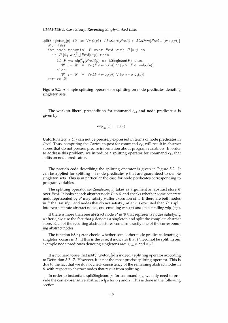
CHAPTER 5. Case Study: Reversing Singly-linked Lists
splitSingletonc[p] (Ψ as ∀v.ψ(v): AbsStore[Pred ]): AbsDom[Pred ∪ {wlpc(p)}]Ψ′:= false
for each monomial P over Pred with P |= ψ doif P 6|=Ψ wlp
#c,Ψ[Pred ](¬p) then
if P |=Ψ wlp#c,Ψ[Pred ](p) or isSingleton(P ) then
Ψ′ := Ψ′ ∨ ∀v.(P ∧wlpc(p)) ∨ (ψ ∧¬P ∧¬wlpc(p))else
Ψ′ := Ψ′ ∨ ∀v.(P ∧wlpc(p)) ∨ (ψ ∧¬wlpc(p))return Ψ′
Figure 5.2: A simple splitting operator for splitting on node predicates denotingsingleton sets.
The weakest liberal precondition for command cl4 and node predicate x isgiven by:
wlpcl4(x) = x.〈n〉.
Unfortunately, x.〈n〉 can not be precisely expressed in terms of node predicates inPred . Thus, computing the Cartesian post for command cl4 will result in abstractstores that do not possess precise information about program variable x. In orderto address this problem, we introduce a splitting operator for command cl4 thatsplits on node predicate x.
The pseudo code describing the splitting operator is given in Figure 5.2. Itcan be applied for splitting on node predicates p that are guaranteed to denotesingleton sets. This is in particular the case for node predicates corresponding toprogram variables.
The splitting operator splitSingletonc[p] takes as argument an abstract store Ψover Pred . It looks at each abstract node P in Ψ and checks whether some concretenode represented by P may satisfy p after execution of c. If there are both nodesin P that satisfy p and nodes that do not satisfy p after c is executed then P is splitinto two separate abstract nodes, one entailing wlpc(p) and one entailing wlpc(¬p).
If there is more than one abstract node P in Ψ that represents nodes satisfyingp after c, we use the fact that p denotes a singleton and split the complete abstractstore. Each of the resulting abstract stores contains exactly one of the correspond-ing abstract nodes.
The function isSingleton checks whether some other node predicate denoting asingleton occurs in P . If this is the case, it indicates that P need not be split. In ourexample node predicates denoting singletons are: x, y, t, and null .
It is not hard to see that splitSingletonc[p] is indeed a splitting operator accordingto Definition 3.2.17. However, it is not the most precise splitting operator. This isdue to the fact that we do not check consistency of the remaining abstract nodes inΨ with respect to abstract nodes that result from splitting.
In order to instantiate splitSingletonc[p] for command cl4, we only need to pro-vide the context-sensitive abstract wlps for cl4 and x. This is done in the followingsection.
45

CHAPTER 5. Case Study: Reversing Singly-linked Lists
c p wlp#c [Pred ](p) wlp#
c [Pred ](¬p)
cl0 y null ¬null
(¬y).U〈n〉.null 〈n∗〉.null ¬〈n∗〉.null
(¬y).S〈n〉.(x∧¬y) x.〈n∗〉 ∧¬(null ∧x) ¬x.〈n∗〉∨ null ∧x
cl2 t y ¬y
cl3 y x ¬x(¬y).U〈n〉.null (¬x).U〈n〉.null ¬(¬x).U〈n〉.null
(¬y).S〈n〉.(x∧¬y) false true
cl4 x false ¬x.〈n∗〉∨ x∧〈n∗〉.null
cl5 x.〈n∗〉 x∨ (¬y).S〈n〉.(x∧¬y)
¬x.〈n∗〉 ∧ y∨ ∀v.y → ¬x.〈n∗〉
(¬y).S〈n〉.(x∧¬y) (¬y).S〈n〉.(x∧¬y) ¬x.〈n∗〉〈n∗〉.null null
∨ (¬y).U〈n〉.null
∨ y∧∀v.t→ (¬y).U〈n〉.null
y∧ t∨ ∀v.y → t
(¬y).U〈n〉.null (¬y).U〈n〉.null ¬wlp#c (p)
(¬x).U〈n〉.null (¬x).U〈n〉.null ∧(¬y).U〈n〉.null
∨ y∧¬x∧∀v.t → (¬x).U〈n〉.null
x∧¬null
Table 5.1: Abstract context-sensitive wlps of node predicates in Pred for atomiccommands in REVERSE.
5.4 Context-sensitive Abstract Weakest Liberal Precon-ditions
We need to give the context-sensitive abstract wlp for each of the chosen abstrac-tion predicates. In order to obtain a representation that is independent of the con-text, we express them in terms of GMNP[n]. Evaluating the quantified formulasunder a given context, as it is formalized in Section 4.4, results in the appropriatecontext-sensitive version.
Table 5.1 lists the context-sensitive abstract wlps for node predicates in Pred .Node predicates that are not explicitly listed in the table do not change under theappropriate command. Since for command cl4 we split on the node predicate x,we only give the context-sensitive abstract wlp for x itself. This is the only one thatis needed in order to compute the operator splitSingletoncl4 [x].
For the computation of the Cartesian post with splitting that is used for com-mand cl4, we extend Pred by node predicate x.〈n〉. The context-sensitive abstractwlps over the refined set of abstraction predicates are given in Table 5.2.
5.5 Computing the Least Fixed PointBefore we can eventually compute the least fixed point of program REVERSE, wefirst need to model the data flow equations and give the abstraction of the initialset of stores under Pred .
The abstract domain AbsDom[Pred ] only describes the abstraction of the pro-gram stores, but contains no information regarding the program locations. We
46

CHAPTER 5. Case Study: Reversing Singly-linked Lists
c p wlp#c [Pred ∪ {x.〈n〉}](p) wlp#
c [Pred ∪ {x.〈n〉}](¬p)
cl4 x x.〈n〉 ¬x.〈n〉x.〈n〉 x∧x.〈n〉 ¬x.〈n∗〉
∨ x.〈n〉 ∧〈n∗〉.null
∨ x∧¬x.〈n〉x.〈n∗〉 x.〈n〉
∨ x.〈n∗〉 ∧¬x∨ x.〈n∗〉 ∧¬〈n∗〉.null
¬x.〈n∗〉∨ x∧¬〈n∗〉.null
(¬y).S〈n〉.(x∧¬y) x.〈n〉 ∧ ¬y∨ x.〈n∗〉 ∧¬x∧∀v.y → (x∧¬x.〈n〉)
∨ x.〈n∗〉 ∧¬〈n∗〉.null
∧∀v.y → (x∧¬x.〈n〉)
y∨ ¬x.〈n∗〉∨ x∧¬〈n∗〉.null
(¬x).U〈n〉.null null
∨ ¬x.〈n〉 ∧(¬x).U〈n〉.null
¬wlp#c (p)
Table 5.2: Abstract context-sensitive wlps for command cl4 over the refined set ofnode predicates.
represent abstract states as tuples over AbsDom[Pred ], where the i-th componentcorresponds to the abstract stores at the i-th program location. The partial order onthose tuples as well, as meat and join operations can be defined as the point-wiseextensions of the corresponding operations on AbsDom[Pred ].
The following abstract post operator on tuples over AbsDom[Pred ] models thedata flow equations in program REVERSE and gives us our final abstract post oper-ator that we will use for the analysis:
post# ∈ (AbsDom[Pred ])7 → (AbsDom[Pred ])7
post#〈Ψ0, . . . ,Ψ6〉 = 〈l0 : false,
l1 : post#cl0,Cart(Ψ0) ∨ post
#cl5,Cart(Ψ5),
l2 : (∀v.x(v) → ¬null(v)) ∧ Ψ1,
l3 : post#cl2,Cart(Ψ2),
l4 : post#cl3,Cart(Ψ3),
l5 : post#cl4,splitSingletoncl4
[x](Ψ4),
l6 : (∀v.x(v) → null(v)) ∧ Ψ1〉.
The initial abstract state init# is given by the tuple:
init#def= 〈Ψinit, false, false, false, false, false, false〉
where Ψinit is the abstraction of the initial set of stores init. The set init containsall singly-linked lists that have at least one element and whose head is pointedto by program variable x. The abstraction of init under Pred , is described by thefollowing table:
x y t null x.〈n∗〉 (¬y).S〈n〉.(x∧¬y) (¬y).U〈n〉.null (¬x).U〈n〉.null 〈n∗〉.null
1 ∗ ∗ 0 1 ∗ ∗ 0 1Ψinit 0 ∗ ∗ 0 1 ∗ ∗ 1 1
0 ∗ ∗ 1 1 ∗ 1 1 1
Each row in the table represents an abstract node in Ψinit. If a cell in a row containsthe value 1, the corresponding predicate occurs positively in the abstract node, the
47

CHAPTER 5. Case Study: Reversing Singly-linked Lists
value 0 means it occurs negated, and ∗ means it does not occur at all. The first rowrepresents the head of the list pointed to by x, the third row represents NULL, andthe second row represents all remaining nodes in the list.
In order to provide a better intuition for the set of concrete stores that is repre-sented by some abstract store, we use the graph notation from [27] which they usefor the representation of three-valued logical structures.
This graph notation is similar to the one we introduced in Section 2.3.1, in or-der to represent two-valued logical structures. The nodes in such a graph givethe partitioning of the universe of the represented logical structures into disjointnonempty subsets. Singly-lined nodes represent singleton sets, whereas doubly-lined summary nodes may represent arbitrary large subsets of concrete nodes.
Predicate symbols over the nodes in the graph may be interpreted indefinitely,denoted by a dashed line between the corresponding nodes. The meaning of sucha dashed line is that each logical structure represented by the graph can interpretthe corresponding predicate symbol arbitrarily on nodes that are represented bythe appropriate abstract nodes.
For each abstract store Ψ, we give a set of such graphs that represents the sameset of concrete stores as Ψ. The initial abstract store Ψinit represents the same set ofconcrete stores as the following two graphs:
y, t null
xn
n
n
nully, t
xn
We are now ready to compute the least fixed point of post# under init#. Theindividual steps of the fixed point iteration are given in Appendix B. If we projectlfp(post#(init#)) on the 7th component, i.e. the one corresponding to programlocation l6, we get the following abstract stores:
x y t null x.〈n∗〉 (¬y).S〈n〉.(x∧¬y) (¬y).U〈n〉.null (¬x).U〈n〉.null 〈n∗〉.null
0 1 0 0 0 0 0 1 1
l6 : 0 0 0 0 1 1 1 1 11 0 1 1 1 1 1 1 1
null , t, x
y
0 0 1 0 0 0 1 1 10 1 0 0 0 0 0 1 1
0 0 0 0 1 1 1 1 11 0 1 1 1 1 1 1 1
null , x
y
t
48

CHAPTER 5. Case Study: Reversing Singly-linked Lists
0 0 0 0 0 0 1 1 10 0 1 0 0 0 1 1 10 1 0 0 0 0 0 1 1
0 0 0 0 1 1 1 1 11 0 1 1 1 1 1 1 1
null , x
y
t
One can see that each of the abstract stores contains an abstract node whichis inconsistent with respect to the other abstract nodes. The corresponding rowsin the table are marked gray. An abstract node P is inconsistent in some abstractstore Ψ, if for all concrete stores represented by Ψ there is no node satisfying P .In the concrete stores represented by the abstract stores above it is always the casethat program variable x points to NULL. Thus, NULL is the only possible node thatis reachable by program variable x. This makes the marked abstract nodes incon-sistent, because they are supposed to be reachable by x but are not NULL.
The inconsistent abstract nodes appear due to the use of the splitting operatorsplitSingletoncl4 [x]. Replacing this splitting operator with the most precise splittingoperator for command cl4 and node predicate x would eliminate all inconsisten-cies.
It may appear disturbing that the information regarding the n predicate for thenodes pointed to by program variables y and t is rather imprecise. This is due tothe fact that the appropriate reachability information is not expressible in terms ofabstraction predicates in Pred .
However, the set of abstraction predicates was chosen in order to synthesize aspecific invariant, namely that the output list of program REVERSE is always acyclic.This invariant is indeed entailed by the least fixed point. All abstract nodes inwhich the node predicate y occurs positively entail the node predicate 〈n∗〉.null .Thus, in all represented concrete stores it is possible to reach NULL from programvariable y. This implies that all corresponding output lists are indeed acyclic.
49


Chapter 6
Related Work
There is a lot of recent work on shape analysis. In the following we compare someof these works to our own results.
6.1 Abstract Domains for Shape Analysis
Abstract domains designed for shape analysis [17, 5, 29, 26] are based on severalvariants of shape graphs. The use of three-valued logical structures as abstract do-main is a generalization of this idea. In the following, we discuss this particularapproach more thoroughly.
A shape analysis algorithm based on three-valued logic is given in [27]. TheTVLA tool [21] implements this algorithm. The abstract domain used in this ap-proach is given by sets of three-valued logical structures. Three-valued logicalstructures are used to finitely abstract infinite sets of two-valued logical structuresthat correspond to sets of program stores.
Their notion of canonical abstraction relates sets of two-valued logical structureswith finite sets of three-valued logical structure. The abstraction is parameterizedby a finite set of unary abstraction predicates on nodes. It collapses all subsetsof nodes in an abstracted structure whose elements are indistinguishable underthe abstraction predicates to single abstract nodes in the universe of the resultingthree-valued logical structure.
The interpretation of a predicate symbol in the three-valued logical structure isgiven by a conservative abstraction of its interpretation on the represented nodesin the abstracted two-valued structures. This is accomplished by using the indef-inite truth value in the three-valued logic. The interpretation of some predicatesymbol p on abstract nodes has the indefinite value, if the interpretation of p on therepresented nodes in the abstracted two-valued structure is ambiguous.
The computation of the abstract post operator is based on predicate-updateformulas, i.e. abstract weakest liberal preconditions of abstraction predicates. Theprecision of the abstract post operator can be improved by adding instrumenta-tion predicates. Instrumentation predicates preserve certain information about theconcrete structures in the abstraction, e.g. acyclicity or sharing. The additionalpredicates can be used to increase the precision of predicate-update formulas. Socalled focus and coerce operations are used to obtain more precise results in thepresence of nondeterminism in the abstract transition system.
We used several ideas from this work. In particular, we adapted the representa-tion of concrete program stores as two-valued logical structures. However, we donot need three-valued logic, because we symbolically abstract sets of stores using
51

CHAPTER 6. Related Work
formulas. Canonical abstraction is the basis of our own node predicate abstraction.Our framework does not provide the ability to define additional instrumentationpredicates. We want to use automated abstraction refinement instead. If the twooperations focus and coerce are combined into a single operation on formulas, theresult corresponds to a splitting operator as given in Section 3.2.6.
A translation from three-valued logical structures, as they arise in [27], intoan isomorphic representation in two-valued first-order logic is first given in [30].Shape analysis constraints [19] generalize this result to a Boolean algebra of first-order formulas that is isomorphic to the same class of three-valued logical struc-tures. The translation of [30] relates each three-valued structure to a conjunction ofthree constraints: a totality constraint expressing that every node is represented bysome abstract node; an existential constraint expressing the non-emptiness of eachabstract node; and a constraint expressing the values of binary predicate symbolson abstract nodes.
Our notion of an abstract store exactly corresponds to the totality constraintin the translation above. Consequently, for the same set of abstraction predicatesour abstract domain is weaker as the one used in TVLA. However, we indicatedin Section 3.1.4 that constraints for the values of binary predicate symbols can betranslated to additional unary abstraction predicates. It may also be possible tostrengthen our abstract stores by adding existential constraints, but existential con-straints complicate the application of Cartesian abstraction.
6.2 Symbolic Methods in Shape AnalysisIn [31] an algorithm for the symbolical computation of most precise operators forshape analysis is given. The paper describes an algorithm implementing an as-sume operation. The operator assume[ϕ](a) takes a closed formula ϕ and a set ofthree-valued logical structures a and computes the best under-approximation ofa satisfying the formula ϕ, provided that a decision procedure for the underlyinglogic exists. The assume operation allows inter-procedural shape analysis basedon assume-guarantee reasoning. Moreover, assume can be instantiated to computebest abstraction functions, most-precise post operators, and the meet operation forabstract domains of three-valued logical structures.
Although this algorithm is primarily designed to be applied in the context ofabstract domains of three-valued logical structures, a modified version could beused to compute most precise splitting operators.
Dams and Namjoshi [9] use predicate abstraction and model checking for shapeanalysis. They abstract pointer programs by Boolean programs using classical pred-icate abstraction [12] based on state predicates. After the predicate abstraction stepthey apply standard finite state model checking techniques to analyze the obtainedBoolean program. Their abstraction predicates describe properties of the shape ofthe program stores, including reachability properties. They give a weakest precon-dition calculus, in order to compute predicate-updates and provide heuristics forabstraction refinement. The calculus makes use of generalized reachability pred-icates. These predicates are parameterized by sets of addresses that have to beavoided on a path. The calculus allows to express weakest preconditions of reach-ability properties in a similar way as it is done in this work using modal nodepredicates.
Although both their and our work use techniques from predicate abstraction,our abstract domain is induced by unary node predicates instead of nullary statepredicates. The size of our abstract domain is triple exponential in the number of
52

CHAPTER 6. Related Work
abstraction predicates, whereas the abstract domain in predicate abstraction is onlydoubly exponential. Hence, in order to get equally precise abstract domains in bothframeworks, predicate abstraction needs 2n state predicates compared to n nodepredicates in our framework. However, the lower bound for the complexity of theabstract post operator is in both frameworks linear in the number of abstractionpredicates. Therefore, the use of unary abstraction predicates in our frameworkgains a better ratio between precision and complexity.
6.3 Decidable Logics for Shape AnalysisDecidable logics that are expressive enough to be useful in shape analysis are rare.Weak monadic second order logic over trees is an example for a logic that is decid-able and used in this application domain [22]. In the following, we discuss somemore recent results on decidable logics that have been primarily studied for theirpotential application in shape analysis.
In [15] the boundary between decidability and undecidability for transitive clo-sure logics is explored. The authors introduce the logic ∃∀(DTC+[E]) and prove itsdecidability. This logic is a fragment of first-order logic with transitive closure ad-hering the following restrictions: the signature contains just one binary predicatesymbol E; formulas are in ∃∀-prenex form; and positive applications of transitiveclosure are only allowed for deterministic paths of the relation E. They show thatweakening any of the above restrictions results in an undecidable logic.
Transitive closure logics can express reachability relations between pairs ofvariables, while guarded fixed point logics – and thus modal node predicates –can do so only for pairs of unary relations. On the other hand, guarded fixed pointlogics remain decidable without being restricted in the number of binary predicatesymbols. This makes it easier to express properties of more complex data struc-tures. However, [16] gives a way to handle data structures that are intractable dueto such limitations by simulating them on structures for decidable logics. The au-thors show that many data structures appearing in practical application, such astrees and doubly-linked lists, can be handled via simulation using just a single bi-nary predicate symbol.
Role logic [18] is a variable free logic equivalent to first-order logic with tran-sitive closure and designed as a specification and annotation language for shapeanalysis. The authors identify the decidable fragment RL2 of role logic. RL2 is asexpressive as two-variable logic with counting. In [20] it is shown that the syn-tax of RL2 can be extended by spatial conjunction from separation logic [25], whileremaining decidable. Spatial conjunction provides an elegant way to express con-catenation of records.
Counting constraints – and thus RL2 – allow the specification of the precise aliasrelationship between heap objects. This particularly includes the ability to expressinformation about sharing. Modal node predicates do not offer such expressive-ness. On the other hand, RL2 cannot express reachability, which was our primaryintention to propose modal node predicates.
53


Chapter 7
Conclusion
7.1 Summary
The goal of this work was to obtain a framework for symbolic shape analysis. Weproposed an appropriate symbolic abstract domain. Conforming to the abstractiontechniques that are used in state-of-the-art shape analysis algorithms such as [27],this abstract domain is parameterized by node predicates.
We used techniques from predicate abstraction to symbolically abstract pro-grams manipulating heap-allocated data structures by Boolean heap programs.Boolean heap programs are characterized as a two-step Cartesian abstraction ofthe best abstract post operator post# on the chosen abstract domain. If the abstracttransition system behaves deterministically, Boolean heap programs do not loseprecision with respect to post#.
We identified the class of modal node predicates, a fragment of first-order logicwith transitive closure. Modal node predicates can be used for the analysis ofreachability properties for linked data structures. We gave a preliminary resultregarding decidability of the satisfiability problem for modal node predicates viatranslation into guarded fixed point logic. Moreover, we showed that for list-likestructures, this class of node predicates is closed under weakest liberal precondi-tions. Both results are useful for the development of an automated abstractionrefinement procedure for modal node predicates.
7.2 Future Work
The primary task for future work should be the development of a tool that imple-ments the presented framework and allows a practical evaluation of the developedtechniques. However, there is a number of interesting theoretical questions openfor future work. We discuss some of them in the following.
7.2.1 Precision of the Abstract Domain
Our notion of an abstract store describes the covering of nodes in concrete storesby abstract nodes, i.e. the equivalence classes of nodes induced by the chosen ab-straction predicates. However, it is a bit disturbing that an abstract store does notrequire each of its abstract nodes to be non-empty. The decision that we restrictourselves to universal constraints over abstract nodes was made, in order to sim-plify the application of Cartesian abstraction. An interesting question is, whetherthe abstract domain can be made more precise by allowing existential constraints
55

CHAPTER 7. Conclusion
over abstract nodes, while still using Cartesian abstraction for the construction ofBoolean heap programs.
7.2.2 Automated Abstraction RefinementWe gave preliminary results for the development of an automated abstraction re-finement procedure for modal node predicates. However, there are open issuesthat still have to be solved.
We did not yet answer the question, whether the satisfiability problem formodal node predicates restricted to the class of program stores is decidable. Themain problem lies in the treatment of functionality constraints, as they appear inthe integrity formulas that define the set of program stores. However, a decisionprocedure for this problem is a key tool for the automated derivation of context-sensitive abstract weakest liberal preconditions. These are needed for the construc-tion of Boolean heap programs. Hence, this is a main prerequisite to use modalnode predicates in a fully automated analysis.
A second open issue is that, so far, we only showed closeness under wlp forthe class of modal node predicates over a single binary predicate symbol. Hence,the application of modal node predicates is restricted to list-like data structures.In order to use them for the analysis of more complex data structures, we need toextend this result to an arbitrary number of binary predicate symbols.
7.2.3 Beyond SafetyTemporal properties of transition systems can be divided into two classes: safetyproperties and liveness properties. Roughly spoken: a safety property specifiesthe absence of finite error traces, whereas a liveness property specifies the absenceof infinite error traces.
Our approach abstracts infinite state systems by finite state systems. The finitestate abstraction is used to synthesize state invariants, i.e over-approximations ofthe reachable set of states of the analyzed system. However, state invariants cor-respond to safety properties. The information needed for the analysis of livenessproperties gets lost during the finite state abstraction.
Transition invariants [24] capture both safety and liveness properties. A transi-tion invariant is an over-approximation of the program’s transition relation. Transi-tion predicate abstraction [23] is a framework for the automatic synthesis of transitioninvariants. It solves the limitations of predicate abstraction by replacing the con-struction of a fixed point operator on an abstract domain of sets of abstract stateswith the construction of a fixed point operator on an abstract domain of binaryrelations on abstract states.
In analogy to predicate abstraction the abstract domain is parameterized bya set of transition predicates. Transition predicates are constraints denoting binaryrelations over states. It is a challenging task to find a suitable class of transitionpredicates for shape analysis that could be used to treat both safety and livenessproperties.
56

Bibliography
[1] Thomas Ball, Andreas Podelski, and Sriram K. Rajamani. Boolean and Carte-sian abstraction for model checking C programs. In Tiziana Margaria andWang Yi, editors, Proceedings of the 7th International Conference on Tools and Al-gorithms for the Construction and Analysis of Systems (TACAS’01), volume 2031of Lecture Notes in Computer Science, pages 268–283. Springer-Verlag, 2001.
[2] Thomas Ball, Andreas Podelski, and Sriram K. Rajamani. Relative com-pleteness of abstraction refinement for software model checking. In Joost-Pieter Katoen and Perdita Stevens, editors, Proceedings of the 8th InternationalConference on Tools and Algorithms for the Construction and Analysis of Systems(TACAS’02), volume 2280 of Lecture Notes in Computer Science, pages 158–172.Springer-Verlag, 2002.
[3] Thomas Ball and Sriram K. Rajamani. Automatically validating temporalsafety properties of interfaces. In Proceedings of the 8th international SPIN work-shop on Model checking of software, pages 103–122. Springer-Verlag, 2001.
[4] Randel E. Bryant. Graph-Based Algorithms for Boolean Function Manipula-tion. IEEE Transactions on Computers, 35(10):677–691, 1986.
[5] David R. Chase, Mark Wegman, and F. Kenneth Zadeck. Analysis of pointersand structures. In Proceedings of the ACM SIGPLAN 1990 conference on Program-ming language design and implementation, pages 296–310. ACM Press, 1990.
[6] Edmund M. Clarke, Orna Grumberg, Somesh Jha, Yuan Lu, and HelmutVeith. Counterexample-Guided Abstraction Refinement. In Allen E. Emersonand Prasad A. Sistla, editors, Proceedings of the 12th International Conference onComputer Aided Verification (CAV’00), volume 1855 of Lecture Notes in ComputerScience, pages 154–169. Springer-Verlag, 2000.
[7] Patrick Cousot and Radhia Cousot. Abstract interpretation: a unified latticemodel for static analysis of programs by construction or approximation offixpoints. In Proceedings of the 4th ACM SIGACT-SIGPLAN symposium on Prin-ciples of Programming Languages, pages 238–252. ACM Press, 1977.
[8] Patrick Cousot and Radhia Cousot. Systematic design of program analysisframeworks. In Conference Record of the Sixth Annual ACM SIGPLAN-SIGACTSymposium on Principles of Programming Languages, pages 269–282. ACM Press,1979.
[9] Dennis Dams and Kedar S. Namjoshi. Shape Analysis through Predicate Ab-straction and Model Checking. In Proceedings of the 4th International Confer-ence on Verification, Model Checking and Abstract Interpretation (VMCAI’03), vol-ume 2575 of Lecture Notes in Computer Science, pages 310–323. Springer-Verlag,2003.
57

BIBLIOGRAPHY BIBLIOGRAPHY
[10] Bernd Finkbeiner. Language containment checking with nondeterministicBDDs. In Proceedings of the 7th International Conference on Tools and Algorithmsfor the Construction and Analysis of Systems (TACAS’01), volume 2031 of LectureNotes in Computer Science, pages 24–38. Springer-Verlag, 2001.
[11] Erich Gradel and Igor Walukiewicz. Guarded Fixed Point Logic. In Proceed-ings of 14th IEEE Symposium on Logic in Computer Science (LICS ‘99), pages45–54. IEEE Computer Society, 1999.
[12] Susanne Graf and Hassen Saıdi. Construction of Abstract State Graphs withPVS. In Orna Grumberg, editor, Proceedings of the 9th International Conferenceon Computer Aided Verification (CAV’97), volume 1254 of Lecture Notes in Com-puter Science, pages 72–83. Springer-Verlag, 1997.
[13] Thomas A. Henzinger, Ranjit Jhala, Rubak Majumdar, and Gregoire Sutre.Software verification with BLAST. In SPIN 03: Model Checking of Software,volume 2648 of Lecture Notes in Computer Science, pages 235–239. Springer-Verlag, 2003.
[14] Thomas A. Henzinger, Ranjit Jhala, Rupak Majumdar, and Gregoire Sutre.Lazy Abstraction. In Proceedings of the 29th ACM SIGACT-SIGPLAN Sympo-sium on Principles of Programming Languages, pages 58–70. ACM Press, 2002.
[15] Neil Immerman, Alexander Rabinovich, Thomas Reps, Mooly Sagiv, andGreta Yorsh. The Boundary Between Decidability and Undecidability forTransitive-Closure Logics. 2004. to appear in CSL’04.
[16] Neil Immerman, Alexander Rabinovich, Thomas Reps, Mooly Sagiv, andGreta Yorsh. Verification Via Structure Simulation. In Rajeev Alur andDoron A. Peled, editors, Proceedings of the 16th International Conference on Com-puter Aided Verification (CAV’04), volume 3114 of Lecture Notes in ComputerScience, pages 281–294. Springer-Verlag, 2004.
[17] Neil D. Jones and Steven S. Muchnick. Flow analysis and optimization of lisp-like structures. In Proceedings of the 6th ACM SIGACT-SIGPLAN symposium onPrinciples of Programming Languages, pages 244–256. ACM Press, 1979.
[18] Viktor Kuncak and Martin Rinard. On role logic. Technical Report 925, MITComputer Science and Artificial Intelligence Laboratory, October 2003.
[19] Viktor Kuncak and Martin Rinard. Boolean Algebra of Shape Analysis Con-straints. In 5th International Conference on Verification, Model Checking and Ab-stract Interpretation (VMCAI’04), volume 2937 of Lecture Notes in Computer Sci-ence, pages 59–72. Springer-Verlag, 2004.
[20] Viktor Kuncak and Martin Rinard. Generalized Records and Spatial Conjunc-tion in Role Logic. In Roberto Giacobazzi, editor, 11th Annual InternationalStatic Analysis Symposium (SAS’04), volume 3148 of Lecture Notes in ComputerScience. Springer-Verlag, August 26–28 2004.
[21] Tal Lev-Ami. TVLA: A framework for Kleene based static analysis. Master’sthesis, Tel-Aviv University, Tel-Aviv, Israel, 2000.
[22] Anders Møller and Michael I. Schwartzbach. The pointer assertion logic en-gine. In Proceedings of the ACM SIGPLAN 2001 conference on Programming lan-guage design and implementation, pages 221–231. ACM Press, 2001.
[23] Andreas Podelski and Andrey Rybalchenko. Transition Predicate Abstractionand Fair Termination. Available from the authors.
58

BIBLIOGRAPHY BIBLIOGRAPHY
[24] Andreas Podelski and Andrey Rybalchenko. Transition Invariants. In Pro-ceedings of 19th IEEE Symposium on Logic in Computer Science (LICS ‘04), pages32–41. IEEE Computer Society, 2004.
[25] John C. Reynolds. Separation Logic: A Logic for Shared Mutable Data Struc-tures. In Proceedings of 17th IEEE Symposium on Logic in Computer Science(LICS’02), pages 55–74. IEEE Computer Society, 2002.
[26] Mooly Sagiv, Thomas Reps, and Reinhard Wilhelm. Solving shape-analysisproblems in languages with destructive updating. ACM Transactions on Pro-gramming Languages and Systems (TOPLAS), 20(1):1–50, 1998.
[27] Mooly Sagiv, Thomas Reps, and Reinhard Wilhelm. Parametric shape anal-ysis via 3-valued logic. ACM Transactions on Programming Languages and Sys-tems (TOPLAS), 24(3):217–298, 2002.
[28] Joseph Sifakis. A unified approach for studying the properties of transitionsystems. Theor. Computer Science, 18:227–258, 1982.
[29] Edward Wang. Analysis of Recursive Types in an Imperative Language. PhDthesis, University of California at Berkeley, 1994.
[30] Greta Yorsh. Logical Characterizations of Heap Abstractions. Master’s thesis,Tel-Aviv University, Tel-Aviv, Israel, 2003.
[31] Greta Yorsh, Thomas Reps, and Mooly Sagiv. Symbolically Computing Most-Precise Abstract Operations for Shape Analysis. In Proceedings of the 10th In-ternational Conference on Tools and Algorithms for the Construction and Analysis ofSystems (TACAS’04), volume 2988 of Lecture Notes in Computer Science, pages530–545. Springer-Verlag, 2004.
59


Appendix A
Proofs
Proposition 2.1.4. For a transition system S the following is equivalent:
(i) R is total and deterministic,
(ii) pre is a homomorphism on the power set Boolean algebra of State.
Proof. “(i) ⇒ (ii)”. Let the transition relation R be total and deterministic. ByProposition 2.3.7 (ii) we know that pre distributes over set union. Thus, in orderto prove that pre is a homomorphism on the power set Boolean algebra of State, itsuffices to show that pre commutes with set complementation. For S ⊂ State, let Sdenote the complement of S. We have:
s ∈ pre(S′) ⇒ ∀s′ ∈ State : (s, s′) ∈ R ⇒ s′ ∈ S′
⇒ ∃s′ ∈ State : (s, s′) ∈ R and s′ ∈ S′ (R total)⇒ ∃s′ ∈ State : (s, s′) ∈ R and s′ 6∈ S′
⇒ s 6∈ pre(S′)
⇒ s ∈ pre(S′)
s ∈ pre(S′) ⇒ ∃s′ ∈ State : (s, s′) ∈ R and s′ 6∈ S′
⇒ ∀s′ ∈ State : (s, s′) ∈ R ⇒ s′ 6∈ S′ (R deterministic)
⇒ ∀s′ ∈ State : (s, s′) ∈ R ⇒ s′ ∈ S′
⇒ s ∈ pre(S′)
Thus we have pre(S′) = pre(S′).
“(ii) ⇒ (i)”. Assume pre is a homomorphism on the power set Boolean alegraof State. If State is the empty set then R is the empty relation and thus total anddeterministic. If otherwise State is non-empty, assume that R was not total. Thenthere exists s ∈ State such that:
∀s′ ∈ State : (s, s′) 6∈ R
⇒ ∀S ⊆ State : s ∈ pre(S)
⇒ ∀S ⊆ State : s ∈ pre(S) and s ∈ pre(S)
⇒ ∀S ⊆ State : s 6∈ pre(S) and s ∈ pre(S)
⇒ ∀S ⊆ State : pre(S) 6= pre(S)
61

APPENDIX A. Proofs
which contradicts the fact that pre commutes with set complementation. Now as-sume R was not deterministic then there are s, s1, s2 ∈ State such that
s1 6= s2 and (s, s1) ∈ R and (s, s2) ∈ R
⇒ s 6∈ pre({s1}) and s 6∈ pre({s1})
⇒ pre({s1}) 6= pre({s1})
which again gives us a contradiction.
Proposition 2.1.7. I ⊆ State is an inductive state invariant if and only if it is closedunder the operator F , i.e. F (I) ⊆ I .
Proof. Let I be an inductive state invariant. Since I is a state invariant, we havereach ⊆ I and therefore init ⊆ I . Since I is inductive, we have post(I) ⊆ I . Hence,we have:
F (I) = init ∪ post(I) ⊆ I.
Let I be closed under the operator F , i.e. F (I) ⊆ I . We have by monotonicity of F :
reach = lfp(F ) =⋂
{S ⊆ State | F (S) ⊆ S }.
From this we can conclude reach ⊆ I . Moreover, by definition of F , we haveF (I) ⊆ I implies post(I) ⊆ I . Hence, I is an inductive state invariant.
Proposition 2.3.2. The operators ext-postc and ext-prec form a Galois connection on thepower set lattice of extended stores.
Proof. Follows immediately from the definitions of ext-postc and ext-prec on sets ofextended stores and the fact that postc and prec form a Galois connection on thepower set lattice of stores.
Proposition 2.3.3. The relation c−→ is total and deterministic if and only if ext-prec is a
homomorphism on the power set Boolean algebra of extended stores.
Proof. Follows immediately from the definition of prec on sets of extended storesand Proposition 2.1.4.
Proposition 2.3.5. If the relation c−→ is total and deterministic and if for every predicate
symbol p there exists a predicate-update formula p′c then the extended wlp of an FOTC for-mula ϕ can be computed by substituting syntactically all occurrences of predicate symbolsin ϕ with their predicate-update formulas:
ext-prec(JϕK) = Jϕ[p′c(v1, . . . , vn)/p(v1, . . . , vn)]K.
Proof. By structural induction on ϕ.ϕ = p(v1, . . . , vn). By definition of predicate-update formulas we have:
ext-prec(Jp(v1, . . . , vn)K) = Jp′c(v1, . . . , vn)K = Jϕ[p′c/p]K.
ϕ = ϕ1 ∨ϕ2. We have:
ext-prec(Jϕ1 ∨ϕ2K) = ext-prec(Jϕ1K ∪ Jϕ2K)= ext-prec(Jϕ1K) ∪ ext-prec(Jϕ2K) (by Prop. 2.3.3)= Jϕ1[p
′c/p]K ∪ Jϕ2[p
′c/p]K (Ind. hypothesis)
= Jϕ1[p′c/p]∨ϕ2[p
′c/p]K
= Jϕ[p′c/p]K
62

APPENDIX A. Proofs
ϕ = (TC v1, v2.ϕ1(v1, v2))(v, v′). Let S be some store and β an assignment. We
have:
(S, β) ∈ ext-prec(JϕK)⇐⇒ ∃u1, . . . , un ∈ U : β v = u1, β v
′ = un and∀1 ≤ i < n : postc(S), β[v1 7→ ui, v2 7→ ui+1] |= ϕ1(v1, v2)
( c−→ total and deterministic)
⇐⇒ ∃u1, . . . , un ∈ U : β v = u1, β v′ = un and
∀1 ≤ i < n : (postc(S), β[v1 7→ ui, v2 7→ ui+1]) ∈ Jϕ1(v1, v2)K⇐⇒ ∃u1, . . . , un ∈ U : β v = u1, β v
′ = un and∀1 ≤ i < n : ext-postc((S, β[v1 7→ ui, v2 7→ ui+1])) ∈ Jϕ1(v1, v2)K(Def. of ext-postc)
⇐⇒ ∃u1, . . . , un ∈ U : β v = u1, β v′ = un and
∀1 ≤ i < n : (S, β[v1 7→ ui, v2 7→ ui+1]) ∈ ext-prec(Jϕ1(v1, v2)K)(by Prop. 2.3.2)
⇐⇒ ∃u1, . . . , un ∈ U : β v = u1, β v′ = un and
∀1 ≤ i < n : (S, β[v1 7→ ui, v2 7→ ui+1]) ∈ Jϕ1[p′c/p](v1, v2)K
(Ind. hypothesis)⇐⇒ ∃u1, . . . , un ∈ U : β v = u1, β v
′ = un and∀1 ≤ i < n : S, β[v1 7→ ui, v2 7→ ui+1] |= ϕ1[p
′c/p](v1, v2)
⇐⇒ S, β |= ϕ[p′c/p]
⇐⇒ (S, β) ∈ Jϕ[p′c/p]K
All remaining cases follow similar argumentations.
Proposition 2.3.7. If c−→ is total and deterministic then for a store S, FOTC formula ϕ
and assignment β, we have:
S, β |= wlpc(ϕ) ⇐⇒ postc(S), β |= ϕ.
Proof.
S, β |= wlpc(ϕ) ⇐⇒ (S, β) ∈ ext-prec(JϕK) (Def. of wlpc and Prop. 2.3.5)
⇐⇒ ∀S′ : Sc
−→ S′ ⇒ (S′, β) ∈ JϕK (Def. of ext-prec)
⇐⇒ (postc(S), β) ∈ JϕK ( c−→ total and determinstic)
⇐⇒ postc(S), β |= ϕ
Proposition 3.1.6. The function γ is a complete meet-morphism and a complete join-morphism.
Proof. Follows easily from the semantics of FOTC formulas.
Proposition 3.1.8. Abstraction function α and concretisation function γ form a Galoisconnection between the posets 〈2Store ,⊆〉 and 〈AbsDom , |=〉.
Proof. By Proposition 3.1.6 we know that the function γ is a complete meet-mor-phism. Thus, by definition of α and Proposition 2.1.9 we get that α and γ form aGalois connection.
63

APPENDIX A. Proofs
Theorem 3.1.10 (Characterization of Best Abstraction). Let M be a set of programstores. The image of M under α is characterized as follows:
α(M) |=|∨
S∈M
∀v.∨
u∈US
PS,u(v).
Proof. Since α and γ form a Galois connection, we know by Proposition 2.1.9 thatα distributes over set union on the concrete lattice, i.e. we have:
α(M) =∨
S∈M
∧{Ψ ∈ AbsDom | S |= Ψ }.
Thus, it suffices to consider the abstraction of a single store S ∈ M and it remainsto prove:
α(S) |=| ∀v.∨
u∈US
PS,u(v).
From the definition of PS,u for u ∈ US it is clear that we have:
S |= ∀v.∨
u∈US
PS,u(v).
Hence, we can immediately conclude:
α(S) |= ∀v.∨
u∈US
PS,u(v).
It remains to prove the right-to-left direction of the congruence. The meet of allformulas in AbsDom that are valid in S must be a single abstract store, rather thena disjunction of abstract stores. If it was a disjunction of abstract stores then Swould already satisfy one of its disjuncts contradicting the fact that it is the meet.Hence, there must be some formula over node predicates ψ(v) ∈ FPred such that:
∧{Ψ ∈ AbsDom | S |= Ψ } |=| ∀v.ψ(v).
Let S′ ∈ Store such thatS′ |= ∀v.
∨
u∈US
PS,u(v).
Given some node u′ ∈ US′
, there must be some node u ∈ US such that S′, u′ |=PS,u(v). Since PS,u(v) is a monomial over Pred satisfied for u in S, it must entailany other Boolean combination of node predicates that is satisfied for u in S. Inparticular we must have PS,u(v) |= ψ(v). From this we can infer that S ′, u′ |= ψ(v)
holds, too. Since u′ was chosen free in US′
, we have S′ |= ∀v.ψ(v) and thus S′ |=α(S). Hence, we have:
∀v.∨
u∈US
PS,u(v) |= α(S).
Proposition 3.2.3. For a given context Γ, the context-sensitive abstract operators havethe following properties:
(i) post#Γ and wlp
#Γ form a Galois connection between the two posets 〈FPred , |=Γ〉 and
〈FPred , |=post(γ(Γ))〉, formally:
∀ϕ, ψ ∈ FPred : post#Γ (ϕ) |=post(γ(Γ)) ψ ⇐⇒ ϕ |=Γ wlp
#Γ (ψ),
64

APPENDIX A. Proofs
(ii) post#Γ and wlp
#Γ are monotone,
(iii) post#Γ ◦wlp
#Γ is reductive,
(iv) wlp#Γ ◦ post
#Γ is extensive,
(v) post#Γ distributes over disjunctions,
(vi) wlp#Γ distributes over conjunctions.
Proof. We prove properties (ii), (iii), and (iv). Properties (i), (v), and (vi) then followfrom the general properties of Galois connections given in Proposition 2.1.9.Proof of (ii). Let ϕ1, ϕ2 ∈ FPred . In order to prove monotonicity of post
#Γ , as-
sume ϕ1 |=Γ ϕ2. By definition of post#Γ (ϕ2) we have ϕ2 |=Γ wlp(post
#Γ (ϕ2)). Thus,
by assumption, we can conclude ϕ1 |=Γ wlp(post#Γ (ϕ2)). However, post
#Γ (ϕ1) is
the conjunction of all formulas ψ ∈ FPred satisfying ϕ1 |=Γ wlp(ψ), i.e. we havepost
#Γ (ϕ1) |= post
#Γ (ϕ2). This implies post
#Γ (ϕ1) |=post(γ(Γ)) post
#Γ (ϕ2). Hence,
post#Γ is monotone.
In order to prove monotonicity of wlp#Γ , assume ϕ1 |=post(γ(Γ)) ϕ2. Let S be
some store such that S |= Γ and β an assignment. We have:
S, β |= wlp(ϕ1)⇔ post(S), β |= ϕ1 (by Prop. 2.3.7)⇒ post(S), β |= ϕ2 (by assumption)⇔ S, β |= wlp(ϕ2) (by Prop. 2.3.7)
Thus, we havewlp(ϕ1) |=Γ wlp(ϕ2) (1)
By definition of wlp#Γ we have wlp
#Γ (ϕ1) |= wlp(ϕ1). With (1) we can conclude
wlp#Γ (ϕ1) |=Γ wlp(ϕ2). However, by definition of wlp
#Γ we know that wlp
#Γ (ϕ2) is
the disjunction of all formulas ψ ∈ FPred satisfying ψ |= wlp(ϕ2), i.e. we havewlp
#Γ (ϕ1) |=Γ wlp
#Γ (ϕ2). Therefore wlp
#Γ is monotone.
Proof of (iii). Let ϕ ∈ FPred . By definition of post#Γ we know post
#Γ (wlp
#Γ (ϕ)) is the
conjunction of allψ ∈ FPred , such that wlp#Γ (ϕ) |=Γ wlp(ψ). Moreover, by definition
of wlp#Γ we have wlp
#Γ (ϕ) |=Γ wlp(ϕ). Thus, we have post
#Γ (wlp
#Γ (ϕ)) |=post(γ(Γ)) ϕ,
i.e. post#Γ ◦wlp
#Γ is reductive.
Proof of (iv). Let ϕ ∈ FPred . By definition of wlp#Γ we know wlp
#Γ (post
#Γ (ϕ)) is the
disjunction of all ψ ∈ FPred , such that ψ |=Γ wlp(post#Γ (ϕ)). Moreover, by defini-
tion of post#Γ we have ϕ |=Γ wlp(post
#Γ (ϕ)). Thus, we have ϕ |=Γ wlp
#Γ (post
#Γ (ϕ)),
i.e. wlp#Γ ◦ post
#Γ is extensive.
Proposition 3.2.6. Let Ψ = ∀v.ψ be an abstract store. The image of Ψ under post#Cart1
isobtained by applying the context-sensitive post operator for Ψ to ψ:
post#Cart1
(Ψ) |=| ∀v. post#Ψ(ψ).
Proof. In the following, consider ϕ1 and ϕ2 to be defined as follows:
ϕ1def=
∧{ϕ ∈ FPred | post#(Ψ) |= ∀v.ϕ }
ϕ2def=
∧{ϕ ∈ FPred | ψ |=Ψ wlp(ϕ) }
65

APPENDIX A. Proofs
In order to prove the proposition, we have to show that ϕ1 and ϕ2 are equivalent.
“ϕ2 |= ϕ1”: Let S be some store such that S is a model of Ψ, i.e. for all nodes u wehave S, u |= ψ. Now assume there was some node u such that S, u 6|= wlp(ϕ1). Wehave:
S, u 6|= wlp(ϕ1) ⇒ post(S), u 6|= ϕ1 (by Prop. 2.3.7)
⇒ post(S) 6|= ∀v.ϕ1
⇒ post#(Ψ) 6|= ∀v.ϕ1 (S |= Ψ implies post(S) |= post#(Ψ))
This contradicts the definition of ϕ1. Thus, for all nodes u we have S, u |= wlp(ϕ1)and therefore ψ |=Ψ wlp(ϕ1). Since ϕ2 is the greatest lower bound of all those for-mulas, we have ϕ2 |= ϕ1.
“ϕ1 |= ϕ2”: Let S be some store such that S |= post#(Ψ), but assume S 6|= ∀v.ϕ2.Then there is some node u such that S, u 6|= ϕ2. If PS,u is the abstract node of u inS then we must have PS,u |= ¬ϕ2.
Case 1: there is some store S ′ which is a model of Ψ and some node u′ such thatpost(S′), u′ |= PS,u. We have:
post(S′), u′ |= PS,u ⇒ post(S′), u′ 6|= ϕ2 (PS,u |= ¬ϕ2)⇒ S′, u′ 6|= wlp(ϕ2) (by Prop. 2.3.7)
which contradicts the definition of ϕ2, since S′, u′ |= ψ.
Case 2: for all stores S ′ either S′ 6|= Ψ or for all nodes u′ we have post(S′), u′ 6|= PS,u.From this we can conclude:
∀S′ : S′ |= Ψ ⇒ ∀u′ ∈ U : post(S′), u′ |= ϕ2 ∧¬PS,u
and again by Prop. 2.3.7 we get:
ψ |=Ψ wlp(ϕ2 ∧¬PS,u)
which contradicts the definition of ϕ2.
Thus, altogether we can conclude:
post#(Ψ) |= ∀v.ϕ2
and we finally get ϕ1 |= ϕ2.
Theorem 3.2.9 (Soundness of Cartesian Post). The operator post#Cart is an approxi-
mation of post#:∀Ψ ∈ AbsStore : post#(Ψ) |= post
#Cart(Ψ).
Proof. Let Ψ be some abstract store of the form ∀v.∨
i Pi. By definition of αCart1 itis clear that αCart1 is reductive, i.e. we immediately observe:
post#(Ψ) |= αCart1 ◦ post#(Ψ) = post#Cart1
(Ψ).
By Proposition 3.2.6 and the fact that post#Ψ distributes over disjunctions we get:
post#(Ψ) |= post#Cart1
(Ψ) = ∀v.∨
i
post#Ψ(Pi).
Again from its definition it is clear that αCart2 is reductive. Thus, we finally get:
post#(Ψ) |= ∀v.∨
i
αCart2 ◦ post#Ψ(Pi) = post
#Cart(Ψ).
66

APPENDIX A. Proofs
Theorem 3.2.10 (Characterization of Cartesian Post). Let Ψ = ∀v.∨
i Pi be an ab-stract store. The Cartesian post of Ψ is characterized as follows:
post#Cart(Ψ) = ∀v.
∨
i
∧{ p ∈ Pred | Pi |=Ψ wlp
#Ψ(p) }.
Proof. We have:
post#Cart(Ψ) = ∀v.
∨
i
αCart2 ◦ post#Ψ(Pi)
|=| ∀v.∨
i
{ p ∈ Pred | post#Ψ(Pi) |=post(Ψ) p }
|=| ∀v.∨
i
{ p ∈ Pred | Pi |=Ψ wlp#Ψ(p) } (by Prop. 3.2.3)
Proposition 3.2.12. Let Ψ be an abstract store. If post# is deterministic with respect toΨ then post
#Cart does not lose precision with respect to post#, i.e.
post#(Ψ) |=| post#Cart(Ψ).
Proof. Let Ψ be some abstract store with Ψ = ∀v.∨
i Pi, where each Pi is a mono-mial. Assume post# is deterministic with respect to Ψ, then we have:
post#(∀v.∨
i
Pi) = ∀v.∨
i
P ′i where for all i P ′
i = post#Ψ(Pi).
and each P ′i is a monomial. By Definition of post
#Cart we have:
post#Cart(Ψ) |=| ∀v.
∨
i
∧
i
{ p ∈ Pred | post#Ψ(Pi) |=post(Ψ) p }
|=| ∀v.∨
i
∧
i
{ p ∈ Pred | P ′i |=post(Ψ) p }
|=| ∀v.∨
i
∧
i
P ′i (P ′
i monomial)
|=| post#(Ψ)
Proposition 3.2.13. Let S be a store. The operator post# is deterministic with respect toα(S) if and only if for all node predicates p in Pred we have:
wlp(p) |=α(S) wlp#α(S)(p).
Proof. For the only if direction, let S be some store with α(S) = ∀v.∨
i Pi whereeach Pi is a monomial. Assume there is some p ∈ Pred such that:
wlp(p) 6|=α(S) wlp#α(S)(p).
Thus, there is some store S ′ and node u′ such that S′ |= α(S) and S′, u′ |= wlp(p)
but S′, u′ 6|= wlp#α(S)(p). Since S′ |= α(S) there must be some i such that S ′, u′ |= Pi.
Then we have:
S′, u′ |= Pi and S′, u′ 6|= wlp#α(S)(p) ⇒ Pi 6|=α(S) wlp
#α(S)(p)
67

APPENDIX A. Proofs
⇒ post#α(S)(Pi) 6|=post(α(S)) p
but we have in addition:
S′, u′ |= wlp(p) ⇒ post(S ′), u′ |= p
⇒ post#α(S)(Pi) 6|=post(α(S)) ¬p
Hence, post#α(S)(Pi) is not a monomial and post# is not deterministic with respect
to α(S). In order to prove the if direction, assume that for all node predicates p inPred we have:
wlp(p) |=Ψ wlp#Ψ(p).
We show that the following two properties hold:
(i) for all i : post#α(S)(Pi) is a monomial,
(ii) ∀v.∨
i post#α(S)(Pi) |= α(post(S)).
From (ii) and the fact that α(post(S)) |= post#(α(S)) holds we can conclude:
∀v.∨
i
post#α(S)(Pi) |= post#(α(S)).
Together with (i) this gives us that post# is deterministic with respect to α(S).Proof of (i). Let Pi be some abstract node in α(S). We have for any node predicatep:
either Pi |=α(S) wlp#α(S)(p)
or Pi |=α(S) ¬wlp#α(S)(p) (Pi monomial)
⇒ either Pi |=α(S) wlp#α(S)(p)
or Pi |=α(S) ¬wlp(p) (wlp(p) |=α(S) wlp#α(S)(p))
⇔ either Pi |=α(S) wlp#α(S)(p)
or Pi |=α(S) wlp(¬p)
⇒ either Pi |=α(S) wlp#α(S)(p)
or Pi |=α(S) wlp#α(S)(¬p) (wlp
#α(S)(¬p) |=α(S) wlp(¬p))
⇔ either post#α(S)(Pi) |=α(S) p
or post#α(S)(Pi) |=α(S) ¬p
Thus, post#α(S)(Pi) is a monomial.
Proof of (ii). Let Pi be some abstract node in α(S). By definition of α we knowthere is some node u such that S, u |= Pi. Moreover, we know that both:
post(S), u |= post#α(S)(Pi) and post(S), u |= Ppost(S),u
hold. Since both post#α(S)(Pi) andPpost(S),u are monomials over Pred we must have:
post#α(S)(Pi) |=| Ppost(S),u.
Thus, we can conclude:
∀v.∨
i
post#α(S)(Pi) |= ∀v.
∨
u∈U
Ppost(S),u = α(post(S)).
68

APPENDIX A. Proofs
Proposition 3.2.15. post# is deterministic if and only if the set of node predicates Pred
is closed under wlp.
Proof. Follows directly from Definition 3.2.14 and Proposition 3.2.13.
Proposition 3.2.19 (Soundness of Cartesian Post with Splitting). Let splitc[P ] bea splitting operator for P and command c. The Cartesian post operator with splittingpost
#c,splitc[P] is an approximation of post#c on AbsDom[Pred ]:
∀Ψ ∈ AbsStore[Pred ] : post#c (Ψ) |= post#c,splitc[P](Ψ).
Proof. Let us first define the following abbreviation:
Pred′ def
= Pred ∪ wlpc(P).
Let splitc[P ] be a splitting operator and let Ψ be some abstract store over Pred . Wehave:
post#c (Ψ) = α[Pred ] ◦ postc ◦γ(Ψ)
|= α[Pred ] ◦ γ ◦ α[Pred ′] ◦ postc ◦γ ◦ α[Pred ′] ◦ γ(Ψ) (γ ◦ α extensive)
= α[Pred ] ◦ γ ◦ post#c [Pred ′] ◦ α[Pred ′] ◦ γ(Ψ)
|= α[Pred ] ◦ γ ◦ post#c,Cart[Pred
′] ◦ α[Pred′] ◦ γ(Ψ) (by Thm. 3.2.9)
|= α[Pred ] ◦ γ ◦ post#c,Cart[Pred ′] ◦ splitc[P ](Ψ) (by def. of splitc[P ])
= post#c,splitc[P](Ψ).
Proposition 3.2.20. The Cartesian post with splitting for the most precise splitting op-erator split#c [Pred ] coincides with the best abstract post operator on the abstract domainAbsDom[Pred ].
Proof. By Proposition 3.2.19 it suffices to show:
∀Ψ ∈ AbsStore[Pred ] : post#
c,split#c [Pred]
(Ψ) |= post#c (Ψ).
Let us first define the following abbreviation:
Pred′ def
= Pred ∪ wlpc(Pred).
Now let Ψ be an abstract store over node predicates Pred . By definition of α andpost
#c,Cart we have:
post#c,Cart[Pred
′] ◦ α[Pred′] ◦ γ(Ψ)
|=|∨
S∈γ(Ψ)
∀v.∨
u∈U
∧{ p ∈ Pred
′ | PS,u |=α[Pred′](S) wlp#c,α[Pred′](S)(p) }
where each PS,u is the monomial over Pred ′ such that S, u |= PS,u. Now we have:∨
S∈γ(Ψ)
∀v.∨
u∈U
∧{ p ∈ Pred
′ | PS,u |=α[Pred′](S) wlp#c,α[Pred′](S)(p) }
|=∨
S∈γ(Ψ)
∀v.∨
u∈U
∧{ p ∈ Pred | PS,u |=α[Pred′](S) wlp
#c,α[Pred′](S)(p) }
(Pred ⊆ Pred′)
69

APPENDIX A. Proofs
|=∨
S∈γ(Ψ)
∀v.∨
u∈U
∧{ p ∈ Pred | PS,u |=α[Pred′](S) wlpc(p) }
|=|∨
S∈γ(Ψ)
∀v.∨
u∈U
∧{ p ∈ Pred | S, u |= wlpc(p) }
(PS,u monomial over Pred′ and wlpc(p) ∈ Pred
′)
|=|∨
S∈γ(Ψ)
∀v.∨
u∈U
∧{ p ∈ Pred | postc(S), u |= p }
(by Prop. 2.3.7)
|=| α[Pred ] ◦ postc ◦γ(Ψ)
= post#c (Ψ)
Thus, we have:
∀Ψ ∈ AbsStore[Pred ] : post#c,Cart[Pred
′] ◦ α[Pred′] ◦ γ(Ψ) |= post#c (Ψ).
Since α[Pred ]◦γ is reductive with respect to |= on AbsDom[Pred ], as well as mono-tone with respect to |= in general, we have for any FOTC formula Φ and abstractvalue Ψ in AbsDom[Pred ]:
Φ |= Ψ implies α[Pred ] ◦ γ(Φ) |= α[Pred ] ◦ γ(Ψ) |= Ψ.
From this we can conclude:
∀Ψ ∈ AbsStore[Pred ] : α[Pred ] ◦ γ ◦ post#c,Cart[Pred
′] ◦ α[Pred′] ◦ γ(Ψ) |= post#c (Ψ)
which proves the proposition.
Proposition 3.2.21. Let splitc[P ] be a splitting operator. If post#c is deterministic thenpost#c and the Cartesian post with splitting for splitc[P ] coincide.
Proof. Follows immediately from Proposition 3.2.12 and the fact that the Cartesianpost on the extended abstract domain AbsDom[Pred∪(wlpc P)] is at least as preciseas the one on the original abstract domain AbsDom[Pred ].
Proposition 4.2.3. Let S be a finite structure over Σ and u ∈ US . The modal nodepredicates p.U〈R〉.q, p.S〈R〉.q, p.U[R].q, and p.S[R].q are characterized as follows:
• S, u |= p.U〈R〉.q(v) ⇐⇒ there is an R-path π in S starting in u such that:∃i ≥ 1 : S, π(i) |= q(v) and ∀j < i : S, π(j) |= p(v)
• S, u |= p.S〈R〉.q(v) ⇐⇒ there is an R−1-path π in S starting in u such that:∃i ≥ 1 : S, π(i) |= q(v) and ∀j < i : S, π(j) |= p(v)
• S, u |= p.U[R].q(v) ⇐⇒ for all R-paths π in S starting in u:∃i ≥ 1 : S, π(i) |= q(v) and ∀j < i : S, π(j) |= p(v)
• S, u |= p.S[R].q(v) ⇐⇒ for all R−1-paths π in S starting in u:∃i ≥ 1 : S, π(i) |= q(v) and ∀j < i : S, π(j) |= p(v)
Proof. We give the proof for p.S[R].q explicitly. The proof for q.U[R].q is analogous,p.U〈R〉.q and p.S〈R〉.q are simple.
Let S = 〈U, ι〉 be a finite structure over Σ and let u ∈ U .“⇒” Assume S, u |= p.S[R].q(v). Let π be some R−1-path starting in u. Assumethat for all i ≥ 1 we have S, π(i) |= ¬q(v).
70

APPENDIX A. Proofs
Case 1: there is k ≥ 1 such that for all n ∈ R, u ∈ U : (ι n)(u, π(k)) = 0. Then wehave:
S, [v 7→ u, v′ 7→ π(k)] |= (TC v, v′.r(v, v′)∧¬q(v))(v′, v) ∨ v≈ v′
and S, π(k) |= ¬q(v) ∧ ∀v′.r+(v′, v)→ ¬q(v′)
From this we can conclude S, u 6|= p.S[R].q(v) which gives us a contradic-tion.
Case 2: for all i ≥ 1 there is n ∈ R such that (ι n)(π(i + 1), π(i)) = 1. Since U isfinite, there must be a cycle in π, i.e. there are k1, k2 such that k1 < k2 andπ(k1) = π(k2). Then we have:
S, [v 7→ u, v′ 7→ π(k1)] |= (TC v, v′.r(v, v′)∧¬q(v))(v, v′) ∨ v≈ v′
and S, π(k1) |= ¬q(v)∧(TC v, v′.r(v, v′)∧¬q(v))(v, v)
this implies S, u 6|= p.S[R].q(v) which again gives us a contradiction.
Thus, we know there is at least one i ≥ 1 such that S, π(i) |= q(v). Let imin be thesmallest of all those i. Assume there is j < imin such that S, π(j) |= ¬p(v). Thenwe have:
S, [v 7→ u, v′ 7→ π(j)] |= (TC v, v′.r(v, v′)∧¬q(v))(v, v′) ∨ v≈ v′
and S, π(j) |= ¬q(v)∧¬p(v)
This once more contradicts the fact that S, u |= p.S[R].q(v) holds. Hence, we haveS, π(imin) |= q(v) and for all j < imin : S, π(j) |= p(v).
“⇐” Assume that for all R−1-paths in S which start in u we have:
∃i ≥ 1 : S, π(i) |= q(v) and ∀j < i : S, π(j) |= p(v) (1)
Let u′ ∈ U such that
S, [v 7→ u, v′ 7→ u′] |= (TC v, v′.r(v, v′)∧¬q(v))(v, v′) ∨ v≈ v′ (2)
Case 1: S, u′ |= q(v). Done.
Case 2: S, u′ |= ¬q(v). From (2) we know there is an R−1-path π starting in u suchthat for some k ≥ 1 : π(k) = u′. Since by assumption π satisfies (1), there issome i ≥ k such that S, π(j) |= q(v) and for all j < i : S, π(j) |= p(v). Thus,we have:
S, u′ |= p(v) ∧ ∃ v′.r+(v′, v)∧ q(v′)
Now assumeS, u′ |= (TC v, v′.r(v, v′)∧¬q(v))(v, v)
then there is m ≥ 1 and u0, . . . , um ∈ U such that
• u0 = um = u′ = π(k) and• ∀1 ≤ j < m : S, [v 7→ uj , v
′ 7→ uj+1] |= r(v, v′)∧¬q(v)
Hence, we can construct an R−1-path π′ starting in u as follows:
π′(n) =
{π(n) for n ≤ k
uj for n > k and j = (n− k) mod m
However, by construction, π′ does not satisfy (1) which contradicts the as-sumption. Hence, we must have:
S, u′ |= ¬(TC v, v′.r(v, v′)∧¬q(v))(v, v)
71

APPENDIX A. Proofs
Since u′ was chosen free in U , we can conclude S, u |= p.S[R].q(v).
Proposition 4.3.4 (Correctness of Translation). Let p ∈ GMNP[R] then p and t(p)are equivalent on finite structures, i.e. for every finite structure S and u ∈ US :
S, u |= p ⇐⇒ S, u |= t(p).
Proof. The proof goes by structural induction on p. The only interesting cases arethose involving fixed point operators. However, according to Proposition 4.2.3these modal node predicates semantically correspond to CTL operators. The trans-lation follows the standard translation of CTL to the modal mu-calculus.
Proposition 4.4.1. For commands c of the form x = y, x = NULL, and x = y->n,the class MNP[n] is closed under wlpc. Formally, for any modal node predicate p there is afinite subset of modal node predicates Pred such that:
∀S ∈ Store : wlp#c,α(S)(p) |=| wlpc(p).
Proof. For all those commands c and all modal node predicates p, we have thatwlpc(p) is contained in MNP[n]. Hence, choose Pred such that is contains wlpc(p).
Lemma 4.4.3. For any program variable x and any FOTC formula ϕ(v):
∀S ∈ Store : S |= ∃ v.x(v)∧ϕ(v) ⇐⇒ S |= ∀v.x(v) → ϕ(v).
Proof. Follows immediately from the fact that all program stores S interpret x as asingleton.
Proposition 4.4.4. For commands c of the form x->n = y and any modal node predicatep, fc(p) and wlpc(p) are equivalent on program stores, i.e.
∀S ∈ Store, u ∈ U : S, u |= fc(p) ⇐⇒ S, u |= wlpc(p).
Proof. By induction on the structure of p. Let S be a store and u ∈ US some node.The proof is quite tedious. We only sketch two of the possible cases, here. All re-maining cases are either trivial or follow similar argumentation.
p = 〈n〉.q:
S, u |= wlpc(〈n〉.q)
⇐⇒ S, u |= wlpc(∃ v′.q(v′)∧n(v, v′))
⇐⇒ S, u |= ∃ v′.wlpc(q)(v′))∧(n(v, v′)∧¬x(v)∨ x(v)∧ y(v′)) (Def. of wlpc)
⇐⇒ S, u |= ∃ v′.fc(q)(v′))∧(n(v, v′)∧¬x(v)∨ x(v)∧ y(v′)) (Ind. hypotheses)
⇐⇒ S, u |= ¬x(v)∧ ∃ v′.fc(q)(v′)∧n(v, v′) ∨
x(v)∧∃ v′.fc(q)(v′)∧ y(v′)
⇐⇒ S, u |= ¬x(v)∧ ∃ v′.fc(q)(v′)∧n(v, v′) ∨
x(v)∧∀v′.y(v′) → fc(q)(v′) (Lemma 4.4.3)
⇐⇒ S, u |= ¬x(v)∧〈n〉.fc(q) ∨ x(v)∧∀v′.y(v′) → fc(q)(v′)
⇐⇒ S, u |= fc(〈n〉.q) (Def. of f )
p = p1.U〈n〉.p2:
S, u |= wlpc(p1.U〈n〉.p2)
72

APPENDIX A. Proofs
⇐⇒ S, u |= ∃ v′.wlpc(p2)(v′)∧((TC v1, v2.wlpc(p1)(v1)∧wlpc(n))(v, v′)∨ v≈ v′)
(Def. of wlpc)⇐⇒ S, u |= ∃ v′.fc(p2)(v
′)∧((TC v1, v2.fc(p1)(v1)∧wlpc(n))(v, v′)∨ v≈ v′)
(Ind. hyp.)where
wlpc(n) = n(v1, v2)∧¬x(v1) ∨ x(v1)∧ y(v2)
Assume S, u |= wlpc(p) holds. If S, u |= fc(p2) then we have:
S, u |= (¬x∧ p1).U〈n〉.p2
and by definition of f we directly get S, u |= fc(p). Thus, assume that S, u 6|= fc(p2)holds, then there exist u1, . . . , un such that:
• u = u1, and
• S, un |= fc(p2), and
• for all 1 ≤ i < n : S, [v1 7→ ui, v2 7→ ui+1] |= fc(p1)(v1)∧wlpc(n)(v1, v2).
Case 1: for all 1 ≤ k < n : S, uk |= ¬x(v). Then there are u1, . . . , un such that:
• u = u1, and• S, un |= fc(p2), and• for all 1 ≤ i < n :S, [v1 7→ ui, v2 7→ ui+1] |= fc(p1)(v1)∧ n(v1, v2)∧¬x(v1).
Thus, we have S, u |= (p1 ∧¬x).U〈n〉.p2 and by definition of f we get S, u |=fc(p).
Case 2: there is at least one k with 1 ≤ k < n such that S, uk |= x(v). Let kmin bethe smallest and kmax be the greatest of all those k. Then there are nodesu1, . . . , un ∈ US such that:
• u = u1, and• S, ukmin
|= fc(p1), and• for all 1 ≤ i < kmin :S, [v1 7→ ui, v2 7→ ui+1] |= fc(p1)(v1)∧ n(v1, v2)∧¬x(v1), and
• S, ukmax+1 |= y(v), and• S, un |= fc(p2), and• if kmax + 1 < n then for all kmax < i < n :S, [v1 7→ ui, v2 7→ ui+1] |= fc(p1)(v1)∧ n(v1, v2)∧¬x(v1).
Thus, we get:
• S, u |= (p1 ∧¬x).U〈n〉.(p1 ∧x)(v), and• S, ukmax+1
|= y(v)∧(p1 ∧¬x).U〈n〉.p2(v).
From this we can conclude:
S, u |= (p1 ∧¬x).U〈n〉.(p1 ∧x)(v)∧ ∃ v′.y(v′)∧(p1 ∧¬x).U〈n〉.p2(v′)
which by Lemma 4.4.3 is equivalent to:
S, u |= (p1 ∧¬x).U〈n〉.(p1 ∧x)(v)∧∀v′.y(v′) → (p1 ∧¬x).U〈n〉.p2(v′).
73

APPENDIX A. Proofs
Hence, we finally get that S, u |= fc(p) and therefore:
∀S ∈ Store, u ∈ U : S, u |= wlpc(p) ⇒ S, u |= fc(p).
The left-to-right direction follows the same argumentation backwards. Startingfrom the fact that fc(p) is satisfied by u in S, we can construct a satisfying path forthe transitive closure operator that occurs in wlpc(p). This gives us soundness offc(p):
∀S ∈ Store, u ∈ U : S, u |= fc(p) ⇒ S, u |= wlpc(p).
Proposition 4.4.6. Let p be a GMNP[n] predicate and let Γ be a closed FOTC formula. Theevaluation of p under true and Γ results in an under-approximation of p, i.e.
eval true Γ p |=Γ p.
Proof. We show the following, more general statement:
eval true Γ p |=Γ p
and p |=Γ eval false Γ p
by structural induction on p. We only consider the two interesting cases for nega-tion and universal constraints. All other cases follow from monotonicity of theappropriate operators with respect to |=Γ.
Let p = ¬p′. By definition of eval we have:
eval t Γ p = ¬(eval (¬t) Γ p′)
If t = true then we have by induction hypothesis:
p′ |=Γ eval false Γ p′
and thus we get:
eval true Γ p = ¬(eval false Γ p′) |=Γ ¬p′ = p.
If on the other hand t = false then we dually have again by induction hypothesis:
eval true Γ p′ |=Γ p′
and thus we get:
p = ¬p′ |=Γ ¬(eval true Γ p′) = eval false Γ p.
Let p = ∀v.x(v) → p′(v). By definition of eval we have:
eval t Γ (∀v′.x(v′) → p′(v′)) =
{t, if Γ |= ∀v.x(v) → (t ↔ eval t Γ p′)
¬t, otherwise
Consider the first case where t = true. If
Γ |= ∀v.x(v) → eval true Γ p′
then by application of the induction hypothesis we get:
∀S ∈ Store : S |= Γ ⇒ S |= ∀v.x(v) → p′
74

APPENDIX A. Proofs
From this we can conclude:
eval true Γ p = true |=Γ p.
If on the other hand:Γ 6|= ∀v.x(v) → eval true Γ p′
then we trivially get:eval true Γ p = false |=Γ p.
Now consider the second case where t = false. If
Γ |= ∀v.x(v) → ¬(eval false Γ p′)
then by application of the induction hypothesis we get:
∀S ∈ Store : S |= Γ ⇒ S |= ∀v.x(v) → ¬p′
From this we can conclude:
∃ v.x(v)∧ eval false Γ p |=Γ false.
Making use of Lemma 4.4.3 we get:
p = ∀v.x(v) → eval false Γ p |=Γ false = eval false Γ p.
If on the other hand:Γ 6|= ∀v.x(v) → ¬(eval true Γ p′)
then we trivially get:p |=Γ true = eval false Γ p.
Lemma 4.4.7. Let S be some store and let Pred be the finite set of abstraction node predi-cates. For any program variable x with x(v) ∈ Pred and formula ϕ(v) ∈ FPred :
either α(S) |= ∀v.x(v) → ϕ(v)
or α(S) |= ∀v.x(v) → ¬ϕ(v).
Proof. Let α(S) = ∀v.∨
i Pi(v) where for all i : Pi(v) is a monomial over Pred . Sincex(v) is in Pred and since S is a store, there is exactly one monomial P (v) amongthe Pi such that P (v) |= x(v) and P (v) is satisfiable. Since P (v) is a monomial overPred and ϕ(v) ∈ FPred , we have:
either P (v) |= ϕ(v)
or P (v) |= ¬ϕ(v).
Since P is unique, we have:
either∨
i
Pi(v) |= x(v) → ϕ(v)
or∨
i
Pi(v) |= x(v) → ¬ϕ(v).
From this we can conclude:
either ∀v.∨
i
Pi(v) |= ∀v.x(v) → ϕ(v)
or ∀v.∨
i
Pi(v) |= ∀v.x(v) → ¬ϕ(v).
75

APPENDIX A. Proofs
Lemma 4.4.9. Let p be a GMNP[n] predicate. The closure of p contains all possible modalnode predicates that may occur in the image of eval, i.e. for every closed FOTC formula Γand truth value t we have:
eval t Γ p ∈ cl1(p) and eval t Γ p ∈ cl(p).
Proof. The function eval replaces every quantified sub-formula occuring in p witheither true or false. So does cl1. A simple induction proof on the structure of pshows:
eval t Γ p ∈ cl1(p)
By definition of cl we have cl1(p) ⊆ cl(p) and get:
eval t Γ p ∈ cl(p).
Lemma 4.4.10. Let p be a GMNP[n] predicate and let
∀v.x(v) → q(v)
be some sub-formula of p then x(v) ∈ cl(p) and for every closed FOTC formula Γ and truthvalue t:
eval t Γ q ∈ cl(p).
Proof. From the definition of cl2 and Lemma 4.4.9 it follows immediately that:
x(v) ∈ cl2(p) and eval t Γ q ∈ cl2(p).
Hence, we have:x(v) ∈ cl(p) and eval t Γ q ∈ cl(p).
Proposition 4.4.11. Let p be a GMNP[n] predicate. If cl(p) ⊆ Pred then:
∀S ∈ Store : p |=|α(S) eval true (α S) p.
Proof. The right-to-left direction follows already from Proposition 4.4.6. For theleft-to-right direction we prove the following more general statement:
∀S ∈ Store : p |=α(S) eval true (α S) p
and ∀S ∈ Store : eval false (α S) p |=α(S) p.
The proof goes by structural induction on p. We only consider the interesting casewhere p is a guarded universal constraint. All other cases follow by simple ap-plication of the induction hypothesis. So, let p be a guarded universal constraintwith:
p = ∀v.x(v) → p′(v).
If t is true then by definition of eval we have:
eval true (α S) p =
{true, if α(S) |= ∀v.x(v) → eval true (α S) p′
false, otherwise
If α(S) |= ∀v.x(v) → eval true (α S) p′ holds then we trivially have:
p |=α(S) eval true (α S) p.
76

APPENDIX A. Proofs
Assume on the other hand that the entailment does not hold, i.e.
α(S) 6|= ∀v.x(v) → eval true (α S) p′.
By Lemma 4.4.10 we know that both x(v) and eval true (α S) p′ are in cl(p). Sincecl(p) is a subset of Pred , we can conclude by Lemma 4.4.7:
α(S) |= ∀v.x(v) → ¬(eval true (α S) p′)
=⇒ ∀S′ ∈ Store : S′ |= α(S) ⇒ S′ |= ∀v.x(v) → ¬p′ (by Proposition 4.4.6)
⇐⇒ ∀S′ ∈ Store : S′ |= α(S) ⇒ S′ |= ¬∃ v.x(v)∧ p′
⇐⇒ ∀S′ ∈ Store : S′ |= α(S) ⇒ S′ |= ¬∀v.x(v) → p′ (by Lemma 4.4.7)
⇐⇒ ∀S′ ∈ Store : S′ |= α(S) ⇒ S′ |= ¬p
From this we can finally conclude:
p |=α(S) eval true (α S) p.
The case where t is false is analogous.
Proposition 4.4.13. For commands c of the form x->n = y and any MNP[n] predicatep there is a finite subset Pred of MNP[n] predicates such that:
∀S ∈ Store : wlp#c,α(S)(p) |=|α(S) wlpc(p).
Proof. The set cl(p) is finite. Hence, we can choose Preddef= cl(p). From Corollary
4.4.12 we know:
∀S ∈ Store : wlpc(p) |=|α(S) eval true (α S) f p.
By Lemma 4.4.9 and the definition of Pred we know:
eval true (α S) f p ∈ Pred .
By definition, wlp#c,α(S)(p) is the best under-approximation of wlpc(p) with respect
to |=α(S) and Pred . Hence, we must have:
∀S ∈ Store : wlp#c,α(S)(p) |=|α(S) eval true (α S) f p.
from which we can finally conclude:
∀S ∈ Store : wlp#c,α(S)(p) |=|α(S) wlpc(p).
77


Appendix B
Least Fixed Point for ProgramReverse
The following table shows the iteration of the abstract post operator post# on theinitial abstract state init# according to the definitions given in Section 5.5. We usethe representation of abstract stores introduced in that section. For each of theimages under post# we only list those components which are different from false.
The least fixed point of post# under init# is given by a tuple over AbsDom[Pred ]whose components correspond to the disjunction of all abstract stores that arelisted for the corresponding program locations in any of the iteration steps.
The least fixed point is reached after 22 iterations of post#. For program loca-tion l6 it is already reached after 17 iterations. Since we are mainly interested inthe abstract stores emerging at program location l6 we show the computation oflfp(post#(init#)) only up to the 17-th iteration.
post#0(init#)
x y t null x.〈n∗〉 (¬y).S〈n〉.(x∧¬y) (¬y).U〈n〉.null (¬x).U〈n〉.null 〈n∗〉.null x.〈n〉
1 ∗ ∗ 0 1 ∗ ∗ 0 1 ∗l0 : 0 ∗ ∗ 0 1 ∗ ∗ 1 1 ∗
0 ∗ ∗ 1 1 ∗ 1 1 1 ∗
y, t null
x
nully, t
x
post#1(init#)
x y t null x.〈n∗〉 (¬y).S〈n〉.(x∧¬y) (¬y).U〈n〉.null (¬x).U〈n〉.null 〈n∗〉.null x.〈n〉
1 0 ∗ 0 1 1 1 0 1 ∗
l1 : 0 0 ∗ 0 1 1 1 1 1 ∗
0 1 ∗ 1 1 1 1 1 1 ∗
t null , y
x
null , yt
x
79

APPENDIX B. Least Fixed Point for Program Reverse
post#2(init#)
x y t null x.〈n∗〉 (¬y).S〈n〉.(x∧¬y) (¬y).U〈n〉.null (¬x).U〈n〉.null 〈n∗〉.null x.〈n〉
1 0 ∗ 0 1 1 1 0 1 ∗
l2 : 0 0 ∗ 0 1 1 1 1 1 ∗
0 1 ∗ 1 1 1 1 1 1 ∗
t null , y
x
null , yt
x
post#3(init#)
x y t null x.〈n∗〉 (¬y).S〈n〉.(x∧¬y) (¬y).U〈n〉.null (¬x).U〈n〉.null 〈n∗〉.null x.〈n〉
1 0 0 0 1 1 1 0 1 ∗
l3 : 0 0 0 0 1 1 1 1 1 ∗
0 1 1 1 1 1 1 1 1 ∗
null , y, t
x
null , y, t
x
post#4(init#)
x y t null x.〈n∗〉 (¬y).S〈n〉.(x∧¬y) (¬y).U〈n〉.null (¬x).U〈n〉.null 〈n∗〉.null x.〈n〉
1 1 0 0 1 0 0 0 1 0
l4 : 0 0 0 0 1 0 1 1 1 ∗
0 0 1 1 1 0 1 1 1 ∗
null , t
x, y
null , t
x, yn
80

APPENDIX B. Least Fixed Point for Program Reverse
post#5(init#)
x y t null x.〈n∗〉 (¬y).S〈n〉.(x∧¬y) (¬y).U〈n〉.null (¬x).U〈n〉.null 〈n∗〉.null x.〈n〉
0 1 0 0 0 0 0 0 1 0
l5 : 1 0 0 0 1 1 1 0 1 0
0 0 0 0 1 1 1 1 1 ∗
0 0 1 1 1 1 1 1 1 ∗
null , t
y
x null , t
y
x
0 1 0 0 0 0 0 0 1 0
0 0 0 0 1 1 1 1 1 ∗
1 0 1 1 1 1 1 1 1 0
null , t, x
y
post#6(init#)
x y t null x.〈n∗〉 (¬y).S〈n〉.(x∧¬y) (¬y).U〈n〉.null (¬x).U〈n〉.null 〈n∗〉.null x.〈n〉
0 1 0 0 0 0 0 1 1 ∗
l1 : 1 0 0 0 1 1 1 0 1 ∗
0 0 0 0 1 1 1 1 1 ∗
0 0 1 1 1 1 1 1 1 ∗
null , t
y
x null , t
y
x
0 1 0 0 0 0 0 1 1 ∗
0 0 0 0 1 1 1 1 1 ∗
1 0 1 1 1 1 1 1 1 ∗
null , t, x
y
81

APPENDIX B. Least Fixed Point for Program Reverse
post#7(init#)
x y t null x.〈n∗〉 (¬y).S〈n〉.(x∧¬y) (¬y).U〈n〉.null (¬x).U〈n〉.null 〈n∗〉.null x.〈n〉
0 1 0 0 0 0 0 1 1 ∗
l6 : 0 0 0 0 1 1 1 1 1 ∗
1 0 1 1 1 1 1 1 1 ∗
null , t, x
y
0 1 0 0 0 0 0 1 1 ∗
l2 : 1 0 0 0 1 1 1 0 1 ∗
0 0 0 0 1 1 1 1 1 ∗
0 0 1 1 1 1 1 1 1 ∗
null , t
y
x null , t
y
x
...post#12(init#)
x y t null x.〈n∗〉 (¬y).S〈n〉.(x∧¬y) (¬y).U〈n〉.null (¬x).U〈n〉.null 〈n∗〉.null x.〈n〉
0 0 1 0 0 0 1 1 1 ∗
l6 : 0 1 0 0 0 0 0 1 1 ∗
0 0 0 0 1 1 1 1 1 ∗
1 0 1 1 1 1 1 1 1 ∗
null , x
y
t
x y t null x.〈n∗〉 (¬y).S〈n〉.(x∧¬y) (¬y).U〈n〉.null (¬x).U〈n〉.null 〈n∗〉.null x.〈n〉
0 0 1 0 0 0 1 1 1 ∗
l2 : 0 1 0 0 0 0 0 1 1 ∗
1 0 0 0 1 1 1 0 1 ∗
0 0 0 0 1 1 1 1 1 ∗
0 0 0 1 1 1 1 1 1 ∗
null
y
t
x
null
y
t
x
...
82

APPENDIX B. Least Fixed Point for Program Reverse
post#17(init#)
x y t null x.〈n∗〉 (¬y).S〈n〉.(x∧¬y) (¬y).U〈n〉.null (¬x).U〈n〉.null 〈n∗〉.null x.〈n〉
0 0 0 0 0 0 1 1 1 ∗
l6 : 0 0 1 0 0 0 1 1 1 ∗
0 1 0 0 0 0 0 1 1 ∗
0 0 0 0 1 1 1 1 1 ∗
1 0 1 1 1 1 1 1 1 ∗
null , x
y
t
0 0 0 0 0 0 1 1 1 ∗
l2 : 0 0 1 0 0 0 1 1 1 ∗
0 1 0 0 0 0 0 1 1 ∗
1 0 0 0 1 1 1 0 1 ∗
0 0 0 0 1 1 1 1 1 ∗
0 0 0 1 1 1 1 1 1 ∗
null
y
tx
null
y
tx
null
y
t
x
null
y
t
x
83