r Technical Repot 1092

C.) -The Role. ofKnowledge inVisual Shape

Representation

Eric Saund

MIT Artificial Intelligence Laboratory

DTICPELECTE

HD!S~hI IN STATEMENT AH

SECURITY CLASSIFICATION OF THIS PAGE (When Date Enterod)

DOCUMENTATION PAGE READ INSTRUCTIONSREPORT DBEFORE COMPLETING FORM

REPORT NUMBER 2. GOVT ACCESSION NO 3. RECIPIENT'S CATALOG NUMBERAI-TR 1092 1

4. TITLE (and Subtitle) S. TYPE OF REPORT & PERIOD COVERED

The Role of Knowledge in Visual Representation technical report

S, PERFORMING ORG. REPORT NUMBER

7. AUTHOR(s) S. CONTRACT OR GRANT NUMBER(@)

Eric Saund N00014-85-K-0124

S. PERFORMING ORGANIZATION NAME AND ADDRESS 10. PROGRAM ELEMENT, PROJECT, TASK

Artificial Intelligence Laboratory AREA & WoRK UNIT NUMBERS545 Technology Square

Cambridge, Massachusetts 02139

11. CONTROLLING OFFICE NAME AND ADDRESS 12. REPORT DATE

Advanced Research Projects Agency October 19881400 Wilson Blvd I3. 1q(MBER OF PAGES

Arlington, Virginia 22209 0

14. MONITORING AGENCY NAME & ADORESS(I1 difafrent from ControllinD Office) IS. SECUR.TY CLASS. (of this report)

Office of Naval Research UNCLASSIFIED

Information Systems

Arlington, Virginia 22217 . DHC&.SEFICATION(OWNGRADING

14. DISTRIBUTION STATEMENT (of this Repott)

Distribution of this document is unlimited.

17. DISTRIBUTION STATEMENT (of the abstract entered In Block 20, It different firom Report)

IS. SUPPLEMENTARY NOTES

None

191. &Y WORDS (Continue on revtse side II neeeeaa mid Idenilp' by block num ber)

shape representation; paceiimenslonality; " /'Iater vision. -rj,r.,- oc ,

knowledge dorsal fin

20. ABSTRACT (Continue an reverse aide It necesary and Idertip b, bleek number)

- This thesis shows how knowledge about the visual world can be built into a shape

representation in the form of a descriptive vocabulary making explicit the impor-tant spatial events and geometrical relationships comprising an object's shape. We

offer two specific computational tools establishing a framework by which a shape

representation may support a variety of later visual processing tasks: -(M By main-

taining shape tokens on a Scale-Space Blackboard, information about configurations

DD I JAN 7 1473 EDITION OF I NOV 65 IS OBSOLETE UNCLASSIFIEDS/N 0.02-014-6601 1

SECURITY CLASSIFICATION OF THIS PAGE (When Data tnted)

-- "mm I I m mII I m J m m i iA

P1ock 20 cont./

-- / of shape events such as contours and regions can be manipulated symbolically, while.,

the pictorial organization inherent to a shape's spatial geometry is preserved. 12iThrough the device of dimensionality-reduction, configurations of shape tokens canbe interpreted in terms of their membership within deformation classes; this pro-vides leverage in distinguishing shapes on the basis of subtle variations reflecting

deformations in their forms. The power in these tools derives from their contri-butions to capturing knowledge about the visual world. In contrast to 'uildingblock"approaches to shape representation,:ri.gge--eralized cylinders)we employ alarge and extensible vocabulary of shape descriptors tailored to the constraints andregularities of particular shape worlds. The approach is illustrated through a com-puter implementation of a hierarchical shape vocabulary designed to offer flexibilityin supporting important aspects of shape recognition and shape comparison in thetwo-dimensional shape domain of the dorsal fins of fishes. )LIi

Acoession For

NTIS GRA&I "DTIC TAB 0Unarm o an c e d C]jTust if tc .,t ion-

Distribution/

Availbility Codes

;Avail and/or

Dist spoolal

The Role of Knowledgein

Visual Shape Representationby

Eric Saund

B.S. California Institute of Technology, 1980

Submitted to the Department ofBrain and Cognitive Sciences

in Partial Fulfillment of the Requirementsfor the Degree of

DOCTOR OF PHILOSOPHYin

COGNITIVE SCIENCE

at theMassachusetts Institute of Technology

October, 1988

@Eric Saund, 1988. All rights reserved. The author hereby grants to MITpermission to reproduce and to distribute copies of this thesis document inwhole or in part.

DSTR.BUTION STATE.2WT A

Approved for pubUc ro1.aseo

Ditril'uticn- Urd ited

The Role of Knowledge inVisual Shape Representation

Eric Saund

Abstract

This thesis shows how knowledge about the visual world can be built into a shaperepresentation in the form of a descriptive vocabulary making explicit the impor-tant spatial events and geometrical relationships comprising an object's shape. Weoffer two specific computational tools establishing a framework by which a shaperepresentation may support a variety of later visual processing tasks: (1) By main-taining shape tokens on a Scale-Space Blackboard, information about configurationsof shape events such as contours and regions can be manipulated symbolically, whilethe pictorial organization inherent to a shape's spatial geometry is preserved. (2)Through the device of dimensionality-reduction, configurations of shape tokens canbe interpreted in terms of their membership within deformation classes; this pro-vides leverage in distinguishing shapes on the basis of subtle variations reflectingdeformations in their forms. The power in these tools derives from their contri-butions to capturing knowledge about the visual world. In contrast to "buildingblock" approaches to shape representation (e.g. generalized cylinders), we employ alarge and extensible vocabulary of shape descriptors tailored to the constraints andregularities of particular shape worlds. The approach is illustrated through a com-puter implementation of a hierarchical shape vocabulary designed to offer flexibilityin supporting important aspects of shape recognition and shape comparison in thetwo-dimensional shape domain of the dorsal fins of fishes.

This document describes research done at the Artificial Intelligence Laboratory of theMassachusetts Institute of Technology. Support for the Laboratory's Artificial IntelligenceResearch is provided in part by the Advanced Research Projects Agency of the Departmentof Defense under Office of Naval Research contract N00014-85-K-0124. While conductingthis research the author was supported by a fellowship from the NASA Graduate StudentResearchers Program.

2

The Role of Knowledge in Visual Shape Representation

Contents

Acknowledgements 6

1 Introduction 71.1 Constraining the Problem 141.2 Outline of the Thesis 15

2 Fundamental Issues as Portrayed in The Shape World of Dorsal Fins 172.1 Naming Chunks of Shape 252.2 Chunks of Shape in Space and Scale 292.3 Tokens on a Scale-Space Blackboard 322.4 Qualitative and Quantitative Properties 382.5 Deformation Classes and Dimensionality-Reduction 472.6 Knowledge in the Descriptive Vocabulary 53

2.6.1 Match the Shape Vocabulary to the Shape World 532.6.2 Support a Wealth of Descriptive Perspectives 592.6.3 Generalization and Spatial Context 63

2.7 Summary 69

3 Background: Representations for Shape Recognition 723.1 Template-Based Approaches to Shape Recognition 73

3.1.1 Feature Labeling Approaches 753.1.2 Pose Generation Approaches 78

3.2 Building-Block Models for Representing Shape 833.2.1 Part Structure and Object Shape 833.2.2 Similarity Measures and Equivalence Classes 863.2.3 Segmentation and Descriptive Instability 89

3.3 Object-Specific Knowledge in CAD Systems 96

3

4 Symbolic Construction of a 2D Scale-Space Image 994.1 Introduction 99

4.1.1 Objectives for Multiple Scale Shape Representation 1024.2 Uniform Numerical Smoothing Methods 104

4.2.1 Contour-Based Smoothing 1044.2.2 Isotropic Region-Based Smoothing 1074.2.3 Oriented Region-Based Filters 111

4.3 The Scale-Space Blackboard 1164.3.1 Tokens vs. Fields of Numbers 1164.3.2 Justification for Scale-Space 1194.3.3 Behavior of Scale-Space 121

4.4 Multiscale Description by Fine-to-Coarse Aggregation 1284.4.1 Fine-to-Coarse Aggregation Procedure 1314.4.2 Results 140

4.5 Pairwise Grouping of Edge Primitives 1454.5.1 Definition of Type 1 Configurations 1454.5.2 The Class of Type 1 Configurations 1484.5.3 Results 149

4.6 Conclusion 154

5 Deformation Classes and Energy-Minimizing Dimensionality-Reducers 1565.1 Introduction 1565.2 "Energy" Specification of Spatial Relationships 1595.3 Dimensionality- Reduction 1635.4 Energy-Minimizing Dimensionality- Reducers 169

5.4.1 Graphics Direction: Interaction Among Abstract Level Specifications 1705.4.2 Perception Direction: Pushing on Shape Tokens

to Influence Abstract Level Parameters 1715.4.3 Hierarchies of Energy-Minimizing Dimensionality-Reducer Modules 1805.4.4 Installing Domain Knowledge 182

5.5 Conclusion 184

4

6 Intermediate Level Shape Descriptors 1866.1 Extended-Edges 189

6.1.1 Rationale for Extended-Edges 1896.1.2 Grouping Rules for Extended-Edges 1966.1.3 Result of Extended-Edge Identification 203

6.2 Partial-Circular-Regions (pcregions) 2056.2.1 Rationale for Pcregions 2056.2.2 Grouping Rules for Pcregions 2076.2.3 Result of Pcregion Identification 212

6.3 Full-Corners (fcorners) 2126.3.1 Rationale for Fcorners 2126.3.2 Grouping Rules for Fcorners 2156.3.3 Result of Fcorner Grouping 222

6.4 Summary and Discussion 224

7 A Shape Vocabulary for Fish Dorsal Fins 2267.1 Fcorners Aligning Across a Protrusion 2297.2 High Level Shape Description in the Dorsal Fin Domain 2367.3 Using the Vocabulary 245

7.3.1 High Level Descriptors and Feature Spaces 2457.3.2 Naming Shape Subspaces and Categories 2457.3.3 Descriptive Perspectives 2557.3.4 The Deformations by which Shapes are Related 263

7.3 Summary 269

8 Conclusion 2718.1 What Has Been Accomplished? 2718.2 The Role of Knowledge in Visual Shape Representation 2728.3 Issues for Future Research 277

Appendix A: Linear-Tabular Dimensional-Reduction 280

Appendix B: Hierarchical Clustering Algorithm 283

Appendix C: Implementation Details 284

References 294

5

Acknowledgements

I would like to thank my committee, Professor Eric Grimson, Professor WhitmanRichards, Professor Shimon Ullman, and Professor Dana Ballard, for reading andcommenting on the thesis. Professor Grimson and Professor Richards advised mein this research. I am especially grateful to Professor Grimson for his consistentsupport and encouragement, for his keen judgement, technical and otherwise, andfor his willingness to nurture risky ideas from their inception. I am especially gratefulto Professor Richards for the thoughtful attention he has consistently paid me asa graduate student. The master, Whitman Richards extracted my best by settingimpossible standards.

I am indebted to Professor John Hollerbach for the freedom he allowed me topursue a wide range of ideas during my years as a student of motor control. Theresearch presented here owes its start to Dr. Mike Brady and the members of hisshape group at the AI Lab who welcomed my inquiries into their pioneering work.

My tenure as a graduate student was made worthwhile by the extraordinaryinteractions I have had with my many colleagues in the Department of Psychology,the Department of Brain and Cognitive Sciences, and the Artificial IntelligenceLaboratory. It is only with one's fellow students (and a post-doc or two!) that onecan stand and argue for hours at a chalkboard. I thank these friends and colleaguesdeeply. Of these, I must mention especially Chris Atkeson, Aaron Bobick, and JimMahoney. The ideas in this thesis owe much of their existance to these individuals.

David Jacobs, Laura Larkin, Jim Mahoney, Aaron Bobick, John Connell, andMargaret Fleck made valuable comments on earlier drafts of the thesis or partsthereof.

Thanks to the many volunteers who performed the "arrange the shapes" task,especially Mr. Steve Bailey and Dr. Les Kaufman of the New England Aquarium.

I thank my dear friend and now fellow Ph.D., Rebecca Ann Kurth Pearson, forwatching over my sanity while I have been a graduate student, and before then even.

My lovely wife, Laura Larkin, has been amazingly supportive and accepting ofmy single-minded pursuit. I thank her with all my heart. The few lasagnas I madeduring her thesis were repaid a thousand times in stir fry vegetables and a wholelot more.

Finally, I would like to thank my mother, Mrs. Dorothy Ann Saund, for teachingcommon sense, and my father, the late Dr. Dalip Saund Jr., for teaching me to askquestions, and to think. It is to them that this thesis is dedicated.

6

Chapter 1

Introduction

With a glance one can recognize in figure 1.1 that the shapes are the profiles of fishes.

Casual inspection reveals that they are not the same kind of fish; one has a wider body,

the other has more fins, their snouts are tapered in different ways. Most people wouldventure that the fish in figure 1.lb is probably some kind of shark, while figure 1.la is not;

the triangular dorsal fin is a clue here. An expert in fishes could say that figure 1. la is a

member of the Herring family, while 1.1b is a Requiem Shark; he would point out that,

among other things, the Shark's tail is asymmetrical, the Herring's pelvic fin is located

directly below the dorsal fin, and the Shark's body is relatively narrow where it meets

the tail. And if a fisherman were to see the figure, he might immediately recognize 1.1a

as an American Shad, perhaps without necessarily being able to say why; his eye simply

a

Figure 1.1: (a) American Shad. (b) Requiem Shark.

7

"knows" what a Shad looks like. In the course of looking at an object, we consciously

or unconsciously make note of various properties and features that form the basis for

interpreting, distinguishing, and classifying what we see. What properties and features

we use is a function of our visual knowledge, that is, roughly, the richness of the internal

language our visual system uses for processing information. What is the visual knowledge

that we use in perceiving, analyzing, and understanding the shapes of objects? This broad

question forms the basis for this thesis research.

The problem we address is known in the field of Computational Vision as that of

shape representation: what information about objects' shapes should be made explicit in

order to support important visual processing tasks? We seek representations subserving a

wide range of tasks, including recognizing, :ategorizing, reasoning about, comparing, and

answering specific questions about shapes. These tasks are associated with Later Visual

processing, as opposed to Early Visual processing which is concerned with the extraction

of significant events such as surfaces and edges from images of a visual scene. A general

purpose shape representation should express not only that figure 1.1b is a Requiem Shark,

but also, what aspects of the figure's spatial geometry-the taper of the snout, the angle of

the dorsal fin, the asymmetry of the tail, and so forth-qualify it to be called a Requiem

Shark. To do this a representation must possess knowledge about the shape world of

fishes.

This thesis shows how knowledge about the visual world can be built into a shape

representation in the form of a descriptive vocabulary making explicit the important spa-

tial events and geometrical relationships comprising an object's shape. The scope of this

knowledge is crucial. Most current approaches to visual shape representation employ a

fixed set of generic shape primitives intended to behave as building blocks leading to a

concise, canonical approximation for virtually any shape. In order to purchase broad ap-

plicability across many classes of objects using a limited vocabulary, these representations

sacrifice the ability to express explicitly the geometrical properties important to particular

shape domains. The objective of this thesis work is to formulate a different approach to

8

shape representation: A vocabulary of shape descriptors should be tailored to the geo-

metrical constraints and regularities of whatever particular world of visual shapes it is to

describe. The vocabulary should be extensible, so that new descriptors may be added to

match the structural properties of additional shape domains. Instead of approximating

shape by piecing together primitive building blocks, the vocabulary should label all sig-

nificant configurations of contours and regions, even when these shape fragments overlap

one another in a fashion more c-,mparable to a fabric than building blocks. Through

its repertoire of descriptive elements, a good representation knows something in advance

about the shapes it will be describing.

Knowledge in this form serves two purposes. First, the volume of knowledge employed

by a visual representation can grow to become very large, simply by extending the descrip-

tive vocabulary. Progress in Computational Vision has taught that it is knowledge about

regularity, structure, and constraints in the external world giving rise to images that per-

mits visual information to be interpreted in terms of meaningful concepts and constructs.

In Early Vision, this knowledge acts in the form of mathematically expressed assumptions

about physical aspects of the imaging process and about the most elemental aspects of

visual scenes (e.g. surface smoothness). For purposes of Later Visual processing, and with

regard to the shapes of objects in particular, the sources of constraint are further removed

from basic physical processes that can be captured concisely. Instead, knowledge about

the visual world must take account of many cases that may be encountered. For example,

most fishes share a common body plan placing a dorsal fin, a pelvic fin, and a tail in certain

rough locations with respect to one another. Therefore it becomes worthwhile to devise a

descriptor that names with great specificity just the relative proximity of these features,

as shown in figure 1.2. Specialized vocabulary elements of this type can make it easier to

perform certain visual tasks such as distinguishing different shapes-the Mackerel Shark

and the Requiem Shark, for example-on the basis of subtle differences in geometry. By

maintaining knowledge in the forL= of a large number of predefined elements describing

particular geometrical configurations that tend to occur in connection with specific types

9

and general classes of objects, a shape representation can achieve both broad applicabil-

ity across many shape domains and fine sensitivity to the important shape properties of

particular domains.

Second, a large vocabulary of shape descriptors permits the description of objects'

shapes in many alternative ways and at many levels of abstraction. For example, some of

the ways of describing the shape of a fish's tail are shown in figure 1.3. At great detail onc

may specify the location of individual pixels; less detail is provided in a polygonal approx-

imation to the contour; only the gross lobe bifurcation is captured by description of its

major parts in terms of "spines"; and finally, the tail's location and approximate size-but

none of its internal structure-are indicated by a circle approximation. A representation

capable of making explicit many aspects of an object's spatial geometry contributes to

the support of a wide variety of computational tasks because the information pertinent

to many tasks can be brought readily to hand without a great deal of extraneous com-

putation. The area covered by the fin can be measured in detail by counting pixels; the

perimeter is easily calculated by adding lengths of polynomial segments; the symmetry

can be judged by examining the relative lengths and orientations of the lobe spines; and

the distance from the snout to the tail may be estimated by measuring from the center

of the circular marker. Part of the job of designing a shape representation involves evalu-

ating visual domains and visual tasks and deciding to just what aspects of shape explicit

descriptors should be devoted. This research mounts a foray into this problem.

In order to elucidate and support the claim that an extensive vocabulary of shape

descriptors may constitute an important component of the visual knowledge useful to

processing shape information, we develop such a vocabulary for a specific world of shapes,

and we show how it supports visual distinctions that are difficult to achieve using other

approaches. This enterprise raises three questions: (1) What is the form of the descriptive

vocabulary elements (a., they feature spaces? frame-like data structures? templates?)

(2) What is the content of the vocabulary? (edges? distinct. parts? specific fin and tail

forms?) (3) How is the vocabulary used in performing specific visual tasks? The major

10

dorsal fin

a

b

100'Figure 1.2: (a) Requiem Shark. (b) Mackerel Shark. (c) A specialized shape de-scriptor helps to distinguish between these sharks by noting the relative locationsof the dorsal fin, pectoral fin, and tail.

I -I

b Cda

Figure 1.3: Shape descriptions at different levels of abstraction: (a) field of pixels,

(b) polygonal approximation to the bounding contour, (c) part "spines," (d) circle

noting tail's approximate size and location.

11

focus of this thesis is on the first of these questions.

In order to keep the size of the vocabulary manageable, the shape domain is a restricted

one, namely, the dorsal fins of fishes.' Though limited, we argue in Chapter 2 that this

class of shapes possesses many important characteristics that reflect fundamental issues in

shape representation for broader classes of objects. Our dorsal fin shape vocabulary has

been implemented in a computer program demonstrating its utility for distinguishing and

recognizing these shapes. Figure 1.4 presents a few highlights of the working program.

Figure 1.4a illustrates that a shape is described at multiple levels of abstraction. In figure

1.4b, two dorsal fins are shown that may be considered similar to one another in one aspect

of shape (their aspect ratios are the same), but different from one another (roundedness

of their corners). Our representation provides the flexibility to emphasize or deemphasize

the significance of either of these properties. Finally, figure 1.4c shows that the descriptive

vocabulary supports graphic illustration of the ways in which one dorsal fin shape would

have to be deformed in order to make it more similar to another.

This work offers two specific computational tools contributing to the representation

and manipulation of information about spatial relationships in a way that is useful for

describing the shapes of objects. These characterize the form of a shape vocabulary, and

are called the Scale-Space Blackboard and dimensionality-reduction. These tools support

two types of useful abstraction over spatial information: (1) grouping and naming of

spatial events localized in position, orientation, and scale (or size), and (2) classifying and

interpreting geometrical configurations in terms of families of spatial deformations. The

ways in which scale-space and dimensionality-reduction support these kinds of abstractions

in shape representation are introduced in Chapter 2. These tools facilitate the design

of vocabularies of shape descriptors that make explicit shape information at levels of

abstraction appropriate to capturing the regularities, structure, and constraints of target

shape domains. Shape representations constructed in terms of these vocabularies can be

said to possess knowledge about a particular world of visual shapes.

'The class of dorsal fins considered is limited to those that protrude outward from the body; we exclude

fishes whose dorsal fins extend along the entire length of the body.

12

IN"'

a

b

Figure 1.4: (a) A shape vocabulary for fish dorsal fins employs parameterized tokens

making explicit: (i) at a primitive level, figure/ground boundaries and regions, (ii)

at an intermediate level, smooth extended contours, corners, and regions, and, (iii)

at an abstract level, certain configurations of intermediate level descriptors. (b)

A comparison of two s, %pes should identify aspects of both their similarities (e.g.

aspect ratio) and differences (e.g. curvatures of sides). (c) One computation that

our shape vocabulary supports is an evaluation of the ways in which one shape must

be geometrically deformed in order to make it more similar to another shape.

13

1.1 Constraining the Problem

This work concerns shapes of objects, not grey-scale images of objects. It does not address

the early vision problems of computing shape from shading, shape from texture, shape from

contour, and so forth. Furthermore, in order to avoid the complexity inherent in the three

dimensional world and focus on purely representational issues, I deal with a binary world

of two-dimensional shapes, such as the profiles of fishes, and in particular, their dorsal

fins. Note that this does not refer to two-dimensional projections of inherently three-

dimensional objects, in which case it might be useful to recover the three-dimensional

shape of the objects; we regard the objects of our laboratory shape world as truly flat

(though they may overlap). In this thesis, the word, "image," is generally used to refer to

a black and white silhouette in an array of pixels.

This work emphasizes representation, not control. Representation refers to data struc-

tures for expressing information-what is made explicit?-plus the operations defined for

combining, transforming, transporting, and otherwise computing on data, while control

refers to the conduct of the application of the operations-which operations are applied

when, and on what data structures? The question of how a shape vocabulary is used in

performing specific visual tasks is very much a control issue, and secondarily a representa-

tion issue. Certainly, the utility of a representation can only be demonstrated with regard

to its support of visual tasks, and control issues are addressed to some extent. However,

in focusing on shape representation as such, we explore certain choices about the form

and content of a shape vocabulary, for the moment leaving aside the control strategies

specifying when, and how, in the course of carrying out at task, decisions are made as

to which of the various descriptors to compute. For example, we completely avoid issues

related to visual attention. In this regard we interpret this work as complementary to

current work on visual routines [Ullman, 1983; Mahoney, 1986], which is, in a broad sense,

concerned with the means by which sequences of computational operations are chosen and

executed for the purposes of performing various visual tasks.

This work is about the purpose and design of shape representation, not about learning a

14

representation. Forceful arguments can perhaps be made that a representation embodying

a great deal of knowledge can only be built via some means for acquiring knowledge

automatically through experience. Nonetheless, the learning problem introduces many

complications in itself, and while a good representation might profitably be amenable to

modification through learning, this work relies on building and enhancing the capabilities

of shape representation by hand.

1.2 Outline of the Thesis

Chapter 2 introduces the basic ideas and motivation for the research. The shape world

of dorsal fins is presented in the context of a simply-stated visual task concerned with

judging and distinguishing among various fish dorsal fin shapes. The task raises several

fundamental issues associated with the representation of shape, and it focuses attention

on the issue of making important information explicit. Through the dorsal fin example,

the important structural properties of scale and deformation in visual shape worlds are

illustrated; these motivate the tools of scale-space and dimensionality-reduction. We show

how multiple-scale token-based shape representations using descriptors of predefined de-

formation classes support the construction of shape vocabularies that permit judgments

about subtle aspects of an object's geometry.

Chapter 3 reviews previous work in shape representation, most of which is directed

toward the task of shape recognition. This chapter contains a critique of "building-block"

approaches to shape representation, of which members of the generalized cylinder family

are the most prominent.

Chapter 4 expands upon the significance of scale and spatial relationships in the repre-

sentation of shape, and develops a technique for building multiple scale shape descriptions

through token grouping. The Scale-Space Blackboard is presented as a data structure

extending the Primal Sketch EMarr, 1976], and bridging pictorial and propositional frame-

works for visual representation.

Chapter 5 expands upon the significance of deformation and spatial relationships in

15

the study of shape, and shows how the technique of dimensionality-reduction can be used

to interpret shapes in terms of useful deformation classes. This chapter also shows how

dimensionality-reduction can be applied to configurations of shape tokens via an energy-

minimization technique.

Chapters 6 and 7 return to the shape domain of dorsal fins. Equipped with the

tools of dimensionality-reduction and multiple scale shape descriptions on the Scale-Space

Blackboard, we present an example shape vocabulary existing at three levels of abstraction.

Several intermediate level shape descriptors are developed in Chapter 6. Then, Chapter

7 offers a specific vocabulary of thirty-one descriptors tailored to the dorsal fin shape

domain. We show how the domain-specialized descriptive vocabulary supports important

aspects of shape recognition and shape comparison requiring evaluation of the similarities

and differences among shapes from a variety of perceptual vantage points.

Chapter 8 concludes by reconsidering the role that knowledge of the visual world plays

in the representation of visual shape.

16

Chapter 2

Fundamental Issues as Portrayed in

The Shape World of Dorsal Fins

Let us consider the following informal experiment: A volunteer is presented with a set of

silhouette images of the dorsal fins of about forty fishes, printed on little squares of paper.

The task is to arrange the fins in an orderly fashion so that similarly shaped fins are placed

near to one another. See figure 2.1. The rather open-ended and unstructured nature of this

exercise demands some versatility in the analysis of shape information-versatility which

is certainly a hallmark of the human visual system. There is no "right" answer. Rather,

the various fin shapes are similar to and different from one another in very many ways, and

many arrangements are possible that emphasize certain aspects or properties over others.

The performance of human volunteers on this task yields clues as to what aspects of

spatial geometry might achieve perceptual salience, and what information can perhaps be

regarded as less significant. By analyzing dorsal fin shapes in the context of the "arrange

the shapes" task, we encounter several fundamental issues in shape representation, and

we gain insight into what, in computational terms, is required of a shape representation

capable of supporting this and other general purpose vision tasks.

This chapter conducts a tour through several fundamental issues in shape representa-

tion which motivate this thesis work. The "arrange the shapes" task and the dorsal fin

world serve as focal points for the discussion. The main ideas presented are the following:

* A shape representation should make it possible to name useful fragments or chunks

of shape data, to access these chunks in accordance with their arrangement in space,

and to handle scale in a natural way. These criteria lead to an approach to shape rep-

resentation whereby shape tokens are placed on a Scale-Space Blackboard. Grouping

operations and other operations manipulate shape information symbolically by ex-

17

4 b 6 Ap 19L 'P46

Figure 2.1: Forty-three dorsal fin shapes. The visual system is capable of identifyingmany aspects in which various shapes may be considered similar or different fromone another. This becomes apparent when volunteers are asked to arrange theseshapes on a page so that similar shapes are placed together.

18

. .. . •- .- M . m ram-ur num l mnmmIn IN um~w~m m m

m IJ

aminmng the contents of the blackboard, by performing pattern-matching, by adding

and deleting shape tokens, and by moving tokens around on the blackboard.

" Serious difficulties underlie any attempt to describe a continuous world (such as

a world of shapes) in categorical terms (such as with discrete symbolic shape to.

kens). Useful constraints can nonetheless be exploited by explicitly naming certain

classes of continuous deformation. The tool of dimensionality-reduction allows shape

descriptors to parameterize configurations of shape tokens according to degree of de-

formation along constraint manifolds.

* A vocabulary of shape descriptors constitutes a store of knowledge about the shape

world it is intended to describe. It is advantageous to design large and extensible

vocabularies whose knowledge extends beyond generic shape properties common to

all shape worlds. By offering prefabricated shape descriptors tailored to the spatial

configurations known to occur in particular shape domains, a shape representation

gains breadth and depth in the variety of ways that shapes may be described indi-

vidually or in comparison with one another. Later vision exploits this flexibility by

its ability to interpret shape information with respect to a multitude of descriptive

perspectives.

The shape world of dorsal fins is a suitable test domain for this inquiry because it stands

in many ways as a microcosm of the complete shapes of fishes and even of the shapes of

most objects occurring in the everyday world: dorsal fins have an overall characteristic

plan, yet there are many variations on the plan; metric information about distances, sizes,

and angles are often important, but categorical properties can also be identified. The

major difference between the domain of dorsal fins and the shape domain of, say, chairs,

is that dorsal fins have no clearly discernible internal part structure. A fin protrudes from

a fish's body, but the details of the fin shape itself cannot be described in terms oi part

attachment. This characteristic forces the present exploration to examine the problem of

shape representation from a viewpoint often ignored by part-based approaches.

19

A central purpose for a shape representation is to support the transformation from

primitive, image-level data to more abstract expressions at the level of task goals. The

starting point for the "arrange the shapes" task is a set of images of fish dorsal fins. In

the present case of binary shape profiles, each image may be considered a two dimensional

array of pixels taking the value 0 or 1. From these images must be computed some

description of similarity and difference among shapes supporting decisions as to how shapes

should be placed on a page. For example, it might be useful to compute such things as:

[Fin A has similarity-measure to Fin B equal to X], or [Fin A is more similar to Fin B

than to Fin C], or [The shape difference between fins A and B is analogous to the shape

difference between fins C and D, therefore A should be placed relative to B as C is placed

relative to D]. Assertions such as these are abstractions that condense the large volume of

information contained in arrays of pixels down into concise statements.

A great diversity of abstract assertions may be computed and employed for the purpose

of arranging dorsal fin shapes according to various aspects in which they may be consid-

ered similar or different from one another. Figure 2.2 shows some criteria considered

significant by some human volunteers. Volunteer DD classilied dorsal fins as "curvy" or

"triangular," and saw triangular fins as either "smooth" or "hard," apparently depending

upon the roundedness of the fin's corners. Volunteer KS identified five categories of dorsal

fins, based in part on the number of corners and sides, and on the convexity of the "2nd

side." Other volunteers did not form categories, but laid out fins according to continuously

variable properties. For example, Volunteer KW's arrangement might be said to have an

axis roughly corresponding to the relative size of the "notch" and to the fin's "rounded-

ness." Volunteer RH filled the page almost uniformly, labeling regions as "protruberant,"

"equilateral triangle," and "convex." Many volunteers used a hybrid organization. For

example, DC divided fins into "notch" and "no notch," then subdivided according to the

sharpness/roundedness and angle of a prominent corner, and finally arranged fins within

each subdivision according to an angle of "tilting back."

20

Arrange the Shape

lstructos

Thes ae silhoumettes of the dorsal, Ans of fish.. The purpose of thisc is to gather data about the characteristics of shapes that make them

appear similar and differvat. Your task is to arrange thee shape in anorganised fashion on an 11 x 17 inch piece of paper. Similarly shaped finsshould be placed together. For ceple, you may fnd that the shape faillnaturally into several groups. Pay attention to the shape of the fin only, notto its overall siea. nor to the shae of the portia of the bods below the fin,that happese to be showns. Tak as much tim as you like. When you havearranged the shape to your satufactioa, ples. anchor them with scotchtape. If you would lie to, explain your critaura ae oWanm the shape bywriting or d&wing directly an the papr.

Figure 2.2: (a) Instructions provided to volunteers performing the informal "arrangethe shapes" task. (b) through (g) Arrangements of dorsal fin shapes by several hu-man volunteers, illustrating several properties and strategies for organizing theseshapes according to similarity. In some cases fins were grouped into discrete cat-egories, in other cases they were spread evenly according to continuously varyingpropertes.

21

,6,

"'4,4

2.2b: Volunteer DD

"1' *,d4S

2.2c: Volunteer KS

22

• • . . A PI

A&&

A.i

2.2d: Volunteer KW

^,-7 Ap AO Ar 4&al . .

(T(

IIP f6

2.2e: Volunteer DC

23

Ii, 4,,

T6

ap4

44 ( '4,,f

2.2f: Volunteer RH

4- d.J ' - - 4--,

'A&

2.2g: Volunteer BM

24

m.m,. n imaannnanm lml ~ l i i liin 1ni lg ~

2.1 Naming Chunks of Shape

Among the most important computational devices implicit in volunteers' dorsal fin ar-

rangements is the following: data in the images of fins is grouped or chunked over space.

The properties that people find significant in judging similarity and difference among dor-

sal fins are not directly computable from the pixels comprising the image, as would be a

property such as NUMBER OF PIXELS, or TOTAL LENGTH OF PERIMETER. Rather, signifi-

cant properties of the shapes of dorsal fins concern their two-dimensional spatial structure,

and they involve such concepts as the proximity of edges, the roundedness of corners, and

the elongation of regions. These properties involve measures over extended portions of a

shape image, and they involve measures that treat extended portions of a shape image as

whole units.

A shape representation should provide the capacity to collect together and name im-

portant groups of data, or chunks of an image. The underlying reasons for this have

been widely discussed [Mar, 1982; Witkin and Tenenbaum, 1983; Mahoney, 1987; Ull-

man, 1983; Pentland, 1986a; Lowe and Binford, 1983; Biederman, 1985]. The essential

argument leads eventually to the issue of the efficiency and convenience of canrying out

computations. Mar's [1976] Principle of Explicit Naming argued that any time a collec-

tion of data is treated as a whole, the collection should be given a name. By doing so,

operations acting upon the whole may be saved the expense of manipulating each data

element individually. It is important to note that the matter of "expense" or "inconve-

nience" is not a trivial one, but can be of major significance in determining whether or not

a computation can be practicably carried out at all. The difficulty in multiplying numbers

using the notation of Roman Numerals is a famous illustration of this point (Mar, 1982].

A crucial question arising in the design of a shape representation is, just what infor-

mation about shape will tend to be treated as a whole, what geometrical structures merit

their own explicit names in a vocabulary for describing shapes? We reflect upon two sorts

of answer. One sort of answer emphasizes that data may be profitably chunked accord-

ing to the computational requirements of certain perceptual tasks [Mahoney, 1987). For

25

3S

Iz

Figure 2.3: The task of computing path distances between points in an image (suchas the shortest path distance between the two circles) is facilitated by chunkinguniform segments of arc into units and precomputing arc lengths for these chunks.(Adapted from [Mahoney, 1987].)

example, were it commonly required to estimate the lengths of various contours in a line

drawing, these computations would be facilitated by having precomputed the lengths of

smaller pieces of contour falling between breaks and junctions (see figure 2.3). Another

sort of answer notes that the information manipulated by a perceptual system will in all

likelihood reflect the regularities and structure of the external world. For example, in a

world containing many rectilinear objects, identification of objects would be facilitated by

identifying projections of parallel lines in images [Lowe, 1987].

Many possible natural chunks or groupings over image data can be found that reflect

morphological regularities in the world of dorsal fins. In general, these regularities are

grounded in the laws of biological phylogeny and the hydrodynamics of swimming. Dorsal

26

a b

-/0g h i

Figure 2.4: It is useful to chunk and name many types of shape fragments occurringon dorsal fin shapes. These include: (b) edges, (c) corners, (d) the leading edge(only), (e) the top corner (if there is one), (f) the posterior "notch," (g) the imaginaryline forming the base of the fin, (h) the best fitting ellipse grossly approximating thefin's shape, (i) the region behind the fin. The internal properties of fragments suchas these (for example, the vertex angle of a corner) and the spatial relations amongthem, are the constituents defining the geometry of the dorsal fin.

fins take the shapes they do, not by accident, but because of the way they are formed

and the functions they fulfill [Gregory, 1928; Lindsey, 1978; Blake, 19831. A very simple

regularity is the EDGE, or figure/ground boundary (see figure 2.4); edges can be smooth or

jagged, straight or curved. Edges occur in the natural world because of the coherence of

matter; fins are relatively compact masses of tissue, distinct from the surrounding water.

27

Another common structure is the CORNER; corners can vary in several properties, such as

vertex-angle, and roundedness. A corner occurs where an edge contour changes direction.

Other, more complex groupings of image data in the domain of dorsal fins that may be

named as wholes include shape fragments corresponding to the leading edge of a fin (but to

no other edge), the top edge or corner, a posterior notch (occurring on only some fins), the

imaginary line defining the base of the fin, the region enclosed by the best-fitting ellipse,

the space just behind the fin, and more that we will see later. Volunteers consciously

identify some of these structures as units, and not others. To the extent that grouped

or chunked structures such as these occur and vary over the set of dorsal fins that the

perceptual system may be called upon to observe, the explicit assertion of these elements

can facilitate decisions about similarities and differences among fin shapes.

Well chosen chunks of shape serve computational tasks, such as determining in what

ways two fins may be considered similar or different, in part because they provide a means

for holding intermediate results. A given portion of a shape image often contributes to the

computation of many abstract assertions, including assertions directly supporting visual

task requirements (such as deciding how dorsal fins should be arranged on a page). By

grouping image data and naming useful intermediate level chunks, a multitude of later

computations can then refer to significant geometrical properties and events without hav-

ing to examine a great deal of pixel-level image data. For example, once edges have been

named (corresponding to portions of a shape image containing an extended figure/ground

boundary), then the spatial relationships among edges, such as the angle between the

leading edge and the forward body edge, the distance between the center of the leading

edge and the end of the posterior body edge, and the curvature of the trailing edge, may

be computed cheaply and without reference to the many pixels comprising the edges. We

pursue the notion that this principle carries over to more complex and more abstractly

defined units of shape data.

Another, related, motivation for naming chunks of shape is that complex structures

can be built advantageously out of simpler structures. For example, one minght imagine

28

that corners are found by first computing edges, and then grouping pairs of edges that

form a corner configuration. Note that chunks of shape need not necessarily be spatially

localized. A pair of parallel edges, or a pair of edges that align with one another across a

great distance, could be grouped and treated as a unit, if so desired. An important aspect

of the knowledge we will build into a vocabulary of shape descriptors lies in the chunks of

shape to which these descriptors refer.

2.2 Chunks of Shape in Space and Scale

Many chunks of shape useful in generating abstract assertions about similarities and dif-

ferences between dorsal fin shapes have a rather obvious yet significant property: they

recur at various locations, orientations, and sizes in images of dorsal fins. This may be

called a spatial recurrence regularity. For example, figure 2.5a highlights a number of

instances in which corners appear in dorsal fin shapes, and figure 2.5b presents several

a

b

Figure 2.5: Useful fragments of shape can occur at any location, orientation, andsize, or scale. (a) Corners, (b) Elongated regions (depicted here by ellipses).

29

caes in which image data may be chunked and named as elongated regions. By iden-

tifying corners, elongated regions, and other chunks wherever they occur in a shape, a

representation buys the means for generalizing, or treating data according to equivalence

classes, in the course of computation. For example, several volunteers classified dorsal

fins on the basis of "smoothness," "roundedness," "sharpness," or "pointiness" (of a fin's

corners). The measurement of these abstract properties is facilitated by the ability to

identify and extract information from a fin about every corner, regardless of where each

corner occurs on the fin. Section 2.6.3 discusses further the significance of generalization

in shape representation.

The spatial recurrence regularity makes certain suggestions about the design of a data

structure responsible for maintaining assertions about chunks of shape that have been

identified in a shape image. First, it makes sense to explicitly describe the location,

orientation, and size (or scale) of each chunk. This information facilitates the measurement

of spatial relations between parts of a shape, for example, the distances between corners,

or the alignment of edges. Second, this regularity suggests the utility of a type/token

relationship in the representation: certain types of shapes descriptors are established, and

tokens are instantiated whenever data are found to fit the descriptions.

A type/token relationship in shape representation can be realized in several ways. One

way is through a collection of fields, each of which spans the entire two-dimensional im-

age. In a computer, each field could be represented by a two-dimensional array. Each field

stands for a given type of chunked structure, and, under the simplest model, a token of

that type is interpreted as having been instantiated wherever the contents of the field is

TRUE; no token of that type is asserted in the remaining locations which are assigned the

value FALSE. For example, a stack of eight fields could be used to assert edges at 450 in-

tervals of orientation [Walters; 1987]. Another way to achieve a type/token relationship is

through acollection of symbolic markers or tokens, where each token becomes a packet of

information carrying the token's type, pose (location, orientation, and scale), and perhaps

other information as well. A symbolic token approach carries the advantage that a great

30

deal of information can be associated with a symbol without having to define entire sep-

arate fields for each property. In addition, symbolic tokens are mobile. The information

indicating a token's location may be changed, say, to correspond to a change in the fin's

movement in an image, but the remaining contents of the packet remain unchanged. (For

a somewhat less literal interpretation of symbol mobility see [Touretzky and Derthick,

1987]).

The information relevant to a dorsal fin's identity or similarity to another dorsal fin is

closely tied to its two-dimensional spatial structure. It is important to be able to compute

information about where each chunk or fragment of shape lies with respect to others in its

vicinity. A field-based representation facilitates such computations because shape infor-

mation is organized pictorially, that is, shape assertions are arranged in the data structure

in an image-like fashion, analogously to their arrangement in space. To investigate what

shape features are, say, above and to the right of a given location, one need only "look"

there in the field. In other words, a field-based representation supports indexing of in-

formation on the basis of spatial location. This is not necessarily the case with shape

tokens represented as symbolic packets of information, for a shape event's location is car-

ried within a packet of information belonging to its corresponding symbolic token, but the

set of tokens could be organized along arbitrary criteria. The next section introduces the

Scale-Space Blackboard, which is a hybrid data structure combining advantages from both

field-based and symbolic token-based approaches.

Dorsal fins illustrate that the issue of scale assumes major significance in the description

of objects' shapes. An edge, corner, or other named chunk of shape data can occur at any

size or scale, as well as at any spatial location and orientation. All of this information

should be identified. The explicit treatment of scale in shape representation serves three

purposes" First, it simplifies the isolation of different types of spatial structure occurring

at different scales but at the same location. For example, figure 2.6 shows a situation

in which an EDGE is present when viewed at a large or coarse scale, but at a fine scale

a CORNERl is locally salient. It is important to assert the presence of both structures

31

Figure 2.6: It is important to make explicit the multiscale structure of a shape.Here, the large scale form of this contour is an edge, while the fine scale structurecontains a corner.

because either could be important to asserting identity or otherwise distinguishing the

shape. Second, explicit identification of scale makes it possible to compute distinguishing

properties related to the relative sizes of shape features. For example, Volunteer GK

established a classification scheme, in the "arrange the shapes" task, whereby dorsal fins

fell into four groups corresponding in part to the relative sizes of the fin itself and its

posterior "notch" (figure 2.7). Third, explicit treatment of scale facilitates computation of

spatial relations among shape features in a manner that removes effects of their absolute

magnification in the image. It is the relative distances among the corners of a Herring

dorsal fin that define the fin's geometry, not their absolute distances, and a scale-dependent

distance measure (developed in Chapter 4) simplifies the computation of the essential

properties (figure 2.7b).

2.3 Tokens on a Scale-Space Blackboard

In an attempt to attain shape representations making explicit instances of useful chunks

or fragments of shape in a manner that exploits advantages of both symbolic token and

field-based data structures, this work adopts the following approach: place symbolic shape

tokens on a Scale-Space Blackboard. Shape tokens compactly name instances of useful

shape features occurring in the pixel-level image, but the set of tokens is organized in

correspondence with the visual field, that is, mimicking a spatial arrangement, as shown

32

,S 4 4' :''ML

446

Figure 2.7: (a) Volunteer GK organized dorsal fins into four major categories thatcorrespond quite closely with the relative size of the fin and the posterior notch. (b)An object's geometry is characterized by the relative distances among its features,not their absolute distances.

33

MI soft 3.6

//

0-10

Figure 2.8: (a) Edge fragments asserted by shape tokens named 001 through 005.(b) Although shape tokens internally maintain information as to the pose (location,orientation, and scale) of the shape fragment they describe, useful spatial relationsamong fragments can be cumbersome to assess if the tokens fall haphazardly into anamorphous data structure. (c) By placing tokens on a spatially organized blackboarddata structure, computations may be designed to efficiently determine importantspatial relations. For example, the question, "what is the orientation of the tokennearest to and above token 004?" may be answered by "looking" above token 004,without having to query all of the other tokens in the data structure.

34

.. .... O Sm-4I I 3i"i I lI I

in figure 2.8. This integration of symbolic and pictorial approaches to shape representation

follows that of Marr's [1976] Primal Sketch.

In addition to the two spatial dimensions corresponding to the z and y dimensions of

two-dimensional geometry, the Scale-Space Blackboard provides a third, scale (a) dimen-

sion corresponding to the size (or scale) of the shape feature denoted by a shape token.

The term "scale-space," is borrowed from Witkin [1983], and refers to the devotion of an

independent dimension to scale. In this way, the Scale-Space Blackboard may be called a

mutiscale shape representation, in that it segregates information about geometrical struc-

tures according to their sizes [Witkin, 1983; Mokhtarian and Mackworth, 1986; Asada and

Brady, 1986; Pizer et al., 1986; Koenderink, 1984; Burt and Adelson, 1983; Crowley and

Parker, 1984; Crowley and Sanderson, 1984; Sammet and Rosenfeld, 1980]. Figure 2.9

illustrates the way in which this segregation serves in distinguishing dorsal fins according

to size-related criteria such as, for example, Volunteers KW and GK's schemes of classi-

fying fins incorporating the relative size of the fin and posterior notch. The greater the

relative size difference of these chunked entities, the greater will be their separation along

the scale axis. Shape features represented as tokens in the Scale-Space Blackboard may

be indexed on the basis of their spatial locations and on the basis of their sizes or scales.

The Scale-Space Blackboard is designed to serve as a scratchpad or substrate for

any of a number of operations on shape data. Among the most important of these are

operations performing grouping or chunking. The general scenario is as follows (see figure

2.10): A shape description at some stage of computation exists as a constellation of shape

tokens in the Scale-Space Blackboard. For instance, these may be tokens corresponding

to contour edges present in the original shape image. The contents of the Blackboard are

inspected by pattern matching rules looking for certain spatial configurations of tokens,

for example, two edges that form a corner. When a qualified configuration is found, the

rule writes a new token on the Blackboard at the appropriate location. In this way a

complex description, perhaps employing tokens of more specialized types, may be built

hierarchically based on a simple token description that can be computed directly from

35

Figure 2.9: In a Scale-Space Blackboard data structure, shape tokens are placedalong the scale dimension according to the size of the shape fragment they denote.The relative size of two fragments, such as the size of the notch relative to thesize of the body of the fin, is determined by measuring the distance along thescale dimension between the shape tokens representing these fragments. Note thatAV, > AVo'2 .

the pixel-level image. Chapter 4 presents grouping rules for building a mltiscale shape

description based on fine-to-coarse grouping of primitive edge type tokens. In addition,

Chapter 4 offers rules for combining edges into primitive regions of shape such as corners

and bars. More complex spatial configurations can be identified by the token grouping

operations presented in Chapters 6 and 7.

Other operations on the contents of the Scale-Space Blackboard may include searching

for certain tokens or configurations of tokens, modifying a shape by replacing certain

structures with others, modifying shape by moving and rearranging tokens, and comparing

shapes by matching and aligning corresponding parts. Some of these possibilities are

36

% %

(scale) %

'z'ft

% %

PRIMITIVE-EDGES PRIMITIVE-PARTIAL-REGIONS

Figure 2.10: Computation of multiscale primitive edge and region description bytoken grouping. First, shape tokens denoting fine scale primitive edges (denoted bytokens of type, PRIM ITIVE-EDGE) are computed from the pixel level boundary con-tour. Next, token grouping operations compute additional, coarser scale, PRIMITIVE-

EDGES in a fine to coarse fashion. Pictured are tokens occurring at three scales.Then, primitive regions (denoted by tokens of type PRIMITIVE-PARTIAL-REGION)are computed at each scale wherever pairs of P.RIM ITIVE-EDGES lie in a suitable con-figuration with respect to one another. Additional, more abstract, shape fragmentsare computed at later stages (not pictured here) and are named by appropriatetoken types computed from P RIMITIVE-EDGES and PRIMITIVE-PARTIAL-REGIONS.

37

discussed in the later chapters of the thesis.

The token grouping scenario resembles the architecture of a raw production system; it

is very general and its power to actually carry out computations is as yet undeveloped. A

further examination of the dorsal fin domain leads to further insights into the nature of

the structure and regularities in the world of visual shapes, and therefore to suggestions

as to the form and content of a vocabulary of shape tokens that might support later visual

tasks such as the "arrange the shapes" exercise.

2.4 Qualitative and Quantitative Properties

The world of shape images is a continuum.' Any dorsal fin shape can be continuously

deformed into any other dorsal fin shape, and the deformation can take any of an infinity

of paths. This is illustrated fancifully in figure 2.11. Dorsal fin shapes actually observed on'More precisely, the set of all binary profile shapes may be regarded effectively as a continuum when

the shapes are large in comparison to the pixel size.

A Ao

Swordfish Pike

Figure 2.11: The world of shapes is a continuum; any shape may be deformed intoany other shape along any of an infinity of paths. Two paths between the Swordfishand Pike dorsal fivs are shown. One problem posed for shape representation isexemplified by the question, "At what points in the deformation do the shapes onthe left cease to be a Swordfish fin?"

38

real fishes are scattered throughout this continuum, in some places more or less uniformly,

in others, clustering into shape categories. This quality leads to a number of important

issues in shape representation.

Many volunteers on the "arrange the shapes" task attempt to place dorsal fins into

distinct categories; these efforts reveal a fundamental tension between quantitative and

qualitative modes of shape description. On the one hand, it is apparent to the human eye

that there are qualitative distinctions to be made about dorsal fin shapes, and furthermore,

that distinct categories of fins can be identified according to these distinctions. On the

other hand, the boundaries of potential categories, and the qualifications for membership

in a given category, are unclear, in large part because dorsal fins may often assume shapes

anywhere along the continuum separating discrete categories. Figure 2.12 presents

some results of volunteers' encounter with this phenomenon. One qualitative distinction

by which most fins can be classified is whether they are "two-sided, " or "triangular"

versus whether they are "three-sided" or have a posterior "notch."2 As it happens, some

fins have such a small notch that it is debatable into which category the fin should be

placed. Take, for example, the Mackerel Shark dorsal fin, whose gross structure is clearly

triangular although it has a distinct yet very small posterior notch. Volunteers BG and

KS included this fin in the notched category, while LL and DL placed the Mackerel Shark

fin with clearly triangular fins. Some volunteers attempted to handle the fuzziness of

category boundaries by blurring the groups into which they placed fins on the page. For

example, Volunteer PW labeled a region, "triangle," and introduced uotched fins on the

outskirts of this region.

It is important to note that even under an idealized case in which qualitative de-

scriptive features may be decided unambiguously, many categorizations of dorsal fins are

possible, generated under the many intersecting criteria by which fins can be distinguished.

Figure 2.13 offers two examples of categories into which dorsal fins may be partitioned,

based on qualitative measures on the curvature of edges, the relative location of the top2"Triangular, fins are considered to be 'two-ided" because the third side of the triangle is the base of

the fin, which does not form a figure/ground boundary.

39

46 A&

Sd h

4

2.12a: Volunteer DL

4b4

42.12b: Volunteer LL

Figure 2.12: The Mackerel Shark dorsal fin (figure 1.2) has such a small posteriornotch that it falls on the boundary in an attempt to categorize dorsal fins as "withnotch" and "without notch." Volunteers LL and DL placed the Mackerel Shark nearfins "without a notch, " while BG and KS (figure 2.2) interpreted this fin as havinga notch. Volunteer PW escaped this choice by placing the Mackerel Shark dorsalfin midway between fins clearly with a notch and fins clearly without.

40

,-J.- .

b6 ,~

______ _____ _____ _____2.12c: Volunteer EG _ _ _ _ _ _ _ _ _ _ _ _

A'p

41

(Si

III

a

b

Figure 2.13: Even when qualitatively distinct features are present, many catego-rizations of shapes are possible by organizing along different intersections of thesefeatures. Here are shown two conflicting but independently valid hierarchical cat-egorizations for seven dorsal fins. (a) categories: (i) fin has rounded top, (ii) topcorner lies posterior to notch, (iii) top corner lies anterior to notch. (b) categories:(i) fin has a concave edge, (ii) forward body edge projects above rear body edge,(iii) forward body edge aligns with rear body edge.

42

corner and the posterior notch, and other properties. Note in these examples that some

distinguishing properties become relevant only within the boundaries of categories defined

by other properties. For example, it becomes meaningful to inquire as to the location of

the top corner only for fins that have a readily identifiable top corner, and not for purely

rounded fins. The complications of attempting to organize dorsal fins into meaningful

categories are magnified when descriptive features can return ambiguous or continuous-

valued measures, such as with the distinction between triangular and three-sided dorsal

fins.

One computing model for how shape data might be organized according to categories

falls under prototype theory [Posner and Keele, 1968; Roach et al., 1976; Hollerbach, 1975].

Under this model, the visual system maintains one or more descriptions of ideal or proto-

typical members for each category. As a newly presented shape is evaluated, it is compared

with the various stored prototypes and classified according to the one to which it is most

similar. Thus, even if similarity between shapes is judged on a continuum, categorical

distinctions can be assigned based on the relative magnitudes of continuous-valued mea-

sures. Some volunteers in the "arrange the shapes" task alluded to using a prototype

strategy.3 Typically, one of these volunteers might point to or circle a single dorsal fin

within a group, saying, "these fins are all like this one" (see figure 2.14). Prototype theory

is appealing because it promises a ready-made answer for how at least some volunteers are

able to organize the dorsal fins in terms of categories. Fuzzy category boundaries occur

because some shapes may be judged relatively equally similar to more than one proto-

type. It is thus natural to entertain gradedneu in category membership, corresponding to

interpretation of the similarity measure as the degree to which the object fits or matches

the prototype.

A prototype account of dorsal fin shape interpretation exposes some serious issues for a

shape representation attempting to analyze novel shapes in terms of comparison with other

shapes. Under the prototype model, a statement is required as to how one determines the3 A subset of these may have had prior exposure to prototype theory.

43

m.Aw 46 l d 6

' q4

44

",m '///. 1gih t--,

a& /

,11 4" C, l

e, ~ ~ ~ .6 lid4 a,%"

4 & la2.14& Volunter OS

rs\ .4L ,, -T - . '

4b

........ . . .ft I%--% 2.14b Vo 4Figure 2.14: Some volunteers attempted to organize dorsal fine by identifying asmall number of models or prototypes, and classifying others according to which

prototype they were most similar to. Volunteer OS drew pictures to model two ofthe fin types she identified.

44

Silverside Mooneye Trout-Perch

Figure 2.15: To which fin is the Mooneye dorsal fin to be considered more similar?The answer to the question depends upon the relative weight accorded propertiessuch as, "squared," "concave trailing edge," and "aspect ratio," and these propertiesmay be assigned different weights under different circumstances.

degree of similarity between a given presented shape and this or that prototype. As shown

in figure 2.15, the Mooneye fin may be considered similar to the Silverside fin in that they

both have squared corners and a concave trailing edge, but it may be considered similar to

the Trout-Perch fin in that they have the same aspect ratio. To which is it more similar?

One way of viewing this situation is that prototype theory-and, indeed, the "arrange the

shapes task" itself-asks that a multitude of component similarity measures be combined

into a global similarity measure. The component measures are presumably to be each

simpler, more localized, and less ambiguous than any attempt to compare entire shapes

directly. In order to combine the components, each must be weighted in accord with its

importance with respect to the others. Thus, if aspect ratio is more important than corner

squareness and edge concavity, then these components argue that the Mooneye fin is more

similar to the Trout-Perch than to the Silverside, and vice versa.

But how is the proper weighting of component features arrived at? The performance

of "arrnge the shapes" volunteers indicates that many such weightings are valid. Some

consider the roundedness of corners of great significance, others give greater weight to the

angles of the leading and trailing edges, and so forth. Perhaps then the visual system

45

is not designed to entertain the question, "how similar to fin A is fin B," but rather,

"how similar to fin A is fin B with respect to properties X, Y, and Z?" Volunteers' fin

arrangements support a view under which the properties X, Y, and Z become a descriptive

perspective from which to organize one's interpretation of shapes. Part of the flexibility

of later vision derives from its ability to adopt a multitude of such perspectives. Each

of the volunteers' arrangements of dorsal fins may be regarded as a sensible one, with

respect to the descriptive perspective adopted by that volunteer. The issue of selecting

and evaluating among the universe of descriptive perspectives is addressed in Section 2.6.

What are simpler, more localized, and less ambiguous component properties that might

contribute to more complex and more sophisticated interpretations of the similarities and

differences among shapes, such as the generation of shape categories based on one or

another descriptive perspective? The underlying argument of this thesis is that the ability

of a shape representation to support sensible shape categorizations, shape comparisons,

and shape distinctions hinges on the vocabulary of shape descriptors available for making

explicit various component geometrical features and component measures on significant

spatial relationships. The problem we face is understanding how to transform shape data

described in terms of pixel-level images into features and measures that can serve as useful

components at more abstract levels of processing. To say that a shape description is built

through grouping operations on shape tokens takes us only part way toward solving this

problem. In order to know what knowledge to build into a shape vocabulary, we must also

have an account of the constraints and regularities that structure the visual world. This

issue is addressed in the following sections.

The fundamental dilemma of describing a continuous world in terms of discrete sym-

bolic elements applies at all levels of abstraction. The assertion that some fragment of

shape merits being chunked and named with an EDGE type shape token, for example, is

a form of classifying or categorizing, and it suffers from the difficulty of having to decide

upon the qualifications required for category membership, just as does the decision as to

whether a fin is triangular or notched. In the case of a shape representation employing a

46

a b c

Figure 2.16: The problem of asserting categorical descriptors to the continuum uni-verse of shapes arises at the level of placing discrete shape tokens in the Scale-SpaceBlackboard. (a) Shape tokens denoting primitive edges should clearly be placed atthese poses. (c) These are clearly inappropriate poses for primitive-edge assertions.(b) It is difficult to devise principled criteria for deciding whether primitive-edgetokens should identify these questionable edges.

vocabulary of shape token types, this problem surfaces as the question: How is it decided

whe.re in the shape image a token of a given type should be instantiated? Figure 2.16

illustrates. Suppose the vocabulary includes the shape descriptor, EDGE. Then there are

clearly some places on the dorsal fins where an edge should be asserted. However, at other

places it becomes questionable whether a qualified figure/ground boundary edge is present

or not. One approach to this problem is to assign a quality measure, or estimate of the

degree to which a given shape token fits the supporting data; this is equivalent to allowing

graded degrees of category membership. This line of attack is worthy and is raised again

in Chapter 4. However, the universe of object shapes yet offers an interesting structural

property suggesting a more powerful representational tool that may be brought to bear.

2.5 Deformation Classes and Dimensionality-Reduction

A further look at the nature of the dorsal fin shape world yields insight into the problem

of computing qualitative, categorical descriptors on the basis of shape data residing in the

effectively continuous medium of an array of pixels. The shapes of dorsal fins, and the

47

shapes of objects in general, are related to one another by certain deformations on their

spatial geometries. Furthermore, deformations may be identified that are not arbitrary,

but instead obey certain constraints. Volunteers performing the "arrange the shapes" task

identify several classes of such deformation, some of which are apparent in figures 2.2,

2.12, and 2.14. Clear classes of deformation are associated with rounding or sharpening

corners, modifying the concavity or convexity of edges, modifying the angle of corners,

and stretching or extending the form in a particular direction. A shape representation

may exploit this manner of regularity in shape worlds by employing shape descriptors

that explicitly name useful classes of deformation.

Deformation types vary with regard to their applicability to shapes in general, versus

their specificity to dorsal fin shapes, or shapes drawn from other circumscribed domains in

particular. For example, deformations corresponding to magnifying or stretching a shape

are quite general and can apply to any shape object. Other types of deformation may be

meaningful only with respect to certain classes of shapes. Deforming a corner in order to

change its vertex angle or roundedness is generic to any corner, but it is not meaningful to

attempt to change the vertex angle of an edge. which after all has no vertex. Bending or

tapering are useful deformations for a "bar" shape; currently popular approaches to shape

representation often provide handles for modifying shapes through generic deformation of

this type [Binford, 1971; Pentland, 1986b; Barr, 1984]. Finally, deformation classes exist

that are only applicable within specific shape domains. Figure 2.17 shows several sets of

dorsal fins that are related by characteristic spatial deformations such as, for example, a

change in the angle of a particular edge on the fins.

The capture of these deformation classes is assisted by the representational device

discussed in Section 2.3 of grouping or chunking shape data and naming these chunks

using shape tokens. Shape deformations may be described not in terms of modifications

of contours and regions expressed through the locations of individual pixels, but instead

in terms of spatial relations among shape tokens such as EDGE type tokens and COItNEi.

type tokens abstracting over individual pixel locations. At the level of more abstract

48

C

Figure 2.17: Four sets of dorsal fins related largely in terms of characteristic de-formation classes. Note variations in: (a) trailing edge angle, (b) relative depth ofposterior notch, (c) roundedness of top corner, (d) curvature of trailing edge. Shapedescriptors noting fins' locations along these continua are useful for distinguishingamong dorsal fins occurring within these deformation classes.

shape descriptors, the fragments of shape data named need not be based on a fixed proto-

typical spatial configuration of edges, corners, or other more primitive elements. Rather,

deformable prototypes are possible; a categorical shape descriptor may accept as qualified

members any of a class of spatial configurations, where this class is specified by a certain

locus of geometrical deformation. The simplest case in which this occurs is that of a

primitive corner. A primitive corner is created whenever a pair of edges occurs within a

certain class of spatial proximities to one another, as shown in figure 2.18a.

To interpret a configuration of shape tokens as a member of a deformation class of con-

figurations is to exploit constraint. This constraint has a mathematical interpretation in

terms of feature spaces, where the features measure aspects of the metrical relations among

49

a

D

?12

b

DA

c

Figure 2.18: A deformation class is generated by a locus of spatial configurations ofshape tokens. (a) A pair of edge tokens constrained to lie end-to-end generates aset of corners with varying vertex-angle. (b) The spatial relationship among a pairof tokens can be expressed as a point in a configuration component feature space,where the feature dimensions may be the tokens' distance, D, relative orientation,0, and relative angle, 4. (c) The constraint on a deformation class, such as theconstraint that a pair of edge tokens lies end-to-end, dictates that the locus of tokenconfigurations lies on a lower-dimensional constraint-surface in the configurationcomponent feature space. Location on this constraint surface corresponds to theconfiguration's identity within the deformation class. In this case, location on theconstraint surface corresponds to the corner's vertex angle.

50

tokens. Consider the simple case of a pair of EDGE type shape tokens occurring in a two-

dimensional plane (ignoring the scale dimension for the moment). Then three measures are

required to specify the spatial relationship between these edges. One convenient triple of

such measures forming a three-dimensional configuration-component feature apace is: the

distance between the tokens, D, their relative orientation, 0, and their "direction," 0, (see

figure 2.18b). Note that only a subset of locations in this space correspond to configura-

tions of edges that form a corner. This subset constitutes a lower-dimensional constraint

surface embedded in the high-dimensional configuration-component feature space. The

locus of points on this constraint surface generates the deformation class associated with

the range of configurations of EDGE token pairs forming a CORNER.

Formulated in this way, a shape descriptor can now interpret a configuration of tokens

in terms of its identity within the membership of a deformation class. This occurs when

the descriptor explicitly names location with respect to some coordinate system defined

on the constraint surface. For example, the location along the CORNER constraint surface

in figure 2.18 becomes a parameter corresponding to the vertex-angle of the corner.

The computation mapping between the description of a point in a high-dimensional fea-

ture space (say, representing a spatial configuration of shape tokens), and the description

of this point in terms of its location on a lower-dimensional constraint-surface embedded

in the high-dimensional feature space, is called dimenuionality-reduction. Dimensionality-

reduction can be carried out by any of a number of computational devices, including as-

sociative or content-addressable memory schemes [Kohonen, 1984], backpropagation net-

works [Saund, 1987aJ, or modified linear models (Appendix A). Common to all of these

techniques is the fact that a dlmensionality-reducer carries knowledge. Specifically, it car-

ries knowledge of a particular constraint surface, with respect to which it interprets data.

In general, in shape representation it is useful to employ a collection of dimensionality-

reducers, each of which maintains knowledge of one deformation class over configurations

of shape tokens.

By associating categorical shape descriptors, named by shape tokens, with the dimen-

51

sionality-reducers generating deformation classes of configurations of more primitive shape

tokens, the vocabulary of descriptors becomes the repository of knowledge about defor-

mation constraints or regularities occurring in the shape world. These descriptors make

explicit not only the token type, and pose (location, orientation and scale) of the relevant

chunk of shape in the shape image, but also other attributes as well, in particular, param-

eters localizing the shape within the deformation class of the token. In this way, shape

tokens carry out a form of abstraction over shape data, each interpreting data according

to its deformation class. For example, two types of shape token might be defined, each

grouping a pair of edges, and each noting a different aspect of the geometry of a triangu-

lar fin, as shown in figure 2.19. In this example one token's dimensionality-reducer makes

ab

Figure 2.19: Two useful deformation classes for a triangle configuration might make

explicit (a) aspect ratio, and (b) skew.

52

explicit the "aspect ratio" of the triangles, and the other names the triangle's leftward

or rightward "skew." Through the interaction of many such parameterized deformation

descriptors the entire geometry of a dorsal fin or other shape can be specified in detail.

2.6 Knowledge in the Descriptive Vocabulary

Given the tools of: 1. grouping and naming fragments or chunks of shape using shape

tokens placed in the Scale-Space Blackboard, and 2. dimensionality-reduction as a means

of naming membership within predefined deformation classes of spatial configurations of

shape tokens, we are now in a position to discuss the ways in which a collection of shape

descriptors may capture and exploit knowledge about a visual shape world.

We offer two central criteria governing the relationship between: (1) a vocabulary

of shape descriptors, and (2) the structural regularities operating in the shape world it

is to represent. First, the shape fragments and deformation classes made explicit by

vocabulary elements should match the recurrent spatial configurations and deformation

classes found in the visual world. Second, in order to support a wide variety of visual tasks,

the vocabulary should make available shape descriptions from many perceptual vantage

points, or descriptive perspectives. The next two sections argue that satisfaction of the

first criterion leads to satisfaction of the second. The third following section elaborates

on the ways in which a good shape vocabulary addresses a difficult outstanding problem

in shape representation: that of spatial context in the interpretation of shape data.

2.6.1 Match the Shape Vocabulary to the Shape World

The efficiency and effectiveness of transmitting, storing, and manipulating data is en-

hanced when the data is encoded into a language exploiting regularities and redundancies

imposed by the data's source. This fundamental idea from Information Theory may be

imported to visual information processing [Restle, 1982; Leeuwenberg, 1971; Buffart et al.,

1981; Simon, 1972; Marr, 1970], and it underlies the Principle of Explicit Naming [Marr,

1976]. By providing explicit descriptors in anticipation of visual events and situations that

53

are likely to occur, a visual system equips itself with apparatus appropriate for classifying

and interpreting data. Moreover, properties likely to be useful for recognizing and judging

visual input are also likely to be useful for inferring the significance to the organism of the

events observed (Marr, 1970; Bobick, 1987]. For the purposes of shape representation, we

seek to design vocabularies reflecting or matching the structural regularities of particular

worlds of visual shapes. The strategies of naming significant chunks of shape by placing

tokens on Scale-Space Blackboard, and of naming deformation classes of configurations

of shape tokens, provide two major tools for doing this. Through the example world of

dorsal fin shapes, we turn our attention to the specific nature of the geometric regularities

that might be named by explicit vocabulary elements using these tools.

In the dorsal fin shape world, a great many geometric regularities occur at what may

be called an "intermediate" level of abstraction. They involve spatial relationships among

rather simple shape fragments such as edges, corners, and regions, but significant recur-

rent configurations of these elements describe only part of a complete dorsal fin. The

intermediate level of abstraction is therefore more complex than the primitive edge and

region chunk level (and well above the pixel level) but less encompassing than any symbol

denoting a complete object (an object being in this case, the dorsal fin).4 For example,

many dorsal fins have a posterior "notch" formed by a characteristic arrangement of two

corners and an included (trailing) edge, as shown in figure 2.20a. By naming this fragment

of an object's shape explicitly, a representation is better equipped to evaluate spatial re-

lations involving this feature, such as the relative size of the notch and the rest of the

fin, the location of the notch with respect to the leading edge, and the angle between the

leading edge and trailing edge.

Many such intermediate level shape fragments recur in dorsal fin shapes. Moreover,

these fragments overlap one another, that is, they share support at the level of more

primitive edges, corners, and regions. For example, the lower corner participating in the

4Chapters 6 and 7 refer to "intermediate level" and "high level" shape descriptors. Since none of the

descriptors encompass an entire dorsal fin, these may both be considered "intermediate" within the context

of the present discussion.

54

%

%

II

a b e.

C

Figure 2.20: Edge and corner chunks participate in many overlapping spatial con-figurations comprising a dorsal fin shape. The corner at the base of the posteriornotch (a) also forms a particular configuration with respect to the leading edge (b).The leading edge in turn forms configurations with other parts of the fin (c).

notch feature also plays a role in another geometric situation inherent to dorsal fin shapes

involving the configuration of this corner and the leading edge. This is shown in figure

2.20b. And the leading edge in turn plays a role in several configurations independently

involving the back edge, the imaginary line forming the bae of the fin, the posterior corner

(the upper corner of the notch), and so on (figure 2.20c). Typically, these spatial relations

involve deformations, as different dorsal fins will exhibit somewhat different configurations

among their component posterior corners, leading edges, back edges, and so forth. An

extensive vocabulary of shape descriptors for dorsal fins is presented in Chapter 7.

In this way the recurring geometric configurations encountered in the dorsal fin shape

domain may be likened to the overlapping and interweaving fibers of a fabric, in contrast

55

to the metaphor of piecing building blocks together that characterizes most current ap-

proaches to shape representation (this work is discussed in Chapter 3). Our representation

is redundant. By the laws of geometry, a change in one spatial property, for example, the

distance from the notch to the leading edge, leads to changes on other spatial relationships.

We accept this property because it reflects that fact that the objectives of a general pur-

pose shape representation differ from those of Information Theory; we seek not to encode

an object's shape as cheaply as possible, but rather to provide a rich description making

explicit all of the relevant spatial relationships characterizing the shape. Either of these

objectives, however, nonetheless demands that the descriptive language reflect regularity

in the shape world.

Another important quality characterizing the structure of the shape world of dorsal

fins is that it consists of many cases. The overlapping configurations of subsets of edge,

corner, and region elements that comprise a dorsal fin are numerous, and they are for

the most part different from the configurations that form, say, a tail, or a snout. By

devising a prefabriated vocabulary element for each of the configuration caes, a shape

representation can prepare itself to make explicit significant geometrical events as they

are encountered in shape data. To the extent that vocabulary elements are matched

to spatial configurations common only to a particular shape domain, for example, the

domain of dorsal fins, the vocabulary can be said to possess knowledge about that domain.

Furthermore, this store of knowledge can be extended to other shape domains simply by

adding elements to the vocabulary.

In order to achieve sensitivity in the measurement of shapes' distinguishing character-

istics, it becomes useful to provide shape descriptors tailored to very specific geometrical

situations, many of which may be relevant to only subclasses of objects within a given

shape domain. For example, figure 2.21a shows that a number of "isosceles triangular

notched" dorsal fins lie on a two-dimensional manifold indexed by aspect ratio and corner

roundedness. It is not meaningful, however, to attempt to place fins not sharing the basic

isosceles plan, such as "rounded" fins, in this subspace. For rounded fins, another special-

56

triangleaspect ratio 44

corner roundednessa

Figure 2.21: Shape descriptors may be tailored to measure properties of specificclasses or subsets of the universe of dorsal fins. (a) The measures, "corner round-edness," and "aspect ratio" are two significant dimensions along which "notchedtriangular" dorsal fins may be organized. However, it is less meaningful to attemptto interpret "rounded" fins in these terms (b). (c) Shape descriptors specialized todistinguish among rounded fins may measure such properties as the location of thecircle inscribed along the rounded top edge with respect to the notch and leadingedge, the arc length of this circle, and the angle between the leading and trail-ing edges. Specialized shape descriptors offer enhanced sensitivity in distinguishingamong shapes on the basis of subtle differences.

57

uv4

2.21b

I

Ip -

2.21c

58

ized class of descriptors might be profitably designated to pick out the moat significant

dimensions of variability, as shown in figure 2.21b. Useful measures for these fins pertain

to the curvature of the top edge, the location of a roughly circular region inscribed by this

edge, the arc swept by this circle, the angle between the leading and trailing edges, and

more as shown in the figure. Thus, under a shape representation employing a large and

extensible vocabulary of shape descriptors, it becomes appropriate-to design measures or

feature dimensions that apply only to a certain region of the universe of dorsal fins, but

whose significance wanes, away from this region. In this way our approach differs from

conventional representations in terms of "feature spaces" [Shepard, 1962; Kuennapas and

Janson, 1969; Krumhansl, 1978; Tversky, 1977]. If one wished, one could view our shape

descriptors as the component dimensions of a huge feature space; but, this feature space

is distinguished by the notable fact that the components are so specialized that most

dimensions have no meaningful interpretation with respect to most shapes.

2.6.2 Support a Wealth of Descriptive Perspectives

A shape representation intended to serve later visual tasks such as the "arrange the shapes"

task must support the transformation from the pixel-level image to abstract assertions such

as assessments of similarities and differences among shapes. The performance of human

volunteers suggests that these assessments can take place with respect to a wide range

of descriptive perspectives, where, as discussed in Section 2.4, a descriptive perspective

i6 some subset of features, properties, parameters, or measurements on shapes that are

selected out for performing comparison or discrimination (see [Fischler and Boles, 1986]).

Among the many possible components of descriptive perspectives for judging dorsal fin

shapes are triangular vs. 3-sided, relative size of fin and notch, sweepback of leading edge,

trailing edge, or fin as a whole, roundedness of corners, aspect ratio or protuberance, and

convexity vs. concavity of edges.

The universe of descriptive perspectives opened by intermediate level shape descriptors

grows as the number of such descriptors increases. Therefore it is advantageous to make

59

explicit many properties. One may choose to distinguish dorsal fin shapes on the basis of

relative size of the notch and the leading edge, relative orientation of leading edge and back

edge, relative length of back edge and base line, relative length of base line to fin height,

and so on. From a large and extensible descriptive vocabulary with which to construct

descriptive perspectives are more likely to be found the ingredients needed for carrying

out a range of visual tasks. In some cases descriptive perspectives may be selected that

differentiate shapes on the basis of peculiar or specialized attributes or subtle geometric

qualities of form. Other descriptive perspectives reveal dusters or natural categories of

shapes. For example figure 2.22 presents a two-dimensional plot of the parameter, "relative

angle ofposterior corner

.0

* *•

radius of top edge or corner

Figure 2.22: Dorsal fins cluster into well-distinguished categories when interpretedin terms of certain properties. Here, fins are plotted dAccording to "angle of poste-rior corner" versus "radius of top edge or corner (relative to width of the base)."The three categories correspond to dorsal fin categories identified by several humanvolunteers as, "triangular, without notch," "triangular, with notch," and "rounded."

60

curvature of the top edge or corner" versus the parameter, "vertex-angle of posterior

fin/body junction," for the set of dorsal fins used in the "arrange the shapes task." The

scatter plot shows three dusters of fins defining three fairly well separated categories

of dorsal fins. These categorical organizations of dorsal fins are in fact reflected in the

arrangements of several human volunteers.

The properties leading to interesting descriptive perspectives will be those that reflect

the structural regularities of the particular shape world in question. In the dorsal fin

case, these will be shape descriptors naming particular spatial configurations common to

dorsal fins, and naming the parameters by which these configurations vary or deform from

fin to fin. In other words, a descriptive vocabulary built to match the constraints and

regularities of a given shape domain will be one that yields the components for useful

descriptive perspectives with which to evaluate shapes from that domain.

It might be expected that human volunteers possessing familiarity with a given visual

domain would have acquired a richer descriptive vocabulary than lay people. Evidence

for the tuned "perceptual" abilities of domain experts is diverse [Chase and Simon, 1973;

Diamond and Carey, 1986]. Anecdotally, we may note here the ways in which ichthy-

ologists deploy their familiarity with fish shapes in performing the "arrange the dorsal

fins" task. Their organizations and comments employ many geometric attributes similar

to those mentioned by naive volunteers, including notions of pointedness, roundedness of

corners, curvatures of edges, and notice of the posterior notch feature, but these compo-

nent attributes are combined in sophisticated ways to make inferences about the fish's

phylogenetic identity, the fin's location on the body, and especially about the dorsal fin's

functional role in the fish's swimming behavior. For example expert Volunteer LK or-

ganized fins along the property of "incisiveness" of the posterior edge, which roughily

combines the size of the posterior notch with the degree of concavity of the posterior edge

(figure 2.23). This partially corresponded with his assessment of the fin's stiffness and

drag. Expert volunteers tend to judge whether the fin serves a keel or stability function,

versus whether it is used for maneuvering, versus its role as a fleshy Adipose fin (probably

61

1^ I "

2.23a: Volunteer LK

qmp A

44

AP ~ ~ - -M--

2.23b: Volunteer SB

Figure 2.23: Dorsal fins organized by expert volunteers on the "arrange the shapes"task.

62

for dampening turbulence). These properties are judged on the basis of the fins' base of

support (baseline length with respect to its overall width and height), on its aspect ratio,

on whether it has a triangular top, and on its roundedness. In some cases, expert volun-

teers just blurt out "shark," "catfish," or "killifish" without articulating what particular

geometric properties led them to these classifications. We should note that the fish ex-

perts proficiency in analyzing subtleties in shape becomes especially striking with regard

to the entire fish profile; variation of dorsal fin shape among individuals plus evolutionary

convergence conspire to render the identification of fish species based solely on dorsal fin

shape a sometimes problematical exercise. The power of a large, domain specialized shape

vocabulary is magnified in the more complex domain of complete fish shapes in which a

multitude of spatial relations become significant, including the aspect ratio of the body,

taper of the snout, relative placements of fins, alignments of edges of fins, width of the

join between the body and tail, forkedness of the tail, etc.

We have mentioned that a descriptive vocabulary reflecting knowledge of a shape

domain enhances shape discrimination and the construction of useful descriptive perspec-

tives because it leads to greater sensitivity and specificity in the measurement of subtle

variations in spatial relationships. However, a rich shape vocabulary offers yet another

important attribute: it leads to powerful generalizations over useful classes of spatial con-

figurations. This issue is conveniently illustrated in connection with the very difficult

problem of integrating information from surrounding context in the course of computing

a description for a viewed shape.

2.6.3 Generalization and Spatial Context

The information that bears on the decision as to whether or not a portion of a shape image

should be collected as a chunk, named with a shape token, or assigned to a category

includes data that might be considered "within the scope" of the descriptive element,

and data that might be considered surrounding context. The role of context in visual

interpretation is certain but difficult to attack. To illustrate, figure 2.24 presents an

63

Figure 2.24: Rhombusfish.

imaginary "Rhombusfish" shape. Here, the individual components of the fish do not look

a great deal like the body, fins, and tail of any real fish, yet when placed in appropriate

proximity to one another, a dorsal fin, ventral fin, tail, and so forth can easily be identified.

The rhombuses are able to assume the roles of the different structures on a fish not so

much because of their inherent geometry, but because of their spatial relationships to

other things.

The question raised by this observation is, in what ways does the notion of a dorsal

fin generalize to forms sharing only some of the properties normally associated with ideal

instances? What range of shapes could qualify to fill the "dorsal fin" slot in configuration

of parts arranged roughly in accord with fishes' body plans? Figure 2.25 offers a few

suggestions as to the scope and limits of forms naturally interpretable as a dorsal fin.

We suggest that the present approach to shape representation lends insight into this

problem. A large and rich vocabulary of shape descriptors offers the means to tailor

the contours of generalizations, or equivalence classes of shapes, shape fragments, and

spatial configurations. The shapes in figure 2.25 that are easiest to interpret as dorsal fins

share certain properties in common. They all protrude from the body, they fall within

64

4P4.p< .40

Figure 2.25: Some of the shapes occupying the dorsal fin position on the fish shapesatisfy the qualifications for interpretation as a dorsal fin more naturally than do oth-ers. The relevant morphological properties include size, elongation, height, width,slant, contour texture, and slant angle.

65

a certain size range, they tend to slant rearward to some extent, they have smoothly

curving contours, the "notch" feature, if it appears, appears at the posterior base of

the fin. In a representation encouraging extensible shape vocabularies, it is possible to

devote descriptive elements to large numbers of such distinguishing features of a protruding

shape. These descriptors provide sensitivity in defining the limits of the range of shapes

that satisfy the qualifications for a dorsal fin within the context of the fish body plan; they

provide a language for assessing rather directly whether the properties of a novel observed

protrusion shape satisfy those of a fish's dorsal fin. Furthermore, shape descriptors tailored

to specialized classes of spatial configurations not only collectively define the contours of

shape equivalence classes, but they offer precision in assessing the ways in which some

shapes fail to meet the qualifications for inclusion into a shape category. When a novel

observed shape falls outside a given equivalence class, the descriptive vocabulary is able

to tell why, that is, in exactly what properties the observed shape violates the requisite

qualifications. For example, the shape in figure 2.25n is not a very good candidate for a

dorsal fin because it violates the constraint that dorsal fins are slanted backward.

Furthermore, the capacity to name explicitly many spatial properties leads to flexi-

bility and adaptability in molding equivalence classes for particular tasks or contextual

situations. Figure 2.26 illustrates. A very long and pointed dorsal fin appears ill-placed on

a fish proportioned as in figure 2.26a, but it appears natural within the context of other

elongated and pointed features. The availability in the descriptive vocabulary of such pa-

rameters as "elongation," and "pointedness" simplifies the adjustment or normalization of

the boundaries characterizing the class of protruding shapes that might qualify as a dorsal

fin, within a given context. By asserting these and other abstract properties explicitly,

the representation supports computations comparing protrusions to one another in direct

terms, property for property. This facilitates appeals to global constraints on a fish's mor-

phological characteristics, and it facilitates evaluation of a single fin's description within

the context of other fins. For example, if the fins of a fish tend to share the property,

"fin pointedness," in common, then the fin in figure 2.26a is easily determined anomalous,

66

Figure 2.26: The dorsal fin shape on the left appears out of place. But in thecontext of other portions of the object sharing similar properties of elongation andpointedness, the fin fits naturally. A representation gains power in evaluating a shapewith respect to surrounding context when it provides a rich vocabulary of shapeproperties by which a shape fragment and surrounding context can be compared.

along this property, in comparison to the other fins on the fish shape. If all of the fins

were pointed, however, then the dorsal fin would no longer stand out with respect to this

property.

The problem of interpreting geometrical structure in terms of in the presence of sur-

rounding context arises within the shapes of dorsal fins as well as in the whole fish

case. Figure 2.27a presents the fin of a bullhead catfish. Many volunteers utilizing a

triangular/three-sided distinction classify this fin as three-sided. This suggests that the

portion of the posterior contour segment bounded by the arrows in the figure may be

interpreted as a corner, albeit, perhaps, a shallow corner. Figure 2.27b, however, presents

the same section of contour under different context; the contour segment now becomes a

part of what is passibly a circle shape. The "corner" interpretation for this contour seg-

ment is supported in situations where shape descriptors fitting to other fragments of the

67

b

a

Figure 2.27: (a) Bullhead Catfish dorsal fin. Many volunteers classify this as a"three-sided" fin, suggesting that the segment of contour lying between the arrowsmay be interpreted as a CORNER. (b) The contour segment between the arrows isidentical to the corresponding contour segment in (a), yet in this different context thecontour is interpreted as an arc of an imperfectly sketched circle. (c) A collection ofshape descriptors tailored to the spatial configuration of "flaglike" dorsal fins shapes(figure 2.17) may include many slots seeking to be filled by a corner bounding thetrailing edge and the posterior notch. These descriptors offer structural memberssupporting the interpretation of the ambiguous contour segment as a CORNER.

68

fin shape maintain slots or expectations for a corner type feature at this pose, as shown in

figure 2.27c. This example shows that alternative abstract level descriptors for shape data

may have overlapping generalizations. That is, the presence of surrounding context can

support alternative interpretations for a given fragment of shape. A specialized vocabu-

lary of shape descriptors that "know" about configurations of edges, corners, and so forth,

occurring in the dorsal fin domain or some other particular shape domain, constitutes the

descriptive structure that cements one interpretation or another.

2.7 Summary

The shape world of dorsal fins supports an exploration of many fundamental issues and

principles in shape representation. As illustrated by the "arrange the shapes" task, the

requirements of Later Visual processing demand flexibility in the capacity of a represen-

tation to make explicit many aspects of geometry and spatial relationships. Shapes can

be viewed as similar or different from one another, or as qualifying for membership in

distinct categories, according to a wide variety of criteria and perspectives. In an effort to

develop an approach to shape representation offering the richness and versatility to sup-

port the open-ended requirements of Later Visual processing, this chapter has discussed

the following points:

" It is important for a shape representation to be able to group fragments of shape

into chunks that can be treated as units.

" Certain configurations of shape data that may be chunked tend to recur over space,

orientation, and scale.

" It is advantageous to maintain a type/token relationship whereby characteristically

recurring fragments of shape are assigned categorical types, and instances of these

types in shape data are named by shape tokens maintaining information as to pose

(location, orientation, and scale).

69

" A Scale-Space Blackboard data structure offers a means for organizing shape tokens

pictorially, so that spatial relationships in an image are maintained in an analogous

fashion in the computational apparatus Unlike a true image, the contents of the

Scale-Space Blackboard can include symbolic entities that refer in abstract ways to

the contents of the pixel-level image. Token grouping operations using the Scale-

Space Blackboard are discussed at greater length in Chapter 4.

" A fundamental difficulty emerges in any attempt to describe an inherently continuous

domain, such as the domain of a class of shapes, in symbolic terms. This difficulty,

having to do with discretizing a continuum, arises in the assignment of fin shapes to

shape categories, and it arises in the computation of instantiations of shape tokens

in the Scale-Space Blackboard.

" A shape's interpretation in terms of defined classes of shapes is to be viewed with

respect to one or another descriptive perspective, or subset of properties that can be

measured and evaluated in comparison to other shapes. The richness of the set of

descriptive perspectives afforded by a shape representation contributes to the variety

and subtlety in the specification of shape categories according to which shapes may

be classified or distinguished.

" Among the important classes of shape fragments that become useful to name explic-

itly in a shape representation are those defined by constrained spatial deformations.

" The tool of dimensionality-reduction provides a means for translating between high-

dimensional feature space characterizations of the spatial relationships among a set

of tokens, and a lower-dimensional characterization of the configuration in terms

of a degree of deformation along predefined constraint manifolds. Computational

apparatus for performing dimensionality-reduction is developed in Chapter 5.

" The vocabulary of shape descriptors offered by a shape representation for identifying

particular shape fragments or configurations of shape tokens may include descriptors

70

tailored to the spatial relationships commonly occurring only in particular shape do-

mains. These descriptors contribute sensitivity and richness to the representation's

ability to distinguish among shapes occurring within that domain. Such a special-

ized vocabulary constitutes knowledge about a particular shape domain. An example

shape vocabulary embodying knowledge of the shape domain of dorsal fins is devel-

oped in Chapters 6 and 7.

The domain-specific knowledge resident in a descriptive shape vocabulary contributes

to the ability of the representation to tailor the boundaries of shape categories ac-

cording to geometrical properties that may be specific to that domain, and to in-

terpret shape data with regard to surrounding context chaxacteristic to that shape

domain.

The preceding discussion justifies our attempt to establish a framework by which a

shape representation may embody a great deal of knowledge about a world of visual shapes

in the form of a vocabulary of shape descriptors. After a review of previous approaches

to shape representation, we proceed by developing in detail the specific tools of the Scale-

Space Blackboard and dimensionality-reduction, and we put these tools to work in an

example shape vocabulary for the world of fish dorsal fins.

71

Chapter 3

Background: Representations for Shape Recognition

Most approaches to shape representation in the field of computational vision axe intended

to support the task of recognition, that is, deciding in which of a set of known categories

a novel shape belongs. As suggested in Chapter 2, the evaluation of a shape can, however,

involve much more than simply assigning it to a single predefined category: shapes may

be viewed as similar or different from one another in a great many ways. Shape categories

may be established that refer to just some aspects of geometry; the boundaries between

categories can become fuzzy or malleable; and sometimes it is most useful to evaluate

shapes according to continuous measures instead of with respect to categorical distinctions.

Nonetheless, our intuition is strong that objects in the world are of distinct types. The

idealized view that objects' shapes fall into well-defined categories, and that the visual

system may be able to classify viewed shapes according to these categories, is a useful

model, and shape recognition remains the target problem for a large fraction of current

research in computational vision. This chapter reviews some major approaches to shape

representation, most of which have been brought to the task of shape recognition, and it

makes an effort to identify aspects of these approaches that might contribute to the more

flexible kinds of processing taking place later in the visual system as suggested by the

"arrange the shapes" task.

Central to virtually all modern shape representations designed to support shape recog-

nition is some manner of approximating the shape of an object. Generally, a library of

object models is maintained that approximate the shapes of known objects, and when a

novel object is presented to the system, its approximation is compared with the models

in the library. One of the key questions we may ask is, What devices are provided for

performing abstraction, that is, for naming useful fragments or chunks of shape data and

treating them as wholes? Named shape chunks are useful for approximating shapes eco-

72

nomically, and they are useful for indexing into the library to identify object models to

match a viewed object.

We distinguish two polar extremes in shape representation research that differ in their

use of abstraction in the form of shape chunking. In template'-based recognition systems,

an object's shape is generally approximated very closely by shape primitives of relatively

small spatial extent (such as contour fragments) localized with respect to a global reference

frame. The recognition task becomes one of identifying the correct template-like model

in the library, and identifying a pose (positional displacement, orientation, and scaling

factor) that will align this template with primitives extracted from an image. If collec-

tions of shape fragments are grouped into larger chunks or shape features, these are used

only for the purpose of accelerating and improving the process of indexing into the library

and finding good object-model/pose hypotheses. By contrast, building-block shape rep-

resentations crudely approximate objects' shapes using a smaller number of larger shape

fragments that typically correspond to the object's natural parts. Significant information

lies in the spatial relations among the parts. The recognition process usually consists

not of aligning the object model with primitives extracted from the viewed image, but of

evaluating shape properties at the level of the abstract part structure model, e.g. lollipop

= long skinny part attached at its end to a round part. Both template-based recognition

systems and building-block shape representations offer insights into how knowledge of the

visual world can be used to advantage in shape recognition.

3.1 Template-Based Approaches to Shape Recognition

Template-based shape recognition systems maintain a library of internal object models

in terms of a spatial configuration of primitives. The objects may be two-dimensional

(Bolles and Cain, 1982; Grimson and Lozano-Prez, 1987; Turney et al., 1985; Tucker et

al., 1988] or three-dimensional (Faugeras and Hebert, 1986; Lowe, 1987; Thompson and

Mundy, 1987; Huttenlocher and Ullman, 1987; Bhanu, 1984]. The primitives typically

consist of edge fragments, but can also include individual points along a contour, extended

73

line segments, polynomial curve approximations, and, in the case of three-dimensional

object recognition, two-dimensional surface patches. Localized shape primitives are able

to approximate object's shapes very accurately, and larger primitives such as extended

line segments are used only in cases where the objects themselves contain extended linear

edges. Shape primitives comprising the object model are localized with respect to a

global coordinate frame defined for the object as a whole. Although the term, "template,"

sometimes connotes fixed shape patterns, the template-based recognition paradigm may be

extended to parameterized deformable configurations of primitive shape features [Grimson,

1987b; Ullman, 1987]. The goal of template-based recognition algorithms is to select

objects from the object model library, and to identify poses of these objects, in order to

account for measured image data. The image description can include grey-level edges,

object boundary contours, or three-dimensional depth data. Typically, the image data is

itself processed in order to extract shape primitives corresponding to those used in the

object models.

A template-based recognition algorithm consists conceptually of two stages. First, a

hypothesis generation stage performs some sort of processing on a description of the in-

coming image in order to generate a set of hypotheses, or candidate pairs consisting of (1)

an object model selected from the library, and (2) a pose for that object (position, orienta-

tion, and optionally, scale). Second, a testing or verification stage evaluates hypotheses in

order to select out those that, if correct, would predict primitive feature data matching the

image data actually measured. Hypothesis testing is viewed as a relatively straightforward

computation because it is more or less equivalent to projecting object model primitives

into a two-dimensional image. But, the expense incurred in testing large numbers of false

candidates drives the quest for effective hypothesis generation techniques. It is from this

first stage of template-based recognition algorithms that more general lessons about shape

representation may be drawn.

The problem faced by template-based recognition algorithms is one of exploring a

large search space. The space may be cast in either of two ways: it may be cast in terms

74

of the large number of possible matchings between features occurring on object models

and features extracted from an image (these may be called feature labeling approaches)

[Faugeras and Hebert, 1986; Bolles and Cain, 1982; Bhanu and Faugeras, 1984; Grimson

and Lozano-P~rez, 1987], or, it may be cast more directly in terms of the large number

of possible poses in which the members of the object model library may appear (for con-

venience we call these pose generation approaches) [Thompson and Mundy, 1987; Tucker

et al., 1988; Huttenlocher and Ullman, 1987; Lamdan et al., 1987; Turney et al., 1985;

Lowe, 1987]. Both formulations attack the search problem by exploiting knowledge about

the set of shapes the recognition system is to identify. By and large, feature labeling

formulations use precompiled knowledge about spatial relationships among simple shape

features in order to direct and constrain feature matching search, while pose generation

formulations tend to employ knowledge in the form of more sophisticated shape features

used to limit and improve the candidate poses generated.

3.1.1 Feature Labeling Approaches

When object recognition is viewed as a problem of searching a space of possible image-

feature/model-feature matchings (called here feature labeling, but also called the inter-

pretation tree by Grimson and Lozano-P~rez [1984], and segment labeling by Bhanu and

Faugeras [1984]; see figure 3.1), then geometrical constraints may be brought to bear

that guide the recognition process toward plausible interpretations of the data. These

constraints can be as simple as noting that a pair of image features must bear the same

spatial relationship to one another as the pair of model features to which they are matched.

For example, in figure 3.1, the edges dl and d2 found in an image cannot be assigned to

the model edges, ml and m2, respectively, because their distance is too great. This con-

straint is used, for example by Grimson and Lozano-P~rez [1984, 1987] and by Faugeras

and Hebert [1986], in order to exclude incorrect branches from the interpretation tree; a

more localized version of this constraint is used by Bhanu and Faugeras [1984] and Bhanu

[1984] in the cost functional of a relaxation labeling process.

75

d5

d6

d4 2 d3

model d9 d..d

a d12

data

b

(dl:ml) (dl:m2)

( (d2:ml) 0

(d3:m3)

Figure 3.1: (a) The edges, ml through m6, of a template-like object model. (b)Edges d, through d12, as might be found in an image of the target object occludedby another object. (c) The feature labeling search space (Interpretation Tree). Eachbranch represents a pairing of a data feature, d,, with a model edge, mi. The sub-branch, d2 : m2 can be pruned from the branch, (d, : mi), because the measureddata features, (d, and d2) are found at too great a distance for them to be assignedto the model features, mi and M 2 , respectively.

76

This use of geometrical constraint in image-feature/model-feature matching involves

precomputing certain information on the library of object models prior to performing

recognition on viewed data. In particular, data structures are built making explicit allowed

and disallowed spatial relationships between primitive features on the basis of the spatial

relationships occurring among features approximating shapes in the object library. The

precomputation step speeds run-time pruning of the search space.

This idea is amplified by Bolles and Cain [1982] and by Goad (1983]. The Local Feature

Focus Method (Bolles and Cain, (1982]) employs features such as holes and corners that are

somewhat more distinguished than mere edge fragments. A preprocessing step identifies

special clusters of these features that serve to focus or direct the run-time search. A

hypothesis is generated when a cluster of features in the image is found to match a cluster

occurring on an object model. An important part of the preprocessing step is selecting

feature clusters for each model object that, if found, will uniquely distinguish that object

and its pose in the image. Goad's [1983] method involves extensive precomputing of an

efficient search tree for each three-dimensional object in the library. This tree embodies

information as to which model features are visible from each of 218 different viewing

positions, and it permits feature matches reflecting implausible viewpoints to be pruned

rapidly.

Feature labeling approaches to shape recognition demonstrate that leverage can be

obtained by precompiling certain information about the geometrical properties of the

object model library. This information, which may be viewed as knowledge about the

stored set of objects that may be recognized, improves the efficiency of shape recognition

by directing the run-time exploration of the feature labeling search space. The emphasis of

this form of knowledge is thus on contributing to the control of processing. In contrast, the

form of knowledge emphasized in this thesis work involves the vocabulary for describing

shape; this latter interpretation of the use of knowledge is emphasized by pose generation

approaches to shape recognition by template matching.

77

3.1.2 Pose Generation Approaches

When object recognition is cast directly as a problem of searching a space of shape models

in the object library along with possible poses (locations, orientations, and scales) for

object models, then it becomes important to limit the number of incorrect poses proposed

for testing (or verification).

Among the most widely used methods for generating candidate poses are variants

on the Hough transform [Merlin and Farber, 1975; Sklansky, 1978; Ballard, 1981]. This

technique involves having image-feature/model-feature pairs vote for the pose of the model

that brings them into correspondence. Votes are accumulated from all such feature pairs

in a pose space indexed by the pose parameters of location and orientation. Regions of

pose space acquiring a high density of votes become candidates for the pose of the object

template model.

The Hough transform can suffer from several serious difficulties related to the detection

of vote clusters in the transform space [Grimson and Huttenlocher, 1988]. Small errors in

the object model or in feature localization lead to smearing of the clusters; clusters be-

come severely weakened when large portions of an object's contour become occluded (even

though sufficient information may still be present to identify the object); spurious vote

clusters can arise from incorrect feature pairings. The performance of Houghing techniques

has been found to improve with increases in the specificity of image-feature/model-feature

pairs matched. For example, Ballard [1981] shows that the vote clusters in Hough trans-

form space become more distinct if oriented edge features are used constraining the object

model's orientation. One trend in pose generation approaches to shape recognition has

therefore been to improve the specificity of the shape features matched.

A weak version of this approach has been used by Tucker et al. [1988] in developing a

two-dimensional shape recognition program for a data parallel computer (the Connection

Machine). Corner features are found in the image based on intersection between linear edge

segments. These are paired with corners on object models. Each possible image/model

corner match specifies a pose for the model, and a very large number of pose hypotheses are

78

generated by each such pairing. The processing power of the computer makes it possible

to nonetheless test many of these hypotheses quickly. The Hough technique is used to

order these hypotheses so that poses accumulating many votes, which are more likely to

correspond to be correct, may be tested before poses accumulating fewer votes.

Stronger versions of the drive for greater specificity in the shape features used to

generate candidate poses have been proposed by Huttenlocher and Ullman [1987], and

by Lamdan et al. (1987]. These alignment methods involve identifying a limited set of

informative features that can uniquely define a small number of canonical poses for the

object in space (preferably one pose), regardless of the object's identity. Then, the search

for matches hetween the image and object models reduces to a search over all object

models, transformed into the canonical pose, but not over the full space of possible poses.

For example, if an axis of elongation can be found, then the set of permissible poses of

stored object models is constrained at the hypothesis testing step: candidate objects must

align with this axis.

The search for an object-model/pose match to image data can be constrained even

further by the use of ever more distinguished local shape features. Turney et al. [1985]

discuss methods in which "subtemplates," or especially useful boundary contour segments,

are identified over the set of objects in the library. The precomputation stage evaluates the

entire object library at once in order to select "salient" subtemplates. These are boundary

segments that, if found, would be particularly useful in identifying a particular object and

its pose. For example, figure 3.2a shows a set of distinguishing contour segments on four

hypothetical parts. Because they are smaller and simpler than an entire object boundary,

and because they define a local contour orientation, subtemplates are easier to identify by

straightforward techniques such as the Hough transform than would be an entire object.

Furthermore, local subtemplates can be identified even when other portions of an object's

bounding contour are occluded.

Ettinger (1987] takes a similar approach in which the object model library is evaluated

in advance in order to identify "subparts" that, because of their relative simplicity and

79

fact & Fact a

pact A Fact C

a

me Two concave cornerconnection

"-Straight smoothconnection

BallEnd

b

Figure 3.2: (a) Salient boundary contour segments (thick lines) are useful for hy-pothesizing which of the parts, A, B, or C, is present (from [Turney et al., 1995]).(b) Plausible st -pat hierarchy for a class of hammer shapes. Subparts are sharedamong complete objects (from Ettinger,[1987]).

80

spatial locality, can be identified more readily than entire objects. As shown in figure 3.2b,

subparts may be shared among different known objects; it is the particular combination of

subparts, and their spatial relations, that identifies an object model uniquely. Ettinger's

analysis includes examples showing that this two-stage recognition process, in which shape

data is grouped into chunks at an intermediate level of abstraction before whole objects

are identified, proves to be a more efficient attack on the object model/pose search space

than attempting to recognize objects directly from the primitive features. Jacobs [19881

presents a related approach under which groups of shape features are formed according to

computed probabilities, under certain assumptions, that they belong to the same object.

Lowe [1987] pushes this idea toward more general "perceptual grouping" of primitive

image edge features occurring on three-dimensional objects (see also [Witkin and Tenen-

baum, 1983]). The groupings he describes correspond to parallel edges, edges converging

at vertices, and edges colinear across gaps. See figure 3.3. Unlike Turney et al. and

Ettinger's subtemplates and subparts, these are not identified as structures which hap-

pen to be salient with respect to particular object model libraries. Rather, instances of

parallel edges and so forth are arguably common to images of large classes of manmade

and natural objects. In Lowe's approach, increasingly domain-dependent structure is in-

troduced later in the system in the form of a hierarchy of more specialized groupings such

as, for example, parallel lines forming a skew-symmetry configuration. Lowe's system uses

matches between instances of grouped structures found in the image, and enumerations

of locations on model - in the object library that could have produced these structures, in

order to generate hypotheses for the poses of objects in the scene.

The addition by Turney et al. and Ettinger of "subtemplates" or "subparts," and by

Lowe of "perceptual feature grouping" to aid in the successful generation of candidate

object model poses, amounts to installing knowledge about the shape domain in the form

of a vocabulary of intermediate level shape descriptors. The present work advocates

taking this approach to the design of shape representations supporting later visual tasks

extending beyond template-based shape recognition.

81

IV

Figure 3.3: Line drawing of a "razor" shape illustrating the prevalence of parallellines, lines converging at corners, and lines colinear across gaps. "Perceptual group-ing" of these structures is a useful intermediate step toward hypothesizing the poseof an object model to account for edges measured in an image (adopted from Lowe,[1987]).

82

3.2 Building-Block Models for Representing Shape

The predominant candidate approach to shape representation that might extend beyond

shape recognition to more general later visual processing encompasses a family of rep-

resentations that may be called building block models: a fixed, predefined vocabulary of

shape primitives is employed that amount to a set of building blocks for approximating

object's shapes. [Binford, 1971; Hollerbach, 1975; Marn and Nishihara, 1978; Nevatia

and Binford, 1977; Brooks, 1981; Biederman, 1985; Pentland, 1987; Brady and Asada,

1984; Connell, 1985; Truv6 and Richards, 19871. Although building block shape represen-

tations have been advanced primarily to support the task of shape recognition, they are

also viewed as offering properties conducive to other sorts of tasks such as construction of

category hierarchies (Brooks, 1981], and Computer Aided Design. Building block represen-

tations are closer to providing a "language" for flexible and general purpose manipulation

of shape information than are the shape descriptions used in template-based recognition

algorithms, but, as realized to date, they nonetheless carry significant drawbacks limiting

their expressive power.

3.2.1 Part Structure and Object Shape

The central insight behind most building block representations is that an object's part

structure leads to a natural scheme for its partitioning into chunks or units of shape. [Mar

and Nishihara, 1978; Pentland, 1987; Hoffman and Richards, 1984]. Thus, a building block

representation generally consists of two components: (1) a way of describing the shapes

of parts themselves, and (2) a way of describing spatial relationships among the parts.

Because an objective is to assign to each of an object's individual parts a single build-

ing block descriptor, the parts' geometries can often be only crudely approximated. Typi-

cally, the building blocks consist of some mathematically convenient parameterized region

or volume. For example, Pentland proposes three-dimensional part models, called su-

perquadrics, utilizing two degrees of freedom controlling squareness or roundedness from

two viewpoints, and augmented by parameters corresponding to stretch, taper, bend,

83

and twist [Pentland, 1986b]. An alternative proposal by Biederman [1985] is to select

part models from a library of volumetric solids (such as cubes, pyramids, cylinders, etc.),

called geons, which may, if desired, be parameterized in order to vary the dimensions or

other fundamental properties of each basic part shape. Under these schemes, a human

arm might be approximated by a couple of cylindrical solids, joined end-to-end at the

elbow joint. Note, however, that this approximation does not capture many subtleties

of an arm's shape such as the visible bumps and bulges of the bones and muscles which

govern the contours taken by the skin. Theoretically, the generalized cylinder representa-

tion [Binford, 1971; Marr and Nishihara, 19781 can support more complexity and subtlety

in shape description because it allows an arbitrarily complex path for a "spine" and an

arbitrarily complex cross section, or "sweeping rule." However, one of the purposes for

chunking shapes into parts is to simplify, compress, and abstract over the description

of an object's shape. In practice, the spine and sweeping rule of generalized cylinders

descriptions are usually approximated by mathematically convenient functions such as a

spine's circular curvature approximation, and a simple round or rectangular cross section.

(See also [Brady and Asada, 1984], and [Connell, 1985], for two-dimensional analogues of

generalized cylinder models).

The spatial arrangement of building block part descriptors can be specified either with

respect to the object as a whole, or with respect to one another. Common practice is

to define a local coordinate frame embedded in each part, and to speak of the spatial

transformations among these coordinate systems for adjacent or connected parts. Several

advantages follow from defining the spatial relations among parts locally in this fashion

[Marn and Nishihara, 1978; Brooks, 1981; Hinton, 1979]. First, the physical constraints

holding an object together operate locally, at the joins between parts. Thus, the spatial

relationship between the fingers and palm of a hand persevere even as the hand is moved

through space; it is natural for the shape description of the hand to preserve this invariance

by describing local spatial relationships explicitly, in local terms. Second, partial object

descriptions are unaffected by global spatial events. Using locally defined coordinate

P4

transformations, the description of a hand in terms of the relative locations of fingers and

palm can remain the same whether the hand fills the field of view or whether it appears

in the context of an entire human form. Third, locally defined coordinate systems are

natural for establishing hierarchies of size and detail. An approximation of the hand in

terms of one part descriptor is useful for describing the spatial relationship between the

hand and the arm, while the same hand coordinate frame is also convenient for describing

the locations of the hand's details-the palm and fingers.

A building block shape description is typically realized as a graph representation, where

the nodes of the graph correspond to the parts and are attributed with the part parameters,

and the links are attributed with the spatial relations among the parts. Shape recognition

then becomes a problem of graph matching, that is, of matching nodes and links in the

part description of a viewed object with the nodes and links of building block object

models. Note that this interpretation of what it means to recognize a shape is different

from that of template-based recognition algorithms. The units of shape information that

must find correspondence between image data and object models are at the level not of

the primitive edge or contour fragments extracted from an image, but rather, of the larger

and more abstract chunks of shape that more nearly approach natural interpretations of

the functional purposes, and the fabrication, generation and growth processes believed to

govern the part structures of objects (Hoffinan and Richards, 1984; Pentland, 1986a].

By attempting to carry out all manipulation of shape information at the level of rel-

atively large and abstract units of shape such as object parts, building block models

facilitate certain aspects of shape recognition and reasoning about shape, and they hinder

others. A review of what kinds of computations on shape are easy and difficult to perform

using shape building blc, cks lends support to the suggestion that, while part decomposi-

tions can be an important component to effective representation of objects' shapes, the

structures to which explicit shape descriptors are devoted should not be limited to a small,

fixed, vocabulary of building blocks.

85

3.2.2 Similarity Measures and Equivalence Classes

One test of a shape representation is the expressive power it provides for judging sim-

ilarities and differences among shapes. As discussed in Chapter 2, shape comparisons

are useful components of interesting visual tasks in their own right. Furthermore, the

computations involved in judging shape similarities and differences are closely allied with

important steps of shape recognition. The efficiency, subtlety, and precision with which

shapes may be compared parallels a representation's facility at defining equivalence classes,

or categories of shapes. A form of similarity judgment is required when shape recognition

is cast as a problem of deciding whether or not a viewed shape "matches" one or another

prototype shape model selected from an object model library. This computation demands

attention to generalizations of shape descriptions. Different instances of the same type of

object (instances of chairs, cups, and cows, for example) differ in their precise geometries,

and even the same individual object may on different occasions or under differing view-

ing conditions be assigned somewhat different descriptions, as we shall see. What tools

do building block representations offer for comparing shapes with one another, and for

naming aspects of geometry and spatial configuration that might be used to define the

contours of shape categories encompassing a spectrum of shape descriptions?

A parts-based shape representation makes explicit certain information about the qual-

itative part structure of an object, that is, about the topology of part connectivity, and

it makes explicit certain metric information about the shapes of parts and about spatial

relations among parts. In particular, it provides direct access to the identity and/or defor-

mation parameters of the part models (geons, superquadrics, generalized cylinders), and

it provides direct access to the parameters specifying the spatial transformations among

part coordinate frames (translation vectors, axes and degrees of rotation). Two versions

of shape comparison in building block representations then arise: (1) situations in which

two shape descriptions share a common qualitative part structure, and (2) situations in

which two shape descriptions have qualitatively different part structures.

When two shape descriptions share a common qualitative part structure, their similar-

86

ities and differences are to be judged on the basis of their component metric parameters.

In general, it is convenient to perform comparisons on the basis of spatial properties mea-

sured directly by the parameters provided. For example, consider a shape recognition task

where the building block approximation of a human arm shape must be compared with

prototypes in an object model library. It is typically easy to define a class of shape models

that encompass common gross differences in human arm shapes: cylindrical solids corre-

sponding to the upper arm and forearm would each be assigned upper and lower bounds

in their allowed length, taper, diameter, and curvature. Parts in a novel image observed

to fall within the prescribed parameter ranges would be accepted as potential matches to

the upper arm or forearm nodes in an object model graph. The parts model also makes

it relatively easy to speak of some aspects of the spatial relations among parts, and even

some kinds of articulated joints. If the coordinate transformation between the upper and

lower arms is defined appropriately (with respect to the elbow joint), then elbow motion

appears as a variable value in one rotation parameter.

However, other sorts of spatial properties become more difficult to specify when they

are not directly expressed in terms of part parameters. For example, figure 3.4a exhibits

a shape for which one very salient characteristic is the continuous curvature of the outer

edge. This property is quite cumbersome to express in terms of the parameters of part

spine curvature, taper, flare, and the spatial transformation between parts. In figure 3.4b,

the Cardinalfish prominently exhibits alignment of the posterior edges of the dorsal and

anal fins. Again, however, the part description of the fish would offer little support for

making this property explicit. Figures 3.4c and 3.4d present other situations in which

the fixed, generic, predefined vocabulary offered by domain-independent building block

representations does not capture the salient characteristics of objects' shapes.

The most concrete proposal to date for dealing with spatial properties corresponding

not to explicitly named building block parameters, but resulting from interactions among

the predefined part and transformation parameters, is by Brooks [1981]. His method

involves maintaining algebraic relationships between part parameters, for, example, spec-

87

bbaI

C

d

Figure 3.4: (a) The large circular outer arc is a prominent feature of this object. Ina part-based building block representation the object would be described in termsof the length, curvature, taper, and flare part parameters of the three componentparts, as well as the spatial coordinate transformations between these parts. Notonly is the circular arc not explicit in this representation, but even detecting itspresence would involve rather cumbersome and involved computations on the partparameter description. (b) The Cardinalfish is characterized by alignment of theposterior edges of the dorsal and anal fins. A parts-based decomposition of thefish's shape would not only fail to capture subtleties in the contours of each fin,but it would obscure this global spatial alignment. (c) At a coarse scale, the outerboundary of this shape is round. A parts-based description of the shape wouldignore this obvious feature. (d) The proximity of the two tips is easily judged in animage without regard to the shape of the rest of the object. In a parts-based model,the spatial transformation among parts usually follows part connectivity; in orderto find the spatial relationship between the tips, a computation would have to tracelink by link, through the object, from one tip to the other.

88

ifying not only that an arm part must be of length, Lrni, < L < Lm,,, but that the upper

arm and lower arm must be of similar length: ILupperivm - LforearmI < Lnax-difference.

This idea is incorporated into a complicated constraint propagation scheme for interpret-

ing image data and has to date not lead to any widely accepted technique for generating

building block based object categories for shape recognition.

Difficulties in conparing shapes or defining important classes of shape equivalence

using building block models are not limited to situations in which a common graph model

is applicable, that is, in which the same parts and links are present in both the shape

object model and the viewed object. Any attempt to extract a meaningful interpretation

of the comparison between two building block shape descriptions becomes even more

problematical when the shapes are assigned qualitatively different part structures. Figure

3.5 offers an illustrative example. The central figure appears in many ways more similar to

the shape on the right, which has a different qualitative part structure, than it does to the

shape on the left, with which it shares a common part structure. It is important to note

that although the reconstruction of two shapes from their part descriptions may appear

similar to the human eye, they may be quite different with respect to the operations

provided by a shape representation for comparing abstract shape descriptions. Seldom

does the literature developing building block shape models address the problem of devising

similarity measures on part descriptions that take into account the interacting effects on

spatial geometry of both qualitative part structure and quantitative part parameters.

3.2.3 Segmentation and Descriptive Instability

The problem of creating similarity measures over building block shape descriptions is

important because very similar shapes can be assigned very different part decompositions.

One of the strengths of building block representations-that they attempt to capture the

natural part structure of objects-also becomes one of their weaknesses when an object's

"natural" part decomposition is not obvious. Figure 3.6a illustrates one such case, where

it is ambiguous whether an ankle is best described as a single curved part or as an assembly

89

ab c

Figure 3.5: Under a representation making explicit only qualitative part structureand metric part parameters, it can be difficult to combine qualitative and metricinformation to arrive at global judgments about similarities and differences betweenshapes. This example shows that a shape (b) can appear in many ways more similarto another shape possessing a different qualitative part structure (a) than to a shapesharing the same part structure (c).

consisting of a leg and a foot. Because indexing, comparison, and recognition of shape

takes place at the part level of abstraction, a visual system using the building block

representation is forced to commit to a part segmentation at an early stage. If the object

model for an ankle consists of a foot part attached to a leg part, but in a particular scene

only one curved part is extracted, then finding a correct match becomes uncertain. The

issue has been confronted most forthrightly by Pentlauu [1986b], who offers the rather

unsatisfying suggestion of maintaining multiple object models with different qualitative

part decompositions.

The fundamental problem with forced decompositions of shapes In terms of parts is

that in many cases a part segmentation is descriptively unstable. This is to say, the criteria

90

inketch at m iketch of SeaW

a

\ I

I \

Figure 3.6: (a) Two exploded-view illustrations (from [Pentland, 1986b]) of a humanfigure constructed by hand (left), and the parts reconstructed by a computer, froma synthetic image of this model (right). Note that the ankle in the left-hand figureconsists of separate leg and foot parts, it is approximated in the right-hand figureby a single curved part. Part-by-part matching of viewed object and models iscomplicated by descriptive instability of this kind. (b) Descriptive instability arisingfrom two equally plausible part decompositions of a branching shape.

91

for parsing an object into parts become arbitrary in borderline cases, and a small change

in an object's shape can lead to a large change in its abstract level description. Figure

3.6b presents another example of this kind of situation. The problem arises for two related

reasons (1) building block models attempt to jump directly from a shape description at a

very primitive level (in terms of edge fragments for the entire boundary, for example) to a

description at a very abstract level containing many fewer descriptive parameters (namely,

only the part parameters), and (2) the variations in shape of the objects in the world do

not always correspond to the variations in geometry accorded by the free parameters of

part models. The price paid for these characteristics of building block approaches to

shape representation includes, as we have seen. the inability to capture subtleties in shape

geometry, difficulty in defining appropriate shape similarity measures, and descriptive

instability in part segmentation. These problems surface in the shape recognition task at

the steps of computing the iescription of a novel, viewed shape, and indexing into the

library of object models.

Because the first major step in shape recognition under a building block representation

is to compute the abstract level shape description from primitive shape data closely tied

to the image (for example, fitting generalized cylinders to range data) the problem of

descriptive instability appears immediately: decisions must be made as to whether to

segment the shape this way or that. Criteria for making these decisions typically appear

as heuristic rules in computer programs attempting to perform the parsing automatically.

For example, figure 3.7 presents a number of situations in which rules might be brought to

bear to decide under what circumstances a corner cut out of a block should be parsed as

a a conjunction of two parts, versus the removal from a single block of a "negative" part.

Bagley [1985], Fleck [1985], and Connell [1985] discuss at length the difficulties encountered

in attempting to devise appropriate heuristics in the absence of any principled grounds

for choosing them.

A related problem encountered in computing building block shape descriptions from

image level data occurs when only partial data is available. This occurs in two-dimensional

92

a

b

Figure 3.7: What is the "correct" building block decomposition of these shapes? (a)Depending upon certain dimensions, this may be interpreted either as a larger blockwith a chip removed, or as a block with a small block glued on. (b) Any proposedset of rules governing which interpretation is to be preferred can become arbitrarilycomplex and ad hoc. These shapes illustrate some of the factors that can influencethe interpretation. It is uncertain that a satisfactory set of rules can be devisedfor interpreting shapes purely in terms of part-based building blocks in a consistentmanner.

93

shape recognition when an object is partially occluded, and in three-dimensional shape

recognition when the backside of an object is not visible (even if a depth map is available

for the visible surfaces). See figure 3.8. Because the abstract level description of a shape

exists only in terms of parts, if any sort of matching is to take place, a building block

recognition system can be forced into attempting to infer part structure by guessing at

the existence of properties such as occluded boundary contours and part symmetry. The

result is another set of heuristic rules about fitting abstract level part approximations to

image level data; in this case, the rules attempt to state circumstances under which it

is permitted to hallucinate unobserved surfaces and contours. This unfortunate necessity

of violating the principle of least commitment [Marr, 1976] is required because a part-

level descriptive vocabulary lacks terminology for effectively naming and using sub-part

collections of shape data.

The second major step of shape recognition under a building block representation is

indexing into a library of known object models. Any encumbering computational cost or

clumsiness encountered in comparing two shapes, such as that discussed in Section 3.2.2,

is multiplied when a shape model matching a viewed shape must be selected among a

database of known objects.

One of the stated goals of many building block shape representations is the ability to

derive a unique canonical description for an object's shape [Mart and Nishihara, 1978].

The idea is that any shape should give rise to only one description, and that description

should lead to a unique address for the shape in a database. This could simplify the

problem of searching through the database in order to locate the model to which the

description of a viewed shape matches. Also, the ability to index to a unique address

would enable a representation to decide that it does not recognize a novel object for which

no model is stored at the address computed for this object. While the notion of a canonical

description seems worthy, the prospects are doubtful for achieving such a scheme using

building block representations. The elements of an address would presumably have to

be drawn from the vocabulary for describing the qualitative part structure and metric

94

Figure 3.8: A building block shape representation is -compelled to interpret scenesin terms of its vocabulary of building block shape descriptors. When only partialprimitive level object descriptions are available from an image (such an when objectsocclude one another), part segmentation rules can be forced to hallucinate missinginformation on the basis of heuristic rules. The inference that two simple parts arepresent (b) would be incorrect were the situation actually as shown in (c).

95

part parameters of building blocks. As discussed above, this vocabulary is limited in the

information about shape that it can make explicit. The following three conditions would

have to hold in order for part-based building block representations to form a suitable basis

for canonical shape representation: (1) the essential and salient characteristics of a shape

would have to be made plain simply in terms of just the building block part parameters,

(2) the part descriptions of all object types encountered in the world would have to fall

into clear and distinct categories, and (3) the part description would have to be reliably

and reproducibly computable from all complete and partial views of an object. None of

these conditions is true of any building block representation proposed to date.

3.3 Object-Specific Knowledge in CAD Systems

Thus far we have explored a number of difficulties arising in attempts to describe shapes

according to building block approaches. Building block representations may be said to

lack knowledge of any particular shape domain because they offer a fixed, predefined

vocabulary of generic shape descriptors that are intended to span all shapes.' The only

information made explicit in a shape's description is the information contained in the part

models and in the spatial transformations localizing the parts in space. As a result, chunks

of shape data and spatial relationships not made explicit by the building blocks can be very

difficult, cumbersome, or in some cases impossible to access, even if, for particular shape

domains, this latent information may be especially useful for distinguishing, categorizing,

and reasoning about shapes.

The building block approach to manipulating shape information has been used not only

in computational vision, but also in the area of Computer Aided Design (CAD). Recent

trends in CAD systems offer useful insights into the role that extensible vocabularies of

shape descriptors can play in manipulating shape information.

While many CAD systems employ building blocks consisting of volumetric solids equiv-

1In fact, the succem of Hollerbaclh's [1975] progam for identifying Greek vases using a generalized

cylinder-based representation may be attributable to its focus on this particular shape domain.

96

.. .. .. . . .. .. ... .. . .. ... . .. .... . . .. ... .. . . . . . . . . . . . . . . .

alent to Biederman's geons or to generalized cylinders, we focus here on systems for which

the elemental units of shape data are edges, corners, and surfaces (called boundary repre-

srntations). The purpose of these systems is essentially to facilitate the task of drawing

the shape of a part on a computer screen. User-interactive tools are provided for drawing

lines, for magnifying and reducing views, and for moving collections of drawn features

around on the screen using a mouse or other pointing device.

It has become evident in the development of CAD systems that it is useful to provide

tools for a designer to specify that certain geometric constraints should hold among the

lines or other elements that have been drawn on the screen [Sutherland, 1963; Light and

Gossard, 1982; Newell and Parden, 1983; Aldefeld, 1988] For example, figure 3.9 illustrates

a situation in which a designer may have declared that one pair of lines should remain

perpendicular to each other, that another pair of lines should be parallel and at a certain

distance, and that the circle should lie a certain distance from one of the lines. Under

these constraints, the designer is free to, say, move corner A to the right if he decides that

the flange should be oriented more toward the square end of the object. But, under the

interactive computer assistance, the locations and orientations of the other lines and the

circle can be adjusted appropriately in order to maintain the specified constraints.

In essence, this kind of CAD tool enables a designer to manipulate shape interactively

under the umbrella of a form of knowledge, that is, the computer "knows" certain informa-

tion about the geometric configuration of elements that the designer wishes to maintain.

This knowledge may be called object-specific, because it applies only to the machine part

or object that the designer is drawing at the moment.

Typically, a large number of interacting constraints among points and surfaces are

required to specify an object's geometry-in fact, the approach to using a constraint-based

CAD system parallels that of a drafter dimensioning a drawing. Many of the geometric

properties in which designers are interested, such as distances between surfaces, radii of

holes, and other measures relating to the fit, weight, and strength of machine parts, occur

at the level of the elemental descriptors provided, that is, edges, points, and surfaces.

97

PERPEM I ULAK

PIAPARALLEL-)''

FIXF. OL

DISTA~NCE,,

Figure 3.9: A constraint-based CAD system might allow a designer to declare that

lines a and b are to remain parallel and at a certain distance, that lines a and c are

to remain perpendicular, and that the hole remain at a certain distance from line a.

The designer may then interactively tug on corner A (arrow), while the computermaintains the other constraints. The database of user-specified constraints amounts

to a form of object-specific knowledge about the geometric relationships holding inthe object under design. (This example is hypothetical: most current CAD systemsdo not necessarily support this degree of real time human/computer interaction.)

By allowing the designer to name his own constraints over these elements, CAD systems

afford a designer flexibility in specifying precisely the geometric properties of significance

to the particular shape he is creating. This step toward specialized vocabularies of shape

descriptors tailored to special shape domains and tasks can be taken in CAD systems in

part because an intelligent human is in the loop. One intent of the present thesis work is

to comprehend how this idea might illuminate our understanding of autonomous machine

and biological vision systems.

98

Chapter 4

Symbolic Construction of a 2D Scale-Space Image l

4.1 Introduction

The shapes of naturally occurring objects characteristically involve spatial events occurring

at a multitude of scales. For example, the fish shape in figure 4.1 appears at a coarse scale

simply as an elongated blob; at a medium scale as a somewhat more well-defined blob with

smaller blobs (fins) attached; and finally, at a fine scale, as a sharply defined Anchovy

complete with pronounced fin contours, pointed tall flukes, and a mouth. Shape details

appearing at finer scales are situated in relation to one another by the spatial structure

emergent at coarser scales. It is important to make explicit the multiscale structure of a

shape object 2 in order to effectively perform shape recognition or to engage in other forms

of reasoning about shape because important distinguishing characteristics or features may

occur at any scale.

For this reason one widely cited goal for early visual shape processing is to construct

a description of a shape at a variety of scales (Witkin, 1983; Mokhtarian and Mackworth,

1986; Mackworth and Mokhtarian, 1984, 1988; Asada and Brady, 1986; Pizer et al.,

1986; Koenderink, 1984; Burt and Adelson, 1983; Crowley and Parker, 1984; Crowley and

Sanderson, 1984; Sammet and Rosenfeld, 1980]. From these descriptions may be extracted

important primitive shape events to be used by later stages devoted to object recognition

or other visual tasks. This chapter is concerned with building multiscale shape descriptions

of two dimensional binary (silhouette) shape images in terms of edge and region (blob)

shape primitives.

Currently available techniques for multiscale shape analysis are of two basic types:

'This Chapter appears as MIT Al Memo 1028.2We refer to a figure whoe shape we are analysing as a shape object

99

contour-based smoothing and region-based smoothing. Both of these approaches are based

on the application of a numerical smoothing operator uniformly to some one-dimensional

(contour-based) or two-dimensional (region-based) array of shape data. The operator is

typically characterized by a size or width parameter indicating the degree of smoothing

performed and hence the scale of the result. Region-based smoothing techniques may

be further subdivided into isotropic smoothing operators, and oriented filters. As will

be shown, at coarse scales both contour-based smoothing and isotropic region smoothing

approaches fail to capture in a consistent manner important structure inherent to shape

objects. The prospects for oriented filters are uncertain.

dh.

NU I 4'

/ ,.

Figure 4.1: Important shape features occur at many scales.

100

This chapter describes a fundamentally different approach to extracting primitive

shape descriptions at multiple scales. The approach is based on grouping of shape tokens

in the style of the Primal Sketch [Marr, 1976]. Each token may bear more information

than just the local magnitude of an image intensity or local orientation of a contour. The

approach may be considered symbolic because the tokens are, conceptually, discrete enti-

ties, and because the grouping steps actually taken depend necessarily on the shape data

itself. This is in contrast to uniform numeric smoothing algorithms which carry out the

same arithmetic procedure everywhere regardless of the shape content of the data.

An important tool we introduce for carrying out the grouping operations is the Scale-

Space Blackboard. Tokens are placed on the Blackboard according to their location, ori-

entation, and scale. The Scale-Space Blackboard facilitates manipulation of shape infor-

mation because it permits tokens to be indexed on the basis of location and scale.

The grouping procedures specify situations under which a collection of tokens should

give ris., to a new token. Two types of grouping operation are presented: (1) Fine-to-coarse

aggregation of edge primitives generates a coarser scale edge map from finer scale edge

primitives, (2) Pairwise grouping of symmetrically placed edge primitive tokens supports

assertions of curved-contour, primitive-corner, and bar events, all of which demark partial-

regions. These events are marked by partial-region type tokens placed on the Scale-Space

Blackboard.

The outline of the chapter is as follows: The remainder of the Introduction explores

characteristics desired of a multiscale shape representation. Sections 4.2.1 and 4.2.2 briefly

illustrate disadvantages of contour-based smoothing and isotropic region based smoothing

approaches to identifying important coarse scale structure in shape images, while Section

4.2.3 shows that oriented edge filters offer some improvement over isotropic region-based

smoothing operators. Section 4.3 introduces the Scale-Space Blackboard as a data structure

which allows shapes to be manipulated symbolically, while preserving a pictorial quality

to the organization of spatial information. Section 4.4 offers an algorithm for fine-to-

coarse aggregation of edge primitives through token grouping. Section 4.5 presents rules

101

for grouping edge primitives in order to identify more complex structures constituting

partial-regions.

4.1.1 Objectives for Multiple Scale Shape Representation

The motivation for describing shapes at multiple scales is to separate geometric features

and properties of differing size or scale, on the assumption that they are likely to reflect

different parts, processes, or functional properties of objects encountered in the visual

world. For example, the body and stem of an apple are related to one another by, among

other things, a difference in relative size. If the early stages of visual processing can

deliver object descriptions making explicit relative sizes, then later stages of processing,

such as visual recognition, may be assisted in carrying out tasks such as matching these

descriptions to internal models of known objects: An apple consists of a large blob (body)

with a small elongated part (stem) attached.

In evaluating the performance of a multiple scale shape description, it is important

to have established, at the outset, expectations for just what sorts of geometric structure

the computation is intended to segregate according to size or scale. We proceed from the

following notion: size or scale corresponds to spatial eztent in the image of a shape object.

Thus, the body of an apple is considered a larger scale feature than the stem because it

has greater spatial extent.

To be more precise, however, the term, "spatial extent," may be interpreted in either

of two ways: as linear distance, or as area. It is clear that the body of an apple is a large

scale feature relative to the stem, both because its diameter is larger than the length of

the stem, and because it has greater area than the stem. But suppose the apple is hanging

from a string. (See figure 4.2). The string may have a length comparable to the diameter

of the apple, but, because of its narrow width, cover an area more similar to that of the

stem. So should the string be considered a large or small scale spatial event?

This example suggests that a multiscale shape representation treat object boundaries

differently from the regions they enclose. Thus, the scale assigned to a contour boundary,

102

such as the edge of a piece of string, should depend on its linear extent, while the scale

assigned to a local blob or region, such as the body of the apple or a snippet of string,

should depend upon its area.

If the purpose of a multiscale shape description is to segregate features according to

scale, then shape events at different scales should not interfere with one another. For

example, the rounded top of an apple forms a large scale boundary between the body of

the apple and the background, as shown in figure 4.2d. The presence of the small scale

apple stem, or even the string, does not change this gross feature, and the coarse scale

description of this boundary should not be affected by the presence or absence of the stem

or string. Conversely, the description of smaller scale shape features or properties should

remain unchanged no matter what their proximity to large features. For example, were

the apple placed next to another, much larger object, the body of the apple would become,

in comparison, a small scale object (figure 4.2c). Nonetheless, the description of the apple

body should remain unaffected; the apple is still a roughly circular blob with dimples on

the top and bottom.

b 1da b c

Figure 4.2: A two-dimensional apple shape (a) retains its fine and coarse scalestructure even when the apple hangs from a string (b) and when the apple is placednear another large object (c). (d) The large scale figure/ground boundary formedby the top of the apple remains unchanged under these circumstances.

103

4.2 Uniform Numerical Smoothing Methods

A two-dimensional region, and the one-dimensional contour enclosing this region, are

complementary ways of describing a two-dimensional shape object. Accordingly, two al-

ternative schemes are available for representing a shape object at the pixel level: as a

two-dimensional array indexed by z, y spatial coordinates, or, as a one dimensional array

indexed by distance along the contour, s. With each type of representation are associated

natural approaches to obtaining descriptions at different scales by applying some form of

numerical smoothing technique uniformly to the data.

4.2.1 Contour-Based Smoothing

Contour based shape representations organize the description of a shape in terms of a

succession of points along an object's boundary. Several variations of contour based shape

representation have been used. These include encoding of: (1) successive pixel (z, y)

location, e.g. [Mokhtarian and Mackworth, 1986; Mackworth and Mokhtarian, 19841,

(2) differences in successive pixel locations (Ax, A ), e.g. [Freeman, 1.974], and (3) local

orientation (arctani), e.g. [Asada and Brady, 1986]. Contour smoothing operations

modify the path of the two-dimensional contour curve in space, and sometimes also its

length. Here we illustrate contour based smoothing under the technique of encoding pixel

(z, y) location as a function of arc length, a (measured in terms of pixel count), and

smoothing the x(s) and V(s) functions independently:

G

Z'(o)=ax ) (4.1)

Y'(s) = G,(i)( - i), (4.2)

where G is a Gaussian of width or and the factor, a, effectively truncates the tail of the

Gaussian (a = 3 is a suitable number). Under this scheme a closed contour is guaranteed

to remain closed after smoothing, while this is not true for representations of orientation

versus arc length. Figure 4.3 shows the contour of an apple shape under different degrees

104

Figure 4.3: Apple shape encoded in terms of pixels along its bounding contour, z(a)and y(s). Smoothing these one-dimensional arrays yields a smoothed shape contour.

of contour smoothing obtained by using Gaussians of various widths.

For some shape objects, contour-based smoothing does a good job of removing fine

scale detail while preserving the larger scale aspects of the shape. Indeed, the apple is one

example of such a case. However, many other shapes exist for which contour smoothing

fails to identify important coarse scale structure, or else inappropriately suggests the

presence of nonexistent coarse scale structure. Figure 4.4 illustrates. To the human eye,

in figure 4.4a two parallel bars are prominent; under contour smoothing one of the bars

remains at a coarse scale, while the other breaks up. In figure 4.4b, the apple is shown

hanging from a string. Contour smoothing to a coarse scale results in misleading distortion

and absurd implications about the gross shape. These effects can create hardships for any

later processing stages which may seek to perform part segmentation, match to object

models, or otherwise interpret coarser scale shape descriptions. A related problem arising

with contour-based smoothing occurs in figure 4.4c. Here, a banana is placed near the

apple. A very small change in shape, resulting from the banana being moved a little closer

to the apple, leads to a very large change in the coarsely smoothed contour.

As these examples show, contour based representations place undue emphasis on the

topology of shape boundaries. The resulting descriptive instabilities are likely to introduce

insurmountable complications later on. We conclude that purely contour-based smoothing

approaches do not provide an appropriate basis for constructing multiscale shape descrip-

tions.

105

P Do

100b

Figure 4.4: (a) Contour smoothing fails to capture the large scale interpretationthat two parallel bars are present. (b) Under contour smoothing, a string tied tothe apple grossly distorts the apple's shape at coarse scales. (c) Moving a bananaso that it just touches the apple leads to a large and discontinuous change in thecoarse scale description. Contour-based smoothing methods place undue emphasison the topology of bounding contours.

106

4.2.2 Isotropic Region-Based Smoothing

Region based smoothing techniques start with representations for shape consisting of two-

dimensional arrays of numbers. A two-dimensional shape object (silhouette) assigns the

value, (say) 1, to locations in a two-dimensional array covered by the object (figure), and 0

to the surrounding space (ground). In general, filtering a two-dimensional array of binary-

valued pixels results in an array containing real numbers. Each such grey-level value may

be interpreted as the "strength" of the filtering kernel response at that location.

Most popular among region-based smoothing operators is convolution with the circu-

larly symmetric Gaussian. This operator is spatially isotropic, and is often followed by a

differential operator such as the Gradient Magnitude or Laplacian. The latter is usually

incorporated into the Gaussian smoothing step, yielding the well known V2G, and its ap-

proximation, the DOG (Difference of Gaussians). The outputs of these filtering operators

typically feed some sort of thresholding step resulting in edge [Marr and Hildreth, 1980;

Canny, 19861 or region/blob [Crowley and Sanderson, 1984; Crowley and Parker, 1984;

Voorhees, 1987] assertions.

Figure 4.5 shows the result after Gaussian smoothing the binary silhouette of an apple

with filters of various widths. Also shown are edges found by thresholding and then

thinning the gradient magnitude3 . Gaussian smoothing yields a field of numbers that

may be interpreted as the "density of matter" at each spatial location, averaged in all

directions. The edges found by taking peaks in the gradient magnitude of this map do

a good job of removing small scale details about the apple's bounding contour, while

preserving its overall, large scale shape.

Figures 4.6 and 4.7, however, show that the isotropic Gaussian blurring operation may

obliterate evidence of extended edges when they occur in proximity to large yet unrelated

regions or when they enclose narrow regions. In figure 4.6, the string tied to the apple

is lost altogether under thresholding following Gaussian blurring. Because of its narrow

width, it dissipates away under even moderate amounts of blurring.

3This is the foundation of the popular Canny edge detector.

107

o0-

I 0

-" i I I.....I....i.

lipfl

Figure 4.6: Under Gaussian blurring the string dissipates away even though it haslarge spatial extent along its length.

109

Figure 4.7: When the apple is placed near the banana, Gaussian blurring bleeds

them together and distorts evidence of their large scale geometry.

110

The converse problem arises in figure 4.7, in which the apple shape is placed next to the

banana. Now, the results of Gaussian smoothing and coarse scale edge detection yield an

apparent coarse scale contour for the apple shape that is substantially different from the

one obtained in figure 4.5. What happens is that, at coarse degrees of smoothing, "matter"

from the banana leaks over to the region of the apple. Evidently, under Gaussian blurring,

the coarse scale description of an object's shape cannot be trusted to remain stable under

the presence of nearby objects, even when no object occludes any other. Again, as in the

contour smoothing case, this instability effectively undermines the purpose of multiscale

shape analysis.

4.2.3 Oriented Region-Based Filters

Another class of region based operators for extracting events at multiple scales are oriented

filters, such as the Gabor filters [Daugman, 1985]. Here, we illustrate the performance

of oriented edge masks consisting of a Gaussian weighting along the length of the edge,

and the derivative of a Gaussian across the edge (figure 4.8) (see [Zucker and Iverson,

Figure 4.8: Oriented two-dimensional edge mask.

111

1987], who use the 2nd derivative of the Gaussian). Orientation tuning is determined by

the relative widths of these profiles. Because oriented filters carry out spatial averaging

non-isotropically, that is, depending upon the orientation and eccentricity of the mask,

they perhaps stand a better chance of achieving smoothing along the length of a contour,

while isolating regions lying on opposite sides of the contour.

Figure 4.9 shows the results of oriented edge detection for the apple shape. The filter

mask was convolved with the original binary image at sixteen different orientations for each

scale, and yields sixteen grey-level arrays for each scale. In order to facilitate presentation,

it is convenient to condense this large amount of information into two arrays of numbers

for each scale. One (figure 4.9b) depicts the strength of the maximally responding filter

response, at each spatial location, the other (figure 4.9a) shows the orientation of the

maximally responding filters for a selected subset of spatial locations, such as, for example,

locations where the filter response is above a certain threshold.

Figure 4.10 indicates that the performance of oriented filters in identifying extended

edges at coarse scales is improved over isotropic Gaussian smoothing. For example, in

the absence of background clutter, the string is detected at fairly coarse scales when its

boundary contour aligns with the orientation axis of the elongated mask.

However, figure 4.11 suggests that cases yet exist where oriented edge filters fail to

identify important coarse scale edges. One source of difficulty arises from the fact that

large aspect ratios may be required to detect long edges bounding an object placed very

near to another object. Such greatly elongated filters by and large bring severe orientation

tuning, and an inordinate number of them may be required to cover the visual field at

all orientations. It is not clear to what extent this problem tarnishes the advantages of

oriented filters.

Uniform numerical smoothing techniques are conceptually straightforward and simple

to apply, but these in themselves amount to no sound bases for believing that they should

necessarily extract the important shape properties that later visual processes can most

effectively use. It seems possible, though, that oriented filters may yet offer some promise

112

a

b

Figure 4.9: Apple shape under oriented edge filtering. (a) Line segments denoteorientations of edges after thinning and thresholding. (b) Maximum filter responseout of 16 orientations. 113

-c

tz t

Cb.

0 -

11)

for finding large scale structure in shape images. We leave them as a subject for additional

study, and turn next to a very different approach to multiscale shape analysis.

4.3 The Scale-Space Blackboard

4.3.1 Tokens vs. Fields of Numbers

The purpose of a shape representation is to distinguish, identify, and characterize-to make

explicit-certain shape properties and spatial events in the shape image that are likely to

have significance either in the external world or to the system's task goals. By highlighting

and naming these events, important information can be more easily manipulated by later

processes carrying out pattern matching, counting, tracing, perceptual grouping, and other

operations.

Alternative interpretations are available for what it takes to "make information ex-

plicit." In the case of typical region-based edge detecting filters, for example, "edgeness"

is made explicit over the entire image in the form of a field of numbers describing the

response strength of a convolution kernel centered at each pixel. On the other hand, edge

information may also be said to have been made explicit in a list of line segments fit to edges

in the image. The former representation may be called iconic, or image-like [Pylyshyn,

1973, 1981; Anderson, 1978; Kosslyn, et. al. 1979], while the latter is considered symbolic.

Most approaches to later shape interpretation employ symbolic representations because

they offer greater flexibility in assigning meaningful interpretations to parts of shape, for

example, that "this edge corresponds to the stem of an apple."

This work adopts an intermediate representational format preserving the spatial char-

acter of an iconic representation while permitting symbolic tags to be attached to spatial

events occurring in a shape image. The genus may be called semi-iconic representation.

Information is made explicit via symbolic tokens. Tokens are symbolic in that, unlike pixel

values, each token can maintain lists of properties, pointers, and other items of internal

state. Yet, the pictorial aspect of spatial geometry is preserved by the assignment to each

116

token of a location on the shape image. Furthermore, as is discussed in the next section,

the tokens may be indexed by spatial location. Not every point in the image is necessarily

covered by a token, however, and some locations may be associated with more than one

token. The use of tokens in making explicit important image events was introduced by

Marr [1976, 1982] in his proposal of the Primal Sketch as an early visual image repre-

sentation, and has been applied to multiscale straight line extraction by Weiss and Boldt

[1986] (see also Boldt and Weiss, [1987]).

The transition from an iconic to a symbolic representation raises an issue of discretiza-

tion. Shapes are fundamentally continuous things. Consider the sharp corner shape shown

in figure 4.12e. This may be continuously deformed into a flattened corner, figure 4.12a.

An iconic representation has no trouble describing shapes anywhere along this continuum

because every loc. tion is assigned some pixel value. In contrast, a symbolic or a semi-

iconic representation is inherently discrete: properties are asserted only for locations where

a symbol or token has been assigned. Any time a discrete representation is to be computed

from a continuous representation, qualitative decisions must be made of the form, "Should

we put a token here?" Usually this decision involves the use of some threshold value, for

example, "put a token everywhere an edge is present stronger than z".

It is important that later processes performing operations on discretized representa-

tions not rely upon the presence or absence of tokens that might or might not have been

asserted had a threshold been slightly different. This is to say, it is desirable for a shape

representation to preserve the continuous qualities that the world of naturally occurring

a b c d

Figure 4.12: A sharp corner may be continuously deformed into a flattened corner.

As the flattened edge gradually disappears, at some point a decision must be madethat a corresponding edge token should no longer be asserted. A priori, no principledgrounds exist for defining the decision criteria.

117

shapes in fact displays. We attempt to abide by this principle by endowing each token

with a strength parameter4. The strength parameter indicates to roughly what degree

the shape property associated with a token is asserted at that token's particular location

in the image. Later processes manipulating the information conveyed by shape tokens

are intended to achieve independence from the instabilities of early quantization steps by

modulating their computations according to the tokens' strength parameters. As a given

shape property fades from significance its later implications can have waned before its

associated token disappears entirely.

The primary token employed in building multiscale shape descriptions is the edge

primitive. In addition to strength, an edge primitive possesses the attributes of z spatial

location, y spatial location, orientation, and scale. The primitive edge token denotes a

boundary between figure and ground occurring approximately along its length axis, in

much the same way as that measured by the oriented edge filter shown in figure 4.8.

Though its token is assigned specific (z,y) coordinates, an edge primitive is to be in-

terpreted as asserting information about some elongated local region as shown in figure

4.13. The edge assertion is to be considered strongest at the center of the region, and it

diminishes with increasing distance.

'Alternatively this may be called a reaponse-etregth or activitV parameter.

a)/&

Figure 4.13: An edge primitive is marked by a token. The edge is viewed as havingspatial extent roughly corresponding to a gaussian ellipsoid. A primitive edge tokenis displayed either as an ellipse (a), or as a line segment with a circle at the "front"end indicating the figure/ground orientation of the edge (b).

118

4.3.2 Justification for Scale-Space

Despite their deficiencies in extracting coarse scale structure, contour based and region

based numeric smoothing techniques deliver identical results in the limit of the finest scales

ot resolution. For example, were we to distribute edge-denoting tokens at nearby inter-

vals along a very slightly smoothed object boundary contour, these would agree with to-

kens located by taking the maximum gradient magnitude following slight two-dimensional

Gaussian smoothing. Although we would properly label these as fine scale edges, the

coarse scale structure of the shape remains implicit in the distribution of tokens about the

image. Our goal is to make this coarser scale structure explicit, for example by placing

appropriate additional tokens on an image.

The approach we offer to computing where such additional tokens might go is to look

directly at patterns of smaller scale tokens already present. The style of computation

corresponds to what is widely known as a "blackboard architecture" in the Artificial

Intelligence literature: maintain a set of current assertions, as if they were written out on

a blackboard. A set of rules or procedures performs pattern matching on the contents of

the blackboard, and updates these contents by erasing, adding, and modifying assertions.

In the present case, assertions about shape are made by placing shape tokens into the

blackboard.

Indexing Spatial Information in a Blackboard

A number of important design choices are available as to just where and how various as-

pects of shape information are to be stored and organized, using a blackboard architecture.

Note that having two-dimensional (as in a physical blackboard) or n-dimensional spatial

arrangement is only an optional component to the organization of blackboard architectures

as they are classically viewed.

The most crucial set of issues revolves around the means provided for indezing into

the blackboard, that is, for addressing and accessing the shape information it contains.

The following question arises: To what degree is information viewed as residing "inside"

119

a token, and to what degree in terms of the token's location in some coordinate system

defined on the blackboard. To illustrate, the information borne by each edge token could

be written on a scrap of paper tossed in a heap; one examines symbols written on the scraps

to read off tokens' location in space, orientation, and other properties. The blackboard

becomes then the :eap of paper. Alternatively, a physical blackboard on a wall may easily

be assigned a two-dimensional coordinate system making explicit horizontal and vertical

distance from an origin; a shape token might correspond to a dot drawn on the blackboard,

this token expressing information only by virtue of its location on the board's surface.

Obviously, each scheme has its advantages and disadvantages. The token-as-scraps-of-

paper scheme permits each token to maintain a large number of properties about itself,

such as location, orientation, strength, time of day that it was created, and so forth, but

this scheme offers no efficient way of attacking the heap to find a token possessing a given

set of properties. Conversely, the coordinate-system scheme provides a handy means

for indexing information on the basis of content-is there an edge at location (4,5)?,

just go there and look-but it requires that the blackboard have as many dimensions as

independent pieces of information denoted by each token.

For the present purposes, we adopt an intermediate course: tape scraps of paper to the

blackboard. Tokens are localized on the blackboard in terms of a coordinate system orga-

nizing along a few crucial properties, but each token possesses internal state maintaining

additional useful information. The interesting design choice arising is, which information

is important enough to merit its own coordinate dimension on the blackboard?

In the world of two-dimensional shape objects, four leading candidates present them-

selves. These are, z spatial location, y spatial location, orientation, and scale. These are

the four geometric parameters fixing an edge primitive in the representation: Where is it?,

What is its orientation?, and How big is it? Because shape silhouettes are by definition

two-dimensional images, z,y coordinates are obvious choices for structuring the black-

board. As for the other two candidates, Walters [19871 has argued in favor of rho-space, in

which a third, p, dimension makes explicit the orientation of features, and Witkin [1983]

120

suggests creating a scale-space by establishing a separate scale dimension5 .

Scale-space segregates spatial events of different sizes, that is, it provides a handle for

indexing information on the basis of scale. The size of an edge primitive, for example, is

indicated by the placement, along a separate scale (a) dimension, of a token corresponding

to that edge. This organization simplifies the sequence of operations required to query a

shape description as to whether certain properties are true of the object under observation.

If a pattern matching rule needs to know whether a medium scale edge at location (5,6) and

orientation 32 is present in order to decide that an object has parallel sides, then under

a scale-space organization it may more rapidly narrow down the set of tokens that must

be examined than if it had to check through tokens representing all scales. Depending

upon the degree to which algorithms for analyzing shape regard scale as an important

shape property, this gain in efficiency may be as significant as that obtained by ruling the

blackboard with z, y spatial coordinates.

Similar gains in efficiency may be obtainable, for some purposes, with blackboard

organizations making explicit a separate orientation dimension. However, given the stated

purpose of identifying the multiscale structure of shapes, and because of the difficulties in

managing high-dimensional spaces, the present work sacrifices the possibility of indexing

shape information directly on the basis of orientation, and instead employs a Scale-Space

Blackboard consisting of two spatial dimensions plus one scale dimension.

4.3.3 Behavior of Scale-Space

Scale-space possesses a number of useful and interesting properties whose examination

clarifies what it means for a shape event to be "at a certain scale." The maintenance of

these desirable properties may depend upon the enforcement of certain definitions and con-

ventions over the computational operations that act upon the scale-space data structure.

SWitkin's original presentation of scale-space dealt with the evolution across scales of zero-crossings of

a DOG-filtered one-dimensional signal, as the width of the Gaussian filter increases. Here, we forbear zero

crossings, Gaussians, and linear filtering operations and instead refer only to the use of an independent

dimension denoting size or scale.

121

Self-Similarity Across Scales

The principle quality offered by scale-space is self-similarity acrosa scales [Burt and Adel-

son, 1983]: it is most convenient that a computation performed on any shape of a given

size yields the same results as the same computation performed on an identical shape that

has been uniformly magnified (or reduced) in size. For example, the tests establishing

whether four line segments are arranged as a square-adjacent edges perpendicular, op-

posite edges lie at a distance equal to their lengths, ratio of diagonal to edge length equals

vl, and so forth--should be the same no matter how large or small the square is.

The most important implication of the self-similarity principle is that computations

on scale space should be defined so that magnifications in the spatial dimensions correlate

with uniform translations in the scale dimension. Figure 4.14 illustrates in the case of a

simplified scale-space consisting of a scale dimension and only one spatial dimension. Two

shape features possessing different sizes and spatial locations are represented as tokens

placed at different scales and spatial locations in scale space. Call their proximity in scale

Aar

Aar

z

a b

Figure 4.14: (a) A one-dimensional figure composed of two binary pulses. (b) Thesame figure magnified in the spatial dimension by a factor, m. Scale-space imagesof these shapes are shown above. Each pulse is depicted as a dot, and the widthof the pulse determines the dot's placement along the scale (a) dimension. Theprinciple of self-similarity across scales dictates that when the relative distance ofshape features is preserved, their distance along the scale dimension (Aa) is alsopreserved. 122

space, (Ax, Av). Now, take the original shapes and simply magnify the picture by a factor,

m. Obviously, the features each grow in size, and the distance between them increases by

this factor, but, their relative distance (distance relative to size) does not change. Under

the self-similarity principle, the scale space image of this new picture places tokens in

proximity to each other, (mAx, Aa); the shape features' preserved relative sizes becomes

manifest as a preserved distance along the scale dimension.

In order to enforce this property the scale dimension is graduated on a logarithmic scale

[Witkin, 1983; Schwartz, 1980]. Consider a shape event, for example an edge primitive,

occurring at some reference scale, a = 0. The placement along the scale dimension of

another edge primitive which is identical to the first, but uniformly magnified by a factor,

m, is given by:

o = Alogm, (4.3)

where A is a constant.

Another significant consequence of the self-similarity principle is that precision in the

specification of a spatial event's spatial location depends upon the scale of that event.

Suppose that some tolerance is associated with stating the exact placement, in : and

y, of a token denoting a primitive edge. This tolerance region may for convenience be

considered equivalent to the region of space described by a shape token (figure 4.13).

Then self-similarity implies that this tolerance region grows proportionally with the size

of the edge primitive. This is to imply that a large scale edge primitive alone does not

precisely localize the boundary of the shape object that gave rise to it.

Further implications arise concerning the meaning contained by the assertion of a

primitive shape event occurring "at scale a". As illustrated in figure 4.15, a long, well

defined edge, and a long jagged edge, appear at coarse scales as identical in terms of edge

primitives. It is only when one examines medium and finer scale information that descrip-

tive edge primitives obtain sufficient precision to discriminate between these two shape

events. Thus, a complete description of even a geometrically simple shape object must

involve analysis of information across a wide range of scales. For example, the description

123

Figure 4.15: At coarse scales a long smooth edge and a long jagged edge appear

identical. Only at finer scales do edge primitives obtain sufficient resolution to

distinguish smaller scale detail.

of a long, straight contour boundary, in terms of tokens denoting edge primitives placed

on a Scale-Space Blackboard, will be comprised of a collection of tokens lying all along

the boundary, and at various depths in the scale dimension.

The Scale-Space Blackboard leaves open the possibility of inventing more complex

types of tokens that integrate shape information occurring over several scales.

Scale-Normalised Distance

The measurement of distance plays an integral role in the analysis and interpretation of

shape. In order to conform to the principle of self-similarity across scales, it is necessary

that computations involving distance measurements among shape tokens in the Scale-

Space Blackboard be able to take into account the relationship between distance and

scale. Just stating that two edge tokens are parallel and lie at 2cm distance from one

another does not complete the story, for if they are both fine scale tokens then they could

have arisen from opposite ends of an object, while if they are both coarse scale tokens they

124

Figure 4.16: Whether or not the contours described by two edge primitive tokensare in fact the same contour depends upon the tokens' scales as well as their relativedistance and orientation.

must by necessity be asserting virtually the same information (see figure 4.16). Relative

distance (distance relative to scale) is the important property, not actual distance.

For this reason we define .cale-normalized distance with the property that the scale-

normalized distance between a pair of tokens remains constant as the configuration un-

dergoes uniform magnification. By taking this step, whenever computations take place

involving relative distances between shape tokens, scale is automatically taken into ac-

count. Some leeway is afforded in the selection of the scale-normalized distance measure.

We choose the following:

Definition: The Scale Normalized Distance (un-distance) between two tokens occur-

ring at scales 0, and v2 , respectively, and separted by a distance D, is given by

D"D - D (4.4)(e*? + e7

The justification for this definition is as follows: If a unit distance is measured at scale

a = 0, then this distance is magnified at scale or by a factor, eA (inverse of equation (4.3)).

Sn-distance adjusts for the scale of two tokens by dividing the spatial distance between

them by the average of their associated magnification factors.

It is instructive to consider the behavior of the sn-distance between two tokens occur-

125

AT T A B

b

a

Figure 4.17: (a) When colinear tokens occur at the same scale, then scale-normalizeddistances behave according to the law, BnD(A,B) + snD(B,C) = OnD(A,C). (b)However, when token B is moved to a coarser scale this relationship no longer holds.

ring at different scales. Imagine three tokens, A, B, and C, positioned colinearly and as

shown in figure 4.17. Their pairwise distances obey the relationship,

D(A,B) + D(B,C) = D(A,C) (4.5)

When the tokens all occur at the same scale, their pairwise scale-normalized distances also

obey this relationship:

DnV(A,B) + OD(B,C) = 'D(A,C) (4.6)

But consider what happens when token B increases in scale while the three tokens remain

colinear in space. Then, by equation (4.4), the sn-distances between tokens A and B, and

between tokens B and C decrease, while the sn-distance between tokens A and C remains

unchanged. In general, the laws of Euclidian distances for spatially colinear locations as

expressed by equation (4.6) do not hold for scale-normalized distance.

Quantization and Sampling

The z-y-o Scale-Space Blackboard data structure permits algorithms to index into a shape

description on the basis of spatial location and scale. This is conceptually a continuous

126

space. However, for purposes of implementing the Scale-Space Blackboard on a computer,

it becomes necessary to quantize the space so that, for example, points in scale-space may

be assigned to elements of an array. As a purely practical matter, how might we go about

tesselating scale-space?

First, note that as long as shape tokens behave as scraps of paper on which may be

written down any information desired, then an appropriate strategy is to include among

this list of properties a token's pose in scale-space (spatial location, orientation and scale).

Computations involving a token's pose should use this information rather than the quan-

tized array indices specifying the token's address in the Scale-Space Blackboard. This

tactic ensures that whatever array quantization scheme is used, its effects may be con-

fined to the efficiency of computation but not the results.

The array quantization issue separates into two: quantization along the spatial coor-

dinates, and quantization along the scale coordinate. Quantization of the scale coordinate

will depend in part on how closely spaced along the scale dimension two different shape

tokens, specifying different properties, yet occurring at the same spatial location, might

be placed. To illustrate the question more clearly, figure 4.18 shows a figure whose local

orientation at a coarse scale is quite different from its local orientation measured at a fine

Figu.e 4.18: At a given spatial location, the jagged contour can give rise to edgeprimitives with different orientations at different scales.

127

scale. Over how small a distance in the scale dimension might such a phenomenon occur?

We present no theoretical analysis but simply relate empirical experience suggesting that

a magnification of about a factor of two (one octave) characterizes the rapidity with which

the information asserted at one scale can differ from the information asserted at another

scale. Thus, scale quantization at steps in the neighborhood one octave or slightly less

seem about right.

As for the spatial dimensions, coordinate quantization should accord with the purposes

of the algorithms that consult the Scale-Space Blackboard. One of the most common

operations is likely to be a query of the form, "Is there a token at pose PM. The purpose

in making this query is of course really to discover whether the shape object under analysis

displays some spatial event such as an edge at pose P, under the assumption that this

spatial event will be represented by a token (or tokens) in the Scale-Space Blackboard. It

would therefore seem reasonable to choose a tesselation size in the neighborhood of the

range of poses that a token might take in describing a given single localized spatial event,

i.e. choose array bin sizes to cover about the same spatial extent as the spatial localization

tolerance of a shape primitive (figure 4.13).

Note that individual elements or bins in the array maintaining the contents of the

Scale-Space Blackboard may contain not just one but several tokens. Note also that

appropriate spatial quantization changes with scale, so that many fewer array elements

need be provided per unit area at coarse scales than at fine scales. A suitable picture

is of a collection of two-dimensional arrays stacked at octave distances along the scale

dimension, as shown in figure 4.19. This data structure closely parallels pyramid style

image representations [Sammet and Rosenfeld, 1980; Burt and Adelson, 1983].

4 4 Multiscale Description by Fine-to-Coarse Aggregation

We are now equipped to offer a procedure for building a multiscale shape description

one scale at a time, from fine scales to coarse. A shape is at this early stage described

in terms of edge primitives possessing the attributes of location, orientation, scale, and

128

Figure 4.19: A stack of two-dimensional arrays for implementing the scale-spaceblackboard. Each array bin holds a list of tokens falling within its domain of scale-space. Coarser tesselation at coarser scales gives resemblance to a pyramid datastructure.

129

strength. A token's strength attribute indicates something like "how good" an edge is

present at the token's pose. The objective for the fine-to-coarse aggregation procedure is

to place "good" edges at successively coarser scales, starting with primitive edge tokens

placed at intervals along the shape object's boundary contour at some initial (finest) scale.

The aggregation procedure iterates, proceeding from fine scales to coarse, until a desired

coarseness of description is reached.

The design of a fine-to-coarse aggregation procedure is motivated by considering con-

figurations of edge primitives that give rise to good coarser scale edges. A sampling of

prototypical situations is presented in figure 4.20.

Figure 4.20a is the simplest case. A collection of finer scale edges that align with one

another give rise straightforwardly to a coarser scale edge. Note in this figure that the

portion of the image that a given edge token describes may overlap with that of other edge

tokens. The spacing of primitive edge assertions along a contour is a free parameter of

the representation. For reasons elaborated below, we find it useful for one edge primitive

to overlap the next by about 50% of its length.

a b

c

d

Figure 4.20: Configurations of finer scale edge primitives (solid ellipses) supportingassertions of edge primitives one octave coarser in scale (dashed ellipses).

130

Figure 4.20b shows that a section of curved contour gives rise to edge tokens very

well aligned with one another at fine scales, but with increasing orientation difference

at coarser scales. We suggest that coarser scale primitive edges associated with curved

contours be considered weaker than edge primitives associated with straight contours, in

much the same way that a coarse scale oriented edge filter would give a weaker response

to a curved contour than to a straight edge.

Figure 4.20c illustrates that a broken contour appearing at a fine scale as two aligned

yet disparate portions of a shape may nevertheless be described by a single edge primitive

at a coarser scale. This is to say, the pattern matching methods deciding where coarse

scale edges are to be placed must be able to identify pairs of finer scale edges aligning

with one another across a gap or protrusion.

Finally, 4.20d shows that, when appropriately configured, a collection of fine scale

edges may individually have very different orientations from the coarser scale edge that the

collection generates. The algorithm described in this chapter omits explicit consideration

of this type of situation.

4.4.1 Fine-to-Coarse Aggregation Procedure

The basic step of the fine to coarse aggregation procedure takes as input a set of primitive

edge tokens occurring at a single scale, ai, in the Scale-Space Blackboard, and it returns

a set of new edge primitives at scale c. Let us refer to scale ai as the current "input"

scale, and scale o, as the "coarser" scale. As implemented, the new tokens delivered are

one octave coarser in scale than the input tokens, though the algorithm does not depend

upon this rate of aggregation. The basic step proceeds in four smaller steps:

I. Identify seed poses for new coarser scale tokens.

II. Starting from the seeds, refine the placement of new coarser scale tokens based on

primitive edge tokens occurring at the input scale.

III. Determine the strengths of these coarser scale tokens.

131

IV. Prune redundant coarser scale tokens.

These steps are discussed in turn.

Step I. Identify seed poses for coarser scale tokens

A seed pose is an initial guess as to where a coarser scale token might be well placed.

Observing figure 4.20, we introduce seed poses at every primitive edge token at the input

scale, and at locations where two primitive edge tokens approximately align with one

another across an sn-distance (scale-normalized distance) approximately equal to twice

the length of a token. Call the latter case, "gap-jumping" seeds. The orientation of a

gap-jumping seed is taken to be the average orientation of the two input tokens that gave

rise to it.

The detection of gap-jumping seeds requires checking of input tokens pairwise to de-

termine whether or not they fulfill the seeding qualifications, i.e. proper distance and

alignment (and no other token aligned in between). This operation is assisted enormously

by the spatial and scale indexing provided by the Scale-Space Blackboard, as this data

structure greatly facilitates the inspection of only tokens lying within some spatial neigh-

borhood.

Step II. Refine the placement of coarser scale tokens

The second step is, for each seed, to determine the best pose for a new coarser scale token

suggested by this seed. Selecting the "best pose" originating from a given seed involves

finding a pose that tends to maximize the strength of the resulting coarser scale token

while tethering the new pose so that it still "belongs" to the seed.

The general approach of the fine-to-coarse grouping procedure is that a coarser scale

description is to be aggregated from the information contained in the finer scales. Ac-

cordingly, the algorithm computes a coarser scale token's pose as a weighted average of

pose information over some support set of input tokens in the neighborhood of the seed

(see figure 4.21). A question immediately arises as to how each supporting input token

132

Figure 4.21: A token at scale a, is placed by taking a weighted average of informationcontained in a set of support tokens occurring at scale aj.

associated with a given new coarser scale token is to be weighted relative to the other

supporting tokens. The factors influencing this weighting are: (1) the spatial relationship

between the seed pose and the pose of the supporting input scale token, (2) the proximity

of other nearby, possibly redundant, supporting input scale tokens, and (3) this supporting

input scale token's strength. These factors are dealt with as follows:

1. Spatial relationship between seed pose and supporting input scale token.

Figure 4.22a shows several possible configurations among a seed pose and the pose of an

input-scale token that will have some influence on the placement of a new, coarser scale

token initially placed at the seed pose. How should this influence, or weight, be assigned,

say, as a number between 0 (low influence) and 1 (high influence)? From figure 4.22 we

reason that influence should: (1) decrease with distance from the seed pose, (2) decrease

with distance faster across the orientation of the seed pose than along its orientation,

(3) decrease as the relative orientation of the seed pose and the supporting token differ,

but (4) less so as their sn-distance decreases. These factors translate into the following

expression for calculating the raw-influence-weight, W', of a token, Ti, occurring at scale

133

0 0-

i-_o-0

bc

Figure 4.22: (a) A number of possible spatial relationships between a coarser scaletoken placed at its seed pose (larger line segment) and one of its supporting finerscale tokens (shorter line segment). The supporting token's influence is consideredgreater when it is near to and aligned with the seed pose. (b) The distance, D, andangle, 0, entering into the Gaussian weighting ellipsoid, G(mnD, 0,,i), shown in (c).

ai, on the pose of a token, To, at the next scale, ac, which has been initially placed at its

seed pose:

W ,- G(*'D, O.,i)[1 - min(l, B 'nDP)J sin AOi], (4.7)

where anD is the sn-distance between the seed and the supporting input scale token, 4)c,

is the direction from token T, to token Ti, Afci is their relative orientation, and G(D, 0) is

an ellipsoidal two-dimensional Gaussian weighting function with major axis aligned with

0 = 0 (see figures 4.22b and c). B and p are positive constants. The ellipsoidal Gaussian

weighting function has maximum value 1 when G = 0, and it trails off to 0 at infinity.

This ellipsoid's aspect ratio is a free parameter, for which the value 4 : 1 has been found

to serve acceptably. The term in brackets drops below 1 only when tokens are relatively

134

Figure 4.23: The two smaller scale support tokens supply redundant pose informa-tion.

distant and have substantially different orientations.

2. The proximity of nearby, possibly redundant, supporting input scale tokens.

Figure 4.23 presents a situation in which two input scale tokens are very near to one an-

other, and would contribute similar influence on the pose of a coarser scale token initiated

at the seed pose shown. The information that these two tokens offer about the underlying

finer scale shape is redundant, and these two tokens should not both share equal weight

with other tokens providing very different information. Some scheme is required causing

the information from input tokens located very near one another to saturate in their col-

lective influence upon the pose of the coarser scale token under construction. This effect

is achieved by the following procedure:

I. Sort supporting input tokens by decreasing raw-influence-weight, WI.

II. For input token T, identify the supporting input token, Tj, that: (1) has greater or

equal raw-influence-weight, and (2) is most similar in pose. Pose similarity, L, may

be estimated by the following expression:

L(Ti, Tj) = G("D, O.j) cos AO,,j (4.8)

III. Choose the value of the modified-influence-weight, W', for token T in such a manner

that it decreases according to its degree of similarity to its most similar stronger

neighbor, Ti:

W .' - W,(1- L(Ti, T)) (4.9)

135

3. Strength of this supporting input scale token. The influence-weight of a sup-

porting input scale token on the pose of a coarser scale token should be proportional to

the primitive edge strength, Si, of that input token. Thus, finally, the influence-weight,

Wi, of an input scale token Ti on a given coarser scale token is expressed by

Wi - S.W." (4.10)

Once the influence-weights of all of its supporting input scale tokens have been es-

tablished, then the pose of each new coarser scale token may be determined. The new

token's (z, y) location can simply be taken as the weighted average of the (z, y) locations

of supporting tokens, and its orientation as that providing best alignment with the lo-

cations of the supporting tokens, in the least-squares sense. If desired, it is possible to

devise formulas assigning the coarse scale token's orientation on the basis of the aggregate

orientations of the supporting tokens as well as their locations.

Step III. Determine coarser scale token strength

Under the Scale-Space Blackboard representation, the qualitative presence or absence of

a descriptive token such as, for example, an edge primitive, is to be modulated with an

indication of how strongly the token asserts that its attribute is actually present, at a

corresponding pose, in the shape object under observation. This is the token's strength

parameter. Every seed generated in step I leads to the placement of a coarser scale shape

token in step 1I. However, some of these coarser scale tokens represent better primitive

edges than others. Figure 4.24 presents a few examples of situations in which the assertion

of a coarser scale edge is more strongly or more weakly supported by the finer scale edges

present. Step III assigns a strength, S, 0 < S < 1, to every newly created coarser scale

primitive edge token.

Reasoning from the examples in figure 4.24, a coarser scale edge is strongly supported

when finer scale edges are aligned all along its length. Strength decreases when: (1) the

orientations of supporting finer scale edges deviate from that of the coarser scale edge,

and when (2) supporting tokens fail to span its entire length. A math amatical expression

136

b

Figure 4.24: A coarser scale token is assigned a strength according to whether finerscale tokens are aligned with it all along its length. The situation in (a) receivesgreater strength than in (b), (c), or (d).

reflecting these criteria is:

S i-m min{l, [min(V..,C) + min(V1 .. ,, C) + min(V...,C)]}, (4.11)

where C is a positive constant. V.,m is a Pum over all supporting tokens, Ti, of each

supporting token's contribution to the strength of the new coarser scale token.

VMI= Vi (4.12)

Vi = a cos Ak0 ,, (4.13)

where p and q are positive constants, and AS is the differeace between the orientation of

the coarse scale token and that of the supporting finer scale token, Ti. The use of the

influence-weight, Wi, ensures that redundant supporting tokens do not unduly influence

the strength computation. The terms, Vv.t and V,., in equation (4.11), weigh support

at the two ends of the coarser scale edge, as follows:

Vnt = , V"D,,o.I (4.14)

37= VIDjwojI (4.15)

137

I

Figure 4.25: D,o,,j is the distance from a token to a reference token, projected ontothe reference token's length axis.

$nDpo. is the scale-normalized distance between supporting token Ti and the new coarse

scale token, projected onto the length axis of the coarse scale token (see figure 4.25).

Equation (4.11) is constructed so that in order for a token to receive a maximum strength

of 1, it must receive substantial support along its entire length.

Step IV. Subsample the coarser scale description

By the principle of self-similarity, coarser scale edge primitives describe larger portions of

a shape image than do edge primitives occurring at finer scales. Also, they are propor-

tionately less precise in specifying absolute spatial location. Therefore, the coarse scale

description of a shape employs tokens more sparsely distributed across the shape image

than does a fine scale description. This is analogous to the case in signal processing, in

which the sampling required to reconstruct a signal depends upon its bandwidth.

The procedure for generating coarse scale tokens creates a new token at every seeded

location. When the jump in scale is one octave, approximately twice as many coarse

scale tokens are generated as are necessary. While this should not be harmful to later

computations for any fundamental reasons, it is wasteful, and it adversely affects the

perspicuity of the coarse scale shape description. For this reason the fourth step in the

138

b

Figure 4.26: Tokens are pruned, weakest first, when they: (a) lie very near in poseto another token, or (b) are sandwiched between other tokens.

fine-to-coarse aggregation procedure is to prune the coarse scale shape description so that

tokens overlap one another by approximately 50% of their length.

The design of a procedure for subsampling the coarser scale description follows three

guidelines: (1) prune tokens of weaker strength first, (2) prune a token lying very near

another token in location and orientation, (3) prune a token closely sandwiched between

and aligned with two other tokens. See figure 4.26. A satisfactory algorithm is the

following:

I. Sort tokens by decreasing strength, S.

I. In three passes through the sorted list of all tokens, remove tokens falling under

criteria 2. and 3.

The three passes are taken with increasingly stringent bounds on how near to another

token a given token may not be. Taking several increasingly severe passes has been found

helpful in ensuring that weaker tokens which may perhaps yet describe important nuances

in shape are not prematurely stomped out by stronger tokens.

139

4.4.2 Results

Performance of the fine to coarse edge primitive aggregation procedure is illustrated in

figures 4.27 though 4.30. As seen in figure 4.27, the coarse scale description of the apple

survives well even when the contour is interrupted by the protrusion of a string (figure

4.27d), and when other large objects are in proximity (figure 4.27b). In figure 4.27c, when

the banana moves close enough to occlude part of the apple's contour, much of the apple's

boundary in the vicinity of the banana is nonetheless detected at coarser scales.

Figure 4.28 helps to illustrate the fact that as scale increases, primitive edge tokens

demark figure/ground boundaries of decreasing spatial resolution. This figure depicts

grey-level images "reconstructed" from the tokens residing in each of six slices of the

Scale-Space Blackboard. For each token, a lightened region (figure) and a darkened region

(ground) were colored into an 8-bit image on either side of each token. For convenience,

the light/dark colored region for each token takes the form of the oriented filter mask

shown in figure 4.8. As the pseudo-blurred images show, at coarser scales the primitive

edge information describes figure/ground boundaries of greater spatial extent while smaller

details of the object's boundary are smoothed over.

In order to illustrate the significance of a token's strength parameter, figure 4.29 dis-

plays edge tokens at three scales using three different thresholds on token strength. As

may be observed, coarser scale edges that bridge gaps and cut corners are assigned lesser

strength than edges falling along a line of smaller scale edges.

Figure 4.30 shows a situation in which the aggregation procedure fails to identify coarse

scale structure. Note that the smooth pear and rippled pear give rise to nearly identical

coarse scale descriptions. However, when the contour texture of the pear is extremely

jagged, finer scale edge tokens lie nearly perpendicular to the large scale figure/ground

boundary, and are not successfully grouped into coarse scale tokens falling along the

boundary. Detection of this sort of contour may be addressed by the development of

additional grouping rules, or else by some form of numeric smoothing operation.

We have shown that symbolic processes operating on collections of tokens in a Scale-

140

0

CD 141

Y

/

)(

'N) o

00

.4 ~

~., .~ '-

I- - z

~ -~

0-0

C.)

6~ -~ -~

~-J

Ni

Iv- V/

N'

Q

N

/

142

143

0.9 0.5 0.2

Figure 4.29: Edge primitives are w~ipued a strength between 0 ad 1. Tokensstronger than a threshold are displayed at three scales, for threshold values 0.2, 0.5,and 0.9. Tokens aligning with well defined figure/ground boundaries are stronger.

143

E-4

Il

04

cxv 4

144~

Space Blackboard are able in most cases to construct successively coarser shape descrip-

tions in terms of a simple vocabulary in which tokens denote edge primitives. The Scale-

Space Blackboard also supports other interesting grouping operations making explicit

more complex shape entities.

4.5 Pairwise Grouping of Edge Primitives

Symbolic tokens denoting edge primitives are extremely simple, possessing only the at-

tributes of pose (location, orientation, and scale) and strength. Let us refer to these as

primitive-edge, or Type 0 tokens. This section introduces another class of shape token,

called primitive-partial-region, or Type I tokens, possessing one additional parameter of

internal state.6 Type 1 tokens are constructed from pairs of Type 0 tokens. The spatial

configurations (Type I configurations) subsumed by this class of tokens form a contin-

uum which includes shapes that might be called, "curved contour segments," "primitive-

corners," and "bars." These terms are elaborated below. In analogy to the fine-to-coarse

aggregation procedure, we construct pattern matching procedures to identify Type 1 con-

figurations occurring in the Scale-Space Blackboard, and then mark these occurrences by

placing Type 1 tokens appropriately.

4.5.1 Definition of Type 1 Configurations

Two tokens in scale-space are spatially related to one another by four numbers. These

numbers must collectively specify the tokens' relative z and y location, relative orientation,

and relative scale. Type I tokens possess one internal parameter whose range generates

a one-dimensional family of configurations, in other words, a one-dimensional constraint-

curve in the four-dimensional space of a pair of Type 0 tokens' relative configuration (see

[Saund, 1987]). The definition for Type 1 tokens must therefore constrain or otherwise

account for three remaining degrees of freedom.

6For brevity, this chapter uses the shorthand, Type 0 and Type 1; the remaining chapters use the more

descriptive names, PRuaTxvBEDOE and PRIwITrE-PA=RTAL-REGION, respectively.

145

Type 1 configurations are defined by specifying three constraints on the relative poses

of the two component Type 0 tokens: (1) The Type 0 tokens must occur at the same scale,

(2) The Type 0 tok-ns must be symmetrically placed, (3) The Type 0 tokens must lie at

a fixed, prespecified, scale-normalized distance from one another.

The first condition, that two Type 0 tokens satisfying a Type 1 configuration must

occur at the same scale, is straightforward.

The second requirement states that a Type 1 configuration must be comprised of Type

0 tokens that are symmetrically placed. This condition is illustrated in figure 4.31; the

relative orientations between each token and the line segment joining them must be equal.

This specification of angular equality lies behind the definition of the Smoothed Local

Symmetries shape representation [Brady and Asada, 1984; Connell, 1985, Fleck, 1985],

and has also been called "co-circularity" by Parent and Zucker [1985].

Strictly speaking the first two conditions allow no tolerance for the tokens to differ

in scale or to deviate from symmetrical placement by even a slight amount. Obviously,

some tolerance is desirable. A potential question arising is then, how much tolerance is

acceptable? We handle this question by appealing to a token's strength parameter. The

closer to identical scale and perfectly symmetrical alignment a pair of Type 0 tokens are

/a

a b

Figure 4.31: Constraints on the spatial relationship of a pair of Type 0 tokens (edgeprimitives) if they are to satisfy the Type 1 configuration conditions: (a) symmetric

placement (co-circularity) (b) fixed, predetermined scale-normalized distance. An

additional condition is that the Type 0 tokens must occur at the same scale.

146

placed, the closer to 1 can be the strength of the Type 1 token naming the pair. As the

Type 0 tokens stray, the Type 1 token strength must drop to 0.

The third condition suggests that two Type 0 tokens satisfying the conditions of a

Type 1 configuration must lie at a characteristic predefined sn-distance, OnDtarget, from

one another. See figure 4.31. Now, a pair of Type 0 tokens may certainly lie at virtually

any (true) distance from one another, depending upon the geometry of the shape object

giving rise to it. By equation (4.4), a given true distance (D) corresponds to another given

scale-normalized distance (for example, nDtarget) only at one particular scale. However,

the fine-to-coarse aggregation procedure places Type 0 tokens only at octave intervals

in the scale dimension. We cannot guarantee that Type 0 tokens will have been placed

precisely where needed along the scale dimension in order to satisfy condition 3 of the

definition of a Type 1 configuration.

The resolution to this matter is to note that a shape description does not change

rapidly across scales. In other words, the orientation and strength attributes computed

for a primitive edge token at one scale would be almost identical to those of a primitive

edge positioned at a closely nearby scale. Therefore it is fair to adopt the following tactic:

pretend that a Type 0 token placed at a given scale generates a virtual set of Type 0

tokens possessing the same (z, y) location and orientation, but placed at all surrounding

scales within, say, a one-half octave range. Then, Type 1 grouping takes place on just

the pair of virtual tokens required to satisfy condition 3. The resolution amounts to this:

place a Type 1 token in scale-space at a scale coordinate depending upon the measured

sn-distance between the two component Type 0 tokens. Specifically,

SnDTI

aTi = oT0 + Alog nDT , (4.16)

where aTI is the placement of the Type 1 token along the scale dimension, aTO and SfDTO

are respectively the scale of and scale-normalized distance between the constituent Type 0

tokens, and 'nDt.,et is the characteristic sn-distance defined for the Type 1 configuration.

147

4.5.2 The Class of Type 1 Configurations

The internal parameter of a Type 1 token makes explicit one remaining degree of freedom

in the spatial configuration of two Type 0 tokens. This degree of freedom is equivalent

to the relative orientation of the Type 0 tokens. Figure 4.32 illustrates the range of

configurations generated as this parameter varies. Intuitive interpretations of several of

these shapes come readily to mind. When the Type 0 tokens' orientations are roughly

aligned, the parameter makes explicit the local curvature of a curved-contour segment.

When the relative orientation is more or less 900, the parameter describes the vertex angle

of a primitive-corner.7 Finally, when the Type 0 tokens are oriented approximately 1800

with respect to one another, the parameter describes the taper of a bar. Bars, primitive-

corners and to a lesser extent, curved-contours demark local partial-regions, as shown

by the shaded areas in figure 4.32. Note that the Type 1 parameter may take either

positive or negative values. Parameter values of opposite sign are related by reversal of

the figure/ground relationship.

7The term, "primitive-corner" is us-d to emphasize that the Type 1 shape deicription occurs indepen-

dently at different scales. The term, "corner" is reserved for future descriptors of corner shapes integrating

information across several scales.

curved-contour primitive-corner bar

Figure 4.32: Members of the class of Type 1 configurations. Each member definesthe open boundary of a partial-region.

148

Computation of Type 1 tokens from Type 0 tokens is quite straightforward. Pairs of

Type 0 tokens satisfying the three criteria are easily found by virtue of the spatial indexing

and scale indexing afforded by the Scale-Space Blackboard data structure. Wherever a

Type 1 configuration is found, a Type 1 token is placed at some suitable pose on the

Blackboard, such as midway between the constituent Type 0 tokens.

4.5.3 Results

Figures 4.33 through 4.35 present the results of Type 1 token grouping for several shape

objects. Each Type 1 token is displayed as a line segment placed at the token's pose in the

image, with a small circle at one end indicating its orientation. In addition, the two Type

0 tokens supporting this Type 1 token are also drawn. For clarity, those Type 1 tokens

are omitted which describe a gently curved section of contour; only primitive-corners and

bars are shown.

Figure 4.33 shows partial-regions found for a Trout-Perch shape. Note that Type 1

tokens make explicit salient negative or background partial regions, such as the fork of

the tail, as well as regions forming parts of the figure itself. These are distinguished by

the sign of the Type 1 parameter within each Type 1 token (although this number is not

displayed). Figures 4.34 and 4.35 show that large scale partial-region description of the

body of an apple is not fazed by a radical alteration in the bounding contour formed when

the apple is hung from a string, nor by the presence of a nearby object such as a banana.

Figures 4.33 through 4.35 also show that the Type 0 and Type 1 grouping rules in-

terpret the scale of regions and the scale of contours in a different manner. Type 0

fine-to-coarse aggregation places figure/ground boundaries at a coarse scale if they are of

large linear (one-dimensional) extent. Thus, the string tied to the apple generates coarse

scale Type 0 tokens. In contrast, Type 1 partial-region grouping places shape features at

a coarse scale according to their two-dimensional spatial extent, or area. Therefore the

string, which is of locally small area because of its narrow width, appears only at fine

scales in the Type 1 representation.

149

400

ts-

Cd c Z

\ . ' - ~ .- '

1504

74ib-a

1511

06

44.9

0

0 4-P

o

152

It is worth noting that one aspect of shape structure not sought by the Type 1 grouping

rules is nonlocal symmetry. This is to say, structure is found only at distances commen-

surate with the scale of the tokens being grouped. In particular, at this early stage

no attempt is made to identify configurations such as shown in figure 4.36, where fine

scale tokens form a symmetrical pair but are spaced remotely with respect to their scale.

This attitude bounds the complexity of the Type 1 grouping operation because it lim-

its the neighborhood within which to search for other Type 0 tokens forming a Type I

configuration with any given Type 0 token. The spatial and scale indexing provided by

the Scale-Space Blackboard provides the substrate mechanism supporting this spatially

limited search. Because the neighborhood of a Type 0 token is defined in terms of scale-

normalized distance, that is, that it's absolute size depends upon the scale of the Type

0 token itself, symmetrical configurations spanning large distances are identified by the

Type 1 grouping rules, but only when their component Type 0 tokens are themselves

of a large scale. This scale-relative quality of the computation arises naturally from the

property of self-similarity across scales supported by the scale-space representation.

Figure 4.36: Type 1 grouping does not attempt to group pairs of edge primitiveslocated remotely with respect to their scale.

153

4.6 Conclusion

This chapter has presented an alternative to numerical smoothing or blurring approaches

to building multiscale shape descriptions. By performing grouping operations on symbolic

shape tokens, coarse scale structure is made explicit based on information present at

finer scales of description. Unlike numerical blurring, however, the symbolic grouping

rules afford substantial control over just what kinds of coarser scale structure is and

is not identified. As a result, the multiscale description of an object's shape retains

stability under the presence of other nearby objects, such as when an apple is placed near

a banana, and under disruptions of perceptually salient contours, such as when an apple

is hung from a string. We acknowledge the importance of treating regions and contours as

complementary aspects of shape geometry, and therefore have designed distinct operations

for extracting multiscale contour and region information.

In the course of developing the symbolic grouping approach to multiscale shape repre-

sentation, we have introduced the Scale-Space Blackboard as a tool for maintaining and

accessing spatial information. Shapes are represented in terms of symbolic tokens placed

on the Blackboard. This strategy serves as a step toward bridging the gulf between the

iconic or image-like representation of a shape implicit in an array of pixels, and later stages

of representation making use of purely symbolic data structures. The tokens placed on

the Scale-Space Blackboard are symbolic in that they may contain not just a grey-level

value, but frame slots, numbers, lists, and pointers, yet the representation is image-like

in that the Scale-Space Blackboard provides for indexing of tokens based on location and

scale. The use of symbolic tokens, spatially arranged, was first suggested by Marr [1976]

in his discussion of the Primal Sketch. Although Marr recognized the significance of scale,

the possibility of interpreting scale as a distinct dimension in addition to the spatial di-

mensions was not elaborated until some years later by Witkin [1983]. This work unites

these two ideas. A similar approach to finding extended straight lines in grey-level images

is adopted by (Weiss and Boldt, 1986] and [Boldt and Weiss, 1987].

The stage is now set to construct additional procedures operating over the contents of

154

the Scale-Space Blackboard in order to identify more complex and more abstract geometric

events and shape properties. Chapter 6 proceeds along this line of attack. But first, the

next chapter develops a technique for "shoving" shape tokens around on the Scale-Space

Blackboard according to the constraints imposed by known classes of spatial deformation.

155

Chapter 5

Deformation Classes and

Energy-Minimizing Dimensionality-Reducers

5.1 Introduction

One job for a shape representation is to support transforms between levels of abstraction

in the description of spatial geometry. While at an early stage an object may be described

in terms of shape primitives corresponding closely to features measured in images, it is

desirable at later stages to deal in terms of more complex geometric structures allied with

objects' identifying or functional properties. For example, figure 5.1 presents the two-

dimensional profiles of several simple fish dorsal fin shapes.1 At a primitive level, these

shapes may be said to consist of a number of edges and corners distributed about the

image; directly measurable information includes the distances and angles among edge and

corner primitives. A more useful descriptive language for these fin shapes would, however,

tell about "height," "sweepback," "taper," and other properties of significance within the

universe of dorsal fins. It is these more meaningful descriptors that capture the essential

similarities and differences among the fins of different fishes.

The transformation between primitive and abstract levels of shape description may

proceed in either the bottom-up, interpretive, or top-down, generative, direction. We

refer to the former roughly as the "perception" direction of computation, and to the latter

as the "graphics" direction [Witkin et al., 1988]. For a number of reasons, it may be

useful to seek shape representations capable of operating in both directions. For example,

models of machine and human visual processing often incorporate both interpretive and

generative aspects of visual computation, such as in hypothesis testing for model-based

'In order to focus on the deformation issues this chapter deals primarily with a simplified version of

the dorsal fin shape containing no rounded comers and no posterior 'notch."

156

C

A

a aD F

c B H

A.C WMI_

C.E --FIN-TAPER

E.G iN_

G.I _ i- _ FIN-SKEW

A.E __ FIN-TOPTILT

E.IFIN-HEIGHT

F.H FIN-WMTH

D.F

B.H iI

Primitive Description Level Abstract Description Level

perceptual direction

graphics direction

Figure 5.1: (a) Simple squared-off dorsal fin shapes with varying taper, sweepback(skew), height, etc. (b) Shape tokens residing in a Scale-Space Blackboard denoteprimitive level corners and edges. (For simplicity, in this chapter all tokens areplaced at the same scale). Circle indicates the orientation of the token. (c) Abstractlevel properties can depend upon many aspects of spatial geometry reflected inconfigurations of primitives. 157

recognition, e.g. [Ayache and Faugeras, 1986; Bolles and Cain, 1982; Grimson and Lozano-

P4rez, 1984], and in human mental imagery, e.g. [Kosslyn et al., 1979; Shepard, 19821.

Because the perception and graphics problems are inverses of one another, they are likely to

share underlying principles offering a common framework for their solutions. In particular,

both shape perceptual interpretation and generative shape graphics involve the interaction

between (1) information made explicit in a representational language or data structure,

and (2) additional knowledge about the geometric structure of the external world. The

problem addressed by this chapter is to construct shape representations capable of treating

computations in both the perception and graphics directions under a common framework.

We present a tool, called the Energy-Minimizing Dimensionality-Reducer, for perform-

ing bidirectional transformation among levels of abstraction in the description of shape.

Two objectives govern the design of this tool: (1) shape information must flow fluently

across and within levels of description, and (2) a shape language must reflect the regularity

and structure of the shape world within which it operates. The first of these objectives

is met through the popular technique of minimizing an energy function2 [Grimson, 1982;

Hildreth, 1984; Hummel and Zucker, 1983; Poggio and Torre, 1984; Poggio and Koch,

1984; Hopfield and Tank, 1985; Terzopoulos et al., 1987, Kass et al., 1987; Kirkpatrick

et al., 1983]; this provides a convenient mechanism by which different shape descriptors

may interact by "pushing" on one another according to the aspects of shape geometry

they specify. The second objective requires that a shape representation possess knowledge

about constraints on spatial relationships inherent in the set of shapes it may be called

upon to describe. We focus on a particular kind of constraint identified in Chapter 2: for

many shape domains, similarities and differences in objects' shapes can be characterized

by classes of geometric deformations specific to those objects. This kind of structural reg-

ularity is captured through dimensionality-reduction, a technique for exploiting constraint

under mappings between descriptive parameter spaces. Combined into a modular build-

ing block, the Energy-Minimizing Dimensionality-Reducer, the energy minimization and2 We use the term, energy, loosely and do not necessarily imply strict analogy with physical notions of

energy including adherence of conservation laws, etc.

158

dimensionality-reduction tools permit the construction of domain-specific shape vocabu-

laries supporting flexible interpretation and specification of geometric properties at levels

of abstraction well suited to visual tasks such as shape recognition and shape comparison.

5.2 "Energy" Specification of Spatial Relationships

A great deal of recent work has shown how different sources of visual data and world

knowledge can be integrated within the framework of minimizing an "energy" cost func-

tion (Terzopoulos et al., 1987; Kass et al., 1987; Koch et al., 1985; Hopfield and Tank,

1985; Grimson, 1982; Hildreth, 1984]. Under this framework, the relationships among

descriptive assertions are expressed in terms of constraints, or cost generators. Each con-

straint contributes cost according to the degree to which the evidence and assertions with

which it deals become mutually incompatible. For example, Grimson [1982] reconstructs

smooth three-dimensional surface depth assertions from sparse stereo depth data by in-

troducing two kinds of cost term: a data congruity term penalizes deviation between the

reconstructed depth assertion and stereo depth measurements, and a smoothness term

penalizes solutions for which neighboring pixels adopt very different depth or orientation

assertions.

The energy minimization paradigm is very general, and its effectiveness in any particu-

lar problem depends upon the formulation of the various contributing constraint or energy

terms. In the present case we seek to characterize the spatial geometry of two-dimensional

shape objects. At the most primitive level of description, objects' shape are described in

terms of shape tokens placed on the Scale-Space Blackboard (figure 5.1b).3 Each token

possesses a location and orientation (pose), and it marks some primitive shape event such

as an edge, corner, or blob. Constraint costs in energy functions arise in part from the

spatial relationships among tokens.

Figure 5.2 illustrates that the spatial relationship between a pair of tokens in the plane

'For simplicity, in this chapter we confine all shape tokens to a single scale in the Scale-Space Black-

board. The analysis extends directly to multiple scale shape representation.

159

D

D "(Dt,.,t, ta,.t, O,.'9.,)

929

ba

Figure 5.2: (a) The spatial relationship between a pair of shape tokens occurringat the same scale is characterized by three meaurefients: Distance, D, RelativeOrientation, 9, and "Direction," 0. (b) These can form the coordinate axes of athree-dimensional configuration component feature space. Circles denote an "energylandscape" surrounding a target configuration (point attractor).

(neglecting change in their scale) is characterized by three degrees of freedom. In order

to achieve translation and rotation-invariant shape representation, it is usually desirable

to specify a pair of tokens' relative location and orientation independent of their absolute

pose in the image. For example, convenient measures are the distance between a pair

of tokens, D, their relative orientation, 0, and the "direction" from one to the other, 0.

Thus, the spatial relationship between a pair of tokens is characterized by the location of

a point in a three-dimensional configuration-component feature space.

Top-down influences on tokens' spatial relationships, and therefore on the shape of an

object as described at the primitive token level, may be exerted by the use of "energy land-

scapes" in tokens' configuration-component feature spaces. For example, one convenient

landscape is defined by:

E(D, D,,oet, 0, 0t.e.t,1,t,,.,y.t) = (D - Dt,. 96,) 2 + ( -tt) 2 + (,i , - t..,o.t) 2 (5.1)

160

This energy function creates a point attractor at the spatial relationship defined by the

target values of distance, D, relative orientation, 0, and direction, 0, between a pair of

tokens.

The energy approach provides a convenient mechanism for handling interactions and

conflicts among various influences on shape. For example, figure 5.3 illustrates a case

in which five shape tokens are given an energy landscape such that each seeks to align

with its forward and rearward neighbor: the total energy cost is the sum of five pairwise

A

-0-

/'\ -1/\~

c

b

Figure 5.3: (a) A point attractor can be placed in configuration-component feature

space so that shape tokens seek to align with one another. When five shape tokens

each seek to align with its forward and rearward neighbor (b), a minimum energy

solution is a pentagonal ring (c). (c) shows steps in an iterative relaxation en-

ergy minimization procedure when the tokens were initially placed at the locationsenclosed by ellipses.

161

spatial relationship cost functions in the form of equation (5.1). No configuration of

tokens exists that satisfies all of these target constraints simultaneously (that is, that

(D - Dtarget) = (8 - 0t.,get) = (0 - Ot.,rget) = 0 for all pairs of tokens), but the energy

minimization mechanism offers a "compromise" solution, under which the tokens form a

pentagonal ring.

An important issue is the method by which a minimum energy solution is found once

the cost landscape has been created. In general, more than one local minimum in energy

cost may exist, and the expense of searching a large parameter space for the global mini-

mum can be high. Recent research in energy minimization approaches has been concerned

with techniques by which the energy landscape may be "smoothed" in order to improve

the chances of settling into a more opitmal solution [Hopfield and Tank, 1985; Saund,

1987a]. For the present purposes we elect to focus on situations for which an initial esti-

mate of the solution is assumed to be available, so that the final solution can be found by

a straightforward technique such as gradient descent [Luenberger, 1984].

Perfcrming gradient descent in the energy cost landscape is equivalent to treating

each influence or constraint on spatial relations among tokens as a force generator. For

example, some systems may be simulated by treating each attractor target as the rest

position of a physical spring tugging on a pair of tokens, attempting to coerce them into

the configuration defined by a target location in their configuration component feature

space. In general, this chapter formulates energy minimizing techniques in terms of force

generators instead of energy functions. While the significance of a complex energy function

can be rather obscure, forces may be interpreted directly in terms of "pushing" on shape

tokens to change their spatial configurations.

Under the energy minimization or force generation paradigm, the goal of building

shape representations capable of transforming between levels of abstraction becomes one

of designing shape descriptors whose assertions about spatial geometry are established in

terms of appropriately defined cost functions or force generators. Section 5.4 shows how

abstract level assertions can modify the driving energy lh-,4scapes in order to interact

162

with a shape's primitive level geometry. This is done in conjunction with the tool of

dimensionality-reduction, discussed next.

5.3 Dimensionality-Reduction

A useful abstract level representation for a fin shape would permit one to deal in terms of

properties such as FIN-SKEW (sweepback) or FIN-TAPER. These properties may depend in

complex ways upon the information made explicit at the primitive token level. For exam-

ple, as illustrated in figure 5.1c, modifying the FIN-TAPER of a fin shape involves modifying

a number of angles and distances among the edges, corners, and regions comprising the

image-level components of the fin. Achieving a means for performing such mappings

between primitive and abstract levels of description would permit a visual system to ma-

nipulate shape information using vocabularies well-suited to given visual domains and

tasks.

One potentially useful type of abstract shape descriptor specifies a family of shapes

defined in terms of the configurations attained by a set of shape primitives undergoing

continuous deformation in the plane. An example of such a situation is shown in figure

5.4: a pair of scissors generates a family of shapes as the blades pivot. At the level

of shape primitives, the spatial relations among measurable elements can be cast as a

high-dimensional feature space. For instance, the feature dimensions in the scissors case

might consist of pairwise distances among identifiable edges and corners. Each instance

of the scissors defines one point in the feature space. But because the set of spatial

relations defined by this object are physically constrained to one degree of freedom, the

set of points generated by the scissors is constrained to lie on a one-dimensional constraint

surface embedded in the high-dimensional feature space. Two alternative representations

for an instance of the scissors are therefore possible: in terms of its coordinates, (fl, f2,...),

in the original high-dimensional feature space, or in terms of its location, ot, along the one-

dimensional constraint surface.

The computational mapping between the description of data in terms of its coordinates

163

f

12

0;0

Figure 5.4: Pairwise distances among identifiable features such as corners form amany-dimensional feature space. A two-dimensional slice of feature space illustratesthat scissors generate a one-dimensional constraint surface.

164

in a high-dimensional feature space, and in terms of its location on a lower-dimensional

constraint surface, is called dimensionality-reduction [Krishnaiah and Kanal, 1982; Koho-

nen, 1984]. We adopt the following notation:

t m e =RC"S)

"S = R-1C

R is the dimensionality-reducer transforming data with respect to the m-dimensional

constraint-surface, C, embedded in some n-dimensional feature space, m < n; S is a point

in this space contained by C, and a expresses this point's location on C in terms of some

(for now unspecified) m-dimensional coordinate system. Note that the dimensionality-

reduction mapping is one-to-one, so both the forward and inverse transformations, R and

R- 1, are well-defined (i.e. R- I does not mean "matrix inverse").

Dimensionality-reduced representations can be employed to make explicit descriptive

parameters capturing the natural degrees of variability inherent to classes of shapes related

by constrained deformation. For example, a shape description stating that a viewed object

lies on the family of scissors shapes, and that its location within the family corresponds to

the scissors being open 20*, is certainly preferable to a listing of the coordinate locations

of each of the original feature measurements. Should a primitive feature level shape

description, S, not fall upon a given dimensionality-reducer's constraint surface, then

the shape is interpreted ao not falling within the class of shapes to which this abstract

descriptor applies: i.e., the object is not scissors. A suitably constructed collection of

dimensionality-reducers can form components of an abstract level, domain-dependent,

shape vocabulary.

Dimensionality-reduction is a form of data recoding, and is possible only when a rep-

resentation possesses prior knowledge about the likely source of the data, that is, about a

regularity or constraint, in the form of the constraint surface, C, which will be latent in

data obtained from a given visual domain. The construction of a dimensionality-reducer

therefore involves the installation of this knowledge, typically by generalizing over samples

165

of data points drawn from the constraint surface during some "training" period. This issue

is discussed further in section 5.4.4.

A dimensionality-reduction mapping can be performed by any of a number of compu-

tational mechanisms [Kohonen, 1984; Saund, 1986, 1987a]. One simple mechanism, called

the Linear- Tabular Dimensionality-Reducer, is described in Appendix A. In general, the

lower-dimensional constraint surface of a dimensionality-reducer can be of dimensionality

one, two, or greater, up to the dimensionality of the high-dimensional feature space. The

present work employs dimensionality-reducers reducing to one dimension only, in an at-

tempt to characterize useful properties of shapes in terms of collections of one-dimensional

parameterized descriptors. The ideas presented are straightforwardly generalizable should

higher dimensional abstract parameters eventually prove necessary.

For the purposes of developing shape representations making explicit abstract geo-

metrical properties such as FIN-TAPER and FIN-SKEW, dimensionality-reducers are useful

in mapping between the values of abstract parameters and the distance, relative orien-

tation, and direction configuration components describing pairwise spatial relationships

among shape tokens. Depending upon the implementation of dimensionality-reduction

used, these mappings can be nonlinear and rather complex. For example, figure 5.5 shows

a sequence of configurations of shape tokens tracing the motion of a seagull wing in flight,

as viewed head-on. Once the mapping between the abstract parameter, "location in flap-

ping cycle," and configurations of shape tokens representing the wing and body has been

established, the coordinated flapping motion of the several shape tokens simply corre-

sponds to varying the single abstract parameter.

An arrangement of shape tokens corresponds to a point in a configuration-component

feature space describing the spatial relations among the tokens. An abstract level de-

scriptor representing membership in a continuous family of spatial configurations defines

a lower-dimensional constraint-surface embedded in the feature space. Strictly speaking,

it is permitted to transform a shape description from high-dimensional feature space co-

ordinates into a location along the constraint surface only if the point lies exactly on the

166

/\

Figure 5.5: In general, a dimensionality-reduction mapping can be nonlinear andcomplex. Here, a one-dimensional parameter controls the configuration of a set oftokens whose spatial arrangement corresponds to a seagul's wings in flight.

167

constraint surface. However, in many cases it is desirable to relax this condition so that

an abstract parameter may be used to describe spatial configurations lying within some

sausage-like volume surrounding the constraint surface. For example, figure 5.6a shows a

set of right-angle fin shapes with various degrees of taper. These define a one-dimensional

constraint surface in the space of spatial relations among the base, sides, and top edges

of the fin. It is desirable also to be able to describe the taper of the fin shown in figure

5.6b, although this fin is swept back somewhat and consequently does not lie on the con-

straint surface defined by right-angle fins of varying taper. This generalization of strict

dimensionality-reduction is achieved by interpreting the abstract parameter value of con-

b'

C1

Figure 5.6: (a) Right angle wing shapes of varying taper. (b) It is desirable toevaluate the taper of a skewed (sweptback) wing. (c) This can be accomplished bytaking the nearest distance projection onto the constraint surface of interest.

168

figurations represented by points lying nearby but not on a given constraint surface in the

following way: take the nearest-distance projection onto the constraint surface, as shown

in figure 5.6c. This is denoted as follows:

a = POjRc(S),

where the point, S, is no longer required to lie on C.4 Thus, dimensionality-reduction is

used as a convenient tool for carrying out certain types of many-to-one mappings between

parameter spaces. In other words, dimensionality-reduction is a device for interpreting

primitive level feature data, S, in terms of abstract level parameters, a, and for gener-

ating assignments to primitive level features on the basis of the values of abstract level

parameters.

For the purposes of shape representation, the most effective use of dimensionality-

reduction is likely not to involve abstract shape parameters embedded in huge feature

spaces combining all primitive shape tokens at once. A more sensible approach is to

break problems into smaller pieces, so that, for example, the dorsal fin of a fish would be

treated separately from the tail. As will be shown shortly, dimensionality-reducers may

be used hierarchically: abstract parameters defined in terms of one feature space may in

themselves serve as primitive coordinate dimensions for other spaces.

5.4 Energy-Minimizing Dimensionality-Reducers

The problem of building shape representations supporting both interpretive perceptual

and generative graphics computations is complicated by the fact that the mapping be-

tween primitive and abstract levels of description is many-to-many (see figure 5.1c). The

interpretation of any given abstract feature, such as FIN-SKEW, may depend upon a large

number of features as described at the primitive level. Conversely, in the graphics di-

rection any image level feature, such as the angle between a pair of edges, may depend

upon the specifications assigned to several abstract properties. Some means is required

'We elect to leave the issue of how near S must lie to C-the sausage radius--unsettled at this time.

169

for reconciling within and between primitive and abstract level assertions about an ob-

ject's shape, so that a coherent shape description may be obtained when either or both

top-down and bottom-up information is available. For example, what configuration of

shape tokens corresponds to a fin shape that has a leading edge angle (angle AC) of 700

(primitive level assertion) and a FIN-TAPER. of 800 (abstract level assertion)? The en-

ergy minimization technique discussed in section 5.2 can be combined with the tool of

dimensionality-reduction to answer questions such as this.

The computational vehicle we present for propagating and combining shape asser-

tions arising at different levels of abstraction is a module called the Energy-Minimizing

Dimensionality-Reducer. This module serves as a kind of computational transmission, or

gearbox, that applies forces to primitive level and abstract level descriptive shape param-

eters in such a way as to minimize an energy cost. The energy cost roughly assesses the

degree of incongruity between assertions made at the primitive and abstract levels. Sec-

tion 5.4.1 sets forth the basic technique for combining shape assertions in the top-down,

graphics, direction, and section 5.4.2 shows how primitive level assertions can also exert

forces bottom-up, in the perception direction.

5.4.1 Graphics Direction: Interaction Among Abstract Level Specifications

The dimensionality-reduction tool provides a handy means to move the energy well or point

attractor corresponding to a target configuration of shape tokens around along predefined

paths in distance-orientation-direction configuration-component space. Every such path is

the constraint surface known by a given dimensionality-reducer: simply place the attractor

at the location along the constraint surface indicated by the value of the corresponding

abstract parameter. In this way more abstract shape descriptors can exert control on con-

figurations of primitives at the image level by deforming the energy landscapes governing

the spatial relationships into which shape tokens settle.

Interactions among abstract parameters which share support in terms of primitive

spatial relationships may be handled by summing each of their contributions into the

170

total energy to be minimized. For example, a dimensionality-reducer belonging to the

FIN-TAPER. abstract parameter places point attractors in the configuration component

feature spaces defining pairwise spatial relationships among shape tokens relevant to this

property, such as those pairs specifying angles between top, base and sides of the fin.

To this energy landscape is added other point attractors corresponding to the FIN-SKEW,

FIN-HEIGHT, FIN-WIDTH, and other abstract parameters. Under an iterative relaxation

or gradient descent energy minimization procedure, the point attractor energy landscapes

generate "forces" on primitive level tokens, as illustrated in figure 5.7. Under these forces,

tokens push and tug on one another in order to optimize their configuration with respect

to the target spatial relations specified by abstract level descriptors.

5.4.2 Perception Direction: Pushing on Shape Tokens to Influence Abstract

Level Parameters

As discussed in Section 5.3, a shape description expressed at a primitive level in terms

of the spatial relationships among shape tokens is transformed to a more abstract level

through dimensionality-reduction, that is, by interpreting points in high-dimensional con-

figuration-component feature spaces in terms of locations on lower-dimensional constraint

surfaces. The energy minimization technique can be integrated with dimensionality-

reduction in two ways to permit information asserted at the primitive feature level to

interact, bottom-up, with assertions made at abstract levels. These are called the Energy

Trough scheme and the Parallel Forces scheme, described below.

Bottom-up influences on shape are smoothly integrated into the energy-minimization

approach because these influences behave simply as additional forces on shape descriptors.

As shown in section 5.4.1, top-down influence on shape is achieved by the establishment

of point attractor energy landscapes in the configuration-component feature spaces rep-

resenting the spatial configuration of primitive level shape tokens. Under a relaxation or

gradient descent procedure, these energy landscapes behave as generators of forces acting

upon the point in feature space representing the configuration of shape tokens. Bottom-up

171

, ..ED, is t

fore

TMI-TAJI 4 CfFUN-TAPER

---

E 0

-- r -C - Tqsz 4= ar7-SKE-W

Aa i(>7I.S(

Figure 5.7: Abstract parameters such as wing-taper and wing-skew generate forces

on shape tokens via the placement of point attractors, T, in D-E-b configuration

component feature spaces according to dimensionality-reduction mappings, (R- 1 ).

The energy-minimization paradigm allows abstract level influences to interact with

one another by summing their respective forces on shape tokens.

172

Figure 5.8: Forces on tokens can arise from external sources such as an edge token'sattraction to figure/ground boundaries in an image. Here are shown successive stepsin an iterative relaxation process as a shape token is drawn to the back edge of adorsal fin.

influences on abstract shape descriptors arise when these forces are themselves given the

power to move point attractors around in configuration-component feature space.

Forces acting in a bottom-up fashion may arise from sources other than energy land-

scapes. For example, a primitive level token that roams about an image may be designed

to behave as if it is attracted to certain image features such as edges (see figure 5.8). (See

also (Kass et al., 1987]). Such forces on the primitive shape tokens appear as components of

an "external" force vector in configuration-component feature space. The Energy Trough

scheme and the Parallel Forces scheme represent two alternative methods for combining

top-down forces with forces arising externally from image data or from other sources of

pressure on the spatial relationships among shape tokens.

Energy Troughs

Under the energy minimization paradigm, a system's state, as indicated by a point in

configuration-component feature space, evolves according to forces arising from the en-

ergy landscape, as well as from external forces such as attraction of tokens to image fea-

tures. Section 5.4.1 showed that through the tool of dimensionality-reduction mapping,

173

abstract level shape pL ,ameters are used to deform energy landscapes in configuration-

component feature spaces by moving point attractors along dimensionality-reducers' pre-

defined constraint-surfaces.

If, however, an attractor is allowed to roam freely on the constraint surface, then the

energy landscape effectively assumes a topography different from the energy well created

by a single point attractor fixed by its placement along the constraint-surface. Specifically,

the energy landscape then becomes a trough defining a family or class of minimum energy

configurations centered along the constraint surface. This is achieved by the following

tactic: maintain the point attractor at that location along the constraint surface which is

the projection onto the constraint surface of the system's current state, as shown in figure

5.9, and as described by the following expressions:

ai .- v'°R(si)T - R-,(ai), (5.2)

(5.2

a b

Figure 5.9: Energy-Trough scheme: (a) If the point-attractor (T) is maintained atthe projection of the current state (S) onto the constraint surface, then the resultingenergy landscape becomes a trough as shown in (b).

174

where Si is the state of the system at time i as expressed by a point in configuration-

component feature space, a is the location of the point attractor on the constraint surface,

and T is the computed location of a point attractor or target state in the configuration

component feature space. At each step of the iterative relaxation process, the point

attractor T tracks the projection of S onto the constraint surface as the location of S is

updated as a result of the bottom-up forces acting upon it:

Si+ ,- Si + cI(T, - Si) + C2 Fe,&,.ntj, (5.3)

cl and c2 act as spring constants or gain factors weighting the sources of pressure on S.

By this method, constraints on objects' shapes may be established that permit cer-

tain classes of deformation, while opposing others. The deformations permitted are those

defined by constraint surfaces embedded in the high-dimensional configuration compo-

nent feature spaces of primitive spatial relations among tokens. As an illustrative exam-

ple, figure 5.10 shows a pair of shape tokens whose spatial relationship is governed by a

dimensionality-reducer enforcing a "simple-corner" configuration of the tokens. Change in

the abstract parameter, o, corresponds to the tokens pivoting as about a hinge centered at

the vertex of the corner. External forces on the shape tokens appear as an external force

vector, Fete,ni, in equation (5.3), that can cause tokens to move around on the plane, but

the internal energy landscape applies additional forces to maintain the tokens in a corner

configuration. Because of the trough behavior of this landscape, however, any vertex angle

for the corner corresponds to an energy minimum, so is energetically acceptable.

According to the procedure reflected in equation (5.2) the trough character of the

energy landscape is generated by permitting external forces to control the location of a

point attractor on a constraint surface. This update rule may be modified so that top-

down factors can simultaneously exert their own influence on the topography of the energy

landscape and therefore on the configuration settled upon by the primitive shape tokens.

This is accomplished by establishing a target value of the abstract parameter, a, but

then placing the point attractor on the constraint surface at some compromise location,

i3, between this target value and the projection of the current state onto the constraint

175

a

Figure 5.10: (a) Various configurations of a pair of shape tokens forming a SIMPLE-CORNER constraint surface. (b) The SIMPLE-CORNER latches onto corners foundin images when its component edge tokens are attracted to edges in the :mage asillustrated in Figlire 5.8. Shown are initial poses (i), succebsive stages cf iterativerelaxation (ii) and final poses (iii) of the SIMPLE-CORNER for two differer dorsalfins. Under the energy-trough scheme (described in the text), forces are createdenforcing the constraint that the two tokens must form a symmetrical or co-circularconfiguration. But because the energy minimum is a trough, the configurationconstraints are equally well satisfied by each of the differing vertex angles of the twodorsal fins.

176

ab

Figure 5.11- The Energy-Trough scheme can be modified so that a target value ofthe abstract parameter (Gt~vgeg) also exerts forces on configurations of shape tokens.The resulting energy landscape is shown in (b).

surface. This is illustrated in figure 5.11, and is expressed by the following update rule:

a 4- P7oR(S,)

P3,- ka, + (1 - k)at.,ot

T, +- .R-'(0,)

k is a constant between 0 and 1 weighing the relative influence of the bottom-up forces

acting upon S, and the target value for the abstract parameter, a. Depending upon the

value of k, the energy landscape varies in eccentricity between a point attractor and a

trough. In the case of the simple-corner, (ktarget can be used to pressure the corner toward

taking a particular vertex angle.

177

Parallel kbrces

As discussed in section 5.3, abstract shape descriptors such as FIN-TAPEI can be useful for

characterizing classes of configurations of primitive level shape tokens corresponding not

just to points lying directly on dimensionality-reducers' constraint surfaces, but also to

volumes, or sausages, in configuration-component space. The abstract parameter makes

explicit information about the shape corresponding to where it lies along the length of

the sausage, but not about its location within the cross section. In the approach to shape

representation we aim for, it is only over the collection of abstract descriptors such as FIN-

TAPER, FIN-SKEW, HEIGHT, and so forth-a collection of sausages cutting configuration-

component space in different directions-that all aspects of a shape's spatial geometry

might be addressed (see [Rumelhart et al., 1986; Hinton, 1986; Ballard, 1986]).

The Parallel Forces scheme for combining bottom-up and top-down influences on shape

descriptors permits a representation to enforce the condition that certain abstract param-

eters may vary, and shape deformations corresponding to these variations will be allowed,

while the geometrical constraints imposed by stated values of other abstract parameters

must be obeyed, and their corresponding deformations prohibited. Unlike the Energy

Trough scheme, the Parallel Forces scheme does not attempt to attract configurational

states toward abstract parameters' defining constraint-surfaces. Rather, the forces gener-

ated by abstract descriptors operate only parallel to the constraint surfaces, regardless of

the location of the actual state within the volumetric sausage in configuration-component

feature space. This is illustrated in figure 5.12. s Under the Parallel Forces scheme, the

target state, T, is computed according to the following rule:

p4- ka- + (1 -

Ti- Si + [R-'(i) - R-(at)]

SActually, the force direction becomes truly parallel to the constraint surface only as S approaches T.

1T8

,,energy minimum

a b

Figure 5.12: (a) Placement of the point attractor (T) in configuration componentfeature space under the Parallel Forces scheme. (b) Resulting energy landscape.

The constant k weights the relative influence from top-down (at,.t) and bottom-up

pressures on the placement of the point attractor, T. By this rule, as in the Energy

Trough scheme, the description of a shape at an abstract level, and its description at a

primitive level (and hence the geometrical configuration adopted by the primitive level

shape tokens) are arrived at by an interaction between two influences: (1) bottom-up

influences arising from external forces on shape tokens, and (2) top-down influences arising

from higher level specifications of target abstract parameter values. In other words, image

features can push against shape tokens which can push against abstract level descriptive

parameters, and abstract level descriptive parameters can push back. An example of this

interaction at work in the dorsal fin shape is presented below. As in the previous cases, for

purposes of shoving tokens around in space we are only interested in the local character

of the resulting energy landscape, not in its global topography.

179

5.4.3 Hierarchies of Energy-Minimizing Dimensionality-Reducer Modules

The Energy-Minimizing Dimensionality-Reducer (EMDR), of either the Energy-Trough

or Parallel Forces type, can be used as a modular building block for constructing shape

representations. Each EMDR performs a mapping between a high-dimensional feature

space and a lower-dimensional abstract parameter whose value corresponds to a location

on a constraint-surface embedded in the feature space. For each descriptive feature or

parameter, information flows in two directions, as shown in figure 5.13a. In the bottom-up

direction, a shape description enters the primitive feature side of an EMDR as a vector,

S, describing a point in the high dimensional feature space. An interpretation of this

description, in terms of a location on the constraint surface maintained by this EMDR,

emerges at the abstract parameter side; this is the input vector's projected location, a, on

the constraint surface. In the top-down direction, a target value for the abstract parameter

value, Citget,, enters the abstract parameter side of the EMDR. This is translated into

target vector, T, for the component feature dimensions on the primitive side of the EMDR.

Energy-minimizing dimensionality-reducers may be stacked hierarchically, as shown in

figure 5.13b. The abstract parameter emerging from one EMDR can serve as a component

feature dimension of a later EMDR, and the target feature values of later EMDRS can

sum downward as target as for earlier EMDRs. The ability to build hierarchies of Energy-

minimizing dimensionality-reducers serves two purposes. First, it permits the construction

shape vocabularies whose explicit parameters fit naturally to the dimensions of variability

observed in given shape domains at many levels of abstraction. Second, it helps to manage

the sizes and complexities of the dimensionality-reducers needed.

Energy minimization occurs iteratively as actual and target values of primitive and

abstract parameters are updated according to various forces. Forces are generated as a

result of mismatch between actual parameter values and target parameter values associated

with minima in the energy landscape of each EMDR. Additionally, external forces arising

from image data, from object identity hypotheses, or from a graphic artist's specifications,

may also contribute to forces affecting the iterative state update. As described above, the

180

I- ~+

+1

I. I~ t

I 0

0

U 44

181g

state update rule differs according to whether the EMDR is of the Energy Trough or

Parallel Forces type.

Figure 5.14 shows a two-stage hierarchical vocabulary of Parallel Forces type Energy-

minimizing dimensionality-reducers for the simple dorsal fin shape constructed from five

"edge" type shape tokens plus four "corner" type tokens. In two stages, the vocabulary

proceeds from a primal level of description in terms of relative angle and relative distance

among pairs of primitives, to a more abstract level making explicit fin height, width, taper,

skew, and tip-angle.

This representation supports flexible manipulation of fin geometry because fin-specific

shape attributes are referred to explicitly through the vocabulary of shape descriptors pro-

vided, instead of only indirectly through primitive level spatial relations among individual

edge, corner, and blob tokens. For example, one abstract parameter represents the angle

between the tip of the fin and the base, another represents the angle between the tip of

the fin and the fin's axis, while another represents the skew or sweepback of the fin. With

incorporation into a suitable user interface, a user may adjust FIN-SKEW under alternative

constraints: (1) that the TIP-ANGLE remain parallel to the base, or, (2) that TIP-ANGLE

remain perpendicular to the fin axis. Geometrical constraints are enforced by the clamping

of explicit parameter values within the shape description hierarchy. Through the energy

minimization procedure, geometrical constraints at any level of abstraction are enforced

equally and independently of whether forces for modifying a shape arise at primitive or

abstract levels of description. Thus, a partial description of a fin shape at the primitive

level, such as information that the leading edge angle, (angle AC) is 700, can be combined

with abstract level hypotheses, such as that the FIN-TAPER is 800, in order to reconstruct

a complete picture of a dorsal fin meeting these constraints.

5.4.4 Installing Domain Knowledge

The Energy-Minimizing Dimensionality-Red icer caia serve as a representational medium

from which to construct vocabularies of shape descriptors making explicit geometrical

182

-P

IV~

to~

C,.o~

In~

183~

properties important to specific visual shape domains. The task of building such vocab-

ularies involves identifying these properties, discovering the primitive level spatial rela-

tionships upon which they depend, and then building dimensionality-reducers mapping

between the primitive and abstract levels. Decisions as to which properties might best

be named at which level in a hierarchy rest with the representation builder. The process

is not automatic, but instead requires careful analysis of the regularities and structure

inherent to the set of shapes which the representation will be called upon to handle.

Each dimensionality-reducer maintains a mapping between primitive level features

and values of an abstract parameter in the form of a lower-dimensional surface embed-

ded in a high-dimensional feature space. Different implementations of dimensionality-

reduction will represent knowledge of a constraint-surface in different ways. Regardless

of the form in which knowledge of constraint-surfaces is stored, this information must be

imported into each dimensionality-reducer built. Typically, this is done by presenting a

dimensionality-reducer with a "training set" of data samples drawn from the constraint

surface, from which the device is to generalize the entire constraint surface, say, as a

smooth function through the training samples. Appendix A discusses how the Linear-

Tabular Dimensionality-Reducer accomplishes this. In the case of building a shape rep-

resentation, the representation builder selects samples of shapes illustrating a range of

values of the abstract property to be trained upon. For example, instances of fish dorsal

fins with various degrees of taper (figure 5.6) served as samples for training the FIN-TAPER

abstract parameter.

5.5 Conclusion

A central lesson in the computational study of vision is that the perceptual system must

employ knowekdge about the external world giving rise to sensory input. Whereas in

early vision knowledge about fundamental physical properties of the world may be cap-

tured conveniently in the form of analytically expressed assumptions such as the surface

smoothness constraint, the world knowledge supporting meaningful interpretation at later

184

visual stages is likely to be much more complicated. The sources of constraint in object

shape are complex and in general inaccessible from first principles because real objects

take the shapes they do for myriad rational, irrational, and obscure reasons. No simple

mathematical formula is likely to express the constraints on an object's shape that may

allow it to be called, "dorsal fin."

The tool of dimensionality-reduction offers one means for a visual system to store

and access one type of these more complicated sorts of knowledge, namely, knowledge

of deformation classes inherent to particular shape domains. By supporting successive

(often nonlinear) transformations into appropriate feature spaces, a representation can

make explicit many different aspects of shape at many different levels of abstraction. The

domain-specific, knowledge-based, approach to describing the deformations by which the

objects' shapes are related contrasts with other approaches seeking domain-independent

principles based on implicit general assumptions about shape formation processes [Leyton,

1988] or morphological homology [Thompson, 1942].

This chapter shows how dimensionality-reduction may be coupled with an energy min-

imization mechanism so that descriptive assertions about shape may propagate in bottom-

up, data driven fashion to abstract levels, as well as in the top-down, hypothesis driven

or graphics direction. The energy-minimization paradigm is a convenient one for combin-

ing disparate sources of evidence and constraint. In analogy to a physical device, shape

descriptors are treated as "force" generators that exert pressure on other descriptors with

which they communicate information about shape properties.

185

Chapter 6

Intermediate Level Shape Descriptors

Collections of natural shapes exhibit geometrical structure and regularity at many levels

of abstraction. At the simplest level, the recurrence of figure/ground boundaries at vari-

ous locations, orientations, and scales is an important regularity common to virtually all

objects in our physical world. This regularity motivates the use of edge and region descrip-

tors in computational approaches to shape representation, including the PRIMITIVE-EDGE

(Type 0) and PRIMITIVE-PARTIAL-REGION (Type 1) tokens introduced in Chapter 4. At

more abstract levels, geometrical structure is found in the spatial relations among simple

edges and regions. Chapter 5 addressed the fact that important structural regularities

occurring in objects' shapes are captured through classes of deformations over spatial

arrangements of shape primitives. This and the following chapter describe a specific vo-

cabulary of intermediate and higher level shape descriptors naming important geometrical

properties of two-dimensional shape objects.

The underlying argument of this thesis pertains to knowledge about a visual shape

world that is contained in the vocabulary of shape descriptors comprising a shape repre-

sentation. A good representation for shape is noted by the fact that the spatial configura-

tions and deformation classes named by the descriptj-u vocabulary must reflect the spatial

configurations and deformations occurring in the shape world that the representation is in-

tended to describe. Corollary to this argument, the shape descriptors capturing primitive

spatial regularities common to most or all shape objects will have universal applicability.

For example, almost any shape can be described at an early stage by the PRIMITIVE-EDGE

and PRIMITIVE-PARTIAL- REGION tokens. But conversely, spatial regularities characteristic

of only certain classes or domains of shapes demand the design of domain-specific shape

vocabulary elements that will be useful only for describing members of those particular

shape domains.

186

This chapter examines shape descriptors at an intermediate level of abstraction. We

describe three types of shape descriptor that identify two-dimensional spatial structure

occurring in configurations of PRIMITIVE-EDGES and PRIMITIVE-PARTIAL-REGIONS. These

shape descriptors were designed with the purpose of supporting, at a later stage, the

abstract levels of a shape vocabulary devoted to the shape world of the dorsal fins of

fishes (Chapter 7). However, not surprisingly, it will become apparent that the geometrical

regularities named at this intermediate level of abstraction are common to many objects

in the natural visual world, not just fish dorsal fins.

The intermediate level shape descriptors are called: extended-edges, partial-circular

regions (pcregions), and full-corners (fcorners). See figure 6.1. Formal specifications for

these descriptors arise by virtue of the procedures for their computation given in this chap-

ter. Configurations of shape primitives comprising these structures are found by grouping

PRIMITIVE-EDGES and/or PRIMITIVE-PARTIAL-REGIONS residing in the Scale-Space Black-

board, in the manner described in Chapter 4. New tokens, of type EXTENDED-EDGE,

PCREGION, or FCO -iER, are placed in the Scale-Space Blackboard as these structures

are identified in shape data. Each type of intermediate level shape descriptor encom-

passes a family of configurations of primitive level Shape tokens, related by deformation in

the spatial arrangement of the constituent primitives. For example, EXTENDED-EDGES are

comprised of a string of PRIMITIVE-EDGE tokens lying along a circular arc, and accordingly,

the family of EXTENDED-EDGES is parameterized by the curvature of the arc. The sym-

bolic tokens naming intermediate level structures are therefore given internal attributes

for the deformation parameters associated with each type. As described in Chapter 4, the

overall spatial structure of a shape object is preserved by the fact that each intermediate

level shape token is placed into the Scale-Space Blackboard according to the location and

scale of the shape fragment it identifies. Although the specific tool of energy-minimizing

dimensionality-reducers (Chapter 5) is not employed by the token grouping operations of

intermediate level shape description, the computational device of dimensionality-reduction

nonetheless plays a crucial role conceptually. The way in which intermediate-level token

187

FCRNER

EXTENDED-EDGE

a PCREGION

/*4A

PCREGION FCORNER

EXTENDED-EDGE

PRIMITIVE-PARTIAL-REGION

(Type 1)

PRIMITIVE-EDGE b

(Type 0)

Figure 6.1: (a) 2D shape fragments identified by three intermediate level shapedescriptors. (b) Computing dependency hierarchy for primitive and intermediatelevel shape descriptors. 188

grouping is a form of dimensionality-reduction is elucidated at the end of the chapter.

6.1 Extended-Edges

6.1.1 Rationale for Extended-Edges

The Type 0, or PRIMITIVE-EDGE type of descriptive shape token introduced in Chapter

4 marks an oriented figure/ground boundary. The parameters of z-location, y-location,

orientation, and scale localize the token in the Scale-Space Blackboard. The scale of a

PRIMITIVE-EDGE indicates a boundary fragment's spatial extent, and this includes not

only the fragment's length, but also the width of the "fuzzy" region in which the precise

contour might fall. As shown in figure 6.2, a variety of contours differing in their fine scale

detail can give rise to the same PRIMITIVE-EDGE description at a coarse scale. This section

introduces the EXTENDED-EDGE token, which offers a means of concisely describing the

fine scale structure of certain classes of spatially extended figure/ground boundaries.

EXTENDED-EDGE tokens are computed through grouping of PRIMITIVE-EDGE tokens

satisfying certain configuration constraints. For the present purposes we employ a con-

straint reflecting an important regularity in the visual world: many naturally occurring

shape contours are well approximated by circular arcs. Thus, the grouping rules used to

compute EXTENDED-EDGES will attempt to identify collections of PRIMITIVE-EDGES falling

along circular arcs. Circular contour descriptors have been used by many investigators

[e.g. Perkins, 1978; Brady and Asada, 1984; Grimson, 1987a], but in defining EXTENDED-

EDGES computed from symbolic PRIMITIVE-EDGES this effort departs from previous work

on contour description in several regards that will become apparent.

An EXTENDED-EDGE token contains th4. standard attributes of z-location, y-location,

orientation, and scale, plus two others. The scale of an EXTENDED-EDGE token indicates

the chord length of the circular arc.

One additional internal attribute of an EXTENDED-EDGE token describes the contour's

curvature, P. Curvature is conventionally defined as 1/radius-of-curvature, but because

189

Figure 6.2: All of the shape boundary contours at right give rise to the same coarsescale description. Coarse scale tokens at left are depicted at top in standard fash-ion (line with a circle at one end denoting orientation) and at bottom by ellipsesindicating the tolerance region for the precise location of the boundary.

extended edges are used as part of a multiscale shape representation, a slight augmentation

is in order. Figure 6.3 illustrates that extended edges of different sizes are self-similar

with respect to magnification not when radius of curvature is preserved, but when the

arc's angular extent is maintained as the edge changes size (or equivalently, translates in

the scale dimension). Accordingly, the curvature of an EXTENDED-EDGE token is assigned

according to the following:

190

Definition: The scale-normalized-curvature, snx, of the circular arc denoted by an

EXTENDED-EDGE is given byonx = xel, (6.1)

where a is the location along the scale dimension of the EXTENDED-EDGE token (as de-

termined by its size), r. is the absolute curvature of the arc as measured at some reference

scale, o = 0, and A is the constant relating distance along the scale dimension to magni-

fication (see equation (4.3)).

Suppose we say that the scale of an EXTENDED-EDGE token is defined as follows: An

EXTENDED-EDGE whose arc length is the constant 10, is said to have scale 0 = 0. Then

by equation (4.3) an EXTENDED-EDGE whose scale is a has arc length

same scale-normalized same absolute same scale-normalized

curvature curvature curvature

Figure 6.3: An EXTENDED-EDGE'S scale-normalized curvature parameter remainsconstant as the circular arc is magnified or diminished in size, while its absolutecurvature changes.

191

I = 1oe*"

andMrd = = lf = Lao, (6.2)

where A is the angular extent of the arc (and r is its radius of curvature). That is, unlike

absolute curvature, scale-normalized curvature is proportional to angular extent.

Under our definition the scale-normalized curvature of an EXTENDED-EDGE contour

is preserved as that contour is magnified or reduced in size. This is easily verified: Take

some circular arc whose scale a is 0. Suppose its curvature is r.o = 1/ro, where the radius

of curvature, ro, is measured at the reference scale, a = 0. By the definition above, the

edge's scale-normalized curvature, snic also is mco. Now, magnify the token in size by a

factor, m, such that the token's scale is now a = a,. By equation (4.3),

m, = e't. (6.3)

Under this magnification, the token's new radius of curvature, rl, becomes r, = mir0,

and its new absolute curvature becomes

1 1(6.4)K1 = - = -. (.4ri m ro

Plugging (6.4) and (6.3) into definition (6.1), the scale-normalized curvature for the token

remains uK = I/to = Ko.

A second internal attribute of EXTENDED-EDGE tokens pertains to the precision or

smoothness of the contour modeled as a circular arc. Figure 6.4 shows circular contour

segments forming EXTENDED-EDGES of identical scale and curvature, but supported by

PRIMITIVE-EDGE tokens of different scales. The EXTENDED-EDGE supported by finer scale

PRIMITIVE-EDGES can make a stronger assertion about the smoothness of the circular

arc, or the precision to which the figure/ground boundary of the actual shape object truly

follows the circular arc. The contour boundary asserted by coarser scale PRIMITIVE-EDGES

is "fuzzier" than that asserted by finer scale PRIMITIVE-EDGES.

192

greater smoothness less smoothness

Figure 6.4: The EXTENDED-EDGE modeled by a circular arc can be supported byPRIMITIVE-EDGE tokens occurring at any of a number of scales. The EXTENDED-

EDGE smoothness parameter indicates the precision to which the EXTENDED-EDGEarc must fit the shape object's actual boundary.

Definition: The smoothness of an EXTENDED-EDGE is given by:

smoothness = 0 exended-edge - ofspport, (6.5)

where ae.ded-edge is the scale of the EXTENDED-EDGE (as determined by its contour

length), and r,,pt is the scale of the PRIMITIVE-EDGE tokens supporting the assertion

of the EXTENDED-EDGE (under the grouping rules described below.)

Because the scale dimension is defined logarithmically with respect to magnification,

as discussed in Section 4.3.3, this definition corresponds to the ratio of the sizes of the

EXTENDED-EDGE and supporting PRIMITIVE-EDGE tokens.

By maintaining an explicit assertion of contour smoothness in this way, the multiscale

token grouping approach to building shape descriptions addresses an important issue in

the analysis of shape contours. This issue is illustrated in figure 6.5. Suppose we were to

set forth the task of approximating the shape profile of this fish with circular arcs. There

193

\\ 7 /7

('~N

EU

0

A6..

~ 'U%~ 'J.~

'U~'~'-0~

'U

F ~,~U u-0IW I A 'U ~'-A ~

'U

* ~

A

'U 0 A

194

is an inherent tradeoff between using fewer arcs, (figure 6.5a), versus approximating the

contour more accurately (figure 6.5b). The key to this tradeoff lies in the issue of scale.

In order to preserve the property of self-similarity under magnification, that is, that tho

shape should be approximated by the same number of arcs no matter what its absolute

magnification, the appropriate measure of the accuracy of the contour approximation is

not absolute approximation error, but approximation error relative to the size of each arc

used. For example, an approximation tolerance may be specified such that the deviation

from the boundary to an approximating arc must be no more than 5% of the arc's length.

This is exactly the sort of information made explicit by the EXTENDED-EDGE smoothness

parameter.

Naturally occurring shapes rarely offer contours consisting of a sequence of well-

demarcated uniform curvature segments. More typically, a segment of approximately

uniform curvature gradually blends into a segment of approximately uniform but different

curvature. See figure 6.6. Furthermore, the determination as to whether some section

of contour is to be considered a single segment or a number of segments depends upon

the desired approximating contour smoothness. Depending upon the purposes of later

processing tasks, any of a number of contour segmentations may contain the appropri-

ate interpretation. Current approaches to curve description in terms of curved contour

segments typically seek a series of "knot" points along a curve, and then fit curves to

contour sections bounded by successive pairs of knot points [e.g. Pavlidis, 1982, Plass and

Stone, 1983]. These approaches can lead to situations in which, in order to capture certain

extended contour segments, knot points are forced to fall on (and break) other, equally

important extended contour segments, as shown in figures 6.6b and 6.6c. When the goal

of the segmentation is simply to approximate the curve cheaply, these instances cause no

harm. However, our purpose in grouping PRIMITIVE-EDGE tokens into EXTENDED-EDGES

is not simply to encode a curve, but to identify all contour segments of approximately uni-

form curvature, in the anticipation that it is important to explicitly name these fragments

of shape so that the spatial relations among them might be measured in later stages of

195

a b

Figure 6.6: (a) The curving contours of natural shapes often blend smoothly intoone another. One approach to boundary contours approximation is in terms of asequence of arcs bounded by "knot" points, and joined end-to-end. Knot pointscan fall in the middle of smoothly curving segments, as shown in (b) and (c). Ourapproach to EXTENDED-EDGES allows arcs to overlap one another so that everysmoothly curving segment is made explicit.

shape processing. Therefore, we set as the goal for the computational procedure grouping

PRIMITIVE-EDGES into EXTENDED-EDGES to identify the locations, orientations, curva-

tures, and smoothnesses of all contour fragments of approximately uniform curvature.

Fragments of curve chunked into EXTENDED-EDGE segments may overlap one another,

and a given fragment of contour may participate in several EXTENDED-EDGE segments.

6.1.2 Grouping Rules for Extended-Edges

The procedure we have developed for grouping PRIMITIVE-EDGE tokens residing in the

Scale-Space Blackboard into tokens of type, EXTENDED-EDGE, naming contour fragments

of roughly uniform curvature is carried out in two major steps:

I. Identify groups of PRIMITIVE-EDGE tokens lying along circular arcs for all scales of

PRIMITIVE-EDGES independently, and create EXTENDED-EDGE tokens for them.

196

II. Prune less salient EXTENDED-EDGE tokens.

These major steps are discussed in turn.

Step I: Identify uniformly curved contour segments

The output of the procedure described in Chapter 4 for constructing a multiscale shape

description in terms of PRIMITIVE-EDGE type tokens (Type 0 tokens) leaves a collection

of PRIMITIVE-EDGES at octave intervals in the Scale-Space Blackboard. The procedure

described in this section identifies subsets of PRIMITIVE-EDGES occurring at a single scale

that lie along curved arcs. This procedure is run independently for each scale of PRIMITIVE-

EDGE tokens. The routine proceeds in the following steps1 :

1.1 Identify short contour segments of uniform curvature at seed locations along the con-

tour, and measure the local curvature of each short contour segment.

1.2 Merge short contour segments lying along a common circular arc, as determined by

their poses and curvatures.

1.3 Assign shape tokens of type EXTENDED-EDGE to these longer contour segments.

1.1 Identify short contour segments at seed locations: A least squares method

can be used to fit arc segments to PRIMITIVE-EDGES describing a shape object's bounding

contour. (For convenience, we fit a parabolic arc, which at the vertex locally approximates

a circular arc.) In general, the average squared error between the arc model and the

PRIMITIVE-EDGE data will grow as the model attempts to span a larger section of contour,

as shown in figure 6.7. We begin by attempting to fit local arc models of limited extent

very accurately, centered at closely spaced seed intervals along the contour. Call these

"short contour segments." Seeds are spaced at approximately the length of one PRIMITIVE-

EDGE token. Thus, because PRIMITIVE-EDGES overlap one another by approximately half

their length, an arc is seeded at approximately every other PRIMITIVE-EDGE token along

'Some details of the computing procedures described in this chapter are omitted for clarity.

197

a

Figure 6.7: (a) The error between a boundary contour and its approximation bya circular arc (or any analytic model for that matter) will generally grow as themodel attempts to fit a larger portion of the contour. (b) The terms in the least-squares error measure for fitting an arc model to PRIMITIVE-EDGE data includesdistance from a PRIMITIVE-EDGE token to the arc, d, and orientation between thePRIMITIVE-EDGE and the point on the arc closest to it, 6.

198

the contour. For each such short contour segment, the local curvature of the contour is

delivered as a result of the least-squares fit. The least-squares error measure between

the arc model and the PRIMITIVE-EDGE data combines both location and orientation

information, as follows:

E= d? + b6?, (6.6)iEN

where di is the scale-normalized distance from the ith PRIMITIVE-EDGE token to the arc, b

is a constant, and 6i is the difference in orientation between this token and the arcs' ori-

entation at the most proximal point along the arc, as shown in figure 6.7b. The neighbor-

hood, N, includes all PRIMITIVE-EDGE tokens lying within some scale-normalized distance

of the seed PRIMITIVE-EDGE, and is sized to typically include the two nearest neighbor

PRIMITIVE-EDGES on each side of the seed. Thus, typically five PRIMITIVE-EDGES con-

tribute to the estimation of each short contour segment. If the error measure, E, falls

above a threshold value, then the local contour segment is discarded.

1.2 Merge short contour segments lying along a common circular arc: Each

short contour segment is described in terms of an arc location, orientation, and curvature.

The following expression estimates the Mutual Similarity Cost, M, of two arcs, that is,

the degree to which two arcs may be said to lie on the same circle, for purposes of merging

short contour segments into larger chunks:

M = Md + MO + M. (6.7)

Mutual similarity cost increases as two arcs become less similar, and is the sum of three

terms, a distance term, Md, a cotangency term, M#, and a curvature difference term, M,.

The distance term and cotangency term require the construction of a point in space, P,

which is approximately the point of intersection, or else the point of nearest approach, of

the two arcs, as shown in figure 6.8. The distance term, Md, is the sum of the distances

from this point to each arc, and the cotangency term, Mg, is the difference in the orien-

tations of the arcs at the projection points. The curvature difference term, Mg, is simply

the difference in the curvatures of the arcs.

199

Figure 6.8: The Mutual Similarity Cost measure of the degree to which two arcs arepart of the same contour makes use of the point, P, constructed as follows: Find thepoint, q, midway between the two EXTENDED-EDGE arcs (or proportionally closerto the smaller arc if the arcs are of different size). Find the points of perpendicularprojection to each arc. P lies midway between these points. So constructed, P liesat approximately the intersection between two arcs, or else at the "point of nearestapproach."

Short contour segments found by Step 1.1 are compared with others in their spa-

tial vicinity, and those whose Mutual Similarity Cost falls below a preset threshold are

merged into a larger contour segment whose location, orientation, and curvature are com-

puted based on the union of the PRIMITIVE-EDGES supporting the merged short contour

segments.

1.3 Assign shape tokens of type EXTENDED-EDGE to these longer contour seg-

ments: For each larger contour segment created by merging short contour segments,

write a new token into the Scale-Space Blackboard of type, EXTENDED-EDGE. The lo-

cation and orientation of this token are set according to the centroid and orientation

of the arc contour segment, and the token's scale is set according to the arc's chord

length. The scale-normalized curvature of the extended-edge token is set by normalizing

the arc's curvature according to the token's scale, as described in equation (6.1), and the

EXTENDED-EDGE'S smoothness is assigned based on the token's scale and the scale of the

200

Figure 6.9: All EXTENDED-EDGE tokens resulting from step 1.1 of the EXTENDED-EDGE grouping procedure.

PRIMITIVE-EDGES supporting the curved arc, as described in equation (6.5).

Step II: Prune less salient EXTENDED-EDGE tokens

Figure 6.9 presents the results of Step I of EXTENDED-EDGE token grouping for an example

fish shape profile. Two points are worth noting. First, some contours are named by more

than one EXTENDED-EDGE token. This is because EXTENDED-EDGES are computed in

Step I based on PRIMITIVE-EDGES at each scale independently, so every contour segment

is actually "seen" by collections of PRIMITIVE-EDGES at several scales. Second, some of the

EXTENDED-EDGE contours in figure 6.9 appear to terminate in the middle of a smoothly

arcing contour. This is ob-erved mainly for EXTENDED-EDGE tokens supported by finer

scale PRIMITIVE-EDGES, and is due in part to the fact that at the finest scales of support

EXTENDED-EDGE arcs are required to fit the primitive-edge data extremely accurately.

The purpose of Step II of the EXTENDED-EDGE grouping procedure is twofold: First,

simplify the EXTENDED-EDGE description by pruning any EXTENDED-EDGE token that

201

covers the same section of boundary contour as another EXTENDED-EDGE token, but is sup-

ported by PLIMITIVE-EDGE tokens of a coarser scale. In other words, keep the smoothest

possible EXTENDED-EDGES for each fragment of contour. Second, prune EXTENDED-EDGE

tokens that describe less salient contour fragments. The "salience" of a contour fragment

refers to the degree to which the ends of the contour fragment mark a discontinuity in the

contour's orientation or curvature.

II.1: Characterize EXTENDED-EDGE salience: The salience of each end of an EXTEND-

ED-EDGE is estimated independently by computing the Mutual Similarity Cost between

the EXTENDED-EDGE and other neighboring EXTENDED-EDGES found on each end, as

shown in figure 6.10. For pairs of EXTENDED-EDGES with high Mutual Similarity Cost,

more salient less salient

Figure 6.10: The more salient EXTENDED-EDGE contours are those whose neighbor-

ing EXTENDED-EDGES differ markedly in orientation or curvature, as indicated by

the Mutual Similarity Cost.

202

their junction can be further characterized by whether the segments differ primarily in

orientation or in curvature. The salience of an EXTENDED-EDGE token is taken to be the

salience of the least salient end.

11.2: Prune less smooth and less salient EXTENDED-EDGE tokens: First, EXTEND-

ED-EDGE tokens are separated into two groups: very high salience and moderate salience.

The former are EXTENDED-EDGES whose salience falls above a very high threshold; these

are tokens that span a contour segment bounded by sharp corners. Moderate salience

EXTENDED-EDGES are segments whose neighbors differ moderately in orientation and/or

curvature. Of the very salient EXTENDED-EDGES, the smoothest EXTENDED-EDGE for

each contour segment is accepted. Redundant less smooth EXTENDED-EDGE tokens, that

is, EXTENDED-EDGE tokens supported by coarser scale PIIMITIVE-EDGES, are discarded.

The moderate salience EXTENDED-EDGES are then sorted in order of decreasing salience.

These EXTENDED-EDGES are examined in order, and either accepted, if no other previously

accepted EXTEN DED-EDGE spans its fragment of the shape contour, or discarded, if another

spatially redundant (and more salient) EXTENDED-EDGE has already been accepted.

6.1.3 Result of EXTENDED-EDGE Identification

The result of EXTENDED-EDGE identification is a collection of EXTENDED-EDGE tokens

that name salient extended gently curving fragments of a shape's bounding contour-

rather like what a person might draw if asked to sketch the contour in a few strokes.

See figure 6.11. Each contour segment is of roughly uniform curvature, and is bounded

on each end by another contour segment of at least moderately different curvature or

orientation at their junction (or in some cases, bounded by no other EXTENDED-EDGE).

Note that in some caes the contours found are quite significant to the human eye, but

are very subtle in terms of the magnitude of the difference in orientation or curvature

among neighboring contours. The sensitivity of this procedure for identifying EXTENDED-

EDGES derives largely from the fact that the essential computations are in terms of the two

203

Figure 6.11: The result of EXTENDED-EDGE grouping. At top are shown the poses

of the EXTENDED-EDGE tokens, and at bottom are the circular arcs they represent.

204

dimensional spatial relations among events on the two-dimensional plane, that is, in terms

of two-dimensional spatial configurations of shape tokens, and not based on attempts

to segment one-dimensional data such as contour orientation or contour curvature as a

function of arc length.

6.2 Partial-Circular-Regions (pcregions)

6.2.1 Rationale for Pcregions

The Type 1, or PRIMITIVE-PARTIAL-REGION type of descriptive shape token introduced

in Chapter 4 marks co-circular pairs of PRIMITIVE-EDGES that form a simple "curved-

contour-segment," "primitive-corner," or "bar" configuration, depending upon the relative

orientation of the component PaiMrrivE-EDGES. This degree of freedom is named by an

internal attribute of PRIMITIVE-PARTIAL-R.EGION tokens (called the T1 parameter). This

section and the following define procedures for grouping collections of PRIM ITIVE-PARTIAL-

REGION tokens that form configurations reflecting more complex spatial structures.

Figure 6.12a presents the underlying model for an important class of geometrical con-

figurations that can be called the partial-circular-region (pcregion). These occur when

a shape's bounding contour partially encloses a region roughly circular in form. Figure

6.12b depicts the character of PRIMITVE-PARTIAL-REGION tokens that typically obtain

from a partial-circular-region encountered in an observed shape. Relatively large scale

PRIMITIVE-PARTIAL- REGION tokens lying near the center of the region take T1 parame-

ter values corresponding to a "bar," while the PRIMITIVE-PARTIAL-REGIONS decrease in

scale, and the angle between their component PRIMITIVE-EDGES becomes more obtuse,

toward the periphery of the region. These structural characteristics of the PRIMITIVE-

PARTIAL-In.GION descn, tion of a partial-circular-region make it possible to devise token

grouping strategies for identifying partial-circular-regions in shape data on the basis of

PRIMITIVE-PARTIAL-REGION tokens.

A partial-circular-region is named by a token of type, PC-REGION, having two internal

205

aC

b

I / I 1

Figure 6.12: (a) The PCR.EGION token makes explicit instances of partial-circular.regions in shape data. (b) Partial-circular-regions typically give rise to a charac-teristic pattern PIMITIVE-PAItrIAL- REGION (Type 1) tokens. At the center of thepartial-circular-region, PRIMITIVE-PART[AL-iLEGIONS are large in scale and have aninternal parameter (Ti parameter) value corresponding to a "bar." Nearer the pe-riphery of the partial-circular-region, PIMITIVE-PAR.TIAL-RlEGIONS tokens decreasein scale and become more "corner.like." (c) An internal parameter of PCREGIONtokens describes the region's angular extent.

parameters in addition to location, orientation, and scale. The first parameter describes

the region's angular extent, as shown in figure 6.12c. In addition, one additional bit of

information is required to specify the figure/ground relation (whether the region is a round

part or a hole).

The PC-REGION shape descriptor is related to the EXTENDED-EDGE because they are

both based on a circular arc model. However, they differ in the ranges of shape fragments

they are designed to identify. EXTENDED-EDGES, based on groupings of PRIMITIVE-EDGES

206

that align with one another, are intended to capture relatively smooth and shallow arcs,

while PCKREOONS, based on groupings of PRIMITIVE-PARTIAL-REGIONS, identify regions

that are deeper (span a greater angular extent) and tolerably less precisely circular. In-

termediate depth curved contours may be identified by both descriptors.

6.2.2 Grouping Rules for Pcregions

A procedure for grouping PRJIMITIVE-PARTIAL-R EGION tokens residing in the Scale-Space

Blackboard into PCiEGIONS operates in four steps:

I Link Neighboring P.IMITIVE-PAR.TIAL-.EGION tokens.

II Partition the set of PD[MITIVE-PAItTIAL-IEGION tokens into groups of tokens all de-

scribing the same partial-circular-region.

III Name these groups with tokens of type PCREGION.

IV Prune inadequately supported and redundant PCIEGION tokens.

These steps are described in turn:

Step I: Link neighboring PRIMITIVE-PARTIAL- REGION tokens

The first step of the PCREGION grouping procedure is to establish links among related

PRIMITIVE-PAITIAL-REGION, or Type 1, tokens. Each link will contain information as to

the degree to which a pair of PRIMITIVE-PAILTIAL-IEGIONS describes the same PCREGION.

This information is needed in order to find clusters of PKIMITIVE-PARTIAL-LEGION tokens

that all describe the same PCR.EGION.

Every PRIMITIVE-PARTIAL-lREGION token defines a circle, as figure 6.12b indicates. A

suitable measure of the degree to which two PIMITIVE-PAITIAL-ItEGION tokens describe

the same PCREGION is given by the following expression assessing the. degree to which two

circles, C1 and C2 , are different:

Cc,d,W.f ,,,,,(C1, C2) = 'Dc,.c + 'Dpc, + 'Dc,,p (6.8)

207

0 Q(Q( ooS.9 .M511 1.4a 1.257 5.9i?

Figure 6.13: Examples of the Circiedifference Cost measure. Circles are consideredmore similar when their centers are nearer, and when they are of more equal size.Because it employs the scale-normalized distance, the Circiedifference cost measureis invariant with respect to magnification of a circle pair.

Ceiredif ference is a cost (called the Circledifference Cost) which is 0 when the circles C

and C2 are identical. The first term in the expression is the scale-normalized distance

between the centers of the circles. The scale of a circle, that is, a circle's placement along

the Scale-Space Blackboard's scale dimension, is that of the PRIMITIVE-PARTIAL-LEGION

token spanning its diameter. The second two terms of equation (6.8) are the normalized

distance from each of the circles, respectively, to the point, P, midway between the two

circles. If the circles intersect, then these two terms are zero. Figure 6.13 presents examples

of the Circledifference cost for a number of circle pairs.

For each PRIMITIVE-PARTIAL-IEGION token in the Scale-Space Blackboard, a link is

established with all other PIMITIVE-PARTIAL-REGION tokens for which the Circlediffer-

ence Cost falls below a threshold value. By equation (6.8), the size of the neighborhood

within which below-threshold PRIMITIVE-PAITIAL-REGION tokens might be found is lim-

ited. Therefore, the computational cost of establishing links is improved substantially by

exploiting the spatial indexing properties of the Scale-Space Blackboard data structure.

208

Step II: Partition PRIMITIVE-PARTIAL-REGION tokens into clusters

P RIMITIVE-PARTIAL- REGION tokens are next partitioned into groups of tokens that are

likely to identify fragments of a common PCR.EGION. These groups are characterized by

low Circledifference Cost links among pairs of tokens within the group. A straightforward

hierarchical clustering algorithm is used to isolate these groups of related PRIMITIVE-

PARTIAL-REGION tokens from other tokens associated with unrelated portions of the shape

object. The clustering method is described in (Anderberg, 1983] and is presented for refer-

ence in Appendix B. Figure 6.14 shows the PARTIAL-PRIMITIVE-REGION clusters extracted

for an example fish shape.

Step I1L Anfert PCREGION tokens

For each group, or cluster, of PRIMITIVE-PARTIAL-REGION tokens, assert a new token of

type, PCREGIX, naming the partial-circular-region. The pose of this token is computed

based on the data contained in the supporting PRIMrIVE-PARTIAL-REGION tokens, as

follows:

First, the weighted averages of the z-location, y-location, and scale, respectively, of

each of the circles associated with the PRIMITIVE-PAITIAL-.EGION tokens are computed.

Each token's strength parameter serves as its weighting factor (see Chapter 4, pg. 118).

This fixes the location and scale of the new PCREGION token.

Next, the orientation and arc extent parameter are determined based on the set of

PRIMITIVE-EDGE tokens supporting the PRIMITIVE-PARTIAL-REGIONS. The orientation of

each supporting PRIMITIVE-EDGE is examined, and the most clockwise and most counter-

clockwise PRIMITIVE-EDGES extracted. The orientation of the PCREGION token is taken

simply as the mean of these two orientations, and the arc extent as the difference of

these orientations. The PCREGION 's figure/ground polarity bit is set as the sign of the Ti

parameter of the supporting PRIMITIVE- PARTIAL-REGIONS.

209

Figure 6.14: PIIMITIVE-PARTIAL- REGION clusters supporting primitive-partial-regions. At top are shown just the tokens denoting each PIIMITIVE-PARTIAL-REGION, and at bottom are shown the PRIMITIVE-PA.TIAL-.EGION tokens alongwith their supporting PRIMITIVE-EDGE tokens. As usual, the length of a tokenindicates is location along the scale dimension of the Scale-Space Blackboard.

210

Figure 6.15: PCREGION tokens asserted on the basis of P RIMITIVE-PARTIAL- REGIONclusters of figure 6.14. A pruning step is required to remove spurious PcREGION

tokens, as described in the text.

Step IV: Prune inadequately supported and redundant PCILEGION tokens

Figure 6.15 presents PCREGIONS found for the example fish shape at the completion of

the three steps above. Note that some spurious or unlikely PCREGIONS are present. These

occur when the PCREGION'S arc expanse is too small, or when supporting PRIMITIVE-

EDGES span the ends of the arc but are absent in the middle sections. In order to prune

these invalid PCIREGION assertions, each PCILEGION token is tested and retained only if its

arc expanse parameter falls above a minimum threshold, and if its supporting PRIMITIVE-

PARTIAL-REGION tokens contain supporting PRIMITIVE-EDGE tokens spanning the entire

arc extent, including sections midway between the endpoints of the circular arc model.

Figure 6.15 also ilustrates a situation commonly occurring when PCREGIONS are com-

puted in the vicinity of a rounded comer. Two PCILEGIONS are found, one describing the

rounded corner arc, and another based primarily on the bounding edges of the corner.

211

In this type of situation we elect to discard the larger PCREGION token because only the

smaller token accurately describes the rounded nature of the corner's vertex.

6.2.3 Result of PCIEGION Identification

The final result of PCILEGION identification is shown for two fish shapes in figure 6.16. The

PCREGION tokens themselves are shown at top, while the PRIMITIVE-EDGE and PRIMITIVE-

PARTIAL-REGION tokens supporting them are shown at bottom. PCREGION tokens as

introduced in this chapter contain no smoothness parameter analogous to that belonging to

EXTENDED-EDGES. Consequently, partial-circular-regions can be identified whose contours

are only very roughly circular, as well as regions whose boundary is well approximated by

a circular arc. Obviously, the PCD.EGION token definition could be extended to include a

smoothness parameter. In practice, this has proven possible to accomplish by identifying

and maintaining a list of EXTENDED-EDGES lying along the arc's contour.

The PCREGION description is comparable to the shape description delivered by Fleck's

[1985] Local Rotational Symmetries (LRS) computation. Fleck achieves self-similarity

across scales for the LRS computation of partial-circular-regions by controlling the degree

of smoothing of a two-dimensional grey-scale image. The LBS computation is pixel-based

and requires exhaustive evaluation of evidence for a partial circular region centered at

essentially every pixel. In contrast, the token grouping basis for PCREGION identification

lends itself to speedy execution even in implementation on a serial computer (on the order

of minutes instead of hours).

6.3 Full-Corners (fcorners)

6.3.1 Rationale for Fcorners

A third useful intermediate level shape descriptor elaborates on the "primitive-corner"

and "bar" interpretations of the PRIMITIVE-PARTIAL-REGION token (see figure 4.32). Two

shape fragments that fall under the domain of full-corner, or fcorner configurations are

212

ild

- .g

U,

4o 4

coo

2132

A

a/ -.

213~C

I I I I II I I I I I I I I I I I . I I i I i

shown in figure 6.1. These shapes are composed of two contours roughly forming a wedge.

Full-corner configurations are named by tokens of type, FCORNEEL, possessing four in-

ternal parameters in addition to location, orientation, and scale. These are taper, flare,

skew, and nlength; the deformations in an FCORNER's form that these parameters reflect

are shown in figure 6.17. Taper refers to the orientation between the two contours bound-

ing the FCORN El's interior. Fare refers to the degree to which the contours are curved

outward or curved inward. Skew reflects the degree to which the form bends leftward or

taper skew flare nlength

Figure 6.17: The FcoltNER (full-corner) shape descriptor identifies shape fragmentsconsisting of two boundary contours in a "wedge" configuration. Four internalparameters name the taper, skew, flare, and relative length of the wedge.

214

rightward. Finally, niength (scale-normalized length) describes the length or depth of the

wedge, relative to its scale. Note that nlength varies independently from the scale parame-

ter, which may be thought of as naming the distance between the bounding contours. The

taper, flare, and skew degrees of freedom as described here are alluded to by the Smoothed

Local Symmetries representation [Brady and Asada, 1984; Connell, 1985], which is based

on the pairing of boundary contours roughly forming a wedge configuration. These pa-

rameters of a wedge-based shape model are sufficient to permit close approximation to a

large number of the corner and bar configurations encountered in natural shapes.

6.3.2 Grouping Rules for Fcorners

Because they span a broad continuum of spatial configurations, FCOiLNER assertions can

be founded on several types of supporting data. By and large, FCORNERS describing

extended bars are identified by grouping PR[MITIVE-PAR.TIAL-REGION tokens aligning with

one another, while FCORNE1S describing wide, shallow corners are sought by identifying

pairs of EXTENDED-EDGES that form shallow corners. FCORNER.S describing wedge-like

contour configurations whose taper is in the 900 range are supported by both types of

information. In addition, under some circumstances it is appropriate to assert an FCORN ER

descriptor supported by a single EXTENDED-EDGE.

A procedure for identifying FCORNER configurations in shape data operates in four

steps:

I Identify full-corner configurations by independently: (1) grouping collections of aligning

PRIMITIVE-PARTIAL-REGION tokens, (2) grouping pairs of EXTrNDED-EDGE tokens

forming shallow corners, (3) identifying situations under which a single EXTENDED-

EDGE gives rise to a full corner.

II Name these candidate full-corner configurations with tokens of type, FCORNER.

III Combine or else remove redundant FCORNER tokens.

IV Determine the internal parameter values of surviving FCORNER tokens.

215

These steps are described in turn:

I: Identify fcorner configurations in shape data

1.1: Grouping Collections of Aligning PRIMITIVE- PARTIAL-REGION Tokens

Section 6.2.2 showed how PRIMITIVE-PARTIAL-REGION tokens can be grouped into

clusters corresponding to shape fragments forming partial-circular-regions. A similar pro-

cedure is used to extract groups of PRIMITIVE-PARTIAL-REGION tokens corresponding to

extended bars by linking related PRIMITIVE-PARTIAL-REGION tokens and performing hier-

archical clustering to isolate groups. The determinant as to what sort of structure will be

identified by the clustering procedure lies in the measure of pairwise similarity between

PRIMITIVE-PARTIAL- REGIONS. In section 6.2.2, the PRIMITIVE-PARTIAL-REGION linking

algorithm used a measure of similarity corresponding to the degree to which a pair of

PRIMITIVE-PARTIAL-REGIONS corresponded to the same circle model. Here, in order to

detect extended bar configurations, we employ a different measure, called Misalignment

Cost, essentially assessing the degree to which the supporting PRIMITIVE-EDGES of two

PRIMITIVE-PARTIAL-REGIONS are misaligned with one another:

EMisalignnment = Tright + Tieit + cl 'D (6.9)

T is a measure of the alignment of two PRIMITIVE-EDGE tokens, and right and left refer

to those PRIMITIVE-EDGES on either the right or left sides of the PRIMITIVE-PARTIAL-

REGION tokens being linked. The nD term, weighted by the positive constant cl, causes

the Misalignment Cost between two PRIMITIVE-PARTIAL-REGIONS to increase with their

scale-normalized distance (Section 4.3.3).

The PRIMITIVE-EDGE alignment measure, T, is given by:

T = C2 SnD* +9 2 (6.10)

where here, snD is the scale-normalized distance between the two PRIMITIVE-EDGE to-

kens, 10 is the direction parameter illustrated in figure 6.18a, 0 is the difference in their

216

D 171

172 iI - V2

9 -- v1 -v-- 72 - 172

V2

a

b

0-*-/e/-4&-- /.2154 .2a2 1.k ".2311 .6979

.345 48An 1.62

4.942 .509 9. 4 .2

Figure 6.18: (a) The PRIMITIVE-PARTIAL-REGION Misalignment Cost measure in-volves assessing the degree to which a pair of PRIMITIVE-EDGE tokens are alignedwith one another. (b) Examples of the Misalignment Cost for pairs of PRIMITIVE-PARTIAL-REGIONS in various spatial relationships to one another. The MisalignmentCost is used in clustering PRIMITIVE-PARTIAL-REGIONS tokens into groups of tokensbelonging to the same FCORNER.

217

orientations, and c2 is a constant. Examples of the misalignment cost for a number of

PRIMITIVE-PARTIAL-REGION token pairs are shown in figure 6.18b.

Using the Misalignment Cost measure, all pairs of PRIMITIVE-PARTIAL-REGION tokens

whose spatial relationship is such that they could describe the same FCORNER are linked,

and each link is labeled with the value of the Misalignment Cost. The hierarchical clus-

tering algorithm of Appendix B is then invoked to isolate groups of PRIMITIVE-PALTIAL-

REGION tokens describing a common FCORNER shape fragment.

1.2: Grouping Pairs of EXTENDED-EDGE Tokens Forming a Shallow Corner

Shallow FCORNERS are detected by finding pairs of EXTENDED-EDGE tokens joined

roughly end-to-end and forming a shAllow corner at their junction. In order for two

EXTENDED-EDGES to assert an FCORNER, certain geometric conditions must hold involv-

ing the relative orientation at their junction, their curvatures, and their relative scales.

Figure 6.19 illustrates these conditions through examples of EXTENDED-EDGE pairs that

are qualified or unqualified to support an FCORNER assertion. The Scale-Space Black-

board facilitates the search for qualified pairs of EXTENDED-EDGES because it permits the

computation to neglect consideration of the large majority of EXTENDED-EDGE token pairs

that are a priori too remote (with respect to their scales) to possibly form an ECORNER.

1.3: Single EXTENDED-EDGE Tokens Supporting an FCORNER,

Figure 6.20a presents a number of shape situations in which observation suggests that

a (rather rounded) corner is present, but in which this corner will be detected by neither

PRIMITIVE-PARTIAL-REGION token grouping nor pairwise EXTENDED-EDGE token group-

ing. The section of contour in question is described by a single EXTENDED-EDGE, however,

and it is possible to devise a rule for recognizing spatial configurations of this sort. The

prototype configuration is illustrated in figure 6.20b, and the rule involves a requirement

for a candidate EXTENDED-EDGE to form a smooth junction with another EXTENDED-EDGE

on one end, and the presence of a PRIMITIVE-EDGE oriented roughly perpendicularly at

the other end. Once again, the spatial indexing power of the Scale-Space Blackboard

facilitates the search for qualified two-dimensional spatial configurations of shape tokens.

218

qualified unqualified

Figure 6.19: Pairs of EXTENDED-EDGE arcs some of which are qualified and someof which are unqualified to support an FCORNER assertion. An EXTENDED-EDGE

pair must meet approximately end-to-end, have sufficiently great Mutual SimilarityCost, and have sufficiently different orientation at their junction in order to assertan FCORNEI.

219

a2b

Figure 6.20: (a) Arrows show contour segments desirable to classify under theFCORNER descriptor and described by a single EXTENDED-EDGE. (b) The proto-type configuration forming the basis for devising a rule identifying this class ofFCORNER. The EXTENDED-EDGE must be of sufficiently high scale-normalized cur-vature, it must join smoothly with a low curvature EXTENDED-EDGE on one end,and it must make a sharp angle with a PRIMITIVE-EDGE on the other end.

II: Assign FCORNER tokens

A shape token of type FCORNER is asserted for every PRIMITIVE-PARTIAL-REGION clUS-

ter, EXTENDED-EDGE pair, or single EXTENDED-EDGE token for which Step I determines

that a full-corner shape fragment is present. The placement of the FCORNER token in

the Scale-Space Blackboard is determined by the supporting shape data in the following

manner: First, the PRIMITIVE-EDGE tokens giving rise to the rcORNER. are identified, and

new EXTENDED-EDGES tokens are generated describing the FCORNER's bounding sides, as

220

Figure 6.21: The pose of an FCORNER is determined by first extracting the finestscale PRIMITIVE-EDGES identifiable as supporting each of the wedge's sides, then con-structing new EXTENDED-EDGE tokens approximating each side, and finally placingthe FCOINER at the centroid and mean orientation of the sides.

shown in figure 6.21. Next, the location of the new FCOINER token is set at the center of

the region bounded by the EXTENDED-EDGES, its orientation taken as the mean orienta-

tion of the bounding EXTENDED-EDGE sides, and its scale is set according to the distance

between these EXTENDED-EDGES.

III: Combine or remove redundant FCORNER tokens

Because FCO3.NER tokens are generated by multiple grouping paths, that is, through

both PRIMITIVE-PARTIAL-REGION token grouping and EXTENDED-EDGE token grouping,

on many occasions more than one FCORNER token will be created for a given qualified

shape fragment. Therefore, a consolidation step is needed to combine and remove redun-

dant FCORNER tokens. This step involves searching in the vicinity of each FCORNER token

to identify others with which it might be combined, grouping together all FCO RN ERS which

can be combined, merging these FCORNERS' support data, and asserting a new FCORNER

token encompassing all of the supporting data according to Step I.

221

IV: Determine FCORNER tokens' internal parameters

Finally, the taper, skew, flare, and nlength parameters are asserted for each FCORNER

token. Taper is taken to be the relative orientation of the FCORNER'S side contours. Skew

is the sum of their curvatures, and flare is the difference of their curvatures. In other words,

skew measures the amount that the FCORNER bends and flare measures the amount that

the FCORNER. bows in or bows out, by reference to the curvatures of the bounding sides.

Nlength is the length of the fcorner region, normalized with respect to the scale of the

FCORNER token.

6.3.3 Result of FCORNER Grouping

The results of FCORNER identification for two test fish shapes are presented in figure 6.22.

The top half of this figure shows the poses of the tokens themselves, while the bottom half

offers a reconstruction of the original shapes based on the information present purely in

the FCORNER tokens. The reconstruction is generated by drawing the bounding sides for

each FCORNER based on the FCORNEFL'S pose and internal taper, skew, flare, and nlength

parameters.

The FCORNER description is similar in many ways to the Smoothed Local Symmetries

representation. Both involve identifying pairs of contour boundaries forming a wedge-like

spatial configuration. Because FCORNEILS are based on grouping of shape tokens residing in

a Scale-Space Blackboard, self-similarity with respect to magnification is achieved without

effort, and spurious contour pairs arising from boundary contours distant with respect to

their sizes are not generated.

Unlike Smoothed Local Symmetries, the identification of FCOR.NER.S does not incor-

porate a conscious attempt to perform part segmentation or to build a structural shape

description based on part connectivity. While it is true that the spatial configurations

named by FCORNERS may in some cases indeed correspond to natural parts, we adopt

the position that concern for "segmentation," "objects," "parts," and "function," may be

postponed until later stages when more domain knowledge can come into play.

222

4

00

00t 0 5 -0 16.

0 .A .1 1-0 0

0d j

ad 0 : 0

0 ~ ~ 'A .0B

Q -00. ad o0

223Q

6.4 Summary and Discussion

This chapter has presented three shape descriptors identifying spatial structure occur-

ring in arrangements of edge and region shape primitives. The configurations labeled,

EXTENDED-EDGES, PCREGIONS, and FCO.NEIRS, lie at an intermediate level of abstrac-

tion; they are common in natural shapes, yet are constrained enough that useful specific

information is obtained by their identification. We have presented procedures for com-

puting EXTENDED-EDGES, PCREGIONS, and FCORNERS under the framework of grouping

symbolic shape tokens residing in the Scale-Space Blackboard.

The grouping of primitive level shape tokens into intermediate level shape descriptors

is a form of abstraction and data compression. A large number of PRIMITIVE-EDGE (Type

0) or PRIMITIVE-PARTIAL-REGION (Type 1) tokens are collected under each intermediate

level token. While many degrees of freedom characterize the universe of possible spatial

relations among the primitives, intermediate level tokens capture structure by defining

constrained classes of allowable configurations. In the cases of EXTENDED-EDGES and

FCORNERS, these allowable configurations are generated by deformation in the primitives'

spatial arrangements. The parameters of deformation are made explicit by internal at-

tributes given to each token. In this way, grouping into intermediate level shape descriptors

is an instance of dimensionality-reduction, as discussed in Chapter 5.

Many more types of intermediate level shape descriptors could be devised, and bet-

ter procedures than the ones offered here can certainly be developed for computing

EXTENDED-EDGES, PCREGIONS, and FCORNERsS. The PCREGION token, for example, is

based on a circular region model, when perhaps an elliptical model would be better be-

cause it would provide an eccentricity parameter naming a region's elongation. The present

procedures do not adequately exploit shape tokens' strength parameters. Not only do

the token grouping operations not take into sufficient account the strength parameters

of PRIMITIVE-EDGE and PRIMITIVE-PARTIAL-REGION tokens, but the intermediate level

shape descriptors themselves do not assert their own "goodness" by means of the strength

parameter. Much work is left to be done.

224

The purpose for intermediate level shape description is to identify and name instances

of important classes of spatial configurations of primitive edges and regions occurring in

shape data. It is no accident that these chunks often reflect meaningful physical events,

but in our view, the business of attempting to extract this meaning in its own right is

a separate issue. In this regard the motivation for EXTENDED-EDGES, PCREGIONS, and

FCOINERS is more modest than that of building block approaches to shape representation,

which typically aim for part segmentation at an early stage. Whereas building block

representations usually demand that no fragment of an object's shape fall within the

domain of more than one building block, our intermediate level shape description abounds

with overlapping tokens and tokens sharing primitive level support.

Continuing within the framework of grouping shape tokens residing in the Scale-Space

Blackboard, the next chapter shows how increasingly complex structures can be identi-

fied and specific classes of object shapes delineated in terms of spatial arrangements of

intermediate level shape tokens.

225

Chapter 7

A Shape Vocabulary for Fish Dorsal Fins

This chapter shows how a vocabulary of shape descriptors can be built supporting the

interpretation of a natural class of shapes-the dorsal fins of fishes.' This domain is

well suited for illustrating the role of knowledge in the representation of visual shape.

Dorsal fins exhibit geometric regularity, and dorsal fins exhibit geometric variation. As is

evident in figure 7.1, dorsal fin shapes share a common basic configuration, protruding

from the fish's body, swept backward slightly. Within this common plan exists a great

deal of variation. Some fins are rounded, others are sharply pointed; some fins are tall,

others are squat; some fins stand up more or less straight, others sweep backward a great

deal. And within these variations, there is again structure. Fins that are tall tend also

to sweep backward in a certain way, fins that are rounded usually have a notch at the

base; categories of fins can be identified within which the fins more or less "look like"

one another; and fins fall in families related by deformations of their parts. In Chapter

2, through the performance of human volunteers we saw that shapes can be perceived

and interpreted in many different ways. Depending upon the aspects of spatial structure

emphasized, any number of valid perceptual viewpoints can be found organizing dorsal

fins into related families or partitioning fins into categories.

Our shape vocabulary supports the construction of a variety of shape families and

categories, including those identified by human volunteers, and including partitionings we

argue to be sufficient for robust shape recognition. The vocabulary achieves descriptive

power because, although it may be applied to any shape world, it is tailored to the dorsal

fin domain, that is, it makes explicit the geometric properties and relations that are

important to distinguishing and differentiating among dorsal fins. In this sense we say

'The class of dorsal fins considered is limited to single fins projecting outward from the fish's body; we

do not attempt to deal with multiple dorsal fins, nor fins extending along the entire length of the body.

226

Anchovies Barracudas Bonefishes Bullhead-Catfishes

Cardinalfishes Carpet-Sharks Carps-and-Minnows Cat-Sharks

Cavefishes Characins Codfishes Cow-Sharks

Dogfish-SharCB Gars Goatfishes Herrings

Kififishesi, Killifishes2 Livebearersi Liveearrs2

Figure 7.1: Dorsal fini shape test set.

227

Lizardfishes Mackerel-Sharks Mooneyes Mudininnows

Mullets Perches Pikes Pirate-Perches

Porcupinefishes Puffer Requiem-Sharks Sand-Tigers

Sea-Catfishes Silversides Sleepers smelts

Snooks Swordfishes Suckers Thresher-Sharks

Trout-Perches Trouts 28Whale-Sharks;

that a vocabulary of shape descriptors can possess knowledge of a particular shape domain.

Computation of dorsal fin shape descriptors' is based on grouping of intermediate

level shape tokens (EXTENDED-EDGES, PCREGIONS, and FCORNERS) residing in the Scale-

Space Blackboard. Because these tokens make explicit important intermediate results-

natural chunks or groupings of the image level shape data such as edges and corners-

they simplify the present job which involves identifying spatial relations among a fin's

component substructures. It would be difficult to characterize geometric configurations

of extended edges, full corners and partial circular regions by sorting through directly a

multitude of PRIMITIVE-EDGE (Type 0) and PRIMITIVE-PARTIAL-REGION (Type 1) tokens

which do not in themselves make explicit this information. In a few cases, a new token is

added to the Scale-Space Blackboard when a high level assertion is made. Usually, though,

at this level of abstraction a shape descriptor refers to spatial location by reference to its

supporting intermediate level tokens.

For the purpose of illustrating our arguments about building knowledge into a shape

representation, the vocabulary constructed for the dorsal fin domain consists of approxi-

mately thirty-one high level shape descriptors. Although the vocabulary is idiosyncratic

and subject to changes and improvements of many kinds, it proves adequate to capture

most important geometrical aspects in the range of dorsal fins spanned by the 43-fin test

set. The set of high level descriptors can be roughly divided into approximately nine fam-

ilies based on the types and configurations of intermediate level descriptors used in their

support. We begin by examining one family of descriptor in some detail to see how high

level shape descriptors are defined and computed from shape data.

7.1 FCORNERS Aligning Across a Protrusion

Dorsal fins share the property that they protrude from a fish's body. As shown in figure

7.2, the base of a protrusion characteristically includes a pair of comers oriented such

that two of their edges roughly align with one another along the contour of the body. A

2 For coavenieace we will refer to these a "high level" descriptors.

229

Figure 7.2: A protrusion is characterized by two corners whose respective left-handand right-hand edges align with one another.

great deal of variability exists within the class of spatial configurations of corner pairs

that might correspond to the base of a protrusion in this way. The ability to identify such

configurations in shape data is a useful step toward locating and interpreting significant

shape features such as fins on fishes.

The spatial relationship between a pair of shape tokens consists of four degrees of

freedom, as shown in figure 7.3. One set of parameters spanning these degrees of freedom

is: the scale-normalized distance between the tokens, GD (see Section 4.3.3), their relative

orientation, 9, the "direction" between the tokens, 0, and their relative size or distance

along the scale dimension a. It is straightforward to define a class of spatial relationships

between tokens, called a configumtion clan, as a rectangular volume in a four-dimensional

space created by specifying minimum and maximum limits on each of these parameters.

This is the basis for the approach we use to specify useful classes of spatial relationships

between intermediate level tokens naming shape fragments such as corners and extended-

edges.

In most cases it becomes useful to extend the repertoire of parameters used to define

such volumes. For example, suppose one wished to define a class of spatial relationships

such that one token lies within a predetermined distance of the axis of the other. See

figure 7.3b. Then the projected distance to this axis, yproj, can become a new feature

230

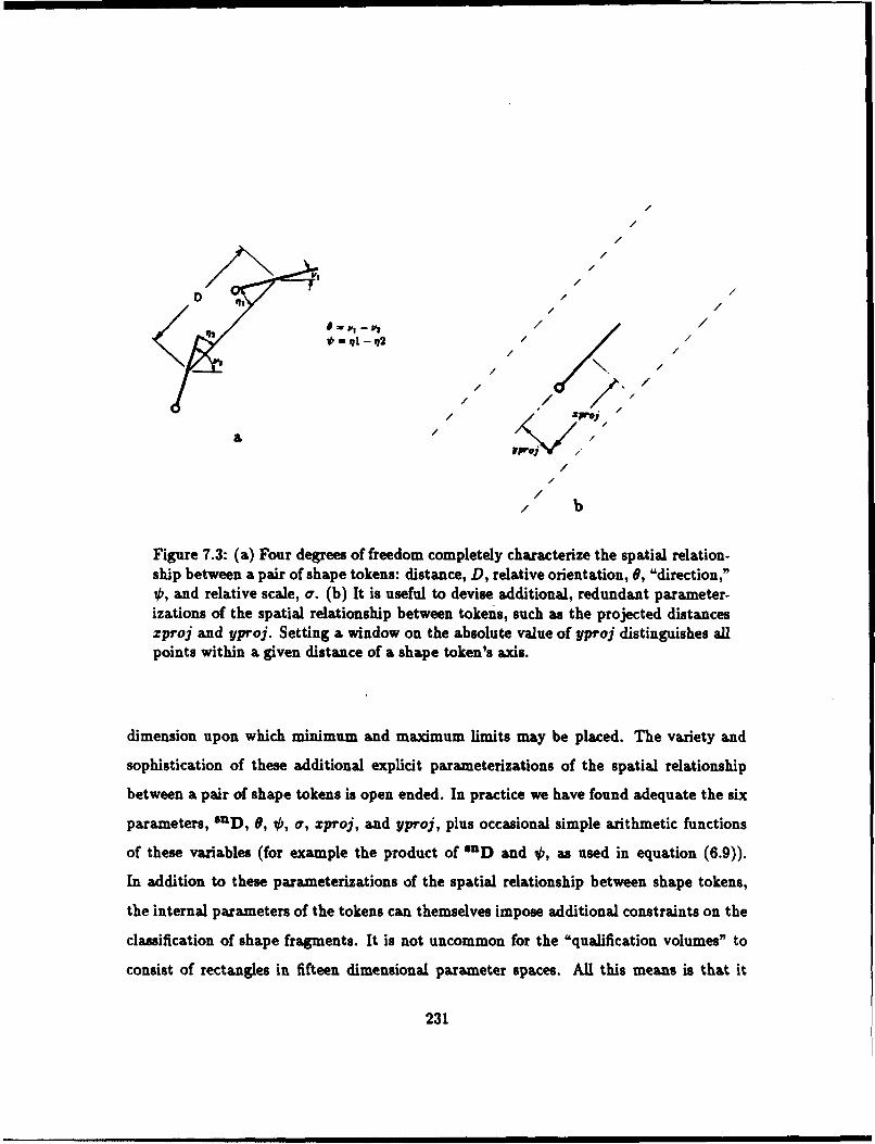
l~~ -V .92i

/

/

/U, /

/ /

/ /

/ /b./ /

/ /"/ 7Z /

a /

/

// b

Figure 7.3: (a) Four degrees of freedom completely characterize the spatial relation-ship between a pair of shape tokens: distance, D, relative orientation, 0, "direction,"0, and relative scale, o. (b) It is useful to devise additional, redundant parameter-izations of the spatial relationship between tokens, such as the projected distanceszproj and yproj. Setting a window on the absolute value of yproj distinguishes allpoints within a given distance of a shape token's axis.

dimension upon which minimum and maximum limits may be placed. The variety and

sophistication of these additional explicit parameterizations of the spatial relationship

between a pair of shape tokens is open ended. In practice we have found adequate the six

parameters, 54D, 0, 0, o, zproj, and yproj, plus occasional simple arithmetic functions

of these variables (for example the product of *nD and 0, as used in equation (6.9)).

In addition to these parameterizations of the spatial relationship between shape tokens,

the internal parameters of the tokens can themselves impose additional constraints on the

classification of shape fragments. It is not uncommon for the "qualification volumes" to

consist of rectangles in fifteen dimensional parameter spaces. All this means is that it

231

becnmes at times useful to establish rather circumscribed classes of spatial configurations.

A case in point is the class of configurations of corner pairs forming the base of a pro-

trusion. We define a class of configurations of FCORNER token pairs called the ALIGNING-

FCORNERS configuration. The qualification for membership in this class includes the

requirement that a pair of FCORNER. tokens falls within a prescribed volume in a 4 dimen-

sional parameter space. (See also [Jacobs, 1988]). Figure 7.4 illustrates how the collection

of parameters describing the spatial relationship between two FCORNER tokens plus their

internal parameters are used to define this volume so that an FCORNER pair is accepted as

a member of the ALIGNING-FCORNERS configuration class only if it does indeed represent

a shape fragment conforming to the base of a protrusion. In addition to spatial require-

ments on the FCORNER tokens themselves, requirements are imposed upon the spatial

relationships among the bounding sides of the fcorners. A symbolic shape token main-

tains pointers to the more primitive data that supported its assertion, and each FCtORNER

token maintains pointers to EXTENDED-EDGE type tokens representing its bounding sides.

In order for a pair of FCOR.NER tokens to be included under the ALIGNING-FCORNERS

classification, two of their sides must align with one another, and two of the sides must

be roughly parallel to one another, within some substantial tolerance.

Figure 7.5b presents all of the ALIGNING-FCOR.NER pairs found on a test fish shape.

When several protrusions occur next to one another along the same baseline, the ALIGNING-

FCORNERS grouping rules above will actually identify all pairs of aligning left-hand/right-

hand FCORN ELS, regardless of whether they belong to the same protrusion or not, as shown

in figure 7.5c. Therefore, for the purpose of locating protrusions corresponding to dorsal

fins on fish shapes, a processing step is added to exclude from the ALIGNING-FCORNERS

classification any FCORNER. pair jumping across another, narrower protrusion.

Once a collection of intermediate level tokens has been classified as belonging to a

given configuration class, it becomes useful to measure metric properties on aspects of

that configuration. The ALIGNING-FCORNERS shape fragment, for example, provides the

basis for a number of geometric assessments that are particularly useful for interpreting

232

qualified unqualified

///

//

Figure 7.4: A rectangular volume in parameter space distinguishes pairs of FCORNE&shape tokens qualifying for membership in the ALIGNING-FCORNERS configurationclass. A qualified pair lies within a certain window of relative orientation, 6, direc-tion, 0, normalized distance, D, and relative scale, a. In addition, the FCOLNERS'

internal parameters of taper, skew, and flare must each faill within a certain window,and the appropriate EXTENDED-EDGE tokens representing the rCOaNEnS' boundingsides must align with one another, as determined by their spatial configuration andinternal (edge curvature) parameters.

233

a

b

IL

C

Figure 7.5: (a) A test fish shape (Trout-Perches). (b) All ALIGNING-FCOILNERS

configurations identified on the Trout-Perches shape. (c) Spurious FCORNEL pairs

can occur when an FCORINER aligns with several other FCOILNERS. All but the

nearest aligned FCOILNER pairs are therefore excluded from the ALIGNING-FCORNERS

configuration class.

234

Figure 7.6: The ALIGNING-FCOftNERS configuration class gives rise to the high levelshape descriptor, LEADING-EDGE-ANGLE.

dorsal fin shapes. One of these, called LEADING-EDGE-ANGLE, is shown in figure 7.6.

LEADING-EDGE-ANGLE is a measure of the relative orientation of the two bounding sides

of the left-hand FCOiNER of an ALIGNING-FCORNER-PAIi, at their meeting point. With

this measurement we have the ingredients for a high level shape descriptor.

A high level shape descriptor consists of a pair of the following kind: (1) a configura-

tion class maintaining geometric qualifications on the spatial arrangement of a collection

of intermediate-level shape tokens (often a pair or triple), and (2) a scalar measue pa-

rameterizing some aspect of the spatial geometry of the shape fragment identified by the

intermediate level tokens.

Whereas the scalar measure occurs simply in terms of the descriptive parameters of in-

termediate level shape tokens, the configuration class establishes a framework determining

among which intermediate level tokens the measurement should be made. The ALIGNING-

FCORNEZ-PAK configuration effectively contains slots labeled, "left-hand FCOtNER" and

"right-hand FCOINER," and it is these labels that ensure that the edges forming the an-

gle measured do indeed belong to the leading edge and not, say, the trailing edge of the

protruding dorsal fin.

235

7.2 High Level Shape Description in the Dorsal Fin Domain

Our high level shape vocabulary for the dorsal fin domain consists of approximately thirty-

one scalar measures on the internal parameters of or spatial relationships among inter-

mediate level shape descriptors. Each of these measures is situated within the framework

provided by one of approximately nine spatial configuration classes. These classes of

spatial configurations of intermediate level shape descriptors, plus the scalar measures

completing the vocabulary, are presented in full in figure 7.7.

Each of the high level shape descriptors is specialized for naming a certain aspect of

spatial geometry important to distinguishing among dorsal fins. For example, because, as

many volunteers pointed out, dorsal fins can be differentiated by the degree of sharpness or

roundedness of the corners, a FIN-ROUNDEDNESS shape descriptor is provided measuring

this property by evaluating the flare of certain of the fins' constituent FCOR.NEIS and the

scale of PCI.EGIONS associated with these FCOINER.S. Or, because fins can be tall or squat,

it is useful to provide descriptors making explicit the vertex angle of the top corner (TOP-

CORN ER-VERTEX-ANGLE), and the relative height of this corner above the fin's baseline

(CON FIG-I1-H EIGHT- BASE-WIDTH-ILATIO).

Note that while the shape fragments identified by the nine configuration classes are

tailored for dorsal fins, these configurations are not found exclusively within dorsal fins. In

fact, the very shape fragments that collectively comprise a dorsal fin are each in themselves

so elementary that they are actually encountered all over a complete fish shape. Figure

7.8 illustrates this point. For several of the configuration classes contributing to the dorsal

fin shape vocabulary, the figure displays all instances of this spatial configuration found on

a test fish. Dorsal fins are distinguished from other structures on the fish shape because

it is only at the dorsal fin that the various component shape fragments all converge to

collectively give definition to a complete protrusion form. As with intermediate level shape

descriptors, and in complete contrast to building block approaches to shape representation,

high level shape descriptors spatially overlap one another as a matter of course, and they

regularly share support at the level of less abstract tokens. In these regards the style

236

Figure 7.7: The complete high level shape vocabulary of shape descriptors developedfor distinguishing dorsal fins. Nine configuration classes give rise to thirty-one scalarparameters. Each configuration class identifies a class of arrangements of intermedi-ate level shape tokens. Here, EXTENDED-EDGES are depicted as a single curved line,and FCORNESs are depicted as a pair of slightly curved lines meeting at a corner.For each configuration class, the "prototypical" or median configuration is pictured,with participating intermediate level tokens connected by a dashed line. Below eachconfiguration class is presented the set of high level descriptive parameters whichit spawns. The names of these high level descriptors are mostly self-explanatory,and for each an accompanying illustration indicates the spatial event(s) to whichit refers. In some cases, the descriptive parameter refers to an internal parametersuch as a curvature or skew of an intermediate level descriptor. Note that somedescriptive parameters are shared between configuration classes, that is, they makeuse of PCO.NER.S and EXTENDED-EDGES identified by more than one configuration-class, so require both to be present. Configuration class PARALLEL-SIDES spawnsno descriptive parameters itself, but participates in the definition of the CONFIG-Iconfiguration class. Configuration classes CONFIG-I and CONFIG-111 are built on topof the ALIGNING-FCORNE.S configuration class.

237

configuration-class: LECPE

LECPE-BACK-EDGE-ORIENTATIONA

LECPE-BACK-EDGE-CURVATURE

configuration-class PICLE

NOTCH-DEPTH-PICLE-WIDTH- RATIO(with NOTCHSTUFF)

CONFIG-11-HEIGHT-PICLE-WIDTH-RATIO

(with CONFIG-lI) 1

238

configuration-class: ALIGNING-FCORNERS

LEADING-EDGE- ANGLE

NOTCH-DEPTH-BASE-WIDTH-RATIO(with NOTCHSTUFF)

configuration-class: PARALLEL-SIDES

configuration-class: CONFIG-J(ALIGNING-FCORNERS Plus PARALLEL-SIDES)

PARALLEL-SIDES-RELATIVE-SCALE

PARALLEL-SIDES-NDISTANCE

PARALLEL-SJDES-SWEEPBACK-ANGLE1A

PARALLEL-SIDES-RELATIVE-ORIENTATIONJ

239

configuration-class: CONFIG-Il

CONFIG-II-TOP-CORNER-ROUNDEDNESS

CONFIG-II-VERTEX-PROJ -ONTO-BASE-PROPORTION

CONFIG-II-TOP-CORNER-VERTEX-ANGLE

CONFIG-Il-HEIGHT-BASE- WiTH-RATIO

CONFIG-II-TOP-CORNER-SKEW

CON FIG-1I-TOP-CORNER-BASE-DORIENTATION i~...

CONFIG-11-TOP-CORNER-FLARE

CONFIG-II-TOP-CORNER-ROUNDFLARE

alsoCO NFIG- I I-HEIG HT-PICLE-WIDTH- RATIO (with NOTCHSTUFF)LEADING-EDGE-REL- LENGTH 2 (with PECLE)

240

configuration-class: PECLE

LEADING-EDGE-CURVATURE

LEADING-EDGE-REL-LENGTH 1

LEADING-EDGE-REL-LENGTH2(with CONFIG-JI)

configuration-class: CONFIG-I

CONFIG-I-TOPAC-CURVATURE J \

CON FIG-111-TOPARC-ORIENTATION

CONFIG-UI-TOPARC-SIZE-DASE-WIDTH-RATIO

CONFIG-III-TOPARC-HEIGHT-BASE-WIDTH-RATIO

241

configuration-class: NOTCHSTUFF

NOTCH-F W-EDGE-CURVATURE

NOTCH-VERTEX-ANGLE

NOTCH-PI-VERTEX-ANGLE-SUM

NOTCH-PI- VERTEX-ANGLE-DIFFERENCE

NOTCH-SIZE

NOTCH-DEPTH- BASE-WIDTH-RATIO(with ALIGNING-FCORNERS)9

alsoNOTCH -DEPTH-PICLE-WIDTH-RATIO (with PICLE)

242

AL1O~ O~,co qzas ('~'PAPA R A L L S DEs

-ZCL CONFIG-11

PICLZLECPZ

Figure 7.8: Instances of six configuration classes identified on a test fish shape(Trout-Perches). These are shown individually for each configuration class, andtogether (upper right). The configuration classes overlap and share support atthe level Of EXTENDED-EDGES and FPCORNER.s. Each FPCOR.NER is depicted by ashape token plus arcs denoting its bounding sides. For the CON FIG-11 Configurationclass, a shape token denotes the imaginary line joining the ALIGNING- FCORN ERSparticipating in the shape fragment.

243

of shape representation we offer resembles the distributed representations of recent work

in ( onnectionist networks [Rumelhart et al., 1986; Hinton, 1986; Touretzky and Hinton,

1985].

The shape vocabulary of figure 7.7 was chosen completely "by hand," on the basis of

intuition. In other words, the decisions as to exactly what spatial relationships within a

dorsal fin's shape are sufficiently important to warrant devoting a high level shape de-

scriptor were made as a result of human observation and experience, not by any machine

learning program or other automated procedure. A methodology for going about this pro-

cess is not formalized. Roughly, however, it consisted in identifying collections of dorsal

fin shapes that appeared obviously similar or different in some regard, and analyzing the

geometric relationships among intermediate level shape fragments that contributed to the

similarities or differences in appearance. For example, the distinguished protruberant ap-

pearance of "fiaglike" fins led to the development of the high-level descriptors, CONFIG-II-

HIEIGHT-BASE-WIDTH- RATIO and CONFIG-II-TOP-CORNER-BASE-DORIENTATION. An im-

portant part of the task was simply to become thoroughly familiar with the spatial re-

lationships and geometrical regularities that structure the dorsal fin shape domain. The

contributions of human volunteers in the "arrange the shapes" task were helpful in iden-

tifying properties by which various collections of dorsal fins could be viewed as mutually.. ..........- + -k 4.4 &U-. h ......t~ wait,& ariea a dorsal' fin

vocabulary differing from the present one in at least some regards. Although it would be

nice to be able to bring formal tools or even an automatic machine learning program to

bear on the problem of distilling the structure inherent in a given shape world, the issues

are formidable and lie beyond the scope of this work.

244

7.3 Using The Vocabulary

7.3.1 High Level Descriptors and Feature Spaces

Because each high level shape descriptor makes explicit a scalar valued measurement on a

spatial relationship or geometric parameter, the set of vocabulary elements could be viewed

as a single huge "feature space." This view can be misleading, however, and caution must

be used before attempts are made to import computations conventionally carried out in

feature space representations.

Since each high level assertion adds one coordinate dimension to a hypothetical feature

space, the number of feature dimensions varies from fin to fin or from scene to scene. High

level shape descriptors employ a type/token relationship in the same way as primitive and

intermediate level shape descriptors. Although high level descriptors usually do not give

rise to new symbolic tokens placed into the Scale-Space Blackboard, a given high level

descriptor could still be asserted at several poses differing in location, orientation, and/or

scale; the pose information resides in the poses of the supporting intermediate level tokens.

Moreover, most high level descriptors do not apply to most dorsal fin shapes. In order

to achieve sensitivity to particular spatial relationships important to differentiated subsets

of dorsal fins, a high level shape descriptor typically sacrifices entirely any relevance to

the remaining fins. In fact, this is the purpose fulfilled by configuration classes which

identify specific narrowly defined arrangements of intermediate level tokens. For example,

as shown in figure 7.7, the coNwiG-m configuration class selects for a shape fragment

present on only those dorsal fins squat and rounded in shape. This fragment gives rise

to a whole host of high level scalar parameters, whose meanings can only be interpreted

with respect to this class of fins.

7.3.2 Naming Shape Subspaces and Categories

The space of dorsal fin shapes is not populated uniformly. Many human volunteers in the

"arrange the shapes" exercise discover subsets of dorsal fins that share similar properties,

245

that "look like" one another. These subsets emerge as subspaces and regions in a feature

space view of dorsal fin representation. The subspaces are collections of high level shape

descriptors, or feature dimensions, that all apply to a particular class of shapes. For

example, rounded fins all reside in a subspace consisting in part of the high level descriptors

generated under the CONFIG-I1 configuration class. Flaglike fins have no existence in this

subspace. Populated regions in feature space are locations in certain subspaces around

which the parameter values for a set of dorsal fins are found to cluster. Fins within such

a region look like one another in some regard: since a change in the value of a high level

shape descriptor reflects a deformation in some aspect of spatial geometry, fins that appear

similar in shape may be expected to differ little in many of the dimensions of deformation

along which they could vary.

As discussed in Chapter 2, valid shape categories can be established in a multitude

of ways depending upon the spatial properties chosen to define the categories. This is to

say, there is more than one way in which one dorsal fin can be said to look like another.

Depending upon the subspace of high level descriptive parameters examined, a set of fins

might all be considered similar in shape, or different. For example, in figure 7.9b, the

Mudminnows, Sleepers, and Killifishes2 dorsal fins cluster in one region of a subspace

evaluating the orientation and height of the back of a fin (CONFIG-III-TOPARC-HEIGHT-

BASE-WIDTH-RATIO and CON FIG-III-TOPARC-ORIENTATION), while they disperse from one

another and cluster with other fins in a subspace evaluating the relative orientation of the

leading and trailing edges and the vertex angle of the posterior notch (PARALLEL-SIDES-

RELATIVE-ORIENTATION and NOTCH-VERTEX-ANGLE).

Despite the fact that different valid clusterings of dorsal fins may be found, certain

groups or categories of dorsal fins tend to recur in volunteers' organizations of fins. In

our representation, these groups consist of fins that tend to lie in rather large common

subspaces (subspaces consisting of many high level descriptors) and share similar values

along several high level descriptor coordinate dimensions. For example, figure 7.9a presents

several two-dimensional slices of a five-dimensional subspace in which a certain group of

246

CONFIG- lI-TOP-CORNER- VERTEX-ANGLE

N

NOTCH-D EPTH-PICLE-WIDTH-RATIO

a

Figure 7.9: (a) Five two-dimensional slices of a five-dimensional subspace in whicha group of "flaglike" dorsal fins become segregated from the remaining fins. Flaglikefins protrude from the body in a way that is characterized by a top corner that isvery narrow in vertex angle and placed far rearward and high with respect to thebase, a nearly vertical back edge, and a relatively deep posterior notch. (b) Wide,squat fins (Mudminnows, Sleepers, and Kilifishes2) cluster in a subspace measuringthe curvature and relative height of the back edge, but disperse and form clusterswith other fins in a subspace examining notch vertex angle and relative orientationof leading and trailing edges.

247

LECPE-BACK-EDGE-ORIENTATION

CONFIG-11-HEIGHT-PICLE-WIDTH-RATIO

CONFJGz~-I-TOP-CORNER-BASE-DORENTATION

NOTCH-DEPTH-PICLE-WEDTH-RATIO

248

CONFI- HIHT-PICLE-WIDTII-RATIO

CONFIG-11-TOP-CORNER-VERTEX-ANGLE

CONFIG-U-TOP-CORNER-VERTEX-ANGLE

LECPE-DACK-EDGE-ORIENTATION

249

CONFIG-111-TOPARC-HEIGHT-BASE-WIDTH-RATIO

CONFIG-III-TOPARC-ORIENTATION

NOTCH-VERTEX-ANGLE

PARALLEL-SIDES-RELATIVE-ORIENTATION

250

dorsal fins tends to cluster or become segregated from the remaining shapes. This group of

fins is one that many human volunteers called, "fiaglike." As an exercise of our high level

shape vocabulary for dorsal fins, we have fabricated criteria for classifying the corpus of

test dorsal fin shapes according to six prominent categories.3 These categories are shown

in figure 7.10, and are seen to correspond with groupings generated by human volunteers

presented in Chapter 2 (most of the categories are actually named after labels given to

their shape types by volunteers).

A dorsal fin's membership in a given category is decided by virtue of its high level

parameter values in relation to those establishing the category. Our classification mech-

anism computes a cost, IC, (called the Category Incompatibility Cost) that accumulates

according to incompatibilities in high level parameters, according to the following rule:

IC(F) = E I min(pco,tmx, wppe.ro,) if p E PF (7.1)PE Plackin otherwise

P - Ps if P > Anas

Peor= f- Pmin - P if p < Pnin

0 otherwise,

where Pc is the set of high level parameters comprising the category feature subspace,

P. is the set of high level parameters computable for fin F, Pco.st.x, Packing, Pn.,, and

Pmin are constants associated with parameter p for this category, and wp is a weighting

factor discussed below. The rule for computing Category Incompatibility Cost given by

this expression can be summarized as follows: The category is defined as a rectangle in

a subspace, Pc, whose coordinate dimensions are high level descriptive parameters; an

ideally qualified dorsal fin falls within some minimum and maximum limits, Pron and

p,,., along each of the dimensions of this subspace. When a novel shape is viewed, its

description is computed in terms of the high level parameters. For each parameter in

Pc, some cost is incurred if the novel shape possesses a value of this parameter falling3 For convenience we refer to these as basic categories of the fin domain. This nomenclature is

unrelated to the "basic level categories" of the Cognitive Science literature.

251

CATEGOY-OWO I CIK

. *3. -- 3e--~.5.. 1.316

1.512 2.Y126 - 2. 232 2.34

CATEGMA-FLRO.1KE

__-/2

Figure 7.10: Six prominent categories (we call, "basic categories") of dorsal fins.A number below each fin within the category gives the Category IncompatibilityCost. Higher cost indicates that the fin lies on the outskirts of the volume definingthe category in the parameter space of high level shape descriptors. Fins in thetest set excluded from the category (because their Category Incompatibility Costlies above a preset threshold) are shown reduced in size below the included fins.These categories will be seen as corresponding to many of the groupings identifiedby human volunteers in the "arrange the shapes" task of Chapter 2.

252

CRTEGORY-UMTCED

CASMTIMMMCE

.9m1 .9627 .3626 .3651 .4912

253

CRTEG-EQ Ufl!E.MI9 G

e~~~g. S..19'm .

e~g S. . ~ g gg254

outside the ideal window. In addition, some (usually greater) cost, Placking, is incurred if

the dorsal fin under evaluation lacks a value of this high level parameter altogether (that

is, that the fin does not qualify under the configuration class required for measuring that

high level parameter).

Under this scheme, membership in a category is a graded value. Degree of category

membership may be interpreted in terms of Category Incompatibility Cost. Furthermore,

because the high level parameters correspond to deformations tuned specifically for dorsal

fin domain, it is possible not only to assess degree of category membership, but also to

ascertain, in some meaningful geometrical sense, the way in which a viewed dorsal fin

shape fails to fall under any given category's qualifications (see [Smith and Medin, 1981]).

This is illustrated in figure 7.11. Here a number of fins are evaluated with respect to

two of the basic fin categories. The sources of Incompatibility Cost are listed; these are

the descriptive parameters whose values fall outside the category's limits, and they reflect

the inappropriateness of one or another geometrical feature comprising the shape of the

excluded fin.

Some of the six dorsal fin categories overlap. That is, they include some dorsal fins in

common. This is the case, for example, for the EQUILATEHAL-TRIANGLE and TRIANGU LAB.-

NOTCHED fin categories. Human volunteers included many of the same dorsal fins into

either of these categories.

7.3.3 Descriptive Perspectives

Subspaces of high level shape descriptors are a way of formalizing the notion of descriptive

perspective introduced in Chapter 2. A descriptive perspective is a subset of features

or properties with regard to which shape is evaluated or interpreted. The high level

descriptive vocabulary we have presented for the dorsal fin domain constitutes a rich

and appropriate resource from which to construct descriptive perspectives. The six shape

categories discussed above are examples of descriptive perspectives at work. Each category

attends to some significant subset of properties made explicit by the vocabulary, and

255

(corout-c leat ie -cobt-ar-no opql-fleel ikos * cavafiglhe@)cllwiI--MEIGHT -31-iI IT*4ffl10 value on1 coat 1.39LEU'I-I=EDNECWWRE value .62 ost .696Cvous-u1-Cp-CaS3-ME-11aENlAI value -1.6 Cost .452COWIG-I-TaP-CamER-WTEW-01HOE value -1.? 1coat .419LEK-K43-6E-NI4AT ION value -.69 Cast .66MCa0exe-UI-EICr-CLI-IDN6TIO value 1. 2 cat 0.2PICLE-,fl6op-coS6U-yW3TEN-FtlGL value 1., meat M63

LEDIS-264L.3N2value 1.54 cat .065riOTC*.D6PTH-PICLI-IGDIN-W610 value .449 coat 3.6Co~ir-I-YEVTEJ-POTO-M-POPTION value 49.6 coat 6.6NorC"-I-V(RrE-GE-6l value 1.2 cost 3.93.221611?

Ccoaut-claaaltlcaton-coat-fot".m soql-flael ikes *mnlts)cawe--aTrE-Poj-oTo-noa-3wlO value 40.3 cat 2.1COWIG- I -IGT -U-MITH4itZo value .35M cost 1.2HOT CH- KPT-"I CLE -WI OT -RAT 10 value .152 coat 1.19CaWIS-1-TOP-CSIER-36-63IETAUON" value -1.6 coat .542LERDM-EM-M-1LE110112 value 1.21 cost 6.29C0WeG-UI-WZ160-fICL-U1D71441X0 value 1.699 coat .312CaPIzS-11- TOP-COIEU-vET EK-66ILE value -1.9 Cat .192LECPI-GACI-EDGE-OEIENIATION value -1. 1 coat . 14?PICLE-PflTEIO-CONlE-YITEN-iN6LE value 1.15 coat 3.6LECK-OAX-DEM-CJWTU*6 value 6.3 coat 6.8J1TCH-#z-WE3?s**GLE-S4l1 value 1.16 coat 6.67. 276M6

(conputa-clI amit lest t on-coat-Var-a. opql-f el ikes 'aonchovies)CWXS-I-ETEN-6OJ-HTO-3m6(-1PROMG value -. 15 cat 4.6COWIGQ1-I H14-ti-illf1N4TIO value 3.43 coat 2.6nOTCH-IIPT"-fCLE-uflT4NIO value .112 coat 1.51COMFIQ1-U-TOP-COER-O-1IENTRION Value -1.A coat 1.3?CONUIG-It-TOP-CCE301-MfTSI-ffiL value -1.3 Daft .154CCSUIG-11-HEIGHT -PICLE-IIDTN-OAhI10 value . 751 coat .642LECPI-SAC-EMNOIE1711TII value -. 6V coat .534LEADING-EDGI-RL-LEGTM2 value 1.14 cat 6.44110TCH-fl-ENE-OILE-4N1 value .?Is coat .23PICLE-MISENIO-00I EE-YRIE-0GLE value 1.13 coat 6.69LECI-6CK-EME-CNWTU*! value -. 61 coat 6.612. 255653

Ccoputa-cl satleeict ioii-cost-for-me tpal -boomiatick* 'opwnatlihaa)CmVIS-tiI-T fl-IE-A64UIDTHN4NTIO value 2.59 cost 1.9COHFI6-III-1 in-CWUflTURE value .964 coat .384P63fiLLEL-SI3ES-I6R1IV-1ETfTION value .425 cot.025LECK-M-I-(-CUmVATUMI value .914 cot .6LEC1-K-1M G6-0CIENINTICN value -. 68 soft 6.03APftLEL-6IS-I3S~IC value 16.3 coat 3.6P66NLLIL-GI3IS-fMIV-CFLE Value 3.9y coat 3.3

NOTN-IN-61UIDW-10value .90 .coa 3.6COWC-111-TOPC-0hIE11RIN value -2.2 cot 0.01.3591274

(ccouto-0~ cal fleet lon-cost-for-no Pl1 -broonstttake pitt.'s)CWIB-1i'C-66-IETATION value NIL st 1.9COIC-11-TPMC-CUWJAIIK value NIL coat 1.6LIEI-C-f NI6-CWAfTUK Vvu 6.6 coat 6.6

LECI-C-4II-OIENATIIVvalue -1.2 sot An3PLEL61flHUSTCEvalue 6."? ast .616

PftILLL-SIIES-MlRtIVE-CRIEWIIAIW value .212 eat 3.69Pm.LIL-IKuS-MA6 TIVE-6CAE value 4.54 cat I.6IPOTCH-DEPT14-311-HIDTN46Ill value 1.64 ost 9.9USVI-1Ut-rOPm-61f--113U-36zo value MIL coat 0.04.8436M

(coaA-cl cal fleat ion-cast-tor-,. apql bfoomaticks 'threshe-sharks)LECKA-11-(NEnaMMU value -. 82 coat 4.0MICH-flWT*-6fS-UI3IN-M 10O value NIL coat 1.6C2PIS-11-TOPC-NIETATIOH value NIL cat 1.3owUie-UI-toplau-CUNTlflI value NIL coat 1.6

LECP-WC-t=-IEll1TtON value -1.2 -oab .5112P4NLEL-1111184ILNUElW- IENUOM value NI11 coat 6.6

P66ftLEL-616-IUUSTA value NIL cat 0.0P66..LEL- SN-MERI I-CJ value NIL cat 6. 9cowiG-i-III-lWc-s-6I2u6-I2TINTIo value NIL cot .8?.5"1945

Figure 7.11: Computer output of the evaluation of several shapes with respect tothe "flaglike" and "broomstick" dorsal fin shape categories. The components of thehigh level descriptive subspace in which each category is defined are listed in orderof their contribution to Category Incompatibility Cost. For example, the Cavefishesdorsal fin takes a value of .878 on the descriptive parameter, CON FIG-I1-H EIGHT-BASE-WIDTH- RATIO, and this falls outside of the allowable window for the "fiaglike"category such that this contributes a Category Incompatibility Cost of 1.09. Thetotal Category Incompatibility Cost for Cavefishes with respect to the "fiaglike"category is 3.32. 256

ignores others.

The concept of descriptive perspective is useful not only for evaluating shapes in terms

of category membership, but also for considering families of shapes related by geomet-

ric deformation. Several volunteers organized dorsal fin shapes according to continuous

properties, such as relative size of the notch or degree of sweepback. By selecting appro-

priate high level descriptors, descriptive perspectives can be built that reflect these ways

of structuring an interpretation of the dorsal fin shape domain. Figure 7.12 illustrates.

Instead of a descriptive perspective consisting simply of a subset of shape descrip-

tors, the construct can be elaborated by allowing different degrees of emphasis on one or

another component dimension. This is accomplished by assigning a weighting factor to

each contributing high level parameter. The technique is especially useful for purposes

of defining shape categories, as it adds flexibility in tailoring the contours of a category's

boundaries. The terms, wp, in equation (7.1) indicate how this device is used in computing

membership in the basic shape categories as discussed above.

By adjusting the relative weights of the component parameter dimensions of descrip-

tive perspectives, assessments of similarity and differences between shapes can be cast

in different ways, yielding a diversity of similarity metrics analagous those displayed by

human volunteers on the "arrange the shapes" task. For example, the question posed in

figure 2.15 and again in figure 7.13 is: To which fin is the Mooneyes dorsal fin more sim-

ilar? Because the Mooneyes fin is more similar to the Silversides fin in one regard (corner

roundedness) and more similar to the Trout-Perches fin in another regard (aspect ratio),

the answer to this question is indeterminate at this stage of perceptual interpretation.

However, the tools provided for choosing among descriptive perspectives offer elements

of a language with which the perceptual system may communicate with other stages of

a perceptual/cognitive system. We can effectively make available a "knob" adjusting the

relative significance accorded the various aspects by which these dorsal fins may be con-

sidered similar or different. This knob asks, "which aspect of shape do you care more

about," and its "meaning" maps though the dorsal fin descriptive vocabulary directly to

257

CONFIG-II-TOP-CORNER-BASE-DORIENTATION

LECPE-BACK-EDGE-ORIENTATION

a

Figure 7.12: Three subspaces reflecting descriptive perspectives along which inter-esting continuously varying shape properties become apparent. In (a), (b), and(c), the principle axis may be said to roughly correspond to "sweepback angle,""hardness" or "roundedness," and "tip rearward angle," respectively.

258

CONFIG-lI- TOP-CORNER-FLARE

CONFIG-II-TOP-CORNER-ROUNDFLARE

7.12b

L EC P E- BACK- EDGE-CURVATURE "

CON FIG- II-TOP-CORNER-SKEW

7.12c

259

Figure 7.13: Computer output assessing the similarity of the Trout-Perches andSilversides dorsal fins to the Mooneyes dorsal fin under two different descriptiveperspectives. This figure illustrates the representation's ability to interpret shapesimilarity according to differing criteria, in a manner analagous to that observedin the performance of human volunteers on the "arrange the shapes" task. Thetwo drawn pictures show in each case the three fins in order of increasing ShapeDissimilarity Cost to the Mooneyes dorsal fin. The leftmost fin drawn is alwaysthe Mooneyes fin because its dissimilarity to itself is zero. Under the drawings, areshown a decomposition of the Shape Dissimilarity Cost for the Trout-Perches andSilversides fins with respect to the Mooneyes fin, in terms of component high levelshape descriptors. The two different descriptive perspectives weight these compo-nents differently. For example, the difference in LECPE-BACK-EDGE-ORIENTATIONbetween the Mooneyes and Trout-Perches dorsal fins is 0.191. Under the descrip-tive perspective operating in the top half of the figure, this contributes a ShapeDissimilarity Cost of 2.86, but under the descriptive perspective operating in thebottom half of the figure, this contributes a Shape Dissimilarity Cost of only 1.91.The top descriptive perspective places emphasis on a fin's aspect ratio, while thebottom descriptive perspective places emphasis on the curvatures of a fin's edgesand roundedness of its corners.

260

(UZUPL9-SZZLE-U~u3iEININ166aY OnS. (list FAmmAM trout-gwohms 54 lwsrsidssO laq1-ta1nilaw-wotchd-ob

(~W67U6-m6S-ZIUK 4-~6IUEY*pq-tpian*#lor-uistoh*i-d*2$ vionwm tr-out-parch"o)

LEN~gm-IE-mgm. srr. cost -5. 1LwI6m~E3-4.m~7Ig sor .191 post 2.6

COWI--TOP-COMUR-F arw--p cot -2.69LEcP-K-UAmTUM epwgm post 2.46CSUG11--WEDI-e66-MIo-6- 6aU1 wt w4.-- a co st. 2.5CeUIa-IZ-TU-Camm-6-IwvmIffIaKO auwor.2U 0ost 2.36CUI-ZI-TP-CIR-NM orror.64S cost 2.23NOTCi-WERIE-01". wror-.21 cost -2.1LIUISU-636-M-LUSIIU wr- .17 cost -1.7UOTO-Fl-EMUMfVE maro-.1 owt -1.4COWK-EIN-I-UI~I wi-w.69 cost 1. 41104O-KPTH-U6-w631-IhI s- owi .12 aost 1.2

CI-1-MOzueICL-13TIO-MIO -. 75 LEN3INS4IU-ClIMU~N& .579 COUIS-11TOP-C0U*WRYTI-U: - .36MOTCN-mPN-.PICLE-ITH-ffITIO .2

36.71617(cUFM-es6smE-41v4Iin~Wl~nY sq]-twimieru-wotihd-oU aconso i l versides)

CinUI6-1-TaP-COME-YEVEN-06LE aw-or.m1 cost 11.9CCFIBUIImffU-IT-UIO -or-IS ost -5.7PLEWEPO-CEK-MNENTAIC mrwo.86 coat 1.41COMF G-11-MO-FImA-aWIOMnO wvw-.25 pent -3.6LEMI-UIK-US.E arovr-.25 cost -1.1NOTcN-Ci-06E-NdAUh ai-or-Un ost -2.9

ISICN-UP-61-u1T-WUOv -. 92 LERSIN-E36-M-LW~sI -.66 CSUIU-11-WTE-POJ-MtO-M-PNoMohyza .746CmfOs-I-TP-CE6M6-MzENTNTIaN: .646 LUMP-M-EM6-CUMUs .571 NOTCH-WIEN-OiULEs .367CIUI-1-T-inMMV-fLM -6.1 LSMIN6-M3-CUVATUf .129 #STCN-OE"W-PZCL-W2ITN-WTIOs -. 04

(DZSPM-SZNILIM-SNUPEIS-sTuIN-aMeIM moonsyes (list nosiso trout-pocles .4luesdes) sqi -tI-iangul o-vwtchdm)

0.4 27. 4 26.61NIL(CoswI-SS63U1'i--SVwS P1-trawle-notches uow~ trout-porchas)

COWIG-11-TOP-CWAM6-FLK arror-U1 ost -6.9LM-O-K-UW49TU orwo.662 Dost 6.15

LEN6,S-EUE-mLE wor4.5 oot -1.6~UI-U-flPCm3S~aroer.641 cost 4.47

COWII-11-WRIIN-9IS-ONTO-6A6-UPUIC arrw6.4P pst 2.UCOuIS-1-TP-CMU3-mS-NU61Enlmt~ wrw.28 ot 2.36N0704-IERVI-vw wi-or- .21 oust -2.1LECP-WCK-El-WMETATIaN orror.19t ost 1.91L1R61-fv4 tE-L-LBIS@2 wrw-r.7 pst -1.7Laill"6INU-CUMM1 ar-or.214 post 1.41ITO1C-f"Ih-CsMATIS wror-.1 amst -1.4

Sl~-1U94-N61iiIIN-1IOwi-4.12 cot 1.2

CmUIS-1Z1-M-Wft-WI3T-WIOs .964 CfI6-1~~1-9ICLE-MIT1WI -4.5 WNC-3lPTH-PICLE§aI31-W1Ot 0.26COI-1-TOMMIU-ME~hN-ULE -. 19

38.0694(Cm -l-Tw-SIS-8I uiO-muiinS *ppi -trangulw-r~osoww FMosY o1ilvosifts)

COmWIs-rp-camFI-ME-ngmI si-ow-U cost S. soCuUI-IINIIff-E-IIUT-6R~a row-.26 Gost -3.6L~cP4Pm~SI4Iini~~an w-iw.61 sost I.61

,'ia.-w-su-aNMi W-r-.6 ost -2.3LIN6II-EmUUA aw-r-25 cost -2.5CSOII1-I -fI-PIO.-iDIN-6R s-r-.U5 sot -2.!

LECKOw-m-Cumumw-r.614 oune 1.43

NOTO-UV-gU-WX311-TIOv -. 92 LIRBIZI-4-LDGTNI, -. 86 COUIS-TOP-Ca62-FLMI. -.76cafu--a~x71.-a1~i-uaouu~ .746 cmi-u;P-ma-iinmunm1mm.66N IO4 EI-00" .367

LEI3U-I6-CUMM1W, .M2 HOTCM-WTN-P1O.E-Ui31*6NT10s -. 84 CUI-1-TO-COME3-NKEa .61!27.361676

261

the geometries of dorsal fins' shapes.

The technique of adjusting the relative weightings of component feature dimensions

serves ? related purpose in a shape recognition task. Suppose we are shown a novel dorsal

fin and are asked to decide what kind of fin it is (what fish it is from). Within the current

framework, we recast this question as follows: To which known type of fin is the viewed fin

most similar? In comparing high level shape descriptions, we employ a strategy similar to

that used in classifying dorsal fins according to the six basic categories. Two fins' Shape

Dissimilarity Cost, R, is accrued based on the fins' relative measures along a subset of

component high level feature dimensions:

R(F 1,F 2) _ wpevor if p E PF A p E PF (7.2)PEP IPlacking otherwise,

where Pc is the set of high level parameters comprising a category feature subspace, PF1

and PF2 are the high level descriptors computed for the two fins, respectively, Plackin is

a constant associated with parameter p for ,he category containing the two fins, and wp

is the weighting factor for parameter p. See [Tversky, 1977] and [Krumhansl, 1978] for

related approaches to interpreting perceptual/cognitive similarity.

In carrying out shape recognition under this scheme, the basic categories come into

play in two important ways. First, a novel fin is initially classified according to the basic

categories. This serves as a pruning step limiting the set of known dorsal fins against

which it need be comp4-ed. The Shape Dissimilarity Cost between the novel fin and

known fins is only computed for known fins sufficiently similar to the novel fin as to

fall within the same basic category. Second, the Discimilarity Cost computation can be

tailored individually for each basic fin category. The Shape Dissimilarity Cost employs a

descriptive perspective consisting of a set of high level shape descriptors, plus a weighting

of each of these descriptive parameters. Many times a given high level descriptor will play

relatively greater significance to fins' identities within one category than within others.

For example, the NOTCH-VERTEX-ANGLE parameter is useful in distinguishing among fins

in the Flaglike shape category, but is of no value in the Equilateral-Triangle category which

262

evaluates dorsal fins in terms of their properties viewed as triangles, regardless of whether

they possess a posterior notch or not. Thus this parameter is given a relatively large weight

in computing Shape Dissimilarity Cost among Flaglike dorsal fins, but negligible weight in

comparing Equilateral-Triangle dorsal fins. In other words, the equipment provided makes

it possible for a shape descriptor to assume greater or lesser significance, as appropriate,

as one travels through the space of dorsal fin shapes.

As with evaluation of a fin's Category Incompatibility Cost, the Shape Dissimilarity

Cost not only offers an assertion of the degree to which two dorsal fin shapes are similar,

but it can also be decomposed according to the spatial properties by which two fins differ

in shape, and this is reflected in figure 7.13. Figures 7.14 further illustrates the role

of shape comparison in dorsal fin recognition. In figure 7.14, fins are arranged in order

of dissimilarity to the target fin. With suitable normalization, a novel fin may be said

to be "recognized" by the known fin to which the Shape Dissimilarity Cost is least (and

perhaps as long as it falls below a certain threshold). The reasons why a target fin may or

may not be recognized as a given known fin are directly available because the descriptive

components of Shape Dissimilarity Cost declare the ways in which two shapes differ in

geometry.

7.3.4 The Det .-mations by which Shapes are Related

Because our specialized dorsal fin shape vocabulary makes explicit classes of spatial con-

figurations reflecting spatial deformations common to the dorsal fin world, the vocabulary

is well-suited for describing the ways in which one dorsal fin must be deformed in order

to make it more similar to another. As shown in 7.13 the comparison of two dorsal fins

is delivered in terms of a subset of high level shape descriptors meaningful to compute

for both fins. For each such descriptor, the difference in its scalar parameter measure

indicates how a particular aspect of dorsal fin geometry differs between the two fins.

Since high level shape descriptors refer directly to internal parameters of, and spa-

tial relations among, intermediate level shape tokens, in many cases it becomes a fairly

263

target: Lizardfishes category: unnotched

9.4 7.289 12.62 15.12 15.11

18.1 19.25 2 7.61 29.44 33.N6

target: Thresher-Sharks category: unnotched

0.S 18.4 19.1 23. 4? 2.6 20.36

A 29.39 34.6 3491 " 42.54.3

Figure 7.14: Shape Recognition in the dorsal domain. Within the context providedby the high level shape vocabulary, the principle computation in the task of shaperecognition is an assessment of the Shape Dissimilarity Cost between known fins andan unknown target fin. In a two step process, a target fin is first classified accordingto the basic dorsal fin categories, then its Shape Dissimilarity Cost is computed withrespect to known members of the category (or categories) to which it belongs. Thisfigure presents rankings of dorsal fins by similarity to target fins. In each instance,the target fin is shown at the upper left. Its Shape Dissimilarity Cost with respectto itself is 0. The other members of its category are displayed in order of increasingShape Dissimilarity Cost. For each category, a descriptive perspective was used thatwas judged to balance the various component high level shape descriptors more orless equally. Because different numbers of component high ievel shape descriptorsenter into the Shape Dissimilarity calculation for different shape categories, thevalues of Shape Dissimilarity Cost can be compared only within a category, butnot between categories. This figure illustrates that the dorsal fin shape vocabularysupports assessments of similarity among these shapes that might be consideredsubjectively agreeable to human observers. In other words, the description of aknown dorsal fin generalizes well under the shape variations that occur within thedorsal fin domain.

264

target: Anchovies category: triangular-notched

16.9is 22.6 21 . .99

32.2? 37.17 9. 39.1 39.3 42.20

16 " 45.11 49.9? 95.%1

target: Trout-Perches category: triangular-notched

2. 24.64 34.12

34.92 38.29 36. 5 4. 45.9

52.56 U. 62.65

target: Mullets category: triangular-notched

~" ~22.65 28.42 36.96 31.5? 34.51

35.9 399293 9.53 44.6? 46.9

target: Sea-catfishes category: flaglike

.9. . 42.3 .62.31

265

target: Mudminnows category: rounded

622.52

target: Kilifishesl category: rounded

target: Gars category: rounded

14. ~44.3 62 -/.

target: Gars category: broomstick

. ............

266

a

Anchovies Trout-Perches

/

Puffers Cavefishes

Porcupinefishes Puffers

d

Mullets Carps-and-Minnows

Figure 7.15: The comparison of two dorsal fins can be decomposed to make explicitvarious aspects of geometry by which the fins are found to differ in shape. Thesemay be understood directly in terms of the deformations that would be required totransform one fin into the other. Here, for a number of dorsal fin pairs, on the basis ofthe high level shape descriptions a computer program automatically generated arcs,lines, and arrows displaying a few aspects of deformation that are easily visualized.For example, in (a) these markers show that to transform a Trout-Perches fin intoan Anchovies fin, the top corner would be moved downward and to the right, thetop corner vertex angle would be expanded, the curvatures of the leading edge andback edge would be reduced, the leading edge angle would be reduced, the back edgewould be rotated to a more horizontal orientation, and the posterior corner (abovethe notch) would be expanded.

267

straightforward matter to diagrammatically display the spatial deformations to which they

correspond. Figure 7.15 presents a number of pairs of dorsal fir shapes, along with arcs,

lines, and arrows showing the deformations relating the two shapes. For example, the

parameter, LECPE-BACK-EDGE-CURVATURE of the Trout-Perches dorsal fin is greater than

the value of this parameter for the Anchovies dorsal fin. To illustrate the "bend" required

to straighten out the Trout-Perches back edge, an arrow is drawn next to the location

of the back edge's EXTENDED-EDGE token, pointing in the direction of the bend, and

with a size proportional to the requisite degree of bend. Similarly, the two descriptors,

CON FIG-II-VERTEX-PROJ-ONTO-BASE-PROPORTION and CON FIG-II-H EIGHT-BASE-WIDTH-

RATIO, collectively indicate that the top corner of the Trout-Perches dorsal fin is relatively

higher, and more forward with respect to the base than is the top corner of the Anchovies

fin. The amounts of these relative displacements determine the vertical and horizontal

components, respectively, of an arrow showing how the top corner of one fin would have

to be displaced in order to put it in the same relative location as it occurs on the other

fin.

In a restricted sense, this exercise of our shape vocabulary amounts to a form of shape

comparison by analogy. The problem of reasoning by analogy decomposes into two parts:

(1) identify mappings between "corresponding parts" of different situations (2) describe

similarities and differences in terms of properties and relations of those parts [Winston,

1980; Gentner, 19831. In the case of our world of fish dorsal fins, the problem of finding

corresponding parts-top corner, back edge, posterior notch, etc.-between pairs of shapes

is greatly simplified by the fact that all dorsal fins share a similar basic form. Our shape

vocabulary is attuned to this basic form so that corresponding parts on two fins will be

named by the same type of high level descriptor, e.g. CONFIG-II-TOP-CORNER-VERTEX-

ANGLE (see figure 7.7). The problem of identifying corresponding parts between two fins

therefore amounts to one of identifying abstract level vocabulary elements appearing in the

descriptions of both fins. Similarities and differences among analogous parts are described

in terms of the values of the scalar parameters belonging to these descriptors.

268

The geometric properties and spatial relations that may be used to describe and com-

pare shapes is limited to the set of shape descriptors supplied by our vocabulary. The

shape recognition and shape comparison tasks highlight the significance in the fact that

our high level shape vocabulary is not arbitrary, but is tuned to the dorsal fin domain.

A collection of 31 arbitrarily chosen measures, for example Walsh transform components

or some sort of hashing of the chain coded bounding contour [Freeman, 19741, might be

able to differentiate one dorsal fin instance from another, but would have no descriptive

basis for generalizing classes of shapes defined in terms of important structural properties

common to dorsal fins, nor for delivering comparisons of dorsal fin shapes in terms readily

identifiable as salient aspects of these shapes' geometries.

The representation is designed to be easily extensible as useful new constraints or

regularities are encountered. An important goal for future research is to expand the

vocabulary to new domains, so that shape comparison and other forms of Later Visual

reasoning might take place among very different shapes as well as within circumscribed

classes such as fish dorsal fins. In addition, a general purpose shape representation would

likely be able to generate new descriptors "on the fly," as important similarities among

shapes are encountered and analogous spatial configurations are noticed.

7.4 Summary

This chapter has shown how it is possible to build a vocabulary of shape descriptors re-

flecting the geometrical regularities and spatial relationships important to a specific shape

domain. The vocabulary elements sometimes denote abstract properties of shape such as

ratios of sizes and sums of curvatures, yet, they are strongly grounded in two-dimensional

spatial configuration. Because high level shape descriptors arise from groupings of inter-

mediate level shape tokens based on their spatial arrangements in the Scale-Space Black-

board, it is possible to construct descriptors sensitive to very subtle aspects of spatial

geometry that may be inherent to limited classes of shapes.

The character of this vocabulary differs markedly from that of generalized cylinders

269

or other building block approaches to shape representation. Instead of attempting to

approximate the shape of an entire part with a single parameterized model, our shape

descriptors each name a limited slape fragment, for example a pair of corners whose sides

align in a certain way across the base of a protrusion. The fragments named overlap one

another and share support extensively at the level of primitive edges and regions. The

resulting description of a shape is purposefully redundant because this makes it rich: a

great man; spatial properties are named explicitly and are therefore made immediately

available for later stages of computation.

We have shown how this vocabulary can be used in defining categories of similar shapes

based not only on the values of measured properties, but also on whether or not a viewed

shape may be interpreted as even possessing a property at all. The representational tools

offer flexibility in interpreting shape information with respect to a variety of descriptive

perspectives, or subspaces of the complete descriptive vocabulary. This flexibility accords

with the diversity of interpretations of shape similarity observed in human performance.

By manipulating the relative significance accorded different properties, shapes may be

assigned measures of similarity to one another according to criteria specified outside the

immediate perceptual system. Although we have demonstrated these capabilities through

implementation of simple shape recognition and shape comparison tasks, we view the

specific algorithms presented as less significant than the more fundamental ideas about

the role of knowledge in shape representation-in the form of the vocabulary of shape

descriptors-that they are intended to support.

270

Chapter 8

Conclusion

8.1 W~hat Has Been Accomplished?

This work has explored an approach to visual shape representation intended to support the

flexible task requirements of Later Visual processing. In the context of two-dimensional

shape, we have presented an alternative to the building block model for shape representa-

tion, and have demonstrated how a large, extensible, domain-specific vocabulary of shape

descriptors may be used to perform flexible shape comparison and shape recognition based

on subtle differences in object geometry. Along the way, we have extended and developed

a number of computational deVices:

" We have brought a scale dimension to Marr's [1976] Primal Sketch in the form of

the Scale-Space Blackboard.

" We have demonstrated rules for grouping shape tokens in order to build shape de-

scriptions at multiple scales and at multiple levels of abstraction.

" Through the example of the dorsal fins of fishes, we have illuminated the ways in

which classes of naturally occurring shapes can be viewed as related by deformation

of their geometric features. We have adopted the tool of dimensionality-reduction in

order to explicitly name important classes of deformation over spatial arrangements

of shape tokens.

" We have shown how energy minimization techniques can be incorporated in order

for shape descriptors to communicate with one another, through dimensionality-

reducers, about geometric constraints on objects' sha-es.

" We have presented an example descriptive vocabulary and demonstrated its utility

for distinguishing one class of natural shapes-that of fish dorsal fins. The vocabu-

271

lary is easily extensible to other shape domains.

* We have formalized the notion of descriptive perspective in terms of the domain

specific shape vocabulary. Through selection and weighting of the parameters de-

scribing shapes at an abstract level, different aspects of spatial geometries can be

emphasized in evaluating and comparing objects' shapes.

All of these tools have been implemented as parts of a computer program.

8.2 The Role of Knowledge in Visual Shape Representation

This thesis began by asking, "What is the visual knowledge that we use in perceiving,

analyzing, and understanding the shapes of objects?" We have built an argument on

computational grounds in favor of one answer to this question: Knowledge resides in the

descriptive vocabulary used to make explicit the spatial events and spatial relationships

comprising an object's geometry.

To consider the implications of this statement, it is worth comparing the role of visual

knowledge within several contrasting views of shape representation.

First, knowledge about shape could reside primarily in the library of object models

buut from a fixed, predetermined, set of parameterized building blocks. We have asserted

(see especially Chapter 3) that the information made explicit in a structural building block

representation is inadequate to capture many of the important spatial properties estab-

lishing objects' identities, similarities, and distinguishing characteristics. By attempting

to span every shape domain, representations based on a generic set of primitive building

blocks sacrifice the ability to name the especially relevant properties inherent to particular

shape domains. If domain-specific knowledge can be maintained only at the level of object

models, the scope of this knowledge is limited by the paucity of information that can be

made explicit in term' of the initial vocabulary of primitives. The approach to shipe

representation advocated in this thesis may be viewed as "filling in" the space between

the initial primitive level of shape description, and the level of full symbolic object models.

272

The "filling," or shape descriptors at intermediate levels of abstraction, constitute a place

to put domain-specific knowledge of regularity and structure occurring over configurations

of shape primitives, below the level of complete objects or object parts.

Second, knowledge about objects' shapes could be said to reside primarily in the def-

initions of prototypical shapes represented as points within large feature spaces whose

dimensions are properties measured on objects in visual scenes. The facility with which

such representations can be used to compare objects' shapes, define regions in feature

space corresponding to shape categories, and focus on selected task-specified aspects of

shape geometry is governed by (1) the operations provided for manipulating the feature

space representation (for example by defining similarity measures and regions over feature

space) and by (2) the set of features offered. While a great deal of attention has been de-

voted to manipulation of feature space representations [e.g. Tversky, 1977; Shepard, 1962;

Sattah and Tversky, 1987; Ashby and Perrin, 1988; Krumhansl, 1978], the present work

may be viewed as emphasizing the central significance of the latter factor. What should

be the features or properties measured for the purpose of perceiving and understanding

the shapes of objects? In essence, we advocate devoting new feature dimensions liber-

ally: we have shown how to build in knowledge about particular shape domains or classes

of shapes by explicitly naming as new coordinate dimensions the particular geometric

properties important to distinguishing these shapes.

Third, knowledge about the spatial configurations comprising objects' shapes could be

said to reside in stored memories of patterns of co-occurances among shape primitives.

This formulation is typically cast in terms of a graph or network whose links store pairwise

or higher order associations; incoming data interacts with this knowledge via an activity

propagation or relaxation scheme that settles on patterns compatible with the a priori

domain constraints (e.g. Smolensky, 1986; Anderson and Mozer, 1981; Feldman and Bal-

lard, 1982). A central difficulty of this general approach lies in the need to find consistent

global interpretations on the basis of large numbers of very local constraints-namely, con-

figurations of primitives. While the present work in Energy-Minimizing Dimensionality-

273

Reducers borrows from the technique of constraint satisfaction through relaxation, our

crucial point derives by taking seriously Marr's Principle of Explicit Naming (Marr, 1976].

Specifically, if a pattern or class of configurations of shape primitives is found to recur over

samples from a given shape domain, do not merely encode knowledge of this regularity

in terms of links among primitives, but give it a name by building a new, more abstract

descriptor (or node) encoding this pattern. This chunking strategy diminishes the cost

of integrating, over an entire scene, data arising at a small scale or primitive level. The

ability to name recurring patterns is actually the goal behind connectionist network learn-

ing algorithms employing "hidden" units. While our work has not addressed the learning

issue, we have demonstrated that, at least in a limited-but natural-shape domain, it is

possible to build an effective shape vocabulary "by hand." Some connectionist work has

followed Marr's Explicit Naming prescription by building by hand networks employing

abstraction hierarchies for simple artificial worlds [Mjolsness et al, 1988; Sabbah, 1985].

However, by adopting a token grouping framework that avoids the encumberances of the

activity propagation paradigm, the present work has taken a direct route to demonstrating

the value of placing knowledge in the vocabulary of shape descriptors themselves.

One general computational model that does align with this thesis work is the produc-

tion system [Newell and Simon, 19721. Our vocabulary of shape descriptors comprises a

"knowledge base" from which descriptive elements are selected and written onto the Scale-

Space Blackboard. The Blackboard serves as a scratchpad or working memory, and pattern

matching (token grouping) rules operate on the contents of the Blackboard to build an

increasingly rich shape description as tokens are drawn from increasingly domain-specific

"knowledge sources."

However, to state merely that one is using a blackboard computing architecture is to

leave a great deal unspecified. Chapter 1 raised three probing questions concerning the

nature of a vocabulary of shape descriptors embodying knowledge about a shape domain:

(1) What is the form of the vocabulary? (2) What is the content of the vocabulary? (3)

How is the vocabulary used in performing specific visual tasks? This work has presented

274

a specific answer to the first of these questions, and has shed some light on the second

question and to a limited extent the third.

To recapitulate, the form of our approach to visual shape representation retains both

propositional and pictorial qualities. Through the computational model of symbolic tokens

placed on the Scale-Space Blackboard, abstractly defined shape events may be indexed by

spatial location and size, they may take internal parameters specifying the type and spe-

cific characteristics of shape events, and they may refer to other tokens through pointers.

Through the device of dimensionality-reduction, tokens are able to refer to classes of de-

formations over configurations of other (more primitive) tokens, and their internal param-

eters may specify degree of deformation. In addition, the technique of Energy-Minimizing

Dimensionality-Reducers permits tokens to push one another around on the Scale-Space

Blackboard according to bottom-up and top-down constraints. This conception of the

form of a shape representation is roughly comparable to the notion in Computational

Linguistics that a child is predisposed to learn human language by virtue of a genetically

endowed complement of principles and parameters which are set or tuned according to

the linguistic environment [Chomsky, 1986].

As for the content of a shape vocabulary, we have submitted an example hierarchy

of shape descriptors displaying several significant characteristics: First, the vocabulary

elements name coherent chunks or fragments of shape in space. These may refer to con-

tours, regions, or configurations of contours and/or regions; tokens' internal parameters

may describe properties of these fragments such as the curvature of an edge or the span of

a region. Second, the shape vocabulary proceeds from the primitive, image, level to more

abstract levels rather gradually, in relatively small steps, and accordingly, the domain-

specific character of the vocabulary becomes more pronounced at more abstract levels.

The configurations and geometric regularities named at the level of PRIMITIVE-EDGES and

PRIMITIVE-PARTIAL-REGIONS are nearly universal; at an intermediate level, EXTENDED-

EDGES, PCREGIONS, and FCORNERS are common to many but not all classes of shapes;

and, at an abstract level, the specific dorsal fin vocabulary names shape fragments that are

275

found occasionally on other shapes, but are so tailored that they respond collectively only

to shapes fitting the basic plan of a fish dorsal fin. Third, the elements of the descriptive

vocabulary are of relatively small "grain size." Their descriptions of shape fragments are

limited in scope, extending in some cases over substantial distance or area, and in other

cases over several scales, but rarely over both. Consequently, the complete description of

a shape is delivered in terms of many fragments that overlap one another, each making

explicit some limited aspect of the shape's geometry. In this regard our hand-built shape

representation resembles the distributed style of representation introduced by research

in connectionist networks [Rumelhart et al., 1986; Hinton, 1986; Touretzky and Hinton,

1986; Sejnowski and Rosenberg, 1987]. Finally, the geometrical regularities on which our

dorsal fin vocabulary is based are in some cases rather subtle and obscure to the casual

observer of one or a few of these shapes. While we do not mean to imply that we have in

any sense found The correct and complete set of dorsal fin descriptors, we do suggest that

the task of building a descriptive shape vocabulary-or a descriptive vocabulary for any

kind of visual representation-demands substantial analysis and effort in order to discover

the constraints and regularities operating in the particular domain in question.

With regard to the question of how a shape description of the present sort is to be

computed and used for performing specific tasks within a full scale general purpose visual

system, this thesis professes limited ambitions. Nonetheless, we have presented demon-

strations of ways in which the dorsal fin shape vocabulary supports (1) the construction

of significant shape categories, (2) comparison among shapes according to geometrically

salient properties of the dorsal fin shape domain, and (3) basic similarity judgments un-

derlying shape racognition. Further, the ability of the representation to support shape

interpretation with respect to different perceptual vantage points, or descriptive perspec-

tives, offers a handle for other stages of perceptual processing to specify task-dependent

parameters for the evaluation of shape information. While a great deal of work would

remain in order to develop, say, an efficient shape recognition engine, we believe that

the work presented illustrates the value gained, both to shape recognition and to other

276

tasks, from a descriptive vocabulary reflecting knowledge about the geometrical properties

important to distinguishing objects within particular shape domains.

8.3 Issues for Future Research

This thesis has emphasized representation-the data structures and operations provided

for expressing and manipulating information-as opposed to control-how these opera-

tions are applied during the course of visual processing. We have presented operations for

building hierarchical shape descriptions using shape tokens, mechanisms for propagating

geometric constraints among shape tokens, and formalisms contributing to the interpreta-

tion of similarities and differences among shapes. But it would be premature to attempt

at this time to place these components into a comprehensive picture of human or machine

visual perception; many open questions loom large.

One set of questions concerns the locus of information processing. Is computation

spatially uniform or spatially focused? Is computation carried out in parallel or serially?

Thanks to the spatial indexing properties of the Scale-Space Blackboard data structure,

the token grouping operations we have presented for the primitive and intermediate levels

of shape description are spatially local and are amenable to implementation in parallel

hardware. In this thesis the computations are expressed mathematically, and while they

are easy to program in software, formulating them in terms of simple hard wiring stands

as a challenging (but rewarding) task. At higher levels of abstraction, however, grouping

operations are introduced that combine tokens at increasing scale-normalized distances.

The (wiring) cost of carrying out these computations in simple parallel hardware may

become prohibitive. An interef sing line of future work would involve integrating the token

grouping procedures with mechanisms for spatial focus [Ullman, 1983; Mahoney, 1987].

A related issue concerns residence for domain-specific "knowledge sources." How does

a given location in the visual field, or in the Scale-Space Blackboard, obtain access to

the entire corpus of shape tokens that could possibly be placed there? It may be sensible

for the entire visual f -1d to have immediate and direct access to the grouping operations

277

asserting primitive level, universally applicable shape descriptors. However, to replicate

the entire knowledge base of abstract level shape descriptors over the complete visual field

seems impractical, and suggests a motivation for incorporating some capacity for directed

visual attention.

Another control issue concerns the procedure for indexing into domain specific knowl-

edge sources. Is the entire descriptive vocabulary available at once, or does the system gain

access to, say, dorsal fin descriptors, only after it has computed a more generic protrusion

description?

Although we have cast the token grouping operations of Chapters 4, 6, and 7 in the

same computational framework as the token shoving operations of Energy-Minimizing

Dimensionality-Reducers introduced in Chapter 5, the presentation reflects only limited

integration of these devices. Therefore, an immediate objective of future research would

be to fold the abstraction and constraint satisfaction mechanisms of Energy-Minimizing

Dimensionality-Reducers more directly into the high level shape vocabulary. One could

then determine, by tracking "forces," what aspects of a dorsal fin's geometry must change

if, say, the angle of the leading edge were made more vertical.

More attention is certainly due the range of later visual tasks that could be supported

by the apparatus of the Scale-Space Blackboard, symbolic shape tokens, and Energy-

Minimizing Dimensionality-Reducers. For example, it seems likely that physical reason-

ing may be facilitated by the spatial indexing inherent to the Scale-Space Blackboard-is

something supporting this object? Just "look" below it-and by the condensed repre-

sentations for meaningful chunks of shape afforded by shape tokens [Saund, 198To]. For

another example, we have alluded to the ways in which later, more cognitive, stages can

interact with and give direction to shape interpretation through choices among different

descriptive perspectives. Protocol for this potential interaction is left to be understood,

perhaps as further research in Later Vision yields insight into the precise ways in which

the perceptual system serves an organi!,m as a whole.

Finally, this thesis has dealt with purely binary two-dimensional shapes. Two obvious

278

directions for extending this work would be to (1) develop an analogous shape vocabulary

for three-dimensional objects, and (2) develop analogous grouping operations for grey level

images. With regard to the former, it would be interesting to explore not only primitive

and intermediate level shape tokens for surfaces and three-dimensional volumes, but also

the possibilities for a 21 dimensional semi-iconic representation with symbolic tokens'

internal parameters referring to viewpoint dependent depth, slant, and tilt, in analogy to

the 21-D sketch [Marr, 19781.

To develop token grouping operations for grey level images was the intent of the Primal

Sketch [Marr, 1976]. Since the introduction of this idea, a great deal has been learned

about Early visual processing. A rich description of important events in the visual world

will incorporate information from many sources, including stereo disparity, motion, color,

and texture. We are closer to the day when a comprehensive array of perceptual grouping

processes may unite the insights of Gestalt Perceptual Psychology with the analytical

machinery of modern Computational Vision. This thesis work endorses the viability of

the token based approach to proceeding from the image level to more abstract symbolic

representations for visual information. By placing emphasis on the descriptive vocabulary

for making explicit shape or other information, this approach acknowledges the central

role that knowledge of the visual world must play in visual perception.

279

Appendix A

Linear-Tabular Dimensional-Reduction

A number of computational mechanisms are available for performing dimensionality-reduction. Among the most straightforward is one called Linear-Tabular Dimensionality-Reduction. This technique amounts to augmenting a linear model of a constraint surfacewith a lookup table describing deviations of the actual constraint surface from the linearmodel. This method is useful when the constraint surface does not double back on itself(see figure A.1).

A.1 Constructing a Linear-Tabular Dimensionality-Reducer

A Linear-Tabular Dimensionality-Reducer is constructed from an unordered sample ofn-dimensional data points drawn from an m-dimensional constraint surface embedded inthe n-dimensional space. First, a linear model of the constraint surface is constructed byfitting an m-dimensional hyperplane passing through the centroid of the data. Convenientcoordinate axes are the eigenvectors, h, corresponding to the m largest eigenvalues ofthe covarience matrix; the origin is the centroid of the data. The linear model is thenaugmented with an m-dimensional lookup table. The lookup table is quantized to, say,

a b

Figure A.1: (a) The Linear-Tabular Dimensionality.Reducer augments a linearmodel of a constraint curve with a lookup table that partitions the linear modelinto bins. (b) This scheme does not work if the constraint surface doubles back onitself.

280

10 divisions per coordinate dimension. Thus, for m = 2 the lookup table will have 100bins. Each entry in the table is a vector of length n describing the error between the linearmodel and the average of all data samples falling within that table bin. If no data samplehappens to fail within a particular bin, this entry in the table may be interpolated fromsurrounding entries for which data samples were available.

A.2 Top-down and Bottom-up Mapping Using a Linear-Tabular Dimensionality-Reducer

Given a specification of a data point in terms of an m-dimensional vector, a, describinga point on the constraint surface, the n-dimensional coordinates of this data point in theembedding feature space are given by:

S = Snj + aih, + LT(a), (A.1)

where hi is the ith coordinate axis of the linear model, and LT(a) is the lookup tableentry for the coordinates of a. If desired, the lookup table contribution to S may beinterpolated across neighboring bins according to the proximity between a and the binboundaries.

Given an n-dimensional point, S, in the embedding feature space, its coordinates, a,on the m-dimensional constraint surface, C, may be estimated by taking the orthogonalprojection of S onto the rn-dimensional hyperplane estimation of C:

04',etmate = (S - S,,tttoid) " hi (A.2)

The estimated coordinates of a can be used straightaway, or, if desired, a hill-climbingsearch can be conducted to find the a corresponding to the point on the constraint surfacewhich is a local minimum in distance to S. In certain cases this method can of coursereturn as which are not optimal, as shown in figure A.2b. The limitations of the Linear-Tabular Dimensionality-Reducer are purchased along with their simplicity and efficiencyin implementation on conventional computers as compared to more general associativememory [Kohonen, 1984] or network propagation [Saund, 1987a] methods.

281

A

%

h ~C

centriod 0

a b

Figure A.2: (a) The linear model consists of a statement of the centroid of a sampleof "training" data, plus the first m eigenvectors, h, of the covariance matrix. (b)In estimating the point on the constraint surface which is the minimum distanceprojection of a given data point, A, sometimes the strategy of hill-climbing from thepoint, B, corresponding to the perpendicular projection of A onto the linear modelof the constraint surface can give the wrong result. Here, this method returns thepoint, C, when in fact D is the point on the constraint surface closest to A.

282

Appendix B

Hierarchical Clustering Algorithm

A straightforward hierarchical clustering algorithm is used in Chapter 6 to collect PRIM-

ITIVE-PARTIAL- REGION (Type 1) tokens into groups reflecting rounded partial regions orextended bars. The algorithm we use is called by Anderberg [1983] a Centroid Methodvariant on the Central Agglomerative Procedure.

Individual data elements are initially provided ae a set of points in some feature space.Each point is assigned weight, 1.0. A measure is defined assigning a scalar "similarity"value between any two points in the space. For example, a simple similarity measure isEuclidian distance between points. In Chapter 6 the data elements correspond to shapetokens, and the dimensios of the feature space describe tokens' geometric proximitiessuch as relative location, orientation and scale. The text of Chapter 6 discusses how wemodulate the grouping of shape tokens by choosing the similarity measure.

A cluster of data elements is represented in the feature space by a point whose locationis the centroid of the elements' locations. The weight of the point representing the clusteris equal to the number of data elements contributing to the cluster. Note therefore that apoint in feature space can represent either an individual data element or a cluster of dataelements.

The clustering procedure builds a hierarchy of clusters by successively grouping nearbydata elements or clusters into larger clusters. The algorithm proceeds as follows:

1. Examine data points pairwise and identify the pair that is most similar.

2. Combine these into a cluster by replacing the two data points with a new point in thefeature space. Assign i . s point a location in the feature space which is a weightedaverage of the locations of the two contributing data points (their centroid). Assignthe cluster a weight which is the sum of the weights of the two contributing datapoints.

3. Iterate steps 1 and 2 until all points have been combined into a single cluster.

The result is a tree whose leaves are the original data elements and whose nodesrepresent clusters of these elements. An important question is, which nodes represent themost salient clusters, that is, groups of data elements that are all similar to one anotherin relation to their similarities to data elements assigned to other groups. This issue isaddressed in depth by Bobick [1987] in terms of selecting the level or depth in the tree atwhich important clusters are deemed to occur. For the present purposes, we find a simplemethod satisfactory. Along with the centroid and weight of each duster, we maintaina measure of tightness of the grouping in terms of the variance of the distribution ofcontributing data elements. A simple threshold on the variance serves to segregate groupsof shape tokens corresponding to different geometrical structures on dorsal fin shapes.

283

Appendix C

Implementation Details

This Appendix contains implementation details of the grouping procedures described inthe text, including thresholds, weights, and the settings of free parameters of the compu-tations.

C.1 Multiscale Primitive Token Grouping (Chapter 4)

The constant A, which relates spatial magnification to translation in the scale dimension(equation (4.3), page 123):

A - sigmcrange - 1(log Imax - log 1min)

In the current implementation, sigmarange = 10.0,/,.m. = 20.0, 1min = 2.0, thereforeA = 3.90865. Units of absolute distance %re in pixels. The size of a shape token is definedsuch that the length of a shape tc, en whose scale a = 0 is 8 pixels. By equation (4.4) thelength of a shape token has scale-normalLed distance, 5nD = 8.0.

C.1.1 Fine-to-Coarse Aggregation Procedure

Step I. Identify seed poses for coarser scale tokens (page 132)

Condition on two Type 0 tokens in order for them to give rise to a "gap-jumping" seed:8.0 < *nD < 16.0,0 < 30*, 0 < 308 (see figure 2.18b). Condition on a third tokenfilling in the gap and therefore vetoing the gap-jumping seed: scale-normalized distanceto the midpoint of the two bounding tokens must be < 4.0, difference in "filling token's"orientation and mean orientation of bounding tokens must be < 30*.

Step II. Refine the placement of coarser scale tokens (page 132)

In expression (4.7): Major and minor axes of Gaussian ellipsoid, G(D, 0): 0 ,mao, =

20.0, amnio, = 5.0 (where in this case, a refers to the standard deviation of the Gaussian);the constants, B and p: B = 0.0016,p = 4.

Step I1. Determine coarser scale token strength (page 136)

In expression (4.11), C = 3.0, E = 4.0. In equation (4.13), p = 2,q = 4.

Step IV. Subsample the coarser scale description (page 138)

In step II (page 139), Type 0 tokens are removed that are redundant with other, stronger,Type 0 tokens. Three passes are taken though the entire set of Type 0 tokens, each

284

pass with a more lenient test for whether: (1) a token is considered very near to anystronger token or (2) it is considered to be sandwiched between two stronger tokens. (Inthe following table thz bounds on Condition (2) apply to both of the sandwiching tokens.)

Condition (1) Condition (2)Pass H nD 0 snD 0

1 0.5 200 1.0 3002 1.0 200 2.0 3003 1.5 200 2.5 300

C.1.2 Pairwise Grouping of Edge Primitives

Definition of Type 1 Configurations

Diminishing of the strength parameter, STI, of a Type 1 token as its component Type 0tokens deviate from symmetrical placement (page 146):

O'range 4'11 + T?2

STI 4- (1.0 - - )STO.1STO,.,gh,.Orne

77, = 80, iT = ir/3. STo1 .f, and STO,., h, are the internal strength parameters of the twoType 0 tokens supporting the Type 1 token. Note that when the Type 0 tokens aresymmetrically placed 0 = 0 and ST1 = STO,.,,STo,,h,.

In equation (4.16), OnDt.rget = 8-.0.

C.2 Intermediate Level Shape Descriptors (Chapter 6)

C.2.1 Extended-Edges

Step 1.1: Identify short contour segments at seed locations

In equation (6.6), b = 1.5,thresholdforE : 0.75.

Step 1.2: Merge short contour segments lying along a circular arc

In equation (6.7)(Mutual Similarity), the relative weights of the distance, cotangency, andcurvature difference terms are assigned by the following multiplicative factors, respectively:0.2, 5.0, 200.0. These factors arise from the fact that information expressed in threedifferent sorts of units (length, angle, and curvature) all enter into the same equation.The Mutual Similarity Cost threshold for merging short contour segments (page 199) is0.2.

285

Step 11.2: Prune less smooth and less salient EXTENDED-EDGE tokens (page 201)

Separating EXTENDED-EDGE tokens into very high salience and moderate salience groups:The salience of an EXTENDED-EDGE token is determined by the Mutual Similarity Costbetween this token and its neighbors on each end as described in the text, under thefollowing condition: the Mutual Similarity Cost between two EXTENDED-EDGE tokens isonly computed if the tokens roughly join end-to-end. The conditions for two tokens tobe considered as joining end-to-end are as follows: (1) The tokens must not overlap tosuch a degree that an end of either token extends beyond the center of the other token (2)the scale-normalized distance between the nearest two endpoints of the EXTENDED-EDGES

must be < 3.2. (3) the scale-normalized distance between the the nearest two endpointsof each EXTENDED-EDGE, and the EXTENDED-EDGES' meeting point (see figure 6.8), mustbe < 2.5.

The threshold for moderate salience EXTENDED-EDGES: 20.0. Threshold for very highsalience extended-edges: 1000.0. Very high salience EXTENDED-EDGES are those that formsharp corners with other EXTENDED-EDGES on both ends. In cases where two EXTENDED-EDGES meet at an angle sharper than 400 the Mutual Similarity computation ceases to givea useful differentiation between different degrees of salience and the junction is assignedthe salience, 1001.0.

C.2.2 Pcregions

Step I: Link neighboring PRIMITIVE-PARTIAL-REGION tokens (page 207)

PRIMITIVE-PARTIAL-REGION tokens are linked pairwise when their Circledifference fallsbelow the threshold value, 2.0. A number of isolated networks of PRIMITIVE-PARTIAL-

REGION tokens are formed by this step.

Step II: Partition PRIMITIVE-PARTIAL-REGION tokens into clusters (page 209)

The hierarchical clustering algorithm of Appendix B forms a tree of clusters of PRIMITIVE-

PARTIAL-REGION tokens based on Circledifference Cost. (Actually, hierarchical clusteringis performed independently for each of the networks of PRIMITIVE-PARTIAL-REGION tokensformed in step I.) Clusters for forming PCREGION tokens are extracted by slicing the treeat a depth such that the the maximum Circledifference between components of a clusteris 0.5 (see concluding paragraph of Appendix B).

Step IV: Prune inadequately supported and redundant PCREGION tokens

The minimum arc expanse for the PRIMITIVE-EDGES supporting a PCREGION is 400. Inorder for the PRIMITIVE-EDGES supporting a PCREGION token to be accepted as spanningthe entire arc, at least one PRIMITIVE-EDGE must occur every 600 between the mostclockwise and most counterclockwise PRIMITIVE-EDGE of the arc.

286

(page [211]) The larger of two PCREGION tokens is discarded if it subsumes a smallerPCREGION tokens under the following conditions: 0 (relative-orientation) < 10° , a (relativescale) < 2.0, scale-normalized distance between the forward end of the two tokens < 2.0.

C.2.3 Fcorners

Step 1.1: Grouping collections of aligning PRIMITIVE-PARTIAL-REGION tokens

In equation (6.9) the value of the constant c1 is 0.05. In equation (6.10) the value of the con-stant c2 is 0.1. The threshold on Misalignment Cost below which two PRIMITIVE-PARTIAL-REGION tokens may be linked is 2.0. A number of networks of PRIMITIVE-PARTIAL-REGIONtokens are formed by this step (see A.2.2, above). The hierarchical clustering algorithmis invoked for each such network, and clusters for forming FCOINER. tokens are extractedby slicing the tree at a depth such that the the maximum Misalignment Cost betweencomponents of a cluster is 2.0.

Step 1.2: Grouping pairs of EXTENDED-EDGE tokens forming a shallow corner(page 218)

Two EXTENDED-EDGE tokens may be grouped into an FCORNER under the following con-ditions: (1) The two EXTENDED-EDGE tokens must join end-to-end, as described above.(2) Each EXTENDED-EDGE must have smoothness > 3.0. (3) the Mutual Similarity be-tween the two EXTENDED-EDGES must be > 30.0. (4) Their difference in scales must be< 2.0. In addition, one of conditions, (5), (6), or (7) must also hold: (5) Their relativeorientation is > 300 AND both tokens have scale-normalized curvature (absolute value)< 0.01, oR their relative orientation is > 45 . (6) 2heir relative orientation is > 100AND both tokens have scale-normalized curvature (absolute value) < 0.03 AND both to-kens have smoothness > 5.0 AND the tokens' curvatures are in the same direction as theirrelative orientation. (7) Their relative orientation is > 200 AND the absolute value of thedifference of the tokens' scale-normalized curvatures is < 0.05 AND no other EXTENDED-EDGE forms a smooth "seam" between these two extended-edges. The conditions for sucha seam are that (a) The scale of the "seaming" EXTENDED-EDGE must be no greaterthan the scale of either joining EXTENDED-EDGE. (b) The Mutual Similarity betweenthe seaming EXTENDED-EDGE and each of the joining EXTENDED-EDGES must be < 1.0.(c) The seaming EXTENDED-EDGE must not extend beyond the center of either joiningEXTENDED-EDGE.

Step 1.3: Single EXTENDED-EDGE tokens supporting an FCORNE (page 218)

Conditions for a single EXTENDED-EDGE to support an FCORNER: (1) The scale-normalizedcurvature of the candidate extended-edge must be < 0.04. (2) Another EXTENDED-EDGEtoken must occur on one end (call this the "forward" end) of the candidate EXTENDED-EDGE token (note that this can be either end, however) such that: (2a) The absolutevalue of its curvature, transformed to the scale of the candidate EXTENDED-EDGE token,

287

is at least .04 less than the absolute value of the candidate EXTENDED-EDGE token's scale-normalized curvature AND (2b) the tokens must be considered as joining end-to-end asdescribed above AND (2c) their difference in orientation at their point of intersection mustbe < 200. (3) A PRIMITIVE-EDGE token must occur at the other end of the candidateEXTENDED-EDGE token (call this the the "rearward" end) such that: (3a) Its scale is 2.7±3.0 less than the scale of the candidate EXTENDED-EDGE token AND (3b) its orientationis within 900 ± 600 from the orientation of the rearward end of the candidate EXTENDED-

EDGE token AND (3c) its location is within 8.0 (scale-normalized distance) of a target

location situated at a distance of half the length of the candidate EXTENDED-EDGE tokenfrom the rearward end, in a direction perpendicular to the axis of the EXTENDED-EDGEtoken.

Step III. Combine or remove redundant FCORNER tokens (page 221)

FcoRN ER tokens describing the same shape fragment are consolidated into a single FCORNERtoken according to their Misalignment Cost. Misalignment Cost is computed by treatingthis FCORNER tokens as if they were PRIMITIVE-PARTIAL-REGION tokens: the boundingEXTENDED-EDGES of an FCORNER token fills the role of the constituent PRIMITIVE-EDGEtokens of a PRIMITIVE-PARTIAL-REGION token. A linking and clustering procedure is car-ried out for the FCORNER tokens in a manner identical to the procedure for clusteringPRIMITIVE-PARTIAL-REGION tokens as described above and in the text. The Misalign-ment Cost threshold for linking is 2.0 and the Misalignment Cost value for slicing thehierarchical cluster tree is 1.2.

C.3 Dorsal Fin Vocabulary (Chapter 7)

C.3.1 Definitions for Configuration Classes

Qualifications for configuration class LECPE: The configuration class, LECPE, definesa class of configurations of an EXTENDED-EDGE token and FCORNER token as follows: (1)The FCORNER must have concave taper (taper < 0*)(in other words the enclosed interiormust be ground, not figure). (2) The FCORNER must be larger in scale (a) than 2.5.(3) The absolute-value of the scale-normalized curvature of the EXTENDED-EDGE tokenmust be > 0.08. (4) The salience of the EXTENDED-EDGE token must be > 35.0. (5)The scale-normalized distance between the tip of the FCORNER token and the EXTENDED-

EDGE token must be > 2.5 and < 30.0. In addition, certain conditions apply on thespatial relationship between the EXTENDED-EDGE token and one of the bounding sidesof the FCORNER token. Call the EXTENDED-EDGE token, "EE." The FCORNER token hastwo bounding sides which are themselves represented by EXTENDED-EDGE type tokens.One of these may be considered "in front" of the other, as determined by their spatialarrangement. For example, in figure 7.3a the left hand shape token is "in front" of theright hand shape token whenever h + th < r. For an FCORNER token, call its frontwardEXTENDED-EDGE token, "FE." For a candidate pair of an EXTENDED-EDGE (EE) and

288

FCORNER to fulfill the qualifications for a LECPE configuration, the following conditionsmust hold between the tokens, EE and FE: (6) 200 <9 < 1300. (7) -1550 < , < -250.(8) -50 < th < 95 o.

Qualifications for configuration class PICLE: The configuration class, PICLE, definesa class of configurations of an EXTENDED-EDGE token and FCORNER token as follows: (1)The FCORNER must have convex taper (taper > 0°)(in other words the enclosed interiormust be figure, not ground). (2) The FCORNER must be larger in scale (a) than 3.0. (3)The absolute-value of the scale-normalized curvature of the EXTENDED-EDGE token mustbe > 0.09. (4) The salience of the EXTENDED-EDGE token must be > 35.0. (5) The anglespanned by the FCORNER token must be at least 200. In addition, the following conditionsmust hold between the FCORNER and EXTENDED-EDGE tokens: (6) 600 < 0 < 1600. (7)-550 < ,h < -1450. (8) -400 < 712 <400. (9) 2.5 <SnD < 25.0.

Qualifications for configuration class ALIGNING-FCORNERS: The configuration class,ALIGNING-FCORNERS, defines a class of configurations of a pair of FCORNER type tokensas follows: (1) The FCORNERS must both have concave taper (taper < 00)(the enclosedinterior must be ground, not figure). (2) The FCORNERS must be within scale-normalizeddistance 35.0. In addition, the forward boundary edge of one FCORNER must align withthe rearward boundary edge of the other FCORNER as follows (call these "rw" and "Rw,"respectively): (3) FW must lie in front of Rw, as measured by rh and r (see figure 7.3a) oras determined by xproj (figure 7.3b). (4) The Mutual Similarity measure (assessing thedegree to which two EXTENDED-EDGES lie on the same circular arc) of Fw and Rw mustbe < 35.0. (5) The other two boundary edges of the FCORNER tokens must be oriented inroughly opposite directions: Th < 00 AND ?h < 00.

Qualifications for configuration class PARALLEL-SIDES: The configuration class,PARALLEL-SIDES, defines a class of configurations of a pair of EXTENDED-EDGE type tokensas follows: (1) The EXTENDED-EDGES must both have salience > 35.0. (2) The EXTENDED-EDGES must both have absolute value of scale-normalized curvature < 0.09. The spatialrelationship between the EXTENDED-EDGES in the Scale-Space Blackboard must also obeythe following constraints: (3) -1200 < O < -1200. (4) 600 < (900 - 7) < 1200. (5)600 < (900 - rh) < 1200. (6) 4.0 < anD < 25.0. (7) -7.003 < a < 7.003 (the relative sizesof the two EXTENDED-EDGES must be within a distance 7.003 along the scale dimension,which by equation (4.3) translates to a factor of 6 in magnification).

Qualifications for configuration class CONFIG-I: The configuration class, CONFIG-I,is comprised of an ALIGNING-PCORNERS configuration and a PARALLEL-SIDES configurationthat share EXTENDED-EDGE tokens in common as shown in figure 7.7.

Qualifications for configuration class CONFIG-lI: The configuration class, CONFIG-i,defines a class of configurations of a single FCORNER token and an ALIGNING-FCORNERS

289

configuration. In order to facilitate the computation, a shape token is created whoselocation, orientation, and scale are such that it bridges the tips of the aligning FCORNERS

of the ALIGNING-FCORNERS configuration (that is, it marks the base of the fin). Callthis token, the "BASE token." An FCORNER. token qualified to participate in a CONFIG-11configuration must (1) be convex, so that the interior of the fcorner is figure, not ground.(2) have a taper such that the corner's vertex angle is > 20g. In order to satisfy thequalifications for a CONFIG-II configuration, the FCORNER and the BASF token must havea spatial relationship satisfying the following conditions: (3) -1400 < 0 < -600. (4)650 < r < 1450. (5) -300 < r < 300. (6) 2.0 < anD < 20.0 (7) -7.0 < a < 5.0.

Qualifications for configuration class PECLE: The configuration class, PECLE, definesa class of configurations of an EXTENDED-EDGE token and FCORNER. token as follows: (1)The FCO RNER must have concave taper (taper < 00)(the enclosed interior must be ground,not figure). (2) The FCORNER must be larger in scale (a) than 3.5. (3) The absolute-value of the scale-normalized curvature of the EXTENDED-EDGE token must be > 0.09.(4) The salience of the EXTENDED-EDGE token must be > 35.0. (5) The angle spannedby the FCORNER token must be at least 500. In addition, the following conditions musthold between the FCORNER. and EXTENDED-EDGE tokens: (6) -1000 < 0 < -200. (7)-150 ° < rh < -300. (8) 1050 < rh < 1950. (9) 2.5 < 5aD < 20.0.

Qualifications for configuration class CONFIG-111: The configuration class, CONFIG-In, defines a class of configurations of an EXTENDED-EDGE token and an ALIGNING-

FCOR.NERS configuration. As with the CON FIG-II configuration class, a BASE token bridgingthe two aligning FCOR.NER.S simplifies the definition. An EXTENDED-EDGE token quali-fied to participate in a CONFIG-II configuration must have (1) scale-normalized curvature> .055. In order to satisfy the qualifications for a CONFIG-11 configuration, the EXTENDED-EDGE and the BASE token must have a spatial relationship satisfying the following con-ditions: (2) -600 < 0 < 200. (3) 600 < rh < 1400. (4) -1400 < n < -600. (5)2.0 < 8aD < 20.0 (7) -3.0 < a < 3.0.

Qualifications for configuration class NOTCHSTUFF: The configuration class, NOTCH-STUFF, defines a class of configurations of a pair of FCOR.NER. tokens. Let us refer to thetwo candidate FCORNERS as "PE" and "Pi" (for "posterior internal" and "posterior exter-nal," respectively). In order for a pair of candidate FCOR.NERS to satisfy the NOTCHSTUFF

criteria, (1) The PE FCOR.NER. must be concave (taper < 0°). (2) The PI FCOR.NER. mustbe convex (taper > 00). (3) The PI FCORNER must span at least 50. (4) The rearwardEXTENDED-EDGE of the P1 FCORNER must have an orientation aligned within 400 of the for-ward EXTENDED-EDGE of the PE FCOR.NER. In addition, the spatial relationship betweenPE and Pi must obey the following conditions: (5) 600 < 9 < 1800. (6) 100 < th < 1700.(7) 700 < r1 < 1800. (8) 2.0 < snD < 14.0.

290

C.3.2 Parameters of the Basic Categories

The following tables contain specifications for the six "basic" categories of dorsal finsdescribed in the text. For every category we list the parameters associated with each ofthe high level descriptors in the set PC defining the category's boundaries (see equation(7.1). Note that other descriptors not listed in the table are used for distinguishing amongfin shapes within each category, even though they are not used in determining categorymembership.

category: BROOMSTICK

high level descriptor [p,, P.... W, I Plackng [ Pcotmax

LECPE- BACK- EDGE-CU RVATU RE 0.04 1 80 0 4LECPE-BACK-EDGE-ORIENTATION -1.1 -0.5 8 0 4

PARALLEL-SIDES-RELATIVE-ORIENTATION -0.1 0.4 1 0 1PARALLEL-SIDES-N DISTANCE 8 20 0.5 0 1PARALLEL-SIDES-RELATIVE-SCALE 2.0 7 0.5 0 1NOTCH-DEPTH-BASE-WIDTH-RATIO 0.6 2.0 1 1 1CON FIG-III-TOPARC-SIZE- BAS E-WIDTH-RATIO -0.8 2.0 1.5 0 1CON FIG-III-TOPARC-ORIENTATION -2.5 -1.5 1 1 1CON FIG-III-TOPARC-CU RVATURE 1.3 4.0 1 1 1

category: FLAGLIKE _______

high level descriptor PmI Pm I oo Plac. Pom

PICLE-POSTERIOR-CORNER-VERTEX-ANGLE 0.9 1.7 1 1 1CON FIG-II-H EIGHT-BASE-WIDTH-RATIO 1.0 2.0 9 3 3CON FIG-II-TOP-CORN ER-BASE-DORIENTATION -2.2 -1.7 8 2 2CON FIG-II- H EIGHT-PICLE-WIDTH- RATIO 1.4 2.0 1 1 1LEADING-EDGE-REL- LENGTH2 1.6 2.2 1 1 1CON FIG-I-TOP-CORN ER-VERTEX-ANG L E -2.7 -2.1 1 1 1LECPE-BACK-EDGE-CURVATURE -0.02 0.04 32 8 8LECPE- BACK- EDGE-ORIENTATION -1.8 -1.2 1 1 1NOTCH- DEPTH- PICLE-WIDTH- RATIO 0.3 0.6 8 2 2CON FIG-II-VERTEX-PROJ-ONTO-BASE- PROPORTION -2.0 -0.5 16 4 4NOTCH-PI-VERTEX-ANGLE-SUM 1.0 2.1 1 1 1

291

category: UNNOTCHED

high level descriptor J Pmni Px WP Packin Pcostmax

NOTCH-SIZE I"0.11 0 1 0 1

category: TRIANGULAR-NOTCHED

high level descriptor .. i IPmax tWpt Plackig [ Pcostmax

NOTCH- PI-VERTEX-ANGLE-SU M 0.25 1.7 1 1 1CON FIG-II-TOP-CORN ER-BASE-DORIENTATION -1.8 -1.3 1 1 1CON FIG-I-TOP-CORN ER-SKEW -0.05 0.04 1 1 1CON FIG-II- H EIGHT-PICLE-WIDTH- RATIO 0.7 1.1 1 1 1LEADING-EDGE-REL-LENGTH2 0.9 1.3 1 1 1CON FIG-I1-TOP-CORNER-VERTEX-ANGLE -2.1 -1.0 1 1 1L ECP E- BACK- EDG E-ORIENTATION -1.2 -0.4 1 1 1LECPE-BACK-EDGE-CURVATURE -0.03 0.05 1 1 1CONFIG-II-VERTEX- PROJ-ONTO- BASE-P RO PORTION -0.6 0.2 1 1 1NOTCH- DEPTH- PICLE-WIDTH-RATIO 0.09 0.33 1 1 1NOTCH- DEPTH- BASE-WIDTH-RATIO 0.04 0.7 1 1 1

category: EQUILATERAL-TRIANGLE

high level descriptor Pmi ( Pma I wp Ptacki", PcostaxU

NOTCH-SIZE 0 1530 0.01 0 1PARALLEL-SIDES-RELATIVE-SCALE 4.0 1000 1 0 1NOTCH- DEPTH- PICLE-WIDTH-RATIO 0 0.35 1 0 1

CON FIG-I I-VERTEX- PROJ-ONTO- BASE-PROPORTION -0.5 0.2 1 1 1CON FIG-II-TOP-CORN ER-BASE-DORIENTATION -1.8 -1.3 1 1 1

LEADING- EDGE-REL-LENGTH2 0.921 1.4 1 1 1LECPE- BACK- EDGE-ORIENTATION -1.2 -0.4 1 1 1

category: ROUNDED

high level descriptor 11 Pmin Jp P I Placking PcostmaxNOTC H-DEPTH- BAS E-WIDTH-RATIO 10.5 2.0 1 1 1CO N FIG-III-TOPARC-ORIENTATION -2.0 -1.0 1 1 ICON FIG-III-TOPARC-CU RVATURE 1.1 4.0 8 4 4

292

ReferencesAldefeld, B., [1988], "Variation of Geometries Based on a Geometric-Reasoning

Method," CAD: Computer-Aided Design, 20:3, 117-126.Anderberg, M., [1983], Cluster Analysis for Applications, Academic Press, New

York.Anderson, J. A., and Mozer, M., [1981], "Categorization and Selective Neurons,"

in Hinton, G., and Anderson, J. A., eds., Parallel Models of Associative Memory,Lawrence Erlbaum Assoc., Hillsdale, NJ.

Anderson, J. R., [1978], "Arguments Concerning Representations for Mental Im-agery," Psychological Review, 85:4, 249-277.

Asada, H., and Brady, M. [1984], "The Curvature Primal Sketch," IEEE Trans.PAMI, 8:1, 2-14.

Ashby, F. G., and Perrin, N., [1988], "Toward a Unified Theory of Similarity andRecognition," Psychological Review, 95:1, 124-150.

Audubon Society Field Guide to North American Fishes, Whales, and Dolphins,[1983], A. A. Knopf, New York.

Ayache, N., and Faugeras, 0., [1986], "HYPER: A New Approach for the Recog-nition and Positioning of Two-Dimensional Objects," IEEE Trans. PAMI, 8:1,44-54.

Bagley, S., [1985], "Using Models and Axes of Symmetry to Describe Two-Dimensional Polygonal Shapes," MS Thesis, Dept. EECS, MIT.

Bajczy, R., and Broit, C., [1982], "Matching of Deformed Images," Proc. 6thIJCPR, 351-353.

Ballard, D., [1986], "Cortical Connections and Parallel Processing: Structure andFunction," Behavioral and Brain Sciences, 9, 67-120.

Ballard, D., [1981], "Generalizing the Hough Transform to Detect ArbitraryShapes," Pattern Rec., 13:2, 111-122.

Ballard, D., Brown, C., and Feldman, J., [1978], "An Approach to Knowledge-Directed Image Analysis," in Hanson, A., and Riseman, E., eds., Computer VisionSystems, Academic Press, New York.

Barr, A., [1984], "Global and Local Deformations of Solid Primitives," ComputerGraphics, 18:3, 21-30.

Bhanu, B., [1984], "Representation and Shape Matching of 3-D Objects," IEEETrans. PAMI, 6:3, 340-351.

Bhanu, B., and Faugeras, 0., [1984], "Shape Matching of Two-Dimensional Ob-jects," IEEE Trans. PAM, 6:2, 137-156.

Biederman, I., [1985], "Human Image Understanding: Recent Research and a The-ory," Comp. Vis., Graphics, Image Processing, 32, 289-73.

Binford, T., [1971] "Visual Perception by a Computer," IEEE Conf. Systems andControl, Miami, FL.

293

Blake, R., [1983], Fish Locomotion, Cambridge University Press, Cambridge, Gr.Br.

Bolles, R., and Cain, R., [1982], "Recognizing and Locating Partially Visible Ob-jects: The Local-Feature-Focus Method," Int. J. Robotics Res., 1:3, 57-82.

Bobick, A., [1987], "Natural Object Categorization," MIT AI Lab TR 1001.Boldt, M., and Weiss, R, [1987], "Token-Based Extraction of Straight Lines,"

COINS Tech. Report 87-104, UMass, Amherst, MA.Brady and Asada, [1984], "Smoothed Local Symmetries and their Implementation,"

Int. J. Robotics Res., 3:3, 36-61.Brooks, R., [1981], "Symbolic Reasoning Among 3-D Models and 2-D Images,"

Artificial Intelligence, 17, 285-348.Buffart, H, Leeuwenberg, E., and Restle, F., [1981], "Coding Theory of Visual

Pattern Completion," J. Exp. Psychology:HPP, 7, 241-274.Burt, P., and Adelson, T., [1983], "The Laplacian Pyramid as a Compact Image

Code," IEEE Trans. Communications, 31:4, 532-540.Canny, J., [1986], "A Computational Approach to Edge Detection," IEEE Trans.

PAMI, 8:6, 679-698.Chase, W., and Simon, H., [1973], "Perception in Chess," Cognitive Science, 4,

44-81.Chomsky, N., [1986], Knowledge of Language: Its Nature, Origin, and Use, Praeger,

New York.Connell, J., [1985] "Learning Shape Descriptions: Generating and Generalizing

Models," MIT Al Lab TR 853.Crowley, J., and Parker, A., [1984], "A Representation for Shape Based on Peaks

and Ridges in the Difference of Low-Pass Transform," IEEE Trans. PAMI, 6,156-170.

Crowley, J., and Sanderson, A., [1987], "Multiple Resolution Representation andProbabilistic Matching of 2D Grey Scale Shape," IEEE Trans. PAMI, 9:1, 113-121.

Daugman, J., [1985], "Uncertainty relation for resolution in space, spatial frequency,and orientation optimized by two-dimensional visual cortical filters," J. Opt. Soc.Am., 2:7, 1160-1169.

Diamond, R., and Carey, S., [1986], "Why Faces Are and Are Not Special: AnEffect of Expertise," J. Exp. Psychology: General, 115:2, 107-117.

Ettinger, G., [1987] "Hierarchical Object Recognition Using Libraries of Parame-terized Model Sub-Parts," MIT AI Lab TR. 963.

Faugeras 0., and Hebert, M, [1986], "The Representation, Recognition, and Local-ization of 3-D Objects," Int. J. Robotics Res., 5:3, 27-52.

Feldman, J., and Ballard, D., [1982], "Connectionist Models and their Properties,'Cognitive Science, 6, 205-254.

294

Fischler, M., and Bolles, R., [19861, "Perceptual Organization and Curve Partition-ing," IEEE Trans. PAMI, 8:1, 100-105.

Fleck, M., (1985], "Local Region Symmetries," MIT Al Lab TR 852.Freeman, H., [1974], "Computer Processing of Line Drawing Images," Computer

Surveys, 6:1, 57-98.Gentner, D., [1983], "Structure-Mapping: A Theoretical Framework for Analogy,"

Cognitive Science, 7, 155-170.Goad, C., [1983], "Special Purpose Automatic Programming for 3D Model-Based

Vision," Proc. DARPA Image Understanding Workshop, Virginia, 94-104.Gregory, W., [1928], "Studies on the Body Forms of Fishes," Zoologica (N. Y.), 8,

325-421.Grimson, W.E.L., [1982], "A Computational Theory of Visual Surface Interpola-

tion," Phil. Trans. R. Soc. Lond. B 298, 395-427.Grimson, W.E.L., [1987a], "On the Recognition of Curved Objects," MIT AI Memo

983.Grimson, W.E.L., [1987b], "On the Recognition of Parameterized Objects," MIT

Al Memo 985.Grimson, W.E.L., and Huttenlocher, D., [1988], "On the Sensitivity of the Hough

Transform for Object Recognition," MIT Al Memo 1044, also to appear, Proc.Int. Conf. Computer Vision.

Grimson, W.E.L., and Lozano-Prez, T., [1984], "Model-Based Recognition andLocalization from Sparse Range or Tactile Data," Int. J. Robotics Res., 3:3, 3-35.

Gr'mson, W. E. L., and Lozano-Pirez, T., [1987], "Localizing Overlapping Parts bySearching the Interpretation Tree," IEEE Trans. PAMI, 9:4, 469-482.

Hildreth, E., [1984], "Computation of the Velocity Field," Proc. R. Soc. Lond. B.,221, 189-220.

Hinton, G., [1979], "Some Demonstrations of the Effects of Structural Descriptionsin Mental Imagery," Cognitive Science, 3, 231-250.

Hinton, G., [1986], "Learning Distributed Representations of Concepts," Proc. 8thAn. Conf. Cognitive Science Society, 1-12.

Hoffman D., and Richards, W., [1984], "Parts of Recognition," Cognition, 18, 65-96.Hollerbach, J., [1975], "Hierarchical Shape Decomposition of Objects by Selection

and Modification of Prototypes," MIT Al Lab TR 346.Hopfield, J., and Tank, D., [1985], " 'Neural' Computation of Decisions in Opti-

mization Problems," Biol. Cybern., 52, 141-152.Hummel, R., and Zucker, S., [1983], "On the Foundations of Relaxation Labeling

Processes," IEEE Trans. PAMI, 5, 267-287.Huttenlocher, D., and Ullman, S., [1987], "Recognizing Rigid Objects by Aligning

Them with an Image," MIT Al Memo 937.

295

Jacobs, D., [1988], "The Use of Grouping in Visual Object Recognition," Master'sThesis, Department of Electrical Engineering and Computer Science, MIT.

Kass, M., Witkin, A., Terzopoulos, D., [1987], "Snakes: Active Contour Models,",ICCV-87, 259-268.

Kirkpatrick, S., Gelatt, S., and Vecchi, M., [1983], "Optimization by SimulatedAnnealing," Science, 220, 671-680.

Koch, C., Marroquin, J., and Yuille, A., [1985], "Analog 'Neural' Networks in EarlyVision," MIT AI Memo 751.

Koenderink, J., [1984], "The Structures of Images," Biol. Cybern. 50, 363-370.Kohonen, T., [1984], Self-Organization and Associative Memory, Springer-Verlag,

Berlin.Kosslyn, S., Pinker, S., Smith, G., and Schwartz, S., [19791, "On the Demystification

of Mental Imagery," Behavioral and Brain Sciences, 2, 535-581.Krishnaiah and Kanal, eds., [1982], Handbook on Statistics, Vol. 2: Classification,

Pattern Recognition, and Reduction of Dimensionality, North-Holland.Krumhansl, C., [1978], "Concerning the Applicability of Geometric Models to Sim-

ilarity Data: The Interrelationship Between Similarity and Spatial Density," Psy-chological Review, 85:5, 445-463.

Kuennapas, T.; and Janson, A. [1969], "Multidimensional Similarity of Letters,"Perceptual and Motor Skills, 28, 3-12.

Leeuwenberg, E., [1971], "A Perceptual Coding Language for Visual and AuditoryPatterns," Am. J. Psychology, 84, 307-349.

Lamdan, Y., Schwartz, J., and Wolfson, H., [1987], "On Recognition of 3-D Objectsfrom 2-D Images," Courant Institute Robotics Report 122, New York University.

Leyton, M., [1988], "A Process Grammar for Shape," Artificial Intelligence, 34,213-247.

Light, R., and Gossard, D., [1982], "Modification of Geometric Models ThroughVariational Geometry," Computer-Aided Design, 14:4, 209-214.

Lindsey, C., [1978], "Form, Function, and Locomotory Habits of Fishes," in Hoar,W., and Randall, D., eds, Fish Physiology, Vol VII, Locomotion, Academic Press,New York.

Lowe, D., [1987], "Three-Dimensional Object Recognition from Single Two-Dimensional Images," Artificial Intelligence, 31, 355-395.

Lowe, D., and Binford, T., [1983], "Perceptual Organization as a Basis for VisualRecognition," Proc. National Conference on Artificial Intelligence, Washington,DC., 255-260

Luenberger, D., Linear and Nonlinear Programming, Addison-Wesley.Mackworth, A., and Mokhtarian, F., [1984], "Scale-Based Descriptions of Planar

Curves," Pror. 5th Bien. Conf. Canadian Soc. for Computational Studies ofIntelligence., 114-118.

296

Mackworth, A., and Mokhtarian, F., [1988], "The Renormalization of CurvatureScale-Space and the Evolution Properties of Planar Curves," Proc. IEEE Conf.CVPR.

Mahoney, J., [1987], "Image Chunking: Defining Spatial Building Blocks for SceneAnalysis," MIT AI Lab TR 980.

Marr, D., [1970], "A Theory of Cerebral Neocortex," Phil. Trans. R. Soc. Lond.B 200, 269-294.

Marr, D., [19761, "Early Processing of Visual Information," Phil. Trans. R. Soc.Lond. B 275, 483-519.

Mar, D., [1978], "Representing Visual Information-a computational approach," inHanson, A., and Riseman, E., eds., Computer Vision Systems, Academic Press.

Mar, D., [1982], Vision, Freeman & Co., New York.Marr, D., and Hildreth, E., [1980], "Theory of Edge Detection," Proc. R. Soc.

Lond. B 207, 187-217.Marr, D., and Nishihara, K., [1978], "Representation and Recognition of the Spatial

Organization of Three-Dimensional Shapes," Proc. R. Soc. Lond. B 200, 269-294.

Merlin, P. and Farber, D. [1975], "A Parallel Mechanism for Detecting Curves inPictures," IEEE Trans. Computers, 24, 96-98.

Mjoslness, E., Gindi, G., and Anandan, P., [1988], "Optimization in ModelMatching and Perceptual Organization: A First Look," Research ReportYALEU/DCS/RR-634, Department of Computer Science, Yale University.

Mokhtarian, F., and Mackworth, A., [1986], "Scale-Based Description and Recog-nition of Planar Curves and Two-Dimensional Shapes," IEEE Trans. PAM, 8:1,34-43.

Nevatia R., and Binford, T., [1977], "Description and Recognition of Curved Ob-jects," Artificial Intelligence, 8, 77-98.

Newell, R., and Parden, G., [1983], "Parametric Design in the Medusa System," inWarman, E., ed., Computer Applications in Production and Engineering, North-Holland, 667-677.

Newell, A., and Simon, H., [1972], Human Problem Solving, Prentice-Hall, NewJersey.

Parent, P., and Zucker, S., [1985], "Trace Inference, Curvature Consistency, andCurve Detection," CIM-86-3, McGill Univ.

Pavlidis, T., [1982], Algorithms for Graphics and Image Processing, Computer Sci-ence Press.

Pentl.-nd, A., [1986a] "Perceptual Organization and the Representation of NaturalFoz. " Artificial Intelligence, 28, 293-331.

Pentland, A., [1986b] "Recognition by Parts," Technical Note No. 406, SRI Inter-national, Menlo Park, CA.

297

Perkins, W., [1978], "A Model-Based Vision System for Industrial Parts," IEEETrans. Computers, 27:2, 126-143.

Pizer, S., Koenderink, J., Lifshitz, L., Helmink, L., and Kaasjager, A., [1986],"An Image Description for Object Deformation Based on Extremal Regions inthe Stack," in Bacharach, S., ed., Information Processing in Medical Imaging,Martinus Nijhoff, Boston, 24-37.

Plass, M., and Stone, M., [1983], "Curve-Fitting with Piecewise Parametnc Cubics,"ACM Computer Graphics (SIGGRAPH) 17:3, 229-239.

Poggio, T., and Torre, V., [1984], "I-Posed Problems and Regularization Analysisin Early Vision," MIT Al Memo 773.

Poggio, T., and Koch, C., [1984], "An Analog Model of Computation for the Ill-Posed Problems of Early Vision," MIT Al Memo 783.

Posner, M., and Keele, S., [1968], "On the Genesis of Abstract Ideas," J. Ezp.Psychology, 77:3, 353-363.

Pylyshyn, Z., [1973), "What the Mind's Eye Tells the Mind's Brain," PsychologicalBulletin, 80:1, 1-24.

Pylyshyn, Z., [1981], "The Imagery Debate: Analog Media versus Tacit Knowl-edge," in Block, ed., Imagery, MIT Press, Cambridge, MA.

Restle, F., [19821, "Coding Theory as an Integration of Gestalt Psychology and In-formation Processing Theory," in Beck., J., ed., Organization and Representationin Perception, Erlbaum, New Jersey.

Richards, W., Dawson, B., and Whittington, D., [1986], "Encoding Contour Shapeby Curvature Extrema," J. Opt. Soc. Am. 3, 1483-1492.

Rosch, E., Simpson, C., Miller, R., [1976], "Studies in the Internal Structure ofCategories," J. Ezp. Psychology: HPP, Vol. 2 No. 4, 491-502.

Rumelhart, D., Hinton, G., and Williams, R., [1986], Parallel Distributed Process-ing: Explorations in the Structure of Cognition, Bradford Books, Cambridge, MA.

Sabbah, D., [1985], "Computing with Connections in Visual Recognition of OriganiObjects," Cognitive Science, 9:1, 25-50.

Sammet, H., and Rosenfeld, A., "Quadtree Representations of Binary Images" Proc.Fifth Int. Conf. Pattern Rec., 815-818.

Saund, E., [1986], "Abstraction and Representation of Continuous Variables in Con-nectionist Networks," Proceedings of the Fifth National Conference on ArtificialIntelligence, 638-644.

Saund, E., '1987a], "Dimensionality-Reduction Using Connectionist Networks,"MIT Al Memo 941, also IEEE Trans. PAMI, in press.

Saund, E., [1987b] "Qualitative Physics and the Shapes of Objects," AAAI Quali-tative Physics Workshop, June, Urbana-Champaign, IL.

Sattah, S., and Tversky, A., [1987], "On the Relation Between Common and Dis-tinctive Feature Models," Psychological Review, 94:1, 16-22.

298

Schwartz, E., [1980], "Computational Anatomy and Functional Architecture of Stri-ate Cortex: A Spatial Mapping Approach to Perceptual Coding," Vsion Research,20, 645-669.

Sejnowski, T., and Rosenberg, C., [1987], "Parallel Networks that Learn to Pro-nounce English Text," Complez Systems, 1, 145-168.

Shepard, R., [1962a & b], "The Analysis of Proximities: Multidimensional Scalingwith an Unknown Distance Function," Psychometricka, 27, 125-140, 219-246.

Shepard, R., [1982], Mental Images and Their Transformations, MIT Press, Cam-bridge, MA.

Simon, H., [1972], "Complexity and the Representation of Patterned Sequences ofSymbols," Psychological Review, 79, 369-382.

Sklansky, J., [1978], "On the Hough Transform for Curve Detection," IEEE Truns.Computers, 27, 923-926.

Smith, E., and Medin, D., [19811 Categories and Concepts, Harvard UniversityPress, Cambridge, MA.

Smolensky, P., [1986], "Information Processing in Dynamical Systems: Foundationsof Harmony Theory," in Rumelhart, D., Hinton, G., and Williams, R., [1986], Par-allel Distributed Processing: Ezplorations in the Structure of Cognition, BradfordBooks, Cambridge, MA.

Sutherland, I., [1963], "Sketchpad: A Man-Machine Graphical Communication Sys-tem," Proc. AFIPS Spring Joint Computer Conference, 329-346.

Terzopoulos, D., Witkin, A., Kass, M., [1987], "Symmetry-Seeking Models for 3DObject Reconstruction," ICCV.87, 269-276.

Thompson, D., [1942], On Growth and Form, Cambridge University Press.Thompson, D., and Mundy, J., [1987], "Three-Dimensional Model Matching From

an Unconstrained Viewpoint," IEEE Joint Int. Conf. Robotics and Automation,Raleigh, 208-220.

Touretzky, D., and Hinton, G., [1985], "Symbols Among the Neurons: Details of aConnectionist Inference Architecture," Proc. Ninth IJCAI, Los Angeles, 238-243.

Touretzky, D., and Derthick, M., [1987], "Symbol Structures in Connectionist Net-works: Five Properties and Two Architectures," Proc. IEEE COMPCON, SanFrancisco, 30-34.

TruvA, S., and Richards, W, [1987], "From Waltz to Winston (via the ConnectionTable)," Proc. IEEE lot Int. Conf. Computer Vision, London, 393-404.

Tucker, L., Feynman, C., and Fritzsche, D., [1988], "Object Recognition Using theConnection Machine," Proc IEEE Conf. Computer Vision and Pattern Recogni-tion

Turney, J., Mudge, T., and, Volz, R., [1985], "Recognizing Partially OccludedParts," IEEE Trans. PAMI, 7:4, 410-421. -

Tversky, A., [1977], "Features of Similarity," Psychological Review, 84:4, 327-352.

299

Ullman, S., [1983], "Visual Routines," Cognition, 18, 97-159.Ullman, S., [1987] "An Approach to Object Recognition: Aligning Pictorial De-

scriptions," MIT Al Memo 931.Voorhees, H., [1987], "Finding Texture Boundaries in Images," MIT Al Lab TR

968.Walters, D., [19871, "Rho-Space: A Neural Network for the Detection and Repre-

sentation of Oriented Edges," Proc 9th Conf. Cog. Sci. Soc., 455-460.Weiss, R., and Boldt, M., [1986], "Geometric Grouping Applied to Straight Lines,"

Proc. IEEE Conf. CVPR, 489-495.Winston, P., [1980], Learning and Reasoning by Analogy in Communications of the

ACM, 23:12, 689-703.Witkin, A., [1983], "Scale-Space Filtering," Proc 8th Int. Joint Conf. Artificial

Intelligence, 1019-1022.Witkin, A., Kass, M., Terzopoulos, D., and Fleischer, K., [1988], "Physical Modeling

for Vision and Graphics," Proc. AAAI Spring Symposium Series on Physical andBiological Approaches to Computational Vision, Palo Alto, 72-76.

Witkin, A. and Tenenbaum, J., [1983], "On the Role of Structure in Vision," inBeck, J., Hope, B., and Rosenfeld, A., eds, Human and Machine Vision, AcademicPress, New York.

Zucker, S., and Iverson, L. [1987], "From Orientation Selection to Optical Flow,"Comp. ViS. Graphics Image Processing, 37, 196-220.

300