Feasibility analysis for robustness quantification by symbolic model checking

Form Methods Syst Des (2011) 39:165–184DOI 10.1007/s10703-011-0121-5

Feasibility analysis for robustness quantification bysymbolic model checking

Souheib Baarir · Cécile Braunstein ·Emmanuelle Encrenaz · Jean-Michel Ilié ·Isabelle Mounier · Denis Poitrenaud · Sana Younes

Published online: 26 May 2011© Springer Science+Business Media, LLC 2011

Abstract We propose and investigate a robustness evaluation procedure for sequential cir-cuits subject to particle strikes inducing bit-flips in memory elements. We define a generalfault model, a parametric reparation model and quantitative measures reflecting the robust-ness capability of the circuit with respect to these fault and reparation models. We providealgorithms to compute these metrics and show how they can be interpreted in order to betterunderstand the robustness capability of several circuits (a simple circuit coming from theVIS distribution, circuits from the itc-99 benchmarks and a CAN-Bus interface).

Keywords Circuit robustness evaluation · Dependability analysis · Soft errors · Symbolicmodel checking · Bounded model checking

This work was supported in part by French Research Founding managed by the French NationalResearch Agency ANR in the frame of the project FME3 (ANR-07-SESU-006).

S. Baarir (�) · C. Braunstein · E. Encrenaz · J.-M. Ilié · I. Mounier · D. Poitrenaud · S. YounesLIP6, CNRS UMR 7606, Université P. & M. Curie, 4 Place Jussieu, Paris, Francee-mail: [email protected]

C. Braunsteine-mail: [email protected]

E. Encrenaze-mail: [email protected]

J.-M. Iliée-mail: [email protected]

I. Mouniere-mail: [email protected]

D. Poitrenaude-mail: [email protected]

S. Younese-mail: [email protected]

mailto:[email protected]







166 Form Methods Syst Des (2011) 39:165–184

1 Introduction

Dependability analysis is a major concern of embedded hardware designers, when VLSIcircuits are assumed to be submitted to particle strikes, electromagnetic interferences andother signal integrity problems. This could result in unsafe soft errors that may drasticallycorrupt the expected behaviors, although no damage degrades the hardware. This problembecomes even more critical with current transistor technology shrinking down below 40 nm;the impact of the perturbation is stronger than with older technologies. With this technologyshrinking, a particle impact may modify simultaneously several signals and the cross-talkphenomena, induced by simultaneous signal edges are increased with the reduced distancebetween signals.

Analyzing the application-level robustness with respect to soft errors is usually carriedout by means of fault injection campaigns. Fault injection is based on simulation [18] orhardware emulation [1] of (VHDL) design models in which faults have been injected by dif-ferent means, producing either “mutant descriptions” [22], or introducing “saboteur blocks”[18].

Emulation-based approaches In practice, fault occurrences may cause tons of possibleerror configurations to be studied, therefore, exhaustive fault injection campaigns are of-ten considered as unaffordable. As a consequence, standard approaches consider restrictivecases, such as a single occurrence of fault, e.g. one bit-flip in the Single Event Upsets ap-proach (SEU) or one erroneous signal edge in the Single Event Transients approach (SET).The development of efficient FPGA-based emulation tools and innovative fault injection[24] inside RAM-FPGA lead significant improvements in the robustness analysis of com-plex systems: in [15], weak parts of a PIC micro-controller are identified by autonomousfault emulation and hardened. The emulation campaigns ran over 80 million of SEU faultsand presented a failure rate lower than 1% with a hardening of 24% of the circuit flip-flop.However, these campaigns represent only a fragment of all possible SEU failures, and com-puted values lack of confidence margins. Statistical Fault Injection (SFI) proposes to ran-domly select a reduced number of the possible erroneous configurations and, by statisticalanalysis, gives robustness measures and confidence margins on the results [9, 23].

Analytical versus behavioral formal methods We try to obtain guaranteed results based onthe use of formal methods. Formal-based analysis framework establishes rigorously the ro-bustness level of a system, for a given fault model and a particular robustness criterion. Sev-eral fault models and repairing capabilities may be integrated into the same formal frame-work and one can compare several robustness criteria. Among formal robustness analysisapproaches, one can distinguish between analytical and behavioral approaches. The firstone considers the probability of a signal to be faulted, and evaluates the probability of theoutput to be faulted due to the propagation of the faulted input [20, 25]. This method essen-tially applies to combinatorial circuits subject to single transient fault and is the basis forselective hardening of small circuits [26] up to medium size circuits (with approximations,[27]). Behavioral approaches on the other hand ground the robustness analysis on the behav-ioral analysis of the system, seen as (potentially diverging) sequences of states. Obviously,this latest approach cannot produce results for systems being as big as those analyzed bysimulation or emulation, and it is limited to small designs. The results obtained are veryrich: as it will be presented in this paper, the failure recovery can be defined as a behavioralpattern, the potential or unavoidable reparation can be stated, the repairing speed can beguaranteed; these information provide a deep understanding of the repairing capabilities ofthe circuit, which can guide the designer to select the most important part to be hardened.

Form Methods Syst Des (2011) 39:165–184 167

Related works on behavioral formal approaches. In the trend of the initial proposal of [21],some recent papers describe preliminary solutions to apply behavioral formal approaches inthe context of dependability evaluation.

The approach of [19] focuses on measuring the quality of fault-tolerant designs. Theanalyzed circuit contains error detection or correction logic and the purpose is to evaluatethe efficiency of such logic against injected faults (SEU). Faults are categorized into severalclasses depending on the severity of their consequences. BDD based symbolic model check-ing techniques are used to count the fault of different classes. These classes are analyzed toevaluate the coverage of the error detection/correction logic.

In [28], a circuit is considered to be robust if, after a fault injection, the initial specifica-tion is still verified. In this context, the robustness evaluation highly depends on the accuracyof the initial specification. Soft errors are considered in latches, using the SEU error model.The model checker SMV is then used to check whether the formal specification of the orig-inal circuit still holds in each case, thus indicating whether the corresponding latch must beprotected or not.

The aim of papers [13, 14] is to give lower and upper bounds measures of robustnesscircuits subject to SET (or restricted MET) fault model (faults are injected into combinatorialgates and may propagate into latches). The robustness criterion is behavioral equivalencebetween the faulted and golden model and its evaluation reduces to bounded sequentialequivalence checking. The consequence of injected fault applied on a component is analyzedalong a bounded sequence. Along this sequence, this fault may have propagated through theprimary outputs (the faulted component is not robust) or not. In this last case, the faultmay appear later (the faulted component is unclassified) or never (the faulted componentis robust). Each faulted component is identified according to this classification (robust, nonrobust, unclassified). The proportion of these three sets gives lower and upper bounds forthe robustness of the circuit.

All of these methods are adapted for the analysis of small systems ranking up to 20 or 50flip-flops, manageable with BDD or SAT model-checking techniques.

SEU versus MEU fault models With the shrinking of transistor technology, a particle im-pact may modify several signals or register bits simultaneously. Moreover, electromagneticperturbations affecting spatial applications may cause several disturbances occurring at dif-ferent instants. We have to consider both the spatial multiplicity and the temporal multi-plicity of faults; current faults models distinguish between the spatial multiplicity: Singleevent Upset (SEU) considers a unique bit-flip at a unique instant and Multiple Event Upset(MEU) supposes simultaneous bit-flips in several registers [3]. The current fault injectioncampaigns and formal approaches rarely address the combination of spatial and temporalmultiplicity.

In this paper, we aim at considering Multiple bit-flips, whatever the fault origin, eventupset (EU) or event transient (ET), and in both dimensions, temporal and spatial.

Our contributions

• We propose to analyze the circuit’s robustness under a general fault model that deals withboth the spatial and temporal multiplicity of faults occurrences. We propose two faultmodels in the same setting:– A mono-spatial and mono-temporal multiplicity fault occurrence, corresponding to the

standard SEU fault model;– A multi-spatial and multi-temporal multiplicity fault occurrence (initially described in

[2]), that is a generalization of the standard MEU (which corresponds to a multi-spatialand mono-temporal multiplicity fault occurrence).


The model we built encompasses all SEU or all generalized MEU in a unique description.With this approach, we do not need to enumerate all particular cases.

• We concentrate on analyzing the self-healing capabilities of circuits, under the generalfault model we propose. The repairing model we define refers to self-stabilization [11,12]: a system is self-stabilizing if, from any possible configuration reached after a pe-riod of particle strikes, once no perturbation occurs anymore and for any evolution ofthe system, the system progresses towards a desired set of configurations, named SafeConfigurations, ensuring that subsequent executions are correct. In many applications(video-stream, weak synchronization schemes, . . .), these weak robustness models are ac-ceptable. In our proposal, the Repairing Sequences and Safe Configurations are specifiedby a repairing automaton that determines the robustness level required by the designer.The repairing automaton offers a more general framework for evaluating robustness thanthe strict comparison with the non-faulted model or its specification as done in previouscited works [13, 14, 28].

• Moreover, we introduce new measures to help designers choosing part of the design thathas to be hardened and our method allows for comparison of different implementations ofa component with regards to its robustness level. Based on symbolic model-checking andSAT solving, we show how robustness can be quantified in two new interesting measures:– The number of potentially or eventually repairable states yields information about the

self-healing capabilities and it may guide the search of minimal subsets of registers tobe protected;

– The healing speed of a robust circuit allows one to compare several functionally-similarcircuits, in order to select the most rapid to self-repair.

The circuit is modeled at the register transfer level (RTL). Synchronous digital circuitsare assumed to be described in VHDL or Verilog, however, there is no assumption con-cerning the functionality of the circuit. We experienced these measures, under our faultmodels, on several examples: several versions of the gcd computation, described in theVIS distribution [30], some circuits of the itc-99 benchmark suite, and a CAN bus inter-face. We analyze the robustness of these circuits wrt. these measures and explain how theirinterpretation can guide the designer to select one version of a design instead of another—less robust—one, or determine a subset of the registers to be protected to ensure a totalrobustness. The circuits being analyzed are manageable with BDD- or SAT-based model-checking techniques, hence are of comparable size as these given in [13, 14, 19, 28]. Inthe cited papers, no results are given about MEU faults with temporal multiplicity, norabout reparation speed.

Structure of the paper The remaining of the paper is structured as follows: Sect. 2 providesbasic definitions. Sections 3 and 4 introduce our fault and reparation models respectively.The two measurements and their computation are described in Sect. 5. Several case studiesare presented in Sect. 6. Section 7 concludes the paper.

2 Preliminaries

Our approach is applied on circuits described at the RTL level. The representation of thetransition and output functions is automatically extracted and easily transformed into theinput formats of the verification tools. Hence, a circuit is defined as follows.

Definition 1 (Sequential circuit [6]) A sequential circuit C is defined by a tuple 〈I,O,R,

δ,λ,R0〉, where,


– I is a finite set of boolean inputs signals.– O is a finite set of boolean outputs signals.– R is a finite set of boolean sequential elements (registers).– δ : 2I × 2R → 2R is the transition function.– λ : 2R → 2O is the output function.– R0 ⊆ 2R is the set of initial states.

States (or configurations) of the circuit correspond to boolean configurations of all thesequential elements. From now on, let C = 〈I,O,R, δ,λ,R0〉 be a sequential circuit.

We define a sequence of a circuit as an infinite word on the alphabet 2I × 2R × 2O

satisfying the reachability conditions.

Definition 2 (Sequence) Let σ = 〈i0, r0,o0〉, 〈i1, r1,o1〉, . . . an infinite word such that ∀j ≥0, ij ∈ 2I , rj ∈ 2R and oj ∈ 2O . σ is a sequence of C if

1. r0 ∈ R0 and,2. ∀j ≥ 0, rj+1 = δ(ij , rj ) and oj = λ(rj ).

Moreover, a finite sequence is defined as usual.

However, not any input sequence may be considered: hypothesis on the environment aremodeled as fairness constraints on the inputs. In our context, we limit ourselves to weakfairness constraints as defined in [7]. In the following and when necessary, we will precisehow these constraints are taken into account.

3 The fault model

When a circuit is submitted to a peak of particle strikes, bit-flips may occur within thesequential elements in the circuit. Keeping in mind that the hardening of all the registers isoften not feasible or costs too much, our intention is to select and protect only some of themagainst bit-flips. We claim that studying different strategies of protection helps designers toidentify the set of registers to be hardened. To be exhaustive hence formal, we must considerthat bit-flips may occur at any state and within one or more registers.

– Faults are bit-flips occurring within the sequential elements of unprotected registers.– A fault may affect multiple sequential elements at the same time.– Different faults may occur at different times.

The following definition of MEU error states accords with our MEU fault model, enablingall spatial and temporal multiplicities of faults, with respect to the unprotected registers.

Definition 3 (MEU error states) Let P � R be a set of protected registers of a circuit C.The set Errormeu(P ), is built inductively as the smallest subset of 2R satisfying the followingassertions :

1. R0 ⊆ Errormeu(P )

2. r ∈ Errormeu(P ) ⇒ {r′ ∈ 2R | ∀p ∈ P, r′[p] = r[p]} ⊆ Errormeu(P )

3. r ∈ Errormeu(P ) ⇒ {r′ ∈ 2R | ∃i ∈ 2I such that r′ = δ(i, r)} ⊆ Errormeu(P )

The first and last items of Definition 3 forces to consider the reachable states as erroneous.Actually, it could appear that a bit-flip may cancel the effect of another bit-flip, therefore all


the states of the circuit must be suspected. In the second item, error states stem from bit-flips in an unprotected registers. Lastly, bit-flip propagations are taken into account, towardsall of the registers accordingly to the transition relation δ. As a consequence, the size ofErrormeu(P ) encompasses the number of states directly altered by some bit-flips.

Computing the Error states is the starting point of our measurements. It is easy to provethat each of the error states derives from a reachable state of the circuit, from at least a se-quence composed of transition steps in alternation with a fault injection occurrence and ter-minated by a fault injection. Our implementation is based on an adaptation of the symbolicreachability procedure designed for symbolic model checkers and starts from the reachableset of states as the first set of error states. From such a set, an effective injection procedureis called to generate all the newly possible error states, by means of a symbolic relaxationof the binary values within the unprotected registers. The reachability procedure is used toimplement the error propagation through the registers, therefore adding new error states tothe previously visited ones implies to iterate both the reachability and injection procedures,until no new error state can be computed.

Compare to the fault injection approaches of [14, 19, 28], our method does not requireto use any additional component nor source code modification. Instead, the computationof the reachable states is augmented to consider the extra states and transitions induced byfaults. For sake of memory and time computation, our approach can easily be adapted tocompute more restricted set of error states. This is demonstrated in some of the measure-ments presented in Sect. 6, where each error state is due to a unique fault occurrence, henceimplementing the SEU fault model. This causes a drastic reduction of the number of errorstates, injection procedure is only applied once from standard Reachability set.

Definition 4 (SEU error states) Let P � R be a set of protected registers of a circuit C. Theset of reachable states under unique bit-flips is named Errorseu(P ).

Errorseu(P ) = {r ∈ 2R | ∃r′ ∈ reach,∃f ∈ (R \ P ) s.t.

r[f ] �= r′[f ] ∧ ∀r ∈ R \ {f }, r[r] = r′[r]}where reach represents the set of reachable states of the circuit, in case of no fault occur-rences.

4 Repairing model

Let us now study the ability of the circuit to recover, directly after the bit flip period andassuming that no more fault can occur during this stage. The circuit is then in one of theerror states. From such a state, the circuit designer could be interested to know whether thecircuit can reach a safe state from which the circuit certainly recovers.

However, the designer which knows more upon the circuit and its application context,would agree the possibility to introduce some additional constraints that do not only con-cern the reach safe states but also the way to reach them. For instance, while progressing,the circuit should be expected to visit some mandatory states and in contrast, to avoid somecritical ones. Such a specification can be described by using the theory of finite state au-tomata [16]: a finite sequence starting from an error state is considered as repairing if it isrecognized by a finite automaton, namely, a repairing automaton whose accepting states aresafe states. Repairing automaton and its associated notion of repairing sequence are definedas follows.


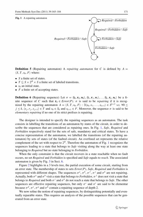
Fig. 1 A repairing automaton

Definition 5 (Repairing automaton) A repairing automaton for C is defined by A =〈S,T , s0,F 〉 where:

• S a finite set of states.• T ⊆ S × 2R × S a finite set of labeled transitions.• s0 an initial state.• F a finite set of accepting states.

Definition 6 (Repairing sequence) Let σ = 〈i0, r0,o0〉, 〈i1, r1,o1〉, . . . 〈ik, rk,ok〉 be a fi-nite sequence of C such that r0 ∈ Error(P ). σ is said to be repairing if it is recog-nized by the repairing automaton A = 〈S,T , s0,F 〉 : ∃〈s0, s1, . . . , sk+1〉 ∈ Sk+2 s.t. ∀0 ≤j ≤ k, 〈sj , rj , sj+1〉 ∈ T and s0 ∈ S0 and sk+1 ∈ F . Moreover, the sequence σ is said to beelementary repairing if no one of its strict prefixes is repairing.

The designer is intended to specify the repairing sequences as an automaton. The taskconsists in labelling the transitions of an automaton by states of the circuit, in order to de-scribe the sequences that are considered as repairing ones. In Fig. 1, Safe, Required andForbidden respectively stand for the sets of safe, mandatory and critical states. To have aconcise representation of the automaton, we labelled the transitions (of the repairing au-tomaton) by sets of states (of the faulted circuit). An overlined set represents the relativecomplement of the set with respect to 2R . Therefore the automaton of Fig. 1 recognizes thesequences leading to a state that belongs to Safe visiting along the way at least one statebelonging to Required but no state belonging to Forbidden.

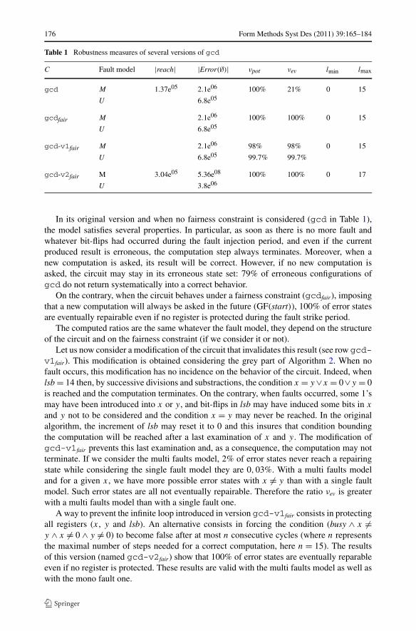
When the only constraint is that the circuit recovers in a state reachable when no faultoccurs, no set Required and Forbidden is specified and Safe equals to reach. The associatedautomaton is given by Fig. 3 in Sect. 6.

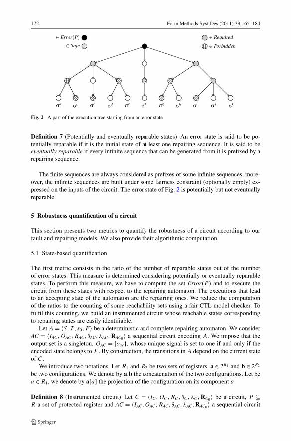
Figure 2 highlights in a 3 levels tree, the partial execution of some circuit, starting froman error state. The membership of states to sets Error(P ), Safe, Required and Forbidden isrepresented with different shapes. The sequences σa , σb , σf , σ j and σ k are not repairing.Actually, both σa and σb visit a state that belongs to Forbidden, σf does not visit a state thatbelongs to Required and both σ j and σ k do not reach a state that belongs to Safe. The othersequences are effective repairing sequences, but only σ c and σ i are said to be elementarbecause σd , σ e , σg and σh contain a repairing sequence of depth 2.

We now refine the notion of repairing sequences, by distinguishing potentially and even-tually reparable states. This requires an analysis of the possible sequences that can be gen-erated from an error state.


Fig. 2 A part of the execution tree starting from an error state

Definition 7 (Potentially and eventually reparable states) An error state is said to be po-tentially reparable if it is the initial state of at least one repairing sequence. It is said to beeventually reparable if every infinite sequence that can be generated from it is prefixed by arepairing sequence.

The finite sequences are always considered as prefixes of some infinite sequences, more-over, the infinite sequences are built under some fairness constraint (optionally empty) ex-pressed on the inputs of the circuit. The error state of Fig. 2 is potentially but not eventuallyreparable.

5 Robustness quantification of a circuit

This section presents two metrics to quantify the robustness of a circuit according to ourfault and repairing models. We also provide their algorithmic computation.

5.1 State-based quantification

The first metric consists in the ratio of the number of reparable states out of the numberof error states. This measure is determined considering potentially or eventually reparablestates. To perform this measure, we have to compute the set Error(P ) and to execute thecircuit from these states with respect to the repairing automaton. The executions that leadto an accepting state of the automaton are the repairing ones. We reduce the computationof the ratios to the counting of some reachability sets using a fair CTL model checker. Tofulfil this counting, we build an instrumented circuit whose reachable states correspondingto repairing states are easily identifiable.

Let A = 〈S,T , s0,F 〉 be a deterministic and complete repairing automaton. We considerAC = 〈IAC,OAC,RAC, δAC, λAC,RAC0〉 a sequential circuit encoding A. We impose that theoutput set is a singleton, OAC = {oac}, whose unique signal is set to one if and only if theencoded state belongs to F . By construction, the transitions in A depend on the current stateof C.

We introduce two notations. Let R1 and R2 be two sets of registers, a ∈ 2R1 and b ∈ 2R2

be two configurations. We denote by a.b the concatenation of the two configurations. Let bea ∈ R1, we denote by a[a] the projection of the configuration on its component a.

Definition 8 (Instrumented circuit) Let C = 〈IC,OC,RC, δC,λC,RC0〉 be a circuit, P �

R a set of protected register and AC = 〈IAC,OAC,RAC, δAC, λAC,RAC0〉 a sequential circuit


encoding the repairing automaton of C. In consequence, we set IAC = RC and OAC = {oac}.The instrumented circuit C ⊗ AC = 〈I,O,R, δ,λ,R0〉 is defined by:

– I = IC , O = OC ∪ OAC and R = RC ∪ RAC

– ∀i ∈ 2IC ,∀rc ∈ 2RC , rac ∈ 2RAC

– ∀rc ∈ RC, δ(i, rc.rac)[rc] = δC(i, rc)[rc]– ∀rac ∈ RAC, δ(i, rc.rac)[rac] = δAC(rc, rac)[rac]

– ∀rc ∈ 2RC , rac ∈ 2RAC

– ∀oc ∈ OC,λ(rc.rac)[oc] = λC(rc)[oc]– λ(rc.rac)[oac] = λAC(rac)[oac]

– R0 = Error(P ) × RAC0

Thanks to the output signal oac , we are able to detect if the instrumented circuit reachesa repaired configuration. According to the repairing automaton, the set of repaired configu-rations is defined by Repaired = {r ∈ 2R | λ(r)[oac] = 1}.

In this context, the potentially repairing states verify the CTL formula EFfairRepaired andthe eventually ones verify AFfairRepaired (where fair represents the fairness constraint). Inthe following, a CTL formula denotes the set of configurations of the instrumented circuitsatisfying it. We denote νpot (resp. νev) the ratio of potentially (resp. eventually) reparablestates out of the number of error states. The two ratios are defined as follows.

νpot = |EFfairRepaired ∩ R0||R0| , νev = |AFfairRepaired ∩ R0|

|R0|The computation of νpot and νev is performed using a CTL model-checker on the instru-

mented circuit.

5.2 Sequences-based quantification

The idea of the second metric is to highlight the velocity of the circuit to recover from anerror state. This last metric can be used to compare different architectures with the samefunctionalities.

We focus on the elementary repairing sequences containing no loop. We want to findout the minimal and maximal length of such sequences. We limit ourselves to sequenceswithout loop since, if an elementary sequence contains such a loop, the maximal bounddoes not exist. Moreover, for sequences without loop, we aim at counting the number ofelementary repairing ones for each possible length between these two bounds.

The computation of these bounds is performed by solving SAT problems iteratively [4,29]. The counting of elementary repairing sequences of a given length is then reduced to a#SAT problem [5].

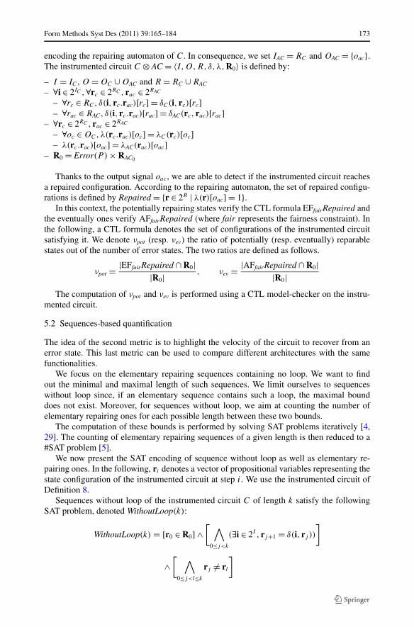
We now present the SAT encoding of sequence without loop as well as elementary re-pairing ones. In the following, ri denotes a vector of propositional variables representing thestate configuration of the instrumented circuit at step i. We use the instrumented circuit ofDefinition 8.

Sequences without loop of the instrumented circuit C of length k satisfy the followingSAT problem, denoted WithoutLoop(k):

WithoutLoop(k) = [r0 ∈ R0] ∧[ ∧

0≤j<k

(∃i ∈ 2I , rj+1 = δ(i, rj ))

]

∧[ ∧

0≤j<l≤k

rj �= rl

]


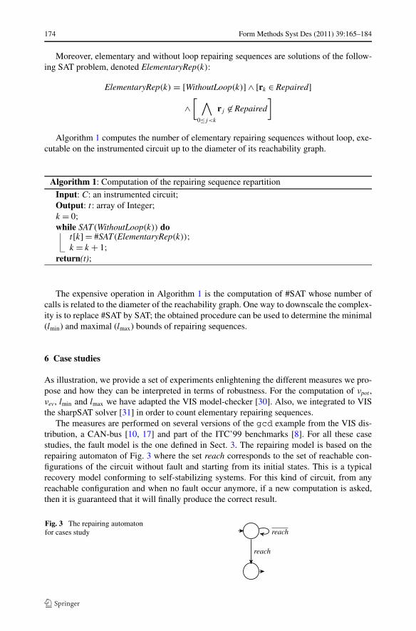
Moreover, elementary and without loop repairing sequences are solutions of the follow-ing SAT problem, denoted ElementaryRep(k):

ElementaryRep(k) = [WithoutLoop(k)] ∧ [rk ∈ Repaired]

∧[ ∧

0≤j<k

rj �∈ Repaired

]

Algorithm 1 computes the number of elementary repairing sequences without loop, exe-cutable on the instrumented circuit up to the diameter of its reachability graph.

Algorithm 1: Computation of the repairing sequence repartition

Input: C: an instrumented circuit;Output: t : array of Integer;k = 0;while SAT(WithoutLoop(k)) do

t[k] = #SAT(ElementaryRep(k));k = k + 1;

return(t);

The expensive operation in Algorithm 1 is the computation of #SAT whose number ofcalls is related to the diameter of the reachability graph. One way to downscale the complex-ity is to replace #SAT by SAT; the obtained procedure can be used to determine the minimal(lmin) and maximal (lmax) bounds of repairing sequences.

6 Case studies

As illustration, we provide a set of experiments enlightening the different measures we pro-pose and how they can be interpreted in terms of robustness. For the computation of νpot ,νev, lmin and lmax we have adapted the VIS model-checker [30]. Also, we integrated to VISthe sharpSAT solver [31] in order to count elementary repairing sequences.

The measures are performed on several versions of the gcd example from the VIS dis-tribution, a CAN-bus [10, 17] and part of the ITC’99 benchmarks [8]. For all these casestudies, the fault model is the one defined in Sect. 3. The repairing model is based on therepairing automaton of Fig. 3 where the set reach corresponds to the set of reachable con-figurations of the circuit without fault and starting from its initial states. This is a typicalrecovery model conforming to self-stabilizing systems. For this kind of circuit, from anyreachable configuration and when no fault occur anymore, if a new computation is asked,then it is guaranteed that it will finally produce the correct result.

Fig. 3 The repairing automatonfor cases study


The common columns of the Tables 1, 3, 4 and 5, are C that denotes the circuit, |reach|the number of reachable states from the initial states when no fault occurs, the two consid-ered fault models denoted M for “multiple faults” and U for “single fault”, |Error(P )| thenumber of error states according to the fault model, νpot and νev the potentially and even-tually repairing ratios and lmin and lmax the minimal and maximal bounds of elementaryrepairing sequences.

For all these experiments, the times spent to compute the presented ratios are negligiblequantities, thus are not figured. Also, the times to compute the lengths of sequences are notrepresented. In fact, the waiting time for circuits having lmax < 100 is very weak, but westop computations for circuits having greater values since the time spent can be huge.

6.1 gcd

The measures are performed on several versions of the 8-bits gcd example from the VISdistribution. This circuit computes the greatest common divisor of two operands (inputs a

and b) on request (input signal start). The computation takes several cycles (output signalbusy is set to 1) and when the result is computed, it is produced on output o (busy is setto 0). The computation makes use of three internal registers (lsb, x and y). The implementedalgorithm is presented in Algorithm 2. For all experiments, no register is protected, P = ∅.

Algorithm 2: Original algorithm of gcd and, in gray, modification v1

Input: start : signal; a, b : integer[8];Output: busy : signal; o : integer[8];Registers: lsb : integer[3]; x, y : integer[8];begin initialisation

x ← 0; y ← 0; lsb ← 0; busy ← 0; o ← 0;

for each positive edge clock doif (start ∧ ¬busy) then

x ← a; y ← b; lsb ← 0; busy ← 1;else if (busy ∧ x �= y ∧ x �= 0 ∧ y �= 0) then

tmp : integer[2];tmp ← 2.x[lsb] + y[lsb];switch tmp do

case b’00if (lsb < 15) then

lsb ← lsb + 1;

case b’01x ← x/2;

case b’10y ← y/2;

case b’11if (x < y) then

y ← (y − x)/2;else

x ← (x − y)/2;

else if (busy ∧ (x = y ∨ x = 0 ∨ y = 0)) theno ← (x < y ? x : y); busy ← 0;


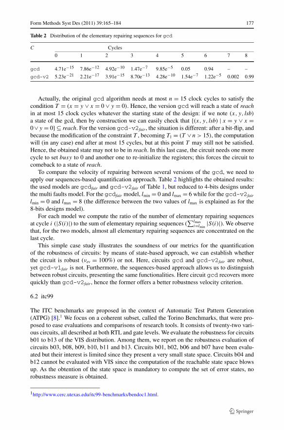
Table 1 Robustness measures of several versions of gcd

C Fault model |reach| |Error(∅)| νpot νev lmin lmax

gcd M 1.37e05 2.1e06 100% 21% 0 15

U 6.8e05

gcdfair M 2.1e06 100% 100% 0 15

U 6.8e05

gcd-v1fair M 2.1e06 98% 98% 0 15

U 6.8e05 99.7% 99.7%

gcd-v2fair M 3.04e05 5.36e08 100% 100% 0 17

U 3.8e06

In its original version and when no fairness constraint is considered (gcd in Table 1),the model satisfies several properties. In particular, as soon as there is no more fault andwhatever bit-flips had occurred during the fault injection period, and even if the currentproduced result is erroneous, the computation step always terminates. Moreover, when anew computation is asked, its result will be correct. However, if no new computation isasked, the circuit may stay in its erroneous state set: 79% of erroneous configurations ofgcd do not return systematically into a correct behavior.

On the contrary, when the circuit behaves under a fairness constraint (gcdfair), imposingthat a new computation will always be asked in the future (GF(start)), 100% of error statesare eventually repairable even if no register is protected during the fault strike period.

The computed ratios are the same whatever the fault model, they depend on the structureof the circuit and on the fairness constraint (if we consider it or not).

Let us now consider a modification of the circuit that invalidates this result (see row gcd-v1fair). This modification is obtained considering the grey part of Algorithm 2. When nofault occurs, this modification has no incidence on the behavior of the circuit. Indeed, whenlsb = 14 then, by successive divisions and substractions, the condition x = y ∨x = 0∨y = 0is reached and the computation terminates. On the contrary, when faults occurred, some 1’smay have been introduced into x or y, and bit-flips in lsb may have induced some bits in x

and y not to be considered and the condition x = y may never be reached. In the originalalgorithm, the increment of lsb may reset it to 0 and this insures that condition boundingthe computation will be reached after a last examination of x and y. The modification ofgcd-v1fair prevents this last examination and, as a consequence, the computation may notterminate. If we consider the multi faults model, 2% of error states never reach a repairingstate while considering the single fault model they are 0,03%. With a multi faults modeland for a given x, we have more possible error states with x �= y than with a single faultmodel. Such error states are all not eventually repairable. Therefore the ratio νev is greaterwith a multi faults model than with a single fault one.

A way to prevent the infinite loop introduced in version gcd-v1fair consists in protectingall registers (x, y and lsb). An alternative consists in forcing the condition (busy ∧ x �=y ∧ x �= 0 ∧ y �= 0) to become false after at most n consecutive cycles (where n representsthe maximal number of steps needed for a correct computation, here n = 15). The resultsof this version (named gcd-v2fair) show that 100% of error states are eventually reparableeven if no register is protected. These results are valid with the multi faults model as well aswith the mono fault one.


Table 2 Distribution of the elementary repairing sequences for gcd

C Cycles

0 1 2 3 4 5 6 7 8

gcd 4.71e−15 7.86e−12 4.92e−10 1.47e−7 9.85e−5 0.05 0.94 – –

gcd-v2 5.23e−21 2.21e−17 3.91e−15 8.70e−13 4.28e−10 1.54e−7 1.22e−5 0.002 0.99

Actually, the original gcd algorithm needs at most n = 15 clock cycles to satisfy thecondition T = (x = y ∨ x = 0 ∨ y = 0). Hence, the version gcd will reach a state of reachin at most 15 clock cycles whatever the starting state of the design: if we note (x, y, lsb)

a state of the gcd, then by construction we can easily check that {(x, y, lsb) | x = y ∨ x =0∨y = 0} ⊆ reach. For the version gcd-v2fair , the situation is different: after a bit-flip, andbecause the modification of the constraint T , becoming T1 = (T ∨n > 15), the computationwill (in any case) end after at most 15 cycles, but at this point T may still not be satisfied.Hence, the obtained state may not to be in reach. In this last case, the circuit needs one morecycle to set busy to 0 and another one to re-initialize the registers; this forces the circuit tocomeback to a state of reach.

To compare the velocity of repairing between several versions of the gcd, we need toapply our sequences-based quantification approach. Table 2 highlights the obtained results:the used models are gcdfair and gcd-v2fair of Table 1, but reduced to 4-bits designs underthe multi faults model. For the gcdfair model, lmin = 0 and lmax = 6 while for the gcd-v2fair

lmin = 0 and lmax = 8 (the difference between the two values of lmax is explained as for the8-bits designs model).

For each model we compute the ratio of the number of elementary repairing sequencesat cycle i (|S(i)|) to the sum of elementary repairing sequences (

∑lmaxi=lmin

|S(i)|). We observethat, for the two models, almost all elementary repairing sequences are concentrated on thelast cycle.

This simple case study illustrates the soundness of our metrics for the quantificationof the robustness of circuits: by means of state-based approach, we can establish whetherthe circuit is robust (νev = 100%) or not. Here, circuits gcd and gcd-v2fair are robust,yet gcd-v1fair is not. Furthermore, the sequences-based approach allows us to distinguishbetween robust circuits, presenting the same functionalities. Here circuit gcd recovers morequickly than gcd-v2fair , hence the former offers a better robustness velocity criterion.

6.2 itc99

The ITC benchmarks are proposed in the context of Automatic Test Pattern Generation(ATPG) [8].1 We focus on a coherent subset, called the Torino Benchmarks, that were pro-posed to ease evaluations and comparisons of research tools. It consists of twenty-two vari-ous circuits, all described at both RTL and gate levels. We evaluate the robustness for circuitsb01 to b13 of the VIS distribution. Among them, we report on the robustness evaluation ofcircuits b03, b08, b09, b10, b11 and b13. Circuits b01, b02, b06 and b07 have been evalu-ated but their interest is limited since they present a very small state space. Circuits b04 andb12 cannot be evaluated with VIS since the computation of the reachable state space blowsup. As the obtention of the state space is mandatory to compute the set of error states, norobustness measure is obtained.

1http://www.cerc.utexas.edu/itc99-benchmarks/bendoc1.html.

http://www.cerc.utexas.edu/itc99-benchmarks/bendoc1.html


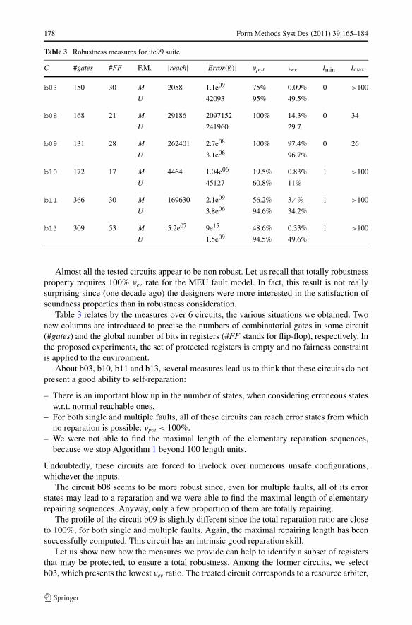
Table 3 Robustness measures for itc99 suite

C #gates #FF F.M. |reach| |Error(∅)| νpot νev lmin lmax

b03 150 30 M 2058 1.1e09 75% 0.09% 0 >100

U 42093 95% 49.5%

b08 168 21 M 29186 2097152 100% 14.3% 0 34

U 241960 29.7

b09 131 28 M 262401 2.7e08 100% 97.4% 0 26

U 3.1e06 96.7%

b10 172 17 M 4464 1.04e06 19.5% 0.83% 1 >100

U 45127 60.8% 11%

b11 366 30 M 169630 2.1e09 56.2% 3.4% 1 >100

U 3.8e06 94.6% 34.2%

b13 309 53 M 5.2e07 9e15 48.6% 0.33% 1 >100

U 1.5e09 94.5% 49.6%

Almost all the tested circuits appear to be non robust. Let us recall that totally robustnessproperty requires 100% νev rate for the MEU fault model. In fact, this result is not reallysurprising since (one decade ago) the designers were more interested in the satisfaction ofsoundness properties than in robustness consideration.

Table 3 relates by the measures over 6 circuits, the various situations we obtained. Twonew columns are introduced to precise the numbers of combinatorial gates in some circuit(#gates) and the global number of bits in registers (#FF stands for flip-flop), respectively. Inthe proposed experiments, the set of protected registers is empty and no fairness constraintis applied to the environment.

About b03, b10, b11 and b13, several measures lead us to think that these circuits do notpresent a good ability to self-reparation:

– There is an important blow up in the number of states, when considering erroneous statesw.r.t. normal reachable ones.

– For both single and multiple faults, all of these circuits can reach error states from whichno reparation is possible: νpot < 100%.

– We were not able to find the maximal length of the elementary reparation sequences,because we stop Algorithm 1 beyond 100 length units.

Undoubtedly, these circuits are forced to livelock over numerous unsafe configurations,whichever the inputs.

The circuit b08 seems to be more robust since, even for multiple faults, all of its errorstates may lead to a reparation and we were able to find the maximal length of elementaryrepairing sequences. Anyway, only a few proportion of them are totally repairing.

The profile of the circuit b09 is slightly different since the total reparation ratio are closeto 100%, for both single and multiple faults. Again, the maximal repairing length has beensuccessfully computed. This circuit has an intrinsic good reparation skill.

Let us show now how the measures we provide can help to identify a subset of registersthat may be protected, to ensure a total robustness. Among the former circuits, we selectb03, which presents the lowest νev ratio. The treated circuit corresponds to a resource arbiter,


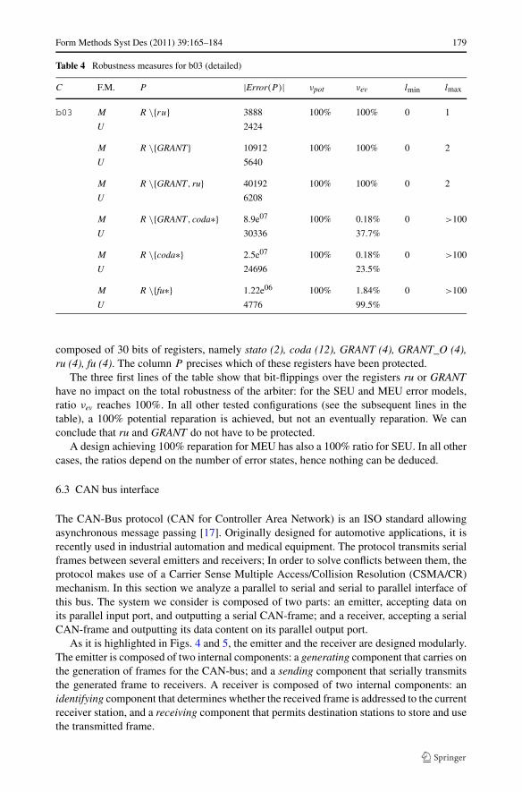
Table 4 Robustness measures for b03 (detailed)

C F.M. P |Error(P )| νpot νev lmin lmax

b03 M R \{ru} 3888 100% 100% 0 1

U 2424

M R \{GRANT} 10912 100% 100% 0 2

U 5640

M R \{GRANT, ru} 40192 100% 100% 0 2

U 6208

M R \{GRANT, coda∗} 8.9e07 100% 0.18% 0 >100

U 30336 37.7%

M R \{coda∗} 2.5e07 100% 0.18% 0 >100

U 24696 23.5%

M R \{fu∗} 1.22e06 100% 1.84% 0 >100

U 4776 99.5%

composed of 30 bits of registers, namely stato (2), coda (12), GRANT (4), GRANT_O (4),ru (4), fu (4). The column P precises which of these registers have been protected.

The three first lines of the table show that bit-flippings over the registers ru or GRANThave no impact on the total robustness of the arbiter: for the SEU and MEU error models,ratio νev reaches 100%. In all other tested configurations (see the subsequent lines in thetable), a 100% potential reparation is achieved, but not an eventually reparation. We canconclude that ru and GRANT do not have to be protected.

A design achieving 100% reparation for MEU has also a 100% ratio for SEU. In all othercases, the ratios depend on the number of error states, hence nothing can be deduced.

6.3 CAN bus interface

The CAN-Bus protocol (CAN for Controller Area Network) is an ISO standard allowingasynchronous message passing [17]. Originally designed for automotive applications, it isrecently used in industrial automation and medical equipment. The protocol transmits serialframes between several emitters and receivers; In order to solve conflicts between them, theprotocol makes use of a Carrier Sense Multiple Access/Collision Resolution (CSMA/CR)mechanism. In this section we analyze a parallel to serial and serial to parallel interface ofthis bus. The system we consider is composed of two parts: an emitter, accepting data onits parallel input port, and outputting a serial CAN-frame; and a receiver, accepting a serialCAN-frame and outputting its data content on its parallel output port.

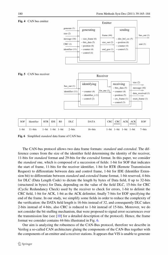
As it is highlighted in Figs. 4 and 5, the emitter and the receiver are designed modularly.The emitter is composed of two internal components: a generating component that carries onthe generation of frames for the CAN-bus; and a sending component that serially transmitsthe generated frame to receivers. A receiver is composed of two internal components: anidentifying component that determines whether the received frame is addressed to the currentreceiver station, and a receiving component that permits destination stations to store and usethe transmitted frame.


Fig. 4 CAN bus emitter

Fig. 5 CAN bus receiver

Fig. 6 Simplified standard data frame of CAN bus

The CAN-bus protocol allows two data frame formats: standard and extended. The dif-ference comes from the size of the identifier field determining the identity of the receiver,11-bits for standard format and 29-bits for the extended format. In this paper, we considerthe standard one, which is composed of a succession of fields: 1-bit for SOF that indicatesthe start of frame, 11-bits for the receiver identifier, 1-bit for RTR (Remote TransmissionRequest) to differentiate between data and control frame, 1-bit for IDE (Identifier Exten-sion bit) to differentiate between standard and extended frame format, 1-bit reserved, 4-bitsfor DLC (Data Length Code) to dictate the length by bytes of Data field, 0 up to 32-bits(structured in bytes) for Data, depending on the value of the field DLC, 15-bits for CRC(Cyclic Redundancy Check) used by the receiver to check for errors, 1-bit to delimit theCRC field, 1-bit for ACK, 1-bit as the ACK delimiter, finally 7-bits for EOF specifying theend of the frame. In our study, we simplify some fields in order to reduce the complexity ofthe verification: the DATA field length is 16-bits instead of 32, and consequently DLC takes2-bits instead of 4-bits, also CRC is reduced to 1-bit instead of 15-bits. Moreover, we donot consider the bit stuffing mechanism, that were proposed to signal error occurrences overthe transmission line (see [10] for a detailed description of the protocol). Hence, the frameformat we consider contains 44-bits illustrated in Fig. 6.

Our aim is analyzing the robustness of the CAN-Bus protocol, therefore we describe inVerilog a so-called CAN architecture gluing the components of the CAN-Bus together withthe components of an emitter and a receiver stations. It appears that VIS is unable to generate


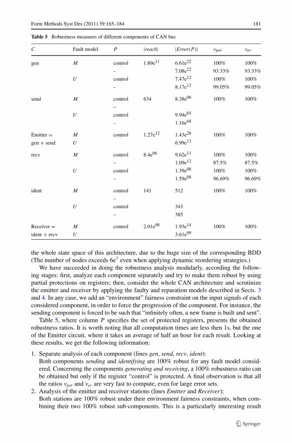
Table 5 Robustness measures of different components of CAN bus

C Fault model P |reach| |Error(P )| νpot νev

gen M control 1.89e11 6.61e22 100% 100%

– 7.08e22 93.33% 93.33%

U control 7.47e12 100% 100%

– 8.17e12 99.05% 99.05%

send M control 634 8.38e06 100% 100%

–

U control 9.94e03

– 1.16e04

Emitter = M control 1.27e12 1.43e28 100% 100%

gen + send U 6.99e13

recv M control 8.4e06 9.62e11 100% 100%

– 1.09e12 87.5% 87.5%

U control 1.39e08 100% 100%

– 1.59e08 96.69% 96.69%

ident M control 141 512 100% 100%

–

U control 343

– 385

Receiver = M control 2.01e08 1.93e14 100% 100%

ident + recv U 3.61e09

the whole state space of this architecture, due to the huge size of the corresponding BDD(The number of nodes exceeds 6e7 even when applying dynamic reordering strategies.)

We have succeeded in doing the robustness analysis modularly, according the follow-ing stages: first, analyze each component separately and try to make them robust by usingpartial protections on registers; then, consider the whole CAN architecture and scrutinizethe emitter and receiver by applying the faulty and reparation models described in Sects. 3and 4. In any case, we add an “environment” fairness constraint on the input signals of eachconsidered component, in order to force the progression of the component. For instance, thesending component is forced to be such that “infinitely often, a new frame is built and sent”.

Table 5, where column P specifies the set of protected registers, presents the obtainedrobustness ratios. It is worth noting that all computation times are less then 1s, but the oneof the Emitter circuit, where it takes an average of half an hour for each result. Looking atthese results, we get the following information:

1. Separate analysis of each component (lines gen, send, recv, ident):Both components sending and identifying are 100% robust for any fault model consid-ered. Concerning the components generating and receiving, a 100% robustness ratio canbe obtained but only if the register “control” is protected. A final observation is that allthe ratios νpot and νev are very fast to compute, even for large error sets.

2. Analysis of the emitter and receiver stations (lines Emitter and Receiver):Both stations are 100% robust under their environment fairness constraints, when com-bining their two 100% robust sub-components. This is a particularly interesting result


since, in general, the combination of two 100% robust components may not systemati-cally result in a 100% robust assembly. Actually from any two 100% robust components,e.g. C1 and C2, and their respective reachable state sets, reach(C1) and reach(C2), arobust composed circuit C1 × C2 taken after a perturbation period, must reach one stateof its reachable states reach(C1 × C2). The problem comes from the fact that this lastset is included in reach(C1) × reach(C2), but not necessarily equal to. Thanks to ourexperiments, we demonstrate that these stations are quite robust.

3. Analysis of the whole CAN architecture:Assuming the environment fairness constraints, we check that the following two proper-ties hold: (a) from all the states in reach(Emitter), a new frame will eventually be sentby the Emitter; (b) from all the states of reach(Receiver), a new frame will eventuallybe received by the Receiver. Combined with item 2, we conclude that the emitter andreceiver stations will eventually recover.

The presented experiment showed the ability of a CAN architecture to recover by itself aftera perturbation period over the register elements. We exhibited the minimal set of registers ofthe elementary components to be protected. The ability to recover after a bounded perturba-tion period, relaxes the robustness criterion standardly provided by the CRC and bit-stuffingmechanisms, which detect and correct erroneous frames on-the-fly. It is worth noting thatour fault model is larger than considering bit-flipping during the serial transmission. Thebit-flips also concern the components that generate the frame and the ones that analyze it,before and after the serial transmission. For instance, bit-flips may cause the production ofinconsistent frames, and we then prove that after the recovery period, consistent frames aretransmitted again.

7 Discussion and conclusion

We propose a novel framework to analyze the robustness of circuits submitted to particlesstrikes. Our approach allows to cope with multiple transient faults captured as bit-flips insequential elements, and relaxes the robustness criterion. In this paper, we illustrate ourmethodology applying it to different circuits, showing the soundness of our approach andthe interest of our measures.

To the best of our knowledge, MEU is rarely considered when evaluating robustness,since this requires to cope with a combinatorial explosion of fault instants. In this paper, weconsider two models of faults, one corresponding to standard SEU, and another one extend-ing MEU to multiple occurrences in time. We presented an original approach to computeefficiently the set of error states for these two models, exploiting the foundations of BDDssymbolic representation and temporal model checking algorithms.

The model of robustness focuses on the self-healing reparability of circuits. Among thetwo metrics we propose, the first one quantifies the number of erroneous states that are re-pairable. Thus, with this measure, one can determine between several versions of a givencircuit, which one is more robust (see gcd example, Sect. 6.1). In a more general way, it canbe used to determine a minimal set of registers to be protected for guaranteeing a recovery(see itc-b03 and CAN-Bus interface examples, in Sects. 6.2 and 6.3). Even for non robustcircuits, we bring out information since the potential recovering capability is computed inaddition to the eventual one. Our second metric evaluates the velocity of circuits to recoverby computing the lengths of elementary repairing sequences. The distribution of these se-quences on the different lengths yields more precision about the way erroneous states arerepaired (see gcd example).


Our model of robustness relaxes the strict conformance to a golden model which is gen-erally adopted. Such a conformance is the highest level of robustness a circuit may conform,however this often leads to harden a lot of registers to obtain it (e.g. add protection byreplication and vote). In many applications (video stream, loose synchronization), weakerrobustness conformance are acceptable, like “guaranteeing a recovery into a safe state aftersome bounded sequence”. Our reparation model allows for characterizing the way the sys-tem recover by restricting the repairing sequences to conform to the reparation automaton.

A first perspective consists in refining this reparation model. In the presented study, therepairing sequences are selected by reaching safe states, simply defined by the reparationautomaton. We plan to consider more information into account, about the circuit executionor its environmental context. Indeed, the robustness requirement a circuit has to achievegreatly depends on its environment. In some cases, the so-called safe-configurations to bereached depend on the past of the error state, and this is not captured by the reparationautomaton.

In its present state, the proposed approach opens interesting questions to be addressedto extend the size of circuits to be analyzed. The computation of robustness measures wepropose is implemented in a BDD- and SAT-model-checking framework; as it can be seen inthe Experiment Section, measure computation is very efficient for small sized circuit (up to20–50 flip-flops) but the combinatorial blow up is quickly reached. The computation timesof the Emitter and Receiver stations of the CAN bus interface illustrates this problem, and acompositional reasoning has to be adopted to combine the measures of internal components.Indeed, the 100% robustness of two components does not guarantee the 100% robustnessof their product, other synchronization properties have to be added. Another way to analyzecomplex systems concerns the use of abstractions, however one has to carefully define thereparation automaton of the abstracted model in order to ensure the automatic transpositionof 100% robustness result from the abstract model to the concrete one. These two pointswill be subjects of forthcoming research.

References

1. Abke J, Bohl E, Henno C (1998) Emulation based real time testing of automotive applications. In: Procof 4th IEEE international on-line testing workshop, pp 28–31

2. Baarir S, Braunstein C, Clavel R, Encrenaz E, Ilié J-M, Leveugle R, Mounier I, Pierre L, Poitrenaud D(2009) Complementary formal approaches for dependability analysis. In: Proc international symposiumon defect and fault tolerance in VLSI systems. IEEE Comput Soc, Los Alamitos, pp 331–339

3. Bidgoli H (2006) Handbook of information security, vol 3. Wiley, New York4. Biere A, Cimatti A, Clarke EM, Zhu Y (1999) Symbolic model checking without BDDs. In: Proc inter-

national conference on tools and algorithms for construction and analysis of systems. Lecture notes incomputer science, vol 1579. Springer, Berlin, pp 193–207

5. Birnbaum E, Lozinskii EL (1999) The good old Davis-Putnam procedure helps counting models. J ArtifIntell Res 10:457–477

6. Church A (1957) Application of recursive arithmetic to the problem of circuit synthesis. In: Summariesof talks presented at the summer institute for symbolic logic. Princeton. Communications Research Di-vision, Institute for Defense Analyses, Princeton, pp 3–50

7. Clarke EM, Emerson EA, Sistla AP (1986) Automatic verification of finite-state concurrent systemsusing temporal logic specifications. ACM Trans Program Lang Syst 8(2):244–263

8. Corno F, Sonza Reorda M, Squillero G (2000) RT-level ITC 99 benchmarks and first ATPG results. IEEEDes Test Comput 17(3):44–53

9. Daveau J-M, Blampey A, Gasiot G, Bulone J, Roche P (2009) An industrial fault injection platform forsoft-error dependability analysis and hardening of complex system-on-a-chip. In: IEEE RPS-CDR 47thannu int reliability physics symp, Montreal, Canada. IEEE Press, New York

10. Davis RI, Burns A, Bril R, Lukkien J (2007) Controller area network (can) schedulability analysis:Refuted, revisited and revised. Real-Time Syst 35(3):239–272


11. Dijkstra EW (1974) Self-stabilization systems in spite of distributed control. Commun ACM 17:643–644

12. Dolev S (2000) Self-stabilization. MIT Press, Cambridge13. Fey G, Drechsler R (2008) A basis for formal robustness checking. In: Proc IEEE international sympo-

sium on quality electronic design. IEEE Comput Soc, Los Alamitos, pp 784–78914. Fey G, Sülflow A, Drechsler R (2009) Computing bounds for fault tolerance using formal techniques.

In: Proc design automation conference. ACM, New York, pp 190–19515. Garcia-Valderas M, Portela-Garcia M, Lopez-Ongil C, Entrena L (2010) Extensive SEU impact analysis

of a pic microprocessor for selective hardening. IEEE Trans Nucl Sci 57(4)16. Hopcroft JE, Motwani R, Ullman JD (2006) Introduction to automata theory, languages, and computation

(3rd edn.). Addison-Wesley/Longman, Boston17. ISO technical committees TC22/SC3 (2003) Road vehicles—controller area networks—parts 1 to 5.

International Organization for Standardization, Geneva18. Jenn E, Arlat J, Rimen R, Ohlsson J, Karlsson J (1994) Fault injection into VHDL models: the

MEPHISTO tool. In: Proc of 24th symposium on fault-tolerant computing (FTCS), pp 66–7519. Krautz U, Pflanz M, Jacobi C, Tast H, Weber K, Vierhaus H (2006) Evaluating coverage of error detection

logic for soft errors using formal methods. In: Proc conference on design, automation and test in Europe.European Design and Automation Association, pp 176–181

20. Krishnaswamy S, Viamontes GF, Markov IL, Hayes J (2008) Probabilistic transfert matrices in symbolicreliability analysis of logic circuits for reliability evaluation of logic circuits. Trans Des Autom ElectronSyst 13(1)

21. Leveugle R (2005) A new approach for early dependability evaluation based on formal property checkingand controlled mutation. In: Proc IEEE international on-line testing symposium. IEEE Comput Soc,Los Alamitos, pp 260–265

22. Leveugle R, Hadjiat K (2003) Multi-level fault injections in VHDL descriptions: alternative approachesand experiments. J Electron Test Theory Appl. 19(5):559–575

23. Leveugle R, Calvez A, Maistri P, Vanhauwaert P (2009) Statistical fault injection: quantified error andconfidence. In: Proc of design, automation and test in Europe conference (DATE), pp 502–506

24. Lopez-Ongil C, Garcia-Valderas M, Portela-Garcia M, Entrena L (2007) Autonomous fast emulation:a new FPGA-based acceleration system for hardness evaluation. IEEE Trans Nucl Sci 54(1)

25. Naviner L, Naviner JF, Franco D, Vasconcelos M (2008) Signal probability for reliability evaluation oflogic circuits. Microelectron Reliab J 48

26. Naviner L, Naviner JF, Goncalves dos Santos G Jr, Crespo Marques E (2010) Using error tolerance of tar-get application for efficient reliability improvement of digital circuits. Microelectron Reliab J 50(9–11)

27. Polian I, Hayes JP, Sudhakar MR, Becker B (2010) Modeling and mitigating transient errors in logiccircuits. IEEE Trans Dependable and Secure Comput 99(PrePrints)

28. Seshia S, Li W, Mitra S (2007) Verification-guided soft error resilience. In: Proc conference on design,automation and test in Europe. EDA Consortium, San Jose, pp 1442–1447

29. Shtrichman O (2000) Tuning SAT checkers for bounded model checking. In: Proc international con-ference on computer aided verification. Lecture notes in computer science, vol 1855. Springer, Berlin,pp 480–494

30. The VIS group (1996) VIS: a system for verification and synthesis. In: Proc international conference oncomputer aided verification. Lecture notes in computer science, vol 1102. Springer, Berlin, pp 428–432

31. Thurley M (2006) sharpSAT—counting models with advanced component caching and implicit BCP. In:Theory and applications of satisfiability testing (SAT’06). Lecture notes in computer science, vol 4121.Seattle, WA, USA, August 2006. Springer, Berlin, pp 424–429

Feasibility analysis for robustness quantification by symbolic model checking

Documents

Transcript of Feasibility analysis for robustness quantification by symbolic model checking