SECURITY AND ROBUSTNESS OF LOCALIZATION TECHNIQUES FOREMERGENCY SENSOR NETWORKS

BY

MURTUZA SHABBIR JADLIWALA

THESIS

Submitted in partial fulfillment of the requirementsfor the degree of Doctor of Philosophy in Computer Science and Engineering

in the Graduate School of theState University of New York at Buffalo, 2008

Buffalo, New York

© Copyright by Murtuza Shabbir Jadliwala, 2008All Rights Reserved

To my family.

iii

Abstract

Recent advancement in radio and processor technology has seen the rise of Wireless Sensor Net-

works (WSN) as a reliable and cost-effective tool for real-time information gathering and analysis

tasks during emergency scenarios like natural disasters, terrorist attacks, military conflicts, etc.

Post-deployment localization is extremely important and necessary in these applications. But,

current distributed localization approaches are not designed for such highly hostile and dynamic

network conditions. This dissertation studies the adverse effects of factors like cheating behavior,

node disablement and measurement inconsistencies on the corresponding localization protocols

and attempts to provide simple and efficient solutions in order to overcome these problems.

The first problem addressed in this dissertation is, how to perform efficient distance-based

localization in the presence of cheating beacon nodes? This dissertation attempts to answer two

fundamental questions in distance-based localization: (i) In the presence of cheating beacons,

what are the necessary and sufficient conditions to guarantee a bounded localization error? and (ii)

Under these conditions, what class of algorithms can provide that error bound? In this part of the

dissertation, it is shown that when the number of cheating beacons is greater than or equal to some

threshold, there is no localization algorithm that can guarantee a bounded error. Furthermore, it is

also proved that when the number of malicious beacons is below that threshold, a non-empty class

of bounded error localization algorithms can be identified. Two secure distance-based localization

algorithms are outlined and their performance is verified using simulation experiments.

The next part of the dissertation underscores the lack of fault-tolerance in existing localiza-

tion protocols and proposes simple mechanisms to overcome this problem. Sensor node disable-

ment adversely affects the overall node deployment distribution and the efficiency of localization

iv

techniques that depend on this distribution, for example, signature-based techniques. In order

to improve the fault-tolerance in these schemes, it is important to first construct a probabilistic

model for node disablement. In this direction, the phenomenon of sensor node disablement is

modeled as a stochastic time process. A novel deployment strategy that non-uniformly deploys

sensor nodes over the monitored area is also outlined. Then, a fault-tolerance related improvement

to existing localization schemes is proposed, which discards observations from unhealthy groups

of nodes during the localization process. In order to overcome the complexity concerns, a simple

signature-based technique, called ASFALT, is also proposed. ASFALT estimates the target location

by first predicting distances to known location references using the underlying node distribution

and a simple averaging argument. Extensive measurements from simulation experiments verify

the fault-tolerance and performance of the proposed solutions.

In the final part of this dissertation, the problem of efficiently mitigating inconsistencies in

location-based applications is addressed. Inconsistencies in location information, caused by cheat-

ing behavior or measurement errors can be modeled using a weighted, undirected graph and a

cheating location function that can assign incorrect locations to the nodes or a cheating (but ver-

ifiable) distance function that can assign inconsistent distances to edges. In either case, an edge

relation where the assigned edge distance is not within some very small factor of the Euclidean

distance between the connecting nodes represents some inconsistency and is referred to as an in-

consistent edge. The problem of efficiently mitigating location inconsistencies in the network can

then be formulated as an optimization problem that determines the largest induced subgraph (ob-

tained by eliminating a subset of vertices) containing only consistent edges. Two optimization

problems can be stated. The first maximizes the number of vertices in the consistent subgraph,

while the second maximizes the number of consistent edges in the consistent subgraph. Combi-

natorial properties including hardness and approximation ratio for these problems are studied and

intelligent solution strategies are proposed. A comparative analysis that verifies the practical effi-

ciency of these algorithms by using measurements from simulation experiments is also presented.

v

Acknowledgments

I would like to begin by thanking my advisor and mentor over the past 4 years, Dr. Shambhu J.

Upadhyaya. Without his continuous support and direction, I don’t think this dissertation would

have been possible. Input provided by him during the numerous technical discussions and project

meetings helped me in not only shaping my dissertation topic but also in overcoming key road-

blocks during the research and experimentation phase. I feel really lucky and privileged to get his

guidance and direction towards the completion of this dissertation.

I would also like to thank Dr. Sheng Zhong and Dr. Jinhui Xu for being in my dissertation com-

mittee and being so actively involved with my research and dissertation in general. The lengthy

discussions with them during research meetings were always insightful and technically invigorat-

ing. I would like to thank Dr. H. Raghav Rao for being an active member of my dissertation

committee and providing invaluable suggestions and feedback during my proposal presentation.

I would also like to express my gratitude towards Dr. Sviatoslav Braynov, who was my graduate

student advisor during the course of my Masters degree. He got me started on the right foot by

getting me involved with his research activities and projects early. He was also an excellent teacher.

I would also like to thank the numerous other faculty members at UB, including Dr. Chunming

Qiao, Dr. Hung Ngo, Dr. Murat Demirbas, Dr. Kenneth Regan and Dr. Alan Selman from

the Department of Computer Science and Engineering and Dr. Raj Sharman from the School of

Management, who were actively involved with my research in some way or the other.

I would like to extend my special thanks to all my colleagues and friends in the CEISARE re-

search group. Suranjan Pramanik, my house-mate, office-mate and also a close friend was always

available, either it be for discussing a research idea or for watching a movie. Mohit Virendra would

vi

never be late to share a quick joke or a recent related paper at MOBICOM. Ashish Garg would al-

ways be available if you ever need a unique perspective on a recent submission or a great deal on

the latest electronic gadget. I have learned a lot, both technically and personally, from other col-

leagues in the research group, notably, Ramkumar Chinchani, Madhusudhanan Chandrasekaran,

Vidyaraman Sankaranarayanan and Sunu Mathew. I had the opportunity to work in the company

of a talented bunch of people! Outside of the research group, I am really thankful to Qi Duan and

Manik Taneja for their efforts towards the completion of the various research projects and experi-

ments that are a part of this dissertation. Over the period of time, I made many friends here at UB.

Some of the most important ones have been my past housemates Gaurav Sinha and Megha Parekh,

and a group of friends nicknamed “buffalodudes”. Guys, thank you very much for your love and

support! I would also like to thank all other graduate students that attended Dr. Upadhyaya’s

research group meetings and gave valuable feedback on this dissertation.

My sisters, Sakina bhen and Kaniza, have always been supportive of my career ambitions. I ex-

press my heartfelt gratitude to you both for your continuous love and support during the completion

of this dissertation.

There are no words to describe how grateful I am to my wife, Tasneem, for all the love and

support I received from her, especially during the final stages of this dissertation. She always

motivated me to work hard and never to give up in life. Tasneem, I thank you with all my heart.

Finally, this dissertation would not have been possible, if it were not for the unconditional love,

support and sacrifices from my beloved Mom and Dad. My Dad has been a tremendous motivator

and has always inspired me to bring out the best in myself, whether it be life or graduate studies. It

is a matter of great sorrow that he moved on to a better place during the course of this dissertation

and could not witness its completion. But, I am sure that he is constantly watching over me and is

extremely proud to see me finish this dissertation. To Mom and Dad, I dedicate this dissertation to

you both!

vii

Table of Contents

Abstract . . . . . . . . . . . . . . . . . . . . . . . . . . . . . . . . . . . . . . . . . . . . . iv

Acknowledgments . . . . . . . . . . . . . . . . . . . . . . . . . . . . . . . . . . . . . . . vi

Chapter 1 Introduction . . . . . . . . . . . . . . . . . . . . . . . . . . . . . . . . . . . 11.1 Emergency Sensor Networks . . . . . . . . . . . . . . . . . . . . . . . . . . . . . 11.2 Localization in ESNs . . . . . . . . . . . . . . . . . . . . . . . . . . . . . . . . . 3

1.2.1 Beacon-based Localization . . . . . . . . . . . . . . . . . . . . . . . . . . 31.2.2 Signature-based (Beaconless) Localization . . . . . . . . . . . . . . . . . 6

1.3 Dissertation . . . . . . . . . . . . . . . . . . . . . . . . . . . . . . . . . . . . . . 91.3.1 Motivation . . . . . . . . . . . . . . . . . . . . . . . . . . . . . . . . . . 91.3.2 Original Contributions . . . . . . . . . . . . . . . . . . . . . . . . . . . . 111.3.3 Outline of the Disseration . . . . . . . . . . . . . . . . . . . . . . . . . . 14

Chapter 2 Background and Related Work . . . . . . . . . . . . . . . . . . . . . . . . . 162.1 Introduction . . . . . . . . . . . . . . . . . . . . . . . . . . . . . . . . . . . . . . 16

2.1.1 Chapter Organization . . . . . . . . . . . . . . . . . . . . . . . . . . . . . 162.2 Theoretical Foundations for Localization Schemes in Sensor Networks . . . . . . . 17

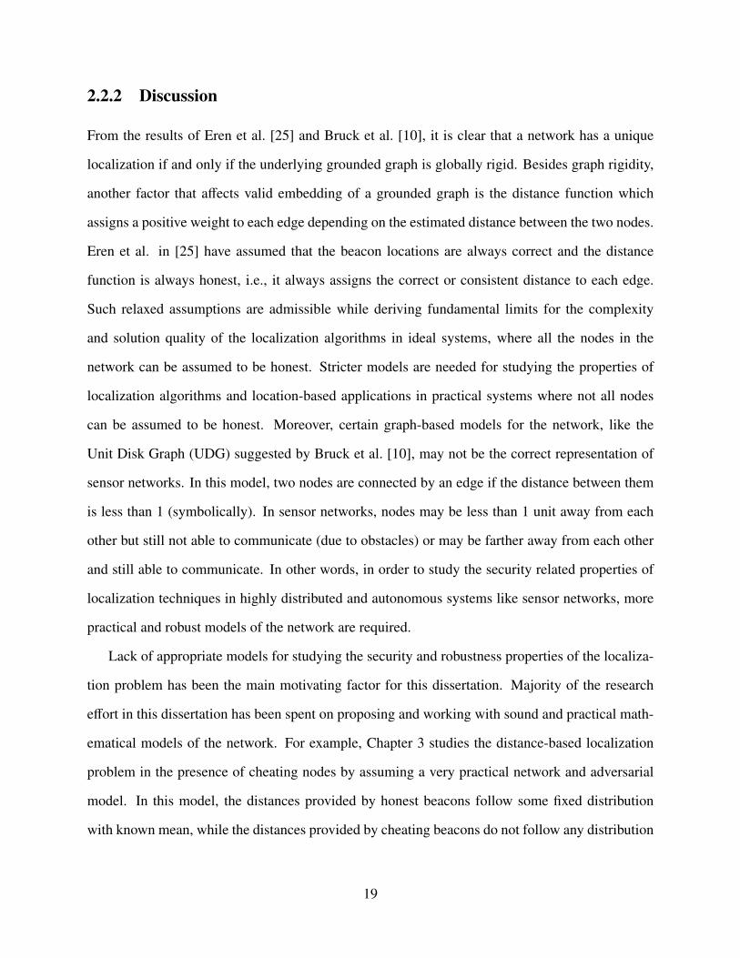
2.2.1 Current Models and Results for Localization . . . . . . . . . . . . . . . . 172.2.2 Discussion . . . . . . . . . . . . . . . . . . . . . . . . . . . . . . . . . . 19

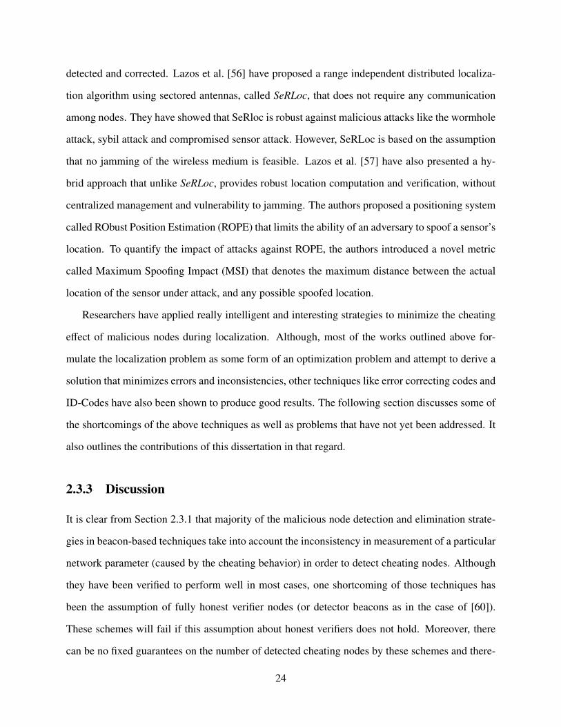
2.3 Secure Localization . . . . . . . . . . . . . . . . . . . . . . . . . . . . . . . . . . 202.3.1 Malicious Node Detection and Elimination . . . . . . . . . . . . . . . . . 212.3.2 Robust Localization Schemes for Sensor Networks . . . . . . . . . . . . . 222.3.3 Discussion . . . . . . . . . . . . . . . . . . . . . . . . . . . . . . . . . . 24

2.4 Fault-tolerance . . . . . . . . . . . . . . . . . . . . . . . . . . . . . . . . . . . . 262.4.1 Fault-tolerance of Localization Schemes . . . . . . . . . . . . . . . . . . . 262.4.2 Discussion . . . . . . . . . . . . . . . . . . . . . . . . . . . . . . . . . . 28

2.5 Conclusion . . . . . . . . . . . . . . . . . . . . . . . . . . . . . . . . . . . . . . 28

Chapter 3 Robust Distance-based Localization in the Presence of Cheating Beacons . 303.1 Introduction . . . . . . . . . . . . . . . . . . . . . . . . . . . . . . . . . . . . . . 30

3.1.1 Motivation and Problem Statement . . . . . . . . . . . . . . . . . . . . . . 303.1.2 Chapter Organization . . . . . . . . . . . . . . . . . . . . . . . . . . . . . 32

3.2 Network and Adversary Model . . . . . . . . . . . . . . . . . . . . . . . . . . . . 323.3 Robust Bounded Error Localization . . . . . . . . . . . . . . . . . . . . . . . . . 35

viii

3.3.1 Necessary Condition for Bounded Error Localization . . . . . . . . . . . . 353.3.2 Algorithm Class for Robust Bounded Error Localization . . . . . . . . . . 393.3.3 Error Bound Analysis . . . . . . . . . . . . . . . . . . . . . . . . . . . . 42

3.4 Bounded Error Localization Algorithms . . . . . . . . . . . . . . . . . . . . . . . 473.4.1 A Polynomial Time Algorithm . . . . . . . . . . . . . . . . . . . . . . . . 483.4.2 A Fast Heuristic Algorithm . . . . . . . . . . . . . . . . . . . . . . . . . . 50

3.5 Evaluation . . . . . . . . . . . . . . . . . . . . . . . . . . . . . . . . . . . . . . . 513.5.1 Experimentation Setup . . . . . . . . . . . . . . . . . . . . . . . . . . . . 513.5.2 Polynomial Time Algorithm . . . . . . . . . . . . . . . . . . . . . . . . . 523.5.3 Fast Heuristic Algorithm . . . . . . . . . . . . . . . . . . . . . . . . . . . 54

3.6 Extension to Three Dimensional Coordinate Systems . . . . . . . . . . . . . . . . 563.7 Conclusion . . . . . . . . . . . . . . . . . . . . . . . . . . . . . . . . . . . . . . 59

Chapter 4 Fault-tolerant Signature-based Localization . . . . . . . . . . . . . . . . . . 614.1 Introduction . . . . . . . . . . . . . . . . . . . . . . . . . . . . . . . . . . . . . . 61

4.1.1 Motivation and Problem Statement . . . . . . . . . . . . . . . . . . . . . . 614.1.2 Chapter Organization . . . . . . . . . . . . . . . . . . . . . . . . . . . . . 64

4.2 Case Study: Signature-based Localization . . . . . . . . . . . . . . . . . . . . . . 644.2.1 Deployment Model and Localization Scheme . . . . . . . . . . . . . . . . 654.2.2 Shortcomings . . . . . . . . . . . . . . . . . . . . . . . . . . . . . . . . . 67

4.3 Node Deployment . . . . . . . . . . . . . . . . . . . . . . . . . . . . . . . . . . . 704.3.1 Stochastic Model for Node Destruction . . . . . . . . . . . . . . . . . . . 714.3.2 Emergency Level-based Deployment Strategy . . . . . . . . . . . . . . . . 734.3.3 Deployment Distribution . . . . . . . . . . . . . . . . . . . . . . . . . . . 80

4.4 Improving Signature-based Localization . . . . . . . . . . . . . . . . . . . . . . . 824.4.1 Group Selection Protocol (GSP) . . . . . . . . . . . . . . . . . . . . . . . 834.4.2 Analysis of GSP . . . . . . . . . . . . . . . . . . . . . . . . . . . . . . . 84

4.5 ASFALT: A Simple FAult-tolerant Signature-based Localization Technique . . . . 864.5.1 Assumptions . . . . . . . . . . . . . . . . . . . . . . . . . . . . . . . . . 864.5.2 Localization Scheme . . . . . . . . . . . . . . . . . . . . . . . . . . . . . 874.5.3 Determining ASFALT Algorithm Parameters . . . . . . . . . . . . . . . . 894.5.4 Analysis . . . . . . . . . . . . . . . . . . . . . . . . . . . . . . . . . . . 90

4.6 Evaluation . . . . . . . . . . . . . . . . . . . . . . . . . . . . . . . . . . . . . . . 904.6.1 Experimental Setup . . . . . . . . . . . . . . . . . . . . . . . . . . . . . . 914.6.2 Estimated Error vs Number of Destroyed Nodes . . . . . . . . . . . . . . 924.6.3 Estimated Error vs Radio Range . . . . . . . . . . . . . . . . . . . . . . . 93

4.7 Conclusion . . . . . . . . . . . . . . . . . . . . . . . . . . . . . . . . . . . . . . 94

Chapter 5 Mitigating Inconsistencies in Location Information . . . . . . . . . . . . . 965.1 Introduction . . . . . . . . . . . . . . . . . . . . . . . . . . . . . . . . . . . . . . 96

5.1.1 Motivation and Problem Statement . . . . . . . . . . . . . . . . . . . . . . 975.1.2 Chapter Organization . . . . . . . . . . . . . . . . . . . . . . . . . . . . . 99

5.2 Network Model . . . . . . . . . . . . . . . . . . . . . . . . . . . . . . . . . . . . 1005.3 Maximum Consistent Grounded Subgraph . . . . . . . . . . . . . . . . . . . . . . 104

ix

5.3.1 Problem Statement . . . . . . . . . . . . . . . . . . . . . . . . . . . . . . 1045.3.2 Hardness Result . . . . . . . . . . . . . . . . . . . . . . . . . . . . . . . 1055.3.3 Approximation Algorithm . . . . . . . . . . . . . . . . . . . . . . . . . . 107

5.4 Largest Consistent Grounded Subgraph . . . . . . . . . . . . . . . . . . . . . . . 1115.4.1 Problem Statement . . . . . . . . . . . . . . . . . . . . . . . . . . . . . . 1115.4.2 Hardness Result . . . . . . . . . . . . . . . . . . . . . . . . . . . . . . . 1115.4.3 Inapproximability Result . . . . . . . . . . . . . . . . . . . . . . . . . . . 116

5.5 Heuristics for LARGEST-CON . . . . . . . . . . . . . . . . . . . . . . . . . . . . 1185.5.1 Greedy Algorithm . . . . . . . . . . . . . . . . . . . . . . . . . . . . . . 1185.5.2 Local Solution Search . . . . . . . . . . . . . . . . . . . . . . . . . . . . 119

5.6 Experimental Evaluation . . . . . . . . . . . . . . . . . . . . . . . . . . . . . . . 1235.6.1 Experimental Setup . . . . . . . . . . . . . . . . . . . . . . . . . . . . . . 1245.6.2 Results and Evaluation . . . . . . . . . . . . . . . . . . . . . . . . . . . . 124

5.7 Further Improvements . . . . . . . . . . . . . . . . . . . . . . . . . . . . . . . . . 1275.7.1 Simulated Annealing . . . . . . . . . . . . . . . . . . . . . . . . . . . . . 1275.7.2 Linear Programming-based Optimization . . . . . . . . . . . . . . . . . . 129

5.8 Conclusion . . . . . . . . . . . . . . . . . . . . . . . . . . . . . . . . . . . . . . 130

Chapter 6 Conclusion . . . . . . . . . . . . . . . . . . . . . . . . . . . . . . . . . . . . 1326.1 Summary . . . . . . . . . . . . . . . . . . . . . . . . . . . . . . . . . . . . . . . 1326.2 Research Impact . . . . . . . . . . . . . . . . . . . . . . . . . . . . . . . . . . . . 1376.3 Open Problems and Future Research . . . . . . . . . . . . . . . . . . . . . . . . . 140

References . . . . . . . . . . . . . . . . . . . . . . . . . . . . . . . . . . . . . . . . . . . 143

Vita . . . . . . . . . . . . . . . . . . . . . . . . . . . . . . . . . . . . . . . . . . . . . . . 155

x

List of Figures

1.1 An Example of a Forest Fire ESN Application . . . . . . . . . . . . . . . . . . . . 21.2 Beacon-based Localization Technique . . . . . . . . . . . . . . . . . . . . . . . . 41.3 Cheating Beacons in Beacon-based Localization . . . . . . . . . . . . . . . . . . . 61.4 Signature-based Localization . . . . . . . . . . . . . . . . . . . . . . . . . . . . . 7

3.1 Two Scenarios for Lower Bound Theorem . . . . . . . . . . . . . . . . . . . . . . 363.2 Some Terminology for Class of Robust Localization Algorithms . . . . . . . . . . 393.3 Existence of Intersection of Rings (k = 2) . . . . . . . . . . . . . . . . . . . . . . 413.4 Intersection of Rings (Lemma 3.4) . . . . . . . . . . . . . . . . . . . . . . . . . . 433.5 Polynomial time algorithm with measurement error uniformly distributed between

[−ε,+ε] (a) Localization Error vs Number of Malicious Nodes (b) Simulation Timevs Number of Malicious Nodes . . . . . . . . . . . . . . . . . . . . . . . . . . . . 52

3.6 Polynomial time algorithm with measurement error Normally distributed between[−ε,+ε] with mean 0 and variance ε2 (a) Localization Error vs Number of MaliciousNodes (b) Simulation Time vs Number of Malicious Nodes . . . . . . . . . . . . . 54

3.7 Fast Heuristic algorithm with measurement error uniformly distributed between[−ε,+ε] (a) Localization Error vs Number of Malicious Nodes (b) Simulation Timevs Number of Malicious Nodes . . . . . . . . . . . . . . . . . . . . . . . . . . . . 55

3.8 Fast Heuristic algorithm with measurement error Normally distributed between[−ε,+ε] with mean 0 and variance ε2 (a) Localization Error vs Number of MaliciousNodes (b) Simulation Time vs Number of Malicious Nodes . . . . . . . . . . . . . 57

4.1 Effect of node destruction on the accuracy of signature-based localization ap-proaches. (a) No nodes destroyed, Node in question at θ(x, y) and |Gi| = mi = ai =

15 (b) No nodes destroyed, Node in question at θ′(x′, y′) and |Gi| = mi = ai = 8 (c)7 nodes destroyed, Node in question at θ(x, y), |Gi| = mi = 15 and ai = 8 . . . . . . 67

4.2 (a) Table of gi(zi) values (Equation (4.1)), R = 200, σ = 50 (b) Plot of Num-ber of Disabled Nodes vs. Localization Accuracy in Signature-based LocalizationScheme by Fang et al. [26] . . . . . . . . . . . . . . . . . . . . . . . . . . . . . . 69

4.3 Fires and smoke in Southeast Australia, NASA Satellite image, 18 Jan, 2003 [93] . 724.4 Simulation setup – topology and node deployment . . . . . . . . . . . . . . . . . . 924.5 Comparison of the average localization error of the algorithm proposed by Lei et

al. [26] (with and without GSP) and ASFALT. (a) σ = 50 (b) σ = 100 . . . . . . . 934.6 ASFALT(α = 5, β = 10), Average Estimation Error vs. Transmission Range . . . . 94

5.1 Cheating/Inconsistency in Location Claims/Verification . . . . . . . . . . . . . . . 98

xi

5.2 (a) PCGG, G = (V, E ∪ E′); (b) Maximum CSG of G; (c) LARGEST CSG of G . . 1045.3 (a) Input graph for the VERTEX - COVER problem, G = (V , E); (b) Input graph

for the MAX-CON problem, G = (V, E ∪ E′) . . . . . . . . . . . . . . . . . . . . 1065.4 (a) Input graph for the MAX-CON problem, G = (V, E ∪ E′); (b) Input graph for

the VERTEX-COVER problem, G = (V , E) . . . . . . . . . . . . . . . . . . . . . 1085.5 Construction of a PCGG G = (V, E ∪ E′) from the MAX-2SAT formula F =

(x1 ∨ x2) ∧ (x2 ∨ x3) ∧ (x1 ∨ x3) ∧ (x1 ∨ x2) . . . . . . . . . . . . . . . . . . . . . 1135.6 Plot of solution quality versus radio range for a network with (a) 80 Nodes; (b) 100

Nodes; (c) 120 Nodes . . . . . . . . . . . . . . . . . . . . . . . . . . . . . . . . . 126

xii

List of Abbreviations

ESN Emergency Sensor Network.

GPS Global Positioning System.

ToA Time of Arrival.

TDoA Time Difference of Arrival.

RSSI Received Signal Strength Indicator.

MLE Maximum Likelihood Estimation.

MDS Multidimensional Scaling.

GSP Group Selection Protocol.

CRLB Cramér Rao Lower Bound.

MMSE Minimum Mean Square Estimation.

PCGG Partially Consistent Grounded Graph.

xiii

Chapter 1

Introduction

“We’re not lost. We’re locationally challenged.”

− John M. Ford

1.1 Emergency Sensor Networks

An emergency, as defined by the American Heritage Dictionary, is a “serious situation or occur-

rence that happens unexpectedly and demands immediate action." This serious situation can be a

result of natural calamities like hurricanes, forest fires, earthquakes, etc., or due to human related

actions like terrorist attacks, industrial accidents and wars. During such emergencies, one of the

most important tasks of the government and related agencies is to minimize the loss of life and

property. Irrespective of the cause/type of emergency, accurate information from the emergency

site is very essential in order to successfully execute any response or rescue operation. But, due to

the hostility, inaccessibility and unpredictability at the site of the emergency, traditional methods of

information collection like aircraft surveillance, humans and satellite images may not be feasible or

may not be able to give the ground truth. Thus, traditional means of information collection during

emergencies are reinforced by employing a network of miniature, battery-powered sensor motes†

that monitor critical parameters like temperature, pressure, acceleration, etc., at the emergency site

and provide real-time information which can be effectively used for emergency response. These†the words mote and node are used interchangeably

1

motes are cheap, commercially available and can self organize to form a wireless, ad-hoc network

without much infrastructure support. These motes communicate with each other using small range

wireless radio links and can also interface with other high-end devices like laptops, PDAs, etc.,

on a wired or wireless interface. Such specialized wireless networks, often referred to as wireless

sensor networks, are slowly gaining popularity for use in critical emergency and first response ap-

plications like environmental monitoring [13,37,51], healthcare [82,88], emergency response [64]

and military applications [77]. Wireless sensor networks used for such specialized emergency ap-

plications are also referred to as Emergency Sensor Networks (ESNs) [48]. Figure 1.1 presents an

illustrative example of an ESN deployed in a forest fire scenario. It shows sensor nodes deployed

Figure 1.1: An Example of a Forest Fire ESN Application

over a forest area to monitor the spread of forest fire. The sensor network relays the temperature

information from the various parts of the forest back to the fire station. Response coordinators

at the station use information aggregated by these sensors to coordinate a response and direct fire

fighters to areas needing immediate attention.

ESNs are gaining tremendous importance, especially in emergency, first response and mili-

tary applications, as highlighted in the article published by the Department of Homeland Secu-

rity [1]. This article shortlists plans by the department to pursue long-term research and develop-

ment projects in sensor networks. But, the implementation and deployment of sensor networks for

2

emergency and military applications is not straightforward. There are a variety of issues in services

like routing, localization, coverage, deployment, synchronization, etc., that need to be addressed

before successfully deploying and implementing such networks for emergency and other monitor-

ing applications [86]. This dissertation addresses the issue of robust and fault-tolerant localization

in ESNs and related applications.

1.2 Localization in ESNs

Localization or location discovery is the problem of determining the position of each sensor node

after being deployed at an area of interest. Localization is important in ESNs because information

in emergency response applications is extremely location critical. Any information collected by

the sensors is useless unless it is associated with the location (of occurrence) information. Also,

location information is required in providing an effective response in emergency situations. For

example, in fire rescue situations it is very important for fire fighters to know which locations

within the building have the highest temperature measurements so that they can effectively execute

rescue operations without risking personal injury. Also, localization is necessary because manual

deployment may not be possible in such networks. In case of manual deployment, the location

of each node can be noted as it is deployed and post-deployment localization is not required if

the nodes in the network are static. But, localization is required as a post-deployment service if

deployment is done by alternative methods like aerial scattering, where the final position of the

nodes is not known after deployment or if the network topology is dynamic (node mobility can be

one reason for this). Distributed localization protocols for WSNs can be classified into two broad

categories: (1) Beacon-based and (2) Beaconless or Signature-based approaches.

1.2.1 Beacon-based Localization

Beacon-based approaches [4,11,14,39,62,70,75,84,91] require a few special nodes called beacon

(or anchor) nodes. These beacons already know their absolute locations via GPS [42] or manual

3

configuration and are fitted with high power transmitters. Remaining nodes first compute distance

(or angle estimates) to these fixed set of beacons and then estimate their location by using basic

trilateration (or triangulation). The working of a basic two-dimensional beacon-based localization

scheme is depicted in Figure 1.2. In this figure, nodes B1, B2, B3 and B4 located at positions

B3(x3, y3)

z1

z4

T (xT , yT )

B1(x1, y1)

B4(x4, y4)

z2

B2(x2, y2)

z3

Figure 1.2: Beacon-based Localization Technique

(x1, y1), (x2, y2), (x3, y3) and (x4, y4) respectively, act as beacon nodes. The target node T estimates

distances z1, z2, z3 and z4 respectively to these beacon nodes and computes its location (xT , yT ) by

trilateration. Efficient techniques for computing distances like Received Signal Strength Indicator

(RSSI), Time of Arrival (ToA), Time Difference of Arrival (TDoA) exist and have been successfully

used in the various localization protocols [3,40]. RSSI estimates distance by applying well-known

radio propagation models to radio power loss (difference in the packet receipt and sent power at the

receiver) [66], while ToA [69] and TDoA [94] estimate distance by observing the time of packet

receipt or delay in packet receipt, respectively. One of the most common examples of a beacon-

based localization technique can be found in today’s GPS receivers. GPS receivers are able to

compute their absolute location by efficiently computing distances to four or more GPS satellites

4

(that acts as beacons) using the Time of Arrival distance computation technique [42]. Despite their

high utility in modern infrastructure-based networks and devices, beacon-based schemes suffer

from some major drawbacks and cannot be used with the same ease and efficiency in wireless

sensor networks, especially ESNs [48].

Problems with Beacon-based Approaches

Some of the limitations in applying existing beacon-based approaches to sensor networks, espe-

cially ESNs, are:

1. GPS receivers are costly and the cost of fitting each beacon node (or each node in the net-

work) with a GPS receiver may be infeasible for a large sensor network.

2. GPS receivers do not work well for indoor environments and may affect the accuracy of the

location advertised by the beacon nodes.

3. Beacon nodes can cheat by either advertising incorrect self location in order to disrupt the

trilateration process or by manipulating transmit power levels, packet time-stamps, etc., to

disrupt accurate distance estimation. From Figure 1.3, we can see that Beacons B1, B2 and

B4 are honest while B3 cheats by manipulating the distance estimation and B′3 cheats by

lieing about its location. Moreover, B3 and B′3 can also collude causing the target node T to

compute its location incorrectly.

The first two problems discussed above are technology related constraints and can easily be

overcome with better and cheaper technology. But, from the point of view of deployment in

hostile and military scenarios, the problem of cheating beacons is much more significant. During

wartime emergencies and terrorist attacks, nodes can be captured by the enemy and reprogrammed

to propagate malicious data and inaccurate information to thwart localization and other services.

Similar attacks can also be carried out by disgruntled workers or military deserters (insiders).

Thus, it is extremely important to study the robustness of beacon-based localization techniques in

5

B3(x3, y3)

T (xT , yT )

B4(x4, y4)

B1(x1, y1)

B2(x2, y2)

z′

3

z3

z1

z4

B′

3(x′

3, y′

3)

z2

T ′(xT ′, yT ′)

Figure 1.3: Cheating Beacons in Beacon-based Localization

the presence of cheating beacon nodes. Such a study is required in order to design algorithms that

not only overcome the cheating effect of malicious nodes but also run efficiently on the already

resource constrained sensor motes.

1.2.2 Signature-based (Beaconless) Localization

Signature-based (sometimes called Beaconless) localization techniques [10, 23, 26, 50, 68, 76, 76,

81, 96] do not require specialized beacon nodes that know their own positions. These schemes

take advantage of any non-uniformity present in the overall node distribution over the deployment

area to determine location. The main idea is to derive a mapping between the distribution of nodes

and all the possible locations in the network. A target node computes its location by observing

its neighborhood and using it as a “signature” to map to its correct location. An example of a

signature-based scheme is depicted in Figure 1.4. It can be seen from Figure 1.4 that nodes are

distributed in groups around fixed points (with known locations) in a non-uniform fashion. Based

6

T

R

x1, y1 x3, y3

x6, y6

x7, y7 x8, y8 x9, y9

x2, y2

x4, y4

x5, y5

z1

Figure 1.4: Signature-based Localization

on this distribution, the probability for each location observing a fixed number of nodes from each

group is then derived. The target node observes its neighborhood and chooses a location that maxi-

mizes the probability of observing that neighborhood. In this particular case, the “signature” is the

number of nodes observed from each group. This idea is also intuitive. For example, if a node ob-

serves large number of nodes from groups 1, 2 and 4 as compared to the other groups then it is very

likely that it lies within the square region surrounded by groups 1, 2 and 4. Apart from this, various

other statistical and mathematical techniques, e.g., Maximum Likelihood Estimation (MLE) [26],

Multidimensional Scaling (MDS) [50,81], Error Control Coding Theory [96], ID-Codes [76], etc.,

have also been used to correlate node distribution and network locations. Experimental results have

shown that signature-based schemes produce coarse-grained localization as compared to beacon-

based schemes. Nevertheless, they are effective in situations where it is not possible to deploy or

work with beacon nodes. Similar to beacon-based systems, signature-based schemes also suffer

from a myriad of problems, as discussed next.

7

Problems with Signature-based (Beaconless) Approaches

Some of the limitations in existing signature-based approaches are:

1. The accuracy of signature-based approaches depends on how closely it is able to approximate

the actual on-the-ground distribution of sensor nodes. The more accurate this approximation,

the better the resulting localization accuracy. But, this localization accuracy suffers if the on-

the-ground distribution of nodes changes continuously. Current approaches assume that the

distribution of nodes is static throughout the period of the application, which is not a practical

assumption. The distribution of nodes can change after the initial deployment due to factors

like node destruction, node movement, etc., caused by events at the deployment site. This is

especially true in ESN applications.

2. Signature-based schemes generally involve complex computations and may have high space

(memory) requirement, which sometimes may not be feasible on the already resource con-

strained sensor motes.

3. The security of signature-based schemes is also an issue. An adversary can easily modify the

on-the-ground distribution by inserting extra nodes in each group. Although such attacks,

referred to as False Node Injection attacks [48], can be thwarted using efficient cryptographic

schemes [63], it does not prevent an adversary from replaying communications from nodes

that are not in the range of the target node. This can adversely alter the neighborhood ob-

servation of the target node, thus affecting the accuracy of the associated signature-based

localization scheme.

The security issues in signature-based schemes, as discussed in point 3 above, are either directly

related to shortcomings associated with existing cryptographic techniques in sensor networks or

well documented attacks like “Wormhole” [95] or “Reply” [35] attacks. A variety of strong cryp-

tographic techniques [2, 30] and strategies to overcome replay attacks [35, 72] in sensor networks

have been proposed in the literature. These solutions can overcome the above mentioned secu-

8

rity related problem. However, what has not been addressed, is the problem of fault-tolerance in

signature-based schemes. To ensure efficient deployment and localization, it is very important to

ensure that signature-based approaches are not only simple and efficiently executable on sensor

nodes but are also robust and fault-tolerant in highly hostile and dynamic scenarios.

1.3 Dissertation

Localization, as discussed earlier, is an extremely important service in wireless sensor networks

and is also a highly studied topic within the research community. Past research has resulted in

a variety of efficient and intelligent strategies for obtaining location information in a distributed

fashion. Despite these advances, the applicability of the above techniques in highly hostile, error

prone and dynamic applications is still a major concern. With the increasing popularity of wireless

sensor networks for emergency response, extreme weather monitoring, military and anti-terrorism

applications, the problems concerning the security and robustness of localization services can no

longer be ignored. Obtaining efficient solutions to the various issues surrounding localization and

location-based services in ESNs is the crux of this dissertation.

1.3.1 Motivation

Current localization techniques and applications for sensor networks were not designed with secu-

rity and fault-tolerance in mind. This dissertation is motivated by the following specific security

and robustness issues that arise in existing localization protocols and location-based services.

• In majority of the existing localization protocols, nodes that are programmed with the in-

tention to help other nodes localize themselves, namely beacon nodes, are always assumed

to be honest. But, such beacon or anchor nodes can cheat or behave maliciously, thus dis-

rupting the ensuing localization service. This is especially true in scenarios where nodes

can be easily accessed by an adversary or an insider and reprogrammed to thwart its correct

9

functioning. The question to be addressed then is: Is it possible to overcome the malicious

effect of beacon or anchor nodes in beacon-based localization protocols?

• In the past, localization protocols for sensor networks have assumed that the sensor nodes

over the deployment area are static and undisturbed. But, in reality there can be consider-

able topology changes, especially in ESNs, due to various emergency related factors like

fire, falling objects, flowing water, terrain changes, etc. Depending on the seriousness of

the emergency, nodes in the network can be arbitrarily destroyed after deployment. This

problem is further exacerbated due to the miniature and fragile nature of current day sen-

sor motes, e.g., Crossbow® Mica2 [16] and iMote2 [15] platforms. There is a significant

change in node distribution due to these factors and it eventually affects the accuracy of

signature-based localization algorithms that depend on node distribution information. As

a result, it is extremely essential to study the fault-tolerance of these localization schemes

in order to guarantee application success in hostile and harsh conditions. The question that

needs immediate attention is: Is it possible to design and feasibly implement signature-based

localization techniques that are fault-tolerant to changes in node distribution and topology?

• In addition to causing problems during localization, cheating behavior by nodes in the net-

work can also adversely affect other services that use location information, e.g., location

aware routing [8, 53], neighborhood detection [72], etc. Nodes can cheat on location by ad-

vertising incorrect self-locations or transmitting at random power levels. Although location

claims can be securely verified by neighboring nodes [78,92], verifiers can also cheat by pro-

viding false verification information. This verification for location claims is generally done

by estimating the distance between the claimant and the verifier and comparing it with the

Euclidean distance between the location claims. There is an inconsistency if the estimated

distance between the two nodes does not match with the Euclidean distance between their

advertised locations. Such inconsistencies can adversely affect the location-based services

that depend on location information for successful execution. The problem of interest then

10

is, how to efficiently eliminate such inconsistent location information from the network?

1.3.2 Original Contributions

As outlined in the previous section, the main motivation in this dissertation is to improve the

robustness and fault-tolerance of localization schemes and location-based services so that they can

be efficiently used in ESNs and related applications. Each of the localization related issues listed

in the previous section adversely affects a specific class of localization algorithms or applications

and poses important questions regarding its efficiency in a specific situation. Thus, it is best to

address each of the above issues separately and in the context of the localization approach it affects

the most. Thus, this dissertation can be divided into three main parts.

Robust Distance-based Localization in the Presence of Cheating Beacons

As discussed earlier, beacon nodes in a distance-based localization protocol can cheat by providing

incorrect distance or location information to nodes trying to compute their own location. In this

part of the dissertation, the problem of robust distance-based localization in the presence of cheat-

ing beacon nodes is addressed. It can be formally described as, assuming a reasonable network

model and a fixed upper bound on the number of cheating beacons, how to efficiently perform

distance-based localization. This approach of localization in the presence of cheating nodes is in

line with the philosophy of “living with the bad guys” as compared to detecting and eliminating

them from consideration. In this regard, the specific questions that this dissertation aims to provide

answers for are: Under what condition can a distance-based localization scheme overcome cheat-

ing behavior by malicious beacons? How to define or determine specific algorithms for doing this

and what kind of guarantee on the solution quality can these algorithms provide? This dissertation

specifically makes the following contributions in this direction [98].

• It lays a theoretical foundation for the problem of distance-based localization in the presence

of cheating beacons. More specifically, it derives the Necessary and Sufficient conditions for

11

robust localization in the presence of such malicious or cheating beacons.

• It designs algorithms that are not only efficient to run but can also provide a guarantee on the

maximum localization error. Specifically, it defines a class of algorithms that can localize

with a bounded error and outlines two algorithms, namely the Polynomial Time algorithm

and the Fast Heuristic-based algorithm, belonging to this class of bounded error localization

algorithms.

• In order to show the generality of the proposed ideas, this dissertation extends existing anal-

ysis and results for a two dimensional coordinate system to a three dimensional coordinate

system. It derives the required necessary and sufficient conditions for robust distance-based

localization in a three dimensional coordinate system and defines a class of bounded error

localization algorithms for these systems.

• Finally, it verifies the computational efficiency and error bounds of the proposed localization

algorithms using measurements from computer simulation experiments.

Fault-tolerant Signature-based Localization

This part of the dissertation focuses on evaluating the effect of changes in node distribution on

the accuracy of signature-based localization techniques. Here, we specifically focus on distribu-

tion changes due to destruction or disablement of nodes, which is a significant factor in ESNs.

The eventual goal of this dissertation is to design fault-tolerant deployment and signature-based

localization techniques that are robust against node disablement and suitable for use in ESN appli-

cations. This dissertation makes the following contributions in this direction [47, 49].

• First, it proposes an Emergency Level-based deployment strategy that provides an efficient

distribution of sensor nodes over the monitored area, especially during emergency situations

and hostile environments. This strategy distributes sensor nodes over the monitored area by

dividing the area into various emergency levels depending on the severity of the emergency

12

at each point on the area. Then, it proposes a non-homogeneous stochastic framework for

modeling sensor node destruction over the deployment area. This stochastic model of node

destruction is employed by the deployment strategy to make deployment decisions like de-

termining deployment size for each group and predicting post-deployment node distribution.

In addition to this, the deployment strategy also has provisions to monitor changes in node

distribution due to random node disablement.

• Next, it proposes a node selection strategy, called Group Selection Protocol (GSP), which

complements current signature-based schemes by choosing appropriate groups of nodes for

participation in the localization process. Results from simulation experiments are used to

show that GSP improves the accuracy of existing signature-based localization approaches

even in the presence of node disablement.

• Although GSP provides some improvement in accuracy, it does not simplify the localization

process. Signature-based schemes are computationally intensive involving complex func-

tions that may not be feasible on the resource constrained sensor nodes. To simplify the lo-

calization process, this dissertation proposes A Simple, FAult-Tolerant (ASFALT) Signature-

based Localization scheme. ASFALT uses the distribution of nodes over the deployment area

and a simple averaging argument to compute distances to known deployment points. Once

these distances are known, simple trilateration can be used to compute location. Results from

simulation experiments using the J-Sim network simulator [80] have shown that the perfor-

mance and localization accuracy of ASFALT are better than that of other signature-based

algorithms, especially in the presence of arbitrary node disablement.

Elimination of Cheating in Location-based Applications

In the final part of this dissertation, the problem of eliminating cheating behavior in location-

based services and applications is addressed. Inconsistencies (or cheating behavior) in location

advertisement and verification can be represented by a special type of edge in a graph-based model

13

of the network, called the Partially Consistent Grounded Graph (PCGG). As a result, the edge

set of a PCGG can be partitioned into two distinct sets, namely, a set of consistent edges and a

set of inconsistent edges. The problem of eliminating location-based inconsistencies in a network

can then be formulated as the problem of determining a fully consistent subgraph from the PCGG

of the network. Two optimization problems are formulated, namely, MAX-CON and LARGEST-

CON. MAX-CON is the problem of obtaining the largest consistent graph in terms of vertices

while LARGEST-CON is the problem of obtaining the largest consistent graph in terms of the

number of consistent edges. This dissertation makes the following specific contributions in this

direction [46]:

• It proves the combinatorial hardness of the MAX-CON and LARGEST-CON problems.

• It shows that an efficient algorithm for the VERTEX-COVER problem can be used to ob-

tain a solution for the MAX-CON problem. It also proves that LARGEST-CON cannot be

approximated within a constant ratio unless P = NP.

• It proposes four polynomial time algorithms for LARGEST-CON, namely, Greedy Approach,

Local Solution Search, Simulated Annealing and Linear Programming (LP) based approach.

• It compares the efficiency and accuracy of these algorithms using measurements from com-

puter simulations.

1.3.3 Outline of the Disseration

Chapter 2 discusses the background and related work in the area of localization (both beacon-

based and signature-based), outlines some of the advances in the area of robust and fault-tolerant

localization and discusses shortcomings in current approaches that have been addressed in this

dissertation. Chapter 3 studies the problem of robust distance-based localization in the presence

of cheating beacon nodes. Chapter 4 addresses the problem of fault-tolerance in signature-based

localization schemes by outlining an efficient node deployment strategy and a novel, fault-tolerant

14

signature-based localization approach. Chapter 5 addresses the problem of eliminating inconsistent

location information from graph-based models for location-dependent services and applications in

sensor networks. Finally, Chapter 6 summarizes the major results outlined in the previous chapters

and provides an overall perspective on the research discussed in this dissertation. It also draws

important conclusions and provides directions for future research on a variety of open problems

and topics related to secure and robust localization.

15

Chapter 2

Background and Related Work

“Fundamental progress has to do with the reinterpretation of basic ideas.”

− Alfred North Whitehead

2.1 Introduction

Chapter 1 introduced the problem of localization in sensor networks including a brief description

and survey of each type of localization technique and their shortcomings in specific sensor network

applications. This chapter discusses the theoretical foundations for the problem of distributed

localization in sensor networks and presents a detailed survey of the past and recent research efforts

in overcoming the various security and robustness issues related to it. Such a study is not only

helpful in understanding the current state-of-art in localization but is also useful in bringing out the

novelty in the research described in this dissertation and putting it in perspective.

2.1.1 Chapter Organization

Section 2.2 surveys prior work in mathematical formulation and analysis of the distributed local-

ization process in wireless sensor networks and presents some important theoretical results in this

area. Section 2.3 surveys prior research efforts on securing localization schemes against mali-

cious behavior by nodes and against large measurement errors. Section 2.4 surveys prior work on

16

improving the robustness and fault-tolerance of localization schemes in sensor network applica-

tions. Each of these sections also discusses how some of the issues which have been overlooked or

unaddressed in the current literature are addressed in this dissertation.

2.2 Theoretical Foundations for Localization Schemes in

Sensor Networks

In order to have a better understanding of the computational model and fundamental limits associ-

ated with solving the problem of distributed localization, a thorough study of existing mathematical

formulations and related theoretical results is extremely essential. It also serves as a good starting

point and motivates the design of novel and efficient formal methods to tackle the security and

robustness issues associated with localization.

2.2.1 Current Models and Results for Localization

The first result in this direction has been presented by Savvides et al. [79]. They have derived

the Cramér-Rao lower bound (CRLB) for network localization, expressed the expected error char-

acteristics for an ideal algorithm and compared it to the actual error in an algorithm based on

multilateration. The authors have concluded that the error introduced by the algorithm is just as

important as the measurement error in assessing end-to-end localization accuracy. Eren et al. [25]

have provided a theoretical foundation for the problem of network localization in which some

nodes know their locations and other nodes determine their locations by measuring the distances

to their neighbors (beacon-based approaches). They constructed Grounded Graphs to model net-

work localization such that the vertices of the graph correspond to nodes in the network and an

edge exists between two nodes if they are in the radio range of each other. A distance function

assigns each edge a value that signifies the estimated distance between the two nodes. The authors

have proved that a network has a unique localization if and only if its underlying grounded graph

17

is generically globally rigid. In addition, the authors have also studied the computational complex-

ity of the network localization problem and have showed that a certain subclass of globally rigid

graphs, trilateration graphs, can be constructed and localized in linear time. Goldenberg et al. [31]

took this a step further by studying Partially Localizable Networks (PLN), i.e., networks in which

there exist nodes whose positions cannot be uniquely determined. The authors have demonstrated

the relevance of partially localizable networks and using the grounded graph model of Eren et

al. [25] designed a framework for two dimensional network localization with an efficient compo-

nent to correctly determine which nodes are localizable and which are not. Bruck et al. [10] have

modeled the localization problem by representing the sensor network as a Unit Disk Graph (UDG)

and have studied the localization problem as an embedding problem in the corresponding UDGs

for the network. A UDG is an unweighted graph induced by a set of points in the Euclidean plane

such that two points have an edge connecting them if and only if the distance between them is no

more than 1. They have showed that it is NP-Hard to find a valid embedding in the plane such

that neighboring nodes are within distance 1 from each other and non-neighboring nodes are at

least distance 1 away. Bruck et al. [10] suggested that despite the NP-Hardness of finding a valid

embedding in a UDG, one can find a planar spanner of a UDG by using only local angles. The

authors have also proposed a practical beaconless embedding scheme by solving a Linear Program

(LP).

In summary, it is clear that the network localization problem can be viewed as a two-dimensional

graph realization (embedding) problem that assigns coordinates to each vertex such that all (or a

maximum number of) the edge constraints are satisfied. Moreover, knowing the locations of the

beacon nodes, provided they behave honestly and advertise their correct locations, is a good par-

tial solution to the realization problem in the corresponding graph of the network. Despite the

above results, the existing graph-theoretic models cannot be used to study the problem of secure

localization as explained in the following section.

18

2.2.2 Discussion

From the results of Eren et al. [25] and Bruck et al. [10], it is clear that a network has a unique

localization if and only if the underlying grounded graph is globally rigid. Besides graph rigidity,

another factor that affects valid embedding of a grounded graph is the distance function which

assigns a positive weight to each edge depending on the estimated distance between the two nodes.

Eren et al. in [25] have assumed that the beacon locations are always correct and the distance

function is always honest, i.e., it always assigns the correct or consistent distance to each edge.

Such relaxed assumptions are admissible while deriving fundamental limits for the complexity

and solution quality of the localization algorithms in ideal systems, where all the nodes in the

network can be assumed to be honest. Stricter models are needed for studying the properties of

localization algorithms and location-based applications in practical systems where not all nodes

can be assumed to be honest. Moreover, certain graph-based models for the network, like the

Unit Disk Graph (UDG) suggested by Bruck et al. [10], may not be the correct representation of

sensor networks. In this model, two nodes are connected by an edge if the distance between them

is less than 1 (symbolically). In sensor networks, nodes may be less than 1 unit away from each

other but still not able to communicate (due to obstacles) or may be farther away from each other

and still able to communicate. In other words, in order to study the security related properties of

localization techniques in highly distributed and autonomous systems like sensor networks, more

practical and robust models of the network are required.

Lack of appropriate models for studying the security and robustness properties of the localiza-

tion problem has been the main motivating factor for this dissertation. Majority of the research

effort in this dissertation has been spent on proposing and working with sound and practical math-

ematical models of the network. For example, Chapter 3 studies the distance-based localization

problem in the presence of cheating nodes by assuming a very practical network and adversarial

model. In this model, the distances provided by honest beacons follow some fixed distribution

with known mean, while the distances provided by cheating beacons do not follow any distribution

19

and are arbitrary. Moreover, the proposed adversary model is also very strong and considers all

possible cases of collusion among cheating nodes. There has been no prior research in the liter-

ature on network localization that has employed such a strong network and adversary model. A

similar trend can be seen in Chapter 5 where the problem of efficient elimination of inconsistent

location information in the network is formulated by describing a more practical variant of the

Grounded Graph model by Eren et al. [25], called the Partially Consistent Grounded Graphs. In

summary, it can be said that a lack of appropriate models had left a gap between the current results

for the problem of distance-based network localization and their translation to a more practical

scenario consisting of adversaries. This dissertation attempts to fill this gap by employing efficient

techniques for modeling the network together with the adversary, in order to derive the necessary

conditions and fundamental limits for secure localization and location related services.

2.3 Secure Localization

As discussed in Section 1.2, cheating behavior by participating nodes (including beacons) can

not only adversely affect the accuracy of localization schemes but also disrupt the working of all

location dependent applications. Cheating in localization schemes is generally characterized by

either nodes providing incorrect self-locations or by neighboring nodes manipulating the distance

estimation process. More specifically, data provided by the cheating nodes during localization is

arbitrary in nature and may deviate from the actual value by a large margin. On the contrary, data

from honest nodes is generally accurate or within some small error margin. Even measurement

and noise errors due to certain network conditions follow some fixed pattern or distribution and

are generally bounded. In this section, the earlier research efforts towards securing localization

schemes in wireless networks are surveyed. Some of the schemes outlined here were not designed

for sensor networks, but the basic idea used for securing localization in such schemes is still pretty

interesting and worth exploring. Most of the prior works in this area have followed one of the

following two themes as described next.

20

2.3.1 Malicious Node Detection and Elimination

One approach followed by researchers to secure the location discovery process in wireless sensor

networks is to detect the cheating nodes and eliminate them from consideration during the local-

ization process. Liu et al. [59] have proposed a method for securing beacon-based localization by

eliminating malicious data. This technique, called attack-resistant Minimum Mean Square Estima-

tion (MMSE), took advantage of the fact that malicious location references introduced by cheating

beacons are usually inconsistent with the benign ones. It filters out malicious beacon signals (loca-

tion references) by examining inconsistency among multiple beacon signals (location references)

as indicated by the mean square error of estimation. Similarly, the Echo location verification proto-

col proposed by Sastry et al. [78] can securely verify the location claims by computing the relative

distance between a prover and a verifier node. The Echo protocol uses the time of propagation

of ultrasound signals for this purpose. Nodes for which the location verification fails are labeled

as malicious nodes. However, this verification technique could also come under attack if a mali-

cious node can cause the ultrasound signal to travel at a faster rate by manipulating the media of

propagation. Capkun et al. [90] have also shortlisted and analyzed various attacks related to node

localization in sensor networks. They proposed mechanisms like authenticated distance estimation,

authenticated distance bounding, verifiable trilateration and verifiable time difference of arrival by

which nodes can verify their mutual distances and locations, and demonstrated the applicability

of these mechanisms for securing the beacon-based localization process. Pires et al. [74] have

proposed protocols to detect malicious nodes in range-based localization approaches by detecting

malicious message transmissions. A message is considered malicious if its signal strength is in-

compatible with its originator’s geographical position. In other words, the verifier node compares

the received signal strength of communication from another node with its expected value which

is calculated using the nodes’ geographical information and pre-defined transceiver specifications.

In addition to this, the authors have also proposed a protocol for disseminating information about

malicious nodes to other nodes in the network. In another work by Liu et al. [60], the authors have

21

proposed techniques to detect malicious beacon nodes in beacon-based localization approaches by

employing special detector nodes that can capture malicious message transmissions by cheating

beacons and disseminate this information to other benign nodes and detectors.

In summary, the basic premise of the above approaches has been that localization in wireless

sensor networks can be improved by identifying and eliminating such malicious message transmit-

ting nodes.

2.3.2 Robust Localization Schemes for Sensor Networks

The second approach is to design techniques that are robust enough to tolerate the cheating effect

of malicious nodes (or beacons), rather than explicitly detecting and eliminating them. Moore et

al. [68] have formulated the localization problem in wireless sensor networks as a two-dimensional

graph realization problem and have described a beaconless (anchor-free), distributed, linear-time

algorithm for localizing nodes in the presence of large range measurement noise. The authors have

defined the probabilistic notion of robust quadrilaterals as a way to avoid flip ambiguities, which

would otherwise corrupt localization computations.

Some other research attempts in the past have also tried to solve the robust localization problem

by formulating it as a global optimization problem. Li et al. [58] have developed robust statistical

methods to make localization attack-tolerant. The authors have proposed an adaptive least squares

and least median squares position estimator for beacon-based localization using triangulation. Al-

ternatively, Doherty et al. [23] have described a localization method using connectivity constraints

and convex optimization, where some number of beacon nodes are initialized with known posi-

tions. The authors have formulated the localization problem as a feasibility problem with radial

constraints. Nodes that can hear each other are constrained to lie within a certain distance of each

other. Semi-definite programming has been used to find a globally optimal solution to this con-

vex constraint problem. In the case where communication is directional, the method formulates

the localization problem as a LP problem, which is solved by an interior point method. But, one

shortcoming of this approach is that it needs beacon nodes to be placed on the outer boundary,

22

preferably at the corners. Only in this setup are the constraints tight enough to yield a useful con-

figuration. When all anchors are located in the interior of the network, the position estimation of

outer nodes can easily collapse toward the center, which can lead to large estimation errors. Liu

et al. [59] have designed a voting-based scheme where the deployment area is divided into a grid

of cells. In this scheme, the target node resides in one of the cells and each beacon node votes on

each cell depending on the distance between the target node and the beacon. The location of the

target node is then estimated as being within the cell that has the maximum number of votes. Other

researchers have attempted to overcome the problem of malicious beacons by proposing localiza-

tion techniques that do away with beacons altogether. For example, Yi et al. [81] and Ji et al. [50]

have applied efficient data analysis techniques like Multi-Dimensional Scaling (MDS) using con-

nectivity information and distances between neighboring nodes to infer target locations. Similarly,

Priyantha et al. [75] have proposed the CRICKET system which has eliminated the dependence

on beacon nodes by using communication hops in order to estimate the network’s global layout

and then used force-based relaxation to optimize this layout. Fang et al. [26] have modeled the

localization problem as a statistical estimation problem by using Maximum Likelihood Estimation

(MLE) to estimate the most probable location given a set of neighborhood observations.

Recently, ideas from the coding theory have also been applied to achieve robust localization.

For example, Ray et al. [76] have proposed a new framework for providing robust location de-

tection in wireless sensor networks based on the theory of Identifying Codes (ID-Codes). High

powered transmitters are fitted in such a way that each localizable point on the terrain is covered

by a unique set of transmitters. Then, each node localizes itself by hearing from the transmitters

and mapping to the corresponding location. Similarly, Yedavalli et al. [96] have used the theory

of error correcting codes for robust localization in sensor networks. For each localizable point,

they used distances from a fixed set of neighboring nodes to that point as a “codeword” for that

point. One property of this set of codewords is that the “distance” between any two codewords is

fixed. In coding theory, the distance between any two codewords is the number of bits they dif-

fer. Any cheating behavior by the participating nodes can result in an illegal codeword and can be

23

detected and corrected. Lazos et al. [56] have proposed a range independent distributed localiza-

tion algorithm using sectored antennas, called SeRLoc, that does not require any communication

among nodes. They have showed that SeRloc is robust against malicious attacks like the wormhole

attack, sybil attack and compromised sensor attack. However, SeRLoc is based on the assumption

that no jamming of the wireless medium is feasible. Lazos et al. [57] have also presented a hy-

brid approach that unlike SeRLoc, provides robust location computation and verification, without

centralized management and vulnerability to jamming. The authors proposed a positioning system

called RObust Position Estimation (ROPE) that limits the ability of an adversary to spoof a sensor’s

location. To quantify the impact of attacks against ROPE, the authors introduced a novel metric

called Maximum Spoofing Impact (MSI) that denotes the maximum distance between the actual

location of the sensor under attack, and any possible spoofed location.

Researchers have applied really intelligent and interesting strategies to minimize the cheating

effect of malicious nodes during localization. Although, most of the works outlined above for-

mulate the localization problem as some form of an optimization problem and attempt to derive a

solution that minimizes errors and inconsistencies, other techniques like error correcting codes and

ID-Codes have also been shown to produce good results. The following section discusses some of

the shortcomings of the above techniques as well as problems that have not yet been addressed. It

also outlines the contributions of this dissertation in that regard.

2.3.3 Discussion

It is clear from Section 2.3.1 that majority of the malicious node detection and elimination strate-

gies in beacon-based techniques take into account the inconsistency in measurement of a particular

network parameter (caused by the cheating behavior) in order to detect cheating nodes. Although

they have been verified to perform well in most cases, one shortcoming of those techniques has

been the assumption of fully honest verifier nodes (or detector beacons as in the case of [60]).

These schemes will fail if this assumption about honest verifiers does not hold. Moreover, there

can be no fixed guarantees on the number of detected cheating nodes by these schemes and there-

24

fore the accuracy of the ensuing localization algorithms. Any undetected cheating beacon node

will only add to the error of the localization algorithm. This dissertation does not address the

problem of detecting and eliminating cheating beacons, but addresses two very related problems

that can overcome the above mentioned security and robustness concerns. Chapter 3 studies the

problem of robust distance-based localization in the presence of cheating nodes where the focus is

not to detect and eliminate cheating beacons but to design algorithms that can withstand the effect

of such cheating beacons. Assuming a practical network and a very strong adversary model, it

outlines conditions for robust localization and proposes efficient bounded error distance-based lo-

calization algorithms to overcome the cheating effect of a certain fixed number of malicious nodes.

These algorithms do away with the requirement for (honest) verifier or detector nodes and their

bounded error property guarantees the localization accuracy. Chapter 5 studies an intuitively sim-

ilar problem, but in this case rather than locally detecting and eliminating inconsistency causing

nodes, the central idea is to obtain the largest globally consistent network structure. This would

imply efficiently eliminating the inconsistency causing nodes. The current problem of eliminating

cheating beacon nodes from beacon-based localization techniques can be efficiently modeled as

this problem of obtaining the largest globally consistent beacon network.

Localization schemes discussed in Section 2.3.2 improve the robustness of the localization pro-

cedure by employing intelligent statistical or optimization techniques on global information like

distance between nodes, neighborhood relations, location information of some nodes, etc., to weed

out or minimize the effect of inconsistent or erroneous data in order to improve localization ac-

curacy. This particular methodology is very similar to the one used for the robust distance-based

localization discussed in Chapter 3. On the contrary, one of the schemes outlined in Section 2.3.2,

namely the voting-based technique proposed by Liu et al. [59], belongs to the class of bounded er-

ror, robust distance-based localization algorithms defined in this chapter. As compared to the other

similar works in this direction, e.g., [23, 58, 81], the robust distance-based localization scheme

(Chapter 3) in this dissertation does not use complex statistical and optimization techniques to

achieve robustness against cheating beacons, but employs heuristics that are not only computa-

25

tionally feasible but also practically efficient. Moreover, it also presents a complete analytical

treatment of the problem which was absent in some of the previous works. Next, a detailed survey

on prior work in the area of fault-tolerance in localization schemes is presented.

2.4 Fault-tolerance

Node Failure, as discussed in sections 1.2 and 1.3, is a significant problem in ESNs. Failure of

nodes to operate or communicate correctly can adversely affect various services (including local-

ization) in highly distributed systems like wireless sensor networks. De Souza et al. [20] have

provided an excellent taxonomy of the various faults in wireless sensor networks and surveyed the

various fault-detection and fault-recovery mechanisms. One such technique for detecting faults

due to physical impacts or incorrect orientation has been proposed by Harté et al. [36]. The au-

thors have designed a flexible circuit using accelerometers that can act as a sensing layer around

each node and is capable of sensing and reporting the physical condition of each node. Macedo et

al. [65] have studied the effects of physical and communication faults on routing protocols, while

Liu et al. [61] have proposed a fault-tolerant node placement technique so that data can be effi-

ciently relayed throughout the network even in the presence of faults and broken links. Paradis

et al. [73] have provided an excellent survey and comparison of existing fault tolerant techniques

for various sensor applications like routing, transport and/or application layers. The next section

outlines some recent and past efforts in the direction of fault-tolerant localization.

2.4.1 Fault-tolerance of Localization Schemes

Despite these advances in the area of fault-tolerance in sensor networks, the problem of fault-

tolerance of localization protocols has not received much attention. Since beacon-based schemes

solely depend on beacon or anchor nodes for localization, their performance suffers drastically

when beacon nodes fail, i.e., failure of a beacon node affects the localization process of all the

nodes utilizing information from that beacon. Tools like error correcting codes [96] and ID-

26

codes [76], as discussed in the previous section, have been successfully used to provide some

level of fault-tolerance against disabled beacon nodes. In another work, Bulusu et al. [12] have

argued that beacon placement (position of beacon nodes) strongly affects the quality of spatial lo-

calization in beacon-based approaches. The authors have further showed that uniform and dense

placement of beacon nodes is not always viable for localization and will be inadequate in noisy

environments. Moreover, arbitrary movement (and obviously, disablement) of beacon nodes will

prevent them from being in good positions in the network, thus affecting the accuracy of the asso-

ciated localization schemes.

Similarly, there has been little progress in the design of fault-tolerant mechanisms for signature-

based or beaconless type of localization schemes. The most notable work, although not directly

in the domain of wireless sensor networks, was proposed by Tinós et al. [87]. The authors have

presented a novel fault tolerant localization scheme for a system of mobile robots, called Millibots,

that measured distances between themselves and used maximum likelihood estimation process to

determine their locations. In this technique, fault tolerance was achieved in two steps: the system

first detected and isolated the faults based on the information redundancy in the dead reckoning and

distance measurements. The localization algorithm then reconfigured itself to overcome the faults.

In another related work, Ding et al. [21] have proposed a median-based mechanism for reducing

the effect of faulty sensor nodes in certain types of target detection and localization algorithms.

As evident from the above survey, there has been some research on mechanisms to detect and

eliminate node faults in sensor networks. But, fault-tolerance of localization schemes in these

networks has been highly overlooked. Also, the problem of fault-tolerance is gaining a lot of

importance, especially due to the extreme and hostile nature of modern day sensor network appli-

cations. In conclusion, the ground is fertile for research on fault-tolerance in localization schemes.

The next section discusses some of the shortcomings of existing localization schemes as far as

fault-tolerance is concerned and the contributions of this dissertation in order to overcome them.

27

2.4.2 Discussion

With the very limited progress in the area of fault-tolerant localization mechanisms, it is extremely

essential to initiate and pursue worthwhile research on this problem. To partly address the issue

of node failure, sensor node manufacturers have introduced protective covers to reduce/eliminate

physical damage to the highly fragile sensor nodes in extreme conditions. But, physical impact or

damage may not be the only reason for a node to be rendered useless. A node’s inability to com-

municate with other nodes due to some external factors is as good as the node being dead. In other

words, physical covers do not provide immunity from damage and failures can still occur. Past

works on localization schemes, as discussed previously in this chapter, have completely ignored

this issue of damaged/faulty nodes during localization. For example, the signature-based scheme

by Lei et al. [26] was not designed with fault-tolerance in mind. This is evident from the very

simplistic node deployment strategy proposed by the scheme. Similarly, beacon-based schemes

are affected by disablement of the participating beacon nodes.

This dissertation takes the first step to address the fault-tolerant localization issue in sensor net-

works. Since the problem is much more challenging in signature-based schemes as compared

to beacon-based schemes, it first focuses on the problem of fault-tolerance in signature-based

schemes. It addresses the fault-tolerance issue by providing an emergency level-based deploy-

ment strategy, which unlike the scheme by Lei et al. [26] does not deploy equal sized groups and

also has provisions to monitor changes in node distribution. It also proposes a novel signature-

based scheme, which is not only fault-tolerant but also less complex as compared to the scheme

proposed by Lei et al. [26].

2.5 Conclusion

This chapter presented a detailed survey of mechanisms used in existing literature to overcome the

security and fault-tolerance related problems in localization schemes for sensor networks. It also

outlined drawbacks and shortcomings of these solutions, keeping in mind the specific requirements

28

and conditions of ESN applications, and highlighted advances made by this dissertation in over-

coming some of these shortcomings. The first problem studied in this dissertation, i.e., the problem

of robust distance-based localization in the presence of cheating beacon nodes, is presented next.

29

Chapter 3

Robust Distance-based Localization in thePresence of Cheating Beacons

“No, we don’t cheat. And even if we did, I’d never tell you.”

− Tommy Lasorda (American Baseball Player and Coach, 1927)

3.1 Introduction

In this chapter, the problem of robust distance-based localization in the presence of cheating (ma-

licious) beacon nodes is addressed. This chapter first presents a detailed analytical treatment of

the problem by deriving necessary conditions for robust localization and then defines a class of

algorithms that can achieve localization with a bounded error. Two novel algorithms that belong to

this class are also outlined and evaluated using extensive simulation experiments.

3.1.1 Motivation and Problem Statement

As discussed in Chapter 1, beacon-based algorithms are a popular choice for location discovery

in a variety of distributed wireless network systems including ESNs. In beacon-based schemes,

nodes first estimate distances to a set of beacon nodes and then use trilateration or any other con-

straint satisfaction technique to compute their own location. Majority of the existing beacon-based

techniques assume that the nodes acting as beacons are always honest and provide the correct

30

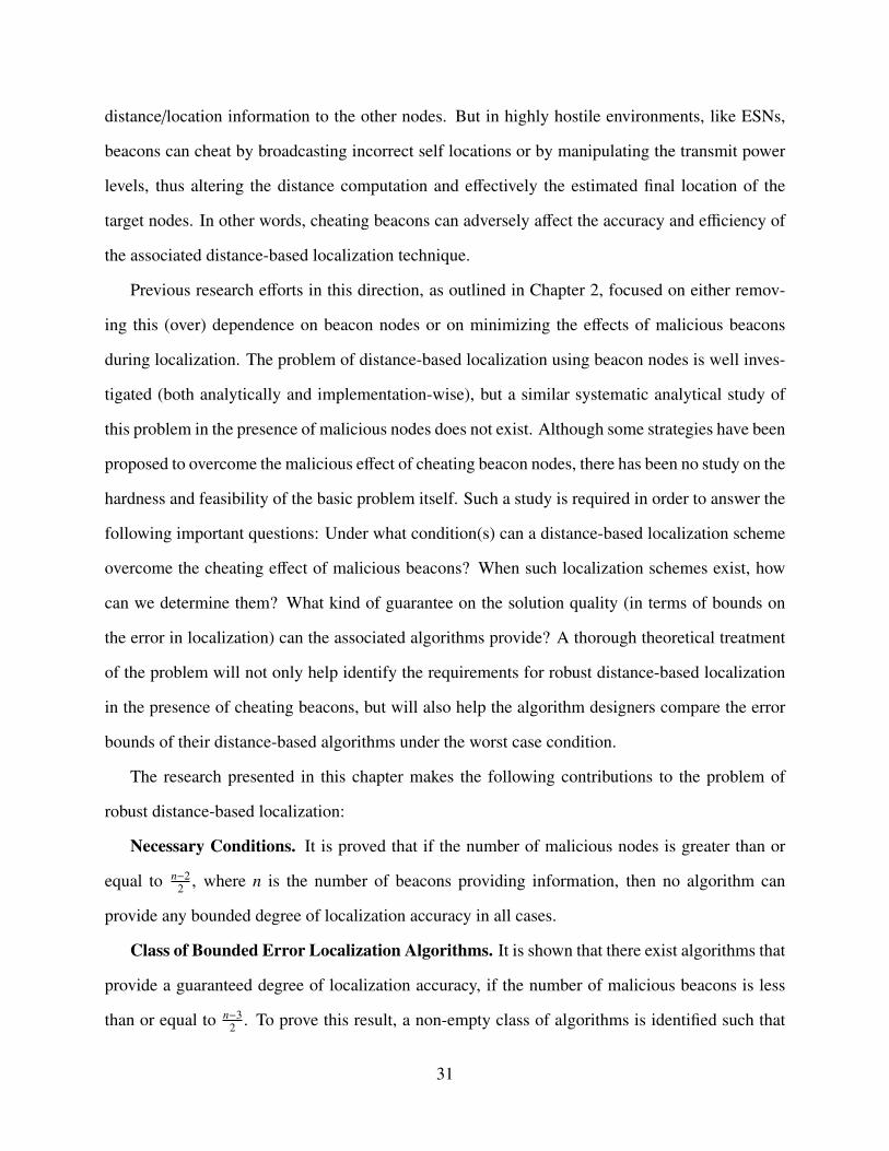
distance/location information to the other nodes. But in highly hostile environments, like ESNs,

beacons can cheat by broadcasting incorrect self locations or by manipulating the transmit power

levels, thus altering the distance computation and effectively the estimated final location of the

target nodes. In other words, cheating beacons can adversely affect the accuracy and efficiency of

the associated distance-based localization technique.

Previous research efforts in this direction, as outlined in Chapter 2, focused on either remov-

ing this (over) dependence on beacon nodes or on minimizing the effects of malicious beacons

during localization. The problem of distance-based localization using beacon nodes is well inves-

tigated (both analytically and implementation-wise), but a similar systematic analytical study of

this problem in the presence of malicious nodes does not exist. Although some strategies have been

proposed to overcome the malicious effect of cheating beacon nodes, there has been no study on the

hardness and feasibility of the basic problem itself. Such a study is required in order to answer the

following important questions: Under what condition(s) can a distance-based localization scheme

overcome the cheating effect of malicious beacons? When such localization schemes exist, how

can we determine them? What kind of guarantee on the solution quality (in terms of bounds on

the error in localization) can the associated algorithms provide? A thorough theoretical treatment

of the problem will not only help identify the requirements for robust distance-based localization

in the presence of cheating beacons, but will also help the algorithm designers compare the error

bounds of their distance-based algorithms under the worst case condition.

The research presented in this chapter makes the following contributions to the problem of

robust distance-based localization:

Necessary Conditions. It is proved that if the number of malicious nodes is greater than or

equal to n−22 , where n is the number of beacons providing information, then no algorithm can

provide any bounded degree of localization accuracy in all cases.

Class of Bounded Error Localization Algorithms. It is shown that there exist algorithms that

provide a guaranteed degree of localization accuracy, if the number of malicious beacons is less

than or equal to n−32 . To prove this result, a non-empty class of algorithms is identified such that

31

every algorithm in this class determines the target location with bounded localization error in all

cases.

Localization Algorithms. Two illustrative examples of algorithms in this class are proposed.

The first algorithm has a worst-case polynomial complexity (specifically, O(n3), where n is the

number of beacon nodes). The second algorithm is based on a clever heuristic and has much

better practical efficiency. The localization accuracy and computational efficiency of the proposed

algorithms are further verified through simulation experiments.

Generalization of Results. Current results for two dimensional systems are extended to three

dimensional systems.

3.1.2 Chapter Organization

This chapter is organized as follows. Section 3.2 presents the network and the adversary model.

Section 3.3 addresses the problem of robust distance-based localization in the presence of cheating

beacons. Section 3.3.1 derives and proves the necessary condition for existence of localization

algorithms with a guaranteed error bound; Section 3.3.2 gives the definition of the algorithm class

that provides the above mentioned guaranteed degree of accuracy while Section 3.3.3 presents the

error bound analysis. Two novel algorithms that belong to this class are outlined in Section 3.4,

while the experimental evaluations for these algorithms are presented in Section 3.5. The extension

to the three dimensional scenario is given in Section 3.6. Section 3.7 concludes the chapter with

some remarks and discussions on the significant results presented in the chapter.

3.2 Network and Adversary Model

In our network model, a mobile device M in a non-trustworthy environment wants to compute its

own location using distance estimates to a set of beacon nodes. These beacon nodes know their

own location and may or may not cheat about their location to other nodes. The target node M and

the beacon nodes are currently assumed to be located on a two dimensional area (plane), i.e., the

32

location of each of these entities can be represented as two dimensional coordinates (x, y) where,

x, y ∈ R. First, the results and analysis for a two dimensional system are presented and later in

Section 3.6 these results are extended to three dimensional systems.

Now, suppose that the target node M has n beacons available for localization. Let these beacon

nodes be denoted as B1, . . . , Bn. Among these n beacons, some beacons are malicious (cheating

beacons). Let k denote the number of malicious or cheating beacons. It is important to note that k

is not necessarily known to the mobile device or to any of the honest beacons. However, the value

of k clearly has a great influence on whether a bounded localization error can be achieved or not.

In Section 3.3.1, the condition for having a bounded localization error based on the value of k is

established. Let kmax (≤ n) be an upper bound on the number of malicious nodes, i.e., kmax is the

maximum number of malicious nodes that can exist in the network at any time. The parameter

kmax is a system or environment dependent constant and is generally known to the localization

algorithm.

Beacons that are not malicious are honest, i.e., they fully cooperate with the localization proto-

col by disclosing the information as truthfully as possible. More details on the cheating behavior

by the beacon nodes will follow shortly. Regardless of being honest or dishonest, each beacon Bi

provides M with a measurement di of the distance between Bi and M. (In practice, each beacon Bi

actually provides M with some information from which the distance di can be computed efficiently

by M. In order to simplify the current exposition, it is assumed here that Bi provides M the dis-

tance measurement di directly. This should not affect the presented results.) The precise distance

between Bi and M is the Euclidean distance between the position coordinates of Bi and M and is

denoted by dst(Bi,M). Let the set of honest beacons be denoted by H. Then, for each beacon

Bi ∈ H, di is assumed to be a random variable that follows some fixed probability distribution,

denoted as msr(dst(Bi,M)), such that

E[di] = dst(Bi,M),

33

i.e., the expected (mean) value of the estimated distance di for each beacon Bi in H, is the precise

distance between the beacon Bi and the node M. In the case when Bi is honest, the difference

between the estimated and the true distance is assumed to be very small, i.e.,

|di − dst(Bi,M)| < ε,

where ε is a small constant. Ideally, this difference should be zero when the beacon is honest, but

such discrepancies in distance estimates can occur due to factors like measurement errors either at

the source or target.

For each beacon Bi < H, i.e., a cheating beacon, the corresponding di is a value selected

arbitrarily by the adversary. Note that, colluding attacks are implicitly allowed here: In the model

presented here, it is assumed that a single adversary controls all malicious beacon nodes (all Bi <

H) and decides di for them. This is a very strong adversary model, which in addition to independent

adversaries also covers all possibility of collusion.

Since a distance-based localization strategy is assumed here, the output O of the corresponding

localization algorithm can be defined by a function F of the measured distances (di) from the

device M to every beacon node in the network as shown below.

O = F(d1, . . . , dn)

The error e of the localization algorithm is defined as the Euclidean distance between the actual

position of the mobile device and the one output by the algorithm.

e = E[dst(M,O)]

The next step is, given the above model, to derive the necessary conditions for the existence of

an algorithm that can perform distance-based localization with a bounded localization error in the

presence of malicious beacon nodes.

34

3.3 Robust Bounded Error Localization

The main focus of this section is to design bounded error distance-based localization algorithms

that are robust against cheating beacon nodes. In this direction, the necessary and sufficient con-

ditions for bounded error localization, given the above network and adversary model, are first

derived. Then, a class of robust localization algorithms is defined such that if these necessary

conditions are satisfied then a bounded localization error can be guaranteed. In addition to this,

theoretical properties like maximum error bound for this class of algorithms is also studied.

3.3.1 Necessary Condition for Bounded Error Localization

In order to achieve a bounded localization error, the first step is to derive a threshold of the num-

ber of malicious beacons k in terms of the total number beacons such that if k is greater than or

equal to this threshold then no algorithm would be able to guarantee a bounded localization error

just based on the distances to the beacon nodes. Consequently, having the number of malicious

beacons below this threshold is a necessary condition for getting a bounded localization error out

of any distance-based localization algorithm. In other words, it is required to fix the minimum

number of beacon nodes required, assuming that some of these beacons will cheat, to correctly

compute the location using just the distance information. Theorem 3.1 gives this threshold or nec-

essary condition.

Theorem 3.1. Lower Bound Theorem: Suppose that k ≥ n−22 . Then, for any distance-based local-

ization algorithm, for any locations of the beacons, there exists a scenario in which e is unbounded.

Proof. Without loss of generality, let k = n−22 (because more malicious beacons clearly can launch

any attack that n−22 malicious beacons can launch). The proof for the above theorem follows a

contradiction argument. Suppose that, in all scenarios the output error e < a, where a is a constant.

It is shown that this supposition leads to a contradiction. It is first proved that for a fixed set of

beacon nodes and beacon locations, if the above threshold holds (and if the exact identities of the

35

malicious nodes are not known) then there exists at least two distinct scenarios having the same

distribution of distances from the target node to the beacon nodes. This makes it impossible for any

algorithm to differentiate between the two scenarios. Since the target locations in the two scenarios

are significantly different, any algorithm must fail in one of the two scenarios.

Consider the two scenarios S 1 and S 2, as shown in Figure 3.1. The locations of all the beacons

are same in both the scenarios, but the set of honest beacon nodes and the position of the target

node M is assumed to be different in each scenario. Select an arbitrary point P in the line segment

B1B2 and draw a line L through P such that L is perpendicular to B1B2. Choose an arbitrary number

a′ > a. Then there are two points P1 and P2 on the line L such that

dst(P1, P) = dst(P2, P) =12

dst(P1, P2) = a′ ≥ a.

Figure 3.1: Two Scenarios for Lower Bound Theorem

In scenario S 1, M is at location P1 and the set of honest beacons is H1 = {B1, B2, B3, . . . , Bk+2}.

Denote by di,1 the measurement di in scenario S 1. So, for each Bi ∈ H1,

di,1 ∼ msr(dst(Bi, P1))

36

In scenario S 2, M is at location P2 and the set of honest beacons is H2 = {B1, B2, Bk+3, . . . , B2k+2}.

Denote by di,2 the measurement di in scenario S 2. So, for each Bi ∈ H2,

di,2 ∼ msr(dst(Bi, P2))

Assume that in scenario S 1, the adversary chooses dk+3,1, . . . , d2k+2,1 such that

∀i ∈ {k + 3, . . . , 2k + 2}, di,1 ∼ msr(dst(Bi, P2))

Similarly, assume that in scenario S 2, the adversary chooses d3,2, . . . , dk+2,2 such that

∀i ∈ {3, . . . , k + 2}, di,2 ∼ msr(dst(Bi, P1))

Since B1 and B2 are on the perpendicular bisector of line segment P1P2, we have

dst(B1, P1) = dst(B1, P2), and

dst(B2, P1) = dst(B2, P2)

Therefore, we get two pairs of identical distributions as shown below.

msr(dst(B1, P1)) � msr(dst(B1, P2)), and

msr(dst(B2, P1)) � msr(dst(B2, P2))

Now, it is easy to see that (d1,1, d2,1, d3,1, . . . , d2k+2,1) and (d1,2, d2,2, d3,2, . . . , d2k+2,2) are identically

distributed. Consequently, the two outputs

O1 = F(d1,1, d2,1, d3,1, . . . , d2k+2,1)

37

and

O2 = F(d1,2, d2,2, d3,2, . . . , d2k+2,2)

are also identically distributed. This implies that

E[dst(P2,O1)] = E[dst(P2,O2)]

On the other hand, from the previous assumption it can be seen that the output errors in both

scenarios are less than a.

e1 = E[dst(P1,O1)] < a, and

e2 = E[dst(P2,O2)] < a

Consequently,

dst(P1, P2) = E[dst(P1, P2)]

≤ E[dst(P1,O1)] + E[dst(P2,O1)]

= E[dst(P1,O1)] + E[dst(P2,O2)]

< a + a

= 2a.

This is contradictory to the fact that dst(P1, P2) = 2a′ ≥ 2a.

�

This brings us to the next result which shows that, given the network model as explained in

Section 3.2 and no more than n−32 cheating beacons, the location of M can be definitely computed

(for all the scenarios) with an error bound proportional to ε.

38

3.3.2 Algorithm Class for Robust Bounded Error Localization

Theorem 3.1 showed that having n−22 or more cheating beacons makes it impossible to compute

the location of M with a bounded error. The next set of result establishes that having n−32 or

fewer cheating beacons makes it possible to compute the location of M with a bounded error.

This particular condition can also be viewed as a sufficient condition for robust distance-based

localization in the presence of cheating beacons. Moreover, a class of algorithms that can compute

the location under this condition with a bounded localization error is also identified.

Before defining this algorithm class, let us introduce some terminology used during its defini-

tion (See Figure 3.2). For each beacon Bi, define a ring Ri using the following inequality:

Inner Boundary Circle

Critical Point

Outer Boundary Circle

Continuous Region

Continuous Arc

B3

2ǫ

B1

B2

Figure 3.2: Some Terminology for Class of Robust Localization Algorithms

di − ε < dst(Bi, X) < di + ε.

As mentioned in Section 3.2, ε is a small constant denoting some small measurement error. Clearly,

there are altogether n rings. The boundary of these n rings consists of 2n circles — called the

39

boundary circles. In particular, the inner circle of a ring is called an inner boundary circle, while

the outer circle of a ring is called an outer boundary circle.

Definition 3.1. A point is a critical point if it is the intersection of at least two boundary circles.

An arc is a continuous arc if it satisfies the following three conditions:

• The arc is part of a boundary circle.

• If the arc is not a complete circle, then its two ends are both critical points.

• There is no other critical point in the arc.

An area is a continuous region if it satisfies the following two conditions:

• The boundary of this area is one or more continuous arcs.

• There is no other continuous arc inside the area.

The class of robust localization algorithms can then be defined based on these rings as follows.

Definition 3.2. A localization algorithm is in the class of robust localization algorithms if its output

is a point in a continuous region r such that r is contained in the intersection of at least k + 3 rings.

Note that, the class of robust localization algorithms defined above is a non-empty class of

algorithms. This statement follows from the following theorem which proves that as long as k ≤

n−32 , it is always possible to find a non-empty continuous region r satisfying the requirements in

Definition 3.2.

Theorem 3.2. For k ≤ n−32 , there exists a non-empty continuous region r in the intersection of at

least k + 3 rings.

Proof. Consider the real location of mobile device M. Clearly, for each honest beacon Bi, M must

be in the ring Ri as shown below.

di − ε < dst(Bi,M) < di + ε.

40

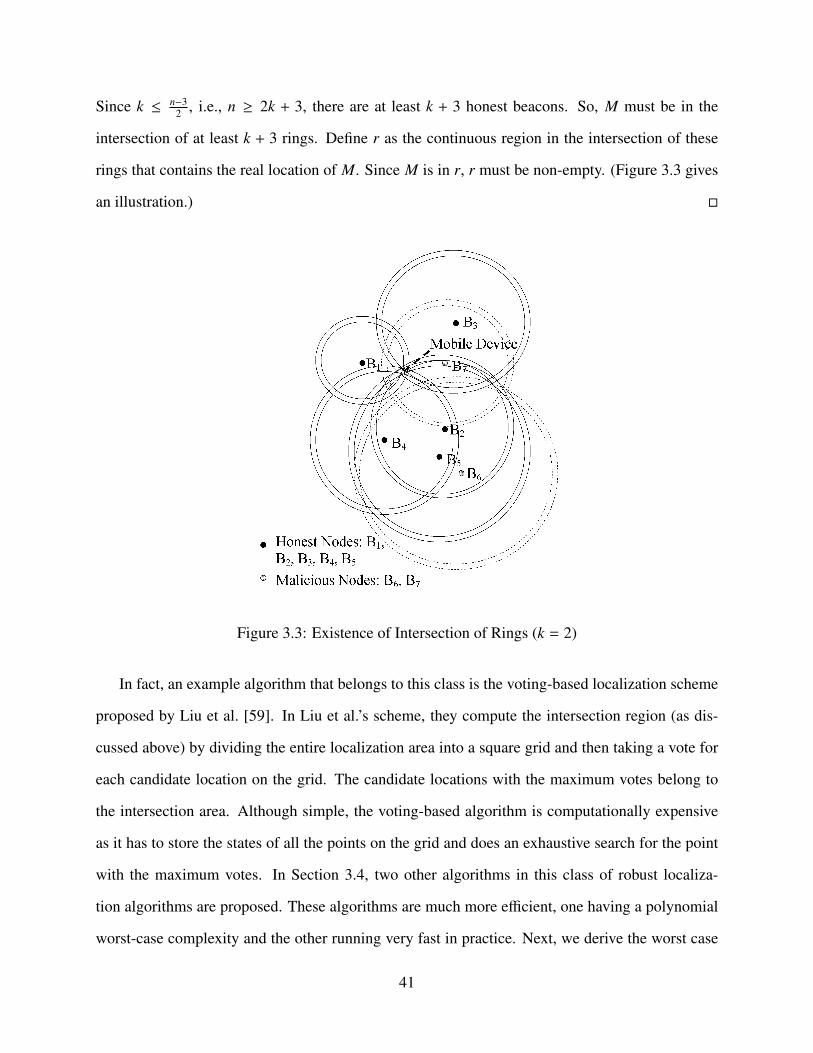
Since k ≤ n−32 , i.e., n ≥ 2k + 3, there are at least k + 3 honest beacons. So, M must be in the

intersection of at least k + 3 rings. Define r as the continuous region in the intersection of these

rings that contains the real location of M. Since M is in r, r must be non-empty. (Figure 3.3 gives

an illustration.) �

Figure 3.3: Existence of Intersection of Rings (k = 2)

In fact, an example algorithm that belongs to this class is the voting-based localization scheme

proposed by Liu et al. [59]. In Liu et al.’s scheme, they compute the intersection region (as dis-

cussed above) by dividing the entire localization area into a square grid and then taking a vote for

each candidate location on the grid. The candidate locations with the maximum votes belong to

the intersection area. Although simple, the voting-based algorithm is computationally expensive

as it has to store the states of all the points on the grid and does an exhaustive search for the point

with the maximum votes. In Section 3.4, two other algorithms in this class of robust localiza-

tion algorithms are proposed. These algorithms are much more efficient, one having a polynomial

worst-case complexity and the other running very fast in practice. Next, we derive the worst case

41

error bound of algorithms in this class of robust localization algorithms.

3.3.3 Error Bound Analysis

To analyze the error bound of algorithms in this class, two new definitions are needed.

Definition 3.3. The beacon distance ratio (γ) is defined as the minimum distance between a pair

of beacons divided by the maximum distance between a beacon and the mobile device.

γ =minBi,B j dst(Bi, B j)maxBi dst(Bi,M)

.

Definition 3.4. Consider the lines going through pairs of beacons. Denote by ang(BiB j, Bi′B j′) the

angle between lines BiB j and Bi′B j′ — to avoid ambiguity, we require that 0◦ ≤ ang(BiB j, Bi′B j′) ≤

90◦. The minimum beacon angle (α) is defined as the minimum of such angles.

α = minBi,B j,Bi′ ,B j′

ang(BiB j, Bi′B j′).

The following theorem bounds the maximum localization error possible in the presented robust

localization framework.

Theorem 3.3. For k ≤ n−32 , if ε � minBi dst(Bi,M) and there are no three beacons in the same line,

then the output error of any algorithm in the class of algorithms for robust localization, as defined

in Definition 3.2, is

e <2ε

min{sin arcsin(γ sin(α/2))

2 , cos arcsin(γ sin(α/2))2

} .Proof. Consider the continuous region r. It is in the intersection of at least k + 3 rings. Since there

are at most k dishonest beacons, at least 3 of these rings belong to honest beacons. Suppose that

Ri1 , Ri2 , and Ri3 are three rings belonging to honest beacons among the at least k+3 rings. Let r′ be

the continuous region in the intersection of Ri1 , Ri2 , and Ri3 that contains r. Since O is in r, clearly

O is also in r′. Next, let’s show that M is also in r′. Since M is also in the intersection of Ri1 , Ri2 ,

42

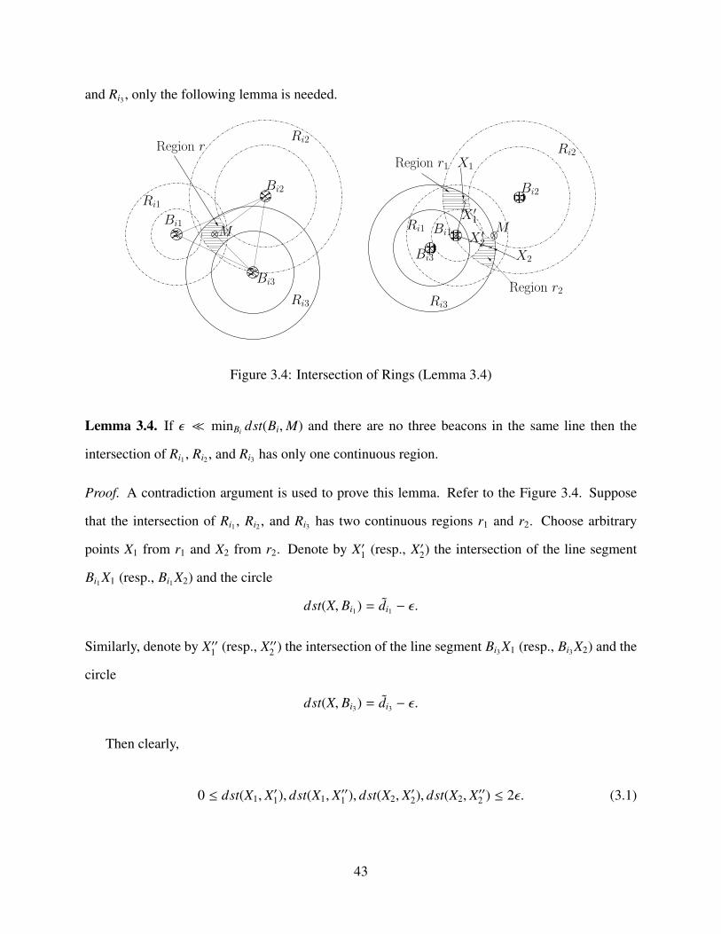
and Ri3 , only the following lemma is needed.

Bi2

Ri1

Ri2

Bi1

Bi3

Ri3

Region r

Ri3

Bi2

Ri2

Region r2

X2

X1

X′

1

Bi3

X′

2

Region r1

Ri1 Bi1M M

Figure 3.4: Intersection of Rings (Lemma 3.4)

Lemma 3.4. If ε � minBi dst(Bi,M) and there are no three beacons in the same line then the

intersection of Ri1 , Ri2 , and Ri3 has only one continuous region.

Proof. A contradiction argument is used to prove this lemma. Refer to the Figure 3.4. Suppose

that the intersection of Ri1 , Ri2 , and Ri3 has two continuous regions r1 and r2. Choose arbitrary

points X1 from r1 and X2 from r2. Denote by X′1 (resp., X′2) the intersection of the line segment

Bi1 X1 (resp., Bi1 X2) and the circle

dst(X, Bi1) = di1 − ε.

Similarly, denote by X′′1 (resp., X′′2 ) the intersection of the line segment Bi3 X1 (resp., Bi3 X2) and the

circle

dst(X, Bi3) = di3 − ε.

Then clearly,

0 ≤ dst(X1, X′1), dst(X1, X′′1 ), dst(X2, X′2), dst(X2, X′′2 ) ≤ 2ε. (3.1)

43

Also it can be seen that

ang(Bi1 Bi3 , Bi1 X1) = arccos(dst(Bi1 , X1)2 + dst(Bi1 , Bi3)2 − dst(X1, Bi3)

2)

= arccos((dst(Bi1 , X′1) + dst(X1, X′1))2 + dst(Bi1 , Bi3)

2

−(dst(X′′1 , Bi3) + dst(X1, X′′1 ))2)

= arccos((di1 − ε + dst(X1, X′1))2 + dst(Bi1 , Bi3)2

−(di3 − ε + dst(X1, X′′1 ))2).

Note that di1 > dst(Bi1 ,M) − ε � ε. Similarly, di3 � ε. Combining these facts with Equation (3.1)

we have

ang(Bi1 Bi3 , Bi1 X1) = arccos((di1 − ε + dst(X1, X′1))2 + dst(Bi1 , Bi3)2

−(di3 − ε + dst(X1, X′′1 ))2)

≈ arccos((di1)2 + dst(Bi1 , Bi3)

2 − (di3)2)

≈ arccos((di1 − ε + dst(X2, X′2))2 + dst(Bi1 , Bi3)2

−(di3 − ε + dst(X2, X′′2 ))2)

= arccos((dst(Bi1 , X′2) + dst(X2, X′2))2 + dst(Bi1 , Bi3)

2

−(dst(X′′2 , Bi3) + dst(X2, X′′2 ))2)

= arccos(dst(Bi1 , X2)2 + dst(Bi1 , Bi3)2 − dst(X2, Bi3)

2)

= ang(Bi1 Bi3 , Bi1 X2). (3.2)

Similarly, it can be shown that

ang(Bi1 Bi2 , Bi1 X1) ≈ ang(Bi1 Bi2 , Bi1 X2). (3.3)

However, when the two equations above (equations (3.2) and (3.3)) are put together, a contradiction

44

is reached. Without loss of generality assume that

ang(Bi1 Bi2 , Bi1 X1) < ang(Bi1 Bi3 , Bi1 X1),

since otherwise the indices i2 and i3 can be switched. It is easy to see that

ang(Bi1 Bi2 , Bi1 X1) = ang(Bi1 Bi3 , Bi1 X1) − ang(Bi1 Bi2 , Bi1 Bi3)

≤ ang(Bi1 Bi3 , Bi1 X1) − α

≈ ang(Bi1 Bi3 , Bi1 X2) − α

= ang(Bi1 Bi2 , Bi1 X2) − ang(Bi1 Bi2 , Bi1 Bi3) − α

≤ ang(Bi1 Bi2 , Bi1 X2) − 2α

≈ ang(Bi1 Bi2 , Bi1 X1) − 2α.

which is a contradiction.

�

Thus, it has been established that both M and O are in r′. This fact will be used to show that

e <2ε

min{sin arcsin(γ sin(α/2))

2 , cos arcsin(γ sin(α/2))2

}But before this result can be proved, another lemma is needed.

Lemma 3.5. If there are no three beacons in the same line, then either

ang(Bi1 M, Bi2 M) ≥ arcsin(γ sin(α/2)),

or

ang(Bi1 M, Bi3 M) ≥ arcsin(γ sin(α/2)).

45

Proof. Since ang(Bi1 Bi2 , Bi1 Bi3) ≥ α, either ang(Bi1 Bi2 , Bi1 M) ≥ α/2 or ang(Bi1 Bi3 , Bi1 M) ≥ α/2.

Below it is shown that, if ang(Bi1 Bi2 , Bi1 M) ≥ α/2 then

ang(Bi1 M, Bi2 M) ≤arcsin(γ sin(α/2))

2.

Similarly, if ang(Bi1 Bi3 , Bi1 M) ≥ α/2 then

ang(Bi1 M, Bi3 M) ≤arcsin(γ sin(α/2))

2.

Denote by D the distance from Bi2 to the line Bi1 M. Then,

ang(Bi1 M, Bi2 M) = arcsin(

Ddst(Bi2 ,M)

)= arcsin

(dst(Bi1 , Bi2) sin(ang(Bi1 Bi2 , Bi1 M))

dst(Bi2 ,M)

)≥ arcsin

(dst(Bi1 , Bi2) sin(α/2)

dst(Bi2 ,M)

)≥ arcsin(γ sin(α/2)).

�

Using the above lemma, without loss of generality let us assume that

ang(Bi1 M, Bi2 M) ≥ arcsin(γ sin(α/2)).

Denote by r′′ the continuous region in the intersection of Ri1 and Ri2 that contains r′. Since both M

and O are in r′, they should also be in r′′.

Each of the two rings involved has a pair of circles. Consider the four intersection points of

these two pairs of circles. Without loss of generality, suppose that the four intersection points

are V1, V2, V3, and V4, ordered in the clockwise direction, and that ∠V2V1V4 is acute. Since ε �

46

minBi dst(Bi,M), r′′ can be approximated using the quadrangle V1V2V3V4. It is easy to show that

ang(V1V2, Bi1 M) ≈ 90◦ ≈ ang(V3V4, Bi1 M)

Thus, it is clear that the line V1V2 is parallel to the line V3V4. Similarly, we can get that the line

V1V4 is parallel to the line V2V3. Therefore, V1V2V3V4 is a parallelogram. Furthermore, it can be

seen that

∠V2V1V3 = arcsin(

2εdst(V1,V3)

)= ∠V3V1V4.

Therefore, V1V2V3V4 is actually a rhombus. In a rhombus, the farthest distance between two points

is the length of its longer diagonal line. Therefore,

e = dst(M,O) ≤2ε

sin(∠V2V1V3)

=2ε

sin(∠V2V1V4

2

)≈

2ε

min{sin

(ang(Bi1 M,Bi2 M)2

), sin

(90◦ − ang(Bi1 M,Bi2 M)

2

)}≤

2ε

min{sin

(arcsin(γ sin(α/2))

2

), cos

(arcsin(γ sin(α/2))

2

)} .�

Next, two example algorithms in this class of robust localization algorithms are presented.

3.4 Bounded Error Localization Algorithms

The class of robust localization algorithms, as defined in Definition 3.2, contains algorithms that

output the location of a target in the continuous region of at least k + 3 rings. Two algorithms

47

belonging to this class are proposed here. The first algorithm has a worst case computational

complexity of O(n3 log n) (Refer to Lemma 3.7 for this result), which is polynomial in terms of

the number of beacons n. Clearly, this is much faster than an exhaustive search of all the grid

points [59]. But due to the cubic complexity and the involved exhaustive search, it runs slow

even for reasonable large values of n. To overcome this problem, a second algorithm based on a

clever heuristic is proposed. Although it does not have a worst-case complexity analysis as the

first algorithm, it runs very fast in practice. Recall that these algorithms work under the condition

k ≤ n−32 . Thus, an upper bound for k (number of malicious beacons) can be defined as kmax =

n−32 .

Both the algorithms presented here find the continuous region r in the intersection of kmax + 3 rings

and output a point in this region. However, the two algorithms find this continuous region using

different techniques.

3.4.1 A Polynomial Time Algorithm

Before a polynomial-time algorithm is presented, a lemma that gives the relationship between the

continuous region and the continuous arcs on its boundary is required.

Definition 3.5. A ring is related to a continuous arc if the continuous arc is inside but not on the

boundary of this ring.

Lemma 3.6. Suppose that r is a continuous region and c is a continuous arc on the boundary of r.

Then r is in the intersection of at least k + 3 rings if and only if at least k + 2 rings are related to c.

Proof. The proof is straightforward.

�

The main idea of the polynomial-time algorithm is that in order to determine a continuous

region in the intersection of at least kmax + 3 rings it is sufficient to count the number of rings

related to each continuous arc and then find a continuous arc such that at least kmax + 2 rings are

related to it (It is easy to check if a ring is related to a continuous arc by comparing the distance

48

between the arcs end points and the center of the ring to the inner and outer radii of the ring).

Once such an arc is found, depending on whether the arc is on an outer boundary circle or an inner

boundary circle, a point can be picked from either the inner region or the outer region of the arc

respectively. The details of the algorithm are as shown in Algorithm 1.

1: Let S be a set initially containing the two boundary circles of ring R1

2: for i = 2, . . . , n do3: Let S i be a set initially containing the two boundary circles of ring Ri

4: for each arc in S and each arc in S i do5: if the above two arcs intersect then6: Split each of these two arcs using the intersection(s), and replace them in the corre-

sponding arc sets (S or S i) with the new splitted arcs (result of the splitting operation)7: end if8: end for9: Let S = S ∪ S i

10: end for11: for each arc c j in S do12: Set the corresponding counter λ j to 013: for i = 1, . . . , n do14: if Ri is related to c j then15: λ j = λ j + 116: end if17: end for18: if λ j ≥ kmax + 2 then19: if c j is on an inner boundary circle then20: Output is defined on the side out of this circle21: else if c j is on an outer boundary circle then22: Output is defined on the side inside this circle23: end if24: Stop the algorithm25: end if26: end for

Algorithm 1: Polynomial-time Algorithm

Lemma 3.7. The worst-case time complexity of the above algorithm is O(n3 log n).

As discussed before, although the worst case time complexity of the polynomial time algorithm

is polynomial in terms of the total number of beacons in the system, it runs pretty slow for most

cases. The reason behind this is that for all the cases it attempts to compute all the continuous arcs

49

and searches for the best related arc among these. This computation is even slower for reasonable

large values of n (e.g., n ≈ 50). The execution time is in the order of seconds which is not good

(See Section 3.5.2 for the results of the simulation experiments for the polynomial time algorithm.)

To overcome this problem, a smart heuristic is proposed next. This heuristic attempts to guess the

target location around a critical point that lies on the intersection of large number of rings.

3.4.2 A Fast Heuristic Algorithm

The details of the heuristic are as follows: Note that kmax + 3 is already a large number of rings.

Since the region r is contained in at least kmax + 3 rings, the rings containing r are intersecting with

large numbers of other rings. In other words, if a ring Ri is intersecting with a large number of rings,

it is very likely that Ri contains r. Therefore, the heuristic first considers the rings intersecting with

a large numbers of other rings. The details of the heuristic algorithm is outlined in Algorithm 2.

1: Count the number of rings intersecting with each ring2: for each ring Ri, in the order of decreasing number of rings intersecting with it do3: for each ring R j,R j , Ri, in the order of decreasing number of rings intersecting with it do4: Compute the intersection points of the boundary circles of Ri and R j

5: for m = 1, . . . , γ do6: Choose a random intersection point computed above7: Choose a random point O near this intersection point (such that the distance between

them is less than ε)8: Count the number of rings containing O9: if there are at least kmax + 3 rings containing O then

10: Output O11: Stop the Algorithm12: end if13: end for14: end for15: end for

Algorithm 2: Fast Heuristic Algorithm

The next section verifies the accuracy and practical efficiency of the above algorithms by using

measurements from computer simulation experiments.

50

3.5 Evaluation

Performance evaluation of the proposed localization algorithms includes verification and compar-

ison of the localization accuracy and simulation time for each of these algorithms under varying

parameters like beacon node distribution over the deployment area, number of malicious nodes (k)

and the maximum distance measurement error (ε). Currently, network properties like communi-

cation overhead of these algorithms is not being evaluated. This is because, these algorithms are

very general and properties like communication overhead depends on the specific type of ranging

or distance measurement technique used. Moreover, other network related factors like radio inter-

ference, signal loss, obstructions, etc., can also affect the accuracy and efficiency of the proposed

algorithms. The current study aims to first evaluate these algorithms only under ideal network con-

ditions by assuming a small distance measurement error ε. In view of this, the current simulation

experiments do not employ a software network simulator tool like ns-2 [32]. Experimental objec-

tives for evaluating the proposed algorithms are easily achieved just by coding them using basic

C++ language [17] programs. Results from this study would act as a stepping stone for improving

these algorithms further and porting them to more complex network environments, for example,

using network simulators and test beds that employ more practical network and radio models.

3.5.1 Experimentation Setup

The experimental setup is pretty straightforward. The simulation area consists of a 500m × 500m

two dimensional plane. There are a total of 43 beacon nodes and one target node and there is

no node mobility. The radio range of each node (including the beacons and the target node) is

250m. The positions of each of the nodes is selected uniformly over the 500m × 500m area. Each

algorithm has been evaluated under similar conditions and for two different distributions of the

distance measurement error, namely, Uniform distribution and Normal distribution. For each of

these two distributions, the influence of the number of malicious beacons (k) and the maximum

measurement error (ε) on the localization error and the algorithm execution time is studied.

51

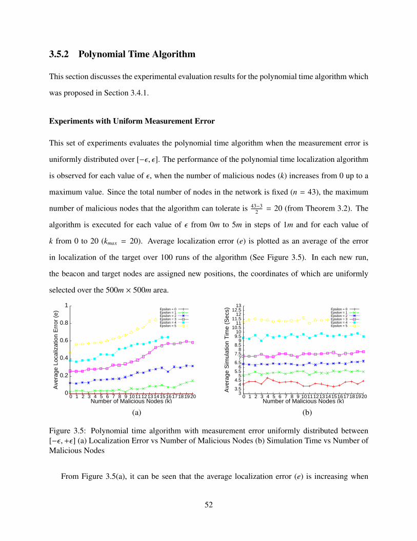
3.5.2 Polynomial Time Algorithm

This section discusses the experimental evaluation results for the polynomial time algorithm which

was proposed in Section 3.4.1.

Experiments with Uniform Measurement Error

This set of experiments evaluates the polynomial time algorithm when the measurement error is

uniformly distributed over [−ε, ε]. The performance of the polynomial time localization algorithm

is observed for each value of ε, when the number of malicious nodes (k) increases from 0 up to a

maximum value. Since the total number of nodes in the network is fixed (n = 43), the maximum

number of malicious nodes that the algorithm can tolerate is 43−32 = 20 (from Theorem 3.2). The

algorithm is executed for each value of ε from 0m to 5m in steps of 1m and for each value of

k from 0 to 20 (kmax = 20). Average localization error (e) is plotted as an average of the error

in localization of the target over 100 runs of the algorithm (See Figure 3.5). In each new run,

the beacon and target nodes are assigned new positions, the coordinates of which are uniformly

selected over the 500m × 500m area.

0

0.2

0.4

0.6

0.8

1

0 1 2 3 4 5 6 7 8 9 10 11 12 13 14 15 16 17 18 19 20

Ave

rage

Loc

aliz

atio

n E

rror

(e)

Number of Malicious Nodes (k)

Epsilon = 0Epsilon = 1Epsilon = 2Epsilon = 3Epsilon = 4Epsilon = 5

3 3.5

4 4.5

5 5.5

6 6.5

7 7.5

8 8.5

9 9.5 10

10.5 11

11.5 12

12.5 13

0 1 2 3 4 5 6 7 8 9 10 11 12 13 14 15 16 17 18 19 20

Ave

rage

Sim

ulat

ion

Tim

e (S

ecs)

Number of Malicious Nodes (k)

Epsilon = 0Epsilon = 1Epsilon = 2Epsilon = 3Epsilon = 4Epsilon = 5

(a) (b)

Figure 3.5: Polynomial time algorithm with measurement error uniformly distributed between[−ε,+ε] (a) Localization Error vs Number of Malicious Nodes (b) Simulation Time vs Number ofMalicious Nodes

From Figure 3.5(a), it can be seen that the average localization error (e) is increasing when

52

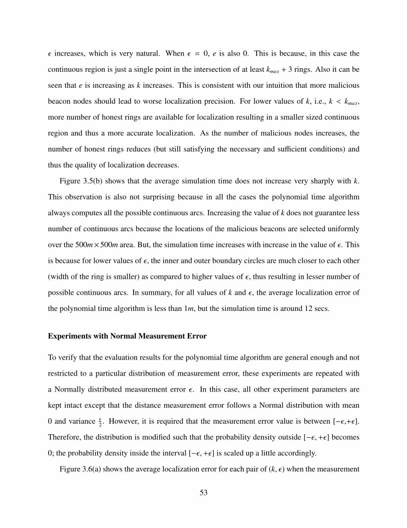
ε increases, which is very natural. When ε = 0, e is also 0. This is because, in this case the

continuous region is just a single point in the intersection of at least kmax + 3 rings. Also it can be

seen that e is increasing as k increases. This is consistent with our intuition that more malicious

beacon nodes should lead to worse localization precision. For lower values of k, i.e., k < kmax,

more number of honest rings are available for localization resulting in a smaller sized continuous

region and thus a more accurate localization. As the number of malicious nodes increases, the

number of honest rings reduces (but still satisfying the necessary and sufficient conditions) and

thus the quality of localization decreases.

Figure 3.5(b) shows that the average simulation time does not increase very sharply with k.

This observation is also not surprising because in all the cases the polynomial time algorithm

always computes all the possible continuous arcs. Increasing the value of k does not guarantee less

number of continuous arcs because the locations of the malicious beacons are selected uniformly

over the 500m×500m area. But, the simulation time increases with increase in the value of ε. This

is because for lower values of ε, the inner and outer boundary circles are much closer to each other

(width of the ring is smaller) as compared to higher values of ε, thus resulting in lesser number of

possible continuous arcs. In summary, for all values of k and ε, the average localization error of

the polynomial time algorithm is less than 1m, but the simulation time is around 12 secs.

Experiments with Normal Measurement Error

To verify that the evaluation results for the polynomial time algorithm are general enough and not

restricted to a particular distribution of measurement error, these experiments are repeated with

a Normally distributed measurement error ε. In this case, all other experiment parameters are

kept intact except that the distance measurement error follows a Normal distribution with mean

0 and variance ε2 . However, it is required that the measurement error value is between [−ε,+ε].

Therefore, the distribution is modified such that the probability density outside [−ε,+ε] becomes

0; the probability density inside the interval [−ε,+ε] is scaled up a little accordingly.

Figure 3.6(a) shows the average localization error for each pair of (k, ε) when the measurement

53

error follows the Normal distribution. Figure 3.8(b) shows the corresponding simulation time plot.

It can be seen that the curves are analogous to those in Figures 3.5(a) and 3.5(b) respectively, except

that the localization error increases more slowly with k in this case. Thus, it has been verified that

the presented evaluation results are valid for different distributions of measurement errors.

0

0.5

1

1.5

2

2.5

0 1 2 3 4 5 6 7 8 9 10 11 12 13 14 15 16 17 18 19 20

Ave

rage

Loc

aliz

atio

n E

rror

(e)

Number of Malicious Nodes (k)

Epsilon = 0Epsilon = 1Epsilon = 2Epsilon = 3Epsilon = 4Epsilon = 5

2 2.25

2.5 2.75

3 3.25

3.5 3.75

4 4.25

4.5 4.75

5 5.25

5.5 5.75

6

0 1 2 3 4 5 6 7 8 9 10 11 12 13 14 15 16 17 18 19 20

Ave

rage

Sim

ulat

ion

Tim

e (S

ecs)

Number of Malicious Nodes (k)

Epsilon = 0Epsilon = 1Epsilon = 2Epsilon = 3Epsilon = 4Epsilon = 5

(a) (b)

Figure 3.6: Polynomial time algorithm with measurement error Normally distributed between[−ε,+ε] with mean 0 and variance ε

2 (a) Localization Error vs Number of Malicious Nodes (b)Simulation Time vs Number of Malicious Nodes

In conclusion, we can see that although the polynomial time algorithm is pretty accurate, it is

very inefficient and slow with execution time in the order of seconds.

3.5.3 Fast Heuristic Algorithm

This section discusses the evaluation of the fast heuristic algorithm proposed in Section 3.4.2.

Experiments with Uniform Measurement Error

Similar to the experiments for the polynomial time algorithm, first the scenario for uniformly

distributed measurement error (over [−ε, ε]) is studied. The performance of the heuristic-based

localization algorithm for each value of ε, when the number of malicious nodes (k) in the network

increases, is observed. Since the total number of nodes in the network is fixed (n = 43), the

maximum number of malicious nodes that the algorithm can tolerate is 43−32 = 20 (from Theorem

54

3.2). The simulation of the fast heuristic-based algorithm is run for each value of ε from 0m to 50m

in steps of 10m and each value of k from 0 to 20 (kmax = 20). Note that here we have drastically

increased the value of ε as compared to the evaluation for the polynomial time algorithm. This is

done to observe the effects of large measurement errors on the localization accuracy and execution

times of the algorithm. Average localization error (e) is then plotted as an average of the error in

localization of the target node over 1000 runs (See Figure 3.7). In each new run, the beacon and

target nodes are assigned new positions, the coordinates of which are uniformly selected over the

500m × 500m area.

0

5

10

15

20

25

30

0 1 2 3 4 5 6 7 8 9 10 11 12 13 14 15 16 17 18 19 20

Ave

rage

Loc

aliz

atio

n E

rror

(e)

Number of Malicious Nodes (k)

Epsilon = 0Epsilon = 10Epsilon = 20Epsilon = 30Epsilon = 40Epsilon = 50

0 0.01 0.02 0.03 0.04 0.05 0.06 0.07 0.08 0.09

0.1 0.11 0.12 0.13 0.14 0.15 0.16 0.17 0.18 0.19

0.2

0 1 2 3 4 5 6 7 8 9 10 11 12 13 14 15 16 17 18 19 20

Ave

rage

Sim

ulat

ion

Tim

e (s

ecs)

Number of Malicious Nodes (k)

Epsilon = 0Epsilon = 10Epsilon = 20Epsilon = 30Epsilon = 40Epsilon = 50

(a) (b)

Figure 3.7: Fast Heuristic algorithm with measurement error uniformly distributed between[−ε,+ε] (a) Localization Error vs Number of Malicious Nodes (b) Simulation Time vs Numberof Malicious Nodes

From Figure 3.7(a), it can be seen that the average localization error (e) is increasing when ε

increases, which is again a very intuitive observation. Also, e is increasing as k increases. This

is also consistent with our intuition that more malicious beacon nodes should lead to worse local-

ization precision. For lower values of k, i.e., k < kmax, more number of honest rings are available

for localization resulting in a smaller region of intersection and eventually a more precise local-

ization. As the number of malicious nodes increases, the number of honest rings reduces (but still

satisfying the necessary and sufficient conditions) and thus the quality of localization decreases.

Figure 3.7(b) shows that the average simulation time of the fast heuristic algorithm increases

in k, but increases only very slightly. This observation is also not surprising since the algorithm is

55

computing the intersection of the same number of rings for each value k. The main reason for the

slight increase in simulation time is that a larger number of malicious beacons makes it harder to

find the right continuous region in the intersection of kmax + 3 rings using the proposed heuristic.

For all values of k and ε, the average localization error of the heuristic-based algorithm is less than

25m and the simulation time is less than 0.035 secs.

Experiments with Normal Measurement Error

Once again, to ensure that the evaluation results are not only restricted to a uniformly distributed

measurement error, the experiments are repeated with a Normally distributed measurement error.

All other experiment parameters except the distance measurement error distribution are kept intact.

The distance measurement error follows a Normal distribution with mean 0 and variance ε2 . As

before, the distribution is modified such that the probability density outside [−ε,+ε] becomes 0.

Figure 3.8(a) shows the average localization error for each pair of (k, ε) when the measure-

ment error follows the Normal distribution. Figure 3.8(b) shows the corresponding simulation

time. We can see that the curves are analogous to those in Figures 3.7(a) and 3.7(b) respectively,

except that the localization error increases more slowly with k. Therefore, it is verified that the

presented evaluation results for the fast heuristic algorithm are also valid for different distributions

of measurement errors.

3.6 Extension to Three Dimensional Coordinate Systems

Results and observations for the problem of robust distance-based localization outlined up to this

point are applicable only to two dimensional coordinate systems, i.e., systems where the nodes

(both target and beacon nodes) are located in a two dimensional space. Node positions in this case

are expressed by two dimensional coordinates (x, y), where x, y ∈ R. But, in certain environments

(like mountains, valleys, etc.) and applications, three dimensional localization is needed. In this

section, the results previously proposed for two dimensional localization systems are extended for

56

0 1 2 3 4 5 6 7 8 9

10 11 12 13 14 15 16 17 18 19 20 21 22 23 24 25 26 27 28 29 30

0 1 2 3 4 5 6 7 8 9 10 11 12 13 14 15 16 17 18 19 20

Ave

rage

Loc

aliz

atio

n E

rror

(e)

Number of Malicious Nodes (k)

Epsilon = 0Epsilon = 10Epsilon = 20Epsilon = 30Epsilon = 40Epsilon = 50

0 0.01 0.02 0.03 0.04 0.05 0.06 0.07 0.08 0.09

0.1 0.11 0.12 0.13 0.14 0.15 0.16 0.17 0.18 0.19

0.2

0 1 2 3 4 5 6 7 8 9 10 11 12 13 14 15 16 17 18 19 20

Ave

rage

Sim

ulat

ion

Tim

e (s

ecs)

Number of Malicious Nodes (k)

Epsilon = 0Epsilon = 10Epsilon = 20Epsilon = 30Epsilon = 40Epsilon = 50

(a) (b)

Figure 3.8: Fast Heuristic algorithm with measurement error Normally distributed between[−ε,+ε] with mean 0 and variance ε

2 (a) Localization Error vs Number of Malicious Nodes (b)Simulation Time vs Number of Malicious Nodes

the three dimensional case. Similar to the analysis presented for the two dimensional case, first the

necessary condition for robust three dimensional localization in the presence of cheating beacon

nodes is derived. It turns out that for the three dimensional case the maximum number of malicious

beacons (in terms of the total number of beacons) that can be tolerated is slightly smaller than the

two dimensional case. As a result, the definition of the class of robust localization algorithms

including the fundamental error limits of these algorithms vary for the three dimensional case. The

basic notations and the network model used here is similar to the two dimensional case except that

the position of each node is represented by three dimensional coordinates (x, y, z), where x, y, z ∈ R.

Theorem 3.8. Suppose that k ≥ n−32 . Then, for any distance-based 3-dimensional localization

algorithm, for any locations of the beacons, there exists a scenario in which the localization error

e is unbounded.

With k ≤ n−42 , a class of bounded error algorithms for 3-dimensional localization can also be

established. But to obtain this result, a few new definitions are needed.

For each beacon Bi, a global shell similar to the ring in the two dimensional case is defined as

shown below.

di − ε < dst(Bi, X) < di + ε.

57

For simplicity, denote the above global shell using Ri. The globes on the boundary of these shells

are called the boundary globes; the inner globe of a shell is called an inner boundary globe, while

the outer globe of a shell is called an outer boundary circle. A continuous three dimensional

region is part of the space such that its boundary consists of parts of boundary globes, and that

no boundary globe goes through its internal. The class of three dimensional robust localization

algorithms can be defined as follows:

Definition 3.6. An algorithm belongs to the class of three dimensional robust localization algo-

rithms if and only if its output is a point in a continuous three dimensional region r such that r is

in the intersection of at least k + 4 global shells.

Definition 3.7. Consider the planes going through triples of beacons. Denote by ang(Bi1 Bi2 Bi3 , Bi′1Bi′2

Bi′3)

the angle between the two planes Bi1 Bi2 Bi3 and Bi′1Bi′2

Bi′3— to avoid ambiguity, we require that

0◦ ≤ ang(Bi1 Bi2 Bi3 , Bi′1Bi′2

Bi′3) ≤ 90◦. The minimum beacon plane angle is defined as the minimum

of such angles:

α? = minBi1 ,Bi2 ,Bi3 ,Bi′1

,Bi′2,Bi′3

ang(Bi1 Bi2 Bi3 , Bi′1Bi′2

Bi′3).

Given the above definitions, the result on three dimensional localization analogous to Theorem

3.3 can now be stated.

Theorem 3.9. For k ≤ n−42 , if ε � minBi dst(Bi,M) with no three beacons in the same line nor

four beacons on the same plane, the output error of algorithms in the class of robust localization

algorithms (for three dimensional coordinate systems) is

e < 2ε

√1β2 + (

1sinα?

+1

β · tanα?)2

and, β = min{sin

(arcsin(γ sin(α/2))

2

), cos

(arcsin(γ sin(α/2))

2

)}.

It is clear from the above analysis that the number of cheating beacons that can be tolerated

for the three dimensional case is lower and the localization error bound is higher as compared to

58

the two dimensional case. Moreover, the proposed localization algorithms can also be easily ex-

tended for the three dimensional case. In the polynomial time algorithm for the three dimensional

case, it would be required to compute the continuous parts of the inner or outer boundary globes

instead of the inner or outer continuous arcs as in the two dimensional case. Whereas for the fast

heuristic-based algorithms, it would be required to compute the intersection point of a maximum

number of globes as the first step. Naturally, the programming effort required to implement these

algorithms would be greater than the two dimensional case due to the difficulty in representing

three dimensional systems.

3.7 Conclusion

This chapter addressed the problem of robust distance-based localization in the presence of cheat-

ing beacon nodes. Assuming a practical network and adversary model, the question of whether

robust distance-based localization in the presence of cheating nodes is possible or not, has been

answered by means of a sound mathematical analysis. More precisely, the necessary and sufficient

conditions for achieving a bounded error for the secure localization problem are derived and a

non-empty class of algorithms that can achieve such a bounded error is identified. In order to gain

a better understanding of these algorithms, important analytical properties including the maximum

error bound are also derived for these algorithms.

Following a detailed theoretical study of the secure localization problem and the class of ro-

bust distance-based algorithms, two novel algorithms that belong to this class are proposed. First,

a polynomial-time algorithm that guarantees to finish in polynomial time (specifically, cubic com-

plexity), even in the worst case, is proposed. Next, a fast heuristic-based algorithm that is suitable

and efficient even for reasonably large values of beacon nodes n is proposed. By means of computer

simulation experiments, the localization accuracy and execution efficiency of both the algorithms

are verified. Simulation experiments showed that although the polynomial time algorithm provided

good localization precision, it was rather slow for larger values of n. The heuristic-based algorithm

59

on the other hand, provided good localization precision with a very small time cost even for larger

values of n. Experiments also showed that both the algorithms worked consistently for different

distributions of the distance measurement error ε. Finally, to show the generality of the analytical

findings and the proposed localization algorithms, an extension to the 3-dimensional case was also

provided.

The next chapter studies the problems of efficient sensor node deployment and fault-tolerant

signature-based localization in sensor network applications where sensor node disablement is

prevalent.

60

Chapter 4

Fault-tolerant Signature-based Localization

“What does not destroy me, makes me stronger.”

− Friedrich Wilhelm Nietzsche

4.1 Introduction

In this chapter, the problem of fault-tolerance in signature-based localization schemes is addressed.

It first introduces a novel strategy for node deployment, which employs a stochastic model of node

destruction for making deployment decisions and has provisions for monitoring node destruction

within node groups. Such a strategy is extremely useful during ESN deployment in emergency,

first response and military applications. In addition to the deployment strategy, this chapter also

outlines and verifies fault-tolerance related improvements to existing signature-based schemes and

proposes a novel yet simple technique for fault-tolerant signature-based localization.

4.1.1 Motivation and Problem Statement

As discussed in Chapter 1, the feasibility of beacon-based schemes for localization depends on

factors like cost of beacon nodes, risk associated with beacon deployment, difficulty associated

with localizing the beacons themselves (GPS-related problems), etc. Moreover, the success of

beacon-based schemes solely depends on the available beacon nodes, i.e., if sufficient number of

61

beacon nodes fail then there is a good chance that the other nodes may not be able to localize them-

selves. These scenarios are possible during information collection and monitoring applications in

emergencies like wars, forest fires, earthquakes, etc. An emergency scenario is generally charac-

terized by an unpredictable or sometimes predictable sequence of events occurring with different

magnitudes over various parts of the emergency area. In such scenarios, sensor node deploy-

ment is highly specific for each part of the emergency area and the size of the node group around

each part depends on the intensity of the event there. In other words, there is some form of non-

uniformity, inherently present in such deployments, that can be exploited by the signature-based

schemes for localization. Signature-based schemes work by assuming that nodes are distributed in

a non-uniform fashion over the deployment area and then utilize this non-uniform distribution to

compute location for each target node. Each target node observes its neighborhood and uses this

observation as a signature to map to its most likely location. Signature-based schemes, which are

beaconless in nature, generally use statistical techniques such as Maximum Likelihood Estimation

(MLE) and Multi-dimensional scaling to generate the correct mapping between data like node dis-

tribution, connectivity information, etc., and the target locations. Efficient localization algorithms

that employ intelligent signature-based strategies exist in the literature (outlined in Chapter 2.)

All the above factors suggest that signature-based schemes could effectively replace beacon-based

schemes in ESN applications.

But despite these advances, fault-tolerance of signature-based localization approaches, espe-

cially in ESN applications, is still an issue. Given the fragility of sensor nodes and the nature of

the emergency related applications, it is natural to expect that nodes will be destroyed/disabled dur-

ing the period of the application. One weakness of existing signature-based schemes is that they

are not resistant to changes in node distribution. Since majority of the signature-based schemes

use node distribution to predict location, their accuracy is adversely affected by factors like node

disablement that alter the node distribution [48]. To further verify this, experiments that simulate

random node disablement in a classical signature-based scheme like the beaconless scheme pro-

posed by Lei et al. [26] are conducted. As discussed later in the chapter, these experiments confirm

62

that the localization accuracy of the above algorithm decreases as the number of destroyed/disabled

nodes increases.

The main focus of this chapter is the construction of signature-based localization schemes that

are robust against random node destruction/disablement. In order to achieve this goal, the two main

factors that affect the accuracy of signature-based schemes, viz., 1) the initial node distribution

over the deployment area, and 2) random node disablement need to be addressed. To provide an

efficient distribution of sensor nodes in applications with high disablement rate, a well-planned

deployment strategy is required. This strategy should not only be robust against the vagaries of the

external factors that cause sensor node disablement but should also help the process of signature-

based localization in a productive way. In this direction, an emergency level-based deployment

strategy is first proposed. This strategy distributes the sensor nodes over the emergency area by

dividing the area into various emergency levels depending on the severity of the emergency at

each point. The process of node destruction around each point is modeled as a non-homogeneous

stochastic process. The emergency level-based deployment strategy employs this model of node

destruction to make various deployment decisions including determining deployment size for each

group. The deployment strategy also has provisions to continuously monitor node disablement in

each group and disseminate this information to other nodes. Due to its relevance to ESNs, this

chapter currently only focuses on the problem of node disablement and its effect on signature-

based schemes. The issue of dynamic node distribution due to internal node failures, random node

movement, false node injection attacks [48], etc., and their effects on signature-based schemes is a

non-trivial topic by itself and will be addressed in the future as an extension of the current work.

The next part of the chapter deals with improving the fault-tolerance of existing signature-

based schemes. In that direction, first an intuitive and simple improvement to existing signature-

based schemes, called Group Selection Protocol (GSP), is proposed. GSP is a node selection

strategy that complements signature-based schemes by choosing appropriate groups of nodes for

participation in the localization process and dropping measurements from groups with a large

number of faulty nodes. Although GSP works towards improving the fault-tolerance of existing

63

signature-based schemes, it does not simplify the localization process. Signature-based schemes

are computationally intensive, involving complex functions that are sometimes not feasible on low

powered, resource constrained sensor nodes. To overcome this problem, A Simple FAult-Tolerant

signature-based localization scheme (ASFALT) is proposed. ASFALT uses the distribution of

nodes over the deployment area, and a simple averaging argument to compute distances to known

deployment points, which in turn are used in localizing target nodes by means of trilateration.

Measurement results from simulation experiments are used to verify the performance and accuracy

of localization of both GSP and ASFALT as compared to other popular signature-based algorithms

like the beaconless algorithm by Lei et al. [26] in situations of arbitrary disablement of nodes.

4.1.2 Chapter Organization

This chapter is organized as follows. Section 4.2 presents the case study of a well known signature-

based localization technique and discusses its shortcomings for use in applications with high node

disablement rate. Section 4.3 discusses a stochastic model of node destruction and presents an

emergency level-based node deployment strategy that employs this model to make deployment

decisions. Section 4.4 outlines the Group Selection Protocol (GSP), while Section 4.5 proposes

the ASFALT signature-based localization technique. Section 4.6 presents the evaluation results

and a comparative analysis of the proposed solutions. The chapter concludes with a summary of

contributions in Section 4.7.

4.2 Case Study: Signature-based Localization

The case study of a typical signature-based localization technique, specifically the scheme pro-

posed by Fang et al. [26], serves two purposes. First, it explains the mechanics of an ideal

signature-based localization scheme and attempts to bring out its advantages and limitations in

an ESN setting. Second, it acts as a good starting point for improving the fault-tolerance and

robustness of existing signature-based techniques.

64

4.2.1 Deployment Model and Localization Scheme

The localization technique discussed in this case study employs a group-based deployment strategy

where the entire deployment area is first divided into a grid of, say, n points. Then, nodes are

planned to be deployed in groups of equal sizes at each such point on the grid. The final position

of each node after deployment is not the same as the planned point and is assumed to follow some

non-uniform distribution, e.g., Normal (Gaussian), around the point of deployment with the mean

as that point. Since, many physical phenomena in nature can be easily modeled using a Normal

distribution, a group of sensor nodes dropped at a point can be assumed to be scattered in a Normal

distribution around it. Then, the average deployment distribution of any sensor node over the entire

region, if there are n groups, can be given as

foverall(x, y) =1n

n∑i=1

12πσ2 e−[(x−xi)2+(y−yi)2]/2σ2

where, (x, y) is the location of the target node, (xi, yi) is the location of the ith deployment point and

σ2 is the variance of the Normal distribution. The eventual goal is to get distance estimates from

the target node located at θ(x, y) to each of the fixed points on the grid where nodes are planned to

be deployed in groups, so that θ(x, y) can be determined by trilateration. Let a = (a1, . . . , an) be a

vector representing the neighborhood observation of the target node, i.e., the target node can hear

from ai number of nodes in group Gi or in other words, ai number of nodes from group Gi are in

the neighborhood of the target node. Given the initial number mi of nodes deployed in each group

Gi and the probability distribution function (p.d.f) of the deployment, the probability that a1, . . . , an

nodes are observed by the target node can be computed as follows: Let Xi be a random variable that

represents the number of nodes from group Gi that are neighbors to the target node. The probability

that a is observed by the target node at θ (provided all X′i s are mutually independent) is,

fn(a|θ) = Pr(X1 = a1, . . . , Xn = an|θ)

= Pr(X1 = a1|θ) . . . Pr(Xn = an|θ)

65

Let, gi(θ) be the probability that a node from group Gi can land within the neighborhood of the

point θ. It is obvious that

fi = Pr(Xi = ai|θ) =

mi

ai

(gi(θ))ai(1 − gi(θ))mi−ai

Let zi represent the distance from θ to the point where group Gi is deployed. Let gi(zi) represent

the probability that a node from group Gi can land within a circle (with some radius R), the center

of which is zi distance from the deployment point of Gi. It is clear that, gi(zi) = gi(θ). Thus, the

problem of estimating the distance zi between the target location θ and the deployment point of

group Gi is reduced to finding gi(zi) for which the above likelihood function is maximized. Using

a maximum likelihood analysis it can be shown that fi is maximized when

gi(zi) =ai

mi

Once such a value of gi(zi) is known, zi can be estimated from it by inverting the function gi

(zi = g−1i (gi(zi))). In order to do this, a mathematical formulation for gi(zi) is required. Fang et al.

have used geometric techniques to formulate gi(zi). It is independent of mi and depends only on

the variance σ2 of the distribution and the range R of the node’s receiver. The formulation of gi(zi)

is not discussed in this chapter as it is not relevant to the present discussion. The important point

here is that this formulation of gi(zi) is a complicated function as shown in the equation below.

gi(zi) = 1{zi < R}[1 − e

−(R−zi)2

2σ2

]+

12πσ2 .

∫ zi+R

l=|zi−R|e−l2

2σ2 . 2lcos−1(l2 + z2

i − R2

2lzi

)dl (4.1)

where 1{.} is the set indicator function†.

From Equation (4.1) it is clear that gi cannot be inverted easily and without substantial compu-

tation, which may not be feasible on the already resource constrained and low power sensor nodes.

†The value of 1{.} is 1 when the evaluated condition is true, 0 otherwise

66

Sensor NodesTarget Node

Group Head

zi

θ(x, y)

pi(xi, yi)Gi

Group Head

Target NodeSensor Nodes

pi(xi, yi)

Θ′(x′, y′)

Gi

z′

i

Target NodeSensor NodesGroup Head

Gi

zi

Θ(x, y)

pi(xi, yi)

(a) (b) (c)

Figure 4.1: Effect of node destruction on the accuracy of signature-based localization approaches.(a) No nodes destroyed, Node in question at θ(x, y) and |Gi| = mi = ai = 15 (b) No nodes destroyed,Node in question at θ′(x′, y′) and |Gi| = mi = ai = 8 (c) 7 nodes destroyed, Node in question atθ(x, y), |Gi| = mi = 15 and ai = 8

In order to overcome this problem, a table look-up approach has been proposed that computes zi

given ai and mi, i.e., gi(zi) is pre-calculated (sampled) in an offline fashion for discrete values of zi

and stored as a table in the node’s memory. Once ai and mi are known, a sensor node can ascertain

the most likelihood value for zi by looking up the corresponding gi(zi) = aimi

in the table. Trilatera-

tion can then be used to compute θ(x, y) once distances to at least three or more deployment points

(zi’s) are known.

4.2.2 Shortcomings

Signature-based localization schemes, like the one discussed in the case study above, implicitly

assume that the node distribution over the deployment area is fixed (static), i.e., node positions

and the total number of nodes do not change throughout the duration of the application. But in

outdoor and fragile networks like ESNs, node distribution can change due to factors like node

destruction/disablement, faulty nodes, node movement, etc. Figure 4.1 depicts how random node

destruction affects localization in signature-based schemes. In Figure 4.1(a), there are no destroyed

nodes in group Gi and the target node at a position θ(x, y) observes the entire group Gi, i.e., ai = mi,

because the whole group is in the radio range of the target node at θ. In this case, the distance

(zi) between θ and the point of group deployment pi can be computed correctly. But, the above

67

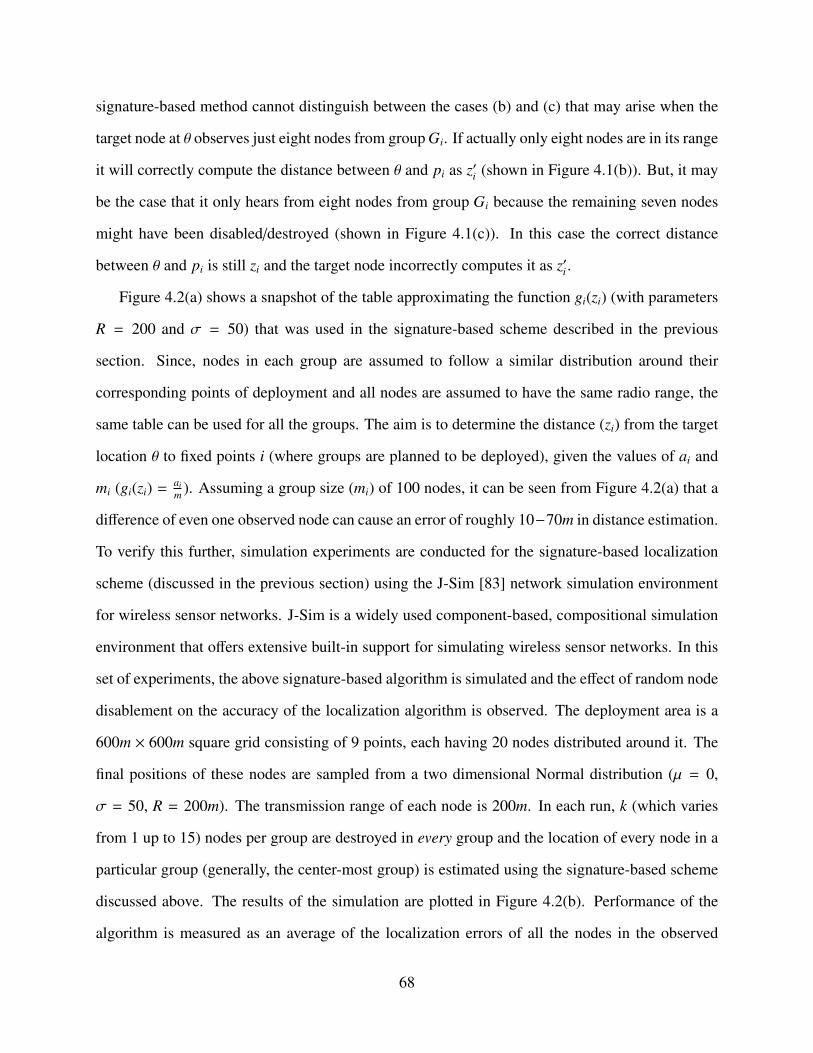
signature-based method cannot distinguish between the cases (b) and (c) that may arise when the

target node at θ observes just eight nodes from group Gi. If actually only eight nodes are in its range

it will correctly compute the distance between θ and pi as z′i (shown in Figure 4.1(b)). But, it may

be the case that it only hears from eight nodes from group Gi because the remaining seven nodes

might have been disabled/destroyed (shown in Figure 4.1(c)). In this case the correct distance

between θ and pi is still zi and the target node incorrectly computes it as z′i .

Figure 4.2(a) shows a snapshot of the table approximating the function gi(zi) (with parameters

R = 200 and σ = 50) that was used in the signature-based scheme described in the previous

section. Since, nodes in each group are assumed to follow a similar distribution around their

corresponding points of deployment and all nodes are assumed to have the same radio range, the

same table can be used for all the groups. The aim is to determine the distance (zi) from the target

location θ to fixed points i (where groups are planned to be deployed), given the values of ai and

mi (gi(zi) = aim ). Assuming a group size (mi) of 100 nodes, it can be seen from Figure 4.2(a) that a

difference of even one observed node can cause an error of roughly 10−70m in distance estimation.

To verify this further, simulation experiments are conducted for the signature-based localization

scheme (discussed in the previous section) using the J-Sim [83] network simulation environment

for wireless sensor networks. J-Sim is a widely used component-based, compositional simulation

environment that offers extensive built-in support for simulating wireless sensor networks. In this

set of experiments, the above signature-based algorithm is simulated and the effect of random node

disablement on the accuracy of the localization algorithm is observed. The deployment area is a

600m × 600m square grid consisting of 9 points, each having 20 nodes distributed around it. The

final positions of these nodes are sampled from a two dimensional Normal distribution (µ = 0,

σ = 50, R = 200m). The transmission range of each node is 200m. In each run, k (which varies

from 1 up to 15) nodes per group are destroyed in every group and the location of every node in a

particular group (generally, the center-most group) is estimated using the signature-based scheme

discussed above. The results of the simulation are plotted in Figure 4.2(b). Performance of the

algorithm is measured as an average of the localization errors of all the nodes in the observed

68

zi gi(zi)1.00 0.999...

...55.00 0.99656.00 0.995...

...74.00 0.989...

...88.00 0.98089.00 0.979...

... 0

10

20

30

40

50

60

70

0 1 2 3 4 5 6 7 8 9 10 11 12 13 14 15

Ave

rage

Loc

aliz

atio

n E

rror

(m

eter

s)Number of Destroyed Nodes per Group

(a) (b)

Figure 4.2: (a) Table of gi(zi) values (Equation (4.1)), R = 200, σ = 50 (b) Plot of Number ofDisabled Nodes vs. Localization Accuracy in Signature-based Localization Scheme by Fang etal. [26]

group. From the plot, it can be seen that the average localization error increases as k increases.

Another trend that can be observed in this plot is that at high values of k, the localization inaccuracy

increases less steadily. This shows that beyond a certain threshold, the disablement of nodes has

little effect on increasing the (already large) localization error. Moreover, the average localization

error in the case of zero node destruction (i.e., k = 0) is just under 30m, which is high. One reason

for the low accuracy of this algorithm, even when k = 0, is the complex continuous function gi(zi)

(Equation (4.1)) that is approximated by a table of discrete values.

From the above results, it is clear that in order to improve the accuracy and efficiency of

signature-based schemes in dynamic environments and emergency applications two issues need to

be addressed: 1) improve fault-tolerance against disabled nodes and 2) reduce complexity. Since

the accuracy of signature-based schemes depends on the initial distribution of nodes, an efficient

strategy for sensor node deployment in emergency applications first needs to be formulated. This

issue is addressed in the following section.

69

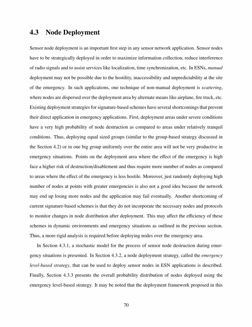
4.3 Node Deployment

Sensor node deployment is an important first step in any sensor network application. Sensor nodes

have to be strategically deployed in order to maximize information collection, reduce interference

of radio signals and to assist services like localization, time synchronization, etc. In ESNs, manual

deployment may not be possible due to the hostility, inaccessibility and unpredictability at the site

of the emergency. In such applications, one technique of non-manual deployment is scattering,

where nodes are dispersed over the deployment area by alternate means like airplane, fire truck, etc.

Existing deployment strategies for signature-based schemes have several shortcomings that prevent

their direct application in emergency applications. First, deployment areas under severe conditions

have a very high probability of node destruction as compared to areas under relatively tranquil

conditions. Thus, deploying equal sized groups (similar to the group-based strategy discussed in

the Section 4.2) or in one big group uniformly over the entire area will not be very productive in

emergency situations. Points on the deployment area where the effect of the emergency is high

face a higher risk of destruction/disablement and thus require more number of nodes as compared

to areas where the effect of the emergency is less hostile. Moreover, just randomly deploying high

number of nodes at points with greater emergencies is also not a good idea because the network

may end up losing more nodes and the application may fail eventually. Another shortcoming of

current signature-based schemes is that they do not incorporate the necessary nodes and protocols

to monitor changes in node distribution after deployment. This may affect the efficiency of these

schemes in dynamic environments and emergency situations as outlined in the previous section.

Thus, a more rigid analysis is required before deploying nodes over the emergency area.

In Section 4.3.1, a stochastic model for the process of sensor node destruction during emer-

gency situations is presented. In Section 4.3.2, a node deployment strategy, called the emergency

level-based strategy, that can be used to deploy sensor nodes in ESN applications is described.

Finally, Section 4.3.3 presents the overall probability distribution of nodes deployed using the

emergency level-based strategy. It may be noted that the deployment framework proposed in this

70

chapter, including the stochastic models for node destruction and overall node distribution, is ap-

plicable only in unobstructed two dimensional terrains. Deployment in three dimensional scenarios

would be different and is outside the scope of this research.

4.3.1 Stochastic Model for Node Destruction

A stochastic model for the process of sensor node destruction, as outlined in this section, is not

only useful in deciding if it is feasible to deploy a specific number of nodes around each planned

point over the emergency area but also in fixing the number of nodes that should be deployed

at each such point. In the proposed framework, the phenomenon of node destruction is modeled

as a stochastic time process. A stochastic time process is a process that can be described by a

probability distribution with domain as the time interval of the process. In other words, it is a

collection of random variables indexed by some set T , which represents the time interval of the

process. Before introducing the details of this model, some important definitions and assumptions

are required.

Assume that the area of interest (emergency area) is divided into a rectangular grid as shown

in Figure 4.3. Each dot in the grid represents a deployment point, say pi.

Definition 4.1. A deployment point is a point on the terrain (grid) where a node (or group of

nodes) is planned to be deployed. The point where a node actually resides after deployment, not

necessarily the same as the deployment point, is called the resident point.

Let (xi, yi) be the coordinates of the deployment point pi (assume a two-dimensional coordinate

system). Assuming that there are k deployment points p1(x1, y1), p2(x2, y2), . . . , pk(xk, yk), k groups

of nodes, G1,G2, . . . ,Gk, are planned to be deployed at each deployment point. In other words,

group Gi is to be deployed at deployment point pi. Since, this chapter focuses only on modeling

the effects of external factors on node failure, it is assumed here that sensor nodes can be disabled

only by external factors like fire, temperature, force, etc., and not by internal/self factors like

battery failures, component malfunction.

71

Figure 4.3: Fires and smoke in Southeast Australia, NASA Satellite image, 18 Jan, 2003 [93]

Let, ta be the start time of the application and tb be the end time of the application (i.e., ta < tb).

We assume that all the deployed sensor nodes are healthy and free from internal technical glitches

throughout the period of the application ta,b (= tb − ta). At any instance in time between ta and

tb, every deployment point pi is associated with an emergency level λi based on the emergency

condition at that point at the time. In other words, an emergency level is a quantification of the

intensity of emergency at a point, as defined next.

Definition 4.2. An emergency level λi at any instance for a deployment point i is defined as the

average number of nodes destroyed in group Gi per unit time at that instance and the corresponding

function λi(t) : t → N is called the generalized emergency level function.

In the above definition, a node is considered destroyed or disabled if it is not capable of commu-

nicating with any of its neighboring nodes. An emergency level associated with a deployment point

at any time instance is proportional to the severity of the emergency at the point at that instance.

Higher the severity, higher is the node destruction rate and as a result higher will be the emergency

level at the deployment point at any instance. Moreover, the emergency level at that point at a later

instance in time can be higher or lower depending on whether the emergency situation at that point

has worsened or subsided. This relationship is given by the generalized emergency function λi(t),

72

as discussed later. The probability of the number of disabled nodes in a group over a fixed period

of time can be expressed as a Poisson distribution because these disablement occur with a known

average rate (emergency level) during that interval and are independent of the time since the last

node disablement. Since the phenomenon of disablement of nodes over a period of time (here, ta,b)

is discrete in nature, it can be modeled as a Poisson process, specifically as a non-homogeneous

Poisson process. This is because, the average rate of node disablement (emergency level) may

change over time (between the start and the end of the application) as the effect of the emergency

at that point changes. Thus, the number of nodes disabled in a group Gi over a deployment point

pi in the time interval (ta, tb] , given as Ni(tb) − Ni(ta), is as shown in Equation (4.2).

Pr[(Ni(tb) − Ni(ta)) = ki] = f (ki, λa,bi )

=e−λ

a,bi (λa,b

i )ki

ki!, (4.2)

where ki = 0, 1, . . . |Gi|

Here, λa,bi is the overall emergency level for the deployment point pi over the time interval (ta, tb].

As mentioned earlier, an emergency level at a point cannot be assumed constant throughout the

time interval (ta, tb]. As a result, the overall emergency level λa,bi for the deployment point pi can

be defined in terms of the generalized emergency level function λi(t) as shown in Equation (4.3)

λa,bi =

∫ tb

t=taλi(t)d(t). (4.3)

4.3.2 Emergency Level-based Deployment Strategy

Before describing the emergency level-based node deployment strategy, the process of assigning

emergency levels to each deployment point needs to be fixed.

73

Determining Emergency Levels

An emergency scenario is generally a sequence of events occurring at various points over the

emergency area. From the point of view of an ESN, an event can be defined as follows.

Definition 4.3. An event Ei at any point i during an emergency is any distinguishable, measurable

and sometimes observable force of nature or external factor which has a distinct effect on the

working and operation of the sensor nodes deployed on or around that point.

During any emergency, each deployment point is associated with a sequence of events; each

event produces a different rate of node destruction. For example, a forest fire emergency can

have some areas that are directly under a wall of fire where the destruction rate is the highest.

While some others where the fire is out but still under the effect of burning objects may have a

comparatively lower rate of destruction, while some others that are just under the influence of

smoke might have an even lower rate of destruction. These sequence of events at any deployment

point play an important role in determining the emergency level for that point. Moreover, some

events are easily observable, e.g., fire, while others might not be visible to the naked eye but are

easily measurable, e.g., high/low pressure. Different intensities of the same event can be modeled

as multiple sequential events with different rates of node destruction. Depending on the emergency

situation, the sequence of events forming the emergency can be easily predictable (and can be

determined even before the emergency occurs) or can be completely unpredictable. It is easy to

determine the emergency level at each deployment point if the sequence and duration of events can

be predicted easily. But, real-life emergencies are generally associated with a lot of uncertainty

and the sequences of events during the emergency cannot be predicted easily. Below, each case is

discussed separately.

Predictable Sequence of Events: If the sequence of events at any deployment point i during an

emergency can be predicted easily then the emergency level at that point is nothing but the sum of

the number of nodes destroyed by each predicted event in the sequence during the entire period of

74

the emergency ta,b. Let, ta,b be divided into r time slots of equal lengths, say, ta,1, t1,2 . . . tr−1,b. Let,

Ei = E1i , E

2i . . . , E

ri be the predicted sequence of r events at deployment point pi, where E1

i occurs

during time slot ta,1, E2i occurs during time slot t1,2 and so on. Let kE1

i, kE2

i. . . , kEr

ibe the sensor

node destruction rate for the events E1i , E

2i . . . , E

ri respectively, i.e., kEr

inumber of nodes per unit

time are destroyed during event Eri . Then, the emergency level at deployment point i through time

ta,b can be given as shown in Equation (4.4),

λa,bi = kE1

i.ta,1 + kE2

i.t1,2 + . . . + kEr

i.tr−1,b (4.4)

Unpredictable Sequence of Events – Controlled Emergency Simulations: In situations where

the sequence of events cannot be predicted easily, the best way to determine emergency levels is by

conducting controlled emergency simulations. In such experiments, the desired emergency that one

is trying to model is simulated in a controlled environment and the various parameters affecting

the simulated emergency and/or the deployed sensor nodes are studied. In the past, researchers

have carried out similar experiments to not only study the effect of emergencies on the structures

and surroundings but also to provide vital data to first responders and other related agencies. As

an example, consider the NEESWood project [19] at the Structural Engineering and Earthquake

Simulation Laboratory at The State University of New York at Buffalo. In this project, earthquakes

are simulated using shake tables to study the effect of seismic activity on the structure of wooden

framework buildings. The eventual goal of this project is to provide an economical design of

low and mid-rise wood-frame construction for seismic regions. Similar experiments in simulation

of building [97] and forest [27, 71] fires have been conducted with the aim of developing accurate

models for predicting the various events and the spread of these events during the emergency. Such

models are essential for building efficient decision support systems for use by the fire fighters and

first responder personnel. As evident from the success of the above examples, it can be concluded

that a great deal about the various events during an emergency can be learnt by conducting such

simulated or controlled emergency experiments.

75

Thus, to prepare for an actual ESN deployment during a real-life emergency, similar repeated

controlled simulations of the emergency can be carried out over the target area in advance. A fixed,

large group of nodes (mmax, explained later) are deployed initially at each deployment point i and

the number of destroyed nodes can be noted during each trial run of the simulation. Simulations can

be repeated for a total of, say, n times and the number of destroyed nodes in each run j and at each

point i (k ji ) is measured. Now, given a sample of n measured values of disabled nodes (k1

i , k2i . . . k

ni )

for a point i, the overall emergency level λa,bi for that point needs to be estimated. Maximum

Likelihood Estimation (MLE) analysis can be used to show that if the number of destroyed nodes

(k ji ) during each trial simulation runs follows a Poisson distribution, then the mean of the sample

(k1i , k

2i . . . k

ni ) is in fact the most likely value of the emergency level λa,b

i .

Let, f (k ji , λ

a,bi ) be the probability that k j

i number of nodes are destroyed at deployment point i

in the jth run of the test. Now, the value of λa,bi that maximizes the likelihood function f needs to

be computed as shown below.

f =n∏

j=1

f (k ji , λ

a,bi )

In order to compute the maximum likelihood value of λa,bi , first form the log-likelihood function as

shown below.

L( f ) = ln(n∏

j=1

f (k ji , λ

a,bi ))

=

n∑j=1

ln

e−λa,bi (λa,b

i )k ji

k ji !

= −nλa,b

i + ln(λa,bi )

n∑j=1

k ji

− n∑j=1

ln(k ji !)

Now, to compute the value of λa,bi for which the above log-likelihood function is maximized take

the derivative of L( f ) w.r.t λa,bi and equate it to zero.

d

dλa,bi

L( f ) = 0⇐⇒ −n +

n∑j=1

k ji

1

λa,bi

= 0

76

Solving for λa,bi gives us the maximum-likelihood estimate for λa,b

i as shown in Equation (4.5).

λMLEi = λa,b

i =1n

n∑j=1

k ji (4.5)

An important point that needs to be stressed here is that the techniques discussed above for deter-

mining emergency levels by simulating the emergency in a controlled environment are just one of

the many ways to determine emergency levels for deployment points. In general, larger the num-

ber of ki’s (observations) available for each sequence of events at the corresponding deployment

point, better the prediction of the related emergency level λi at that point. These ki’s can be either

determined by simulating the emergency repeatedly (as discussed above) or even from past real

life experiences during similar emergency situations. The next section focuses on determining the

actual group size or the total number of nodes to be deployed at each deployment point based on

the emergency level at that point.

Determining Deployment Size

Before jumping into the discussion on determining the deployment size, let’s first outline the formal

definition of a deployment size from the point of view of an ESN deployment.

Definition 4.4. The deployment size mi for any deployment point i associated with an emergency

level λa,bi is the actual number of sensor nodes that are planned to be deployed at that point.

The deployment size mi for a deployment point i depends on the overall emergency level λa,bi at

that point and is determined as follows. The deployment size consists of two components. The first,

called the standard deployment (msi ), is a fixed application specific constant. The next component,

called varied deployment (mvi ), is determined by the rate of node destruction at the deployment

point and is proportional to the overall emergency level at the point i, i.e., mvi ∝ λ

a,bi . Thus, the

deployment size mi at a deployment point i is a combination of the standard deployment and the

varied deployment components, i.e., mi = msi +mv

i . Intuitively, more number of sensors are required

at deployment points with higher emergency levels as compared to lower ones. According to the

77

proposed quantification of the deployment size, as the variable component mvi of the deployment

size is proportional to the emergency level it will make sure that areas with higher emergencies

receive a larger deployment size. Moreover, while the variable component mvi of the deployment

size offsets the effects of node destruction around a deployment point, the standard component msi

will make sure that there exists enough nodes to carry out the information collection task around

that point. Let, mmax be an application dependent upper bound on the maximum number of nodes

that can be deployed at any point. The bound mmax depends on application specific factors like

required network density, cost of nodes, priority of coverage, etc. Sensor nodes will be deployed at

each deployment point in groups of size mi if and only if this determined deployment size per group

is less than the maximum upper bound on the group size, i.e., mi ≤ mmax. Another factor that would

affect the size of the deployed group mi is the area to be covered by the group of sensor nodes, i.e.,

the average distance between the deployment points. Intuitively, more number of sensor nodes

are required to cover a larger area, but depending on the emergency situation at the area, a very

high coverage might not be required. Currently, coverage issues are not addressed in this research

and it is assumed that the deployment size for a group is independent of the distance between the

deployment points.

Hierarchical Deployment

Due to the low computation power and storage capacity of sensor nodes, sensor network appli-

cations normally employ a store and forward model like the single-tier model or the two-tier

model [89]. In the two-tier model, only some nodes are attached with sensing equipment and

deployed at the area of interest. Data from these sensor nodes are forwarded to specially des-

ignated forwarding nodes, called forwarders. Forwarders are not data generators and their sole

purpose is to forward data from the sensor nodes to the base station for aggregation and analysis.

In the single-tier model, there are no forwarders and the sensor nodes in addition to collecting

data also forward data for other nodes. In this work, a hierarchical deployment model is employed

which is basically a single-tier deployment model with a hierarchical communication structure.

78

In this model, every group Gi consists of at least one node designated as the group head. Sensor

nodes forward data to their respective group heads as soon as it develops, which in turn aggregates

it and forward it up the hierarchy to other group heads and eventually to the base-station. Because

of such a hierarchical design, group heads are aware of all the active nodes within the group. Such

a hierarchical design can also be used in signature-based localization schemes to decide which

groups have sufficient number of nodes to perform localization accurately, as discussed in Section

4.4. But, one problem with this model is that the group head can become a single point of failure.

To overcome this, a group can appoint more than one group heads depending on factors like group

size, distance between deployment points, etc. To elucidate the current exposition, it is assumed

here that each group consists of a single, always on (i.e., it can never be disabled/destroyed) group

head. The group head can either be similar, in terms of the computation and battery power, to the

other nodes or it can be a high-end device. The group heads for the respective groups can either

be determined prior to deployment or it can be decided upon after deployment through efficient

cluster head appointment algorithms [5, 33, 85].

The deployment strategy can now be summarized as follows:

1. Divide the deployment area into a fixed set of deployment points. Associate an emergency

level with each point based on the severity of the emergency at that point.

2. Assuming that there are k deployment points, prepare k groups of nodes to be deployed at the

corresponding deployment point, each of size determined by their corresponding emergency

levels (as discussed above).

3. Information like the group sizes, emergency levels, node distribution (discussed later), etc.,

called the pre-deployment information, is loaded into the memory of every node before de-

ployment.

4. Finally, deploy each group of nodes at the corresponding deployment point using non-

manual techniques like aerial scattering by an airplane or dispersion from a fire truck ladder.

79

The next section discusses the overall post-deployment node probability distribution and its impact

on the signature-based localization schemes.

4.3.3 Deployment Distribution

For a group of nodes scattered at a deployment point, the probability that the final position of a

node from the group is at the deployment point is the highest and the probability decreases as

we move away from the deployment point. The final position (resident point) of the nodes after

deployment can be modeled as a continuous random variable with a certain fixed non-uniform

probability distribution function (p.d.f). Generally, random variates in physics and natural sciences

with unknown probability distributions can safely assumed to be Normal (Gaussian). Thus, the

node distribution around a deployment point can be assumed to be Normal as shown in Equation

(4.6).

fi =1√

2πσe−[(x−xi)2+(y−yi)2]/2σ2

(4.6)

For a group Gi, the mean (µ) of the p.d.f is the corresponding deployment point pi(xi, yi). The

standard deviation (σ) is an application specific constant and depends on the coverage required

around the deployment point. Let Pri be the probability that a node selected at random belongs to

the group Gi. Then,

Pri =mi

m1 + m2 + . . . + mk(4.7)

where mi, i = 1 . . . k is the deployment size of the group Gi. Thus, the overall probability distri-

bution of a (randomly selected) node over the emergency area at the moment nodes are deployed

is:

foverall =

k∑i=1

Pri × fi (4.8)

Probability distribution of node positions, as shown in Equation (4.8), is composed of two com-

ponents. The first component of this distribution Pri (Equation (4.7)), is directly affected by the

destruction of nodes in the groups. Whereas the second component, which gives the distribution

80

of nodes from a particular group around the corresponding deployment point fi (Equation (4.6)),

is affected by factors that change the node locations, e.g., node movement. It can be assumed

that the distribution function fi remains unchanged throughout the period of the application ta,b,

because the current work does not intend to study the effects of factors like node movement on the

node distribution and the corresponding signature-based schemes. It will be undertaken as a part

of future work.

Equation (4.8) represents the probability distribution of the final position of nodes just at the

moment they are deployed, i.e., at the start of the application (t = ta). But as previously mentioned,

this changes with time as nodes in the various groups are disabled by the various events during

the period of the emergency ta,b. Thus, an expression that models this change in distribution is

required. Let, foverall(t) : t → R be the corresponding overall node distribution function and

Pri(t) : t → R be the corresponding group probability function in time t. The overall probability

distribution function can be given as,

foverall(t) =∫ k∑

i=1

(Pri(t) × fi)

dt (4.9)

Since the nodes are deployed exactly at time ta, we can assume that for t < ta, Pri(t) = 0 ∀i. Thus,

the probability distribution at the time of deployment (t = ta) is

foverall(ta) =∫ ta

t=0

k∑i=1

(Pri(t) × fi)

dt

= f1

∫ ta

t=0Pr1(t)d(t) + f2

∫ ta

t=0Pr2(t)d(t) + . . . + fk

∫ ta

t=0Prk(t)d(t)

= f1 × Pr1 + f2 × Pr2 + . . . + fk × Prk (From Equation (4.7))

=

k∑i=1

Pri × fi

= foverall (Equation (4.8))

Now, the overall probability distribution function (Equation (4.9)) can be expressed in terms of the

81

generalized emergency level function λi(t) as,

foverall(t) =k∑

i=1

(fi ×

∫Pri(t)dt

)

=

k∑i=1

(fi ×

∫mi − λi(t)

(m1 − λ1(t)) + (m2 − λ2(t)) + . . . (mk − λk(t))dt

)(4.10)

The overall probability distribution function during the entire period of the application ta,b can be

obtained by limiting the integral in Equation (4.10) between ta and tb as shown in Equation (4.11)

below.

foverall(tb) =k∑

i=1

(fi ×

∫ tb

t=ta

mi − λi(t)(m1 − λ1(t)) + (m2 − λ2(t)) + . . . (mk − λk(t))

dt)

(4.11)

Thus at the beginning of the application when the nodes are just deployed, the probability that

a randomly selected node lies closer to deployment points with higher emergency levels is high.

But, with time this may no longer be true. Nodes in groups near higher emergency levels may

also be destroyed with a higher rate and as a result the actual size of such groups may be fairly

smaller as compared to their original size at deployment. As discussed in Section 4.2.2, current

signature-based localization schemes assume that the node distribution, approximated at the time

of deployment (Equation (4.8)), holds true for the entire period of the emergency application,

which is not true. The loss of nodes in each group changes this distribution as shown above and

the localization schemes should use the most current node distribution. Next, a very simple and

intuitive solution to the above problem, called the Group Selection Protocol (GSP), is discussed.

4.4 Improving Signature-based Localization

Group Selection Protocol or GSP, which is implemented on top of a signature-based localization

algorithm (like the one discussed in Section 4.2), continuously monitors changes to the node dis-

tribution due to disablement and helps improve the accuracy of the localization algorithm.

82

4.4.1 Group Selection Protocol (GSP)

Let, ai be the number of nodes from group Gi that the target node at point θ(x, y) can hear from

and let zi be the distance from the target node to the deployment point of group Gi. The problem

with the localization algorithm discussed in Section 4.2 is that in emergency situations, not every

observation ai in {a1, . . . , an} is correct or accurate. Groups where the node destruction rate is high

might not be able to provide the correct value of ai for localization. These incorrect values of ai

increase the localization error during trilateration. One way to overcome this problem is by being

selective in choosing groups Gi’s (and the corresponding observations ai’s) for the localization

process. GSP uses ai’s from only those groups that are healthy. First, lets define the notion of

group health.

Definition 4.5. The health of a group is quantified by the number of active nodes in the group. A

node is active if it is able to communicate with at least one other node in the same group.

This notion of a healthy group is application dependent. In other words, a group is considered

healthy if its size is at least equal to some application dependent lower bound. Without loss of

generality, let us assume here that a group is healthy at any instance if its size at that instance

is equal to its standard deployment size (msi ), which was fixed at the time of deployment. Now,

GSP uses only observations from those groups for localization where the current health is at least

equal to its standard deployment size (msi ). Such a modification might reduce the number of zi’s

(distances) available for localization. But, as long as at least 3 relatively accurate values of zi’s

can be determined, localization can be done efficiently. Absence of at least 3 values for zi due to

unavailability of healthy group observations will cause the localization process to fail. But, due to

the criticality of the applications in emergency situations sometimes no location is better than an

incorrect value.

In GSP, group heads are used to monitor the health of their corresponding groups. As the

ad-hoc network comes up after deployment, nodes begin sending initial setup information to their

respective group heads. The group head updates the health of its group by either using these

83

setup communications or by using the explicit health update packets that can also be sent by the

nodes. At regular intervals, the group heads broadcast the current health of their respective groups.

These broadcasts are forwarded by all nodes in the network up to a certain hop count so that even

nodes in other groups (and farther away from the group head) can know the health status of a

particular group. Based on the current health of a group, the target node decides on whether or not

to use neighborhood observations from that group to compute the distance to the corresponding

deployment point. In addition to this, communications between the nodes and the group heads

can be synchronized with the sleep-wake cycles of nodes in order to save power and to make the

process more efficient for the nodes. The Group Selection Protocol (GSP) is outlined in Algorithm

3.

1: Observe the neighborhood, i.e., {a1, a2 . . . ak| ai is the number of nodes from group Gi that arein radio range. }

2: Wait and observe health broadcasts (hi) from the group heads. Update hi to the latest value foreach group.

3: for all groups Gi for which hi is known do4: if The group is healthy, say (hi ≥ ms

i ) then5: Compute g(zi) = ai/hi.6: Compute zi from g(zi) by looking up the table for g(zi).7: end if8: end for9: if zi corresponding to at least 3 distinct groups Gi is known then

10: Compute θ(x, y) by trilateration (using zi’s and their corresponding pi’s)11: else12: “Cannot do Localization!”13: end if

Algorithm 3: Group Selection Protocol (GSP)

4.4.2 Analysis of GSP

Although the GSP proposes only minor and intuitive improvements, it performs better than existing

signature-based localization algorithms in dynamic scenarios. This claim has been verified by

simulation experiments, as outlined in detail in Section 4.6. Simulation results show that GSP does

improve the localization accuracy of signature-based algorithms when nodes over the deployment

84

area are randomly disabled. But, this improvement comes at the cost of extra communication

and processing overhead. Below, the extra costs that may be incurred by the network in order to

implement GSP have been enumerated.

1. There is an additional requirement for a node to act as a group head. In this regard, a cluster

formation or group head selection algorithm might have to be executed immediately after

deployment.

2. Each node in any group Gi may have to generate an extra health update packet. In addition

to this, it has to forward at most mi extra (health update) packets for nodes in the same group.

3. The group head has to receive and process at most mi extra (health update) packets from

nodes in the same group and broadcast an extra health notification packet to all nodes.

Despite the improvement in localization accuracy by employing GSP, there are still some prob-

lems with existing signature-based approaches that have been left unaddressed. Current signature-

based schemes are extremely complex involving hard to compute functions. Simplifying the pro-

cess by using regression-based or table-based approximation techniques [26] results in loss of

accuracy in addition to other issues like offline computation and storage of complex functions in

the memory of the resource constrained sensor nodes. Although GSP provides some improvement

in terms of accuracy, it does not improve the complexity of signature-based schemes. Moreover,

just employing GSP is not sufficient if the node destruction is widespread and not localized only

to certain deployment points over the emergency area. To overcome these problems, a simple and

novel signature-based localization approach, called ASFALT, is proposed. Rather than using just

the neighborhood observations, ASFALT uses distance measurements to groups of nodes (in the

neighborhood) for distance computation. ASFALT not only improves the localization accuracy but

is also much more computationally efficient as explained in the following section.

85

4.5 ASFALT: A Simple FAult-tolerant Signature-based

Localization Technique

ASFALT together with GSP is not only fault-tolerant against random node disablement, but also

removes the requirement for storing large tables, executing complex computations or performing

costly table look-up operations. In this localization approach, instead of just observing its neigh-

borhood (number of nodes from each group that are in radio range), the target node computes

distances to each such node in its neighborhood. The set of distance estimates from the target node

to all nodes in a particular group is called the distance vector, while the set of distance estimates

from the target node to all neighborhood nodes from a particular group is called the observed dis-

tance vector for that group. Assuming that the distribution of the nodes around the corresponding

deployment point is Normal, these distance vectors are nothing but samples from the two dimen-

sional Normal distribution with mean as the distance between the target node and the deployment

point of the group. Thus, given a distance vector (or an observed distance vector), the distance

from the target to a deployment point can be approximated by computing the mean of the vector

(sample). Given three or more such distances, the location of the target node can be computed by

using trilateration or any other suitable constraint satisfaction technique.

4.5.1 Assumptions

One of the requirement for ASFALT is that nodes should be deployed over the deployment area

using a non-uniform deployment strategy like an emergency level-based deployment strategy (Sec-

tion 4.3). As discussed earlier, in an emergency level-based deployment strategy the final position

of nodes in a group can be assumed to follow a two dimensional Normal distribution with mean µ as

the corresponding deployment point and an application dependent constant variance σ2 (Equation

(4.6)). In addition to this, any node is accurately and efficiently able to estimate its distance to all

of its one hop neighbors. Efficient techniques to estimate distances like Received Signal Strength

Indicator (RSSI), Time of Arrival (ToA), Time Difference of Arrival (TDoA), etc., [40,42] exist in

86

the literature. Although the simulation experiments for ASFALT, as discussed in Section 4.6, use

RSSI to compute the distance between nodes, the algorithm itself is general enough and works well

with other distance estimation (ranging) techniques. Lastly, the nodes within a particular group are

randomly selected for disablement and do not follow any specific pattern/distribution. This is a rea-

sonable assumption because nodes within a group with a specific emergency level have an equal

probability of being destroyed. This is different from the number of nodes destroyed which is still

a Poisson process and depends on the rate of destruction at a deployment point. As a result, the

probability distribution function of the remaining nodes in a group is still Normal. All the symbols

and terminology used in this section are same as Section 4.3.

4.5.2 Localization Scheme

Let M be the target node for which localization has to be done and let θ(x, y) be the actual position

of M. Let zi be the actual distance between θ(x, y) and some deployment point i. Let the total

number of nodes deployed at deployment point i (group Gi) be mi and let d1i , d

2i . . . d

mii |d

ji ∈ R be

the distances of the nodes from the deployment point i (d ji > 0, if the position of node j is after i

on the real line and d ji < 0 otherwise). Assuming that all mi (ms

i + mvi ) nodes in Gi are in the radio

range of M, let z1i , z

2i . . . z

mii be the distances of these nodes from the target node M. As discussed

earlier, the distances in the set {d1i , d

2i . . . d

mii } follow a Normal distribution. Let, d be the random

variable that takes values in this distribution. Thus, the expected value of d is as shown in Equation

(4.12).

E(d) = 0 (4.12)

In other words, the mean value of all distances selected from this distribution is 0. Now, let Zi

be the random variable that takes values in the distribution followed by the distance between each

node of group Gi and the target node M. Since each z ji depends on the corresponding d j

i , from

Equation (4.12), it can be said that

E(Zi) = zi (4.13)

87

The ASFALT localization technique can then be outlined as shown in Algorithm 4. In order to

1: Observe the neighborhood. Compute {a1, a2 . . . ak| ai is number of nodes from Gi in radiorange. }.

2: for all groups Gi for which ai , 0 do3: Compute z1

i , z2i . . . z

aii i.e., distance to all the ai nodes.

4: Observe health broadcasts (hi) from the group head. Update hi to the latest value for thegroup.

5: end for6: for all groups Gi for which hi is known do7: if The group is healthy, say (hi ≥ ms

i ) then8: if (ai < αi) then9: Continue; {Sufficient samples not available for approximating zi}

10: else if (ai ≥ αi) and (ai < βi) then11: Compute zi = max{z1

i , z2i . . . z

aii }; {Sample not large enough to represent the entire dis-

tribution}12: else if (ai ≥ βi) then

13: Compute zi =

∑aij=1 z j

i

ai{Compute mean of all samples}

14: end if15: else16: if (ai < βi) then17: Continue;18: else19: Compute zi =

∑aij=1 z j

i

ai

20: end if21: end if22: end for23: if zi corresponding to at least 3 distinct groups Gi is known then24: Compute θ(x, y) by trilateration (using zi’s and their corresponding pi’s)25: else26: “Cannot do Localization!”27: end if

Algorithm 4: ASFALT Localization Algorithm

compute θ(x, y) by trilateration, M needs at least 3 or more zi’s (or distances to known deployment

points). M first observes it neighborhood (a1, a2 . . . ak), where ai is the number of nodes from

group Gi in the radio range of M. Using any efficient distance computation method, M computes

the observed distance vectors {z1 = (z11, z

21 . . . z

a11 ), z2 = (z1

2, z22 . . . z

a22 ) . . . zk = (z1

k , z2k . . . z

akk )}. It

then computes the corresponding zi by taking the mean of the scalar values (z1i , z

2i . . . z

aii ) of the

corresponding observed distance vector zi. The distance to the deployment point i (zi) can be

88

computed as shown in Equation (4.14).

zi =

∑aij=1 z j

i

ai(4.14)

It is obvious that larger the size ai of the observed distance vector zi, better is the approximation

for zi. The best approximation is when distances from the whole group, i.e., a distance vector is

available. But, a distance vector may not be available due to two reasons: 1) only some nodes in a

group may be in the radio range of the target node (Figure 4.1b), or 2) some nodes in a group may

be disabled (Figure 4.1c). These two cases need to be distinguished and handled separately during

localization. In order to accomplish this, GSP is implemented on top of ASFALT. GSP monitors

the health of the neighboring groups. If a group is healthy (hi ≥ msi ) but still the target node hears

from only a few nodes from that group, it would imply that not all nodes in that group are in the

radio range. Otherwise, if the group is not healthy (hi < msi ), the usefulness of the observation

vector is determined by the number of nodes visible (ai) and a parameter βi discussed next.

4.5.3 Determining ASFALT Algorithm Parameters

The ASFALT algorithm, as discussed above, requires two parameters to determine if an observed

distance vector zi = (z1i , z

2i . . . z

aii ) for any deployment point i is large enough to approximate the

distance zi with reasonable accuracy. The mean threshold βi for a group Gi is the minimum size of

the observed distance vector or the minimum number of distance values required in the observed

distance vector for that group so that it represents the original distribution of nodes around the

corresponding deployment point with reasonable accuracy. If the size of the observed sample is

at least βi then the algorithm computes the distance zi as the mean of the distance values in the

sample. If the size of the observed sample is less than βi then it means only part of the group can

be heard by the target node. In this case, one heuristic to estimate zi, if the group is healthy, is to

pick the largest value of the distance in the sample as a possible choice for zi. In the ideal situation,

βi = |msi |, i.e., βi equals the size of the healthy group. But, it has been observed that β = |m

si |

2 , i.e., half

89

of the healthy group size has worked well for most cases during the simulation experiments. The

minimum threshold αi is the minimum number of distance values required in the observed distance

vector to make a fair estimation of the distance zi. If the size of the observed distance vector is less

than αi, ASFALT discards that observation from consideration in the localization process. This

prevents inclusion of erroneous measurements in the trilateration process. The minimum threshold

αi is generally assigned a low value. Simulation experience has shown that αi ≈|ms

i |

3 works well for

most cases. Although, an analytical representation of αi and βi would be more useful in deciding

their optimal values for particular situations, such a mathematical formulation is non-trivial and

depends on factors like the variance of the node probability distribution around the deployment

point and the locations of the nodes in the observed distance vector. This study will be a part of

future research.

4.5.4 Analysis

Since ASFALT uses GSP, the communication overhead required for GSP also applies to ASFALT

(Section 4.4.2). Other than the communication overhead imposed by GSP, ASFALT requires no

other extra communication as compared to the beaconless scheme discussed in Section 4.2. Con-

trary to the scheme in Section 4.2, ASFALT also does not require extra storage and look-up for the

g(z) function table (Equation (4.1)). It does require computation of the observed distance vector for

each group and the eventual distance from the target node to each of the deployment points. But,

these computations are comparatively simple and straightforward involving basic mathematical

operations, and can be easily implemented on the sensor nodes.

4.6 Evaluation

A detailed evaluation of the fault-tolerance related enhancements proposed in this chapter is carried

out using the J-Sim network simulation tool [83] and a comparative analysis of the performance of

the proposed fault-tolerant schemes against existing signature-based schemes is presented. In the

90

first set of simulation experiments, the beaconless algorithm by Lei et al. [26] both with and without

the GSP improvement and the ASFALT algorithm are simulated under similar network conditions

and their performance in the presence of random node disablement are evaluated. The metric for

evaluating performance is the average of the localization error of all nodes from a chosen group

of nodes, and is measured in meters. The second experiment observes the effect of radio range

R of the target node on the accuracy of the ASFALT algorithm. The results of these experiments

verify the claim that the proposed improvements, namely GSP and ASFALT, actually improve the

fault-tolerance of the signature-based localization process.

4.6.1 Experimental Setup

The deployment area for the simulation experiments is a two dimensional unobstructed terrain that

is divided into a grid of size 600m × 600m. The deployment area and node deployment for these

experiments is depicted in Figure 4.4. As shown in the figure, the area of interest on the grid

consists of 9 deployment points each 100m apart. Each deployment point has 20 nodes deployed

around it in a group, and each group of nodes follows a two dimensional Normal distribution

around the corresponding deployment point with mean as the deployment point and a standard

deviation (σ) of 50. Readers should note that the node positions in Figure 4.4 are not symbolical

of the actual positions of the nodes during the simulation experiments. Figure 4.4 is just used to

give the readers a rough idea of the experimental setup. Another point to note here is that the main

aim of these experiments is to observe the effect of node destruction on the accuracy of the various

signature-based localization schemes and not to determine an efficient deployment of nodes based

on the emergency levels at each deployment point. As a result, the deployment size for each group

in the current set of experiments is fixed (20 in this case). In each run of the experiment, nodes

are assigned new positions that follow a Normal distribution with the same parameters. In each

group, one node selected at random is assigned to be the group head. This node is never disabled

during the experiments. The location estimation error for each node is measured as the Euclidean

distance between the actual position and the position estimated by the localization algorithm being

91

simulated.

Group HeadNormal Node

1

3 4 5

876

0 2

200 300 400

200

300

400

(meters)100,100

(meters)

Figure 4.4: Simulation setup – topology and node deployment

4.6.2 Estimated Error vs Number of Destroyed Nodes

In this set of experiments, both the beaconless algorithm by Lei et al. [26] (with and without GSP)

and the ASFALT algorithm are simulated in dynamic conditions. Nodes are destroyed from groups

one and five (marked with dotted circles in Figure 4.4) only† and the number of destroyed nodes

in each group is varied from 1 up to 15. The standard deviation (σ) of the Normal distribution

around each deployment point is 50 and the transmission range of each node is 200m. For each

group, the mean threshold βi is 10 and the minimum threshold αi is 5. The average location

estimation error of all the nodes from group four (the center-most group) is plotted against the

number of nodes disabled in each of groups one and five as shown in Figure 4.5(a). In order

to avoid the boundary nodes, only the localization errors of nodes in group four are considered.

This is because localization error in the boundary nodes is generally high due to lack of available

samples for localization. From Figure 4.5(a), it can be seen that the ASFALT localization algorithm

performs better as compared to the other two algorithms. As the number of disabled nodes per

group increases the average localization error of all the three algorithms increases. For lower

†As compared to experiments in Section 4.2.2 where nodes from all the groups are destroyed

92

0

10

20

30

40

50

60

0 1 2 3 4 5 6 7 8 9 10 11 12 13 14 15

Ave

rage

Loc

aliz

atio

n E

rror

(m

eter

s)

Number of Destroyed Nodes per Group

Signature-basedSignature-based with GSP

ASFALT 0

10

20

30

40

50

60

70

80

90

100

0 1 2 3 4 5 6 7 8 9 10 11 12 13 14 15

Ave

rage

Loc

aliz

atio

n E

rror

(m

eter

s)

Number of Destroyed Nodes per Group

Signature-basedSignature-based with GSP

ASFALT

(a) (b)

Figure 4.5: Comparison of the average localization error of the algorithm proposed by Lei etal. [26] (with and without GSP) and ASFALT. (a) σ = 50 (b) σ = 100

number of destroyed nodes, the beaconless algorithm by Lei et al. [26] outperforms its variant

with the GSP. This is because, the GSP employed in this experiment does not consider samples

from any group whose advertised health (hi) differs even slightly from its original health. Thus, it

completely disregards samples from groups one and five even when the number of destroyed nodes

is low. GSP improves the performance of the algorithm when the number of disabled nodes is a

little higher. The most interesting trend that can be seen in this plot is that the average localization

error of ASFALT increases much less sharply as compared to the other two algorithms. Similar

experiments have also been carried out for σ = 100, i.e., when nodes are sparsely distributed

around the deployment point. The plot for these experiments is shown in Figure 4.5(b). It can be

seen that the trend in the accuracy of the algorithms is very similar to the case with σ = 50, but the

localization error is comparatively higher in this case.

4.6.3 Estimated Error vs Radio Range

In this experiment, the effect of radio (transmission) range of nodes on the performance of ASFALT

is observed. The experiment begins with a radio range of 50m and re-runs the simulations for

ASFALT by increasing the range of the nodes by 50m in each run. The positions of the nodes

93

are changed in each run, but they still follow the same distribution. An average of the localization

errors of all nodes in group four is plotted against the radio range. The number of nodes destroyed

in groups one and five remain constant at 10 and the standard deviation (σ) of the distribution

is fixed at 50. The simulation results for this experiment are outlined in Figure 4.6. The results

are quite intuitive and it can be observed that as the radio range increases the localization error

decreases. This can be attributed to the fact that as the radio range increases, each node is able

to cover a larger area and thus distance samples of a larger size are available from each group for

localization.

0

2

4

6

8

10

12

14

16

18

20

22

24

26

28

30

50 100 150 200 250

Ave

rage

Loc

aliz

atio

n E

rror

(m

eter

s)

Transmission Range (meters)

Figure 4.6: ASFALT(α = 5, β = 10), Average Estimation Error vs. Transmission Range

4.7 Conclusion

This chapter addressed the problem of robust sensor node deployment and fault-tolerant localiza-

tion in ESN applications, especially sensor network applications where node disablement exists.

Signature-based algorithms are a popular alternative to costly, and at times, inefficient beacon-

based approaches for use in ESN localization, except that they are not fault-tolerant. By means of

a case study and related simulation experiment results, this chapter showed that popular signature-

based or beaconless algorithms failed to perform well in situations where node disablement was

present. Another drawback, as evident from the presented case study, was the high complexity and

94

resource requirements of existing signature-based schemes.

The root cause of the lack of fault-tolerance in signature-based localization, as concluded after

the case study, was the poor node deployment strategy employed by earlier techniques. To over-

come this problem, this chapter first proposed an efficient strategy for node deployment, called the

emergency level-based node deployment strategy. This strategy deployed nodes at points over the

deployment area based on the rate of node disablement at those points. It employed a stochastic

model of node disablement that provides a prediction for the total number of disabled nodes, and

thus the emergency levels, at all the points over the deployment area. Next, a simple enhance-

ment to existing signature-based schemes, called Group Selection Protocol (GSP), was proposed.

GSP improved current signature-based schemes by monitoring changes in node distribution. Ex-

perimental results showed that implementing this protocol over current signature-based schemes

improved their fault-tolerance slightly. Finally, a novel, fault-tolerant signature-based localization

technique, called ASFALT, was proposed. ASFALT was shown to be simple and easily imple-

mentable on fragile and low power systems like wireless sensor networks. ASFALT used the

emergency level-based deployment strategy, GSP and a simple averaging argument to estimate

node locations. The fault-tolerance of ASFALT was verified using simulation experiments, which

showed that it performed better than other popular signature-based approaches, especially in situ-

ations where the degree of node disablement was high.

The next chapter studies the problem of efficient mitigation of inconsistent location information

in localization schemes and location-based services.

95

Chapter 5

Mitigating Inconsistencies in LocationInformation

“There is nothing constant in this world but inconsistency.”

− Jonathan Swift

5.1 Introduction

Up to this point, the main focus of this dissertation was to address the security and robustness

issues associated with the process of location discovery or localization. Specifically, the problem

of cheating beacons in distance-based localization schemes and the problem of disabled nodes in

signature-based localization schemes were addressed. This chapter addresses a related problem,

which is to efficiently mitigate inconsistencies and cheating behavior during location advertisemen-

t/verification in localization and location-based services for wireless sensor networks. Location de-

pendent applications in sensor networks can be modeled using a graph-theoretic framework such

that inconsistent location information or cheating behavior in such applications can be represented

by a set of inconsistent edges in this graph model of the network. The problem of eliminating loca-

tion inconsistencies can then be formulated as an optimization problem that determines the largest

consistent subgraph of the graph-based model of the network. This chapter studies the combinato-

rial properties for two variants of this problem and outlines intelligent heuristics to provide efficient

96

solutions for them.

5.1.1 Motivation and Problem Statement

As discussed in Chapter 1, location information is extremely essential and critical in wireless sen-

sor network applications involving monitoring and emergency response. Any information without

the associated location of occurrence or location of generation is generally useless. Thus, the lo-

calization service of the network, which helps the individual sensor nodes determine their own

location, is extremely essential and an integral part of such highly distributed and autonomous

network systems.

Nodes in a sensor network application generally associate their own location with the moni-

tored/sensed data. This location is easily verifiable at the neighboring nodes, provided the neigh-

bors know their own location and the distance between them can be determined efficiently. The

verifier node simply needs to compare this estimated distance (using RSSI, ToA, TDoA or other

well-known techniques [3, 40]) to the Euclidean distance between its own location and the adver-

tised location of the neighboring node. If the difference between these distances is greater than

some threshold, then there is definitely some inconsistency, either in location advertisement or in

location verification. Figure 5.1 depicts one such scenario, where node 2 sends its location (x2, y2)

along with the monitored data to its neighbor node 4 (at location (x4, y4)) who can then verify if

node 2 is telling the truth about its location. Such a verification procedure has also been used in

some localization techniques to weed out malicious beacon nodes [74].

This inconsistency in location information, as discussed above, could be due to multiple rea-

sons. Cheating behavior (in terms of incorrect advertised self location or distance manipulation

techniques) in localization protocols was discussed in Chapters 1 and 3. Such cheating behavior

by nodes is also possible post-localization in order to mislead other nodes about one’s own location

or to falsify the generated data that would prevent successful completion of the data-related appli-

cation. Either the location advertising node can cheat or the location verification node can cheat.

Cheating behavior may not necessarily be the only cause of such an inconsistency. External fac-

97

I am node 4 at (x4, y4), Lets verify node 2’s claim.

I am node 2 at location (x2, y2), Temp = 140 F

Figure 5.1: Cheating/Inconsistency in Location Claims/Verification

tors like radio interference, large objects, etc., can also result in the neighboring nodes not able to

verify each others locations correctly. For example, assume that two (wireless) neighboring nodes

use RSSI to estimate the distance between them. A large object or obstruction between the two

nodes can cause the radio signals originating from these nodes to lose more power than normal.

As a result, despite the nodes’ honest behavior, the estimated distance (by RSSI) between them

will never match with the Euclidean distance between their advertised locations. Irrespective of

the cause of this inconsistency, it needs to be mitigated in an efficient manner. As discussed earlier,

inconsistent location information in a network is not good for multiple reasons. Firstly, inaccurate

location information can render the information collected by the network useless and can be used

to mislead the users of this information. Secondly, this inconsistent information can adversely

affect related network services like routing, neighborhood discovery, etc., that use location infor-

mation to make network-wide decisions. This chapter focuses on studying the problem of efficient

elimination of such inconsistent location data from a theoretical point of view. Such a study is

extremely essential in order to understand the feasibility (in terms of computational complexity) of

solving the problem and to fix bounds on the worst case solution quality. All this eventually helps

in designing efficient algorithms that can not only be applied to the domain of sensor networks but

98

also extended to other distributed and autonomous network system domains.

In this direction, this chapter first introduces an efficient graph-theoretic framework for model-

ing location based services in wireless sensor networks. This model is inspired from the Grounded

Graph model by Eren et al. [25] where each vertex of the graph corresponds to a sensor node; an

edge exists between two nodes if and only if they are in radio range of each other. In the model

presented here, a location function assigns each vertex a value indicating the advertised location

by the corresponding node and a distance function assigns each edge a value indicating the esti-

mated distance between the two connecting nodes. Contrary to the model by Eren et al. where

the distance function is always honest, the distance function in this model can assign inaccurate

values to the edges. Similarly, the location function can also cheat. Moreover, in Eren’s model

only some nodes know their locations, i.e., the beacon nodes, whereas in this model all nodes are

assumed to know their own locations (through some localization process). Such a graph for the

network is referred to as a Partially Consistent Grounded Graph (PCGG). The problem of efficient

elimination of location inconsistencies can then be formulated as the problem of obtaining the

largest consistent subgraph of the PCGG of the network. Specifically, two optimization problems

are formulated, namely MAX-CON and LARGEST-CON. MAX-CON is the problem of obtaining

the consistent subgraph with the largest number of vertices, while LARGEST-CON maximizes the

number of consistent edges in the subgraph. The combinatorial properties of these optimization

problems are studied and approximation algorithms based on popular heuristics are proposed for

solving these problems. These algorithms are compared and verified using computer simulation

measurements.

5.1.2 Chapter Organization

Section 5.2 presents a graph-theoretic framework for modeling location-based services in highly

distributed and autonomous network systems like wireless sensor networks and introduces the

concept of Partially Consistent Grounded Graphs (PCGG). Section 5.3 formulates the MAX-CON

problem and presents the related combinatorial results. Section 5.4 formulates the LARGEST-

99

CON problem and presents the related combinatorial results. Section 5.5 presents heuristics-based

algorithms for LARGEST-CON, while Section 5.6 outlines results from the experimental evalua-

tion of these algorithms. Section 5.8 concludes the chapter with a summary of results.

5.2 Network Model

Before defining the graph model for the network, let us introduce the concept of location state for

a node.

Definition 5.1. The location state of a node is the most recent value of the actual location of the

node.

The location state of a node i is denoted as pi = (xi, yi), where x, y ∈ R. Without loss of gen-

erality, let pi ∈ Rd, d = 2, i.e., assume a two dimensional coordinate system. However, the results

presented here can be easily extended to three or higher coordinate systems. A node determines its

location state by employing the localization service that is available for the network. It is assumed

here, that the localization service itself is honest and that each node is able to accurately determine

its location using the localization algorithm. The location state is private to each node. The actual

advertised location by each node may or may not be the same as its location state. Details of this

are explained later.

Let N = {1, 2, . . . , n} be the set of n nodes and let P = {p1, p2, . . . , pn} be the set of their

corresponding location states. Define the graph G = (V, E ∪ E′) for the network as follows. The

set V = {v1, v2, . . . , vn} of vertices contains a vertex corresponding to each node in the network.

An edge exists between two vertices i and j in the graph G if and only if the corresponding nodes

are in the radio range of each other, i.e., they are able to communicate with each other directly

(in one hop.) This relationship is assumed to be symmetric, i.e., if node i is in the radio range of

node j, then node j is also in the radio range of node i. Thus, the edges in this graph model of the

network are undirected. The set E ∪ E′ is the set of all the edges as defined above. More details

on the composition of individual edge subsets E and E′ will follow later. Two nodes are said to

100

be neighbors if and only if there exists an edge connecting their corresponding vertices. In other

words, E ∪ E′ gives the neighborhood relation for each node in the network. For simplicity, the

graph G defined above is assumed to be a connected graph, i.e., every vertex is reachable from

every other vertex through a sequence of edges.

The graph G is associated with two weight functions. The first function, called the location

function w, w : V → (R,R), assigns a two dimensional coordinate value to each vertex. This value

represents the location advertised by the node. If a node i is honest then w(i) = pi, i.e., the value

of the location function equals to the location state for the node. If the node cheats in advertising

its location then the value w(i) is arbitrarily selected by the location function. If w(i) = pi, ∀i ∈ V

then the location function is an honest location function, otherwise if there is at least one node j

such that w( j) , p j then the location function is cheating.

The second function, called the distance function δ, δ : E ∪ E′ → R, assigns a value to each

edge signifying the estimated distance between the nodes. As discussed earlier, this estimation

can be carried out by the verifier node in the pair (of nodes). There are multiple ways in which

this function can be efficiently executed in practice and have been discussed in detail in Chapter

1. The exact details of this function will vary from application to application and it can be safely

assumed that such a function exists and can be efficiently computed. If there is at least one pair of

nodes (edge) such that the distance between them cannot be estimated correctly then the distance

function is called a cheating distance function. The distance function is honest otherwise. Note

that the notion of cheating used here is a weak notion. Cheating here not only includes errors

resulting from malicious intent but also includes cases where the distances cannot be estimated

correctly due to external factors like radio interference, obstructions, etc. The weak notion suffices

in this model, because here the aim is to eliminate inconsistencies (defined later) and not to detect

cheating nodes. A similar model, called Grounded Graphs, was proposed by Eren et al. [25].

The authors used Grounded Graphs to formulate the problem of beacon-based localization as a

Constraint Satisfaction Problem (CSP) where some nodes know their own locations and other

nodes attempt to localize themselves by solving a set of edge constraints (value of the distance

101

function).

Now, lets formally define the notion of an inconsistency. The actual distance value between a

pair of nodes is the Euclidean distance between the advertised location values (value of the location

function) of the two nodes. Thus, the actual distance value between two nodes i and j with location

function values w(i) = (xi, yi) and w( j) = (x j, y j) can be computed as,

dst(i, j) =√

(xi − x j)2 + (yi − y j)2 (5.1)

The difference between the actual distance value and the value of the distance function is called the

estimation error. Let ε denote the maximum allowable estimation error in the system, also called

the error tolerance factor. The value of ε should be zero ideally, but in most practical cases it is

assumed to have a very small value. Edge consistency can be defined as follows.

Definition 5.2. An edge (i, j) in the Grounded Graph is said to be consistent if and only if its

estimated distance function value is within some small system-dependent error tolerance factor ε

of its actual distance value.

dst(i, j) − ε ≤ δ(i, j) ≤ dst(i, j) + ε (5.2)

An edge that is not consistent is said to be an inconsistent edge. From Equation (5.1) and

Equation (5.2), it can be seen that an inconsistent edge results from either a cheating location

function or a cheating distance function. At this point, let’s make some important observations.

1. The first observation is that nodes with malicious intent do not cheat all the time. In other

words, malicious behavior is random. As a result, not all edges coming out of a particular

malicious node will be inconsistent. If they do, then such a behavior is trivial to detect. For

example, nodes may behave maliciously at random or intermittently to avoid easy detection.

There will be some exceptions to this rule but their numbers are generally small.

2. The second observation is that cheating does not always imply inconsistency. For example,

102

refer to Figure 1.3 in Chapter 1. Here node B2 can advertise its location as any point on the

circle (not shown in the figure) with center T and radius z2. The distance from the node T

will still be determined correctly as z2 and the edge (B2,T ) will always be consistent. But,

in doing this the node B2 will not be able to fool its third neighbor with whom its estimated

distance will not match the actual distance.

3. The attack, as described in the second point, will be successful only if all the neighbors of,

say, node B2 collude. Such kind of collusion attacks will not result in any inconsistent edges.

This issue of collusion is not addressed here.

The graph-based model, as defined above, consisting of at least one or more inconsistent edges

is referred to as a Partially Consistent Grounded Graph (PCGG) and can be formally defined as

follows.

Definition 5.3. A Partially Consistent Grounded Graph (PCGG) G = (V, E∪E′, δ,w) is a graph G

as defined above, where V is the set of vertices corresponding to nodes in the network and the edge

set is defined by the neighborhood relation. The edge set can be partitioned into two non-empty

disjoint subsets, namely the set of consistent edges (E) and the set of inconsistent edges (E′). δ is

the distance function and w is the location function.

Definition 5.4. A Consistent Grounded Subgraph (CSG): A Consistent Grounded Subgraph (CSG)

G = (V , E) is an induced subgraph of a PCGG G = (V, E ∪ E′, δ,w), where E′ , φ, such that the

vertex set V ⊂ V and the edge set E contains only consistent edges i.e., E ⊆ E.

The size of a CSG is the cardinality of its vertex set. The edge size of a CSG is the cardinality

of its edge set. A CSG is maximal if its vertex set is not a proper subset of the vertex set of any

other CSG. A maximum CSG is a maximal CSG with maximum size.

Definition 5.5. A Largest Consistent Grounded Subgraph (LCSG) of a PCGG is a CSG that has

the maximum edge size, if more than one CSG exists.

103

Figure 5.2(a) shows a PCGG G = (V, E ∪E′), Figure 5.2(b) shows its corresponding maximum

CSG and Figure 5.2(c) shows the largest CSG.

1

54

3

2

76

����������������������������

����������������������������

����������������������������������������

����������������������������������������

1

54

3

2

76

����������������������������������������

����������������������������������������

��������������������������������

��������������������������������

��������������������������������

��������������������������������

1

54

3

2

76

V = {1, 2, 3, 4, 5, 6, 7} OPT MAX−CON = {2, 3, 4, 6, 7} OPT LARGES T−CON = {4, 5, 6, 7}

E = {(2, 6), (3, 6), (4, 5), (4, 6), (4, 7), (5, 6), (5, 7), (6, 7)} Number of consistent edges in solution = 5 Number of consistent edges in solution = 6

E′ = {(1, 4), (1, 5), (1, 6), (1, 7), (2, 5), (3, 5)}

(a) (b) (c)

Figure 5.2: (a) PCGG, G = (V, E ∪ E′); (b) Maximum CSG of G; (c) LARGEST CSG of G

From now on, a PCGG will be denoted just by G = (V, E ∪ E′); the location and distance

functions will not be explicitly specified with the definition of PCGG. These functions are just

required to partition the edge set into a set of consistent edges and a set of inconsistent edges.

Once we have the two distinct edge sets, these functions are no longer required for the formulation

of the problem of mitigating inconsistencies (or obtaining the consistent subgraph.) In order to

simplify the notation, these functions are ignored from the definition of PCGG. In the following

section, the optimization problem for obtaining a maximum CSG from a PCGG is formulated and

its combinatorial properties are studied.

5.3 Maximum Consistent Grounded Subgraph

5.3.1 Problem Statement

The Maximum Consistent Grounded Subgraph problem can be stated as follows: Given a PCGG

G = (V, E ∪ E′), find the maximum CSG G(V , E) of G. This problem is denoted by MAX-CON.

All the notations have the same meaning as discussed before. The problem can be alternatively

stated as the problem of eliminating a minimum number of vertices from G such that the subgraph

104

induced by the remaining vertices consists of only consistent edges. MAX-CON is an optimization

problem and its decision version can be stated as:

MAX-CON

Input: A PCGG G = (V, E ∪ E′) and a positive integer k s.t. k ≤ ‖V‖.

Question: Does G contain a CSG of size k or more?

5.3.2 Hardness Result

In this section, the computational hardness of the MAX-CON problem is established. More specif-

ically, MAX-CON is shown to be NP-complete. This implies that MAX-CON ∈ NP and that the

deterministic complexity of MAX-CON is as hard as any other problem in NP. Thus, it is highly

improbable that MAX-CON will have a deterministic polynomial time solution unless P = NP.

This result is proved by a polynomial time many-one reduction from the VERTEX-COVER prob-

lem. VERTEX-COVER is a well known NP-Complete problem. The vertex cover of an undirected

graph is a subset of vertices that contains at least one vertex of every edge in the graph, and the

VERTEX-COVER problem (also called minimum vertex cover problem) is to find such a subset

of the smallest cardinality. VERTEX-COVER, NP-Completeness and polynomial time many-one

reductions are explained in the seminal paper by Karp [54]. Before proceeding ahead let us state

the decision version of the VERTEX-COVER problem [43].

VERTEX-COVER

Input: A graph G = (V , E) and a positive integer k s.t. k ≤ ‖V‖.

Question: Is there a vertex cover of size ≤ k for G?

Theorem 5.1. MAX-CON is NP-complete.

Proof. It is easy to see that MAX-CON ∈ NP: Given a graph G = (V, E∪E′), guess a set of vertices

105

V (s.t. ‖V‖ ≥ k), and check whether the subgraph induced by V consists of only consistent edges

(i.e., all the induced edges only belong to the set E). This clearly can be done deterministically in

polynomial time, provided it can be decided whether an edge is inconsistent or not in polynomial

time. Now, to show the hardness of MAX-CON it is required to show that VERTEX-COVER ≤Pm

MAX-CON, i.e., VERTEX-COVER many-one (m) reduces in polynomial time (P) to the MAX-

CON problem.

Construction: A polynomial time construction that maps an instance G = (V , E) of the VERTEX-

COVER problem to an instance G = (V, E ∪ E′) of the MAX-CON problem is described, such that

G has a vertex cover of size ≤ k (k ≤ ‖V‖) if and only if G has a CSG of size ≥ ‖V‖ − k. The

construction is shown in Figure 5.3.

3 4

1 2

3 4

1 2

V = {1, 2, 3, 4} V = {1, 2, 3, 4}

E = {(1, 2), (2, 3), (2, 4), (3, 4)} E = {(1, 3), (1, 4)}

E′ = {(1, 2), (2, 3), (2, 4), (3, 4)}

(a) (b)

Figure 5.3: (a) Input graph for the VERTEX - COVER problem, G = (V , E); (b) Input graph forthe MAX-CON problem, G = (V, E ∪ E′)

1. For each vertex v in the vertex set V of G, place a vertex v in the vertex set V of G.

2. For each edge (u, v) ∈ E s.t. u, v ∈ V , add an edge (u, v) in the inconsistent edge set E′ of G.

These edges are shown as dotted lines in Figure 5.3(b).

3. For each edge (u, v) < E s.t. u, v ∈ V , add an edge (u, v) in the consistent edge set E of G.

These edges are shown as solid lines in Figure 5.3(b).

It is clear that the above construction can be completed in polynomial time. Let us now show that

the graph G has a vertex cover of size k if and only if the graph G has a CSG of size ‖V‖ − k.

106

Suppose the graph G in Figure 5.3 has a vertex cover C (C ⊆ V) of size k (‖C‖ = k). Since

C is a vertex cover, ∀(u, v) ∈ E, either u or v or both are in C. By our construction, ∀(u, v) ∈ E,

(u, v) ∈ E′ (inconsistent edge set). In other words, C also covers all the inconsistent edges in G. In

other words, V − C is a CSG. ‖V − C‖ = ‖V‖ − k. Thus, if G has a vertex cover of size k, G has a

CSG of size ‖V‖ − k.

Now, let us prove the other direction. Let C be the CSG of G of size m (m ≤ ‖V‖). By definition

of CSG, C contains only consistent edges, i.e., for all edges (u, v) in C, (u, v) ∈ E. Thus, V − C

covers all edges in the inconsistent edge set E′. If this was not true, then there is an edge (u, v) ∈ E′

s.t. both u and v are not in V − C. Thus, both u and v are in C and it is not a CSG which is a

contradiction. Thus, V −C covers all inconsistent edges. From our construction, V −C is a vertex

cover of the graph G (there is a one-one mapping of edges in G to inconsistent edges in G) and its

size is ‖V‖ − m, i.e., ‖V‖ − m since ‖V‖ = ‖V‖.

Thus, VERTEX-COVER many-one reduces in polynomial time to MAX-CON. Since VERTEX-

COVER is NP-complete, MAX-CON is NP-complete.

�

5.3.3 Approximation Algorithm

Before outlining an algorithm for solving MAX-CON, another result that gives the relationship

between the VERTEX-COVER problem and the MAX-CON problem is required.

Theorem 5.2. MAX-CON many-one reduces in polynomial time (≤Pm) to the VERTEX-COVER

Problem.

Proof. The proof of this lemma has a construction very similar to the one in Theorem 5.1. This

construction maps an instance G = (V, E∪E′) of the MAX-CON problem to an instance G = (V , E)

of the VERTEX-COVER problem in polynomial time such that G has a CSG of size k (k ≤ ‖V‖) if

and only if G has a vertex cover of size ‖V‖ − k.

1. For each vertex v in the vertex set V of PCGG G, place a vertex v in the vertex set V of G.

107

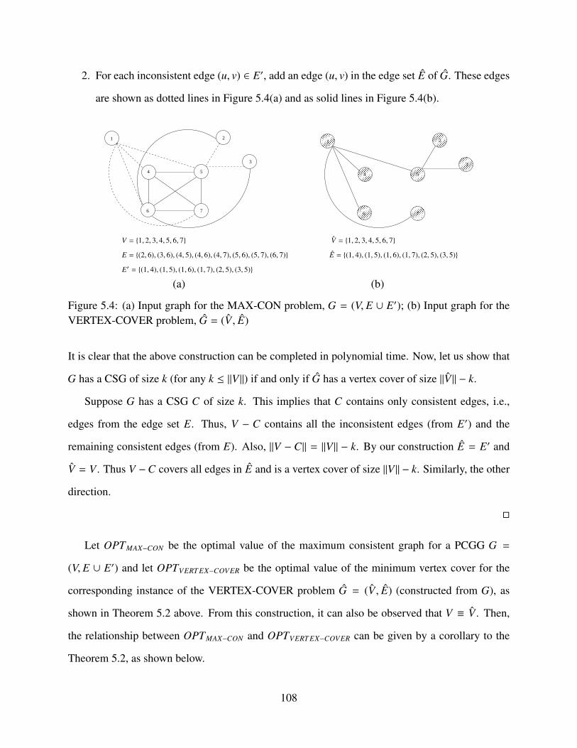
2. For each inconsistent edge (u, v) ∈ E′, add an edge (u, v) in the edge set E of G. These edges

are shown as dotted lines in Figure 5.4(a) and as solid lines in Figure 5.4(b).

1

54

3

2

76

����������������������������������������

����������������������������������������

��������������������������������

��������������������������������

�����������������������������������

�����������������������������������

����������������������������

����������������������������

����������������������������

����������������������������

��������������������������������

��������������������������������

��������������������������������

��������������������������������

1

54

3

2

76

V = {1, 2, 3, 4, 5, 6, 7} V = {1, 2, 3, 4, 5, 6, 7}

E = {(2, 6), (3, 6), (4, 5), (4, 6), (4, 7), (5, 6), (5, 7), (6, 7)} E = {(1, 4), (1, 5), (1, 6), (1, 7), (2, 5), (3, 5)}

E′ = {(1, 4), (1, 5), (1, 6), (1, 7), (2, 5), (3, 5)}

(a) (b)

Figure 5.4: (a) Input graph for the MAX-CON problem, G = (V, E ∪ E′); (b) Input graph for theVERTEX-COVER problem, G = (V , E)

It is clear that the above construction can be completed in polynomial time. Now, let us show that

G has a CSG of size k (for any k ≤ ‖V‖) if and only if G has a vertex cover of size ‖V‖ − k.

Suppose G has a CSG C of size k. This implies that C contains only consistent edges, i.e.,

edges from the edge set E. Thus, V − C contains all the inconsistent edges (from E′) and the

remaining consistent edges (from E). Also, ‖V − C‖ = ‖V‖ − k. By our construction E = E′ and

V = V . Thus V −C covers all edges in E and is a vertex cover of size ‖V‖ − k. Similarly, the other

direction.

�

Let OPTMAX−CON be the optimal value of the maximum consistent graph for a PCGG G =

(V, E ∪ E′) and let OPTVERT EX−COVER be the optimal value of the minimum vertex cover for the

corresponding instance of the VERTEX-COVER problem G = (V , E) (constructed from G), as

shown in Theorem 5.2 above. From this construction, it can also be observed that V ≡ V . Then,

the relationship between OPTMAX−CON and OPTVERT EX−COVER can be given by a corollary to the

Theorem 5.2, as shown below.

108

Corollary 5.3. OPTMAX−CON = |V | − OPTVERT EX−COVER.

Theorem 5.2 implies that any efficient algorithm for solving the VERTEX-COVER problem

can be used to solve the MAX-CON problem. Thus, the approximation algorithm for MAX-CON

can be outlined as shown in Algorithm 5 below.

1: E ⇐ E′ {place all inconsistent edges in E}2: for all edge (u, v) ∈ E′ do3: if u < V then4: V ← u {and corresponding vertices in V}5: end if6: if v < V then7: V ← v8: end if9: end for

10: C = A(V , E) {execute approx algorithm for VERTEX-COVER}11: Return V −C {solution of MAX-CON}

Algorithm 5: Calculating the Maximum CSG of the PCGG G = (V, E ∪ E′)

Let, A(V , E) be an algorithm for solving the VERTEX-COVER problem, where V and E are the

set of vertices and edges respectively of the input graph G. Algorithm A returns the set of vertices

that form the minimum vertex cover for the graph G. The approximation algorithm for MAX-CON

is very straightforward. It first constructs an instance G(V , E) of the VERTEX-COVER problem

from an instance G = (V, E ∪ E′) of the MAX-CON problem. It then uses the approximation

algorithm A for the VERTEX-COVER problem as a subroutine to find the vertex cover C for G.

From Theorem 5.2, the CSG of G is nothing but V −C.

The for loop in Algorithm 5 runs no more than

‖V‖r times. Also, the running time and solution

quality of Algorithm 5 are bounded by the running time and solution quality respectively of the

approximation algorithm A for solving the VERTEX-COVER problem. The minimum VERTEX-

COVER problem is a fundamental and a highly researched problem in graph theory and combi-

natorial optimization with a large number of constant and fixed ratio approximation algorithms.

Hastad [38] showed that VERTEX-COVER cannot be approximated within a factor of 7/6. It was

further improved to 10√

5−21 by Dinur et al. [22]. Gavril introduced a 2-approximation algorithm

109

for the VERTEX-COVER problem [29]. This was further improved to 2 − loglog|V |2log|V | by Bar-Yehuda

et al. [7, 67] and later to 2 − lnln|V |ln|V | (1 − o(1)) by Halperin [34], before it was eventually improved to

2−Θ( 1√log n

) by Karakostas [52]. An interesting generalization of the VERTEX-COVER problem

is the weighted VERTEX-COVER problem in which positive weights are assigned to each vertex

and the problem is to find the vertex cover with minimum cumulative weight. The first well-known

2-approximation algorithm for the weighted VERTEX-COVER problem was discovered indepen-

dently by Bar-Yehuda et al. [6] and Hochbaum [41]. An important point to note here is that all the

approximation results for the unweighted case also hold for the weighted case.

Let A′(G) be a subroutine for solving the MAX-CON problem. Also, let the size of the vertex

set |V | be n. Now, if A(G) is a subroutine for the VERTEX-COVER problem with an approximation

ratio α (α > 1) that is invoked by A then the relationship between the approximation ratio of MAX-

CON and VERTEX-COVER can be given by Lemma 5.4, as outlined below.

Lemma 5.4. The approximation ratio for MAX-CON is bounded by n−α.|A||A′ | .

Proof. The proof for this lemma is straightforward. Let β be the approximation ratio for the sub-

routine A for solving MAX-CON. Then, β can be given as,

β =OPTMAX−CON

|A′|

Similarly, α can be given as,

α =OPTVERT EX−COVER

|A|

From Corollary 5.3,

β =n − OPTVERT EX−COVER

|A′|=

n − α.|A||A′|

�

Next, the optimization problem for obtaining the largest CSG from a PCGG is formulated and

110

its combinatorial properties studied.

5.4 Largest Consistent Grounded Subgraph

5.4.1 Problem Statement

The Largest Consistent Grounded Subgraph problem, denoted as LARGEST-CON, is the problem

of finding the largest CSG (Definition 5.5) of a PCGG G = (V, E ∪ E′). The problem can be alter-

natively stated as the problem of eliminating vertices from G such that the subgraph induced by the

remaining vertices consists of only consistent edges and the cardinality of these consistent edges

is maximized. From Figure 5.2, we can clearly see that an optimal solution for MAX-CON is not

necessarily an optimal solution for LARGEST-CON. These two are different problems with differ-

ent combinatorial properties and solutions. The decision version of the LARGEST-CON problem

can be stated as:

LARGEST-CON

Input: A PCGG G = (V, E ∪ E′) and a positive integer k s.t. k ≤ ‖E‖.

Question: Does G contain a CSG of edge size k or more?

5.4.2 Hardness Result

In this section, the combinatorial hardness of the LARGEST-CON problem is proved. Specif-

ically, it is shown that LARGEST-CON is NP-Complete, i.e., LARGEST-CON ∈ NP and the

deterministic complexity of LARGEST-CON is as hard as any other problem in NP. Thus, it is

highly improbably that LARGEST-CON will have a deterministic polynomial time solution. This

result is proved by a polynomial time many-one reduction from the MAX-2SAT or Maximum 2-

Satisfiability problem. MAX-2SAT is a well known NP-Complete problem [29]. MAX-2SAT is a

restricted version of a related NP-Complete problem called the MAX-SAT or Maximum Satisfia-

111

bility problem. MAX-SAT is the problem, given a set S of disjunctive form clauses, to find a truth

assignment to the literals such that maximum number of clauses are satisfied [29]. MAX-2SAT is

restricted to at most two literals per clause. It can be formally stated as:

MAX-2SAT

Input: A Conjunctive Normal Form (CNF) formula F on Boolean variables x1, x2, . . . , xn and m

clauses C1,C2, . . . ,Cm, each containing at most two literals, where each literal is either Boolean

variable xi or its negation xi (¬xi) and a positive integer k (k < m).

Question: Is there a truth assignment to the variables that satisfies k or more clauses?

Theorem 5.5. LARGEST-CON is NP-Complete.

Proof. A technique identical to the polynomial time reduction from 3-SAT which was used to

prove the NP-Completeness of the VERTEX-COVER problem [43] is applied here to prove the

above result.

It is easy to see that LARGEST-CON ∈ NP: Given a graph G = (V, E ∪ E′), guess a set of

consistent edges E (s.t. ‖E‖ ≥ k and E ⊆ E). Let V be the set of vertices of all these guessed

edges. Check in polynomial time whether the other edges induced by V are consistent. This pro-

cedure clearly can be accomplished in polynomial time and thus LARGEST-CON ∈ NP. Now, it

needs to be shown that MAX-2SAT ≤Pm LARGEST-CON, i.e., MAX-2SAT many-one reduces in

polynomial time to LARGEST-CON. Since MAX-2SAT is NP-Complete, it can be claimed that

LARGEST-CON is NP-Complete.

Construction of an instance of LARGEST-CON, G = (V, EUE′): A polynomial time construction

that maps an instance F of MAX-2SAT to an instance G = (V, EUE′) of the LARGEST-CON

problem is described such that F satisfies k clauses if and only if G has a CSG of edge size k.

Figure 5.5 shows the construction of a PCGG G = (V, E ∪ E′) from the MAX-2SAT formula

F = (x1 ∨ x2) ∧ (x2 ∨ x3) ∧ (x1 ∨ x3) ∧ (x1 ∨ x2). The consistent edges are shown as solid lines and

112

the inconsistent edges are shown as dotted lines.

x1

x2

c1

1

c2

1

c2

4

c1

3c2

3

c1

2

x3

x3

x1

x2

c1

4

c2

2

Figure 5.5: Construction of a PCGG G = (V, E∪E′) from the MAX-2SAT formula F = (x1∨ x2)∧(x2 ∨ x3) ∧ (x1 ∨ x3) ∧ (x1 ∨ x2)

The construction of G consists of the following 3 steps, each adds a different component to the

graph.

1. Let U = VAR(F), be the set of variables in the Boolean formula F. For each variable ui ∈ U,

put ui and ui in the vertex set V and put (ui, ui) into the edge set E′, i.e., the set of inconsistent

edges in graph G. This is the first component of the graph.

2. Let C = CLAUS E(F) be the set of clauses in F, i.e., F =∧

c j∈Cc j. For each clause c j in

the formula F put vertices c1j and c2

j in V . Put an edge (c1j , c

2j) in the set E′, i.e., the set of

inconsistent edges. This is the second component of the graph G.

3. In this step we create a new component by connecting components from the first two steps.

This component depends on the literals that are contained in the clauses. As mentioned

before, each clause c j ∈ C is a disjunction of two literals and literals are variables or their

negations. Consider one such clause c j = (x j ∨ y j), where x j and y j are literals. For each

clause c j, put edges (x j, c1j) and (y j, c2

j) in E, i.e., the set of consistent edges of G. This forms

the third set of components of the graph G.

It is now required to show that the PCGG G (as constructed above) has a CSG G = (V , E)

of edge size k, i.e., ‖E‖ = k if and only if F has k satisfiable clauses. Suppose, there exists an

113

assignment t s.t. exactly k clauses are satisfied. Then for each variable ui ∈ U either t(ui) = 1

or t(ui) = 1 but both cannot be 1. Place ui in the vertex set V of the subgraph G of the PCGG

G if t(ui) = 1 or place ui in V if t(ui) = 1. Thus, V contains one vertex of each edge in the first

component. Now, for a clause c j = (x j ∨ y j), c j is satisfiable if either literals x j or y j or both are

true. Thus, either x j or y j or both are in the set V based on their truth assignment. If both x j and

y j are in V , randomly (with a probability 1/2) select vertex c1j or c2

j and add it to V (never both). If

only one of x j or y j is 1, pick the corresponding cij (based on the construction of component 3) and

place it V . One thing to note here is that when the clause c j is satisfied, only one c1j or c2

j is in the

set V . When it is not satisfied, none of them are in V . It follows that the vertex set V induces edges

only from the consistent edge set E of the PCGG G. Thus, the graph induced by V is consistent

and G = (V , E) is a CSG. Also from the above procedure, if k clauses are satisfied then exactly k

consistent edges get induced in E. As a result, G = (V , E) is a CSG with edge size k. Now, let us

prove the other direction.

Suppose, G = (V , E) is a CSG of the PCGG G s.t. ‖E‖ = k, for some positive integer k. From

the above construction, it is clear that all the consistent edges are of the form (ui, cij), where ui is

the ith (i ∈ 1, 2) literal in the jth clause c j of the formula F. Also, if ui ∈ {xi, xi}, since the graph G

is a CSG, the edges of the form (xi, xi) and (c1j , c

2j) cannot be in E, i.e., both xi and xi or c1

j and c2j

cannot be in the vertex set V of the CSG G. Now, define an assignment t : U → {0, 1} s.t. t(ui) = 1

if ui ∈ V and t(ui) = 0 if ui < V . Similarly, t(ui) = 1 if ui ∈ V and t(ui) = 0 if ui < V . It can

be claimed that this assignment is consistent. Moreover, if there are k edges in E then there are k

satisfied clauses by the above assignment. Since G is a CSG of the PCGG G, none of the edges in

the first two components of our construction can be present in G. Thus, for any variable xi, both xi

and xi cannot be in V . As a result, the assignment t above will consistent. Similarly, for a clause ci,

both c1i and c2

i cannot be in V . Thus, both edges in the third component in the construction above

of the form (u, c1j) and (v, c2

j) cannot be in G at the same time, where u and v are some literals.

If this was not true, (c1j , c

2j) would also be induced in G making it inconsistent. Thus, there is a

one-one correspondence between an edge in G and the corresponding satisfied clause and since all

114

these edges span distinct clauses there are exactly k satisfied clauses.

�

The next lemma gives the relationship between the solutions for the MAX-CON and the

LARGEST-CON problem.

Lemma 5.6. Let OPTLAR(G) and OPTMAX(G) be the optimal solutions of the LARGEST-CON and

MAX-CON problems respectively on any input PCGG G(V, E ∪ E′). Let LAR(G) and MAX(G) be

the set of all the feasible solutions for the LARGEST-CON and MAX-CON problems respectively

on G. Then,

1. cost(OPTLAR(G)) ≤ cost(OPTMAX(G)) i.e., ‖OPTLAR(G)‖ ≤ ‖OPTMAX(G)‖

2. LAR(G) =MAX(G)

3. Let A ∈ LAR(G) (MAX(G)) and B ∈ LAR(G) (MAX(G)) s.t. C = A ∩ B and C , φ. Then,

A ∪ B < LAR(x) (MAX(x)) ⇒ ∃u ∈ A − C and ∃v ∈ B − C s.t. (u, v) ∈ E′, i.e., in the set of

inconsistent edges of G

Proof. 1. Assume that there exists a PCGG such that the inequality 1 above is not true. This

means that there exists an optimal solution of LARGEST-CON that has more vertices than

an optimal solution for MAX-CON. But, then the solution for MAX-CON is not a maximum

CSG, thus not optimal, and that is a contradiction. Therefore, no such PCGG exists.

2. The proof of this point is trivial and follows directly from the definitions of MAX-CON and

LARGEST-CON.

3. Since A and B are both feasible solutions, there are no two vertices u and v both in A s.t.

(u, v) is inconsistent. Similarly, there are no such vertices in either B or C. Also, since A∪ B

is not a feasible solution which implies that there exists two vertices u, v ∈ (A ∪ B) such

that (u, v) is inconsistent. The above two points imply that ∃u ∈ A and v ∈ B s.t. (u, v) is

inconsistent.

115

�

Next, the inapproximability result for LARGEST-CON is presented.

5.4.3 Inapproximability Result

Before proving the inapproximability result for LARGEST-CON, let’s introduce another hard

problem called CLIQUE. In graph theory, a clique in an undirected graph is a set of vertices

such that for every two vertices in this set, there exists an edge in the graph connecting the two.

CLIQUE was one of the first problems shown to be NP-Complete [9]. The decision version of

CLIQUE can be stated as [43]:

CLIQUE

Input: A graph G = (V , E) and a positive integer j ≤ ‖V‖.

Question: Does G contain a clique of size j or more?

Bomze et al. [9] have proved important combinatorial results for the CLIQUE problem. In

summary, they showed that CLIQUE does not have a polynomial time approximation algorithm

unless P = NP. In other words, there is strong evidence that CLIQUE cannot be approximated

with any ratio less than 1.

Theorem 5.7. If there exists an approximation algorithm that can approximate LARGEST-CON

with an approximation ratio ε (ε > 0) then there exists an algorithm that approximates CLIQUE

with ratio 1 −√

1−ε2 .

Proof. Suppose the graph G = (V , E) is an instance of CLIQUE. A new graph G = (V , E) can be

constructed such that the new graph G has the same vertex set as G and E = E ∪ Ec where Ec

contains all the edges that are not in E (in the complete graph induced by the vertex set V). Now,

if E is taken to be the set of consistent edges and Ec to be the set of inconsistent edges then G is

a PCGG. Also, it is easy to see that any CLIQUE in graph G corresponds to a CSG in G and vice

116

versa. Let A be the ε-approximation algorithm for solving the LARGEST-CON problem. Apply A

on the graph G to get the largest CSG in G. Let this largest CSG be G = (V , E). Also, let |V | = m

and M be the vertex cardinality of the optimal solution.

Since A has an approximation ratio ε, we have

∣∣∣∣∣∣∣∣∣∣∣∣∣∣∣∣∣∣∣∣

M2 −

m2M2

∣∣∣∣∣∣∣∣∣∣∣∣∣∣∣∣∣∣∣∣=

M2 − M − m2 + mM2 − M

≤ ε

Then,

1 − ε ≤m2 − mM2 − M

<m2

M2 − M

Without loss of generality we can assume M ≥ 2. Then,

1 − ε < 2( m

M

)2which is,

M − mM

< 1 −

√1 − ε

2

This means that an approximation algorithm for CLIQUE with ratio 1 −√

1−ε2 has been found.

�

The inapproximability of LARGEST-CON can be expressed as a corollary of Theorem 5.7.

Corollary 5.8. Unless P = NP, the approximation threshold of LARGEST-CON is 1.

Proof. This directly follows from the fact that CLIQUE cannot be approximated with any ratio

less than 1 under the hypothesis P , NP.

�

Corollary 5.8 implies that LARGEST-CON cannot be approximated with any ratio less than 1

under the hypothesis P , NP. The next section presents two solution strategies for the LARGEST-

CON problem based on popular heuristics.

117

5.5 Heuristics for LARGEST-CON

Heuristics like greedy choice and local solution search have been used in the design of solution

strategies for the LARGEST-CON problem. Experimental results, discussed later in Section 5.6,

have found that both the strategies work reasonably well for randomly generated connected graphs.

But, an exact theoretical bound on the solution quality of these algorithms is not known and is still

an open question.

5.5.1 Greedy Algorithm

Let the PCGG G = (V, E ∪ E′) be an instance of LARGEST-CON, where E and E′ are the sets

of consistent and inconsistent edges respectively. For a vertex v ∈ V , let con(v) be the number of

consistent edges of v and let incon(v) be the number of inconsistent edges of v. In other words,

con(v) is the consistent edge degree of the vertex v while incon(v) is the inconsistent edge degree

of v. The basic idea of the greedy algorithm is to eliminate all the inconsistent edges of G by

greedily selecting inconsistent vertices (vertices with inconsistent edge degree at least one) that

are connected to lowest number of consistent edges. The greedy approach for obtaining the largest

CSG is shown in Algorithm 6.

1: C ⇐ φ; {Initialize the solution to empty set}2: C = {v| v ∈ V ′ and incon(v) = 0}3: V ′ ← V ′\C;4: while E′′ , φ do5: pick a vertex v ∈ V ′ of minimum con(v);6: V ′ ← V ′\{v}7: E′′ ← E′′\{e|v ∈ e}8: end while9: C ← C + V ′;

10: Return C {solution of LARGEST-CON}

Algorithm 6: Greedy Algorithm

The greedy approach, as discussed above, first removes from consideration all vertices that

are only connected to consistent edges. Then in each iteration, it randomly selects a vertex for

118

elimination with inconsistent degree at least one and lowest consistent edge degree. The algorithm

continues this until all the inconsistent edges are eliminated and the graph G contains only con-

sistent edges. The greedy approach is pretty straightforward, with a running time bounded by the

execution of the while loop, which is O(n2), where |V | = n. One problem with this greedy strategy

is that the decision to select a particular vertex for elimination at each step is solely based on the

consistent edge degree of the vertex (i.e., the number of consistent edges lost from the final CSG).

This may not always be a good decision as there might be another vertex connected to the same

number of consistent edges but more number of inconsistent edges. Thus, selecting this vertex at

that particular step would be much more efficient. The above greedy algorithm can be modified

slightly by using an alternative heuristic and is outlined in Algorithm 7 below.

1: C ⇐ φ; {Initialize the solution to empty set}2: C = {v| v ∈ V ′ and incon(v) = 0}3: V ′ ← V ′\C;4: while E′′ , φ do5: pick a vertex v ∈ V ′ of minimum con(v)

incon(v) ;6: V ′ ← V ′\{v}7: E′′ ← E′′\{e|v ∈ e}8: end while9: C ← C + V ′;

10: Return C {solution of LARGEST-CON}

Algorithm 7: Modified Greedy Algorithm

According to the modified greedy heuristic, in each iteration of the algorithm, a vertex v with

the lowest ratio of consistent to inconsistent edge degree ( con(v)incon(v) ) is selected for elimination. The

running time of the modified greedy algorithm is also O(n2) where |V | = n. The greedy heuristic

is experimentally evaluated in Section 5.6. Next, an algorithm for LARGEST-CON based on the

neighborhood search strategy is proposed.

5.5.2 Local Solution Search

Local Solution Search (LSS) is a popular algorithm design technique for optimization problems.

Before giving details on this technique, let’s introduce a few important concepts. Let U be an

119

optimization problem and x be an input problem instance for U. Let M(x) be the set of feasible

solutions of the problem U for the input instance x.

Definition 5.6. Neighborhood: For an optimization problem U and for every input instance x, a

neighborhood on the set of feasible solutions (M(x)) is any mapping fx : M(x) → Pot(M(x)) (Pot

denotes the power set) such that

1. α ∈ fx(α) for every α ∈ M(x),

2. if β ∈ fx(α) for some α ∈ M(x), then α ∈ fx(β), and

3. for all α, β ∈ M(x) there exists a positive integer k and γ1, . . . , γk ∈ M(x) such that γ1 ∈ fx(α),

γi+1 ∈ fx(γi) for i = 1, . . . , k − 1, and β ∈ fx(γk)

If α ∈ fx(β) for some α, β ∈ M(x), then α and β are said to be neighbors in M(x). The set fx(α) is

called the neighborhood of the feasible solution α in M(x) [44].

Now, let’s introduce the concept of local optima.

Definition 5.7. Let U be an optimization problem and for every input instance x of the problem

let fx be the neighborhood function on M(x). Let cost be the cost function that assigns a positive

real number to each feasible solution. A feasible solution α ∈ M(x) is a local optima for the input

instance x of U according to fx, if

cost(α) = (max) or (min){cost(β)|β ∈ fx(α)}

Denote the set of all local optima for x according to the neighborhood fx by LocOPT U(x, fx) [44].

Neighborhood Definition for LARGEST-CON: The formalisms of functions and relations does

not work when introducing neighborhoods on M(x) in practical problems like LARGEST-CON.

The standard way to introduce a neighborhood on M(x) is to use a so-called local transformation

on M(x). Informally, a local transformation transforms a feasible solution α to a feasible solution

120

β by some local changes of the specification of α. To define a neighborhood for an instance of the

LARGEST-CON problem, a transformation called a n-neighborhood transformation is introduced.

For simplicity, let us first introduce a 1-neighborhood transformation. Let x = G(V, E ∪ E′) be an

instance of the LARGEST-CON problem. Let M(x) be the set of feasible solutions for LARGEST-

CON on input x. For α ∈ M(x), the 1-neighborhood of α is defined as follows:

To define a 1-neighbor of a feasible solution α, pick a vertex v ∈ V\α s.t. v has an inconsistent

edge degree of exactly one and this inconsistent edge connects v to a vertex in α. Let this vertex in

α to which v connects be called w. If there are no such vertex w in α then α has no 1-neighbors.

Now to get a 1-neighbor of α, add v in α and remove w from α. It is clear that this resultant

subgraph is also a feasible solution since the inconsistent edge which was covered by v previously

is now covered by w. Also, addition of v does not induce any inconsistent edge in the resultant

subgraph since its inconsistent edge degree is one and that edge is now covered by w. Such a

subgraph is called the 1-neighbor of the solution α. The set of all the 1-neighbors of α is called

the 1-neighborhood of α and is represented as Neigh1x(α). Similarly, to define a 2-neighborhood,

a vertex v ∈ V\α with inconsistent edge degree of exactly two (to vertices in α) is selected. This

vertex is added in α and the two vertices that v connects by inconsistent edges are removed from α.

One thing to note here is that 1-neighbors of α have the same vertex set cardinality as α while its

2-neighbors have their vertex set cardinality reduced by 1. Similarly 3-neighborhoods are defined.

Local Solution Search Algorithm for LARGEST-CON: A Local Search Solution or LSS al-

gorithm starts off with an initial solution and then continually tries to find a better solution by

searching neighborhoods of that solution. If there is no better solution in the neighborhood, then

it stops. By having a structure on the set of feasible solutions M(x), determined by a neighbor-

hood Neighx, for every input instance x of an optimization problem U, one can describe a general

scheme of local search as shown in Algorithm 8.

The success of the local search algorithm depends on the choice of the neighborhood. If

a neighborhood Neighx has a property such that Neighx(α) has a small cardinality for every

121

1: Find a feasible solution α ∈ M(x)2: while α < LocOPT U(x,Neighx) do3: find a β ∈ Neighx(α) such that cost(β) < cost(α) if U is a minimization problem or cost(β) >

cost(α) if U is a maximization problem;4: If such a β is found, α = β;5: end while6: Return α

Algorithm 8: Local Search Scheme according to a neighborhood Neigh

α ∈ M(x), then one iterative improvement of the while loop of Algorithm 8 can be executed

efficiently, but the risk that there are many local optima (potentially with a cost that is very far

from the optimal solution) can substantially grow. On the other hand, large |Neighx(α)| can lead

to feasible solutions with costs that are closer to the optimal solution than smaller neighborhoods

can, but the complexity of the execution of one run of the while cycle can increase too much.

Besides the choice of the neighborhood, there are two other factors that affect the execution of

the local search algorithm. The first factor is the method by which the initial feasible solution is

computed. The choice of the initial solution can essentially influence the quality of the resultant

local optimum. The initial feasible solution can be either chosen randomly for problems in which

the structure of the feasible solution is simple or it can be precomputed. In the LSS algorithm for

LARGEST-CON, the initial feasible solution is precomputed. From Lemma 5.6, it is clear that a

solution for the MAX-CON problem is also a solution for the LARGEST-CON problem. Thus,

any algorithm that produces an optimal solution for MAX-CON can be used as a good starting

solution for the LARGEST-CON problem. Further improvement can be done by starting the LSS

algorithm with multiple initial feasible solutions. The second factor affecting the performance of

the LSS algorithm is the way in which a cost-improving feasible solution is selected inside the

while loop. There are two strategies in doing this, namely, the First Improvement Strategy and

the Best Improvement Strategy. In the first improvement strategy, the current feasible solution is

replaced by the first cost-improving feasible solution found by the neighborhood search. The best

improvement strategy replaces the current feasible solution by the best feasible solution in the

neighborhood. A LSS for solving LARGEST-CON is outlined in Algorithm 9.

122

1: Let x = G(V, E ∪ E′) be a PCGG and an instance of LARGEST-CON and let A be an efficientalgorithm for solving MAX-CON.

2: Let α = A(x) be the initial feasible solution.3: while α < LocOPT U(x,Neigh1

x(α)) do4: Either by first improvement or best improvement, find a β ∈ Neigh1

x(α) such that cost(β) >cost(α) {cost function outputs the edge count (consistent) of a solution}

5: If such a β is found, α = β;6: end while7: Return α

Algorithm 9: Local Search Scheme for LARGEST-CON using Neigh1x

One shortcoming of the approach outlined in Algorithm 9 is that in each iteration of the while

loop only the 1-neighborhoods (Neigh1x) of the feasible solution α is checked. But, α might

not have 1-neighborhoods at all or there might be better solutions in the 2-neighborhoods and

3-neighborhoods. Thus, the above algorithm can be further improved by also checking the 2-

neighborhoods and 3-neighborhoods of the feasible solution in each loop. The local search algo-

rithm is also experimentally evaluated next (Section 5.6) and its solution quality is compared with

that of the greedy heuristic.

5.6 Experimental Evaluation

The greedy and local solution search algorithms for the LARGEST-CON problem are experimen-

tally evaluated by implementing these algorithms using C++ programs and executing them on an

Intel® Pentium® 4 processor-based computer system. The results from the current set of experi-

ments are useful in understanding the behavior of these algorithms (in terms of the solution quality)

under various network topologies, specifically when the density of the input PCGG increases. A

comparative analysis of the solution quality of the two heuristic-based algorithms is performed

in order to determine if one algorithm clearly performs better than the other. The details of the

experimental setup are described next.

123

5.6.1 Experimental Setup

In the current set of experiments, the heuristics for LARGEST-CON proposed in Section 5.5 are

tested on Random Graphs. Random graphs are graphs without any specific topology or physical

characteristics and are generated in the following way: All vertices in the graph represent the nodes

in the sensor network that are randomly distributed in a 500m×500m region. Each node has a radio

range R. If the distance between two nodes is less than or equal to the radio range R (all nodes are

assumed to have the same radio range) then the two corresponding vertices are connected by an

edge in the graph.

The number of nodes (n) and the radio range (R) are adjustable parameters in this simulation.

Without loss of generality, currently only one third of the total number of nodes are randomly se-

lected to be malicious. But, this is an experimental parameter and can be modified accordingly in

order to observe the efficiency of the proposed algorithms for more number of cheating nodes. For

any edge between a malicious node and an honest node (or another malicious node), it is assigned

to be inconsistent with a probability of 1/2. This is because, as mentioned earlier, malicious behav-

ior is random and that malicious node may not cheat all the time. All other edges between honest

nodes are always consistent. It is obvious that if all the malicious nodes and the corresponding

edges are removed then the resulting subgraph becomes consistent. This subgraph may or may

not be the optimal solution. Such a subgraph is called a sub-optimal solution. Since it is com-

putationally infeasible to get the true optimal solution for large graphs, the solution quality of the

algorithms are measured by evaluating the sub-optimal solution. Specifically, the solution quality

of the algorithms is measured as the ratio of the number of consistent edges in the CSG output by

the algorithm to the number of consistent edges in the sub-optimal solution.

5.6.2 Results and Evaluation

The two variants of the greedy algorithm (greedy approach and modified greedy approach) and the

two variants of local search algorithms (first improvement strategy and best improvement strategy)

124

are tested with some fixed values for n and R. It is observed that the performance difference

between the two greedy algorithms is negligible. For this reason only one indicative data curve for

the greedy algorithms is included here. Similarly, the performance difference of the two variants

of the local search algorithms is also negligible and as a result only one indicative data curve for

the local search algorithms is included here. All data values are obtained as the average over 100

runs. Figure 5.6(a), 5.6(b) and 5.6(c) plots the solution quality of the algorithms against the radio

range of the nodes with n = 80, n = 100 and n = 120 respectively. The radio range is plotted along

the X-axis and the solution quality is plotted along the Y-axis.

The following observations can be made from the plots in Figure 5.6:

1. None of the algorithms return a solution that is better than the sub-optimal solution.

2. The performance or solution quality of both the algorithms decreases as the number of nodes

increases.

3. Also, the performance or solution quality of both the algorithms decreases as the radio range

increases (i.e., the graph becomes more dense), and the solution quality stabilizes after the

radio range reaches some threshold value.

4. In summary, the local search algorithm has some improvement over the greedy algorithm,

but the improvement is not significant. Moreover, the solution quality does not deteriorate

below 0.4 and that the average solution quality for all cases is close to 0.5 for both the

algorithms.

Despite the negative inapproximability result for LARGEST-CON, it can be observed that both

the greedy and local search algorithms produce good solutions and the solution quality is close to

0.5 even for large, highly dense graphs. These results are encouraging.

125

(a)

(b)

(c)

Figure 5.6: Plot of solution quality versus radio range for a network with (a) 80 Nodes; (b) 100Nodes; (c) 120 Nodes

126

5.7 Further Improvements

Although the greedy and local solution search algorithms have been experimentally shown to pro-

vide solution qualities close to 0.5, there are still some issues with these simple heuristics. For

example, the local solution search algorithm may get stuck in a poor local optima for some choice

of an initial feasible solution. Similarly, depending on the choice of the first vertex selected for

elimination, the greedy strategy may or may not be able to produce a good solution. In order to

overcome these problems, two other optimization strategies have been proposed in this section.

The simulated annealing algorithm, as discussed next, overcomes the poor local optima problem

by accepting a deterioration in the hope of producing an overall better solution. Following this

algorithm, the Linear Programming (LP) formulation of the LARGEST-CON problem is outlined

where an optimal solution is the one that satisfies all the constraints and maximizes a cost function.

5.7.1 Simulated Annealing

One problem with the local solution search or LSS algorithm discussed in Section 5.5.2 is that

there may be instances of LARGEST-CON for which the local search algorithm can get stuck

in an arbitrary poor local optima. One approach to overcome this problem is to start the local

search algorithm several times with different randomly chosen initial solutions. Another approach,

called the simulated annealing, is to add the possibility of leaving a local optimum to move to

a weaker solution (deterioration) by some kind of coin tossing (random probability) in order to

find better solutions. This approach is motivated from the annealing process which is used to

obtain low energy states of a solid in a heat bath. In this approach, the probability of accepting a

deterioration in the iterative process depends on the size of the deterioration as well as the number

of iterations executed up till now. The simulated annealing approach for the LARGEST-CON

problem is outlined in Algorithm 10.

There are two main free parameters in the simulated annealing algorithm that affect the solution

quality. The first parameter is the neighborhood Neigh1x and the second is the cooling scheme which

127

1: Let x = G(V, E ∪ E′) be an instance of LARGEST-CON and let A be an efficient algorithm forsolving MAX-CON.

2: Let α = A(x) be the initial feasible solution.3: Let T be an initial control parameter (temperature).4: Select a temperature reduction function f as a function of two parameters; T and time.5: Select a counter I := 06: while T > 0 (or T is not too close to 0) do7: Either by first improvement or best improvement, find a β ∈ Neigh1

x(α)8: if cost(β) ≤ cost(α) {cost function outputs the edge count (consistent) of a solution } then9: α := β

10: else11: Generate a random number r uniformly in the range (0, 1)12: if r < e−

cost(β)−cost(α)T then

13: α := β14: end if15: end if16: I := I + 117: T := f (T, I)18: end while19: Return α

Algorithm 10: Simulated Annealing Scheme for LARGEST-CON using Neigh1x

determines the rate of decrease of the parameter T . It can be observed that a slow decrease of T

may result in an extremely large time complexity of the algorithm. But, it has been proved that the

increase of time complexity increases the probability of getting feasible solutions of high quality

[44]. Moreover, factors like initial choice of control parameter or temperature T , the temperature

reduction function f , and the termination condition which decides when the simulated annealing

algorithm stops for T ≤ term; all decide how much improvement can be achieved by the simulated

annealing process. These factors are not discussed here and further details can be found in the

book by Juraj et al. [44].

Simulated annealing has been presented here as a possible improvement to the existing greedy

and local search algorithms for solving the LARGEST-CON problem. The actual performance

of this algorithm and the values for the various cooling scheme parameters have not been fixed

and experimentally verified. Next, a LP-based optimization technique for the LARGEST-CON

problem is presented.

128

5.7.2 Linear Programming-based Optimization

The LARGEST-CON problem can also be formulated as an Integer Program (IP); more specifically

a 0-1 Program. Let G = (V, E ∪ E′) be an instance of the LARGEST-CON problem, where E is

the set of consistent edges and E′ is the set of inconsistent edges. Let Uk ∈ {0, 1} where k ∈ E,

be the variable representing whether a consistent edge k is selected or not. The value of Uk = 1

implies that the consistent edge k is present in the solution and Uk = 0 implies that it is not. Let

vi ∈ {0, 1} where i ∈ V , be a variable representing whether each vertex i in the graph is present in

the solution or not. Similarly, vi = 1 implies that the vertex i is in the solution and vi = 0 implies

that it is not. Let ‖V‖ = n, i.e., there are total number of n vertices. Let ‖E‖ = m, i.e., the size of

the consistent edge set is m. Then, the IP of the LARGEST-CON problem for an input instance G

can be formulated as shown below.

Maximizem∑

i=1

Uk

S ub ject to (vi + v j − 2Uk) ≥ 0; ∀k = (i, j) ∈ E

(vi + v j) ≤ 1; ∀(i, j) ∈ E′

and vi, v j,Uk ∈ {0, 1}; ∀i, j ∈ V, k = (i, j) ∈ E

Solving an Integer Program is a well-known NP-hard problem [54]. To overcome this hurdle, a

Linear Program (LP) relaxation for the above Integer Program can be obtained. A Linear Program

is solvable in polynomial time [55] using efficient techniques like the simplex algorithm [18]. If

the LP relaxation has an integral solution then that can be the solution for the above IP also. But

if LP relaxation does not have integral solution then techniques like rounding, branch and bound,

etc., can be used to obtain a close to optimal solution.

129

5.8 Conclusion

This chapter addressed the problem of efficiently mitigating location inconsistencies in localization

services and location-based applications in highly distributed network systems like wireless sensor

networks. Inconsistent location information results from either cheating behavior by nodes or due

to large measurement errors, often caused by external and uncontrollable factors. Such inconsis-

tent location information cause location dependent applications and services to fail and needs to be

efficiently eliminated from the network. Towards achieving that goal, this chapter first presented

a practical graph-theoretic framework, called Partially Consistent Grounded Graph, for modeling

location-based services in highly distributed and autonomous network systems like wireless sen-

sor networks. In this model, inconsistent location information in the network was modeled as a

subset of the set of all edges in the network, referred to as the set of inconsistent edges. Based

on this graph-theoretic model of the network, two optimization problems, namely MAX-CON and

LARGEST-CON, were formulated.

MAX-CON is the problem of maximizing the number of vertices in the completely consistent

subgraph of the Partially Consistent Grounded Graph, while LARGEST-CON is the problem of

maximizing the number of consistent edges. A number of combinatorial properties, including com-

putational hardness and approximability for these problems were studied. Both the problems were

proved to be NP-Complete. The hardness of these problems is indicative of the difficulty involved

in efficiently eliminating inconsistency causing nodes in a highly distributed system, even in the

presence of full knowledge (or complete location information). Although MAX-CON was guar-

anteed to have a constant ratio approximation algorithm, no such guarantees could be made for the

LARGEST-CON problem. LARGEST-CON was proved to not have a constant approximation ra-

tio, unless P = NP. Following this inapproximability result, two algorithms for LARGEST-CON,

namely the greedy algorithm and the local solution search algorithm, were outlined. Experimental

results showed that the local search algorithm performs slightly better than the greedy algorithm

for randomly generated graphs and that the performance of both the algorithms deteriorated as the

130

number of nodes and radio range increased. Another important observation in these experiments

was that the average solution quality was around 0.5, which is encouraging considering the inap-

proximability result. In order to overcome some of the drawbacks of the basic greedy and local

search heuristics, two more solution strategies, one based on the simulated annealing technique and

another on a Linear Programming approach, were also proposed. Although no experimental results

are available for these strategies at this time, intuitively it does not seem that they will perform any

worst than the greedy or the local search heuristic.

The next chapter concludes this dissertation by presenting a summary of contributions and a

quick recap of the major research results, followed by a discussion of the impact of the research

presented in this dissertation and how these results can be used and interpreted by other researchers

and practitioners. The chapter finally ends with a road-map for further research on a variety of open

problems and unresearched topics in the area of secure and robust localization.

131

Chapter 6

Conclusion

“This is not the end. It is not even the beginning of the end. But it is, perhaps, the end

of the beginning.”

−Winston Churchill

This chapter presents a detailed summary of the important results from the previous chapters

and discusses its role in achieving the basic goals of secure and robust localization that were out-

lined at the start of the dissertation. It also puts the research of this dissertation in perspective by

highlighting the significance of the published results in context of their utility in securing and im-

proving the robustness of localization services and location-based applications in ESNs. Finally,

this chapter lists a set of open problems on robust localization that have not been addressed in this

dissertation and outlines a plan for further research on these and a variety of other problems in this

area.

6.1 Summary

Wireless sensor networks are a byproduct of the basic concept of wireless ad-hoc networks, i.e.,

networks that generally do not require any fixed infrastructure or organization for successful oper-

ation. The main difference in sensor networks is the low power (both battery and computational)

and robustness of the sensor devices as compared to the high-end devices found in modern day

132

wireless (ad-hoc) networks. Due to the location critical nature of the applications associated with

such networks, knowledge of the node locations is extremely important and as a result, the prob-

lem of localization or location discovery in wireless sensor networks has gained a lot of research

attention. Most of the earlier research efforts on localization in sensor networks were derivatives

of similar work in wireless LAN (IEEE 802.11) or ad-hoc networks. Although researchers focused

on developing distributed localization schemes for low power and resource constrained devices,

other issues regarding security, robustness and fault-tolerance of such schemes were overlooked.

These are important issues, especially considering the harsh and hostile conditions in which sensor

networks are deployed and used.

This dissertation has addressed the problem of robust localization in wireless sensor networks

with a special focus on sensor networks used for emergency, military and first response applica-

tions, referred to as Emergency Sensor Networks (ESNs). There are various issues associated with

the problem of efficient localization in ESNs. On the one hand, due to the open nature of the net-

work, security of nodes and services like localization is an issue. On the other hand, harsh and

extreme conditions can cause nodes to fail, which can act as a strong deterrent to the success of

the localization process in such networks. In addition to these, inaccurate location discovery can

also adversely affect other location dependent network-wide services and applications. The main

goal of this dissertation was to provide efficient solutions to these and other problems related to the

process of localization, keeping in mind the specific requirements, constraints and factors affecting

ESNs.

In line with this goal, the first order of business in this dissertation was to survey existing

localization schemes by dividing them into two broad classes, followed by a study of the appli-

cability of each such scheme in ESNs by identifying their shortcomings and disadvantages under

specific situations. The survey of the two classes of localization techniques, namely beacon-based

techniques and signature-based techniques, their advantages, shortcomings, etc., were outlined in

detail in Chapter 1. Two main problems in existing localization techniques for sensor networks

were identified. The first one was the problem of cheating or malicious beacon nodes in beacon-

133

based localization approaches that use distance information. The second problem underlined the

lack of fault-tolerance in existing signature-based approaches. An effective solution strategy to

each of the above problems would go a long way in successfully implementing and deploying

these localization techniques for a variety of ESN applications. A careful study of other research

efforts in this direction was also conducted in Chapter 2, which not only discussed specific limita-

tions in those proposals but also summarized steps that were taken in this dissertation in order to

overcome those shortcomings.

In Chapter 3, the problem of distance-based localization in the presence of cheating or ma-

licious beacon nodes was addressed. By assuming a very practical network model and a strong

adversary model (which also includes collusion attacks), couple of important analytical results for

this problem were presented. The first set of results fixed the necessary and sufficient conditions for

secure distance-based localization in terms of the number of malicious nodes that can be success-

fully tolerated by any distance-based localization algorithm. The second set of results, identified

and defined a class of distance-based localization algorithms that can guarantee a bounded local-

ization error, provided the necessary and sufficient conditions are satisfied. These results laid the

foundation for identification of two algorithms belonging to this class of robust distance-based

localization algorithms. The first algorithm, called the polynomial time algorithm, was proved to

have a cubic (n3logn) worst-case running time complexity in terms of the total number of beacon

nodes n. The second algorithm was based on an intelligent heuristic of searching for the target

location near intersection points of a large number of circles (denoting coverage area of nodes).

Although no running time guarantees could be provided for the heuristic-based algorithm, it was

found to perform very well in most scenarios. Also, experimental results showed that even though

both the polynomial time algorithm and the heuristic-based algorithm had low localization errors,

the heuristic-based algorithm outperformed the polynomial time algorithm in execution time. In

order to show the generality of the proposed results and solutions, an extension of the current

framework to the three dimensional coordinate system was also proposed. Moreover, the proposed

algorithms were tested with various distributions of target and beacon locations to show that the

134

performance of the algorithms was not dependent on a specific distribution of node locations.

Following a rigorous analytical and experimental treatment of the secure distance-based local-

ization problem, the focus of the dissertation shifted to the problem of fault-tolerant localization in

Chapter 4. More specifically, this chapter addressed the problem of robust signature-based local-

ization in the presence of disabled or failed nodes. Although beacon-based approaches have been

shown to work well in most cases, signature-based approaches provide a good alternative when it

is not feasible to deploy or implement beacon-based techniques. Similar to beacon-based schemes,

signature-based techniques have been shown (as explained in Chapter 1) to suffer from a variety

of problems, the most prominent of it being the fault-tolerance of such schemes. This problem

is also significant from the point of view of its feasibility in ESNs and related applications. In

that direction, Chapter 4 first presented a detailed case study describing the mechanics of a typi-

cal signature-based scheme, and by means of simulation experiments showed that the localization

accuracy of such schemes deteriorated rapidly as the number of disabled nodes increased. From

the case study, it was also clear that node deployment and the post-deployment node distribution

greatly influence the accuracy of signature-based localization. Node deployment strategies in exist-

ing signature-based schemes do not posses the necessary mechanisms in order to monitor and adapt

to the changes in node distribution due to factors like movement, disablement, etc., which is the

main cause of the lack of fault-tolerance in these schemes. To overcome this issue, an emergency

level-based deployment strategy was proposed that deploys nodes around fixed points over the de-

ployment area based on the rate of node disablement at those points. In order to predict the node

disablement around deployment points, a stochastic model of node destruction was formulated, and

the deployment strategy employs this model to make deployment decisions. Then, a simple and in-

tuitive technique to improve the fault-tolerance of current signature-based localization techniques,

called Group Selection Protocol (GSP), was outlined. GSP monitors node distribution changes due

to disablement by employing specialized nodes, called group heads. One task of the group heads

is to collect and forward the health status updates of their corresponding groups to other nodes in

the network. Although employing GSP resulted in some improvement as far as fault-tolerance was

135

concerned, it did not improve the complexity of the localization scheme in terms of computation

and memory look-up. In order to achieve that, a simple, fault-tolerant signature-based localization

scheme, called ASFALT, was proposed. ASFALT works by computing distances to neighborhood

nodes and utilizes the non-uniformity in node distribution to compute the target location. Results

of simulation experiments verified that ASFALT outperforms the other signature-based scheme

(with and without GSP) in situations of random node disablement.

Finally, in Chapter 5 another problem related to localization was addressed. Here, instead of

accurately localizing the nodes, it was assumed that all nodes know their own locations (or at least

pretend to know their own locations). The problem then is, how to eliminate nodes that do not dis-

close their location information correctly? Inaccurate location reporting/verification is detrimental

to the success of sensor network applications, especially emergency related applications because

they are extremely location critical. Such inaccurate location reporting/verification can be either a

result of cheating behavior or due to external factors. Nevertheless, it’s very important to efficiently

eliminate inaccurate location information in order to get a location-consistent view of the network,

which can be used to localize other nodes or to make other network-wide decisions. This prob-

lem was modeled as a combinatorial optimization problem in a graph-theoretic framework of the

network, called Partially Consistent Grounded Graphs (PCGG). Two variants of the problem were

addressed. In the first variation, called MAX-CON, the number of vertices in the consistent sub-

graph of the PCGG was maximized, while in the second one, called LARGEST-CON, the number

of edges in the consistent subgraph was maximized. Important combinatorial properties for these

problems, including combinatorial hardness and approximability were studied. Although both the

problems were proved to be NP-Complete, it was shown that MAX-CON has a constant time ap-

proximation algorithm while it was not possible to approximate LARGEST-CON with a constant

ratio unless P = NP. Efficient algorithms based on popular heuristics like, greedy approach, local

solution search, simulated annealing and Linear Programming based approaches were proposed.

Although currently no analysis that gave a bound on the solution quality of these algorithms was

provided, experimental results showed that both the greedy and local solution search performed

136

well for randomly generated graphs, with an average solution quality of around 0.5.

The following section discusses the impact of the results presented in this dissertation on the

development of efficient localization and security tools for futuristic networks like the Emergency

Sensor Networks.

6.2 Research Impact

The research presented in this dissertation is multi-faceted with a single goal: to provide secure and

robust localization services for Emergency Sensor Networks. It works towards this goal by identi-

fying shortcomings in existing localization approaches at various levels and fronts, and attempts to

overcome these weaknesses by leveraging on mathematically sound analytical tools and rigorous

simulation experiments. Three main factors that affect the accuracy of localization services and

location-based applications are identified.

The first factor is the security of localization services in Emergency Sensor Networks. Simi-

lar to other services and applications in wireless and computer networks, localization security in

sensor networks was an afterthought. Until recently there was very little or no research on se-

curing localization services in wireless sensor networks. Securing the localization process against

malicious or cheating nodes is crucial to the success of the network application. This problem is

more pronounced in ESNs because of the harshness and the hostility of the environment in which

such networks are deployed. The research on securing localization services presented in this dis-

sertation targets a very specific type of localization technique, referred to as the beacon-based

technique. Unlike previous techniques on securing beacon-based localization, this dissertation

takes a two-pronged approach. Rather than directly going out for a solution based on some heuris-

tic, this dissertation conducts a detailed mathematical analysis of the problem using a practical

network model and a strong adversary model. The necessary and sufficient conditions and the

bounds on the worst case localization errors obtained by this study may help in understanding how

best any distance-based algorithm could perform. Such bounds are also useful to other researchers

137

and algorithm designers, because they provide a reference scale to compare the solution quality of

new algorithms in this area. The class of robust localization algorithms defined in this chapter can

also help in deriving a taxonomy of secure distance-based localization approaches. Following the

important analytical results, a series of experimental studies reported in this dissertation can help

identify how some of the algorithms in this class stack up against each other under different pa-

rameters like the number of malicious nodes, measurement errors and location distribution. Since

these algorithms are guaranteed to have a bounded localization error, the parameters on which

they can be further improved are the simulation time and execution efficiency. These experiments,

although not executed on a sensor network test-bed or simulation environment, can give ample

insight into the mechanics and performance of these algorithms. These results will be very useful

when designing secure localization algorithms for real sensor network applications. These results

have been published in [98].

The second factor that affects the accuracy of localization in Emergency Sensor Networks is

the random disablement or failure of nodes. Fault-tolerance is an extremely important property of

localization schemes employed in ESNs because of the high probability of node failures in ESN

applications. A detailed study of existing literature reveals very little or no work in the direction

of fault-tolerant localization schemes. The research presented in this dissertation is among one

of the first works in this area. Achieving fault-tolerance in beacon-based techniques is pretty

straightforward. Beacon node disablement may result in insufficient number of beacons available

for localization and the way to overcome this problem is by increasing the beacon node redundancy

in the network. But, the problem becomes non-trivial in signature-based localization schemes. The

emergency level based node deployment strategy is the first step in achieving fault-tolerance in

such schemes. It provides a simple and effective way to deploy nodes over the emergency area in

an ESN. The strategy itself and the various related probabilistic models are generic enough to be

used by network designers to develop deployment policies for emergency specific sensor network

applications. Also, the fault-tolerance related improvements in the form of ASFALT and GSP are

very simple, intuitive and straightforward to implement. Moreover, measurements from extensive

138

simulation-based experiments have verified the improvement brought about by these algorithms.

But before these algorithms can be used in real world, extensive testing in a much more realistic

scenario like a sensor network test-bed would be required. In that case, measurements from the

current simulation experiments would be relevant in order to carry out a comparative analysis and

can provide hints on improving these schemes further. This part of the research was presented

in [47, 49].

Apart from the problem of location discovery, another intriguing question that needed attention

was, how can nodes in the network be sure that other nodes are truthful about their locations?

For node pairs that are truthful, the Euclidean distance between their locations should match the

estimated distance between the nodes. And for the ones that this does not match, it implies that

there is a location inconsistency. From a network-wide point of view, one is viewing at a structure

in which some nodes are consistent with each other in terms of locations, while others are not.

A consistent structure is important for multiple reasons. First, it assures other nodes not within

the consistent structure that localization done by using nodes from the consistent structure will be

accurate. Second, nodes within the consistent structure can be used by a variety of other location

dependent services like routing, neighborhood detection, etc., to make their own network-wide

decisions. Such a consistent structure is also useful to network designers and administrators for

making redeployment decisions, information segregation, etc. This problem of obtaining a fully

location consistent substructure of the network, given complete knowledge of the node locations

and distances between them, has only been first addressed in this dissertation. The approach in

order to obtain a solution for this problem has been very systematic. Rather than providing random

heuristics, this dissertation first modeled the problem as a graph-based optimization problem and

studied its combinatorial properties like computational hardness and approximability. These results

were useful in developing meaningful heuristics to solve this problem. This work appeared in [46].

The next section lists some interesting open problems and directions for future research in the

area of secure and robust localization.

139

6.3 Open Problems and Future Research

This dissertation has attempted to provide answers to a variety of questions in the area of secure

and fault-tolerant location discovery for wireless sensor networks. However, there are numerous

avenues for extending the research presented in this dissertation. The following directions hold a

lot of promise in terms of future research in this area.

This dissertation presented significant theoretical analysis on the problem of secure distance-

based localization in the presence of malicious or cheating beacon nodes. Specifically, the neces-

sary and sufficient conditions for secure localization and a class of robust localization algorithms

that guaranteed a bounded localization error were presented. Two algorithms that belong to this

class were also outlined. These algorithms estimated the target location by computing a point in

the intersection of at least kmax + 3 rings. The analysis verified that these algorithms can guarantee

a bounded localization error. But, an intriguing question in this direction is, what is the best algo-

rithm to find this intersection of rings, in terms of worst-case complexity and in terms of average

computational time? Obviously, the best algorithm is the one that finds the target location pre-

cisely. But, given a non-zero maximum distance estimation error ε, can an algorithm predict the

exact location efficiently all the time? More importantly, it would be interesting to see if a bound

lower than the current bound of the localization error can be derived. All these are interesting open

research questions. One shortcoming of the existing work in relevance to real world systems is that

ideal radio and signal propagation models have been assumed here. Such assumptions are required

when deriving mathematical limits and bounds, but in a more practical scenario these assumptions

would not hold. Radio coverage around nodes is not in circles and signal propagation is not ideal

but depends on external factors like interference, obstructions, etc. As a result, an important next

step would be to take these experiments to real sensor network test-beds. An analysis of the lo-

calization error of the proposed algorithms in real test-bed experiments would reveal important

information on their actual performance and feasibility in real world systems.

The next set of results in this dissertation were aimed at improving the fault-tolerance of lo-

140

calization schemes, specifically signature-based schemes. This research was motivated by the

fact that random node disablement/failure changes the pre-deployment node distribution used by

signature-based schemes to estimate node locations. To overcome this problem, well-designed

stochastic models for predicting node failures due to external conditions are used to reconstruct

the node distribution at any point in time after deployment. Such a deployment strategy improves

the fault-tolerance of the associated signature-based scheme. But, there are other factors prevalent

during emergency situations that can modify the pre-deployment node distribution as the applica-

tion progresses. For example, node movement and injection of false nodes by an adversary can

also alter this pre-deployment node distribution and thus, adversely affect the performance of the

associated signature-based scheme. An interesting research direction would be to study the ef-

fects of these factors on the performance of signature-based schemes in a systematic manner and

integrate the results with the current deployment and localization framework. Also, currently the

experimental results presented in this dissertation are mostly simulation based. It would be very

useful and significant to move the experimentation to a real sensor network test-bed platform. It

would be useful initially to just simulate the proposed algorithms, i.e., GSP and ASFALT, on this

test-bed. Node disablement can be simulated by randomly choosing nodes from the groups for fail-

ure at a fixed rate. Real-time measurements from these experiments can be used to further verify

the efficiency and performance of the proposed fault-tolerant signature-based algorithms. In order

to further strengthen the stochastic node destruction and distribution models, significant real-time

experiments involving simulation of actual emergencies should be performed as a separate set of

experiments.

Analysis of the MAX-CON and LARGEST-CON problems in the last part of the dissertation

highlighted the hardness in efficiently mitigating location inconsistencies even in the presence of

global (network-wide) location and distance information. Although LARGEST-CON was proved

to not have an approximation ratio less than 1, a lower bound on the solution quality of LARGEST-

CON is still an open question. A good starting point would be to investigate the solution quality

of the heuristic-based solutions proposed for LARGEST-CON. Another interesting observation is

141

that the combinatorial results for LARGEST-CON presented in this dissertation holds for randomly

generated graphs. As part of future research, it would be useful to investigate whether the hardness

and inapproximability results for LARGEST-CON also hold for other specific types of graphs, e.g.,

planar graphs, completely connected graphs, bi-partite graphs, etc. Obviously, results for the graph

type that best models wireless sensor networks would be most relevant. It would also be interesting

to conduct similar studies for other network services like time synchronization [24, 28], and to

observe the relationship between the results presented here and the ones for similar optimization

problems in time synchronization. Such an effort has been initiated and some preliminary results

can be found in the technical report by Jadliwala et al. [45].

This dissertation highlighted the security and fault-tolerance related shortcomings in existing

localization techniques and proposed efficient solutions to overcome these problems. Sound math-

ematical analysis and measurements from rigorous simulation experiments were used to verify the

performance and efficiency of these solutions with the hope that these efforts will lead to a wider

adoption of the ideas presented here to real world wireless sensor network systems and applica-

tions.

142

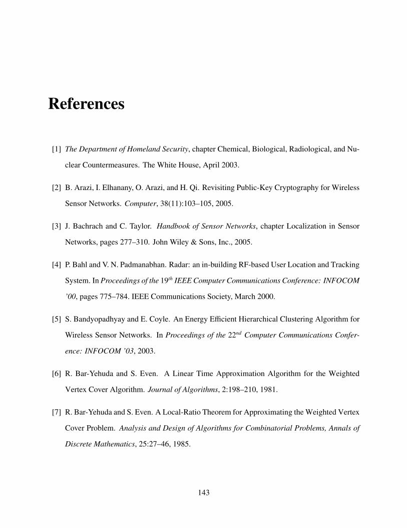
References

[1] The Department of Homeland Security, chapter Chemical, Biological, Radiological, and Nu-

clear Countermeasures. The White House, April 2003.

[2] B. Arazi, I. Elhanany, O. Arazi, and H. Qi. Revisiting Public-Key Cryptography for Wireless

Sensor Networks. Computer, 38(11):103–105, 2005.

[3] J. Bachrach and C. Taylor. Handbook of Sensor Networks, chapter Localization in Sensor

Networks, pages 277–310. John Wiley & Sons, Inc., 2005.

[4] P. Bahl and V. N. Padmanabhan. Radar: an in-building RF-based User Location and Tracking

System. In Proceedings of the 19th IEEE Computer Communications Conference: INFOCOM

’00, pages 775–784. IEEE Communications Society, March 2000.

[5] S. Bandyopadhyay and E. Coyle. An Energy Efficient Hierarchical Clustering Algorithm for

Wireless Sensor Networks. In Proceedings of the 22nd Computer Communications Confer-

ence: INFOCOM ’03, 2003.

[6] R. Bar-Yehuda and S. Even. A Linear Time Approximation Algorithm for the Weighted

Vertex Cover Algorithm. Journal of Algorithms, 2:198–210, 1981.

[7] R. Bar-Yehuda and S. Even. A Local-Ratio Theorem for Approximating the Weighted Vertex

Cover Problem. Analysis and Design of Algorithms for Combinatorial Problems, Annals of

Discrete Mathematics, 25:27–46, 1985.

143

[8] J. Beaver, M. A. Sharaf, A. Labrinidis, and P. K. Chrysanthis. Location-aware routing for

data aggregation for sensor networks. 2003.

[9] I. Bomze, M. Budinich, P. Pardalos, and M. Pelillo. The Maximum Clique Problem. In D.-Z.

Du and P. M. Pardalos, editors, Handbook of Combinatorial Optimization, volume 4. Kluwer

Academic Publishers, Boston, MA, 1999.

[10] J. Bruck, J. Gao, and A. A. Jiang. Localization and Routing in Sensor Networks by Local

Angle Information. In Proceedings of the 6th ACM International Symposium on Mobile Ad

hoc Networking and Computing: MobiHoc ’05, pages 181–192, 2005.

[11] N. Bulusu, J. Heidemann, and D. Estrin. GPS-less Low Cost Outdoor Localization for Very

Small Devices. IEEE Personal Communications Magazine, pages 28–34, Oct 2000.

[12] N. Bulusu, J. Heidemann, and D. Estrin. Density adaptive algorithms for beacon placement.

In The 21st International Conference on Distributed Computing Systems (ICDCS-21), page

489. IEEE Computer Society, April 2001.

[13] R. Cardell-Oliver, K. Smettem, M. Kranz, and K. Mayer. A Reactive Soil Moisture Sensor

Network: Design and Field Evaluation. International Journal of Distributed Sensor Net-

works, 1(2):149–162, 2005.

[14] M. W. Carter, H. H. Jin, M. A. Saunders, and Y. Ye. Spaseloc: An Adaptive Subproblem

Algorithm for Scalable Wireless Sensor Network Localization. SIAM J. on Optimization,

17(4):1102–1128, 2006.

[15] Crossbow. Imote2 IPR2400 High Performance Wireless Sensor Network Node Datasheet.

[16] Crossbow. MICA2 Wireless Measurement System Datasheet.

[17] N. B. Dale, C. Weems, and M. R. Headington. Programming and Problem Solving With C++.

Jones & Bartlett Publishers, 1998.

144

[18] R. B. Darst. Introduction to Linear Programming: Applications and Extensions. 2004.

[19] J. V. de Lindt, D. Rosowsky, A. Filiatrault, M. Symans, and R. Davidson. Development

of a performance-based seismic design philosophy for mid-rise woodframe construction:

Progress on the neeswood project. In 9th World Conference on Timber Engineering, pages 8

p., on CD–ROM, Portland, OR, August 6–10 2006.

[20] L. M. S. de Souza, H. Vogt, and M. Beigl. A Survey on Fault Tolerance in Wireless Sensor

Networks. 2007.

[21] M. Ding, F. Liu, A. Thaeler, D. Chen, and X. Cheng. Fault-Tolerant Target Localiza-

tion in Sensor Networks. EURASIP Journal on Wireless Communications and Networking,

2007(1):19–19, 2007.

[22] I. Dinur and S. Safra. On the Hardness of Approximating Minimum Vertex-Cover. Annals

of Mathematics, 162(1), 2005.

[23] L. Doherty, L. E. Ghaoui, and K. S. J. Pister. Convex Position Estimation in Wireless Sensor

Networks. In Proceedings of the 20th IEEE Computer Communications Conference: INFO-

COM ’01, Anchorage, April 2001. IEEE Communications Society.

[24] J. Elson and D. Estrin. Time Synchronization for Wireless Sensor Networks. In Proceedings

of the 15th International Parallel & Distributed Processing Symposium: IPDPS ’01, page

186. IEEE Computer Society, 2001.

[25] T. Eren, D. Goldenberg, W. Whiteley, Y. R. Yang, A. S. Morse, B. Anderson, and P. Bel-

humeur. Rigidity, Computation and Randomization of Network Localization. In Proceed-

ings of the 23rd IEEE Computer Communications Conference: INFOCOM ’04, Hong Kong,

China, April 2004. IEEE Computer and Communications Society.

[26] L. Fang, W. Du, and P. Ning. A Beacon-Less Location Discovery Scheme for Wireless

145

Sensor Networks. In Proceedings of the 24th IEEE Computer Communications Conference:

INFOCOM ’05. IEEE Communications Society, March 2005.

[27] A. Forghani, B. Cechet, J. Radke, M. Finney, and B. Butler. Applying Fire Spread Simulation

over Two Study Sites in California: Lessons Learned and Future Plans. In Proceedings of the

Geoscience and Remote Sensing Symposium: IGARSS ’07, pages 3008–3013, July 2007.

[28] S. Ganeriwal, S. Capkun, C.-C. Han, and M. B. Srivastava. Secure Time Synchronization

Service for Sensor Networks. In Proceedings of the 4th ACM workshop on Wireless Security:

WiSe ’05, pages 97–106, 2005.

[29] M. R. Garey and D. S. Johnson. Computers and Intractability : A Guide to the Theory of

NP-Completeness. W. H. Freeman, 1979.

[30] G. Gaubatz, J.-P. Kaps, and B. Sunar. Security in Ad-hoc and Sensor Networks, Lecture

Notes in Computer Science, volume 3313/2005, chapter Public Key Cryptography in Sensor

Networks-Revisited, pages 2–18. Springer Berlin / Heidelberg, 2005.

[31] D. Goldenberg, A. Krishnamurthy, W. Maness, Y. Yang, A. Young, A. Morse, A. Savvides,

and B. Anderson. Network Localization in Partially Localizable Networks. In Proceedings

of the 24th IEEE Computer Communications Conference: INFOCOM ’05, Miami, FL, March

2005.

[32] M. Greis. Tutorial for the Network Simulator “ns". VINT group, 2005.

http://www.isi.edu/nsnam/ns/.

[33] M. Halgamuge, S. Guru, and A. Jennings. Energy Efficient Cluster Formation in Wireless

Sensor Networks. In Proceedings of the 10th International Conference on Telecommunica-

tions ICT ’03, volume 2, pages 1571–1576, 23 February - 1 March 2003.

[34] E. Halperin. Improved Approximation Algorithms for the Vertex Cover Problem in Graphs

146

and Hypergraphs. In Proceedings of the 11th ACM-SIAM Symposium on Discrete Algorithms,

2000.

[35] S. Han, E. Chang, L. Gao, and T. Dillon. EC2ND 2005, Proceedings of the 1st European

Conference on Computer Network Defence School of Computing, University of Glamor-

gan, Wales, UK, chapter Taxonomy of Attacks on Wireless Sensor Networks, pages 97–105.

Springer London, 2006.

[36] S. Harté, A. Rahman, and K. Razeeb. Fault Tolerance in Sensor Networks using Self-

diagnosing Sensor Nodes. In The IEE International Workshop on Intelligent Environments,

pages 7–12, 2005.

[37] C. Hartung, R. Han, C. Seielstad, and S. Holbrook. FireWxNet: A Multi-tiered Portable

Wireless System for Monitoring Weather Conditions in Wildland Fire Environments. In Pro-

ceedings of the 4th International Conference on Mobile Systems, Applications and Services:

MobiSys ’06, pages 28–41, 2006.

[38] J. Hastad. Some Optimal Inapproximability Results. In Proceedings of the 29th ACM Sym-

posium on Theory of Computing: STOC ’97, pages 1–10, 1997.

[39] T. He, C. Huang, B. M. Blum, J. A. Stankovic, and T. Abdelzaher. Range-free Localization

Schemes for Large Scale Sensor Networks. In Proceedings of the 9th Annual International

Conference on Mobile Computing and Networking: MobiCom ’03, pages 81–95, New York,

NY, USA, 2003. ACM Press.

[40] J. Hightower and G. Borriello. Location Systems for Ubiquitous Computing. Computer,

34(8):57–66, August 2001.

[41] D. S. Hochbaum. Approximation Algorithms for the Weighted Set Covering and Node Cover

Problems. SIAM Journal on Computing, 11:555–556, 1982.

147

[42] B. Hofmann-Wellenhof, H. Lichtenegger, and J. Collins. Global Positioning System: Theory

and Practice. Springer Verlag, 1997.

[43] S. Homer and A. L. Selman. Computability and Complexity Theory, chapter Nondeterminism

and NP-Completeness, pages 122–144. Springer-Verlag, 2001.

[44] J. Hromkovic. Algorithms for Hard Problems. Springer-Verlag, 2004.

[45] M. Jadliwala, Q. Duan, S. Upadhyaya, and J. Xu. On the Hardness of Eliminating Cheating

Behavior in Time Synchronization Protocols for Sensor Networks. Technical Report 2008-

08, State University of New York at Buffalo, April 2008.

[46] M. Jadliwala, Q. Duan, J. Xu, and S. Upadhyaya. On Extracting Consistent Graphs in Wire-

less Sensor Networks. International Journal of Sensor Networks, 2(3/4):149–162, 2007.

[47] M. Jadliwala and S. Upadhyaya. Robust Deployment and Localization in Emergency Sensor

Networks. Pervasive and Mobile Computing, Elsevier, (Under Review).

[48] M. Jadliwala, S. Upadhyaya, H. R. Rao, and R. Sharman. Security and Dependability Issues

in Location Estimation for Emergency Sensor Networks. In The 4th Workshop on e-Business:

WeB ’05, Venetian, Las Vegas, Nevada, USA, December 2005.

[49] M. Jadliwala, S. Upadhyaya, and M. Taneja. ASFALT: A Simple Fault-Tolerant Signature-

based Localization Technique for Emergency Sensor Networks. In Proceedings of the 26th

IEEE International Symposium on Reliable Distributed Systems: SRDS ’07, pages 3–12,

Beijing, China, October 2007. IEEE Computer and Communications Society.

[50] X. Ji and H. Zha. Sensor Positioning in Wireless Ad-hoc Sensor. Networks using Multidi-

mensional Scaling. In Proceedings of 23rd IEEE Computer Communications Conference:

INFOCOM ’04, March 2004.

148

[51] P. Juang, H. Oki, Y. Wang, M. Martonosi, L. S. Peh, and D. Rubenstein. Energy-efficient

Ccomputing for Wildlife Tracking: Design Tradeoffs and Early Experiences with ZebraNet.

SIGOPS Operating Systems Review, 36(5):96–107, 2002.

[52] G. Karakostas. A Better Approximation Ratio for the Vertex Cover Problem. In Proceedings

of the International Colloquium on Automata, Languages and Programming, 2005.

[53] B. Karp and H. T. Kung. GPSR: Greedy Perimeter Stateless Routing for Wireless Networks.

In Proceedings of the 6th International Conference on Mobile Computing and Networking:

MOBICOM’00. ACM SIGMOBILE, August 2000.

[54] R. Karp. Complexity of Computer Computations, chapter Reducibility Among Combinatorial

Problems, pages 85–104. Plenum Press, 1972.

[55] F. Klee and G. J. Minty. How Good is the Simplex Algorithm? Inequalities III, pages

159–175, 1972.

[56] L. Lazos and R. Poovendran. SeRLoc: Secure Range-Independent Localization for Wireless

Sensor Networks. In Proceedings of the ACM Workshop on Wireless Security: WiSe ’04,

pages 21–30, New York, NY, USA, 2004. ACM Press.

[57] L. Lazos, R. Poovendran, and S. Capkun. Rope: RObust Position Estimation in Wireless Sen-

sor Networks. In Proceedings of the 4th International Symposium on Information Processing

in Sensor Networks, page 43, 2005.

[58] Z. Li, W. Trappe, Y. Zhang, and B. Nath. Robust Statistical Methods for Securing Wireless

Localization in Sensor Networks. In Proceedings of the 4th International Symposium on

Information Processing in Sensor Networks: IPSN ’05, page 12, 2005.

[59] D. Liu, P. Ning, and W. Du. Attack-Resistant Location Estimation in Sensor Networks. In

Proceedings of the 4th International Symposium on Information Processing in Sensor Net-

works: IPSN ’05, pages 99–106, April 2005.

149

[60] D. Liu, P. Ning, and W. Du. Detecting Malicious Beacon Nodes for Secure Location Dis-

covery in Wireless Sensor Networks. In Proceedings of the 25th International Conference on

Distributed Computing Systems: ICDCS ’05, pages 609–619. IEEE Computer Society, June

2005.

[61] H. Liu, P.-J. Wan, and X. Jia. Computing and Combinatorics, Lecture Notes in Computer Sci-

ence, volume 3595/2005, chapter Fault-Tolerant Relay Node Placement in Wireless Sensor

Networks, pages 230–239. Springer Berlin / Heidelberg, 2005.

[62] J. Liu, Y. Zhang, and F. Zhao. Robust Distributed Node Localization with Error Management.

In Proceedings of the 7th ACM International Symposium on Mobile Ad hoc Networking and

Computing: MobiHoc ’06, pages 250–261, 2006.

[63] J. Lopez. Unleashing Public-key Cryptography in Wireless Sensor Networks. Journal of

Computer Security, 14(5):469–482, 2006.

[64] K. Lorincz, D. Malan, T. R. F. Fulford-Jones, A. Nawoj, A. Clavel, V. Shnayder, G. Main-

land, S. Moulton, and M. Welsh. Sensor networks for emergency response: Challenges and

opportunities. IEEE Pervasive Computing, Special Issue on Pervasive Computing for First

Response, 3(4):16–23, October 2004.

[65] D. F. Macedo, L. H. A. Correia, A. L. dos Santos, A. A. F. Loureiro, J. M. S. Nogueira, and

G. Pujolle. Evaluating Fault Tolerance Aspects in Routing Protocols for Wireless Sensor

Networks, volume 197/2006, chapter Challenges in Ad Hoc Networking, pages 285–294.

Springer Boston, 2006.

[66] G. Mao, B. D. O. Anderson, and B. Fidan. Path Loss Exponent Estimation for Wireless

Sensor Network Localization. Computer Networks, 51(10):2467–2483, 2007.

[67] B. Monien and E. Speckenmeyer. Ramsey Numbers and an Approximation Algorithm for

the Vertex Cover Problem. Acta Information, 22:115–123, 1985.

150

[68] D. Moore, J. Leonard, D. Rus, and S. Teller. Robust Distributed Network Localization with

Noisy Range Measurements. In Proceedings of the 2nd International Conference on Embed-

ded Networked Sensor Systems: SenSys ’04, pages 50–61, 2004.

[69] R. Moses, D. Krishnamurthy, and R. Patterson. A self-localization method for wireless sensor

networks. Eurasip Journal on Applied Signal Processing, Special Issue on Sensor Networks,

2003(4):148–158, March 2003.

[70] D. Niculescu and B. Nath. DV based Positioning in Ad hoc Networks. Journal of Telecom-

munication Systems, 2003.

[71] L. Ntaimo, B. Khargharia, B. Zeigler, and M. Vasconcelos. Forest Fire Spread and Suppres-

sion in DEVS. SIMULATION, 80(10), 2004.

[72] P. P. Papadimitratos, M. Poturalski, P. Schaller, P. Lafourcade, D. Basin, S. Capkun, and J.-

P. Hubaux. Secure Neighborhood Discovery: A Fundamental Element for Mobile Ad Hoc

Networking. IEEE Communications Magazine, 46(2), 2008.

[73] L. Paradis and Q. Han. A Survey of Fault Management in Wireless Sensor Networks. Journal

of Network and Systems Management, 15(2):171–190, 2007.

[74] W. Pires, T. H. de Paula Figueiredo, H. C. Wong, and A. A. Loureiro. Malicious Node

Detection in Wireless Sensor Networks. In Proceedings of the 18th International Parallel

and Distributed Processing Symposium: IPDPS ’04, page 24. IEEE Computer Society, April

2004.

[75] N. Priyantha, A. Chakraborty, and H. Balakrishnan. The Cricket Location-Support System.

In Proceedings of the 6th Annual International Conference on Mobile Computing and Net-

working: MOBICOM ’00, pages 32–43. ACM SIGMOBILE, August 2000.

[76] S. Ray, R. Ungrangsi, F. de Pellegrini, A. Trachtenberg, and D. Starobinski. Robust Location

Detection in Emergency Sensor Networks. In Proceedings of the 22nd IEEE Computer Com-

151

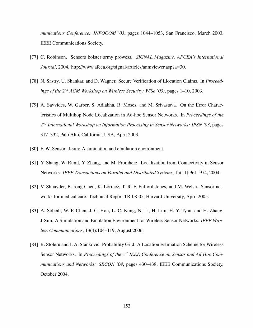
munications Conference: INFOCOM ’03, pages 1044–1053, San Francisco, March 2003.

IEEE Communications Society.

[77] C. Robinson. Sensors bolster army prowess. SIGNAL Magazine, AFCEA’s International

Journal, 2004. http://www.afcea.org/signal/articles/anmviewer.asp?a=30.

[78] N. Sastry, U. Shankar, and D. Wagner. Secure Verification of Llocation Claims. In Proceed-

ings of the 2nd ACM Workshop on Wireless Security: WiSe ’03:, pages 1–10, 2003.

[79] A. Savvides, W. Garber, S. Adlakha, R. Moses, and M. Srivastava. On the Error Charac-

teristics of Multihop Node Localization in Ad-hoc Sensor Networks. In Proceedings of the

2nd International Workshop on Information Processing in Sensor Networks: IPSN ’03, pages

317–332, Palo Alto, California, USA, April 2003.

[80] F. W. Sensor. J-sim: A simulation and emulation environment.

[81] Y. Shang, W. Ruml, Y. Zhang, and M. Fromherz. Localization from Connectivity in Sensor

Networks. IEEE Transactions on Parallel and Distributed Systems, 15(11):961–974, 2004.

[82] V. Shnayder, B. rong Chen, K. Lorincz, T. R. F. Fulford-Jones, and M. Welsh. Sensor net-

works for medical care. Technical Report TR-08-05, Harvard University, April 2005.

[83] A. Sobeih, W.-P. Chen, J. C. Hou, L.-C. Kung, N. Li, H. Lim, H.-Y. Tyan, and H. Zhang.

J-Sim: A Simulation and Emulation Environment for Wireless Sensor Networks. IEEE Wire-

less Communications, 13(4):104–119, August 2006.

[84] R. Stoleru and J. A. Stankovic. Probability Grid: A Location Estimation Scheme for Wireless

Sensor Networks. In Proceedings of the 1st IEEE Conference on Sensor and Ad Hoc Com-

munications and Networks: SECON ’04, pages 430–438. IEEE Communications Society,

October 2004.

152

[85] K. Sun, P. Peng, P. Ning, and C. Wang. Secure Distributed Cluster Formation in Wireless

Sensor Networks. In Proceedings of the 22nd Annual Computer Security Applications Con-

ference: ACSAC ’06, pages 131–140, 2006.

[86] A. S. Tanenbaum, C. Gamage, and B. Crispo. Taking Sensor Networks from the Lab to the

Jungle. Computer, 39(8):98–100, 2006.

[87] R. Tinos, L. Navarro-Serment, and C. Paredis. Fault tolerant Localization for Teams of Dis-

tributed Robots. In Proceedings of the IEEE International Conference on Intelligent Robots

and Systems, pages 1061–1066, Maui, HI, 2001.

[88] W. Tollefsen, M. Pepe, D. Myung, M. Gaynor, M. Welsh, and S. Moulton. iRevive, a Pre-

hospital Mobile Database for Emergency Medical Services. International Journal of Health-

care Technology and Management: IJHTM, May-August 2004.

[89] M. A. Tubaishat and S. Madria. Sensor Networks: An Overview. IEEE Potentials, 22(2):20–

23, April-May 2003.

[90] S. Capkun and J.-P. Hubaux. Secure Positioning of Wireless Devices with Application to

Sensor Networks. In Proceedings of the 24th IEEE Computer Communications Conference:

INFOCOM ’05, pages 1917–1928, Miami, FL, March 2005. IEEE Computer and Communi-

cations Society.

[91] R. Want, A. Hopper, V. Falcao, and J. Gibbons. The Active Badge Location System. ACM

Transaction on Information Systems, pages 91–102, Jan 1992.

[92] Y. Wei, Z. Yu, and Y. Guan. Location Verification Algorithms for Wireless Sensor Net-

works. In Proceedings of the 27th International Conference on Distributed Computing Sys-

tems: ICDCS’07, page 70, 2007.

[93] T. Worthington. Waterbombing operation over canberra.

http://www.tomw.net.au/2003/actfire.html, January 2003.

153

[94] J. Xiao, L. Ren, and J. Tan. Research of TDOA Based Self-localization Approach in Wireless

Sensor Network. In Proceedings of the IEEE/RSJ International Conference on Intelligent

Robots and Systems, pages 2035–2040, October 2006.

[95] Y. Xu, G. Chen, J. Ford, and F. Makedon. Critical Infrastructure Protection, IFIP Interna-

tional Federation for Information Processing, volume 253/2007, chapter Detecting Worm-

hole Attacks in Wireless Sensor Networks, pages 267–279. Springer Boston, 2007.

[96] K. Yedavalli, B. Krishnamachari, S. Ravula, and B. Srinivasan. Ecolocation: A Sequence

Based Technique for RF-only Localization in Wireless Sensor Networks. In Proceedings of

the 4th International Conference on Information Processing in Sensor Networks: IPSN ’05,

Los Angeles, CA, USA, April 2005.

[97] R. Yin and W. Chow. Building Fire Simulation with a Field Model based on Large Eddy

Simulation. Architectural Science Review, 2002.

[98] S. Zhong, M. Jadliwala, S. Upadhyaya, and C. Qiao. Towards a Theory of Robust Local-

ization Against Malicious Beacon Nodes. In Proceedings of the 27th IEEE Computer Com-

munications Conference: INFOCOM ’08, pages 1391–1399, Phoenix, AZ, April 2008. IEEE

Computer and Communications Society.

154

Vita

June 19, 1978 .................................... Born - Calcutta, IndiaJune 2000 .......................................... B.E., Computer Science and Engineering, University of

Mumbai, India.June 2000 - June 2002 ....................... Technical Leader, Investment Research and Information Ser-

vices Ltd., Mumbai, India.September 2004 .................................. M.S. Computer Science, The University at Buffalo, SUNY.August 2003 - present ......................... Teaching Assistant, The University at Buffalo, SUNY.May - August 2005, 2006 ................... Research Assistant, Center of Excellence in Information

Systems Assurance Research and Education, The Universityat Buffalo, SUNY.

May - August 2007, 2008 .................... Research Associate, NSF-Cisco Wireless Security Labora-tory, The University at Buffalo, SUNY.

Research PublicationsJournals

• Jadliwala, M., Duan, Q., Xu, J. and Upadhyaya, S. (2007) “On Extracting Consistent Graphsin Wireless Sensor Networks”, International Journal of Sensor Networks (IJSNET): SpecialIssue on Theoretical and Algorithmic Aspects in Sensor Networks, Vol. 2, Nos. 3/4, pp.149-162.

Conferences and Symposia

• Zhong, S., Jadliwala, M., Upadhyaya, S. and Qiao, C., “Towards a Theory of Robust Local-ization against Malicious Beacon Nodes”, in the Proceedings of The 27th IEEE InternationalConference on Computer Communication (INFOCOM 2008), pages: 1391-1399, Phoenix,Arizona, April 15-17, 2008. (acceptance rate: 21%).

• Jadliwala, M., Upadhyaya, S. and Taneja, M., “ASFALT: A Simple Fault-Tolerant Signature-based Localization Technique for Emergency Sensor Networks”, in the Proceedings of The26th IEEE International Symposium on Reliable Distributed Systems (SRDS 2007), pages:3-12, Beijing, CHINA, October 10-12, 2007 . (acceptance rate: 15%).

• Virendra M., Jadliwala M., Chandrasekaran M., Upadhyaya S., “Quantifying Trust in MobileAd-Hoc Networks”, In Proceedings of the IEEE International Conference on Integration of

155

Knowledge Intensive Multi-agent Systems (KIMAS’05), Waltham, MA, Apr 2005, pp. 65-71.

• Braynov, S. and Jadliwala, M. 2004. “Detecting Malicious Groups of Agents”, in proceed-ings of the 1st IEEE Symposium on Multi-agent Security and Survivability, Drexel Univer-sity, Philadelphia, PA, USA - August 30-31, 2004.

Workshops

• Jadliwala, M., Upadhyaya, S., Rao, H.R. and Sharman, R. “Security and Dependability Is-sues in Location Estimation for Emergency Sensor Networks”, The Fourth Workshop one-Business (WeB 2005), Venetian, Las Vegas, Nevada, USA - December 10, 2005.

• Braynov, S. and Jadliwala, M. 2003. “Representation and Analysis of Coordinated Attacks”,at The 2003 ACM Workshop on Formal Methods in Security Engineering (Washington,D.C.). FMSE ’03. ACM Press, New York, NY, pp. 43-51.

Under Review/Submission

• Jadliwala, M., Upadhyaya, S., Robust Deployment and Localization in Emergency SensorNetworks, Under review at the Pervasive and Mobile Computing Journal (Elsevier Publica-tions).

• Jadliwala, M., Zhong, S., Upadhyaya, S. and Qiao, C., Robust Distance-based Localizationagainst Malicious Beacon Nodes in Mobile Networks, Under preparation for submission toIEEE Transactions on Mobile Computing.

• Jadliwala, M., Duan, Q., Xu, J. and Upadhyaya, S., On Theory of Robust Time Synchro-nization in Mobile Computer Networks, Under Preparation.

Research InterestsWireless Data Networks including Wireless LANs, Sensor and Mesh Networks, Operating

System and Network Security, Vulnerability Analysis, Cryptography, Combinatorial Optimization,Approximation Algorithms, Game Theory and Multi-agent Systems. Specific topics of interestsinclude:

• Secure and fault-tolerant distance-based and signature-based localization, robust time syn-chronization and robust deployment in pervasive and ubiquitous networks.

• Stimulating cooperation in wireless networks using economic mechanism design and gametheory.

• Context-aware computing.

• Efficient cryptographic protocols and signature schemes for low power sensor and ad-hocnetworks.

156

• Future generation wireless and ad-hoc networks.

• Modeling and analysis of complex, multi-stage and coordinated computer threats.

157