Optimization of the Robustness of Radiotherapy against ...

Optimization of the Robustness ofRadiotherapy against Stochastic

Uncertainties

Dissertationder Mathematisch-Naturwissenschaftlichen Fakultat

der Eberhard Karls Universitat Tubingen

zur Erlangung des Grades eines

Doktors der Naturwissenschaften(Dr. rer. nat.)

vorgelegt von

Benjamin Sobotta

aus Muhlhausen

Tubingen2011

Tag der mundlichen Qualifikation: 25. 05. 2011

Dekan: Prof. Dr. Wolfgang Rosenstiel

1. Berichterstatter: Prof. Dr. Wilhelm Kley

2. Berichterstatter: Prof. Dr. Dr. Fritz Schick

Zusammenfassung

In dieser Arbeit wird ein Ansatz zur Erstellung von Bestrahlungsplanen inder Krebstherapie prasentiert, welcher in neuartiger Weise den Fehlerquellen,die wahrend einer Strahlentherapie auftreten konnen, Rechnung tragt. Aus-gehend von einer probabilistischen Interpretation des Therapieablaufs, wirdjeweils eine Methode zur Dosisoptimierung, Evaluierung und gezielten Indi-vidualisierung von Bestrahlungsplanen vorgestellt. Maßgebliche Motivationhierfur ist die, trotz fortschreitender Qualitat der Bildgebung des Patien-ten wahrend der Behandlung, immer noch unzureichende Kompensation vonLagerungsfehlern, Organbewegung und physiologischer Plastizitat der Pa-tienten sowie anderen statistischen Storungen. Mangelnde Berucksichtigungdieser Einflusse fuhrt zu einer signifikanten Abnahme der Planqualitat unddamit unter Umstanden zur Zunahme der Komplikationen bei verringerterTumorkontrolle.Im Zentrum steht ein vollig neuartiger Ansatz zur Berucksichtigung vonUnsicherheiten wahrend der Dosisplanung. Es ist ublich, das Zielvolumendurch einen Saum zu vergroßern, um zu gewahrleisten, dass auch unter geo-metrischen Abweichungen das gewunschte Ziel die vorgesehene Dosis erhalt.Der hier vorgestellte Optimierungsansatz umgeht derlei Maßnahmen, indemden Auswirkungen unsicherer Einflusse explizit Rechnung getragen wird.Um die Qualitat einer Dosisverteilung hinsichtlich ihrer Wirksamkeit in ver-schiedenen Organen zu erfassen, ist es notig, Qualitatsmetriken zu definieren.Die Gute einer Dosisverteilung wird dadurch von n Skalaren beschrieben.Die Schlusselidee dieser Arbeit ist somit, samtliche Eingangsunsicherheitenim Planungsprozess quantitativ bis in die Qualitatsmetriken zu propagieren.Das bedeutet, dass die Bewertung von Bestrahlungsplanen nicht mehr an-hand von n Skalaren vorgenommen wird, sondern mittels n statistischerVerteilungen. Diese Verteilungen spiegeln wider, mit welchen Unsicherheitendas Ergebnis der Behandlung aufgrund von Eingangsunsicherheiten wahrendder Planung und Behandlung behaftet ist.Der in dieser Arbeit beschriebene Optimierungsansatz ruckt folgerichtig dieoben beschriebenen Verteilungen an Stelle der bisher optimierten skalarenNominalwerte der Metriken in den Mittelpunkt der Betrachtung. Dadurchwerden alle moglichen Szenarien zusammen mit deren jeweiligen Wahrschein-lichkeiten mit in die Optimierung einbezogen. Im Zuge der Umsetzung dieser

neuen Idee wurde als erstes das klassische Optimierungsproblem der Be-strahlungsplanung neu formuliert. Die Neuformulierung basiert auf Mittel-wert und Varianz der Qualitatsmetriken des Planes und bezieht ihre Recht-fertigung aus der Tschebyschew-Ungleichung. Der konzeptionell einfachsteAnsatz zur Errechnung von Mittelwert und Varianz komplexer Comput-ermodelle wie des Patientenmodells ist die klassische Monte Carlo Meth-ode. Allerdings muss dafur das Patientenmodell sehr haufig neu evaluiertwerden. Fur eine Reduzierung der Anzahl der Neuberechnungen konntejedoch ausgenutzt werden, dass kleinen Anderungen der unsicherheitsbe-hafteten Parameter nur leichte Fluktuationen der Qualitatsmetriken folgen,d.h. der Ausgang der Behandlung hangt stetig von den unsicheren geo-metrischen Parametern ab. Durch diesen funktionalen Zusammenhang wirdes moglich, das Patientenmodell durch ein Regressionsmodell auszutauschen.Dazu wurden Gauß-Prozesse, eine Methode zur nichtparametrischen Regres-sion, verwendet, die mit Hilfe von wenigen Evaluierungen des Patientenmod-ells angelernt werden. Nach der Anlernphase nimmt der Gauß-Prozess dieStelle des Patientenmodells in den folgenden Berechnungen ein. Auf diesemWege konnen samtliche zur Optimierung relevanten Großen sehr effizientund haufig berechnet werden, was dem iterativen Optimierungsalgorithmusentgegen kommt. Die dadurch erreichte Beschleunigung des Optimierungsal-gorithmus ermoglicht dessen Anwendung unter realen Bedingungen. Umdie klinische Tauglichkeit des Algorithmus zu demonstrieren, wurde dieserin ein Bestrahlungsplanungssystem implementiert und an Beispielpatientenvorgefuhrt.Zur Evaluierung optimierter Bestrahlungsplane wurden die klinisch etab-lierten Dosis-Volumen-Histogramme (DVHs) unter Einbeziehung der zusatz-lich durch probabilistische Patientenmodelle bereitgestellten Informationenerweitert. Durch die Verwendung von Gauß-Prozessen kann die DVH-Unsi-cherheit unter verschiedenen Bedingungen auf aktueller Computerhardwarein Echtzeit abgeschatzt werden. Der Planer erhalt auf diese Weise wertvolleHinweise bezuglich der Auswirkungen verschiedener Fehlerquellen als aucheinen ,,Uberblick” uber die Effektivitat potentieller Gegenmaßnahmen. Umdie Prazision der Vorhersagen auf Gauß-Prozessen zu verbessern wurde dieBayesian Monte Carlo Methode (BMC) maßgeblich erweitert mit dem Ziel,neben Mittelwert und Varianz auch die statistische Schiefe zu berechnen.Der letzte Teil dieser Arbeit befasst sich mit der Verbesserung von Bestrah-lungsplanen, die gegebenenfalls dann notwendig wird, wenn der vorliegendePlan noch nicht den klinischen Anspruchen genugt. Oftmals, beispielsweisedurch zu streng verschriebene Schranken fur die Dosis im Normalgewebe,kommt es im Zielvolumen zu punktuellen Unterdosierungen. In der Praxis istsomit von erheblicher Bedeutung, das Zusammenspiel aller Verschreibungen

zu durchleuchten, um einen bestehenden Plan in moglichst wenigen Schrittenden Vorgaben anzupassen. Mit anderen Worten: Der vorgestellte Ansatz hilftdem Planer, lokale Konflikte binnen kurzester Zeit zu losen.Es konnte gezeigt werden, dass die statistische Behandlung unvermeidlicherStorgroßen in der Strahlentherapie mehrere Vorteile birgt. Zum einen er-moglicht der gezeigte Algorithmus, Bestrahlungsplane zu erzeugen, die indi-viduell auf den Patienten und dessen Muster geometrischer Unsicherheitenzugeschnitten sind. Dies war bislang nicht der moglich, da die momen-tan verwendeten Sicherheitssaume die Unsicherheiten nur summarisch undfur das Zielvolumen behandeln. Zum anderen bietet die Evaluierung vonBestrahlungsplanen unter expliziter Berucksichtigung statischer Einflusse demPlaner wertvolle Anhaltspunkte fur das zu erwartende Ergebnis einer Be-handlung.Eines der großten Hindernisse fur eine weitere Steigerung der Effizienz derStrahlentherapie stellt die Behandlung geometrischer Unsicherheiten dar,die, sofern sie nicht eliminiert werden konnen, durch die Bestrahlung einesdeutlich vergroßerten Volumens kompensiert werden. Diese ineffiziente undwenig schonende Vorgehensweise konnte durch die hier vorgestellte Behand-lung des Optimierungsproblems der Strahlentherapie als statistisches Prob-lem abgelost werden. Durch die Verwendung von Gauß-Prozessen als Substi-tute des Originalmodells konnte ein Algorithmus geschaffen werden, welcherin klinisch akzeptablen Zeiten im statistischen Sinne fur alle Organe robusteDosisverteilungen liefert.

Contents

1 Introduction 2

2 Robust Treatment Plan Optimization 5

2.1 Main Objective . . . . . . . . . . . . . . . . . . . . . . . . . . 7

2.1.1 Explicit Incorporation of the Number of Fractions . . . 13

2.2 Efficient Treatment Outcome Parameter Estimation . . . . . . 14

2.2.1 Gaussian Process Regression . . . . . . . . . . . . . . . 16

2.2.2 Uncertainty Analysis with Gaussian Processes . . . . . 21

2.2.3 Bayesian Monte Carlo . . . . . . . . . . . . . . . . . . 24

2.2.4 Bayesian Monte Carlo vs. classic Monte Carlo . . . . . 26

2.3 Accelerating the Optimization Algorithm . . . . . . . . . . . . 28

2.3.1 Constrained Optimization in Radiotherapy . . . . . . . 29

2.3.2 Core Algorithm . . . . . . . . . . . . . . . . . . . . . . 29

2.3.3 Convergence Considerations . . . . . . . . . . . . . . . 31

2.3.4 Efficient Computation of the Derivative . . . . . . . . . 32

2.4 Evaluation . . . . . . . . . . . . . . . . . . . . . . . . . . . . . 35

2.5 Discussion and Outlook . . . . . . . . . . . . . . . . . . . . . 40

3 Uncertainties in Dose Volume Histograms 43

3.1 Discrimination of Dose Volume Histograms based on their re-spective Biological Effects . . . . . . . . . . . . . . . . . . . . 45

3.2 Quantitative Analysis . . . . . . . . . . . . . . . . . . . . . . . 46

3.3 Accounting for Asymmetry . . . . . . . . . . . . . . . . . . . . 48

3.3.1 Skew Normal Distribution . . . . . . . . . . . . . . . . 49

3.3.2 Extension of Bayesian Monte Carlo to compute theSkewness in Addition to Mean and Variance . . . . . . 50

3.4 Determination of Significant Influences . . . . . . . . . . . . . 53

3.5 Summary and Discussion . . . . . . . . . . . . . . . . . . . . . 54

i

Contents

4 Spatially Resolved Sensitivity Analysis 564.1 The Impact of the Organs at Risk on specific Regions in the

Target . . . . . . . . . . . . . . . . . . . . . . . . . . . . . . . 574.1.1 Pointwise Sensitivity Analysis . . . . . . . . . . . . . . 584.1.2 Perturbation Analysis . . . . . . . . . . . . . . . . . . 60

4.2 Evaluation and Discussion . . . . . . . . . . . . . . . . . . . . 62

5 Summary & Conclusions 64

A Calculations 76A.1 Solutions for Bayesian Monte Carlo . . . . . . . . . . . . . . . 76

A.1.1 Ex[µ(X)] . . . . . . . . . . . . . . . . . . . . . . . . . . 77A.1.2 Ex[µ2(X)] . . . . . . . . . . . . . . . . . . . . . . . . . 77A.1.3 Ex[µ3(X)] . . . . . . . . . . . . . . . . . . . . . . . . . 78

A.2 Details of the Incorporation of Linear Offset into the Algo-rithm for the Variance Computation . . . . . . . . . . . . . . 78

A.3 Details of the Incorporation of Linear Offset into the Algo-rithm for the Skewness Computation . . . . . . . . . . . . . . 80A.3.1 Ex [µ2(X)m(X)] . . . . . . . . . . . . . . . . . . . . . . 80A.3.2 Ex [µ(X)m2(X)] . . . . . . . . . . . . . . . . . . . . . . 80A.3.3 Ex [m3(X)] . . . . . . . . . . . . . . . . . . . . . . . . 81

B Details 82B.1 Relating the Average Biological Effect to the Biological Effect

of the Average . . . . . . . . . . . . . . . . . . . . . . . . . . . 82B.2 Mean, Variance and Skewness of the Skew Normal Distribution 83

C Tools for the analysis of dose optimization: III. Pointwisesensitivity and perturbation analysis 84

D Robust Optimization Based Upon Statistical Theory 92

E On expedient properties of common biological score func-tions for multi-modality, adaptive and 4D dose optimization103

F Special report: Workshop on 4D-treatment planning in ac-tively scanned particle therapy - Recommendations, techni-cal challenges, and future research directions 111

G Dosimetric treatment course simulation based on a patient-individual statistical model of deformable organ motion 119

ii

List of Abbreviations

ARD Automatic Relevance Determination

BFGS method Broyden Fletcher Goldfarb Shanno method

BMC Bayesian Monte Carlo

CT Computed Tomography

CTV Clinical Target Volume

DVH Dose-Volume Histogram

EUD Equivalent Uniform Dose

GP Gaussian Process

GTV Gross Tumor Volume

IMRT Intensity Modulated Radiotherapy

MC Monte Carlo

MRI Magnetic Resonance Imaging

NTCP Normal Tissue Complication Probability

OAR Organ At Risk

PCA Principal Component Analysis

PET Positron Emission Tomography

PRV Planning Organ-at-Risk Volume

PTV Planning Target Volume

R.O.B.U.S.T. Robust Optimization Based Upon Statistical Theory

iii

Contents

RT Radiotherapy

TCP Tumor Control Probability

1

Chapter 1

Introduction

Radiotherapy is the application of ionizing radiation to cure malignant dis-ease or slow down its progress. The principal goal is to achieve local tumorcontrol to suppress further growth and spread of metastases, while, at thesame time, immediate and long term side effects to normal tissue should beminimized. This trade-off between normal tissue sparing and tumor controlis the fundamental challenge of radiotherapy and continues to drive develop-ment in the field.

In the planning stage, prior to treatment, images from various modalities,e.g. CT, MRI and PET, are used to create a virtual model of the patient.Based on this model, the dose to any organ can be precisely predicted. Froma medical viewpoint, the idealized dose distribution tightly conforms to thedelineated target volume. The main task of treatment planning is to bridgethe gap between the idealized dose distribution and a distribution that isphysically attainable. To accomplish this, the method of constrained opti-mization has proven particularly useful. The idea is to maximize the dose inthe target under the condition that the exposure of the organs at risk mustnot exceed a given threshold. In order to quantify the merit of a given dosedistribution, the optimizer employs cost functions. In recent years, biologicalcost functions experienced increasing popularity. Biological cost functions,in contrast to physical cost functions, incorporate the specific dose responseof a given organ into the optimization.

Typically, radiation is administered in several treatment sessions. Frac-tionated radiotherapy exploits the inferior repair capabilities of malignanttissue. Through fractionation, the damage to normal tissue is significantlyreduced. This is the key to reach target doses as high as 80 Gy. In mostcases, radiotherapy is concentrated on a region around the tumor. Depend-ing on the particular scenario, the target region may be expanded to alsoinclude adjacent tissue such as lymph nodes. Apart from clinical reasons for

2

Chapter 1. Introduction

such an expansion, a margin around the tumor is typically added to compen-sate for movement that occurs during treatment. Such movement comprisesmotion that may occur during a treatment session as well as displacementsthat happen between treatment fractions.

Unfortunately, motion compensation via margins comes at the price ofa severely increased dose to surrounding normal tissue. Furthermore, themargin concept is entirely target centered and completely neglects poten-tially hazardous effects of motion on the organs at risk. Several approacheshave been put forth to alleviate this problem [BABN06, BYA+03, CZHS05,OW06, CBT06, SWA09, MKVF06, YMS+05, WvdGS+07, TRL+05, LLB98].Perhaps the simplest extension to the margin concept is coverage probability[BABN06]. The basic idea is to superimpose several CT snapshots to gen-erate an occupancy map of any organ of interest. The resulting per voxeloccupancies are used as weights in the optimization. Through these occu-pancy maps, the specific motion of the organs in essence replaces the moreunspecific margins. Even though the problem of overlapping volumes is al-leviated, it is not solved. The probability clouds of the organs may still verywell have common regions. In contrast, other authors [BYA+03, MKVF06,SWA09, TRL+05] use deformable patient models to track the irradiation ofevery single volume element. These methods evaluate dose in the referencegeometry while the dose is calculated in the deformed model. Compared tocoverage probability, this method is more demanding, as it requires deforma-tion vector fields between the CT snapshots and the optimization on severalgeometry instances. Additionally, this technique introduces further sourcesof error.

The core of this thesis is an entirely new concept for uncertainty man-agement. The key difference to the previously outlined methods is that itpays tribute to the inherent uncertainties in a purely statistical manner. Alltreatment planning techniques up to this point culminate in the optimiza-tion of nominal values to reflect the treatment plan merits. The approach inthe present work handles all treatment outcome metrics as statistical quan-tities. That is, instead of optimizing a nominal value, our approach directlyoptimizes the shape of dose metric distribution. Because it is independentof geometric considerations, any treatment parameter, whose uncertainty isquantifiable, can be incorporated into our framework. Requiring no changesto the infrastructure of the optimizer, it seamlessly integrates into the ex-isting framework of constrained optimization in conjunction with biologicalcostfunctions. The new method will also reveal its true potential in conjunc-tion with heavy particle therapy because many concepts that are currently inuse will fail and other sources of error, such as particle range uncertainties,besides geometric deviations have to be considered.

3

Chapter 1. Introduction

Once a plan has been computed, it needs to be evaluated. Dose volumehistograms (DVHs) are used to express the merit of a 3D dose distributioninto an easy to grasp 2D display. Today, DVHs are ubiquitous in the fieldradiation oncology. Classic DVHs reflect the irradiation of an organ only fora static geometry, hence provide no indication how the irradiation patternchanges under the influence of uncertainties. Consequently, to assess theinfluence of organ movement and setup errors, DVHs should reflect the as-sociated uncertainties. This work augments DVHs such that the assumed ormeasured error propagates into the DVH, adding error bars for each sourceof uncertainty individually, or any combination of them. Furthermore, itis possible to discriminate DVHs based on biological measures, such as therealized equivalent uniform dose (EUD).

The very nature of the radiotherapy optimization problem, i.e. contra-dictory objectives, almost always demands further refinements to the initialplan. In the realm of constrained optimization, this translates into the needto predict the changes to the dose distribution if a constraint is altered.While this can be done by sensitivity analysis in terms of treatment metrics,the introduced method in this work introduces spatial resolution to trade-offanalysis. It is especially suitable to eliminate so-called cold spots, i.e. re-gions in the target that experience underdosage. The algorithm screens theoptimization setting and determines which constraints need to be loosenedin order to raise the dose in the cold spot to an acceptable level. This isespecially useful if a multitude of constraints can be the cause of the coldspot. This way, tedious trial and error iterations are reduced.

To sum up, this thesis introduces a novel framework for uncertainty man-agement. In contrast to earlier publications in the field, it explicitly accountsfor the fact that the inherent uncertainties in radiotherapy render all asso-ciated quantities random variables. During optimization and evaluation, allrandom variables are rigorously treated as such. The algorithm seamlesslyintegrates as cost function into existing optimization engines and can bepaired with arbitrary dose scoring functions. To provide the physician withessential information needed to evaluate a treatment plan under the influ-ence of uncertainty, DVHs, a cornerstone in every day clinical practice, wereaugmented to reflect the consequences of potential error sources. The expertis provided with valuable information to facilitate the inevitable trade-off be-tween tumor control and normal tissue sparing. The last part of this thesisdeals with a new tool for the efficient customization of a treatment plan tothe needs of each individual patient.

4

Chapter 2

Robust Treatment PlanOptimization

In the presence of random deviations from the planning patient geometry,there will be a difference between applied and planned dose. Hence, the de-livered dose and derived treatment quality metrics become random variables[MUO06, BABN04, LJ01, vHRRL00].

Evidently, the statistical nature of the treatment also propagates intothe treatment quality metrics, e.g. dose volume histogram (DVH) points orequivalent uniform dose (EUD) [Nie97]. Any one of these metrics becomesa random variable, having its own patient and treatment plan specific prob-ability distribution. This distribution indicates the likelihood that a certainvalue of the metric will be realized during a treatment session. Because theoutcome distribution is sampled only a few times, namely the number oftreatment sessions, it becomes important to consider the width of the dis-tribution in addition to the mean value, fig. 2.1(a) [UO04, UO05, BABN04].The wider a distribution becomes, the more samples are necessary to obtainreliable estimates of the mean. In the treatment context, this translates intothe need to minimize the distribution width of the quality metrics to arriveat the planned mean of the metric with a high probability. This is to assurethat the actual prescription is met as closely as possible in every potentiallyrealized course of treatment.

The standard approach to address this problem is to extend the clinicaltarget volume (CTV) to obtain a planning target volume (PTV) [oRUM93].Provided that the margin is properly chosen [vHRL02, SdBHV99], the doseto any point of the CTV remains almost constant across all fractions, leadingto a narrow distribution of possible treatment outcomes, fig. 2.1(b). However,the PTV concept only addresses the target, not the organs at risk (OARs).The addition of margins for the OARs was suggested by [MvHM02], lead-

5

Chapter 2. Robust Treatment Plan Optimization

(a) (b)

Figure 2.1: (a) The mean of only a few samples (blue) may not resemble themean of the distribution. This is confounded if the width of the distributionincreases. (b) The treatment outcome distribution (e.g. in terms of EUD)plotted against target margin width. If the target margin becomes larger,the target distribution becomes more and more located (top 3 panels). Thecontrary is the case regarding the organ at risk distribution. With increasingtarget margin, this distribution widens toward higher doses as the gradientmoves into organ space.

ing to planning risk volumes (PRVs). This increases the overlap region ofmutually contradictory plan objectives even more [SH06].

In order to overcome these problems, numerous approaches have beensuggested [BABN06, BYA+03, CZHS05, OW06, CBT06, SWA09, MKVF06,YMS+05, WvdGS+07, TRL+05, LLB98] that explicitly incorporate the mag-nitude of possible geometric errors into the planning process. Depending onthe authors’ view on robustness, and thereby the quantities of interest, theproposed methods are diverse.

The method of coverage probabilities can be regarded as the most ba-sic extension of the PTV concept in that it assigns probability values to aclassic or individualized PTV/PRV to indicate the likelihood of finding theCTV/OAR there [SdBHV99]. The work of [BABN06] addresses the problemof overlapping volumes of interest by incorporating a coverage probabilitybased on several CTs into the optimization process. Through these occu-pancy maps, the specific motion of the organs in essence replaces the moreunspecific margins. Even though the problem of overlapping volumes is alle-viated, it is not solved. The respective probability clouds of the organs maystill very well have common regions, since there is no notion of correlatedmotion. A related concept, namely the optimization of the expectation of

6


tumor control probability (TCP) and normal tissue complication probability(NTCP) was investigated [WvdGS+07]. Notice that coverage probability isstill based on a static patient model, i.e. the dose is evaluated in dose space.

In contrast, other authors use deformable patient models to track theirradiation of every single volume element (voxel). This means that whiledose scoring and evaluation is done in a reference geometry of the patient, thedose is calculated on the deformed model. The authors of [BYA+03] broughtforth a method of accounting for uncertainties by substituting the nominaldose in each voxel of a reference geometry with an effective dose. The effectivedose is obtained by averaging the doses in the voxel over several geometryinstances. This also allows for the use of biological cost functions. A similarapproach with the addition of dose recomputation for each geometry instancehas been presented [MKVF06, SWA09, TRL+05]. The authors of [CZHS05]and [OW06] propose a method that models organ movement as uncertaintiesin the dose matrix. In essence, their method addresses the robustness ofthe dose on a per voxel basis. Thus, their method is restricted to physicalobjective functions.

Naturally, all the above methods require precise information about thepatient movement prior to treatment. Due to the limits of available infor-mation, these deformation models themselves provide for another source oferrors. A method to take these errors of the model of motion into accounthas also been suggested [CBT06].

In consequence, even concepts that go beyond margins to alleviate theimpact of geometric variation have to deal with uncertain outcome metrics.

In this chapter, a general probabilistic optimization framework, R.O.B.-U.S.T. - Robust Optimization Based Upon Statistical Theory, is proposedfor any type of cost function, that pays tribute to the statistical nature ofthe problem by controlling the treatment outcome distribution of target andOARs alike. Any treatment parameter, for which the uncertainty is quan-tifiable, can be seamlessly incorporated into the R.O.B.U.S.T. framework.By actively controlling the width of the outcome distributions quantitativelyduring the optimization process, the finite amount of treatment fractions canalso be considered.

2.1 Main Objective

As the exact patient geometry configuration during each treatment fractionis unknown, the delivered dose becomes a statistical quantity. Due to thestatistical nature of the delivered dose, all associated quality metrics becomerandom variables, in the following denoted by Y for objectives and Z for con-

7


(a)

outcome metric

rela

tive o

ccurr

ence

(b)

Figure 2.2: (a) The indispensable properties of a treatment outcome distribu-tion: 1. the mean (red) should be close to the prescribed dose (black) 2. Thedistribution should be as narrow as possible, because patients are treated inonly a few treatment sessions. (b) In case of the target, the red area, depict-ing undesirable outcomes, is minimized. This corresponds to maximizing theblue area. In other words, the optimization aims to squeeze the treatmentoutcome distribution into the set interval.

straints. Because the geometric uncertainties are specific for every individualpatient, the probability distribution of the quality metrics for any given planis also patient specific. Hence, it is essential to consider the shape of theoutcome metric distribution p(y) instead of just a nominal value y for theoutcome.

Two basic properties are postulated, that any outcome distribution ofa robust plan should possess, fig. 2.2(a). First of all, it is important thatthe planned value of the metric and the mean of the distribution coincide,i.e. the delivered dose should resemble the planned one. If the treatmenthad very many fractions, this condition would suffice to ensure that theproper dose is delivered. In this case, sessions with a less than ideal deliverywould be compensated by many others. However, in a realistic scenario afailed treatment session cannot be compensated entirely. It is therefore alsonecessary to take the outcome distribution width into consideration. Bydemanding that the outcome distribution should be as narrow as possible,it is ensured that any sample taken from it, i.e. any treatment session, iswithin acceptable limits. This issue becomes more serious for fewer treatmentsessions.

Consequently, any robust treatment optimization approach should keepcontrol over the respective outcome distributions of the involved regions of

8


95% 105%

% oc

curre

nce

95% 105%

target

95% 105%

100%

% oc

curre

nce

100%

organ at risk

100%

Figure 2.3: Exemplary outcome distributions in relation to the aspired treat-ment outcome region. The green area denotes acceptable courses of treat-ment whereas red indicates unfavorable treatment outcomes. The top rowillustrates the two-sided target cost function (e.g. the green area could in-dicate 95%-105% of the prescribed dose). The distribution in the left panelis entirely located within the acceptable region, indicating that the patientwould receive the proper dose during all courses of treatment. While the dis-tribution width in the middle panel is sufficiently narrow, its mean is too low,pointing towards an underdosage of the target. The distribution on the rightpanel is too wide and its mean too low. In practice, this means that there isa significantly reduced chance that the patient will receive proper treatment.The bottom panels show the one-sided OAR cost function. From left to rightthe complication risk increases. Notice, that even though the mean in themiddle panel is lower than on the leftmost panel, the overall distribution isless favorable because of a probability of unacceptable outcomes.

9


interest. In case of the target, it is desirable to keep the distribution narrowand peaked at the desired dose. The organ at risk distributions, however,should be skewed towards low doses and only a controlled small fractionshould be close or above the threshold. This ensures that in the vast majorityof all possible treatment courses, the irradition of the organ at risk is withinacceptable limits, fig. 2.3.

The course of treatment is subject to several sources of uncertainty (e.g.setup errors). Suppose each of these sources is quantified by a continuousgeometry parameter x (e.g. displacement distance), its value indicating apossible realization during a treatment session. The precise value of anyof these geometry parameters is unknown at treatment time, making themstatistical quantities. Thus as random variables, X, they have associatedprobability distributions, p(x), indicating the probability that a certain valuex is realized. These input distributions need to be estimated either prior toplanning based on patient specific or population data, or data acquired duringthe course of treatment.

The central goal is to obtain reliable estimates of the outcome distribu-tion p(y) given the input uncertainty p(x). First a number of samples, x1...N ,is drawn from the uncertainty distributions. Then, for all those geometryinstances the outcome metric, yk = f(D,xk), 0 ≤ k ≤ N , is computed. Ifthis is repeated sufficiently often, i.e. for large N , the treatment outcome dis-tribution, p(y), can be obtained and alongside an estimate of the probabilitymass, M, present in the desired interval, Itol.

M[Y ] =

∫dx p(x)

1 ⇔ f(x) ∈ Itol0 ⇔ f(x) 6∈ Itol

(2.1)

The interval Itol is the green area in fig. 2.3.

However, there are two major problems with the practical implementationof this approach. First and foremost, for dependable estimates, large num-bers of samples are required, rendering this method becomes prohibitivelyexpensive, especially with dose recalculations involved. Secondly, the quan-tity of interest, M[Y ] (2.1), cannot be computed in closed form, an essentialrequirement for efficient optimization schemes. The next paragraph will in-troduce a cost function with similar utility that does not suffer from theselimitations.

Typical prescriptions in radiotherapy demand that the interval containslarge parts of the probability mass, e.g. 95% of all outcomes must lie within.This means that the exact shape of the actual distribution loses importancewhile concentrating on the tails by virtue of the Chebyshev inequality. Looselyspeaking, it states that if the variance of a random variable is small, then

10


the probability that it takes a value far from its mean is also small. If Y isa random variable with mean µ and variance σ2, then

P (|Y − µ| ≥ kσ) ≤ 1

k2, k ≥ 1 (2.2)

limits the probability of a sample being drawn k standard deviations awayfrom the mean, independently of the density p(y). For the problem at hand,k is calculated by determining how many standard deviations fit in the pre-scription interval Itol. If most of the probability mass is already concentratedin the desired area, its spread is relatively small compared to the extent ofthe acceptable region. This means that k is large, and by virtue of (2.2),the probability of a sample lying outside Itol is low. This holds regardless ofwhat the real outcome distribution may look like.

Hence, instead of trying to obtain the entire outcome distribution, it isassumed that its tails can be approximated by a Gaussian to compute allquantities necessary for the optimizer. This is justified by the Chebyshevinequality (2.2). The idea is shown in fig. 2.2(b). Given this assumption, itis sufficient to compute mean, Ex[Y ], and variance, varx[Y ]. It is importantto note that even if p(y) does not resemble a normal distribution, the aboveapproximation is still reasonable in the context of the proposed prescriptionscheme. It is sufficient to assume that the tails of p(y) (two sided for targetvolumes, one sided for OARs) can be described by the tails of the GaussianN (y|Ex[Y ], varx[Y ]). This approximation becomes more powerful for frac-tionated treatments because of the central limit theorem[BT02]. It statesthat the sum of n random variables is normally distributed if n is sufficientlylarge.

Incorporating the assumption above, the probability mass enclosed in theinterval of interest can be approximated analytically,

M[Y ] ≈max Itol∫

min Itol

dy N (y|Ex[Y ], varx[Y ]) (2.3)

which is crucial for the formulation of an objective function for the optimizer.The entire optimization problem reads

maximize M [Y ] (2.4a)

subject to 1−M [Zk] ≤ ck (2.4b)

and φj ≥ 0 ∀j. (2.4c)

Loosely speaking, this amounts to maximizing the probability mass of treat-ment outcomes for the tumor inside the prescription interval via (2.4a), while

11


(a) (b)

Figure 2.4: (a) Constrained optimization in conjunction with classic costfunctions. (b) The R.O.B.U.S.T. probabilistic approach. Notice that thealgorithm is entirely concealed from the optimizer. Hence, no alterations arenecessary.

at the same time allowing only a controlled portion of the organ at risk dis-tribution over a set threshold in (2.4b).

Since the Gaussian approximation tries to squeeze the probability massinto the interval, it points the optimizer into the right direction, independentlyof the actual shape of p(y). This is guaranteed by the Chebyshev inequality.Further refinements regarding the error bounds are possible, but beyond thescope of this work. For the optimization of (2.4) to work, it is important thatthe Chebyshev inequality exists, but not necessarily how accurate it is. TheChebyshev bounds can be tightened by re-adjusting the imposed constraintsck in (2.4b). Notice that the actual distribution depends on the intermediatetreatment plans of the iterative optimization, and hence constantly changesits shape. The more the dose distribution approaches the optimization goal,the less probability mass stays outside the prescription interval and the betterthe Gaussian approximation and the tighter the Chebyshev bound become.

The algorithm for the cost function computation works as follows, c.f.fig. 2.4:

12


1. For each of the N geometry instances the cost function, f , is computed,yk = f(D,xk), 1 ≤ k ≤ N

2. Mean, Ex[Y ], and variance, varx[Y ], of those N samples is determined.

3. Use mean and variance to approximate a GaussianN (y|Ex[Y ], varx[Y ]),fig. 2.2(b).

4. Compute the objective function, (2.3), and return the value to theoptimizer.

Results of the algorithm, as well as a side by side comparison againstdifferent robust optimization methods can be found in [SMA10].

2.1.1 Explicit Incorporation of the Number of Frac-tions

It was mentioned earlier that the spread of the outcome distribution becomesincreasingly important as one moves towards smaller fraction numbers. Thisis substantiated by the law of large numbers in probability theory[BT02].In this section, the previous observation is quantified and the cost functionaugmented accordingly.

In the present context, the final outcome An can be regarded as the samplemean of all n sessions Yi

An =

∑ni=1 Yin

. (2.5)

However, notice that the quantity of interest is typically the EUD of thecumulative dose. Taking into account the curvature properties of the EUDfunctions, one can establish a relation between the two quantities to provethat it is sufficient to consider the average EUD instead of the EUD of theaverage dose. Given a convex function f and a random variable D, Jensen’sinequality [Jen06] establishes a link between the function value at the averageof the random variable and the average of the function values of the randomvariable, namely

f(E[D]) ≤ E[f(D)]. (2.6)

The converse holds true if f is concave. With the general form of the EUD

EUD(D) = g−1(

1

V

∑

v∈Vg(Dv)

)(2.7)

it can be shown that (2.5) provides a lower bound for the tumor controland an upper bound for normal tissue damage. For details regarding thisargument, please refer to appendix B.1 and [SSSA11].

13


The random variable An, (2.5) has mean Ex[An] = Ex[Y ] ≡ µ and vari-

ance varx[An] = varx[Y ]n

≡ σ2

n. Again, the Chebyshev inequality, (2.2), is

employed to obtain an approximation for the probability mass inside theprescription interval. With k ≡ ε

σand the mean and variance of An,

P (|An − µ| ≥ ε) ≤ σ2

nε2(2.8)

is obtained, where ε is the maximum tolerated error. The probability of atreatment violating the requirements, i.e. the realized outcome is more thanε away from the prescription, is proportional to the variance of a single frac-tion, σ2, and goes to zero as the number of treatment fractions, n, increases.Further refinements can be made by reintroducing the Gaussian approxi-mation. The accuracy of the approximation increases with the number offractions, n, as indicated by the central limit theorem [BT02]. It states thatthe sum of a large number of independent random variables is approximatelynormal. The actual convergence rate depends on the shape of Yi. For exam-ple, if Yi was uniformly distributed, n ∼ 8 would suffice [BT02]. The ensuingprobability mass is computed analogously to (2.3),

M[An] ≈max Itol∫

min Itol

dy N (y|Ex[An], varx[An])

=

max Itol∫

min Itol

dy N (y|Ex[Y ],varx[Y ]

n).

(2.9)

By explicitly including fractionation effects in the cost function, (2.9), theinfluence of the variance is regulated. That is, one quantitatively accountsfor the fact that a given number of fractions offers a certain potential fortreatment errors to even out. Notice that in the limit of very many fractions,the initial statement that the mean value alone suffices to ensure propertreatment is recovered.

2.2 Efficient Treatment Outcome Parameter

Estimation

To estimate the robustness of a treatment plan, it is necessary to capture theresponse of the treatment outcome metric if the uncertain inputs are variedaccording to their respective distributions. Only if the response is sufficiently

14


−2 0 273.2

73.4

73.6

73.8

Prostate

σ

EU

D

−2 0 250

55

60

65

Bladder

σ

EU

D−2 0 2

55

60

65

Rectum

σ

EU

D

Mode 0

Mode 1

Mode 2

Figure 2.5: Sensitivity of the EUDs of different organs to gradual shapechanges for a prostate cancer patient. The latter were modelled with principalcomponent analysis (PCA) of a set of CT scans. The plots show the effectsof the first three eigenmodes. For example, the first mode roughly correlatesto A-P motion induced by the varying filling of rectum and bladder. Noticethat the prostate EUD is fairly robust toward the uncertainties in question.

well behaved, i.e. does not depart from its tolerance limits, the treatmentplan can be considered robust.

This section deals with the estimation of the treatment outcome distribu-tion. This is commonly referred to as uncertainty analysis. The most directway to do this is the Monte Carlo (MC) method. Samples are drawn fromthe input uncertainty distributions and the model is rerun for each setting.While MC is conceptionally very simple, an excessive number of runs maybe necessary. For computer codes that have a non-negligible run time, thecomputational cost can quickly become prohibitive.

To alleviate this problem, an emulator for the real patient model is in-troduced. The underlying assumption is that the patient model output is afunction f(·) that maps inputs, i.e. uncertain parameters X, into an outputy = f(x), i.e. the dose metric. The behavior of the EUDs of four exemplaryprostate cancer plans is shown in fig. 2.5. 1 An emulation µ(·) in place ofthe patient model f(·) is employed. If the emulation is good enough, thenthe results produced by the analysis will be sufficiently close to those thatwould have been obtained using the original patient model. Because the

1Notice that due to the continuous nature of physical dose distributions, and their finitegradients, the smoothness assumption holds true for all physical and biological metricscommonly employed in dose optimization.

15


computation of the approximate patient model response using the emulatoris much faster than the direct evaluation of the patient model, comprehensiveanalyses become feasible.

To replace the patient model, Gaussian Processes (GPs) [RW06, Mac03]are used. In the present context, they are used to learn the response of thepatient model and subsequently mimic its behavior. GPs have been used toemulate expensive computer codes in a number of contexts / applications[SWMW89, KO00, OO02, OO04, PHR06, SWN03]. Notice that GP regres-sion is also commonly referred to as “kriging” in literature.

This section is divided as follows. First, a brief introduction in Gaussianprocess regression is provided. Afterwards, it is presented how GPs can beused to greatly accelerate treatment outcome Monte Carlo analyses by sub-stituting the patient model. It turns out that under certain conditions theintroduced computations can be further accelerated while increasing preci-sion. This technique, as well as benchmarks, is subject of the remainder ofthe section.

2.2.1 Gaussian Process Regression

In the following, the sources of uncertainty during treatment time are quan-tified by the vector-valued random variable X. The associated probabilitydistribution, p(x), indicates the likelihood that a certain vector x is realized.The dimensionality of x is denoted by S, i.e. x ∈ RS. For a given dose dis-tribution and any given vector x, the patient model computes the outcomemetric y ∈ R. The input uncertainty inevitably renders the outcome metrica random variable Y .

Some fundamentals of Gaussian processes are only briefly recaptured, asa comprehensive introduction is beyond the scope of this work. For a detailedintroduction, consult [RW06], [Mac03, ch. 45] or [SS02, ch. 16].

To avoid confusion, it is stressed that the method of Gaussian processesis used to provide a non-parametric, assumption-free, smooth interpretationof f(x), for which otherwise only a few discrete observations are available.The GP does not make any assumptions about the nature of the probabilitydistribution p(x).

Assume a data set S = xn, yn with N samples is given, stemming from apatient model. It is the goal to utilize this data to predict the model responsef(x∗) at a previously unseen location, e.g. geometry configuration, x∗. Thekey idea is to incorporate that for any reasonable quality metric f , f(x′) ≈f(x∗) holds if x′ is sufficiently close to x∗, i.e. f is a smooth, continuousfunction. For example, if x denotes the displacement of the patient fromthe planning position, minor geometry deviations should entail only a small

16


−5

0

5length scale 1.0

f(x)

−5

0

5length scale 0.3

f(x)

−5 0 5−2

0

2length scale 3.0

f(x)

x

(a)

−5 0 5−4

−3

−2

−1

0

1

2

3

4

f(x)

x

(b)

Figure 2.6: (a) Random functions drawn from a Gaussian process prior. No-tice the influence of the scaling hyperparameter on the function. (b) Randomfunctions drawn from a Gaussian process posterior where sample positionsare marked with crosses. Notice that all functions pass through the observedpoints.

change in the dose metric y. 1

GPs can be thought of as a generalization of linear parametric regression.In linear parametric regression, a set of J basis functions φj(x) is chosen andis linearly superimposed:

f(x) =J∑

j=1

αj φj(x) = α> · φ(x) (2.10)

Bayesian inference of the weighting parameters α follows two steps. First, aprior distribution is placed on α, reflecting the beliefs of the modeller beforehaving seen the data. The prior, p(α), is then updated in light of the data Svia Bayes’ rule leading to the posterior distribution, p(α|S) ∝ p(S|α) · p(α).The posterior reflects the updated knowledge of the model.

The properties of the model in (2.10) depend crucially on the choice ofbasis functions φ(x). Gaussian process modelling circumvents this problemby placing the prior directly on the space of functions, fig. 2.6(a), eliminatingthe need to explicitly specify basis functions, thus allowing for much greaterflexibility. Following the scheme of Bayesian inference, the GP prior is up-dated using Bayes’ rule yielding the posterior, when observations becomeavailable, fig. 2.6(b).

By definition, a Gaussian process is a collection of random variables, anyfinite number of which have a joint Gaussian distribution [RW06]. That

17


is, the joint distribution of the observed variables, [f(x1) . . . f(xN)]>, is amultivariate Gaussian.

(f(x1), . . . , f(xN)) ∼ N (f |µ,Σ) (2.11)

with mean vector µ and covariance matrix Σ. A Gaussian process can bethought of a generalization of a Gaussian distribution over a finite dimen-sional vector space to an infinite dimensional function space [Mac03]. Thisextends the concept of random variables to random functions.

A Gaussian process is completely specified by its mean and covariancefunction:

µ(x) = Ef [f(x)] (2.12a)

cov(f(x), f(x′)) = Ef [(f(x)− µ(x)) (2.12b)

(f(x′)− µ(x′))]

In the context of Gaussian processes, the covariance function is also calledkernel function,

cov(f(x), f(x′)) = k(x,x′). (2.13)

It establishes the coupling between any two dose metric values f(x), f(x′).A common choice for k(·, ·) is the so-called squared exponential covariancefunction

kse(x,x′) = ω20 exp

(−1

2(x′ − x)>Ω−1(x′ − x)

), (2.14)

where Ω is a diagonal matrix with Ω = diagω21 . . . ω

2S. If the locations x,

x′ are close to each other, the covariance in (2.14) will be almost one. Thatin turn implies that the respective function values, f(x), f(x′) are assumedto be almost equal. As the locations move apart, the covariance decaysrapidly along with correlation of the function values. Given some covariancefunction, the covariance matrix of the Gaussian in (2.11) is computed withΣij = k(xi,xj), i, j = 1 . . . N .

Because it governs the coupling of the observations, the class of functionswhich is embodied by the Gaussian process, is encoded in the covariance func-tion. In (2.14) the behavior is steered by ω, the so-called hyperparameters.While ω0 is the signal variance, ω1...S are scaling parameters. The scaling pa-rameters reflect the degree of smoothness of the GP. Their influence on theprior is shown in fig. 2.6(a). In (2.14) a separate scaling parameter is used foreach input dimension. This allows for the model to adjust to the influenceof the respective input dimensions. This is known as Automatic RelevanceDetermination [Mac95, Nea96]. If the influence of an input dimension is

18


−5 0 5−4

−3

−2

−1

0

1

2

3

4

f(x)

x

3σ

2σ

1σ

µ

Figure 2.7: The mean function as well as the predictive uncertainty of a GP.

rather small, the length scale in that dimension will be large, indicating thatfunction values are relatively constant (or vice versa).

Given this prior on the function f , p(f |ω), and the data S = xn, yn, theaim is to get the predictive distribution of the function value f(x∗). Becausethe patient model typically exists on a voxel grid, its discretization may alsohave an influence on y, especially since the dependency of y on some kindof continuous movement is modelled. Consequently, it must be taken intoaccount that the data may be contaminated by noise, i.e.

y = f(x) + ε. (2.15)

Standard practice is to assume Gaussian noise, ε ∼ N (ε|0, ω2n). Hence, an

extra contribution, ω2n, is added to the variance of each data point. The final

kernel matrix now reads

Kij = Σij + ω2n δij (2.16)

where δ is the Kronecker delta. By additionally accounting for possible noisein the data, the constraint that the posterior has to go exactly throughthe data points is relaxed. This is a very powerful assumption, becauseit allows for the data explaining model to be simpler, i.e. the function isless modulated. Thus, the hyperparameters of the GP are larger. This, inturn, entails that fewer sample points are needed to make predictions withhigh accuracy. The trade-off between model simplicity and data explanationwithin the GP framework follows Occam’s razor [RG01]. In other words, themodel is automatically chosen as simple as possible while being at the sametime as complex as necessary. Patient model uncertainties that arise dueto imprecise image segmentation, discretization errors, etc. are effectivelyhandled this way.

19


Within the GP framework, the predictive distribution, p(f∗|x∗,S,ω), fora function value f∗ ≡ f(x∗) is obtained by conditioning the joint distributionof unknown point and data set, p(f∗,S|ω), on the data set [Mac03]. Sinceall involved distributions are Gaussians, the posterior predictive distributionis also a Gaussian,

p(f∗|x∗,S,ω) = N (f∗|µ(x∗), σ2(x∗)). (2.17a)

with mean µ(x∗) = k(x∗)>K−1y (2.17b)

and variance σ2(x∗) = k(x∗,x∗) (2.17c)

−k(x∗)>K−1k(x∗)

where k(x∗) ∈ RN×1 is the vector of covariances between the unknown pointand data set, i.e. [k(x∗)]j ≡ k(xj,x∗). Fig. 2.7 shows the mean function(2.17b) as well as the confidence interval (2.17c) for an exemplary dataset.For a detailed derivation of (2.17), please refer to [RW06, chap. 2]. Noticethat the mean prediction (2.17b) is a linear combination of kernel functionscentered on a training point. With β ≡ K−1y (2.17b) can be rewritten as

µ(x∗) = k(x∗)>β. (2.18)

Loosely speaking, the function value f(x∗) at an unknown point x∗ isinferred from the function values of the data set S weighted by their relativelocations to x∗.

It is important to notice that Gaussian process prediction does not returna single value. Instead, it provides an entire probability distribution overpossible values f(x∗), (2.17). However, the mean (2.17b) is often regarded asapproximation, but the GP also provides a distribution around that mean,(2.17c), which describes the likelihood of the real value being close by.

At last it is briefly covered how the hyperparameters are computed. Again,this is presented in much greater detail in [RW06, ch. 5], [Mac03, ch. 45],[SS02, ch. 16]. Up to this point the hyperparameters ω were assumed asfixed. However, it was shown that their values critically affect the behaviorof the GP, fig. 2.6(a). In a sound Bayesian setting, one would assign a priorover the hyperparameters and average over their posterior, i.e.

p(f∗|x∗,S) =

∫dωp(f∗|x∗,S,ω) p(ω|S). (2.19)

However, the integral in (2.19) cannot be computed analytically. A commonchoice in this case is not to evaluate the posterior of the parameters ω, but toapproximate it with a delta distribution, δ(ω − ω∗). Thus, (2.19) simplifiesto:

p(f∗|x∗,S) ≈ p(f∗|x∗,S,ω∗) (2.20)

20


The preferred set of hyperparameters maximizes the marginal likelihood

ω∗ = argmaxω

p(S|ω) (2.21)

It can be computed in closed form and optimized with a gradient basedscheme. In the implementation the negative log likelihood is optimized

− log[p(S|ω)] = −1

2log detK − 1

2y>K−1y − N

2log(2π) (2.22)

with the BFGS method. Since the kernel matrix K is symmetric and positive-definite, it can be inverted using Cholesky decomposition. Generally, theselection of the hyperparameters is referred to as training of the Gaussianprocess.

2.2.2 Uncertainty Analysis with Gaussian Processes

The central goal of this work is to efficiently compute the treatment outcomedistribution under the influence of uncertain inputs. The benefits of GPregression to accelerate classical Monte Carlo computations are investigatedin the following. The most straightforward way to use the GP emulator isto simply run an excessive number of evaluations based on the GP mean,(2.17b). This approach implicitly exploits the substantial information gainin the proximity of each sample point. This proximity information is lost inclassical Monte Carlo methods.

The application of Gaussian processes as a model substitution is inher-ently a two stage approach. First, the Gaussian process emulator is built andsubsequently used in place of the patient model to run any desired analysis.Only one set of runs of the patient model is needed, to compute the samplepoints necessary to build the GP. Once the GP emulator is built, there is nomore need for any additional patient model evaluations, no matter how manyanalyses are required of the simulator’s behavior. This contrasts with conven-tional Monte Carlo based methods. For instance, to compute the treatmentoutcome for a slightly altered set of inputs, fresh runs of the patient modelare required.

GPs are used to learn the behavior of a head and neck patient model underrigid movement. The primary structures of interest, Chiasm and GTV, aredirectly adjacent to each other as depicted in fig. 2.9. This is the reason whya slight geometry change leads not only to a target EUD decline, but also toa rapid dose increase in the chiasm.

For the experiment, 1000 sample points, i.e. displacement vectors, weredrawn at random. For all runs, the same dose distribution was used. To

21


5 10 15 20EUD

GTV

Patient Model

GP 100 pts

GP 10 pts

(a)

0 2 4 6 8 10quadratic overdose

Chiasm

Patient ModelGP 100 ptsGP 10 pts

(b)

Figure 2.8: Treatment outcome histograms obtained with different methodsfor (a) the GTV and (b) the Chiasm. The blue bar stands for 1000 evaluationsof the patient model. The green and red bars stand for 1000 evaluations ofa Gaussian process trained on 100 or 10 points, respectively.

Figure 2.9: The GTV and Chiasm in a head and neck case. Both structuresare colored according to the delivered dose (dose increasing from blue to red).Notice the extremely steep dose gradient between GTV and Chiasma.

22


no. of pat. model runs 10 100MC on pat. model. 12.3 ± 31% 13.36 ± 10.0%

MC on GP 13.1 ± 0.3% 12.9 ± 0.3%

no. of pat. model runs 1000 100000MC on pat. model. 12.96 ± 3.1% 12.89 ± 0.3%

MC on GP 12.89 ± 0.3% –

Table 2.1: Computation of the average treatment outcome (EUD) for theGTV under random rigid movement. The second row shows the result forthe standard approach of simply averaging over the computed outcomes.Accordingly, the error bound becomes tighter as more samples are involved.The third row shows the results of computing the average via MC on aGaussian Process that mimics the patient model. The MC error is alwaysat a minimum because in every run 105 samples were computed on the GP.Merely the number of original patient model evaluations to build the GP isvaried.

establish a ground truth, the patient model was evaluated for each displace-ment vector and included in the analysis. To evaluate the Gaussian Processperformance, only a small subset of points was chosen to build the emula-tor. Once built, the rest of the 1000 points were evaluated with the emulator.Fig. 2.8 shows the outcome histograms of GTV and chiasm respectively if thedisplacement in x-y-direction is varied by max. ±1cm. The plots show thatas few as 10 points suffice to capture the qualitative behavior of the model.With only 100 points, i.e. 10% of the MC model runs, the GP histogram isalmost indistinguishable from the patient model histogram obtained throughclassical MC.

For instance, one could use the emulator runs µ1 = µ(x1), µ2 = µ(x2), . . .to compute the mean treatment outcome. It is important to note that withincreasing sample size, the value for the mean does not converge to the truemean of the patient model, but the mean of the GP. However, given a rea-sonable number of sample points to build the GP, it is often the case thatthe difference between GP and actual patient model is small compared to theerror arising from an insufficient number of runs when computing the meanbased on the actual patient model.

To clarify this, consider the head and neck case illustrated in fig. 2.9.For all practical purposes, the true average treatment outcome of the GTVis 12.89 Gy based on 105 patient model runs. In table 2.1, the results of

23


both methods for a varying number of patient model runs are collected. Thetheoretical error margin of the Monte Carlo method, 1/

√N , is also included.

The means based on the GP were computed using 105 points resulting in anerror of 0.3%. Consequently, the residual deviations stem from errors in theGaussian Process fit.

A similar argument can be made for the variance of the treatment out-comes.

2.2.3 Bayesian Monte Carlo

It was previously shown that the use of GP emulators to bypass the originalpatient model greatly accelerates the treatment outcome analysis. Becauseall results in the previous section were essentially obtained through MonteCarlo on the GP mean, this approach still neglects that the surrogate modelitself is subject to errors. In the following, a Bayesian approach is presentedthat does not suffer from these limitations.

The R.O.B.U.S.T. costfunction (2.3) is based entirely on mean and vari-ance of the outcome metric, Y . Consequently, it is the objective to obtainboth quantities as efficiently as possible. The underlying technique to solveintegrals (such as mean and variance) over Gaussian Processes has been in-troduced as Bayes Hermite Quadrature [O’H91] or Bayesian Monte Carlo(BMC) [RG03].

It was established that in case of Gaussian input uncertainty, p(x) =N (x|µx, B), in conjunction with the squared exponential kernel, (2.14), meanand variance can be computed analytically [GRCMS03]. The remainder ofthis subsection deals with the details of computing these quantities.

Given the GP predictive distribution, (2.17), the additional uncertaintyis incorporated by averaging over the inputs. This is done by integratingover x∗:

p(f ∗|µx,Σx,S,ω) =

∫dx∗ p(f∗|x∗,S,ω) p(x∗|µx,Σx) (2.23)

Notice that p(f ∗|µx,Σx,S,ω) can be seen as marginal predictive distribution,as the original predictive distributions has been marginalized with respect tox∗. It only depends on the mean and variance of the inputs.

For notational simplicity, set p(x) ≡ p(x|µx,Σx). The quantities of inter-est are the expectation of the mean, µf |S , and variance, σ2

f |S [OO04, PHR06],

µf |S ≡ Ef |S [Ex[f(X)]] = Ex

[Ef |S [f(X)]

]

= Ex [µ(X)]

=

∫dx p(x)k(x)>K−1y = z>K−1y,

(2.24)

24


where µ is the GP mean, (2.17b). The estimated variance of the functionover p(x∗|µx,Σx) decomposes to

σ2f |S ≡ Ef |S [varx[f(X)]] = varx

[Ef |S [f(X)]

]︸︷︷︸

Term 1

+ Ex

[varf |S [f(X)]

]︸︷︷︸

Term 2

− varf |S [Ex[f(X)]]︸︷︷︸Term 3

(2.25)

If the GP had no predictive uncertainty, i.e. varf |S [·] = 0, the expectation ofthe input variance with respect to the posterior would be solely determinedby the variance of the posterior mean, i.e. term 1,

varx[Ef |S [f(X)]

]= varx [µ(X)]

=

∫dx p(x)

(k(x)>K−1y

)2 − E2x [µ(X)]

= (K−1y)>L(K−1y)− E2x [µ(X)] .

(2.26a)

The remaining terms 2 & 3 account for the GP uncertainty, (2.17c),

Ex

[varf |S [f(X)]

]= Ex

[σ2(X)

]

=

∫dx p(x)

[k(x,x)− k(x)>K−1k(x)

]

= k0 − tr[K−1L

](2.26b)

and

varf |S [Ex[f(X)]] = Ef |S[(

Ex[f(X)]− Ef |S [Ex[f(X)]])2]

=

∫dx p(x)

∫dx′p(x′)covf |S [f(x), f(x′)]

=

∫dx p(x)

∫dx′p(x′)k(x,x′)

− k(x)>K−1k(x′)

= kc − z>K−1z.

(2.26c)

Some basic, re-occurring quantities can be identified:

kc =

∫dx p(x)

∫dx′ p(x′) k(x,x′) (2.27a)

k0 =

∫dx p(x) k(x,x) (2.27b)

zl =

∫dx p(x) k(x,xl) (2.27c)

Ljl =

∫dx p(x) k(x,xl) k(x,xj) (2.27d)

25


The l-th sample point is denoted by xl. It becomes apparent from (2.27) thatthe problem can be reduced to an integral over some product of the inputdistribution and the kernel. Normally, high dimensional integrals as in (2.27)are hard to solve and analytically intractable. With Σx = diagσ2

x1. . . σ2

xS,

the input distribution factorizes, p(x) =∏

i pi(xi) =∏

iN (xi|µxi , σ2xi

) andone S-dimensional integral can be decomposed into S 1-dimensional integrals.Because the solutions for kc, k0, z and L tend to be lengthy, they were movedto appendix A.1.

Summarizing the above, closed form expressions for mean and variance ofthe outcome Y were derived. The calculation consists of the following steps:

1. Generate a set of samples, S = xn, yn, from the original patient model

2. Utilize this sampleset to train a Gaussian process, (2.17), that subse-quently replaces the patient model

3. Compute mean, (2.24), and variance, (2.25), of outcome Y based onthe GP

Aside from taking the GP uncertainty into account, BMC also eliminatesMC errors due to a finite sample size. Because the computations are cheap,even compared to brute force MC on the GP, BMC is more expedient.

2.2.4 Bayesian Monte Carlo vs. classic Monte Carlo

To make R.O.B.U.S.T. computationally efficient, the number of recompu-tations of potential courses of treatment has to be minimal. Hence, it is ofgreat interest to evaluate the predictive performance of Bayesian Monte Carloopposed to classical Monte Carlo. To establish a ground truth, the EUDsfor a fixed dose distribution for 106 randomly drawn PCA geometries wereevaluated. For each setting, 100 runs with randomly drawn samples werecomputed. The trials include the first three most significant PCA modes.

Fig. 2.10 show the convergence properties of mean and variance as afunction of the number of points used. For every organ, BMC consistentlyoutperformed MC by several orders of magnitude. Compared to MC, BMCuses the information from each sample point more efficiently, which is thekey to make R.O.B.U.S.T. feasible under realistic conditions. Exploiting thefact that minor perturbations in the inputs induce only slight changes inthe outcome metrics ultimately leads to a major reduction of the number ofpoints necessary to obtain reliable results for mean and variance.

26


30

35

40

45

prostate variance

EU

D

70

75

80

85

prostate mean

0

2

4

6

8

bladder variance

EU

D

61

62

63

64

bladder mean

101

102

103

104

105

0

10

20

rectum variance

# pts

EU

D

101

102

103

104

105

66

68

70

rectum mean

# pts

Figure 2.10: Convergence speed of BMC compared to classical MC for thepredictive mean and predictive variance. The blue line denotes the groundtruth. Light gray is the standard deviation (3σ) from MC and dark grayfrom BMC. For all organs in question, BMC reaches reliable results with asignificantly reduced number of points, thus clearly outperforming classicalMC.

27


PCAoriginal generated

Figure 2.11: Based on only a few real CTs, Principal Component Analysis(PCA), can be used to generate an arbitrary amount of realistic geometryconfigurations[SBYA05].

2.3 Accelerating the Optimization Algorithm

In the proof of principle optimizer [SMA10], the main ingredients of theR.O.B.U.S.T. costfunction (2.3), mean and variance of the treatment out-come, were obtained via a crude Monte Carlo approach. However, classicalMonte Carlo has many limitations and drawbacks. Firstly, in a realistic sce-nario, model evaluation runs are at a premium. Obtaining a large samplesize, required for accurate computation of mean and variance, is prohibitive.Hence, further measures should be taken to utilize the available samples asefficiently as possible. Secondly, as [O’H87] argues, MC uses only the ob-servations of the output response quantity [y1, . . . , yN ], not the respectivepositions [x1, . . . ,xN ]. Hence, MC estimates are error prone to an unevendistribution of samples. Quasi Monte Carlo techniques, such as Latin Hy-percube [MBC79], have been introduced to alleviate this problem. However,they are still based on point estimates, hence make no full use of the infor-mation at hand.

It was shown that by introducing GPs as fast surrogates, these problemscan be addressed. Additionally, in case of Gaussian input uncertainty, BMCcan be used instead of classical Monte Carlo. All operations after the GPemulator is built can be carried out in closed form, thus very efficiently andwith no precision issues (2.27). Furthermore, the uncertainty in the GP itselfis accounted for (2.25).

Now the details of the integration of augmented R.O.B.U.S.T. into anexisting IMRT optimizer are elaborated. It was integrated into the Hyper-

28


ion treatment planning system, which has been developed at the Universityof Tubingen. It was fused into its constrained optimizer, allowing for acombination of classical and R.O.B.U.S.T. cost functions. The underlyinguncertainty model was based on the work of [SBYA05, SSA09]. They modelorgan deformation based on the dominant eigenmodes of geometric variabil-ity obtained via principal component analysis (PCA). This method takes intoaccount the correlated movement between organs, hence there are no moreoverlap regions. Since it manages to capture the significant aspects of a pa-tient’s movement only in terms of a few parameters, namely the dominanteigenmodes, and, alongside, delivers (Gaussian) probabilities for any value ofa mode being realized, it is very well suited as a basis for the algorithm. Byvarying the model parameters along the eigenmodes, an arbitrary number ofrealistic geometry configurations can be generated, fig. 2.11. In essence, itserves as a statistical biomechanical model.

2.3.1 Constrained Optimization in Radiotherapy

In this section a generic approach to IMRT optimization is reviewed [AR07].The method of constrained optimization to maximize dose to the target whilemaintaining reasonable organ at risk dose levels is employed. In this context,the kth constraint, which is a function of the dose distribution D, is denotedby gk(D). For the sake of simplicity, assume that there is only one objective,f(D). All cost functions can be physical (maxDose, DVH) or biological(EUD, gEUD). The incident beams are discretized into so-called beamlets orbixels. Each one of those beamlets is assigned a weight φj to model the fluencemodulation across the beam. The dose distribution is the product of thedose operator T and the beamlet weights φ. The element Tij relates the dosedeposited in voxel i by beamlet j, thus the dose in voxel i is Di =

∑j Tijφj.

The entire optimization problem can now be stated as

find φ such that f(Tφ) 7→ min (2.28a)

while gk(Tφ) ≤ ck (2.28b)

and φj ≥ 0 ∀j, (2.28c)

where ck is the upper limit of constraint k. It is evident that the optimumdepends upon c. Notice that in many cases the number of beamlets mayexceed 104, resulting in a very high dimensional optimization problem.

2.3.2 Core Algorithm

In this section, R.O.B.U.S.T. [SMA10] is augmented with the previously in-troduced techniques. Since the cost function, (2.3), is based on mean and

29


variance of the outcome metric, it is crucial to obtain both quantities as effi-ciently as possible. That is, to make the approach computationally feasible,the number of recomputations of potential courses of treatment, N , has tobe as low as possible. This is done by making further assumptions about thebehavior of the patient model. Namely, the functional dependency betweentreatment parameter and outcome is exploited.

While a complete patient model substitution by a GP is appealing becauseit would allow instant reoptimizations, say, under altered conditions, it isinfeasible due to the extremely high dimensional nature of the IMRT problem.Instead, a hybrid approach is proposed, where in each optimization step onlythe behavior of the model with respect to the uncertain parameters is learned.This way, the number of beamlets is decoupled from the uncertainty handling.

The initial step is to sample several values [x1, . . . ,xN ] from the supportof X. Notice that the actual shape of the distibution p(x) enters the analysisanalytically in (2.24) and (2.25), hence it is sufficient to cover the supportof p(x) uniformly. In order to improve the filling of the input space, theimplementation uses a Latin Hypercube scheme [MBC79].

In each iteration, that is, for a given set of fluence weights, φ, a dosedistribution D is calculated. Now that D is available, the dose metric isevaluated in each training scenario, yi = f(xi). Subsequently, the GP istrained on the dataset S = xi, yi that was generated in the previous step.Mean and variance of Y are calculated using (2.24) and (2.25) respectively.Equation (2.3) can now readily be calculated.

The fit can be improved by introducing a classical regression model priorto the GP fit. In practice this means that a regression model is fitted to thedata and then a GP is used to explain the residuals. By using the GP only torepresent the variation of the residuals the GP is allowed to have increasedsmoothness, so that even fewer training runs are required [O’H06]. In manycases, a simple linear offset already suffices. Notice, in fig. 2.5 the EUDexhibits linear tendencies in many cases. In the following, the non-linear GP,µ(x), is combined with a linear part, m(x) = a>x + b. Mean and varianceare extended to

Ex[µ(X) +m(X)] = Ex[µ(X)] + Ex[m(X)] (2.29)

varx[µ(X) +m(X)] = varx[µ(X)] + varx[m(X)]

+2 covx[µ(X),m(X)]. (2.30)

For details regarding the computation of (2.29) and (2.30), please refer tothe appendix A.2.

30


0 10 20 30 40 50 60 70 80 90 100−0.5

0

0.5

1

R.O.B.U.S.T.derivative

Figure 2.12: Unaltered (solid line) and augmented (dashed line)R.O.B.U.S.T. costfunctions along with their respective derivatives. The plotsshows the value of (2.3) as a function of µ with σ2 = 10 and Itol = [48, 52].Notice that the unaltered R.O.B.U.S.T. gradient is practically zero as µmoves away from Itol, rendering such points infeasible as starting points forthe IMRT optimization.

2.3.3 Convergence Considerations

Regarding the technical aspects of IMRT optimization, there is one majorproblem associated with the R.O.B.U.S.T. cost function, (2.3). If the out-come distribution is far away from the prescription interval, the cost functionand its gradient. If such a point is chosen as a starting point, the optimizationwill not succeed, fig. 2.12.

There are two principal ways to address this problem. Firstly, is the use ofa classic cost function, e.g. EUD, to optimize the dose distribution to a pointwhere the probability mass inside the interval, (2.3) is non-zero and thenlaunch R.O.B.U.S.T. from there. The second possibility is to augment (2.3)to have a non-zero gradient everywhere. In this work, the latter possibilitywas chosen.

The idea is to introduce an extra term to (2.3) that vanishes as soon asthe enclosed probability mass turns non-zero. The heuristic used during thiswork is

exp(−η ·M[Y ])(Ex[Y ]− µI)

2

µ2I

−M[Y ] (2.31)

where µI is the mean of the interval I. The first term, exp(−η · M[Y ]), isdesigned to vanish if the actual cost function M[Y ] becomes non-zero. Thefading speed is determined by parameter η. For values far from the desiredinterval I, the augmented cost function effectively minimizes the square dis-

31


tance from the expected outcome to the interval mean, (Ex[Y ]− µI)2.

2.3.4 Efficient Computation of the Derivative

The efficiency of the optimization can be greatly improved if gradients areavailable. Again, since the cost function (2.3) consists of mean and variance,the gradients of the latter quantities are of interest.

∂Ex[f(φ,X)]

∂φ= Ex

[∂f(φ,X)

∂φ

](2.32a)

∂varx[f(φ,X)]

∂φ=

∂Ex[f 2(φ,X)]

∂φ(2.32b)

−∂E2x[f(φ,X)]

∂φ

= 2Ex

[f(φ,X)

∂f(φ,X)

∂φ

](2.32c)

−2Ex[f(φ,X)]Ex

[∂f(φ,X)

∂φ

]

Because the gradients can be expressed in terms of expectation values, theycan also be computed with BMC. Mind that each component of the gradientconstitutes a dataset of its own that needs to be learned to conduct BMC.Notice also that optimizing the hyperparameters, i.e (2.22), involves the in-version of K, a N × N matrix, which is a O(N3) process. Clearly, withthe amount of beamlets for complicated cases being in the order of 104, thisbecomes prohibitively expensive.

Nonetheless, the problem can still be handled by taking into account thatneighboring beamlets in a beam will ‘see’ similar influences of fluctuations ofuncertain parameters on the cost function gradient. In other words, adjacentbeamlets will very likely have similar hyperparameters, i.e. with varyingx, ∂f(φi,x)

∂φichanges on similar length scales to

∂f(φj ,x)

∂φjif beamlets i and j

lie sufficiently close. In consequence, the joint likelihood of the datasetsof several beamlets,

∏k p(Sk,ω) is optimized. In practice, this amounts

to summing over the respective log marginal likelihoods, (2.22), for eachbeamlet.

log

[∏

k

p(Sk,ω)

]=∑

k

log [p(Sk,ω)] (2.33)

This is also known as multi-task learning.The implementation currently groups the beamlets by beam. That is, for

each beam a set of hyperparameters was learned during gradient computa-tion. The rationale is that the impact of a given source of uncertainty has on

32


xxxxxxxxxxxxxxxxxxxxxxxxxxxxxxxxxxxxxxxxxxxxxxxxxxxxxxxxxxxxxxxxxxxxxxxxxxxxxxxxxxxxxxxxxxxxxxxxxxxxxxxxxxxxxxxxxxxxxxxxxxxxxxxxxxxxxxxxxxxxxxxxxxxxxxxxxxxxxxxxxxxxxxxxxxxxxxxxxxxxxxxxxxxxxxxxxxxxxxxxxxxxxxxxxxxxxxxxxxxxxxxxxxxxxxxxxxxxxxxxxxxxxxxxxxxxxxxxxxxxxxxxxxxxxxxxxxxxxxxxxxxxxxxxxxxxxxxxxxxxxxxxxxxxxxxxxxxxxxxxxxxxxxxxxxxxxxxxxxxxxxxxxxxxxxxxxxxxxxxxxxxxxxxxxxxxxxxxxxxxxxxxxxxxxxxxxxxxxxxxxxxxxxxxxxxxxxxxxxxxxxxxxxxxxxxxxxxxxxxxxxxxxxxxxxxxxxxxxxxxxxxxxxxxxxxxxxxxxxxxxxxxxxxxxxxxxxxxxxxxxxxxxxxxxxxxxxxxxxxxxxxxxxxxxxxxxxxxxxxxxxxxxxxxxxxxxxxxxxxxxxxxxxxxxxxxxxxxxxxxxxxxxxxxxxxxxxxxxxxxxxxxxxxxxxxxxxxxxxxxxxxxxxxxx

Beam 1

Beam

2

B

A

Figure 2.13: Suppose there are two principal directions of movement (A,B).While the impact of movement direction B is negligible for beam 1, it is quitesignificant for the second beam. The opposite is the case for direction A.

a beam may vary drastically with beam direction. The idea is illustrated infig. 2.13. However, depending on the nature of the problem at hand, differentpartitioning schemes are conceivable.

Implementational Details of Multi-task Learning Gradient

The hyperparameters of a number of beamlet datasets are computed viagradient descent of (2.33). A naive implementation of the gradient of (2.33)via summation of the constituent derivatives is inefficient and slow. Becausethe optimization of (2.33) is performed frequently, an improved computationscheme for the gradient of (2.33) is presented. Starting from the gradient oflog likelihood (2.22), [RW06, ch. 5],

∂ log [p(S,ω)]

∂ωj=

1

2tr

((ββ> −K−1

) ∂K∂ωj

)(2.34)

33


the gradient of the multitask log likelihood (2.33) can be written as

∂

∂ωj

∑

k

log [p(Sk,ω)] =∑

k

1

2tr

((βkβ

>k −K−1

) ∂K∂ωj

)(2.35)

=1

2tr

((∑

k

βkβ>k −K−1

)∂K

∂ωj

)(2.36)

=1

2tr

(BkB

>k −K−1

)︸︷︷︸

rank update

∂K

∂ωj

(2.37)

where B is a column matrix consisting of the individual β-vector for eachof the beamlets. The term

(BkB

>k −K−1

)is identified with the symmet-

ric rank update of matrix K−1, an operation for which high-performanceimplementations, e.g. Atlas [WPD01], exist.

Implementational Details of IMRT gradient computation

In the following, the attention is directed to the computation of ∂f(φ,X)∂φ

, thederivative of the IMRT cost function.

Typically, IMRT cost functions define a mathematical measure of thedose. The measure of a set of voxels is the sum of its constituent subsets. Inthat sense, these subsets, labelled f(Di) and g(Di) respectively, are entirelylocal quantities, only depending upon the dose in a given voxel i. Hence,cost functions structurally resemble volume integrals. Notice that objectivesas well as constraints can be arbitrary functions of the local dose [Alb08,RDL04].

In order to solve the IMRT optimization problem, (2.28), efficiently, thegradients of the objectives are needed. Applying the chainrule yields

∂f

∂φj=∑

i∂f∂Di

∂Di∂φj

(2.38)

=∑

i∂f∂Di

Tij. (2.39)

Notice that the summation in (2.39) is fairly expensive to compute becausethe index i runs over the entire voxel grid and needs to be repeated by thenumber of beamlets. Additionally, due to its sheer size, the dose operator re-mains in a compressed format in memory, requiring in-flight decompression.Since R.O.B.U.S.T. is carried out on a multitude of geometry instances, an-other penalty factor is added, making ∂f(φ,X)

∂φvery expensive to obtain. Again,

34


the problem is re-stated so it can be handled with existing high-performancelinear algebra libraries, e.g. Atlas [WPD01].

The key is to extract the voxels that are occupied by the hull of the singleinstances of an organ. This submatrix is denoted by Tij. Because typicallythe volume relevant for R.O.B.U.S.T., e.g. the target, is small compared tothe dose cube, Tij is stored uncompressed. Notice that this needs to be doneonly once prior to optimization. The matrix product of the row matrix ofvariation grids and Tij, yields a column matrix containing the derivatives ofcost function f with respect to φj.

2.4 Evaluation

The results were obtained using the first 3 eigenmodes, i.e. p(x) =∏3

i N (xi|0, σ2xi

)of the PCA model. Notice that the Gaussians are zero-mean because PCAreturns the deviation from a mean geometry. The likelihood of a certainconfiguration is indicated by its standard deviation σx.

The basis for this analysis were the CT datasets of four prostate cancerpatients, consisting of ∼ 15 images each. Included into the optimizationwere prostate, rectum and bladder and biological optimization [AN99] wasemployed. The tolerance interval, Itol, for the prostate was chosen to rangefrom 74 Gy EUD to 76 Gy EUD based on the Poisson cell kill model. Bladderas well as rectum were assumed to be governed by a serial complication modeland the limits were set such that no more than 10% may exceed 57.5 GyEUD and 65.5 Gy EUD respectively. The optimizer used 3mm voxels and,depending on patient, had about 5000-8000 2× 4mm beamlets. These werearranged in eight beams. The basis for the GP training were 70 geometriessampled prior to the optimization. In the present study the dose distributionis assumed to be invariant under organ deformations [BYA+03, WvdGS+07].In practice, an optimization run took between and 20 and 30 minutes on aquad core workstation.

The investigation was twofold. Firstly, for each patient, N CTs weredrawn at random from the image pool and the (PCA) patient model basedon these CTs was used for optimization. The procedure was run 20 times.Secondly, it was investigated whether the treatment outcome distributions,as predicted by the optimizer, coincide with the outcome distributions thatare obtained if the model of motion is built using all available imagery, whichserved as a gold standard. Both procedures were repeated for varying N .

35


3 5 7 10 15 all0

0.2

0.4

0.6

0.8

1

1.2

1.4

1.6

1.8

2

# CTs

σ2 [

Gy]

Pat. 1

Pat. 2

Pat. 3

Pat. 4

Figure 2.14: Std. dev. of predictive mean (solid) and predicitive std. dev.(dashed) using different CTs each trial. (Each point represents 20 samples.)

Dependence of outcome variability on CT choice

In this section it is investigated how the projected treatment outcome isaffected by the choice of CTs initially included into the optimization. Toascertain the credibility of the predictions, the spread of the relevant quan-tities, (2.24), (2.25) was investigated. In fig. 2.14 the standard deviation ofboth quantities with respect to the number of CTs are shown. In both cases,the standard deviation rapidly declines as more CTs are included. Startingfrom about 5 CTs, both standard deviations are around or below one gray.

Comparison with gold standard

A similar picture becomes apparent if the deviation from the gold standardis considered. The average difference from the gold standard is plotted infig. 2.15(a). Again mean and standard deviation show similar tendencies.A closer look at fig. 2.15(a) as well as fig. 2.14 reveals that it is always thesame patients who require more imagery than others. Naturally, the questionarises for the possibility to identify these before a large amount of images isavailable. The key insight here is that the need for additional informationcomes from the increased movement of individual patients, i.e. large move-ment patients require more imagery. For similar prescriptions, the predictivestandard deviation serves as a measure for a patient’s geometric variability,i.e. how much the projected outcome is spread by the patient’s movement.Fig. 2.15(b) shows the predictive standard deviations. It is possible to iden-tify large movement patients starting from very few CTs. This way, patientswhich require more images can be identified from a very early stage.

36


3 5 7 10 15 all0

0.2

0.4

0.6

0.8

1

1.2

1.4

1.6

1.8

2

# CTs

ave

rag

e d

iffe

ren

ce

[G

y]

Pat. 1

Pat. 2

Pat. 3

Pat. 4

(a)

3 5 7 10 15 all0

0.5

1

1.5

2

2.5

3

3.5

# CTs

σ2 [

Gy]

Pat. 1

Pat. 2

Pat. 3

Pat. 4

(b)

Figure 2.15: (a) Average differences of predicitive mean (solid) and predic-itive std. dev. (dashed lines) to the all image gold standard model. (Eachpoint represents 20 samples.) (b) Predictive standard deviations. Notice theelevated standard deviations for the large movement patients. (green, black)

Interpretation of the results

Exemplary optimization results of two patients are shown in fig. 2.16. Thetarget EUD range for the prostate was set to 74 Gy - 76 Gy. The prescriptionsfor the organs at risk, i.e. bladder and rectum, were that no more than 10%of the outcome distribution may exceed 57.5 Gy and 65.5 Gy, respectively.

The treatment outcome distribution for the prostate of a large amplitudemovement patient, fig. 2.16(a), is not entirely situated in the desirable doserange. This is because at least one, in case of fig. 2.16(a) both constraintsare exhausted. The reason is a fairly large overlap region of the occupancyclouds of prostate and rectum in fig. 2.17(a). More specifically, this forcesthe optimizer to contain high doses to regions of very high probability ofprostate occupancy in order to keep the radiation exposure of the rectumwithin predefined limits. In other words, the resulting dose distribution infig. 2.17(a) pays tribute to the serial nature of the rectum by ensuring thatthe probability for high dose exposure is sufficiently low, while at the sametime allowing lower doses to extend into regions of higher probability ofrectum occupancy. In contrast, the high dose region in fig. 2.17(b) evenencompasses regions of a low probability of prostate occupancy, especiallytowards the rectum. The resulting treatment outcome distribution of theprostate is fairly narrow and sharply peaked, fig. 2.16(b). Notice that theoptimizer irradiates regions with very low prostate occupancy with high dosesbecause the rectum constraint is still slack in fig. 2.16(b).

37


(a)

(b)

Figure 2.16: Partial screenshots of the R.O.B.U.S.T. front-end. There arethree costfunctions that were handled with R.O.B.U.S.T. - tumor control inprostate, and serial complication in rectum and bladder, respectively. Tol-erable EUD ranges are marked green. The Gaussian approximations, asseen by the optimizer, are illustrated in red. The histograms in the fore-ground are the treatment outcomes of the single geometry instances handledby the R.O.B.U.S.T. engine. Mind that these histograms are only for illus-trational purposes, the optimizer is solely based on the Gaussian approxi-mations. Shown are the final optimization results for (a) a large amplitudemovement patient and (b) a patient with small amplitude movement. Noticethat the rectum constraint in (b) is not reached.

38


(a)

(b)

Figure 2.17: Sagittal images of prostate (red), bladder (blue), and rectum(yellow) of a (a) large (b) small amplitude movement patient. The stippledlines indicate boundaries of organ occupancy levels. Darker tones indicatea higher probability of the volume of interest occupying a certain region.Notice that the overlap of prostate and rectum is significantly smaller in(b). Consequently, as indicated by the isodose lines, the optimizer is able toirradiate regions with a lower likelihood of prostate occupancy with full dose.The corresponding treatment outcome distributions are in fig. 2.16.

39


This case illustrates the difference between coverage probability and R.O.-B.U.S.T. While coverage probability introduces spatial weighting solely basedon organ occupancy, R.O.B.U.S.T. maintains the spatial correlation betweenvolume elements. In other words, contrary to coverage probability, R.O.B.-U.S.T. assesses the individual outcomes under the influence of uncertaintyalong with their respective probabilities. Hence, it can detect extraordinarilyhazardous scenarios (e.g. a sizeable, compact, part of an organ moves into ahigh dose region) and adapt accordingly or, conversely, escalate the dose tothe target as long as the effect to the organs at risk in conjunction with theprobability of being realized is justifiable.

2.5 Discussion and Outlook

In the first part of this chapter, a new approach towards robust treatmentplan optimization was presented. Accepting the fact that all outcome metricsare random variables in the presence of geometry uncertainties, it addressesrobustness in the sense that under all possible uncertainties, the treatmentoutcome quality metrics should remain within a specified range across alltreatment fractions. It focuses on controlling the position and width of theoutcome distribution instead of a nominal value of the metric. By quantify-ing the uncertainty of the treatment outcome for each metric, it provides ameasure for the robustness of the plan.

If the optimization problem is stated like (2.4), precise knowledge of theoutcome distribution is not necessary and the Gaussian approximation ispossible by virtue of the Chebyshev inequality. This greatly reduces theeffort of uncertainty sampling.

Because the method maintains different organ geometry setups, it is ableto preserve correlations in geometric shifts. This means that there are nomore ambiguous prescriptions. However, due to the fact that the method isoffline, there may still be ambiguous dose volumes. Since it also explicitlytakes the shape of the uncertainty distributions of the treatment parametersinto account, it can detect a potentially hazardous scenario and assess itslikelihood. This way, the plan will neither be overly conservative, nor lenienttowards dangerous organ doses.

The robustness regarding the treatment outcome was investigated interms of EUD. The method relies on sampling the distribution of each sourceof uncertainty. R.O.B.U.S.T. is very versatile because it can handle allsources of error and is only limited by the available patient uncertaintymodel. This is currently a very active field of research. In a number ofworks, e.g.[vSSLC07], new models of motion only depending upon very few

40


1

EUD0

outcome

1

EUD0

instance

one geometric

unique, static

patient model

1

EUD0

1

EUD0

1

EUD0

optimizer

Gaussian fit

optimizer

1

EUD0

classic

multiple outcomes

optimizer

1

EUD0

R.O.B.U.S.T.+ GPR.O.B.U.S.T.

instances

multiple geometric

model

variable patient

instances

multiple geometric

model

variable patient

MULTIPLE outcomes

mean, variance with GP+BMC

MCexhaustive MC with samplesvery few

Figure 2.18: Side-by-side comparison of classical IMRT optimization,R.O.B.U.S.T. and R.O.B.U.S.T. with Gaussian Processes. The key toR.O.B.U.S.T. is the optimization of the outcome distribution in place ofthe nominal value. Gaussian Processes are introduced to obtain a precise es-timate of mean and variance with only few samples. This leads to a greatlyreduced computational effort.

41


parameters have been proposed. Each of these may leverage R.O.B.U.S.T.In the second part of the chapter, an algorithm to facilitate the compu-

tation of mean and variance for any dose metric under arbitrary influence ofuncertainty was introduced. It was described how to augment the previouslypresented probabilistic optimizer.

The method exploits the fact that practically all dose quality metricsundergo only minor changes if the fluctuations in the uncertain inputs aresufficiently small, i.e. the metrics are smooth, continuous functions of theinputs. Gaussian processes are used to mimic those functions and finallycompute the essential quantities, i.e. mean and variance, analytically. Er-rors introduced by the Gaussian process fit are accounted for. Any sourceof uncertainty quantifiable in terms of probability distributions can be seam-lessly included.

Side by side comparisons of the classic and augmented version showedthat Gaussian process regression allows for a significant reduction of samplesto be considered during treatment plan optimization, fig. 2.10.

The augmented R.O.B.U.S.T. algorithm in conjunction with PCA wasimplemented into the in-house planning system Hyperion. Investigationsbased on four prostate cancer patients showed that R.O.B.U.S.T. deliversdependable results with realistic computational effort. Large movement pa-tients, requiring more imagery, are identified at a very early stage duringtreatment. This way the method leaves enough room for further measures tobe taken, if necessary. The predicted outcome distributions can be updatedin light of additional data acquired during the course of treatment. Thisallows for adaptive radiotherapy schemes.

Because R.O.B.U.S.T. is applicable to any kind of uncertainty, futurework will include the evaluation of its performance in other fields and appli-cations, e.g. the realm of particle therapy.

42

Chapter 3

Uncertainties in Dose VolumeHistograms

The previous chapter dealt with uncertainty management at the planningstage, i.e. how to take uncertainties into account in the IMRT optimizationprocess. Given a treatment plan, the complementary need arises to quanti-tatively evaluate its merits in the presence of uncertainties.

In that context, it is proposed to augment the well established Dose Vol-ume Histograms (DVHs) with additional information about the impact ofpotential error sources.

Approaches pursuing similar goals have been presented [CvHMB02, MUO06,HC08, NHBT09]. The authors of [HC08] address DVH uncertainty on a pervoxel basis. They propose to compute the DVH based on the average dose re-ceived by a voxel in the volume of interest. This entails that the uncertaintydistribution for each voxel needs to be known. DVHs based on populationdata, (DVPH) have been introduced by [NHBT09]. They describe a methodto incorporate the distribution of systematic and random errors into the DVHwhere the magnitude of the geometrical errors is calculated based on the pop-ulation distribution. The basis of their algorithm is to simulate numeroustreatment outcomes. Despite measures to re-use computed samples, theiralgorithm remains computationally expensive.

The approach presented in this work uses Gaussian process regression todetach the uncertainty analysis from the patient model. The two advantagesthat come with this approach are speed and the ability to interpolate DVHsdirectly, i.e. without the need to re-compute patient model parameters, e.g.rigid shifts or deformations for each previously unseen parameter set. Theconcept of interpolation of DVHs has been validated in [CvHMB02]. Theirmethod of choice is B-spline interpolation. However, as the authors pointout, while B-spline interpolation as applicable in higher dimensions, it scales

43

Chapter 3. Uncertainties in Dose Volume Histograms

0 10 20 30 40 50 60 70 80 900

0.1

0.2

0.3

0.4

0.5

0.6

0.7

0.8

0.9

1re

l. V

olum

e

Dose [Gy]

(a)

0 10 20 30 40 50 60 70 80 900

0.1

0.2

0.3

0.4

0.5

0.6

0.7

0.8

0.9

1

rel.

Vol

ume

Dose [Gy]

(b)

Figure 3.1: Rectum DVHs for a single prostate cancer patient under the influ-ence of uncertainty. (a) Each DVH corresponds to one of 15CTs taken duringthe course of treatment. (b) Interpolated DVHs computed with a Gaussianprocess based on the 15 CTs obtained during treatment. Because the GPgenerates a DVH for any uncertainty realization, a continuous spectrum ofDVH may be computed. A darker tone indicates a more likely scenario. No-tice that, especially for doses around 40 Gy, the most likely scenario does notcoincide with the mean.

very poorly in terms of memory consumption. Furthermore, it yields nostatistical information.

In the present work, DVHs are extended in three ways. Firstly, the DVHscan be annotated by additional measures, such as biological effect (EUD).For example, the DVHs of an organ at risk that correspond to a certain EUDin the target may be extracted. Secondly, by propagating the assumed ormeasured error distribution into the DVH, error bars may be supplied. Be-cause the algorithm establishes a mapping from input uncertainty to DVHerror bars, it is also possible to screen the influence of each input separately.This substantial information gain facilitates the inevitable trade-off betweenorgan at risk sparing and tumor control. And thirdly, it is also shown that asensitivity analysis can be implemented very efficiently with the tools devel-oped in the previous two points.

44


3.1 Discrimination of Dose Volume Histograms

based on their respective Biological Ef-

fects

Since each uncertain parameter may take a different value at treatment time,a multitude of scenarios may be realized. Fig. 3.1(a) shows several DVHsthat arise for different treatment scenarios. It is evident from the plot thatsingle DVHs suffer from limited expressiveness. In order to break the oneimage (CT) ⇔ one DVH constraint, i.e. move from a few to a host of DVHsregardless of the available imagery, it is necessary to interpolate DVHs acrossthe uncertainty space. The goal of this section is to derive a method thatprovides an overview over the treatment plan merits as a whole. That is,instead of only emphasizing the single patient geometry instances, all possibleDVHs along with their likelihood and biological effect are presented.

Mathematically, DVHs can be understood as a function of dose, h : R+ 7→[0, 1], i.e. for any given dose d, h(d) returns the percentage of the organreceiving d Gy or less. Suppose the treatment is subject to random influencesreflected by the S dimensional random variable X, e.g. displacements froma mean position. Since the DVH reflects the irradiation of a volume ofinterest, it is also influenced by the random variable, h(d,X). This is shownin fig. 3.1(a) for 15 distinct samples (CTs) of X. To overcome the limitof only being able to display DVHs of previously recorded CTs, Gaussianprocess regression is employed to interpolate between the patient geometrysamples.

Thus, the goal is to learn the behavior of the DVH as a function of doseand the uncertain parameters, h(d,X), i.e. emulate a RS+1 7→ [0, 1] functionwith a Gaussian process. The distinct benefit is that this enables interpola-tion in uncertainty space. The GP training data are randomly chosen pointsfrom the DVHs depicted in fig. 3.1(a). The result is shown in fig. 3.1(b),where GP interpolated DVHs are plotted for several realizations of the un-certain parameters X. Notice the transition from discretely spaced DVHsin fig. 3.1(a) to a continuous representation in fig. 3.1(b). The DVHs areshaded based on their likelihood of being realized, i.e. p(x).

In order to assess the merits of a treatment plan, it is useful to considerbiological measures. That means, in addition to purely physical doses, theexpected biological effect is taken into account. Typically, the function thatmaps a physical dose to a biological effect is highly organ specific becauseorgans react differently depending on the irradiation pattern. Using GPs, amultitude of DVHs can be generated and with added post-processing, ad-ditional information can be incorporated, fig. 3.2. One could also color the

45


0 10 20 30 40 50 60 70 80 900

0.1

0.2

0.3

0.4

0.5

0.6

0.7

0.8

0.9

1

rel.

Vol

ume

Dose [Gy]

Figure 3.2: Bladder DVHs of a prostate cancer treatment plan. The hueencodes the biological effect (EUD). The likelihood is reflected by the satu-ration. Notice the broad green region of equal toxicity. The toxicity infor-mation in conjunction with the likelihood of a given scenario, provides anoverview of the treatment plan merits.

DVHs of the organs at risk based on the EUD of the target to reveal cross-correlations.

GP regression of DVHs provides a qualitative overview of the risk fora certain organ that comes with a given treatment plan. A quantitativeanalysis of the risk is the subject of the second part of this chapter.

3.2 Quantitative Analysis

Recall that, given an S-dimensional uncertain input, the DVH is a functionof dose d and S-dimensional random variable X, h(d,X). In the previoussection, a method to compute a host of DVHs, independent of the numberof available imagery, was introduced. This was made possible by the use ofGaussian process regression to interpolate the DVHs at values x, e.g. dis-placements, where no CT is available. If the probability distribution of thetreatment uncertainties X is Gaussian, p(x) = N (x), error bars indicat-ing the probability of a deviation from the nominal value can be efficientlycomputed. Next, the mathematical foundations for the DVH error bar com-putation are laid out.

In essence, the DVH error bars are independently computed the at eachdose d0. DVHs at a given dose, h(d = d0), can be interpreted as distributionof a treatment metric, i.e. the statistical methods that were introducedin the previous chapter can be re-applied. Notice, however, that in theprevious chapter the integral in (2.24) and (2.25) ran over all inputs of the

46


0 10 20 30 40 50 60 70 80 900

0.1

0.2

0.3

0.4

0.5

0.6

0.7

0.8

0.9

1

Dose [Gy]

rel.

volu

me

99.8%95.4%68.2%mode

Figure 3.3: Rectum DVH with confidence levels. At every dose, a Gaussianis computed via BMC. The quantiles are marked in the plot.

GP, whereas now the dose is not integrated out, but held constant at d = d0.Within the framework that was presented in the previous chapter, this canbe conveniently done by setting

p(d) = δ(d− d0) = N (d|d0, a) with a→ 0. (3.1)

Thus, the mean and variance of the DVHs at dose d0 are given by

Ex[h(d0, X)] =

∫dx p(x)h(d0,x) and (3.2)

varx[h(d0, X)] =

∫dx p(x)h2(d0,x)− E2

x[h(d0, X)] (3.3)

respectively. Together they provide an indicator of the expected DVH of thetreatment along with an estimate of possible deviations. Again, (3.2) and(3.3) can be solved analytically if p(x) = N (x).

With the methods at hand, the first step to compute DVH errors barsis to learn the behavior of the DVH as a function of dose and the uncertainparameters, h(d,X). The basis of the GP training remains identical to theprevious section, i.e. several samples are taken at random from the DVHsof each CT, fig. 3.1(a). The resulting GP is shown in fig. 3.1(b). Once theGP is trained, mean (3.2) and variance (3.3) are computed using BayesianMonte Carlo at every dose. With mean and variance at hand, the maximumentropy principle suggests to assume a Gaussian at each dose. Given thisnormality assumption, quantiles can readily be computed. Using the GPshown in fig. 3.1(b) to compute mean and variance via BMC yields fig. 3.3.

To this point, it was presented how Gaussian process regression can beused to augment DVHs. The idea is to understand DVHs as functions of dose

47


0 10 20 30 40 50 60 70 80 900

0.1

0.2

0.3

0.4

0.5

0.6

0.7

0.8

0.9

1

rel.

Vol

ume

Dose [Gy]

Figure 3.4: Prostate DVHs for 15 CTs taken during treatment with the DVHof the planning geometry in red.

and uncertainty parameters and that as such, they can be learned and substi-tuted by GPs. It was shown that the substitution has two major advantages.Firstly, while classical DVHs are CT bound, GPs can estimate a DVH forpreviously unseen patient geometries, i.e. uncertainty realizations. Hence,the uncertainty space may be traversed freely resulting in a family of DVHs.Secondly, using the trained GP, quantile information may be obtained by in-tegrating out the uncertainty parameters. The required computations can becarried out analytically via Bayesian Monte Carlo, i.e. in place of numericalintegration methods, if the input uncertainty distribution are Gaussian.

While statistical information may already be extracted from fig. 3.3, itstill somewhat lacks a basic property that the plot fig. 3.1(b) exhibits, specif-ically asymmetry. The normality assumption entails that the mean coincideswith the mode and that uncertainty intervals are equal on both sides of themean. In the next section, BMC will be extended to quantitatively predictthe level of asymmetry.

3.3 Accounting for Asymmetry

Perturbations of the DVH typically do not lead to a symmetrical distributionaround the mean as implied by the normality assumption. Consider, forexample, the fact that a DVH that is at unity for a given dose can onlydecrease under perturbations, i.e. not all of the organ volume is containedentirely in the high dose region anymore. The DVH plotted red in fig. 3.4is the DVH of the planning geometry. Notice that between 55 Gy and 65Gy, the DVH moves toward lower volumes only. Consequently, the ensuingasymmetry should be quantitatively taken into account. Thus, the grade of

48


−4 −3 −2 −1 0 1 2 3 40

0.1

0.2

0.3

0.4

0.5

0.6

0.7

0.8

α=−10α=−4α=−1α=0α=1α=4α=10

(a) (b)

Figure 3.5: (a) Probability density functions of the skew normal distributionfor difference choices of the shape parameter α. (b) The histogram of theDVHs in fig. 3.1(b) at 42Gy. Green is the normal approximation based onmean and variance. To take the asymmetry into account the skew normaldistribution is used (red).

the error bounds is greatly improved by including the skewness,

skewx[h(d,X)] =Ex[(h(d,X)− Ex[h(d,X)])3]√

var3x[h(d,X)](3.4)

in addition to mean, (3.2), and variance, (3.3). Typically, the computation oferror bounds is based on the Gaussian distribution. However, the Gaussiandistribution does not allow for the inclusion of skewness. Hence, a distri-bution is needed that is based on the first three moments to compute errorbars that reflect the asymmetry in the underlying data. In the upcomingparagraphs, a distribution is presented that can be parameterized in termsof mean, variance and skewness.

3.3.1 Skew Normal Distribution

Given mean and variance, error bars are typically based on the quantiles ofthe normal distribution. The inclusion of the skewness, however, demandsa distribution that includes mean, variance as well as skewness directly orindirectly as parameters. The extension of the normal distribution to non-zero skewness has been presented by the authors of [Azz85]. With the densityfunction of the normal distribution, φ(x), and its cumulative distributionfunction, Φ(x), the skew normal distribution density can be written as

f(x) = 2φ(x)Φ(αx) (3.5)

49


where α is the shape parameter. Fig. 3.5(a) shows the density, (3.5), forseveral α. For α = 0 the normal distribution is recovered, for α > 0 thedistribution is right skewed and for α < 0 the it is left skewed. Via thetransformation x 7→ x−ξ

ωlocation ξ and scale ω parameters are added. The

transformed density now reads

f(x) =2

ω· φ(x− ξω

)· Φ(αx− ξω

). (3.6)

The values of ξ, ω and α are estimated via the method of moments frommean µ, variance σ2 and skewness ν. Given the sample skewness ν, theshape parameter α is computed according to

|θ| =

√√√√π

2

|ν| 23|ν| 23 +

(4−π2

) 23

. (3.7a)

where θ ≡ α1+α

. With θ and the sample variance σ2, the scale parameter ω is

ω =

√σ2

1− 2θ2

π

(3.7b)

and similarly the location ξ

ξ = µ− ωθ√

2

π. (3.7c)

These equations are obtained by inverting the relations for mean, varianceand skewness of the skew normal distribution given in appendix B.2. Fig. 3.5(b)depicts the histogram of the DVHs in fig. 3.1(b) at 42Gy. The Gaussian(green) was fitted to the histogram based on mean and variance, whereas theskewed Gaussian (red) was fitted based mean, variance and skewness of thedata.

3.3.2 Extension of Bayesian Monte Carlo to computethe Skewness in Addition to Mean and Variance

In order to compute the skewness of the DVH distribution in each dose point,BMC needs to be extended. Previously, details on the computation of themean Ef |S [Ex[f(X)]] and variance Ef |S [varx[f(X)]] were given in (2.24) and(2.25), respectively. Similarly, a solution for the skewness will now be derived.

50


However, instead of computing Ef |S [skewx[f(X)]], the latter is approximatedwith a solution for

skewx

[Ef |S [f ]

]≡ Ex

Ef |S [f ]− Ex

[Ef |S [f ]

]√

varx[Ef |S [f ]

]

3

=Ex

[E3f |S [f ]

]− 3Ex

[Ef |S [f ]

]varx

[Ef |S [f ]

]− E3

x

[Ef |S [f ]

]√

var3x[Ef |S [f ]

] ,

(3.8)

where Ex

[Ef |S [f ]

]stems from (2.24) and varx

[Ef |S [f ]

]from (2.26a). This

corresponds to neglecting the GP predictive uncertainty, varf |S [f ] (2.17c).To see this, bear in mind that skewx

[Ef |S [f ]

]computes the skewness solely

based on the mean of the GP, Ef |S [f ] (2.17b). Hence, for GPs with a lowpredictive uncertainty, the approximation is reasonable.

The only new term in (3.8) that needs to be computed is Ex

[E3f |S [f ]

].

With (2.18) this can be rewritten as Ex[(k(x, X)> ·β)3]. In the computationof the average, only the kernel depends on x,

Ex[(k(x, X)> · β)3] =

∫dx p(x)(k(x,x)> · β)3

=∑

i

∑

j

∑

k

βiβjβk

∫dx p(x)k(x,xi)k(x,xj)k(x,xk)

≡∑

i

∑

j

∑

k

βiβjβkΓijk

(3.9)

rendering Γ the only quantity of interest. Under the condition of Gaussianinput uncertainty p(x) = N (x|µx,Σx) as well as the usage of the squaredexponential kernel (2.14), there exists a closed form solution

Γijk =ω60

∣∣3Ω−1Σx + 1∣∣−1/2 · exp

(−1

2(xi − xj)

>(2Ω)−1(xi − xj)

)

exp

(−1

2(xij − xk)

>(

3

2Ω

)−1(xij − xk)

)

exp

(−1

2(xijk − µx)>

(1

3Ω + Σx

)−1(xijk − µx)

)(3.10)

where xij ≡ 12(xi+xj), xijk ≡ 1

3(xi+xj+xk) and xl denotes the l-th training

point. A detailed derivation of (3.10) is given in appendix A.1.

51


0 10 20 30 40 50 60 70 80 900

0.1

0.2

0.3

0.4

0.5

0.6

0.7

0.8

0.9

1

Dose [Gy]

rel.

volu

me

99.8%95.4%68.2%mode

Figure 3.6: DVH with confidence levels. Due to the inclusion of the skewness,the confidence intervals on both sides of the mode are non-symmetric.

The skew normal distribution is used to compute mode and confidenceintervals. This was done for the rectum DVHs in depicted in fig. 3.1(a).As opposed to the first analysis which was based only on mean and variancefig. 3.3 the result of the full analysis is shown in fig. 3.6. The asymmetry thatis apparent in fig. 3.1(b) is now reproduced, greatly increasing the accuracyof the analysis.

Accounting for a linear offset in the BMC skewness calculation

It was argued in the previous chapter, that the overall fit can be improvedif a linear offset is substracted before the actual GP fit [O’H87]. In essence,this means that the GP is used to solely represent the non-linear parts of thebehavior. Hence, with m(x) = a>x + b, the GP µ(x), and (3.8), the goal isto compute the skewness of the sum of both,

skewx[m(X) + µ(X)] =Ex [(m(X) + µ(X))3]− E3

x [m(X) + µ(X)]√var3x[µ(X) +m(X)]

− 3 Ex [m(X) + µ(X)] varx[µ(X) +m(X)]√var3x[µ(X) +m(X)]

.

(3.11)

To recover expression for which results were given earlier, (3.11) is decom-posed into expectations and variance of m(X) and µ(X) individually, where

52


possible. Some algebra yields

skewx[m(X) + µ(X)] =Ex [µ3(X)] + Ex [m3(X)]√

var3x[µ(X) +m(X)]

+3Ex [µ2(X)m(X)] + 3Ex [µ(X)m2(X)]√

var3x[µ(X) +m(X)]

− (Ex [m(X)] + Ex [µ(X)])3√var3x[µ(X) +m(X)]

− 3 (Ex [m(X)] + Ex [µ(X)]) varx[µ(X) +m(X)]√var3x[µ(X) +m(X)]

.

(3.12)

The variance of the sum µ(X) +m(X) is calculated according to (2.30). Ex-cept for Ex [µ2(X)m(X)], Ex [µ(X)m2(X)] and Ex [m3(X)], solutions for allterms have been given. Detailed derivations for the three missing expressionsare given in appendix A.3.

3.4 Determination of Significant Influences

To this point, it was dealt with the overall impact of uncertainty on the DVHsof a given treatment plan. However, it is also of great interest to screen thesetup for the influence of each source of uncertainty. With the aid of suchinformation, the practitioner may evaluate whether additional measures foruncertainty reduction (e.g. IGRT) promise to be worthwhile for a specificpatient.

To conduct a sensitivity analysis, a certain input uncertainty distribution,e.g. the setup error, is held fixed while the others, e.g. breathing motionamplitude are varied. A superposition with the DVHs where all inputs werevaried, quickly reveals which factors have a great impact, and may requirespecial care in planning or treatment.

Based on the techniques that were introduced, this functionality can beimplemented very efficiently. In fact, all computations run in real time be-cause the Gaussian process emulator decouples all calculations from the orig-inal patient model. In this context, it is important to note that the inputdistribution p(x) which is subject to variation during the analysis, entersanalytically into the computations (2.24),(2.25),(3.8). This reduces the com-putational effort even further.

The sensitivity of the rectum DVHs, fig. 3.1(a)/fig. 3.6, was examinedwith respect to uncertain model parameters. In order to identify the most

53


0 10 20 30 40 50 60 70 80 900

0.1

0.2

0.3

0.4

0.5

0.6

0.7

0.8

0.9

1

Dose [Gy]

rel.

volu

me

99.8%95.4%68.2%mode

(a)

0 10 20 30 40 50 60 70 80 900

0.1

0.2

0.3

0.4

0.5

0.6

0.7

0.8

0.9

1

Dose [Gy]

rel.

volu

me

99.8%95.4%68.2%mode

(b)

Figure 3.7: Rectum DVH with confidence levels. To screen the influencesquantitatively, the (a) first (b) second input was held constant at its nominalvalue. (a) Notice that fixing the first parameter significantly reduces thespread in the high dose region of the DVH. (b) The second parameter isclearly responsible for the DVH spread in lower doses, pointing towards thefact that the rectum is not moved into the high dose region by this parameter.See also fig. 3.6 for comparison when all inputs are varied.

influential source of errors, they were each held fixed one at a time to theirrespective nominal value x. For brevity, it is assumed that the inputs areindependent, i.e. p(x) can be decomposed into

∏l pl(xl). To employ BMC,

it it necessary to further restrict the input distribution to Gaussians p(x) ≡∏N (xl|xl, σ2l ). The results for the first input being fixed, p(x) ≡ p(x|x1 =

x1), at the nominal position are shown in fig. 3.7(a). This parameter is criticalbecause it does influence the high dose irradiation of parts of the rectum.Since these localized high dose exposures play a paramount role in triggeringside effects, further control for this patient would be worthwhile. Quite theopposite is the case for the second parameter, fig. 3.7(b). The movementencoded by the latter does not influence high dose exposure. However, itdoes have an impact on the irradiation of most of the volume. The rectumbeing a serial organ, it is not expected that this would affect the treatmentoutcome. For an organ with a different dose response, the biological relevanceof both parameters may be reversed.

3.5 Summary and Discussion

The primary goal of this chapter was to incorporate the additional informa-tion that becomes available in probabilistic patient models into DVHs in a

54


meaningful manner. At the core of the introduced techniques lie Gaussianprocesses (GPs) that are used to substitute DVHs. It was shown that thisis useful in three distinct ways. Firstly, the extra information can be prop-agated into the DVH, enabling the calculation of DVH error bars. Theseprovide an overview of the risks associated with a treatment plan. Secondly,the computed set of DVHs can be correlated with EUDs, which adds infor-mation about the biological effect to each DVH. And lastly, the dependenciesof the error bars on the different sources of uncertainty may be investigatedinteractively.

Starting from a small number of patient geometries or other models ofgeometric setup error, the DVHs are computed for each geometry instance.These DVHs each represent a particular realization of a treatment with itsassumed probability. The DVHs, along with the uncertainty parametriza-tion, are used to train a Gaussian process (GP) surrogate model. It replacesthe patient model in subsequent calculations. The analytical structure ofthe GP in conjunction with Gaussian input distributions can be exploitedto compute the DVH uncertainty in closed form via Bayesian Monte Carlo(BMC). Because the input probability distributions enter the analysis ana-lytically, they can be varied freely without having to resample geometries anddose calculations from the patient model. This was exploited to implementa sensitivity analysis. To quantitatively account for inherent asymmetry ofthe distribution of DVHs at a given dose, BMC was extended by the com-putation of the skewness in addition to mean and variance. The ensuingdistribution based on these moments was modelled with the skew-normal-distribution. The parameters of the latter are estimated via the method ofmoments, keeping the necessary computations at a minimum. Notice thatthe algorithm is not limited to geometric deviations, but can accommodateall kinds of uncertainties.

With the methods at hand, it was demonstrated that DVH error barsprovide more clarity than the DVHs computed on the CTs of the patientalone. Apart from the better overview, quantitative information to facili-tate risk assessment for a given treatment plan may also be extracted. DVHerror bars prove their usefulness especially in conjunction with sensitivityanalysis. By providing uncertainty-source specific DVH error bars, the ex-pert gains valuable information about the likelihood that a certain course oftreatment is realized. The introduced method uncovers the otherwise hiddenlinkage between a given source of uncertainty and its specific effect on theDVH. Labelling DVHs according to the corresponding biological effect fur-ther supports the expert in the evaluation of the merits of a treatment planat hand.

55

Chapter 4

Spatially Resolved SensitivityAnalysis

In the previous chapters, a new framework for robust dose optimization andevaluation was introduced. The optimization algorithm is to negotiate a com-promise between normal tissue sparing and target coverage. If the objectivesare mutually contradictory, the algorithm will not be able to achieve all ob-jectives. Quite frequently, the optimum may exhibit underdosage in sometarget volume or otherwise does not meet the expectations of the expert,hence mandating further refinements. As the compromise of the optimizermay not be easily comprehendable, the need for an analysis of the solutionspace arises.

The IMRT optimization problem can be addressed using constrained op-timization. This means that any solution has to meet a set of constraintswhile an objective function is minimized. Typically, the setup is chosen suchthat delivered dose to the tumor is maximized while the dose to the organsat risk (OAR) is limited by the constraints. In case the dose is not satisfying,it is necessary to refine the constraints until the plan is acceptable. In orderto do this, the expert needs to know what steps are necessary to tailor theoptimum as needed.

Frequently, if constraints are chosen too tightly, the initial plan is notsatisfactory due to underdosage in the target. Such cold spots are clinicallyunacceptable. It is therefore highly desirable to not only determine the activeconstraints in the target as a whole, as done by sensitivity analysis [ABN02],but also spatially resolved.

This chapter introduces a simple, yet powerful heuristic to identify theset of active constraints for each subvolume of the target not satisfying thedesired dose. The proposed method potentially helps to reduce trial-and-error adjustments of the constraints to eliminate the cold spot. The expert

56

Chapter 4. Spatially Resolved Sensitivity Analysis

(a) (b)

Figure 4.1: (a) Elevated variation grid (grey levels) in zones of conflict. Chi-asm (purple) and blood vessels (yellow) are OARs. (b) Optimized plan withPTV (red), chiasm (purple) and blood vessels (yellow). Notice the extendedhigh dose region towards the OARs.

selects an offending region and the algorithm quantifies the impact of theconstraints, thus supporting in resolving the conflict at hand.

4.1 The Impact of the Organs at Risk on spe-

cific Regions in the Target

In the following, a formula to compute the most influental cost functionfor any given voxel in the patient model will be derived. For convenience,the IMRT optimization problem (2.28) is restated. The kth constraint isdenoted by gk(D). There is only one objective, f(D). The beamlet weightsare denoted by φj to model the fluence modulation across the beam. Thedose distribution is the product of the dose operator T and the beamletweights φ. The element Tij relates the dose deposited in voxel i by beamletj, thus the dose in voxel i is Di =

∑j Tijφj. The entire optimization problem

can be stated as

find φ such that f(Tφ) 7→ min (4.1a)

while gk(Tφ) ≤ ck (4.1b)

and φj ≥ 0 ∀j, (4.1c)

where ck is the upper limit of constraint k. Typically, IMRT cost functionsdefine a mathematical measure of the dose. The measure of a set of voxelsis the sum of its constituent subsets. In that sense, these subsets, labelled

57


f(Di) and g(Di) respectively, are entirely local quantities, only dependingupon the dose in a given voxel i. Notice that objectives as well as constraintscan be arbitrary functions of the local dose.

4.1.1 Pointwise Sensitivity Analysis

The algorithm for pointwise sensitivity analysis is based on the gradients,(2.39), used to solve the IMRT optimization problem, (2.28),

∂f

∂φj=∑

i

∂f

∂Di︸︷︷︸1

∂Di

∂φj︸︷︷︸2

(4.2)

=∑

i∂f∂Di

Tij. (4.3)

In the following, the attention is directed towards the first term, which isrefered to as first variation of the objective. It states that every voxel iin the volume of interest is assigned a value, since it solely depends uponthe local dose at point i by construction. Fig. 4.1(a) depicts the resultingvariation grid of the head and neck case example. It consists of 25 costfunctions being defined in 18 volumes of interest. The target is located inbetween the right optical nerve and the chiasm. It comprises ∼ 4.2 cm3 andwas prescribed 18 Gy per fraction. The irradiation geometry consists of 6non-coplanar arcs with 9 beams each. The setup of the optimization problemincluded constraints on the maximum equivalent dose (EUD) as well as themaximum dose of the organs at risk. A constraint for the maximum dose forthe EUD objective was also imposed. Fig. 4.1(a) indicates that in zones ofcontradictory objectives, the variation of f is quantitatively elevated. This isintuitively clear as the objective function, in the present case EUD, is highlynon-linear.

A non-linearly constrained optimization problem is commonly solved bytransformation into an unconstrained subproblem. This is usually done viathe method of Lagrange multipliers (λ). The objective function of the un-constrained problem is the so-called Lagrange function or Lagrangian (L). Itconsists of the weighted sum of all constraints and objectives. The Lagrangeformalism will play a central role in the derivation of the algorithm.

L(φ,λ) = f(Tφ) +∑

k

λkgk(Tφ) subject to φ ≥ 0 (4.4)

A necessary condition for the Lagrangian, (4.4), at a minimum is that its

58


first variation must vanish, thus

∂L

∂φj

!= 0 (4.5)

=∑

l

∂f(Dl)

∂Dl

Tlj +∑

k

λk∑

m

∂gk(Dm)

∂Dm

Tmj. (4.6)

Eq. (4.6) can be interpreted as a dose weighted mean of the first variations

along the path of the beamlet. It accumulates negative(∂f/∂Di

)as well

as positive (∂gk/∂Di) contributions on its way through the patient. If bothcontributions compensate, the sum vanishes. In fact, it is the primary goalof the constrained optimizer to alter the multipliers until this equilibrium isachieved. Therefore, in the optimum, any beamlet that sees massive negativecontributions by some target structure will also pass through their positivecounterparts in the OARs at some point. In consequence, an elevated varia-tion in a given target subvolume entails a counterpart in another region, e.g.organ.

To shed some light on the composition of the dose limiting subvolume,several steps are necessary. The central idea is to exploit the fact that thenegative and positive contributions to the variation of the Lagrangian mustbe equal in the optimum.

Multiplying (4.6) with the dose operator Tij and applying the chain rulereversely yields:

∑

j

Tij∂f(Tφ)

∂φj= −

∑

k

λk∑

j

Tij ·∂gk(Tφ)

∂φj. (4.7)

Recall that the dose deposition operator T establishes the link between beam-let weights, scalar quantities and voxels. By applying the same line of thoughtto gradients instead of beamlet weights, the left side of (4.7) can be under-stood as the potential change of the dose that takes place in a given voxeli, if a step in the direction of steepest descent of the objective was taken. IfDi was a cold spot, this is the quantity of interest as an improvement of Fmeans an increase of the dose there. Hence, it is worthwhile to analyze thesingle components of the sum on the right hand side. Clearly, the impactof a constraint on a voxel in the target is reflected by the magnitude of itscontribution to the sum. The term

ηik = λk∑

j

Tij ·∂gk(Tφ)

∂φj(4.8)

59


Table 4.1: Results of the analysis for three voxels. The queried voxels aremarked in fig. 4.1(a).Constraint Voxel 1 Voxel 2 Voxel 3Dose (% prescription) 59 62 101

Chiasm 1 0.23 0.02Blood vessel 0.85 1 0.04Max. Dose 0.0 0.0 1

denotes the impact on a given voxel i, induced by a certain constraint ck.Thus, the expert gains insight into what actions to take in order to addressproblems with the dose distribution in the target.

Notice that computing (4.8) is possible almost instantaneously in practice.Because the constraint derivative ∂gk

∂φjdoes not contain the voxel index i, it

can be precomputed. The dose operator T as well as the Lagrange multipliersλ are also readily available.

The method was applied to the test case mentioned above. Assumethat the initial optimization run yielded the dose distribution depicted infig. 4.1(a). The dosage in the lower left part of the target volume is notsatisfactory. Consequently, a voxel was picked in that region to investigatewhich constraints are dose limiting. The results for three voxels are shown intable 4.1. Because η has no physical interpretation, all values are normalizedto the maximum impact. As expected, voxel 1 and 2 receive the highestinfluence from the abutting OARs. The elevated value of the blood vessel inthe distant voxel suggests that its overall target influence is higher comparedto the chiasm. After slightly loosening the constraints for chiasm and bloodvessel, the dose distribution looks as in fig. 4.1(b).

4.1.2 Perturbation Analysis

In the previous section, a novel method to perform spatially resolved sen-sitivity analyses was proposed. It allows the expert to take action directly,avoiding cumbersome trial and error. In order to further accelerate the plan-ning process, comprehensive predictions of the outcome of potential changesare useful. In the present context, this translates into predicting the dosechange if a constraint was altered. However, because constraints are inter-dependent, a step in the direction of the steepest decent, ∇g, is not a goodapproximation of the expected outcome.

To see this, recall that in the optimum, the first variation of the La-grangian vanishes, (4.6). If a constraint is altered, its corresponding La-grange multiplier changes. This leads to a residual gradient ∇g. A step

60


c1 c2

P

g

g

Figure 4.2: Iso constraint lines of constraints c1, c2 (solid, dashed). The sys-tem will not follow the gradient ∇g (dashed arrow) if c1 is adjusted, becausethat would entail a violation of c2. The anticipated behavior is approximatedby the orthogonal projection P∇g (solid arrow).

along the direction of ∇g may violate the remaining constraints. Hence, theconstrained optimization algorithm chooses a step that does not entail suchviolations. The effective direction is the projection P∇g, only permittingdose changes along the isoconstraint lines of the remaining constraints. Thisis illustrated in fig. 4.2. Shown are the isoconstraint lines of two constraints.Suppose that the solid constraint c1 is under investigation. If the gradient(dashed arrow, ∇g) was followed, the other constraint would be violated.To alleviate this problem, the orthogonal projection P of the gradient ontothe isoconstraint line (solid arrow, P∇g) is used. The projected vector, aparallel to the unaltered constraint, is a reasonable approximation for theoutcome of the constraint adjustment. Notice that this is a consequence ofsolving a constrained optimization problem. Notice also that the resultingvector has to be projected onto all constraints, allowing for the treatment ofhigher dimensional problems.

Fig. 4.3(b) displays the projected dose changes, if a given constraint isrelaxed. As anticipated, the dose changes locally where the OAR meetsthe PTV. This suggests that both constraints have to be loosened in order toachieve a better target coverage. The dose distribution after the adjustmentsis shown in fig. 4.1(b).

61


(a) (b)

Figure 4.3: (a) chiasm (purple) is loosened (b) blood vessel (yellow) is loos-ened

4.2 Evaluation and Discussion

In radiotherapy it is crucial to obtain a satisfactory cost-benefit ratio be-tween tumor control and normal tissue sparing. Experience shows that indifficult situations, numerous refinements of the initial plan are necessary. Inorder to make changes more predictable, [ABN02] put forward a method toassess the impact of certain contraints on the value of the target objectivein the optimum, i.e. a sensitivity analysis. This is achieved by analyzing thetangential hyperplane of the Pareto surface in the solution of the constrainedoptimization problem.

The novelty is the pointwise 3D analysis of impact of each constraint ona cold spot in the target. This is especially useful when several constraintsare relevant in the optimization, such that the interplay between the singleobjectives is not intuitively clear any longer, e.g. fig. 4.4. It was shownthat in different areas of the target, different constraints may be limiting thedose. The algorithm enables the expert to quickly screen such scenarios, thushelping to refine the plan in an efficient manner.

62


Figure 4.4: 3D reconstruction of many of the volumes of interest in a headand neck case. The interconnections between various costfunctions are hardto overlook intuitively.

63

Chapter 5

Summary & Conclusions

This thesis addresses one essential problem of radiation therapy: setup er-ror, organ movement along with other inevitable sources of uncertainty cansignificantly degrade the tumor control probability or increase the risk ofcomplications.

Based on the workflow of the treatment planning process, this thesis isdivided into three different parts.

First and foremost, an entirely new approach to account for uncertaintiesat planning time was presented. The key idea is to quantitatively incorpo-rate the fact that different uncertainty realizations entail different treatmentoutcomes. In essence, the merit of a treatment plan is no longer quantifiedby a nominal value but by a treatment outcome distribution. This distribu-tion, reflecting all possible outcomes, is optimized. This means that everyscenario in conjunction with its likelihood of being realized is taken into con-sideration by the optimizer. The first step of putting the idea into practicewas to introduce a new formulation of the IMRT optimization problem. Thisapproach is based upon mean and variance of the treatment outcome metricand is mathematically justified by the Chebyshev inequality. Numerically,the front-end for the optimizer is based on a Gaussian approximation of thetreatment outcome metric. Normally, the computation of mean and vari-ance would require brute force sampling, but it was shown that the smoothresponse of the treatment outcome metric to fluctuations in the inputs canbe exploited to drastically reduce the number of patient model evaluations.This is made possible by employing Gaussian process regression, a machinelearning algorithm. It effectively decouples the patient model, which requiresextremely costly computations, from the subsequent analysis. By introduc-ing an emulator between optimizer and patient model, all crucial quantitiesfor the optimization are obtained very efficiently, thus enabling the treat-ment plan optimization to complete in a clinically feasible timeframe. That

64

Chapter 5. Summary & Conclusions

was demonstrated by implementing the algorithm into a clinical treatmentplanning system. It was evaluated on four prostate cancer patients.

Secondly, at the analysis stage of the treatment plan workflow, an ap-proach to augment classical DVHs to incorporate additional informationmade available by non-static patient models that are typically used in ro-bust treatment plan optimization was introduced. By employing Gaussianprocesses, the uncertainty in a DVH under varying conditions can be quan-tified in real time. The expert is provided with valuable information aboutthe impact of error sources, and the effectiveness of countermeasures againstthem. To increase the accuracy of the analysis, Bayesian Monte Carlo (BMC)was considerably extended to account for the skewness apart from mean andvariance.

Lastly, a tool was introduced that accelerates any prescription refinementsteps after a plan has been computed and evaluated. Frequently, the planresulting from the initial run exhibits spots of insufficient radiation exposureof the target. The introduced 3D sensitivity analysis helps to illuminate theinterplay between dose limiting constraints and dose maximizing objectives,thus it helps the expert with the resolution of localized conflicts. While thereare already approaches that reveal the interconnection between organs in atreatment plan, the presented approach adds spatial resolution, i.e. insteadof treating an organ as a whole, specific subregions can be addressed.

The optimization and evaluation approaches presented in this work arebased on an entirely new line of thought. The optimization algorithm (R.-O.B.U.S.T.) is versatile in that it is not bound to any specific source ofuncertainty. A proof of principle of the algorithm in conjunction with a de-formable biomechanical patient model was given. Combining R.O.B.U.S.T.with other patient models, e.g. rigid shifts to account for setup errors, isvery well possible.

The aforementioned proof of principle of R.O.B.U.S.T. was run with-out dose recalculations. That is, it was implicitly assumed that the patientmodel deformation entailed only negligible dose deviations. Since the algo-rithm requires only very few patient model evaluations, dose recalculationsare feasible. This is the key to use the algorithm in the realm of heavy par-ticle therapy, as the dose distributions are highly susceptible to geometricvariations of the patient.

Despite the fact that the current speed is already within the range ofclinical applicability, it can be further improved. Because GP training lies atthe core of algorithm, there is still tremendous acceleration potential by usingsparse approximations during GP training. Furthermore it may be possibleto incorporate the skewness into the optimization. This may be worthwhilebecause it enables the optimizer to find even better compromises between

65

Chapter 5. Summary & Conclusions

normal tissue sparing and tumor control.To this point, clinical dose optimization is conducted on a static patient

model without uncertainty quantification. In contrast, R.O.B.U.S.T. is a fea-sible method to optimize dose on a probabilistic patient model with quantifieduncertainties. Because treatment is inherently a random process, the qualityof each goal is reflected by a probability distribution within R.O.B.U.S.T.,as opposed to a single number in traditional approaches. Without detaileduncertainty information, the expert has to rely on experience and good faithto ensure that the countermeasures against uncertainties are adequate. Withthe method presented in this thesis, the effectiveness of countermeasures canbe quantified and explicitly incorporated into the optimization for a morerobust dose distribution.

66

Bibliography

[ABN02] M. Alber, M. Birkner, and F. Nusslin. Tools for the analysis ofdose optimization: II. Sensitivity analysis. Physics in Medicineand Biology, 47:N265–N270, 2002.

[Alb08] Markus Alber. Normal tissue dose-effect models in biologicaldose optimisation. Z. Med. Phys., 18(2):102–110, 2008.

[AN99] Markus Alber and Fridtjof Nusslin. An objective function forradiation treatment optimization based on local biological mea-sures. Physics in Medicine and Biology, 44:479–493, 1999.

[AR07] M. Alber and R. Reemtsen. Intensity modulated radiother-apy treatment planning by use of a barrier-penalty multi-plier method. Optimization Methods and Software, 22:391–411,2007.

[Azz85] A. Azzalini. A Class of Distributions Which Includes the Nor-mal Ones. Scandinavian Journal of Statistics, 12:171–178,1985.

[BABN04] Christoph Baum, Markus Alber, Mattias Birkner, and FridtjofNusslin. Treatment simulation approaches for the estimationof the distributions of treatment quality parameters generatedby geometrical uncertainties. Physics in Medicine and Biology,49:5475–5488, 2004.

[BABN06] Christoph Baum, Markus Alber, Mattias Birkner, and FridtjofNusslin. Robust treatment planning for intensity modulatedradiotherapy of prostate cancer based on coverage probabili-ties. Radiotherapy and Oncology, 78:27–35, 2006.

[BT02] Dimitri P. Bertsekas and John N. Tsitsiklis. Introduction toProbability. Athena Scientific, Belmont, MA, 1st edition, 2002.

67

Bibliography

[BYA+03] Mattias Birkner, D. Yan, M. Alber, J. Liang, and F. Nusslin.Adapting inverse planning to patient and organ geometricalvariation: algorithm and implementation. Medical Physics,30:2822–2831, 2003.

[CBT06] T. C. Y. Chan, T. Bortfeld, and J. N. Tsitsiklis. A robustapproach to IMRT optimization. Physics in Medicine and Bi-ology, 51:2567–2583, 2006.

[CvHMB02] B. C. John Cho, Marcel van Herk, Ben J. Mijnheer, and HarryBartelink. The effect of set-up uncertainties, contour changes,and tissue inhomogeneities on target dose-volume histograms.Medical Physics, 29:2305–2318, 2002.

[CZHS05] Millie Chu, Yuriy Zinchenko, Shane G Henderson, andMichael B Sharpe. Robust optimization for intensity modu-lated radiation therapy treatment planning under uncertainty.Physics in Medicine and Biology, 50:5463–5477, 2005.

[GRCMS03] A. Girard, C. Rasmussen, J. Candela, and R. Murray-Smith.Gaussian process priors with uncertain inputs – application tomultiple-step ahead time series forecasting, 2003.

[HC08] Francisco Cutanda Henrıquez and Silvia Vargas Castrillon. ANovel Method for the Evaluation of Uncertainty in Dose Vol-ume Histogram Computation. International Journal of Radi-ation Oncology Biology Physics, 70:1263–1271, 2008.

[Jen06] J. L. W. V. Jensen. Sur les fonctions convexes et les inegalitesentre les valeurs moyennes. Acta Mathematica, 30(1):175–193,1906.

[KO00] M. C. Kennedy and A. O’Hagan. Predicting the Output froma Complex Computer Code When Fast Approximations AreAvailable. Biometrika, 87:1–13, 2000.

[LJ01] K. M. Langen and D. T. L. Jones. Organ motion and its man-agement. International Journal of Radiation Oncology BiologyPhysics, 50:265–278, 2001.

[LLB98] Johan Lof, Bengt K Lind, and Anders Brahme. An adaptivecontrol algorithm for optimization of intensity modulated ra-diotherapy considering uncertainties in beam profiles, patient

68

Bibliography

set-up and internal organ motion. Physics in Medicine andBiology, 43:1605–1628, 1998.

[Mac95] David J. C. MacKay. Probable networks and plausible predic-tions - a review of practical Bayesian methods for supervisedneural networks. Network: Computation in Neural Systems,6:469–505, 1995.

[Mac03] David J. C. MacKay. Information Theory, Inference andLearning Algorithms. Cambridge University Press, 2003.

[MBC79] M. D. McKay, R. J. Beckman, and W. J. Conover. A Compar-ison of Three Methods for Selecting Values of Input Variablesin the Analysis of Output from a Computer Code. Technomet-rics, 21:239–245, 1979.

[MKVF06] D. L. McShan, M. L. Kessler, K. Vineberg, and B. A. Fraass.Inverse plan optimization accounting for random geometric un-certainties with a multiple instance geometry approximation(MIGA). Medical Physics, 33:1510–1521, 2006.

[MUO06] D Maleike, J Unkelbach, and U Oelfke. Simulation and vi-sualization of dose uncertainties due to interfractional organmotion. Physics in Medicine and Biology, 51:2237–2252, 2006.

[MvHM02] Alan McKenzie, Marcel van Herk, and Ben Mijnheer. Marginsfor geometric uncertainty around organs at risk in radiother-apy. Radiotherapy and Oncology, 62:299–307, 2002.

[Nea96] Radford M. Neal. Bayesian Learning for Neural Networks.Springer-Verlag New York, 1996.

[NHBT09] T. B. Nguyen, A. C. F. Hoole, N. G. Burnet, and S. J. Thomas.Dose volume population histogram: a new tool for evaluatingplans whilst considering geometrical uncertainties. Physics inMedicine and Biology, 54:935–947, 2009.

[Nie97] Andrzej Niemierko. Reporting and analyzing dose distribu-tions: A concept of equivalent uniform dose. Medical Physics,24:103–110, 1997.

[O’H87] Anthony O’Hagan. Monte Carlo is Fundamentally Unsound.Journal of the Royal Statistical Society. Series D (The Statis-tician), 36:247–249, 1987.

69

Bibliography

[O’H91] Anthony O’Hagan. Bayes-Hermite Quadrature. Journal ofStatistical Planning and Inference, 29:245–260, 1991.

[O’H06] Anthony O’Hagan. Bayesian analysis of computer code out-puts: a tutorial. Technical report, University of Sheffield, UK,2006.

[OO02] Jeremy Oakley and Anthony O’Hagan. Bayesian Inferencefor the Uncertainty Distribution of Computer Model Outputs.Biometrika, 89:769–784, 2002.

[OO04] Jeremy E. Oakley and Anthony O’Hagan. Probabilistic Sen-sitivity Analysis of Complex Models: A Bayesian Approach.Journal of the Royal Statistical Society. Series B (StatisticalMethodology), 66:751–769, 2004.

[oRUM93] International Commission on Radiation Units and Measure-ments. Prescribing, recording and reporting photon beam ther-apy. ICRU, Washington, DC, report 50 edition, 1993.

[PHR06] T. Pfingsten, D. Herrmann, and C. E. Rasmussen. Model-based Design Analysis and Yield Optimization. IEEE Trans-actions on Semiconductor Manufacturing, 19:475–486, 2006.

[RDL04] H Edwin Romeijn, James F Dempsey, and Jonathan G Li. Aunifying framework for multi-criteria fluence map optimizationmodels. Physics in Medicine and Biology, 49:1991–2013, 2004.

[RG01] C. E. Rasmussen and Z. Ghahramani. Occam’s razor. In NIPS13, pages 294–300, 2001.

[RG03] Carl Edward Rasmussen and Zoubin Ghahramani. BayesianMonte Carlo. In S. Thrun S. Becker and K. Obermayer, editors,Advances in Neural Information Processing Systems 15, pages489–496. MIT Press, Cambridge, MA, 2003.

[RW06] Carl Edward Rasmussen and Christopher K. I. Williams. Gaus-sian Processes for Machine Learning. The MIT Press, 2006.

[SBYA05] M. Sohn, M. Birkner, D. Yan, and M Alber. Modelling indi-vidual geometric variation based on dominant eigenmodes oforgan deformation: implementation and evaluation. Physicsin Medicine and Biology, 50:5893–5908, 2005.

70

Bibliography

[SdBHV99] Joep C. Stroom, Hans C. J. de Boer, Henk Huizenga, andAndries G. Visser. Inclusion of geometrical uncertainties inradiotherapy treatment planning by means of coverage prob-ability. International Journal of Radiation Oncology BiologyPhysics, 43:905–919, 1999.

[SH06] Joep C. Stroom and Ben J.M. Heijmen. Limitations of theplanning organ at risk volume (PRV) concept. InternationalJournal of Radiation Oncology Biology Physics, 66:279–286,2006.

[SMA08] B. Sobotta, M. Sohn, and M. Alber. Quantifying the Robust-ness of IMRT Treatment Plans from a Statistical OptimizationModel to account for organ deformation. Radiotherapy andOncology, 88 (Supplement 2):S121–S122, 2008.

[SMA09] B. Sobotta, M. Sohn, and M. Alber. What is the minimumnumber of geometry samples for a statistical patient model forrobust treatment planning? Radiotherapy and Oncology, 92(Supplement 1):S86–S86, 2009.

[SMA10] B. Sobotta, M. Sohn, and M. Alber. Robust OptimizationBased Upon Statistical Theory. Medical Physics, 37:4019–4028,2010.

[SSSA11] B. Sobotta, M. Sohn, W. Shaw, and M. Alber. On expedi-ent properties of common biological score functions for multi-modality, adaptive and 4D dose optimization. Physics inMedicine and Biology, accepted, 2011.

[SS02] Bernhard Scholkopf and Alex Smola. Learning with Kernels.MIT Press, Cambridge, MA, 2002.

[SSA09] Matthias Sohn, Benjamin Sobotta, and Markus Alber. Dosi-metric Treatment Course Simulation based on a Patient-individual Statistical Model of deformable Organ Motion. Ra-diotherapy and Oncology, 92 (Supplement 1):S65, 2009.

[SSPA08] B. Sobotta, M. Sohn, M. Putz, and M. Alber. Tools forthe analysis of dose optimization: III. Pointwise sensitivityand perturbation analysis. Physics in Medicine and Biology,53:6337–6343, 2008.

71

Bibliography

[SWA09] Matthias Sohn, Martin Weinmann, and Markus Alber.Intensity-Modulated Radiotherapy Optimization in a Quasi-Periodically Deforming Patient Model. International Journalof Radiation Oncology Biology Physics, 75:906–914, 2009.

[SWMW89] J. Sacks, W. J. Welch, T. J. Mitchell, and H. P. Wynn. Designand Analysis of Computer Experiments. Statistical Science,4(4):409–423, 1989.

[SWN03] Thomas J. Santner, Brian J. Williams, and William I. Notz.The Design and Analysis of Computer Experiments. Springer-Verlag New York, 2003.

[TRL+05] Alexei Trofimov, Eike Rietzel, Hsiao-Ming Lu, Benjamin Mar-tin, Steve Jiang, George T Y Chen, and Thomas Bortfeld.Temporo-spatial IMRT optimization: concepts, implementa-tion and initial results. Physics in Medicine and Biology,50:2779–2798, 2005.

[UO04] Jan Unkelbach and Uwe Oelfke. Inclusion of organ movementsin IMRT treatment planning via inverse planning based onprobability distributions. Physics in Medicine and Biology,49:4005–4029, 2004.

[UO05] Jan Unkelbach and Uwe Oelfke. Incorporating organ move-ments in IMRT treatment planning for prostate cancer: Min-imizing uncertainties in the inverse planning process. MedicalPhysics, 32:2471–2483, 2005.

[vHRL02] M. van Herk, P. Remeijer, and J.V. Lebesque. Inclusion ofgeometric uncertainties in treatment plan evaluation. Interna-tional Journal of Radiation Oncology Biology Physics, 52:1407–1422, 2002.

[vHRRL00] Marcel van Herk, Peter Remeijer, Coen Rasch, and Joos V.Lebesque. The probability of correct target dosage: dose-population histograms for deriving treatment margins in radio-therapy. International Journal of Radiation Oncology BiologyPhysics, 47:1121–1135, 2000.

[vSSLC07] M. von Siebenthal, Gaber Szekely, A. Lomax, and Philippe C.Cattin. Medical Image Computing and Computer AssistedIntervention, MICCAI 2007, volume 4791 of Lecture Notes

72

Bibliography

in Computer Science, chapter Inter-subject Modelling ofLiver Deformation During Radiation Therapy, pages 659–666.Springer Berlin / Heidelberg, 2007.

[WPD01] R. Clint Whaley, Antoine Petitet, and Jack J. Dongarra. Au-tomated Empirical Optimization of Software and the ATLASProject. Parallel Computing, 27(1–2):3–35, 2001.

[WvdGS+07] M.G. Witte, J. van der Geer, C. Schneider, Lebesque J.V., Al-ber M., and M. van Herk. IMRT optimization including ran-dom and systematic geometric errors based on the expectationof TCP and NTCP. Medical Physics, 34:3544–3555, 2007.

[YMS+05] Jie Yang, Gig S. Mageras, Spiridon V. Spirou, Andrew Jack-son, Ellen Yorke, C. Clifton Ling, and Chen-Shou Chui.A new method of incorporating systematic uncertaintiesin intensity-modulated radiotherapy optimization. MedicalPhysics, 32:2567–2579, 2005.

[OW06] Arinbjorn Olafsson and Stephen J Wright. Efficient schemesfor robust IMRT treatment planning. Physics in Medicine andBiology, 51:5621–5642, 2006.

73

Acknowledgments

First and foremost, I wish to thank my advisor Dr. Markus Alber. Heprovided the main guideline for this thesis, while, at the same time, givingme leeway for ideas of my own. His support and invaluable advice shapedthis work considerably. Apart from countless contributions to this work, hisrefreshing views upon reality paired with somewhat unusual metaphors weregreatly appreciated.

I would like to express my deepest gratitude to Dr. Matthias Sohn, whoaccompanied me every step of the way and was always available for fruitfuldiscussions. Many parts of this work thrived on his ideas.

I am deeply indebted to Prof. Dr. Kley, whose support, not only for thisthesis, I will never be able to reciprocate. Furthermore, I owe many thanksto Prof. Dr. Dr. Schick for his help and kindness.

To my colleagues:To Dr. Martin Soukup for many critical discussions and great times at con-ferences.To Bettina Frey for patiently explaining countless clinical issues.To my long term ‘office mate’ Liv Hysing for the great times, inspiring dis-cussions, making my day so often and for simply being in a good mood.To Dr. Oliver Dohm who enlightened me on the practical side of radiother-apy.To Philip Oberhammer for managing the teaching of medical technicians andfor pointing me toward VTK as well as numerous discussions on software andalgorithms.To Dr. Daniela Thorwarth for her support during the final phase of my work.To Alexander Horst for not letting me build perebak and for providing tech-nical support at my defense.To David Monnich for being able to humorously recapture a scene from theSimpsons for any possible occasion.

To my ‘quasi-wife’ Emeline, who enabled me to do this work and have afamily at the same time by keeping pretty much everything non-work relatedoff my back. All in all, this most certainly required more energy than I will

74

Bibliography

ever have. She also frequently reminded me that everyone needs to sleepevery once in a while and that a break from work every now and then is agood thing. Merci!

I also owe many thanks to free software authors. Without their contri-bution, this work would not have been possible. This thesis is written inLATEX all my files are stored in Subversion repositories, and were editedwith emacs. Amongst many others, the GNU compiler collection, theBoost libraries, Atlas as well as the FreeBSD operating system playedessential roles for this work. Thanks everyone!

Thanks to my parents and family, who always believed in me.

75

Appendix A

Calculations

A.1 Solutions for Bayesian Monte Carlo

The goal is to compute

Ex[µa(X)] with µ(X) = k(x, X)> · β (A.1)

where β ≡ K−1y ∈ RN×1 and a = 1, 2, 3. The results apply for squaredexponential kernel, (2.14). The input distribution is Gaussian

p(x) = N (x|µx,Σx) (A.2)

Let xl denote the l-th training point. A very useful relation for thefollowing derivations is the product of Gaussian densities

N (x|m1,Σ1) · N (x|m2,Σ2) = c · N (x|mc,Σc) (A.3)

with

c = N (m1|m2, (Σ1 + Σ2))

mc = (Σ−11 + Σ−12 )−1(Σ−11 m1 + Σ−12 m2)

Σc = (Σ−11 + Σ−12 )−1.

For k0 and kc in (2.27) we obtain

k0 = ω20 (A.4)

kc = ω20

∣∣2 Ω−1B + 1∣∣ 12 . (A.5)

The solutions for zi, Lij as well as the derivation of Γijk, (3.10), are found inthe following sections.

76


A.1.3 Ex[µ3(X)]

The details on the computation of (3.10) is presented in the following.

Ex[µ3(X)] =∑

i

∑

j

∑

k

Γijkβiβjβk with: (A.17)

Γijk =

∫dx k(xi,x)k(xj,x)k(xk,x)p(x) (A.18)

= ω60(2π)

D2 |2Ω−1|− 1

2 exp

(−1

2(xi − xj)

>(2Ω)−1(xi − xj)

)

(2π)D2 |Ω| 12

∫dxN

(x|xij,

1

2Ω

)N (x|µx,Σx)N (x|xk,Ω) (A.19)

= ω60(2π)

D2 |3Ω−1|− 1

2 exp

(−1

2(xi − xj)

>(2Ω)−1(xi − xj)

)

exp

(−1

2(xij − xk)

>(

3

2Ω

)−1(xij − xk)

)

∫dxN

(x|xijk,

1

3Ω

)N (x|µx,Σx) (A.20)

= ω60

∣∣3Ω−1Σx + 1∣∣−1/2 · exp

(−1

2(xi − xj)

>(2Ω)−1(xi − xj)

)

exp

(−1

2(xij − xk)

>(

3

2Ω

)−1(xij − xk)

)

exp

(−1

2(xijk − µx)>

(1

3Ω + Σx

)−1(xijk − µx)

)(A.21)

where xij ≡ 12(xi + xj) and xijk ≡ 1

3(xi + xj + xk).

A.2 Details of the Incorporation of Linear

Offset into the Algorithm for the Vari-

ance Computation

In this section, we present the details of the incorporation of the linear offsetinto the variance computation. Plugging in the definition of the covariance,cov(X, Y ) = E[XY ]−E[X]E[Y ], along with m(x) = a>x+ b yields for (2.29)

78


and (2.30)

Ex[µ(X) +m(X)] = Ex[µ(X)] + a>Ex[X] + b

= Ex[µ(X)] + a>µx + b (A.22)

varx[µ(X) +m(X)] = varx[µ(X)] + a>a varx[X]

+2(Ex[m(X)µ(X)]

−Ex[m(X)] Ex[µ(X)])

= varx[µ(X)] + a>aσ2x

+2a>(Ex[X µ(X)] (A.23)

−µx Ex[µ(X)]).

From (A.23) it becomes apparent that the expectation of X ·µ(X) is required,

Ex[X µ(X)] =

∫dx p(x) xµ(x) = Q>K−1y (A.24)

where Q is a N × D matrix, N being the total number of trainings pointsand D is the dimensionality of the data. Hence, an extra term to (2.27) isadded

ql =

∫dx p(x) x k(x,xl), (A.25)

where ql is the l-th column of Q.

With the squared exponential kernel, (2.14) and Gaussian input distri-bution (A.2), the columns of the matrix Q can also be computed in closedform

ql = ω20(2π)

D2 |Ω| 12 ·

∫dx xN (x|µx,Σx) · N (x|xl,Ω) (A.26)

= ω20 |Ω|

12 · |Ω + Σx|−

12 · Ex[X] (A.27)

exp

(−1

2

[(xl − µx)>(Ω + Σx)−1(xl − µx)

])

= zl ·((Ω−1 + Σ−1x )−1Ω−1xl + (Ω−1 + Σ−1x )−1Σ−1x µx

)︸︷︷︸

Ex[X]

(A.28)

= zl · (Ω−1 + Σ−1x )−1(Ω−1xl + Σ−1x µx

)(A.29)

= zl ·(Ω−1Σx + 1

)−1 (Σx Ω−1xl + µx

)(A.30)

79


A.3 Details of the Incorporation of Linear

Offset into the Algorithm for the Skew-

ness Computation

The goal is to compute the skewness of the sum of the linear offset and the GP.The unknown expressions in (3.12) are Ex [µ2(X)m(X)], Ex [µ(X)m2(X)]and Ex [m3(X)]. Ex [µ2(X)m(X)] and Ex [µ(X)m2(X)] can be derived byextending the computation of L and q in (A.13) and (A.25), respectively.Again, the results given depend on the use of the squared exponential kernel,(2.14), Gaussian input noise, (A.2) and m(x) = a>x + b.

A.3.1 Ex

[µ2(X)m(X)

]

Ex

[µ2(X)m(X)

]= Ex

[(aX + b)µ2(X)

]

= a>Ex

[Xµ(X)2

]+ bEx

[µ(X)2

] (A.31)

An expression for Ex [µ(X)2] has been given in (A.12). The calculation ofEx [Xµ(X)2] adds the expectation of X to (A.13).

Ex

[Xµ(X)2

]=∑

i

∑

j

L′ijβiβj with: (A.32)

L′ij =

∫dx x p(x)k(x,xi)k(x,xj) (A.33)

= Lij · (2Ω−1 + Σ−1x )−1(2Ω−1xij + Σ−1x µx) (A.34)

where we have used (A.3) and (A.13).

A.3.2 Ex

[µ(X)m2(X)

]

Ex

[µ(X)m2(X)

]= a>aEx

[X2µ(X)

]

+ 2a>bEx [Xµ(X)] + b2Ex [µ(X)](A.35)

Except for Ex [X2µ(X)], the constituent terms of Ex [µ(X)m2(X)] are givenby (A.6) and (A.24).

Ex

[X2µ(X)

]=

∫dx p(x) x>xµ(x) = u>K−1y (A.36)

80


where u is an N -dimensional vector. Similar to the computation of (A.6)and (A.28), u can be expressed as

ul = zl

∫dx x>xN (x|µx,Σx)N (x|xi,Ω) (A.37)

= zl((Ω−1 + Σ−1x )−1

(Ω−1xl + Σ−1x µx

))2

+zl tr((Ω−1 + Σ−1x )−1

)(A.38)

where we have used that

E[X2] = µ2 + tr (Σ) (A.39)

if X is a Gaussian random variable with mean µ and covariance matrix Σ.

A.3.3 Ex

[m3(X)

]

Ex

[m3(X)

]= Ex

[a3X3 + 3a2X2b+ 3aXb2 + b3

](A.40)

= a3Ex

[X3]

+ 3aEx

[X2]b+ 3aEx [X] b+ b3 (A.41)

= a3(µ3x + 3µxΣx

)+ 3a

(µ2x + Σx

)b

+3aµxb+ b3 (A.42)

where we have used (A.39) and

E[X3] = µ3 + 3µΣ (A.43)

if X is a Gaussian random variable with mean µ and covariance matrix Σ.

81

Appendix B

Details

B.1 Relating the Average Biological Effect to

the Biological Effect of the Average

With the general form of the EUD, (2.7), we can distinguish the followingcases.

Serial complication

Given that the serial complication function, g(D) = Da, a ≥ 1, renders(2.7) a convex function[AN99], it follows from (2.6), that EUD(E[D]) ≤E[EUD(D)]. Hence, considering the average EUD as outcome, (2.5), alwaysoverestimates the risk for the patient, i.e. the EUD of the mean dose iscertain to be lower.

Poisson cell kill

The basic reasoning is similar to the serial complication mechanism. How-ever, (2.7) in conjunction with g(D) = exp(−αD) is concave. Thus, therelation in (2.6) reverses to EUD(E[D]) ≥ E[EUD(D)]. That is, in case ofthe target we underestimate the cell kill by taking the average EUD, (2.5).

Parallel complication

The parallel complication function, g(D) = (1+(Dtol/D)b)−1, where Dtol isthe tissue tolerance dose, is convex for D ≤ Dtol and concave for D ≥ Dtol.In consequence, the above reasoning cannot be directly applied. However,typical prescriptions demand that large parts of the organ are kept intact,hence most of the organ volume is irradiated with D < Dtol. For this organ

82

Appendix B. Details

logistic function

linear extension at inflexion

Figure B.1: The parallel complication cost function (logistic function) islinearly extended at the inflexion point to be convex on its entire support.This is useful to relate the mean value of the cost function to the value ofthe costfunction based on the mean dose.

subvolume, the estimate (2.5) is, again, an upper bound. For the part of theorgan that may be sacrificed, the average EUD underestimates the risk. Butkeeping in mind that (2.5) overestimates the risk of the functional reservebeing destroyed while underestimating the damage to tissue we are willing tosacrifice, this seems acceptable.

If a safe upper bound is desired the parallel cost function may be linearlyextented at its inflexion point. This ensures convexity for all doses D. Thisis shown in fig. B.1.

B.2 Mean, Variance and Skewness of the Skew

Normal Distribution

Given the probability density function of the skew normal distribution (3.6)with location parameter ξ, scale parameter ω and shape parameter α,

the mean is ξ + ωθ√

2π

, (B.1a)

the variance ω2(

1− 2θ2

π

)and (B.1b)

the skewness 4−π2

(θ√

2π

)3

(1− 2θ2

π

) 32

(B.1c)

with θ ≡ α1+α

.

83

Appendix C

Tools for the analysis of doseoptimization: III. Pointwisesensitivity and perturbationanalysis

published inPhysics in Medicine and Biology 2008; 53: 6337-6343

84

IOP PUBLISHING PHYSICS IN MEDICINE AND BIOLOGY

Phys. Med. Biol. 53 (2008) 6337–6343 doi:10.1088/0031-9155/53/22/005

Tools for the analysis of dose optimization: III.Pointwise sensitivity and perturbation analysis

B Sobotta, M Sohn, M Putz and M Alber

Abt. Medizinische Physik, Radiologische Uniklinik, Universitat Tubingen,72076 Tubingen, Germany

E-mail: [email protected]

Received 6 June 2008, in final form 1 September 2008Published 20 October 2008Online at stacks.iop.org/PMB/53/6337

Abstract

The major challenge in intensity-modulated radiotherapy planning is to findthe right balance between tumor control and normal tissue sparing. Themost desirable solution is never physically feasible, and a compromise hasto be found. One possible way to approach this problem is constrainedoptimization. In this context, it is worthwhile to quantitatively predict theimpact of adjustments of the constraints on the optimum dose distribution.This has been dealt with in regard to cost functions in a previous paper. Theaim of the present paper is to introduce spatial resolution to this formalism. Ourmethod reveals the active constraints in a target subvolume that was previouslyselected by the practitioner for its insufficient dose. This is useful if a multitudeof constraints can be the cause of a cold spot. The response of the optimaldose distribution to an adjustment of constraints (perturbation) is predicted.We conclude with a clinical example.

(Some figures in this article are in colour only in the electronic version)

1. Introduction

Dose optimization is a vital ingredient in intensity-modulated radiotherapy (IMRT) planning.The purpose of the optimization algorithm is to assist the expert in negotiating a compromisebetween normal tissue sparing and target coverage. If the objectives are mutually contradictory,the algorithm will not be able to achieve all objectives. In order to resolve these conflicts,methods are needed that enable the expert to quickly screen the problem.

In order to quantify the merit of a given dose distribution, cost functions are employed inthe optimization (Webb 2000, Wang et al 1995, Bortfeld et al 1997, Raphael 1992). Dependingon the desired dose–response characteristics, many different types have been devised (Romeijnet al 2004, Censor et al 2006). Whereas physical cost functions act solely on the delivereddose, their biological counterparts strive to take biological effects into account (Alber and

0031-9155/08/226337+07$30.00 © 2008 Institute of Physics and Engineering in Medcine Printed in the UK 6337

6338 B Sobotta et al

Belka 2006, Alber 2008). A widely used concept is equivalent uniform dose (EUD) (Niemierko1997, Alber and Nusslin 1999, Wu et al 2002, Thieke et al 2003). Olafsson et al (2005)additionally provide an overview regarding the general development of cost functions. Theparticular choice of cost functions for certain organs is of importance as it gives rise to differentamounts of dose inhomogeneity. Quite frequently, the optimum may exhibit underdosage insome target volume or otherwise does not meet the expectations of the expert, hence mandatingfurther refinements. As the compromise of the optimizer may not be easily comprehendable,the need for an analysis of the solution space arises.

One possible approach is to assign a weight factor to each objective, indicating its priorityto the optimizer. Unfortunately, there exists no straightforward method to determine theweights prior to the optimization since this requires an understanding which criteria arecompeting and non-competing. This leads to a trial and error process that involves multipleoptimization runs. Multicriterial optimization is a promising approach to reduce the numberof iterations required (Monz et al 2008, Hoffmann et al 2006). This technique treats eachobjective separately, giving rise to a vector-valued objective function. One way to judge thegrade of a solution vector is to use Pareto optimality. A point on the so-called Pareto surfaceis characterized by the fact that no criteria can be improved without worsening another. Inpractice, the Pareto surface is approximated by generating a variety of plans (Craft et al2007). From that surface, the practitioner then selects the best plan for the case at hand(Thieke et al 2007).

Alternatively, the IMRT optimization problem can be addressed using constrainedoptimization (Alber 2000, Alber and Reemtsen 2007). This means that any solution hasto meet a set of constraints while an objective function is minimized. This translates into thedelivery of a prescribed dose to the tumor while limiting the dose deposited in organs at risk(OAR). Clearly, the target dose is limited only by the imposed constraints. In case the doseis not satisfying, it is necessary to refine the constraints until the plan is overall acceptable.In order to do this, the expert needs to know what steps are necessary to tailor the optimumas needed (Alber et al 2002). Varieties of the constrained optimization approach have beenintroduced by Jee et al (2007) and Wilkens et al (2007).

For the sake of simplicity, assume that all normal tissue objectives have been givenmaximum priority so that only the target underdosage reflects the conflicting objectives. Moreoften than not, the initial plan is not satisfactory due to underdosage in the target. Such coldspots are clinically unacceptable. It is therefore highly desirable to not only determine theactive constraints in the target as a whole, as done by sensitivity analysis (Alber et al 2002),but also in certain subregions. In this paper we present a simple yet powerful heuristic toidentify the set of active constraints for each subvolume of the target not satisfying the desireddose. The proposed method potentially helps to reduce human iteration loops, where theconstraints are adjusted to eliminate the cold spot. The expert selects an offending regionand the algorithm quantifies the impact of the constraints, thus supporting the practitioner inresolving the conflicts at hand.

2. Methods and materials

2.1. Prerequisites

Before elaborating on the algorithm, we briefly review a generic approach to IMRToptimization. The kth constraint, which is a function of the dose distribution D, is denoted byGk(D). For the sake of simplicity, assume that there is only one objective, F(D). Typically,these cost functions define a mathematical measure of the dose. The measure of a set of voxels

Tools for the analysis of dose optimization 6339

(a) (b)

Figure 1. Left panel: optimized plan with underdosage region. Right panel: optimized plan withadjusted constraints. (a) Elevated variation grid (gray levels) in zones of conflict. Chiasm (purple)and blood vessels (yellow) are OARs. (b) Optimized plan with PTV (red), chiasm (purple) andblood vessels (yellow). Note the extended high dose region towards the OARs.

is the sum of its constituent subsets. In that sense, these subsets, labeled f (Di) and g(Di)

respectively, are entirely local quantities, only depending upon the dose in a given voxel i.Hence, cost functions structurally resemble volume integrals. Note that objectives as well asconstraints can be arbitrary functions of the local dose (Alber 2008, Romeijn et al 2004).

The incident beams are discretized into so-called beamlets or bixels. Each one of thosebeamlets is assigned a weight φj to model the fluence modulation across the beam. The dosedistribution is the product of the dose operator T and the beamlet weights φ. The element Tij

relates the dose deposited in voxel i by beamlet j , thus the dose in voxel i is Di = ∑j Tijφj .

The entire optimization problem can now be stated as

find φ such that F(T φ) → min (1a)

while Gk(T φ) ck (1b)

and φj 0 ∀j, (1c)

where ck is the upper limit of constraint k. It is self-evident that the optimum depends upon c.Consequently, the constraints need to be adjusted if the result does not meet the requirementson F.

In order to solve the above optimization problem efficiently, the gradients of the objectivesare needed. Applying the chainrule yields

∂F

∂φj

=∑

i

∂f

∂Di︸︷︷︸1

∂Di

∂φj︸︷︷︸2

(2)

=∑

i

∂f

∂Di

Tij . (3)

In the following, we direct our attention toward the first term, which we refer to as firstvariation of the objective. It states that every voxel i in the volume of interest is assigneda value, since it solely depends upon the local dose at point i by construction. Figure 1(a)depicts the resulting variation grid of our head and neck case example. It consists of 25 cost


functions being defined on 18 volumes of interest. The target is located in between the rightoptical nerve and the chiasm. It comprises ∼4.2 cm3 and was prescribed 18 Gy per fraction.The irradiation geometry consists of 6 non-coplanar arcs with 9 beams each. The setup of theoptimization problem included constraints on the maximum equivalent dose (EUD) as wellas the maximum dose of the organs at risk. A constraint for the maximum dose for the EUDobjective was also imposed. Figure 1(a) indicates that in zones of contradictory objectives,the variation of F is quantitatively elevated. This is intuitively clear as the objective function,in our case EUD, is highly nonlinear.

A nonlinearly constrained optimization problem, (1), is commonly solved bytransformation into an unconstrained subproblem. This is usually done via the method ofLagrange multipliers (λ). The objective function of the unconstrained problem is the so-called Lagrange function or Lagrangian (L). It consists of the weighted sum of all constraintsand objectives. The Lagrange formalism will play a central role in the derivation ofour algorithm.

L(φ, λ) = F(T φ) +∑

k

λkGk(T φ) subject to φ 0. (4)

A necessary condition for the Lagrangian, (4), at a minimum is that its first variation mustvanish, thus

∂L

∂φj

!= 0 (5)

=∑

l

∂f (Dl)

∂Dl

Tlj +∑

k

λk

∑m

∂gk(Dm)

∂Dm

Tmj . (6)

Equation (6) can be interpreted as a dose weighted mean of the first variations along the pathof the beamlet. It accumulates negative (∂f/∂Di) as well as positive (∂gk/∂Di) contributionson its way through the patient. If both contributions compensate, the sum vanishes. In fact, itis the primary goal of the constrained optimizer to alter the multipliers until this equilibrium isachieved. Therefore, in the optimum, any beamlet that sees massive negative contributions bysome target structure will also pass through their positive counterparts in the OARs at somepoint. In consequence, an elevated variation in a given target subvolume entails a counterpartin another region, e.g. organ.

2.2. Algorithm

2.2.1. Pointwise sensitivity analysis. To shed some light on the composition of the doselimiting subvolume, several steps are necessary. The central idea is to exploit the fact thatthe negative and positive contributions to the variation of the Lagrangian must be equal in theoptimum.

Multiplying (6) with the dose operator Tij and applying the chain rule reversely yields∑

j

Tij

∂F (T φ)

∂φj

= −∑

k

λk

∑

j

Tij · ∂Gk(T φ)

∂φj

. (7)

Bear in mind that the dose deposition operator T establishes the link between beamlet weights,scalar quantities and voxels. By applying the same line of thought to gradients instead ofbeamlet weights, the left side of (7) can be understood as the potential change of the dose thattakes place in a given voxel i, if a step in the direction of steepest descent of the objective wastaken. If Di was a cold spot, this is the quantity we are interested in as an improvement of F


Table 1. Results of our analysis for three voxels. The queried voxels are marked in figure 1(a).

Constraint Voxel 1 Voxel 2 Voxel 3Dose (% prescription) 59 62 101

Chiasm 1 0.23 0.02Blood vessel 0.85 1 0.04Maximum dose 0.0 0.0 1

means an increase of the dose there. Hence, it is worthwhile to analyze the single componentsof the sum on the right-hand side. Clearly, the impact of a constraint on a voxel in the targetis reflected by the magnitude of its contribution to the sum. By

ηik = λk

∑

j

Tij · ∂Gk(T φ)

∂φj

(8)

we denote the impact on a given voxel i, induced by a certain constraint ck . Thus, the expertgains insight into what actions to take in order to address problems with the dose distributionin the target.

Note that computing (8) is possible almost instantaneously in practice. Because theconstraint derivative ∂Gk

∂φjdoes not contain the voxel index i, it can be precomputed. The dose

operator T as well as the Lagrange multipliers λ are also readily available.We applied the method to the test case mentioned above. Assume that our initial

optimization run left us with the dose distribution depicted in figure 1(a). The dosage inthe lower left part of our target volume is not satisfactory. Consequently, we pick a voxel inthat region to investigate which constraints are dose limiting. The results for three voxels areshown in table 1. Because η has no physical interpretation, all values are normalized to themaximum impact. As expected, voxels 1 and 2 receive the highest influence from the abuttingOARs. The elevated value of the blood vessel in the distant voxel suggests that its overalltarget influence is higher compared to the chiasm. After slightly loosening the constraints forchiasm and blood vessel, the dose distribution looks as in figure 1(b).

2.2.2. Perturbation analysis. In the previous section, we proposed a novel method to performspatially resolved sensitivity analyses. It allows for the expert to take action directly, avoidingcumbersome trial and error. In order to further accelerate the planning process, comprehensivepredictions of the outcome of potential changes are useful. In the present context, this translatesinto predicting the dose change if a constraint was altered. However, because constraints areinterdependent, a step in the direction of the steepest decent, ∇G, is not a good approximationof the expected outcome.

To see this, recall that in the optimum, the first variation of the Lagrangian vanishes, (6). Ifa constraint is altered, its corresponding Lagrange multiplier changes. This leads to a residualgradient ∇G. A step along the direction of ∇G may violate the remaining constraints. Hence,the constrained optimization algorithm chooses a step that does not entail such violations. Theeffective direction is the projection P∇G, only permitting dose changes along the isoconstraintlines of the remaining constraints. This is illustrated in figure 2. The isoconstraint lines oftwo constraints are shown. Suppose that the solid constraint c1 is under investigation. If wewere to follow the gradient (dashed arrow, ∇G), the other constraint would be violated.To alleviate this problem, we use the orthogonal projection P of the gradient onto theisoconstraint line (solid arrow, P∇G). The projected vector, a parallel to the unalteredconstraint, is a reasonable approximation for the outcome of the constraint adjustment. Note


P

1 c2

G

G

c

Figure 2. Isoconstraint lines of constraints c1, c2 (solid, dashed). The system will not follow thegradient ∇G (dashed arrow) if c1 is adjusted, because that would entail a violation of c2. Theanticipated behavior is approximated by the orthogonal projection P∇G (solid arrow).

(a) chiasm (purple) is loosened (b) blood vessel (yellow) is loosened

Figure 3. Dose change prediction (by gray level) if (a) the chiasm or (b) the blood vessel constraintis loosened. The projected gradients of the objective function, P∇F are shown. Note the localdose increase around the OAR in question.

that this is a consequence of solving a constrained optimization problem. Note also that theresulting vector has to be projected onto all constraints, allowing for the treatment of higherdimensional problems.

Figure 3 displays the projected dose changes, if a given constraint is relaxed. Asanticipated, the dose changes locally where the OAR meets the PTV. This suggests thatboth constraints have to be loosened in order to achieve a better target coverage. The dosedistribution after the adjustments is shown in figure 1(b).

3. Discussion and conclusion

In radiotherapy it is crucial to obtain a satisfactory cost–benefit ratio between tumor controland normal tissue sparing. Experience shows that in difficult situations, numerous refinementsof the initial plan are necessary. In order to make changes more predictable, Alber et al(2002) put forward a method to assess the impact of certain constraints on the value of the


target objective in the optimum, i.e. a sensitivity analysis. This is achieved by analyzing thetangential hyperplane of the Pareto surface in the solution of the constrained optimizationproblem.

In the spirit of the previous paper, the present work introduces spatial resolution into thisframework. The novelty is the pointwise analysis of impact of each constraint on a cold spot inthe target. This is especially useful when several constraints are relevant in the optimization,such that the interplay between the single objectives is not intuitively clear any longer. It wasshown that in different areas of the target, different constraints may be limiting the dose. Thealgorithm enables the expert to quickly screen such scenarios, thus helping to refine the planin an efficient manner.

References

Alber M 2000 A concept for the optimization of radiotherapy PhD Thesis University of TubingenAlber M 2008 Normal tissue dose-effect models in biological dose optimisation Z. Med. Phys. 18 102–10Alber M and Belka C 2006 A normal tissue dose response model of dynamic repair processes Phys. Med. Biol.

51 153–72Alber M, Birkner M and Nusslin F 2002 Tools for the analysis of dose optimization: II. Sensitivity analysis Phys.

Med. Biol. 47 N265–70Alber M and Nusslin F 1999 An objective function for radiation treatment optimization based on local biological

measures Phys. Med. Biol. 44 479–93Alber M and Reemtsen R 2007 Intensity modulated radiotherapy treatment planning by use of a barrier-penalty

multiplier method Optim. Methods Softw. 22 391–411Bortfeld T, Stein J and Preiser K 1997 Proc. 12th Int. Conf. on the Use of Computers in Radiotherapy pp 1–4Censor Y, Bortfeld T, Martin B and Trofimov A 2006 A unified approach for inversion problems in intensity-modulated

radiation therapy Phys. Med. Biol. 51 2353–65Craft D, Halabi T, Shih H and Bortfeld T 2007 An approach for practical multiobjective IMRT treatment planning

Int. J. Radiat. Oncol. Biol. Phys. 69 1600–7Hoffmann A, Siem A, den Hertog D, Kaanders J and Huizenga H 2006 Derivative-free generation and interpolation

of convex Pareto optimal IMRT plans Phys. Med. Biol. 51 6349–69Jee K W, McShan D L and Fraass B A 2007 Lexicographic ordering: intuitive multicriteria optimization for IMRT

Phys. Med. Biol. 52 1845–61Monz M, Kufer K, Bortfeld T and Thieke C 2008 Pareto navigation—algorithmic foundation of interactive multi-

criteria IMRT planning Phys. Med. Biol. 53 985–98Niemierko A 1997 Reporting and analyzing dose distributions: a concept of equivalent uniform dose Med. Phys.

24 103–10Olafsson A, Jeraj R and Wright S J 2005 Optimization of intensity-modulated radiation therapy with biological

objectives Phys. Med. Biol. 50 5357–79Raphael C 1992 Mathematical modelling of objectives in radiation therapy treatment planning Phys. Med. Biol.

37 1293–311Romeijn H E, Dempsey J F and Li J G 2004 A unifying framework for multi-criteria fluence map optimization models

Phys. Med. Biol. 49 1991–2013Thieke C, Bortfeld T, Niemierko A and Nill S 2003 From physical dose constraints to equivalent uniform dose

constraints in inverse radiotherapy planning Med. Phys. 30 2332–9Thieke C, Kufer K, Monz M, Scherrer A, Alonso F, Oelfke U, Huber P, Debus J and Bortfeld T 2007 A new

concept for interactive radiotherapy planning with multicriteria optimization: first clinical evaluation Radiother.Oncol. 85 292–8

Wang X H, Mohan R, Jackson A, Leibel S A, Fuks Z and Ling C C 1995 Optimization of intensity-modulated 3Dconformal treatment plans based on biological indices Radiother. Oncol. 37 140–52

Webb S 2000 Intensity-Modulated Radiation Therapy (Medical Science Series) (Bristol: Institute of PhysicsPublishing)

Wilkens J J, Alaly J R, Zakarian K, Thorstad W L and Deasy J O 2007 IMRT treatment planning based on prioritizingprescription goals Phys. Med. Biol. 52 1675–92

Wu Q, Mohan R, Niemierko A and Schmidt-Ullrich R 2002 Optimization of intensity-modulated radiotherapy plansbased on the equivalent uniform dose Int. J. Radiat. Oncol. Biol. Phys. 52 224–35

Appendix D

Robust Optimization BasedUpon Statistical Theory

published inMedical Physics 2010; 37: 4019-4028

92

Robust optimization based upon statistical theoryB. Sobotta,a M. Söhn, and M. AlberAbt. Medizinische Physik, Radiologische Uniklinik, Universität Tübingen, 72076 Tübingen, Germany

Received 26 October 2009; revised 23 April 2010; accepted for publication 7 June 2010;published 13 July 2010

Purpose: Organ movement is still the biggest challenge in cancer treatment despite advances inonline imaging. Due to the resulting geometric uncertainties, the delivered dose cannot be predictedprecisely at treatment planning time. Consequently, all associated dose metrics e.g., EUD andmaxDose are random variables with a patient-specific probability distribution. The method that theauthors propose makes these distributions the basis of the optimization and evaluation process.Methods: The authors start from a model of motion derived from patient-specific imaging. On amultitude of geometry instances sampled from this model, a dose metric is evaluated. The resultingpdf of this dose metric is termed outcome distribution. The approach optimizes the shape of theoutcome distribution based on its mean and variance. This is in contrast to the conventional opti-mization of a nominal value e.g., PTV EUD computed on a single geometry instance. The meanand variance allow for an estimate of the expected treatment outcome along with the residualuncertainty. Besides being applicable to the target, the proposed method also seamlessly includesthe organs at risk OARs.Results: The likelihood that a given value of a metric is reached in the treatment is predictedquantitatively. This information reveals potential hazards that may occur during the course of thetreatment, thus helping the expert to find the right balance between the risk of insufficient normaltissue sparing and the risk of insufficient tumor control. By feeding this information to the opti-mizer, outcome distributions can be obtained where the probability of exceeding a given OARmaximum and that of falling short of a given target goal can be minimized simultaneously.Conclusions: The method is applicable to any source of residual motion uncertainty in treatmentdelivery. Any model that quantifies organ movement and deformation in terms of probability dis-tributions can be used as basis for the algorithm. Thus, it can generate dose distributions that arerobust against interfraction and intrafraction motion alike, effectively removing the need for indis-criminate safety margins. © 2010 American Association of Physicists in Medicine.DOI: 10.1118/1.3457333

Key words: probabilistic planning, uncertainty, outcome distribution, robust treatment

I. INTRODUCTION

In the presence of deviations from the planning patient ge-ometry, there will be a difference between applied andplanned dose. Hence, the delivered dose and derived treat-ment quality metrics become random variables.1–4

Evidently, the statistical nature of the treatment alsopropagates to the treatment quality parameters, e.g., dosevolume histogram DVH points or equivalent uniform doseEUD.5 Any one of these metrics becomes a random vari-able, having its own patient-specific probability distribution.This distribution indicates the likelihood that a certain valueof the metric will be realized during a treatment session.Because the outcome distribution is sampled only a fewtimes, namely, the number of treatment sessions, it becomesimportant to consider the width of the distribution in additionto the mean value.2,6,7 The wider a distribution becomes, themore samples are necessary to obtain reliable estimates ofthe mean. In the treatment context, this translates into theneed to minimize the distribution width of the quality metricsto arrive at the planned mean of the metric with a high prob-ability Fig. 1. This is to assure that the actual prescription ismet as closely as possible in every course of treatment.

The standard approach to address this problem is to ex-tend the clinical target volume CTV to obtain a planningtarget volume PTV.8 Provided that the margin is properlychosen,9,10 the dose to any point of the CTV remains almostconstant across all fractions, leading to a narrow distributionof possible treatment outcomes Fig. 2. However, the PTVconcept only addresses the target, not the organs at riskOARs. The addition of margins for the OARs was sug-gested by McKenzie et al.,11 leading to planning risk vol-umes PRVs. This increases the inevitable overlap region ofmutually contradictory plan objectives even more.12

In order to overcome these problems, numerous ap-proaches have been suggested13–23 that explicitly incorporatethe magnitude of possible geometric errors into the planningprocess. Depending on the authors’ view on robustness, andthereby the quantities of interest, the proposed methods arediverse.

The method of coverage probabilities can be regarded asthe most basic extension of the PTV concept in that it assignsprobability values to a classic or individualized PTV/PRV toindicate the likelihood of finding the CTV/OAR there.10

Baum et al.13 address the problem of overlapping volumes of

4019 4019Med. Phys. 37 „8…, August 2010 0094-2405/2010/37„8…/4019/10/$30.00 © 2010 Am. Assoc. Phys. Med.

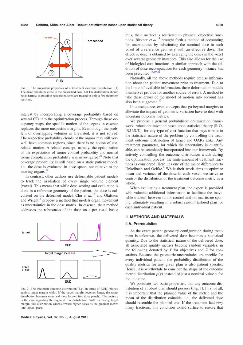
interest by incorporating a coverage probability based onseveral CTs into the optimization process. Through these oc-cupancy maps, the specific motion of the organs in essencereplaces the more unspecific margins. Even though the prob-lem of overlapping volumes is alleviated, it is not solved.The respective probability clouds of the organs may still verywell have common regions, since there is no notion of cor-related motion. A related concept, namely, the optimizationof the expectation of tumor control probability and normaltissue complication probability was investigated.21 Note thatcoverage probability is still based on a static patient model,i.e., the dose is evaluated in dose space, not relative to themoving organs.14

In contrast, other authors use deformable patient modelsto track the irradiation of every single volume elementvoxel. This means that while dose scoring and evaluation isdone in a reference geometry of the patient, the dose is cal-culated on the deformed model. Chu et al.15 and Ólafssonand Wright16 propose a method that models organ movementas uncertainties in the dose matrix. In essence, their methodaddresses the robustness of the dose on a per voxel basis;

thus, their method is restricted to physical objective func-tions. Birkner et al.14 brought forth a method of accountingfor uncertainties by substituting the nominal dose in eachvoxel of a reference geometry with an effective dose. Theeffective dose is obtained by averaging the doses in the voxelover several geometry instances. This also allows for the useof biological cost functions. A similar approach with the ad-dition of dose recomputation for each geometry instance hasbeen presented.18,19,22

Naturally, all the above methods require precise informa-tion about the patient movement prior to treatment. Due tothe limits of available information, these deformation modelsthemselves provide for another source of errors. A method totake these errors of the model of motion into account hasalso been suggested.17

In consequence, even concepts that go beyond margins toalleviate the impact of geometric variation have to deal withuncertain outcome metrics.

We propose a general probabilistic optimization frame-work, robust optimization based upon statistical theory R.O-.B.U.S.T., for any type of cost function that pays tribute tothe statistical nature of the problem by controlling the treat-ment outcome distribution of target and OARs alike. Anytreatment parameter, for which the uncertainty is quantifi-able, can be seamlessly incorporated into our framework. Byactively controlling the outcome distribution width duringthe optimization process, the finite amount of treatment frac-tions is considered. Here lies one of the major differences toUnkelbach and Oelfke.6 While their work aims to optimizemean and variance of the dose in each voxel, we strive tocontrol the distribution of the treatment outcome metric as awhole.

When evaluating a treatment plan, the expert is providedwith valuable additional information to facilitate the inevi-table tradeoff between tumor control and normal tissue spar-ing, ultimately resulting in a robust custom tailored plan foreach individual patient.

II. METHODS AND MATERIALS

II.A. Prerequisites

As the exact patient geometry configuration during treat-ment is unknown, the delivered dose becomes a statisticalquantity. Due to the statistical nature of the delivered dose,all associated quality metrics become random variables, inthe following denoted by Y for objectives and Z for con-straints. Because the geometric uncertainties are specific forevery individual patient, the probability distribution of thequality metrics for any given plan is also patient specific.Hence, it is worthwhile to consider the shape of the outcomemetric distribution py instead of just a nominal value y forthe outcome.

We postulate two basic properties, that any outcome dis-tribution of a robust plan should possess Fig. 1. First of all,it is important that the planned value of the metric and themean of the distribution coincide, i.e., the delivered doseshould resemble the planned one. If the treatment had verymany fractions, this condition would suffice to ensure that

FIG. 1. The important properties of a treatment outcome distribution. 1The mean should be close to the prescribed dose. 2 The distribution shouldbe as narrow as possible because patients are treated in only a few treatmentsessions.

FIG. 2. The treatment outcome distribution e.g., in terms of EUD plottedagainst target margin width. If the target margin becomes larger, the targetdistribution becomes more and more located top three panels. The contraryis the case regarding the organ at risk distribution. With increasing targetmargin, this distribution widens toward higher doses as the gradient movesinto organ space.

4020 Sobotta, Söhn, and Alber: Robust optimization based upon statistical theory 4020

Medical Physics, Vol. 37, No. 8, August 2010

the proper dose is delivered. In this case, sessions with a lessthan ideal delivery would be compensated by many others.However, in a realistic scenario, a failed treatment sessioncannot be compensated entirely. It is therefore also necessaryto take the outcome distribution width into consideration. Bydemanding that the outcome distribution should be as narrowas possible, it is ensured that any sample taken from it, i.e.,any treatment session, is within acceptable limits. This issuebecomes more serious for fewer treatment sessions.

Consequently, any robust treatment optimization approachshould keep track of the respective outcome distributions forthe involved regions of interest. In case of the target, it isdesirable to keep the distribution narrow and peaked at thedesired dose. The organ at risk distributions, however, shouldbe skewed toward low doses and only a controlled smallfraction should be close or above the threshold. This ensuresthat in the vast majority of all possible treatment courses, theirradiation of the organ at risk is within acceptable limitsFig. 3.

The R.O.B.U.S.T. algorithm extends our approach to in-tensity modulated radiotherapy optimization.24 We employthe method of constrained optimization to maximize dose tothe target while maintaining reasonable organ at risk doselevels. In this context, the kth constraint, which is a functionof the dose distribution D, is denoted by gkD. For the sakeof simplicity, assume that there is only one objective, fD.All cost functions can be physical maxDose or DVH orbiological EUD or gEUD. The incident beams are dis-cretized into beamlets or bixels. Each one of these beamletsis assigned a weight j. The dose distribution is the productof the dose operator T and the beamlet weights . The ele-

ment Tij relates the dose deposited in voxel i by beamlet j,thus the dose in voxel i is Di= jTij j. The entire optimiza-tion problem can now be stated as

find such that fT min, 1a

while gkT ck, 1b

and j 0 ∀ j , 1c

where ck is the upper limit of constraint k. It is evident thatthe optimum depends on c. An outline of the algorithm isshown in Fig. 4a.

95% 105%

%o

ccu

rre

nce

95% 105%

target

95% 105%

100%

%o

ccu

rre

nce

100%

organ at risk

100%

FIG. 3. Exemplary outcome distributions in relation to the aspired treatmentoutcome region. The top row illustrates the two-sided target cost functione.g., the area of acceptable treatment outcomes could range from 95% to105% of the prescribed dose. The distribution in the left panel is entirelylocated within the acceptable region, indicating that the patient would re-ceive the proper dose during all courses of treatment. While the distributionwidth in the middle panel is sufficiently small, its mean is too low, pointingtoward an underdosage of the target. The distribution on the right panel istoo wide and its mean too low. In practice, this means that there is a sig-nificantly reduced chance that the patient will receive proper treatment. Thebottom panels show the one-sided OAR cost function the area of acceptableoutcomes ranges up to 100%. From left to right, the complication riskincreases. Note that even though the mean in the middle panel is lower thanon the leftmost panel, the overall distribution is less favorable.

FIG. 4. a Constrained optimization in conjunction with classic cost func-tions. b Our probabilistic approach. Notice that the algorithm is entirelyconcealed from the optimizer, hence no alterations are necessary.



II.B. Algorithm

The course of treatment is subject to several sources ofuncertainty e.g., setup errors. Suppose each of thesesources is quantified by a geometry parameter e.g., displace-ment distance, its value indicating a possible realization dur-ing treatment. The precise value of any of these geometryparameters is unknown at treatment time, making them sta-tistical quantities. Thus as random variables X, they haveassociated probability distributions px, indicating the prob-ability that a certain value x is realized. These input distri-butions need to be estimated prior to planning based eitheron pretreatment data, data acquired during the course oftreatment, or population data.

The initial step is to obtain reliable estimates of the meanand the variance of the outcome distribution py given theinput uncertainty px. First a number of samples x1,. . .,N isdrawn from the uncertainty distributions. Then, for all thosegeometry instances the outcome metric yk= fD ,xk , 0kN is computed. If this is repeated sufficiently often, i.e., forlarge N, the treatment outcome distribution py can be ob-tained and alongside an estimate of the probability mass Mpresent in the desired interval Itol.

MY = dxpx1 ⇔ fx Itol

0 ⇔ fx” Itol . 2

The interval Itol is the green area in Fig. 3. However, thereare two major problems with this approach. First and fore-most, for dependable estimates, this method becomes pro-hibitively expensive, especially with dose recalculations in-volved. Second, the quantity of interest, Eq. 2, cannot becomputed in closed form, an essential requirement for effi-cient optimization schemes.

Typical prescriptions in radiotherapy demand that the in-terval contains large parts of the probability mass, i.e., 95%of all outcomes must lie within. That means that the exactshape of the actual distribution loses importance. Instead oftrying to obtain the entire outcome distribution, we assumethat its tails can be approximated by a Gaussian. The idea isshown in Fig. 5. Given this assumption, it is sufficient tocompute mean ExY and variance varxY. It is important tonote that even if py does not resemble a normal distribu-tion, the above approximation is still reasonable in the con-text of the proposed prescription scheme Eq. 2. It is suf-ficient to assume that the tails of py two-sided for targetvolumes, one-sided for OARs can be described by the tailsof the Gaussian Ny ExY ,varxY. This approximation be-comes more powerful for fractionated treatments because ofthe central limit theorem.

Incorporating the assumption above, we can state that theprobability mass enclosed in the interval of interest can becomputed analytically

MY min Itol

max Itol

dyNyExY,varxY , 3

which is crucial for the formulation of an objective functionfor the optimizer. The new optimization problem reads

maximize MY , 4a

subject to 1 − MZk ck, 4b

and j 0 ∀ j . 4c

It is desirable to quantify the error introduced by the ap-proximation in Eq. 3. The Chebyshev inequality providesfor an estimate. Loosely speaking, it states that if the vari-ance of a random variable is small, then the probability thatit takes a value far from its mean is also small. If Y is arandom variable with mean and variance 2, then

PY − k 1

k2 , k 1 5

limits the probability of a sample being drawn k standarddeviations away from the mean, independently of the densitypy. For the problem at hand, k is calculated by determininghow many standard deviations fit in the prescription intervalItol. If most of the probability mass is already concentrated inthe desired area, its spread is relatively small compared tothe extent of the acceptable region. This means that k islarge, and by virtue of Eq. 5, the probability of a samplelying outside Itol is low. This holds regardless of what thereal outcome distribution may look like. Since the Gaussian

outcome metric

rela

tive

occu

rre

nce

actual distribution

Gaussian

(a)

outcome metric

rela

tive

occu

rre

nce

(b)

FIG. 5. a The tails of the actual outcome distribution are approximatedwith a Gaussian with identical mean and variance to enable us to formulatea cost function in closed form. b In case of the target, the area of the tailsof the Gaussian, depicting undesirable outcomes, is minimized. In otherwords, the optimization aims to squeeze the treatment outcome distributioninto the set interval.



approximation tries to squeeze the probability mass into theinterval, it points the optimizer into the right direction, inde-pendently of the actual shape of py. Further refinementsregarding the error bounds are possible, but beyond thescope of this paper.

In order to visualize the quality of the Chebyshev inequal-ity, consider Fig. 6a. Suppose the red area reflects the out-come distribution. The blue Gaussian included in the figurehas identical mean and variance. The green bars are the up-per and lower limits of the desired interval.

Figure 6b shows the behavior of the Chebyshev boundas a function of the interval width, i.e., k in Eq. 5. The reddashed curve is the area enclosed in the interval for our ex-emplary pdf. For illustrational purposes, we also included theGaussian approximation, which serves as objective functionfor the optimizer. As the optimizer squeezes increasingamounts of the Gaussian inside the interval, it also inevitablyforces the actual distribution inside. Notice that the actualdistribution depends on the intermediate treatment plans ofthe iterative optimization, and hence constantly changes itsshape. The more the dose distribution approaches the opti-mization goal, the less probability mass stays outside theprescription interval and the better the Gaussian approxima-tion and the tighter the Chebyshev bound become.

The final algorithm is illustrated in Fig. 4b. Its incorpo-ration into an existing optimizer is straightforward, since themethod can be encapsulated. In Fig. 4b, the entire algo-rithm is encased in the red box which acts as a single costfunction to the outside. In summary, the algorithm works asfollows:

1 For each of the N geometry instances, the cost functionf is computed, yk= fD ,xk, 1kN.

2 Mean ExY, and variance varxY of those N samplesare determined.

3 Use mean and variance to approximate a GaussianNy ExY ,varxY Fig. 5.

4 Compute the objective function, Eq. 3, and return thevalue to the optimizer.

II.B.1. Accounting for fractionation

We have mentioned earlier that the spread of the outcomedistribution becomes increasingly important as we move to-ward smaller fraction numbers. This is substantiated by thelaw of large numbers in probability theory.25 In this section,we quantify the previous observation and augment our costfunction accordingly.

In the present context, the final outcome can be regardedas the sample mean for details regarding this approximation,please see the Appendix of all n sessions

An =i=1

nYi

n. 6

The random variable An has mean ExAn=ExY andvariance varxAn=varxY /n2 /n. Again, we employ theChebyshev inequality, Eq. 5, to obtain an approximationfor the probability mass inside the prescription interval. Withk / and the mean and variance of An

PAn − 2

n2 7

is obtained, where is the maximum error we are willing totolerate. We observe that the probability of a treatment vio-lating the requirements, i.e., the realized outcome is morethan away from the prescription, is proportional to thevariance of a single fraction 2, and goes to zero as thenumber of treatment fractions n increases. Further refine-ments can be made by reintroducing our Gaussian approxi-mation. The accuracy of the approximation increases withthe number of fractions n, as indicated by the central limittheorem.25 It states that the sum of a large number of inde-pendent random variables is approximately normal. The ac-tual convergence rate depends on the shape of Yi. For ex-ample, if Yi was uniformly distributed, n8 would suffice.25

The ensuing probability mass is computed analogously toEq. 3,

f(x)

Gaussian approx.RealInterval

100

101

0

10

20

30

40

50

60

70

80

90

100

k

perc

enta

ge

insid

ein

terv

al

Chebyshev Bound

Gaussian approx.

Example

(b)

(a)

FIG. 6. a An arbitrary distribution foreground is approximated by aGaussian background with identical mean and variance. b The errormade by the Gaussian approximation is bounded from below by the Cheby-shev inequality. The more probability mass is enclosed in the desired inter-val increasing k, the tighter the bound becomes.



MAn min Itol

max Itol

dyNyExAn,varxAn

= min Itol

max Itol

dyN yExY,varxY

n . 8

By explicitly including fractionation effects in the cost func-tion, Eq. 8, the influence of the variance is regulated. Thatis, we quantitatively account for the fact that a given numberof fractions offers a certain potential for treatment errors toeven out. Note that in the limit of very many fractions, werecover our initial statement that the mean value alone suf-fices to ensure proper treatment.

III. RESULTS

In this section, we compare R.O.B.U.S.T. to the PTVmethod and a method that controls the dose variance in eachpoint of a volume, proposed by Unkelbach and Oelfke.7 Weutilize a simplified 2D model implemented in MATLAB TheMathWorks, Inc., Natick, MA. It is driven by the con-strained nonlinear multivariable function optimizer from theMATLAB optimization toolbox. For brevity, we only considerrigid movement in two directions. Recall that our method isby no means restricted to rigid movement; the inclusion offurther sources of uncertainty is deemed unnecessary to il-lustrate the optimization problem and its solution. Our modelconsists of one tumor as well as two organs at risk. Weemploy biological cost functions.26 The Poisson cell killmodel was chosen for the target. The organs at risk werechosen to be represented by the parallel and serial complica-tion model, respectively. There are four beams impinging onthe target, each having 100 beamlets. To avoid artifacts suchas a very high modulation of the beam profiles, a penumbrawas also modeled Jelen et al.,27 Eq. 3. The input uncer-tainty was chosen to be independent Gaussians, i.e.,px=ipixi=iNxi 0,i

2. The variances i2 were all

equal, implying isotropic movement. In order to computemean and variance, 1000 sample geometries were drawnfrom X prior to the optimization. To save computation time,these were used throughout the optimization process. Underthe assumption of a static dose distribution, the cost func-tions of each geometry were computed and subsequentlymean and variance obtained.

The geometry is depicted in Fig. 7a. In order to makethe setup challenging, the tumor is embedded in the organs atrisk. The parallel organ is located to the lower left side of thetumor, whereas the serial organ is on the right side.

III.A. Comparison to PTV based optimization

We computed several plans using the described modeloptimizer. First of all, we created a plan disregarding anyuncertainties, i.e., all prescriptions were to the CTV, calledthe nominal plan. As expected, the possible treatment out-comes in terms of EUD for the tumor are wide spread Fig.7b. Notice that the organ at risk distributions are mostlywithin the acceptable region.

Next we employed the PTV approach to increase the ro-bustness in the target. The margin was set to one . As ex-pected, the target outcome distribution is well localizedaround the prescription Fig. 7c. However, compared tothe nominal plan, the dose to the adjacent organs is clearlyelevated. Moreover, the potentially delivered dose in slightlyshifted setups lies greatly beyond the nominal threshold. Thisemphasizes the fact that the PTV concept as a whole ignoresthe dose to the nearby organs.

The goal for R.O.B.U.S.T. was to fit the target outcomedistribution in between 97% and 103% of the prescribedEUD. At the same time, no more than 10% of all possibleoutcomes were allowed to exceed the organ at risk con-straints. The resulting distributions, along with their Gauss-ian approximations, are depicted in Fig. 7d. While the tar-get distribution closely resembles its margin counterpart, theEUDs of the organs at risk are significantly lower. Noticealso that the target distribution of R.O.B.U.S.T. is left-skewed. This can be explained by taking a closer look at theOAR Gaussian approximations. Both already exceed theEUD limit by 10% red part of the Gaussians in Fig. 7d,thereby preventing further improvements to the objective.

Table I shows a brief summary of the test runs.

III.B. Comparison to Unkelbach robust optimizationscheme

In the following paragraphs, we briefly compare R.O-.B.U.S.T. to the method of Unkelbach and Oelfke.7 Theyargue that the variance due to a finite amount of treatmentfractions needs to be accounted for and they quantitativelyincorporate the number of fractions in their cost function.According to Unkelbach and Oelfke,7 Eq. 7, the cost func-tion for the target is

fuD = iCTV

ExDi − DCTV2 +1

nExDi

2 − Ex2Di 9

and for the kth organ at risk, they propose

gukD =

iOARk

ExDi − DOARk+

2 , 10

where · + is the one-sided overdose, Di is the dose to voxeli, and DCTV and DOARk

are the prescriptions for target andorgans at risk, respectively. Notice that not unlike Eq. 8, theinfluence of the variance decreases as the number of frac-tions increases in Eq. 9.

While Eqs. 9 and 10 are designed to tightly control thedose delivered to each voxel, the optimization of Eq. 3 and8 implies control over the outcome distribution of an entirevolume. In consequence, our approach allows intervolumetradeoffs of the mean dose per voxel, a basic requirement forbiological cost functions. Their approach deals exclusivelywith the voxelwise quadratic deviation cost functionD−D02.

For the following comparison, we set n=30 fractions.Each point of the histograms in Fig. 8 consequently repre-sents the average over 30 sample geometries. Note that thetarget distribution, Fig. 8d, now lies entirely in the desired



interval as opposed to Fig. 7d. This is because the vari-ance is rescaled by the number of fractions and therefore theOAR constraints allow for a higher mean EUD to the target.Also note that the distributions look Gaussian. This is a di-rect consequence of the central limit theorem.

For the Unkelbach approach, we initially set DCTV to thetarget EUD value and DOARk

were chosen according to their

respective EUD tolerance doses. For better comparability,the optimized dose was slightly rescaled for the serial organdoses to match. The outcome distributions of the Unkelbachmethod are shown in Fig. 8c. The target EUD distributionlies outside the desired interval, due to a persistent cold spotthat is heavily penalized by the Poisson EUD. It is also sig-nificantly wider than its R.O.B.U.S.T. counterpart. Further-more, the parallel organ is overdosed due to a relatively highmean dose.

We also examined the results of both methods based onthe criteria suggested by Unkelbach and Oelfke.7 Figure 8ashows the DVH of the expected dose in the respective re-gions of interest. Both methods exhibit underdosage in thetarget. However, the Unkelbach method enforces strictertradeoffs between the standard deviation and the mean dosein a voxel, which results in a larger volume being under-dosed than by R.O.B.U.S.T., which increased the mean doseslightly to minimize the most extreme cold spots. This is alsoreflected by the respective EDVH.

60 70 80 90 100 110 120

tumor

60 70 80 90 100 110 120

serial organ at risk

60 70 80 90 100 110 120

parallel organ at risk

(b)

60 70 80 90 100 110 120

tumor

60 70 80 90 100 110 120


60 70 80 90 100 110 120


(c)

60 70 80 90 100 110 120

tumor

60 70 80 90 100 110 120


60 70 80 90 100 110 120


(d)

(a)

FIG. 7. The model geometry and treatment outcome histograms obtained from several methods. a The organ setup. Tumor center, Poisson model, parallelorgan lower left, and serial organ right. In the histograms b–d, the highlighted area denotes the region of acceptable dosage. The horizontal axes showthe percentage of the prescription for the respective organs. Note that these histograms apply for a single fraction. b The treatment outcome histogram forthe plan without motion compensation. c The PTV margin greatly reduces the width of the target distribution, but worsens the organ at risk counterparts. dThe outcome distributions along with their Gaussian approximation in the probabilistic case R.O.B.U.S.T..

TABLE I. The first column indicates what fraction of treatment outcomeswould be in the 97%–103% prescription interval Eq. 2. The second andthird columns show the percentage of treatment outcomes that are over thedefined threshold for the serial and parallel organ at risk, respectively.

Goal

Tumor Serial OAR Parallel OAR

All cases Max. 10% of cases97%–103% presc. Overconstraint

No compensation 43% 0% 7%PTV plan 96% 48% 47%R.O.B.U.S.T. plan 92% 10% 9%



Additionally, Unkelbach and Oelfke7 propose to examinethe standard-deviation-volume-histogram to visualize the un-certainty of the dose prediction provided by the expectationvalue. The SDVHs for R.O.B.U.S.T. and the Unkelbachmethod are shown in the top left plot of Fig. 8b. R.O-.B.U.S.T. succeeds for the target because the standard devia-tion is consistently lower than its counterpart from the Un-kelbach method. The R.O.B.U.S.T. SDVH for the parallelorgan, however, shows increased variability for about 30% ofthe volume. This can also be attributed to the dose gradientin the parallel organ as its cost function penalizes homoge-neous irradiation. This can be seen in the top right plot inFig. 8b. The maximum standard deviation of the dose to thefunctional reserve, i.e., the part of the volume in the low doseregion 0%–40% of prescribed dose, is similar to its coun-terpart from the Unkelbach method. The higher dose SD-VHs, i.e., the bottom plots in Fig. 8b, however, show anincreased standard deviation which is acceptable because

the irradiated volume may be sacrificed. In essence,R.O.B.U.S.T. shapes the dose distribution such that the func-tional reserve is kept intact under all circumstances that mayoccur based on their respective probabilities px.

Notice that in the absence of constraints, both methodstend to deliver near identical results data not shown. How-ever, as soon as constraints come into play, R.O.B.U.S.T.benefits from its larger space of potential solutions, due tothe incorporation of nonlocal effects and absence of voxel-wise constraints.

IV. DISCUSSION AND CONCLUSION

We have presented a new approach toward robust treat-ment plan optimization. Accepting the fact that all outcomemetrics are random variables in the presence of geometryuncertainties, it addresses robustness in the sense that underall possible uncertainties, the treatment outcome quality met-

80 90 100 110

tumor

80 90 100 110


80 90 100 110


(d)

0 5 10 150

20

40

60

80

100

σ2

[% of prescribed dose]

vo

lum

e[%

]

0 5 10 150

20

40

60

80

100

σ2

[% of prescribed dose] [0−40]

vo

lum

e[%

]

0 5 10 150

20

40

60

80

100

σ2


vo

lum

e[%

]

0 5 10 150

20

40

60

80

100

σ2


vo

lum

e[%

]

(b)

80 90 100 110

tumor

80 90 100 110


80 90 100 110


(c)

0 20 40 60 80 1000

10

20

30

40

50

60

70

80

90

100

dose [% of prescribed dose]

volu

me

[%]

serial

parallel

tumor

(a)

FIG. 8. A brief comparison of the Unkelbach method and R.O.B.U.S.T. The solid lines in a and b are from the Unkelbach method whereas the dashed linesstem from R.O.B.U.S.T. a The DVH of the expected dose. The dotted horizontal line shows the prescription for the target. b. The standard-deviation-volume-histogram provides insight over the dose variability in each voxel. Note that in SDVHs, better graphs are further left, i.e., less variability in the dose.For more transparency, additionally to the comprehensive SDVH in the top left panel, we included three SDVHs, each for a different dose interval. The EUDtreatment histograms for the c Unkelbach method and d R.O.B.U.S.T. It is important to note that these plots consider 30 fractions. Consequently, each entryin the histograms is the average over 30 randomly drawn sample geometries.



rics should remain within a specified range across all treat-ment fractions. It focuses on controlling the shape of theoutcome distribution instead of a nominal value of the met-ric. By quantifying the uncertainty of the treatment outcomefor each metric, it provides a measure for the robustness ofthe plan.

If the optimization problem is stated like Eq. 3, preciseknowledge of the outcome distribution is not necessary andthe Gaussian approximation is possible by virtue of theChebyshev inequality. This greatly reduces the effort of un-certainty sampling.

Because our method maintains different organ geometrysetups, it is able to preserve correlations in geometric shifts.This means that there are no overlapping regions of interestin the patient model. Since it also explicitly takes the shapeof the uncertainty distributions of the treatment parametersinto account, it can detect a potentially hazardous scenarioand assess its likelihood. This way, the plan will neither beoverly conservative, nor lenient toward dangerous organdoses.

In this work, we investigated robustness regarding thetreatment outcome in terms of EUD. The method relies onsampling the distribution of each source of uncertainty.R.O.B.U.S.T. is very versatile because it can handle allsources of error and is only limited by the available patientuncertainty model.

Accelerations in the evaluation of the R.O.B.U.S.T. costfunctions to make the method suitable for clinical problemsare possible and are subject of future work.28,29

APPENDIX: DETAILS ON THE EVALUATION OFEUD ACROSS FRACTIONS

We have stated earlier that we regard the final treatmentoutcome EUD as the average of the EUDs of its constituentsessions. However, the quantity of interest is typically theEUD of the cumulative dose. Taking into account the respec-tive properties of the EUD functions, one can establish arelation between the two quantities. Given a convex functionf and a random variable D, Jensen’s inequality30 establishesa link between the function value at the average of the ran-dom variable and the average of the function values of therandom variable, namely,

fED EfD . A1

The converse holds true if f is concave. With the generalform of the EUD

EUDD = g−1 1

VvV

gDv , A2

we can discriminate the following cases.

I. Serial complication

Given that the serial complication function gD=Da,a1, renders Eq. A2 a convex function,26 it follows fromEq. A1, that EUDEDEEUDD. Hence, consider-ing the average EUD as outcome, Eq. 6, always overesti-

mates the risk for the patient, i.e., the EUD of the mean doseis certain to be lower.

II. Poisson cell kill

The basic reasoning is similar to the serial complicationmechanism. However, Eq. A2 in conjunction withgD=exp−D is concave. Thus, the relation in Eq. A1reverses to EUDEDEEUDD. That is, in case of thetarget we underestimate the cell kill by taking the averageEUD Eq. 6.

III. Parallel complication

The parallel complication function gD= 1+ Dtol /Db−1 is convex for DDtol and concave forDDtol. In consequence, the above reasoning cannot be di-rectly applied. However, typical prescriptions demand thatlarge parts of the organ are kept intact, hence most of theorgan volume is irradiated with DDtol. For this organ sub-volume, the estimate Eq. 6 is, again, an upper bound. Forthe part of the organ that may be sacrificed, the average EUDunderestimates the risk. But keeping in mind that Eq. 6overestimates the risk of the functional reserve being de-stroyed while underestimating the damage to tissue we arewilling to sacrifice, this seems acceptable.

In summary, we have shown that using the average EUDas outcome metric for fractionated radiotherapy is viable be-cause it leads to underestimation of tissue damage for thetarget and overestimation of tissue damage for the organs atrisk.

aElectronic mail: [email protected]. Maleike, J. Unkelbach, and U. Oelfke, “Simulation and visualizationof dose uncertainties due to interfractional organ motion,” Phys. Med.Biol. 51, 2237–2252 2006.

2C. Baum, M. Alber, M. Birkner, and F. Nüsslin, “Treatment simulationapproaches for the estimation of the distributions of treatment qualityparameters generated by geometrical uncertainties,” Phys. Med. Biol. 49,5475–5488 2004.

3K. M. Langen and D. T. L. Jones, “Organ motion and its management,”Int. J. Radiat. Oncol., Biol., Phys. 50, 265–278 2001.

4M. van Herk, P. Remeijer, C. Rasch, and J. V. Lebesque, “The probabilityof correct target dosage: Dose-population histograms for deriving treat-ment margins in radiotherapy,” Int. J. Radiat. Oncol., Biol., Phys. 47,1121–1135 2000.

5A. Niemierko, “Reporting and analyzing dose distributions: A concept ofequivalent uniform dose,” Med. Phys. 24, 103–110 1997.

6J. Unkelbach and U. Oelfke, “Inclusion of organ movements in IMRTtreatment planning via inverse planning based on probability distribu-tions,” Phys. Med. Biol. 49, 4005–4029 2004.

7J. Unkelbach and U.Oelfke, “Incorporating organ movements in IMRTtreatment planning for prostate cancer: Minimizing uncertainties in theinverse planning process,” Med. Phys. 32, 2471–2483 2005.

8International Commission on Radiation Units and Measurements, “Pre-scribing, recording and reporting photon beam therapy,” ICRU ReportNo. 50 ICRU, Washington, DC, 1993.

9M. van Herk, P. Remeijer, and J. V. Lebesque, “Inclusion of geometricuncertainties in treatment plan evaluation,” Int. J. Radiat. Oncol., Biol.,Phys. 52, 1407–1422 2002.

10J. C. Stroom, H. C. J. de Boer, H. Huizenga, and A. G. Visser, “Inclusionof geometrical uncertainties in radiotherapy treatment planning by meansof coverage probability,” Int. J. Radiat. Oncol., Biol., Phys. 43, 905–9191999.

11A. McKenzie, M. van Herk, and B. Mijnheer, “Margins for geometricuncertainty around organs at risk in radiotherapy,” Radiother. Oncol. 62,



299–307 2002.12J. C. Stroom and B. J. M. Heijmen, “Limitations of the planning organ at

risk volume PRV concept,” Int. J. Radiat. Oncol., Biol., Phys. 66, 279–286 2006.

13C. Baum, M. Alber, M. Birkner, and F. Nüsslin, “Robust treatment plan-ning for intensity modulated radiotherapy of prostate cancer based oncoverage probabilities,” Radiother. Oncol. 78, 27–35 2006.

14M. Birkner, D. Yan, M. Alber, J. Liang, and F. Nüsslin, “Adapting inverseplanning to patient and organ geometrical variation: Algorithm and imple-mentation,” Med. Phys. 30, 2822–2831 2003.

15M. Chu, Y. Zinchenko, S. G., Henderson, and M. B. Sharpe, “Robustoptimization for intensity modulated radiation therapy treatment planningunder uncertainty,” Phys. Med. Biol. 50, 5463–5477 2005.

16A. Ólafsson and S. J. Wright, “Efficient schemes for robust IMRT treat-ment planning,” Phys. Med. Biol. 51, 5621–5642 2006.

17T. C. Y. Chan, T. Bortfeld, and J. N. Tsitsiklis, “A robust approach toIMRT optimization,” Phys. Med. Biol. 51, 2567–2583 2006.

18M. Söhn, M. Weinmann, and M. Alber, “Intensity-modulated radio-therapy optimization in a quasi-periodically deforming patient model,”Int. J. Radiat. Oncol., Biol., Phys. 75, 906–914 2009.

19D. L. McShan, M. L. Kessler, K. Vineberg, and B. A. Fraass, “Inverseplan optimization accounting for random geometric uncertainties with amultiple instance geometry approximation MIGA,” Med. Phys. 33,1510–1521 2006.

20J. Yang, G. S. Mageras, S. V. Spirou, A. Jackson, E. Yorke, C. C. Ling,and C.-S. Chui, “A new method of incorporating systematic uncertaintiesin intensity-modulated radiotherapy optimization,” Med. Phys. 32, 2567–2579 2005.

21M. G. Witte, J. van der Geer, C. Schneider, J. V. Lebesque, M. Alber, and

M. van Herk, “IMRT optimization including random and systematic geo-metric errors based on the expectation of TCP and NTCP,” Med. Phys.34, 3544–3555 2007.

22A. Trofimov, E. Rietzel, H.-M. Lu, B. Martin, S. Jiang, G. T. Y. Chen, andT. Bortfeld, “Temporo-spatial IMRT optimization: Concepts, implemen-tation and initial results,” Phys. Med. Biol. 50, 2779–2798 2005.

23J. Löf, B. K. Lind, and A. Brahme, “An adaptive control algorithm foroptimization of intensity modulated radiotherapy considering uncertain-ties in beam profiles, patient set-up and internal organ motion,” Phys.Med. Biol. 43, 1605–1628 1998.

24M. Alber and R. Reemtsen, “Intensity modulated radiotherapy treatmentplanning by use of a barrier-penalty multiplier method,” Optim. MethodsSoftware 22, 391–411 2007.

25D. P. Bertsekas and J. N. Tsitsiklis, Introduction to Probability, 1st ed.Athena Scientific, Belmont, MA, 2002.

26M. Alber and F. Nüsslin, “An objective function for radiation treatmentoptimization based on local biological measures,” Phys. Med. Biol. 44,479–493 1999.

27U. Jeleń, M. Söhn, and M. Alber, “A finite size pencil beam for IMRTdose optimization,” Phys. Med. Biol. 50, 1747–1766 2005.

28B. Sobotta, M. Söhn, and M. Alber, “Quantifying the robustness of IMRTtreatment plans from a statistical optimization model to account for organdeformation,” Radiother. Oncol. 88, S121–S122 2008.

29B. Sobotta, M. Söhn, and M. Alber, “What is the minimum number ofgeometry samples for a statistical patient model for robust treatment plan-ning?,” Radiother. Oncol. 92, S86 2009.

30J. L. W. V. Jensen, “Sur les fonctions convexes et les inégalités entre lesvaleurs moyennes,” Acta Math. 30, 175–193 1906.



Appendix E

On expedient properties ofcommon biological scorefunctions for multi-modality,adaptive and 4D doseoptimization

published inPhysics in Medicine and Biology 2011; 56: N123-N129

103

IOP PUBLISHING PHYSICS IN MEDICINE AND BIOLOGY

Phys. Med. Biol. 56 (2011) N123–N129 doi:10.1088/0031-9155/56/10/N01

NOTE

On expedient properties of common biological scorefunctions for multi-modality, adaptive and 4D doseoptimization

B Sobotta1, M Sohn2, W Shaw3 and M Alber1

1 Section for Biomedical Physics, Radioonkologische Uniklinik, Universitat Tubingen,72076 Tubingen, Germany2 Department of Radiation Oncology, University Hospital Grosshadern, LMU Munchen,81377 Munchen, Germany3 Department of Medical Physics, Faculty of Health Sciences, University of the Free State,PO Box 339, Bloemfontein 9300, South Africa


Received 1 January 2011, in final form 9 March 2011Published 13 April 2011Online at stacks.iop.org/PMB/56/N123

AbstractFrequently, radiotherapy treatments are comprised of several dose distributionscomputed or optimized in different patient geometries. Therefore, the needarises to compute the comprehensive biological effect or physical figure ofmerit of the combined dose of a number of distinct geometry instances. Forthat purpose the dose is typically accumulated in a reference geometry throughdeformation fields obtained from deformable image registration. However, itis difficult to establish precise voxel-by-voxel relationships between differentanatomical images in many cases. In this work, the mathematical properties ofcommonly used score functions are exploited to derive an upper boundary forthe maximum effect for normal tissue and a lower boundary for the minimumeffect for the target of accumulated doses on multiple geometry instances.

(Some figures in this article are in colour only in the electronic version)

1. Introduction

The need to compute the combined effect of several dose distributions in distinct geometriesarises in a number of applications. For example, some approaches to 4D IMRT optimizationoptimize dose simultaneously on multiple geometries (Birkner et al 2003, McShan et al 2006,Sohn et al 2009, Trofimov et al 2005) by warping the dose in each instance to a referencegeometry, thereby realizing optimization in ‘tissue-eye-view’. Also in combined modalitytreatment, e.g. brachytherapy and external beam therapy, the overall effect has to be computed(Osorio et al 2010). Similar problems occur with the dose recomputation in mobile organs,

0031-9155/11/100123+07$33.00 © 2011 Institute of Physics and Engineering in Medicine Printed in the UK N123

N124 B Sobotta et al

e.g. prostate on daily cone beam CT (Morin et al 2006, Rong et al 2010). Since particle therapyis very sensitive to geometry changes, especially in regions with heterogeneous density, doseshave to be computed on several geometries and subsequently combined (Soukup et al 2009,Knopf et al 2010).

All of these methods require a correspondence between the volume elements (voxels) ofeach geometry instance to add up each dose contribution correctly. In general this requiresdeformable registration. Given the independently computed doses in each patient geometry,the voxel correspondence is used to warp the individual doses back to some reference geometry.In this reference geometry, the doses are accumulated and evaluated. Unfortunately, there areseveral issues with this approach. The computation of the deformation fields is fraught withuncertainties and difficult to verify. The computation frequently needs human surveillanceand the data set may be incomplete or disturbed by artifacts. Some organs, especially bowel,are difficult to model because of variations in filling and the lack of fiducials. Incompleteknowledge of the extent of movement due to infrequent and sparse imaging may also affect theaccuracy of the model. Additionally, special care must be taken to ensure energy conservationduring dose warping and accumulation. Dose distributions are frequently analyzed with scorefunctions that are a sum over all volume elements of an organ. In contrast to pointwise scores,a lot of the effort that goes into correct dose accumulation is washed out in the summation.Very often, these score functions are convex, which opens a possibility for very powerfulestimations of their true value without going through the process of proper dose accumulation.

This note derives how the mathematical properties of commonly used cost functions, e.g.equivalent uniform dose (EUD) (Niemierko 1997), can be exploited to compute boundariesof the combined effect of the dose distributions in different geometries. These boundariesare computed without the need for deformable registration. For the target, lower boundarieswill be given, and for the critical structures upper boundaries. Thus, a worst case scenariois obtained that may be used for a quick scoring of a treatment plan at only a fraction of thecost of a full analysis. The method is demonstrated on a prostate case with interfractionalmovement and a 4D lung case.

2. Methods and materials

Suppose F is a score function and let Dk be the dose distribution of the full treatment appliedto the kth geometry instance Ik. For dose accumulation, a reference geometry I0 is chosen.Dk denotes the warped dose in the reference geometry, i.e. the deformation field from Ik to I0

applied to dose Dk. Hence, the quantity of main interest, the accumulated dose, is

E[D] = 1

N

N−1∑

k=0

Dk with D0 ≡ D0. (1)

Note that the accumulated dose is expressed as an average in (1). Average and sum areequivalent because the dose distribution may be rescaled by a constant factor.

Dose warping as well as dose accumulation is a linear operation and therefore the doseintegral of Dk over the volume of interest equals that of Dk . This is a direct consequence ofenergy and volume conservation. By virtue of this, and by way of definition

F(Dk) = F(Dk). (2)

If no deformation field is available, the single doses Dk cannot be warped back to thereference geometry, and in other words Dk is inaccessible. However, by virtue of Jensen’sinequality (Jensen 1906) for a convex function F,

F(E[D]) E[F(D)] = E[F(D)] (3)

Properties of common biological score functions N125

can be established. Conversely, for concave functions F, (3) reverses to

F(E[D]) E[F(D)] = E[F(D)], (4)

where E[F(D)] ≡ 1/N∑N−1

k=0 F(Dk) is the sum of the score function evaluated for eachoriginal geometry instance. The equality relations in (3) and (4) are due to (2).

Convex functions (curved upward) are commonly associated with normal tissues or otherdose-limiting objectives. Examples include maximum dose, one-sided dose-limiting quadraticpenalty and EUD for serial organs (Alber and Nusslin 1999), i.e. f (D) = Da , a 1. Notethat the mean dose is also covered by the inequality because it is synonymous with the serialEUD cost function with a = 1. The parallel EUD (Alber and Nusslin 1999) is an exceptionbecause it is neither convex nor concave; however, it can still be handled within the proposedframework, see below. A commonly used cost function for the target volume, the Poisson cellkill EUD (Niemierko 1997, Alber and Nusslin 1999), is concave.

In practice, this means that in the case of normal tissue the score function value of theaccumulated dose (F(E[D])) is always smaller than the sum of the score functions of theinstance doses (E[F(D)]) (3). For the target, the EUD of the accumulated dose is alwayslarger than the sum of the EUDs of the instance doses (4). Hence, using Jensen’s inequality,worst case boundaries for the score function of the accumulated dose can be derived withoutthe need for a deformable registration model.

Note that EUD and other cost functions are volume averages and are therefore insensitiveto changes of the absolute volume of some organ or tumor. Still, uncertainties in delineationor volume shrinkage can introduce errors into the above inequalities. In order to maintainthe validity of the inequality, it is sufficient to formulate a worst case. For normal tissue, thiswould be equivalent to using the smallest volume of the organ of interest in any geometryinstance to normalize EUD in each instance. In case of tumor shrinkage, it is helpful to resortto the mechanistic basis of the model. Tumor EUD is derived from the initial number ofclonogenic cells, which can be expressed as the mean cell density times the tumor volume.Under the assumption that no clonogenic cells are lost from the initial population by effectsother than those caused by radiation, the primary quantity cell number is preserved despitevolume loss. A volume reduction then results in an increase of clonogenic cell density. For thepurpose of inequality, the EUDs of different geometry instances may be added although theypertain to differently sized volumes since EUD is independent of cell density. However, if thequantity of interest were the expected number of surviving clonogens instead, the increase incell density would have to be considered.

The parallel complication function f (D) = (1 + (Dtol/D)b)−1 is convex for doses belowthe dose Dtol and concave for doses above, i.e. it has a point of inflection at D = Dtol. Inconsequence, the above reasoning cannot be directly applied. However, typical prescriptionsdemand that large parts of the organ are kept intact; hence, most of the organ volume isirradiated with doses below Dtol. For this fraction of the volume, (3) applies, i.e. the damageis overestimated. To account for the entire volume of the parallel organ, the cost function canbe convexified by linear extrapolation at the point of inflection, see figure 1.

Note that the above relation (3) is not valid for dose–volume constraints. Table 1 containsan overview of the properties of commonly used score functions.

3. Results and discussion

The presented method is valuable because it provides a safe upper boundary on normal tissuedoses and effects, and a safe lower boundary for tumor EUD. It is applicable even if deformationfields are not available or tumor shrinkage makes warping and accumulation difficult.


logistic function

linear extension at inflexion

Figure 1. The parallel complication cost function (logistic function) is linearly extended at theinflection point to be convex on its entire support.

Table 1. Properties of various cost functions.

Cost function Property

Poisson cell kill EUD ConcaveParallel EUD –Generalized EUD k 1 Convex(Serial EUD)Generalized EUD k 1 ConcaveAverage dose Convex and concaveDVH constraints –Maximum dose ConvexQuadratic deviation Convexpenalty

To illustrate one possible application, the method was applied to a prostate cancer case.Target, bladder and rectum (wall) EUDs were evaluated in 18 geometries and their averagescomputed, table 2. The biomechanical model, which is the basis of the deformation fieldfor the dose accumulation, is based on Yan et al (1999). The EUD computations based onthe accumulated dose and the estimated boundaries yielded 71.601 Gy (> 70.31 Gy) for theprostate, 59.897 Gy (< 61.28 Gy) for the bladder and 56.675 Gy (< 57.8 Gy) for the rectalwall. As predicted, for the target the average EUD in table 2 is lower than the EUD of theaverage dose. The contrary is the case for the organs at risk. Resultingly, a useful worst caseapproximation of the EUDs was obtained without dose accumulation.

To illustrate another application, the method was employed for a 4D lung cancer case.The EUDs for the gross tumor volume (GTV) (Poisson cell kill) and the lung (mean dose)were investigated. The basis were eight 4D CT scan instances taken during a breathing cycle.Each of these instances is associated with an instance weight that was computed from thebreathing PDF. It reflects the relative fraction of a breathing cycle that is represented by agiven instance. During dose accumulation, the doses of the respective instances were also


Table 2. EUDs for 18 patient geometries and their average.

Prostate Bladder RectumPoisson EUD (Gy) Serial EUD (Gy) Serial EUD (Gy)

CT # α = 0.4 a = 8 a = 12

1 71.73 59.24 63.72 70.81 58.61 49.563 55.28 62.62 42.414 71.7 57.21 57.355 70.68 62.80 48.756 71.7 60.07 60.97 71.63 62.49 54.898 64.18 63.97 58.169 71.76 60.43 59.44

10 71.5 58.14 64.4111 71.87 63.72 58.3912 71.79 60.96 61.1613 71.63 61.04 62.2314 71.95 63.76 58.0815 71.88 64.43 59.1616 71.67 61.48 58.1217 71.87 61.65 62.3118 71.88 60.38 61.46

70.31 61.28 57.80

Table 3. Instance weights and EUDs for GTV and lung from a breathing cycle (inhale (In) exhale(Ex) respiratory levels in the range 0–100) and the weighted sum of the EUD.

GTV EUD Weighted GTV EUD Lung EUD weighted lung EUDBreathing Poisson EUD Poisson EUD Serial EUD Serial EUDphase Weight (Gy) α = 0.4 (Gy) α = 0.4 (Gy) a = 1 (Gy) a = 1

0 In 0.402 48.029 19.312 4.66 1.87425 In 0.088 48.127 4.229 4.48 0.39450 In 0.077 49.656 3.800 4.37 0.33475 In 0.084 49.661 4.190 4.24 0.358

100 Ex 0.117 48.250 5.629 4.29 0.50175 Ex 0.033 50.718 1.682 4.38 0.14550 Ex 0.048 49.851 2.379 4.43 0.21125 Ex 0.152 49.661 7.528 4.51 0.684

48.749 4.501

weighted. For details, please refer to Sohn et al (2009). The EUD of the accumulated dose is49.835 Gy (> 48.749 Gy) for the GTV and 4.501 Gy ( 4.501 Gy) for the lung. Again theprediction in table 3 proves to be a worst case estimate. Note that the EUDs for the lung areequal for both methods by necessity, reflecting energy and volume conservation. This is due


to the fact that the mean dose score function is linear, hence concave and convex at the sametime.

Further applications of this relation have been outlined in the introduction, whereby thecombination of brachytherapy and teletherapy is of particular usefulness in practice. Here,

EUD(DEBT + DBT) EUD(DEBT) + EUD(DBT) (5)

for normal tissues and

EUD(DEBT + DBT) EUD(DEBT) + EUD(DBT) (6)

for targets. This work also lays the foundation for robust optimization schemes that requireno deformation fields (Sobotta et al 2010). The application of Jensen’s inequality to theoptimization of doses for variable patient geometries is the subject of future work.

4. Conclusions

A method to derive boundaries on the score function of the accumulated dose of multiple patientgeometries was presented. By virtue of Jensen’s inequality and the mathematical nature ofcommonly used score functions, in particular EUD and other biological score functions, it ispossible to compute a worst case approximation on the combined effect of doses applied tovariable geometries. Because the approach circumvents the computation of the accumulateddoses by means of deformation fields, it eliminates the need for deformable registration anddose warping.

Acknowledgment

We would like to thank D Yan and J Liang from Beaumont Hospital, Royal Oak, MI, USA,for providing the sample prostate cancer patient and the corresponding deformation fields.

References

Alber M and Nusslin F 1999 An objective function for radiation treatment optimization based on local biologicalmeasures Phys. Med. Biol. 44 479–93

Birkner M, Yan D, Alber M, Liang J and Nusslin F 2003 Adapting inverse planning to patient and organ geometricalvariation: algorithm and implementation Med. Phys. 30 2822–31

Jensen J L W V 1906 Sur les fonctions convexes et les inegalites entre les valeurs moyennes Acta Math. 30 175–93Knopf A et al 2010 Special report: workshop on 4D-treatment planning in actively scanned particle therapy—

Recommendations, technical challenges, and future research directions Med. Phys. 37 4608–14McShan D L, Kessler M L, Vineberg K and Fraass B A 2006 Inverse plan optimization accounting for random

geometric uncertainties with a multiple instance geometry approximation (MIGA) Med. Phys. 33 1510–21Morin O, Gillis A, Chen J, Aubin M, Bucci M K, Roach M and Pouliot J 2006 Megavoltage cone-beam CT: system

description and clinical applications Med. Dosim. 31 51–61Niemierko A 1997 Reporting and analyzing dose distributions: a concept of equivalent uniform dose Med.

Phys. 24 103–10Osorio E M V, Hoogeman M S, Teguh D N, Al Mamgani A, Kolkman-Deurloo I K K, Bondar L, Levendag P C

and Heijmen B J 2010 Three-dimensional dose addition of external beam radiotherapy and brachytherapy fororopharyngeal patients using nonrigid registration Int. J. Radiat. Oncol. Biol. Phys. at press

Rong Y, Smilowitz J, Tewatia D, Tom W A and Paliwal B 2010 Dose calculation on KV cone beam CT images: aninvestigation of the Hu-density conversion stability and dose accuracy using the site-specific calibration Med.Dosim. 35 195–207

Sobotta B, Sohn M and Alber M 2010 Robust optimization based upon statistical theory Med. Phys. 37 4019–28Sohn M, Weinmann M and Alber M 2009 Intensity-modulated radiotherapy optimization in a quasi-periodically

deforming patient model Int. J. Radiat. Oncol. Biol. Phys. 75 906–14


Soukup M, Sohn M, Yan D, Liang J and Alber M 2009 Study of robustness of IMPT and IMRT for prostate canceragainst organ movement Int. J. Radiat. Oncol. Biol. Phys. 75 941–9

Trofimov A, Rietzel E, Lu H M, Martin B, Jiang S, Chen G T Y and Bortfeld T 2005 Temporo-spatial IMRToptimization: concepts, implementation and initial results Phys. Med. Biol. 50 2779–98

Yan D, Jaffray D and Wong J 1999 A model to accumulate fractionated dose in a deforming organ Int. J. Radiat.Oncol. Biol. Phys. 44 665–75

Appendix F

Special report: Workshop on4D-treatment planning inactively scanned particletherapy - Recommendations,technical challenges, and futureresearch directions

published inMedical Physics 2010; 37: 4608-4614

111

Special report: Workshop on 4D-treatment planning in activelyscanned particle therapy—Recommendations, technical challenges,and future research directions

Antje Knopfa

Center for Proton Therapy, Paul Scherrer Institut, 5232 Villigen, Switzerland

Christoph BertGSI Helmholtzzentrum für Schwerionenforschung GmbH, Abt. Biophysik, 64291 Darmstadt, Germany

Emily Heath,b Simeon Nill, and Kim KrausDeutsches Krebsforschungszentrum, 69120 Heidelberg, Germany

Daniel RichterGSI Helmholtzzentrum für Schwerionenforschung GmbH, Abt. Biophysik, 64291 Darmstadt, Germany

Eugen HugCenter for Proton Therapy, Paul Scherrer Institut, 5232 Villigen, Switzerland and Proton-Radiotherapy,University of Zuerich, 8006 Zurich, Switzerland

Eros Pedroni, Sairos Safai, and Francesca AlbertiniCenter for Proton Therapy, Paul Scherrer Institut, 5232 Villigen, Switzerland

Silvan Zenklusen and Dirk BoyeCenter for Proton Therapy, Paul Scherrer Institut, 5232 Villigen, Switzerland and ETH,8092 Zuerich, Switzerland

Matthias Söhn,c Martin Soukup,d and Benjamin SobottaSection for Biomedical Physics, University Hospital for Radiation Oncology, 72076 Tuebingen, Germany

Antony LomaxCenter for Proton Therapy, Paul Scherrer Institut, 5232 Villigen, Switzerland and ETH,8092 Zuerich, Switzerland

Received 19 April 2010; revised 13 July 2010; accepted for publication 13 July 2010;published 10 August 2010

This article reports on a 4D-treatment planning workshop 4DTPW, held on 7–8 December 2009at the Paul Scherrer Institut PSI in Villigen, Switzerland. The participants were all members ofinstitutions actively involved in particle therapy delivery and research. The purpose of the 4DTPWwas to discuss current approaches, challenges, and future research directions in 4D-treatment plan-ning in the context of actively scanned particle radiotherapy. Key aspects were addressed in plenarysessions, in which leaders of the field summarized the state-of-the-art. Each plenary session wasfollowed by an extensive discussion. As a result, this article presents a summary of recommenda-tions for the treatment of mobile targets intrafractional changes with actively scanned particlesand a list of requirements to elaborate and apply these guidelines clinically. © 2010 AmericanAssociation of Physicists in Medicine. DOI: 10.1118/1.3475944

Key words: particle therapy, motion, 4D-treatment planning

I. OVERVIEW

The 4D-treatment planning workshop 4DTPW focused ontechnical aspects of 4D-treatment planning and delivery inthe context of intrafractional motion.1 Consequences of in-terfractional motion are, for example, examined in Refs. 2and 3. The topics which were discussed at the 4DTPW in-cluded

• methods to take into account intrafractional, nonrigidanatomical changes and resulting variations in densitiesthrough the use of deformable image registration and

dose calculation techniques, together with the inherentuncertainties of these approaches,

• advanced treatment planning approaches including 4Doptimization for proton and heavy ion therapy,

• treatment simulations and experimental validation ofscanning in the presence of motion to quantify the ef-fects for different delivery strategies, and

• latest developments in beam tracking, gating, andrescanning.

This report is structured in two parts. First, in Sec. II, anoverview of the current status of motion mitigation ap-

4608 4608Med. Phys. 37 „9…, September 2010 0094-2405/2010/37„9…/4608/7/$30.00 © 2010 Am. Assoc. Phys. Med.

proaches for scanned particle therapy is given and areas forfuture investigation are identified. Second, in Sec. III, somesuggested research directions from the point of view of theparticipants of the workshop in the field of 4D-treatmentplanning are summarized. Final comments are given in Sec.IV.

II. CURRENT OPTIONS FOR THE TREATMENTOF TARGET LOCATIONS SITUATEDIN TEMPORALLY CHANGING ANATOMICAL SITES

There are many ideas of how to mitigate effects due totemporal changes in anatomy e.g., breathing. Such changescan be taken into account during planning simply through theuse of the internal target volume ITV approach4 or usingthe more sophisticated approach of 4D-inverse planning.5,6

Alternatively, treatments planned on a static geometry can bedelivered in a way that compensates for changes of theanatomy. This approach is followed in beam rescanning, gat-ing, and tracking. For the three latter techniques, the com-mon expectation is that none of the methods represents theultimate solution. Rather, different approaches have differentadvantages in different scenarios. Many of the motion man-agement strategies rely on motion information acquired priorto the actual treatment for example, 4DCT. In this case, oneshould always be aware that 4DCTs only provide a snapshotof the present motion and the resulting uncertainties at thetime of treatment should be taken into consideration. Theparameters which should be considered in the choice of themotion management approach include the following:

• The facility specifications such as scanning speed en-ergy modulation speed, time for lateral position adjust-ment, and dose rate, the available scanning methodraster-scan, spot-scan, and continuous scan, the deliv-erable dose resolution, the time latency in actively con-trolled beam delivery, and the available imaging tools;

• patient specific parameters such as the target volumeand location, surrounding critical structures, motion pa-rameters, clinical status, and patient compliance, and

• the fractionation scheme used.Below, we summarize the current status of motion man-

agement approaches in particle therapy and identify areas forfuture investigation.

II.A. Margin-based approach

The use of margins alone for motion management is likelynot sufficient for scanned particle beams because of interplayeffects.7 Nonetheless, margins and ITVs could be requiredalso for scanned particle beam treatments since some motionmanagement techniques are of limited precision and thusmargins have to cover for the uncertainties. This is especiallyimportant for rescanning which does not perform any sur-veillance of the patient’s motion and thus relies on margins.Implementation of the ITV, or any margin approach, usingconcepts defined for photon beams may well be invalid forprotons and heavy ions due to the high sensitivity of the dosedistribution to density variations in the entrance channel. Al-

ternatives to a margin definition in geometrical units e.g., a5 mm CTV-PTV margin that is, for example, based onwater-equivalent units, approaches incorporating the depen-dence of the dose on the density variations, are discussed inRefs. 8–11. The development of general margin recipes re-quires further investigation.

II.B. Rescanning

With rescanning,12 the ITV/PTV is irradiated multipletimes within each field delivery, with the rationale that inter-play effects will be smoothed out and thus a homogeneouscoverage of the CTV is achieved. However, this will inevi-tably be at the cost of therapeutic dose in the internal mar-gins that form the PTV. Multiple delivery modes for per-forming rescanning exist, with the most prominentdistinction being whether the scans are first repeated within a2D energy layer slice-by-slice rescanning or the whole 3Dvolume is rescanned volumetric rescanning.8 In bothmodes, different repainting strategies can be employed as,for example, scaled rescanning, for which the beam weightof each scan position is divided by the number of rescans orisolayered rescanning, for which fixed beam weights are ap-plied per rescan.13,14 When implementing rescanning, par-ticular awareness has to be given to machine specificationssuch as the scanning speed, the scanning method, and thedose deliverable resolution which can place limitations onthe rescanning approach.

For the determination of the appropriate repainting strat-egy, the fractionation scheme, number of fields,15 as well asthe number and temporal sequence of the energy layers con-tributing to a beam position should be considered. For asingle-field-uniform-dose plan,16 all of these parameters havebeen shown to contribute an intrinsic rescanning effect,which should be considered in the decision of how manyrescans and what type of rescanning should be employed.Extensive simulations and experimental work are required tocomprehensively evaluate these effects for different patientand plan parameters. Synchronization effects due to the pe-riodicity of target motion and individual rescans, especiallyfor repetitive scaled rescanning, are a potential source oflarge underdosage in the CTV.8,17 Their impact has to bestudied more extensively8,18 and possible solutions, such asthe introduction of random pauses between rescans,16 have tobe investigated.

II.C. Gating

Gating refers to an irradiation technique in which thebeam is turned on during specific motion phases only, the socalled gating window.19,20 Gating thus requires a motionmonitoring system that determines the motion phase of thepatient during treatment delivery. Reviews on motion moni-toring methods are given by Murphy and Evans.21,22 Gatinghas been used for treatment with scattered particle beams forseveral years.19,20,23 For application to scanned beams, theresidual motion within the gating window and the scanningprocess interfere, leading to a residual interplay effect.24,25

4609 Knopf et al.: 4D-treatment planning in actively scanned particle therapy 4609

Medical Physics, Vol. 37, No. 9, September 2010

To mitigate this interplay effect, a combination ofrescanning26 and an increased overlap between neighboringpencil beams have been proposed.24

With respect to treatment planning, gating requires opti-mization of gating window size and the parameters that miti-gate the dosimetric effect of the residual interplay. Robust-ness analysis to investigate the effect of baseline drifts,limited precision of the motion monitoring system, andvariations in patient breathing parameters are also required.

II.D. Beam tracking

Beam tracking for particle therapy refers to the lateraladaptation of pencil beam position, combined with appropri-ate energy changes to modify the position of the Braggpeak27 in order to compensate for target motion in all direc-tions. Like gating, tracking relies on motion monitoring; ide-ally, real time 3D imaging should be employed or alterna-tively pretreatment acquired 4DCT in combination with amotion surrogate. For tracking, it is particularly important tominimize the time lag between the detection of a geometrychange and the corresponding adaptation of the beam. De-spite an experimental implementation of tracking for carbonbeam radiotherapy,28,29 beam tracking has not yet been usedclinically. Due to the strong dependence of the dose on theradiological depth, the adaptation parameters are currentlydetermined prior to treatment delivery based on 4DCT data,which leads to concerns about variations in patient anatomyand respiratory motion between the 4DCT scan and the timeof treatment. By minimizing the time between pretreatmentimaging, potential online plan adaptation, and treatment de-livery, these uncertainties can be reduced, but there is need toinvestigate the robustness of beam tracking, particularly overthe time scales of fractionated delivery. The main points thatshould be investigated prior to clinical implementation arecompensation of dose changes due to tissue deformation, al-ternative range adaption methods, robustness against uncer-tainties in the motion monitoring system, changes in the pa-tient geometry, and respiratory motion variations duringtreatment delivery. For carbon ion beams, the impact of therelative biological effectiveness which is also a concern forother motion management strategies on the compensationvectors has to be investigated. Investigation of the trackingaccuracy requirements for proton and heavy ion beams isalso needed to provide criteria for future developments inbeam control, motion prediction, and target tracking.

Especially for single-field-plans delivered in hypofrac-tionated schema, gating and tracking might be advantageousas in this scenario, the probability to run into serious inter-play effects for the rescanning approach is relatively high. Inaddition, gating and especially beam tracking most likelyrequire smaller internal margins and can thus minimize theirradiation of normal tissues.

II.E. Other approaches

Manipulation of the patient’s respiration, for example, byusing breath hold techniques, has not yet been investigatedfor scanned beam delivery. Gantry 2 at PSI is designed to

scan an energy slice 1010 cm2 on a time scale of210 ms and a volume of 1 l within 6.5 s,30 when nolimits on the required dose rate are considered. However, theclinical application of 2 Gy to a volume of 1 l for a typicalbeam current of 2.5106 protons /ms, in continuous line-scanning mode and with ten rescans should lead to a deliv-ery time of approximately 2 min. In this scenario, each res-can could be delivered within a single breath hold. For adetailed discussion on possible scanning modes at the newGantry 2 at PSI and the consequent delivery time, see Refs.13 and 14. For hypofractionated radiotherapy, the use of ap-nea a short induced suspension of the breathing orjet-ventilation31–33 to immobilize the patient respirationmight be clinically justifiable.

In some situations, combinations of the abovementionedmotion management methods, such as gated phase-controlledrescanning,26 could be advantageous compared to a singleapproach. Assuming that the technical requirements for beamtracking, gating, and rescanning can be adequately ad-dressed, the patient specific recipe of Rietzel and Bert8 canbe followed, which bases the choice of mitigation techniqueon the motion characteristics. For instance, rescanning is rec-ommended for target motion amplitudes below 5 mm andirregularly moving tumors. Gating, and later beam tracking,on the other hand is recommended for patients with largermotion amplitudes due to the increased CTV dose conforma-tion.

In general, the choice of the management technique for aspecific set of patient, machine, and plan parameters has tobe investigated much more extensively. Qualitatively, differ-ent effects have been reported.27,34–37 The severity of motioneffects for different treatment scenarios has, however, onlybeen roughly quantified so far. For some of the treatmentapproaches currently used for stationary target tumors, tem-poral changes of the anatomy would likely result in onlyclinically negligible distortions. Furthermore, it is expectedthat different mitigation techniques have a different sensitiv-ity to variations in motion and deformation.38 Therefore, be-sides quantitative studies, detailed robustness studies are alsoneeded to ultimately decide on the most suitable 4D-treatment approach, taking into account all the treatment pa-rameters including fractionation scheme and the number offields delivered per fraction.

III. GENERAL DEMANDS IN THE FIELDOF 4D-TREATMENT PLANNING

III.A. The development of a standardized 4D phantom

Over the past years, many institutes have developed4D-treatment planning tools that incorporate temporalchanges in the anatomy, and which can calculate the dosedistributions resulting from different motion managementtechniques.9,39–41 The experimental verification of these 4Ddose calculations, however, still remains a problem. In par-ticular, this has been hampered by the lack of a realistic 4Dphantom. So far, only a few attempts have been made42–44 to



construct a phantom satisfying the requirements of the whole4D community and no commercial product is currently avail-able for such measurements.

For 4D imaging, sophisticated phantoms exist; however,they do not incorporate dosimeters capable of measuring de-livered dose.45,46 For IMRT, quality assurance tools are avail-able, but are mainly limited to a single ionizationchamber47–49 and they have not been tested for scanned par-ticle beam delivery, where multiple measurement points arerequired to detect interplay patterns. For motion monitoring,phantoms have been constructed that enable external surfacemotion detection, but no internal dose detection has beenincorporated.48 In addition, motion phantoms have also beenused for testing registration software. What is ultimatelyneeded, however, is a commercial product that combines allthese features. The currently available in-house solutions arelimited in function, often difficult to handle, and are gener-ally not suitable for performing interdepartmental measure-ments.

Ideally, a 4D phantom for dosimetric verifications shouldhave at least the following specifications. It should

• be capable of being programed to simulate nonrigid,irregular, and reproducible breathing patterns with vary-ing periods and amplitudes;

• be capable of performing deformations involving real-istic density changes;

• consist of tissue equivalent materials suitable for 4DCTand MR imaging;

• be able to simulate realistic surface behavior to extractexternal surface motion to perform beam tracking andgating;

• be capable to hold radiochromic or light-shielded radio-graphic films in multiple positions for 3D dose mea-surements;

• be equipped with ionization chamber arrays for 4D dosemeasurements; and

• allow accurate measurements of the deformations i.e.,with implanted markers at multiple points so that theaccuracy of image registration can be evaluated.

The participants of the 4DTPW feel that it is an urgentneed to formulate a universal product tender for a sophisti-cated 4D phantom. If such a tender is supported by manyparticipating institutes, we believe there is a greater chanceand motivation for a firm to develop such a phantom.

III.B. Experimental validation of 4D-treatment planning

Given the availability of a realistic 4D-treatment planningphantom, experimental validation is required to benchmarkdifferent 4D dose calculation approaches. However, the pa-rameter space in 4D radiotherapy is too large to experimen-tally validate all possible treatment scenarios. Despite thegrowing number of particle therapy centers, the availablebeam time for proton and heavy ion measurements is limited.The participants of 4DTPW therefore propose that standard-ized experiments, similar to Ref. 25, should be established toefficiently benchmark 4D-treatment planning.

III.C. 4D database

Many institutes have developed their own dedicated 4D-treatment planning tools. Besides an experimental verifica-tion, an interinstitutional verification of the different toolswould also be desirable. One of the reasons why that has notbeen attempted until yet is the absence of a commonly usable4DCT data sets. Only a few 4D patient CT data sets areavailable for straightforward public download, for example,the ten lung cases available from the MD Anderson CancerCenter.50,51 These images also contain a large number 100 of manually identified landmarks for the purpose ofdeformable image registration evaluation. Another thoraxdata set with vector fields and landmarks is available fordownload via the Institut National des Sciences AppliquéesINSA de Lyon.52

For an interinstitutional 4D-treatment planning study,however, we emphasize the need for the establishment of acomprehensive open 4DCT database, containing 4DCT datasets of various target locations, defined volumes, and non-rigid transformation data. Another possibility is the creationof motion libraries to simulate specific motion scenarios fol-lowing the work by von Siebenthal et al.53,54 In this ap-proach, motion information acquired over relatively longtime periods 1 h by MRI can be applied to 3DCT data setsto obtain 4DCT data sets. Motion vectors for example casesare already accessible over the web.55

A commonly available database would enable interinstitu-tional comparisons of 4D-treatment plans, excluding the per-turbing influence of registration quality and different patientdata sets. As a short term solution, it would be useful todefine one, “standard” 4D CT data set for such comparisons.This could either be a real patient data set, for example, fromthe databases mentioned above,51,52 or data of an anatomi-cally realistic virtual phantom. For the latter, the 4DNURBS-based cardiac-torso NCAT phantom could beused.56–59 The NCAT phantom models common patient mo-tions such as the cardiac and respiratory motions in fourdimensions and has already been used for 4D Monte Carlotreatment plan studies.60 The use of one standardizedanatomy would be the first step toward quantitative interin-stitutional 4D-treatment plan comparisons.

III.D. Evaluation of different deformable registrationmethods

Deformable registration is needed for a variety of tasks toestablish voxel correspondence, for example, in different res-piratory phases. Sequential 3D and 4D imaging highlightsthe obvious nonrigid nature of motion of the human body,and therefore deformable registration is needed to accommo-date the complex physiologic motion and changes inanatomy. Among other applications, it is used for contourpropagation, dose accumulation, treatment adaption, dosim-etric evaluation, and 4D optimization. One advanced ap-proach enabling fully automatic, multimodality deformableregistration was presented during the 4DTPW.61 Many par-ticipants of the 4DTPW have worked on deformable regis-tration related topics.9,42,62



As stated in Ref. 63, several methods of image registra-tion are currently available, both commercially and in re-search environments. However, algorithmic accuracy hasonly been tested inconsistently, test cases are usually limitedto a narrow range of clinical situations e.g., imaging modal-ity or disease site, and reported errors vary widely even formethods that are nominally similar. This confounds the abil-ity to objectively benchmark algorithms and hinders thewidespread adoption of such algorithms into clinical prac-tice. Although each algorithm has its benefits and limitations,it is likely that the results of different studies could, at leastpartially, be dependent on the deformable registration algo-rithm used.

So far, only a few attempts have been made to provide aconsistent quantitative metric of accuracy of such registra-tions which allow for direct comparisons of the various al-gorithms. One multi-institutional study conducted on a 4Dphantom, although showing acceptable results overall, nev-ertheless had the potential for large errors in regions withlarge deformations.64 A multi-institutional study on patientdata highlighted the success achieved in deformable registra-tion for anatomic sites imaged with consistent contrast i.e.,4DCT of the lung but also pointed out the work that must bedone to ensure that these results are also obtained for multi-modality images and anatomy that has less contrast variationi.e., prostate. Furthermore, it was stated in this work thatmaximum errors, which were large for some algorithms, andespecially their effect on applications e.g., dose accumula-tion, should be investigated further.63

It is out of the scope of this workshop to follow thesesuggestions or to perform more extensive quantifications ofdifferent deformable registration algorithms. However, whendoing interinstitutional 4D-treatment plan comparisons, onehas to be aware that a non-negligible source of differences isdue to the different methods used for deformable registra-tion. We therefore propose to establish a quantitative esti-mate of the influence of different deformable registration al-gorithms on the dose accumulation in 4D-treatmentplanning. Thus, in addition to a commonly usable 4DCT da-tabase, a standard 4D deformable registration tool could thenbe established.

III.E. Standards for 4D-treatment plan evaluation

During the workshop, several 4D-treatment planningstudies were presented, reflecting the rising number of pub-lications in this field. Besides the problem of different dosecalculation codes, patient data sets and deformable registra-tion algorithms used, the quantification of dosimetric effectsdue to temporal changes in the anatomy on 4D-treatmentplans is also an open question. Generally, dose volume his-tograms and/or mean dose values are reported and D5–D95

values are calculated to evaluate the dose homogeneity in thetarget volume. However, combining all effects per plan intoone curve or number probably does not reflect the entireclinical picture.65,66 Just as important as the existence of doseinhomogeneities is their spatial distribution and how theyvary over time, especially in treatment situations affected by

temporal anatomy changes. For example, besides target dosehomogeneity, the dose to neighboring organs also has to beevaluated.

Radiation therapy is inherently probabilistic.67 One cannotbe certain as to whether a tumor will be controlled orwhether any given normal tissue will be damaged. Theseoutcomes can be stated only in terms of probabilities, whichis particularly the case when tumors are situated in areas oftemporally changing anatomy. An overview of how to calcu-late and present the consequences of temporal changes in theanatomy has been given by Goitein.68 To make a clinicallyrelevant plan evaluation in these complex treatment situa-tions, we propose that old concepts such as the calculation ofupper-bound and lower-bound dose distributions, also knownas worst case or best case dose distributions,69 should berevisited and relevant metrics for plan evaluation should beestablished.

III.F. 4D-treatment plan optimization

Many of the participants of the 4DTPW have also workedon optimization related topics.70–74 In 4D-treatment planning,the parameter space is considerably larger than in 3D-treatment planning and the parameter space for the optimi-zation of scanned particle beams is considerably larger thanthat for IMRT with photons. Treatment plan optimization istherefore expected to play an important role in reducing mo-tion effects at the planning/optimization stage. Generally,4D-inverse planning refers to methods which explicitly opti-mize the accumulated dose in the moving tissue tumor andorgans-at-risk by using multiple CT instances from a4DCT and the respective deformation fields, as well as theprobability density function pdf of breathing motion.5,6 Infact, for photon radiotherapy, it has been shown that 4D-inverse planning results in comparable results to this of beamtracking75 and gating.73 For heavy ion/proton radiotherapy,however, only few studies have been performed,76 and thereare still many issues to be addressed until 4D-inverse plan-ning could be used clinically. A drawback of the current ap-proaches to 4D optimization is that treatment plans are usu-ally optimized for the motion derived from the planning4DCT, i.e., for one sample probability distribution only,while the breathing pattern and extent typically change on adaily basis. Quantification of the sensitivity of treatmentplans to such uncertainties is an important issue especially inscanned particle therapy. Generally, it is desirable to explic-itly incorporate measures of robustness into the planningprocess.71,72,77 Methods for robust optimization in the pres-ence of breathing-pdf uncertainties74,78 and other uncertain-ties like setup errors and range uncertainties79 have been pro-posed in this context.

So far, only a few attempts have been made to incorporatethe “time” dimension explicitly in the optimization algorithmand to fully exploit it in terms of “optimized tracking,”where the treatment plan is optimized in all phasessimultaneously.6,80 Furthermore, no consideration of the tem-poral aspects of the dose delivery has been included in theoptimization approaches developed thus far. In a first step,



the magnitude of interplay effects for such first-order robustoptimization approaches needs to be evaluated. Indeed, treat-ment plan optimization in the scope of 4D radiotherapy is anexpansive topic itself and we believe deserves a dedicatedworkshop of its own.

III.G. Image guidance

Apart from the above mentioned topics related to 4D-treatment planning, we would like to emphasize the need forfurther development of image guidance in particle beamtherapy. In-room volumetric imaging as, for example, conebeam CT is a fairly mature technology for photon therapybut there is a need to translate this technology to particleradiotherapy to quantify range uncertainties due to densitychanges or anatomical variations. Compared to photonbeams, particle therapy, especially intensity modulated par-ticle therapy, exhibit a higher sensitivity to patient misalign-ments. Thus, the expected gains from introduction of ad-vanced image guidance in particle therapy is not only limitedto intrafractionally moving targets but will most likely alsoimprove the treatment of interfractionally moving as well asstationary targets.

IV. FINAL COMMENTS

This workshop provided a dynamic platform for discuss-ing the current status of 4D-treatment planning in particlebeam therapy. As a result, we have tried to identify the mosturgent challenges in this field and the likely research oppor-tunities that should be addressed. The topic of 4D-treatmentplanning is very complex. Clearly, not one group of research-ers can solve such challenges on their own, neither in termsof manpower nor in financial regards. For projects like astandardized 4D phantom or a comprehensive 4D database,interinstitutional collaborations are urgently needed. Afollow-up of this successful workshop is planned for the endof 2010 at the GSI Helmholtz Centre for Heavy Ion Researchin Darmstadt, Germany.

aElectronic mail: [email protected] address: Department of Physics, Ryerson University,

Toronto M5B 2K3, Canada.cPresent address: Radiation Oncology, University Hospital Grosshadern,

LMU 80539 Munich, Germany.dPresent address: CMS GmbH, 79100 Freiburg, Germany.1S. Mori, H. M. Lu, J. A. Wolfgang, N. C. Choi, and G. T. Chen, “Effectsof interfractional anatomical changes on water-equivalent pathlength incharged-particle radiotherapy of lung cancer,” J. Radiat. Res. Tokyo506, 513–519 2009.

2Z. Hui, X. Zhang, G. Starkschall, Y. Li, R. Mohan, R. Komaki, J. D. Cox,and J. Y. Chang, “Effects of interfractional motion and anatomic changeson proton therapy dose distribution in lung cancer,” Int. J. Radiat. Oncol.,Biol., Phys. 725, 1385–1395 2008.

3M. Engelsman, S. J. Rosenthal, S. L. Michaud, J. A. Adams, R. J.Schneider, S. G. Bradley, J. B. Flanz, and H. M. Kooy, “Intra- and inter-fractional patient motion for a variety of immobilization devices,” Med.Phys. 3211, 3468–3474 2005.

4ICRU, “Prescribing, recording and reporting photon beam therapysupplement to ICRU Report 50,” ICRU Report No. 62 InternationalCommission on Radiation Units and Measurements, Bethesda, MD,1999.

5D. L. Mc Shan, M. L. Kessler, K. Vineberg, and B. A. Fraass, “Inverseplan optimization accounting for random geometric uncertainties with a

multiple instance geometry approximation MIGA,” Med. Phys. 325,1510–1521 2005.

6A. Trofimov, E. Rietzel, H. M. Lu, B. Martin, S. Jiang, G. T. Y. Chen, andT. Bortfeld, “Temporo-spatial IMRT optimization: Concepts, implemen-tation and initial results,” Phys. Med. Biol. 50, 2779–2798 2005.

7P. J. Keall, G. S. Mageras, J. M. Balter, R. S. Emery, K. M. Forster, S. B.Jiang, J. M. Kapatoes, D. A. Low, M. J. Murphy, B. R. Murray, C. R.Ramsey, M. B. Van Herk, S. S. Vedam, J. W. Wong, and E. Yorke, “Themanagement of respiratory motion in radiation oncology report of AAPMTask Group 76,” Med. Phys. 3310, 3874–3900 2006.

8E. Rietzel and C. Bert, “Respiratory motion management in particletherapy,” Med. Phys. 372, 449–460 2010.

9C. Bert and E. Rietzel, “4D treatment planning for scanned ion beams,”Radiat. Oncol. 2, 2–24 2007.

10M. Engelsman, E. Rietzel, and H. Kooy, “Four-dimensional proton treat-ment planning for lung tumors,” Int. J. Radiat. Oncol., Biol., Phys. 645,1589–1595 2006.

11M. Van Herk, P. Remeijer, C. Rasch, and J. Lebesque, “The probability ofcorrect target dosage: Dose-population histograms for delivering treat-ment margins in radiotherapy,” Int. J. Radiat. Oncol., Biol., Phys. 474,1121–1135 2000.

12M. Phillips, E. Pedroni, H. Blattmann, T. Boehringer, A. Coray, and S.Scheib, “Effects of respiratory motion on dose uniformity with a chargedparticle scanning method,” Phys. Med. Biol. 371, 223–234 1992.

13S. Zenklusen, E. Pedroni, and D. Meer, “Preliminary investigation fordeveloping repainted beam scanning on the PSI Gantry 2,” 47th PTCOGConference, 2008.

14S. Zenklusen, E. Pedroni, and D. Meer, “A study on repainting strategiesfor treating moderately moving targets with proton pencil beam scanningfor the new Gantry 2 at PSI,” Phys. Med. Biol. 55, 1–19 2010.

15A. Knopf, E. Hug, and A. Lomax, “Scanned proton radiotherapy formobile targets—Systematic study on the need and effectiveness of re-scanning in the context of different treatment planning approaches andmotion characteristics,” Int. J. Radiat. Oncol., Biol., Phys. submitted.

16T. F. DeLaney and H. Kooy, Proton and Charged Particle RadiotherapyLippincott Williams and Wilkins, Philadelphia, 2008.

17J. Seco, D. Robertson, A. Trofimav, and H. Paganetti, “Breathing inter-play effects during proton beam scanning: Simulation and statisticalanalysis,” Phys. Med. Biol. 54, N283–N294 2009.

18A. Knopf, E. Hug, and A. Lomax, “Re-scanned proton radiotherapy forvarious plan scenarios—The influence of patient specific parameters likemotion amplitude, motion phase and target geometry,” in Proceedings ofESTRO 29, 2010.

19H. D. Kubo and B. C. Hill, “Respiration gated radiotherapy treatment: Atechnical study,” Phys. Med. Biol. 41, 83–91 1996.

20S. Minohara et al., “Respiratory gated irradiation system for heavy-ionradiotherapy,” Int. J. Radiat. Oncol., Biol., Phys. 47, 1097–1103 2000.

21P. Evans, “Anatomical imaging for radiotherapy,” Phys. Med. Biol. 53,R151–R191 2008.

22M. Murphy, “Tracking moving organs in real time,” Semin. Radiat. On-col. 141, 91–100 2004.

23H. M. Lu et al., “A respiratory-gated treatment system for protontherapy,” Med. Phys. 34, 3273–3278 2007.

24C. Bert, A. Gemmel, N. Saito, and E. Rietzel, “Gated irradiation withscanned particle beams,” Int. J. Radiat. Oncol., Biol., Phys. 734, 1270–1275 2009.

25C. Bert, S. O. Grözinger, and E. Rietzel, “Quantification of interplayeffects of scanned particle beams and moving targets,” Phys. Med. Biol.53, 2253–2265 2008.

26T. Furukawa et al., “Design study of a raster scanning system for movingtarget irradiation in heavy-ion radiotherapy,” Med. Phys. 34, 1085–10972007.

27S. O. Grözinger, C. Bert, T. Haberer, G. Kraft, and E. Rietzel, “Motioncompensation with a scanned ion beam: A technical feasibility study,”Radiat. Oncol. 3, 3–34 2008.

28N. Saito, C. Bert, N. Chaudhri, A. Gemmel, D. Schardt, and E. Rietzel,“Speed and accuracy of a beam tracking system for treatment of movingtargets with scanned ion beams,” Phys. Med. Biol. 54, 4849–4862 2009.

29C. Bert, N. Saito, A. Schmidt, N. Chaudhri, D. Schardt, and E. Rietzel,“Target motion tracking with a scanned particle beam,” Med. Phys.3412, 4768–4771 2007.

30E. Pedroni et al., “The PSI Gantry 2: A second generation proton scan-ning gantry,” Z. Med. Phys. 141, 25–34 2004.



31R. D. Sanders, “Two ventilating attachments for bronchoscopes,” Del.Med. J. 39, 170–192 1967.

32D. Bohn, “The history of high-frequency ventilation,” Respir. Care Clin.N. Am. 7, 535–548 2001.

33H. Hof, K. Herfarth, and M. Münter, “Stereotactic single-dose radio-therapy of stage I non-small cell cancer NSCLC,” Int. J. Radiat. Oncol.,Biol., Phys. 562, 335–341 2003.

34S. van de Water, R. Kreuger, S. Zenklusen, E. Hug, and A. J. Lomax,“Tumour tracking with scanned proton beams: Assessing the accuracyand practicalities,” Phys. Med. Biol. 5421, 6549–6563 2009.

35S. Mori, T. Yanagi, R. Hara, G. C. Sharp, H. Asakura, M. Kumagai, R.Kishimoto, S. Yamada, H. Kato, S. Kandatsu, and T. Kamada, “Compari-son of respiratory-gated and respiratory-ungated planning in scattered car-bon ion beam treatment of the pancreas using four-dimensional computedtomography,” Int. J. Radiat. Oncol., Biol., Phys. 761, 303–312 2010.

36G. D. Hugo, J. Campbell, T. Zhang, and D. Yan, “Cumulative lung dosefor several motion management strategies as a function of pretreatmentpatient parameters,” Int. J. Radiat. Oncol., Biol., Phys. 742, 593–6012009.

37J. Seco, G. C. Sharp, Z. Wu, D. Gierga, F. Buettner, and H. Paganetti,“Dosimetric impact of motion in free-breathing and gated lung radio-therapy: A 4D Monte Carlo study of intrafraction and interfraction ef-fects,” Med. Phys. 351, 356–366 2008.

38M. Soukup, M. Söhn, D. Yan, J. Liang, and M. Alber, “Study of robust-ness of IMPT and IMRT for prostate cancer against organ movement,”Int. J. Radiat. Oncol., Biol., Phys. 753, 941–949 2009.

39Y. Y. Vinogradskiy, P. Balter, D. S. Followill, P. E. Alvarez, R. A. White,and G. Starkschall, “Verification of four-dimensional photon dose calcu-lations,” Med. Phys. 368, 3438–3447 2009.

40T. Roland, P. Mavroidis, A. Gutierrez, V. Goytia, and N. Papanikolaou,“A radiobiological analysis of the effect of 3D versus 4D image-basedplanning in lung cancer radiotherapy,” Phys. Med. Biol. 5418, 5509–5523 2009.

41G. Starkschall, K. Britton, M. F. McAleer, M. D. Jeter, M. R. Kaus, K.Bzdusek, R. Mohan, and J. D. Cox, “Potential dosimetric benefits offour-dimensional radiation treatment planning,” Int. J. Radiat. Oncol.,Biol., Phys. 735, 1560–1565 2009.

42M. Serban, E. Heath, G. Stroian, D. L. Collins, and J. Seuntjens, “Adeformable phantom for 4D radiotherapy verification: Design and imageregistration evaluation,” Med. Phys. 353, 1094–1102 2008.

43Y. Y. Vinogradskiy, P. Balter, D. S. Followill, P. E. Alvarez, R. A. White,and G. Starkschall, “Comparing the accuracy of four-dimensional photondose calculations with three-dimensional calculations using moving anddeforming phantoms,” Med. Phys. 3611, 5000–5006 2009.

44M. Szegedi, P. Rassiah-Szegedi, J. Hinkle, and B. Salter, A Proto-TypeDesign of a Real Tissue Phantom for the Validation of Deformation Al-gorithm and 4D Dose Calculations, 51st AAPM Conference, 2009.

45http://www.qrm.de/content/products/dynamic.htm46http://www.cirsinc.com/008A.html47http://www.modusmed.com/quasar_resp_phantom.html48http://www.standardimaging.com/products.php?id349http://www.rpdinc.com/html/imrt_dose_verification_phantom.html50R. Castillo, E. Castillo, R. Guerra, V. E. Johnson, T. McPhail, A. K. Garg,

and T. Guerrero, “A framework for evaluation of deformable image reg-istration spatial accuracy using large landmark point sets,” Phys. Med.Biol. 54, 1849–1870 2009.

51http://www.dir-lab.com52http://www.creatis.insa-lyon.fr/rio/popi-model53M. von Siebenthal, G. Székely, U. Gamper, P. Boesiger, A. Lomax, and P.

Cattin, “4D MR imaging of respiratory organ motion and its variability,”Phys. Med. Biol. 526, 1547–1564 2007.

54M. Von Siebenthal, G. Székely, A. Lomax, and P. Cattin, Inter-subjectmodelling of liver deformation during radiation therapy, in Proceedingsof the 10th International Conference on Medical Image Computing andComputer-Assisted Intervention—Volume Part I, Brisbane, Australia,2007, edited by N. Ayache, S. Ourselin, and A. Maeder Lecture Notes inComputer Science, Springer-Verlag, Berlin, Heidelberg, 659–666.

55http://www.vision.ee.ethz.ch/4dmri/index.shtml

56W. P. Segars, D. S. Lalush, and B. M. W. Tsui, “A realistic spline-baseddynamic heart phantom,” IEEE Trans. Nucl. Sci. 463, 503–506 1999.

57W. P. Segars, D. S. Lalush, and B. M. W. Tsui, “Modeling respiratorymechanics in the MCAT and spline-based MCAT phantoms,” IEEE Trans.Nucl. Sci. 481, 89–97 2001.

58W. P. Segars, Biomedical Engineering University of North CarolinaPress, Chapel Hill, 2001.

59http://dmip.rad.jhmi.edu/people/faculty/Paul/Segars_research.htm#simulation60R. McGurk, J. Seco, M. Riboldi, J. Wolfgang, P. Segars, and H. Paganetti,

“Extension of the NCAT phantom for the investigation of intra-fractionrespiratory motion in IMRT using 4D Monte Carlo,” Phys. Med. Biol.555, 1475–1490 2010.

61M. Söhn, M. Birkner, Y. Chi, J. Wang, Y. Di, B. Berger, and M. Alber,“Model-independent, multimodality deformable image registration by lo-cal matching of anatomical features and minimization of elastic energy,”Med. Phys. 353, 866–878 2008.

62Z. Wu, E. Rietzel, V. Boldea, D. Sarrut, and G. C. Sharp, “Evaluation ofdeformable registration of patient lung 4DCT with subanatomical regionsegmentations,” Med. Phys. 352, 775–781 2008.

63K. K. Brock, “Results of a multi-institution deformable registration accu-racy study MIDRAS,” Int. J. Radiat. Oncol., Biol., Phys. 762, 583–596 2010.

64K. Rojano et al., “Objective assessment of deformable image registrationin radiotherapy—A multi-institution study,” Med. Phys. 3512, 5944–5953 2008.

65A. Niemierko and M. Goitein, “Dose-volume distributions: A new ap-proach to dose-volume histograms in three-dimensional treatment plan-ning,” Med. Phys. 211, 3–11 1994.

66M. Goitein, Radiation Oncology: A Physicist’s-Eye View Springer, NewYork, 2007.

67Journal of the ICRU 7, 131–134 2007.68M. Goitein, “Organ and tumor motion: An overview,” Semin. Radiat.

Oncol. 141, 2–9 2004.69M. Goitein, “Calculation of the uncertainty in the dose delivered during

radiation therapy,” Med. Phys. 12, 608–612 1985.70B. Sobotta, M. Söhn, M. Pütz, and M. Alber, “Tools for the analysis of

dose optimization: III. Pointwise sensitivity and perturbation analysis,”Phys. Med. Biol. 5322, 6337–6343 2008.

71B. Sobotta, M. Söhn, and M. Alber, “Quantifying the robustness of IMRTtreatment plans from a statistical optimization model to account for organdeformation,” Radiother. Oncol. 88, S121–S122 2008.

72B. Sobotta, M. Söhn, and M. Alber, “What is the minimum number ofgeometry samples for a statistical patient model for robust treatment plan-ning?,” Radiother. Oncol. 92, S86 2009.

73M. Söhn, M. Weinmann, and M. Alber, “Intensity-modulated radio-therapy optimization in a quasi-periodically deforming patient model,”Int. J. Radiat. Oncol., Biol., Phys. 753, 906–914 2009.

74E. Heath, J. Unkelbach, and U. Oelfke, “Incorporating uncertainties inrespiratory motion into 4D treatment plan optimization,” Med. Phys.367, 3059–3071 2009.

75P. Zhang, G. D. Hugo, and D. Yan, “Planning study comparison of real-time target tracking and four-dimensional inverse planning for managingpatient respiratory motion,” Int. J. Radiat. Oncol., Biol., Phys. 724,1221–1227 2008.

76M. Söhn, M. Soukup, and M. Alber, “4D lung IMPT planning and evalu-ation on multiple deformable geometries,” 48th PTCOG Conference,2009.

77J. Unkelbach and U. Oelfke, “Inclusion of organ movements in IMRTtreatment planning via inverse planning based on probability distribu-tions,” Phys. Med. Biol. 49, 4005–4029 2004.

78T. C. Y. Chan, T. Bortfeld, and J. N. Tsitsiklis, “A robust approach toIMRT optimization,” Phys. Med. Biol. 51, 2567–2583 2006.

79J. Unkelbach, T. Bortfeld, B. C. Martin, and M. Soukup, “Reducing thesensitivity of IMPT treatment plans to setup errors and range uncertaintiesvia probabilistic treatment planning,” Med. Phys. 361, 149–163 2009.

80L. Lee, Y. Ma, Y. Ye, and L. Xing, “Conceptual formulation on four-dimensional inverse planning for intensity modulated radiation therapy,”Phys. Med. Biol. 54, N255–N266 2009.



Appendix G

Dosimetric treatment coursesimulation based on apatient-individual statisticalmodel of deformable organmotion

submitted toPhysics in Medicine and Biology 2011;

119

Dosimetric treatment course simulation based on a

statistical model of deformable organ motion

M Sohn1,2, B Sobotta2 and M Alber2

1Department of Radiation Oncology, University Hospital Grosshadern, LMU

Munchen, Marchioninistr. 15, 81377 Munchen, Germany2Section for Biomedical Physics, University Hospital for Radiation Oncology,

Hoppe-Seyler-Str. 3, 72076 Tubingen, Germany


Abstract. We present a method of modelling dosimetric consequences of organ de-

formation and correlated motion of adjacent organ structures in radiotherapy. Based

on a few organ geometry samples and the respective deformation fields as determined

by deformable registration, Principal Component Analysis (PCA) is used to create

a low-dimensional parametric statistical organ deformation model (Sohn et al 2005,

PMB 50(24)). PCA determines the most important geometric variability in terms of

eigenmodes, which represent 3D-vector fields of correlated organ deformations around

the mean geometry. Weighted sums of a few dominating eigenmodes can be used to

simulate synthetic geometries, which are statistically meaningful inter- and extrapola-

tions of the input geometries, and predict their probability of occurrence.

We present the use of PCA as versatile treatment simulation tool which allows com-

prehensive dosimetric assessment of the detrimental effects that deformable geometric

uncertainties can have on a planned dose distribution. For this, a set of random syn-

thetic geometries is generated by a PCA model for each simulated treatment course,

and the dose of a given treatment plan is accumulated in the moving tissue elements

via dose warping. This enables the calculation of average voxel doses, local dose vari-

ability, DVH uncertainties, probability distributions of organ equivalent uniform doses

(EUDs) and thus of TCP and NTCP, and other dosimetric and biologic endpoints.

The method is applied to the example of deformable motion of prostate/bladder/rectum

in prostate IMRT. Applications include dosimetric assessment of the adequacy of mar-

gin recipes, adaptation schemes etc., as well as prospective ‘virtual’ evaluation of the

possible benefits new radiotherapy schemes.

1. Introduction

Geometric uncertainties caused by patient set-up errors and internal organ motion lead

to nontrivial deviations of the actually applied doses to the moving and deforming tumor

and organs-at-risk (OARs) as compared to the planned static dose distribution. Methods

that allow simulation of such dosimetric uncertainties are vital for an assessment of

existing radiotherapy schemes and the potential benefit of new schemes in terms of

prospective ‘virtual treatment simulations’. In such simulations planning parameters

Dosimetric treatment course simulation 2

like margin sizes, adaptation schemes etc. are systematically varied in order to determine

optimal parameters for a given level of geometric uncertainties. Uncertainties caused

by patient set-up errors and rigid organ motion can be modelled in terms of shifts and

rotations. For this, methods for evaluation of treatment plan quality and dosimetric

consequences have been proposed (Killoran et al 1996, van Herk et al 2002, Baum et al

2004, Gordon et al 2007). Probability distributions of the translational and rotational

parameters can be derived from population data or estimated on a patient-individual

level retrospectively. Usually, Gaussian distributions are assumed for the parameters.

Corresponding methods for modelling deformable organ motion are desirable.

However, while rigid uncertainties can be described by 6 parameters, organ motion

is of a seemingly much higher dimensionality. Therefore, it is not clear a-priori (1) how

to parametrize and model deformable organ motion, (2) how to model correlated

motion and deformation of adjacent organ structures, (3) how to define probability

distributions over and assign probabilities to different deformation states, (4) how to

obtain meaningful inter- and extrapolations of observed organ deformation samples,

and (5) how to incorporate both patient-individual and population deformation data

into a statistical deformation model. In a previous study, it was shown that Principal

Component Analysis (PCA) can be used to compress the large and unorganized

amount of data that results from several observations of organ deformation into a low-

dimensional system of base vectors, the eigenmodes (Sohn et al 2005). As compared to

the widely used approach to model rigid uncertainties by Gaussian distributions in 6-

dimensional parameter space, PCA is its natural multidimensional generalization to non-

ridid, deformable organ motion, which is able to address all of the challenges mentioned

above. Organ geometries and -deformations are parametrized in terms of a collection of

organ points and -displacement vectors which are used as input to the method. From

this, PCA extracts the most important ‘deformation modes’ for the deformation patterns

present in a number of input geometries. Each deformation mode is a normalized 3D-

vector field, for which PCA provides a quantitative prediction of variability in terms of

a Gaussian distribution. It has been shown that a small number of eigenmodes suffices

to represent the observed variability of a typical sample set (Sohn et al 2005). Weighted

superposition of a few dominating deformation modes applied to the mean geometry can

be used to simulate new, synthetic geometries, which are statistically meaningful inter-

and extrapolations of the input geometries with associated probability of observation.

The idea to use PCA for low-dimensional statistical modelling of geometric variability

has been applied to the calculation of coverage probabilities (Price and Moore 2007),

to respiratory motion as represented by RCCT datasets (Zhang et al 2007), and to

intra- and interfractional motion of structures in lung radiotherapy (Badawi et al 2010).

Recently, the method of PCA has been extended to allow population-based deformation

modelling (Budiarto et al 2011).

In the following, we describe how PCA can be used for dosimetric treatment course

simulations including organ deformations. This enables a comprehensive assessment of

treatment plan quality in terms of dose-to-moving-tissue for a variety of dosimetric


endpoints including biologic parameters such as EUD. Preliminary results of this

research have been presented in Sohn et al 2009.

2. Methods

2.1. Statistical model of deformable organ motion based on PCA

2.1.1. Parametrization of organ geometries Given multiple 3-dimensional organ

geometries as seen in a series of N CT scans of an individual patient, a straightforward

parametrization of a geometry i in terms of an organ geometry vector p(i) is given by

p(i) = (~x1(i), . . . , ~xM(i)) ∈ R3M , i = 1 . . . N (1)

of positions ~xj(i) ∈ R3 of j = 1 . . .M organ points.

An organ geometry vector p may refer to a single anatomical organ or a composite

geometry of multiple organs, where in the latter case p(i) in eq. (1) is to be understood

as partitioned collection of points distributed over multiple organs. For the following

it is important that for each point index j the series ~xj(1), . . . , ~xj(N) refers to the

same anatomical position, i.e. the set of geometry vectors p(i)i=1...N is a collection

of corresponding points. Therefore, p(i2) − p(i1), which is a field of M 3-dimensional

vectors, represents the deformation field between the organ geometry instances i1 and

i2. Any suitable deformable registration method can be used for generating a set of

organ geometry vectors p(i)i=1...N by applying the respective deformation fields to a

reference geometry (say, the organ point positions p(1) as seen in the planning CT ‘1’).

For population-based deformation modelling, inter-patient point-correspondence

between different organ geometry samples needs to be established. A method to realize

this has been described by Budiarto et al 2011.

2.1.2. Principal component analysis (PCA) of organ geometric change A comprehen-

sive introduction into the theory of PCA-based statistical modelling of geometric vari-

ability can be found in our previous study (Sohn et al 2005).

In short, the set of organ geometry vectors p(i)i=1...N are regarded as random

samples from a stochastic process of organ motion/deformation. Due to anatomical

reasons the displacements of theM organ points are highly correlated, which implies that

the underlying dimensionality of this multivariate statistical problem is actually much

smaller than 3M . A standard method from multivariate statistics for dimensionality

reduction is PCA, which models the variability of this dataset as a multivariate Gaussian

distribution, represented by the first two moments of the probability distribution, i.e.

the mean shape vector p ∈ R3M ,

p =1

N

N∑

i=1

p(i), (2)


and the covariance matrix C ∈ R3M×3M ,

C =1

N − 1

N∑

i=1

(p(i) − p) · (p(i) − p)T , (3)

where () · ()T denotes the outer product of the two 3M -dimensional vectors. The

covariance matrix C can be interpreted as ‘generalized standard deviation’ for high-

dimensional datasets.

Being interested in correlations in the displacements of the M organ points, the

covariance matrix C is diagonalized: C = diag(λ1, . . . , λ3M). The resulting eigenvectors

ql ∈ R3M of the covariance matrix are the mutually independent modes of correlated

deformation, also called eigenmodes. Each eigenmode represents a 3D-vector field of

correlated displacements for the 3M organ points. Each eigenvalue λl ∈ R quantifies

the variance of the N geometry samples p(i), eq. (1), in the (3M -dimensional) direction

of the corresponding eigenmode, and the relative eigenvalue λl = 100% ·λl/∑

l′=1...3M λl′

is a measure for the fraction of the overall geometric variability modelled by the l-th

eigenmode, and thus for its relative importance for representing the geometric variability

present in the input samples. Thus, the eigenmodes with largest eigenvalues (the

dominating eigenmodes) capture the ‘principal’ deformation modes that span the space

of largest dataset variability, i.e. the space in which the majority of deformations occurs.

2.1.3. Construction of organ geometries using eigenmodes New geometry samples can

be generated within the low dimensional ‘deformation space’ by deforming the mean

shape with a weighted sum of L ≪ 3M dominating eigenmodes

psimul = p +L∑

l=1

cl · ql, ‖ql‖ = 1 (4)

According to the theory of PCA, the coefficients cl ∈ R are drawn from Gaussian

distributions with the corresponding eigenvalues λl as variances: σ2l = λl. Thus, a

simulated organ geometry psimul is associated with the following realization probability:

P (c1, . . . , cL) =L∏

l=1

1√2πλl

exp

(−1

2c2l /λl

)=

L∏

l=1

P (cl) (5)

2.2. PCA for dosimetric treatment simulations

By repeatedly drawing random sets of coefficients c1, . . . , cL from the Gaussian

probability distribution, eq. (5), a multitude of random geometry samples p[k]simul

(with k as sample index) can be generated according to eq. (4). In this way PCA

serves as statistical model of organ motion/deformation with only a small number L of

parameters. As this model explicitly provides information about the correlated motion of

all organ points/tissue elements, this can be used for dosimetric evaluation of simulated

treatment courses and thereby for evaluation of the actual dose coverage of moving


organ structures as described in the following.

Let

d[p, D] = (d1, . . . , dMD) = (D(~x′

1), . . . , D(~x′MD

)) ∈ RMD (6)

be the dose vector associated with an organ geometry vector p, i.e. dj is the dose value

of a given dose distribution D at the position ~x′j within an organ. In the simplest case

these positions coincide with the M organ points represented by the organ geometry

vector p: ~x′j = ~xj ∀j = 1 . . .M . Generally the MD positions ~x′

j in eq. (6) can be

interpolated from the M organ points, if required by reasons of accuracy, speed etc. of

the specific implementation (see results section for an example).

Generating Nfrac random organ geometies p[k]simulk=1...Nfrac

based on the PCA

model, the corresponding accumulated dose for a single simulated treatment course

with Nfrac treatment fractions is

daccum =

Nfrac∑

k=1

d[p[k]simul, D

[k]] (7a)

≈ 1

Nfrac

Nfrac∑

k=1

d[p[k]simul, Dplanned]. (7b)

Eq. (7a) takes into consideration that the physical dose distribution itself is subject to

changes along with the patient’s anatomical changes (D[k] denotes the fractional dose

distribution of treatment fraction k). To accelerate computations further, this effect can

be neglected for photon irradiation of deep seated targets in homogeneous tissue, where

the fractional dose distribution D[k] can be represented by the static dose distribution

Dplanned as calculated on the planning CT: D[k] ≈ Dplanned/Nfrac (Birkner 2002, Birkner

et al 2003). In this case daccum can be calculated according to eq. (7b) as will be assumed

in the following. Note that eqs. (7a) and (7b) formally represent dose accumulation of

fractional doses as warped to the moving ‘tissue coordinate system’.

In eq. (7b), daccum is based on a single set p[k]simulk=1...Nfrac

of random geometries,

which only represents one of many possible realizations of a treatment course with Nfrac

fractions. Thus, daccum itself is a random variable, the statistics of which is accessible

via S ≫ 1 repeat simulations of single treatment courses according to eq. (7b) by means

of a Monte Carlo (MC) approach:

MC-simulations: d[s]accums=1...S (8)

This quantity is the basis of a variety of informative treatment plan quality measures:

• voxel-wise dose statistics: The dose statistics can be evaluated on a per-

voxel-/tissue-element-basis from eq. (8) by assessing the distribution d[s]accum,j of

dose values for theMD dose sampling points. This allows calculation of the expected

value 〈dj〉 and its standard deviation ∆dj for organ point j:

〈dj〉 =1

S

S∑

s=1

d[s]accum,j (9)


∆dj =1

S − 1

S∑

s=1

(d[s]accum,j − 〈dj〉)2 (10)

• Dose-volume histograms (DVHs): The DVH of the expected organ dose distribution

as well as DVH-uncertainties induced by organ motion/deformations can be

assessed by plotting the DVHs associated with the dose vector 〈d〉, eq. (9), resp.

the dose vectors of the S simulated treatment courses, eq. (8). Besides the dose

values dj, calculation of a DVH requires information about the relative organ volume

νj associated with each dose sampling point j, which is determined in the mean

geometry p.

• EUD statistics: Equivalent uniform doses (EUDs) and other dosimetric measures

derive from the DVH. In this context it is a special strength of the PCA appoach

that multiple organs can be modelled simultaneously in terms of a composite PCA

model as described in sect. 2.1.1. Thus not only single organ EUD-distributions,

but also joint probability distributions of EUDs for multiple organs are accessible.

The following two EUD-definitions are used in this study: The poisson cell-kill

EUD derived from the standard Poisson model of TCP (Niemierko 1997),

EUDpoisson = − 1

αln

(∑

i

νi exp(−αDi)

)(11)

with the cell-sensitivity parameter α; and the generalized EUD as dosimetric

measure for serial organs-at-risk (Niemierko 1999),

EUDserial =

(∑

i

νiDai

)1/a

(12)

with the volume-effect parameter a ≥ 1.

3. Materials

As an example, the method was applied to the dataset of a prostate cancer patient.

The patient received a planning CT scan as well as multiple repeat CT scans that

were aquired immediately before or after treatment delivery. The repeat CT scans were

matched to the planning CT scan using bony anatomy, thereby reducing the geometric

variability to be described by the PCA model to internal organ motion/deformation.

The contours of prostate, bladder and rectal wall were manually delineated for each CT

dataset (fig. 1a).

The sets of corresponding points required as input data for the PCA model

were generated by the finite element method (FEM) described in Yan et al 1999

as applied to the above contour data (see also Sohn et al 2005). This deformable

registration method is based on a biomechanical model of tissue and provides the

position of each tissue element of the organs in the repeat CT scans, when the positions

of corresponding boundary points on the organ surfaces are given as input data.

For this method, the organs were decomposed into small tetrahedronal subvolumes,


prostate

rectum

(a) (b)

mean geometry

bladder

bladder

prostate

rectum

Figure 1. (a) Transversal CT slice of the example patient with contours for

bladder, prostate and rectum as seen in the planning CT and the first four daily

pretreatment CTs. These organ geometries were used as input for the PCA

model. The dose distribution of the example IMRT plan is shown in terms of the

70.0/66.5/63.0/56.0/49.0/35.0 Gy isodose lines. (b) The mean geometry of the PCA

model as sagittal 3D-view in front of the dose distribution.

resulting in 30240/19437/38304 tetrahedrons with 6253/3740/8379 nodes representing

the prostate/bladder/rectal wall of the example patient. The altogether M = 18372

node positions in N = 5 CT datasets (planning CT scan plus four repeat CT scans

of the first treatment fractions) were used to form composite organ geometry vectors

p(i)i=1...N as input data for a simultaneous PCA of all three organs. Notice, that

in this way correlated motion of these three organs is explicitly modelled by the PCA

model, which would not be the case when three separate PCA models were created for

the single organs.

An example IMRT plan was created as basis for dosimetric treatment course

simulations (fig. 1). The dose to the PTV (prostate as seen in the planning CT plus 1 cm

isotropic margin) was prescibed as 70 Gy poisson cell-kill EUD (eq. (11) with α = 0.4)

to be applied in 35 fractions under dose constraints to the two relevant organs-at-risk:

max. 62 Gy serial EUD (eq. (12) with a = 12) to rectal wall, max. 58.5 Gy serial EUD

(a = 8) to bladder.

4. Results

A simultaneous PCA of the N = 5 composite organ geometry vectors representing

prostate, bladder and rectal wall of the example patient was performed. This resulted

in the following spectrum of relative eigenvalues: 40.7/36.5/13.7/9.1%∗. Thus about

90.9% of the overall geometric variability present in the N = 5 input samples can be

represented by the first three eigenmodes. In the following, we will only consider these

∗ Note that a PCA model with N input samples has only N − 1 eigenmodes with nonzero eigenvalue.


−σ +σmean geometry

mod

e 1

mod

e 3

mod

e 2

Figure 2. Visualization of the displacement fields given by the first three eigenmodes

of the example patient (first eigenmode in first row etc.). Shown are sagittal 3D-views

of prostate, rectum and bladder. The center column shows the mean geometry p,

whereas the left/right colums are deformations of the mean geometry by the respective

eigenvector ql according to p = p ± σl · ql (eq. (4)). The arrows illustrate the local

motion/deformation.

three dominating eigenmodes.

Fig. 2 provides a visualization of these eigenmodes. While for this specific example

the first and third eigenmode are governed by changes in bladder filling and correlated

motion/deformation of prostate and rectum, the second eigenmode is driven by changes

in rectum filling. It should be noted in this context that the character of geometric

variations represented by single eigenmodes is highly patient specific and does not

necessarily have clear anatomical interpretation (eg. ‘bladder-filling driven’) for each

patient and mode. Only superpositions of dominating modes according to eq. (4) define

an anatomically meaningful ‘deformation space’.

Dosimetric treatment course simulations for the example IMRT plan were based

on the above PCA model with L = 3 dominating eigenmodes. For this S = 1000

treatment courses of Nfrac = 35 fractions were simulated by repeat sampling of organ

geometries based on eqs. (4) and (5). Sampling of the coefficients cl was restricted

to the range [−2σl, 2σl]. For each sampled geometry, dose was evaluated at the

centers of the FEM-tetrahedrons, resulting in MD = 30240/19437/38304 dose points for

prostate/bladder/rectal wall. As compared to directly using the M = 6253/3740/8379

organ points explicitly modelled by the PCA model in terms of the organ geometry

vector p, this not only provides an increased sampling rate of dose values (and thus

higher dosimetric accuracy), but also has the advantage that the corresponding relative


(a) (b)

0 Gy

70 Gy<d> ∆d

0 Gy

1.5 Gy

Figure 3. Transversal slice of the planning CT of the patient example in fig. 1,

overlayed with the distributions of (a) the voxelwise expected values of dose 〈d〉 and

(b) corresponding standard deviations ∆d for prostate (CTV), bladder and rectal wall

as resulting from repeat PCA-based dosimetric treatment course simulations (S = 1000

simulated treatment courses of Nfrac = 35 fractions). For visualization purposes, the

distributions of 〈d〉 and ∆d have been warped to the geometry of the planning CT to

match the contours of the respective organs as seen in the planning CT.

organ volumes νj needed for DVH- and EUD-calculations (eqs. (11), (12)) are readily

available as relative volumes of the tetrahedrons of the FEM-dataset.

Fig. 3 shows the result of these simulations in terms of the voxelwise expected values

of dose 〈d〉, eq. (9), and the corresponding spatial distribution of standard deviations

∆d, eq. (10), warped to the geometry of the planning CT. Obviously, the expected values

of dose for prostate (CTV) meet the prescribed dose of 70 Gy with slightly increased

local dose standard deviations in the region adjacent to the bladder. Thus, at least

according to this slice the PTV-margin of 1 cm was sufficient to guarantee correct CTV

dosage in presence of organ motion/deformation. As can be expected, the local expected

values of dose for regions of the bladder and rectal wall close to the prostate are also in

the order of 70 Gy due to the relatively large margin. Interestingly, the local standard

deviations of dose do not have their maximum directly at the border to prostate but at

a distance of ∼ 1cm. This can be understood by the fact that tissue elements in direct

neighbourhood to the prostate are almost always residing within the PTV despite organ

motion, due to the relatively large PTV margin, while tissue elements that move within

the region of the dose gradient have increased standard deviations of local dose.

Fig. 4a shows the DVHs of 300 of the 1000 simulated treatment courses of 35

fractions together with the DVHs of the expected organ dose distributions 〈d〉 shown

in fig. 3a. According to this, the expected dose distribution for the prostate (CTV)

proves clinically acceptable target dosage also in presence of organ motion, and the

corresponding DVH uncertainties are small (red prostate DVHs of the 300 simulated

treatment courses). Similarly, the DVH uncertainties of bladder and rectal wall

are relatively small. In contrast, the single-fraction DVH uncertainties (fig. 4b) are


(a) Nfrac = 35, S = 300 (b) Nfrac = 1, S = 300

dose [Gy]

rel.

volu

me

[%]

prostate(CTV)

bladder

rectal wall

dose [Gy]

rel.

volu

me

[%]

Figure 4. Visualization of DVH uncertainties resulting from repeat PCA-based

dosimetric treatment course simulations for the patient example: DVHs of prostate

(CTV), bladder and rectal wall as resulting from (a) 300 simulated treatment courses

of 35 fractions each and (b) 300 simulated single fractions (rescaled to the dose of a full

treatment course for easier visual comparison to (a)). For reasons of visual clarity only

300 DVHs of the 1000 simulated treatment courses are shown. The saturation of the

DVH colors in (b) was scaled according to equation (5) to give a visual impression of

the relative realization probabilities for the different simulated fractions. The dashed

black DVHs are the DVHs of the expected doses 〈d〉 for the different organs.

considerably larger. A comparison of figs. 4a and b shows that local hot and cold spots

in the moving tissue elements cancel out in the accumulated dose to a certain extent,

thereby effectively reducing dose uncertainties for Nfrac ≫ 1.

Notice, that it is a special strength of the PCA method that the realization probability

of simulated geometries and thereby treatment fractions is readily available via eq.

(5). This can be used for providing additional visual information about the relative

probability of each DVH to be realized as shown in fig. 4b by scaling the DVH-color

accordingly. In this way, extreme ‘outliers’ can be easily distinguished from more

probable DVHs.

Finally, fig. 5 shows exemplarily how the presented method facilitates evaluation of

treatment plan quality in terms of the probability distributions of dosimetric measures

like EUDs. According to the single-organ EUD-distributions given in fig. 5a, the prostate

(CTV) receives the prescribed EUD of 70 Gy both with high probability and small

uncertainty, reconfirming that the PTV-margin was chosen large enough to ensure

coverage of the moving CTV. Compared to this, both bladder and rectal wall show

increased EUD uncertainties due to organ motion/deformation. Moreover, a systematic

difference to the maximal EUD-values used as constraints during planning is present:

While rectal wall EUDs stay well below the dose constraint of 62 Gy for 100% of all

simulated treatment courses, bladder is overdosed slightly by up to ∼ 1 Gy EUD in the

majority of the simulated treatment courses.

Simultaneous PCA for more than one organ provides full information about

correlated motion/deformation and thus also correlated organ dosage. Thus, not

only single-organ EUD distributions can be determined, but also joint probability


(a) (b)

50 55 60 65 70 75EUD [Gy]

rel.

freq

uenc

y []

bladder (serial EUD)prostate (poisson cell-kill EUD)rectal wall (serial EUD)

69 70prostate, poisson cell-kill EUD [Gy]

56

57

58

59

60

blad

der,

ser

ial E

UD

[G

y]

Figure 5. (a) Histograms of the single-organ EUD-distributions for prostate

(CTV), bladder and rectal wall as resulting from repeat PCA-based treatment course

simulations (S = 1000 simulated treatment courses of Nfrac = 35 fractions each).

Information about the EUD-correlation structure is readily available in this approach

as shown in the scatterplot (b) for the example of prostate vs. rectal wall treatment

course EUDs. The dashed lines mark the EUD-values used as prescription/constraints

for planning.

distributions of more than one EUD as shown in fig. 5b. This 2D-scatterplot shows

the distribution and correlation of EUDs of bladder and prostate for the 1000 simulated

treatment courses and reveals the correlation structure of these two dosimetric measures.

5. Discussion and conclusion

Dosimetric effects of geometric uncertainties for a given treatment plan need to be

assessed by treatment simulations. To get a realistic picture about the influence of all

kinds of geometric uncertainties including the most general case of non-rigid deformable

organ motion, the limitations of static patient models and rigid modelling approaches

need to be overcome. The PCA-method presented here proves to be a powerful and

efficient tool for this. It is shown how PCA facilitates the statistical evaluation of

the actual organ doses, i.e. the accumulated doses-to-moving-tissue. Deformable organ

motion is modelled in terms of a small number of so-called eigenmodes, which are the

generalized main ‘directions’ of correlated geometric changes with associated Gaussian

probability distributions. This gives rise to the possibility of low-dimensional parametric

statistical modelling based on PCA with full information about correlated motion of all

organ points/tissue elements of both single and multiple organs.

The current paper presents in detail how such a PCA model can be used for Monte

Carlo simulations of treatment courses, enabling a comprehensive assessment of both

local and global dosimetric measures. This can be performed in terms of local expected

values of (voxel-)dose and their uncertainty, DVHs of the expected dose distributions and

corresponding DVH-uncertainties, as well as probability distributions of EUD. Such a


‘virtual treatment simulator’ tool has important applications for evaluation of existing

radiotherapy schemes as well as prospective assessment of potential benefits of new

radiotherapy schemes. For example, the dosimetric adequacy of margin recipes or plan

adaptation schemes can be investigated by performing virtual treatment simulations

for a number of patients, which have multiple (conebeam-)CT scans and thus multiple

organ deformation samples available as input samples to patient-individual PCA models.

Alternatively, corresponding simulations can be based on a population PCA model

(Budiarto et al 2011).

For prostate (Sohn et al 2005) and lung patients (Badawi et al 2010) it has

been shown that information about patient-individual geometric variability can be

typically expressed by 3-5 dominating eigenmodes, which translates into ∼ 5 repeat

CT scans as minimal imaging requirement. Population-based PCA models typically

require more dominating eigenmodes in order to represent a comparable fraction

of the overall variability present in the input samples, as shown for deformable

motion of prostate/semicle vesicles (Budiarto et al 2011). These studies, however,

mainly investigated geometric modelling accuracy in terms of representation residuals

and similar geometric measures. Being interested in the dosimetric consequences of

geometric variability, the consequent follow-up question is how this relates to the

number of input geometries N and dominating modes of a PCA model with respect

to dosimetric accuracy and predictive power. To a certain extent this will depend on

the treatment (planning) method involved (dose gradients etc.) (Gordon and Siebers

2008). A systematic investigation of the presented PCA method for use as a predictive

model is beyond the scope of this manuscript and will be subject to future research.

Another advantage of the presented method is calculation speed. Thanks to

algorithmic optimizations as described in Appendix B of Sohn et al 2005, performing

the PCA itself (calculation of eigenmodes and -values) is essentially independent of the

number of organ points used to form the organ geometry vectors p and typically takes

less than a second on modern PC hardware. For the example case one simulation run

of a single treatment course (i.e. dose accumulation for 35 simulated organ geometries

of prostate/bladder/rectal wall) took ∼ 1s using in-house developed single-threaded

software code. The very nature of Monte Carlo simulations allows parallelization in

a straightforward manner, which facilitates calculation times in the order of 1min on

recent multiprocessor/-core computer hardware for Monte-Carlo simulations of 1000

treatment courses.

The implementation of the PCA method as presented here uses a static dose

distribution as basis for dosimetric treatment course simulations (eq. (7b)). This

is a valid approximation for eg. the pelvic region with relatively small density

inhomogeneities in the vicinity of the moving CTV and OARs. In anatomical regions

with large density inhomogenieties (eg. lung, head-and-neck) and especially in particle

therapy (protons, heavy ions), however, changes of the physical dose distribution itself

along with anatomical motion/deformations invalidate this approximation. For such

cases, dosimetric simulations require dose calculation on deformed density distributions


according to eq. (7a). It is a strength of PCA, that it can provide such synthetic density

distributions as shown by Zhang et al 2007 for the example of 4D-CTs of lung.

To summarize, the presented PCA-based method facilitates the creation of

low-dimensional parametric statistical organ motion/deformation models, and thus

represents a powerful treatment simulator tool, which allows in-depth assessment of

the dosimetric effects of geometric uncertainties in terms of accumulated dose and its

uncertainties in the moving and deforming tissue. As such it has important applications

in the evaluation of radiotherapy schemes with respect to the adequacy of margin sizes,

adaptation schemes etc. in the presence of all types of geometric uncertainties beyond

rigid uncertainties.

Acknowledgements

The authors thank D. Yan and J. Liang (Beaumont Hospital, Royal Oak, MI, USA) for

kindly providing the example patient dataset incl. deformable registration data as well

as fruitful discussions about potential applications of PCA-based geometric modelling.

References

Badawi A M, Weiss E, Sleeman IV W C, Yan C and Hugo G D 2010 ptimizing principal component

models for representing interfraction variation in lung cancer radiotherapy Phys. Med. Biol. 37

5080–91

Baum C, Alber M, Birkner M and Nusslin F 2004 Treatment simulation approaches for the estimation

of the distribution of treatment quality parameters generated by geometrical uncertainties Med.

Phys. 49 5475–88

Birkner M 2002 Bildgestutzte, adaptive Bestrahlungsplanung intensitatsmodulierter Strahlentherapie

(PhD thesis University of Tubingen, available under http://nbn-resolving.de/urn:nbn:de:bsz:21-

opus-5429)

Birkner M, Yan D, Alber M, Liang J and Nusslin F 2003 Adapting inverse planning to patient and

organ geometrical variation: algorithm and implementation Med. Phys. 30 2822–31

Budiarto E, Keijzer M, Storchi P R, Hoogeman M S, Bondar L, Mutanga T F, de Boer H C J and

Heemink A W 2011 A population-based model to describe geometrical uncertainties in radiotherapy:

applied to prostate cases Phys. Med. Biol. 56 1045–61

Gordon J J, Crimaldi A J, Hagan M, Moore J and Siebers J V 2007 Evaluation of clinical margins via

simulation of patient setup errors in prostate IMRT treatment plans Med. Phys. 34 202-14

Gordon J J and Siebers J V 2008 Evaluation of dosimetric margins in prostate IMRT Med. Phys. 35

569–75

Killoran J H, Kooy H M, Gladstone D J, Welte F J and Beard C J 1997 A numerical simulation

of organ motion and daily setup uncertainties: implications for radiation therapy Int. J. Radiat.

Oncol. Biol. Phys. 37 213–21

Niemierko A 1997 Reporting and analyzing dose distributions: A concept of equivalent uniform dose

Med. Phys. 24 103–10

Niemierko A 1999 A generalized concept of equivalent uniform dose [Abstract] Med. Phys. 26 1100

Price G J and Moore C J 2007 A method to calculate coverage probabilities from uncertainties in

radiotherapy via a statistical shape model Phys. Med. Biol. 52 1947–65

Sohn M, Birkner M, Yan D and Alber M 2005 Modeling individual geometric variation based on

dominant eigenmodes of organ deformation: Implementation and evaluation Phys. Med. Biol. 50

5893–908


Sohn M, Sobotta B and Alber M 2009 Dosimetric treatment course simulation based on a patient-

individual statistical model of deformable organ motion Radiother. Oncol. 92(1 Suppl) S65-6

van Herk M, Remeijer P and Lebesque J V 2002 Inclusion of geometric uncertainties in treatment plan

evaluation Int. J. Radiat. Oncol. Biol. Phys. 52 1407–22

Yan D, Jaffray D A and Wong J W 1999 A model to accumulate fractionated dose in a deforming organ

Int. J. Radiat. Oncol. Biol. Phys. 44 665–75

Zhang Q, Pevsner A, Hertanto A, Hu Y C, Rosenzweig K E, Ling C C and Mageras G S 2007 A patient-

specific respiratory model of anatomical motion for radiation treatment planning Med. Phys. 34

4772–81


Figure captions

Figure 1. (a) Transversal CT slice of the example patient with contours for

bladder, prostate and rectum as seen in the planning CT and the first four daily

pretreatment CTs. These organ geometries were used as input for the PCA

model. The dose distribution of the example IMRT plan is shown in terms of the

70.0/66.5/63.0/56.0/49.0/35.0 Gy isodose lines. (b) The mean geometry of the PCA

model as sagittal 3D-view in front of the dose distribution.

Figure 2. Visualization of the displacement fields given by the first three eigenmodes

of the example patient (first eigenmode in first row etc.). Shown are sagittal 3D-views

of prostate, rectum and bladder. The center column shows the mean geometry p,

whereas the left/right colums are deformations of the mean geometry by the respective

eigenvector ql according to p = p ± σl · ql (eq. (4)). The arrows illustrate the local

motion/deformation.

Figure 3. Transversal slice of the planning CT of the patient example in fig. 1,

overlayed with the distributions of (a) the voxelwise expected values of dose 〈d〉 and

(b) corresponding standard deviations ∆d for prostate (CTV), bladder and rectal wall

as resulting from repeat PCA-based dosimetric treatment course simulations (S = 1000

simulated treatment courses of Nfrac = 35 fractions). For visualization purposes, the

distributions of 〈d〉 and ∆d have been warped to the geometry of the planning CT to

match the contours of the respective organs as seen in the planning CT.

Figure 4. Visualization of DVH uncertainties resulting from repeat PCA-based

dosimetric treatment course simulations for the patient example: DVHs of prostate

(CTV), bladder and rectal wall as resulting from (a) 300 simulated treatment courses

of 35 fractions each and (b) 300 simulated single fractions (rescaled to the dose of a full

treatment course for easier visual comparison to (a)). For reasons of visual clarity only

300 DVHs of the 1000 simulated treatment courses are shown. The saturation of the

DVH colors in (b) was scaled according to equation (5) to give a visual impression of

the relative realization probabilities for the different simulated fractions. The dashed

black DVHs are the DVHs of the expected doses 〈d〉 for the different organs.

Figure 5. (a) Histograms of the single-organ EUD-distributions for prostate

(CTV), bladder and rectal wall as resulting from repeat PCA-based treatment course

simulations (S = 1000 simulated treatment courses of Nfrac = 35 fractions each).

Information about the EUD-correlation structure is readily available in this approach

as shown in the scatterplot (b) for the example of prostate vs. rectal wall treatment

course EUDs. The dashed lines mark the EUD-values used as prescription/constraints

for planning.

Optimization of the Robustness of Radiotherapy against ...

Documents

Transcript of Optimization of the Robustness of Radiotherapy against ...